Embed Size (px)
Citation preview

Alexander Stepanov Notes on Programming 10/3/2006
Preface.............................................................................................................................. 2 Lecture 1. Introduction .............................................................................................. 3 Lecture 2. Designing fvector_int ....................................................................... 8 Lecture 3. Continuing with fvector_int ......................................................... 24 Lecture 4. Implementing swap.............................................................................. 36 Lecture 5. Types and type functions .................................................................. 43 Lecture 6. Regular types and equality ............................................................... 51 Lecture 7. Ordering and related algorithms .................................................... 56 Lecture 8. Order selection of up to 5 objects ................................................. 64 Lecture 9. Function objects .................................................................................... 69 Lecture 10. Generic algorithms ............................................................................ 78
10.1. Absolute value ............................................................................................. 78 10.2. Greatest common divisor ........................................................................ 83
10.2.1. Euclid’s algorithm ............................................................................... 83 10.2.2. Stein’s algorithm ................................................................................ 88
10.3. Exponentiation............................................................................................. 94 Lecture 11. Locations and addresses ............................................................... 110 Lecture 12. Actions and their orbits ................................................................. 113 Lecture 13. Iterators............................................................................................... 129 Lecture 14. Elementary optimizations ............................................................. 136 Lecture 15. Iterator type-functions .................................................................. 139 Lecture 16. Equality of ranges and copying algorithms ........................... 139 Lecture 17. Permutation algorithms ................................................................. 139 Lecture 18. Reverse ................................................................................................ 143 Lecture 19. Rotate ................................................................................................... 154 Lecture 20. Partition ............................................................................................... 167 Lecture 21. Optimizing partition ........................................................................ 178 Lecture 22. Algorithms on Linked Iterators ................................................... 183 Lecture 23. Stable partition ................................................................................. 192 Lecture 24. Reduction and balanced reduction ............................................ 199 Lecture 25. 3-partition ........................................................................................... 207 Lecture 26. Finding the partition point ............................................................ 211 Lecture 27. Conclusions......................................................................................... 215
1

Alexander Stepanov Notes on Programming 10/3/2006
Preface This is a selection from the notes that I have used in teaching programming courses at SGI and Adobe over the last 10 years. (Some of the material goes back even further to the courses I taught in the 80s at Polytechnic University.) The purpose of these courses was to teach experienced engineers to design better interfaces and reason about code. In general, the book presupposes a certain fluency in computer science and some familiarity with C++. This book does not present a scholarly consensus. It presents my personal opinions and should, therefore, be taken with a grain of salt. Programming is a wonderful activity that goes well beyond the range of what a single programmer can experience in a lifetime. This is not a book about C++. Although it uses C++ and would be difficult to write the focus is on programming rather than programming language. This is not a book about STL. I often refer to STL as a source of examples both good and (more often than I would like) bad. This book will not help one become a fluent user of STL, but it explains the principles used to design STL. This book does not attempt to solve complicated problems. It will attempt to solve very simple problems which most people find trivial: minimum and maximum, linear search and swap. These problems are not, however, as simple as they seem. I have been forced to go back and revisit my view of them many times. And I am not alone. I often have to argue about different aspects of the interface and implementation of such simple functions with my old friends and collaborators. There is more to it, than many people think. I do understand that most people have to design systems somewhat more complex than maximum and minimum. But I urge them to consider the following: unless they can design a three line program well, why would they be able to design a three hundred thousand line program. We have to build our design skills by following through simple exercises, the way a pianist has to work through simple finger exercises before attempting to play a complicated piece. This book would never have been written without the constant encouragement of Sean Parent, who has been my manager for the last three years. Paul McJones and Mark Ruzon had been reviewing every single page of every single version of the notes and came up with many major improvements. I was also helped by many others who assisted me in developing my courses and writing the notes. I have to mention especially the following: Dave Musser, Jim Dehnert, John Wilkinson, John Banning, Greg Gilley, Mat Marcus, Russell Williams, Scott Byer, Seetharaman Narayanan, Vineet Batra, Martin Newell, Jon Brandt, Lubomir Bourdev, Scott Cohen. (Names are listed in a roughly chronological order of appearance.) It is to them and to my many other students who had to suffer for years through my attempts to understand how to program that I dedicate my book.
2

Alexander Stepanov Notes on Programming 10/3/2006
Lecture 1. Introduction I have been programming for over 30 years. I wrote my first program in 1969 and became a full time programmer in 1972. My first major project was writing a debugger. I spent two whole months writing it. It almost worked. Sadly, it had some fundamental design flaws. I had to throw away all the code and write it again from scratch. Then I had to put hundreds of patches onto the code, but eventually I made it work. For several more years I stuck to this process: writing a huge blob of code and then putting lots of patches to make it work. My management1 was very happy with me. In 3 years I had 4 promotions and at the age of 25 obtained a title of a Senior Researcher – much earlier than all of my college friends. Life seemed so good. By the end of 1975 my youthful happiness was permanently lost. The belief that I was a great programmer was shattered. (For better or for worse, I never regained the belief. Since that time I have been a perplexed programmer searching for a guide. This book is an attempt to share some of the things I learned during my quest.) The first idea was a result of reading the works of the Structured Programming School: Dijkstra, Wirth, Hoare, Dahl. By 1975 I became a fanatical disciple. I read every book and paper authored by the giants. I was, however, saddened by the fact that I could not follow their advice. I had to write my code in assembly language and had to use goto statement. I was so ashamed. And then in the beginning of 1976 I had my first revelation: the ideas of the Structured Programming had nothing to do with the language. One could write beautiful code even in assembly. And if I could, I must. (After all I reached the top of the technical ladder and had to either aspire to something unattainable or go into management.) I decided that I will use my new insight while doing my next project: implementing an assembler. Specifically I decided to use the following principles:
1. the code should be partitioned into functions; 2. every function should be most 20 lines of code; 3. functions should not depend on the global state but only on the arguments; 4. every function is either general or application specific, where general function is
useful to other applications; 5. every function that could be made general – should be made general; 6. the interface to every function should be documented; 7. the global state should be documented by describing both semantics of individual
variables and the global invariants. The result of my experiment was quite astonishing. The code did not contain serious bugs. There were typos: I had to change AND to OR, etc. But I did not need patches. And over 95% of the code was in general functions! I felt quite proud. There remained a problem that I could not yet precisely figure out what it meant that a function was
1 Natalya Davydovskaya, Ilya Neistadt and Aleksandr Gurevich – these were my original teachers and I am very grateful to them. All three were hardware engineers by training. They were still thinking in terms of circuits and minimality of the design was very important to them.
3

Alexander Stepanov Notes on Programming 10/3/2006
general. As a matter of fact, it is possible to summarize my research over the next 30 years as an attempt to clarify this very point. It is easy to overlook the importance of what I discovered. I did not discover that general functions could be used by other programmers. As a matter of fact, I did not think of other programmers. I did not even discover that I could use them later. The significant thing was that making interfaces general – even if I did not quite know what it meant – I made them much more robust. The changes in the surrounding code or changes in the grammar of the input language did not affect the general functions: 95% of the code was impervious to change. In other words: decomposing an application into a collection of general purpose algorithms and data structures makes it robust. (But even without generality, code is much more robust when it is decomposed into small functions with clean interfaces.) Later on, I discovered the following fact: as the size of application grows so does the percentage of the general code. I believe, for example, that in most modern desktop applications the non-general code should be well under 1%. In October of 1976 I had my second major insight. I was preparing for an interview at a research establishment that was working on parallel architectures. (Reconfigurable parallel architectures – sounds wonderful but I was never able to grasp the idea behind the name.) I wanted this job and was trying to combine my ideas about software with parallelism. I also managed to get very sick and while in the hospital had an idea: our ability to restructure certain computations to be done in parallel depended on the algebraic properties of operations. For example, we can re-order a + (b + (c + d)) into (a + b) + (c + d) because addition is associative. The fact is that you can do it if your operation is a semigroup operation (this is just a special way of saying that the operation is associative). This insight lead to the solution of the first problem: code is general if it is defined to work on any inputs – both individual inputs and their types – that possess the necessary properties that assure its correctness. It is worthwhile to point out again that using the functions that depend only on the minimal set of requirements assures the maximum robustness. How does one learn to recognize general components? The only reasonable approach is that one has to know a lot of different general- purpose algorithms and data structures in order to recognize new ones. The best source for finding them is still the great work of Don Knuth, The Art of Computer Programming. It is not an easy book to read; it contains a lot of information and you have to use sequential access to look for it; there are algorithms that you really do not need to know; it is not really useful as a reference book. But it is a treasure trove of programming techniques. (The most exciting things are often to be found in the solutions to the exercises.) I have been reading it for over 30 years now and at any given point I know 25% of the material in it. It is, however, an ever-changing 25% – it is quite clear now that I will never move beyond the one-quarter mark. If you do not have it, buy it. If you have it, start reading it. And as long as you are a programmer, do not stop reading it! One of the essential things for any field is to have a canon: a set of works that one must know. We need to have such a canon and Knuth’s work is the only one that is clearly a part of such canon for programming.
4

Alexander Stepanov Notes on Programming 10/3/2006
It is essential to know what can be done effectively before you can start your design. Every programmer has been taught about the importance of top-down design. While it is possible that the original software engineering considerations behind it were sound, it came to signify something quite nonsensical: the idea that one can design abstract interfaces without a deep understanding of how the implementations are supposed to work. It is impossible to design an interface to a data structure without knowing both the details of its implementation and details of its use. The first task of good programmers is to know many specific algorithms and data structures. Only then they can attempt to design a coherent system. Start with useful pieces of code. After all, abstractions are just a tool for organizing concrete code. If I were using top-down design to design an airplane, I would quickly decompose it into three significant parts: the lifting device, the landing device and the horizontal motion device. Then I would assign three different teams to work on these devices. I doubt that the device would ever fly. Fortunately, neither Orville nor Wilbur Wright attended college and, therefore, never took a course on software engineering. The point I am trying to make is that in order to be a good software designer you need to have a large set of different techniques at your fingertips. You need to know many different low-level things and understand how they interact. The most important software system ever developed was UNIX. It used the universal abstraction of a sequence of bytes as the way to dramatically reduce the systems’ complexity. But it did not start with an abstraction. It started in 1969 with Ken Thompson sketching a data structure that allowed relatively fast random access and the incremental growth of files. It was the ability to have growing files implemented in terms of fixed size blocks on disk that lead to the abolition of record types, access methods, and other complex artifacts that made previous operating systems so inflexible. (It is worth noting that the first UNIX file system was not even byte addressable – it dealt with words – but it was the right data structure and eventually it evolved.) Thompson and his collaborators started their system work on Multics – a grand all-encompassing system that was designed in a proper top-down fashion. Multics introduced many interesting abstractions, but it was a still-born system nevertheless. Unlike UNIX, it did not start with a data structure! One of the reasons we need to know about implementations is that we need to specify the complexity requirements of operations in the abstract interface. It is not enough to say that a stack provides you with push and pop. The stack needs to guarantee that the operations are taking a reasonable amount of time – it will be important for us to figure out what “reasonable” means. (It is quite clear, however, that a stack for which the cost of push grows linearly with the size of the stack is not really a stack – and I have seen at least one commercial implementation of a stack class that had such a behavior – it reallocated the entire stack at every push.) One cannot be a professional programmer without being aware of the costs of different operations. While it is not necessary, indeed, to always worry about every cycle, one needs to know when to worry and when not to worry. In a sense, it is this constant interplay of considerations of abstractness and efficiency that makes programming such a fascinating activity.
5

Alexander Stepanov Notes on Programming 10/3/2006
It is essential for a programmer to understand the complexity ramifications of using different data structures. Not picking the right data structure is the most common reason for performance problems. Therefore, it is essential to know not just what operations a given data structure supports but also their complexity. As a matter of fact, I do not believe that a library could eliminate the need for a programmer to know algorithms and data structures. It only eliminates the need for a programmer to implement them. One needs to understand the fundamental properties of data structures to use them properly so that the application satisfies its own complexity requirements. By complexity I do not mean just the asymptotic complexity but the machine cycle count. In order to learn about it, it is necessary to acquire a habit of writing benchmarks. Time and time again I discovered that my beautiful designs were totally wrong after writing a little benchmark. The most embarrassing case was when after claiming publicly on multiple occasions that STL had the performance of hand-written assembly code, I published my Abstraction Penalty Benchmark that showed that my claims were only true if you were using a specialized preprocessor from KAI. It was particularly embarrassing because it showed that the compiler produced by my employer – Silicon Graphics – was the worst in terms of abstraction penalty and compiling STL. The SGI compiler was eventually fixed, but the performance of STL on the major platforms keeps getting worse precisely because customers as well as vendors do not do benchmarking and seem to be totally unconcerned about performance degradation. Occasionally there will be assignments that require benchmarking. Please do them. It is good for a programmer to understand the architecture of modern processors, it is important to understand how the cache hierarchy affects the performance, and it is imperative to know that virtual memory does not really help: if your working set does not fit into your physical memory you are in big trouble. It is very sad that many young programmers never had a chance to program in assembly language. I would make it a requirement for any undergraduate who majors in computer science. But even experienced programmers need the periodic refresher in computer architectures. Every decade or so the hardware changes enough to make most of our intuition about the underlying hardware totally obsolete. Data structures that used to works so well on PDP-20 might be totally inappropriate on a modern processor with a multi-layer caches. Starting at the bottom, even at the level of individual instructions, is important. It is, however, equally important not to stay at the bottom but always to proceed upwards through a process of abstraction. I believe that every interesting piece of code is a good starting point for abstraction. Every so-called “hack,” if it is a useful hack, could serve as a base for an interesting abstraction. It is equally important for programmers to know what compilers will do to the code they write. It is very sad that the compiler courses taught now are teaching about compiler-writing. After all, a miniscule percentage of programmers are going to write compilers and even those who will, will quickly discover that modern compilers have little to do with what they learned in an undergraduate compiler construction course. What is needed is a course that teaches programmers to know what compilers actually do.
6
Alexander Stepanov Notes on Programming 10/3/2006
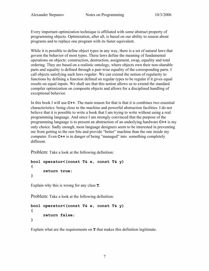
Every important optimization technique is affiliated with some abstract property of programming objects. Optimization, after all, is based on our ability to reason about programs and to replace one program with its faster equivalent. While it is possible to define object types in any way, there is a set of natural laws that govern the behavior of most types. These laws define the meaning of fundamental operations on objects: construction, destruction, assignment, swap, equality and total ordering. They are based on a realistic ontology, where objects own their non-sharable parts and equality is defined through a pair-wise equality of the corresponding parts. I call objects satisfying such laws regular. We can extend the notion of regularity to functions by defining a function defined on regular types to be regular if it gives equal results on equal inputs. We shall see that this notion allows us to extend the standard compiler optimization on composite objects and allows for a disciplined handling of exceptional behavior. In this book I will use C++. The main reason for that is that it is combines two essential characteristics: being close to the machine and powerful abstraction facilities. I do not believe that it is possible to write a book that I am trying to write without using a real programming language. And since I am strongly convinced that the purpose of the programming language is to present an abstraction of an underlying hardware C++ is my only choice. Sadly enough, most language designers seem to be interested in preventing me from getting to the raw bits and provide “better” machine than the one inside my computer. Even C++ is in danger of being “managed” into something completely different. Problem: Take a look at the following definition: bool operator<(const T& x, const T& y) { return true; } Explain why this is wrong for any class T. Problem: Take a look at the following definition: bool operator<(const T& x, const T& y) { return false; } Explain what are the requirements on T that makes this definition legitimate.
7
Alexander Stepanov Notes on Programming 10/3/2006
Project: C arrays have size determined at compile time. Design a C++ class that provides you with objects that behave like arrays of int except that their size is determined at run time. Explain the reasons for your design decisions.
Lecture 2. Designing fvector_int One of your assignments was to design a class that provides the functionality of a C array of int but allows a user to define array bounds at run time. I received many different solutions – as a matter of fact, every “interesting” mistake that I was planning to show you during this lecture was submitted as somebody’s solution. The question, of course, is to be able to distinguish a correct solution from an incorrect one. We will start by showing a solution and incrementally improving and refining it. It closely corresponds to the way most people usually work on their code. In my case it takes many iterations to get something reasonable. Many of my original attempts to implement STL vectors were not far removed from the half-baked pieces of code from which we start. Let us look at the following code: class fvector_int { private: int* v; // v points to the allocated area public: explicit fvector_int(std::size_t n) : v(new int[n]) {} int get(std::size_t n) const { return v[n]; } void set(std::size_t n, int a) { v[n] = a; } }; It clearly works. One can write: fvector_int squares(std::size_t(64)); for (size_t i = 0; i < 64; ++i) { squares.set(i, int(i * i)); } It even uses a correct type for indexing. std::size_t is the machine-dependent unsigned integral type that allows one to encode the size of the largest object in memory. There is an obvious benefit in std::size_t being unsigned: one does not need to worry about passing a negative value to the constructor. (Later in the course we will talk about the problems that are caused by the decision to make std::size_t unsigned and a different type from std::ptrdiff_t. In case you forgot, std::size_t and std::ptrdiff_t are defined in <cstddef>.) It is also good that the designer of the class decided to make the constructor explicit. Implicit conversions are one of the main
8

Alexander Stepanov Notes on Programming 10/3/2006
flaws of C and C++, and it is good to assure that your class will not be a part of this wicked game. If a function expects an fvector_int as an argument and somebody gives it an integer instead, it would be good not to convert this integer into our data structure. (Open your C++ book and read about the explicit keyword! Also petition your neighborhood C++ standard committee member to finally abolish implicit conversions. There is a common misconception, often propagated by people who should know better, that STL depends on implicit conversions. Not so!) It is written in a clear object-oriented style with getters and setters. The proponents of this style say that the advantage of having such functions is that it allows programmers later on to change the implementation. What they forget to mention is that sometimes it is awfully good to expose the implementation. Let us see what I mean. It is hard for me to imagine an evolution of a system that would let you keep the interface of get and set, but be able to change the implementation. I could imagine that the implementation outgrows int and you need to switch to long. But that is a different interface. I can imagine that you decide to switch from an array to a list but that also will force you to change the interface, since it is really not a very good idea to index into a linked list. Now let us see why it is really good to expose the implementation. Let us assume that tomorrow you decide to sort your integers. How can you do it? Could you use the C library qsort? No, since it knows nothing about your getters and setters. Could you use the STL sort? The answer is the same. While you design your class to survive some hypothetical change in the implementation, you did not design it for the very common task of sorting. Of course, the proponents of getters and setters will suggest that you extend your interface with a member function sort. After you do that, you will discover that you need binary search and median, etc. Very soon your class will have 30 member functions but, of course, it will be hiding the implementation. And that could be done only if you are the owner of the class. Otherwise, you need to implement a decent sorting algorithm on top of the setter-getter interface from scratch and that is a far more difficult and dangerous activity than one can imagine. Even a simple standard function swap will not work; you cannot just say: fvector_int foo(size_t(15)); //some stuff std::swap(foo[0], foo[14]); as you can with arrays. You need to define your own function: inline void fvector_int_swap(fvector& v, std::size_t n, std::size_t m) { int tmp = v.get(n); v.set(n, v.get(m));
9

Alexander Stepanov Notes on Programming 10/3/2006
v.set(m, tmp); } and only then can you do: fvector_int_swap(foo, 0, 14); In a couple of years somebody else will need to swap elements between two different fvectors. And instead of the trivial (but not object oriented): std::swap(foo[0], bar[0]); they will have to define a new function: inline void fvector_int_swap(fvector& v, std::size_t n, fvector& u, std::size_t m) { int tmp = v.get(n); v.set(n, u.get(m)); u.set(m, tmp); } And then when somebody wants to start swapping between fvector and an array of int, it quickly becomes apparent that a third version of swap is needed. Setters and getters make our daily programming hard but promise huge rewards in the future when we discover better ways to store arrays of integers in memory. But I do not know a single realistic scenario when hiding memory locations inside our data structure helps and exposure hurts; it is, therefore, my obligation to expose a much more convenient interface that also happens to be consistent with the familiar interface to the C arrays. When we program in C++ we should not be ashamed of its C heritage, but make full use of it. The only problems with C++, and even the only problems with C, arise when they themselves are not consistent with their own logic. It is quite obvious that all these problems disappear if we replace the convoluted getter/setter interface with an interface that exposes memory locations in which integers are stored: class fvector_int { private: int* v; // v points to the allocated memory public: explicit fvector_int(std::size_t n) : v(new int[n]) {} int& operator[](std::size_t n) {
10

Alexander Stepanov Notes on Programming 10/3/2006
return v[n]; } const int& operator[](std::size_t n) const { return v[n]; } }; Notice how we use overloading on const to assure that the right kind of reference is returned when we construct a constant object. If the bracket operator is applied to a constant object it will return a constant reference and it will not be possible to assign to that location. Now we can easily swap elements with the help of the standard swap – we will soon see how standard swap is implemented. And if we overcome our shyness and disclose in our interface description that the references to consecutive integers reside in consecutive locations of memory – and I fully understand that it will prevent us in the future from storing them in random locations – we can sort them quite easily: fvector_int foo(std::size_t(10)); // fill the fvector with integers std::sort(&foo[0], &foo[0] + 10); (My remark about exposing the address locations of consecutive integers is not facetious. It took a major effort to convince the standard committee that such a requirement is an essential property of vectors; they would not, however, agree that vector iterators should be pointers and, therefore, on several major platforms – including the Microsoft one – it is faster to sort your vector by saying the unbelievably ugly if (!v.empty()) { sort(&*v.begin(), &*v.begin() + v.size()); } than the intended sort(v.begin(), v.end()); Attempts to impose pseudo-abstractness at the cost of efficiency can be defeated, but at a terrible cost. C++ Quiz: Figure out why you need to check for v.empty() and why you cannot write &*v.end(). Do not just check it with your compiler: the fact that your compiler might let you get away with something – does not make it a standard conforming C++.)
11

Alexander Stepanov Notes on Programming 10/3/2006
Our class is still far from perfect. Some of you noticed that it lacks a destructor. What happens if we do not write a destructor? As a matter of fact, if we do not write a destructor, one will be provided for us by the compiler. Such a destructor is called a synthesized destructor. A synthesized destructor applies individual member destructors to all its members in the reverse order in which they are declared. Since we have only one member of the class, and since this member is a pointer and a pointer destructor is an empty operation, our synthesized destructor is going to do nothing. Why is it wrong? A typical usage of our class might be something like: void print_shuffled_integers(std::size_t n) { fvector_int integers(n); for (std::size_t i = 0; i < n; ++i) integers[i] = int(i); std::random_shuffle(&integers[0], &integers[n]); for (std::size_t i = 0; i < n; ++i) std::cout << integers[i] << std::endl; } Our procedure is going to allocate memory during construction and then let it disappear into a black hole during destruction. Now the first mission of the constructor is to obtain resources needed for the object: storage, files, devices, etc. (The only reason for a constructor to raise an exception is the unavailability of the needed resources.) And the stack-based model of computation dictates that when an object is destroyed all the resources it acquired are released. (The only reason for an object to raise an exception during destruction is to indicate that resources acquired by it disappeared without a trace – which should never occur in a properly designed system.) The idea of an object owning a resource is a wonderful idea missing from many programming languages. In Lisp, for example, a list does not own its cons cells, and – in the case of lexically scoped dialects of Lisp – even procedural objects do not own their local state which can survive and be used long after the exit from the procedure. The total lack of ownership makes centralized garbage collection essential and encourages a rather wasteful style of programming. Why, indeed, bother to recycle if the resources are unlimited? The model of ownership-based semantics was first introduced in ALGOL 60, which actually had dynamic arrays – something very close to what we are trying to design. C++ does not have built-in dynamic arrays, but the fundamental mechanism of constructors/destructors allows us to implement them. As a matter of fact, we will make all kinds of different data structures that behave according to the stack-based machine model. I am not an enemy of garbage collection. There are many important algorithms in the area of memory management, and I have been urging Hans Boehm for years to write a book about them – the chapter in the first volume of Knuth while still essential is very incomplete. While reference counting tends to be a more important tool for general
12

Alexander Stepanov Notes on Programming 10/3/2006
system design, all memory management techniques are important. What I object to is the insistence that garbage collection is the only way. My second objection to “automatic memory management” whether it is garbage collection, reference counting or ownership-based container semantics is that none of these techniques is sufficient to solve real problems. It is essential for any serious application to develop a data model that clearly describes who de-allocates and when. Anything else is just trading one kind of bug for another. If, when we design a corporate system, we do not assure that when a person is purged from the employee database he is purged from the corporate library, having garbage collection will not help. The record of the long-gone person will still be pointed to by the library. We are trading dangling pointers for memory leaks. A long time ago I read a proposal that every object needs to maintain a list of all the objects which point to it and that when an object is destroyed it should go and zero all the pointers pointing at it. It is a bizarre idea if it is applied to every object, but for certain classes of objects it is a good solution. Again, there is no single right way to manage storage or other resources. And now let us get back to fvector_int. It is trivial to add a proper destructor: class fvector_int { private: int* v; // v points to the allocated memory public: explicit fvector_int(std::size_t n) : v(new int[n]) {} ~fvector_int() { delete [] v; } int& operator[](std::size_t n) { return v[n]; } const int& operator[](std::size_t n) const { return v[n]; } }; but one has to admit that the syntax of new and delete in C++ is an example of a syntactic embarrassment. They are function calls or, more precisely, template function calls and should look like function calls. The resource allocation/de-allocation is done properly as long as we have a single copy of the object. The problem changes when we attempt to pass it to a function. At present the class does not define a copy constructor. As is the case with the destructor, the compiler provides us with a synthesized copy constructor. It applies their copy constructors to all the members, doing a member-wise construction. In our case, there is only one member, a pointer to the allocated memory, and it is constructed by copying its value. Now we have two copies of the same class sharing the same array of integers. Sharing and private
13

Alexander Stepanov Notes on Programming 10/3/2006
ownership do not work well together. At the procedure’s exit point it calls the destructor of the copied object and according to the fundamental principle of private ownership – après nous, le déluge, it de-allocates the memory which leaves the original owner in a rather peculiar situation. (Copy-on-write data structures do not allow sharing but delay copying. It is possible to design STL conforming containers which do copy-on-write. It is, after all, an optimization that does not change the semantics. In my experience, however, the primitive data structures such as vector and list do not benefit from such optimization.) It is worthwhile to observe that the way arrays are passed to functions is another embarrassment. It dates back to the time when C did not allow passing large objects to a function. Even structures could not be passed by value. As a “convenient” feature, passing an array would result in converting it to a pointer and passing the pointer. Within a few years it became possible to pass structures by value. (Fortunately, there was no “convenient” conversion of a structure to a pointer to it.) But arrays remained in the embarrassing state. You can pass an array by value if you enclose it in a structure: template < std::size_t m> struct cvector_int { int values[m]; int& operator[](std::size_t n) { assert(n < m); return values[n]; } const int& operator[](std::size_t n) const { assert(n < m); return values[n]; } }; template < std::size_t m> cvector_int<m> reverse_copy(cvector_int<m> x) { std::reverse(&x[0], &x[m]); return x; } We need our fvector_int class to behave like the cvector_int class. In other words, we need to provide it with an appropriate copy constructor. After all, the main reason for the existence of fvector_int is that the size of cvector_int has to be known at compile time. (One of the reasons for the demise of Pascal – a wonderful language in many respects – was the fact that its arrays – at least in the original version of the language – were pretty much like cvector_int; it is really important to be able to have arrays whose size is determined at run time.) But its semantics should mimic the wonderful semantics of cvector_int that fits into our stack based machine model and
14
Alexander Stepanov Notes on Programming 10/3/2006
has ownership semantics. In general, we will attempt to make our classes behave like familiar C objects. Our containers will behave like structures and our iterators will behave like pointers. Such an approach has two advantages. First, it imposes a consistent behavior between primitive objects and our extensions; and second, it assures that our abstractions are based on something that has been proven useful. It is quite simple to provide our class with an appropriate copy constructor except for one little detail. The copy constructor does not know the size of the original object. Our class does not have enough members. It is constructionally incomplete. We call a class constructionally incomplete if it cannot implement its own copy. If we look back at our examples of usage, we always used the size available externally. We need to store it internally and that, incidentally, will also allow us to put proper asserts into our bracket operators: class fvector_int { private: std::size_t length; // the size of the allocated area int* v; // the pointer to the allocated area public: fvector_int(const fvector_int& x); explicit fvector_int(std::size_t n) : length(n), v(new int[n]) {} ~fvector_int() { delete [] v; } int& operator[](std::size_t n) { assert(n < length); return v[n]; } const int& operator[](std::size_t n) const { assert(n < length); return v[n]; } }; fvector_int::fvector_int(const fvector_int& x) : length(x.length), v(new int[x.length]) { for(std::size_t i = 0; i < length; ++i) (*this)[i] = x[i]; } The fact that we need to store the size with the vector is the result of a sloppy design of operators new [] and delete []; that design goes back to a sloppy design of the malloc/free calls in C. It should be perfectly clear that the implementation of the array operators new and delete knows what is the number of the objects allocated by it. If it did not, it would not be able to destroy them when the operator delete is applied
15

Alexander Stepanov Notes on Programming 10/3/2006
to the pointer returned by new. The same is, of course, true for malloc/free. This is why we now need to store the length together with the pointer, duplicating the information that is stored by the system. It is even worse, since the system knows both the amount of storage allocated and the amount of storage where objects are actually constructed. If we had access to both we could implement a type-safe version of realloc and even reduce the size of the header of std::vector to the size of one pointer which would make operations on vectors of vectors really efficient. And it would improve the memory utilization since instead of two sections of unused memory – one in the vector and another one in the allocated memory block – we would have only one. But all my offers to redesign the memory allocation interfaces in C++ were rejected since it was viewed that new and delete are part of the core language and I was not authorized to touch them. It does not take much to realize that we have one more problem. Indeed, while we provided a copy constructor, we did not provide an assignment operation. We will, of course, be provided with a synthesized one, and it is fairly easy to guess the semantics of it: it will do pair-wise assignments between the members in the order they are defined. That is, of course, not at all what we need. Copying and assignment must be consistent. Before we implement our assignment we need to answer an important question: should we be able to assign fvector_ints if their size is different? Since we agreed that the size is determined at construction time, it should not change. Should we check for the size being equal and raise an exception? The problem does not arise with cvector_int since two cvector_ints of the same type have the same size; we cannot, therefore, use them as a guide for what to do. That would be unwise since it will break two wonderful rules of any good type: a = b is always legal and should raise an exception only if we run out of resources to construct a copy of b in a; secondly, programmers should be able to write: T a; a = b; whenever they can write T a(b); and these program fragments should mean the same thing and be interchangeable. Here we are meeting for the first time one of our major design principles: when a code fragment has a certain meaning for all built-in types, it should preserve the same meaning for user-defined types. Since the two code fragments are equivalent for all built-in types, they should be equivalent for our class. (This is why I object to using operator+ for string concatenation. For all built-in types and their non-singular values – as we shall see later in this lecture we often need to make this exception for mysterious singular values because of another standard, the IEEE floating point one – we can be sure that a + b == b + a. Notice, that no mathematician will use + for a non-commutative operation. This is why Abelian groups use + and non-Abelian groups use multiplication. It would have been perfectly fine to use * for string concatenation – after
16

Alexander Stepanov Notes on Programming 10/3/2006
all that’s what was traditionally done in the Formal Language Theory. If a set has one binary operation defined on it and it is designated by *, we have a right to assume that it is not commutative.) This is why we are going to allow assignment between fvector_int of different sizes. Now there should be a really easy way of obtaining an assignment operator: first we need to clean up the left side of the assignment using the destructor and then copy into our fresh storage the value from the right side of the assignment. It is, of course, important not to do any of this when both sides refer to the same object. In such a case, we can safely do nothing. That gives us a boilerplate for a generic assignment operator: T& T::operator=(const T& x) { if (this != &x) { this -> ~T(); // destroy object in place new (this) T(x); // construct it in place } return *this; } Unfortunately, there is a problem with this definition of assignment. If there is an exception during the construction, the object is going to be left in an unacceptable “destroyed” state. In the next lecture we will learn that there is a better “generic” definition of assignment that could be used, but, at least for the time being let us ignore the “advanced” notion of exception safety and proceed with the one we have now. (Some of you might think that such definition of assignment without proper exception safety would never appear anywhere real. Well, this was the definition of assignment used in all the implementations of STL for the first 4 years of its life. It was seen by all the main experts and nobody ever objected. It was a result of gradual evolution – not complete even today – of a notion of exception safety that eventually made this definition suspect. We will talk more about it in the next lecture.) There is a sad obligation to return a reference from the assignment. C introduced the dangerous ability to write a = (b = c). C++ made it so that we can write the even more dangerous (a = b) = c. I would rather live in a world where assignments return void. And while we are forced to make our assignments to conform to the standard semantics, we should avoid using this semantics in our code. (This is similar to Jon Postel’s Robustness Principle: “TCP implementations will follow a general principle of robustness: be conservative in what you do, be liberal in what you accept from others.”) In the case of fvector_int, there is, however, a nice optimization. If two instances have the same size then we can copy values from one to the other without any need for
17

Alexander Stepanov Notes on Programming 10/3/2006
allocation. That gives us the nice property that if two fvector_ints are of the same size we can guarantee that the assignment does not raise an exception: class fvector_int { private: std::size_t length; // the size of the allocated area int* v; // the pointer to the allocated area public: fvector_int(const fvector_int& x); explicit fvector_int(std::size_t n) : length(n), v(new int[n]) {} ~fvector_int() { delete [] v; } fvector_int& operator=(const fvector_int& x); int& operator[](std::size_t n) { assert(n < length); return v[n]; } const int& operator[](std::size_t n) const { assert(n < length); return v[n]; } }; fvector_int::fvector_int(const fvector_int& x) : length(x.length), v(new int[x.length]) { for(std::size_t i = 0; i < length; ++i) (*this)[i] = x[i]; } fvector_int& fvector_int::operator=(const fvector_int& x) { if (this != &x) if (this->length == x.length) for (std::size_t i = 0; i < length; ++i) (*this)[i] = x[i]; else { this -> ~fvector_int (); new (this) fvector_int (x); } return *this; } Let us observe another fact that follows from the equivalence of the two program fragments T a; // default constructor
18

Alexander Stepanov Notes on Programming 10/3/2006
a = b; // assignment operator and T a(b); // copy constructor Since we want them to have the same semantics and would like to be able to write one or the other interchangeably, we need to provide fvector_int with a default constructor – a constructor that takes no arguments. The postulated equivalence of two program fragments gives us an important clue about the resource requirements for default constructors. It is almost totally clear that the only resource that a default constructor should allocate is the stack space for the object. (It will become totally clear when we discuss the semantics of swap and move.) The real resource allocation should happen during the assignment. The compiler provides a synthesized default constructor only when no other constructors are defined. (It is, of course, an embarrassing rule: adding a new public member function – a constructor is a special kind of a member function – to a class can make an existing legal code into code that would not compile.) Clearly the default constructor should be equivalent to constructing an fvector_int of the length zero: class fvector_int { private: std::size_t length; // the size of the allocated area int* v; // the pointer to the allocated area public: fvector_int() : length(std::size_t(0)), v(NULL) {} fvector_int(const fvector_int& x); explicit fvector_int(std::size_t n) : length(n), v(new int[n]) {} ~fvector_int() { delete [] v; } fvector_int& operator=(const fvector_int& x); int& operator[](std::size_t n) { assert(n < length); return v[n]; } const int& operator[](std::size_t n) const { assert(n < length); return v[n]; } }; Let us revisit our design of the copy constructor and assignment. While we now know why we needed to allocate a different pool of memory, how do we know that we need to copy the integers from the original to the copy? Again, let us look at the semantics of copy that is given to us by the built-in types. It is very clear (especially if we ignore
19

Alexander Stepanov Notes on Programming 10/3/2006
singular values given to us by the IEEE floating point standard) that there is one fundamental principle that governs the behavior of copy constructors and assignments for all built-in types and pointer types: T a(b); assert(a == b); and T a; a = b; assert(a == b); It is a self-evident rule: to make a copy means to create an object equal to the original. The rule, unfortunately, does not extend to structures. Neither C nor C++ define an equality operator. (operator== – I do hate the equality/assignment notation in C; I would be so happy if we moved back to Algol’s notation := for the assignment and to the five century old mathematical symbol = for equality. I do, however, find != to be a better choice than Wirth’s <>.) The extension would be quite simple to define: compare members for equality in the order they are defined. I have been advocating such an addition for about 12 years without any success. (In the programming language of the future it would not be necessary to have built-in semantic definition for synthesized equality. It would be possible to say in the language that for any type for which its own equality is not defined – or, as might be the case for some irregular types – is “undefined”, the equality means the member-wise equality comparison. The same, of course, would be done for synthesized copy constructors, default constructors, etc. Such things would require some simple reflection facilities that are absent from C++. ) The same extension should work for arrays except for the unfortunate automatic conversion of arrays into pointers. It is easy to see the correct equality semantics for cvector_int: template <std::size_t m> bool operator==(const cvector_int<m>& x, const cvector_int<m>& y) { for (std::size_t i(0); i < m; ++i) if (x[i] != y[i]) return false; return true; } The reason we define the equality as a global function is because the arguments are symmetric, but more importantly because we want it to be defined as a non-friend function that accesses both objects through their public interface. The reason for that is that if equality is definable thorough the public interface then we know that our class is equationally complete, or just complete. In general, it is a stronger notion than
20

Alexander Stepanov Notes on Programming 10/3/2006
constructional completeness, since it requires that we have a public interface that is powerful enough to distinguish between different objects. We can easily see that fvector_int is incomplete. The size is not publicly visible. It is now easy to see that it is not just equality definition that is not possible. No non-trivial function – that is a function that will do different things for different values of fvector_int is definable. Indeed if we are given an instance of fvector_int we cannot look at any of its locations without the possibility of getting an assert violation. After all, it could be of size 0. And since operator[] is the only way to observe the differences between the objects we cannot distinguish between two instances. Should we make our member length public? After all, I have been advocating exposing things to the user. Not in this case, because it would allow a user to break class invariants. What are our invariants? The first invariant is that length must be equal to the area of the allocated memory divided by sizeof(int). The second invariant is that the memory will not be released prematurely. This is the reason why we keep these members private. In general: only members that are constrained by class invariants need to be private. While we could make a member function to return length, it is better to make it a global friend function. If we do that, we will be able eventually to define the same function to work on built-in arrays and achieve greater uniformity of design. I made size into a member function in STL in an attempt to please the standard committee. I knew that begin, end and size should be global functions but was not willing to risk another fight with the committee. In general, there were many compromises of which I am ashamed. It would have been harder to succeed without making them, but I still get a metallic taste in my mouth when I encounter all the things that I did wrong while knowing full how to do them right. Success, after all, is much overrated. I will be pointing to the incorrect designs in STL here and there: some were done because of political considerations, but many were mistakes caused by my inability to discern general principles.) Now let us see how we do the equality and the size: class fvector_int { private: std::size_t length; // the size of the allocated area int* v; // v points to the allocated area public: fvector_int() : length(std::size_t(0)), v(NULL) {} fvector_int(const fvector_int& x); explicit fvector_int(std::size_t n) : length(n), v(new int[n]) {} ~fvector_int() { delete [] v; } fvector_int& operator=(const fvector_int& x); friend std::size_t size(const fvector_int& x) {
21

Alexander Stepanov Notes on Programming 10/3/2006
return x.length; } int& operator[](std::size_t n) { assert(n < size(*this)); return v[n]; } const int& operator[](std::size_t n) const { assert(n < size(*this)); return v[n]; } }; bool operator==(const fvector_int& x, const fvector_int& y) { if (size(x) != size(y)) return false; for (std::size_t i = 0; i < size(x); ++i) if (x[i] != y[i]) return false; return true; } It is probably worthwhile to change even our definitions of the copy constructor and assignment to use the public interface. fvector_int::fvector_int(const fvector_int& x) : length(size(x)), v(new int[size(x)]) { for(std::size_t i = 0; i < size(x); ++i) (*this)[i] = x[i]; } fvector_int& fvector_int::operator=(const fvector_int& x) { if (this != &x) if (size(*this) == size(x)) for (std::size_t i = 0; i < size(*this); ++i) (*this)[i] = x[i]; else { this -> ~fvector_int (); new (this) fvector_int (x); } return *this; } We can also “upgrade” our cvector_int class to match fvector_int by providing it with a size function:
22

Alexander Stepanov Notes on Programming 10/3/2006
template <std::size_t m> struct cvector_int; template <std::size_t m> inline size_t size(const cvector_int<m>&) { return m; } template < std::size_t m> struct cvector_int { int values[m]; int& operator[](std::size_t n) { assert(n < size(*this)); return values[n]; } const int& operator[](std::size_t n) const { assert(n < size(*this)); return values[n]; } }; And now we can write equality for cvector_int by copy-and-pasting the body of the equality of fvector_int. It does an unnecessary comparison of sizes – since they are always the same the comparison could safely be omitted – but any modern compiler will optimize it away: template <std::size_t m> bool operator==(const cvector_int<m>& x, const cvector_int<m>& y) { if (size(x) != size(y)) return false; for (std::size_t i = 0; i < size(x); ++i) if (x[i] != y[i]) return false; return true; } One of the goals of the first part of the course is to refine this code to the point that the same cutting-and-pasting methodology will work for any of our data structures. After all the code could be restated in English as the following rule: two data structures are equal if they are of the same size and are element-by-element equal. In general, we will try to make all our functions as data structure-independent as possible. Problem 1.
23
Alexander Stepanov Notes on Programming 10/3/2006
Refine your solution to Problem 1 of Lecture 1 according to what we learned today. Problem 2. Extend your fvector_int to be able to change its size.
Lecture 3. Continuing with fvector_int In the previous lecture we implemented operator== for fvector_int. It is an important step since now our class can be used together with many algorithms that use equality, such as, for example, std::find. It is, however, not enough to define equality. We have to define inequality to match it. Why do we need to do that? The main reason is that we want to preserve the freedom to be able to write a != b and !(a == b) interchangeably. The statements that two things are unequal to each other and two things are not equal to each other should be equivalent. Unfortunately, C++ does not dictate any semantic rules on operator overloading. A programmer is allowed to define equality to mean equality but the inequality to mean inner product or division modulo 3. That is, of course, totally unacceptable. Inequality should be automatically defined to mean the negation of equality. It should not be possible to define it separately and it has to be provided for us the moment equality is defined. But it is not. We have to acquire a habit to define both operators together whenever we define a class. Fortunately, it is very simple: inline bool operator!=(const fvector_int& x, const fvector_int& y) { return !(x == y); } Unfortunately, even such a self-evident rule as the equivalence of inequality and negation of equality does not hold everywhere. The floating-point data types (float and double) contain a value NaN (not-a-number) that possesses some remarkable properties. The IEEE 754 standard requires that every comparison (==, <, >, <=, >=) involving NaN should return false. This was a terrible decision that overruled the meaning of equality and made it difficult to do any careful reasoning about programs. It makes it impossible to reason about programs since equational reasoning is central to
24

Alexander Stepanov Notes on Programming 10/3/2006
reasoning about programs. Because of the unfortunate standard we can no longer postulate that: T a = b; assert(a == b); or a = b; assert(a == b); The meaning of construction and assignment is compromised. Even the axioms of equality itself are no longer true since because of NaN the reflexivity of equality is no longer true and we cannot assume that: assert(a == a); holds. (We shall see later that the consequences for ordering comparisons are equally unpleasant.) The only reasonable approach is to ignore the consequences of the rules, assume that all the basic laws of equality hold, and then postulate that the results of our reasoning and all of the program transformations that such reasoning allows us to do, hold only when there are no NaNs generated during our program execution. Such an approach will give us reasonable results for most programs. For the duration of our lectures we will make such an assumption. (There is a lesson in this: the makers of the IEEE standard concentrated on the semantics of floating point numbers but ignored the general rules that govern the world: the law of identity that states that everything is equal to itself and the law of excluded middle that states that either a proposition or its negation is true. They made a clumsy attempt to map a multi-valued logic {true, false, undefined} into a two-valued logic {true, false}, and we have to suffer the consequences. The standards are seldom overturned to conform to reason and, therefore, we have to be very careful when we propose something as a standard.) We will return to our discussion of equality in the next lecture, but now let us consider if we should implement operator< for fvector_int. When a question like that is asked, we need to analyze it in terms of what we will be able to do if we define it. And the immediate answer is that we will be able to sort an array of fvector_int. While we are going to study sorting much later in the course, every programmer knows why sorting is important: it allows us to find things quickly using binary search and to implement set operations such as union and intersection. It is clearly a useful thing to do and it is not hard to see how to compare two instances of fvector_int: we will compare them lexicographically. As with operator== it is proper to define operator< as a global function that uses only the public interface: bool operator<(const fvector_int& x, const fvector_int& y) {
25

Alexander Stepanov Notes on Programming 10/3/2006
size_t i(0); while (true) { /* if (i >= size(x) && i >= size(y)) return false; if (i >= size(x)) return true; if (i >= size(y)) return false; // these three if statements are equivalent // to the next two */ if (i >= size(y)) return false; if (i >= size(x)) return true; if (y[i] < x[i]) return false; if (x[i] < y[i]) return true; ++i; } } Or slightly more cryptic: bool operator<(const fvector_int& x, const fvector_int& y) { size_t min_size(std::min(size(x), size(y))); size_t i(0); while (i < min_size && x[i] == y[i]) ++i; if (i < min_size) return x[i] < y[i]; return size(x) < size(y); } Quiz: Convince yourself that the two implementations are equivalent. Which one is more efficient and why? Test if your efficiency guess is correct. Now, we clearly want to preserve the rule that programmers can write a < b and b > a interchangeably. Moreover, we would like to be certain that !(a < b) is equivalent to
26
Alexander Stepanov Notes on Programming 10/3/2006
a >= b and a <= b is equivalent to !(a > b) As with equality, C++ does not enforce that all of the relation operators should be defined simultaneously. It is important to define them simultaneously and while it is tedious, it is not intellectually challenging. While it is not strictly speaking necessary, I recommend that you always define operator< first and then implement the other three in terms of it: inline bool operator>(const fvector_int& x, const fvector_int& y) { return y < x; } inline bool operator<=(const fvector_int& x, const fvector_int& y) { return !(y < x); } inline bool operator>=(const fvector_int& x, const fvector_int& y) { return !(x < y); } If a type has operator< defined on it, it should mean total ordering; otherwise some other notation should be used. In particular, it is strictly totally ordered. (That means that a < a is never true.) As I said before, having a total ordering on a type is essential if we want to implement fast set operations. It is, therefore, quite remarkable that C and C++ dramatically weaken the ability to obtain total ordering provided by the underlying hardware. The instruction set of any modern processor provides instructions for comparing two values of any built-in data type. It is easy to extend them to structures using lexicographical ordering. Unfortunately, there is a trend to hide hardware operations that has clearly affected even the C community. For example, one is not allowed to compare void pointers. Even with non-void pointers, they can be compared only when they point to the same array. That, for example, makes it impossible to sort an
27

Alexander Stepanov Notes on Programming 10/3/2006
array of pointers to heap-allocated objects. Compilers, of course, cannot enforce such a rule since it is not known where the pointer is pointing. I would say that all built-in types need to provide < by at least exposing the natural ordering of their bit patterns. It is terribly nice if the ordering preserves the topology of algebraic operations, so that if a < b we know that a + c < b + c, and it should do so in many natural cases. It is, however, essential to allow people to sort their data even if ordering is not consistent with other operations. If it is provided, we can be sure that the data can be found quickly. For user-defined structures, the compiler can always synthesize a lexicographical ordering based on members, or a user needs to define a more semantically relevant ordering. In any case, the definition of < should be consistent with the definition of == so that the following always holds: !(a < b) && !(b < a) is equivalent to a == b Only the classes that have the relational operators defined can be effectively used with the standard library containers (set, map, etc) and algorithms (sort, merge, etc). (One of the omissions that I made in STL was the omission of relational operators on iterators. STL requires them only for random access iterators and only when they point to the same container. It makes it impossible to have a set of iterators into a list. Yes, it is impossible to assure the topological ordering of such iterators – the property that if a < b then ++a < ++b or, in other words, that the ordering imposed by < coincides with the traversal ordering – but such a property is unneeded for sorting. The reason that I decided not to provide them was that I wanted to prevent people writing something like for (std::list<int>::iterator i = mylist.begin(); i < mylist.end(); ++i) sum += *i; In other words, I considered “safety” to be a more important consideration than expressibility, or uniform semantics. It was a mistake. People would have learned that it was not a correct idiom quickly enough, but I made it much harder for me to maintain that all regular types – we will be defining what “regular” means in the next lecture but, simply speaking, the types that you assign and copy – should have not just equality but also the relational operators defined. General principles should not be compromised for particular, expedient reasons. ) Now we can create a vector of fvector_int vector<fvector_int> my_vector(size_t(100000),
28

Alexander Stepanov Notes on Programming 10/3/2006
fvector_int(1000)); and after we fill all the elements of the vector with data, we can sort it. It is very likely that somewhere inside std::sort, there is a piece of code that swaps two elements of the vector using std::swap. As we shall discover in this course, swapping is one of the most important operations in programming. We encountered it in the previous lecture when we wanted it to work with elements of fvector_int. Now we need to consider applying swap to two instances of fvector_int. It is fairly easy to define a general purpose swap: template <class T> // T models Regular // the previous comment will be // explained later inline void swap(T& x, T& y) { // assert(true); // no preconditions // T x_old = x; assert(x_old == x); // T y_old = y; assert(y_old == y); T tmp(x); // assert(tmp == x_old); x = y; // assert(x == y_old); y = tmp; // assert(y == x_old); // assert(x == y_old && y == x_old); } It is a wonderful piece of code that depends on fundamental properties of copy and assignment. We are going to use the assertions later on to derive axioms that govern copying and assignment. I am sure that some of you are astonished that I am ignorant of the basic mathematical fact that one does not derive axioms but only theorems. You have to think, however, about where axioms come from. It is not hard to see that short of demanding a private revelation for every set of axioms, we have to learn how to induce axioms governing the behavior of our (general) objects from observing the behavior of some particular instances. Induction – not the mathematical induction but the technique of generalizing from the particular to the general – is the most essential tool of science (the second most essential being the experimental verification of the general rules obtained through the inductive process.). There is, of course, a tricky way of doing swap without using a temporary: inline void swap(unsigned int& x, unsigned int& y) { // assert(true); // no preconditions // unsigned int x_old = x; assert(x_old == x); // unsigned int y_old = y; assert(y_old == y); y = x ^ y; // assert(y == x_old ^ y_old);
29

Alexander Stepanov Notes on Programming 10/3/2006
x = x ^ y; // assert(x == y_old); y = x ^ y; // assert(y == x_old); // assert(x == y_old && y == x_old); } This code, nowadays, is almost always slower than the one with a temporary. It might on very rare occasions be useful in assembly language programming for swapping registers on processors with a limited number of registers. But it is beautiful and frequently appears as a job interview question. It is interesting to note that we do not really need the exclusive-or to implement it. One can do the same with + and -: y = x + y; // assert(y == x_old + y_old); x = y - x; // assert(x == y_old); y = y - x; // assert(y == x_old); The general purpose swap clearly works for fvector_int. All the operations that are used by the body of the template are available for fvector_int and you should be able to prove all of the assertions without much difficulty. There are, however, two problems with this implementation. First, it takes a long time. Indeed we need to copy an fvector_int – which takes time linear in its size – and then we do two assignments – which are also linear in its size. (Plus the time of the allocation and de-allocation which, while usually amortized constant, could be quite significant.) Second, our swap can throw an exception if there is not enough memory to construct a temporary. It seems that both of these things are generally unnecessary. If two objects use extra resources, they can just swap pointers to them. And swap should never cause an exception since it does not need to ask for additional resources. It is quite obvious how to do that: swap members of the class member-by-member. In general, we call a type swap-regular if its swap can be implemented by swapping the bit-patterns of corresponding objects. All the types we are going to encounter are going to be swap-regular. (One can obtain a non-swap-regular type by defining a class with remote parts that contain pointers to the object itself. It is usually unnecessary and can always be avoided by creating a remote header node to which the inverted pointers can point.) Swap allows us to produce a better implementation of assignment. The general purpose assignment that we introduced in the previous lecture looked like: T& T::operator=(const T& x) { if (this != &x) { this -> ~T(); // destroy object in place new (this) T(x); // construct it in place } return *this; }
30

Alexander Stepanov Notes on Programming 10/3/2006
If the copy constructor raises an exception we are left in a peculiar situation since the object on the left side of the assignment is left in an undefined state. It is clearly bad since, when the stack is unwound and objects are destroyed, it is likely that the destructor will be applied to the object again. And it is highly improper to destroy things twice. Moreover, even if we ignore this aspect, it would be terribly nice if incomplete assignments left the object unmodified. (If you cannot store a new value at least leave the old value untouched.) If we have swap that is fast and exception-free we can always implement the assignment with the properties we desire: T& T::operator=(const T& x) { if (this != &x) { T tmp(x); swap(*this, tmp); } return *this; } Notice that if the copy constructor throws an exception, *this is left untouched. Otherwise after swapping, the temporary is destroyed and the resources that used to belong to *this before the swap are de-allocated. Somebody might object that there are circumstances when the old definition is better since it does not try to obtain memory before the old memory is returned. That might be more beneficial when dealing with assignments of large data structures. We might prefer to trade the preservation of the old value in case of an exception to ability to encounter the exception less frequently. It is, however, easy to fix. We need to provide a function that returns memory and call it before the assignment. It is trivial to implement for fvector_int: inline void shrink(fvector_int& x) { fvector_int tmp; swap(x, tmp); } Now we need only to call shrink and then do the assignment. Swap is more efficient than assignment for objects that own remote parts that need to be copied. Indeed let us look at the complexity of the operations that we have defined on fvector_int. Before we can talk about complexity of operations we need to figure out how we measure the size of objects. C/C++ provide us with a built-in type-function sizeof. It is clearly not indicative of the “real” size of the object. In the case of fvector_int we have size that tells us how many integers it contains. We can
31
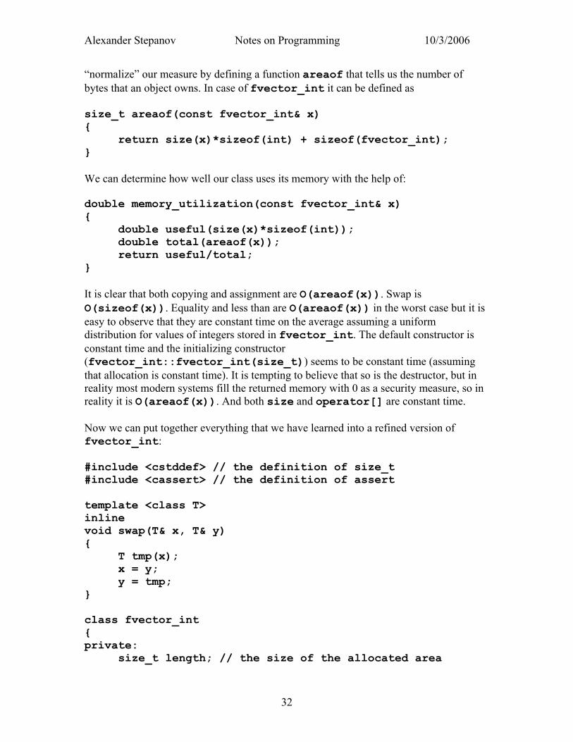
Alexander Stepanov Notes on Programming 10/3/2006
“normalize” our measure by defining a function areaof that tells us the number of bytes that an object owns. In case of fvector_int it can be defined as size_t areaof(const fvector_int& x) { return size(x)*sizeof(int) + sizeof(fvector_int); } We can determine how well our class uses its memory with the help of: double memory_utilization(const fvector_int& x) { double useful(size(x)*sizeof(int)); double total(areaof(x)); return useful/total; } It is clear that both copying and assignment are O(areaof(x)). Swap is O(sizeof(x)). Equality and less than are O(areaof(x)) in the worst case but it is easy to observe that they are constant time on the average assuming a uniform distribution for values of integers stored in fvector_int. The default constructor is constant time and the initializing constructor (fvector_int::fvector_int(size_t)) seems to be constant time (assuming that allocation is constant time). It is tempting to believe that so is the destructor, but in reality most modern systems fill the returned memory with 0 as a security measure, so in reality it is O(areaof(x)). And both size and operator[] are constant time. Now we can put together everything that we have learned into a refined version of fvector_int: #include <cstddef> // the definition of size_t #include <cassert> // the definition of assert template <class T> inline void swap(T& x, T& y) { T tmp(x); x = y; y = tmp; } class fvector_int { private: size_t length; // the size of the allocated area
32

Alexander Stepanov Notes on Programming 10/3/2006
int* v; // v points to the allocated area public: fvector_int() : length(std::size_t(0)), v(NULL) {} fvector_int(const fvector_int& x); explicit fvector_int(std::size_t n) : length(n), v(new int[n]) {} ~fvector_int() { delete [] v; } fvector_int& operator=(const fvector_int& x); friend void swap(fvector_int& x, fvector_int& y) { swap(x.length, y.length); swap(x.v, y.v); } friend std::size_t size(const fvector_int& x) { return x.length; } int& operator[](std::size_t n) { assert(n < size(*this)); return v[n]; } const int& operator[](std::size_t n) const { assert(n < size(*this)); return v[n]; } }; fvector_int::fvector_int(const fvector_int& x) : length(size(x)), v(new int[size(x)]) { for(std::size_t i = 0; i < size(x); ++i) (*this)[i] = x[i]; } fvector_int& fvector_int::operator=(const fvector_int& x) { if (this != &x) if (size(*this) == size(x)) for (std::size_t i = 0; i < size(*this); ++i) (*this)[i] = x[i]; else { fvector_int tmp(x); swap(*this, tmp);
33

Alexander Stepanov Notes on Programming 10/3/2006
} return *this; } bool operator==(const fvector_int& x, const fvector_int& y) { if (size(x) != size(y)) return false; for (std::size_t i = 0; i < size(x); ++i) if (x[i] != y[i]) return false; return true; } inline bool operator!=(const fvector_int& x, const fvector_int& y) { return !(x == y); } bool operator<(const fvector_int& x, const fvector_int& y) { for (size_t i(0); ; ++i) { if (i >= size(y)) return false; if (i >= size(x)) return true; if (y[i] < x[i]) return false; if (x[i] < y[i]) return true; } } inline bool operator>(const fvector_int& x, const fvector_int& y) { return y < x; } inline bool operator<=(const fvector_int& x, const fvector_int& y) { return !(y < x); } inline bool operator>=(const fvector_int& x, const fvector_int& y) { return !(x < y); } size_t areaof(const fvector_int& x)
34

Alexander Stepanov Notes on Programming 10/3/2006
{ return size(x)*sizeof(int) + sizeof(fvector_int); } double memory_utilization(const fvector_int& x) { double useful(size(x)*sizeof(int)); double total(areaof(x)); return useful/total; }
35

Alexander Stepanov Notes on Programming 10/3/2006
Lecture 4. Implementing swap Up till now we have dealt mostly with two types: fvector_int and int. These type have many operations in common: copy construction, assignment, equality, less than. It is possible to write code fragments that can work for either. We almost discovered such a fragment when we looked at the implementation of swap: T tmp(x); x = y; y = tmp; While the code makes sense when we replace T with either of the types, we discovered that there is an implementation of swap for fvector_int that is far more efficient. The question that we need to raise is whether we can find a way of making codes that would work efficiently for both cases. Let us look at a very useful generalization of swap: template <typename T> inline void cycle_left(T& x1, T& x2, T& x3) // rotates to the left { T tmp(x1); x1 = x2; x2 = x3; x3 = tmp; } While it clearly works for both types, it is quite inefficient for fvector_int since it is complexity is linear in the sum of the sizes of three arguments, and it might raise an exception if there are not enough resources to make a copy of x1. We can do much better if we replace it with the following definition: template <typename T> inline void cycle_left(T& x1, T& x2, T& x3) // rotates to the left { swap(x1, x2); swap(x2, x3); } Since swap is a constant time operation on fvector_int, we can use this definition without much of a problem. Unfortunately, this kind of definition is often going to be slower since it is going to expand to:
36
Alexander Stepanov Notes on Programming 10/3/2006
T tmp1(x1); x1 = x2; x2 = tmp1; T tmp2(x2); x2 = x3; x3 = tmp2; and while there is a chance that a good optimizing compiler will make it as fast as the first version for int and double, it is unlikely that extra operations will be eliminated when we deal with structures, and the potential performance loss might be around 50% . So we need both definitions – one to use with fvector_int and other classes with remote parts and the other to use with the built-in types and user-defined types which have no user defined copy-constructors, assignments and destructors. C++ language specialists call such types POD types where POD stands for plain old data. There is at present no easy way in C++ to write code that will do one thing for POD types and something else for more complicated types. We can, however, attempt to unify our two versions with the help of a weaker version of assignment operation. We will call such an operation move. When we do an assignment we know that assert(b == c); a = b; assert(a == b && b == c); In other words, assignment makes its left-hand side equal to the right-hand side, while leaving the right hand side unchanged. move has weaker semantics: assert(b == c && &b != &c); move(b, a); assert(a == c); In other words, move assures that the value moves from the source to the destination; there are no guarantees that the source is unchanged. The weaker semantics of move frequently allows for faster implementation. We can define the most general version of move to default to assignment: template <typename T> inline void move(T& source, T& destination) { destination = source; } Note that we take the source argument as a reference and not a constant reference. While it is not needed for the most general case, its refinements will modify the source, and we want to have our signature consistent between the general case and the refinements.
37
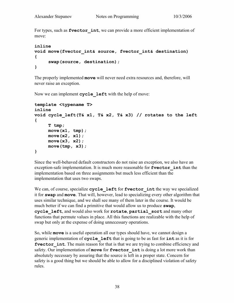
Alexander Stepanov Notes on Programming 10/3/2006
For types, such as fvector_int, we can provide a more efficient implementation of move: inline void move(fvector_int& source, fvector_int& destination) { swap(source, destination); } The properly implemented move will never need extra resources and, therefore, will never raise an exception. Now we can implement cycle_left with the help of move: template <typename T> inline void cycle_left(T& x1, T& x2, T& x3) // rotates to the left { T tmp; move(x1, tmp); move(x2, x1); move(x3, x2); move(tmp, x3); } Since the well-behaved default constructors do not raise an exception, we also have an exception-safe implementation. It is much more reasonable for fvector_int than the implementation based on three assignments but much less efficient than the implementation that uses two swaps. We can, of course, specialize cycle_left for fvector_int the way we specialized it for swap and move. That will, however, lead to specializing every other algorithm that uses similar technique, and we shall see many of them later in the course. It would be much better if we can find a primitive that would allow us to produce swap, cycle_left, and would also work for rotate, partial_sort and many other functions that permute values in place. All this functions are realizable with the help of swap but only at the expense of doing unnecessary operations. So, while move is a useful operation all our types should have, we cannot design a generic implementation of cycle_left that is going to be as fast for int as it is for fvector_int. The main reason for that is that we are trying to combine efficiency and safety. Our implementation of move for fvector_int is doing a lot more work than absolutely necessary by assuring that the source is left in a proper state. Concern for safety is a good thing but we should be able to allow for a disciplined violation of safety rules.
38

Alexander Stepanov Notes on Programming 10/3/2006
We can weaken the semantics of move even further by introducing a notion of the raw move. It is not guaranteed to leave the source in a valid state. In particular, the source might not be destructible. It should be possible, however, to make an object in an invalid state valid by moving a valid object back into it. As was the case with move we can implement the general version of move_raw with the help of the assignment: template <typename T> inline void move_raw(T& source, T& destination) { destination = source; } Now we can provide an implementation of move_raw for fvector_int: friend void move_raw(fvector_int& source, fvector_int& destination) { destination.length = source.length; destination.v = source.v; } Now, the problem with move_raw is that it is difficult to find a way of using it safely. Before we formulate the rules, let us try using it to implement cycle_left: template <typename T> inline void cycle_left(T& x1, T& x2, T& x3) // rotates to the left { T tmp; move_raw(x1, tmp); move_raw(x2, x1); move_raw(x3, x2); move_raw(tmp, x3); } At the end x1, x2 and x3 have the correct values in them. The problem is that we now have an invalid object in tmp before we exit the function and calling the destructor on an invalid object is very dangerous. We could “fix” the problem at least in the case of fvector_int, by changing the code to: template <typename T> inline void cycle_left(T& x1, T& x2, T& x3) // rotates to the left
39

Alexander Stepanov Notes on Programming 10/3/2006
{ T tmp; move_raw(x1, tmp); move_raw(x2, x1); move_raw(x3, x2); move_raw(tmp, x3); move_raw(T(), tmp); } This version keeps tmp valid by relying on the fact that move_raw out of the anonymous default value that was constructed by T() does not make any resource allocations. Now we introduce a rule that move_raw should leave a default-constructed object in a valid state so that it can be safely destroyed. The rule is not particularly onerous since we already agreed that it is good for a default constructor not to allocate any resources and, therefore, it does not need to de-allocate them. But this solution is not general enough and leads to a totally unnecessary fifth move_raw. What we need is the ability to turn off the destruction of tmp and that will eliminate the need for keeping tmp in a valid state. (We would also like to avoid doing any work during its construction but shall address that issue later.) It could be easily imagined how to do this if for any type T we had another type U such that we can move objects from T into U and back such that U would be left in a valid state for destruction. In other words we want a type that will treat the bit pattern that describes T as a bit pattern only. We will call such a type an underlying type. If we had such a type we could implement cycle_left as: template <typename T> inline void cycle_left(T& x1, T& x2, T& x3) // rotates to the left { UNDERLYING_TYPE(T) tmp; move_raw(x1, tmp); move_raw(x2, x1); move_raw(x3, x2); move_raw(tmp, x3); } provided that move_raw was also defined between T and UNDERLYING_TYPE(T) and the other way around. Here we encounter for the first time an example of a type function, a function that takes a type and returns a type. The type returned by a type function is called an affiliated type. Defining type functions in C++ is very difficult, so before we attempt to do it, let us define it in English. First, it is clear that for any built-in type its underlying type is identical to the type itself. For user-defined types we can define it to be equal to a struct composed sequentially out of the underlying types of its members. Now, for built-in
40
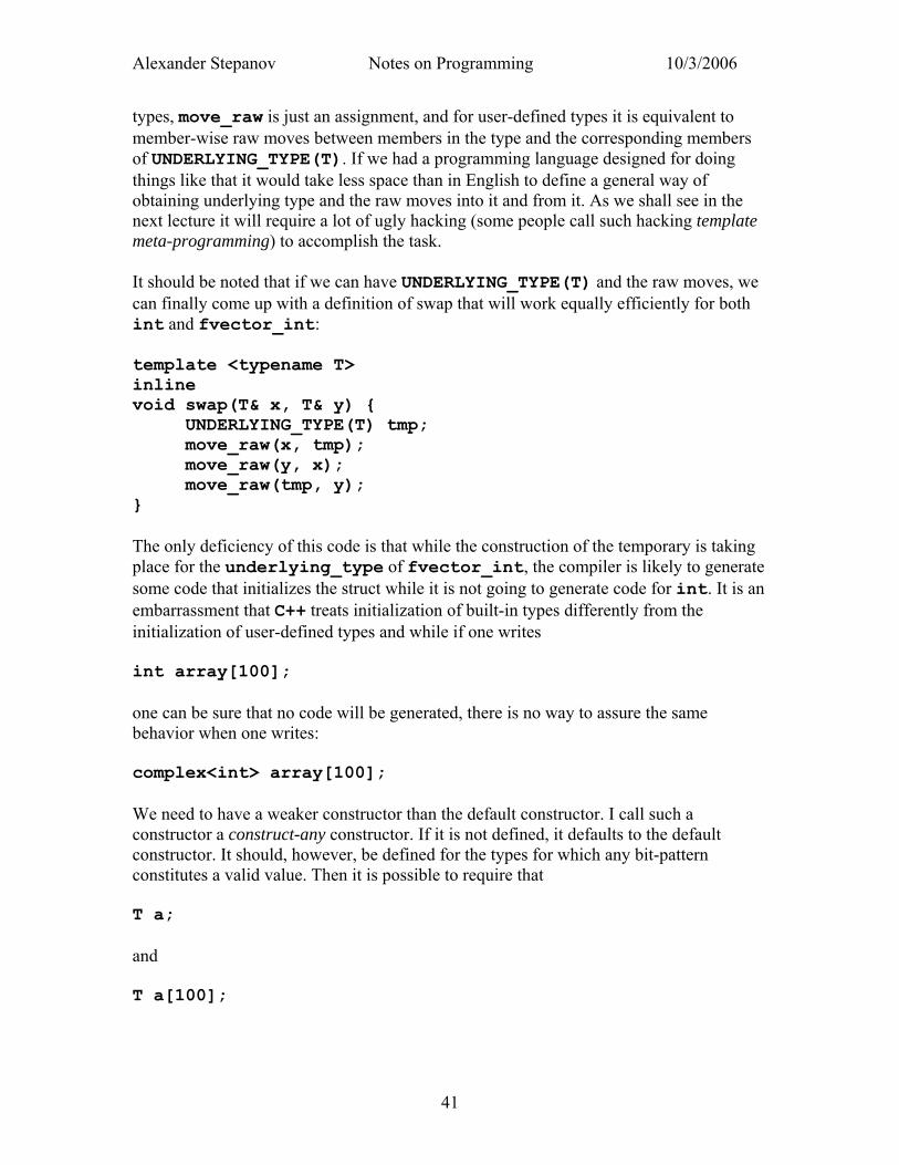
Alexander Stepanov Notes on Programming 10/3/2006
types, move_raw is just an assignment, and for user-defined types it is equivalent to member-wise raw moves between members in the type and the corresponding members of UNDERLYING_TYPE(T). If we had a programming language designed for doing things like that it would take less space than in English to define a general way of obtaining underlying type and the raw moves into it and from it. As we shall see in the next lecture it will require a lot of ugly hacking (some people call such hacking template meta-programming) to accomplish the task. It should be noted that if we can have UNDERLYING_TYPE(T) and the raw moves, we can finally come up with a definition of swap that will work equally efficiently for both int and fvector_int: template <typename T> inline void swap(T& x, T& y) { UNDERLYING_TYPE(T) tmp; move_raw(x, tmp); move_raw(y, x); move_raw(tmp, y); } The only deficiency of this code is that while the construction of the temporary is taking place for the underlying_type of fvector_int, the compiler is likely to generate some code that initializes the struct while it is not going to generate code for int. It is an embarrassment that C++ treats initialization of built-in types differently from the initialization of user-defined types and while if one writes int array[100]; one can be sure that no code will be generated, there is no way to assure the same behavior when one writes: complex<int> array[100]; We need to have a weaker constructor than the default constructor. I call such a constructor a construct-any constructor. If it is not defined, it defaults to the default constructor. It should, however, be defined for the types for which any bit-pattern constitutes a valid value. Then it is possible to require that T a; and T a[100];
41
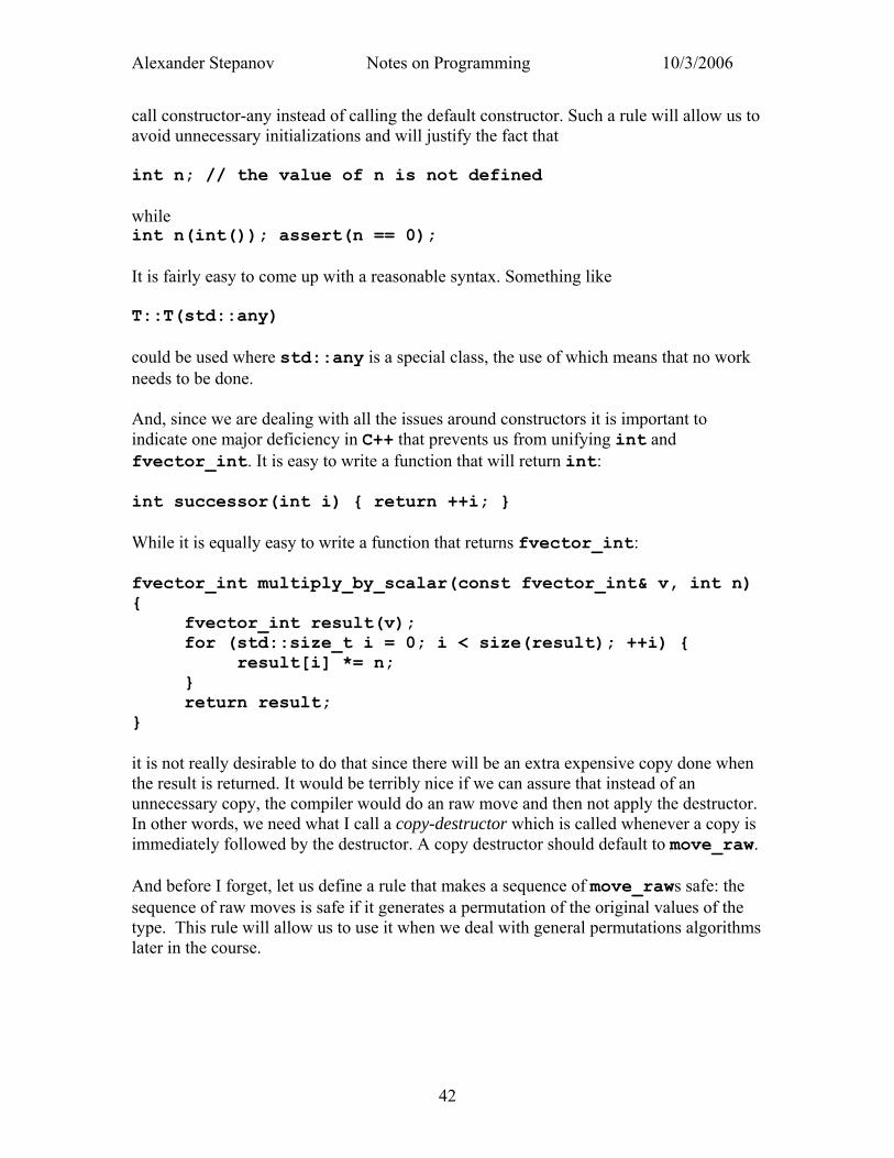
Alexander Stepanov Notes on Programming 10/3/2006
call constructor-any instead of calling the default constructor. Such a rule will allow us to avoid unnecessary initializations and will justify the fact that int n; // the value of n is not defined while int n(int()); assert(n == 0); It is fairly easy to come up with a reasonable syntax. Something like T::T(std::any) could be used where std::any is a special class, the use of which means that no work needs to be done. And, since we are dealing with all the issues around constructors it is important to indicate one major deficiency in C++ that prevents us from unifying int and fvector_int. It is easy to write a function that will return int: int successor(int i) { return ++i; } While it is equally easy to write a function that returns fvector_int: fvector_int multiply_by_scalar(const fvector_int& v, int n) { fvector_int result(v); for (std::size_t i = 0; i < size(result); ++i) { result[i] *= n; } return result; } it is not really desirable to do that since there will be an extra expensive copy done when the result is returned. It would be terribly nice if we can assure that instead of an unnecessary copy, the compiler would do an raw move and then not apply the destructor. In other words, we need what I call a copy-destructor which is called whenever a copy is immediately followed by the destructor. A copy destructor should default to move_raw. And before I forget, let us define a rule that makes a sequence of move_raws safe: the sequence of raw moves is safe if it generates a permutation of the original values of the type. This rule will allow us to use it when we deal with general permutations algorithms later in the course.
42

Alexander Stepanov Notes on Programming 10/3/2006
Lecture 5. Types and type functions We observe that there are similarities between int and fvector_int. We also discovered that it is possible to connect a type with another type through the use of type functions. But what do we mean by a type? This question is one of the central questions in programming. We will be talking about it throughout the course. But we will start now with the most general definition: a type is a method of assigning meaning to data stored in computer memory. This definition is important for us because it states that types have existence irrespective of the programming language that we use. Even if we program in assembly language we assign meaning to different sequences of bits in memory. This meaning is usually expressed in operations that we define on them, the properties we expect them to obey and the mappings from them onto the physically observable values through input/output. The types that our programming language provides for us are just approximations to the full meanings that we see in the bit patterns of our applications. It is important to remember this so that we do not drive our designs by the limitations of the language but come up with the intended definitions of types and only then map them onto the programming language. In other words, design your data structures and algorithms first and only then map them into a programming language. Do not start with inheritance or templates but with linked lists and hash functions. Think in assembly language or C and then implement in a high level language such as C++. Every type has a (potentially infinite) set of computable functions definable on it. Out of this set we can select a subset such that all other functions can be defined in terms of it. I call such a subset a computational basis of a type. I call a computational basis efficient if all the functions on the type can be expressed in terms of the basis as efficiently as if they had access to the bit representation of the type. I call a computational basis orthogonal if no functions in it can be expressed in terms of other functions without loss of efficiency. (It is less important to design an orthogonal basis than an efficient basis for a type; we will frequently insert “unnecessary” helper functions to make the interface more convenient. For example, operator!= is not strictly necessary but we will require it for all regular types.) It is frequently necessary to define (at least conceptually) functions that operate on types themselves – not on the objects. I call such functions type functions. The best example of a type function in C and C++ is the sizeof operator. It takes a type and returns size_t; its pseudo-signature is: size_t sizeof(type); Another example of a type function is a postfix unary operator* that takes a type and returns a pointer type pointing to it. Sadly enough, C and C++ not only lack facilities for defining type functions but do not provide most useful type functions for extracting different type attributes that are trivially
43

Alexander Stepanov Notes on Programming 10/3/2006
known to the compiler. It is impossible to find out how many members a type has; it is impossible to find the types of the members of a structure type; it is impossible to find out how many arguments a function takes or their types; it is impossible to know if a function is defined for a type; the list goes on and on. The language does its best to hide the things that the compiler discovers while processing a program. That is why it is impossible to express the most self-evident things such as the default definition of equality: if equality is not defined for a type, provide it with member-by-member equality. And that is what makes it so difficult for us to give a compilable definition of the underlying_type type function and the corresponding move_raw. This fundamental limitation of the language caused the development of a collection of techniques that is called template meta-programming. As I said before, it is a good example of programming technique known as ugly hacking. It should be noted that I do not claim that people who do it are ugly. (After all, I am personally responsible for unleashing this thing onto the world: STL was not just the first major example of generic programming but the first major example of template hacking.) I consider ugly hacking to be a technical term that describes techniques that use machinery designed for some other purpose to provide fragile partial solutions of fundamental problems. Ugly hacking is invariably “clever”. It is similar to playing the violin with one’s feet. It is admirable that it can be done but its place is in the circus and not in the Conservatoire. While I am at it, let me put a disclaimer about the use of the term generic programming. The term was introduced by David Musser and me in our 1988 paper “Generic Programming” which defines the term like so: “Generic programming centers around the idea of abstracting from concrete efficient algorithms to obtain generic algorithms that can be combined with different data representations to produce a wide variety of useful software. For example, a class of generic sorting algorithms can be defined which work with finite sequences but which can be instantiated in different ways to produce algorithms working on arrays or linked lists.” It has nothing to do with templates or template meta-programming. It has everything to do with algorithms and data structures. Unfortunately, the term was kidnapped and is frequently used to describe the “clever” use of templates. Almost every week I am met by somebody in an elevator who lets me know that he is interested in attending my template meta-programming course. I try to teach programming, not template meta-programming! Unfortunately, I will have to use ugly hacking to do certain things. It will allow me to introduce some essential ideas. But please remember that it is an act of desperation. Do not do it yourself unless absolutely necessary. And if you do, do not be proud of your accomplishments but be sad that you had to inflict such ugliness on future readers of your code. It is relatively easy to implement a basic type function for structures and classes as long as we define a function for every point of its domain, one definition at a time. For example if inside our definition of fvector_int we put the following definition:
44

Alexander Stepanov Notes on Programming 10/3/2006
public: struct underlying_type { size_t length; int* v; }; friend void move_raw(fvector_int& x, underlying_type& y) { y.length = x.length; y.v = x.v; } friend void move_raw(underlying_type& x, fvector_int& y) { y.length = x.length; y.v = x.v; } friend void move_raw(fvector_int& x, fvector_int& y) { y.length = x.length; y.v = x.v; } It seems that we are almost there. If we define: #define UNDERLYING_TYPE(T) typename T::underlying_type we can use our final generic definition of swap template <typename T> inline void swap(T& x, T& y) { UNDERLYING_TYPE(T) tmp; move_raw(x, tmp); move_raw(y, x); move_raw(tmp, y); } with fvector_int and get rid of the specialized version of swap for this class. Unfortunately, that will make our “generic” definition unable to swap two integers since we can not put the following line inside the definition of int: typedef int underlying_type; There seems to be no way for extracting a type from int the way we are extracting a type from fvector_int. Sadly enough there is an ugly hack that allows us to squeeze by. (I say, sadly enough, because if it were not for ugly hacks the core language designers
45
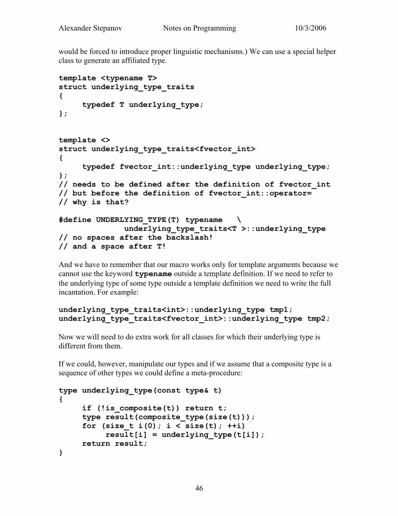
Alexander Stepanov Notes on Programming 10/3/2006
would be forced to introduce proper linguistic mechanisms.) We can use a special helper class to generate an affiliated type. template <typename T> struct underlying_type_traits { typedef T underlying_type; }; template <> struct underlying_type_traits<fvector_int> { typedef fvector_int::underlying_type underlying_type; }; // needs to be defined after the definition of fvector_int // but before the definition of fvector_int::operator= // why is that? #define UNDERLYING_TYPE(T) typename \ underlying_type_traits<T >::underlying_type // no spaces after the backslash! // and a space after T! And we have to remember that our macro works only for template arguments because we cannot use the keyword typename outside a template definition. If we need to refer to the underlying type of some type outside a template definition we need to write the full incantation. For example: underlying_type_traits<int>::underlying_type tmp1; underlying_type_traits<fvector_int>::underlying_type tmp2; Now we will need to do extra work for all classes for which their underlying type is different from them. If we could, however, manipulate our types and if we assume that a composite type is a sequence of other types we could define a meta-procedure: type underlying_type(const type& t) { if (!is_composite(t)) return t; type result(composite_type(size(t))); for (size_t i(0); i < size(t); ++i) result[i] = underlying_type(t[i]); return result; }
46

Alexander Stepanov Notes on Programming 10/3/2006
And – isn’t it nice to be able to program in an imaginary programming language – we would be able to define all raw moves once and for all! If we return to reality, we can produce a version of our fvector_int that includes all of our newly discovered facilities: #include <cstddef> // the definition of size_t #include <cassert> // the definition of assert template <typename T> struct underlying_type_traits { typedef T underlying_type; }; #define UNDERLYING_TYPE(T) typename \ underlying_type_traits<T>::underlying_type template <typename T> inline void swap(T& x, T& y) { UNDERLYING_TYPE(T) tmp; move_raw(x, tmp); move_raw(y, x); move_raw(tmp, y); } template <typename T> inline void cycle_left(T& x1, T& x2, T& x3) { UNDERLYING_TYPE(T) tmp; move_raw(x1, tmp); move_raw(x2, x1); move_raw(x3, x2); move_raw(tmp, x3); } template <typename T> inline void cycle_right(T& x1, T& x2, T& x3) { cycle_left(x3, x2, x1); } class fvector_int { private:
47

Alexander Stepanov Notes on Programming 10/3/2006
size_t length; // the size of the allocated area int* v; // v points to the allocated area public: fvector_int() : length(std::size_t(0)), v(NULL) {} fvector_int(const fvector_int& x); explicit fvector_int(std::size_t n) : length(n), v(new int[n]) {} ~fvector_int() { delete [] v; } fvector_int& operator=(const fvector_int& x); friend std::size_t size(const fvector_int& x) { return x.length; } int& operator[](std::size_t n) { assert(n < size(*this)); return v[n]; } const int& operator[](std::size_t n) const { assert(n < size(*this)); return v[n]; } struct underlying_type { size_t length; int* v; }; friend void move_raw(fvector_int& x, underlying_type& y) { y.length = x.length; y.v = x.v; } friend void move_raw(underlying_type& x, fvector_int& y) { y.length = x.length; y.v = x.v; } friend void move_raw(fvector_int& x, fvector_int& y) { y.length = x.length; y.v = x.v; } }; template <>
48
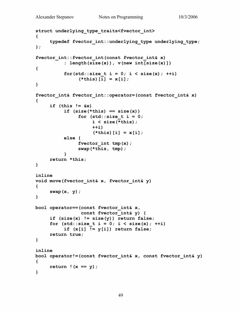
Alexander Stepanov Notes on Programming 10/3/2006
struct underlying_type_traits<fvector_int> { typedef fvector_int::underlying_type underlying_type; }; fvector_int::fvector_int(const fvector_int& x) : length(size(x)), v(new int[size(x)]) { for(std::size_t i = 0; i < size(x); ++i) (*this)[i] = x[i]; } fvector_int& fvector_int::operator=(const fvector_int& x) { if (this != &x) if (size(*this) == size(x)) for (std::size_t i = 0; i < size(*this); ++i) (*this)[i] = x[i]; else { fvector_int tmp(x); swap(*this, tmp); } return *this; } inline void move(fvector_int& x, fvector_int& y) { swap(x, y); } bool operator==(const fvector_int& x, const fvector_int& y) { if (size(x) != size(y)) return false; for (std::size_t i = 0; i < size(x); ++i) if (x[i] != y[i]) return false; return true; } inline bool operator!=(const fvector_int& x, const fvector_int& y) { return !(x == y); }
49
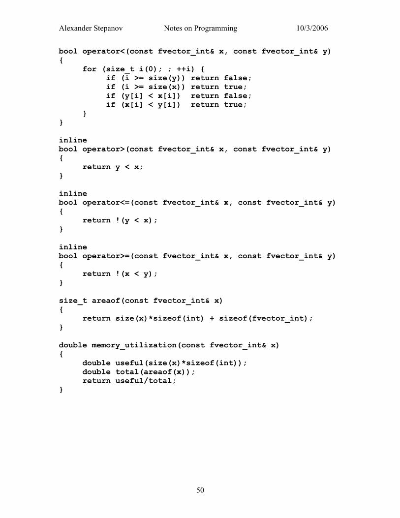
Alexander Stepanov Notes on Programming 10/3/2006
bool operator<(const fvector_int& x, const fvector_int& y) { for (size_t i(0); ; ++i) { if (i >= size(y)) return false; if (i >= size(x)) return true; if (y[i] < x[i]) return false; if (x[i] < y[i]) return true; } } inline bool operator>(const fvector_int& x, const fvector_int& y) { return y < x; } inline bool operator<=(const fvector_int& x, const fvector_int& y) { return !(y < x); } inline bool operator>=(const fvector_int& x, const fvector_int& y) { return !(x < y); } size_t areaof(const fvector_int& x) { return size(x)*sizeof(int) + sizeof(fvector_int); } double memory_utilization(const fvector_int& x) { double useful(size(x)*sizeof(int)); double total(areaof(x)); return useful/total; }
50
Alexander Stepanov Notes on Programming 10/3/2006
Lecture 6. Regular types and equality The introduction of move_raw and UNDERLYING_TYPE dismayed many of you. They seemed to contradict common rules of software engineering allowing us to violate type invariants and put our objects in an unsafe state. And so they do. That, of course, requires an explanation. There are two main reasons why I choose to ignore commonly accepted software engineering strictures. The first reason is that the goal of my quest in programming is to combine two seemingly irreconcilable desires:
– to write programs in the most general terms, and – to write programs as efficient as the underlying hardware allows.
The desire to write programs in the most general terms forces me to extend my type system to be able to deal with complex data structures (such as fvector_int) as if they were built-in types. I would like to be able to store them in other data structures and use them with standard algorithms such as swap. That requires that certain operations such as copying and assignment preserve certain fundamental invariants. Preserving invariants is, however, a costly activity. And sometimes I can ignore them if there is a rule that allows me to assure that a sequence of operations restores invariants. It is not acceptable to make a fundamental operation several times slower than it needs to be only to assure that all the intermediate states are valid. What is essential is that the validity is restored at the conclusion of an operation or when an exception occurs. The second reason for ignoring software engineering rules is that I do not accept attempts to build safety through syntactic restrictions. For years we have been told that avoiding gotos or pointers or other perfectly valid programming constructs will make our code robust. It is clearly not the case, as the number of bugs in any major software product attests. All attempts to legislate robustness or security through the draconian means of restricting our access to some machine types or operations have not produced more robust software. In some fundamental sense it is impossible to keep a programming model expressive enough to be Turing-complete and make it robust. It will always be possible for a programmer to write programs that do unwanted things. I believe that the way to safety does not go through the creation of slow virtual machines and languages that hide the machine from programmers but through the development of reliable and efficient components. If we provide programmers with efficient algorithms and data structures with precisely specified interfaces and complexity guarantees they will not need to use unsafe operations such as move_raw (they will be used only by the few writers of fundamental algorithms). Moreover, through the use of correct “standard” algorithms instead of writing their own “partially correct” ones, they will be able in many cases to avoid using statements such as for and while that can cause non-robust behavior.
51
Alexander Stepanov Notes on Programming 10/3/2006
I have to admit that my attempts to combine abstraction with efficiency have been only partially successful. STL algorithms deteriorate quite dramatically on certain perfectly legitimate inputs. Try using partial sort with strings and see how terrible the performance is. On strings it is almost invariably faster to use sort than to use partial_sort. The reason for such performance degradation is the fact that partial sort uses assignments and not swaps. There are serious reasons to do it, and it makes partial sort much faster for built-in types but slower for strings. It is in order to fix this performance degradation that I introduced move_raw and UNDERLYING_TYPE. Yes, an entry-level programmer should not use them or even know about them, but they are essential for people who want to design efficient and reusable algorithms and data structures. But, be that as it may, the present day STL is not yet capable of fully combining abstraction and efficiency. And that leads us to a more general question: what are the requirements on a type that will let it reside in STL containers and work with STL algorithms? Does STL rely on any unwritten assumptions? As a matter of fact, they are unwritten because the powers that be told me that I cannot put any requirements on general C++ types. As they see it, programmers should be able to write anything they want, and it is nobody’s business to put requirements on the behavior of arbitrary types. I admire their dedication to programming freedom, but I claim that such freedom is an illusion. Finding the laws that govern software components gives us freedom to write complex programs the same way that finding the laws of physics allows us to construct complex mechanical and electrical systems. I call types that work with all STL algorithms and containers regular types. One of the most shameful mistakes of my technical career is that I did not insist on inclusion of the requirements of regular types into the C++ standard and that I did not even assure that all the STL types are themselves regular. So what are the fundamental operations that STL expects any type to have? They belong to 3 groups:
1. Equality: in order to use find and other related algorithms STL requires operator== to be defined and assumes certain properties of it.
2. Total ordering: sorting and binary searching that allow us to find equal elements fast and on which sorted associative containers are based require operator< and assume that it possesses certain properties. Total ordering must be consistent with equality.
3. Copying and assignment: in order to put things into containers and to move them with the help of different mutating algorithms STL assumes the existence of copy constructors, assignment and related operations. They must be consistent with equality.
Notice that groups 2 and 3 depend on group 1. Equality is conceptually central and it happens to be the least understood of all the operations on regular types.
52

Alexander Stepanov Notes on Programming 10/3/2006
When I asked you to figure out what the requirements on equality are, those of you who attempted to do the homework suggested that equality is an operation that is:
• reflexive: a == a • symmetric: a == b implies b == a • transitive: a == b && b == c implies a == c
These are, of course, the properties of equality that define it as an equivalence relationship. But these are not the essential properties of equality. There could be many different equivalence relationship between elements of a type, but only one of them, a very specific one, is called equality. (Discussions of equality and identity were one of the stock discussions for analytic philosophers in the last century. Since 1892 many a paper has been written to decide if the morning star is the evening star and what “is” means. We will leave both stars to philosophers and the meaning of “is” to presidential historians and attempt to give a more computationally-oriented understanding of equality.) When we say that two objects of the same type are equal we are attempting to say that they are interchangeable as far as observations on them are concerned. All the measurements (or at least all essential measurements) on them will return equal results. We know that this is not really true. The total equality of all measurements will include position (the address operator), and that will give us identity but not equality. We know that there are non-identical but equal objects because we know that we can create copies of objects. And a copy is equal but not identical to the original. In some sense, equality is a relationship that is preserved by copying and assignment, but that is not its essential definition either. We cannot implement equality through it. We can get closer to equality if we define the notion of a regular function. We call a function that takes an argument of a type T regular over this argument if it can be substituted by an equal argument without changing the behavior of the function except possibly some adjustment in complexity (the equal argument can, for example, be “further” away, like not being in the cache). And we call a function regular if it is regular over all of its arguments. Different types have different sets of regular functions and it is a very important task to identify them. Quiz: Which functions in the interface of fvector_int are regular? Observe that most common optimization techniques are based on the equality-preserving properties of regular functions. Compilers can do constant folding and constant propagation, common sub-expression elimination and even use general SSA (static single assignment) form optimization on types if they know that types and the functions on them are regular.
53

Alexander Stepanov Notes on Programming 10/3/2006
There are functions that are not by themselves regular but possess the property that composing them with some other functions produces regular functions. For example, the address operator is not a regular function since a == b does not imply &a == &b. The composition of the address with dereferencing gives us a regular function because *&a == *&b. We call such functions dereference-regular. More precisely, a function f is dereference-regular if and only if the composition of f and the dereference operator (operator*) is a regular function (a == b implies *f(a) == *f(b)). When we extend our fvector_int with iterators and begin and end functions we will observe that begin is dereference-regular when dereferencing is defined. A modifying operation on a type is called regular if after it is applied to two (non-identical) equal objects they remain equal afterwards. In general, if a non-modifying regular function is applied to the same non-volatile object twice without any modifying operations happening in between the results will be the same. On the other hand, if there are three different but equal objects a, b and c, and a is modified so that a != b, it must still remain true that b == c. We also expect that the equality operation on regular types is fast. The worst case complexity of comparing two objects should be linear in the area of the smaller one. And assuming the uniform distribution of bit values in a data structure, we can even expect that the average complexity should be constant time. While there are many different kinds of types that we need in programming, one of the most important types is a data structure. The C++ community usually calls data structures containers. I will use both terms indiscriminately. Let us try to outline briefly what we mean by data structures. Knowing what data structures are will allow us to come up with a more precise definition of equality and other operations on regular types. A data structure is a collection of several objects called its parts. There are two different kinds of parts: proper parts and connectors. For example, in fvector_int integers stored in the allocated memory are proper parts. The pointer and the length fields in the header are connectors. In other words, proper parts are those parts of the object that are “interesting” to the user, while the connectors provide accessibility to the proper parts. By the way, I just introduced a notion that is very important: header. The header is the part of a data structure that allows an object to get to all of its parts and is strictly an object in the traditional C++ sense: a struct with several members. I extend the notion of object to include all the memory owned by it. A part of a data structure does not have to be co-located with its header. The notion of type, which started with simple word-sized things like integer and real in Fortran, then developed further to include record types in Algol-68, Pascal, and C that allowed combining several objects laid out in consecutive memory locations, needs to embrace all kind of data structures: lists, hash tables, trees, etc.
54
Alexander Stepanov Notes on Programming 10/3/2006
Now let me introduce a bunch of definitions. Eventually, as we build more and more data structures, you will understand their significance. A part of a data structure that resides in its header is called local. A non-local part is called remote. The need for non-local parts arises from the need for objects whose size is not known at compile time and also from the need for objects that change their size and shape. Another advantage of non-local parts is making the header smaller to make it cheaper to “move” the data structure should that be necessary. All parts of an object are destroyed when an object is destroyed. If two objects share a part, then one object is a part of the other. That means that there is no sharing of parts. This semantics does not, of course, preclude copy-on-write, which is fundamentally an optimization technique that does not violate the essential property of non-sharing: if one object is modified, other objects that are not its parts remain unchanged. There is no circularity among objects - an object cannot be a part of itself and, therefore, cannot be part of any of its parts. That does not mean that we cannot have circular data structures but only that one node in a data structure does not own another; all the nodes are jointly owned by the same data structure. An addressable part is a part for which a reference can be obtained through public member functions. An accessible part is a part for which the value can be determined through public member functions. Every addressable part is also accessible since if a reference is available, it's trivial to obtain the value. An opaque object is an object with no addressable parts. An object is called an open data structure or an open container if all of its proper parts are addressable. Two open data structures are equal if all corresponding proper parts are equal. The problem is to figure out what are corresponding parts. We clearly do not want the sequence {1 ,2 ,3} to be considered equal to the sequence {2, 1, 3}. The corresponding parts are determined by traversal protocols or iteration protocols of the data structure. An object is called fixed-size if it has the same set of parts over its lifetime. An object is called extensible if it is not of fixed size. A part is called permanently placed if it resides at the same memory location over its lifetime. Knowing that a part is permanently placed or not allows us to know how long a pointer that points to it is valid. An object is called permanently placed if every part of the object is permanently placed. In general, a properly specified object should have precisely specified time intervals when its parts are not being reallocated. An object is called simple if it is of fixed size and permanently placed.
55

Alexander Stepanov Notes on Programming 10/3/2006
A concept is a collection of similar types together with a collection of similar programs written in terms of the types and the properties of such programs and types.
Lecture 7. Ordering and related algorithms Equality allows us to find an object in a sequence; it is impossible to implement the simplest version of linear search without equality. We need to have an ordering if we want to find things quickly. If we can order, we can sort, and if we can sort, we can use binary search. While we are not yet ready to look at sorting and binary searching, we can do many interesting little things with ordering. We already encountered operator< when we were implementing it for fvector_int. I remarked then that it is one of four relational operators that are available in C++. I also stated that they should all be defined together. The language does not require that. You can have a class that defines both < and > with x < y not equivalent to y > x. A design like that causes people to consider overloaded operators to be a big nuisance. The fundamental rule for overloading is that operators on user-defined types should mean the same as on built-in types and in common mathematical usage. It would be nice if the compiler would synthesize the three remaining relational operators for any class after any one of the four (<, >, <=, >=) is defined. I could not do it like that but attempted to do something almost equivalent by providing STL with the following three templates that defined >, <=, >= when < was defined: template <typename T> // T models Strict Totally Ordered inline bool operator>(const T& x, const T& y) { return y < x; } template <typename T> // T models Strict Totally Ordered inline bool operator<=(const T& x, const T& y) { return !(y < x); } template <typename T> // T models Strict Totally Ordered inline bool operator>=(const T& x, const T& y) { return !(x < y); }
56

Alexander Stepanov Notes on Programming 10/3/2006
The standards committee in its infinite wisdom kept the definitions but moved them into a special namespace that makes them quite useless. Be that as it may, I suggest that you always copy these templates after your definition of operator< for your class and then replace T with the name of your class until such time when the language and the compiler do it for you automatically. Since all four operators are equivalent, one has to make a choice of which one of them is going to be used as a default operator in those cases when we define an algorithm that uses total ordering. I chose operator<. I assumed that ascending ordering of elements is more natural to us, and I also assumed that < requires less typing than <=. Both assumptions could be challenged, but I still do not see why any other default would be better. Operator less-than must satisfy the three axioms of strict total ordering: Irreflexive law: a == b implies !(a < b) From this law we can easily derive that a == b implies !(b < a). Indeed, by symmetry of equality a == b implies b == a and that implies that !(b < a). Transitive law: a < b && b < c implies a < c From this we can easily derive that !(a < b && b < a). Indeed, if a < b && b < a then by transitivity a < a and that contradicts the irreflexive law. In other words, irreflexivity and transitivity imply anti-symmetry. And, finally Trichotomy law: a != b implies a < b || b < a Notice that strict total ordering presupposes equality. While equality by itself does not allow us to write many interesting algorithms – one needs at least an ability to iterate to have something like linear search – we can write some really useful algorithms solely in terms of ordering. A good starting point is a very simple algorithm that many people get wrong: a function to return the minimum of two objects. You could frequently find the following “generic” definition of minimum: template <typename T> T min(T x, T y) { return x < y ? x : y; }
57
Alexander Stepanov Notes on Programming 10/3/2006
This is a terrible piece of code. It has nothing to do with generic programming though it starts with the keyword template. It is easy to see the most fundamental reason for its terribleness if we attempt to restate the algorithm in English: To find a minimum object out of two objects we first need to copy these two objects and if the copy of the first is less than the copy of the second then we return a copy of the copy of the first, otherwise we return a copy of the copy of the second. We are clearly doing a bit more copying than absolutely necessary. One does not need to know much about computer science to realize that to pick the smaller of the two objects no copying is needed. And since this code takes an arbitrarily large T the overhead of three unneeded copies could be quite dramatic. Comparing two objects should not raise any exceptions but copying usually can. (Unfortunately, I have seen operator< raise exceptions; there are, of course, no reasonable rules that the “experts” do not break. The same experts then demand that sorting routines when faced with an exception should restore a sequence to its original state. Otherwise, they say, your sort is not exception safe.) This code takes something that should have constant-time average complexity – the less-than operator should be linear in the worst case and constant time on the average – and makes it into a linear-time operation that might throw an exception because of lack of resources. It is quite easy to see that we need to pass our objects by reference: template <typename T> inline T& min(T& x, T& y) { return x < y ? x : y; } We should also inline it since the body is so short that inlining will frequently not just speed things up but shorten the code size. (Unfortunately, quite frequently modern compilers ignore the inline directive. It would be fine if they would inline the functions that really need inlining but it is not so. In 2005 a major desktop application was losing 15% performance because the compiler would not inline the indexing operator on vectors.) Unfortunately, the code will not work for constant objects even though it does not modify them. The solution is an annoying duplication of code. We need to overload on const and produce an additional version of min: template <typename T> inline const T& min(const T& x, const T& y) { return x < y ? x : y; } Now if at least one of the two objects is constant the second version will be selected. We still, however, use it with non-constant objects to do something like:
58

Alexander Stepanov Notes on Programming 10/3/2006
++min(a, b); // increment the smaller of the two objects We are still far from the generic algorithm. To make it truly generic we need to see if the set of requirements on the type is too restrictive. Indeed, we might use a minimum not only when we deal with the default total ordering defined by operator< but also with a different strict total ordering. Or we might use it with a strict weak ordering such as an ordering of pairs of integers on their first elements: struct pair_int_int { int first; int second; }; inline bool first_ordering(const pair_int_int& x, const pair_int_int& y) { return x.first < y.first; } The strict weak ordering obeys axioms similar to the axioms of strict total ordering but instead of being based on equality it is based on a (often implied) weaker equivalence relation eq that is: Reflexive: a == b implies eq(a, b) Symmetric: eq(a, b) implies eq(b, a) Transitive: eq(a, b) && eq(b, c) implies eq(a, c) Then a relation r(a, b) is a strict weak ordering if it obeys the following laws: Irreflexive law: eq(a, b) implies !r(a, b) From that we can easily show that eq(a, b) implies !r(b, a). Indeed, by symmetry of eq, eq(a, b) implies eq(b, a) and that implies !r(b, a). Transitive law: r(a, b) && r(b, c) implies r(a, c) From that we can easily show that !(r(a, b) && r(b, a)). Indeed, if r(a, b) && r(b, a) then by transitivity r(a, a) and that contradicts the irreflexive law. As with strict total ordering, irreflexivity and transitivity imply anti-symmetry. And, finally, Trichotomy law: !eq(a, b) implies r(a, b) || r(b, a)
59
Alexander Stepanov Notes on Programming 10/3/2006
Quiz: If first_ordering is our strict weak ordering, define the function that implements the corresponding equivalence relation. We can easily fix our min function to accept any strict weak ordering and even make it default to the standard strict total ordering on the type. template <typename T, // T models Any typename R> // R models StrictWeakOrdering on T inline T& min(T& x, T& y, R r) { return r(x, y) ? x : y; } Notice that we pass T by reference while we pass R by value. The reason for that is the fact that T can be very big and copying is expensive. R tend to be very small, often not even having a state. It is, therefore, faster to pass it by value. The general convention that we are going to be following is to pass small things (function objects and iterators) by value, and to pass arbitrarily large objects by reference or constant reference. The convention, however, is based on my performance measurements done in the early 1990ties and do not represent “eternal” truth but will need to be revised eventually. I hope that eventually (in the future system programming language) all the arguments will be passed by reference or constant reference and the passing by value will be done behind the scene by the compiler wherever appropriate as a complier optimization. And we can obtain the less general version by passing the total ordering as a default: template <typename T> // T models Strict Totally Ordered inline T& min(T& x, T& y) { return min(x, y, std::less<T>()); } and template <typename T, // T models Any typename R> // R models Strict Weak Ordering on T inline const T& min(const T& x, const T& y, R r) { return r(x, y) ? x : y; } template <typename T> // T models Strict Totally Ordered
60
Alexander Stepanov Notes on Programming 10/3/2006
inline const T& min(const T& x, const T& y) { return min(x, y, std::less<T>()); } (If you do not know what std::less<T>() is doing, just accept on faith that it will let the code use operator<. We will study function objects in a couple of lectures.) Notice that while C++ allows us to write min, it requires us to write 4 different functions to do the same rather trivial thing. Part of the reason is that it is impossible to unify the const T& and T& signatures into a single function. It is a tricky language design problem to find a way to unify them in C++ or in a future language. Finding such a unification would reduce the number of interfaces from four to two. Another factor-of-two reduction would be possible without much work when compilers will allow us to write this standard-conforming code: template <typename T, // T models Any typename R = std::less<T> > // R models Strict Weak Ordering on T inline T& min(T& x, T& y, R r = R()) { return r(x, y) ? x : y; } Since it is tedious to write the four versions of the same code I will from now on do only one with T& and explicit comparison. It is assumed that the versions with const T& and explicit comparison are defined analogously. While it might appear that we are finally done, there is another problem that lurks beneath the surface of this very simple code. To see it, let us implement another function that could be done with two objects and a strict weak ordering on them, namely, a sorting function. It seems that we can do it without much difficulty by swapping the inputs when they are out of order: template <typename T> // T models Strict Totally Ordered inline void sort_2(T& x, T& y) { if (!(x < y)) swap(x, y); } This code possesses the unpleasant property that equivalent objects are swapped. In other words, our sort_2 does more work than necessary and is not stable. A stable preserves
61
Alexander Stepanov Notes on Programming 10/3/2006
the relative order of equivalent objects. As we shall see later in the course, stability is an important property, and we should not abandon it without necessity. As a matter of fact, it is trivial to fix the problem by performing the swap only when the second object is strictly less than the first: template <typename T> // T models Strict Totally Ordered inline void sort_2(T& x, T& y) { if (y < x) swap(x, y); } Now it is obvious that there should be a relationship between sort_2 and min: after we sort two elements, the first one should be the minimum: template <typename T> // T models Strict Totally Ordered inline void sort_2(T& x, T& y) { if (y < x) swap(x, y); assert(x == min(x, y)); } This, however, is not true. Our min function is going to return the second object when both objects are equivalent, and sort_2 is going to leave them alone and assume the first object is the smaller one. We need to make our min stable: template <typename T> // T models TotallyOrdered inline T& min(T& x, T& y) { return y < x ? y : x; } Now we need one more sensible function: maximum. It is invariably the case that even when people define min in a stable manner they assume, somehow, that max requires only flipping the relation around (see, for example, the implementation of max in SGI STL at http://www.sgi.com/tech/stl/stl_algobase.h): template <typename T> // T models TotallyOrdered inline T& max(T& x, T& y) { return x < y ? y : x; }
62

Alexander Stepanov Notes on Programming 10/3/2006
(It is hard for me to blame people who do so: after all, they just follow the C++ standard specification of max written by me. It took me several years to see that I was mistaken.) When both objects are equivalent the first one is returned. That, of course, will break another self-evident post-condition for sort_2: template <typename T> // T models TotallyOrdered inline void sort_2(T& x, T& y) { if (y < x) swap(x, y); assert(x == min(x, y)); assert(y == max(x, y)); } As a matter of fact, in order for this condition to hold, max should return the first object only when it is strictly greater than the second: template <typename T> // T models TotallyOrdered inline T& max(T& x, T& y) { return y < x ? x : y; } There is an additional advantage of doing it this way. We can always obtain the “old” semantics of max by passing the transposed ordering relation to min. (For the default total ordering we can pass greater<T>() and for any user specified ordering r we can pass the transpose(r) function object – and you have to wait a little while longer to learn what transpose does and how it does it.) Problem: Implement median_3 function that returns the median of 3 elements. Problem: Implement median_5 function that returns the median of 5 elements.
63
Alexander Stepanov Notes on Programming 10/3/2006
Lecture 8. Order selection of up to 5 objects Now we know how to find the maximum and minimum of two elements. While we will study algorithms dealing with arbitrary sequences of objects with strict weak ordering defined on them later in the course, it is instructive to see how our algorithms defined on 2 objects generalize to 3, 4 and 5 objects. In this lecture we shall concentrate on implementing these operations with the smallest possible number of comparisons. We will occasionally overlook stability. (I will address techniques for guaranteeing stability and the move minimization in future lectures.) Those of you who succeeded in implementing median_5 know that it is a fairly difficult undertaking. One of the goals is to see how we can handle the design of this function without heroic efforts and by using a systematic approach. In general, the technique of finding the solution through decomposition of problems into small reusable steps is the central idea of the course. It is clear that we can easily generalize our min and max to 3 elements. template <typename T> inline T& min_3(T& x1, T& x2, T& x3) { return min(min(x1, x2), x3); } template <typename T> inline T& max_3(T& x1, T& x2, T& x3) { return max(max(x1, x2), x3); } It is self-evident how to define versions of them for 4 or more arguments. When we learn how to iterate through arbitrary sequences, we will write iterative versions of these functions. If we have n elements we need n – 1 comparisons to find the minimum or the maximum, since with a smaller number we cannot connect the elements together, and if the comparison graph is disconnected we cannot possibly know in which connected component the minimum or the maximum belongs. It is a little bit more difficult to find the median element. The technique we are going to use for finding an algorithm for median is by reducing it to a simpler problem. (It is not that difficult to write the algorithm by doing a brute-force case analysis, but we shall see that the technique will serve us well in the much more difficult case of median of 5. In general, it is an important technique that needs to be mastered.) It is often good to start searching for the solution by first assuming that that we are halfway there. Let us assume that somehow the first two objects are known to be in the right order, that is, the second is not greater than the first. Then we can define a simple
64
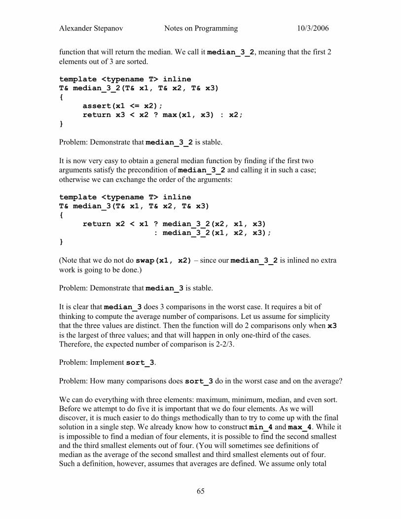
Alexander Stepanov Notes on Programming 10/3/2006
function that will return the median. We call it median_3_2, meaning that the first 2 elements out of 3 are sorted. template <typename T> inline T& median_3_2(T& x1, T& x2, T& x3) { assert(x1 <= x2); return x3 < x2 ? max(x1, x3) : x2; } Problem: Demonstrate that median_3_2 is stable. It is now very easy to obtain a general median function by finding if the first two arguments satisfy the precondition of median_3_2 and calling it in such a case; otherwise we can exchange the order of the arguments: template <typename T> inline T& median_3(T& x1, T& x2, T& x3) { return x2 < x1 ? median_3_2(x2, x1, x3) : median_3_2(x1, x2, x3); } (Note that we do not do swap(x1, x2) – since our median_3_2 is inlined no extra work is going to be done.) Problem: Demonstrate that median_3 is stable. It is clear that median_3 does 3 comparisons in the worst case. It requires a bit of thinking to compute the average number of comparisons. Let us assume for simplicity that the three values are distinct. Then the function will do 2 comparisons only when x3 is the largest of three values; and that will happen in only one-third of the cases. Therefore, the expected number of comparison is 2-2/3. Problem: Implement sort_3. Problem: How many comparisons does sort_3 do in the worst case and on the average? We can do everything with three elements: maximum, minimum, median, and even sort. Before we attempt to do five it is important that we do four elements. As we will discover, it is much easier to do things methodically than to try to come up with the final solution in a single step. We already know how to construct min_4 and max_4. While it is impossible to find a median of four elements, it is possible to find the second smallest and the third smallest elements out of four. (You will sometimes see definitions of median as the average of the second smallest and third smallest elements out of four. Such a definition, however, assumes that averages are defined. We assume only total
65
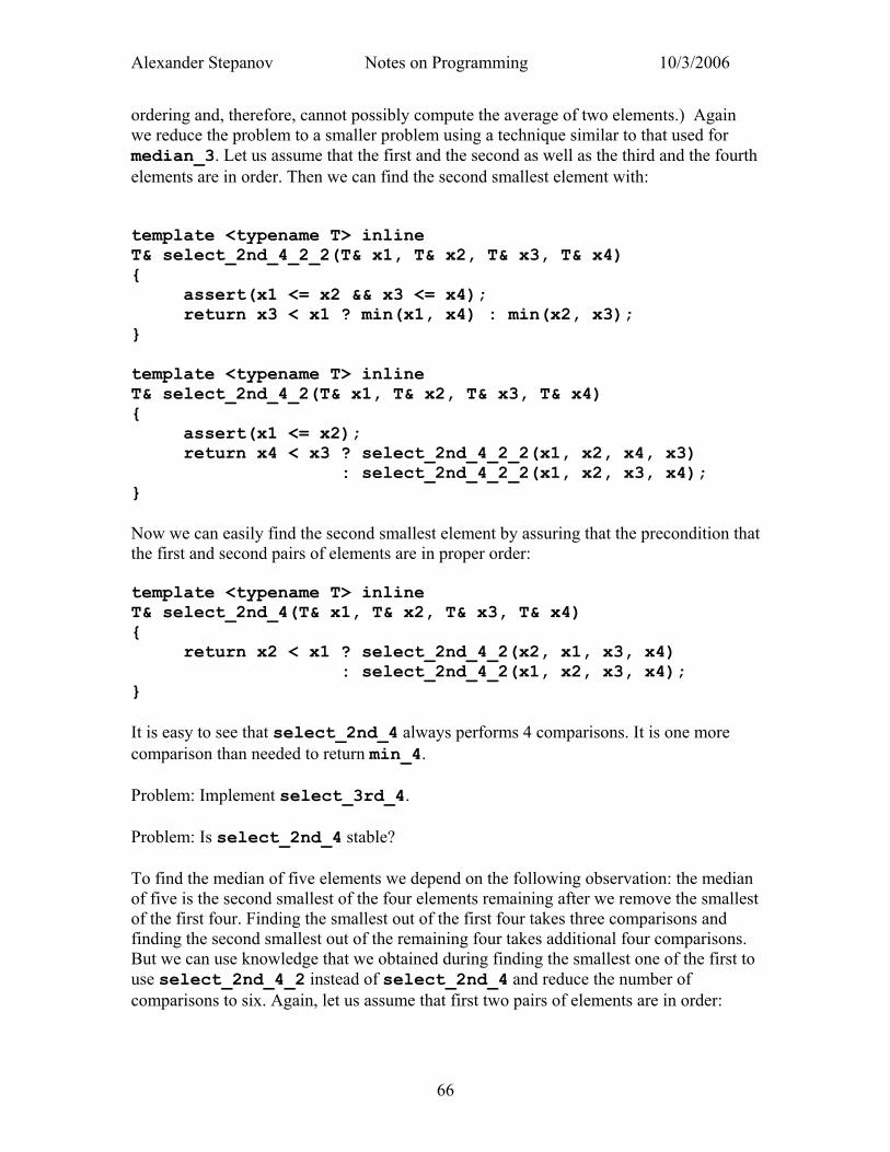
Alexander Stepanov Notes on Programming 10/3/2006
ordering and, therefore, cannot possibly compute the average of two elements.) Again we reduce the problem to a smaller problem using a technique similar to that used for median_3. Let us assume that the first and the second as well as the third and the fourth elements are in order. Then we can find the second smallest element with: template <typename T> inline T& select_2nd_4_2_2(T& x1, T& x2, T& x3, T& x4) { assert(x1 <= x2 && x3 <= x4); return x3 < x1 ? min(x1, x4) : min(x2, x3); } template <typename T> inline T& select_2nd_4_2(T& x1, T& x2, T& x3, T& x4) { assert(x1 <= x2); return x4 < x3 ? select_2nd_4_2_2(x1, x2, x4, x3) : select_2nd_4_2_2(x1, x2, x3, x4); } Now we can easily find the second smallest element by assuring that the precondition that the first and second pairs of elements are in proper order: template <typename T> inline T& select_2nd_4(T& x1, T& x2, T& x3, T& x4) { return x2 < x1 ? select_2nd_4_2(x2, x1, x3, x4) : select_2nd_4_2(x1, x2, x3, x4); } It is easy to see that select_2nd_4 always performs 4 comparisons. It is one more comparison than needed to return min_4. Problem: Implement select_3rd_4. Problem: Is select_2nd_4 stable? To find the median of five elements we depend on the following observation: the median of five is the second smallest of the four elements remaining after we remove the smallest of the first four. Finding the smallest out of the first four takes three comparisons and finding the second smallest out of the remaining four takes additional four comparisons. But we can use knowledge that we obtained during finding the smallest one of the first to use select_2nd_4_2 instead of select_2nd_4 and reduce the number of comparisons to six. Again, let us assume that first two pairs of elements are in order:
66

Alexander Stepanov Notes on Programming 10/3/2006
template <typename T> inline T& median_5_2_2(T& x1, T& x2, T& x3, T& x4, T& x5) { assert(x1 <= x2 && x3 <= x4); return x3 < x1 ? select_2nd_4_2(x1, x2, x4, x5) : select_2nd_4_2(x3, x4, x2, x5); } template <typename T> inline T& median_5_2(T& x1, T& x2, T& x3, T& x4, T& x5) { assert(x1 <= x2); return x4 < x3 ? median_5_2_2(x1, x2, x4, x3, x5) : median_5_2_2(x1, x2, x3, x4, x5); } template <typename T> inline T& median_5(T& x1, T& x2, T& x3, T& x4, T& x5) { return x2 < x1 ? median_5_2(x2, x1, x3, x4, x5) : median_5_2(x1, x2, x3, x4, x5); } This version of median_5 does the smallest possible number of comparisons in the worst case. We can, however, do slightly fewer comparisons on the average. Indeed, if we logically sort the first three elements we can compare the fourth and the fifth with the median. If they fall on the different sides of the median then the median of the first three is the median of five. If they fall on the same side, then we need to return max_3 or min_3 correspondingly, depending on whether they are smaller or larger than the median of the first three. Let us assume that the first three elements are in order: template <typename T> inline T& median_5_3(T& x1, T& x2, T& x3, T& x4, T& x5) { assert(x1 <= x2 && x2 <= x3); return x4 < x2 ? x5 < x2 ? max_3(x1, x4, x5) : x2 : x5 < x2 ? x2 : min_3(x3, x4, x5); } template <typename T> inline T& median_5_2b(T& x1, T& x2, T& x3, T& x4, T& x5) { assert(x1 <= x2); return x3 < x2 ? x3 < x1 ? median_5_3(x3, x1, x2, x4, x5) : median_5_3(x1, x3, x2, x4, x5) : median_5_3(x1, x2, x3, x4, x5);
67

Alexander Stepanov Notes on Programming 10/3/2006
} template <typename T> inline T& median_5b(T& x1, T& x2, T& x3, T& x4, T& x5) { return x2 < x1 ? median_5_2b(x2, x1, x3, x4, x5) : median_5_2b(x1, x2, x3, x4, x5); } Now let us separate the computation of the expected number of the comparisons into two parts. First, let us find the expected number of the comparisons that is done by median_5_3. When the fourth and fifth elements are on different sides of the median of the first three, we do two comparisons. If they are on the same side we need two more. So the average number of comparisons is equal to 2p+4(1- p) where p is the probability they will be on different sides. The probability of the fifth element falling on the same side as the fourth is 3/5, and that makes the expected number of comparisons to be 3-1/5. The first stage of the algorithm does either 2 comparisons if the third element is larger than the maximum of the first two or 3 comparisons otherwise. The expected number of comparisons is 2-2/3 and that gives us the total expected number of 5-13/15. The second algorithm is just over 2% faster on average. Problem: Implement select_2nd_5. Problem: Implement select_4th_5. You can learn more about the subject if you read section 5.3.3 Minimum Comparison Selection, in the 3rd volume of The Art of Computer Programming. We will revisit this material several times during the course.
68

Alexander Stepanov Notes on Programming 10/3/2006
Lecture 9. Function objects One of the stumbling blocks facing a programmer learning C++ is the sad fact that there are often several different mechanisms for accomplishing the task. This problem is the result of the long evolutionary development of the language. Some features are inherited from the C language, some result from being once positioned in a different ecological niche, and some are dead ends. The most important of these alternative linguistic mechanisms are, of course, inheritance and templates, which provide two different ways to produce abstract, generalized software components. We are not yet ready to handle this problem and will address it much later in the course. But now we need to address the second most common problem faced by C++ programmers: when to use functions and when to use function objects. As we shall see, it is the problem has no clear-cut solution since both mechanisms have different advantages and disadvantages. Let us consider several problems that we face while using components such as min, max and median_3, or sort. We often need to use sort with a comparison object that is different from operator<. For example, we might want to sort an array of doubles in ascending order of absolute values. That could be accomplished by calling std::sort with the following function: bool less_abs_fun(double x, double y) { return std::abs(x) < std::abs(y); } int main() { double array[10000]; std::sort(array, array + 10000, less_abs_fun); } This code is much slower than sorting them with operator<. The reason is that where before we were executing a single comparison, now we are doing a function call. Problem: How much slower is sorting with less_abs_fun than with operator< on your computer? (Sort an array of 10000 numbers many times and see how long it takes.) Declaring less_abs_fun to be inline is not going to help, because compilers do not inline calls to functions passed to templates through a pointer. Compilers will instantiate std::sort with the following argument types: double, double, bool (*)(double, double) and then call it, passing it a pointer to less_abs_fun. After all, templates are instantiated for different types, not for different argument values. That was the first
69

Alexander Stepanov Notes on Programming 10/3/2006
reason for introducing function objects: to pass snippets of code into templates for inlining. We need to find a way to affiliate the code of less_abs_fun with a type. We can do it by defining: struct less_abs { bool operator()(double x, double y) const { return std::abs(x) < std::abs(y); } }; We are defining a type with no data members and will be passing instances of this class to sort in order to force the inlining of the code inside sort: int main() { double array[10000]; std::sort(array, array + 10000, less_abs()); } We put parentheses after the name of less_abs to construct an unnamed or anonymous object of the class. The object contains no data, and we pass it to the function only for its type. (Interestingly enough, an object containing no data still has non-zero size, since in C++ two different objects cannot have the same address. On most systems the size of an empty object is 1 byte. Unfortunately, in many situations one byte effectively means one word.) When using an anonymous function object we have to remember to construct it by appending a pair of parentheses. After all, we cannot pass a class to a function. If we want to compare two doubles with our function objects we write: less_abs()(1.5, -4.7) // returns true Also we can avoid the extra pair by creating a named object: less_abs my_compare; my_compare(1.5, -4.7); The second reason for using function objects is that often we need to associate a datum that is computed at run-time with a piece of code. For example, we might want to sort our numbers based on their distance to some number a. It can, of course, be done with the help of a function and a global variable: double a; bool less_distance_fun(double x, double y)
70
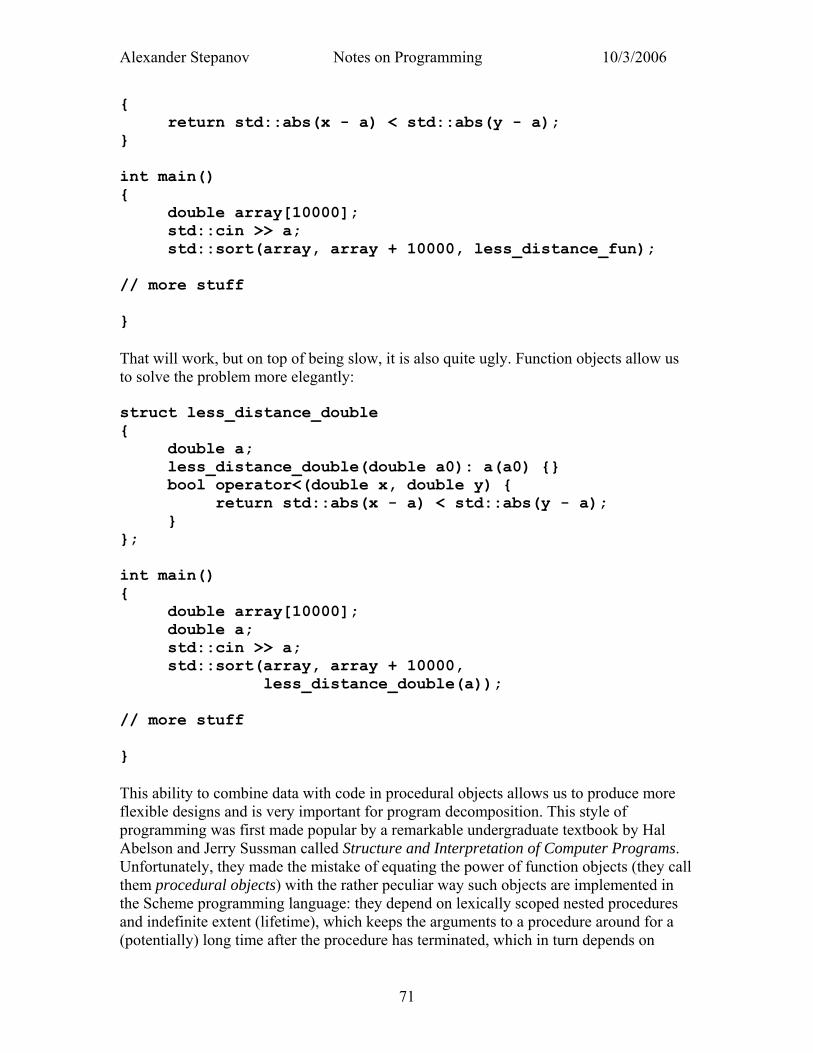
Alexander Stepanov Notes on Programming 10/3/2006
{ return std::abs(x - a) < std::abs(y - a); } int main() { double array[10000]; std::cin >> a; std::sort(array, array + 10000, less_distance_fun); // more stuff } That will work, but on top of being slow, it is also quite ugly. Function objects allow us to solve the problem more elegantly: struct less_distance_double { double a; less_distance_double(double a0): a(a0) {} bool operator<(double x, double y) { return std::abs(x - a) < std::abs(y - a); } }; int main() { double array[10000]; double a; std::cin >> a; std::sort(array, array + 10000, less_distance_double(a)); // more stuff } This ability to combine data with code in procedural objects allows us to produce more flexible designs and is very important for program decomposition. This style of programming was first made popular by a remarkable undergraduate textbook by Hal Abelson and Jerry Sussman called Structure and Interpretation of Computer Programs. Unfortunately, they made the mistake of equating the power of function objects (they call them procedural objects) with the rather peculiar way such objects are implemented in the Scheme programming language: they depend on lexically scoped nested procedures and indefinite extent (lifetime), which keeps the arguments to a procedure around for a (potentially) long time after the procedure has terminated, which in turn depends on
71

Alexander Stepanov Notes on Programming 10/3/2006
having garbage collection. (And, of course, they come from a tradition that considered static typing to be a nuisance.) That led to a total disregard of this style of programming by the mainstream programming community, which needed to ship products and could not possibly afford writing them in a functional language. C++ allowed this style of programming to migrate into the mainstream by actually assuring that the programs written this way are often faster than traditional C-style programs and definitely faster than object-oriented programs that heavily depend on calling functions through function pointers. Since the datum is kept inside the function object it is possible to templatize less_distance: template <typename T> // T models linearly ordered group inline T abs(const T& x) { return x < T(0) ? –x : x; } template <typename T> // T models linearly ordered group struct less_distance { T a; less_distance(const T& a0): a(a0) {} bool operator<(const T& x, const T& y) const { return std::abs(x - a) < std::abs(y - a); } }; (It is curious to note that the C++ powers-that-be rejected the definition of abs from the inclusion in the standard remarking that C++ programmers do not use linearly ordered groups. Then they proceeded to include versions of it for several additional types.) To use our templatized code we will have to re-write our call to sort to look like: std::sort(array, array + 10000, less_distance<double>(a)); We can eliminate the need to specify the type that less_distance takes by providing an auxiliary maker function: template <typename T> // T models linearly ordered group inline less_distance<T> make_less_distance(const T& x) { return less_distance<T>(x);
72
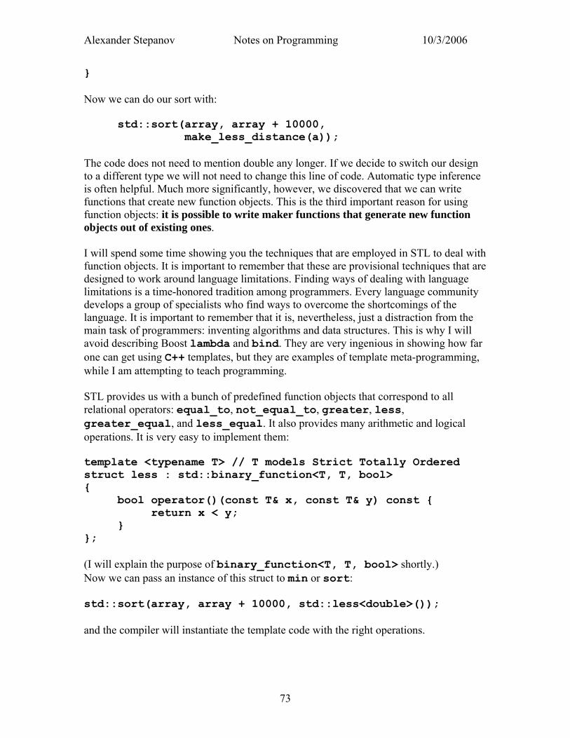
Alexander Stepanov Notes on Programming 10/3/2006
} Now we can do our sort with: std::sort(array, array + 10000, make_less_distance(a)); The code does not need to mention double any longer. If we decide to switch our design to a different type we will not need to change this line of code. Automatic type inference is often helpful. Much more significantly, however, we discovered that we can write functions that create new function objects. This is the third important reason for using function objects: it is possible to write maker functions that generate new function objects out of existing ones. I will spend some time showing you the techniques that are employed in STL to deal with function objects. It is important to remember that these are provisional techniques that are designed to work around language limitations. Finding ways of dealing with language limitations is a time-honored tradition among programmers. Every language community develops a group of specialists who find ways to overcome the shortcomings of the language. It is important to remember that it is, nevertheless, just a distraction from the main task of programmers: inventing algorithms and data structures. This is why I will avoid describing Boost lambda and bind. They are very ingenious in showing how far one can get using C++ templates, but they are examples of template meta-programming, while I am attempting to teach programming. STL provides us with a bunch of predefined function objects that correspond to all relational operators: equal_to, not_equal_to, greater, less, greater_equal, and less_equal. It also provides many arithmetic and logical operations. It is very easy to implement them: template <typename T> // T models Strict Totally Ordered struct less : std::binary_function<T, T, bool> { bool operator()(const T& x, const T& y) const { return x < y; } }; (I will explain the purpose of binary_function<T, T, bool> shortly.) Now we can pass an instance of this struct to min or sort: std::sort(array, array + 10000, std::less<double>()); and the compiler will instantiate the template code with the right operations.
73
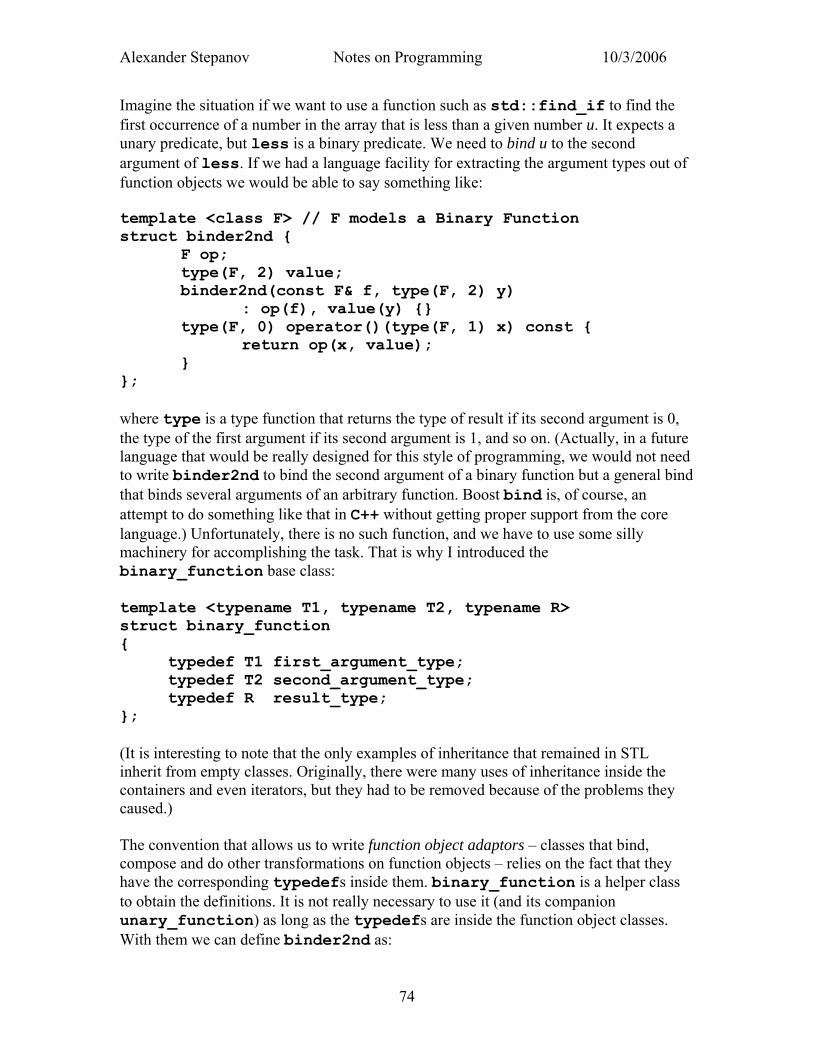
Alexander Stepanov Notes on Programming 10/3/2006
Imagine the situation if we want to use a function such as std::find_if to find the first occurrence of a number in the array that is less than a given number u. It expects a unary predicate, but less is a binary predicate. We need to bind u to the second argument of less. If we had a language facility for extracting the argument types out of function objects we would be able to say something like: template <class F> // F models a Binary Function struct binder2nd { F op; type(F, 2) value; binder2nd(const F& f, type(F, 2) y) : op(f), value(y) {} type(F, 0) operator()(type(F, 1) x) const { return op(x, value); } }; where type is a type function that returns the type of result if its second argument is 0, the type of the first argument if its second argument is 1, and so on. (Actually, in a future language that would be really designed for this style of programming, we would not need to write binder2nd to bind the second argument of a binary function but a general bind that binds several arguments of an arbitrary function. Boost bind is, of course, an attempt to do something like that in C++ without getting proper support from the core language.) Unfortunately, there is no such function, and we have to use some silly machinery for accomplishing the task. That is why I introduced the binary_function base class: template <typename T1, typename T2, typename R> struct binary_function { typedef T1 first_argument_type; typedef T2 second_argument_type; typedef R result_type; }; (It is interesting to note that the only examples of inheritance that remained in STL inherit from empty classes. Originally, there were many uses of inheritance inside the containers and even iterators, but they had to be removed because of the problems they caused.) The convention that allows us to write function object adaptors – classes that bind, compose and do other transformations on function objects – relies on the fact that they have the corresponding typedefs inside them. binary_function is a helper class to obtain the definitions. It is not really necessary to use it (and its companion unary_function) as long as the typedefs are inside the function object classes. With them we can define binder2nd as:
74

Alexander Stepanov Notes on Programming 10/3/2006
template <class F> // F models a Binary Function struct binder2nd { typedef typename F::first_argument_type argument_type; typedef typename F::second_argument_type value_type; typedef typename F::result_type result_type; F op; value_type value; binder2nd(const F& f, const value_type& y) : op(f), value(y) {} result_type operator()(const argument_type& x) const { return op(x, value); } }; Now we can call find_if: double array[10000]; // put some data into array double u = 1.1010010001; double* p = find_if(array, array + 10000, binder2nd<less<double> >(less<double>(), u)); To make it easier to call, STL defines a useful function that saves typing the name of the type of the binary function object twice: template <class F, // F models binary function class T> // T is convertible to // F::second_argument_type inline binder2nd<F> bind2nd(const F& op, const T& x) { return binder2nd<F>(op, typename F::second_argument_type(x)); } And now our code becomes: double* p = find_if(array, array + 10000, bind2nd(less<double>(), u));
Problem: Implement binder1st and bind1st, which bind the first argument of a binary function object.
75

Alexander Stepanov Notes on Programming 10/3/2006
Binding is only one of several useful function object adaptors. Another useful function object operation is composition. It takes two function objects f(x) and g(x) and returns a function object that computes f(g(x)). It is easy to see how to make such an adaptor: template <class F, // F models unary function class G> // G models unary function struct unary_compose { typedef typename G::argument_type argument_type; typedef typename F::result_type result_type; F f; G g; unary_compose(const F& f0, const G& g0) : f(f0), g(g0) {} result_type operator()(const argument_type& x) const { return f(g(x)); } }; template <class F, // F models unary function class G> // G models unary function inline unary_compose<F, G> compose1(const F& f, const G& g) { return unary_compose<F, G>(f, g); } Problem: Define a class binary_compose and a helper function compose2 to be able to take a binary function object f(x, y) and two unary function objects g(x) and h(x) and construct a binary function object that performs f(g(x), h(y)). Both compose1 and compose2 were included in HP STL. They were not, however, parts of the proposal and were not included in the C++ standard. I have no idea why they were not in the proposal. It is possible that somebody on the committee objected, or, it is possible that it was a result of my oversight. Another adaptor that we will eventually need is f_transpose, which takes a binary function object f(x, y) and returns a binary function object f(y, x): template <class F> // F models a Binary Function struct transposer { typedef typename F::first_argument_type second_argument_type; typedef typename F::second_argument_type first_argument_type; typedef typename F::result_type result_type;
76

Alexander Stepanov Notes on Programming 10/3/2006
F fun; transposer(const F& f) : fun(f) {} result_type operator()(const first_argument_type& x, const second_argument_type& y) const { return fun(y, x); } }; template <typename F> // F models Binary Function inline transposer<F> f_transpose(const F& f) { return transposer<F>(f); } Problem: Implement classes unary_negate and binary_negate and the helper functions not1 and not2 that convert unary and binary predicates to their negations.
While function objects are often useful, we still use lots of functions. There are three reasons for that:
1. The syntax for defining function objects is more cumbersome.
2. The language does not do type deduction even when it is self-evident. In general, there is no type deduction for template parameters when objects are constructed. For example if we write: int a, b; pair p(&a, &b), the compiler cannot deduce the type of the pair. We need to write pair<int*, int*>(&a, &b).
3. It is really annoying to add an extra pair of parentheses.
Hopefully, a future language will give us only one way of writing something like min and will allow us to do all kinds of operations on it in a simple way.
77

Alexander Stepanov Notes on Programming 10/3/2006
Lecture 10. Generic algorithms When we dealt with max, min and other order selection operations we observed that they are defined on types that satisfy certain requirements: namely, they provide a strict weak ordering or, in cases when we use operator<, a strict total ordering. A collection of types that satisfy a common set of requirements is called a concept. A common example of a concept is the concept of Integral: a collection of all integer types in C. A type in the collection associated with a particular concept is said to model this concept or, using a noun instead of a verb, is a model of this concept. int is a model of Integral. An algorithm that is defined on all the types in a concept is called a generic algorithm. (It was an unfortunate mistake that in 1988 Dave Musser and I introduced the terms generic algorithm and generic programming. They gave people the idea that they are algorithms that use generic facilities of a given programming language. But using generic facilities is a syntactic mechanism. One can have generic algorithms even in a language without such facilities. They might require manual instantiation for each particular model, but that is a secondary issue. In my opinion, we should have used the term generalized algorithm and generalized programming. But what’s done is done.) It is my belief that behind every useful line of code hides a generic algorithm. This belief is based on a personal experience: when I see a piece of code I immediately start asking, “What is the underlying concept that makes this code work?” It remains to be seen if this is a psychological aberration peculiar to me and several of my friends, or if it is an indication that there is a scientific path to programming. I, of course, believe that there is nothing peculiar in the way I approach programming, and that’s why I hope that I can teach something useful. It should be remembered, however, that the history of computer science (as well as science in general) is full of self-deluded charlatans. Being sincere is not a defense – sincerity is much overrated – after all, I told my students in the middle of the eighties that within 5 years most code will be written in Scheme, and in the early seventies I was equally convinced of the total victory of Algol-68 and tagged architectures. Fortunately, I lack the abilities to be a successful charlatan, and the spread of the ideas of generic programming is quite slow. It is, believe it or not, a good sign. Now, let us spend some time deriving generic algorithms. The approach is quite simple. First we need to find a useful piece of code. We can use all kinds of sources: existing libraries, Knuth, application code. It should, however, be a useful piece. There should be some evidence that people use it or want to use it. Secondly, we see what makes it work and try to abstract the requirements and identify the concept on which it is really defined.
10.1. Absolute value Let us start with something that we already encountered: the abs function. It is a good starting example because it is so simple. Let us look at the code of abs: return x < 0 ? –x : x;
78

Alexander Stepanov Notes on Programming 10/3/2006
(By the way, that is the way we will always proceed: from the inside out, from the implementation to the interface. I know that this is not the way software engineering is taught, but this is the only way I know how to operate.) When does it work? It clearly works when x is int. It also works if x is short, but in this case it relies on the fact that literal 0 is converted into short. I do not like implicit conversions so I would rather see: return x < type_of(x)(0) ? –x : x; but C++ does not allow us to find what the type of a variable or an expression is. We, therefore, have to assume that we somehow managed to find the type of x and called it T. return x < T(0) ? –x : x; There is, of course a different possibility, namely, to assume that there is an operator< defined between the type of x and int, but let us reserve it for the total ordering relation on a type, not on some cross-type relation. Let us keep its nice laws of irreflexivity, transitivity and the trichotomy. Now one could say that the concept on which this code is defined is a concept of all types that have operator<, can be constructed from int (or, at least, can be constructed from one particular int), and have unary operator-. This is correct in some strictly syntactic way. Clearly the code will not compile unless these things are true. But this piece of code has some intended meaning, and we need to figure out what it is and come up with the semantic requirements on T. It is quite clear that there is an assumption about the unary operator-. While this code does not use binary operator+ and binary operator-, it is clear that anybody reading this code assumes that: x – y == x + (-y) x – x == T(0) I remarked before that most of the human race familiar with the sign + assumes that it signifies some commutative and associative operation. In other words, there is an (unwritten) assumption that this code works on an additive (and, therefore, Abelian or commutative) group. But there is more to it. They clearly expect that there is some connection between operator+ (and both unary and binary operator-) and operator<. For example, most people assume that abs should satisfy the triangle inequality: abs(x + y) <= abs(x) + abs(y) There is a mathematical structure that satisfies our intuitive expectations. It is called a totally ordered abelian group. Sometimes it is also called a fully ordered abelian group or a linearly ordered abelian group. In spite of their supposed rigor, mathematicians are
79
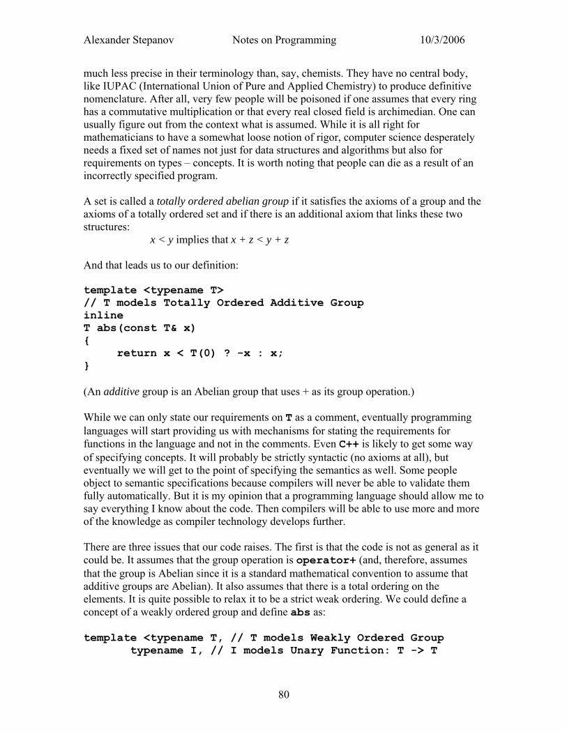
Alexander Stepanov Notes on Programming 10/3/2006
much less precise in their terminology than, say, chemists. They have no central body, like IUPAC (International Union of Pure and Applied Chemistry) to produce definitive nomenclature. After all, very few people will be poisoned if one assumes that every ring has a commutative multiplication or that every real closed field is archimedian. One can usually figure out from the context what is assumed. While it is all right for mathematicians to have a somewhat loose notion of rigor, computer science desperately needs a fixed set of names not just for data structures and algorithms but also for requirements on types – concepts. It is worth noting that people can die as a result of an incorrectly specified program. A set is called a totally ordered abelian group if it satisfies the axioms of a group and the axioms of a totally ordered set and if there is an additional axiom that links these two structures: x < y implies that x + z < y + z And that leads us to our definition: template <typename T> // T models Totally Ordered Additive Group inline T abs(const T& x) { return x < T(0) ? -x : x; } (An additive group is an Abelian group that uses + as its group operation.) While we can only state our requirements on T as a comment, eventually programming languages will start providing us with mechanisms for stating the requirements for functions in the language and not in the comments. Even C++ is likely to get some way of specifying concepts. It will probably be strictly syntactic (no axioms at all), but eventually we will get to the point of specifying the semantics as well. Some people object to semantic specifications because compilers will never be able to validate them fully automatically. But it is my opinion that a programming language should allow me to say everything I know about the code. Then compilers will be able to use more and more of the knowledge as compiler technology develops further. There are three issues that our code raises. The first is that the code is not as general as it could be. It assumes that the group operation is operator+ (and, therefore, assumes that the group is Abelian since it is a standard mathematical convention to assume that additive groups are Abelian). It also assumes that there is a total ordering on the elements. It is quite possible to relax it to be a strict weak ordering. We could define a concept of a weakly ordered group and define abs as: template <typename T, // T models Weakly Ordered Group typename I, // I models Unary Function: T -> T
80

Alexander Stepanov Notes on Programming 10/3/2006
typename R> // R models Binary Predicate inline T abs(const T& x, I inverse, R less) { return less(x, identity_element(inverse)) ? inverse(x) : x; } If we now define: template <typename T> inline T identity_element(const std::negate<T>&) { return T(0); } we can obtain the previous definition of abs by calling: abs(x, std::negate<int>(), std::less<int>()) We can then use our code with the totally ordered multiplicative group of positive rational numbers or with the weakly ordered group of non-zero rational numbers. That, however, is something that I call excessive genericity: extending an algorithm further than the set of known models. The new function is more general, but it is not more useful. At present, I do not know of any useful applications. We need to develop a sense of where to stop. Generalizing an algorithm is useful only when there are useful, known models. I know of many useful models for a more general min that assumes only weak ordering and takes a comparison as an argument. I have not yet seen the need to generalize abs. In other words, I suggest that abstraction should be based on the models we know, not just on our ability to make code more abstract. One should not multiply abstractions without necessity. The second problem with abs is that there is a different way of defining absolute value. We decided to follow the notion of absolute value as a “positive” value affiliated with an element. It assumes that the elements are either positive or negative depending on their relation to the identity and that one can get a positive element by inverting (negating) a negative element. There is a different way of defining it: the distance to zero. It allows us to define abs for std::complex as template <typename T> inline double abs(const complex<T>& z) { return std::sqrt(double(std::norm(z)));
81
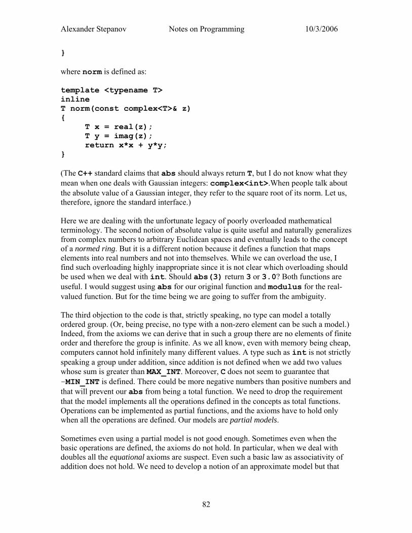
Alexander Stepanov Notes on Programming 10/3/2006
} where norm is defined as: template <typename T> inline T norm(const complex<T>& z) { T x = real(z); T y = imag(z); return x*x + y*y; } (The C++ standard claims that abs should always return T, but I do not know what they mean when one deals with Gaussian integers: complex<int>.When people talk about the absolute value of a Gaussian integer, they refer to the square root of its norm. Let us, therefore, ignore the standard interface.) Here we are dealing with the unfortunate legacy of poorly overloaded mathematical terminology. The second notion of absolute value is quite useful and naturally generalizes from complex numbers to arbitrary Euclidean spaces and eventually leads to the concept of a normed ring. But it is a different notion because it defines a function that maps elements into real numbers and not into themselves. While we can overload the use, I find such overloading highly inappropriate since it is not clear which overloading should be used when we deal with int. Should abs(3) return 3 or 3.0? Both functions are useful. I would suggest using abs for our original function and modulus for the real-valued function. But for the time being we are going to suffer from the ambiguity. The third objection to the code is that, strictly speaking, no type can model a totally ordered group. (Or, being precise, no type with a non-zero element can be such a model.) Indeed, from the axioms we can derive that in such a group there are no elements of finite order and therefore the group is infinite. As we all know, even with memory being cheap, computers cannot hold infinitely many different values. A type such as int is not strictly speaking a group under addition, since addition is not defined when we add two values whose sum is greater than MAX_INT. Moreover, C does not seem to guarantee that -MIN_INT is defined. There could be more negative numbers than positive numbers and that will prevent our abs from being a total function. We need to drop the requirement that the model implements all the operations defined in the concepts as total functions. Operations can be implemented as partial functions, and the axioms have to hold only when all the operations are defined. Our models are partial models. Sometimes even using a partial model is not good enough. Sometimes even when the basic operations are defined, the axioms do not hold. In particular, when we deal with doubles all the equational axioms are suspect. Even such a basic law as associativity of addition does not hold. We need to develop a notion of an approximate model but that
82
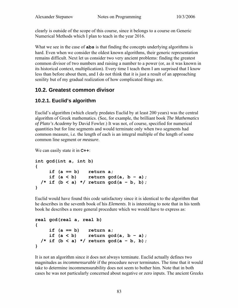
Alexander Stepanov Notes on Programming 10/3/2006
clearly is outside of the scope of this course, since it belongs to a course on Generic Numerical Methods which I plan to teach in the year 2016. What we see in the case of abs is that finding the concepts underlying algorithms is hard. Even when we consider the oldest known algorithms, their generic representation remains difficult. Next let us consider two very ancient problems: finding the greatest common divisor of two numbers and raising a number to a power (or, as it was known in its historical context, multiplication). Every time I teach them I am surprised that I know less than before about them, and I do not think that it is just a result of an approaching senility but of my gradual realization of how complicated things are.
10.2. Greatest common divisor
10.2.1. Euclid’s algorithm Euclid’s algorithm (which clearly predates Euclid by at least 200 years) was the central algorithm of Greek mathematics. (See, for example, the brilliant book The Mathematics of Plato’s Academy by David Fowler.) It was not, of course, specified for numerical quantities but for line segments and would terminate only when two segments had common measure, i.e. the length of each is an integral multiple of the length of some common line segment or measure. We can easily state it in C++: int gcd(int a, int b) { if (a == b) return a; if (a < b) return gcd(a, b – a); /* if (b < a) */ return gcd(a – b, b); } Euclid would have found this code satisfactory since it is identical to the algorithm that he describes in the seventh book of his Elements. It is interesting to note that in his tenth book he describes a more general procedure which we would have to express as: real gcd(real a, real b) { if (a == b) return a; if (a < b) return gcd(a, b – a); /* if (b < a) */ return gcd(a – b, b); } It is not an algorithm since it does not always terminate. Euclid actually defines two magnitudes as incommensurable if the procedure never terminates. The time that it would take to determine incommensurability does not seem to bother him. Note that in both cases he was not particularly concerned about negative or zero inputs. The ancient Greeks
83

Alexander Stepanov Notes on Programming 10/3/2006
did not have the notion of a negative number or zero. (It is possible to argue that they had a rather modern notion of real numbers and that the Eudoxian theory of proportion is equivalent to the 19th century theory of Dedekind cuts; it is even possible to argue that Archimedes in his Sandreckoner demonstrated that he had a notion of zero; but I cannot find any evidence for negative numbers among the Greeks. The first hint of negative numbers appears 9 centuries after Euclid in the works of the Indian mathematician Brahmagupta.) So we need to rename our function and add an assertion: int gcd_positive_subtractive_recursive(int a, int b) { assert(0 < a && 0 < b); if (a == b) return a; if (a < b) return gcd(a, b – a); /* if (b < a) */ return gcd(a – b, b); } (We will have to deal with zero and negative inputs later on.) It is clear why it works: we rely on the fact that if a number divides two numbers it divides their difference. Therefore we can keep replacing the larger with the difference of larger and the smaller. Since at every step a + b is getting smaller eventually the process must stop. (The argument is based on a wonderful principle the Greeks were using instead of mathematical induction: a monotonically decreasing sequence of natural numbers is finite.) Notice that our algorithm is tail-recursive: the recursive call returns the value that is immediately returned. There are computer scientists who believe that it is essential that compilers recognize tail recursion and eliminate the recursive call automatically. I belong to a school of thought that thinks it is essential that programmers recognize tail-recursion and learn how to transform it into iteration. It will often make the code even more readable and will not rely on an optimization probably not supported by your production compiler. Problem: Test if your compiler eliminates the tail call in our gcd. It is very easy to transform a tail-recursive algorithm into an iterative one: we need to replace the recursive calls with assignments to the input variables and put them inside a loop: int gcd_positive_subtractive(int a, int b) { assert(0 < a && 0 < b); while (a != b) { while (a < b) b -= a; while (b < a) a -= b; } return a;
84
Alexander Stepanov Notes on Programming 10/3/2006
} and we can easily patch it to accept zero and negative numbers: int gcd_subtractive(int a, int b) { make_abs(a); make_abs(b); assert(0 <= a && 0 <= b); if (a == 0) return b; if (b == 0) return a; assert(0 < a && 0 < b); while (a != b) { while (a < b) b -= a; while (b < a) a -= b; } return a; } where make_abs is a useful auxiliary function: template <typename T> // T models Totally Ordered Additive Group inline void make_abs(T& x) { if (x < T(0)) x = -x; } (It is tempting to use x = abs(x) inside the function, but all the compilers nowadays will punish us by generating an unnecessary assignment especially when assignment is user-defined function. In fact, the reason that we even introduce the function is to avoid the unnecessary assignment.) It is a really important piece of code. It is commonly known as the subtractive gcd algorithm. It is faster than one might think. While its worst-case complexity is indeed slow and is proportional to max(a, b), its average-case complexity is relatively low. There is a remarkable result by Yao and Knuth that the number of iterations of the subtractive gcd is on the average proportional to the square of the logarithm of the max(a, b). But the square of the logarithm is not as good as the logarithm without a square, and we can reduce the complexity of the subtractive algorithm using the modulus operator to compute remainders. (We shall see, however, that even when the modulus operator is available, the subtractive algorithm can give us some performance advantages when used in combination with the remainder version. We will also find that the computational structure of the algorithms will reappear in contexts quite removed from number theory.)
85

Alexander Stepanov Notes on Programming 10/3/2006
It is clear how to use remainders to speed up the algorithm. Instead of relying on the fact that the difference of a and b is divisible by any of their common divisors, we rely on the fact that the remainder of a divided by b is divisible by any of their common divisors. The code in question is quite simple: int gcd_modulus(int a, int b) { while (true) { if (b == 0) return a; a %= b; if (a == 0) return b; b %= a; } } Problem: Prove that the algorithm terminates by proving that the sum of the absolute values of a and b decreases with every iteration. It should be noted that the code that we have is going to work for negative numbers and 0 but with somewhat unexpected results: gcd_modulus(1, -1) will return -1 and somebody might object that -1 is not the greatest common divisor of 1 and -1 since, clearly, -1 < 1. We can, of course, do what we did in the case of the subtractive algorithm and replace a and b with their absolute values, but it is not a good thing to do. That will make our algorithm depend on the existence of a total ordering and while it is not an issue for integers, it is going to be a major obstacle for generalizing it. Instead of that we will use the definition of greatest common measure known to Euclid but frequently forgotten now: a greatest common divisor is a divisor divisible by any other divisor. This definition relies on the divisibility relation only to determine the greatest common divisor. This definition, of course, allows for multiple greatest common divisors of two elements. For example, both 2 and -2 are then the greatest common divisors of 6 and 8. (In general, there are as many greatest common divisors as there are invertible elements or units in our domain, since we can obtain a new greatest common divisor by multiplying the original one by a unit.) That insight allows us to extend our algorithm to domains where there is no total ordering. In 1585 the great Flemish scientist Simon Stevin extended Euclid’s algorithm to work on polynomials. Around 1830, Carl Gauss realized that he could use Euclid’s algorithm on complex numbers x + yi with integer coefficients x and y. (These numbers are known as Gaussian integers.) Both of these domains are not totally ordered and there is no unique greatest common divisor. Therefore we can generalize our algorithm: template <typename T> // T models Weak Euclidean Domain T gcd_euclid(T a, T b) {
86
Alexander Stepanov Notes on Programming 10/3/2006
while (true) { if (b == T(0)) return a; a %= b; if (a == T(0)) return b; b %= a; } } Now our task is to find the requirements for a Weak Euclidean Domain. Abstract algebra defines a Euclidean domain as an integral domain with a norm that satisfies certain axioms. You can find the definition in any book on abstract algebra. We, however, will look for a different, less restrictive definition, since the mathematical definition would not allow us to use Euclid’s algorithm on many domains on which it is actually useful, well-defined and was intended to work even by Euclid himself, such as rational numbers. Till people started taking abstract algebra too seriously it was quite clear to everybody what was the gcd of 1/3 and 1/2. And it was even clear how to use Euclid’s algorithm to find their gcd. So let us try to restore the algorithm to its original generality. It is clear that the only operation explicitly needed by the algorithm is operator% or, being quite precise, operator%=. It is reasonable to assume that a %= b; is equivalent (except for possibly being faster) to a = a % b; (I would, of course, demand such equivalence for all such operators but, as I complained before, C++ allows you to overload operators without any semantic constrains.) In general, for T to be a weak Euclidean domain, we assume that there is a related operation called quotient that will normally default to operator/ (but will be a special function called quotient for a field such as rationals and other domains with divisions). The following conditions should be satisfied: 1. T is a commutative semiring (a set with + and * where they are both commutative and associative and * distributes over +) with 0. 2. a == b * (quotient(a, b)) + a % b 3. There exists a function D: T x T -> Unsigned Integers such that if either a or b is equal to 0 then D(a, b) and D(b, a) are 0. Otherwise, D(a%b, b) < D(a, b) or D(a, b%a) < D(a, b). It is clear that if these conditions hold then the algorithm will terminate since at every iteration D(a, b) is going to decrease. It is equally easy to construct a function D for all
87
Alexander Stepanov Notes on Programming 10/3/2006
domains on which the algorithm terminates by defining it being equal to the number of modulus operations done by the algorithm. Problem: Define meaningful quotient, remainder and D functions for rational numbers. One of the problems with using the remainder-based algorithm is that modulus (or integer division) is a very expensive operation. On the Pentium 4 it takes 80 cycles. The AMD Athlon is better by about a factor of two but is still quite slow. (See, for example, http://swox.com/doc/x86-timing.pdf.) This is why it is often good to look for ways to avoid doing the remainder. One approach is to try to use subtraction whenever we can and compute remainders only when the magnitudes of a and b are very far apart. (The idea of combining remainder-based gcd and subtractive gcd was suggested to me by Sean Parent. I was not able to find references to it in the published literature.) We can implement a parameterized function that will let us set the threshold for switching from one algorithm to the other: template <int shift> int gcd_hybrid(int a, int b) { make_abs(a); make_abs(b); assert(0 <= a && 0 <= b); sort_2(a, b); while (a != 0) { assert(a <= b); if (a < b>>shift) b %= a; else do b -= a; while (a <= b); swap(a, b); } return b; } Problem: What is the best value of shift on your computer for different ranges of integers?
10.2.2. Stein’s algorithm An interesting algorithmic development happened in 1961 when an Israeli physicist Yosef Stein discovered a totally new way of finding the greatest common divisor. His algorithm is based on the observation that finding if a number is even and dividing it by 2
88
Alexander Stepanov Notes on Programming 10/3/2006
are much faster operations than the modulus operator. In particular, his algorithm is based on the following self-evident facts:
1. gcd(a, a) = a 2. gcd(2a, 2b) = 2gcd(a, b) 3. gcd(2a, 2b+1) = gcd(a, 2b+1) 4. gcd(2a+1, 2b) = gcd(2a+1, b) 5. a < b implies gcd(a, b) = gcd(a, b-a) 6. b < a implies gcd(a, b) = gcd(a-b, b)
To simplify the problem let us look at the case of when both inputs are known to be odd and positive. (The intuition that tells me to start with them is that it is any non-zero inputs can be easily turned into odd input by iteratively factoring out 2.) We assume that we are dealing with a concept of Binary Integer that provides us with fast operations for dividing by 2 and finding if a number is even or odd. template <typename T> // T models Binary Integer inline T stein_gcd_odd(T a, T b) { assert(is_positive(a) && is_positive(b)); assert(is_odd(a) && is_odd(b)); while (a != b) { if (a < b) { b -= a; halve_till_odd(b); } else { a -= b; halve_till_odd(a); } assert(is_odd(a) && is_odd(b)); } return a; } Where halve_till_odd is normally defined as: template <typename T> // T models Binary Integer inline void halve_till_odd(T& a) { assert(is_positive(a) && !is_odd(a)); do { halve_non_negative(a); } while (!is_odd(a));
89
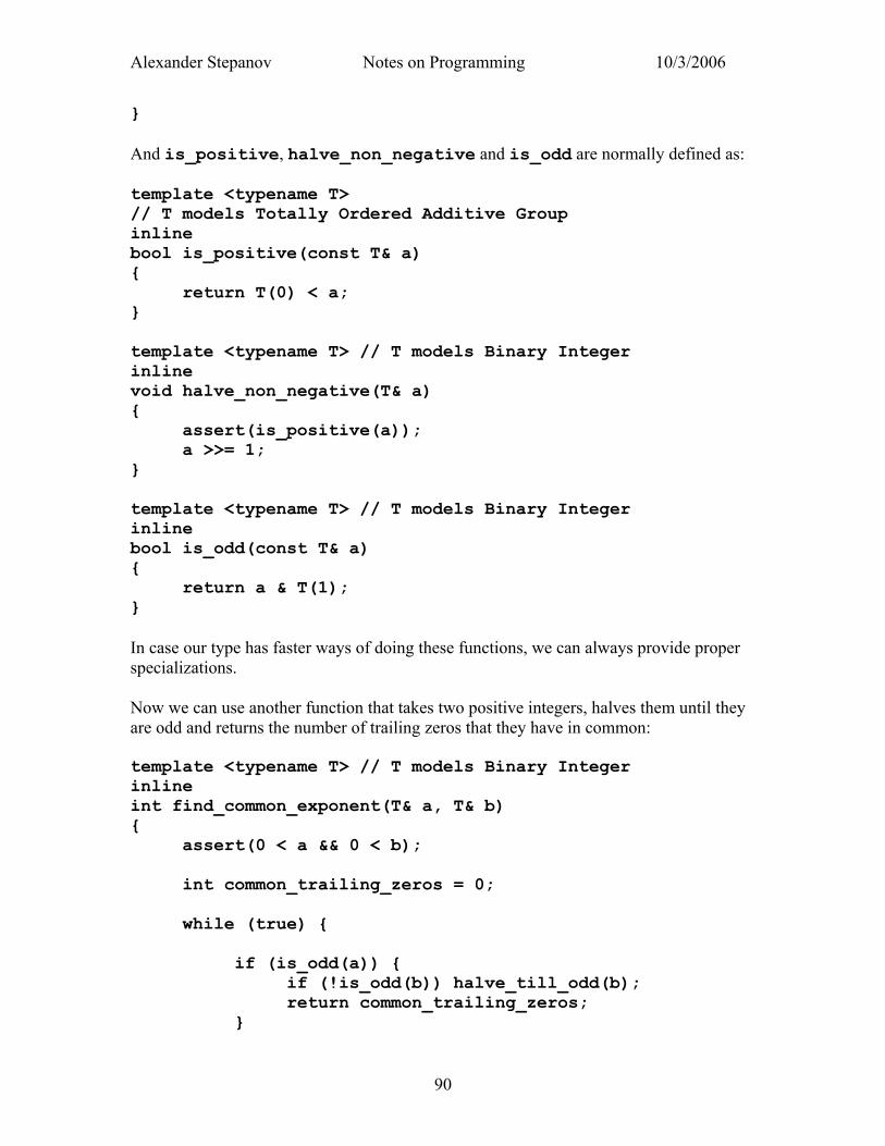
Alexander Stepanov Notes on Programming 10/3/2006
} And is_positive, halve_non_negative and is_odd are normally defined as: template <typename T> // T models Totally Ordered Additive Group inline bool is_positive(const T& a) { return T(0) < a; } template <typename T> // T models Binary Integer inline void halve_non_negative(T& a) { assert(is_positive(a)); a >>= 1; } template <typename T> // T models Binary Integer inline bool is_odd(const T& a) { return a & T(1); } In case our type has faster ways of doing these functions, we can always provide proper specializations. Now we can use another function that takes two positive integers, halves them until they are odd and returns the number of trailing zeros that they have in common: template <typename T> // T models Binary Integer inline int find_common_exponent(T& a, T& b) { assert(0 < a && 0 < b); int common_trailing_zeros = 0; while (true) { if (is_odd(a)) { if (!is_odd(b)) halve_till_odd(b); return common_trailing_zeros; }
90

Alexander Stepanov Notes on Programming 10/3/2006
if (is_odd(b)) { assert(!is_odd(a)); halve_till_odd(a); return common_trailing_zeros; } halve_non_negative(a); halve_non_negative(b); ++common_trailing_zeros; } } Now it is quite easy to implement the complete algorithm: template <typename T> // T models Binary Integer T stein_gcd(T a, T b) { if (is_zero(a)) return b; if (is_zero(b)) return a; make_abs(a); make_abs(b); assert(is_positive(a) && is_positive(b)); int common_trailing_zeros = find_common_exponent(a, b); assert(is_odd(a) && is_odd(b)); return left_shift(stein_gcd_odd(a, b), common_trailing_zeros); } where is_zero and left_shift are defined as: template <typename T> // T models Additive Monoid inline bool is_zero(const T& a) { return a == T(0); } template <typename T> // T models Binary Integer inline T left_shift(T a, int n) {
91

Alexander Stepanov Notes on Programming 10/3/2006
assert(0 <= n); assert(is_positive(a)); return a << n; } All the little auxiliary functions that I used for implementing stein_gcd together with a few others (such as is_even) belong to a header file binary_integer.h which is frequently useful. We will use them again when we study the Russian Peasant algorithm. Stein’s algorithm is usually faster than Euclid’s in practice. It is quite clear what its complexity is: it shifts at least one of its arguments to the right at every iteration. That makes the number of iterations to be not greater than the sum of the positions of the most significant bits minus 2. But there is a remarkable result by Brigitte Vallée that for binary encoded integers the theoretical average complexity of Stein’s algorithm in terms of bit operations is about 60% better than Euclid’s. Stein’s algorithm is frequently called binary gcd but does not really deal with binary integers only. As Euclid’s algorithm was found to work on different domains, the same thing happened to Stein’s. First people noticed that it can be used with polynomials over a field with division by 2 being replaced by division by x. (I do not know who people are. I discovered it independently but later on found it as an exercise 4.6.1.6 in Knuth. He does not state who discovered it first.) In 2000 Andre Weilert realized that it could be used on Gaussian integers if one uses the division by 1+i instead of 2. And in 2003 and 2004 Gudmund Skovbjerg Frandsen and his collaborators at Aarhus University showed that the algorithm can be used in other rings of algebraic integers including ones where Euclid’s algorithm does not work! It is quite clear that there is a concept underlying Stein’s algorithm that is as interesting as the one behind Euclid’s algorithm. If we look at what unifies the applications of Stein’s algorithm to different domain it is the notion of division by the smallest prime. After all, 2 for integers, x for polynomials, 1 + i for Gaussian integers share the nice property of being a smallest prime. There are, of course, several smallest primes in each of these domains: 2 and -2 for integers, 1 + i, 1 – i, –1 + i and –1 – i for Gaussian integers, and ax + b for polynomials. Division by the smallest prime possesses a nice property of always giving an invertible element (a unit) as a remainder when the remainder is not equal to 0. And that means that two elements with non-zero remainders (odd elements) can be multiplied by units so that the corresponding remainders could be cancelled. We can then define a generalized Stein algorithm as: template <typename T> // T models Stein Domain T generalized_stein_gcd(T a, T b) { if (is_zero(a)) return n; if (is_zero(b)) return m;
92

Alexander Stepanov Notes on Programming 10/3/2006
int exponent1 = find_exponent(a); int exponent2 = find_exponent(b); while (!are_associates(a, b)) { if (norm(a) < norm(b)) swap(a, b); cancel_remainder(a, b); do { halve(a); } while (!is_odd(a)); } return shift_left(a, min(exponent1, exponent2)); } where find_exponent is defined as: int find_exponent(T& a) { int n = 0; while (!is_odd(a)) { halve(a); ++n; } return n; } In this case is_odd, halve and shift_left are extended to mean correspondingly the same operations as the operations for binary integers but in terms of the smallest prime of the domain. (We need to pick one in terms of which the Stein domain is defined.) Notice, that we are now using halve and not halve_non_negative. We need also define functions are_associates that determines if one element is equal to the other multiplied by a unit, cancel_remainder that takes two arguments a and b and replaces a with unit1*a - unit2*b where units are selected so that the difference is divisible by the smallest prime and norm that maps the elements of the domain into positive integers that decrease after the difference is divided by the smallest prime. The tricky task happens to be finding cancel_remainder function for new domains as well as proving the decrease of the corresponding norm. I have been struggling for many years to prove that every Euclidean domain is a Stein domain without much luck. In general, I do not know the relations between Euclidean domains, weak Euclidean domains and Stein domains. It seems that Frandsen established that there are Stein domains that are not Euclidean, but the rest is still unclear. Problem: Define additional functions that will make generalized_stein_gcd work for built-in signed integral types. Problem: Measure the performance of subtractive gcd, remainder gcd, hybrid gcd (with different shifts) and Stein gcd for different ranges of 32 and 64 bit integers.
93

Alexander Stepanov Notes on Programming 10/3/2006
10.3. Exponentiation The next problem we are going to look at is the problem of multiplying a repeatedly: a * a * … * a. The Greeks knew about squares (a * a) and cubes (a * a * a). Archimedes, who clearly was about 2000 years ahead of his time knew about higher powers, but they were quickly forgotten. Since about 1600 the notion of raising a number or other object to the nth power became a routine operation. Euler remarks that we can, of course, write a, a * a, a * a * a, a * a * a* a, a * a * a * a * a, and so on, but as he says, “we soon feel the inconvenience attending this manner of writing the powers, which consists in the necessity of repeating the same letter very often, to express higher powers; and the reader would have no less trouble, if he were obliged to count all the letters, to know what power is intended to be represented. The hundredth power, for example, could not be conveniently written in this manner; and it would be equally difficult to read it” (Elements of Algebra, page 51). He was looking to reduce the linear-space notation into a logarithmic-space one. We will be looking to reduce linear time to logarithmic time. Writing a useful implementation of power is an exemplary starting point for understanding generic programming, since it combines both algorithmic difficulties and abstraction difficulties while remaining manageable in both dimensions. Before we attempt to write an efficient exponentiation algorithm, let us try to write a simple-minded inefficient one. It is usually good to do it for several reasons. First, it allows us to face the interface design without dealing with extra algorithmic complexity. Second, it is useful to have a different algorithm to check the correctness of the fast one. Finally, as we will discover, sometimes fast algorithms are not as fast as they seem. As usual, let us start with a preliminary implementation starting from the inside out: while (--n != 0) result = result * a; return result; The middle of the code seems to be straightforward. We decrement the exponent and multiply the result by a. Does it really matter that we write: result = result * a; instead of writing: result = a * result;
94
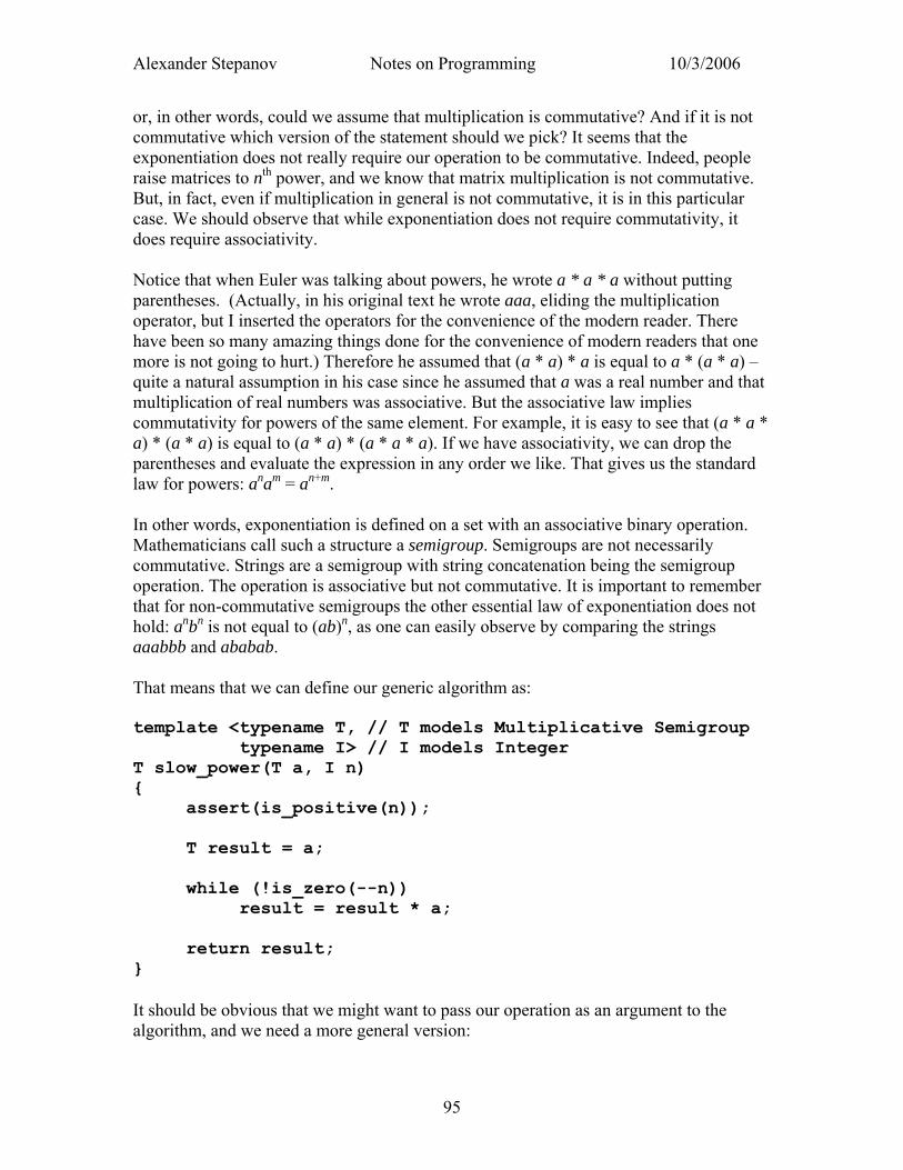
Alexander Stepanov Notes on Programming 10/3/2006
or, in other words, could we assume that multiplication is commutative? And if it is not commutative which version of the statement should we pick? It seems that the exponentiation does not really require our operation to be commutative. Indeed, people raise matrices to nth power, and we know that matrix multiplication is not commutative. But, in fact, even if multiplication in general is not commutative, it is in this particular case. We should observe that while exponentiation does not require commutativity, it does require associativity. Notice that when Euler was talking about powers, he wrote a * a * a without putting parentheses. (Actually, in his original text he wrote aaa, eliding the multiplication operator, but I inserted the operators for the convenience of the modern reader. There have been so many amazing things done for the convenience of modern readers that one more is not going to hurt.) Therefore he assumed that (a * a) * a is equal to a * (a * a) – quite a natural assumption in his case since he assumed that a was a real number and that multiplication of real numbers was associative. But the associative law implies commutativity for powers of the same element. For example, it is easy to see that (a * a * a) * (a * a) is equal to (a * a) * (a * a * a). If we have associativity, we can drop the parentheses and evaluate the expression in any order we like. That gives us the standard law for powers: anam = an+m. In other words, exponentiation is defined on a set with an associative binary operation. Mathematicians call such a structure a semigroup. Semigroups are not necessarily commutative. Strings are a semigroup with string concatenation being the semigroup operation. The operation is associative but not commutative. It is important to remember that for non-commutative semigroups the other essential law of exponentiation does not hold: anbn is not equal to (ab)n, as one can easily observe by comparing the strings aaabbb and ababab. That means that we can define our generic algorithm as: template <typename T, // T models Multiplicative Semigroup typename I> // I models Integer T slow_power(T a, I n) { assert(is_positive(n)); T result = a; while (!is_zero(--n)) result = result * a; return result; } It should be obvious that we might want to pass our operation as an argument to the algorithm, and we need a more general version:
95
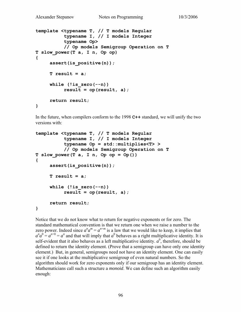
Alexander Stepanov Notes on Programming 10/3/2006
template <typename T, // T models Regular typename I, // I models Integer typename Op> // Op models Semigroup Operation on T T slow_power(T a, I n, Op op) { assert(is_positive(n)); T result = a; while (!is_zero(--n)) result = op(result, a); return result; } In the future, when compilers conform to the 1998 C++ standard, we will unify the two versions with: template <typename T, // T models Regular typename I, // I models Integer typename Op = std::multiplies<T> > // Op models Semigroup Operation on T T slow_power(T a, I n, Op op = Op()) { assert(is_positive(n)); T result = a; while (!is_zero(--n)) result = op(result, a); return result; } Notice that we do not know what to return for negative exponents or for zero. The standard mathematical convention is that we return one when we raise a number to the zero power. Indeed since anam = an+m is a law that we would like to keep, it implies that ana0 = an+0 = an and that will imply that a0 behaves as a right multiplicative identity. It is self-evident that it also behaves as a left multiplicative identity. a0, therefore, should be defined to return the identity element. (Prove that a semigroup can have only one identity element.) But, in general, semigroups need not have an identity element. One can easily see it if one looks at the multiplicative semigroup of even natural numbers. So the algorithm should work for zero exponents only if our semigroup has an identity element. Mathematicians call such a structure a monoid. We can define such an algorithm easily enough:
96
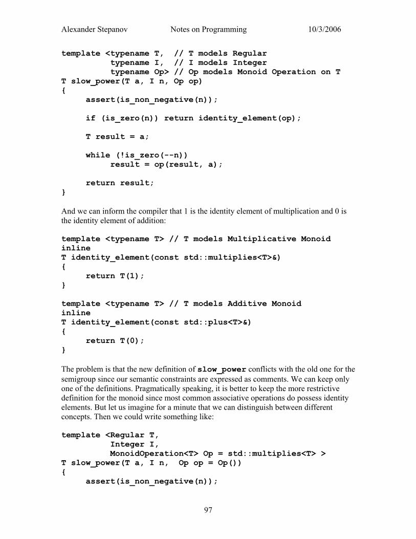
Alexander Stepanov Notes on Programming 10/3/2006
template <typename T, // T models Regular typename I, // I models Integer typename Op> // Op models Monoid Operation on T T slow_power(T a, I n, Op op) { assert(is_non_negative(n)); if (is_zero(n)) return identity_element(op); T result = a; while (!is_zero(--n)) result = op(result, a); return result; } And we can inform the compiler that 1 is the identity element of multiplication and 0 is the identity element of addition: template <typename T> // T models Multiplicative Monoid inline T identity_element(const std::multiplies<T>&) { return T(1); } template <typename T> // T models Additive Monoid inline T identity_element(const std::plus<T>&) { return T(0); } The problem is that the new definition of slow_power conflicts with the old one for the semigroup since our semantic constraints are expressed as comments. We can keep only one of the definitions. Pragmatically speaking, it is better to keep the more restrictive definition for the monoid since most common associative operations do possess identity elements. But let us imagine for a minute that we can distinguish between different concepts. Then we could write something like: template <Regular T, Integer I, MonoidOperation<T> Op = std::multiplies<T> > T slow_power(T a, I n, Op op = Op()) { assert(is_non_negative(n));
97
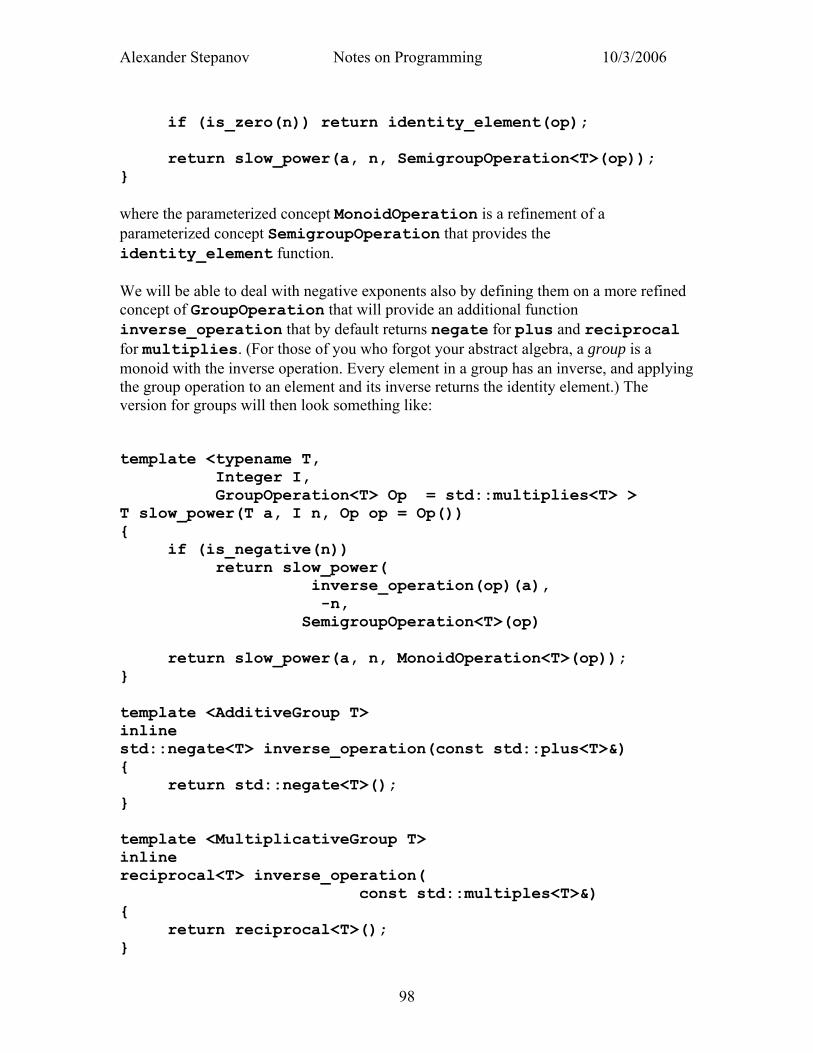
Alexander Stepanov Notes on Programming 10/3/2006
if (is_zero(n)) return identity_element(op); return slow_power(a, n, SemigroupOperation<T>(op)); } where the parameterized concept MonoidOperation is a refinement of a parameterized concept SemigroupOperation that provides the identity_element function. We will be able to deal with negative exponents also by defining them on a more refined concept of GroupOperation that will provide an additional function inverse_operation that by default returns negate for plus and reciprocal for multiplies. (For those of you who forgot your abstract algebra, a group is a monoid with the inverse operation. Every element in a group has an inverse, and applying the group operation to an element and its inverse returns the identity element.) The version for groups will then look something like: template <typename T, Integer I, GroupOperation<T> Op = std::multiplies<T> > T slow_power(T a, I n, Op op = Op()) { if (is_negative(n)) return slow_power( inverse_operation(op)(a), -n, SemigroupOperation<T>(op) return slow_power(a, n, MonoidOperation<T>(op)); } template <AdditiveGroup T> inline std::negate<T> inverse_operation(const std::plus<T>&) { return std::negate<T>(); } template <MultiplicativeGroup T> inline reciprocal<T> inverse_operation( const std::multiples<T>&) { return reciprocal<T>(); }
98

Alexander Stepanov Notes on Programming 10/3/2006
where reciprocal is defined as: template <MultiplicativeGroup T> struct reciprocal : std::unary_function<T, T> { T operator()(const T& x) const { return identity_element(std::multiples<T>()) / x; } }; And we can even provide an implementation of slow_power in terms of left_power algorithm defined on GroupoidOperation. A groupoid, or, as my old friend Nicolas Bourbaki calls it, a magma, is a set with a binary operation with no associativity or any other property assumed; that is why we need to define the order of evaluation of power. It is an interesting question why we default our power to left_power. One of the reasons, of course, is my European habit of writing left-to-right which makes it more natural to view (a * a) * a as a default, rather than a * (a * a). But there is a less frivolous reason: later on in the course we will study the reduction algorithm, and since it is natural to view slow_power as a reduction of an operation on a sequence of n equal elements, we should use the most general kind of reduction which happens to be left reduction. It is a remarkable fact, but there is no programming language that allows us to write algorithms in their proper mathematical setting. I have been hoping for one for over 25 years now. It is possible that you will live long enough to see one, but I am losing hope that I will get to write power the way it should be written. As the Greeks used to say, “The mills of the gods grind slowly…” Exponentiation, when viewed as an operation, defines a multiplication operation connecting the domain of the original semigroup operation and integers. It allows us to “multiply” any element of a semigroup by a positive integer. For example, if we take strings and concatenation operation, exponentiation will provide us with an ability to multiply any string, say “foo“, by a number, say 3, and obtain a result, “foofoofoo“. For a monoid we obtain a multiplication by non-negative integers and for a group multiplication by any integer. In general, this multiplication does not distribute over the semigroup operation, but it does distribute when we deal with Abelian (or commutative) semigroups. A mathematician would say that exponentiation turns an Abelian semigroup into a semi-module over the semi-ring of natural numbers and an Abelian group into a module over a ring of integers. It sounds terribly complicated, but in reality is some really trivial stuff. People are often scared away from mathematics because of the use of unknown terms and strange symbols. It is, however, important to remember that the real point of mathematics is to make thing clear. That is why I hope that eventually we will be able to program with things like semigroups and groups. I am way too stupid to be able to program well without the help of simple mathematical structures.
99

Alexander Stepanov Notes on Programming 10/3/2006
It is important to notice that power, if used with addition as its operation, gives us multiplication. This is, as a matter of fact, the context in which the fast way of exponentiation was first discovered. It is hard for us to say how far back the discovery goes. It was already known to the Egyptian scribe Ahmes (Ahmos) who described a way to multiply two numbers around 1650BC, but he claimed that he copied it from a text hundreds of years earlier. (The scroll written by Ahmes is known as the Rhind papyrus after its Scottish discoverer Alexander Henry Rhind.) Later on, the method was known to the Greeks as Egyptian multiplication and has been practiced in Europe and among the Arabs for thousands of years. Ahmes used an example to describe the algorithm. (Using examples is frowned upon nowadays; one of the people who attended my course was so disgusted with my explanation of this algorithm from examples that he quit after letting me know that I will turn my students into really terrible programmers. I would, however, like to know what he would say if he ever read Diophantus, who constructed what is probably the second most important book in the history of mathematics as a list of well-chosen examples. But, back to Ahmes! ) Let us multiply two numbers, say, 41 and 59. Let us start with a pair (1, 59) and let us keep doubling both elements till the second one exceeds 41.
1 59 ◄
2 118
4 236
8 472 ◄
16 944
32 1888 ◄
64 … - we do not need to bother doubling 1888.
Now we mark the rows such that the sum of the first elements in the marked rows is equal to 41. (This shows us that the binary representation of integers has been around for quite a while.) Ahmes relies on the fact that 41 * 59 is equal to (1 + 8 + 32) * 59 which is equal to 59 + 472 + 1888. So if you add the second elements of the marked rows you will get the correct answer: 2419.
The procedure survived till the 19th century in societies that relied on the abacus for calculation, since doubling required by the procedure is easy with an abacus. In particular, a refined version of it was apparently observed by Western travelers to Russia, and the algorithm for exponentiation based on it is known in the West (but not in Russia!) as Russian Peasant Algorithm. (The oldest reference I was able to find appears in the
100
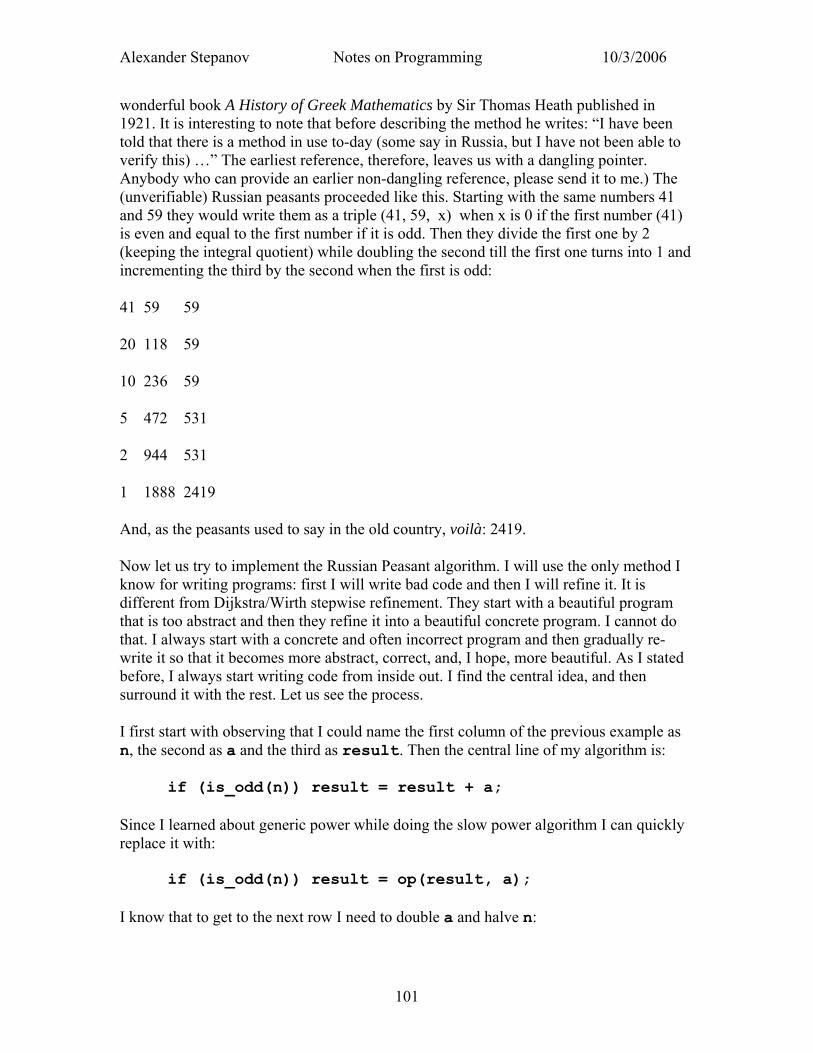
Alexander Stepanov Notes on Programming 10/3/2006
wonderful book A History of Greek Mathematics by Sir Thomas Heath published in 1921. It is interesting to note that before describing the method he writes: “I have been told that there is a method in use to-day (some say in Russia, but I have not been able to verify this) …” The earliest reference, therefore, leaves us with a dangling pointer. Anybody who can provide an earlier non-dangling reference, please send it to me.) The (unverifiable) Russian peasants proceeded like this. Starting with the same numbers 41 and 59 they would write them as a triple (41, 59, x) when x is 0 if the first number (41) is even and equal to the first number if it is odd. Then they divide the first one by 2 (keeping the integral quotient) while doubling the second till the first one turns into 1 and incrementing the third by the second when the first is odd:
41 59 59
20 118 59
10 236 59
5 472 531
2 944 531
1 1888 2419
And, as the peasants used to say in the old country, voilà: 2419.
Now let us try to implement the Russian Peasant algorithm. I will use the only method I know for writing programs: first I will write bad code and then I will refine it. It is different from Dijkstra/Wirth stepwise refinement. They start with a beautiful program that is too abstract and then they refine it into a beautiful concrete program. I cannot do that. I always start with a concrete and often incorrect program and then gradually re-write it so that it becomes more abstract, correct, and, I hope, more beautiful. As I stated before, I always start writing code from inside out. I find the central idea, and then surround it with the rest. Let us see the process.
I first start with observing that I could name the first column of the previous example as n, the second as a and the third as result. Then the central line of my algorithm is:
if (is_odd(n)) result = result + a;
Since I learned about generic power while doing the slow power algorithm I can quickly replace it with:
if (is_odd(n)) result = op(result, a);
I know that to get to the next row I need to double a and halve n:
101

Alexander Stepanov Notes on Programming 10/3/2006
if (is_odd(n)) result = op(result, a); a = op(a, a); halve_non_negative(n); And since I know that when I halve 1 I will get 0 and the inner loop is done: while (!is_zero(n)) { if (is_odd(n)) result = op(result, a); a = op(a, a); halve_non_negative(n); } return result; Now I just need to initialize result and the algorithm is done: template <typename T, // T models Regular typename I, // I models Integral typename Op> // Op models MonoidOperation on T T fast_power_0(T a, I n, Op op) { assert(!is_negative(n)); T result = identity_element(op); while (!is_zero(n)) { if (is_odd(n)) result = op(result, a); a = op(a, a); halve_non_negative(n); } return result; } In reality, however, it is at best under-done. It does one extra operation squaring a during the last iteration. It is not just an extra operation. It might cause an overflow or a memory exception. The technique for fixing it is well known: we need to rotate the loop so that the exit condition is checked before we square a. To do that we need to interchange squaring and halving, since we need to halve before we check for exit: template <typename T, // T models Regular typename I, // I models Integral typename Op> // Op models MonoidOperation on T T fast_power_1(T a, I n, Op op) { assert(!is_negative(n)); T result = identity_element(op); if (is_zero(n)) return result; while (true) { if (is_odd(n)) result = op(result, a); halve_non_negative(n);
102
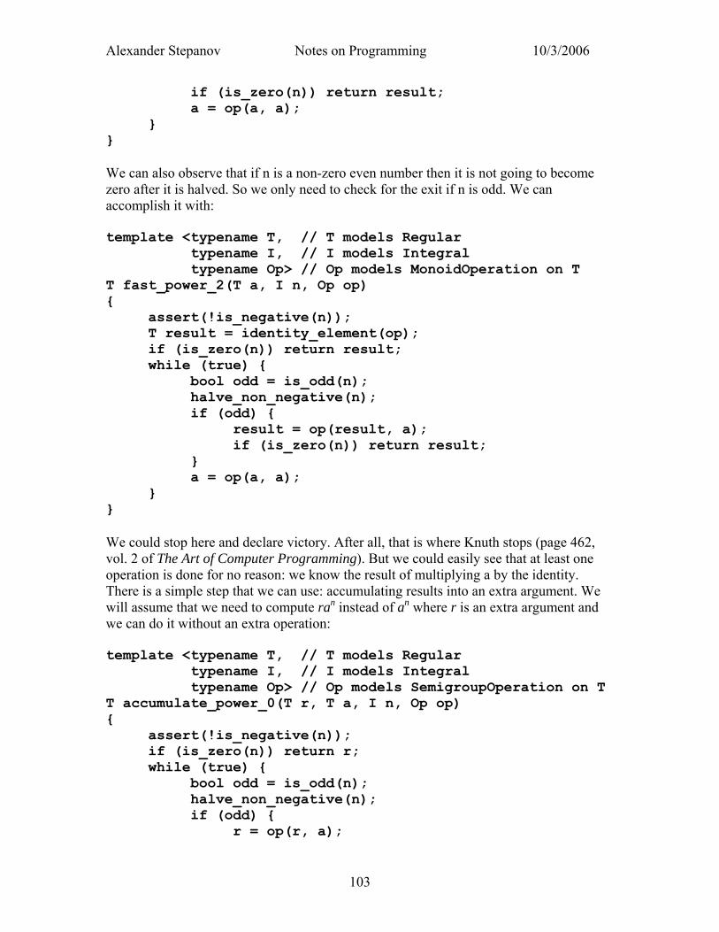
Alexander Stepanov Notes on Programming 10/3/2006
if (is_zero(n)) return result; a = op(a, a); } } We can also observe that if n is a non-zero even number then it is not going to become zero after it is halved. So we only need to check for the exit if n is odd. We can accomplish it with: template <typename T, // T models Regular typename I, // I models Integral typename Op> // Op models MonoidOperation on T T fast_power_2(T a, I n, Op op) { assert(!is_negative(n)); T result = identity_element(op); if (is_zero(n)) return result; while (true) { bool odd = is_odd(n); halve_non_negative(n); if (odd) { result = op(result, a); if (is_zero(n)) return result; } a = op(a, a); } } We could stop here and declare victory. After all, that is where Knuth stops (page 462, vol. 2 of The Art of Computer Programming). But we could easily see that at least one operation is done for no reason: we know the result of multiplying a by the identity. There is a simple step that we can use: accumulating results into an extra argument. We will assume that we need to compute ran instead of an where r is an extra argument and we can do it without an extra operation: template <typename T, // T models Regular typename I, // I models Integral typename Op> // Op models SemigroupOperation on T T accumulate_power_0(T r, T a, I n, Op op) { assert(!is_negative(n)); if (is_zero(n)) return r; while (true) { bool odd = is_odd(n); halve_non_negative(n); if (odd) { r = op(r, a);
103
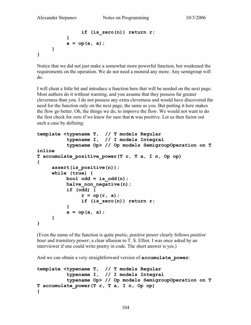
Alexander Stepanov Notes on Programming 10/3/2006
if (is_zero(n)) return r; } a = op(a, a); } } Notice that we did not just make a somewhat more powerful function, but weakened the requirements on the operation. We do not need a monoid any more. Any semigroup will do. I will cheat a little bit and introduce a function here that will be needed on the next page. Most authors do it without warning, and you assume that they possess far greater cleverness than you. I do not possess any extra cleverness and would have discovered the need for the function only on the next page, the same as you. But putting it here makes the flow go better. Oh, the things we do, to improve the flow. We would not want to do the first check for zero if we knew for sure that n was positive. Let us then factor out such a case by defining: template <typename T, // T models Regular typename I, // I models Integral typename Op> // Op models SemigroupOperation on T inline T accumulate_positive_power(T r, T a, I n, Op op) { assert(is_positive(n)); while (true) { bool odd = is_odd(n); halve_non_negative(n); if (odd) { r = op(r, a); if (is_zero(n)) return r; } a = op(a, a); } } (Even the name of the function is quite poetic; positive power clearly follows positive hour and transitory power; a clear allusion to T. S. Elliot. I was once asked by an interviewer if one could write poetry in code. The short answer is yes.) And we can obtain a very straightforward version of accumulate_power: template <typename T, // T models Regular typename I, // I models Integral typename Op> // Op models SemigroupOperation on T T accumulate_power(T r, T a, I n, Op op) {
104

Alexander Stepanov Notes on Programming 10/3/2006
assert(!is_negative(n)); if (is_zero(n)) return r; return accumulate_positive_power(r, a, n, op); } We could easily obtain a version of power by accumulating n-1 elements into the first one: template <typename T, // T models Regular typename N, // N models Integral typename Op> // Op models SemigroupOperation on T T fast_positive_power_0(T a, N n, Op op) { assert(is_positive(n)); if (is_one(n)) return a; return accumulate_positive_power(a, a, --n, op); } template <typename T, // T models Regular typename N, // N models Integral typename Op> // Op models MonoidOperation on T T fast_power_3(T a, N n, Op op) { assert(!is_negative(n)); if (is_zero(n)) return identity_element(op); return fast_positive_power_0(a, n, op); } While fast_power_3 is going to do fewer operations than fast_power_2 when n is 17 it will do many more when n is equal to 16. We need to start accumulating with the first significant bit of the exponent. We can easily transform a and n so that the problem is reduced to the case of an odd number: template <typename T, // T models Regular typename N, // N models Integral typename Op> // Op models SemigroupOperation on T inline void square_while_even(T& a, N& n, Op op) { assert(is_positive(n)); while (!is_odd(n)) { halve_non_negative(n); a = op(a, a); } } And now we are ready for the final version:
105

Alexander Stepanov Notes on Programming 10/3/2006
template <typename T, // T models Regular typename N, // N models Integral typename Op> // Op models SemigroupOperation on T T fast_positive_power(T a, N n, Op op) { assert(is_positive(n)); square_while_even(a, n, op); halve_non_negative(n); if (is_zero(n)) return a; return accumulate_positive_power(a, op(a, a), n, op); } template <typename T, // T models Regular typename N, // N models Integral typename Op> // Op models MonoidOperation on T T fast_power(T a, N n, Op op) { assert(!is_negative(n)); if (is_zero(n)) return identity_element(op); return fast_positive_power(a, n, op); } It is really easy to see the number of operations that the algorithm does: one squaring for every significant bit but the last one, plus one accumulation for every 1 encountered after the first one. It is pretty clear that the worst cases are the numbers with only ones in their binary representation. The number of operations done by the Russian Peasant Algorithm is very small, but, interestingly enough, not always optimal. The first example of the suboptimal behavior is when the exponent is 15. According to our formula the number of operations is going to be: (4 – 1) + (4 – 1) = 6. But we can do better by first computing a5 which can be done with three operations and then raising it to the 3rd power with two more operations for a total of 5. There is a complicated theory of addition chains that deals with the optimal number of operations for exponentiation described in the second volume of Knuth. Without going into theoretical complications, we can use minimal addition chains to generate a little library for doing optimal exponentiation in the special case where the exponent is known at compile time. It is also a little example of template metaprogramming with a modicum of algorithmic substance. I give the optimal code for n ≤ 50. The code is sufficiently trivial not to require much explanation. I use a convention that names of function objects that depends on a compile time constant end with _k: template <int k> struct conditional_operation { template <typename T, // T models Regular typename Op> // Op Models BinaryOperation(T) T operator()(const T& a, const T& b, Op op)
106

Alexander Stepanov Notes on Programming 10/3/2006
{ return op(a, b); } }; template <> struct conditional_operation<0> { template <typename T, // T models Regular typename Op> // Op Models BinaryOperation(T) T operator()(const T& a, const T&, Op) { return a; } }; template <int k> struct power_k; template <> struct power_k<0> { template <typename T, typename Op> // Op Models MonoidOperation(T) T operator()(const T& a, Op op) { return identity_element(op); } }; template <> struct power_k<1> { template <typename T, typename Op> // Op Models SemigroupOperation(T) T operator()(const T& a, Op) { return a; } }; template <> struct power_k<2> { template <typename T, typename Op> T operator()(const T& a, Op op) {
107
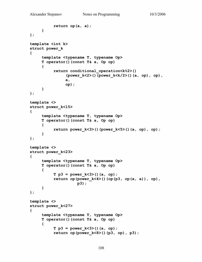
Alexander Stepanov Notes on Programming 10/3/2006
return op(a, a); } }; template <int k> struct power_k { template <typename T, typename Op> T operator()(const T& a, Op op) { return conditional_operation<k%2>() (power_k<2>()(power_k<k/2>()(a, op), op), a, op); } }; template <> struct power_k<15> { template <typename T, typename Op> T operator()(const T& a, Op op) { return power_k<3>()(power_k<5>()(a, op), op); } }; template <> struct power_k<23> { template <typename T, typename Op> T operator()(const T& a, Op op) { T p3 = power_k<3>()(a, op); return op(power_k<4>()(op(p3, op(a, a)), op), p3); } }; template <> struct power_k<27> { template <typename T, typename Op> T operator()(const T& a, Op op) { T p3 = power_k<3>()(a, op); return op(power_k<8>()(p3, op), p3);
108
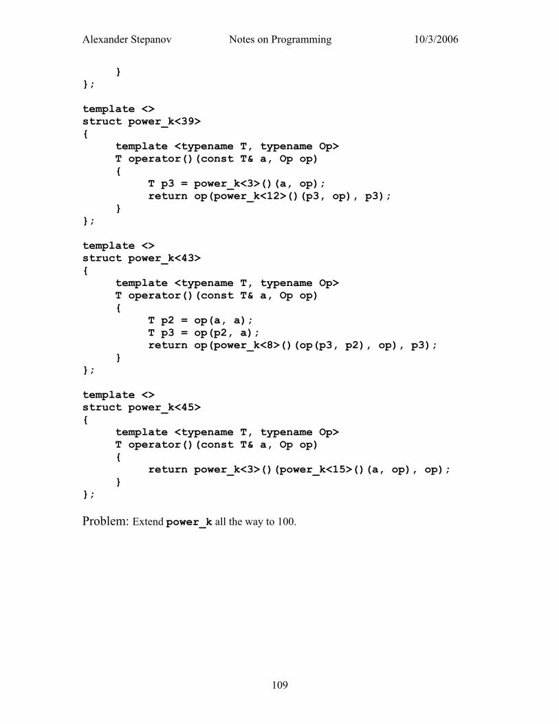
Alexander Stepanov Notes on Programming 10/3/2006
} }; template <> struct power_k<39> { template <typename T, typename Op> T operator()(const T& a, Op op) { T p3 = power_k<3>()(a, op); return op(power_k<12>()(p3, op), p3); } }; template <> struct power_k<43> { template <typename T, typename Op> T operator()(const T& a, Op op) { T p2 = op(a, a); T p3 = op(p2, a); return op(power_k<8>()(op(p3, p2), op), p3); } }; template <> struct power_k<45> { template <typename T, typename Op> T operator()(const T& a, Op op) { return power_k<3>()(power_k<15>()(a, op), op); } }; Problem: Extend power_k all the way to 100.
109
Alexander Stepanov Notes on Programming 10/3/2006
Lecture 11. Locations and addresses In the previous lecture we discovered that we can think about algorithms as being defined on mathematical structures, such as total ordering, Euclidean rings, monoids, semigroups, etc. It is a wonderful discovery since it allows us to view our activity as a continuation of a great mathematical tradition. It should not be particularly surprising, since computer science was discovered by mathematicians such as Alan Turing and John von Neumann. The perception that we are pre-occupied with routine tasks that are less glamorous than the job of a mathematician is an illusion. The great mathematicians of the past such as Archimedes, Euler and Gauss were not at all averse to solving practical problems. The disdain for solving practical problems is usually an indication of the decline of a particular science. But are we just repeating the path of mathematics? Are we rediscovering anew a set of well-known basic abstractions? Or is there something in our discipline that adds to the set of abstractions discovered by mathematicians? My answer is an emphatic yes to the last question and no to the others. The great discovery of Turing and von Neumann that set us on a new path was the discovery of memory. We are not just dealing with numbers: we are storing them in different locations. As computer science developed, the notion of memory developed with it. At first Turing introduced memory as a (potentially) infinite tape. I say “potentially” since at any moment of computation only a finite amount of tape is actually used. Then it became clear that the model that we really need is a model of a random-access machine that uses natural numbers as its addresses and can retrieve or store data from a location in a “constant” amount of time. (“Constant” is sometimes logarithmic, but we have to remember that logarithms are constant for all practical purposes.) Then there was the amazing discovery that we can model different behavior of memory by creating different data structures. The problem is that in the last 40 years the number of different individual data structures that control our access to locations grew up dramatically. We need to use the well-tested method of abstraction to handle them. The challenge that we face is to develop abstract concepts that deal with locations. If traditional mathematics deals with sets of values and operations on them, value algebras, we have to deal with sets of locations and operations on them: location algebras. A location algebra is not a data structure but an abstraction of a particular set of operations on locations. Let us quickly give several important definitions of different classes of location algebras. A location algebra is called homogeneous if all of the locations in the algebra contain values of the same type. In this course we will deal mostly with homogeneous algebras. A location algebra is free if there are no constraints on the values contained in the locations. A linked list is free. If we guarantee that it is sorted, it is not free.
110

Alexander Stepanov Notes on Programming 10/3/2006
While it is possible to keep providing more and more definitions, it is not the correct approach to building a theory. We often get the idea that a mathematical theory is built in a logical way starting from definitions and axioms. This is not the case. The definitions and axioms appear at the very end of the development of a good theory. It invariably starts with simple facts that later on are generalized into theorems, and only at the very end the formal definitions and axioms are developed. Sadly enough, many people who try to apply mathematics to programming start with axioms and then end up criticizing the real programs for not corresponding to their “beautiful” axioms. To build a theory of data structures we need to start with simple algorithms operating on data structures and only when we have looked at many specific algorithms can we come up with satisfactory theories. It is almost impossible to capture the process in my lectures. After all, I already know the answers and, willy-nilly, present the conclusions in a more deductive way than they have really been derived. The inductive process that is central to the discovery is lost. But let us try the best we can by using my favorite “inside-out” way of design. We will start with the simplest possible location-based algorithm – linear search – and attempt to derive a theory of iterators – or objects that define locations. I have to admit that I have grave misgivings about the term iterator. I did not use it originally and used interchangeably the terms position and coordinate. I was very familiar with the notion of iterators in Clu and knew that it was not what I needed. Unfortunately, the C++ community borrowed the notion of iterators from Clu and when I started explaining my ideas they insisted that they already had a term for things like my coordinates and they should be called iterators. Of course, random access iterators have no relation to Clu-like iterators used in C++ before STL, but the name stuck and I have to use it now. The name is especially inappropriate for the most basic kind of iterators, trivial iterators, since they do not iterate! A type is called a trivial iterator to some class T if it is a regular type that provides an (amortized) constant-time dereferencing operation that returns a reference to T. We refer to T as the value type of the iterator and the reference to T as the reference type of the iterator. There are serious complications in precisely defining what reference types in C++ are. It is possible to create proxy classes that behave almost like references. Unfortunately, almost is not good enough. I suggest that you stay away from them, and in this course we will deal only with plain references: T& and const T&. The notion of reference is hardwired into the language and all attempts to extend it I have seen were not very convincing. Since I was probably one of the first if not the first person to attempt to introduce such proxy references in vector<bool>, I have earned the right to be skeptical of them. The concept of a trivial iterator is important theoretically, but is much less so in practice for the simple reason that there are not many algorithms that use trivial iterators. While STL uses unary operator* for dereference I will use a function deref to designate such an operation. It will make certain things more consistent and will make my code less dependent on the peculiarities of the C++ syntax. In particular, that will enable us to
111
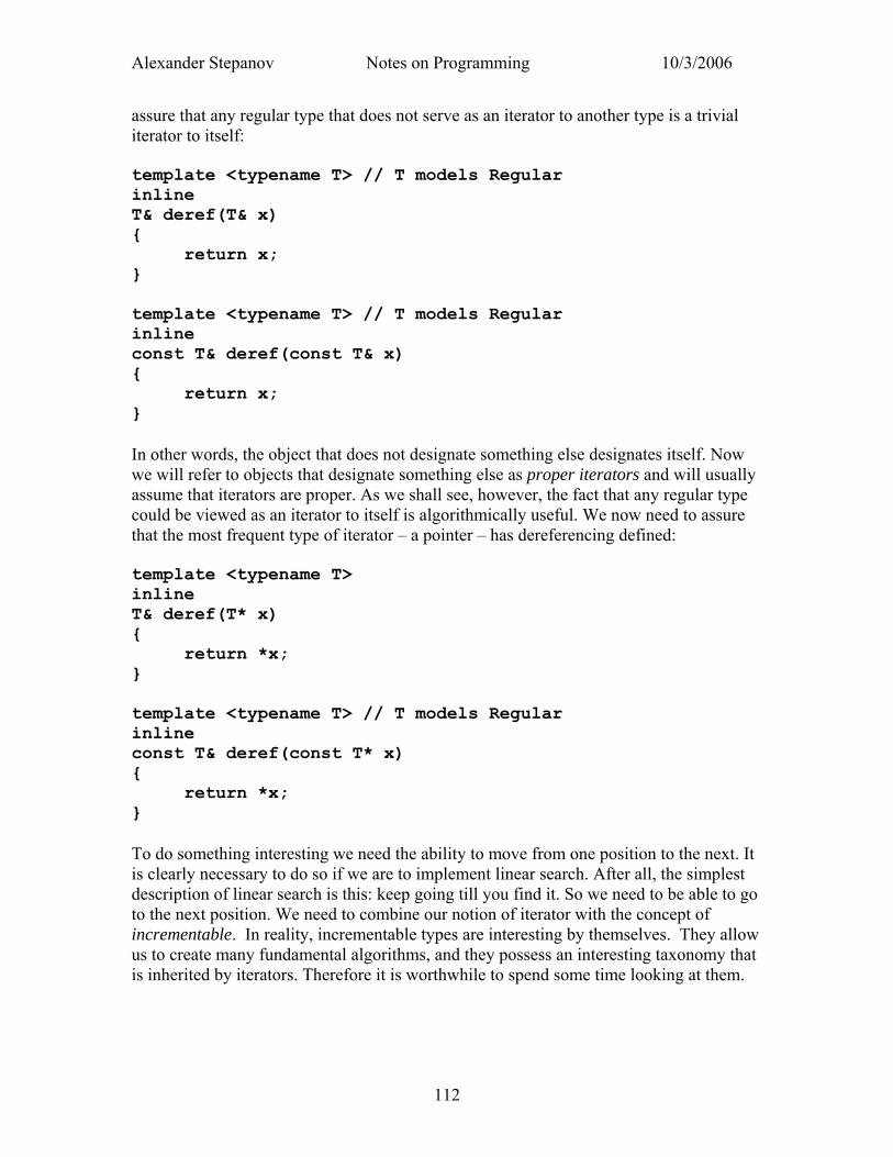
Alexander Stepanov Notes on Programming 10/3/2006
assure that any regular type that does not serve as an iterator to another type is a trivial iterator to itself: template <typename T> // T models Regular inline T& deref(T& x) { return x; } template <typename T> // T models Regular inline const T& deref(const T& x) { return x; } In other words, the object that does not designate something else designates itself. Now we will refer to objects that designate something else as proper iterators and will usually assume that iterators are proper. As we shall see, however, the fact that any regular type could be viewed as an iterator to itself is algorithmically useful. We now need to assure that the most frequent type of iterator – a pointer – has dereferencing defined: template <typename T> inline T& deref(T* x) { return *x; } template <typename T> // T models Regular inline const T& deref(const T* x) { return *x; } To do something interesting we need the ability to move from one position to the next. It is clearly necessary to do so if we are to implement linear search. After all, the simplest description of linear search is this: keep going till you find it. So we need to be able to go to the next position. We need to combine our notion of iterator with the concept of incrementable. In reality, incrementable types are interesting by themselves. They allow us to create many fundamental algorithms, and they possess an interesting taxonomy that is inherited by iterators. Therefore it is worthwhile to spend some time looking at them.
112

Alexander Stepanov Notes on Programming 10/3/2006
Lecture 12. Actions and their orbits The concept of an incrementable type is tied to an operator++ defined on the type that mutates the object and sets its value to the next value of the type. In reality we need a more general concept of a type with an action – a function or a function object that mutates the value of an object. After all, there are many different increment-like operations on a type. For example, in the case of integers we could have a function object that does x += c or x = x * c % m for constants c and m. An action is called total if it is defined for any value of the type. In programming we often deal with non-total or partial actions. An action of type A on type T is called explicitly defined if there is a function: bool is_defined(A a, T x) that returns true if action a is defined on x and false otherwise. (As a matter of fact, such a function always exists as an implicit function. An implicit function is a function on a type that is mathematically well-defined but might not have an explicit implementation. It is often essential to introduce implicit functions to be able to express the semantics of a concept.) An object for which action a is not defined is called a bottom of a, or, if it is clear which action is discussed, simply a bottom. We can provide a default for total actions: template <typename T, // T models Regular <typename A> // A models Action on T inline bool is_defined(const A&, const T&) { return true; } An explicitly defined action of type A is called regular if, for two actions a and b and two distinct objects x and y of type T, the following holds true: assert(is_defined(a, x) && a == b && x == y); assert(is_defined(b, y)); In other words, the action is defined on equal values. Also the following holds true: assert(is_defined(a, x)); assert(&x != &y && x == y && a == b); a(x); b(y); assert(x == y);
113

Alexander Stepanov Notes on Programming 10/3/2006
In other words, applying equal actions to equal but not identical objects maintains the equality. (Actions take their argument by reference and return void.) Sometimes we want to apply the action several times: template <typename T, // T models Regular typename A, // A models Action on T typename I> // I models Integer inline void advance(T& x, I n, A a) { while (n > Integer(0)) { assert(is_defined(a, x)); a(x); --n; } } We can easily make a version of it that will behave as the STL version of advance by defining: template <typename T> // T models Incrementable struct increment { void operator()(T& x) { ++x; } }; template <typename T, // T models Incrementable typename I> // I models Integer inline void advance(T& x, I n) { advance(x, n, increment<T>()); } Often we can use functional versions of advance: template <typename T, typename A, // A models Action on T typename I> // I models Integer inline T successor_n(T x, I n, A a) { advance(x, n, a); return x; }
114

Alexander Stepanov Notes on Programming 10/3/2006
template <typename T, typename I> // I models Integer inline T successor_n(T x, I n) { return successor_n(x, n, increment<T>()); } template <typename T> inline T successor(T x) { increment<T>()(x); return x; } Problem: Define function_objects advance_k and successor_k that take a template integer argument. (Hint: look at the code for power_k.) Sometimes we cannot be sure that we can advance all the way; we can then use a version that will advance as much as it can and then return the number of advances remaining to be done: template <typename T, // T models Regular typename A, // A models Action on T typename I> // I models Integer I guarded_advance(T& x, I n, A action) { while (n > I(0) && is_defined(action, x)) { action(x); --n; } return n; } Problem: Implement guarded versions of successor and successor_n. Now we can define an algorithmic inverse of advance: a function distance that counts the number of applications it takes to reach one value from another. The code is practically indistinguishable from advance, but we face the problem of determining the type we should use for counting. Let us introduce a type function COUNT_TYPE that for every type returns an integer type big enough to count the number of distinct values that the original type may have. In some future language we will have special facilities for type functions. In C++ we use the standard convention of implementing type functions through type traits:
115

Alexander Stepanov Notes on Programming 10/3/2006
template <typename T> // T models Countable struct count_type_traits { typedef size_t type; }; #define COUNT_TYPE(T) typename count_type_traits<T>::type This code establishes a default that returns size_t as COUNT_TYPE(T) for most types. If something else is needed we can partially specialize count_type_traits for our type or a parameterized family of types: template <> struct count_type_traits<short> { typedef unsigned short type; }; or, template <typename T> struct count_type_traits<vector<T> > { typedef uint32 type; // the number of different vectors is less than 2^32 }; We will call a type on which COUNT_TYPE is defined a countable type. Now it is easy to define the distance function: template <typename T, // T models Regular typename A> // A models Action on T COUNT_TYPE(T) distance(T first, T last, A action) { COUNT_TYPE(T) n(0); while (first != last) { action(first); ++n; } return n; } From now on we will assume that actions are partial, explicitly defined and regular unless otherwise specified.
116
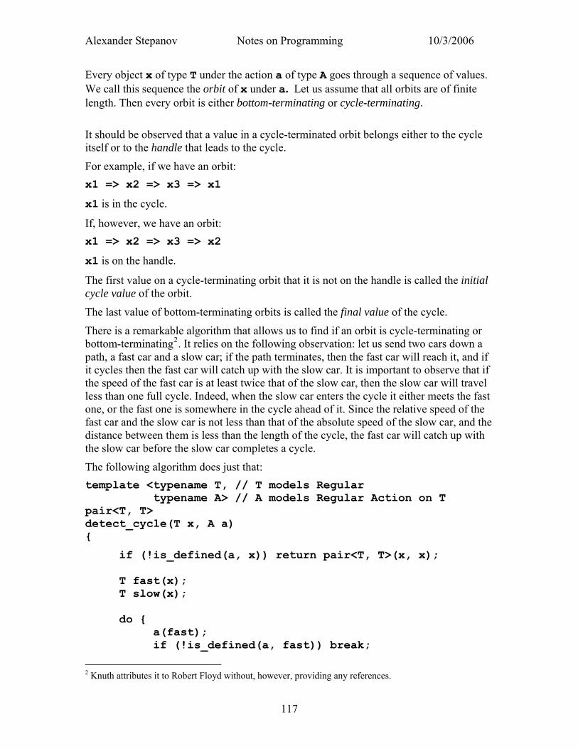
Alexander Stepanov Notes on Programming 10/3/2006
Every object x of type T under the action a of type A goes through a sequence of values. We call this sequence the orbit of x under a. Let us assume that all orbits are of finite length. Then every orbit is either bottom-terminating or cycle-terminating.
It should be observed that a value in a cycle-terminated orbit belongs either to the cycle itself or to the handle that leads to the cycle.
For example, if we have an orbit: x1 => x2 => x3 => x1
x1 is in the cycle.
If, however, we have an orbit: x1 => x2 => x3 => x2
x1 is on the handle.
The first value on a cycle-terminating orbit that it is not on the handle is called the initial cycle value of the orbit.
The last value of bottom-terminating orbits is called the final value of the cycle.
There is a remarkable algorithm that allows us to find if an orbit is cycle-terminating or bottom-terminating2. It relies on the following observation: let us send two cars down a path, a fast car and a slow car; if the path terminates, then the fast car will reach it, and if it cycles then the fast car will catch up with the slow car. It is important to observe that if the speed of the fast car is at least twice that of the slow car, then the slow car will travel less than one full cycle. Indeed, when the slow car enters the cycle it either meets the fast one, or the fast one is somewhere in the cycle ahead of it. Since the relative speed of the fast car and the slow car is not less than that of the absolute speed of the slow car, and the distance between them is less than the length of the cycle, the fast car will catch up with the slow car before the slow car completes a cycle.
The following algorithm does just that: template <typename T, // T models Regular typename A> // A models Regular Action on T pair<T, T> detect_cycle(T x, A a) {
if (!is_defined(a, x)) return pair<T, T>(x, x); T fast(x); T slow(x); do { a(fast); if (!is_defined(a, fast)) break;
2 Knuth attributes it to Robert Floyd without, however, providing any references.
117

Alexander Stepanov Notes on Programming 10/3/2006
a(slow); a(fast); if (!is_defined(a, fast)) break; } while (fast != slow); // slow == fast iff orbit of x is cyclic // in such case fast moved exactly // twice as many steps as slow return pair<T, T>(slow, fast); } We have to assume that T is regular since we need equality. We also need our assumption that A is a regular action. We return a pair of the slow and the fast values. If we return a pair of equal values and the action is defined on them, then the orbit is cycle-terminating, if not then the first element of the pair points to the middle value of the orbit. Problem: Define what the middle value of a bottom-terminating orbit is. Sometimes we can benefit from keeping the count and returning a triple with the second and third elements being slow and fast and the first being the count of the number of actions applied to fast. template <typename T, // T models Regular and Countable typename A> // A models Action on T triple<COUNT_TYPE(T), T, T> detect_count_cycle(T x, A a) { typedef COUNT_TYPE(T) I; if (!is_defined(a, x)) return triple<I, T, T>(I(0), x, x); I n(0); T fast(x); T slow(x); do { a(fast); ++n; if (!is_defined(a, fast)) break; a(slow);
118
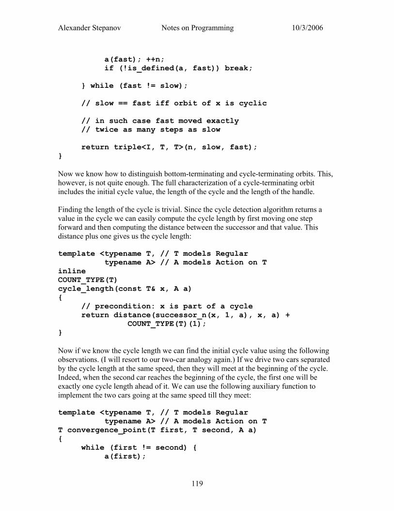
Alexander Stepanov Notes on Programming 10/3/2006
a(fast); ++n; if (!is_defined(a, fast)) break; } while (fast != slow); // slow == fast iff orbit of x is cyclic // in such case fast moved exactly // twice as many steps as slow return triple<I, T, T>(n, slow, fast); } Now we know how to distinguish bottom-terminating and cycle-terminating orbits. This, however, is not quite enough. The full characterization of a cycle-terminating orbit includes the initial cycle value, the length of the cycle and the length of the handle. Finding the length of the cycle is trivial. Since the cycle detection algorithm returns a value in the cycle we can easily compute the cycle length by first moving one step forward and then computing the distance between the successor and that value. This distance plus one gives us the cycle length: template <typename T, // T models Regular typename A> // A models Action on T inline COUNT_TYPE(T) cycle_length(const T& x, A a) { // precondition: x is part of a cycle return distance(successor_n(x, 1, a), x, a) + COUNT_TYPE(T)(1); } Now if we know the cycle length we can find the initial cycle value using the following observations. (I will resort to our two-car analogy again.) If we drive two cars separated by the cycle length at the same speed, then they will meet at the beginning of the cycle. Indeed, when the second car reaches the beginning of the cycle, the first one will be exactly one cycle length ahead of it. We can use the following auxiliary function to implement the two cars going at the same speed till they meet: template <typename T, // T models Regular typename A> // A models Action on T T convergence_point(T first, T second, A a) { while (first != second) { a(first);
119
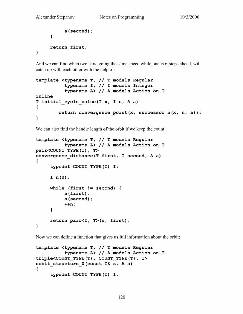
Alexander Stepanov Notes on Programming 10/3/2006
a(second); } return first; } And we can find when two cars, going the same speed while one is n steps ahead, will catch up with each other with the help of: template <typename T, // T models Regular typename I, // I models Integer typename A> // A models Action on T inline T initial_cycle_value(T x, I n, A a) { return convergence_point(x, successor_n(x, n, a)); } We can also find the handle length of the orbit if we keep the count: template <typename T, // T models Regular typename A> // A models Action on T pair<COUNT_TYPE(T), T> convergence_distance(T first, T second, A a) { typedef COUNT_TYPE(T) I; I n(0); while (first != second) { a(first); a(second); ++n; } return pair<I, T>(n, first); } Now we can define a function that gives us full information about the orbit: template <typename T, // T models Regular typename A> // A models Action on T triple<COUNT_TYPE(T), COUNT_TYPE(T), T> orbit_structure_0(const T& x, A a) { typedef COUNT_TYPE(T) I;
120

Alexander Stepanov Notes on Programming 10/3/2006
triple<I, T, T> t = detect_count_cycle(x, a); if (!is_defined(a, t.third)) // bottom-terminated orbit: return triple<I, I, T> (t.first, 0, t.third); // cycle-terminated orbit: I n = cycle_length(t.third); T y = successor_n(x, n, a); // y is a full cycle length ahead of x pair<I, T> q = convergence_distance(x, y, a); // q contains the handle length and the initial // cycle value return triple<I, I, T> (q.first, n, q.second); } What is the number of action applications done by the algorithm? If we denote c as our cycle length and h as the handle length, then the call to detect_count_cycle is going to do at most 3(c+h) actions when the orbit is cycle-terminating. (In case of the bottom-terminating orbit the number is 1.5h.) Computing the cycle length adds c actions. Computing the handle length and the initial cycle value adds 2h+c actions. That gives us a bound on the total number of actions of 5(c+h) or 5 times the number of values in the orbit. We can reduce the total number of actions by c if we change our code to: template <typename T, // T models Regular typename A> // A models Action on T triple<COUNT_TYPE(T), COUNT_TYPE(T), T> orbit_structure(const T& x, A a) { typedef COUNT_TYPE(T) I; triple<I, T, T> t = detect_count_cycle(x, a); if (!is_defined(a, t.third)) // bottom-terminated orbit: return triple<I, I, T> (t.first, 0, t.third); // cycle-terminated orbit: I n = cycle_length(t.third); pair<I, T> q = convergence_distance(x, t.third, a);
121

Alexander Stepanov Notes on Programming 10/3/2006
return triple<I, I, T> (q.first, n, q.second); } Problem: Explain why the above code works. Problem: It is possible to reduce the number of advances even further by (almost always) not walking the full cycle to compute its length as it is done with the call to cycle_length in the code above. Find the way to do it. In 1981 Leon Levy published a paper containing the following algorithm that computes the orbit structure in a different way: template <typename T, // T models Regular typename A> // A models Action on T triple<COUNT_TYPE(T), COUNT_TYPE(T), T> orbit_structure_1(T x, A a) { typedef COUNT_TYPE(T) I; triple<I, I, T> t = orbit_cycle_length(x, I(1), a); if (!is_defined(a, t.third)) return t; T y = successor(x, t.second, a); pair<I, T> q = convergence_distance(x, y, a); return triple<I, I, T> (q.first, n, q.second); } Where orbit_cycle_length is defined in the following way using a helper function orbit_length_bounded: template <typename T, // T models Regular typename I, // I models Integer typename A> // A models Action on T triple<I, I, T> orbit_length_bounded(T first, I bound, A a) { typedef triple<I, I, T> result_t; T last(first); I n(0); while (n < bound) { if (!is_defined(a, first)) return result_t(n + bound, 0, first); a(first);
122

Alexander Stepanov Notes on Programming 10/3/2006
++n; if (first == last) return result_t(n + bound, n, first); } return triple<I, I, T>(n + n, n + n, first); } template <typename T, // T models Regular typename I, // I models Integer typename A> // A models Action on T triple<I, I, T> orbit_cycle_length(T first, I n, A a) { assert (n > 0); while (true) { triple<I, I, T> t = orbit_length_bounded(first, n, a); if (t.first != t.second) return t; n = t.first; first = t.third; } } Problem: Figure out how Levy’s algorithm works. Problem: Analyze its complexity. Problem: Create a benchmark that compares three different versions of orbit_structure. Finding orbits is an important task when we deal with linked structures. It is also important when analyzing periods of random number generators. In general, the notion of action on a type is quite fundamental, and just about any algorithm can be represented as an action working on a type representing its state. We can, for example, represent Euclid’s algorithm with the help of an action that takes a pair of elements from a Euclidean domain and replaces it with a pair representing the next state of the algorithm: template <typename T> // T models Euclidean Domain struct euclidean_action { void operator() (pair<T, T>& x) { T tmp = x.first % x.second; x.first = x.second; x.second = tmp; }
123

Alexander Stepanov Notes on Programming 10/3/2006
}; It is clear that the action is not defined when the second component of the pair is equal to zero: template <typename T> // T models Euclidean Domain inline bool is_defined(euclidean_action<T>, const pair<T, T>& x) { return x.second != T(0); } Now we need to have a function that will keep applying an action till it is undefined: template <typename T, // T models Regular typename A> // A models Action on T inline void advance_while_defined(T& x, A a) { while (is_defined(a, x)) a(x); } And we can obtain our old friend with: template <typename T> // T models Euclidean Domain T gcd_action_based(T a, T b) { pair<T, T> p(a, b); advance_while_defined(p, euclidean_action<T>()); return p.first; } While in some cases we need to apply an action till it becomes undefined, it is often the case that we want to do the application up to a certain point on the orbit. The sequence of values in an orbit is called a range. There are three common ways to specify a range:
1. by end value, 2. by the number of values, 3. by predicate.
That gives us two additional versions of advance: template <typename T, // T models Regular typename A> // A models Action on T inline void advance_till_last(T& first, const T& last, A a) { while (first != last) {
124
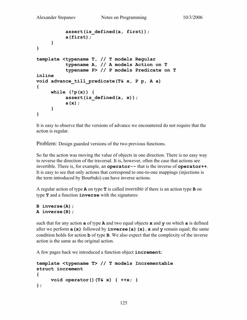
Alexander Stepanov Notes on Programming 10/3/2006
assert(is_defined(a, first)); a(first); } } template <typename T, // T models Regular typename A, // A models Action on T typename P> // P models Predicate on T inline void advance_till_predicate(T& x, P p, A a) { while (!p(x)) { assert(is_defined(a, x)); a(x); } } It is easy to observe that the versions of advance we encountered do not require that the action is regular. Problem: Design guarded versions of the two previous functions. So far the action was moving the value of objects in one direction. There is no easy way to reverse the direction of the traversal. It is, however, often the case that actions are invertible. There is, for example, an operator-- that is the inverse of operator++. It is easy to see that only actions that correspond to one-to-one mappings (injections is the term introduced by Bourbaki) can have inverse actions. A regular action of type A on type T is called invertible if there is an action type B on type T and a function inverse with the signatures: B inverse(A); A inverse(B); such that for any action a of type A and two equal objects x and y on which a is defined after we perform a(x) followed by inverse(a)(x), x and y remain equal; the same condition holds for action b of type B. We also expect that the complexity of the inverse action is the same as the original action. A few pages back we introduced a function object increment: template <typename T> // T models Incrementable struct increment { void operator()(T& x) { ++x; } };
125
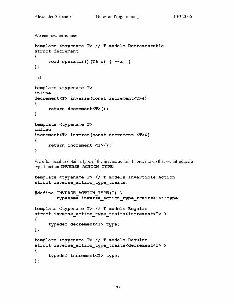
Alexander Stepanov Notes on Programming 10/3/2006
We can now introduce: template <typename T> // T models Decrementable struct decrement { void operator()(T& x) { --x; } }; and template <typename T> inline decrement<T> inverse(const increment<T>&) { return decrement<T>(); } template <typename T> inline increment<T> inverse(const decrement <T>&) { return increment <T>(); } We often need to obtain a type of the inverse action. In order to do that we introduce a type-function INVERSE_ACTION_TYPE: template <typename T> // T models Invertible Action struct inverse_action_type_traits; #define INVERSE_ACTION_TYPE(T) \ typename inverse_action_type_traits<T>::type template <typename T> // T models Regular struct inverse_action_type_traits<increment<T> > { typedef decrement<T> type; }; template <typename T> // T models Regular struct inverse_action_type_traits<decrement<T> > { typedef increment<T> type; };
126

Alexander Stepanov Notes on Programming 10/3/2006
Now we can construct the following algorithm that traverses a range from both directions: template <typename T, // T models Regular typename A, // A models Invertible Action on T typename U, // U models Binary Function on T,T typename V> // V models Function on T inline triple<U, V, bool> bidirectional_traversal(T& first, T& last, A a, U u, V v) { INVERSE_ACTION_TYPE(A) b(inverse(a)); while (first != last) { b(last); if (first == last) { v(first); return triple<U, V, bool>(u, v, true); } u(first, last); a(first); } return triple<U, V, bool>(u, v, false); } Problem: Justify the interface of the above function. Let us introduce a couple of little (but generally useful) function objects: template <typename T> struct null_action { void operator()(const T&){} }; template <typename I> // I models TrivialIterator struct iterator_swapper { void operator()(I x, I y) { swap(*x, *y); } }; (In case of such function objects the best way of documenting or specifying them is by giving the code. I do not believe that saying “// null_action does nothing” does more than just clutter the code. Ditto for iterator_swapper.)
127
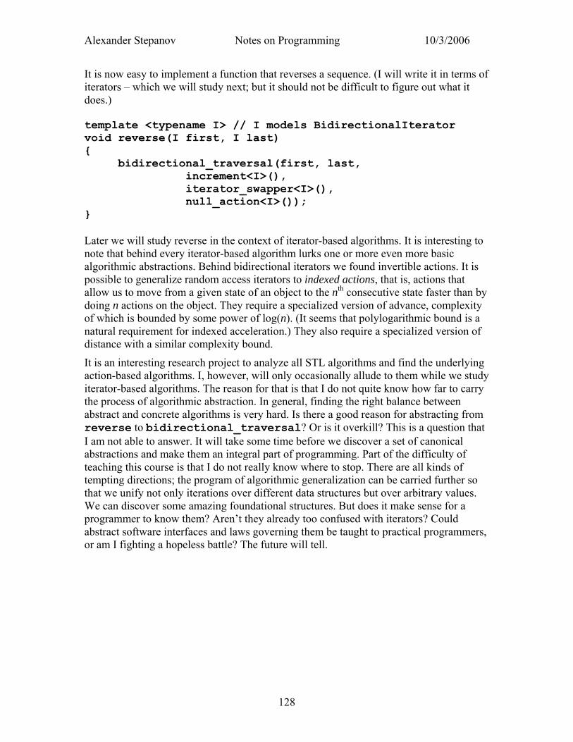
Alexander Stepanov Notes on Programming 10/3/2006
It is now easy to implement a function that reverses a sequence. (I will write it in terms of iterators – which we will study next; but it should not be difficult to figure out what it does.) template <typename I> // I models BidirectionalIterator void reverse(I first, I last) { bidirectional_traversal(first, last, increment<I>(), iterator_swapper<I>(), null_action<I>()); } Later we will study reverse in the context of iterator-based algorithms. It is interesting to note that behind every iterator-based algorithm lurks one or more even more basic algorithmic abstractions. Behind bidirectional iterators we found invertible actions. It is possible to generalize random access iterators to indexed actions, that is, actions that allow us to move from a given state of an object to the nth consecutive state faster than by doing n actions on the object. They require a specialized version of advance, complexity of which is bounded by some power of log(n). (It seems that polylogarithmic bound is a natural requirement for indexed acceleration.) They also require a specialized version of distance with a similar complexity bound.
It is an interesting research project to analyze all STL algorithms and find the underlying action-based algorithms. I, however, will only occasionally allude to them while we study iterator-based algorithms. The reason for that is that I do not quite know how far to carry the process of algorithmic abstraction. In general, finding the right balance between abstract and concrete algorithms is very hard. Is there a good reason for abstracting from reverse to bidirectional_traversal? Or is it overkill? This is a question that I am not able to answer. It will take some time before we discover a set of canonical abstractions and make them an integral part of programming. Part of the difficulty of teaching this course is that I do not really know where to stop. There are all kinds of tempting directions; the program of algorithmic generalization can be carried further so that we unify not only iterations over different data structures but over arbitrary values. We can discover some amazing foundational structures. But does it make sense for a programmer to know them? Aren’t they already too confused with iterators? Could abstract software interfaces and laws governing them be taught to practical programmers, or am I fighting a hopeless battle? The future will tell.
128

Alexander Stepanov Notes on Programming 10/3/2006
Lecture 13. Iterators It might be surprising to you, but I find the subject of iterators extremely hard to teach. The main reason is that I find the notion self-evident and all the fundamental design decision non-negotiable. But I also know that somehow even those people who are very enthusiastic about iterators, the STL “specialists,” often demonstrate that their understanding of iterator fundamentals is quite shaky. The fact that I find the concept so self-evident is the result of many years of trying alternatives and finding that they do not work. In some sense the only way for someone to fully understand why they have to be the way they are is by trying hundreds of different algorithms and finding the abstraction that allows the most beautiful and efficient representation of them. As a matter of fact, the only way of finding a useful abstraction is by trying to write code in terms of it. Sadly enough, people tend to define abstractions faster than they try them. There is even a pernicious idea of having “architects,” which are often people who produce abstractions without writing code. It is a worthwhile thing to remember that the most successful abstraction ever introduced in computer science – an abstraction of a file as a sequence of bytes with the help of which Ken Thompson revolutionized systems design – did not originate as an abstraction at all, but as a specific data structure for implementing files. Good abstractions come from efficient algorithms and data structures and not from “architectural” considerations. The problem with teaching, however, is that I cannot show you 20 wrong ways that I tried first before I show you the right way. I have to cheat and present something that became self-evident to me only after multiple wrong tries as the first and only alternative. I would, nevertheless, attempt to show you a step-by-step approach to iterators by considering the simplest and most fundamental problem that can be expressed with the help of iterators, linear search. We often need to find a piece of data. Later in the course we will study clever ways of doing it that speed things up considerably. But first let us look at the problem of finding things by looking at them one at a time. Our first attempt could be done even with the most basic category of iterators, trivial iterators. Since they do not provide a way of moving from one position to the next (and thus do not iterate at all), the only way of finding something is by explicitly giving all the positions to our function. It seems that it is really easy to find something if only one position is given: template <typename I> // I models TrivialIterator // VALUE_TYPE(I) models Regular inline bool find_trivial_0(I i, VALUE_TYPE(I) a) { return deref(i) == a; } The problem with this design is that it does not generalize to the case when we are given several different trivial iterators. It is not enough to return a Boolean value indicating that we found the right value after dereferencing one of them. (It is, of course, a useful
129

Alexander Stepanov Notes on Programming 10/3/2006
function, but it is not finding.) We need to return the first position where the value was found. For example, if we are searching through a sequence with two positions i1 and i2, we clearly want to have something like this in our code: if (deref(i1) == a) return i1; if (deref(i2) == a) return i2; The problem is that we need to return something in case we do not find the value. And there is nothing to return. We are only given two possible positions. Here we see one of the real difficulties many people have with iterators. It is important to understand that algorithms that deal with sequences of n elements usually require n+1 different positions to describe the result or the input. If we have an extra position limit that does not belong to the ones through which we search, we can have our find: template <typename I> // I models TrivialIterator // VALUE_TYPE(I) models Regular inline I find_trivial(I i1, I i2, I limit, const VALUE_TYPE(I)& a) { if (deref(i1) == a) return i1; if (deref(i2) == a) return i2; return limit; } We can define several versions of find_trivial for different number of arguments: template <typename I> // I models TrivialIterator // VALUE_TYPE(I) models Regular inline I find_trivial(I i1, I i2, I i3, I limit, const VALUE_TYPE(I)& a) { if (deref(i1) == a) return i1; if (deref(i2) == a) return i2; if (deref(i3) == a) return i3; return limit; } template <typename I> // I models TrivialIterator // VALUE_TYPE(I) models Regular inline I find_trivial(I i1, I i2, I i3, I i4, I limit, const VALUE_TYPE(I)& a) { if (deref(i1) == a) return i1; if (deref(i2) == a) return i2;
130

Alexander Stepanov Notes on Programming 10/3/2006
if (deref(i3) == a) return i3; if (deref(i4) == a) return i4; return limit; } We can even fix the definition for the case with one position: template <typename I> // I models TrivialIterator // VALUE_TYPE(I) models Regular inline I find_trivial(I i1, I limit, const VALUE_TYPE(I)& a) { if (deref(i1) == a) return i1; return limit; } Sadly enough, C++ does not provide us with a useful way of defining a family of functions that take different numbers of arguments. Such a facility would often be important. When we defined max_3 and max_4 we were doing it out of desperation. What we need would be one max that takes as many arguments as a user has and returns the largest. The same applies to cycle_left that we encountered in our section on swap. The same, of course, applies to find_trivial. (I would like to remark that it is possible to use a Boolean flag instead of an extra value of the iterator to signal that the search was not successful, but it makes the interface uglier. I used such an interface in my unsuccessful attempt to introduce an iterator-like abstraction in Ada. Ada compilers failed to compile my code, most of my experimental library perished without a trace except for one algorithm that Dave Musser and I used for one of our papers, and I had to wait for C++ templates. It was quite fortunate since the notion of iterator that I developed – called coordinate at the time – was much less elegant than the one that I developed for C++.) We can often combine the concept of trivial iterator with the concept of incrementable – a type that has an action that is performed by operator++. The combined concept is called forward iterator when the action is regular and input iterator when it is not. The simple way of thinking about the difference between the two is that forward iterators allow us to move forward from a given position as many times as we need. Input iterators cannot guarantee that if we increment equal positions we will get to equal positions. They are good only for single pass algorithms. Fortunately, finding is a single pass algorithm. We can use the range idiom that we studied in the previous chapter to define a generic find: template <typename I> // I models InputIterator // VALUE_TYPE(I) models Regular
131

Alexander Stepanov Notes on Programming 10/3/2006
I find(I first, I limit, VALUE_TYPE(I) a) { while (first != limit && deref(first) != a) ++first; return first; } Problem: In find_trivial I passed a by constant reference. In find, I pass it by value. Is there a reason for that? Here we can make a stop and discuss the type function VALUE_TYPE and its use in find. First, it is important to notice that when STL was originally designed, there was no way at all to implement a type function in C++. That led to many “interesting” design decisions. Some interfaces had to be relaxed. Instead of specifying the exact type of elements to which iterators point, I had to allow an arbitrary element type. The STL find is defined as: template <typename I, // I models InputIterator typename A> I find(I first, I limit, const A& a) { while (first != limit && deref(first) != a) ++first; return first; } Sadly enough, even now this interface is safer than the one that attempts to exactly specify the value type. If, for example, we try to find 100000 in an array of short (I assume that short is a two byte quantity) containing a 0, we will unfortunately succeed with the code that takes VALUE_TYPE, since the C++ compiler will introduce a narrowing conversion that will make 100000 into 0 and find it in our sequence. The STL code, while theoretically unsound, will spare us this particular bug since instead of narrowing implicit conversion on entry, compiler will generate a widening conversion from short to int inside the body of the function. It is a design nightmare to write generic programs in a language that contains implicit conversions since any attempt to specify exact relationships among types is defeated by the fact that a random type conversion can be inserted at any point in the code. (As a matter of fact, it is a design nightmare to write any code, generic or not, in a language with implicit conversions. It is astonishing that in 2006 I have to argue that strong typing is good.) We use the end of our range as a limit. That allows us to have an extra value of the iterator. (Let us again emphasize that we need one extra value for many other sequence operations. For example, if we want to insert an element into a sequence of n elements, it is quite easy to see that there are n+1 insertion points.)
132
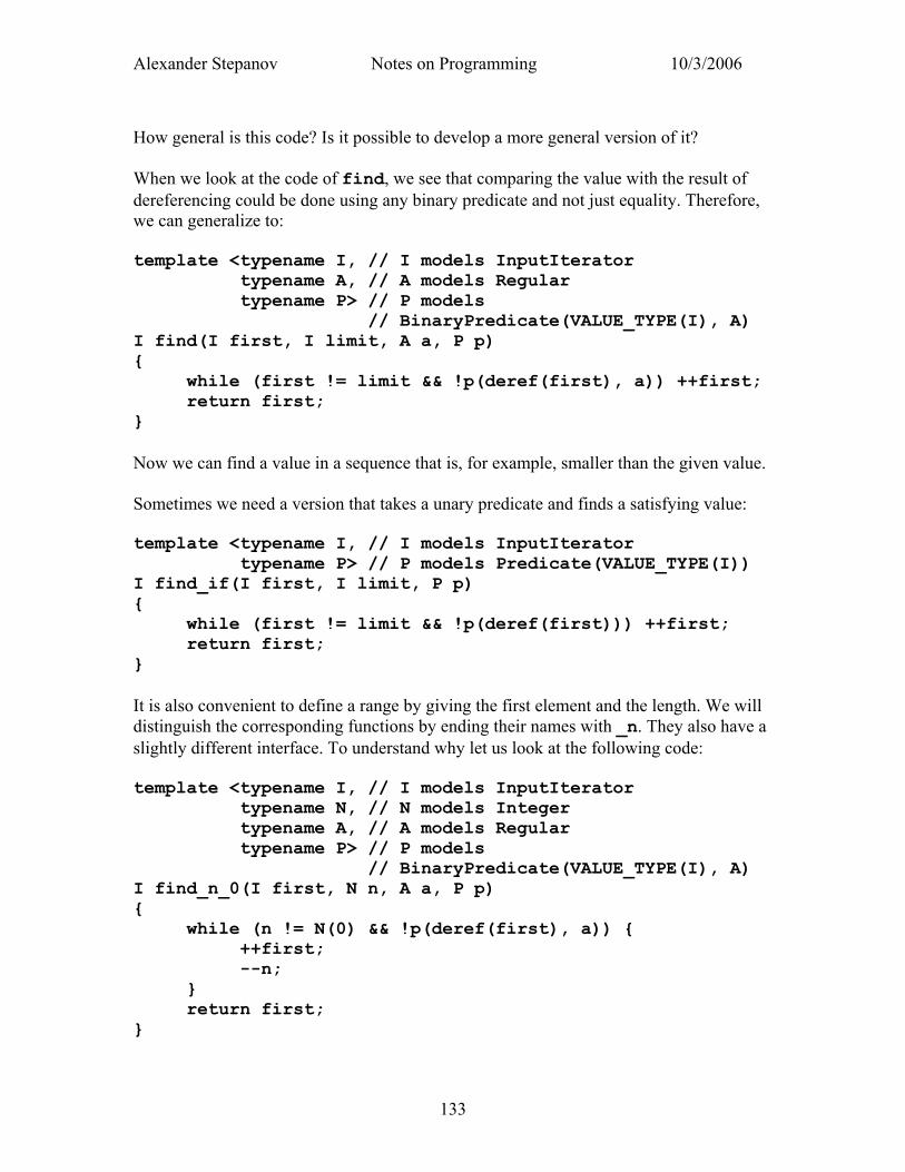
Alexander Stepanov Notes on Programming 10/3/2006
How general is this code? Is it possible to develop a more general version of it? When we look at the code of find, we see that comparing the value with the result of dereferencing could be done using any binary predicate and not just equality. Therefore, we can generalize to: template <typename I, // I models InputIterator typename A, // A models Regular typename P> // P models // BinaryPredicate(VALUE_TYPE(I), A) I find(I first, I limit, A a, P p) { while (first != limit && !p(deref(first), a)) ++first; return first; } Now we can find a value in a sequence that is, for example, smaller than the given value. Sometimes we need a version that takes a unary predicate and finds a satisfying value: template <typename I, // I models InputIterator typename P> // P models Predicate(VALUE_TYPE(I)) I find_if(I first, I limit, P p) { while (first != limit && !p(deref(first))) ++first; return first; } It is also convenient to define a range by giving the first element and the length. We will distinguish the corresponding functions by ending their names with _n. They also have a slightly different interface. To understand why let us look at the following code: template <typename I, // I models InputIterator typename N, // N models Integer typename A, // A models Regular typename P> // P models // BinaryPredicate(VALUE_TYPE(I), A) I find_n_0(I first, N n, A a, P p) { while (n != N(0) && !p(deref(first), a)) { ++first; --n; } return first; }
133
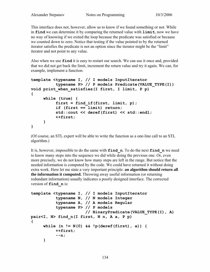
Alexander Stepanov Notes on Programming 10/3/2006
This interface does not, however, allow us to know if we found something or not. While in find we can determine it by comparing the returned value with limit, now we have no way of knowing if we exited the loop because the predicate was satisfied or because we counted down to zero. Notice that testing if the value pointed to by the returned iterator satisfies the predicate is not an option since the iterator might be the “limit” iterator and not point to any value. Also when we use find it is easy to restart our search. We can use it once and, provided that we did not get back the limit, increment the return value and try it again. We can, for example, implement a function: template <typename I, // I models InputIterator typename P> // P models Predicate(VALUE_TYPE(I)) void print_when_satisfies(I first, I limit, P p) { while (true) { first = find_if(first, limit, p); if (first == limit) return; std::cout << deref(first) << std::endl; ++first; } } (Of course, an STL expert will be able to write the function as a one-line call to an STL algorithm.) It is, however, impossible to do the same with find_n. To do the next find_n we need to know many steps into the sequence we did while doing the previous one. Or, even more precisely, we do not know how many steps are left in the range. But notice that the needed information is computed by the code. We could have returned it without doing extra work. Here let me state a very important principle: an algorithm should return all the information it computed. Throwing away useful information (or returning redundant information) usually indicates a poorly designed interface. The corrected version of find_n is: template <typename I, // I models InputIterator typename N, // N models Integer typename A, // A models Regular typename P> // P models // BinaryPredicate(VALUE_TYPE(I), A) pair<I, N> find_n(I first, N n, A a, P p) { while (n != N(0) && !p(deref(first), a)) { ++first; --n; }
134
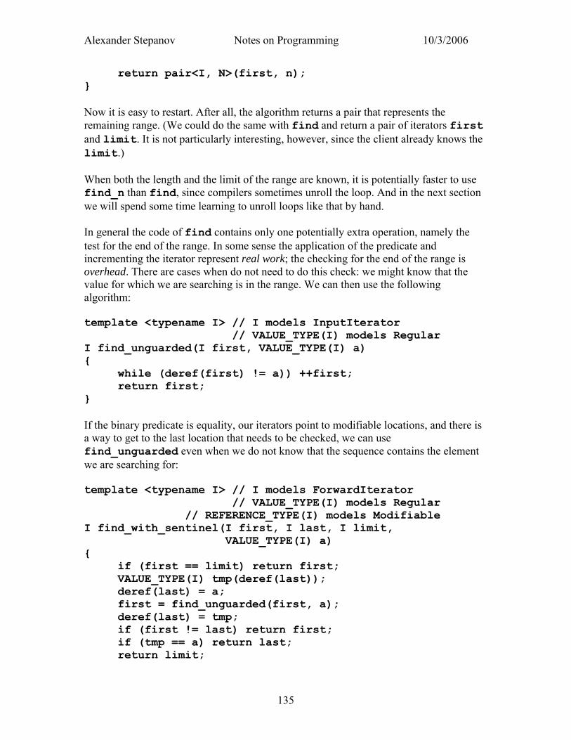
Alexander Stepanov Notes on Programming 10/3/2006
return pair<I, N>(first, n); } Now it is easy to restart. After all, the algorithm returns a pair that represents the remaining range. (We could do the same with find and return a pair of iterators first and limit. It is not particularly interesting, however, since the client already knows the limit.) When both the length and the limit of the range are known, it is potentially faster to use find_n than find, since compilers sometimes unroll the loop. And in the next section we will spend some time learning to unroll loops like that by hand. In general the code of find contains only one potentially extra operation, namely the test for the end of the range. In some sense the application of the predicate and incrementing the iterator represent real work; the checking for the end of the range is overhead. There are cases when do not need to do this check: we might know that the value for which we are searching is in the range. We can then use the following algorithm: template <typename I> // I models InputIterator // VALUE_TYPE(I) models Regular I find_unguarded(I first, VALUE_TYPE(I) a) { while (deref(first) != a)) ++first; return first; } If the binary predicate is equality, our iterators point to modifiable locations, and there is a way to get to the last location that needs to be checked, we can use find_unguarded even when we do not know that the sequence contains the element we are searching for: template <typename I> // I models ForwardIterator // VALUE_TYPE(I) models Regular // REFERENCE_TYPE(I) models Modifiable I find_with_sentinel(I first, I last, I limit, VALUE_TYPE(I) a) { if (first == limit) return first; VALUE_TYPE(I) tmp(deref(last)); deref(last) = a; first = find_unguarded(first, a); deref(last) = tmp; if (first != last) return first; if (tmp == a) return last; return limit;
135
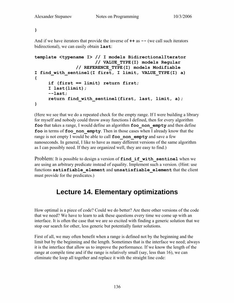
Alexander Stepanov Notes on Programming 10/3/2006
} And if we have iterators that provide the inverse of ++ as -- (we call such iterators bidirectional), we can easily obtain last: template <typename I> // I models BidirectionalIterator // VALUE_TYPE(I) models Regular // REFERENCE_TYPE(I) models Modifiable I find_with_sentinel(I first, I limit, VALUE_TYPE(I) a) { if (first == limit) return first; I last(limit); --last; return find_with_sentinel(first, last, limit, a); } (Here we see that we do a repeated check for the empty range. If I were building a library for myself and nobody could throw away functions I defined, then for every algorithm foo that takes a range, I would define an algorithm foo_non_empty and then define foo in terms of foo_non_empty. Then in those cases when I already know that the range is not empty I would be able to call foo_non_empty and save a few nanoseconds. In general, I like to have as many different versions of the same algorithm as I can possibly need. If they are organized well, they are easy to find.) Problem: It is possible to design a version of find_if_with_sentinel when we are using an arbitrary predicate instead of equality. Implement such a version. (Hint: use functions satisfiable_element and unsatisfiable_element that the client must provide for the predicates.)
Lecture 14. Elementary optimizations How optimal is a piece of code? Could we do better? Are there other versions of the code that we need? We have to learn to ask these questions every time we come up with an interface. It is often the case that we are so excited with finding a generic solution that we stop our search for other, less generic but potentially faster solutions. First of all, we may often benefit when a range is defined not by the beginning and the limit but by the beginning and the length. Sometimes that is the interface we need; always it is the interface that allow us to improve the performance. If we know the length of the range at compile time and if the range is relatively small (say, less than 16), we can eliminate the loop all together and replace it with the straight line code:
136

Alexander Stepanov Notes on Programming 10/3/2006
template <int K> struct find_k; template <> struct find_k<0> { template <typename I, // I models InputIterator typename A, // A models Regular typename P> // P models // BinaryPredicate(VALUE_TYPE(I), A) pair<I, int> operator()(I i, A, P) { return pair<I, int>(i, 0); } }; template <int k> struct find_k { template <typename I, // I models InputIterator typename A, // A models Regular typename P> // P models // BinaryPredicate(VALUE_TYPE(I), A) pair<I, int> operator()(I i, A a, P p) { if (p(deref(i), a)) return pair<I, int>(i, k); ++i; return find_k<k-1>()(i, a, p); } }; Sometimes we do not know the length of the sequence at compile time, but we know that it is small (not greater than 16). We can come up with a relatively good implementation: template <typename I, // I models InputIterator typename A, // A models Regular typename P> // P models // BinaryPredicate(VALUE_TYPE(I), A) inline pair<I, int> find_small_n(I i, int n, A a, P p) { assert (n <= 16); switch (16 – n) { case 0: if (p(deref(i), a)) return pair<I, int>(i, 16); ++i; case 1: if (p(deref(i), a))
137
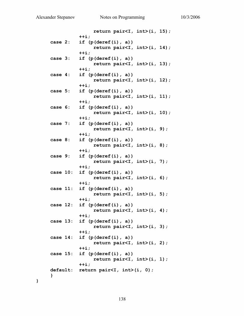
Alexander Stepanov Notes on Programming 10/3/2006
return pair<I, int>(i, 15); ++i; case 2: if (p(deref(i), a)) return pair<I, int>(i, 14); ++i; case 3: if (p(deref(i), a)) return pair<I, int>(i, 13); ++i; case 4: if (p(deref(i), a)) return pair<I, int>(i, 12); ++i; case 5: if (p(deref(i), a)) return pair<I, int>(i, 11); ++i; case 6: if (p(deref(i), a)) return pair<I, int>(i, 10); ++i; case 7: if (p(deref(i), a)) return pair<I, int>(i, 9); ++i; case 8: if (p(deref(i), a)) return pair<I, int>(i, 8); ++i; case 9: if (p(deref(i), a)) return pair<I, int>(i, 7); ++i; case 10: if (p(deref(i), a)) return pair<I, int>(i, 6); ++i; case 11: if (p(deref(i), a)) return pair<I, int>(i, 5); ++i; case 12: if (p(deref(i), a)) return pair<I, int>(i, 4); ++i; case 13: if (p(deref(i), a)) return pair<I, int>(i, 3); ++i; case 14: if (p(deref(i), a)) return pair<I, int>(i, 2); ++i; case 15: if (p(deref(i), a)) return pair<I, int>(i, 1); ++i; default: return pair<I, int>(i, 0); } }
138

Alexander Stepanov Notes on Programming 10/3/2006
<< more on unrolling; Duff’s device; software pipelining and the need for special control structure indicating that there are no dependencies between iterations: do_parallel, the need for the language to be able to express all the information necessary for the compiler to generate efficient code, intrinsics to find out the exact cache/memory structure, adequate handling of arithmetic operations: intrinsics for multiplication returning full result and division/remainder pair; language interface to vector operations>>
Lecture 15. Iterator type-functions << Dealing with type-functions in the original STL; count and count_if; nested typedefs in containers and function objects; no support for built-in types; partial specialization and traits classes; the need for real type-functions>>
Lecture 16. Equality of ranges and copying algorithms
<<different versions of mismatch; equality of ranges; copy and output iterators; semantics of copy; copy_parallel for non-intersecting ranges; copy_n; copy_backward>>
Lecture 17. Permutation algorithms In the previous lecture we have seen how to copy objects from one range into another. (Actually, it is quite amazing how much time computers spend moving data from one place to another without doing any meaningful modifications of them. It would be interesting to find out how many times characters that I type now are copied before you read them.) There is, fortunately, more to computing than copy. One of the most basic things we can do with data is to rearrange it. I call the algorithms that do such rearrangements permutation algorithms. To me they appear as a rich and wonderful toolset that every programmer should know and love. A range of objects [f1, l1) is called a permutation of a range [f0, l0) if there is a one-to-one correspondence between the objects in the ranges and the corresponding objects are equal. While this definition sounds “mathematical” since it talks of “one-to-one correspondence,” it is quite useless for finding out if two sequences are permutations of each other. What are we supposed to do when given two ranges? Should we go through all n! possible one-to-one mappings checking if the corresponding elements are equal? A definition that requires an exponential number of steps to check is called
139
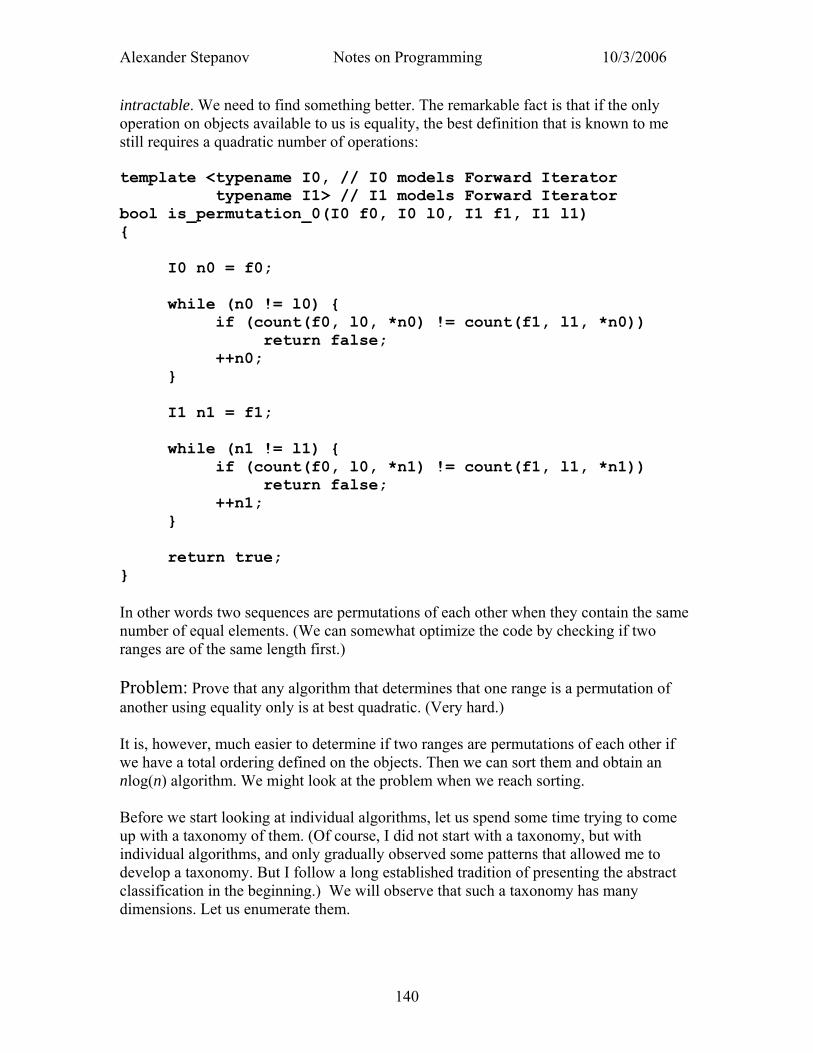
Alexander Stepanov Notes on Programming 10/3/2006
intractable. We need to find something better. The remarkable fact is that if the only operation on objects available to us is equality, the best definition that is known to me still requires a quadratic number of operations: template <typename I0, // I0 models Forward Iterator typename I1> // I1 models Forward Iterator bool is_permutation_0(I0 f0, I0 l0, I1 f1, I1 l1) { I0 n0 = f0; while (n0 != l0) { if (count(f0, l0, *n0) != count(f1, l1, *n0)) return false; ++n0; } I1 n1 = f1; while (n1 != l1) { if (count(f0, l0, *n1) != count(f1, l1, *n1)) return false; ++n1; } return true; } In other words two sequences are permutations of each other when they contain the same number of equal elements. (We can somewhat optimize the code by checking if two ranges are of the same length first.) Problem: Prove that any algorithm that determines that one range is a permutation of another using equality only is at best quadratic. (Very hard.) It is, however, much easier to determine if two ranges are permutations of each other if we have a total ordering defined on the objects. Then we can sort them and obtain an nlog(n) algorithm. We might look at the problem when we reach sorting. Before we start looking at individual algorithms, let us spend some time trying to come up with a taxonomy of them. (Of course, I did not start with a taxonomy, but with individual algorithms, and only gradually observed some patterns that allowed me to develop a taxonomy. But I follow a long established tradition of presenting the abstract classification in the beginning.) We will observe that such a taxonomy has many dimensions. Let us enumerate them.
140

Alexander Stepanov Notes on Programming 10/3/2006
An algorithm is called mutative if it replaces the original sequence of objects with its permutation. An algorithm is called copying if it places the resulting permutation in a different range. We will often need both versions and will use a standard suffix _copy to name a copying version of a permutation algorithm. For example, it is quite useful to have both reverse and reverse_copy algorithms. One can, of course, implement reverse_copy as copy followed by reverse, but there are ways to construct faster copying versions of mutative algorithms. While it is not strictly necessary, we usually assume that mutative algorithms do not use much extra storage. An algorithm is called in-place or in-situ if it uses extra storage which is at most logarithmic in the size of the original range. We shall introduce also a class of algorithms that while not in-place are practically very important: memory adaptive algorithms that use an additional buffer that is linear in the size of the range. They are important since they often give a better performance than in-place algorithms while using a buffer that is 1% to 10% of the original range. Theoreticians prefer logarithmic (or polylogarithmic) extra storage to linear extra storage with a small coefficient. In practice, however, finding a buffer of size 0.01N is not really difficult. The second dimension of our classification depends on what kind of information algorithms use. There are some algorithms that move objects around without looking at them. Their final destinations depend only on their original positions. I call such algorithms position-based permutation algorithms. Algorithms for reversing a range or randomly shuffling it are examples. Sometimes we look at the individual values and the final position depends on the value of a predicate on an object. For example we might want to put the even numbers before the odd numbers. I call such algorithms predicate-based algorithms. In addition to the range they take a predicate (or a multi-valued predicate) that determines the relative position of the objects. And, finally, sometimes we rearrange objects depending on their mutual relations. We might want, for example, to move the smallest element up front. I call such algorithms comparison-based permutation algorithms. (The comparisons they use are ordering relations. As with max and min we will assume that all the ordering relations are strict.) It should be noted that it is possible that eventually people will discover other categories of algorithms. It is possible that there are some permutations that are determined not by a single value or binary comparison but by a function that compares three objects in some interesting way. But so far, I have not found any such operations. Problem: Try to come with several examples of different position-based, predicate-based and comparison-based operations. Finally, often we permute values in a range by assigning or swapping them. But sometimes we can obtain similar effect by changing the relative positions of the iterators. Indeed, there are data structures that allow us to modify which location follows a given location. I call such data structures linked structures and permutation algorithms that modify the links I call link-modifying algorithms. As we shall see there are subtle
141

Alexander Stepanov Notes on Programming 10/3/2006
differences in the semantics of regular permutation operations and their link-modifying equivalents. It is important for us to understand how many assignments we need to do when we are implementing a mutative permutation algorithm. Actually, it should be self-evident that we do not really need full-blown assignment. A permutation involves no net construction or destructions of objects, just moving existing ones around, whereas assignment constructs a new value. We can, therefore, use the same primitives that we discovered when we were studying swap: namely, UNDERLYING_TYPE and raw_move. After all, swap is a permutation algorithm and any other permutation algorithm is just a more elaborate version of swap and cycle_left. For any permutation of a range there is a (usually implicit) permutation action defined on iterators in the range: if as a result of a permutation an object pointed to by an iterator from ends up in a location pointed by an iterator to, then the action when applied to an object containing a value to will make it equal to the value from. (A permutation action moves along the iterator values in the order opposite to the movement of the objects in the permutation.) It is easy to see that all the iterators in the range on which the permutation is acting fall into one or more cycles generated by the permutation action. Now if we can define a function object that performs the permutation action we can move objects in one of the cycles with the help of the following function: template <typename I, // I models Forward Iterator typename A> // A models Action on I void do_cycle(I i, A a) { I next = i; a(next); if (next == i) return; UNDERLYING_TYPE(VALUE_TYPE(I)) tmp; move_raw(deref(i), tmp); I first = i; do { move_raw(deref(next), deref(first)); first = next; a(next); } while (next != i); move_raw(tmp, deref(first)); }
142

Alexander Stepanov Notes on Programming 10/3/2006
Now if we can determine a sequence of first elements of cycles, we can obtain our permutation by applying do_cycle to the first elements of each cycle. (As a matter of fact, we do not really need to have first elements; if we can obtain some iterator from every cycle, we are done.) While it is not always easy to do that, we now obtain a firm bound on the number of moves that a permutation needs: : N + Cnontrivial – Ctrivial, where N is the number of elements in the range, Cnontrivial is the number of cycles in the permutation with more than one element and Ctrivial is the number of cycles containing a single element. Problem: Show that the minimal number of moves is never less than N – Ctrivial + 1 and never greater than 3N/2.
Lecture 18. Reverse It is easy to see that in terms of the number of moves, the permutations requiring the most work are those containing N/2 cycles of length 2. Problem: How many different permutations like that are there for a range with N elements? While there is a huge number of different permutations with N/2 cycles of length 2, the number of useful algorithms is very small. While reverse is the one we are going to study in this section, there is at least one more commonly useful one. In my opinion, it is a worthwhile thing to look at something even simpler than reverse to see what we can learn. The algorithm I have in mind could be called adjacent_swap. It takes a sequence ababab and makes it into a sequence bababa. In case there is an odd element at the end, it leaves it in place. The code is relatively straightforward (I got it right on the third try): template <typename I> // I models Forward Iterator // with modifiable reference type void adjacent_swap_0(I first, I limit) { while (true) { if (first == limit) return; I next = successor(first); if (next == limit) return; iterator_swap(first, next); first = successor(next); }
143
Alexander Stepanov Notes on Programming 10/3/2006
} where iterator_swap is defined as: template <typename I1, // I1 models Forward Iterator // with modifiable reference type typename I2> // I2 models Forward Iterator // with modifiable reference type inline void iterator_swap(I i, I j) { swap(deref(i), deref(j)); } The problem, of course, is that our adjacent_swap_0 loses useful information. Without doing any extra work we can determine if there is an odd element at the end of the range. In general, when our exit condition is a disjunction of several simpler conditions it is often useful to return the information indicating which one was satisfied. We can do it simply: template <typename I> // I models Forward Iterator // with modifiable reference type int adjacent_swap(I first, I limit) { while (true) { if (first == limit) return 0; I next = successor(first); if (next == limit) return 1; iterator_swap(first, next); first = successor(next); } } Notice that I decided to return an integer and not a Boolean. The reason for that is that I am returning even/odd parity and it is more natural for me to think of the result as the remainder of dividing the length of the range by 2 than as a logical value. (And it generalizes better to similar algorithms where instead of swap we use cycle_left with three or more arguments.) In general, I do not particularly like the bool type in C++. A type that occupies at least 8 bits to store 1 bit of information is a pedantic invention. After a brave but unsuccessful attempt to provide bit addressable architecture in the IBM Stretch project3 designed in the late 50s, we have to deal with bytes as our smallest unit of addressability. (It is interesting that the design team of Stretch reads like a Who’s Who of computer architecture research: Gene Amdahl, Gerrit Blaauw, Fred Brooks, Werner Buchholz, and John Cocke. It would be the list of the greatest architects who ever lived if it were not for the fact that it did not contain the name of their even 3 IBM 7030 – see: http://www.bitsavers.org/pdf/ibm/7030/Planning_A_Computer_System.pdf
144

Alexander Stepanov Notes on Programming 10/3/2006
greater contemporary Seymour Cray. By the way, if you do not recognize the names, google them! One of them invented the term byte. Who?) Notice that if we have random access iterators, it is possible to speed things up a bit: template <typename I> // I models Random Access Iterator // with modifiable reference type void adjacent_swap_random_access(I first, I limit) { DISTANCE_TYPE(I) n = limit – first; while (n > 1) { iterator_swap(first, first + 1); first += 2; n -= 2; } } Problem: Explain why I changed the interface to return void. Implementing a copying version of adjacent_swap is instructive as well: template <typename I, // I models Input Iterator typename O> // O models Output Iterator pair<O, int> adjacent_swap_copy(I first, I limit, O result) { while (first != limit) { VALUE_TYPE(I) tmp = deref(first); ++first; if (first == limit) { deref(result) = tmp; ++result; return pair<O, int>(result, 1); } deref(result) = deref(first); ++result; ++first; deref(result) = tmp; ++result; } return pair<O, int>(result, 0); } Now let us look at reversing a range. The basic idea is quite clear: we need to swap the first with the last. It is a fairly straightforward thing to do when we have ability to go backwards: template <typename I> // I models Bidirectional Iterator
145

Alexander Stepanov Notes on Programming 10/3/2006
void reverse0(I first, I limit) { while (true) { if (first == limit) return; --limit; if (first == limit) return; iterator_swap(first, limit); ++first; } } We need to think about the return type. (STL returns void, which is yet another indication how inattentive its designer was to the finer details of programming.) It is clear that without doing any extra work in the main loop we can find the middle of the range and also determine its parity. We can do it by returning a range of elements that were not swapped: template <typename I> // I models Bidirectional Iterator pair<I, I> reverse(I first, I limit) { while (true) { if (first == limit) return pair<I, I>(first, limit); --limit; if (first == limit) return pair<I, I>(first, successor(limit)); iterator_swap(first, limit); ++first; } } Now if we know the length of the range, we can reduce the number of tests in the loop: template <typename I, // I models Bidirectional Iterator typename N> // N models Integer // N should be DIFFERENCE_TYPE(I) but for C++ // implicit conversions pair<I, I> reverse_n(I first, I limit, N n) { assert(distance(first, limit) <= n); while (n > N(1)) { --limit; iterator_swap(first, limit); ++first; n -= 2; } return pair<I,I>(first, limit);
146
Alexander Stepanov Notes on Programming 10/3/2006
} It is easy to produce a version of reverse that will dispatch on iterator category and call reverse_n in for random access iterators. When we look at the sequence of swaps inside reverse and reverse_n, we can see that they do not alias. Every element is swapped only once. This is a specific instance of a more general fact that different cycles in a permutation do not intersect. The fact that different swaps do not touch the same locations depends on the precondition that the input range is a valid range. If we do something like: int a[4]; reverse_n(a, a + 4, 8); every location will be an argument to two different swaps. But when our algorithm is called with a valid range – and it is clearly written only for such a case – there is no aliasing. It should be clear that it is hard for the compiler to figure that out. It is important that we should communicate our intent to it. It is clear that any attempt to deal with that through an abuse of a type system4 is not going to work since first and limit point into the same range and do alias each other at the termination point. In general, no-aliasing is a property of iterators that depends on the properties of the algorithm and is not something that a type system could handle. But it is important that the knowledge that the programmer has can be communicated to the compiler and eventually to other programmers. I believe that the solution can be obtained with the introduction of a new language construct initiate(statement) that indicates that the enclosed statement does not need to complete and that the execution of the program can continue till the next completion point is reached. We can then write: while (n > N(1)) { --limit; initiate(iterator_swap(first, limit)); ++first; n -= 2; } // completion point That expresses our assurance that iterator_swaps from different iteration can proceed in parallel without affecting the validity of the algorithm. It is very tempting to develop a mechanism that will allow us to describe arbitrarily complex execution threads, but I suspect that the correct solution is to have a very simple semantics of completion points by inserting them at the end of every while, for and do/while statements and also at the end of stand-alone compound statements. That seems to assure a reasonable exception semantics by assuring that every exception completes all outstanding incomplete statements. The restriction of potential re-ordering to what compiler writers
4 as noalias proponents attempted to do – see Dennis Ritchie’s famous rebuttal at http://www.astro.princeton.edu/~rhl/dmr-on-noalias.html
147

Alexander Stepanov Notes on Programming 10/3/2006
call basic blocks seems to allow aggressive use of software pipelining and speculative load/stores. Before we look at the problem of doing reverse for forward iterators, let us look at the copying versions of reverse. There are four useful versions of it. (STL has only one as a result of pruning during the standardization process.) They are: template <typename I, // I models Bidirectional Iterator typename O> // O models Output Iterator O reverse_copy(I first, I limit, O result) { while (first != limit) { --limit; deref(result) = deref(limit); ++result; } return result; } template <typename I, // I models Bidirectional Iterator typename N, // N modles Integer typename O> // O models Output Iterator pair<I, O> reverse_copy_n(I limit, N n, O result) { while (n > N(0)) { --limit; deref(result) = deref(limit); ++result; --n; } return pair<I, O>(limit, result); } template <typename I, // I models Input Iterator typename B> // B models Bidirectional Iterator B copy_reverse(I first, I limit, B result) { while (first != limit) { --result; deref(result) = deref(first); ++first; } return result; } template <typename I, // I models Input Iterator
148

Alexander Stepanov Notes on Programming 10/3/2006
typename N, // N modles Integer typename B> // B models Bidirectional Iterator pair<I, B> copy_reverse_n(I first, N n, B result) { while (n > N(0)) { --result; deref(result) = deref(first); ++first; --n; } return pair<I, B>(first, result); } Problem: How is copy_reverse different from reverse_copy? Problem: Explain the return types of the algorithms. It is much harder to reverse a range if the iterator to our range is only a forward iterator. If we have additional storage that is large enough to contain the entire range we can easily implement the following useful algorithm: template <typename I, // I models Forward Iterator typename B> // B models Bidirectional Iterator // to UNDERLYING_TYPE(VALUE_TYPE(I)) void reverse_with_buffer(I first, I limit, B buffer) { I current = first; while (current != limit) { move_raw(deref(current), deref(buffer)); ++current; ++buffer; } while (first != limit) { --buffer; move_raw(deref(buffer), deref(first)); ++first; } } Problem: Implement reverse_n_with_buffer. Problem: Prove that there is no linear time, in-place algorithm that reverses a forward iterator range. (Very hard.)
149

Alexander Stepanov Notes on Programming 10/3/2006
The previous problem tells you that I do not know how to reverse a forward iterator range in-place and using linear time. As I just said, it is trivial to do it with an extra buffer using reverse_with_buffer. A quadratic algorithm is quite simple as well. Problem: Implement a quadratic in-place reverse for forward iterators. It is often possible to find an N log N algorithm by using divide and conquer. Indeed, if we can reverse both halves of the sequence abcdefgh and obtain the sequence dcbahgfe we can easily obtain the final result with the help of the very useful function swap_ranges. There are three useful versions of it, with only one included in the standard: template <typename I1, // I1 models Forward Iterator typename I2> // I2 models Forward Iterator I2 swap_ranges(I1 first1, I1 limit1, I2 first2) { while (first1 != limit1) { iterator_swap(first1, first2); ++first1; ++first2; } return first2; } template <typename I1, // I1 models Forward Iterator typename I2> // I2 models Forward Iterator pair<I1, I2> swap_ranges(I1 first1, I1 limit1, I2 first2, I2 limit2) { while (first1 != limit1 && first2 != limit2) { iterator_swap(first1, first2); ++first1; ++first2; } return pair<I1, I2>(first1, first2); } template <typename I1, // I1 models Forward Iterator typename N, // N models Integer typename I2> // I2 models Forward Iterator pair<I1, I2> swap_ranges_n(I1 first1, N n, I2 first2) { while (n > N(0)) { iterator_swap(first1, first2); ++first1; ++first2; --n;
150

Alexander Stepanov Notes on Programming 10/3/2006
} return pair<I1, I2>(first1, first2); } Problem: Explain why we do not need to have a version of swap_ranges that takes both lengths. Now we can produce a version of reverse for forward iterators. A naïve version will look something like: template <typename I> // I models Forward Iterator void naive_reverse(I first, I limit) { DIFFERENCE_TYPE(I) n = distance(first, limit); if (n < 2) return; I middle = successor(first, n/2); naive_reverse(first, middle); if (is_odd(n)) ++middle; naive_reverse(middle, last); swap_ranges(middle, last, first); } Notice that we are not just recursing down but at every recursive level we traverse the range once to find its distance and then traverse it to the middle. We can avoid both of these traversals by making our recursive procedure take the length of the range as its argument – that will eliminate the call to distance, and then return the limit of the range it reversed – and that will eliminate the need for finding the middle: template <typename I, // I models Forward Iterator typename N> // N models Integer I reverse_n_in_place(I first, N n) { if (n == N(0)) return first; if (n == N(1)) return successor(first); I middle = reverse_n_in_place(first, n/2); if (is_odd(n)) ++middle; I limit = reverse_n_in_place(middle, n/2); swap_ranges_n(first, middle, n/2);
151
Alexander Stepanov Notes on Programming 10/3/2006
return limit; } Problem: Unlike reverse, reverse_n returns does not return a range of non-swapped elements from the middle. Design a version of reverse for forward iterators that has the same interface as reverse for bidirectional iterators. (Hint: see if you can make reverse_n return more information.) Now we have two versions of reverse for forward iterators: one with a buffer and one in-place. But in reality we need something in between: we need an algorithm that can use as much extra room as is available. The dichotomy between algorithms that use only polylogarithmic extra storage (in-place or in-situ) and algorithms that can use as much as needed is useful to the inner world of the algorithmists, but it is of little practical utility. If we need to stably partition a million records it is more than likely that an extra buffer containing 10000 records is always available. Even a buffer containing 100000 records is usually not going to change the application performance. In other words, 1% is always available and 10% is frequently available even in the situations when memory is limited. It is, therefore, useful to introduce a different class of algorithms, memory-adaptive algorithms, that improve their performance if more memory is available.
Our reverse_n_in_place algorithm is an ideal candidate for a memory-adaptive algorithm. If the data fits into a buffer, call reverse_n_with_buffer , otherwise use divide and conquer till it fits: template <typename I, // I models Forward Iterator typename N, // N models Integer typename B> // B models Bidirectional Iterator // to UNDERLYING_TYPE(VALUE_TYPE(I)) I reverse_n_adaptive(I first, N n, B b, N m) { if (n == N(0)) return first; if (n == N(1)) return successor(first); if (n <= m) return reverse_n_with_buffer(first, n, b); I middle = reverse_n_adaptive(first, n/2, b, m); if (is_odd(n)) ++middle; I limit = reverse_n_adaptive(middle, n/2, b, m); swap_ranges_n(first, middle, n/2); return limit; }
152

Alexander Stepanov Notes on Programming 10/3/2006
In time-critical applications it is important for the programmer to be able to do a careful allocation of memory resources and it is, therefore, important to provide an interface that allows for manual selection of the buffer. It is, however, often possible for a memory management system to figure out what is a proper buffer size for a given job. To enable programmers to obtain such temporary buffers STL defined a pair of template functions: template <typename T> pair<T*, ptrdiff_t> get_temporary_buffer(ptrdiff_t); template <typename T> void return_temporary_buffer(T*); The first function returns an optimal amount of memory now available which is not greater than the parameter to the function. The second function de-allocates the memory. It was my intention that system vendors would provide a carefully tuned function that will take into account the size of the physical memory, the memory available on the stack, etc. I provided a temporary version that calls malloc with a given argument and, if malloc returns 0, recursively calls it with half the size, etc. I assumed that nobody would keep such stupid code, but that is what the major vendors ship in 2006. I have been trying to convince vendors and standard committees for quite some time now that it is essential to provide standard hooks to memory: cache structure, cache sizes, cache line sizes, physical memory size available to the process, stack size, size of the available stack, etc. So far I have had no success. From all of that it follows that it was a mistake to include algorithms using a temporary buffer into the standard. I should have insisted that the adaptive versions taking an explicit buffer were included. The present day wrappers we are going to see next are useless. In any case, most serious applications do their own memory management, and it would have been much more useful, for example, to provide stable_sort_adaptive to them instead of hiding the buffer inside stable_sort. With a temporary buffer we can produce the following version of reverse_n: template <typename I, // I models Forward Iterator typename N, // N models Integer I reverse_n(I first, N n) { typedef UNDERLYING_TYPE(VALUE_TYPE(I)) UT; pair<UT, ptrdiff_t> tmp = get_temporary_buffer(n); I limit = reverse_n_adaptive(first, n, tmp.first, tmp.second); return_temporary_buffer(tmp.first); return limit; } Unfortunately, as I just remarked it is a useless piece of code since it relies on a pair of functions that are not properly implemented by system vendors. I will not, therefore, provide them for the rest of the memory-adaptive functions in the notes.
153

Alexander Stepanov Notes on Programming 10/3/2006
Lecture 19. Rotate It is quite surprising how few people know about rotate and how few know why and how to use it. Partially it is a result of the ever-growing “architectural” approach to software engineering. Somehow people got convinced that what matters are some high-level strategic decisions and not knowing fundamental algorithms and data structures. When I joined SGI in 1995 I was told by the manager of their C++ group: “At SGI we do not do algorithms…” I was astonished since I always believed in Niklaus Wirth’s dictum that Algorithms + Data Structures = Programs5. But it seems to be a common attitude nowadays. Somehow people believe that you can design major applications without knowing the basic building blocks out of which these applications are constructed. I disagree. A programmer is only as good as his or her algorithmic tool chest. And a programmer without rotate is like a handyman without a screwdriver. Let us see what rotate does. Let us assume that we have a sequence abcdef and we want to form the sequence efabcd. That is an example of a rotation. A typical example of the use of rotate is when we need to insert some number of items – not known ahead of time – at the front of a vector. Insertion one-by-one is a terrible waste, since insertion in front requires us to move all the items one step backward. The correct way of doing it is by inserting them in the back and then rotating the vector. A few years back I was astonished when a leading STL expert told me that they discovered that they could use rotate to speed up a quadratic implementation of the insert member function. I assumed that it was self-evident. There was, however, a peculiar fact that the original STL specification assumed that it is quadratic as well. I cannot imagine making such a silly mistake, but, apparently, I did. (If I ever start behaving as if I know how to program, just whisper in my ear: quadratic insert…) One can, for example, implement the following STL-like function: template <typename T, typename I> // I models Input Iterator to T void insert(std::vector<T>& v, typename std::vector<T>::iterator insertion_point, I first, I limit) { typename std::iterator_traits <typename std::vector<T>::iterator> ::difference_type n(v.end() - v.begin()); // My apologies but this is the “idiomatic” way of
5 His book with this title is a classic and it is very sad that it is out of print. It is a great introductory text for programming, something which is totally missing now. The problem is that we do not have a programming language that comes close to Pascal as a language for instruction. It is sad that most schools abandoned Pascal for Java, C++ or Scheme.
154

Alexander Stepanov Notes on Programming 10/3/2006
// doing the type-functions in C++ // if we had first-class type functions it would look like: // difference_type(iterator(vector(T))) while (first != limit) { v.push_back(*first); ++first; } std::rotate(insertion_point, v.begin() + n, v.end()); } (It is possible to make insertion somewhat faster if we know the length of the range we are inserting and if we are allowed to break certain invariants in a vector.) We shall see later in the course that rotate is a very useful component for other algorithms. There are three different algorithms for doing in-place rotate. It so happens that they have different iterator requirements: the first requires forward iterators, the second requires bidirectional iterators and the third requires random-access iterators. I will start with the second one: the bidirectional iterator version. The algorithm is based on this simple observation: to rotate the elements around the rotation point, we need to put all the elements before the rotation point after the elements after the rotation point while not changing the order between the elements on the same side of the rotation point. Now if we reverse a sequence that will definitely put the elements before the rotation point after the elements after it. For example, if we want to rotate elements abcdef around e, by reversing it we get fedcab, which moves the before and after group to the right position, but, unfortunately, reverses the order inside the groups. That we can easily fix by first reversing both subsequences: abcdef -> dcbaef -> dcbafe -> efabcd That gives us a straightforward implementation: template <typename I> // I models Bidirectional Iterator void rotate_0(I f, I m, I l) // f – first, m – rotation point, l – limit // [f, l) is valid and m is in [f, l) { reverse(f, m); reverse(m, l); reverse(f, l); } (In the course, I will usually use m to designate an iterator inside the range where m stands for middle.)
155

Alexander Stepanov Notes on Programming 10/3/2006
The algorithm is commonly known as three-reverses rotate algorithm. It is not clear who invented it. Don Knuth once told me that it was invented by Vaughan Pratt but I was not able to validate his claim. It is easy to see that it usually does around N swaps where N is the size of the range. More precisely, it does N swaps when all three ranges contain even numbers of elements and N - 2 swaps in every other case. Problem: What is the expected number of swaps? Assuming that swap is equivalent to three moves (a dubious claim in practice) we need 3N moves. (We need to know the number of moves because one of the algorithms will not use swaps, but moves and we need to compare apples only with other apples.) Here we come to a difficult problem: what should rotate return? The original STL rotate – the one in the standard – returns void. I actually suspected that it was the wrong thing to return, but I could not find an easy way of returning the right result. It is possible to return a triple of pairs which are returned by the three reverses, but it is not what we really want. That shows that the principle of not throwing away information needs to be supplemented by another, even more important principle: look at how a function is used. This tells us that any design requires at least two passes: one to develop interfaces and the one to see how they are used and adjust them accordingly. For us mortals, it usually takes much more than two passes – as we shall see even a relatively trivial function like rotate has been giving me headaches for about 20 years. The first rotate I actually shipped was a part of AT&T USL Standard Components. I wrote it in 1987 and it looked roughly like this: void rotate(ptrdiff_t number, TYPE *begin, TYPE *end) { if (begin >= end) return; number %= end - begin; if (number == 0) return; if (number < 0) number += (end - begin); reverse(begin, end); reverse(begin, begin + number); reverse(begin + number, end); }
156

Alexander Stepanov Notes on Programming 10/3/2006
It is written, basically, in C. C++ did not have templates and I tried to use as little of the non-C compatible parts of C++ as possible. It only handled pointers – I knew about iterators but found it impossible to handle them with the help of the preprocessor. I did not know that the interface with three iterators and without the integral shift (number) was much more elegant and was much easier to generalize to the case of non-random access iterators. Only by the early 90’s (1991?) I saw that passing in three iterators makes life much easier. I also observed that in many cases when I used rotate I would immediately need to compute the position of the new rotation point, that is, the position where the beginning of the first sub-range ended. Assuming that we are dealing with random-access iterators, after rotate(f, m, l), I would frequently need f + (l – m). Computing it for random-access iterators is trivial, but it is really slow for linked structures. By the way, if we return such an iterator we obtain that rotate(f, rotate(f, m, l), l) is an identity permutation. While we cannot use it as a definite proof, the existence of such a property makes me comfortable that we are on the right path. Because of this property, I will call m the old rotation point and the result of rotate – the new rotation point. The problem was that while I knew what was needed, I did not know how to implement it without incurring a performance penalty for the three-reverses rotate. This is why when I wrote the specification of rotate for STL in 1994, it was returning void. It was only in 1997 while I was teaching this course at SGI that a couple of my students6 suggested a very elegant solution: template <typename I> // I models Bidirectional Iterator pair<I, I> reverse_until(I f, I m, I l) { while (f != m && m != l) { --l; iterator_swap(f, l); ++f; } return pair<I, I>(f, l); } template <typename I> // I models Bidirectional Iterator pair<I, I> rotate(I f, I m, I l, bidirectional_iterator_tag) { reverse(f, m); reverse(m, l); pair<I, I> p = reverse_until(f, m, l); reverse(p.first, p.second); return p; }
6 Raymond Lo and Wilson Ho.
157

Alexander Stepanov Notes on Programming 10/3/2006
It is astonishing that reverse_until is a simpler function than reverse. It does the same two iterator comparisons per swap as regular reverse, but the loop is much more elegant (please compare them side by side and think about why one is simpler than the other). Splitting the third reverse into two parts – until we reach the rotation point and then from rotation point to the new rotation point that we will return, (and we do not know which one of them is before the other) – allows us to find the return value without doing extra work. Notice that I sneaked a different return value: instead of an iterator I returned a pair. As a matter of fact, I was returning an iterator till 2006 when a student in my course7 observed that I violated the principle of not throwing away useful information. If I return the pair, the caller can find out the relative positions of the old and the new rotation points, something which can be quite handy. And it also simplified the code since I do not need to do the test to check if the new rotation point is before or after the old one. Now, before we discuss two other algorithms, let us develop a little framework to put them in: template <typename I> // I models Forward Iterator inline I rotate(I f, I m, I l) { pair<I, I> p = rotate_basic(f, m, l); return (m != p.first) ? p.first : p.second; } template <typename I> // I models Forward Iterator inline pair<I, I> rotate_basic(I f, I m, I l) { if (f == m || m == l) return pair<I, I>(f, l); return rotate(f, m, l, ITERATOR_CATEGORY(I)); } We do not want to do anything in the case of trivial rotation. We dispatch on the category of the iterator to pick the right algorithm. We provide the public interface which returns a pair (rotate_basic) and the main interface which returns the new rotation point. Now let us develop an algorithm for forward iterators8. We were able to implement rotation with the help of reverse. We can now consider implementing it with the help of another primitive we already defined: swap_ranges. After all, at least in one case it is
7 Joe Tighe. 8 The algorithm in question was first discovered by David Gries and Harlan Mills. See David Gries and Harlan Mills, Swapping Sections, Tech. Report TR81-452, Cornell University Library, 1981. There is an informative discussion of it on pages 222 - 225 of David Gries, Science of Programming, Springer-Verlag, 1981. This book is a classic, and any programmer who will work through it will benefit greatly.
158

Alexander Stepanov Notes on Programming 10/3/2006
possible to do rotate with a single call to swap_ranges. Such is the case when the distance from the beginning to the rotation point is equal to the distance from the rotation point to the end. While it is seldom the case, let us take a look at what happens when we call swap_ranges(f, m, m, l). (Notice that we are using the version of swap_ranges that takes two ranges and returns a pair indicating where it stopped in both ranges when at least one of them became exhausted.) pair<I, I> p = swap_ranges(f, m, m, l); I u = p.first; I v = p.second; assert(u == m || v == l); There are three possibilities:
1. u == m && v == l 2. u == m && v != l 3. u != m && v == l
Now in the first case we are done: abcdef defabc ^ ^ ^ => ^ ^ f m l u v In the second case we know that the elements from f to m reached their final destination but we need to rotate the range [m, l) around v: abcdef cdabef ^ ^ ^ => ^ ^ f m l u v In the third case we know that the elements from f to u reached their final destination but we need to rotate the range [u, l) around m: abcdef efcdab ^ ^ ^ => ^ ^ f m l u v That gives us a simple recursive implementation (I will ignore the return value for now): template <typename I> // I models Forward Iterator void rotate_recursive(I f, I m, I l) { pair<I, I> p = swap_ranges(f, m, m, l); I u = p.first;
159

Alexander Stepanov Notes on Programming 10/3/2006
I v = p.second; if (v != l) { rotate_recursive(u, v, l); } else if (u != m) { rotate_recursive(u, m, l); }
} Since the recursive calls are tail-recursive we can easily transform it into an iterative program: template <typename I> // I models Forward Iterator void rotate_iterative_0(I f, I m, I l) { while (true) { pair<I, I> p = swap_ranges(f, m, m, l); I u = p.first; I v = p.second;
if (v != l) { f = u; m = v; } else if (u != m) { f = u; } else { return; } }
} To understand things better let us track the sizes of the ranges that we swap: template <typename I> // I models Forward Iterator void rotate_iterative_annotated(I f, I m, I l) { DISTANCE_TYPE(I) a = distance(f, m); DISTANCE_TYPE(I) b = distance(m, l); while (true) { pair<I, I> p = swap_ranges(f, m, m, l); I u = p.first; I v = p.second;
if (v != l) { assert(a < b); f = m; m = v; b = b – a; assert(b == distance(m, l)); } else if (u != m) {
160
Alexander Stepanov Notes on Programming 10/3/2006
assert (b < a); f = u; a = a – b; assert (a == distance(f, m)); } else { assert(a == b); return; } }
} You might already see it, but to make it even more clear let us track only the code dealing with distances: while (true) { if (b < a) { a = a – b; } else if (b > a) { b = b – a; } else break; } Euclid strikes again! We see that when we exit a and b are both equal to each other and they are equal to the greatest common divisor of the original lengths. (There are remarkable connections between gcd and rotate. Not only this algorithm but the one for random-access iterators are intimately connected to gcd. For years I have been searching for the connection between the three-reverses rotation algorithms and gcd, but, so far, the connection escapes me.) In some sense, this algorithm is doing subtractive gcd except that it is doing subtraction with the help of swap_ranges. Now to figure out the number of operations we – fortunately – do not need to analyze the complexity of subtractive gcd. We can observe the following two simple facts:
1. the last call to swap_ranges puts two elements into their final destination with every swap it makes;
2. every other call to swap_ranges puts only one element into its final destination with every swap.
That gives us the total number of swaps to be equal to N – gcd(N, K) where K is the length of the first segment. In reality gcd(N, K) is quite small on the average. In about 60% of the cases it is actually equal to 1. For most practical sequences we might safely assume that the expected value of gcd is less than 32. So in terms of the number of swaps the Gries-Mills algorithm is practically indistinguishable from the three-reverses algorithm.
161

Alexander Stepanov Notes on Programming 10/3/2006
We can now apply some simple transformations to optimize our algorithm: template <typename I> // I models Forward Iterator void rotate_iterative_1(I f, I m, I l) { while (true) { pair<I, I> p = swap_ranges(f, m, m, l);
if (p.second != l) { m = p.second; } else if (p.first == m) { return; }
f = p.first; }
} If we inline swap_ranges, we can obtain the following: template <class I> void rotate_returning_void(I f, I m, I l) { assert (f != m && m != l); I i = m; while (true) { iterator_swap(f, i); ++f; ++i; if (f == m) { if (i == l) return; m = i; } else if (i == l) { i = m; } } } Now we need to spend some time developing a final version of the algorithm. After all, we know that returning void was not a right thing to do. We need to develop a version that will return the new rotation point. To do so we need to observe that the new rotation point is found the first time when swap_ranges returns a pair with the second component equal to the end of the range and only when it happens after the first call of swap_ranges the new rotation point is before the old one: template <typename I> // I models Forward Iterator pair<I, I> rotate(I f, I m, I l, forward_iterator_tag) { I old = m; pair<I, I> p = swap_ranges(f, m, m, l);
162
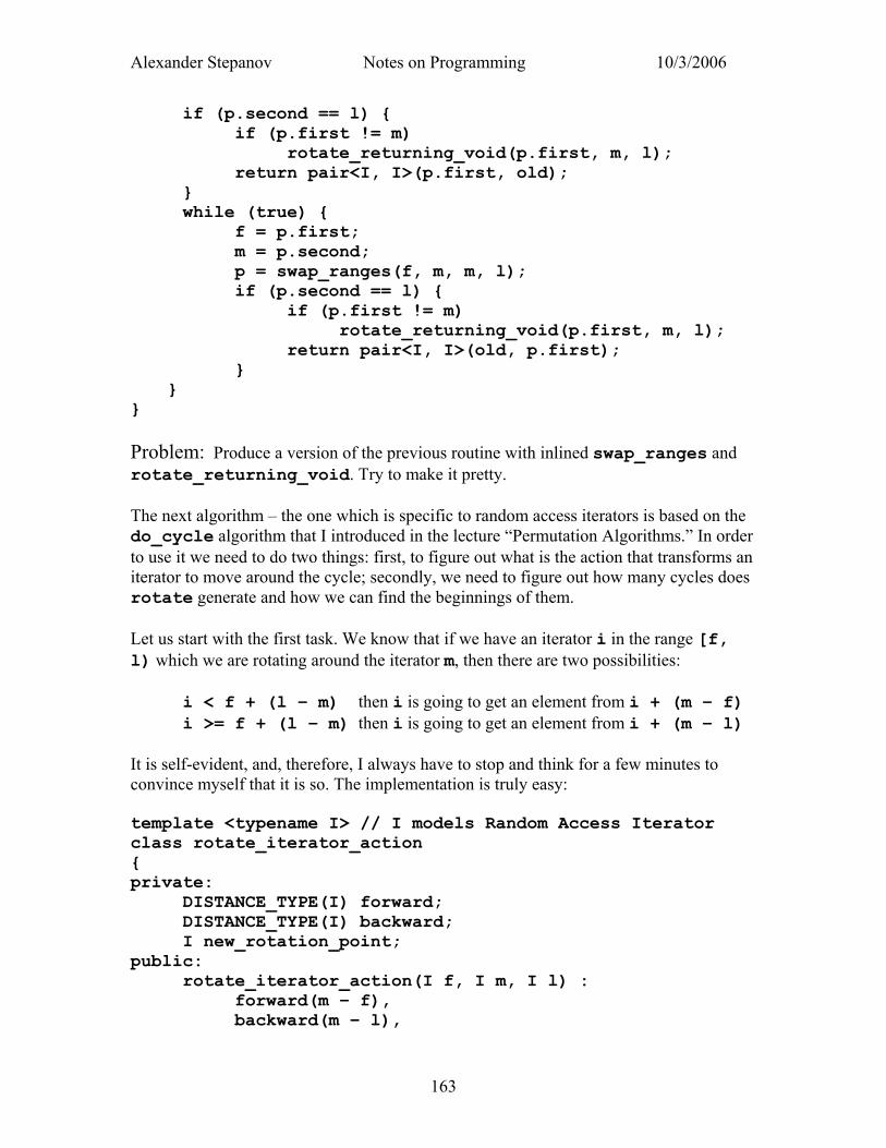
Alexander Stepanov Notes on Programming 10/3/2006
if (p.second == l) { if (p.first != m) rotate_returning_void(p.first, m, l); return pair<I, I>(p.first, old);
} while (true) { f = p.first; m = p.second; p = swap_ranges(f, m, m, l);
if (p.second == l) { if (p.first != m) rotate_returning_void(p.first, m, l); return pair<I, I>(old, p.first); } }
} Problem: Produce a version of the previous routine with inlined swap_ranges and rotate_returning_void. Try to make it pretty. The next algorithm – the one which is specific to random access iterators is based on the do_cycle algorithm that I introduced in the lecture “Permutation Algorithms.” In order to use it we need to do two things: first, to figure out what is the action that transforms an iterator to move around the cycle; secondly, we need to figure out how many cycles does rotate generate and how we can find the beginnings of them. Let us start with the first task. We know that if we have an iterator i in the range [f, l) which we are rotating around the iterator m, then there are two possibilities: i < f + (l – m) then i is going to get an element from i + (m – f) i >= f + (l – m) then i is going to get an element from i + (m – l) It is self-evident, and, therefore, I always have to stop and think for a few minutes to convince myself that it is so. The implementation is truly easy: template <typename I> // I models Random Access Iterator class rotate_iterator_action { private: DISTANCE_TYPE(I) forward; DISTANCE_TYPE(I) backward; I new_rotation_point; public: rotate_iterator_action(I f, I m, I l) : forward(m – f), backward(m – l),
163
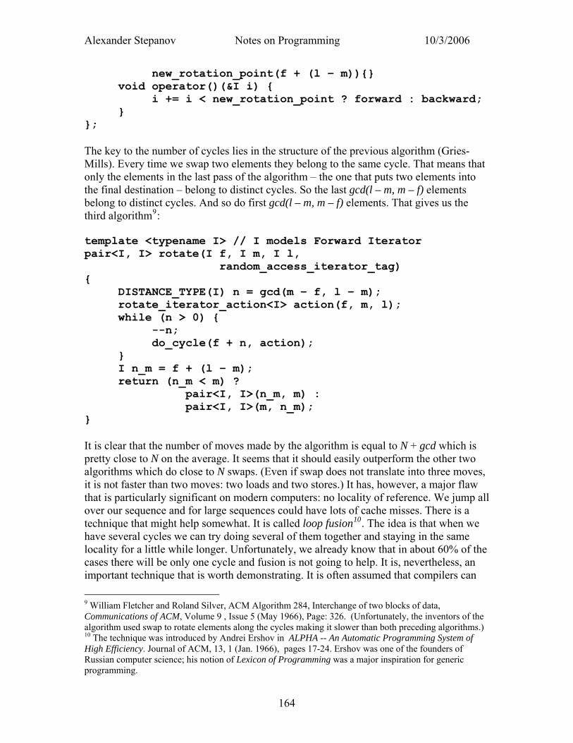
Alexander Stepanov Notes on Programming 10/3/2006
new_rotation_point(f + (l – m)){} void operator()(&I i) { i += i < new_rotation_point ? forward : backward; } }; The key to the number of cycles lies in the structure of the previous algorithm (Gries-Mills). Every time we swap two elements they belong to the same cycle. That means that only the elements in the last pass of the algorithm – the one that puts two elements into the final destination – belong to distinct cycles. So the last gcd(l – m, m – f) elements belong to distinct cycles. And so do first gcd(l – m, m – f) elements. That gives us the third algorithm9: template <typename I> // I models Forward Iterator pair<I, I> rotate(I f, I m, I l, random_access_iterator_tag) { DISTANCE_TYPE(I) n = gcd(m – f, l – m); rotate_iterator_action<I> action(f, m, l); while (n > 0) { --n; do_cycle(f + n, action); } I n_m = f + (l – m); return (n_m < m) ? pair<I, I>(n_m, m) : pair<I, I>(m, n_m); } It is clear that the number of moves made by the algorithm is equal to N + gcd which is pretty close to N on the average. It seems that it should easily outperform the other two algorithms which do close to N swaps. (Even if swap does not translate into three moves, it is not faster than two moves: two loads and two stores.) It has, however, a major flaw that is particularly significant on modern computers: no locality of reference. We jump all over our sequence and for large sequences could have lots of cache misses. There is a technique that might help somewhat. It is called loop fusion10. The idea is that when we have several cycles we can try doing several of them together and staying in the same locality for a little while longer. Unfortunately, we already know that in about 60% of the cases there will be only one cycle and fusion is not going to help. It is, nevertheless, an important technique that is worth demonstrating. It is often assumed that compilers can
9 William Fletcher and Roland Silver, ACM Algorithm 284, Interchange of two blocks of data, Communications of ACM, Volume 9 , Issue 5 (May 1966), Page: 326. (Unfortunately, the inventors of the algorithm used swap to rotate elements along the cycles making it slower than both preceding algorithms.) 10 The technique was introduced by Andrei Ershov in ALPHA -- An Automatic Programming System of High Efficiency. Journal of ACM, 13, 1 (Jan. 1966), pages 17-24. Ershov was one of the founders of Russian computer science; his notion of Lexicon of Programming was a major inspiration for generic programming.
164

Alexander Stepanov Notes on Programming 10/3/2006
do loop fusion for us, but this only happens in relatively simple cases. So let us see how we can do it. template <typename I, // I models Random Access Iterator int size> struct cycle_rotator { private: typedef DISTANCE_TYPE(I) N; N forward; N backward; I n_m; public: cycle_rotator(N fw, N bk, I nm) : forward(fw), backward(bk), n_m(nm) {} I operator()(I i) { UNDERLYING_TYPE(VALUE_TYPE(I)) tmp[size]; raw_move_k<size>()(i, tmp); I hole = i; I next = i + forward; while (true) { raw_move_k<size>()(next, hole); hole = next; if (hole < n_m) next += forward; else { next += backward; if (next == i) break; } } raw_move_k <size>()(tmp, hole); return i + size; } }; Problem: Implement raw_move_k. Problem: Notice that we are testing for the end of the cycle 50% less than when we were using generic do_cycle11. Design a different version of generic do_cycle that will eliminate the redundant test. template <typename I> // I models Random Access Iterator
11 The optimization was suggested by John Wilkinson.
165

Alexander Stepanov Notes on Programming 10/3/2006
inline I rotate_cycle_fused(I i, I nrp, DISTANCE_TYPE(I) fw, DISTANCE_TYPE(I) bk, DISTANCE_TYPE(I) fusion_factor) { switch (fusion_factor) { case 1: return cycle_rotator<I, 1>(fw, bk, nrp)(i); case 2: return cycle_rotator<I, 2>(fw, bk, nrp)(i); case 3: return cycle_rotator<I, 3>(fw, bk, nrp)(i); case 4: return cycle_rotator<I, 4>(fw, bk, nrp)(i); case 5: return cycle_rotator<I, 5>(fw, bk, nrp)(i); case 6: return cycle_rotator<I, 6>(fw, bk, nrp)(i); case 7: return cycle_rotator<I, 7>(fw, bk, nrp)(i); default: return cycle_rotator<I, 8>(fw, bk, nrp)(i); } } template <typename I> // I models Random Access Iterator pair<I, I> rotate_fused(I f, I m, I l) { if (f == m) return l; if (m == l) return f; typedef DISTANCE_TYPE(I) N; N fw = m - f; N bk = m - l; I n_m = l - fw; I end = f + gcd(fw, -bk); while (f < end) f = rotate_cycle_fused(f, n_m, fw, bk, end - f); return (n_m < m) ? pair<I, I>(n_m, m) : pair<I, I>(m, n_m); } Problem: Design a version of rotate that uses a temporary buffer when it is available. It could be useful when rotate is used in the context of memory adaptive algorithms when the buffer is available anyways. Project: Measure the performance of the four rotate algorithms described in this chapter plus the one from the previous problem. Vary the value type from simple built-ins such as
166

Alexander Stepanov Notes on Programming 10/3/2006
char, int and double to structures containing arrays of several of built-in types. Try to see if you can tune the algorithms to improve the results.
Lecture 20. Partition Reverse, rotate and random shuffle are the most important examples of index-based permutations, that is, permutations that rearrange a sequence according to the original position of the elements without any consideration for their values. Now we are going to study a different class of permutation algorithms, predicate-based permutations. The positions into which these algorithms move elements in a sequence depend primarily on whether they satisfy a given condition, not only on their original position. Most of the algorithms in this section are based on the notion of partition: separating elements in a range according to a predicate. I will be able to demonstrate many different techniques looking at this problem. We will find use for many of the functions that we studied before, such as find, reduce and rotate. We will discover many techniques and interfaces that will serve us well. It took me 20 years to come up with the reasonable rule for deciding whether to put elements satisfying the predicate first or last. In 1986 I wrote my first library implementation of partition for a part of Ada Generic Library work12. I had to decide which way the partition is going to place the results: the elements satisfying the predicate before the elements not satisfying it, or the other way around. It appeared to me that it is “self-evident” that the elements satisfying the predicate are “good” and should come first. In any case, I could not see any particular reason for the opposite and both possible solutions seemed to be equivalent. When I was defining partition for STL in 1993, I did not question my prior reasoning and partition, again, moved elements satisfying the predicate in front. It took another 10 years for me to see that I was wrong. When I started considering algorithms for 3-way, 4-way and n-way partitioning, I realized that it is really important that partition assures that the result is sorted according to partition key – the result of the key function. And all of the STL sorting algorithms assumed ascending order. Moreover, it would have allowed the following nice property to hold: partition_3way would have worked just like regular partition if given a two-valued key function returning {0, 1}. Moreover, sort with a comparison based on key-compare would have done partitioning – which is not true now for regular 2-way partition. The problem will become even more visible when we define partition_n_way. I knew about the connection between sorting and partitioning but was not able to assure that the interfaces are consistent. I will now do it the right way – putting elements that do not satisfy the predicate first – but you need to remember that the standard std::partition is doing it in the opposite order. It is very instructive to see how
12 The code for partition appears in David R. Musser and Alexander A. Stepanov, Generic Programming, ISSAC 1988, pages 13-25. It is available at: http://www.stepanovpapers.com/genprog.pdf It could not be a part of the library since no compiler was able to handle deeply nested generics.
167
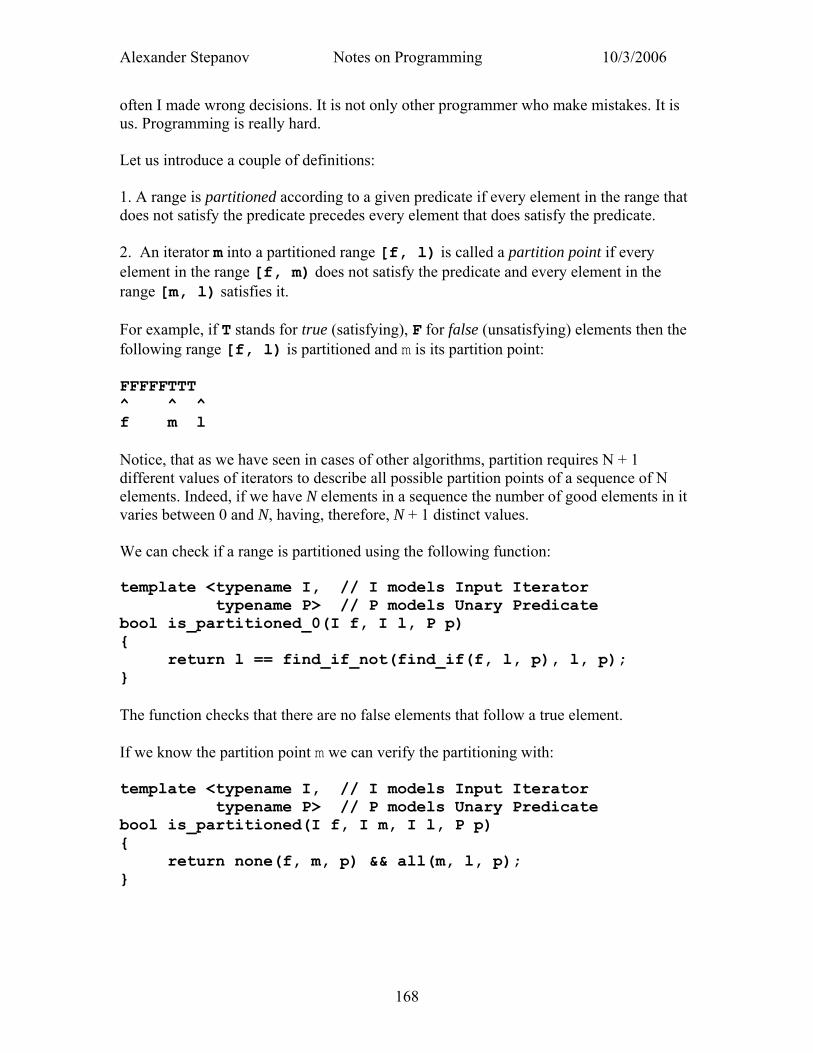
Alexander Stepanov Notes on Programming 10/3/2006
often I made wrong decisions. It is not only other programmer who make mistakes. It is us. Programming is really hard. Let us introduce a couple of definitions: 1. A range is partitioned according to a given predicate if every element in the range that does not satisfy the predicate precedes every element that does satisfy the predicate. 2. An iterator m into a partitioned range [f, l) is called a partition point if every element in the range [f, m) does not satisfy the predicate and every element in the range [m, l) satisfies it. For example, if T stands for true (satisfying), F for false (unsatisfying) elements then the following range [f, l) is partitioned and m is its partition point: FFFFFTTT ^ ^ ^ f m l Notice, that as we have seen in cases of other algorithms, partition requires N + 1 different values of iterators to describe all possible partition points of a sequence of N elements. Indeed, if we have N elements in a sequence the number of good elements in it varies between 0 and N, having, therefore, N + 1 distinct values. We can check if a range is partitioned using the following function: template <typename I, // I models Input Iterator typename P> // P models Unary Predicate bool is_partitioned_0(I f, I l, P p) { return l == find_if_not(find_if(f, l, p), l, p); } The function checks that there are no false elements that follow a true element. If we know the partition point m we can verify the partitioning with: template <typename I, // I models Input Iterator typename P> // P models Unary Predicate bool is_partitioned(I f, I m, I l, P p) { return none(f, m, p) && all(m, l, p); }
168
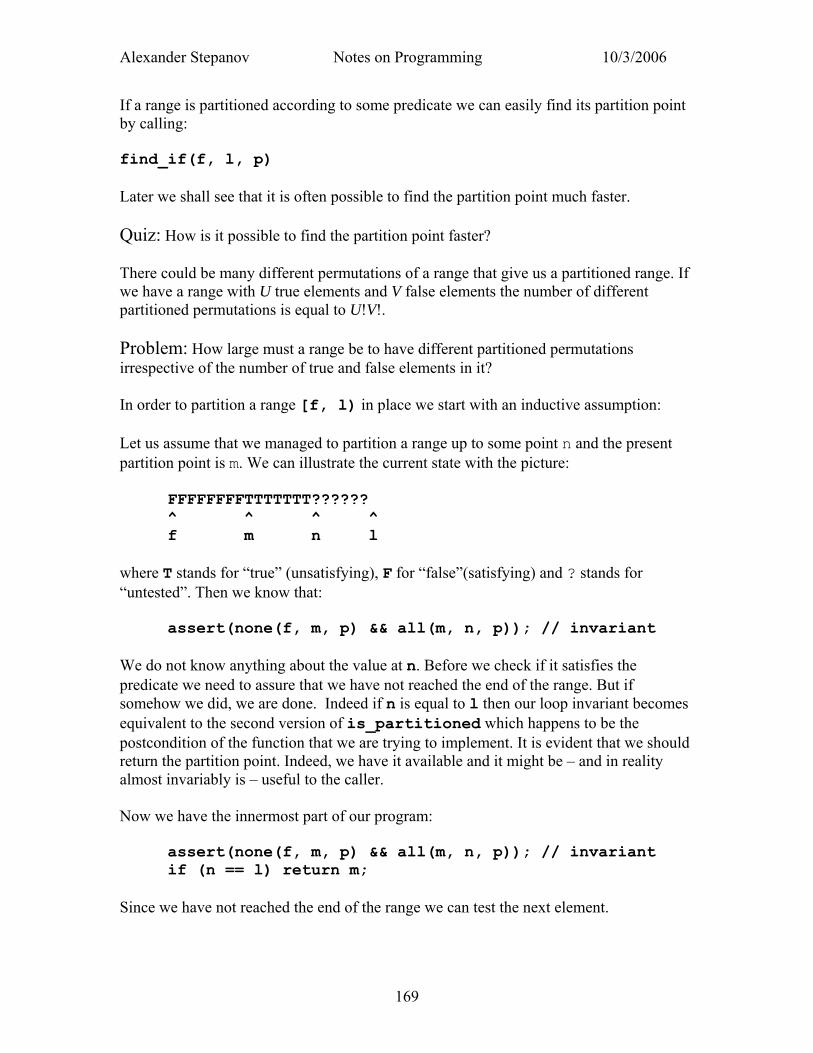
Alexander Stepanov Notes on Programming 10/3/2006
If a range is partitioned according to some predicate we can easily find its partition point by calling: find_if(f, l, p) Later we shall see that it is often possible to find the partition point much faster. Quiz: How is it possible to find the partition point faster? There could be many different permutations of a range that give us a partitioned range. If we have a range with U true elements and V false elements the number of different partitioned permutations is equal to U!V!. Problem: How large must a range be to have different partitioned permutations irrespective of the number of true and false elements in it? In order to partition a range [f, l) in place we start with an inductive assumption: Let us assume that we managed to partition a range up to some point n and the present partition point is m. We can illustrate the current state with the picture: FFFFFFFFTTTTTTT?????? ^ ^ ^ ^ f m n l where T stands for “true” (unsatisfying), F for “false”(satisfying) and ? stands for “untested”. Then we know that: assert(none(f, m, p) && all(m, n, p)); // invariant We do not know anything about the value at n. Before we check if it satisfies the predicate we need to assure that we have not reached the end of the range. But if somehow we did, we are done. Indeed if n is equal to l then our loop invariant becomes equivalent to the second version of is_partitioned which happens to be the postcondition of the function that we are trying to implement. It is evident that we should return the partition point. Indeed, we have it available and it might be – and in reality almost invariably is – useful to the caller. Now we have the innermost part of our program: assert(none(f, m, p) && all(m, n, p)); // invariant if (n == l) return m; Since we have not reached the end of the range we can test the next element.
169
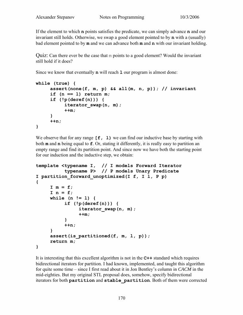
Alexander Stepanov Notes on Programming 10/3/2006
If the element to which n points satisfies the predicate, we can simply advance n and our invariant still holds. Otherwise, we swap a good element pointed to by n with a (usually) bad element pointed to by m and we can advance both m and n with our invariant holding. Quiz: Can there ever be the case that m points to a good element? Would the invariant still hold if it does? Since we know that eventually n will reach l our program is almost done: while (true) { assert(none(f, m, p) && all(m, n, p)); // invariant if (n == l) return m; if (!p(deref(n))) {
iterator_swap(n, m); ++m;
} ++n; } We observe that for any range [f, l) we can find our inductive base by starting with both m and n being equal to f. Or, stating it differently, it is really easy to partition an empty range and find its partition point. And since now we have both the starting point for our induction and the inductive step, we obtain: template <typename I, // I models Forward Iterator typename P> // P models Unary Predicate I partition_forward_unoptimized(I f, I l, P p) { I m = f; I n = f; while (n != l) { if (!p(deref(n))) {
iterator_swap(n, m); ++m;
} ++n; } assert(is_partitioned(f, m, l, p)); return m; } It is interesting that this excellent algorithm is not in the C++ standard which requires bidirectional iterators for partition. I had known, implemented, and taught this algorithm for quite some time – since I first read about it in Jon Bentley’s column in CACM in the mid-eighties. But my original STL proposal does, somehow, specify bidirectional iterators for both partition and stable_partition. Both of them were corrected
170
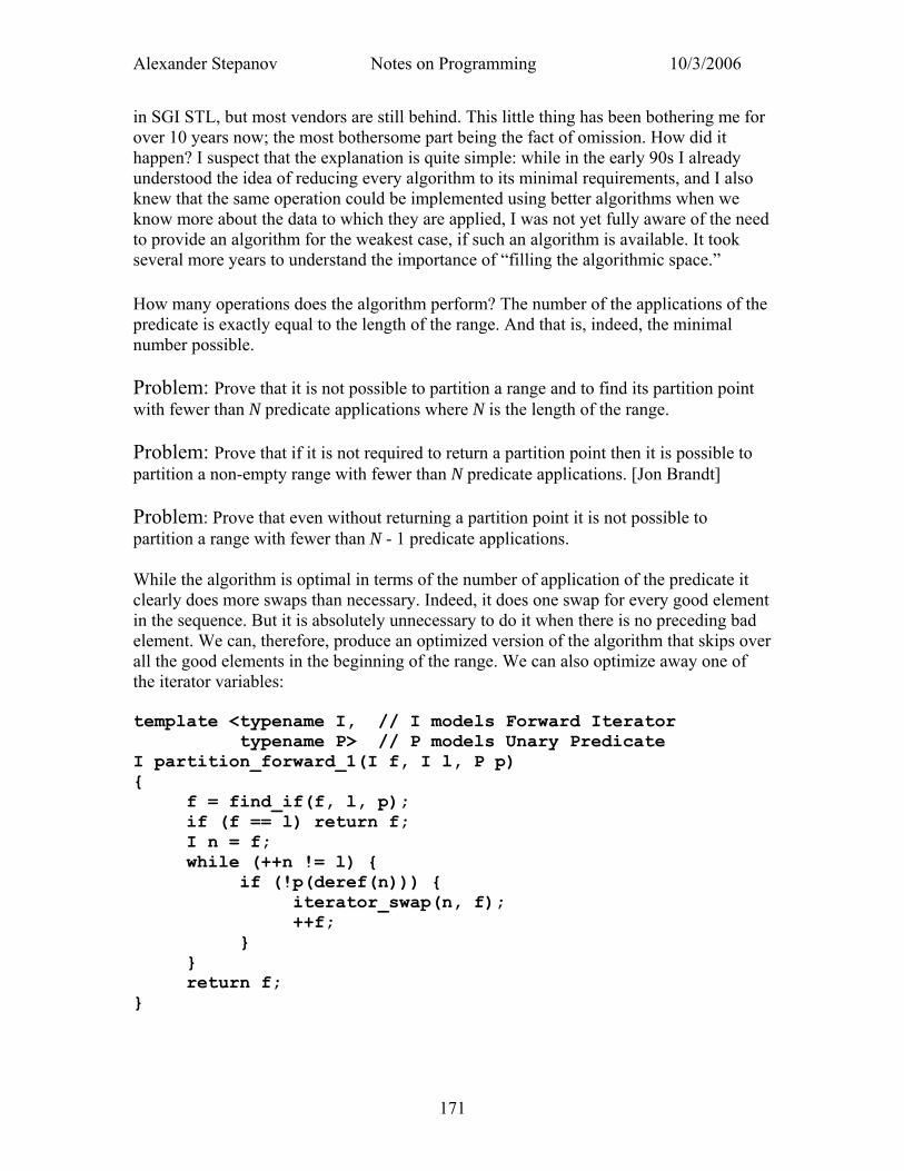
Alexander Stepanov Notes on Programming 10/3/2006
in SGI STL, but most vendors are still behind. This little thing has been bothering me for over 10 years now; the most bothersome part being the fact of omission. How did it happen? I suspect that the explanation is quite simple: while in the early 90s I already understood the idea of reducing every algorithm to its minimal requirements, and I also knew that the same operation could be implemented using better algorithms when we know more about the data to which they are applied, I was not yet fully aware of the need to provide an algorithm for the weakest case, if such an algorithm is available. It took several more years to understand the importance of “filling the algorithmic space.” How many operations does the algorithm perform? The number of the applications of the predicate is exactly equal to the length of the range. And that is, indeed, the minimal number possible. Problem: Prove that it is not possible to partition a range and to find its partition point with fewer than N predicate applications where N is the length of the range. Problem: Prove that if it is not required to return a partition point then it is possible to partition a non-empty range with fewer than N predicate applications. [Jon Brandt] Problem: Prove that even without returning a partition point it is not possible to partition a range with fewer than N - 1 predicate applications. While the algorithm is optimal in terms of the number of application of the predicate it clearly does more swaps than necessary. Indeed, it does one swap for every good element in the sequence. But it is absolutely unnecessary to do it when there is no preceding bad element. We can, therefore, produce an optimized version of the algorithm that skips over all the good elements in the beginning of the range. We can also optimize away one of the iterator variables: template <typename I, // I models Forward Iterator typename P> // P models Unary Predicate I partition_forward_1(I f, I l, P p) { f = find_if(f, l, p); if (f == l) return f; I n = f; while (++n != l) { if (!p(deref(n))) {
iterator_swap(n, f); ++f;
} } return f; }
171
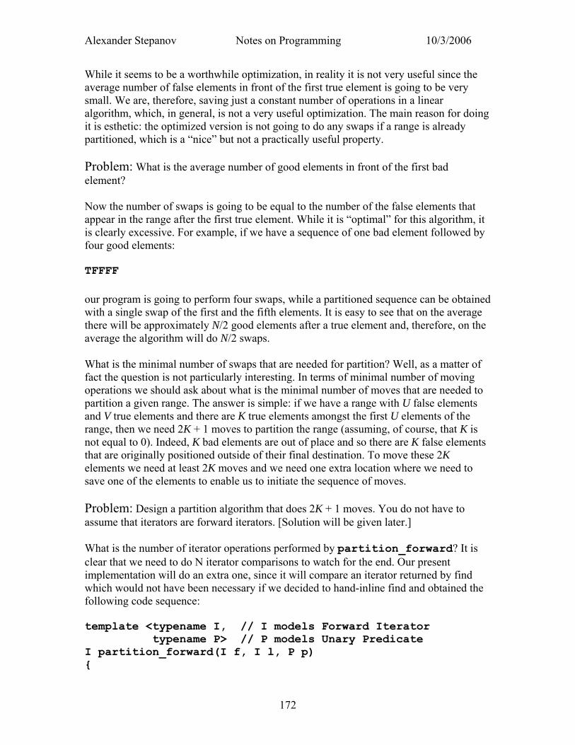
Alexander Stepanov Notes on Programming 10/3/2006
While it seems to be a worthwhile optimization, in reality it is not very useful since the average number of false elements in front of the first true element is going to be very small. We are, therefore, saving just a constant number of operations in a linear algorithm, which, in general, is not a very useful optimization. The main reason for doing it is esthetic: the optimized version is not going to do any swaps if a range is already partitioned, which is a “nice” but not a practically useful property. Problem: What is the average number of good elements in front of the first bad element? Now the number of swaps is going to be equal to the number of the false elements that appear in the range after the first true element. While it is “optimal” for this algorithm, it is clearly excessive. For example, if we have a sequence of one bad element followed by four good elements: TFFFF our program is going to perform four swaps, while a partitioned sequence can be obtained with a single swap of the first and the fifth elements. It is easy to see that on the average there will be approximately N/2 good elements after a true element and, therefore, on the average the algorithm will do N/2 swaps. What is the minimal number of swaps that are needed for partition? Well, as a matter of fact the question is not particularly interesting. In terms of minimal number of moving operations we should ask about what is the minimal number of moves that are needed to partition a given range. The answer is simple: if we have a range with U false elements and V true elements and there are K true elements amongst the first U elements of the range, then we need 2K + 1 moves to partition the range (assuming, of course, that K is not equal to 0). Indeed, K bad elements are out of place and so there are K false elements that are originally positioned outside of their final destination. To move these 2K elements we need at least 2K moves and we need one extra location where we need to save one of the elements to enable us to initiate the sequence of moves. Problem: Design a partition algorithm that does 2K + 1 moves. You do not have to assume that iterators are forward iterators. [Solution will be given later.] What is the number of iterator operations performed by partition_forward? It is clear that we need to do N iterator comparisons to watch for the end. Our present implementation will do an extra one, since it will compare an iterator returned by find which would not have been necessary if we decided to hand-inline find and obtained the following code sequence: template <typename I, // I models Forward Iterator typename P> // P models Unary Predicate I partition_forward(I f, I l, P p) {
172

Alexander Stepanov Notes on Programming 10/3/2006
while (true) { if (f == l) return f;
if (p(deref(f))) break; ++f; } I n = f; ++f; // I changed f and n to make the more symmetric code while (true) {
if (f == l) return f; if (!p(deref(f))) {
iterator_swap(n, f); ++n;
} ++f; } } In this context the optimization is not particularly useful since a single extra comparison does not really affect the performance (a small constant added to a linear function), but we encounter the same transformation in the next algorithm where the extra comparison appears in the inner loop. The transformation starts with the loop of find_if: while (f != l && !p(deref(f))) ++f; and provides two different exits depending on which part of the conjunction holds. The total number of iterator increments is equal to N + W where W is the number of false elements that follow the first true element. As we remarked before, on the average it is going to be approximately N + U – 2 where U is the number of false elements in the range. The forward partition algorithm is due to Nico Lomuto who was looking for a simpler way to implement the quicksort inner loop13. Its main advantages are, firstly, that it works for forward iterators and, secondly, that it preserves the relative ordering of the elements that satisfy the predicate (see the discussion of stable partition). Its disadvantages are that it does more swaps on the average than the next algorithm but especially that it cannot be modified to split the range containing equal elements into two equal parts, which makes it utterly unsuitable for being used in quicksort – for which purpose it is, nevertheless, frequently recommended by supposedly reputable textbooks. As is the case with many algorithms, it has its place but not where its inventor thought it was. 13 Jon Bentley, Programming Pearls. Communications of the ACM, Vol 27, No 4. April 1984. pp. 287-29
173

Alexander Stepanov Notes on Programming 10/3/2006
I do not know a partition algorithm that is more effective for forward iterators than the one we just described. I believe that in some fundamental sense it is optimal, but I do not even know how to state the problem in a rigorous way. We typically analyze the algorithmic performance by counting one kind of operation. In reality we are dealing with several different operations. For partition we need predicate application and move (both of which depend on the type of elements) and iterator increment and equality (both of which depend on the iterator type). I have a general feeling – (Feeling Oriented Programming?) – that element operations (predicate) are potentially costlier than iterator operations (++, ==, deref), since elements could be large while iterators are small. Such vague considerations usually allow us to produce algorithms that are satisfactory in practice, but there is something profoundly unsatisfying about it. It is possible that one can come up with axioms on the complexity measures of different operations that will allow us to prove optimality of certain algorithms. So far, I have not been able either to design such axioms or to interest others in designing them. All the code in the rest of this and the next lectures is based on the remarkable paper by C.A.R. Hoare14. He introduces the algorithm for partition with the minimal number of moves and partition with sentinels which we will study in the next lecture. This paper, in my opinion, is a serious contender for the title of the best ever paper in Computer Science. I wish that every textbook writer before they attempt to implement quicksort would spend some time studying the original paper and not the (usually) inferior secondary sources. It is, unfortunately not easily available and mostly overshadowed by his brief note in the Communications of ACM. While, as we shall see later, it is possible to implement a partition algorithm with a minimal number of moves, in practice it is usually sufficient to replace 2K + 1 moves with K swaps, namely, discover all the K misplaced bad elements and swap them with K misplaced good elements. Our goal is to assure that every swap puts both the false element and the true element in their final destination. If we take the rightmost true element and the leftmost false element we can be sure that if they are out of place we can put both in acceptable positions by swapping them. Indeed, we know that all the elements to the left of the leftmost true element have to be false and are in their final destination; and similarly for the rightmost false element. So if they are out of place – the leftmost true element is before the rightmost false element, then swapping them is putting both into acceptable locations. Finding the rightmost false element efficiently requires that we move from the right and that requires bidirectional iterators. The idea of the algorithm can be illustrated by the following picture: GGGGGGGGT??????FTTTTT ^ ^ ^ ^ f0 f l l0
14 C.A.R. Hoare, Quicksort, The Computer Journal 1962, 5(1), pp.10-16
174

Alexander Stepanov Notes on Programming 10/3/2006
Interchanging the elements pointed to by f and l will put them in the correct subranges: the true element to the right of the partition point and the false element to the left of it. It is worthwhile to observe that the partition point is located somewhere in the range [f, l). We can start our implementation by first finding the new f, then finding the new l and then swapping them or returning whichever one is appropriate: // use find_if to find the first true element // use find_backward_if_not to find the last false element // check if the iterators crossed and return // swap the true and false elements which were just found Before we try to figure out how it works let us have a detour and learn about find_backward. I did not discuss finding backward in the chapter on find. The main reason was that our design for its interface might be better understood next to the first example of its use. But we might eventually decide to move it there. It is often important to find elements in a range while traversing it backwards. It seems to be an easy task; just take find and replace ++ with --: template <typename I, // I models Bidirectional Iterator typename P> // P models Unary Predicate I buggy_find_backward_if_not_1(I f, I l, P p) { while (f != l && !p(deref(l))) -–l; return l; } This, of course, will not work since the first time around we will be dereferencing a past-the-end iterator. We should remember that our ranges are semi-open intervals and the end iterator is not symmetrical with the begin iterator. It seems that we can compensate for it by writing: template <typename I, // I models Bidirectional Iterator typename P> // P models Unary Predicate I buggy_find_backward_if_not_2(I f, I l, P p) { while (true) { if (f == l) return l; --l; if (p(deref(l))) return l; }
175

Alexander Stepanov Notes on Programming 10/3/2006
} The problem now is that we cannot distinguish between finding a false element in the very beginning of the range – but at the end of our search – and not finding a false element at all. We can, of course find out which one is the case by re-testing the first element, but it would require an extra test and would not be symmetric with the ordinary find_if. It would be terribly nice if we could transform a semi-open range [f, l) into a semi-open range [l, f). And we can do it if we just slightly modify our code by incrementing l before returning it when we find a false element: template <typename I, // I models Bidirectional Iterator typename P> // P models Unary Predicate I find_backward_if_not(I f, I l, P p) { do { if (f == l) return l; --l; } while (p(deref(l))); return successor(l); } We return f if we do not find a false element; otherwise, we return the successor to the iterator pointing to the first false element from the right. (We assume that ranges grow from left to right.) Now it is easy to see our program: template <typename I, // I models Bidirectional Iterator typename P> // P models Unary Predicate I partition_bidirectional_1(I f, I l, P p) { while (true) { f = find_if(f, l, p); l = find_backward_if_not(f, l, p); if (f == l) return f; --l; iterator_swap(f, l); ++f; } } The above code looks so elegant, so perfect that it makes me sad that we have to muck it up. But muck it we shall. The present code does several extra operations. As far as the
176
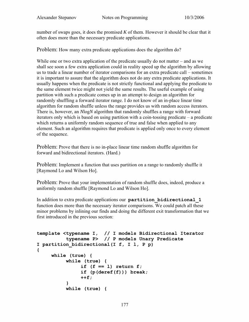
Alexander Stepanov Notes on Programming 10/3/2006
number of swaps goes, it does the promised K of them. However it should be clear that it often does more than the necessary predicate applications. Problem: How many extra predicate applications does the algorithm do? While one or two extra application of the predicate usually do not matter – and as we shall see soon a few extra application could in reality speed up the algorithm by allowing us to trade a linear number of iterator comparisons for an extra predicate call – sometimes it is important to assure that the algorithm does not do any extra predicate applications. It usually happens when the predicate is not strictly functional and applying the predicate to the same element twice might not yield the same results. The useful example of using partition with such a predicate comes up in an attempt to design an algorithm for randomly shuffling a forward iterator range. I do not know of an in-place linear time algorithm for random shuffle unless the range provides us with random access iterators. There is, however, an NlogN algorithm that randomly shuffles a range with forward iterators only which is based on using partition with a coin-tossing predicate – a predicate which returns a uniformly random sequence of true and false when applied to any element. Such an algorithm requires that predicate is applied only once to every element of the sequence. Problem: Prove that there is no in-place linear time random shuffle algorithm for forward and bidirectional iterators. (Hard.) Problem: Implement a function that uses partition on a range to randomly shuffle it [Raymond Lo and Wilson Ho]. Problem: Prove that your implementation of random shuffle does, indeed, produce a uniformly random shuffle [Raymond Lo and Wilson Ho]. In addition to extra predicate applications our partition_bidirectional_1 function does more than the necessary iterator comparisons. We could patch all these minor problems by inlining our finds and doing the different exit transformation that we first introduced in the previous section: template <typename I, // I models Bidirectional Iterator typename P> // P models Unary Predicate I partition_bidirectional(I f, I l, P p) { while (true) { while (true) { if (f == l) return f;
if (p(deref(f))) break; ++f;
} while (true) {
177

Alexander Stepanov Notes on Programming 10/3/2006
--l; if (f == l) return f; if (!p(deref(f))) break; } iterator_swap(f, l); ++f; } } Problem: Prove the program correct by carefully writing asserts. As a matter of fact, we did not muck it up too badly. It still looks very symmetric, very elegant, but as we shall see soon the mucking is not over. As far as the number of operations goes, the present code does N predicate applications (prove it!) and N + 1 iterator comparisons and N + 1 iterator increments and decrements. It also – as promised – does K swaps.
Lecture 21. Optimizing partition
Sometimes we need to study an optimization technique even if at the end we find out that it has few benefits for the algorithm which we used to illustrate the technique. Implementing partition with the minimal number of moves is one such subject. As we have seen earlier in the section, the minimal number of moves necessary for partitioning a range is equal to 2K + 1 where K is the number of true elements that precede the (eventual) partition point. While we have an algorithm that does K swaps, it does not appear to be optimal since we usually consider a swap to be equivalent to 3 moves and 3K is greater than 2K + 1 for most positive integers. (It is optimal, indeed, when K is 1 and we are going to do a single swap.)
Now let us see how we can produce a version with the minimal number of moves. The idea is quite simple we save the first misplaced element and then move other misplaced elements into the holes formed by the first save and the subsequent moves. When we reach the end, we move the saved element into the last hole. In other words, we re-organize our partition permutation from one with K cycles to one with one cycle. Note that implementing this algorithm we demonstrate an interesting property: any sequence can be partitioned with a single cycle.
It should be noted that the result of the algorithm is going to be different from the result of our partition_bidirectional which generates a somewhat different permutation. Now it is fairly straightforward to obtain its implementation: template <typename I, // I models Bidirectional Iterator
178

Alexander Stepanov Notes on Programming 10/3/2006
typename P> // P models Unary Predicate I partition_bidirectional_minimal_moves (I f, I l, P p) {
while (true) { if (f == l) return f; if (p (deref(f))) break; ++f; } // f points to true do { --l; if (f == l) return f; } while (p(deref(l))); // l points to false
UNDERLYING_TYPE(VALUE_TYPE(I)) tmp;
move_raw(*f, tmp); while (true) { // hole at f needs false move_raw(deref(l), deref(f));
// fill the hole at f with false at l // the hole is at l and needs true
do { ++f; if (f == l) goto exit; } while (!p(deref(f))); // f points to true
move_raw(deref(f), deref(l)); // fill the hole at l with true at f // the hole is at f and needs false do { --l;
if (f == l) goto exit; } while (p(deref(l))); // l points to false
} exit: // both f and l are equal and point to a hole
move_raw(tmp, deref(f)); return f; } This piece of code is “optimal” in terms of many operations: it does the minimal number of comparisons, the (almost) minimal number of moves, the minimal number of iterator increments and iterator comparisons. Problem: Find a case when the “optimal” algorithm would do one extra move [Joseph Tighe].
179

Alexander Stepanov Notes on Programming 10/3/2006
Problem: Find a way of avoiding an extra move [keep explicit track of the hole]. Problem: Use the same techniques to reduce the number of moves in partition_forward. It should be noted, however, that in practice – or at least in practice as it is in 2006 – optimizing the number of moves does not significantly speed up the code for most types of elements. While we consider swap to be equivalent to three moves, for most modern computers it appears to be more accurate to consider swap to be equivalent to two loads followed by two stores, while move to be equivalent to one load and one store. If we switch to this system of accounting, we observe that partition_bidirectional does (almost) the same number of memory operations as partition_bidirectional_minimal_moves. It is a worthwhile thing to learn many of the optimization techniques, because of the twofold reason:
- optimization techniques are based on fundamental properties of algorithms that we study and allow us to understand the algorithms better; - optimizations that are not applicable now in some domain will often become applicable again in a different domain.
If we look at the code of the partition_bidirectional_2 we observe that we do one iterator comparison for every predicate application – or almost one since the last iterator comparison during the running of the algorithm is not followed by a predicate application. If we know that our range contains both true and false elements we can implement a function that will be trading an extra predicate call for a linear number of extra comparisons. If there is a true element in the range we can always look for the first true element from the left by writing: while (!p(deref(f))) ++f; and be certain that after we stop none of the elements in the range [f0, f) are going to satisfy the predicate and f will point to a true element. We can now look for the false element from the right: do --l; while (p(deref(l))); and be equally certain that we will stop at a good element. It is very easy to see that the only way they can cross is by one position only. That is, if they crossed then f is going to be the successor of l. (That, of course, presupposes that the predicate is truly functional and returns the same value when applied to the same element twice.) That allows us to eliminate an iterator comparison from the inner loops: template <typename I, // I models Bidirectional Iterator typename P> // P models Unary Predicate I partition_bidirectional_unguarded(I f, I l, P p)
180
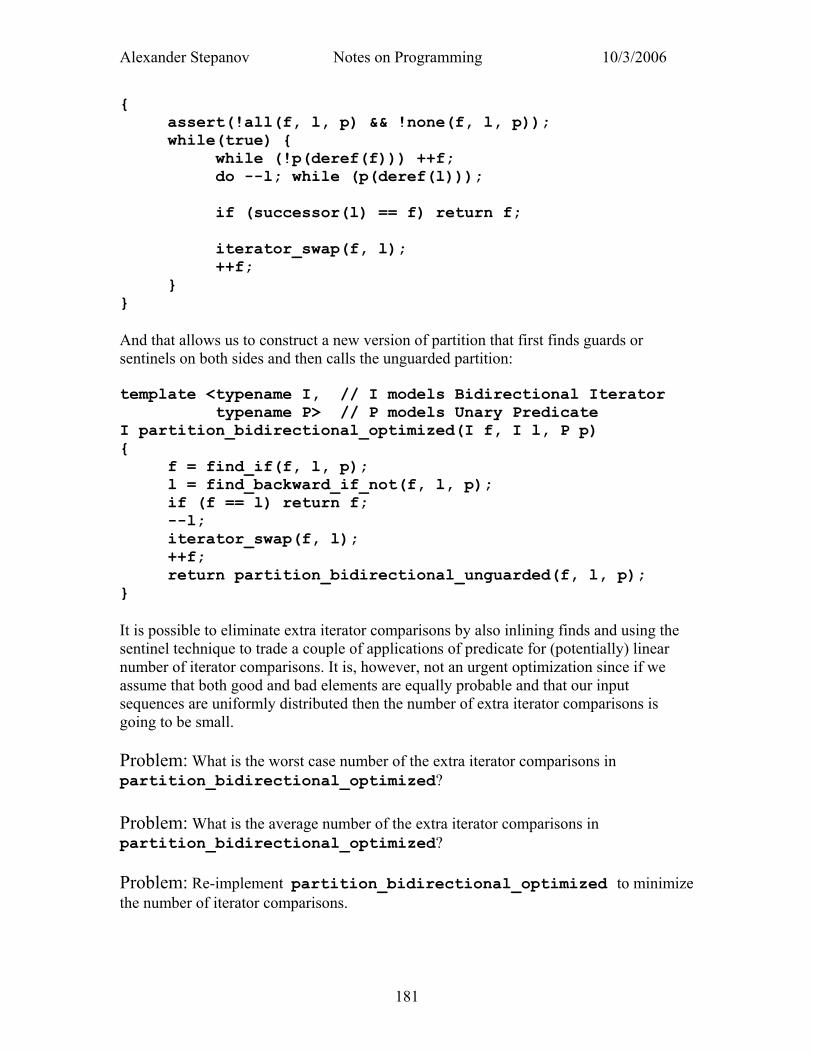
Alexander Stepanov Notes on Programming 10/3/2006
{ assert(!all(f, l, p) && !none(f, l, p));
while(true) { while (!p(deref(f))) ++f;
do --l; while (p(deref(l))); if (successor(l) == f) return f; iterator_swap(f, l); ++f; }
} And that allows us to construct a new version of partition that first finds guards or sentinels on both sides and then calls the unguarded partition: template <typename I, // I models Bidirectional Iterator typename P> // P models Unary Predicate I partition_bidirectional_optimized(I f, I l, P p) {
f = find_if(f, l, p); l = find_backward_if_not(f, l, p); if (f == l) return f; --l; iterator_swap(f, l); ++f; return partition_bidirectional_unguarded(f, l, p);
} It is possible to eliminate extra iterator comparisons by also inlining finds and using the sentinel technique to trade a couple of applications of predicate for (potentially) linear number of iterator comparisons. It is, however, not an urgent optimization since if we assume that both good and bad elements are equally probable and that our input sequences are uniformly distributed then the number of extra iterator comparisons is going to be small. Problem: What is the worst case number of the extra iterator comparisons in partition_bidirectional_optimized? Problem: What is the average number of the extra iterator comparisons in partition_bidirectional_optimized? Problem: Re-implement partition_bidirectional_optimized to minimize the number of iterator comparisons.
181

Alexander Stepanov Notes on Programming 10/3/2006
Problem: Combine the sentinel technique and the minimal moves optimization in a single algorithm. Project: Measure the performance of all the partition algorithms that we have studied so far. Vary the element sizes from 32 bit integers and doubles all the way to structures with 64 byte size. Also use two different predicates: one which is inlined and very simple and the other one which is passed as a pointer to function. Come up with a recommendation on which of the algorithms are worth keeping in a library. Project: Write a simple guide that will tell a user how to select a correct partition algorithm for the job.
Project: Write a library function that will correctly choose which of the partition algorithms to use depending on iterator requirements and, potentially, element size and properties of the predicate.
While it is often important to be able to partition a range in place, it is sometimes equally important to partition elements while copying them into a new place. It is, of course, often possible to accomplish it by first doing copy and then partition. There are two problems with this approach: the performance and the generality.
As far as the performance goes, we will need more than N moves. It would be terribly nice if we can accomplish our task with N moves only. The second problem is that in order to do copy first and partition afterwards we need to be able to traverse the resulting range again. And that means that we cannot use output iterators as a requirement for the destination. As a matter of fact the algorithm that is both minimal in terms of number of operations and absolutely minimal in terms of the requirements on the iterators for the result is so simple that it does not need any explanations. Go through the input range element by element sending good elements to one destination stream and the bad ones to a different one.
It is obvious how to start writing the algorithm: if (p(*f)) { deref(r_b) = deref(f); // bad result ++r_b; } else { deref(r_g) = deref(f); // good result ++r_g; } ++f; The only remaining problem is to figure out what to return. And since the destinations of good and bad elements are different we have to return the final state of both: template <typename I, // I models Input Iterator typename O1, // O1 models Output Iterator typename O2, // O2 models Output Iterator
182

Alexander Stepanov Notes on Programming 10/3/2006
typename P> // P models Unary Predicate pair<O1, O2> partition_copy(I f, I l, O1 r_g, O2 r_b, P p) { while (f != l) { if (p(*f)) { deref(r_b) = deref(f); ++r_b; } else { deref(r_g) = deref(f); ++r_g; } ++f; } return pair<O1, O2>(r_g, r_b); }15
When we treat the stable partition algorithm we will rely on the fact that partition_copy is stable, that is, the relative order of among good elements is preserve and so is the relative order among the bad elements.
Lecture 22. Algorithms on Linked Iterators Up till now we assumed that every iterator has the same successor for at least as long as we use the algorithm. (The assumption, of course, does not hold for input iterators since they do not allow us to advance through the same iterator twice. But even for them we assumed that for as long as advance is possible, we will advance to the same place every time we advance form a given iterator.) There was no way to change the successor of an iterator. But while this is a good assumption to have since we want to develop as many algorithms as possible working with as few assumptions as possible, we should always remember that every theory is limited and be ready to extend it to account for reality. And in reality there are data structures that allow us to change the relationships between their locations. They are known as linked data structures. Singly-linked lists and doubly-linked lists are the most common examples of such structures. It is quite clear how to reverse a linked list: reverse all the links. One way of doing it is by requiring the iterators to the linked structures to provide a set_successor function that guarantees that for any dereferenceable iterator i and any iterator j the following holds: set_successor(i, j); assert(successor(i) == j);
15 It is worth noting that the self-evident interface to a copying version of partition escaped me till 1996 when it was suggested to me by T.K. Lakshman. This is the reason the algorithm is not in the standard.
183
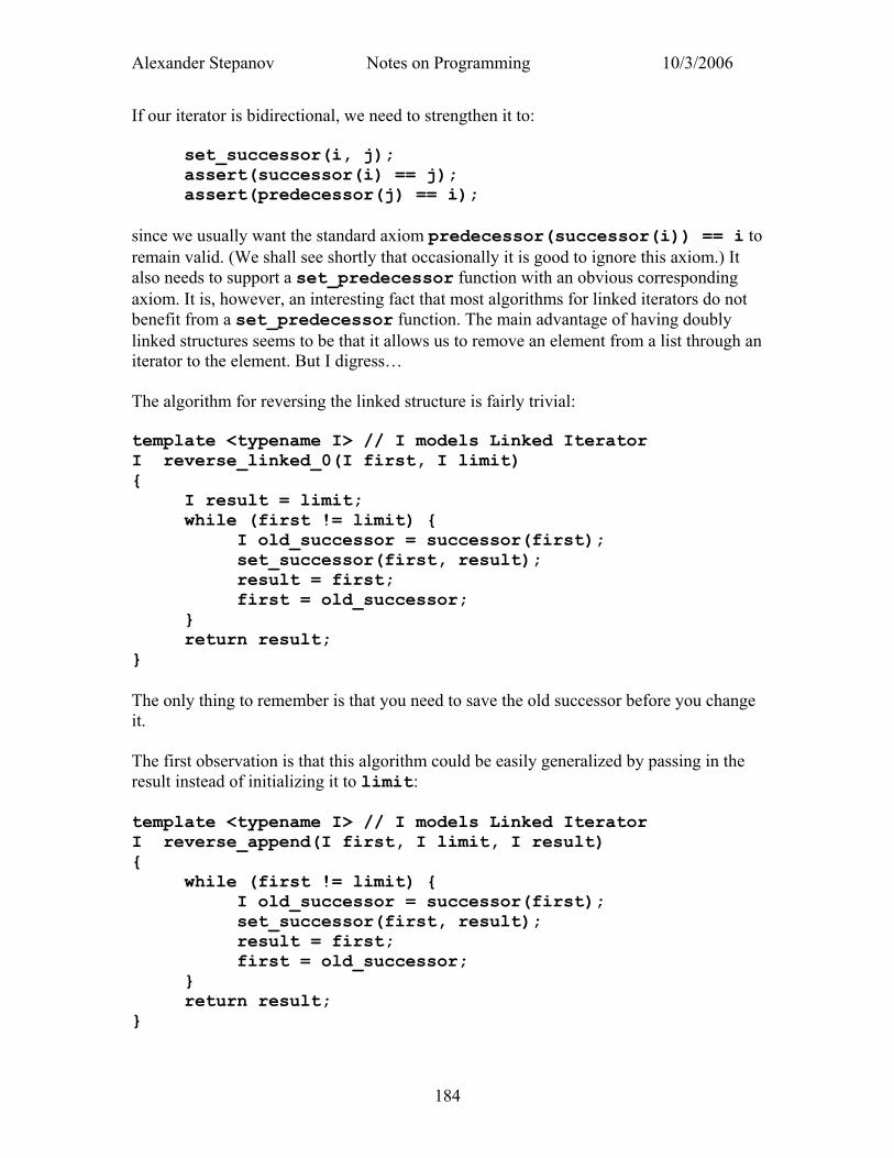
Alexander Stepanov Notes on Programming 10/3/2006
If our iterator is bidirectional, we need to strengthen it to: set_successor(i, j); assert(successor(i) == j); assert(predecessor(j) == i); since we usually want the standard axiom predecessor(successor(i)) == i to remain valid. (We shall see shortly that occasionally it is good to ignore this axiom.) It also needs to support a set_predecessor function with an obvious corresponding axiom. It is, however, an interesting fact that most algorithms for linked iterators do not benefit from a set_predecessor function. The main advantage of having doubly linked structures seems to be that it allows us to remove an element from a list through an iterator to the element. But I digress… The algorithm for reversing the linked structure is fairly trivial: template <typename I> // I models Linked Iterator I reverse_linked_0(I first, I limit) { I result = limit; while (first != limit) { I old_successor = successor(first); set_successor(first, result); result = first; first = old_successor; } return result; } The only thing to remember is that you need to save the old successor before you change it. The first observation is that this algorithm could be easily generalized by passing in the result instead of initializing it to limit: template <typename I> // I models Linked Iterator I reverse_append(I first, I limit, I result) { while (first != limit) { I old_successor = successor(first); set_successor(first, result); result = first; first = old_successor; } return result; }
184

Alexander Stepanov Notes on Programming 10/3/2006
(As a general rule, it is often possible to obtain a more general and quite useful function by replacing a local variable that initializes some computation with an extra parameter.) It is now trivial to obtain reverse_linked as: template <typename I> // I models Linked Iterator inline I reverse_linked(I first, I limit) { return reverse_append(first, limit, limit); } It seems that we are done. We extended the iterator interface to account for the ability to re-link, and we wrote a nice and practically useful algorithm. We can declare victory. The problem is that it is premature to declare victory till we have seen all the consequences of our design. In other words, it is hard to find a right abstraction till we really look deep into the field. As we progress through the course we will discover more and more linked iterator versions of STL algorithms: partition, merge, set_union, set_intersection, etc. The abstraction that we just created is going to hold up quite well. As a matter of fact, it is going to hold up quite well for any one-pass algorithm. It is only when we start doing set_successor many times over for the same iterator that we will notice a problem. Indeed, when we implement sort_linked we will notice that for doubly-linked lists it will start doing a lot of unnecessary work. It is going to call merge_linked and that will re-link the nodes by re-setting both forward and backward pointers. The problem is that it will do twice as much work as necessary to maintain an invariant that is not needed, since while we are sorting and merging our doubly linked list backward pointers and backward traversal are not needed. It is perfectly all right to break our invariant (predecessor(successor(i)) == i) as long as we fix it at the end of the algorithm. (It is a strange idea to require that all invariants are maintained all the time. It does not make programs safe, but it does make them slow. In general, we need to teach programmers to find invariants and to maintain them when necessary and not try to design a fool-proof way of programming. As long as programmers have access to something like the while statement, all our dreams of a finding safe subset of the language are doomed to failure. But theoretical limitations have no relation to what software vendors do, so brace yourself for more and more bizarre error messages complaining that your perfectly safe code is unsafe.) To handle this problem, we need to have a function set_successor_unsafe defined for all linked iterators. For linked forward iterators it will be equivalent to set_successor while for linked bidirectional iterators it will not repair back links and will just leave them in an undetermined state. We will also need set_predecessor_unsafe that will allow us to patch broken back links with the help of a function: template <typename I> // I models Linked Iterator inline
185

Alexander Stepanov Notes on Programming 10/3/2006
void patch_back_links(I first, I limit, forward_iterator_tag) { // no need to patch links } template <typename I> // I models Linked Iterator inline void patch_back_links(I first, I limit, bidirectional_iterator_tag) { while (first != limit) { set_predecessor_unsafe(successor(first), first); ++first; } } template <typename I> // I models Linked Iterator inline void patch_back_links(I first, I limit) { patch_back_links(first, last, ITERATOR_CATEGORY(I)); } Now we will need to use merge_linked with both the regular set_successor when it is used in a stand-alone merge_linked function or with set_successor_unsafe when we need to use it within sort_linked. (There will be some other interesting variations but we do not need to deal with them now since they have no relevance to the design of the interface to reverse_append.) That leads us to a conclusion that we want to parameterize our linked algorithms with a function object that determines what kind of linking is done: template <typename I, // I models Linked Iterator typename S> // S models a function object from I x I -> void // S s; s(i, j); assert(successor(i) == j); I reverse_append(I first, I limit, I result, S setter) { while (first != limit) { I old_successor = successor(first) ; setter(first, result); result = first; first = old_successor; } return result; }
186

Alexander Stepanov Notes on Programming 10/3/2006
While my compiler does not allow me to do it now (isn’t it fun to program in a language for which standard conformance is optional?), eventually we will provide a default for type S as successor_setter<I> where it is defined as: template <typename I> // I models Linked Iterator struct successor_setter { void operator()(I i, I j) { set_successor(i, j); } }; along with a companion function object that calls set_successor_unsafe. (One assumes that constant linked iterators do not allow one to set_successor. That is, however, an interesting example of the limitations of constness. One can imagine a list which allows you to sort it or reverse it but not to change its elements.) As was the case with reverse it is sometimes desirable to have a different paritition algorithm for linked structures. If we transform the structure so that every node keeps its value, but all the nodes with correspondingly true or false elements are linked together, then old linked iterators will maintain their element, but they will be re-linked, correspondingly, into two different linked structures.
There is a standard technique for dealing with accumulating nodes: accumulating them in reverse order. Let us assume that r_f points to the all false nodes that we have already accumulated and r_t to all the true ones. And we also know that f points to a node that we have not yet examined. Then we can see the inner part of our algorithm: if(p(deref(f))) { setter(f, r_g); r_f = f; else { setter(f, r_b); r_t = f; }
Now, we added one more element to the appropriate structure. The problem is that we cannot get to the “old” successor of first. Well, that problem can be easily solved by saving it first. And that gives us the following implementation: template <typename I, // I models Linked Iterator typename P, // P models Unary Predicate typename S> // S models Link Setter of I pair<I, I> partition_node_reversed(I f, I l, P p, S setter) { I r_f = l; I r_t = l;
187

Alexander Stepanov Notes on Programming 10/3/2006
while (f != l) { I n = successor(f); if(p(deref(f))) { setter(f, r_f); r_f = f; else { setter(f, r_t); r_t = f; } f = n; } return pair<I, I>(r_f, r_t); }
It does N predicate applications, N setter applications and N successor operations: clearly minimal for predicate application and successor. And N setter applications is only one greater than the worst case.
Problem: What is the worst case input for any algorithm for partitioning nodes structures if we count only setter applications?
Problem: What is the minimal expected number of setter applications that any algorithm for partitioning node structures will need assuming that true and false elements are equally likely and distributed uniformly?
Now let us try to address the issue of minimizing the number of setter applications. (While solving this problem we will also solve the problem of making node partition stable, that is, assuring that good elements and bad elements are linked in the same order as they were in the original range.) It is pretty clear that we only need to change successor of a false element if the successor is true and the other way around.
As a first step to construct the middle of such an algorithm, let us assume that somehow we obtained two iterators to the tail ends of true and false elements called t_t and t_f. We can the proceed to construct both structures in the right order: while (f != l) { if (p(deref(f))) { setter(t_f, f); t_f = f; } else { setter(t_t, f); t_t = f; } ++f; }
Now let us observe that we are doing too many setter applications. For all we know, t_f might already point to f; after all we came to f either from it or from t_t. The
188

Alexander Stepanov Notes on Programming 10/3/2006
problems can be solved if we keep a flag was_false that indicates if the previous element we examined was true or false: while (f != l) { if (p(deref(f))) { // true if (was_false) { setter(t_t, f); was_false = false; } t_t = f; } else { // false if (!was_false) { setter(t_f, f); was_false = true; } t_f = f; } ++f; } Now we are re-linking only the nodes that have successors of different “polarity”; if the successor of a true element is true the element keeps its successor and the same for false elements. Note that we do not need to save the successor of f, since instead of f pointing to the appropriate substructure, the substructure gets to point to it.
There is an alternative to using a flag. We can duplicate the code for the loop one section for the case when the previous element was good and one for the case when the previous element was bad and then jump to the other section if the predicate value changes: current_false:
do { t_f = f; ++f;
if (f == l) goto exit; } while (!p(deref(f)));
setter(t_t, f); goto current_true; // makes it symmetric
current_true: do { t_t = f; ++f;
if (f == l) goto exit; } while (p(deref(f))); setter(t_f, f); goto current_false; exit:
Now there are only two questions left: what to put after this code and what to put before. Let us start with the somewhat easier question of what to put after this code. Now we know that all the nodes are properly linked. We could also surmise that the tail end
189

Alexander Stepanov Notes on Programming 10/3/2006
elements t_f and t_t correspond to some head elements h_f and h_t. So as a first approximation we can assume that our program ends with: return pair<I, I>(h_f, h_t);
But there is a little glitch with this ending: we just threw away the tail ends of both linked structures. And the client of our program may want to add more things to the tails. That, of course, is easily fixable, by replacing return statement with: return pair<pair<I, I>, pair<I, I> > (pair<I, I>(h_f, t_f), pair<I, I>(h_t, t_t)); It should be noted that if there are no false elements in the sequence the first pair will be [l, l), if there are no true elements the second pair will be [l, l), and, finally, if the tail of either good or bad elements is not equal to l, the successor of the tail is not defined. We could have opted for always setting successor of such tails to last, but decided against it, since usually the head and tail nodes will have to be connected to a list header or spiced into a list.
Now we know what should be the beginning of our algorithm. Before we get into the main loop, we should find h_f and h_t: the head nodes of the false list and the true list. It is obvious that either one of them (or even both of them) might not exist. That raises a question what to return in such a case. The answer is self-evident: we can return a pair make_pair(make_pair(l, l),make_pair(l, l)). What we need to do is to find h_f, h_t, t_f, and t_t.
Now we can write the whole algorithm: template <typename I, // I models Forward Node Iterator typename P> // P models Unary Predicate typename S> // S models Link Setter of I pair<pair<I, I>, pair<I, I> > partition_node(I f, I l, P p, S setter) {
I h_t = l; I h_f = l; I t_t = l; I t_f = l;
if (f == l) goto exit; if (!p(deref(f))) goto first_false;
// else goto first_true; first_true: h_t = f; do { t_t = f; ++f; if (f == l) goto exit; } while (p(deref(f))); h_f = f; goto current_false;
190

Alexander Stepanov Notes on Programming 10/3/2006
first_false: h_f = f;
do { t_f = f; ++f; if (f == l) goto exit; } while(!p(deref(f))); h_t = f; // goto current_true; current_true:
do { t_t = f; ++f;
if (f == l) goto exit; } while (p(deref(f)));
setter(t_f, f); // goto current_false; current_false:
do { t_b = f; ++f;
if (f == l) goto exit; } while (!p(deref(f))); setter(t_t, f);
goto current_true; exit:
return make_pair(make_pair(h_f, t_f), make_pair(h_t, t_t)); } I am fully aware of Dijksra’s strictures against using goto statement16. For years I dutifully followed his dictum. Eventually, I discovered that on rare occasions I could write more elegant and efficient code if I used goto. I maintain that goto is a very useful statement and should not be avoided if it helps to make the code cleaner. When I look at the previous piece of code, I find it beautiful. (Notice that I even added an unnecessary label first_good to make the code more symmetric, more understandable, and, yes, more beautiful. And I even added three unnecessary goto statements for the same reasons – but, not being sure that all the modern compilers eliminate goto from one address to the next, commented them out.) It is easier to understand the algorithm if you view every label as a state and the goto-s as state transitions. In general, state machines are often easier to represent as labeled code sections with goto-s being the transitions. Modern processors with their instruction level parallelism and predicated execution might not benefit at all from eliminating the flag. While we are certain of the pedagogical value of learning this transformation, it might not benefit the performance. But, again, the 16 Edsger W. Dijkstra, Go To Statement Considered Harmful, Communications of the ACM, Vol. 11, No. 3, March 1968, pp. 147-148. See, however, a more careful analysis of the problem in Donald E. Knuth. Structured Programming with Go To Statements. Computing Surveys, 6:261- 301, 1974.
191
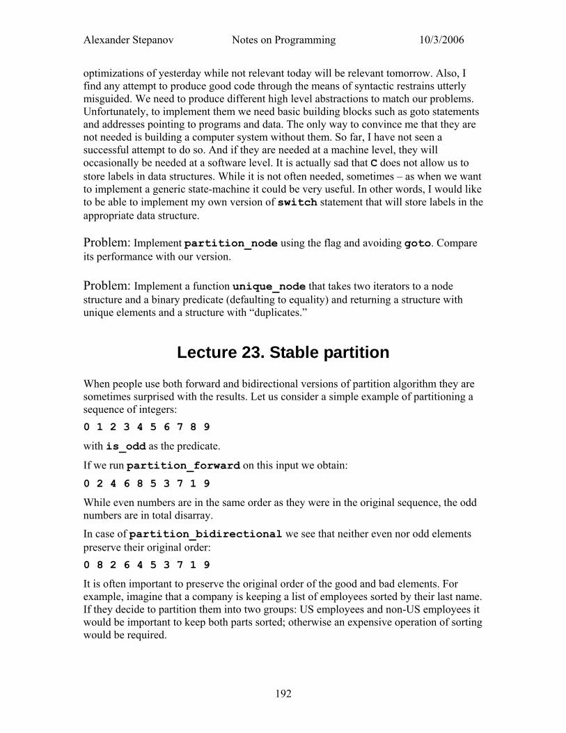
Alexander Stepanov Notes on Programming 10/3/2006
optimizations of yesterday while not relevant today will be relevant tomorrow. Also, I find any attempt to produce good code through the means of syntactic restrains utterly misguided. We need to produce different high level abstractions to match our problems. Unfortunately, to implement them we need basic building blocks such as goto statements and addresses pointing to programs and data. The only way to convince me that they are not needed is building a computer system without them. So far, I have not seen a successful attempt to do so. And if they are needed at a machine level, they will occasionally be needed at a software level. It is actually sad that C does not allow us to store labels in data structures. While it is not often needed, sometimes – as when we want to implement a generic state-machine it could be very useful. In other words, I would like to be able to implement my own version of switch statement that will store labels in the appropriate data structure. Problem: Implement partition_node using the flag and avoiding goto. Compare its performance with our version. Problem: Implement a function unique_node that takes two iterators to a node structure and a binary predicate (defaulting to equality) and returning a structure with unique elements and a structure with “duplicates.”
Lecture 23. Stable partition When people use both forward and bidirectional versions of partition algorithm they are sometimes surprised with the results. Let us consider a simple example of partitioning a sequence of integers: 0 1 2 3 4 5 6 7 8 9
with is_odd as the predicate.
If we run partition_forward on this input we obtain: 0 2 4 6 8 5 3 7 1 9
While even numbers are in the same order as they were in the original sequence, the odd numbers are in total disarray.
In case of partition_bidirectional we see that neither even nor odd elements preserve their original order: 0 8 2 6 4 5 3 7 1 9
It is often important to preserve the original order of the good and bad elements. For example, imagine that a company is keeping a list of employees sorted by their last name. If they decide to partition them into two groups: US employees and non-US employees it would be important to keep both parts sorted; otherwise an expensive operation of sorting would be required.
192

Alexander Stepanov Notes on Programming 10/3/2006
Definition: The partitioning that preserves the relative ordering of both true and false elements is called stable partitioning.
One of the important properties of stable partitioning is that it allows for multipass processing. Indeed, to partition a range [f, l) with a predicate p1 and then partition the resulting sub-ranges with a predicate p2 using a non-stable partition we need to write: I m = partition(f, l, p1); partition(f, m, p2); partition(m, l, p2); If, however, stable_partition is available the same goal can be accomplished with: stable_partition(f, l, p2); // p2 before p1! stable_partition(f, l, p1); This property is very important when many passes are needed and the overhead of keeping track of small sub-ranges becomes difficult and expensive to manage. This property is used with remarkable effect in radix sorting.
Problem: Prove that stable partitioning of a given sequence with a given predicate is unique; that is, prove that there is only one permutation of a range that gives stable partitioning.
It is clear that we cannot implement is_stably_partitioned for an arbitrary type of elements the way we implemented is_partitioned. Indeed if somebody shows us a sequence: 0 4 2 1 3 5
we do not know if it is stable or not because we do not know what was the original order of the elements. It is, however, much easier to determine that one range is the stable partition of the second range than it is to determine if one range is a partition of the second range: uniqueness helps.
Indeed, in order for us to assure that an algorithm for partition works, we need to compare two sequences – the original one and the partitioned one. In order for the partition algorithm to be correct we need to assure two things: first, that the resulting sequence is partitioned and that is easy to test by applying is_partitioned function, and, second, that the resulting sequence is a permutation of the original one. And finding out if a sequence is a permutation of another sequence is difficult unless elements are totally ordered and we can reduce both sequences to a canonical form by sorting them. If the only operation on the elements is equality, we do not know of an efficient way of determining if two sequences are permutations of each other.
Problem: Prove that determining if a sequence is a permutation of another requires O(N2) operations if only equality of elements is available.
For small sequences we can determine if one is a permutation of the other with the help of a useful algorithm that goes through one range and attempts to find the equal element
193

Alexander Stepanov Notes on Programming 10/3/2006
in the other. If elements are found they are moved up front. The algorithm returns if the first range is exhausted or when there is not an equal element in the second: template <typename I1, // I1 models Input Iterator typename I2, // I2 models Forward Iterator typename Eqv> // Eqv models Binary Predicate pair<I1, I2> mismatch_permuted(I1 f1, I1 l1,
I2 f2, I2 l2, Eqv eqv = equal<VALUE_TYPE(I1)>())
{ while (f1 != l1) { I2 n = find_if(f2, l2, bind1st(eqv, deref(f1))); if (n == l2) break; iterator_swap(f2, n); ++f1; ++f2; } return make_pair(f1, f2); } (It should be noted that the second range is re-ordered to match the first. We should also remember not to use the algorithm for long ranges – it is quadratic.) To determine if one range is a permutation of another we call mismatch_permuted and check if both ranges are exhausted: template <typename I1, // I1 models Input Iterator typename I2> // I2 models Forward Iterator inline bool is_permutation(I1 f1, I1 l1, I2 f2, I2 l2) { return mismatch_permuted(f1, l1, f2, l2) == make_pair(l1, l2); }
Problem: Assume that the elements in the range have a total ordering defined with operator< and implement a faster version of is_permutation.
Now we can produce a function that tests if the first range is a partitioning of the second: template <typename I1, // I1 models Forward Iterator typename I2, // I2 models Forward Iterator typename P> // P models a Unary Predicate bool is_partitioning(I1 f1, I1 l1, I2 f2, I2 l2, P p) { return is_partitioned(f1, l1, p) && is_permutation(f1, l1, f2, l2); }
194
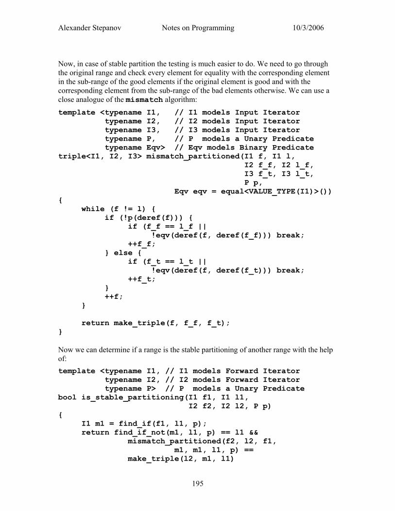
Alexander Stepanov Notes on Programming 10/3/2006
Now, in case of stable partition the testing is much easier to do. We need to go through the original range and check every element for equality with the corresponding element in the sub-range of the good elements if the original element is good and with the corresponding element from the sub-range of the bad elements otherwise. We can use a close analogue of the mismatch algorithm: template <typename I1, // I1 models Input Iterator typename I2, // I2 models Input Iterator typename I3, // I3 models Input Iterator typename P, // P models a Unary Predicate typename Eqv> // Eqv models Binary Predicate triple<I1, I2, I3> mismatch_partitioned(I1 f, I1 l, I2 f_f, I2 l_f, I3 f_t, I3 l_t, P p,
Eqv eqv = equal<VALUE_TYPE(I1)>()) { while (f != l) { if (!p(deref(f))) { if (f_f == l_f || !eqv(deref(f, deref(f_f))) break; ++f_f; } else {
if (f_t == l_t || !eqv(deref(f, deref(f_t))) break;
++f_t; } ++f; } return make_triple(f, f_f, f_t); } Now we can determine if a range is the stable partitioning of another range with the help of: template <typename I1, // I1 models Forward Iterator typename I2, // I2 models Forward Iterator typename P> // P models a Unary Predicate bool is_stable_partitioning(I1 f1, I1 l1,
I2 f2, I2 l2, P p) { I1 m1 = find_if(f1, l1, p); return find_if_not(m1, l1, p) == l1 &&
mismatch_partitioned(f2, l2, f1, m1, m1, l1, p) ==
make_triple(l2, m1, l1)
195
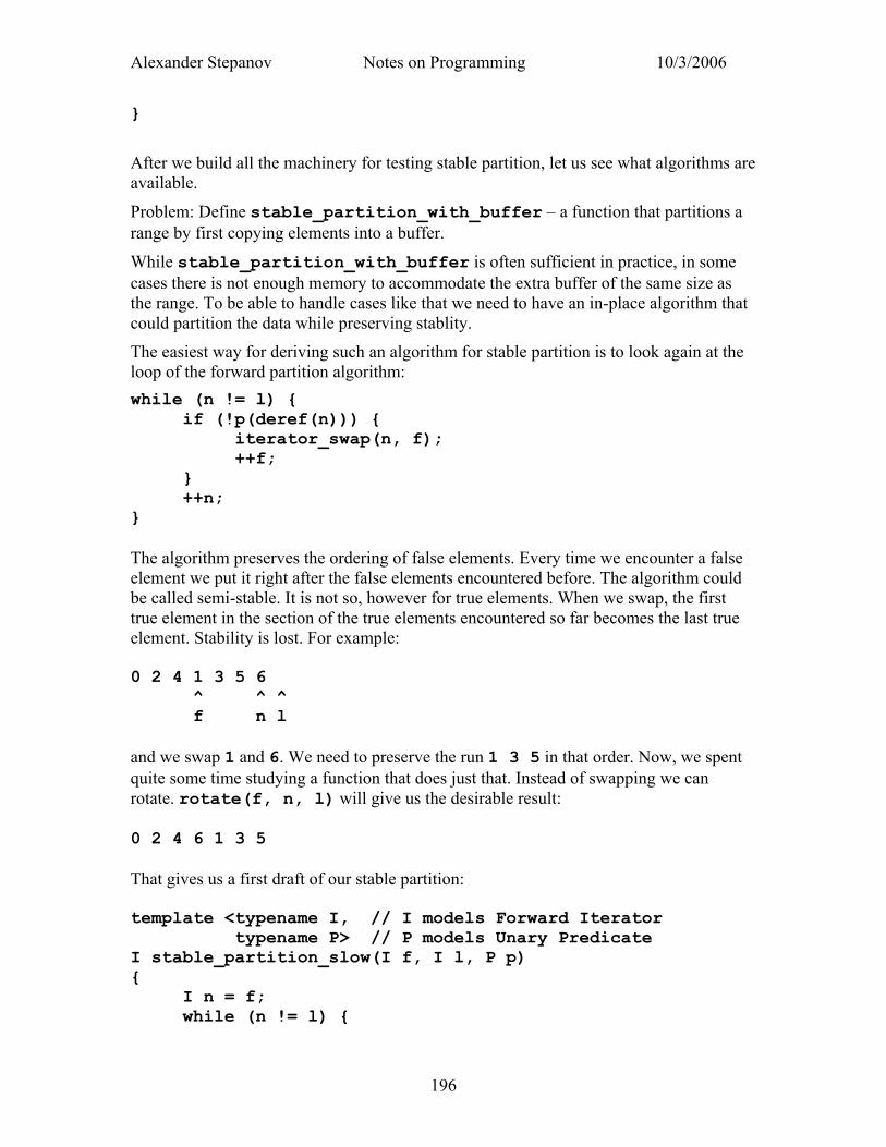
Alexander Stepanov Notes on Programming 10/3/2006
}
After we build all the machinery for testing stable partition, let us see what algorithms are available.
Problem: Define stable_partition_with_buffer – a function that partitions a range by first copying elements into a buffer.
While stable_partition_with_buffer is often sufficient in practice, in some cases there is not enough memory to accommodate the extra buffer of the same size as the range. To be able to handle cases like that we need to have an in-place algorithm that could partition the data while preserving stablity.
The easiest way for deriving such an algorithm for stable partition is to look again at the loop of the forward partition algorithm: while (n != l) { if (!p(deref(n))) {
iterator_swap(n, f); ++f;
} ++n;
} The algorithm preserves the ordering of false elements. Every time we encounter a false element we put it right after the false elements encountered before. The algorithm could be called semi-stable. It is not so, however for true elements. When we swap, the first true element in the section of the true elements encountered so far becomes the last true element. Stability is lost. For example: 0 2 4 1 3 5 6 ^ ^ ^ f n l and we swap 1 and 6. We need to preserve the run 1 3 5 in that order. Now, we spent quite some time studying a function that does just that. Instead of swapping we can rotate. rotate(f, n, l) will give us the desirable result: 0 2 4 6 1 3 5 That gives us a first draft of our stable partition: template <typename I, // I models Forward Iterator typename P> // P models Unary Predicate I stable_partition_slow(I f, I l, P p) { I n = f; while (n != l) {
196
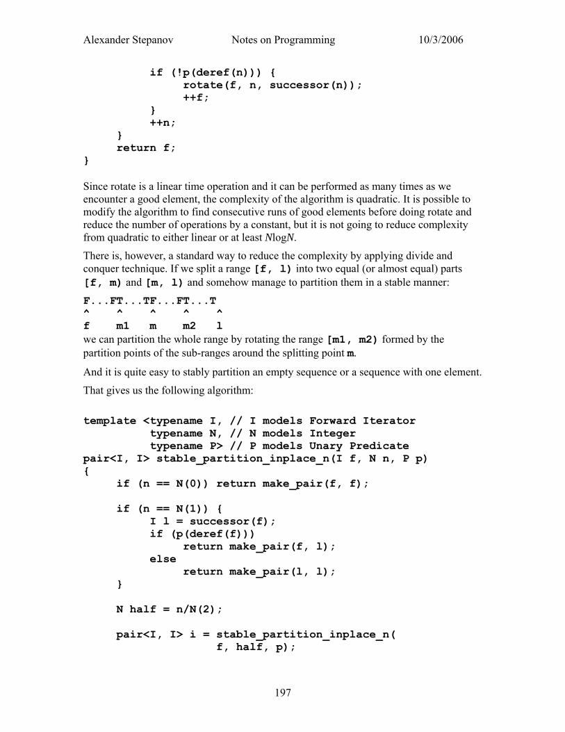
Alexander Stepanov Notes on Programming 10/3/2006
if (!p(deref(n))) { rotate(f, n, successor(n)); ++f;
} ++n; } return f; } Since rotate is a linear time operation and it can be performed as many times as we encounter a good element, the complexity of the algorithm is quadratic. It is possible to modify the algorithm to find consecutive runs of good elements before doing rotate and reduce the number of operations by a constant, but it is not going to reduce complexity from quadratic to either linear or at least NlogN.
There is, however, a standard way to reduce the complexity by applying divide and conquer technique. If we split a range [f, l) into two equal (or almost equal) parts [f, m) and [m, l) and somehow manage to partition them in a stable manner: F...FT...TF...FT...T ^ ^ ^ ^ ^ f m1 m m2 l we can partition the whole range by rotating the range [m1, m2) formed by the partition points of the sub-ranges around the splitting point m.
And it is quite easy to stably partition an empty sequence or a sequence with one element.
That gives us the following algorithm:
template <typename I, // I models Forward Iterator typename N, // N models Integer typename P> // P models Unary Predicate pair<I, I> stable_partition_inplace_n(I f, N n, P p) { if (n == N(0)) return make_pair(f, f); if (n == N(1)) { I l = successor(f); if (p(deref(f))) return make_pair(f, l); else return make_pair(l, l); } N half = n/N(2); pair<I, I> i = stable_partition_inplace_n( f, half, p);
197
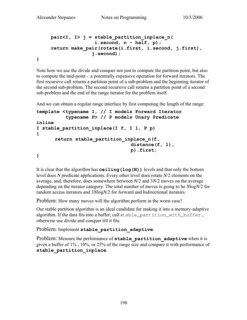
Alexander Stepanov Notes on Programming 10/3/2006
pair<I, I> j = stable_partition_inplace_n( i.second, n - half, p); return make_pair(rotate(i.first, i.second, j.first), j.second); } Note how we use the divide and conquer not just to compute the partition point, but also to compute the mid-point – a potentially expensive operation for forward iterators. The first recursive call returns a partition point of a sub-problem and the beginning iterator of the second sub-problem. The second recursive call returns a partition point of a second sub-problem and the end of the range iterator for the problem itself. And we can obtain a regular range interface by first computing the length of the range: template <typename I, // I models Forward Iterator typename P> // P models Unary Predicate inline I stable_partition_inplace(I f, I l, P p) { return stable_partition_inplace_n(f, distance(f, l), p).first; }
It is clear that the algorithm has ceiling(log(N)) levels and that only the bottom level does N predicate applications. Every other level does rotate N/2 elements on the average, and, therefore, does somewhere between N/2 and 3N/2 moves on the average depending on the iterator category. The total number of moves is going to be NlogN/2 for random access iterators and 3NlogN/2 for forward and bidirectional iterators.
Problem: How many moves will the algorithm perform in the worst case?
Our stable partition algorithm is an ideal candidate for making it into a memory-adaptive algorithm. If the data fits into a buffer, call stable_partition_with_buffer , otherwise use divide and conquer till it fits.
Problem: Implement stable_partition_adaptive.
Problem: Measure the performance of stable_partition_adaptive when it is given a buffer of 1% , 10%, or 25% of the range size and compare it with performance of stable_partition_inplace.
198
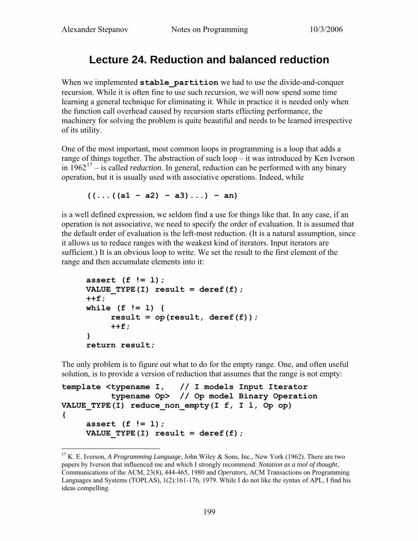
Alexander Stepanov Notes on Programming 10/3/2006
Lecture 24. Reduction and balanced reduction When we implemented stable_partition we had to use the divide-and-conquer recursion. While it is often fine to use such recursion, we will now spend some time learning a general technique for eliminating it. While in practice it is needed only when the function call overhead caused by recursion starts effecting performance, the machinery for solving the problem is quite beautiful and needs to be learned irrespective of its utility. One of the most important, most common loops in programming is a loop that adds a range of things together. The abstraction of such loop – it was introduced by Ken Iverson in 196217 – is called reduction. In general, reduction can be performed with any binary operation, but it is usually used with associative operations. Indeed, while
((...((a1 – a2) – a3)...) – an)
is a well defined expression, we seldom find a use for things like that. In any case, if an operation is not associative, we need to specify the order of evaluation. It is assumed that the default order of evaluation is the left-most reduction. (It is a natural assumption, since it allows us to reduce ranges with the weakest kind of iterators. Input iterators are sufficient.) It is an obvious loop to write. We set the result to the first element of the range and then accumulate elements into it: assert (f != l); VALUE_TYPE(I) result = deref(f); ++f; while (f != l) { result = op(result, deref(f)); ++f; } return result; The only problem is to figure out what to do for the empty range. One, and often useful solution, is to provide a version of reduction that assumes that the range is not empty: template <typename I, // I models Input Iterator typename Op> // Op model Binary Operation VALUE_TYPE(I) reduce_non_empty(I f, I l, Op op) { assert (f != l); VALUE_TYPE(I) result = deref(f);
17 K. E. Iverson, A Programming Language, John Wiley & Sons, Inc., New York (1962). There are two papers by Iverson that influenced me and which I strongly recommend: Notation as a tool of thought, Communications of the ACM, 23(8), 444-465, 1980 and Operators, ACM Transactions on Programming Languages and Systems (TOPLAS), 1(2):161-176, 1979. While I do not like the syntax of APL, I find his ideas compelling.
199

Alexander Stepanov Notes on Programming 10/3/2006
++f; while (f != l) { result = op(result, deref(f)); ++f; } return result; }
But a general question remains. What is the appropriate value to return for an empty range? In case of an associative operation such as + it is commonly assumed that the right value to return is the identity element of the operation (0 in case of +). Indeed, such a convention allows the following nice property to hold. For any range [f, l), for any iterator m inside the range and for any associative operation op on the elements of the range the following is true: op(reduce(f, m, op), reduce(m, l, op)) == reduce(f, l, op)
In order for this to hold when m is equal to either f or l, we need reduce to return the identity element of the operation.
We can accomplish it quite easily with: template <typename I, // I models Input Iterator typename Op> // Op model Binary Operation inline VALUE_TYPE(I) reduce(I f, I l, Op op,
VALUE_TYPE(I) z = identity_element(op)) { if (f == l) return z; return reduce_non_empty(f, l, op); } Clients of the code need to provide either an explicit element to be returned for the empty range or the operation has to provide a way of obtaining its identity element. As we observed when we studied power algorithms some common cases we can provide standard solutions: template <typename T> inline T identity_element(const plus<T>&) { return T(0); } A natural default for an additive identity element is a result of casting 0 into the element type. When the default does not work and it is easy to define a particular version of identity_element.
200

Alexander Stepanov Notes on Programming 10/3/2006
Problem: Define appropriate default identity_element for: struct min_int : binary_function<int, int, int> { int operator()(int a, int b) const { return min(a, b); } }; If the reduction knows what the identity element is, it can do a standard optimization by skipping the identity elements in the range since combining the result with an identity element is not going to change it. This gives us a useful variation of reduce: template <typename I, // I models Input Iterator typename Op> // Op model Binary Operation VALUE_TYPE(I) reduce_nonzeros(I f, I l, Op op,
VALUE_TYPE(I) z = identity_element(op)) { f = find_not(f, l, z); // skip zeros if (f == l) return z; VALUE_TYPE(I) result = deref(f); ++f; while (f != l) { if (deref(f) != z) result = op(result, deref(f)); ++f; } return result; } This version should be used when we want to avoid tests for identity elements inside the operation. In the cases when we have the code for the operation that handles only non-identity element cases, we do not then need to surround the code inside with two checks for identity (for the left and the right argument). Now we can tackle the stable partition. First let us observe that if we have two sub-ranges [f1, l1) and [f2, l2) of a range [f, l) such that for some predicate p:
- distance(f, l1) <= distance(f, f2) – first sub-range is before the second
- all(f1, l1, p) && all(f2, l2, p) – both sub-ranges contain only true elements
- none(l1, f2, p) – and there are no true elements in between them
201

Alexander Stepanov Notes on Programming 10/3/2006
then we can stably partition the combined range [f1, l2) by doing rotate(f1, l1, f2) and the result returned by the rotate is the partition point of the combined range. The following function object class performs the operation on such ranges: template <typename I> // I models Forward Iterator struct combine_ranges : binary_function<pair<I, I>, pair<I, I>, pair<I, I> > {
pair<I, I> operator()(const pair<I, I>& x, const pair<I, I>& y) const { return make_pair(
rotate(x.first, x.second, y.first), y.second);
} }; It is interesting to observe that we need to worry only about the sub-ranges containing true elements. While we are combining the ranges of true elements, the false elements bubble down to the front of the main range. Problem: Prove that combine_ranges is associative. We have an object to combine the ranges. It is a very simple to generate a sequence of trivial ranges containing “bad” elements. For every dereferenceable iterator in the main range we can produce a trivial sub-range with the help of the following: template <typename I, // I models Forward Iterator typename P> // P models Unary Predicate struct partition_trivial : unary_function<I, pair<I, I> > { P p; partition_trivial(const P & x) : p(x) {} pair<I, I> operator()(I i) { if (p(deref(i))) return make_pair(i, i); else return make_pair(i, successor(i)); } }; The only remaining problem is transforming a range of iterators to elements into a range of trivial ranges to be combined by reduce using combine_ranges. And that we can accomplish with the help of the following iterator-adaptor. It is constructed out of an
202

Alexander Stepanov Notes on Programming 10/3/2006
incrementable object (an object with ++ defined on it) and a function object. When incremented, it increments the incrementable object. When dereferenced, it returns the result of an application of the function object to the incrementable object. It is a generally useful adapter: template <typename I, // I models Incrementable typename F = identity<I> > // F models Unary Function class value_iterator { public: typedef typename F::result_type value_type; typedef ptrdiff_t difference_type; typedef forward_iterator_tag iterator_category; private: I i; F f; public: value_iterator() {} value_iterator(const I& x, const F& y) : i(x), f(y) {} value_iterator& operator++() { ++i; return *this; } value_iterator operator++(int) { value_iterator tmp = *this; ++*this; return tmp; } value_type operator*() const { return f(i); } friend bool operator==(const self& a, const self& b) { assert(a.f == b.f); return a.i == b.i; } friend bool operator!=(const self& a, const self& b) { return !(a == b); } }; Problem: Generalize value_iterator further by allowing a user to specify the meaning of ++ and providing a natural default for ++; We can now obtain a slow version of stable partitioning by calling reduce_nonzeros with identity element equal the pair that is made of the last element of the range. (After
203
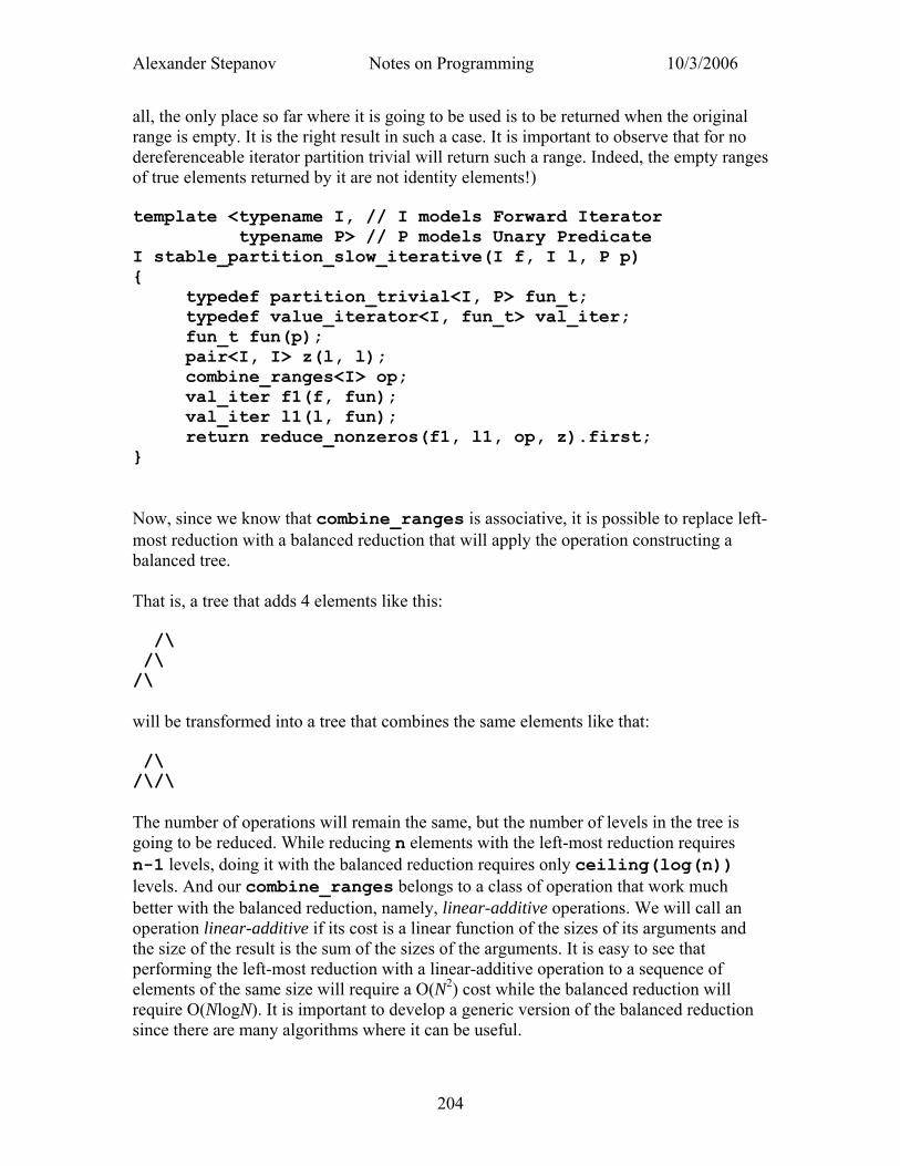
Alexander Stepanov Notes on Programming 10/3/2006
all, the only place so far where it is going to be used is to be returned when the original range is empty. It is the right result in such a case. It is important to observe that for no dereferenceable iterator partition trivial will return such a range. Indeed, the empty ranges of true elements returned by it are not identity elements!) template <typename I, // I models Forward Iterator typename P> // P models Unary Predicate I stable_partition_slow_iterative(I f, I l, P p) { typedef partition_trivial<I, P> fun_t; typedef value_iterator<I, fun_t> val_iter; fun_t fun(p); pair<I, I> z(l, l); combine_ranges<I> op; val_iter f1(f, fun); val_iter l1(l, fun);
return reduce_nonzeros(f1, l1, op, z).first; } Now, since we know that combine_ranges is associative, it is possible to replace left-most reduction with a balanced reduction that will apply the operation constructing a balanced tree. That is, a tree that adds 4 elements like this: /\ /\ /\ will be transformed into a tree that combines the same elements like that: /\ /\/\ The number of operations will remain the same, but the number of levels in the tree is going to be reduced. While reducing n elements with the left-most reduction requires n-1 levels, doing it with the balanced reduction requires only ceiling(log(n)) levels. And our combine_ranges belongs to a class of operation that work much better with the balanced reduction, namely, linear-additive operations. We will call an operation linear-additive if its cost is a linear function of the sizes of its arguments and the size of the result is the sum of the sizes of the arguments. It is easy to see that performing the left-most reduction with a linear-additive operation to a sequence of elements of the same size will require a O(N2) cost while the balanced reduction will require O(NlogN). It is important to develop a generic version of the balanced reduction since there are many algorithms where it can be useful.
204
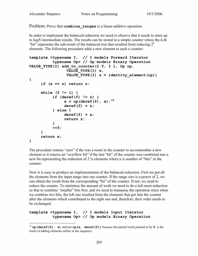
Alexander Stepanov Notes on Programming 10/3/2006
Problem: Prove that combine_ranges is a linear-additive operation. In order to implement the balanced reduction we need to observe that it needs to store up to logN intermediate results. The results can be stored in a simple counter where the k-th “bit” represents the sub-result of the balanced tree that resulted from reducing 2k elements. The following procedure adds a new element to such a counter: template <typename I, // I models Forward Iterator typename Op> // Op models Binary Operation VALUE_TYPE(I) add_to_counter(I f, I l, Op op, VALUE_TYPE(I) x, VALUE_TYPE(I) z = identity_element(op)) { if (x == z) return z; while (f != l) { if (deref(f) != z) { x = op(deref(f), x);18
deref(f) = z; } else { deref(f) = x; return z; } ++f; } return x; } The procedure returns “zero” if the was a room in the counter to accommodate a new element or it returns an “overflow bit” if the last “bit” of the counter was combined into a new bit representing the reduction of 2^n elements where n is number of “bits” in the counter. Now it is easy to produce an implementation of the balanced reduction. First we put all the elements from the input range into our counter. If the range size is a power of 2, we can obtain the result from the corresponding “bit” of the counter. If not, we need to reduce the counter. To minimize the amount of work we need to do a left-most reduction so that to combine “smaller” bits first, and we need to transpose the operation since when we combine two bits, the left one resulted from the elements that got into the counter after the elements which contributed to the right one and, therefore, their order needs to be exchanged: template <typename I, // I models Input Iterator typename Op> // Op models Binary Operation
18 op(deref(f), x) and not op(x, deref(f)) because the partial result pointed to by f is the result of adding elements earlier in the sequence.
205

Alexander Stepanov Notes on Programming 10/3/2006
void reduce_balanced(I f, I l, Op op, VALUE_TYPE(I) z = identity_element(op)) { vector<VALUE_TYPE(I)> v; while (f != l) { VALUE_TYPE(I) tmp = add_to_counter( v.begin(), v.end(), op, deref(f), z); if (tmp != z) v.push_back(tmp); ++f; } return reduce_nonzeros( v.begin(),v.end(), f_transpose(op), z); } Note that the reduce_balanced is not going to apply the operation to the identity element so that we do not need reduce_non_zero_balanced. Finally we can now trivially obtain the balanced non-recursive implementation of stable_partition_inplace by replacing the call to the left-most reduction with the call to the balanced reduction: template <typename I, // I models Forward Iterator typename P> // P models Unary Predicate I stable_partition_inplace_iterative(I f, I l, P p) { typedef partition_trivial<I, P> fun_t; typedef value_iterator<I, fun_t> val_iter; fun_t fun(p); pair<I, I> z(l, l); combine_ranges<I> op; val_iter f1(f, fun); val_iter l1(l, fun);
return reduce_balanced(f1, l1, op, z).first; } Problem: Compare the performance of stable_partition_inplace with the performance of stable_partition_inplace_iterative. Explain the results.
Problem: Implement an iterative version of stable_partition_adaptive using reduce_balanced.
206
Alexander Stepanov Notes on Programming 10/3/2006
Lecture 25. 3-partition Some times the sequences with which we deal are divided into more than two kinds of elements. Before we address a problem of partitioning a range into an arbitrary number of buckets, let us spend some time on a very important case of partition, partition into three categories. The algorithm for the three-way partitioning is commonly known a Dutch National Flag algorithm for the three colors: red, white and blue of the flag of the Kingdom of Netherlands. I do not know who introduced it first; I – as well as most other people – learned about it from an important book of Edsger Dijkstra Discipline of Programming19. In it Dijkstra acknowledges his indebtedness for the problem to W. H. J. Feijen. Instead of colors we are going to use integers; in particular, we assume that instead of a predicate returning a Boolean value – as in partition – we are given a key function that returns three values: {0, 1, 2} known as keys. Now we consider the range to be partitioned 3-ways if it contains no elements with keys 1 and 2 before elements with key 0, and no elements with key 2 before elements with key 1. It is very easy to implement a function to check if a range is partitioned: template <typename I, // I models Forward Iterator typename F> // F models Unary Function bool is_partitioned_3way(I f, I l, F key) { equal_to<int> eq;
f = find_if_not(f, l, compose1(bind2nd(eq, 0), key)); f = find_if_not(f, l, compose1(bind2nd(eq, 1), key)); f = find_if_not(f, l, compose1(bind2nd(eq, 2), key));
return f == l; } Problem: Prove that is_partitioned_3way does what it claims to do. It is important to observe that a different way of stating that a range is partitioned 3-way is by saying that the key function will return non-decreasing sequence of values or that if we assume that we have a function is_sorted we can check the range for being partitioned 3-way by the following simple function: template <typename I, // I models Forward Iterator
19 Dijkstra, E.W.: A Discipline of Programming, Prentice Hall (1976). It is a sad fact that the work of Dijkstra is becoming totally unknown to a modern programmer. While some of Dijkstra’s opinions are extreme and one should occasionally take his pronouncements with a grain of salt, his work is central to programming as a scientific discipline and I would urge every young programmer to study his work. We should be grateful to the Computer Science Department of the University of Texas, Austin for creating the Internet archive of Dijkstra’s works: http://www.cs.utexas.edu/users/EWD/.
207

Alexander Stepanov Notes on Programming 10/3/2006
typename F> // F models Unary Function bool is_partitioned_3way_1(I f, I l, F key) { return is_sorted(
f, l, compose2(less<int>(), key, key)); } As a matter of fact, we can use the same code to verify n-way partitioning: template <typename I, // I models Forward Iterator typename F> // F models Unary Function bool is_partitioned_n_way(I f, I l, F key) { return is_sorted(
f, l, compose2(less<int>(), key, key)); } That shows us that there is a connection between sorting and partitioning. Indeed we can always implement an n-way partition by implementing: template <typename I, // I models Forward Iterator typename F> // F models Unary Function void partition_n_way_0(I f, I l, F key) { sort(f, l, compose2(less<int>(), key, key); } (That, of course, requires a sort that works for forward iterators: something that you will not find in the present standard library. As a matter of fact, this piece of code with a different name would make a very useful library function: template <typename I, // I models Random Access Iterator typename F> // F models Unary Function void sort_by_key(I f, I l, F key) { sort(f, l, compose2(less<int>(), key, key); } ) It is, of course, not a very interesting thing to do for small value of n since it is an NlogN algorithm for a linear time problem. It is much better, as is done in quicksort, to implement sorting in terms of partitioning. Now, let us get back to 3-way partition and Dijkstra’s algorithm. Let us assume that somehow we managed to solve the problem up to some middle point s:
208

Alexander Stepanov Notes on Programming 10/3/2006
0000001111?????22222222 ^ ^ ^ f s l (first, second, last) If s points to an element with key 1 we just advance s. If it is 0 we swap it with an element pointed at by f and advance both f and s. If it is 2 we decrement l; swap elements pointed by l and s and increment s. This algorithm works exactly like Lomuto’s partitition_forward for 0 and 1, but sends 2 to the other end of the range. The code looks like: template <typename I, // I models Bidirectional Iterator typename F> // F models Unary Function pair<I , I> partition_3way_bidirectional(I f, I l, F fun) { I s = f;
while (s != l) { int key = fun(deref(s)); if (key == 0) {
iterator_swap(f, s); ++f; } else if (key == 2) { --l; iterator_swap(l, s); } ++s; } return make_pair(f, l); } It is clear that the algorithm does N predicate application and N swaps in the worst case and 2N/3 swaps on average. Now, let us find an algorithm that allows us to do the 3way partition with forward iterators. Such an algorithm can be easily obtained using our standard inductive technique. Let us assume that somehow we managed to solve the problem up to some middle point: 000000111122222???????? ^ ^ ^ ^ f s t l (first, second, third, last) Then we can partition it with:
209
Alexander Stepanov Notes on Programming 10/3/2006
template <typename I, // I models Forward Iterator typename F> // F models Unary Function pair<I , I> partition_3way_forward(I f, I l, F fun) {
I t = f; I s = f;
while (t != l) { int key = fun(deref(t));
if (key == 0) { cycle_left(deref(t), deref(s), deref(f)); ++s; ++f;
} else if (key == 1) { iterator_swap(s, t); ++s;
} ++t; } return make_pair(f, s); } Problem: Compare the number of operation of partition_3way_bidirectional and partition_3way_forward. Project: Measure the performance of partition_3way_forward and partition_3way_bidirectional for different integral types (char, short, int, long long, etc) with a 3-way predicate that return a remainder of an integer divided by 3. Problem: Implement partition_4way_forward. Problem: Implement partition_4way_bidirectional. Problem: What is the number of operation performed by partition_4way_forward and partition_4way_bidirectional in the worst case and on average? Problem: Implement partiotion_copy_3way. Problem: Implement stable_partiotion_3way.
210
Alexander Stepanov Notes on Programming 10/3/2006
Lecture 26. Finding the partition point We already discussed a problem of finding the partition point of an already partitioned range. There is an obvious solution:
find_if_not(f, l, p)
will definitely return the partition point of a partitioned range. The problem is that we will need to retest all good elements again.
It is easy to observe the following fundamental property of a partitioned range [f, l): if an iterator m inside the range points at a good element then the partition point of [f, l) is located in the range [successor(m), l); if m points at a bad element then the partition point is in the range [f, m).
As far as an empty range goes, its beginning and its end both happen to be the partition points.
Let us assume for the moment that we are dealing with random access iterators and, therefore, can get to any element inside the range in constant time. If we have range represented as a pair of an iterator and an integer (the length of the range) and if we have a function choose that returns some non-negative integer less than the length of the range for any non-empty range, then for any such function choose there is a simple recursive algorithm for finding partition point:
template <typename I, // I models Random Access Iterator typename P> // P models Unary Predicate I partition_point_recursive(I f, DIFFERENCE_TYPE(I) n, P p) { if (n == 0) return f; N m = choose(n); if (p(deref(f + m))) return partition_point_recursive(f + (m + 1), n – (m + 1)); else return partition_point_recursive(f, m); } Since 0 ≤ m < n we can be sure that both n – m – 1 and m are less than n and not less than 0; and, therefore, we can be sure that our program terminates. It is also obvious that a way of assuring that (no matter which path of the if-statement happens to be true) is by picking the choose function that for any positive n returns n/2.
Problem: Prove that picking n/2 is indeed the best course.
If you are wondering if we are describing binary search, you are correct. It is essential to understand the interface and the implementation of the partition point finding algorithm
211

Alexander Stepanov Notes on Programming 10/3/2006
to be able to define binary search correctly. In particular, while it is self-evident what partition_point should return, it is far from self-evident what binary search should return. And even reputable computer scientists often stumble defining it. This is why I believe that it is essential to deal thoroughly with predicate-based operations such as partition before attacking much more treacherous comparison-based operations.
Since our recursive calls are properly tail-recursive we can immediately obtain the following algorithm by resetting the variables in a loop instead of making a recursive call:
template <typename I, // I models Random Access Iterator typename P> // P models Unary Predicate I partition_point_n_random_access
(I f, DIFFERENCE_TYPE(I) n, P p) { while (n != 0) { if (p(deref(f + n/2))) { f = (f + n/2) + 1; n = n – (n/2 + 1); } else { // f = f; n = n/2; } } return f; }
The algorithm does ceiling(log(n)) + 1 predicate applications since we are reducing the length by dividing by 2 at every step.
What can we do if iterators which are given to us are less powerful than random access? While the efficiency of the algorithm will degrade dramatically, it is still quite useful in those cases when the predicate application is more expensive than the operation ++ on the iterators. If we use find_if to find partition point then the expected cost of finding the partition point in a range of length n is
c_linear = (n/2) * c_p + (n/2) * c_i
where c_p is the cost of the predicate application and c_i is the cost of the iterator increment. (In other words, while doing linear search we expect to travel half of the way on the average.) If we use the partition_point_n algorithm the expected cost is going to be
c_binary_best = (log(n) + 1) * c_p + n * c_i
since we are going to advance by n/2, n/4, n/8, etc. In those cases when the linked structure changes its size frequently we need to do another n increments and the cost becomes
c_binary_worst = (log(n) + 1) * c_p + 2 * n * c_i
212

Alexander Stepanov Notes on Programming 10/3/2006
With large N we can safely ignore logarithmic terms and the binary algorithm wins against linear one when c_p > c_i if linked structure does not change its size and when c_p > 3 * c_i if its size needs to be computed anew every time.
In practice, the cost of predicate application should be more than 4 times as expensive as iterator increment to really justify using binary search like algorithms on linked lists. Otherwise, it is usually better to use linear search. It usually means that if your predicate is a small inlined function object then using find is better; if it is a non-inlined function call then binary search is better.
It is perfectly straightforward to modify our algorithm to work with forward iterators and we can do a few little optimizations as well: template <typename I, // I models Forward Iterator typename P> // P models Unary Predicate I partition_point_n(I f, DIFFERENCE_TYPE(I) n, P p) { while (n != 0) { N h = n >> 1; I m = successor(f, h); if (p(*m)) { f = successor(m); n -= h + 1; } else { n = h; } } return f; }
Problem: Implement a partition_point function that takes two iterators [f, l) as its arguments. partition_3way returns a pair of iterators which are two partition points. It is obvious that if a range is already partitioned we can find the partition points with the help of partition_point_n: template <typename I, // I models Forward Iterator
typename F> // F models Unary Function
pair<I , I> partition_point_3way_simple_minded
(I f, DIFFERENCE_TYPE(I) n, F fun)
{
less<int> comp;
213

Alexander Stepanov Notes on Programming 10/3/2006
return make_pair(partition_point_n(f, n,
compose1(bind2nd(comp, 1), fun)),
partition_point_n(f, n,
compose1(bind2nd(comp, 2), fun)));
}
The problem is that we are doing some extra work since both calls will repeat at least the first test of the middle element. Problem: What is the largest number of duplicated tests? We can easily fix that: template <typename I, // I models Forward Iterator typename F> // F models Unary Function pair<I , I> partition_point_3way
(I f, DIFFERENCE_TYPE(I) n, F fun) { equal_to<int> eq; while (n > 0) { DIFFERENCE_TYPE(I) h = n>>1; I m = successor(f, h); switch (fun(*m++)) {
case 0: f = m; n = n – h - 1;
break; case 1:
I i = partition_point_n(f, n – h - 1, compose1(bind2nd(eq, 0), fun)),
I j = partition_point_n(m, h, compose1(bind2nd(eq, 1), fun));
return make_pair(i, j); case 2:
n = h; } } return make_pair(f, f); }
214
Alexander Stepanov Notes on Programming 10/3/2006
Lecture 27. Conclusions In 1968 Doug McIlroy gave a remarkable presentation on the state of software engineering20. Starting with an observation of a dismal state of the software engineering, he called for the creation “of a software components industry is that it will offer families of routines for any given job. No user of a particular member of a family should pay a penalty, in unwanted generality, for the fact that he is employing a standard model routine. In other words, the purchaser of a component from a family will choose one tailored to his exact needs. He will consult a catalogue offering routines in varying degrees of precision, robustness, time-space performance, and generality. He will be confident that each routine in the family is of high quality – reliable and efficient. …He will expect families of routines to be constructed on rational principles so that families fit together as building blocks. In short, he should be able safely to regard components as black boxes.”
20 M. D. McIlroy, Mass produced software components, Proc. NATO Software Eng. Conf., Garmisch, Germany (1968), pages 138-155. The text can be found at http://www.cs.dartmouth.edu/~doug/components.txt. You must read it!
215