Alexander Kowarik sparkTable: Generating Graphical … · Fulham 38 11 16 11 49 A. Villa 38 12 12 14 48 ... provides the following ... a

S T A T I S T I K A U S T R I A

D i e I n f o r m a t i o n s m a n a g e r

Alexander Kowarik1,Bernhard Meindl1 and

Matthias Templ1,2

1. Statistics Austria2. Vienna University of

TechnologyuseR! 2011

Coventry, August 16-18,2011

sparkTable: Generating GraphicalTables for Websites andDocuments with R

Kowarik, Meindl, Templ (STAT, TU) 1 / 26 | Coventry, Aug 16-18, 2011



Contents

Motivation

Introductory examples

The R-package sparkTable

Example

Outline




Motivation

I Providing quick access to additional insights by the use of graphicaltables

I Presentation of numerous data in a well-arranged way

I Improving data density by using spark-graphs

I Results should be easy to modify

I Development of a tool to create graphical tables easily

How can this be achieved? −→ R-package sparkTable




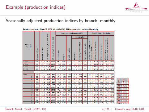
Example (production indices)

Seasonally adjusted production indices by branch, monthly.




Example (production indices enhanced)




Example (developments of the Austrian population)

Männer Frauen 0 bis 19 Jahre 20 bis 64 Jahre65 Jahre

und älter

dar.:

75 Jahre

und älter

1981 7.553.326 3.570.172 3.983.154 896 2.184.224 4.212.971 1.156.131 454.278

1982 7.584.094 3.590.286 3.993.808 899 2.159.778 4.292.823 1.131.493 465.300

1983 7.564.185 3.582.589 3.981.596 900 2.115.305 4.348.057 1.100.823 473.838

1984 7.559.635 3.583.422 3.976.213 901 2.070.767 4.415.758 1.073.110 480.749

1985 7.563.233 3.588.116 3.975.117 903 2.028.352 4.465.937 1.068.944 491.279

1986 7.566.736 3.594.380 3.972.356 905 1.988.702 4.499.348 1.078.686 500.239

1987 7.572.852 3.602.199 3.970.653 907 1.950.892 4.528.383 1.093.577 508.013

1988 7.576.319 3.608.710 3.967.609 910 1.911.761 4.553.802 1.110.756 519.409

1989 7.594.315 3.623.136 3.971.179 912 1.879.112 4.589.333 1.125.870 527.740

1990 7.644.818 3.654.915 3.989.903 916 1.862.258 4.642.719 1.139.841 534.306

1991 7.710.882 3.696.200 4.014.682 921 1.856.653 4.700.847 1.153.382 526.559

1992 7.798.899 3.746.551 4.052.348 925 1.864.333 4.770.187 1.164.379 511.086

1993 7.882.519 3.793.245 4.089.274 928 1.876.578 4.831.640 1.174.301 494.349

1994 7.928.746 3.820.889 4.107.857 930 1.880.290 4.862.793 1.185.663 479.964

1995 7.943.489 3.831.200 4.112.289 932 1.875.112 4.871.503 1.196.874 481.743

1996 7.953.067 3.836.950 4.116.117 932 1.871.831 4.873.219 1.208.017 494.972

1997 7.964.966 3.844.019 4.120.947 933 1.870.818 4.877.700 1.216.448 511.436

1998 7.971.116 3.848.305 4.122.811 933 1.866.873 4.880.028 1.224.215 528.564

1999 7.982.461 3.856.029 4.126.432 934 1.862.619 4.890.127 1.229.715 545.049

2000 8.002.186 3.868.331 4.133.855 936 1.857.356 4.911.163 1.233.667 559.914

2001 8.020.946 3.881.104 4.139.842 938 1.844.074 4.938.856 1.238.016 575.493

2002 8.063.640 3.906.734 4.156.906 940 1.827.823 4.986.599 1.249.218 593.437

2003 8.100.273 3.929.599 4.170.674 942 1.819.450 5.030.344 1.250.479 601.901

2004 8.142.573 3.952.600 4.189.973 943 1.813.186 5.068.488 1.260.899 612.140

2005 8.201.359 3.984.866 4.216.493 945 1.809.717 5.083.697 1.307.945 625.028

2006 8.254.298 4.014.344 4.239.954 947 1.803.687 5.093.024 1.357.587 638.263

2007 8.282.984 4.030.062 4.252.922 948 1.790.880 5.093.505 1.398.599 648.843

2008 8.318.592 4.048.633 4.269.959 948 1.777.869 5.115.684 1.425.039 658.531

2009 8.355.260 4.068.047 4.287.213 949 1.763.948 5.140.425 1.450.887 665.415

Bevölkerung zu Jahresbeginn seit 1981 nach Geschlecht bzw. breiten Altersgruppen (Absolutwerte)

Q: STATISTIK AUSTRIA, Statistik des Bevölkerungsstandes.- Revidierte Ergebnisse für 2002 bis 2008. Erstellt am: 27.05.2009.

Jahr Insgesamt

Nach Geschlecht Nach Altersgruppen

Männer auf

1.000 Frauen




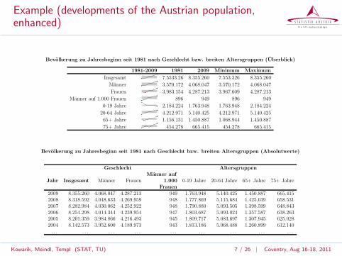
Example (developments of the Austrian population,enhanced)

Bevölkerung zu Jahresbeginn seit 1981 nach Geschlecht bzw. breiten Altersgruppen (Überblick)

1981-2009 1981 2009 Minimum MaximumInsgesamt 7.5533.26 8.355.260 7.553.326 8.355.260

Männer 3.570.172 4.068.047 3.570.172 4.068.047Frauen 3.983.154 4.287.213 3.967.609 4.287.213

Männer auf 1.000 Frauen 896 949 896 9490-19 Jahre 2.184.224 1.763.948 1.763.948 2.184.224

20-64 Jahre 4.212.971 5.140.425 4.212.971 5.140.42565+ Jahre 1.156.131 1.450.887 1.068.944 1.450.88775+ Jahre 454.278 665.415 454.278 665.415

Bevölkerung zu Jahresbeginn seit 1981 nach Geschlecht bzw. breiten Altersgruppen (Absolutwerte)

Geschlecht Altersgruppen

Jahr Insgesamt Männer FrauenMänner auf

0-19 Jahre 20-64 Jahre 65+ Jahre 75+ Jahre1.000Frauen

2009 8.355.260 4.068.047 4.287.213 949 1.763.948 5.140.425 1.450.887 665.4152008 8.318.592 4.048.633 4.269.959 948 1.777.869 5.115.684 1.425.039 658.5312007 8.282.984 4.030.062 4.252.922 948 1.790.880 5.093.505 1.398.599 648.8432006 8.254.298 4.014.344 4.239.954 947 1.803.687 5.093.024 1.357.587 638.2632005 8.201.359 3.984.866 4.216.493 945 1.809.717 5.083.697 1.307.945 625.0282004 8.142.573 3.952.600 4.189.973 943 1.813.186 5.068.488 1.260.899 612.140

. . . . . . . . . . . . . . . . . . . . . . . . . . .

1




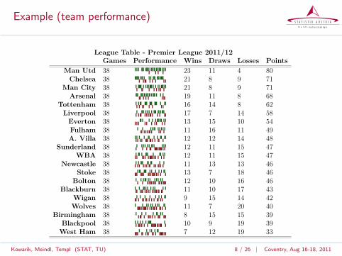
Example (team performance)

League Table - Premier League 2011/12Games Performance Wins Draws Losses Points

Man Utd 38 23 11 4 80Chelsea 38 21 8 9 71

Man City 38 21 8 9 71Arsenal 38 19 11 8 68

Tottenham 38 16 14 8 62Liverpool 38 17 7 14 58

Everton 38 13 15 10 54Fulham 38 11 16 11 49A. Villa 38 12 12 14 48

Sunderland 38 12 11 15 47WBA 38 12 11 15 47

Newcastle 38 11 13 13 46Stoke 38 13 7 18 46

Bolton 38 12 10 16 46Blackburn 38 11 10 17 43

Wigan 38 9 15 14 42Wolves 38 11 7 20 40

Birmingham 38 8 15 15 39Blackpool 38 10 9 19 39

West Ham 38 7 12 19 33

1




Coordinates of European States

WEST − EAST

SO

UT

H −

NO

RT

HIS

FI

NO

EE

LV

SE

DK LT

IENLUK

LU

PLBE

CZSK

DE

LI AT HUCHSI ROHR

BG

TR

IT

MT CY

GRPT ES

FR




Optimal Allocation with Sparklines

IS NO SE FI EEPopulation : Population : Population : Population : Population :

●

● ●

●

●●

●

●●

●

●●

●

●

●

Debt : Debt : Debt : Debt : Debt :●

●

●

● ●

●●

●

●●

NL DE DK LT LVPopulation : Population : Population : Population : Population :

●

●●

●

●

● ●

●●

●

●

● ●

●

●


●●

●

●●

●

●

●

●

●●

●

●●

UK IE BE CZ PL SKPopulation : Population : Population : Population : Population : Population :

●

●●

●

●●

●

●●

●

●●

●

●

● ●

●●

Debt : Debt : Debt : Debt : Debt : Debt :●

●●

●

●●

●

●

●

●

●●

●

●●

●

●

●

LU CH LI AT HU ROPopulation : Population : Population : Population : Population : Population :

●

●●

●

●●

●

●●

●

●●

●

●

● ●

●

●


●●

●

●●

●

●●

●

●●

PT FR SI HR BG TRPopulation : Population : Population : Population : Population : Population :

●

●●

●

●●

●

●●

●

●

● ●

●

● ●

●●


●●

●

●● ●

●

●

●

ES IT MT GR CYPopulation : Population : Population : Population : Population :

●

●●

●

●●

●

● ●

●

●●

●

●●


● ●

●

●●

●

●

●

●

●●

●

●

●

1




The R-package sparkTable

R-package sparkTable (available on CRAN) provides the followingfeatures1

I Different graphical representations

I Combining numerical with graphical information into a table

I Creation of tables for online- or print publication

1for details, see: The Visual Display of Quantitative Information, E. R. Tufte




Overview of sparkTable

I newSparkBar(), newSparkBox(), newSparkLine():Functions tocreate new Spark object

I newSparkTable(): Function to create new SparkTable object

I newGeoTable(): Functions to create a new object of class’geoTable’

I plotSparks(), plotSparkTable(), plotGeoTable(): GenerateOutput from Spark, SparkTable and GeoTable objects

I getParameter(), setParameter(): Functions to view or change theparameters of the object




A (very) simple example I

I We show a very simple example to create a single spark-graph

I Generating random input-data:

dat <- rnorm(25, 100, 25)

I Creating a suitable input-object and setting several graphicparameters:

a <- newSparkLine(values=dat , pointWidth =8)

I Drawing the png-image

plotSparks(a, outputType= ' png ' ,filename= ' testLine1 ' )




A (very) simple example II

I Changing parameters and drawing the pdf-image

a <- setParameter(a, c("darkred", "darkgreen",

"darkblue", "white", "black", "red"),

type= ' allColors ' )getParameter(a, type= ' allColors ' )a <- setParameter(a, 3, type= ' pointWidth ' )a <- setParameter(a, 1, type= ' lineWidth ' )plotSparks(a, outputType="pdf",

filename= ' testLine2 ' )

I Displaying the image as pdf●

●

●(scalable!)

I Displaying the image as png (not scalable!)




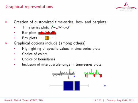
Graphical representations

I Creation of customized time-series, box- and barplotsI Time series plots

●

● ●

I Bar plotsI Box plots ●● ●●

I Graphical options include (among others)I Highlighting of specific values in time series plotsI Choice of colorsI Choice of boundariesI Inclusion of interquartile-range in time-series plots

●

●

●

●




Choosing the output-format

The user can decide to generate pdf, eps or png output

I Pdf, Eps graphics can be included in LATEX for scientific use

I Png can be used to show both graphics on websites




Example (population) I

Mean value Boxplot LinePlot BarPlot Current valueTotal 7884750.66

●

●● 8355260Men 3791573.55

●

●● 4068047Women 4093177.1

●

●● 4287213Men per 1.000 Women 925.97

●

●● 949Age 0-19 1899456.83 ●●●●

●

●

●1763948

Age 20-64 4778240●

●● 5140425Age 65+ 1207053.83 ●

●

●● 1450887Age 75+ 541649.59

●

●● 665415

1

I The data:

data(pop)

head(pop ,5)

time variable value

1 1981 Insgesamt 7553326

2 1982 Insgesamt 7584094

3 1983 Insgesamt 7564185

4 1984 Insgesamt 7559635

5 1985 Insgesamt 7563233




Example (population) II

I Create a content object:

content <- list()

content [[ ' Mean value ' ]] <- function(x) { round(mean(x),2) }

content [[ ' Boxplot ' ]] <- newSparkBox ()

content [[ ' LinePlot ' ]] <- newSparkLine ()

content [[ ' BarPlot ' ]] <- newSparkBar ()

content [[ ' Current value ' ]] <- function(x) { round(tail(x,1),2) }

I Creating a sparkTable object:

varType <- rep("value" ,5)

pop <- pop[,c("variable","value","time")]

pop$time <- as.numeric(as.character(pop$time))

dat <- reshapeExt(pop , idvar="variable", varying=list (2))

sparkTab <- newSparkTable(dat , content , varType)




Example (population) III

I Create the HTML output:

plotSparkTable(sparkTab , outputType="html", filename="t1")

I Create the TEX output:

plotSparkTable(x1,outputType="tex", filename="t2")




Example (team performance) I

League Table - Premier League 2011/12Games Performance Wins Draws Losses Points

Man Utd 38 23 11 4 80Chelsea 38 21 8 9 71

Man City 38 21 8 9 71Arsenal 38 19 11 8 68

Tottenham 38 16 14 8 62Liverpool 38 17 7 14 58

Everton 38 13 15 10 54Fulham 38 11 16 11 49A. Villa 38 12 12 14 48

Sunderland 38 12 11 15 47WBA 38 12 11 15 47

Newcastle 38 11 13 13 46Stoke 38 13 7 18 46

Bolton 38 12 10 16 46Blackburn 38 11 10 17 43

Wigan 38 9 15 14 42Wolves 38 11 7 20 40

Birmingham 38 8 15 15 39Blackpool 38 10 9 19 39

West Ham 38 7 12 19 33

1




Example (team performance) II

I The data:

head(soccer [ ,1:19]) # first half of the season

teams 1 2 3 4 5 6 7 8 9 10 11 12 13 14 15 16 17 18

Man Utd 1 0 1 0 1 0 0 0 1 1 1 0 0 1 1 1 1 -1

Chelsea 1 1 1 1 1 -1 1 0 1 1 -1 1 -1 -1 0 0 0 1

Man City 0 1 -1 0 1 1 1 1 -1 -1 1 0 0 1 0 1 1 -1

Arsenal 0 1 1 1 0 -1 -1 1 1 1 -1 1 1 -1 1 1 -1 1

Tottenham 0 1 -1 0 1 -1 1 1 0 -1 -1 0 1 1 1 0 0 -1

Liverpool 0 -1 1 0 -1 0 -1 -1 1 1 1 0 -1 1 -1 1 -1 1

I reshaping the data:

nrGamedays <- ncol(soccer)-1

dat <- reshapeExt(soccer ,

idvar= ' team ' , v.names=c( ' result ' ), varying=list (2:( nrGamedays +1)),

timeValues =1: nrGamedays

)




Example (team performance) IV

I Create a content object:

b <- newSparkBar ()

b <- setParameter(b, c("red","green","black"), type="barCol")

content <- list()

content [[ ' Games ' ]] <- function(x) { length(x) }

content [[ ' Performance ' ]] <- b

content [[ ' Wins ' ]] <- function(x) { length(which(x==1)) }

content [[ ' Draws ' ]] <- function(x) { length(which(x==0)) }

content [[ ' Losses ' ]] <- function(x) { length(which(x==-1)) }

content [[ ' Points ' ]] <- function(x) {

length(which(x==1))*3 + length(which(x==0)) }

I Creating a sparkTable object:

obj <- newSparkTable(dat , content , varType=rep("result" ,6))

I Creating the TEX output:

plotSparkTable(obj , outputType="tex", filename="tabSoccer")




Example - Optimal Allocation with Sparklines I

IS NO SE FI EEPopulation : Population : Population : Population : Population :

●

● ●

●

●●

●

●●

●

●●

●

●

●


●

●

● ●

●●

●

●●

NL DE DK LT LVPopulation : Population : Population : Population : Population :

●

●●

●

●

● ●

●●

●

●

● ●

●

●


●●

●

●●

●

●

●

●

●●

●

●●

UK IE BE CZ PL SKPopulation : Population : Population : Population : Population : Population :

●

●●

●

●●

●

●●

●

●●

●

●

● ●

●●


●●

●

●●

●

●

●

●

●●

●

●●

●

●

●

LU CH LI AT HU ROPopulation : Population : Population : Population : Population : Population :

●

●●

●

●●

●

●●

●

●●

●

●

● ●

●

●


●●

●

●●

●

●●

●

●●

PT FR SI HR BG TRPopulation : Population : Population : Population : Population : Population :

●

●●

●

●●

●

●●

●

●

● ●

●

● ●

●●


●●

●

●● ●

●

●

●

ES IT MT GR CYPopulation : Population : Population : Population : Population :

●

●●

●

●●

●

● ●

●

●●

●

●●


● ●

●

●●

●

●

●

●

●●

●

●

●

1




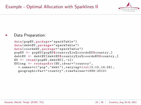
Example - Optimal Allocation with Sparklines II

I Data Preparation:

data(popEU ,package="sparkTable")

data(debtEU ,package="sparkTable")

data(coordsEU ,package="sparkTable")

popEU <- popEU[popEU$country%in%coordsEU$country ,]

debtEU <- debtEU[debtEU$country%in%coordsEU$country ,]

EU <- cbind(popEU ,debtEU [,-1])

EUlong <- reshapeExt(EU,idvar="country",

v.names=c("pop","debt"),varying=list (2:13 ,14:25) ,

geographicVar="country",timeValues =1999:2010)




Example - Optimal Allocation with Sparklines III

I Defining the content and generating the geoTable object:

l <- newSparkLine ()

l <- setParameter(l, ' lineWidth ' , 2.5)

content <- list(function(x){"Population:"},l,

function(x){"Debt:"},l)

varType <- c(rep("pop" ,2),rep("debt" ,2))

xGeoEU <- newGeoTable(EUlong , content , varType ,

geographicVar="country",geographicInfo=coordsEU)

I Writing the geoTable in a tex-File:

plotGeoTable(xGeoEU , outputType="tex",

graphNames="outEU",filename="testEUT",

transpose=TRUE)




Outline

I Package sparkTable is at an early stage of development

I some improvements (e.g. additional customization options,additional graphs) are already planned to be implemented

I User-feedback is (of course) very welcome
