Alcoholic Beverages and Cigarettes: Complements or Substitutes?

A Pseudo Panel Approach

Aycan Koksal, Michael Wohlgenant

Department of Agricultural and Resource Economics

North Carolina State University, Raleigh, NC, 27695

Contact: Aycan Koksal at akoksal@ncsu.edu

Selected Paper prepared for presentation at the Southern Agricultural Economics Association

Annual Meeting, Corpus Christi, TX, February 5-8, 2011

Copyright 2011 by Aycan Koksal and Michael Wohlgenant. All rights reserved. Readers may make

verbatim copies of this document for non-commercial purposes by any means, provided that this

copyright notice appears on all such copies.

2

Abstract

In this paper, using pseudo panel data we analyze the relation between cigarette and alcoholic beverage

consumption within the rational addiction framework. We believe that pseudo panel data approach has

many advantages compared to aggregate and panel data models. We found that alcoholic beverages are

complements for cigarettes, while it is not the same the other way around. Moreover, we found that

alcohol is a gateway for cigarette which further supports our conclusion concerning the reinforcing effect

of alcohol consumption on cigarette consumption. We believe that drinking works as a trigger for

smoking especially in social settings like bars while it is also possible (although less likely) that people

who want to cut cigarette consumption might increase alcohol consumption to cope with resulting

stress, which induces an asymmetry in cross price elasticities. However we point out that the

complementarity relationship is much stronger and significant. Policy implications for the results are

explained and the direction for further research is addressed.

Key words: cigarette, alcohol, rational addiction, pseudo panel

3

1. Introduction

The adverse health effects of cigarettes and alcoholic beverages have long been recognized. There

are also negative externalities associated with the consumption of these two particular goods. The adverse

health effects of passive smoking and the fatalities resulting from drunk driving have made these two

goods the prime targets of excise taxation in many countries.

With the harmful addictive substances, the benefit comes now, in the form of the pleasure, and

the cost, in terms of damage to the individual’s health, comes later. Then, one can argue that people who

consume harmful addictive substances are likely to discount the future more compared to other people. If

being a smoker is, in part, a matter of discounting the future more heavily, smokers should display more

present-oriented behavior in a whole range of activities and are more likely to drink compared to other

people. If cigarette and alcohol are related in consumption, the information on the way in which they are

related may allow a better coordination of the public policies concerning these goods.

When modeling the demand for addictive (habit-forming) goods like cigarettes and alcoholic

beverages, one of the most popular frameworks is the rational addiction model proposed by Becker and

Murphy (1988). Becker and Murphy (1988) claim that addictions to harmful substances are still rational

as the decision involve forward-looking maximization of utility. In their theory of rational addiction,

"rational" means that individuals maximize utility over time, and a good is addictive (habit forming) if

increases in past consumption increase current consumption. The rational addiction model differs from

the myopic models of addictive behavior in the sense that it does not only account for habit formation, but

it also involves rationality. In myopic models, past consumption stimulates current consumption, but

individuals ignore the future when making consumption decisions. In the rational addiction model, the

past and anticipated future consumption both affect current consumption positively.

The rational addiction model has been previously applied to both cigarette consumption (e.g.

Chaloupka, 1991; Becker et al., 1994; Jones and Labeaga, 2003) and alcohol consumption (e.g. Grossman

et al, 1998; Waters and Sloan, 1995). Bask and Melkersson (2004) extended the rational addiction model

to allow for multi-commodity addictions and estimated the demand for cigarettes and alcohol using

4

aggregate time series data. However, to the best of our knowledge, nobody has used individual/household

level data to analyze the relation between cigarette and alcohol consumptions in a rational addiction

framework.

Aggregate data fail to provide detailed insights into individual behavior. On the other hand, while

panel surveys can be used to model the dynamics of individual behavior, they generally span short time

periods and are subject to attrition bias. Thus we employ a pseudo panel data approach in this study.

While the pseudo panel is disaggregated enough, it has main advantages compared with panel data:

It avoids the attrition problem that many panel surveys suffer from.

There may be less bias due to measurement error problems as we are typically working with a

group average.

It eliminates the econometric difficulties due to censoring.

Using 2002-2008 Consumer Expenditure Diary Survey Data by Bureau of Labor Statistics, we

construct a pseudo panel data that follows a cohort for 28 quarters. Then at the cohort level, we estimate

dynamic demand models for cigarettes and alcoholic beverages.

The rest of this paper is organized as follows. Section 2 introduces the rational addiction model

and the theoretical framework for two addictive consumption goods. Section 3 gives a discussion of the

data set used. Section 4 explains the pseudo panel approach. Section 5 presents results. Section 6 explains

policy implications. Section 7 concludes the study, and discusses the direction for future research on the

issue.

2. Theoretical Model

A consumer is said to be addicted to a consumption good, if an increase in past consumption

increases current consumption. Studies of harmful addictions have usually found reinforcement and

tolerance. Tolerance means that the satisfaction from a given consumption level of a good is lower when

past consumption is higher. Reinforcement, on the other hand, means that an increase in the past

5

consumption increases the craving for current consumption. Reinforcement implies that consumption of

the same good at different time periods are complements. Since rational consumers also consider the

future negative consequences of harmful behavior, the reinforcement effect should be high enough in

order to justify current consumption of harmful addictive goods.

Following Bask and Melkersson (2004), we assume:

(1)

where and are the quantities of cigarettes and alcohol consumed by consumer i in period t;

and are the habit stocks of cigarettes and alcoholic beverages in period t respectively;

is the consumption of a non-addictive composite commodity in period t.

We assume a strictly concave utility function. The marginal utility derived from each good is

assumed to be positive ( i.e., , and ; concavity implies , and

). Following rational addiction literature, we assume that habit stocks of harmful substances

affect current utility negatively due to their adverse health effects ( i.e. <0 and ; concavity

implies and ).

Reinforcement implies and . Smoking and drinking are assumed to have no

effect on the marginal utility derived from the consumption of the composite commodity ( i.e.

).

If the two addictive goods are substitutes, < 0 ; if they are complements When the

cigarette consumption does not depend on the level of alcohol consumption .

The intertemporal budget constraint is

where with r being the discount rate, and

are prices of cigarettes and alcoholic

beverages respectively, is the present value of wealth. As in previous studies, we assume that the

discount rate is equal to the interest rate. The composite commodity, N, is taken as numeraire.

6

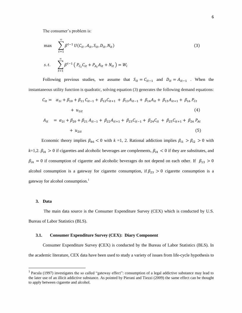
The consumer’s problem is:

Following previous studies, we assume that and . When the

instantaneous utility function is quadratic, solving equation (3) generates the following demand equations:

Economic theory implies with k =1, 2. Rational addiction implies with

k=1,2. if cigarettes and alcoholic beverages are complements, if they are substitutes, and

if consumption of cigarette and alcoholic beverages do not depend on each other. If

alcohol consumption is a gateway for cigarette consumption, if cigarette consumption is a

gateway for alcohol consumption.1

3. Data

The main data source is the Consumer Expenditure Survey (CEX) which is conducted by U.S.

Bureau of Labor Statistics (BLS).

3.1. Consumer Expenditure Survey (CEX): Diary Component

Consumer Expenditure Survey (CEX) is conducted by the Bureau of Labor Statistics (BLS). In

the academic literature, CEX data have been used to study a variety of issues from life-cycle hypothesis to

1 Pacula (1997) investigates the so called “gateway effect”: consumption of a legal addictive substance may lead to

the later use of an illicit addictive substance. As pointed by Pierani and Tiezzi (2009) the same effect can be thought

to apply between cigarette and alcohol.

7

consumer demand (e.g. Nicol, 2003; Villaverde and Krueger, 2007). The CEX consists of a Diary survey

and an Interview survey. Diary component is used in this study. The Diary component is completed by

the consumer units (CUs) for two consecutive one-week periods. The survey is designed to constitute a

representative sample of the U.S. population in each quarter. The data contains information on CU

demographic characteristics and expenditures. The list and the definitions of the demographic variables

used in this study are given in Appendix A. The alcoholic beverage and tobacco expenditures, together

with price variables, are used to calculate the consumption levels of alcoholic beverages and cigarettes

(i.e. cigarette consumption= cigarette expenditure/ cigarette price).

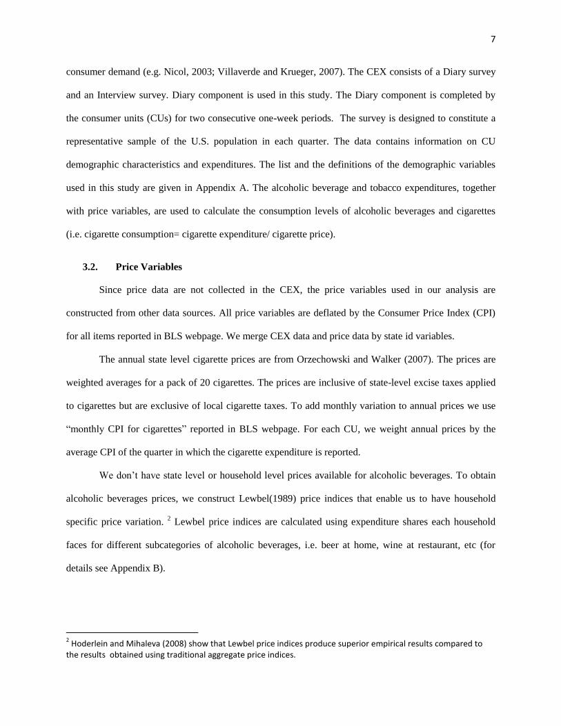
3.2. Price Variables

Since price data are not collected in the CEX, the price variables used in our analysis are

constructed from other data sources. All price variables are deflated by the Consumer Price Index (CPI)

for all items reported in BLS webpage. We merge CEX data and price data by state id variables.

The annual state level cigarette prices are from Orzechowski and Walker (2007). The prices are

weighted averages for a pack of 20 cigarettes. The prices are inclusive of state-level excise taxes applied

to cigarettes but are exclusive of local cigarette taxes. To add monthly variation to annual prices we use

“monthly CPI for cigarettes” reported in BLS webpage. For each CU, we weight annual prices by the

average CPI of the quarter in which the cigarette expenditure is reported.

We don’t have state level or household level prices available for alcoholic beverages. To obtain

alcoholic beverages prices, we construct Lewbel(1989) price indices that enable us to have household

specific price variation. 2 Lewbel price indices are calculated using expenditure shares each household

faces for different subcategories of alcoholic beverages, i.e. beer at home, wine at restaurant, etc (for

details see Appendix B).

2 Hoderlein and Mihaleva (2008) show that Lewbel price indices produce superior empirical results compared to

the results obtained using traditional aggregate price indices.

8

3.3. Sample Selection Criteria

In CEX data, Census Bureau suppresses the value of the variable, STATE, which identifies the

state of residence, for some observations to meet the Census Disclosure Review Board’s criterion that the

smallest geographically identifiable area have a population of at least 100,000. On approximately 17

percent of the records on the FMLY files the STATE variable is blank and approximately 4 percent of

STATE codes are replaced with codes of states other than the state where the CU resides. Because we use

STATE information to match CU’s with state level cigarette prices, the observations with missing and

recoded STATE variables are dropped.

4. Methodology

The advantages of using panel data to estimate models of individual behavior have been widely

stressed in the literature. However, individual panel data generally span short time periods, suffer from

measurement error and are subject to attrition bias. In order to avoid these problems, Deaton (1985)

suggested pseudo panel data approach as an alternative way to estimate models of individual behavior.

The pseudo-panel approach is a relatively new econometric method for estimating dynamic

demand models. It is based on grouping individuals into cohorts and then treating cohort averages as

observations in a panel. It enables us to follow cohorts of individuals over repeated cross-sectional

surveys. Because repeated cross-sectional surveys are typically over longer time-periods than true panels,

pseudo panel allows us to estimate models over longer time periods. Moreover, averaging within cohorts

eliminates individual-level measurement error.

In pseudo-panel analysis, because cohorts are followed over time, they are constructed based on

characteristics that are time invariant, such as geographic region, birth year or the education level of the

reference person. When we allocate individuals into cohorts, we face a trade-off between the number of

cohorts and the number of individuals within cohorts. If individuals are allocated to a large number of

cohorts, there will be a few observations remained in the cohorts which might induce biased estimators.

9

On the other hand, if a few number of cohorts is chosen to have a large number of observations per

cohort, individuals within a cohort might be heterogeneous, which might cause inefficiency. Thus, the

challenge in constructing a pseudo panel is to find the optimal choice between the numbers of cohorts,

and the number of individuals within cohorts. Ideally the optimal choice should minimize the

heterogeneity within each cohort but maximize the heterogeneity among them. In that case, pseudo-panels

lead to consistent and efficient estimators without the problems associated with true panels.

In most of the applied pseudo-panel studies, the sample is divided into small number of cohorts

with a large number of observations in each (i.e. Browning et al., 1985; Blundell et al., 1994; Propper et

al.,2001). Verbeek and Nijman (1992) showed that when cohorts contain at least 100 individuals and the

time variation in the cohort means is sufficiently large, the bias in the standard fixed effects estimator will

be small and can be ignored. This is the approach we take in this study.

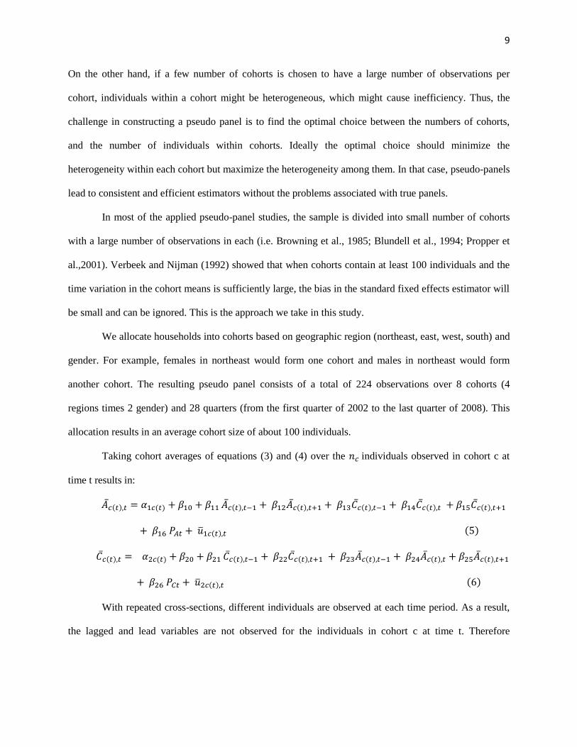
We allocate households into cohorts based on geographic region (northeast, east, west, south) and

gender. For example, females in northeast would form one cohort and males in northeast would form

another cohort. The resulting pseudo panel consists of a total of 224 observations over 8 cohorts (4

regions times 2 gender) and 28 quarters (from the first quarter of 2002 to the last quarter of 2008). This

allocation results in an average cohort size of about 100 individuals.

Taking cohort averages of equations (3) and (4) over the individuals observed in cohort c at

time t results in:

With repeated cross-sections, different individuals are observed at each time period. As a result,

the lagged and lead variables are not observed for the individuals in cohort c at time t. Therefore

10

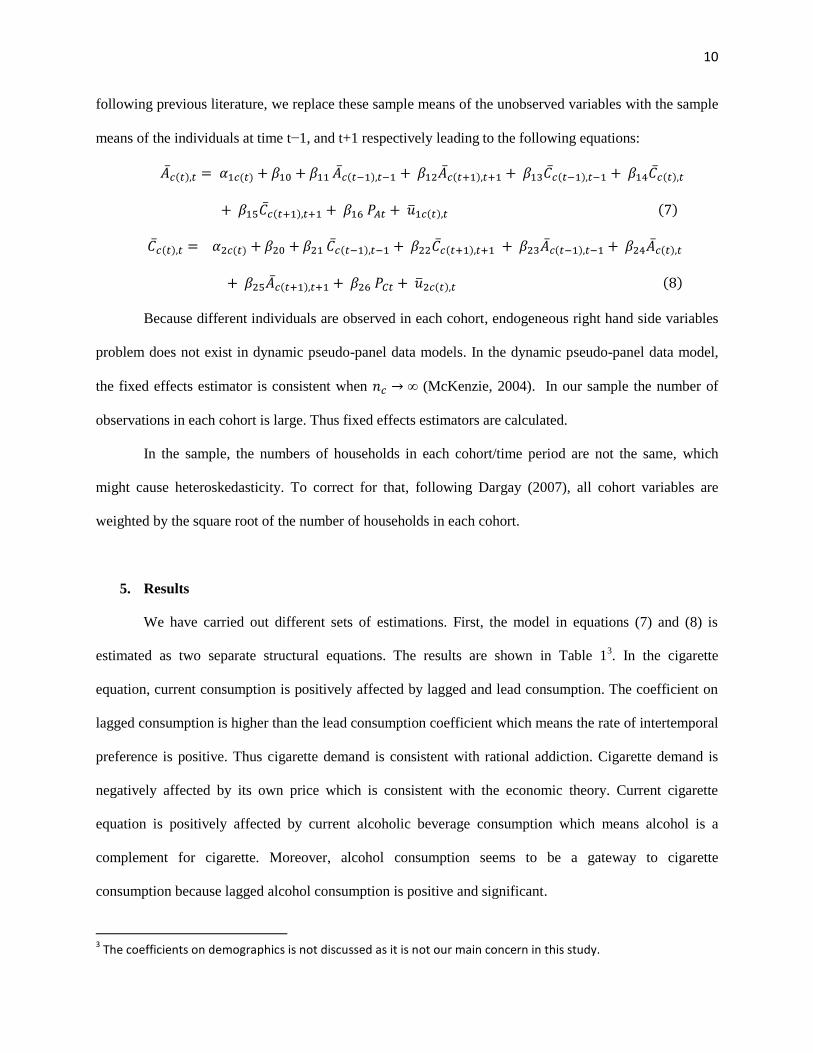
following previous literature, we replace these sample means of the unobserved variables with the sample

means of the individuals at time t−1, and t+1 respectively leading to the following equations:

Because different individuals are observed in each cohort, endogeneous right hand side variables

problem does not exist in dynamic pseudo-panel data models. In the dynamic pseudo-panel data model,

the fixed effects estimator is consistent when (McKenzie, 2004). In our sample the number of

observations in each cohort is large. Thus fixed effects estimators are calculated.

In the sample, the numbers of households in each cohort/time period are not the same, which

might cause heteroskedasticity. To correct for that, following Dargay (2007), all cohort variables are

weighted by the square root of the number of households in each cohort.

5. Results

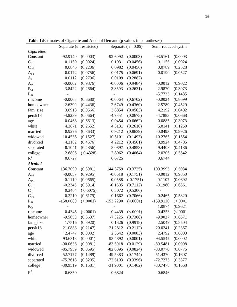
We have carried out different sets of estimations. First, the model in equations (7) and (8) is

estimated as two separate structural equations. The results are shown in Table 13. In the cigarette

equation, current consumption is positively affected by lagged and lead consumption. The coefficient on

lagged consumption is higher than the lead consumption coefficient which means the rate of intertemporal

preference is positive. Thus cigarette demand is consistent with rational addiction. Cigarette demand is

negatively affected by its own price which is consistent with the economic theory. Current cigarette

equation is positively affected by current alcoholic beverage consumption which means alcohol is a

complement for cigarette. Moreover, alcohol consumption seems to be a gateway to cigarette

consumption because lagged alcohol consumption is positive and significant.

3 The coefficients on demographics is not discussed as it is not our main concern in this study.

11

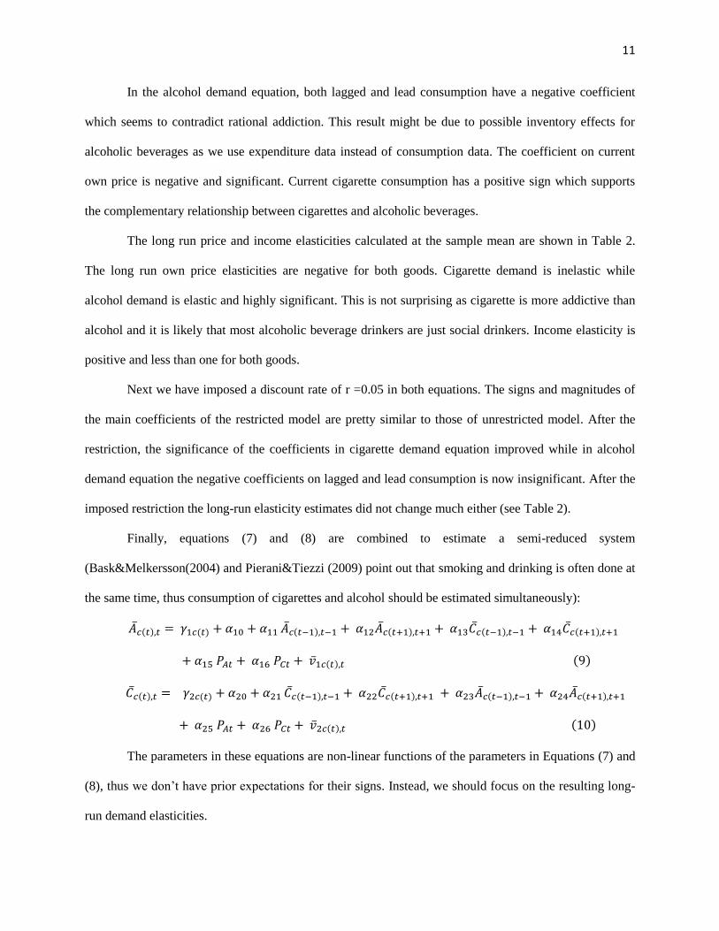
In the alcohol demand equation, both lagged and lead consumption have a negative coefficient

which seems to contradict rational addiction. This result might be due to possible inventory effects for

alcoholic beverages as we use expenditure data instead of consumption data. The coefficient on current

own price is negative and significant. Current cigarette consumption has a positive sign which supports

the complementary relationship between cigarettes and alcoholic beverages.

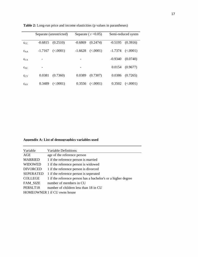
The long run price and income elasticities calculated at the sample mean are shown in Table 2.

The long run own price elasticities are negative for both goods. Cigarette demand is inelastic while

alcohol demand is elastic and highly significant. This is not surprising as cigarette is more addictive than

alcohol and it is likely that most alcoholic beverage drinkers are just social drinkers. Income elasticity is

positive and less than one for both goods.

Next we have imposed a discount rate of r =0.05 in both equations. The signs and magnitudes of

the main coefficients of the restricted model are pretty similar to those of unrestricted model. After the

restriction, the significance of the coefficients in cigarette demand equation improved while in alcohol

demand equation the negative coefficients on lagged and lead consumption is now insignificant. After the

imposed restriction the long-run elasticity estimates did not change much either (see Table 2).

Finally, equations (7) and (8) are combined to estimate a semi-reduced system

(Bask&Melkersson(2004) and Pierani&Tiezzi (2009) point out that smoking and drinking is often done at

the same time, thus consumption of cigarettes and alcohol should be estimated simultaneously):

The parameters in these equations are non-linear functions of the parameters in Equations (7) and

(8), thus we don’t have prior expectations for their signs. Instead, we should focus on the resulting long-

run demand elasticities.

12

The results for own price elasticities and income elasticities are similar to the ones that we

obtained using two separate equations (see Table 2). The cross price elasticity of cigarette with respect to

alcohol price is negative and significant, while the cross price elasticity of alcohol with respect to

cigarette price is positive, small in magnitude and insignificant. This suggests that smokers respond to

alcohol prices while drinkers do not respond much (or at all) to cigarette prices. The intuition for that is an

important number of smokers are just social smokers who smoke when they drink and socialize. Thus a

change in alcohol prices is likely to influence their alcohol consumption and thus their cigarette

consumption as cigarettes and alcohol are complements for them. In addition we found that alcohol is a

gateway for cigarette which further reinforces our conclusion concerning the effect of alcohol

consumption on cigarette consumption.

Decker and Schwartz (2000) found similar cross price elasticities in an analysis of smoking and

drinking participation; i.e. cross price elasticity is negative for cigarette demand while it is positive for

alcohol demand. They view this as potential evidence of different behavioral processes determining

smoking and drinking behavior:

“While investigating the underlying behavioral processes determining

drinking and smoking decisions is outside the scope of this paper, the

measured elasticities are consistent with the following scenario. Increases in

beer prices lead some to stop drinking (say, to not go to a bar after work)

and as the "situational cue" for social smoking is eliminated, their smoking

participation also declines. The effect of cigarette price on drinking

participation follows a different scenario. Increases in cigarette prices lead

some to quit smoking, inducing greater stress among the now-former

smokers who turn to alcohol consumption for its palliative effects.” (Decker

and Schwartz, 2000, p.16)

We agree with the view that cigarettes and alcohol are complements especially in social settings

like bars, etc. while they might be substitutes in certain cases where the individual sees both cigarettes

13

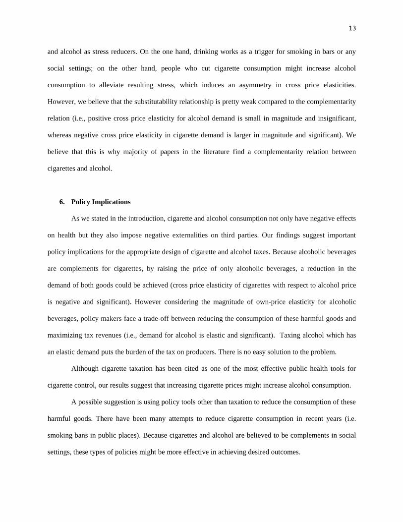
and alcohol as stress reducers. On the one hand, drinking works as a trigger for smoking in bars or any

social settings; on the other hand, people who cut cigarette consumption might increase alcohol

consumption to alleviate resulting stress, which induces an asymmetry in cross price elasticities.

However, we believe that the substitutability relationship is pretty weak compared to the complementarity

relation (i.e., positive cross price elasticity for alcohol demand is small in magnitude and insignificant,

whereas negative cross price elasticity in cigarette demand is larger in magnitude and significant). We

believe that this is why majority of papers in the literature find a complementarity relation between

cigarettes and alcohol.

6. Policy Implications

As we stated in the introduction, cigarette and alcohol consumption not only have negative effects

on health but they also impose negative externalities on third parties. Our findings suggest important

policy implications for the appropriate design of cigarette and alcohol taxes. Because alcoholic beverages

are complements for cigarettes, by raising the price of only alcoholic beverages, a reduction in the

demand of both goods could be achieved (cross price elasticity of cigarettes with respect to alcohol price

is negative and significant). However considering the magnitude of own-price elasticity for alcoholic

beverages, policy makers face a trade-off between reducing the consumption of these harmful goods and

maximizing tax revenues (i.e., demand for alcohol is elastic and significant). Taxing alcohol which has

an elastic demand puts the burden of the tax on producers. There is no easy solution to the problem.

Although cigarette taxation has been cited as one of the most effective public health tools for

cigarette control, our results suggest that increasing cigarette prices might increase alcohol consumption.

A possible suggestion is using policy tools other than taxation to reduce the consumption of these

harmful goods. There have been many attempts to reduce cigarette consumption in recent years (i.e.

smoking bans in public places). Because cigarettes and alcohol are believed to be complements in social

settings, these types of policies might be more effective in achieving desired outcomes.

14

7. Conclusion

It has long been recognized that cigarette and alcohol not only have adverse health effects, but

also negative externalities imposed on third parties. For that reason these two goods became the prime

targets of excise taxation in many countries.

One can argue that people who consume harmful addictive substances like cigarettes and alcohol

are likely to discount the future more compared to other people. Thus, if being a smoker is, in part, a

matter of discounting the future more heavily, smokers should display more present-oriented behavior in

a whole range of activities and are more likely to drink compared to other people. If cigarettes and

alcoholic beverages are related in consumption, the information about how they are related may permit

better coordination of public policies (e.g.,excise taxation) concerning these goods.

In this study, we analyze the relation between cigarette and alcoholic beverage consumption

within the rational addiction framework. We use pseudo panel data approach which has many advantages

compared to aggregate and panel data models. We found that alcohol is a complement for cigarette, and

smokers respond to rising alcohol prices, while it is not the same the other way around. In addition we

found that alcohol is a gateway for cigarette. We believe that drinking works as a trigger for smoking

especially in social setting like bars, etc. On the other hand, it is also possible (although less likely) that

individuals who want to cut cigarette consumption might increase alcohol consumption to relieve

resulting stress. This scenario is consistent with the observed asymmetry in cross price elasticities.

However as we point out the complementarity relationship is stronger and significant.

Because alcoholic beverages are complements for cigarettes, increasing only alcoholic beverages

prices would decrease the demand for both goods. However considering that alcohol demand is pretty

elastic, policy makers face a trade-off between reducing the consumption of these harmful goods and

maximizing tax revenues. Moreover, although cigarette taxation has been cited as an effective public

policy tool for cigarette control, our results suggest that increasing cigarette prices might lead to increased

alcohol consumption.

15

A possible resolution of this conflict is to use other policy tools to reduce the consumption of

these addictive goods. There have been many public policy attempts which aimed reducing cigarette

consumption in recent years (i.e., smoking bans in public places). As we believe that cigarettes and

alcohol are complements in social settings, policies such as smoking bans in bars,etc might be more

effective in achieving the desired outcomes. New insights can be gained by analyzing the effects of these

policies on consumption of cigarettes and alcohol.

16

Table 1:Estimates of Cigarette and Alcohol Demand (p values in parantheses)

Separate (unrestricted) Separate ( r =0.05) Semi-reduced systm

Cigarettes

Constant

-92.9140 (0.0003)

-92.6092 (0.0003)

-93.5161 (0.0003

) Ct-1

0.1159 (0.0924)

0.1031 (0.0456)

0.1156 (0.0924

) Ct+1

0.0845 (0.2206)

0.0982 (0.0456)

0.0789 (0.2528

) At-1

0.0172 (0.0756)

0.0175 (0.0691)

0.0190 (0.0527

) At

0.0112 (0.2796)

0.0109 (0.2882)

-

At+1

-0.0002 (0.9876)

-0.0006 (0.9484)

-0.0012 (0.9022

) PCt

-3.8422 (0.2664)

-3.8593 (0.2631)

-2.9870 (0.3973

) PAt

-

-

-5.7733 (0.1435

) rincome

-0.0065 (0.6680)

-0.0064 (0.6702)

-0.0024 (0.8699

) homeowner

-2.6390 (0.4436)

-2.6749 (0.4360)

-2.5789 (0.4529

) fam_size

3.8918 (0.0566)

3.8854 (0.0563)

4.2192 (0.0402

) perslt18

-4.8239 (0.0664)

-4.7851 (0.0675)

-4.7883 (0.0668

) age

0.0463 (0.6613)

0.0454 (0.6662)

0.0885 (0.3973

) white

4.2871 (0.2652)

4.3131 (0.2610)

5.8141 (0.1250

) married

0.9276 (0.8633)

0.9212 (0.8639)

-0.0493 (0.9926

) widowed

10.4535 (0.1527)

10.5101 (0.1493)

10.2765 (0.1554

) divorced

4.2182 (0.4576)

4.2212 (0.4561)

3.9924 (0.4785

) separated

8.1041 (0.4856)

8.0897 (0.4853)

9.4403 (0.4186

) college

2.6805 ( 0.4328)

2.8062 (0.4064)

2.0206 (0.5542

) R

2

0.6727

0.6725

0.6744

Alcohol

Constant

136.7090 (0.3981)

144.3759 (0.3725)

109.3995 (0.5034

) At-1

-0.0057 (0.9295)

-0.0618 (0.1751)

-0.0012 (0.9850

) At+1

-0.1110 (0.0665)

-0.0588 ( 0.1751)

-0.1107 (0.0692

) Ct-1

-0.2345 (0.5914)

-0.1605 (0.7112)

-0.1980 (0.6561

) Ct

0.2464 ( 0.6075)

0.3072 (0.5206)

-

Ct+1

0.2210 (0.6179)

0.1662 (0.7066)

0.2465 (0.5820

) PAt

-158.0080 (<.0001)

-153.2290 (<.0001)

-159.9120 (<.0001

) PCt

-

-

1.0874 (0.9621

) rincome

0.4345 (<.0001)

0.4439 (<.0001)

0.4353 (<.0001

) homeowner

-9.5653 (0.6637)

-7.3225 (0.7388)

-9.9027 (0.6571

) fam_size

1.7516 (0.8920)

0.1326 (0.9918)

2.5049 (0.8504

) perslt18

21.0883 (0.2147)

21.2812 (0.2112)

20.0241 (0.2367

) age

2.4747 (0.0002)

2.3542 (0.0003)

2.4792 (0.0003

) white

93.6313 (0.0001)

93.4892 (0.0001)

94.5547 (0.0002

) married

-90.0636 (0.0081)

-83.5918 (0.0129)

-89.5481 (0.0098

) widowed

-85.7959 (0.0695)

-82.0095 (0.0824)

-83.0770 (0.0775

) divorced

-52.7177 (0.1489)

-49.5383 (0.1744)

-51.4370 (0.1607

) separated

-75.3618 (0.3205)

-72.5103 (0.3396)

-72.7273 (0.3377

) college

-30.9519 (0.1581)

-31.9001 (0.1462)

-30.7478 (0.1668

) R

2

0.6850

0.6824

0.6846

17

Table 2: Long-run price and income elasticities (p values in parantheses)

Separate (unrestricted)

Separate ( r =0.05)

Semi-reduced systm

εCC

-0.6815 (0.2510)

-0.6869 (0.2474)

-0.5195 (0.3916)

εAA

-1.7167 (<.0001)

-1.6628 (<.0001)

-1.7374 (<.0001)

εCA

-

-

-0.9340 (0.0740)

εAC

-

-

0.0154 (0.9677)

εCY

0.0381 (0.7360)

0.0389 (0.7307)

0.0386 (0.7265)

εAY

0.3489 (<.0001)

0.3556 (<.0001)

0.3502 (<.0001)

Appendix A: List of demographics variables used

Variable Variable Definitions

AGE age of the reference person

MARRIED 1 if the reference person is married

WIDOWED 1 if the reference person is widowed

DIVORCED 1 if the reference person is divorced

SEPERATED 1 if the reference person is seperated

COLLEGE 1 if the reference person has a bachelor's or a higher degree

FAM_SIZE number of members in CU

PERSLT18 number of children less than 18 in CU

HOMEOWNER 1 if CU owns house

18

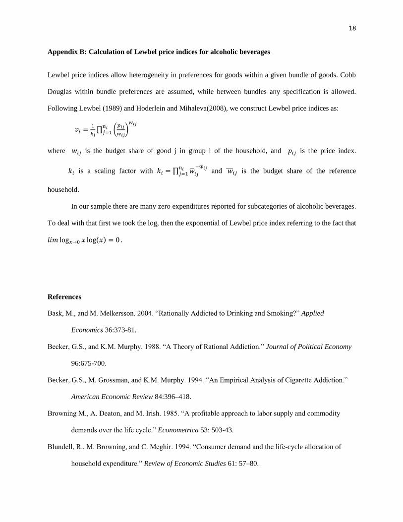
Appendix B: Calculation of Lewbel price indices for alcoholic beverages

Lewbel price indices allow heterogeneity in preferences for goods within a given bundle of goods. Cobb

Douglas within bundle preferences are assumed, while between bundles any specification is allowed.

Following Lewbel (1989) and Hoderlein and Mihaleva(2008), we construct Lewbel price indices as:

where is the budget share of good j in group i of the household, and is the price index.

is a scaling factor with

and is the budget share of the reference

household.

In our sample there are many zero expenditures reported for subcategories of alcoholic beverages.

To deal with that first we took the log, then the exponential of Lewbel price index referring to the fact that

References

Bask, M., and M. Melkersson. 2004. “Rationally Addicted to Drinking and Smoking?” Applied

Economics 36:373-81.

Becker, G.S., and K.M. Murphy. 1988. “A Theory of Rational Addiction.” Journal of Political Economy

96:675-700.

Becker, G.S., M. Grossman, and K.M. Murphy. 1994. “An Empirical Analysis of Cigarette Addiction.”

American Economic Review 84:396–418.

Browning M., A. Deaton, and M. Irish. 1985. “A profitable approach to labor supply and commodity

demands over the life cycle.” Econometrica 53: 503-43.

Blundell, R., M. Browning, and C. Meghir. 1994. “Consumer demand and the life-cycle allocation of

household expenditure.” Review of Economic Studies 61: 57–80.

19

Chaloupka, F. J. 1991. “Rational Addictive Behavior and Cigarette Smoking.” Journal of Political

Economy 99:722–42.

Dargay, J. 2007. “The effect of prices and income on car travel in the UK” Transportation Research

Part A 41:949-60.

Deaton, A. 1985. “Panel data from time series of cross-sections.” Journal of Econometrics 30: 109-26.

Decker S.L., and A. E. Schwartz. 2000. “Cigarettes and Alcohol: Substitutes or Complements?”

NBERWorking Paper 7535

Grossman, M., F.J. Chaloupka, and I. Sirtalan. 1998. “An Empirical Analysis of Alcohol Addiction:

Results from the Monitoring the Future Panels.” Economic Inquiry 36:39–48.

Hoderlein, S., and S.Mihaleva. 2008. “Increasing the price variation in a repeated cross section.” Journal

of Econometrics 147:316-25.

Jones, A.M., and J.M. Labeaga. 2003. “Individual Heterogeneity and Censoring in Panel Data Estimates

of Tobacco Expenditure.” Journal of Applied Econometrics 18:157–77.

Lewbel, A., 1989. “Identification and estimation of equivalence scales under weak separability.” Review

of Economic Studies 56: 311_316.

McKenzie, D. J. 2004. “Asymptotic theory for heterogeneous dynamic pseudo-panels.” Journal of

Econometrics 120(2): 235-62.

Nicol, C.J. 2003. “Elasticities of demand for gasoline in Canada and the United States.” Energy

Economics 25:201–14.

Orzechowski and Walker, 2007. The Tax Burden on Tobacco-Historical Compilation. vol. 42. Arlington,

Virginia: Orzechowski and Walker Consulting.

Pacula, R. L. “Economic Modeling of the Gateway Effect” Health Economics 6:521-524.

Pierani, P., and S. Tiezzi. “Addiction and interaction between alcohol and tobacco consumption”

Empirical Economics 37:1-23

Propper, C., H. Rees and K. Green. “The Demand for Private Medical Insurance in the UK: A Cohort

Analysis” The Economic Journal 111:180-200.

20

Verbeek, M., and T. Nijman. 1992. “Can cohort data be treated as genuine panel data?” Empirical

Economics 17: 9–23.

Villaverde, J.F., and D. Krueger. 2007. “Consumption over the Life-Cycle: Facts from Consumer

Expenditure Survey Data.” The Review of Economics and Statistics 89:552-65.

Waters, T.M., and F.A. Sloan. 1995. “Why do People Drink? Tests of the Rational Addiction Model.”

Applied Economics 27: 727–36.