Embed Size (px)
Citation preview
Introduction Background Design Alcohol Savings Commitment Summary
Alcohol and Self-ControlA Field Experiment in India
Frank Schilbach
MIT
October 16, 2015
1 / 35
Introduction Background Design Alcohol Savings Commitment Summary
Alcohol consumption among the poor
• Heavy drinking is common among low-income males indeveloping countries.
• Harmful use of alcohol is a recognized global health issue.• Limited understanding of the economic aspects of alcohol
2 / 35
Introduction Background Design Alcohol Savings Commitment Summary
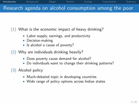
Research agenda on alcohol consumption among the poor
(1) What is the economic impact of heavy drinking?• Labor supply, earnings, and productivity• Decision-making• Is alcohol a cause of poverty?
(2) Why are individuals drinking heavily?• Does poverty cause demand for alcohol?• Do individuals want to change their drinking patterns?
(3) Alcohol policy• Much-debated topic in developing countries• Wide range of policy options across Indian states
3 / 35
Introduction Background Design Alcohol Savings Commitment Summary
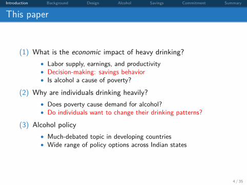
This paper
(1) What is the economic impact of heavy drinking?• Labor supply, earnings, and productivity• Decision-making: savings behavior• Is alcohol a cause of poverty?
(2) Why are individuals drinking heavily?• Does poverty cause demand for alcohol?• Do individuals want to change their drinking patterns?
(3) Alcohol policy• Much-debated topic in developing countries• Wide range of policy options across Indian states
4 / 35
Introduction Background Design Alcohol Savings Commitment Summary
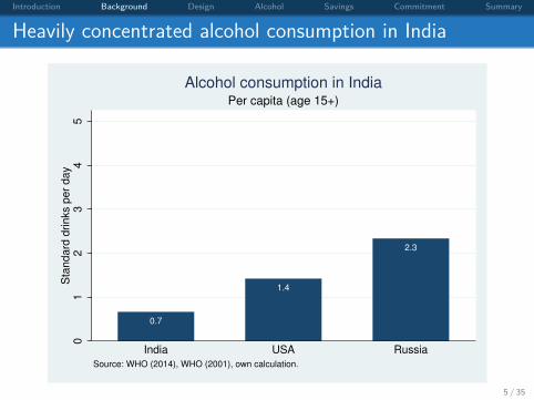
Heavily concentrated alcohol consumption in India
0.7
1.4
2.3
01
23
45
Sta
ndard
drinks p
er
day
India USA Russia
Source: WHO (2014), WHO (2001), own calculation.
Per capita (age 15+)
Alcohol consumption in India
5 / 35
Introduction Background Design Alcohol Savings Commitment Summary
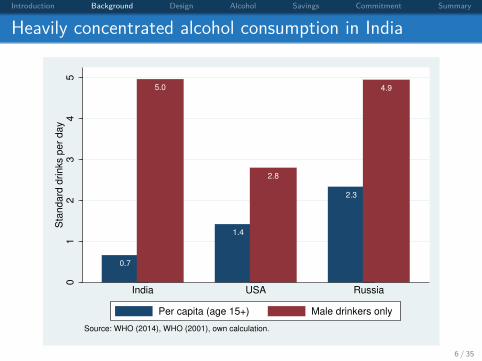
Heavily concentrated alcohol consumption in India
0.7
5.0
1.4
2.8
2.3
4.9
01
23
45
Sta
ndard
drinks p
er
day
India USA Russia
Source: WHO (2014), WHO (2001), own calculation.
Per capita (age 15+) Male drinkers only
6 / 35
Introduction Background Design Alcohol Savings Commitment Summary
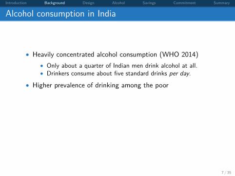
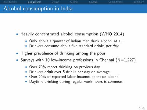
Alcohol consumption in India
• Heavily concentrated alcohol consumption (WHO 2014)• Only about a quarter of Indian men drink alcohol at all.• Drinkers consume about five standard drinks per day.
• Higher prevalence of drinking among the poor
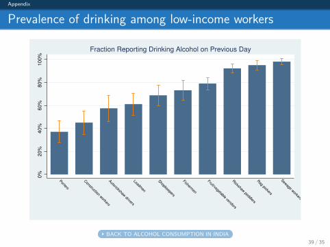
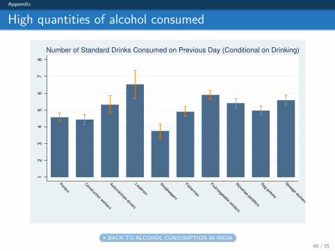
• Surveys with 10 low-income professions in Chennai (N=1,227)• Over 70% report drinking on previous day.• Drinkers drink over 5 drinks per day on average.• Over 20% of reported labor incomes spent on alcohol• Daytime drinking during regular work hours is common.
7 / 35
Introduction Background Design Alcohol Savings Commitment Summary
Alcohol consumption in India
• Heavily concentrated alcohol consumption (WHO 2014)• Only about a quarter of Indian men drink alcohol at all.• Drinkers consume about five standard drinks per day.
• Higher prevalence of drinking among the poor• Surveys with 10 low-income professions in Chennai (N=1,227)
• Over 70% report drinking on previous day.• Drinkers drink over 5 drinks per day on average.• Over 20% of reported labor incomes spent on alcohol• Daytime drinking during regular work hours is common.
7 / 35
Introduction Background Design Alcohol Savings Commitment Summary
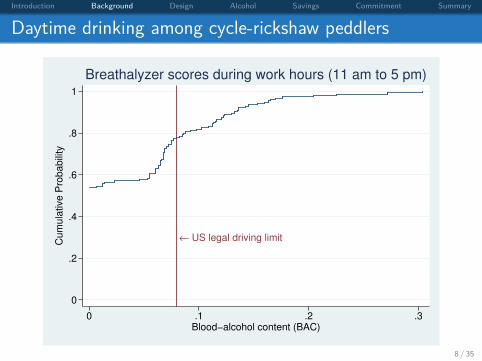
Daytime drinking among cycle-rickshaw peddlers
← US legal driving limit
0
.2
.4
.6
.8
1
Cum
ula
tive P
robabili
ty
0 .1 .2 .3Blood−alcohol content (BAC)
Breathalyzer scores during work hours (11 am to 5 pm)
8 / 35
Introduction Background Design Alcohol Savings Commitment Summary
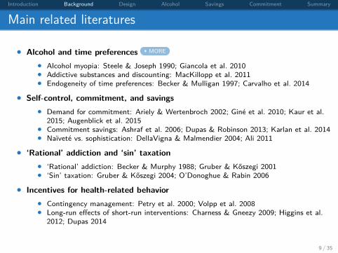
Main related literatures
• Alcohol and time preferences MORE
• Alcohol myopia: Steele & Joseph 1990; Giancola et al. 2010• Addictive substances and discounting: MacKillopp et al. 2011• Endogeneity of time preferences: Becker & Mulligan 1997; Carvalho et al. 2014
• Self-control, commitment, and savings• Demand for commitment: Ariely & Wertenbroch 2002; Gine et al. 2010; Kaur et al.
2015; Augenblick et al. 2015• Commitment savings: Ashraf et al. 2006; Dupas & Robinson 2013; Karlan et al. 2014• Naıvete vs. sophistication: DellaVigna & Malmendier 2004; Ali 2011
• ‘Rational’ addiction and ‘sin’ taxation• ‘Rational’ addiction: Becker & Murphy 1988; Gruber & Koszegi 2001• ‘Sin’ taxation: Gruber & Koszegi 2004; O’Donoghue & Rabin 2006
• Incentives for health-related behavior• Contingency management: Petry et al. 2000; Volpp et al. 2008• Long-run effects of short-run interventions: Charness & Gneezy 2009; Higgins et al.
2012; Dupas 2014
9 / 35
Introduction Background Design Alcohol Savings Commitment Summary
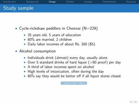
Study sample
• Cycle-rickshaw peddlers in Chennai (N=229)• 35 years old, 5 years of education• 80% are married, 2 children• Daily labor incomes of about Rs. 300 ($5)
• Alcohol consumption• Individuals drink (almost) every day, usually alone.• Over 5 standard drinks of hard liquor (>80 proof) per day• A third of labor incomes spent on alcohol• High levels of intoxication, often during the day• 80% say they would be better off if all liquor stores closed.
SELECTION TABLE
10 / 35
Introduction Background Design Alcohol Savings Commitment Summary
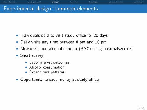
Experimental design: common elements
• Individuals paid to visit study office for 20 days• Daily visits any time between 6 pm and 10 pm• Measure blood-alcohol content (BAC) using breathalyzer test• Short survey
• Labor market outcomes• Alcohol consumption• Expenditure patterns
• Opportunity to save money at study office
11 / 35
Introduction Background Design Alcohol Savings Commitment Summary
Financial incentives for sobriety: treatment groups
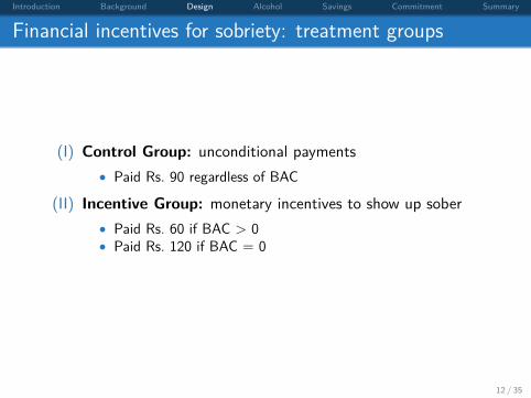
(I) Control Group: unconditional payments• Paid Rs. 90 regardless of BAC
(II) Incentive Group: monetary incentives to show up sober• Paid Rs. 60 if BAC > 0• Paid Rs. 120 if BAC = 0
12 / 35
Introduction Background Design Alcohol Savings Commitment Summary
Financial incentives for sobriety: treatment groups
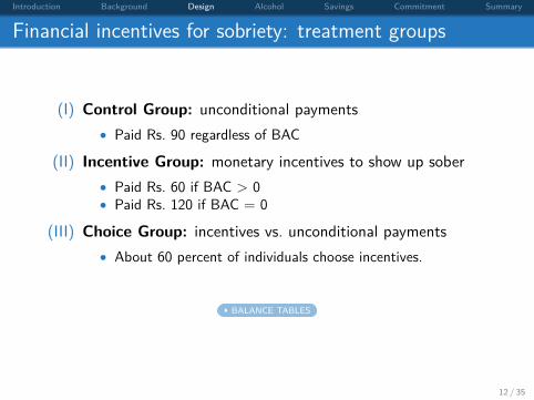
(I) Control Group: unconditional payments• Paid Rs. 90 regardless of BAC
(II) Incentive Group: monetary incentives to show up sober• Paid Rs. 60 if BAC > 0• Paid Rs. 120 if BAC = 0
(III) Choice Group: incentives vs. unconditional payments• About 60 percent of individuals choose incentives.
BALANCE TABLES
12 / 35
Introduction Background Design Alcohol Savings Commitment Summary
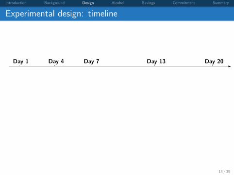
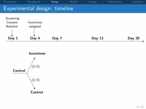
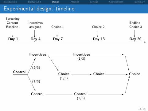
Experimental design: timeline
-Day 1 Day 4 Day 7 Day 13 Day 20
13 / 35
Introduction Background Design Alcohol Savings Commitment Summary
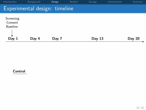
Experimental design: timeline
-Day 1 Day 4 Day 7 Day 13 Day 20?
BaselineConsentScreening
Control
13 / 35
Introduction Background Design Alcohol Savings Commitment Summary
Experimental design: timeline
-Day 1 Day 4 Day 7 Day 13 Day 20?
BaselineConsentScreening
?
Incentivesassigned
Control �����
AAAAU
Incentives
(2/3)
Control
(1/3)
13 / 35
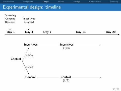
Introduction Background Design Alcohol Savings Commitment Summary
Experimental design: timeline
-Day 1 Day 4 Day 7 Day 13 Day 20?
BaselineConsentScreening
?
Incentivesassigned
Control �����
AAAAU
Incentives
(2/3)
Control
(1/3)
Incentives(1/3)
Control(1/3)
-
-
13 / 35
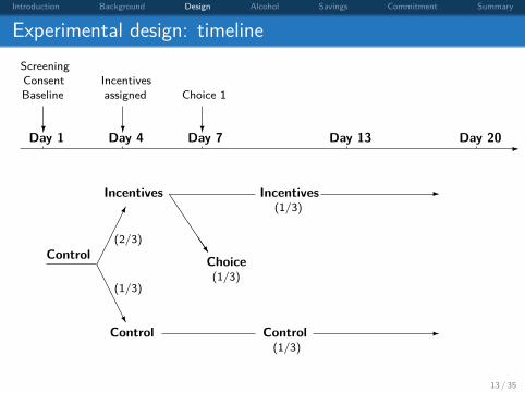
Introduction Background Design Alcohol Savings Commitment Summary
Experimental design: timeline
-Day 1 Day 4 Day 7 Day 13 Day 20?
BaselineConsentScreening
?
Incentivesassigned
?
Choice 1
Control �����
AAAAU
Incentives
(2/3)
Control
(1/3)
Incentives(1/3)J
JJJJ
Choice(1/3)
Control(1/3)
-
-
13 / 35
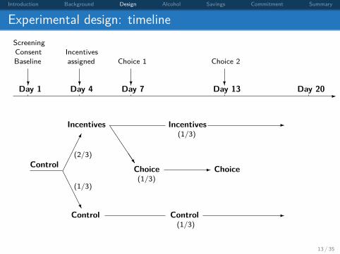
Introduction Background Design Alcohol Savings Commitment Summary
Experimental design: timeline
-Day 1 Day 4 Day 7 Day 13 Day 20?
BaselineConsentScreening
?
Incentivesassigned
?
Choice 1
?
Choice 2
Control �����
AAAAU
Incentives
(2/3)
Control
(1/3)
Incentives(1/3)J
JJJJ
Choice(1/3)
Control(1/3)
-
-
Choice-
13 / 35
Introduction Background Design Alcohol Savings Commitment Summary
Experimental design: timeline
-Day 1 Day 4 Day 7 Day 13 Day 20?
BaselineConsentScreening
?
Incentivesassigned
?
Choice 1
?
Choice 2
?
Choice 3Endline
Control �����
AAAAU
Incentives
(2/3)
Control
(1/3)
Incentives(1/3)J
JJJJ
Choice(1/3)
Control(1/3)
-
-
Choice-
CCCCW
-
������
Choice
13 / 35
Introduction Background Design Alcohol Savings Commitment Summary
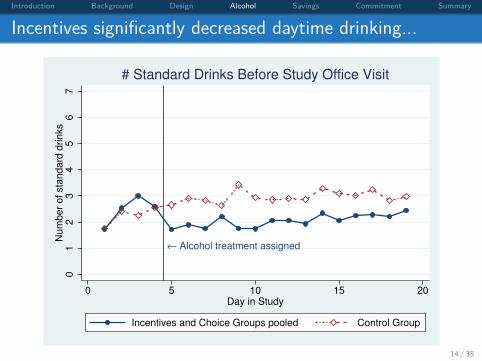
Incentives significantly decreased daytime drinking...
← Alcohol treatment assigned
01
23
45
67
Num
ber
of sta
ndard
drinks
0 5 10 15 20Day in Study
Incentives and Choice Groups pooled Control Group
# Standard Drinks Before Study Office Visit
14 / 35
Introduction Background Design Alcohol Savings Commitment Summary
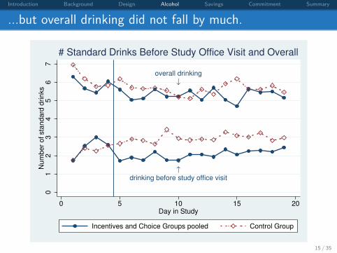
...but overall drinking did not fall by much.
↑drinking before study office visit
overall drinking
↓
01
23
45
67
Num
ber
of sta
ndard
drinks
0 5 10 15 20Day in Study
Incentives and Choice Groups pooled Control Group
# Standard Drinks Before Study Office Visit and Overall
15 / 35
Introduction Background Design Alcohol Savings Commitment Summary
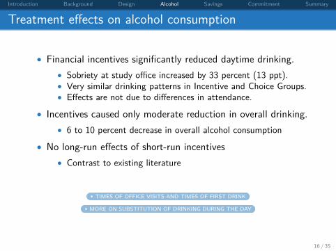
Treatment effects on alcohol consumption
• Financial incentives significantly reduced daytime drinking.• Sobriety at study office increased by 33 percent (13 ppt).• Very similar drinking patterns in Incentive and Choice Groups.• Effects are not due to differences in attendance.
• Incentives caused only moderate reduction in overall drinking.• 6 to 10 percent decrease in overall alcohol consumption
• No long-run effects of short-run incentives• Contrast to existing literature
TIMES OF OFFICE VISITS AND TIMES OF FIRST DRINK
MORE ON SUBSTITUTION OF DRINKING DURING THE DAY
16 / 35
Introduction Background Design Alcohol Savings Commitment Summary
No significant labor market effects of increased sobriety
• Does alcohol affect earnings?• Long literature at least since Irving Fisher (1926, 1928)• Many studies, not much identification (Cook & Moore 2000)• Little evidence from developing countries
• No significant effects on labor market outcomes in my study• Does not imply that alcohol has no labor market effects• First-stage estimates are significant, but not large.• Earnings are imprecisely measured.• Longer-run effects might be quite different (e.g. reputation).• Alcohol may help with physical pain at work.
17 / 35
Introduction Background Design Alcohol Savings Commitment Summary
Measuring the impact of increased sobriety on savings
• All subjects got personalized savings box at study office.• Could save up to Rs. 200 per day• Paid out entire amount plus matching contribution on day 20
• Cross-randomized matching contribution to benchmark effects• 10% vs. 20% of amount saved
• Cross-randomized commitment savings feature• Allowed to withdraw any day between 6 pm and 10 pm
vs. not allowed to withdraw until day 20• Commitment savings is imposed, no elicitation of demand for it
18 / 35
Introduction Background Design Alcohol Savings Commitment Summary
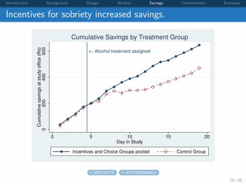
Incentives for sobriety increased savings.
← Alcohol treatment assigned
0200
400
600
Cum
ula
tive s
avin
gs a
t stu
dy o
ffic
e (
Rs)
0 5 10 15 20Day in Study
Incentives and Choice Groups pooled Control Group
Cumulative Savings by Treatment Group
DEPOSITS WITHDRAWALS
19 / 35
Introduction Background Design Alcohol Savings Commitment Summary
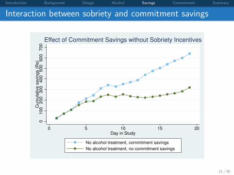
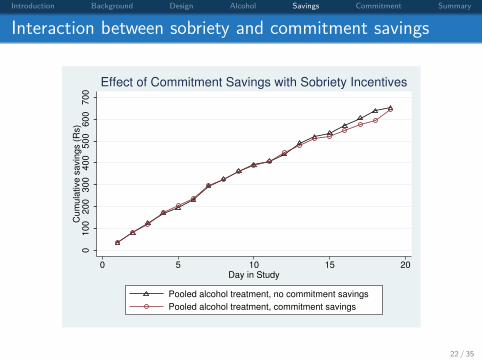
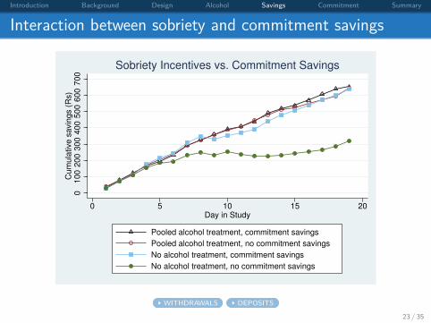
Interaction between sobriety and commitment savings
• Accounting exercise suggests increasing sobriety increasedsavings beyond mechanical effects.
• Commitment savings devices are designed to help overcometime inconsistency and self-control problems in saving.
• If alcohol affects savings by increasing myopia, then it shouldalso affect time inconsistency and self-control.
• Increasing sobriety should lower the effect of commitmentsavings, and vice versa.
20 / 35
Introduction Background Design Alcohol Savings Commitment Summary
Interaction between sobriety and commitment savings
0100
200
300
400
500
600
700
Cum
ula
tive s
avin
gs (
Rs)
0 5 10 15 20Day in Study
No alcohol treatment, commitment savings
No alcohol treatment, no commitment savings
Effect of Commitment Savings without Sobriety Incentives
21 / 35
Introduction Background Design Alcohol Savings Commitment Summary
Interaction between sobriety and commitment savings
0100
200
300
400
500
600
700
Cum
ula
tive s
avin
gs (
Rs)
0 5 10 15 20Day in Study
Pooled alcohol treatment, no commitment savings
Pooled alcohol treatment, commitment savings
Effect of Commitment Savings with Sobriety Incentives
22 / 35
Introduction Background Design Alcohol Savings Commitment Summary
Interaction between sobriety and commitment savings
0100
200
300
400
500
600
700
Cum
ula
tive s
avin
gs (
Rs)
0 5 10 15 20Day in Study
Pooled alcohol treatment, commitment savings
Pooled alcohol treatment, no commitment savings
No alcohol treatment, commitment savings
No alcohol treatment, no commitment savings
Sobriety Incentives vs. Commitment Savings
WITHDRAWALS DEPOSITS
23 / 35
Introduction Background Design Alcohol Savings Commitment Summary
Taking stock: impact of increasing sobriety
• No evidence of effects of sobriety on labor market outcomes• Increasing sobriety significantly raised savings.• Sobriety and commitment savings are substitutes in their
effects on savings.• Alcohol affects savings via changes in myopia. MODEL GRAPH
• Limited role of changes in sophistication
24 / 35
Introduction Background Design Alcohol Savings Commitment Summary
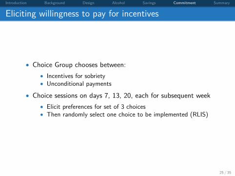
Eliciting willingness to pay for incentives
• Choice Group chooses between:• Incentives for sobriety• Unconditional payments
• Choice sessions on days 7, 13, 20, each for subsequent week• Elicit preferences for set of 3 choices• Then randomly select one choice to be implemented (RLIS)
25 / 35
Introduction Background Design Alcohol Savings Commitment Summary
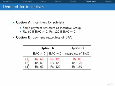
Demand for incentives
• Option A: incentives for sobriety• Same payment structure as Incentive Group• Rs. 60 if BAC > 0, Rs. 120 if BAC = 0
• Option B: payment regardless of BAC
Option A Option B
BAC > 0 BAC = 0 regardless of BAC
(1) Rs. 60 Rs. 120 Rs. 90(2) Rs. 60 Rs. 120 Rs. 120(3) Rs. 60 Rs. 120 Rs. 150
26 / 35
Introduction Background Design Alcohol Savings Commitment Summary
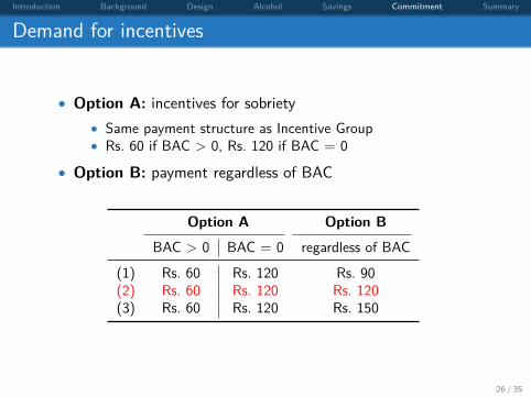
Demand for incentives
• Option A: incentives for sobriety• Same payment structure as Incentive Group• Rs. 60 if BAC > 0, Rs. 120 if BAC = 0
• Option B: payment regardless of BAC
Option A Option B
BAC > 0 BAC = 0 regardless of BAC
(1) Rs. 60 Rs. 120 Rs. 90(2) Rs. 60 Rs. 120 Rs. 120(3) Rs. 60 Rs. 120 Rs. 150
26 / 35
Introduction Background Design Alcohol Savings Commitment Summary
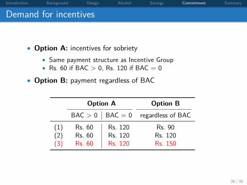
Demand for incentives
• Option A: incentives for sobriety• Same payment structure as Incentive Group• Rs. 60 if BAC > 0, Rs. 120 if BAC = 0
• Option B: payment regardless of BAC
Option A Option B
BAC > 0 BAC = 0 regardless of BAC
(1) Rs. 60 Rs. 120 Rs. 90(2) Rs. 60 Rs. 120 Rs. 120(3) Rs. 60 Rs. 120 Rs. 150
26 / 35
Introduction Background Design Alcohol Savings Commitment Summary
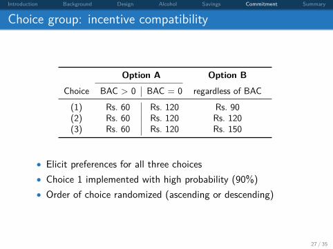
Choice group: incentive compatibility
Option A Option B
Choice BAC > 0 BAC = 0 regardless of BAC
(1) Rs. 60 Rs. 120 Rs. 90(2) Rs. 60 Rs. 120 Rs. 120(3) Rs. 60 Rs. 120 Rs. 150
• Elicit preferences for all three choices• Choice 1 implemented with high probability (90%)• Order of choice randomized (ascending or descending)
27 / 35
Introduction Background Design Alcohol Savings Commitment Summary
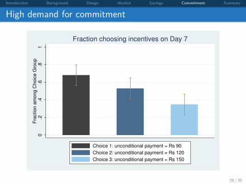
High demand for commitment
0.2
.4.6
.81
Fra
ction a
mong C
hoic
e G
roup
Choice 1: unconditional payment = Rs 90
Choice 2: unconditional payment = Rs 120
Choice 3: unconditional payment = Rs 150
Fraction choosing incentives on Day 7
28 / 35
Introduction Background Design Alcohol Savings Commitment Summary
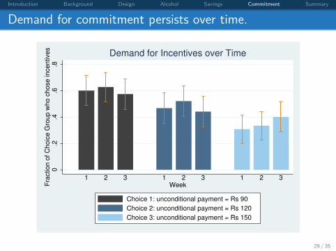
Demand for commitment persists over time.
0.2
.4.6
.8F
raction o
f C
hoic
e G
roup w
ho c
hose incentives
1 2 3 1 2 3 1 2 3Week
Choice 1: unconditional payment = Rs 90
Choice 2: unconditional payment = Rs 120
Choice 3: unconditional payment = Rs 150
Demand for Incentives over Time
29 / 35
Introduction Background Design Alcohol Savings Commitment Summary
Do individuals want to change their drinking patterns?
• Do individuals sacrifice money for incentives for sobriety?• Half of study participants exhibit demand for commitment.• A third is willing to sacrifice 10 percent of daily income.• Demand for incentives persists over time.
• Relating the demand for incentives to drinking patterns
30 / 35
Introduction Background Design Alcohol Savings Commitment Summary
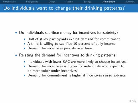
Do individuals want to change their drinking patterns?
• Do individuals sacrifice money for incentives for sobriety?• Half of study participants exhibit demand for commitment.• A third is willing to sacrifice 10 percent of daily income.• Demand for incentives persists over time.
• Relating the demand for incentives to drinking patterns• Individuals with lower BAC are more likely to choose incentives.• Demand for incentives is higher for individuals who expect to
be more sober under incentives.• Demand for commitment is higher if incentives raised sobriety.
30 / 35
Introduction Background Design Alcohol Savings Commitment Summary
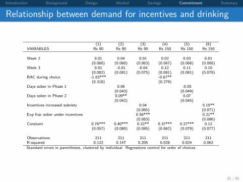
Relationship between demand for incentives and drinking
(1) (2) (3) (4) (5) (6)VARIABLES Rs 90 Rs 90 Rs 90 Rs 150 Rs 150 Rs 150
Week 2 0.01 0.04 0.01 0.02 0.03 0.01(0.060) (0.060) (0.063) (0.067) (0.068) (0.068)
Week 3 0.01 -0.01 -0.04 0.12 0.11 0.10(0.082) (0.081) (0.075) (0.081) (0.081) (0.079)
BAC during choice -1.63*** -0.67**(0.318) (0.279)
Days sober in Phase 1 0.06 -0.05(0.043) (0.049)
Days sober in Phase 2 0.09** 0.07(0.042) (0.045)
Incentives increased sobriety 0.04 0.15**(0.065) (0.071)
Exp frac sober under incentives 0.56*** 0.21**(0.083) (0.086)
Constant 0.76*** 0.40*** 0.22** 0.37*** 0.27*** 0.12(0.057) (0.080) (0.085) (0.062) (0.079) (0.077)
Observations 211 211 211 211 211 211R-squared 0.122 0.147 0.205 0.028 0.024 0.062Standard errors in parentheses, clustered by individual. Regressions control for order of choices.
31 / 35
Introduction Background Design Alcohol Savings Commitment Summary
How well do individuals understand their drinking patterns?
• Fairly accurate forecasts of own daytime sobriety (on average)• Very similar ITT estimates for Incentive and Choice Groups
• IV (= LATE for those who take up the incentive voluntarily) islarger than ATE on the population.
• Suggests compliers are those who have larger impacts.
• Exposure to incentives increases the demand for incentives.• Evidence of learning?
32 / 35
Introduction Background Design Alcohol Savings Commitment Summary
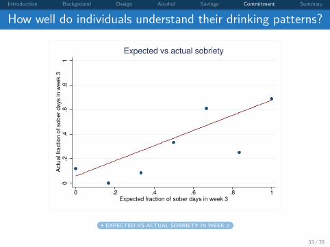
How well do individuals understand their drinking patterns?
0.2
.4.6
.81
Actu
al fr
action o
f sober
days in w
eek 3
0 .2 .4 .6 .8 1Expected fraction of sober days in week 3
Expected vs actual sobriety
EXPECTED VS ACTUAL SOBRIETY IN WEEK 2
33 / 35
Introduction Background Design Alcohol Savings Commitment Summary
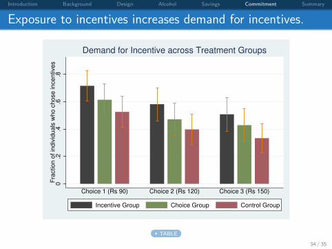
Exposure to incentives increases demand for incentives.
0.2
.4.6
.8F
raction o
f in
div
iduals
who c
hose incentives
Choice 1 (Rs 90) Choice 2 (Rs 120) Choice 3 (Rs 150)
Incentive Group Choice Group Control Group
Demand for Incentive across Treatment Groups
TABLE
34 / 35
Introduction Background Design Alcohol Savings Commitment Summary
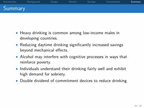
Summary
• Heavy drinking is common among low-income males indeveloping countries.
• Reducing daytime drinking significantly increased savingsbeyond mechanical effects.
• Alcohol may interfere with cognitive processes in ways thatreinforce poverty.
• Individuals understand their drinking fairly well and exhibithigh demand for sobriety.
• Double dividend of commitment devices to reduce drinking
35 / 35
Appendix
Why choose incentives if overall drinking stays constant?
• High demand for incentives, but small changes in behavior?• Substantial willingness to pay for incentives• Yet overall drinking doesn’t fall by much.
36 / 35
Appendix
Why choose incentives if overall drinking stays constant?
• High demand for incentives, but small changes in behavior?• Substantial willingness to pay for incentives• Yet overall drinking doesn’t fall by much.
• Explanations(1) Several small benefits of incentives
• Increased earnings• Decreased alcohol expenditures• Increased savings• Value of daytime sobriety
(2) Partial naıvete?• Naıvete can lower demand for commitment (Laibson 2015).• But people may also overestimate usefulness of commitment.
36 / 35
Appendix
Research agenda on alcohol consumption among the poor
(1) What is the economic impact of heavy drinking?• Larger/more powerful intervention to study labor market effects• Other aspects and timing of decision-making• Impact on families• Is alcohol a cause of poverty?
(2) Why are individuals drinking heavily?• Self-control problems matter greatly.• What is the role of physical pain?• Does poverty cause demand for alcohol?
(3) Alcohol policy: Kerala’s planned introduction of prohibition• Opportunity to evaluate concrete policy• Large-scale, long-term natural experiment
37 / 35
Appendix
Demographic and geographic concentration of drinking
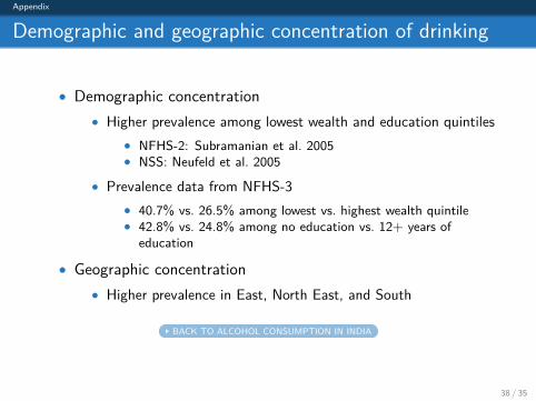
• Demographic concentration• Higher prevalence among lowest wealth and education quintiles
• NFHS-2: Subramanian et al. 2005• NSS: Neufeld et al. 2005
• Prevalence data from NFHS-3• 40.7% vs. 26.5% among lowest vs. highest wealth quintile• 42.8% vs. 24.8% among no education vs. 12+ years of
education
• Geographic concentration• Higher prevalence in East, North East, and South
BACK TO ALCOHOL CONSUMPTION IN INDIA
38 / 35
Appendix
Prevalence of drinking among low-income workers0%
20%
40%
60%
80%
100%
Porters
Construction w
orkers
Autorickshaw drivers
Loadmen
Shopkeepers
Fishermen
Fruit/vegetable vendors
Rickshaw
peddlers
Rag pickers
Sewage w
orkers
Fraction Reporting Drinking Alcohol on Previous Day
BACK TO ALCOHOL CONSUMPTION IN INDIA39 / 35
Appendix
High quantities of alcohol consumed1
23
45
67
8
Porters
Construction w
orkers
Autorickshaw drivers
Loadmen
Shopkeepers
Fishermen
Fruit/vegetable vendors
Rickshaw
peddlers
Rag pickers
Sewage w
orkers
Number of Standard Drinks Consumed on Previous Day (Conditional on Drinking)
BACK TO ALCOHOL CONSUMPTION IN INDIA40 / 35
Appendix
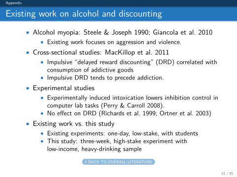
Existing work on alcohol and discounting
• Alcohol myopia: Steele & Joseph 1990; Giancola et al. 2010• Existing work focuses on aggression and violence.
• Cross-sectional studies: MacKillop et al. 2011• Impulsive “delayed reward discounting” (DRD) correlated with
consumption of addictive goods• Impulsive DRD tends to precede addiction.
• Experimental studies• Experimentally induced intoxication lowers inhibition control in
computer lab tasks (Perry & Carroll 2008).• No effect on DRD (Richards et al. 1999; Ortner et al. 2003)
• Existing work vs. this study• Existing experiments: one-day, low-stake, with students• This study: three-week, high-stake experiment with
low-income, heavy-drinking sample
BACK TO OVERALL LITERATURE
41 / 35
Appendix
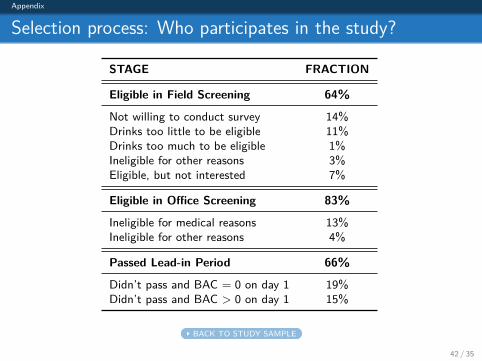
Selection process: Who participates in the study?
STAGE FRACTION
Eligible in Field Screening 64%
Not willing to conduct survey 14%Drinks too little to be eligible 11%Drinks too much to be eligible 1%Ineligible for other reasons 3%Eligible, but not interested 7%
Eligible in Office Screening 83%
Ineligible for medical reasons 13%Ineligible for other reasons 4%
Passed Lead-in Period 66%
Didn’t pass and BAC = 0 on day 1 19%Didn’t pass and BAC > 0 on day 1 15%
BACK TO STUDY SAMPLE
42 / 35
Appendix
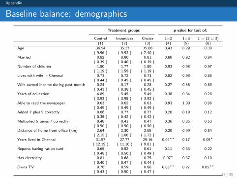
Baseline balance: demographicsTreatment groups p value for test of:
Control Incentives Choice 1=2 1=3 1 = (2 ∪ 3)(1) (2) (3) (4) (5) (6)
Age 36.54 35.27 35.08 0.43 0.29 0.30( 9.96 ) ( 9.92 ) ( 7.40 )
Married 0.82 0.80 0.81 0.80 0.92 0.84( 0.39 ) ( 0.40 ) ( 0.39 )
Number of children 1.80 1.77 1.80 0.93 0.98 0.97( 1.19 ) ( 1.55 ) ( 1.19 )
Lives with wife in Chennai 0.73 0.72 0.73 0.82 0.98 0.88( 0.44 ) ( 0.45 ) ( 0.45 )
Wife earned income during past month 0.24 0.17 0.28 0.27 0.58 0.80( 0.43 ) ( 0.38 ) ( 0.45 )
Years of education 4.89 5.45 5.49 0.38 0.34 0.28( 3.93 ) ( 3.95 ) ( 3.92 )
Able to read the newspaper 0.63 0.62 0.63 0.93 1.00 0.96( 0.49 ) ( 0.49 ) ( 0.49 )
Added 7 plus 9 correctly 0.86 0.77 0.77 0.20 0.19 0.12( 0.35 ) ( 0.42 ) ( 0.42 )
Multiplied 5 times 7 correctly 0.48 0.41 0.47 0.36 0.85 0.53( 0.50 ) ( 0.50 ) ( 0.50 )
Distance of home from office (km) 2.64 2.30 2.65 0.20 0.99 0.54( 2.15 ) ( 1.06 ) ( 1.72 )
Years lived in Chennai 31.57 27.77 29.16 0.04?? 0.17 0.05?
( 12.19 ) ( 11.10 ) ( 9.81 )Reports having ration card 0.65 0.52 0.61 0.11 0.63 0.22
( 0.48 ) ( 0.50 ) ( 0.49 )Has electricity 0.81 0.68 0.75 0.07? 0.37 0.10
( 0.40 ) ( 0.47 ) ( 0.44 )Owns TV 0.76 0.59 0.68 0.03?? 0.27 0.05??
( 0.43 ) ( 0.50 ) ( 0.47 )
BACK TO TREATMENT GROUPS43 / 35
Appendix
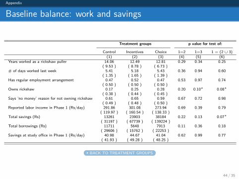
Baseline balance: work and savings
Treatment groups p value for test of:
Control Incentives Choice 1=2 1=3 1 = (2 ∪ 3)(1) (2) (3) (4) (5) (6)
Years worked as a rickshaw puller 14.06 12.49 12.81 0.29 0.34 0.25( 9.53 ) ( 8.78 ) ( 6.73 )
# of days worked last week 5.41 5.18 5.43 0.36 0.94 0.60( 1.35 ) ( 1.65 ) ( 1.39 )
Has regular employment arrangement 0.47 0.52 0.47 0.53 0.97 0.74( 0.50 ) ( 0.50 ) ( 0.50 )
Owns rickshaw 0.17 0.25 0.28 0.20 0.10? 0.08?
( 0.38 ) ( 0.44 ) ( 0.45 )Says ’no money’ reason for not owning rickshaw 0.61 0.65 0.59 0.67 0.72 0.98
( 0.49 ) ( 0.48 ) ( 0.50 )Reported labor income in Phase 1 (Rs/day) 291.86 301.08 273.94 0.69 0.39 0.79
( 119.97 ) ( 160.54 ) ( 138.33 )Total savings (Rs) 13261 23903 38184 0.22 0.13 0.07?
( 31197 ) ( 67739 ) ( 139224 )Total borrowings (Rs) 11711 5648 7913 0.11 0.36 0.18
( 29606 ) ( 15762 ) ( 22253 )Savings at study office in Phase 1 (Rs/day) 40.98 44.67 41.04 0.62 0.99 0.77
( 41.93 ) ( 49.28 ) ( 48.25 )
BACK TO TREATMENT GROUPS
44 / 35
Appendix
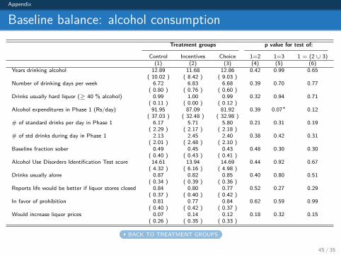
Baseline balance: alcohol consumptionTreatment groups p value for test of:
Control Incentives Choice 1=2 1=3 1 = (2 ∪ 3)(1) (2) (3) (4) (5) (6)
Years drinking alcohol 12.89 11.68 12.86 0.42 0.99 0.65( 10.02 ) ( 8.42 ) ( 9.03 )
Number of drinking days per week 6.72 6.83 6.68 0.39 0.70 0.77( 0.80 ) ( 0.76 ) ( 0.60 )
Drinks usually hard liquor (≥ 40 % alcohol) 0.99 1.00 0.99 0.32 0.94 0.71( 0.11 ) ( 0.00 ) ( 0.12 )
Alcohol expenditures in Phase 1 (Rs/day) 91.95 87.09 81.92 0.39 0.07? 0.12( 37.03 ) ( 32.48 ) ( 32.98 )
# of standard drinks per day in Phase 1 6.17 5.71 5.80 0.21 0.31 0.19( 2.29 ) ( 2.17 ) ( 2.18 )
# of std drinks during day in Phase 1 2.13 2.45 2.40 0.38 0.42 0.31( 2.01 ) ( 2.48 ) ( 2.10 )
Baseline fraction sober 0.49 0.45 0.43 0.48 0.30 0.30( 0.40 ) ( 0.43 ) ( 0.41 )
Alcohol Use Disorders Identification Test score 14.61 13.94 14.69 0.44 0.92 0.67( 4.32 ) ( 6.16 ) ( 4.98 )
Drinks usually alone 0.87 0.82 0.85 0.40 0.80 0.51( 0.34 ) ( 0.39 ) ( 0.36 )
Reports life would be better if liquor stores closed 0.84 0.80 0.77 0.52 0.27 0.29( 0.37 ) ( 0.40 ) ( 0.42 )
In favor of prohibition 0.81 0.77 0.84 0.62 0.59 0.99( 0.40 ) ( 0.42 ) ( 0.37 )
Would increase liquor prices 0.07 0.14 0.12 0.18 0.32 0.15( 0.26 ) ( 0.35 ) ( 0.33 )
BACK TO TREATMENT GROUPS
45 / 35
Appendix
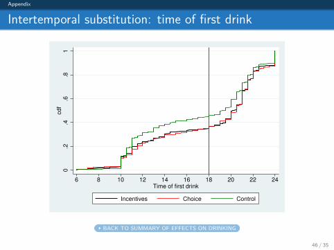
Intertemporal substitution: time of first drink
0.2
.4.6
.81
cdf
6 8 10 12 14 16 18 20 22 24
Time of first drink
Incentives Choice Control
BACK TO SUMMARY OF EFFECTS ON DRINKING
46 / 35
Appendix
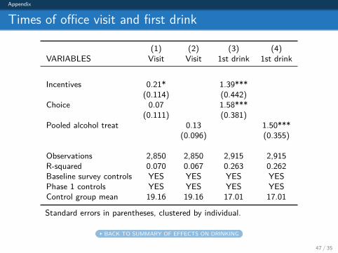
Times of office visit and first drink
(1) (2) (3) (4)VARIABLES Visit Visit 1st drink 1st drink
Incentives 0.21* 1.39***(0.114) (0.442)
Choice 0.07 1.58***(0.111) (0.381)
Pooled alcohol treat 0.13 1.50***(0.096) (0.355)
Observations 2,850 2,850 2,915 2,915R-squared 0.070 0.067 0.263 0.262Baseline survey controls YES YES YES YESPhase 1 controls YES YES YES YESControl group mean 19.16 19.16 17.01 17.01
Standard errors in parentheses, clustered by individual.
BACK TO SUMMARY OF EFFECTS ON DRINKING
47 / 35
Appendix
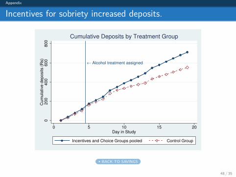
Incentives for sobriety increased deposits.
← Alcohol treatment assigned
0200
400
600
800
Cum
ula
tive d
eposits (
Rs)
0 5 10 15 20Day in Study
Incentives and Choice Groups pooled Control Group
Cumulative Deposits by Treatment Group
BACK TO SAVINGS
48 / 35
Appendix
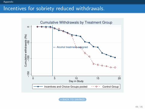
Incentives for sobriety reduced withdrawals.
← Alcohol treatment assigned
−150
−100
−50
0C
um
ula
tive w
ithdra
wals
(R
s)
0 5 10 15 20Day in Study
Incentives and Choice Groups pooled Control Group
Cumulative Withdrawals by Treatment Group
BACK TO SAVINGS
49 / 35
Appendix
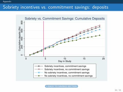
Sobriety incentives vs. commitment savings: deposits
0200
400
600
800
Cum
ula
tive d
epsits (
Rs)
0 5 10 15 20Day in Study
Sobriety incentives, commitment savings
Sobriety incentives, no commitment savings
No sobriety incentives, commitment savings
No sobriety incentives, no commitment savings
Sobriety vs. Commitment Savings: Cumulative Deposits
BACK TO SAVINGS SECTION
50 / 35
Appendix
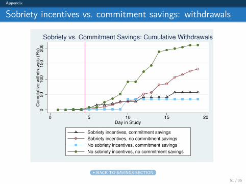
Sobriety incentives vs. commitment savings: withdrawals
050
100
150
200
Cum
ula
tive w
ithdra
wals
(R
s)
0 5 10 15 20Day in Study
Sobriety incentives, commitment savings
Sobriety incentives, no commitment savings
No sobriety incentives, commitment savings
No sobriety incentives, no commitment savings
Sobriety vs. Commitment Savings: Cumulative Withdrawals
BACK TO SAVINGS SECTION
51 / 35
Appendix
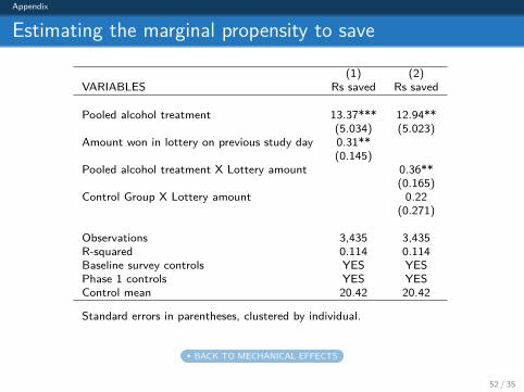
Estimating the marginal propensity to save
(1) (2)VARIABLES Rs saved Rs saved
Pooled alcohol treatment 13.37*** 12.94**(5.034) (5.023)
Amount won in lottery on previous study day 0.31**(0.145)
Pooled alcohol treatment X Lottery amount 0.36**(0.165)
Control Group X Lottery amount 0.22(0.271)
Observations 3,435 3,435R-squared 0.114 0.114Baseline survey controls YES YESPhase 1 controls YES YESControl mean 20.42 20.42
Standard errors in parentheses, clustered by individual.
BACK TO MECHANICAL EFFECTS
52 / 35
Appendix
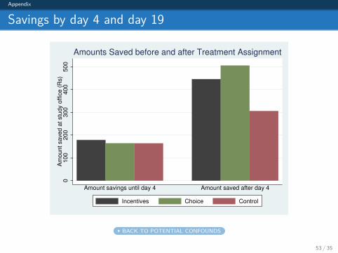
Savings by day 4 and day 19
0100
200
300
400
500
Am
ount saved a
t stu
dy o
ffic
e (
Rs)
Amount savings until day 4 Amount saved after day 4
Incentives Choice Control
Amounts Saved before and after Treatment Assignment
BACK TO POTENTIAL CONFOUNDS
53 / 35
Appendix
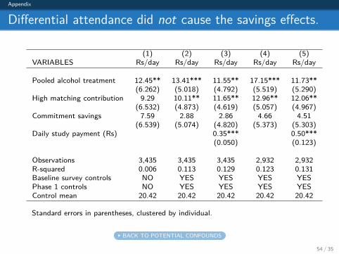
Differential attendance did not cause the savings effects.
(1) (2) (3) (4) (5)VARIABLES Rs/day Rs/day Rs/day Rs/day Rs/day
Pooled alcohol treatment 12.45** 13.41*** 11.55** 17.15*** 11.73**(6.262) (5.018) (4.792) (5.519) (5.290)
High matching contribution 9.29 10.11** 11.65** 12.96** 12.06**(6.532) (4.873) (4.619) (5.057) (4.967)
Commitment savings 7.59 2.88 2.86 4.66 4.51(6.539) (5.074) (4.820) (5.373) (5.303)
Daily study payment (Rs) 0.35*** 0.50***(0.050) (0.123)
Observations 3,435 3,435 3,435 2,932 2,932R-squared 0.006 0.113 0.129 0.123 0.131Baseline survey controls NO YES YES YES YESPhase 1 controls NO YES YES YES YESControl mean 20.42 20.42 20.42 20.42 20.42
Standard errors in parentheses, clustered by individual.
BACK TO POTENTIAL CONFOUNDS
54 / 35

Appendix
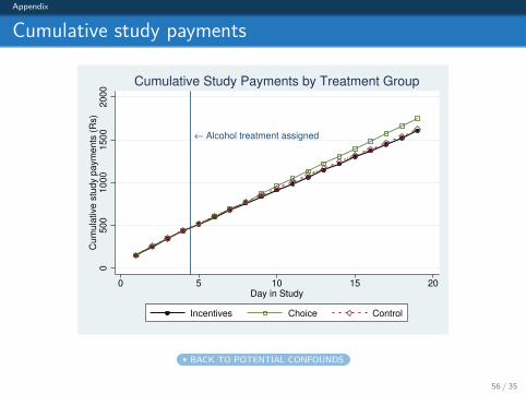
Study payments across treatment groups
• On average, Choice Group earns Rs. 7 per day more thanControl Group
• Control Group individuals earn Rs. 85 per day• Incentive Group individuals earn Rs. 84 per day• Choice Group individuals earn Rs. 92 per day
• Could this account for the difference in savings?• Marginal propensity to save from lottery: 0.22• Suggests that any effects on savings were small.
BACK TO POTENTIAL CONFOUNDS
55 / 35
Appendix
Cumulative study payments
← Alcohol treatment assigned
0500
1000
1500
2000
Cum
ula
tive s
tudy p
aym
ents
(R
s)
0 5 10 15 20Day in Study
Incentives Choice Control
Cumulative Study Payments by Treatment Group
BACK TO POTENTIAL CONFOUNDS
56 / 35
Appendix
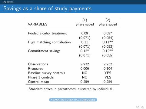
Savings as a share of study payments
(1) (2)VARIABLES Share saved Share saved
Pooled alcohol treatment 0.09 0.09*(0.071) (0.054)
High matching contribution 0.11 0.11**(0.071) (0.052)
Commitment savings 0.12* 0.12**(0.071) (0.055)
Observations 2,932 2,932R-squared 0.006 0.104Baseline survey controls NO YESPhase 1 controls NO YESControl mean 0.259 0.259
Standard errors in parentheses, clustered by individual.
BACK TO POTENTIAL CONFOUNDS
57 / 35
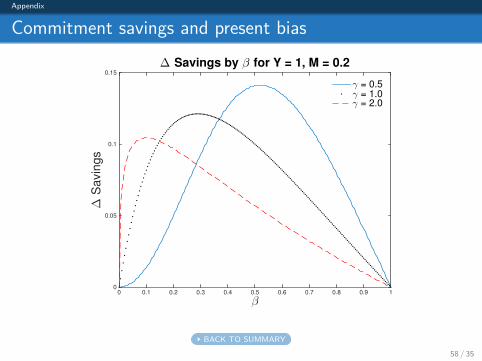
Appendix
Commitment savings and present bias
β0 0.1 0.2 0.3 0.4 0.5 0.6 0.7 0.8 0.9 1
∆ S
avin
gs
0
0.05
0.1
0.15
∆ Savings by β for Y = 1, M = 0.2
γ = 0.5γ = 1.0γ = 2.0
BACK TO SUMMARY
58 / 35
Appendix
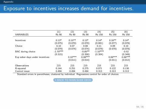
Exposure to incentives increases demand for incentives.
(1) (2) (3) (4) (5) (6)VARIABLES Rs 90 Rs 90 Rs 90 Rs 150 Rs 150 Rs 150
Incentives 0.13* 0.15** 0.13* 0.14* 0.16** 0.14*(0.075) (0.070) (0.070) (0.081) (0.077) (0.078)
Choice 0.10 0.07 0.08 0.11 0.09 0.10(0.079) (0.074) (0.074) (0.079) (0.078) (0.078)
BAC during choice -1.70*** -0.85** -1.10*** -0.52(0.315) (0.358) (0.304) (0.349)
Exp sober days under incentives 0.10*** 0.08*** 0.06*** 0.06***(0.011) (0.014) (0.011) (0.012)
Observations 215 215 215 215 215 215R-squared 0.144 0.251 0.275 0.071 0.122 0.130Control mean 0.494 0.494 0.494 0.313 0.313 0.313
Standard errors in parentheses, clustered by individual. Regressions control for order of choices.
BACK TO MAIN SLIDE DECK
59 / 35
Appendix
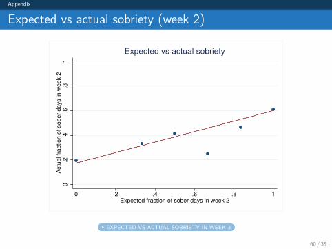
Expected vs actual sobriety (week 2)
0.2
.4.6
.81
Actu
al fr
action o
f sober
days in w
eek 2
0 .2 .4 .6 .8 1Expected fraction of sober days in week 2
Expected vs actual sobriety
EXPECTED VS ACTUAL SOBRIETY IN WEEK 3
60 / 35
Appendix
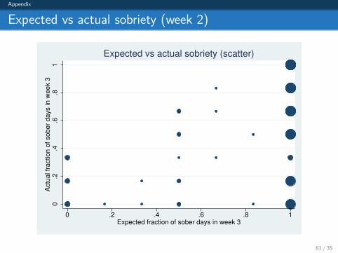
Expected vs actual sobriety (week 2)
0.2
.4.6
.81
Actu
al fr
action o
f sober
days in w
eek 3
0 .2 .4 .6 .8 1Expected fraction of sober days in week 3
Expected vs actual sobriety (scatter)
61 / 35
Appendix
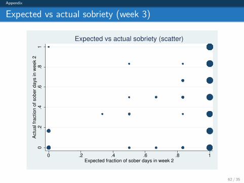
Expected vs actual sobriety (week 3)
0.2
.4.6
.81
Actu
al fr
action o
f sober
days in w
eek 2
0 .2 .4 .6 .8 1Expected fraction of sober days in week 2
Expected vs actual sobriety (scatter)
62 / 35
Appendix
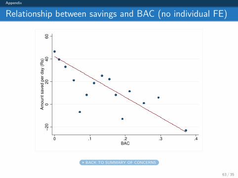
Relationship between savings and BAC (no individual FE)
−20
020
40
60
Am
ount saved p
er
day (
Rs)
0 .1 .2 .3 .4BAC
BACK TO SUMMARY OF CONCERNS
63 / 35
Appendix
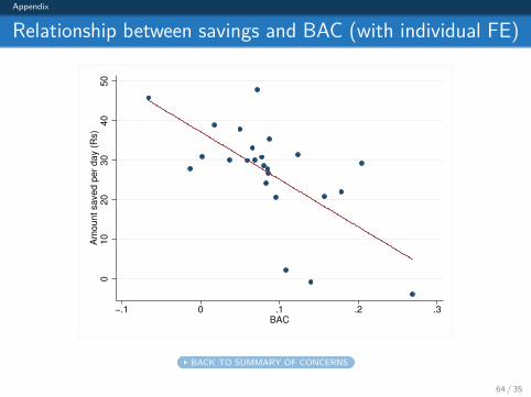
Relationship between savings and BAC (with individual FE)
010
20
30
40
50
Am
ount saved p
er
day (
Rs)
−.1 0 .1 .2 .3BAC
BACK TO SUMMARY OF CONCERNS
64 / 35