INTERNATIONAL JOURNAL OF CLIMATOLOGY, VOL. 16, 8 17-838 (1 996)

ALBEDO AND DEPTH OF MELT PONDS ON SEA-ICE

M. F! MORASSUTTI AND E. F. LEDREW Earth-Observations Laboratory, Institute for Space and Terrestrial Science, University of Waterloo, Waterloo, Ontario N2L 3GI. Canada

e-mail: mike(i&lenn.uwaterloo.ca

Received 22 February 1995 Accepted I I October 1995

ABSTRACT

For a I-month period during the spring-summer season, over 500 in situ measurements of the albedo, depth and selected properties of melt ponds were made at four sea-ice sites in the Canadian Arctic Archipelago. There are three aims of the investigation: to examine the variation in spectral reflectance of melt ponds in relation primarily to clouds, pond depth, and ice type; to compute and assess with reliability, and for the first time, the statistical properties of pond depth; and to derive pond albedo parameterkations for implementation in sea-ice model simulations. It was found that pond reflectance curves vary significantly with cloud cover, pond depth, and ice type. A simple univariate statistical analysis showed that surface ice morphology controls pond depth. Application of the Kruskal-Wallis test evidenced that differences between first-year ice, multi- year ice, and landfast ice-pond-depth distributions are statistically significant. Lastly, calibrated non-linear regression functions show that visible and near-infrared pond albedos decrease exponentially with depth until some critical depth value is exceeded. The relationship is weakest in the visible spectrum, particularly under cloudy sky conditions.

KEY WORDS: sea-ice; melt-pond albedo; melt-pond depth; Arctic; spectrometer.

1. INTRODUCTION

When sea-ice in the Arctic commences its decay in May and June, melt ponds form, covering significant expanses of the sea-ice surface (Scharfen et al., 1987). Increased areal coverage of melt ponds reduces the overall sea-ice albedo and allows for an intensification of solar absorption at the surface. The well-known definition of the ice-albedo feedback states that a reduction in surface albedo raises surface temperatures and accentuates melt, with the net effect being an areal regression of the marine cryosphere (cf. Shine et al., 1984; Ingram et al., 1988) and, as recent sea-ice model simulations have shown (Curry et al., 1995), a possible impact on ice thickness. Realization of this climatically important feedback necessitates sound knowledge of the physical properties and formation of melt ponds, including their associated effects on the total reflective power of sea-ice, and therefore on both its thermodynamic and hydrological regimes.

Unfortunately, hydrological processes on sea-ice are still inadequately understood. Over recent years, however, there has emerged an increasing interest in the hydrology of sea-ice (e.g. Andreas and Ackley, 1982). The only differences occurring between sea-ice-melt hydrology and land hydrology is that, in the former, an 'infinite' under- ice reservoir of water exists and, if the curvature of the ocean is overlooked, the surface slope angle of the ice-pack is essentially 0" (Cogley and Henderson-Sellers, 1985). Knowledge of sea-ice hydrology (in connection with radiative processes) is vital because both ice properties and snowmelt dictate the extent and occurrence of surface water and, therefore, melt-pond formation. Theoretical analyses and assumptions are supplemental here, but they would not substitute for the indispensability of ground-measured data; of which the latter are required for the initialization, formulation, validation of sea-ice models and satellite retrieval algorithms.

2. BACKGROUND

From the period of the 1950s through to the 1970s there were an abundant number of very informative studies on melt ponds over sea-ice surfaces. These studies concerned themselves principally with the relationship between sea-

CCC 0899-841 8/96/0708 17-22 0 1996 by the Royal Meteorological Society

818 M. €! MORASSU'ITI AND E. F. LEDREW

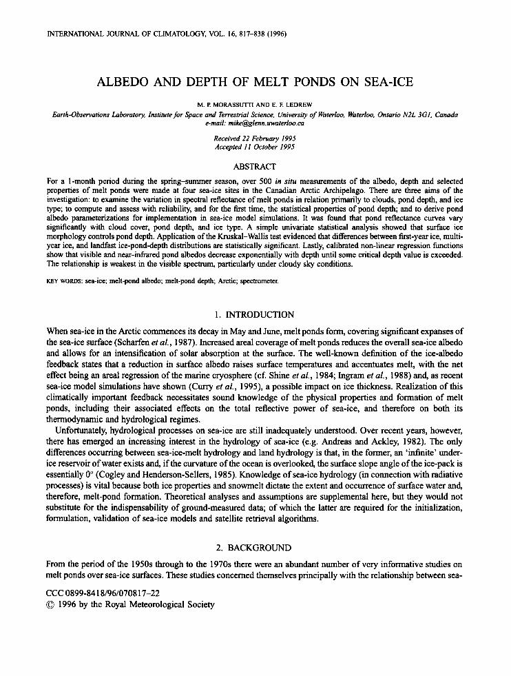
Table I. Regression coefficients (ao, a,) for a linear function ai = a0 - al P that associates sea-ice albedo (ai) to the fractional areal extent of melt ponds (P)

a0 a1 Reference Locality Pond area determination Cloud

0.65 0.38 Hanson (1961) Beaufort and Chukchi Seas Aircraft reconnaissance Cloudy 0.49 0.30 Langleben (1 969) Tanquary Fiord, Ellesmere Photographs from high towers

0.59 0.32 Langleben (1971) Tanquary Fiord, Photographs from high towers < 5/10

0.56 0.34 Grenfell and Maykut (1977) Port Barrow, Alaska, Theoretical Clear

0.70 0.41 Grenfell and Maykut (1977) Port Barrow, Alaska, Theoretical

0.74 1.04 Cogley and Henderson- Near and around North Pole

0.63 0.35 Cogley and Henderson- Near and around North Pole

conditions

Island

Ellesmere Island

Beaufort Sea

Beaufort Sea Overcast

Sellers (1 985)'

Sellers (1985)b

Toefficients are derived from data of Nazintsez (1964) and Buzuev er al. (1965) as presented in Table 2 of Barry (1983). bCoefficients (in footnote a) are corrected by Cogley and Henderson Sellers (1985) for incompatibilities in data organization and/or estimation methods.

ice albedo and the areal extent of melt ponds as observed and measured from aircraft reconnaissance flights, drifting stations and high tower mountings (e.g. Hanson, 1961 ; Nazintsev, 1964; Buzuev et al., 1965; Chernigovski, 1968; Langleben, 1969, 1971; Grenfell and Maykut, 1977). The favoured technique of investigation has been to statistically associate estimates of areal sea-ice albedo with fractional melt pond coverage via the calibration of linear regression equations (Table I). Cogley and Henderson-Sellers (1985) intercompare and assess these types of equations. Figure 1 illustrates that the relationship between sea-ice albedo and pond extent is indeed directly proportional. In general, when melt initiates in late May, pond area progressively increases to a maximum in mid- July (within the range of 25-50 per cent, concurrent with the complete ablation of the snowpack), whereas sea-ice albedo gradually decreases from around 0.75-0.80 to within the range 0.25445. After mid-July, during the intermediate and final stages of break-up, cracks form and ponds drain, hence reducing pond extent. For perennial

t i

RlLlAN DAY Figure I. Sea ice albedo and melt pond areal coverage versus time. Data are from Nazintesev (1964), Buzue~ et al. (1965) as cited in Bany (1983). Lines A and B are, respectively, minimum and maximum albedos. Lines C and D are, mpectively, maximum and mean pond extents

ALBEDO AND DEPTH OF MELT PONDS 819

ice, ponds that do not drain eventually refreeze with the declining temperatures in the ensuing months. This, combined with the eventual accrual of a new snowpack, increases the surface albedo once again until the commencement of the polar night.

Later, from the mid-1980s onwards, satellite data analyses have provided greater spatial and temporal coverages and, consequently, greater understanding of the ice albedo-pond-area interrelationship (e.g. Carsey, 1985; Scharfen et al., 1987; Rossow et al., 1989; Morassutti, 1992; Robinson er al., 1992). Additionally, sea-ice modellers are starting to take serious notice of the influence of melt ponds on the thermodynamic nature of an ice-pack. For instance, a well-developed one-dimensional thermodynamic sea-ice model (Ebert and Curry, 1993) has taken as climatically significant the radiative effects of melt ponds. Three principal melt-pond properties are emulated in the model, namely albedo, areal coverage and depth. Pond albedos for four spectral bands are made a function of pond depth, pond area is made a simple function of time, and pond depth is obtained from a continuity equation (computed from pond area, ice thickness, precipitation, a specified drainage rate, snow and water densities, and solar absorption by water).

Even though information on sea-ice albedo and the areal coverage of melt ponds are readily available to the Arctic research community, data on individual melt-pond reflectances and depths are still extremely deficient. There have been relatively few published measurements of the albedo and spectral reflectance of single melt ponds and even a lesser number of pond-depth measurements (cf. Chukanin, 1954; Grenfell and Maykut, 1977; Grenfell and Perovich, 1984; Perovich, 1994). The meagreness of these data, and a review of the relevant literature (which emphasizes the dearth of in siru melt-pond data of any type), coupled with the oversimplified treatment of melt-pond formation in many sea-ice models, suggests the need for fiuther study. For unless a more realistic melt-pond data set is compiled, hture attempts at modelling any melt-pond process will entail a high measure of uncertainty and the results gleaned therefrom will be, at most, only qualitative. The main problem is due, of course, to the 'harsh realities' associated with the logistics of in situ melt-pond measurement and, hence, the presently existing paucity of pond albedo and depth data available for analysis and model derivation.

In this light, a research project was undertaken in which the spectral reflectances and depths of individual sea-ice melt ponds were measured on first-year, multi-year and landfast ice surfaces, including observations of the pond's coexisting physical properties. These data were collected and collated in detail, having in mind the needs of sea-ice and climate modellers, Arctic remote sensing scientists and cryoclimatologists.

The outline of this paper is as follows: the field programme and study area are discussed in the next section; the spectrometric device and data examination techniques are described in section 4; section 5 consists of the analysis of melt-pond reflectances, a statistical investigation of pond depths, and the development of non-linear empirical functions which relate band albedo to pond depth; the final section outlines the conclusions of our analysis.

3. FIELD PROGRAMME AND STUDY REGION

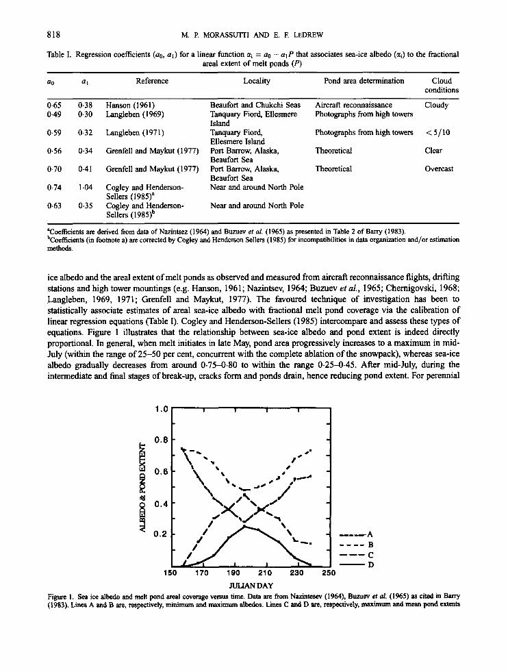
This study is one part of the Seasonal Sea Ice Monitoring and Modelling Site (SIMMS) field experiment which, since 1990, has worked out of various sites within the region of Lancaster Sound-Barrow Strait, Northwest Territories, Canada (Figure 2). For the 1994 SIMMS field programme, team members worked adjacent to the coast of Somerville Island (ca. 74"N 96" W). This multidisciplinary programme has one of its primary themes for study as being the analysis of the exchange of shortwave radiation over both seasonally and areally varying snow covered sea-ice surfaces-all in relation to the interconnections working between sea-ice, the atmosphere and the ocean (see overview in LeDrew and Barber, 1994).

During the 1994 field season, an investigation of melt ponds was undertaken with three particular objectives. The first was to analyse and assess measured spectral reflectances of individual melt ponds in association with concomitant pond properties (depth, colour, ice type, underlying ice texture, the occurrence of aeolian debris, etc.), including its relation to cloud conditions. The second objective was to investigate the statistical nature of melt-pond- depth data. The third objective was to derive a series of empirical functions that relate melt-pond band albedo to pond depth for the purpose of implementation in sea-ice model simulations.

The study period was 1 month (27 May to 26 June). This time frame was selected to follow as best as possible the commencement of melt pond formation through to the mature melt pond stage. Of course, the developmental sequence of melt pond formation will depend on local meteorological conditions, and the region did experience

820 M. F? MORASSUTTI AND E. F. LEDREW

Figure 2. (a) Study region. The small box in lower map denotes approximate areal coverage of satellite image (Fig 2(b)); latitudelongitude approximately 76"56'N, 96"20'W

anomalous weather during the 1994 field experiment. According to Environment Canada (1 984), the mean rainfall for the region in May is only a trace amount and it is only approximately 5 mm in June. Unusually, the amount of rainfall observed for this region in 1994 was much greater than this and was unusually excessive for a locale residing in a 'polar desert'. Along with occurrences of intermittent, light snowfalls throughout the entire study period, there were two very significant episodes of rainfall which had the greatest consequence on the evolutionary sequence of melt-pond formation. The first rainfall event occurred at the beginning of the observational period (on May 27) during which there was over 10 h of persistent rainfall. The heat input and the saturation of the snowpack by the rain began to speedily melt the snowpack and it allowed for an accelerated rate of melt-pond formation. After this event pond extent was observed to be within the range of about 25-35 per cent. From the end of May until late June, temperatures fluctuated within about -2 to 2"C, being in accordance with climate 'normals' in the region (Environment Canada, 1984). After the first major rainfall, there were about 10 minor precipitation events, which consisted predominantly of short periods of light flurries, with a few very light drizzles; the latter sometimes intermixed with wet snow and/or freezing rain. These conditions were conducive to a slow growth in pond depth and extent after a rapid initial melt. There were a few days where temperatures were cold enough to freeze the top layer of the ponds. The thicknesses of these ice layers were highly variable, spanning from 0.1 cm to nearly 5 cm. The accretion of these ice layers and, subsequently, the snow that fell thereon, markedly increased the albedo of the ponds. However, they soon melted due to gradually rising temperatures. The second significant rainfall event

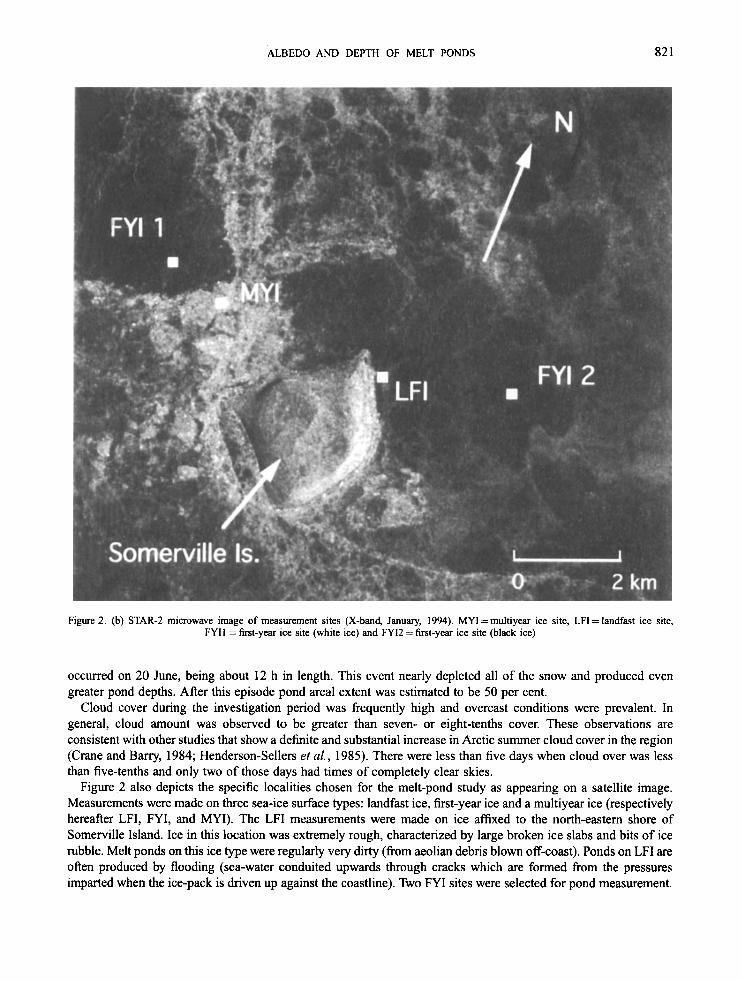
ALBEDO AND DEPTH OF MELT PONDS 82 1

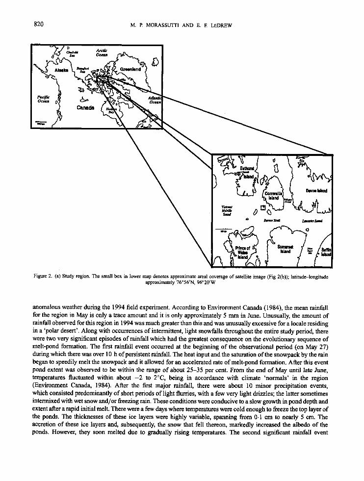
Figure 2. (b) STAR-2 microwave image of measurement sites (X-band January, 1994). MY1 = multiyear ice site, LFI = landfast ice site, FYI 1 = first-year ice site (white ice) and FYI2 = first-year ice site (black ice)

occurred on 20 June, being about 12 h in length. This event nearly depleted all of the snow and produced even greater pond depths. After this episode pond areal extent was estimated to be 50 per cent.

Cloud cover during the investigation period was frequently high and overcast conditions were prevalent. In general, cloud amount was observed to be greater than seven- or eight-tenths cover. These observations are consistent with other studies that show a definite and substantial increase in Arctic summer cloud cover in the region (Crane and Barry, 1984; Henderson-Sellers et al., 1985). There were less than five days when cloud over was less than five-tenths and only two of those days had times of completely clear skies.

Figure 2 also depicts the specific localities chosen for the melt-pond study as appearing on a satellite image. Measurements were made on three sea-ice surface types: landfast ice, first-year ice and a multiyear ice (respectively hereafter LFI, FYI, and MYI). The LFI measurements were made on ice affixed to the north-eastern shore of Somerville Island. Ice in this location was extremely rough, characterized by large broken ice slabs and bits of ice rubble. Melt ponds on this ice type were regularly very dirty (from aeolian debris blown off-coast). Ponds on LFI are often produced by flooding (sea-water conduited upwards through cracks which are formed from the pressures imparted when the ice-pack is driven up against the coastline). Two FYI sites were selected for pond measurement.

822 M. P. MORASSLITTI AND E. F. LEDREW

One on white ice and the other on black ice. Ice thicknesses remained within 2.0 f 0.1 m at both sites for the entire study period and, before the 20 June rainfall event, snow depths ranged from 10 cm to 30 cm. Both FYI ice surfaces had relatively flat topographies. Measurements were also made over a rather small MY1 floe having a diameter of approximately 750 m. Ice thicknesses ranged from approximately 2.5 to 6.0 m. Topographical variations on the floe were quite pronounced. Hummock sizes were observed from around 1 m to more than 2 m. From the beginning of the study period up until mid-June the floe had a very deep and variable snowpack (from 30 cm to up to 90 cm). The snowpack then ablated and later refroze into a very dense crust of less than 5 cm by the end of June.

4. INSTRUMENTATION AND DATA METHODOLOGY

Reflectance measurements of the melt ponds were made with the Analytical Spectral Device’s (ASD) Portable Personal Spectrometer II. The device uses a silicon photodiode detector and a fibre optic cable to estimate the magnitude of ‘light’ within the spectral range 341.5-1066-3 nm (at a spectral resolution of 1.4 nm). The ASD is also equipped with a removable palmtop computer, with two memory cards (each having a 1 MB storage capacity). This is connected on top of the spectrometer housing and permits for a real-time display of reflectance curves and other supplementary information (e.g. integration time, file parameters). The ASD is amenable to low temperature environments. The accuracy for operational temperatures above and below 0°C respectively are 4 and 8 nm. The spectrometer was last calibrated in December of 1993. More detailed descriptions of the spectrometer can be found in the ASD Users Guide (1 993).

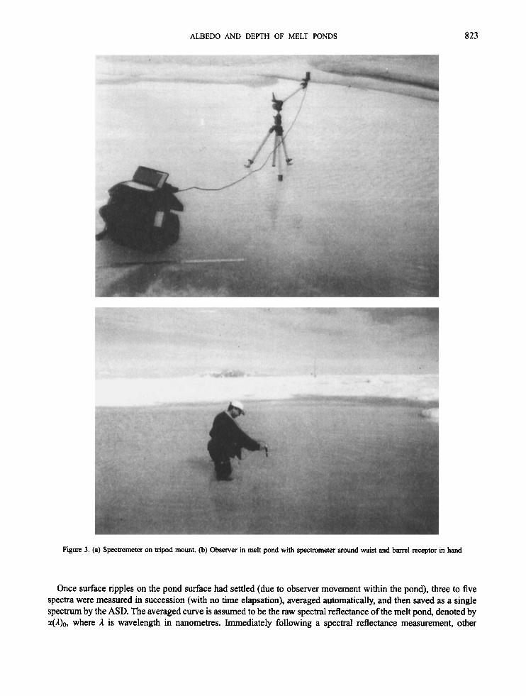
Reflectance spectra can be obtained by one of two methods. In the first method (used for the majority of the measurements) the fibre optic cable, which runs from the main spectrometer housing, is connected to a handheld ‘gun’. Barrel receptors with a specific fields of view (FOV) can be attached to the ‘gun’. We used two FOVs for our ‘gun’ measurements (5” and 18”). In the second method, the fibre optic cable is attached to a ‘cosine receptor’ mounted on a tripod (Figure 3(a)). The FOVof the cosine receptor is 180”.

Before all the spectra are logged during a ‘gun’ recording, a reference measurement is made against a white reference card, hence setting the reflectance to 1.0 (i.e. ‘perfect’ reflection) across the entire solar spectrum so as to be consonant with the prevailing incoming solar flux density. When a sample measurement is taken, the ASD simply compares the measured pond value with the reference spectrum to obtain their corresponding spectra. For tripod measurements (with mounted cosine receptor), the spectral reflectance recorded is the ratio between the measured radiance (sensor pointed down towards surfae) and the previously measured irradiance (sensor pointed vertically

The spectrometer is also outfitted with a carrying case that can be easily strapped to the waist for measurements with the handheld ‘gun’. This feature, the portability of the ASD, with the protection of rubber waders, plus a little dexterity, made it possible to enter into, and traverse through rather expansive melt ponds as deep as 85 cm or so (Figure 3(b)). This added manoeuverability permitted for the measurement of the deepest points in the pond, which are often centrally situated, and where it is extremely arduous, if not impossible, to measure with only a tripod- mounted sensor. All ponds were sampled randomly in area to avoid as much as possible any sampling bias.

Spectra were sampled at a position normal to the pond surface (i.e. vertically underneath the centre of the barrel or cosine receptor) and, unless the sky was completely overcast, the barrel receptor was held, or the tripod’s arm (with the mounted cosine receptor) was situated, in a direction directly opposite the sun. With overcast sky conditions radiation is diffuse and, for obvious reasons, it is not required that the sensor be directly opposite the sun. However, for clear sky conditions, or when the solar disc is partially occluded by a cloud, the orientation of the spectral sensor must be considered (i.e. irradiance is directional and the observer must avoid shadowing the sun). Next, the integration time of the ASD was preset to remove ‘saturation’ over the spectral window. If the instrument is pointed towards an intensely bright surface for too long a time there occurs an overloading of incident photons (‘saturation’) in the sensor (i.e. the integration time is too long). Afterwards, a ‘dark current’ was taken before each reflectance measurement to remove electrical noise generated by the spectrometer. The ‘dark current’ measurement has nothing whatsoever to do with the target to be imaged. The ASD closes its shutter to outside light and measures the voltage in the sensor m y itself (‘dark current’). This voltage of the m y varies with the temperature of the instrument (R. De Abreu, pers. comm.). This electronic noise is removed when the spectrum of the target is subsequently recorded.

upwards into sky).

ALBEDO AND DEPTH OF MELT PONDS 823

Figure 3. (a) Spectrometer on tripod mount. @) Observer in melt pond with spectrometer around waist and barrel receptor in hand

Once surface ripples on the pond surface had settled (due to observer movement within the pond), three to five spectra were measured in succession (with no time elapsation), averaged automatically, and then saved as a single spectrum by the ASD. The averaged curve is assumed to be the raw spectral reflectance of the melt pond, denoted by a(&, where 1 is wavelength in nanometres. Immediately following a spectral reflectance measurement, other

824 M. P. MORASSUTTI AND E. F. LEDREW

Table 11. Colour scheme used for the observation of pond colour. The colour codes specified here were selected to match as closely as possible the colour gradations occurring in the visible spectrum (hm the blue to green and

then on to the red bands, ca. 400-700 nm). Code numbers 1417 were assigned specifically for ‘black’ FYI

Code Colour Code Colour Code Colour

1 White 2 White-grey 3 Grey-white 4 Grey 5 Grey-blue 6 Blue-grey

7 Blue 8 Blue-green 9 Green-blue

10 Green 11 Green-brown 12 Brown-green

13 Brown 14 Dark green 15 Dark blue

17 Black 16 Dark grey

ancillary data were recorded into a log book: (i) Pond properties.

(a) Ice type. Either LFI, FYI or MYI. (b) Depth. At nadir to receptor (i.e. the point on the pond surface directly beneath the centre of the barrel or

(c) Colour. Colours designated span from white and grey, to blue and green, and on to brown and black,

(d) Underlying surface texture. Either rough or smooth, giving some indication of the scattering potential of

(e) Debris presence. On pond bottom or ‘dirty water’. ( f ) Frozen pond. Top layer ice thickness and its characteristics. (g) Other comments. Surrounding surface conditions, problems, etc.

(a) Solar disc obscuration by clouds. Ranged on a scale from 1 to 5 where:

cosine receptor).

including many combinations (see Table 11).

the pond bottom.

(ii) Atmospheric conditions and logistics.

1 = full solar disc 2 =bright sun with some obscuration (usually resultant from the presence of thin cirrus) 3 = obvious reduction in sun brightness 4 = solar disc is faintly observable 5 = solar disc totally occluded.

(b) Field of view. 5” and 18” for barrel receptor, and 180” for cosine receptor. (c) Time. Measurements were made between 0800 and 1800 hours solar time.

Once back from the field, the reflectance curves stored on the palmtop computer (in binary format) were immediately transferred over to a floppy disk. Post-processing programs for the spectrometer allow for quick graphic display and perusal of the reflectance curves, including the conversion of binary to ASCII data for later post- processing procedures. After data conversion, the spectra were truncated to within the range of 400-1000 nm because of excessive detector noise outside this spectral window.

We were unable to do regularly timed, consistent measurements over a single pond (so as obtain time series for a ‘control’ pond) principally because of logistical factors: (i) inclement weather and erratic flight scheduling (hence no routine helicopter flights out to the sites); (ii) changing surface conditions (helicopter landing spots had to change; and even if a previously measured pond was 30 or so metres away, occasional concerns and problems with the ASD (calibrating, attaching/detaching components, difficulty in walking with the device in deep snow), including the short-time we were allowed to do our recordings in some cases (helicopter time restrictions)) also did not permit for consistency in measurement. Diurnally fluctuating pond depths as actuated by tidal fluxes (at the LFI site, see Figure 2(b)), and other factors, proved impossible to find a suitable ‘control’ pond on landfast ice.

Due to panel smudging (from constant handling and dirt accretion), the next step in our analysis involved the laboratory measured correction of the white reference panel used in the field against a ‘perfect’ or unused white reference card (in actuality, the panel used in the field will have a reflectance ranging from about 0.80-0.96, thereby underestimating solar irradiance, and thus overestimating surface reflectance). This was done (after the completion of the field project) by standardly illuminating both the field and unused white cards while coincidentally measuring reflectances of both panels with the ASD spectrometer. The illumination angle of the light source accorded with the

ALBEDO AND DEPTH OF MELT PONDS 825

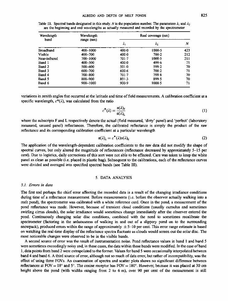
Table 111. Spectral bands designated in this study. N is the population number. The parameters 11 and 12 are the beginning and end wavelengths as actually measured and recorded by the spectrometer

Wavelength band

Broadband Visible Near-infrared Band 1 Band 2 Band 3 Band 4 Band 5 Band 6

400-1000 400-700 700-1 000 400-500 500-600 600-700 700-800 800-900 900-1 000

Real coverage (nm)

1 1 1 2 N

400.0 1000.5 423 400.0 700.2 212 701.7 1000.5 211 400.0 499.6 71 501 .o 599.2 70 600.6 700.2 71 701.7 799.8 70 801.3 899.5 70 900.9 1000.5 71

variations in zenith angles that occurred at the latitude and time of field measurements. A calibration coefficient at a specific wavelength, c*(A), was calculated from the ratio

where the subscripts F and L respectively denote the actual (field measured, 'dirty' panel) and 'perfect' (laboratory measured, unused panel) reflectances. Therefore, the calibrated reflectance is simply the product of the raw reflectance and its corresponding calibration coefficient at a particular wavelength

The application of the wavelength-dependent calibration coefficients to the raw data did not modify the shape of spectral curves, but only altered the magnitude of reflectances (reflectance decreased by approximately 5-15 per cent). Due to logistics, daily corrections of this sort were not able to be effected. Care was taken to keep the white panel as clean as possible (i.e. placed in plastic bag). Subsequent to the calibrations, each of the reflectance curves were divided and averaged into specified spectral bands (see Table 111).

5 . DATA ANALYSIS

5.1. Errors in data

The first and perhaps the chief error affecting the recorded data is a result of the changing irradiance conditions during time of a reflectance measurement. Before measurements (i.e. before the observer actually walking into a melt pond), the spectrometer was calibrated with a white reference card. Once in the pond, a measurement of the pond reflectance was made. However, because of transient cloud conditions (usually cumulus and sometimes swirling cirrus clouds), the solar irradiance would sometimes change immediately after the observer entered the pond. Continuously changing solar disc conditions, combined with the need to sometimes recalibrate the spectrometer (factoring in the arduousness of walking in and out of a slippery pond on to the surrounding snowpack), produced errors within the range of approximately f 5-10 per cent. This error range estimate is based on watching the real-time display of the reflectance spectra fluctuate as clouds would screen out the solar disc. The most noticeable changes were observed to be in the visible bands.

A second source of error was the result of instrumentation noise. Pond reflectance values in band 1 and band 5 were sometimes exceedingly noisy and, in these cases, the data within these bands were modified. In the case of band 1, data points from band 2 were extrapolated to the former. Values for band 5 were occasionally interpolated between band 4 and band 6. A third source of error, although not so much of data error, but rather of incompatibility, was the effect of using three FOVs. An examination of spectra and scatter plots shows no significant difference between reflectances at FOV = 18" and 5". The cosine receptor has FOV = 180". However, because it was placed at 30 cm height above the pond (with widths ranging from 2 to 6 m), over 90 per cent of the measurement is still

826 M. I! MORASSUlTI AND E. E LEDREW

0.8 2 = cloudy, with ice layer

4 = clear, with ice layer -- - 3 =clear. no ice layer - 0.8

1 -_

disc, . 0 is

e

0.8 -

0.6 hp=20

representative of the pond itself. For a more detailed description of errors in measurement and data implication see Morassutti and LeDrew (1 995a).

I I I I I 1 .o f -- -

-_ - 0.8 -- - -_ - 0.6

5.2. Melt-pond spectral reflectance

For the graphical presentation of the reflectance curves, a statistical filtering of each of the melt-pond spectra was undertaken to eliminate any other high frequency noise. The robust locally weighted regression technique devised by Cleveland (1979) was implemented to compute a smoothed spectral reflectance, .(A),.

ALBEDO AND DEPTH OF MELT PONDS 827

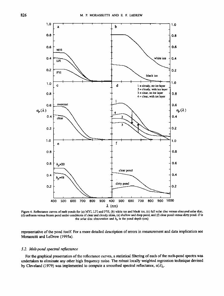
Figure 4(a) shows the differences in reflectances for ponds on FYI, LFI, and MYI. Respectively, their depths are 15, 16, and 20 cm. The FYI pond is dark green whereas both the LFI and MY1 ponds are grey-blue in colour. All were measured under clear-sky conditions. In these curves, it is observed that the largest differences existing between the reflectances occur in the 400-500 nm band (approximately 10-20 per cent). From 500 nm onwards, the differences gradually decrease to almost zero at 800 nm. For wavelengths greater than 800 nm, all three ice types have reflectances that are nearly equal. Because each of the ice types have their own distinguishing physical properties, in the curve comparisons examined below, one surface or solar parameter is made to vary while all others were held as equal to each other as possible. This was done so as to obtain an idea of the importance of the varying parameter on pond reflectance. The large number of spectra measured in the field makes this possible. A few of these comparisons are given below.

Figure 4(b) shows two reflectance spectra on FYI. One pond exists on a ‘white ice’surface, being 2 cm in depth and grey in colour. The ‘black ice’ pond is 6 cm deep with a dark grey colour. Both curves were recorded under overcast skies. It is seen that the difference in reflectance between the two curves is extremely large for all wavelengths. Reflectances on white ice are always greater than those on black ice. The greatest differences in reflectance occur in the visible, by up to 50 per cent, and gradually decline to approximately 20 per cent at near- infrared wavelengths. The ice property that, in this instance, has the greatest effect on the differences is the bubble density of the ice-pack. Higher bubble densities (making the ice appear ‘white’) will greatly scatter and reflect incoming radiation whereas low bubble density (making the ice appear ‘black’) will reflect nearly not as much. For the latter condition when the ice is translucent, the colour is much darker because of the effects of the underlying ocean, namely its low reflectively.

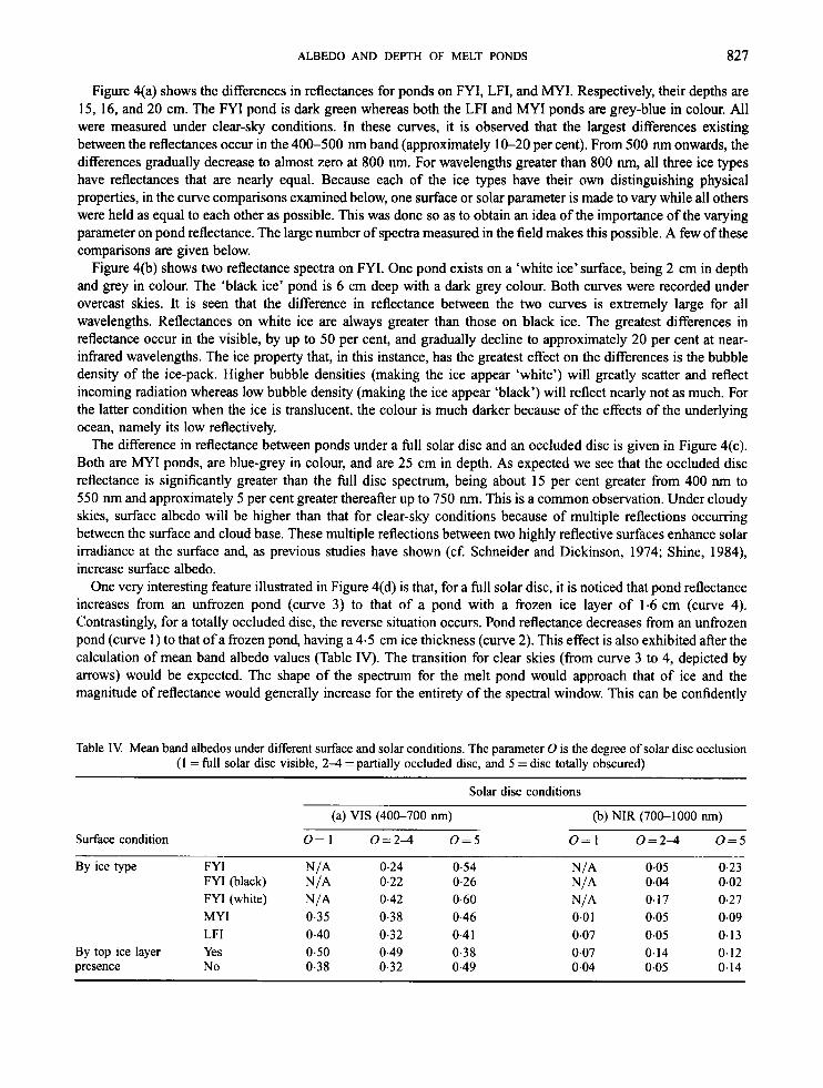
The difference in reflectance between ponds under a full solar disc and an occluded disc is given in Figure 4(c). Both are MY1 ponds, are blue-grey in colour, and are 25 cm in depth. As expected we see that the occluded disc reflectance is significantly greater than the f i l l disc spectrum, being about 15 per cent greater from 400 nm to 550 nm and approximately 5 per cent greater thereafter up to 750 nm. This is a common observation. Under cloudy skies, surface albedo will be higher than that for clear-sky conditions because of multiple reflections occurring between the surface and cloud base. These multiple reflections between two highly reflective surfaces enhance solar irradiance at the surface and, as previous studies have shown (cf. Schneider and Dickinson, 1974; Shine, 1984), increase surface albedo.

One very interesting feature illustrated in Figure 4(d) is that, for a full solar disc, it is noticed that pond reflectance increases from an unfrozen pond (curve 3) to that of a pond with a frozen ice layer of 1.6 cm (curve 4). Contrastingly, for a totally occluded disc, the reverse situation occurs. Pond reflectance decreases from an unfrozen pond (curve 1) to that of a frozen pond, having a 4.5 cm ice thickness (curve 2). This effect is also exhibited after the calculation of mean band albedo values (Table IV). The transition for clear skies (from curve 3 to 4, depicted by arrows) would be expected. The shape of the spectrum for the melt pond would approach that of ice and the magnitude of reflectance would generally increase for the entirety of the spectral window. This can be confidently

Table IV Mean band albedos under different surface and solar conditions. The parameter 0 is the degree of solar disc occlusion (1 = full solar disc visible, 2 4 = partially occluded disc, and 5 = disc totally obscured)

Solar disc conditions

Surface condition

(a) VIS (400-700 nm) (b) NIR (700-1000 nm)

o= 1 0 = 2 4 0 = 5 0=1 0 = 2 - 4 0 = 5

0.05 0.23 0.04 0.02

FYI (white) N/A 0.42 0.60 NIA 0.17 0.27 MY1 0.35 0.38 0.46 0.01 0.05 0.09 LFI 0-40 0.32 0.4 1 0.07 0.05 0.13

0.24 0.54 NIA 0.22 0.26 N/A

By ice type FYI NIA FYI (black) NIA

By top ice layer Yes 0.50 0.49 0.38 0-07 0.14 0.12 presence No 0.38 0.32 0.49 0.04 0.05 0.14

828

- 30 5

-20 8

-10

M. F! MORASSUTTI AND E. F. LEDREW

0.4

0.3

0.2

0.1

0.4

z 8 0.3

f 2 0.2 0.1

0.20

0.1 5

0.10

0.05

a n=220

b FIRST-YEAR ICE 40

n=88 t

C LANDFAST ICE n=1%

t 40 - 30

- 20 -10

1 5 9 13 17 COLOUR

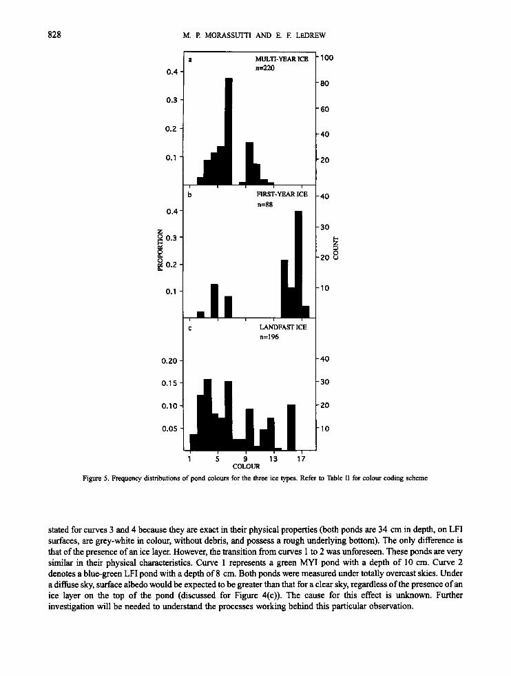
Figure 5 . Frequency distributions of pond colours for the three ice types. Refer to Table I1 for colour coding scheme

stated for curves 3 and 4 because they are exact in their physical properties (both ponds are 34 cm in depth, on LFI surfaces, are grey-white in colour, without debris, and possess a rough underlying bottom). The only difference is that of the presence of an ice layer. However, the transition from curves 1 to 2 was unforeseen. These ponds are very similar in their physical characteristics. Curve 1 represents a green MY1 pond with a depth of 10 cm. Curve 2 denotes a blue-green LFI pond with a depth of 8 cm. Both ponds were measured under totally overcast skies. Under a diffuse sky, surface albedo would be expected to be greater than that for a clear sky, regardless of the presence of an ice layer on the top of the pond (discussed for Figure 4(c)). The cause for this effect is unknown. Further investigation will be needed to understand the processes working behind this particular observation.

ALBEDO AND DEPTH OF MELT PONDS 829

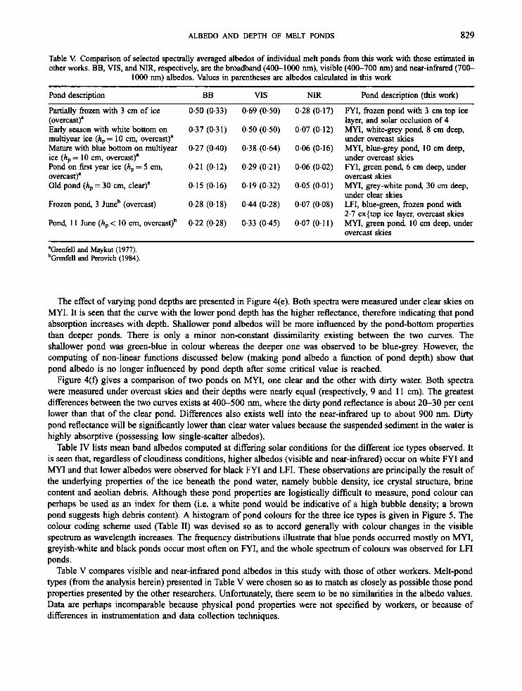
Table V. Comparison of selected spectrally averaged albedos of individual melt ponds from this work with those estimated in other works. BB, VIS, and NIR, respectively, are the broadband (400-1000 nm), visible (400-700 nm) and near-infrared (700-

1000 nm) albedos. Values in parentheses are albedos calculated in this work

Pond description BB VIS NIR Pond description (this work)

Partially frozen with 3 cm of ice (overcast)' Early season with white bottom on 0.37 (0.31) 0.50 (0.50) 0.07 (0.12) MYI, white-grey pond, 8 cm deep, multiyear ice (hp = 10 cm, overcast)a Mature with blue bottom on multiyear 0.27 (0.40) 0.38 (0.64) 0.06 (0.16) MYI, blue-grey pond, 10 cm deep, ice (hp = 10 cm, overcast)' Pond on first year ice (hp = 5 cm, 0.21 (0.12) 0.29 (0.21) 0.06 (0.02) FYI, green pond, 6 cm deep, under overcast)a overcast skies Old pond (hp = 30 cm, clear)' 0.15 (0.16) 0.19 (0.32) 0.05 (0.01) MYI, grey-white pond, 30 cm deep,

under clear skies Frozen pond, 3 Juneb (overcast) 0.28 (0.18) 0.44 (0.28) 0.07 (0.08) LFI, blue-green, frozen pond with

2.7 cx{top ice layer, overcast skies Pond, 11 June (hp < 10 cm, overcast)b MYI, green pond, 10 cm deep, under

overcast skies

0.50 (0.33) 0.69 (0.50) 0.28 (0.17) FYI, frozen pond with 3 cm top ice layer, and solar occlusion of 4

under overcast skies

under overcast skies

0.22 (0.28) 0.33 (0.45) 0.07 (0.1 1)

'Grenfell and Maykut (1977). bGrenfell and Perovich (1984).

The effect of varying pond depths are presented in Figure 4(e). Both spectra were measured under clear skies on MYI. It is seen that the curve with the lower pond depth has the higher reflectance, therefore indicating that pond absorption increases with depth. Shallower pond albedos will be more influenced by the pond-bottom properties than deeper ponds. There is only a minor non-constant dissimilarity existing between the two curves. The shallower pond was green-blue in colour whereas the deeper one was observed to be blue-grey. However, the computing of non-linear functions discussed below (making pond albedo a function of pond depth) show that pond albedo is no longer influenced by pond depth after some critical value is reached.

Figure 4(f) gives a comparison of two ponds on MYI, one clear and the other with dirty water. Both spectra were measured under overcast skies and their depths were nearly equal (respectively, 9 and 11 cm). The greatest differences between the two curves exists at 400-500 nm, where the dirty pond reflectance is about 20-30 per cent lower than that of the clear pond. Differences also exists well into the near-infrared up to about 900 nm. Dirty pond reflectance will be significantly lower than clear water values because the suspended sediment in the water is highly absorptive (possessing low single-scatter albedos).

Table IV lists mean band albedos computed at differing solar conditions for the different ice types observed. It is seen that, regardless of cloudiness conditions, higher albedos (visible and near-infrared) occur on white FYI and MYI and that lower albedos were observed for black FYI and LFI. These observations are principally the result of the underlying properties of the ice beneath the pond water, namely bubble density, ice crystal structure, brine content and aeolian debris. Although these pond properties are logistically difficult to measure, pond colour can perhaps be used as an index for them (i.e. a white pond would be indicative of a high bubble density; a brown pond suggests high debris content). A histogram of pond colours for the three ice types is given in Figure 5. The colour coding scheme used (Table 11) was devised so as to accord generally with colour changes in the visible spectrum as wavelength increases. The frequency distributions illustrate that blue ponds occurred mostly on MYI, greyish-white and black ponds occur most often on FYI, and the whole spectrum of colours was observed for LFI ponds.

Table V compares visible and near-infiared pond albedos in this study with those of other workers. Melt-pond types (from the analysis herein) presented in Table V were chosen so as to match as closely as possible those pond properties presented by the other researchers. Unfortunately, there seem to be no similarities in the albedo values. Data are perhaps incomparable because physical pond properties were not specified by workers, or because of differences in instrumentation and data collection techniques.

830 M. P. MORASSUTTI AND E. F. LEDREW

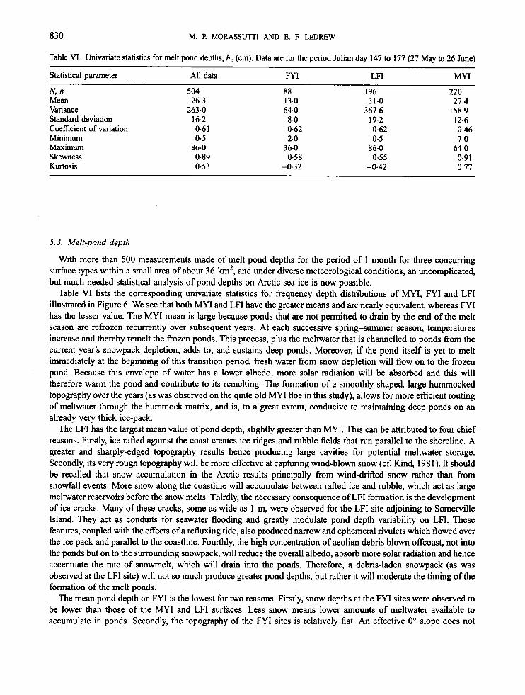
Table VI. Univariate statistics for melt pond depths, h, (cm). Data are for the period Julian day 147 to 177 (27 May to 26 June)

Statistical parameter All data FYI LFI MY1

N, n 504 88 196 220 Mean 26.3 13.0 31.0 27.4 Variance 263.0 64.0 367.6 158.9 Standard deviation 16.2 8.0 19.2 12.6 Coefficient of variation 0.61 0.62 0.62 0.46 Minimum 0.5 2.0 0.5 7.0 Maximum 86.0 36.0 86.0 64.0 Skewness 0.89 0.58 0.55 0.9 1 Kurtosis 0.53 -0.32 -0.42 0.77

5.3. Melt-pond depth

With more than 500 measurements made of melt pond depths for the period of 1 month for three concurring surface types within a small area of about 36 km2, and under diverse meteorological conditions, an uncomplicated, but much needed statistical analysis of pond depths on Arctic sea-ice is now possible.

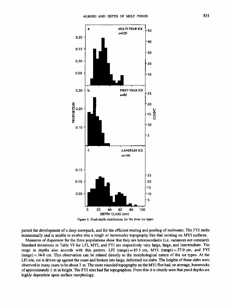
Table VI lists the corresponding univariate statistics for frequency depth distributions of MYI, FYI and LFI illustrated in Figure 6. We see that both MY1 and LFI have the greater means and are nearly equivalent, whereas FYI has the lesser value. The MY1 mean is large because ponds that are not permitted to drain by the end of the melt season are refrozen recurrently over subsequent years. At each successive spring-summer season, temperatures increase and thereby remelt the frozen ponds. This process, plus the meltwater that is channelled to ponds from the current year's snowpack depletion, adds to, and sustains deep ponds. Moreover, if the pond itself is yet to melt immediately at the beginning of this transition period, fresh water from snow depletion will flow on to the frozen pond. Because this envelope of water has a lower albedo, more solar radiation will be absorbed and this will therefore warm the pond and contribute to its remelting. The formation of a smoothly shaped, large-hummocked topography over the years (as was observed on the quite old MY1 floe in this study), allows for more efficient routing of meltwater through the hummock matrix, and is, to a great extent, conducive to maintaining deep ponds on an already very thick ice-pack.

The LFI has the largest mean value of pond depth, slightly greater than MYI. This can be attributed to four chief reasons. Firstly, ice rafted against the coast creates ice ridges and rubble fields that run parallel to the shoreline. A greater and sharply-edged topography results hence producing large cavities for potential meltwater storage. Secondly, its very rough topography will be more effective at capturing wind-blown snow (cf. Kind, 1981). It should be recalled that snow accumulation in the Arctic results principally from wind-drifted snow rather than from snowfall events. More snow along the coastline will accumulate between rafted ice and rubble, which act as large meltwater reservoirs before the snow melts. Thirdly, the necessary consequence of LFI formation is the development of ice cracks. Many of these cracks, some as wide as 1 m, were observed for the LFI site adjoining to Somerville Island. They act as conduits for seawater flooding and greatly modulate pond depth variability on LFI. These features, coupled with the effects of a refluxing tide, also produced narrow and ephemeral rivulets which flowed over the ice pack and parallel to the coastline. Fourthly, the high concentration of aeolian debris blown offcoast, not into the ponds but on to the surrounding snowpack, will reduce the overall albedo, absorb more solar radiation and hence accentuate the rate of snowmelt, which will drain into the ponds. Therefore, a debris-laden snowpack (as was observed at the LFI site) will not so much produce greater pond depths, but rather it will moderate the timing of the formation of the melt ponds.

The mean pond depth on FYI is the lowest for two reasons. Firstly, snow depths at the FYI sites were observed to be lower than those of the MY1 and LFI surfaces. Less snow means lower amounts of meltwater available to accumulate in ponds. Secondly, the topography of the FYI sites is relatively flat. An effective 0" slope does not

ALBEDO AND DEPTH OF MELT PONDS 83 1

0.20

0.1 5

0.10

0.05

0.30

E 2 6

0.20

0

0.10

0.15

0.10

0.05

a MULTI-YEAR ICE n=220

b FIRST-YEAR ICE n=88

C LANDFAST ICE n=1%

50

40

30

20

10

25

20

15 8

10

5

25

20

15

10

5

0 20 40 60 80 100 DEPTH CLASS (crn)

Figure 6 . Pond-depth distributions for the three ice types

permit the development of a deep snowpack, and for the efficient routing and pooling of meltwater. The FYI melts interannually and is unable to evolve into a rough or hummocky topography like that existing on MY1 surfaces.

Measures of dispersion for the three populations show that they are heteroscedastic (i.e. variances not constant). Standard deviations in Table VI for LFI, MYI, and FYI are respectively very large, large, and intermediate. The range in depths also accords with this pattern: LFI (range)= 85.5 cm, MY1 (range)=57.0 cm, and FYI (range) = 34.0 cm. This observation can be related directly to the morphological nature of the ice types. At the LFI site, ice is driven up against the coast and broken into large, deformed ice slabs. The heights of these slabs were observed in many cases to be about 3 m. The more rounded topography on the MY1 floe had, on average, hummocks of approximately 1 m in height. The FYI sites had flat topographies. From this it is clearly seen that pond depths are highly dependent upon surface morphology.

832 M. P. MORASSLITTI AND E. F. LEDREW

Looking at variance only, however, does not furnish all of the necessary information. The shape of the depth distribution also reveals some interesting features. Computed values of kurtosis (the peakedness of the data distribution) in Table V and a look at Figure 6 indicates that MY1 and FYI pond depths are leptokurtic (very peaked) whereas they are mesokurtic (moderately peaked) for LFI. The greatest frequency of pond depths were observed within the range of about 25-35 cm for MYI, 10-15 cm for FYI, and 15-40 cm for LFI. Positive skews for all three distributions are also observed, showing that the majority of depths measured fall below approximately 30 cm. Furthermore, both the MY1 and LFI pond depths exhibit bimodal distributions. Eicken et al. (1994a,b) have reported recently on the bimodal distribution of pond depths on MYI. They attribute the bimodal shape to the debris accumulation in the ponds. As they state: ‘Further data analysis in conjunction with thermodynamic modelling studies will have to establish whether these depth differences are due to the different amounts of heat absorbed by clean and dirty ice within one summer season, or whether these are the result of a sequential deepening during successive years.’ (Eicken et al. (1994a, p. 74)).

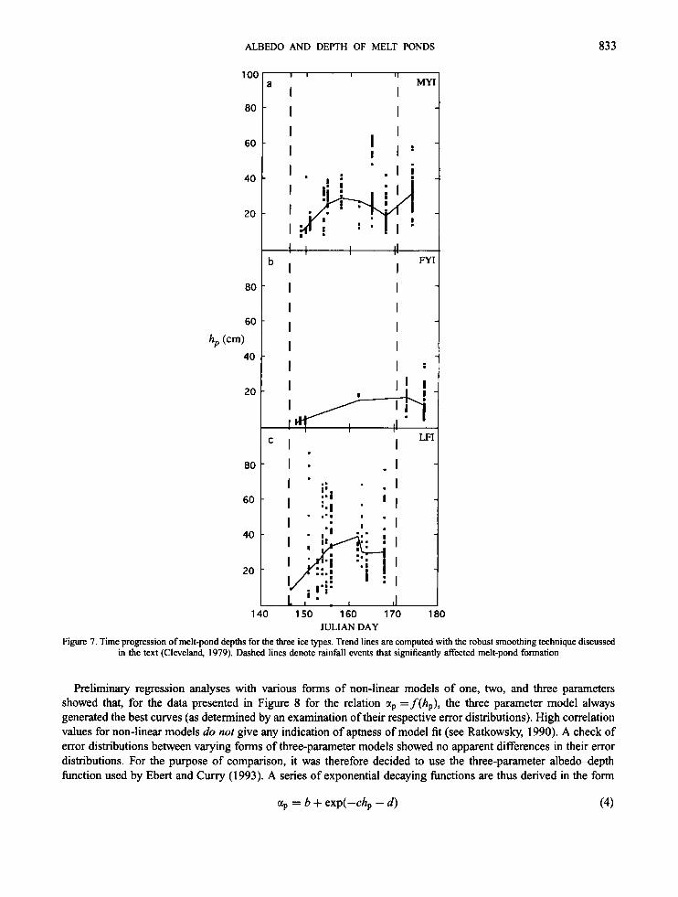
Figure 7 shows the time progression of melt-pond depth for the entire study period over the three surface types. The scatter plots also emphasize the degree of depth variability discussed above. For both FYI and MYI, the variation in depth increases with time, whereas the variability on LFI is large and relatively constant throughout. Overall, it is seen that there is a moderate rate of the increase in ponds depths over time for all three ice types. After the late May rain event (Julian day 147), a rapid rise in pond depth for MY1 and LFI is evident. Afterwards, the trend line plateaus and then the slope becomes negative. Unfortunately, because of the dearth of data for a large segment of this time span (early- to mid-June), this supposition cannot be made for FYI with any measure of assurance. Following the 20 June (Julian day 171) rainfall episode, there is a sharp positive change in the depth trend for MYI. Contrastingly, there is a reduction in the FYI depth trend. No data are available after 20 June for LFI to allow for additional inference.

The temporal variation in pond depth described here can be taken only in a qualitative manner. More systematic measurements over longer periods and under ‘normal’ meteorological conditions are required to adequately characterize the temporal evolution of pond depths in the study region. Moreover, any comparison of the depth data here with those of other workers would be impractical because the data presented in published works, besides being few and far between, are given as ranges, or as values without specific date identification, or the ponds are just described (e.g. ‘shallow pond’, ‘pond, h, > 12 cm’, etc.).

The statistical analysis above and an examination of the frequency and time distributions of depth in Figures 6 and 7 indicate that pond depths over the three surface types apparently exhibit their own characteristic shapes. The non- parametric Kruskal-Wallis statistic is calculated to determine if there is a statistically significant difference between the three sample populations. This technique is designed for comparisons of three or more sample populations and is calculated from the following equation

12 R? H = C - - 3 ( N + 1)

N ( N + 1) i=l ni (3)

where His the test statistic, N is total number of depth measurements in all of the three sample populations, k is the number of sample distributions, R is the sum of the ranks within each sample population, and n is the sample population. In our study, N = 504, nl[MYI] = 220, n2[FYI] = 88, n3[LFI] = 196, and k= 3. Application of this test gives H = 91.96, which is much greater than its critical value (1 6.17) at the 0-001 significant level with two degrees of freedom (k - 1). Therefore, we can confidently state that, for our data, the differences between the sample populations are representative of real depth differences between the three ice types.

5.4. Parameterization development

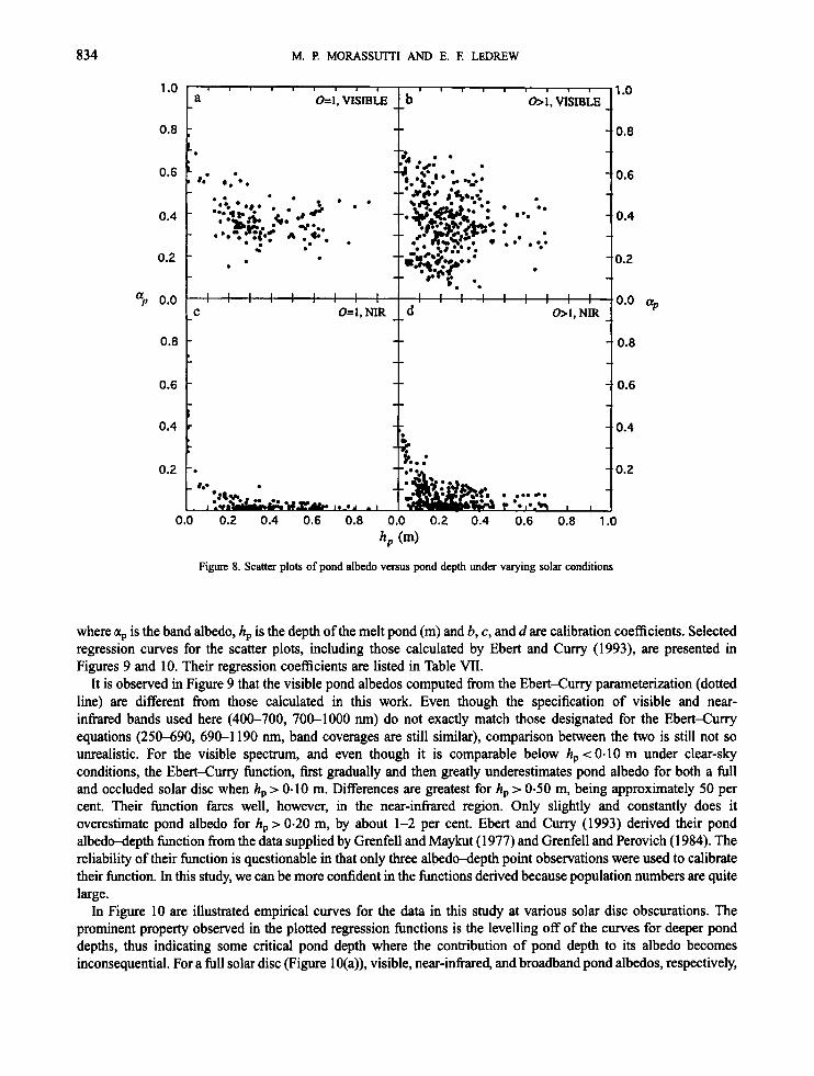
Scatter plots of band albedos (Figure 8) have shown that, in general, melt-pond albedo decreases in an exponential fashion with depth. The strongest relationship exists in the near-infrared window (700-1000 nm) whereas the greatest data dispersion occurs in the visible range (400-700 nm). It is also observed that dispersion is greater when the solar disc is obscured by clouds. These non-linear relationships allow for the derivation of empirical equations.

ALBEDO AND DEPTH OF MELT PONDS 833

1 oc

80

60

40

20

80

60

hp (cm) 40

20

80

60

40

20

I 1 I II

MY I I

a

I I

I I I I I :

I I ' 1

-zzLi c I I LF

I . . I

140 150 160 170 180 JULIAN DAY

Figure 7. Time progression of melt-pond depths for the three ice types. Trend lines are computed with the robust smoothing technique discussed in the text (Cleveland, 1979). Dashed lines denote rainfall events that significantly affected melt-pond formation

Preliminary regression analyses with various forms of non-linear models of one, two, and three parameters showed that, for the data presented in Figure 8 for the relation up =f(hp), the three parameter model always generated the best curves (as determined by an examination of their respective error distributions). High correlation values for non-linear models do not give any indication of aptness of model fit (see Ratkowsky, 1990). A check of error distributions between varying forms of three-parameter models showed no apparent differences in their error distributions. For the purpose of comparison, it was therefore decided to use the three-parameter albedo-depth function used by Ebert and Curry (1 993). A series of exponential decaying hc t ions are thus derived in the form

a, = b + exp(-ch, - d) (4)

834 M. P. MORASSUTTI AND E. E LEDREW

Figure 8. Scatter plots of pond albedo versus pond depth under varying solar conditions

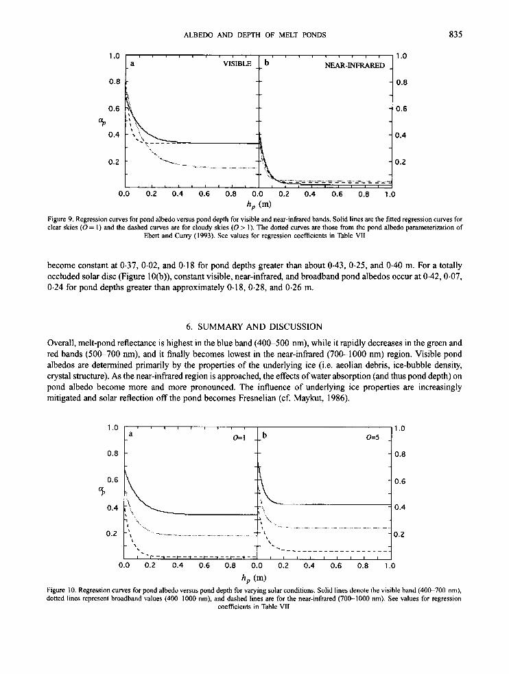
where a, is the band albedo, h, is the depth of the melt pond (m) and b, c, and dare calibration coefficients. Selected regression curves for the scatter plots, including those calculated by Ebert and Curry (1993), are presented in Figures 9 and 10. Their regression coefficients are listed in Table VII.

It is observed in Figure 9 that the visible pond albedos computed from the Ebert-Curry parameterization (dotted line) are different from those calculated in this work. Even though the specification of visible and near- infrared bands used here (400-700, 700-1000 nm) do not exactly match those designated for the Ebert-Curry equations (250-690, 690-1 190 nm, band coverages are still similar), comparison between the two is still not so unrealistic. For the visible spectrum, and even though it is comparable below h,<0.10 m under clear-sky conditions, the Ebert-Curry function, first gradually and then greatly underestimates pond albedo for both a full and occluded solar disc when h, > 0-10 m. Differences are greatest for h, > 0-50 m, being approximately 50 per cent. Their function fares well, however, in the near-infrared region. Only slightly and constantly does it overestimate pond albedo for h, > 0.20 m, by about 1-2 per cent. Ebert and Cuny (1993) derived their pond albedodepth function from the data supplied by Grenfell and Maykut (1 977) and Grenfell and Perovich (1984). The reliability of their function is questionable in that only three albeddepth point observations were used to calibrate their function. In this study, we can be more confident in the functions derived because population numbers are quite large.

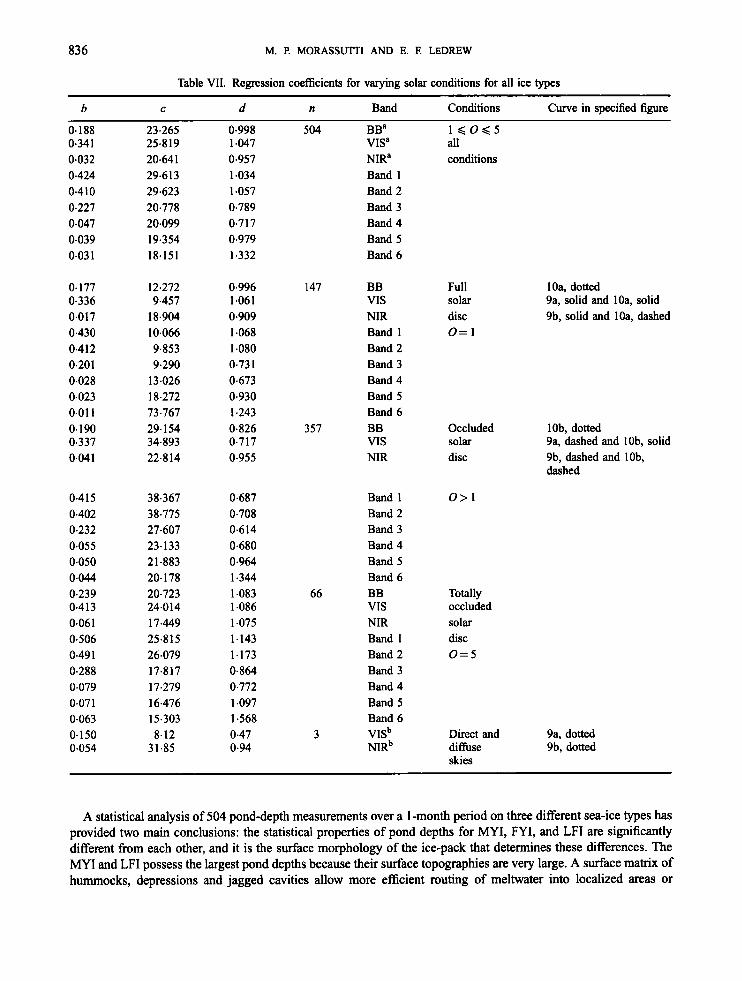
In Figure 10 are illustrated empirical curves for the data in this study at various solar disc obscurations. The prominent property observed in the plotted regression functions is the levelling off of the curves for deeper pond depths, thus indicating some critical pond depth where the contribution of pond depth to its albedo becomes inconsequential. For a full solar disc (Figure 1 O(a)), visible, near-infrared, and broadband pond albedos, respectively,

ALBEDO AND DEPTH OF MELT PONDS 835

1 .o

0.8

0.6

5J 0.4

0.2

0.0 0.2 0.4 0.6 0.8 0.0 0.2 0.4 0.6 0.8 1.0

h, (m) Figure 9. Regression curves for pond albedo v e m s pond depth for visible and near-infrared bands. Solid lines are the fitted regression curves for clear skies (0= 1) and the dashed curves are for cloudy skies (0> I ) . The dotted curves are those from the pond albedo parameterization of

Ebert and Curry (1993). See values for regression coefficients in Table V11

become constant at 0.37, 0.02, and 0.18 for pond depths greater than about 0.43, 0.25, and 0.40 m. For a totally occluded solar disc (Figure lO(b)), constant visible, near-infrared, and broadband pond albedos occur at 0.42,0.07, 0.24 for pond depths greater than approximately 0.18, 0.28, and 0-26 m.

6. SUMMARY AND DISCUSSION

Overall, melt-pond reflectance is highest in the blue band (400-500 nm), while it rapidly decreases in the green and red bands (50&700 nm), and it finally becomes lowest in the near-infrared (700-1000 nm) region. Visible pond albedos are determined primarily by the properties of the underlying ice (i.e. aeolian debris, ice-bubble density, crystal structure). As the near-infrared region is approached, the effects of water absorption (and thus pond depth) on pond albedo become more and more pronounced. The influence of underlying ice properties are increasingly mitigated and solar reflection off the pond becomes Fresnelian (cf. Maykut, 1986).

1 .o

0.8

0.6

9 0.4

0.2

I ' , ~ - l_ - r_+ - - r -+__r_+-_ I I , , 1 1 1 1

0.0 0.2 0.4 0.6 0.8 0.0 0.2 0.4 0.6 0.8 1.0

h, (m> Figure 10. Regression curves for pond albedo versus pond depth for varying solar conditions. Solid lines denote the visible band (40C700 nm), dotted lines represent broadband values (400-1000 nm), and dashed lines are for the near-infrared (700-1000 nm). See values for regression

coefficients in Table VII

836 M. P. MORASSUTTI AND E. F. LEDREW

Table VII. Regression coefficients for varying solar conditions for all ice types

b C d n Band Conditions Curve in specified figure

0.188 0.341 0.032 0.424 0.410 0.227 0.047 0.039 0.03 1

0.177 0.336 0.017 0.430 0.412 0.201 0.028 0.023 0.01 1 0.190 0.337 0.041

0.4 15 0.402 0.232 0.055 0.050 0.044 0.239 0.413 0.061 0.506 0.49 1 0.288 0.079 0.07 1 0.063 0.150 0.054

23.265 25.819 20.641 29.613 29.623 20.778 20.099 19.354 18.151

12.272 9.457

18.904 10.066 9.853 9.290

13.026 18.272 73.767 29.154 34.893 22.814

38.367 38.775 27.607 23.133 21.883 20.178 20.723 24.014 17.449 25.815 26.079 17.817 17.279 16.476 15.303 8.12

31.85

0.998 1 a47 0,957 1.034 1.057 0.789 0.717 0.979 1.332

0.996 1.06 1 0.909 1.068 1.080 0.73 1 0.673 0.930 1.243 0.826 0.717 0.955

0.687 0.708 0.614 0.680 0.964 1.344 1.083 1.086 1.075 1.143 1.173 0.864 0.772 1.097 1.568 0.47 0.94

504 BB" VISB NIR" Band 1 Band 2 Band 3 Band 4 Band 5 Band 6

147 BB VIS NIR Band 1 Band 2 Band 3 Band 4 Band 5 Band 6

357 BB VIS NIR

Band 1 Band 2 Band 3 Band 4 Band 5 Band 6

66 BB VIS NIR Band 1 Band 2 Band 3 Band 4 Band 5 Band 6

3 VISb N I R ~

1g0g5 all conditions

Full solar disc o= 1

IOa, dotted 9a, solid and 10a, solid 9b, solid and IOa, dashed

Occluded lob, dotted solar disc 9b, dashed and lob,

9a, dashed and lob, solid

dashed

o> 1

Totally occluded solar disc 0=5

Direct and 9a, dotted diffuse 9b, dotted skies

A statistical analysis of 504 pond-depth measurements over a 1-month period on three different sea-ice types has provided two main conclusions: the statistical properties of pond depths for MYI, FYI, and LFI are significantly different from each other, and it is the surface morphology of the ice-pack that determines these differences. The MYI and LFI possess the largest pond depths because their surface topographies are very large. A surface matrix of hummocks, depressions and jagged cavities allow more efficient routing of meltwater into localized areas or

ALBEDO AND DEPTH OF MELT PONDS 837

‘ponds’. Contrastingly, FYI has lower pond depths because an effectively ‘flat’ surface will not channel water efficiently and therefore meltwater will not be transported so much in the horizontal direction. From this we can infer that, during the peak melt in the summer season, melt-pond areal extent will be greater on FYI than on MYI. Furthermore, both MY1 and LFI have bimodal depth distributions, most likely due to differences in solar absorption as caused by the presence of debris on pond bottoms (cf. Eicken et al., 1994a,b).

Scatter plots illustrated that both visible and near-infrared albedos decrease exponentially with depth. Exponential decay functions were compared with these data through regression for both clear and cloudy conditions in both the visible and near-infrared bands. Comparisons of these hc t ions with those derived recently by Ebert and Cuny (1 993) shows that the latter underestimate pond albedo for visible wavelengths, and that they slightly overestimate near-infrared values. Also, our regression curves indicated that pond albedo remains constant with changes in pond depth after some critical value is reached, dependmg on the degree of cloud occlusion of the solar disc and the spectral band.

How spatially representative are the data in this study? In other words, can these site-recorded data be extrapolated to sea-ice zones in the middle Arctic. Although these are valid questions, we would still answer yes. Firstly, it must be realized that at present there are little or no pond data available for the central Arctic. One must start somewhere and real-world observations are better than inferred formulations without empirical validation. Secondly, if our depth and albedo data are applicable in other regions, we would emphasize mainly our MY1 and FYI values. The morphology of LFI is radically different than the former two and it is ice morphology that determines pond depth and, to a significant degree, pond albedo. However, rubble ice morphology and even dirty ponds (both of which occur in more centralized sea-ice regions) are not dissimilar to what we observed at our LFI site. So LFI data may still be appropriate for the interior oceans. As a guide, spatial uniformity must be assumed for the time being until more elaborate data and interpretation become available.

The data and analysis presented in this work and two preliminary studies (Morassutti, 1994; Morassutti and LeDrew, 1995b) may provide some sort of groundwork for future studies concerned with the role that melt ponds play within the diverse number of feedbacks and interrelationships existing between the marine cryosphere and the Arctic atmosphere. Some of these would include: the derivation of a theoretically based radiative-hydrological melt- pond model (cf. Podgorny, 1994); the development of realistic formulations of melt-pond processes for implementation in thermodynamic sea-ice models (cf. Ebert and Curry, 1993); the refinement of computationally efficient, empirical parameterizations for use in sea-ice modules of global climate models (cf. Morassutti, 1989, 199 1); and the construction and validation of satellite retrieval algorithms for the marine cryosphere (cf. Robinson et al., 1992). The melt-pond data set (including documentation) is now available in a technical report (Morassutti and LeDrew, 1995a).

ACKNOWLEDGEMENTS

This work was supported by a grant from the Natural Sciences and Engineering Research Council (NSERC) of Canada to Professor Ellsworth LeDrew and by an Institute for Space and Terrestrial Science (ISTS) grant from the Centre of Excellence Program of the Province of Ontario. The staff and logistical support of the Polar Continental Shelf Project (PCSP) are greatly appreciated. Roger De Abreu is thanked for his help with the operation of the ASD spectrometer. We acknowledge Dr H. Eicken who pointed out to us the likely causes of the bimodal shape of the pond-depth distributions. We also thank two anonymous reviewers whose comments and criticisms helped improve this manuscript.

REFERENCES

ASD User’s Guide. 1993. Portable Personal Spectmmeter II, Analytical Spectral Devices, Inc., Boulder, CO., U.S.A. Andreas, E. L. and Ackley, S . F. 1982. ‘On the differences in ablation seasons of Arctic and Antarctic sea ice’, 1 Atmos. Sci., 39, 440447. Bany, R. G. 1983. ‘Arctic Ocean ice and climate: perspectives on a century of polar research’, Ann. Assoc. Am. Geogr, 73,485-501. Buzuev, A. Ya., Shesterikov, N. I? and Timerev, A. A. 1965. ‘Albedo l’da v Arkticheskikh Moryakh PO dannym nablyudeniy s samoleta’, Piwb.

C a y , F. J. 1985. ‘Summer arctic ice characteristics from satellite microwave data’, J. Geophys. Res., 90, 5015-5034. Chernigovski, N. T. 1968. ‘Radiation regime of the central Arctic Basin’, h b . Ark. Antark, 29, 3-1 1. Chukanin, K. I. 1954. ‘Aerometeomlogy’. in Observational Data of the Scientific-Research Dnfhng Station of 195&1951, American

Ark Antark., 20, 49-54.

838 M. P. MORASSUTTI AND E. E LEDREW

Meteorological Society, Vol. 111, NTIS Document AD117139, trans. E. R. Hope. Cleveland, W. S. 1979. ‘Robust locally weighted regression and smoothing scatterplots’, 1 Am. Statist. Assoc., 74, 829-836. Cogley, J. G. and Henderson-Sellers, A. 1985. The Albedo of Ice in Geneml Circulation Models, Trent Technical Note 85-2, Trent University,

Crane, R. G. and Barry, R. G. 1984. ‘The influence of clouds on climate with a focus on high latitude interactions’, 1 Climatol., 4, 71-93. Cuny, J. A., Schramm, J. L. and Ebert, E. E. 1995. ‘Sea ice-albedo climate feedback mechanism’, 1 Climate, 8, 240-247. E M , E. E. and Curry, J. A. 1993. ‘An intermediate one-dimensional thermodynamic sea ice model for investigating ice-atmosphere

interactions’, 1 Geophys. Res., 98, 10085-10019. Eicken, H., Alexandrov, V., Gradinger, R., Ilyin, R., Ivanov, B., Luchetta, A., Martin, T., Olsson, K., Reimitz, R., Pic, R., Poniz, P. and

Weissenberger, J. 1994a. ‘Distribution, structure and hydrography of surface melt puddles’, Ber Polarjbrsch., 149, 73-76. Eicken, H., Gradinger, R., Pac, R., Scheele, N., Ivanov, B. and Alexandrov, V. 1994b. ‘Field studies of surface melt puddles on sea ice in the

Eurasian Arctic’, Abstract 1-5, WCRP Scientiic Conference on the Dynamics of the Arctic Climate System, 7-10 November 1994, Goteborg, Sweden.

Peterborough, Ontario, Canada, 50 pp.

Environment Canada 1984. Principal Station Data, Resolute, PSD-71, Atmospheric Environment Service, Downsview, Ontario, 51 pp. Grenfell, T. C. and Maykut, G. A. 1977. ‘The optical properties of ice and snow in the Arctic Basin’, 1 Glaciol., 18, 445-464. Grenfell, T. C. and Perovich, D. K. 1984. ‘Spectral albedos of sea ice and incident solar irradiance in the Southern Beaufort Sea’, 1 Geophys.

Hanson, K. J. 1961. ‘The albedo of sea ice and ice islands in the Arctic Ocean Basin’, Arctic, 14, 188-196. Henderson-Sellers, A., McGuffie, K. and Cogley, J. G. 1985. ‘Seasonal climatology of cloud at Resolute (75”N)’, Armos. Ocean, 23, 80-93. Ingram, W. J., Wilson, C. A. and Mitchell, J. F. B. 1988. Modelling Climate Change: An Assessment of Sea-Ice and Surface Albedo Feedbacks,

Kind, R. J. 1981. ‘Snow drifting’, in Gray, D. M. and Male, D. H. (eds), The Handbook of Snow: Principles, Processes, Management and Use,

Langleben, M. P. 1969. ‘Albedo and degree of pudding of a melting cover of sea ice’, J: Glaciol., 8, 407412. Langleben, M. I? 1971. ‘Albedo of melting ice in the Southern Beaufort Sea’, 1 Glacial., 10, 101-104. LeDrew, E. F. and Barber, D. G. 1994. ‘The SIMMS program: a study of change and variability within the marine cryosphere’, Arctic, 47,256-

Maykut, G. A. 1986. ‘The surface heat and mass balance’, in Untersteiner, N. (ed.), The Geophysics of Sea Ice, NATO AS1 Series, Series B:

Morassutti, M. P. 1989. ‘Surface albedo parameterization in sea-ice models’, Prop. Phys. Geogr, 13, 348-366. Morassutti, M. I? 1991. ‘Climate model sensitivity to sea ice albedo parameterization’, Theor Appl. Climatol., 44, 25-36. Morassutti, M. P. 1992. ‘Component reflectance scheme for DMSP-derived sea ice reflectances in the Arctic Basin’, Int. 1 Rem. Sens., 13,647-

Morassutti, M. P. 1994. ‘Spectral reflectance of melt ponds’, in Misurak, K. M., Barber, D. G. and LeDrew, E. F. (eds), SIMMS ’94 Data Report,

Morassutti, M. I? and LeDrew, E. F. 1995a. Melt Pond Dataset for use in Sea-Ice and Climate-Related Studies, ISTS-EOL-TR95, Earth-

Morassutti, M. P. and LeDrew, E. F. 1995b. ‘Measurement, analysis and parameterization of melt pond albedo’, in Proceedings of the WCRP

Nazintsez, Yu. L. 1964. ‘Thermal balance of the surface of the perennial ice cover in the central Arctic’, ‘fr Ark. Antark. Nauchno Issled. Inst.,

Perovich, D. K. 1994. ‘Light reflection from sea ice during the onset of melt’, 1 Geophys. Res., 99, 3351-3359. Podgorny, I. A. 1994. ‘Parameterization for short-wave heat fluxes for a melt pond’, Abstract 1-20, WcRPScienhic Conference on the Dynamics

Ratkowsky, D. A. 1990. Handbook of Nonlinear Regression Models, Statistics: Textbooks and Monographs, Vol. 107, Marcel Dekker Inc.,

Robinson, D. A,, Serreze, M. C., Barry, R. G., Scharfen, G. and Kukla, G. 1992. ‘Large-scale patterns and variability of snowmelt and

Rossow, W. B., Brest, C. L. and Gardner, L. C. 1989. ‘Global, seasonal surface variations from satellite radiance measurements’, 1 Climate, 2,

Scharfen, G., Barry, R. G., Robinson, D. A,, Kukla, G. and Serreze, M. C. 1987. ‘Large-scale patterns of snow melt on Arctic sea ice mapped

Schneider, S. H. and Dickinson, R. E. 1974. ‘Parameterization of fractional cloud amounts in climatic models: the importance of modeling

Shine, K. P. 1984. ‘Parametrization of the shortwave flux over high albedo surfaces as a hnction of cloud thickness and surface albedo’, Q. J: R.

Shine, K. I?, Henderson-Sellers, A. and Barry, R. G. 1984. ‘Albedmlimate feedback: the importance of cloud and cryosphere variability’, in

Res., 89, 3573-3580.

Dynamical Climatology Technical Note No. 69, UKMO, Bracknell, United Kingdom, 35 pp.

Pergamon Press, Canada, pp. 338-359.

264.

Physics, Vol. 146, Plenum Press, pp. 395463.

662.

ISTS-EOL-SIMMS-TR94-001, Earth-Observations Laboratory, ISTS, University of Waterloo, Canada, Section 5.3.

Observations Laboratory, ISTS, University of Waterloo, Canada, 53 pp.

Scienhic Conference on the Dynamics of the Arctic Climate System, 7-10 November 1994, Goteborg, Sweden, in press.

267, 110-126.

of the Arctic Climate System, 7-10 November 1994, Goteborg, Sweden.

241 pp.

parameterized surface albedo in the Arctic Basin’, 1 Climate, 5, 1 109-1 1 19.

214247.

from meteorological satellite imagery’, Ann. Glaciol., 9, 200-205.

multiple reflections’, 1 Appl. Meteorol., 15, 1050-1054.

Metereol. Sac., 110, 747-764.

Berger, A. L. and Nicolis, C. (eds.), New Perspectives in Climate Modelling, Elsevier, Amsterdam, pp. 135-155.