Embed Size (px)
DESCRIPTION
akutansi perhitungan 5
Citation preview
Volume 10, Number 2 ISSN 1096-3685
ACADEMY OF ACCOUNTING ANDFINANCIAL STUDIES JOURNAL
An official Journal of theAllied Academies, Inc.
Michael Grayson, Jackson State UniversityAccounting Editor
Denise Woodbury, Southern Utah UniversityFinance Editor
Academy Informationis published on the Allied Academies web page
www.alliedacademies.org
The Allied Academies, Inc., is a non-profit association of scholars, whose purposeis to support and encourage research and the sharing and exchange of ideas andinsights throughout the world.
Whitney Press, Inc.
Printed by Whitney Press, Inc.PO Box 1064, Cullowhee, NC 28723
www.whitneypress.com
Authors provide the Academy with a publication permission agreement. AlliedAcademies is not responsible for the content of the individual manuscripts. Anyomissions or errors are the sole responsibility of the individual authors. TheEditorial Board is responsible for the selection of manuscripts for publication fromamong those submitted for consideration. The Publishers accept final manuscriptsin digital form and make adjustments solely for the purposes of pagination andorganization.
The Academy of Accounting and Financial Studies Journal is published by theAllied Academies, Inc., PO Box 2689, 145 Travis Road, Cullowhee, NC 28723,(828) 293-9151, FAX (828) 293-9407. Those interested in subscribing to theJournal, advertising in the Journal, submitting manuscripts to the Journal, orotherwise communicating with the Journal, should contact the Executive Directorat [email protected].
Copyright 2006 by the Allied Academies, Inc., Cullowhee, NC

iii
Academy of Accounting and Financial Studies Journal, Volume 10, Number 2, 2006
Academy of Accounting and Financial Studies JournalAccounting Editorial Review Board Members
Agu AnanabaAtlanta Metropolitan CollegeAtlanta, Georgia
Richard FernEastern Kentucky UniversityRichmond, Kentucky
Manoj AnandIndian Institute of ManagementPigdamber, Rau, India
Peter FrischmannIdaho State UniversityPocatello, Idaho
Ali AzadUnited Arab Emirates UniversityUnited Arab Emirates
Farrell GeanPepperdine UniversityMalibu, California
D'Arcy BeckerUniversity of Wisconsin - Eau ClaireEau Claire, Wisconsin
Luis GillmanAerospeedJohannesburg, South Africa
Jan BellCalifornia State University, NorthridgeNorthridge, California
Richard B. GriffinThe University of Tennessee at MartinMartin, Tennessee
Linda BresslerUniversity of Houston-DowntownHouston, Texas
Marek GruszczynskiWarsaw School of EconomicsWarsaw, Poland
Jim BushMiddle Tennessee State UniversityMurfreesboro, Tennessee
Morsheda HassanGrambling State UniversityGrambling, Louisiana
Douglass CagwinLander UniversityGreenwood, South Carolina
Richard T. HenageUtah Valley State CollegeOrem, Utah
Richard A.L. CaldarolaTroy State UniversityAtlanta, Georgia
Rodger HollandGeorgia College & State UniversityMilledgeville, Georgia
Eugene CalvasinaSouthern University and A & M CollegeBaton Rouge, Louisiana
Kathy HsuUniversity of Louisiana at LafayetteLafayette, Louisiana
Darla F. ChisholmSam Houston State UniversityHuntsville, Texas
Shaio Yan HuangFeng Chia UniversityChina
Askar ChoudhuryIllinois State UniversityNormal, Illinois
Robyn HulsartOhio Dominican UniversityColumbus, Ohio
Natalie Tatiana ChurykNorthern Illinois UniversityDeKalb, Illinois
Evelyn C. HumeLongwood UniversityFarmville, Virginia
Prakash DheeriyaCalifornia State University-Dominguez HillsDominguez Hills, California
Terrance JalbertUniversity of Hawaii at HiloHilo, Hawaii
Rafik Z. EliasCalifornia State University, Los AngelesLos Angeles, California
Marianne JamesCalifornia State University, Los AngelesLos Angeles, California

iv
Academy of Accounting and Financial Studies JournalAccounting Editorial Review Board Members
Academy of Accounting and Financial Studies Journal, Volume 10, Number 2, 2006
Jongdae JinUniversity of Maryland-Eastern ShorePrincess Anne, Maryland
Ida Robinson-BackmonUniversity of BaltimoreBaltimore, Maryland
Ravi KamathCleveland State UniversityCleveland, Ohio
P.N. SaksenaIndiana University South BendSouth Bend, Indiana
Marla KrautUniversity of IdahoMoscow, Idaho
Martha SaleSam Houston State UniversityHuntsville, Texas
Jayesh KumarXavier Institute of ManagementBhubaneswar, India
Milind SathyeUniversity of CanberraCanberra, Australia
Brian LeeIndiana University KokomoKokomo, Indiana
Junaid M.ShaikhCurtin University of TechnologyMalaysia
Harold LittleWestern Kentucky UniversityBowling Green, Kentucky
Ron StundaBirmingham-Southern CollegeBirmingham, Alabama
C. Angela LetourneauWinthrop UniversityRock Hill, South Carolina
Darshan WadhwaUniversity of Houston-DowntownHouston, Texas
Treba MarshStephen F. Austin State UniversityNacogdoches, Texas
Dan WardUniversity of Louisiana at LafayetteLafayette, Louisiana
Richard MasonUniversity of Nevada, RenoReno, Nevada
Suzanne Pinac WardUniversity of Louisiana at LafayetteLafayette, Louisiana
Richard MautzNorth Carolina A&T State UniversityGreensboro, North Carolina
Michael WattersHenderson State UniversityArkadelphia, Arkansas
Rasheed MblakpoLagos State UniversityLagos, Nigeria
Clark M. WheatleyFlorida International UniversityMiami, Florida
Nancy MeadeSeattle Pacific UniversitySeattle, Washington
Barry H. WilliamsKing’s CollegeWilkes-Barre, Pennsylvania
Thomas PresslyIndiana University of PennsylvaniaIndiana, Pennsylvania
Carl N. WrightVirginia State UniversityPetersburg, Virginia
Hema RaoSUNY-OswegoOswego, New York

v
Academy of Accounting and Financial Studies Journal, Volume 10, Number 2, 2006
Academy of Accounting and Financial Studies JournalFinance Editorial Review Board Members
Confidence W. AmadiFlorida A&M UniversityTallahassee, Florida
Ravi KamathCleveland State UniversityCleveland, Ohio
Roger J. BestCentral Missouri State UniversityWarrensburg, Missouri
Jayesh KumarIndira Gandhi Institute of Development ResearchIndia
Donald J. BrownSam Houston State UniversityHuntsville, Texas
William LaingAnderson CollegeAnderson, South Carolina
Richard A.L. CaldarolaTroy State UniversityAtlanta, Georgia
Helen LangeMacquarie UniversityNorth Ryde, Australia
Darla F. ChisholmSam Houston State UniversityHuntsville, Texas
Malek LashgariUniversity of HartfordWest Hartford, Connetticut
Askar ChoudhuryIllinois State UniversityNormal, Illinois
Patricia LobingierGeorge Mason UniversityFairfax, Virginia
Prakash DheeriyaCalifornia State University-Dominguez HillsDominguez Hills, California
Ming-Ming LaiMultimedia UniversityMalaysia
Martine DuchateletBarry UniversityMiami, Florida
Steve MossGeorgia Southern UniversityStatesboro, Georgia
Stephen T. EvansSouthern Utah UniversityCedar City, Utah
Christopher NgassamVirginia State UniversityPetersburg, Virginia
William ForbesUniversity of GlasgowGlasgow, Scotland
Bin PengNanjing University of Science and TechnologyNanjing, P.R.China
Robert GraberUniversity of Arkansas - MonticelloMonticello, Arkansas
Hema RaoSUNY-OswegoOswego, New York
John D. GroesbeckSouthern Utah UniversityCedar City, Utah
Milind SathyeUniversity of CanberraCanberra, Australia
Marek GruszczynskiWarsaw School of EconomicsWarsaw, Poland
Daniel L. TompkinsNiagara UniversityNiagara, New York
Mahmoud HajGrambling State UniversityGrambling, Louisiana
Randall ValentineUniversity of MontevalloPelham, Alabama
Mohammed Ashraful HaqueTexas A&M University-TexarkanaTexarkana, Texas
Marsha WeberMinnesota State University MoorheadMoorhead, Minnesota
Terrance JalbertUniversity of Hawaii at HiloHilo, Hawaii
vi
Academy of Accounting and Financial Studies Journal, Volume 10, Number 2, 2006
ACADEMY OF ACCOUNTING ANDFINANCIAL STUDIES JOURNAL
CONTENTS
Accounting Editorial Review Board Members . . . . . . . . . . . . . . . . . . . . . . . . . . . . . . . . . . . . . . iii
Finance Editorial Review Board Members . . . . . . . . . . . . . . . . . . . . . . . . . . . . . . . . . . . . . . . . . . v
LETTER FROM THE EDITORS . . . . . . . . . . . . . . . . . . . . . . . . . . . . . . . . . . . . . . . . . . . . . . . viii
LEASING AGREEMENTS AND THEIR IMPACT ONFINANCIAL RATIOS OF SMALL COMPANIES . . . . . . . . . . . . . . . . . . . . . . . . . . . . . 1Thomas R. Noland, The University of Houston
THE SURVIVAL OF FIRMS THAT TAKE SPECIALCHARGES FOR RESTRUCTURINGS AND WRITE-OFFS . . . . . . . . . . . . . . . . . . . . 17Gyung Paik, Brigham Young UniversityKip R. Krumwiede, Boise State University
LOSING LIKE FORREST GUMP:WINNERS AND LOSERS IN THE FILM INDUSTRY . . . . . . . . . . . . . . . . . . . . . . . . 39Martha Lair Sale, Sam Houston State UniversityPaula Diane Parker, University of South Alabama
PREDICTIVE ABILITY OF THE VALUATIONALLOWANCE FOR DEFERRED TAX ASSETS . . . . . . . . . . . . . . . . . . . . . . . . . . . . . 49Do-Jin Jung, West Texas A&M UniversityDarlene Pulliam, West Texas A&M University
INDIVIDUAL INVESTORS, ELECTRONIC TRADINGAND TURNOVER . . . . . . . . . . . . . . . . . . . . . . . . . . . . . . . . . . . . . . . . . . . . . . . . . . . . . 71Vaughn S. Armstrong, Utah Valley State CollegeNorman D. Gardner, Utah Valley State College
vii
Academy of Accounting and Financial Studies Journal, Volume 10, Number 2, 2006
ACCOUNTING FOR DATA: A SHORTCOMING INACCOUNTING FOR INTANGIBLE ASSETS . . . . . . . . . . . . . . . . . . . . . . . . . . . . . . . 85Keith Atkinson, University of Central ArkansasRonald McGaughey, University of Central Arkansas
BUSINESS FAILURE PREDICTION IN RETAILINDUSTRY: AN EMPIRICAL EVALUATION OFGENERIC BANKRUPTCY PREDICTION MODELS . . . . . . . . . . . . . . . . . . . . . . . . . 97Yihong He, Monmouth UniversityRavindra Kamath, Cleveland State University
A REVIEW OF CIVIL WAR TAX LEGISLATIONAND ITS INFLUENCE ON THE CURRENTU.S. INCOME TAX SYSTEM . . . . . . . . . . . . . . . . . . . . . . . . . . . . . . . . . . . . . . . . . . . 111Darwin L. King, St. Bonaventure UniversityMichael J. Fischer, St. Bonaventure UniversityCarl J. Case, St. Bonaventure University
viii
Academy of Accounting and Financial Studies Journal, Volume 10, Number 2, 2006
LETTER FROM THE EDITORS
Welcome to the Academy of Accounting and Financial Studies Journal, an official journalof the Allied Academies, Inc., a non profit association of scholars whose purpose is to encourageand support the advancement and exchange of knowledge, understanding and teaching throughoutthe world. The AAFSJ is a principal vehicle for achieving the objectives of the organization. Theeditorial mission of this journal is to publish empirical and theoretical manuscripts which advancethe disciplines of accounting and finance.
Dr. Michael Grayson, Jackson State University, is the Accountancy Editor and Dr. DeniseWoodbury, Southern Utah University, is the Finance Editor. Their joint mission is to make theAAFSJ better known and more widely read.
As has been the case with the previous issues of the AAFSJ, the articles contained in thisvolume have been double blind refereed. The acceptance rate for manuscripts in this issue, 25%,conforms to our editorial policies.
The Editors work to foster a supportive, mentoring effort on the part of the referees whichwill result in encouraging and supporting writers. They will continue to welcome differentviewpoints because in differences we find learning; in differences we develop understanding; indifferences we gain knowledge and in differences we develop the discipline into a morecomprehensive, less esoteric, and dynamic metier.
Information about the Allied Academies, the AAFSJ, and the other journals published by theAcademy, as well as calls for conferences, are published on our web site. In addition, we keep theweb site updated with the latest activities of the organization. Please visit our site and know that wewelcome hearing from you at any time.
Michael Grayson, Jackson State University
Denise Woodbury, Southern Utah University
www.alliedacademies.org
1
Academy of Accounting and Financial Studies Journal, Volume 10, Number 2, 2006
LEASING AGREEMENTS AND THEIR IMPACT ONFINANCIAL RATIOS OF SMALL COMPANIES
Thomas R. Noland, The University of Houston
ABSTRACT
Current accounting standards specify two ways of reporting leased assets. Operating leasesare viewed as true leasing agreements. Owners simply report the cost of the lease payments madein the current period as rental expense. If, on the other hand, the owner enters into a non-cancelable lease agreement that extends through most of the asset’s useful life, the lease agreementmust be capitalized. These reporting requirements have resulted in operating lease agreementsbeing the contract of choice for small businesses.
The classification rules of leasing agreements currently depend on arbitrarily-establishedlimits set by the Financial Accounting Standards Board in 1976. This approach has been highlycriticized because it focuses on the contract rather than the way in which the underlying asset isbeing used
The Financial Accounting Standards Board periodically reexamines this issue and, at onepoint, issued a special report supporting a position that leases should be viewed in terms of propertyrights, rather than ownership rights. Under this approach, many lease contracts that are currentlyreported as operating leases would be capitalized.
To show the potential impact of this approach, I use a set of 273 privately-held companiesin the trucking industry. Descriptive analyses show the potential impact of leases. These resultsare applicable to industries where leased equipment comprise sizable portions of companies' fixedassets and illustrate the economic impact of leasing on the profitability and liquidity of the business.
INTRODUCTION
The Financial Accounting Standards Board (FASB), in conjunction with the InternationalAccounting Standards Committee (IASC) and the accounting standards boards of Australia, Canada,New Zealand, and the United Kingdom, issued in 1996 a report entitled Accounting for Leases: ANew Approach. The report discusses the perceived deficiencies in existing lease accountingstandards in the US, especially with respect to the recording of operating leases by the lessee.
The report points out that current reporting rules require the capitalization of lease contractsbased on the benefits and risks of ownership, raising concerns that the economic substance of theleasing transaction is often lost through the writing of contracts to suit the self-interests of the parties
2
Academy of Accounting and Financial Studies Journal, Volume 10, Number 2, 2006
involved. The report suggests a new approach for the recognition of leases by lessees that focuseson the property rights and obligations created under lease contracts. This new approach would bemore consistent with the FASB and IASC conceptual frameworks. Under the property rightsapproach, the focus is on whether the entity controls the future economic benefits generated by theleased asset, rather than whether the entity owns the leased asset. The decision to capitalize is basedon qualitative, rather than quantitative criteria that are difficult to manipulate through contracting.This would require many long-term leases that currently fit the definition of operating leases to becapitalized on the lessee's balance sheet.
This issue is relevant to entrepreneurial research because (1) the ratios used in this study areoften used by creditors in evaluating potential borrowers and in debt covenants, (2) accountingnumbers are used in valuation and performance measurement by investors and (3) market evidenceis consistent with investors viewing leases as property rights (Beattie, Goodacre and Thompson,2000(a) and 2000(b)). Several studies provide empirical evidence suggesting that following thelease disclosure rule change requiring capitalization of certain leases (FASB 1976), firms substitutedoperating leases for capital leases to avoid the effects of capitalization. Imhoff, Lipe and Wright(1993) present evidence consistent with the assertion that adjustments for operating leases are notmade to financial ratios in determining management bonuses. This implies that the accountingmethod choice for leased assets and the resulting impact on important financial ratios have thepotential to materially influence at least some financial statement users.
Empirical evidence of market behavior is consistent with the popularly-accepted notion thatanalysts and investors often view leases in a manner similar to the position taken in the jointly-issued report. Beattie, Goodacre and Thompson (2000(b)), Ely (1995) and Imhoff, Lipe and Wright(1993) present results that support the treatment of leases as property rights. This implies that, fromthe investors' and creditors’ perspectives, many leasing agreements may be more appropriatelyrecorded as capital leases. Under current accounting standards, however, investors must convert thefinancial statement numbers on a firm-by-firm basis. This makes a conversion of benchmarkindustry averages impractical in many cases and suggests that the effects of lease capitalization maybe only partially impounded in the stock prices of some companies.
The objective of this paper is to provide evidence on the potential impact of the capitalizationof leases on the financial statements of small and mid-sized individual companies and on industryaverages. The trucking industry was chosen for the analysis because leasing contracts, currentlyreported as operating leases, represent an important form of financing the primary income-producingassets of many companies within the industry. Data from disclosures to the Interstate CommerceCommission (ICC) were used in the analysis because all trucking companies (both publicly-tradedand privately-held) with greater than $3 million in gross revenues were required to file reports. ICCmotor carrier classifications were used to appropriately identify a specific industry segment. Thecompanies used in the data analysis were private, closely-held entities and the reporting methodswere standardized across companies.

3
Academy of Accounting and Financial Studies Journal, Volume 10, Number 2, 2006
This study offers a unique perspective on the impact of lease capitalization because the dataare from private or closely-held firms. Prior research on lease capitalization (such as Imhoff, Lipeand Wright 1991 and 1997) has focused on the mechanics of constructive lease capitalization.Discussion of the financial statement impact has been limited to an analysis of a small group oflarge, publicly traded companies. There is no data in the existing literature on the potential impactof lease capitalization on the financial statements of private companies. The results provideimportant information about the impact of more rigorous standards covering lease capitalization.The results of this study are applicable to any industry where short-term leasing is prevalent.
The next section provides a brief background of the leasing environment. This is followedby a section describing the data set and a section explaining the determination of a typical leasingagreement for the industry. An analysis of the impact of capitalization of leasing agreements on keyfinancial ratios is provided. The final section concludes.
THE LEASING ENVIRONMENT
Lease financing provides a significant source of funds to businesses acquiring property, plantand equipment. Leasing now provides approximately one-eighth of the world's annual equipmentfinancing requirements, and leasing in the U.S. alone amounted to $140.2 billion in 1994 (LondonFinancial Reporting Group 1996).
One potential benefit of leasing is that it promotes efficient and economical assetmanagement. It secures necessary service capacity over the term of the lease and providesmanagement with the flexibility to respond to changes in those needs. Management can respond tochanges in fixed asset requirements resulting from business and economic changes more quickly ifthe assets are leased, rather than owned. Leasing can also allow managers to try different types ofequipment to find the most productive configuration, although lease financing is often moreexpensive than other types of debt financing.
One of the major concerns of the current reporting standards covering lease agreements isthe possibility of off-balance-sheet financing. By utilizing operating leases, companies may realizethe future economic benefits of assets without recording either the asset or the obligation of leasepayments. The cost of the lease is recognized as a level charge on the income statement and theleased asset is not included in the calculation of leverage or liquidity ratios. Companies also avoidthe risk of reported losses due to asset impairment (SFAS No. 121).
Current leasing standards determine whether leases are capitalized based on the risks andrewards of ownership, rather than the conceptual framework concept of future economic benefits.The lessee accounts for the contract as a capital lease, recording both the asset and the liability, ifa non-cancelable lease meets one or more of the following requirements: (1) the lease transfersownership of the property to the lessee, (2) the lease contains a bargain purchase option, (3) the leaseterm is equal to at least 75 percent of the estimated useful life of the leased property, (4) the present
4
Academy of Accounting and Financial Studies Journal, Volume 10, Number 2, 2006
value of the minimum lease payments is at least 90 percent of the fair market value of the leasedproperty.
The proposed approach in the 1996 FASB report is based on the application of the IASCFramework definitions of assets and liabilities. The focus of the approach "is on the capacity of theenterprise to control future economic benefits rather than on whether the entity 'owns' the underlyingphysical resource (p.15)." The lessee acquires a contractual right to the future economic benefitsgenerated by the leased property and incurs a contractual obligation to compensate the lessor for theuse of the leased property over the lease term. The asset and liability recognized would reflect theperiod for which the property is controlled and the related obligation is undertaken. The reportpredicts that, if this approach were adopted, the vast majority of lease contracts in the US would bereported as capital leases.
DATA
For the analysis, data from a very specific segment of the U.S. trucking industry are utilized.Data were obtained from required disclosures to the now-defunct Interstate Commerce Commission(ICC). Each year, Class I and Class II motor carriers were required to file annual reports with theICC using uniform reporting criteria. Class I motor carriers are defined as any carrier with greaterthan $10 million in gross revenue. Class II motor carriers are defined as any carrier with between$3 million and $10 million in gross revenues. Companies with less than $3 million in grossrevenues are not required to report.
The data set has two very important features that lend itself well to a cross-sectional analysisof the potential effects of leasing contracts on financial statements. First, the leasing of majorincome producing assets is common in the industry. Within the industry segment analyzed, half ofthe companies leased a minimum of 44 percent of the tractors in their operating fleets. Cross-sectional comparisons are strengthened by an unusual degree of uniformity within the industry.There little variability in leasing agreements across companies within identified industry segments,simplifying the procedure used to capitalize operating leases. The ICC financial reportingrequirements are also highly standardized (with a standardized set of accounts) and allow very littlevariation in accounting method choices across companies, facilitating cross-company ratiocomparisons.
Second, it is possible to identify a very specific segment within the industry. For example,there are separate classifications for general carriers and several types of specialized carriers. Inaddition, general carriers are divided between "truckload" and "less than truckload." Finally, thedatabase identifies Class I and Class II carriers. For the sample, Class II Truckload GeneralCarriers are used. This sample has both upper and lower bounds on size and consists of companiesthat provide essentially the same services. Because the U.S. federal government required disclosureof all Class I and Class II carriers, the data set includes every firm of comparable size within this
5
Academy of Accounting and Financial Studies Journal, Volume 10, Number 2, 2006
segment. All firms within the final sample are privately held. Finally, the required disclosuresinclude certain operating data, such as the number of leased tractors, the number of owned tractors,etc, that are not required disclosures in SEC filings or annual reports.
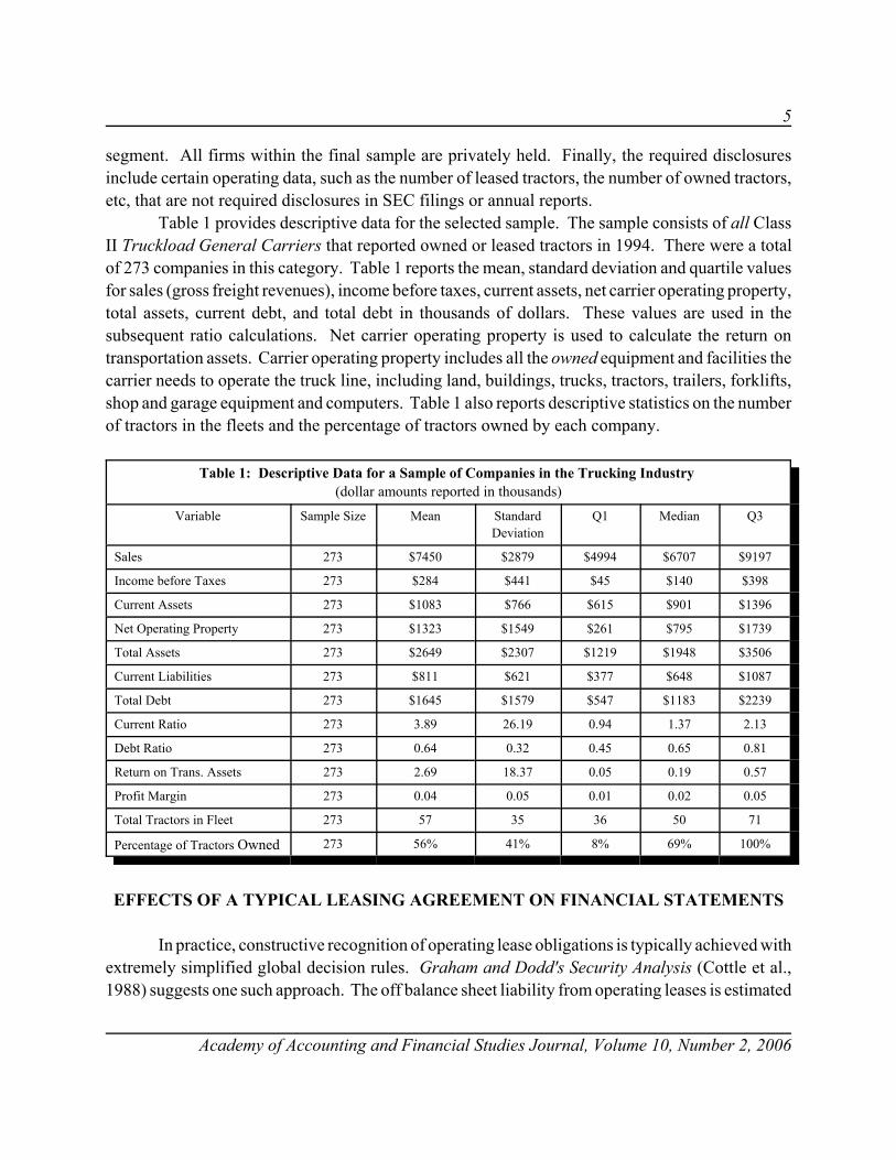
Table 1 provides descriptive data for the selected sample. The sample consists of all ClassII Truckload General Carriers that reported owned or leased tractors in 1994. There were a totalof 273 companies in this category. Table 1 reports the mean, standard deviation and quartile valuesfor sales (gross freight revenues), income before taxes, current assets, net carrier operating property,total assets, current debt, and total debt in thousands of dollars. These values are used in thesubsequent ratio calculations. Net carrier operating property is used to calculate the return ontransportation assets. Carrier operating property includes all the owned equipment and facilities thecarrier needs to operate the truck line, including land, buildings, trucks, tractors, trailers, forklifts,shop and garage equipment and computers. Table 1 also reports descriptive statistics on the numberof tractors in the fleets and the percentage of tractors owned by each company.
Table 1: Descriptive Data for a Sample of Companies in the Trucking Industry (dollar amounts reported in thousands)
Variable Sample Size Mean StandardDeviation
Q1 Median Q3
Sales 273 $7450 $2879 $4994 $6707 $9197
Income before Taxes 273 $284 $441 $45 $140 $398
Current Assets 273 $1083 $766 $615 $901 $1396
Net Operating Property 273 $1323 $1549 $261 $795 $1739
Total Assets 273 $2649 $2307 $1219 $1948 $3506
Current Liabilities 273 $811 $621 $377 $648 $1087
Total Debt 273 $1645 $1579 $547 $1183 $2239
Current Ratio 273 3.89 26.19 0.94 1.37 2.13
Debt Ratio 273 0.64 0.32 0.45 0.65 0.81
Return on Trans. Assets 273 2.69 18.37 0.05 0.19 0.57
Profit Margin 273 0.04 0.05 0.01 0.02 0.05
Total Tractors in Fleet 273 57 35 36 50 71
Percentage of Tractors Owned 273 56% 41% 8% 69% 100%
EFFECTS OF A TYPICAL LEASING AGREEMENT ON FINANCIAL STATEMENTS
In practice, constructive recognition of operating lease obligations is typically achieved withextremely simplified global decision rules. Graham and Dodd's Security Analysis (Cottle et al.,1988) suggests one such approach. The off balance sheet liability from operating leases is estimated

6
Academy of Accounting and Financial Studies Journal, Volume 10, Number 2, 2006
by multiplying the current period's rent expense by eight. Imhoff, Lipe and Wright (1993) citeseveral instances of the use of this method in practice.
To estimate the impact of lease capitalization on the financial statements, I employ a globalconversion technique modified to take into account specific characteristics of leasing contracts ofcompanies contained in the sample. Detailed footnote information necessary for the Imhoff, Lipeand Wright method was not available. The estimation technique uses information concerning fleetsize and type included in the ICC disclosure, but not typically included in annual reports. The veryspecific nature of the regulations governing load size and the high degree of specialization ofcompanies within the industry means that there is little possible variation in tractor leasing terms.Detailed information was gathered on typical leasing contracts within the industry. Truckingindustry periodicals were consulted to obtain information on the average costs of tractors and theusual lease terms, such as down payment requirements, monthly payment structures, interest rates,tractor ownership at lease termination, and guaranteed residual values. Interviews were alsoperformed with operators within the industry and loan officers specializing in the trucking industry.
The results of this investigation are as follows. The length of the lease is determined by thelength of the warranty on the tractor, three years. There is extremely little variation in availableinterest rates due to intense competition among lenders. The waiving of large down payments wastypical for companies of this size within the industry. Variations in payment terms were limited anddid not have a material effect on the reported numbers on the annual financial statements. Thecontracts also fit the current definition of operating leases. They run for less than 75% of theestimated life of the equipment and the present value of the payments is less than 90% of the fairvalue of the equipment. There is an active market for used equipment, utilized by very smalltrucking companies and independent operators.
Table 2: Annual Summary of a Standard Industry 36-Month Leasing Agreement
Year Cash Payment Interest Payment Principal Payment Remaining Balance ofLease Obligation
Year 1 $ 38,401 $ 7,748 $ 30,652 $69,348
Year 2 38,401 5,452 32,949 36,399
Year 3 38,400 2,002 36,399 0
Total 15,202 15,202 100,000
The terms of the lease are assumed to be a 36-month term with a 10 percent interest rate on lease payments with apresent value of $100,000. Payments are assumed to be made at the beginning of each month, with the firstpayment made at the beginning of Year 1. There is no down payment beyond the first month's lease payment,and the asset reverts to the lessor at the termination of the lease.
As a result of the investigation, the following typical industry leasing terms for a tractor areused in the analysis: (a) each lease has a 36-month term and is non-cancelable, (b) ownership of the
7
Academy of Accounting and Financial Studies Journal, Volume 10, Number 2, 2006
equipment reverts to the lessor at the termination of the lease, and there is no guaranteed residualvalue, (c) the present value of the lease payments is $100,000, the implicit interest rate is 10%, thereare level lease payments over the 36-month term of the lease, and there is no required down paymentbeyond the first month's lease payment, (d) the term of the lease is less than 75% of the estimateduseful life of the asset and the present value of the lease payments is less than 90% of the fair valueof the asset. Table 2 reports an annualized summary of the 36-month amortization table, assumingthat the contract was entered into at the beginning of Fiscal Year 1.
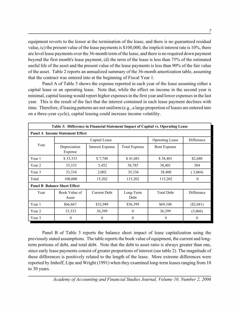
Panel A of Table 3 shows the expense reported in each year of the lease assuming either acapital lease or an operating lease. Note that, while the effect on income in the second year isminimal, capital leasing would report higher expenses in the first year and lower expenses in the lastyear. This is the result of the fact that the interest contained in each lease payment declines withtime. Therefore, if leasing patterns are not uniform (e.g., a large proportion of leases are entered intoon a three-year cycle), capital leasing could increase income volatility.
Table 3: Difference in Financial Statement Impact of Capital vs. Operating Lease
Panel A Income Statement Effect
YearCapital Lease Operating Lease Difference
DepreciationExpense
Interest Expense Total Expense Rent Expense
Year 1 $ 33,333 $ 7,748 $ 41,081 $ 38,401 $2,680
Year 2 33,333 5,452 38,785 38,401 384
Year 3 33,334 2,002 35,336 38,400 ( 3,064)
Total 100,000 15,202 115,202 115,202 0
Panel B Balance Sheet Effect
Year Book Value ofAsset
Current Debt Long-TermDebt
Total Debt Difference
Year 1 $66,667 $32,949 $36,399 $69,348 ($2,681)
Year 2 33,333 36,399 0 36,399 (3,066)
Year 3 0 0 0 0 0
Panel B of Table 3 reports the balance sheet impact of lease capitalization using thepreviously stated assumptions. The table reports the book value of equipment, the current and long-term portions of debt, and total debt. Note that the debt to asset ratio is always greater than one,since early lease payments consist of greater proportions of interest (see table 2). The magnitude ofthese differences is positively related to the length of the lease. More extreme differences werereported by Imhoff, Lipe and Wright (1991) when they examined long-term leases ranging from 10to 30 years.
8
Academy of Accounting and Financial Studies Journal, Volume 10, Number 2, 2006
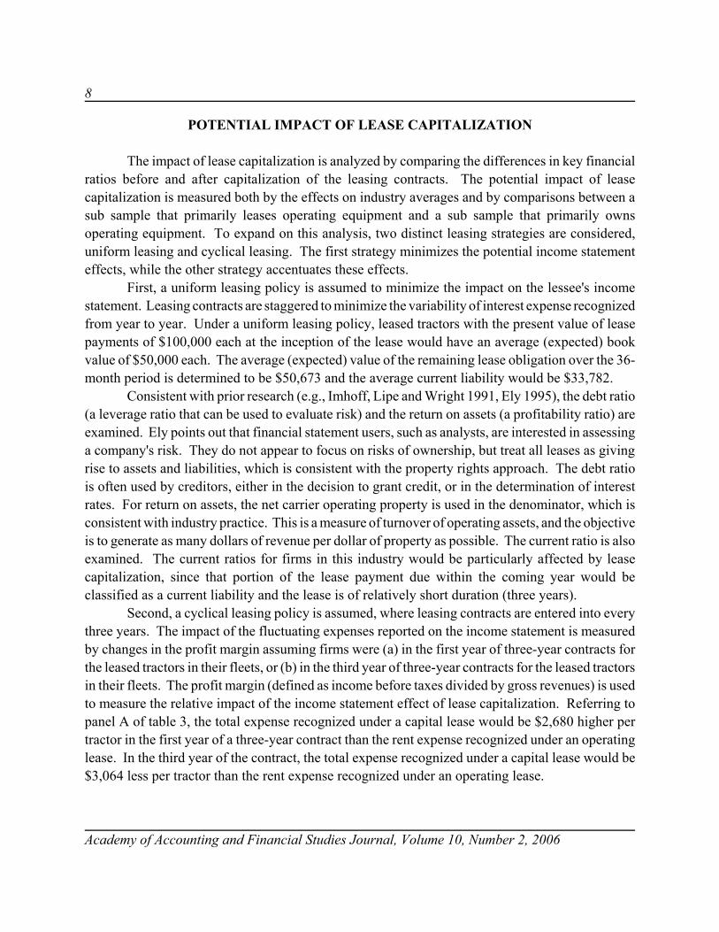
POTENTIAL IMPACT OF LEASE CAPITALIZATION
The impact of lease capitalization is analyzed by comparing the differences in key financialratios before and after capitalization of the leasing contracts. The potential impact of leasecapitalization is measured both by the effects on industry averages and by comparisons between asub sample that primarily leases operating equipment and a sub sample that primarily ownsoperating equipment. To expand on this analysis, two distinct leasing strategies are considered,uniform leasing and cyclical leasing. The first strategy minimizes the potential income statementeffects, while the other strategy accentuates these effects.
First, a uniform leasing policy is assumed to minimize the impact on the lessee's incomestatement. Leasing contracts are staggered to minimize the variability of interest expense recognizedfrom year to year. Under a uniform leasing policy, leased tractors with the present value of leasepayments of $100,000 each at the inception of the lease would have an average (expected) bookvalue of $50,000 each. The average (expected) value of the remaining lease obligation over the 36-month period is determined to be $50,673 and the average current liability would be $33,782.
Consistent with prior research (e.g., Imhoff, Lipe and Wright 1991, Ely 1995), the debt ratio(a leverage ratio that can be used to evaluate risk) and the return on assets (a profitability ratio) areexamined. Ely points out that financial statement users, such as analysts, are interested in assessinga company's risk. They do not appear to focus on risks of ownership, but treat all leases as givingrise to assets and liabilities, which is consistent with the property rights approach. The debt ratiois often used by creditors, either in the decision to grant credit, or in the determination of interestrates. For return on assets, the net carrier operating property is used in the denominator, which isconsistent with industry practice. This is a measure of turnover of operating assets, and the objectiveis to generate as many dollars of revenue per dollar of property as possible. The current ratio is alsoexamined. The current ratios for firms in this industry would be particularly affected by leasecapitalization, since that portion of the lease payment due within the coming year would beclassified as a current liability and the lease is of relatively short duration (three years).
Second, a cyclical leasing policy is assumed, where leasing contracts are entered into everythree years. The impact of the fluctuating expenses reported on the income statement is measuredby changes in the profit margin assuming firms were (a) in the first year of three-year contracts forthe leased tractors in their fleets, or (b) in the third year of three-year contracts for the leased tractorsin their fleets. The profit margin (defined as income before taxes divided by gross revenues) is usedto measure the relative impact of the income statement effect of lease capitalization. Referring topanel A of table 3, the total expense recognized under a capital lease would be $2,680 higher pertractor in the first year of a three-year contract than the rent expense recognized under an operatinglease. In the third year of the contract, the total expense recognized under a capital lease would be$3,064 less per tractor than the rent expense recognized under an operating lease.

9
Academy of Accounting and Financial Studies Journal, Volume 10, Number 2, 2006
Industry averages
Changes in industry averages are reported in table 4. The original numbers reported in thedata set were generated with leasing contracts reported as operating leases. The change in the ratioresulting from capitalization is defined as:
(Capital Lease Ratio - Operating Lease Ratio) / Operating Lease Ratio
The averages reported in table 4 show the change in the ratio caused by capitalization as apercentage of the original ratio using operating leases. All differences are statistically significantat the 0.05 level. The three ratios reported in panel A are analyzed assuming a uniform (as opposedto cyclical) leasing program. The profit margin and debt ratios were windsorised to minimize theimpact of outliers and to facilitate economic interpretation of the reported means. This procedurehas the effect of providing a more conservative interpretation of the impact of capitalizing leases.
Table 4: Changes in Industry Averages Resulting from Lease Capitalization
Panel A Changes in Selected Ratios Assuming Uniform Leasing Patterns
Ratio Sample Size Mean Standard Error t-test Statistic Two-tailed p-value
Current Ratio 273 -0.4098 0.0205 -20.03 0.00
Debt Ratio 273 0.2188 0.0184 11.89 0.00
Return on TransportationAssets
273 -0.4469 0.0234 -19.07 0.00
Panel B Changes in Profit Margin Assuming Cyclical Leasing Patterns
Year Sample Size Mean Standard Error t-test Statistic Two-tailed p-value
Year 1 273 -0.4024 0.0403 -9.98
Year 3 273 0.4602 0.0461 9.98 0.00
Note: The change in the ratio is defined as: (Capital Lease Ratio - Operating Lease Ratio) / Operating LeaseRatio. The Mean x 100 is equal to the percentage change in the ratio due to capitalization of leasing contracts.
The structure of the tests allows for an economic interpretation of the reported means. If theleased tractors were capitalized, the current ratio for this industry segment would decline byapproximately 41 percent. Likewise, the debt ratio would increase by approximately 22 percent, andthe return on transportation equipment would decrease by 45 percent. These differences are not onlysignificant in the statistical sense, but also in the economic sense. Industry benchmarks are oftenused in the evaluation of firm performance. Imhoff, Lipe and Wright (1991) note that many servicesthat provide industry information (Dun & Bradstreet, Value Line, etc.) do not routinely adjustindustry averages for non-capitalized leases. If users estimate the financial statement impact of lease
10
Academy of Accounting and Financial Studies Journal, Volume 10, Number 2, 2006
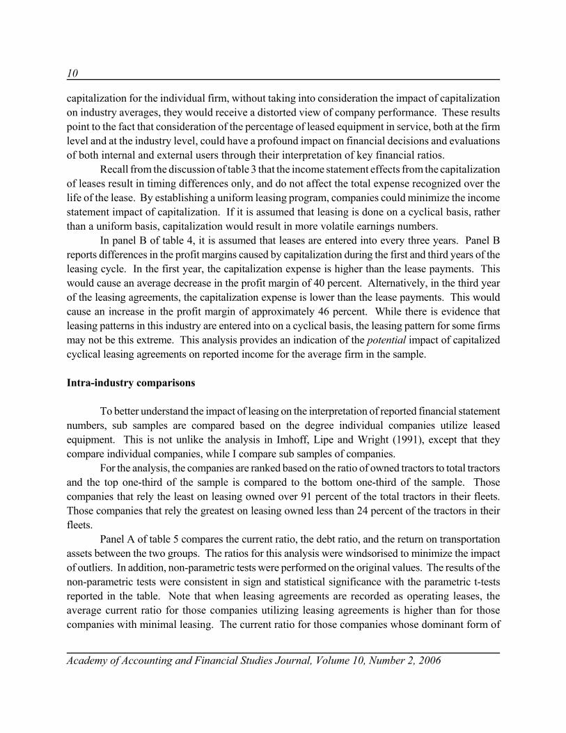
capitalization for the individual firm, without taking into consideration the impact of capitalizationon industry averages, they would receive a distorted view of company performance. These resultspoint to the fact that consideration of the percentage of leased equipment in service, both at the firmlevel and at the industry level, could have a profound impact on financial decisions and evaluationsof both internal and external users through their interpretation of key financial ratios.
Recall from the discussion of table 3 that the income statement effects from the capitalizationof leases result in timing differences only, and do not affect the total expense recognized over thelife of the lease. By establishing a uniform leasing program, companies could minimize the incomestatement impact of capitalization. If it is assumed that leasing is done on a cyclical basis, ratherthan a uniform basis, capitalization would result in more volatile earnings numbers.
In panel B of table 4, it is assumed that leases are entered into every three years. Panel Breports differences in the profit margins caused by capitalization during the first and third years of theleasing cycle. In the first year, the capitalization expense is higher than the lease payments. Thiswould cause an average decrease in the profit margin of 40 percent. Alternatively, in the third yearof the leasing agreements, the capitalization expense is lower than the lease payments. This wouldcause an increase in the profit margin of approximately 46 percent. While there is evidence thatleasing patterns in this industry are entered into on a cyclical basis, the leasing pattern for some firmsmay not be this extreme. This analysis provides an indication of the potential impact of capitalizedcyclical leasing agreements on reported income for the average firm in the sample.
Intra-industry comparisons
To better understand the impact of leasing on the interpretation of reported financial statementnumbers, sub samples are compared based on the degree individual companies utilize leasedequipment. This is not unlike the analysis in Imhoff, Lipe and Wright (1991), except that theycompare individual companies, while I compare sub samples of companies.
For the analysis, the companies are ranked based on the ratio of owned tractors to total tractorsand the top one-third of the sample is compared to the bottom one-third of the sample. Thosecompanies that rely the least on leasing owned over 91 percent of the total tractors in their fleets.Those companies that rely the greatest on leasing owned less than 24 percent of the tractors in theirfleets.
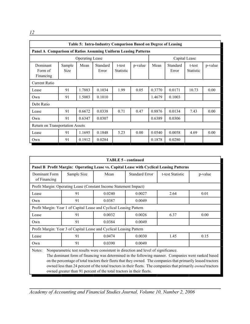
Panel A of table 5 compares the current ratio, the debt ratio, and the return on transportationassets between the two groups. The ratios for this analysis were windsorised to minimize the impactof outliers. In addition, non-parametric tests were performed on the original values. The results of thenon-parametric tests were consistent in sign and statistical significance with the parametric t-testsreported in the table. Note that when leasing agreements are recorded as operating leases, theaverage current ratio for those companies utilizing leasing agreements is higher than for thosecompanies with minimal leasing. The current ratio for those companies whose dominant form of
11
Academy of Accounting and Financial Studies Journal, Volume 10, Number 2, 2006
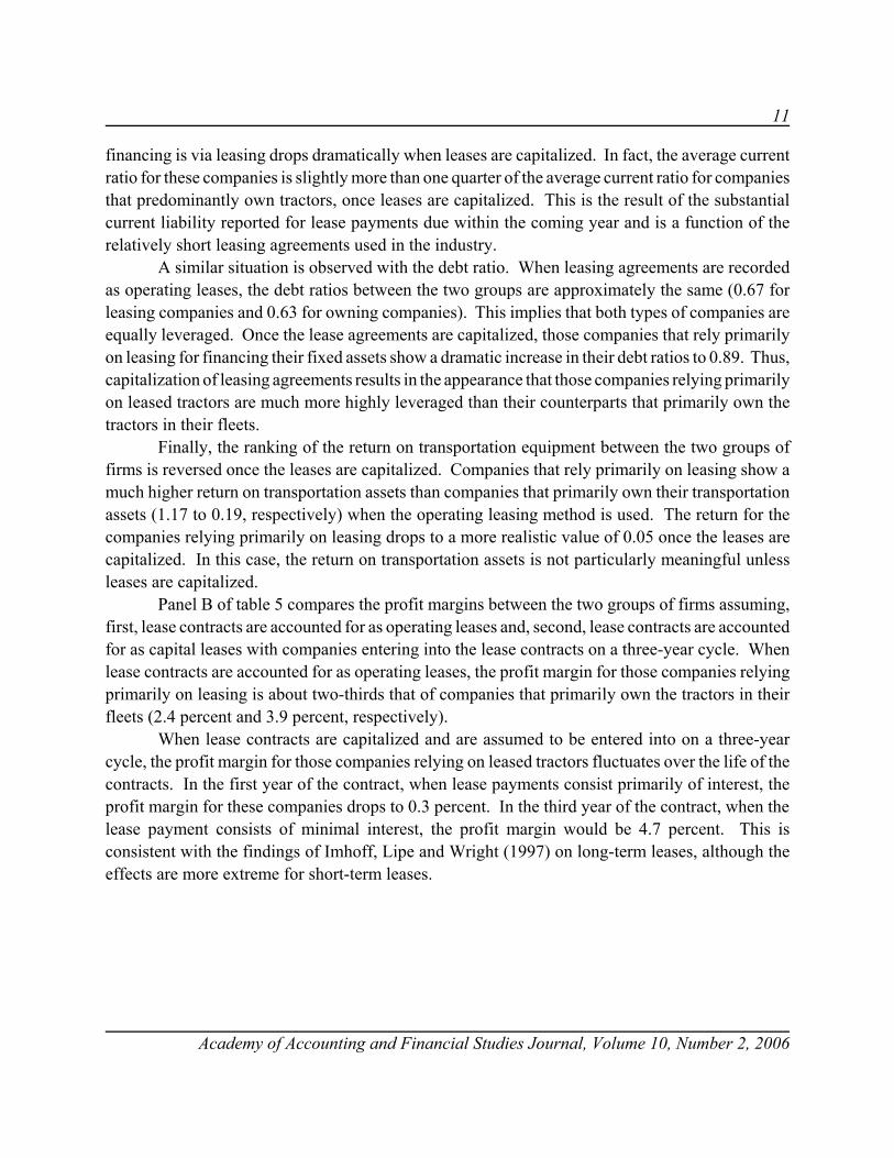
financing is via leasing drops dramatically when leases are capitalized. In fact, the average currentratio for these companies is slightly more than one quarter of the average current ratio for companiesthat predominantly own tractors, once leases are capitalized. This is the result of the substantialcurrent liability reported for lease payments due within the coming year and is a function of therelatively short leasing agreements used in the industry.
A similar situation is observed with the debt ratio. When leasing agreements are recordedas operating leases, the debt ratios between the two groups are approximately the same (0.67 forleasing companies and 0.63 for owning companies). This implies that both types of companies areequally leveraged. Once the lease agreements are capitalized, those companies that rely primarilyon leasing for financing their fixed assets show a dramatic increase in their debt ratios to 0.89. Thus,capitalization of leasing agreements results in the appearance that those companies relying primarilyon leased tractors are much more highly leveraged than their counterparts that primarily own thetractors in their fleets.
Finally, the ranking of the return on transportation equipment between the two groups offirms is reversed once the leases are capitalized. Companies that rely primarily on leasing show amuch higher return on transportation assets than companies that primarily own their transportationassets (1.17 to 0.19, respectively) when the operating leasing method is used. The return for thecompanies relying primarily on leasing drops to a more realistic value of 0.05 once the leases arecapitalized. In this case, the return on transportation assets is not particularly meaningful unlessleases are capitalized.
Panel B of table 5 compares the profit margins between the two groups of firms assuming,first, lease contracts are accounted for as operating leases and, second, lease contracts are accountedfor as capital leases with companies entering into the lease contracts on a three-year cycle. Whenlease contracts are accounted for as operating leases, the profit margin for those companies relyingprimarily on leasing is about two-thirds that of companies that primarily own the tractors in theirfleets (2.4 percent and 3.9 percent, respectively).
When lease contracts are capitalized and are assumed to be entered into on a three-yearcycle, the profit margin for those companies relying on leased tractors fluctuates over the life of thecontracts. In the first year of the contract, when lease payments consist primarily of interest, theprofit margin for these companies drops to 0.3 percent. In the third year of the contract, when thelease payment consists of minimal interest, the profit margin would be 4.7 percent. This isconsistent with the findings of Imhoff, Lipe and Wright (1997) on long-term leases, although theeffects are more extreme for short-term leases.
12
Academy of Accounting and Financial Studies Journal, Volume 10, Number 2, 2006
Table 5: Intra-Industry Comparison Based on Degree of Leasing
Panel A Comparison of Ratios Assuming Uniform Leasing Patterns
Operating Lease Capital Lease
Dominant Form of
Financing
SampleSize
Mean StandardError
t-test Statistic
p-value Mean StandardError
t-testStatistic
p-value
Current Ratio
Lease 91 1.7883 0.1034 1.99 0.05 0.3770 0.0171 10.73 0.00
Own 91 1.5003 0.1010 1.4679 0.1003
Debt Ratio
Lease 91 0.6672 0.0338 0.71 0.47 0.8876 0.0134 7.43 0.00
Own 91 0.6347 0.0307 0.6389 0.0306
Return on Transportation Assets
Lease 91 1.1695 0.1848 5.23 0.00 0.0540 0.0058 4.69 0.00
Own 91 0.1912 0.0284 0.1878 0.0280
TABLE 5 - continued
Panel B Profit Margin: Operating Lease vs. Capital Lease with Cyclical Leasing Patterns
Dominant Form of Financing
Sample Size Mean Standard Error t-test Statistic p-value
Profit Margin: Operating Lease (Constant Income Statement Impact)
Lease 91 0.0240 0.0027 2.64 0.01
Own 91 0.0387 0.0049
Profit Margin: Year 1 of Capital Lease and Cyclical Leasing Pattern
Lease 91 0.0032 0.0026 6.37 0.00
Own 91 0.0384 0.0049
Profit Margin: Year 3 of Capital Lease and Cyclical Leasing Pattern
Lease 91 0.0474 0.0030 1.45 0.15
Own 91 0.0390 0.0049
Notes: Nonparametric test results were consistent in direction and level of significance.The dominant form of financing was determined in the following manner. Companies were ranked basedon the percentage of total tractors their fleets that they owned. The companies that primarily leased tractorsowned less than 24 percent of the total tractors in their fleets. The companies that primarily owned tractorsowned greater than 91 percent of the total tractors in their fleets.
13
Academy of Accounting and Financial Studies Journal, Volume 10, Number 2, 2006
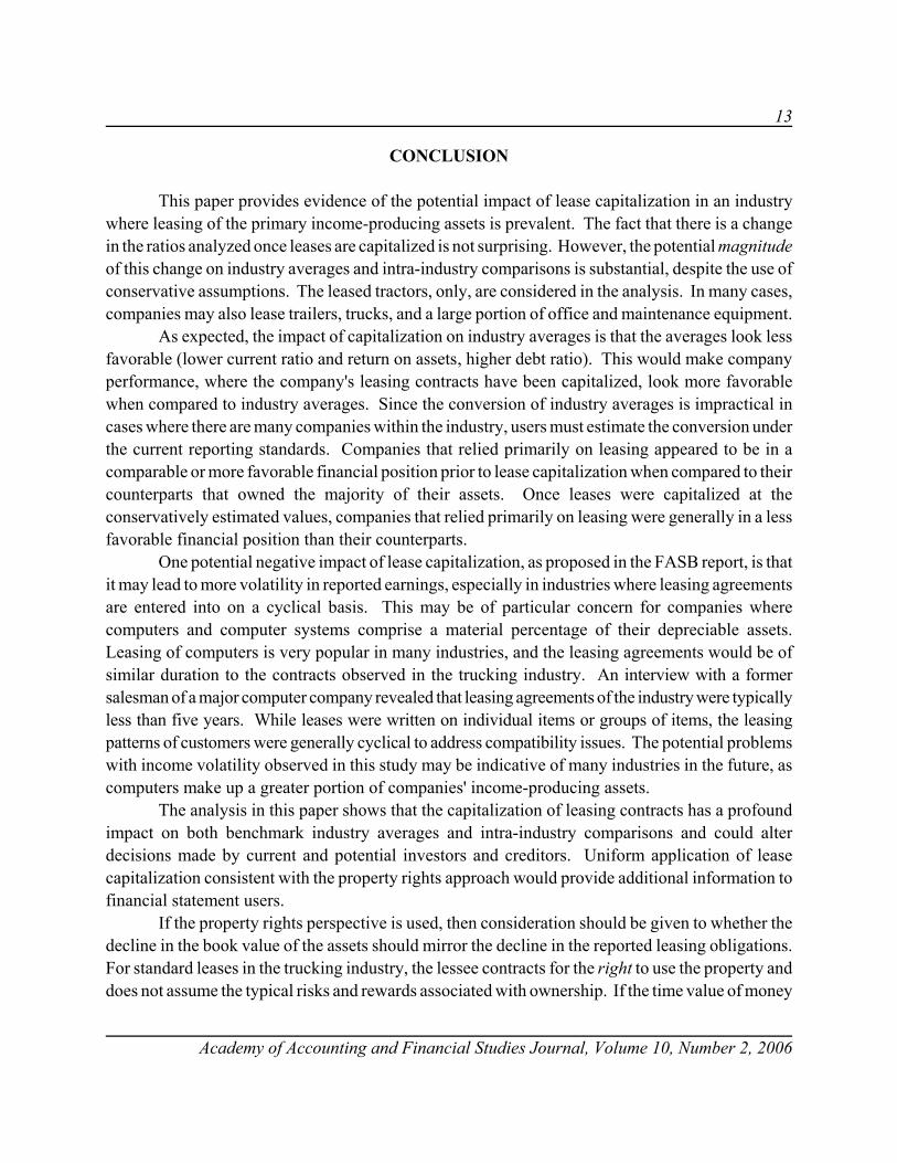
CONCLUSION
This paper provides evidence of the potential impact of lease capitalization in an industrywhere leasing of the primary income-producing assets is prevalent. The fact that there is a changein the ratios analyzed once leases are capitalized is not surprising. However, the potential magnitudeof this change on industry averages and intra-industry comparisons is substantial, despite the use ofconservative assumptions. The leased tractors, only, are considered in the analysis. In many cases,companies may also lease trailers, trucks, and a large portion of office and maintenance equipment.
As expected, the impact of capitalization on industry averages is that the averages look lessfavorable (lower current ratio and return on assets, higher debt ratio). This would make companyperformance, where the company's leasing contracts have been capitalized, look more favorablewhen compared to industry averages. Since the conversion of industry averages is impractical incases where there are many companies within the industry, users must estimate the conversion underthe current reporting standards. Companies that relied primarily on leasing appeared to be in acomparable or more favorable financial position prior to lease capitalization when compared to theircounterparts that owned the majority of their assets. Once leases were capitalized at theconservatively estimated values, companies that relied primarily on leasing were generally in a lessfavorable financial position than their counterparts.
One potential negative impact of lease capitalization, as proposed in the FASB report, is thatit may lead to more volatility in reported earnings, especially in industries where leasing agreementsare entered into on a cyclical basis. This may be of particular concern for companies wherecomputers and computer systems comprise a material percentage of their depreciable assets.Leasing of computers is very popular in many industries, and the leasing agreements would be ofsimilar duration to the contracts observed in the trucking industry. An interview with a formersalesman of a major computer company revealed that leasing agreements of the industry were typicallyless than five years. While leases were written on individual items or groups of items, the leasingpatterns of customers were generally cyclical to address compatibility issues. The potential problemswith income volatility observed in this study may be indicative of many industries in the future, ascomputers make up a greater portion of companies' income-producing assets.
The analysis in this paper shows that the capitalization of leasing contracts has a profoundimpact on both benchmark industry averages and intra-industry comparisons and could alterdecisions made by current and potential investors and creditors. Uniform application of leasecapitalization consistent with the property rights approach would provide additional information tofinancial statement users.
If the property rights perspective is used, then consideration should be given to whether thedecline in the book value of the assets should mirror the decline in the reported leasing obligations.For standard leases in the trucking industry, the lessee contracts for the right to use the property anddoes not assume the typical risks and rewards associated with ownership. If the time value of money

14
Academy of Accounting and Financial Studies Journal, Volume 10, Number 2, 2006
concept is relevant to the obligations incurred, it may also be appropriately applied to the rightsobtained in the contract. This would suggest that a present-value depreciation method, such as issometimes used by utilities, be used for the reported asset. This depreciation approach wouldminimize the negative impact of capitalization on the debt ratio, especially for companies inindustries where typical leasing contracts are of longer duration.
The impact of capitalization on the current ratio may be reduced if the portion of the assetto be depreciated within the coming year is classified as a current item. This is consistent with theinterpretation of the leasing agreement as a contracting of property rights, rather than of ownershiprights. The lessee has contracted for the right to use specific property to generate future economicbenefits. That portion of the right that will expire within the coming year would meet the definitionof a current asset. If this approach were taken, the decrease in the industry average current ratioafter capitalization that is reported in table 4 would be 12 percent, rather than 41 percent.
REFERENCES
Beattie, V., A Goodacre, S. Thompson (2000). Operating Leases and the Assessment of Lease-Debt Substitutability.Journal of Banking and Finance, 24(3), 427-470.
Beattie, V., A Goodacre, S. Thompson (2000). Recognition vs. Disclosure: An Investigation of the Impact on EquityRisk using UK Operating Lease Disclosures. Journal of Business Finance and Accounting, 27(9), 1185-1224.
Brealey, R., and S. Myers (1988). Principles of Corporate Finance, (Third Edition). New York: McGraw-Hill Inc.
Cottle, C., R. F. Murray and F. E. Block (1988). Graham and Dodd's Security Analysis. New York: McGraw-Hill Inc.
El-Gazzar, S., S. Lilien, and V. Pastena (1986). Accounting for Leases by Lessees. Journal of Accounting andEconomics, 8, 217-237.
Ely, K. M. (1995). Operating Lease Accounting and the Market's Assessment of Equity Risk. Journal of AccountingResearch, 33(2) (Autumn), 397-415.
Financial Accounting Standards Board. (1976). Statement of Financial Accounting Standards No. 13. Accounting forLeases. Norwalk, CN: FASB.
Financial Accounting Standards Board. (1980). Statement of Financial Accounting Concept No. 3. Elements ofFinancial Statements of Business Enterprises. Norwalk, CN: FASB.
Financial Accounting Standards Board. (1995). Statement of Financial Accounting Standards No. 121. Accounting forthe Impairment of Long-lived Assets and for Long-lived Assets to be Disposed of. Norwalk, CN: FASB.
Financial Accounting Standards Board.. (1996). Financial Accounting Series Special Report (No. 163-A). Accountingfor Leases: A New Approach. Norwalk, CN: FASB.
15
Academy of Accounting and Financial Studies Journal, Volume 10, Number 2, 2006
Imhoff, E., R. Lipe and D. Wright (1991). Operating Leases: Impact of Constructive Capitalization. AccountingHorizons, (March 1991), 51-63.
Imhoff, E., R. Lipe and D. Wright (1993). The Effects of Recognition versus Disclosure on Shareholder Risk andExecutive Compensation. Journal of Accounting, Auditing and Finance (Fall), 335-368.
Imhoff, E., R. Lipe and D. Wright (1991). Operating Leases: Income Effects of Constructive Capitalization. AccountingHorizons, (June 1997), 12-32.
Imhoff, E. and J. Thomas (1988). Economic Consequences of Accounting Standards: The Lease Disclosure RuleChange. Journal of Accounting and Economics, 10(4), 277-310.
London Financial Group Leasing Report. 1996. World Leasing Yearbook. London: Euromoney Publications.
Ou, J. and S. Penman (1989). Financial Statement Analysis and the Prediction of Stock Returns. Journal of Accountingand Economics, 11(3), 295-329.
Peasnell, K. 1996. Using Accounting Data to Measure the Economic Performance of Firms. Journal of Accounting andPublic Policy, 15, 291-303.
Penman, S. 1992. Return to Fundamentals. Journal of Accounting, Auditing and Finance, 7 (new series)(4), 465-483.

16
Academy of Accounting and Financial Studies Journal, Volume 10, Number 2, 2006
17
Academy of Accounting and Financial Studies Journal, Volume 10, Number 2, 2006
THE SURVIVAL OF FIRMS THAT TAKE SPECIALCHARGES FOR RESTRUCTURINGS AND WRITE-OFFS
Gyung Paik, Brigham Young UniversityKip R. Krumwiede, Boise State University
ABSTRACT
In light of recent, well-publicized corporate failures, financial reporting practices areincreasingly being scrutinized. One area of scrutiny includes special charges for restructurings andwrite-offs. This study investigates the survival of firms that take restructuring charges and write-offs.We examine whether the survival of these firms is associated with management's choice of labeling(i.e., restructuring charge or write-off) as well as with the amount and purpose of the charge. Usinga sample of large negative special charge announcements during 1986-1992 and 1996-1998, we findthat firms reporting smaller charges survive longer than those with larger charges, regardless ofany business actions for improvement mentioned. We also find evidence of a decreasing probabilityof survival for firms using the label of "restructuring" for the charge. These results are consistentwith the popular media perception that managers often seek to mask their firms' true performanceusing special charge labeling.
INTRODUCTION
Financial reports may describe special or unusual charges, which are economic eventsbeyond the normal ongoing economic activities of an enterprise (Ante 2003; Gallagher 2004). Asused herein, a "special charge" is (or should be) the description of a loss related to an event that isunusual or infrequent in the context of the enterprise (Stice, Stice, & Skousen 2004). Examples ofsuch special charges are the write-down or write-off of assets or a corporate restructuring.
However, the term "special charges" is often abused when companies classify unpleasantlosses (instead of unusual or infrequent losses) as special charges. The ploy used when managersmislabel unpleasant losses as special charges is to create a (misleading) impression that the lossesin question are outside the norm and hence something for which management should not be heldresponsible. An egregious example cited by the Wall Street Journal is Motorola which, at the timeof October 2002, was proposing to include special (hence theoretically unusual or infrequent)charges for the fifteenth consecutive quarter.
Therefore, announcements of special charges may confuse investors who are trying toevaluate how well firms have performed and how well they will perform in the future. Further, assuggested by anecdotal reports, managers' choice of labeling special charges as either "restructuring
18
Academy of Accounting and Financial Studies Journal, Volume 10, Number 2, 2006
charges" or "write-offs" may confuse investors even more. An example of the investing community'sconfusion about special charge announcements is found in the following Wall Street Journal excerpt:"A Wall Street analyst said, ‘Every company we follow has a write-off. No one has any idea of whatanyone is earning'" (Smith and Lipin 1996). Accounting regulators have shown concerns in linewith this argument. The Wall Street Journal (January 22, 1999, A2) reported:
"The SEC said company executives concoct a rosy portrait of earnings growth through an assortment of illegalaccounting maneuvers. Among other things, the SEC said, companies take excessive restructuring charges. TheSEC believes many companies are going too far—taking excessive reserves or write-offs in order to manipulatetheir results and hide the real health of their business."
In this paper, we investigate whether the survival of firms making these special charges isassociated with (1) the amount and purpose of the special charge, and (2) managers' labeling choices("restructuring" or "write-off"). First, we analyze the association between the survival of firms thattake restructuring charges or write-offs and the amount and specific purpose of the charge asdescribed in the announcements. This analysis provides evidence on whether the survival ofannouncing firms is related to the economic substance of firms' restructuring charges or write-offs.Next, we investigate the relationship between the survival of announcing firms and the labeling ofthe charges described in the announcements. This analysis provides evidence about whethermanagers' choice of label (restructuring or write-off) is appropriate or is driven more by desires tocover bad operating performance.
We collected information about large negative special charge announcements from pressreleases during the 1986-1992 and 1996-1998 time periods (hereafter "early" and "later" for the1986-1992 and 1996-1998 time periods, respectively). During the early period, there was littleguidance from accounting authorities on special charges, allowing managers to exercise substantialdiscretion in determining when and to what extent special charges should be reported andannounced. After increased pressure from the AICPA, SEC, and other organizations, the FASBattempted to limit management's discretion relating to special charge reporting by adopting EITF94-3 in 1994 and SFAS 121 in 1995. Recently, the FASB adopted SFAS 144 and SFAS 146 in 2001.Although regulators have tried to limit the discretion available regarding special charges,considerable discretion regarding restructuring and write-off special charges persists.
The results provide evidence that firms that report larger amounts of restructuringcharges/write-offs are less likely to survive than firms that report smaller charges and more likelyto disappear in the short-term (four years or less).1 Regarding the reported economic substance ofthe charges, we find little evidence of differences in specific actions mentioned between survivingand non-surviving firms. However, we do find a somewhat higher proportion of write-off firms thatsubsequently disappear in the short term making relatively more PP&E write-off announcements.In addition, among the firms that make restructuring charge announcements and then subsequentlydisappear in the short term, the majority include costs to eliminate or curtail product lines.
19
Academy of Accounting and Financial Studies Journal, Volume 10, Number 2, 2006
The rest of this paper is organized as follows. Section II examines relevant prior literature supportingthe labeling and restructuring action hypotheses. Section III describes the sample selection methodsand Section IV presents the results and analysis. Finally, Section V summarizes the contributionsand limitations of the study.
PRIOR RESEARCH AND HYPOTHESIS DEVELOPMENT
Prior studies have provided insight into distressed firms' survival over time. Turetsky &McEwen (2001) investigated the association between distressed firms' survival and firm-specificattributes. Their study provides evidence that a firm's profitability, market risk, size, and financialleverage are significantly associated with whether the distressed firm will ultimately survive. Chen& Lee (1993) applied survival analysis to examine a sample of oil- and gas- producing companiesat the onset of economic adversity. The intent of the study is to find out how long a firm can endureeconomic adversity before facing financial distress. The results of their study suggest that liquidityratio, leverage ratio, operating cash flows, success in exploration, and size are significant factorsaffecting corporate endurance.
Prior studies relating to restructuring charges have examined firm performance (Atiase, Platt,& Tse 2001; Carter 2000), earnings management (Moehrle 2002; Weiss 1999), CEO compensation(Adut, Cready, & Lopez 2003), impact on stock price (Kross, Park, & Ro 1998; Bunsis 1997;Brickley & Van Drunen 1990) and on analysts' expectations (Chaney, Hogan, & Jeter 1999), andunderlying management actions (Lopez 2002; Hogan & Jeter 1997). Other studies have examinedthe impact of write-off announcements on stock price (Hirschey & Richardson 2003; Francis,Hanna, & Vincent 1996; Elliott & Shaw 1988; Strong & Meyer 1987).
Prior research on the stock market response to the announcements of special chargesprovided mixed results regarding investors' interpretation of these special charges. Hirschey &Richardson (2003), Francis, Hanna, & Vincent (1996), Elliott & Shaw (1988), and Strong & Meyer(1987) provided evidence for negative overall market reactions to write-off special chargeannouncements. On the other hand, Kross, Park, & Ro (1998), Bunsis (1997), and Brickley & VanDrunen (1990) provided evidence for positive market reactions around the announcement date ofrestructuring charges.
Prior research has also provided some empirical evidence regarding the performance ofspecial charge firms. Atiase, et al. (2001) found that the performance of restructuring charge firmsis worse than that of non-restructuring firms in the pre-restructuring period, but it is better than thatof non-restructuring firms in the post-restructuring period. Similarly, Carter (2000) found thatrestructuring firms realize improvements in future operating performance, but these improvementsare not fully realized until at least three years following the restructuring. However, these studiesmay suffer from "survivorship bias" when evaluating the future performance of firms.
20
Academy of Accounting and Financial Studies Journal, Volume 10, Number 2, 2006
Our study is the first to consider the overall special charge –both restructuring charge andwrite-off - announcements. We also address whether management's labeling of special charges(restructuring or write-off), amount of charge, and specific restructuring actions as described in theannouncements are related to a firms' future survival.
HYPOTHESIS DEVELOPMENT
Starting with reports in the national press that many special charge companies are improperlymanipulating special charges to alter their true economic condition, our general hypothesis hereinis that a lower rate of survival will be observed in these companies than is observed in a controlgroup of related companies. More specifically, we propose four hypotheses: (1) companies whichclaim large special charges are more likely to disappear than firms claiming no special charges orvery small special charges; (2) among companies claiming large special charges, those claiming thelargest amounts are more likely to disappear and to disappear sooner; (3) among firms claimingspecial charges, those giving specific reasons for the charge are more likely to survive than thosewhich do not; and, (4) firms taking a special charge for what is labeled a "restructuring" are lesslikely to survive than those taking a special charge for what is labeled a "write-off."
Our first research question is whether there is a relationship between the amount of specialcharge and the future survival of announcing firms. A large special charge (as a percentage of assets)suggests that firms have been experiencing more serious operating problems than those firms thatreport very small or no special charge. Therefore, the risks are perhaps greater and the probabilitiesfor survival are less likely for these large special charge firms than for other firms. We thereforeexpect that firms which take large restructuring/write-off charges are not as likely to survive as firmswhich take very small, if any, restructuring/write-off charges. Therefore, the following hypothesisis proposed:
H1a: Firms which announce large restructuring/write-off charges are not only more likely todisappear, but to disappear sooner than firms which take very small, if any,restructuring/write-off charges.
Additionally, and for the same reasons, we expect that among firms reporting large specialcharges, the higher the amount of restructuring or write-off charge, the less likely the firm willsurvive in the future. Therefore, we expect the amount of the charge (scaled by firm assets) to benegatively correlated with how long the firm will survive in the future. The following hypothesisis proposed:
H1b: Among the firms reporting large special charges, firms which announce relatively largerrestructuring/write-off charges are not only more likely to disappear, but to disappear soonerthan firms that take relatively smaller restructuring/write-off charges.
21
Academy of Accounting and Financial Studies Journal, Volume 10, Number 2, 2006
Our third research question examines the relationship between the future survival of specialcharge announcing firms and specific business/accounting actions mentioned by managementregarding the charges. Prior research has provided some empirical evidence regarding how investorsresponded to specific actions that management pledged to carry out in its' restructuringcharge/write-off announcements. Hogan and Jeter (1997) examined the market returns aroundannouncements for a sample of 128 restructuring charges taken over the period 1990 – 1992. Theyfound an insignificant market reaction to the overall restructuring charge announcements, but theyalso found that the market responded positively to restructuring charges categorized as severanceand other cash outlay charges, as long as there was no current period loss or recent managementchange. Lopez (2002) provides additional evidence that the components of restructuring charges areinformative to analysts. His results indicate a significant relationship between the components of arestructuring charge and analysts' earnings forecast revision reactions.
Firms that include costs for specific actions (e.g., employee severance, eliminate productlines, consolidate operations, etc.) in their special charge may have better plans for dealing with theiroperating or competitive problems than firms that provide no such information. Thus, wehypothesize that firms making restructuring or write-off charges which include costs for specificactions in order to improve future operating performance are more likely to survive than firms thatmerely include costs to recognize their poor past operating performances (e.g., write off inventory,property, plant, and equipment, etc.). We propose the following hypothesis:
H2: Firms that report restructuring or write-off special charges and mention specific actionsgeared toward future operating performance improvements are more likely to survive thanfirms that report charges that merely recognize poor past operating performances.
Our last research question investigates the relationship between the labeling of specialcharges and the future survival of announcing firms. Corporate managers' intentions regarding thelabeling of special charges in terms of potential opportunism has received scant discussion in theliterature. Even though restructuring charges and write-offs result in a similar reduction of currentperiod earnings, the market may react differently to the type of label. The words or labels that acompany uses can play a big part in how the financial press—and market—reacts to anannouncement. In the early 1990's, for example, Hewlett-Packard's first-ever layoffs were reportedas "restructuring" and "reassignments," etc., and caused little attention. Alternatively, IBM andDigital's "first ever layoffs" led to a flurry of negative articles (PR News 1997). Also, Forbes(Condon 1998) reports:
"Restructuring charges are today's favorite. A nice, fat write-off can help your stock. Despite its recenttightening of some accounting rules, the FASB has left definitions of ‘one-time' and ‘restructuring'vague. Management would be less than human if they did not exploit the ambiguities. So, othercompanies' executives say, ‘What the heck, let's call it a restructuring'."
22
Academy of Accounting and Financial Studies Journal, Volume 10, Number 2, 2006
Even before EITF 94-3 and SFAS 121 were passed, the SEC had been looking closely atrestructuring charge announcements. Robert Bayless, Chief Accountant of the SEC'sCorporation-Finance division, warned the accounting profession in 1994 that many explanations ofrestructuring charges were "rather sparse and rather vague" and that some companies claim lossesas restructuring charges when they are not (Harlan 1994). Consistent with accounting regulators'concerns, recent articles in the news media pointed out that corporate managers play the "wordsgame" in addition to the "numbers game" with respect to announcing their earnings numbers toanalysts and investors (Weil 2001).2
Our last hypothesis examines future survival of special charge announcing firms toinvestigate the association between firm survival and the labeling of announcement. Some firms mayuse the "restructuring charge" label to make their special charge look more positive than it really is.We measure the appropriateness of the labels by comparing the survival rates for firms making"restructuring charge" announcements versus "write-off" announcements. We extend therestructuring charge/write-off literature by examining whether managers are trying toopportunistically mask their firms' poor performance by using the "restructuring charge" labelinappropriately. We therefore test the following hypothesis:
H3: Firms that label special charges as restructuring charges are less likely to survive than firmsthat label their charges as write-offs.
SAMPLE SELECTION
We obtained a sample of announcements of large special charges made by corporatemanagers in the news media. Our sample periods cover seven years (1986-1992) prior to theadoption of EITF 94-3 and SFAS 121, and three years (1996-1998) subsequent to theimplementation of these accounting guidelines. We use two different sample periods that areseparated by a three-year break (1993-1995) during which the relevant accounting rules wereadopted. The earlier sample period also allows us to observe firm survival over several moresubsequent years than the later sample.
Using the annual Compustat database we identified 4,477 firm-year companies whichreported special charges in excess of ten percent of their respective total assets (Table 1, column A)during the early and later time periods. Using the ten-percent cutoff requirement ensured that wewould obtain special charges that are significant enough to affect investors' perception of the firms'future performance. Accounting regulators expressed concerns specifically about large negativespecial charges. For example, Arthur Levitt, Chairman of the SEC argued that if special charges arebig enough then, theoretically, stock markets will look beyond a special one-time loss and focus onlyon future performance (Journal of Accountancy, December, 1998).3

23
Academy of Accounting and Financial Studies Journal, Volume 10, Number 2, 2006
1 The amount of negative special charges [Compustat #17] for these firms exceeded tenpercent of their reported total assets [Compustat #6].
2 We used Lexis-Nexis to search for the restructuring charge/write-off announcements madeby the management of these large negative special charge firms.
In order to identify specific actions and labeling of special charges, we obtained news articlesregarding special charge announcements from the Lexis/Nexis database. We identified 924 of the4,447 companies (approximately 21 percent) which made restructuring/write-off announcementsthrough the news media during these same sample periods (Table 1, column B). Of the two timeperiods (early vs. later), we found a greater frequency of restructuring charge/write-offannouncements in the news media for the later time period. Specifically, we identified 357 out of2,415 companies (approximately 15 percent) which made restructuring charge/write-offannouncements during the early sample period compared to 567 out of 2,062 companies(approximately 28 percent) which made these same types of announcements during the later sampleperiod. Notwithstanding the fact that our later sample period is 4 years less than our early sampleperiod (7 years vs. 3 years for the early and later sample periods, respectively), 61 percent of oursample announcements were identified during the later sample period. Our findings therefore show
A: B: Number of Firms Reporting Large Negative Special
Charges 1
Number of Restructuring
Charge/Write-off Announcements 2
1986 310 43 14% 5%1987 275 24 9% 3%1988 287 17 6% 2%1989 306 27 9% 3%1990 385 39 10% 4%1991 424 105 25% 11%1992 428 102 24% 11%Subtotal (1986-1992)
2,415 357 15% 39%
1996 645 214 33% 23%1997 715 174 24% 19%1998 702 179 25% 19%Subtotal (1996-1998)
2,062 567 28% 61%
Total 4,477 924 21% 100%
% (B/A)
% (B/924)
Year
TABLE 1Descriptive Statistics for Sample Firms
24
Academy of Accounting and Financial Studies Journal, Volume 10, Number 2, 2006
that there was an increase in the frequency of special charge announcements in the later sampleperiod for companies taking special charges in excess of 10 percent of their total assets.
RESULTS
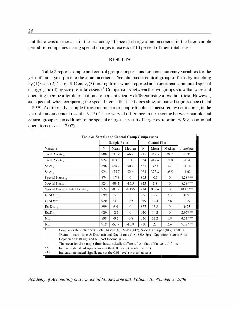
Table 2 reports sample and control group comparisons for some company variables for theyear of and a year prior to the announcements. We obtained a control group of firms by matchingby (1) year, (2) 4-digit SIC code, (3) finding firms which reported an insignificant amount of specialcharges, and (4) by size (i.e. total assets).4 Comparisons between the two groups show that sales andoperating income after depreciation are not statistically different using a two tail t-test. However,as expected, when comparing the special items, the t-stat does show statistical significance (t-stat= 8.39). Additionally, sample firms are much more unprofitable, as measured by net income, in theyear of announcement (t-stat = 9.12). The observed difference in net income between sample andcontrol groups is, in addition to the special charges, a result of larger extraordinary & discontinuedoperations (t-stat = 2.07).
Table 2: Sample and Control Group Comparisons
Variable
Sample Firms Control Firms
t-statisticN Mean Median N Mean Median
Total Assets t-1 900 531.9 66.9 825 449.5 49.7 -0.85
Total Assets t 924 483.3 58 924 447.6 57.8 -0.4
Sales t-1 896 486.2 50.4 821 370 42 -1.14
Sales t 924 475.7 52.6 924 373.8 46.5 -1.02
Special Items t-1 874 -17.8 0 805 -0.3 0 4.28***
Special Items t 924 -89.2 -13.5 923 2.8 0 8.39***
Special Items t / Total Assets t-1 924 -0.39 -0.175 924 0.006 0 10.15***
OIADpre t-1 899 27.7 0 826 32.6 2.3 0.68
OIADpre t 920 24.7 -0.5 919 34.4 2.6 1.29
ExtDis t-1 899 6.4 0 827 13.8 0 0.75
ExtDis t 920 -2.5 0 920 14.2 0 2.07***
NI t-1 899 -9.5 -0.8 826 22.2 1.8 4.21***
NI t 919 -53.7 -10.8 920 23 2.4 9.12***1 Compustat Item Numbers: Total Assets (#6), Sales (#12), Special Charges (#17), ExtDis
(Extraordinary Items & Discontinued Operations: #48), OIADpre (Operating Income AfterDepreciation: #178), and NI (Net Income: #172)
2 The mean for the sample firms is statistically different from that of the control firms:** Indicates statistical significance at the 0.05 level (two-tailed test)*** Indicates statistical significance at the 0.01 level (two-tailed test)

25
Academy of Accounting and Financial Studies Journal, Volume 10, Number 2, 2006
Table 3: Future Survival Length: Sample and Control Group Comparisons
Disappearance Year
Sample Firms Control Firms
A: Number of Firms % B: Number of Firms %
Panel A: Entire Sample Period (1986-1992 and 1996-1998) 1
0-1 21*** 2.3%*** 2*** 0.2%***
1-2 79*** 8.5%*** 29*** 3.1%***
2-3 120*** 13.0%*** 50*** 5.4%***
3-4 92 10% 78 8.40%
0-4 312*** 33.8%*** 159*** 17.2%***
4-16 209 22.60% 213 23.10%
Total Disappearances 521*** 56.4%*** 372*** 40.3%***
Total Survivors 403*** 43.6%*** 552*** 59.7%***
Total 924 100% 924 100%
Panel B: Early Sample Period (1986-1992)
0-1 7*** 2%*** 0*** 0%***
1-2 24*** 6.7%*** 8*** 2.2%***
2-3 37*** 10.4%*** 11*** 3.1%***
3-4 28 7.8%*** 26 7.30%
0-4 96*** 26.9%*** 45*** 12.6%***
4-16 147 41.20% 132 37%
Total Disappearances 243*** 68.1%*** 177*** 49.6%***
Total Survivors 114*** 31.9%*** 180*** 50.4%***
Total 357 100% 357 100%
Panel C: Later Sample Period (1996-1998)
0-1 14*** 2.5%*** 2*** 0.4%***
1-2 55*** 9.7%*** 21*** 3.7%***
2-3 63*** 14.6%*** 39*** 6.9%***
3-4 64 11.3% 52 9.20%
0-4 216*** 38.1%*** 114*** 20.1%***
4-7 62* 10.9%* 80* 14.1%*
Total Disappearances 278 49.0%*** 194 34.2%***
Total Survivors 289 51%*** 373 65.8%***
Total 567 100% 567 100%1 Because the year 2002 is the most recent year available to obtain survival data, we are able to track
survival length for up to 16 years for the 1986 firms, and up to 4 future years for the 1998 firms. 2 T-test (two tailed test) reports that these proportions are statistically different between sample and
control firms:** Indicates statistical significance at the 0.05 level (two-tailed test)*** Indicates statistical significance at the 0.01 level (two-tailed test)
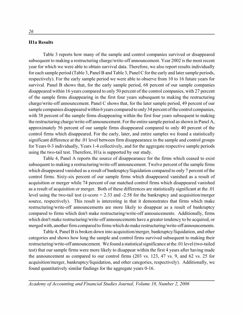
26
Academy of Accounting and Financial Studies Journal, Volume 10, Number 2, 2006
H1a Results
Table 3 reports how many of the sample and control companies survived or disappearedsubsequent to making a restructuring charge/write-off announcement. Year 2002 is the most recentyear for which we were able to obtain survival data. Therefore, we also report results individuallyfor each sample period (Table 3, Panel B and Table 3, Panel C for the early and later sample periods,respectively). For the early sample period we were able to observe from 10 to 16 future years forsurvival. Panel B shows that, for the early sample period, 68 percent of our sample companiesdisappeared within 16 years compared to only 50 percent of the control companies, with 27 percentof the sample firms disappearing in the first four years subsequent to making the restructuringcharge/write-off announcement. Panel C shows that, for the later sample period, 49 percent of oursample companies disappeared within 6 years compared to only 34 percent of the control companies,with 38 percent of the sample firms disappearing within the first four years subsequent to makingthe restructuring charge/write-off announcement. For the entire sample period as shown in Panel A,approximately 56 percent of our sample firms disappeared compared to only 40 percent of thecontrol firms which disappeared. For the early, later, and entire samples we found a statisticallysignificant difference at the .01 level between firm disappearance in the sample and control groupsfor Years 0-3 individually, Years 1-4 collectively, and for the aggregate respective sample periodsusing the two-tail test. Therefore, H1a is supported by our study.
Table 4, Panel A reports the source of disappearance for the firms which ceased to existsubsequent to making a restructuring/write-off announcement. Twelve percent of the sample firmswhich disappeared vanished as a result of bankruptcy/liquidation compared to only 7 percent of thecontrol firms. Sixty-six percent of our sample firms which disappeared vanished as a result ofacquisition or merger while 74 percent of our matched control firms which disappeared vanishedas a result of acquisition or merger. Both of these differences are statistically significant at the .01level using the two-tail test (z-score = 2.33 and -2.58 for the bankruptcy and acquisition/mergersource, respectively). This result is interesting in that it demonstrates that firms which makerestructuring/write-off announcements are more likely to disappear as a result of bankruptcycompared to firms which don't make restructuring/write-off announcements. Additionally, firmswhich don't make restructuring/write-off announcements have a greater tendency to be acquired, ormerged with, another firm compared to firms which do make restructuring/write-off announcements.
Table 4, Panel B is broken down into acquisition/merger, bankruptcy/liquidation, and othercategories and shows how long the sample and control firms survived subsequent to making theirrestructuring/write-off announcement. We found a statistical significance at the .01 level (two-tailedtest) that our sample firms were more likely to disappear within the first 4 years after having madethe announcement as compared to our control firms (203 vs. 123, 47 vs. 9, and 62 vs. 25 foracquisition/merger, bankruptcy/liquidation, and other categories, respectively). Additionally, wefound quantitatively similar findings for the aggregate years 0-16.
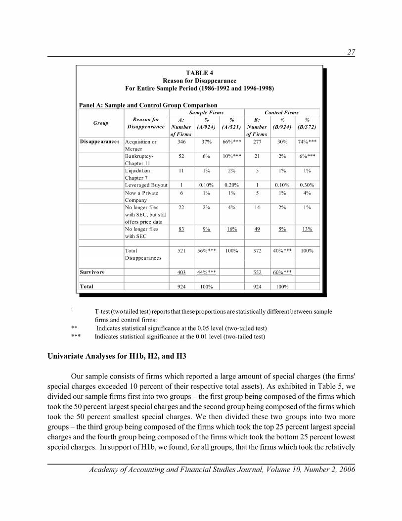
27
Academy of Accounting and Financial Studies Journal, Volume 10, Number 2, 2006
1 T-test (two tailed test) reports that these proportions are statistically different between samplefirms and control firms:
** Indicates statistical significance at the 0.05 level (two-tailed test)*** Indicates statistical significance at the 0.01 level (two-tailed test)
Univariate Analyses for H1b, H2, and H3
Our sample consists of firms which reported a large amount of special charges (the firms'special charges exceeded 10 percent of their respective total assets). As exhibited in Table 5, wedivided our sample firms first into two groups – the first group being composed of the firms whichtook the 50 percent largest special charges and the second group being composed of the firms whichtook the 50 percent smallest special charges. We then divided these two groups into two moregroups – the third group being composed of the firms which took the top 25 percent largest specialcharges and the fourth group being composed of the firms which took the bottom 25 percent lowestspecial charges. In support of H1b, we found, for all groups, that the firms which took the relatively
A: % % B: % % Number of Firms
(A/924) (A/521) Number of Firms
(B/924) (B/372)
Disappe arance s Acquisition or Merger
346 37% 66%*** 277 30% 74%***
Bankruptcy- Chapter 11
52 6% 10%*** 21 2% 6%***
Liquidation – Chapter 7
11 1% 2% 5 1% 1%
Leveraged Buyout 1 0.10% 0.20% 1 0.10% 0.30%Now a Private Company
6 1% 1% 5 1% 4%
No longer files with SEC, but still offers price data
22 2% 4% 14 2% 1%
No longer files with SEC
83 9% 16% 49 5% 13%
Total Disappearances
521 56%*** 100% 372 40%*** 100%
Survivors 403 44%*** 552 60%***
Total 924 100% 924 100%
GroupReason for
Disappearance
Sample Firms Control Firms
TABLE 4Reason for Disappearance
For Entire Sample Period (1986-1992 and 1996-1998)
Panel A: Sample and Control Group Comparison

28
Academy of Accounting and Financial Studies Journal, Volume 10, Number 2, 2006
larger special charges were more likely to disappear in an earlier time frame (within the first 4 yearsof having made the announcement) than were the firms which took the relatively smaller specialcharges (176 vs. 132 and 90 vs. 72 for the first and second group and the third and fourth group,respectively). These findings are statistically significant at the 1 percent level using a two-tailedtest. Interestingly, we also found that for all groups, the firms which take the relatively smallerspecial charges are more likely to disappear in the long term (within 5 to 16 years after having madethe special charge announcement) than are firms which take the relatively larger special charges. Wefeel that the impact of a special charge will most strongly affect a firm within a short time frame,with little, if any, affect being felt by firms in the long-term. Therefore, the fact that firms whichtake relatively smaller special charges are more likely to disappear in the long-term has little to do,if anything, with the special charge announcements we observed. So the results from the preliminaryunivariate analysis support H1b.
1 Other reasons include companies no longer filing with SEC, having disappeared throughleveraged buyouts, or now being private companies.
2 T-test (two tailed test) reports that these proportions are statistically different between samplefirms and control firms:
** Indicates statistical significance at the 0.05 level (two-tailed test)*** Indicates statistical significance at the 0.01 level (two-tailed test)
Acquisition/ Merger
Bankruptcy/ Liquidation Others 1
Acquisition/ Merger
Bankruptcy/ Liquidation Others
19*** 1 1 0*** 0 270*** 6*** 3 29*** 0*** 075*** 17*** 28*** 41*** 2*** 7***
39 23*** 30** 53 7*** 18**203*** 47*** 62*** 123*** 9*** 25***
143 16 50 152 17 46
346*** 63*** 112*** 275*** 26*** 71***
924
Total Survivors403*** 552***
Total 924
Total Disappearances
521*** 372***
Subtotal
4-16
0-4
2-33-4
0-11-2
Disappearance Year*
Sample Firms Control Firms
TABLE 4 (continued)Reason for Disappearance
For Entire Sample Period (1986-1992 and 1996-1998)
Panel B: Future Survival Length
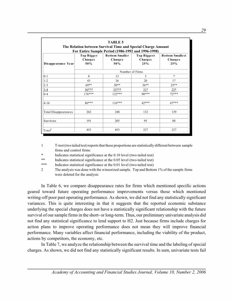
29
Academy of Accounting and Financial Studies Journal, Volume 10, Number 2, 2006
1 T-test (two tailed test) reports that these proportions are statistically different between samplefirms and control firms:
* Indicates statistical significance at the 0.10 level (two-tailed test)** Indicates statistical significance at the 0.05 level (two-tailed test)*** Indicates statistical significance at the 0.01 level (two-tailed test)2 The analysis was done with the winsorized sample. Top and Bottom 1% of the sample firms
were deleted for the analysis
In Table 6, we compare disappearance rates for firms which mentioned specific actionsgeared toward future operating performance improvements versus those which mentionedwriting-off poor past operating performance. As shown, we did not find any statistically significantvariances. This is quite interesting in that it suggests that the reported economic substanceunderlying the special charges does not have a statistically significant relationship with the futuresurvival of our sample firms in the short- or long-term. Thus, our preliminary univariate analysis didnot find any statistical significance to lend support to H2. Just because firms include charges foraction plans to improve operating performance does not mean they will improve financialperformance. Many variables affect financial performance, including the viability of the product,actions by competitors, the economy, etc.
In Table 7, we analyze the relationship between the survival time and the labeling of specialcharges. As shown, we did not find any statistically significant results. In sum, univariate tests fail
Top B igge r Charge s
Bottom Smalle r Charge s
Top Bigge s t Charge s
Bottom Smalle st Charge s
0-1 8 13 3 71-2 43 36 20 172-3 69** 50** 36** 25**3-4 56*** 33*** 31* 23*0-4 176*** 132*** 90*** 72***
4-16 86*** 116*** 42*** 67***
Total Disappearances 262 248 132 139
Survivors 191 205 95 88
Total2 453 453 227 227
Disappe arance Ye ar
Number of Firms
50% 50% 25% 25%
TABLE 5The Relation between Survival Time and Special Charge Amount
For Entire Sample Period (1986-1992 and 1996-1998)
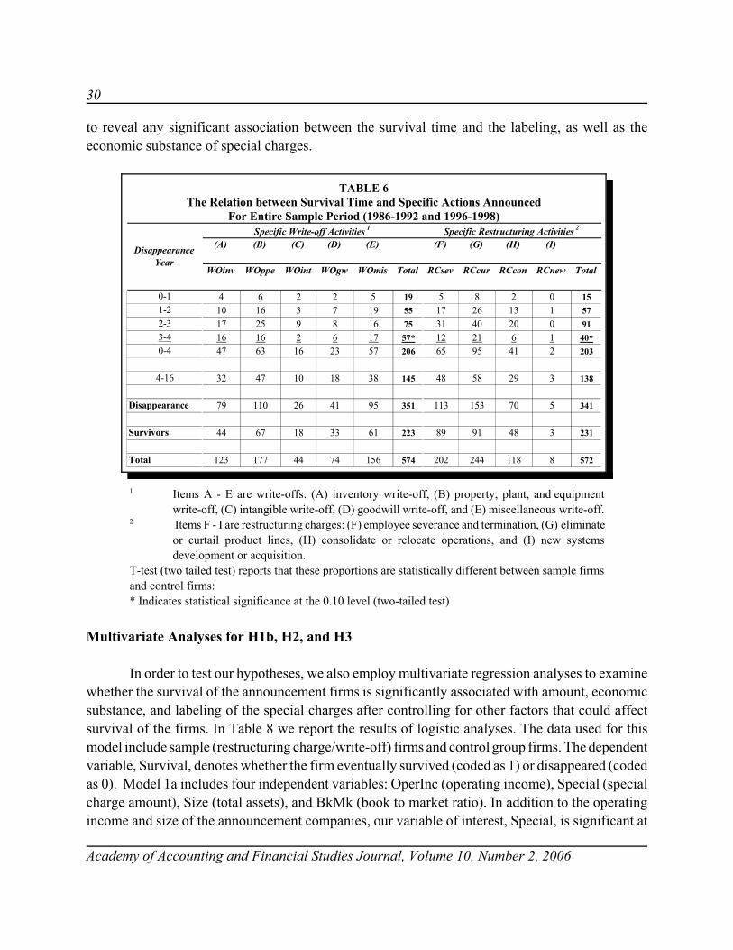
30
Academy of Accounting and Financial Studies Journal, Volume 10, Number 2, 2006
to reveal any significant association between the survival time and the labeling, as well as theeconomic substance of special charges.
1 Items A - E are write-offs: (A) inventory write-off, (B) property, plant, and equipmentwrite-off, (C) intangible write-off, (D) goodwill write-off, and (E) miscellaneous write-off.
2 Items F - I are restructuring charges: (F) employee severance and termination, (G) eliminateor curtail product lines, (H) consolidate or relocate operations, and (I) new systemsdevelopment or acquisition.
T-test (two tailed test) reports that these proportions are statistically different between sample firmsand control firms:* Indicates statistical significance at the 0.10 level (two-tailed test)
Multivariate Analyses for H1b, H2, and H3
In order to test our hypotheses, we also employ multivariate regression analyses to examinewhether the survival of the announcement firms is significantly associated with amount, economicsubstance, and labeling of the special charges after controlling for other factors that could affectsurvival of the firms. In Table 8 we report the results of logistic analyses. The data used for thismodel include sample (restructuring charge/write-off) firms and control group firms. The dependentvariable, Survival, denotes whether the firm eventually survived (coded as 1) or disappeared (codedas 0). Model 1a includes four independent variables: OperInc (operating income), Special (specialcharge amount), Size (total assets), and BkMk (book to market ratio). In addition to the operatingincome and size of the announcement companies, our variable of interest, Special, is significant at
(A) (B) (C) (D) (E) (F) (G) (H) (I)
0-1 4 6 2 2 5 19 5 8 2 0 151-2 10 16 3 7 19 55 17 26 13 1 572-3 17 25 9 8 16 75 31 40 20 0 913-4 16 16 2 6 17 57* 12 21 6 1 40*0-4 47 63 16 23 57 206 65 95 41 2 203
4-16 32 47 10 18 38 145 48 58 29 3 138
Disappearance 79 110 26 41 95 351 113 153 70 5 341
Survivors 44 67 18 33 61 223 89 91 48 3 231
Total 123 177 44 74 156 574 202 244 118 8 572
Disappearance Year
RCsev RCcur RCconWOint WOgw WOmis Total
Specific Write-off Activities 1 Specific Restructuring Activities 2
WOinv WOppe TotalRCnew
TABLE 6The Relation between Survival Time and Specific Actions Announced
For Entire Sample Period (1986-1992 and 1996-1998)

31
Academy of Accounting and Financial Studies Journal, Volume 10, Number 2, 2006
the 10 percent level in explaining whether the firms will survive in subsequent years. The positivecoefficient of 0.242 suggests that when the special charge amount is reduced, the probability offirms' survival will increase (note that special charge amounts have negative values).
Table 7: The Relation between Survival Time and the Labeling ofAnnouncements for the Entire Sample Period (1986-1992 and 1996-1998)
DisappearanceYear
A B C
Labeled asWrite-off
%(A/370)
Labeled asRestructuring Charge
%(B/350)
t-statistic
0-1 10 2.70% 5 1.43% 1.2
1-2 30 8.11% 38 10.86% -1.26
2-3 49 13.24% 52 14.86% -0.62
3-4 33 8.92% 28 8.00% 0.44
0-4 122 32.97% 123 35.14% -0.61
4-16 93 25.14% 95 27.14% -0.61
Disappearance 215 58.11% 218 62.29% -1.14
Survivor 155 41.89% 132 37.71% 1.14
Total 370 100% 350 100%1 T-test (two tailed test) reports that these proportions are statistically differentbetween sample firms and control firms:** Indicates statistical significance at the 0.05 level (two-tailed test)*** Indicates statistical significance at the 0.01 level (two-tailed test)
Model 2a includes variables representing firms' specific actions regarding write-offs, as wellas aforementioned four independent variables. Similar to the first model, Special is still significantat the 10 percent level. Among the variables representing specific actions of write-offs, only WOppe(write-offs of property, plant, and equipment) is significant in explaining whether the firms willsurvive in subsequent years at the 10 percent level. The coefficient of -0.306 suggests that when thefirms announce special charges that are involved with writing off PP&E, the probability of firms'survival will decrease by 30.6 percent.
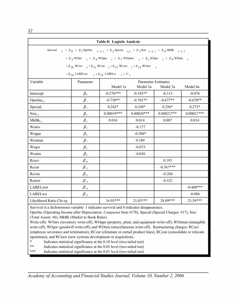
32
Academy of Accounting and Financial Studies Journal, Volume 10, Number 2, 2006
Table 8: Logistic Analysis
iUiLABELrc15βiLABELwo14β
iRCnew13βiRCcon12βiRCcur11βiRCsev10β
iWOmis9βiWOgwβiWOintan7βiWOppe6βiWOinv5β
i1,-tMkBk4βi1,-tSize3βit,Special2βi1,-tOperInc1β0βiSurvival
8
+++
++++
+++++
++++=
Variable Parameter Parameter Estimates Model 1a Model 2a Model 3a Model 4a
Intercept $ 0 -0.276*** -0.183** -0.113 -0.076
OperInct-1 $ 1 -0.730** -0.701** -0.677** -0.670**
Specialt $ 2 0.242* 0.249* 0.256* 0.273*
Sizet-1 $ 3 0.00019*** 0.00020*** 0.00021*** 0.00021***
MkBkt-1 $ 4 0.016 0.014 0.007 0.014
Woinv $ 5 -0.177
Woppe $ 6 -0.306*
Wointan $ 7 0.189
Wogw $ 8 -0.073
Womis $ 9 -0.056
Rcsev $ 10 0.193
Rccur $ 11 -0.567***
Rccon $ 12 -0.204
Rcnew $ 13 -0.522
LABELrest $ 14 -0.400***
LABELwo $ 15 -0.086
Likelihood Ratio Chi-sq 16.93*** 21.03*** 28.89*** 23.59***
Survival is a dichotomous variable: 1 indicates survival and 0 indicates disappearance.OperInc (Operating Income after Depreciation: Compustat Item #178), Special (Special Charges: #17), Size(Total Assets: #6), MkBk (Market to Book Ratio).Write-offs: WOinv (inventory write-off), WOppe (property, plant, and equipment write-off), WOintan (intangiblewrite-off), WOgw (goodwill write-off), and WOmis (miscellaneous write-off). Restructuring charges: RCsev(employee severance and termination), RCcur (eliminate or curtail product lines), RCcon (consolidate or relocateoperations), and RCnew (new systems development or acquisition).* Indicates statistical significance at the 0.10 level (two-tailed test)** Indicates statistical significance at the 0.05 level (two-tailed test)*** Indicates statistical significance at the 0.01 level (two-tailed test)
33
Academy of Accounting and Financial Studies Journal, Volume 10, Number 2, 2006
Model 3a includes variables representing firms' specific actions regarding restructuringcharges, as well as aforementioned four independent variables of OperInc, Special, Size, and BkMk.Similar to the first and second model, our interest variable, special charge amount is still significantat the 10 percent level. Among the variables representing specific actions of restructuring charges,only RCcur (restructuring charges of curtailing product lines) is highly significant at the 1 percentlevel. The coefficient of -0.567 suggests that when firms announce restructuring charges involvingeliminating product lines, the probability of firms' survival will decrease by 56.7 percent.
Model 4a includes variables representing how firms labeled their special charges, either asrestructuring charges or write-offs, in addition to variables of OperInc, Special, Size, and BkMk.Similar to the other models, special charge amount is still significant at the 10 percent level. Besides,LABELrest is very significant in explaining whether the firms will survive in subsequent years atthe 1 percent level. The coefficient of -0.400 suggests that when firms label their special charges asrestructuring charges, the probability of firms' survival will decrease by 40 percent. This findingdocuments decreasing probability for survival for firms using the label "restructuring," and suggeststhat investors need to be cautious with their perceptions of the word.
In sum, the results from logistic analyses reported in Table 8 provide evidence that build onthe findings of prior research in restructuring charge/write-off literature. Atiase, et al. (2001) andCarter (2000) found that the performance of restructuring charge firms is better than that ofnon-restructuring firms in the post-restructuring period. However, these studies may suffer from"survivorship bias" when evaluating the future performance of firms. We find that firms reportingsmaller amount charges survive longer than those with larger charges, regardless of any businessactions announced. We also find evidence of decreasing probability for survival for firms using thelabel of "restructuring" for the charges. Special charge firms that label their charges as "restructuringcharges" are more likely to disappear and more likely to disappear sooner.
CONTRIBUTIONS AND LIMITATIONS
Firms continue to report many special charges, including restructuring and write-offannouncements. Regulators have tried to limit the discretion available regarding special charges (forexample, EITF 94-3, SFAS 121, and more recently SFAS 144, and SFAS 146). However,considerable discretion persists. Due to the subjective information content of these announcements,investors often have difficulty appropriately interpreting the future implications of these specialcharges. Managers' discretion over the amounts, what business actions include, and labels for thesecharges has led to debate over whether or not they are trying to mask their firms' poor performance.In this study, we extend the restructuring charge/write-off literature by investigating the relationshipbetween firm survival and the amount, business action plans mentioned, and labeling of specialcharge announcements. Most of the results are consistent with the predictions made in thehypotheses. First, firms which announce large restructuring/write-off charges are not only more
34
Academy of Accounting and Financial Studies Journal, Volume 10, Number 2, 2006
likely to disappear, but to disappear sooner than firms which announce small, if any, charges. Also,among those firms that report large special charges, firms that report relatively larger amounts ofrestructuring charges/write-offs are not only more likely to disappear, but to disappear sooner thanfirms which announce relatively smaller charges. It seems reasonable that firms with biggereconomic problems will not only tend to make special charges for higher amounts but also be lesslikely to survive in the short-term.
Second, firms reporting restructuring charges/write-offs that mention action plans for futureoperating performance improvements are not necessarily more likely to survive than firms reportingcharges that merely recognize poor past operating performances. Just because firms include chargesfor plans to improve operating performance does not mean they will improve financial performance.Many variables affect financial performance, including the viability of the product, actions bycompetitors, the economy and industry, etc. These items are beyond the scope of this study butwarrant further research.
Lastly, we investigate whether managers' decisions regarding the labeling of theannouncements involve an intent that is consistent with opportunism. The results of our analysisprovide evidence of decreasing probability of survival for firms using the label of "restructuring"for the charge. This finding may suggest more opportunism (and less credibility) in financialreporting during our sample period. As with other financial reporting methods, companies may bemore likely to use the term "restructuring charge" inappropriately these days to alter Wall Streetpredictions.
The study is limited in that variables other than those tested in this research contribute tosurvival of special charge firms. However, this study does provide evidence that the higher theamount of special charge, the less likely the firm will survive, regardless of the business action plansfor improvement mentioned. We also find evidence of increasing use of the term "restructuringcharge" with increasing probability for disappearance.
Because many special charge firms have been taken over or merged after they madeannouncements, future research could examine their stock market performance in subsequent years.Also, future research could potentially evaluate the impact of SFAS 144 and 146 (which becameeffective in 2001) on the survival of restructuring charge/write-off announcement firms.
END NOTES
1 In this paper, we define "disappear" to include acquisition/merger or failure due to bankruptcy/liquidation."Survive" is defined as not disappearing.
2 These reports specifically noted that the managers use special charges to create new terms regarding earnings,such as "operating earnings," "core earnings," or "pro-forma earnings" to favorably affect analysts' andinvestors perception of the firms (Weil 2001).
35
Academy of Accounting and Financial Studies Journal, Volume 10, Number 2, 2006
3 In addition, the use of arbitrary cutoffs was necessary to ensure a reasonable workload for sampling. As wedecrease the required percent of special charges relative to total assets, the number of companies increasessharply. For example, when five percent is used instead of ten percent, the number of firms increases by abouttwo times. Also, when one percent is used instead of ten percent, the number of firms increases by about fourtimes. In 1990, for instance, the number of firms is 385 when a ten percent cutoff is used. The number of firmsincreases to 642 when a five percent requirement is applied. The number increases further to 1,304 when a onepercent cutoff is applied.
4 Control firms were selected by applying the following matching procedure. First, matching on the year,possible control firms were identified. Second, control firms were further identified initially by matching onthe SIC code of four digits. Third, within the same industry and in the same respective year, companies thatreported special charges of zero were selected. When we could not find zero amount of special charge firms,then we selected firms that recorded special charges close to zero within the range of less than - 1% of totalassets (positive special charges were included; that is, control firms' special charges range from - 1 % to positivecharges.) Finally, the control firm was chosen by selecting the firm closest to the sample firm in size. Size wasmeasured by total assets, and control firms had to be within 50% of the sample firm on size.
REFERENCES
Adut, D., Cready, W., and T. Lopez. (2003) Restructuring charges and CEO cash compensation: A reexamination. TheAccounting Review (78): 169-192.
Ante, S. (2003) The secret behind those profit jumps. Business Week Issue 3861 (12/08/2003): 50.
Atiase, R., D. Platt, & S. Tse. (2001). Operational restructuring charges and post-restructuring performance: Thepotential effects of write-off amounts on measured performance. Working Paper, University of Texas at Austin.
Brickley, J. & L. Van Drunen. (1990). Internal corporate restructuring: An empirical analysis. Journal of Accountingand Economics 12: 251-280.
Bunsis, H. (1997). A description and market analysis of write-off announcements. Journal of Business, Accounting andFinance 24 (9/10): 1385-1400.
Carter, M. (2000). Operating and stock market performance following corporate restructurings. Working Paper,Columbia University.
Chaney, P. K., C. E. Hogan, & D. C. Jeter. (1999). The effect of reporting restructuring charges on analysts’ forecastrevisions and errors. Journal of Accounting & Economics 27 (3): 261-284.
Chen, K. & C. J. Lee. (1993). Financial Ratios and Corporate Endurance: A Case of the Oil and Gas Industry.Contemporary Accounting Research 9 (2): 667-694.
Condon, B. (1998). Pick a number, any number. Forbes 161 (6): 124-128.
36
Academy of Accounting and Financial Studies Journal, Volume 10, Number 2, 2006
Elliott, J. & W. Shaw. (1988). Write-offs as accounting procedures to manage perceptions. Journal of AccountingResearch 26 (Supplement): 91-119.
Financial Accounting Standards Board (FASB). (1994). Liability Recognition for Certain Employee TerminationBenefits and Other Costs to Exit an Activity (including Certain Costs Incurred in a Restructuring). EmergingIssues Task Force Issue 94-3. Stamford, CT: FASB.
Financial Accounting Standards Board (FASB). (1995). Accounting for the Impairment of Long- Lived Assets to BeDisposed Of. Statement of Financial Accounting Standards No. 121. Stamford, CT: FASB.
Francis, J., J. Hanna, & L. Vincent. (1996). Causes and effects of discretionary asset write-offs. Journal of AccountingResearch 34 (Supplement): 117-134.
Gallagher, J. (2004). Profits hits and busts. Traffic World (11/01/2004): 1.
Harlan, C. (1994). SEC wants explanations from firms planning to post restructuring losses. Wall Street Journal(February 25): B6.
Hirschey M. and V. Richardson. (2003). Investor underreaction to goodwill write-offs. Financial Analysts Journal (59)Iss. 6: 75-84.
Hogan, C. E., & D. C. Jeter. (1997). The information content of restructuring charges: A contextual analysis. WorkingPaper, Vanderbilt University.
Kross, W., T. Park, & B. Ro. (1998). The impact of operational restructuring announcements on stock price, risk, andtrading volume. Working Paper, Purdue University.
Lane, W., S. Looney, & J. Wansley. (1986). An application of the Cox Proportional Hazards Model to bank failure.Journal of Banking and Finance 10: 511-531.
Lopez, T. (2002). Evidence on the incremental information contained in the components of restructuring charges.Journal of Business Finance and Accounting. 29 (5/6): 613-660.
Moehrle, S. (2002). Do firms use restructuring charge reversals to meet earnings targets? The Accounting Review 77 (2):397-413.
PR News. (1997). Kodak’s layoffs: Not a good snapshot of communication. Vol. 53 (No. 49, December 15).
Smith, R., & S. Lipin. (1996). Are companies using restructuring costs to fudge the figures? Wall Street Journal (January30): A1.
Stice, J., Stice, E. K., & F. Skousen. (2004). Intermediate Accounting 15th edition Thomson South-Western: 181
Strong, J. & J. Meyer. (1987). Asset writedowns: Managerial incentives and security returns. Journal of Finance 42(July): 643-663.
37
Academy of Accounting and Financial Studies Journal, Volume 10, Number 2, 2006
Turetsky, H., & R. McEwen. (2001). An Empirical Investigation of Firm Longevity: A Model of the Ex Ante Predictorsof Financial Distress. Review of Quantitative Finance and Accounting (June): 323-343.
Weil, J. (2001). What’s the P/E ratio? Well, depends on what is meant by earnings. Wall Street Journal (August 21):A1.
Weiss, I. (1999). Earnings management in response to an exogenous non-recurring item. Working Paper, Universityof Chicago.

38
Academy of Accounting and Financial Studies Journal, Volume 10, Number 2, 2006
39
Academy of Accounting and Financial Studies Journal, Volume 10, Number 2, 2006
LOSING LIKE FORREST GUMP:WINNERS AND LOSERS IN THE FILM INDUSTRY
Martha Lair Sale, Sam Houston State UniversityPaula Diane Parker, University of South Alabama
ABSTRACT
There are a number of high-profile cases where films that by most standards of revenueminus cost are very successful, but are reported as providing net losses to the studios. Most of thepublic attention on these cases arises from lawsuits brought by participants who contracted toreceive payment based on a percentage of the profit of the film.
This paper highlights some of the unique costing practices in the film industry and examinesseveral of these well-known “losers” in light of the difference between the gross receipts of the filmand the direct costs of production. It provides some insight into the difference between what wouldbe considered a rational indirect cost allocation basis for other industries and the apparently erraticallocation process used in film.
The analysis includes an examination of the relationship between the gross receipts and theproduction costs of films in a number of categories that might be considered measures of successin the film industry.
INTRODUCTION
In 1999, entertainment accounts for less than one percent of the gross national product of theUnited States (Berton & Harris, 1999). Despite its small percentage, the film industry gains muchattention in the nineties because of its finances (Cheatham, Cheatham, & Davis, 1996). Buzzwordslike “creative accounting” are used, and some accountants assert, “The accounting department is themost creative part of Tinseltown” (Cheatham et al., 1996, p. 1). Several major disputes aid inbringing the film industry’s accounting practices into the limelight.
In one example (Pfeiffer, Capettini, & Whittenburg, 1997), the 1990 court case Art Buchwaldv. Paramount Pictures Corporation, Art Buchwald claims that Paramount’s movie Coming toAmerica is based on a film treatment that Buchwald wrote. Not supprisingly, since the studio hadcontracted with Buchwald to use the material, the court agrees and rules in Buchwald’s favor. Itmakes sense that he should receive the compensation set forth in his original contract withParamount Pictures Corporation. In addition to a fixed fee, Buchwald’s original contract awardshim a share of the net profits of the film. According to this account, the film is a box office success.However, Paramount, reports it as a lost $18 million. Winston Groom, the author of the novel
40
Academy of Accounting and Financial Studies Journal, Volume 10, Number 2, 2006
Forrest Gump, contracts to receive $350,000 and 3% of the net profits of the film for the rights tohis book. When Groom tries to collect his 3%, he learns that Paramount is reporting a loss on thefilm. Forrest Gump earns millions at the box office in 1994, yet Paramount reports its profitabilityin the red. Also fueling the controversy is the fact that director Robert Zemeckis and actor TomHanks receives a percentage of the films fees, but they are awarded their money based on gross boxoffice receipts instead of net profits (Pfeiffer, Capettini, & Whittenburg, 1997). Other popular filmsreport losses, too. Batman shows a $20 million loss, and net profit participants sue Warner Brothers.Net profit participants of the movie JFK go to court after no net profits are reported for the film.(Goldberg, 1997). Rain Man, Dick Tracy, Ghostbusters, Alien, On Golden Pond, Fatal Attractionare all films grossing over $100 million in the 1990’s for which no net profits were reported(Pheiffer, Capettini, & Whittenburg, 1997).
According to Cheatham, Cheatham, and Davis (1996), film costs contain four maincomponents. First, distribution fees are paid to the distributor of the film. In many cases, filmstudios act as their own distributor (Pfeiffer, Capettini, & Whittenburg, 1997). If that is the case,the film studio simply pays itself this money, which usually is 20% to 27% of gross receipts. Thismethod is simply a “positive cash flow item masquerading as an expense,” according to Cheathamet al. (1996, p. 2). Pfeiffer et al. (1997), on the other hand, justify this as the studio earning a returnfor serving as the distributor of the film. In essence, the film studio generates revenue while thespecific film incurs an expense.
In addition to distribution fees, distribution expenses are a cost of films, according toCheatham et al. (1996). These expenses include promotion, advertising, physically moving the reels– everything that is needed to actually distribute the film. Interest expenses are attributed to a filmwhen the film studio serves as the principal investor (Pheiffer et al., 1996). Investing in a film keepsthe studio from investing in alternatives that will yield interest.
The actual production costs in a film are called the negative costs. Levine and Seigal (2001,p. 3) identify the following items included in negative costs:
Film costs include all direct costs incurred in the physical production of a film, such as the costs ofacquiring the story and scenario (film rights to books, stage plays, or original screenplays);compensation of cast members, directors, producers, and extras; costs of set construction, operations,and wardrobe; costs of sound synchronization; costs of rental facilities on location; and postproductioncosts (music, special effects, and editing). Negative costs also include allocations of productionoverhead and capitalized interest costs.
Not only do Cheatham, Cheatham, and Davis (1996) contend that the film industry reportstoo many costs that might not normally be considered properly product cost, they also contend thatit fails to report what in other industries would be revenues. First of all, major revenue comes frombox office receipts. According to Davis (1997), on average film studios receive 50% of gross boxoffice receipts and the movie theaters receive the other 50%. More specifically, film studios use a

41
Academy of Accounting and Financial Studies Journal, Volume 10, Number 2, 2006
sliding scale to determine what percentage they will receive. Early in a film’s release, film studiosgenerally receive a large percentage of the box office receipts. For example, in the first two weeks,the film studio may receive 90%. At the sixth week, the percentage may be down to 60% and thendrop to 10% by week twelve. The purpose of this sliding scale is to encourage movie theaters toshow films for longer periods of time (Davis 1997).
Although gross box office receipts cannot likely be understated, supplementary income can.At the time “Hollywood Profits: Gone with the Wind?” (Cheatham, Cheatham, & Davis) ispublished in 1996, film studios only count 20% of videocassette sales as revenue for a film. Otherancillary income includes non-theatrical showings for groups such as airlines and armed forces,network television, music publishing, sound tracks, literary adaptations, computer games, and othermerchandising like McDonald’s happy meals. (Goldberg, 1997) Foreign markets are oftenminimized as well, in spite of the growing market (Cheatham, et al., 1996).
According to Cheatham, Cheatham, and Davis (1996), the combined effect of high expensesand low revenues result in understated profit. Goldberg (1997) seeks to unravel why film studiossanction this to happen. Goldberg focuses largely on gross profit participants, persons who receivea portion of gross profits for a film. Sought-after actors and directors are generally given apercentage of a film’s gross profit in addition to a fixed sum of money. Studios offer gross profitsto certain participants for several reasons. First, many actors require this kind of contract, andstudios realize that actors draw audiences to movie theaters. A film featuring a popular star likeTom Cruise or Julia Roberts is much more likely to open well at the box office than a film featuringnew talent. Even a director like Steven Spielberg can draw fans. Also, if an actor or director knowsthat his or her compensation is linked to the gross profitability of a film, he or she may be morelikely to promote the film and go the extra mile to ensure its success at the box office (Goldberg,1997).
Goldberg (1997) asserts that when gross profit participants become involved in films, netprofits are likely to disappear. He cites examples like the 1993 movie Indecent Proposal, whichreports a loss of $35 million after paying its five gross profit participants. Star Robert Redfordreportedly receives over $20 million. Others cite similar examples like Hook, in which 40% of thefilm’s gross profits were given to Julia Roberts, Dustin Hoffman, Robin Williams, and StevenSpielberg (Pfeiffer, Capettini, & Whittenburg, 1997). According to Goldberg (1997), IndecentProposal and Hook are naturally doomed for net profit failure because of their large number of grossprofit participants.
Lesser talent and participants often do not receive gross profit rights. Goldberg (1997)explains that Winston Groom, author of Forrest Gum, is a net profit participant. To net profitparticipants, Goldberg (1997) says that although the gross profit participants decrease the likelihoodof receiving any percentage of the net profits, their involvement in a film may yield more profitableresults for certain net profit participants. For example, although Winston Groom did not receive netprofits, he experiences a huge increase in book sales after the release of the movie. Perhaps book

42
Academy of Accounting and Financial Studies Journal, Volume 10, Number 2, 2006
sales would not have been as large if a major actor like Tom Hanks had not been recruited to starin the film.
The intriguing conflict surrounding the motion picture industry in the 1990’s understandablybrings attention to the accounting methods and practices of Hollywood. Changes are made incosting methods specific to the film industry in an attempt to rectify any misreporting. In thenineties, the film industry is surrounded by major public concern and controversy relating to itsaccounting methods and practices. Consequently, in September 1995, the Entertainment and SportsIndustry Committee of the California Society of Certified Public Accountants requests the FinancialAccounting Standards Board investigate the film industry methods and practices arising as a resultof their prior issuance, in December 1981, of Statement of Financial Accounting Standards Number53 which governs the film industry.
In June 2000, the findings from the investigation prompted the Financial AccountingStandards Board to issue the Statement of Financial Accounting Standards Number 139. This newstandard rescinds the Statement of Financial Accounting Standards Number 53 and amends threeother regulatory statements. According to the Financial Accounting Standards Board, the decisionto repeal the Statement of Financial Accounting Standards Number 53 is based on the followingmatters and concerns. First, the film industry is continuously changes that affect their financialposition and financial reporting; particularly regarding revenue recognition as film revenue increasethrough ancillary forms such as DVD’s, private showings, TV, and international markets; second,film studios apply the Statement of Financial Accountins Standards Statement 53 differently; andthird, the accuracy of the film industry’s financial statements are questionable (Financial AccountingStandard Board, 2000).
In August 2000, the American Institute of Certified Public Accountants (AICPA) issues anews release titled “AICPA Issues New Rules for Film Industry” that states three major changesnow exists for the film industry. These include advertising expenses, film amortization, andabandoned projects. Some of these changes discussed by Berton and Harris (1999) includeadvertising costs are now to be amortized against revenues for the appropriate market rather thanagainst revenues for a specific film. Film amortization is to be based on ten years rather than thetwenty-year standard previously used by most film studios. Finally, abandoned projects cannot bewritten off to the overhead pool as commonly done before.
ANALYSIS
Special accounting provisions aside, the actual revenue and cost reported for films is notdifficult to relate to other products. The production budget for films includes all the classificationsof actual costs accountants would generally associate with direct costs of a film. In this respect itis not a budget in the normally accepted definition of the word, it is a report of actual costs. Grossreceipts is a relatively concrete number analogous to what would be considered revenues in
43
Academy of Accounting and Financial Studies Journal, Volume 10, Number 2, 2006
accounting for most products, and is not amenable to easy “management.” Once these two termsare defined, the controversy may be simplified to a question of what indirect costs should beassigned to individual films and what costs should be borne by the studio. Since major participantsin the success of a film are paid on gross receipts it seems likely that the less powerful providers ofcontract services for the film industry are forced to bear a disproportionate burden of indirect costs.
In general GAAP requires that indirect costs be assigned in rational and consistent manner(Horngren, Foster & Datar, p. 486). In most products this rational and consistent manner would bebased on some measure of the cost of the direct inputs. In spite of the film industry’s unique costingmethods, an examination of the relationships between profitability and the success of films asmeasured by production costs and gross receipts offers interesting insight into whether or not someof these films that have been the center of controversy would have been considered profitableproducts using costing methods appropriate to most other products.
In this study, first, the top grossing films of each major film studio are studied. Accordingto Box Office Report (2004), these film studios and specific films are as follows: Disney andMiramax, The Lion King (1994); DreamWorks, Shrek (2001); Fox, Star Wars (1977); MGM/UnitedArtist, Gone with the Wind (1939); Paramount, Titanic (1997); Sony, Spider-Man (2002); Universal,E.T. The Extra-Terrestrial (1982); Warner and New Line, The Two Towers (2002).
Another way of selecting successful films is to examine films that have won the AcademyAward for Best Picture. Intuitively, there should be some connection between the cost of a film andits quality. The Academy Award or Oscar for Best Picture is a surrogate measure for quality. Thisaward is considered by many in the film industry to be the highest award that can be given to a film.Although not a strictly quantitative factor, many film studios do measure success of films by Oscarnominations and wins. The Best Picture Oscar winners for the past ten years are Chicago (2002),A Beautiful Mind (2001), Gladiator (2000), American Beauty (1999), Shakespeare in Love (1998),Titanic (1997), The English Patient (1996), Braveheart (1995), and Forrest Gump (1994) (AcademyAwards Database, 2004).
For each of the films in the two categories data is obtained on gross box office receiptsconsisting of the United States gross receipts plus the foreign gross receipts (ShowBIZ Data, 2004)and production budget (Internet Movie Database, 2004).
After compiling the gross box office data, relevant ratios are computed to show therelationship between the gross box office receipts and the film budget. The ratio is computed bydividing box office gross by the production budget. A ratio or less than one indicates the film didnot gross enough to cover its cost. High ratios indicate that the film makes a significant amount ofgross profit above the film’s budget cost.
The data compiled for film studios’ top films reveal several significant findings. Table 1shows that Titanic produced by Paramount in 1997 is the top grossing film for all major film studios.This is true domestically and internationally. It also showcases the fact that Titanic cost moremoney than any of the other films. This seems to suggest a larger budget can ensure large box office
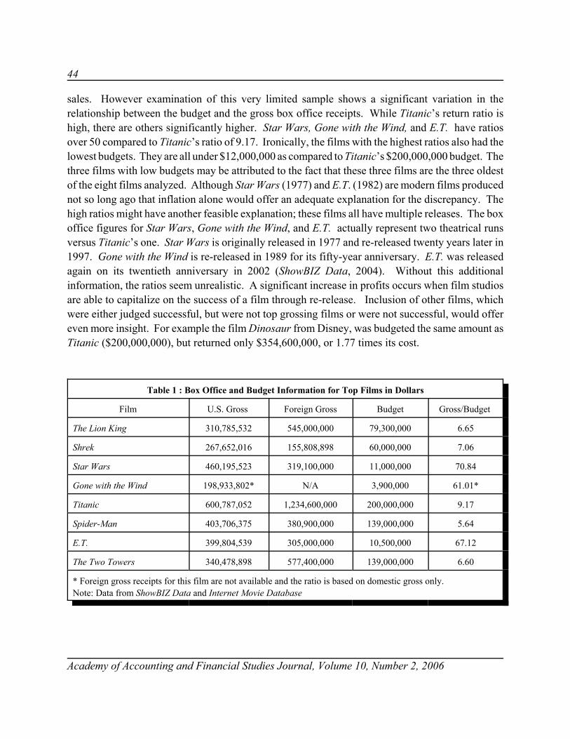
44
Academy of Accounting and Financial Studies Journal, Volume 10, Number 2, 2006
sales. However examination of this very limited sample shows a significant variation in therelationship between the budget and the gross box office receipts. While Titanic’s return ratio ishigh, there are others significantly higher. Star Wars, Gone with the Wind, and E.T. have ratiosover 50 compared to Titanic’s ratio of 9.17. Ironically, the films with the highest ratios also had thelowest budgets. They are all under $12,000,000 as compared to Titanic’s $200,000,000 budget. Thethree films with low budgets may be attributed to the fact that these three films are the three oldestof the eight films analyzed. Although Star Wars (1977) and E.T. (1982) are modern films producednot so long ago that inflation alone would offer an adequate explanation for the discrepancy. Thehigh ratios might have another feasible explanation; these films all have multiple releases. The boxoffice figures for Star Wars, Gone with the Wind, and E.T. actually represent two theatrical runsversus Titanic’s one. Star Wars is originally released in 1977 and re-released twenty years later in1997. Gone with the Wind is re-released in 1989 for its fifty-year anniversary. E.T. was releasedagain on its twentieth anniversary in 2002 (ShowBIZ Data, 2004). Without this additionalinformation, the ratios seem unrealistic. A significant increase in profits occurs when film studiosare able to capitalize on the success of a film through re-release. Inclusion of other films, whichwere either judged successful, but were not top grossing films or were not successful, would offereven more insight. For example the film Dinosaur from Disney, was budgeted the same amount asTitanic ($200,000,000), but returned only $354,600,000, or 1.77 times its cost.
Table 1 : Box Office and Budget Information for Top Films in Dollars
Film U.S. Gross Foreign Gross Budget Gross/Budget
The Lion King 310,785,532 545,000,000 79,300,000 6.65
Shrek 267,652,016 155,808,898 60,000,000 7.06
Star Wars 460,195,523 319,100,000 11,000,000 70.84
Gone with the Wind 198,933,802* N/A 3,900,000 61.01*
Titanic 600,787,052 1,234,600,000 200,000,000 9.17
Spider-Man 403,706,375 380,900,000 139,000,000 5.64
E.T. 399,804,539 305,000,000 10,500,000 67.12
The Two Towers 340,478,898 577,400,000 139,000,000 6.60
* Foreign gross receipts for this film are not available and the ratio is based on domestic gross only.Note: Data from ShowBIZ Data and Internet Movie Database
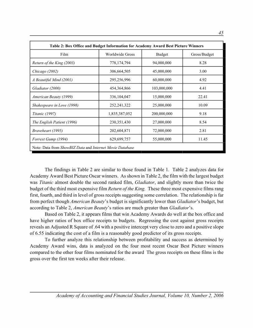
45
Academy of Accounting and Financial Studies Journal, Volume 10, Number 2, 2006
Table 2: Box Office and Budget Information for Academy Award Best Picture Winners
Film Worldwide Gross Budget Gross/Budget
Return of the King (2003) 778,174,794 94,000,000 8.28
Chicago (2002) 306,664,505 45,000,000 3.00
A Beautiful Mind (2001) 295,256,996 60,000,000 4.92
Gladiator (2000) 454,364,866 103,000,000 4.41
American Beauty (1999) 336,104,047 15,000,000 22.41
Shakespeare in Love (1998) 252,241,322 25,000,000 10.09
Titanic (1997) 1,835,387,052 200,000,000 9.18
The English Patient (1996) 230,351,430 27,000,000 8.54
Braveheart (1995) 202,604,871 72,000,000 2.81
Forrest Gump (1994) 629,699,757 55,000,000 11.45
Note: Data from ShowBIZ Data and Internet Movie Database
The findings in Table 2 are similar to those found in Table 1. Table 2 analyzes data forAcademy Award Best Picture Oscar winners. As shown in Table 2, the film with the largest budgetwas Titanic almost double the second ranked film, Gladiator, and slightly more than twice thebudget of the third most expensive film Return of the King. These three most expensive films rangfirst, fourth, and third in level of gross receipts suggesting some correlation. The relationship is farfrom perfect though American Beauty’s budget is significantly lower than Gladiator’s budget, butaccording to Table 2, American Beauty’s ratios are much greater than Gladiator’s.
Based on Table 2, it appears films that win Academy Awards do well at the box office andhave higher ratios of box office receipts to budgets. Regressing the cost against gross receiptsreveals an Adjusted R Square of .64 with a positive intercept very close to zero and a positive slopeof 6.55 indicating the cost of a film is a reasonably good predictor of its gross receipts.
To further analyze this relationship between profitability and success as determined byAcademy Award wins, data is analyzed on the four most recent Oscar Best Picture winnerscompared to the other four films nominated for the award The gross receipts on these films is thegross over the first ten weeks after their release.
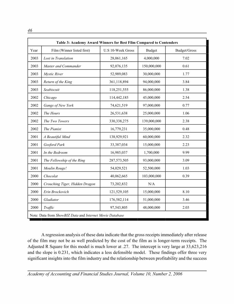
46
Academy of Accounting and Financial Studies Journal, Volume 10, Number 2, 2006
Table 3: Academy Award Winners for Best Film Compared to Contenders
Year Film (Winner listed first) U.S 10-Week Gross Budget Budget/Gross
2003 Lost in Translation 28,061,165 4,000,000 7.02
2003 Master and Commander 92,076,135 150,000,000 0.61
2003 Mystic River 52,989,083 30,000,000 1.77
2003 Return of the King 361,118,894 94,000,000 3.84
2003 Seabiscuit 118,251,555 86,000,000 1.38
2002 Chicago 114,442,185 45,000,000 2.54
2002 Gangs of New York 74,621,519 97,000,000 0.77
2002 The Hours 26,531,638 25,000,000 1.06
2002 The Two Towers 330,338,275 139,000,000 2.38
2002 The Pianist 16,779,231 35,000,000 0.48
2001 A Beautiful Mind 138,929,921 60,000,000 2.32
2001 Gosford Park 33,387,034 15,000,000 2.23
2001 In the Bedroom 16,985,037 1,700,000 9.99
2001 The Fellowship of the Ring 287,573,505 93,000,000 3.09
2001 Moulin Rouge! 54,029,521 52,500,000 1.03
2000 Chocolat 40,062,665 103,000,000 0.39
2000 Crouching Tiger, Hidden Dragon 73,202,832 N/A
2000 Erin Brockovich 121,529,105 15,000,000 8.10
2000 Gladiator 176,582,114 51,000,000 3.46
2000 Traffic 97,543,805 48,000,000 2.03
Note: Data from ShowBIZ Data and Internet Movie Database
A regression analysis of these data indicate that the gross receipts immediately after releaseof the film may not be as well predicted by the cost of the film as is longer-term receipts. TheAdjusted R Square for this model is much lower at .27. The intercept is very large at 33,623,216and the slope is 0.231, which indicates a less defensible model. These findings offer three verysignificant insights into the film industry and the relationship between profitability and the success
47
Academy of Accounting and Financial Studies Journal, Volume 10, Number 2, 2006
of films. First, a studio cannot guarantee box office success of a film by allocating a large budgetto it. Although a substantial budget may lead to large profits as in the case of the 1997 film Titanic,the returns are far from assured and may actually be proportionally better on a less expensive film.Second, one way to increase profits is to re-release films. Studios should consider modeling thestrategy used by Fox, MGM/UA, and Universal in their re-releases of Star Wars, Gone with theWind, and Spider-Man respectively. Last, some film studios may view success beyond profits, inqualitative ways such as winning the Best Picture Academy Award.
Overall, the film industry’s finances are unique, and success is hard to predict. However,regulators, auditors and those disputing payments on contracts do have some data to help assess thelikelihood that the profit or loss claims of the studio are reasonable. The industry distinctiveness,in fact, initiated some accounting changes by regulatory authorities. These accounting regulatorychanges and some specific legal conflicts showcased the creative accounting methods and practicessometimes used by film studios. Perhaps, now, after the issuance of Statement of AccountingStandards Number 139, the accounting and reporting will no longer be the most creative aspect ofHollywood.
REFERENCES:
Academy Awards Database. (2004). Retrieved February 24, 2004, http://www.oscars.org/awardsdatabase/.
AICPA issues new rules for film industry. (2000). Journal of Accountancy [online serial], 190,http://www.aicpa.org/pubs/jofa/aug2000/news3.htm.
Berton, L., & Harris, R. (1999). Reel-world accounting. CFO, 15, 34-40.
Box Office Report. (2004). Retrieved February 24, 2004, http://www.boxofficereport.com.
Buchwald v. Paramount Pictures Corporation, No C 706083, 1990 Cal. App. LEXIS 634, 13 U.S.P.Q.2D (BNA) 1497,January 31, 1990.
Cheatham, C., Cheatham, L. R., & Davis D. A. (1996). Hollywood profits: gone with the wind? CPA Journal, 66, 32-42.
Davis, C. E. (1997). Accounting is like a box of chocolates: a lesson in cost behavior. Journal of AccountingEducation, 15, 307-318.
Financial Accounting Standard Board. (2000). Statement of Financial Accounting Standards No. 139. Norfolk,Connecticut.
Goldberg, V. P. (1997). The net profits puzzle. Columbia Law Review.
48
Academy of Accounting and Financial Studies Journal, Volume 10, Number 2, 2006
Horngren, C. T., Datar, S. M. Foster, G. (1998). Cost Accounting A Managerial Emphasis, Pearson Prentice Hall, UpperSaddle River, NJ.
Internet Movie Database, Inc. (2004). Retrieved February 24, 2004 from http://www.imdb.com/.
Levine, M. H., Siegel, J. G. (2001). Accounting changes for the film industry. CPA Journal, 71, 32-38.
Pfeiffer, G., Capettini, R., Whittenburg, G. (1997). Forrest Gump – accountant: a study of accounting in the motionpicture industry. Journal of Accounting Education, 15, 319 - 344.
ShowBIZ Data. (2004). Retrieved February 24, 2004 http://www.showbizdata.com/.

49
Academy of Accounting and Financial Studies Journal, Volume 10, Number 2, 2006
PREDICTIVE ABILITY OF THE VALUATIONALLOWANCE FOR DEFERRED TAX ASSETS
Do-Jin Jung, West Texas A&M UniversityDarlene Pulliam, West Texas A&M University
ABSTRACT
The valuation allowance for deferred tax assets is an estimate of the portion of deferred taxassets that is not realizable because of insufficient future taxable income. The valuation allowanceaccount might contain forward-looking information on the management's estimates of a firm's futureincome. This study finds that a change in the valuation allowance provides incremental informationbeyond publicly available information in predicting one- and two-year-ahead income and cashflows. The predictive ability of the valuation allowance suggests that recognition of forward-lookinginformation in financial statements has the potential to make these statements more informative.
INTRODUCTION
The primary objective of financial accounting is to provide external users with informationabout the financial health and profitability of the firm in a format that facilitates theirdecision-making (FASB, 1978). There is a demand for forward-looking information on the firm'sfuture earnings and cash flows from users of financial reports, whose decisions depend primarily onestimates of the future. In December, 2002. the AICPA Board of Directors approved a newcommittee to explore how to enhance the delivery and content of business-related information. Thecommittee argues that the current model does serve as an effective foundation from which businessreporting should start; however, it focuses on the lagging indicators (i.e., information on pasttransactions) and lacks leading indicators (i.e., forward-looking information). Accountingstandard-setters are, however, wary of permitting firms to use estimates or projections in generatingtheir financial statement numbers because they may be unreliable. Inclusion of unverifiable numbersin the financial statements may provide opportunities to managers for managing earnings therebyreducing the value of financial statements to investors (Lang and Warfield, 1997).
Consequently, most forward-looking information used by firms in their internaldecision-making is not reported in the financial statements (AICPA, 2002). One exception to thisoccurs when firms are required by SFAS 109 to disclose the valuation allowance for deferred taxassets on their balance sheets from 1992 onwards. The valuation allowance is an estimate of theportion of deferred tax assets that is not realizable because of insufficient future taxable income. Ifa manager receives positive information about future income, (s)he should decrease the valuation

50
Academy of Accounting and Financial Studies Journal, Volume 10, Number 2, 2006
allowance for deferred tax assets because a greater portion of the future tax benefits is likely to berealized. If a manager receives negative information about future income, (s)he should increase thevaluation allowance because a smaller portion of the future tax benefits is likely to be realized dueto lower taxable income in future years. Hence, the valuation allowance account might containforward-looking information on managers' estimates of a firm's future income; a higher (lower) thevaluation allowance would represent the manager's expectation of lower (higher) future income fora given level of deferred tax assets.
On the other hand, SFAS 109 requires changes in the valuation allowance for deferred taxassets to be included (as part of income tax expense or benefit) in income from continuingoperations, which is used to measure the persistent component of earnings by many investors andfinancial analysts. Thus, the valuation allowance that is based on managers' unverifiable forecastsoffers opportunities for earnings management. As an example of the effect of changes in thevaluation allowance on earnings, consider the following from PR Newswire on November 10, 2003:"EZCORP, Inc. (Nasdaq: EZPW) announced today results for its fiscal fourth quarter and 2003fiscal year, which ended September 30, 2003. For the quarter ended September 30, 2003, EZCORPis reporting net income of $4,563,000 ($0.36 per share) compared to net income of $251,000 ($0.02per share) for the prior year comparable period. During the quarter, the company decreased itsvaluation allowance placed on its deferred tax assets by $3,700,000 based on the Company'simproved operating results and outlook for continued earnings growth. This had a favorable netincome effect of $3,700,000 ($0.30 per share)."
Therefore, the valuation allowance for deferred tax assets has two potential characteristics:forward-looking information content and earnings management vehicle. Given this, there is a criticalquestion that must be considered (Rhoades-Catanach, 2003); do we believe that, in practice, thevaluation allowance for deferred tax assets is based on income prediction, its expected value, orsome other amount (i.e., a judgmental value)? If the valuation allowance depends on the manager'sexpectation of future taxable income, it may contain not only public information (e.g., prior income)available to predict future income, but also the manager's private information that will convey newinformation on future income to financial statement users. Investigation of information content ofthe valuation allowance in predicting future income (or cash flows) may provide evidence on thisissue. Prior studies (Amir et al., 1997; Ayers, 1998; Amir and Sougiannis, 1999) document anassociation between the valuation allowance for deferred tax assets and stock prices, but none ofthose studies have examined the association between the valuation allowance and future income (orcash flows). This study investigates the association of the valuation allowance with future income(or cash flows), and thus provides insight into the mechanism by which the valuation allowance isassociated with stock prices.
For this investigation, this study collects 719 news releases of the valuation allowances forthe period 1994-2002 from LEXIS/NEXIS. The empirical results provide evidence of incrementalinformation content of the valuation allowance in predicting future income and cash flows; a change

51
Academy of Accounting and Financial Studies Journal, Volume 10, Number 2, 2006
in the valuation allowance for deferred tax assets contains incremental information (e.g., themanager's private information) beyond publicly available information in predicting one- andtwo-year-ahead income and cash flows. The remainder of this study is organized as follows: SectionII develops hypotheses on information content of the valuation allowance in predicting futureincome (or cash flows). Section III explains research designs used to test these hypotheses. SectionIV provides details on data collection and presents the empirical results. Section V containsconcluding remarks.
HYPOTHESIS DEVELOPMENT
In February 1992, the FASB issued SFAS 109, Accounting for Income Taxes, supersedingSFAS 96 and Accounting Principles Board (APB) Opinion 11. SFAS 96 and APB 11 required firmsto recognize deferred tax liabilities for all taxable temporary differences; on the other hand, theyallowed the recognition of deferred tax assets on deductible temporary differences and operating lossand tax credit carryforwards only to the extent that: (1) taxable income in prior years could be usedto realize deferred tax assets, and (2) taxable income could be projected from the reversals ofexisting temporary differences. Opponents argued that such stringent recognition criteria could leadto misleading and overly conservative amounts recognized as deferred tax assets (Eaton andWilliams, 1998). In response to this criticism, SFAS 109 permits the recognition of deferred taxassets for all deductible temporary differences and operating loss and tax credit carryforwards.However, if future taxable income is not expected to be high enough to utilize the deferred taxassets, a valuation allowance must be estimated and recognized to reduce the net deferred tax assetsto the amount that is "more likely than not" to be realized (More-likely-than-not is intended to meana likelihood of more than 50 percent).
Once a valuation allowance is established, it can be changed in subsequent periods if thereare changes in circumstances that alter expectations about future taxable income expected to beavailable to realize a tax benefit. A manager should consider all evidence, both positive andnegative, to determine whether the valuation allowance should be increased or decreased based onthe weight of that evidence. Positive evidence (e.g., existing contracts or sales backlog, an excessof appreciated asset value over the tax basis of the firm's net assets, and a strong earnings history)reinforces the likelihood that deferred tax assets will be realized, and reduces the need for avaluation allowance. Conversely, negative evidence (cumulative losses in recent years, a history ofoperating loss or tax credit carryforwards expiring unused, losses expected in early future years,unsettled circumstances that, if unfavorably resolved, would adversely affect future operations andprofit levels, and a carryback and/or carryforward period that is so brief that it would limitrealization of tax benefits) reduces the likelihood that deferred tax assets will be realized, andincreases the need for a valuation allowance.
52
Academy of Accounting and Financial Studies Journal, Volume 10, Number 2, 2006
As a result, a change in the valuation allowance for deferred tax assets should result froma change in the manager's judgment about the existence of sufficient taxable income to utilize therelated deferred tax assets in future years. If a manager changes the valuation allowance in responseto information on future income without bias (i.e., a manager increases or decreases the valuationallowance only in response to negative or positive information on future income), the change in thevaluation allowance would likely contain information useful in predicting future income (or cashflows). In summary, since SFAS 109 requires managers to change the valuation allowance fordeferred tax assets when they revise their estimates of future income, changes in the valuationallowance should be associated with future income (or cash flows) if managers follow SFAS 109without bias.
H1: Changes in the valuation allowance for deferred tax assets are negatively associated withfuture income (or cash flows).
Since the FASB issued SFAS 109 in 1992, numerous papers (e.g., Bielstein and Trott, 1992;Read, 1992; Eaton and Williams, 1998) have discussed how to account for the valuation allowancefor deferred tax assets, because the statement provides little direct guidance on how to compute thevaluation allowance (Bielstein and Trott, 1992; Peavey and Nurnberg, 1993; Behn et al., 1998;Eaton and Williams, 1998; Miller and Skinner, 1998). SFAS 109 identifies four possible sources oftaxable income available to realize deferred tax assets: (1) future reversals of existing taxabletemporary differences, (2) future taxable income, (3) taxable income in prior carryback years ifcarryback is permitted, and (4) tax-planning strategies. In order to gain some insight into how firmsare applying the requirements of SFAS 109, this study reviews prior studies that investigate theassociation between the valuation allowance for deferred tax assets and taxable income sourcesavailable to realize deferred tax assets. Table 1 summarizes the research designs and findings ofthese prior studies.
First, the column of "Taxable Temporary Differences" shows the valuation allowance fordeferred tax assets is associated with the future reversals of existing taxable temporary differences.When the deferred tax liabilities exceed the deferred tax assets, there should be an excess of futuretaxable over deductible amounts, thus increasing the likelihood of realization of the deferred taxassets (Guenther and Sansing, 2003). Therefore, the valuation allowance for deferred tax assets ismore likely for firms with net deferred tax assets than for firms with net deferred tax liabilities. Asexpected, a firm with more deferred tax liabilities than deferred tax assets records a smallervaluation allowance (Behn et al., 1998; Miller and Skinner, 1998; Burgstahler et al., 2002; Frankand Rego, 2003). Also, the column indicates that changes in the valuation allowance are positively(negatively) associated with changes in deferred tax assets (liabilities) (Visvanathan, 1998).
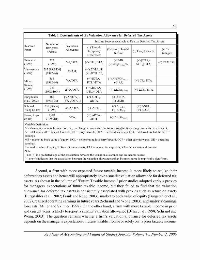
53
Academy of Accounting and Financial Studies Journal, Volume 10, Number 2, 2006
Table 1. Determinants of the Valuation Allowance for Deferred Tax Assets
ResearchPaper
Number offirm-years(Period)
ValuationAllowance
Income Sources Available to Realize Deferred Tax Assets
(1) TaxableTemporaryDifferences
(2) Future TaxableIncome (3) Carryforwards (4) Tax
Strategies
Behn et al.(1998)
322 (1993) VAt/DTAt (-s) DTLt/DTAt
(-s) MBt (-s) AvgE(t-2, t) /At
(-s) [DTAt -NOLt]/DTAt
(-s) TAXt /OEt
Visvanathan(1998)
287 [S&P500](1992-94) )VAt/Pt
(+s) )DTAt / Pt
(-s) )DTLt / Pt
Miller,Skinner (1998)
354 (1992-94) VAt/DTAt
(+s) [DTAt -DTLt]/DTAt
(-s) AvgROA(t-3,t-1)
(-) AFt(+s) CFt / DTAt
333(1992-1994) )VAt/DTAt
(+s) )(DTAt -DTLt) / DTAt
(-s) )ROA(t-3,t-1) (+s) )CFt / DTAt
Burgstahler et al. (2002)
482 (1993-98)
[VAt/DTAt] -[VAt-1/DTAt-1]
(-s) )DTLt /)DTAt
(-) )ROAt
(-) )MBt
Schrand,Wong (2003)
235 [Banks] (1993) )VAt/DTAt (-) )DTLt
(-s) )E(t-2, t)
(-) )OEt+1
(+s) )NOLt
(+s) )OCFt
Frank, Rego(2003)
1,882 (1993-01) )VAt
(+s) )DTAt-)DTLt
(-) )ROA(t-2,t)
Variable Definition: )t = change in amounts from t-1 to t, )(t-i, t) = change in amounts from t-i to t, Avg(t-i, t) = average amounts over t-i and t,A = total assets, AF = analyst forecasts, CF = carryforwards, DTA = deferred tax assets, DTL = deferred tax liabilities, E =earnings, MB = market to book value of equity, NOL = net operating loss carryforward, OCF = other carryforwards, OE = operatingearnings, P = market value of equity, ROA = return on assets, TAX = income tax expenses, VA = the valuation allowanceNote:(-) or (+) is a predicted sign of the association between the valuation allowance and an income source.(-s) or (+s) indicates that the association between the valuation allowance and an income source is empirically significant.
Second, a firm with more expected future taxable income is more likely to realize theirdeferred tax assets and hence will appropriately have a smaller valuation allowance for deferred taxassets. As shown in the column of "Future Taxable Income," prior studies adopted various proxiesfor managers' expectations of future taxable income, but they failed to find that the valuationallowance for deferred tax assets is consistently associated with proxies such as return on assets(Burgstahler et al., 2002; Frank and Rego, 2003), market to book value of equity (Burgstahler et al.,2002), realized operating earnings in future years (Schrand and Wong, 2003), and analysts' earningsforecasts (Miller and Skinner, 1998). On the other hand, a firm with more taxable income in priorand current years is likely to report a smaller valuation allowance (Behn et al., 1998; Schrand andWong, 2003). The question remains whether a firm's valuation allowance for deferred tax assetsdepends on the manager's expectation of future taxable income or solely on its prior taxable income.
54
Academy of Accounting and Financial Studies Journal, Volume 10, Number 2, 2006
If the valuation allowance for deferred tax assets depends on the manager's expectation of futuretaxable income, it may contain the manager's private information, which will be useful for financialstatement users. If the valuation allowance depends on prior income, which is already disclosed, itdoes not convey any new information to financial statement users about future income.
Third, Cross-sectional variation in the valuation allowance for deferred tax assets can occurbecause of differences in the sources of deferred tax assets. For instance, the deferred tax assetscreated by net operating loss carryforwards are less certain to be realized than such assets createdby some deductible temporary differences because the net operating carryforward is normallycreated due to insufficient income. The column of "Carryforwards" presents that a firm with moredeferred tax assets attributable to tax loss or tax credit carryforwards has a larger valuationallowance because of the limitation on the extent to which the tax benefits associated withcarryforward items can be realized (Behn et al., 1998; Miller and Skinner, 1998; Schrand and Wong,2003).
Finally, SFAS 109 considers tax-planning strategies as a source of income available torealize deferred tax assets. Tax planning strategies are as prudent and feasible actions that managersmight not take ordinarily but would take to prevent an operating loss or tax credit carryforward fromexpiring unused. Since this type of information is usually proprietary and not disclosed by firms,most prior studies do not investigate the association between tax-planning strategies and thevaluation allowance for deferred tax assets because Only Behn et al. (1998) use the firm's reportedfederal income tax expense divided by operating income as a proxy for tax-planning strategies. Theyassume that as a firm's effective tax rate increases, its ability to take advantage of potential taxsavings increases (resulting in an increase in income after income tax expense). Consistent with theirexpectation, a firm with higher income tax expense (as a proportion of operating income) is likelyto have a smaller valuation allowance.
Prior findings summarized in Table 1 imply that changes in the valuation allowance fordeferred tax assets in part reflect publicly available information such as deferred tax assets (orliabilities) and prior earnings. If managers use private forward-looking information about futureincome, as well as public information provided in other accounts in determining the valuationallowance, then, in addition to publicly available information, changes in the valuation allowancewill contain information that is useful in predicting future income (or cash flows). This studyinvestigates whether changes in the valuation allowance for deferred tax assets contain usefulinformation (e.g., managers' private forward-looking information) beyond public informationsummarized in other accounts in predicting future income (or cash flows).
H2: Changes in the valuation allowance for deferred tax assets are negatively associated withfuture income (or cash flows) after controlling for other publicly available information.
55
Academy of Accounting and Financial Studies Journal, Volume 10, Number 2, 2006
RESEARCH DESIGN
Since SFAS 109 requires that the effects of changes in the valuation allowance for deferredtax assets ordinarily shall be included in income from continuing operations, income fromcontinuing operations (E t ) is separated into "income from continuing operations before changes inthe valuation allowance for deferred tax assets" (EBVA t ) and "changes in the valuation allowancefor deferred tax assets" ( )VA t ):
(1)ttt VAEBVAE ∆−≡
In equation (1), EBVA t is a measure of the firm's operating performance in year t and )VAt is partially a function of the manager's judgment about future income if the manager changes thevaluation allowance for deferred tax assets without bias.
To illustrate how a change in the valuation allowance for deferred tax assets is a function ofa manager's judgment about future income, consider the sections of SFAS 109. SFAS 109 states thatfirms should reduce deferred tax assets by a valuation allowance if, based on the weight of availableevidence, it is more likely than not that some portion or all of the deferred tax assets will not berealized (17). In determining the valuation allowance, SFAS 109 states that future realization of thedeferred tax assets ultimately depends on the existence of sufficient taxable income in future years(21). In situations where future realization of the deferred tax assets is unclear, application ofjudgment based on a careful assessment of all available evidence is required (98). Therefore, achange in the valuation allowance for deferred tax assets is a function of the manager's judgmentabout future income under SFAS 109, and thus may have information content useful in predictingfuture income (or future cash flows). This study estimates the following regression model toexamine the predictive ability of changes in the valuation allowance for deferred tax assets:
(2)tttit EBVAVAE εααα ++∆+=+ 210
where, Et+i = income from continuing operations in year t+i)VAt = changes in the valuation allowance from year t-1 to tEBVAt = income from continuing operations before changes in the valuation allowance inyear t * Each variable is scaled by the beginning market value of equity at year t.
If managers change the valuation allowance for deferred tax assets in response to informationon future income that is not reflected in EBVAt, "1 will be negative. In the absence of any changesin the valuation allowance (i.e., )VAt = 0), Et is positively associated with Et+i (Ball and Watts 1972;
56
Academy of Accounting and Financial Studies Journal, Volume 10, Number 2, 2006
Albrecht et al. 1977; Watts and Leftwich 1977; Lev 1983; Finger 1994; Dechow et al. 1998; Dechowand Dichev 2002). Therefore, "2 is expected to be positive.
The ability of current earnings (Et) to predict future cash flows (CFt+i) is well-known (e.g.,Watts and Zimmerman 1986; Dechow 1994; Wang 1998; Beaver 1998; Dechow and Dichev 2002).Model (3) examines this predictive ability after controlling for current cash flow:
(3)),(1 ttt CFEfCF =+
Given equation (1), equation (3) can be rewritten as:
(4)),,(1 tttt CFVAEBVAfCF ∆=+
In order to examine the predictive ability of )VAt for future cash flows after controlling forcurrent earnings and cash flow performance, the following regression model is estimated:
(5)ttttit CFEBVAVACF εββββ +++∆+=+ 3210
where, CFt+i = cash flows from operations in year t+i )VAt = changes in the valuation allowance from year t-1 to t EBVAt = income from continuing operations before changes in the valuation allowance inyear t * Each variable is scaled by the beginning market value of equity at year t.
Consistent with prior research, I expect $2 and $3 to be positive. As discussed previously, $1
should be negative if changes in the valuation allowance for deferred tax assets contain informationon future cash flows that is not reflected in EBVAt and CFt.
In order to test whether changes in the valuation allowance for deferred tax assets containincremental information about future income beyond publicly available information (hypothesis H2),this study controls for the components of changes in the valuation allowance that is predictable fromother financial statement variables. Consistent with prior studies (e.g., Burgstahler et al. 2002; Frankand Rego 2003), this study assumes that in the absence of earnings management, two factorsdetermine a change in the valuation allowance for deferred tax assets: sources that create a changein future reversals of taxable temporary differences ()FUT_REVERSALit) and a change in themanager’s expectation about future income ()FUT_INCOMEjt).
57
Academy of Accounting and Financial Studies Journal, Volume 10, Number 2, 2006
(6)∑∑ +∆+∆+≡∆j
tjtjiti
it INCOMEFUTREVERSALFUTVA εµλδ __0
The source that creates a change in future reversals of taxable temporary differences is achange in net deferred tax liabilities because deferred tax liabilities, upon reversal, constitute taxableincome that can be used to realize deferred tax assets. If a firm has an increase (decrease) in deferredtax liabilities relative to deferred tax assets, the valuation allowance should decrease (increase). Asshown in Table 1, Visvanathan (1998), Miller and Skinner (1998), Burgstahler et al. (2002) andFrank and Rego (2003) have previously documented that changes in deferred tax liabilities (assets)are negatively (positively) associated with changes in the valuation allowance. Therefore, this studyconsiders changes in deferred tax assets and liabilities as publicly available information on futureincome in determining changes in the valuation allowance for deferred tax assets.
Since SFAS 109 suggests that a strong earnings history and a history of operating losses are,respectively, positive and negative evidence of sufficient future income to realize deferred tax assets,managers should consider earnings and losses in prior years in determining the valuation allowance.Behn et al. (1998) and Schrand and Wong (2003) provide evidence of the negative associationbetween the valuation allowance for deferred tax assets and earnings in prior years. This study usesearnings over the prior two years as a proxy for the manager’s expectation of future income topredict a change in the valuation allowance for deferred tax assets. This study also adopts a changein the market value of equity as another proxy for a manager’s expectation of future income becausestock prices largely capture information before it is reflected in earnings (Beaver et al. 1980; Beaveret al. 1987; Collins et al. 1987; Freeman 1986).
Therefore, we can predict a change in the valuation allowance for deferred tax assets ()VAt)by considering such public information as changes in deferred tax assets ()DTAt) and liabilities()DTLt), earnings in each of the prior two years (Et-1, Et-2) and changes in the market value of equity()MVEt). The equation (6) is converted to a regression model as follows:
(7)ttttttt MVEEEDTLDTAVA εµµµλλδ +∆+++∆+∆+=∆ −− 32211210
Assuming that a change in the valuation allowance for deferred tax assets containsincremental non-public information (e.g., the manager’s private information) in predicting futureincome, it should be associated with future income after controlling for the public information.1 Inmodel (8), a negative "1 supports the hypothesis that changes in the valuation allowance containuseful information beyond publicly available information in predicting future income.
(8)ttttttttt MVEEEDTLDTAEBVAVAE εαααααααα +∆+++∆+∆++∆+= −−+ 72615432101
58
Academy of Accounting and Financial Studies Journal, Volume 10, Number 2, 2006
where, Et+i = income from continuing operations in year t+i)VAt = changes in the valuation allowance from year t-1 to t EBVAt = income from continuing operations before changes in the valuation allowance inyear t )DTAt = changes in deferred tax assets from year t-1 to t)DTLt = changes in deferred tax liabilities from year t-1 to t )MVEt = changes in market value of equity from year t-1 to t* Each variable is scaled by the beginning market value of equity.
This study also tests the following regression model to examine the information content of)VAt on future cash flows after controlling for current earnings, cash flow performance, andpublicly available information:
(9)tttttttttit MVEEEDTLDTACFEBVAVACF εβββββββββ +∆+++∆+∆+++∆+= −−+ 82716543210
where, CFt+i = cash flows from operations in year t+i )VAt = changes in the valuation allowance from year t-1 to t EBVAt = income from continuing operations before changes in the valuation allowance inyear t )DTAt = changes in deferred tax assets from year t-1 to t)DTLt = changes in deferred tax liabilities from year t-1 to t Et-i = income from continuing operations in year t-i )MVEt = changes in market value of equity from year t-1 to t* Each variable is scaled by the beginning market value of equity at year t.
EMPIRICAL ANALYSIS
The sample for this study is drawn from a search for news releases in the PR Newswire filein LEXIS/NEXIS using the keywords “valuation allowance.”2 PR Newswire delivers full-text,unedited news releases, including announcements of quarterly and annual earnings, dividends, andearnings forecasts. The wire is updated every 30 minutes by teleprinter directly to the newsroomsof wire services, broadcasters, newspapers and magazines. Therefore, PR Newswire plays a key rolein dissemination of time-critical financial information.
Table 2 summarizes the data collection procedure. First, 719 news reports about annualvaluation allowance from 1994 to 2002 were found. SFAS 109 became effective for fiscal yearsbeginning after December 15, 1992; hence, to ensure consistent financial reporting this study
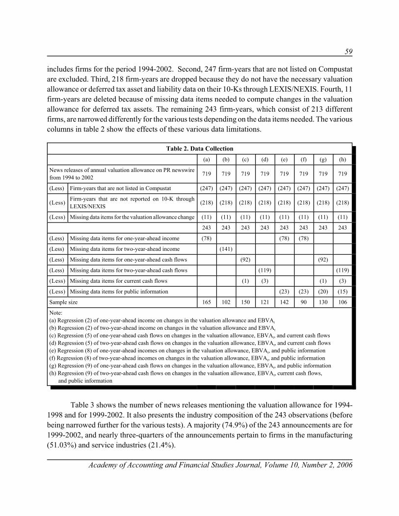
59
Academy of Accounting and Financial Studies Journal, Volume 10, Number 2, 2006
includes firms for the period 1994-2002. Second, 247 firm-years that are not listed on Compustatare excluded. Third, 218 firm-years are dropped because they do not have the necessary valuationallowance or deferred tax asset and liability data on their 10-Ks through LEXIS/NEXIS. Fourth, 11firm-years are deleted because of missing data items needed to compute changes in the valuationallowance for deferred tax assets. The remaining 243 firm-years, which consist of 213 differentfirms, are narrowed differently for the various tests depending on the data items needed. The variouscolumns in table 2 show the effects of these various data limitations.
Table 2. Data Collection(a) (b) (c) (d) (e) (f) (g) (h)
News releases of annual valuation allowance on PR newswirefrom 1994 to 2002 719 719 719 719 719 719 719 719
(Less) Firm-years that are not listed in Compustat (247) (247) (247) (247) (247) (247) (247) (247)
(Less) Firm-years that are not reported on 10-K throughLEXIS/NEXIS (218) (218) (218) (218) (218) (218) (218) (218)
(Less) Missing data items for the valuation allowance change (11) (11) (11) (11) (11) (11) (11) (11)
243 243 243 243 243 243 243 243
(Less) Missing data items for one-year-ahead income (78) (78) (78)
(Less) Missing data items for two-year-ahead income (141)
(Less) Missing data items for one-year-ahead cash flows (92) (92)
(Less) Missing data items for two-year-ahead cash flows (119) (119)
(Less) Missing data items for current cash flows (1) (3) (1) (3)
(Less) Missing data items for public information (23) (23) (20) (15)
Sample size 165 102 150 121 142 90 130 106
Note:(a) Regression (2) of one-year-ahead income on changes in the valuation allowance and EBVAt
(b) Regression (2) of two-year-ahead income on changes in the valuation allowance and EBVAt
(c) Regression (5) of one-year-ahead cash flows on changes in the valuation allowance, EBVAt, and current cash flows (d) Regression (5) of two-year-ahead cash flows on changes in the valuation allowance, EBVAt, and current cash flows(e) Regression (8) of one-year-ahead incomes on changes in the valuation allowance, EBVAt, and public information(f) Regression (8) of two-year-ahead incomes on changes in the valuation allowance, EBVAt, and public information(g) Regression (9) of one-year-ahead cash flows on changes in the valuation allowance, EBVAt, and public information(h) Regression (9) of two-year-ahead cash flows on changes in the valuation allowance, EBVAt, current cash flows, and public information
Table 3 shows the number of news releases mentioning the valuation allowance for 1994-1998 and for 1999-2002. It also presents the industry composition of the 243 observations (beforebeing narrowed further for the various tests). A majority (74.9%) of the 243 announcements are for1999-2002, and nearly three-quarters of the announcements pertain to firms in the manufacturing(51.03%) and service industries (21.4%).

60
Academy of Accounting and Financial Studies Journal, Volume 10, Number 2, 2006
Table 3. Sample Composition
Firm-Years Percentage
1994-1998 61 25.10%
1999-2002 182 74.90%
Total 243 100.0%
Mining and Construction (SIC Code 10-17) 16 6.58%
Manufacturing (SIC 20-39) 124 51.03%
Transportation and Public Utilities (SIC 40-49) 11 4.53%
Wholesale Trade and Retail Trade (SIC 50-59) 16 6.58%
Finance, Insurance, Real Estate (SIC 60-67) 24 9.88%
Services (SIC 70-87) 52 21.40%
Total 243 100.00%
Table 4 reports descriptive statistics of 254 firm-years’ variables that are listed in Compustatand reported on 10-K through LEXIS/NEXIS. The mean (median) earnings (Et) and EBVAt are -$7.2M ($1.1M) and -$7.9M ($2.4M), respectively. The mean market value of equity of $698.4M isabout 40% of the $1,735M mean market value of equity for the Compustat population over 1994-2001.3 These statistics imply that the average sample firms in this study are smaller than theCompustat firms and incurred losses over the sample period. The sample firms, on average, havethe valuation allowance of $40.4M for deferred tax assets of $94.8M and deferred tax liabilities of$56.5M.4 Their mean (median) change in the valuation allowance is $-1.0M ($0) and -7.53% (0%)of the beginning market value of equity.
Table 5 presents the correlations between the valuation allowance for deferred tax assets withother variables. The correlations are consistent with expectations. The valuation allowance isnegatively correlated with future income and cash flows. It is also correlated with such publicinformation, which may provide prediction of changes in the valuation allowance, as changes indeferred tax assets and liabilities, earnings in each of the prior two years and changes in the marketvalue of equity.
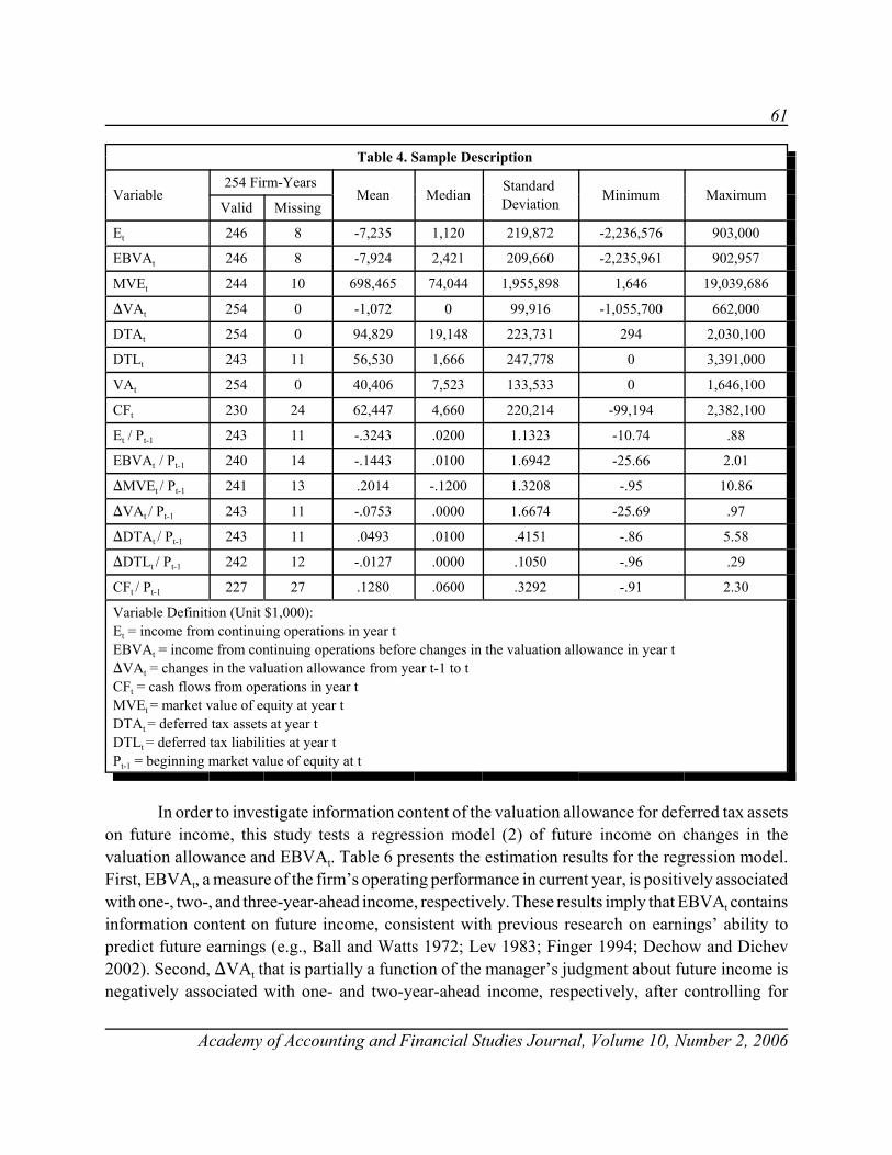
61
Academy of Accounting and Financial Studies Journal, Volume 10, Number 2, 2006
Table 4. Sample Description
Variable254 Firm-Years
Mean Median Standard Deviation Minimum Maximum
Valid Missing
Et 246 8 -7,235 1,120 219,872 -2,236,576 903,000
EBVAt 246 8 -7,924 2,421 209,660 -2,235,961 902,957
MVEt 244 10 698,465 74,044 1,955,898 1,646 19,039,686
)VAt 254 0 -1,072 0 99,916 -1,055,700 662,000
DTAt 254 0 94,829 19,148 223,731 294 2,030,100
DTLt 243 11 56,530 1,666 247,778 0 3,391,000
VAt 254 0 40,406 7,523 133,533 0 1,646,100
CFt 230 24 62,447 4,660 220,214 -99,194 2,382,100
Et / Pt-1 243 11 -.3243 .0200 1.1323 -10.74 .88
EBVAt / Pt-1 240 14 -.1443 .0100 1.6942 -25.66 2.01
)MVEt / Pt-1 241 13 .2014 -.1200 1.3208 -.95 10.86
)VAt / Pt-1 243 11 -.0753 .0000 1.6674 -25.69 .97
)DTAt / Pt-1 243 11 .0493 .0100 .4151 -.86 5.58
)DTLt / Pt-1 242 12 -.0127 .0000 .1050 -.96 .29
CFt / Pt-1 227 27 .1280 .0600 .3292 -.91 2.30
Variable Definition (Unit $1,000):Et = income from continuing operations in year t EBVAt = income from continuing operations before changes in the valuation allowance in year t )VAt = changes in the valuation allowance from year t-1 to t CFt = cash flows from operations in year t MVEt = market value of equity at year t DTAt = deferred tax assets at year t DTLt = deferred tax liabilities at year tPt-1 = beginning market value of equity at t
In order to investigate information content of the valuation allowance for deferred tax assetson future income, this study tests a regression model (2) of future income on changes in thevaluation allowance and EBVAt. Table 6 presents the estimation results for the regression model.First, EBVAt, a measure of the firm’s operating performance in current year, is positively associatedwith one-, two-, and three-year-ahead income, respectively. These results imply that EBVAt containsinformation content on future income, consistent with previous research on earnings’ ability topredict future earnings (e.g., Ball and Watts 1972; Lev 1983; Finger 1994; Dechow and Dichev2002). Second, )VAt that is partially a function of the manager’s judgment about future income isnegatively associated with one- and two-year-ahead income, respectively, after controlling for
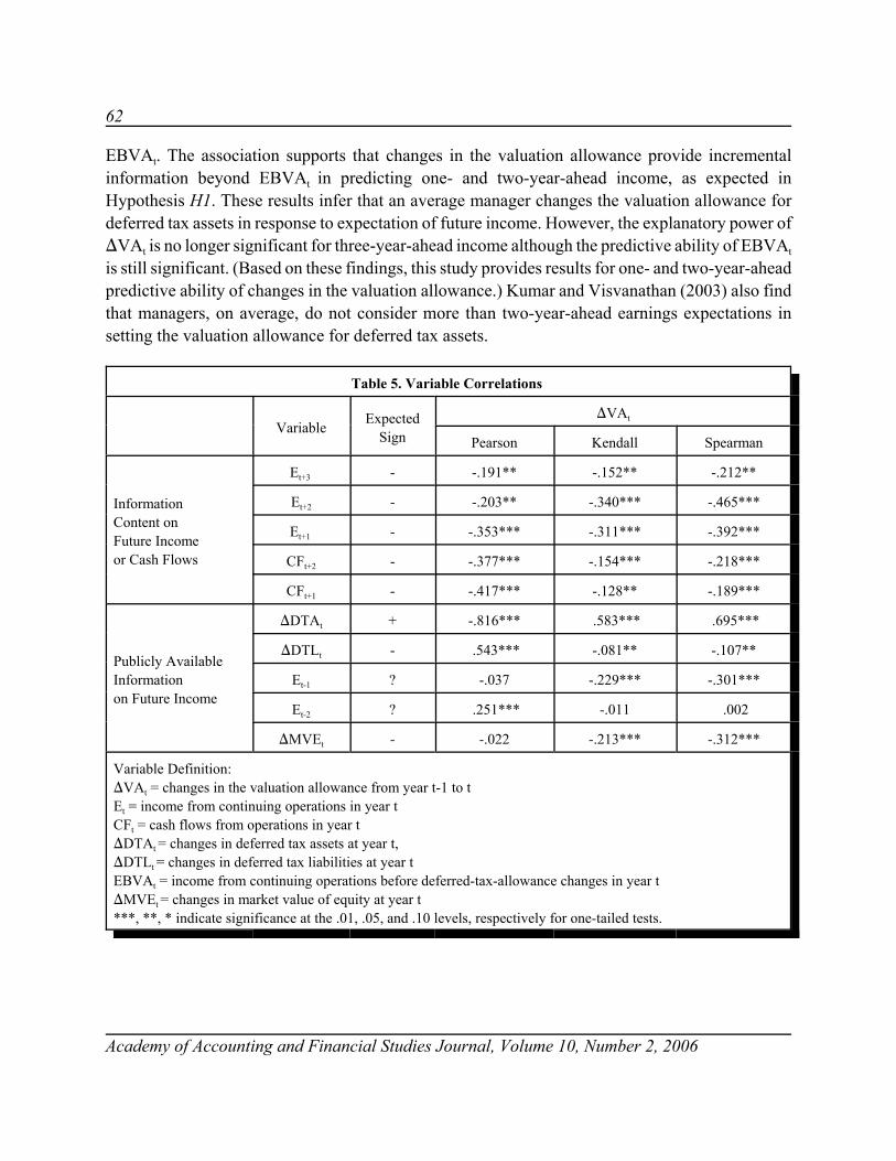
62
Academy of Accounting and Financial Studies Journal, Volume 10, Number 2, 2006
EBVAt. The association supports that changes in the valuation allowance provide incrementalinformation beyond EBVAt in predicting one- and two-year-ahead income, as expected inHypothesis H1. These results infer that an average manager changes the valuation allowance fordeferred tax assets in response to expectation of future income. However, the explanatory power of)VAt is no longer significant for three-year-ahead income although the predictive ability of EBVAt
is still significant. (Based on these findings, this study provides results for one- and two-year-aheadpredictive ability of changes in the valuation allowance.) Kumar and Visvanathan (2003) also findthat managers, on average, do not consider more than two-year-ahead earnings expectations insetting the valuation allowance for deferred tax assets.
Table 5. Variable Correlations
Variable ExpectedSign
)VAt
Pearson Kendall Spearman
InformationContent onFuture Incomeor Cash Flows
Et+3 - -.191** -.152** -.212**
Et+2 - -.203** -.340*** -.465***
Et+1 - -.353*** -.311*** -.392***
CFt+2 - -.377*** -.154*** -.218***
CFt+1 - -.417*** -.128** -.189***
Publicly AvailableInformation on Future Income
)DTAt + -.816*** .583*** .695***
)DTLt - .543*** -.081** -.107**
Et-1 ? -.037 -.229*** -.301***
Et-2 ? .251*** -.011 .002
)MVEt - -.022 -.213*** -.312***
Variable Definition:)VAt = changes in the valuation allowance from year t-1 to t Et = income from continuing operations in year t CFt = cash flows from operations in year t)DTAt = changes in deferred tax assets at year t, )DTLt = changes in deferred tax liabilities at year tEBVAt = income from continuing operations before deferred-tax-allowance changes in year t )MVEt = changes in market value of equity at year t ***, **, * indicate significance at the .01, .05, and .10 levels, respectively for one-tailed tests.
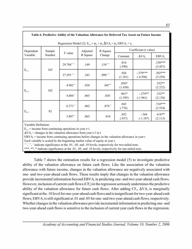
63
Academy of Accounting and Financial Studies Journal, Volume 10, Number 2, 2006
Table 6. Predictive Ability of the Valuation Allowance for Deferred Tax Assets on Future Income
Regression Model (2): Et+i = "0 + "1 )VAt + "2 EBVAt + ,t
Dependent Variable
SampleNumber F value Adjusted
R SquareR SquareChange
Coefficient (t value)
Constant )VAt EBVAt
Et+1 165
29.784+++ .149 .154+++ .014(.599)
.330***(5.457)
27.291+++ .243 .098+++ .026(1.181)
-.379***(-4.596)
.302***(5.259)
Et+2 102
4.982++ .038 .047++ .056* (1.430)
.352**(2.232)
4.484++ .065 .036+ .061* (1.595)
-.274**(-1.961)
.332**(2.130)
Et+3 82
6.371++ .062 .074++ .043(.776)
.710***(2.524)
3.807++ .065 .014 .052(.937)
-.368 (-1.107)
.618**(2.113)
Variable Definition:Et+i = income from continuing operations in year t+i )VAt = changes in the valuation allowance from year t-1 to t EBVAt = income from continuing operations before changes in the valuation allowance in year t Each variable is scaled by the beginning market value of equity at year t.+++, ++, + indicate significance at the .01, .05, and .10 levels, respectively for two-tailed tests.***, **, * indicate significance at the .01, .05, and .10 levels, respectively for one-tailed tests.
Table 7 shows the estimation results for a regression model (5) to investigate predictiveability of the valuation allowance on future cash flows. Like the association of the valuationallowance with future income, changes in the valuation allowance are negatively associated withone- and two-year-ahead cash flows. These results imply that changes in the valuation allowanceprovide incremental information beyond EBVAt in predicting one- and two-year-ahead cash flows.However, inclusion of current cash flows (CFt) in the regression seriously undermines the predictiveability of the valuation allowance for future cash flows. After adding CFt, )VAt is marginallysignificant at the .10 level for one-year-ahead cash flows and is insignificant for two-year-ahead cashflows; EBVAt is still significant at .01 and .05 for one- and two-year-ahead cash flows, respectively.Whether changes in the valuation allowance provide incremental information in predicting one- andtwo-year-ahead cash flows is sensitive to the inclusion of current year cash flows in the regression.

64
Academy of Accounting and Financial Studies Journal, Volume 10, Number 2, 2006
Table 7. Predictive Ability of the Valuation Allowance for Deferred Tax Assets on Future Cash Flows
Regression Model (5): CFt+i = $0 + $1 )VAt + $2 EBVAt + $3 CFt + ,t
Dependent Variable
SampleNumber F value Adjusted
R2
Coefficient (t value)
Constant )VAt EBVAt CFt
CFt+1
150 37.240+++ .327 .204***(4.577)
-.872***(-5.054)
.730***(5.929)
150 79.477+++ .612 .027 (.728)
-.230*(-1.594)
.493***(5.128)
1.129***(10.448)
CFt+2
121 15.487+++ .194 .216***(6.179)
-.595***(-4.273)
.421***(2.577)
121 54.456+++ .572 .090***(3.188)
-.086(-.761)
.254**(2.111)
.835***(10.251)
Variable Definition:CFt+i = cash flows from operations in year t+i )VAt = changes in the valuation allowance from year t-1 to t EBVAt = income from continuing operations before changes in the valuation allowance in year t Each variable is scaled by the beginning market value of equity at year t.+++, ++, + indicate significance at the .01, .05, and .10 levels, respectively for two-tailed tests.***, **, * indicate significance at the .01, .05, and .10 levels, respectively for one-tailed tests.
Publicly available information on future income in predicting changes in the valuationallowance for deferred tax assets is identified in a regression model (7) to test a regression model(8) that examines whether changes in the valuation allowance contain incremental informationcontent (e.g., managers’ private information) on future income beyond the public information. Table8 presents the estimation results of the regression models (7) and (8). The results regarding theassociation between changes in the valuation allowance and public information suggest that anaverage firm with increase (decrease) in deferred tax assets is likely to increase (decrease) itsvaluation allowance for deferred tax assets; on the other hand, an average firm with increase(decrease) in deferred tax liabilities or the market value of equity tends to decrease (increase) itsvaluation allowance for deferred tax assets; also, an average firm considers earnings in each of theprior two years in determining its valuation allowance for deferred tax assets. After controlling forthe public information and EBVAt, changes in the valuation allowance are still negatively associatedwith one- and two-year-ahead income. These results imply that changes in the valuation allowancecontain useful information that may not be delivered by publicly available information to the marketin predicting future income.
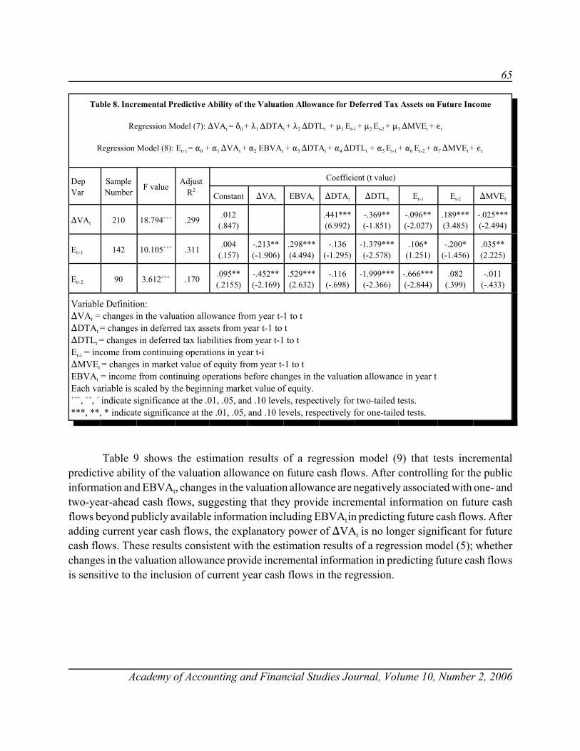
65
Academy of Accounting and Financial Studies Journal, Volume 10, Number 2, 2006
Table 8. Incremental Predictive Ability of the Valuation Allowance for Deferred Tax Assets on Future Income
Regression Model (7): )VAt = *0 + 81 )DTAt + 82 )DTLt + :1 Et-1 + :2 Et-2 + :3 )MVEt + ,t
Regression Model (8): Et+i = "0 + "1 )VAt + "2 EBVAt + "3 )DTAt + "4 )DTLt + "5 Et-1 + "6 Et-2 + "7 )MVEt + ,t
DepVar
SampleNumber F value Adjust
R2
Coefficient (t value)
Constant )VAt EBVAt )DTAt )DTLt Et-1 Et-2 )MVEt
)VAt 210 18.794+++ .299 .012(.847)
.441***(6.992)
-.369**(-1.851)
-.096**(-2.027)
.189***(3.485)
-.025***(-2.494)
Et+1 142 10.105+++ .311 .004(.157)
-.213**(-1.906)
.298***(4.494)
-.136(-1.295)
-1.379***(-2.578)
.106*(1.251)
-.200*(-1.456)
.035**(2.225)
Et+2 90 3.612+++ .170 .095**(.2155)
-.452**(-2.169)
.529***(2.632)
-.116(-.698)
-1.999***(-2.366)
-.666***(-2.844)
.082(.399)
-.011(-.433)
Variable Definition:)VAt = changes in the valuation allowance from year t-1 to t )DTAt = changes in deferred tax assets from year t-1 to t)DTLt = changes in deferred tax liabilities from year t-1 to t Et-i = income from continuing operations in year t-i )MVEt = changes in market value of equity from year t-1 to tEBVAt = income from continuing operations before changes in the valuation allowance in year t Each variable is scaled by the beginning market value of equity.+++, ++, + indicate significance at the .01, .05, and .10 levels, respectively for two-tailed tests.***, **, * indicate significance at the .01, .05, and .10 levels, respectively for one-tailed tests.
Table 9 shows the estimation results of a regression model (9) that tests incrementalpredictive ability of the valuation allowance on future cash flows. After controlling for the publicinformation and EBVAt, changes in the valuation allowance are negatively associated with one- andtwo-year-ahead cash flows, suggesting that they provide incremental information on future cashflows beyond publicly available information including EBVAt in predicting future cash flows. Afteradding current year cash flows, the explanatory power of )VAt is no longer significant for futurecash flows. These results consistent with the estimation results of a regression model (5); whetherchanges in the valuation allowance provide incremental information in predicting future cash flowsis sensitive to the inclusion of current year cash flows in the regression.
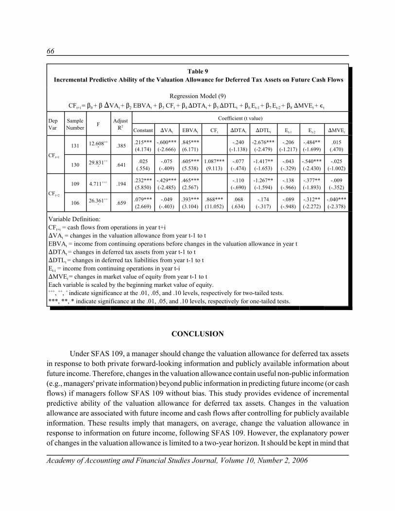
66
Academy of Accounting and Financial Studies Journal, Volume 10, Number 2, 2006
Table 9 Incremental Predictive Ability of the Valuation Allowance for Deferred Tax Assets on Future Cash Flows
Regression Model (9)CFt+i = $0 + $ )VAt + $2 EBVAt + $3 CFt + $4 )DTAt + $5 )DTLt + $6 Et-1 + $7 Et-2 + $8 )MVEt + ,t
DepVar
SampleNumber F Adjust
R2
Coefficient (t value)
Constant )VAt EBVAt CFt )DTAt )DTLt Et-1 Et-2 )MVEt
CFt+1
131 12.608+++ .385 .215***
(4.174)-.600***(-2.666)
.845***(6.171)
-.240(-1.138)
-2.676***(-2.479)
-.206(-1.217)
-.484**(-1.699)
.015(.470)
130 29.831+++ .641 .025
(.554)-.075
(-.409).605***(5.538)
1.087***(9.113)
-.077(-.474)
-1.417**(-1.653)
-.043(-.329)
-.540***(-2.430)
-.025(-1.002)
CFt+2
109 4.711+++ .194 .232***(5.850)
-.429***(-2.485)
.465***(2.567)
-.110(-.690)
-1.267**(-1.594)
-.138(-.966)
-.377**(-1.893)
-.009(-.352)
106 26.361+++ .659 .079***
(2.669)-.049
(-.403).393***(3.104)
.868***(11.052)
.068(.634)
-.174(-.317)
-.089(-.948)
-.312**(-2.272)
-.040***(-2.378)
Variable Definition:CFt+i = cash flows from operations in year t+i )VAt = changes in the valuation allowance from year t-1 to t EBVAt = income from continuing operations before changes in the valuation allowance in year t )DTAt = changes in deferred tax assets from year t-1 to t)DTLt = changes in deferred tax liabilities from year t-1 to t Et-i = income from continuing operations in year t-i )MVEt = changes in market value of equity from year t-1 to tEach variable is scaled by the beginning market value of equity.+++, ++, + indicate significance at the .01, .05, and .10 levels, respectively for two-tailed tests.***, **, * indicate significance at the .01, .05, and .10 levels, respectively for one-tailed tests.
CONCLUSION
Under SFAS 109, a manager should change the valuation allowance for deferred tax assetsin response to both private forward-looking information and publicly available information aboutfuture income. Therefore, changes in the valuation allowance contain useful non-public information(e.g., managers' private information) beyond public information in predicting future income (or cashflows) if managers follow SFAS 109 without bias. This study provides evidence of incrementalpredictive ability of the valuation allowance for deferred tax assets. Changes in the valuationallowance are associated with future income and cash flows after controlling for publicly availableinformation. These results imply that managers, on average, change the valuation allowance inresponse to information on future income, following SFAS 109. However, the explanatory powerof changes in the valuation allowance is limited to a two-year horizon. It should be kept in mind that
67
Academy of Accounting and Financial Studies Journal, Volume 10, Number 2, 2006
the sample for these tests contains a large number of firm-years with incentives to manage earnings.Managers' opportunistic manipulation of the valuation allowance in these years significantlyweakens the predictive ability of the valuation allowance for future income and cash flows. The findings of this study have mixed implications for accounting standard setters and regulators.The predictive ability of the valuation allowance found here suggests that mandating recognition offorward-looking information in financial statements has the potential to make these statements moreinformative. On the other hand, the limited predictive ability of the valuation allowance, which isalso found here, implies managers' ability to fool investors through opportunistic manipulation.Thus, forward-looking information has the potential to make the financial statements not only morebut also less informative. An avenue for future research is to investigate whether the users offinancial statements are able to extract value-relevant information from the valuation allowance withrecognizing earnings management effects on the valuation allowance.
ENDNOTES
1 See Jennings (1990) to review research design that examines the incremental information content of oneaccounting income variable conditional on one or more other income variables.
2 Since none of providers of firms' financial information (e.g., Standard and Poor's) provides the valuationallowance account, I manually collected the valuation allowance information through PR Newswire.
3 Frank and Rego (2003, 35) provide some descriptive statistics for the Compustat population.
4 In general, more than half of the firms reporting deferred tax assets record some amounts of related valuationallowance (Comiskey and Mulford 1994; Petree et al. 1995; Behn et al. 1998).
REFERENCES
Accounting Principles Board (APB). 1967. Opinion No. 11: Accounting for income taxes. New York, NY: AmericanInstitute of Certified Public Accountants.
AICPA. 2002. New business model beginning to emerge – Timeliness, Reliability, Transparency to be improved. TheCPA Letter 82.10.
AICPA Special Committee on Financial Reporting. 1994. Improving business reporting – A customer focus: Meetingthe needs of investors and creditors, from http://www.aicpa.org/members/div/acctstd/ibr/index.htm.
Albrecht, W., L. Lookabill, and J. McKeown. 1977. The time-series properties of annual earnings. Journal of AccountingResearch 15: 226-244.
68
Academy of Accounting and Financial Studies Journal, Volume 10, Number 2, 2006
Amir, E., M. Kirschenheiter, and K. Willard. 1997. The valuation of deferred taxes. Contemporary Accounting Research14. 4: 597-622.
Amir, E., and T. Sougiannis. 1999. Analysts’ interpretation and investors’ valuation of tax carryforwards. ContemporaryAccounting Research 16.1: 1-33.
Ayers, B. 1998. Deferred tax accounting under SFAS No. 109: An empirical investigation ofits incremental value-relevance relative APB No. 11. The Accounting Review 73. 2: 195-212
Ball, R., and R. Watts. 1972. Some time series properties of accounting income. Journal of Finance 27. 663-682.
Beaver, W. 1998. Financial reporting: Accounting revolution, 3rd ed. Prentice-Hall, Inc. New Jersey.
Beaver, W., R. Lambert, and D. Morse. 1980. The information content of security prices. Journal of Accounting andEconomics 2: 3-28.
Beaver, W., R. Lambert, and S. Ryan. 1987. The information content of security prices: A second look. Journal ofAccounting and Research 25.Supplement: 1-36.
Behn, B., T. Eaton, and J. Williams. 1998. The determinants of the deferred tax allowance account under SFAS No. 109.Accounting Horizon 12.1: 63-78.
Bielstein, M., and E. Trott. 1992. The new approach to accounting for income taxes. Strategic Finance 74.2: 43-47.
Burgstahler, D., W. Elliott, and M. Hanlon. 2002. How firms avoid losses: Evidence of use of the net deferred tax assetaccount. Working Paper, University of Washington.
Chandra, U., and B. Ro. The association between deferred taxes and common stock risk. Journal of Accounting andPublic Policy 16. 3: 311-333.
Collins, D., S. Kothari, and J. Rayburn. 1987. Firm size and the information content of prices with respect to earnings.Journal of Accounting and Economics 9 (July): 111-138.
Comiskey, E., and C. Mulford. 1994. Evaluating deferred-tax assets: Some guidance for lenders. Commercial LendingReview 9.3 (Summer): 12-25.
Dechow P., and I. Dichev. 2002. The quality of accruals and earnings: The role of accrual estimation errors. TheAccounting Review 77: 35-59.
Dechow P., S. Kothari, and R. Watts. 1998. The relation between earnings and cash flows. Journal of Accounting andEconomics 25: 133-168.
Eaton, T., and J. Williams. 1998. Valuing deferred tax assets under SFAS 109. Strategic Finance 79.9: 46-50.
Financial Accounting Standards Board (FASB). 1978. Statement of Financial Accounting Concept No.1: Objectives ofFinancial Reporting by Business Enterprises. Norwalk, CT: FASB.
69
Academy of Accounting and Financial Studies Journal, Volume 10, Number 2, 2006
Financial Accounting Standards Board (FASB). 1987. Statement of Financial Accounting Standards No. 96: Accountingfor income taxes. Norwalk, CT: FA
Financial Accounting Standards Board (FASB). 1992. Statement of Financial Accounting Standards No. 109:Accounting for income taxes. Norwalk, CT: FA
Finger. 1994. The ability of earnings to predict future earnings and cash flow. Journal of Accounting Research 32.2: 210-223.
Frank, M., and S. Rego. 2003. Do managers use the valuation allowance account to manage earnings around certainearnings target? Working paper, University of Iowa.
Freeman, R. 1986. The association between accounting earnings and security returns for large and small firms. Journalof Accounting and Economics 9: 195-228.
Guenther D., and R. Sansing. 2003. The valuation relevance of reversing deferred tax liabilities. Working Paper.University of Colorado.
Jennings, R. 1990. A note on interpreting “incremental information content.” The Accounting Review 65.4: 925-932.
Journal of Accountancy. 1994. Focus on: Recommendations of the Special Committee On Financial Reporting. Journalof Accountancy 178.4:41-46.
Kumar, K. R., and G. Visvanathan. 2003. The information content of the deferred tax valuation allowance. TheAccounting Review 78. 2: 471-490.
Lang, M., and T. Warfield. 1997. Response to the FASB invitation to comment, “Recommendations of the AICPASpecial Committee on Financial Reporting and the Association for Investment Management and Research.”Accounting Horizon 11.1: 139-156.
Lev, B. 1983. Some economic determinants of time series properties of earnings. Journal of Accounting and Economics5 (April): 31-48.
Miller, G., and D. Skinner. 1998. Determinants of the valuation allowance for deferred tax assets under SFAS No. 109.The Accounting Review 73. 2: 213-233.
Peavey, D., and H. Nurnberg. 1993. FASB 109: Auditing considerations of deferred tax assets. Journal of Accountancy175.5: 77-81.
Petree, T., G. Gregory, and R. Vitray. 1995. Evaluating deferred tax assets. Journal of Accountancy 179.3: 71-77.
Read, W. 1992. The FASB’s new rules: Here we go again? Business Credit 94.4: 14-16.
Rhoades-Catanach, S. 2003. Discussion of valuation of a firm with a tax loss carryover. Journal of The AmericanTaxation Association 25.Supplement: 83-86.
70
Academy of Accounting and Financial Studies Journal, Volume 10, Number 2, 2006
Schrand, C., and F. Wong. 2003. Earnings management using the valuation allowance for deferred tax assets underSFAS No. 109. Contemporary Accounting Research 20.3: 579-611.
Visvanathan, G. 1998. Deferred tax valuation allowance and earnings management. Journal of Financial StatementAnalysis 3.4: 6-10
Watts, R., and R. Leftwich. 1977. The time-series of annual accounting earnings. Journal of Accounting Research ?:253-171.
Watts, R., and J. Zimmerman. 1986. Positive Accounting Theory. Englewood Cliffs, NJ: Prentice-Hall.
71
Academy of Accounting and Financial Studies Journal, Volume 10, Number 2, 2006
INDIVIDUAL INVESTORS, ELECTRONIC TRADINGAND TURNOVER
Vaughn S. Armstrong, Utah Valley State CollegeNorman D. Gardner, Utah Valley State College
ABSTRACT
We examine how changes in individual investors' cost for information and trading costsaffect stock turnover, i.e., the portion of outstanding stock that trades during a specific period oftime. We also test how individual investors with relatively short investment horizons affect turnover.We find that stock turnover increases when electronic trading becomes available to individualinvestors and that, while turnover is negatively correlated with individual investors' equityownership, it is positively correlated with the level of electronic trading by individuals. Thisconfirms the theory that investors trade relatively more actively when their costs of trading declineand provides further evidence that, when investors have the same trading costs and access toinformation, differences in their investment objectives leads to differences in their contribution tostock turnover.
INTRODUCTION
Not many years ago, it was widely predicted that the internet would transform business invery dramatic ways. Litan and Rivlin (2001) project that business cost savings due to internet usewould add 0.2-0.4% to U.S. productivity. They did not attempt to quantify the effects of consumergains due to greater convenience, wider product mix or enhancements in customization, or theproductivity increases in the computer or software industries. Freund and Weinhold (2002)associate a 1.7% increase in the growth of U.S. exports of services with a 10% growth in internetuse. Cooper, Dimitrov and Rau (2001) report that in 1998 and 1999 a corporate name changesuggesting the company's business is internet related is sufficient to produce abnormal returnsaveraging in excess of 50%. While the bursting of the "tech bubble" may have tempered theexpectations to some degree, there is little question that the internet has affected many aspects ofbusiness. This paper examines how reduced trading costs and improved access to informationassociated with electronic trading affects stock turnover, the portion of a company's stock that tradesduring a given period of time.
It is not surprising that mechanisms designed to reduce trading costs or enhance payment orsettlement systems should affect financial markets. Financial institutions have long made use ofelectronic trading and payments systems and the advent of the internet likely had limited effect on
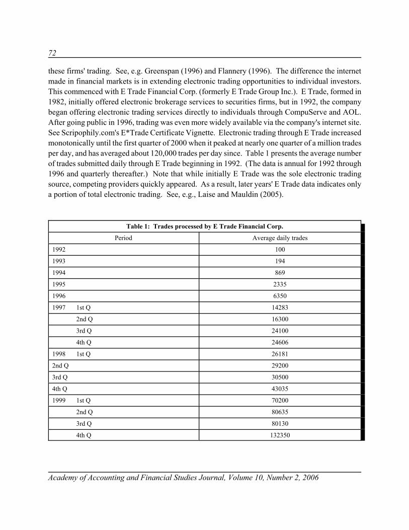
72
Academy of Accounting and Financial Studies Journal, Volume 10, Number 2, 2006
these firms' trading. See, e.g. Greenspan (1996) and Flannery (1996). The difference the internetmade in financial markets is in extending electronic trading opportunities to individual investors.This commenced with E Trade Financial Corp. (formerly E Trade Group Inc.). E Trade, formed in1982, initially offered electronic brokerage services to securities firms, but in 1992, the companybegan offering electronic trading services directly to individuals through CompuServe and AOL.After going public in 1996, trading was even more widely available via the company's internet site.See Scripophily.com's E*Trade Certificate Vignette. Electronic trading through E Trade increasedmonotonically until the first quarter of 2000 when it peaked at nearly one quarter of a million tradesper day, and has averaged about 120,000 trades per day since. Table 1 presents the average numberof trades submitted daily through E Trade beginning in 1992. (The data is annual for 1992 through1996 and quarterly thereafter.) Note that while initially E Trade was the sole electronic tradingsource, competing providers quickly appeared. As a result, later years' E Trade data indicates onlya portion of total electronic trading. See, e.g., Laise and Mauldin (2005).
Table 1: Trades processed by E Trade Financial Corp.
Period Average daily trades
1992 100
1993 194
1994 869
1995 2335
1996 6350
1997 1st Q 14283
2nd Q 16300
3rd Q 24100
4th Q 24606
1998 1st Q 26181
2nd Q 29200
3rd Q 30500
4th Q 43035
1999 1st Q 70200
2nd Q 80635
3rd Q 80130
4th Q 132350
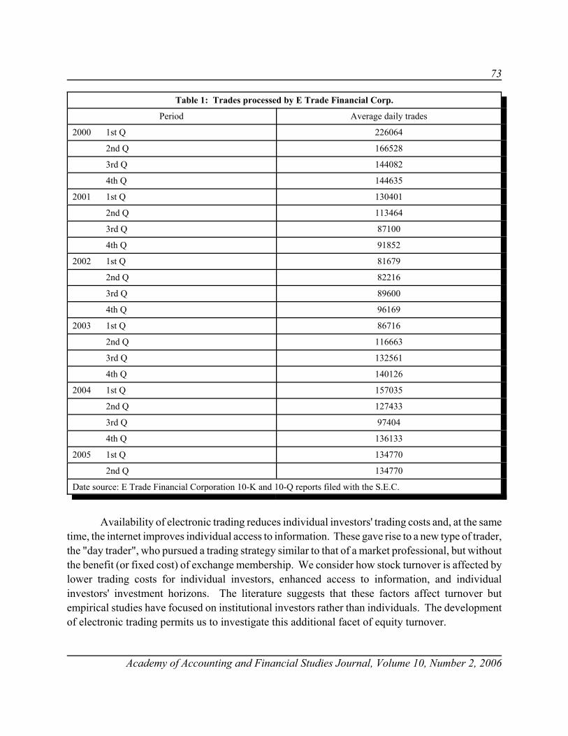
73
Table 1: Trades processed by E Trade Financial Corp.
Period Average daily trades
Academy of Accounting and Financial Studies Journal, Volume 10, Number 2, 2006
2000 1st Q 226064
2nd Q 166528
3rd Q 144082
4th Q 144635
2001 1st Q 130401
2nd Q 113464
3rd Q 87100
4th Q 91852
2002 1st Q 81679
2nd Q 82216
3rd Q 89600
4th Q 96169
2003 1st Q 86716
2nd Q 116663
3rd Q 132561
4th Q 140126
2004 1st Q 157035
2nd Q 127433
3rd Q 97404
4th Q 136133
2005 1st Q 134770
2nd Q 134770
Date source: E Trade Financial Corporation 10-K and 10-Q reports filed with the S.E.C.
Availability of electronic trading reduces individual investors' trading costs and, at the sametime, the internet improves individual access to information. These gave rise to a new type of trader,the "day trader", who pursued a trading strategy similar to that of a market professional, but withoutthe benefit (or fixed cost) of exchange membership. We consider how stock turnover is affected bylower trading costs for individual investors, enhanced access to information, and individualinvestors' investment horizons. The literature suggests that these factors affect turnover butempirical studies have focused on institutional investors rather than individuals. The developmentof electronic trading permits us to investigate this additional facet of equity turnover.
74
Academy of Accounting and Financial Studies Journal, Volume 10, Number 2, 2006
Turnover increases when the market generates more information, Covrig and Ng (2004), andwhen investors' access to information improves, Pollock and Rindova (2004) and Karolyi (2004).Roewenhorst (1999) shows this result in emerging markets. Stock turnover is positively correlatedwith the standard deviation of returns and with firm beta, both of which are associated with volatilityof information about the firm. Turnover is negatively correlated with firm size, consistent with theproposition that information about smaller firms is less accessible. In addition to the rate at whichinformation is generated and the availability of information, the uniformity of interpretation ofavailable information affects stock turnover. The more homogeneous investors' expectations are thelower turnover will be. Domowitz, Glen and Madhavan (2001) confirm the positive correlationbetween firm size and stock turnover in emerging markets, but find that the correlation is negativein developed markets. They suggest this result occurs because in developed markets intensity ofanalysts following of large firms leads to greater conformity in interpretation of information.
Transactions costs are inversely related to stock turnover. Wider bid ask spreads areassociated with lower turnover. Atkins and Dyl (1997). Turnover is positively correlated withownership by institutional investors with lower trading costs. Badrinath, Kale and Noe (1995).Covrig and Ng (2004) also find that trading by low-trading-cost investors has a greater effect ofvolume autocorrelation than trading by high-trading-cost investors.
There is also a relationship between investor objectives and turnover. The larger portion ofa stock held by investors with a relatively long investment horizon the less frequently those sharestrade resulting in lower stock turnover. Armstrong and Gardner (2005) demonstrate that greaterequity ownership by households reduces stock turnover. This is consistent with the idea that ingeneral individual investors have a relatively longer investment horizon than financial institutions.In the case of financial institutions, ownership of equity by some institutions increases stockturnover, while ownership by others reduces it. Different financial institutions have differinginvestment horizons.
This paper examines how changes in individual investors' access to information andtransactions costs affects stock turnover. We also consider the effect of differing investmenthorizons for different individual investors. We use regression analysis to examine stock turnover,controlling specifically for advances in technology which beginning in the early 1990's providedindividual investors with enhanced information availability and reduced their actual costs of tradingand for trading by individual investors with relatively short holding periods, as well as for thoseother factors that affect stock turnover. Our results indicate that while individual investors' holdingsof stock generally reduce turnover, trading by individual investors with relatively short investmenthorizons cause stock turnover to increase. We also find evidence that lower transactions costs forindividual investors and improved access to information increases stock turnover on NASDAQ butonly to a limited extent on the New York Stock Exchange. This suggests that individual investorsrelying on lower trading costs may tend to concentrate their trades in certain types of securities.
75
Academy of Accounting and Financial Studies Journal, Volume 10, Number 2, 2006
The next section describes the sample and our methodology. Section III presents the resultsand Section IV concludes.
SAMPLE AND METHODOLOGY
We examine both share turnover and dollar turnover for the seventy two quarters from 1985through 2002, the last year for which all the data is available. Our analysis uses O.L.S. regressionwith share turnover and dollar turnover on both the New York Stock exchange and NASDAQ asdependent variables. Share turnover is the ratio of shares traded during the quarter to the numberof shares outstanding. We annualize this number by multiplying it by the number of trading daysin the year and dividing by the number of trading days in the quarter. We compute dollar turnoversimilarly using dollar trading volume for the quarter and total share value. Share and dollar volumedata, shares outstanding and share value come from the New York Stock Exchange and NASDAQ.Independent variables to control for factors unrelated to electronic trading include: averagebroker/dealer commissions per share traded to control for transactions costs; total market value ofequity, average standard deviation of the Dow Jones Industrial Average, and the average interestrates on federal funds to control for information, and share holdings of households, financialinstitutions and non-U.S. investors for the quarter. In a separate regression, we use instead thechange in the equity holdings of households, of financial institutions that increase their holdingsduring the quarter, of financial institutions that reduce their holdings during the quarter and ofnon-U.S. investors. These variables control for the effects of these groups' differing investmenthorizons. Data on market value of equity and holdings and changes in holdings comes from theFederal Reserve. Data on broker/dealer commissions is from the S.E.C.
The data for holdings by the various groups of investors and change in those holdingsexhibits multicollinearity because the total holdings for all groups change only due to new issuesand repurchases and those changes are much less than aggregate holdings. Similarly, aggregatechanges in holdings are near zero, with increased holdings by one group offset by decreases in othergroups' holdings. To account for this, the independent variable used in our regression analysis isexcess holdings rather than total holdings (and excess change in holdings rather than actual changein holdings). The excess holding for financial institutions for a quarter is the residual for that quarterobtained by regressing actual financial institution holdings as the dependent variable on total marketvalue of equity as the independent variable. For households, we use the residuals from regressinghousehold holdings (as the dependent variable) on total market value of equity and holdings offinancial institution regression (as independent variables). Excess holdings for the non-U.S.investors are residuals from regressing non-U.S. investor holdings (as the dependent variable) ontotal market value of equity, financial institution holdings, and household holdings (as independentvariables). The order is chosen to reflect average size of holdings in decreasing order. In theanalysis that uses change in holdings, we similarly compute excess change in holdings for financial
76
Academy of Accounting and Financial Studies Journal, Volume 10, Number 2, 2006
institutions that increase their holdings, households, financial institutions that reduce their holdingsand non-U.S. investors (with the order selected by decreasing average absolute change in holdings).We use two variables to observe the effects of change in individual investors' trading costs andaccess to information and of differences in individual investor investment horizons. We use a binaryvariable that equal to zero in quarters before the fourth quarter of 1992 and one thereafter. The year1992 is the first year that individuals have direct access to electronic trading mechanisms. Sincefinancial institutions have access to electronic trading systems prior to this time, the dummy variablecaptures the effect of individuals' lower trading costs and improved access to information.
We control for the effect of differing objectives among individual investors by including asan independent variable the average daily electronic trades executed by E Trade during the quarter.Since individual investors with very short investment horizons (such as "day traders") must exercisemore control over their trading costs than long horizon investors in order to realize desired returns,trades submitted electronically are more likely to include their trading activity than that of individualinvestors with longer investment horizons. This data comes from reports filed by E Trade FinancialCorp. with the S.E.C. (We also perform the regression analysis use alternative data on average dailyelectronic trades from Piper Jaffray for a shorter period of time, the first quarter of 1997 through thesecond quarter of 2000. Results using that data (not reported) are similar to those we obtain usingthe E Trade data.)
Table 2 set forth descriptive statistics for our data. For each of the dependent andindependent variables, it presents the mean and the standard deviation of the variable, as well as itsminimum and maximum values.
RESULTS
We expect electronic trading to lead to increases in stock turnover. Theory suggests thatlower transactions costs should increase turnover. Better access to information should also causegreater turnover unless investors' interpretation of the information is more uniform than when theyhad more limited access. Both of these suggest that the coefficient for the electronic trading binaryvariable should be positive.
We also expect a positive coefficient for the electronic trading volume variable. Weanticipate that that variable will capture the effect of trading by individual investors with relativelyshort investment horizons. Such trading should be associated with greater stock turnover.
Table 3 presents the results of our analysis of turnover on the New York Stock Exchange;with share turnover as the independent variable in panel A, and dollar turnover in panel B. Table4 present the results for NASDAQ.
Results for share turnover and dollar turnover on both the New York Stock Exchange andNASDAQ confirm our expectations regarding electronic trading. The dummy variable is alwayspositive; it is significant for both share and dollar turnover on NASDAQ, but not significant for

77
Academy of Accounting and Financial Studies Journal, Volume 10, Number 2, 2006
NYSE. Higher stock turnover is associated with lower individual trading costs and improved accessto information. This is particularly true for NASDAQ where individual investor influence is likelyto be more important because of the smaller, newer companies trading there.
Table 2: Descriptive statistics (quarterly data 1985-2002).
Mean Std. dev. Maximum Minimum
NYSE share turnover 0.656 0.170 1.110 0.428
NYSE dollar turnover 0.649 0.158 1.037 0.408
NASDAQ share turnover 1.670 0.806 3.857 0.655
NASDAQ dollar turnover 2.104 1.032 5.662 0.879
Daily electronic trades 29001 50671 226064 0
Broker/dealer commissions per share (%) 0.0035 0.0012 0.0057 0.0014
Market value of domestic corporations (x106) 7277695 4781646 17851628 1821439
Std. dev. of daily Dow Jones Industrial Average 97.55 86.37 378.33 12.06
Average federal funds rate (%) 5.63 1.95 9.81 1.34
Holdings by investor groups (x106)
Financial institutions 3817060 2702226 9384467 891737
Households 3742231 2334498 9245400 898614
Non-U.S. investors 640245 528258 1681652 105713
Change in investor group holdings (x106)
Financial institutions with increase 45751 30342 150070 5624
Households -38097 31817 22436 -148765
Financial institutions with decrease -18822 13872 -919 -62344
Non-U.S. investors 9323 15074 66486 -8504
Even after controlling for the effects of lower trading costs and better information access,electronic trading volume also increases stock turnover on both markets. The increase is significantfor both share and dollar volume on NASDAQ and for dollar volume on NYSE. This suggests thatindividual influence on NYSE turnover is greater for higher priced stocks. That may indicate that
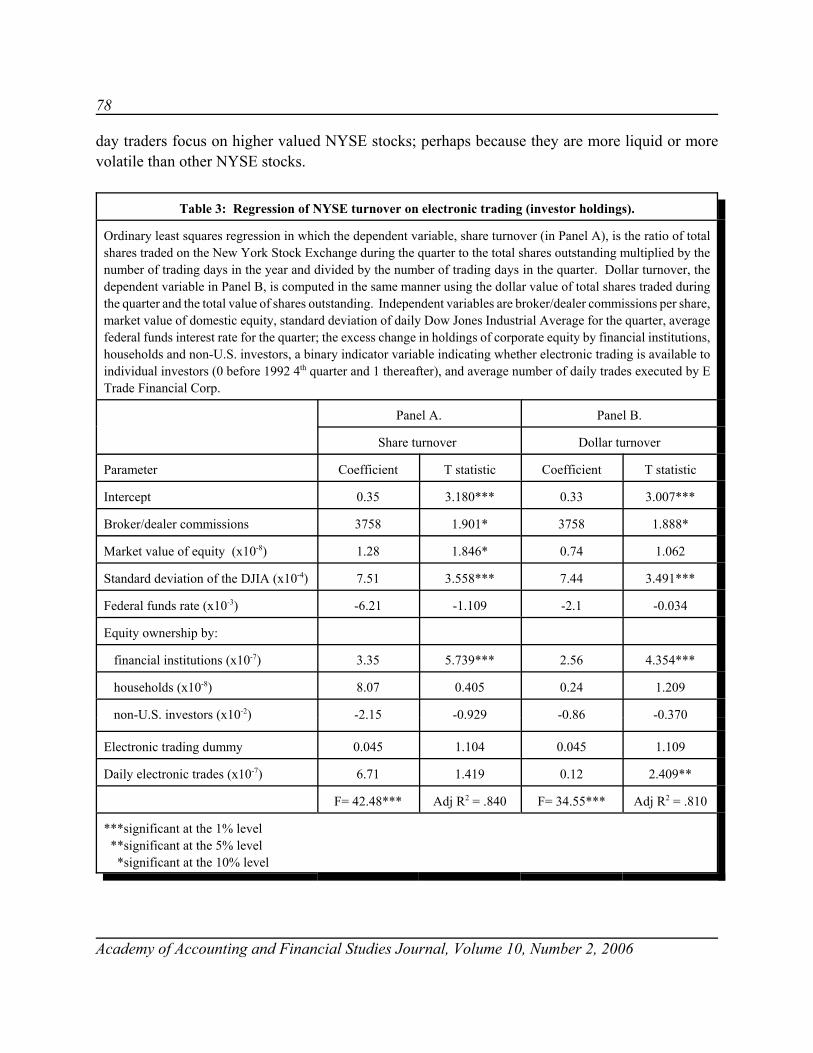
78
Academy of Accounting and Financial Studies Journal, Volume 10, Number 2, 2006
day traders focus on higher valued NYSE stocks; perhaps because they are more liquid or morevolatile than other NYSE stocks.
Table 3: Regression of NYSE turnover on electronic trading (investor holdings).
Ordinary least squares regression in which the dependent variable, share turnover (in Panel A), is the ratio of totalshares traded on the New York Stock Exchange during the quarter to the total shares outstanding multiplied by thenumber of trading days in the year and divided by the number of trading days in the quarter. Dollar turnover, thedependent variable in Panel B, is computed in the same manner using the dollar value of total shares traded duringthe quarter and the total value of shares outstanding. Independent variables are broker/dealer commissions per share,market value of domestic equity, standard deviation of daily Dow Jones Industrial Average for the quarter, averagefederal funds interest rate for the quarter; the excess change in holdings of corporate equity by financial institutions,households and non-U.S. investors, a binary indicator variable indicating whether electronic trading is available toindividual investors (0 before 1992 4th quarter and 1 thereafter), and average number of daily trades executed by ETrade Financial Corp.
Panel A. Panel B.
Share turnover Dollar turnover
Parameter Coefficient T statistic Coefficient T statistic
Intercept 0.35 3.180*** 0.33 3.007***
Broker/dealer commissions 3758 1.901* 3758 1.888*
Market value of equity (x10-8) 1.28 1.846* 0.74 1.062
Standard deviation of the DJIA (x10-4) 7.51 3.558*** 7.44 3.491***
Federal funds rate (x10-3) -6.21 -1.109 -2.1 -0.034
Equity ownership by:
financial institutions (x10-7) 3.35 5.739*** 2.56 4.354***
households (x10-8) 8.07 0.405 0.24 1.209
non-U.S. investors (x10-2) -2.15 -0.929 -0.86 -0.370
Electronic trading dummy 0.045 1.104 0.045 1.109
Daily electronic trades (x10-7) 6.71 1.419 0.12 2.409**
F= 42.48*** Adj R2 = .840 F= 34.55*** Adj R2 = .810
***significant at the 1% level **significant at the 5% level *significant at the 10% level
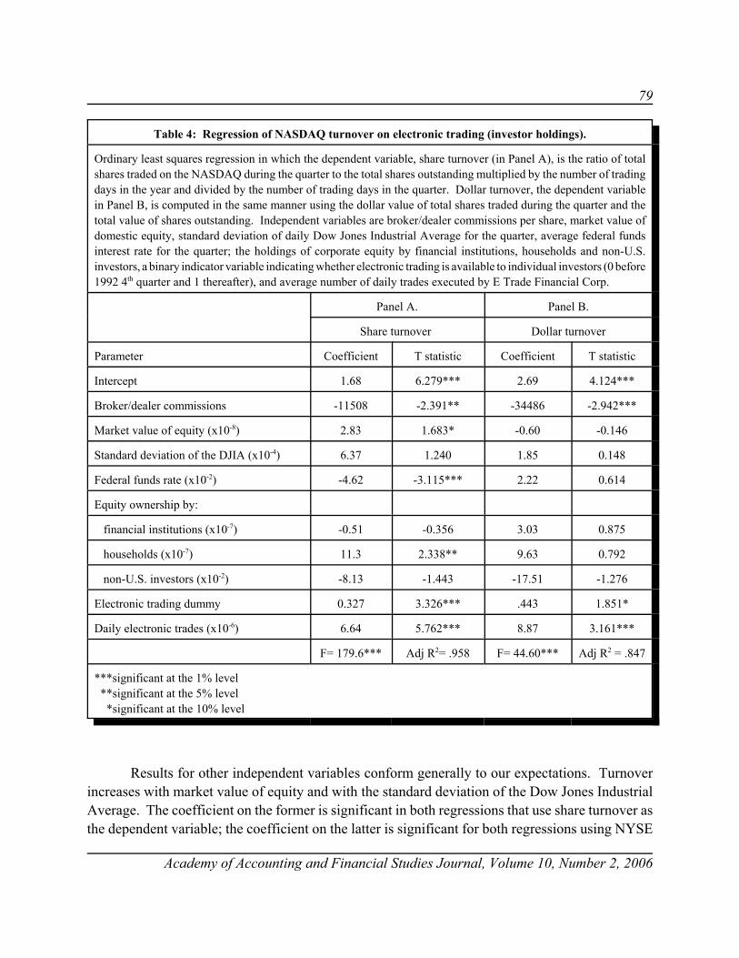
79
Academy of Accounting and Financial Studies Journal, Volume 10, Number 2, 2006
Table 4: Regression of NASDAQ turnover on electronic trading (investor holdings).
Ordinary least squares regression in which the dependent variable, share turnover (in Panel A), is the ratio of totalshares traded on the NASDAQ during the quarter to the total shares outstanding multiplied by the number of tradingdays in the year and divided by the number of trading days in the quarter. Dollar turnover, the dependent variablein Panel B, is computed in the same manner using the dollar value of total shares traded during the quarter and thetotal value of shares outstanding. Independent variables are broker/dealer commissions per share, market value ofdomestic equity, standard deviation of daily Dow Jones Industrial Average for the quarter, average federal fundsinterest rate for the quarter; the holdings of corporate equity by financial institutions, households and non-U.S.investors, a binary indicator variable indicating whether electronic trading is available to individual investors (0 before1992 4th quarter and 1 thereafter), and average number of daily trades executed by E Trade Financial Corp.
Panel A. Panel B.
Share turnover Dollar turnover
Parameter Coefficient T statistic Coefficient T statistic
Intercept 1.68 6.279*** 2.69 4.124***
Broker/dealer commissions -11508 -2.391** -34486 -2.942***
Market value of equity (x10-8) 2.83 1.683* -0.60 -0.146
Standard deviation of the DJIA (x10-4) 6.37 1.240 1.85 0.148
Federal funds rate (x10-2) -4.62 -3.115*** 2.22 0.614
Equity ownership by:
financial institutions (x10-7) -0.51 -0.356 3.03 0.875
households (x10-7) 11.3 2.338** 9.63 0.792
non-U.S. investors (x10-2) -8.13 -1.443 -17.51 -1.276
Electronic trading dummy 0.327 3.326*** .443 1.851*
Daily electronic trades (x10-6) 6.64 5.762*** 8.87 3.161***
F= 179.6*** Adj R2= .958 F= 44.60*** Adj R2 = .847
***significant at the 1% level **significant at the 5% level *significant at the 10% level
Results for other independent variables conform generally to our expectations. Turnoverincreases with market value of equity and with the standard deviation of the Dow Jones IndustrialAverage. The coefficient on the former is significant in both regressions that use share turnover asthe dependent variable; the coefficient on the latter is significant for both regressions using NYSE
80
Academy of Accounting and Financial Studies Journal, Volume 10, Number 2, 2006
turnover. These results confirm that stock turnover increases with the amount of information thatis generated.
Coefficients associated with the equity holdings of different investors groups generally havethe expected sign but are not statistically significant. One significant result, the coefficient forexcess financial institution holdings is positive and significant in the NYSE regressions, is consistentwith results found elsewhere in the literature. The larger the portion of equity held by financialinstitutions, with lower costs of trading and better access to information, the greater the stockturnover. The other significant result, a significantly positive correlation between stock turnoverand excess household equity holdings in the NASDAQ share turnover regression, differs fromArmstrong and Gardner (2005) which finds that household holdings have a significantly negativeeffect on stock turnover. A possible explanations is that when individuals investors have access toelectronic trading, excess household holdings occur because of electronic trading.
Turnover is negatively correlated with the fed funds rate and is significant for share turnoveron NASDAQ. We had expected this variable to be positive as higher interest rates are associatedwith economic expansion. The result may indicate that during our sample period, when theeconomy is expanding, investors' tend to hold stocks longer than when the economy is contracting.The fact that this relationship is strongest for share turnover on NASDAQ, that is, for lower pricedstocks that trade in a market dominated by growth stocks, further suggests that this result reflectstrading activity associated with development and bursting of the "tech bubble".
The coefficient for commissions per share is negative and significant for NASDAQ asexpected. However, that coefficient is significantly positive in the regressions for the NYSE. Thismay indicate that after electronic trading becomes available to individual investors, the variablesassociated with electronic trading capture all the increased stock turnover. Non-electronic tradinggenerates higher broker/dealer commissions. The stock turnover that remains after controlling forelectronic trading is non-electronic and is as a result positively correlated with commissions.
Tables 5 and 6 present the results of regressions where we substitute the change in holdingsof financial institutions, households and non-U.S. investors for the level of those investors' holdings.These results confirm our observations from the investors' equity holding regressions. Stockturnover is positively correlated with the level of electronic trading and the coefficient is usuallystatistically significant. The binary indicator variable for availability of electronic trading is positiveexcept for the NYSE share turnover regression. It is significant only in the NASDAQ share turnoverregression. When we control for changes in the holdings of various investor groups (that is, for thenet results of their trading), the ability of individual investors to trade electronically has little effecton stock turnover, but their actual electronic trading activity increases stock turnover. Results forother independent variables generally conform to our expectations. Stock turnover increases asfinancial institutions increase their equity holdings and declines as they reduce them. Broker/dealercommissions are negatively correlated with stock turnover.
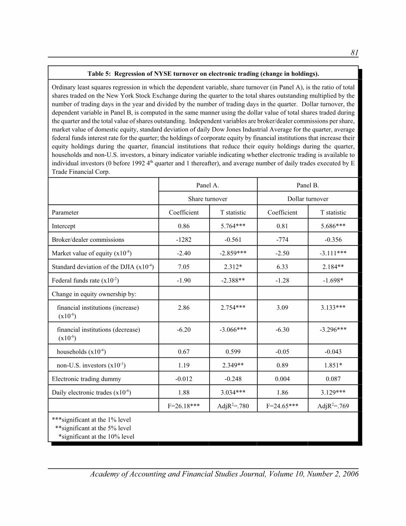
81
Academy of Accounting and Financial Studies Journal, Volume 10, Number 2, 2006
Table 5: Regression of NYSE turnover on electronic trading (change in holdings).
Ordinary least squares regression in which the dependent variable, share turnover (in Panel A), is the ratio of totalshares traded on the New York Stock Exchange during the quarter to the total shares outstanding multiplied by thenumber of trading days in the year and divided by the number of trading days in the quarter. Dollar turnover, thedependent variable in Panel B, is computed in the same manner using the dollar value of total shares traded duringthe quarter and the total value of shares outstanding. Independent variables are broker/dealer commissions per share,market value of domestic equity, standard deviation of daily Dow Jones Industrial Average for the quarter, averagefederal funds interest rate for the quarter; the holdings of corporate equity by financial institutions that increase theirequity holdings during the quarter, financial institutions that reduce their equity holdings during the quarter,households and non-U.S. investors, a binary indicator variable indicating whether electronic trading is available toindividual investors (0 before 1992 4th quarter and 1 thereafter), and average number of daily trades executed by ETrade Financial Corp.
Panel A. Panel B.
Share turnover Dollar turnover
Parameter Coefficient T statistic Coefficient T statistic
Intercept 0.86 5.764*** 0.81 5.686***
Broker/dealer commissions -1282 -0.561 -774 -0.356
Market value of equity (x10-8) -2.40 -2.859*** -2.50 -3.111***
Standard deviation of the DJIA (x10-4) 7.05 2.312* 6.33 2.184**
Federal funds rate (x10-2) -1.90 -2.388** -1.28 -1.698*
Change in equity ownership by:
financial institutions (increase) (x10-6)
2.86 2.754*** 3.09 3.133***
financial institutions (decrease) (x10-6)
-6.20 -3.066*** -6.30 -3.296***
households (x10-6) 0.67 0.599 -0.05 -0.043
non-U.S. investors (x10-1) 1.19 2.349** 0.89 1.851*
Electronic trading dummy -0.012 -0.248 0.004 0.087
Daily electronic trades (x10-6) 1.88 3.034*** 1.86 3.129***
F=26.18*** AdjR2=.780 F=24.65*** AdjR2=.769
***significant at the 1% level **significant at the 5% level *significant at the 10% level
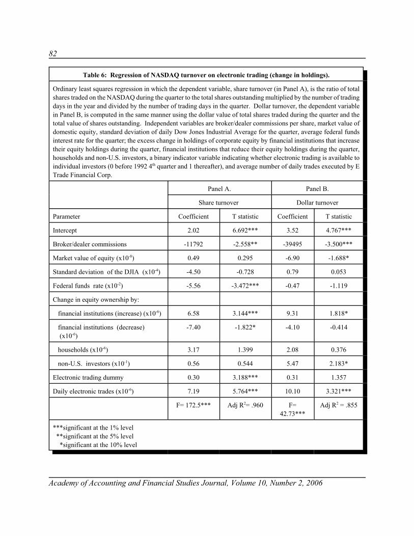
82
Academy of Accounting and Financial Studies Journal, Volume 10, Number 2, 2006
Table 6: Regression of NASDAQ turnover on electronic trading (change in holdings).
Ordinary least squares regression in which the dependent variable, share turnover (in Panel A), is the ratio of totalshares traded on the NASDAQ during the quarter to the total shares outstanding multiplied by the number of tradingdays in the year and divided by the number of trading days in the quarter. Dollar turnover, the dependent variablein Panel B, is computed in the same manner using the dollar value of total shares traded during the quarter and thetotal value of shares outstanding. Independent variables are broker/dealer commissions per share, market value ofdomestic equity, standard deviation of daily Dow Jones Industrial Average for the quarter, average federal fundsinterest rate for the quarter; the excess change in holdings of corporate equity by financial institutions that increasetheir equity holdings during the quarter, financial institutions that reduce their equity holdings during the quarter,households and non-U.S. investors, a binary indicator variable indicating whether electronic trading is available toindividual investors (0 before 1992 4th quarter and 1 thereafter), and average number of daily trades executed by ETrade Financial Corp.
Panel A. Panel B.
Share turnover Dollar turnover
Parameter Coefficient T statistic Coefficient T statistic
Intercept 2.02 6.692*** 3.52 4.767***
Broker/dealer commissions -11792 -2.558** -39495 -3.500***
Market value of equity (x10-8) 0.49 0.295 -6.90 -1.688*
Standard deviation of the DJIA (x10-4) -4.50 -0.728 0.79 0.053
Federal funds rate (x10-2) -5.56 -3.472*** -0.47 -1.119
Change in equity ownership by:
financial institutions (increase) (x10-6) 6.58 3.144*** 9.31 1.818*
financial institutions (decrease) (x10-6)
-7.40 -1.822* -4.10 -0.414
households (x10-6) 3.17 1.399 2.08 0.376
non-U.S. investors (x10-1) 0.56 0.544 5.47 2.183*
Electronic trading dummy 0.30 3.188*** 0.31 1.357
Daily electronic trades (x10-6) 7.19 5.764*** 10.10 3.321***
F= 172.5*** Adj R2= .960 F=42.73***
Adj R2 = .855
***significant at the 1% level **significant at the 5% level *significant at the 10% level

83
Academy of Accounting and Financial Studies Journal, Volume 10, Number 2, 2006
As in the regressions using investor holdings, stock turnover is negatively correlated withfed funds rates. In these regressions, stock turnover is also negatively correlated with market valueof equity. We expect this result occurs because, in this regression, changes in investor groups'holdings captures the effect of information on stock turnover; specifically that financial institutionson average increase their holdings in response to the information reflected in overall market value.
Results from regressions using electronic trading reported by Piper Jaffray (not reported) aresimilar but have generally fewer significant coefficients. This is likely due to the shorter time periodfor which that data is available, fourteen quarters beginning in 1997.
CONCLUSION
We examine how changes in individual investors' information and trading costs anddifferences among individual investors' investment objectives horizon affect share and dollarturnover. We find that as information becomes available to individuals through electronic mediaand as electronic trading mechanisms become available, turnover increases. This is consistent withthe theory that turnover is inversely correlated with transactions costs and positively correlated withinformation. That increase occurs even when we control for changes in equity holdings ofindividuals and financial institutions. We also find that trading activity by individual investors thathave relatively short investment horizons also increases stock turnover. That is, the investmentobjectives of individual investors affect stock turnover. This result is similar to that found byArmstrong and Gardner (2005) for financial institutions.
This study suggests some opportunities for further research. It is possible that other proxiesexist for day trading volume, especially in later years when the number of competing electronictrading services grows. A different proxy for short investment horizon trading by individuals mightassist in explaining some of the unexpected results. Our results also suggest that studies that do notaccount for stock turnover due to electronic trading by individuals (sample periods that include yearsbefore and after 1992) may omit important information regarding the cause of observed turnover.In addition, we find some evidence that the effects of changes in trading costs may differ acrossdifferent classes of stock or in different markets. Further study is needed to determine how differenttypes of stock, such as, small company and large company or value and growth stocks, respond tochanges in the various factors that affect turnover.
REFERENCES
Armstrong, V.S. & N.D. Gardner (2005). Financial Institution Objectives and Turnover, Academy of Accounting andFinancial Studies Journal, 9(3), 13-28.
Atkins, A.B. & E.A. Dyl (1997). Transactions costs and holding periods for common stocks, Journal of Finance, 52(1),309-325.
84
Academy of Accounting and Financial Studies Journal, Volume 10, Number 2, 2006
Badrinath, S.G., J.R. Kale & T.H. Noe (1995). Of shepherds, sheep and the cross-autocorrelation in equity returns,Review of Financial Studies, 8(2), 401-430.
Scripophily.com's E*Trade Certificate Vignette (n.d.). Retrieved August 18, 2005, fromhttp://www.scripophily.net/etrade.html.
Cooper, M.J., O. Dimitrov & P.R. Rau (2001). A rose.com by any other name. Journal of Finance, 56(6), 2371-2388.
Covrig, V. & L. Ng (2004). Volume autocorrelation, information and investor trading. Journal of Banking & Finance,28(9), 2155-2174.
Domowitz, I., J. Glen & A. Madhavan (2001). Liquidity, volatility and equity costs across countries and over time,International Finance, 40, 221-255.
Flannery, M.J. (1996). Technology and payment: Deja vu all over again. Journal of Money, Credit and Banking, 92(4),965-970.
Freund, C. & D. Weinhold (2002). The internet and international trade in services. American Economic Review, 92(2),236-240.
Greenspan, A. (1996). Remarks on evolving payment system issues. Journal of Money, Credit and Banking, 28(4),689-695.
Karolyi, G.A. (2004). The role of American Depository Receipts in the development of emerging equity markets. TheReview of Economics and Statistics, 86(3), 670-690.
Laise, E & W. Mauldin (2005). Hook the right broker. SmartMoney, 14 (8),. Retrieved August 18, 2005 fromhttp://www.smartmoney.com/brokers/index.cfm?story=2005-intro
Litan, R.E. & A.M. Rivlin (2001). Projecting the economic impact of the internet. American Economic Review, 91(2),313-317.
Pollock, T.G. & V.P. Rindova (2003). Media legitimation effects in the market for initial public offerings. Academy ofManagement Journal, 46(5), 631-642.
Roewenhorst, K.G., 1999, Local return factors and turnover in emerging stock markets, Journal of Finance, 54(4),1439-1464.

85
Academy of Accounting and Financial Studies Journal, Volume 10, Number 2, 2006
ACCOUNTING FOR DATA: A SHORTCOMING INACCOUNTING FOR INTANGIBLE ASSETS
Keith Atkinson, University of Central ArkansasRonald McGaughey, University of Central Arkansas
ABSTRACT
In today's economy and in the future, intellectual capital and the proper use of informationwill be critical to the success of many firms. Data has been called the raw material of information.Data can be aggregated, disaggregated, sorted, and subjected to a variety of mathematical andlogical manipulations. Data can be added to a system, removed, bought, sold and used. Data canbe enhanced making it more valuable and it can be made less valuable with repeated use and withthe passage of time. Because data is a critical firm resource, one expects the cost of data to beaccounted for and to appear on the firm's balance sheet with other firm assets. However, dependingon the data's genealogy, the cost of the data may never be shown as an asset.
If data is purchased it finds its way to the balance sheet, however, if the data is developedinternally Accounting Principles Board (APB) Opinion No. 17 prevents it from being capitalized asan asset. The authors argue that the exclusion of internally developed assets, (particularly data)from the balance sheet can mislead investors, and managers. The authors believe that the exclusionis unnecessary -- that data meets the definition of an asset. Problems persist in the management ofdata. The authors believe that placing a value on data and including it in the firm's balance sheetwill contribute to management's capability to mange it.
INTRODUCTION
In most twenty-first century firms data is a critical resource. This fact is substantiated by TheNational Archives & Records Administration study, 2001Cost of Downtime Survey Results (2002).The study reported that ninety-three percent of companies losing their data center for 10 days filedfor bankruptcy within one year, and that forty-percent of the companies surveyed reported theirsurvival was at risk if their data center was lost for seventy-two hours. Financial statement usershave come to expect critical resources to be represented on a firm's balance sheet as an asset.However, it is very likely that if the critical resource is internally developed data, it will not bereported anywhere on the company's balance sheet or in its financial statements. In fact,stockholders and other financial statement users may be unaware of the data's existence. Thisexclusion of a critical firm resource from the balance sheet seems to be at conflict with FinancialAccounting Standards Board (FASB) Concepts Statement No. 1, "Objectives of Financial Reporting
86
Academy of Accounting and Financial Studies Journal, Volume 10, Number 2, 2006
by Business Enterprises," that states financial reporting should provide information that is useful topresent and potential investors and creditors in making rational investment, credit and similardecisions (1978).
Data is a critical firm resource and is just one component of an information system. Datais separable from the information system used to process it. Lawrence (1999, p. 3) defines data as"symbols, images, sounds and ideas that can be encoded, stored and transmitted." More generally,data are facts about an entity when an entity is a person, place or thing. Facts about a customerentity are categorized as attributes of the entity. The attribute of interest may include the customer'sname, address, telephone number, age, sex, income, any number of purchasing habits and more.Data are aggregated, disaggregated, sorted, and/or subjected to a variety of mathematical and logicalmanipulations.
Processed data presented to a user in a meaningful context becomes information.Information is clearly produced from data, making data the raw material in an informationmanufacturing process (Goodhue, Quillard and Rockart, 1988; Sabherwal and King, 1991; Levitinand Redman, 1998). The value of information is a function of how the information is used and thesubsequent outcome. Because information has value, data also has value. Data can be added to asystem, removed, bought, sold, and used. Data can be enhanced, making it more valuable, and itcan be made less valuable with repeated use and with the passage of time. Data is in fact a criticalorganizational resource and should be treated as such.
This paper specifically addresses accounting for data and more generally accounting forintangible assets. The paper begins by reviewing the definition of an asset and continues byreviewing the relevant accounting standards. The paper then compares and contrasts thecharacteristics of data with those of an asset. The paper concludes with the recommendation toaccount for data as an asset
Several current and past accounting standards discuss the uncertainty of future economicbenefits and contribute to the analysis of how we should account for data. The relevant standardsare the Concepts Statements by the FASB that relate to the definition of an asset, Accounting forResearch and Development Costs, Accounting for Software Development, and Accounting forIntangible Assets.
During the 1970s and 1980s, the FASB issued several concepts statements to guide thedevelopment of accounting and reporting principles for use by U.S. companies. At least four of thestatements provide insight into our subject.
According to FASB Concepts Statement (SFAC) No. 1, Objectives of Financial Reportingby Business Enterprises, the objective of financial reporting is to provide useful information. Thecharacteristics of accounting information that make it useful are identified and discussed in FASBSFAC No. 2, Qualitative Characteristics of Accounting Information. The key characteristicsStatement No. 2 identifies and discusses are:

87
Academy of Accounting and Financial Studies Journal, Volume 10, Number 2, 2006
1. benefits of the information disclosure should exceed cost
2. the information should be relevant
3. the information should be reliable
4. the information should be comparable
5. the information should be material.
SFAC No. 5, Recognition and Measurement in Financial Statements of BusinessEnterprises, states in paragraph 63 that an item should be recognized in a financial statement if itmeets the following criteria:
1. The item meets the definition of an element of financial statements (definition criterion);
2. The item has a relevant attribute measurable with sufficient reliability (measurability criterion);
3. Information about the item can make a difference in user decisions (relevance criterion); and
4. The information pertaining to the item must be representationally faithful, verifiable, andneutral (reliability criterion).
SFAC No. 6, Elements of Financial Statements, defines an asset. It states that, "assets areprobable future economic benefits obtained or controlled by a particular entity as a result of pasttransactions or events." The statement continues by identifying three essential characteristics of anasset:
1. it embodies a probable future economic benefit that involves a capacity to contribute directly orindirectly to future net cash flows,
2. a particular entity can obtain the benefit and control others' access to it, and
3. a transaction or event has already occurred that gives the entity the right to, or the control overthe benefit.
That an entity be required to have the right to control the benefits the item produces beforethe organization can record the item as an asset seems straight forward. The most importantcharacteristic of an asset is its capacity to provide future economic benefits that generate net cashinflows. Future economic benefits can be realized through exchanging the asset for something ofvalue, or through use of the asset toward some productive end. A unit of Product X held in finishedgoods inventory is an asset, because there is a high likelihood that it can be exchanged for currency.
88
Academy of Accounting and Financial Studies Journal, Volume 10, Number 2, 2006
Equipment used to produce Product X, though not held for the express purpose of selling it in thefuture, is an asset because it is used to manufacture product X. Its productive use in making ProductX creates future economic benefits for the owner in the form of revenues produced from the sale ofProduct X. Raw materials are assets for the same reason as equipment, because they provide futureeconomic benefits in the way of revenues generated from the sale of finished products made fromthe raw materials. Future economic benefits can also come in the form of more efficient productionthat will result in decreased cost.
In October 1974, The Financial Accounting Standards Board (FASB) issued Statement ofFinancial Accounting Standard (SFAS) No. 2, "Accounting for Research and Development Cost."The standard requires all Research and Development cost to be expensed as incurred. Research anddevelopment are defined, in part, by paragraph 8 of the standard as follows:
Research is planned search or critical investigation aimed at discovery of new knowledge with thehope that such knowledge will be useful in developing a new product or service or a new process ortechnique or in bringing about a significant improvement to an existing product or process.Development is the transition of research findings or other knowledge into a plan or design for a newproduct or process or for a significant improvement to an existing product or process whether intendedfor sale or use. It includes the conceptual formulation, design, and testing of product alternatives,construction of prototypes, and the operation of pilot plan.
In the discussion of the reasons research and development costs are required to be expensed,paragraph 45 of the standard states that they fail to satisfy the measurability test for accountingrecognition. The measurability criterion will be discussed later in the paper, but requires the futureeconomic benefits of an asset be identified and objectively measured.
In August 1986, the FASB issued SFAS No. 86 to establish standards to account for the costsof computer software to be sold, leased, or otherwise marketed as a separate product or part of aproduct or process. SFAS No. 86 requires all cost incurred to establish the technological feasibilityof a computer software product to be sold, leased or otherwise marketed are research anddevelopment cost and should be expensed when incurred. Costs incurred after technologicalfeasibility has been established should be capitalized. The Board required technological feasibilityto be established before the costs are capitalized because of the uncertainty of the future economicbenefits. FAS No. 86 does not address accounting for the cost of computer software created forinternal use because it was not considered a significant problem.
It is noteworthy the definition of an asset does not make reference to physical objects, butrather to future economic benefits. It is the ability of an asset to produce future benefits that is key,not that it is tangible. In fact, many assets are intangible. Intangible assets are generally defined bythe FASB as current and noncurrent assets that lack physical substance. The accounting forintangible assets has been the subject of three different standards and has caused much recentcontroversy.
89
Academy of Accounting and Financial Studies Journal, Volume 10, Number 2, 2006
In 1953, Accounting Research Bulletin (ARB) No. 43 was published by the Committee onAccounting Procedure of the AICPA. ARB 43 discussed accounting for Intangible Assets; however,in the first paragraph it excluded from its consideration the problems of accounting for intangiblesdeveloped in the regular course of business. The ARB did state, in paragraph four, that "The initialamount assigned to all types of intangibles should be cost, in accordance with the generally acceptedaccounting principles that assets should be stated at cost when they are acquired."
In 1970, the Accounting Principles Board (APB), issued Opinion No. 17, "IntangibleAssets". Paragraphs 6 and 11 of the Opinion describe Generally Accepted Accounting Principles(GAAP) prior to the Opinion's issuance. Paragraph 11 of the Opinion states, "Costs incurred todevelop specifically identifiable intangible assets are often recorded as assets if the periods ofexpected future benefit are reasonably determinable. Costs of developing other intangible assets areusually recorded as expenses when incurred." Paragraph 15 of the Opinion appraises the procedureby stating that the cost of developing intangible assets with lives that are indeterminate are notdistinguishable from current costs of operations and are, therefore, not assignable to specific assets.In paragraph nine, the APB concluded, "that a company should record as assets the costs ofintangible assets acquired from others ……. and record as expenses the costs to develop intangibleassets which are not specifically identifiable."
APB Opinion No. 17 required intangible assets purchased from others to be capitalized andinternally developed intangible assets that were not specifically identifiable to be expensed. Theopinion was silent on internally developed intangible assets that were specifically identifiable.However, it became accepted practice in the U.S. to expense all intangible assets that were internallyproduced as evidenced by the FASB's, Proposal for a New Agenda Project: Disclosure ofInformation about Intangible Assets Not Recognized in Financial Statements (2001) which states:
Intangible assets are generally recognized only if acquired, either separately or as a part of a businesscombination. Intangible assets that are generated internally, and some acquired assets that are writtenoff immediately after being acquired, are not reflected in financial statements, and little quantitativeor qualitative information about them is reported in the notes to the financial statements.
Many argue that the economy today is fundamentally different from the economy of fifty oreven thirty years ago and that traditional financial accounting concepts do not capture the essenceof the new economy. It has been argued that the new economy is driven by intellectual capital, orin many instances by intangible assets This movement to a knowledge economy prompted criticismof APB No. 17. This criticism led to the study of the issue and a new accounting standard. In September 2001, the FASB issued Statement No. 142, "Goodwill and Other IntangibleAssets." SFAS No. 142 superceded APB Opinion No. 17 and changed the accounting for someintangibles. The statement does not require the amortization of the intangible asset, but requires anannual test to determine its value. The intangible asset must then be written down to its value.
90
Academy of Accounting and Financial Studies Journal, Volume 10, Number 2, 2006
However, SFAS No. 142 left unchanged the provision in APB No. 17 related to internally developedintangible assets. Paragraph 2 of SFAS No. 142 states:
This statement supersedes APB Opinion No. 17, Intangible Assets; however, it carries forward withoutreconsideration the provisions in Opinion 17 related to internally developed intangible assets. TheBoard did not reconsider those provisions because they were outside the scope of its project onbusiness combinations and acquired intangible assets.
In the FASB Exposure Draft, "Business Combinations and Intangible Assets," an appendixincluded an extensive list of intangible assets that, if present, should be recognized in a businesscombination separately from goodwill. Included in that list are: rights, computer software andlicenses, computer programs, information systems, program formats, unpatented technology,databases, research and development, lists, and files and records. From the standard and theexposure draft, it is clear that if data is purchased from an outsider, it should be accounted for as anintangible asset according to the rules set forth in SFAS No. 142. What is not clear, is why apurchased asset and an internally developed asset are accounted for differently.
Concepts statements No. 1, 2, 4, and 5 provide guidance on the recognition of an item as anasset in a business enterprise's financial statement by listing the criteria that must be met. Additionalguidance can be gleaned from other issued standards. From SFAS No. 2, we see that the futureeconomic benefits provided must be measurable. SFAS No. 86, requires that in developing softwarefor sale, the technological feasibility must be proved before cost can be capitalized. The applicationof APB Opinion No. 17 prohibited internally developed intangible assets from being capitalized.SFAS No. 142 continued to ignore internally developed intangible assets but requires externallypurchased intangibles to be periodically reviewed for value and written down accordingly.
Recognition is the formal process whereby an item is incorporated into the financialstatements of a business enterprise. As previously discussed, SFAC No. 5 outlined the four criteriaan item must meet to be included in a financial statement as an asset in accordance with generallyaccepted accounting principles. The four criteria assume that the benefits of including the itemexceed the cost of including the item in the financial statements. Data meets all the requirementsof SFAC No. 5 to be recognized as an asset in a financial statement.
Recall that an asset is a probable future economic benefit obtained or controlled by an entityas a result of past transactions or events. Given that data are raw materials used in informationmanufacturing their probable future economic benefits are tied to the value of information whichis related to the information's use. Information is not a resource for which we have markets toreadily establish an economic value; however, there is little question whether information isvaluable.
Whether one subscribes to normative theories of information value, economic theories ofinformation value, or neither, nearly everyone recognizes that information has value (West andCourtney, 1993). Lawrence (1999, p. 7) states, "information produces value for an organization
91
Academy of Accounting and Financial Studies Journal, Volume 10, Number 2, 2006
when it improves the solutions to decision problems whose outcomes are consequential to theorganization." Many products are produced without knowing the exact future value (prices) of theproducts because of the economic characteristics of markets wherein they are sold (i.e. prices arequite uncertain for commodities when production decisions are made). One problem already notedwith establishing the value of information is there are not well developed market mechanisms forestablishing its value (Stigler, 1961; West and Courtney, 1993, Lawrence, 1999). The uncertaintyoften inherent in markets and in future prices received for products does not keep firms that producethose products from considering raw materials as inventory, and including the cost of that inventoryin the cost of the finished product. Raw material inventory is but one type of inventory thatcontributes to the inventory value that appears in the asset section of a manufacturing company'sbalance sheet.
Because one cannot establish with certainty the exact value of information created with data,it does not follow that data are not capable of producing future economic benefits. Data providefuture economic benefits. Just as the cost of raw material made its way to the balance sheet, the costof internally developed data can also make its way to a balance sheet through standard costaccounting procedures.
Another part of the definition criteria is that an asset must arise from a past transaction orevent. Whether the firm purchased the data, accumulated the data itself, or some combination of thetwo, the data is most often owned and is/can be controlled by the firm. In fact, the value of dataarises from its use. Today, data management approaches, tools, and techniques make control ofcompany data far more effective than ever before. Firms can, with appropriate data managementtools, control access to and the use of data, maintain the data more effectively to be sure the valueof the data is maintained or enhanced, and use the data more effectively (as in knowledgemanagement systems, data warehouses, data mining, etc.) to maximize its potential to produce futureeconomic benefits. Although the value of data is directly related to its use and the outcomes ofmanagement's decisions, it can and does produce future economic benefits. In addition, data cancertainly be obtained and controlled by an entity as a result of past transactions or events.Accordingly, data meets the definition criterion of an asset.
An attribute is measured reliably, if when measured in the same manner repeatedly, itproduces identical or nearly identical results. The measure that is applied in placing a value on mostassets in organizations is historical cost. Standard cost accounting procedures can produce reliablehistorical cost figures for data just as they have for many other assets, i.e., inventory and fixedassets. FAS No. 142 also provides a tool with which to value data. Just as one will now evaluatethe carrying cost of all intangible assets for impairment of value, data should be evaluatedaccordingly. Standard cost accounting procedures and a periodic evaluation for impairment of valuecan result in an asset with a value that is measurable.
Because data is used in decision making the cost of data is relevant. The resources anorganization devotes to data management communicate something about the organization to both
92
Academy of Accounting and Financial Studies Journal, Volume 10, Number 2, 2006
external and internal decision makers. The value or cost of data an organization owns may beparticularly important to investors in the new knowledge economy. An organization's data can alsobe used internally to help management better utilize its resources. Most organizations spend moneystoring, protecting and managing data that is simply not worth their effort. Estimating the costs ofdata would help internal decision makers make more rational choices about managing the dataresource itself and its complementary resources such as data storage. If organizations betterunderstood the costs of data, and could compare those costs to the potential benefits of the data, theymight make better decisions about what to acquire, what to maintain, and what to remove fromorganizational systems. The above points suggest that data costs are important in the context ofinternal decision making, certainly in the domain of information resource management and datamanagement.
The value of the data asset is also important to those outside an organization attempting toget an accurate picture of the value of an organization, or its propensity to perform now or in thefuture. For example, suppose the world's number one retailer, were to completely lose all of its retaildata for the last 5 years. Would it affect their ability to perform in coming years? Is the datavaluable? Would the news of the loss of its data influence investors' perceptions of the company'slikely future performance? Would current or potential investors be interested in the cost ofre-creating, to the extent possible, that data? Is the cost of the company's data assets important toexternal as well as internal decision makers? The answer to all the above questions is certainly yes.It takes little imagination to conceive of organizations that would be significantly hampered by theloss of data. Knowledge of an organization's data assets can be valuable and important to investors.It is interesting that an insurance claim to recover losses experienced due to the loss of company datacannot be filed. Insurance companies do not know-how to place a value on the data and so do notinsure it (Korzeniowski, 1985; Conry-Murray, 2002). Insurance companies will insure aninformation system, but they will not insure data; however, data can be lost to such a system withthe system itself remaining intact. With the rise of cybercrime, knowing the value of data and beingable to insure data is likely more important than ever before.
Today, business networks, or virtual organizations are becoming increasingly common.Would an existing Virtual business have an interest in the data assets possessed by potentialpartners? Assume one potential partner had significantly more data (quantity) than other potentialpartners, and that was clear from the dollar values placed on the data assets of all potential partners.Assume, also the potential partners were roughly equal in every other respect including the qualityof their respective data assets. The value of the data assets (firm with greatest quantity, given samequality, would have data with greater value) could influence the decision of the Virtual businessregarding which firm to select as a partner? We expect this may also be the case in more traditionalmergers and acquisitions. Knowledge of the cost of data can be consequential in decision makingfor internal and external decision-makers, therefore, data costs meet the relevance criterion forrecognition as an asset.
93
Academy of Accounting and Financial Studies Journal, Volume 10, Number 2, 2006
Reliable information is verifiable, neutral, and it represents faithfully the value of thephenomenon it supposedly represents. A measure is verifiable to the extent it is based on soundunderlying evidence. The evidence, when viewed objectively by competent accountants, would leadthem to essentially the same conclusion. Again, we point out that standard cost accountingprocedures have been used successfully in the past to produce verifiable, neutral, andrepresentationally faithful measures of phenomenon. Standard cost accounting procedures can beused to cost data. Periodic examinations for impairment of value in accordance with FAS No. 142will keep the information reliable.
Prior to the issuance of SFAS No. 142, the FASB published a special report in its FinancialAccounting Series by Wayne Upton (April, 2001), "Business and Financial Reporting, Challengesfrom the New Economy." One section (Chapter 4) of Upton's report deals with intangible assets.Upton concluded, "There is no conceptual basis in the definition of an asset for applying differentrecognition rules to intangible assets purchased from outsiders and the same assets createdinternally. Different recognition rules, if appropriate, require some other justification." SFAS No.142 addresses the accounting for purchased data and requires it to be capitalized, but did notconsider accounting for internally developed data. Therefore, APB Opinion No. 17, issued overthirty years ago, remains the authoritative source for principles related to accounting for internallyproduced data.Many accountants and users of financial statements agree with Upton, in that the genealogy of anintangible asset should be irrelevant to its recognition on a balance sheet. The same rules anddefinitions should be applied to all intangible assets. The case at hand makes a good argument.Data is in fact an asset and should be accounted for as such whether developed internally orpurchased from an outside entity.
CONCLUSION
There is a difference in the accounting for purchased data and internally developed data. Thedefinition of an asset and accounting standards related to data were reviewed herein, only toconclude that differences in how we account for data based on its genealogy is illogical andunnecessary. Internally developed data meets the definition of an asset. The value of data isrelevant, and can be adequately measured. Therefore, the accounting profession should be willingto recognize internally developed data as an asset. There is a need for discussion and research intothis important area. As we move forward into the information age, data will become moreimportant, not less important. Organizations have, are, and will continue to search for ways to bettermanage this critical resource. Problems persist in management of the data resource, andmeasurement is a key to making progress in addressing many of those problems. Placing a valueon data and reflecting it in a firm's balance sheet will contribute to management's capability tomanage it. Measuring the value of data is a "doable" task, and one that begs attention now.
94
Academy of Accounting and Financial Studies Journal, Volume 10, Number 2, 2006
Stigler, in his often quoted article on the Economics of Information (1961), stated thatknowledge is power. Because data is the raw material of information, and information thefoundation of knowledge, it follows that data has value. Expanding on Stigler's work, Lawrence(1999) added considerably to the body of knowledge surrounding the economics of information, buthas had little impact on the way information is managed in organizations, or the way data ismanaged. Placing a value on data and presenting it in a firm's balance sheet will surely impact themanagement of a critical firm resource by holding management accountable for the asset. Excludingthe value of data from a firm's balance sheet does not serve management, stockholders or potentialstockholders.
REFERENCES
American Institute of Certified Public Accountants (AICPA,). (1953). Restatement and Revision of Accounting ResearchBulletins, Accounting Research Bulletin No. 43. New York, NY: AICPA.
AICPA (1970). Intangible Assets, APB Opinion No. 17. New York, NY: AICPA.
Conry-Murray, A. (2002-April 5). Strategies and Issues: Deciphering the Cost of a Computer Crime,NetworkMagazine.com. Accessed on: 8/12/2002.
Financial Accounting Standards Board (FASB). (1974). Accounting for Research and Development Costs, Statementof Financial Accounting Standard No. 2. Norwalk, CT: FASB.
FASB. (1978). Objectives of Financial Reporting by Business Enterprises, Statement of Financial Accounting ConceptsNo. 1. Norwalk, CT: FASB.
FASB. (1980). Qualitative Characteristics of Accounting Information, Statement of Financial Accounting Concepts No.2. Norwalk, CT: FASB.
FASB. (1984). Recognition and Measurement of Financial Statements of Business Enterprises. Statement of FinancialAccounting Concepts No. 5. Norwalk, CT: FASB.
FASB. (1985). Elements of Financial Statements, Statement of Financial Accounting Concepts No. 6. Norwalk, CT:FASB.
FASB. (1985). Accounting for the Cost of Computer Software to be Sold, Leased, or Otherwise Marketed, Statementof Financial Accounting Standard No. 86. Norwalk, CT: FASB.
FASB. (1999). Business Combinations and Intangible Assets, Proposed Statement of Financial Accounting Standards,Norwalk, CT: FASB.
FASB. (2001). Proposal for a New Agenda Project: Disclosure of Information about Intangible Assets Not Recognizedin Financial Statements, Statement of Financial Accounting Standard Norwalk, CT: FASB.
95
Academy of Accounting and Financial Studies Journal, Volume 10, Number 2, 2006
FASB. (2001). Goodwill and Other Intangible Assets, Statement of Financial Accounting Standard No. 142. Norwalk,CT: FASB.
Goodhue, D.L, Quillard, J.A. & Rockart, J.F. (1988). Managing the Data Resource: A Contingency Perspective, MISQuarterly 12(3), 373-392.
Korzeniowski, P. (1985). Firms Run into Obstacles to Insure MIS Data, Computerworld, 19(51), 4-5.
Lawrence, D.B. (1999). The Economic Value of Information, New York: Springer-Verlag.
Levitin, A.V. & Redman, T.C. (1998). Data as a Corporate Resource, Sloan Management Review.
Sabherwal, R. & King, W.R. (1991). Toward a Theory of Strategic Use of Information Resources, Information andManagement, 20(3), 191-212.
Stigler, G. J. (1961). The Economics of Information. The Journal of Political Economy, 69(3), 213-225.
The National Archives & Records Administration (2002), 2001 Cost of Downtime Survey Results,www.ontrack.com/datarecovery/cost.asp.
Upton, W. S. (2001). Business and Financial Reporting, Challenges from the New Economy, Financial AccountingStandards Board, April.
West, L.A. & Courtney, J.F. (1993). The Information Problems in Organizations: A Research Model for the Value ofInformation and Information Systems, Decision Sciences, 24(2), 229-251.

96
Academy of Accounting and Financial Studies Journal, Volume 10, Number 2, 2006
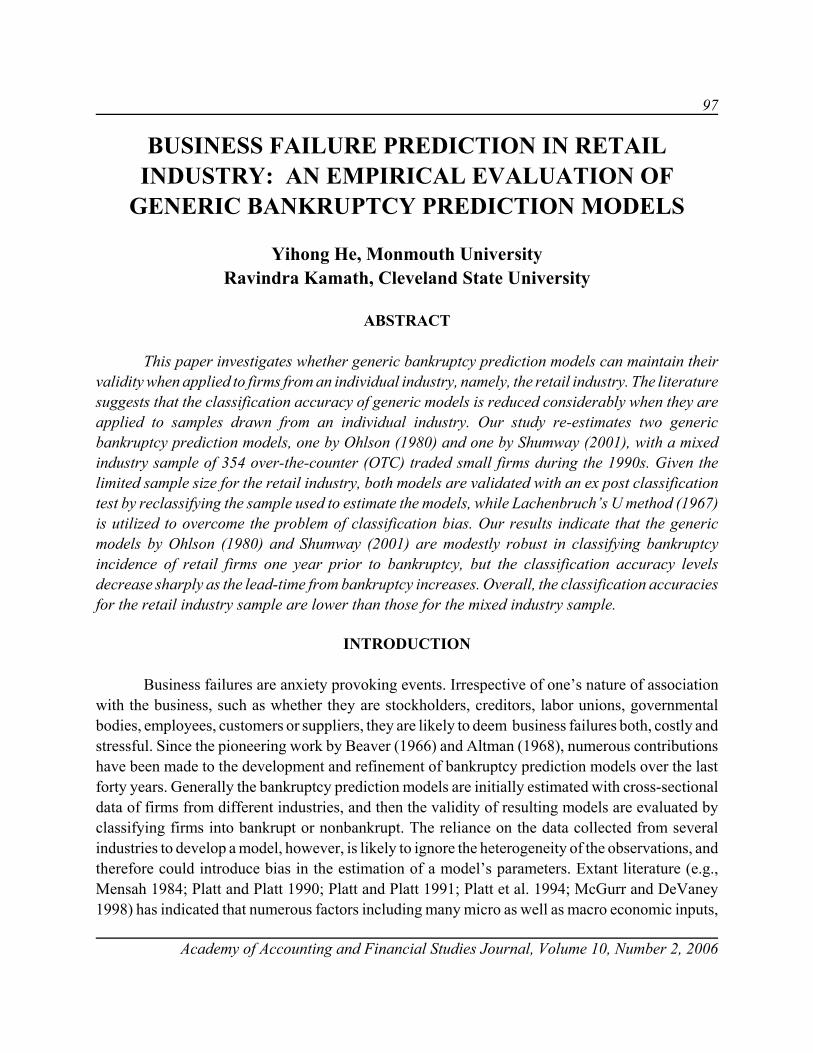
97
Academy of Accounting and Financial Studies Journal, Volume 10, Number 2, 2006
BUSINESS FAILURE PREDICTION IN RETAILINDUSTRY: AN EMPIRICAL EVALUATION OF
GENERIC BANKRUPTCY PREDICTION MODELS
Yihong He, Monmouth UniversityRavindra Kamath, Cleveland State University
ABSTRACT
This paper investigates whether generic bankruptcy prediction models can maintain theirvalidity when applied to firms from an individual industry, namely, the retail industry. The literaturesuggests that the classification accuracy of generic models is reduced considerably when they areapplied to samples drawn from an individual industry. Our study re-estimates two genericbankruptcy prediction models, one by Ohlson (1980) and one by Shumway (2001), with a mixedindustry sample of 354 over-the-counter (OTC) traded small firms during the 1990s. Given thelimited sample size for the retail industry, both models are validated with an ex post classificationtest by reclassifying the sample used to estimate the models, while Lachenbruch’s U method (1967)is utilized to overcome the problem of classification bias. Our results indicate that the genericmodels by Ohlson (1980) and Shumway (2001) are modestly robust in classifying bankruptcyincidence of retail firms one year prior to bankruptcy, but the classification accuracy levelsdecrease sharply as the lead-time from bankruptcy increases. Overall, the classification accuraciesfor the retail industry sample are lower than those for the mixed industry sample.
INTRODUCTION
Business failures are anxiety provoking events. Irrespective of one’s nature of associationwith the business, such as whether they are stockholders, creditors, labor unions, governmentalbodies, employees, customers or suppliers, they are likely to deem business failures both, costly andstressful. Since the pioneering work by Beaver (1966) and Altman (1968), numerous contributionshave been made to the development and refinement of bankruptcy prediction models over the lastforty years. Generally the bankruptcy prediction models are initially estimated with cross-sectionaldata of firms from different industries, and then the validity of resulting models are evaluated byclassifying firms into bankrupt or nonbankrupt. The reliance on the data collected from severalindustries to develop a model, however, is likely to ignore the heterogeneity of the observations, andtherefore could introduce bias in the estimation of a model’s parameters. Extant literature (e.g.,Mensah 1984; Platt and Platt 1990; Platt and Platt 1991; Platt et al. 1994; McGurr and DeVaney1998) has indicated that numerous factors including many micro as well as macro economic inputs,
98
Academy of Accounting and Financial Studies Journal, Volume 10, Number 2, 2006
such as business product cycle, interest rates, and preferences for and uniqueness of capital structure,have different impact on the operations of individual industries, and consequently affect the successof a bankruptcy prediction model when applied to each industry. Accordingly, one relevant inquirywould be to ascertain if a unique bankruptcy prediction model is needed for each individual industryinstead of relying on generic models. McGurr and DeVaney (1998) have in fact recommended “…that future failure studies use single industry samples to enhance their predictive accuracy” (p.169).
The primary goal of this paper is to evaluate the effectiveness of two successful genericbankruptcy models by Ohlson (1980) and Shumway (2001) in discriminating between bankrupt andnonbankrupt firms from an individual industry, namely, the retail industry. To further controlindustry bias, this study avoids large and established conglomerate firms traded on the New YorkStock Exchange (NYSE) and/or the American Stock Exchange (AMSE), which are found in themajority of predecessor studies, since these conglomerates often operate across multiple industries.Instead, the sample of firms utilized in this empirical investigation is comprised of 354 over-the-counter (OTC) traded small firms with an average asset size of less than $37 million. Both Ohlson’s(1980) and Shumway’s (2001) models are first re-estimated with the cross-sectional data of OTCfirms. Then, the re-estimated generic models are validated by classifying the retail industry specificsample, while Lachenbruch’s U method (1967) is adopted to overcome the problem of classificationbias.
Our study extends the previous work, while offering some distinguishing features. First, asdiscussed above, the sample consists of a group of small OTC firms. Only the firms with assets lessthan $130 million are included in this study. The average assets of the bankrupt firms and thenonbankrupt firms are $36.4 million and $35.9 million, respectively. Furthermore, by limiting thefirm size to this magnitude, we have increased the probability that our sample firms belong to oneunique industry (e.g., the retail industry) rather than operating across multiple industries. Second,we contribute to the bankruptcy prediction studies of individual industries by introducingLachenbruch’s U method (1967), which is utilized to examine the possible classification bias, whilesuch bias is not taken into consideration by the existing relevant literature. Furthermore, the validityof models is tested up to three years prior to bankruptcy. Third, this study spans over just the decadeof the 1990s, and as a result, reduces the plaguing issue of extracting and pooling the data fromseveral decades. The narrow window of the study coupled with the re-estimation of the two modelsalso helps in reducing the “time bias” (McGurr and DeVaney 1998). Fourth, the sample of 354mixed industry firms in this examination is considerably larger than those in most previous studies.The process of re-estimating models with the relatively large sample size should enhance thecapturing of the temporal nature of the data so as to improve the reliability of the models forvalidation test. Fifth, the process of matching of bankrupt and nonbankrupt firms is based on threedimensions, namely, the asset size, the industry and the timing of the financial reporting.
The remaining paper is organized in five sections. A brief review of the relevant literatureis the subject of the second section. The methodology and the data utilized are described in the third
99
Academy of Accounting and Financial Studies Journal, Volume 10, Number 2, 2006
section. The empirical findings are discussed in the fourth section. The last section contains asummary of the paper.
RELEVANT LITERATURE
Some of the earliest studies comparing failed and nonfailed firms can be traced to the 1930sdue to the experience of the depression. Beaver (1966, 1968) utilized univariate analysis approachto determine the ability of financial ratios to predict firm failure. Using multivariate discriminantanalysis (MDA), Altman’s bankruptcy prediction model (1968) relied on a linear combination offive financial ratios from the data of sample firms one year prior to bankruptcy. A composite indexcalled Z-score was used to classify bankrupt and nonbankrupt firms. The MDA method has alsobeen utilized by Deakin (1972), Edmister (1972) and Blum (1974), among others.
Recent bankruptcy prediction studies apply the logistic regression analysis (logit) toovercome the potential deficiencies of the MDA technique (Eisenbeis 1977). While the variablecoefficients in a discriminant analysis have a limited use, the coefficients of variables in a logitfunction are interpretable. Ohlson (1980), Zavgren (1985), Gentry et al. (1985), Platt and Platt(1990, 1994), Shumway (2001), He, et al. (2005), and He and Kamath (2005) are some examplesof studies which have utilized the logit methodology. Ohlson’s bankruptcy prediction model (1980)relied on eight financial ratios, representing liquidity, profitability, leverage and solvency. Theclassification results show that Ohlson’s model was able to identify about 88 percent of 105bankrupt firms accurately one year before bankruptcy.
Over time, the wisdom of relying solely on financial statement based ratios to evaluate thefinancial health of any business was challenged. Zavgren (1985), for example, was skeptical aboutthe capability of financial ratios to capture some of the dynamic firm-specific attributes, given thepresence of time lag in receiving the financial information. Such concerns led to investigations ofrelationship between market behavior and bankruptcy incidence by Aharony et al. (1980), Clark andWeinstein (1983), Katz et al. (1985), and Queen and Roll (1987). Given a semi-strong efficientmarket, the capital market mechanism might be better suited for broader financial and nonfinancialinformation, such as solvency deterioration, sales growth decline, or global competition. As a result,the market should be able to assimilate such unfavorable information in a real time, and will alterthe prices of securities of any firm to account for the likelihood of impending troubled days ahead,possibly, well before the eventual bankruptcy. The findings in event studies conducted by Aharonyet al. (1980) and Clark and Weinstein (1983) revealed that stock returns became significantlynegative about three years before the bankruptcy declaration.
Shumway’s bankruptcy prediction model (2001) successfully illustrated the benefits ofteaming financial statement based ratio variables with the market driven variables for the purposesof predicting bankruptcy. The two market variables in the study exhibited strong segregating abilityalong with the two financial ratios, while displaying low correlations among variables. Shumway’s
100
Academy of Accounting and Financial Studies Journal, Volume 10, Number 2, 2006
model reported higher prediction accuracy one year before bankruptcy for a holdout sample, ascompared to the benchmark models, which are solely based on financial statement ratios.
By and large, that the bankruptcy prediction models have been developed using cross-sectional data from different industries, the question about their effectiveness in distinguishingbankrupt firms from nonbankrupt firms for industry specific samples has been raised. Platt and Platt(1990) recommended that industry-relative ratios should be used in lieu of the absolute financialratios for the purposes of model development. The authors contended that such a considerationwould produce better classification rates as the industry-relative ratios help stabilize the predictiveability of the model. Altman (1993), however, did not embrace the industry-relative ratio conceptfor the purpose at hand because of the time lag in obtaining the industry relative data.
McGurr and DeVaney (1998) evaluated the effectiveness of five well-known modelsdeveloped with the mixed industry data in classifying bankruptcy for a sample of retail firms. Thefindings confirmed the authors’ assertion in that the generic models are likely to be less successfulin discriminating between bankrupt and nonbankrupt firms from the retail industry, as compared tothe classification results reported for the mixed industry samples in the original studies. Theyconcluded that “… mixed industry failure prediction models appear to have a limited usefulness ina review of retail firm financial health due to the effect of industry, population, and time biases”(p.175).
He and Kamath (2005) attempted to test the McGurr and DeVaney contention with animproved methodology using re-estimated generic models to predict bankruptcy for a holdoutsample of firms belonging to the Equipment and Machinery Manufacturing (EMM) industry. Theempirical findings showed that the models performed marginally better for a holdout sample of firmsfrom the EMM industry than for the mixed industry holdout sample, up to three years prior tobankruptcy, and thereby contradicted the commonly held view.
METHODOLOGY AND DATA
Models and Variables
The present study can be viewed as an extension of the McGurr and DeVaney study (1998)because both studies focus on the retail industry. The primary objective here is to examine theeffectiveness of two generic bankruptcy prediction models estimated with the mixed industry sampledata in discriminating between bankrupt and nonbankrupt firms from an individual industry. Twoselected models are by Ohlson (1980) and by Shumway (2001) utilizing the logit methodology.While Ohlson’s model utilizes eight financial statement based ratios, Shumway’s model uses acombination of two financial ratios and two market driven measures. The variables of these twomodels are described in Table 2. The size variable, which was used by both models and found to be
101
Academy of Accounting and Financial Studies Journal, Volume 10, Number 2, 2006
a significant predictor in both original studies, is not used in our estimations because the size effectis controlled through the pair matching procedure adopted in this study.
Sample and Data
For a failed firm to be considered for inclusion in this study, it has to file bankruptcy duringthe period of 1990-1999, the firm was traded on OTC market and the total assets of the firm are lessthan $130 million one year before bankruptcy. The search for the bankrupt OTC firms and theirpetition dates is conducted with the help of Moody’s OTC Industrial Manual, Moody’s OTCUnlisted Manual and National Stock Summary. Financial firms (SIC code 6000-6999) are excludedfrom our sample due to differences in accounting reporting.
The financial data needed to compute the variables for the two chosen models comes fromthe Compustat Research File, Moody’s OTC Industrial Manual and Moody’s OTC Unlisted Manual.The market data of Shumway’s model is collected from the CRSP, Compustat and OTC Daily StockPrice Record by Standard & Poor. The Industrial Index of OTC Market Indicator collected fromOTC Daily Stock Prices Record by Standard & Poor is used as the proxy for the market index until1993 and the Industrial Index of Nasdaq Market Indicator collected from Nasdaq Daily Stock PricesRecord by Standard & Poor is used as the proxy for the post-1993 period.
In an attempt to predict a firm’s bankruptcy up to three years prior to bankruptcy, one yearpre-bankruptcy financial data is defined as the data within a firm’s most recent fiscal year but withno less than six months prior to the date of its bankruptcy filing. Thus, for a firm with a December31 fiscal year ending, and filing for bankruptcy on March 20, 1999, the financial data of one yearbefore bankruptcy would be the data for the year ending December 31, 1997. If the bankruptcy filinghad taken place on August 6, 1999, the financial data of the year ending December 31, 1998 wouldbe adopted as the one year before bankruptcy data. Similarly, the market data would also be laggedat least six months before bankruptcy filing. Even though the 6-month lag could have an undesirableeffect on the predictive power of the models, such a convention we believe, substantially increasesits practicality and therefore its appeal to practitioners.
Matching Criteria
A nonbankrupt firm is matched with a bankrupt firm by industry, asset size and fiscal year.The industry matching is accomplished by the same first two digits of the SIC codes of the firms.Our restriction of the OTC firm with the asset size less than $130 million itself lends strong supportfor size matching. Utmost efforts are made to match each nonbankrupt firm as closely as possibleto a bankrupt one as per book value of total assets one year before bankruptcy. To assure that thefinancial statements are reported by the matching firms in the same period, the fiscal year ends ofthe matching nonbankrupt firms have to be within three months of the same for the bankrupt firms.

102
Academy of Accounting and Financial Studies Journal, Volume 10, Number 2, 2006
Resulting Sample
Our final overall sample consists of 354 OTC firms, i.e., 177 matched pairs of bankrupt andtheir counterpart nonbankrupt firms. The asset distributions of the two groups are summarized inPanel A of Table 1. The average assets of the bankrupt firms are $36.41 million as compared to$35.93 million of their counterparts. Of the 354 matched firms, about 75 percent of the firms havetotal assts of less than $50 million, and 92 percent of the firms have assets of less than $100 million,one year before bankruptcy. In comparison, the sample in the McGurr and DeVaney study (1998)consisted of 56 bankrupt retail firms from 1989 to 1993. The asset size of sample companies in theirstudy ranged widely from $3.2 million to $8.3 billion. In some of the retail groups, the mean totalassets of the failed and nonfailed firms deviated by more than 75 percent (see Table 2 of McGurrand DeVaney, 1998). Furthermore, due to the small sample size, they were not able to re-estimatethe original five models developed with the data utilized from the 1940s to the 1980s. As a result,it is not clear if the loss of classification accuracy of these models in retail industry was a result ofthe industry bias or time bias of test period or both.
Table 1. Asset Distribution of OTC Sample Firms, 1990-1999
Panel A – Asset Distribution of the Overall Sample ($000)
Number Minimum Maximum Mean StandardDeviation
p-value
Bankrupt firms 177 1278 128290 36405 33284
Nonbankrupt firms 177 2463 127990 35930 30980
t-test of size difference 0.889
Panel B – Asset Distribution of the Retail Industry Sample ($000)
Number Minimum Maximum Mean StandardDeviation
p-value
Bankrupt firms 20 5273 126926 58223 39820
Nonbankrupt firms 20 4802 127295 52623 38491
t-test of size difference 0.654
As noted, this paper focuses on prediction of bankruptcy in an individual industry, the retailindustry (SIC code 5200-5999). The sub-sample is comprised of 40 retail firms. The asset sizedistributions are shown in Panel B of Table 1. The average assets of the bankrupt firms in the retailindustry are $58.22 million as compared to $52.62 million of the nonbankrupt firms. The t-statisticshows that paired firms are matched closely in size, for the overall sample as well as the retailindustry sub-sample.
103
Academy of Accounting and Financial Studies Journal, Volume 10, Number 2, 2006
The He and Kamath study (2005) was able to utilize the re-estimated generic models topredict bankruptcy for a holdout sample of the EMM industry on an ex ante basis, since they hada larger EMM industry sub-sample. However, the sub-sample of 40 retail firms in this study is notlarge enough to be split in order to accommodate a holdout sample for prediction purpose.Accordingly, the entire sample of 354 firms is used to re-estimate the models. These models are thenused to reclassify the 354 mixed industry firms and the 40 retail industry firms, respectively, on anex post basis. Given the existence of numerous unique aspects of the retail industry as compared tothe other industries, our a priori expectation is that these two generic models by Ohslon (1980) andShumway (2001) will not be able to distinguish bankrupt firms from nonbankrupt firms of the retailindustry, as effectively as for the firms from the mixed industries.
EMPIRICAL FINDINGS
Re-estimation of the Models
Since the data setting in this study is different from the ones in the original studies of Ohlson(1980) and Shumway (2001), we first re-estimate these models by using the sample of 354 mixedindustry firms in 1990s. The re-estimated Ohlson and Shumway models with the data of one yearprior to bankruptcy are presented in Table 2.
The findings of Table 2 indicate that both re-estimated models with 354 mixed industry firmsare statistically significant at the 0.01 level one year prior to bankruptcy, and thus, display a strongability to discriminate bankrupt firms from nonbankrupt firms. Further analysis of the results forOhlson’s model shows that the four variables are statistically insignificant, which are denoted in thetable by underlining the p-values. The results of Shumway’s model appear to be more favorable. Thesigns of the coefficients of each of the four variables display the expected relationships with theprobability of bankruptcy, and the chi-square statistics indicate that all four variables in this modelcontribute in a statistically significant fashion toward bankruptcy prediction.
Validation of the Models
Given that there are only 40 firms from the retail industry in our sample, we do not have theluxury of utilizing a holdout sample for the prediction test. Accordingly, the re-estimated modelsare validated by classification test for the retail industry. Both Ohlson’s and Shumway’s models,which are re-estimated with one year prior to bankruptcy data of 354 mixed industry firms of the1990-1999 period in Table 2, are now used to reclassify the 354 mixed industry firms and the 40retail industry firms for one, two and three years before bankruptcy, respectively. The classificationresults of each model are reported in Tables 3 and 4.
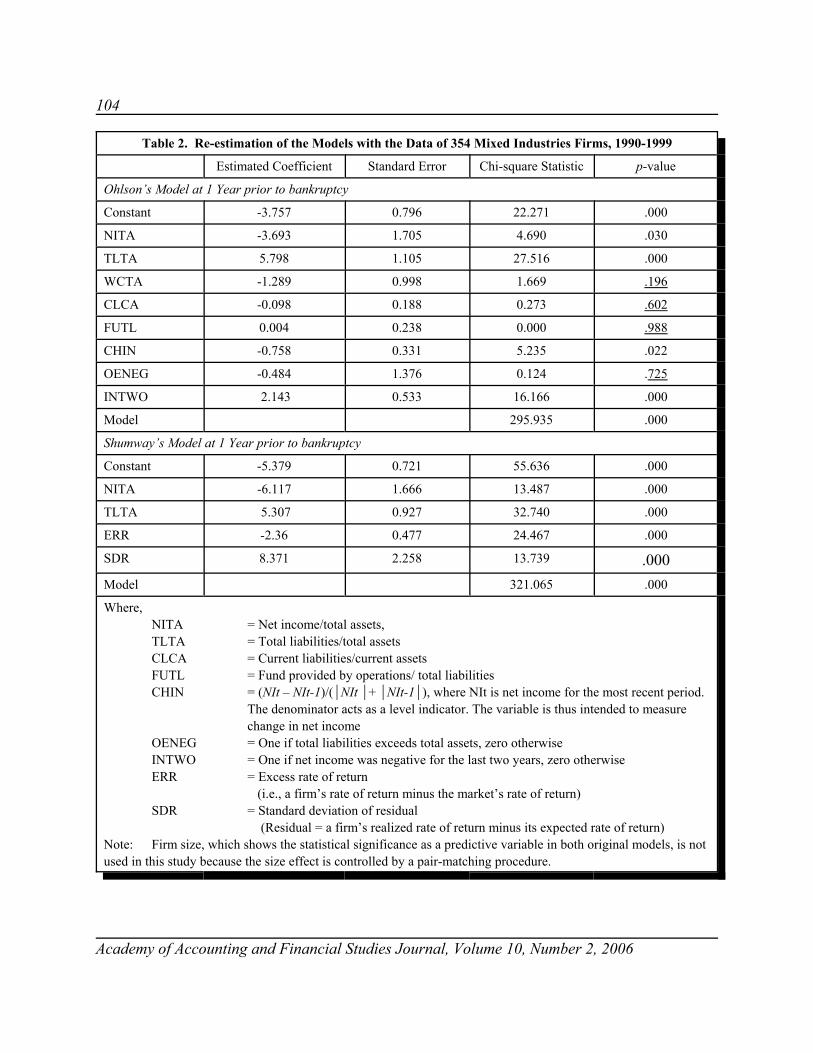
104
Academy of Accounting and Financial Studies Journal, Volume 10, Number 2, 2006
Table 2. Re-estimation of the Models with the Data of 354 Mixed Industries Firms, 1990-1999
Estimated Coefficient Standard Error Chi-square Statistic p-value
Ohlson’s Model at 1 Year prior to bankruptcy
Constant -3.757 0.796 22.271 .000
NITA -3.693 1.705 4.690 .030
TLTA 5.798 1.105 27.516 .000
WCTA -1.289 0.998 1.669 .196
CLCA -0.098 0.188 0.273 .602
FUTL 0.004 0.238 0.000 .988
CHIN -0.758 0.331 5.235 .022
OENEG -0.484 1.376 0.124 .725
INTWO 2.143 0.533 16.166 .000
Model 295.935 .000
Shumway’s Model at 1 Year prior to bankruptcy
Constant -5.379 0.721 55.636 .000
NITA -6.117 1.666 13.487 .000
TLTA 5.307 0.927 32.740 .000
ERR -2.36 0.477 24.467 .000
SDR 8.371 2.258 13.739 .000Model 321.065 .000
Where,NITA = Net income/total assets,TLTA = Total liabilities/total assetsCLCA = Current liabilities/current assetsFUTL = Fund provided by operations/ total liabilitiesCHIN = (NIt – NIt-1)/(*NIt *+ *NIt-1*), where NIt is net income for the most recent period.
The denominator acts as a level indicator. The variable is thus intended to measurechange in net income
OENEG = One if total liabilities exceeds total assets, zero otherwiseINTWO = One if net income was negative for the last two years, zero otherwiseERR = Excess rate of return
(i.e., a firm’s rate of return minus the market’s rate of return)SDR = Standard deviation of residual
(Residual = a firm’s realized rate of return minus its expected rate of return)Note: Firm size, which shows the statistical significance as a predictive variable in both original models, is notused in this study because the size effect is controlled by a pair-matching procedure.
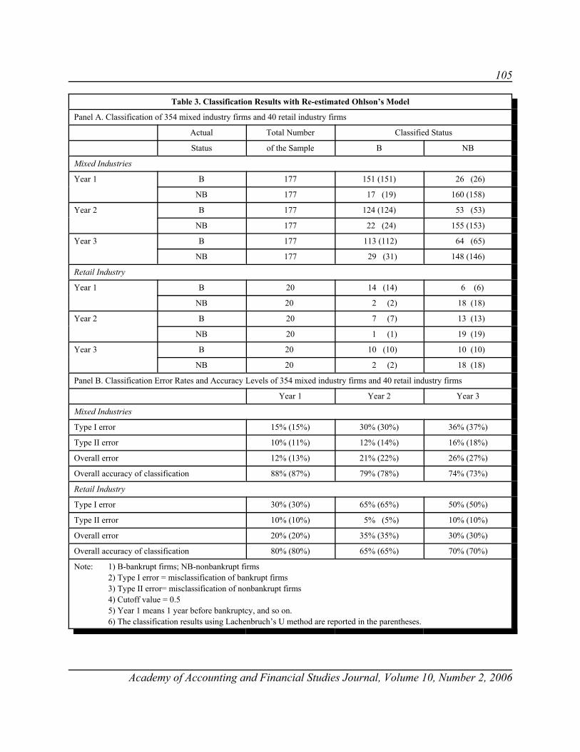
105
Academy of Accounting and Financial Studies Journal, Volume 10, Number 2, 2006
Table 3. Classification Results with Re-estimated Ohlson’s Model
Panel A. Classification of 354 mixed industry firms and 40 retail industry firms
Actual Total Number Classified Status
Status of the Sample B NB
Mixed Industries
Year 1 B 177 151 (151) 26 (26)
NB 177 17 (19) 160 (158)
Year 2 B 177 124 (124) 53 (53)
NB 177 22 (24) 155 (153)
Year 3 B 177 113 (112) 64 (65)
NB 177 29 (31) 148 (146)
Retail Industry
Year 1 B 20 14 (14) 6 (6)
NB 20 2 (2) 18 (18)
Year 2 B 20 7 (7) 13 (13)
NB 20 1 (1) 19 (19)
Year 3 B 20 10 (10) 10 (10)
NB 20 2 (2) 18 (18)
Panel B. Classification Error Rates and Accuracy Levels of 354 mixed industry firms and 40 retail industry firms
Year 1 Year 2 Year 3
Mixed Industries
Type I error 15% (15%) 30% (30%) 36% (37%)
Type II error 10% (11%) 12% (14%) 16% (18%)
Overall error 12% (13%) 21% (22%) 26% (27%)
Overall accuracy of classification 88% (87%) 79% (78%) 74% (73%)
Retail Industry
Type I error 30% (30%) 65% (65%) 50% (50%)
Type II error 10% (10%) 5% (5%) 10% (10%)
Overall error 20% (20%) 35% (35%) 30% (30%)
Overall accuracy of classification 80% (80%) 65% (65%) 70% (70%)
Note: 1) B-bankrupt firms; NB-nonbankrupt firms2) Type I error = misclassification of bankrupt firms3) Type II error= misclassification of nonbankrupt firms4) Cutoff value = 0.55) Year 1 means 1 year before bankruptcy, and so on.6) The classification results using Lachenbruch’s U method are reported in the parentheses.
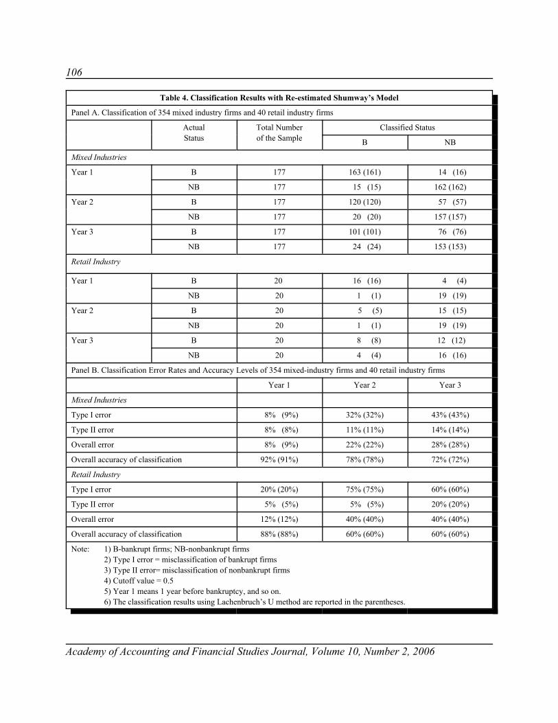
106
Academy of Accounting and Financial Studies Journal, Volume 10, Number 2, 2006
Table 4. Classification Results with Re-estimated Shumway’s Model
Panel A. Classification of 354 mixed industry firms and 40 retail industry firms
ActualStatus
Total Numberof the Sample
Classified Status
B NB
Mixed Industries
Year 1 B 177 163 (161) 14 (16)
NB 177 15 (15) 162 (162)
Year 2 B 177 120 (120) 57 (57)
NB 177 20 (20) 157 (157)
Year 3 B 177 101 (101) 76 (76)
NB 177 24 (24) 153 (153)
Retail Industry
Year 1 B 20 16 (16) 4 (4)
NB 20 1 (1) 19 (19)
Year 2 B 20 5 (5) 15 (15)
NB 20 1 (1) 19 (19)
Year 3 B 20 8 (8) 12 (12)
NB 20 4 (4) 16 (16)
Panel B. Classification Error Rates and Accuracy Levels of 354 mixed-industry firms and 40 retail industry firms
Year 1 Year 2 Year 3
Mixed Industries
Type I error 8% (9%) 32% (32%) 43% (43%)
Type II error 8% (8%) 11% (11%) 14% (14%)
Overall error 8% (9%) 22% (22%) 28% (28%)
Overall accuracy of classification 92% (91%) 78% (78%) 72% (72%)
Retail Industry
Type I error 20% (20%) 75% (75%) 60% (60%)
Type II error 5% (5%) 5% (5%) 20% (20%)
Overall error 12% (12%) 40% (40%) 40% (40%)
Overall accuracy of classification 88% (88%) 60% (60%) 60% (60%)
Note: 1) B-bankrupt firms; NB-nonbankrupt firms2) Type I error = misclassification of bankrupt firms3) Type II error= misclassification of nonbankrupt firms4) Cutoff value = 0.55) Year 1 means 1 year before bankruptcy, and so on.6) The classification results using Lachenbruch’s U method are reported in the parentheses.
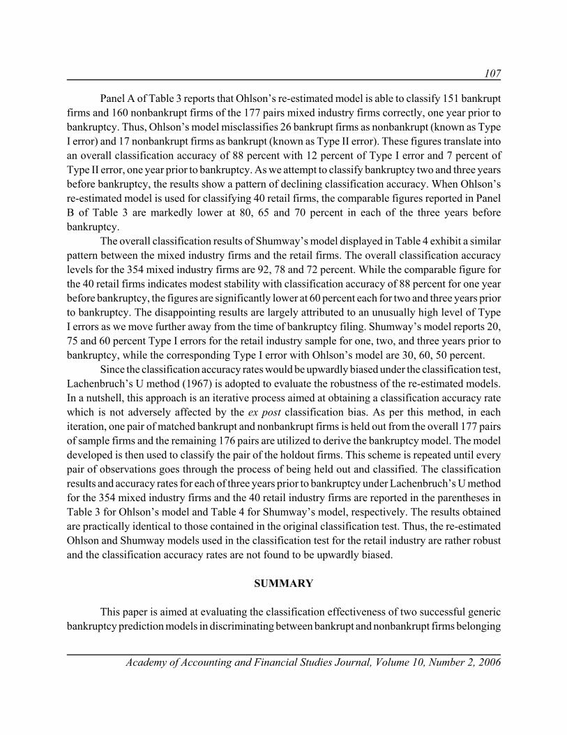
107
Academy of Accounting and Financial Studies Journal, Volume 10, Number 2, 2006
Panel A of Table 3 reports that Ohlson’s re-estimated model is able to classify 151 bankruptfirms and 160 nonbankrupt firms of the 177 pairs mixed industry firms correctly, one year prior tobankruptcy. Thus, Ohlson’s model misclassifies 26 bankrupt firms as nonbankrupt (known as TypeI error) and 17 nonbankrupt firms as bankrupt (known as Type II error). These figures translate intoan overall classification accuracy of 88 percent with 12 percent of Type I error and 7 percent ofType II error, one year prior to bankruptcy. As we attempt to classify bankruptcy two and three yearsbefore bankruptcy, the results show a pattern of declining classification accuracy. When Ohlson’sre-estimated model is used for classifying 40 retail firms, the comparable figures reported in PanelB of Table 3 are markedly lower at 80, 65 and 70 percent in each of the three years beforebankruptcy.
The overall classification results of Shumway’s model displayed in Table 4 exhibit a similarpattern between the mixed industry firms and the retail firms. The overall classification accuracylevels for the 354 mixed industry firms are 92, 78 and 72 percent. While the comparable figure forthe 40 retail firms indicates modest stability with classification accuracy of 88 percent for one yearbefore bankruptcy, the figures are significantly lower at 60 percent each for two and three years priorto bankruptcy. The disappointing results are largely attributed to an unusually high level of TypeI errors as we move further away from the time of bankruptcy filing. Shumway’s model reports 20,75 and 60 percent Type I errors for the retail industry sample for one, two, and three years prior tobankruptcy, while the corresponding Type I error with Ohlson’s model are 30, 60, 50 percent.
Since the classification accuracy rates would be upwardly biased under the classification test,Lachenbruch’s U method (1967) is adopted to evaluate the robustness of the re-estimated models.In a nutshell, this approach is an iterative process aimed at obtaining a classification accuracy ratewhich is not adversely affected by the ex post classification bias. As per this method, in eachiteration, one pair of matched bankrupt and nonbankrupt firms is held out from the overall 177 pairsof sample firms and the remaining 176 pairs are utilized to derive the bankruptcy model. The modeldeveloped is then used to classify the pair of the holdout firms. This scheme is repeated until everypair of observations goes through the process of being held out and classified. The classificationresults and accuracy rates for each of three years prior to bankruptcy under Lachenbruch’s U methodfor the 354 mixed industry firms and the 40 retail industry firms are reported in the parentheses inTable 3 for Ohlson’s model and Table 4 for Shumway’s model, respectively. The results obtainedare practically identical to those contained in the original classification test. Thus, the re-estimatedOhlson and Shumway models used in the classification test for the retail industry are rather robustand the classification accuracy rates are not found to be upwardly biased.
SUMMARY
This paper is aimed at evaluating the classification effectiveness of two successful genericbankruptcy prediction models in discriminating between bankrupt and nonbankrupt firms belonging
108
Academy of Accounting and Financial Studies Journal, Volume 10, Number 2, 2006
to an individual industry. The retail industry is the focus of this inquiry similar to that of McGurran DeVaney (1998). To fulfill our goal, we utilize financial statement ratio based model by Ohlson(1980) and financial and market information based model by Shumway (2001). The sample in thisempirical study is made up of 354 mixed industry firms, including 40 retail firms, traded on OTCmarket over the recent decade of 1990s. The average assets of 354 firms are less than $37 million,one year prior to bankruptcy. Each of the 177 bankrupt firms is matched with a nonbankrupt firmfrom the same industry of comparable asset size as well as the timing of its financial reports.
The Ohlson and Shumway models are re-estimated with data of the entire sample of 354mixed industry firms from the 1990-1999 period. These models are then used to classify theprobability of bankruptcy of the 354 mixed industry firms and the 40 retail industry firms,respectively. Our study improves the classification methodology by utilizing Lachenbruch’s Umethod to overcome the potential introduction of an upward bias in the classification process.
Begley et al. (1996) concluded that the re-estimated models by Altman (1968) and Ohlson(1980) with data in a recent period could not classify the bankrupt firms as well as the respectivemodels had in the original studies. Our results are definitely not in agreement with Begley et al.(1996). Instead, we find that with the recent data of small OTC firms, the re-estimated models ofboth Ohlson (1980) and Shumway (2001) display classification accuracies which are very muchcomparable to those reported in the original studies.
The classification accuracy levels of both models for the retail industry, however, aresignificantly lower than those for the mixed industries, particularly, as the lead-time frombankruptcy increases. The finding that the usefulness of generic bankruptcy prediction models isreduced when applied to an individual industry matches with the priori expectation. McGurr andDeVaney (1998) had suggested that the possible causes of such reductions are “industry, population,and time biases”. While the population bias can never be fully eliminated, the time bias was wellcontrolled due to the short time span of the data used in the study. Thus, our methodology waspredominantly geared toward evaluating the industry bias. Accordingly, we find that the mixedindustry based bankruptcy prediction models lose their effectiveness substantially when applied toan individual industry, such as, the retail industry.
Overall, the findings for the retail industry in our study concur with the expectation that thegeneric bankruptcy prediction models would lose predictive accuracy when applied to an individualindustry, but are at odds with the results presented by He and Kamath (2005), where they reportedimpressive classification and prediction accuracies for the equipment and machinery manufacturing(EMM) industry with help of generic models. One possible explanation of our finding is that the re-estimated models were highly influenced by the large percentage of manufacturing firms in thesample. The breakdown of 354 sample firms shows that only 130 (37 percent) firms are from serviceindustries, including 40 retail firms (11 percent). Given the diametrically opposite findings of ourstudy to what reported by He and Kamath (2005), further research is called for in the area of
109
Academy of Accounting and Financial Studies Journal, Volume 10, Number 2, 2006
applying generic bankruptcy prediction models to classify/predict the bankruptcy of firms fromindividual industries.
REFERENCES
Aharony, H. J., P. Charles & I. Swary, (1980). An analysis of risk and return characteristics of corporate bankruptcyusing capital market data. Journal of Finance 35, 1001-1016.
Altman, E. I, (1968). Financial ratios, discriminant analysis and the prediction of corporate bankruptcy. Journal ofFinance 23, 589-609.
Altman, E. I, (1993). Corporate financial distress and bankruptcy: a complete guide to predicting and avoiding distressand profiting from bankruptcy, Second Edition (New York: John Wiley & Sons, Inc)
Beaver, W. H, (1966). Financial ratios as predictors of failure. Journal of Accounting Research 4 (supplement), 71-111.
Beaver, W. H, (1968). Market prices, financial ratios, and the prediction of failure. Journal of Accounting Research 6,179-192.
Begley, J., M. Jin & S. Watts, (1996). Bankruptcy classification errors in the 1980s: an empirical analysis of Altman’sand Ohlson’s models. Review of Accounting Studies 1, 267-284.
Blum, M, (1974). Failing company discriminant analysis. Journal of Accounting Research 12, 1-25.
Clark, T. A. & M. I. Weinstein, (1983). The behavior of the common stock of bankrupt firms. Journal of Finance 38,489-504.
Deakin, E. B, (1972). A discriminant analysis of predictors of business failure. Journal of Accounting Research 10, 167-179.
Edmister, R. O, (1972). An empirical test of financial ratio analysis for small business failure prediction. Journal ofFinancial and Quantitative Analysis 7, 1477-1493.
Eisenbeis, R. A, (1977). Pitfalls in the application of discriminant analysis in business, finance, and economics. Journalof Finance 32, 875-900.
Gentry, J. A., P. Newbold and D. T. Whitford, (1985). Classifying bankrupt firms with funds flow components. Journalof Accounting Research 23, 146-160.
He, Y., R. Kamath, & H. Meier, (2005). An Empirical Evaluation of Bankruptcy Prediction Models for Small Firms.Academy of Accounting and Financial Studies Journal 9 (1), 1-23.
110
Academy of Accounting and Financial Studies Journal, Volume 10, Number 2, 2006
He, Y., & R. Kamath, (2005). Bankruptcy Prediction of Small Firms in Individual Industries with the Help of MixedIndustry Models. Asia-Pacific Journal of Accounting & Economics 12 (1), 19-36.
Katz, S., S. Lilien & B. Nelson, (1985). Stock market behavior around bankruptcy model distress and recoverypredictions. Financial Analysts Journal 41, 70-74.
Lachenbruch, P.A, (1967). An almost unbiased method of obtaining confidence intervals for the probability ofmisclassification in discriminant analysis. Biometrics 23, 639-645.
McGurr, P. T. & S. A. DeVaney, (1998). Predicting business failure of retail firms: an analysis using mixed industrymodels. Journal of Business Research 43, 169-176.
Mensah, Y. M, (1984). An examination of the stationarity of multivariate bankruptcy prediction models: amethodological study. Journal of Accounting Research 22 (1), 380-395.
Ohlson, J. A, (1980). Financial ratios and the probabilistic prediction of bankruptcy. Journal of Accounting Research18, 109-131.
Platt, H. D. & M. B. Platt, (1990). Development of a class of stable predictive variables: the case of bankruptcyprediction. Journal of Business, Finance and Accounting 17 (1), 31-51.
Platt, H. D. & M. B. Platt, (1991). A note on the use of industry-relative ratios in bankruptcy prediction. Journal ofBanking and Finance 15, 1183-1194.
Platt, H. D., M. B. Platt & J. G. Pedersen, (1994). Bankruptcy discrimination with real variables. Journal of Business,Finance and Accounting 21 (4), 491-510.
Queen, M. and R. Roll, (1987). Firm mortality: using market indicators to predict survival. Financial Analysts Journal43, 9-26.
Shumway, T, (2001). Forecasting bankruptcy more accurately: a simple hazard model. Journal of Business 74, 101-124.
Zavgren, C. V, (1985). Assessing the vulnerability of failure of American industrial firms: a logistic analysis. Journalof Business, Finance and Accounting 12, 19-45.
111
Academy of Accounting and Financial Studies Journal, Volume 10, Number 2, 2006
A REVIEW OF CIVIL WAR TAX LEGISLATIONAND ITS INFLUENCE ON THE CURRENT
U.S. INCOME TAX SYSTEM
Darwin L. King, St. Bonaventure UniversityMichael J. Fischer, St. Bonaventure University
Carl J. Case, St. Bonaventure University
ABSTRACT
The purpose of this paper is to review and compare income tax legislation passed during theCivil War by both the Union and the Confederacy. The major tax act for the Confederacy was titled“An Act to lay taxes for the common defense and carry on the Government of the ConfederateStates.” This legislation was passed on April 24, 1863 and represented the most comprehensive taxsystem employed by the Confederacy. The most significant Union tax law was termed the “NationalTax Law as approved June 30, 1864.” These two major pieces of legislation are compared andcontrasted by examining the types of taxes introduced, rates of tax, and various deductions andexemptions allowed.
This paper reviews the many aspects of Civil War taxation legislation that remain in effecttoday. In particular, numerous income inclusions, exclusions, and deductions found in these 1860’sacts continue to exist in our current Internal Revenue Code. These early pieces of tax legislationcontinue to provide guidance in generating tax receipts to fund our current war efforts inAfghanistan and Iraq.
INTRODUCTION
The Civil War created a desperate financial situation for both the Union and Confederategovernments. The mere reinstatement of excise taxes would not be sufficient to fund the war effortfor either side. For this reason, new types of taxes, which were considered unnecessary in the past,were enacted into law. The major innovative tax of the period was the individual income tax. Thistax was based on concepts that the typical taxpayer was not familiar with and did not readilyunderstand including the principles of self-assessment and voluntary compliance. However, boththe Union and Confederacy realized that a personal income tax was the only alternative that wouldproduce the large amount of funds required to fund military operations.
The Union enacted tax legislation in 1861, 1862, and 1864 with each version becoming morecomprehensive in nature. When the Civil War began, Congress passed the Revenue Act of 1861 on

112
Academy of Accounting and Financial Studies Journal, Volume 10, Number 2, 2006
August 5, which proved to be a poor first attempt at tax legislation. The law reinstated excise taxeson various goods and also introduced a tax on personal incomes (U.S. Treasury Fact Sheet, OPC-77). The income tax rate of 3% was applied to income in excess of $800 per year (the exemptionamount). This exclusion eliminated tax for all but the wealthy. For example, a private in the U.S.Army, during most of the Civil War, earned only $13 per month or under $200 per year, so he wouldpay no income taxes (Revised Regulations for the Army of the United States, 1861).
Although the 1861 act committed the country to income taxation, there were no income taxesactually assessed under this law (Hill, 1894). The 1861 income tax was never enforced or collectedand was replaced by new legislation on July 1, 1862. The first major Internal Revenue Act in 1862required taxpayers “to make a list or return” of the items of income that were being taxed (Doris,1963). An “Assistant Assessor,” who had the right to increase the amount of tax due for the year,audited the taxpayer in an effort to add credence to the system. The concept of a graduated orprogressive tax was also strange to taxpayers who were comfortable with fixed rate excise taxes.
The new concepts of voluntary compliance, self-assessment, and progressive tax ratescreated a system that the typical taxpayer found difficult to understand and comply with. During thespring of 1862, the Federal government’s monetary needs were escalating as the public debtincreased about two million dollars per day (Ibid). On July 1, 1862, the Revenue Act of 1862 waspassed which included excise taxes on playing cards, gunpowder, feathers, telegrams, leather,pianos, yachts, billiard tables, perfumes, drugs, patent medicines, beer, and whiskey (U.S. TreasuryFact Sheet, OPC-77). This new act retained the personal income tax included in the 1861 law withsome significant adjustments.
The income tax regulations in the 1862 law were revised to include the concept of “abilityto pay.” This was the first situation where progressive tax rates were employed by the Federalgovernment. Personal incomes from $600 to $10,000 were taxed at the prior year’s 3% rate. Fortaxpayers with incomes in excess of $10,000, the tax rate increased to 5% (Ibid). A rate of 7-½ %was initially included in the bill but was removed because many in Congress felt that rate to beexcessive (Hill, 1894). Taxpayers were given a $600 standard deduction, which eliminated incometax for the typical laborer.
An additional feature of the 1862, and later the 1864 act, was based on the principle of“stoppage at the source.” This new concept required employers to regularly withhold income taxesfrom employees who had income in excess of $600 per year. This concept was also extended to thepayers of interest and dividends. By using this technique, the government was able to quickly extracttaxes from the general public for use in the war effort. The 1862 act created the Office of theCommissioner of Internal Revenue in the Treasury Department (Parnell, 1980). This created theoriginal organizational structure for our current Internal Revenue Service.
An interesting feature of the 1862 act was that income was calculated based on the calendaryear. Initially the assessment was due by May 1st of the following year with payment due on orbefore June 30th (Hill, 1894). This created a significant problem for the government due to the
113
Academy of Accounting and Financial Studies Journal, Volume 10, Number 2, 2006
amount of lag time before the taxpayers paid taxes. It was not until the Act of 1867 that assessmentswere due March 1st with payments expected on or before April 30th. During the Civil War periodwhen funds were desperately needed for the war effort, it was poor administration to delaycollections for such a lengthy period.
Another major problem resulting from this new form of taxation was the difficulty ofdetermining the actual income of the taxpayer. The assessor and collector relied on taxpayer’swritten lists or returns, which would have been extremely difficult to verify and audit. If a taxpayerrefused to make a list or return, the assessor was required to prepare one “according to the bestinformation based on an examination of such person or his books or accounts or any other evidence”(Ibid). This process required the assessors to play the role of private investigator. A 50% penalty wasassessed to any taxpayer who refused to prepare a list or return. If a fraudulent return was proven,the penalty increased to 100% of the tax due thereby doubling the tax liability (Ibid).
The 1862 revenue act created a foundation for additional legislation that would soon followin 1864. During the first full year of collections under the 1862 law, about twenty million dollarsof income taxes were raised. This, however, was less than the thirty million dollars collected asexcise taxes on distilled spirits (Hill, 1894).
The most significant piece of income taxation during the Civil War was the National TaxLaw approved on June 30, 1864. This legislation will be reviewed in detail and compared to theConfederate version enacted on April 24, 1863. Each of these tax laws contains major proposalsintended to raise significant amounts of money for the war effort. At this point in the war, both sidesrealized the huge costs of funding their respective armies as they moved great distances across thecountry.
The 126 page National Tax Law included much more than an income tax. Its basiccomponents, in addition to the income tax, included the following:
1. Taxes on Spirits, Ale, Beer, and Porter2. License Fees for All Professions3. Duties on Manufacturers and Products4. Legacies and Distributive Shares Tax (An estate tax)5. Stamp Duties (On a wide variety of products).
The Confederacy enacted their first tax legislation in 1861. It was simply a minor tariff actthat raised only $3.5 million dollars over four years (Tax.org, 2000). Later that year, a small directtax of ½% was introduced on real and personal property. The majority of funds raised by theConfederacy were through the issuance of bonds. A $15 million dollar bond issue sold out quicklythe same year. However, a later $100 million dollar issue sold very slowly causing cash flowproblems as the Confederacy increased its military operations.
114
Academy of Accounting and Financial Studies Journal, Volume 10, Number 2, 2006
During the first year of the war, the Confederate government raised only 2% of its revenuesthrough taxes. The vast majority of funds were generated through the issuance of treasury notes(75%) and bonds (23%) (Ibid.). The Confederacy issued over $1.5 billion in paper money, whichtended to depreciate quickly. At the same time, all of the southern states issued state, county, andcity notes. These bills were often poorly printed and served to encourage counterfeiting. Theextensive use of paper money, instead of internal taxation of the citizens, caused inflation thatexceeded 9000% in the South by the end of the war (Ibid.)
By the beginning of 1863, the Confederate government realized that a major piece of taxlegislation was required. Therefore, on April 24th, the act to “lay taxes for the common defense andcarry on the Government of the Confederate States” was enacted. This was an extremelycomprehensive package, which included an income tax, a business inventory tax, excise and licenseduties, taxes on wholesalers and retailers, and a tax-in-kind that applied to numerous agriculturalproducts. The delay in the enactment of this type of revenue producing legislation negativelyaffected the ability of the Confederacy to promptly raise needed funds for military operations.
OVERVIEW OF UNION AND CONFEDERATE TAX LEGISLATION
The comparison of the Union and Confederate tax legislation will be completed utilizing anumber of perspectives. First, a review of the basic requirements of each law will be completed.Second, details related to the individual income tax will be reviewed. Finally, the Confederate taxes-in-kind program will be studied. This unique type of tax was logical for the primarily agriculturallyoriented South.
The appendix of this paper includes tables, which compare numerous tax regulations of eachsystem. References included in this paper relate to the coding system found at the end of each table.In most cases, the section number of each piece of tax legislation serves as the supporting reference.As far as general tax information is concerned, the first consideration is to whom the tax applied.The Union act applied to “individuals, partnerships, firms, associations, and corporations” (Sec. 11).The Confederate plan was also extensive as it related to “every person, co-partnership, associationor corporation” (TB Sec.1). The Union tax legislation was enacted to continue through 1870 (Sec.119), while the Confederate law was only effective through 1865 (unless repealed sooner) (Sec. 18).Both versions of the tax legislation were enacted with a very short life expectancy.
The Union and Confederate tax acts both included penalties for false returns. Similar to thenegligence and fraud penalties that exist today, these laws contained very severe repercussions forviolations. The Union plan imposed fines of up to $1,000 or imprisonment up to one year, or both(Sec. 15). The Confederate system stated if it is found “that the statement of estimate of income andprofits rendered by the taxpayer does not contain more than 4/5 of the true and real amount of histaxable income and profits” the taxpayer can be liable for taxes due plus a penalty of an additional10% (Sec. 8).
115
Academy of Accounting and Financial Studies Journal, Volume 10, Number 2, 2006
Each side also included penalties for nonpayment of tax. The Union act required a 10%additional tax penalty if the payment was from one to ten days late. The penalty increased after tendays as the tax collector charged a twenty-cent issue fee plus mileage of four cents per mile to thetaxpayer’s location in an attempt to settle the debt. The collector was a government agent whoactually received the tax dollars and deposited them to the taxpayer’s account with the government.The collector, within twenty days after receiving the annual collection list from the assessors, hadto “give notice, by advertisement published in each county in his collection district in one newspaperprinted in that county and in at least four public places in each county of the unpaid tax of eachdelinquent taxpayer” (Sec. 28). After an additional ten days, if the tax remained unpaid, the collectorhad the right to “seize property and sell the goods, chattels, or effects of the persons” owing the tax(Ibid.).
The Confederate legislation was evidently patterned after the Union act because it alsoincluded an additional 10% penalty for taxes paid after the due date. Within twenty days thecollector was to inform individual taxpayers of their disregard to pay taxes. After an additional tendays, the collector for the Confederacy also had the right to seize property and sell it to pay the tax(AA Sec. 16). Both sides attempted to collect taxes due within a fairly short time utilizing the threatthat the taxpayer’s property could be seized and sold to make the required payment.
If personal property was sold at auction to pay the tax, both Union and Confederate actsutilized a similar procedure. The Union plan allowed the government to keep all proceeds that“cover the tax due, necessary and reasonable expenses of sale, and a 5% commission” (Sec. 28).Any additional amount raised above this figure was returned to the owner of the property. The Unionlegislation exempted the following property similar to the concept of a standard deduction today.The exempt property of the taxpayer included “ tools of the trade, one cow, arms and provisions,household furniture and apparel for the family” (Ibid.). This, in effect, functioned as a list of assetsnecessary to provide the taxpayer and his family with the necessities of life.
The Confederate tax law also allowed the government to keep all proceeds to cover the taxdue, necessary and reasonable expenses of sale, and a 5% commission. Any additional funds raised,similar to the Union plan, were returned to the taxpayer (AA Sec. 16). In many situations, the saleof personal property was not sufficient to eliminate the taxpayer’s balance due, so the assets seizedand sold next included pieces of real estate.
Both Union and Confederate laws allowed for the sale of real property if the taxpayer didnot own sufficient personal property to eliminate the tax deficiency. The Union act allowed thegovernment to sell the real property and keep funds equal to taxes due plus a 10% penalty and anofficer’s fee of $10. The Confederate system allowed an amount equal to the tax due plus anadditional 20% penalty.
In the event that a taxpayer lost land and buildings in a tax sale, both plans allowed for therepurchase of the property within a limited time period. The Union plan permitted the taxpayer toredeem the land within one year of the tax sale. The price equaled the cost paid by the purchaser plus
116
Academy of Accounting and Financial Studies Journal, Volume 10, Number 2, 2006
20% interest (Sec.30). The Confederate plan called for the same 20% interest payment but allowedfor a redemption period of two years following the date of the tax sale (AA Sec. 19). In effect, bothgovernments considered the temporary financial situation of the taxpayer and allowed forredemption of property sold for taxes within a reasonable period of time.
Section 118 of the Union legislation described the “duty” of the taxpayers to make a “list orreturn under oath or affirmation” of the amount of his or her income. This list or return was sent tothe assessor or assistant assessor in the area. Taxpayers were allowed, under oath or affirmation, toreport to assessors that their income was less than $600 annually. These individuals would then beexempt from income duty. This section also provided for the appeal of a tax due decision made bythe assistant assessor. The taxpayer would then present their case to the assessor in the district whosedecision would be final. This is similar to the system employed today with taxpayers appealing fromlocal to district IRS offices in an effort to resolve a tax dispute.
Both North and South utilized the positions of assessor and collector in the tax administrationprocess. The taxpayer would self-report income or asset values and the assessor would calculate theamount of tax due. Thereafter, citizens would actually make payment of the tax due to the collector.This system was intended to separate the function of establishing the amount of the tax(authorization) and collecting the tax (custody). The actual summarization of income earned orassets owned (recordkeeping) was completed by the taxpayer. In effect, the basic internal controlconcept of segregation of duties was accomplished utilizing this procedure.
Finally, the last general topic relates to the filing date of the returns. Under the Unionlegislation, tax returns had to be filed on or before the first Monday of May following the end of thetax year (Sec. 11). Under the Confederate version, income and profits from the previous year wereto be assessed and ascertained as of January 1st starting in 1864. Payment of tax was expected onthat date. It is clear that the Confederate government was in desperate need of funds and attemptedto collect revenues as soon as possible. The Union, on the other hand, did not require a filing andpayment until four months later.
The items discussed above provide the reader with an overview of both tax systems. It isinteresting to note that many aspects of the Union and Confederate plans are nearly similar. Manyof the details found in the Union 1862 tax act are reflected in the system proposed by theConfederacy in 1863. It appears that, rather than reinventing a complete tax system, the southassumed a tax policy that appeared to be working well for the enemy. The next portion of this paperreviews specific details of income tax legislation.
INDIVIDUAL INCOME TAX REGULATIONS
Both sides realized that duties and property taxes would not raise sufficient funds to financethe war effort. Therefore, the income tax became the “innovative” tax of the Civil War. This tax wasapplied by the Union to “all individuals residing in the United States or any citizens of the United
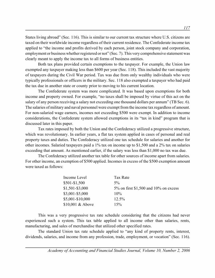
117
Academy of Accounting and Financial Studies Journal, Volume 10, Number 2, 2006
States living abroad” (Sec. 116). This is similar to our current tax structure where U.S. citizens aretaxed on their worldwide income regardless of their current residence. The Confederate income taxapplied to “the income and profits derived by each person, joint stock company and corporation,employment or business whether registered or not” (Sec. 7). This very comprehensive statement wasclearly meant to apply the income tax to all forms of business entities.
Both tax plans provided certain exemptions to the taxpayer. For example, the Union lawexempted any taxpayer making less than $600 per year (Sec. 118). This included the vast majorityof taxpayers during the Civil War period. Tax was due from only wealthy individuals who weretypically professionals or officers in the military. Sec. 118 also exempted a taxpayer who had paidthe tax due in another state or county prior to moving to his current location.
The Confederate system was more complicated. It was based upon exemptions for bothincome and property owned. For example, “no taxes shall be imposed by virtue of this act on thesalary of any person receiving a salary not exceeding one thousand dollars per annum” (TB Sec. 6).The salaries of military and naval personnel were exempt from the income tax regardless of amount.For non-salaried wage earners, incomes not exceeding $500 were exempt. In addition to incomeconsiderations, the Confederate system allowed exemptions in its “tax in kind” program that isdiscussed later in this paper.
Tax rates imposed by both the Union and the Confederacy utilized a progressive structure,which was revolutionary. In earlier years, a flat tax system applied in cases of personal and realproperty taxes and duties. The Confederacy utilized one tax schedule for salaries and another forother incomes. Salaried taxpayers paid a 1% tax on income up to $1,500 and a 2% tax on salariesexceeding that amount. As mentioned earlier, if the salary was less than $1,000 no tax was due.
The Confederacy utilized another tax table for other sources of income apart from salaries.For other income, an exemption of $500 applied. Incomes in excess of the $500 exemption amountwere taxed as follows:
Income Level Tax Rate$501-$1,500 5%$1,501-$3,000 5% on first $1,500 and 10% on excess$3,001-$5,000 10%$5,001-$10,000 12.5%$10,001 & Above 15%
This was a very progressive tax rate schedule considering that the citizens had neverexperienced such a system. This tax table applied to all income other than salaries, rents,manufacturing, and sales of merchandise that utilized other specified rates.
The standard Union tax rate schedule applied to “any kind of property rents, interest,dividends, salaries, and income from any profession, trade, employment, or vocation” (Sec. 116).
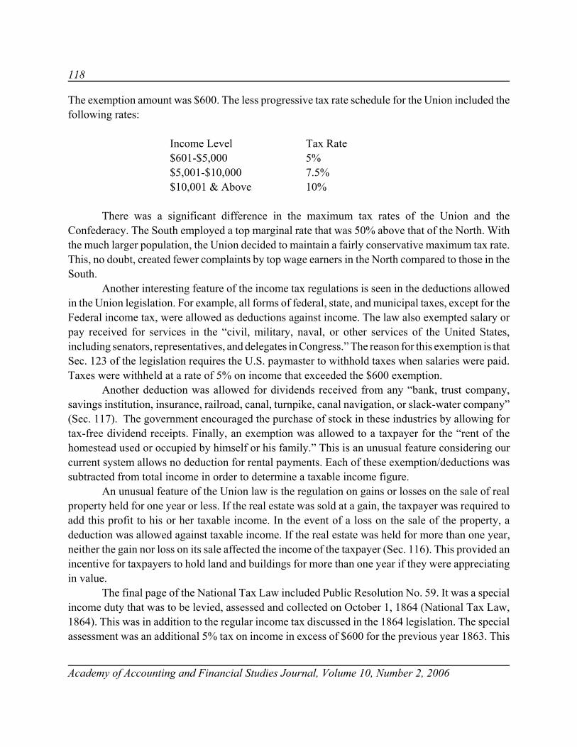
118
Academy of Accounting and Financial Studies Journal, Volume 10, Number 2, 2006
The exemption amount was $600. The less progressive tax rate schedule for the Union included thefollowing rates:
Income Level Tax Rate$601-$5,000 5%$5,001-$10,000 7.5%$10,001 & Above 10%
There was a significant difference in the maximum tax rates of the Union and theConfederacy. The South employed a top marginal rate that was 50% above that of the North. Withthe much larger population, the Union decided to maintain a fairly conservative maximum tax rate.This, no doubt, created fewer complaints by top wage earners in the North compared to those in theSouth.
Another interesting feature of the income tax regulations is seen in the deductions allowedin the Union legislation. For example, all forms of federal, state, and municipal taxes, except for theFederal income tax, were allowed as deductions against income. The law also exempted salary orpay received for services in the “civil, military, naval, or other services of the United States,including senators, representatives, and delegates in Congress.” The reason for this exemption is thatSec. 123 of the legislation requires the U.S. paymaster to withhold taxes when salaries were paid.Taxes were withheld at a rate of 5% on income that exceeded the $600 exemption.
Another deduction was allowed for dividends received from any “bank, trust company,savings institution, insurance, railroad, canal, turnpike, canal navigation, or slack-water company”(Sec. 117). The government encouraged the purchase of stock in these industries by allowing fortax-free dividend receipts. Finally, an exemption was allowed to a taxpayer for the “rent of thehomestead used or occupied by himself or his family.” This is an unusual feature considering ourcurrent system allows no deduction for rental payments. Each of these exemption/deductions wassubtracted from total income in order to determine a taxable income figure.
An unusual feature of the Union law is the regulation on gains or losses on the sale of realproperty held for one year or less. If the real estate was sold at a gain, the taxpayer was required toadd this profit to his or her taxable income. In the event of a loss on the sale of the property, adeduction was allowed against taxable income. If the real estate was held for more than one year,neither the gain nor loss on its sale affected the income of the taxpayer (Sec. 116). This provided anincentive for taxpayers to hold land and buildings for more than one year if they were appreciatingin value.
The final page of the National Tax Law included Public Resolution No. 59. It was a specialincome duty that was to be levied, assessed and collected on October 1, 1864 (National Tax Law,1864). This was in addition to the regular income tax discussed in the 1864 legislation. The specialassessment was an additional 5% tax on income in excess of $600 for the previous year 1863. This

119
Academy of Accounting and Financial Studies Journal, Volume 10, Number 2, 2006
created a total tax rate of 8% (3% regular rate for 1863 plus 5% special income duty) on incomesbetween $600 and $10,000. This rate increased to 10% on incomes in excess of $10,000 (5% regularrate for 1863 plus 5% special income duty). The serious need for cash to supply the war effortcreated a special “double” tax situation.
Both the Union and Confederate legislation incorporated numerous other types of tax inaddition to the newly instituted income tax. These included numerous assessments for businesslicenses, business profits taxes, and duties. Also, the Confederate tax system utilized a special “taxesin kind” program.
CONFEDERATE TAXES IN KIND
Since the southern states were primarily agricultural, it was logical for the Confederategovernment to realize that cash held by its citizens may not be as abundant as meats, grains, andother crops. For this reason, their tax legislation included a “taxes in kind” program. This allowedresidents of the South to pay their taxes in the form of animals and crops raised rather than in cash.Since many residents had invested much of their cash in bonds, nothing but highly discountedConfederate treasury notes were available for the payment of debts. This tax in kind program,therefore, appeared to be a viable alternative for the government. The Confederate Army had to befed and this type of tax provided a dependable supply of meats and produce to meet their needs.
Section 10 of the tax legislation and an amendment dated December 28, 1863 provided thedetails of this program. One aspect of the program pertained to the minimal inventory of productsthat was allowed to each taxpayer to satisfy basic family needs. The law provided for a familyreserve of either 50 bushels of sweet potatoes, or 50 bushels of Irish potatoes, or 100 bushels of corn,or 50 bushels of wheat, or 20 bushels of peas or beans. The idea behind this policy was to allow eachfamily enough food so they were not left in a starvation situation.
The amount of “taxes in kind” due to the Confederacy amounted to one-tenth of the farmer’sproduction of each crop or animal raised. The law stated that individuals “must pay and deliver tothe government 1/10 of the wheat, corn, oats, rye, buckwheat, rice, sweet or Irish potatoes, or hayand fodder” produced during the year (Sec. 10). In addition, 1/10 of the sugar or molasses made wasa required tax when the farmer produced more than 30 gallons. Also, 1/10 of any peas, beans, cotton,wool, and tobacco grown constituted the tax in kind (Ibid.). If a farmer slaughters hogs, the in kindtax was “an equivalent of 1/10 of the cured bacon calculated at the rate of 60 pounds of bacon foreach 100 pounds of total pig weight” (Amendment 12/28/1863).
For the most impoverished of farmers, there were a number of exemptions from the tax inkind. This included a $500 net worth limitation (Sec. 10 I). For very small farms where its ownerhad assets worth less than this exemption amount, no in kind tax was required. This exemptionincreased by $100 for each minor child that the family head had living with him (Sec. 10 II). The$100 allowance was granted in situations where the family head had either lost or had disabled
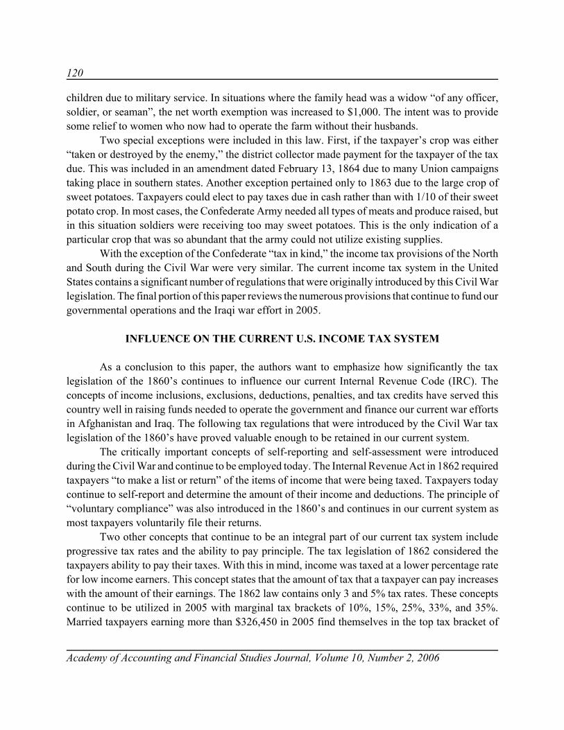
120
Academy of Accounting and Financial Studies Journal, Volume 10, Number 2, 2006
children due to military service. In situations where the family head was a widow “of any officer,soldier, or seaman”, the net worth exemption was increased to $1,000. The intent was to providesome relief to women who now had to operate the farm without their husbands.
Two special exceptions were included in this law. First, if the taxpayer’s crop was either“taken or destroyed by the enemy,” the district collector made payment for the taxpayer of the taxdue. This was included in an amendment dated February 13, 1864 due to many Union campaignstaking place in southern states. Another exception pertained only to 1863 due to the large crop ofsweet potatoes. Taxpayers could elect to pay taxes due in cash rather than with 1/10 of their sweetpotato crop. In most cases, the Confederate Army needed all types of meats and produce raised, butin this situation soldiers were receiving too may sweet potatoes. This is the only indication of aparticular crop that was so abundant that the army could not utilize existing supplies.
With the exception of the Confederate “tax in kind,” the income tax provisions of the Northand South during the Civil War were very similar. The current income tax system in the UnitedStates contains a significant number of regulations that were originally introduced by this Civil Warlegislation. The final portion of this paper reviews the numerous provisions that continue to fund ourgovernmental operations and the Iraqi war effort in 2005.
INFLUENCE ON THE CURRENT U.S. INCOME TAX SYSTEM
As a conclusion to this paper, the authors want to emphasize how significantly the taxlegislation of the 1860’s continues to influence our current Internal Revenue Code (IRC). Theconcepts of income inclusions, exclusions, deductions, penalties, and tax credits have served thiscountry well in raising funds needed to operate the government and finance our current war effortsin Afghanistan and Iraq. The following tax regulations that were introduced by the Civil War taxlegislation of the 1860’s have proved valuable enough to be retained in our current system.
The critically important concepts of self-reporting and self-assessment were introducedduring the Civil War and continue to be employed today. The Internal Revenue Act in 1862 requiredtaxpayers “to make a list or return” of the items of income that were being taxed. Taxpayers todaycontinue to self-report and determine the amount of their income and deductions. The principle of“voluntary compliance” was also introduced in the 1860’s and continues in our current system asmost taxpayers voluntarily file their returns.
Two other concepts that continue to be an integral part of our current tax system includeprogressive tax rates and the ability to pay principle. The tax legislation of 1862 considered thetaxpayers ability to pay their taxes. With this in mind, income was taxed at a lower percentage ratefor low income earners. This concept states that the amount of tax that a taxpayer can pay increaseswith the amount of their earnings. The 1862 law contains only 3 and 5% tax rates. These conceptscontinue to be utilized in 2005 with marginal tax brackets of 10%, 15%, 25%, 33%, and 35%.Married taxpayers earning more than $326,450 in 2005 find themselves in the top tax bracket of

121
Academy of Accounting and Financial Studies Journal, Volume 10, Number 2, 2006
35%. Congress has continued to believe that upper income taxpayers have the “ability to pay” taxat a higher rate than lower income individuals.
The tax legislation of 1862 and 1864 introduced another concept that has proven valuableenough to be retained. This is the practice of “stoppage at the source” where wage earners haveincome taxes withheld from their earnings prior to receiving their paychecks. These Civil War taxlaws required taxes to be withheld by employers on employees with income in excess of $600. Thisallows taxpayers to “pay as they earn” and provides two benefits. First, the employee is not facedwith a huge balance due at the end of the year since taxes are paid in small installments throughoutthe year. Second, the government receives the tax dollars on a timely basis and does not have to waitseveral months to collect the funds.
The general principle of collecting taxes on an annual basis was also introduced by the CivilWar legislation. Taxpayers assessed their income during the calendar year and were required by the1862 legislation to pay the balance due by June 30. This date proved to be too generous resultingin our current final payment date of April 15.
These early pieces of tax legislation also introduced the concept that the income tax must bepaid by not only individuals but also any form of business. Section 11 of the National Tax Actrequired that taxes be paid by “Individuals, Partnerships, Firms, Associations, and Corporations.”This continues to be true in our current tax system as individuals, proprietorships, partnerships, andcorporations must pay taxes on their earnings.
The concept of “comprehensive income” was also introduced during the Civil War. Thisconcept states that income tax is due on all types of earnings unless that item is specificallyexcluded. Section 116 of the National Tax Act required taxes on “Annual gains, profits, or income,whether derived from any kind of property, rents, interests, dividends, salaries, or from anyprofession, trade, employment, or vocation.” The current IRC requires income to be paid onvirtually any type of income with the exception of a few exclusions such as municipal interestincome. Therefore, this policy continues to be valuable today as taxpayers report most types ofreceipts on their Form 1040.
Tax penalties were also included in the tax legislation of the 1860’s. Section 15 of theNational Tax Act included fines of up to $1,000 and one year in prison for filing a false return. Inaddition, fines for non-payment of tax resulted in a 10% late payment penalty. After thirty days, theNational Tax Act contained a system for auctioning a taxpayer’s personal and real property to satisfythe tax lien. These penalties and numerous others continue to be included in our current IRC. Inparticular, the negligence and fraud penalties have been expanded in an effort to collect overduetaxes. Finally, the current penalty on substantial understatement of tax was included in the Civil Warlegislation. Section 8 of the Confederate law stated that if the “taxpayer does not report more than4/5 of their true and real income,” the tax due on the understatement plus an additional 10% penaltywas imposed. In the current IRC, this penalty of substantial understatement has been increase to20%. Finally, the current IRC includes the most severe penalty when fraud is involved. If a

122
Academy of Accounting and Financial Studies Journal, Volume 10, Number 2, 2006
fraudulent underpayment of tax can be proved by the IRS, an additional 75% of the underpaid taxesare owed as a fraud penalty. In summary, penalties continue to be an important component of ourtax law.
Two key deductions continue to be included in our tax system that had their roots in the CivilWar legislation. They include the standard deduction and personal exemptions. In particular, theNational Tax Act included an exemption of $600 per working individual. This compares today toa standard deduction of approximately $5,000 (single) and a personal exemption of a little more than$3,000. This concept was introduced in the early legislation to insure that lower income individualswould owe no tax. This continues to be the case today for singles who earn less than $8,000 (thetotal of the standard deduction and personal exemption). No tax is due for these low incometaxpayers.
A final income tax provision that the authors would like to review is the development ofincome deductions. Section 117 of the National Tax Act allowed a deduction for “all national, state,or municipal taxes other that the federal income tax.” This continues to be important to taxpayerstoday who itemize their deductions. Our current Form 1040-Schedule A allows for the deductionof numerous taxes such as real estate and state income taxes. The National Tax Act was even moregenerous than current law as it allowed a deduction for “the amount paid for rent on a residenceoccupied by the taxpayer or his family.”
The items reviewed above are but a few of the tax provisions that were initially introducedduring the 1860’s and continue to provide benefits in today’s income tax system. In addition toincome taxes, the National Tax Act imposed other taxes that continue currently. For example, thisearly legislation introduced the concept of “sin taxes.” The Federal Government continues to collectsignificant taxes on the sale of alcoholic beverages. The 1864 law included a substantial tax on“spirits, ale, beer, and porter.” The concept of taxing alcoholic beverages and tobacco productsremains a major fund raiser for the government.
As stated earlier, there are an extremely large number of income tax provisions that wereoriginally introduced in the 1860’s and continue to be utilized today. The authors have onlyreviewed a small portion of the regulations that have proven valuable for nearly 150 years. It iswithout question that we can learn much from our history. The situation confronting the governmentduring the Civil War is similar to our current war condition. Income tax funds continue to bedesperately needed for both the Iraqi war effort and the hurricane disaster cleanup on the Gulf ofMexico coast.
CONCLUSION
One of the goals of this paper is to provide the reader with an overview of the verycomprehensive tax legislation enacted by both the Union and the Confederacy during the Civil War.In an effort to raise sufficient funds to finance the war, both the Union and the Confederacy resorted

123
Academy of Accounting and Financial Studies Journal, Volume 10, Number 2, 2006
to new forms of taxation such as the income tax. Income taxes were a very difficult concept for thebulk of 1860’s taxpayers to understand. This situation continues today as the majority of U.S.taxpayers utilize a paid preparer to complete their tax returns.
The authors also want to emphasize the large number of income tax principles and practicesthat were initially introduced during the Civil War era and continue to be included in our currentInternal Revenue Code. The concepts of self-assessment, progressive tax rates, comprehensiveincome, deductions from income, and many other tax principles were introduced by the 1860’slegislation. These practices continue to serve our country in the process of generating sufficient taxrevenues to finance government operations that include both a war effort as well as major hurricanerelief operations on the Gulf of Mexico coast.
REFERENCES
Confederate States of America (1863). The Tax Act of 24th April, 1863, As Amended. Electronic Edition, Property of theUniversity of North Carolina at Chapel Hill, available at the following site:http://docsouth.dsi.internet2.edu/taxasses/taxasses.html Call number 63 Conf. (Rare Books Collection, UNC-CH).
Doris, Lillian (1963). The American Way In Taxation: Internal Revenue, 1862-1963. Englewood Cliffs, NJ: Prentice-Hall, Inc.
Hill, Joseph A. (1894). The Civil War Income Tax. The Quarterly Journal of Economics. Volume VIII, July 1894,p.416-452.
National Tax Law as Approved June 30, 1864 (1864), New York, NY: Beadle and Company.
Parnell, Archie (1980). Congress and the IRS: Improving the Relationship. Fund for Public Policy Research,Washington, D.C.
Revised Regulations For The Army Of The United States, 1861 (1861). Philadelphia, PA: J.G.L. Brown, Printer.
Tax.org – Tax Information Worldwide, retrieved from http://tax.org/, tax history museum section – 1861 to 1865.
United States Treasury, “Fact Sheet OPC-77 – History of the Tax System in the United States”, retrieved fromhttp://www.ustreas.gov/opc/opc0077.html
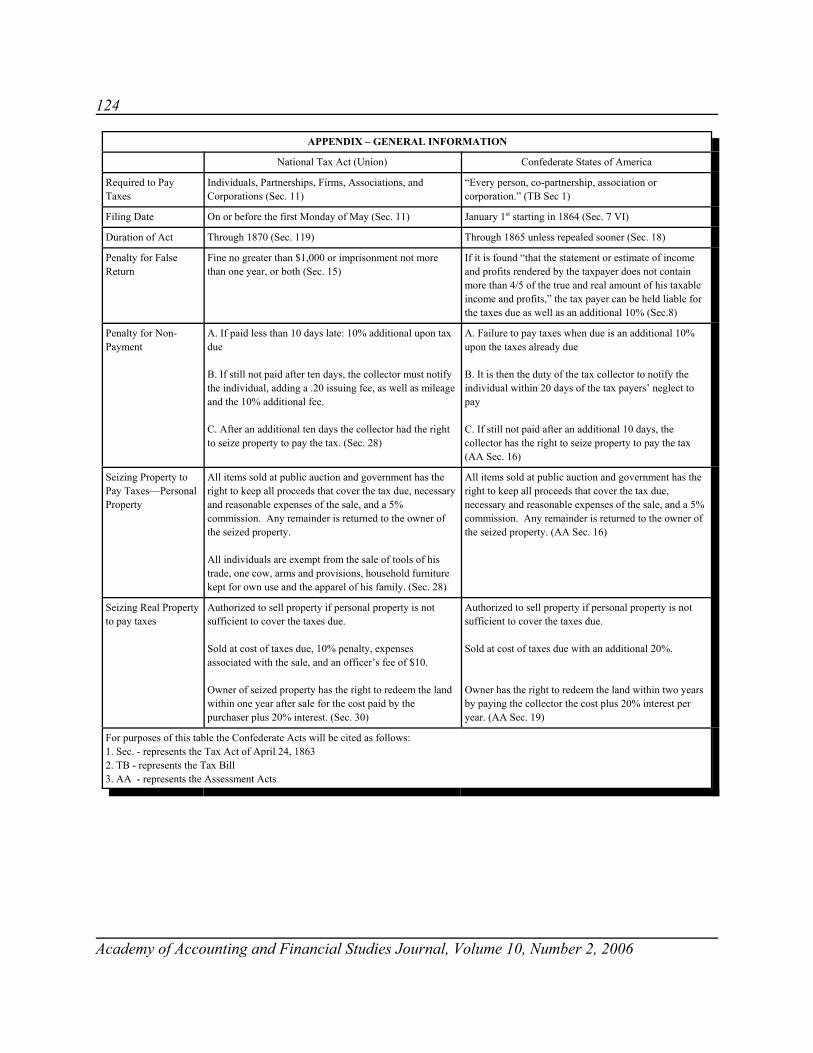
124
Academy of Accounting and Financial Studies Journal, Volume 10, Number 2, 2006
APPENDIX – GENERAL INFORMATION
National Tax Act (Union) Confederate States of America
Required to PayTaxes
Individuals, Partnerships, Firms, Associations, andCorporations (Sec. 11)
“Every person, co-partnership, association orcorporation.” (TB Sec 1)
Filing Date On or before the first Monday of May (Sec. 11) January 1st starting in 1864 (Sec. 7 VI)
Duration of Act Through 1870 (Sec. 119) Through 1865 unless repealed sooner (Sec. 18)
Penalty for FalseReturn
Fine no greater than $1,000 or imprisonment not morethan one year, or both (Sec. 15)
If it is found “that the statement or estimate of incomeand profits rendered by the taxpayer does not containmore than 4/5 of the true and real amount of his taxableincome and profits,” the tax payer can be held liable forthe taxes due as well as an additional 10% (Sec.8)
Penalty for Non-Payment
A. If paid less than 10 days late: 10% additional upon taxdue
B. If still not paid after ten days, the collector must notifythe individual, adding a .20 issuing fee, as well as mileageand the 10% additional fee.
C. After an additional ten days the collector had the rightto seize property to pay the tax. (Sec. 28)
A. Failure to pay taxes when due is an additional 10%upon the taxes already due
B. It is then the duty of the tax collector to notify theindividual within 20 days of the tax payers’ neglect topay
C. If still not paid after an additional 10 days, thecollector has the right to seize property to pay the tax (AA Sec. 16)
Seizing Property toPay Taxes—PersonalProperty
All items sold at public auction and government has theright to keep all proceeds that cover the tax due, necessaryand reasonable expenses of the sale, and a 5%commission. Any remainder is returned to the owner ofthe seized property.
All individuals are exempt from the sale of tools of histrade, one cow, arms and provisions, household furniturekept for own use and the apparel of his family. (Sec. 28)
All items sold at public auction and government has theright to keep all proceeds that cover the tax due,necessary and reasonable expenses of the sale, and a 5%commission. Any remainder is returned to the owner ofthe seized property. (AA Sec. 16)
Seizing Real Propertyto pay taxes
Authorized to sell property if personal property is notsufficient to cover the taxes due.
Sold at cost of taxes due, 10% penalty, expensesassociated with the sale, and an officer’s fee of $10.
Owner of seized property has the right to redeem the landwithin one year after sale for the cost paid by thepurchaser plus 20% interest. (Sec. 30)
Authorized to sell property if personal property is notsufficient to cover the taxes due.
Sold at cost of taxes due with an additional 20%.
Owner has the right to redeem the land within two yearsby paying the collector the cost plus 20% interest peryear. (AA Sec. 19)
For purposes of this table the Confederate Acts will be cited as follows:1. Sec. - represents the Tax Act of April 24, 18632. TB - represents the Tax Bill3. AA - represents the Assessment Acts

125
Academy of Accounting and Financial Studies Journal, Volume 10, Number 2, 2006
APPENDIX – INCOME TAXES
National Tax Act (Union) Confederate States of America
Who must pay All individuals residing in the United States or anycitizens of the United States living abroad (Sec. 116)
“The income and profits derived by each person, joint stockcompany and corporation from every occupation,employment or business, whether registered or not.” (Sec. 7)
Exemptions 1. Anyone making less than $600 per year.2. Anyone who can prove he has already paidsomewhere else (Sec. 118)
1. Property of each head of household $5002. Each minor $1003. Each son in the military or who had been killed in themilitary, $5004. Property of any widow of anyone killed during militaryservice or where there is no widow the family $1,0005. Property of officers, soldiers, etc. “actually engaged in themilitary” or have been disabled, $1,000None of these exemptions apply to anyone whose assessedproperty is greater than $1,000. (TB Sec. 5, I, II, III)
What is taxed andincluded in personalincome
“Annual gains, profits, or income, whether derivedfrom any kind of property, rents, interests, dividends,salaries, or from any profession, trade, employment,or vocation.” (Sec. 116)
Included in personal income:1. Interest above all that paid on all notes, bonds, andmortgages etc. (Sec. 117)2. “All income or gains derived from the purchase andsale of stocks or other property, real or personal, andthe increased value of livestock” (Sec. 117)3. “Amount of sugar, wool, butter, cheese, pork, beef,mutton, or other meats, hay and grain, or othervegetable or other production of the estate of suchperson sold.” (Sec. 117)
Tax of 1% due on all salaries not exceeding $1,500, and a2% tax on the excess over that amount. All salaries ofpeople in the military are exempt from the tax. No tax is duewhen salary is $1,000 or less. (Sec. 6)
Individuals will be taxed 10% on all profits made only in1862 from the purchase and sale of “flour, corn, bacon, pork,oats, hay, rice, salt, or iron, or the manufactures of iron,sugar, molasses made of cane, leather, woolen cloths, shoes,boots, blankets and cotton cloths.” This tax does not applyto any purchases or sales from “the regular course ofbusiness.” (Sec. 9)
Value of property real or personal and mixed unlessotherwise stated, 5%. (TB Sec. 1, I)
“Value of gold and silver wares and plate, jewels, jewelry,and watches, 10%.” (TB Sec. 1 II)“Value of shares or interests held in any bank, bankingcompany or association, canal, navigation, importing orexporting, insurance, manufacturing, telegraph, express,railroad, and dry dock companies, and all other joint stockcompanies, 5%.” (TB Sec. 2)“Upon amount of all gold and silver coin, gold dust, gold orsilver,” 5%.“All monies held abroad or upon the amount of all bills ofexchange,” 5%. (TB Sec. 3 I)“Upon the amount of all solvent credits, and of all bank bill,and all other papers issued as currency, exclusive of non-interest bearing Confederate treasury notes, and notemployed in a registered business, the income derived fromwhich is taxed, 5%.” (TB Sec. 3 II)Also, on the tax “on bonds of the Confederate Statesheretofore issued, shall in no case exceed the interest on thesame, and such bonds, when held by or for minors orlunatics, shall be exempt from the tax in all cases where theinterest on the same shall not exceed $1,000.” (Sec. 8)
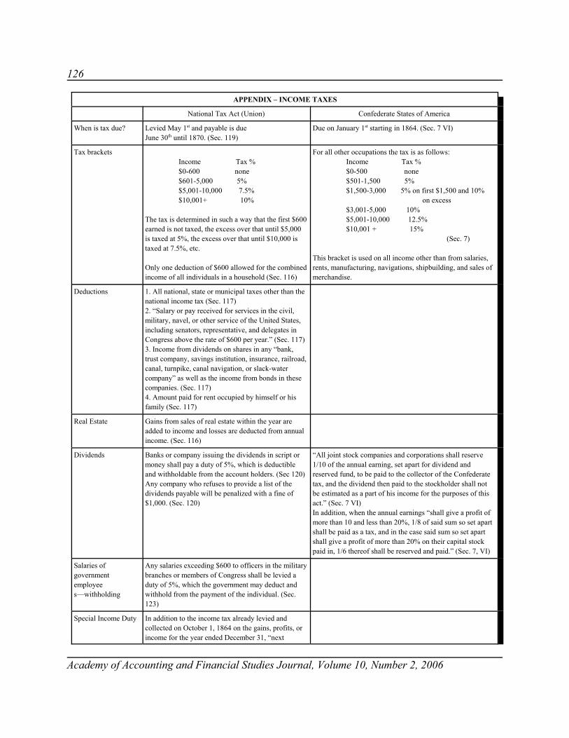
126
APPENDIX – INCOME TAXES
National Tax Act (Union) Confederate States of America
Academy of Accounting and Financial Studies Journal, Volume 10, Number 2, 2006
When is tax due? Levied May 1st and payable is due June 30th until 1870. (Sec. 119)
Due on January 1st starting in 1864. (Sec. 7 VI)
Tax brackets Income Tax %
$0-600 none$601-5,000 5%$5,001-10,000 7.5%$10,001+ 10%
The tax is determined in such a way that the first $600earned is not taxed, the excess over that until $5,000is taxed at 5%, the excess over that until $10,000 istaxed at 7.5%, etc.
Only one deduction of $600 allowed for the combinedincome of all individuals in a household (Sec. 116)
For all other occupations the tax is as follows:Income Tax %$0-500 none$501-1,500 5%$1,500-3,000 5% on first $1,500 and 10%
on excess$3,001-5,000 10%$5,001-10,000 12.5%$10,001 + 15%
(Sec. 7)
This bracket is used on all income other than from salaries,rents, manufacturing, navigations, shipbuilding, and sales ofmerchandise.
Deductions 1. All national, state or municipal taxes other than thenational income tax (Sec. 117)2. “Salary or pay received for services in the civil,military, navel, or other service of the United States,including senators, representative, and delegates inCongress above the rate of $600 per year.” (Sec. 117)3. Income from dividends on shares in any “bank,trust company, savings institution, insurance, railroad,canal, turnpike, canal navigation, or slack-watercompany” as well as the income from bonds in thesecompanies. (Sec. 117)4. Amount paid for rent occupied by himself or hisfamily (Sec. 117)
Real Estate Gains from sales of real estate within the year areadded to income and losses are deducted from annualincome. (Sec. 116)
Dividends Banks or company issuing the dividends in script ormoney shall pay a duty of 5%, which is deductibleand withholdable from the account holders. (Sec 120)Any company who refuses to provide a list of thedividends payable will be penalized with a fine of$1,000. (Sec. 120)
“All joint stock companies and corporations shall reserve1/10 of the annual earning, set apart for dividend andreserved fund, to be paid to the collector of the Confederatetax, and the dividend then paid to the stockholder shall notbe estimated as a part of his income for the purposes of thisact.” (Sec. 7 VI)In addition, when the annual earnings “shall give a profit ofmore than 10 and less than 20%, 1/8 of said sum so set apartshall be paid as a tax, and in the case said sum so set apartshall give a profit of more than 20% on their capital stockpaid in, 1/6 thereof shall be reserved and paid.” (Sec. 7, VI)
Salaries ofgovernmentemployees—withholding
Any salaries exceeding $600 to officers in the militarybranches or members of Congress shall be levied aduty of 5%, which the government may deduct andwithhold from the payment of the individual. (Sec.123)
Special Income Duty In addition to the income tax already levied andcollected on October 1, 1864 on the gains, profits, orincome for the year ended December 31, “next

127
APPENDIX – INCOME TAXES
National Tax Act (Union) Confederate States of America
Academy of Accounting and Financial Studies Journal, Volume 10, Number 2, 2006
preceding the time herein named.” The duty will be“5% on all sums exceeding $600.” In addition, “inestimating the annual gains, profits, or income asaforesaid, for the foregoing special income duty, nodeductions shall be made for dividends or interestreceived from any association, corporation, orcompany, nor shall any deduction be made for anysalary or pay received.” (Public Resolution No. 59)
Payment Options “Secretary of the Treasury may prescribe regulations toenable any tax-payer to pay into the treasury, in advancesuch sum as he may choose on account of taxes to accrueagainst him, and to obtain therefore a certificate bearinginterest at the rate of 5% a year until his taxes are payable,but such certificate shall not be transferable.” (AA Sec. 42)
“When cotton or other property subject to taxation in money,shall have been burned or otherwise destroyed,” the taxpayermay ask for the tax to be removed from what is due orrefunded. (Amendment 2/13/1864)
Penalties Anything not received for an additional 10 days afterJune 30th will be assessed an additional 10%. (Sec.119)
Any person providing a “false or fraudulent list or statement,with intent to defeat or evade the valuation” will be fined upto $500 as well as the cost of the trial. (AA Sec. 9)
For purposes of this table the Confederate Acts will be cited as follows:1. Sec. - represents the Tax Act of April 24, 18632. TB - represents the Tax Bill3. AA - represents the Assessment Acts

128
Academy of Accounting and Financial Studies Journal, Volume 10, Number 2, 2006
APPENDIX – TAXES IN KIND
National Tax Act (Union) Confederate States of America
Reserves Allowed 1. 50 bushels of sweet potatoes 2. 50 bushels of Irish potatoes 3. 100 bushels of corn or 50 bushels of wheat 4. 20 bushels of peas or beans in total (Sec. 10)
Taxes in Kind Due 1. Individuals “must pay and deliver to the government 1/10 of the wheat, corn, oats, rye, buckwheat or rice, sweet and Irish potatoes, and of the cured hay and fodder.” (Sec. 10) 2. In addition 1/10 of the sugar, molasses made of cane or sorghum, when the farmer produces “more than 30 gallons,” cotton, wool, and tobacco. (Sec. 10) 3. 1/10 of the peas, beans, and ground peas produced during the year. (Sec. 10) 4. Any farmer that slaughters hogs will be charged a tax in kind “an equivalent for 1/10 of the same in cured bacon, at the rate of 60 pounds of bacon to the 100 weight of pork.” Government also has the authority to demand salt pork instead of the bacon (Amendment 12/28/1863)
Exemptions 1. Each family head not worth more than $500 (Sec. 10 I) 2. “Each family head with minor children, not worth more than $500 for himself and $100 for each minor living with him, and $500 in addition thereto, for each minor son he has living, or may have lost, or had disabled in the military.” (Sec. 10 II) 3. “Each officer, soldier, or seaman, in the army or nave, or who has been discharged therefrom for wounds, and is not worth more than $100.” (Sec. 10 III) 4. “Each widow of any officer, soldier, or seaman, not worth more than $1,000.” (Sec.10 IV) 5. Farmers are also exempt if they do not produce more than 50 bushels of Irish potatoes, 200 bushels of corn, 20 bushels of peas and beans, 10 pounds of wool or more than 15 pounds of ginned cotton. (Sec. 10 IV)
Exceptions 1. Any time the crop to be paid is “taken or destroyed by the enemy the district collector may remit the tax.” (Sec. 2, Amendment 2/13/1864) 2. For the year 1863, the producers of sweet potatoes may pay the tax in kind with cash (Amendment 12/28/1863)
Penalties If the farmer does not deliver the goods by the due day, “he shall be liable to pay five times the estimated value of the portion aforesaid.” (Sec. 10 IV)
For purposes of this table the Confederate Acts will be cited as follows:1. Sec. - represents the Tax Act of April 24, 18632. TB - represents the Tax Bill3. AA - represents the Assessment Acts

129
Academy of Accounting and Financial Studies Journal, Volume 10, Number 2, 2006
Allied Academies
invites you to check our website at
www.alliedacademies.org
for information concerning
conferences and submission instructions

130
Academy of Accounting and Financial Studies Journal, Volume 10, Number 2, 2006
Allied Academies
invites you to check our website at
www.alliedacademies.org
for information concerning
conferences and submission instructions