Embed Size (px)
Citation preview

Mikhail Yu. Khachay, Natalia Konstantinova, Alexander Panchenko, Radhakr-ishnan Delhibabu, Nikita Spirin, Valeri G. Labunets (Eds.)
AIST’2015 — Analysis of Images, Social Networks andTexts
Supplementary Proceedings of the 4th International Conference on Analysis ofImages, Social Networks and Texts (AIST’2015)April 2015, Yekaterinburg, Russia
The proceedings are published online on the CEUR-Workshop web site in a serieswith ISSN 1613-0073, Vol-1452.
Copyright c© 2015 for the individual papers by the papers’ authors. Copyingpermitted only for private and academic purposes. This volume is published andcopyrighted by its editors.

Preface
This volume contains proceedings of the fourth conference on Analysis of Im-ages, Social Networks and Texts (AIST’2015)1. The first three conferences in2012–2014 attracted a significant number of students, researchers, academicsand engineers working on interdisciplinary data analysis of images, texts, andsocial networks.
The broad scope of AIST makes it an event where researchers from differ-ent domains, such as image and text processing, exploiting various data analysistechniques, can meet and exchange ideas. We strongly believe that this may leadto crossfertilisation of ideas between researchers relying on modern data analy-sis machinery. Therefore, AIST brings together all kinds of applications of datamining and machine learning techniques. The conference allows specialists fromdifferent fields to meet each other, present their work, and discuss both theo-retical and practical aspects of their data analysis problems. Another importantaim of the conference is to stimulate scientists and people from the industry tobenefit from the knowledge exchange and identify possible grounds for fruitfulcollaboration.
The conference was held during April 9–11, 2015. Following an already es-tablished tradition, the conference was organised in Yekaterinburg, a cross-roadsbetween European and Asian parts of Russia, the capital of Urals region.The keytopics of AIST are analysis of images and videos; natural language processing andcomputational linguistics; social network analysis; pattern recognition, machinelearning and data mining; recommender systems and collaborative technologies;semantic web, ontologies and their applications.
The Program Committee and the reviewers of the conference included well-known experts in data mining and machine learning, natural language process-ing, image processing, social network analysis, and related areas from leadinginstitutions of 22 countries including Australia, Bangladesh, Belgium, Brazil,Cyprus, Egypt, Finland, France, Germany, Greece, India, Ireland, Italy, Luxem-bourg, Poland, Qatar, Russia, Spain, The Netherlands, UK, USA and Ukraine.
This year the number of submission has doubled and we have received 140submissions mostly from Russia but also from Algeria, Bangladesh, Belgium,India, Kazakhstan, Mexico, Norway, Tunisia, Ukraine, and USA. Out of 140only 32 papers were accepted as regular oral papers (24 long and 8 short). Thus,the acceptance rate of this volume was around 23%. In order to encourage youngpractitioners and researchers we included 5 industry papers to the main volumeand 25 papers to the supplementary proceedings. Each submission was reviewedby at least three reviewers, experts in their fields, in order to supply detailedand helpful comments.
The conference also featured several invited talks and tutorials, as well as anindustry session dedicated to current trends and challenges.1 http://aistconf.org/
ii

Invited talks:
– Pavel Braslavski (Ural Federal University, Yekaterinburg, Russia), QuestionsOnline: What, Where, and Why Should we Care?
– Michael Khachay (Krasovsky Institute of Mathematics and Mechanics UBRAS & Ural Federal University, Yekaterinburg, Russia), Machine Learning inCombinatorial Optimization: Boosting of Polynomial Time ApproximationAlgorithms.
– Valeri Labunets (Ural Federal University, Yekaterinburg, Russia), Is the Hu-man Brain a Quantum Computer?
– Sergey Nikolenko (National Research University Higher School of Economics& Steklov Mathematical Institute, St. Petersburg, Russia), ProbabilisticRating Systems
– Andrey Savchenko (National Research University Higher School of Eco-nomics, Nizhny Novgorod, Russia), Sequential Hierarchical Image Recog-nition based on the Pyramid Histograms of Oriented Gradients with SmallSamples
– Alexander Semenov (International laboratory for Applied Network Researchat HSE, Moscow, Russia), Attributive and Network Features of the Users ofSuicide and Depression Groups of Vk.com
Tutorials:
– Alexander Panchenko (Technische Universitat Darmstadt, Germany), Com-putational Lexical Semantics: Methods and Applications
– Artem Lukanin (South Ural State University, Chelyabinsk, Russia), TextProcessing with Finite State Transducers in Unitex
The industry speakers also covered a wide variety of topics:
– Dmitry Bugaichenko (OK.ru), Does Size Matter? Smart Data at OK.ru– Mikhail Dubov (National Research University Higher School of Economics,
Moscow, Russia), Text Analysis with Enhanced Annotated Suffix Trees: Al-gorithmic Base and Industrial Usage
– Nikita Kazeev (Yandex Data Factory), Role of Machine Learning in HighEnergy Physics Research at LHC
– Artem Kuznetsov (SKB Kontur), Family Businesses: Relation Extractionbetween Companies by Means of Wikipedia
– Alexey Natekin (Data Mining Labs), ATM Maintenance Cost Optimizationwith Machine Learning Techniques
– Konstantin Obukhov (Clever Data), Customer Experience Technologies: Prob-lems of Feedback Modeling and Client Churn Control
– Alexandra Shilova (Centre IT), Centre of Information Technologies: DataAnalysis and Processing for Large-Scale Information Systems
We would also like to mention the best conference paper selected by theProgram Committee. It was written by Oleg Ivanov and Sergey Bartunov andis entitled “Learning Representations in Directed Networks”.
iii

We would like to thank the authors for submitting their papers and themembers of the Program Committee for their efforts in providing exhaustivereviews. We would also like to express special gratitude to all the invited speakersand industry representatives.
We deeply thank all the partners and sponsors, and owe our gratitude tothe Ural Federal University for substantial financial support of the whole con-ference, namely, the Center of Excellence in Quantum and Video InformationTechnologies: from Computer Vision to Video Analystics (QVIT: CV → VA).We would like to acknowledge the Scientific Fund of Higher School of Economicsfor providing AIST participants with travel grants. Our special thanks goes toSpringer editors who helped us, starting from the first conference call to the finalversion of the proceedings. Last but not least, we are grateful to all organisers,especially to Eugeniya Vlasova and Dmitry Ustalov, and the volunteers, whoseendless energy saved us at the most critical stages of the conference preparation.
Traditionally, we would like to mention the Russian word “aist” is more thanjust a simple abbreviation (in Cyrillic), it means a “stork”. Since it is a wonderfulfree bird, a symbol of happiness and peace, this stork brought us the inspirationto organise the AIST conference. So we believe that this young and rapidlygrowing conference will be bringing inspiration to data scientists around theWorld!
April, 2015 Mikhail Yu. KhachayNatalia KonstantinovaAlexander Panchenko
Radhakrishnan DelhibabuNikita Spirin
Valeri G. Labunets
iv

Organisation
The conference was organized by a joint team from Ural Federal University(Yekaterinburg, Russia), Krasovsky Institute of Mathematics and Mechanics,Ural Branch of Russian Academy of Sciences (Yekaterinburg, Russia), and theNational Research University Higher School of Economics (Moscow, Russia). Itwas supported by a special grant from Ural Federal University for the Centerof Excellence in Quantum and Video Information Technologies: from ComputerVision to Video Analystics (QVIT: CV → VA).
Program Committee Chairs
Mikhail Khachay Krasovsky Institute of Mathematics and Mechanicsof UB RAS, Russia
Natalia Konstantinova University of Wolverhampton, UKAlexander Panchenko Technische Universitat Darmstadt, Germany & Uni-
versite catholique de Louvain, Belgium
General Chair
Valeri G. Labunets Ural Federal University, Russia
Organising Chair
Eugeniya Vlasova National Research University Higher School of Eco-nomics, Moscow
Proceedings Chair
Dmitry I. Ignatov National Research University Higher School of Eco-nomics, Russia
Poster Chairs
Nikita Spirin University of Illinois at Urbana-Champaign, USADmitry Ustalov Krasovsky Institute of Mathematics and Mechanics
& Ural Federal University, Russia
International Liaison Chair
Radhakrishnan Delhibabu Kazan Federal University, Russia
v

Organising Committee and Volunteers
Alexandra Barysheva National Research University Higher School of Eco-nomics, Russia
Liliya Galimzyanova Ural Federal University, RussiaAnna Golubtsova National Research University Higher School of Eco-
nomics, RussiaVyacheslav Novikov National Research University Higher School of Eco-
nomics, RussiaNatalia Papulovskaya Ural Federal University, YekaterinburgYuri Pekov Moscow State University, RussiaEvgeniy Tsymbalov National Research University Higher School of Eco-
nomics, RussiaAndrey Savchenko National Research University Higher School of Eco-
nomics, RussiaDmitry Ustalov Krasovsky Institute of Mathematics and Mechanics
& Ural Federal University, RussiaRostislav Yavorsky National Research University Higher School of Eco-
nomics, Russia
Industry Session Organisers
Ekaterina Chernyak National Research University Higher School of Eco-nomics, Russia
Alexander Semenov National Research University Higher School of Eco-nomics, Russia
vi

Program Committee
Mikhail Ageev Lomonosov Moscow State University, RussiaAtiqur Rahman Ahad University of Dhaka, BangladeshIgor Andreev Mail.Ru, RussiaNikolay Arefiev Moscow State University & Digital Society Lab,
RussiaJaume Baixeries Politechnic University of Catalonia, SpainPedro Paulo Balage Universidade de Sao Paulo, BrazilSergey Bartunov Lomonosov Moscow State University & National Re-
search University Higher School of Economics, Rus-sia
Malay Bhattacharyya Indian Institute of Engineering Science and Technol-ogy, India
Vladimir Bobrikov Imhonet.ru, RussiaVictor Bocharov OpenCorpora & Yandex, RussiaDaria Bogdanova Dublin City University, IrelandElena Bolshakova Lomonosov Moscow State University, RussiaAurelien Bossard Orange Labs, FrancePavel Botov Moscow Institute of Physics and Technology, RussiaJean-Leon Bouraoui Universite Catholique de Louvain, BelgiumLeonid Boytsov Carnegie Mellon University, USAPavel Braslavski Ural Federal University & Kontur Labs, RussiaAndrey Bronevich National Research University Higher School of Eco-
nomics, RussiaAleksey Buzmakov LORIA (CNRS-Inria-Universite de Lorraine),
FranceArtem Chernodub Institute of Mathematical Machines and Systems of
NASU, UkraineVladimir Chernov Image Processing Systems Institute of RAS, RussiaEkaterina Chernyak National Research University Higher School of Eco-
nomics, RussiaMarina Chicheva Image Processing Systems Institute of RAS, RussiaMiranda Chong University of Wolverhampton, UKHernani Costa University of Malaga, SpainFlorent Domenach University of Nicosia, CyprusAlexey Drutsa Lomonosov Moscow State University & Yandex,
RussiaMaxim Dubinin NextGIS, RussiaJulia Efremova Eindhoven University of Technology, The Nether-
landsShervin Emami NVIDIA, AustraliaMaria Eskevich Dublin City University, IrelandVictor Fedoseev Samara State Aerospace University, RussiaMark Fishel University of Zurich, Germany
vii

Thomas Francois Universite catholique de Louvain, BelgiumOleksandr Frei Schlumberger, NorwayBinyam Gebrekidan Gebre Max Planck Computing & Data Facility, GermanyDmitry Granovsky Yandex, RussiaMena Habib University of Twente, The NetherlandsDmitry Ignatov National Research University Higher School of Eco-
nomics, RussiaDmitry Ilvovsky National Research University Higher School of Eco-
nomics, RussiaVladimir Ivanov Kazan Federal University, RussiaSujay Jauhar Carnegie Mellon University, USADmitry Kan AlphaSense Inc., USANikolay Karpov National Research University Higher School of Eco-
nomics, RussiaYury Katkov Blue Brain Project, SwitzerlandMehdi Kaytoue INSA de Lyon, FranceLaurent Kevers DbiT, LuxembourgMichael Khachay Krasovsky Institute of Mathematics and Mechanics
UB RAS, RussiaEvgeny Kharitonov Moscow Institute of Physics and Technology, RussiaVitaly Khudobakhshov Saint Petersburg University & National Research
University of Information Technologies, Mechanicsand Optics, Russia
Ilya Kitaev iBinom, Russia & Voronezh State University, RussiaEkaterina Kochmar University of Cambridge, UKSergei Koltcov National Research University Higher School of Eco-
nomics, RussiaOlessia Koltsova National Research University Higher School of Eco-
nomics, RussiaNatalia Konstantinova University of Wolverhampton, UKAnton Konushin Lomonosov Moscow State University, RussiaAndrey Kopylov Tula State University, RussiaKirill Kornyakov Itseez, Russia & University of Nizhny Novgorod,
RussiaMaxim Korolev Ural State University, RussiaAnton Korshunov Institute of System Programming of RAS, RussiaYuri Kudryavcev PM Square, AustraliaValentina Kuskova National Research University Higher School of Eco-
nomics, RussiaSergei O. Kuznetsov National Research University Higher School of Eco-
nomics, RussiaValeri G. Labunets Ural Federal University, RussiaAlexander Lepskiy National Research University Higher School of Eco-
nomics, RussiaBenjamin Lind National Research University Higher School of Eco-
nomics, Russia
viii

Natalia Loukachevitch Research Computing Center of Moscow State Uni-versity, Russia
Ilya Markov University of Amsterdam, The NetherlandsLuis Marujo Carnegie Mellon University, USA & Universidade de
Lisboa, PortugalSergio Matos University of Aveiro, PortugalJulian Mcauley The University of California, San Diego, USAYelena Mejova Qatar Computing Research Institute, QatarVlado Menkovski Eindhoven University of Technology, The Nether-
landsChristian M. Meyer Technische Universitat Darmstadt, GermanyOlga Mitrofanova St. Petersburg State University, RussiaNenad Mladenovic Brunel University, UKVladimir Mokeyev South Ural State university, RussiaGyorgy Mora Prezi Inc., USAAndrea Moro Universita di Roma, ItalySergey Nikolenko Steklov Mathematical Institute & National Research
University Higher School of Economics, RussiaVasilina Nikoulina Xerox Research Center Europe, FranceDamien Nouvel National Institute for Oriental Languages and Civi-
lizations, FranceDmitry Novitski Institute of Cybernetics of NASUGeorgios Paltoglou University of Wolverhampton, UKAlexander Panchenko Universite catholique de Louvain, BelgiumDenis Perevalov Krasovsky Institute of Mathematics and Mechanics,
RussiaGeorgios Petasis National Centre of Scientific Research “Demokritos”,
GreeceAndrey Philippovich Bauman Moscow State Technical University, RussiaLeonidas Pitsoulis Aristotle University of Thessaloniki, GreeceLidia Pivovarova University of Helsinki, FinlandVladimir Pleshko RCO, RussiaJonas Poelmans Alumni of Katholieke Universiteit Leuven, BelgiumAlexander Porshnev National Research University Higher School of Eco-
nomics, RussiaSurya Prasath University of Missouri-Columbia, USADelhibabu Radhakrishnan Kazan Federal University and Innopolis, RussiaCarlos Ramisch Aix Marseille University, FranceAlexandra Roshchina Institute of Technology Tallaght Dublin, IrelandEugen Ruppert TU Darmstadt, GermanyMohammed Abdel-MgeedM. Salem
Ain Shams University, Egypt
Grigory Sapunov Stepic, RussiaSheikh Muhammad Sarwar University of Dhaka, BangladeshAndrey Savchenko National Research University Higher School of Eco-
nomics, Russia
ix

Marijn Schraagen Utrecht University, The NetherlandsVladimir Selegey ABBYY, RussiaAlexander Semenov National Research University Higher School of Eco-
nomics, RussiaOleg Seredin Tula State University, RussiaVladislav Sergeev Image Processing Systems Institute of the RAS,
RussiaAndrey Shcherbakov Intel, RussiaDominik Slezak University of Warsaw, Poland & Infobright Inc.Gleb Solobub Agent.ru, RussiaAndrei Sosnovskii Ural Federal University, RussiaNikita Spirin University of Illinois at Urbana-Champaign, USASanja Stajner University of Lisbon, PortugalRustam Tagiew Alumni of TU Freiberg, GermanyIrina Temnikova Qatar Computing Research Institute, QatarChristos Tryfonopoulos University of Peloponnisos, GreeceAlexander Ulanov HP Labs, RussiaDmitry Ustalov Krasovsky Institute of Mathematics and Mechanics
& Ural Federal University, RussiaNatalia Vassilieva HP Labs, RussiaYannick Versley Heidelberg University, GermanyEvgeniya Vlasova Higher School of EconomicsSvitlana Volkova Johns Hopkins University, USAKonstantin Vorontsov Forecsys & Dorodnicyn Computing Center of RAS,
RussiaEkaterina Vylomova Bauman Moscow State Technical University,
MoscowPatrick Watrin Universite catholique de Louvain, BelgiumRostislav Yavorsky National Research University Higher School of Eco-
nomics, RussiaRoman Zakharov Universite catholique de Louvain, BelgiumMarcos Zampieri Saarland University, GermanySergei M. Zraenko Ural Federal University, RussiaOlga Zvereva Ural Federal University, Russia
Invited Reviewers
Sujoy Chatterjee University of Kalyani, IndiaAlexander Goncharov CVisionLab, RussiaVasiliy Kopenkov Image Processing Systems Institute of RAS, RussiaAlexis Moinet University of Mons, BelgiumEkaterina Ostheimer Capricat LLC, USASergey V. Porshnev Ural Federal University, RussiaParaskevi Raftopoulou Technical University of Crete, GreeceAli Tayari Technical University of Crete, Greece
x

Sponsors and Partners
Ural Federal UniversityKrasovsky Institute of Mathematics and MechanicsGraphiConExactproIT CentreSKB KonturJetBrainsYandexUral IT ClusterNLPubDigital Society LaboratoryCLAIM
xi

Table of Contents
Mathematical Model of the Impulses Transformation Processes inNatural Neurons for Biologically Inspired Control Systems Development . 1
Aleksandr Bakhshiev, Filipp Gundelakh
Construction of Images Using Minimal Splines . . . . . . . . . . . . . . . . . . . . . . . . 13Irina Burova, Olga Bezrukavaya
Fast Infinitesimal Fourier Transform for Signal and Image Processingvia Multiparametric and Fractional Fourier Transforms . . . . . . . . . . . . . . . . 19
Ekaterina Osthaimer, Valeriy Labunets, Stepan Martyugin
Approximating Social Ties Based on Call Logs: Whom Should WePrioritize? . . . . . . . . . . . . . . . . . . . . . . . . . . . . . . . . . . . . . . . . . . . . . . . . . . . . . . . 28
Mohammad Erfan, Alim Ul Gias, Sheikh Muhammad Sarwar, KaziSakib
Identification of Three-Dimensional Crystal Lattices by Estimation ofTheir Unit Cell Parameters . . . . . . . . . . . . . . . . . . . . . . . . . . . . . . . . . . . . . . . . 40
Dmitriy Kirsh, Alexander Kupriyanov
Construction of Adaptive Educational Forums Based on IntellectualAnalysis of Structural and Semantics Features of Messages . . . . . . . . . . . . . 46
Alexander Kozko
The Investigation of Deep Data Representations Based on DecisionTree Ensembles for Classification Problems . . . . . . . . . . . . . . . . . . . . . . . . . . . 52
Pavel Druzhkov, Valentina Kustikova
Families of Heron Digital Filters for Images Filtering . . . . . . . . . . . . . . . . . . 56Ekaterina Ostheimer, Valeriy Labunets, Filipp Myasnikov
Imitation of human behavior in 3D-shooter game . . . . . . . . . . . . . . . . . . . . . 64Ilya Makarov, Mikhail Tokmakov, Lada Tokmakova
The Text Network Analysis: What Does Strategic Documentation TellUs About Regional Integration? . . . . . . . . . . . . . . . . . . . . . . . . . . . . . . . . . . . . 78
Andrey Murashov, Oleg Shmelev
A Nonlinear Dimensionality Reduction Using Combined Approach toFeature Space Decomposition . . . . . . . . . . . . . . . . . . . . . . . . . . . . . . . . . . . . . . . 85
Evgeny Myasnikov
Studies of Anthropometrical Features using Machine Learning Approach . 96The Long Nguyen, Thu Huong Nguyen, Aleksei Zhukov
An Approach to Multi-Domain Data Model Development Based on theModel-Driven Architecture and Ontologies . . . . . . . . . . . . . . . . . . . . . . . . . . . 106
Denis A. Nikiforov, Igor G. Lisikh, Ruslan L. Sivakov
xii

Implementation of Image Processing Algorithms on the GraphicsProcessing Units . . . . . . . . . . . . . . . . . . . . . . . . . . . . . . . . . . . . . . . . . . . . . . . . . . 118
Natalia Papulovskaya, Kirill Breslavskiy, Valentin Kashitsin
Am I Really Happy When I Write “Happy” in My Post? . . . . . . . . . . . . . . . 126Pavel Shashkin, Alexander Porshnev
Study of the Mass Center Motion of the Left Ventricle Area inEchocardiographic Videos . . . . . . . . . . . . . . . . . . . . . . . . . . . . . . . . . . . . . . . . . . 137
Sergey Porshnev, Vasiliy Zyuzin, Andrey Mukhtarov, Anastasia Bobkova,Vladimir Bobkov
Accuracy Analysis of Estimation of 2-D Flow Profile in Conduits byResults of Multipath Flow Measurements . . . . . . . . . . . . . . . . . . . . . . . . . . . . 143
Mikhail Ronkin, Aleksey Kalmykov
Semi-Automated Integration of Legacy Systems Using Linked Data . . . . . . 154Ilya Semerhanov, Dmitry Mouromtsev
Adaptive Regularization Algorithm Paired with Image Segmentation . . . . 166Tatyana Serezhnikova
Algorithm of Interferometric Coherence Estimation for SyntheticAperture Radar Image Pair . . . . . . . . . . . . . . . . . . . . . . . . . . . . . . . . . . . . . . . . 172
Andrey Sosnovsky, Victor Kobernichenko
Irregularity as a Quantitative Assessment of Font Drawing and ItsEffect on the Reading Speed . . . . . . . . . . . . . . . . . . . . . . . . . . . . . . . . . . . . . . . . 177
Dmitry Tarasov, Alexander Sergeev
Fast Full-Search Motion Estimation Method Based On Fast FourierTransform Algorithm . . . . . . . . . . . . . . . . . . . . . . . . . . . . . . . . . . . . . . . . . . . . . . 183
Elena I. Zakharenko, Evgeniy A. Altman
Development of Trained Algorithm Detection of Fires for MultispectralSystems Remote Monitoring . . . . . . . . . . . . . . . . . . . . . . . . . . . . . . . . . . . . . . . . 187
Sergey Zraenko, Margarita Mymrina, Vladislav Ganzha
About The Methods of Research Digital Copies Works of Art toDetermine Their Specific Features . . . . . . . . . . . . . . . . . . . . . . . . . . . . . . . . . . . 196
Viktoriya Slavnykh, Alexander Sergeev, Viktor Filimonov
Evolving Ontologies in the Aspect of Handling Temporal or ChangeableArtifacts . . . . . . . . . . . . . . . . . . . . . . . . . . . . . . . . . . . . . . . . . . . . . . . . . . . . . . . . . 203
Aleksey Demidov
xiii

Mathematical Model of the Impulses Transformation
Processes in Natural Neurons for Biologically Inspired
Control Systems Development
Bakhshiev A.V., Gundelakh F.V.
Russian State Scientific Center for Robotics and Technical Cybernetics (RTC) , Saint-
Petersburg, Russian Federation
alexab, [email protected]
Abstract. One of the trends in the development of control systems for autono-
mous mobile robots is the approach of using neural networks with biologically
plausible architecture. Formal neurons do not take into account some important
properties of a biological neuron, which are necessary for this task. Namely - a
consideration of the dynamics of data changing in neural networks; difficulties
in describing the structure of the network, which cannot be reduced to the
known regular architectures; as well as difficulties in the implementation of bio-
logically plausible learning algorithms for such networks. Existing neurophys-
iological models of neurons describe chemical processes occurring in a cell,
which is too low level of abstraction.
The paper proposes a neuron’s model, which is devoid of disadvantages de-
scribed above. The feature of this model is description cell possibility with tree-
structured architecture dendrites. All functional changes are formed by modify-
ing structural organization of membrane and synapses instead of parametric
tuning. The paper also contains some examples of neural structures for motion
control based on this model of a neuron and similar to biological structures of
the peripheral nervous system.
Keywords: neural network, natural neuron model, control system, biologically
inspired neural network, motion control
1 Introduction
Nowadays, a lot of attention is paid to the study of the nervous system’s functioning
principles in the problems of motion control and data processing and the creation of
biologically inspired technical analogues for robotics [1,2,3].
At the same time borrowing just part of the data processing cycle inherent to natu-
ral neural structures, seems to be ineffective. In this case, we can't avoid the step of
converting the "inner world's picture" of our model, expressed in the structure and set
of the neural network's parameters, set up in the narrow context in the terms of current
problem. Such conversion can nullify the effectiveness of the approach. It is neces-
sary to start with a construction of simple self-contained systems that function in an
1

environment model, and then gradually complicate them. For example, it is possible
to synthesize the control system functionally similar to the reflex arc of human nerv-
ous system (Fig. 1).
Fig. 1. Control system similar to reflex arc of human nervous system
In this case, position control neural network has input and output layers of neurons,
as well as several hidden layers. Input and output layers have connections with neu-
rons of other neural networks, while neurons of the hidden layers are connected only
to the neurons of current neural network [4].
However, the most promising is the development of full-scale systems that imple-
ment all phases of the data transformation from sensors to effectors inherent to natural
prototypes.
There are many models of neuronal and neural networks. These models may be
quite clearly divided into two groups: for applied engineering problems (derived from
the formal neuron model) [5], and models, designed for the most complete quantita-
tive description of the processes occurring in biological neurons and neural networks
[6,7] .
Considering modeling of natural neuron, we investigate the transition from formal
neuron models to more complex models of neurons as a dynamic system for data
transformation [8] suitable for control tasks (Fig. 2).
Controller neural network
Actuator
Data from sensors Control action
Position control neural network
Data from afferent neurons Control action on interneurons
2

Fig. 2. Evolution of neuron model
Where 1x –
mx - neuron input signals;
1w –
mw - weights;
y - neuron output signal;
u - membrane potential value;
- threshold function;
F - activation function;
N - number of membrane segments at the dendrite branching node;
CC , - constants for expected level of membrane potential contribution;
uu , - contributions to the membrane potential from depolarizing and
hyperpolarizing ionic mechanisms;
Figure 2-1 represents a universal model of the formal neuron in general. Classic
formal neurons can be derived from this model, if we abandon the temporal summa-
tion of signals to establish a fixed threshold and choose, for example, a sigmoid acti-
vation function.
Further development of this model may be adding a description of the structural
organization of the neuron membrane (Fig. 2-2), with a separate calculation of the
contribution to the total potential (Fig. 2-3) to provide at each site the ability to inte-
grate information about the processes occurring with different speeds, as well as re-
jection of the an explicit threshold setting and move to the representation of the signal
in the neural network as a stream of pulses (Fig. 2-4). As a result, the potential value
of the neuron membrane segment is derived not only from the values of the inputs and
the weights of synapses, but also from the average value of the membrane potential of
other connected membrane segments. This will simulate the structure of the dendritic
and synaptic apparatus of neurons and carry out more complex calculations of the
spatial and temporal summation of signals on the membrane of the neuron. Thus,
membrane segment should be considered as the minimal functional element of the
neural network.
Given the existence of temporal summation of signals, the structural organization
allows to implement separate processing of signals with different functionality on a
3

single neuron. To do this, may be selected a single dendrite, which will provide, for
example, only the summation of signals on the current position of the control object
formed by afferent neurons, as well as to the signal of corrections to position, that
formed by the highest level of control. The individual dendrite will implement similar
behavior, for example, the speed of the object and the body of the neuron will provide
the integral combination of these control loops, which otherwise would require adding
an additional neuron.
2 Neuron model
It is assumed that the inputs of the model get pulsed streams, which are converted by
synapses into the analog values that describe the processes of releasing and metabo-
lizing of the neurotransmitter in the synaptic cleft. The model assumes that the input
and output signals of the neuron is zero for the absence of a pulse, and constant for
the duration of the pulse. The pulse duration is determined by the time parameters of
the neuron’s membrane. Membrane of soma and dendrites is represented by a set of
pairs of ionic mechanisms’ models that describe the function of depolarization and
hyperpolarization mechanisms, respectively. The outputs of the ionic mechanisms’
models represent the total contribution to the intracellular potential of depolarization
and hyperpolarization processes occurring in the cell. The signals from the synapses
modifies the ionic mechanisms’ activity in the direction of weakening their functions,
which simulates the change in the concentration of ions inside the cell under the in-
fluence of external influences. It is proposed to distinguish the type of ionic mecha-
nism in the sign of the output signal. A positive value of the output characterizes de-
polarizing influence, while negative characterizes hyperpolarization. Thus, the total
value of the output values will characterize the magnitude of the membrane segment
contribution to the total intracellular neuron potential [9].
The role of synaptic apparatus in the model is the primary processing of the input
signals. It should be noted that the pattern of excitatory and inhibitory synapses are
also identical to each other, and the difference in their effects on cell’s membranes is
determined by which of the ionic mechanisms each particular synapse is connected to.
Each synapse in this model describes a group of natural neuron synapses.
More detailed model of the membrane is shown in Fig. 3.
Fig. 3. Functional diagram of the i-th membrane segment model Mi
Участок мембраны нейрона Mi
Тормозной ионный механизм Ia
i
Возбуждающий ионный механизм Is
i
uai
usi
Membrane segment Mi
ua
us
gsiΣ
gaiΣ
vaiΣ
uaΣ
usΣ
waΣ
wsΣ
Inhibitory ionic
mechanism Iai
Excitatory ionic mechanism Is
i
uai
usi
ua
us
gsiΣ
gaiΣ
vsiΣ
waΣ
wsΣ
4

Each membrane segment LiM i ,1, consists of a pair of mechanisms - hyperpolar-
ization mechanism ( i
aI ), and depolarization mechanism ( i
sI ). Output of the mem-
brane’s segment is a pair of the contribution values of hyperpolarization (au ) and
depolarization (su ), which determines the contribution to the total intracellular poten-
tial.
Each membrane’s segment iM can be connected to previous membrane’s segment jM taking its values
j
au ,j
su as inputs. When specified membrane’s segment is the
last in the chain (the end of the dendrite or the segment of soma), as signals j
au , j
su
stands pair of fixed values -Em, Em simulating some of the normal concentration of
ions in the cell in a fully unexcited state.
Excitatory i
i
ks Mkx ,1, and inhibitory i
i
ka Nkx ,1, neuron’s inputs are in-
puts of many models of excitatory i
i
ks MkS ,1, and inhibitory i
i
ka NkS ,1,
synapses, for each of the membrane’s segmentsiM .
The resulting values of the effective influence on the mechanisms of synaptic hy-
perpolarization ( i
sg ) and depolarization ( i
ag ) are obtained by summation:
iM
k
i
ks
i
s gg1
,
iN
k
i
ka
i
a gg1
. (1)
Outputs of all membrane segment models are summed by following formula:
L
i
iuL
u1
1
The resulting signal is assumed as total intracellular potential of the neuron. Each
pair (depolarization and hyperpolarization mechanisms), depending on their internal
properties, can be regarded as model of dendrite segment or soma segment. Increasing
the number of pairs of such mechanisms automatically increases the size of the neu-
ron, and allows simulating a neuron with a complex organization of synaptic and
dendritic apparatus.
Similarly, the summation of signals at branching nodes of dendrites - the total con-
tribution of the hyperpolarization and depolarization mechanisms j
au ,j
su are
divided by their number.
Fig. 4 contains a general view of the neuron’s membrane structure [10].
5

Fig. 4. Structural diagram of the neuron membrane
The body of the neuron (soma), we assume those parts of the membrane that are
covered by feedback from the generator of the action potential. It should also be noted
that the closer a membrane’s segment located to the generator, the more effective its
contribution to the overall picture of synapses in neuronal excitation.
Thus, in terms of the model:
1. carried out on the dendrites spatial and temporal summation of signals over long
periods of time (a small contribution to the excitation of the neuron from each syn-
apse), and accumulation of potential does not depend on the neuron discharges;
2. in the soma of a neuron produced summation of signals at short intervals of time (a
big contribution to the excitation of the neuron from each synapse) and accumulat-
ed potential is lost when the neuron discharges;
3. in low-threshold area is carried impulse formation on reaching the threshold of
generation and signal of membrane recharge.
The following discloses the mathematical description of the neuron model elements.
Synapse model. It is known that the processes of releasing and metabolizing of the
neurotransmitter are exponential, and besides the process of releasing neurotransmit-
ter, usually is much faster than the metabolizing process.
Another important factor is the effect presynaptic inhibition consists in that, when
the concentration of the neurotransmitter exceeds certain limit values, synaptic influ-
ence on ion channel starts to decrease rapidly - despite the fact that the ion channel is
fully open. Reaching the limit concentration is possible when synapse is stimulated by
the pulsed streams with high pulse frequency.
Model that implements all three main features of the synapse’s functioning can be
described by the following equations:
M1
ML-1
Mi
U1
U2
Generator of the action potential
G(UΣ,P)UΣ
ML
UL
Mn
Y
Uf
MkMm
gsn
Σ
gan
Σ
gsLΣ
gaLΣ
gsm
Σ
gam
Σ
Dendrites Soma Low-threshold area
--
-
Neuron threshold
P
Branching node
of dendrite
Membrane
overcharge feedback
Em
Em
Em
Em-
6

.0 при ,0
,0 при ,
)(4
,
,.0 при ,
,0 при ,
,)(
*
**
1
2
*
1
g
ggRg
g
x
xT
xEtdt
dT
s
d
s
S
yS
(2)
Where s - time constant of releasing neurotransmitter,
d - time constant of metabolizing neurotransmitter,
),5.0[ - limit value of neurotransmitter’s concentration needed to
presynaptic inhibition effect,
0SR - synapse’s resistance (“weight”), that characterizes the efficiency
of synapse’s influence on the ionic mechanism,
yE - the amplitude of the input signal.
Initial conditions: 0)0( .
Model’s input is a discrete signal x(t), which is a sequence of pulses with a dura-
tion of 1 ms and an amplitude E. The releasing and metabolizing processes of the
neurotransmitter are proposed to simulate the first order inertial element with logic
control by time constant. Variable characterizes the concentration of neurotrans-
mitter released in response to a pulse. Usage of variable *g allows us to simulate
presynaptic inhibition effect.
Model's output g(t) is an efficiency of influence on ionic mechanism and it is pro-
portional to the synapse's conduction. Thus, in the absence of input actions synapse
conductance tends to zero, which corresponds to the open switch in the equivalent
circuit of the membrane.
Model of membrane's ionic mechanism. It is known that the ion channel can be
represented by an equivalent electrical circuit [11], which has three major characteris-
tics - the resistance mR , capacitance
mC and ion concentration vEm maintained
within the cell membrane pump function. Product mmm CRT characterizes inertia of
the channel that defines the rate of recovery of the normal concentration of ions mE
in the cell. Synapse’s influence on the ionic mechanism consists in the loss of effi-
ciency of the channel’s pumping function and reducing the ions’ concentration in the
cell, with the time constant of the process:
m
I CRT . (3)
Resistance RI is determined from the relation:
mm
nI Rg
Rggg
R
11...
121
. (4)
7
Where nggg ,...,, 21 - conductions of active synapses’ models that have an influ-
ence on the current ionic channel. Reduction in ions’ concentration at the same time is
proportional to the product mRg and the less, the lower the ions’ concentration in
the cell is.
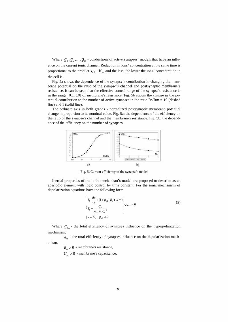
Fig. 5a shows the dependence of the synapse’s contribution in changing the mem-
brane potential on the ratio of the synapse’s channel and postsynaptic membrane’s
resistance. It can be seen that the effective control range of the synapse's resistance is
in the range [0.1: 10] of membrane's resistance. Fig. 5b shows the change in the po-
tential contribution to the number of active synapses in the ratio Rs/Rm = 10 (dashed
line) and 1 (solid line).
The ordinate axis in both graphs - normalized postsynaptic membrane potential
change in proportion to its nominal value. Fig. 5a: the dependence of the efficiency on
the ratio of the synapse's channel and the membrane's resistance. Fig. 5b: the depend-
ence of the efficiency on the number of synapses.
Fig. 5. Current efficiency of the synapse's model
Inertial properties of the ionic mechanism’s model are proposed to describe as an
aperiodic element with logic control by time constant. For the ionic mechanism of
depolarization equations have the following form:
1
(1 )
, 0
, 0
I s m
am
I
s m
am
duT g
E
R u vdt
gC
Tg R
u g
(5)
Where ag - the total efficiency of synapses influence on the hyperpolarization
mechanism,
sg
- the total efficiency of synapses influence on the depolarization mech-
anism,
0mR - membrane's resistance,
0mC - membrane's capacitance,
8

v - the expected contribution of the model in the value of the intracellular
potential in the absence of external excitation. This value is determined by the activity
of neighboring membrane segments,
u - a real model’s contribution to the value of the intracellular potential.
Initial conditions: u(0)=0.
For ionic mechanism of hyperpolarization equations are analogous up to relocation
of the effects of excitatory and inhibitory synapses and Em - on Em+.
Action’s potential generator’s model. Generator’s model performs the formation of
rectangular pulses of given amplitude Ey as a result of exceeding fixed threshold P by
the potentialu . The model can be described by the following equations:
).(
,
*
**
uFy
uudt
duT
G
G (6)
Where P > 0 – neuron’s threshold,
GT - time constant, which determines the duration of the feedback over-
charging membrane and characterizing pulse durations,
)( *uFG - Function describing the hysteresis. The output of the function is
Ey, if Pu * and zero if 0* u .
Initial conditions: 0)0(* u .
Output signal y(t) goes to overcharge feedbacks of cell’s soma.
3 Research
Setting the model’s parameters was based on experimental data on the time parame-
ters of the processes occurring in the natural neuron [10].
Fig. 6 shows a typical response of a neuron model to the exciting pulse. In the
graph of intracellular potential (2) can be seen a typical region of the neuron mem-
brane depolarization is preceded by the formation of an action potential, the zone of
hyperpolarization after pulse generation and residual membrane depolarization at the
end of the generation's pattern.
9

Fig. 6. Neuron with synapse on its dendrite (1 - stimulating effect 2 - intracellular membrane
potential on the generator of the action potential, 3 - neuron responses combined with the graph
of the intracellular potential)
One of the main characteristics of the natural neuron qualitatively affects the trans-
formation of the pulsed streams is the size of the membrane. Unlike small neuron
large neuron is less sensitive to the effects of input and generates a pulse sequence
typically in a lower frequency range and generally corresponds to input effects with
single pulses.
The developed model allows to build neurons with different membrane structure
and location of synapses on it. Changing the number of the membrane segments neu-
rons of different sizes can be modeled, without changing the values of the parameters.
With the increasing size of the soma at the same stimulation of the neuron number
of pulses in the pattern of neuron response decreases and the interval between them
increases. Fig. 7a demonstrates dependence of the response's average frequency from
the number of pulses Np in it. Fig. 7b demonstrates dependence of response's average
frequency from the number of neuron's soma segments L.
Fig. 7. Discharge frequency, depending on the neuron's soma size
As a simple neural structures with feedback considered element, which is a widely
held in the nervous system connection excitatory inhibitory neurons, first studied in
neurophysiological experiments, the interaction of motoneuron and Renshaw's cells
(Fig. 8).
Fig. 8. The scheme of recurrent inhibition by the example of the regulation of motoneuron
discharges
Motoneuron
Renshaw cell
excitatory effect
inhibitory effectexcitatory effect
10

There are two mechanisms for increasing the strength of muscle contraction. The
first is to increase the pulse repetition frequency at the output of motoneuron. Second
- increasing the number of active motoneurons, the axons of which are connected to
the muscle fibers of the muscle. Specialized inhibition neuron in the chain of recur-
rent inhibition - Renshaw cell - limits and stabilizes the frequency of motoneuron
discharges. Example of such a structure shows an analog model (Fig. 9), the behavior
of which corresponds to neurophysiological data [11].
Fig. 9. Recording pulsed streams in studying the interaction of motoneuron and Renshaw cells
motoneuron at the excitation frequency of 20Hz (a) and 50 Hz (b): 1 - excitatory motoneuron
input; 2 - Renshaw cell's discharges; 3 - motoneuron output pulses. Above - the time stamp 10
ms
The graphs show that the frequency of motoneuron stimulation enhances the inhib-
itory effect on Renshaw cells with motoneuron, causing, in turn, decrease the fre-
quency of motoneuron discharges. Thus, when the frequency of motoneuron stimula-
tion increases, the frequency of the pulses at the output of the first moments increases
and then stabilizes at a low level with a duration of interpulse intervals determined by
the duration of the Renshaw cell’s discharge. It is essential that this limit is dependent
on whether the motoneuron by recurrent inhibition "own" Renshaw cells or not.
Computer simulation has allowed a more detailed study of the interaction of neurons.
The results of the experiment are shown in Fig. 10, where the top-down plotted in-
put pulsed stream at the input of motoneurons and pulsed streams of motoneuron
Renshaw cell with recurrent inhibition and, accordingly, these neurons without feed-
back when motoneuron excites Renshaw cell, but it does not slow motoneuron.
Fig. 10. Reactions of structure “motoneuron-Renshaw cell” upon excitation of motoneurons
pulsed stream at 50 Hz: 1 - input pulsed stream; 2 – motoneuron’s reaction with enabled FB; 3 -
Renshaw cell responses with enabled FB; 4 – motoneuron’s reaction without FB; 5 - Renshaw
cell responses without FB
11

4 Conclusion
The paper presents a model of a neuron, which can serve as the basis for constructing
models of neural networks of living organisms and study their applicability in solving
the problems of motion control of robotic systems. The model allows to describe the
structure of the neuron’s membrane (dendritic and synaptic apparatus).
Plasticity model is also based primarily on changes in the structure of the mem-
brane, rather than adjusting the parameters of the model (synapse weights, neuron’s
threshold, etc.), which simplifies the construction of models of specific known biolog-
ical neural structures.
5 Sources
1. McKinstry, J. L., Edelman, G. M., Krichmar, J. L.: A cerebellar model for predictive mo-
tor control tested in a brain-based device. PNAS, February 28, 2006, vol. 103, No.9, pp.
3387–3392 (2006)
2. Hugo de Garis, Chen Shuo, Ben Goertzel, Lian Ruiting.: A world survey of artificial brain
projects, Part I: Large-scale brain simulations. Neurocomputing 74, pp. 3–29 (2010)
3. Bakhshiev, A.V., Klochkov, I.V., Kosareva, V.L., Stankevich, L.A.: Neuromorphic robot
control systems. Robotic and Technical Cybernetics No. 2(3)/2014, pp.40–44. Russia,
Saint-Petersburg, RTC (2014)
4. Bakhshiev, A.V., Gundelakh. F.V.: Investigation of biosimilar neural network model for
motion control of robotic systems. Robotics and Artificial Intelligence: Proceedings of the
VI Russian Scientific Conference with international participation, 13 december 2014,
Zheleznogorsk, Russia (2014)
5. McCulloch, W. S., Pitts W.: A logical calculus of the ideas immanent in nervous activity //
Bulletin of Mathematical Biophysics, vol. 5, pp. 115-133 (1943)
6. Hodgkin, A.L., Huxley, A.F.: A quantitative description of membrane current and its ap-
plication to conduction and excitation in nerve. J. Physiology, 117, pp. 500–544 (1952)
7. Izhikevich, E.M.: Simple model of spiking neurons. IEEE transactions on neural networks.
A publication of the IEEE Neural Networks Council, vol. 14, No. 6, pp. 1569–1572
(2003)
8. Romanov, S.P.: Neuron model. Some problems of the Biological Cybernetics. Russia, pp.
276-282 (1972)
9. Bakhshiev, A.V., Romanov, S.P.: Neuron with arbitrary structure of dendrite, mathemati-
cal models of biological prototypes. Neurocomputers: development, application, Russia,
No.3, pp. 71-80 (2009)
10. Bakhshiev, A.V., Romanov, S.P.: Reproduction of the reactions of biological neurons as a
result of modeling structural and functional properties membrane and synaptic structural
organization. Neurocomputers: development, application, Russia, No.7, pp. 25–35 (2012)
11. John Carew Eccles. The Physiology of Synapses. Springer-Verlag (1964)
12

The Construction of ImagesUsing Minimal Spline
Burova I.G. and Bezrukavaya O.V.
St. Petersburg State University, St. Petersburg, Russia,[email protected],
Abstract. Tasks of data compression, transmission, subsequent recov-ery with a given accuracy are of great practical importance. In this paperwe consider a problem of constructing graphical information on a planewith the help of a parametric defined splines with different properties.Here we compare the polynomial and the trigonometric splines of thefirst and the second order, the polynomial integro-differential splines,the trigonometric integro-differential splines. We consider a compressionof the image to a relatively small number of points, and a restoration ofgraphic information with the given accuracy.
Keywords Image Construction, Polynomial Splines, TrigonometricalSplines, Integro-differential Splines, Interpolation
1 Introduction
Plotting functions by means of splines is widely used in practice [3–8]. Here wecompare the polynomial and the trigonometric splines of the first and the sec-ond order, the polynomial integro-differential splines, the trigonometric integro-differential splines. These splines are characterized by the fact that the approx-imation of a function is constructed at each grid interval separately as a linearcombination of values of the functions in neighboring grid nodes and some ba-sic functions (see [1, 2]). The image can be compressed to a small number ofpoints, which we call the control points (points of interpolation). The result ofthe image compression has the form of the control points and information of theapplied basic splines. If it is necessary, the user can restore the image throughan appropriate algorithm.
2 Right polynomial, right trigonometric splines
Let n be natural number, a, b be real numbers, tj be ordered equidistant setof nodes on [a, b], h = tj+1 − tj .
Let function u be such that u ∈ C3[a, b]. We use the approximation for u(t)in the form
u(t) = u(tj)ωj(t) + u(tj+1)ωj+1(t) + u(tj+2)ωj+2(t), t ∈ [tj , tj+1], (1)
13

where ωj(t), ωj+1(t), ωj+2(t) we determine from the system
u(x) = u(x), u(x) = ϕi(x), i = 1, 2, 3. (2)
Here ϕi(x), i = 1, 2, 3, is Chebyshev system on [a, b], ϕi ∈ C3[a, b].
2.1 Right polynomial splines
In polynomial case we take ϕi(x) = xi−1, So we have from (2)
ωj(t) =(t− tj+1)
(tj − tj+1)· (t− tj+2)
(tj − tj+2), ωj+1(t) =
(t− tj)(tj+1 − tj)
· (t− tj+2)
(tj+1 − tj+2), (3)
ωj+2(t) =(t− tj)
(tj+2 − tj)· (t− tj+1)
(tj+2 − tj+1). (4)
We obtain for t ∈ [tj , tj+1] the estimation of the error of the approximationby the polynomial splines (1), (3) – (4): |u(t)−u(t)| ≤ K1h
3‖u′′′‖[tj ,tj+2], K1 =0.0642.
2.2 Right trigonometric splines
In trigonometric case we take ϕ1 = 1, ϕ2 = sin(x), ϕ3 = cos(x). So we have fromthe system (2):
ωj(t) =sin(t/2− tj+1/2)
sin(tj/2− tj+1/2)· sin(t/2− tj+2/2)
sin(tj/2− tj+2/2), (5)
ωj+1(t) =sin(t/2− tj/2)
sin(tj+1/2− tj/2)· sin(t/2− tj+2/2)
sin(tj+1/2− tj+2/2), (6)
ωj+2(t) =sin(t/2− tj/2)
sin(tj+2/2− tj/2)· sin(t/2− tj+1/2)
sin(tj+2/2− tj+1/2). (7)
The error of the approximation u(t) by (1), (5)–(7) is the next:
|u(t)− u(t)| ≤ K2h3‖u′ + u′′′‖[tj ,tj+2], K2 > 0, t ∈ [tj , tj+1].
3 Integro-differential splines
Integro-differential polynomial splines were invented by Kireev V.I [3]. Theway of constructing the nonpolynomial integro-differential splines is in [2]. Theintegro-differential right spline of the third order has the form:
u(t) = u(tj)wj(t) + u(tj+1)wj+1(t) +
∫ tj+2
tj
u(t)dt w<1>j (t), t ∈ [tj , tj+1], (8)
where ωj(t), ωj+1(t), w<1>j (t) we determine from the system (2).
14

3.1 Integro-differential right polynomial splines
In polynomial case we have
wj(t) =A1
(tj − tj+2)(tj − tj+1)(tj − 3tj+1 + 2tj+2), (9)
A1 = (−tj+1+t)(3tj+2t+3ttj−6tj+1t−2t2j−2tjtj+2−2t2j+2+3tj+1tj+2+3tj+1tj),
wj+1(t) =(−tj + t)(3t− tj − 2tj+2)
(tj − tj+1)(tj − 3tj+1 + 2tj+2), (10)
w<1>j (t) =
6(−tj+1 + t)(−tj + t)
(tj − tj+2)2(tj − 3tj+1 + 2tj+2). (11)
We can use in (8) the next formula:∫ tj+2
tj
u(t)dt ≈ (tj+2 − tj)(u(tj) + 4u(tj+1) + u(tj+2))/6.
We obtain |u(t)− u(t)| ≤ K3h3‖u′′′‖[tj ,tj+2], K3 > 0, t ∈ [tj , tj+1].
3.2 Integro-differential right trigonometrical splines
In trigonometric case we have
wj(t) =A3
B3, wj+1(t) =
A4
B4, (12)
whereA3 = (cos(−tj+1+ tj)−cos(tj+1− tj+2)− tj+2 sin(t− tj+1)+ tj sin(t− tj+1)−
cos(t− tj) + cos(t− tj+2)),B3 = (cos(−tj+1+tj)−cos(tj+1−tj+2)−tj+2 sin(−tj+1+tj)+tj sin(−tj+1+
tj)− 1 + cos(tj − tj+2)),A4 = (cos(t− tj)− cos(t− tj+2)+ tj+2 sin(t− tj)− tj sin(t− tj)−1+cos(tj −
tj+2)),B4 = (cos(−tj+1+tj)−cos(tj+1−tj+2)−tj+2 sin(−tj+1+tj)+tj sin(−tj+1+
tj)− 1 + cos(tj − tj+2)),
w<1>j (t) = (sin(t− tj+1)− sin(−tj+1 + tj)− sin(t− tj))/B5, (13)
B5 = (cos(−tj+1+tj)−cos(tj+1−tj+2)−tj+2 sin(−tj+1+tj)+tj sin(−tj+1+tj)− 1 + cos(tj − tj+2)).
If we know only the values u(tj), u(tj−1) = u(tj − h), u(tj+2) = u(tj + 2h),then we can use in (8) the formula:
It =
tj+2∫
tj
u(t)dt = u(tj−1)2h cos(h)− 2 sin(h)
cos(h)− cos(2h)− u(tj)
−2h cos(h) + sin(h) + h
cos(h)− 1+
+u(tj+2)2 sin(h) cos(h)− h− sin(h)
− cos(h)− 1 + 2 cos2(h)+R1.
It can be shown that R1 = 0, if u(t) = 1, sin(t), cos(t), andIt = (−(4/9)u(tj−1) + (5/3)u(tj) + (7/9)u(tj+2))h+O(h3).
15

4 Constructing approximation on the plane
4.1 Piecewise linear set of parametric spline
Let function u be such that u ∈ C2[a, b].We build the approximation of u(t) in the form
u(t) = −A (u(tj)− u(tj+1)) + u(tj), A =t− tj
tj+1 − tj, (14)
Here t ∈ [tj , tj+1], j = 0, . . . , n− 1. We can obtain for t ∈ [tj , tj+1]
|u(t)− u(t)| ≤ K0h2‖u′′‖[tj ,tj+1], K0 = 0.125.
Consider the approximation of the curve on the plane using the linear splines.Let n points z1, z2, . . ., zn are given on the plane. Suppose point zi has coordi-nates (xi, yi). Then we can construct the next approximations:
x(t) = −A (x(tj)− x(tj+1)) + x(tj), y(t) = −A (y(tj)− y(tj+1)) + y(tj),where A = (t− tj)/(tj+1 − tj), if t ∈ [tj , tj+1]. The error of the approximationon the plain is the next: R(t) =
√|x(t)− x(t)|2 + |y(t)− y(t)|2.
4.2 Minimal quadratic set of the right polynomial parametricspline
Consider the approximation of the curve on the plane with the help of quadraticsplines (1), (3)–(4). Let functions x = x(t) and y = y(t) be such that x, y ∈C3[a, b], x(tj) is the value of x in the node tj , y(tj) is the value of y in the nodetj . Then we can use the following formulas:
x(t) = ACx(tj)−ABx(tj+1) +BCx(tj+2), y(t) = ACy(tj)−ABy(tj+1) +BCy(tj+2) on [tj , tj+1], j = 1, . . . , n − 1, where A = (t− tj+2)/(tj − tj+1),B = (t− tj)/(tj+1 − tj+2), C = (t− tj+1)/(tj − tj+2).
5 Numerical experiments
Let function z(t) = (x(t), y(t) be such that x(t) = sin(t), y(t) = cos(t). Supposewe have zj = (x(j), y(j)), j = 1, 2, . . . , 9. We construct z = (x(t), y(t)), with thehelp of splines (1), (3)–(4), (1), (5)–(7), (8), (9)–(11), (8), (12)–(13). The resultsof application the splines (1), (3)–(4), and the splines (1), (5)–(7) are presentedon graphs 1a, 1b. The results of application the splines (8), (9)–(11), and thesplines (8), (12)–(13) are presented on graphs 2a, 2b.
Now we take x(t) = t− 2 sin(t), y(t) = 1− 2 cos(t). The result of applicationthe trigonometric splines (1), (5)–(7) is presented on graph 3a. The result ofapplication the polynomial splines (8), (9)–(11) is presented on graph 3b.
16

(a)
–1
–0.5
0.5
1
–1 –0.5 0.5 1
(b)
–1
–0.5
0
0.5
1
–1 –0.5 0.5 1
Fig. 1. Graphs of approximation by the minimal polynomial splines (1), (3)–(4): (a);by the trigonometric splines (1), (5)–(7): (b)
(a)
–1
–0.5
0
0.5
1
–1 –0.5 0.5 1
(b)
–1
–0.5
0
0.5
1
–1 –0.5 0.5 1
Fig. 2. Graphs of approximation by the right polynomial integro-differential splines(8), (9)–(11): (a), by the right trigonometric integro-differential splines (8), (12)–(13):(b)
6 Imaging of letters using a piecewise linear splines
Here we construct, compress and restore the image of the letters using splines.For example, consider the construction and compression of the letter A. Co-
ordinates of points for the letter "A" zi, i = 1, 2, 3, 4, 5, we take in the form:
x[1]:=2:x[2]:=3:x[3]:=4:x[4]:=3.5:x[5]:=2.5:y[1]:=2:y[2]:=4:y[3]:=2:y[4]:=3:y[5]:=3:t[1]:=1:t[2]:=2:t[3]:=3:t[4]:=4:t[5]:=5:
Coordinates of points for the letter "E" zi, i = 1, 2, 3, 4, 5 are given as:Figure 4a shows the letter "A" which is constructed with the help of the
control points: (2;2),(3;4),(4;2),(3.5;3), (2.5;3), and Fig. 4b shows the letter "E"which is constructed with the help of the points: (4;4), (2;4), (2;3), (3;3), (2;3),(2;2), (4;2) and the splines (14).
Each letter is given by a minimum number of the control points. For differentletters the number of control points is different. Now we can compress the imageand have only the control points and the information about the basis splines. Wecan hold or send the information someone. The recipient can restor the lettersusing the control points and information about the splines.
17

(a)
–1
0
1
2
3
5 10 15 20 25 30
(b)
–1
0
1
2
3
5 10 15 20 25 30
Fig. 3. Graphs of the approximation x(t) = t − 2 sin(t), y(t) = 1 − 2 cos(t) by theright trigonometric splines (1), (5)–(7): (a); by the right polynomial integro-differentialsplines (8), (9)–(11): (b)(a)
2
2.5
3
3.5
4
2 2.5 3 3.5 4
(b)
2
2.5
3
3.5
4
2 2.5 3 3.5 4
Fig. 4. Plot of the letter "A" (the control points: (2;2),(3;4),(4;2),(3.5;3), (2.5;3)) (a).Plot of the letter "E" (the control points: (4;4), (2;4), (2;3), (3;3), (2;3), (2;2), (4;2)): (b).
References1. Burova I.G., Demyanovich Yu.K. Minimal Splines and theirs Applications. Spb.
(2010) (Russian).2. Burova Irina. On Integro Differential Splines Construction. Advances in Applied
and Pure Mathematics. Proceedinngs of the 7-th International Conference on FiniteDifferences, Finite Elements, Finite Volumes, Boundary Elements (F-and-B’14).Gdansk. Poland. pp. 57–61 (May 15-17, 2014)
3. Kireev V.I., Panteleev A.V. Numerical methods in examples and tasks. M. 480 p.(2008)(in Russian)
4. Ruzanski, E. P., Chandrasekar, V. Weather radar data interpolation using a kernel-based lagrangian nowcasting technique. IEEE Transactions on Geoscience and Re-mote Sensing. Vol. 53, Issue 6(1), pp. 3073–3083 (June 2015)
5. Mariani, M. C., Basu, K. Spline interpolation techniques applied to the study ofgeophysical data. Physica A: Statistical Mechanics and its Applications. Vol. 428,15. pp. 68–79 (June 2015)
6. Parker, W.D., Umrigar, C.J., Alfe, D., Petruzielo, F.R., Hennig, R.G., Wilkins,J.W. Comparison of polynomial approximations to speed up planewave-basedquantum Monte Carlo calculations. Journal of Computational Physics. Vol. 287,pp. 77–87 (April 05, 2015)
7. Tzivelekis, C.A., Yiotis, L.S., Fountas, N.A., Krimpenis, A.A. Parametrically au-tomated 3D design and manufacturing for spiral-type free-form models in an inter-active CAD/CAM environment. International Journal on Interactive Design andManufacturing. 10 p. (10 February 2015) (Articles not published yet)
8. Zavjalov Yu.S., Kvasov B.I., Miroshnichenko V.L. Metody spline-functions.M.(1980) (Russian)
18
Fast Infinitesimal Fourier Transform for Signaland Image Processing via Multiparametric and
Fractional Fourier Transforms
Ekaterina Ostheimer1, Valeriy Labunets2, and Stepan Martyugin3
1 Capricat LLC, 1340 S., Ocean Blvd., Suite 209, Pompano Beach,33062 Florida, [email protected],
2 Ural Federal University, pr. Mira, 19,Yekaterinburg, 620002,Russian Federation
[email protected],3 SPA Automatics, named after Academician N.A. Semikhatov,
Mamina Sibiryaka, 145, Yekaterinburg, 620002, Russian [email protected]
Abstract. The fractional Fourier transforms (FrFTs) is one-parametricfamily of unitary transformations Fα2πα=0. FrFTs found a lot of applica-tions in signal and image processing. The identical and classical Fouriertransformations are both the special cases of the FrFTs. They corre-spond to α = 0 (F0 = I) and α = π/2 (Fπ/2 = F), respectively. Up tonow, the fractional Fourier spectra Fαi = Fαi f , i = 1, 2, ...,M , hasbeen digitally computed using classical approach based on the fast dis-crete Fourier transform. This method maps the N samples of the originalfunction f to the N samples of the set of spectra FαiMi=1 , which re-quires MN (2 + log2N) multiplications and MN log2N additions. Thispaper develops a new numerical algorithm, which requires 2MN multi-plications and 3MN additions and which is based on the infinitesimalFourier transform.
Keywords: Fast fractional Fourier transform, infinitesimal Fourier trans-form, Schrodinger operator, signal and image analysis
1 Introduction
The idea of fractional powers of the Fourier operator Fa4a=0 appeared in themathematical literature [1,2,3,4]. The idea is to consider the eigen-value decom-position of the Fourier transform F in terms of the eigen-values λn = ejnπ/2
and eigen-functions in the form of the Hermite functions. The family of FrFTFa4a=0 is constructed by replacing the n-th eigen-value λn = ejnπ/2 by itsa-th power λan = ejnπa/2 for a between 0 and 4. This value is called the trans-
form order. There is the angle parameterization Fα2πα=0 , where α = πa/2is a new angle parameter. Since this family depends on a single parameter,
19

the fractional operators Fa4a=0 (or Fα2πα=0) form the Fourier-Hermite one-
parameter strongly continuous unitary multiplicative group FaFb = Fa⊕4b
(or
FαFβ = Fα⊕2πβ
), where a⊕4b = (a+ b) mod4 (or α⊕
2πβ = (α+ β) mod2π) and
F0 = I. The identical and classical Fourier transformations are both the spe-cial cases of the FrFTs. They correspond to α = 0 (F0 = I) and α = π/2(Fπ/2 = F), respectively.
In 1980, Namias reinvented the fractional Fourier transform (FrFT) againin his paper [6]. He used the FrFT in the context of quantum mechanics as away to solve certain problems involving quantum harmonic oscillators. He notonly stated the standard definition for the FrFT, but, additionally, developedan operational calculus for this new transform. This approach was extended byMcBride and Kerr [7]. Then Mendlovic and Ozaktas introduced the FrFT intothe field of optics [8] in 1993. Afterwards, Lohmann [9] reinvented the FrFTbased on the Wigner-distribution function and opened the FrFT to bulk-opticsapplications. It has been rediscovered in signal and image processing [10]. Inthese cases, the FrFT allows us to extract time-frequency information from thesignal. A recent state of the art can be found in [11]. In the series of papers[12,13,14,15,16], we developed a wide class of classical and quantum fractionaltransforms.
In this paper, the infinitesimal Fourier transforms are introduced, and therelationship of the fractional Fourier transform with the Schrodinger operator ofthe quantum harmonic oscillator is discussed. Up to now, the fractional Fourierspectra Fαi = Fαi f , i = 1, 2, ...,M, have been digitally computed usingclassical approach based on the fast discrete Fourier transform. This methodmaps the N samples of the original function f to the NM samples of theset of spectra FαiMi=1 , which requires MN (2 + log2N) multiplications andMN log2N additions. This paper develops a new numerical algorithm, whichrequires 2MN multiplications and 3MN additions and which is based on theinfinitesimal Fourier transform.
2 Eigen-decomposition and Fractional DiscreteTransforms
Let F = [Fk (i)]N−1k,i=0 be an arbitrary discrete unitary (N × N)-transform, λn
and Ψn (t) n = 0, 1, . . . , N − 1 be its eigen-values and eigen-vectors, respectively.
Let U =
[Ψ0(i)|Ψ1(i)|
...|ΨN−1(i)
]be the matrix of the F-transform eigen-vectors.
Then U−1·F·U = Diag λn. Hence, we have the following eigen-decomposition:F = [Fk(i)] = U ·Λ ·U−1 = U ·Diag λn ·U−1.Definition 1. [12]. For an arbitrary real numbers a0, . . . , aN−1, we introducethe multi-parametric F-transform
F (a0,...,aN−1) := Udiag
(λa00 , . . . , λ
aN−1
N−1)
U−1. (1)
20

If a0 = . . . = aN−1 ≡ a then this transform is called fractional F-transform[12,13,14,15,16]. For this transform we have
Fa := Udiag
(λa0 , . . . , λ
aN−1
)U−1 = UΛaU−1. (2)
The zero-th-order fractional F-transform is equal to the identity transform: F0 =UΛ0U−1 = UU−1 = I , and the first-order fractional Fourier transform operatorF1 = F is equal to the initial F-transform F1 = UΛU−1.
The familiesF(α0,...,αN−1)
(α0,...,αN−1)∈RN
and Faa∈R form multi- and
one-parameter continuous unitary groups, respectively, with multiplication rules
F (a0,...,aN−1)F (b0,...,bN−1) = F (a0+b0,...,aN−1+bN−1) and FaFb = Fa+b.Indeed, FaFb = UΛaU−1 ·UΛbU−1 = UΛa+bU−1 = Fa+b and
F (a0,...,aN−1)F (b0,...,bN−1) =
= Udiag
(λa00 , . . . , λ
aN−1
N−1)
U−1 ·U
diag(λb00 , . . . , λ
bN−1
N−1
)U−1 =
= U
diag(λa0+b00 , . . . , λ
aN−1+bN−1
N−1
)U−1 = F (a0+b0,...,aN−1+bN−1).
Let F = [Fk (i)]N−1k,i=0 be a discrete Fourier (N × N)-transform (DFT), then
λn = ejπn/2 ∈ ±1,±j , where j =√−1 and Ψn (t)N−1n=0 are the Kravchuk
polynomials.
Definition 2. The multi-parametric and fractional DFT are
F (a0,...,aN−1) := U
diag(ejπ0a0/2, ejπ1a1/2, . . . , ejπ(N−1)aN−1/2
)U−1,
Fa := U
diag(ejπna/2
)U−1
and
F (α0,...,αN−1) := U
diag(ej0α0 , ej1α1 , . . . , ej(N−1)αN−1
)U−1,
Fα := Udiag
(ejnα
)U−1
in a- and α-parameterizations, respectively, where α = πa/2.
The parameters (a0, . . . , aN−1) and a can be any real values. However, theoperators F (a0,...,aN−1) and Fa are periodic in each parameter with period 4 since
F4 = I. Hence, F (a0,...,aN−1)F (b0,...,bN−1 = F(a0⊕
4b0,...,aN−1⊕
4bN−1)
and FaFb =
Fa⊕4b
, where ai⊕4bi = (ai + bi) mod4, ∀i = 0, 1, ..., N − 1. Therefore, the ranges
of (a0, . . . , aN−1) and a are (Z/4Z)N
= [0, 4]N
= [−2, 2]N
and Z/4Z = [0, 4] =[−2, 2], respectively.
In the case of α-parameterization, we have αi⊕2πβi = (αi + βi) mod2π, ∀i =
0, 1, ..., N−1. So, the ranges of (α0, . . . , αN−1) and α are (Z/2πZ)N
= [0, 2π]N
=
[−π, π]N
and Z/2πZ = [0, 2π] = [−π, π], respectively.
21

3 Canonical FrFT
The continuous Fourier transform is a unitary operator F that maps square-integrable functions on square-integrable ones and is represented on these func-tions f(x) by the well-known integral
F (y) = (Ff) (y) =1√2π
∫
x∈Rf(x)e−jyxdx. (3)
Relevant properties are that the square(F2f
)(x) = f(−x) is the inversion
operator, and that its fourth power(F4f
)(x) = f(x) is the identity. Hence,
F3 = F−1. Thus, the operator F generates a cyclic group of the order 4. In1961, Bargmann extended the Fourier transform in his paper [5] where he gavedefinition of the FrFT that was based on the Hermite polynomials as an integraltransformation. If Hn (x) is a Hermite polynomial of order n, where Hn (x) =
(−1)nex
2 dn
dxn ex2
, then for n ∈ N0, functions Ψn(x) = 1√2nn!
√πHn(x)e−x
2/2 are
the eigen-functions of the Fourier transform
F [Ψn (x)] =1
2π
∫ +∞
−∞Ψn (x) e2πjyxdx = λnΨn (y) = e−j
π2 nΨn (y)
with λn = jn = e−jπ2 n being the eigen-value corresponding to the n-th eigen-
function. According to Bargmann, the fractional Fourier transform Fα = [Kα (x, y)]is defined through its eigen-functions as
Kα (x, y) := Udiag
(e−jαn
)U−1 =
∞∑
n=0
e−jαnΨn (x)Ψn (y) . (4)
Hence,
Kα (x, y) :=∞∑
n=0
e−jαnΨn (x)Ψn (y) = e−(x2+y2)∞∑
n=0
e−jαnHn(x)Hn(y)
2nn!√π
=
=1√
π√
1− e−2jα· exp
2xye−jα − e−2jα
(x2 + y2
)
1− e−2jα
exp
−(x2 + y2
)
2
,
(5)where Kα (x, y) is the kernel of the FrFT. In the last step we used the Mehlerformula [19]
∞∑
n=0
e−jαnHn(x)Hn(y)
2nn!√π
=1√
π√
1− e−2jαexp
2xye−jα − e−2jα
(x2 + y2
)
1− e−2jα
.
Expression (5) can be rewritten as
Kα(x, y) =
√1− j cotα
2πexp
j
2 sinα
[(x2 + y2) cosα− 2xy
],
22

where α 6= πZ (or a 6= 2Z). Obviously, functions Ψn(x) are eigen-functions ofthe fractional Fourier transform Fα [Ψn(x)] = ejnαΨn(x) corresponding to then-th eigen-values ejnα, n = 0, 1, 2, . . .. The FrFT Fα is a unitary operator thatmaps square-integrable functions f(x) on square-integrable ones
Fα(y) = (Fαf) (y) =
∫
x∈Rf(x)Kα(x, y)dx =
=e−
j2 (π2 α−α)
√2π |sinα|
∫
R
f(x) exp
j
2 sinα
[(x2 + y2
)cosα− 2xy
]dx.
There exist several algorithms for fast calculation of spectrum of the frac-tional Fourier transform Fα(y). But all of them are based on the following trans-form of the FrFT:
Fα(y) = (Fαf) (y) =e−
j2 (π2 α−α)ejy
2 cosα2 sinα√
2π |sinα|
∫
R
[f(x)ej
x2
2 cotα]e−jxydx =
= Aα(y) · F f(x) ·Bα(x) (y),
where Aα(y) = e− j
2 (π2 α−α)ejy2 cosα
2 sinα√2π|sinα|
, Bα(x) = ejx2
2 cotα.
Let us introduce the uniform discretization of the angle parameter α on Mdiscrete values α0, α1, ..., αi, αi+1, ..., αM−1 , where αi+1 = αi+∆α, αi = i∆αand ∆α = 2π/M.
The set of M spectra Fα0 (y) , Fα1 (y) , ..., FαM−1 (y) can be computed byapplying the following sequence of steps for all α0, α1, ..., αM−1:
1. Compute products f(x)Bαk(x), which require N multiplications.2. Compute the Fast Fourier Transform (N log2N multiplications and addi-
tions).3. Multiply the result by Aα(y) (N multiplications).This numerical algorithm requiresMN log2N additions andMN (2 + log2N)
multiplications.
4 Infinitesimal Fourier Transform
In order to construct fast multi-parametric F-transform and fractional Fouriertransform algorithms we turn our attention to notion of a semigroup and itsgenerator (infinitesimal operator). Let L2(R,C) be a space of complex-valuedfunctions (signals), and let Op(L2) be the Banach algebra of all bounded linearoperators on L2(R,C) endowed with the operator norm. A family U(α)α∈R ⊂Op(L2) is called the Hermite group on L2(R,C) if it satisfies the Abel functionalequations U(α + β) = U(α)U(β), α, β ∈ R and U(0) = I, and the orbitmaps α → Fα = U(α) f are continuous from R into L2(R,C) for everyf ∈ L2(R,C).
23

Definition 3. The infinitesimal generator A(0) of the group U(α)α∈R andthe infinitesimal transform U(dα) are defined as follows [18,19]:
A(0) =∂U(α)
∂α
∣∣∣∣α=0
, U(dα) = I + dU(0) = I + A(0)dα.
Obviously,
U(α0 + dα) = U(α0) + dU(α0) = U(α0) +∂U(α)
∂α
∣∣∣∣α0
dα =
= U(α0) + A(α0)dα.
But
U(α0 + dα) = U(dα0)U(α0) = [I + dU(0)] U(α0) =
= U(α0) +∂U(α)
∂α
∣∣∣∣α=0
U(α0)dα =
= U(α0) + A(0)U(α0)dα = [I + A(0)] U(α0)dα.
Hence, A(α0) = A(0)U(α0) and Fα0+dα(y) =[I + A(0)
]Fα0(y)dα.
Define now the linear operator H = 12
(d2
dx2 − x2 + 1)
. It is known that
HΨn(x) =1
2
(d2
dx2− x2 + 1
)Ψn(x) = nΨn(x). (6)
From (4) and (6) we have
j∂
∂αFα(y)
∣∣∣∣α=0
= j∂
∂αFαF (y)
∣∣∣∣α=0
=∞∑
n=0
nΨn(y)
∫
R
Ψn(x)f(x)dx,
HFα(x) =∞∑
n=0
nΨn(y)
∫
R
Ψn(x)f(x)dx.
Therefore, j ∂Fα(x)∂α = HFα(y), ∂F
α(x)Fα(x) = −jH∂α. The solution of this equa-
tion is given by Fα(x) =e−jαHF
and Fα = e−jαH = e
−jα[
12
(d2
dx2−x2+1
)].
Obviously,
Fα+dα = FdαFα ' (I + dFα) exp [−jαH] =
=
(I +
∂Fα∂α
dα
)exp (−jαH) = (I− jHdα) exp (−jαH) ,
where the operator
Fdα = (I− jHdα) = I− j 1
2
(d2
dx2− x2 + 1
)dα (7)
24

is called the infinitesimal Fourier transform or the generator of the fractionalFourier transforms [17,18].
Let us introduce operators (Mxf) (x) := xf(x) and (MyF ) (y) := yF (y).Using the Fourier transform (3), the first of ones may be written as Mx =
F−1(j ddy
)F . Obviously, x2 = M2
x = −F1
(d2
dy2
)F . Then
Fdα = I− j 1
2
(d2
dx2+ F−1
(d2
dy2
)F + 1
)dα.
Discretization of x-domain with the interval discretization ∆x is equal to theperiodization of y-domain
d2
dx2+ F−1
(d2
dy2
)F + 1 −→ D∆x
[d2
dx2
]+ F−1
(P2π/∆x
[d2
dy2
])F + 1.
Discretization of y-domain with the interval discretization ∆y is equal to theperiodization of x-domain
D∆x
[d2
dx2
]+ F−1
(P2π/∆x
[d2
dy2
])F + 1 −→
−→ P2π/∆yD∆x
[d2
dx2
]+ F−1
(P2π/∆xD∆y
[d2
dy2
])F + 1.
An approximation for the second derivative can be given by the second ordercentral difference operator
d2
dx2f(x) ≈ f(n
N1)− 2f(n) +F (n⊕
N1),
d2
dy2F (y) ≈ F (k
N1)− 2F (k) +F (k⊕
N1),
where N = 2π/∆x∆y. On the other hand,
F−1(d2
dy2F (y)
)F ≈ F−1
[F (k
N1)− 2F (k) + F (k⊕
N1)
]F =
=(f(n)e−j
2πN n − 2f(n) + f(n)ej
2πN n)
= 2f(n)
(cos
2π
Nn− 1
).
These allow one to give the approximation for H = 12
(d2
dx2 − x2 + 1)
as follows:
Hf(x) =
[1
2
(d2
dx2− x2 + 1
)]f(x) ≈
≈ 1
2
[f(n
N1)− 2f(n) + f(n⊕
N1)
]+ 2f(n)
(cos
2π
Nn− 1
)+ f(n)
=
= −[cos
2π
Nn− 3/2
]f(n) +
1
2
[f(n
N1) + f(n⊕
N1)
].
25
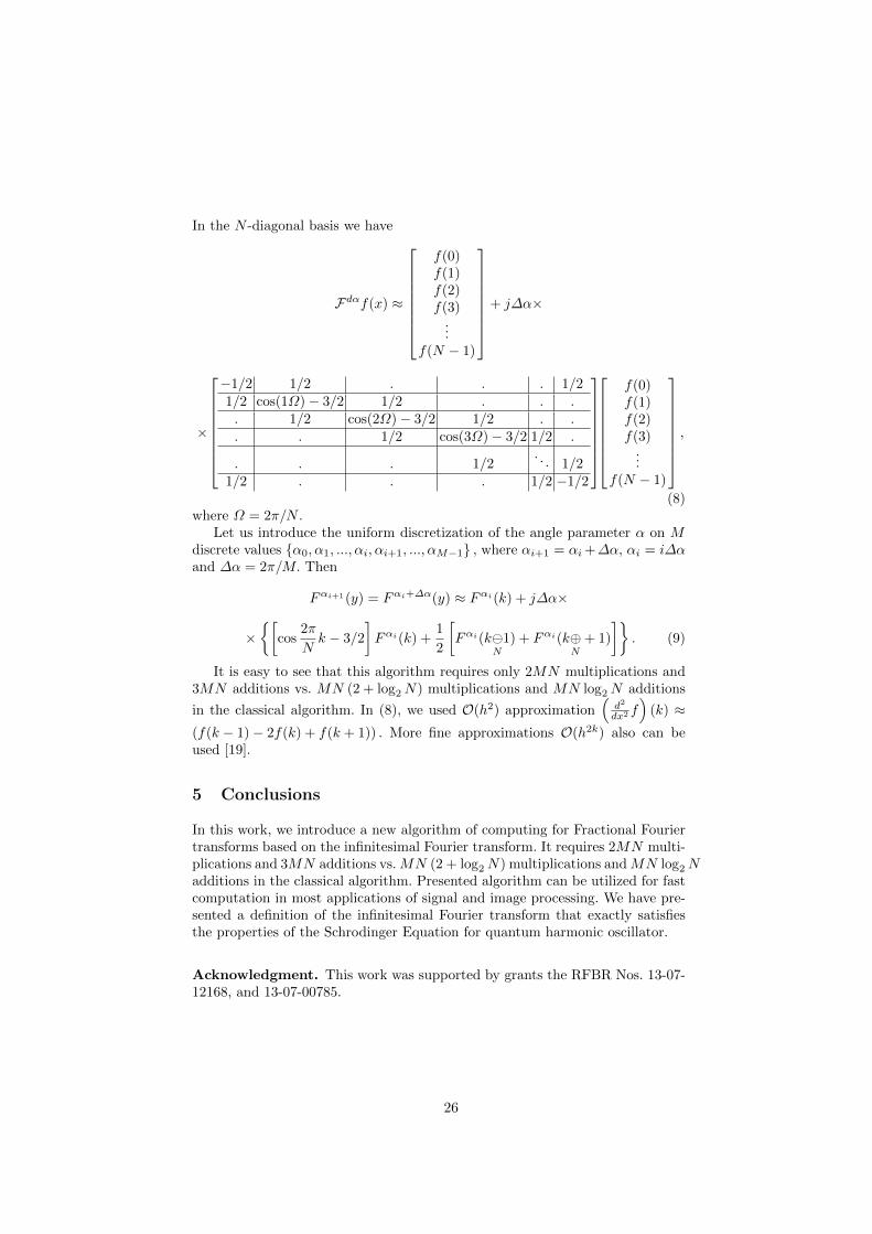
In the N -diagonal basis we have
Fdαf(x) ≈
f(0)f(1)f(2)f(3)
...f(N − 1)
+ j∆α×
×
−1/2 1/2 . . . 1/21/2 cos(1Ω)− 3/2 1/2 . . .. 1/2 cos(2Ω)− 3/2 1/2 . .. . 1/2 cos(3Ω)− 3/2 1/2 .
. . . 1/2. . . 1/2
1/2 . . . 1/2 −1/2
f(0)f(1)f(2)f(3)
...f(N − 1)
,
(8)where Ω = 2π/N .
Let us introduce the uniform discretization of the angle parameter α on Mdiscrete values α0, α1, ..., αi, αi+1, ..., αM−1 , where αi+1 = αi+∆α, αi = i∆αand ∆α = 2π/M. Then
Fαi+1(y) = Fαi+∆α(y) ≈ Fαi(k) + j∆α×
×[
cos2π
Nk − 3/2
]Fαi(k) +
1
2
[Fαi(k
N1) + Fαi(k⊕
N+ 1)
]. (9)
It is easy to see that this algorithm requires only 2MN multiplications and3MN additions vs. MN (2 + log2N) multiplications and MN log2N additions
in the classical algorithm. In (8), we used O(h2) approximation(d2
dx2 f)
(k) ≈(f(k − 1)− 2f(k) + f(k + 1)) . More fine approximations O(h2k) also can beused [19].
5 Conclusions
In this work, we introduce a new algorithm of computing for Fractional Fouriertransforms based on the infinitesimal Fourier transform. It requires 2MN multi-plications and 3MN additions vs.MN (2 + log2N) multiplications andMN log2Nadditions in the classical algorithm. Presented algorithm can be utilized for fastcomputation in most applications of signal and image processing. We have pre-sented a definition of the infinitesimal Fourier transform that exactly satisfiesthe properties of the Schrodinger Equation for quantum harmonic oscillator.
Acknowledgment. This work was supported by grants the RFBR Nos. 13-07-12168, and 13-07-00785.
26

References
1. Mitra, S.K.: Nonlinear Image Processing. Academic Press Series in Communications,Networking, and Multimedia, San Diego, New York, 248 (2001)
2. Wiener, N.: Hermitian polynomials and Fourier analysis. J. Math. Phys. 8, 70–73(1929).
3. Condon, E.U.: Immersion of the Fourier transform in a continuous group of func-tional transforms. Proc. Nat. Acad. Sci. 23, 158–164 (1937)
4. Kober, H.: Wurzeln aus der Hankel- und Fourier und anderen stetigen Transforma-tionen. Quart. J. Math. Oxford Ser. 10, 45–49 (1939)
5. Bargmann, V.: On a Hilbert space of analytic functions and an associated integraltransform. Part 1. Commun. Pure Appl. Math. 14, 187–214 (1961)
6. Namias, V.: The fractional order Fourier transform and its application to quantummechanics. J. Inst. Math. Appl. 25, 241–265 (1980)
7. McBride, A.C., Kerr, F.H.: On Namias’ fractional Fourier transforms. IMA J. Appl.Math. 39, 159–265 (1987).
8. Ozaktas, H.M., Mendlovic, D.: Fourier transform of fractional order and their opticalinterpretation. Opt. Commun. 110, 163–169 (1993)
9. Lohmann, A.W.: Image rotation, Wigner rotation, and the fractional order Fouriertransform. J. Opt. Soc. Am. A. 10, 2181–2186 (1993)
10. Almeida, L.B.: The fractional Fourier transform and time-frequency representation.IEEE Trans. Sig. Proc. 42, 3084–3091 (1994)
11. Ozaktas, H.M., Zalevsky, Z., Kutay M.A.: The fractional Fourier transform. Wiley,Chichester, (2001)
12. Rundblad–Labunets, E., Labunets, V., Astola, J., Egiazarian, K.: Fast fractionalFourier-Clifford transforms. Second International Workshop on Transforms and Fil-ter Banks. Tampere, Finland, TICSP Series, 5, 376–405 (1999)
13. Rundblad, E., Labunets, V., Astola, J., Egiazarian, K., Polovnev, S.: Fast fractionalunitary transforms. Proc. of Conf. Computer Science and Information Technologies,Yerevan, Armenia, 223–226 (1999)
14. Creutzburg, R., Rundblad, E., Labunets, V.: Fast algorithms for fractional Fouriertransforms. Proc. of IEEE-EURASIP Workshop on Nonlinear Signal and ImageProcessing. Antalya, Turkey, June 20–23, 383–387 (1999)
15. Rundblad, E., Labunets, V., Astola, J., Egiazarian, K., Smaga, A.: Fast fractionalFourier and Hartley transforms. Proc. of the 1999 Finnish Signal Processing Sym-posium. Oulu, Finland, 291–297 (1999)
16. Labunets, E., Labunets, V.: Fast fractional Fourier transforms. Proc. of Eusipco-98,Rhodes, Greece, 8–11 Sept. 1757–1760 (1998)
17. Goldstein, J.: Semigroups of Linear Operators and Applications, Oxford U. Press,New York, (1985)
18. Griffiths, R.B.: Consistent Quantum Theory. http://www.cambridge.org19. Candan C.: The Discrete Fractional Fourier Transform, M.S. thesis, Bilkent Univ.,
Ankara, Turkey, (1998)
27

Approximating Social Ties Based on Call Logs:Whom Should We Prioritize?
Mohammad Erfan, Alim Ul Gias, Sheikh Muhammad Sarwar, and Kazi Sakib
Institute of Information TechnologyUniversity of Dhaka, Dhaka–1000, Bangladesh
bit0326,alim,smsarwar,[email protected]
Abstract. Telecommunication service providers could analyze the calllogs of individual users to provide personalized services like recommend-ing Friends and Family (FnF) numbers, that could be registered for hav-ing lower tariff during communication. However, suggesting such num-bers is not simple as the decision making process can often be misledby factors like overall talk-time or call frequency. This paper proposesa technique to assist mobile phone users for effectively identifying FnFnumbers using the underlying social network of a call graph. It resem-bles to a star network, having the user at the center, where each of theedges are weighted using three call log attributes: call duration, call lo-cation and call period. The weighted call graph is then used to calculateuser’s social closeness based on which FnF numbers are suggested. Theexperiment was conducted on a set of real life data and it is seen thatthe proposed technique can effectively suggest FnF numbers with an F-measure value of 0.67.
Keywords: Social network, mobile phone call graph, call log attributes,social closeness
1 Introduction
Personalized services can be defined as context-specific services to each individ-ual client [1]. Since mobile phone can always be carried by the client, it has thepotential to be an ideal medium of such personalization. This potential allowstelecommunication service providers to offer multiple personalized services likecustomized ring tone suggestions or different location based information. Pro-viding such services can increase the popularity of the service providers [2] andhelp them to sustain in the competitive market. Thus, it is high time telecom-munication companies focused more on providing personalized services to eachuser for eventually increasing their overall revenue.
Recommending Friends and Family (FnF) numbers [3], that can be registeredby the user for having lower call rate, could be an example of customized personalservices. To provide such service, it is essential to retrieve each user’s calling pat-tern by analyzing their respective call logs. However, analysis and interpretationof these call logs is particularly difficult and introduces major research issues [4].
28

A possible solution could be, utilizing the underlying social network [5] of thosecall logs. Nevertheless, constructing such network involves multiple challengeslike relative prioritization of in and out degrees, and assigning weight to edgesby using different call log attributes.
Although multiple research has been conducted based on mobile phone calllogs, none has focused directly to provide personalized services to each individualuser. There have been some work that focus on investigating social ties based ondifferent call attributes [6], [7]. Some of the researchers have focused on predictinguser behavior [8] and community dynamics [9]. Moreover, there are works whichforecast incoming calls [10] and correlate international calls with the export-import business of the country [11]. However, it is arguable that whether thesestate of the arts can be used to provide effective personalized services that cansatisfy each individual user.
This paper proposes a methodology to create a weighted call graph based onindividual call logs and use the graph’s underlying social network for predictingFnF numbers. To weight the edges, three call log attributes are used which are -call duration, call period and call location. The technique empirically measuresthe effect of these attributes towards social closeness and calculates their relativesignificance. The summation of these relative significances, that prevents any ofthe attributes being predominated, is considered as the weight. A closeness scoreis then calculated by aggregating the product of the weights with values respectto their call being either incoming or outgoing. This score is used by the methodto rank and suggest numbers for registering as FnF.
The method was implemented and its performance was evaluated based ona real life dataset. The dataset includes all required call log attributes alongwith a user provided score which indicates the strength of social tie with theperson of that particular call. These scores were considered as the ground truthwhen weights for edges of the graph are being learned. The social closeness wasthen measured, based on which numbers were ranked, to predict FnF numbers.The performance of the proposed technique was compared along with traditionalapproaches based on overall talk-time and call frequency. It seen that the methodoutperforms the call frequency and overall talk-time based approaches with 38%and 10% higher F-measure value.
Rest of the paper is organized as follows: Section 2 highlights state of theart techniques for analyzing call logs to derive different social contexts. Theproposed technique to predict FnF numbers is presented in Section 3. Section4 includes the experimental details and performance of the proposed technique.Finally, this paper is concluded in Section 5 with a discussion about our workand future research directions.
2 Literature Review
Although log analysis has been a major research concern for a considerableamount of time [12], its application in mobile phone call pattern analysis hasstarted comparatively later. To the best of authors’ knowledge, no work directly
29
focus on utilizing the underlying social network obtained from a single user’s calllogs to provide customized services. The work that have been done mostly focuson constructing social networks from call logs, predicting the user behavior andidentifying multiple social contexts like social affinity or community dynamics.This section highlights these contributions and discusses how they contrast toour problem domain.
There have been some significant work which are concerned with predictingthe user behavior. For an example, Dong et. al. proposed a technique to create anundirected binary graph from the call log to find the human behavior of differentage and gender [8]. The researchers in [13] proposed a method to derive the userrelation using Bayesian network. Phithakkitnukoon et. al. analyzed multiple calllog attributes such as call location, talk-time, calling time and inter-arrival timeto infer behavioral dependencies [10]. The researcher in [14] inferred friendshipnetwork by utilizing the behavioral and survey data. Zhang et. al. have focused oninformation retrieval techniques to find human behavior patterns and communitydynamics [9]. There have also been work to assess the strength of social tie basedon call duration [6].
Identifying different social contexts has been another field of major researchinterest. Phithakkitnukoon et. al. proposed a method to identify social networkbased on the user phone call log [15]. They have used correlation coefficient to se-lect call log features and then extracted user’s social behavioral pattern from thatnetwork. Another work of Phithakkitnukoon et. al. has been presented in [16]where they created a network graph to derive socially closest and distant mem-bers. The researchers in [11] analyzed international phone calls from Rwanda,between January 2005 to December 2008, to derive the interpersonal connec-tions between the people of different countries. They have used those findings tomeasure and evaluate the social tie between nations.
Researchers have also focused on the construction of call graph by utilizingdifferent call log attributes. The researchers in [17] created a social network graphusing call duration, source number, destination number and physical location ofthe user. They have extracted these information from Call Detail Record (CDR)[18] files and and generated the adjacency matrix. The edges were weighted usingthe call duration value. Motahari et. al. have also used the CDR files and createdmultiple affinity networks such as family members, utility network, friends andco-workers [7]. They have used CDR files containing 4.3 million phone call datawhich was collected from 360,000 subscribers.
Review of the state of the art shows that these works are generally focusedon predicting users’ behavioral pattern rather than utilizing those patterns forproviding better user experience. It is arguable that whether these methods canbe used for determining user’s social tie along with utilizing the findings in aseparate strategy to suggest FnF numbers. From different research, it is alsoseen that the edges of the constructed call graph is weighted using call duration.Nevertheless, it may not be the correct representation of social affinity. Thereason behind this is though frequent or long communication likely indicates astrong tie, little or no communication does not necessarily indicate a weak tie [6].
30

Thus it is required to incorporate other call log attributes, to assign weights ongraph edges, for actual representation of individual’s social tie. This weightedgraph can be easily used to infer the socially closest members and their numberscan be suggested as FnF.
3 Proposed Method
This research proposes a methodology to create a social network graph using thephone call log. The network will resemble to a star network where the phone userwill be the center node and individuals with whom communication has occurredare the peripheral nodes. There will be weighted edges between the central andperipheral nodes which will indicate the strength of their social ties.The graphwill have two type of edges, one for the incoming calls and other for the outgoingones. The frequency of calls will not effect the number of edges since it will beconsidered during the weight calculation. A sample social network is presentedin Figure 1. From the figure it can be seen that communications are representedby weighted edges where the outgoing call to individual pn has a weight wn1 andthe incoming call has a weight wn2.
User
Fig. 1. Call graph generated from a single user’s call logs
Initially call log records will be taken from the phone. The call logs shouldhave the following information: call duration, call period (a period of the daylike 3:00 AM to 6:00 AM) and call location (the place from which the call wasmade). It is essential to utilize all these information for weighting graph edgessince using only call duration can often misled regarding the approximation ofsocial closeness. For an example, a user may talk with a person at his office fora long time. However, that person could be a client instead of being a friend
31

or relative. So it will be wrong to consider that person as a socially close onebased on the call duration. Moreover, talking with a someone during the officehours (like 9:00 AM to 5:00 PM ) for a long time might misled in estimating thenature of social affinity. Thus it would be more reasonable to assign a weight bycombining all these three information. The proposed method utilizes these calllog attributes to assign a weight which is defined in Equation (1).
ωij =N∑
k=1(α · δijk
+ βq(ijk) + γr(ijk)) (1)
In Equation (1), ωij refers to the weight of the edge between the person pi
and phone’s user for all calls of type j (like incoming, outgoing or missed). Theset of all j type calls, with respect to person pi is represented by Cij . If |Cij | = N ,the weight ωij will be the summation of N values. The values will depend oncall duration (δ), call period and call location. The value of call duration is usedby multiplying it with a weight α that reflects the significance of call durationtowards social ties. To represent the significance of call period and call location,two sets of values, S and L has been introduced. The elements of those two setsare represented by β and γ respectively. To define their relation with the set ofcalls Cij , two mapping functions q : Cij → S and r : Cij → L are defined.
In a nutshell, the weight will be calculated by considering each of the callsof type j from person pi. For each particular call k, its duration will be mul-tiplied by a significance factor α. This multiplied value will be added with thecorresponding β and γ value of that particular call. However, the system mustat first calculate those significance values. The social closeness should then haveto be calculated for suggesting the FnF numbers. The procedure for these tasksare discussed in details in the following subsections.
3.1 Determining the significance values
Since longer communications likely indicate a strong tie [6], the proposed methoduses the correlation coefficient between the call duration and social closeness asthe value of α. However, information regarding the social closeness of people fromeach call is a pre-requisite to calculate the coefficient. To determine the values ofβ and γ, one has to first fix the number of call periods and locations that shouldbe considered. The set of these periods and locations are defined as T and Lrespectively. For each of the elements in set T and L, the method generates aseparate value of β and γ respectively. These values, combined together, are thenrepresented by two sets S and L respectively.
The first step in calculating the values of β and γ requires to define a thresholdvalue σ. This value is used to identify the people who are socially closest to thephone user. If the social closeness value of a person is above the threshold,that individual is considered as having a strong social tie. The second stepsinvolves calculating the percentage of people over σ for each of the call periodsand locations. These percentages provide an insight regarding the significance ofeach period and location. However, to consider those as weights, their relative
32

significance is needed to be considered which is calculated at the final step. Thiswhole procedure is illustrated in Algorithm 1.
Algorithm 1 Determining the significance valuesInput: The set of all selected call periods T and locations LOutput: α, S and L1: Begin2: Set the value of α to the correlation coefficient between call duration and social
closeness3: Define a threshold σ for social closeness to determine socially closest persons4: Calculate the percentage of calls from people whose social closeness value is overσ on each call period ti ∈ T and location li ∈ L
5: Initialize S ← ∅ and L ← ∅6: for each ti ∈ T do7: βi = percentage of people over σ for period ti
summation of percentage values ∀ti∈T
8: S ∪ βi9: end for10: for each li ∈ L do11: γi = percentage of people over σ for location li
summation of percentage values ∀li∈L
12: L ∪ γi13: end for14: End
3.2 Calculating Social Closeness and Suggesting FnF numbers
After determining the values of α, β and γ, the weight ωij of call type j fromperson pi can be calculated using Equation (1) . The weights ωij for each of theindividuals are included in the setWij which is used by the proposed method torepresent a social network as shown in Figure 1. To calculate the social closenessof the person pi, the method uses a mapping function φ : J → I, where Jand I represent the set of call types and their significances respectively. Thismapping function φ is used to determine the weight of different call types. As-signing different weights to different call types is important since the significanceof different call types (incoming or outgoing) could be different. During the cal-culation of social closeness for person pi, as shown in Equation (2), the weightsof that person ωij for call type j is multiplied by its respective weight providedby the mapping function φ.
θi =M∑
j=1φ(j) · ωij (2)
The process of determining the social closeness and ranking the individualsbased on that score is presented in Algorithm 2. Initially, as used in Algorithm 1,
33

a threshold σ is defined to identify socially closest persons. This threshold is usedto calculate the percentage of socially closest persons for each call of type j. Thepercentage values are then used to determine the relative significance of differentcall types. Using these relative significance values, the method calculates thesocial closeness as defined in Equation (2). Each of the individuals, with whomcommunication has occurred, are sorted in descending order of social closeness.The method then suggests the numbers of certain individuals, at the top of thelist, as FnF numbers.
Algorithm 2 Calculating Social ClosenessInput: The set Wij , Cij , J and the mapping function φOutput: List of individuals sorted in descending order of social closeness1: Begin2: Define a threshold σ for social closeness to determine socially closest persons3: Calculate the percentage of calls from people whose social closeness value is overσ for each j type of calls
4: Initialize I ← ∅5: for each j ∈ J do6: λj = percentage of people over σ for call type j
summation of percentage values ∀j∈J7: I ∪ λj8: end for9: Use Equation (2) to calculate social closeness for each of individual10: Sort the list of individuals in descending order of social closeness11: End
4 Experimental Setup and Results
This section discusses about different experimental parameters that were usedduring the evaluation of our proposed approach. It also includes the performanceof the proposed technique with a comparison along with two baseline approachesto suggest FnF numbers.
4.1 Experimental Parameters
For experimental purpose the call logs were collected from 18 individuals. Thecall logs included the person’s mobile phone number, call duration and call time.The call location was manually collected from them. The participants had alsoprovided a social closeness score, to each of the persons from the call log, in ascale of 1-10. Moreover, each of them were also asked to select 3 numbers fromthese call logs which they could register as FnF numbers. 5 of the participantsprovided those numbers and thus their data were used for the testing purpose.Rest of the data were used to train the proposed method that involves learningthe values of α, β, γ and λ. During the calculation of these weights, the value of
34

σ was set to 8 which is considerably higher enough in the social closeness scalefor recognizing socially closest persons.
The value of α was calculated by determining the correlation coefficient be-tween call duration and social closeness. It has been found that the call durationand social closeness has a positive relationship, though not that much strong.This has been illustrated in Figure 2 by a scatter diagram where social closenessis plotted against call duration. The value of correlation coefficient was found tobe 0.14 and it was set as the value of α.
0
2
4
6
8
10
12
14
0 2 4 6 8 10
Call D
ura
tion
Social Closeness
Fig. 2. Scatter diagram representing the correlation coefficient between social closenessand call duration
For the calculation of β, we have divided a day into 8 time periods. The per-centage of socially closest calls and their relative weight is presented in Table 1.A scatter diagram is presented in Figure 3 to illustrate the percentage of sociallyclosest people in two different time periods.
Table 1. Relative significance of different time periods used in the experiment
Period Percentage of calls above σ Relative weight12:00 AM to 3:00 AM 60% 0.1633:00 AM to 6:00 AM 67% 0.186:00 AM to 9:00 AM 25% 0.079:00 AM to 12:00 PM 55% 0.1512:00 PM to 3:00 PM 26% 0.0713:00 PM to 6:00 PM 41% 0.1126:00 PM to 9:00 PM 56% 0.1539:00 PM to 12:00 AM 37% 0.101
For calculating the value of γ, the locations were categorized before collectingthe data. For each of the call logs, the location was selected as either home orwork place. Although there were instances where users were neither in home nor
35

0
2
4
6
8
10
12
14
0 5 10 15 20 25 30 35 40
Socia
l C
loseness
Number of Instances
(a) Time period 3:00 PM to 6:00 PM
0
2
4
6
8
10
12
14
0 5 10 15 20 25 30
Socia
l C
loseness
Number of Instances
(b) Time period 9:00 PM to 12:00 AM
Fig. 3. Visualization of calls from socially closest persons in two different time periods
in work place, still they had used various measures two provide the location in-formation. Examples include selecting the place nearest to their current positionor based on the nature of call and its period. These data, as presented in Figure4, was used to calculate the value of γ. For the home and workplace, the valueturned out to be 0.44 and 0.56 respectively.
0
2
4
6
8
10
12
14
0 20 40 60 80 100 120
Socia
l C
loseness
Number of Instances
(a) Location - Home
0
2
4
6
8
10
12
14
0 10 20 30 40 50 60 70 80 90
Socia
l C
loseness
Number of Instances
(b) Location - Workplace
Fig. 4. Visualization of calls from socially closest persons in two separate locations
In this work, ignoring the missed calls, incoming and outgoing calls has beenconsidered to measure the value of λ. The percentage of calls from socially closestpersons for outgoing and incoming calls can be visualized from Figure 5. Sincethere were only two call types, after calculating the weight of work place, theother weight was calculated by Equation 3. The weights for the incoming andoutgoing calls has been calculated as 0.44 and 0.56 respectively.
φ(j) =λ if the value of j is 11− λ otherwise (3)
36

0
2
4
6
8
10
12
14
0 20 40 60 80 100 120 140 160
Socia
l C
loseness
Number of Instances
(a) Outgoing calls
0
2
4
6
8
10
12
14
0 20 40 60 80 100 120 140 160
Socia
l C
loseness
Number of Instances
(b) Incoming calls
Fig. 5. Visualization of incoming and outgoing calls from socially closest persons
4.2 Performance Evaluation
The proposed technique tried to match 2 out of 3 FnF numbers provided by eachindividuals. The system suggested 5 numbers, one after another, and stoppedat the point where two numbers had being matched. Thus for 5 individuals,the system tried to match 10 FnF numbers with at most 25 attempts. We havecompared the performance of our system with two baseline approaches which arebased on overall call duration and call frequency. The evaluation technique forthese two approaches remained the same. It is seen that the proposed methodhas identified 7 FnF numbers with 22 attempts. On the other hand, the duration-based and frequency based approaches has identified 6 and 3 numbers with 22and 25 attempts respectively.
Table 2. Performance comparison of the proposed technique with respect to duration-based and frequency based approaches
Approaches Precision Recall F-measureDuration-based 0.27 0.6 0.57Frequency-based 0.8 0.2 0.19
Proposed technique 0.32 0.7 0.67
The performance of the technique, as shown in Table 2, is interpreted in termsof precision, recall and F-measure. It is seen that proposed method outperformsthe other two approaches though the value of the precision is low. However, inthis case, recall is more important than precision. This is because for each of theindividuals, we are suggesting at most 5 numbers to match with 2 numbers. Dueto this, the precision will always be lower due to having more false positives.Nevertheless, the user will always be satisfied if the system chooses more fromthe set of relevant numbers. So during the calculation of F-measure, as done in[19], the method needs to vary the weights of precision and recall. Thus in our
37

case, recall has been weighted five times higher than the precision during thecalculation of F-measure using Equation (4).
FB = (1 +B2) · precision · recallB2 · precision+ recall
(4)
For the individuals with whom the performance was evaluated, the patternof score provided by the system and the social closeness score provided by thephone users is illustrated in Figure 6. Although the scale of those two scoresare different, it is seen that their curves are very much similar. As the systemsuggested FnF numbers based on calculated closeness scores, the performance isbetter than the other two approaches.
0
0.2
0.4
0.6
0.8
1
1.2
0 20 40 60 80 100 120 140 160
Score
Number of Instances
CollectedCalculated
Fig. 6. The pattern of the scores collected from the individuals and calculated by theproposed method
5 Conclusion and Future WorkThis paper introduces a technique to prioritize individuals based on call logsand suggest FnF numbers using that prioritize list. The method utilizes theunderlying social network of the call graph for a single phone user. The edges ofthe call graph has been weighted during the prioritization process to incorporatedifferent call log attributes like duration, period and location. The proposedmethodology was implemented and tested against a set of real life data. Thesystem has illustrated its effectiveness in identifying FnF numbers with an F-measure value of 0.67. This research also introduces a set of new research ideasfor the research communities. This includes assessing the existence of a nonlinearrelationship, between duration and social closeness, to improve the performanceof the system. Moreover, one could utilize other call log attributes and optimizetheir total number to get better performance.
AcknowledgementThis work is supported by the University Grant Commission, Bangladesh underthe Dhaka University Teachers Research Grant No-Regi/Admn-3/2015/48747.
38

References1. Ho, S.Y., Kwok, S.H.: The attraction of personalized service for users in mobile
commerce: an empirical study. ACM SIGecom Exchanges 3(4), 10–18 (2002)2. Witteman, M.: Efficient proximity detection among mobile clients using the GSM
network. Master’s thesis, University of Twente (2007)3. Dey, B., Newman, D., Prendergast, R.: Analysing appropriation and usability in
social and occupational lives: An investigation of bangladeshi farmers’ use of mobiletelephony. Information Technology & People 24(1), 46–63 (2011)
4. De Melo, P.O.V., Akoglu, L., Faloutsos, C., Loureiro, A.A.: Surprising patternsfor the call duration distribution of mobile phone users. In: Machine learning andknowledge discovery in databases, pp. 354–369. Springer (2010)
5. Chin, A., Zhang, D.: Mobile Social Networking. Springer (2014)6. Wiese, J., Min, J.K., Hong, J.I., Zimmerman, J.: Assessing Call and SMS Logs as
an Indication of Tie Strength. Tech. rep., Human-Computer Interaction Institute,School of Computer Science, Carnegie Mellon University (2014)
7. Motahari, S., Mengshoel, O.J., Reuther, P., Appala, S., Zoia, L., Shah, J.: Theimpact of social affinity on phone calling patterns: Categorizing social ties fromcall data records. In: Proceedings of the Sixth Workshop on Social Network Miningand Analysis. pp. 1–9. ACM (2012)
8. Dong, Z.B., Song, G.J., Xie, K.Q., Wang, J.Y.: An experimental study of large-scale mobile social network. In: Proceedings of the 18th International Conferenceon World Wide Web. pp. 1175–1176. ACM (2009)
9. Zhang, D., Guo, B., Yu, Z.: The emergence of social and community intelligence.Computer 44(7), 21–28 (2011)
10. Phithakkitnukoon, S., Dantu, R., Claxton, R., Eagle, N.: Behavior-based adaptivecall predictor. ACM Transactions on Autonomous and Adaptive Systems (TAAS)6(3), 21 (2011)
11. Blumenstock, J.E.: Using mobile phone data to measure the ties between nations.In: Proceedings of the 2011 iConference. pp. 195–202. ACM (2011)
12. Oliner, A., Ganapathi, A., Xu, W.: Advances and challenges in log analysis. Com-munications of the ACM 55(2), 55–61 (2012)
13. Park, H.S., Cho, S.B.: Building mobile social network with semantic relation usingBayesian network-based life-log mining. In: Second International Conference onSocial Computing (SocialCom). pp. 401–406. IEEE (2010)
14. Eagle, N., Pentland, A.S., Lazer, D.: Inferring friendship network structure byusing mobile phone data. Proceedings of the National Academy of Sciences 106(36),15274–15278 (2009)
15. Phithakkitnukoon, S., Dantu, R.: Inferring social groups using call logs. In: Onthe Move to Meaningful Internet Systems: OTM 2008 Workshops. pp. 200–210.Springer (2008)
16. Phithakkitnukoon, S., Dantu, R.: Mobile social group sizes and scaling ratio. AI &society 26(1), 71–85 (2011)
17. Zargari, H.: Social network modelling: Retrieval correlated graphs by mobilephone’s chronological billing files. In: The Second International conference “Prob-lems of Cybernetics and Informatics”. pp. 67–70 (2008)
18. Horak, R.: Telecommunications and Data Communications Handbook. John Wiley& Sons (2007)
19. Li, X., Wang, Y.Y., Acero, A.: Learning query intent from regularized click graphs.In: Proceedings of the 31st Annual International ACM SIGIR Conference on Re-search and Development in Information Retrieval. pp. 339–346. ACM (2008)
39

Identification of Three-DimensionalCrystal Lattices by Estimation of Their
Unit Cell Parameters?
Dmitriy Kirsh1,2 and Alexander Kupriyanov1,2
1 Samara State Aerospace University (National Research University),Samara, Russian Federation
2 Image Processing Systems Institute of Russian Academy of Sciences,Samara, Russian Federation
Abstract. The problem of the identification of three-dimensional crys-tal lattices is considered in the article. Two matching methods basedon estimation of unit cell parameters were developed to solve this prob-lem. The first method estimates and compares main parameters of Bra-vais unit cells. The second method estimates and compares volumes ofWigner-Seitz unit cells. Both methods include normalised similarity mea-sures: an edge similarity measure and an angle similarity measure forBravais cells and a volume similarity measure for Wigner-Seitz cells.The results of computational experiments on the large set of simulatedlattices showed that the developed methods allowed to achieve the iden-tification accuracy above 90% for four lattice systems.
Keywords: crystal lattice, unit cell parameters, Monte Carlo method,similarity measure, structural identification
1 Introduction
One of the basic problems related to X-ray diffraction analysis is the identifica-tion of crystal lattices [5]. It is usually solved by comparing estimated parametersof analysed lattice with those of selected sample [2]. The lattice parameters ei-ther previously investigated or derived by modeling can be used as samples.Therefore the accurate identification of a crystal lattice requires a large database of the preselected sample parameters.
Among the main methods for identification of three-dimensional crystal lat-tices the following ones can be singled out: NIST lattice comparator [1], iden-tification on the basis of atomic packing factor [4] and centered cubic lattice
? The work was financially supported by the Ministry of education and science ofthe Russian Federation in the framework of the implementation of the Program ofincreasing the competitiveness of SSAU among the worlds leading scientific and ed-ucational centers for 2013-2020 years; by the Russian Foundation for Basic Researchgrants (# 14-01-00369-a, # 14-07-97040-p povolzh’e a); by the ONIT RAS program# 6 Bioinformatics, modern information technologies and mathematical methods inmedicine 2015.
40

comparison method [3]. These methods have a number of drawbacks limitingtheir application field: complexity of crystal preparation, high error in compari-son of lattices, which are similar in volume, etc.
The new approach based on estimation of unit cell parameters attempts toavoid these drawbacks. The algorithms proposed in the work allow calculatinga similarity measure for any two crystal lattices.
2 Models of Crystal Lattices
There are several methods to describe crystal lattices. The most widespreadmethod was offered by Auguste Bravais [5]. Bravais unit cell is characterised bya set of six parameters: lengths of the three edges l1, l2, l3 and values of the threeangles between the edges α1, α2, α3 (Fig. 1).
l1
l2
l3
α1
α2α3
Fig. 1. The main parameters of Bravais unit cell
All Bravais lattices are subdivided into seven lattice systems. Table 1 showscharacteristics of their unit cells.
Table 1. Characteristics of lattice systems
Lattice system Symbol Edge lengths Angles
Triclinic aP l1 6= l2 6= l3 α1 6= α2 6= α3
Monoclinic mP l1 6= l2 6= l3 α1 = α2 = 90 6= α3
Orthorhombic oP l1 6= l2 6= l3 α1 = α2 = α3 = 90
Tetragonal tP l1 = l2 6= l3 α1 = α2 = α3 = 90
Cubic cP l1 = l2 = l3 α1 = α2 = α3 = 90
Rhombohedral hR l1 = l2 = l3 α1 = α2 = α3 6= 90
Hexagonal hP l1 = l2 6= l3 α1 = 120;α2 = α3 = 90
41

Another model of crystal lattices was offered by Jeno Wigner and FrederickSeitz [6]. Wigner-Seitz unit cell is characterised by a set of normal vectors whichare drawn to limiting planes. In a three-dimensional space it is a polyhedronwhich contains inside itself one lattice node (Fig. 2).
Fig. 2. Body-centered cubic Wigner-Seitz cell
3 Method of Crystal Lattice Identification on the Basisof Bravais Unit Cell Parameter Estimation
The initial data of the identification method are the set of radius-vectors deter-mining the spatial position of crystal lattice nodes.
The following algorithm was designed to calculate the six main parametersof the Bravais unit cell:
1. Center the lattice.2. Superpose the first radius-vector of minimal length with the axis OX.3. Transfer the second radius-vector of minimal length into the plane XOY .4. Select the third radius-vector of minimal length.5. Calculate the main six parameters: l1, l2, l3, α1, α2, α3.
Two normalised measures were introduced to determine separately the degreeof the edge similarity and the degree of the angle similarity of two Bravais unitcells.
Similarity measure of edges:
‖l1 − l2‖ = 1−
√(l11 − l21)
2+ (l12 − l22)
2+ (l13 − l23)
2
max
√(l11)
2+ (l12)
2+ (l13)
2,
√(l21)
2+ (l22)
2+ (l23)
2
(1)
42

Similarity measure of angles:
‖α1 −α2‖ = 1−max sin (|α11 − α21|), sin (|α12 − α22|), sin (|α13 − α23|) (2)
4 Method of Crystal Lattice Identification on the Basisof Wigner-Seitz Unit Cell Volume Estimation
The initial data of the identification method are the number of scattering pointsL and the set of radius-vectors determining the spatial position of crystal latticenodes.
The following algorithm was designed to calculate the volume of the Wigner-Seitz cell:
1. Center the lattice.2. Determine the normal vectors from central lattice node to the planes limiting
Wigner-Seitz cell.3. Calculate the volume of cell limited by planes with the use of the Monte
Carlo method.(a) Generate L-values of three-dimensional random vectors which are uni-
formly distributed in the whole lattice volume.(b) Count the number of vectors that hit in the region limited by planes and
calculate the volume of cell based on the fact that the probability of hitin the Wigner-Seitz cell region is proportional to its measure (volume).
A normalised measure was introduced to determine the degree of the volumesimilarity for two Wigner-Seitz unit cells:
‖V1 − V2‖ = 1−
√(V1 − V2)
2
max V1, V2(3)
The following computational experiments of crystal lattice identification onthe large set of simulated three-dimensional lattices were conducted to analysethe efficiency of the introduced similarity measures.
5 Results of Experimental Computations
The initial data for experiments were 7,000 lattices (1000 lattices of each latticesystem) obtained by simulation. The lengths of edges and values of angles weredetermined by values of a uniformly distributed random variable.
Each lattice was matched with all the rest lattices in pairs: two lattices wereconsidered to be similar in edges or in angles, if the value of the correspondingsimilarity measure was no less than 0.95. Selection of this limiting value relatesto the fact that currently the error of lattice parameter determination is no lessthan 5% [1].
43

Two lattices in the first experiment were brought into comparison only bythe value of the edge similarity measure. Matching of two lattices in the secondexperiment was carried out only by the value of the angle similarity measure.However, the derived values of the percentage of lattice exact identification werenear 14% for all lattice system in both experiments. These results show thatthe partitioning of all Bravais crystal lattices into seven lattice systems by usingonly the edge similarity measure or the angle similarity measure is not uniformand separable.
Consequently more exact lattice identification requires the simultaneous ap-plication of both similarity measures. For this reason in the third experiment twolattices were considered to be similar if values of the edge similarity measure andthe angle similarity measure were no less than 0.95. Table 2 shows the results.
Table 2. Percentage of lattice exact identification for the main lattice systems bysimultaneous edges and angles comparison
Estimated Sample cellcell aP mP oP tP cP hR hP
aP 98 1 1 0 0 0 0mP 7 39 36 14 1 0 3oP 6 36 39 14 1 1 3tP 5 26 26 34 4 4 1cP 4 12 12 23 26 23 0hR 11 2 2 3 4 78 0hP 12 3 3 2 0 0 80
Table data show average percent of coincidence of the estimated lattices withsample lattices (both similarity measures are no less than 0.95). For example theset of sample lattices which have coincided with one of the rhombohedral latticesin the third experiment consists on the average of 11% triclinic, of 2% monoclinic,of 2% orthorhombic, of 3% tetragonal, of 4% cubic, of 78% rhombohedral andof 0% hexagonal.
The use of the volume similarity measure of Wigner-Seitz unit cells was thelast step to increase the identification accuracy. Matching of two lattices in thefinal fourth experiment was conducted with the application of all three similaritymeasures simultaneously: edges and angles of Bravais unit cells and volumes ofWigner-Seitz unit cells. Table 3 shows the results of the experiment.
According to Table 2 and Table 3 data it can be concluded that the accu-racy of lattice identification increased by average 15%. The maximum increaseof accuracy was achieved for monoclinic lattices by 51%. However, there is a sep-arate group (orthorhombic, tetragonal, cubic) with the low percentage of latticeexact identification and, therefore, the problem of delimiting these three latticesystems cannot be considered as solved.
44

Table 3. Percentage of lattice exact identification for the main lattice systems bysimultaneous edges, angles and volumes comparison
Estimated Sample cellcell aP mP oP tP cP hR hP
aP 99 1 0 0 0 0 0mP 2 90 4 3 0 0 1oP 2 22 54 20 1 1 0tP 1 10 34 44 6 5 0cP 0 3 15 26 30 26 0hR 1 0 2 3 4 90 0hP 1 7 0 0 0 0 92
6 Conclusion
The developed methods of crystal lattice identification allowed to achieve theidentification accuracy above 90% for four lattice systems (triclinic, monoclinic,rhombohedral and hexagonal).
Basing on the performed calculation it can be concluded that the best way toidentify the lattice system for the generated set of 7,000 lattices is simultaneousapplication of all three introduced similarity measures.
Identification accuracy of the remaining three lattice systems (orthorhombic,tetragonal and cubic) is not still sufficiently high. They require further researchfor the purpose of finding additional similarity measures (for example, compari-son of isosurfaces, tensor representation of unit cells, etc.).
References
1. Kessler, E., Henins, A., Deslattes, R., Nielsen, L., Arif, M.: Precision Comparison ofthe Lattice Parameters of Silicon Monocrystals. Journal of Research of the NationalInstitute of Standards and Technology 99, 1–18 (1994)
2. Kupriyanov, A.: Texture analysis and identification of the crystal lattice type uponthe nanoscale images. Computer Optics 35, 128–135 (2011) (in Russian)
3. Patera, J., Skala, V.: Centered cubic lattice method comparison. In: 17th ALGO-RITMY Conference on Scientific Computing, pp. 309–319. Slovakia (2005)
4. Smith, W.: Foundations of Materials Science and Engineering. McGraw-Hill, NewYork (2004)
5. Soifer, V., Kupriyanov, A.: Analysis and recognition of the nanoscale images: con-ventional approach and novel problem statement. Computer Optics 35, 136–144(2011) (in Russian)
6. Tilley, R.: Crystals and crystal structures. John Wiley & Sons, Chichester (2006)
45

Construction of Adaptive Educational Forums Based on
Intellectual Analysis of Structural and Semantics
Features of Messages
Alexander Kozko
Chelyabinsk State University,
Chelyabinsk, Russia
Abstract. The paper deals with organization of interaction and communication between sub-
jects of the distance learning process through forums and comment system. Considered existing
software tools, their structure and disadvantages. Propose a model of adaptive educational fo-
rums, as well as the structural and semantic similarity metrics for extracting dialogues and the-
matic discussions from arrays of individual comments, as a basis for the construction of adap-
tive educational forums.
Keywords: distance learning · online discussion forums · semantic similarity
1 Introduction
Development of information technologies makes distance education more available for
everyone, and technology of management and support of education process becomes
more and more important. Many scientific works dedicated to LMS (Learning Manage-
ment System), for example works [1, 2, 3], give a description of LMS, and works [4,
5] devoted to review of existing LMS products. However, these works consider of
learning management tools mainly from the following perspectives: development, man-
agement, courses and distribution of education materials, but not paying enough atten-
tion to the issues of communication and information exchange between the different
subjects of education process.
At present, modern learning theories such as the theory of connectivism proposed
by George Siemens and Stephen Downes, indicate as the basic conditions for successful
learning activities not only communication with the teacher, but also the interaction
between students and the exchange between them so-called “sensemaking artifacts” [6].
Sensemaking artifacts means blog posts, notes, podcasts, and other educational materi-
als that created by a student for discussion with other students. In the paper [7] analyzed
this learning approach and claimed it more effective in comparison with traditional.
Thus, the theme of the organization of communication and interaction between sub-
jects of distance education process is extremely relevant today, but it isn't considered
in the existing works.
46

2 Instruments of communication and informational exchange
for education process
Consider the instruments of communication that are used in distance education.
On the one hand LMS, like Moodle, ILIAS, and Sakai and the other hand, of the
platform for organization MOOCs (Massive open online course), such as Stepic,
Udemy, Coursera, EdX, Udacity propose to use for interaction within the course online
forums, blogs, chat rooms, questions and answers websites, wiki-pages and in addition
allowed commenting learning materials. For some courses, authors suggest to use third
party sites such as Reddit, StackExchange or social networks instead of internal plat-
form tools.
Irrespective of the specifics and type of a course the main tools that are used for
communication within the course are standard forums, blogs, questions and answers
system, as well as various materials commenting system. However, such instruments
do not take into account the specificity of education process and do not provide any
applicable analytical functions for organization of education.
3 Overview of informational exchange tools
3.1 Interaction tools
Forum, in generally, - is an online tool for website's visitors communication. The
essence of any forum is to create topics with its subsequent discussion. Users can com-
ment on created topics, ask questions and receive answers, and answer other forum
user’s questions of the forum and give them advice. Thus, each topic is an initial entry
with a set of comments.
Blogs are a set of copyright entries, sorted by creation time, usually from the newest
to the oldest. Blogs characterized by the ability to publish reviews (comments) by other
users, and that makes blogs an instrument for information exchange. Technically, each
blog entry as well as forum topic is the initial post with a set of comments to it.
Comment systems additionally used in distance education platforms to allow discuss
of any course materials, such as videos or articles.
3.2 Comments structure
Structuring of post's comments may also vary depending on the implementation.
There are three main types of structuring:
• Tree comments - comments list is presented as a hierarchical tree view. New mes-
sage is placed right after the previous one (quoting it isn't necessary). New comment
can also start its own discussion branch.
• Linear (flat) comments - comments within the same topic are published under each
other, as they become available; new message is placed last (usually at the bottom);
interactive relationship between comments is based on specially decorated citations of
references to the author and other means.
47

• Hybrid comments - represent a cross between a tree and a linear structure, now, it
is the most popular form of comments submission.
Comments are usually ordered by date, popularity and the number of votes. Each
comment has text but it also has the following attributes: Author Name and Timestamp.
4 Adaptive learning forums
As noted earlier, the above instruments of online communication do not take into
account the specifics of education process and do not provide any specific functions for
it. Furthermore, they are not designed for a large number of participants, which is usual
for MOOC. Problems such as a large number of overlapping topics, unanswered ques-
tions, incorrectly exposed statuses and tags, are an evidence that the forum is not an
effective communication instrument, we lack of effectiveness of the learning process.
To increase the effectiveness of forum usage, as an instrument of communication
and information exchange within education process we propose develop the technology
of adaptive educational forums, based on data mining.
Adaptive educational forum is an online forum, whose structure is rebuilt depending
on student educational trajectory, his information needs, the features of the course and
users activity. For teachers, the analysis of information from educational forum can be
a source of data for implicit course quality feedback, student's problems with the un-
derstanding of educational materials, student's activity evaluation, etc. Thus, the tech-
nology of adaptive educational forums could be a way to increase the quality of distance
learning.
5 Analysis of comments on online discussion forum
Based on the overview, it can be argued that in such systems, the main content is
often not the whole topic and not individual comments, but thematic discussions and
dialogues, consisting of comments and united by one common theme. Therefore, the
primary tasks are extracting individual discussions of the whole comments list, and the
problem of determining the semantic similarity of discussions among themselves. For
dialogues extracting of the whole comments list we offer use at both the semantics of
messages and their location in the structure of comments.
5.1 Extracting tree commenting relations from linear comments
Because linear structure's main distinction is implicit comments relations, we pro-
pose an approach to the reduction of the linear structure to explicit comments tree struc-
ture.
For comments linear structure conversion to the tree and find comments relations,
proposed focus on the comment text and message attributes, for example, author nick-
name, post timestamp, user's nickname which are responsible, text of citation, position
in comments list.
48

Using these attributes, and the semantics of messages for analyze, for linear com-
ments conversion into a tree we propose determine the pairwise comments relations. In
general, the numerical metric defines an association between two messages comments
represented by equation 1.
𝑟𝑒𝑙(c1,c2) = 𝑘𝑠𝑒𝑚 ∙ 𝑠𝑖𝑚𝑠𝑒𝑚(t1,t2) + 𝑘𝑎𝑡𝑡𝑟 ∙ 𝑠𝑖𝑚𝑎𝑡𝑡𝑟(𝑎1, 𝑎2) (1)
𝑟𝑒𝑙(c1,c2) – relations between the two commentaries, 𝑠𝑖𝑚𝑠𝑒𝑚(t1,t2) – semantic simi-
larity of the two comments texts, 𝑠𝑖𝑚𝑎𝑡𝑡𝑟(𝑎1, 𝑎2) – attribute similarity of the two com-
ments, defined by their attributes, 𝑘𝑠𝑒𝑚 и 𝑘𝑎𝑡𝑡𝑟 – coefficients.
To extract tree structure, it is necessary to calculate each comment's c1 degree of
relation with all previous time comments c2, then c2 comment that has a maximum
relation score becomes the parent of the current comment c1 in a tree structure.
5.2 Extraction of thematic discussions
In a discussion with a large number of participants some of the participants might
drift away from the main theme and start to discuss unrelated topics. Such thematic
discussions (subtopics) within the main topic can also provide useful information for
the user, but their detection difficult. Therefore we propose to allocate such subtopics
in separate entities and use them in the construction of adaptive educational forums.
In tree-like comment systems, a message has the following attributes: author nick-
name, post timestamp, comment depth in tree. Based on this, we proposed similarity
metric for two comments, represented by equation 2.
𝑠𝑖𝑚(c1,c2) = 𝑘𝑠𝑒𝑚 ∙ 𝑠𝑖𝑚𝑠𝑒𝑚(t1,t2) ∗ ( 1
𝑑𝑖𝑠𝑡(c1,c2) + 𝑘𝑎𝑡𝑡𝑟 ∙ 𝑠𝑖𝑚𝑎𝑡𝑡𝑟(𝑎1, 𝑎2)) (2)
𝑠𝑖𝑚(c1,c2) – similarity between the two commentaries, 𝑠𝑖𝑚𝑠𝑒𝑚(t1,t2) – semantic
similarity of the two comments texts, 𝑠𝑖𝑚𝑎𝑡𝑡𝑟(𝑎1, 𝑎2) – attribute similarity of the two
comments, 𝑑𝑖𝑠𝑡(c1,c2) – the distance between the two comments in the tree,
𝑘𝑠𝑒𝑚 , 𝑘𝑎𝑡𝑡𝑟 – coefficients.
To unite a group of comments in a thematic discussion we proposed to use an ap-
proach based on clustering algorithms, the result of which (clusters of comments)
should be used as boundaries for thematic subtopics.
5.3 Semantic similarity metrics for comments
We consider separately the question of calculating the semantic similarity between
the two сomments texts. First it is worth noting the specifics of messages - basically all
posts extremely short - from a few words to 2-3 sentences, so the use of methods for
calculating the semantic similarity of documents can be difficult. It is proposed to de-
termine the similarity of the documents, as similarity of containing concepts.
Existing semantic similarity metrics can be divided into several classes. In work [8]
it is proposed to the following classification:
49

1) Measures based on a corpus of texts: for example, LSA, Web-based - NGD and
PMIIR.
2) Measures based on ontologies: measures by Wu and Palmer, Leackock and Cho-
dorow, Resnik, Lin and others.
3) Measures based on definitions: ExtendedLesk, GlossVectors.
Another group of metrics that can be allocated -
4) The metrics based on Wikipedia: Wikipedia Link-based Measure (WLM), Ex-
plicit Semantic Analysis (ESA), WikiWalk, WikiRelate! and others.
Choosing a semantic similarity metric for concepts it's necessary to pay attention to
the specific learning courses. Themes of learning courses may be beyond ontology but
in domain that is disclosed in course may contain specific concepts which well-known
ontologies as WordNet don't include and specific ontologies for course does not exist.
Therefore, a similarity measure metrics based on ontologies can be used to analyze
educational forums, only if a teacher will build the ontology of course by himself.
For this reason assumed to use the metrics based on the online encyclopedia Wik-
ipedia. The advantages of using Wikipedia as a source of data are a volume and wide
range of different themes, relevance and partial structure.
6 Related Work
Forums analysis is not widely discussed in scientific papers, however it is possible
to highlight the following investigation.
Work [9] devoted to the study groups Usenet, it proposes a method for measuring
the similarity of the different groups on the activity of participants in them, as well as
introduce a measure for evaluation post belonging specific group, which allows exclude
cross-posts from the analysis.
In study [10] proposes a model to estimate the probability of involvement or non-
involvement of a user in a specific online discussion based on the activity of his friends
and his interests, and the list of friends and user’s interests based on the previous activ-
ity in other topics.
In the work [11] is proposed an approach for extracting context information, as well
as questions and answers from the topic using the method of SVM, in [12] considered
other methods used for this purpose.
Finally, in [13], the authors propose an approach that combines both structural and
semantic analysis for search discussions and find of key messages in the threads.
7 Conclusion
Thanks to the Internet, distance education has been made available for millions of
people around the world, and now it's getting increasingly important role of supporting
communication within education process. Number of students enrolled to courses is
increased, and growth of the distance education percentage in the education process
realm sets new requirements that existing communication tools, do not respond, it re-
duces the efficiency of education process as a whole.
50

We propose the concept and the model of adaptive educational forums, the use of
which, in our opinion, will increase the efficiency of interaction between students, as
well as enhance the role of communication environment in distance education process
and give teachers the ability for automatically collect information about students as well
as the quality of the course.
For creation of adaptive educational forums, we propose to use an approach that
includes allocation of individual thematic subtopics that in turn bases on messages
structural and semantic features.
References
1. Dalsgaard, C.: Social software: E-learning beyond learning management systems. European
Journal of Open, Distance and E-Learning, 2 (2006)
2. Sclater, N.: Web 2.0, personal learning environments, and the future of learning manage-
ment systems. Research Bulletin, 13 (2008)
3. Coates, H., James, R., & Baldwin, G.: A critical examination of the effects of learning man-
agement systems on university teaching and learning. Tertiary education and management,
11, 19-36 (2005)
4. Ketcham G., Landa K., Brown K., Charuk K., DeFranco T., Heise M.,
McCabe R., Youngs-Maher P.: Learning Management
Systems Review. (2011) http://openscholar.purchase.edu/sites/de-
fault/files/keith_landa/files/doodle_lmsreport_final.pdf
5. Siemens G.: Learning or Management Systems? A Review of Learning Management System
Reviews. Learning Technologies Centre, University of Manitoba (2006)
6. Siemens G.: Connectivism: Design and Delivery of Social Networked Learning. The Inter-
national Review of Research in Open and Distance Learning 2011; 12:3-11. (2011)
7. Mott J., Wiley D.: Open for Learning: The CMS and the Open Learning Network. In edu-
cation, 15(2). (2009)
8. Panchenko A.: Similarity Measures for Semantic Relation Extraction (Ph.D. Thesis). Uni-
versité catholique de Louvain & Bauman Moscow State Technical University, (2012-2013)
9. McGlohon M., Hurst M.: Community Structure and Information Flow in Usenet: Improving
Analysis with a Thread Ownership Model. ICWSM. (2009).
10. Wu, H., Bu, J., Chen, C., Wang, C., Qiu, G., Zhang, L., Shen, J.: Modeling Dynamic Multi-
Topic Discussions in Online Forums. In AAAI. (2009)
11. Cao, Y., Yang, W. Y., Lin, C. Y., Yu, Y.: A structural support vector method for extracting
contexts and answers of questions from online forums. Information Processing & Manage-
ment, 47(6), 886-898. (2011)
12. Cong, G., Wang, L., Lin, C. Y., Song, Y. I., Sun, Y.: Finding question-answer pairs from
online forums. In Proceedings of the 31st annual international ACM SIGIR conference on
Research and development in information retrieval (pp. 467-474). ACM. (2008)
13. Lin, C., Yang, J. M., Cai, R., Wang, X. J., Wang, W.: Simultaneously modeling semantics
and structure of threaded discussions: a sparse coding approach and its applications. In Pro-
ceedings of the 32nd international ACM SIGIR conference on Research and development
in information retrieval (pp. 131-138). ACM. (2009)
51

The Investigation of Deep Data RepresentationsBased on Decision Tree Ensembles
for Classification Problems
Pavel Druzhkov and Valentina Kustikova
Lobachevsky State University of Nizhni Novgorod,Nizhni Novgorod, Russian Federation
Abstract. A classification method based on deep representation of in-put data and ensembles of decision trees is introduced and evaluatedsolving the problem of vehicle classification and image classification withlarge number of categories.
Keywords: classification; decision trees; random forest, deep learning.
1 Introduction
Deep learning studies machine learning algorithms that enable automatic con-struction of feature description hierarchies thus making data representationsmore efficient in terms of the solved problem. Currently, the deep learning meth-ods for solving image classification and object detection problems are makinggood headway (see, for example, a review of [1] and [2]) as a part of neuralnetwork (NN) models.
Although the deep learning ideas are for now best reflected in NN approaches,the integration of hierarchical data representation into other methods such asdecision trees and bag-of-words is of special interest, because these combinationsmay help to reduce complexity of learning and/or the use of deep models andgive a better understanding of their success. There were attempts to use decisiontrees for induction of new feature descriptions [3, 4]. Nevertheless, no examplesof successful applications of such models stacks are known to the authors. Thispaper studies applicability of a deep classification method based on hierarchicalrepresentation of data obtained using decision tree ensembles.
2 The Proposed Classification Method
The decision tree divides the feature space into non-overlapping areas, corre-sponding to tree nodes, by means of a recursive procedure [5]. Given a datapoint decision tree performs a sequence of tests determining the way from theroot to one of its leaves, that in turn defines the classification result. To ensurebetter statistical stability of the classifier, such methods for grouping the set of
52

trees as boosting [6] and bagging [7] are used. The output of a trees ensembledepends on the leaves that receive a certain object. In this context, Vens et al. [3]supposed that the set of tests performed for a certain data point could representa better object view. Martyanov et al. [4] review different ways to use the inter-nal structure of the random forest model [7] to construct efficient features. Theseideas are further developed in this paper and a classification method based onhierarchical (deep) data representation is proposed. This method consists of thefollowing stages:
1. Initial data representation is used to construct the ensemble of trees classifier.2. Each tree in the ensemble defines a new feature whose value equals to the
index of the leaf receiving the object in question.3. New ensemble is constructed based on the derived features.4. Steps 2 and 3 are repeated to ensure the required model depth.5. The resulting feature descriptions are used to construct the classifier.
A possible advantage of the proposed method is that it can operate arbi-trary initial feature descriptions. Therefore, using ones, that have been alreadysuccessfully applied for computer vision purposes, one can improve both theclassifier performance and the model quality. Deep model learning using thismethod can be based on widely known algorithms that are less complex com-pared to NN learning methods. The same is true for the use of a tuned modelin the classification process, especially in case of cascaded classifiers enablingcomputation of feature values only when required.
Open-source C++ implementation of the proposed method utilizing randomforest as a decision tree ensemble component was done [8]. Implementation al-lows an arbitrary initial feature description, however HOG [9] was used in allexperiments described below.
3 Experimental Results
3.1 Vehicle Classification
To put the proposed classifier to the test the vehicle classification problem wassolved. The MIT2 dataset [10] from [11] was used. It contains images of fourclasses: sedan, van, taxi and car. Because of the essential classes overlap onlytwo-class problems were considered: car vs van and sedan vs taxi. The trainingset consist of 200 images while the test one includes 730. Sizes of objects in thedataset vary considerably with the average of 72 × 38 px. To properly applydifferent machine learning techniques, images were cropped and scaled to makeall vehicles position and size identical.
It can be seen from the derived results (Table 1) that the proposed methodhas almost the same accuracy as (shallow) NN approaches: 97.5% and 97.75%correspondingly. According to Ma et al. [11], the best known result for the samedata is 98.5% that is achieved by a Bayesian classifier applied to SIFT-like fea-tures. However this approach requires a complex parameter selection procedure.
53

In the absence of an open implementation nor a more detailed description it be-comes even more tangled. Repeatability activities to obtain the results from [11]provided the accuracy of only 79.25% [12].
In case of less significant cross-class distinctive features the NN approachesshowed a much lower classification accuracy than the proposed algorithm andthe Bayesian classifier. The accuracy of convolutional NN on sedans vs taxis taskis 36% compared to 94.24% and 96.06%, respectively (Table 1).
Table 1. Classification accuracy for MIT2 dataset
Classifier car vs van, % sedan vs taxi, %
Linear NN: fully-connected and softmax layer 97.75 0
Convolutional NN: convolutional and softmax layer 50.3 36.00
Bayesian classifier on SIFT-like features [11] 98.5 96.06
Bayesian classifier on SIFT-like features [12] 79.25 —
Proposed method: 3 levels, 500 trees of depth 2 at each 97.5 94.24
3.2 Image Classification with Large Number of Categories
To expect how the proposed method scales with the growth of classes count,experiments on CIFAR-100 dataset [13] were carried out. Dataset contains 60,00032 × 32 px images. Each image belongs to one of the 100 classes that cover awide range of visual objects. The whole set of images is divided into the learning(50,000 images) and test (10,000 images) parts.
Although the random forest, which is at the heart of the proposed method,is known as an algorithm that does not require careful selection of learningparameters, the optimal number of trees and their depth were determined onthe basis of OOB accuracy [7] to find balance between model quality and size.Hyperparameters were selected in a greedy fashion: ones for the first layer wereselected and fixed, then the second layer is explored.
For the first layer the OOB accuracy of 15.16% is obtained for 500 trees withthe depth of 20. This is close enough to the observed maximum of 16.04% thatcorresponds to a much larger ensemble of 1000 trees. But this requires greatercomputational resources for learning and classification purposes and may alsohinder learning of the second layer due to increased dimension of the new featurespace. So 500 trees of depth 20 were fixed for the first layer setup. Achievedtest accuracy for the one-layer model is 16.97%, while additional layer (1000trees of depth 25) reduced it to 12.42%. It is much lower than the best knownresults of deep NN models for the same problem reaching 61–65% [14]. Sucha gap may be explained by the nature of the solved problem, properties ofthe proposed algorithm and appropriateness of HOG description to which theproposed algorithm was applied.
54

Insufficient quality combined with uselessness of model depth increment forthe considered problem indicates that the approach needs to be modified. Thepossible ways of improvement include the use of boosting instead of the randomforest, replacement of the initial features or use of image patches of differentsize on different layers, to make connection between model layers and featureabstraction levels more explicit. Higher resolution images may be subject toquality improvement due to the use of keypoint descriptors by analogy with [4].
4 Conclusion
In this paper, a classification method based on hierarchical (deep) initial datarepresentation was proposed. This method was tested by solving the vehicleclassification problem and large scale image classification.
Acknowledgments. This work is supported by Russian Foundation for BasicResearch (project No 14-07-31269) and has been done in the IT laboratory atCMC Department of Lobachevsky State University of Nizhni Novgorod.
References
1. Kustikova, V.D., Druzhkov, P.N.: A Survey of Deep Learning Methods and Softwarefor Image Classification and Object Detection. In: Proc. of OGRW. (2014)
2. Russakovsky, O., Deng, J., Su, H., Krause, J., Satheesh, S., Ma, S., Huang, Z.,Karpathy, A., Khosla, A., Bernstein, M., Berg, A.C., Fei-Fei, L.: ImageNet LargeScale Visual Recognition Challenge. In: arXiv:1409.0575. (2014)
3. Vens, C., Costa, F.: Random Forest Based Feature Induction. In: Proc. of ICDM.pp. 744-753. (2011)
4. Martyanov, V., Polovinkin, A., Tuv, E.: Feature Learning for Image Classificationwith Code Book Based on Decision Tree Ensembles. In: Proc. of ICIM. pp. 188-191.(2013)
5. Breiman, L., Friedman, J.H., Olshen, R.A., Stone, C.J.: Classification and Regres-sion Trees. Wadsworth & Brooks. (1984)
6. Freund, Y., Schapire, R.: A decision-theoretic generalization of online learning andan application to boosting. In: Comp. and Sys. Sciences. Vol. 55. pp. 119-139. (1997)
7. Breiman, L.: Random Forests. Machine Learning. Vol. 45. No. 1. pp. 5-32. (2001)8. Deep random forest implementation in SWOD (Sliding Window Object Detection)
library, https://github.com/druzhkov-paul/swod/tree/deep_random_forest9. Dalal, N.: Finding people in images and videos. (2006)10. Vehicle Classification in Surveillance (MIT2), http://people.csail.mit.edu/
xiaoxuma/proj/vehi_reco/index_vehi_reco.htm11. Ma, X., Grimson, W.E.L.: Edge-based rich representation for vehicle classification.
In: Proc. of the 10th IEEE Int. Conf. on CV (ICCV05). Vol. 2. pp. 1185-1192. (2005)12. Khanova, T.A., Kustikova, V.D.: One approach to solving the problem of vehicle
classification. In: Proc. of HPC-2014. pp. 453-459. (2014) (In Russian)13. Krizhevsky, A.: Learning Multiple Layers of Features from Tiny Images. (2009),
http://www.cs.toronto.edu/~kriz/learning-features-2009-TR.pdf14. Classification datasets results, http://rodrigob.github.io/are_we_there_yet/
build/classification_datasets_results.html
55

Families of Heron Digital Filters for ImagesFiltering
Ekaterina Ostheimer1, Valeriy Labunets2, and Filipp Myasnikov2
1 Capricat LLC, 1340 S., Ocean Blvd., Suite 209, Pompano Beach,33062 Florida, [email protected],
2 Ural Federal University, pr. Mira, 19, Yekaterinburg, 620002,Russian Federation
[email protected], [email protected]
Abstract. The basic idea behind this work is in extraction (estimation)of the uncorrupted image from the distorted or noised one. The idea isalso referred to as the image denoising. Noise removal or noise reductionin an image can be done by linear or nonlinear filtering. The most popu-lar linear technique is based on averaging (or meaning) linear operators.Usually, denoising via linear filters does not work sufficiently since boththe noise and edges (in the image) contain high frequencies. Therefore,any practical denoising model has to be nonlinear. In this paper, we pro-pose two new nonlinear data-dependent filters, namely, the generalizedmean and median Heronian ones. These filters are based on the Hero-nian means and medians that are used for developing a new theoreticalframework for image filtering. The main goal of the work is to show thatnew elaborated filters can be applied to solve problems of image filteringin a natural and effective manner.
Keywords: Nonlinear filters, generalized aggregation mean
1 Introduction
The basic idea of this work is in application of a systematic method to nonlinearfiltering based on the Heronian averaging and median nonlinear operators [1–4].The classical Heronian mean and median of two positive real numbers a and bhave the following forms
MeanHeron(a, b) = (√aa+
√ab+
√bb)/3,
MedHeron(a, b) = (√aa,√ab,√bb).
We are going to generalize and use these mean and median operators for con-structing new classes of nonlinear digital filters. The general aim of this work isto clarify whether the filters based on such exotic meanings have any smoothingproperties.
56

2 Generalized Heronian means and medians
Let (x1, x2, . . . , xN ) be an N -tuple of positive real numbers.
Definition 1. The following generalized means and median
MeanHeronI2(x1, . . . , xN ) =1
MH2
∑
i
∑
6j
√xixj ,
MeanHeronII2 (x1, . . . , xN ) =
√1
MH2
∑
i
∑
6jxixj , (1)
MedHeron2(x1, . . . , xN ) = Med
[√xixj
i6j
]=
√Med
[xixj
i6j
]
are called the Heronian means and median of the first and second kinds [1–3],respectively, where MH2 = N(N + 1)/2 = MeanHeron2(1, 1, . . . , 1).
Here, we want to generalize Definition 1 by summarizing up the k-th rootsof all possible distinct products of k elements of (x1, . . . , xN ) with repetition.The number of all such products is CkN+k−1 = MHk.. This determines thenormalization factor and leads to the following definitions:
MeanHeronIk(x1, . . . , xN ) =1
MHk
∑
i16
∑
i26· · ·∑
6ik
k√xi1xi2 · · ·xik ,
(2)
MeanHeronII2 (x1, . . . , xN ) =1
MHkk
√∑
i16
∑
i26· · ·∑
6ikxi1xi2 · · ·xik
for the generalized Heronian means and
MedHeronk(x1, . . . , xN ) = Med
[k√xi1xi2 · · ·xik
i16i26···6ik
]=
(3)
= k
√Med
[xi1xi2 · · ·xik
i16i26···6ik
].
for the generalized Heronian median, where MHk = MedHeronk(1, 1, . . . , 1).Let us introduce the observation model and notion used throughout the pa-
per. We consider noise images in the form f(i, j) = s(i, j))+η(i, j), where s(i, j)is the original grey-level image and η(i, j) denotes the noise introduced into s(i, j)to produce the corrupted image f(i, j). Here, (i, j) ∈ Z2 are 2D coordinates thatrepresent the pixel location. The aim of image enhancement is to reduce thenoise as much as possible or to find a method, which, for the given s(i, j), de-rives an image s(i, j)) as close as possible to the original s(i, j) subjected to a
57

suitable optimality criterion. In the standard linear and median 2D-filters withthe square N -cellular window M(i, j) and located at (i, j), the mean and medianreplace the central pixel
s(i, j) = Mean [f(m,n)] ,(m,n)∈M(i,j)
s(i, j) = Med [f(m,n)] ,(m,n)∈M(i,j)
(4)
where s(i, j) is the filtered image, f(m,n)(m,n)∈M(i,j) is an image block of
the fixed size N = Q × Q extracted from f by moving window M(i, j) at theposition (i, j), and Mean and Med are the classical mean and median operators,where Q = 2r + 1 is an odd integer. All pixels of this block are numberedby the following way: (m,n) → r has the following form r = Q(m + 1) +(n + 1). For example, for the 9-cellular window of size N = 3 × 3 = 9 wehave (−1,−1) → 0, (−1, 0) → 1, (−1, 1) → 2, (0,−1) → 3, (0, 0) → 4, (0, 1) →5, (1,−1)→ 6, (1, 0)→ 7, (1, 1)→ 8 :
f(m,n)(m,n)∈M(i,j) =f(−1,−1) f(−1, 0) f(−1, 1)f(0,−1) f(0, 0) f(0, 1)f(1,−1) f(1, 0) f(1, 1)
−→f0 f1 f2
f3 f4 f5
f6 f7 f8.
3 Heronian mean and median filters
Now we modify the classical mean and median filters (4) in the following way:
s(i, j) = MeanHeronIk [f(m,n)] =(m,n)∈M(i,j)
MeanHeronIk
[fr(i,j)
]=
r=1,2,...,N
=1
MHk
∑
r16
∑
r26· · ·∑
6rk
k
√fr1(i,j), f
r2(i,j), . . . , f
rk(i,j), (5)
s(i, j) = MeanHeronIIk [f(m,n)] =(m,n)∈M(i,j)
MeanHeronIIk
[fr(i,j)
]=
r=1,2,...,N
= k
√1
MHk
∑
r16
∑
r26· · ·∑
6rkfr1(i,j), f
r2(i,j), . . . , f
rk(i,j) (6)
for the generalized Heronian meaning filers of the first and the second kinds,respectively, and
MeanHeronIk
[fr(i,j)
]=
r=1,2,...,N
MeanHeronIIk
[fr(i,j)
]=
r=1,2,...,N
= Med
[k
√fr1(i,j), f
r2(i,j), . . . , f
rk(i,j)
r16r26···6rk
](7)
for the generalized Heronian median filter.
58

4 Generalized Heronian aggregation
The aggregation problem [5, 6] consist in aggregating N -tuples of objects allbelonging to a given set D, into a single object of the same set S, i.e., Agg :SN −→ S. In the case of mathematical aggregation operator (AO) the set S,is an interval of the real S = [0, 1] ⊂ R, or integer numbers S = [0, 255] ⊂ Z.In this setting, an AO is simply a function, which assigns a number y to anyN -tuple of numbers (x1, x2. . . . , xN ): y = Agg(x1, x2, . . . , xN ) that satisfies:
1. Agg(x) = x.2. Agg(a, a, . . . , a) = a.
In particular, Agg(0, 0, . . . , 0) = 0 and Agg(1, 1, . . . , 1) = 1(or Agg(255, 255, . . . , 255) = 255).
3. min(x1, x2, . . . , xN ) ≤ Agg(x1, x1, . . . , xN )) ≤ max(x1, x2, . . . , xN .
Here min(x1, x2, . . . , xN ) and max(x1, x2, . . . , xN are respectively the minimumand the maximum values among the elements of (x1, x2. . . . , xN ). All other prop-erties may come in addition to this fundamental group. For example, if for everypermutation ∀σ ∈ SN of 1, 2, . . . , N the AO satisfies:
y = Agg(xσ(1), xσ(2), . . . , xσ(N)) = Agg(x1, x2, . . . , xN ),
then it is invariant (symmetric) with respect to the permutations of the elementsof (x1, x2, . . . , xN ). In other words, as far as means are concerned, the order ofthe elements of (x1, x2, . . . , xN ) is - and must be – completely irrelevant.
We list below a few particular cases of means:
1. Arithmetic mean (K(x) = x): Mean(x1, x2, . . . , xN ) = 1N
N∑i=1
xi.
2. Geometric mean (K(x) = log(x)): Geo(x1, x2, . . . , xN ) = N
√(∏Ni=1 xi
).
3. Harmonic mean (K(x) = x−1): Harm(x1, x2, . . . , xN ) =
(1N
N∑i=1
x−1i
)−1.
4. One-parametric family quasi arithmetic (power or Holder) means corre-
sponding to the functionsK(x) = xp: Hold(x1, x2, . . . , xN ) = p
√(1N
N∑i=1
xpi
).
This family is particularly interesting, because it generalizes a group of com-mon means, only by changing the value of p.
A very notable particular cases correspond to the logic functions (min,max,median): y = Min(x1, . . . , xN ), y = Max(x1, . . . , xN ), y = Med(x1, . . . , xN ).
When filters 5–7 are modified as follows:
s(i, j) = Agg [f(m,n)] ,(m,n)∈M(i,j)
(8)
we get the unique class of nonlinear aggregation filters [8–11].In this work, we are going to use aggregation operator to the Heronian (ex-
tended) data. Let (x1, x2, . . . , xN ) be an N -tuple of positive real numbers.
59

Definition 2. The following generalized aggregations
HeronAggI2(x1, . . . , xN ) = Aggi≤j√
xixj, (9)
HeronAggII2 (x1, . . . , xN ) =√
Aggi≤j xixj (10)
are called the Heronian aggregations of the first and second kinds, respectively.
Here, we want to generalize Definition 2 by summarizing up the k-th rootsof all possible distinct products of k elements of (x1, . . . , xN ) with repetition.The number of all such products is CkN+k−1 = MHk. They form the Heronian(extended) data. This determines the following definitions:
HeronAggIk(x1, . . . , xN ) = Aggi1≤i2≤···≤ik xi1xi2 · · ·xik , (11)
HeronAggIIk (x1, . . . , xN ) = k
√Aggi1≤i2≤···≤ik xi1xi2 · · ·xik. (12)
5 Heronian aggregation filters
Now we modify the classical mean and median filters (4) in the following way:
s(i, j) = HeronAggIk
[fr1(i,j), f
r2(i,j), . . . , f
rk(i,j)
]=
(m,n)∈M(i,j)
HeronAggIk
[fr(i,j)
]=
r=1,2,...,N
= Aggr1≤r2≤...≤k
k
√fr1(i,j), f
r2(i,j), . . . , f
rk(i,j)
, (13)
s(i, j) = HeronAggIIk
[fr1(i,j), f
r2(i,j), . . . , f
rk(i,j)
]=
(m,n)∈M(i,j)
HeronAggIIk
[fr(i,j)
]=
r=1,2,...,N
= k
√Aggr1≤r2≤...≤k
fr1(i,j), f
r2(i,j), . . . , f
rk(i,j)
, (14)
for the generalized Heronian aggregating filters of the first and the second kinds,respectively. In particular case (k = 1) we get the unique class of nonlinearaggregation filters [8, 9].
6 Experiments
Generalized aggregation Heronian filtering with Agg = Mean, Med has beenapplied to noised 256 × 256 gray level images “Dog” (Figures 1b, 2b). The de-noised images are shown in Figures 1–2. All filters have very good denoisingproperties. This fact confirms that further investigation of these new filters isperspective. Particularly, very interesting is a question about the types of noises,for which such filters are optimal.
60

7 Conclusions
We suggested and developed a new theoretical framework for image filteringbased the Heronian mean and median. The main goal of the work is to showthat Heronian mean and median can be used to solve problems of image filteringin a natural and effective manner.
Acknowledgment. This work was supported by grants the RFBR Nos. 13-07-12168 and 13-07-00785.
References
1. Mitra, S.K.: Nonlinear Image Processing. Academic Press Series in Communications,Networking, and Multimedia, San Diego, New York, p.248, (2001)
2. Sykora, S.: Mathematical Means and Averages: Generalized Heronian means I.Stan’s Library, Ed. S.Sykora, I (2009)
3. Sykora, S.: Generalized Heronian means II. Stan’s Library, Ed. S.Sykora, II (2009)4. Sykora, S.: Generalized Heronian means III. Stan’s Library, Ed. S.Sykora, III (2009)5. Mayor, G., Trillas, E.: On the representation of some Aggregation functions. In
Proceeding of ISMVL, 20, 111–114 (1986)6. Ovchinnikov, S.: On Robust Aggregation Procedures. Aggregation Operators for
Fusion under Fuzziness. Bouchon-Meunier B. (eds.), 3–10 (1998)7. Kolmogorov, A.: Sur la notion de la moyenne. Atti Accad. Naz. Lincei, 12, 388-391
(1930)8. Labunets V. G.: Filters based on aggregation operators. Part 1. Aggregation Oper-
ators. 24th Int. Crimean Conference Microwave & Telecommunication Technology(CriMiCo2014), Sevastopol, Crimea, Russia, 24, 1239–1240 (2014)
9. Labunets, V.G., Gainanov, D.N., Ostheimer, E.: Filters based on aggregation op-erators. Part 2. The Kolmogorov filters. 24th Int. Crimean Conference Microwave& Telecommunication Technology (CriMiCo2014), Sevastopol, Crimea, Russia, 24,1241–1242 (2014)
10. Labunets, V.G., Gainanov, D.N., Tarasov A.D., Ostheimer E.: Filters based onaggregation operators. Part 3. The Heron filters. 24th Int. Crimean ConferenceMicrowave & Telecommunication Technology (CriMiCo2014), Sevastopol, Crimea,Russia, 24, 1243–1244 (2014)
11. Labunets, V.G., Gainanov, D.N., Arslanova, R.A., Ostheimer, E.: Filters basedon aggregation operators. Part 4. Generalized vector median filters . 24th Int.Crimean Conference Microwave & Telecommunication Technology (CriMiCo2014),Sevastopol, Crimea, Russia, 24, 1245–1246 (2014)
61

Appendix. Figures
a) Original image b) Noise image, PSNR = 21.83
c)MeanHeron, PSNR = 32.364
d)MedHeron, PSNR = 31.297
Fig. 1. Original (a) and noise (b) images; noise: Salt-Pepper; denoised images (c)–(f)
62

a) Original image b) Noise image, PSNR = 28.24
c)MeanHeron, PSNR = 31.293
d)MedHeron, PSNR = 29.531
Fig. 2. Original (a) and noise (b) images; noise: Laplasian PDF; denoised images (c)-(f)
63

Imitation of Human Behavior in 3D-Shooter Game
Makarov Ilya, Tokmakov Mikhail, Tokmakova Lada
National Research University Higher School of Economics,
Department of Data Analysis and Artificial Intelligence [email protected]
Abstract. There are many algorithms for 3D-shooter game artificial intelligence
that are based on automatic target recognition with the help of ray casting, script-
based event systems and many others. In such models game agents have an ad-
vantage over human player because computers do not need time for enemy recog-
nition and target aiming processes. The main goal of our research is to imitate a
realistic enemy player under PC control, which acts similar to a human reaction.
We consider such aspects of shooter in-game processes as visual recognition of
players, the delay for the response on each game event and distributed strategies
of decision making. The paper presents method of visual recognition of player's
3D-model with the use of geometry knowledge of the three-dimensional maze
and target sighting with respect to human motor reflexes. The implementation is
made in Unreal Engine 4, which provides large variety of methods for program-
ming game agents.
Keywords: Game Artificial Intelligence, Neural Network, Visual Recognition,
Sparse Network of Winnows, Boosting, Rule-based Systems.
1 Introduction
Entertainment industry provides a vast variety of different games, every time attempt-
ing to improve realism of virtual world. It involves modeling of an enemy under auto-
matic computer control (so called, BOT) having reaction that is similar to human reac-
tion. In fact, the user has to spend some time for enemy visual recognition, and adapt
motor reflexes for target sighting of proper level. These circumstances together with
the use of ray-casting algorithms allow an enemy to obtain immediate perfect target
aim without even small time delays and sighting errors.
Multiple algorithms are presented to compensate BOT supremacy over human
player, such as simulated time delay to fire back, bad accuracy during shooting process,
almost infinite health level and infinite regeneration of human player and many other
methods to retain balance between entertainment and game challenge in virtual world.
We focus on creating game artificial intelligence agent for a 3-D shooter game imitating
human-like behavior.
The article represents a new approach to the problem of creating realistic game agent
for 3D-shooter. We try to find a solution to the inverse problem using machine and
64

neural learning algorithms to obtain maximum likelihood estimators of target correc-
tion parameters and enemy detection. We also make statistical experiment to find cor-
responding clusters of such delays relative to skill-level of human player.
Implementation is made using modern technologies of game agent modeling, which
allow us to combine different schemes and algorithms into one common behavior tree
algorithm, saving the properties of complementarity and interchangeability of the indi-
vidual modules for decision making models and different visual recognition patterns.
The Blueprints visual scripting system in Unreal Engine 4 is a complete gameplay
scripting system based on the concept of using a node-based interface to create game-
play elements from within Unreal Editor.
With the use of Blueprints, programmers can implement and modify any gameplay
element:
Gameplay conditions and rules.
Developing diverse meshes and Materials or character customization.
New camera perspectives and change dynamically the camera view.
Items - weapons, pickups, med kits, triggers, and others.
Environments - create procedurally-generated items.
Blueprints combine the best properties of previous AI models and propose sufficient
interface to create complex models in short time.
Finally, we may say that developers frequently use existing models of computer
player's behavior, which sometimes do not allow to achieve sufficient realism. In dif-
ferent games we may have texture issues, bad organized respawn, wanton shooting and
the worst – disadvantage of human player in comparison with game AI due to wide-
spread usage of engine algorithms in decision making algorithms. Our work is an at-
tempt to form our own pattern of AI, which will combine human and machine visual
perception and decision making models to implement human-like BOT.
Real-time game play has always been major setback for AI in video games. If the
action continues arbitrary long, there will be no time to compute all possible actions
and future states. In order to achieve diverse BOT difficulty levels a specific model
should be constructed, providing computational part for:
Confidence intervals for time delay and sighting accuracy using grade of visual
recognition;
Target sighting on fire recognition with adjusted parameters;
Statistical model for the curves of the first (initial) and the second (correction) tar-
geting accuracy and delays;
Adaptation of shooting process with respect to recoil;
Rule-based decision making system for priority actions with respect to a map of
game events.
The first part of the paper is brief review of existing games. We analyze the history of
BOT developing and snow minuses of automatically visual recognition. The second
part of the article considers methods of image processing with the help of geometry
65

knowledge of three-dimensional maze. We present a statistical prediction model to ob-
tain possible dangerous directions where an enemy appearance may occur more fre-
quently and we organize some data structure to process these frequencies as priority
goals for decision making module. The third part of our article describes basic algo-
rithms of visual recognition and their applications to our problem relative to practical
success in terms of time complexity and percent of successful enemy recognition. We
deal with the description of samples’ properties, and use neural network for frequencies,
obtained from the geometry of a maze, to increase the possibilities for enemy recogni-
tion in dangerous zones. It does improve the quality of recognition in difficult places
such as corners, box’s covers, and does not affect for enemy recognition in front of a
player, where the recognition method gives good results by itself. The next part of the
paper deals with the decision making model and represents a combination of two men-
tioned above approaches into one AI algorithm. The article ends with the description
of gaming process.
2 Brief Review of Existing 3D-shooters
The first “3-D action” was created in 1992 with the use of «Wolfenstein 3D» engine.
The game has the same name, and visualization of 3D map and models was achieved
by ray casting. This method emits one ray for each column of pixels, evaluates to see
whether it has intersection with a wall and draws textures creating a one-dimensional
Z-buffer. The game has widely popularized the genre on the PC and has found the basic
run-and-gun type for many subsequent first-person shooter games (FPS games).
The game mentioned above was not as popular as its analog “Doom”, which was
developed in 1993. It was based on «Doom engine», which belongs to the same series
of engines like «Wolfenstein 3D». In comparison with Wolfenstein 3D the Doom en-
gine includes such features as non-perpendicular walls, full texture mapping of all sur-
faces, dynamic platforms and floors. In addition to ray casting the BSP tree technology
created by Bruce Naylor was used. The lifelike environment was achieved by using the
stereo sound system, which made it possible to quickly determine the direction and
distance of a sound effect made by an enemy or occasional environment event. The
player has to be on guard while he hears monsters’ roars, and receives additional
knowledge to find new areas in the form of sounds of some door which open remotely.
Enemies can also become aware of the player's presence by hearing distant gunshots.
There were also popular features of the Doom engine, such as the ability to create cus-
tom scenarios contributed significantly to the game's popularity.
It was the first step of FPS gameplay evolution. Nowadays the market of computer
games is overcrowed. An artificial intelligence of many shooters has several shortcom-
ings because developers concentrate more efforts on visual effects and entertainment,
whereas BOT action can be not realistic. We shall now move to brief review of several
modern games relative to artificial intelligence models and their properties in the con-
text of setting goals for BOT.
One of the most popular FPS games, "Call of duty: Ghosts", was published in 2013
[1]. Despite the high-quality graphic and large variety of cinematic effects CoD series
66

continued modern tradition to publish AAA projects without sufficient testing proce-
dures. One's virtual players can shoot the ceiling trying to kill enemies, which are on
the floor above. Also, some adversaries can rest against the wall and not notice User in
two steps. There is also a famous bug migrating in the CoD series: after the player’s
death reloading last checkpoint activates all enemy AIs without even appearing of
player in the viewing angle. Some bugs appeared from wrong scripts, but many others
involve low-level command block and determined algorithms, which do not cover all
gameplay opportunities. One of the things that were highlighted during the Call of duty:
Ghosts presentation was the feature that fish AI moves out of the way when user gets
close. Actually, this feature is not even an innovation — it was nearly 20 years old!
The so-called "NextGen" notion for next generation of games is apparently relevant
only for the graphical part of the games, but the vision of AI models is in creating tools
for different games and simple developer kit but not for peculiar game properties.
"Counter-Strike: Global offensive" was developed in 2012. BOTs' interaction with
outside world is not realistic in some cases, for example, enemies can jump from the
second floor and their level of health will not change. However, to support the many
community-created maps, CS:Source and CS:Global Offensive include an automatic
mesh generation system. The first time you play a custom map with BOTs, the genera-
tion system will build a .nav file for that map. Depending on the size and complexity
of the map, this process may go for a few minutes to a few hours.
The following steps occur during Navigation Mesh generation:
Starting at a player spawn point, space for walking is sampled by "flood-filling"
outwards from that spot, searching for adjacent walkable points
Right-Angled Navigation Areas are built from the sampled data
Hiding and Sniper spots are computed
Encounter Spots and Approach Points are calculated (this can take awhile)
Initial Encounter areas are computed
There are general mesh problems, for example, extraneous areas on stairs and ramps,
railings, preventing excessive jumping, dealing with rotating doors.
BOTs will sometimes try to walk through the opened door brush from one nav area
to another and get stuck.
Although mesh navigation had leading positions for a few years there were many
issues with moving scene, extreme position cases, so a new concept for programming
BOT action has appeared.
Summing up, we see that automatically enemy detection can lead to different types
of errors in shooter games. It does not represent realism, for instance, identification of
enemies through the walls and appearance of BOT in textures. The research aims to
create own detection module in order to avoid mentioned above mistakes.
67
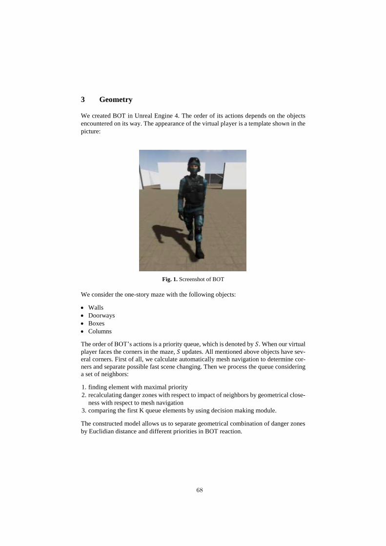
3 Geometry
We created BOT in Unreal Engine 4. The order of its actions depends on the objects
encountered on its way. The appearance of the virtual player is a template shown in the
picture:
Fig. 1. Screenshot of BOT
We consider the one-story maze with the following objects:
Walls
Doorways
Boxes
Columns
The order of BOT’s actions is a priority queue, which is denoted by 𝑆. When our virtual
player faces the corners in the maze, 𝑆 updates. All mentioned above objects have sev-
eral corners. First of all, we calculate automatically mesh navigation to determine cor-
ners and separate possible fast scene changing. Then we process the queue considering
a set of neighbors:
1. finding element with maximal priority
2. recalculating danger zones with respect to impact of neighbors by geometrical close-
ness with respect to mesh navigation
3. comparing the first K queue elements by using decision making module.
The constructed model allows us to separate geometrical combination of danger zones
by Euclidian distance and different priorities in BOT reaction.
68

Let's look at an example illustrated in the picture:
Fig. 2. Around the corner
We obtain the event “look around the corner” skipping visual recognition of the objects
as if we already know them. We find out similar events with nearby distance from the
current corner and include them in our calculations. The situation is separated by three
simple steps. The first of them is the case in which BOT meets the nearest corner (the
right side of the doorway). Then we process boxes as consequent corners in our model
with respect to their priority and distance. The probability to turn on the angle X from
0 to 90 degrees with respect to the right wall is represented by density functions. A little
circle represents BOT position.
Fig. 3. Processing priority queue when looking around the corner
The obtained density functions represent the process of visual recognition of objects
when we search for an enemy but have to spend some time on processing object’s
shapes. Using geometry knowledge we reduce amount of time on visual recognition of
objects using its statistical equivalent to find dangerous zones as equivalent of compar-
ing visual images of objects and an enemy.
𝜋
2
𝜋
2
𝜋
2
𝜋
2
69

4 Visual Recognition
Visual recognition is the assignment of given pictures to a particular class of objects
with the help of known methods of classification. We implement three standard steps
of it:
The converting of the source image to the initial idea;
The extracting characteristic values of recognition;
The classification of the image to a certain class with the use of the classifier.
In our work we consider three basic approaches to the visual recognition:
Heuristic methods [2, 3]
Full heuristic model. Expert compiled a set of rules that describe the image of
the object (built model), according to which detection is produced.
Search for characteristic invariant attributes. It is the description of character-
istics of the object, which are invariant with respect to possible distortions
(lighting changes, rotation, scaling).
Method of pattern matching. It is the creation of a template for the image of the
whole object or its characteristic features. The pattern can be a complicated struc-
ture and allows for different deformations and transformations. This approach al-
lows implementation in real time.
Methods of learning by precedents. The model is automatically built on the set of
images of an object compiled beforehand from the possible input data of the system
[4, 5, 6, 7].
The latter approach is the most interesting for us, because results of testing process
show that such methods are more appropriate, so let’s consider the last approach in
detail. It consists of two units: converting the image into a feature vector and classifi-
cation. The former means the most complete and informative representation of an im-
age in the form of a numerical vector. The latter fact implies the verification of hypoth-
esis accessories image to the class object images based on the observation that is the
feature vector.
Denote a feature vector for 𝑥 ∈ 𝑋 ⊆ 𝑅𝑛 - the description of the object, which is out-
put of the conversion unit. Class will be called a subset 𝐾𝑦 = 𝑥 ∈ 𝑋, 𝑦∗(𝑥) = 𝑦 of the
set 𝑋, 𝑦 ∈ 𝑌 ⊆ 𝑍 – the set of the class markers. We will view the case of binary classi-
fication (the image is an image of the desired object or the image is an image of anything
else), consequently 𝑌 = −1; 1. 𝑦∗(𝑥) – the mapping, which is defined for all 𝑥 ∈ 𝑋
and is specified the partition into subsets 𝐾𝑦. It is worth noting that classes 𝐾𝑦 can over-
lap, because the feature vector is only a description of an object’s attributes, and two
different images can have the same specifications. The training set is pairs of precedents
𝑇 = (𝑥1, 𝑦1), … , (𝑥𝑙 , 𝑦𝑙): 𝑦∗(𝑥𝑖) = 𝑦𝑖 . 𝑖 = 1, 𝑙. For the application of classification algorithms and pattern recognition we make the
following hypothesis: the set 𝑋 × 𝑌 is a probability space with probability measure 𝑃,
70

precedents (𝑥1, 𝑦1), … , (𝑥𝑙 , 𝑦𝑙) appear randomly and independently in accordance with
the distribution 𝑃.
The task of classification is to build the function 𝐹(𝑥), which approximates the map-
ping 𝑦∗(𝑥) with the help of the training set.
Let’s consider several methods of learning by precedents, which we tested in our
work.
4.1 Bayesian Classification Methods
The first method is the principle of posteriori probability maximum [8]. It is based on
following hypothesis:
𝑋 × 𝑌 is the probability space with probability measure 𝑃 , precedents
(𝑥1, 𝑦1), … , (𝑥𝑙 , 𝑦𝑙) appear randomly and independently in accordance with the dis-
tribution 𝑃.
We know density distributions of classes 𝑝𝑦(𝑥) = 𝑝(𝑥|𝐾𝑦), 𝑦 ∈ 𝑌, which we will
call likelihood functions.
We know the probability of occurrence of each object from classes 𝑃𝑦 = 𝑃(𝐾𝑦), 𝑦 ∈
𝑌, which we will call the priori probabilities.
Decision rule can be written in the following form:
𝐹(𝑥) = 𝑎𝑟𝑔 max𝑦∈𝑌
𝑃(𝐾𝑦|𝑥) = 𝑎𝑟𝑔 max𝑦∈𝑌
𝑝𝑦(𝑥)𝑃𝑦 (1)
The second method is called Bayesian networks [9]. This approach is based on the
combination of the principle of posteriori probability maximum with graph theory. The
idea is to create a graph with vertices corresponding to any component of the feature
vector, and edges indicating a causal relationship.
4.2 Classical Neural Networks
The main idea is the serial conversion of a signal with the elementary functional ele-
ments (neurons), operating in parallel [10]. The basic principle of neural network con-
figuration is to use optimization methods to minimize the mean square error. Also, the
neuron networks are capable of retraining.
4.3 SVM - Support Vector Machine
The SVM algorithm constructs a linear separating surface (hyperplane), equidistant
from the convex hulls of the classes, convex hull is based on the precedents [11]. If the
hyperplane does not exist (classes are not linearly separable), sound conversion will
apply for nonlinear classification, which projects 𝑋 in the space of higher dimension,
probably, infinite. The algorithm for constructing the classifier is reduced to the prob-
lem of quadratic programming. The solution of this task will be unique and the found
extremum will be global.
71

4.4 SNoW - Sparse Network of Winnows
Sparse network of Winnows is a special type of neural networks [12]. The network
consists of two (the number of possible classes) of linear neurons associated with the
feature vector components. Geometrically, SNoW consists in two hyperplanes in the
space of feature vectors. Vector belongs to the class, corresponding to which the hyper-
plane is the closest. The resulting separating surface is thus a hyperplane in the original
space 𝑋.
4.5 Classifier Boosting
This approach combines primitive classifications into one stronger method. The main
idea is an iterative minimization of a convex functional classification error. Boosting
attempts to project the original data into a space where the classes are linearly separable.
4.6 Results
In our research we obtained the following results, using data from demorecords of mul-
tiplayer game sessions:
SNoW and boosting distinguish the highest percentage of correct detections, about
94% [13, 14];
SVM, SNoW and boosting provide high speed of recognition;
SNoW and boosting have low level of the second kind error.
The correctness of visual recognition was manually checked. Thus, at the current level
of experiment the most appropriate method for our problem is the combination of two
methods: Sparse network of Winnows and Classifier boosting.
The picture below represents the result of visual recognition unite, using classifier
boosting.
Fig. 4. Result of visual recognition
72

In this situation there are two objects, which can be recognized as enemies: the virtual
player and its shadow. But the geometry unit defines that the latter is on the floor, so
AI focuses only on the first one.
5 Decision Making Model
In the most basic games, there was simply a lookup table for what was currently hap-
pening and the appropriate best action. In the most complex cases, the computer would
perform a short minimax search of the possible state space and return the best action
[15]. The minimax search had to be of short depth since the game was occurring in real-
time.
We use the blueprints visual scripting system in Unreal Engine 4 [16, 17]. The node-
based interface allows us to create the maze with different objects (for instance, boxes,
doors). Also, this concept gives an opportunity to make any appearance of BOT and to
determine the direction of the eye with the help of a camera-element. The virtual player
is the combination of several blueprints, each of which corresponds to the certain ac-
tion: moving, shooting, behavior during shooting and search for enemies.
We focus on a rule-based system (RBS) [18, p.169] to identify simple situations and
make a choice for a complex processes as a tuple of simple rules. RBS works with
instructions and the interpreter. In our case, rules are oriented tree structures. Let’s dis-
cuss the short list of game events:
1) Walking
a) Bypassing and Search
b) Moving toward some point in the maze
c) Finding cover
2) Shooting
a) Sighting
b) Opening fire
c) Correction relative to recoil and motor reflexes
3) Visual recognition
a) Recognition of objects
b) Recognition of dangerous zones
c) Recognition of enemy
The simplest set of rules may be the following:
1𝑎) ∧ 1𝑐) → 1𝑎) (just bypassing)
1𝑎) ∧ 3𝑏) → 2𝑎) ∧ 1𝑏) (accurate obstacle avoidance)
1𝑎) ∧ 3𝑐) → 2𝑎) ∧ 2𝑏) ∧ 2𝑐) (shooting after enemy recognition)
We give only a superficial representation of these rules, which are much more compli-
cated when we go into details with respect to implementation in game engine.
Rule based system allow us to implement the neural network method when we have
to choose another rule with the same premise, for example, if we have a rule:
73

1𝑎) ∧ 3𝑐) → 1𝑏) ∧ 1𝑐) (2)
This rule should be used, if a player has low health and his chance to win against
enemy is almost zero, so he should hide and create an ambush for an enemy.
If we have time-limit and command should defend some place we should use the
following rule:
1𝑎) ∧ 3𝑐) → 1𝑏) ∧ 2𝑏) (3)
So we will distract an enemy or sacrifice player to win some time for a command.
In a real game the player chooses different rules depending on his psychological
temper, emotions or calculations, so it is really a good place to use learning techniques.
For each type of game we produce rules, which say whether or not player achieve
his current goal and increase a part of command goal for this game. Of course command
goal has greater priority, but in fact, in each situation the player decides without hesi-
tation operating with current situation and parameters from visual recognition.
Formal Concept Analysis methods are used to find out a basis of rules (implications)
when we have a non-empty intersection of premises. Machine Learning is used to find
weight combination for rules, which have the same premises.
Model of neuron networks can be applied to univariate and multivariate analysis. In
our work using neuron approach is appropriate to imitate personal and team player’s
goals. One player worries about its level of health; also, it is interested in winning.
These two ideas characterize its behavior during the game; it means that the following
situation is possible: BOT may decide to shoot and be with the low level of its health,
because it will win. But, when we consider team game, BOT will not risk by it-self, it
will defend, possible, shoot or run away. This case of game is complicated, but we can
divide it into several simple cases, each of them is the same as for personal game. That
is why neural networks can successfully reflect behavior of players in shooter.
6 Process of Gaming
Process of gaming starts with visual recognition. As far as BOT defines an enemy with
certain threshold probability or after enemy fire identification, it starts to aim. Given
that X is the horizontal rotation change speed, and Y is the vertical. The relative error
depends on the angle between BOT’s rotation movements and direction on the target,
and the sign of this angle. It also depends on X-speed and Y-speed: the stronger the
need to change the speed of rotation change, the greater the relative error will occur.
Let’s consider two situations of possible targeting. In both examples visual recogni-
tion shows the place of the enemy. Also, we can see the rotation of BOT, which de-
scribes by means of the sum vector of X and Y. Black circles shows the approximate
trajectory of aiming which is close to the human response to the detection of the adver-
sary. The figure 5 represents the situation in which the direction to the target is opposite
to the BOT rotation, therefore the relative error will be very high.
74

Fig. 5. Example 1
The figure 6 displays the case in which the direction to the goal and the rotation are the
same; consequently, the relative error will be rather low.
Fig. 6. Example 2
So, we divide aiming by three phases:
inertia during recognition,
instant aiming,
braking or correction near the goal,
and include them in our model.
75
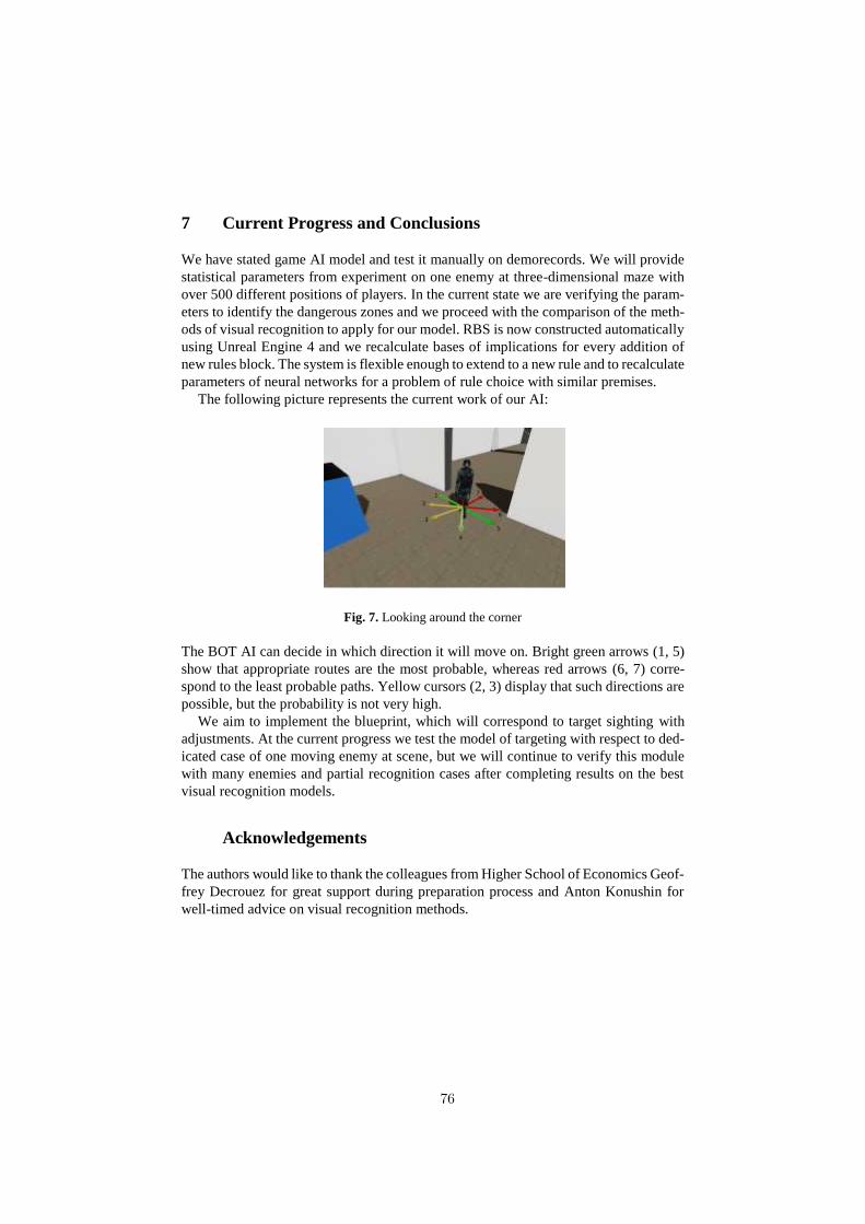
7 Current Progress and Conclusions
We have stated game AI model and test it manually on demorecords. We will provide
statistical parameters from experiment on one enemy at three-dimensional maze with
over 500 different positions of players. In the current state we are verifying the param-
eters to identify the dangerous zones and we proceed with the comparison of the meth-
ods of visual recognition to apply for our model. RBS is now constructed automatically
using Unreal Engine 4 and we recalculate bases of implications for every addition of
new rules block. The system is flexible enough to extend to a new rule and to recalculate
parameters of neural networks for a problem of rule choice with similar premises.
The following picture represents the current work of our AI:
Fig. 7. Looking around the corner
The BOT AI can decide in which direction it will move on. Bright green arrows (1, 5)
show that appropriate routes are the most probable, whereas red arrows (6, 7) corre-
spond to the least probable paths. Yellow cursors (2, 3) display that such directions are
possible, but the probability is not very high.
We aim to implement the blueprint, which will correspond to target sighting with
adjustments. At the current progress we test the model of targeting with respect to ded-
icated case of one moving enemy at scene, but we will continue to verify this module
with many enemies and partial recognition cases after completing results on the best
visual recognition models.
Acknowledgements
The authors would like to thank the colleagues from Higher School of Economics Geof-
frey Decrouez for great support during preparation process and Anton Konushin for
well-timed advice on visual recognition methods.
76

References
1. Yanovich I. “Review of Call of Duty: Ghosts” (in Russian) http://kanobu.ru/articles/syuzhetnaya-kampaniya-call-of-
duty-ghosts-367451/
2. Yang G. and Huang T. S., “Human Face Detection in ComplexBackground”. Pattern
Recognition, vol. 27, no. 1, pp. 53-63, 1994.
3. Kotropoulos C. and Pitas I., “Rule-Based Face Detection in Frontal Views”. Proc. Int'l Conf.
Acoustics, Speech and Signal Processing, vol. 4, pp. 2537-2540, 1997.
4. Pham T. V., Worring M., and Smeulders A. W. M. “Face detection by aggregated bayesian
network classifiers”. Pattern Recognition Letters, 23(4):451-461, February 2002.
5. Henry A. Rowley, Shumeet Baluja, and Takeo Kanade. “Human face detection in visual
scenes”. Technical Report CMU- CS-95-158R, School of Computer Science, Carnegie
Mellon University, November 1995.
6. Roth D., Yang M.-H., and Ahuja N. “A SNoW-based face detector”. Advances in Neural
Information Processing Systems 12 (NIPS 12), MIT Press, Cambridge, MA, pp. 855-861,
2000.
7. Viola P. and Jones M. “Robust Real-time Object Detection”. In Proc. 2nd Int'l Workshop on
Statistical and Computational Theories of Vision - Modeling, Learning, Computing and
Sampling, Vancouver, Canada, July 2001.
8. Vorontsov K.V. “Bayesian classification algorithms. Drafts of lectures” (in Russian) http://www.ccas.ru/voron/download/Bayes.pdf
9. Heckerman, D. “A Tutorial on Learning with Bayesian Networks”. In Jordan, M. (Ed.),
Learning in Graphical Models, MIT Press, 1998.
10. Vezhnevec A. “ Popular neural network architecture” (in Russian) http://cgm.graphicon.ru/metodyi/populyarnyie_neyrosetevyie_a
rh itekturyi.html
11. Vapnik V. and Lerner A. J. “Generalized portrait method for pattern recognition”. Auto-
mation and Remote Control, vol. 24, no. 6, 1963.
12. Roth D. “The SNoW Learning Architecture”. Technical Report UIUCDCS-R-99-2102,
UIUC Computer Science Department, 1999.
13. Ming-Hsuan Yang, David Kriegman, and Narendra Ahuja. “Detecting Faces in Images: A
Survey”. IEEE Transactions on Pattern Analysis and Machine Intelligence (PAMI), vol. 24,
no. 1, pp. 34-58, 2002.
14. Viola P. and Jones M. “Robust Real-time Object Detection”. In Proc. 2nd Int'l Workshop
on Statistical and Computational Theories of Vision - Modeling, Learning, Computing and
Sampling, Vancouver, Canada, July 2001.
15. Szelinski R. “Computer Vision: Algorithms and Applications”. Springer, 2011.
16. https://www.unrealengine.com
17. http://unreal-engine4.ru
18. Champandard A.J. “AI Game Development: Synthetic Creatures with Learning and Reac-
tive Behaviors”. New Riders Games, 2003.
77

The Text Network Analysis: What Does Strategic
Documentation Tell Us About Regional Integration?
A.Murashov1, O.Shmelev2
1 Yaroslav-the-Wise Novgorod State University
([email protected]) 2 Kalashnikov Izhevsk State Technical University
Abstract. Values and attitudes towards the regional integration process of the
Russian political elites are considered as an indication of what regional integra-
tion (RI) tends to be and how it evolves over time. This paper suggests how to
systematically grasp and integrate elite’s attitude into the analysis of RI by
means of text network analysis. The text network analysis allows one to visual-
ize the meanings and agendas present within political manifests which are sup-
posed to reflect values and attitudes towards RI of the local political elite.
Keywords. igraph, political elite attitude, R, regional integration, regional strat-
egy, system of indicators, text mining, text network analysis (TNA)
1 Introduction
This paper is a part of PhD thesis aimed at constructing a so-called System of Indica-
tors of Regional Integration in Russia. Values and attitudes towards the regional inte-
gration process of the Russian political elites are considered as an indication of what
regional integration tends to be and how it evolves over time. One of the shortcom-
ings of conventional approaches is insufficient and unsystematic consideration of
political elite's attitude towards regional integration and decision-making in this field.
The question how to systematically grasp and integrate elite’s attitude into analysis
remains open.
In comparative politics measuring the attitudes of the political elite is often under-
taken either by expert surveys or by the analysis of political manifests [De Lombaerde
P. et al., 2011]. Our interest lies in researching the political manifests – a regional
strategy reflects opinion of a local authority, like a party manifest directly reflects
opinion of a political party.
Research questions are those related to monitoring and analyzing regional integra-
tion process. How do regions cooperate? What forms of integration emerge within the
selected regions? What problems / challenges does integration impose? Which indus-
tries are mainly affected by integration process? How do regions choose their region-
partners? What is beyond the choice?
78
2 Background
From theoretical perspective this paper is supposed to contribute to the investigation
of values and attitudes towards the regional integration process that are represented in
political manifests. This topic is covered in particular by:
(1) Comparative Manifesto Project (CMP) maintained by Manifesto Research
Group. Their purpose is to discover party stances by quantifying their statements and
messages to their electorate, method used is quantitative content-analysis [CMP,
2014];
(2) Leontief Center’s Study of Russian Regions’ Strategies aimed at, among other
things, building a classification of regional strategies based on their content, method
used is expert review and content-analysis [Zhikharevich B. et al., 2013];
(3) Philippe De Lombaerde from United Nations University, Institute on Compara-
tive Regional Integration Studies (UNU-CRIS) and his team who employing multi-
disciplinary approach in developing quantitative and qualitative tools to monitor re-
gional integration process [De Lombaerde P. et al., 2011].
3 Method
From methodological perspective this paper applies an approach which combines two
methods - comparative text-mining and graph analysis – “text network analysis”. The
text network analysis allows one to visualize the meanings and agendas present within
political manifests. This approach outputs a graph of relations between key terms
where each node represents a term and edges express logical associations between
terms.
Putting it in a general scenario of social networks, the terms are taken as people
and the segments of text as groups on LinkedIn or Facebook, and the term-document
matrix can then be taken as the group membership of people. Several notions of co-
occurrence have been used in the literature to group words [Saeedeh M. et al., 2010]:
document-wise/sentence-wise /window-wise/syntax-wise co-occurrence. We build a
network of terms based on their co-occurrence in the same text segments (paragraphs)
extracted from the documents in the course of expert review. There is an edge be-
tween two terms if they appear in the same text segments (paragraphs). The weight of
an edge is its frequency [Batagelj V. et al. 2002, Polanco X., 2006]. Such a network
(or conceptual map [Chernyak Е. et al., 2014]) visualizes logical associations between
concepts presented in the political manifests.
1. Establish text corpus and transform it
Data to analyze is regional strategies of socio-economic development as a central
and most capacious source of information about political elite’s views on regional
integration process. We are interested in 6 Russian regions situated alongside the
Moscow – St Petersburg transport corridor: Moscow, Moscow region, Tver’ region,
Novgorod region, Leningrad region, St Petersburg. Their strategies are studied. There
may exist a wide range of other official documents on regional integration but unfor-
79

tunately we are not able to cover all of them, so we decided to limit our sample by
regional strategies only.
Using Atlas.ti (qualitative data analysis software) we establish text corpus and re-
trieve those text segments (paragraphs) from the regions’ strategies which refer to
regional integration process, refine it in a specific way then (lemmatization, filter
stopwords, punctuation and numbers removing, etc.).
2. Explore text corpus (igraph & tm packages)
Text network analysis is performed with R [Yanchang Zhao, 2012], specifically,
with packages igraph and tm (provides functions for text mining). We build a
document-term matrix, after that, it is transformed into a term-term adjacency matrix,
where the rows and columns represent terms, and every entry is the number of con-
currences of two terms, after that, frequent words and their associations (fast-
greedy.community) are found from the matrix.
3. Visualization
Finally, we visualize the result by means of igraph package in R environment:
(1) plot the graph to show the relationship between frequent terms (graph.adjacency,
layout = layout.fruchterman.reingold, delete.edges), (2) dendrogram (dendPlot).
4 Results
First we review general graph statistics. Snapshot of the network metrics is in the
table following (tab.1). Volume of the strategies varies from 396 vertices for Moscow
region to 800 vertices for Tver’ region. Function assortativity.degree uses vertex de-
gree (minus one) as vertex values. The coefficient throughout the corpora is negative
suggesting that the connected vertices tend to have different degrees. Centralization is
a general method for calculating graph-level centrality score based on node-level
centrality measure. Novgorod region’s strategy is that one having most centralized
structure (centralization degree of 68% of its theoretical maximum). We also arrive at
the conclusion that there is a substantial amount of centralization in the Moscow re-
gion’s strategy. In general, the power of individual terms varies rather substantially,
and this means that, overall, positional advantages are rather unequally distributed in
each strategy. The global version of clustering coefficient (function transitivity) indi-
cates that the degree to which nodes in a graph tend to cluster together is relatively
low. This makes sense since we removed from the graphs singular edges for the sake
of simplicity (here we refer to a parameter n which is discussed below). Fastgreedy
algorithm identifies from 6 to 10 communities in the graphs with moderate modulari-
ty. As we can see from the table 1 the graphs are quite similar in terms of their math-
ematical conception. Much more insightful and interesting results come from analysis
of the networks’ content.
80

Table 1. Graphs’ key metrics1
To demonstrate some examples for applying the strategies to study regional inte-
gration the graphs following are built (fig.1). They are based on the strategy of St
Petersburg. The graph (fig.1,a) is crowded with many vertices and edges, it represents
most of the ideas we can find in the strategy. To simplify the graph we remove insig-
nificant terms. With function delete.edges, we remove edges which have weight less
than a certain value. To do it in our experiment we introduce a parameter n referring
to a number of text segments (paragraphs) where a certain term appears. After remov-
ing edges, some vertices become isolated and are also removed. The produced graph
is on fig.1,b. The interpretation is that we exclude from the scope of analysis most
rare and random concepts.
Let us set n equal to 8. The resulting graph on fig.2,a is crowded with many verti-
ces and edges, we can interpret it at some extent but we need to get more precise pic-
ture. We identify vertices whose removal increases the number of connected compo-
nents in the graph. They are: city, petersburg, development, etc. To simplify the graph
and find relationship between terms beyond the selected keywords, we remove major
articulation points (or alternatively those terms whose removal, we expect, will lead
to a result we are looking for) so that the layout is rearrange and new concepts and
links between them are revealed. We see that some of the articulation points are not
necessarily meaningful but just the highly frequent words carrying less meaning than
those with a moderate or low frequency and are thus not very valuable to explore.
1 SP = St Petersburg, M = Moscow, LO = Leningrad region, NO = Novgorod region, TO =
Tver’ region, MO = Moscow region
SP M LO NO TO MO
Number of vertices vcount 737 463 490 491 800 396
Number of edges ecount 5039 2311 2517 2913 7296 1897
Assortativity assortativity.degree -0.25 -0.34 -0.32 -0.24 -0.31 -0.29
Transitivity transitivity 0.19 0.22 0.16 0.21 0.22 0.16
Average path length average.path.length 2.54 2.64 2.48 2.43 2.52 2.58
Graph density graph.density 0.019 0.022 0.021 0.024 0.023 0.024
Centralization Degree centralization.degree 0.49 0.41 0.52 0.68 0.48 0.68
Centralization Closeness centralization.closeness 0.54 0.48 0.53 0.67 0.50 0.61
Centralization Betweenness centralization.betweenness 0.30 0.30 0.27 0.55 0.19 0.39
Eigenvector Centrality Scores centralization.evcent 0.92 0.91 0.92 0.92 0.91 0.92
Diameter diameter 13 10 13 13 10 14
Number of communities (best split) fastgreedy.community 6 6 10 8 8 8
Modularity (best split) fastgreedy.community 0.40 0.49 0.35 0.38 0.32 0.38
StrategyParameter igraph function
81

Fig. 1. Example of graph evolution (a – initial graph; b – truncated graph)
Next, we try to detect communities in the graph. Graph community structure is cal-
culated with the fastgreedy algorithm [Kincharova A., 2013]. The nodes that cluster
together (communities) are shown with the same color on fig. 2, indicating contextual
proximity of the terms used. The communities tell us that the local authorities focus
quite heavily on patterns of spatial development , unique role of St Petersburg and its
attractiveness for migrants, close association between the City and Leningrad region,
etc.
Fig. 2. Graph improvement by managing articulation points (a – initial graph; b – refined
graph)
We can also have a further look at which terms colocations are most frequent in
each strategy (fig.3). Parameter n tells us how many times the plotted collocations
appear. Parameter n is a lower bound of the frequency, that is, collocation «Moscow –
82

St Petersburg» appears not less than 33 times in different text segments within Tver’
region’s strategy. Each strategy mentions those regions more frequently which are
supposed to be their main partners.
Fig. 3. Most frequent terms colocations
Plots for Moscow region and Leningrad region suggest that the development of the
two regions is strongly connected to two largest Russian cities that they surround. For
instance, the Leningrad region strategy suggests strong spatial planning on territories
adjoined to St Petersburg. The Moscow region strategy repeatedly highlights im-
portance of Moscow and its agglomeration.
5 Concluding remarks
Given the work-in-progress style of our study, it has a number of weaknesses; among
them is a lack of the comparative perspective. A solution might be to build a network
of text segments (paragraphs) based on the terms shared by them (two-mode net-
work). Alternatively, we would probably arrive at some interesting insights if could
put a network on another one to see joint term clusters and terms-outliers [Ermakov
A. et al., 2002]. We appreciate the more sophisticated models use phrases or n-grams
instead of words and this also could be a possibility to improve our analysis. These
basic tools implemented here are only the beginning of possibilities for applications
of TNA. It is worth noting that we were not meant to provide an extension of the base
technology of computer-supported TNA but suggest an example of its practical im-
plementation in social science.
The text-mining approach combined with graph theory appears to be a valuable
method for extracting elite’s attitude towards regional integration process from public
strategic documentation (allows us to access a large amount of textual material, re-
gional analysis may provide interesting input for text network analysis, etc.). Model-
ing the data using this method provided us with the specific insights on what local
authorities really focus on and how the strategies differ from each other.
83

References
1. Batagelj V., Mrvar A., Zaversnik M. Network analysis of texts. URL:
http://nl.ijs.si/isjt02/zbornik/sdjt02-24bbatagelj.pdf (25.03.2015).
2. Chernyak Е., Morenko Е., Mirkin B. Conceptual Maps: Construction Over a Text Collec-
tion and Analysis. Analysis of Images, Social Networks and Texts Communications in
Computer and Information Science Volume 436, 2014, pp.163-168.
3. De Lombaerde P. et al. The Regional Integration Manual: Quantitative and Qualitative
Methods. Routledge, London, 2011.
4. Ermakov A., Pleshko V. Informatization and information security of enforcement officials.
XI International scientific conference. Conference proceedings, Moscow, 2002, pp. 343-
347.
5. Kincharova A. Application of community detection algorithms for sociological investiga-
tion of blogs: results of a piloting study. URL:
www.hse.ru/data/2013/06/10/1283702757/dzh.pdf (25.03.2015).
6. Manifesto Project Database. URL: https://manifestoproject.wzb.eu/
(25.03.2015).
7. Polanco X., San Juan E. Text data network analysis using graph approach. Vicente P.
Guerrero-Bote. I International Conference on Multidisciplinary Information Sciences and
Technology, Oct 2006, Merida, Spain. Open Institute of Knowledge, vol. 2, pp.586-592.
URL: https://hal.archives-ouvertes.fr/hal-00165964 (25.03.2015).
8. Saeedeh M. et al. A Comparative Study of Word Co-occurrence for Term Clustering in
Language Model-based Sentence Retrieval. Human Language Technologies: The 2010
Annual Conference of the North American Chapter of the ACL, pp. 325–328, Los Ange-
les, California, June 2010. URL: http://www.aclweb.org/anthology/N10-1046
(25.03.2015).
9. Yanchang Zhao. R and Data Mining: Examples and Case Studies. Academic
Press, Elsevier, 2012.
10. Zhikharevich B., Zhunda N., Rusetskaya O. Proclaimed and actual priorities of regional
and local authorities: approaches to reveal and compare // The Region: Economics and So-
ciology, 2013, 2, pp. 108 – 132.
84

A Nonlinear Dimensionality Reduction Using Combined
Approach to Feature Space Decomposition
Myasnikov E.V.
Samara State Aerospace University,
Image Processing Systems Institute of the Russian Academy of Science
Samara, Russia
Abstract. In this paper we propose a new combined approach to feature space
decomposition to improve the efficiency of the nonlinear dimensionality reduc-
tion method. The approach performs the decomposition of the original multidi-
mensional space, taking into account the configuration of objects in the target
low-dimensional space. The proposed approach is compared to the approach us-
ing hierarchical clustering in the original space and to the approach based on the
decomposition of the target space using KD-Tree.
Keywords: dimensionality reduction; multidimensional scaling; Sammon's
mapping; hierarchical clustering; KD-Tree
1 Introduction
Dimensionality reduction methods, operating on the principle of preserving the pair-
wise distances between objects can be used as a means to display multidimensional
data in scientific research and in production activities in a number of areas: biology,
genetics, sociology, economics, etc. In modern information systems, such methods
can be used to create navigation systems for multimedia databases, as well as in inter-
face design to virtual directories. In the field of image analysis and processing nonlin-
ear dimensionality reduction techniques have been applied not only for research but
also to solve a number of applied problems: creation of automated systems for image
segmentation, thematic mapping from satellite imagery and others.
One of the most well-known dimensionality reduction methods is a method [9],
which minimizes the following error of multidimensional data representation
ji
Ooo ji
jiji
ji
Ooo
jiji
ji
ood
oodood
ood,
2*
,
),(
),(),(
),(
1 (1)
85

where io is an object from a set O, ),( ji ood is the distance between objects in the
original space, ),(*ji ood is the distance between objects in the target space.
Iterative procedure that minimizes the error (1) may be based on the following re-
currence relations for the coordinates yi in the target low-dimensional space (gradient
descent):
Oo
jiii
j
oomtt ),()()1( ςyy (2)
where (m can be calculated once):
ji
Ooo
ji
ji
ood
m
,
),(
2
ji
jiji
jijiji
oodood
oodoodoo yyς
),(),(
),(),(),(
*
*
(3)
It is worth noting that the performance of the nonlinear mapping has been improved
by extending multidimensional data representation error (1) with Bregman divergenc-
es [11, 12].
Unfortunately, a significant drawback of the nonlinear dimensionality reduction
techniques, operating according to the iteration scheme (similar to that shown above)
is the high computational complexity (O(K2) per iteration, where OK is the num-
ber of objects). For this reason a number of techniques with a reduced computational
complexity have been proposed [3, 4, 5, 6, 7].
One of the most effective ways to reduce the computational complexity is the hier-
archical decomposition of space. After performing such decomposition objects can be
considered not individually, but in groups, that allows to speed up the iterative opti-
mization process. So, if all the objects of the original set O are divided into groups
Ss j , then (2) takes the form
Ss
jiii
j
somtt ),(~)()1( ςyy (4)
jsi
jiji
jijijji
sodsod
sodsodsso yyς
),(),(
),(),(),(~
*
*
(5)
where ),( ji sod is the distance from the object to the center of the group sj in the
original space, ),(*ji cod is the distance from the object to the center of the group in
the target space, jsy is the coordinates of the center of the group in the target space.
86

Such decomposition allows to reduce the computational complexity to O(LK) per
iteration, where SL is the number of groups.
It is obvious that the expression (4) allows to approximate (2) with a certain accu-
racy that depends on how well objects are divided into groups. For this reason, there
is a question about how to better carry out such decomposition. It is understood that
the decomposition can be performed in both the source and target space. Approach
based on decomposition of the original space, is implemented in a nonlinear method
for dimensionality reduction of data using reference nodes [5] proposed by the author
of this article. Approach based on decomposition of the target space has been imple-
mented, for example, in [1] (regular decomposition) and [8] (hierarchical decomposi-
tion) to solve the problem of drawing graphs to approximate the forces acting on the
vertices of the graph.
In this paper we propose a new method that uses the combined approach to feature
space decomposition to improve the efficiency of the nonlinear dimensionality reduc-
tion method. The proposed method is based on the nonlinear method for dimension-
ality reduction of data using reference nodes [5] that performs the decomposition of
the original space, and complemented with the additional control on the configuration
of objects in the target space. The proposed method is compared to the method based
on the decomposition of the original space, and to the method based on the decompo-
sition of the target space, both in terms of the quality of the mapping, as well as in
terms of the operating time.
The paper is organized as follows. The next section is devoted to the description of
the known approaches used in the present study, and consists of two subsections. The
third section is devoted to the description of the proposed method. The fourth section
presents the results of numerical experiments. At the end of the paper the conclusion
is given.
2 Brief Description of the Methods Used in the Study
2.1 Nonlinear Method for Dimensionality Reduction of Data Using Reference
Nodes
Approach based on the decomposition of the original space, is implemented in a non-
linear method for dimensionality reduction of data using reference nodes [5]. This
method consists of four steps, briefly described below.
The inputs to the method are the feature vectors describing the objects in the origi-
nal multidimensional space. The outputs of the method are the feature vectors describ-
ing the objects in the target low-dimensional space.
Step 1: Construction of a hierarchy of clusters. At the first stage of the method
we make a hierarchical partition of the initial set of objects into clusters (subsets of
objects with similar characteristics in the original feature space). When we refer to the
hierarchy of clusters we mean tree-like data structure, the root of which is a cluster of
87

top-level, and each vertex-cluster contains either subclusters or the objects of the orig-
inal set.
Step 2: Initialization of the coordinates of objects in the target space. Initializa-
tion of the coordinates of objects in the target space can be performed in various
ways, e.g., using random values, the results of the PCA method, etc.
Step 3: Construction of the lists of reference nodes. At the third stage, for each
object of the original set the lists of reference nodes are built. The reference node of
the object o refers to a certain object ooi or group of objects Niio
..1 that pos-
sesses close characteristics in the original multidimensional space and considered as a
single object.
Let o be an object for which we need to form a list S of the reference nodes and
let C be an arbitrary cluster of the hierarchy. By using the hierarchy of clusters ob-
tained at the first stage the construction of the reference nodes list may be implement-
ed using the following recursive algorithm.
1. If the cluster C satisfies the decomposition criterion with respect to the considered
object and subclusters NiCCi ..1, are contained in cluster C , then one must
apply this recursive algorithm to each of the subclusters NCCC ,..,, 21 .
2. If the cluster C satisfies the decomposition criterion with respect to the considered
object and objects NiCoi ..1, are contained in cluster C , then one must:
(a) add all objects that close to the considered object to the list of reference nodes
S ;
(b) distinguish the set V of objects situated at a distance from the considered ob-
ject as an incomplete cluster;
(c) in the case when this set V is nonempty, add it to the list of reference nodes.
3. If the cluster C doesn’t satisfy the decomposition criterion with respect to the con-
sidered object then add it to the list of reference nodes S .
Decomposition criterion used in this paper is slightly different from the criterion used
in [5] and restricts (by the value ) the estimation of the angle at which the
hypersphere of the cluster is observed from the object o in the original space.
Figure 1 illustrates this process. The cluster, which is observed from an object o at
an angle will be divided into three clusters if . The cluster, which is ob-
served at an angle will be considered as a whole if .
88

Fig. 1. Illustration to the construction of a list of reference nodes
Step 4: Iterative optimization procedure. At the final stage of the method iterative procedure is performed, which allows to clarify the position of objects in the target low-dimensional space. The work of the iterative procedure is based on (4), (5).
2.2 Nonlinear Dimensionality Reduction Method Using KD-Tree for the
target space decomposition
In contrast to the approach discussed above decomposition of the target space inevita-
bly leads to the need for periodic renewal or adjustment of the structure by which the
decomposition is performed. The reason for this consists in changing the coordinates
of objects in the target space as you perform the optimization process.
In this paper, KD-trees are used for the decomposition of the target space. Tree
construction is performed at each iteration of the optimization process using the fol-
lowing recursive procedure.
1. Calculation of the characteristics of the current tree node (average coordinates in
the source and target space, boundaries of the node in the target space).
2. In the case when the node contains only one object, then exit.
3. Splitting the node into the two child nodes using the perpendicular to the most
elongated boundary so that the number of objects in the child nodes is approxi-
mately the same.
4. Perform this procedure for the newly formed child nodes.
Constructed tree is used to perform the next iteration of the optimization process. For
each object, the sum (4) is calculated by traversing the tree as follows.
1. If the decomposition criterion is not satisfied and the objects contained in the cur-
rent node of the tree can be considered as a group, then the next term in (4) is cal-
culated using (5).
2. Otherwise decomposition criterion is satisfied, and both subtrees (child nodes)
traversed similarly.
89

A decomposition criterion used in the tree traversal is similar to the above, and re-
stricts (by the value ) the estimation of the angle at which the minimum bounding
rectangle of the node is observed from the position of the object o in the target space.
Figure 2 illustrates this process. Different decomposition levels are shown using
different lines: the first level is shown by the solid line, the second level is shown by
the dash-dot line, the third level is shown by the dashed line. A group of four objects
(minimum bounding rectangle is shown by dots) will be devided into two groups if
the angle at which the minimum bounding rectangle is observed from the position
of the object o is greater than the decomposition angle .
Fig. 2. Illustration of decomposition in the target space using KD-Tree
It is worth noting that this algorithm is executed at each iteration for each object, so to
improve the efficiency the constructed tree is traversed not recursively, but iteratively
using special pointers.
Note that some additional experimental results on comparison of methods de-
scribed in this section can be found in [6].
3 Proposed Method
As noted above the expression (4) approximates (2) with some accuracy. The error
of approximation for some object o and the set s of individual objects can be repre-
sented using (5) as follows:
),(~
),(),(
),(),(),(
*
*
sooodood
oodoodso
so
j
jj
jj
j
ςyy
. (6)
90

Unfortunately, the use of the described above approaches can cause significant (in
some cases unbounded) approximation errors as in the first case the decomposition
criterion takes into account only the characteristics of nodes in the original space and
in the second case criterion takes into account only the characteristics of nodes in the
target space. The way out of this situation may be a combination of the original space
decomposition with the additional control on the configuration of objects in the target
space.
In this paper, for this purpose a nonlinear method for dimensionality reduction of
data using reference nodes is complemented by the preservation and analysis of the
boundaries of nodes in the target space. The proposed method consists of the same
steps as the base method [5]:
1. Construction of a hierarchy of clusters
2. Initialization of objects coordinates in the target space
3. Construction of reference nodes lists
4. Iterative optimization procedure
At the first step the difference between the proposed method and the base one is in
the structure of nodes in the cluster tree. In the proposed method each node contains
information about its boundaries in the target low-dimensional space. The second and
the third steps are the same as in the base method. At the fourth step iterative optimi-
zation procedure is different in the proposed method.
At the each step of the optimization process for each object Ooi with the corre-
sponding reference nodes list iS it recalculates the coordinates yi in the target low-
dimensional space. To do this according to (4) it iterates through the list of reference
nodes iS and calculates the approximated term for a given node ij Ss using the
following recursive algorithm.
1. If the given node js is the object Oo j of the initial set of objects, then the ex-
act value of the corresponding term is calculated using (3).
2. If the decomposition criterion is not satisfied for given node js in the target low-
dimensional space and the objects contained in the given node can be considered as
a group, then the approximated term is calculated using (5).
3. Otherwise the decomposition criterion is satisfied for the given node js in the tar-
get low-dimensional space, and all subtrees of the given node in the cluster tree
traversed similarly using this algorithm.
4 Experimental Study
In this paper all the studied methods have been implemented in C++ language in the
integrated development environment Borland Turbo C++ 2006 Explorer. The PC
91

based on Intel Core i5-3470 CPU 3.2 GHz has been used in the experiments. Corel
Image Features Data Set (http://archive.ics.uci.edu/ml/databases/CorelFeatures/
CorelFeatures.data.html) has been used in the experiments as an initial dataset. This
dataset contains a set of features, calculated from the digital images from the Corel
image collection (http://corel.digitalriver.com/). In particular, the following feature
sets have been used.
Feature set 1 contains color moments [10]. Three features were calculated for each
color component: mean, standard deviation, and skewness. The dimensionality of the
feature space is 9.
Feature set 2 contains color histograms [13] constructed in the HSV color space.
Color space was divided into 8 ranges of H and 4 ranges of S. The dimensionality of
the feature space is 32.
Feature set 3 contains texture features based on co-occurrence matrices [2]. Four
co-occurrence features (second angular moment, contrast, inverse difference moment,
and entropy) were computed in four directions (horizontal, vertical, and two diago-
nal). The dimensionality of the feature space is 16.
Fragments containing features information for the required number of images has
been selected from these feature sets. Then for sets 1 and 3, the identity component
has been added to the feature information and normalization has been performed.
To evaluate effectiveness of the methods the value of multidimensional data repre-
sentation error (1) has been calculated and the average per iteration execution time of
the optimization procedure has been measured.
Work of the methods stopped when the rate of decreasing the error slowed down
(i.e. the relative decrease in error for ten iterations does not exceed 0.05). In all cases,
the dimension of the target space has been set equal to two (two-dimensional data
mapping). Initialization is performed using the PCA method.
Some results for the feature set 1 are shown in Fig. 3-6.
Fig. 3 and 4 show the dependence of the qualitative and temporal characteristics on
the decomposition angle at which the algorithm moves to the child nodes of the
corresponding hierarchical structure (cluster tree or KD-tree).
As can be seen from these results, the large values of the angle leads to the ex-
pected deterioration of the mapping quality due to a coarser approximation, which is
reflected in the higher values of the multidimensional data representation error (see
Fig. 3). The time it takes to perform a single iteration, decreases with increasing angle
(see Fig. 4), due to the smaller number of processed nodes of the corresponding
hierarchical structure during the construction of approximations.
It should be noted that the approach using the original space decomposition pro-
vides less value of multidimensional data representation error than the approach
using the decomposition of the target space.
92

(a) (b)
Fig. 3. Dependence of the multidimensional data representation error
on the decomposition angle (in fractions of radian)
Fig. 4. Dependence of the average execution time per iteration (in ms)
on the decomposition angle (in fractions of radian)
At the same time the average execution time per iteration is much smaller when using
the approach with the decomposition of the original space in the range
[0.05 , 0.2 ].
The use of the combined approach allows slightly reduce the multidimensional data
representation error in comparison with the approach based on the decomposition of
the original space. At the same time the average time per iteration using a combined
approach is significantly larger than when using other considered approaches.
Dependencies of quality and temporal characteristics on the number of objects
shown in the figures 5 and 6 confirm said above. The approach using the original
space decomposition provides less value of multidimensional data representation error
than the approach using the decomposition of the target space (fig. 5a). The quality
of mapping, measured by the multidimensional data representation error , formed
using decomposition in the original feature space is only slightly inferior to the com-
bined approach (fig. 5b). The quality of mapping formed using combined approach is
virtually identical to the quality obtained with the base method without decomposi-
tion.
At the same time approach, using the decomposition of the original space, allows
us to construct mapping much faster than the other considered approaches (Fig. 6).
93

Figure 5a also shows the multidimensional data representation error obtained after
initialization of objects coordinates in the target low-dimensional space using the
PCA.
(a) (b)
Fig. 5. Dependence of the multidimensional data representation error
on the number of objects
Note that the experiments performed on other datasets described above, show simi-
lar results.
Fig. 6. Dependence of the average execution time per iteration (in ms)
on the number of objects
5 Conclusion
In this paper, we conducted a study of different approaches to the decomposition of
space in terms of quality and speed of the nonlinear dimensionality reduction method.
The study showed that for the presented data sets decomposition of the original space
is more preferable than the decomposition of target space in terms of both quality and
time. Combining the decomposition of the original space with the decomposition of
target space has allowed slightly improve quality.
94

Acknowledgments. This work was financially supported by the Ministry of educa-
tion and science of the Russian Federation in the framework of the implementation of
the Program of increasing the competitiveness of SSAU among the world's leading
scientific and educational centers for 2013-2020 years and by the Russian Foundation
for Basic Research, project 15-07-01164 -a.
6 References
1. Fruchterman, T., Reingold, E.: Graph Drawing by Force-directed Placement. Software –
Practice and Experience, vol. 21, no. 11, pp. 1129-1164 (1991)
2. Haralick, R.M., Shanmugam, K., Dinstein, I.: Texture Features for Image Classification.
IEEE Trans. on Sys. Man. and Cyb. SMC-3(6) (1973)
3. Lee, R.C.T., Slagle, J.R., Blum, H. A.: Triangulation Method for the Sequential Mapping
of Points from N-Space to Two-Space. IEEE Transactions on Computers, vol. 26, no. 3,
pp. 288-292 (1977)
4. Morrison, A., Ross, G., Chalmers, M.: Fast Multidimensional Scaling through Sampling,
Springs and Interpolation. Information Visualization, vol. 2, pp.68-77 (2003)
5. Myasnikov, E.V.: A Nonlinear Method for Dimensionality Reduction of Data Using Ref-
erence Nodes. Pattern Recognition and Image Analysis, vol. 22, no. 2, pp. 337–345 (2012)
6. Myasnikov, E.V.: The Choice of a Method for Feature Space Decomposition for Non-
Linear Dimensionality Reduction. Computer optics, vol. 38, no. 4, pp. 790-797 (2014)
7. Pekalska, E., de Ridder, D., Duin, R.P.W., Kraaijveld, M.A.: A New Method of General-
izing Sammon Mapping with Application to Algorithm Speed-up. Proc. ASCI'99, 5th An-
nual Conf. of the Advanced School for Computing and Imaging, pp. 221-228. Heijen,
Netherlands (1999)
8. Quigley, A., Eades, P.: FADE: Graph Drawing, Clustering, and Visual Abstraction. Pro-
ceedings of the 8th International Symposium on Graph Drawing, pp. 197–210 (2001)
9. Sammon, J.W. Jr.: A Nonlinear Mapping for Data Structure Analysis. IEEE Transactions
on Computers, vol. C-18, no. 5, pp. 401-409 (1969)
10. Stricker, M., Orengo, M.: Similarity of color images. In Proc. SPIE Conf. on Vis.
Commun. and Image Proc (1995)
11. Sun, J., Crowe, M., Fyfe, C.: Extending metric multidimensional scaling with Bregman di-
vergences. Pattern Recognition, 44 (5), pp. 1137–1154 (2011)
12. Sun, J., Fyfe, C., Crowe, M.: Extending Sammon mapping with Bregman divergences. In-
formation Sciences (2011)
13. Swain, M., Ballard, D.: Color indexing. International Journal of Computer Vision, 7(1)
(1991)
95

Studies of Anthropometrical Features usingMachine Learning Approach
The Long Nguyen1, Thu Huong Nguyen1, and Aleksei Zhukov2
1 Irkutsk State Technical University, Irkutsk, Russiathelongit88,[email protected]
2 Irkutsk State University, Irkutsk, [email protected]
Abstract. In this article we propose the novel approach to measureanthropometrical features such as height, width of shoulder, circumfer-ence of the chest, hip and waist. The sub-pixel processing and convexhull technique are used to efficiently measure the features from 2d im-age. The SVM technique is used to classify men and women based onmeasured features. The results of real data processing are presented.
Keywords: anthropometrical features, SVM, image processing, bodysize, support vector machine
1 Introduction
Development of efficient methods of image recognition is an important field ofcomputer sciences. The theory of such methods uses the machine learning meth-ods enabling an automatic scenes analysis.
Recently, automatic detection and feature extraction of the human bodies iswidely used in many fields such as non-contact measurements of body size [1],the construction of 3D models of humans [2,3], [12], the analysis of human action[4] and pose estimation [5].
In this paper we propose a system of non-contact anthropometrical featuresextraction based on the analysis of digital images of humans. Background sub-traction is used to detect contours data. Edge detection operators are employedfor contour detection (silhouette). This approach combines with the algorithm offace recognition, background subtraction, the detection of skin color and contouranalysis. The convexity hull defects are also used for anthropometrical featuresextraction, then the support vector machine (SVM) will be applied for genderclassification.
Cluster analysis methods allow to analyze the space of feature vectors whichobtained sizes to find out the clusters corresponding to the most characteristicanthropometric features of people, that can help to develop recommendationsfor the clothing industry, and also can be used in other fields of natural science,such as axiology.
The novelty and motivation of our approach is usage of the image process-ing techniques for efficient measurement of anthropometric features for further
96

classification with machine learning techniques. As an application male/femaleclassification task was examined.
2 Related Work
All detection methods of body parts can be divided into two main categories:model based and learning methods. Model based approaches are the “top-down”methods, which are used to obtain preliminary information, e.g. about the shapesof the human body in various poses [6]. In machine learning, one apply theprinciple of learning data to extract useful knowledge from the data.
In [7] an effective approach for silhouette detections is presented. It is usedto represent the contour curves of the form of the human body in the formof 8-connected chain code Freeman [8]. The classic algorithm for backgroundsubtraction and the Canny edge detector are used to get the silhouette. Thenthe contour data is divided into a number of segments. Thus, special rules formeasuring the differences between the directions of the segments are used forfeature extraction points. This approach has several disadvantages including highsensitivity noise.
The contour of body is also divided into the parts in [9]. The convexity andcurvature boundaries of each segment of the contour are used to define the bodyparts.
In [6] the approach for body parts segmentation in noisy silhouette imageswas proposed. The weighted radial histogram of distances and directions areused as features. Authors also used Hidden Markov Model (HMM) to model thesilhouette as a sequence of body parts. A general model is trained using shapecontext features extraction from the labeled synthetic data.
In [10] authors use the segmentation method based on sub-pixel data process-ing and relatively large regions or segments. It also detects a significant upperand lower extremities from these segments, identifies potential head and torsopositions at the same time. Both modules combine these parts from partial im-ages configuration of the body, by applying global constraints to recover fullbody configurations.
3 Anthropometric Data Extraction
In the first part of the approach we detect the silhouette using the backgroundsubtraction method. The morphological operations including erosion, dilation,opening, and closing are performed to reduce noise and to smooth the silhouettecontour. A convex hull is created around the silhouette frame, and convexitydefects are used as the features for analysis. Individually these features are thestart and end convexity defect points and convexity defect locations.
To find the convex hull of a 2D set points, we use the Sklansky’s algorithm[14] that has O(N logN) complexity.
97

Fig. 1. Flowchart of machine learning with anthropological features extraction.
Background Subtraction Algorithm: The method is based on a compar-ison between the two images, namely foreground (FG) and background images(BG). The scene of background image is obtained when there is no object mo-tion [9,10]. Call FG(x, y) is the intensity values of pixel with coordinates (x, y)in the foreground image, belonging to the interval [0.255]. BG(x, y) is the in-tensity values of pixel with coordinates (x, y) of the background image. A pixelwith coordinates (x, y) in the foreground image of the dominant component if itsatisfies: |FG(x, y)−BG(x, y)| > T
Where, T (x, y) is the threshold value, which enables initializing by the valuewas determined. Pixels with label 1 are an object if |FG(x, y)− BG(x, y)| > Tor not object (value 0) if |FG(x, y)−BG(x, y)| < T .
Sub-pixel Processing: To achieve better accuracy sub-pixel processing weemployed sub-pixel processing. Conventional image processing is performed inunits of 1 pixel, while the sub-pixel processing method performs position detec-tion in units down to 0.01 pixels. This enables high accuracy position detection,expanding the application range to precise part location and dimension mea-surement.
As described in [18] sub-pixel procedure iterates to find the sub-pixel accuratelocation of corners, as shown on the fig. 2.
Sub-pixel accurate corner locator is based on the observation that every vec-tor from the center q to a point p located within a neighborhood of q is orthogonal
98

.
Fig. 2. Sub-pixel corner location principle illustration (Red arrows mean gradient di-rection).
to the image gradient at p subject to image and measurement noise. Considerthe expression:
εi = DIpiT · (q − pi)
where DIpi is an image gradient at one of the points pi in a neighborhood of q.The value of q is to be found so that εi is minimized. A system of equations maybe set up with εi set to zero:
∑
i
(DIpi ·DIpiT )−∑
i
(DIpi ·DIpiT · pi)
where the gradients are summed within a neighborhood of q. Calling the firstgradient term G and the second gradient term b gives:
q = G−1 · b
.The algorithm sets the center of the neighborhood window at this new center
q and then iterates until the center stays within a set threshold. In our work weuse OpenCV library to perform sub-pixel corner detection [18].
99

.
Fig. 3. Sub-pixel processing result.
In our approach sub-pixel helps us to find corners. It uses the dot producttechnique to refine corners. The function works iteratively, refining the cornersuntil the termination criteria is reached. Most sub-pixel algorithms require agood estimate of the location of the feature. Otherwise, the algorithms may beattracted to the noise instead of desired features.
Features Extraction based on Convexity Hull Defects:
In our approach the human body is described by convexity defect triangles.The bodies are represented by triangles with three coordinates called the con-vexity defect start (xds; yds), defect end (xde; yde), and defect position points(xdp; ydp), labeled as P1,P2 and P3 respectively.
We applied the convex hull method to extract contours and obtained a lot ofconvexity defects, including areas with very small depth, even a value of 0 - theseare not areas containing features to be extracted. So, we determined the area ofinterest which contains the parts of the body is area that has depth > 50. Thatdepth value was obtained empirically. Thus we got 5 convex regions correspondto conditions. Then we determined of the human body, which contains threeparts of chest, waist and hips. We continue applying the convex hull to locatethe waist.
Once we got the coordinates of the points determined, we perform calculationof the distances between points in pixels, and finally converted the measurementsinto cm. The convexity defect of triangle is determined based on: (xds; yds),(xde; yde), and (xdp; ydp). A convexity defect is presented wherever the contourof the object is away from the convex hull drawn around the same contour.Convexity defect gives the set of values for every defect in the form of vector.
100
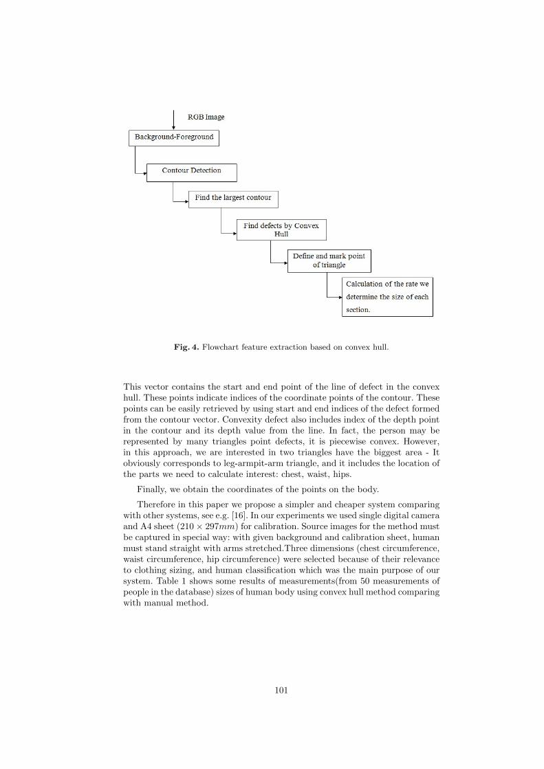
Fig. 4. Flowchart feature extraction based on convex hull.
This vector contains the start and end point of the line of defect in the convexhull. These points indicate indices of the coordinate points of the contour. Thesepoints can be easily retrieved by using start and end indices of the defect formedfrom the contour vector. Convexity defect also includes index of the depth pointin the contour and its depth value from the line. In fact, the person may berepresented by many triangles point defects, it is piecewise convex. However,in this approach, we are interested in two triangles have the biggest area - Itobviously corresponds to leg-armpit-arm triangle, and it includes the location ofthe parts we need to calculate interest: chest, waist, hips.
Finally, we obtain the coordinates of the points on the body.
Therefore in this paper we propose a simpler and cheaper system comparingwith other systems, see e.g. [16]. In our experiments we used single digital cameraand A4 sheet (210 × 297mm) for calibration. Source images for the method mustbe captured in special way: with given background and calibration sheet, humanmust stand straight with arms stretched.Three dimensions (chest circumference,waist circumference, hip circumference) were selected because of their relevanceto clothing sizing, and human classification which was the main purpose of oursystem. Table 1 shows some results of measurements(from 50 measurements ofpeople in the database) sizes of human body using convex hull method comparingwith manual method.
101

Table 1. Results of measurement sizes of human body using convex hull method.
BODY SIZES Manual method Convex hull method
Chest 87.98 cm 88.12 cmWaist 67.95 cm 68.05 cmHip 90.52 cm 91.68 cm
Chest 88.64 cm 89.02 cmWaist 66.61 cm 67.13 cmHip 93.58 cm 94.93 cm
Chest 87.22 cm 88.15 cmWaist 67.19 cm 67.96 cmHip 89.36 cm 89.01 cm
Chest 88.16 cm 89.46 cmWaist 65.64 cm 66.42 cmHip 92.17 cm 93.02 cm
Chest 90.96 cm 91.23 cmWaist 71.44 cm 70.82 cmHip 93.56 cm 94.19 cm
Chest 86.94 cm 87.12 cmWaist 67.68 cm 68.12 cmHip 85.28 cm 84.56 cm
Measurements errors are mostly caused by camera resolution or non tightclothing and noises of environment near by the object. In our case, we used abasis phone camera of model Samsung Galaxy S4 with resolution 13 Mega Pixel.We recommended using high-quality resolution camera with flash opened duringthe time capture photos and people should wear tight clothes body to reducemaximum noises as measurements errors. In addition, we have also performedaveraging over several measurements to reduce measurement and calibrationerrors.
The circumferential measures were generated by approximating the shape ofthe respective body part. For example, neck circumference was approximatedwith the elliptical shape. The major and minor axes lengths were obtained fromthe front and side views. The chest circumference was determined by approx-imating the shape as a combination of a rectangle and an ellipse, using themethod with formula mentioned in [16].
4 Anthropometric Data Analysis
Base on method anthropometric features extraction which mentioned in previoussection, we collected sizes of human body parts. We have a train set containssizes of 50 people sizes (25 men and 25 women) and test set from 18 people (10men and 8 women). Each measurement contains 3 feature for each object: chest,waist and hip circumferences.
102

4.1 Classification of Men/Women using Support VectorMachine(SVM)
To solve the problems of classification we used well-known machine learningmethod – support vector machine (SVM), proposed by Vladimir Vapnik [11].We choose SVM as a one of the most effective algorithm which have many realworld applications [17].
Our goal is use a support vector machine for gender classification based onanthropometric data. As a features we use three human body parameters: chest,waist, hip circumferences.
The LibSVM library [15] was used as Support Vector Machine implementa-tion. The following main parameters of SVM were chosen. Radial basis functionwith γ = 0.333 parameter was used as a kernel function. SVM model param-eters Gamma (γ) and cost (C) were obtained empirically. Gamma parameteris needed for all types of kernels except linear. Constant C is an regularizationterm in the Lagrange formulation. We will use the supplied parameter ranges(C - cost, γ - gamma), using the train set. The range to gamma parameter isbetween 0.000001 and 0.1. For cost parameter the range is from 0.1 until 10.It’s important to understanding the influence of this two parameters, becausethe accuracy of an SVM model is largely dependent on the selection them. Forexample, if C is too large, we have a high penalty for non separable points andwe may store many support vectors and over-fit. If it is too small, we may havean under-fitting. The results of this algorithm is shown in Fig.5. Obtained testclassification error for current dataset is 20%.
Fig. 5. The result of classification by SVM. Blue dots: men, red dots: women, greendots: support vectors.
103
5 Conclusion
Human classification is an useful application for many future scenarios of human-computer interaction. Our approach is presented in this paper describes theclassification of people based on the anthropometrical features using machinelearning approach. Proposed approach allows to extract form images a numberof anthropometrical features, including the length of arms, chest width, shoulderwidth, hips, leg length. In this article we propose solution of male/female clas-sification task by image based on support vector machine. Obtained test erroris sufficiently large but in feature work we are going to examine more classifiersto choose best one and also use bigger datasets to reduce misclassification rate.Based on these results, we hope to build solution that can help to solve tasks ofthe clothing industry.
References
1. Lin, Y.-L., Wang, M.-J.J.: Automatic Feature Extraction from Front and SideImages. In: International conference on Industrial Engineering and EngineeringManagement, pp. 1949–1953. IEEE, Singapore (2008)
2. Lin, Y.-L., Wang, M.-J.J.: Constructing 3D Human Model from 2D Images. In:International conference on Industrial Engineering and Engineering Management,pp. 1902–1906. IEEE, Xiemen (2010)
3. Lin, Y.-L., Wang, M.-J.J.: Constructing 3D Human Model from Front and SideImages. Expert Systems with Applications, Vol. 39, No. 5, 5012–5018 (2012)
4. Rahman, S.A., Cho, S.-Y., Leung, M.K.H.: Recognizing Human Actions by Ana-lyzing Negative Spaces. IET Computer Vision, Vol. 6, No. 3, 197–213 (2012)
5. Pickup, D., Sun, X.-F., Rosin, P.L., Martin, R.R., Cheng, Z.-Q., Lian, Z., Aono,M., BenHamza, A., Bronstein, A., Bronstein, M., Bu, S., Castellani, U., Cheng,S., Garro, V., Giachetti, A., Godil, A., Han, J., Johan, H., Lai, L., Li, B., Li, C.,Li, H., Litman, R., Liu, X., Liu, Z., Lu, Y., Tatsuma, A., Ye, J.: SHREC’14 Track:Shape Retrieval of Non-Rigid 3D Human Models. In: Proc. 7th of EurographicsWorkshop on 3D Object Retrieval, pp. 101–110. Eurographics, Strasbourg (2014)
6. Barnard, M., Matilainen, M., Heikkila, J.: Body part segmentation of noisy humansilhouette images. In: Multimedia and Expo, IEEE International Conference on,pp. 1189–1192. IEEE, Hannover(2008)
7. Jiang, L., Yao, J., Li, B., Fang, F., Zhang, Q., Meng, M.Q.-H.: Automatic BodyFeature Extraction from Front and Side Images. Journal of Software Engineeringand Applications, Vol. 5, No. 12, 94–100 (2012)
8. Freeman, H.: On the Encoding of Arbitrary Geometric Configuration. IRE Trans-actions on Electronics Computers, Vol. EC-10, No. 2, 264–268 (1961)
9. Mittal, A., Zhao, L., Davis, L.S.: Human Body Pose Estimation using Silhou-ette Shape Analysis. In: Advanced Video and Signal Based Surveillance, 2003.Proceedings. IEEE Conference on, pp. 263–270. IEEE, USA (2003)
10. Mori, G., Ren, X., Efros, A.A., Malik, J.: Recovering Human Body Configura-tions: Combining Segmentation and Recognition. In: Computer Vision and Pat-tern Recognition. Proceedings of the 2004 IEEE Computer Society Conferenceon, Vol. 2, pp. 326–333. IEEE, Washington (2004)
104

11. Cortes, C., Vapnik, V.: Support-Vector Networks. Machine Learning, Vol. 20, No.3, 273–297 (1995)
12. Han, E.: 3D Body-Scanning to Help Online Shoppers find the Perfect Clothes fit.The Sydney Morning Herald. National Newspaper (Australia) (2015)
13. MacQueen, J. B.: Some Methods for Classification and Analysis of Multivari-ate Observations. In: Proceedings of 5th Berkeley Symposium on MathematicalStatistics and Probability 1, pp. 281–297. University of California Press, USA(2009)
14. Sklansky, J.: Finding the Convex Hull of a Simple Polygon. Pattern RecognitionLetters, Vol. 1, No. 2, 79–83 (1982)
15. Chang, C.-C., Jen, C.: LIBSVM - A Library for Support Vector Machines, http://www.csie.ntu.edu.tw/~cjlin/libsvm
16. Kohlschetter, T.: Human Body Modelling by Development of the AutomaticLandmarking Algorithm. Technical Report No. DCSE/TR-2012-11 (2012)
17. Wang, Lipo, ed. Support Vector Machines: theory and applications. Vol. 177.Springer Science & Business Media (2005).
18. OpenCV 2.4.11.0 documentation, http://docs.opencv.org/modules/imgproc/
doc/feature_detection.html
105

An Approach to Multi-Domain Data Model Development
Based on the Model-Driven Architecture and Ontologies
Denis A. Nikiforov, Igor G. Lisikh, Ruslan L. Sivakov
Centre of Information Technology, Ekaterinburg, Russia
Denis.Nikiforov,Igor.Lisyih,[email protected]
Abstract. To date, there are many diverse data representation technologies
(EDIFACT, XML, JSON, CSV, relational model, NoSQL). Transition to new
technologies or the integration of information systems based on different techno-
logical stacks is a complex and expensive process. Platform-independent models
take an important role in this process. The structure of such a model is described
in this article. However, given the data model has been created at the junction of
different domains, it may be not enough. In such case, a one more step of abstrac-
tion and a movement to the computation-independent model is required. The au-
thors propose to create it in an ontological form.
Keywords: ontology, model-driven architecture, platform-independent model,
computation-independent model, data model
1 Introduction
When developers create complex, heterogeneous, distributed information systems,
they face a number of questions: which technologies for data storage and transfer to
choose, how to ensure data-model consistency across different participants of infor-
mation exchange, and how to simplify future maintenance of the system under devel-
opment. In order to assist the developers of such information systems, the OMG con-
sortium has developed the model-driven architecture [1]. This architecture considers an
information system as a set of models and the development process is transformation
of some models into others.
The architecture is not a technical specification. It describes only basic principles.
Specifically, it describes platform-dependent, platform-independent, computation-in-
dependent models without governing the structures thereof. In other words, developers
choose existing or create new modeling languages (metamodels) for each specific in-
formation system. The NIEM specification [2] is an example of such a metamodel. It
describes a platform-independent metamodel and a platform-dependent metamodel as
well as the rules for transforming instances of the former into instances of the latter.
We have also developed a similar platform-independent metamodel as well as the rules
for transforming its instances into platform-dependent models (an XML schema and an
ER model).
106

As a rule, the platform-independent model solves a considerable number of problems
related to the development and maintenance of an information system without the need
to provide the third level of abstraction (in the computation-independent model). How-
ever, if information exchange is sufficiently complex and covers multiple domains, then
the computation-independent model is required.
The purpose hereof is to describe the problems occurring in the data-modeling pro-
cess that could indicate the need for the computation-independent model. We also show
that such a model is actually an ontology. We hope that our experience will help the
developers of complex, heterogeneous, distributed information systems to take correct
architectural decisions. We will try to answer the question whether and why ontologies
are needed for data modeling.
2 The Platform-Dependent Data Model
Let us consider the following example. Some organization produces shrimps at its
aquafarm and sells these to another organization. If the organizations reside in different
countries, then this process additionally involves customs, sanitary and veterinary,
transport and other control authorities. All the stages of this process are carried out
together with the storage, transfer, and processing of data on the consignor, consignee,
forwarder, transport vehicle, cargo, and other objects (Fig. 1).
Fig. 1. The process of delivering the commodity and its accompanying data
The participants process data on the same objects. However, they can use different
technologies for data storage (RDBMS, NoSQL, Excel) and transfer (XML, JSON,
CSV). It means that, in the general case, every participant can have its own platform-
dependent data models.
For example, an applicant can file a customs declaration in electronic form in the
XML format, whereas a customs authority can store the same data in a relational DB
(Fig. 2). In this case, they need two platform-dependent data models: an XML schema
and an ER model, respectively.
In order to enable the customs authority to extract the data from the XML message
and save the data in its DB, another model mapping XML elements to DB fields is
required, and such a model always exists. Even if operators manually input details into
the DB, this model exists in their minds or as text instructions. In the general case, the
107

number of mapping models is proportional to the square of the number of exchanging
information systems. Obviously, the integration of such heterogeneous information sys-
tems with different data storage, transfer and mapping models is rather labor-consum-
ing and error-prone. All these models will have to be changed in case a data structure
changes.
Fig. 2. The example of platform-dependent models and metamodels
3 The Platform-Independent Data Model
Platform-dependent models described above have rather different forms but, on the
whole, consider more or less the same data. The development and maintenance of all
these models can be significantly simplified if we abstract away from data-representa-
tion differences between different platforms and create a single platform-independent
model. If one needs to modify a data structure, corrections will have to be made only
in this model and then platform-dependent models and mapping models will be auto-
matically generated on its basis. Such an approach is described in the model-driven
architecture [1]. An example of the platform-independent model is shown in Fig. 3.
108

Fig. 3. The example of the platform-independent data model
In our approach, a UML [3] profile is used to develop platform-independent models
(Fig. 4). The profile is based on ISO/IEC 11179 [4] and contains the following stereo-
types.
Classifier is any object of a data model.
Namespace is the container for logically-related objects with unique names.
Namespace Subset is the subset of related objects of the Namespace.
Platform is the set of the Primitive Types of a certain platform.
Primitive Type is the primitive data type of a certain platform.
Base Type is the data type used to abstract away from the platform. It is to be imple-
mented by exactly one primitive data type for every platform.
109

Fig. 4. The profile of the platform-independent data metamodel
Element is the data unit with the designated definition, identifier, representation, and
permitted values.
Simple Element is the data element without properties.
110

Complex Element is the data element with properties.
Simple Type is the set of permitted values of the Simple Element.
Complex Type is the set of the Element’s properties that are also Elements, in their
turn.
Component is the Element’s property.
Attribute is the context characteristic of the data type.
There are two types of inheritance: extension and restriction.
Every data element and type is described as a separate independent entity. This al-
lows generating maximally-normalized platform-dependent models: XML schemas of
the “Garden of Eden” pattern and relational models with the relations in the 6th normal
form. If necessary, one can generate less normalized models. In other words, such a
platform-independent model contains enough information to generate platform-de-
pendent models on its basis with any required characteristics. Further, the metamodel
allows describing, using the OCL language [5], business rules that can be converted
into SQL or XPath expressions. Model transformation is implemented in [6] using the
QVTo language [7], which detailed description falls beyond the scope hereof.
On the one hand, data elements in the described platform-independent model are
abstracted away from specific data-modeling languages. They are not XML elements,
not entities, not relations but some syntax-neutral data units. On the other hand, the data
elements can be re-used in different data structures. This means that the same properties
of real-world objects are described using the same data element in all particular data
sets (documents, messages). One can conclude that, in fact, delinking of data elements
from specific data-representation languages and from their contexts makes the de-
scribed model conceptual (Fig. 5). The next section shows why this is not the case, and
what difficulties it can cause.
Fig. 5. A conceptual model
4 The Computation-Independent Data Model
The platform-independent data metamodel described above can considerably sim-
plify the development and maintenance of information systems. However, if we attempt
to create a single model for different participants (Fig. 1), then the following problems
will be encountered.
Firstly, the participants can use different dictionaries and code lists for semantically
identical data elements. For instance, a customs authority can code commodities based
on the Harmonized Commodity Description and Coding System, whereas a sanitary
111

and veterinary authority can use different classification codes of the products under
control. Kinds of submitted documents for which every participant has its own code list
is another example. Such semantically identical data elements can be combined in two
ways: either to unify code lists or to accompany codes with references to the used code
lists.
Secondly, the participants can structure details of the same objects in different ways.
For example, customs authority needs to know a commodity code, price, intended use
of goods, packaging kind, and mass. Transport control authority is not interested in
price and intended use of goods. Sanitary and veterinary control authority checks date
of production, best before date, and age and taxon information of shrimps (Fig. 6). All
these appropriate authorities keep under control transportation of one and the same ob-
ject, i.e. shrimps, but we had to create separate data types for each kind of authority. It
increases the size of the model and complicates its maintenance. We can try to harmo-
nize these types by one of the three methods: extension (general characteristics are put
in a base data type), restriction (all possible characteristics are put to a base data type,
and usage of these characteristics in derived data types is restricted), or composition
(each characteristic is described as independent object wherein composite data types
refer to these global characteristics only).
Fig. 6. Different details of one and the same object (shrimps)
Thirdly, the participants use different terminologies. For example, a customs author-
ity mainly uses the term “commodity”, a transport authority uses the term “cargo”, and
a sanitary and veterinary authority uses the term “product” to designate the shrimps
(Fig. 1). In spite of this, the same object is controlled by all the authorities, which means
that only one term should correspond to this object in a single data model. The question
is: which of the above terms? Some sources use these terms as synonyms. Other sources
state that “a commodity is a product of labor made for sale.” On the other hand, for
example, a land lot can be a commodity without being a product of labor. In its turn, a
cargo can or cannot be a commodity or a product, and so on.
Although the first and the second problems can be solved within the mentioned plat-
form-independent model, they imply that this model is not as universal as was described
above. It can contain several different types and elements in order to represent details
of the same object. This fact complicates the integration of information systems and the
maintenance of the model.
112

The third problem explicitly indicates a fundamental shortcoming of the described
model. Despite abstracting away from particular data-representation forms (relational
model, XML schema, et al.), our model still depends on the usage context, on the do-
main.
This is connected with the fact that the model describes particular sets of details of
real-world objects (particular documents, messages), which can be different for differ-
ent participants, rather than the objects themselves. A single model can be developed
only if the context, documents, messages are disregarded and real-world objects are
modeled. The goal of the process described in Fig. 1 is not to transfer the documents
but to change the statuses, properties, and relations of the real-world objects. Docu-
ments are only a tool to reach the process’s goal. If we abstract away from the docu-
ments, a single computation-independent model for all the participants can be obtained.
Fig. 7. The example of harmonization of different object’ details by means of ontology
Upon reaching the ontological level of modeling, we can conclude that a commodity,
a cargo, and a product are not the entity of the object (which data we transfer in the
process) but the temporal roles that this object can play. A commodity is the role of the
object that has a seller and a buyer. A cargo is the role of the object that has a consignor,
113
a consignee, and a forwarder. A product is the role of the object that has a producer and
a consumer. If the difficulties described in this section occur in the data-modeling pro-
cess, this means that the capacity of the used modeling language is insufficient and an
ontology is required.
An example of such ontology is presented in Fig. 7.With our approach; the ontology
can include concepts of three types: classes, roles and events. Class describes an intrin-
sic essence of the object. Role describes temporary characteristics or relations of the
object which appear only in a particular context [8, 9]. Context can be presented by a
class (for example, an employee is a role of a man appearing in the context of organi-
zation) or by an event. Some authors extract one more kind of a context, i.e. process.
[10]. However, we view processes as compound events [11]. The computation-inde-
pendent model, firstly, does not have duplicate elements and types, and, secondly, does
not change significantly with appearance of new messages or by change of existing
documents or messages.
5 Similar Studies
As early as in the 1970-ies, the need for conceptual data modeling was understood,
which resulted in the development of ER models and IDEF1X. It is interesting that the
conceptual level of the ER model contains minimum information on which basis a more
particular and detailed logical model is further created. In other words, the conceptual
model is considered as the first approximation to a logical and then physical model.
However, in IDEF1X, a conceptual model is needed to integrate several external and
internal data models. Moreover, the conceptual model contains a single, integral, suffi-
ciently detailed representation of data rather than the minimum information or the first
approximation to other models.
Our approach based on the model-driven architecture is very similar to ER and
IDEF1X: it also has 3 levels but slightly different ones. The first level is a computation-
independent model describing real-world objects, the relations and properties thereof.
In fact, this is a conceptual model but more detailed than the one of the ER model (in
addition to entities and relations, it also contains properties) and less detailed than the
one of IDEF1X (it does not indicate data types). The second level is a platform-inde-
pendent model describing particular structures of documents, messages that contain
data of real-world objects. This model is something between external and conceptual
models as approached by IDEF1X. The third level is a platform-dependent model that
is similar to the logical ER model but can also be non-relational. Another difference
between our approach and the ER model and IDEF1X is that transformations of plat-
form-independent models into platform-dependent ones are completely formalized and
automated. Finally, our platform-independent model describes not only a data schema
but also business rules in the OCL language.
NIEM is another analog of our approach [2]. Similarly, it is based on the model-
driven architecture, its specification considers platform-independent and platform-de-
pendent models, transformation of one model into the other is described using the
QVTo language, and the metamodel is implemented as a UML profile. There are no
114
other similarities, however. Firstly, our approach does not have a profile for platform-
dependent models. There is no need for it as such a model is fully automatically gener-
ated from the platform-independent model. If a platform-dependent model with other
characteristics needs to be generated, then the transformation itself should be changed.
Secondly, the platform-independent model of NIEM contains several kinds of complex
types (objects, roles, associations, et al.). In our approach, such a division is done on
the level of the computation-independent model that NIEM lacks. In contrast to our
approach, NIEM does not allow describing business rules using the OCL language and
transforming these into XPath expressions.
CCTS is another analog of our approach [12]. Similarly, this one is based on
ISO/IEC 11179 [4]. Data is modeled on two levels: core components and business-
information entities that, for the purposes of this discussion, correspond to the compu-
tation-independent and the platform-independent models used in our approach. The dif-
ference is that, in CCTS, basic core components, association core components (and the
corresponding business-information entities) cannot be reused. For this reason, only
partially-normalized platform-dependent models can be generated from such a plat-
form-independent model (the “Garden of Eden” and the 6th normal form are impossi-
ble). The second distinction is that new aggregate core components (and aggregate busi-
ness information entities) cannot be defined in CCTS by extension or restriction; only
qualification can be used that is not supported by any platform that the authors hereof
are aware of. The third distinction is that, despite the fact that CCTS allows describing
business rules in a data model, business rules are described using the XPath language
and supported only in XML schemas but, for example, cannot be transformed into SQL
expressions. In our platform-independent model, business rules are described using the
OCL language and can potentially be transformed into expressions in the language of
any platform.
Finally, Semantic Web gains rather significant popularity recently [13]. RDF and
OWL allow to describe real-world objects conceptually and computation-inde-
pendently. Moreover, several working groups developed data integration standards
(ISO 15926, ISO 21127), intended on active usage of these technologies. Some authors
propose to use RDF as a universal language for data exchange. [14], [15]. Other authors
allow usage of XML or relational models for data exchange, but they propose to trans-
form XML schemas and ER models to ontology [16], [17]. The latter, in turn, can be
used for data integration.
Our approach goes in the opposite direction. Firstly, we consider that it is not always
possible to be limited to usage of RDF and triplestore in data transfer and storage,
sometimes XML schemas or relational models are required. Secondly, computation-
independent model describing real-world objects must be primal. A data modeler has
to develop platform-independent model describing documents and messages on basis
of it. This platform-independent model can be transformed into platform-dependent
models (XML schemas, ER models). We found no one article with description of trans-
formation of OWL model to ER model or XML schema. Only backward transfor-
mations are available. However, for us, this direct transformation is of the most interest.
115
6 Conclusion and Follow-up Studies
Data modelers (including authors of this article) often face an issue of motivation
for the use of one or another data modeling approach: ontologies, model-driven archi-
tecture, IDEF1X, ER. In this article, we tried to correlate these approaches. We also
tried to specify problems which can testify a necessity of use of model-driven architec-
ture and ontologies.
Multi-level data models including the conceptual model were developed as early as
in the 1970-ies. At large, neither ontologies nor the model-driven architecture intro-
duces anything fundamentally new into this field. These are only steps on the way to
generalize, unify existing ideas. Ontologies play exactly the same role as the classical
conceptual ER models or IDEF1X in the data-modeling process. In the first case, the
ontology is the first approximation to a more particular, detailed, contextual data model
that describes the sets of details of real-world objects represented by documents, mes-
sages rather than the objects themselves. In the second case, the ontology is a suffi-
ciently detailed data model common for several participants.
If only data-exchange schemas (documents, messages) or particular data-storage
schemas need to be designed, then XML schemas, relational models, or other logical
models are sufficient, there is no need to use ontologies. If there is a need to unify all
these particular data schemas, then we should abstract away from the sets of objects’
details and start modeling the real-world objects themselves, and for this purpose, on-
tologies can be used. The possibilities of the languages intended for data modeling on
a logical (rather than conceptual) level are rather limited when there is a need to unify
data structures using different code lists, slightly different sets of details, and different
terminologies. Such languages allow modeling only particular sets of details of objects
rather than the real-world objects themselves.
It should also be noted that the developers of data models based on the model-driven
architecture, as a rule, restrict themselves to platform-independent and platform-de-
pendent models thus omitting computation-independent models. The present paper at-
tempts to show that platform-dependent models can be well dispensed with as these can
be automatically generated from platform-independent models. However, if the devel-
oped model is rather complex, covers multiple domains, the computation-independent
model (describing real-world objects rather than particular sets of details thereof) can
considerably simplify the development and maintenance of information systems. Fur-
thermore, the computation-independent data model is an ontology.
The metamodel presented in this article has no essential novelty. As already stated,
similar metamodels were discussed in [2], [12]. As a rule, these metamodels have only
one target architecture. Our approach has a benefit: from one platform-independent
model we form not only XML schemas but ER models as well. Secondly, we describe
not only data schema but also business rules, and we do it in platform-independent
OCL, not in a language of target architecture. Thirdly, we predicate that in some situa-
tions one platform-independent model is not enough, and a computation-independent
model is required.
Currently, a metamodel is used for data modeling in several domains: customs con-
trol, transport control, technical regulation, sanitary and veterinary control, and others.
116

Our approach to data modeling can be used with other types of B2G or G2G interaction.
Developed platform-independent model has around 2,000 elements and types. Around
100 exchange structures were developed on the basis of this model. XML schemas and
ER models are formed automatically from this model. Unfortunately, transformation
rules [6] are too voluminous to present them in this article. It will be described in details
in next articles.
At this date, development of the computation-independent data model is in the initial
stage. In next articles, we shall describe in details the model formation rules and rules
for creation of platform-independent model on its basis. We shall also try to evaluate at
what extent the computation-independent model will help to improve the quality of the
platform-independent model.
7 References
1. Miller, J., Mukerji, J.: MDA Guide Version 1.0.1 (2003). http://www.omg.org/cgi-
bin/doc?omg/03-06-01
2. Object Management Group: UML Profile for NIEM, version 1.0 (2014)
3. Object Management Group: OMG Unified Modeling Language, version 2.4.1 (2011)
4. ISO: ISO/IEC 11179-1:2004. Information technology – Metadata registries – Part 1: Frame-
work (2004)
5. Object Management Group: Object Constraint Language, version 2.4 (2014)
6. Nikiforov, D.A.: UML Model to XML Schema 1.1 Transformation. doi:10.5281/ze-
nodo.16151 (2013)
7. Object Management Group: Meta Object Facility (MOF) 2.0 Query/View/Transformation
Specification, version 1.1 (2011)
8. Pradel, M., Henriksson, J., Aßmann, U.: A good role model for ontologies: Collaborations.
In: International Workshop on Semantic-Based Software Development (2007)
9. Henriksson, J., Pradel, M., Zschaler, S., and Pan, J. Z.: Ontology Design and Reuse with
Conceptual Roles. In Proceedings of the 2nd International Conference on Web Reasoning
and Rule Systems, RR ’08, pp. 104–118, Berlin, Heidelberg. Springer-Verlag (2008)
10. Mizoguchi, R., Kozaki, K., and Kitamura, Y.: Ontological Analyses of Roles. FedCSIS, pp.
489-496 (2012)
11. Partridge, C.: Business Objects: Re-Engineering for Re-Use, section 8.3.1.4. Butterworth
Heinemann (1996)
12. UN/CEFACT: Core Components Technical Specification, version 3.0 (2009)
13. W3C: Semantic Web. http://www.w3.org/standards/semanticweb/
14. Gorshkov, S. “Business Semantics” practice of application integration using Semantic Web
technologies. In international data science conference on Analysis of Images, Social Net-
works, and Texts (2013)
15. Booth, D., Dowling, C., Fry, C. E., Huff, S., Mandel, J.: RDF as a Universal Healthcare
Exchange Language. In Semantic Technology and Business Conference San Francisco, CA
(2013)
16. Bedini, I., Matheus, C., Patel-Schneider, P., Boran, A., Nguyen B.: Transforming XML
schema to OWL using patterns. ICSC 2011 – 5th IEEE International Conference on Seman-
tic Computing, Palo Alto, United States. pp.1-8 (2011)
17. Myroshnichenko, I., Murphy, M. C. Mapping ER Schemas to OWL Ontologies. In ICSC
'09. IEEE International Conference on Semantic Computing (2009)
117

Implementation of Image Processing Algorithmson the Graphics Processing Units
Natalia Papulovskaya, Kirill Breslavskiy, and Valentin Kashitsin
Department of Information Technologies of the Ural Federal University,620002, 19 Mira street, Ekaterinburg, Russia
Abstract. The paper describes features of the multithreaded algorithmsimplementation on contemporary CPU and GPU. The features of accessof a graphics processing unit (GPU) memory are reviewed. The bottle-necks have been identified, in which there is a loss of speed in imageprocessing. Recommendations are made for optimization of algorithmsfor processing image of various size. Examples of implementation of thealgorithms are given in the software and hardware architecture CUDA,which is well suited for a wide range of applications with high parallelism.
Keywords: Image processing, Graphics processing unit, Parallel com-puting, CUDA
1 Introduction
Restricted computing power is one of the problems for solving many tasks. Es-pecially, it appears in processing huge arrays or real-time problems. Processorperformance growth of processors has always been associated with increasing thefrequency and number of transistors. However, according to the Moore’s Law [1],the lost of power is because the laws of physics cannot be changed. Namely, in-creasing the frequency and amount of transistors can not be infinite. Recent tenyears have been devoted to search for other solution: despite projected increasein frequency, there were optimizations of structure and growth of cores quantity.But cores quantity growth is not an absolute solution. New opportunities arisefor parallel computing after introducing General Purpose Computing on Graph-ics Processing Units (GPGPU) [2] and Compute Unified Device Architecture(CUDA) by NVIDIA company [3,4,5].
Usually, the Central Processing Unit (CPU) has only 4 or 8 computingthreads. But the Graphics Processing Unit (GPU) has hundreds and thousandscomputing threads. It provides significant acceleration for algorithms with highparallelism degree. Nevertheless, sometimes the CPU wins in competition withthe GPU on well-paralleled tasks.
Mostly, image processing algorithms are easy for parallelization. However,under certain conditions, an algorithm implementation on the central processingunit (CPU) is faster. For proper use of GPU, it is necessary to identity itsbottlenecks and describe capabilities of computing resources in tasks of imageprocessing and analysis.
118
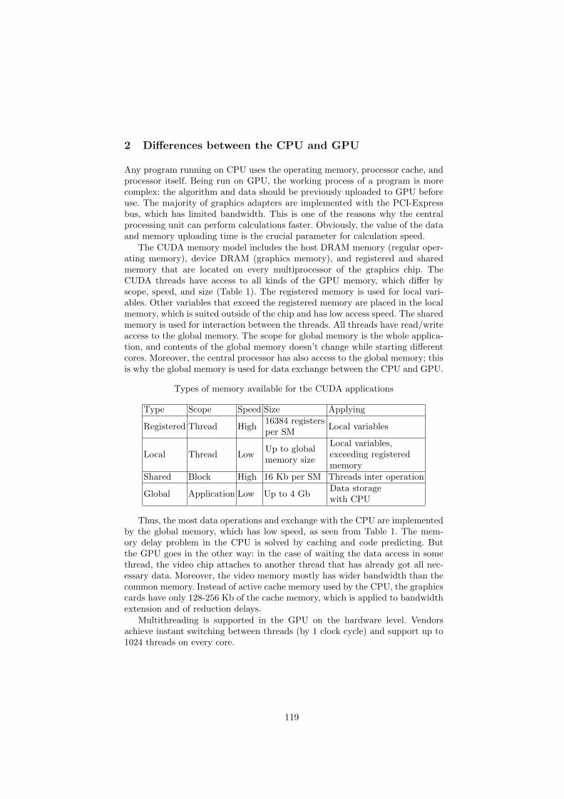
2 Differences between the CPU and GPU
Any program running on CPU uses the operating memory, processor cache, andprocessor itself. Being run on GPU, the working process of a program is morecomplex: the algorithm and data should be previously uploaded to GPU beforeuse. The majority of graphics adapters are implemented with the PCI-Expressbus, which has limited bandwidth. This is one of the reasons why the centralprocessing unit can perform calculations faster. Obviously, the value of the dataand memory uploading time is the crucial parameter for calculation speed.
The CUDA memory model includes the host DRAM memory (regular oper-ating memory), device DRAM (graphics memory), and registered and sharedmemory that are located on every multiprocessor of the graphics chip. TheCUDA threads have access to all kinds of the GPU memory, which differ byscope, speed, and size (Table 1). The registered memory is used for local vari-ables. Other variables that exceed the registered memory are placed in the localmemory, which is suited outside of the chip and has low access speed. The sharedmemory is used for interaction between the threads. All threads have read/writeaccess to the global memory. The scope for global memory is the whole applica-tion, and contents of the global memory doesn’t change while starting differentcores. Moreover, the central processor has also access to the global memory; thisis why the global memory is used for data exchange between the CPU and GPU.
Types of memory available for the CUDA applications
Type Scope Speed Size Applying
Registered Thread High16384 registersper SM
Local variables
Local Thread LowUp to globalmemory size
Local variables,exceeding registeredmemory
Shared Block High 16 Kb per SM Threads inter operation
Global Application Low Up to 4 GbData storagewith CPU
Thus, the most data operations and exchange with the CPU are implementedby the global memory, which has low speed, as seen from Table 1. The mem-ory delay problem in the CPU is solved by caching and code predicting. Butthe GPU goes in the other way: in the case of waiting the data access in somethread, the video chip attaches to another thread that has already got all nec-essary data. Moreover, the video memory mostly has wider bandwidth than thecommon memory. Instead of active cache memory used by the CPU, the graphicscards have only 128-256 Kb of the cache memory, which is applied to bandwidthextension and of reduction delays.
Multithreading is supported in the GPU on the hardware level. Vendorsachieve instant switching between threads (by 1 clock cycle) and support up to1024 threads on every core.
119

Large number of threads in the CPU is not advisable due to significant timeloss while switching, which may consume up to several hundreds of clock-cycles.In addition, one CPU core is able to process only 1 or 2 threads simultaneously.
3 Benchmarks
3.1 Baseline
Performance tests were done on image processing algorithms software imple-mentation. Four different resolutions of image (50x50, 150x150, 300x300, and512x512) were used with the quality of JPEG Quality 25 and JPEG Quality100. As a reference image, the well-known file Lena.jpg [6], was used. Lenna orLena is the name given to a standard test image widely used in the field of imageprocessing since 1973.
The images were processed by application of Sarcis [7] developed by theDepartment of Information Technologies of the Ural Federal University. Thisprogram is designed for image processing of color and gray scale images andcan be used for calculation both on the CPU and GPU. For the tests, fouralgorithms were chosen: the weighted linear filter, reverse gradient filter, edgedetection Canny’s filter, and morphology processing filter erosion. An exampleof application of the Canny’s filter is shown in Fig.1. Workstation configurations
Fig. 1. Image processing by the Sarcis program
used for benchmarks:
CPU Intel Core i5-2450 (4 threads, 2.5Ghz), GPU NVIDIA GT630M (96 CUDAcores, 800Mhz);
120

CPU Intel Core i7-860 (8 threads, 2.8Ghz), GPU NVIDIA GTX260 (216 CUDAcores, 576Mhz);CPU Intel Core i5-3470 (4 threads, 3.2Ghz), GPU NVIDIA GTX760Ti (1344CUDA cores, 915Mhz).
3.2 Theoretical description of filtering algorithms
Weighted linear filtering. The linear smoothing filters are good ones for re-moving the Gaussian noise and, also, the other types of noise. A linear filter isimplemented using the weighted sum of the pixels in the successive windows.Typically, the same pattern of weights is used in each window; this means thatthe linear filter is spatially invariant and can be implemented using a convolutionmask. If different filter weights are used for different parts of the image (but thefilter is still implemented as a weighted sum), then the linear filter is spatiallyvaried [8].
One of the simplest linear filters is implemented by a local averaging opera-tion where the value of each pixel is replaced by the average of all the values inthe local neighborhood. The weighted linear filtering mask is given by the mask
M = 116
1 2 12 4 21 2 1
. The main strategy is to set the largest weight at the central
pixel and inversely proportional to distance values to other pixels:Reverse gradient filter. The idea of the reverse gradient filter is in choosing
the mask weights. The greater bright difference between the central and the nextpoint, the less weight is prescribed to the next point.
The mean gradient module value calculated for each aperture brightness levelis:
HG(l) =1
h(l)
h(l)∑
m=1
Gml (i, j)
Where HG(l) is the mean brightness gradient function value for l; h(l) is thenumber of points with brightness l; Gl(i, j) is the gradient value in the mth point
with brightness l at position (i, j). The Laplace operator 52 =
−1 −1 −1−1 +8 −1−1 −1 −1
is
used to calculate the gradient valueCanny filter. The Canny filter is considered to be the optimal choice for
any task, which requires edge extraction or edge enhancement of elements withdifferent shapes and characteristics. This is due to its easy implementation andability to be adapted to different circumstances [9].
There are the following three criteria for the algorithm:
• smart detection (increasing the signal/noise ratio);• good localization (correct definition of boundary position);• only one response to the border.
121

The Canny filter differs from other classic edge detecting filters because it consid-ers directionality of the element and permits personalization of the filter behaviorby choosing the value of parameters of the algorithm. This provides changes indirection of the filter polarization and sensibility of the edge extraction.
The algorithm runs in 5 separate steps [10].
1. Smoothing: blurring of the image to remove noise.
2. Finding gradients: the edges should be marked where the gradients of theimage have large magnitudes.
3. Non-maximum suppression: only local maxima should be marked as edges.
4. Using the double thresholds: potential edges are determined by using thethresholds.
5. Edge tracking by hysteresis: the final edges are determined by suppressingall edges that are not connected to a strongly determined edge.
Morphological Image Processing. The morphological image processingis a collection of non-linear operations related to the shape or morphology theimage features. Erosion of images is generally used for getting rid of the imageof random insertions. The idea is that the inclusions are eliminated by blurring,while large and, thus, more visually important regions remain.
a) b) c)
Fig. 2. Morphological image processing example; a) source image; b) kernel; c) erosionresult
Erosion (morphological narrowing) is a convolution of the image or its areaselected with some kernel. The kernel may be of arbitrary shape and size. Here,in calculating the convolution, only one leading position is selected in core, whichis aligned with the current pixel. In many cases, the core is selected as a squareor circle with a leading position at the center (Fig. 2b). The core can be regardedas a pattern or a mask.
Applications of dilation is reduced to the passage pattern throughout theimage and use some operator to search for a local minimum intensities of thepixels in the image, which covers the template. The gray color filled pixels appearblack due to erosion (Fig. 2c).
122

3.3 Benchmark results
Weighted linear filtering. As seen from graphs in Fig. 3, the images with size50× 50 are processed for the same time by both the CPU and GPU, excludingNVIDIA GTX260, which works a little better. The larger images are processedfaster by the GPU.
Fig. 3. Weighted linear filter benchmarks
Fig. 4. Reverse gradient filter benchmarks
Fig. 5. Canny filter benchmarks
123

Reverse gradient filter.As seen from graphs in Fig. 4, application of thereverse gradient filter gives comparable results w.r.t. the weighted linear filter.
Canny filter. It is obvious from Fig. 5 that the CPU runs faster on imagesup to 150 × 150 quality 25, but the GPU NVIDIA GT630M takes advantagein times on larger images. The GPU NVIDIA GTX260 works better when theCPU starts from images 300× 300 regardless of image quality.
Morphological Image Processing. Analysis of graphs in Fig. 6 showsthat in using the morphological processing similar to Canny’s filter, the GPUNVIDIA GT630M starts process faster than CPU from images size 50× 50; andthe GPU NVIDIA GTX260 is faster from size 300× 300.
Fig. 6. Morphological Image Processing benchmarks
4 Conclusion
Results of this research show a rise in the efficiency of the GPU computing whileimage size grows. Nowadays, the images with resolution less than 1024×768 canbe found rarely. From resolutions 300 × 300, the GPU starts to process imagesfaster than the CPU; so, it is advisable to use image processing algorithmsapplying the GPU computing. The CPU computing is suitable in small imageprocessing or hardware systems without the GPU.
References
1. Moore’s Law, http://www.mooreslaw.org/ csl783/canny.pdf (2009)2. GPGPU. General-Purpose Computation on Graphics Hardware, http://gpgpu.
org.3. Halfhill, T. R.: Parallel processing with CUDA. Micriprocessor report, http://www.
nvidia.com/docs/IO/55972/220401-Reprint.pdf (2008)4. NVIDIA. CUDA in Action, http://www.nvidia.com/object/cuda-home-new.html5. NVIDIA CUDA: Compute Unified Device Architecture, NVIDIA Corp. (2007).6. The Lenna Story, http://www.cs.cmu.edu/~chuck/lennapg/lenna.shtml7. Dorosinsky, L.G., Kruglov, V.N., Papulovskaya, N.V., Chiryshev, A.V.: CUDA tech-
nology in digital image processing, Ekateringurg, 192 p.,(2011)
124

8. Jain, R., Kasturi, R., Schunck, B.G.: Machine vision, http://www.cse.usf.edu/
~r1k/MachineVisionBook/MachineVision.files/MachineVision-Chapter4.pdf,118-122
9. Pirotti, F., Vettore, A.: Canny filter applications and implementation with grass,http://www.academia.edu/313972/
10. Canny Edge Detection, http://www.cse.iitd.ernet.in/~pkalra/
125

Am I Really Happy When I Write “Happy” in MyPost?
Pavel Shashkin and Alexander Porshnev
National Research University Higher School of [email protected], [email protected]
Abstract. Posts published on the Internet could serve as a valuablesource of information regarding emotion. Recommendation systems, stockmarket forecast and other areas are likely to benefit from the advance-ment in mood classification. To deal with this task, researchers com-monly rely on preassembled lexicons of emotional words. In this paperwe discuss the possibility of extracting emotion-specific words from user-annotated blog entries. The study is based on analysis of the collectionfrom 14800 Live Journal posts containing the “Current mood” tag, spec-ified by the author. The analysis findings and possible applications arediscussed.
Keywords: sentiment analysis, user-annotated data, computational lin-guistics, emotional states, psycholinguistics
Introduction
Over the last few years, a considerable amount of work has been done to reducethe overload of user-generated web content [1]. The possibility of grouping datain accordance with sentiment is repeatedly discussed in recent investigations [2,3]. The system capable of extracting emotions inherent in the text is likely toassist both human-computer and human-human interactions, and help in varioustasks. For example, automatic analysis of emotions could be used in some appli-cations, such as: recommendation systems (personal emotions expressed duringevaluation could be taken into account), monitoring of psychological user states(customer satisfaction or diagnostics of potential illness), business intelligence(evaluation of the emotional tone of comments circulating about one’s companycan be used to improve financial decisions).
Online diaries provide researchers with extremely diverse and manifold data.Blog entries are rich in deeply personal and subjective content. Unlike othercorpora used in sentiment analysis, "Current Mood" is a text attribute directlyspecified by the author at the time of writing, rather than by some independentannotator. We expect that analysis of user-annotated data could provide newinformation about words people use to express their emotional states.
126

Related work
Over the past few decades there have been several projects devoted to analysisof emotions in the Internet posts. For example, a research project for measuringemotions is “Pulse of a nation” is based on analysis of Twitter messages fromSeptember 2006 to August 2009 [4]. In their research, Mislove and coauthorstried to find places where life is sweet, people are happier, and to reveal theunhappiest time of a day. Although, we were unable to find scientific articles,the authors of the “Pulse of a nation” project took part in several TV programsand published the results in newspapers and periodicals (including The WallStreet Journal and The New York Times).
To measure emotions in each tweet, Mislove and coauthors used the ANEWword list [5]. The methodology of emotion analysis was to calculate a sentimentscore as a ration of the amount of positive messages to that of negative messages.A message is regarded as positive if it has at least one positive word and asnegative if it has at least one negative word (the same message can be bothnegative and positive) [6].
The project focused on the expression of happiness in social media was de-veloped by a group of researchers from the University of Vermont. They tried tomeasure happiness in Twitter posts [7].
First of all, Dodds and his coauthors conducted a survey using Amazon Me-chanical Turks to obtain happiness evaluations of over 10,000 individual words,representing a tenfold size improvement over similar existing word sets (cho-sen by frequency of usage in collected samples of nearly 4.6 billion expressionsposted over a 33 month span). The created words list contains ranks of theirrelation to happiness. For example, the top happiness words in their rank arelaughter (rank=1) and happiness (rank=2). Next, they created on-line servicehedonometer.org, which provides real time happiness analytics based on analysisof frequencies of the words from the list. It is worth mentioning that this servicealso has a rank for the word “birthday”, so the expression “Happy Birthday” isnot excluded from analysis.
Lansdall-Welfare, Lampos, and Cristianini tried to measure several emotionsin twitter posts by counting the frequency of emotion-related words in each textpublished on a given day [8]. They also use a lexical approach and base theiranalytics on the word lists extracted from the WordNet Affect ontology [9].
After this pre-processing Lansdall-Welfare, Lampos, & Cristianini compiledfour word lists containind 146 anger words, 92 fear words, 224 joy words and 115sadness words. The evaluation of emotions in tweets was based on counting theamount of tweets containing each word from the compiled list. Lansdall-Welfare,Lampos, & Cristianini say they do not expect the high frequency of the word‘happy’ to necessarily signify a happier mood in the population, as this can bedue to expressions of greeting, like “Happy Birthday”. Although they do not filterthis and similar expressions in their analysis.
We can conclude that the projects running analysis of emotions and moods insocial networks usually use the lexicon methodology based on expert-annotatedwords lists.
127

Application of the lexicon approach based on expert or naïve rating of emo-tions in the Internet posts can be supported by the findings made by Gill, Gergle,French and Oberlander. They examined the ability of naive raters of emotion todetect one of the eight emotional categories by asking participants to read 50 and200 word samples of a real blog text and evaluate whether this message expressesone of the eight emotions: anticipation, acceptance, sadness, disgust, anger, fear,surprise, joy or being neutral [10]. Comparing the results of evaluation by expertraters and naive experts allowed the conclusion that rater agreement increasedwith longer texts, and was high for ratings of joy, disgust, anger and anticipation,but low for acceptance and ‘neutral’ texts.
Although raters show agreement in annotation of emotions, we can raise aquestion about its validity from the psychological perspective. We are not surethat all people express their emotions in a straightforward way, using wordsclosest to the chosen mood category.
An interesting study of emotion in the context of a computer-mediated en-vironment was conducted by Hancock, Landrigan, & Silver [11]. They organizedan experimental study, in which some of the participants were asked to ex-press either positive (happy) or negative (unhappy) emotions during a chat con-versation, without explicitly describing their (projected) emotional state. Eventhough, their chat partners did not know about their instructions and theiremotional state, they could accurately perceive their interlocutor’s emotions.Linguistic analysis showed that the authors portraying positive emotions used agreater number of exclamation marks and more words overall. The participantsportraying negative emotions used an increased number of affective words, wordsexpressing negative feeling, and negations.
In this study the people understand emotions of their partner even if theseemotions were not explicitly expressed. This raises a question: could we extendthe lists of emotional words by analyzing data annotated with the current moodof an author?
Analysis of text semantics, therefore, can provide information about useremotions and we expect analysis of user-annotated data from LiveJournal tohelp extend the existing words lists related to emotions.
Data collection
We used DuckDuckGo1 search engine in conjunction with "GoogleScraper"2
Python module to make a list of English-speaking LiveJournal users who haveat least once used the "Current Mood" functionality. The list of obtained URLsis passed down to the web crawler hosted on "import.io"3 platform. Each visitedpage is parsed to extract user messages and links to other LiveJournal blogs tobe added to crawling query (e.g. from the comment section). Data collecting
1 https://duckduckgo.com/2 https://github.com/NikolaiT/GoogleScraper3 https://import.io/
128

continues until the specified maximum page depth is reached.
Start URLs
Blog Queue EntryParser
OutgoingLinks
ExtractedContent
Fig. 1. Data collection system architecture
Data-set highlights
For each message in visited blogs we extract a web address, title, text contentand mood tag (usually accompanied by "Current mood:", "Feeling rather:" orjust "Mood:"). Although the presence of subjective content in a title or webaddress is questionable, they are needed to identify continuous entries (eg. storiesdivided into series of posts). Blog posts, especially the ones with a fair amountof text, are not as frequent as, say, twitter posts. For that reason we do not usetime stamps and rarely present geolocation data. The acquired dataset contains14,800 documents tagged with 800 unique mood labels. 6% of the labels wereresponsible for 60% of data entries (Figure 2). Average text length is 420 words.An approximate post count for the average author is 5 messages (Figure 3). Themost popular mood tags are: "accomplished", "cheerful", "tired" and "amused".
Pre-Processing
The initial step is to clean data from invalid entries (non-Latin or comprisingonly media content). The dictionary is then reduced by transforming everythingto lowercase, stemming words, removing punctuation, stopwords and numbers.If we find negations, like “don’t”, “didn’t” or “not”, the subsequent token is re-placed by not_token. For example, “they didn’t come” includes three tokens:“they”, “didn’t”, “come”. We also keep negations as we can expect negative moodsnegotiations to carry some additional information. URLs are shortened to theirrespective domains and repeating letters (more than three) are reduced to three.Words and numbers representing time or date are replaced with "time_date".
129

apatheticthirsty
accomplished
hungry
mis
chie
vous
disappointed
creativescared
full crazy
drained
rush
ed
angry
ditzy
ecstatic
thoughtful
pensiveproductive
boredaggravated
gloomy
optimistic
relaxeddorky
restless
groggy
merrygiggly
crappy
depressed
determined
nerdy
location
conte
nt
silly
satisfied
peaceful
sleepy
loved
thankful
cheerful
bitchy
busy
devious
bouncy
lethargic
curious
sore
pissed
grateful
geeky
hopeful
sick
crushed
weird
confusedstr
esse
d
cranky
lazy
mellow
horny
uncomfortable
goodcomplacent
sad
excitedokay
embarrassed
tired
frustrated
amused
melancholy
energeticindescribable
happy
hyper
blank
nervous
wo
rkin
g
artistic
distressed
cold
giddy
contemplative
anxio
us
irritated
hot
worried
jubilant
chipper
relieved
exhausted
annoyed
ple
ase
d
impressed
blah
awakecalm
grumpy
Fig. 2. Label frequencies
0 50 100 150
0.00
0.02
0.04
Number of sentences
Den
sity
0 500 1000 1500 2000 25000.00
000.
0010
0.00
200.
0030
Number of words
Den
sity
0 10 20 30
0.00
0.02
0.04
0.06
Words in sentence
Den
sity
0 5 10 15 20
0.00
0.05
0.10
0.15
Entries per user
Den
sity
Fig. 3. Empirical distribution density for text statistics (sentences detected withopenNLP, outliers removed)
130

likejust
backonecan
eyestime
knowsaidget
evennowway
headaround
accomplished
likejust
backonetime
knownowcanget
evenreallyeyes
somethingstill
said
tired
justonelike
tradedbacksaidtime
knowgetcannow
reallygot
eyeseven
amused
likejustone
backknoweyessaidget
timehead
canevenfacenow
really
cheerful
likeone
backjust
eyesnowtime
knowevencan
somethingway
aroundget
said
happy
likejust
backone
knowtimecanget
headeyesnow
reallysayssaid
even
sleepy
likebackjustonesaid
knowtimenoweyes
getcan
aroundevenhead
still
busy
likejust
backone
eyestimeevenknow
aroundnowget
wayhead
cansomething
bouncy
Fig. 4. Word frequencies distribution for popular mood labels
After pre-processing the portion of non-sparse terms doubled. Overall dimen-sionality of feature space was reduced by more than 3 times.
Fifteen highest word frequencies for 8 most used mood labels are very similarand do not provide any evidence that people use emotional words to mark theiremotions (Figure 4). We can see that words highly associated with a mood arenot included in the list with top 20 frequencies. For example, it is not oftenthat messages tagged “Happy” contain “happy” in their body. The list of top 20words does not contain many words from emotional lists. Words “like”, “one”,“back” are not put on the list of 10,000 words related to “happy” according to aHedonometrics survey [7]. They are not included in the list of Affective Normsfor English Words either [5].
The TF-IDF coefficient frequently used for document classification can pro-vide more focused information about semantics of each emotion categories. Tocalculate TF-IDF, we joined all documents of the category into one document.First, the calculated TF-IDF allowed us to find most of the names used inposts. The words with the highest TF-IDF scores were “leo", "maes", "vam-pir", "jare","sandi","gaara", and "roger". After including the names in a list ofstopwords, we received almost the same situation as with calculation of termfrequencies (see Table 1).
131

accomplished tired cheerful sleepyhand 505.7 hand 222.4 artwork 173.3 ghost 342.0said 447.1 rift 216.7 hand 167.7 hand 170.2eye 416.0 say 191.8 said 154.5 margin 153.3
back 389.8 f*ck 170.9 head 151.1 head 151.1head 375.5 eye 156.9 eye 142.8 back 144.5smile 368.7 back 155.6 smile 135.7 color 142.3look 360.8 look 149.5 face 135.2 say 140.1say 355.2 head 148.6 back 119.3 eye 130.8
robot 353.5 doesnt 145.5 look 117.9 superhero 130.0mule 338.5 said 145.2 lip 110.8 said 125.4
amused happy busy bouncytrade 692.7 array 279.9 dev 263.9 sampl 120.7prize 379.7 hand 164.9 alt 178.5 hand 115.1ward 143.9 eye 164.7 hand 148.6 introspect 106.3claim 135.6 back 137.1 said 147.0 head 91.3vote 128.4 lip 127.4 border 133.4 back 89.4said 91.6 smile 125.5 back 118.3 said 84.8hand 86.6 head 122.0 head 114.8 charact 80.6bill 86.0 knew 122.0 eye 114.7 lip 76.5
materia 79.7 realis 121.2 knew 101.3 look 74.6back 69.4 face 119.1 multi 101.1 kiss 74.4
Table 1. Words with highest TF-IDF score for eight most popular mood labels (withproper nouns removed)
Next, we introduced the TF-ICF coefficient. In order to identify importantgroup-specific words, the term frequencies TFij for word i in group j are mul-tiplied by:
log||D||
∑||D||j=1
TFij
maxt∈TjTFtj
(1)
where ||D|| is the number of document groups and Tj - unique words in documentgroup j.
The results produced by this transformation are listed in Figure 5 (apartfrom persons, locations and brands on top of the list) and provide more infor-mation regarding sentiment. For example, the word "finally" has a high value indocuments tagged with "accomplished" or "tired". Although, some of these re-sults are relatively counter-intuitive or even contradictory (e.g. "bed" is presentin "accomplished", "bouncy", "cheerful", "busy", but absent in "sleepy").
This suggests that the distance between documents written in different emo-tional states could be shorter than that between documents written in the sameemotional state by different authors. To test this hypothesis, we filtered docu-ments by author and then, using vector representation of documents, we calcu-
132

momentkeep
wordsfingers
helpfinallylookssaysokay
mouthyeah
maybebedpart
turned
accomplished
f*ckingthree
alreadyopen
knowsworklooksmightsaysf*ck
almostyeah
mouthokay
without
tired
armsput
almostkind
wantedyeahokay
mouthbedhair
looksbettersays
maybeturned
cheerful
gavename
stoptalktoldboy
mindeverything
fingerswordsyeah
withoutbetterturned
body
amused
ghostcolor
shoulderbehind
helpokaykindarm
fingersknows
sayslooks
mouthbetter
part
sleepy
worldwork
behindkeepplacecamemind
wordsalmost
triedmight
withoutbodyside
maybe
happy
foundbest
probablypleasegettingcame
putmindmightplacehelppartbedside
turned
busy
bitmaking
endseriesarmskindside
withoutbetterbodyhairbedpart
everythingsays
bouncy
Fig. 5. Most important words according to TF ICF (with proper nouns removed)
lated cosine similarity between every pair of documents. The same procedurewas carried out for documents filtered by current mood tag.
The only pair of tags "nervous" and "accomplished" has the distance betweenmood labels shorter than the average distance between different authors. This isprobably because they carry a lot of objective content, which should have beenfiltered at earlier stages. The previously mentioned self-containing states of mindfall within the same group of labels, whose distances do not exceed the globalaverage.
The vector model, therefore, contained enough information to distinguishemotions and what we needed was to find an approach to extracting wordswith maximum information. To solve this task, we used the Mutual Informationfeature selection algorithm [12].
Application of the mutual information feature selection algorithm showedthat the word “happy” provided relevant information about the mood of anauthor. However, the top twelve terms for the “happy” category only containedtwo emotional words included in the Hedonometics or ANEW list (“happy” and“wonder”).
We saw that, according to mutual information feature selection, many ofthe categories were determined by the terms not included in emotional wordslists. Then we checked whether or not category name synonyms obtained fromWordNet were frequently encountered in the documents labeled with the samemood [13]. Most of the time mood was not specified in the text in an obvious
133

accomplished tired cheerful sleepyeye 0.0084 three 0.0014 yes 0.0005 found 0.0009
head 0.0080 got 0.0011 feel 0.0004 name 0.0007pull 0.0079 home 0.0010 still 0.0004 probabl 0.0007turn 0.0074 day 0.0010 like 0.0004 knew 0.0007smile 0.0072 lot 0.0009 way 0.0003 side 0.0006arm 0.0071 tell 0.0009 right 0.0003 bad 0.0006first 0.0070 realli 0.0009 see 0.0003 tri 0.0006pair 0.0069 far 0.0008 guy 0.0003 rate 0.0006
behind 0.0069 think 0.0008 think 0.0003 time 0.0005hand 0.0068 let 0.0008 girl 0.0003 walk 0.0005away 0.0067 time 0.0008 hold 0.0002 mayb 0.0005side 0.0063 part 0.0008 just 0.0002 find 0.0005
amused happy busy bouncyknew 0.0008 happi 0.0020 thank 0.0012 your 0.0006still 0.0008 dont 0.0006 set 0.0011 far 0.0006way 0.0007 found 0.0005 pleas 0.0010 someon 0.0005week 0.0007 ive 0.0005 use 0.0010 feel 0.0004cant 0.0007 wonder 0.0004 everi 0.0010 ask 0.0004pleas 0.0007 thank 0.0004 ask 0.0009 sinc 0.0003feel 0.0007 wait 0.0004 man 0.0009 talk 0.0003far 0.0006 also 0.0004 ill 0.0007 word 0.0003will 0.0006 home 0.0004 leav 0.0007 dont 0.0003tri 0.0005 one 0.0004 found 0.0007 guy 0.0003
found 0.0005 isnt 0.0003 comment 0.0006 way 0.0003day 0.0005 day 0.0003 tag 0.0006 see 0.0003
Table 2. Most important words according to mutual information feature selection al-gorithm
way. Only 14 of 50 popular moods or their synonyms are frequently encounteredin a text tagged with the same mood: crazy (stressed, crazy, sick), curious (good,curious, sore), depressed (depressed, hopeful, artistic), ecstatic (hopeful, ecstatic,productive), hopeful (hopeful, crazy, sad), pissed off (pissed off, nervous, okay),sad (sad, frustrated, pissed), sick (confused, crazy, sick), sleepy (stressed, sleepy,sick), sore (sad, ecstatic, sore), stressed (stressed, depressed, curious).
Surprised by such results, we tried to analyze the document using wordsfrom the Hedonometrics list. Analysis of frequencies of top twelve words fromthe Hedonometrics list in texts written in different moods showed that thesewords have the most common usage in emotional states different from “happy”(Table 3). Only one word “successful” is used more frequently by authors whotagged their message with the current mood “happy”.
134
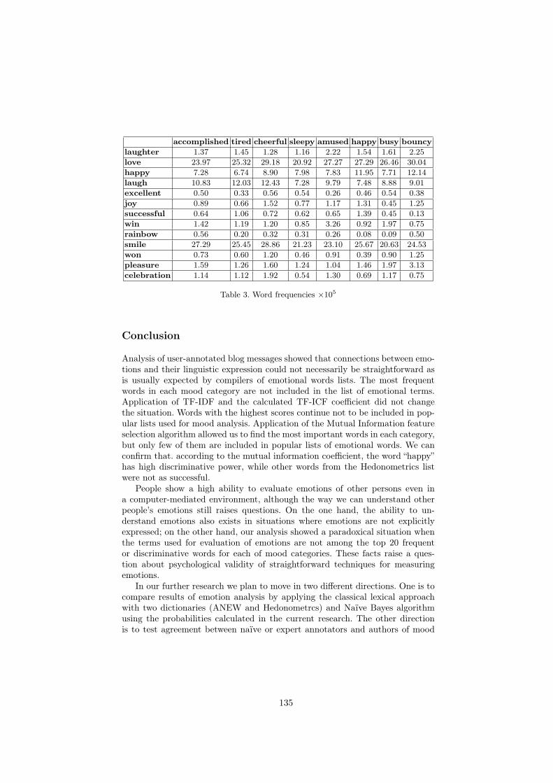
accomplished tired cheerful sleepy amused happy busy bouncylaughter 1.37 1.45 1.28 1.16 2.22 1.54 1.61 2.25love 23.97 25.32 29.18 20.92 27.27 27.29 26.46 30.04happy 7.28 6.74 8.90 7.98 7.83 11.95 7.71 12.14laugh 10.83 12.03 12.43 7.28 9.79 7.48 8.88 9.01excellent 0.50 0.33 0.56 0.54 0.26 0.46 0.54 0.38joy 0.89 0.66 1.52 0.77 1.17 1.31 0.45 1.25successful 0.64 1.06 0.72 0.62 0.65 1.39 0.45 0.13win 1.42 1.19 1.20 0.85 3.26 0.92 1.97 0.75rainbow 0.56 0.20 0.32 0.31 0.26 0.08 0.09 0.50smile 27.29 25.45 28.86 21.23 23.10 25.67 20.63 24.53won 0.73 0.60 1.20 0.46 0.91 0.39 0.90 1.25pleasure 1.59 1.26 1.60 1.24 1.04 1.46 1.97 3.13celebration 1.14 1.12 1.92 0.54 1.30 0.69 1.17 0.75
Table 3. Word frequencies ×105
Conclusion
Analysis of user-annotated blog messages showed that connections between emo-tions and their linguistic expression could not necessarily be straightforward asis usually expected by compilers of emotional words lists. The most frequentwords in each mood category are not included in the list of emotional terms.Application of TF-IDF and the calculated TF-ICF coefficient did not changethe situation. Words with the highest scores continue not to be included in pop-ular lists used for mood analysis. Application of the Mutual Information featureselection algorithm allowed us to find the most important words in each category,but only few of them are included in popular lists of emotional words. We canconfirm that. according to the mutual information coefficient, the word “happy”has high discriminative power, while other words from the Hedonometrics listwere not as successful.
People show a high ability to evaluate emotions of other persons even ina computer-mediated environment, although the way we can understand otherpeople’s emotions still raises questions. On the one hand, the ability to un-derstand emotions also exists in situations where emotions are not explicitlyexpressed; on the other hand, our analysis showed a paradoxical situation whenthe terms used for evaluation of emotions are not among the top 20 frequentor discriminative words for each of mood categories. These facts raise a ques-tion about psychological validity of straightforward techniques for measuringemotions.
In our further research we plan to move in two different directions. One is tocompare results of emotion analysis by applying the classical lexical approachwith two dictionaries (ANEW and Hedonometrcs) and Naïve Bayes algorithmusing the probabilities calculated in the current research. The other directionis to test agreement between naïve or expert annotators and authors of mood
135

labels. We also intend to develop more sophisticated procedures to filter objectivecontent and detect invalid entries, establish a meaningful connection betweencontent and label and further extend our database to improve validity of ourstudy.
References
1. Agichtein, E., Castillo, C., Donato, D., Gionis, A., Mishne, G.: Finding high-qualitycontent in social media. In: Proceedings of the 2008 International Conference onWeb Search and Data Mining, ACM (2008) 183–194
2. Pang, B., Lee, L., Vaithyanathan, S.: Thumbs up?: Sentiment classification us-ing machine learning techniques. In: Proceedings of the ACL-02 Conference onEmpirical Methods in Natural Language Processing - Volume 10. EMNLP ’02,Stroudsburg, PA, USA, Association for Computational Linguistics (2002) 79–86
3. Yu, L.C., Wu, J.L., Chang, P.C., Chu, H.S.: Using a contextual entropy model toexpand emotion words and their intensity for the sentiment classification of stockmarket news. Know.-Based Syst. (March 2013) 89–97
4. Mislove, A., Lehmann, S., Ahn, Y.Y., Onnela, J.P., Rosenquist, J.: Pulse of theNation: U.S. Mood Throughout the Day inferred from Twitter (2010)
5. Bradley, M.M., Lang, P.J.: Affective norms for English words (ANEW): Instructionmanual and affective ratings. Technical report, Technical Report C-1, The Centerfor Research in Psychophysiology, University of Florida (1999)
6. O’Connor, B., Balasubramanyan, R., Routledge, B.R., Smith, N.A.: From tweetsto polls: Linking text sentiment to public opinion time series. In: Proceedings ofthe International AAAI Conference on Weblogs and Social Media. (2010) 122–129
7. Dodds, P.S., Harris, K.D., Kloumann, I.M., Bliss, C.A., Danforth, C.M.: Temporalpatterns of happiness and information in a global social network: Hedonometricsand Twitter. PloS one (2011)
8. Lansdall-Welfare, T., Lampos, V., Cristianini, N.: Effects of the Recession onPublic Mood in the UK. In: Proceedings of the 21st international conferencecompanion on World Wide Web, ACM (2012) 1221–1226
9. Strapparava, C., Valitutti, A., Stock, O.: The affective weight of lexicon. In:Proceedings of the Fifth International Conference on Language Resources andEvaluation. (2006) 423–426
10. Gill, A.J., Gergle, D., French, R.M., Oberlander, J.: Emotion rating from short blogtexts. In: Proceedings of the SIGCHI Conference on Human Factors in ComputingSystems, ACM (2008) 1121–1124
11. Hancock, J.T., Landrigan, C., Silver, C.: Expressing emotion in text-based commu-nication. In: Proceedings of the SIGCHI conference on human factors in computingsystems, ACM (2007) 929–932
12. Manning, C.D., Raghavan, P., Schütze, H.: Introduction to information retrieval.Volume 1. Cambridge university press Cambridge (2008)
13. Miller, G.A.: Wordnet: A lexical database for english. Commun. ACM (November1995) 39–41
136

Study of the Mass Center Motion of the LeftVentricle Area in Echocardiographic Videos
Porshnev S.V.1, Mukhtarov A.A.1, Bobkova A.O.1, Zyuzin V.V.1, andBobkov V.V.2
1 Ural Federal Universitynamed after First President of Russia B.N. Yeltsin,
Ekaterinburg, Russia (620002, Ekaterinburg, Mira Str., 19)[email protected],[email protected],
[email protected],[email protected] Ural State University of Economics and Ural Institute of Business,Ekaterinburg, Russia, (620144, Ekaterinburg, 8 th of March Str. 62)
Abstract. The study of the mass center (CM) motion of the left ventri-cle (LV) area in echocardiographic videos is presented. CM of any phaseof the cardiac cycle is inside an ellipse. An area of the ellipse is not morethan 2% of the area of LV in systole. The criterion to identify correctand incorrect forms of contours are proposed for automatic contouringof LV in the frames of a video sequence.
Keywords: left ventricle, contouring, echocardiographic images (echocar-diography), image processing.
1 Introduction
Echocardiography is one of the most wide spread ways of not invasive heartmuscle deseases diagnosis, which most commonly uses ultrasound (US) imagesof the apical four-chamber heart projection. Sequence analysis of ultrasoundimages allows to analyze the dynamics of the heart muscle. Of particular interestto cardiologists is left ventricle (LV), since most various diseases and pathologiesof the heart can change their state.
To assess the state of the LV, cardiologist puts contour on each frame ofultrasound sequence, which limits the region of the LV. As a rule, the cardiolo-gist makes it manually or by semiautomatic modes. Using the contouring, theycalculate the geometric dimensions of the LV (systolic and diastolic volumes),ejection fraction, wall contractility, etc. The obtained quantitative indicatorsprovide reliable assessment of the heart muscle condition.
Analysis of the experience of cardiac ultrasound shows that in most cases theLV boundary is conducted subjectively and depends on the skill of the physicianwho performs the processing of ultrasound images. In this context, the task ofdeveloping algorithms for automated delineation of the LV on echocardiography
137

images, that eliminate the element of subjectivity and increase the processingspeed of ultrasound images of the heart, is relevant.
In this article the results of the kinematics analysis of mass center on theultrasound images are discussed and the identification approach of inaccurateLV contour built in automatic mode are submitted.
2 Statement of the Problem
Let’s consider the features of contouring procedures LV on the ultrasound image.Typical source frame of an ultrasound image is presented in figure 1. Figure 1shows that the images are low-contrast. There is a variety of artifacts due to thepresence of the papillary muscle in the heart tissue. The figure 1 also presents theexpert LV contour. The expert had the right border of the LV, ignoring existingartifact in the image.
Fig. 1. The ultrasound frame with expert LV contour.
It should be noted that the presence of this artifact is critical for automaticalgorithm. This problem is illustrated in figure 2, the results of the automaticdelineation LV from the image are shown in figure 1.
Consequently, the automatic contouring process should have a pre-treatmentprocedure to remove speckle noise, artifacts and to enhance the contrast of ultra-sound images. These algorithms are considered in [1], [4], [7] [8]. Analysis of theexperience of their application shows that they really can improve the contrast
138

Fig. 2. The LV area is obtained from ultrasound image.
of the ultrasound images and in some cases remove artifacts. However, this canbe done not for every patient.
Also the works [2], [3] should be particularly noted. For LV wall motion of theheart the optical flow algorithm [5] was used and analysis of LV shape changesover time. Work [9] describes the isolation area of the LV on echocardiogra-phy image. However, in these works the criteria to evaluate the correctness ofcontouring are not given.
Comparative analysis of the LV contour built by the expert and the contourbuilt in automatic mode (see. Fig. 2), allows us to conclude that the CM coor-dinates of these contours are significantly different from each other. Thus, wecan assume that the CM coordinate values are an informative parameter. Thisparameter allows to distinguish the contours of regular and irregular shapes(Fig. 3).
Fig. 3. Expert and contouring with the center of mass.
To test this hypothesis, the CM motion of expert contours was investigated.The results are presented in the next section.
139

3 The study of the CM LV motion.
In the course of the research ultrasound records of 16 patients were used, the totalnumber of frames was 320. At each frame LV contours were built by experts.Figure 4 shows the coordinates of the CM expert LV contours of the heart.Figure 4 shows that the position of a CM is inside the minimal ellipse [6].
Fig. 4. CM of expert contours for one patient and ellipse constructed by CM points.
Similar calculations were performed for the remaining patients. Next, foreach patient area of the respective ellipses was calculated. This area is comparedwith the area of LV in systole. Calculated coefficients are presented in table 1.
Table 1. The ratio of the ellipse area covering CM LV to the area of expert contourin systole.
Patient Coefficient Coefficient Patient Coefficient Coefficient
(expert data) (data obtained (expert data) (data obtained
from automatic from automatic
algorithm) algorithm)
B 0.0086 0.0424 K 0.0137 0.5185
C 0.0113 0.1180 L 0.0117 0.0237
D 0.0168 0.0110 N 0.0163 0.0349
E 0.0138 0.0117 O 0.0161 0.0189
F 0.0095 0.0136 R 0.0200 0.0235
G 0.0143 0.0674 T 0.0254 0.0205
H 0.0173 0.0533 V 0.0167 0.0981
I 0.0168 0.0987 X 0.0193 0.2188
140

Table 1 shows that the ellipse area encompassing LV CM does not exceed 2%of the left ventricular in systole. The results of similar calculations for contoursconstructed automatically, some of which have an irregular shape, are presentedin table 1. (The automatic algorithm is considered in [10]).The maximum valueof the ratio of the ellipse area, covered CM LV, to expert contour area in LVsystole is 51%. Thus, the position of the CM allow to automatically identify thecorrect construction of the contour, using the following step:
1. Calculate the CM coordinates of the each video frame.2. Construct a minimum ellipse which includes the CM of all contours.3. Calculate the area of the ellipse.4. Calculate the ratio of the areas of the ellipse to the area of LV in systole.5. If the ratio is greater than 2% then apply the clustering procedure CM [11].6. Identify the contours of the irregular shape which CM are assigned to a
remote cluster.
Figure 5 shows the CM arrangement examples in the case, where the shapeof one contour is incorrect. Figure 5 shows that CM for contours with regularshape are grouped in a certain region, while the contours of irregular shape arelocated at a remote distance from the grouping area.
It should be noted that the errors of second type (the contour is wrong, butCM belongs to the ellipse) were not found.
Fig. 5. Location of CM for patient X, one circuit is built wrong.
141

4 Conclusion
The CM for regular shape countours are grouped within the ellipse area. TheCM for irregular shape countours are located out of this area. Methods of pointsclustering can solve this problem. An approach based on an analysis of the CMLV contours location, allowing to identify the contours of an irregular shape,is given in this work. The approach will be embeded in automatic algorithm ofcontouring the LV area.
References
1. Amerbaev, V., Kalnej, S., Rychagov, M., Frolova, G.: Restoration of medical ultra-sound images based on the effective deconvolution of scan data. Medical equipment(3), 9–12 (2004)
2. Bosnjak, A., Colmenares, L., Montilla, G., Venezuela, V.: Spatial and temporal es-timation of left ventricle wall from ultrasound images using optical flow algorithm.Computing in Cardiology (CinC) pp. 573–576 (2012)
3. Comaniciu, D., Zhou, X.S., Krishnan, S.: Robust real-time myocardial bordertracking for echocardiography: an information fusion approach. Medical Imaging,IEEE Transactions on 23(7), 849–860 (2004)
4. Gonzalez, R., Wood, R.: Digital image processing, vol. 1072 (2005)5. Lai, S.H., Vemuri, B.C.: Reliable and efficient computation of optical flow. Inter-
national Journal of Computer Vision 29(2), 87–105 (1998)6. Loa, C.F.V.: Using the ellipse to fit and enclose data points, http://www.cs.
cornell.edu/cv/otherpdf/ellipse.pdf
7. Porshnev, S., Zyuzin, V., Bobkov, V., Bobkova, A.: Analysis of methods for re-moving noise and artifacts on echocardiographic images. In: The 11th Interna-tional Conference: “PATTERN RECOGNITION and IMAGE ANALYSIS: NEWINFORMATION TECHNOLOGIES”. pp. 525–528. No. 8-1 (2013)
8. Priorov, A., Hrjashhev, V., Sladkov, M.: Improving the quality of ultrasound med-ical images. Medical equipment (4), 11–14 (2008)
9. Varlamov, A., Makarova, E.: An automatic selection method of objects on heart’sultrasound images. Algorithms, methods and data processing systems 17, 49–54(2011)
10. Yatchenko, A.: Numerical methods of analysis and heart’s image processing. Ph.D.thesis, Lomonosov Moscow State University (2013)
11. Zagoruiko, N.: Applied methods of data analysis and knowledge (1999)
142

Accuracy Analysis of Estimation of 2–D FlowProfile in Conduits by Results of Multipath
Flow Measurements
Mikhail Ronkin and Aleksey Kalmykov
Ural Federal University, pr. Mira, 19, Yekaterinburg, 620002,Russian Federation
Abstract. The paper presents a model of distorted velocity distributionof a flow in conduit, which passes through its bent section. The proposedmodel is properly analyzed. An algorithm for recovering the pipe profileby multipath ultrasonic measurements in the presence of a priori infor-mation is proposed. Numerical simulations with the proposed algorithmare performed as well.
Keywords: flow measurements, flow profile, multipath flowmeter
1 Introduction
In practice, it is important to know the set of values of the stream head of a flowin each section of the pipeline. The flow head is one of the main characteristicsof the conduit. When the flow passes through a bent section (such as elbow orvalve, etc.), its head gets lost. In practice, losses of the head are determined byexperiments [1]. The loss of head is connected with the flow profile distortion.There is a symmetric flow profile in a long straight section of pipeline (Fig. 1a,b).However, when flow passes a bent section (such as elbow, valve, etc.), the flowprofile, i.e., the distribution of velocity in the cross section of the pipe, becomesdistorted (Fig. 1 c,d). Thus, the profile of flow characterizes a bent section ofthe pipe [1].
One way to determine the flow profile is to recover it by ultrasonic multi-path flow measurements. The ultrasonic technology allows measurement of thevelocity distribution in a number of planes between two transducers/receivers ofacoustic waves as it is shown in Fig. 2a. The distortion of a flow profile can berecovered by approximation of such measured values in a sufficient number ofplanes [2].
The task of ultrasonic measurement of the flow rate is the radar task ofmeasurement of propagation time in an investigated media. The emitted waveaccelerates when moving in the direction of a flow and slows down in the oppositedirection (Fig. 2b). The velocity of a flow is calculated as a difference of measuredtimes of propagation:
t12 =L
c+ vl cosα, t21 =
L
c− vl cosα, (1)
143

vl =∆tc2
2L cosα, vz =
∆tc2
2Ltanα, (2)
where t12 is the time of propagation in the flow direction; t21 is the time ofpropagation in the opposite direction; c is the speed of acoustic wave; α is theangle between direction of the flow and direction of the wave propagation; L isthe length of the wave path in the investigated media; vl is the projection of theflow velocity on the wave path; vz is the velocity in z–direction of the flow [3].
The velocity profile is always distributed not uniformly through the cross–section area of a pipe. This means that velocity in the central region is usuallyhigher than near the wall. The measured value of velocity vl is the average ofthis distribution in the direction of the path. Measured value usually differs fromaverage velocity through the whole cross section vc:
vl =
∫ L
0
v(l)dl, Q =
∫
s
v(x, y)dS, (3)
k =Q
πR2vl, (4)
where v(l) is the distribution of velocity in the direction of the wave propagation;Q is the flow rate; v(x, y) is the distribution of velocity through the whole cross–section of the conduit; R is the radius of the pipe; S is the cross–section area ofthe pipe; k is the meter factor, which is connected with the measured and actualflow rate [3].
Equation (4) is valid for any symmetric flow. However, in the case of asym-metric propagation of the flow wave patch, the flow rate would be calculatedwith error. The type of function v(x, y) for asymmetric flow does not have gen-eral analytical expression. The function of flow distribution strongly depends onthe conduit configuration, and its characteristics (such as material, roughness,temperature of the controlled media, etc.). The error of the calculated flow ratefor a single path flow meter can achieve a 10% and be even larger [3].
The meter factor can be calibrated in laboratory conditions. Such calibrationis generally performed on a long straight section of a conduit where a symmetryflow profile takes place [3]. In the case of multipath flow meter, all asymmetricfeatures are assumed to be present for calibration of a symmetric flow. In -practice, it is necessary to have more than 4 paths to consider the meter factor as1 with error less than 0.1% [4, 5]. However, the solution of the task of recoveringa flow profile with such accurate flow measurements is an open issue.
For some types of flow profiles, the analytical expression has been obtained bySalami [6]. Based on his works, some authors proposed analysis of configurationof the multipath measurements and suggested some interpretations of analyti-cal profiles [4–8]. The solution of the profile recovering problem by ultrasonicflow measurements was only proposed on the basis of ultrasonic tomographyor by Abel’s integration transform, which doesn’t take into account asymmetryfeatures of flow [2, 9].
144

In this work, a technique is suggested for recovering the flow profiles using themultipath measurements and a priori information about discretionary function,which can be determined for each type of a bent section of the conduit.
Fig. 1. Flow profiles for a) m=2, a=0; b) m=5, a=0; ) m=5, a=0.3; d) m=5, a=0.7
2 Model of flow profile
The model of flow profile, which have been proposed by authors [6, 7] can beconsidered as a particular case of a flow profile that has passed through a conduitsection, whose specified characteristic determines the distortion of the velocitydistribution. The proposed model and generalized approach can be analyzedregarding to the accuracy of the profile recovering.
In general, the flow rate could be calculated as an integral of velocity distri-bution over the cross-section area as
Q =
∫
s(z)
vz(x, y)dS =
∫ x2=R
x1=−R
[∫ y2=√(R2−x2)
y1=−√(R2−x2)
vz(x, y)dy
]dx, (5)
Thus
Q =
∫ R
−Rvz(x)dx =
c2 tan(α)
2
∫ R
−R∆t(x)dx, (6)
where ∆t(x) is the distribution of difference values of measured propagation timein the flow direction and in the opposite one versus the coordinate. In theoryof numerical integration, it is proposed to substitute the integral by sum withspecified weight, which may be chosen, for instance, by criteria of optimal distri-bution of nodes locations and corresponding coefficients (the Gauss quadrature
145

Fig. 2. Schematic draw picture a) multipath flowmeter and b) the center plane cut, ηiis the ith plane
method). The solution is presented in Table 1.
ξ =x
R
∫ R
−R∆(x)dx → R
∫ 1
−1∆(ξ)dξ = R
n∑
i
λi∆t(ξ), (7)
where ξ is the normalized coordinate of the measurement plane, λi is the coef-ficient of weight function (determined by solution of the Gauss quadrature taskfor number of measurements); ∆t(ξi), i = 1, 2 . . . n are differences of propagationtimes in planes with coordinate ξi; n is the number of planes. In the case of a
Table 1. Solution of Gauss quadrature task [10]
n=2 n=3 n=4 n=5
λi ± 0,5773 0 ± 0,7746 ± 0.3400 ± 0.8611 0 ± 0.5385 ± 0.9062
ξi 1 0.8889 0.5556 0, 6521 0,3479 0.5689 0.2369 0.4786
multipath flow meter, the flow rate can be calculated in accordance with (6) as
Q = kc2R tan(α)
2
n∑
i
λi∆t(ξi) = kn∑
i=1
λivz(ξi), (8)
where the meter factor k can be considered as 1 if there are more than 4 measuredplanes [4]. There are many profiles proposed by Salami [6], which have beenverified by experiments. For instance, authors [2] noted that profile of flow thatpasses through a single elbow could be expressed as follows:
vz(r, ϕ)
v0= sin
(π2
(1− r)1/m)
+ α sin(π(1− r)1/2
)exp(−0.2ϕ) sin(ϕ), (9)
146

where vz(r, ϕ) is the velocity distribution in cylindrical coordinates; r is theradius; ϕ is the angle; v0 is the velocity of flow at the center of cross-section(vz(0, 0) = v0); α is the velocity of flow at the center of cross-section; m isthe coefficient of symmetric flow profile, which characterizes the flow profiledepending on velocity if asymmetric coefficient is equal to zero. In the originalwork [6], the author proposed values m = 5, α = 0.3. The first part of theright side of equation (4) corresponds to the symmetric part of the flow, and thesecond part corresponds to asymmetry distortion with coefficient α [6]. Withoutasymmetry distortion, the flow rate is calculated according to the equations(8)-(9) as
Q =
∫
S
sin(π
2(1− r) 1
m
)dS =
∫ 2π
0
∫ R
−Rsin(π
2(1− r) 1
m
)rdrdϕ, (10)
Q = kRn∑
i=1
λivz (ξi) . (11)
For symmetric model of flow (10, 11) calibration m = f(k) = f(Q/v0) couldbe performed. Normalized profiles are shown in Fig. 1 a,b. It can be notedthat profile with m=2 corresponds to the laminar flow mode, and cannot beconsidered in model. Profile with m=5 corresponds to the turbulent mode [2].It is well known that the profile of a flow changes toward symmetry distributionwith distance from a section of the conduit, which caused distortion [3]. So, itmay be supposed that the influence of the second part of equation (9) decreases asasymmetric coefficient tends to zero with increasing distance from the distortedsection of the conduit. Based on the condition of constant flow (Q(z) = const)it should be noted that m is also changing with distance from the section of theconduit that caused the distortion.
It may be proposed that type of the second part of the right side of equation(9) depends on the type of section of the conduit, which caused distortion. Suchexpressions can be defined theoretically or from experiments. In this work, typeof the profile (9), which corresponds to signal elbow [2], is considered. Profiles offlow for m = 5, α = 0.3 and α = 0.7 are shown in Fig. 2c,d. It has been mentionedabove that in each measurement plane, the value of velocity is the integral overthe direction of acoustic wave propagation. The normalized measured velocityin the plane with coordinate xi corresponds to equation (9) can be expressed as
vz(xi)
v0=
=
∫ +A
−A
[sin(π
2(1− (x2i + y2)1/2
)1/m]+
[α sin
(π(
1− (x2 + y2)1/2)1/2)]
×
× exp(−0.2 arctan
(y
xi
)sin
(arctan
(y
xi
))dy, (12)
147

where A =√R2 − x2i . Denote:
F1 (xi,m) =
∫ +A
−A
[sin(π
2(1− (x2i + y2)1/2
)1/m]dy, (13)
F2 (xi) =
[α sin
(π(
1− (x2 + y2)1/2)1/2)]
×
× exp(−0.2 arctan
(y
xi
)sin
(arctan
(y
xi
))dy. (14)
Consequently,vz (xi)
v0=F1 (xi,m) +αF2 (xi) , (15)
where F1(xi,m) is the function, which characterizes symmetric part of flow,F2(xi) is the function, which characterizes an asymmetric part of flow when itpasses through a bent section. Expression of the flow rate corresponding to (15)is
Q =
∫ R
−Rvz(x)dx = v0
∫ R
−R[F1(xi,m) + αF2(xi)] dx ≈ kR
n∑
i=1
λivz(ξi). (16)
In accordance with (15), the flow rate can be expressed as
Q ≈ v0Rn∑
i
λi [F1(ξi,m) + αF2(ξi)] . (17)
In equation (17), the meter factor is not used because since it is included in thecalibration dependence for F1(xi,m). From equation (17) in accordance with(11) and (16), the symmetric flow rate normalized on v0 can be expressed as
Qcv0
= R
[k
n∑
i=1
λivz (ξi)− αv0n∑
i=1
λiF2(ξi2)
]= f−1(m), (18)
where f−1(m) = Qc/v0 denotes the calibration relation in coordinates f(Qc/v0).Such calibration can be implemented because of symmetry of function F1(xi,m)and symmetry of profile Qc. Hence, if we know the flow rate under symmetricconditions and radius of the pipe, we can deduce v0.
There are three unknown parameters in equation (17): v0 is the value ofvelocity at the center of the pipe cross-section; m is the coefficient of symmet-ric part of flow; α is the asymmetric coefficient. Here, it is assumed that typeof function F2(xi) is known as a function of distorted section of the conduit.Relation m = f(F1(x,m)) = f(Q/vc) assumed to be known from preliminarycalibrations on a long straight pipeline. The determination of parameters namedabove requires solution of the system of equations for each parameter. The po-sition of planes (xi) is supposed to be chosen here in accordance with Table 1
148

and from symmetry of F1(xi,m). The solution of the system mentioned abovehas the following expression:
α = [(vz(x3)− vz(x1))F1(x1,m)]/[F2(x2)vz(x1)− vz(x3)F2(x1)],
v0 = [F2(x3)vz(x1)− vz(x3)F2(x1)]/[F1(x1,m) (F2(x1)− F2(x3))],
n∑i=1
λiF1(xi,m) =[k
n∑i=1
λivz(xi)− αv0n∑i=1
λiF2(xi)]/v0 = f−1(m).
(19)
Here, the first and the second equations are calculated depending on F1 andhence on m. However, the multiplier αv0 may be calculated without the thirdequation:
αv0 =vz(x3)− vz(x1)
F2(x1)− F2(x3). (20)
In the third equation, the meter factor can be considered as 1 if more than 4measurement planes are used. Consequently, in the third equation m is deter-mined from the calibration relation. The solution of system (19) allows one tocalculate velocity distribution in accordance with (15) for distorted flow profilein cross-section of the conduit.
3 Results of Modeling
In the Matlab software, simulation of the algorithm described above is carriedout for function of distorted profile (9). The first stage of modeling requires thenumber of measurement planes and their positions. In our study, 4 planes (k ≈ 1in this case) have been chosen according to the Table 1. For the chosen modelof distortion relation, functions m = f(Q/v0) have been calibrated, shown onFig. 3.
x1 = 0.34R, x2 = 0.86R, x3 = −0.34R, x4 = −0.86R,
λ1 = 0.652, λ2 = 0.347, λ3 = 0.652, λ4 = 0.347.
In Figure 4 function F2(x) for the chosen type of distortion section of the conduitis shown. In the model of profile (9), coefficients were selected as m = 5, α =0.3, v0 = 1, along with the measured values of velocities:
vz(x1) = 1.9; vz(x2) = 1; vz(x3) = 1.4; vz(x4) = 0.5.
The calculated value αv0 accordingly to (20) αv0 = 0.3. The calculated value ofthe flow rate (considering that k = 1) is Q = 2.7307.
The relation for m (Fig.3) has been found from the third equation of system(9). For calibration, the value m = 2.83 has been determined. The differenceof the measured and the preliminary chosen m value may be explained by notsufficient accuracy of the assumption that k ≈ 1 or with influence of F1 on F2,which is not taken into account in the proposed model.
149
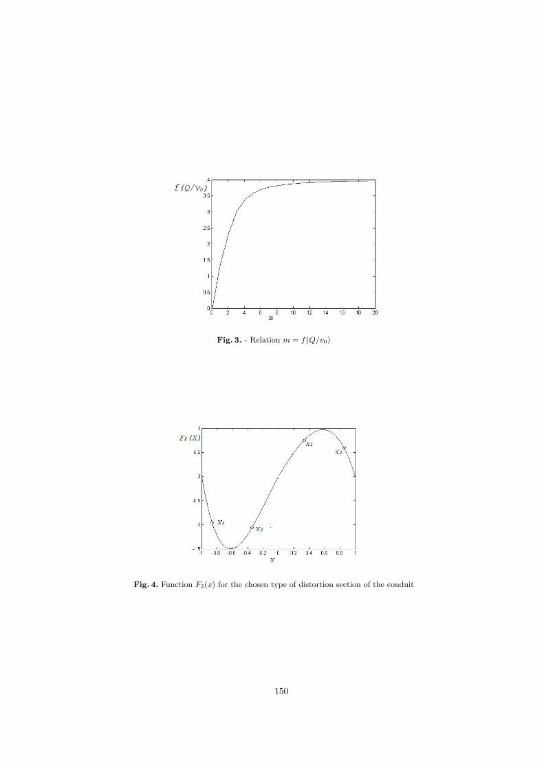
Fig. 3. - Relation m = f(Q/v0)
Fig. 4. Function F2(x) for the chosen type of distortion section of the conduit
150

The calculated values of F1(m,xi), in accordance with (13) and the deter-mined m, are
F1(m,x1) = F1(m,x3) = 1.51; F1(m,x2) = F1(m,x4) = 1.1.
From the estimated value of m F1(m,xi) and by calculation of equations (20)α = 0.26, v0 = 1.16. The error of determination α, v0 obviously connected withaccuracy of estimation m.
The error of recovering the profile of a flow (9) with the calculated values ofparameters and set values estimated as
(1−Qteor
Qcalc
)100% = 6.7%, (21)
whereQteor is the flow rate calculated form the selected valuesm,α, v0, andQcalcis the flow rate calculated from estimated values of parameters. The relation oferror versus the asymmetry coefficient and m = 5, 7, 10 shown in Fig. 5. The
Fig. 5. Relation of error depending on asymmetry coefficient with m = 5, 7, 10 andv0 = 1
accuracy analysis shows that the error dependence has a constant part thatcorresponds to symmetry flow distribution m = f(Q/v0). Such constant value ofthe error can be decreased by correction of calibration relationship m = f(Q/v0).The result with such calibration for each value m is shown in Fig. 6. In the whole,such behavior of the error can be caused by the insufficient accuracy of the modelassumptions. Particularly, it may be supposed that the asymmetry part of F2(x)in (13) is influenced by the symmetry part of F1(x,m).
The general algorithm of flow profile recovering on the basis of multipathultrasonic flow rate measurements and a priori information about distortingfunction of the conduit section has the following stages:
151

Fig. 6. Relation of error with corrected m = f(Q/v0) depending on asymmetry coeffi-cient with m = 5, 7, 10 and v0 = 1.
1. selection of the function F2 (x,m) type;2. carrying out calibration for symmetric flow m = F (Q);3. measurements of flow velocities in planes for each xi and determination the
flow rate by equation (16);4. calculation value αv0 from (20);5. determination of m in agree with (18) and calibration of the relationship;6. evaluation of correction relation m = F (Q) for decreasing symmetric flow
error (α = 0);7. calculation of values F1(m,xi), α and v0 by equations (19);8. calculation of velocity distribution and flow profile.
4 Conclusion
The new model of behavior of velocity distribution in conduit and the algorithmfor flow profile recovering based on it are proposed in the paper. The modelgeneralizes analytical expressions for distorted flow profiles in the conduit, whichwere proposed by Salami. In contrast to [6], here, some coefficients of the modelhas been generalized and their physical interpretation provided.
The algorithm for profile recovering on the basis of multipath ultrasonicmeasurements and a priori information about distorting section of conduit isproposed. The model can be used for any type of profile with theoretical orexperimental description.
The numerical simulation for generalized expression of the function for profileafter single elbow has been carried out [2]. The results of simulation have beenpresented in the paper. The flow profile after single elbow, measured by ultrasonicin 4 planes is considered. The error is estimated as the relation between the flow
152

rate calculated with theoretical set of parameters and parameters that weredetermined by the proposed algorithm. The obtained accuracy gives less than1% error.
The reached that the model can be considered as reliable. In further devel-opments of the model, the influence of symmetry part of flow on asymmetrypart will be investigated. Moreover, investigation of number of measurementsand orientation of planes influence on accuracy should be done.
References
1. Idelchik, I.E.: Handbook of hydraulic resistance. Mashinostroenie, Moscow (1992)(in Russian)
2. Rychagov, M., Tereshenko, S.: Multipath flowrate measurements of symmetric andasymmetric flows. Invers Problems, 16, 495–504 (2000)
3. Kremlevskij, P.P.: Flowmeters and counters of the amount of substance. Handbook.Politeh, Saint-Peterburg (2004)
4. Brown, G.J., Augenstein, D.R., and Cousins T.: An 8-patch ultrasonic mastermeter for oil custody transfer. XVIII IMEKO WORLD CONGRESS, 17–22 (2006)
5. Rychagov, M.N.: Ultrazvukovye izmereniya potokov v mnogoploskostnyh izmeri-tel’nyh mod-uljah. Akusticheskij zhurnal 44 (6), 829–836 (1998) (in Russian)
6. Salami, L.A.: Application of a computer to asymmetric flow measurement in cir-cular pipes. Trans. Inst. MC. 6(4), 197–206 (1984)
7. Moore, P., Brown and J., Stimpsom, B.: Ultrasonic transit–time flowmeters mod-eled with theoretical velocity profiles: methodology. Meas. Sci. Technol., 11, 1802–1811 (2000)
8. Zheng, D., Zhao, D. and Mei, J.: Improved numerical investigation method forflowrate of ultrasonic flowmeter based on Gauss quadrature for non-ideal flowfields. Flow measurement and Instrumentation. 41, 28-25 (2000)
9. Lui, J., Wang, B., Cui, Y. and Wang, H.: Ultrasonic tomographic velocimeter forvisualization of axial flow fields in pipes. Flow measurement and instrumentation,41, 57-66 (2000)
10. Krylov, V.I.: An approximate calculation of integrals. Nauka, Moscow (1967)
153

Semi-automated Integration of Legacy SystemsUsing Linked Data
Ilya Semerhanov and Dmitry Mouromtsev1
ITMO University, Saint-Petersburg 197101, Russia,[email protected]
Abstract. A lot of valuable data is stored in standalone legacy systemsinside enterprise infrastructure across different domains. It was always abig challenge to integrate such systems with each other even on structurallevel, but with the recent development of Semantic Web technologies itsnow clear that integration on semantic level could be achieved and datafrom different sources could be used more effectively. Its now becoming atrend to open data to the public according to Linked Data principals, butthere is no common workflow that could be used with legacy systems.In this paper we propose our solution for semi-automated integration oflegacy systems using Linked data principals. We analyze the motivationand current state of the art in the domain, present our method and al-gorithms for data extraction, transformation, mapping and interlinking.Finally we show our own implementation of the proposed solution anddiscuss the results.
Keywords: Semantic Web, Linked Data, Database integration, Ontol-ogy, Resource Description Framework
1 Introduction
Data integration nowadays is a big and challenging problem, due to the fact thata lot of business and personal data is stored in large amount of different computersystems: Customer Relationship Management systems, Supply Chain Manage-ment systems, Enterprise Resource Planning systems and etc. Also informationis stored in web based applications such as intranet portals, blogs, personal webpages and so on. The amount of such data is growing rapidly every year andbecause of this industry is in need of a solution for accessing and managingdistributed data. Data integration approaches can be separated in two differ-ent groups: consolidation approaches and virtualization approaches. Approachesfrom the first group are meant to physically transfer data from distributed datasources into one unified storage. On other hand approaches from the secondgroup concentrate on providing a virtual way of accessing the data withoutany physical relocation. In this paper we understand integration according tothe approach from the second group, as a unified virtual interface for accessingdistributed heterogeneous data sources. But we can go with classification evenfurther and separate virtual data integration approach into several classes: struc-ture based and semantic based integration. The structural integration is based
154

2
on an idea that full integration can be achieved by providing a mapping betweendifferent structural parts of integrated systems. A lot of approaches and meth-ods were developed in past years with this idea and the most popular that areused now are usually based on such technologies as Web Services, for exampleService Oriented Architecture. For data representation general approach in sucha case is to use a markup language, for example XML, and for data transferring -some transport network protocol, like, for example, HTTP. Thus we can say thatstructure based integration methods are mostly used for representing and trans-ferring data from different systems in a common way and providing a solutionfor mapping one system structure to another system structure. Semantic dataintegration, on other hand, is dealing not only with structural mapping, but alsotrying to define equivalency in semantic meaning of distributed integrated data.This kind of integration, compared to the structural integration, is operatingseveral levels above in DIKW pyramid, using not only simple data structuresfor integration, but also context of its usage and knowledge of how to use it [1].This approach can bring several benefits, like for example it can increase level ofautomatic decision making and provide means for better analytical data search.In other words semantic integration methods can make integration tools moreintelligent and help them deal more effectively with big amount of data.
This paper consists of 6 sections. Section 2 explains our motivation in thiswork and why we started the research. Section 3 focus on the state of the art itthe area and related work. Section 4 covers our proposed solution for the problem,including method, algorithms for data integration and also implementation of itas a tool. Sections 5 and 6 concludes the paper and focus on discussion of resultsand future work.
2 Motivation
It is an indisputable fact that currently most of the applications and com-puter systems in different domains use traditional technologies such as relationaldatabases for data storage and retrieving. From the perspective of Semantic Webthey could be called legacy systems, or in other words outdated computer sys-tems. Applying semantic integration approach to the legacy systems could takea big amount of the effort and manual work, and as a result it could be an obsta-cle for introduction of such approach, regardless the benefits that it could bring.There are already several solutions for mapping relational databases to ResourceDescription Framework (RDF) datasets available, as well as there is also a WorldWide Web Consortium (W3C) R2RML language specification that intends tostandardize the approaches for such mapping [2]. Nevertheless we are convincedthat they all miss the unified methodology for data retrieval from different typesof relational databases and publication on the Web. The level of automationin such tools is still no enough, so they require a lot of manual work throughwhole data integration life cycle. In this paper we present our own view on theproblem and a solution for semi-automated integration of legacy systems. Thissolution will include the methodology and algorithms for data extraction and
155

3
transformation, as well as a prototype of a tool, that is used by us for evaluationof the results.
3 Related Work
Semantic data integration approaches are discussed for a long time by profession-als in data integration domain and we can already say that the most promisingsolutions are based on metadata usage. Some brief survey of the current state ofthe art in the domain was presented by Klaus R. Dittrich and Patrick Ziegler [3].One of the directions of development of metadata approach is closely linked tothe idea to use ontology models for data integration and system interoperability.This idea is not really a new one and was already presented for example in thepaper [4]. Usually there are 3 main approaches for ontology based integration:single ontology approach, multi ontology approach or hybrid approach. The ideabehind single ontology is based on the assumption that its possible to createsingle ontology that could describe all entities and concepts in integrated sys-tems. This is a straightforward solution that could be applied only if all systemsworks in one domain and it was implemented in SIMS [5]. In second approach,instead of one ontology each integrated system provide its own ontology. Com-pared to first solution in this case its easier to integrate new system, becauseontologies could be developed independently for all integrated systems, like forexample in OBSERVER [6]. But without common vocabulary its problematicto interlink concepts in different ontologies. Thats why there is a third solutionthat uses both ideas: for describing systems it uses several single ontologies; forinterlinking them with each other global ontology is used as a vocabulary. Butstill there are a lot unresolved problems in this approach, for example its still notclear how to get single ontology for every system automatically and how to mapthem automatically with each other with the use of global ontology. The solu-tions for relational database mapping to RDF data sets are described in a W3CRDB2RDF Incubator Group survey [7] and in survey [8]. In this surveys severaltools and techniques for data transformation are described and could be sepa-rated in three classes: direct mapping solutions, semi-automated direct mappingsolutions and solutions that use domain semantic for extracting the data fromrelational database. Although some of them are already a mature software theystill lack solutions for stable automated ontology mappings, duplicates discoveryand other features that could make data integration process more friendly.
4 Implementation
4.1 Semantic integration with ontology
According to Tomas Gruber definition, ontology is an explicit specification ofconceptualization [9]. It can describe concepts and relationships that can existin one domain and basically it is a set of concepts, relations and functions that
156

4
connects them with each other:
O =T,R, F
, where : (1)
O – ontology of the domain;T - set of concepts in described domain;R - set of relationships in the domain;F - set of functions that connects concepts and relationships inside one domain.
By using it for data integration concepts and relationships could be describedin every integrated subsystem as well as in the whole subject domain. In orderto do that every object that has some valuable data in the integrated systemsshould be described with the use of semantic metadata, in terms of one generalontology of subject domain in which all systems work. Metadata is informationpresented in special format that describes content of objects, it also could becalled data, that describes data. In formal form we can express it as:
Mi = Ti ∨ Ei, where : (2)
Mi - metadata of object i ;Ti - set of concepts connected to object i ;Ei - set of concept instances in ontology.In other words ontology of subject domain plays a role of coordinate systemfor all integrated applications. There are a lot of benefits of using ontology forsemantic data integration:
– Instead of simple structure mapping we have a relationship mapping thatdescribes how to use data. In other word we are moving from data level toinformation and knowledge level in DIKW pyramid.
– Ontology could be parsed automatically and it could provide ways for auto-matic decision making with the use of description logic.
– Ontology can be easily extended with new concepts and relations, thus wecan integrate new subsystems without additional effort.
– One of the big advantages is that ontology can have several levels. Low levelontology could describe every individual system, middle level ontology coulddescribe the set of integrated systems in one subject domain and high levelontology could describe integrated systems even between different domains.
In order to use such approach for integration, data that is originally stored indistributed legacy systems should be transformed to semantic friendly formatfirst and then ontology for describing this data and systems should be created.There are numbers of methodologies for manual ontology creating, for exampleIDEF5, TOVE, METHONTOLOGY [10, 11]. However, there is no standard ap-proach for semi-automatic ontology generation from legacy systems that shouldbe later integrated, therefore we present in this paper our own solution for that.
157

5
4.2 Linked data approach
One of the good things behind ontology based semantic integration is that itcan be used to integrate not only structured data, but also semi-structured andunstructured. Using Linked Data principals as the basis for integration gives us apossibility to apply the same techniques for integrating any kind of data. LinkedData describes a method of publishing data on the web so that it can be inter-linked and become more useful. It is based on W3C standard technologies, suchas HTTP, RDF, Web Ontology Language (OWL), and according to Tom Heathand Christian Bizer this is one of the best solutions for publishing interlinkeddata on the web [12]. By defining relationships between data, in the way thatit can be parsed by the computers, Linked Data gives a possibility to aggregatethe information from distributed data sources, create new relations, visualizeconnections and also extend it by connecting to other external resources. Inthis approach it is also possible to use ontology and Ontology Web Languagefor describing relations between objects in order to achieve semantic integrationgoal. In other words Linked Data will play a role of unified virtual interface foraccessing data, stored in distributed legacy systems. The big challenge of thisresearch was a legacy systems data extraction, transformation and load problem.In order to overcome it we developed our own method and several algorithms forETL (Extract, Transform, Load) procedure. As the overwhelming majority oflegacy systems, such as Enterprise Resource Planning systems (ERP), CustomerRelationship Management systems (CRM) and custom applications, make use ofrelational databases to store the data we focused on this kind of data storages.
4.3 Method
In legacy computer systems, that use relational databases, data is stored in ta-bles, where rows represent entity instance and columns represent attribute val-ues, describing each instance. To achieve integration with Linked Data principalsdata should be extracted from tables and published on the Web in appropriateformat. Usually in one infrastructure there are several legacy systems, that storedifferent kind if data, but in one subject domain. That allows us to use domainontology for describing common relations in all systems in the domain. Further-more some general relations are independent from the domain and could be usedin any computer system. We intend to combine legacy system data model, do-main ontology and upper ontology in order to automatically extract data fromdistributed relational databases and publish it as integrated Linked Data onthe Web. For this purpose we developed a method, that is based on the IDEF5method for ontology modeling, but instead of manual ontology creation it pro-vide steps for semi-automated ontology generation from data storage structure.This method consists of four main steps:
1. Individual RDF structure. Extracting information about data model struc-ture of every integrated legacy system and transforming it to RDF model;
2. Common RDF structure. Combining extracted RDF models in a commonRDF model;
158

6
3. Common global ontology. Creation of global ontology model on the basis ofupper ontology, subject domain ontology and extracted common RDF modelof legacy systems;
4. Integrated data ontology. Extracting data from distributed data sources andpresenting it as semantic metadata with the use of common global ontologyand automated decision making tools.
According to the method on the first step there is a primary translation oflegacy system data model to the RDF model. In case of relational databasestable names transforms to RDF classes, table fields to RDF properties. Then,on the second step extracted RDF models automatically combined into one com-mon RDF model. On this step we also provide a solution for searching for similarproperties and classes and providing relations between them. On the next stepgenerated RDF model should be enriched by different concepts and relationsfrom subject domain ontology and upper ontology, such as Friend Of A Friendontology (FOAF). This step is not automated and should be done manuallywith the use of ontology editors. On the last step, based on the common globalontology, data is extracted from distributed legacy systems and described withsemantic metadata. This metadata is stored together with common global on-tology in OWL format and could be published on the web as Linked Data.
Provided method make use of semantic relations, described by combined on-tology, between objects in integrated systems across the domain, for automateddata extraction and interlinking with other data. The benefit from this approachis that there is no need for manual interlinking between extracted data, insteadsemantics relations between objects will be used for this purpose. Semantic re-lations, on other hand, will be extracted automatically from initial data modeland then extended manually by the domain experts.
4.4 Algorithms
Within the proposed method we also provide several supporting algorithms thatshould be used for legacy systems integration:
– Algorithm for automated common RDF model extraction from legacy sys-tems data model;
– Algorithm for data extraction from distributed legacy systems with the useof common global ontology and publishing it on the Web as Linked Data.
We also used similarity analysis procedure in our method for comparing entitiesin integrated systems.
Common RDF model extraction algorithm was developed in order to ex-tract data model from each of integrated systems as RDF, and combine it to-gether as unified RDF data model. Given there are two legacy systems LS1 andLS2 in one subject domain, that use relational databases for storing the data.In this case the algorithm goal is to transform LS1 and LS2 database structure
159

7
into common RDF model. In relational databases for description of its structuredatabase schema is used. This schema defines the tables, fields, relationships,views and a lot of other elements, however this is only enough for integrationon structural level. In order to achieve semantic integration domain ontologyshould be used and in this case it will add to the extracted model relations be-tween concepts in the subject domain. The input data for proposed algorithm isdatabase schema of each integrated systems and domain ontology.
Legacy system LS1 is using database schema S1 and system LS2 – databaseschema S2:
S1 =Tb1, . . . , T bn
, S2 =
Tb1, . . . , T bk
, where : (3)
S1, S2 - database schemes,Tbn , Tbk - schema tables.
Tb1 =At1, . . . , Ati
, where : (4)
Ati – table attributes.
The algorithm consists of five steps:
1. Structure mapping. Sequential mapping of S1 and S2 into RDF format.
Tbn → Tm, T bk → Tm, Ati → Ai
where Tm - RDF classes, Ai - RDF properties.2. Automatic relations creation. Providing semantic properties Pj , by auto-
matic similarity analysis of database structure. Analysis is based on severalmeasures: data types similarity, database names similarity, string similarity.
3. Enrichment. Subject domain ontology and upper ontology import with theuse of OWL property owl:import.
4. Manual relations creation. Editing of extracted model with the ontology ed-itor. Manual creation of relations between concepts from upper and domainlevel ontologies and objects in extracted model.
5. Output of created common RDF model into file or in RDF triple store.
The output is a common RDF model that describe objects and their relationsin legacy systems, as well as concepts and their relations inside subject domain.
Data extraction algorithm was designed for data extraction from distributedlegacy systems with the use of previously generated common RDF model, andfor later publishing on the Web. The input data for this algorithm is commonRDF data model and list of tables from which data should be extracted. Supposein input there are i number of tables with data, then:
Tbi =V1, . . . , Vn
, where : (5)
160

8
Tbi - table database i ;Vn - table entry.
The algorithm consists of five steps:
1. Import of common global model. Import of extracted earlier common globalRDF model.
2. Entries extraction. Extraction of every Vn entry from table Tbi in eachintegrated database.
3. Similarity analysis. Similarity analysis of extracted entries with each other.If there is a match, one of the tree semantic properties should be applied:skos:closeMatch, skos:narrowMatch, skos:exactMatch.
4. Reasoning. Creation of new semantic properties by logical reasoning, thatis working because of description logic, which were imported from commonglobal model.
5. Output of created integrated data ontology in OWL format in a file or inRDF store.
The result of the algorithm is global meta model that contains objects and itsrelations in the subject domain and also interlinked data in RDF format.
Similarity analysis was done in both algorithms in the method. In commonRDF model extraction algorithm it is used for automated creation of relationsbetween objects in different integrated systems. In data extraction algorithm itis used for comparing extracted string values.
For automated creation of relations between objects in different systems dur-ing common model extraction, we propose to use complex method of comparisonby several parameters:
– string comparison of elements names and descriptions, for example attributenames in tables of relational database.
– comparison by data type. Different relational databases use different datatypes, however in the research we created common mapping between allrelational databases data types and XML Schema data types.
– corpus-based comparison of elements. By using subject domain ontology asthesaurus, we can find relations between objects during extraction.
For string similarity comparison there are several approaches available, forexample Jaccard similarity coefficient, Tanimoto similarity coefficient, Leven-shtein distance or Sorensen-Dice similarity coefficient [13]. For all approaches wepropose to use it not against a single character in a string or a whole line, butagainst a string, separated in intersecting N-grams. N-gram is a contiguous se-quence of N items from a given sequence of text and it can be of arbitrary length.We propose to select length dynamical, based on the length of the initial stringand use w-shingling for tokenizing it in N-grams. For example for Sorensen-Dicesimilarity coefficient, that originally looks like:
p =2 · |X ∧ Y ||X|+ |Y | , where : (6)
161

9
p – similarity coefficient,X,Y – number of characters in string X and Y.The solution with N-grams and Sorensen-Dice coefficient should look like:
p =2 · |Ngrams(X) ∧Ngrams(Y )||Ngrams(X)|+ |Ngrams(Y )| , where : (7)
p – similarity coefficient,Ngrams(X) – function calculating N-grams sets from string X.
Every parameter, that is used for complex comparison has its own weight.In the end every compared element could be described as a set of parametersimilarity coefficient and its weight:
sim(S,E) =p1w1, . . . , pkwk
, where : (8)
sim(S,E) – final similarity between element S and E in integrated system,pk – similarity coefficient of parameter k,wk – weight of parameter k.In real implementation of the algorithms the final similarity value should becomputed as a leaner function or with some more effective approach, for examplelinear regression [14].
4.5 Semantic data integration tool
For practical implementation and testing of our method and algorithms we devel-oped a prototype of semantic data integration tool. The high-level architectureof the tool, called R2RMapper, is illustrated on figure 1. The tool consists offour main modules: R2RMapperCore, R2RMapperWi, R2RMapperBatch andMatchingDB. R2RMapperCore is the main module that is used for data extrac-tion from distributed legacy systems. It can work like a standalone library orinside R2RMapper tool. Communication with integrated data sources is achievedby web services or by direct JDBC connection. R2RMapperWi module is a webfrontend that gives access for the user to the main features. R2RMapperBatch isa module for scheduling of different tasks, for example nightly synchronizationwith integrated systems. MatchingDB is a Redis based memory caching mech-anism that caches different information, such as similarity analysis results, inmemory during ontology extraction. The extracted OWL ontology is stored asRDF in Jena TDB storage from where it is published by Jena Fuseki server on theweb as a linked data cloud. This linked data cloud works as a virtual interface,with which client systems or users can access data in distributed legacy systemsby SPARQL queries. As the linked data is backed up by the real ontology withthe sets of concepts and relations, all benefits of ontology based integration areprovided.
For testing of the tool we used a CentOS 6.2 server with 16GB RAM andIntel i5 processor 3.10 GHz. We executed it against Oracle 11g database with 50000 entries. The results of the execution are presented on figure 2. Due to use
162

10
Fig. 1. R2RMapper architecture
of Redis as a caching mechanism we managed to decrease time for extraction ofdata from relational databases two times.
As a result of integration, user can work with integrated data through oneendpoint and more effectively. For example there is a possibility to do an an-alytical semantic search query which will also include in search results relatedinformation about the required resource. Thus we can say that by using suchapproach users can work not only with the integrated data, but with integratedsemantic knowledge of how to use this data.
5 Discussion
Today providing of an easy access to the big amount of stored data is becominga trend, no matter whether it is inside one organisation infrastructure or dis-tributed between different organisations and domains. It is equally importantfor big enterprise companies, open communities and research centers to openthe data and make it available for other internal systems, external clients andof course users. In the research we were developing a unified method that couldbe applied to every domain for data extraction, transformation, publication andintegration. The main goal is to automate the process as much as possible byusing hybrid multilevel ontology approach, natural language processing and ma-chine learning for automated decision making during integration. Although themethod and its implementation is an already working solution it still has a roomfor improvement, for example in the area of semi-structured and unstructureddata extraction. We also attempt to make global ontology extraction proceduremore convenient for the users and domain experts.
As one of the first big practical use cases of presented method we intendto develop a platform for publishing of open science data from universities as
163
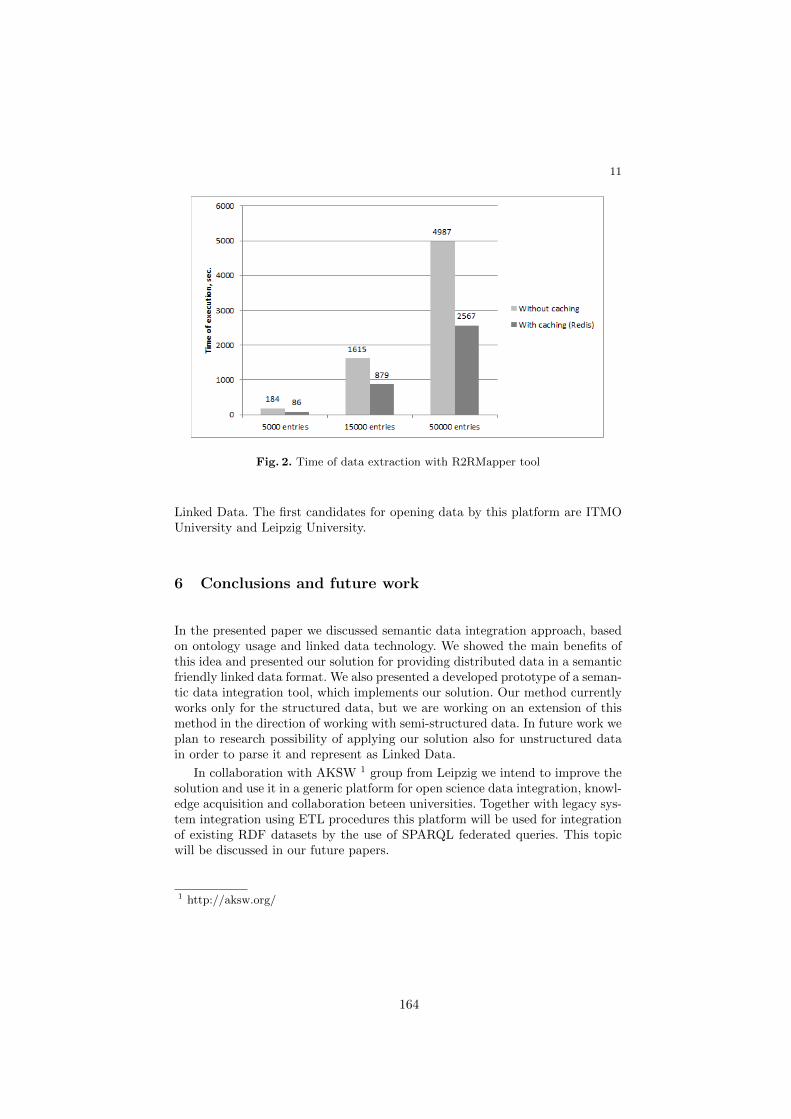
11
Fig. 2. Time of data extraction with R2RMapper tool
Linked Data. The first candidates for opening data by this platform are ITMOUniversity and Leipzig University.
6 Conclusions and future work
In the presented paper we discussed semantic data integration approach, basedon ontology usage and linked data technology. We showed the main benefits ofthis idea and presented our solution for providing distributed data in a semanticfriendly linked data format. We also presented a developed prototype of a seman-tic data integration tool, which implements our solution. Our method currentlyworks only for the structured data, but we are working on an extension of thismethod in the direction of working with semi-structured data. In future work weplan to research possibility of applying our solution also for unstructured datain order to parse it and represent as Linked Data.
In collaboration with AKSW 1 group from Leipzig we intend to improve thesolution and use it in a generic platform for open science data integration, knowl-edge acquisition and collaboration beteen universities. Together with legacy sys-tem integration using ETL procedures this platform will be used for integrationof existing RDF datasets by the use of SPARQL federated queries. This topicwill be discussed in our future papers.
1 http://aksw.org/
164

12
References
1. Rowley J. The wisdom hierarchy: representations of the DIKW hierarchy. Journalof Information Science, 33(2):163–180, 2007.
2. R2RML: RDB to RDF mapping language. http://www.w3.org/TR/r2rml/. Ac-cessed: 2015-03-20.
3. Dittrich K. R. Ziegler P. Three decades of data integration - all problems solved?World Computer Congress - IFIP, pages 3–12, 2004.
4. Visser U. Stuckenschmidt . Wache H., Vogele . Ontology-based integration of infor-mation - a survey of existing approaches. IJCAI-01 proceedings of the SeventeenthInternational Joint Conference on Artificial Intelligence, pages 4–10, aug 2001.
5. Yigal Arens, Chun-Nan Hsu, and Craig A. Knoblock. Readings in agents. chap-ter Query Processing in the SIMS Information Mediator, pages 82–90. MorganKaufmann Publishers Inc., San Francisco, CA, USA, 1998.
6. Eduardo Mena, Arantza Illarramendi, Vipul Kashyap, and AmitP. Sheth. Ob-server: An approach for query processing in global information systems based oninteroperation across pre-existing ontologies. Distributed and Parallel Databases,8(2):223–271, 2000.
7. Sebastian Hellmann Kingsley Idehen Ted Thibodeau Jr Sren Auer Juan SequedaAhmed Ezzat Satya S. Sahoo, Wolfgang Halb. A survey of current approachesfor mapping of relational databases to RDF. Technical report, W3C RDB2RDFIncubator Group, jan 2009.
8. Catherine Faron-Zucke Franck Michel, Johan Montagnat. A survey of RDB toRDF translation approaches and tools. Under review in Semantic Web Journal,2014.
9. Gruber T. A translation approach to portable ontology specifications. KnowledgeAcquisition, 5(2):199–220, 1993.
10. Perakath C. Benjamin, Christopher P. Menzel, Richard J. Mayer, Florence Fillion,Michael T. Futrell, Paula S. deWitte, and Madhavi Lingineni. IDEF5 MethodReport, September 1994.
11. Uschold M. King M. Towards a methodology for building ontologies. In Workshopon Basic Ontological Issues in Knowledge Sharing., 1995.
12. Bizer C Heath T. Linked data: Evolving the web into a global data space (1stedition). Synthesis Lectures on the Semantic Web: Theory and Technology, pages1–136, 2011.
13. Safa’a I. Hajeer. Comparison on the effectiveness of different statistical similaritymeasures. International Journal of Computer Applications, (8), 2012.
14. Anhai Doan, Jayant Madhavan, Pedro Domingos, and Alon Halevy. Learning tomap between ontologies on the semantic web. WWW-02 Proceedings of the 11thinternational conference on World Wide Web, pages 662–673, 2002.
165

Adaptive Regularization Algorithm Paired withImage Segmentation
Tatiana Serezhnikova1,2
1 Krasovsky Institute of Mathematics and Mechanics UB RAS2 Ural Federal University, Ekaterinburg, Russia
Abstract. This paper presents the subsequent improvements of ouradaptive regularization algorithm. The current version of the algorithmcontains an additional stabilizer. This stabilizer includes the coefficient,which utilizes prior information about segmentation of an image to beprocessed. We demonstrate that our adaptive regularization algorithmcan exploit only the observed image segmentation for both the adaptivecoefficient calculation and successful restoration of the original imagesegmentation.
Keywords: image restoration, Tikhonov regularization, adaptation, im-age segmentation
1 Introduction
In the model experiments, see [1-4], we demonstrated, that our adaptive reg-ularization algorithm can successfully restore and provide more deblurred anddenoisy intensity of the original model image. In this paper, we improve ouralgorithm, which is based on the results from [5-7], by an additional stabilizer.This stabilizer includes the coefficient, which utilizes some information aboutsegmentation of an image to be restored.
Most artificial objects are made of surfaces, resulting in images with severalsubimages (or a single subimage) together with their boundary lines.
These facts motivate us to use ideas from image segmentation in order toimprove our algorithm. In the sequel, we describe the stabilizer coefficient con-struction, using ideas from image segmentation.
Image segmentation algorithms are based on properties of intensity values:discontinuity and similarity, see [8-11]. Starting with the observed object inten-sity, setting β(x, y) ≡ 0 in our adaptive algorithm, we successfully apply theoriginal approach for both sub-images and their boundaries. In the next iter-ations, the adaptive algorithm utilizes this initial result for calculation of thecoefficient β.
Thus, we consider image segmentation both as result and tool in every imagerestoration.
We prove numerically that the proposed algorithm can reveal the latent imagesegmentation of observed images.
166
The paper is organized as follows. In Section 2, we describe regularizingfunctionals and present our adaptive technique. In Section 3, we describe thecalculation process of our stabilizer coefficient. The last section concludes thepaper.
2 Mathematical Model for Image Deblurring
We consider the following two-dimensional Fredholm integral equation of thefirst kind:
Au ≡1∫
0
1∫
0
K(x− ξ, y − η)u(x, y)dx, dy = f(ξ, η). (1)
In image restoration, the estimation of u from the observation of f is referredto as the two-dimensional image deblurring problem.
We construct and develop the novel technique for numeric solution of equa-tion (1). Abstract methods with convergence analysis of regularization for thisproblem are presented in [3-7].
The foundation of the regularization method is given by
min||Ahu− fδ||2L2
+ α (||u||2L2+ J(u)) : u ∈ U
, J(u) =
∫
D
|∇u| dx, (2)
where ∇u denotes the gradient of smooth function u, (u ∈W 11 (D)), J(u) is
the total variation of the function u on D. The practical implementation of thismethod requires minimization of the functional in (2).
The novelty was that we proposed to add the version of the iterative tech-nique, containing additional parameters βi,j , βi,j ≥ 0 , see [1-4]:
uk = arg min ΦαN (u) +∑
i,j
βi,j (ui,j − uk−1i,j )2 : u ∈ RN . (3)
Here, N = n2, ΦαN (u) is the discrete form of the functional in (2).
∑i,j
βi,j (ui,j − uk−1i,j )2 is a discrete form for the additional stabilizer in (3).
We use the iterative subgradient method in order to compute uk defined in(3), see details in [1-4].
167

3 Stabilizer coefficient selection
3.1 Image Segmentation: Motivation
The previous version of the algorithm (3) used the constant β in every meshpoint of discrete models. The low resulting accuracy of this two-dimensionalmodel led us to change the way of βi,j selection.
As we said above, most man-made objects are made of surfaces, resultingin images with a single image or some sub-images. The quality of the imagesrestoration features the quality of sub-images restoration together with sub-image boundary lines restoration.
In [1], we proposed the more general form of the stabilizer Iβ :
Iβ =
∫
Q
β(x, y)[u(x, y)− uk(x, y)]2 dxdy, (4)
we used β(x, y) = umax, for (x, y) ∈ Q,β(x, y) = 0, for (x, y) ∈ Π/Q, where
(5)
umax = maxutrue(x, y) , (x, y) ∈ Π = [0, 1]× [0, 1], (6)
(x, y) ∈ Q⇔ utrue(x, y) = umax. (7)
So, in [1] our regularization algorithm stabilizer includes the coefficient β,which uses some information about true image segmentation, see (6) and (7).This facts motivates us to exclude true image parameters. We approach thispurpose using image segmentation ideas.
3.2 Image Segmentation as Tool
In this paper we propose to begin calculations with the parameter β ≡ 0.So, in this case, we use standard regularization method:
min||Ahu− fδ||2L2
+ α (||u||2L2+ J(u)) : u ∈ U
, J(u) =
∫
D
|∇u| dx, (8)
where ∇u denotes the gradient of smooth function u, J(u) is the totalvariation of the function u on D.
After obtaining the solution of problem (8), we get approximate u0(x, y) , Q0 , ΓQ0 ,and we use them for the βi,j construction:
βi,j ∈ o; c, c = maxu0(x, y), (x, y) ∈ Q0 ∪ ΓQ0. (9)
168

3.3 Image Segmentation as Result
Now, using β calculated in (9), the algorithm computes the final image restora-tion including its final image segmentation.
Numerical experiments have confirmed our ideas. Thus, we see in Figure 1:
(a) the observed image; (b) the restoration image;
(c) the central image segment restoration, Q0∪ΓQ0 , calculated with β ≡ 0;
(b) the central image segment restoration, Q∪ΓQ, calculated with adapted β.
a) The observed image b) The recovered image
c) The model segment restorationfor β(x, y) ≡ 0
d) The model segment restorationfor the adapted stabilizer coeffi-cient β(x, y)
Fig. 1. Model experiments
It is clear, that we can write the final image segmentation of the recoveredimage in the form:
Π = Π/Q ∪ Q, (10)
were Q ∪ ΓQ we see in Figure 1.(d), Π = [0, 1]× [0, 1].
169

3.4 Conclusion
In this paper, we have described and verified the image segmentation approachfor the construction of stabilizer coefficient β.
Starting with the observed object intensity and setting the stabilizer coef-ficient β ≡ 0 in the regularization algorithm, we successfully apply the initialapproach for both the sub-image and the sub-image boundary, Q0, ΓQ0 .
After that, we use calculated results for construction of the adaptive stabilizercoefficient β. At this step the image segmentation is a tool.
Using the calculated coefficient β, the algorithm computes the final recoveredimage. We obtain a good localization of segments, Q, ΓQ, and we see a moredeblurred final image segmentation.
As a result, in this paper, we have described and verified that our adaptivealgorithm does not need a priori information. For successful image restorationand restoration of image segmentation, our adaptive algorithm can utilize theimage of an observed object only.
We plan the following modifications and experiments:
– inclusion of the solution estimate for equation u(x, y, ΓQ(x, y)) = c to theestimate list;
– validation of βk inclusion in (4), where k is the iteration number;– processing of thin lines and narrow segments.
Acknowledgments The author expresses special gratitude to Prof. V.V.Vasinfrom the Institute Mathematics and Mechanics of Ural Branch of RAS. Theauthor would like to thank the colleagues from AIST Program and OrganizingCommittees for their helpful advice and guidance in the paper preparations.This work was supported by the Program of UB RAS “Mathematical models,algorithms, high-performance computational and information technologies andapplications”, project 15-7-1-13.
References
[1] T.I. Serezhnikova. An algorithm based on the special method of the reg-ularizationand the adaptation for improving the quality of image restora-tions.Univer.J.Comp.Math.,V.2(1) 11–16 (2014)
[2] T.I. Serezhnikova. Image restoration algorithm based on regularization andadaptation.In.: AIST 2014, CCIS 436, Springer, 213–221 (2014)
[3] V.V. Vasin and T.I. Serezhnikova. A regularizing algorithm for approximation ofa nonsmooth solution of Fredholm integral equations of the first kind. J. VICH.TECH., V. 15(2), 15–23 ( 2010)
[4] V.V. Vasin and T.I. Serezhnikova. Two steps method for approximation of a nons-mooth solutions and nosy image reconstructions. J. Avt. Tel., No.2, 126–135 (2004)
170

[5] V.V. Vasin. Proximal algorithm with projection in problems of the convexprogramming.Ural Sci. Center AN SSSR, Instit. Mathem. I Mekhan., Sverdlovsk,pp. 47 (1982)
[6] A.N. Tikhonov and V. Arsenin. Solutions of Ill-Posed Problems. Wiley, New York(1977)
[7] C.R. Vogel. Computational methods for inverse problems. SIAM, Philadelphia(2002)
[8] R.C. Gonzalez, R.E. Woods. Digital image processing,3-ed ed. Prentice Hall,NewJersey(2008)
[9] X.Chen, M.K. Ng, C. Zhang. Non-Lipshitz lp− regularization and box constrainedmodel for image reconstruction. IEEE Tr. Im. Proc. V.21(12), 4709–4721 (2012)
[10] P. Arbelaer, M. Maire, Ch. Eowlkes, J. Malik. Contour detection and hierarchicalimage segmentation. IEEE Trans. Pattern Analysis and Machine Intelligence.33(5), 898-916 (2011)
[11] J.Canny A computational approach to edge detection. IEEE Trans. Pattern Anal-ysis and Machine Intelligence. V.8(6), 679-698 (1986)
171

Algorithm of Interferometric CoherenceEstimation for Synthetic Aperture Radar Image
Pair
Andrey Sosnovsky and Victor Kobernichenko
Ural Federal University, pr. Mira, 19, Yekaterinburg, 620002,Russian Federation
Abstract. Interferometric coherence is an important indicator of relia-bility for interferograms obtained by interferometric synthetic apertureradar (Interferometric SAR, InSAR). Areas with low coherence values areunsuitable for interferometric data processing. Also, it may be used asa classification parameter for various coverage types. Coherence magni-tude can be calculated as an absolute value of the correlation coefficientbetween two complex SAR images with averaging in a local window.The problem in coherence estimation is in its dependence on phase slopecaused by relief topography (topographic phase). A method for suppres-sion of the topographic phase influence is proposed, based on the spatialphase derivation.Keywords: Synthetic aperture radar images, InSAR systems, Coherenceestimation
1 Introduction
Interferometric data processing for extraction of information about the Earthterrain and its changes becomes one of the general guidelines in the develop-ment of contemporary space-based radar systems together with the implemen-tation modes of ultra-high spatial resolution (1-3 meters) and full–polarimetricprocessing. The method of space-based radar interferometry implies a joint pro-cessing of the phase fields obtained by simultaneous scattering of the terrainwith two antennas or by non-simultaneous scattering with one antenna movedby two different parallel orbits [1, 4]. This method combines high accuracy of thephase measurements with high resolution of the synthetic aperture radars (SAR)technology. Technology of the differential SAR interferometry (InSAR) makespossible to get maps of the elevation changes between the radar passages. Thestages of the interferometric processing are implemented in specialized softwaresystems for the remote sensing data processing such as the SARscape, IMAGINERadar Mapping, Photomod Radar, RadarTools. So we can talk about Informa-tion technology (IT) of the digital elevation models (DEM) generation by remotesensing data.
However, for practical application of these technologies, one has to overcomea number of significant problems. Two general problems of interferometry are
172

the temporal and spatial decorrelation of the received data and the problem ofphase unwrapping, i.e. a recovery of the absolute phase information from therelative phase, which is wrapped into [−π, π]-interval. Another important field ofinvestigation in radar interferometry is selection of the most efficient processingalgorithms and obtaining the experimental estimates of the generated DEMaccuracy. This work is devoted to the first of the mentioned problems, i.e. to thedata decorrelation (summary temporal and spatial) and its estimation.
2 Interferometric coherence
Interferometric coherence is an important indicator of suitability of the datascene obtained by a radar remote sensing system for the further processing andsolving the final problem, i.e. generation of digital elevation model or terrainchanges map. The coherence factor is calculated as the absolute value of thecorrelation coefficient between samples of two complex radar images (single-lookdata complex, SLC) got in the local windows
γ0 = | ˆρ0| =Σz1(m,n) · z2(m,n)√Σ|z1(m,n)|2 · |z2(m,n)|2
, (1)
where z1(2)(m,n) is the SLC samples (z1(2)(m,n) are complex-conjugate sam-ples) [2–5], γ0 takes values in interval [0, 1], near-zero values correspond to areasof high or full decorrelation, which are not suitable for interferometric data pro-cessing. The values higher than 0.5 mean good data correlation.
However, this approach entails some problems because, in fact, a randomvariable is estimated here, but not a random process. So, any phase gradientscaused by both natural topography variability and by point-of-view geometry(remote sensing radar systems have a side-scattering configuration) lead to thedegradation of the estimate (1). Its value depends on the slope and tends towardsthe value |ρ12(N)|ρ=0, i.e. a bias of the estimate for independent Gaussian valuesof the correlation coefficient (N is the number of samples) [3], which in practicetakes the value about 0.1–0.3. Thus, coherence loses its properties as measureof the quality of the interferogram, its value becomes dependent on relationbetween topographic and fluctuation components of the phase.
3 Differential phase coherence estimate
To eliminate the effect described above, the following modification of the coher-ence estimate can be offered taking into account influence of the topographiccomponent. Modified coherence evaluates not the samples z1(m,n) and z2(m,n)of the SLC–image pair, but the following values:
w1(m,n) = z1(m,n) · z1(m+ 1, n), w2(m,n) = z2(m,n) · z2(m+ 1, n), (2)
where the new phase values of the w1(m,n) and w1(m,n) will characterize theslope of the topographic phase in the direction of growth of the mth picture co-ordinate. So, this operation performs the phase derivation along one coordinate.
173

Similarly, one can use the gradients along the nth coordinate. Expression for thecoherence estimation using values (2) looks as follows:
γ1 =
√Σw1(m,n) · w2(m,n)√Σ|w1(m,n)|2 · |w2(m,n)|2
. (3)
Although this estimate is non-Gaussian, it is wealthy, and it can be shown thatit is insensitive to the linear phase trend.
4 Experimental results
Test now the work of the coherence estimation algorithms for RADARSAT–1data (wavelength 56 mm). Figure 1 presents a fragment of the radar image of anarea with surfaces of different reflectance including surfaces with volume scatter-ing and the water surface, which has generally low coherence. Signal differentialphase for the given fragment has a slope in the horizontal direction of the orderof 0.3 radians per sample (due scattering geometry). The coherence maps of thefragment were constructed using conventional estimate γ0 and modified estimateγ1 with the sampling size 11× 11 are presented in Figs. 2a, 2b.
Fig. 1. A RADARSAT-1 radar image scene
One can see that the first map is degraded since different surfaces give thesame low coherence values regardless on the surface type. The map obtained
174

a) Traditional estimate γ0 b) Modified estimate γ1
Fig. 2. Coherence map calculated
using modified estimate (Fig. 2b) has a good sensitivity to the surface type.However, the estimate has a larger bias at low values than the γ0, and, so, itrequires increasing the sample value towards to γ0 (Fig. 3a, 3b). A quantitativeaccuracy assessment for the scene is not available because of poor reference DEMfor this territory.
a) Traditional estimate γ0 b) Modified estimate γ1
Fig. 3. Coherence estimates biases for different sample sizes (N=2, 5, 10, 25)
5 Conclusion
A modified method for estimation of spatial coherence of the interferometricradar images pairs is developed. The method consists in calculation of the cor-
175

relation between pairs of complex multiplications of neighbour elements. Theresearch is implemented on radar images RADARSAT–1. The result shows thatthe modification allows one to solve the problem of estimate degradation underthe differential phase trend, which always takes place in side-scattering radarsystems.
Acknowledgment The work was supported by the RFBR grants Nos. 13-07-12168, 13-07-00785.
References
1. Elizavetin,I. V., Ksenofontov, E. A.: Resultaty experimentalnogo issledovaniya voz-mozhnosti pretsizionnogo izmereniya reliefa Zemli interferentsionnym metodom podannym kosmicheskogo RSA [The results of experimental research of precious Earthrelief measurement by interferometric method with space-based SAR]. IssledovaniyaZemli iz kosmosa, 1, 75–90 (1996) (in Russian)
2. Touzi, R., Lopes, A., Bruniquel,J., Vachon, P.W.: Coherence Estimation for SARImagery. IEEE Trans. Geosci. Remote Sensing, 37, 135–149 (1999)
3. Lopez-Martinez, C., Pottier, E.: Coherence Estimation in Synthetic Aperture RadarData based on Speckle Noise Modeling. Applied Optics, 46(4), 544–558 (2007)
4. Kobernichenko, V. G., Sosnovsky, A. V.: Particular Qualities of Digital ElevationMaps Generation in Interferometric SAR Technology. SPIIRAS Proceedings, 5(28),194–208 (2013)
5. Kobernichenko, V. G., Sosnovsky,A. V.: Coherence Estimation in InterferometricSAR Data Processing. 2014 24th Int. Crimean Conference Microwave and Telecom-munication Technology (CriMiCo–2014). 7–13 September, Sevastopol, Crimea, Rus-sia, 24, 1153-1154 (2014)
176

Irregularity as a Quantitative Assessment of Font
Drawing and Its Effect on the Reading Speed
Dmitry Tarasov1, Alexander Sergeev1,2
1Ural Federal University, Ekaterinburg, RUSSIA 2Institute of Industrial Ecology, UB of RAS, Ekaterinburg, RUSSIA
Abstract. It is proposed to use irregularity, the scale invariant index based on
the ideas of fractal geometry to assess the spatial features of font drawings. The
index is sensitive to the shape of characters in the font, which affects text legi-
bility. Preliminary results have shown promising application of the proposed
index for classifying fonts by reading speeds.
Keywords. Font; Fractal; Scale invariance; Legibility; Typeface
1 Introduction
Research in the fields of legibility and readability are maintained for over a hundred
years. They are particularly important for the development of textual materials in-
tended for readers with emerging reading skills. A significant place in these studies
takes fonts. Many researchers have investigated the clarity, legibility, readability of
different fonts, the influence of serifs, the influence of the pattern and spatial charac-
teristics of the font on the understanding and memorising the content of the text and
some other factors. The obtained results are contradictory. So far there is no consen-
sus on what fonts features and how affect the reading process. This is largely due to
the lack of an objective index, which could describe the typeface, and allows compar-
ing different fonts.
Artemov [1] proposed to divide the concepts of visibility and readability of the font.
Readability is influenced by reader’s physiological characteristics. Visibility depends
on the quality of font drawing and vision features of the person. Differences in type-
face readability investigated in [2-4]. Some fonts are marked as the most readable.
The superiority of some small book fonts connected to their shapes and drawings is
demonstrated. Thick font reads faster. At the same time, respondents preferred the
other fonts. Similar results were obtained in [5]. Studies have shown the presence of
subjective preferences of readers, as well as an objective difference in readability of
fonts with different shapes. The review [6] analysed the various features of fonts with
respect to their readability, but also contains a large number of different, often con-
flicting, views on the impact of serifs, size and font style for readability. Results of
study [7] compares the readability of some common fonts by testing the reading speed
177

of texts in Russian. A higher reading speed for serif fonts is demonstrated. However,
no explicit font characteristics affecting readability are identified. The work [8] pro-
vides an overview of the situation of modern typography of textbooks and considers
contradictions of the current state with the font design to the rules of the current tech-
nical regulations. Lots of researchers consider serif fonts more legible and it is be-
cause of their serifs which add more information to the eyes [9] and enhance the legi-
bility of a text by helping the readers to distinguish the letters and words more easily
[10]. Results in [11], [12] indicated serif fonts are believed to be read faster due to
their invisible horizontal line made by serifs. Results of study [13] is against the
prominence of serif fonts. The space between letters in serif fonts is slightly reduced
due to the ornaments that they have. Consequently, as mentioned in [14], serifs act as
visual noise when the readers’ eyes attempt to detect the letters and words. The reduc-
tion of the space leads to other problems: One is a problem of crowding which is hin-
dering of letter recognition when a letter is flanked by other letters (cited in [15]) and
the other is that letter position coding may be hindered which decreases the ability of
word recognition [13]. The results of studies [15], [16] showed out equal legibility
and perception between serif typefaces and sans serif ones.
Thus, almost equal numbers of studies showed advantages and disadvantages of ser-
ifs, as well as a preference of other features of text. The preferences of specific font
features and font size are highly dispersed, too. It can be suggested that legibility is
more sensitive to some combinations of spatial features of text. No special type font is
suggested to use. The point to pay attention to is the familiarity of the subjects with
special typefaces and subjects’ preferences. The aim of this work is to find the way to
assess the spatial features of font drawings by using an objective scale invariant in-
dex.
2 Approach
An assessment of the visual characteristics of fonts represents certain difficulties as-
sociated with the difference in approaches to the understanding of what is a set of
visual characteristics and what criteria should be used in their assessment. The simi-
larity of some graphic elements of letters in font and the letters themselves, as well as
the font as a whole, suggests the possibility of using the ideas of fractal geometry to
make the assessment. A special case of the fractal dimension d is expressed by well-
known formula that combines the number of objects n, with which the measurement
is taken, and the geometric size of the object a:
d = log n : log a-1. (1)
Mandelbrot showed [17] that for fractal sets the expression relating the length of the
perimeter of the object P and its area S is performed:
P1/d : S1/2 = const, (2)
which implies that S ~ P2/d.
178

The fractal dimension can be understood as the degree of filling of the space by irreg-
ularly distributed substance. Thus, in either family of flat figures (like font), geomet-
rically similar but having different linear dimensions, the ratio of the length of the
shapes border to the square root of its area is a number that is completely determined
by the general form for the family. The equivalence of different linear extensions in
many cases is very useful [17]. The relation between abris’ length (perimeter P) of the
character or set of characters in the font and its area (S) can be used as a unique font
index. Considering the font as a coherent geometric set, by analogy with the way
proposed in [18], it is possible to apply the definition of compactness of the set C (3),
circularity coefficient Cc (4) and irregularity Cn (5) which is proposed to use as such
unique font index.
C = P2 : S. (3)
Cc = 4πS : P2, (4)
Cn = Cc-1 = C : 4π = P2 : 4πS (5)
Vector graphics software having an intrinsic macro language based on VBA can helps
to solve the task of index calculation. In the present work a public macro CurveInfo
for CorelDraw package is used. The macro calculates perimeter (in mm) and area (in
mm2) of a coherent vector object.
Fig. 1. Set of font letters and its division
As a representation of a font the full set of 66 uppercase and lowercase letters (for
Russian language) of each font is used (see Fig. 1). To obtain information about the
perimeter of a particular letter the perimeter of the external abris of a letter (Pout) must
be added to (if available) of the internal perimeter of the letter space (Pin). The perim-
eter of the full set of 66 letters (P) equals the sum of the perimeters of all letters (6).
To obtain an area of a letter it must subtract the internal area of the letter space (Sin)
from the general area bounded by the outer abris of the letter (Sout). The area of the
full set of 66 letters (S) is equal to the sum of the areas of all the letters (7).
P = Σ (Pout + Pin) (6)
S = Σ (Sout – Sin) (7)
3 Results and discussion
For the measurement 21 fonts (straight light drawing, sizes 12 and 18 pt) were select-
ed: 9 sans serif fonts, 11 serif fonts and a script font. For the selected set of fonts the
described procedures and formulas were applied. By the distribution of the values of
irregularity Cn for groups of serif and sans-serif fonts the mapping is undertaken.
179

Also, 5 fonts among the full set are used to test their reading speeds. Participants of
the experiment are 10 students. They read text samples with different font layout and
count the reading speed. The correlation between reading speeds and irregularities is
assessed. The results of calculations by formula (5) and reading speed measures for 5
fonts are given in Table 1. As it can be seen from Table 1, a irregularity has almost
constant values for each font. It indicates the objective nature of the scale invariant
index proposed that is useful for research. A small variation of the index for some
fonts can be explained by features of font scaling. Figure 2 shows the distribution of
irregularity for groups of serif and sans-serif fonts by peer review. Serif fonts are read
slightly faster than sans serif ones, on average. Script fonts have a low reading speed
but extremely high irregularity. Figure 3 shows the distribution of reading speeds and
its dependence from irregularity for 5 selected fonts, regression and confidence inter-
vals. Statistical analysis reveals strong negative correlation between reading speed
and irregularity (correlation coefficient –0,69, p<0,05).
Table 1. Irregularities and reading speeds.
No Font Feature Reading
speed, chars
per sec
Cn, 12 pt Cn, 18 pt
1 sans-serif 305 305
2 sans-serif 418 418
3 sans-serif 439 416
4 sans-serif 459 464
5 sans-serif 470 470
6 sans-serif 43,2 481 469
7 sans-serif 575 575
8 sans-serif 35,5 605 605
9 sans-serif 825 825
10 serif 472 472
11 serif 585 585
12 serif 653 653
13 serif 33,6 675 655
14 serif 682 682
15
serif 703 704
16 serif 714 714
17 serif 778 792
18 serif 31,4 796 796
19 serif 875 875
20 serif 880 802
21 script 28,5 1717 1651
180

Fig. 2. Distribution of irregularity for groups (numbers) of serif (above) and sans-serif (below)
fonts by peer review
Fig. 3. Distribution of reading speeds and its dependence from irregularity for 5 fonts, regres-
sion and confidence intervals (drops).
4 Conclusion
Although there are massive bodies of analysis considering typography and font fea-
tures, there is no agreement among researchers regarding legibility factors in print.
One of the most complicated issue is accounting for the effect of font drawing on
legibility. The work offers a solution to this problem. The scale invariant index to
assess the spatial features of font drawing is proposed. Accounting for the index in
research of reading (e.g. [19]) might help to identify predictors of reading speed, as
well as quality of assimilation not only for paper, but also for electronic texts. In any
case, the scale invariance of the proposed index allows to accumulate experimental
results without any subsequent processing or conversion, which is convenient.
181

5 References
1. Artemov V.A. Technographic analisys of summarized letters of new alphabet. Writing and
revolution. 1933, 1, 58–76.
2. Ushakova M.N. The new typeface for newspapers. Polygraphic manufacturing. 1952, 4, 22–
23.
3. Ushakova M.N. The new typeface for narrative literature. Polygraphic manufacturing. 1952,
11, 26–28.
4. Ushakova M.N. The new typeface for large circulation narrative literature. Polygraphic man-
ufacturing. 1959, 11, 26–27.
5. Alexandrova N.A., Chiminova V.G. New typefaces for newspapers. Polygraphic manufac-
turing. 1962, 5, 57–61.
6. Tokar O.V., Zilbergleit M.A., Petrova L.I. Legibility of typefaces. Proceedings of the higher
educational institutions. Problems of printing and publishing. 2004, 2. 79–92..
7. Tokar O.V., Zilbergleit M.A., Litunov S.N. Font legibility assessment on the sample of offi-
cial document. Omsk scientific herald. 2009, 2(80). 246–249.
8. Tarbeev A.V. Font design of modern textbook. Proceedings of the higher educational institu-
tions. Problems of printing and publishing. 2004, 4. 93–102.
9. Geske J. (1996). Legibility of Sans Serif Type for Use as Body Copy in Computer Mediated
Communication. Presented at Annual Meeting of the Association for Education in Journal-
ism and Mass Communication 1996
10. McCarthy M.S. & Mothersbaugh D.L. (2002). Effects of typographic factors in advertising-
based persuasion: A general model and initial empirical tests. Psychology &Marketing,
19(7-8), 663–691.
11. Romney C. (2006). Improving the visual appeal of classroom handouts. JALT2005 Confer-
ence Proceeding. Tokyo: JALT. Retrieved May 21, 2012, from http://jalt-
publications.org/archive/proceedings/2005/E121.pdf
12. Arditi A. & Cho J. (2005). Serifs and font legibility. Vision Research, 45, 2926–2933.
13. Perea M. & Moret-Tatay C., Gómez P. (2011). The effects of inter letter spacing in visual
word recognition. Acta Pschologica, 137, 345–351.
14. Woods R. J., Davis K., Scharff L.V.F. (2005). Effects of typeface and font size on legibility
for children. American Journal of Psychological Research, 1(1), 86–102.
15. O’Brien B.A., Mansfield J.S., Legge G.E. (2005). The effect of print size on reading speed
in dyslexia. J Res Read, 28(3), 332–349.
16. Paterson D. G. & Tinker M. A. (1932). Studies of typographical factors influencing speed
of reading. X. Style of type face. Journal of Applied Psychology, 16(6), 605–613.
17. Mandelbrot B. Fractal geometry of nature. Moscow, Institute of computer studies, 2002,
p.656.
18. Alexanina M.G., Karnatsky A.Y. Comparison of the spatial characteristics of the fields of
sea ice and cloud according to the visible channel AVHRR / NOAA on the example of the
Okhotsk Sea / The Sixth All-Russian Open Annual Conference "Modern Problems of Re-
mote Sensing of the Earth from Space". Moscow, IKI RAS 10-14 nov 2008, 299–302.
19. Tarasov D.A. & Sergeev A.P. The leading as a factor of readability: development of the
methodology for educational use. Procedia – Social and Behavioral Sciences, Elsevier,
v.106, 2013. 2914–2920.
182

Fast Full-Search Motion Estimation Method Based On
Fast Fourier Transform Algorithm
Elena I. Zakharenko, Evgeniy A. Altman
Omsk State Transport University
zaxarenko.elena, [email protected]
Abstract. Motion estimation (ME) is used extensively in video codecs based on
MPEG-4 standards to remove interframe redundancy. Motion estimation is
based on the block matching method which evaluates block mismatch by the
sum of squared differences (SSD) measure. Winograd’s Fourier transform is
applied and the redundancy of the overlapped area computation among refer-
ence blocks is eliminated in order to reduce the computational amount of the
ME. When the block size is N × N and the number of reference blocks in a
search window is the same as the current block, this method reduces the compu-
tational amount (additions and multiplications) by 58 % of the straightforward
approach for N = 8 and to 81 % for N = 16 without degrading motion tracking
capability. The proposed fast full-search ME method enables more accurate mo-
tion estimation in comparison to conventional fast ME methods, thus it can be
applied in video systems.
Keywords: motion estimation, fast Fourier transform, correlation, convolution
theorem, full-search, video encoding.
1 Introduction
The popularity of video as a mean of data representation and transmission is in-
creasing. Hence the requirements for a quality and size of video are growing. High
visual quality of video is provided by coding. In 1960s the motion estimation (ME)
and compensation were proposed to improve the efficiency of video coding [1].
The current frame is divided into non-overlapping blocks. For each block of the
current frame the most similar block of the reference frame within the limited search
area is found. The criterion of the similarity of the two blocks is called a metric com-
parison of the two blocks. The position of the block, for which an extremum of metric
is founded, determines the coordinates of the motion vector of the current block.
The full search algorithm is the most accurate method of the block ME, i.e. the
proportion of true motion vectors found is the highest [2]. The current block is com-
pared to all candidate blocks within the restricted search area in order to find the best
match.
This ME algorithm requires a lot of computing resources. Therefore, a lot of alter-
native fast motion estimation algorithms were developed. In 1981 T. Koga and other
authors proposed a three-step search algorithm (TTS) [3].
183

The disadvantage of fast search methods is finding a local extremum of a function
of the difference of two blocks. Consequently motion estimation degrades by half
degradation in some sequences compared to brute-force and visual quality of video
degrades as well [4].
2 The Criterion To Compare Blocks
The standards of video coding do not regulate the choice of criterion for matching
two blocks (metric).
One of the most popular metrics is the sum of square difference (SSD):
1 1
2
0 0
( , ) ( ( , ) ( , )) ,h wN N
y x
SSD i j B x y S x i y j
(1)
where i, j – the coordinates of the motion vector of the current block, i ϵ (–Vw/2; Vw/2),
j ϵ (–Vh/2; Vh/2), where Vw × Vh – size of the area which can be is the upper left corner
of the title block on the reference frame; x, y – coordinates of the current block B;
Nw × Nh – block size B; S – reference area of size Sw × Sh, where Sw = Nw + Vw, Sh =
= Nh + Vh; B and S – luminance images in color format YUV.
Inside the search area size Sw × Sh is the minimum value of SSD criterion for the
current block B, which determines the coordinates of the motion vector in order.
SSD can be calculated through fewer number of operations by decomposition into
three components [5]:
1 1
2
0 0
( , )h wN N
y x
B x y
(2)
1 1
0 0
( , ) ( , )h wN N
y x
B x y S x i y j
(3)
1 1
2
0 0
( , ),h wN N
y x
S x i y j
(4)
In [5, 6] for the (3) computation were used Fast Fourier Transform (FFT). We
propose to replace this algorithm by other fast transforms: Winograd algorithm and
the number-theoretic transform of Farm (NTT).
3 Research Results
A programming model for block motion estimation using SSD metrics was imple-
mented in Matlab in order to analyze the effectiveness of the fast Fourier transform
algorithm for computing the block matching criterion.
Expression (4) is calculated using the algorithm described in [2].
184

To analyze the effectiveness of the algorithms of fast Fourier transform (FFT) for
motion estimation were considered Cooley-Tukey and Winograd algorithms. We
selected B block 16 × 16 and 8 × 8 pixels, a reference area S is twice as much as B
block, i.e. is 32 × 32 and 16 × 16, respectively.
Operating time of algorithm is significant for processing and analysis of video, it
depends on its computational complexity. The number of arithmetic operations (mul-
tiplications (×) and additions (+)) is significant when the complexity of the method
for motion estimation is measured. Therefore, this criterion was chosen as the metric
calculation efficiency of SSD.
Table 1 shows the results for a block size of 16 × 16 pixels and the reference area S
32 × 32 dots.
Table 1. The computational complexity of algorithms SSD
when S = 2B = 32 for one of the current block
Algorithms
Real arithmetic operations
In
total
Th
e co
m-
ple
xit
y, %
expres-
sion (2)
expression
(3)
expression
(4) in total
× + × + × + × +
SSD according
to (1), FS – – – – – – 65 536 130 816 196 352 100
SSD according
to (1), TTS – – – – – – 2 560 5 110 7 670 4
SSD according
to (2), (3) and (4) 256 255 65 536 65 280 65 536 65 280 131 328 130 815 262 143 134
Winograd FFT 0 0 7 203 25 923 1 426 2 115 8 629 28 038 36 667 19
Cooley-Tukey FFT
0 0 23 552 33 792 1 426 2 115 24 978 35 907 60 885 31
The results for block 8×8 and the search area 16×16 similar to presented in Table 1.
Winograd algorithms reduces the computational complexity of the ME algorithm by
58 % for block size 8×8.
Having analyzed the results shown in Tables 1, it is obvious that the choice of con-
volution algorithm has a significant impact on the computational complexity of moti-
on estimation.
For the hardware implementation of a significant impact on the area occupied on
the chip, providing multiplication. As can be seen from Table 1 application of the
Winograd algorithms for calculating SSD reduces number of the real multiplications.
The algorithms examined operate with complex numbers in order to get the result.
For identifying more efficient ways to compute the two-dimensional convolution the
number-theoretic transform of Farm (NTT) was considered. This algorithm is based
on modular arithmetic and uses only integer real numbers.
It is hard to assess the computational efficiency by the number of arithmetic opera-
tions of NTT relative to considered algorithms, because besides addition and multipli-
cation there are operations modulo Farm. In this case the criterion of comparison of
these methods is the estimated performance. This criterion evaluates the time required
185

to calculate the coordinates of the moving blocks with each of the FFT algorithms
considered in the developed model. The results of Matlab simulation are presented in
Table 2.
Table 2. The estimated performance of the algorithms SSD
when S=2B=16 for one of the current block
Algorithms Time, ms
Winograd FFT 5,5
Cooley-Tukey FFT 6,7
NTT 6,1
As shown in Table 2 motion estimation method based on block matching using
Winograd algorithm has the lowest complexity.
4 Conclusions
A new fast full search algorithm for block motion estimation based on convolution
theorem and Winograd’s Fourier transform is presented. Proposed method reduces the
computational complexity of the ME algorithm by 58 % the size of block 8 × 8, and –
81 % the size of block 16 × 16 pixels for the search area, exceeding twice the size of
the current block. The developed motion estimation algorithm of full search can be
used in the environment with a high demand for the quality of video, and the compu-
tational complexity of the algorithm is not critical. The further direction of research in
this area will be the analysis of fast algorithm for computing two-dimensional convo-
lution through its decomposition into several convolutions shorter length.
References
1. Haskell B.G., Limb J.O.: Predictive video encoding using measured subjective velocity.
U.S. Patent No. 3,632,865 (1972)
2. Lee C.-H., Chen L.-H.: A Fast Motion Estimation Algorithm Based on the Block Sum
Pyramid. J. IEEE Trans. Image Processing, vol. 6, pp. 1587–1591 (1997)
3. Koga T., Iinuma K., Hirano A., Iijima Y., Ishiguro T.: Motion compensated interframe
coding for video conferencing. In: Proc. Nat. Telecommun. Conf., New Orleans, LA, pp.
G5.3.1–5.3.5 (1981)
4. Cheung C. H., Po L. M.: A novel cross-diamond search algorithm for fast block motion es-
timation. J. IEEE Trans. Circuits Syst. Video Technol., vol. 12, no. 12, pp. 1168–1177
(2002)
5. Kilthau S. L., Drew M. S., Moller T. Full search content independent block matching
based on the fast Fourier transform. IEEE 1CIP, I, pp. 669–672 (2002)
6. Zubarev Iu.B., Dvorkovich V.P., Nechepaev V.V., Sokolov A.Iu.: Metody analiza i
kompensatsii dvizheniia v dinamicheskikh izobrazheniiakh. J. Elektrosviaz', no. 11, pp.
15–21 (1998)
186

Development of Trained Algorithm Detection ofFires for Multispectral Systems Remote
Monitoring
Sergey Zraenko, Margarita Mymrina, and Vladislav Ganzha
Ural Federal University, Mira str., 19, Yekaterinburg, 620002,Russian Federation
Abstract. The paper describes research of a trained threshold algo-rithm for analysis of the fire situation using multispectral remote sensingdata. The algorithm is based on application of sub-satellite informationabout the fire on the territory covered by a satellite image. Thresholdsare selected for each of the spectral bands for the determination of knownfire threshold and then are used to select all thermal anomalies in thepicture. According to study of the algorithm the informative spectralchannels are defined for detecting fires. Combination of the results fromthe multiple channels spectroradiometer MODIS for increasing the prob-ability of correct detection is demonstrated.
Keywords: Forest fires, MODIS spectroradiometer, MOD14 algorithm,trained threshold algorithm, spectral channels, probability of fire detec-tion
1 Introduction
Data of the earth remote sensing (ERS) is widely used for forest fire detection.In this case, pictures of Imaging Spectroradiometer MODIS [1], which is a partof equipment of American Terra and Aqua satellites, are intensively used now.An operative receiving of information from MODIS is carried out by personalreceiving ground stations, one of which (UniScan-24 [2]) is set at the Ural FederalUniversity.
The MODIS data are formed in 36 spectral bands and characterized by awide swath (2300 km) and high frequencyof udate (up to several times a day).However, these images have low spatial resolution (1 km in the most of theinfrared spectral channels) that does not allow one to detect reliably fires in afraction of a hectare under various observation conditions (surface fire, lack offire intensity, poor weather conditions, etc.).
187

2 Problem formulation and development of trainedthreshold algorithm
Complexity of solving the problem of detection of the forest fires using remotesensing data may be shown by presence of a large number of Russian and foreignInternet services. This information about the fires differs not only from theactual, but, also, among the sources. The evidence of this is confirmed [3] byanalysis of the fire in State Nature Reserve ”Denezhkin Kamen” (Fig. 1) in 2010according to the data of several online fire detection and monitoring services.
Information from these services is based on the MODIS sensor data that areprocessed by the MOD14 fire detection algorithm and its modifications [4].
Fig. 1. Daily snapshot MODIS 31.07.2010 combined with mask fires and theboundary of the reserve ”Denezhkin Kamen”
This algorithm uses the temperature data of the pixels at two infrared spec-tral channels: 4 µm (21 channel) and 11 µm (channel 31). The brightness tem-perature of a ”hot” pixel in channel 21 should be higher 312K by day and 305Kby night. In addition, if the temperature difference of a pixel between the 21 and31 channels and the difference between channel 21 and the environment tem-perature are larger, the probability that the pixel belongs to the fire is higher.Pre-image is also evaluated under presence of clouds using masks clouds andglobal clouds; and the pixels belonging to the solar flare are eliminated. As aresult, the mask of fires is built that contains the so-called ”thermal points”,i.e., the pixels exceeding the preset temperature thresholds.
It should be noticed that this algorithm is currently the basis for a number ofspecialized software tools for processing remote sensing data, such as the programproduct ScanEx Image Processor [5]. In the fact, efficiency of the MOD14 isinsufficient in areas with high forest vegetation, and it can detect only relativelylarge fires. This factor is caused by fixed values of temperature thresholds thatdo not take into account specific conditions of the observation.
188

To increase the likelihood of a correct detection of temperature anomalies, wehave proposed [6] to train our threshold algorithm on the basis of sub-satelliteinformation about the current fire. Selection of the threshold level was madeusing channel 21 of the spectroradiometer MODIS for pictures dated by July 28(night) and July 29 (day), 2010. The training was based on the known fire in thereserve ”Denezhkin Kamen”. For this purpose, a part of the Sverdlovsk regionwas cut and converted to a range of brightness from 0 to 255, and after that thedetection thresholds were determined. It is also supposed (Fig. 2) that there isthe area free from fire adjacent with another seat of fire, the area of 1 pixel size(gray area) separated from the fire at the distance about 0.5 – 1.5 pixels is theboundary region part, which can be occupied with the fire (white square) roundthe seat of fire (a dark oval). In our case (Fig. 2), when the seat of the fire is inthe pixel with coordinates (X = 217, Y = 193), this means that ”hot” pixels areabsent at the points X = 215–219 when Y = 191 and Y = 195 and at the pointsY = 191–195 when X = 215 and X = 219.
Fig. 2. The definition of adjacent area to the fire
The threshold in spectral channel 21 (IPOR) is defined as the average of theluminance values of pixels from the known fire hearth (IOI) and the adjacentregion (ISI)
IPOR = (IOImin + ISImax)/2,IOImin = min (IOI),ISImax = max (ISI).
(1)
Here, IOImin is the minimum brightness of a pixel of the source area with knownfire, ISImax is the maximum brightness of a pixel of the adjacent area. In thiscase, (I = 1) are pixels (correlated with the fire) in the image (I) exceeding this
189

threshold
I =
0, if I < IPOR ,
1, if I ≥ IPOR .(2)
3 Research of the trained algorithm
Study of the proposed algorithm was performed using MODIS imagery territoryof the Sverdlovsk region 28–29 July, 2010 and 01.08.2012. The actual fire situ-ation was determined by the summary of the Ministry of Emergency situationsposted the Internet. In the night picture, the threshold of detection of fire inthe reserve ”Denezhkin Kamen” in channel 21 MODIS (in relative brightnessvalues 0–255) was determined in the range B21NIGHT = 59–69. After select-ing the middle value B21NIGHT = 64, the mask of detected fires (Fig. 3) wasconstructed. The fire figures (black dots) are visible in the reserve ”DenezhkinKamen”, Garinsky, and Sosvinsky counties.
Fig. 3. Mask fires of the trained algorithm for the night snapshot, 28.07.2010; theblack dots are selected thermal points
Table 1 presents information about known fires and the results of detectionof the thermal points obtained (using the night MODIS image) by the proposedalgorithm and the MOD14 algorithm with selected (from the condition of max-imum detection of existing fires) value T21NIGHT = 300K.
The chosen threshold value T21NIGHT = 300K = 270C was lower than thevalue T21NIGHT = 305K, which is considered as the boundary for the recognitionof the pixel to be the thermal points. It is quite realistic to suppose that this was
190

the night temperature of crowns of trees in the Northern part of the Sverdlovskregion. Note that the proposed algorithm has demonstrated its efficiency, but itshowed slightly worse results compared to the MOD14 with selected thresholdsin channels 21 and 31.
Table 1. Detection of fire by the night snapshot 28.07.2010; the number of thermalpoints in each snapshot is given in parentheses
County Actualfires
MOD14 (selected thresholds) Trainedalgorithm
reserve ”Denezhkin Kamen” 1 3 (4; 3; 1) 2 (3; 1)
Severouralsky 11 2 (1; 1) no
Sosvinsky 15 6 (2; 3; 4; 2; 2; 12) 3 (3; 1; 1)
Ivdelsky 9 1 (1) no
Garinsky 10 10 (1; 1; 1; 2; 1; 1; 2; 3; 2; 7) 3 (6; 3; 1)
When applying the proposed methodology on a daily snapshot, it took to useas a training standard the fire in Garinsky county because the creeping fire inthe reserve ”Denezhkin Kamen” failed to be detected due to its masking by thecanopy of trees. In this case, the average value of the threshold B21DAY = 43 forchannel 21 fires in Sosvinsky, Garinsky, Krasnoturinsky, Serovsky, Kachkanarsky,and Karpinsky counties were detected.
In this experiment, the threshold value T21DAY = 320K was selected by thecondition of maximum detection of existing fires and was slightly above therecommended (T21DAY = 312K) to reduce the number of false thermal points.Analysis (Table 2) has determined that the false ”hot” pixels were detected inKachkanarsky county, and the fires in the reserve ”Denezhkin Kamen”, Sever-ouralsky, and Ivdelsky counties were skipped. According to the above data, thetrained algorithm showed approximately the same results as MOD14 with thresh-olds chosen to the highlight of known fires. In general, the results of a dailysnapshot for both algorithms were slightly worse than for the night ones becauseof the influence of surface temperature and possible specular reflections fromwater surfaces and edges of the clouds.
Verification of the trained algorithm was carried out using the daily MODISimage of the Sverdlovsk region dated 01.08.2012. In this case, the fire at Kras-nouralsky county was selected as ”training”. The comparison of the results ob-tained here for the trained algorithm with the actual number of fires, as well as,with the MOD14 algorithm with a threshold chosen for the situation in 2010 isgiven in Table 3.
The obtained result demonstrates the effectiveness of the proposed algorithm(selected only one false fire) compared to the MOD14 algorithm where the thresh-old was selected for the snapshot of the same territory made two years earlier(with a precision of 3 days), where lots of false fires were found.
191

Table 2. Detection of fires on a daily snapshot 29.07.2010; the number of thermalpoints in each snapshot is given in parentheses
County Actualfires
MOD14 (selected thre-sholds)
Trained algorithm
reserve ”Denezhkin Kamen” 1 no no
Severouralsky 12 no no
Sosvinsky 15 2 (1; 1) 1 (1)
Ivdelsky 9 2 (1; 1) no
Garinsky 11 6 (1; 2; 2; 2; 3; 5) 4 (5; 2; 1; 1)
Karpinsky 7 1 (1) 2 (3; 1)
Krasnoturinsky 3 no 2 (8; 1)
Serovsky 1 2 (1; 1) 1 (11)
Kachkanarsky 1 1 (12) 2 (15; 12)
Table 3. Detection of fires on a daily snapshot 01.08.2012
County Actualfires
MOD14 (the thresholdsselected for the 29.07.2010snapshot)
Trained algorithm
Krasnouralsky 1 1 1
Kachkanarsky no 2 1
Sosvinsky no 1 no
Ivdelsky no 7 no
Severouralsky no 1 no
Krasnoturinsky no 1 no
Karpinsky no 2 no
Further improvement of accuracy of fires detection using MODIS data canbe done by integration of the detection results obtained by processing a series ofimages (especially day and night) received at the same or next day. However, atthe time of the next shooting, some fires can be extinguished, and some new firesmay appear. Shooting conditions can also change. Therefore, the most expedientway is to extract information about the fire according to the other spectralchannels of a single snapshot. Thus, parameters of the signal passing throughthe atmosphere from a thermopoint are various for different spectral channels(depend on a condition of the atmosphere, temperature of a thermopoint andtemperature sensitivity of the channel). So we conducted research of temperaturesensitivity of different channels.
In contrast to our previous publications [3], [6], this paper shows the resultsthat were received using pictures 28.07.2010 (night) and 29.07.2010 (day) withthe subsequent association of results in spectral channels. Results for the MODISchannels that are informative to find thermal anomalies are presented in Table4. The appearance of the sign ”–” for channel 24 means that it is uninformativeduring the day because it could not allocate any points of real fires. In addition,
192
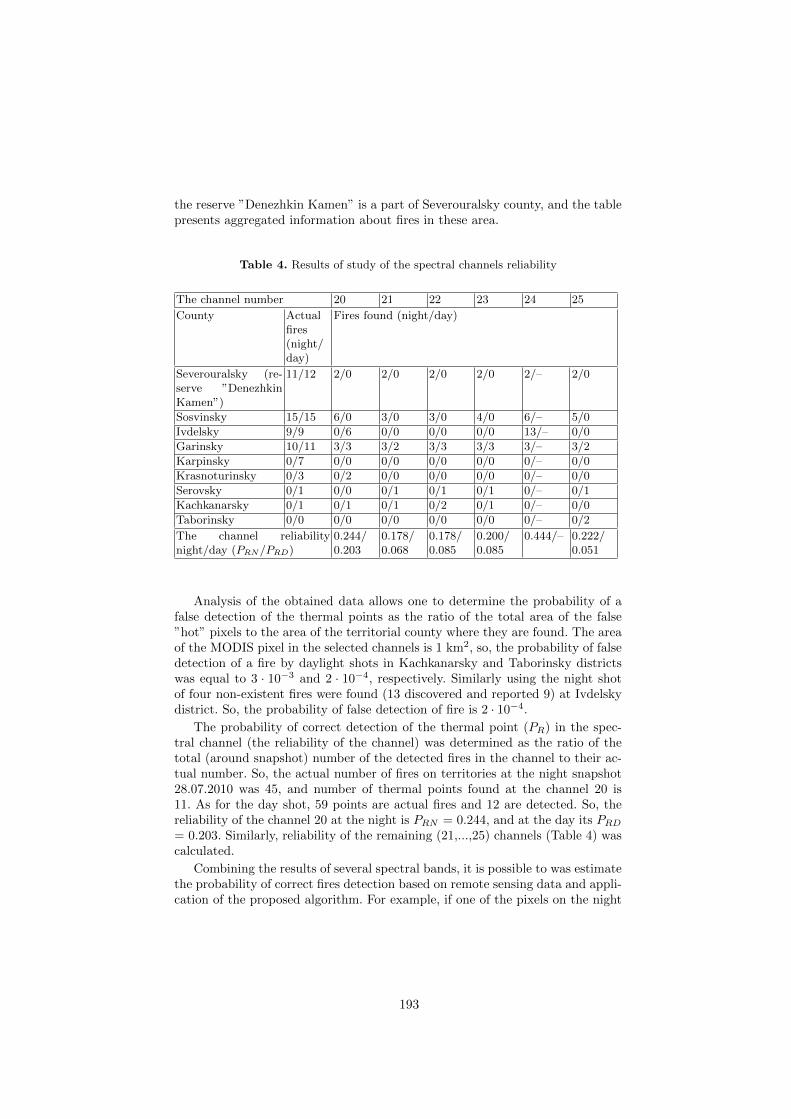
the reserve ”Denezhkin Kamen” is a part of Severouralsky county, and the tablepresents aggregated information about fires in these area.
Table 4. Results of study of the spectral channels reliability
The channel number 20 21 22 23 24 25
County Actualfires(night/day)
Fires found (night/day)
Severouralsky (re-serve ”DenezhkinKamen”)
11/12 2/0 2/0 2/0 2/0 2/– 2/0
Sosvinsky 15/15 6/0 3/0 3/0 4/0 6/– 5/0
Ivdelsky 9/9 0/6 0/0 0/0 0/0 13/– 0/0
Garinsky 10/11 3/3 3/2 3/3 3/3 3/– 3/2
Karpinsky 0/7 0/0 0/0 0/0 0/0 0/– 0/0
Krasnoturinsky 0/3 0/2 0/0 0/0 0/0 0/– 0/0
Serovsky 0/1 0/0 0/1 0/1 0/1 0/– 0/1
Kachkanarsky 0/1 0/1 0/1 0/2 0/1 0/– 0/0
Taborinsky 0/0 0/0 0/0 0/0 0/0 0/– 0/2
The channel reliabilitynight/day (PRN/PRD)
0.244/0.203
0.178/0.068
0.178/0.085
0.200/0.085
0.444/– 0.222/0.051
Analysis of the obtained data allows one to determine the probability of afalse detection of the thermal points as the ratio of the total area of the false”hot” pixels to the area of the territorial county where they are found. The areaof the MODIS pixel in the selected channels is 1 km2, so, the probability of falsedetection of a fire by daylight shots in Kachkanarsky and Taborinsky districtswas equal to 3 · 10−3 and 2 · 10−4, respectively. Similarly using the night shotof four non-existent fires were found (13 discovered and reported 9) at Ivdelskydistrict. So, the probability of false detection of fire is 2 · 10−4.
The probability of correct detection of the thermal point (PR) in the spec-tral channel (the reliability of the channel) was determined as the ratio of thetotal (around snapshot) number of the detected fires in the channel to their ac-tual number. So, the actual number of fires on territories at the night snapshot28.07.2010 was 45, and number of thermal points found at the channel 20 is11. As for the day shot, 59 points are actual fires and 12 are detected. So, thereliability of the channel 20 at the night is PRN = 0.244, and at the day its PRD= 0.203. Similarly, reliability of the remaining (21,...,25) channels (Table 4) wascalculated.
Combining the results of several spectral bands, it is possible to was estimatethe probability of correct fires detection based on remote sensing data and appli-cation of the proposed algorithm. For example, if one of the pixels on the night
193
image of the Garinsky district exceeded trained 20,...,25 channels thresholds, theprobability that it belongs to the fire is
PRN = 1 −25∏
k=20
(1 − PRNk) = 0.823. (3)
Using information of only one channel, you can get the reliability of thefire detection not more than PRN24 = 0.444. If the pixel at the day image ofthe Garinsky district exceeded the threshold of 20,...,23, and 25 channels, theprobability that it is thermal point is PRD = 0.410. And finally, if it is the samepixel on both daylight and night shots, the probability that it belongs to the fireis
PR = 1 − (1 − PRN )(1 − PRD) = 0.896. (4)
Comparing our algorithm with well-known ones, for example [7], [8], weshould say that in them information about statistical characteristics of fire andbackground pixels is used to define a threshold of detection. But we suggest theapproach that doesn’t assume any initial allocation of potentially hot pixels fordefinition of distribution function of probability density for brightness of fire-fighters and the pixels surrounding them. It is based on the fact that detectionof thresholds is performed at spectral channels on the basis of allocation of theknown fire in the picture, according to the subsatellite information. In this case,it is possible to exclude an uncertainty in temperature of a surface and, partially,in the atmosphere parameters.
The conducted experimental study of our algorithm, which is based on theexisting fire, allows one to conclude that the results received with its help aren’tworse than ones of the well-known algorithm MOD14. Similar results are re-ceived in papers [7], [8] that allows one to judge efficiency of our algorithm incomparison with ones offered there. We plan to conduct further researches usingmore extensive actual material for receiving adequate quantitative estimates.Combination of our results with ones received by the mentioned algorithms willallow increasing probability of the forest fires correct detection.
The further increase of probability of the correct fire detection according toMODIS is possible by exception of reflections from stationary natural (water)and anthropogenous (industrial and civil constructions) objects, and, also, fromnonstationary objects (edges of clouds).
4 Conclusion
The paper presents description of the trained threshold algorithm that uses thetrue ground information about one of the fires and builds an effective proceduresfor analysis of the fire situation on the basis of the territory shot obtained by thespectroradiometer MODIS. Study of the proposed algorithm was implementedfor the forest fire detection using data by 21 spectral channels of one night and
194
two daylight MODIS images. Good coincidence of the results of the fires detec-tion with the ground true data and results of work of the well-known MOD14algorithm was obtained. Informativity of the MODIS spectral channels for forestfire detection using the trained algorithm was analyzed. The example shows thatapproximately double increase of the probability of correct detection of fires (upto 0.896) is possible by combining the results of spectral bands 20,...,25 of thenight and day shots.
5 Acknowledgment
The work was partially supported by the RFBR grants Nos 13-07-12168, and13-07-00785.
References
1. MODIS specifications. NASA. http://modis.gsfc.nasa.gov/about/specifications.php2. UniScan-ground station for X–band data reception from polar-orbiting remote sens-
ing satellites. RnD Center ”ScanEx”. http://www.scanex.com/en/stations3. Zraenko, S. M., Mymrina, M. A., Ganzha, V. V.: Obuchaemyi algoritm ob-
naruzheniya pozharov po dannym distantsionnogo zondirovaniya [Learning algo-rithm of fire detection from remote sensing data]. Zhurnal radioelektroniki: elek-tronnyi zhurnal, 11 (2014), URL: http://jre.cplire.ru/jre/nov14/8/text.pdf
4. Algorithm Technical Background Document. MODIS Fire Products.http://modis.gsfc.nasa.gov/data/atbd/atbd-mod14.pdf
5. SCANEX IMAGE PROCESSOR. In-depth Processing of Remotely SensedData and Creation of Thematic Products. RnD Center ”ScanEx”.http://www.scanex.com/en/software
6. Zraenko, S. M., Mymrina, M. A., Ganzha, V. V.: Application of remote sensingdata for forest fires detection with the use of a trained thresholding algorithm /Proc. 24th International Crimean Conference Microwave and TelecommunicationTechnology (CriMiCo–2014), 2, 1151–1152 (2014).
7. Ying, Li, Vodacek, A., Kremens, R. L., e.a.: A Hybrid Contextual Approach to Wild-land Fire Detection Using Multispectral Imagery. IEEE Transactions on Geoscienceand Remote Sensing, 43 (9), 2115–2126 (2005).
8. Chin, S., Liew, A., Lim, L., Keong, K.: New Methods of Active Fire Detection UsingMODIS Data. Proc. 26th Asian Conference on Remote Sensing and 2nd Asian SpaceConference, 1, 411–415 (2005).
195

О методах исследования цифровых копий
художественных произведений для определения их
индивидуальных особенностей
Славных В.А. , Сергеев А.П., Филимонов В.В.
УрФУ имени первого Президента России Б.Н. Ельцина
[email protected], [email protected], [email protected]
Аннотация. Работа посвящена обзору отечественных исследований и
патентных разработок в области определения индивидуальных
особенностей художественного произведения. Систематизированы
характерные признаки авторских стилей, выделяемые различными
исследователями и представлены методы определения указанных
признаков. Обзор опубликованных работ показал, что данная тема
недостаточно представлена в отечественной литературе. Большинство
исследований посвящено решению задачи идентификации автора.
Ключевые слова: цифровое изображение, атрибуция, классификация,
идентификация автора, признаки авторского стиля, экспертиза.
1 Введение
Индивидуальное своеобразие художника формируется в процессе его
профессиональной деятельности и выражается в неповторимости его произведения.
Среди множества критериев творчества одним из главных является способность
отражения индивидуальных позиций и передача мыслей и отношений к реальности.
Установление авторства произведений искусства является актуальной
проблемой. Во-первых, она возникает во время аукционных торгов, при
определении стоимости произведения искусства. Во-вторых, при работе с
музейными коллекциями. В-третьих, существует большой пласт художественных
произведений, авторство которых еще не установлено. Актуальным также остается
вопрос о большом количестве копий произведений искусства.
Важной задачей является систематизация произведений искусства и организация
цифровых баз данных музейных коллекций, архивов и библиотек в Интернете.
Подобная деятельность необходима для поиска новой информации о ранее
неизвестном произведении и сличения с цифровой копией уже атрибутированных
работ предполагаемого автора. Деятельность, направленную на выявление
соответствия произведения искусства заявленным атрибутам называют
«экспертизой».
Экспертиза произведений искусства решает задачи, которые мы предлагаем
разделить на технико-технологические и искусствоведческие.
Технико-технологические задачи - установление состояния сохранности
объекта и предполагаемая стоимость реставрации, техники и технологии исполнения
представленной работы, ее возраста и рыночной стоимости.
196

Технико-технологическая экспертиза использует современные физические,
химические и физико-химические методы анализа материалов, из которых состоит
картина, иногда требующие изъятия пробы. Полное технологическое исследование
произведений искусства имеет необходимость использования, технически хорошо
оснащенной лаборатории, высококвалифицированного персонала, а также наличие
сравнительного материала, достаточно высокую стоимость и по этой причине не
всегда целесообразно.
Искусствоведческие задачи - определение авторства художественного
произведения, принадлежности художественному направлению, стилю или школе,
поиск влияний и связей между художниками, культурной или исторической
ценности произведения.
Искусствоведческая экспертиза использует сравнительно-исторический,
формальный, иконологический, семиотический методы анализа формы, композиции,
технических приемов.
К экспертизе привлекаются специалисты в соответствующей области
деятельности. Оценка экспертной комиссии зависит от квалификации и знаний
каждого члена группы. Только специалисты могут обеспечить полноту
исследования и надежность выводов. В связи с чем, важной задачей представляется
изучение и развитие новых компьютерных методов бесконтактного исследования
произведений искусства для целей атрибуции.
Цель работы: обзор исследований и патентных разработок в области атрибуции
произведений искусства по их цифровым копиям.
2 Отечественные работы по исследованию цифровых копий
художественных произведений
Мурашов Д.М., Березин А.В., Иванова Е.Ю. [1-2] (Москва, Вычислительный
центр им. А.А. Дородницына РАН, Государственный Исторический музей)
предложили описание фактуры картин на основе характеристик хребтов
полутоновых изображений мазков и локальных признаков структурного тензора на
изображении фрагмента. «Гистограмма формируется по значениям составляющих
градиента уровней полутонов в точках, расположенных на хребтах информативных
фрагментов» [1].
Размер кисти художника (толщина волоса, ширина кисти) вычисляется на основе
значения модуля волнового вектора, который определяет пространственный период
волны в направлении ее распространения. Данные для исследования формируется по
информативным фрагментам изображений без предварительной сегментации
отдельных мазков кисти. Для сравнения информативных фрагментов применяется
теоретико-информационная мера различия на основе дивергенции Кульбака-
Лейблера - меры удаленности друг от друга двух вероятностных распределений.
Данные исследования показали, что значения исследуемого признака фрагментов
картин разных авторов различаются в пять раз больше, чем значения признака на
картинах одного автора. Описанная методика была протестирована на изображениях
портретов, написанных в XVIII–XIX вв. [1].
Иваненко Ю.М., и др. [3] выдвинули гипотезу: живописное произведение
обладает внутренней динамикой, которая характеризуется соотношением
детерминированности и хаотичности. Исследователи выявили, что полутоновые
изображения отличаются конечностью размерности аттрактора. На основе отсчетов
197
яркости реального изображения были выбраны специальные переменные для
построения многомерного фазового пространства, в котором производился анализ
динамики исследуемого изображения путем вычисления интегральной
корреляционной функции аттрактора. Исследователи установили, что значения
размерности аттрактора отражают вид изображения: «полиграфическая копия»
произведения искусства, фотографическое изображение лица, фрагменты
скульптурного изображения, зафиксированные с помощью видеокамеры,
модельные изображения различных объектов, сгенерированные на компьютере, в
соответствии с разработанной шкалой сложности изображений. Определенная
зависимость размерности аттрактора от числа фазовых переменных позволяет
произвести идентификацию индивидуального творческого почерка художника [3].
Новиков Г.И. [4] (Институт физиологии им. И.П. Павлова РАН) предложил для
идентификации автора художественных произведений использовать
колориметрические измерения «контраста цветового насыщения»,
(противопоставление ярких, насыщенных и блеклых, затемненных цветов),
зависящего от пропорций и равновесности композиции, присущего конкретным
авторам. Исследователь предложил вычислять соотношение основных и
дополнительных цветов на основе сопоставления цвета картины в разных точках по
отношению к нейтральному серому фону. Вывод был основан на рассмотрении
колориметрических измерений объектов русской и западноевропейской живописи
второй половины XIX и начала XX веков.
Костюков Ю.В. [5] (Краснодарский краевой художественный музей им. Ф.А.
Коваленко) предлагает осуществлять отбор характерных признаков для
исследования художественного произведения, статистическими методами, которые
позволят выявить тесноту связи между признаками и выделить наиболее
идентификационно значимые. Он предложил устанавливать факт наличия
взаимосвязи между признаками и ее значимости на основе критерия хи – квадрат.
Описанная методика была протестирована при анализе декорировки столовой и
чайной посуды завода Гарднера конца XVIII – последней трети XIX вв. В результате
исследования Костюков Ю.В. установил, что на изделиях завода Гарднера наиболее
тесно связаны между собой признаки «тема» и «форма» декора. Зная значение
одного из них, можно с определенной вероятностью предсказать значение другого
[5].
3 Отечественные патенты на изобретения
Хачатрян А.Х. [6] (ООО «Научно-исследовательский институт экспертизы
произведений искусств и архитектуры») описывает три запатентованных технологии
бесконтактного неразрушающего анализа произведений искусства:
«Способ бесконтактного неразрушающего анализа художественных полотен
и других произведений искусства по их цифровым копиям для определения
индивидуального рисунка рельефа и углублений поверхностных и внутренних
слоев» [7].
«Способ опосредованного неразрушающего исследования художественных
полотен, монументального и других произведений искусства для выявления их
скрытых индивидуальных особенностей (варианты), способ определения
подлинности и/или авторства художественного или других произведений
искусства» [8].
198

«Способ защиты художественного полотна и других произведений искусства
от подделки, а также определения их авторства» [9].
Цифровая копия обрабатывается в графическом редакторе (увеличение масштаба,
затемнение до появления углублений и контуров, осветление до более четкого
проявления рельефа, обработка при помощи инструмента «контурная резкость» до
получения максимально четких контуров). При этом каждая отдельно взятая
цифровая копия художественного произведения разделяется на слои и сохраняется в
отдельные файлы, как часть исследуемого произведения искусства. Каждая из них
обрабатывается отдельно; количество слоев конкретного произведения зависит от
индивидуального характера каждого из них, а каждый изученный слой
рассматривается как отдельное исследование. Далее эксперт зрительно анализирует
полученные копии художественного полотна [6].
По мнению авторов, предложенные способы выявляют скрытые индивидуальные
особенности композиции и характер художественного произведения, что позволяет
определить их подлинность, послойно рассмотреть картины разных художников,
обнаружить тайные знаки, раскрывающие замысел и обнаружить пустоты, полости и
скрытые предметы в художественных произведениях [6].
Кастальская-Бороздина Н.К. [10] (Свято-Троице Сергиева Лавра) предлагает
способ идентификации художественных произведений через сопоставление наборов
зашифрованных данных фрагментов живописи по соответствующим цветам
палитры произведения. Исследователь утверждает, что у каждого автора
существует неповторимый набор исходных «полу(четверть) тоновых шкал колеров»
[10] ожидаемых в любой его работе. Кастальская-Бороздина Н.К. предлагает
идентификацию исследуемого объекта осуществлять на основе сравнения
«выявленных уникальных признаков произведения живописи и оригинала по
графическим зависимостям коэффициента гашения обертонов от суммарного
колера, состоящего из красного, зеленого и синего цветов, вычисленным по самым
темным, самым светлым и срединным колерам с учетом естественной аппаратной
погрешности» [10]. Описанный способ был опробован на цифровых копиях таких
художников как, Айвазовский И., Левитан И., Кустодиев Б., Поленов В.
Шольцен В. [11] предлагает способ определения автора художественного
произведения по ее цифровой копии путем сравнения характеризующих признаков и
деталей характеризующих признаков (точек, линий, групп точек или линий, узоров),
полученных преобразованием Хафа.
4 Характерные признаки авторских стилей
Таким образом, на основе проведенного обзора можно выделить следующие
характерные признаки авторских стилей и способы их вычисления, используемые
различными исследователями.
Фактура картины:
Определяемая, гистограммой направлений хребтов полутоновых изображений
мазков, формируемой на основе вторых частных производных от функции,
описывающей полутоновый рельеф изображения по пространственным координатам
и гистограммой локальной ориентации окрестностей на изображении фрагмента
картины, формируемой на основе первых частных производных от функции,
описывающей полутоновый рельеф изображения по пространственным координатам
[2].
Получаемая, после обработки в графическом редакторе Adobe Photoshop или FS
Viewer путем масштабирования, затемнения, осветления, увеличения контурной
199

резкости (настройка параметров эффекта резкости, радиуса пикселей, и порога
уровней), яркости и контрастности. [8]
Получаемая, после обработки в графическом редакторе путем масштабирования,
затемнения, осветления, увеличения контурной резкости (настройка параметров
эффекта резкости, радиуса пикселей, и порога уровней) [9].
Размер кисти, использовавшейся художником – локальное волновое число,
получаемое из изображения при использовании преобразования Рисса [1].
Выразительные графические средства (точки, группы точек, линии, группы
линий, узоры), определяемые методом Хафа. Дополнительно устанавливаются
опорные признаки, путем масштабирования, растяжения или сжатия, изменения или
изгибания линии, изменения угла между двумя линиями соответствующего
характеризующего признака [11].
Цветовой контраст:
Яркость изображения, определяемая зависимостью размерности аттрактора от
числа фазовых переменных [3].
Контраст цветового распространения, зависящий от пропорций и
равновесности композиций автора. Сопоставление цветов картины в разных точках
по отношению к нейтральному серому фону. Количественные расчеты производятся
исходя из установленных И. Гёте простых числовых выражений. Контраст
цветового распространения подчинен гармонии равновесия отношения светлоты и
дополнительных цветов. [4]
Цвет, получаемый после обработки в графическом редакторе Adobe Photoshop
или FS Viewer путем масштабирования, затемнения, осветления [8].
Цветовые пятна, определяемые графической зависимостью коэффициента
гашения обертонов и суммарного колера, вычисленным по самым темным, самым
светлым и серединным колерам с учетом естественной аппаратной погрешности
[10].
5 Выводы
В результате проведенного обзора были выявлены характерные признаки
авторских стилей, выделяемые различными исследователями для целей атрибуции
художественных произведений. Все признаки можно разделить на три основные
группы: фактура картины, цветовой контраст, выразительные графические средства.
Рассмотренные в настоящей работе исследования в области анализа цифровых
копий произведений искусства направлены на определение авторства
художественного произведения. Однако в области экспертизы художественных
произведений остается еще целый ряд задач, которые можно решать: классификация
стилей, жанров и периода создания, установление взаимовлияний и связей между
художниками. Дальнейшие исследования могут быть направлены на развитие и
апробацию бесконтактных методов анализа художественных произведений, которые
недостаточно представлены в отечественной литературе, а также изучение опыта
зарубежных исследователей.
В представленных работах не предложено описание технологии получения и
критерии оценки качества, предъявляемые к цифровым копиям художественных
произведений, в свиязи с чем, возникает вопрос об объективности результатов
исследования изображений, имеющихся в сети Интернет.
200

Очевидно, что для успешного использования цифровых бесконтактных методов
анализа художественных произведений необходимо наличие обширных баз
оригинальных атрибутированных работ, а так же баз вычисленных данных для
сравнения.
Список литературы
1. Мурашов Д.М., Березин А.В., Иванова Е.Ю. Формирование признакового описания
фактуры картин // Машинное обучение и анализ данных. 2013. Т. 1, 6. C. 779–786.
2. Мурашов Д.М., Березин А.В., Иванова Е.Ю. Сравнение изображений картин по
информативным фрагментам // Машинное обучение и анализ данных. 2014. Т. 1. 8.
C. 941–948.
3. Иваненко Ю.М., Макулов В.Б., Раскин А.Г., Трифонов М.И. Математическая
формализация художественной ценности произведения искусства, их голографический
копий и компьютерных изображений // Информационный бюллетень РФФИ, 5 (1997)
Науки о человеке и обществе.
4. Новиков Г.И.Колориметрические исследования в живописи // Материалы IX
Международной конференции «Прикладная оптика-2010», 18–22 октября 2010, Санкт-
Петербург, С. 236–240.
5. Костюков Ю.В. Возможности применения вероятностно-статистического метода для
оценки значимости признаков в идентификации произведений искусства // Теория и
практика актуальных исследований (Материалы Международной научно-практической
конференции, 17 апреля 2012).
6. Хачатрян А.Х. Исследование произведений монументального и изобразительного
искусства с помощью нового изобретения, его роль и важность в мировой науке //
Гуманитарные, социально-экономические и общественные науки. 2013, 4. C. 461–
470.
7. Хачатрян А.Х., Симонян З.А., Хачатрян В.А. Способ бесконтактного неразрушающего
анализа художественных полотен и других произведений искусства по их цифровым
копиям для определения индивидуального рисунка рельефа и углублений
поверхностных и внутренних слоев // Патент России 2012157043, 10.07.2014.
8. Хачатрян А.Х., Симонян З.А., Хачатрян В.А. Способ опосредованного
неразрушающего исследования художественных полотен, монументального или
других произведений искусства для выявления их скрытых индивидуальных
особенностей (варианты), способ определения подлинности и/или авторства
художественного полотна, монументального или других произведений искусства //
Патент России 2012138269, 20.03.2014.
9. Хачатрян А.Х., Симонян З.А., Хачатрян В.А. Способ анализа художественных полотен
и других произведений искусства для определения их авторства и/или защиты от
подделки // Патент России 2012118006, 10.11.2013.
10. Кастальская-Бороздина Н.К. Способ идентификации произведений живописи на
предмет их авторства // Патент России 2333613, 10.09.2008.
11. Шольцен В. Устройство и способ идентификации автора произведения искусства //
Патент России 2011149157, 27.06.2013.
201

About The Methods of Research Digital Copies Works of
Art to Determine Their Specific Features
Viktoriya Slavnykh , Alexander Sergeev, Viktor Filimonov
Ural Federal University named after the first President of Russia Boris Yeltsin,
[email protected], [email protected], [email protected]
Abstract. The work is devoted to the review of Russian studies and patents to
determine the specific features of works of art. The article provides a
classification the characteristic features of the author's style works of painting
and are described methods for determining specified characteristics.
Keywords: digital image, image features, classification, attribution of paintings.
202

Эволюционирующие онтологии в аспектеуправления темпоральными или
изменяющимися фактами
А. А. Демидов
Институт программных систем им. А.К. Айламазяна РАН,[email protected]
Аннотация В работе предлагается алгебраический подход к по-строению онтологий, способных к эволюции под влиянием новыхфактов и обладающих внутренними механизмами валидации. Дляэтой цели строится формальная модель взаимодействия объектов ивыясняются ограничения на операции с объектами, накладываемыетакой моделью. Затем в контексте формальной модели определяютсяосновные понятия модели представления знаний: концепты, экзем-пляры, свойства и отношения. При этом формальные ограниченияпереносятся в модель представления знаний естественным образом.
Ключевые слова: эволюционирующие онтологии, представлениезнаний, формальные системы.
Введение
Онтология — это система понятий и утверждений об этих понятиях, наоснове которых можно строить классы, объекты, отношения, функции и тео-рии. В общем случае онтологии содержат концепты (понятия или классы),экземпляры (индивиды или объекты), свойства концептов и экземпляров(атрибуты или роли), отношения между концептами или экземплярами, атакже дополнительные ограничения, определяемые аксиомами и правиламивывода. Сформулировано множество определений понятия онтологии, наи-более точным из них представляется следующее: «Онтология — это фор-мальная теория, ограничивающая возможные концептуализации» [1]. По-скольку мы хотели бы также хранить в онтологии отдельные экземпляры,данное определение требует обобщения: «Онтология — это формальная си-стема, взятая вместе с её интерпретацией».
Эволюция онтологии — это процесс последовательной адаптации онто-логии к происходящим изменениям и непротиворечивого распространенияэтих изменений [2]. Это нетривиальный процесс, поскольку изменение в од-ной части онтологии может привести к возникновению противоречия в дру-гих её частях, информация различных источников может оказаться непол-ной или противоречивой. В силу сложности учёта большого количества фак-торов инженер по знаниям оказывается не в состоянии учесть все побочные
203

эффекты вносимых изменений, поэтому необходима реализация специаль-ных механизмов, отвечающих за поддержание согласованности онтологии впроцессе её актуализации.
Можно выделить два основных подхода к представлению онтологий: ло-гический и объектный [3]. Логический подход связан с представлением онто-логии как формальной системы со своим синтаксисом, аксиомами и прави-лами вывода, он находится в русле классического искусственного интеллек-та, изучающего способы представления знаний. Объектный подход предпо-лагает представление онтологии в виде графа, состоящего из классов, объ-ектов и связей между ними, он удобнее для реализации и чаще используетсяв прикладных разработках, в рамках него обычно создаются сверхбольшиересурсы, используемые в широких предметных областях: различного родасловари, таксономии, рубрикаторы и тезаурусы.
Обладая лучшей наглядностью и удобством, объектный подход имеет се-рьёзный недостаток: он не предоставляет никаких внутренних механизмовконтроля непротиворечивости — в отличие от формальных систем, имею-щих средства контроля полноты и непротиворечивости. Поэтому при объ-ектном подходе инженер по знаниям должен определить систему внешнихограничений, описывающих допущения предметной области. Но проблемав том, что предметная область сама зависит от вновь прибывающих фак-тов, она всё время меняется. Поэтому система внешних ограничений такжедолжна всё время меняться. Но тогда возникает проблема контроля непро-тиворечивости изменений уже этой системы ограничений — получается за-мкнутый круг.
1 Постановка задачи
Несложно показать, что онтологии, создаваемые в рамках обоих подхо-дов, могут быть преобразованы от одного вида к другому путём перехода котношениям: каждая непротиворечивая формальная теория имеет модельв теоретико-множественном представлении, с другой стороны, каждый объ-ект может быть представлен как набор записей реляционной базы данных.Поэтому корректней говорить о различных представлениях одной и той жеонтологии — логическом и объектном. Вопрос состоит в том, какой возмож-ный механизм контроля в объектном представлении может соответствоватьконцепции противоречивости в логическом представлении.
2 Состояние исследований
Большинство работ по эволюции онтологии, известных в настоящее вре-мя, описывают различные эвристические подходы — их обзор дан в работеФ. Заблиса и др. [4]. Как правило, в этих работах предлагается некий слож-ный эвристический алгоритм, берущий на себя рутинную часть работы посогласованию изменений, и предполагается участие инженера по знаниям,выполняющего интеллектуальную часть работы. Другие системы — такие
204

как EvoPat, RUL — реализуют возможность автоматического разрешенияконфликтов, но они действуют на основе жесткой системы внешних огра-ничений, заданных априори при создании онтологии.
Более перспективно выглядят методы эволюции онтологий, обоснован-ные теоретически. В работе П. Хаазе и Л. Стояновича [5] выделяется тривида непротиворечивости: структурная (синтаксическая), логическая (се-мантическая) и определяемая пользователем (внешняя). Большинство дина-мических онтологий обеспечивают только синтаксическую непротиворечи-вость на основе соответствия языку описания онтологии или схеме данных.В работе не предлагается решения, обеспечивающего логическую непроти-воречивость, однако приводятся эффективные алгоритмы локализации иустранения логических противоречий с помощью исключения конфликтую-щих аксиом.
В работах Т. Шарренбаха и др. [6,7] конфликты аксиом не запрещают-ся, поэтому их исключение из онтологии не требуется. Вместо исключенияаксиом (явных знаний) авторы предлагают объявлять недействительнымиконкретные выводы (неявные знания), которые вызывают противоречие вонтологии. Так, оба заключения A и ¬A могут оказаться выводимы, невыво-димым останется только противоречие A&¬A. Это приводит к неоднознач-ности онтологии.
Задача поиска механизма контроля онтологии в объектном представле-нии, который соответствовал бы концепции противоречивости в логическомпредставлении, в явном виде ранее не ставилась.
3 Мир как динамическая система
3.1 Формальная логика и клеточные автоматы
Машина Тьюринга как универсальный вычислитель способна реализо-вать как систему продукций аксиоматизируемой формальной логическойсистемы, так и систему продукций клеточного автомата. Отсюда следует,что выразительные способности тьюринг-полных клеточных автоматов до-статочны для представления логических ограничений на структуру знаний.
Далее мы будем рассматривать явления предметной области в терминахдинамических систем — как изменения состояния динамической системы,эволюционирующей с течением времени. Покажем, что клеточный автоматтакже может рассматриваться как динамическая система, введём в этоймодели понятие объектов, опишем их взаимодействия. Поскольку возмож-ностей тьюринг-полного клеточного автомата достаточно для моделирова-ния произвольного процесса эволюции, то найденные закономерности будутсправедливы и в общем случае.
205

3.2 Динамические системы
В самом общем смысле динамическая система есть тройка (T,X, φ), гдеT — аддитивный моноид, X — множество, а φ — функция
φ : T ×X → X, (1)
такая что
φ(0, x) = x,
φ(t2, φ(t1, x)) = φ(t1 + t2, x),
где T — множество неотрицательных вещественных чисел R+ (непрерывноевремя), либо натуральных чисел с нулём N (дискретное время) [8,9].
Функция φ(t, x) называется оператором эволюции динамической систе-мы, она ставит в соответствие каждой точке множества X единственныйобраз, зависящий от переменной t, называемой параметром эволюции. Мно-жество X называется фазовым пространством (или пространством состоя-ний), в котором переменная x определяет начальное состояние системы.
3.3 Клеточные автоматы
Пусть G — группа, а A — множество. Тогда (см. [10])
Определение 1. Клеточный автомат над группой G и алфавитом A естьотображение τ : AG → AG, обладающее свойством: существует конечноеподмножество S ⊂ G и отображение µ : AS → A, такие что
τ(x)(g) = µ((g−1x)|S) (2)
для всех x ∈ AG и g ∈ G, где запись (g−1x)|S означает сужение конфигу-рации g−1x на множество S.
Путём последовательных итераций клеточного автомата τ : AG → AG
можно получить дискретную динамическую систему. Это означает, что кон-фигурация может пониматься эволюционирующей во времени в соответ-ствии с τ : если x ∈ AG — конфигурация в момент времени t ∈ N, то τ(x)— конфигурация в момент времени t + 1. Суперпозиция τ t = τ τ · · · τитераций по параметру t даёт оператор эволюции динамической системы вовремени
φ(t, x) = τ t(x). (3)
3.4 Объекты в конфигурационном пространстве
Неформально говоря, объектом будем считать глайдер в конфигураци-онном пространстве. Глайдеры — это хорошо известные стабильные дина-мические структуры (паттерны) в клеточном пространстве игры Конвея
206

«Жизнь». Глайдер (солитон) является возмущением в активной среде, рас-пространяющимся в этой среде с постоянной скоростью и сохраняющимсвою целостность в течение некоторого времени.
Отображение µ : AS → A в формуле (2) определяет систему окрестностейO(g) = g ∪ Sg для каждого g ∈ G. Окрестностью множества O(g) являетсяобъединение
O(O(g)) =⋃
q∈O(g)
(q ∪ Sq
). (4)
Последовательные итерации этой формулы задают систему окрестностей P,определяющую предбазу топологии на G
P(t, g) = Ot(g) : t ∈ N, g ∈ G. (5)
Если для gt, g0 ∈ G выполняется условие gt ∈ Ot(g0), то будем говорить,что элемент gt причинно зависит от g0 на интервале времени t.
Определение 2. Объектом O назовём динамическую область конфигура-ционного пространства O(gi) ∈ P, где gi пробегает последовательностьпричинно зависимых элементов g0, . . . , gt, такую что все конфигурацииAO(gi) равны между собой.
4 Модель взаимодействия объектов
4.1 Взаимодействие как эволюция состояния
Будем рассматривать изменение объектов — их взаимное превращениев результате взаимодействия в некоторой области конфигурационного про-странства G с заданной на этом пространстве конфигурацией x ∈ AG, эво-люционирующей под действием моноида времени T .
Нас будет интересовать только конечный результат взаимодействия по-сле того, как объекты разойдутся в конфигурационном пространстве на до-статочное расстояние, чтобы не оказывать влияния друг на друга.
Обозначим через Ψ множество конфигураций всех возможных объектов
Ψ = AO : O ∈ P. (6)
Тогда процесс изменения конфигурации ψ = ψ1 ⊗ . . . ⊗ ψn системы вза-имодействующих объектов можно записать в привычном виде
ψ′ = Uψ, (7)
где U = U(t, x) — оператор эволюции состояния x ∈ AG за время t ∈ T , аψ ∈ Ψ — функция состояния системы объектов.
207

4.2 Взаимодействие как преобразование объектов
Произвольным образом разобьём исходную динамическую систему надве подсистемы — ψa и ψb так, чтобы ψaψb = ψ (для удобства будем опус-кать знак операции «⊗»). Взаимодействие систем ψb и ψa тогда может бытьзадано с помощью операции «» в виде
ψ′a = ψa ψbψ′b = ψb ψa,
(8)
где первое равенство описывает трансформацию ψa в ψ′a с помощью системыψb, а второе — обратное влияние системы ψa на ψb.
Модель взаимодействия тогда вполне определяется двумя операциями
⊗ : Ψ2 → Ψ, «из чего состоит» в пространстве, (9) : Ψ2 → Ψ, «как изменяется» во времени. (10)
Операция «⊗» ассоциативна, поскольку свойство «из чего состоит», оче-видно, удовлетворяет тождеству (ψa ⊗ ψb) ⊗ ψc = ψa ⊗ (ψb ⊗ ψc). Но некоммутативна — порядок аргументов важен, поскольку задаёт расположе-ние объектов в пространстве. Свойства операции «» будут установленыдалее (очевидна лишь некоммутативность).
Правила преобразования конфигураций могут быть заданы функциямина множестве Ψ . Иначе говоря, существует инъекция
ξ : Ψ → F(Ψ), (11)
позволяющая отождествить конфигурации объектов Ψ с элементами сим-метрической полугруппы F(Ψ) преобразований над ними.
4.3 Связь двух операций «⊗» и «»
Теорема 1. Инъекция ξ : Ψ → F(Ψ) множества конфигураций объектовв симметрическую полугруппу преобразований является гомоморфизмомотносительно операции «», если эта операция действует в простран-стве T , связанном с пространством G преобразованием масштаба.
Доказательство. Зададим начальное разбиение системы ψ ∈ Ψ в простран-стве G так, чтобы она состояла из трёх подсистем следующим образом:ψaψbψc = ψ. Будем попарно объединять эти подсистемы и описывать взаи-модействие такого объединения с оставшейся частью полной системы.
Поскольку результат операции «⊗» зависит от порядка аргументов, приобъединении необходимо следить за тем, в какой системе координат произ-водится данное действие. Для удобства введём унарную операцию ¬ : Ψ → Ψповорота системы координат, связанную с операцией «⊗» тождеством
¬(ψaψb) = ¬ψb¬ψa. (12)
208

Объединим подсистемы ψaψb = ψab, тогда правила трансформации ди-намической системы ψaψbψc = ψabψc запишутся в виде
ψ′ab = ψab ψc = ψc(ψab)
ψ′c = ¬(¬ψc ¬ψab) = ¬ψ¬b¬a(ψ¬c).(13)
Во втором уравнении появляется операция обращения аргументов, посколь-ку относительно подсистемы ψc, на которую действует объединённая подси-стема, подсистемы ψa и ψb расположены в порядке ψb, ψa — именно в такомпорядке и происходит действие. Операция обращения всего выражения от-вечает за возврат системы координат в исходное положение.
Теперь объединим подсистемы ψbψc = ψbc, тогда правила трансформа-ции динамической системы ψaψbψc = ψaψbc запишутся в виде
ψ′a = ψa ψbc = ψbc(ψa)
ψ′bc = ¬(¬ψbc ¬ψa) = ¬ψ¬a(ψ¬c¬b).(14)
Во втором уравнении также появляется операция обращения аргументовпо аналогичной причине: подсистема ψa действует сперва на ближайшуюк ней подсистему ψb, и только затем — на ψc. Операция обращения всеговыражения отвечает за возврат системы координат в исходное положение.
Поскольку ψ′abψ′c = ψ′aψ
′bc = ψ′ = Uψ, то можно приравнять правила
трансформации первой и второй систем уравнений:
((ψa ⊗ ψb) ψc) ⊗¬(¬ψc (¬ψb ⊗ ¬ψa)) = (15)= (ψa (ψb ⊗ ψc)) ⊗¬((¬ψc ⊗ ¬ψb) ¬ψa). (16)
Равенство выполняется, если и только если существует унарная операция∝ : Ψ → Ψ , связывающая операции «» и «⊗» тождеством
∝ (ψaψb) = ψa ψb, (17)
— тогда равенство можно преобразовать к очевидной форме:
∝ ((ψa ⊗ ψb)⊗ ψc) ⊗¬ ∝ (¬ψc ⊗ (¬ψb ⊗ ¬ψa)) = (18)=∝ (ψa ⊗ (ψb ⊗ ψc)) ⊗¬ ∝ ((¬ψc ⊗ ¬ψb)⊗ ¬ψa). (19)
Унарная операция «∝» существенно ограничивает возможный вид опе-рации «», в частности, должно соблюдаться условие
(∀ψx, ψy ∈ Ψ) ψxψy = ψa → ψx ψy =∝ ψa, (20)
которое означает, что все решения уравнения x⊗ y = ψa с двумя неизвест-ными также являются решениями уравнения x y =∝ ψa. В этом смыслеоперации «⊗» и «» эквивалентны с точностью до преобразования мас-штаба, определяемого операцией «∝». При этом операция «» оказывается,вообще говоря, неассоциативной:
(ψa ψb) ψc 6= ψa (ψb ψc), (21)
209

∝ (∝ (ψaψb)ψc) 6= ∝ (ψa ∝ (ψbψc)). (22)
Введём формальное обозначение ∝−1∝ ψa = ψa и перепишем тожде-ство (17) в виде
∝ (ψaψb) =∝−1∝ ψa ∝−1∝ ψb, (23)
обозначим операцию «» вместе с преобразованием «∝−1» обратного мас-штабирования её аргументов через : Ψ2 → Ψ , тогда станет очевиден изо-морфизм
∝ (ψa ⊗ ψb) =∝ ψa ∝ ψb. (24)
Также, после замены переменных ψa →∝ ψa и ψb →∝ ψb в тождестве (17)и перехода к обозначению ⊗ : Ψ2 → Ψ , объединяющему операцию «⊗» вме-сте с преобразованием «∝» прямого масштабирования её аргументов, выяв-ляется изоморфизм
∝ (ψa⊗ψb) =∝ ψa ∝ ψb. (25)
Изоморфизмы (24) и (25) связывают пространства T и G преобразова-нием масштаба, определяемом операцией (17).
Операция «⊗» — ассоциативна, поэтому полугруппа 〈Ψ,⊗〉 вкладываетсяв симметрическую полугруппу F(Ψ) трансформаций множества Ψ . В силуизоморфизма (24) операция «» тождественна операции «⊗», если все еёаргументы переведены в пространство T преобразованием «∝−1». Следова-тельно, инъекция ξ : Ψ → F(Ψ) (11) является однозначным гомоморфизмомотносительно операции «».
4.4 Спецификация модели взаимодействия объектов
Таким образом, построенная модель включает:
– алгебру 〈Ψ,⊗,〉 динамических систем (6) и (9);– симметрическую полугруппу F(Ψ) преобразований (11);– инъективный гомоморфизм ξ : Ψ → F(Ψ) (теорема 1);– преобразование масштаба ∝ (ψaψb) = ψa ψb (17),
где операции «⊗» и «» связаны равенством
ψa ⊗ ψb = (∝−1 ψa) (∝−1 ψb). (26)
5 Модель представления знаний
Построенная модель взаимодействия объектов сводится к подполугруппеJ симметрической полугруппы J ⊂ F(Ψ) преобразований множества Ψ , ко-торая равномощна этому множеству |Ψ | = |J | < |2Ψ |. Такое сокращение чис-ла допустимых преобразований указывает на существование естественныхмодельных ограничений, что может быть использовано для целей контроляонтологии, однако число степеней свободы всё ещё очень велико.
210

Определение 3. Если по отношению к динамической системе ψa подмно-жество систем ΨB ⊂ Ψ является эквивалентным в смысле тождества
(∀ψb ∈ ΨB)(ψa ψb = ψ′a),
то множество ΨB будем называть классом со свойством ψa → ψ′a.
Совокупность всех свойств объекта ψb полностью определяет преобразо-вание ψb : Ψ → Ψ из полугруппы J . Совокупность всех свойств класса такжеопределяет преобразование, частично определённое на множестве Ψ , кото-рое является пересечением преобразований всех объектов данного класса
ψB =⋂
ψb∈ΨB
ψb. (27)
В эволюционирующей онтологии ни один объект не определён окончательно,под влиянием новых фактов отношения достраиваются и перестраиваются.Поэтому между объектами и классами нет принципиальной разницы — теи другие являются частично определёнными преобразованиями.
В прикладных задачах построения онтологий часто приходится иметьдело не с функциями, а с отношениями. Можно показать, что такой пере-ход правомерен, если в теореме 1 перейти к гомоморфизму ξ : Ψ → 2Ψ . Всилу однозначного гомоморфизма ξ : Ψ → 2Ψ операция «⊗» является су-перпозицией отношений соответствующих объектов. С другой стороны, онавыражается через операцию «» с помощью унарной операции «∝−1» пре-образования масштаба (26). Тождество
ψb ψa = ψa ⊗ ψb = (∝−1 ψa) (∝−1 ψb), (28)
где слева стоят отношения, а справа — соответствующие им объекты, яв-ляется мощным средством обеспечения непротиворечивости онтологии, длячего даже не требуется просматривать весь ресурс знаний.
Для организации хранения знаний можно предложить следующую базо-вую структуру из двух таблиц.
Таблица 1. Структура хранения знаний (с валидацией)
headid Идентификаторlabel Наименование
bodysubj Subject (→ head.id)obj Object (→ head.id)prop Result subj obj (→ head.id)test Result subj ⊗ obj (→ head.id)
На начальном этапе все таблицы пусты. В процессе работы каждое новоепонятие фиксируется в таблице head, а каждое его свойство попадает в таб-лицу body. Пока функция ∝−1 не определена, поле body.test не заполняется
211

— это можно сделать позже на основе значения body.prop. Классы можнополучать динамически как пересечение нескольких отношений, однако изсоображений быстродействия имеет смысл запустить автономный процесс,который бы создавал и удалял классы на основе устойчивых корреляциймежду объектами. Этот же процесс мог бы выполнять трудоёмкую зада-чу вычисления полей body.test пока быстрое вычисление с использованиемфункции ∝−1 не станет возможным.
Тождество (28) позволяет вычислять значения функции ∝−1 : Ψ → Ψдинамически по мере добавления новых фактов: поскольку все объекты яв-ляются отношениями, кажется, что их суперпозиция тоже должна задаватьобъект; это почти так — если отношения предварительно масштабироватьфункцией ∝−1, а результат масштабировать обратно с помощью ∝. Длявсех пар ψa ψb данная функция должна быть одной и той же — если так неполучается, то можно констатировать наличие в онтологии противоречия.
6 Заключение
В работе предложен алгебраический подход к построению онтологий,способных к эволюции под влиянием новых фактов и обладающих внут-ренними механизмами валидации. Для этой цели установлено соответствиемежду двумя основными подходами к представлению онтологий: логиче-ским и объектным. В результате этого в объектном представлении удалосьотыскать такой механизм контроля непротиворечивости онтологии, кото-рый соответствует концепции противоречивости в логическом представле-нии — на основе функции ∝−1. В терминах алгебраического подхода опре-делены основные понятия модели представления знаний: концепты, экзем-пляры, свойства и отношения. При таком подходе формальные ограниченияпереносятся в модель представления знаний естественным образом.
Найденное решение является новым, его можно использовать для по-строения больших прикладных онтологий, не пренебрегая средствами кон-троля непротиворечивости. Что, в свою очередь, открывает возможности корганизации процесса эволюции такой онтологии в автоматическом режиме,что до сих пор было невозможным.
Построенная алгебра с двумя операциями — суперпозицией отображе-ний «⊗» и неассоциативной операцией «» — является программной ал-геброй. Программные алгебры интенсивно исследуются в настоящее времяв контексте построения высокопроизводительных параллельных вычисли-тельных систем [11].
Результаты данной работы планируется использовать при построенииресурса знаний большого объёма для системы извлечения информации изтекстов ИСИДА-Т [12].
Благодарности. Работа выполнена в рамках НИР «Моделирование модально–временного аспекта описания ситуаций в задаче извлечения информации изтекстов», номер гос. регистрации 01201455353.
212

Список литературы
1. Guarino, N., Giaretta, P. Ontologies and Knowledge Bases // Towards Very LargeKnowledge Bases: Knowledge Building and Knowledge Sharing // InternationalConference on Building and Sharing Very Large-Scale Know: Towards aTerminological Classification — Amsterdam: Ios Press, 1995, pp. 3–28.
2. Stojanovic, L. Methods and Tools for Ontology Evolution, PhD thesis, Universityof Karlsruhe, 2004, August 5. — 249 p.
3. Лукашевич, Н.В. Тезаурусы в задачах информационного поиска. М.: Издатель-ство Московского университета, 2011. — 512 с.
4. Zablith, F., Antoniou, G., d’Aquin, M., Flouris, G., Kondylakis, H., Motta, E.,Plexousakis, D., Sabou, M. Ontology Evolution: A Process Centric Survey // TheKnowledge Engineering Review. — Cambridge University Press, 2013. — pp. 1–31.
5. Haase, P., Stojanovic, L. Consistent Evolution of OWL Ontologies // The SemanticWeb: Research and Applications // Proceedings of the 2-nd European Semantic WebConference (ESWC). Lecture Notes in Computer Science — Berlin: Springer-Verlag,2005. Vol. 3532, pp. 182–197.
6. Scharrenbach, Th., d’Amato, C., Fanizzi, N., Grutter, R., Waldvogel, B., Bernstein,A. Unsupervised Conflict-Free Ontology Evolution Without Removing Axioms //Proceedings of the 4th InternationalWorkshop on Ontology Dynamics (IWOD). —Shanghai, China, 2010.
7. Scharrenbach, Th., d’Amato, C., Fanizzi, N., Grutter, R., Waldvogel, B., Bernstein,A. Default Logics for Plausible Reasoning with Controversial Axioms // Proceedingsof the 6th International Workshop on Uncertainty Reasoning for the Semantic Web(URSW). — Shanghai, China, 2010.
8. Broer, H.W., Dumortier, F., van Strien, S. J., Takens, F. Structures in Dynamics:Finite Dimensional Deterministic Studies (Studies in Mathematical Physics). North-Holland, Amsterdam, 1991. — 253 p.
9. Chueshov, I. D. Introduction to the Theory of Infinite-Dimensional DissipativeSystems. ACTA Scientific Publishing House, Kharkiv, Ukraine, 2002. — 418 p.
10. Ceccherini-Silberstein, T., Coornaert, M. Cellular automata and groups. SpringerMonographs in Mathematics. Berlin: Springer-Verlag, 2010. — 439 p.
11. Непейвода, Н.Н. Алгебраический подход к управлению // Проблемы управ-ления, 2013, 6, с. 2–14.
12. Кормалев, Д.А., Куршев, Е.П., Сулейманова, Е.А., Трофимов, И.В. Извле-чение информации из текста в системе ИСИДА-Т // Труды 11-й Всероссийскойнаучной конференции «Электронные библиотеки: перспективные методы и тех-нологии, электронные коллекции» (RCDL’2009). — Петрозаводск, Россия, 2009.
213

Evolving Ontologies in the Aspect of HandlingTemporal or Changeable Artifacts
A. A. Demidov
Program Systems Institute of [email protected]
Abstract. We propose an algebraic approach to building ontologieswhich capable of evolution under the influence of new facts and whichhave some internal mechanisms of validation. For this purpose we builda formal model of the interactions of objects, and find out the limitationson transactions with objects imposed by this model. Then, in the contextof the formal model, we define basic entities of the model of knowledgerepresentation: concepts, samples, properties, and relationships. In thiscase the formal limitations are induced into the model of knowledge rep-resentation in a natural way.
Keywords: ontology, knowledge representation, ontology evolution, for-mal system.
214