Air–sea interaction mechanisms and low-frequency climate variability in the South Indian Ocean region

INTERNATIONAL JOURNAL OF CLIMATOLOGY

Int. J. Climatol. 18: 391–405 (1998)

AIR–SEA INTERACTION MECHANISMS AND LOW-FREQUENCYCLIMATE VARIABILITY IN THE SOUTH INDIAN OCEAN REGION

C.J.C. REASONa,*, C.R. GODFRED-SPENNINGa, R.J. ALLANb and J.A. LINDESAYc

a School of Earth Sciences, Uni6ersity of Melbourne, Park6ille, Victoria 3052, Australiab CSIRO Di6ision of Atmospheric Research, PMB 1, Aspendale, Victoria 3195, Australia

c Department of Geography, Australian National Uni6ersity, Canberra A.C.T. 0220, Australia

Recei6ed 11 December 1996Re6ised 10 September 1997

Accepted 15 September 1997

ABSTRACT

Long-term observations indicate that the Indian Ocean displays significant low-frequency variability in mean sea-levelpressure, near-surface wind, cloud and sea-surface temperature (SST). A general circulation model is used to study theresponse of the atmosphere to an idealized SST anomaly pattern (warm in southern mid-latitudes, cool in southerntropics) that captures the essence of observed multidecadal SST variability as well as that associated with ENSO inthe South Indian Ocean. The major objectives are to investigate air–sea interaction mechanisms potentially associatedwith the variability and whether the atmospheric response to the SST is likely to lead to maintenance or damping ofthe original SST anomaly pattern, and on what time scale. Two types of experiment are performed to tackle theseobjectives.

An ensemble of roughly 1-year-long integrations suggests that the seasonal-scale response of the atmosphere to theimposed SST anomaly includes reduced genesis and density of cyclones in the mid- to higher latitudes, and anindication of a shift in their tracks relative to climatology. It is argued that these changes together with those to thenear-surface winds could be expected to lead to variations in surface fluxes that would tend to reinforce the originalSST anomaly pattern on seasonal scales.

A 21 year integration of the model with the SST anomaly pattern imposed throughout indicates that a low isgenerated near, and downstream of, the warm mid-latitude anomaly. On decadal/multidecadal scales, the associatedchanges to the surface winds are argued as being likely to lead to changes in surface fluxes and in the strength of theSouth Indian subtropical gyre that would oppose the original anomaly. The current and previous model resultstogether with the observations then support the idea that the observed multidecadal variability in atmosphericcirculation and SST of the South Indian Ocean during the past century may have arisen through a combination ofbasin scale atmosphere–ocean interaction and a remotely forced component. © 1998 Royal Meteorological Society.

KEY WORDS: South Indian Ocean; general circulation model; climate variability; sea-surface temperature; atmosphere–oceaninteraction; Indian Ocean currents

1. INTRODUCTION

Analysis of COADS (Woodruff et al., 1987), UKMO GISST (Parker et al., 1995) and UKMO/CSIROGMSLP (Allan et al., 1996) data sets has provided significant evidence of low-frequency climatevariability in the South Indian Ocean region on time scales from interannual through to multidecadal(Allan et al., 1995; Jones and Allan, 1997; Reason et al., 1997). In terms of sea-surface temperature (SST),the Agulhas Current system, including its outflow in the Agulhas Return Current and South Indian OceanCurrent across the southern mid-latitudes of the Indian Ocean is a prominent region for this low-fre-

* Correspondence to: School of Earth Sciences, University of Melbourne, Parkville, Victoria 3052, Australia. E-mail:[email protected]

Contract grant sponsor: Commonwealth Department of Environment, Sport and TerritoriesContract grant sponsor: State Governments of Victoria, Queensland, Western Australia and Northern TerritoryContract grant sponsor: Australian Research Council

CCC 0899–8418/98/040391–15$17.50© 1998 Royal Meteorological Society

C.J.C. REASON ET AL.392

quency variability. Associated with the patterns of SST variability in this region are often pronouncedchanges to the atmospheric circulation. For example, Allan et al., (1995) and Jones and Allan (1997)found evidence of multidecadal strengthening and weakening of the semi-permanent South Indian Oceananticyclone during epochs of warmer or cooler SST anomalies in the Agulhas system and southernmid-latitudes. Although not basin scale, large areas of low-level wind anomalies have been linked withinterannual SST anomalies in the south-west Indian Ocean (Shannon et al., 1990; Reason and Lutje-harms, 1998).

Relationships between the observed SST and wind variability are not completely understood. Experi-ments with ocean general circulation models (OGCMs) forced with the observed multidecadal variabilityin winds, air temperature and derived humidity over the Indian Ocean have suggested that local air–seainteraction may be responsible for the SST anomalies over much of the basin, with dynamic adjustmentsof the South Indian subtropical gyre to the imposed winds making a contribution to SST changes in theAgulhas system and southern mid-latitudes (Reason et al., 1996a; Reason, 1997). Other experiments,aimed at understanding interannual variability in the region, have also pointed to the potentialimportance of air–sea interaction.

In order to explore such air–sea interaction mechanisms in the South Indian Ocean region further, theobjective in this study is to investigate the atmospheric response to the low frequency SST variability withan atmospheric GCM. Of particular interest will be whether the model atmosphere responds in a way thatis dependent on the time scale of the SST variability, and whether this response would be likely to leadto damping or maintenance of the original SST anomalies. Although such an approach is an idealizationof the real coupled system, it facilitates understanding of fundamental air–sea interaction mechanismsthat appear likely (on the basis of observational analyses in Allan et al., 1995; Jones and Allan, 1997;Reason and Lutjeharms, 1998; Reason et al., 1997) to have some relevance to the generation andevolution of observed patterns of low-frequency climate variability in the South Indian Ocean region.

2. DESCRIPTION OF THE MODEL

A brief description of the Melbourne University GCM used in this study is given below. In the horizontal,variables are represented in terms of spherical harmonics rhomboidally truncated at wave number 21.Prognostic variables are represented at 9 s-levels. Envelope topography spectrally analysed from the1°×1° topography data set of Gates and Nelson (1975) is used. Soil moisture content is computed froma two-layer scheme developed by Deardorff (1977) and surface fluxes are derived using Monin–Obukhovsimilarity theory as in Simmonds (1985). Precipitation in the model can be generated by the large-scalecirculation whenever the relative humidity reaches 100%, and also through convective processes. Parame-terization of the latter is via a modification (Weymouth, personal communication) of the moist convectiveadjustment scheme of Manabe et al., (1965). The prescribed SST used in control integrations of the modelis that of Reynolds (1988).

As discussed by Simmonds et al. (1988), the model represents the current climate reasonably well andits performance is comparable with other GCMs of its type (e.g. Boer et al., 1992). A number of climatesensitivity studies have been performed with the Melbourne University GCM, many to do with SSTforcing in the tropics and related circulation and rainfall changes (e.g. Simmonds and Smith, 1986; Buddand Simmonds, 1990; Simmonds, 1990; Rocha and Simmonds, 1997).

3. EXPERIMENTAL DESIGN AND METHODS

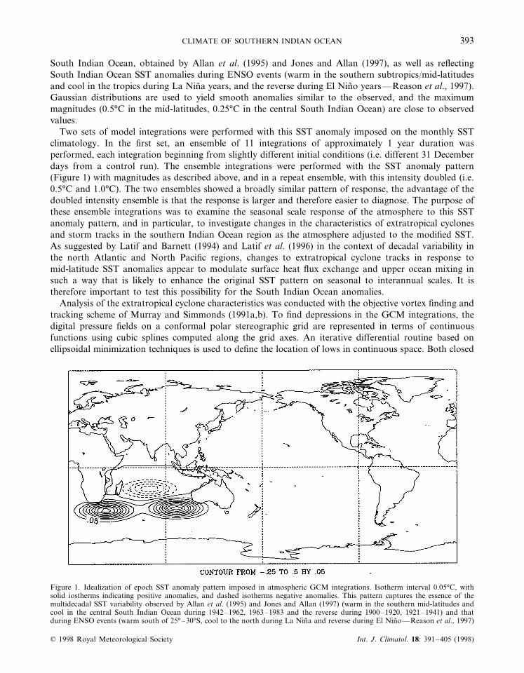
In order to clearly isolate the fundamental air–sea interaction mechanisms likely to be of relevance to thevariability, an idealized SST anomaly pattern (Figure 1) is imposed on the monthly SST climatology usedto force the GCM. This pattern captures the essence of the multidecadal patterns, i.e. largest anomaliesin the southern mid-latitudes of the Indian Ocean with a weaker anomaly of opposite sign in the central

© 1998 Royal Meteorological Society Int. J. Climatol. 18: 391–405 (1998)

CLIMATE OF SOUTHERN INDIAN OCEAN 393

South Indian Ocean, obtained by Allan et al. (1995) and Jones and Allan (1997), as well as reflectingSouth Indian Ocean SST anomalies during ENSO events (warm in the southern subtropics/mid-latitudesand cool in the tropics during La Nina years, and the reverse during El Nino years—Reason et al., 1997).Gaussian distributions are used to yield smooth anomalies similar to the observed, and the maximummagnitudes (0.5°C in the mid-latitudes, 0.25°C in the central South Indian Ocean) are close to observedvalues.

Two sets of model integrations were performed with this SST anomaly imposed on the monthly SSTclimatology. In the first set, an ensemble of 11 integrations of approximately 1 year duration wasperformed, each integration beginning from slightly different initial conditions (i.e. different 31 Decemberdays from a control run). The ensemble integrations were performed with the SST anomaly pattern(Figure 1) with magnitudes as described above, and in a repeat ensemble, with this intensity doubled (i.e.0.5°C and 1.0°C). The two ensembles showed a broadly similar pattern of response, the advantage of thedoubled intensity ensemble is that the response is larger and therefore easier to diagnose. The purpose ofthese ensemble integrations was to examine the seasonal scale response of the atmosphere to this SSTanomaly pattern, and in particular, to investigate changes in the characteristics of extratropical cyclonesand storm tracks in the southern Indian Ocean region as the atmosphere adjusted to the modified SST.As suggested by Latif and Barnett (1994) and Latif et al. (1996) in the context of decadal variability inthe north Atlantic and North Pacific regions, changes to extratropical cyclone tracks in response tomid-latitude SST anomalies appear to modulate surface heat flux exchange and upper ocean mixing insuch a way that is likely to enhance the original SST pattern on seasonal to interannual scales. It istherefore important to test this possibility for the South Indian Ocean anomalies.

Analysis of the extratropical cyclone characteristics was conducted with the objective vortex finding andtracking scheme of Murray and Simmonds (1991a,b). To find depressions in the GCM integrations, thedigital pressure fields on a conformal polar stereographic grid are represented in terms of continuousfunctions using cubic splines computed along the grid axes. An iterative differential routine based onellipsoidal minimization techniques is used to define the location of lows in continuous space. Both closed

Figure 1. Idealization of epoch SST anomaly pattern imposed in atmospheric GCM integrations. Isotherm interval 0.05°C, withsolid iostherms indicating positive anomalies, and dashed isotherms negative anomalies. This pattern captures the essence of themultidecadal SST variability observed by Allan et al. (1995) and Jones and Allan (1997) (warm in the southern mid-latitudes andcool in the central South Indian Ocean during 1942–1962, 1963–1983 and the reverse during 1900–1920, 1921–1941) and thatduring ENSO events (warm south of 25°–30°S, cool to the north during La Nina and reverse during El Nino—Reason et al., 1997)



(systems having a closed isobar at a given interval) and open depressions were included in the analysis.Locations of closed depressions were defined by minimization of the pressure functions, whereas opendepressions, indicating inflections in the pressure field, were found by searching for minima in the absolutevalue of the local pressure gradient. To prevent the inclusion of small-scale or broad, shallow featuresassociated with topography or other effects rather than genuine, migrating systems, a minimum curvaturetest (e.g. Jones and Simmonds, 1993) was applied. The ability of the Murray and Simmonds scheme toidentify and track systems in the observational record has been demonstrated by Jones and Simmonds(1993), to whom the reader is referred for further details of the scheme’s technical aspects andperformance.

In the second experiment, a 21 year integration of the GCM was performed with the SST anomaly ofFigure 1 imposed throughout. This integration was the same duration as the observational epochs usedin Allan et al. (1995) and Jones and Allan (1997). The imposed SST perturbation (see Figure 1) had amaximum positive anomaly of 0.5°C in the two southern mid-latitude regions and a minimum negativeanomaly in the central South Indian Ocean of −0.25°C. A GCM integration of this length effectivelygenerates its own statistics and enables one to determine the long-term adjustment of the atmosphere tothe SST anomaly. As with the short-term integrations, focus is placed on understanding how theatmospheric adjustments might influence SST evolution.

4. MODEL RESULTS

4.1. Ensemble of short-term integrations

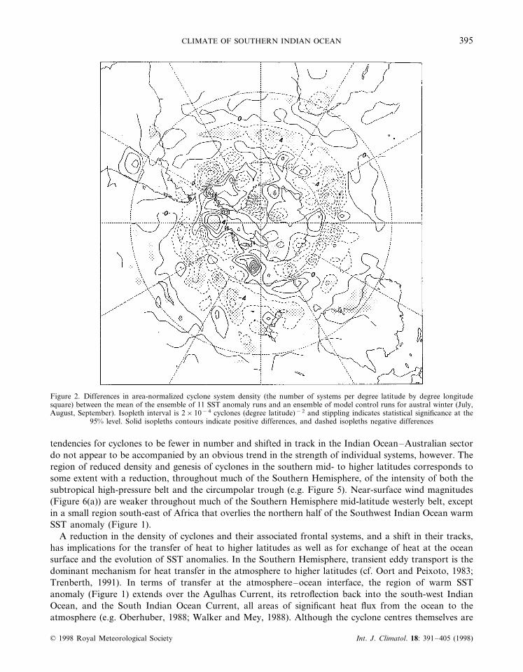
In this section, the seasonal-scale response of the atmosphere to the SST anomaly pattern (Figure 1) isanalysed with particular emphasis on the characteristics of the extratropical cyclones. To illustrate theseasonal-scale response in the ensemble of SST anomaly runs most succintly, conditions during the australwinter season (July, August, September) following model initialization on each respective 31 Decemberare considered. Figure 2 shows the difference in area-normalized cyclone system density (the number ofsystems per degree latitude by degree longitude square) between the mean of the 11 SST anomaly runsand the model climatology. It is evident that much of the circumpolar trough region, particularly in thesouth-east Atlantic, Indian and Australian sectors of the Southern Ocean near, and south of, the imposedSST anomaly, displays a significant reduction in the density of extratropical cyclones by comparison withthe model climatology.

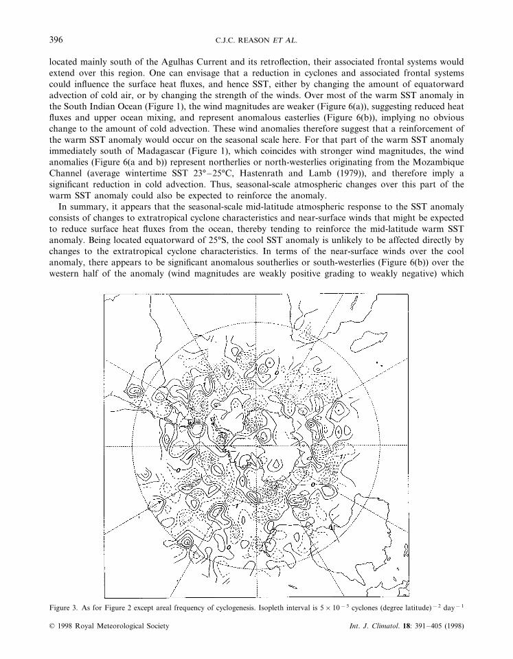
Related to this reduction in density is a decrease in the SST anomaly ensemble mean of the arealfrequency of cyclogenesis in much of the circumpolar trough region (Figure 3). There are also smallregions of increased cyclogenesis, very few of which are statistically significant. Most of the Indian Oceansector shows significant decreases in cyclogenesis, an exception is in the central part of this sector duesouth of the weakest region of imposed SST anomaly.

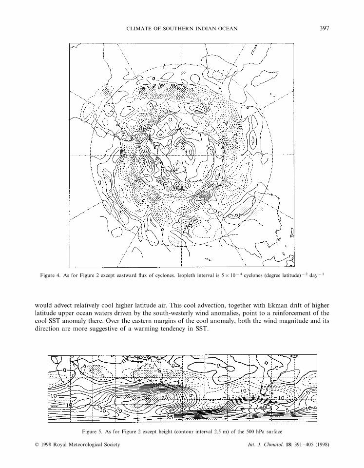
To determine whether this tendency for extratropical cyclones to be fewer in number in the ensembleof SST anomaly runs might be accompanied by a shift in the track of these systems, the eastward andnorthward flux of systems between the ensemble and climatology was compared. These parametersrespectively measure the number of systems tracking eastward and northward per day through a givenlatitude by longitude square. Figure 4 indicates that much of the circumpolar trough region is character-ized by a significant reduction in eastward flux of extratropical cyclones in the ensemble of SST anomalyruns. The corresponding difference in northward flux (not shown) indicated regions of significant increaseand decrease throughout the circumpolar trough, with most of the Indian Ocean–Australian sector(except south of the region of weakest SST anomaly) displaying an increase, or tendency for greaternorthward track, of systems.

Taken together, these results suggest that the ensemble of SST anomaly runs show a tendency forreduced genesis and density of cyclones in the southern mid- to higher latitudes, and that the track ofthese systems may be somewhat displaced from their climatological paths in the westerlies. These



Figure 2. Differences in area-normalized cyclone system density (the number of systems per degree latitude by degree longitudesquare) between the mean of the ensemble of 11 SST anomaly runs and an ensemble of model control runs for austral winter (July,August, September). Isopleth interval is 2×10−4 cyclones (degree latitude)−2 and stippling indicates statistical significance at the

95% level. Solid isopleths contours indicate positive differences, and dashed isopleths negative differences

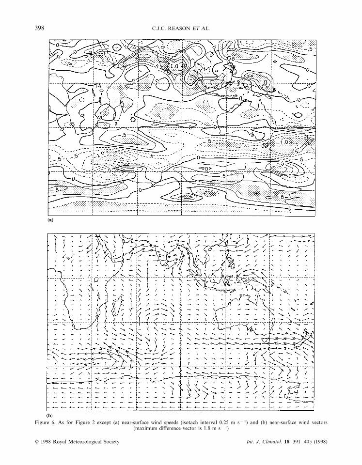
tendencies for cyclones to be fewer in number and shifted in track in the Indian Ocean–Australian sectordo not appear to be accompanied by an obvious trend in the strength of individual systems, however. Theregion of reduced density and genesis of cyclones in the southern mid- to higher latitudes corresponds tosome extent with a reduction, throughout much of the Southern Hemisphere, of the intensity of both thesubtropical high-pressure belt and the circumpolar trough (e.g. Figure 5). Near-surface wind magnitudes(Figure 6(a)) are weaker throughout much of the Southern Hemisphere mid-latitude westerly belt, exceptin a small region south-east of Africa that overlies the northern half of the Southwest Indian Ocean warmSST anomaly (Figure 1).

A reduction in the density of cyclones and their associated frontal systems, and a shift in their tracks,has implications for the transfer of heat to higher latitudes as well as for exchange of heat at the oceansurface and the evolution of SST anomalies. In the Southern Hemisphere, transient eddy transport is thedominant mechanism for heat transfer in the atmosphere to higher latitudes (cf. Oort and Peixoto, 1983;Trenberth, 1991). In terms of transfer at the atmosphere–ocean interface, the region of warm SSTanomaly (Figure 1) extends over the Agulhas Current, its retroflection back into the south-west IndianOcean, and the South Indian Ocean Current, all areas of significant heat flux from the ocean to theatmosphere (e.g. Oberhuber, 1988; Walker and Mey, 1988). Although the cyclone centres themselves are



located mainly south of the Agulhas Current and its retroflection, their associated frontal systems wouldextend over this region. One can envisage that a reduction in cyclones and associated frontal systemscould influence the surface heat fluxes, and hence SST, either by changing the amount of equatorwardadvection of cold air, or by changing the strength of the winds. Over most of the warm SST anomaly inthe South Indian Ocean (Figure 1), the wind magnitudes are weaker (Figure 6(a)), suggesting reduced heatfluxes and upper ocean mixing, and represent anomalous easterlies (Figure 6(b)), implying no obviouschange to the amount of cold advection. These wind anomalies therefore suggest that a reinforcement ofthe warm SST anomaly would occur on the seasonal scale here. For that part of the warm SST anomalyimmediately south of Madagascar (Figure 1), which coincides with stronger wind magnitudes, the windanomalies (Figure 6(a and b)) represent northerlies or north-westerlies originating from the MozambiqueChannel (average wintertime SST 23°–25°C, Hastenrath and Lamb (1979)), and therefore imply asignificant reduction in cold advection. Thus, seasonal-scale atmospheric changes over this part of thewarm SST anomaly could also be expected to reinforce the anomaly.

In summary, it appears that the seasonal-scale mid-latitude atmospheric response to the SST anomalyconsists of changes to extratropical cyclone characteristics and near-surface winds that might be expectedto reduce surface heat fluxes from the ocean, thereby tending to reinforce the mid-latitude warm SSTanomaly. Being located equatorward of 25°S, the cool SST anomaly is unlikely to be affected directly bychanges to the extratropical cyclone characteristics. In terms of the near-surface winds over the coolanomaly, there appears to be significant anomalous southerlies or south-westerlies (Figure 6(b)) over thewestern half of the anomaly (wind magnitudes are weakly positive grading to weakly negative) which

Figure 3. As for Figure 2 except areal frequency of cyclogenesis. Isopleth interval is 5×10−5 cyclones (degree latitude)−2 day−1



Figure 4. As for Figure 2 except eastward flux of cyclones. Isopleth interval is 5×10−4 cyclones (degree latitude)−2 day−1

would advect relatively cool higher latitude air. This cool advection, together with Ekman drift of higherlatitude upper ocean waters driven by the south-westerly wind anomalies, point to a reinforcement of thecool SST anomaly there. Over the eastern margins of the cool anomaly, both the wind magnitude and itsdirection are more suggestive of a warming tendency in SST.

Figure 5. As for Figure 2 except height (contour interval 2.5 m) of the 500 hPa surface



Figure 6. As for Figure 2 except (a) near-surface wind speeds (isotach interval 0.25 m s−1) and (b) near-surface wind vectors(maximum difference vector is 1.8 m s−1)



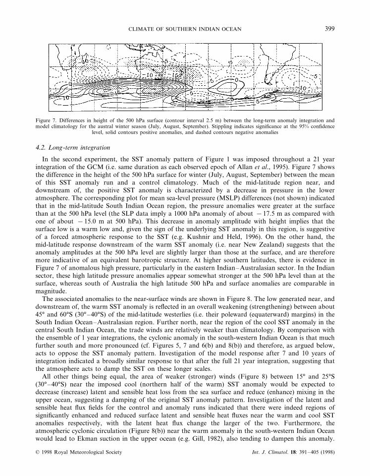
Figure 7. Differences in height of the 500 hPa surface (contour interval 2.5 m) between the long-term anomaly integration andmodel climatology for the austral winter season (July, August, September). Stippling indicates significance at the 95% confidence

level, solid contours positive anomalies, and dashed contours negative anomalies

4.2. Long-term integration

In the second experiment, the SST anomaly pattern of Figure 1 was imposed throughout a 21 yearintegration of the GCM (i.e. same duration as each observed epoch of Allan et al., 1995). Figure 7 showsthe difference in the height of the 500 hPa surface for winter (July, August, September) between the meanof this SST anomaly run and a control climatology. Much of the mid-latitude region near, anddownstream of, the positive SST anomaly is characterized by a decrease in pressure in the loweratmosphere. The corresponding plot for mean sea-level pressure (MSLP) differences (not shown) indicatedthat in the mid-latitude South Indian Ocean region, the pressure anomalies were greater at the surfacethan at the 500 hPa level (the SLP data imply a 1000 hPa anomaly of about −17.5 m as compared withone of about −15.0 m at 500 hPa). This decrease in anomaly amplitude with height implies that thesurface low is a warm low and, given the sign of the underlying SST anomaly in this region, is suggestiveof a forced atmospheric response to the SST (e.g. Kushnir and Held, 1996). On the other hand, themid-latitude response downstream of the warm SST anomaly (i.e. near New Zealand) suggests that theanomaly amplitudes at the 500 hPa level are slightly larger than those at the surface, and are thereforemore indicative of an equivalent barotropic structure. At higher southern latitudes, there is evidence inFigure 7 of anomalous high pressure, particularly in the eastern Indian–Australasian sector. In the Indiansector, these high latitude pressure anomalies appear somewhat stronger at the 500 hPa level than at thesurface, whereas south of Australia the high latitude 500 hPa and surface anomalies are comparable inmagnitude.

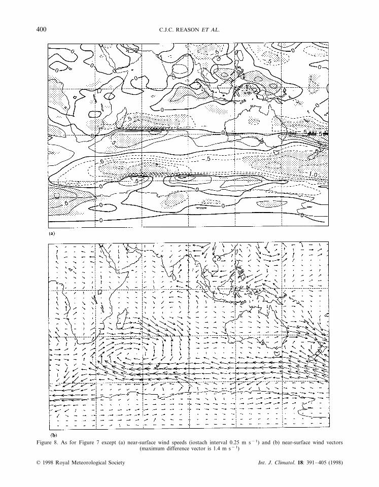
The associated anomalies to the near-surface winds are shown in Figure 8. The low generated near, anddownstream of, the warm SST anomaly is reflected in an overall weakening (strengthening) between about45° and 60°S (30°–40°S) of the mid-latitude westerlies (i.e. their poleward (equaterward) margins) in theSouth Indian Ocean–Australasian region. Further north, near the region of the cool SST anomaly in thecentral South Indian Ocean, the trade winds are relatively weaker than climatology. By comparison withthe ensemble of 1 year integrations, the cyclonic anomaly in the south-western Indian Ocean is that muchfurther south and more pronounced (cf. Figures 5, 7 and 6(b) and 8(b)) and therefore, as argued below,acts to oppose the SST anomaly pattern. Investigation of the model response after 7 and 10 years ofintegration indicated a broadly similar response to that after the full 21 year integration, suggesting thatthe atmosphere acts to damp the SST on these longer scales.

All other things being equal, the area of weaker (stronger) winds (Figure 8) between 15° and 25°S(30°–40°S) near the imposed cool (northern half of the warm) SST anomaly would be expected todecrease (increase) latent and sensible heat loss from the sea surface and reduce (enhance) mixing in theupper ocean, suggesting a damping of the original SST anomaly pattern. Investigation of the latent andsensible heat flux fields for the control and anomaly runs indicated that there were indeed regions ofsignificantly enhanced and reduced surface latent and sensible heat fluxes near the warm and cool SSTanomalies respectively, with the latent heat flux change the larger of the two. Furthermore, theatmospheric cyclonic circulation (Figure 8(b)) near the warm anomaly in the south-western Indian Oceanwould lead to Ekman suction in the upper ocean (e.g. Gill, 1982), also tending to dampen this anomaly.



Figure 8. As for Figure 7 except (a) near-surface wind speeds (iostach interval 0.25 m s−1) and (b) near-surface wind vectors(maximum difference vector is 1.4 m s−1)



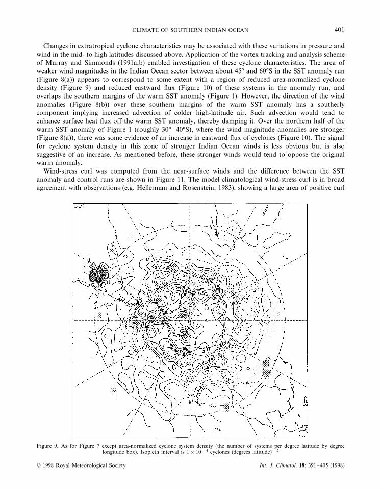
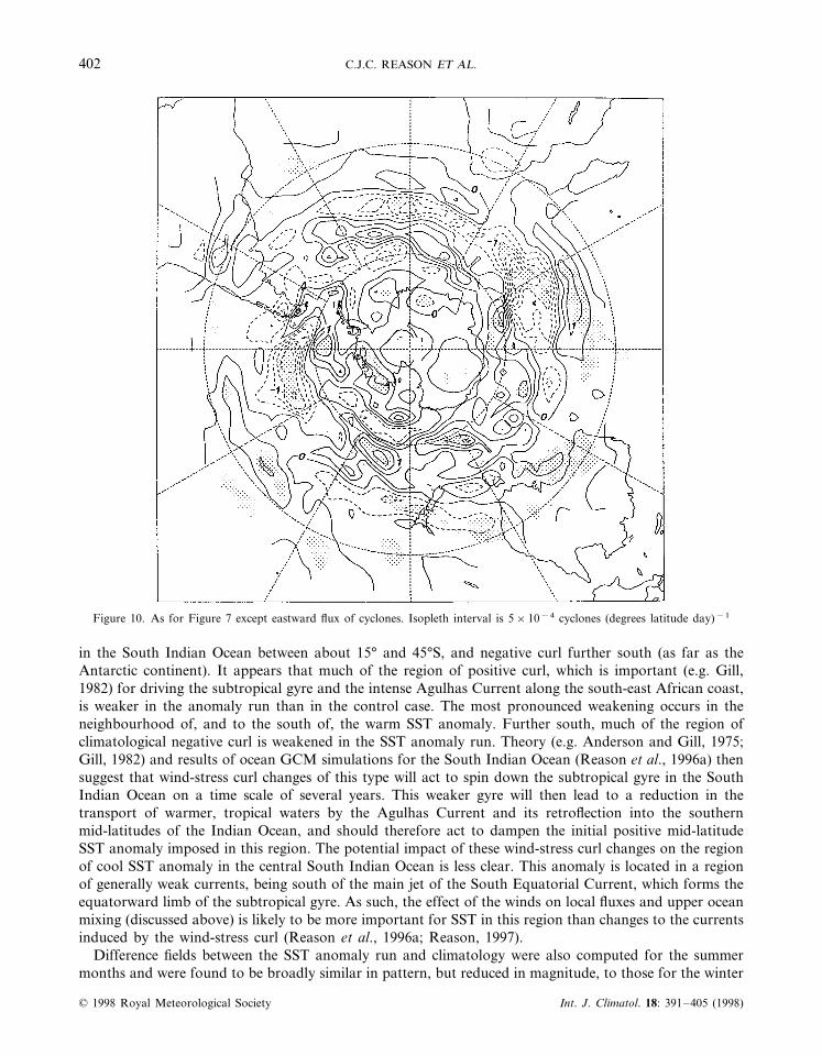
Changes in extratropical cyclone characteristics may be associated with these variations in pressure andwind in the mid- to high latitudes discussed above. Application of the vortex tracking and analysis schemeof Murray and Simmonds (1991a,b) enabled investigation of these cyclone characteristics. The area ofweaker wind magnitudes in the Indian Ocean sector between about 45° and 60°S in the SST anomaly run(Figure 8(a)) appears to correspond to some extent with a region of reduced area-normalized cyclonedensity (Figure 9) and reduced eastward flux (Figure 10) of these systems in the anomaly run, andoverlaps the southern margins of the warm SST anomaly (Figure 1). However, the direction of the windanomalies (Figure 8(b)) over these southern margins of the warm SST anomaly has a southerlycomponent implying increased advection of colder high-latitude air. Such advection would tend toenhance surface heat flux off the warm SST anomaly, thereby damping it. Over the northern half of thewarm SST anomaly of Figure 1 (roughly 30°–40°S), where the wind magnitude anomalies are stronger(Figure 8(a)), there was some evidence of an increase in eastward flux of cyclones (Figure 10). The signalfor cyclone system density in this zone of stronger Indian Ocean winds is less obvious but is alsosuggestive of an increase. As mentioned before, these stronger winds would tend to oppose the originalwarm anomaly.

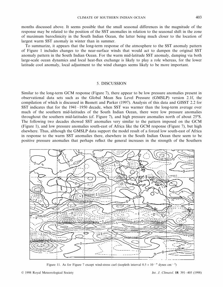
Wind-stress curl was computed from the near-surface winds and the difference between the SSTanomaly and control runs are shown in Figure 11. The model climatological wind-stress curl is in broadagreement with observations (e.g. Hellerman and Rosenstein, 1983), showing a large area of positive curl

Figure 9. As for Figure 7 except area-normalized cyclone system density (the number of systems per degree latitude by degreelongitude box). Isopleth interval is 1×10−4 cyclones (degrees latitude)−2



Figure 10. As for Figure 7 except eastward flux of cyclones. Isopleth interval is 5×10−4 cyclones (degrees latitude day)−1

in the South Indian Ocean between about 15° and 45°S, and negative curl further south (as far as theAntarctic continent). It appears that much of the region of positive curl, which is important (e.g. Gill,1982) for driving the subtropical gyre and the intense Agulhas Current along the south-east African coast,is weaker in the anomaly run than in the control case. The most pronounced weakening occurs in theneighbourhood of, and to the south of, the warm SST anomaly. Further south, much of the region ofclimatological negative curl is weakened in the SST anomaly run. Theory (e.g. Anderson and Gill, 1975;Gill, 1982) and results of ocean GCM simulations for the South Indian Ocean (Reason et al., 1996a) thensuggest that wind-stress curl changes of this type will act to spin down the subtropical gyre in the SouthIndian Ocean on a time scale of several years. This weaker gyre will then lead to a reduction in thetransport of warmer, tropical waters by the Agulhas Current and its retroflection into the southernmid-latitudes of the Indian Ocean, and should therefore act to dampen the initial positive mid-latitudeSST anomaly imposed in this region. The potential impact of these wind-stress curl changes on the regionof cool SST anomaly in the central South Indian Ocean is less clear. This anomaly is located in a regionof generally weak currents, being south of the main jet of the South Equatorial Current, which forms theequatorward limb of the subtropical gyre. As such, the effect of the winds on local fluxes and upper oceanmixing (discussed above) is likely to be more important for SST in this region than changes to the currentsinduced by the wind-stress curl (Reason et al., 1996a; Reason, 1997).

Difference fields between the SST anomaly run and climatology were also computed for the summermonths and were found to be broadly similar in pattern, but reduced in magnitude, to those for the winter



months discussed above. It seems possible that the small seasonal differences in the magnitude of theresponse may be related to the position of the SST anomalies in relation to the seasonal shift in the zoneof maximum baroclinicity in the South Indian Ocean, the latter being much closer to the location oflargest warm SST anomaly in winter than in summer.

To summarize, it appears that the long-term response of the atmosphere to the SST anomaly patternof Figure 1 includes changes to the near-surface winds that would act to dampen the original SSTanomaly pattern in the South Indian Ocean. For the warm mid-latitude SST anomaly, damping via bothlarge-scale ocean dynamics and local heat-flux exchange is likely to play a role whereas, for the lowerlatitude cool anomaly, local adjustment to the wind changes seems likely to be more important.

5. DISCUSSION

Similar to the long-term GCM response (Figure 7), there appear to be low pressure anomalies present inobservational data sets such as the Global Mean Sea Level Pressure (GMSLP) version 2.1f, thecompilation of which is discussed in Basnett and Parker (1997). Analysis of this data and GISST 2.2 forSST indicates that for the 1941–1950 decade, when SST was warmer than the long-term average overmuch of the southern mid-latitudes of the South Indian Ocean, there were low pressure anomaliesthroughout the southern mid-latitudes (cf. Figure 7), and high pressure anomalies north of about 25°S.The following two decades showed SST anomalies very similar to the pattern imposed on the GCM(Figure 1), and low pressure anomalies south-east of Africa like the GCM response (Figure 7), but highelsewhere. Thus, although the GMSLP data support the model result of a forced low south-east of Africain response to the warm SST anomalies there, elsewhere in the South Indian Ocean there seem to bepositive pressure anomalies that perhaps reflect the general increases in the strength of the Southern

Figure 11. As for Figure 7 except wind-stress curl (isopleth interval 0.5×10−9 dynes cm−3)



Hemisphere semi-permanent anticyclones that are apparent during the decades after 1950 (Jones andAllan, 1997; Reason et al., 1997). Consistent with generally higher subtropical pressure, and hencestronger winds and an increased transport of tropical waters polewards by the South Indian gyre (eitherdirectly via the stronger South Indian Ocean anticyclone, or via a modulated Indonesian throughflow—Reason et al., 1996b), SST anomalies in the Agulhas Current system and southern mid-latitudes tend tobe warm during this post-1950 period. Further research is needed to confirm the apparent relationshipsbetween decadal/multidecadal variability in SST and atmospheric circulation over the South IndianOcean, but it appears that both a basin scale coupled interaction of the atmosphere–ocean system in theSouth Indian Ocean (similar to the hypothesis of Latif and Barnett (1994) and Latif et al. (1996) fordecadal North Pacific and North Atlantic variability) as well as a hemispheric scale modulation of theSouthern Hemisphere subtropical semipermanent anticyclones may contribute. The interconnectedness ofthe Southern Hemisphere oceans via the Antarctic Circumpolar Current, Indonesian throughflow, andleakage of Agulhas rings into the south-east Atlantic offers one possibility as to how a particular oceanbasin may reflect decadal/multidecadal variability originating from elsewhere in the Southern Hemisphere.

6. CONCLUSIONS

The Melbourne University atmospheric GCM has been used to study the atmospheric response to anidealized SST anomaly pattern in the South Indian Ocean that captures the essence of both observedENSO (La Nina) and multidecadal SST variability in this region. This pattern consists of a warmanomaly extending across the southern mid-latitudes of the South Indian Ocean, and a cool anomaly inthe central South Indian Ocean. The primary objective has been to investigate air–sea interactionmechanisms potentially associated with the observed low-frequency variability in this region, and whetherthe atmospheric response to the SST is likely to lead to damping or maintenance of the original SSTanomaly pattern, and on what time scale. Analysis of an ensemble of 1 year long integrations with theimposed SST anomaly has suggested that changes in extratropical cyclone characteristics and associatedfluxes in the South Indian Ocean are likely to lead to enhancement of the original SST anomaly patternon the seasonal scale.

On the other hand, the decadal to multidecadal response of the GCM to the SST suggests that theatmosphere might respond in such a way that favours damping of the original anomaly. This dampingoccurs both through changes to the wind-stress curl, which spin down the subtropical gyre in the SouthIndian Ocean, and through changes to the surface fluxes and upper ocean mixing. In terms of theatmospheric circulation, because the surface to mid-level low generated near the mid-latitude warm SSTanomaly is that much further south in the long-term integration compared with the seasonal-scale runs,and therefore relative to the background climatology, the anomalous near-surface winds and fluxes wouldtend to dampen the original SST anomaly pattern on longer time scales.

ACKNOWLEDGEMENTS

We thank Ian Simmonds, Ross Murray and Mark Holzer for useful discussions. RJA acknowledgessupport from the CSIRO Climate Change Research Program, funded in part by the CommonwealthDepartment of Environment, Sport and Territories, and the State Governments of Victoria, Queensland,Western Australia and the Northern Territory. Partial funding for this work from the Australian ResearchCouncil is gratefully acknowledged.

REFERENCES

Allan, R.J., Lindesay, J.A. and Reason, C.J.C. 1995. ‘Multidecadal variability in the climate system over the Indian Ocean regionduring the austral summer’, J. Climate, 8, 1853–1873.

Allan, R.J., Lindesay, J.A. and Parker, D.E. 1996. El Nino Southern Oscillation and Climatic Variability, CSIRO Publishing,Collingwood, Victoria, 416 pp.



Anderson, D.L.T. and Gill, A.E. 1975. ‘Spin-up of a stratified ocean, with application to upwelling’, Deep-Sea Res., 22, 583–596.Basnett, T.A. and Parker, D.E. 1997. De6elopment of the Global Mean Sea Le6el Pressure Data Set GMSLP Version 2, United

Kingdom Meteorological Office, Climate Research Technical Note, 79, 16 pp.Boer, G.J., et al. 1992. ‘Some results from an intercomparison of the climates simulated by 14 atmospheric general circulation

models’, J. Geophys. Res., 97, 12771–12786.Budd, W.F. and Simmonds, I.H. 1990. Influence of Ocean Temperatures on the Atmosphere and the Atmosphere on Ocean

Temperatures, Bureau of Meteorology Research Centre, Research Report No. 21, Australian Bureau of Meteorology, pp. 84–87.Deardorff, J.W. 1977. ‘A parameterization of ground-surface moisture content for use in atmospheric prediction models’, J. Appl.

Meteorol., 16, 1182–1185.Gates, W.L. and Nelson, A.B. 1975. A New (re6ised) Tabulation of the Scripps Topography on a 1° Global Grid. Part I: Terrain

Heights. The Rand Corporation, R-1276-1-ARPA, 132 pp.Gill, A.E. 1982. Atmosphere–Ocean Dynamics, Academic Press, New York, 662 pp.Hastenrath, S. and Lamb, P.J. 1979. Climatic Atlas of the Indian Ocean, Part I: Surface Climate and Atmospheric Circulation.

University of Wisconsin Press.Hellerman, S. and Rosenstein, M. 1983. ‘Normal monthly windstress over the world ocean with error estimates’, J. Phys. Oceanogr.,

13, 1093–1104.Jones, D.A. and Simmonds, I.H. 1993. ‘A climatology of Southern Hemisphere extratropical cyclones’, Climate Dyn., 9, 131–145.Jones, P.D. and Allan, R.J. 1997. ‘Climate change and long-term variability’, in Karoly, D. Vincent, D. (eds), Meteorology of the

Southern Hemisphere, American Meteorology Society Monograph, in press.Kushnir, Y. and Held, I.M. 1996. ‘Equilibrium atmospheric response to North Atlantic SST anomalies’, J. Climate, 9, 1208–1220.Latif, M. and Barnett, T.P. 1994. ‘Causes of decadal climate variability over the North Pacific and North America’, Science, 266,

634–637.Latif, M., Groetzner, A. and Barnett, T.P. 1996. ‘A mechanism for decadal climate variability’, Atlantic Climate Change Prog. Notes,

3(1), 1–3.Manabe, S., Smagorinsky, J. and Strickler, R.F. 1965. ‘Simulated climatology of a general circulation model with a hydrologic

cycle’, Mon. Wea. Re6., 93, 769–798.Murray, R.J. and Simmonds, I.H. 1991a. ‘A numerical scheme for tracking cyclone centres from digital data. Part I: development

and operation of the scheme’, Aust. Meteorol. Mag., 39, 155–166.Murray, R.J. and Simmonds, I.H. 1991b. ‘A numerical scheme for tracking cyclone centres from digital data. Part II: application

to January and July GCM simulations’, Aust. Meteorol. Mag., 39, 167–180.Oberhuber, J.M. 1988. An Atlas Based on the COADS Data Set: the Budgets of Heat, buoyancy, and Turbulent Kinetic Energy at the

Surface of the Global Ocean, Report No. 15, Max-Planck Institut fur Meteorologie.Oort, A.H. and Peixoto, J.P. 1983. ‘Global angular momentum and energy balance requirements from observations’, Ad6. Geophys.,

25, 355–490.Parker, D.E., Jackson, M. and Horton, E.B. 1995. The GISST2.2 Sea Surface Temperature and Sea-ice Climatology, Climate

Research Technical Note 63, Hadley Centre, United Kingdom Meteorological Office, Bracknell, 35 pp.Reason, C.J.C. 1997. ‘Local air–sea interaction and multidecadal climate variability in the Indian Ocean region’, J. Climate,

submitted.Reason, C.J.C. and Lutjeharms, J.R.E. 1998. ‘Variability of the South Indian Ocean and implications for southern African rainfall’,

S. Afr. J. Sci., in press.Reason, C.J.C., Allan, R.J. and Lindesay, J.A. 1996a. ‘Dynamical response of the oceanic circulation and temperature to

interdecadal variability in the surface winds over the Indian Ocean’, J. Climate, 9, 97–114.Reason, C.J.C., Allan, R.J. and Lindesay, J.A. 1996b. ‘Evidence for the influence of remote forcing on interdecadal variability in

the southern Indian Ocean’, J. Geophys. Res., 101, 11867–11882.Reason, C.J.C., Allan, R.J. and Lindesay, J.A. 1997. ‘Climate variability on decadal time scales: mechanisms and implications for

climate change’, in Palaeoclimates: Data and Modelling, accepted.Reynolds, R.W., 1988. ‘A real-time global sea surface temperature analysis’, J. Climate, 1, 75–86.Rocha, A. and Simmonds, I.H. 1997. ‘Interannual variability of Southern African summer rainfall. Part II: modelling the impact of

sea-surface temperatures on rainfall and circulation’, Int. J. Climatol. 17, 267–290.Shannon, L.V., Agenbag, J.J., Walker, N.D. and Lutjeharms, J.R.E. 1990. ‘A major perturbation in the Agulhas retroflection area

in 1986’, Deep Sea Res., 37, 493–512.Simmonds, I.H. 1985. ‘Analysis of the ‘spinup’ of a general circulation model’, J. Geophys. Res., 90, 5637–5660.Simmonds, I.H. 1990. ‘A modelling study of winter circulation and precipitation anomalies associated with Australian region ocean

temperatures’, Aust. Meteorol. Mag., 38, 151–162.Simmonds, I.H. and Smith, I.N. 1986. ‘The effect of the prescription of zonally-uniform sea surface temperatures in a general

circulation model’, J. Climatol., 6, 641–659.Simmonds, I.H., Trigg, G. and Law, R. 1988. The Climatology of the Melbourne Uni6ersity General Circulation Model, Publication

31, Meteorology, School of Earth Sciences, University of Melbourne, 67 pp. (NTIS PB 88 227491).Trenberth, K.E. 1991. ‘Storm tracks in the Southern Hemisphere’, J. Atmos. Sci., 48, 2159–2178.Walker, N.D. and Mey, R.D. 1988. ‘Ocean–atmosphere heat fluxes within the Agulhas retroflection region’, J. Geophys. Res., 93,

15473–15483.Woodruff, S.D., Slutz, R.J., Jenne, R.L. and Steurer, P.M. 1987. ‘A comprehensive ocean–atmosphere data set’, Bull. Am. Meteorol.

Soc., 68, 1239–1250.


Documents

Air–sea interaction mechanisms and low-frequency climate variability in the South Indian Ocean region