Embed Size (px)
Citation preview

FinalReport
Airport Deployment Study
Ref MC/045
Issued to: Ofcom Version: 1.5 Issue Date: 19th July 2011
Real Wireless Ltd
PO Box 2218
Pulborough
West Sussex
RH20 4XB
United Kingdom
www.realwireless.biz
Tel: +44 207 117 8514
Fax: +44 808 280 0142

2
Contents Final Report ..........................................................................................................................................................1
Airport Deployment Study ................................................................................................................................1
1 Executive Summary ......................................................................................................................................9
1.1 Study context ........................................................................................................................................9
1.2 Key findings and recommendations .................................................................................................. 10
1.3 Our approach and assumptions ........................................................................................................ 21
1.4 Study results in detail ........................................................................................................................ 23
2 Introduction ............................................................................................................................................... 28
2.1 Airport deployment study ................................................................................................................. 30
2.2 Structure of report ............................................................................................................................ 30
3 Background and scope .............................................................................................................................. 33
3.1 Background ........................................................................................................................................ 33
3.2 Scope of study ................................................................................................................................... 35
4 Characteristics of 2.6 GHz equipment ....................................................................................................... 38
4.1 LTE and WiMAX equipment ............................................................................................................... 38
4.2 Equipment performance statistics .................................................................................................... 40
4.3 Practical considerations for mobile communications equipment operation .................................... 45
5 Overview of stakeholder engagement ...................................................................................................... 54
5.1 Mobile Network Operator view ........................................................................................................ 54
5.2 Equipment vendor view .................................................................................................................... 55
5.3 Airport operator support ................................................................................................................... 56
5.4 Summary of RF site survey at Heathrow Airport ............................................................................... 58
5.5 Summary of stakeholder engagement .............................................................................................. 60
6 Interference Analysis Modelling ................................................................................................................ 61
6.1 Objectives .......................................................................................................................................... 61
3
6.2 Interference assessment methods .................................................................................................... 61
7 Overview of software model ..................................................................................................................... 68
7.1 Model flowcharts ............................................................................................................................... 68
7.2 Program structure ............................................................................................................................. 77
8 Parameters ................................................................................................................................................ 79
8.1 Main input parameters ...................................................................................................................... 79
8.2 Base station and mobile station parameters .................................................................................... 80
8.3 Radar parameters .............................................................................................................................. 90
8.4 Modelling assumptions and simulation parameters ......................................................................... 93
9 Explanation of modelling outputs ........................................................................................................... 106
9.1 Statistical analysis ............................................................................................................................ 106
9.2 Example result output plots ............................................................................................................ 109
9.3 Interference over all angles ............................................................................................................. 116
10 Interference modelling results from base stations and mobile station scenarios without additional
mitigations ....................................................................................................................................................... 118
10.1 Base station to radar – Single base station transmitter at variable distance from the radar with
challenging case conditions ......................................................................................................................... 119
10.2 Base station to radar – Challenging Heathrow layout ..................................................................... 125
10.3 Base station to radar – Typical Heathrow layout ............................................................................ 130
10.4 Base station to radar – Challenging synthetic layout ...................................................................... 134
10.5 Summary findings of base station to radar ..................................................................................... 141
10.6 Mobile station to radar – Single mobile station transmitter at variable distance from the radar with
challenging case conditions ......................................................................................................................... 146
10.7 Mobile station to radar – Challenging case ..................................................................................... 152
10.8 Mobile station to radar – Typical case ............................................................................................ 156
10.9 Mobile station to radar – Measured emissions case....................................................................... 160
10.10 Summary of findings for mobile station to radar ........................................................................ 163
10.11 Mitigation techniques identified from interference analysis ...................................................... 168
4
11 Interference modelling results with mitigations ................................................................................. 172
11.1 Discussion of mitigation approaches ............................................................................................... 172
11.2 Performance of Mitigation solutions............................................................................................... 174
11.3 Findings ............................................................................................................................................ 183
11.4 Mobile station to radar .................................................................................................................... 187
11.5 Impact on cost to 2.6 GHz deployments ......................................................................................... 191
12 Conclusions and summary recommendations .................................................................................... 196
12.1 Conclusions ...................................................................................................................................... 196
12.2 Summarised conclusions ................................................................................................................. 196
12.3 Recommendations ........................................................................................................................... 199
13 Glossary ............................................................................................................................................... 202
14 References ........................................................................................................................................... 203
5
Figure 1-1 Example of modified radar receiver block diagram ........................................................................ 22
Figure 2-1 Structure of final report ................................................................................................................... 32
Figure 3-1: Main interference mechanisms ...................................................................................................... 34
Figure 4-1 Mobile broadband USB dongle modem ........................................................................................... 43
Figure 4-2 ACLR emission plot from RFI Global Services Ltd measurement of Samsung LTE UE – 1 at maximum
transmitted power 21 dBm ............................................................................................................................... 44
Figure 4-3 ACLR emission plots from RFI Global Services Ltd measurement of Samsung LTE UE – 2 at reduced
power -4 dB ....................................................................................................................................................... 44
Figure 4-4 Base station form factor comparison GSM v WiMAX ...................................................................... 46
Figure 4-5 UE equipment likely to deployed in 2.6 GHz .................................................................................... 47
Figure 4-6 Noise floor estimates for BS and MS (FDD/TDD) referred to the antenna connector ..................... 49
Figure 4-7 CDF of power control of the mobile ................................................................................................. 51
Figure 4-8 Physical Resource Block configurations ........................................................................................... 52
Figure 5-1 High level layout plan of Heathrow Airport ..................................................................................... 57
Figure 5-2 High level layout of Central Terminal Area with cellular sites locations .......................................... 58
Figure 5-3 High level layout of the area surrounding Terminal 4 and the S-band radar at Heathrow airport . 58
Figure 6-1 Out-of-band and in-band 2.6 GHz interference mechanisms into radar receiver NOTE: There are
complex intermodulation and radar receiver mixing effects which can cause a result similar to the sum of
both effects ....................................................................................................................................................... 62
Figure 7-1 MATLAB software model flowchart ................................................................................................. 68
Figure 7-2 High level model flowchart of simulation process for the uplink .................................................... 69
Figure 7-3 High level model flowchart of simulation process for the downlink ............................................... 69
Figure 7-4 Medium level model flowchart of simulation process for the uplink (Part 1) ................................. 70
Figure 7-5 Medium level model flowchart of simulation process for the uplink (Part 2) ................................. 71
Figure 7-6 Medium level model flowchart of simulation process for the downlink (Part 1) ............................ 73
Figure 7-7 Medium level model flowchart of simulation process for the downlink (Part 2) ............................ 74
Figure 7-8 Mobile station and base station position plotted on map area ....................................................... 76
Figure 7-9 Blocking power from all base stations at radar antenna connector ................................................ 77
Figure 8-1 WiMAX BS CDF of the EIRP used in the model ................................................................................. 80
Figure 8-2 LTE BS CDF of the EIRP used in the model ....................................................................................... 81
Figure 8-3 WiMAX BS PDF of the EIRP used in the model ................................................................................. 82
Figure 8-4 LTE BS PDF of the EIRP used in the model........................................................................................ 82
Figure 8-5 Creating an OFDM signal .................................................................................................................. 83
Figure 8-6 Example combination of multiple sine waves to obtain PAPR ......................................................... 84
6
Figure 8-7 3GPP BS spectrum emission mask including Ofcom BEM ................................................................ 86
Figure 8-8 3GPP UE spectrum emissions mask including Ofcom BEM .............................................................. 86
Figure 8-9 WiMAX BS IEEE specification spectrum emission mask including Ofcom BEM ............................... 87
Figure 8-10 WiMAX MS IEEE specification spectrum emission mask including Ofcom BEM ............................ 87
Figure 8-11 LTE BS typical case spectrum emission mask including Ofcom BEM ............................................. 88
Figure 8-12 LTE UE typical case spectrum emission mask including Ofcom BEM ............................................. 88
Figure 8-13 WiMAX BS typical case spectrum emission mask including Ofcom BEM ....................................... 89
Figure 8-14 WiMAX MS typical case spectrum emission mask including Ofcom BEM ..................................... 89
Figure 8-15 Block diagram of modified generic radar receive chain ................................................................. 91
Figure 8-16 1st RF filter response (isotek) ......................................................................................................... 93
Figure 8-17 Three sector base station horizontal antenna pattern .................................................................. 95
Figure 8-18 Simulation area polygons: the star represents the radar location ................................................ 97
Figure 8-19 Heathrow Airport Central Terminal Area clutter layers ............................................................... 100
Figure 8-20 Heathrow Airport Central Terminal Area landscape .................................................................... 100
Figure 8-21 Path distance with line of sight – Radar and MS nearby .............................................................. 102
Figure 8-22 Far away path distance taking clutter into account ..................................................................... 102
Figure 9-1 Example cumulative distribution functions (CDF) of power received at the radar antenna
connector. Each line represents the distribution for a given radar orientation angle. The line with crosses
represents the composite worst-case CDF across all angles. .......................................................................... 107
Figure 9-2 Polar plot of angle of highest interference showing blocking level from direction of the base
stations ............................................................................................................................................................ 109
Figure 9-3 Example CDF of blocking levels from base stations at point A and point B in the receiver showing
its corresponding threshold limit .................................................................................................................... 110
Figure 9-4 Example graph of each base station peak blocking level at Point A in radar receiver Noise rise at
the radar receiver co-channel with the radar centre frequency from base stations ...................................... 111
Figure 9-5 I/N level from base station into radar ............................................................................................ 111
Figure 9-6 Bar graph of each base station I/N level into the radar receiver ................................................... 112
Figure 9-7 Example CDF results of blocking levels from mobile stations showing blocking at point A and point
B in radar receiver with its corresponding threshold. ..................................................................................... 113
Figure 9-8 2D and 3D polar plots for detailed analysis of angle of worst interference .................................. 114
Figure 9-9 Example CDF results of interference noise rise for MS into radar ................................................. 115
Figure 9-10 Comparison of CFD curve at 1% time between the worst angle and over all angles .................. 116
Figure 10-1 Base station locations under investigation .................................................................................. 120
7
Figure 10-2 Blocking at point A for base station positions 1 to 5 using challenging case parameters (Before
filtering) ........................................................................................................................................................... 121
Figure 10-3 Blocking at point B for base station positions 1 to 5 using challenging case parameters (after
filtering) ........................................................................................................................................................... 121
Figure 10-4 I/N levels for base station positions 1 to 5 using challenging case parameters .......................... 122
Figure 10-5 Combined pathloss and vertical-pattern attenuation vs distance from the radar. Radar effective
vertical HPBW = 4.4deg, radar height = 5m, radar uptilt = 2deg, BS height = 25m, BS downtilt = 0deg, BS
vertical HPBW = 6.5deg. .................................................................................................................................. 124
Figure 10-6 Base stations modelled for BS to radar scenarios ........................................................................ 125
Figure 10-7 Blocking levels from BS into radar receiver - Challenging Heathrow layout scenario ................. 126
Figure 10-8 Peak I/N level from BS into radar receiver – Challenging case Heathrow layout scenario .......... 127
Figure 10-9 Received peak interference power at Point A of the receiver chain, when the rotation angle of
the radar points at each BS ............................................................................................................................. 128
Figure 10-10 Peak interference noise rise, when the rotation angle of the radar points at each BS ............. 129
Figure 10-11 Blocking level from BS into radar – Typical Heathrow layout .................................................... 131
Figure 10-12 I/N level from BS into radar – Typical Heathrow layout ............................................................ 132
Figure 10-13 Blocking levels from BS into radar - Typical Heathrow layout ................................................... 132
Figure 10-14 Peak I/N levels from BS to radar - Typical Heathrow layout ...................................................... 133
Figure 10-15 Base stations at incremental distances from the radar – Challenging synthetic layout ............ 134
Figure 10-16 Overall blocking levels at worst angle of BS into radar – Challenging synthetic layout (outdoor)
......................................................................................................................................................................... 135
Figure 10-17 I/N levels at worst angle of BS into radar – Challenging synthetic layout (outdoor) ................. 136
Figure 10-18 Results of peak blocking level at point A – Challenging synthetic layout (outdoor) .................. 137
Figure 10-19 Results from peak interference noise power – Challenging synthetic layout (outdoor) ........... 137
Figure 10-20 Overall blocking levels at worst angle of BS into radar – Challenging synthetic layout (indoor)138
Figure 10-21 I/N levels at worst angle – Challenging synthetic layout (indoor) ............................................. 139
Figure 10-22 Blocking from each base station at Point A................................................................................ 139
Figure 10-23 Results from peak interference noise power – Challenging synthetic layout (indoor) .............. 140
Figure 10-24 Polygon positions for mobile station investigation. Blue dots represent the mobile station
random location. See Table 6 for the distance of the polygon to the radar location. .................................... 147
Figure 10-25 Average interference blocking levels at point A positions 1 to 5 ............................................... 148
Figure 10-26 Average interference blocking levels at point B positions 1 to 5 ............................................... 149
Figure 10-27 Average I/N levels for positions 1 to 5 ....................................................................................... 150
8
Figure 10-28 Combined pathloss and vertical-pattern attenuation vs distance from the radar. Radar effective
vertical HPBW = 4.4deg, radar height = 5m, radar uptilt = 2deg, MS height = 1.5m. ..................................... 151
Figure 10-29 Average blocking levels from MS into radar – Challenging case ................................................ 153
Figure 10-30 I/N level from MS into radar receiver – Challenging case .......................................................... 153
Figure 10-32 Average blocking from MS into radar - Typical case .................................................................. 157
Figure 10-33 Average I/N levels from MS into radar - Typical case ................................................................ 157
Figure 10-34 Plots to identify angles of highest interference – Typical case .................................................. 159
Figure 10-35 Peak spurious emission measurements of LTE FDD device in the S-band ................................. 160
Figure 10-36 Polar plot of the CDF of the noise rise (I/N) under challenging case technical parameters,
overlaid on the simulation area. The radar location is at the pole of the polar plot. ..................................... 167
Figure 11-1 Peak I/N results difference when the radar points at the angle of BS 1 ...................................... 176
Figure 11-2 Peak I/N results difference when the radar points at the angle of BS 8 ...................................... 176
Figure 11-3 Peak I/N levels with Outdoor Mitigation 8 applied to the challenging synthetic layout (outdoor
base stations), see Figure 10-15 ...................................................................................................................... 177
Figure 11-4 Peak I/N levels with Outdoor Mitigation 8 applied to the Heathrow-specific layout (outdoor base
stations where BS 7, 8, 9 are indoors), see Figure 10-6 .................................................................................. 177
Figure 11-5 Peak blocking levels at point A in receiver chain ......................................................................... 178
Figure 11-6 Indoor BS antenna height chart ................................................................................................... 179
Figure 11-7 Peak I/N levels with Indoor Mitigation 4 applied to the challenging synthetic layout (indoor base
stations), see Figure 10-15 .............................................................................................................................. 180
Figure 11-8 Peak I/N levels with Indoor Mitigation 4 applied to the Heathrow specific layout (indoor base
stations), see Figure 10-6 ................................................................................................................................ 180
Figure 11-9 Unwanted emission attenuation versus distance from radar...................................................... 187
Figure 11-10 Unwanted emission attenuation versus distance from radar.................................................... 191

9
1 Executive Summary
This document represents the final report of Real Wireless’ study of potential airport deployments of
mobile broadband technology in the 2.6 GHz band and its potential interference impact on nearby
radars operated in the 2.7 GHz band (also known as S-band). This is a deliverable on behalf of Ofcom
within contract MC/045.
This document should be read in association with the Appendices document “Final Report
Appendices - Airport Deployment Study” and the Addendum document to the final report “Phase 2 –
Airport deployment study, impact to second modified radar design”.
1.1 Study context
1.1.1 Ofcom has an on-going programme to minimise potential interference
from 2.6GHz devices to S-band radar
Ofcom is intending to make a combined spectrum award, which includes the 2.6 GHz spectrum, to
the market in Q1 of 2012 as announced in Ofcom’s combined spectrum auction consultation of
March 20111. The 2.6 GHz spectrum is of importance to the development of next generation mobile
services which can be used to offer, for example, mobile broadband via wireless technologies such
as LTE and WiMAX. However, previous studies have shown that there is potential for devices
deployed in the 2.6GHz band to cause interference to sensitive radar systems operated in the 2.7
GHz S-band radar band. This work forms part of Ofcom’s wider radar upgrade program whose aim is
to introduce modifications to the front end selectivity of S-band ATC radars deployed across the UK
and thus help enable better co-existence between S-band ATC radars and 2.6 GHz systems.
1.1.2 This study focuses on the likelihood of interference to radar in a
practical deployment based on London’s Heathrow airport
This study into 2.6 GHz deployments at airports defines the interference environment that exists in
the neighbourhood of an S-band (2.7 – 2.9 GHz) Air Traffic Control (ATC) radar to determine the
impact of different 2.6 GHz deployment strategies. In contrast to previous work in this area, this
study includes consideration of the practical deployment situation around airports, using London’s
Heathrow Airport as an exemplar, and includes the impact of both base stations and mobile stations
operating in a mix of indoor and outdoor environments. Where there is scope for interference,
potential mitigation techniques are examined for their efficacy and practicality. The study informs
1 Ofcom Consultation on assessment of future mobile competition and proposals for the award of 800 MHz
and 2.6 GHz spectrum and related issues, 22 March 2011
10
the Government’s on-going radar remedial programme, which is modifying ATC radars to improve
their selectivity. The analysis relates to the performance expected from radars after completion of
this remedial programme.
Specifically it was important for this report to address and determine how practical 2.6 GHz
deployments could co-exist with modified S-band radar receiver designs using the most relevant and
current data available.
This final report captures the effects of blocking2 and noise rise from both base stations and mobile
stations into one particular radar design which is a generic modified radar3 based on actual receiver
design characteristics. Mobile emissions were characterised based on levels derived from 3GPP
standards.
The behaviour of mobile emissions into the radar receiver was of particular interest due to the
uncontrolled nature of mobile use and the potential close proximity that roaming mobiles can have
to the radar. The addendum to this report (see document “Addendum to Final Report – Airport
Deployment Study, impact second modified radar design”) captures the effects of noise rise from the
measured emissions of an LTE FDD mobile device into another radar design to provide a confidence
check on more than one airport radar type. Measurements of a commercially available LTE FDD
mobile device performed by RFI Global Service Ltd were used to characterise mobile emissions from
a realistic 2.6 GHz device into the S-band. A representation of the emissions from this particular
device was incorporated into the model and analysed to determine what level of interference it
causes to both types of radar receiver.
1.2 Key findings and recommendations
1.2.1 Our results show that interference from 2.6GHz devices is unlikely to
be an issue at airports under realistic deployment conditions
Heathrow Airport was used as a key case study of a challenging but real-world environment for the
deployment of 2.6 GHz systems, such as LTE and WiMAX mobile broadband networks. Our study
found that interference to S-band radar from both base stations and mobile equipment at 2.6GHz is
manageable but will require mitigation action to cover worst case deployment scenarios. Base
stations and mobile stations operating indoors produced less interference due to the attenuation
2 Definition of blocking is the signal level that would cause the loss of radar performance due to a mechanism
such as target compression, intermodulation and other effects 3 In this study a generic modified radar represents a typical ATC radar receiver design that is modified to the
new improved front end filter selectivity levels as specified by Ofcom
11
from building penetration losses and therefore caused a reduced impact to the radar by a margin of
up to 14 dB.
The following key findings form the fundamental outcome of the study:
Key finding 1: A commercially available 2.6 GHz LTE FDD mobile device can co-exist with two types
of S-band radars when deployed in an environment such as Heathrow airport without any
additional emission restrictions
Key finding 2: 2.6 GHz base stations will need some level of coordination and practical site
engineering applied when deployed at a principal airport such as Heathrow to ensure satisfactory
co-existence with S-band radars
Key finding 3: Further synthesis of base stations, mobile stations and radar parameters were
necessary to establish the corner cases that could impact upon normal operations of S-band radars
in an airport environment
The analysis proceeded via simulations and assumed a generic radar, modified to provide improved
selectivity. Two interference conditions were modelled in this environment a challenging case and a
typical case (parameters detailed in section 10). The challenging case conditions include
assumptions such as low radar towers and high base station transmit powers. The typical case is
aimed at covering the majority of realistic deployments and what is more likely to occur in practice.
In the challenging case this represents the more difficult deployment corner cases which are still
feasible but less likely to occur in practice.
The study results indicate that when deploying 2.6 GHz base stations at airports exemplified by our
case study:
• Under typical case conditions no blocking of the radar receiver occurs at any point in the
receive chain. The radar noise rise is also kept below the maximum threshold I/N level of -5
dB except for 1% of time4 when the radar antenna points in the direction of the highest
interference. These short bursts of interference can be mitigated by careful planning of
mast height and antenna orientation of base station deployments.
• Under challenging case conditions the radar may be affected by both blocking and a rise in
noise. Under these conditions, the impact can be managed by careful planning of the 2.6
GHz equipment. In our analysis we found that a combination of careful planning of antenna
orientation, power control the base station when in the radar main beam, improving
spurious emissions and applying a coordination zone of 660m for outdoor deployments
4 The 1% of time refers to point in time when the radar is directed towards the highest level of recorded
interference over the horizontal beamwidth of the radar
12
(reduced to 120m for indoor deployments) was required to bring both blocking and the rise
in noise floor to within acceptable levels.
We also examined the impact of mobile equipment on radar performance. The results in this
case showed:
• In the measured case using emission levels based on a commercially available FDD LTE
mobile device, mobile devices did not cause blocking or noise rise to occur at the radar
receiver. There was 57 dB margin between the 3GPP emission limit and the measured
spurious emission of the mobile device
• However, when we introduced an artificially generated spurious emission appearing on the
centre frequency of the radar, the results showed that if the emission level exceeds -32
dBm/MHz (in the case of radar 1) and -39 dBm/MHz (in the case of radar 2) this will exceed
the acceptable noise threshold limits in the radar receiver, but is 57 dB (max) higher than the
measured level.
• Under typical case conditions no blocking of the radar receiver occurs. The radar noise rise
is kept to an acceptable level except for 1% of time when the radar antenna points in the
direction of the highest interference. These short bursts of interference generated by
spurious emissions are close to the acceptable noise rise threshold limits and will depend on
the quality of the mobile equipment being used.
• Under challenging case conditions the radar may be affected by both blocking and a rise in
noise. In our analysis we found that a combination of applying a coordination zone and
reducing the spurious emission levels relative to current specifications was required to bring
both blocking and the noise rise due to mobile equipment to within acceptable levels.
The findings are summarised in the following table:
Challenging Case Typical Case
Base
Station
Impact:
• Blocking occurs and I/N threshold
exceeded.
Mitigation:
• Careful planning of antenna
orientation
• Upgrade installation to power
control the base station when in
the radar main beam
• Adhere to a significantly improved
spurious emission mask (24dB
improvement suggested over
current limits)
• Apply a coordination zone
Suggested coordination zones:
• Base stations may be deployed
outdoors at distances greater than
Impact:
• Blocking levels not exceeded. I/N
threshold marginally exceeded but only
for 1% of the time the radar points in
the direction of the highest
interference source.
Mitigation:
• Careful planning of mast height and
antenna orientation at base station
deployment
13
660m from the radar if combined
with the other suggested
mitigation options listed above.
This increases to 1km if no extra
mitigation action is taken.
• Indoor base stations may be
deployed at distances greater than
120m from the radar if the
suggested reduction in spurious
emissions is also applied.
Mobile
Equipment
Impact:
• Blocking occurs and I/N threshold
exceeded.
Mitigation:
• Adhere to a significantly improved
spurious emission mask (26dB
improvement suggested over
current limits).
• Apply a coordination zone
Suggested coordination zones:
• Mobile stations may be deployed
outdoors at distances greater than
300m from the radar if used in
combination with suggested
reductions in spurious emissions.
• Mobile stations may be deployed
indoors at distances greater than
70m from the radar if used in
combination with suggested
reductions in spurious emissions.
Impact:
• Blocking levels not exceeded. I/N
threshold just exceeded but only for 1%
of the time the radar points in the
direction of the highest interference
source.
Mitigation:
• Ensure good quality handsets with low
spurious emissions as interference is
already close to an acceptable level
Table 1-1 – Summary of findings
1.2.2 There is a range of mitigation techniques that could be applied to
2.6GHz equipment which would make interference at airports
manageable even in the most challenging deployments
In the absence of specific mitigations, there are circumstances in which interference due to blocking
and noise rise can be significant. Although these circumstances are fairly unusual and may not
represent typical deployments, there remains a risk that a particular deployment may exhibit
behaviour closer to the challenging case than the typical case. For example, under different
deployment conditions such as a lower radar height, or a radar channel much closer in frequency to
the 2.6 GHz band compared to the generic modified radar, or mobile stations having higher spurious
emissions than those assumed.
14
In order to ensure that any individual deployment has an acceptably low risk of causing interference
over the whole range of its operating conditions, a number of mitigation techniques were proposed
and investigated for their efficacy and practicality.
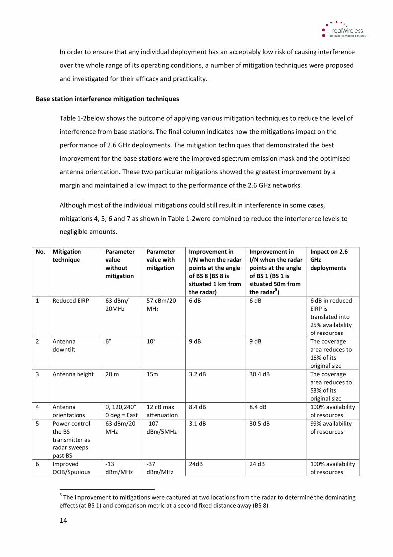
Base station interference mitigation techniques
Table 1-2below shows the outcome of applying various mitigation techniques to reduce the level of
interference from base stations. The final column indicates how the mitigations impact on the
performance of 2.6 GHz deployments. The mitigation techniques that demonstrated the best
improvement for the base stations were the improved spectrum emission mask and the optimised
antenna orientation. These two particular mitigations showed the greatest improvement by a
margin and maintained a low impact to the performance of the 2.6 GHz networks.
Although most of the individual mitigations could still result in interference in some cases,
mitigations 4, 5, 6 and 7 as shown in Table 1-2were combined to reduce the interference levels to
negligible amounts.
No. Mitigation
technique
Parameter
value
without
mitigation
Parameter
value with
mitigation
Improvement in
I/N when the radar
points at the angle
of BS 8 (BS 8 is
situated 1 km from
the radar)
Improvement in
I/N when the radar
points at the angle
of BS 1 (BS 1 is
situated 50m from
the radar5)
Impact on 2.6
GHz
deployments
1 Reduced EIRP 63 dBm/
20MHz
57 dBm/20
MHz
6 dB 6 dB 6 dB in reduced
EIRP is
translated into
25% availability
of resources
2 Antenna
downtilt
6° 10° 9 dB 9 dB The coverage
area reduces to
16% of its
original size
3 Antenna height 20 m 15m 3.2 dB 30.4 dB The coverage
area reduces to
53% of its
original size
4 Antenna
orientations
0, 120,240°
0 deg = East
12 dB max
attenuation
8.4 dB 8.4 dB 100% availability
of resources
5 Power control
the BS
transmitter as
radar sweeps
past BS
63 dBm/20
MHz
-107
dBm/5MHz
3.1 dB 30.5 dB 99% availability
of resources
6 Improved
OOB/Spurious
-13
dBm/MHz
-37
dBm/MHz
24dB 24 dB 100% availability
of resources
5 The improvement to mitigations were captured at two locations from the radar to determine the dominating
effects (at BS 1) and comparison metric at a second fixed distance away (BS 8)
15
emissions (EIRP)
7 Coordination
zone
N/A 600 - 700m -2 dB 45.1 dB The area
covered reduces
to 84% of its
original size
8 Combined
mitigations 4-7
41.6 dB 63.5 dB The area
covered reduces
to 83% of its
original size
Table 1-2 Results of mitigations applied to reduce interference from base stations
The efficacy of any given mitigation should be balanced against the cost and other impact on the
relevant network deployment, as indicated in Table 1-3.
No Mitigation Impact to 2.6 GHz deployments Estimated cost to 2.6 GHz
deployment
1 Reduce EIRP
levels of BS
May require up to four additional
low power sites to maintain the
same level coverage/capacity
Four times base station build at up to
100,000 GBP a site if coverage limited.
2 Improve
unwanted
spectrum
emission
mask
May require the addition of high
specification cavity filter which
would mean additional cost per
site
Cost of cavity filter and installation up
to £500 - £1000 per transmitter
3 Optimise
antenna
orientation
to lowest
gain facing
radar
Adjustment to antenna orientation
will not only impact coverage to
the network but will affect the re-
use pattern adopted to
surrounding sites which could
mean extensive on-going
optimisation to an operators
network
Cost neutral. Site specific engineering
would be included at the point of
installation
4 Increase
downtilt of
antenna
Adjustment to antenna downtilt
will have an impact on the
coverage of the network which
may require the addition of fill in
sites to cover the shortfall
Cost neutral. Site specific engineering
would be included at the point of
installation
5 Lower
antenna
height
Adjustment to antenna height will
have an impact on coverage and
require more power to compensate
Could require additional sites to
maintain coverage.
16
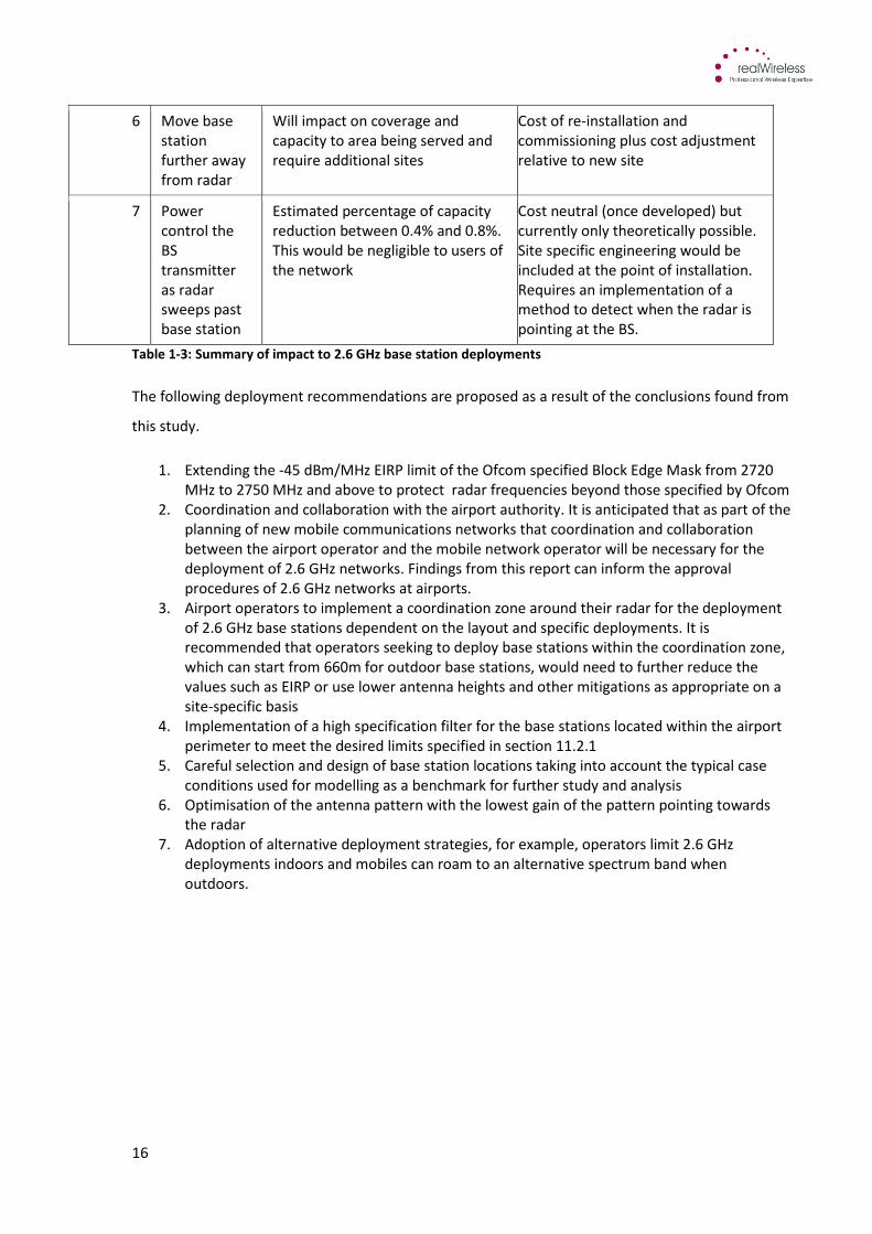
6 Move base
station
further away
from radar
Will impact on coverage and
capacity to area being served and
require additional sites
Cost of re-installation and
commissioning plus cost adjustment
relative to new site
7 Power
control the
BS
transmitter
as radar
sweeps past
base station
Estimated percentage of capacity
reduction between 0.4% and 0.8%.
This would be negligible to users of
the network
Cost neutral (once developed) but
currently only theoretically possible.
Site specific engineering would be
included at the point of installation.
Requires an implementation of a
method to detect when the radar is
pointing at the BS.
Table 1-3: Summary of impact to 2.6 GHz base station deployments
The following deployment recommendations are proposed as a result of the conclusions found from
this study.
1. Extending the -45 dBm/MHz EIRP limit of the Ofcom specified Block Edge Mask from 2720
MHz to 2750 MHz and above to protect radar frequencies beyond those specified by Ofcom
2. Coordination and collaboration with the airport authority. It is anticipated that as part of the
planning of new mobile communications networks that coordination and collaboration
between the airport operator and the mobile network operator will be necessary for the
deployment of 2.6 GHz networks. Findings from this report can inform the approval
procedures of 2.6 GHz networks at airports.
3. Airport operators to implement a coordination zone around their radar for the deployment
of 2.6 GHz base stations dependent on the layout and specific deployments. It is
recommended that operators seeking to deploy base stations within the coordination zone,
which can start from 660m for outdoor base stations, would need to further reduce the
values such as EIRP or use lower antenna heights and other mitigations as appropriate on a
site-specific basis
4. Implementation of a high specification filter for the base stations located within the airport
perimeter to meet the desired limits specified in section 11.2.1
5. Careful selection and design of base station locations taking into account the typical case
conditions used for modelling as a benchmark for further study and analysis
6. Optimisation of the antenna pattern with the lowest gain of the pattern pointing towards
the radar
7. Adoption of alternative deployment strategies, for example, operators limit 2.6 GHz
deployments indoors and mobiles can roam to an alternative spectrum band when
outdoors.
17
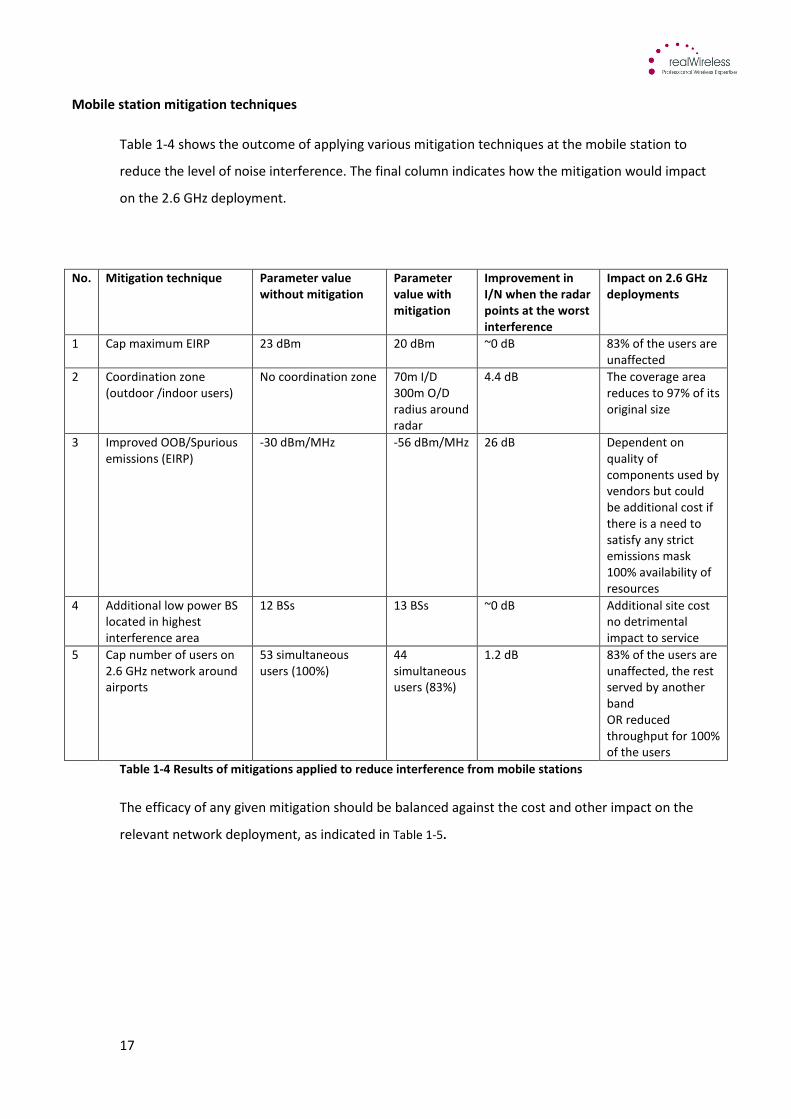
Mobile station mitigation techniques
Table 1-4 shows the outcome of applying various mitigation techniques at the mobile station to
reduce the level of noise interference. The final column indicates how the mitigation would impact
on the 2.6 GHz deployment.
No. Mitigation technique Parameter value
without mitigation
Parameter
value with
mitigation
Improvement in
I/N when the radar
points at the worst
interference
Impact on 2.6 GHz
deployments
1 Cap maximum EIRP 23 dBm 20 dBm ~0 dB 83% of the users are
unaffected
2 Coordination zone
(outdoor /indoor users)
No coordination zone 70m I/D
300m O/D
radius around
radar
4.4 dB The coverage area
reduces to 97% of its
original size
3 Improved OOB/Spurious
emissions (EIRP)
-30 dBm/MHz -56 dBm/MHz 26 dB Dependent on
quality of
components used by
vendors but could
be additional cost if
there is a need to
satisfy any strict
emissions mask
100% availability of
resources
4 Additional low power BS
located in highest
interference area
12 BSs 13 BSs ~0 dB Additional site cost
no detrimental
impact to service
5 Cap number of users on
2.6 GHz network around
airports
53 simultaneous
users (100%)
44
simultaneous
users (83%)
1.2 dB 83% of the users are
unaffected, the rest
served by another
band
OR reduced
throughput for 100%
of the users
Table 1-4 Results of mitigations applied to reduce interference from mobile stations
The efficacy of any given mitigation should be balanced against the cost and other impact on the
relevant network deployment, as indicated in Table 1-5.
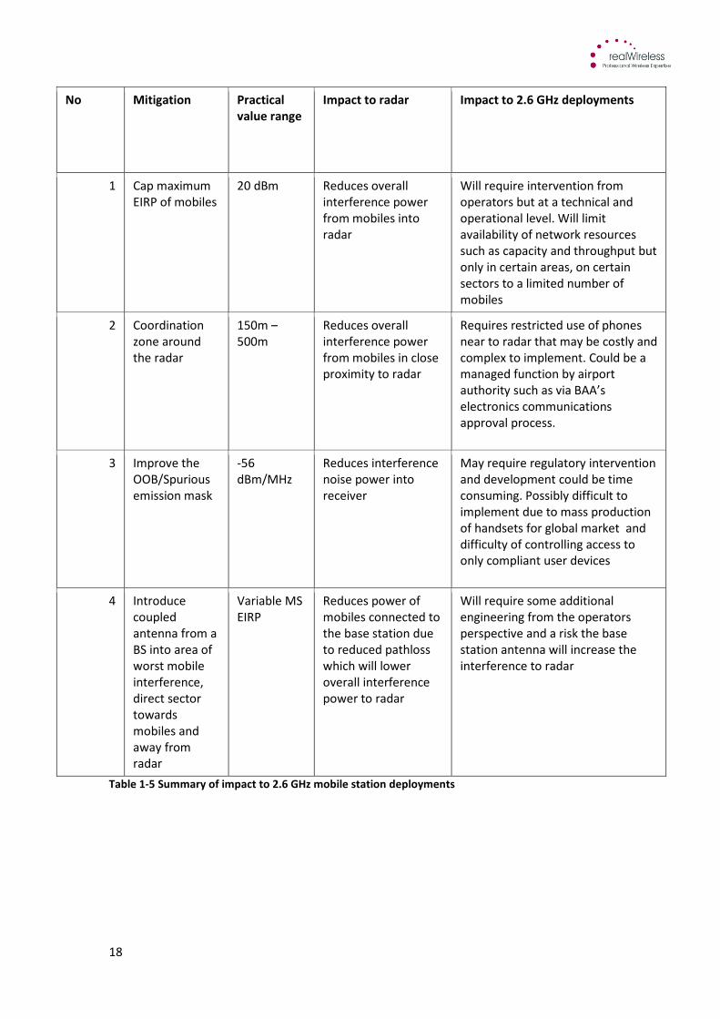
18
No Mitigation Practical
value range
Impact to radar Impact to 2.6 GHz deployments
1 Cap maximum
EIRP of mobiles
20 dBm Reduces overall
interference power
from mobiles into
radar
Will require intervention from
operators but at a technical and
operational level. Will limit
availability of network resources
such as capacity and throughput but
only in certain areas, on certain
sectors to a limited number of
mobiles
2 Coordination
zone around
the radar
150m –
500m
Reduces overall
interference power
from mobiles in close
proximity to radar
Requires restricted use of phones
near to radar that may be costly and
complex to implement. Could be a
managed function by airport
authority such as via BAA’s
electronics communications
approval process.
3 Improve the
OOB/Spurious
emission mask
-56
dBm/MHz
Reduces interference
noise power into
receiver
May require regulatory intervention
and development could be time
consuming. Possibly difficult to
implement due to mass production
of handsets for global market and
difficulty of controlling access to
only compliant user devices
4 Introduce
coupled
antenna from a
BS into area of
worst mobile
interference,
direct sector
towards
mobiles and
away from
radar
Variable MS
EIRP
Reduces power of
mobiles connected to
the base station due
to reduced pathloss
which will lower
overall interference
power to radar
Will require some additional
engineering from the operators
perspective and a risk the base
station antenna will increase the
interference to radar
Table 1-5 Summary of impact to 2.6 GHz mobile station deployments
19
The following deployment recommendations are proposed as a result of the findings from the
investigation of interference generated by mobile stations within an airport environment.
1. The introduction of an outdoor and indoor coordination zone around the radar. The
simulations found that a 300m outdoor coordination and a 70m indoor coordination zone
are sufficient to reduce interference to below the threshold for each mechanism. For smaller
coordination zones parameters such as EIRP and building penetration loss must be
investigated in detail for the particular airport.
2. Appreciation of the typical case conditions used for modelling as a benchmark for further
study and analysis of the interference within an airport environment. For example the
activation of power control for the uplink with appropriate parameters was found to help
reduce the interference levels into the radar.
3. Identify the range of out-of-band and spurious emissions produced by commercial mobiles
and re-model using the measured data. This will establish more firmly the degree of
additional mitigations which will be needed to ensure operation within the threshold limits
of interference and can co-exist in an airport environment.
1.2.3 Further investigation into the viability of suggested mitigation
techniques would confirm they are pragmatic, commercially viable
and suitable for other airport deployments
Further investigation into the viability of some of the suggested mitigations would help confirm their
suitability in a practical airport deployment. The following suggestions have been made on that
basis:
• Understand the coordination procedures with the relevant airport authorities, as many different
deployment parameters can materially affect the interference performance of 2.6 GHz base
stations in and around airports6.
• Analysis of the power control feature of a base station that could offer the potential reduction in
interference power as the radar rotates passed the base station
• A catalogue of the radar heights at other UK airports would help ensure suitable coordination
zones are established where necessary.
• Commercial and technical factors in site sharing should be reviewed as suggested mitigations
applied by the airport owners could include the restriction on the number of base stations
transmitting from a single site.
• Spurious emission measurements of a wider selection of mobile device types, such as
smartphones, tablet PC’s and laptops to determine their behaviour in the S-band.
6 These are specified in Section 8.
20
Ofcom’s on-going work/studies
Ofcom has other scoping studies in progress that complement the work of this study including:
• Measurements campaign of the unwanted emissions of base stations and mobile devices to address
the reality of LTE and WiMAX equipment performance of spurious and out-of-band emissions.
Specifically, results from the measurements of an FDD LTE mobile device were used to inform part
of the modelling of mobile emission behaviour
• Radar design and selectivity studies which quantify the improvement in front end filter selectivity for
each of the airport radars. Each radar manufacturer will design its filter to maximise selectivity and
minimise blocking. The addendum to this report includes analysis of a second modified hypothetical
radar design which captures a second representative set of filters that could be deployed at an
airport.
21
1.3 Our approach and assumptions
1.3.1 Our approach
The study used software modelling to assess the interference mechanisms caused by 2.6 GHz
systems into a modified radar receiver operating in the S-band. The interfering effects analysed
included:
• Blocking2 to the front end of the radar receiver from high power in-band emissions,
potentially causing false target identification and confusion with valid targets
• A rise in noise powers co-channel with the radar centre frequency from out-of-band and
spurious emissions of 2.6 GHz systems, degrading the sensitivity of the radar receiver and
thus its usable range.
The main steps of the study were as follows:
• Determining network deployment scenarios and associated technical parameters which are
likely for 2.6 GHz operation around airport environments, taking particular account of inputs
received from stakeholders such as mobile operators, equipment vendors and BAA.
• Creating and validating a simulation environment suitable for assessing the relevant
interference mechanisms over the full set of scenarios, and accounting for interference from
both multiple base stations, with some from shared sites and multiple active mobile
stations.
• Conducting simulations for the different network deployment scenarios.
• Assessing the potential radar interference levels based on both extreme cases and overall
statistical behaviour.
• Determining mitigation techniques which could reduce the impact of potential interference
while being practical to apply without undue restriction on 2.6 GHz operation.
• Examining the efficacy of the most promising mitigation techniques via simulation and
evaluating their potential impact on network services and costs of implementation.
1.3.2 Scenarios and assumptions analysed
There is a wide and varied range of parameters which impact on potential interference so the
simulations included the study of three main cases for the various parameters modelled:
1. A challenging case where parameters are set to represent an extreme situation where
interference to a radar might occur. Whilst such a case is, in principle, possible within the
airport environment and consistent with a 2.6 GHz licensee’s technical conditions, it is
unlikely to occur in practice. This case consists of 13 base stations at distances ranging
between 50m and 1674m and mobile stations at a density consistent with levels of usage
which could occur in the airport environment. Spurious emissions are assumed to be at the
relevant specification limits. Mobiles are assumed to be transmitting at full power.
2. A typical case where parameters are set to represent a plausible, though high-capacity,
practical deployment. This case consists of 13 base stations at distances ranging between
50m and 1674m and mobile stations at the same density as in the challenging case. Spurious
22
emissions are assumed to be at levels significantly below the specification limits based on
expectations from practical equipment and consultation with vendors. Mobiles are assumed
to be power controlled by the serving base stations.
3. A measured case where measurements, conducted to determine the behaviour and
performance of emissions in the S-band from an LTE FDD mobile device, were used for
modelling the impact from the spurious emissions, co-channel with the radar receiver whilst
all other parameters remained the same as the typical case.
The incidence of interference was judged based on the following conditions and metrics:
Conditions:
• When the power at particular points within the radar receiver exceeded thresholds specified
by Ofcom as likely to cause 1 dB compression within the radar receiver sub-systems
• When the total power caused the radar receiver noise floor to increase, producing a carrier
to noise ratio lower than a threshold between the example range-5 dB and -15 dB.
Metrics:
• The metric used for evaluating the results of the interference from base stations and mobile
stations was the peak level which refers to 1% time the radar points at the worst interferer
(i.e. ~0.01% of the time overall). This means the highest levels of interference are captured
when the main beam of the radar antenna points at the highest interferer. This also suggests
that lower (30 dB) levels of interference point towards the radar antenna sidelobes but at an
attenuated level.
• Result metrics below 1% of time should be adjusted by adding maximum 5 dB for 0.1% and
adding maximum 12 dB for< 0.01% time for systems with variability such as mobile. In
contrast for base stations, due to little variability, only 1 dB is added for percentage time
below 1%
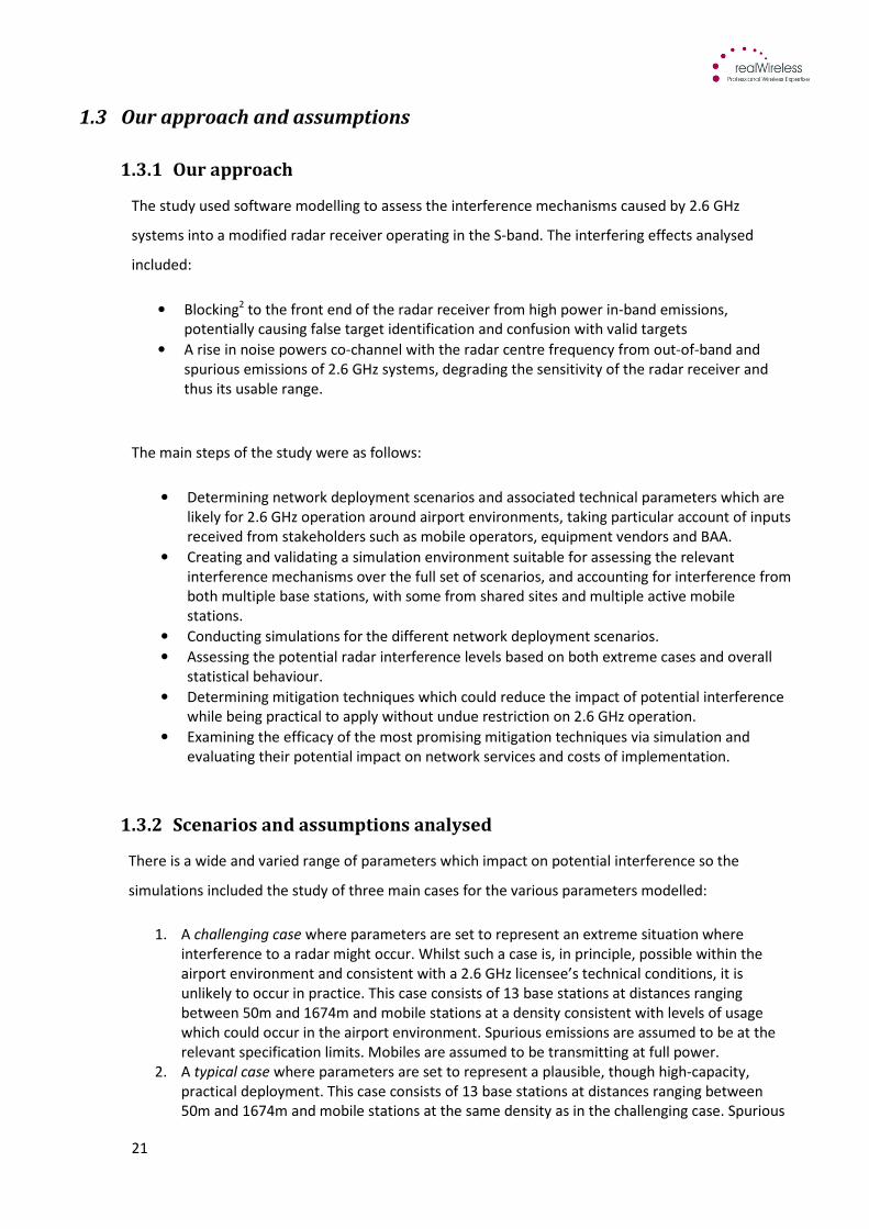
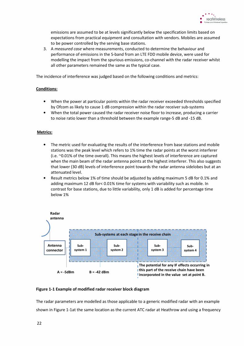
Figure 1-1 Example of modified radar receiver block diagram
The radar parameters are modelled as those applicable to a generic modified radar with an example
shown in Figure 1-1at the same location as the current ATC radar at Heathrow and using a frequency
Sub-
system 2
Sub-
system 3
Sub-
system 1
B = -42 dBm
Radar
antenna
Sub-systems at each stage in the receive chain
Antenna
connector
A = -5dBm
Sub-
system 4
The potential for any IF effects occurring in
this part of the receive chain have been
incorporated in the value set at point B.
23
of 2750 MHz. This is a hypothetical deployment but is based on composite design analysis and
physical deployments and therefore constitutes a receiver that could potentially be deployed in
practice. The analysis focused on 2.6 GHz mobile systems causing excessive blocking in the receiver
at point A and point B and excessive I/N across the receiver bandwidth. The second hypothetical
radar design that was used to model spurious emissions from mobile devices can be found in the
addendum document (“Addendum to Final Report Phase 2 - Airport Deployment Study, impact to
second modified radar design”).
1.4 Study results in detail
1.4.1 Analysis of interference from base stations into radar
The analysis examined two types of layout environments for the base stations. 1) A layout
representing the Heathrow airport environment, 2) a synthetic layout representing base stations at
equidistant intervals from the generic modified radar. The two layouts were used to establish the
extent of interference from base stations with the synthetic layout used to further analyse the
required mitigations. The challenging case which could in principle occur in practice but is relatively
extreme was used in both layouts, while the typical case, which is considered more realistic, was
used in the Heathrow layout only. Both layouts consist of 13 base stations at distances ranging
between 50m and 1674m from the radar.
The typical case results for the Heathrow layout showed no blocking occurs from base stations since
the highest blocking level recorded did not exceed the – 5 dBm threshold level due to more realistic
network deployment parameters being used. In addition, the signal level recorded at the input to
the LNA (point B) was attenuated by 40 dB due to the modified front end radar RF filter. Some noise
rise did occur and exceeded the minimum I/N threshold level (-15 dB) by 8 dB and the ITU I/N level (-
10 dB) by 3 dB. The highest level of interference under typical case conditions came from the closest
outdoor base station situated 660m from the radar.
The findings from the analysis of the base station to radar interference (see Table 1-6 and Table 1-7)
showed the following results under the challenging case conditions without mitigations on the
highest interferer:
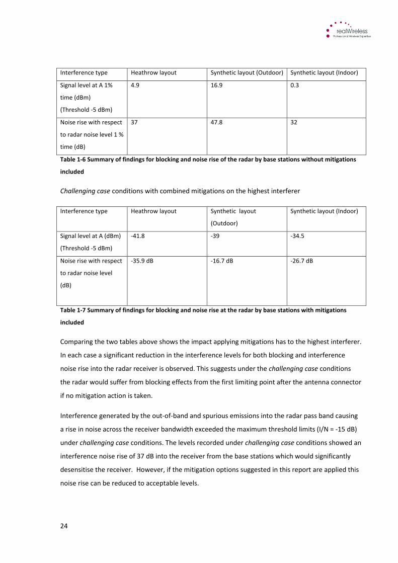
24
Interference type Heathrow layout Synthetic layout (Outdoor) Synthetic layout (Indoor)
Signal level at A 1%
time (dBm)
(Threshold -5 dBm)
4.9 16.9 0.3
Noise rise with respect
to radar noise level 1 %
time (dB)
37 47.8 32
Table 1-6 Summary of findings for blocking and noise rise of the radar by base stations without mitigations
included
Challenging case conditions with combined mitigations on the highest interferer
Interference type Heathrow layout Synthetic layout
(Outdoor)
Synthetic layout (Indoor)
Signal level at A (dBm)
(Threshold -5 dBm)
-41.8 -39 -34.5
Noise rise with respect
to radar noise level
(dB)
-35.9 dB -16.7 dB -26.7 dB
Table 1-7 Summary of findings for blocking and noise rise at the radar by base stations with mitigations
included
Comparing the two tables above shows the impact applying mitigations has to the highest interferer.
In each case a significant reduction in the interference levels for both blocking and interference
noise rise into the radar receiver is observed. This suggests under the challenging case conditions
the radar would suffer from blocking effects from the first limiting point after the antenna connector
if no mitigation action is taken.
Interference generated by the out-of-band and spurious emissions into the radar pass band causing
a rise in noise across the receiver bandwidth exceeded the maximum threshold limits (I/N = -15 dB)
under challenging case conditions. The levels recorded under challenging case conditions showed an
interference noise rise of 37 dB into the receiver from the base stations which would significantly
desensitise the receiver. However, if the mitigation options suggested in this report are applied this
noise rise can be reduced to acceptable levels.
25
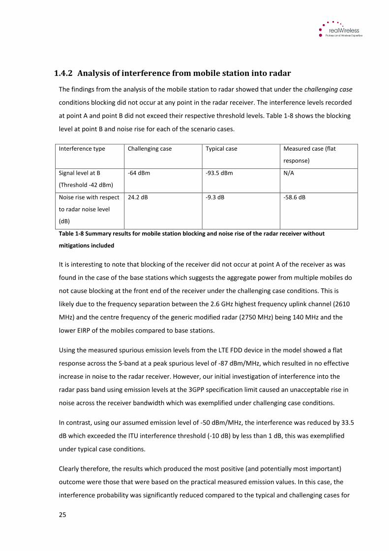
1.4.2 Analysis of interference from mobile station into radar
The findings from the analysis of the mobile station to radar showed that under the challenging case
conditions blocking did not occur at any point in the radar receiver. The interference levels recorded
at point A and point B did not exceed their respective threshold levels. Table 1-8 shows the blocking
level at point B and noise rise for each of the scenario cases.
Interference type Challenging case Typical case Measured case (flat
response)
Signal level at B
(Threshold -42 dBm)
-64 dBm -93.5 dBm N/A
Noise rise with respect
to radar noise level
(dB)
24.2 dB -9.3 dB -58.6 dB
Table 1-8 Summary results for mobile station blocking and noise rise of the radar receiver without
mitigations included
It is interesting to note that blocking of the receiver did not occur at point A of the receiver as was
found in the case of the base stations which suggests the aggregate power from multiple mobiles do
not cause blocking at the front end of the receiver under the challenging case conditions. This is
likely due to the frequency separation between the 2.6 GHz highest frequency uplink channel (2610
MHz) and the centre frequency of the generic modified radar (2750 MHz) being 140 MHz and the
lower EIRP of the mobiles compared to base stations.
Using the measured spurious emission levels from the LTE FDD device in the model showed a flat
response across the S-band at a peak spurious level of -87 dBm/MHz, which resulted in no effective
increase in noise to the radar receiver. However, our initial investigation of interference into the
radar pass band using emission levels at the 3GPP specification limit caused an unacceptable rise in
noise across the receiver bandwidth which was exemplified under challenging case conditions.
In contrast, using our assumed emission level of -50 dBm/MHz, the interference was reduced by 33.5
dB which exceeded the ITU interference threshold (-10 dB) by less than 1 dB, this was exemplified
under typical case conditions.
Clearly therefore, the results which produced the most positive (and potentially most important)
outcome were those that were based on the practical measured emission values. In this case, the
interference probability was significantly reduced compared to the typical and challenging cases for
26
both blocking and noise rise in the radar receiver from 2.6 GHz mobile devices. This suggests that
one particular commercially available 2.6 GHz LTE mobile device can co-exist with S-band radars
when deployed within an airport environment without restrictions.
We highlight the following factors (apart from the modification to the radar receiver) that contribute
to the reduction in interfering signal arriving at the receiver in the typical case compared to the
challenging case:
1. Activation of power control from the mobile – If base station parameters are appropriately
set, then mobile stations having a low path loss to their serving base station will be reduced
in power significantly. This will also be impacted by the location of the base stations relative
to the radar.
2. Use of realistic noise estimated spectrum emission mask – 2.6 GHz equipment, in the case
of mobile devices have shown reduced spurious emissions of around 50 dB below the
standard specification limits within the radar band. Therefore the assumed margin used for
the typical case which was 20 dB below the specification limit into the radar band was
conservative in comparison to the realistic value.
3. Increased radar height – Increasing the radar height has the effect of limiting the
opportunity of interference to be captured in the main beam of the radar. As the height
increases, so does the horizontal distance beyond the radar at which the main beam
intersects the ground, thereby increasing the path loss to mobiles most likely to affect the
radar.
Overall results with combined mitigations for 1% of the time that the radar points at the highest
interferer were as follows.
Interference type Mitigated case
Signal level at B
(Threshold -42 dBm)
-98.8 dBm
Noise rise with respect to radar
noise level (dB)
-17.7 dB
Table 1-9 Summary results for mobile station blocking and noise rise of the radar receiver with mitigations
included
The results shown in the table above give the interference levels generated after applying the
combined mitigations of a coordination zone and improved spurious emission levels in the
challenging case.
In the case where interference was marginal and close to the threshold such as noise rise from
mobiles in the typical case. We illustrated the impact percentages of time below 1% would have on
the radar, which showed an additional 6 dB of extra interference at 0.01% and below. Under typical
case conditions this means the noise rise with respect to the radar noise level is within the ITU (-10
dB) threshold level thus still enabling the unrestricted use of mobiles at airports.
27
1.5 Acknowledgements
The authors would like to thank the stakeholders who provided input to this study, particularly BAA,
who provided details of the physical layout of Heathrow airport and the associated mobile
infrastructure.
28
2 Introduction
Ofcom, CAA, MOD, MCA and other interested parties have been investigating the compatibility issues of
emissions from mobile communications systems operating in the 2.6 GHz band into radar receivers
operating in the upper adjacent 2.7 GHz band. Results that have been produced from a previous study1
have identified the specific mechanisms that could cause critical degradation to the performance of Air
Traffic Control radars and derived the associated protection criteria. In addition, field and laboratory
trials have been conducted on behalf of Ofcom, to demonstrate the different effects on the different
categories of radar. The results have shown that for a number of different scenarios the required
protection distances estimated range from 1km within an urban environment up to more than 40km for
a rural environment. These estimations were conducted for a range of different transmit and receive
heights depending on those found within each environment.2
The compatibility work that has been conducted contributes to the overall radar remedial work
programme which supports wider Ofcom policy. Ofcom under its statutory obligations and EC mandate
under EC Decision 2008/477/EC (the “2.6 GHz RSC Decision”) must make the 2.6 GHz spectrum available
via award to the market in a timely manner. In advance of the spectrum award the technical licence
conditions must be produced and regulations made which can be included in the new licences that will
be awarded. The outcome of the airport deployment study will inform the development of technical
conditions for 2.6 GHz deployments in and around airports potentially resulting in restrictions such as
reduced EIRP, coordination zones and modified antenna patterns. These conditions could be applied in
the licenses, or else in the form of agreement and approval process between stakeholders.
The extensive work already undertaken by Ofcom and other stakeholders has resulted in the generation
of radar protection criteria as part of the technical conditions for the proposed spectrum licence award3
and overall safety case. These have been incorporated in the analysis presented here.
This study focuses on interference from both base station and mobile station emissions into the
adjacent radar band and investigates the various deployment scenarios and practical network
configurations of technologies such as LTE and WiMAX which are likely to be operated in the 2.6 GHz
band.
Specifically the modelling includes:
• detailed analysis of multiple base station deployments in and around airports
• different scenarios representing mobile usage and densities
29
• interference environment including propagation characteristics and clutter
• practical mitigation strategies from both a mobile operator, airport operator and radar
operator perspective
The focus of this study is on the performance after application of the remedial work, rather than
unmodified radars.
30
2.1 Airport deployment study
Ofcom initiated the radar remedial programme to address the modification of the radar receiver
front end for those operating in the S-band and deployed at airports throughout the UK. This
extensive programme includes a number of scoping studies each investigating the different areas of
concern, one of which is the airport deployment study.
The intention of the airport deployment study was to focus on the mobile network deployments for
LTE and WiMAX at airports, understand the authorisation processes of deployment of electronic
communications equipment at airports and the types of mitigation strategies that can be practically
and cost effectively applied to both the base stations and mobile stations to reduce interference to
an acceptable level.
The basic scope of the study was to develop a fully modelled mobile communications network that
could take into consideration all the necessary parameters of a 2.6 GHz mobile network which could
simulate interference in a practical scenario in close proximity to a radar. Following the initial
analysis suitable mitigation techniques could be applied to demonstrate any improvement to the
interference situation.
2.2 Structure of report
This report is structured to address the findings of the study in a clear and logical way and describe
how the main tasks have been tackled and analyse the effects of interference from base stations and
mobile stations into radar receivers. The main chapters include:
Chapter 2, this Introduction, presents the main concepts of the airport deployment study and
highlights the work which has previously taken place
Chapter 3, Background and scope describes the background of the study in more detail including a
description of the interference mechanisms that are to be investigated, the focus on analysis of the
modified radar receivers and importance of emissions from multiple interferers.
Chapter 4, Characteristics of 2.6 GHz equipment describes the findings from desk research of
commercially available 2.6 GHz equipment from both LTE and WiMAX vendors.
31
Chapter 5, Stakeholder engagement describes the findings from stakeholder engagement including
the views from operators and vendors with an interest in 2.6 GHz spectrum and also from BAA the
airport authority for six UK airports including Heathrow Airport.
Chapter 6, Interference analysis modelling describes the methods for analysing the interference and
the choice of modelling approach taken for the study.
Chapter 7, Parameters introduce the key input technical parameters used by the software model
and describe the simulation assumptions made in order to develop the modelling environment.
Chapter 8, Model overview presents an overview of the software model and describes how the
model works at a simplistic level.
Chapter 9, Model outputs describes how the modelling outputs such as graphs and plots are
presented and explains what the outputs mean to the overall study.
Chapter 10, Interference results without additional mitigation presents results from simulations of
base station and mobile station emission interference to radar with no mitigation techniques added.
Chapter 11, Interference results with mitigation presents results from simulations of base station
and mobile station emission interference to radar with mitigation techniques added.
Chapter 12, Conclusions and summary recommendations describes the conclusions from the
findings and provides a summary of recommendations.
Chapter 13 and 14 provide a glossary and full references respectively. A separate set of appendices7
provides further technical details of the parameters used in the study.
7 “Final Report Appendices Airport Deployment Study”
32
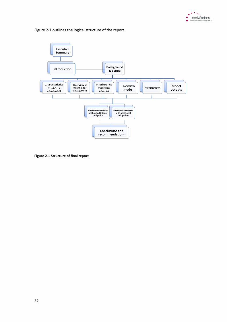
Figure 2-1 outlines the logical structure of the report.
Figure 2-1 Structure of final report
33
3 Backgroundandscope
3.1 Background
Ofcom would like to determine the potential impact of LTE and WiMAX emissions on radar receivers
operating in airport environments. Specifically, the investigation is into interference:
• from LTE and WiMAX base stations, handsets and other user devices transmitting in the 2.5-
2.69 GHz band
• to radar receivers operating in the 2.7-3.1 GHz band.
Previous work conducted by Ofcom4 has been extensive including a study to assess the impact of 2.6
GHz transmissions on ATC radars. The modelling assumptions used to estimate the interference
power levels input to the radar receiver are representative of a generic modified ATC radar created
for the purposes of modelling, which whilst being representative in a generic sense does not
represent any specific radar.
The aggregate impacts on ATC radars estimated by Ofcom focused on the potential for macrocell
base station transmitters having a transmit EIRP 61 dBm and a 30m antenna height to determine the
extent of the coordination area around the radars. The estimations were based on the impact to the
Watchman ATC radar which is the predominant ATC radar used in the UK.
This investigative work has led to the development of modified filtering applied to the radar receiver
chain. For example, to improve the selectivity of the front end of a generic modified radar there is a
requirement for an additional RF filter in front of the LNA. This would improve the selectivity and
thus reduce the level of received interference from in band 2.6 GHz emissions.
The aim of this study is to investigate the performance of only the modified radar which at this stage
is based on a generic modified design prior to the development of any commercially available ATC
radars. Therefore this study addresses the impact of interference to the upgraded radars and
focuses on the mitigations from 2.6 GHz equipment that reduce the interference levels.
This study extends the previous work in the following ways:
• Incorporating the actual physical and operational characteristics of key airport
environments.
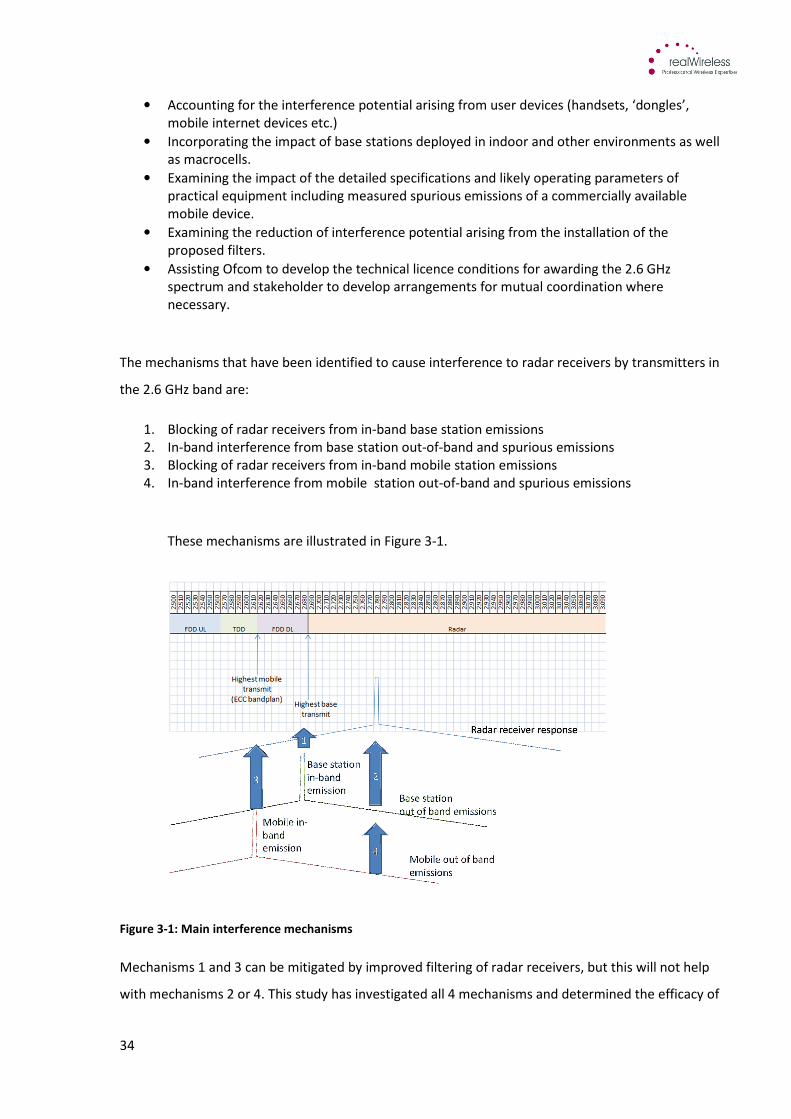
34
• Accounting for the interference potential arising from user devices (handsets, ‘dongles’,
mobile internet devices etc.)
• Incorporating the impact of base stations deployed in indoor and other environments as well
as macrocells.
• Examining the impact of the detailed specifications and likely operating parameters of
practical equipment including measured spurious emissions of a commercially available
mobile device.
• Examining the reduction of interference potential arising from the installation of the
proposed filters.
• Assisting Ofcom to develop the technical licence conditions for awarding the 2.6 GHz
spectrum and stakeholder to develop arrangements for mutual coordination where
necessary.
The mechanisms that have been identified to cause interference to radar receivers by transmitters in
the 2.6 GHz band are:
1. Blocking of radar receivers from in-band base station emissions
2. In-band interference from base station out-of-band and spurious emissions
3. Blocking of radar receivers from in-band mobile station emissions
4. In-band interference from mobile station out-of-band and spurious emissions
These mechanisms are illustrated in Figure 3-1.
Figure 3-1: Main interference mechanisms
Mechanisms 1 and 3 can be mitigated by improved filtering of radar receivers, but this will not help
with mechanisms 2 or 4. This study has investigated all 4 mechanisms and determined the efficacy of
35
the filtering mitigation in realistic airport scenarios and evaluated additional mitigations to assist
with challenging conditions for all 4 mechanisms.
It should be noted that the limiting case of interference from individual mobile transmissions will
occur for mobile use at the top end of the unpaired 2.6 GHz spectrum (i.e. at 2.62 GHz assuming the
ECC bandplan), which may be used by either WiMAX or TD-LTE mobiles. However, FDD LTE mobiles
transmitting up to 2.57 GHz may be more numerous and contribute a larger aggregate interference
level.
3.2 Scope of study
The scope of the study was to create a software model that could perform simulations of the
different interference scenarios applicable in an airport environment. They type of simulation
required the development and creation of the transmission characteristics of the base stations and
mobile stations for both in band and out of band emissions, the inclusion of the OFDMA specific
peak to average power ratio for the simulated signals and the antenna geometry for both the base
stations and the radar.
In addition the software included the creation of the airport environment to be modelled based on a
particularly busy London airport layout which required the construction of specific features in and
around the airport such as all the buildings and roads in the Central Terminal Area, plus the buildings
and roads around the terminal which is in close proximity to the radar.
The model structure was created based on a collection of parameter assumptions gathered through
desk research and engagement with stakeholders and the use of appropriate interference
calculations capturing all relevant effects at each point in the environment. The simulations were
carried out by applying different deployment scenarios that would either trigger interference in the
radar receiver or not. An assessment could then be made of the impact from a 2.6 GHz deployment
before commencement of the mitigation strategies.
The simulations took into account the main technical parameters which are significant in setting the
interference levels. Firstly the emissions from both the base stations and mobile stations required
the model to enable the adjustment of certain parameters, including:
36
• EIRP
• Antenna height of the radar and base stations
• Antenna tilt
• Power control
• Propagation model
• Spectrum emission mask
Secondly, the rotation of the radar and the radar antenna pattern were modelled to ensure all
possible interfering effects were captured. Developing the modified radar receiver characteristics
required a number of different generic representative filters in the receiver chain to establish the
entire receiver selectivity from the front end to the limiting amplifiers. In addition, assumptions were
made regarding the radar antenna patterns, for example a synthetic antenna pattern was derived for
the side lobes of the horizontal pattern, to ensure a smooth roll off of attenuation occurred rather
than a sharp cut-off.
The parameter information gathered was from a variety of sources but mainly from the
specifications of commercially available equipment, technical parameters from mobile field trials,
real-world mobile device emission measurements, specification limits from equipment standards
and the regulatory conditions as specified in various Ofcom published material.
Specific attention was paid to the out of band and spurious emissions which can cause co-channel
interference on the radar centre frequency occurring as a rise in noise over the receiver bandwidth.
In particular the production of the spectrum emission masks which were used for the different
scenario cases and the real world emission measurements from a single FDD LTE mobile device as an
exemplar.
The information relating to the radar technical parameters was mainly developed and obtained from
Ofcom, with the specific parameter values being based on material provided by Ofcom for a generic
modified radar. This information was used to determine the receiver characteristics of the modified
radar with the newly designed front end filters applied. Other information regarding the radar
receiver includes:
• Receiver bandwidth
• Radar antenna pattern
• Radar antenna gain
• Radar noise floor
Once all the input parameters, assumptions and calculation functions were defined the model was
constructed. The software model was designed to incorporate the necessary calculations to
37
evaluate the interference and enable different deployment scenarios to be simulated and introduce
the different mitigation techniques. Furthermore, Monte Carlo analysis was built into the software
model to account for the random nature of the deployment of mobile stations within the airport
area and enable the production of cumulative distribution functions for the results as a form of
output.
The deployment scenarios contribute to the evaluation of the impact from each of the potential
situations that could occur for a practical network deployment in the 2.6 GHz spectrum band and
within an airport environment. The main assessments that have been considered for this study
include:
• Multiple base stations in proximity to the radar both indoor and outdoor
• Multiple active mobiles in use in proximity to the radar both indoor and outdoor
For each of the scenarios a more detailed analysis was conducted that examined a challenging case
scenario followed by a more typical case deployment scenario that is likely to occur in an airport
environment. Once an assessment for each of these scenarios was complete, a set of mitigation
techniques was identified and applied to the model to determine the improvement to the overall
interference generated from both base stations and mobile stations. Establishing the mitigation
techniques assisted with understanding further the improvements required to reduce interference
and what specific actions need to be taken in relation to base station and mobile station
characteristics. The mitigation techniques were then compared to determine their efficacy and
impact on the mobile network cost and performance.
The outputs of the study present the results from the interference modelling of the base station and
the mobile station in terms of percentage time of interference occurring against a threshold level for
either blocking the different parts of the radar receiver or exceeding the specified threshold I/N
levels. The assessment was conducted for both in band blocking and co-channel interference from
out-of-band and spurious emissions and for simulations without mitigation and simulations with
mitigation. The results show a comparison of the extent to which both the base station and mobile
station produce interference into the radar receiver and how this relates to the overall increase in
allowable interference and ultimately demonstrates the overall impact of introducing 2.6 GHz
networks in an airport environment.
38
4 Characteristicsof2.6GHzequipment
Advances in wireless technology have seen impressive developments in the production of mobile
communications equipment. Most recently the developments in wireless standards such as WiMAX
and LTE which have chosen to adopt novel spectrum access techniques such as OFDMA for improved
spectrum efficiency and flexible allocation of network resources. This airport deployment study has
focused on these next generation or (loosely, ‘4G’) technologies which will likely be deployed in the
2.6 GHz spectrum. Although 2.6 GHz was originally intended as a capacity enhancing expansion band
for 3G technology, there is little commercial support for this so will not be investigated in this study.
The study has investigated the emissions performance of the equipment so that an in depth analysis
of the realistic scenarios can be evaluated. Sources of information have included desk research of
the relevant base station and mobile station specifications and also direct engagement with
stakeholders.
The following section addresses the technologies that will be deployed in 2.6 GHz band, the
performance of transmission equipment and their practical constraints.
4.1 LTE and WiMAX equipment
The candidate radio technologies that are most likely to be deployed in awarded spectrum at 2.6
GHz are going to be LTE or WiMAX technology or some mixture of the two. Already WiMAX
deployments are being rolled out in markets across the world at 2.6 GHz with a maturing equipment
portfolio. In addition LTE pre-commercial deployments at 2.6 GHz have been launched which
provides supporting evidence of these technologies to be deployed in the UK.
The 2.6 GHz band was designated an IMT band at WRC 2000 for mobile terrestrial services at which
point regulators, operators and vendors started referring to it as the 3G expansion band and
expected 3G services to be deployed. In more recent years LTE and WiMAX have been identified as
candidates for deployment in the 2.6 GHz band. Both technologies include the band as one of those
supported by the relevant standards bodies (3GPP for LTE and IEEE/WiMAX Forum for WiMAX).
WiMAX technology has seen an increasing number of deployments appear around the world in
recent years due to an early to market strategy and technology choice in OFDM in TDD mode.
WiMAX has taken advantage of the flattened network topology, which means fewer nodes in the
overall network architecture, and IP based infrastructure as a competing technology in the mobile
broadband market. However, the technology has had some issues to overcome specifically in the
39
areas of hard handover and high speed mobility due to the legacy of WiMAX, which was originally
intended for wireless DSL or last mile replacement and not intended for mobile broadband.
In terms of numbers of deployments and time to market WiMAX is clearly ahead of LTE. The WiMAX
Forum states that WiMAX has over 560 network deployments worldwide out of which 112
deployments use 2.6 GHz spectrum5. A significant proportion of the deployments are in the Asia
Pacific region however, more deployments are emerging in developed markets such as the US, Korea
and Italy.
Although LTE has been at an earlier stage of development than WiMAX, it is gaining momentum and
already there are showpiece deployments of LTE in the 2.6 GHz band. For example, TeliaSonera
deployed the first commercial LTE network in Stockholm, Sweden in December 20098 which
demonstrates the pace at which LTE standards development has been set. Also Verizon9 and AT&T
10in the US have chosen to deploy LTE using their 700 MHz spectrum across their network to
compete with Clearwire11 which is rolling out WiMAX across the US in the 2.6 GHz band. It is possible
that in the future Clearwire will also deploy TD-LTE technology12, and they have proposed that the
3GPP LTE specification supports TDD across the whole 2.6GHz band rather than purely the central
unpaired 50 MHz sub-band as is presently the case.
Furthermore, LTE is based on the 3GPP family of standards which has significant support from an
operators’ upgrade path perspective. It is very likely those operators that have adopted the use of
3GPP systems such as UMTS/HSPA will naturally upgrade their network to LTE which also supports
backwards compatibility6 from LTE to HSPA. The benefits to operators are likely to outweigh any
decision to adopt a non-3GPP technology and therefore likely to be the dominant technology
deployment within the FDD portion of the 2.6 GHz band.
The table shown in appendix F in the Appendices document provides a non-exhaustive list of vendor
equipment for both WiMAX and LTE equipment available on the market. The table includes best
product information available based on the manufacturers’ technical specification such as maximum
output power, modulation and coding scheme and bandwidth. The first commercial products to
8http://www.teliasonera.com/News-and-Archive/Press-releases/2009/TeliaSonera-first-in-the-world-with-4G-
services/ 9https://www.lte.vzw.com/AboutLTE/VerizonWirelessLTENetwork/tabid/6003/Default.aspx
10http://gigaom.com/2008/04/03/open-access-restrictions-may-have-undervalued-spectrum/
11http://www.clearwire.com/
12http://www.clearwire.com/
40
market typically include limited features and can perform closer to the specifications, with features13
added and performance improving over time as newer generations of each model is introduced. The
information in this table has been used to inform the modelling parameters to ensure the typical
scenarios take account of the practical limitations of current equipment types.
4.2 Equipment performance statistics
This study has researched the performance of the emissions from mobile communications
equipment designed to operate in the 2.6 GHz band. The two key parameters investigated in this
research were the out-of- band emissions and spurious emissions of the equipment. It is these
emissions that can cause interference as a rise in the noise floor of the radar receiver which is
fundamental to the interference analysis.
In general poor emissions performance can be related to equipment who’s OOB and spurious
emissions operate close to the specification limits in terms of causing co-channel interference into
the radar receiver pass band.
Typically manufacturers design their equipment to meet the minimum requirements of the standard
in order for safe and compliant use of the equipment and so their equipment can be placed on the
market.
The standard specification limits of interest for this study are found in the standards listed below:
• IEEE 802.16e7 standard for the case of mobile WiMAX equipment for both base stations and
mobile stations emissions
• 3GPP standards TS 36.1048 for base stations and TS 36.1019 for mobile stations for the case
of LTE equipment
In the case of 2.6 GHz equipment the 3GPP and IEEE standard specification limits for spurious
emissions are as follows:
Band Measurement bandwidth Allowed emission Level
30 MHz ≤ f< 1000 MHz 100 kHz -36 dBm
1 GHz ≤ f < 13.45 GHz 30 kHz If 2.5 x BW <= │fc-f│<10 xBW
300 kHz If 10 x BW <= │fc-f│<12 x BW
1 MHz If 12 x BW <= │fc-f│
-30 dBm
13
GSA Status of the LTE ecosystem report June 2011
http://www.gsacom.com/gsm_3g/info_papers.php4shows evolutions of mobile devices with enhanced
features
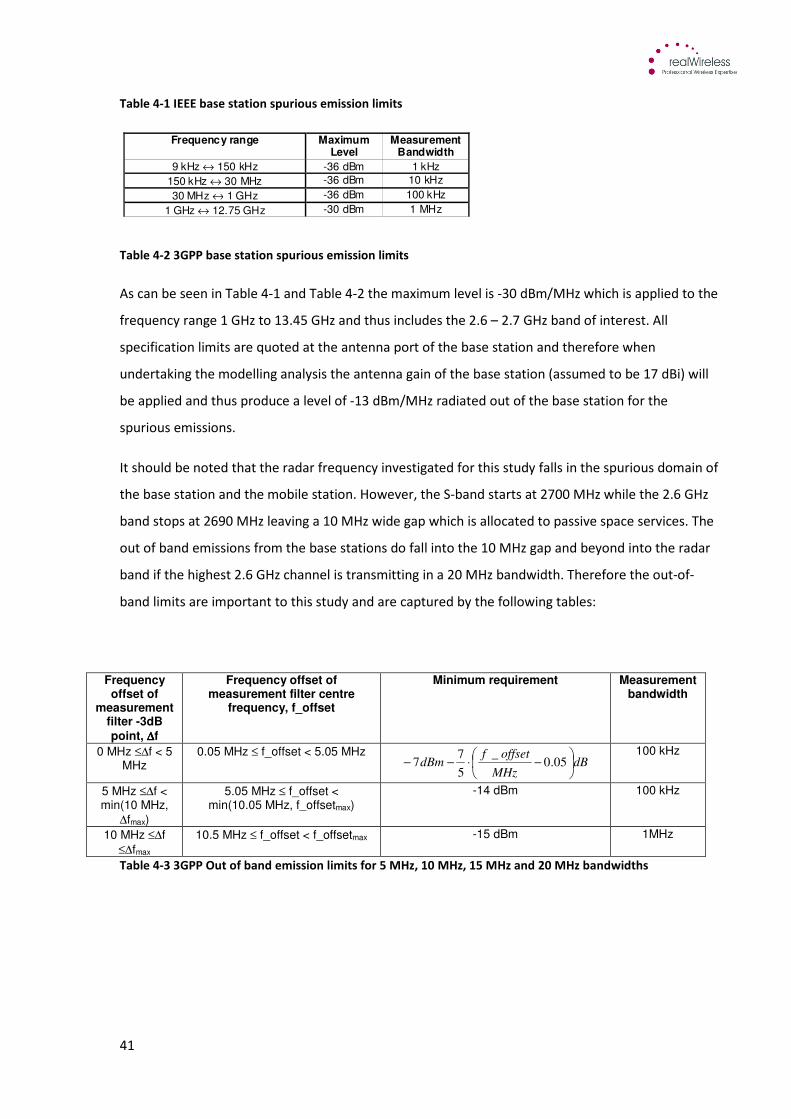
41
Table 4-1 IEEE base station spurious emission limits
Table 4-2 3GPP base station spurious emission limits
As can be seen in Table 4-1 and Table 4-2 the maximum level is -30 dBm/MHz which is applied to the
frequency range 1 GHz to 13.45 GHz and thus includes the 2.6 – 2.7 GHz band of interest. All
specification limits are quoted at the antenna port of the base station and therefore when
undertaking the modelling analysis the antenna gain of the base station (assumed to be 17 dBi) will
be applied and thus produce a level of -13 dBm/MHz radiated out of the base station for the
spurious emissions.
It should be noted that the radar frequency investigated for this study falls in the spurious domain of
the base station and the mobile station. However, the S-band starts at 2700 MHz while the 2.6 GHz
band stops at 2690 MHz leaving a 10 MHz wide gap which is allocated to passive space services. The
out of band emissions from the base stations do fall into the 10 MHz gap and beyond into the radar
band if the highest 2.6 GHz channel is transmitting in a 20 MHz bandwidth. Therefore the out-of-
band limits are important to this study and are captured by the following tables:
Frequency offset of
measurement filter -3dB
point, ∆∆∆∆f
Frequency offset of measurement filter centre
frequency, f_offset
Minimum requirement Measurement bandwidth
0 MHz ≤∆f < 5 MHz
0.05 MHz ≤ f_offset < 5.05 MHz
100 kHz
5 MHz ≤∆f < min(10 MHz,
∆fmax)
5.05 MHz ≤ f_offset < min(10.05 MHz, f_offsetmax)
-14 dBm 100 kHz
10 MHz ≤∆f
≤∆fmax
10.5 MHz ≤ f_offset < f_offsetmax -15 dBm 1MHz
Table 4-3 3GPP Out of band emission limits for 5 MHz, 10 MHz, 15 MHz and 20 MHz bandwidths
Frequency range Maximum Level
Measurement Bandwidth
9 kHz ↔ 150 kHz -36 dBm 1 kHz
150 kHz ↔ 30 MHz -36 dBm 10 kHz
30 MHz ↔ 1 GHz -36 dBm 100 kHz
1 GHz ↔ 12.75 GHz -30 dBm 1 MHz
dBMHz
offsetfdBm
−⋅−− 05.0
_
5
77
42
Frequency offset from
centre
Allowed emission level Measurement bandwidth
5 ≤ f < 6 MHz -13 dBm 50 kHz
6 ≤ f < 25 MHz -13 dBm 1 MHz
Table 4-4 IEEE Out of band emission limits for 10 MHz bandwidths
In contrast the Block Edge Mask proposed by Ofcom3 for inclusion in future 2.6 GHz licences specifies
a limit of -45dBm/MHz EIRP. Assuming a 17 dBi antenna gain this results in a -62dBm/MHz level at
the antenna connector. It should be noted that as part of Ofcom’s spectrum award program for 2.6
GHz this limit is specified beyond the end of the band (2690 MHz) up to 2720 MHz. The centre
frequency modelled as part the study is 2750 MHz which is not covered by the Ofcom BEM which
means emissions beyond 2720 MHz are less restrictive compared the block edge mask. The limits
that apply at frequencies above 2720 MHz must adopt the spurious emission limits specified in ITU-R
SM 32920 which is the same as those specified by the 3GPP and IEEE standard for the spurious
emission limits and are applied in the model for the challenging case conditions.
There are a growing number of 2.6 GHz deployments emerging around the world, however all are
relatively new, with the first network (Teliasonera in Sweden) being deployed in 2009. So there is
only limited experience of the emissions from 2.6 GHz causing interference in the out-of-
band/spurious domain into the upper adjacent band.
Therefore in terms of parameters used in the study, a set of assumptions were made based on the
available product data of 2.6 GHz equipment performance of the filters normally found in base
stations and also for mobile station equipment. The modelled emissions were set either at or some
margin below the standard specification limit depending on whether it was the challenging or typical
case being analysed. However, in the latter stages of the study measurements of a mass produced
LTE FDD mobile device were made available for additional analysis (See addendum report).
This study has used the discussions held with stakeholders who have reported that equipment
performs within a certain, variable margin below the emission specifications of the base station
equipment. For example, the following table shows the vendor estimates for the emission margin
that could be seen in practice.
43
Specification limit Vendor estimate
Spurious emission -30 dBm/MHz -35 to -50 dBm/MHz
Table 4-5 Spurious emission specification levels vs vendor estimates
It can be seen in Table 4-5 that a 5-15 dB range for the improvement in the out-of-band and spurious
emission domain below the mobile equipment specifications has been quoted by manufacturers 10.
Equipment vendors such as Alvarion, Airspan, Nokia Siemens, Samsung, Huawei and Motorola are
key players in the development of both WiMAX and LTE standards and manufacture both base
station equipment and user equipment within their product portfolios. However, there is limited
availability of emissions performance statistics from these vendors and therefore specific
assumptions have been made which can be found in appendix B of the Appendices document with
regards to the margin of improvement for the out-of-band and spurious emissions actually
transmitted by the equipment.
RFI Global has conducted some spectrum emission measurements to demonstrate the general
performance of a commercially available FDD LTE device operating in the 2.6 GHz band. The device
under test was a 2.6 GHz FDD USB mobile broadband modem, which is a very common device (see
Figure 4-1 as an example), and used by many mobile operators around the world on, HSPA, WiMAX
and LTE networks.
Figure 4-1 Mobile broadband USB dongle modem
The results from the measurements were used in the latter stages of the study which captured the
behaviour of spurious emissions in the S-band. The measurement results produced by RFI Global
Services Ltd provides detailed test set up and measurement results which includes the in-band
power, measured Adjacent Channel Leakage Ratio (ACLR), CCDF of the peak to mean ratio and the
spurious domain emissions.
44
Figure 4-2 ACLR emission plot from RFI Global Services Ltd measurement of Samsung LTE UE – 1 at maximum
transmitted power 21 dBm
Figure 4-3 ACLR emission plots from RFI Global Services Ltd measurement of Samsung LTE UE – 2 at reduced
power -4 dB
-92
-82
-72
-62
-52
-42
-32
-22
-12
-2
8
2,5
20
2,5
23
2,5
26
2,5
29
2,5
32
2,5
35
2,5
38
2,5
41
2,5
44
2,5
47
2,5
50
Po
we
r (d
Bm
)
Frequency (MHz)
ACLR Max RB-50 - Middle Channel
-92
-82
-72
-62
-52
-42
-32
-22
-12
-2
8
2,5
20
2,5
23
2,5
26
2,5
29
2,5
32
2,5
35
2,5
38
2,5
41
2,5
44
2,5
47
2,5
50
Po
we
r (d
Bm
)
Frequency (MHz)
ACLR Max-4 RB-50 - Middle Channel
45
Figure 4-2 and Figure 4-3 show the ACLR measurement plots of the signal transmissions from the
Samsung UE. The output produced shows the spectral emissions that have been specifically set up to
measure the in band and ACLR emissions. The red line is the 3GPP UE spectrum mask to show how
the emissions fit within the mask at 0dBm reference level.
These plots are used to illustrate the actual emissions performance that can be achieved by
commercial devices. The measurements show how the unwanted emission levels change with a
change to the output power. The measurements are of the adjacent channel power and do not
explicitly show the specific emission levels in the radar band. Therefore these plots are used to
demonstrate how the adjacent channel power changes with reduced in-band power.
In Figure 4-2 the total carrier power shown on the analyser was set to 21 dBm in a 10 MHz
bandwidth the measurements were taken using some attenuation which has been applied to the
input and therefore the output power recorded across the bandwidth is around 2 dBm. The
unwanted emissions are those found either side of the channel edge of the main carrier centred on
2535 MHz. At 15 MHz offset from the right of the channel edge shows peak levels reaching -44
dBm/100 kHz. This is compared to Figure 4-3which used a reduced total carrier power of 17 dBm.
The unwanted emission at 15 MHz offset from the right of the channel edge shows peak levels
reaching approximately -55dBm/100kHz.
The two sets of measurements show how a reduction in carrier power of 4 dB impacts the unwanted
emissions in the adjacent channels. In Figure 4-2 at maximum output power there is around 20 – 30
dB margin between the 3GPP mask and the measured emissions, this, compared to the plot in Figure
4-3, shows a 30 – 40 dB margin between the 3GPP mask and the measured emissions. This non-
linear reduction effect in unwanted emissions in the adjacent channel demonstrates, in part the type
of behaviour exhibited by commercially available mobile devices. It should be noted, however, that
measurements in the S-band showed no change of power in the spurious domain of the mobile
device with a change in in-band power. This is discussed further in section 10.9.
4.3 Practical considerations for mobile communications equipment
operation
Macrocell outdoor base station equipment is of key interest to this study due to the potential for
high power transmissions located relatively close to the radar without site shielding. However, in
recent years the form factor of the base station equipment has reduced in size and can now be
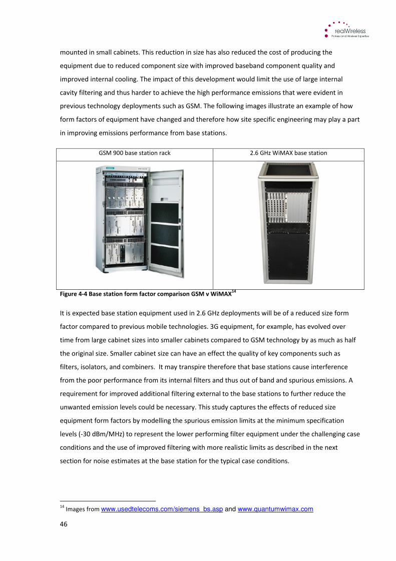
46
mounted in small cabinets. This reduction in size has also reduced the cost of producing the
equipment due to reduced component size with improved baseband component quality and
improved internal cooling. The impact of this development would limit the use of large internal
cavity filtering and thus harder to achieve the high performance emissions that were evident in
previous technology deployments such as GSM. The following images illustrate an example of how
form factors of equipment have changed and therefore how site specific engineering may play a part
in improving emissions performance from base stations.
GSM 900 base station rack 2.6 GHz WiMAX base station
Figure 4-4 Base station form factor comparison GSM v WiMAX14
It is expected base station equipment used in 2.6 GHz deployments will be of a reduced size form
factor compared to previous mobile technologies. 3G equipment, for example, has evolved over
time from large cabinet sizes into smaller cabinets compared to GSM technology by as much as half
the original size. Smaller cabinet size can have an effect the quality of key components such as
filters, isolators, and combiners. It may transpire therefore that base stations cause interference
from the poor performance from its internal filters and thus out of band and spurious emissions. A
requirement for improved additional filtering external to the base stations to further reduce the
unwanted emission levels could be necessary. This study captures the effects of reduced size
equipment form factors by modelling the spurious emission limits at the minimum specification
levels (-30 dBm/MHz) to represent the lower performing filter equipment under the challenging case
conditions and the use of improved filtering with more realistic limits as described in the next
section for noise estimates at the base station for the typical case conditions.
14
Images from www.usedtelecoms.com/siemens_bs.asp and www.quantumwimax.com
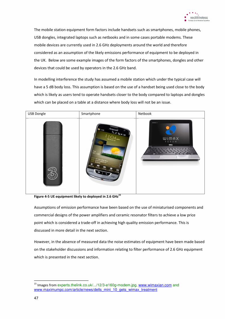
47
The mobile station equipment form factors include handsets such as smartphones, mobile phones,
USB dongles, integrated laptops such as netbooks and in some cases portable modems. These
mobile devices are currently used in 2.6 GHz deployments around the world and therefore
considered as an assumption of the likely emissions performance of equipment to be deployed in
the UK. Below are some example images of the form factors of the smartphones, dongles and other
devices that could be used by operators in the 2.6 GHz band.
In modelling interference the study has assumed a mobile station which under the typical case will
have a 5 dB body loss. This assumption is based on the use of a handset being used close to the body
which is likely as users tend to operate handsets closer to the body compared to laptops and dongles
which can be placed on a table at a distance where body loss will not be an issue.
USB Dongle Smartphone Netbook
Figure 4-5 UE equipment likely to deployed in 2.6 GHz15
Assumptions of emission performance have been based on the use of miniaturised components and
commercial designs of the power amplifiers and ceramic resonator filters to achieve a low price
point which is considered a trade-off in achieving high quality emission performance. This is
discussed in more detail in the next section.
However, in the absence of measured data the noise estimates of equipment have been made based
on the stakeholder discussions and information relating to filter performance of 2.6 GHz equipment
which is presented in the next section.
15
Images from experts.thelink.co.uk/.../12/3-e160g-modem.jpg, www.wimaxian.com and
www.maximumpc.com/article/news/dells_mini_10_gets_wimax_treatment
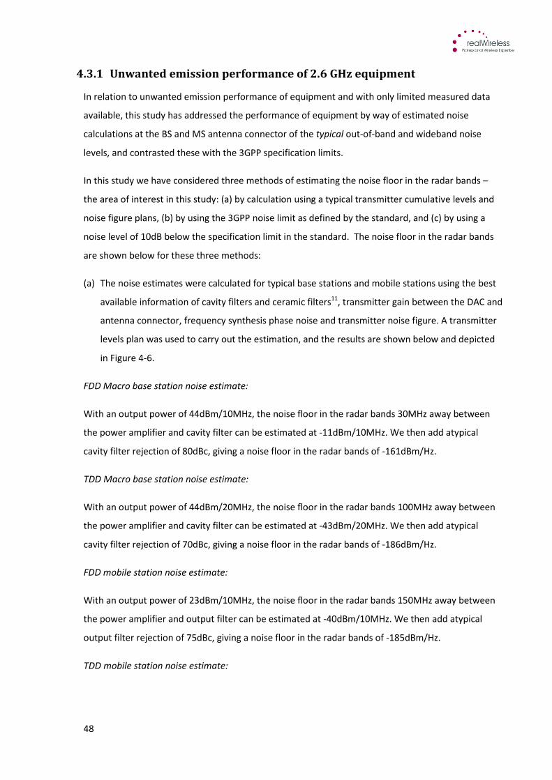
48
4.3.1 Unwanted emission performance of 2.6 GHz equipment
In relation to unwanted emission performance of equipment and with only limited measured data
available, this study has addressed the performance of equipment by way of estimated noise
calculations at the BS and MS antenna connector of the typical out-of-band and wideband noise
levels, and contrasted these with the 3GPP specification limits.
In this study we have considered three methods of estimating the noise floor in the radar bands –
the area of interest in this study: (a) by calculation using a typical transmitter cumulative levels and
noise figure plans, (b) by using the 3GPP noise limit as defined by the standard, and (c) by using a
noise level of 10dB below the specification limit in the standard. The noise floor in the radar bands
are shown below for these three methods:
(a) The noise estimates were calculated for typical base stations and mobile stations using the best
available information of cavity filters and ceramic filters11, transmitter gain between the DAC and
antenna connector, frequency synthesis phase noise and transmitter noise figure. A transmitter
levels plan was used to carry out the estimation, and the results are shown below and depicted
in Figure 4-6.
FDD Macro base station noise estimate:
With an output power of 44dBm/10MHz, the noise floor in the radar bands 30MHz away between
the power amplifier and cavity filter can be estimated at -11dBm/10MHz. We then add atypical
cavity filter rejection of 80dBc, giving a noise floor in the radar bands of -161dBm/Hz.
TDD Macro base station noise estimate:
With an output power of 44dBm/20MHz, the noise floor in the radar bands 100MHz away between
the power amplifier and cavity filter can be estimated at -43dBm/20MHz. We then add atypical
cavity filter rejection of 70dBc, giving a noise floor in the radar bands of -186dBm/Hz.
FDD mobile station noise estimate:
With an output power of 23dBm/10MHz, the noise floor in the radar bands 150MHz away between
the power amplifier and output filter can be estimated at -40dBm/10MHz. We then add atypical
output filter rejection of 75dBc, giving a noise floor in the radar bands of -185dBm/Hz.
TDD mobile station noise estimate:
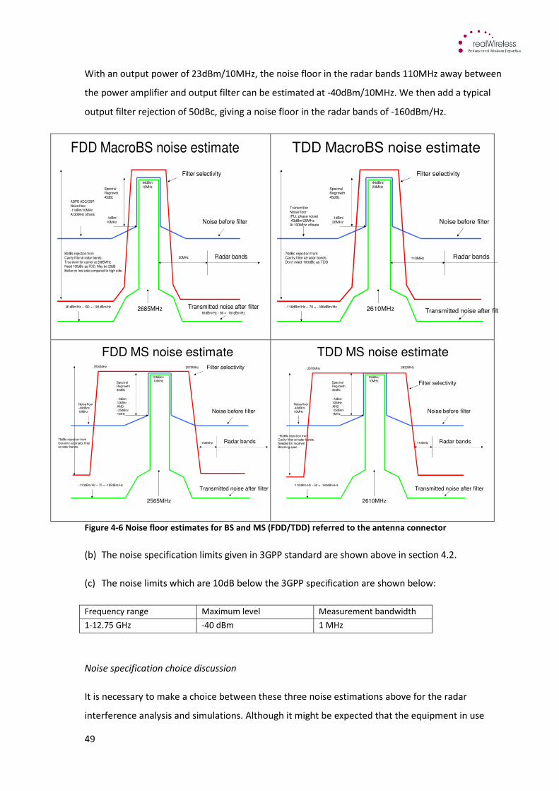
49
With an output power of 23dBm/10MHz, the noise floor in the radar bands 110MHz away between
the power amplifier and output filter can be estimated at -40dBm/10MHz. We then add a typical
output filter rejection of 50dBc, giving a noise floor in the radar bands of -160dBm/Hz.
Figure 4-6 Noise floor estimates for BS and MS (FDD/TDD) referred to the antenna connector
(b) The noise specification limits given in 3GPP standard are shown above in section 4.2.
(c) The noise limits which are 10dB below the 3GPP specification are shown below:
Frequency range Maximum level Measurement bandwidth
1-12.75 GHz -40 dBm 1 MHz
Noise specification choice discussion
It is necessary to make a choice between these three noise estimations above for the radar
interference analysis and simulations. Although it might be expected that the equipment in use
FDD MacroBS noise estimate
Noise before filter
Transmitted noise after filter
Filter selectivity
44dBm/10MHz
SpectralRegrowth45dBc
-1dBm/10MHz
ADPD ADC/DSPNoise floor-11dBm/10MHzAt 30MHz offsets
80dBc rejection fromCavity filter at radar bands.True even for carrier at 2685MHzNeed 100dBc as FDD. May be 20dBBetter on low side compared to high side
-81dBm/Hz – 100 = -181dBm/Hz 2685MHz
Radar bands
-81dBm/Hz – 80 = -161dBm/Hz
30MHz
TDD MacroBS noise estimate
Noise before filter
Transmitted noise after filter
Filter selectivity
44dBm/20MHz
SpectralRegrowth45dBc
-1dBm/20MHz
TransmitterNoise floor(PLL phase noise)-43dBm/20MHzAt 100MHz offsets
70dBc rejection fromCavity filter at radar bands.Don’t need 100dBc as TDD
-116dBm/Hz – 70 = -186dBm/Hz 2610MHz
Radar bands110MHz
FDD MS noise estimate
Noise before filter
Transmitted noise after filter
Filter selectivity
23dBm/10MHz
SpectralRegrowth30dBc
-7dBm/10MHzAND-25dBm/1MHz
Noise floor-40dBm/10MHz
75dBc rejection fromCeramic resonator filterat radar bands.
-110dBm/Hz – 75 = -185dBm/Hz
2565MHz
Radar bands150MHz
2500MHz 2570MHz
TDD MS noise estimate
Noise before filter
Transmitted noise after filter
Filter selectivity23dBm/10MHz
SpectralRegrowth30dBc
~50dBc rejection fromCavity filter at radar bands.Needed for receiverBlocking spec.
-110dBm/Hz – 50 = -160dBm/Hz
2610MHz
Radar bands110MHz
-7dBm/10MHzAND-25dBm/1MHz
Noise floor-40dBm/10MHz
2570MHz 2620MHz
50
around Heathrow airport might typically produce a noise floor in the radar bands as estimated in (a)
above, it may not be safe to assume such favourable equipment characteristics are and will be
present without specific steps being taken to ensure this. Manufacturers are always trying to cost
reduce their designs whilst remaining specification compliant. In this study we have therefore
decided to use the 3GPP specification limits (b) as the worst case levels, and 10dB inside this (c) for
the typical case levels.
4.3.2 Uplink Power control for LTE
LTE uses uplink power control to set the power levels of the user equipment within specific channel
conditions. This feature is used so that powers from multiple mobile stations do not saturate the base
station receiver. Additionally, power control acts as an efficiency mechanism as the power is nominally
reduced from maximum down to a given lower level depending on the path loss from the base station
receiver thus preserving battery life of the mobile station and reducing interference levels to other
cells.
In LTE the power control parameter is important for optimising system capacity. The mobile stations
calculate the path loss to determine the transmit power necessary to maintain the link budget.
Furthermore power control can be combined with frequency-domain resource allocation strategies
which allow interference coordination to further enhance cell edge performance and allow higher
overall spectral efficiency16. However, interference coordination of the UEs is the responsibility of the
scheduler and is dependent on the vendor’s scheduling algorithms and the associated parameters set
by the operator. Thus, operators can adjust the maximum transmit power of UEs on any given cell and
also the range and rate of power control applied.
Power control in LTE can improve the potential interference situation within an airport environment in
a number of ways:
• A reduction in transmit power from the UE based on its path loss from the base station within a
cell reduces overall interference and thus would be of benefit to radar receivers
• The functionality is implementation dependent and could be designed by the operator to
operate at an overall lower power level within close proximity to a radar.
The software model uses the total path loss between the mobile and each base station to determine
the power control operation using the following calculation:
Total pathloss = free space loss + log-normally distributed shadowing
16
LTE- The UMTS Long Term Evolution from theory to practice by Baker, Sesia Toufik

51
The transmit power of each mobile station is then calculated from the following equation:
�� � �max � min 1,max �min, � PLPL�ile�
���
where�max is the maximum transmit power, �min is the minimum power reduction ratio to prevent
mobile users with good channels from transmitting at a very low power level, PL is the total path
loss and PL�ile is the 95th percentile of the path loss (plus shadowing) value. With this power control
equation, the � percent of mobile users that have the highest path loss will transmit at �max.Finally,
0 � � � 1 is the balancing factor for terminals with bad channel and terminals with good channels12.
The values of these parameters are defined in Appendix B of the Appendices document.
The serving site is chosen from the base stations which provide the minimum total pathloss. The
following example graph illustrates the UE transmit power that results from employing the power
control algorithm. The plot is based on the statistics of a large number of UE locations within the
simulation polygons and with the presented network deployment. The transmit power is 23 dBm for
5% of the locations, whereas the power level falls to less than 15 dBm for 90% of the time. There is
an almost linear decline in the transmit power from 90% to 20% where the transmit power falls from
15 dBm to 5 dBm. For 50% of the time the transmit power of the mobile is below 10dBm.
Furthermore for small percentages of time (about 5%) it can be seen that the power falls below 0
dBm.
Figure 4-7 CDF of power control of the mobile
The power control functionality of the mobile network operating at 2.6 GHz introduces a powerful
interference reduction mechanism. In this example the base stations were positioned at their real
locations, see Figure 7-8. Given that the transmit power levels increase with an increasing BS-UE

52
pathloss, one particularly useful mitigation would be to locate the base stations within as close a
distance as possible to the location of high mobile user density areas.
In contrast to the base station for which the transmit power density is constant, the maximum
power of the mobile is independent of the transmission bandwidth. Thus a mobile which is
occupying all the resource blocks in a 20 MHz bandwidth will have its maximum power of 23dBm
divided equally amongst all resource blocks, while the whole of the power will be radiated in a single
180 kHz bandwidth if a single resource block is transmitted by the mobile, see Figure 4-8.
Figure 4-8 Physical Resource Block configurations
It is useful to note that the power control algorithm, as specified in the 3GPP standard (see Ref 3),
regulates the power in discrete steps. This function limits the possible transmit power values that
the mobile station can assume so as to mitigate the usage of the control channel. However, in the
software model the power control is assumed to be perfect, i.e. the step size is not discrete and the
transmit power values is equal to that required, regardless of consequences at the control channel.
This is a common assumption in such simulations and is not expected to significantly affect the
results.
53
4.3.3 Allocation of uplink resources for LTE
The use of resource blocks provides a method for allocating resources efficiently. In LTE there are a
number of different strategies for allocating resources. Allocations of resources are made based on a
set of conditions within the scheduling process at a high level, these are the channel state and traffic
measurement.
Based on the available channel measurements the scheduling algorithm implemented in the eNodeB
manages all the UE requirements within the cells under its control. This is to ensure that sufficient
radio transmission resources are allocated to each UE within acceptable latencies to meet their QoS
requirements in a spectrally efficient way. The impact of resource allocation relies on being able to
adapt the power dynamically according to the channel state. This level of system dynamism is not
typical of other cellular technologies and therefore may play a role in system deployments in and
around airports.
Ultimately the scheduling algorithms are the responsibility of the vendor/operator wishing to
produce optimum performance with minimum cost. However, there could be an opportunity for
operators/vendors to use the algorithms in way that minimises interference from the UE into a radar
and maintains a certain level of performance.
Resource allocation is used in the software model to represent a fair allocation of network resources
to the mobile stations and ensure equal spread of the power.
54
5 Overview of stakeholder engagement
The stakeholder engagement element of the study included a mixture of discussions, interviews and
correspondence with a select number of organisations. The stakeholders were chosen from a list of
organisations known to be interested or involved in work and development of 2.6 GHz equipment
and networks. The objective of the stakeholder engagement was to gather the vital information
which could inform the technical aspects of the study in relation to the technical parameters and
simulation assumptions for input to the interference model.
Real Wireless developed a stakeholder questionnaire which can be found in appendix G of the
Appendices report, with the aim of obtaining specific information in relation to:
• Performance of base station and mobile station equipment
• Mobile network deployment strategies in the 2.6 GHz band around airports
Views were gathered from respondents represented from both the mobile equipment vendor
industry and the mobile network operator industry in order to seek the required information. In
total five stakeholders responded to the questionnaire, two mobile operators and three equipment
vendors including one chipset manufacturer, handset manufacturer and base station vendor.
In general stakeholders expressed an interest in the 2.6 GHz spectrum band and provided views of
likely technical characteristics of network deployments and equipment performance. In the sections
below a summary of the information gathered from the perspective of both equipment vendors and
network operators is discussed.
5.1 Mobile Network Operator view
In summary, the views from the mobile operators based on issues concerning 2.6 GHz deployments
at airports include the following:
• The operators would use existing sites for 2.6 GHz deployments and load the macrocell
network to capacity deploying a carrier at each site where possible.
• The operator would need to upgrade their distributed antenna systems (DAS) to
accommodate 2.6 GHz frequencies as they currently only operate up to 2.1 GHz.
• Upgrades to the existing antennas would be needed to accommodate 2.6 GHz combined
with the other cellular bands
• 2 x 20 MHz channels are the only bandwidths being considered for high capacity networks.
Some thought has been given to 2 x 10 MHz for more rural deployments to improve
coverage but this is an unlikely configuration for a high capacity location such as an airport

55
• It is expected existing arrangements and processes exist between existing operators as to
the RF parameters used for shared sites and it is expected that these will be extended to
include the specific characteristics of 2.6 GHz equipment. It is therefore plausible that a
single site could support multiple 2.6 GHz operators.
• It is not foreseen that UMTS would be used at 2.6 GHz the band has clearly been earmarked
for 4G technologies
• Although 100% resource occupancy is possible, 70% occupancy of resource blocks were used
for trial simulations and seen as a good benchmark, although 100% would have to be treated
as the worst case for interference analysis.
5.2 Equipment vendor view
In summary, the views from mobile station equipment manufacturers based on issues concerning
equipment performance and 2.6 GHz deployments at airports include the following:
View on network deployments:
• Mostly deployments will be indoor microcells to deliver high capacity using one carrier per
site. It is not anticipated that macrocells will be heavily used if at all for 2.6 GHz. Assuming
operators have access to lower frequency bands such as 800 MHz.
• Operators are likely to acquire either 1 FDD channel 2 x 20 MHz or 2 x 10 MHz or 1 TDD
channel 1 x 20 MHz or 1 x 10 MHz. This could mean 3 operators obtaining 2 x 20 MHz each
and one operator obtaining the final 2 x 10 MHz.
• It is likely a frequency reuse of 1 will have to be used due to the restricted number of 2 x 20
MHz channels available in the band and the competition for it
• There could be a mix of FDD and TDD used by operators. For example if some operators also
obtained TDD this could be used for extra capacity in the downlink.
• UMTS 2.6 GHz is supported by some chipsets but there is little demand for it. Most demand
is for LTE or WiMAX at 2.6 GHz.
• Use of maximum output power is likely since if WiMAX operators obtain spectrum they will
be seeking blanket coverage and have no alternative spectrum to make up any shortfall in
coverage
• It is likely that 2.6 GHz deployments would use distributed antenna systems and femtocells
although more likely to use picocells for an airport deployment
• Peak to mean power ratios being observed for UEs are in the range 4:1 with maximum
power for UEs at 23 dBm
View on UE equipment emissions
• Vendors apply the ACLR as the critical limit to be met, therefore if equipment meets the
ACLR limit the out of band limits are easily met
• Spurious emissions from equipment is always much better than the specification. For
example -50dBm/MHz is a typical level. However spikes can occur on the intermodulation
frequencies that reach the spurious limit of -30 dBm/MHz
• There is little difference in the performance between handsets and USB dongles due to the
limited range of RF filtering components available on the market
• Power control performance is measured from the point the UE is transmitting at full power.
As long as the UE respects the ACLR emission mask at full power then vendors are generally
satisfied. There is little concern over performance at lower powers as long as the minimum
requirement is met at full power, so it should be met easily at lower powers
56
• Maximum power of the UEs is 23 dBm and is going to remain so for the future. There are no
plans to increase this due to the need to preserve battery life and Specific Absorption Rate
limits under the Health and Safety guidelines
5.3 Airport operator support
The main focus of this study was to determine interference from 2.6 GHz emissions within an airport
environment and thus close proximity to the radar. This has required essential input and support
from BAA the airport operator at Heathrow particularly, the information relating to the positions of
electronic communications equipment.
BAA provided data that supported the placement of base stations at the specific airport locations so
that a meaningful interference analysis could be conducted. The information related to confirmation
of cellular site locations and the geographical layout of the airport. It is worth noting that BAA uses a
formal process to facilitate the use and operation of electronic communications equipment within
the airport perimeter. This process ensures the necessary policies and compliances are met in
accordance with Health and Safety, spectrum usage and managed infrastructure.
In addition BAA supplied the layout plans of Heathrow airport for use to derive the locations of base
stations in line with the actual deployment that exists at the airport. The layout plans used for the
study can be seen in the three figures below which show:
• A high level layout plan of Heathrow Airport
• A detailed layout plan of the Central Terminal Area
• A detailed layout plan of the area around Terminal 4
The model used the following specific layout areas and locations:
• Central Terminal Area (consisting of Terminals 1 and 3 and surrounding area) and position of
base stations 1, 2, 3,4 and 5 including antenna heights and number of carriers per site
• Terminal 4 and surrounding area (including outside airport perimeter) and position of base
stations, 6 – 13 including antenna heights and number of carriers per site
The airport is currently undergoing re-development within the Central Terminal Area with
construction of new Terminal 2 buildings which may impact upon the present location of the base
stations. This is due to BAA adopting a common approach for the deployment of electronic
communications equipment as seen at Terminal 5 which uses common infrastructure for both indoor
and outdoor sites.
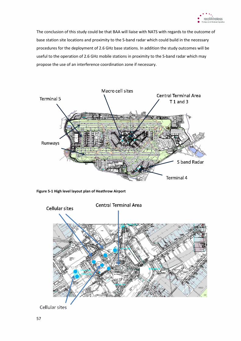
57
The conclusion of this study could be that BAA will liaise with NATS with regards to the outcome of
base station site locations and proximity to the S-band radar which could build in the necessary
procedures for the deployment of 2.6 GHz base stations. In addition the study outcomes will be
useful to the operation of 2.6 GHz mobile stations in proximity to the S-band radar which may
propose the use of an interference coordination zone if necessary.
Figure 5-1 High level layout plan of Heathrow Airport
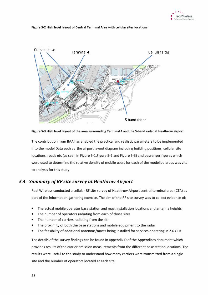
58
Figure 5-2 High level layout of Central Terminal Area with cellular sites locations
Figure 5-3 High level layout of the area surrounding Terminal 4 and the S-band radar at Heathrow airport
The contribution from BAA has enabled the practical and realistic parameters to be implemented
into the model Data such as the airport layout diagram including building positions, cellular site
locations, roads etc (as seen in Figure 5-1,Figure 5-2 and Figure 5-3) and passenger figures which
were used to determine the relative density of mobile users for each of the modelled areas was vital
to analysis for this study.
5.4 Summary of RF site survey at Heathrow Airport
Real Wireless conducted a cellular RF site survey of Heathrow Airport central terminal area (CTA) as
part of the information gathering exercise. The aim of the RF site survey was to collect evidence of:
• The actual mobile operator base station and mast installation locations and antenna heights
• The number of operators radiating from each of those sites
• The number of carriers radiating from the site
• The proximity of both the base stations and mobile equipment to the radar
• The feasibility of additional antennas/masts being installed for services operating in 2.6 GHz.
The details of the survey findings can be found in appendix D of the Appendices document which
provides results of the carrier emission measurements from the different base station locations. The
results were useful to the study to understand how many carriers were transmitted from a single
site and the number of operators located at each site.

59
The information gathered from the site survey was used as input to the modelling parameters and
assumptions which can be found in appendix B of the Appendices document.
Heathrow Airport CTA is not typical of most UK airport environments this is based on a number of
factors that differentiate it from other airports such as:
• The ATC radar at Heathrow is one of the tallest out of all licensed S-band ATC radars in the UK at
40m above local terrain (Note our modelled assumptions are based on generic radar
parameters)
• Heathrow has the most number of terminal buildings of any airport and can accommodate
several million passengers per month
• According to the Ofcom Sitefinder the extent of mobile phone operator outdoor deployments
for the Heathrow CTA exceeds the next largest airport, Gatwick, by more than 2:1.
The findings from the RF survey showed that up to three operators were co-located at some of the
rooftop sites transmitting a combination of both GSM and UMTS carriers which demonstrates the
need for site sharing at the airport. In addition, it was noted that there was clear line of sight path
from the rooftop to the radar that contributes to the decision to use a propagation model that takes
account of free space at distances greater than 1km. In relation to the present study macro sites for
2.6 GHz deployments would need the highest rooftop sites to maximise coverage which may come
at a premium based on the number of existing services and operators already established at the
airport.
However, it was found that it may be possible for additional outdoor masts and antennas to be built
at the current sites with the current CTA layout to accommodate upgrades or new installations at 2.6
GHz. As discussed in the previous section the CTA at Heathrow is undergoing renovation and any
new layout is likely to be very different to the present layout. It is not known at this stage in detail
what the new CTA layout will look like and therefore understanding the coordination zones for the
radar may help inform the planning stages of CTA development.
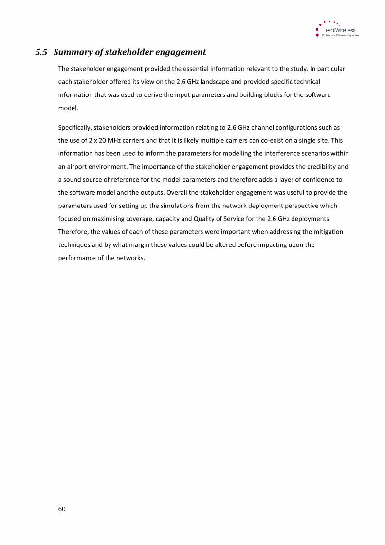
60
5.5 Summary of stakeholder engagement
The stakeholder engagement provided the essential information relevant to the study. In particular
each stakeholder offered its view on the 2.6 GHz landscape and provided specific technical
information that was used to derive the input parameters and building blocks for the software
model.
Specifically, stakeholders provided information relating to 2.6 GHz channel configurations such as
the use of 2 x 20 MHz carriers and that it is likely multiple carriers can co-exist on a single site. This
information has been used to inform the parameters for modelling the interference scenarios within
an airport environment. The importance of the stakeholder engagement provides the credibility and
a sound source of reference for the model parameters and therefore adds a layer of confidence to
the software model and the outputs. Overall the stakeholder engagement was useful to provide the
parameters used for setting up the simulations from the network deployment perspective which
focused on maximising coverage, capacity and Quality of Service for the 2.6 GHz deployments.
Therefore, the values of each of these parameters were important when addressing the mitigation
techniques and by what margin these values could be altered before impacting upon the
performance of the networks.
61
6 InterferenceAnalysisModelling
This section describes the options for addressing the interference analysis approach and discusses
the different elements required to undertake the analysis. This section also addresses the choice of
modelling option used for evaluating the interference at an airport between both base stations and
mobile stations operating in the 2.6 GHz band and an air surveillance radar operating in the upper
adjacent S-band.
6.1 Objectives
The objectives of the interference modelling were to:
• Use practical technical parameters likely to be employed at 2.6 GHz
• Produce modelling results which clearly show the most challenging case and typical case impact
of emissions from the 2.6 GHz band into the 2.7 GHz S-band.
• Provide robust rationale for the choice of modelling criteria and supply evidence that can be
used as an input contribution for radar interference levels and protection criteria.
• Replicate real world network performance parameters such as power control, cell edge
performance and high quality of service for users as far as practicable while still producing a
tractable simulation approach.
• Understand the interference implications for deployments at airports
• Include the flexibility to model mitigation techniques to the deployment scenarios
6.2 Interference assessment methods
The assessment of interference and co-existence is addressed by many publications from the ITU or
CEPT with specific studies conducted depending on the particular type of services to co-exist. For
example ECC report 14813 which addresses the performance of DVB-T receiver in the presence of LTE
transmitters and ECC report 14014 which addresses the compatibility between RLAN on board
aircraft and radars in the bands 5250-5350 MHz/5470-5725 MHz are studies that include specific
assessment methods that address the nature of the interference mechanism.
However, the interference mechanisms investigated in this study are commonly found in many co-
existence/compatibility studies in European Communications Office Spectrum Engineering Working
Group. For example SE42 (now closed) was studying flexible bands, WAPECS and new sharing

62
approaches which included the 2.6 GHz band. Therefore an acknowledged and well-established
approach has been adopted for this study.
Figure 6-1 Out-of-band and in-band 2.6 GHz interference mechanisms into radar receiver17
NOTE: There are
complex intermodulation and radar receiver mixing effects which can cause a result similar to the sum of
both effects
Blocking the radar receiver front end from base stations and mobile stations:
In-band interference manifests itself as the integrated power into the front end of the receiver when
emissions of a certain magnitude cause saturation of the sensitive components in the receiver. The
mechanism can be seen at a basic level on the left hand side of Figure 6-1 showing how the signal-to-
noise ratio is reduced, producing an equivalent effect to reducing the wanted signal relative to the
noise. The LNA and other components in a radar receiver are highly sensitive to allow detection of
low level signal reflections from moving targets. Each component in the receiver chain exhibits a
different threshold level for the 1 dB compression point and if the total integrated power from in
band 2.6 GHz systems exceeds the threshold level that particular component goes into compression
and thus degrades the performance of the radar. In the case of base stations the interference is
more significant due to the close separation in frequency between the top of the 2.6 GHz band and
the bottom of the adjacent 2.7 GHz band. The large in band emissions from base stations could
cause compression of the active components of the radar receiver if close enough to the radar and in
certain circumstances can cause a noise floor rise.
The potential for interference from mobiles is much lower for several reasons:
17
Diagram sourced from Cobham Technical Services report
S
N
S
N
S
N
S
N
Radar signal
suppressed
Signal-to-
noise ratio
(SNR)
Noise floor
raised
No
Interference
No
Interference
With
Interference
With
Interference
Radar effects from out-of-band
communication signals
Radar effects from in-band
communication signals
63
• A wider frequency separation of the mobile portion of the 2.6 GHz band and the reduced
power output. There is a 98 MHz minimum frequency separation from the highest uplink
channel 2610 MHz and the lowest radar channel 2708 MHz.
• In addition the mobile station transmit power is also much lower than the base stations
which will also minimise the interference levels into the front end of the radar.
• Power control will typically be used, so that mobiles rarely transmit at their maximum rated
power.
However, these reductions are offset somewhat by the reduced potential to suppress spurious
emissions in mass-market devices, and this will remain a source of significant uncertainty for this
investigation until the performance of practical devices becomes more clear.
Noise rise co-channel with radar centre frequency from base stations and mobile stations:
Systems operating in the 2.6 GHz band are very likely going to use 20 MHz bandwidths and can
generate a noise rise in the radar receiver. The right hand side of Figure 6-1 shows how the
mechanism affects the radar when an increase in noise impacts on the SNR and thus degrades
performance.
Any rise in noise can affect the performance of the radar and therefore a protection ratio is applied
to the radar noise floor to provide sufficient protection from interference. The interference
threshold level is the allowed interference which if exceeded by the interference noise power from
2.6 GHz emissions will de-sensitise the receiver and degrade performance of the radar.
The interference noise power is calculated by integrating the spurious and out of band emissions
from 2.6 GHz system applied across the radar band. The rise in noise is calculated in the following
way:
Allowed interference (I) = Radar Noise floor + Protection ratio (I/N)
These methods for analysing interference are generally used for the assessment between two
different systems but can be used for the assessment between two types of the same system such as
co-existence between FDD and TDD systems in the same band. The analysis is also dependent on a
number of factors such as the frequency band of operation, the location of the transmitters,
terrestrial or space, propagation model and so on.
In the case of co-existence between mobile communications systems and other services, CEPT
published report ECC report 04515 which addresses the interference between UMTS/IMT 2000
systems operating in the 2500-2690 MHz band and other services. It describes the methods for
interference analysis using Minimum Coupling Loss calculations and Monte Carlo and the benefits of
64
adopting each approach. This is relevant to the present study based on a similar set of parameter
requirements for the mobile communications system in addition to the victim parameters which in
this case is the radar receiver.
These two approaches are addressed in more detail in the following sections.
6.2.1 Initial blocking interference analysis
Ofcom has conducted a number of previous studies4 to establish the impact of 2.6 GHz systems
causing interference to radar in the adjacent 2.7 GHz band and identified there is a significant
problem from base station emissions causing interference to current ATC radars. Each of the studies
performed the basic calculations to establish the out-of-band emissions, path loss, protection
distance and interference power for either blocking the radar or increase in interference noise
power. The results from the calculations were used to validate the findings from practical trials or
the laboratory tests and thus inform the necessary regulatory decisions for spectrum award.
It is useful to develop a full appreciation of the impact which 2.6 GHz emissions have on radars in the
2.7 GHz band and making some high level calculations provides the baseline outputs. Prior to this
study Ofcom made some initial calculations16 to understand the impact of interference using
minimum coupling loss calculations. The minimum coupling loss is often used for an initial
assessment of the interference scenarios and generates values in the order of magnitude expected
of a static scenario. This occurs for example, when a single transmitter causes interference into a
single receiver and not intended to represent a realistic scenario.
For the present study an initial assessment was made using the same method to establish a basic
understanding of how each interference mechanism is treated which showed good correlation
between the two sets of results.
Using the minimum coupling loss equation below and the main parameters from the parameters
assumption booklet (found in appendix B of the Appendices report) the following minimum coupling
loss and thus protection distance can be calculated for blocking:
MCL = Transmit power (dBm) + Transmit antenna gain (dBi) + Receive antenna gain (dBi) –
Receive interference threshold (dBm)
Where:

65
MCL is the minimum coupling loss in dB
Transmit power is the transmitter power in a given bandwidth = 50 dBm/(20) MHz
Transmit antenna gain is the gain of the transmit antenna = 17 dBi
Radar antenna gain is the gain of the receive antenna (horizontal direction) = 28 dBi
Equivalent pre LNA power level required for no radar performance degradation = -42dBm (pre
modified radar filter)
MCL = 50 + 17 +28 – (-42)
MCL = 137 dB
The minimum coupling loss of 137 dB is the minimum amount of loss necessary to not cause
interference to the front end of the radar LNA. This equation and calculation is useful to calculate
the protection distance using basic free space path loss equation to establish a high level protection
distance. Using free space path loss the following protection distance applies:
FSPL = 32.45 + 20 log(f) MHz + 20 log (d) km
137 = 32.45 + 20 log(2685) + 20 log (d)
d =10 (137– 32.45 – 68.5)/20
d = 63 km
This distance d of 63 km is the result of realistic input parameters used in this basic calculation
function. This distance suggests that base stations transmitting at full power should be 63 km away
or more from the radar under free space conditions to not exceed the blocking level at the input to
the LNA. A result of this nature is useful to establish the extent of a problem and in this case suggests
a more detailed further examination is necessary. The minimum coupling loss equations only allow a
limited static case to be examined for the interference without the considerations of dynamic
changes in the mobile environment such as movement of mobiles, power control and rotation of the
radar antenna. The aim of this study is to obtain the realistic mobile environment within an airport
and the output from the minimum coupling loss does not provide the sufficient information to
conduct the full analysis.
Therefore, the minimum coupling loss calculations are useful for establishing indicative values to
provide the order of magnitude of results and have not been taken any further for this study. The
66
requirement for this study was to consider a more detailed analysis of the interference situation,
provide the ability to use actual, realistic system parameters and take account of the antenna
patterns for example and the actual pathloss between the interferer and the victim. A more
appropriate method for this type of interference assessment is Monte Carlo analysis which is
discussed in more detail in the next section.
6.2.2 Monte Carlo simulation
An alternative and more detailed method for interference analysis is the use of Monte Carlo
simulations. Monte Carlo simulations add a layer of complexity to the scenarios by introducing a
probability of interference for a given set of parameters and deployments. In addition Monte Carlo
simulations offer more realistic results, offers a dynamic and variable modelling environment but are
highly dependent on the accuracy and knowledge of the input parameters.
In the case of the present study the Monte Carlo method enables the ability to randomly distribute
the mobiles within the defined modelling areas of the airport and repeat the generation of
interference to the radar multiple times and at different locations. This method has the benefit of
fine tuning the statistical outputs that produce confident and robust results.
The placement of active mobiles in random locations is representative of mobiles moving around a
densely populated area such as an airport terminal to represent a realistic scenario as much as
possible. Another important factor is the use of accurate input data such as the technical
parameters. The more accurate and precise the input technical parameters the more accurate and
precise the outcomes will be.
Furthermore, Monte Carlo analysis is used extensively by regulators across the European Community
as an established approach to evaluate co-existence between different radio services and determine
various modelled outcomes. For example the Seamcat (Spectrum Engineering Advanced Monte
Carlo Analysis Tool) has been used in the spectrum engineering community of CEPT to analyse many
different co-existence studies and scenarios such as co-existence between FDD and TDD systems in
the 2.6 GHz band17. Therefore Monte Carlo analysis has been deemed as an appropriate analysis
approach for this study.
There are some downsides of using Monte Carlo analysis, specifically the level of complexity in
modelling the dynamic mobile environment and the difficulty of determining reliable values for
parameters such as the density and duty cycle of mobiles. In order to capture the interfering effects
from the mobiles the software model makes calculations for the mobiles in each position, this
requires a significant level of computer processing and calculation complexity since the pathloss
67
between each mobile and the base station is taken into account in addition to the pathloss between
the mobile and the radar for each mobile position. Nevertheless, the resulting model is tractable for
realistic environments and provides insight into the interference situation which more simplistic
approaches could not replicate.
6.2.3 Choice of modelling approach
There is a clear choice for the modelling approach to use for an investigation such as the airport
deployment study and Monte Carlo analysis was considered to be the simplest credible technique
for each of the given scenarios.
The decision to use Monte Carlo analysis with the inclusion of specific propagation models for the
study was made based on a trade-off for modelling complexity against the use of a commercial
propagation modelling tool which may offer a more generic static path model. In comparison the
accuracy that can be realised from adopting a Monte Carlo analysis with specific propagation models
provides a unique blend of interference analysis from the dynamic perspective to model the
movement of mobiles and inclusion of functions such as power control in addition to analysing the
specific paths that exist within an airport environment. These functions combined provide a
powerful tool for modelling a full 2.6 GHz deployment for a specific simulation area.
A generic model would have been a suitable alternative for modelling the airport environment but
with generic models the user is restricted to the input variables offered by the particular model
which may remove the ability to perform certain functions for the simulations. The particular
function which is not usually available within generic models is the power control mechanism from
mobiles. The choice of method adopted enabled the activation of power control which is deemed to
be a fundamental feature in minimising interference into radar from mobiles.
Furthermore, Monte Carlo analysis provides the flexibility to build up statistics of results to a very
detailed level which means extensive sensitivity analysis can be carried to refine and tune the
results.
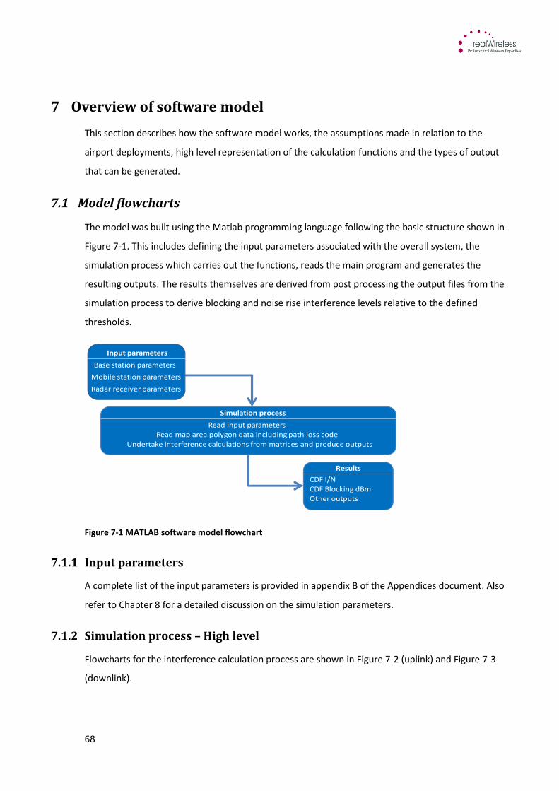
68
7 Overview of software model
This section describes how the software model works, the assumptions made in relation to the
airport deployments, high level representation of the calculation functions and the types of output
that can be generated.
7.1 Model flowcharts
The model was built using the Matlab programming language following the basic structure shown in
Figure 7-1. This includes defining the input parameters associated with the overall system, the
simulation process which carries out the functions, reads the main program and generates the
resulting outputs. The results themselves are derived from post processing the output files from the
simulation process to derive blocking and noise rise interference levels relative to the defined
thresholds.
Figure 7-1 MATLAB software model flowchart
7.1.1 Input parameters
A complete list of the input parameters is provided in appendix B of the Appendices document. Also
refer to Chapter 8 for a detailed discussion on the simulation parameters.
7.1.2 Simulation process – High level
Flowcharts for the interference calculation process are shown in Figure 7-2 (uplink) and Figure 7-3
(downlink).
Other outputs
CDF I/N
CDF Blocking dBm
Read input parameters
Read map area polygon data including path loss code
Undertake interference calculations from matrices and produce outputs
Simulation process
Results
Base station parameters
Mobile station parameters
Radar receiver parameters
Input parameters
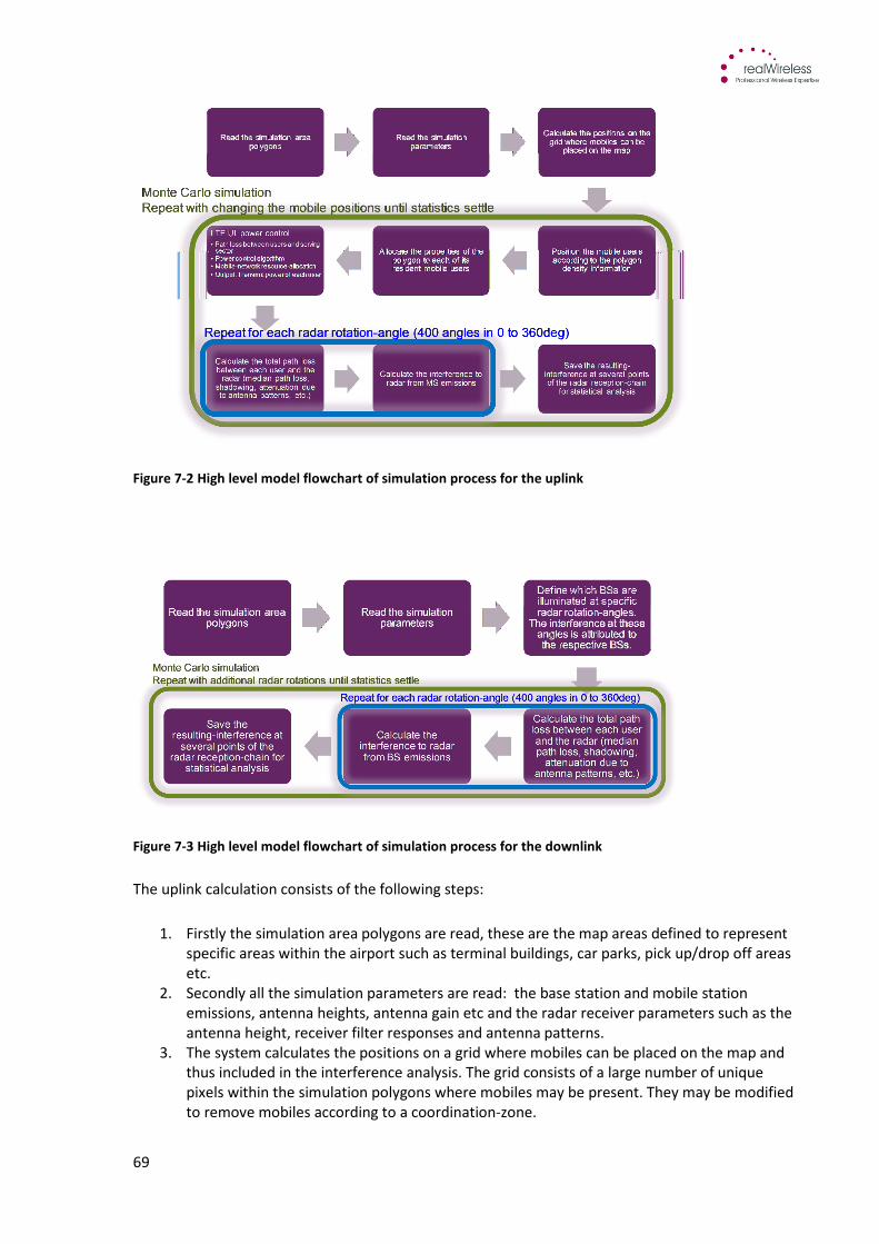
69
Figure 7-2 High level model flowchart of simulation process for the uplink
Figure 7-3 High level model flowchart of simulation process for the downlink
The uplink calculation consists of the following steps:
1. Firstly the simulation area polygons are read, these are the map areas defined to represent
specific areas within the airport such as terminal buildings, car parks, pick up/drop off areas
etc.
2. Secondly all the simulation parameters are read: the base station and mobile station
emissions, antenna heights, antenna gain etc and the radar receiver parameters such as the
antenna height, receiver filter responses and antenna patterns.
3. The system calculates the positions on a grid where mobiles can be placed on the map and
thus included in the interference analysis. The grid consists of a large number of unique
pixels within the simulation polygons where mobiles may be present. They may be modified
to remove mobiles according to a coordination-zone.
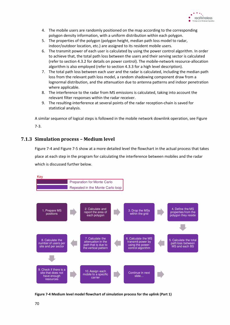
70
4. The mobile users are randomly positioned on the map according to the corresponding
polygon density information, with a uniform distribution within each polygon.
5. The properties of the polygon (polygon height, median path loss model to radar,
indoor/outdoor location, etc.) are assigned to its resident mobile users.
6. The transmit power of each user is calculated by using the power control algorithm. In order
to achieve that, the total path loss between the users and their serving sector is calculated
(refer to section 4.3.2 for details on power control). The mobile-network resource-allocation
algorithm is also employed (refer to section 4.3.3 for a high level description).
7. The total path loss between each user and the radar is calculated, including the median path
loss from the relevant path loss model, a random shadowing component draw from a
lognormal distribution, and the attenuation due to antenna patterns and indoor penetration
where applicable.
8. The interference to the radar from MS emissions is calculated, taking into account the
relevant filter responses within the radar receiver.
9. The resulting-interference at several points of the radar reception-chain is saved for
statistical analysis.
A similar sequence of logical steps is followed in the mobile network downlink operation, see Figure
7-3.
7.1.3 Simulation process – Medium level
Figure 7-4 and Figure 7-5 show at a more detailed level the flowchart in the actual process that takes
place at each step in the program for calculating the interference between mobiles and the radar
which is discussed further below.
Figure 7-4 Medium level model flowchart of simulation process for the uplink (Part 1)
1. Prepare MS positions
2. Calculate and report the area of
each polygon
3. Drop the MSswithin the grid
4. Define the MS properties from the polygon they reside
5. Calculate the total path loss between MS and each BS
6. Calculate the MS transmit power by using the power-control algorithm
7. Calculate the attenuation in the path that is due to the vertical pattern
8. Calculate the number of users per site and per sector
9. Check if there is a site that does not
have enough resources
10. Assign each mobile to a specific
carrier
Continue in next slide…
Key
Preparation for Monte Carlo
Repeated in the Monte Carlo loop
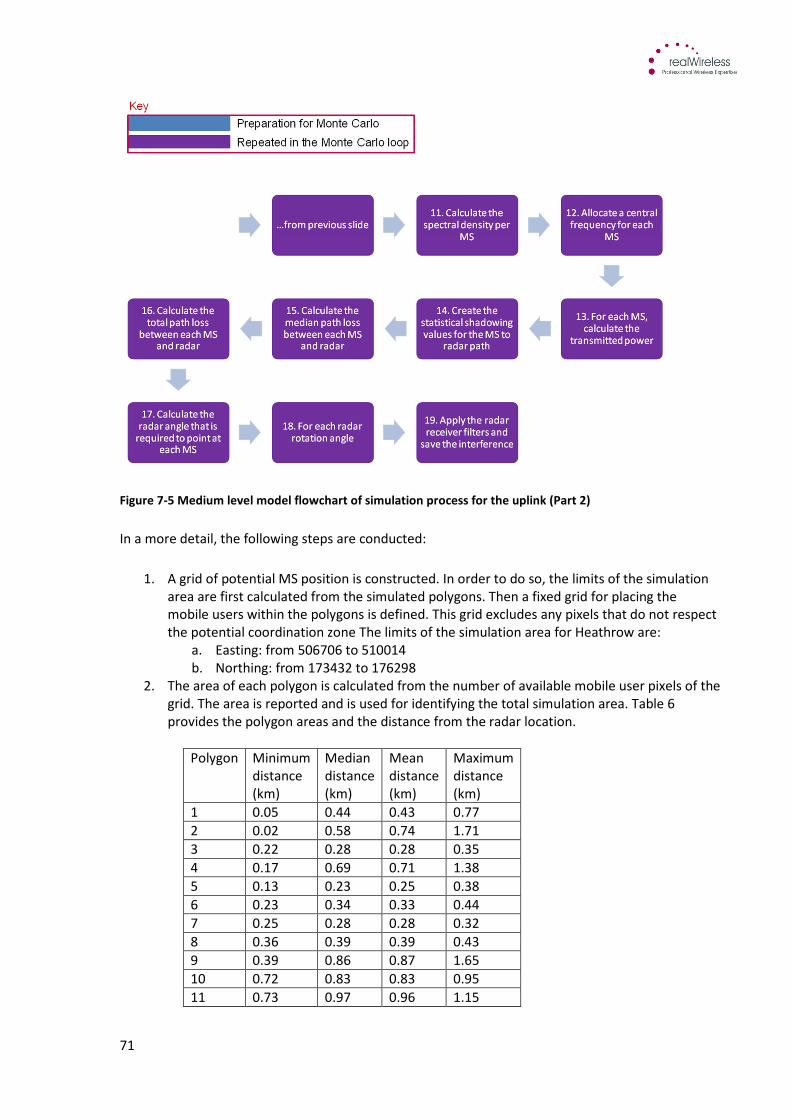
71
Figure 7-5 Medium level model flowchart of simulation process for the uplink (Part 2)
In a more detail, the following steps are conducted:
1. A grid of potential MS position is constructed. In order to do so, the limits of the simulation
area are first calculated from the simulated polygons. Then a fixed grid for placing the
mobile users within the polygons is defined. This grid excludes any pixels that do not respect
the potential coordination zone The limits of the simulation area for Heathrow are:
a. Easting: from 506706 to 510014
b. Northing: from 173432 to 176298
2. The area of each polygon is calculated from the number of available mobile user pixels of the
grid. The area is reported and is used for identifying the total simulation area. Table 6
provides the polygon areas and the distance from the radar location.
Polygon Minimum
distance
(km)
Median
distance
(km)
Mean
distance
(km)
Maximum
distance
(km)
1 0.05 0.44 0.43 0.77
2 0.02 0.58 0.74 1.71
3 0.22 0.28 0.28 0.35
4 0.17 0.69 0.71 1.38
5 0.13 0.23 0.25 0.38
6 0.23 0.34 0.33 0.44
7 0.25 0.28 0.28 0.32
8 0.36 0.39 0.39 0.43
9 0.39 0.86 0.87 1.65
10 0.72 0.83 0.83 0.95
11 0.73 0.97 0.96 1.15
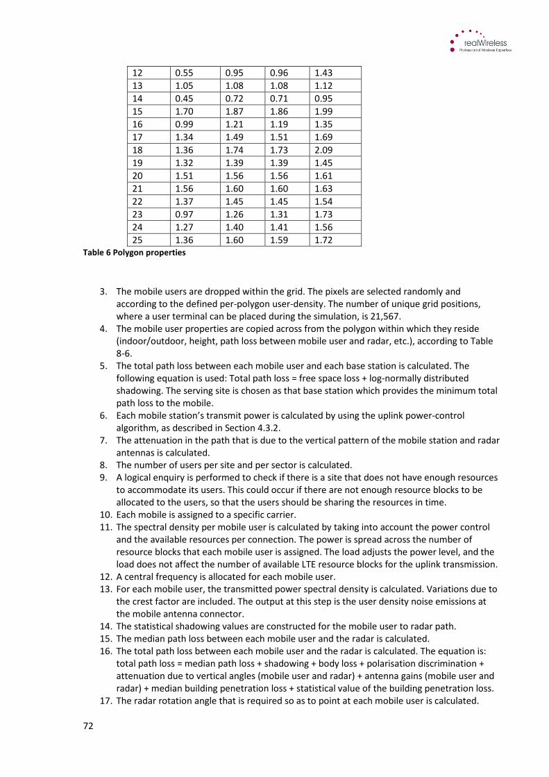
72
12 0.55 0.95 0.96 1.43
13 1.05 1.08 1.08 1.12
14 0.45 0.72 0.71 0.95
15 1.70 1.87 1.86 1.99
16 0.99 1.21 1.19 1.35
17 1.34 1.49 1.51 1.69
18 1.36 1.74 1.73 2.09
19 1.32 1.39 1.39 1.45
20 1.51 1.56 1.56 1.61
21 1.56 1.60 1.60 1.63
22 1.37 1.45 1.45 1.54
23 0.97 1.26 1.31 1.73
24 1.27 1.40 1.41 1.56
25 1.36 1.60 1.59 1.72
Table 6 Polygon properties
3. The mobile users are dropped within the grid. The pixels are selected randomly and
according to the defined per-polygon user-density. The number of unique grid positions,
where a user terminal can be placed during the simulation, is 21,567.
4. The mobile user properties are copied across from the polygon within which they reside
(indoor/outdoor, height, path loss between mobile user and radar, etc.), according to Table
8-6.
5. The total path loss between each mobile user and each base station is calculated. The
following equation is used: Total path loss = free space loss + log-normally distributed
shadowing. The serving site is chosen as that base station which provides the minimum total
path loss to the mobile.
6. Each mobile station’s transmit power is calculated by using the uplink power-control
algorithm, as described in Section 4.3.2.
7. The attenuation in the path that is due to the vertical pattern of the mobile station and radar
antennas is calculated.
8. The number of users per site and per sector is calculated.
9. A logical enquiry is performed to check if there is a site that does not have enough resources
to accommodate its users. This could occur if there are not enough resource blocks to be
allocated to the users, so that the users should be sharing the resources in time.
10. Each mobile is assigned to a specific carrier.
11. The spectral density per mobile user is calculated by taking into account the power control
and the available resources per connection. The power is spread across the number of
resource blocks that each mobile user is assigned. The load adjusts the power level, and the
load does not affect the number of available LTE resource blocks for the uplink transmission.
12. A central frequency is allocated for each mobile user.
13. For each mobile user, the transmitted power spectral density is calculated. Variations due to
the crest factor are included. The output at this step is the user density noise emissions at
the mobile antenna connector.
14. The statistical shadowing values are constructed for the mobile user to radar path.
15. The median path loss between each mobile user and the radar is calculated.
16. The total path loss between each mobile user and the radar is calculated. The equation is:
total path loss = median path loss + shadowing + body loss + polarisation discrimination +
attenuation due to vertical angles (mobile user and radar) + antenna gains (mobile user and
radar) + median building penetration loss + statistical value of the building penetration loss.
17. The radar rotation angle that is required so as to point at each mobile user is calculated.
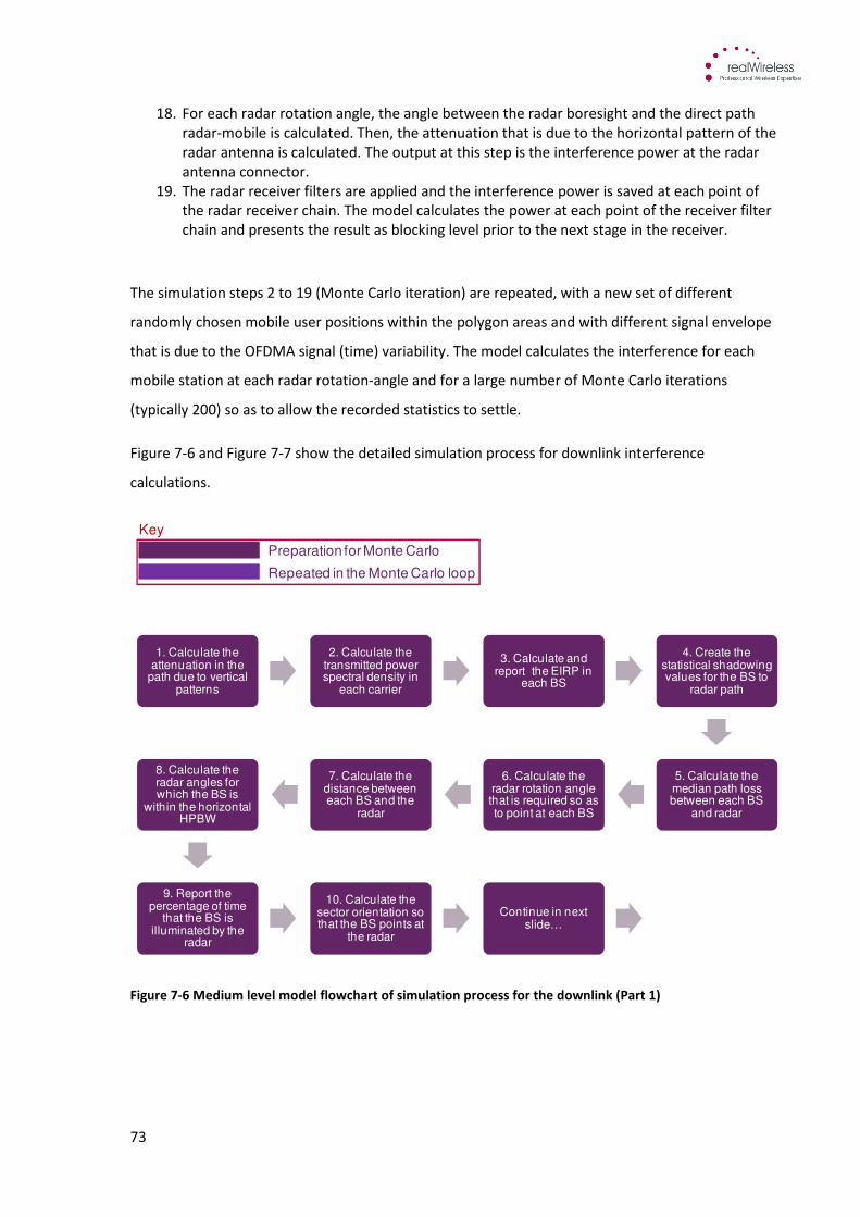
73
18. For each radar rotation angle, the angle between the radar boresight and the direct path
radar-mobile is calculated. Then, the attenuation that is due to the horizontal pattern of the
radar antenna is calculated. The output at this step is the interference power at the radar
antenna connector.
19. The radar receiver filters are applied and the interference power is saved at each point of
the radar receiver chain. The model calculates the power at each point of the receiver filter
chain and presents the result as blocking level prior to the next stage in the receiver.
The simulation steps 2 to 19 (Monte Carlo iteration) are repeated, with a new set of different
randomly chosen mobile user positions within the polygon areas and with different signal envelope
that is due to the OFDMA signal (time) variability. The model calculates the interference for each
mobile station at each radar rotation-angle and for a large number of Monte Carlo iterations
(typically 200) so as to allow the recorded statistics to settle.
Figure 7-6 and Figure 7-7 show the detailed simulation process for downlink interference
calculations.
Figure 7-6 Medium level model flowchart of simulation process for the downlink (Part 1)
1. Calculate the attenuation in the
path due to vertical patterns
2. Calculate the transmitted power spectral density in
each carrier
3. Calculate and report the EIRP in
each BS
4. Create the statistical shadowing values for the BS to
radar path
5. Calculate the median path loss between each BS
and radar
6. Calculate the radar rotation angle that is required so as to point at each BS
7. Calculate the distance between each BS and the
radar
8. Calculate the radar angles for which the BS is
within the horizontal HPBW
9. Report the percentage of time
that the BS is illuminated by the
radar
10. Calculate the sector orientation so that the BS points at
the radar
Continue in next slide…
Key
Preparation for Monte Carlo
Repeated in the Monte Carlo loop
74
Figure 7-7 Medium level model flowchart of simulation process for the downlink (Part 2)
The following steps are followed for the downlink:
1. The attenuation in the path that is due to the vertical pattern of the base station and radar
antennas is first calculated.
2. For each site, the transmitted power spectral density is calculated for each of the active
carriers. The output after this step, which includes the effect of signal envelope variability, is
the base station noise emissions at the antenna connector.
3. The EIRP of each base station is calculated. The EIRP is reported for a checkpoint against the
simulation desired inputs.
4. The statistical shadowing values for the base station to radar path are created.
5. The median path loss between each base station and the radar is calculated.
6. The radar rotation-angle that is required so as to point at each base station is calculated.
7. The distance between each base station and the radar is calculated.
8. For each base station, the radar rotation-angles for which the base station is within the
horizontal Half-Power Beam-Width (HPBW) of the radar are calculated. More details about
the radar antenna pattern and the HPBW are provided in the appendix B of the Appendices
document.
9. The percentage of time that the base station is illuminated by the radar is calculated. This
percentage is reported and is equal to the percentage of time that the base station is
required to be inactive to mitigate interference to the radar receiver.
10. The orientation of each sector is calculated, for the sectors whose orientation is not
explicitly defined by the user. At this step, the sector’s boresight is set to point at the radar
(worst-case orientation), or the sector’s HPBW is set to point towards the radar (best-case
orientation).
…from previous slide
11. For each radar rotation angle
12. For each BS, calculate the
transmitted power spectral density
13. Calculate the median path loss between each BS
and the radar
14. Calculate the total path loss
between each BS and the radar
15. Calculate the interference power
at the radar antenna connector
16. Apply the radar receiver filters and save the interference
Key
Preparation for Monte Carlo
Repeated in the Monte Carlo loop
75
11. For each radar rotation angle, the angle between the radar boresight and the direct path
radar-site is calculated. The attenuation that is due to the horizontal pattern of the radar
antenna is calculated.
12. For each base station, the transmitted power spectral-density is calculated. The output at
the end of this step is the base station emissions at the antenna connector. In the calculation
of the base station emissions the variability due to the signal envelope and the reduced EIRP
in the restricted spectrum-block are taken into account. More information on the restricted
block is provided in section 8.2.
13. The median path loss between each base station and the radar is calculated.
14. The total path loss between each base station and the radar is calculated. The equation is:
total path loss = median path loss + shadowing + body loss + polarisation discrimination +
attenuation due to vertical angles (base station and radar) + antenna gains (base station and
radar) + median building penetration loss + statistical value of the building penetration loss.
15. For each radar rotation-angle, the interference power at the radar antenna connector is
calculated.
16. The radar receiver filters are applied. The interference power at each point of the radar
receiver chain is saved for statistical analysis.
The simulation steps 11 to 16 (Monte Carlo iteration) are repeated, with the same base station
positions, however with a varying signal envelope due to the OFDMA signal variability. The model
calculates the interference for each mobile station at each radar rotation-angle, and for [25] Monte
Carlo iterations so as to allow the recorded statistics to settle.
7.1.4 Form of output
Figure 7-8 shows the simulation area, and plots the base stations and mobile stations on to the
polygon areas. The pink triangles represent the base station locations, the blue dots represent
randomly distributed mobile stations and the red star is the radar location. The polygon areas are
represented by different coloured shapes that are based on the different areas of the airport such as
a terminal building or car park. The mobiles can be placed in each polygon which has its own specific
properties in relation to the simulation parameters. The properties for each polygon include the
mobile height, mobile user density and median path loss model for the link polygon-radar.
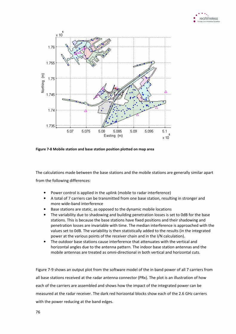
76
Figure 7-8 Mobile station and base station position plotted on map area
The calculations made between the base stations and the mobile stations are generally similar apart
from the following differences:
• Power control is applied in the uplink (mobile to radar interference)
• A total of 7 carriers can be transmitted from one base station, resulting in stronger and
more wide-band interference
• Base stations are static, as opposed to the dynamic mobile locations
• The variability due to shadowing and building penetration losses is set to 0dB for the base
stations. This is because the base stations have fixed positions and their shadowing and
penetration losses are invariable with time. The median interference is approached with the
values set to 0dB. The variability is then statistically added to the results (in the integrated
power at the various points of the receiver chain and in the I/N calculation).
• The outdoor base stations cause interference that attenuates with the vertical and
horizontal angles due to the antenna pattern. The indoor base station antennas and the
mobile antennas are treated as omni-directional in both vertical and horizontal cuts.
Figure 7-9 shows an output plot from the software model of the in band power of all 7 carriers from
all base stations received at the radar antenna connector (PRx). The plot is an illustration of how
each of the carriers are assembled and shows how the impact of the integrated power can be
measured at the radar receiver. The dark red horizontal blocks show each of the 2.6 GHz carriers
with the power reducing at the band edges.
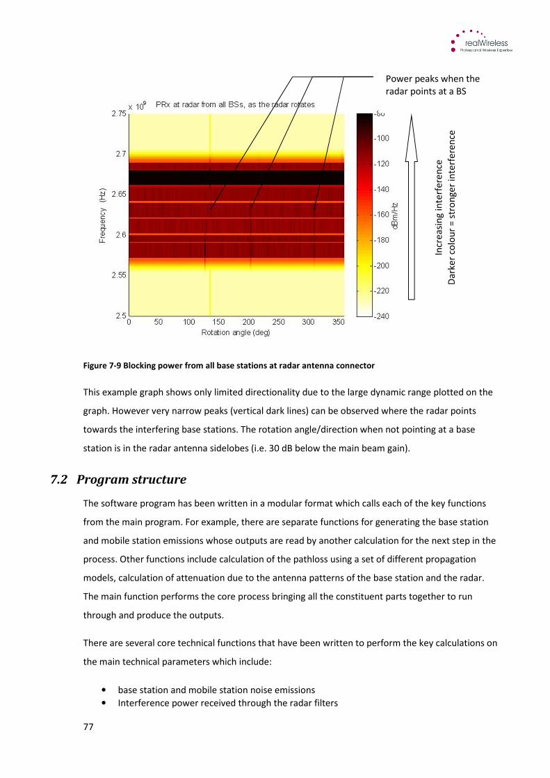
77
Figure 7-9 Blocking power from all base stations at radar antenna connector
This example graph shows only limited directionality due to the large dynamic range plotted on the
graph. However very narrow peaks (vertical dark lines) can be observed where the radar points
towards the interfering base stations. The rotation angle/direction when not pointing at a base
station is in the radar antenna sidelobes (i.e. 30 dB below the main beam gain).
7.2 Program structure
The software program has been written in a modular format which calls each of the key functions
from the main program. For example, there are separate functions for generating the base station
and mobile station emissions whose outputs are read by another calculation for the next step in the
process. Other functions include calculation of the pathloss using a set of different propagation
models, calculation of attenuation due to the antenna patterns of the base station and the radar.
The main function performs the core process bringing all the constituent parts together to run
through and produce the outputs.
There are several core technical functions that have been written to perform the key calculations on
the main technical parameters which include:
• base station and mobile station noise emissions
• Interference power received through the radar filters
Power peaks when the
radar points at a BS
Power peaks when the
radar points at a BS
Power peaks when the
radar points at a BS
Incr
ea
sin
g in
terf
ere
nce
Da
rke
r co
lou
r =
str
on
ger
inte
rfe
ren
ce
78
• Attenuation due to antenna pattern
• Read map (plot base stations and polygon areas for mobile stations)
• Pathloss (call different pathloss codes corresponding to each given path)
These functions contain invariable parameters that are not expected to change when running
through the various scenarios. The model also includes a function which contains the variable
parameters and provides the capability to adjust the input parameters to reflect the different
scenario criteria. The input parameters function allows the user to set the values of each of the main
input and simulation parameters.
A list of the variable type of parameter values that can be modified are given below:
• Base station and mobile station EIRP
• Base station and mobile station spectrum emission mask
• Base station and mobile station antenna height
• Base station and mobile station antenna gain
• Base station antenna tilt
• Base station carrier loading
• Mobile station body loss
• Building penetration loss
• Shadowing variability
• Radar antenna height
• Radar uptilt
• Radar filter responses
• Radar antenna gain
• Radar half power beamwidth
• Radar vertical pattern
• Radar frequency
A change to the input parameters function will reflect a change to the outputs that are produced.
For example, when simulating the challenging case scenario the maximum base station EIRP was
used. This value was then reduced from the input parameters function to a lower EIPR to reflect the
typical case scenario to a more realistic EIRP value.
The final step in the modelling process is the production of the outputs. The outputs are established
as MATLAB (.mat) files output to a user defined folder directory. A MATLAB results output file is
created for every Monte Carlo iteration and contains the resulting power and time percentage
spread for each snapshot. The actual results are pasted into a pre-prepared MS Excel spread sheet
where the resulting CDF curves are created.
79
8 Parameters
The following section addresses the input technical parameters used in the software model and
includes a description of the key parameters that are critical to the credible, accurate and successful
generation of sensible results. Also addressed are the simulation assumptions which have been made
in order to establish a synthetic mobile communication network deployment within the proximity of
a radar receiver in an airport environment.
8.1 Main input parameters
The aim of achieving accurate outputs from the software model is highly dependent on the quality
and accuracy of the input technical parameters. The technical parameters were discussed and agreed
with Ofcom and presented in the appendix B of the Appendices document. This Appendix lists in detail
the parameters, the associated values and assumptions including reference sources required for
generating the defined outputs and interference environment which are addressed in more detail in
section 9.
Appendix B also captures the parameters in a way that represents both the challenging and typical
case values. In both cases, 13 base stations were simulated at distances ranging between 50m and
1674m and 53 mobile stations assuming high levels of usage in the airport environment. In more
detail:
1. Challenging case- The parameters are set to represent an extreme situation. Whilst such a
case is, in principle, possible within the airport environment and consistent with a 2.6 GHz
licensee’s technical conditions, it is unlikely to occur in practice. Spurious emissions are
assumed to be at the relevant specification limits. Mobiles are transmitting at full power (no
power control is assumed).
2. Typical case- The parameters are set to represent a plausible, practical deployment and a
busy day with respect to airport passengers and mobile network demand. Spurious emissions
are assumed to be at levels significantly below the specification limits based on expectations
from practical equipment and consultation with vendors. Mobiles are assumed to be power
controlled by the serving base stations.
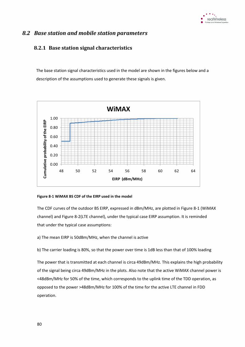
80
8.2 Base station and mobile station parameters
8.2.1 Base station signal characteristics
The base station signal characteristics used in the model are shown in the figures below and a
description of the assumptions used to generate these signals is given.
Figure 8-1 WiMAX BS CDF of the EIRP used in the model
The CDF curves of the outdoor BS EIRP, expressed in dBm/MHz, are plotted in Figure 8-1 (WiMAX
channel) and Figure 8-2(LTE channel), under the typical case EIRP assumption. It is reminded
that under the typical case assumptions:
a) The mean EIRP is 50dBm/MHz, when the channel is active
b) The carrier loading is 80%, so that the power over time is 1dB less than that of 100% loading
The power that is transmitted at each channel is circa 49dBm/MHz. This explains the high probability
of the signal being circa 49dBm/MHz in the plots. Also note that the active WiMAX channel power is
<48dBm/MHz for 50% of the time, which corresponds to the uplink time of the TDD operation, as
opposed to the power >48dBm/MHz for 100% of the time for the active LTE channel in FDD
operation.
0.00
0.20
0.40
0.60
0.80
1.00
48 50 52 54 56 58 60 62 64
Cu
mu
lati
ve
pro
ba
bil
ity
of
the
EIR
P
EIRP (dBm/MHz)
WiMAX
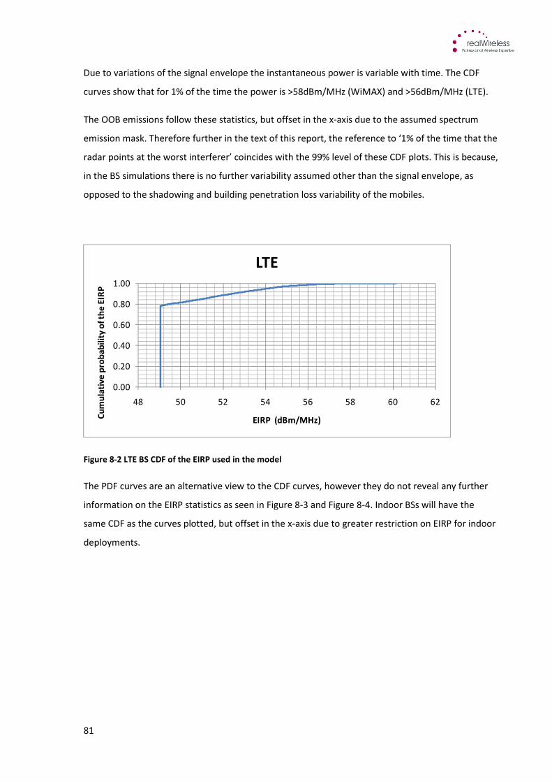
81
Due to variations of the signal envelope the instantaneous power is variable with time. The CDF
curves show that for 1% of the time the power is >58dBm/MHz (WiMAX) and >56dBm/MHz (LTE).
The OOB emissions follow these statistics, but offset in the x-axis due to the assumed spectrum
emission mask. Therefore further in the text of this report, the reference to ‘1% of the time that the
radar points at the worst interferer’ coincides with the 99% level of these CDF plots. This is because,
in the BS simulations there is no further variability assumed other than the signal envelope, as
opposed to the shadowing and building penetration loss variability of the mobiles.
Figure 8-2 LTE BS CDF of the EIRP used in the model
The PDF curves are an alternative view to the CDF curves, however they do not reveal any further
information on the EIRP statistics as seen in Figure 8-3 and Figure 8-4. Indoor BSs will have the
same CDF as the curves plotted, but offset in the x-axis due to greater restriction on EIRP for indoor
deployments.
0.00
0.20
0.40
0.60
0.80
1.00
48 50 52 54 56 58 60 62
Cu
mu
lati
ve
pro
ba
bil
ity
of
the
EIR
P
EIRP (dBm/MHz)
LTE

82
Figure 8-3 WiMAX BS PDF of the EIRP used in the model
Figure 8-4 LTE BS PDF of the EIRP used in the model
8.2.2 Peak to average power ratio (PAPR)
The variations in the signal envelope are due to the peak to average power ratio found in OFDMA
systems such as LTE and WiMAX, to help keep the limiting aspects of the base station power
amplifier within a sensible range, for example the BS power amplifier can support up to 10 dB of
signal variability.
0
20
40
60
80
100
120
140
160
180
200
48 50 52 54 56 58 60 62 64
Pro
ba
bil
ity
de
nsi
ty f
un
ctio
n o
f th
e
EIR
P
EIRP (dBm/MHz)
WiMAX
0
20
40
60
80
100
120
140
160
180
200
48 50 52 54 56 58 60 62
Pro
ba
bil
ity
de
nsi
ty f
un
ctio
n o
f th
e
EIR
P
EIRP (dBm/MHz)
LTE

83
Figure 8-5 Creating an OFDM signal18
Figure 8-5 shows the creation of an OFDM signal from the serial data input which is passed through a
serial to parallel converter. The spectral components of each symbol are identified and input to an
Inverse Fast Fourier Transform (IFFT) process. The IFFT process converts the frequency domain
signals into time domain signals. Each resulting time domain FFT symbols is now mapped onto its
sub-carrier, and the final time domain signal is a composite of all sub-carriers.
The technical challenges presented by OFDM are the resulting composite waveforms which display
large variations in amplitude caused by the combination of a number of individual signals. The
resultant effect displays the signal fluctuating in amplitude as a result of the combining of many
signals with discrete phase and amplitude differences. See Figure 8-6 as an example the OFDM
waveform.
The signal used in the model for the study used 20 individual sine waves combined to form a near-
Rayleigh distribution which is truncated to the average level. The mean value of the resulting
distribution is slightly higher than the input-average value and the specific peak to mean values used
in the code are shown in the table below.
2.6 GHz Equipment type Modelled PAPR values
WiMAX BS PAPR 11 dB (64 QAM)
LTE BS PAPR 8 dB (64 QAM)
WiMAX MS PAPR 8.3 dB
LTE MS PAPR 7.8 dB (16 QAM)
Table 8-1 PAPR values for LTE/WiMAX both base stations and mobile stations source can found in Appendix
B of Appendices document
18
Source Informa Telecoms & Media course notes – LTE Air Interface course
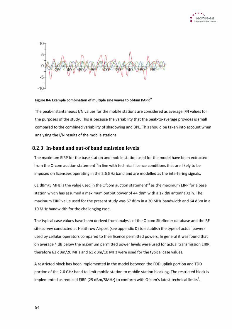
84
Figure 8-6 Example combination of multiple sine waves to obtain PAPR18
The peak-instantaneous I/N values for the mobile stations are considered as average I/N values for
the purposes of the study. This is because the variability that the peak-to-average provides is small
compared to the combined variability of shadowing and BPL. This should be taken into account when
analysing the I/N results of the mobile stations.
8.2.3 In-band and out-of band emission levels
The maximum EIRP for the base station and mobile station used for the model have been extracted
from the Ofcom auction statement 3in line with technical licence conditions that are likely to be
imposed on licensees operating in the 2.6 GHz band and are modelled as the interfering signals.
61 dBm/5 MHz is the value used in the Ofcom auction statement18 as the maximum EIRP for a base
station which has assumed a maximum output power of 44 dBm with a 17 dBi antenna gain. The
maximum EIRP value used for the present study was 67 dBm in a 20 MHz bandwidth and 64 dBm in a
10 MHz bandwidth for the challenging case.
The typical case values have been derived from analysis of the Ofcom Sitefinder database and the RF
site survey conducted at Heathrow Airport (see appendix D) to establish the type of actual powers
used by cellular operators compared to their licence permitted powers. In general it was found that
on average 4 dB below the maximum permitted power levels were used for actual transmission EIRP,
therefore 63 dBm/20 MHz and 61 dBm/10 MHz were used for the typical case values.
A restricted block has been implemented in the model between the FDD uplink portion and TDD
portion of the 2.6 GHz band to limit mobile station to mobile station blocking. The restricted block is
implemented as reduced EIRP (25 dBm/5MHz) to conform with Ofcom’s latest technical limits3.

85
Base station and mobile station out of band and spurious emission levels
The out of band and spurious emissions from base stations and mobile stations are used to calculate
the increase in noise to the radar receiver landing co-channel on the radar centre frequency. The key
to values that are likely to cause interference that exceed the I/N threshold levels of the receiver are
the minimum limits specified in the LTE and WiMAX standards7,8,9 which assumes a constant emission
level into the radar band. The assumptions made on the typical case values regarding the out-of-
band spectrum emission mask and the spurious emissions falling inside the radar band assume a roll
off of 1-2 dB/decade into the radar band which formed the basis of the typical case emissions.
The challenging case uses the 3GPP and IEEE specification mask to simulate the possibility of
equipment performing up to the specification limits. This means, in the case of emissions in the
downlink portion of the band with the carrier centre frequency 2680 MHz and 20 MHz bandwidth,
the out-of band emissions extend into the radar band by up to 40 MHz, this is clarified based on the
following criteria:
Out-of-band domain extends ±250% outside of the necessary bandwidth therefore 2.5 x 20 MHz =
50 MHz after which point the spurious domain predominates19. Therefore at the channel edge 2690
MHz + 50 MHz (out-of-band) equates to 2740 MHz and the limit can reach up to -15 dBm/MHz in this
out of band domain. However, outside of these limits within the spurious domain the level is
specified from ITU-R SM 32920 as:
Frequency
band
Maximum
level
Measurement
bandwidth
1 GHz –
12.75 GHz
-30 dBm 1 MHz
Table 8-2 3GPP and IEEE spurious emission limits
At the maximum level a number of assumptions can be made. For example, setting a constant level
for the spurious emissions captures the possibility of a discrete spurious emission falling co-channel
with the radar centre frequency, which emulates a challenging case scenario. Each of the spectrum
emission masks shows the EIRP in dBm/MHz.
All of the unwanted emission masks incorporate the Ofcom Block Edge Mask (BEM). In the case of
base stations the -45 dBm/MHz BEM extends 30 MHz from upper most block edge in the downlink
portion of 2.6 GHz band from 2690 MHz to 2720 MHz in the upper adjacent S-band. In the case of
the mobile stations the -19 dBm/MHz BEM extends from top block edge of uplink portion the 2.6
GHz band to 2720 MHz in the upper adjacent S-band. The emissions limits from ITU-R SM 32920 were
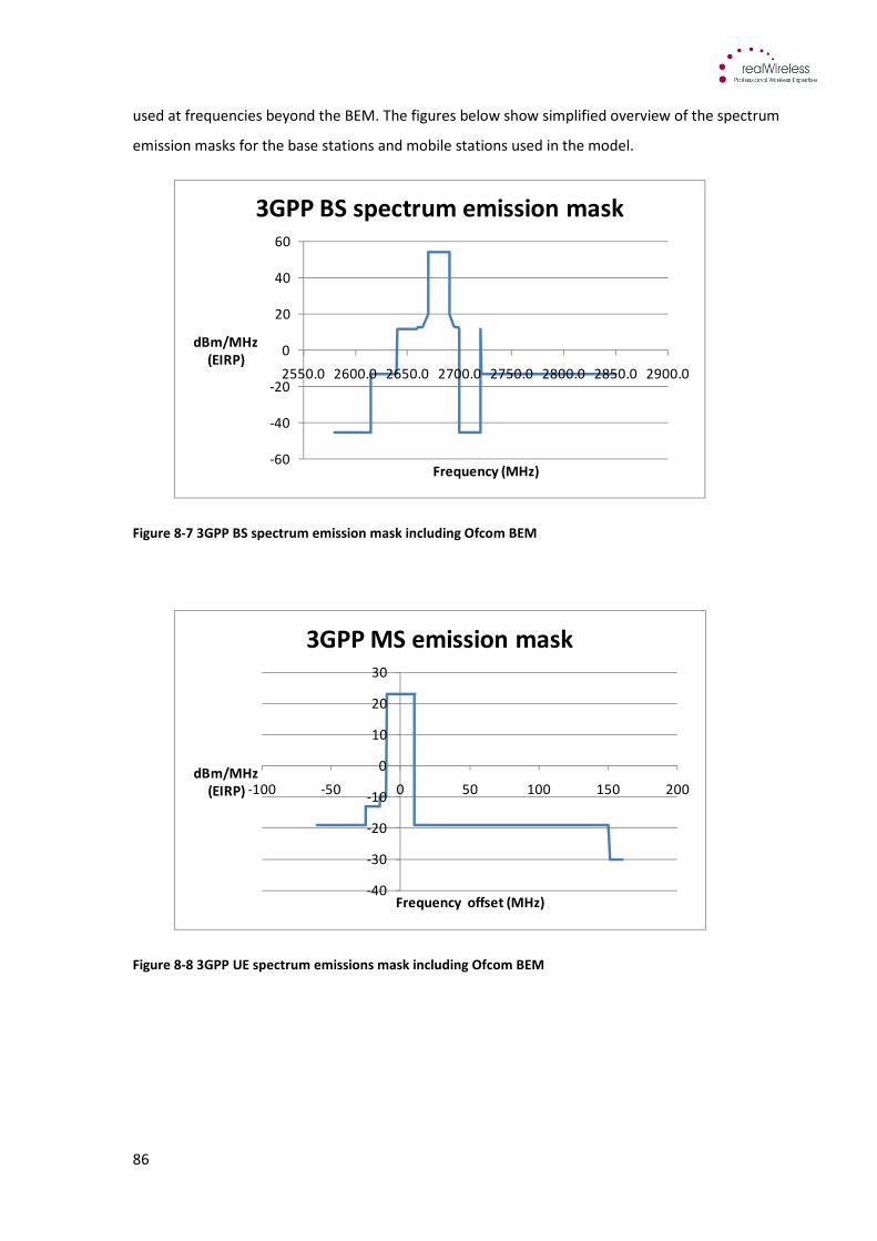
86
used at frequencies beyond the BEM. The figures below show simplified overview of the spectrum
emission masks for the base stations and mobile stations used in the model.
Figure 8-7 3GPP BS spectrum emission mask including Ofcom BEM
Figure 8-8 3GPP UE spectrum emissions mask including Ofcom BEM
-60
-40
-20
0
20
40
60
2550.0 2600.0 2650.0 2700.0 2750.0 2800.0 2850.0 2900.0
dBm/MHz
(EIRP)
Frequency (MHz)
3GPP BS spectrum emission mask
-40
-30
-20
-10
0
10
20
30
-100 -50 0 50 100 150 200dBm/MHz
(EIRP)
Frequency offset (MHz)
3GPP MS emission mask
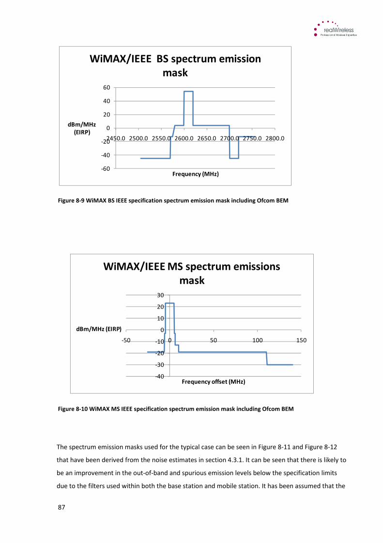
87
Figure 8-9 WiMAX BS IEEE specification spectrum emission mask including Ofcom BEM
Figure 8-10 WiMAX MS IEEE specification spectrum emission mask including Ofcom BEM
The spectrum emission masks used for the typical case can be seen in Figure 8-11 and Figure 8-12
that have been derived from the noise estimates in section 4.3.1. It can be seen that there is likely to
be an improvement in the out-of-band and spurious emission levels below the specification limits
due to the filters used within both the base station and mobile station. It has been assumed that the
-60
-40
-20
0
20
40
60
2450.0 2500.0 2550.0 2600.0 2650.0 2700.0 2750.0 2800.0
dBm/MHz
(EIRP)
Frequency (MHz)
WiMAX/IEEE BS spectrum emission
mask
-40
-30
-20
-10
0
10
20
30
-50 0 50 100 150
dBm/MHz (EIRP)
Frequency offset (MHz)
WiMAX/IEEE MS spectrum emissions
mask
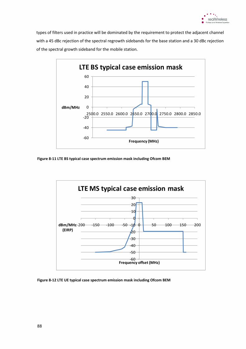
88
types of filters used in practice will be dominated by the requirement to protect the adjacent channel
with a 45 dBc rejection of the spectral regrowth sidebands for the base station and a 30 dBc rejection
of the spectral growth sideband for the mobile station.
Figure 8-11 LTE BS typical case spectrum emission mask including Ofcom BEM
Figure 8-12 LTE UE typical case spectrum emission mask including Ofcom BEM
-60
-40
-20
0
20
40
60
2500.0 2550.0 2600.0 2650.0 2700.0 2750.0 2800.0 2850.0
dBm/MHz
Frequency (MHz)
LTE BS typical case emission mask
-60
-50
-40
-30
-20
-10
0
10
20
30
-200 -150 -100 -50 0 50 100 150 200dBm/MHz
(EIRP)
Frequency offset (MHz)
LTE MS typical case emission mask
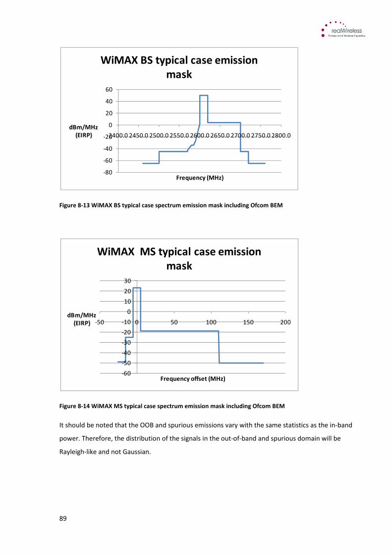
89
Figure 8-13 WiMAX BS typical case spectrum emission mask including Ofcom BEM
Figure 8-14 WiMAX MS typical case spectrum emission mask including Ofcom BEM
It should be noted that the OOB and spurious emissions vary with the same statistics as the in-band
power. Therefore, the distribution of the signals in the out-of-band and spurious domain will be
Rayleigh-like and not Gaussian.
-80
-60
-40
-20
0
20
40
60
2400.0 2450.0 2500.0 2550.0 2600.0 2650.0 2700.0 2750.0 2800.0
dBm/MHz
(EIRP)
Frequency (MHz)
WiMAX BS typical case emission
mask
-60
-50
-40
-30
-20
-10
0
10
20
30
-50 0 50 100 150 200dBm/MHz
(EIRP)
Frequency offset (MHz)
WiMAX MS typical case emission
mask
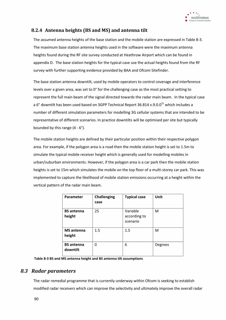
90
8.2.4 Antenna heights (BS and MS) and antenna tilt
The assumed antenna heights of the base station and the mobile station are expressed in Table 8-3.
The maximum base station antenna heights used in the software were the maximum antenna
heights found during the RF site survey conducted at Heathrow Airport which can be found in
appendix D. The base station heights for the typical case use the actual heights found from the RF
survey with further supporting evidence provided by BAA and Ofcom Sitefinder.
The base station antenna downtilt, used by mobile operators to control coverage and interference
levels over a given area, was set to 0° for the challenging case as the most practical setting to
represent the full main beam of the signal directed towards the radar main beam. In the typical case
a 6° downtilt has been used based on 3GPP Technical Report 36.814 v.9.0.021 which includes a
number of different simulation parameters for modelling 3G cellular systems that are intended to be
representative of different scenarios. In practice downtilts will be optimised per site but typically
bounded by this range (4 - 6°).
The mobile station heights are defined by their particular position within their respective polygon
area. For example, if the polygon area is a road then the mobile station height is set to 1.5m to
simulate the typical mobile receiver height which is generally used for modelling mobiles in
urban/suburban environments. However, if the polygon area is a car park then the mobile station
heights is set to 15m which simulates the mobile on the top floor of a multi-storey car park. This was
implemented to capture the likelihood of mobile station emissions occurring at a height within the
vertical pattern of the radar main beam.
Parameter Challenging
case
Typical case Unit
BS antenna
height
25 Variable
according to
scenario
M
MS antenna
height
1.5 1.5 M
BS antenna
downtilt
0 6 Degrees
Table 8-3 BS and MS antenna height and BS antenna tilt assumptions
8.3 Radar parameters
The radar remedial programme that is currently underway within Ofcom is seeking to establish
modified radar receivers which can improve the selectivity and ultimately improve the overall radar
91
receiver. The following radar parameters take account of the modified radar parameters expected to
be deployed at airports in future.
The radar parameters that have been used in the model have been derived from generic modified
radar receiver design characteristics. This is due to the commercial sensitivity of bespoke radar
designs and the limited availability of information for specific receivers.
The study has focused on the radar filter responses used to protect the different amplifiers in the
receive chain and the noise floor of the receiver since it is this part of the radar that is sensitive to
incoming interference. However, in order to generate an accurate deployment scenario the other
parameters such as radar antenna height, radar uptilt, half power beamwidth etc. have all been
established based on previous studies or trials reports2, and are shown in Table 8-4.
The block diagram shown in Figure 8-15 is a high level representation of the radar receiver chain
which was incorporated into the software model. The diagram shows the two critical points in the
receiver chain that can either cause complete shutdown of the radar it the interference threshold is
exceeded (point A) or significant performance degradation if the interference threshold is exceeded
(point B). It should be noted that the levels expressed at these points are the interference
(blocking)threshold levels referred to the antenna connector which takes into account all the losses
and gains of the whole receiver. The values have been estimated based on a representative set of
radar receiver assumptions which comprise a sub system level filter and amplifier at each stage in
the receiver. The aim of the upgrade is to improve the selectivity of the front end which would
include improved filtering. It has been assumed that the front-end filtering and the protection
threshold (-42 dBm) at point B is low enough to remove any IF mixing effects that could cause
problems further down the receive chain. Therefore, sub-system 3 and sub-system 4 are not
included in the analysis but required for calculation purposes.
Figure 8-15 Block diagram of modified generic radar receive chain
Sub-
system 2
Sub-
system 3
Sub-
system 1
B = -42 dBm
Radar
antenna
Sub-systems at each stage in the receive chain
Antenna
connector
A = -5dBm
Sub-
system 4
The potential for any IF effects occurring in
this part of the receive chain have been
incorporated in the value set at point B.
92
The interference noise threshold levels have been derived from an example range of -5 dB to -15 dB.
This range establishes the upper and lower bounds of the interference spread of interest. ITU-R
report M 146431 shows that a threshold level of -10 dB is a particular level of interest which falls in
the middle of the example range.
Parameter Challenging case Typical case Unit
Radar receiver
IF BW (-3dB)
1.7 1.7 MHz
Radar system
noise
temperature
379 379 K
Thermal noise
for radar
-110.5 (1.7 MHz) -110.5(1.7MHz)
dBm
Radar antenna
gain (horizontal)
28 28 dBi
Feeder loss 2 2 dB
Radar antenna
HPBW hor
1.4 1.4 degrees
Radar antenna
HPBW ver
5.2 5.2 degrees
Radar uptilt 2 2 degrees
Polarisation
discrimination
0 3 dB
Position of
radar on map
area
TQ08427468
Radar antenna
height
5 20 M
Table 8-4 Radar parameters
The assumed filter responses of each stage in the generic modified radar receiver have been
incorporated into the software model. Figure 8-16 shows the first RF filter response as developed by
Isotek22 which is one example filter that could be used in the generic modified radar design. This RF
filter was placed in sub-system 1 to improve selectivity to the front end of the receiver and help
attenuate the powerful transmissions from the 2.6 GHz band.
93
Figure 8-16 1st RF filter response (isotek)
Previous studies23 have shown an improvement in selectivity in the order of 20-30 dB is needed to
reduce blocking to acceptable levels. The filter responses for sub-systems 2 to 4 are assumed to
provide further attenuation at each stage but are not included in the analysis at those stages.
The attenuation of the RF filter is taken into account when calculating the blocking level at point B. It
is assumed the filter response continues linearly towards the edge of the 2.6 GHz band.
8.4 Modelling assumptions and simulation parameters
This section discusses the simulation parameters that have not been addressed in the above sections
i.e. not directly related to base station and mobile station emissions or the radar receiver
parameters. The following parameters are discussed in more detail in this section:
� Pathloss
� Shadowing
� Penetration loss from indoor BS/MS
� Sector orientation of the base station antenna
� Attenuation due to antenna patterns
� Channel raster and frequency assignment
� Density of mobile deployment
These parameters are associated with functions related to the communications channel such as the
pathloss or a more specific feature with the base station or mobile station. For example, there is a
function to calculate the pathloss which takes into consideration all the possible path types that will

94
be simulated and included as options for selection by the program depending on the properties of
the path. The path types and propagation models are discussed in more detail in the following
sections. The other simulation parameters are discussed in more detail below.
1) Shadowing occurs due to the obstructions in the path and will impact the signals between
the base station and the radar and the mobile station and the radar. The shadowing used for
simulating interference from base stations has been set to 0 dB due to the static nature of
the interference from base stations with no variability in the path and the relatively high
heights of both the BSs and the radar. An assumption of 0 dB has been made on the basis
the radio path will remain constant.
2) Penetration loss due to indoor base stations and mobile stations has been included in the
model to take account of these types of deployments. Confirmation from BAA and Ofcom
Sitefinder indicates a number of indoor base stations are deployed across the airport and
therefore considered in the model. A value for the typical case of 13.5 dB for indoor
penetration loss has been used for the model based on derived values from previous case
studies and simulation parameters used for example in Ofcom report “Application of
spectrum liberalisation and trading for the mobile sector”24. The value for indoor
penetration loss for the challenging case is 3.5 dB based on a value for a windowed wall25.
3) Sector orientation of the base station antenna takes into account the direction of maximum
gain of the three sector antenna. The software model is able to rotate the base station to
direct the antenna pattern towards the radar. This has the added benefit of directing the null
sections of the antenna pattern towards the radar and thus reducing the interference power
levels. The antenna orientation directed the maximum gain towards the radar antenna to
simulate the challenging case and directed the null of the base station antenna towards the
radar antenna to simulate the mitigation technique.
4) Attenuation due to antenna patterns for both the base station and radar antenna has been
implemented into the software model. The effect of using the attenuation of the antenna
patterns represents the practical deployment environment for both the mobile
communications installation and the radar installation. The base station antenna pattern has
been sourced from theoretical horizontal and vertical patterns developed in 3GPP technical
report TR 36.814 v9.0.026 which has been modified according to Kathrein “2-Multi-band
Panel, Dual Polarization, 1710-2200 and 2300-2690” base station antenna. The following
values have been used for the challenging case scenario:
• Half power beamwidth (Vertical) = 6.5°
• Half power beamwidth (Horizontal) = 60°
The base station horizontal antenna pattern can be seen in Figure 8-17
95
Figure 8-17 Three sector base station horizontal antenna pattern
5) The channel plan assumed for the software model can be seen in Table 8-5 which has been
based on one possible outcome of the spectrum award of 2.6 GHz band. Although the
outcome of the auction is unknown including likely number of bidders an assumption can be
made on a particular outcome that could be considered possible from the auction. The
channel configuration was also derived to maximise the potential for interference into the
radar. For example, using 20 MHz bandwidth for the highest FDD channel aims to ensure the
out-of-band emissions from the FDD fall within the radar band and thus represent the worst
case. Information that contributed to the channel configuration was gathered from the
stakeholder engagement and knowledge of the use of 2.6 GHz frequencies and from the
equipment characteristics being developed for the market, it should be noted no
competitive analysis or considerations have been given to the share of spectrum amongst
operators and was purely based on deriving the optimum interference characteristics for
modelling.
The following assumptions have been made for the parameter inputs to the modelling:
It is unlikely 5 MHz LTE channels will be deployed by operators, since operators will wish to
make the most of the additional bit rate and capacity capabilities of LTE, particularly in the
2.6 GHz band relative to lower frequency bands such as 800 MHz. Therefore 20 MHz
channels are the most likely option with the remaining 10 MHz picked up for additional
capacity. An example channel configuration which can be seen in Table 8-5 could result in a
total of seven potential carriers being awarded and thus potentially transmitted from a
single shared site. The assumed downlink configuration includes:
o 3 x 20 MHz Downlink FDD
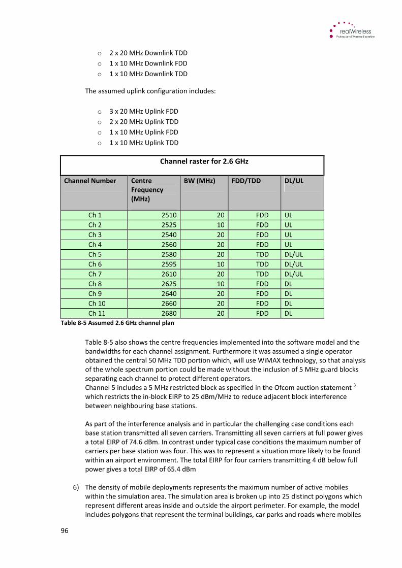
96
o 2 x 20 MHz Downlink TDD
o 1 x 10 MHz Downlink FDD
o 1 x 10 MHz Downlink TDD
The assumed uplink configuration includes:
o 3 x 20 MHz Uplink FDD
o 2 x 20 MHz Uplink TDD
o 1 x 10 MHz Uplink FDD
o 1 x 10 MHz Uplink TDD
Channel raster for 2.6 GHz
Channel Number Centre
Frequency
(MHz)
BW (MHz) FDD/TDD DL/UL
Ch 1 2510 20 FDD UL
Ch 2 2525 10 FDD UL
Ch 3 2540 20 FDD UL
Ch 4 2560 20 FDD UL
Ch 5 2580 20 TDD DL/UL
Ch 6 2595 10 TDD DL/UL
Ch 7 2610 20 TDD DL/UL
Ch 8 2625 10 FDD DL
Ch 9 2640 20 FDD DL
Ch 10 2660 20 FDD DL
Ch 11 2680 20 FDD DL
Table 8-5 Assumed 2.6 GHz channel plan
Table 8-5 also shows the centre frequencies implemented into the software model and the
bandwidths for each channel assignment. Furthermore it was assumed a single operator
obtained the central 50 MHz TDD portion which, will use WiMAX technology, so that analysis
of the whole spectrum portion could be made without the inclusion of 5 MHz guard blocks
separating each channel to protect different operators.
Channel 5 includes a 5 MHz restricted block as specified in the Ofcom auction statement 3
which restricts the in-block EIRP to 25 dBm/MHz to reduce adjacent block interference
between neighbouring base stations.
As part of the interference analysis and in particular the challenging case conditions each
base station transmitted all seven carriers. Transmitting all seven carriers at full power gives
a total EIRP of 74.6 dBm. In contrast under typical case conditions the maximum number of
carriers per base station was four. This was to represent a situation more likely to be found
within an airport environment. The total EIRP for four carriers transmitting 4 dB below full
power gives a total EIRP of 65.4 dBm
6) The density of mobile deployments represents the maximum number of active mobiles
within the simulation area. The simulation area is broken up into 25 distinct polygons which
represent different areas inside and outside the airport perimeter. For example, the model
includes polygons that represent the terminal buildings, car parks and roads where mobiles
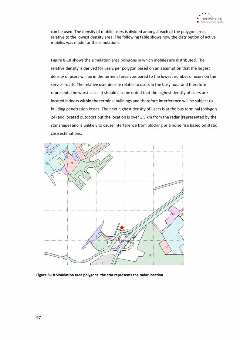
97
can be used. The density of mobile users is divided amongst each of the polygon areas
relative to the lowest density area. The following table shows how the distribution of active
mobiles was made for the simulations.
Figure 8-18 shows the simulation area polygons in which mobiles are distributed. The
relative density is derived for users per polygon based on an assumption that the largest
density of users will be in the terminal area compared to the lowest number of users on the
service roads. The relative user density relates to users in the busy hour and therefore
represents the worst case. It should also be noted that the highest density of users are
located indoors within the terminal buildings and therefore interference will be subject to
building penetration losses. The next highest density of users is at the bus terminal (polygon
24) and located outdoors but the location is over 1.5 km from the radar (represented by the
star shape) and is unlikely to cause interference from blocking or a noise rise based on static
case estimations.
Figure 8-18 Simulation area polygons: the star represents the radar location

98
Polygon
number
Name Indoor/
outdoor
Height
wrt
ground
Relative
user
density
Propagation
path/model
LOS/
NLOS
PL
Code
24 Bus
Terminal
Outdoor 1.5m 15 COST 231 NLOS 7
20, 21, 22 Car Park Outdoor 15m 9 ITU-R P
1546
LOS 8
18 Terminal 3 Indoor 1.5m 60 COST 231 Pen
Loss/
NLOS
7
19 Car Park Outdoor 15m 9 ITU-R P
1546
LOS 8
15, 16, 17, 23 Pier Indoor 4.5m 30 COST 231 Pen
Loss/
NLOS
7
15 Service
Roads
Outdoor 1.5m 3 COST 231 NLOS 7
25 Drop off
area
Outdoor 1.5m 6 COST 231 NLOS 7
1 Terminal 4 Indoor 1.5m 60 FSPL Pen
Loss/
LOS
1
2 Pier Indoor 4.5m 30 FSPL Pen
Loss/
LOS
1
3,4,5,6,7,8 Road Outdoor 1.5m 9 FSPL LOS 1
9,10,11,12,13 Low rise
residential
area
Outdoor 1.5m 45 FSPL Pen
Loss/LOS
1
14 Industrial
site
Outdoor 1.5m 5 FSPL LOS 1
Table 8-6 Polygon area properties
The maximum number of active mobiles has been derived from a variety of assumptions which are
given in appendix B of the Appendices document. BAA data on the number of passengers flowing
through the airport and associated assumptions on the potential penetration of LTE lead to an
assumption that the number of active users distributed across the simulation area polygons is 53.
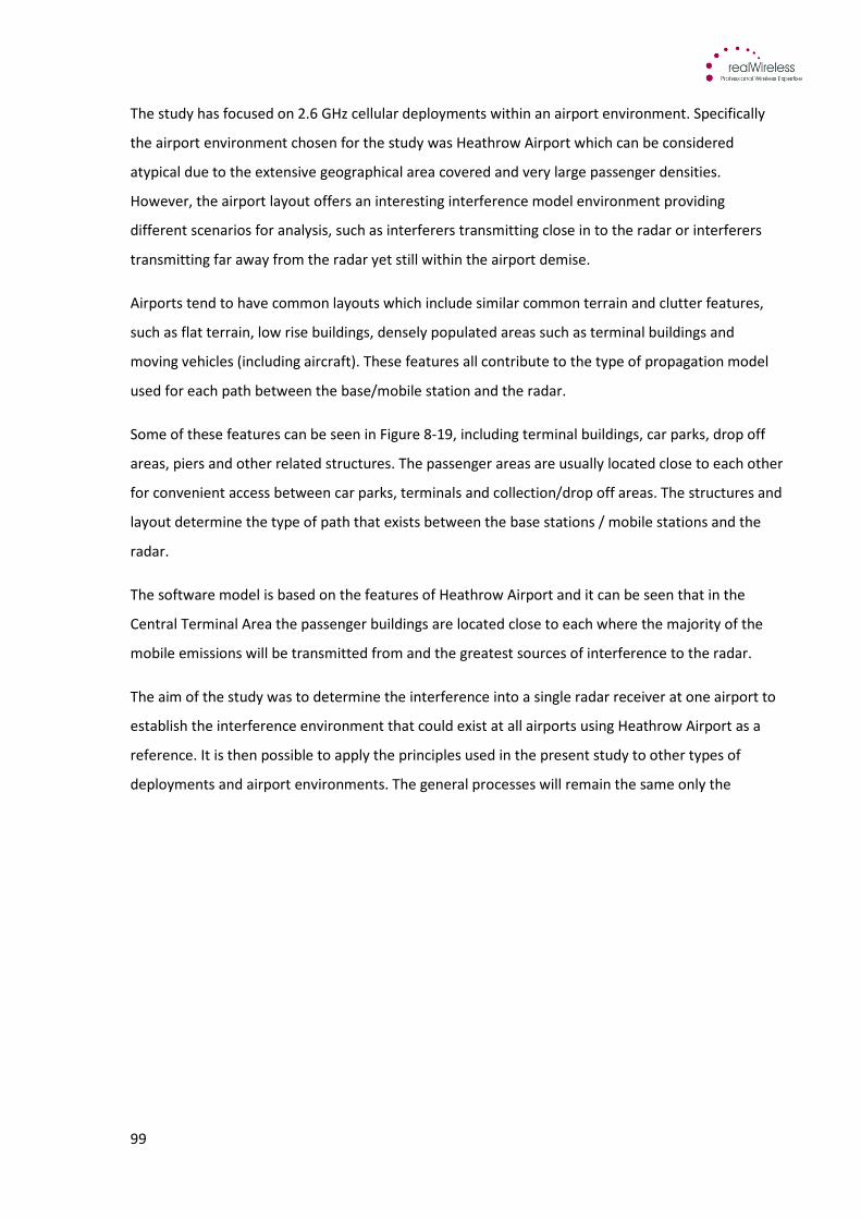
99
The study has focused on 2.6 GHz cellular deployments within an airport environment. Specifically
the airport environment chosen for the study was Heathrow Airport which can be considered
atypical due to the extensive geographical area covered and very large passenger densities.
However, the airport layout offers an interesting interference model environment providing
different scenarios for analysis, such as interferers transmitting close in to the radar or interferers
transmitting far away from the radar yet still within the airport demise.
Airports tend to have common layouts which include similar common terrain and clutter features,
such as flat terrain, low rise buildings, densely populated areas such as terminal buildings and
moving vehicles (including aircraft). These features all contribute to the type of propagation model
used for each path between the base/mobile station and the radar.
Some of these features can be seen in Figure 8-19, including terminal buildings, car parks, drop off
areas, piers and other related structures. The passenger areas are usually located close to each other
for convenient access between car parks, terminals and collection/drop off areas. The structures and
layout determine the type of path that exists between the base stations / mobile stations and the
radar.
The software model is based on the features of Heathrow Airport and it can be seen that in the
Central Terminal Area the passenger buildings are located close to each where the majority of the
mobile emissions will be transmitted from and the greatest sources of interference to the radar.
The aim of the study was to determine the interference into a single radar receiver at one airport to
establish the interference environment that could exist at all airports using Heathrow Airport as a
reference. It is then possible to apply the principles used in the present study to other types of
deployments and airport environments. The general processes will remain the same only the
100
parameters will require change depending on the type of environment to be modelled.
Figure 8-19 Heathrow Airport Central Terminal Area clutter layers
Figure 8-20 Heathrow Airport Central Terminal Area landscape19
Figure 8-20 shows a landscape view of the Central Terminal Area at Heathrow airport to
demonstrate the types of structures that feature between the interferers and the radar. Generally
the structure heights are low apart from those structures necessary for air traffic control. Typically
heights do not exceed 25-30m in the Central Terminal area and predominantly are the multi-storey
car parks (where the photo was taken from) and the terminal buildings. It can be seen that mobile
use outdoors will be at ground level or from the roof of the multi-storey car parks, otherwise it is
indoors. Additionally, base stations on the roof of the car parks and terminal buildings will have
unobstructed paths to the radar location.
19
Image sourced from Google images
101
8.4.1 Propagation models
The software model includes a list of relevant propagation models that are used by the program
depending on the path type, described in the section above, that exists between the victim receiver
and interfering transmitter. Each propagation or loss model was selected based on the relevant
propagation criteria found within the specific airport environment. The following types of
propagation/loss models were considered relevant for inclusion in the software model were:
Free space path loss models used for distances greater than 1km become meaningless due to the
impact of terrain and obstacles that must be taken into account. Therefore FSPL are useful for the
airport deployment study due to the short coordination distances of interest.
Empirical models such as COST 23127 or ITU-R Rec P.123828 are used for indoor and short distances
which are appropriate for an airport environment and will be used for this study.
The benefits to this study from the use of the more complex models due to the short distances
include:
• Consideration given for high clutter environments (representative of airport environment)
• Provides accuracy of results
• Robust and confident set of results
The study did not consider the use of detailed site specific models such as ray tracing due to the
complexity involved in modelling the path from each base stations site and each mobile. There
would be intensive computer processing required for the analysis from each interferer which would
be time consuming and considered unnecessary due to the suitability and appropriateness of
standard propagation models within an airport environment.
In previous related studies one particular propagation model that has been used for interference
assessment was ITU-R Rec P.452-1229. This propagation model is used for the interference
assessment of stations on the surface of the Earth above 0.7 GHz and was independently verified for
Ofcom. A previous study 30 concluded the propagation model ITU-R Rec P.452-12 is an appropriate
model for calculating co-ordination areas around radars by calculating the minimum safe distance an
interference source transmitting in the 2.5 to 2.69 GHz could be from a radar without exceeding a
defined signal level at the radar receiver.
On the basis of the above layout the following paths were used to derive the propagation models:
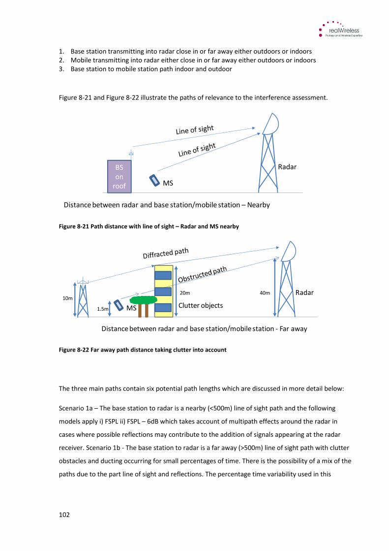
102
1. Base station transmitting into radar close in or far away either outdoors or indoors
2. Mobile transmitting into radar either close in or far away either outdoors or indoors
3. Base station to mobile station path indoor and outdoor
Figure 8-21 and Figure 8-22 illustrate the paths of relevance to the interference assessment.
Figure 8-21 Path distance with line of sight – Radar and MS nearby
Figure 8-22 Far away path distance taking clutter into account
The three main paths contain six potential path lengths which are discussed in more detail below:
Scenario 1a – The base station to radar is a nearby (<500m) line of sight path and the following
models apply i) FSPL ii) FSPL – 6dB which takes account of multipath effects around the radar in
cases where possible reflections may contribute to the addition of signals appearing at the radar
receiver. Scenario 1b - The base station to radar is a far away (>500m) line of sight path with clutter
obstacles and ducting occurring for small percentages of time. There is the possibility of a mix of the
paths due to the part line of sight and reflections. The percentage time variability used in this
BS on
roof MS
Radar
Distance between radar and base station/mobile station – Nearby
MS
Radar
Clutter objects
Distance between radar and base station/mobile station - Far away
10m
1.5m
20m 40m
103
scenario was 99.9% as specified from previous Ofcom studies30. The propagation model used in the
software was ITU-R P 452 with options 8a (LOS) and 8b (LOS with sub path diffraction).
Scenario 1c - The base station indoor path to radar, used very low power and penetration loss
through walls and windows using FSPL
Scenario 2a - The mobile station to nearby radar. The path is line of sight using time variability of
99.9% for Monte Carlo at 1.5m above ground level. There is a fixed path loss around the base station
so FSPL will be the worst case scenario surrounded by scatterers. Therefore the Rayleigh fading case
was applied with a range of 3-5 dB i.e. an ‘inverted’ Rayleigh distribution coming from the mobile
due to the application of power control.
Scenario 2b - The mobile station to radar for far out distances. The propagation model used for this
instance is COST 231 Hata27 modified for 2.6 GHz at ground level. This was due to the path being LOS
with some clutter likely causing obstruction. As the mobiles increase in height above local ground
another option is ITU-R Rec P. 452 or ITU R Rec P 154620. ITU-R Rec P. 1546 includes a correction
factor for varying the height of the mobile.
As discussed above in the case of an airport deployment, considerations of interfering signals within,
a 5km radius have been analysed. Therefore a propagation model must take into account the
specific loss effects of the signal within the defined environment. In the case of ITU-R Rec P.452-1229,
considerations for line of sight, clutter losses and diffraction are given whose effects would all be
appropriate for an airport deployment specific scenario.
The other models of interest to the study are considered due to the mix of paths for example,
multiray losses, short-range and indoor propagation which have been taken into consideration. The
propagation models that have been used are specific to the paths between each of the base station
locations and the radar with the same principle applied to the mobile stations using the properties of
the polygon area as method to assign the specific propagation model. In addition for an airport
deployment environment there is a mixture of indoor sites using a distributed antenna system and
outdoor sites using a mixture of shared infrastructure and individual sites. This mix of propagation
paths means that considerations for the various losses are accounted for by different models.
20
ITU-R P. 1546 Method for point-to-area for terrestrial services in the frequency range 30 MHz to 3000 MHz
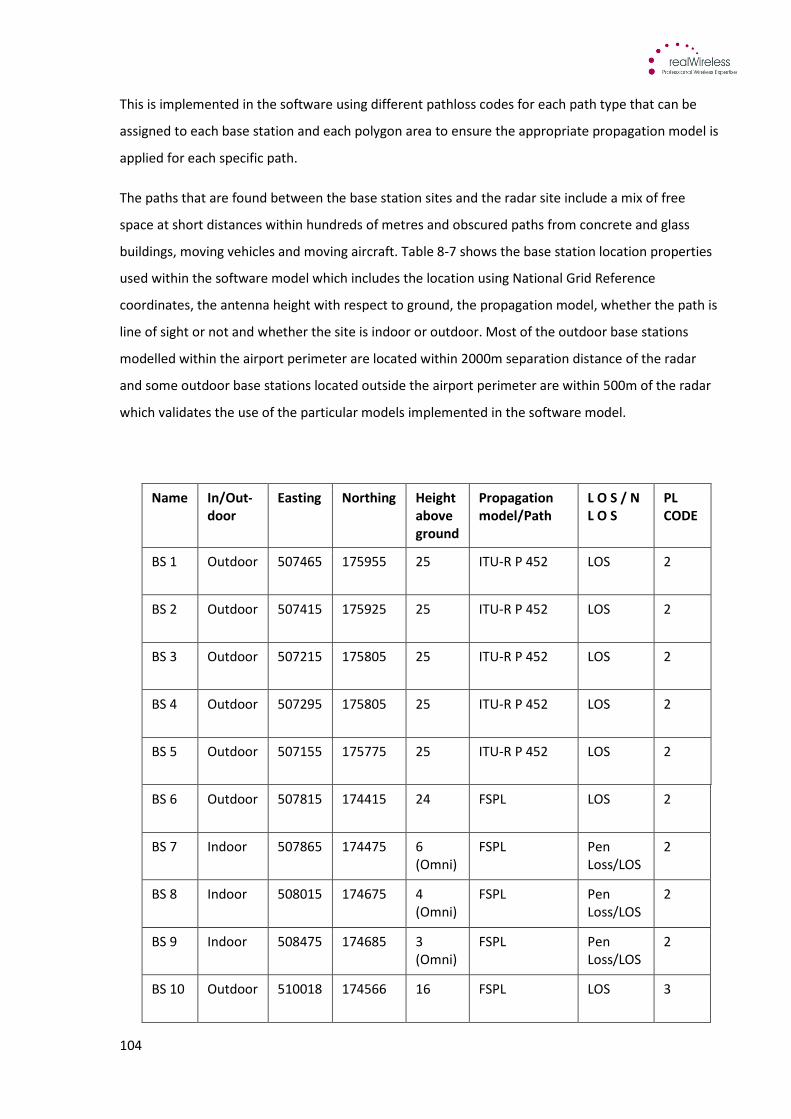
104
This is implemented in the software using different pathloss codes for each path type that can be
assigned to each base station and each polygon area to ensure the appropriate propagation model is
applied for each specific path.
The paths that are found between the base station sites and the radar site include a mix of free
space at short distances within hundreds of metres and obscured paths from concrete and glass
buildings, moving vehicles and moving aircraft. Table 8-7 shows the base station location properties
used within the software model which includes the location using National Grid Reference
coordinates, the antenna height with respect to ground, the propagation model, whether the path is
line of sight or not and whether the site is indoor or outdoor. Most of the outdoor base stations
modelled within the airport perimeter are located within 2000m separation distance of the radar
and some outdoor base stations located outside the airport perimeter are within 500m of the radar
which validates the use of the particular models implemented in the software model.
Name In/Out-
door
Easting Northing Height
above
ground
Propagation
model/Path
L O S / N
L O S
PL
CODE
BS 1 Outdoor 507465 175955 25 ITU-R P 452 LOS 2
BS 2 Outdoor 507415 175925 25 ITU-R P 452 LOS 2
BS 3 Outdoor 507215 175805 25 ITU-R P 452 LOS 2
BS 4 Outdoor 507295 175805 25 ITU-R P 452 LOS 2
BS 5 Outdoor 507155 175775 25 ITU-R P 452 LOS 2
BS 6 Outdoor 507815 174415 24 FSPL LOS 2
BS 7 Indoor 507865 174475 6
(Omni)
FSPL Pen
Loss/LOS
2
BS 8 Indoor 508015 174675 4
(Omni)
FSPL Pen
Loss/LOS
2
BS 9 Indoor 508475 174685 3
(Omni)
FSPL Pen
Loss/LOS
2
BS 10 Outdoor 510018 174566 16 FSPL LOS 3
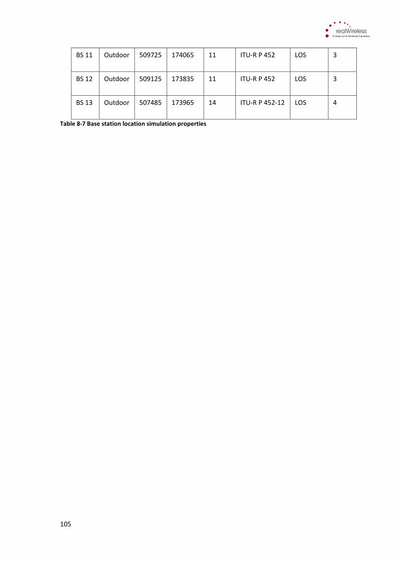
105
BS 11 Outdoor 509725 174065 11 ITU-R P 452 LOS 3
BS 12 Outdoor 509125 173835 11 ITU-R P 452 LOS 3
BS 13 Outdoor 507485 173965 14 ITU-R P 452-12 LOS 4
Table 8-7 Base station location simulation properties
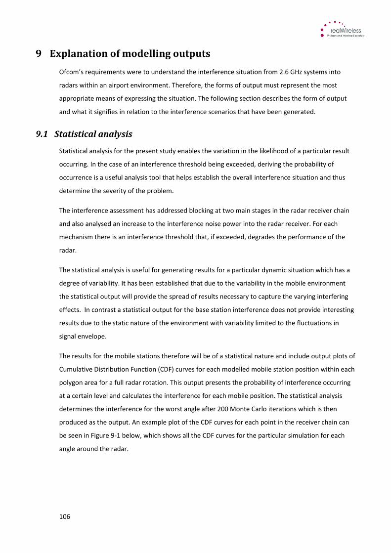
106
9 Explanation of modelling outputs
Ofcom’s requirements were to understand the interference situation from 2.6 GHz systems into
radars within an airport environment. Therefore, the forms of output must represent the most
appropriate means of expressing the situation. The following section describes the form of output
and what it signifies in relation to the interference scenarios that have been generated.
9.1 Statistical analysis
Statistical analysis for the present study enables the variation in the likelihood of a particular result
occurring. In the case of an interference threshold being exceeded, deriving the probability of
occurrence is a useful analysis tool that helps establish the overall interference situation and thus
determine the severity of the problem.
The interference assessment has addressed blocking at two main stages in the radar receiver chain
and also analysed an increase to the interference noise power into the radar receiver. For each
mechanism there is an interference threshold that, if exceeded, degrades the performance of the
radar.
The statistical analysis is useful for generating results for a particular dynamic situation which has a
degree of variability. It has been established that due to the variability in the mobile environment
the statistical output will provide the spread of results necessary to capture the varying interfering
effects. In contrast a statistical output for the base station interference does not provide interesting
results due to the static nature of the environment with variability limited to the fluctuations in
signal envelope.
The results for the mobile stations therefore will be of a statistical nature and include output plots of
Cumulative Distribution Function (CDF) curves for each modelled mobile station position within each
polygon area for a full radar rotation. This output presents the probability of interference occurring
at a certain level and calculates the interference for each mobile position. The statistical analysis
determines the interference for the worst angle after 200 Monte Carlo iterations which is then
produced as the output. An example plot of the CDF curves for each point in the receiver chain can
be seen in Figure 9-1 below, which shows all the CDF curves for the particular simulation for each
angle around the radar.

107
Figure 9-1 Example cumulative distribution functions (CDF) of power received at the radar antenna
connector. Each line represents the distribution for a given radar orientation angle. The line with crosses
represents the composite worst-case CDF across all angles.
For each output CDF curve individual CDF curves are produced which represent different radar
rotation angles. Each CDF represents variation due to mobile locations, shadowing, power control
and signal envelope fluctuations. The worst-case CDF is derived from the set of angles that are
characterised by the greatest interference power as shown in Figure 9-1.
Across the statistical range the interference or blocking levels are output and the interference level
at a particular percentage of time can be determined. The worst angle is a result of all the
calculations which provides the information to be used for each interference scenario. For example,
if the output shows significant levels of interference identified from a particular angle from the radar
then the next stage of analysis can investigate the mitigation techniques required to combat the
sources of interference in that specific area.
As the radar rotates the main beam of its antenna creates a rotating sector which sweeps across the
simulation area and illuminates several mobile- and base-stations. For a given illuminated sector the
mobile stations have a variable position and transmit power, due to user mobility, shadowing and
building penetration loss variability, mobile-network power-control, signal envelope variability and
Final data set selected for CDF results presented in Ch10

108
resource allocation. Therefore, for a particular radar rotation-angle the received interference power
at the radar is a variable. Each rotation-angle thus corresponds to a CDF, as plotted in Figure 9-1
Note that each CDF curve corresponds to a specific illuminated simulation area sector. Therefore,
the percentage of time (probability in a CDF plot) in the x-axis refers to the percentage of time
instances that the power is less than that of the x-axis, given that the radar illuminates that
particular sector. This conditional-probability should not be confused with the probability of
occurrence that is irrespective of the radar-angle. The conditional-probability is of interest in this
study, because as the radar rotates it periodically sweeps across the worst-case polygons (or base
stations). Therefore, overall the blocking probability of the radar is very small, partially because the
radar-antenna horizontal-pattern attenuates the interference by several decibels (see Figure 8-16),
even though the blocking probability may be systematically high at the particular worst-case angle.
The CDF plots given later in this report correspond to the worst-case conditional probability of
interference.
Also note that, the CDF curves in Figure 9-1 are an example of received interference from mobile
stations. The interference from base stations is expected to have less variability when compared to
Figure 9-1, due to the base stations’ fixed locations, and therefore the CDF curves are anticipated to
be flatter.
Due to the mobile stations’ mobility within the simulated polygon areas the worst-case CDF is built
across a range of rotation-angles, for which the worst-case polygon is illuminated. In order to pick-
out the worst-case CDF we choose the greatest interference-power across the rotation-angles. This
is shown by example in Figure 9-1 with the x-markers.
To give an example of how the angles of interference are represented against a large interferer can
be seen in Figure 9-2. The plot shows a spike on the diagram with a blocking level of -25 dBm at an
angle of 135°. All other angles show lower levels of interference below -50 dBm. It is also noted that
the polar plot designates 0° angle towards the East from the radar and the angles increase in an
anticlockwise direction from 0°. Therefore 90° lies to the North of the radar and so on and all angles
expressed in the results are based on the polar plots shown in Figure 9-2.
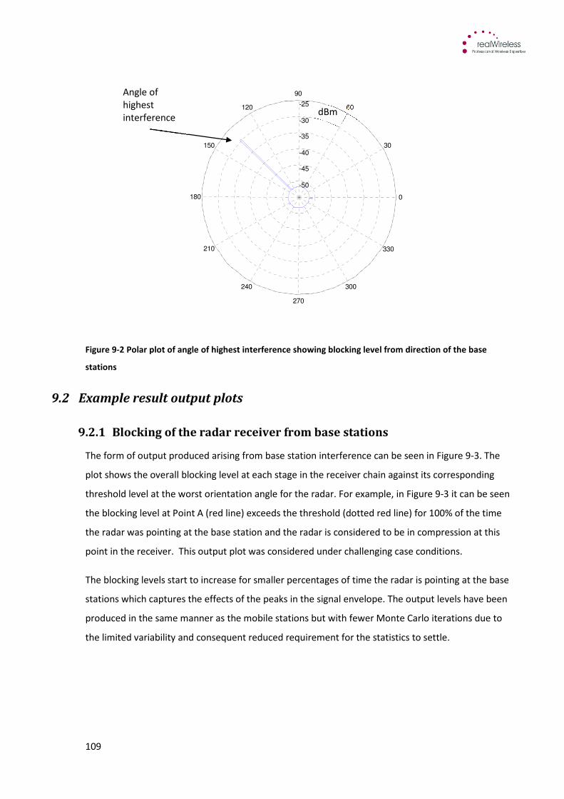
109
Figure 9-2 Polar plot of angle of highest interference showing blocking level from direction of the base
stations
9.2 Example result output plots
9.2.1 Blocking of the radar receiver from base stations
The form of output produced arising from base station interference can be seen in Figure 9-3. The
plot shows the overall blocking level at each stage in the receiver chain against its corresponding
threshold level at the worst orientation angle for the radar. For example, in Figure 9-3 it can be seen
the blocking level at Point A (red line) exceeds the threshold (dotted red line) for 100% of the time
the radar was pointing at the base station and the radar is considered to be in compression at this
point in the receiver. This output plot was considered under challenging case conditions.
The blocking levels start to increase for smaller percentages of time the radar is pointing at the base
stations which captures the effects of the peaks in the signal envelope. The output levels have been
produced in the same manner as the mobile stations but with fewer Monte Carlo iterations due to
the limited variability and consequent reduced requirement for the statistics to settle.
-50
-45
-40
-35
-30
-25
0
30
60
90
120
150
180
210
240
270
300
330
dBm
Angle of
highest
interference
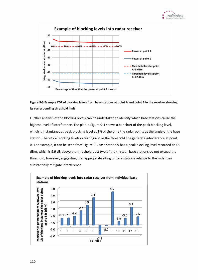
110
Figure 9-3 Example CDF of blocking levels from base stations at point A and point B in the receiver showing
its corresponding threshold limit
Further analysis of the blocking levels can be undertaken to identify which base stations cause the
highest level of interference. The plot in Figure 9-4 shows a bar chart of the peak blocking level,
which is instantaneous peak blocking level at 1% of the time the radar points at the angle of the base
station. Therefore blocking levels occurring above the threshold line generate interference at point
A. For example, it can be seen from Figure 9-4base station 9 has a peak blocking level recorded at 4.9
dBm, which is 9.9 dB above the threshold. Just two of the thirteen base stations do not exceed the
threshold, however, suggesting that appropriate siting of base stations relative to the radar can
substantially mitigate interference.
-60
-50
-40
-30
-20
-10
0
10
0% 20% 40% 60% 80% 100%In
teg
rate
d p
ow
er
at
po
int
A (
dB
m)
Percentage of time that the power at point A > x-axis
Blocking levels into radar receiver
Power at point A
Power at point B
Threshold level at point
A -5 dBm
Threshold level at point
B -42 dBm
Example of blocking levels into radar receiver
Example of blocking levels into radar receiver from individual base
stations
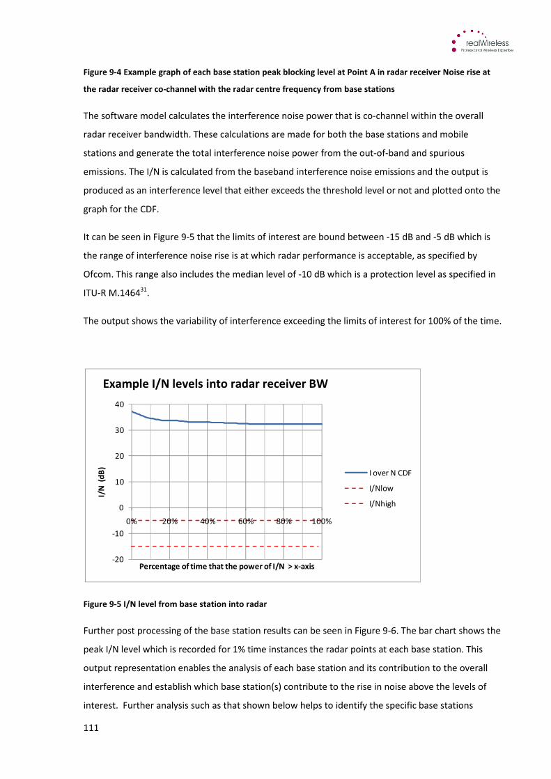
111
Figure 9-4 Example graph of each base station peak blocking level at Point A in radar receiver Noise rise at
the radar receiver co-channel with the radar centre frequency from base stations
The software model calculates the interference noise power that is co-channel within the overall
radar receiver bandwidth. These calculations are made for both the base stations and mobile
stations and generate the total interference noise power from the out-of-band and spurious
emissions. The I/N is calculated from the baseband interference noise emissions and the output is
produced as an interference level that either exceeds the threshold level or not and plotted onto the
graph for the CDF.
It can be seen in Figure 9-5 that the limits of interest are bound between -15 dB and -5 dB which is
the range of interference noise rise is at which radar performance is acceptable, as specified by
Ofcom. This range also includes the median level of -10 dB which is a protection level as specified in
ITU-R M.146431.
The output shows the variability of interference exceeding the limits of interest for 100% of the time.
Figure 9-5 I/N level from base station into radar
Further post processing of the base station results can be seen in Figure 9-6. The bar chart shows the
peak I/N level which is recorded for 1% time instances the radar points at each base station. This
output representation enables the analysis of each base station and its contribution to the overall
interference and establish which base station(s) contribute to the rise in noise above the levels of
interest. Further analysis such as that shown below helps to identify the specific base stations
-20
-10
0
10
20
30
40
0% 20% 40% 60% 80% 100%
I/N
(d
B)
Percentage of time that the power of I/N > x-axis
I/N levels in radar receiver BW
I over N CDF
I/Nlow
I/Nhigh
Example I/N levels into radar receiver BW

112
contributing the highest levels of interference and address the types of mitigation that could be
implemented. The results below show that a 42 dB reduction is necessary to bring the peak noise
power within the minimum (-15 dB) threshold level.
Figure 9-6 Bar graph of each base station I/N level into the radar receiver
9.2.2 Blocking of the radar receiver from mobile stations
The form of output produced from the mobile station interference can be seen in Figure 9-7. The
plot shows how the overall blocking levels vary with the x-axis. This is due to the variable nature of
the mobile station environment as discussed in the previous section.
The larger changes in blocking level occur at each end of the curve with a gentle sloping middle
section. The particular output occurs due to the cases where high levels of blocking have been
recorded infrequently across the spread of results.
Similar to the base stations the plot shows the highest overall blocking level recorded from each
iteration and calculated for each stage in the receiver against its corresponding threshold level. In
Figure 9-7 it can be seen the blocking level at Point A does not exceed the threshold level. The
blocking level begins to increase for percentages of time of 10% and lower as the statistics capture
the high levels of interference for the smaller percentages of time. This output plot was considered
under challenging case conditions.
Example of I/N levels into radar receiver from individual base stations
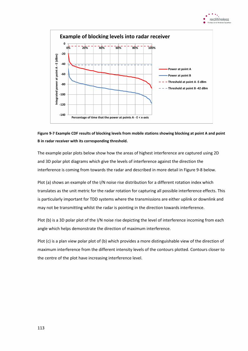
113
Figure 9-7 Example CDF results of blocking levels from mobile stations showing blocking at point A and point
B in radar receiver with its corresponding threshold.
The example polar plots below show how the areas of highest interference are captured using 2D
and 3D polar plot diagrams which give the levels of interference against the direction the
interference is coming from towards the radar and described in more detail in Figure 9-8 below.
Plot (a) shows an example of the I/N noise rise distribution for a different rotation index which
translates as the unit metric for the radar rotation for capturing all possible interference effects. This
is particularly important for TDD systems where the transmissions are either uplink or downlink and
may not be transmitting whilst the radar is pointing in the direction towards interference.
Plot (b) is a 3D polar plot of the I/N noise rise depicting the level of interference incoming from each
angle which helps demonstrate the direction of maximum interference.
Plot (c) is a plan view polar plot of (b) which provides a more distinguishable view of the direction of
maximum interference from the different intensity levels of the contours plotted. Contours closer to
the centre of the plot have increasing interference level.
-140
-120
-100
-80
-60
-40
-20
0
0% 20% 40% 60% 80% 100%
Inte
gra
ted
po
we
r a
t p
oin
t A
-E
(d
Bm
)
Percentage of time that the power at points A - E < x-axis
Blocking level into radar receiver
Power at point A
Power at point B
Threshold at point A -5 dBm
Threshold at point B -42 dBm
Example of blocking levels into radar receiver

114
(a) Noise rise level at the radar receiver as the radar
rotates. Colour intensity is used as scale of the noise rise
value. The starting rotation angle is when the radar points
east. The radar rotates counter-clockwise. Different rows
depict the noise rise for varying mobile locations. For each
angle (column of values) the CDF of the noise rise can be
assessed, see subplot (b).
(b) CDF of the noise rise level at the radar receiver as the
radar rotates (3D view). The noise rise values are
positioned on the longitudinal-axis. The percentage of
time that the noise rise exceeds the level of the
longitudinal-axis is given by the polar-axis. The further the
horizontal cut, at a given threshold value in the
longitudinal-axis, is from the longitudinal-axis, the higher
the probability of the noise rise exceeding this threshold
value. Two horizontal cuts are plotted at the maximum
and minimum I/N thresholds. Each radar rotation-angle
corresponds to a column of values from subplot (a).
Colour intensity is used as scale of the noise rise value.
(c) CDF of the noise rise level at the radar receiver as the
radar rotates (contour view). This is a top-down view of
subplot (b), and it plots the horizontal cuts at different
contour levels. The percentage of time that the noise rise
exceeds the contour-level is given by the polar-axis. The
further the cut is from the pole, the higher the probability
of the noise rise exceeding this contour level value.
Colour intensity is used as scale of the noise rise value in
the plotted contours.
Figure 9-8 2D and 3D polar plots for detailed analysis of angle of worst interference
-15 dB
-5 dB
East
I/N
(d
B)
East
0 dB -5 dB
-15 dB
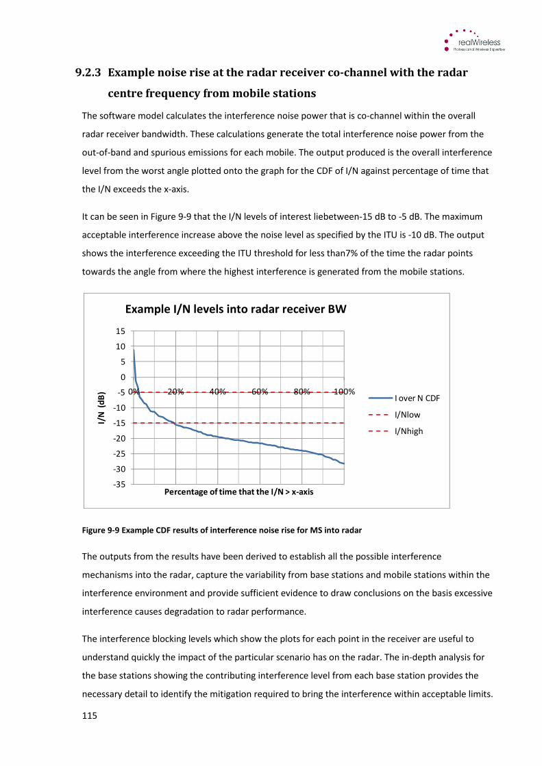
115
9.2.3 Example noise rise at the radar receiver co-channel with the radar
centre frequency from mobile stations
The software model calculates the interference noise power that is co-channel within the overall
radar receiver bandwidth. These calculations generate the total interference noise power from the
out-of-band and spurious emissions for each mobile. The output produced is the overall interference
level from the worst angle plotted onto the graph for the CDF of I/N against percentage of time that
the I/N exceeds the x-axis.
It can be seen in Figure 9-9 that the I/N levels of interest liebetween-15 dB to -5 dB. The maximum
acceptable interference increase above the noise level as specified by the ITU is -10 dB. The output
shows the interference exceeding the ITU threshold for less than7% of the time the radar points
towards the angle from where the highest interference is generated from the mobile stations.
Figure 9-9 Example CDF results of interference noise rise for MS into radar
The outputs from the results have been derived to establish all the possible interference
mechanisms into the radar, capture the variability from base stations and mobile stations within the
interference environment and provide sufficient evidence to draw conclusions on the basis excessive
interference causes degradation to radar performance.
The interference blocking levels which show the plots for each point in the receiver are useful to
understand quickly the impact of the particular scenario has on the radar. The in-depth analysis for
the base stations showing the contributing interference level from each base station provides the
necessary detail to identify the mitigation required to bring the interference within acceptable limits.
-35
-30
-25
-20
-15
-10
-5
0
5
10
15
0% 20% 40% 60% 80% 100%
I/N
(d
B)
Percentage of time that the I/N > x-axis
I/N level in radar receiver BW
I over N CDF
I/Nlow
I/Nhigh
Example I/N levels into radar receiver BW
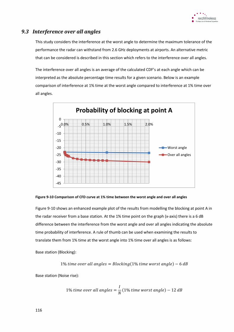
116
9.3 Interference over all angles
This study considers the interference at the worst angle to determine the maximum tolerance of the
performance the radar can withstand from 2.6 GHz deployments at airports. An alternative metric
that can be considered is described in this section which refers to the interference over all angles.
The interference over all angles is an average of the calculated CDF’s at each angle which can be
interpreted as the absolute percentage time results for a given scenario. Below is an example
comparison of interference at 1% time at the worst angle compared to interference at 1% time over
all angles.
Figure 9-10 Comparison of CFD curve at 1% time between the worst angle and over all angles
Figure 9-10 shows an enhanced example plot of the results from modelling the blocking at point A in
the radar receiver from a base station. At the 1% time point on the graph (x-axis) there is a 6 dB
difference between the interference from the worst angle and over all angles indicating the absolute
time probability of interference. A rule of thumb can be used when examining the results to
translate them from 1% time at the worst angle into 1% time over all angles is as follows:
Base station (Blocking):
1% !"#$%#&'((')*(#+ � ,($-.!)*/1% !"#0$&+ ')*(#1 2 64,
Base station (Noise rise):
1% !"#$%#&'((')*(#+ � 56 /1% !"#0$&+ ')*(#1 2 124,
-45
-40
-35
-30
-25
-20
-15
-10
-5
0
0.0% 0.5% 1.0% 1.5% 2.0%
Probability of blocking at point A
Worst angle
Over all angles
117
Mobile station (Blocking):
1% !"#$%#&'((')*(#+ � ,($-.!)*/1% !"#0$&+ ')*(#1 2 64,
Mobile station (Noise rise):
1% !"#$%#&'((')*(#+ � 56 /1% !"#0$&+ ')*(#1 2 5.54,
The decrease in the level of interference in the order of 6-12 dB arises due to the mix of variables
contributing to the interference levels. These include different antenna heights, mix of distances of
the base stations from the radar and reduced level of interference from indoor sites.
118
10 Interferencemodellingresultsfrombasestationsandmobile
stationscenarioswithoutadditionalmitigations
The following chapter presents the modelling results from the simulations of interference from both
base stations and mobile stations into radar without additional mitigations beyond the improved
radar filtering specified by Ofcom. The results are presented to demonstrate the impact of
interference under various scenario conditions that builds up the picture of interference that occurs
from 2.6 GHz deployments into a nearby S-band radar receiver.
The interference scenarios are broadly categorised into two main cases for the analysis:
• Challenging case – Parameters chosen are set to the maximum levels possible but unlikely
(or rarely) to be used in practice and the values are given in Table 10-1 and Table 10-5
• Typical case – Parameters chosen are set to the more realistic practical level and more likely
to be used in practice and the values are given in Table 10-4
An additional measured case was conducted to determine the impact from spurious emissions of a
commercially available FDD LTE mobile device into a radar receiver and the analysis is discussed
further in section 10.9.
The interference environment is presented in a way that initially validates the results from the
model by moving a single interferer closer to the radar which can be seen in sections 10.1 for the
base station and section 10.6 for the mobile station. The next analysis investigates the base station
interference mechanisms which simulated the challenging and typical cases for a fully deployed 2.6
GHz network using the synthetic network at Heathrow Airport which can be seen in sections 10.2
and 10.3. Section 10.4 presents the results from a challenging synthetic layout case placing all the
base stations in a spiral formation at different distances away from the radar.
The final analysis investigated the mobile station interference mechanisms which simulated the
challenging, typical and measured cases for a sample 2.6 GHz network using the actual base station
locations at Heathrow Airport.
The output results are presented in the following way showing Cumulative Distribution Function
(CDF) curves of interference to the radar from the overall worst angle at 1% of the time for:
a. The interference blocking level at the different points in the radar receiver chain to
determine if the blocking threshold level was exceeded and thus cause degradation to the
radar performance.
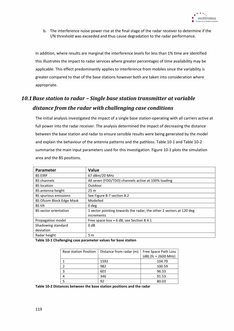
119
b. The interference noise power rise at the final stage of the radar receiver to determine if the
I/N threshold was exceeded and thus cause degradation to the radar performance.
In addition, where results are marginal the interference levels for less than 1% time are identified
this illustrates the impact to radar services where greater percentages of time availability may be
applicable. This effect predominantly applies to interference from mobiles since the variability is
greater compared to that of the base stations however both are taken into consideration where
appropriate.
10.1 Base station to radar – Single base station transmitter at variable
distance from the radar with challenging case conditions
The initial analysis investigated the impact of a single base station operating with all carriers active at
full power into the radar receiver. The analysis determined the impact of decreasing the distance
between the base station and radar to ensure sensible results were being generated by the model
and explain the behaviour of the antenna patterns and the pathloss. Table 10-1 and Table 10-2
summarise the main input parameters used for this investigation. Figure 10-1 plots the simulation
area and the BS positions.
Parameter Value BS EIRP 67 dBm/20 MHz
BS channels All seven (FDD/TDD) channels active at 100% loading
BS location Outdoor
BS antenna height 25 m
BS spurious emissions See Figure 8-7 section 8.2
BS Ofcom Block Edge Mask Modelled
BS tilt 0 deg
BS sector orientation 1 sector pointing towards the radar, the other 2 sectors at 120 deg
increments
Propagation model Free space loss + 6 dB, see Section 8.4.1
Shadowing standard
deviation
0 dB
Radar height 5 m
Table 10-1 Challenging case parameter values for base station
Base station Position Distance from radar (m) Free Space Path Loss
(dB) (fc = 2600 MHz)
1 1592 104.79
2 982 100.59
3 601 96.33
4 346 91.53
5 92 80.03
Table 10-2 Distances between the base station positions and the radar

120
Figure 10-1 Base station locations under investigation
Figure 10-2 and Figure 10-3 show the CDF plots of the results from interference calculations for each
base station position at point A and point B in the receiver chain (refer to Figure 8-15). Within each
plot the result shows the blocking levels for the different base station positions as the distance was
reduced towards the radar. It can be seen from the results that blocking levels from positions 1, 2,
and 3 exceed the -5 dBm threshold level at point A in the radar receiver for 100% of the time the
radar is pointing at the base station. Blocking level from Position 4 exceeds the threshold level at
point A for 23% of the time and below the radar is pointing at the base station. The interference
from the base station at position 5 does not exceed the threshold at point A in the receiver. The
plots show a steady increase in blocking level against the percentage time the radar is pointing at the
base station which begins to decrease from 20% and below. At percentages of time less than 10%
the blocking level rises more sharply compared to the rest of the plot demonstrating the instances in
the variability of the signal envelope power at its maximum level. Blocking at point B does not occur
for all five positions of the base station with 11 dB of margin between the threshold level and the
highest recorded interference level.
Position 1
Position 2 Position 3
Position 4
Position 5
Radar
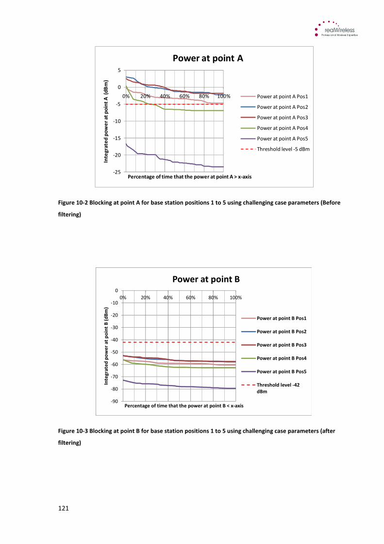
121
Figure 10-2 Blocking at point A for base station positions 1 to 5 using challenging case parameters (Before
filtering)
Figure 10-3 Blocking at point B for base station positions 1 to 5 using challenging case parameters (after
filtering)
-25
-20
-15
-10
-5
0
5
0% 20% 40% 60% 80% 100%
Inte
gra
ted
po
we
r a
t p
oin
t A
(d
Bm
)
Percentage of time that the power at point A > x-axis
Power at point A
Power at point A Pos1
Power at point A Pos2
Power at point A Pos3
Power at point A Pos4
Power at point A Pos5
Threshold level -5 dBm
-90
-80
-70
-60
-50
-40
-30
-20
-10
0
0% 20% 40% 60% 80% 100%
Inte
gra
ted
po
we
r a
t p
oin
t B
(d
Bm
)
Percentage of time that the power at point B < x-axis
Power at point B
Power at point B Pos1
Power at point B Pos2
Power at point B Pos3
Power at point B Pos4
Power at point B Pos5
Threshold level -42
dBm
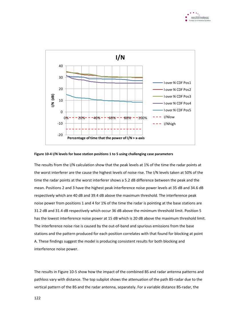
122
Figure 10-4 I/N levels for base station positions 1 to 5 using challenging case parameters
The results from the I/N calculation show that the peak levels at 1% of the time the radar points at
the worst interferer are the cause the highest levels of noise rise. The I/N levels taken at 50% of the
time the radar points at the worst interferer shows a 5.2 dB difference between the peak and the
mean. Positions 2 and 3 have the highest peak interference noise power levels at 35 dB and 34.6 dB
respectively which are 40 dB and 39.4 dB above the maximum threshold. The interference peak
noise power from positions 1 and 4 for 1% of the time the radar is pointing at the base stations are
31.2 dB and 31.4 dB respectively which occur 36 dB above the minimum threshold limit. Position 5
has the lowest interference noise power at 15 dB which is 20 dB above the maximum threshold limit.
The interference noise rise is caused by the out-of-band and spurious emissions from the base
stations and the pattern produced for each position correlates with that found for blocking at point
A. These findings suggest the model is producing consistent results for both blocking and
interference noise power.
The results in Figure 10-5 show how the impact of the combined BS and radar antenna patterns and
pathloss vary with distance. The top subplot shows the attenuation of the path BS-radar due to the
vertical pattern of the BS and the radar antenna, separately. For a variable distance BS-radar, the
-20
-10
0
10
20
30
40
0% 20% 40% 60% 80% 100%
I/N
(d
B)
Percentage of time that the power of I/N > x-axis
I/N
I over N CDF Pos1
I over N CDF Pos2
I over N CDF Pos3
I over N CDF Pos4
I over N CDF Pos5
I/Nlow
I/Nhigh

123
attenuation due to the vertical patterns changes for close distance to the radar. The attenuation is at
maximum when the direct path crosses the vertical patterns from the sidelobe region. For far
distances the attenuation is smaller because the BS gets closer to the radar main beam.
The bottom subplot shows the attenuation of the path BS-radar due to the median path loss model +
attenuation due to the vertical patterns. The path loss is greater with an increasing distance.
The combined effect of path loss plus pattern is that, very close to the radar the high attenuation
due to the vertical patterns means that emissions in that zone do not cause interference.
Bear in mind that the above apply for uneven height between radar and BS. In the case that the
heights are equal, the attenuation due to the vertical patterns is constant with the distance, and
therefore emissions from close to the radar cause greater interference than further away.
Using the plot in Figure 10-5 the results can be interpreted based on the attenuation for a variable
BS distance from the radar location. The attenuation in the y-axis of the bottom subplot is the
combination from the BS and radar antenna vertical-patterns, and from the median path loss model.
It can be seen from the top subplot that the attenuation of Position 1 due to the vertical patterns is
0.1 dB (due to the BS antenna) plus 4.6 dB (due to the radar antenna). Position 1 has the furthest
distance from the radar and therefore the greater median pathloss. As the position of the BS is
moved closer to the radar (Position 2 and 3) the attenuation due to the vertical patterns becomes
greater, however the attenuation due to the path loss becomes smaller. The effect of the path loss is
greater than the vertical patterns for Position 2 and 3, so that the interference increases with a
decreasing distance.
The antenna patterns begin to make a greater impact with respect to the path loss for distances
closer than Position 3 (Positions 4 to 5). This explains the lower interference level of Position 4
against Position 1, 2 and 3. Note that in Position 5, which is the closest position considered in this
investigation, the emissions are attenuated by 50 dB due to the antenna patterns.
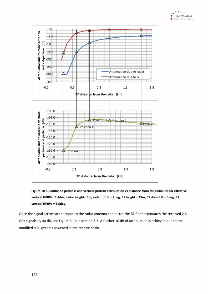
124
Figure 10-5 Combined pathloss and vertical-pattern attenuation vs distance from the radar. Radar effective
vertical HPBW= 4.4deg, radar height= 5m, radar uptilt = 2deg, BS height = 25m, BS downtilt = 0deg, BS
vertical HPBW = 6.5deg.
Once the signal arrives at the input to the radar antenna connector the RF filter attenuates the received 2.6
GHz signals by 40 dB, see Figure 8-16 in section 8.3. A further 10 dB of attenuation is achieved due to the
modified sub-systems assumed in the receive chain.
-35.0
-30.0
-25.0
-20.0
-15.0
-10.0
-5.0
0.0
-0.2 0.3 0.8 1.3 1.8
Att
en
ua
tio
n d
ue
to
ra
da
r-a
nte
nn
a
ve
rtic
al-
pa
tte
rn
(dB
)
2D distance from the radar (km)
Attenuation due to radar
Attenuation due to BS
Position 5
Position 4
Position 3 Position 2Position 1
-140.0
-135.0
-130.0
-125.0
-120.0
-115.0
-110.0
-105.0
-100.0
-0.2 0.3 0.8 1.3 1.8
Att
en
ua
tio
n d
ue
to
an
ten
na
ve
rtic
al-
pa
tte
rns
an
d p
ath
loss
(d
B)
2D distance from the radar (km)
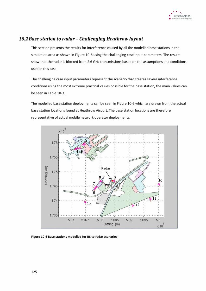
125
10.2 Base station to radar – Challenging Heathrow layout
This section presents the results for interference caused by all the modelled base stations in the
simulation area as shown in Figure 10-6 using the challenging case input parameters. The results
show that the radar is blocked from 2.6 GHz transmissions based on the assumptions and conditions
used in this case.
The challenging case input parameters represent the scenario that creates severe interference
conditions using the most extreme practical values possible for the base station, the main values can
be seen in Table 10-3.
The modelled base station deployments can be seen in Figure 10-6 which are drawn from the actual
base station locations found at Heathrow Airport. The base station locations are therefore
representative of actual mobile network operator deployments.
Figure 10-6 Base stations modelled for BS to radar scenarios
Radar
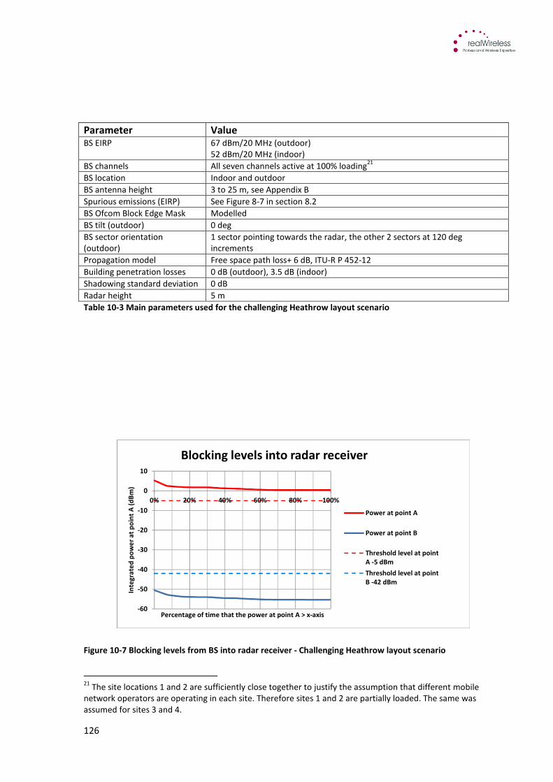
126
Parameter Value BS EIRP 67 dBm/20 MHz (outdoor)
52 dBm/20 MHz (indoor)
BS channels All seven channels active at 100% loading21
BS location Indoor and outdoor
BS antenna height 3 to 25 m, see Appendix B
Spurious emissions (EIRP) See Figure 8-7 in section 8.2
BS Ofcom Block Edge Mask Modelled
BS tilt (outdoor) 0 deg
BS sector orientation
(outdoor)
1 sector pointing towards the radar, the other 2 sectors at 120 deg
increments
Propagation model Free space path loss+ 6 dB, ITU-R P 452-12
Building penetration losses 0 dB (outdoor), 3.5 dB (indoor)
Shadowing standard deviation 0 dB
Radar height 5 m
Table 10-3 Main parameters used for the challenging Heathrow layout scenario
Figure 10-7 Blocking levels from BS into radar receiver - Challenging Heathrow layout scenario
21
The site locations 1 and 2 are sufficiently close together to justify the assumption that different mobile
network operators are operating in each site. Therefore sites 1 and 2 are partially loaded. The same was
assumed for sites 3 and 4.
-60
-50
-40
-30
-20
-10
0
10
0% 20% 40% 60% 80% 100%
Inte
gra
ted
po
we
r a
t p
oin
t A
(d
Bm
)
Percentage of time that the power at point A > x-axis
Blocking levels into radar receiver
Power at point A
Power at point B
Threshold level at point
A -5 dBm
Threshold level at point
B -42 dBm
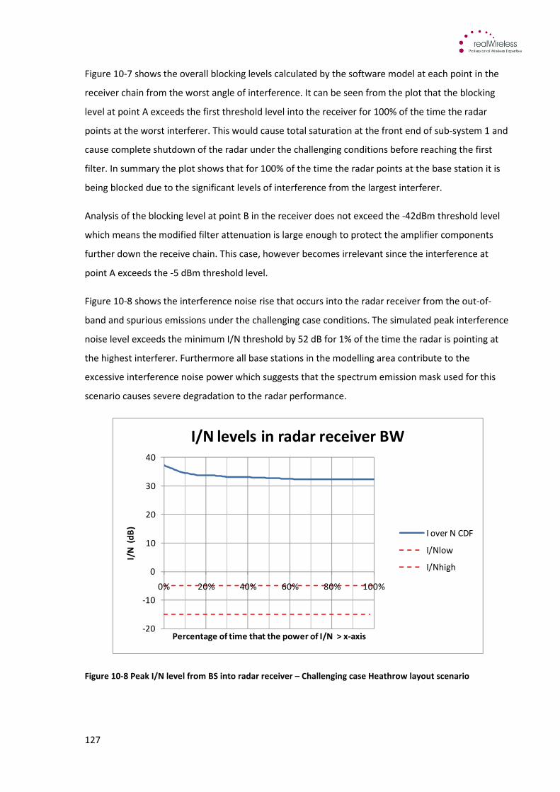
127
Figure 10-7 shows the overall blocking levels calculated by the software model at each point in the
receiver chain from the worst angle of interference. It can be seen from the plot that the blocking
level at point A exceeds the first threshold level into the receiver for 100% of the time the radar
points at the worst interferer. This would cause total saturation at the front end of sub-system 1 and
cause complete shutdown of the radar under the challenging conditions before reaching the first
filter. In summary the plot shows that for 100% of the time the radar points at the base station it is
being blocked due to the significant levels of interference from the largest interferer.
Analysis of the blocking level at point B in the receiver does not exceed the -42dBm threshold level
which means the modified filter attenuation is large enough to protect the amplifier components
further down the receive chain. This case, however becomes irrelevant since the interference at
point A exceeds the -5 dBm threshold level.
Figure 10-8 shows the interference noise rise that occurs into the radar receiver from the out-of-
band and spurious emissions under the challenging case conditions. The simulated peak interference
noise level exceeds the minimum I/N threshold by 52 dB for 1% of the time the radar is pointing at
the highest interferer. Furthermore all base stations in the modelling area contribute to the
excessive interference noise power which suggests that the spectrum emission mask used for this
scenario causes severe degradation to the radar performance.
Figure 10-8 Peak I/N level from BS into radar receiver – Challenging case Heathrow layout scenario
-20
-10
0
10
20
30
40
0% 20% 40% 60% 80% 100%
I/N
(d
B)
Percentage of time that the power of I/N > x-axis
I/N levels in radar receiver BW
I over N CDF
I/Nlow
I/Nhigh
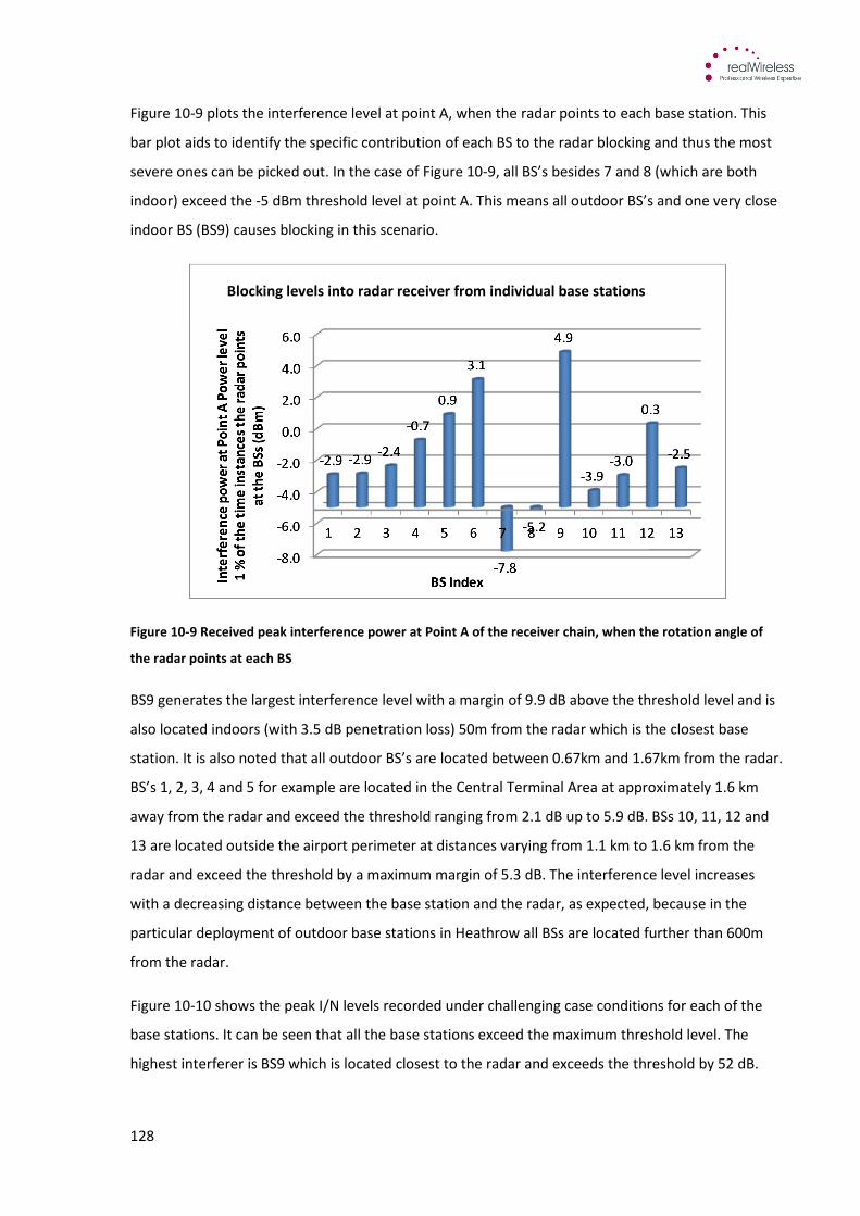
128
Figure 10-9 plots the interference level at point A, when the radar points to each base station. This
bar plot aids to identify the specific contribution of each BS to the radar blocking and thus the most
severe ones can be picked out. In the case of Figure 10-9, all BS’s besides 7 and 8 (which are both
indoor) exceed the -5 dBm threshold level at point A. This means all outdoor BS’s and one very close
indoor BS (BS9) causes blocking in this scenario.
Figure 10-9 Received peak interference power at Point A of the receiver chain, when the rotation angle of
the radar points at each BS
BS9 generates the largest interference level with a margin of 9.9 dB above the threshold level and is
also located indoors (with 3.5 dB penetration loss) 50m from the radar which is the closest base
station. It is also noted that all outdoor BS’s are located between 0.67km and 1.67km from the radar.
BS’s 1, 2, 3, 4 and 5 for example are located in the Central Terminal Area at approximately 1.6 km
away from the radar and exceed the threshold ranging from 2.1 dB up to 5.9 dB. BSs 10, 11, 12 and
13 are located outside the airport perimeter at distances varying from 1.1 km to 1.6 km from the
radar and exceed the threshold by a maximum margin of 5.3 dB. The interference level increases
with a decreasing distance between the base station and the radar, as expected, because in the
particular deployment of outdoor base stations in Heathrow all BSs are located further than 600m
from the radar.
Figure 10-10 shows the peak I/N levels recorded under challenging case conditions for each of the
base stations. It can be seen that all the base stations exceed the maximum threshold level. The
highest interferer is BS9 which is located closest to the radar and exceeds the threshold by 52 dB.
Blocking levels into radar receiver from individual base stations
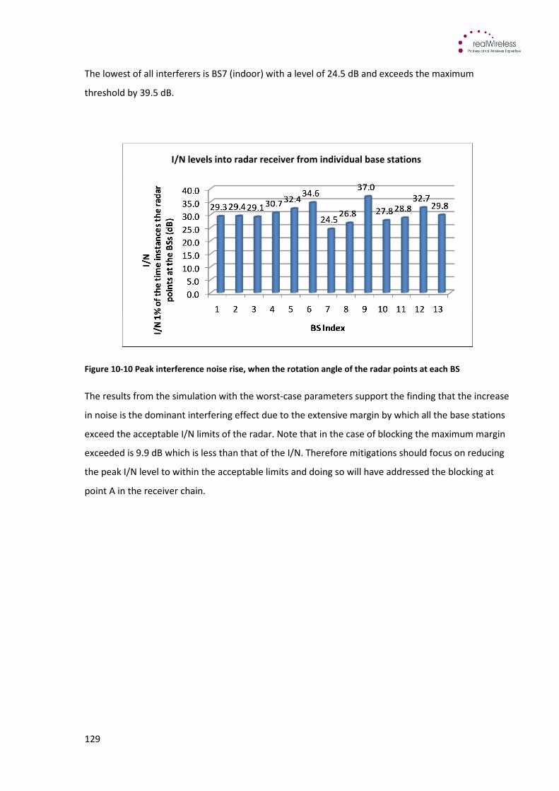
129
The lowest of all interferers is BS7 (indoor) with a level of 24.5 dB and exceeds the maximum
threshold by 39.5 dB.
Figure 10-10 Peak interference noise rise, when the rotation angle of the radar points at each BS
The results from the simulation with the worst-case parameters support the finding that the increase
in noise is the dominant interfering effect due to the extensive margin by which all the base stations
exceed the acceptable I/N limits of the radar. Note that in the case of blocking the maximum margin
exceeded is 9.9 dB which is less than that of the I/N. Therefore mitigations should focus on reducing
the peak I/N level to within the acceptable limits and doing so will have addressed the blocking at
point A in the receiver chain.
I/N levels into radar receiver from individual base stations
130
10.3 Base station to radar – Typical Heathrow layout
The base station to radar under typical case conditions was conducted to determine the impact of
interference into the radar at the Heathrow Airport. Figure 10-6 plots the simulation area and Table
10-4 summarises the values used for the typical case. The complete set of chosen parameters for the
typical case is provided in appendix B.
Parameter Value BS EIRP 63 dBm/20 MHz (outdoor)
48 dBm/20 MHz (indoor)
BS channels Max four channels active at 80% loading22
BS location Indoor and outdoor
BS antenna height 3 to 25 m, see Appendix B
Spurious emissions (EIRP) See Figure 8-11 in section 8.2
BS Ofcom Block Edge Mask Modelled
BS tilt (outdoor) 6 deg
BS sector orientation (outdoor) 1 sector pointing east, the other 2 sectors at 120 deg increments
Propagation model Free space path loss+ 6 dB, ITU-R P 452-12
Building penetration losses 0 dB (outdoor), 14dB (indoor)
Shadowing standard deviation 0 dB
Radar height 20 m23
Table 10-4 Typical case parameters
Figure 10-11 shows the blocking levels calculated by the software model at each point in the receiver
chain for the typical-case parameters. It can be seen from the plot that the overall blocking level at
point A does not exceed the threshold level into the receiver and would not cause blocking at the
input of sub-system 1. The highest overall blocking level recorded for the worst angle was -16 dBm
which is 11 dB below the threshold level at Point A of the receiver chain.
The blocking level recorded at point B further down the receiver chain is around 40 dB below its
respective threshold level. The improved selectivity of the modified radar filters attenuate the
already low blocking levels from the 2.6 GHz band frequencies compared to the challenging case.
It can be seen from Figure 10-11 that blocking does not exceed the interference threshold limit at
point A or point B across the statistical range and therefore considered to not cause blocking in the
radar receiver under typical scenario conditions.
22
The site locations 1 and 2 are sufficiently close together to justify the assumption that different mobile
network operators are operating in each site. Therefore sites 1 and 2 are partially loaded. The same was
assumed for sites 3 and 4. 23
20m antenna height was used for the model as the radar antenna height at Heathrow Airport is 40m which
was not considered to be typical of radar heights found in general.
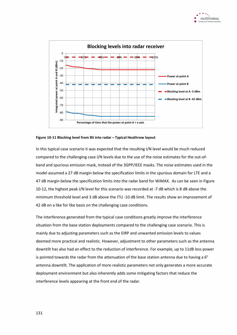
131
Figure 10-11 Blocking level from BS into radar – Typical Heathrow layout
In this typical case scenario it was expected that the resulting I/N level would be much reduced
compared to the challenging case I/N levels due to the use of the noise estimates for the out-of-
band and spurious emission mask, instead of the 3GPP/IEEE masks. The noise estimates used in the
model assumed a 27 dB margin below the specification limits in the spurious domain for LTE and a
47 dB margin below the specification limits into the radar band for WiMAX. As can be seen in Figure
10-12, the highest peak I/N level for this scenario was recorded at -7 dB which is 8 dB above the
minimum threshold level and 3 dB above the ITU -10 dB limit. The results show an improvement of
42 dB on a like for like basis on the challenging case conditions.
The interference generated from the typical case conditions greatly improve the interference
situation from the base station deployments compared to the challenging case scenario. This is
mainly due to adjusting parameters such as the EIRP and unwanted emission levels to values
deemed more practical and realistic. However, adjustment to other parameters such as the antenna
downtilt has also had an effect to the reduction of interference. For example, up to 11dB less power
is pointed towards the radar from the attenuation of the base station antenna due to having a 6°
antenna downtilt. The application of more realistic parameters not only generates a more accurate
deployment environment but also inherently adds some mitigating factors that reduce the
interference levels appearing at the front end of the radar.
-90
-80
-70
-60
-50
-40
-30
-20
-10
0
0% 20% 40% 60% 80% 100%In
teg
rate
d p
ow
er
at
po
int
A a
nd
B (
dB
m)
Percentage of time that the power at point A < x-axis
Blocking levels into radar receiver
Power at point A
Power at point B
Blocking level at A -5 dBm
Blocking level at B -42 dBm
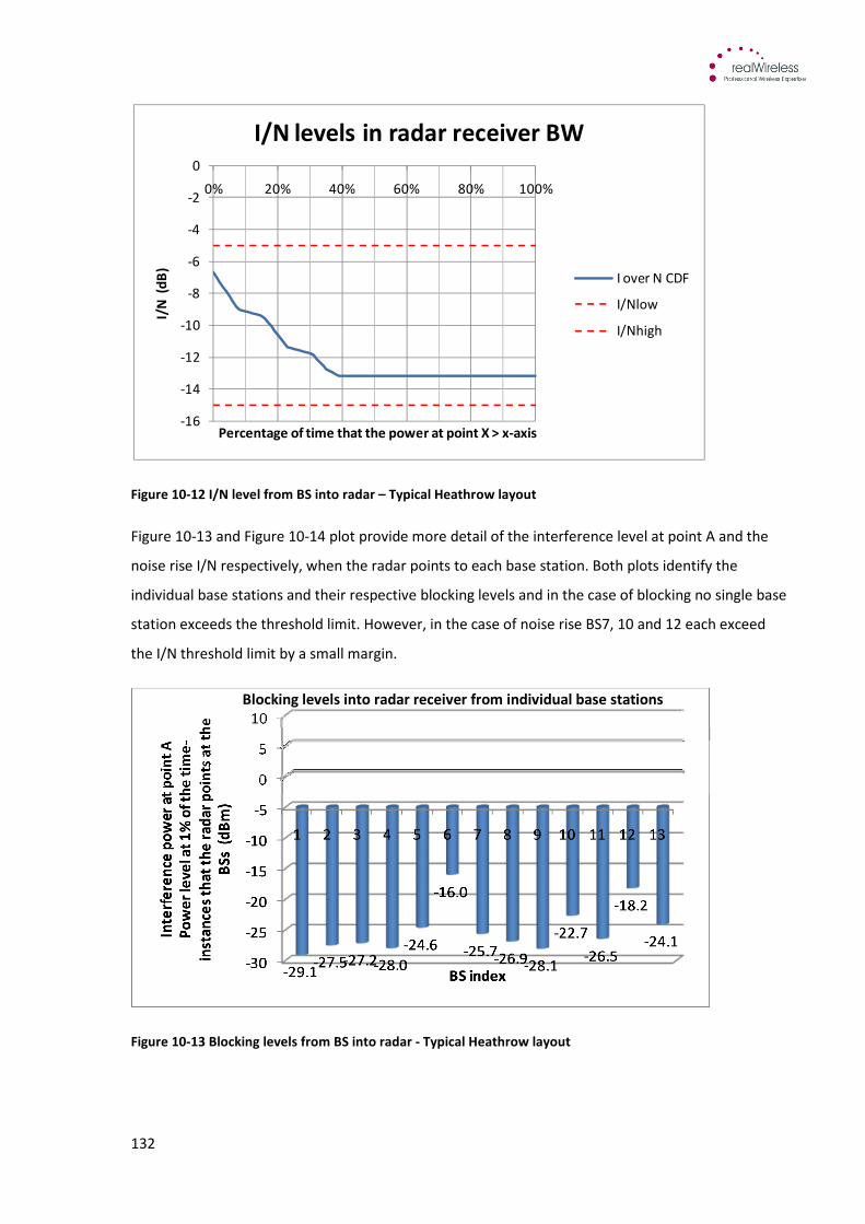
132
Figure 10-12 I/N level from BS into radar – Typical Heathrow layout
Figure 10-13 and Figure 10-14 plot provide more detail of the interference level at point A and the
noise rise I/N respectively, when the radar points to each base station. Both plots identify the
individual base stations and their respective blocking levels and in the case of blocking no single base
station exceeds the threshold limit. However, in the case of noise rise BS7, 10 and 12 each exceed
the I/N threshold limit by a small margin.
Figure 10-13 Blocking levels from BS into radar - Typical Heathrow layout
-16
-14
-12
-10
-8
-6
-4
-2
0
0% 20% 40% 60% 80% 100%
I/N
(d
B)
Percentage of time that the power at point X > x-axis
I/N levels in radar receiver BW
I over N CDF
I/Nlow
I/Nhigh
Blocking levels into radar receiver from individual base stations
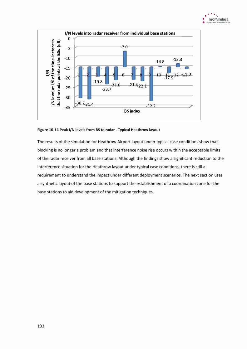
133
Figure 10-14 Peak I/N levels from BS to radar - Typical Heathrow layout
The results of the simulation for Heathrow Airport layout under typical case conditions show that
blocking is no longer a problem and that interference noise rise occurs within the acceptable limits
of the radar receiver from all base stations. Although the findings show a significant reduction to the
interference situation for the Heathrow layout under typical case conditions, there is still a
requirement to understand the impact under different deployment scenarios. The next section uses
a synthetic layout of the base stations to support the establishment of a coordination zone for the
base stations to aid development of the mitigation techniques.
I/N levels into radar receiver from individual base stations
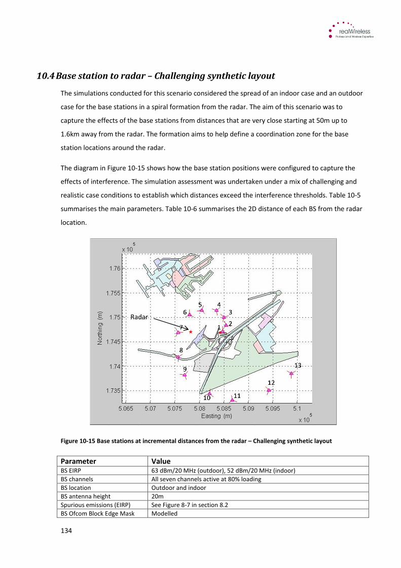
134
10.4 Base station to radar – Challenging synthetic layout
The simulations conducted for this scenario considered the spread of an indoor case and an outdoor
case for the base stations in a spiral formation from the radar. The aim of this scenario was to
capture the effects of the base stations from distances that are very close starting at 50m up to
1.6km away from the radar. The formation aims to help define a coordination zone for the base
station locations around the radar.
The diagram in Figure 10-15 shows how the base station positions were configured to capture the
effects of interference. The simulation assessment was undertaken under a mix of challenging and
realistic case conditions to establish which distances exceed the interference thresholds. Table 10-5
summarises the main parameters. Table 10-6 summarises the 2D distance of each BS from the radar
location.
Figure 10-15 Base stations at incremental distances from the radar – Challenging synthetic layout
Parameter Value BS EIRP 63 dBm/20 MHz (outdoor), 52 dBm/20 MHz (indoor)
BS channels All seven channels active at 80% loading
BS location Outdoor and indoor
BS antenna height 20m
Spurious emissions (EIRP) See Figure 8-7 in section 8.2
BS Ofcom Block Edge Mask Modelled
Radar
135
BS tilt (outdoor) 6 deg
BS sector orientation
(outdoor)
1 sector pointing away from the radar, the other 2 sectors at 120 deg
increments
Propagation model Free space path loss+ 6 dB
Building penetration losses 0 dB (outdoor), 14 dB (indoor)
Shadowing standard deviation 0 dB
Radar height 20m
Table 10-5 Incremental distances from radar – Challenging synthetic layout
BS Index 1 2 3 4 5 6 7 8 9 10 11 12 13
Distance (m) 50 185 321 456 591 727 862 997 1133 1268 1403 1539 1674
Intermediate
distances
between…
1
and
2
2
and
3
3
and
4
4
and
5
5
and
6
6
and
7
7
and
8
8
and
9
9
and
10
10
and
11
11
and
12
12
and
13
Distance (m) 118 253 389 524 659 795 930 1065 1201 1336 1471 1607
Table 10-6 Incremental distances from radar
10.4.1 Challengingsyntheticlayout-Outdoorcase
The outdoor case was treated first and the results are shown below. The overall blocking level from
the worst angle shows that blocking occurs at point A in the receiver. The peak blocking level, which
is recorded at 1% of the time the radar points at the worst interferer, at point B is 2.1 dB above the
threshold limit. This is caused by the very close proximity base station and the excessive power levels
that would cause blocking at this very close range. The modified RF filter is not able to attenuate the
signal below the threshold level for 1% of the time. Peak blocking at point A exceeds its threshold by
20.1 dB for 1% of the time the radar points at the base station and would therefore cause the radar
to cease operating.
Figure 10-16 Overall blocking levels at worst angle of BS into radar – Challenging synthetic layout (outdoor)
-50
-40
-30
-20
-10
0
10
20
0% 20% 40% 60% 80% 100%
Inte
gra
ted
po
we
r a
t p
oin
t A
an
d B
(d
Bm
)
Percentage of time that the power at point A > x-axis
Blocking levels into radar receiver
Power at point A
Power at point B
Blocking level at A -5 dBm
Blocking level at B -42 dBm
136
Figure 10-17 plots the CDF of the I/N levels at the worst angle. It is noted that the BSs’ noise
emissions are at the levels specified from 3GPP/IEEE specs (See section 8.2.3). The minimum
threshold level (-15dB) is exceeded by 62.8 dB for 1% of the time the radar points at the worst angle.
This margin is used to set the target for reduction of the overall interference levels. Focusing on
reducing the noise rise will also resolve the situation for blocking into the receiver.
Figure 10-17 I/N levels at worst angle of BS into radar – Challenging synthetic layout (outdoor)
The investigation can be analysed further using the detailed results shown below which identifies
the specific base stations and distances at which the interference starts to become a problem. The
received power when the radar points at BS1 to BS4 exceed the -5 dBm threshold at point A for 1%
of the time the radar is pointing at each BS. The blocking threshold at point A in the receiver is
exceeded by 20.1 dB from BS1, 8.6 dB by BS2, 8.2 dB by BS3 and 1.9 dB by BS4. BS5 to BS13 do not
exceed the threshold level at point A. The pattern shows a steady decrease of the peak blocking level
starting from the closest base station with the highest blocking level of 15.1 dB and quickly reducing
in magnitude for each base station at distances further away from the radar. In general at distances
beyond base station 4 (456m) the received interference levels at Point A of the receiver chain drop
below the -5 dBm limit.
-20
-10
0
10
20
30
40
50
60
0% 20% 40% 60% 80% 100%
I/N
(d
B)
Percentage of time that the power of I/N > x-axis
I/N levels in radar receiver BW
I over N CDF
I/Nlow
I/Nhigh
137
Figure 10-18 Results of peak blocking level at point A – Challenging synthetic layout (outdoor)
As already discussed the peak noise rise exceeds the threshold by a margin that is greater than the
interference power exceeding the thresholds at the various points of the receiver chain. Figure 10-19
shows that all base stations exceed the minimum threshold for I/N. Therefore any exclusion zone
would commence at a distance much beyond the furthest base station modelled. For example using
free space path loss the coordination zone would need to be 140km under the conditions used for
this scenario.
Figure 10-19 Results from peak interference noise power – Challenging synthetic layout (outdoor)
Blocking levels into radar receiver from individual base stations
I/N levels into radar receiver from individual base stations
138
10.4.2 Challengingsyntheticlayout-Indoorcase
The results from the indoor case can be seen below which uses the same process and layout as the
challenging synthetic layout outdoor case. The figure below plots the CDF curves of the received
powers at the various points of the receiver chain and their respective threshold blocking-levels. The
peak interference level at point B is 12.4 dB below its threshold limit. Blocking occurs at Point A
(exceeds its threshold by 5.3 dB for 1% time) which means the closely located base stations, even
when indoors, will cause blocking to the radar in this layout.
Figure 10-20 Overall blocking levels at worst angle of BS into radar – Challenging synthetic layout (indoor)
Figure 10-21 plots the noise rise CDF when the radar points at the worst-interference angle. The
minimum threshold level (-15dB) is exceeded by 47 dB for 1% time. This margin (47 dB) is the target
for interference reduction that is required so that blocking does not occur and the peak I/N is below
the acceptable threshold level (-10 dB). Note that the BS emissions mask in this scenario is as
defined in the 3GPP/IEEE specifications (See section 8.2.3).
-70
-60
-50
-40
-30
-20
-10
0
10
0% 20% 40% 60% 80% 100%
Inte
gra
ted
po
we
r a
t p
oin
t A
an
d B
(d
Bm
)
Percentage of time that the power at point A > x-axis
Blocking levels into radar receiver
Power at point A
Power at point B
Blocking level at A -5 dBm
Blocking level at B -42 dBm
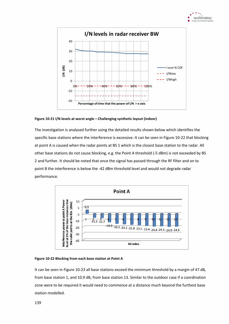
139
Figure 10-21 I/N levels at worst angle – Challenging synthetic layout (indoor)
The investigation is analysed further using the detailed results shown below which identifies the
specific base stations where the interference is excessive. It can be seen in Figure 10-22 that blocking
at point A is caused when the radar points at BS 1 which is the closest base station to the radar. All
other base stations do not cause blocking, e.g. the Point A threshold (-5 dBm) is not exceeded by BS
2 and further. It should be noted that once the signal has passed through the RF filter and on to
point B the interference is below the -42 dBm threshold level and would not degrade radar
performance.
Figure 10-22 Blocking from each base station at Point A
It can be seen in Figure 10-23 all base stations exceed the minimum threshold by a margin of 47 dB,
from base station 1, and 10.9 dB, from base station 13. Similar to the outdoor case if a coordination
zone were to be required it would need to commence at a distance much beyond the furthest base
station modelled.
-20
-10
0
10
20
30
40
0% 20% 40% 60% 80% 100%
I/N
(d
B)
Percentage of time that the power of I/N > x-axis
I/N levels in radar receiver BW
I over N CDF
I/Nlow
I/Nhigh
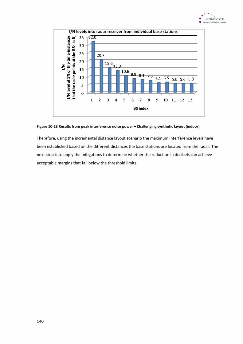
140
Figure 10-23 Results from peak interference noise power – Challenging synthetic layout (indoor)
Therefore, using the incremental distance layout scenario the maximum interference levels have
been established based on the different distances the base stations are located from the radar. The
next step is to apply the mitigations to determine whether the reduction in decibels can achieve
acceptable margins that fall below the threshold limits.
I/N levels into radar receiver from individual base stations
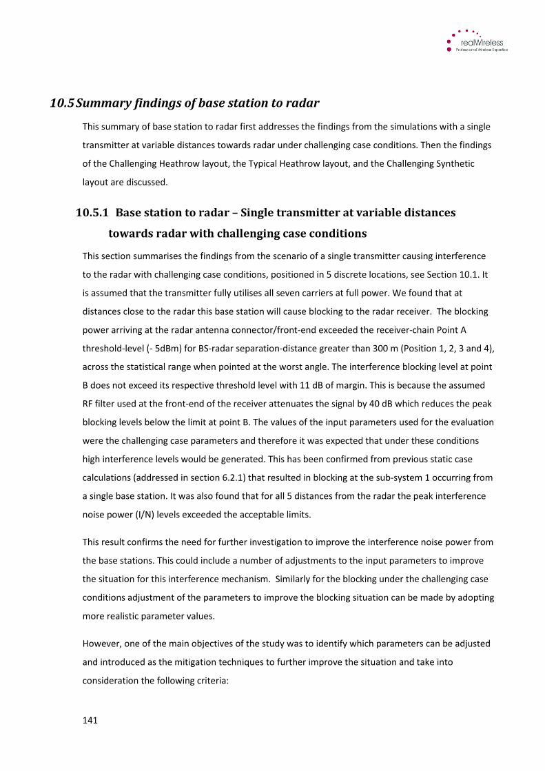
141
10.5 Summary findings of base station to radar
This summary of base station to radar first addresses the findings from the simulations with a single
transmitter at variable distances towards radar under challenging case conditions. Then the findings
of the Challenging Heathrow layout, the Typical Heathrow layout, and the Challenging Synthetic
layout are discussed.
10.5.1 Basestationtoradar–Singletransmitteratvariabledistances
towardsradarwithchallengingcaseconditions
This section summarises the findings from the scenario of a single transmitter causing interference
to the radar with challenging case conditions, positioned in 5 discrete locations, see Section 10.1. It
is assumed that the transmitter fully utilises all seven carriers at full power. We found that at
distances close to the radar this base station will cause blocking to the radar receiver. The blocking
power arriving at the radar antenna connector/front-end exceeded the receiver-chain Point A
threshold-level (- 5dBm) for BS-radar separation-distance greater than 300 m (Position 1, 2, 3 and 4),
across the statistical range when pointed at the worst angle. The interference blocking level at point
B does not exceed its respective threshold level with 11 dB of margin. This is because the assumed
RF filter used at the front-end of the receiver attenuates the signal by 40 dB which reduces the peak
blocking levels below the limit at point B. The values of the input parameters used for the evaluation
were the challenging case parameters and therefore it was expected that under these conditions
high interference levels would be generated. This has been confirmed from previous static case
calculations (addressed in section 6.2.1) that resulted in blocking at the sub-system 1 occurring from
a single base station. It was also found that for all 5 distances from the radar the peak interference
noise power (I/N) levels exceeded the acceptable limits.
This result confirms the need for further investigation to improve the interference noise power from
the base stations. This could include a number of adjustments to the input parameters to improve
the situation for this interference mechanism. Similarly for the blocking under the challenging case
conditions adjustment of the parameters to improve the blocking situation can be made by adopting
more realistic parameter values.
However, one of the main objectives of the study was to identify which parameters can be adjusted
and introduced as the mitigation techniques to further improve the situation and take into
consideration the following criteria:

142
a) Limit the adjustment of parameters to ensure minimal loss in performance of the 2.6 GHz
network
b) Limit the cost of introducing new parameters or additional costly adjustments to the base
stations as much as possible
c) Maximum value is maintained of the 2.6 GHz spectrum in the vicinity of airports
Table 10-7 summarises the blocking power levels at Point A of the receiver chain. Some observations
about the received interference are:
i. As the position of the BS moves closer to the radar the attenuation due to the vertical
patterns (BS and radar) becomes greater. In the closest BS position to the radar the
attenuation due to patterns is greatest.
ii. As the position of the BS moves closer to the radar the attenuation due to the path loss
becomes smaller. This is because the separation distance between the radar and the BS
becomes smaller.
iii. The combined effect of the vertical-patterns and pathloss is that the interference is worst
for distances greater than about 400m from the radar, see Figure 10-5.
Position Distance from
radar (m)
Peak blocking power at Point A, 1% of the time the radar
points at the worst-angle (dBm)
Blocking threshold at
point A (dBm)
1 1592 -0.5 -5
2 982 2.9 -5
3 601 2.4 -5
4 346 -0.1 -5
5 92 -17.1 -5
Table 10-7 Base station to radar initial investigation results summary
The table above can be compared to the basic link level analysis (See section 6.2.1) when the base
stations appear in the half power beamwidth of the radar antenna. Blocking arises at distances of
300m to 400m and beyond and is maximum at a point between 300m and 1500m. After 1500m the
blocking levels begin to decrease as the pathloss starts to take effect.
10.5.2 Basestationtoradar–ChallengingHeathrow,TypicalHeathrow,and
Challengingsyntheticlayouts
This section summarises the findings from the scenarios Challenging Heathrow layout, Typical
Heathrow layout, and Challenging Synthetic layout. In the first two scenarios the transmitters were
located at real sites on the Heathrow Airport map. Within the Heathrow layout, this summary
demonstrates that the interference problem under typical-case parameters is improved compared
to the challenging-case parameters.
143
The results from the analysis in this section informed the next stage of the study by identifying the
mitigation techniques that could be implemented to resolve the interference to a more acceptable
level that aims to satisfy the safety case criteria of the regulatory authorities. The findings from the
main investigation show the impact of interference to the radar under the different scenario
conditions. The scenario conditions analysed included:
• Challenging Heathrow layout. Heathrow layout with the most challenging parameters. This
scenario is investigated so as to reveal the maximum potential of the blocking problem.
• Typical Heathrow layout. Heathrow layout with typical parameters. This scenario
approaches the Heathrow-specific deployment and a busy 2.6 GHz mobile network.
• Challenging synthetic layout. Synthetic layout with a mix of challenging and realistic
parameters. The base stations are positioned at incremental distances from the radar.
The findings from the Challenging Heathrow layout, which used the most extreme settings to
produce severe interference conditions into the radar, showed significant blocking levels appearing
at point A of the radar receiver. The blocking was predominantly caused by the indoor base station
located 50m away from the radar, regardless of its low EIRP, most probably due to the low building
penetration losses assumption (3.5 dB). The outdoor base stations in the Central Terminal Area on
the roof of the car parks and the roof of Terminal 4 contributed the next highest levels of blocking
(e.g. the outdoor base station 6 is located 660m away from the radar, at height 24m with a line of
sight to the radar).
The findings from the Typical Heathrow layout, in which the parameters were adjusted to the
Heathrow-specific typical values (e.g. tilt at 6°, EIRP 4 dB lower than the challenging value,
OOB/spurious emission masks reflecting a typical high-end commercial transmitter), showed
reduction of the blocking level, when compared against the Challenging Heathrow layout. The
results suggested that base stations do not cause blocking of the radar, but exceed the minimum
threshold I/N level by 8 dB.
The findings from the Challenging synthetic layout, assisted in the investigation of potential
mitigations, due to the incremental distance of the base stations from the radar and because of the
different angle each base station is illuminated as the radar rotates. The findings from this layout
showed that blocking occurred up to at a distance of 659m from the radar. After this distance the
interference from all other base stations did not exceed the threshold at point A. Although blocking
occurs under these conditions the dominating interference mechanism was the interference noise
rise, whose maximum threshold was exceeded by each base station modelled and therefore more
challenging to resolve using mitigations. In all instances the maximum threshold was exceeded with
144
the furthest base station exceeding the maximum threshold by 37.5 dB. The focus of the
investigation in the next chapter seeks to reduce the peak interference noise power by introducing
the mitigation techniques and reduce the I/N levels within the acceptable limits.
To summarise, some observations about the received interference are:
• Different antenna heights of the base station and the radar. The maximum interference is
received at the radar when the BS and the radar antennas are at the same height
• Radar antenna height. The radar antenna height in the Typical Heathrow layout is 20m
which is considered to be a typical height for the radar. However, the actual antenna height
at Heathrow is 40m which means the results obtained will be more conservative compared
to reality.
• Separation distance between the base station and the radar. Increasing the separation
distance between the base station and the radar increases the path loss and therefore
reduces the amount of interference into the radar, see Figure 10-5
• Combined pathloss and vertical –pattern attenuation vs. distance from the radar. At BS
within close proximity to the radar the attenuation from the radar antenna pattern is capped
at the maximum attenuation (30 dB). The attenuation due to path loss is small. For greater
distances the attenuation from the radar and BS antenna patterns is smaller, because the BS
gets closer to the main radar beam, see Figure 10-5.
• The base station antenna downtilt. It was found that by increasing the downtilt of the base
station antenna from 0° (Challenging Heathrow layout scenario) case to 6° (Typical Heathrow
layout scenario) reduces the interference. This is because the downtilt increases the
attenuation due to the antenna pattern from the base station.
• The mobile network carriers. A reduction in the loading level of the carriers causes a
moderate drop of interfering levels
• Spectrum emissions mask. Typical high-end transmitters have spurious emissions below the
3GPP/IEEE specification limits at the radar band. The suggested margin is 24 dB below the
specification limit at the radar band frequency.
• Radar frequency. The generic modified radar frequency modelled was 2750 MHz. Licensed
frequencies assigned to radars found at other airports may be closer in frequency to the 2.6
GHz band and the impact from adjacent 2.6 GHz emissions at these frequencies may
generate higher interference levels compared to the generic modified radar frequency.
The following tables below summarise the findings from the Challenging synthetic layout scenario to
show the highest blocking (Table 10-8) and interference noise rise levels (Table 10-9) that will help
determine the distance from which the mitigations will apply. It can be seen that at very close
distances the threshold I/N limits are exceeded by a maximum margin of 62.8 dB for outdoor base
stations. It is possible to establish a coordination zone which is introduced by eliminating the
interferers closest to the radar. The effect of eliminating the first base station, for example, closest
to the radar would start the coordination zone at about 120m radius from the radar, see Table 10-6.
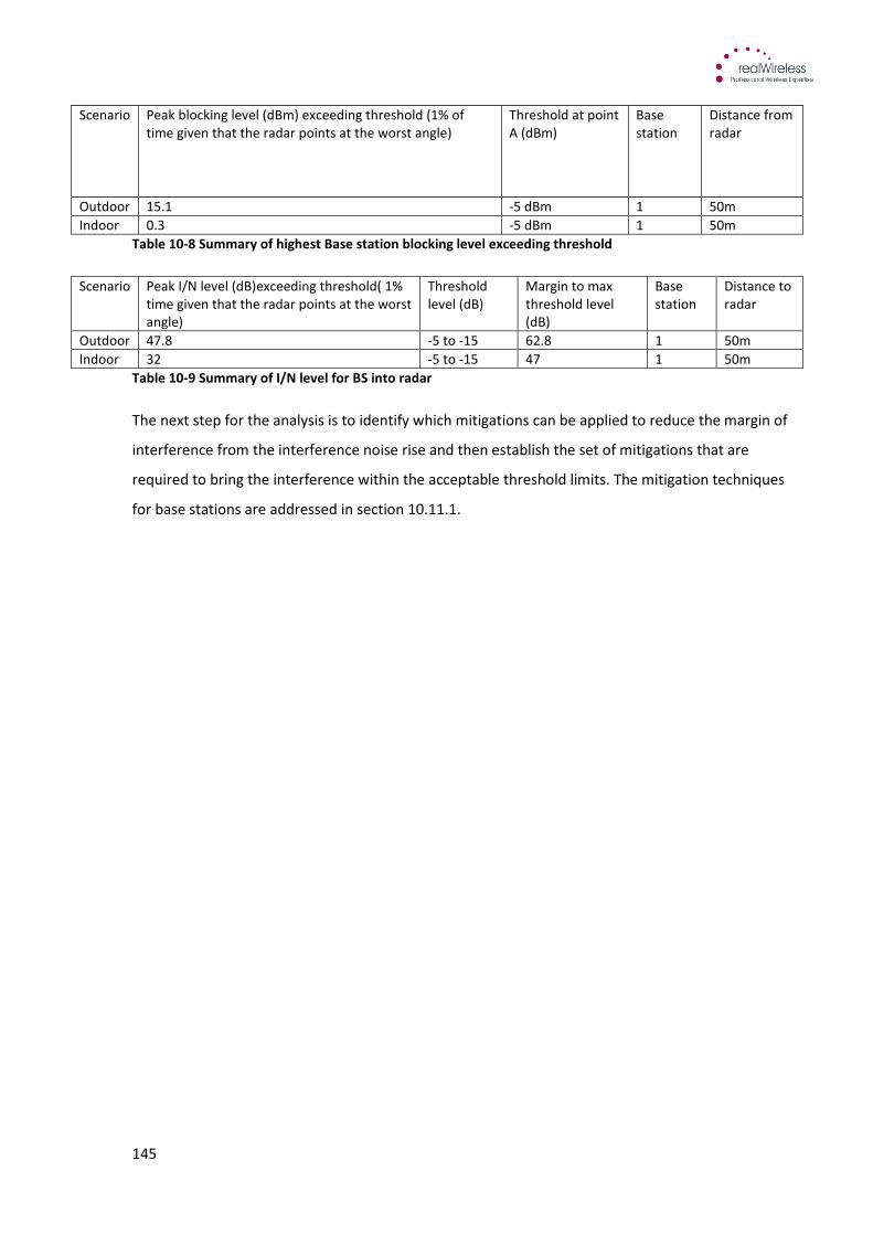
145
Scenario Peak blocking level (dBm) exceeding threshold (1% of
time given that the radar points at the worst angle)
Threshold at point
A (dBm)
Base
station
Distance from
radar
Outdoor 15.1 -5 dBm 1 50m
Indoor 0.3 -5 dBm 1 50m
Table 10-8 Summary of highest Base station blocking level exceeding threshold
Scenario Peak I/N level (dB)exceeding threshold( 1%
time given that the radar points at the worst
angle)
Threshold
level (dB)
Margin to max
threshold level
(dB)
Base
station
Distance to
radar
Outdoor 47.8 -5 to -15 62.8 1 50m
Indoor 32 -5 to -15 47 1 50m
Table 10-9 Summary of I/N level for BS into radar
The next step for the analysis is to identify which mitigations can be applied to reduce the margin of
interference from the interference noise rise and then establish the set of mitigations that are
required to bring the interference within the acceptable threshold limits. The mitigation techniques
for base stations are addressed in section 10.11.1.

146
10.6 Mobile station to radar – Single mobile station transmitter at variable
distance from the radar with challenging case conditions
The analysis of interference from a single mobile station into the radar was modelled by deploying a
single mobile station at 200 random locations (200 Monte Carlo iterations) for 5 different polygon
areas. The simulation calculates the interference as the radar antenna main beam sweeps past the
polygon area and is illuminated by the mobile at a particular angle from the radar in each location
per rotation.
The mobile station was assigned a single FDD uplink channel at 2560 MHz with a 20 MHz bandwidth.
The analysis determined the impact of decreasing the distance between the mobile station and the
radar to discuss the model results.
The main input parameters used for this investigation were challenging case conditions which can be
seen in the table below.
Parameter Value MS EIRP 23dBm/20 MHz
MS Power control Not active
MS antenna height 1.5 m
MS body loss 0 dB
MS spurious emissions -30 dBm/MHz (3GPP/IEEE)
Propagation model Free space loss + 6 dB, see Section 8.4.1
Radar height 5 m
Table 10-10 Challenging case parameter values for the mobile station
Figure 10-24 shows the different polygon areas that correspond to each position that were chosen
for the analysis. The aim of the investigation, similar to the initial investigation for the base station,
was to determine the increase of interference from the mobile as the distance was reduced towards
the radar. This was achieved by simulating random deployments of the mobile station in a range of
polygon areas at distances closer to the radar.

147
Mobile station position 1 (Polygon 15) Mobile station position 2 (Polygon 24)
Mobile station position 3 (Polygon 11) Mobile station position 4 (Polygon 9)
Mobile station position 5 (Polygon 5)
Figure 10-24 Polygon positions for mobile station investigation. Blue dots represent the mobile station
random location. See Table 6 for the distance of the polygon to the radar location.
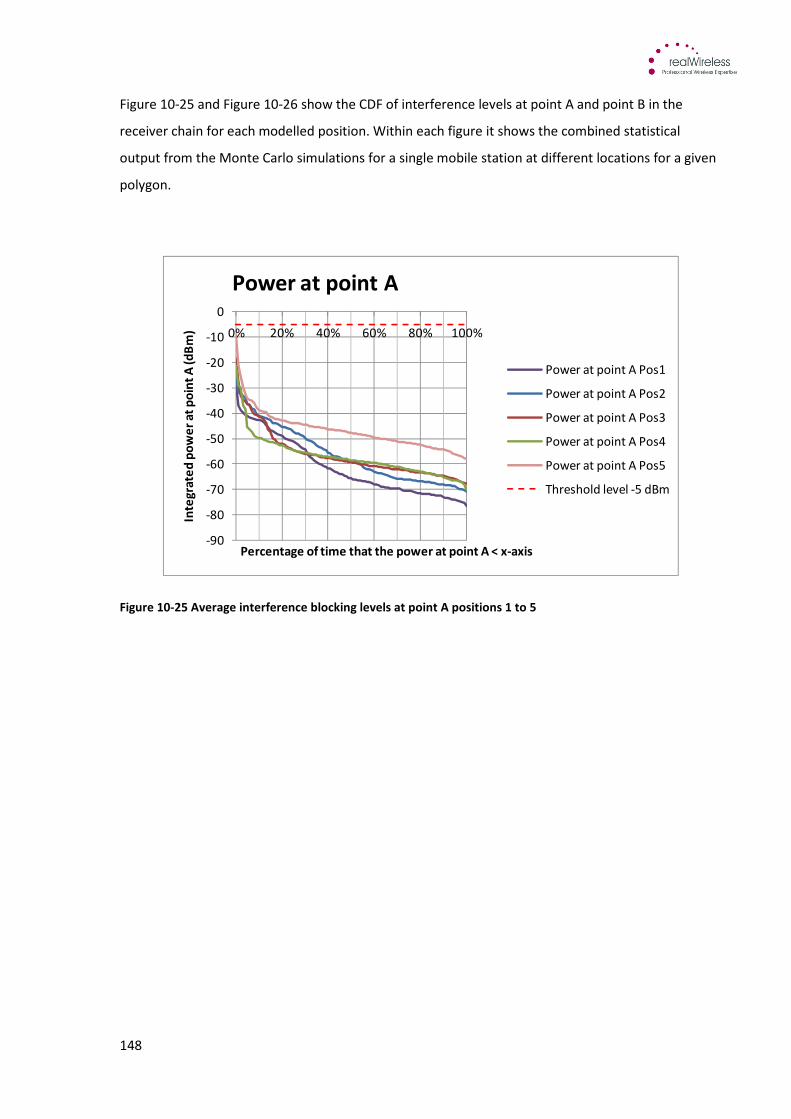
148
Figure 10-25 and Figure 10-26 show the CDF of interference levels at point A and point B in the
receiver chain for each modelled position. Within each figure it shows the combined statistical
output from the Monte Carlo simulations for a single mobile station at different locations for a given
polygon.
Figure 10-25 Average interference blocking levels at point A positions 1 to 5
-90
-80
-70
-60
-50
-40
-30
-20
-10
0
0% 20% 40% 60% 80% 100%
Inte
gra
ted
po
we
r a
t p
oin
t A
(d
Bm
)
Percentage of time that the power at point A < x-axis
Power at point A
Power at point A Pos1
Power at point A Pos2
Power at point A Pos3
Power at point A Pos4
Power at point A Pos5
Threshold level -5 dBm

149
Figure 10-26 Average interference blocking levels at point B positions 1 to 5
It can be seen from the results that blocking of the radar does not occur at any of the positions for
points A and B in the radar as the blocking threshold level is not exceeded at those points in the
receiver. Note that for percentages of time greater than 20%, there is a clear distinction between the
interference levels that are the result from the different mobile station polygons. This is in contrast
to percentages less than 20%, where the position that generates the highest levels of interference is
less consistent which is due to:
• Variability in the peak envelope power
• Variability due to shadowing
• In Position 4 the polygon area extends in a wide range of distances from the radar location
A steep rise in interference occurs for small percentages of time (<1% time) due to the variability in
the shadowing and the signal envelope power, and the radar receiver appears to be blocked for a
small fraction of time.
-120
-100
-80
-60
-40
-20
0
0% 20% 40% 60% 80% 100%
Inte
gra
ted
po
we
r a
t p
oin
t B
(d
Bm
)
Percentage of time that the power at point B < x-axis
Power at point B
Power at point B Pos1
Power at point B Pos2
Power at point B Pos3
Power at point B Pos4
Power at point B Pos5
Threshold level -42 dBm
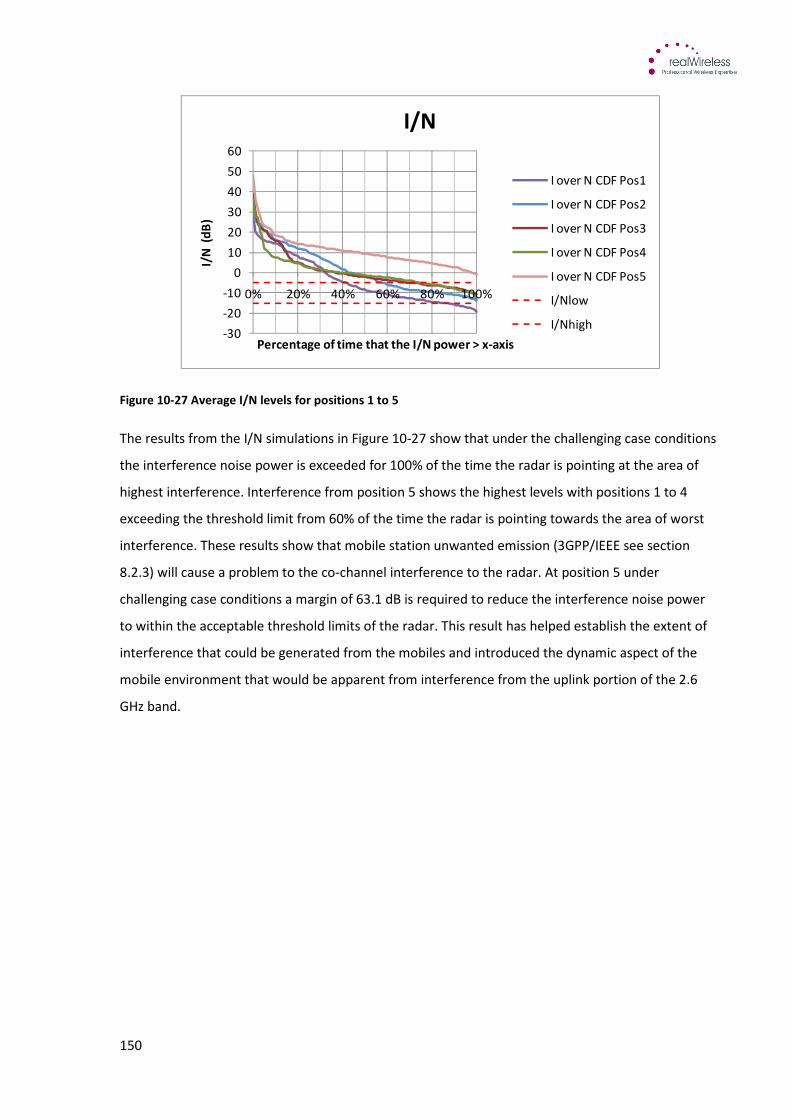
150
Figure 10-27 Average I/N levels for positions 1 to 5
The results from the I/N simulations in Figure 10-27 show that under the challenging case conditions
the interference noise power is exceeded for 100% of the time the radar is pointing at the area of
highest interference. Interference from position 5 shows the highest levels with positions 1 to 4
exceeding the threshold limit from 60% of the time the radar is pointing towards the area of worst
interference. These results show that mobile station unwanted emission (3GPP/IEEE see section
8.2.3) will cause a problem to the co-channel interference to the radar. At position 5 under
challenging case conditions a margin of 63.1 dB is required to reduce the interference noise power
to within the acceptable threshold limits of the radar. This result has helped establish the extent of
interference that could be generated from the mobiles and introduced the dynamic aspect of the
mobile environment that would be apparent from interference from the uplink portion of the 2.6
GHz band.
-30
-20
-10
0
10
20
30
40
50
60
0% 20% 40% 60% 80% 100%
I/N
(d
B)
Percentage of time that the I/N power > x-axis
I/N
I over N CDF Pos1
I over N CDF Pos2
I over N CDF Pos3
I over N CDF Pos4
I over N CDF Pos5
I/Nlow
I/Nhigh
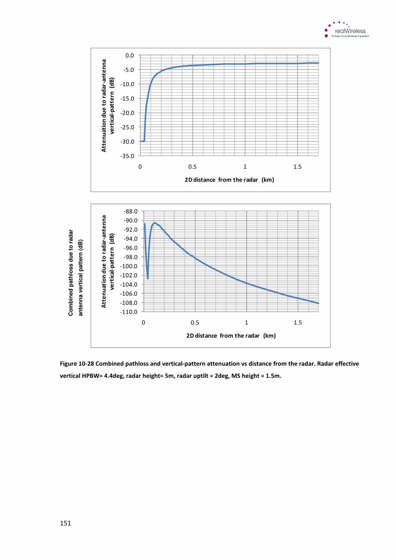
151
Figure 10-28 Combined pathloss and vertical-pattern attenuation vs distance from the radar. Radar effective
vertical HPBW= 4.4deg, radar height= 5m, radar uptilt = 2deg, MS height = 1.5m.
-35.0
-30.0
-25.0
-20.0
-15.0
-10.0
-5.0
0.0
0 0.5 1 1.5
Att
en
ua
tio
n d
ue
to
ra
da
r-a
nte
nn
a
ve
rtic
al-
pa
tte
rn
(dB
)
2D distance from the radar (km)
-110.0
-108.0
-106.0
-104.0
-102.0
-100.0
-98.0
-96.0
-94.0
-92.0
-90.0
-88.0
0 0.5 1 1.5
Att
en
ua
tio
n d
ue
to
ra
da
r-a
nte
nn
a
ve
rtic
al-
pa
tte
rn
(dB
)
2D distance from the radar (km)
Co
mb
ined
path
loss d
ue t
o r
ad
ar
an
ten
na v
ert
ical
patt
ern
(d
B)

152
10.7 Mobile station to radar – Challenging case
The mobile station to radar challenging case scenario aims to investigate the interference caused by
all the modelled mobile stations in the simulation area. The input parameters used for this scenario
have been selected to create severe interference conditions using challenging values. The main input
parameter values can be seen in Table 10-11.
Parameter Value MS max EIRP 23dBm
MS power control All mobiles at maximum power
MS location Outdoor
MS antenna height 1.5 m
MS body loss 0 dB
MS spurious emissions -30 dBm/MHz (3GPP/IEEE)
Number of mobiles 53 simultaneously active per iteration
BS channels All channels at 100% loading24
Propagation model Free space path loss+ 6 dB
Building penetration losses 0 dB (outdoor)
Shadowing standard deviation 8.3 dB
Radar height 5 m
Table 10-11 Challenging case parameters for mobile station
Figure 10-29 shows the blocking levels calculated at each point in the receiver chain, when the radar
was pointing at the angle of highest interference. Blocking of the radar does not occur when the
radar is pointing in the direction of highest interference. Note that the steep rise in the blocking level
occurs at percentages of time 10% and below.
The average blocking level at point A is -33.9 dBm which is 28.9 dB below the -5 dBm threshold limit
and thus blocking does not occur at this stage. The next stage in the receiver through which the
signal passes, is the RF filter stage. It can be seen that the RF filter attenuates the signal by just over
30 dB which brings the blocking level down below the threshold of input to sub-system 2. At point B
the level is -64 dBm for 1% time the radar points at the worst interference which still provides a 22
dB margin below the threshold. It can also be seen from Figure 10-29 the interference levels at
percentage time below 1% are well below the threshold at point B which means no blocking occurs.
24
The site locations 1 and 2 are sufficiently close together to justify the assumption that different mobile
network operators are operating in each site. Therefore sites 1 and 2 are partially loaded. The same was
assumed for sites 3 and 4.
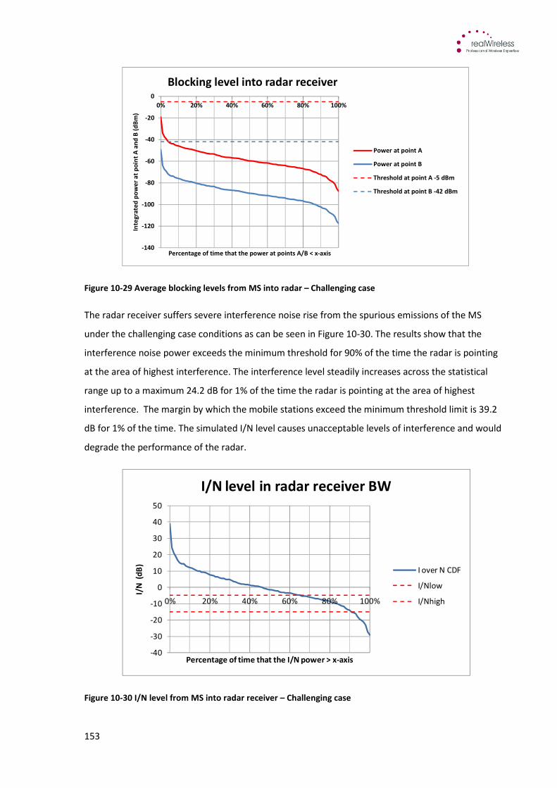
153
Figure 10-29 Average blocking levels from MS into radar – Challenging case
The radar receiver suffers severe interference noise rise from the spurious emissions of the MS
under the challenging case conditions as can be seen in Figure 10-30. The results show that the
interference noise power exceeds the minimum threshold for 90% of the time the radar is pointing
at the area of highest interference. The interference level steadily increases across the statistical
range up to a maximum 24.2 dB for 1% of the time the radar is pointing at the area of highest
interference. The margin by which the mobile stations exceed the minimum threshold limit is 39.2
dB for 1% of the time. The simulated I/N level causes unacceptable levels of interference and would
degrade the performance of the radar.
Figure 10-30 I/N level from MS into radar receiver – Challenging case
-140
-120
-100
-80
-60
-40
-20
0
0% 20% 40% 60% 80% 100%
Inte
gra
ted
po
we
r a
t p
oin
t A
an
d B
(d
Bm
)
Percentage of time that the power at points A/B < x-axis
Blocking level into radar receiver
Power at point A
Power at point B
Threshold at point A -5 dBm
Threshold at point B -42 dBm
-40
-30
-20
-10
0
10
20
30
40
50
0% 20% 40% 60% 80% 100%
I/N
(d
B)
Percentage of time that the I/N power > x-axis
I/N level in radar receiver BW
I over N CDF
I/Nlow
I/Nhigh
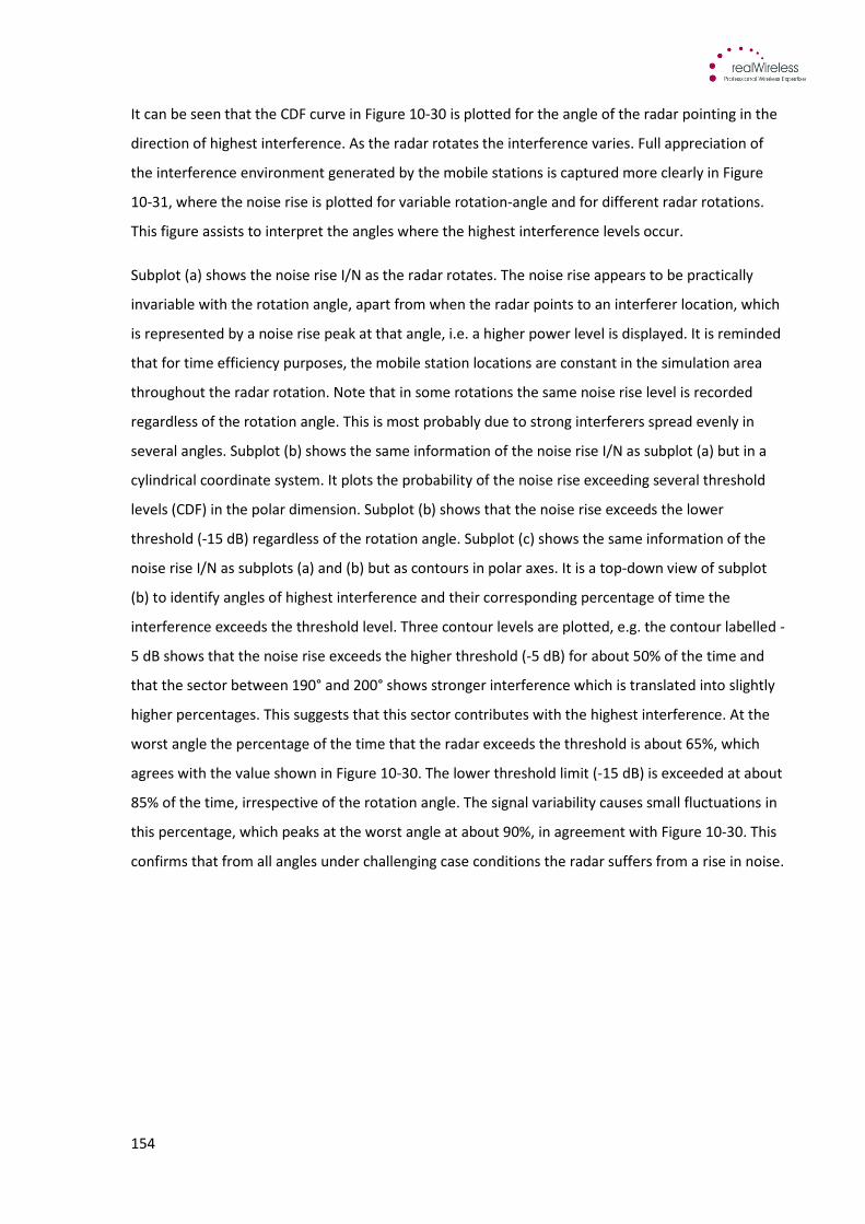
154
It can be seen that the CDF curve in Figure 10-30 is plotted for the angle of the radar pointing in the
direction of highest interference. As the radar rotates the interference varies. Full appreciation of
the interference environment generated by the mobile stations is captured more clearly in Figure
10-31, where the noise rise is plotted for variable rotation-angle and for different radar rotations.
This figure assists to interpret the angles where the highest interference levels occur.
Subplot (a) shows the noise rise I/N as the radar rotates. The noise rise appears to be practically
invariable with the rotation angle, apart from when the radar points to an interferer location, which
is represented by a noise rise peak at that angle, i.e. a higher power level is displayed. It is reminded
that for time efficiency purposes, the mobile station locations are constant in the simulation area
throughout the radar rotation. Note that in some rotations the same noise rise level is recorded
regardless of the rotation angle. This is most probably due to strong interferers spread evenly in
several angles. Subplot (b) shows the same information of the noise rise I/N as subplot (a) but in a
cylindrical coordinate system. It plots the probability of the noise rise exceeding several threshold
levels (CDF) in the polar dimension. Subplot (b) shows that the noise rise exceeds the lower
threshold (-15 dB) regardless of the rotation angle. Subplot (c) shows the same information of the
noise rise I/N as subplots (a) and (b) but as contours in polar axes. It is a top-down view of subplot
(b) to identify angles of highest interference and their corresponding percentage of time the
interference exceeds the threshold level. Three contour levels are plotted, e.g. the contour labelled -
5 dB shows that the noise rise exceeds the higher threshold (-5 dB) for about 50% of the time and
that the sector between 190° and 200° shows stronger interference which is translated into slightly
higher percentages. This suggests that this sector contributes with the highest interference. At the
worst angle the percentage of the time that the radar exceeds the threshold is about 65%, which
agrees with the value shown in Figure 10-30. The lower threshold limit (-15 dB) is exceeded at about
85% of the time, irrespective of the rotation angle. The signal variability causes small fluctuations in
this percentage, which peaks at the worst angle at about 90%, in agreement with Figure 10-30. This
confirms that from all angles under challenging case conditions the radar suffers from a rise in noise.
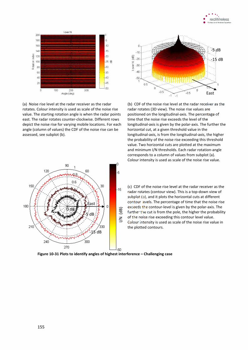
155
(a) Noise rise level at the radar receiver as the radar
rotates. Colour intensity is used as scale of the noise rise
value. The starting rotation angle is when the radar points
east. The radar rotates counter-clockwise. Different rows
depict the noise rise for varying mobile locations. For each
angle (column of values) the CDF of the noise rise can be
assessed, see subplot (b).
(b) CDF of the noise rise level at the radar receiver as the
radar rotates (3D view). The noise rise values are
positioned on the longitudinal-axis. The percentage of
time that the noise rise exceeds the level of the
longitudinal-axis is given by the polar-axis. The further the
horizontal cut, at a given threshold value in the
longitudinal-axis, is from the longitudinal-axis, the higher
the probability of the noise rise exceeding this threshold
value. Two horizontal cuts are plotted at the maximum
and minimum I/N thresholds. Each radar rotation-angle
corresponds to a column of values from subplot (a).
Colour intensity is used as scale of the noise rise value.
(c) CDF of the noise rise level at the radar receiver as the
radar rotates (contour view). This is a top-down view of
subplot (b), and it plots the horizontal cuts at different
contour levels. The percentage of time that the noise rise
exceeds the contour-level is given by the polar-axis. The
further the cut is from the pole, the higher the probability
of the noise rise exceeding this contour level value.
Colour intensity is used as scale of the noise rise value in
the plotted contours.
Figure 10-31 Plots to identify angles of highest interference – Challenging case
-15 dB
-5 dB
East
I/N
(d
B)
East
0 dB -5 dB
-15 dB
156
10.8 Mobile station to radar – Typical case
This section studies the interference from mobile stations to radar under typical case assumptions.
The input parameters used for this scenario have been selected to create a Heathrow-specific 2.6
GHz mobile deployment. The technical parameter values of the mobile stations are more realistic
when compared to the challenging case, see Table 10-12.
Parameter Value MS max EIRP 23dBm
MS power control Activated
MS location Outdoor and indoor
MS antenna height Variable according to the polygon
MS body loss 5 dB
MS spurious emissions -50 dBm/MHz (assumption for typical value)
Number of mobiles 53 simultaneously active per iteration
BS channels All channels at 80% loading25
Propagation model Given by the polygon to radar propagation
model
Building penetration losses 0 dB (outdoor), 14 dB (indoor)
Shadowing standard deviation 8.3 dB
Radar height 40 m
Table 10-12 Typical case parameters for mobile station
Figure 10-32 shows the average blocking levels calculated by the software model and it can be seen
from the plot that the blocking level at point A is below the first threshold level of -5 dBm for all
percentages of time under the typical case conditions. The blocking levels recorded at point A that
occur for 1% of the time the radar was pointing at the area of highest interference was -48.8 dBm
which is 43.8 dB below the first threshold level.
25
The site locations 1 and 2 are sufficiently close together to justify the assumption that different mobile
network operators are operating in each site. Therefore sites 1 and 2 are partially loaded. The same was
assumed for sites 3 and 4.

157
Figure 10-32 Average blocking from MS into radar - Typical case
The blocking levels recorded at point B shows increased attenuation as the signal passes through the
RF filter. These filters provide approximately 40 dB of rejection after the first RF filters thus
eliminating any blocking effects from the in band mobile emissions. This demonstrates no blocking
occurs in the radar from mobile station emissions under typical case conditions.
Figure 10-33 Average I/N levels from MS into radar - Typical case
Similar to the challenging case the results in Figure 10-33 for the I/N interference into the radar
receiver show interference noise power from the mobile stations exceeds the minimum threshold
-160
-140
-120
-100
-80
-60
-40
-20
0
0% 20% 40% 60% 80% 100%In
teg
rate
d p
ow
er
at
po
int
A a
nd
B (
dB
m)
Percentage of time that the power at point A/B < x-axis
Blocking levels into radar receiver
Power at point A
Power at point B
Threshold level at A -5 dBm
Threshold level at B -42 dBm
-60
-50
-40
-30
-20
-10
0
0% 20% 40% 60% 80% 100%
I/N
(d
B)
Percentage of time that the I/N > x-axis
I/N level in radar receiver BW
I over N CDF
I/Nlow
I/Nhigh
158
level at <3% of the time the radar is pointing at the area of highest interference. In this scenario it
was expected the resulting I/N level would be reduced compared to the challenging case I/N levels
due to the improvement to the simulation environment parameters; the I/N level recorded was -9.3
dB for 1% time the radar is pointing to the area of highest interference. This has been demonstrated
from the results. However, there is still a margin of 5.7 dB the level exceeds the threshold at 1% of
the time the radar is pointing at the area of highest interference. This indicates a requirement for
additional mitigations to be incorporated to reduce the 5.7 dB margin below the maximum threshold
limits of the radar receiver.
It can also be seen from the plot in Figure 10-33 for interference levels below 1% time there is up to
6 dB additional interference which therefore means up to 11.7 dB (maximum) may be required to
bring the excess interference below the threshold level for 0.01% of the time and below.
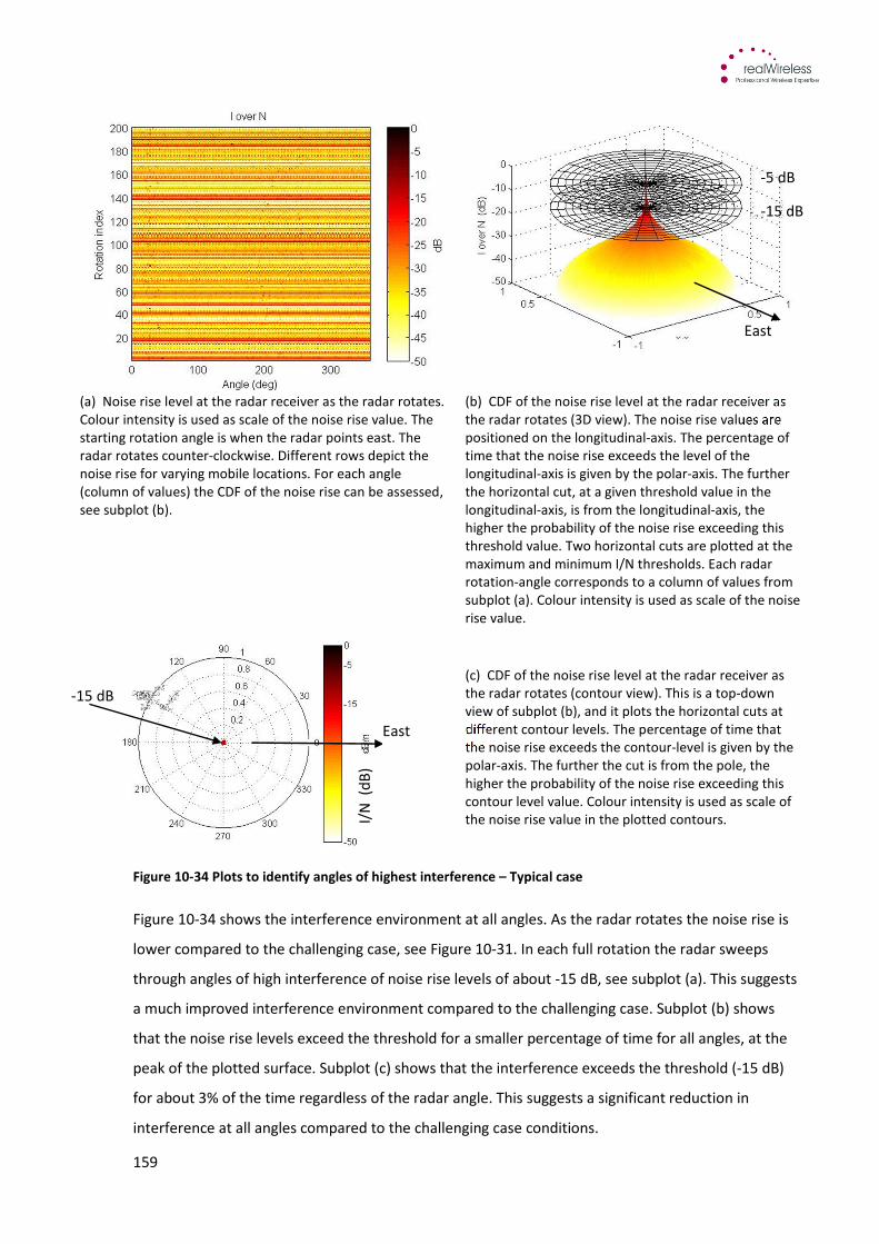
159
(a) Noise rise level at the radar receiver as the radar rotates.
Colour intensity is used as scale of the noise rise value. The
starting rotation angle is when the radar points east. The
radar rotates counter-clockwise. Different rows depict the
noise rise for varying mobile locations. For each angle
(column of values) the CDF of the noise rise can be assessed,
see subplot (b).
(b) CDF of the noise rise level at the radar receiver as
the radar rotates (3D view). The noise rise values are
positioned on the longitudinal-axis. The percentage of
time that the noise rise exceeds the level of the
longitudinal-axis is given by the polar-axis. The further
the horizontal cut, at a given threshold value in the
longitudinal-axis, is from the longitudinal-axis, the
higher the probability of the noise rise exceeding this
threshold value. Two horizontal cuts are plotted at the
maximum and minimum I/N thresholds. Each radar
rotation-angle corresponds to a column of values from
subplot (a). Colour intensity is used as scale of the noise
rise value.
(c) CDF of the noise rise level at the radar receiver as
the radar rotates (contour view). This is a top-down
view of subplot (b), and it plots the horizontal cuts at
different contour levels. The percentage of time that
the noise rise exceeds the contour-level is given by the
polar-axis. The further the cut is from the pole, the
higher the probability of the noise rise exceeding this
contour level value. Colour intensity is used as scale of
the noise rise value in the plotted contours.
Figure 10-34 Plots to identify angles of highest interference – Typical case
Figure 10-34 shows the interference environment at all angles. As the radar rotates the noise rise is
lower compared to the challenging case, see Figure 10-31. In each full rotation the radar sweeps
through angles of high interference of noise rise levels of about -15 dB, see subplot (a). This suggests
a much improved interference environment compared to the challenging case. Subplot (b) shows
that the noise rise levels exceed the threshold for a smaller percentage of time for all angles, at the
peak of the plotted surface. Subplot (c) shows that the interference exceeds the threshold (-15 dB)
for about 3% of the time regardless of the radar angle. This suggests a significant reduction in
interference at all angles compared to the challenging case conditions.
-15 dB
-5 dB
East
I/N
(d
B)
East
-15 dB
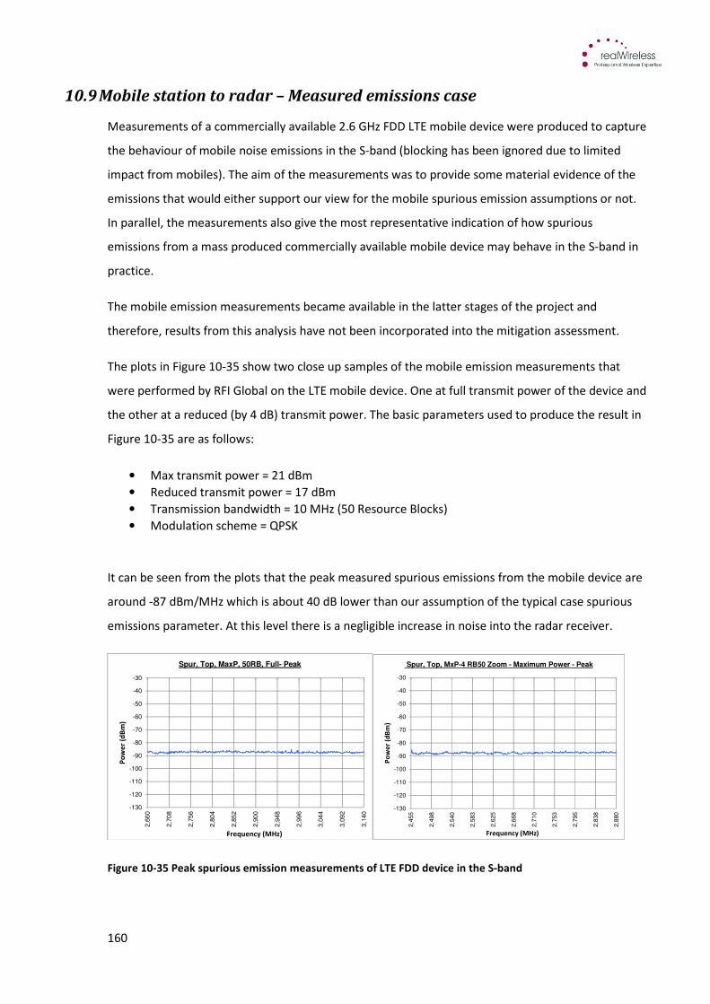
160
10.9 Mobile station to radar – Measured emissions case
Measurements of a commercially available 2.6 GHz FDD LTE mobile device were produced to capture
the behaviour of mobile noise emissions in the S-band (blocking has been ignored due to limited
impact from mobiles). The aim of the measurements was to provide some material evidence of the
emissions that would either support our view for the mobile spurious emission assumptions or not.
In parallel, the measurements also give the most representative indication of how spurious
emissions from a mass produced commercially available mobile device may behave in the S-band in
practice.
The mobile emission measurements became available in the latter stages of the project and
therefore, results from this analysis have not been incorporated into the mitigation assessment.
The plots in Figure 10-35 show two close up samples of the mobile emission measurements that
were performed by RFI Global on the LTE mobile device. One at full transmit power of the device and
the other at a reduced (by 4 dB) transmit power. The basic parameters used to produce the result in
Figure 10-35 are as follows:
• Max transmit power = 21 dBm
• Reduced transmit power = 17 dBm
• Transmission bandwidth = 10 MHz (50 Resource Blocks)
• Modulation scheme = QPSK
It can be seen from the plots that the peak measured spurious emissions from the mobile device are
around -87 dBm/MHz which is about 40 dB lower than our assumption of the typical case spurious
emissions parameter. At this level there is a negligible increase in noise into the radar receiver.
Figure 10-35 Peak spurious emission measurements of LTE FDD device in the S-band
-130
-120
-110
-100
-90
-80
-70
-60
-50
-40
-30
2,6
60
2,7
08
2,7
56
2,8
04
2,8
52
2,9
00
2,9
48
2,9
96
3,0
44
3,0
92
3,1
40
Po
we
r (d
Bm
)
Frequency (MHz)
Spur, Top, MaxP, 50RB, Full- Peak
-130
-120
-110
-100
-90
-80
-70
-60
-50
-40
-30
2,4
55
2,4
98
2,5
40
2,5
83
2,6
25
2,6
68
2,7
10
2,7
53
2,7
95
2,8
38
2,8
80
Po
we
r (d
Bm
)
Frequency (MHz)
Spur, Top, MxP-4 RB50 Zoom - Maximum Power - Peak
161
The spurious emission levels between the two plots are practically the same but for different in-band
power levels (4dB difference) indicating no correlation between in-band power and spurious
emissions of the particular device. The shape of the emissions plot is generally flat with many very
small peaks but there is no sign of a discrete spurious occurring within this measurement. Therefore,
using the measurement plot data we imposed a discrete spurious occurring on the centre frequency
of the radar receiver into our model, to capture any effects from the likelihood of it appearing.
10.9.1 Assumptionsfordiscretespurious
The lowest measured level of -89 dBm/MHz was set as the reference and from this level we
increased the amplitude of the discrete spurious from 0 dB to 50 dB in 10 dB increments since we
did not anticipate significant change in the output with smaller levels. We then increased the
amplitude from 50 dB to 59 dB in 1 dB increments because these levels are approaching the 3GPP
specification limit and could potentially be a level that exceeds the threshold. The model treats the
spurious as if it was a function of the in band channel power of the mobile and therefore only occurs
on a specific frequency (2560 MHz) with a 20 MHz bandwidth. However, the amplitude of the
discrete spurious does not vary with power control due to the limited fluctuation in noise from any
change in in-band power. Furthermore, the bandwidth of the discrete spurious is twice the
bandwidth of the transmission of the mobile if we assume it is in an image of the mobile centre
frequency.
We also assumed that the discrete spurious would not occur on all mobiles from all base stations
and the following list of base stations were used in the model to serve the mobiles which produced
the discrete spurious. Refer to Figure 10-6 for the position with respect to radar in each case.
• BS6
• BS10
• BS11
• BS13
These base stations were chosen randomly based on the mix of distances from the radar with those
in close proximity likely to cause more interference than those further away. (Note BS7, BS8 and BS9
are indoor and serve indoor mobiles which are unlikely to be of sufficient power to cause a problem)
10.9.2 Resultsfrommodellingdiscretespuriousemissions
The results were generated using parameters from the typical case, the only change in parameters
were the, radar height (increased to 40m) spurious emission levels and discrete spurious. Table
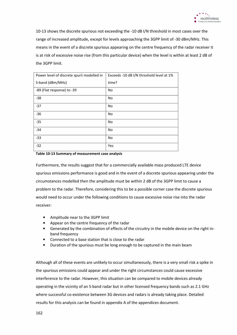
162
10-13 shows the discrete spurious not exceeding the -10 dB I/N threshold in most cases over the
range of increased amplitude, except for levels approaching the 3GPP limit of -30 dBm/MHz. This
means in the event of a discrete spurious appearing on the centre frequency of the radar receiver it
is at risk of excessive noise rise (from this particular device) when the level is within at least 2 dB of
the 3GPP limit.
Power level of discrete spurii modelled in
S-band (dBm/MHz)
Exceeds -10 dB I/N threshold level at 1%
time?
-89 (Flat response) to -39 No
-38 No
-37 No
-36 No
-35 No
-34 No
-33 No
-32 Yes
Table 10-13 Summary of measurement case analysis
Furthermore, the results suggest that for a commercially available mass produced LTE device
spurious emissions performance is good and in the event of a discrete spurious appearing under the
circumstances modelled then the amplitude must be within 2 dB of the 3GPP limit to cause a
problem to the radar. Therefore, considering this to be a possible corner case the discrete spurious
would need to occur under the following conditions to cause excessive noise rise into the radar
receiver:
• Amplitude near to the 3GPP limit
• Appear on the centre frequency of the radar
• Generated by the combination of effects of the circuitry in the mobile device on the right in-
band frequency
• Connected to a base station that is close to the radar
• Duration of the spurious must be long enough to be captured in the main beam
Although all of these events are unlikely to occur simultaneously, there is a very small risk a spike in
the spurious emissions could appear and under the right circumstances could cause excessive
interference to the radar. However, this situation can be compared to mobile devices already
operating in the vicinity of an S-band radar but in other licensed frequency bands such as 2.1 GHz
where successful co-existence between 3G devices and radars is already taking place. Detailed
results for this analysis can be found in appendix A of the appendices document.
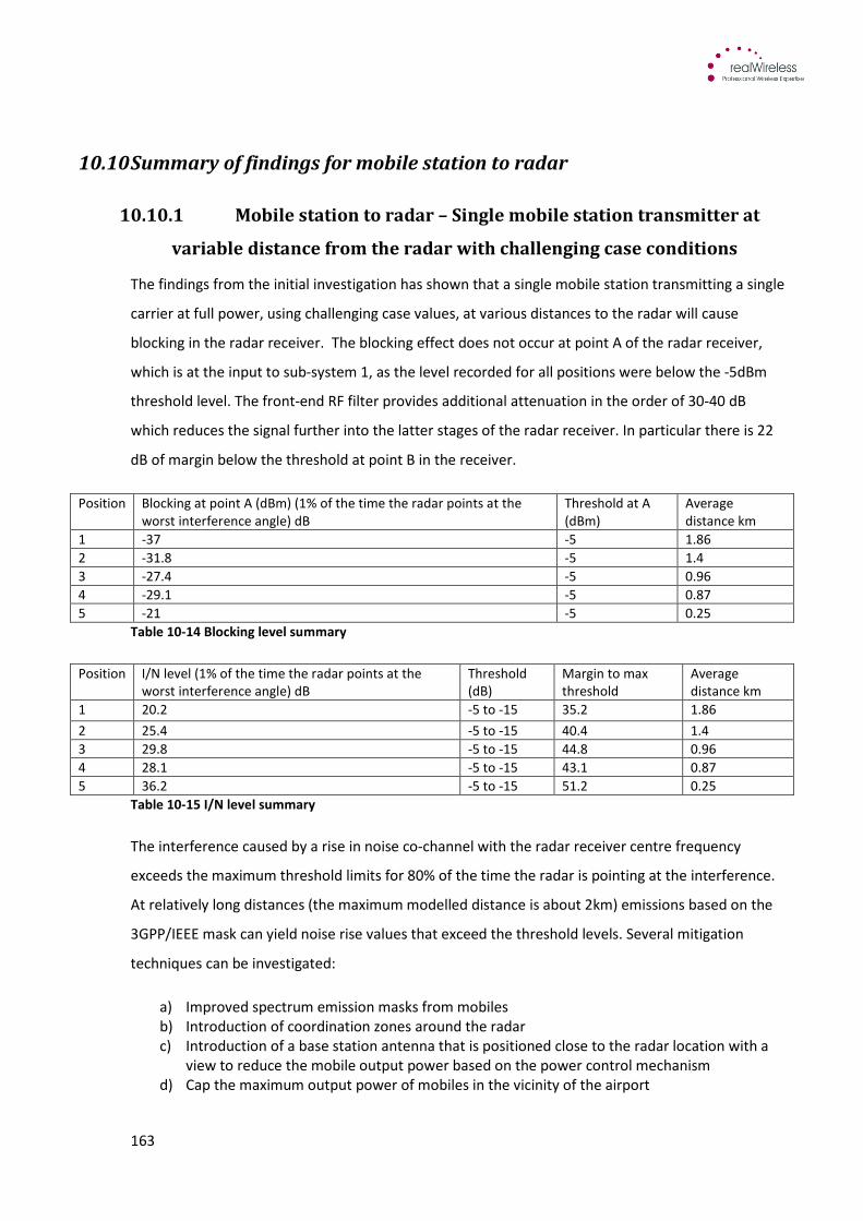
163
10.10 Summary of findings for mobile station to radar
10.10.1 Mobilestationtoradar–Singlemobilestationtransmitterat
variabledistancefromtheradarwithchallengingcaseconditions
The findings from the initial investigation has shown that a single mobile station transmitting a single
carrier at full power, using challenging case values, at various distances to the radar will cause
blocking in the radar receiver. The blocking effect does not occur at point A of the radar receiver,
which is at the input to sub-system 1, as the level recorded for all positions were below the -5dBm
threshold level. The front-end RF filter provides additional attenuation in the order of 30-40 dB
which reduces the signal further into the latter stages of the radar receiver. In particular there is 22
dB of margin below the threshold at point B in the receiver.
Position Blocking at point A (dBm) (1% of the time the radar points at the
worst interference angle) dB
Threshold at A
(dBm)
Average
distance km
1 -37 -5 1.86
2 -31.8 -5 1.4
3 -27.4 -5 0.96
4 -29.1 -5 0.87
5 -21 -5 0.25
Table 10-14 Blocking level summary
Position I/N level (1% of the time the radar points at the
worst interference angle) dB
Threshold
(dB)
Margin to max
threshold
Average
distance km
1 20.2 -5 to -15 35.2 1.86
2 25.4 -5 to -15 40.4 1.4
3 29.8 -5 to -15 44.8 0.96
4 28.1 -5 to -15 43.1 0.87
5 36.2 -5 to -15 51.2 0.25
Table 10-15 I/N level summary
The interference caused by a rise in noise co-channel with the radar receiver centre frequency
exceeds the maximum threshold limits for 80% of the time the radar is pointing at the interference.
At relatively long distances (the maximum modelled distance is about 2km) emissions based on the
3GPP/IEEE mask can yield noise rise values that exceed the threshold levels. Several mitigation
techniques can be investigated:
a) Improved spectrum emission masks from mobiles
b) Introduction of coordination zones around the radar
c) Introduction of a base station antenna that is positioned close to the radar location with a
view to reduce the mobile output power based on the power control mechanism
d) Cap the maximum output power of mobiles in the vicinity of the airport
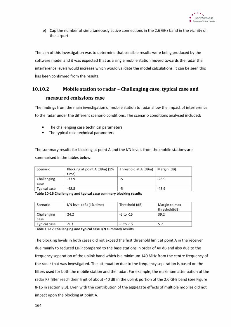
164
e) Cap the number of simultaneously active connections in the 2.6 GHz band in the vicinity of
the airport
The aim of this investigation was to determine that sensible results were being produced by the
software model and it was expected that as a single mobile station moved towards the radar the
interference levels would increase which would validate the model calculations. It can be seen this
has been confirmed from the results.
10.10.2 Mobilestationtoradar–Challengingcase,typicalcaseand
measuredemissionscase
The findings from the main investigation of mobile station to radar show the impact of interference
to the radar under the different scenario conditions. The scenario conditions analysed included:
• The challenging case technical parameters
• The typical case technical parameters
The summary results for blocking at point A and the I/N levels from the mobile stations are
summarised in the tables below:
Scenario Blocking at point A (dBm) (1%
time)
Threshold at A (dBm) Margin (dB)
Challenging
case
-33.9 -5 -28.9
Typical case -48.8 -5 -43.9
Table 10-16 Challenging and typical case summary blocking results
Scenario I/N level (dB) (1% time) Threshold (dB) Margin to max
threshold(dB)
Challenging
case
24.2 -5 to -15 39.2
Typical case -9.3 -5 to -15 5.7
Table 10-17 Challenging and typical case I/N summary results
The blocking levels in both cases did not exceed the first threshold limit at point A in the receiver
due mainly to reduced EIRP compared to the base stations in order of 40 dB and also due to the
frequency separation of the uplink band which is a minimum 140 MHz from the centre frequency of
the radar that was investigated. The attenuation due to the frequency separation is based on the
filters used for both the mobile station and the radar. For example, the maximum attenuation of the
radar RF filter reach their limit of about -40 dB in the uplink portion of the 2.6 GHz band (see Figure
8-16 in section 8.3). Even with the contribution of the aggregate effects of multiple mobiles did not
impact upon the blocking at point A.
165
In the challenging case scenario the noise rise from the mobile stations exceeded the threshold for
more than 97% of the time that the radar was pointing at the highest interference angle. In other
words the radar noise rise exceeds the threshold at least once in every rotation, with a probability of
97%. The noise rise level recorded for 1% of the time the radar was pointing at the area of highest
interference was 24.2dB, which exceeds the lower threshold (-15 dB) by 39.2 dB. It is this margin
which requires further analysis in order to reduce the interference level to below the threshold limit
so that no degradation to the radar performance occurs.
This challenging case results were produced based on the out-of-band and spurious emission mask
set to the minimum specified levels (-30 dBm/MHz) from the equipment standards. This means
mobile equipment built to operate up to the specification limits with little improvement to the filter
components could cause a problem with a rise in noise to S-band radars within an airport
environment. It was expected under typical case conditions the interference levels would be
reduced below the threshold limits for both interfering mechanisms and occur at levels either below
or much closer to the threshold limits.
The improvement to the interference for both mechanisms was demonstrated under typical case
conditions and described in more detail below. The analysis required changes to the main parameter
settings for both the mobile station and the radar. For example settings such as the activation of
power control, improvement to the OOB/spurious emission mask and increase to the radar height
were made to represent a more realistic Heathrow-specific scenario.
The findings from the analysis under typical case conditions showed a 15 dB improvement to the
blocking level and a 33.5 dB improvement to the interference noise power. The problems identified
for blocking under the challenging case conditions were eliminated in this scenario. In addition a
major contributor to the improvement to the interference noise power was due to the 20 dB
reduction below the challenging case limits of the OOB and spurious mask. This was further
improved when implementing the measured emission levels and increasing the radar height to 40m.
The outcome showing no impact from 2.6 GHz mobiles for both blocking and noise rise in a
Heathrow airport environment.
The combined analyses are put into perspective based on the rationale listed below which describes
a number of contributing factors that must be considered for such a reduction in interfering signal to
occur at the radar receiver:
1. Uplink power control – The mobiles adjust their EIRP in accordance to the path loss to
their serving base station. Thus a base station close to the radar location would result in
reduced output power for its connected mobiles.

166
2. Use of noise estimated/measured spectrum emission mask – The roll-off of spurious
emissions once in the radar band is significant to the order of 50 dB. Therefore the
margin of 20 dB below the 3GPP specification assumed for the typical case was
conservative. The reduction in unwanted emissions had a significant impact to the I/N
levels recorded and meant the noise occurred well below the acceptable threshold
limits.
3. Increased radar height – Increasing the radar height has the effect of limiting the
opportunity of interference to be captured in the main beam of the radar. As the height
increases so does the clearance distance between the main beam and the ground.
4. Body loss – The impact of the body loss can be the difference between exceeding the
threshold of interference or not. Usage of handsets and other mobile devices will be
subject to body loss due to the user obstructing the path between the mobile station
and the radar, and in this case contributed a small effect to the overall interference
level.
The impact of the interference from mobile stations under typical case conditions does not cause a
problem to the radar from a blocking perspective but did exceed the maximum threshold for the
noise rise using assumed spurious emission level. It is therefore necessary to identify the source of
interference in order to address the reduction of interference and apply the mitigations. This can be
done by using the polar plots shown in Figure 10-31 and Figure 10-34 (c) to identify the angles of the
highest levels of interference and the origin area. The polar plots show that the worst interference is
coming mainly from all angles, see Figure 10-36, which is suggestive of high interference arising from
locations very close to the radar. A small increase in the interference levels is identified when the
radar points at the terminal or the airport perimeter roads.
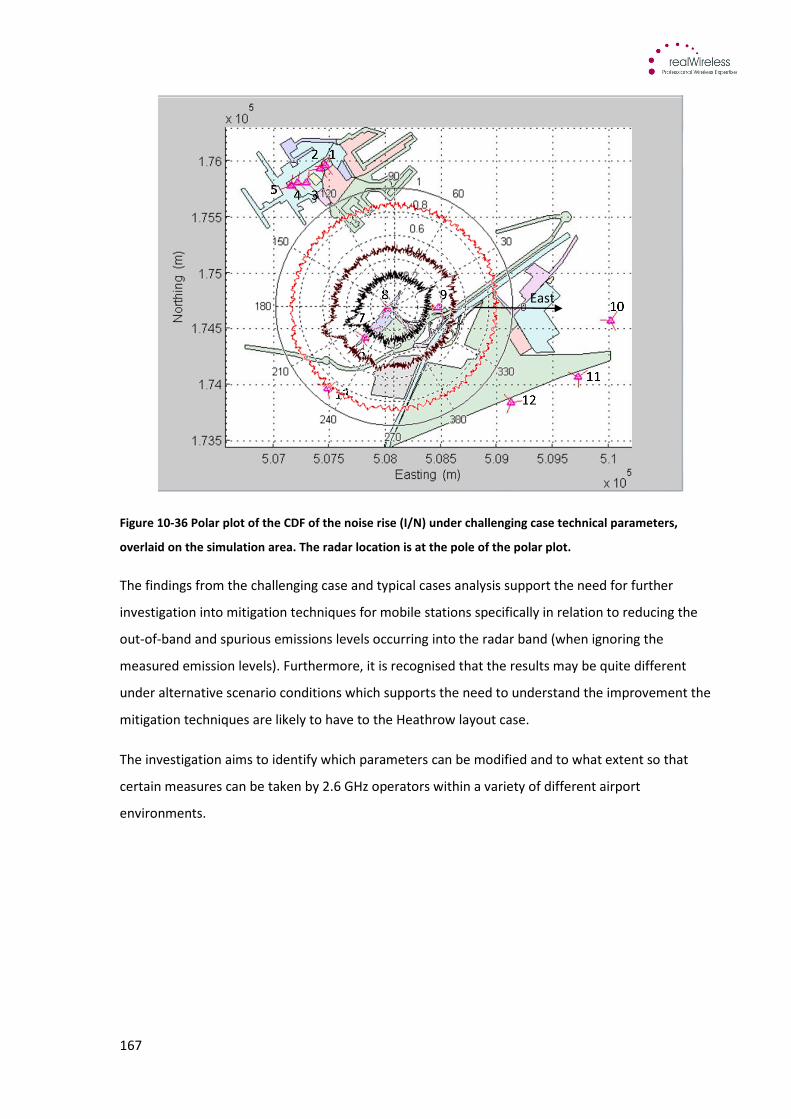
167
Figure 10-36 Polar plot of the CDF of the noise rise (I/N) under challenging case technical parameters,
overlaid on the simulation area. The radar location is at the pole of the polar plot.
The findings from the challenging case and typical cases analysis support the need for further
investigation into mitigation techniques for mobile stations specifically in relation to reducing the
out-of-band and spurious emissions levels occurring into the radar band (when ignoring the
measured emission levels). Furthermore, it is recognised that the results may be quite different
under alternative scenario conditions which supports the need to understand the improvement the
mitigation techniques are likely to have to the Heathrow layout case.
The investigation aims to identify which parameters can be modified and to what extent so that
certain measures can be taken by 2.6 GHz operators within a variety of different airport
environments.
East
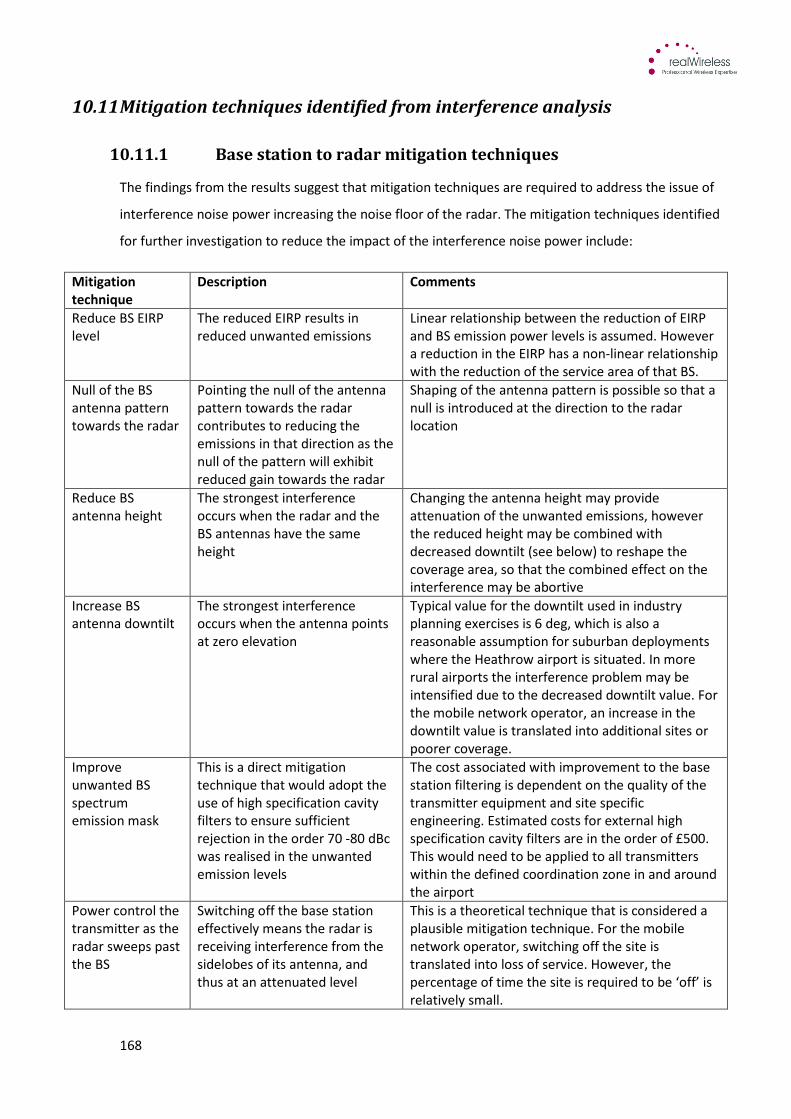
168
10.11 Mitigation techniques identified from interference analysis
10.11.1 Basestationtoradarmitigationtechniques
The findings from the results suggest that mitigation techniques are required to address the issue of
interference noise power increasing the noise floor of the radar. The mitigation techniques identified
for further investigation to reduce the impact of the interference noise power include:
Mitigation
technique
Description Comments
Reduce BS EIRP
level
The reduced EIRP results in
reduced unwanted emissions
Linear relationship between the reduction of EIRP
and BS emission power levels is assumed. However
a reduction in the EIRP has a non-linear relationship
with the reduction of the service area of that BS.
Null of the BS
antenna pattern
towards the radar
Pointing the null of the antenna
pattern towards the radar
contributes to reducing the
emissions in that direction as the
null of the pattern will exhibit
reduced gain towards the radar
Shaping of the antenna pattern is possible so that a
null is introduced at the direction to the radar
location
Reduce BS
antenna height
The strongest interference
occurs when the radar and the
BS antennas have the same
height
Changing the antenna height may provide
attenuation of the unwanted emissions, however
the reduced height may be combined with
decreased downtilt (see below) to reshape the
coverage area, so that the combined effect on the
interference may be abortive
Increase BS
antenna downtilt
The strongest interference
occurs when the antenna points
at zero elevation
Typical value for the downtilt used in industry
planning exercises is 6 deg, which is also a
reasonable assumption for suburban deployments
where the Heathrow airport is situated. In more
rural airports the interference problem may be
intensified due to the decreased downtilt value. For
the mobile network operator, an increase in the
downtilt value is translated into additional sites or
poorer coverage.
Improve
unwanted BS
spectrum
emission mask
This is a direct mitigation
technique that would adopt the
use of high specification cavity
filters to ensure sufficient
rejection in the order 70 -80 dBc
was realised in the unwanted
emission levels
The cost associated with improvement to the base
station filtering is dependent on the quality of the
transmitter equipment and site specific
engineering. Estimated costs for external high
specification cavity filters are in the order of £500.
This would need to be applied to all transmitters
within the defined coordination zone in and around
the airport
Power control the
transmitter as the
radar sweeps past
the BS
Switching off the base station
effectively means the radar is
receiving interference from the
sidelobes of its antenna, and
thus at an attenuated level
This is a theoretical technique that is considered a
plausible mitigation technique. For the mobile
network operator, switching off the site is
translated into loss of service. However, the
percentage of time the site is required to be ‘off’ is
relatively small.
169
Coordination zone
for BSs
The coordination zone is an area
around the radar, e.g. a disc
where BSs are not allowed to be
deployed
For the mobile network operator, a coordination
zone may interfere with the optimisation of the
network and in proving additional capacity for the
passenger users. For a 2.6 GHz -only network, the
coordination zone may result in a high loss of
revenue.
Table 10-18 Summary of mitigation techniques for base stations
It is acknowledged that the application of the mitigation techniques to the base station will also
cause a certain amount of degradation in performance to the 2.6 GHz networks. The types of impact
this could cause to network operations include:
i. A reduction in the downlink coverage area from base stations
ii. Limit the availability or number of resources available to network users
iii. Limit the throughput available on the downlink
iv. Reduction in Quality of Service such as Guaranteed Bit Rate
v. Potentially de-value the spectrum around airports
The values identified for each of the mitigation techniques are adjusted to the most practical yet
appropriate level possible with the aim of minimising the impact caused to the deployment of the
network. Furthermore, this approach will help minimise cost per base station to the essential
components which would likely include the addition of a cavity filter.
10.11.2 Mobilestationtoradarmitigationtechniques
The analysis of the mobile station interference into a radar receiver has found there is no
requirement for additional mitigation techniques to be applied in order to reduce blocking under the
typical case scenario investigated. However it might be the case for other deployment scenarios that
mobile stations cause blocking or more likely cause interference noise power increase that does
exceed the threshold levels of the radar under different scenario conditions.
The mitigation techniques that have been considered are listed below:
Mitigation
technique
Description Comments
Reduce MS
maximum EIRP
level
Limit maximum EIRP level to 20
dBm
Linear relationship between the reduction of EIRP
and MS emission power levels is assumed. However
a reduction in the EIRP has a non-linear relationship
with the reduction of throughput and/or quality of
service. Especially for high power mobiles, which
are at the cell edge, reduction of power may lead to
dropped calls and coverage holes.

170
Improve MS
unwanted
spectrum
emission mask
This is a direct mitigation
technique that would require the
adoption of improved ceramic
filtering within the mobile device
to ensure sufficient rejection in the
order 70 -80 dBc into the radar
band
There is little published evidence of spurious
emissions performance for different device types
into the S-band. Mobile devices are already
entering the market and understanding their
spurious emissions performance is critical for the
deployment of mobiles at airports.
Coordination
zone for MSs
The coordination zone is an area
around the radar, e.g. a disc where
MSs are not allowed to be on the
2.6 GHz band
This may be achievable by careful planning from
the mobile network operator so that the signal level
is below the handover threshold when the MS is
within the predefined coordination zone. A signal
jammer may also be deployed to shape the
coordination zone. For a 2.6 GHz -only network, the
coordination zone may result in a high loss of
revenue.
Additional BS Introduce an additional site or
coupled antenna close to areas of
high interferers to minimise the
output power of the mobile via the
power control mechanism
The mitigation of introducing additional sites may
be difficult in practice, because of potential
saturation in the site locations. Further, the
reduction in power levels is rather local, and the
number of new sites that are required to lower the
emissions may be large. Introduction of coupled
antennas does not contribute to additional
capacity, so that transmission takes place in a small
quantity of spectrum with a high power.
Cap the
maximum
number of 2.6
GHz users
Cap the maximum number of
simultaneously active connections
in the vicinity of the airport
At the cell-edges there are clusters of high emitting
users that are captured within the main horizontal
beam as the radar rotates. In more rural airports,
compared to Heathrow, the number of active
connections will be reduced, compared to the
simulation value, which provides an inherent
mitigation to the interference problem. This
mitigation may require further analysis on its
applicability, taking into account the complex
resource allocation mechanisms in LTE and WiMAX.
Table 10-19 Summary of mitigation techniques for mobile stations
The values to be used for each of the mitigation techniques should be adjusted to the most practical
yet appropriate level possible. However, it has been recognised that adjustments to the mobile
station technical parameters or to the uplink can impact upon the performance of the 2.6 GHz
network. For example, limiting the EIRP of the mobile station will reduce the throughput per mobile
which may cause a noticeable reduction in performance. In addition there is a limit to the
adjustments that can be made to mass produced equipment such as mobiles, built to a standardised
specification. Therefore, e.g. improvement in the spectrum emissions mask may in practice be
difficult to implement as national interface requirements may stipulate tighter limits on the masks
would usually be developed at a regional or International level. This analysis considered all
171
mitigations listed above and therefore it was expected each one to contribute some reduction to the
interference levels in close proximity to the radar.

172
11 Interferencemodellingresultswithmitigations
11.1 Discussion of mitigation approaches
The mitigation techniques identified for further investigation are analysed in this section. The
mitigation techniques were derived from Section 10 based on the analysis of interference from a
challenging case and typical case perspective for both the base- and the mobile-stations. The
analysis highlighted the particular parameters that could be adjusted further and improve the
interference environment so that the noise rise is reduced to levels within the acceptable threshold
limits of the radar receiver. In addition to that, resolving the noise rise problem ascertains resolution
to blocking problems at the various stages of the receiver chain for both base- and mobile-stations.
The aim of introducing the mitigation techniques was to establish that even under specific
deployment conditions the variety of scenarios will vary widely. Using the Heathrow Airport as one
example demonstrates how under typical case conditions for the specific deployment environment
greatly minimises the potential for interference from blocking and interference noise power.
However, these conditions may not apply under different deployment circumstances, therefore the
mitigations offer a set of generic parameters that can be modified further for different deployment
conditions.
Reducing the interference into the radar receiver comes at a cost to the deployment of 2.6 GHz
networks. The cost implications arise from making adjustments to the network parameters to satisfy
an additional (mobile operator exclusive) requirement. The introduction of mitigation techniques
could have the following impact on 2.6 GHz network deployments:
• Additional CAPEX and OPEX per base station to the deployment of 2.6 GHz networks in and
around airports
• Further engineering complexity required to manage the interference situation
• Introduction of new approval processes required for 2.6 GHz network equipment to be
implemented by the airport authority
The mitigation techniques that were identified for both the base- and the mobile-stations in section
10 are shown in Table 11-1 and Table 11-2.
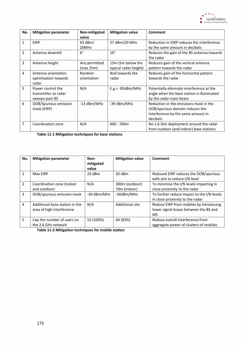
173
No. Mitigation parameter Non-mitigated
value
Mitigation value Comment
1 EIRP 63 dBm/
20MHz
57 dBm/20 MHz Reduction in EIRP reduces the interference
by the same amount in decibels
2 Antenna downtilt 6° 10° Reduces the gain of the BS antenna towards
the radar
3 Antenna height Any permitted
(max 25m)
15m (5m below the
typical radar height)
Reduces gain of the vertical antenna
pattern towards the radar
4 Antenna orientation
optimisation towards
radar
Random
orientation
Null towards the
radar
Reduces gain of the horizontal pattern
towards the radar
5 Power control the
transmitter as radar
sweeps past BS
N/A E.g.< -85dBm/MHz Potentially eliminate interference at the
angle when the base station is illuminated
by the radar main beam
6 OOB/Spurious emission
mask (EIRP)
-13 dBm/MHz -39 dBm/MHz Reduction in the emissions mask in the
OOB/spurious domain reduces the
interference by the same amount in
decibels
7 Coordination zone N/A 600 - 700m No 2.6 GHz deployment around the radar
from outdoor (and indoor) base stations
Table 11-1 Mitigation techniques for base stations
No. Mitigation parameter Non-
mitigated
value
Mitigation value Comment
1 Max EIRP 23 dBm 20 dBm Reduced EIRP reduces the OOB/spurious
with aim to reduce I/N level
2 Coordination zone (indoor
and outdoor)
N/A 300m (outdoor)
70m (indoor)
To minimise the I/N levels impacting in
close proximity to the radar
3 OOB/spurious emission mask -30 dBm/MHz -56dBm/MHz To further reduce impact to the I/N levels
in close proximity to the radar
4 Additional base station in the
area of high interference
N/A Additional site Reduce EIRP from mobiles by introducing
lower signal losses between the BS and
MS
5 Cap the number of users on
the 2.6 GHz network
53 (100%) 44 (83%) Reduce overall interference from
aggregate power of clusters of mobiles
Table 11-2 Mitigation techniques for mobile station
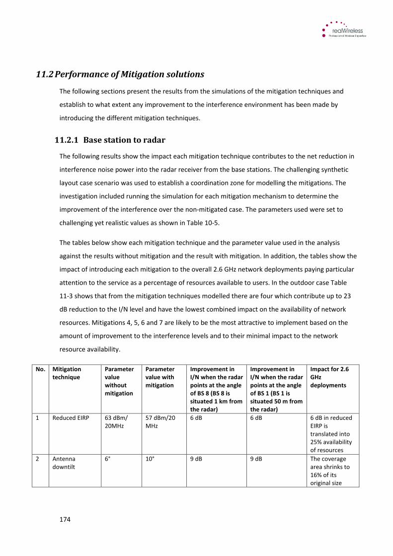
174
11.2 Performance of Mitigation solutions
The following sections present the results from the simulations of the mitigation techniques and
establish to what extent any improvement to the interference environment has been made by
introducing the different mitigation techniques.
11.2.1 Basestationtoradar
The following results show the impact each mitigation technique contributes to the net reduction in
interference noise power into the radar receiver from the base stations. The challenging synthetic
layout case scenario was used to establish a coordination zone for modelling the mitigations. The
investigation included running the simulation for each mitigation mechanism to determine the
improvement of the interference over the non-mitigated case. The parameters used were set to
challenging yet realistic values as shown in Table 10-5.
The tables below show each mitigation technique and the parameter value used in the analysis
against the results without mitigation and the result with mitigation. In addition, the tables show the
impact of introducing each mitigation to the overall 2.6 GHz network deployments paying particular
attention to the service as a percentage of resources available to users. In the outdoor case Table
11-3 shows that from the mitigation techniques modelled there are four which contribute up to 23
dB reduction to the I/N level and have the lowest combined impact on the availability of network
resources. Mitigations 4, 5, 6 and 7 are likely to be the most attractive to implement based on the
amount of improvement to the interference levels and to their minimal impact to the network
resource availability.
No. Mitigation
technique
Parameter
value
without
mitigation
Parameter
value with
mitigation
Improvement in
I/N when the radar
points at the angle
of BS 8 (BS 8 is
situated 1 km from
the radar)
Improvement in
I/N when the radar
points at the angle
of BS 1 (BS 1 is
situated 50 m from
the radar)
Impact for 2.6
GHz
deployments
1 Reduced EIRP 63 dBm/
20MHz
57 dBm/20
MHz
6 dB 6 dB 6 dB in reduced
EIRP is
translated into
25% availability
of resources
2 Antenna
downtilt
6° 10° 9 dB 9 dB The coverage
area shrinks to
16% of its
original size
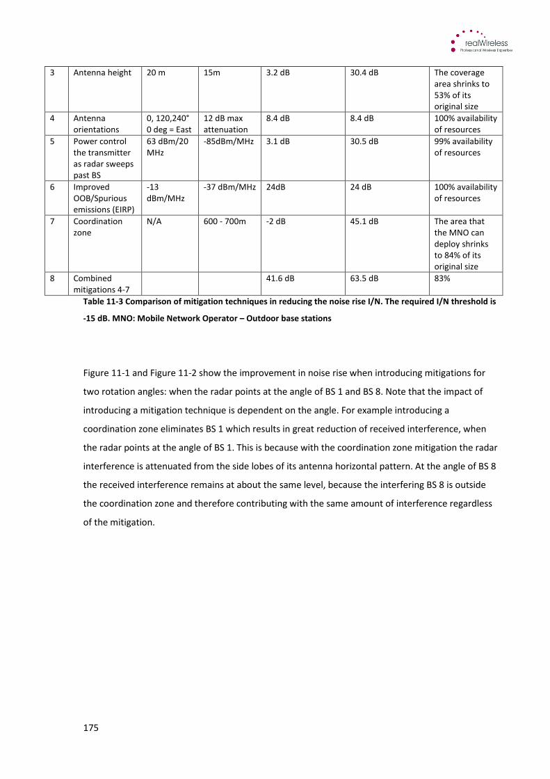
175
3 Antenna height 20 m 15m 3.2 dB 30.4 dB The coverage
area shrinks to
53% of its
original size
4 Antenna
orientations
0, 120,240°
0 deg = East
12 dB max
attenuation
8.4 dB 8.4 dB 100% availability
of resources
5 Power control
the transmitter
as radar sweeps
past BS
63 dBm/20
MHz
-85dBm/MHz 3.1 dB 30.5 dB 99% availability
of resources
6 Improved
OOB/Spurious
emissions (EIRP)
-13
dBm/MHz
-37 dBm/MHz 24dB 24 dB 100% availability
of resources
7 Coordination
zone
N/A 600 - 700m -2 dB 45.1 dB The area that
the MNO can
deploy shrinks
to 84% of its
original size
8 Combined
mitigations 4-7
41.6 dB 63.5 dB 83%
Table 11-3 Comparison of mitigation techniques in reducing the noise rise I/N. The required I/N threshold is
-15 dB. MNO: Mobile Network Operator – Outdoor base stations
Figure 11-1 and Figure 11-2 show the improvement in noise rise when introducing mitigations for
two rotation angles: when the radar points at the angle of BS 1 and BS 8. Note that the impact of
introducing a mitigation technique is dependent on the angle. For example introducing a
coordination zone eliminates BS 1 which results in great reduction of received interference, when
the radar points at the angle of BS 1. This is because with the coordination zone mitigation the radar
interference is attenuated from the side lobes of its antenna horizontal pattern. At the angle of BS 8
the received interference remains at about the same level, because the interfering BS 8 is outside
the coordination zone and therefore contributing with the same amount of interference regardless
of the mitigation.
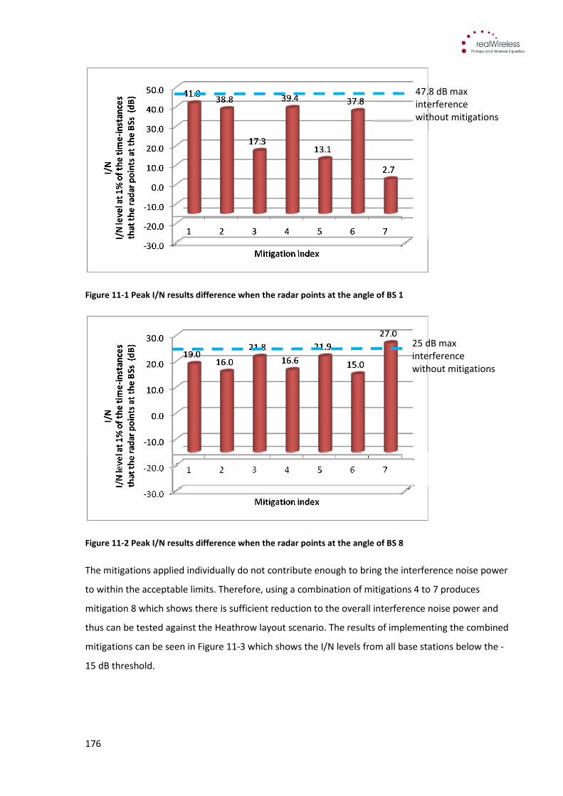
176
Figure 11-1 Peak I/N results difference when the radar points at the angle of BS 1
Figure 11-2 Peak I/N results difference when the radar points at the angle of BS 8
The mitigations applied individually do not contribute enough to bring the interference noise power
to within the acceptable limits. Therefore, using a combination of mitigations 4 to 7 produces
mitigation 8 which shows there is sufficient reduction to the overall interference noise power and
thus can be tested against the Heathrow layout scenario. The results of implementing the combined
mitigations can be seen in Figure 11-3 which shows the I/N levels from all base stations below the -
15 dB threshold.
25 dB max
interference
without mitigations
47.8 dB max
interference
without mitigations
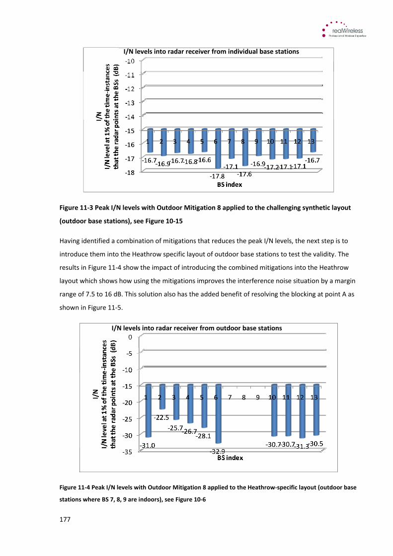
177
Figure 11-3 Peak I/N levels with Outdoor Mitigation 8 applied to the challenging synthetic layout
(outdoor base stations), see Figure 10-15
Having identified a combination of mitigations that reduces the peak I/N levels, the next step is to
introduce them into the Heathrow specific layout of outdoor base stations to test the validity. The
results in Figure 11-4 show the impact of introducing the combined mitigations into the Heathrow
layout which shows how using the mitigations improves the interference noise situation by a margin
range of 7.5 to 16 dB. This solution also has the added benefit of resolving the blocking at point A as
shown in Figure 11-5.
Figure 11-4 Peak I/N levels with Outdoor Mitigation 8 applied to the Heathrow-specific layout (outdoor base
stations where BS 7, 8, 9 are indoors), see Figure 10-6
I/N levels into radar receiver from individual base stations
I/N levels into radar receiver from outdoor base stations
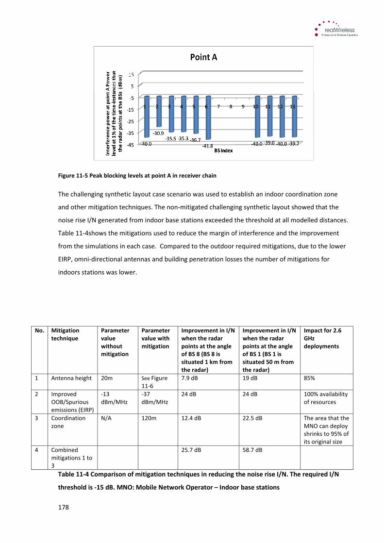
178
Figure 11-5 Peak blocking levels at point A in receiver chain
The challenging synthetic layout case scenario was used to establish an indoor coordination zone
and other mitigation techniques. The non-mitigated challenging synthetic layout showed that the
noise rise I/N generated from indoor base stations exceeded the threshold at all modelled distances.
Table 11-4shows the mitigations used to reduce the margin of interference and the improvement
from the simulations in each case. Compared to the outdoor required mitigations, due to the lower
EIRP, omni-directional antennas and building penetration losses the number of mitigations for
indoors stations was lower.
No. Mitigation
technique
Parameter
value
without
mitigation
Parameter
value with
mitigation
Improvement in I/N
when the radar
points at the angle
of BS 8 (BS 8 is
situated 1 km from
the radar)
Improvement in I/N
when the radar
points at the angle
of BS 1 (BS 1 is
situated 50 m from
the radar)
Impact for 2.6
GHz
deployments
1 Antenna height 20m See Figure
11-6
7.9 dB 19 dB 85%
2 Improved
OOB/Spurious
emissions (EIRP)
-13
dBm/MHz
-37
dBm/MHz
24 dB 24 dB 100% availability
of resources
3 Coordination
zone
N/A 120m 12.4 dB 22.5 dB The area that the
MNO can deploy
shrinks to 95% of
its original size
4 Combined
mitigations 1 to
3
25.7 dB 58.7 dB
Table 11-4 Comparison of mitigation techniques in reducing the noise rise I/N. The required I/N
threshold is -15 dB. MNO: Mobile Network Operator – Indoor base stations
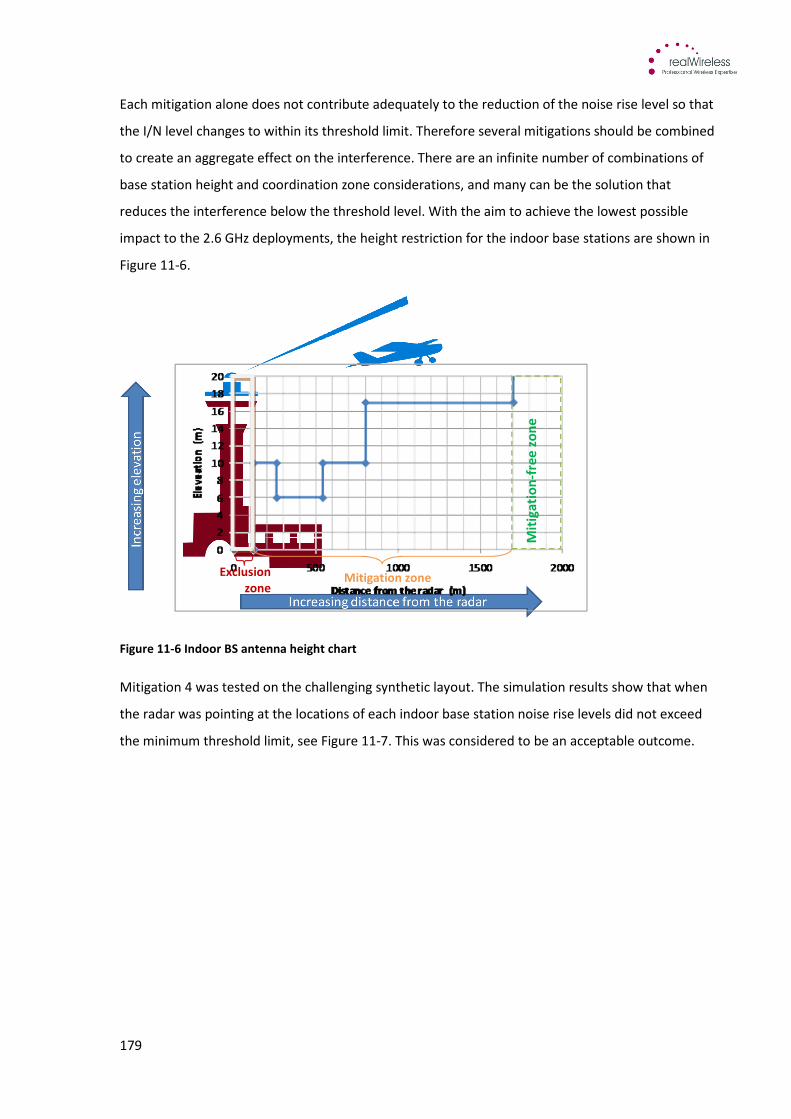
179
Each mitigation alone does not contribute adequately to the reduction of the noise rise level so that
the I/N level changes to within its threshold limit. Therefore several mitigations should be combined
to create an aggregate effect on the interference. There are an infinite number of combinations of
base station height and coordination zone considerations, and many can be the solution that
reduces the interference below the threshold level. With the aim to achieve the lowest possible
impact to the 2.6 GHz deployments, the height restriction for the indoor base stations are shown in
Figure 11-6.
Figure 11-6 Indoor BS antenna height chart
Mitigation 4 was tested on the challenging synthetic layout. The simulation results show that when
the radar was pointing at the locations of each indoor base station noise rise levels did not exceed
the minimum threshold limit, see Figure 11-7. This was considered to be an acceptable outcome.
Mit
iga
tio
n-f
ree
zo
ne
Exclusion
zoneMitigation zone
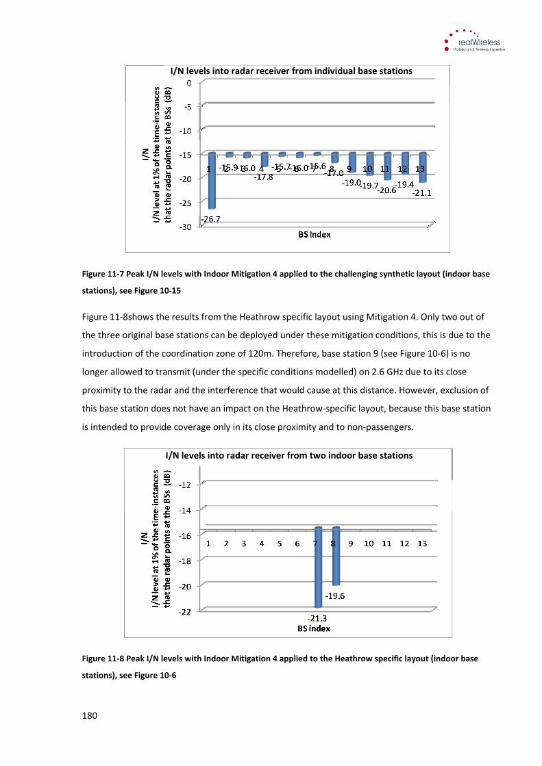
180
Figure 11-7 Peak I/N levels with Indoor Mitigation 4 applied to the challenging synthetic layout (indoor base
stations), see Figure 10-15
Figure 11-8shows the results from the Heathrow specific layout using Mitigation 4. Only two out of
the three original base stations can be deployed under these mitigation conditions, this is due to the
introduction of the coordination zone of 120m. Therefore, base station 9 (see Figure 10-6) is no
longer allowed to transmit (under the specific conditions modelled) on 2.6 GHz due to its close
proximity to the radar and the interference that would cause at this distance. However, exclusion of
this base station does not have an impact on the Heathrow-specific layout, because this base station
is intended to provide coverage only in its close proximity and to non-passengers.
Figure 11-8 Peak I/N levels with Indoor Mitigation 4 applied to the Heathrow specific layout (indoor base
stations), see Figure 10-6
I/N levels into radar receiver from individual base stations
I/N levels into radar receiver from two indoor base stations
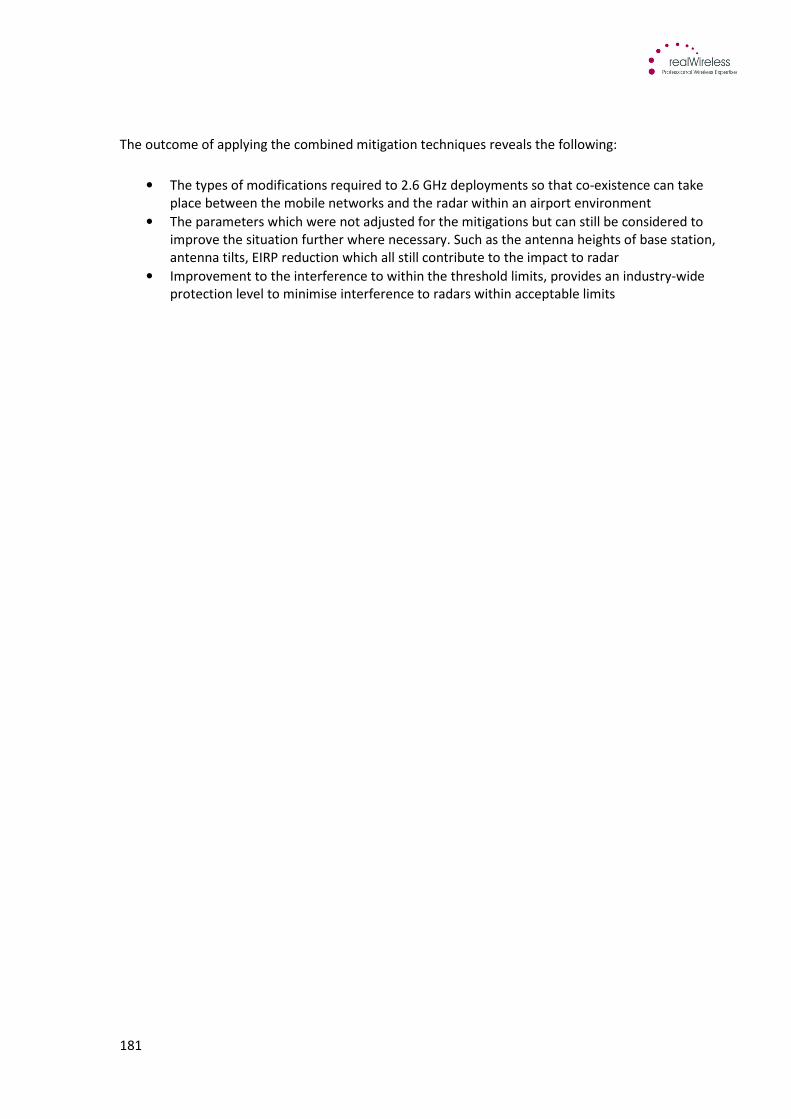
181
The outcome of applying the combined mitigation techniques reveals the following:
• The types of modifications required to 2.6 GHz deployments so that co-existence can take
place between the mobile networks and the radar within an airport environment
• The parameters which were not adjusted for the mitigations but can still be considered to
improve the situation further where necessary. Such as the antenna heights of base station,
antenna tilts, EIRP reduction which all still contribute to the impact to radar
• Improvement to the interference to within the threshold limits, provides an industry-wide
protection level to minimise interference to radars within acceptable limits
182
11.2.2 Mobilestationtoradar
The following results show the impact each mitigation technique contributes to the net reduction in
interference into the radar receiver from the mobile stations. It has already been established that
blocking does not occur under both the challenging case and typical case conditions therefore, the
metric in this analysis is the reduction of the noise power in the radar receiver it is reminded that the
simulation is designed to capture the statistical effects from the variability of the mobile emissions.
This includes the fluctuations in the signal envelope, the shadowing and the building penetration
losses variability.
The table below shows each mitigation technique modelled and the parameter used in the analysis
against the results without mitigation and the result with mitigation and the improvement to the
interference margin in dB. The table also shows the impact the mitigation has to the 2.6 GHz
network deployment.
No. Mitigation technique Parameter value
without
mitigation
Parameter
value with
mitigation
Improvement in I/N
when the radar points
at the worst
interference
Impact for 2.6 GHz
deployments
1 Cap maximum EIRP 23 dBm 20 dBm ~0 dB 83% of the users are
unaffected
2 Coordination zone
(outdoor /indoor
users)
No coordination
zone
70m I/D
300m O/D
radius around
radar
4.4 dB The coverage area
shrinks to 97% of its
original size
3 Improved
OOB/Spurious
emissions (EIRP)
-30 dBm/MHz -56 dBm/MHz 26 dB Cost of equipment that
satisfies the more
strict emissions mask
100% availability of
resources
4 Additional BS located
in highest
interference area
12 BSs 13 BSs ~0 dB Additional site cost
5 Cap number of users
on 2.6 GHz network
around airports
53 users (100%) 44 users (83%) 1.2 dB 83% of the users are
unaffected, the rest
served by another
band
OR reduced
throughput for 100%
of the users
Table 11-5 Comparison of mitigation techniques in reducing the noise rise I/N. The required I/N threshold is
-15 dB. MNO: Mobile Network Operator – Mobile stations
It can be seen in Table 11-5 that for each of the modelled mitigation techniques only one reduces
the interference noise power into the radar significantly. Improvement to the spectrum emission
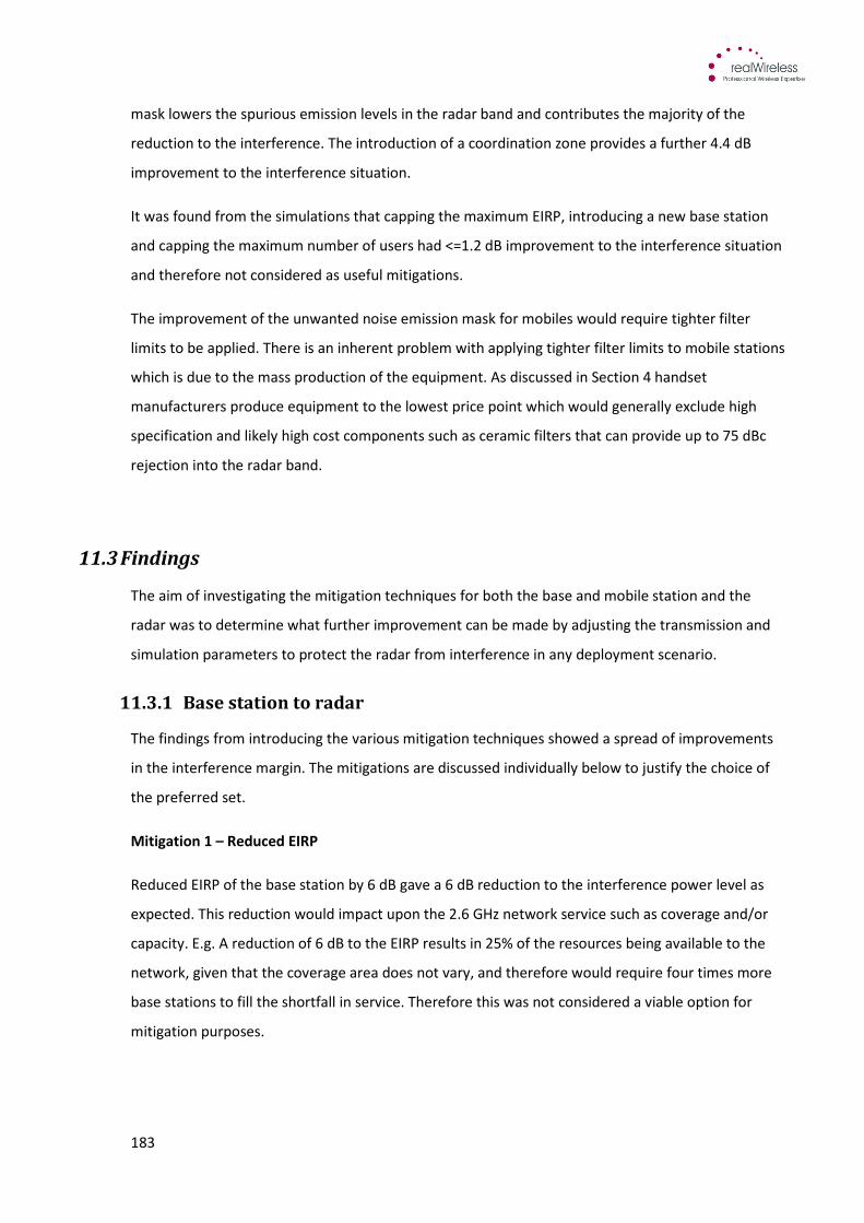
183
mask lowers the spurious emission levels in the radar band and contributes the majority of the
reduction to the interference. The introduction of a coordination zone provides a further 4.4 dB
improvement to the interference situation.
It was found from the simulations that capping the maximum EIRP, introducing a new base station
and capping the maximum number of users had <=1.2 dB improvement to the interference situation
and therefore not considered as useful mitigations.
The improvement of the unwanted noise emission mask for mobiles would require tighter filter
limits to be applied. There is an inherent problem with applying tighter filter limits to mobile stations
which is due to the mass production of the equipment. As discussed in Section 4 handset
manufacturers produce equipment to the lowest price point which would generally exclude high
specification and likely high cost components such as ceramic filters that can provide up to 75 dBc
rejection into the radar band.
11.3 Findings
The aim of investigating the mitigation techniques for both the base and mobile station and the
radar was to determine what further improvement can be made by adjusting the transmission and
simulation parameters to protect the radar from interference in any deployment scenario.
11.3.1 Basestationtoradar
The findings from introducing the various mitigation techniques showed a spread of improvements
in the interference margin. The mitigations are discussed individually below to justify the choice of
the preferred set.
Mitigation 1 – Reduced EIRP
Reduced EIRP of the base station by 6 dB gave a 6 dB reduction to the interference power level as
expected. This reduction would impact upon the 2.6 GHz network service such as coverage and/or
capacity. E.g. A reduction of 6 dB to the EIRP results in 25% of the resources being available to the
network, given that the coverage area does not vary, and therefore would require four times more
base stations to fill the shortfall in service. Therefore this was not considered a viable option for
mitigation purposes.
184
Mitigation 2 – Antenna downtilt
The increased antenna downtilt showed a 9 dB noise rise reduction. Mobile operators optimise their
networks based on specific antenna orientation criteria, therefore adjustment of downtilt too much
or not enough may impact on service provision to the cell edge such as throughput performance. A
10° downtilt results in a coverage area shrink to 16% compared to the size of a 6° downtilt. Thus it
would require 5 to 6 times more sites to fill the shortfall in service. The increased antenna downtilt
was not implemented for the mitigation scenarios and remained a 6°.
Mitigation 3 – Lower antenna height
The base station antenna height was reduced 5m below the radar antenna height. The impact of
this reduction was to introduce the effects of the combined antenna patterns of the base station and
the radar. The interference reduction is dependent on the radar rotation angle, see Table 11-3. The
2.6 GHz network service area was reduced to 53% of its original size, which would require twice as
many sites to fill the shortfall. Thus this mitigation is not likely to be desirable to implement and it
was not utilised in further analysis.
Mitigation 4 – Antenna orientation so that nulls occur towards radar
This mitigation may suggest that there is a substantial dip in the antenna pattern that can be
directed towards the radar. However, cellular network operators plan their networks based on a 3
sector antenna pattern and attempt to avoid any reduction in antenna gain in every direction. The
point of this mitigation was to rotate the antenna to the point where the edge of the sectors meet.
This meant directing the antenna with the lowest gain (10-12 dB) towards the radar.
The knock on effect of this mitigation means that the operator may need to adjust other base station
antenna orientations to maintain the optimum cell re-use plan.
Mitigation 5 – Power control the transmitter as radar sweeps passed base station
This mitigation26was considered to be a theoretical yet plausible method using a more novel (rather
than standard) approach to avoid causing interference into the radar as the main beam sweeps
26
Although no standard exists for this mitigation technique the concept is plausible. The ability to power
control the base station by whatever means is technically possible, the challenging part is to synchronise this
with the rotation of the radar.

185
passed the transmitter. The interference reduction is dependent on the radar rotation angle, see
Table 11-3. Consider the following example for the explanation of the reduction’s dependence on
the distance: Assume the base station locations as in the Challenging synthetic layout, see Figure
10-15. Without implementation of the switch-off mitigation, when the radar points at the angles of
BS 1 and BS 8, let the received powers be I1 and I8. Due to the propagation model: I1>I8. With the
switch-off mitigation, when the radar points at the angle of:
i) BS 1, the received interference is I8-30, thus the reduction of interference is I1-I8+30
ii) BS 8, the received interference is I1-30, thus the reduction of interference is I8-I1+30
The reduction of interference is greater when the radar points at the angle of BS 1: I1-I8+30 > I8-I1+30.
This mitigation has small footprint on the 2.6 GHz network. Switching the base station power off for
the interval that it is illuminated by the radar is translated to 98%27 availability of network resources
in the Heathrow base station layout. In less mobile network congested airports the effect of
switching off the power to the network will be even smaller. At a practical level the operator should
synchronise the base station with the rotation of the radar and consider switching off the particular
sector facing the radar rather than all sectors.
Mitigation 6 – Improved spectrum mask OOB/spurious emissions
An improvement to the spectrum emission mask over the 3GPP/IEEE specifications reduced the
noise rise. A 10 dB reduction to the emission mask produced a 10 dB reduction to the interference
noise levels. It is possible to reduce the noise rise with the introduction of high specification cavity
filters at the base station sites. The impact to the 2.6 GHz network service is trivial as the wanted
emissions are not affected. There is however the cost of procurement, installation and
commissioning of the cavity filter to consider for this mitigation technique. This is a required
mitigation technique.
Mitigation 7 – Coordination zone
The coordination zone was not established in isolation. Mitigations 4, 5 and 6 were applied to derive
the coordination zone. This is apparent since the coordination zone would be many tens of
kilometres without additional mitigations to contribute to minimising interference closer to the
threshold limits. The base stations located closest to the radar were systematically removed to
establish a coordination zone. Simulations were conducted on a step by step basis starting by
27
It was assumed that the base station is illuminated when the attenuation due to the horizontal
pattern > 30 dB
186
removing the closest base station to the radar and then removing the next closest base station and
so on until the interference noise levels satisfied the desired margin. The results showed a 660m
coordination zone is necessary to minimise the interference noise power to a point it will not exceed
the threshold and must be applied in combination with the following mitigations:
• Power control the base station transmitter when illuminated by the radar
• Use of improved out-of-band and spurious emission mask
• Orientation of base station antenna pointing lowest gain at the radar
Table 11-2 summarises the mitigations chosen for implementation. It should be noted that all
mitigations must be used in combination for the full effects to the radar to be realised. The
mitigations in Table 11-2 it can be seen that an attempt has been made to minimise the cost to 2.6
GHz network deployments. Mitigations 4, 6 and 7 which are the antenna optimisation, switching off
the base station and a coordination zone around the radar are considered to be relatively low cost
solutions to implement. For example antenna optimisation is undertaken at commissioning of the
station and can form part of the overall installation costs. The base station switch-off may require
some specific base station engineering or technology add-on to introduce this mitigation but it is not
deemed very high cost compared to building to a new site.
No Mitigation Practical
value range
Impact to 2.6 GHz deployments
4 Optimise antenna
orientation to lowest
gain facing radar
10-12 dB
attenuation
The reduction in availability of network resources
is trivial. The adjustment to the antenna
orientation may impact the re-use pattern
adopted to surrounding sites.
5 Improve unwanted
spectrum emission mask
-46 dBm/MHz Will require the addition of high specification
cavity filter which would mean additional cost per
site. This has trivial impact to the 2.6 GHz
network service availability.
6 Power control the
transmitter as radar
sweeps past base station
-85dBm/MHz Estimated percentage of network resource
availability is98%
7 Coordination zone 660 m Estimated percentage of network resource
availability is84%
Table 11-6 BS mitigations
187
The introduction of a coordination zone is an administrative matter for the airport authority and
Ofcom depending on where the coordination zone lies. In the case of Heathrow, the coordination
zone is partly on airport land and partly on public land, which may require some joined up policy on
how to apply the coordination zone in practice.
The only significant cost, therefore will be the installation of a high specification cavity filter at the
base station sites to reduce the out-of-band and spurious emissions. The analysis has been confined
to the airport environment which will assist the airport operators to understand and implement the
required mitigations to ensure satisfactory operation of the networks in proximity to the radar.
However, the impact cannot be treated in isolation as the interference is generated from base
stations beyond the airport perimeter which is out of the control of the airport operator and
becomes the responsibility of the mobile operator and the technical licence conditions set by Ofcom.
The following chart shows how the additional requirement for filtering drops with distance based on
free space pathloss. The required level of attenuation reduces from a radius distance of 1.7 km to
26.7 km away from the radar and suggests that even for the highest levels of filtering the additional
attenuation requirements are likely to be deemed achievable using some standard equipment types.
Figure 11-9 Unwanted emission attenuation versus distance from radar
11.4 Mobile station to radar
The findings from introducing the various mitigation techniques showed a spread of noise rise
reduction. The majority of the improvements were found to be <1.2 dB and the following section
gives an explanation of why these findings occurred.
0
10
20
30
40
50
60
0 5,000 10,000 15,000 20,000 25,000 30,000
Att
en
ua
tio
n (
dB
)
Distance from the radar (m)
Level of spurii emissions at the radar band, typical
equipment (WiMAX)
Required level of spurii emissions at the radar band
from the BS equipment, improvement over the [….]
Level of spurii emissions at the radar band, typical
equipment (LTE)

188
Mitigation 1 – Restricted maximum EIRP
A cap on the maximum EIRP from the mobile has a dual impact. Reduced in band power helps to
reduce blocking of the radar receiver in addition to reducing the noise emissions from the out-of-
band and spurious domain.
The improvement from restricting the maximum EIRP was about 0 dB. This could be due to the
distance of the highest interferers from the radar, see also the reduction of interference vs. distance
in the Mitigation 5 example in Section 11.3.1. 83% of the users were not affected by the maximum
power capping. This means that users at cell-edge will be subject to low throughputs and/or
coverage holes. This mitigation was not considered to be an effective technique.
Mitigation 2 – Implementation of a coordination zone
A coordination zone was derived for both indoor and outdoor users around the radar based on trial
and error. The coordination zone was derived with the implementation of a 22 dB improved filter
mask as without it the radius would have been > 1.7 km from the radar location. The radius of the
outdoor coordination was found to be 300m and the radius of the indoor coordination zone was
70m. These coordination zones were derived based on the optimum improvement to the
interference level that that can be gained whilst limiting the impact to the 2.6 GHz network users.
For example the combined indoor and outdoor coordination zone yields to a service area that is 97%
of its original size.
Mitigation 3 – Improved spectrum mask OOB/spurious emissions
An improvement to the spectrum emission mask over the 3GPP/IEEE specifications reduced the
noise rise. A 10 dB reduction to the emission mask produced a 10 dB reduction to the interference
noise levels.
It is suggested that this mitigation alone can reduce the interference noise power levels below the
threshold limits if 26 dB or more improvement over the 3GPP/IEEE masks, can be obtained from the
practical filter. This will remove the requirement for a coordination zone or any other mitigation for
the mobile stations. However, the emission requirements can be relaxed by 4.4 d B if a coordination
zone as identified above is implemented.
189
Mitigation 4 – Low power base station antenna in area of worst interference or deployed close to
the radar
The deployment of a low power base station antenna within an area of the worst mobile station
interference has the effect of powering down the mobiles in the vicinity of highest interference. The
location of the base station could also be close to the radar position.
Using the model it was possible to produce a snapshot of the area with the highest interference and
identify an optimum position for the low power base station. It was found that the highest
interference occurred at various distances from the radar from different combinations of snapshots.
The highest interferer could be a single mobile close to the radar or a cluster of mobiles far away
from the radar. Therefore, this solution would require adopting a planned network of additional
base stations to cover all eventualities of interference which is not a cost effective mitigation
strategy for consideration.
In the case of uncontrolled mobile stations roaming close to the radar, a single low power base
station can be deployed in close proximity to the radar as a final backstop. This low power base
station could be used to control or reduce the emissions output from the mobile stations thus
minimising interference within a given radius from the base station/radar. A more in-depth analysis
of the mechanism to reduce the mobile emissions is captured in appendix H.
Mitigation 5 – Cap the maximum number of users on 2.6 GHz network around airports
Capping the maximum number of users of the 2.6 GHz network aimed to reduce the total active
users that contribute interference at the radar receiver. It was found from that a 1.2 dB
improvement was gained by reducing the number of users by 17% which, as a mitigation alone, does
not contribute enough of a reduction to the interference. Furthermore, limiting the number of users
for such a small improvement has a negative cost impact and therefore, effort in obtaining gains
elsewhere is more worthwhile than implementing this mitigation.
11.4.1 Summary
It can be deduced that the improved spectrum emission mask is the most appropriate and effective
mitigation from those modelled. It is not worth considering the introduction of a coordination zone if
improved spectrum emissions can be achieved from the mobile handsets. If it transpires that the
mobile station filters used in 2.6 GHz equipment cannot achieve the maximum reduction in
emissions then further investigation into the coordination zones is required.
190
Table 11-7 summarises the findings and those mitigations identified for implementation.
No Mitigation Practical value
range
Impact to 2.6 GHz deployments
1 Cap maximum EIRP of mobiles Not considered Will require intervention from operators but
at a technical and operational level. Will limit
service such as capacity and throughput but
only in certain areas, on certain sectors to a
limited number of mobiles
2 Coordination zone around the
radar
300 m outdoor
70 m indoor
for 22 dB mask
improvement
No coordination
for 26 dB mask
improvement
Requires restricted use of phones near to
radar that may be costly and complex to
implement. Could be managed function by
airport authority such as BAA’s ECAP
3 Improve the OOB/Spurious
emission mask
See row above May require regulatory intervention which
could be time consuming and difficult to
implement and ultimately equipment vendors
would burden the cost
4 Introduce coupled antenna from
a BS into area of worst mobile
interference, direct sector
towards mobiles and away from
radar
Not considered Will require some additional engineering from
the operators perspective and may also
increase the interference to radar from the
base station antenna
5 Cap the maximum number of
users on 2.6 GHz network around
airports
Not considered Will require intervention from the mobile
operators and possible cost due to reduced
subscribers active on the network
Table 11-7 Summary of mobile station mitigations
Implementing the mitigation identified above under the Heathrow specific layout will enable the co-
existence of mobile stations and radars within an airport environment.
The following chart shows how the additional requirement for filtering drops with distance based on
free space pathloss.
191
Figure 11-10 Unwanted emission attenuation versus distance from radar
The mitigation to improve the spectrum emission mask is a challenging one to adopt based on the
potential for manufacturers to amend the filtering designs within their handsets. However, at the
present time it is not known the extent of quality of handsets in terms of their actual out-of-band
and spurious emission levels and it would be very useful to understand the measured emissions
radiated from mobile devices into the radar band to determine to what extent development of
handset design is required.
Measured data from mobile device emissions could usefully inform the study and help provide more
accurate results in terms of the interference noise power received at the radar receiver.
11.5 Impact on cost to 2.6 GHz deployments
This chapter has investigated the implementation of mitigation techniques to help reduce the
interference from base stations and mobile stations and introduced the cost implications that would
also impact on 2.6 GHz deployments when incorporating the mitigation techniques.
The following section discusses the high level cost to licensees and the airport authorities when
planning 2.6 GHz deployments in and around airports.
One main consideration is the cost impact that applies to outdoor sites that are built within the
airport perimeter. Site acquisitions within airports are likely to be scarce and are resourced and
managed by the airport owner. This also applies to indoor sites where shared common infrastructure
0
5
10
15
20
25
30
0 5,000 10,000 15,000 20,000 25,000 30,000
Att
en
ua
tio
n (
dB
)
Distance from the radar (m)
Required level of spurii emissions
at the radar band from the MS
equipment, 26dB improvement
over the 3GPP/IEEE mask
Required level of spurii emissions
at the radar band from the MS
equipment, 22dB improvement
over the 3GPP/IEEE mask
Typical level of spurii emissions
at the radar band, assumption
192
is used and the addition of new services may introduce complex engineering work to already heavily
loaded infrastructure.
The types of cost that are likely to be applicable under the circumstances modelled in the study
include:
• Capital costs, such as new hardware components, software upgrades etc
• Operational costs, such as additional site rental
• Site engineering re-design
The mitigations identified for both indoor and outdoor base stations sought to minimise the cost
burden to operators as much as possible. This was mainly to avoid the requirement to build
additional base sites to fill any shortfall in coverage which is considered to be the greatest expense.
It is possible that under certain circumstances not building new sites is unavoidable and therefore
this will be the greatest cost. Under the conditions modelled in the study the greatest cost to
operators will be the installation of the high specification cavity filters for the base stations which
will need to be installed for the co-existence of 2.6 GHz network within an airport environment.
11.5.1 Impacttobasestations
The significant costs are realised if the addition of new base station sites are required. New sites
would have been proposed based on the requirement to fill in gaps in coverage, capacity, service
created by the degradation in service due to the mitigations.
Based on the analysis of the mitigations and the possible shortfall in service provision from 2.6 GHz
network operators the following estimates have been considered:
193
No Mitigation Impact to 2.6 GHz deployments Estimated cost to 2.6 GHz
deployment
1 Reduce EIRP
levels of BS
May require additional low power
sites to maintain coverage/capacity
For example if four times the number
of base stations are required to fill a
capacity shortfall at up to 100,000 GBP
a site could result in a negative
cost/benefit ratio and be prohibitively
expensive.
2 Improve
unwanted
spectrum
emission
mask
May require the addition of high
spec cavity filter which would mean
additional cost per site
Cost of cavity filter up to £500 per
transmitter for an operator with 10 to
20 transmitters in and around the
airport this becomes a significant cost
3 Optimise
antenna
orientation
to lowest
gain facing
radar
Adjustment to antenna orientation
will not only impact coverage to
the network but will affect the re-
use pattern adopted to
surrounding sites which could
mean extensive on-going
optimisation to an operators
network
Cost neutral. Site specific engineering
would be included at the point of
installation
4 Increase
downtilt of
antenna
Adjustment to antenna downtilt
will have an impact to coverage of
the network which may require the
addition of fill in sites to cover the
shortfall
Cost neutral. Site specific engineering
would be included at the point of
installation
5 Lower
antenna
height
Adjustment to antenna height will
have an impact on coverage and
require more power to compensate
Cost neutral. Site specific engineering
would be included at the point of
installation
6 Power
control
transmitter
as radar
sweeps past
base station
Estimated percentage of service
reduction between 0.4% and 0.8%.
This would be negligible to users of
the network
Cost neutral. Site specific engineering
would be included at the point of
installation
7 Coordination
zone
Estimated percentage of network
resource availability is84%. Users
may notice some reduction in
network quality such as throughput
to users of the network
Cost neutral. Requires mobile
operator, airport operator and
regulator intervention to coordinate
specific coordination zone around
airports
Table 11-8 Cost impact to the deployment of base stations
Another major cost is the incorporation of a high specification cavity filter which can greatly reduce
the out-of-band and spurious emission levels transmitted from the base station and improving the
194
interference situation at the radar receiver. This requirement is based on 2.6 GHz base station
equipment no longer designed with high specification filtering in mind to reduce size of the units and
reduce cost of production. Furthermore, reduced sized components requires less cooling and thus
cuts costs of cooling systems installed into base sites.
The types of filters expected to be used in the 2.6 GHz band have been estimated by Ofcom in the
2.6 GHz auction statement3 at a cost of around £500. This was based on providing enough selectivity
to protect in band TDD/FDD systems. The advantage of this will be the additional selectivity the
filters will provide into the upper adjacent S-band. Furthermore, the additional filters will only need
to be installed at the sites in areas that cause an impact to the radar.
195
11.5.2 Impacttomobilestations
No Mitigation Impact to 2.6 GHz
deployments
Estimated cost to 2.6 GHz
industry
1 Cap maximum
EIRP of mobiles
Will require intervention
from operators but at a
technical and operational
level. Will limit service such
as capacity and throughput
but only in certain areas, on
certain sectors to a limited
number of mobiles
Cost neutral. Site specific
engineering would be included
at the point of installation
2 Coordination
zone around the
radar
Requires restricted use of
phones near to radar that
may be costly and complex
to implement. Could be
managed function by
airport authority such as
BAA’s ECAP
Cost neutral. This will require
mobile operator, airport
operator coordination and
regulatory intervention
3 Improve the
OOB/Spurious
emission mask
May require regulatory
intervention which could be
time consuming and
difficult to implement and
ultimately cost to
equipment vendors
Potential development costs to
handsets, dongles and
integrated laptops. Cost could
be significant based on
inclusion of higher specification
components
4 Introduce
coupled antenna
from a BS into
area of worst
mobile
interference,
direct sector
towards mobiles
and away from
radar
Will require some additional
engineering from the
operators perspective and
may also increase the
interference to radar from
the base station antenna
Additional site or relay build
required at cost of new
antennas, and feeders
approximately £20,000 to
£50,000
5 Cap number of
active users on
2.6 GHz network
Will require specific
network engineering to cap
users and switch them to
alternative spectrum
resources, where available
Medium to low cost based on
software and NOC upgrades.
Potential revenue impact
based on reduced number of
users and inefficient use of
spectrum
Table 11-9 Cost impact to the deployment of mobile stations
196
12 Conclusionsandsummaryrecommendations
12.1 Conclusions
This study has addressed the interference environment from 2.6 GHz systems into the adjacent 2.7
GHz radar band at an airport and found that under more realistic scenarios the interference levels
were below the acceptable threshold limits and the overall impact to the radar minimal thus
enabling the deployment of 2.6 GHz systems for both base stations and mobile stations within an
airport environment.
However, in specific challenging corner case deployment conditions severe interference can be
generated causing degradation to the performance of the radar that required further investigation
on a more detailed basis.
12.2 Summarised conclusions
The summarised conclusions from this study are as follows:
1. Interference from LTE and WiMAX base stations and mobile stations operating in the 2.6
GHz band to Air Traffic Control radars operating in the adjacent 2.7 GHz band has been
analysed via simulations representative of installations in and around Heathrow airport.
2. The analysis examined two types of layout environments for the base stations. 1) A layout
representing the Heathrow airport environment, 2) a synthetic layout representing base
stations at equidistant intervals from the generic modified radar. The two layouts were used
to establish the extent of interference from base stations with the synthetic layout used to
further analyse the required mitigations. The challenging case which could in principle occur
in practice but is relatively extreme was used in both layouts, while the typical case, which is
considered more realistic, was used in the Heathrow layout only. Both layouts consist of 13
base stations at distances ranging between 50m and 1700m.
3. Mobile stations were modelled within the Heathrow layout for both the challenging case
and the typical case at a density consistent with levels of usage which could occur in the
airport environment. Spurious emissions of the mobiles are assumed to be at the standard
specification limits and transmitting at full power in the challenging case. Under the typical
case the spurious emission of the mobiles were assumed to be at 20 dB below the standard
specification limits with power control activated.
4. Mobile stations were also modelled using measured emissions data from tests performed to
determine the behaviour of a commercially available FDD LTE mobile device. We found that
negligible noise rise occurred from the measured emissions, this was due to -87 dBm/MHz
spurious level across the S-band. Even when imposing a discrete spurious emission co-
channel with the radar centre frequency, the amplitude required to exceed the I/N threshold
of the radar receiver, was 57 dB.
5. Base stations were found to cause blocking of the radar receiver at the radar antenna
connector input and a rise in noise under the challenging case conditions from locations
inside and outside the airport perimeter and from both in-buildings and outdoors. Blocking
197
from the base stations at a distance of 50 m from the radar exceeded the -5 dBm threshold
by 9.9 dB. The noise rise from the base stations was as high as 47.8 dB for small percentages
of time, which exceeded the desired threshold of between -5 and -15 dB.
6. Mobile station spurious emissions under challenging case conditions, did, generate a noise
rise in the radar receiver which exceeded the maximum (-15 dB) threshold by 39.2 dB for
small percentages of time. However, the spurious emission levels were set to -30 dBm/MHz
(3GPP limit) to achieve this.
7. The blocking situation for both base stations and mobile stations is substantially improved
when under these typical case conditions. For example blocking levels arising from base
stations are reduced to -16 dBm compared to the -5 dBm threshold, and from mobile
stations to -107 dBm compared to the -80 dBm threshold.
8. The noise rise was not completely resolved under the typical case for base stations or mobile
stations. The maximum threshold limit of -15 dB I/N was exceeded by 8 dB for base stations
and 5.7 dB for mobile stations, for small percentages of time. This result led to the
determination of specific mitigation techniques, such as 2.6GHz base stations not
transmitting for the small period of time when the main radar beam is known to be pointing
directly at it, to reduce the noise rise to below the threshold limits.
9. The noise rise at the generic modified radar receiver was reduced by introducing several
mitigation techniques. These techniques showed various degrees of improvement, when
compared to the interference of the Synthetic Challenging layout (base stations base line
scenario) and the Challenging case technical parameters (mobile stations base line scenario).
The criterion assumed to avoid interference is that the noise rise is allowed to exceed -15dB
for 1% of the time for which the radar antenna is oriented towards the most significant
interferer. For a single dominant interferer, such a condition only occurs for around 1% of
the time, leading to an overall interference instance of around 0.01%.
10. To achieve this level of protection, a combination of mitigations is required. This will include
an improvement of the spurious emissions of 2.6 GHz equipment over the 3GPP/IEEE
standards by 24 dB for base stations and 26 dB for mobile stations which are considered
reasonable levels from discussions with vendors. If, however, a higher level of interference
or an increased percentage of time could be tolerated, other mitigations can be used on
their own, such as creating a coordination zone around the radar and preventing base
station transmissions when the radar is oriented towards the base station.
11. For any individual deployment, the application of site-specific mitigation techniques can
reduce the risk of interference to minimal levels. Such mitigation techniques vary in their
efficacy and impact on the 2.6 GHz deployment, but taken in combination with appropriate
initial network design they can ensure appropriate coexistence. Such mitigations should be
monitored to ensure they are appropriate via an appropriate approvals process, via a
calculation methodology which is accepted by the 2.6 GHz operators, the airport authorities
and the CAA. This methodology could potentially use the simulation framework developed
for this study. This process could be incorporated into existing arrangements, such as BAA’s
Electronic Communications Approval Process.
The study found that the dominant interfering mechanism is the interference noise power generated
from both base stations and mobile stations. The increase in peak noise levels exceeded the
acceptable limits in the challenging case and required further investigation into mitigation
techniques.
198
Under typical case conditions the blocking and I/N levels caused by base stations at an airport were
quite dramatically reduced compared to challenging case conditions. This is due to the reduced in-
band emission levels, the attenuation due to the antenna patterns and the radar antenna height
positioned above the base station antenna height.
Applying the mitigations led to the satisfactory outcome of deployment of 2.6 GHz systems at both a
synthetic layout and Heathrow layout. The tradeoffs from applying mitigations included:
• Further coordination required for base stations deployed within the coordination zone, that
could lead to the introduction of unacceptable deployment parameters to satisfy
requirements
• The use by operators of high specification cavity filters on the base stations
• Introduction of the theoretical concept for transmitter ‘switch-off’ as the radar sweeps
passed the base station for which there is no standard technique available at present
• The use by operators of handsets and mobile devices with ceramic filters whose spurious
performance levels are 40 -50 dB below the 3GPP limit
• Optimised orientation of BS antenna with lowest gain of the pattern pointing towards the
radar
It was identified that combining four out of the seven mitigations contributed the most to reducing
the interference whilst minimising the performance and service quality impact on the 2.6 GHz
network deployments was the solution. This has the effect of bringing the interference noise power
to within the threshold limits considered to be acceptable to the regulatory authorities. The
mitigation options; the coordination zone, transmitter power control, improved spurious emissions
and antenna orientation, modelled were considered to be the most cost effective solution without
having to build new sites at very high cost.
The study revealed that emissions from shared sites do cause a problem to radar receivers which in
an airport environment, is a common deployment technique. BAA, the owner of Heathrow Airport
uses its electronic equipment approvals requirements to manage the use of sites on their property
which includes shared site infrastructure. Therefore site specific solutions could be adopted by the
airport operator to address this problem.
Similar to the base station analysis, the mobile stations do not cause blocking to the radar under
typical case conditions and would co-exist with radars at an airport on that basis. This means that for
the blocking interference mechanism mobile stations do not cause a problem to the radar.
The interference noise increase generated by multiple mobiles in the vicinity of the radar receiver
under the typical case marginally exceeded the desired I/N threshold and is considered to be
manageable with careful network planning. Upon identifying the mitigations in the challenging case,

199
it was found that mitigations such as coordination zone and improved spurious emissions had a
neutral effect on the performance and service quality of 2.6 GHz network deployments and did
reduce the interference level below the acceptable limit.
There was negligible noise rise from the spurious emissions of a commercial off the shelf FDD LTE
mobile device. This one example device suggests good emissions performance with very low risk to
the satisfactory operation of radars at airports under the particular scenario conditions of this study.
There is a strong likelihood of mass deployment of this particular device type or, future generations
of it by LTE networks operators in the UK and in particular at airports. However with only one
example 2.6 GHz device measured, we cannot assume the same positive effects will occur for other
mobile devices such as laptops, tablet PC’s and smartphones. As 2.6 GHz networks mature the mix of
devices will increase and thus the uncertainty in performance of mobile devices. Therefore, a deeper
understanding of the performance of a wider selection of mobile device types would provide a more
representative sample of the environment to be found in future.
Furthermore, the results show that upgrading the radars such as the one used in the model
attenuates the blocking levels from 2.6 GHz emissions by up to 40 dB at the RF front end. The
modified design of the generic modified radar receiver used in the model shows that co-existence is
possible in the presence of 2.6 GHz systems and that attention on reducing the interference before
the filtering, i.e. at the antenna connector is of more concern.
12.3 Recommendations
This section makes the recommendations that have been identified from the outcome of the study
and that are applicable to the deployment of 2.6 GHz networks within an airport environment in
close proximity to an S-band radar.
These recommendations are supported by the findings of the study that will help meet Ofcom’s
objectives with regard to the award of 2.6 GHz spectrum in the medium term.
12.3.1 Recommendations to improve the interference situation at airports
Base stations:
Implementing the mitigation techniques outlined in section 11.2.1 will provide maximum reduction
in interference for both blocking and interference noise rise. The following recommendations are
based on the conclusions found from this study.
200
1. Extending the -45 dBm/MHz EIRP limit of the Ofcom specified Block Edge Mask from
2720 MHz to 2750 MHz and above to protect radar frequencies beyond those specified
by Ofcom
2. Coordination and collaboration with the airport authority. It is anticipated that as part of
the planning of new mobile communications networks that coordination and
collaboration between the airport operator and the mobile network operator will be
necessary for the deployment of 2.6 GHz networks. Findings from this report can inform
the approval procedures of 2.6 GHz networks at airports.
3. Airport operators to implement a coordination zone for the deployment of 2.6 GHz base
stations dependent on the layout and specific deployments. It is recommended that
operators seeking to deploy base stations within the coordination zone would need to
further reduce the values such as EIRP or use lower antenna heights.
4. Implementation of a high specification filter for the base stations located within the
airport perimeter to meet the desired limits specified in section 11.2.1
5. Careful selection and design of base station locations taking into account the typical case
conditions used for modelling as a benchmark for further study and analysis
6. Optimisation of the antenna pattern with the lowest gain of the pattern pointing
towards the radar
7. Adoption of alternative deployment strategies, for example, operators limit 2.6 GHz
deployments indoors and mobiles can roam to an alternative spectrum band when
outdoors.
Mobile stations:
The following recommendations are based on the findings from the investigation of interference
generated by mobile stations with assumed spurious emissions within an airport environment.
1. The introduction of an outdoor and indoor coordination zone around the radar. The
simulations found that a 300m outdoor coordination and a 70m indoor coordination zone
are sufficient to reduce interference to below the threshold for each mechanism. For smaller
coordination zones parameters such as EIRP should be reduced further or investigate in
detail the specific building penetration loss for the particular airport which may offer more
attenuation than the 14 dB assumed in the model.
2. Appreciation of the typical case conditions used for modelling as a benchmark for further
study and analysis of the interference within an airport environment For example the
activation of power control for the uplink in the model helped reduce the interference levels
into the radar.
3. Where possible identify the mobiles manufacturers with the best and worst out-of-band and
spurious emissions and re-model using the measured data. This will establish a set of
mobiles (and vendors) whose equipment will operate within the threshold limits of
interference and can co-exist in an airport environment.
The addendum to this report provides details of the recommendations of the analysis of measured
emissions from a commercially available LTE FDD mobile device into a second modified radar design.
201
12.3.2 Recommendations for further analysis
The results from the study suggest that there is merit in further detailed analysis of the airport
environment using more specific conditions. The following recommendations are given for further
analysis:
1. In order to understand the combined interference from base stations and mobile stations
further analysis should be undertaken to establish the blocking and interference noise levels
incorporating both base stations and mobile stations operating simultaneously.
2. Appropriate design parameters should be determined on an airport-specific basis and
coordinated with the relevant authorities as appropriate as many different deployment
parameters can materially affect the interference performance of 2.6 GHz base stations in
and around airports28
3. Analysis of low power a base station located close to the radar to minimise interference
from roaming mobiles that could potentially cause significant interference
4. Consideration of the type of action to be taken by the mobile operators or airport owner to
restrict use of 2.6 GHz emissions within the coordination zone in the case for mobile
stations.
5. Radar heights at other UK airports should be catalogued to ensure they have been covered
by this study. The radar heights found at other UK airports vary widely from 5m at the
lowest height up to 40m for the greatest height. There are increased levels of interference
from 2.6 GHz deployments into radars with antenna heights below that of the 2.6 GHz
transmitter
6. Consideration of a mobile station’s ability to hand over to a spectrum band other than 2.6
GHz for outdoor deployments at airports when the conditions for avoiding radar
interference cannot be satisfied.
7. Commercial and technical factors in site sharing should be reviewed as suggested
mitigations applied by the airport owners could include the restriction on the number of
base stations transmitting from a single site.
8. Spurious emission measurements of a wider selection of mobile device types, such as
smartphones, tablet PC’s and laptops to determine their behaviour in the S-band.
28
These are specified in Section 8.

202
13 Glossary
3GPP Third Generation Partnership project
ACLR Adjacent Channel Leakage Ratio
CAA Civil Aviation Authority
CDF Cumulative Distribution Function
dB Decibels
dBc Decibels relative to carrier power
dBm Decibels relative to 1mW
D/L Downlink
ECC Electronic Communications Committee
EIRP Equivalent Isotropic Radiated Power
FDD Frequency Division Duplex
FSPL Free Space Path Loss
GHz Gigahertz
IEEE Institute of Electronic and Electrical Engineers
IF Intermediate Frequency
IMT International Mobile Telecommunications
I/N Interference to Noise ratio
LNA Low Noise Amplifier
LOS Line of Sight
LTE Long Term Evolution
MCA Maritime and Coast Guard Agency
MHz Megahertz
MOD Ministry of Defence
NLOS Non-Line of Sight
OFDM Orthogonal Frequency Division Multiplexing
OOB Out-of-band emissions
PDF Probability Distribution Function
RF Radio Frequency
TDD Time Division Duplex
U/L Uplink
WiMAX Worldwide interoperability for Microwave Access
203
14 References
1 UK Radar adjacent band selectivity submission to ITU Working Party 5B 2009
2 Cobham Technical Services – Radiated out of band Watchman radar testing at RAF Honington April 2009
3 Ofcom - Auction of Spectrum 2500-2690MHz, 2010-2025MHz, Information Memorandum April 2008
4 Ofcom Information Update Co-existence of S-band radar systems and adjacent future services 11 December
2009
5 WiMAX Forum www.wimaxforum.org
6 Mobile Broadband Evolution: the roadmap HSPA to LTE – February 2009 UMTS Forum
7 IEEE 802.16e Air interface for Fixed and Mobile Broadband Wireless Access Systems
8 3GPP TS 36.104 3
rd Generation Partnership Project Technical Specification Group Radio Access Network;
Evolved Universal Terrestrial Radio Access (E-UTRA); Base Station (BS) radio transmissions and reception
(Release 9)
9 3GPP TS 36.101 3
rd Generation Partnership Project Technical Specification Group Radio Access Network;
Evolved Universal Terrestrial Radio Access (E-UTRA); User Equipment (UE)radio transmissions and reception
(Release 9)
10 Airport deployment study stakeholder interviews – June 2010 Real Wireless
11www.klfilterwizard.com – filterKL.pdf
12 3GPP TR 36.942 v9.0.1 3
rd Generation Partnership Project Technical Specification Group Radio Access
Network; Evolved Universal Terrestrial Access Network (E-UTRA); Radio Frequency (RF) system scenarios
(Release 9)
13 ECC Report 148 – Measurements of the performance of DVB-T receivers in the presence of interference
from the mobile service (especially from LTE), Marseille June 2010
14 ECC Report 140 – Compatibility between RLAN on board aircraft and radars in the bands 5250 – 5350 MHz
and 5470 – 5727 MHz – Tromso May 2010
15 ECC Report 045 – Sharing and adjacent band compatibility between UMTS/IMT 2000 in the band 2500-2690
MHz and other services – Granada February 2004
16 Results to date from radar study – Ofcom internal only Kamlesh Masrani 4
th April 2009
204
17
ECC Report 119 – Co-existence between mobile systems in the 2.6 GHz frequency band at the FDD/TDD
boundary – Kristiansand June 2008
18 Ofcom statement: Award of available spectrum: 2500-2690 MHz, 2010-2025 MHz – 4 April 2008
19 ECC REC 02/05 Unwanted Emissions
20 ITU-R SM 329-8 – Unwanted emissions in the spurious domain
21 3GPP TR 36.814 v9.0.0 3rd Generation Partnership Project;Technical Specification Group Radio Access
Network;Evolved Universal Terrestrial Radio Access (E-UTRA);Further advancements for E-UTRA physical layer
aspects(Release 9)
22 Isotek electronics Limited - High Q filter feasibility study for Base Station and Radar receiver applications ,
Duncan Austin, 15/10/09
23 ITU Document 5B/-E 2009 United Kingdom of Great Britain and Northern Ireland Radar Adjacent Band
Selectivity - 2009
24Ofcom report Application of spectrum and liberalisation and trading for the mobile sector 2008
25 Factors influencing outdoor to indoor radio wave propagation – S Stavrou and S R Saunders
26 3GPP TR 36.814 v9.0.0 Technical Specification Group Radio Access Network Evolved Universal Terrestrial
Radio Access; Further Advancements for E-UTRA physical layer aspects (Release 9)
27 COST 231 Final Report, Digital Mobile Radio: COST 231 Viw on the Evolution Towards 3
rd Generation
Systems, Commission of the European Communities and COST Telecommunications, Brussels 1999
28 ITU-R P 1238-6 Propagation data and prediction methods for the planning of indoor radiocommunication
systems and radio local area networks in the frequency range 900 MHz to 100 GHz
29 ITU-R P. 452-12 Prediction procedure for the evaluation of microwave interference between stations on the
surface of the Earth at frequencies above about 0.7 GHz
30 Helios – Review of Radar Receiver Adjacent Channel Thresholds of UK S- band ATC Radar –Final Report
10/12/09
31 ITU-R M.1464 Characteristics of radiolocation radars, and characteristics and protection criteria for sharing
studies for aeronautical radionavigation and meteorological radars in the radiodetermination service operating
in the frequency band 2 700-2 900 MHz 1 January 2003