Embed Size (px)
Citation preview
Airglow emissions : fundamentals of theory and experiment
R Chattopadhyay1* and S K Midya2,3
1Haripal G.D. Institution, Khamarchandi, Hooghly-712 405, West Bengal, India2Department of Physics, Serampore College, Serampore, Hooghly-712 201, West Bengal, India
3Centre for Space Physics, 43 Chalantika, Garia Station Road, Kolkata-700 084, India
E-mail : [email protected]
Received 30 April 2004, accepted 17 November 2005
Abstract : In this article, discovery of airglow and ionosphere has been discussed briefly in the historical and scientific perspectives. Mentioningabout all significant atmospheric parameters, different areas of research in airglow and different ionospheric layers of importance have been brieflydescribed. Different types of airglow emissions, related chemical kinetics, different excitation mechanisms of the involved atomic, molecular or ionicspecies have been discussed giving stress specially to four main airglow emissions. Different layers of ionosphere, their characteristic material contentand specific ranges of responses to different kinds of interacting fields etc. have also been briefly discussesd. The Sun has been described as the mainsource of all kinds of energetic interactions with the terrestrial ionosphere. Specific solar parameters, that are representatives of various solar activity,have been discussed briefly in relation with the corresponding covariation of various ionospheric parameters involved in the calculations of airglowintensity. Different solar activity periodicities that have been discovered upto date are mentioned. Relations of different airglow emissions withionospheric activities and specific ionospheric parameters have been briefly described. The important role of ozone in the stratosphere and lowerthermosphere in the production of some airglow emissions has been discussed with exemplary works. Different wellknown features of airglow intensityvariations such as altitudinal variation, latitudinal variation etc have also been mentioned. Different atmospheric models have been briefly describedalong with their usefulness. Descriptions of different missions and campaigns with which a number of airglow experiment sets are involved , have beenpresented in a tabular form. Discovery of some new airglow lines, some newly proposed excitation mechanisms and related kinetics, and someremeasured or reevaluated constants and coefficients have been reported too. Effect of different types of solar activity, of different kinds of lunarinfluences and of various terrestrial atmospheric features, such as, geomagnetic field alignment, geomagnetic storm, lightning, earthquake, dynamicalcoupling between layers of thermosphere, E x B drift and ring current etc on terrestrial airglow emissions have also been briefly discussed. Someinteresting airglow related features which have been discovered in recent past are discussed. Applications of different airglow features have beenreported. Lastly, facts and speculation about ionospheric compositions, activities and possible airglow emission features of other inner and outerplanets, satellites, comets and meteors have been discussed very briefly.
Keywords : Airglow, solar indices, ionospheric activities
PACS Nos. : 94.10 Rk, 94.20 Ji, 93.30 Dl
Indian J. Phys. 80 (2), 115-166 (2006)
© 2006 IACS
* Corresponding Author
'
'
Review
Plan of the Article
1. A brief introduction to airglow study
1.1 A brief historical and scientific introduction to airglowstudy
1.2 Classification of airglow phenomena
1.3 Different atmospheric physical parameters, observationalmethods and instrumentation
1.4 Most important airglow emissions and other emissions,chemical reactions, kinetics and excitation mechanismsfor main airglow emissions
2. Ionospheric activities and their relation with airglowemission phenomena
2.1 Classification of terrestrial atmosphere andionosphere
2.2 The Sun as the main source of various ionosphericactivities
2 .3 Ionospheric physics and chemistry for different layersand regions of ionosphere
2.4 Interrelation between ionospheric activities and airglowemissions
2.5 Ozone chemistry and its importance in airglow study
R Chattopadhyay 1.p65
116 R Chattopadhyay and S K Midya
3. Well-known features of terrestrial airglow emissions
3.1 Altitudinal distribution of vertical profile
3.2 Latitudinal variation of airglow intensity
3.3 Longitudinal variation
3.4 Hourly and diurnal variations, SZA and dynamicalcoupling
3.5 Dynamical coupling
3.6 Barium cloud feature
3.7 Seasonal variation
3.8 Semiannual and annual variations
3.9 Hydrodynamical oscillation type variation
3.10 Rotational and Doppler temperatures
3.11 Limb-view of Earth’s airglow spectra
4. Different atmospheric, thermospheric and ionosphericmodels related to airglow phenomena
4.1 Wulf’s worldwide circulation system
4.2 Vestine’s wind systems of geomagnetic disturbance
4.3 Goldie’s average planetary circulation
4.4 Kellog-Schilling model of stratospheric circulation
4.5 Yerg’s ionospheric wind system
4.6 Deb’s model of ionospheric circulation
4.7 Brasefield’s empirical wind system
4.8 Palmer model of circulation in the lower stratosphere
4.9 CIRA model
4.10 Jacchia model
4.11 MSIS Hedin
4.12 MSIS-86
4.13 MSIS-90( Hedin )
4.14 CHIU model
4.15 SLIM and FAIM
4.16 CTIPM
4.17 TSMGCM
4.18 QPS model
4.19 EVF model
4.20 TDIM model
4.21 SUPIM
4.22 TIEGCM
4.23 FLIP model
4.24 MWM
4.25 IRI model
4.26 Belikov model
4.27 UBAIM model
5 Different missions and campaigns related to airglowobservations
6. Newly discovered airglow lines , features, newly proposedexcitation mechanism and newly determined constantsand coefficients
6.1 O(1D) rate constants and their temperature dependence
6.2 New values of rate constants and branching ratio forN
2++O reaction
6.3 New value of Einstein’s coefficient for spontaneousemission of the O
2 ( a 1D
g ) sate
6.4 Revised cross- sections of O+ 834 Å dayglow
6.5 Carroll-Yoshino band problem
6.6 New finding about OI 844.6 nm emission mechanism
6.7 New quenching value of O(1D)
6.8 Self absorption theory
6.9 New inference about Na nightglow excitation
6.10 On the analysis of geophysical data for an unknownconstant
6.11 Inference about quenching rates for O2 Herzberg I bands
6.12 Measurement of rate constant for quenching CO2 by
atomic oxygen at low temperature
7 Effects of different physical factors on airglow emissions
7.1 Effects of purely solar origin
7.2 Effects of purely lunar origin
7.3 Effects of other cosmic bodies
7.4 Terrestrial atmospheric features on which airglowemissions depend
8 Newly identified airglow related features
8.1 Light pollution
8.2 Sprites
8.3 Radiation belt particle contamination
8.4 Disturbance of airglow measurements
8.5 Artificial satellite-space-vehicle -glow and laboratorymodelling
8.6 Space-shuttle-induced optical contamination
8.7 Travelling ionospheric disturbances
8.8 SNE or South to North propagating Events
8.9 Vertical propagation of atmospheric waves ordisturbances
8.10 SSL or sudden sodium layers
8.11 Features of ionospheric plasma depletion or IPD
9 Applications of airglow study
9.1 Atomic oxygen profiles at midlatitude and equatorderived from airglow observation
9.2 Recovering ionization frequency and oxygen atom densitywith the help of airglow data
R Chattopadhyay 1.p65
Airglow emissions : fundamentals of theory and experiment 117
9.3 Analysis of vibrational states of oxygen Herzberg I systemusing nightglow
9.4 Atomic oxygen concentration from airglow data
9.5 UV airglow and the knowledge of upper atmosphericconditions
9.6 Procedure for extraction of precise airglow data inpresence of strong background radiation
9.7 Ozone data from airglow observation
9.8 Electron density determination
10 Nonterrestrial solar planetary aeronomy : facts andspeculations
10.1 Mercury
10.2 Venus
10.3 Mars
10.4 Jupiter
10.5 Jupiter’s satellite (IO)
10.6 Saturn
10.7 Saturn’s satellite Titan
10.8 Comet
10.9 Moon
10.10 Meteors
1. A brief account of airglow study
1.1 A brief historical and scientific introduction to airglowstudy
The existence of the phenomenon of ‘airglow’ was probablydiscovered before 1800 [1]. Yntema [1] was the first person tophotometrically establish the phenomenon of ‘airglow’ whichhe termed as Earthlight. Following the suggestion of Otto Struve,Elvey[2] introduced the name ‘airglow’ for the first time. Thetwo main facts that led scientists to the discovery of ‘airglow’were as follows:
(i) Insufficiency of scattered starlight or galactic lightfor explaining the then observed increase of lightintensity towards horizon.
(ii) Brightness of the night sky was found to be moretowards other direction than towards the Milky-Way.
After Yntema [1 ] , Newcomb [3] and Burns [4] measuredthat extra brightness of night sky by means of visual aidsfollowing which the same was measured photographically byTownley [ 5 ] and Fabry [6] . Oxygen green line ( l = 5577Å)was the first of all kinds of auroral emissions, as known now, tobe detected in all parts of the sky and this was found to exist forall time. Yntema called that emission as a permanent aurora whichwas termed as nonpolar aurora by Rayleigh. Van Rhijn [ 7] wasthe first to give a precise mathematical expression of airglowintensity :
I I a a z= - +02 2
12
1 ( ) sin ,Y{ } (1.1)
where a – radius of Earth , z – height of the emitting layer, Y –the angle of declination towards the direction of incidence.VanRhijn considered a very simple case of a homogeneous, thinlayer of emission for a completely transparent sphericalatmosphere.
There was a major problem at that time with the percentagecontribution of different sources to the total brightness of thenight sky. The main sources of emissions, as was known at thattime, are broadly classified as
(i) Zodiacal light,
(ii) Galactic light,
(iii) Self luminescence of the upper atmospheric gases.
The main problem at that time was to distinguish separatelythe contributions of purely galactic light, galactic light scatteredby interplanetary gas and dust and purely terrestrial atmosphericemissions to night sky brightness. Rayleigh [ 8 ] was the firstperson to succeed at least partially in this regard. Babcock andDufay [ 9 ] used the polarization property of light in theirobservation of night sky brightness and inferred about amountof light coming in certain direction of observation . It wasRayleigh [8] who made for the first time, the absolutemeasurement of intensity of green line emission from night skyand was the first to express it in terms of the number of atomictransitions per second in a column along the line of sight as
I F r dr= =
¥
z4 40
p pI ( ) and
I A F r dr=
¥
zW 40
pa f ( ) , (1.2)
where F(r) – No. of photons / c.c. sec. observed in an arbitrarydirection of line of sight at a distance of ‘r’ from thesource of emission,
A - The effective areal aperture of the photometer,
Ù - The effective angular range of clear vision for thediameter of the lense of the photometer expressed interms of the unit of solid angle i.e. steradian . This isactually small enough relative to the angular range ofirregularities of emitting layer.
I - No. of incident photons / cm2 sec. sterad.
E - No. of incident photons / cm2 sec . (column).
I - Total radiation striking the photometer per second(photons/sec.)
R Chattopadhyay 1.p65
118 R Chattopadhyay and S K Midya
Amongst many other scientists who helped in establishinga standard theoretical basis of the science of airglow, thefollowings are noteworthy : J Dufay, H Vogel, A J Angstrom, EWiechert, W W Campbell, H D Babcock, V M Slipher, L Vegard,J C.Melennan, J H Mc.Leod, G M Shrum, W Brunner, S Chapman,J Cabane, J S Bowen [ 9] identified for the first time some of theforbidden lines in the spectra of planetary nebula. S Chapman[10 ] was the first person who attempted to explain theoretically,the phenomenon and different features of airglow in general.Radiations emitted from the atmosphere and induced by extra-atmospheric atomic or subatomic particles, comprise what isknown as Aurora. Regarding different characteristic features,there is similarity between the aurora and the airglow. Forexample, although the aurora is specifically produced by theinteractions of particles, radiations emitted within the loweratmosphere by the interactions of cosmic rays are regarded asairglow emissions. Although light from auroral origin is muchbrighter in general, than light from airglow emissions, in somecases like that of l 5577Å green line, there is little differencebetween the two. Non-thermal radiations emitted by terrestrialatmosphere are mainly the airglow emissions, although similarradiations produced by lightning, meteor trains or similarphenomena like explosions within the atmosphere areconsidered as auroral emissions. Considering all, a componentof airglow is sometimes termed as permanent aurora or nonpolaraurora [10].
The whole of the terrestrial atmosphere is continuouslybeing excited by the flux of energy which are coming from thecosmos. Those agencies of cosmic origin are very broadlyknown as cosmic rays. Cosmic rays constitute of electromagneticradiations ranging from very large wavelength backgroundradiations down to very small wavelength characteristicradiations and streams of high energy particles such as proton,electron, meson, hyperon etc. As major part of the cosmic energyflux comes in the form of electromagnetic radiation for which thecollision crosssection is also very high within the terrestrialatmosphere, we consider electromagnetic radiation as the onlyresponsible agent of excitation of atmospheric constituents.Moreover, we know that most of this electromagnetic energyflux comes from the Sun. Hence, solar energy plays a vital role inthe overall excitation of the constituents of the terrestrialatmosphere.
Molecules and atoms throughout the atmosphere are excitedby solar energy in presence of the Sun in the sky and theseexcited atmospheric molecules and atoms return to their ground-state emitting electromagnetic radiation in space which becomesclearly observable in the absence of the Sun from the sky [11].Thus, the atmospheric excitation must bear a relation with theSun’s appearance in and disappearance from the sky. The airglowis accordingly very broadly classified as twilight airglow, nightairglow and day-airglow. The twilight airglow is further classifiedas : Morning twilight airglow and Evening twilight airglow.
The proportional amount and wavelength of radiations inthe absorption and emission by atmospheric molecules dependon the molecular concentration, reaction rate and scatteringcrosssection of those molecules, respectively. The thermalexcitation and emission by atmospheric molecules, whicheventually take place in the lower part of the atmosphere, are ofspecial interest to geophysicists and meteorologists. Thespectral range is from near infrared to far ultraviolet. Thisphenomenon eventually happens in the ionosphere wheremolecules are continuously dissociated by incident radiation toproduce ions and the ions are continuously recombined withelectrons to produce excited atoms. Emission by these excitedatoms comprises what is known as the airglow. Thus, an airglowresearcher is primarily concerned with the ionosphere.Depending on the ionospheric content and the characteristicsof response to radio waves propagation, the ionosphere hasbeen subdivided into finer layers such as E-layer, F-layer,D-layer , and so on. Which layer should we be interested in,depends mostly on which characteristic wavelength range dowe study. For example, if we study the 6300 Å Oxygen red line,we would be interested in F2-layer. Subdivision of sublayerssuch as F1,F2, occurs only in day time whenceforth these twosublayers merge together in absence of solar energy-flux at nightand produce one single layer which is the F-layer.
Different areas of research in ‘Airglow study’ :
Among so many areas of research in airglow study, thefollowings are the most important :
(i) Verification of different mechanisms such asChapmann’s mechanism, Barth’s mechanism etcwhich are proposed for explaining the production ofvarious airglow lines.
(ii) Verification of the validity of some empiricalequations, such as the equation due to Barbier, whichconnects intensity of a particular line and the criticalfrequency and virtual height of the layer responsiblefor producing that line.
(iii) Chemical modelling by means of proposing some kindof reaction for the interpretation of various observedphysicochemical properties of a particular line.
(iv) Seasonal variation of intensity of a particular line.
(v) Latitudinal variation of intensity of a particular line.
(vi) Discovery of new airglow lines.
(vii) Effect of lunar tidal variation on the airglow lineintensity.
(viii) Effect of various solar activities on the airglow lineintensity.
R Chattopadhyay 1.p65
Airglow emissions : fundamentals of theory and experiment 119
(ix) Speculation about the possible airglow mode in theMartian, Venusian, and Jovian atmospheres.
(x) Discovering the influence of ozone depletion on themode of variation of some specific line intensity.
(xi) Examining the possibility of and searching for airglowlines of very short wavelengths such as X-rays andgamma rays.
Besides, there may be many other interesting featuresconcerning airglow that one may encounter while performingresearch in airglow.
1.2 Classification of airglow phenomena :
Airglow spectra may in general be of three different types :
i) Airglow lines ,
ii) Airglow band system ,
iii) Airglow continuum.
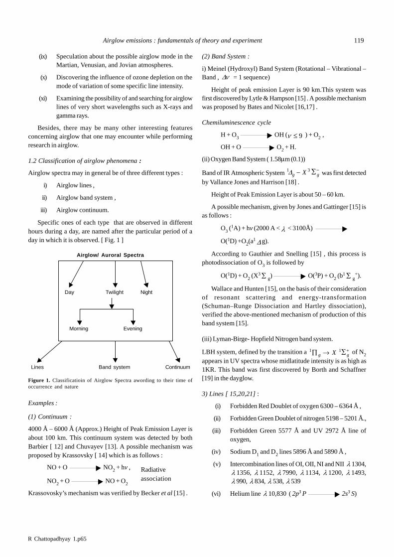
Specific ones of each type that are observed in differenthours during a day, are named after the particular period of aday in which it is observed. [ Fig. 1 ]
Airglow/ Auroral Spectra
Day Twilight Night
Morning Evening
Lines Band system Continuum
Figure 1. Classificatioin of Airglow Spectra awording to their time ofoccurrence and nature
Examples :
(1) Continuum :
4000 Å – 6000 Å (Approx.) Height of Peak Emission Layer isabout 100 km. This continuum system was detected by bothBarbier [ 12] and Chuvayev [13]. A possible mechanism wasproposed by Krassovsky [ 14] which is as follows :
NO + O NO2 + hv , Radiative
NO2 + O NO + O2association
Krassovosky’s mechanism was verified by Becker et al [15] .
(2) Band System :
i) Meinel (Hydroxyl) Band System (Rotational – Vibrational –Band , Dn = 1 sequence)
Height of peak emission Layer is 90 km.This system wasfirst discovered by Lytle & Hampson [15] . A possible mechanismwas proposed by Bates and Nicolet [16,17] .
Chemiluminescence cycle
H + O3 OH (n £ 9 ) + O2 ,
OH + O O2 + H.
(ii) Oxygen Band System ( 1.58mm (0.1))
Band of IR Atmospheric System 1 3Dg gX- å- was first detectedby Vallance Jones and Harrison [18] .
Height of Peak Emission Layer is about 50 – 60 km.
A possible mechanism, given by Jones and Gattinger [15] isas follows :
O3 (1A) + hv (2000 A <l < 3100Å)
O(1D) +O2(a1 D g).
According to Gauthier and Snelling [15] , this process isphotodissociation of O3 is followed by
O(1D) + O2 (X3 å g) O(3P) + O2 (b
1 å g+).
Wallace and Hunten [15], on the basis of their considerationof resonant scattering and energy-transformation(Schuman–Runge Dissociation and Hartley dissociation),verified the above-mentioned mechanism of production of thisband system [15].
(iii) Lyman-Birge- Hopfield Nitrogen band system.
LBH system, defined by the transition a 1 1Õ ® å+g gX of N2
appears in UV spectra whose midlatitude intensity is as high as1KR. This band was first discovered by Borth and Schaffner[19] in the dayglow.
3) Lines [ 15,20,21] :
(i) Forbidden Red Doublet of oxygen 6300 – 6364 Å ,
(ii) Forbidden Green Doublet of nitrogen 5198 – 5201 Å.,
(iii) Forbidden Green 5577 Å and UV 2972 Å line ofoxygen,
(iv) Sodium D1 and D2 lines 5896 Å and 5890 Å ,
(v) Intercombination lines of OI, OII, NI and NII l 1304,l 1356, l 1152, l 7990, l 1134, l 1200, l 1493,l 990, l 834, l 538, l 539
(vi) Helium line l 10,830 ( 2p3 P 2s3 S)
R Chattopadhyay 1.p65
120 R Chattopadhyay and S K Midya
(vii) Forbidden 7320 and 7330 Å doublet of OII and 5755Å line of NII ,
(viii) O+ 2p – 4s l 2470 UV [15, 19 ]
(ix) Li (6708 Å) [ 15, 19 ]
(x) Fe (3860 Å ) [ 15 ] ,
(xi) Mg+ Doublet l 2796, l 2803 [ 19 ],
(xii) HI 1216 Å [ 15, 19 ] ;
1.3 Different atmospheric physical parameters, observationalmethods and instrumentation:
The most fundamental physical parameters which play vital rolesin various features of terrestrial atmosphere are as follows ;
(i) Temperature, (ii) Pressure, (iii) Density, (iv) Composition,(iv) Radiation (Corpuscular), (v) Radiation (electromagneticspecially radiowave, microwave, UV, EUV, X-ray, g-ray ),(vi) Wind system, (vii) Humidities, (viii) Electron - and ion-density and (ix) Vertical distribution of ozone.
The main sources and probes for collecting informationabout the above-mentioned characteristic physicalparameters related to upper atmosphere in early 50’s were asfollows [20] :
(i) Gun shell explosions (ii) Rocket observations, (iii) Highaltitude balloons (iv) Noctilucent clouds (v) Meteorobservations, (vi) Emission from the sky (vii) Propagation ofsound waves, (viii) Propagation of radio waves, (ix) Searchlightmeasurements and (x) Theoretical studies.
Among those all possible probes for collecting informationabout upper atmosphere, the ‘Emission from the sky’ and‘theoretical studies’ are mainly dealt with in this work and arebriefly mentioned below.
Emission from the sky :
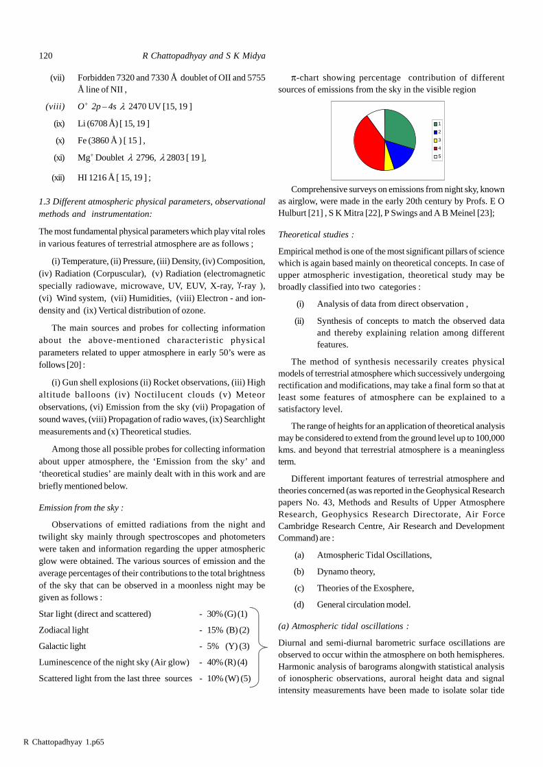
Observations of emitted radiations from the night andtwilight sky mainly through spectroscopes and photometerswere taken and information regarding the upper atmosphericglow were obtained. The various sources of emission and theaverage percentages of their contributions to the total brightnessof the sky that can be observed in a moonless night may begiven as follows :
Star light (direct and scattered) -30% (G) (1)
Zodiacal light - 15% (B) (2)
Galactic light - 5% (Y) (3)
Luminescence of the night sky (Air glow) -40% (R) (4)
Scattered light from the last three sources -10% (W) (5)
1
2
3
4
5
p-chart showing percentage contribution of differentsources of emissions from the sky in the visible region
Comprehensive surveys on emissions from night sky, knownas airglow, were made in the early 20th century by Profs. E OHulburt [21] , S K Mitra [22], P Swings and A B Meinel [23];
Theoretical studies :
Empirical method is one of the most significant pillars of sciencewhich is again based mainly on theoretical concepts. In case ofupper atmospheric investigation, theoretical study may bebroadly classified into two categories :
(i) Analysis of data from direct observation ,
(ii) Synthesis of concepts to match the observed dataand thereby explaining relation among differentfeatures.
The method of synthesis necessarily creates physicalmodels of terrestrial atmosphere which successively undergoingrectification and modifications, may take a final form so that atleast some features of atmosphere can be explained to asatisfactory level.
The range of heights for an application of theoretical analysismay be considered to extend from the ground level up to 100,000kms. and beyond that terrestrial atmosphere is a meaninglessterm.
Different important features of terrestrial atmosphere andtheories concerned (as was reported in the Geophysical Researchpapers No. 43, Methods and Results of Upper AtmosphereResearch, Geophysics Research Directorate, Air ForceCambridge Research Centre, Air Research and DevelopmentCommand) are :
(a) Atmospheric Tidal Oscillations,
(b) Dynamo theory,
(c) Theories of the Exosphere,
(d) General circulation model.
(a) Atmospheric tidal oscillations :
Diurnal and semi-diurnal barometric surface oscillations areobserved to occur within the atmosphere on both hemispheres.Harmonic analysis of barograms alongwith statistical analysisof ionospheric observations, auroral height data and signalintensity measurements have been made to isolate solar tide
R Chattopadhyay 1.p65
Airglow emissions : fundamentals of theory and experiment 121
atmosphere-circulation (to be discussed later). Dynamo-theoryalso reveals the fact that the main phase of a magnetic storm isconsistent with diurnal features of atmospheric motion deducedfrom radio-star scintillations and auroral motion.
According to the Dynamo theory, electrical conductivity ofthe ionosphere was found out to be much higher than that dueto electron density obtained only from Radio wavemeasurements. Rocket measurements confirmed the existenceof a very high ion density and of a horizontal current sheet andthus, the requirement of dynamo theory was found to be trulyrealistic.
Ionosphere comprises of equal number of positive andnegative ions embedded in a neutral gas which at some height,moves mainly by solar and lunar tidal forces. This motion ofionospheric region is presumably eased or mobilized by internalmotion caused by thermal energy. Bulk of charged particles withinthe ionosphere moves as a whole in permanent steadygeomagnetic field and this fact is obviously analogous to thecase of a dynamo in which a conductor moves within a magneticfield and produces emf. That is why the production of someamount of atmospheric emf and consequent atmospheric currentcaused by this kind of motion of ionospheric charged particlesis known as the Atmospheric Dynamo Effect [24]. Ionosphericcurrent caused by the atmospheric dynamo effect on the otherhand, produces another magnetic field which interacts with theprimary magnetic field of the Earth. This interaction followssuccessively the trio of Ampere’s circuital law, Faraday’s lawand Lenz’s law and produces a repulsive force between thesources respectively of the primary and the secondary magneticfield i.e the Earth and the ionospheric conducting sheet. As aresult of this repulsion, the electron-ion plasma in theionosphere moves as a whole, to the range of strong geomagneticfield. This is again some kind of effect that occurs within anelectrical motor. Thus, this effect is called the Atmospheric Motoreffect.
It has been found that as a first approximation, the ‘dynamo’is situated in E-region and the ‘motor’ in the F-region [24] .
(c) Theories of Exosphere :
Terrestrial atmosphere, being gravitationally bound by Earth,rotates with Earth’s axial rotation and it experiences theinfluences primarily of the following factors :
(i) Earth’s Gravitational force,
(ii) Centrifugal force due to Earth’s axial rotation,
(iii) Thermal energy which manifests mostly in the formof mean molecular kinetic energy within theatmosphere (mean free path, density, pressure),
(iv) Conservation of angular momentum ,
(v) Influence of external gravitating cosmic bodies(mainly the ‘Sun’ and the ‘Moon’),
from lunar tide. The fact that semi-diurnal barometric variationdue to the Sun is 16 times that due to Moon while tide raisingforce of the Moon is twice that of the Sun, was first pointed outby Sir William Thomson [ 20 ] and was tentatively explained byhimself on the basis of his proposition that the terrestrialatmosphere, having a period of free oscillation of nearly 12 hrs.,produces resonance. Analogously with the Thomson’sproposition, Taylor- Pekeri’s theory tells that for a particulartemperature, the height-distribution of terrestrial atmospheremay have two modes of free oscillation. Gerson [ 20 ] found thatalthough tidal variations in the terrestrial atmosphere causedby the Sun is greater than that caused by the Moon; the solartidal effect can not be easily isolated from the strong semi-diurnalharmonics of atmosphere while lunar tidal effect can readily bydetermined.
Any proposed model giving the altitudinal variation oftemperature can easily be tested by means of calculations of itsperiods of free oscillation. According to the tidal theory, thepressure distribution generates a world-wide wind system. Windsystems play important role in upper atmospheric processbecause its average speed is much higher than that within thetroposphere. Lunar tidal variations have been detected in D, E,F1 and F2 layer while solar tidal influence leaves its signaturemainly in F2-layer. The general theory of tidal oscillations,developed by Martyn [20] which is also known as‘electrodynamical theory’, is based primarily on the postulatethat the ions and electrons move only along geomagnetic fieldlines even if the tidal motions are mainly horizontal. Kirkpatrickand Mitra [20] made significant contributions in this field.
(b) Dynamo theory :
On regular undisturbed or quiet day, diurnal variations in theEarth’s magnetic field and associated parameters that necessarilyincludes the upper atmospheric current system can be explainedby the Dynamo theory first proposed by Stewart and Schuster[20]. There are two other theories ; namely, Diamagnetic theoryof Ross Gunn [20] and Chapman’s [20] Drift current theory. Thesetwo theories can not explain most of the ionospheric phenomenasatisfactorily. The two basic requirements, common for both thediamagnetic and drift current theories are high temperature andhigh electron density that prevail in source-region of terrestrialionosphere while the motion of the whole atmosphere is not atall a necessary requirement for either of these theories. But theDynamo theory is consistent with the electrical and thermalproperties of ionosphere as mentioned above and with the windsystem. World-wide regular wind systems in the ionosphericregion is presumably, partly due to variation in temperature andpartly due to tidal forces.
With the help of Dynamo theory, Vestine [ 20 ] showed thata simple monthly mean wind system of geomagnetic disturbanceagrees fairly with Kellog - Schilling model [20] of upper
R Chattopadhyay 1.p65
122 R Chattopadhyay and S K Midya
(vi) Incidence of electromagnetic radiation and cosmicray particles from outside,
(vii) Effect of geomagnetic field, Atmospheric Dynamoand Motor etc.
Amongst these, the first four determine the limit of someatmospheric equillibrium at which density becomes minimumand molecular mean-free-path becomes very very large. Theorder of magnitude of this limiting height of the terrestrialatmosphere is about 35500 kms above sea level for the equatorialplane. At this height, the mean free paths of molecules becomevery large and collisions become infrequent. Consequently, gasparticles are subjected to the gravitational force only. Thoseparticles at this height, move in conic sectional orbits. Some ofthe particles fall back to denser region of the atmosphere butescape entirely from the Earth’s vicinity after free flight for awhile. This region is called the fringe region of the atmosphereor the exosphere. Various information regarding the density andtemperature associated with the degrees of dissociation andionization and also the rates of escape of different gas-molecularspecies can be derived from calculations based on some suitablemodel.
(d) General circulation Models (GCMs) :
On the basis of consideration of general convective and othertype of circulation, some appropriate model has been constructedand with the help of those models, attempts have been made toknow about various features of terrestrial atmosphere.
Instrumentation
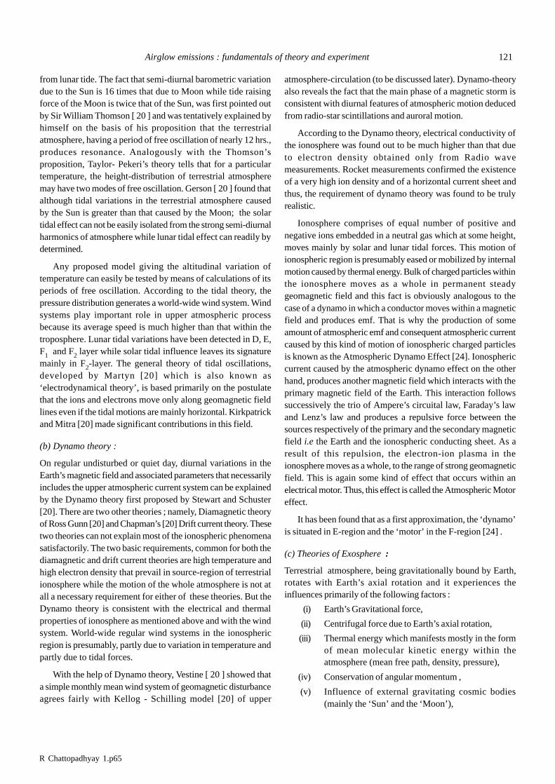
The basic physical observable of greatest concern in the studyof airglow is the intensity (i.e the brightness, total or specificline emission) of radiations. Methods of observations are mainlyof two types, each of which is subdivided on the basis oftechnological means of observation into three categories [Fig. 2]
Airglow Observation
Ground Based Observation High altitude orSpace-based Observation
Visual Photographic PhotoelectricRocket Borne Spaceshuttle-
operated(Manned Space Vehicle)
Photographic Photoelectric Visual Photometric
Advanced Imaging devices Photographic(Recent Development)
Figure 2. Different methods of airglow observation are showncategorically.
The instrument, devised mainly for the measurement ofintensity is called photometer which, according to the mechanicalor technological devices may be of three different types:
(i) Visual photometer ,
(ii) Photographic photometer,
(iii) Photoelectric photometer,
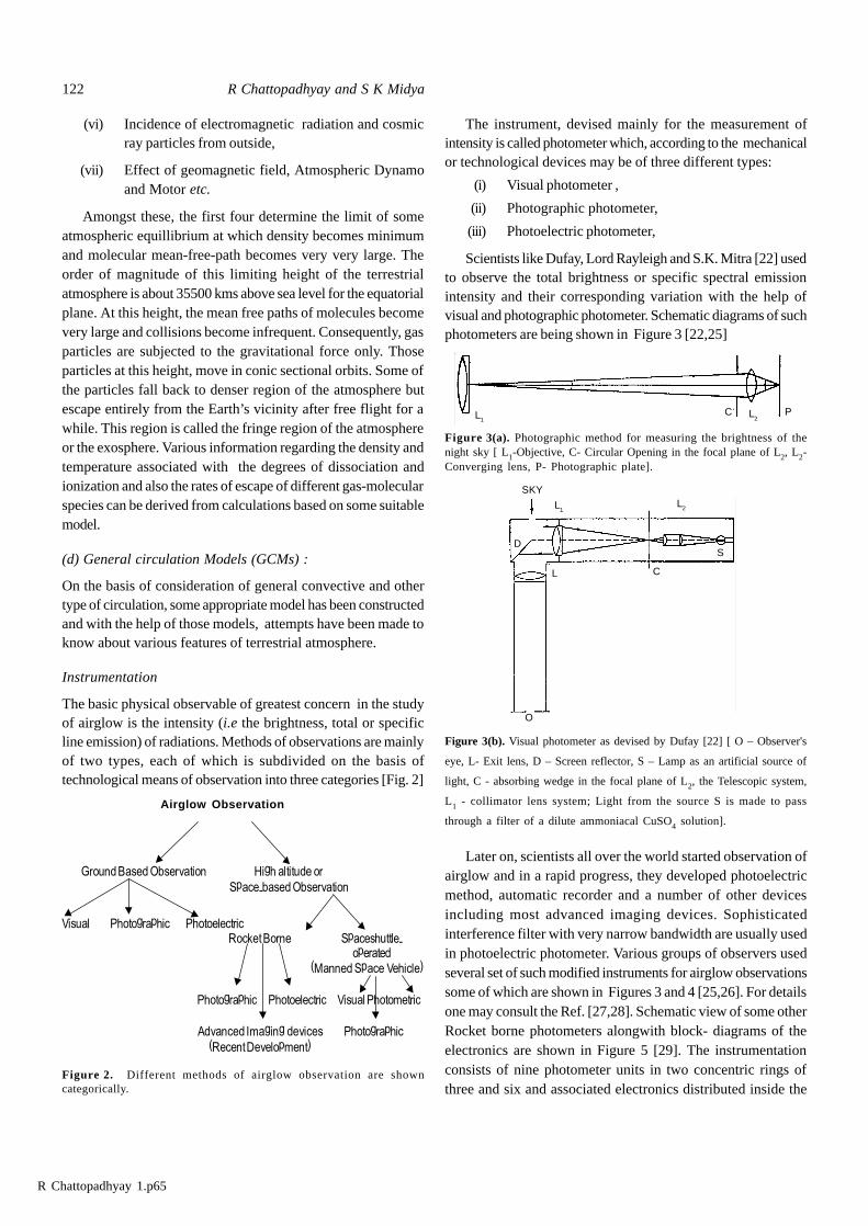
Scientists like Dufay, Lord Rayleigh and S.K. Mitra [22] usedto observe the total brightness or specific spectral emissionintensity and their corresponding variation with the help ofvisual and photographic photometer. Schematic diagrams of suchphotometers are being shown in Figure 3 [22,25]
Figure 3(a). Photographic method for measuring the brightness of thenight sky [ L1-Objective, C- Circular Opening in the focal plane of L2, L2-Converging lens, P- Photographic plate].
Figure 3(b). Visual photometer as devised by Dufay [22] [ O – Observer's
eye, L- Exit lens, D – Screen reflector, S – Lamp as an artificial source of
light, C - absorbing wedge in the focal plane of L2, the Telescopic system,
L1 - collimator lens system; Light from the source S is made to pass
through a filter of a dilute ammoniacal CuSO4 solution].
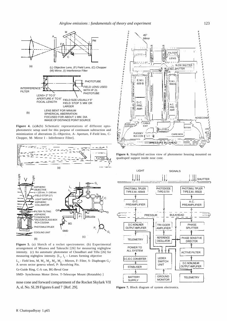
Later on, scientists all over the world started observation ofairglow and in a rapid progress, they developed photoelectricmethod, automatic recorder and a number of other devicesincluding most advanced imaging devices. Sophisticatedinterference filter with very narrow bandwidth are usually usedin photoelectric photometer. Various groups of observers usedseveral set of such modified instruments for airglow observationssome of which are shown in Figures 3 and 4 [25,26]. For detailsone may consult the Ref. [27,28]. Schematic view of some otherRocket borne photometers alongwith block- diagrams of theelectronics are shown in Figure 5 [29]. The instrumentationconsists of nine photometer units in two concentric rings ofthree and six and associated electronics distributed inside the
L1L
2C P
L1
L2
L C
SKY
SD
O
R Chattopadhyay 1.p65
Airglow emissions : fundamentals of theory and experiment 123
Figure 5. (a) Sketch of a rocket spectrometer. (b) Experimentalarrangement of Misawa and Takeuchi [26] for measuring nightglowintensity. (c) An automatic photometer of Choudhuri and Tillu [26] formeasuring nightglow intensity. [L1, l2 – Lenses forming objective
L3 - Field lens, M, M1, M2, M3, M4 – Mirrors, F- Filter, S- Diaphragm G1-A seven sector geneva wheel, P- Revolving Pin.
Gr-Guide Ring, C-A can, BG-Beval Gear
SMD- Synchronus Motor Drive. T-Telescope Mount (Rotatable) ]
Figure 6. Simplified section view of photometer housing mounted onquadruped support inside nose cone.
(a)
(b)(c)
Figure 7. Block diagram of system electronics.
Ligh
t
Ligh
t
ASPHERICOBJECTIVEe = 120 nm, f = 240 nmFIELD STOP (1O)
LIGHT SAFFLESASPHERICCOLLIMATOR
FILTER-TILTINGASPHERICCONDENCERVACUUM GLASS BOXRCA C31034A
PHOTOMULTIPLIER
COOLING UNIT
Lens
(F2.
0)
BG
GR
SMD
P
L1
L2
G1
C
G
P1
G1
M1
M
M2
45O
Mirror
RE
F B
UL
B
CA
L B
UL
B
FILTER
LENS
SLOW SHUTTERFAST SHUTTER
E.M.I.609 B
E.M.I.9592 B
D.C.PRE.AMP.
A.C.PRE.AMP.T
RIG
GE
R P
HO
TO
-DIO
DE
CABLEEXIT
CARE BOXPLESSEYBLK.CON
NOSECONE
FLEXIBLECONDUIT
MOTORS
QUADRUPEDSUPPORT
LIGHT SIGNALS
SHUTTER
PHOTOMUL TIPLIERTYPE E.M.I. 6094 B
PHOTODIODETYPE IS 701
PHOTOMUL TIPLIERTYPE E.M.I. 9592 B
D.C.PREAMPLIFIER
A.C.PREAMPLIFIER
PRESSUR BULKHEAD
D.C. NONLINEROUTPUT AMPLIFIER
TRI GGERAMPLIFIER
PHASESPLITTER
TELEMETRYREFERENCEOSCILLATOR
PHASE SENSITIVEDIRECTOR
POWER TOALL SYSTEM
D.C./D.C. CONVERTER LEDEXSWITCHUNIT
ACTIVE FILTER
STABLISER
BATTERYSUPPLY
GROUNDMONITOR
TELEMETRY
D.C. NONLINEAROUTPUT AMPLIFIER
Figure 4. (a)&(b) Schematic representations of different opto-photometric setup used for this purpose of continuum subtraction andminimization of aberrations [L–Objective, A- Aperture, F-Field lens, C-Chopper, M- Mirror I - Inferfernece Filter].
(a)
(b)
L A
M
PM
C
F
(L) Objective Lens, (F) Field Lens, (C) Chopper(M) Mirror, (I) Interference Filter
I
INTERFERENCEFILTER
LENS= 2" TO 3"APERTURE 4" TO 6"FOCAL LENGTH
FIELD SIZE USUALLY 50
FIELD STOP 5 MM ORLARGER
PHOTOTUBE
FIELD LENS USEDWITH IP 21PHOTOTUBE
LENS BENT FOR MINIUMSPHERICAL ABERRATIONFOCUSED FOR ABOUT 1 MM. DIAIMAGE OF DISTANCE POINT SOURCE
nose cone and forward compartment of the Rocket Skylark VIIA, sl. No. SL39 Figures 6 and 7 [Ref. 29].
R Chattopadhyay 1.p65
124 R Chattopadhyay and S K Midya
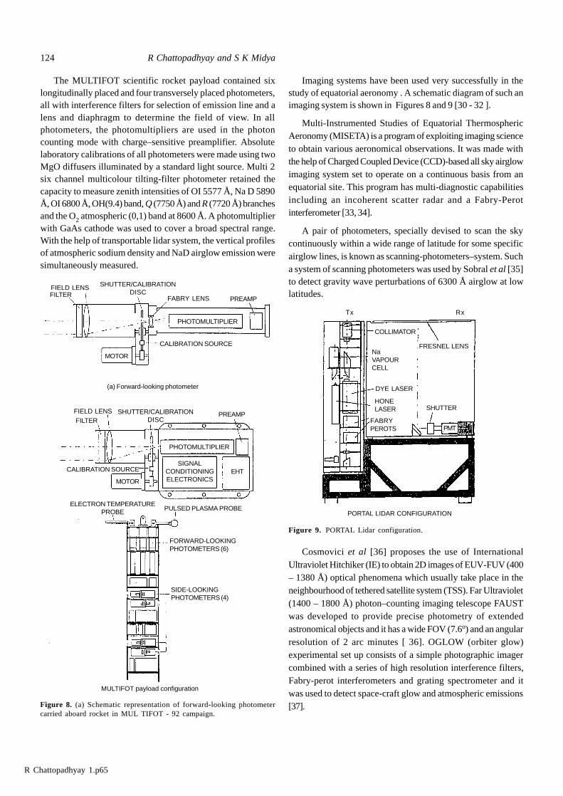
The MULTIFOT scientific rocket payload contained sixlongitudinally placed and four transversely placed photometers,all with interference filters for selection of emission line and alens and diaphragm to determine the field of view. In allphotometers, the photomultipliers are used in the photoncounting mode with charge–sensitive preamplifier. Absolutelaboratory calibrations of all photometers were made using twoMgO diffusers illuminated by a standard light source. Multi 2six channel multicolour tilting-filter photometer retained thecapacity to measure zenith intensities of OI 5577 Å, Na D 5890Å, OI 6800 Å, OH(9.4) band, Q (7750 Å) and R (7720 Å) branchesand the O2 atmospheric (0,1) band at 8600 Å. A photomultiplierwith GaAs cathode was used to cover a broad spectral range.With the help of transportable lidar system, the vertical profilesof atmospheric sodium density and NaD airglow emission weresimultaneously measured.
Imaging systems have been used very successfully in thestudy of equatorial aeronomy . A schematic diagram of such animaging system is shown in Figures 8 and 9 [30 - 32 ].
Multi-Instrumented Studies of Equatorial ThermosphericAeronomy (MISETA) is a program of exploiting imaging scienceto obtain various aeronomical observations. It was made withthe help of Charged Coupled Device (CCD)-based all sky airglowimaging system set to operate on a continuous basis from anequatorial site. This program has multi-diagnostic capabilitiesincluding an incoherent scatter radar and a Fabry-Perotinterferometer [33, 34].
A pair of photometers, specially devised to scan the skycontinuously within a wide range of latitude for some specificairglow lines, is known as scanning-photometers–system. Sucha system of scanning photometers was used by Sobral et al [35]to detect gravity wave perturbations of 6300 Å airglow at lowlatitudes.
Figure 9. PORTAL Lidar configuration.
Cosmovici et al [36] proposes the use of InternationalUltraviolet Hitchiker (IE) to obtain 2D images of EUV-FUV (400– 1380 Å) optical phenomena which usually take place in theneighbourhood of tethered satellite system (TSS). Far Ultraviolet(1400 – 1800 Å) photon–counting imaging telescope FAUSTwas developed to provide precise photometry of extendedastronomical objects and it has a wide FOV (7.6o) and an angularresolution of 2 arc minutes [ 36]. OGLOW (orbiter glow)experimental set up consists of a simple photographic imagercombined with a series of high resolution interference filters,Fabry-perot interferometers and grating spectrometer and itwas used to detect space-craft glow and atmospheric emissions[37].
MULTIFOT payload configuration
Figure 8. (a) Schematic representation of forward-looking photometercarried aboard rocket in MUL TIFOT - 92 campaign.
Tx Rx
PORTAL LIDAR CONFIGURATION
FIELD LENSFILTER
SHUTTER/CALIBRATIONDISC
FABRY LENS PREAMP
PHOTOMULTIPLIER
CALIBRATION SOURCE
MOTOR
(a) Forward-looking photometer
FIELD LENSFILTER
SHUTTER/CALIBRATIONDISC
PREAMP
PHOTOMULTIPLIER
MOTOR
CALIBRATION SOURCE EHTSIGNAL
CONDITIONINGELECTRONICS
PULSED PLASMA PROBEELECTRON TEMPERATURE
PROBE
FORWARD-LOOKINGPHOTOMETERS (6)
SIDE-LOOKINGPHOTOMETERS (4)
COLLIMATOR
FRESNEL LENSNaVAPOURCELL
DYE LASER
HONELASER SHUTTER
FABRYPEROTS PMT
R Chattopadhyay 1.p65
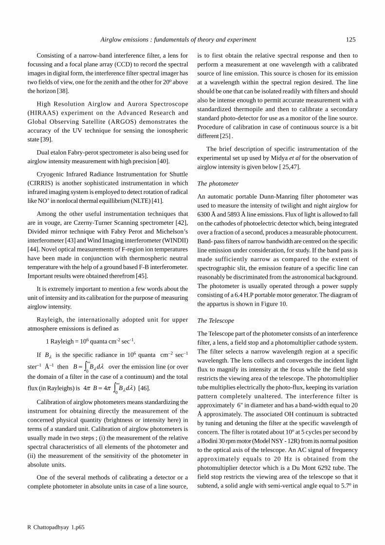
Airglow emissions : fundamentals of theory and experiment 125
Consisting of a narrow-band interference filter, a lens forfocussing and a focal plane array (CCD) to record the spectralimages in digital form, the interference filter spectral imager hastwo fields of view, one for the zenith and the other for 20o abovethe horizon [38].
High Resolution Airglow and Aurora Spectroscope(HIRAAS) experiment on the Advanced Research andGlobal Observing Satellite (ARGOS) demonstrates theaccuracy of the UV technique for sensing the ionosphericstate [39].
Dual etalon Fabry-perot spectrometer is also being used forairglow intensity measurement with high precision [40].
Cryogenic Infrared Radiance Instrumentation for Shuttle(CIRRIS) is another sophisticated instrumentation in whichinfrared imaging system is employed to detect rotation of radicallike NO+ in nonlocal thermal equillibrium (NLTE) [41].
Among the other useful instrumentation techniques thatare in vouge, are Czerny-Turner Scanning spectrometer [42],Divided mirror technique with Fabry Perot and Michelson’sinterferometer [43] and Wind Imaging interferometer (WINDII)[44]. Novel optical measurements of F-region ion temperatureshave been made in conjunction with thermospheric neutraltemperature with the help of a ground based F-B interferometer.Important results were obtained therefrom [45].
It is extremely important to mention a few words about theunit of intensity and its calibration for the purpose of measuringairglow intensity.
Rayleigh, the internationally adopted unit for upperatmosphere emissions is defined as
1 Rayleigh = 106 quanta cm-2 sec-1.
If Bl is the specific radiance in 106 quanta cm–2 sec–1
ster–1 Å–1 then B B d=¥z l l0
over the emission line (or over
the domain of a filter in the case of a continuum) and the total
flux (in Rayleighs) is 4 40
p p llB B d=¥z ) [46].
Calibration of airglow photometers means standardizing theinstrument for obtaining directly the measurement of theconcerned physical quantity (brightness or intensity here) interms of a standard unit. Calibration of airglow photometers isusually made in two steps ; (i) the measurement of the relativespectral characteristics of all elements of the photometer and(ii) the measurement of the sensitivity of the photometer inabsolute units.
One of the several methods of calibrating a detector or acomplete photometer in absolute units in case of a line source,
is to first obtain the relative spectral response and then toperform a measurement at one wavelength with a calibratedsource of line emission. This source is chosen for its emissionat a wavelength within the spectral region desired. The lineshould be one that can be isolated readily with filters and shouldalso be intense enough to permit accurate measurement with astandardized thermopile and then to calibrate a secondarystandard photo-detector for use as a monitor of the line source.Procedure of calibration in case of continuous source is a bitdifferent [25] .
The brief description of specific instrumentation of theexperimental set up used by Midya et al for the observation ofairglow intensity is given below [ 25,47].
The photometer
An automatic portable Dunn-Manring filter photometer wasused to measure the intensity of twilight and night airglow for6300 Å and 5893 Å line emissions. Flux of light is allowed to fallon the cathodes of photoelectric detector which, being integratedover a fraction of a second, produces a measurable photocurrent.Band- pass filters of narrow bandwidth are centred on the specificline emission under consideration, for study. If the band pass ismade sufficiently narrow as compared to the extent ofspectrographic slit, the emission feature of a specific line canreasonably be discriminated from the astronomical background.The photometer is usually operated through a power supplyconsisting of a 6.4 H.P portable motor generator. The diagram ofthe appartus is shown in Figure 10.
The Telescope
The Telescope part of the photometer consists of an interferencefilter, a lens, a field stop and a photomultiplier cathode system.The filter selects a narrow wavelength region at a specificwavelength. The lens collects and converges the incident lightflux to magnify its intensity at the focus while the field stoprestricts the viewing area of the telescope. The photomultipliertube multiplies electrically the photo-flux, keeping its variationpattern completely unaltered. The interference filter isapproximately 6" in diameter and has a band-width equal to 20Å approximately. The associated OH continuum is subtractedby tuning and detuning the filter at the specific wavelength ofconcern. The filter is rotated about 10o at 5 cycles per second bya Bodini 30 rpm motor (Model NSY - 12R) from its normal positionto the optical axis of the telescope. An AC signal of frequencyapproximately equals to 20 Hz is obtained from thephotomultiplier detector which is a Du Mont 6292 tube. Thefield stop restricts the viewing area of the telescope so that itsubtend, a solid angle with semi-vertical angle equal to 5.7o in
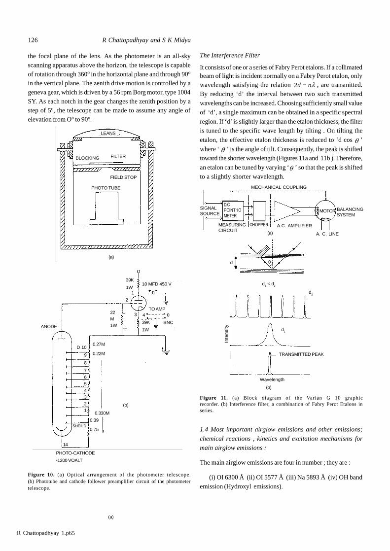
R Chattopadhyay 1.p65
126 R Chattopadhyay and S K Midya
the focal plane of the lens. As the photometer is an all-skyscanning apparatus above the horizon, the telescope is capableof rotation through 360o in the horizontal plane and through 90o
in the vertical plane. The zenith drive motion is controlled by ageneva gear, which is driven by a 56 rpm Borg motor, type 1004SY. As each notch in the gear changes the zenith position by astep of 5o, the telescope can be made to assume any angle ofelevation from Oo to 90o.
Figure 10. (a) Optical arrangement of the photometer telescope.(b) Phototube and cathode follower preamplifier circuit of the photometertelescope.
The Interference Filter
It consists of one or a series of Fabry Perot etalons. If a collimatedbeam of light is incident normally on a Fabry Perot etalon, onlywavelength satisfying the relation 2d n= l , are transmitted.
By reducing ‘d’ the interval between two such transmittedwavelengths can be increased. Choosing sufficiently small value
of ‘d’, a single maximum can be obtained in a specific spectral
region. If ‘d’ is slightly larger than the etalon thickness, the filteris tuned to the specific wave length by tilting . On tilting the
etalon, the effective etalon thickness is reduced to ‘d cos q ’
where ‘ q ’ is the angle of tilt. Consequently, the peak is shiftedtoward the shorter wavelength (Figures 11a and 11b ). Therefore,
an etalon can be tuned by varying ‘q ’ so that the peak is shifted
to a slightly shorter wavelength.
Figure 11. (a) Block diagram of the Varian G 10 graphicrecorder. (b) Interference filter, a combination of Fabry Perot Etalons inseries.
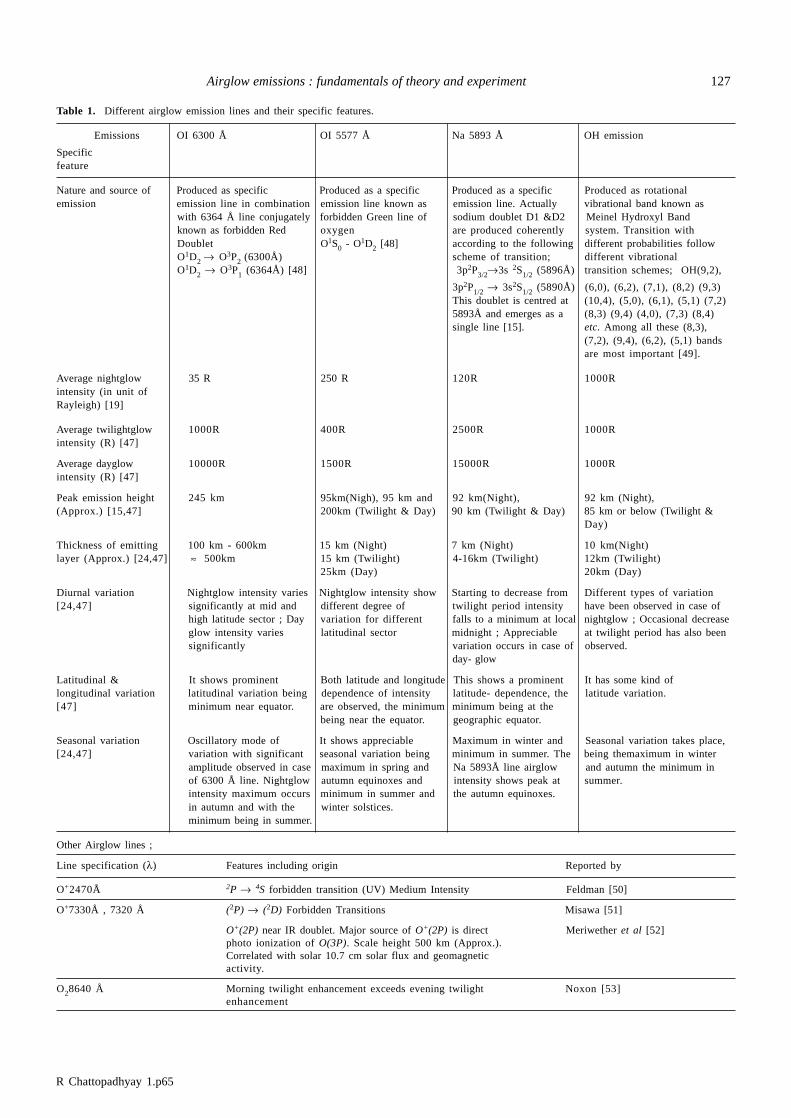
1.4 Most important airglow emissions and other emissions;
chemical reactions , kinetics and excitation mechanisms for
main airglow emissions :
The main airglow emissions are four in number ; they are :
(i) OI 6300 Å (ii) OI 5577 Å (iii) Na 5893 Å (iv) OH bandemission (Hydroxyl emissions).
(a)
(a)
(a)
(b)
(b)
LEANS
BLOCKING FILTER
FIELD STOP
PHOTO TUBE
ANODE
0.27M
0.22M
PHOTO-CATHODE
-1200 VOALT
0.330M
0.39
0.75
10 MFD 450 V39K
1W1
2
22M1W
TO AMP3 4 0
39K
1W
BNC
D 10
9
8
765
4321
SIGNALSOURCE
D.CPOINT 1OMETER
MECHANICAL COUPLING
MEASURINGCIRCUIT
CHOPPER A.C. AMPLIFIER
MOTOR BALANCINGSYSTEM
A. C. LINE
d 0
d1 < d
2
d2
Inte
nsi
ty d1
TRANSMITTED PEAK
Wavelength
SHEILD
14
R Chattopadhyay 1.p65
Airglow emissions : fundamentals of theory and experiment 127
Table 1. Different airglow emission lines and their specific features.
Emissions OI 6300 Å OI 5577 Å Na 5893 Å OH emission
Specificfeature
Nature and source of Produced as specific Produced as a specific Produced as a specificProduced as rotationalemission emission line in combinationemission line known as emission line. Actually vibrational band known as
with 6364 Å line conjugately forbidden Green line of sodium doublet D1 &D2 Meinel Hydroxyl Bandknown as forbidden Red oxygen are produced coherently system. Transition withDoublet O1S0 - O
1D2 [48] according to the following different probabilities followO1D2 ® O3P2 (6300Å) scheme of transition; different vibrationalO1D2 ® O3P1 (6364Å) [48] 3p2P3/2®3s 2S1/2 (5896Å) transition schemes; OH(9,2),
3p2P1/2 ® 3s2S1/2 (5890Å) (6,0), (6,2), (7,1), (8,2) (9,3)This doublet is centred at (10,4), (5,0), (6,1), (5,1) (7,2)5893Å and emerges as a (8,3) (9,4) (4,0), (7,3) (8,4)single line [15]. etc. Among all these (8,3),
(7,2), (9,4), (6,2), (5,1) bandsare most important [49].
Average nightglow 35 R 250 R 120R 1000Rintensity (in unit ofRayleigh) [19]
Average twilightglow 1000R 400R 2500R 1000Rintensity (R) [47]
Average dayglow 10000R 1500R 15000R 1000Rintensity (R) [47]
Peak emission height 245 km 95km(Nigh), 95 km and 92 km(Night), 92 km (Night),(Approx.) [15,47] 200km (Twilight & Day) 90 km (Twilight & Day) 85 km or below (Twilight &
Day)
Thickness of emitting 100 km - 600km 15 km (Night) 7 km (Night) 10 km(Night)layer (Approx.) [24,47] » 500km 15 km (Twilight) 4-16km (Twilight) 12km (Twilight)
25km (Day) 20km (Day)
Diurnal variation Nightglow intensity varies Nightglow intensity show Starting to decrease fromDifferent types of variation[24,47] significantly at mid and different degree of twilight period intensity have been observed in case of
high latitude sector ; Day variation for different falls to a minimum at local nightglow ; Occasional decreaseglow intensity varies latitudinal sector midnight ; Appreciable at twilight period has also beensignificantly variation occurs in case of observed.
day- glow
Latitudinal & It shows prominent Both latitude and longitude This shows a prominent It has some kind oflongitudinal variation latitudinal variation being dependence of intensity latitude- dependence, the latitude variation.[47] minimum near equator. are observed, the minimum minimum being at the
being near the equator. geographic equator.
Seasonal variation Oscillatory mode of It shows appreciable Maximum in winter and Seasonal variation takes place,[24,47] variation with significant seasonal variation being minimum in summer. The being themaximum in winter
amplitude observed in case maximum in spring and Na 5893Å line airglow and autumn the minimum inof 6300 Å line. Nightglow autumn equinoxes and intensity shows peak atsummer.intensity maximum occursminimum in summer and the autumn equinoxes.in autumn and with the winter solstices.minimum being in summer.
Other Airglow lines ;
Line specification (l) Features including origin Reported by
O+2470Å 2P ® 4S forbidden transition (UV) Medium Intensity Feldman [50]
O+7330Å , 7320 Å (2P) ® (2D) Forbidden Transitions Misawa [51]
O+(2P) near IR doublet. Major source of O+(2P) is direct Meriwether et al [52]photo ionization of O(3P). Scale height 500 km (Approx.).Correlated with solar 10.7 cm solar flux and geomagneticactivity.
O28640 Å Morning twilight enhancement exceeds evening twilight Noxon [53]enhancement
R Chattopadhyay 1.p65
128 R Chattopadhyay and S K Midya
O2(0-1) 8645 Å High correlation with 5577 Å indicates that its origin is the Misawa [54]same as that of 5577 Å line.
Inter combination lines 834 Å 2s2p4(4P) —> 2p3(4So) Fastie et al [58]
of OI & OII 538 Å 2p4(2P) —> 2p3(2Do) Brune et al [59]
539 Å 3s (4P) —> 2p3(4So) Christensen [60]
1304 Å Triplet (1304) 2p33s3(So) - 2p4(3P) Feldman et al [61]
8446 Å (1356) 3s5(So) - 2p4(3P)
4368 Å (1152) 3s1(1D0) - 2p4(1D)
1356 Å (990) 3s2 (3Do)- 2p4(3P)
7774 Å Quintet (7990) 3s2(3Do) - 3p(3P)
9264 Å Shows geomagnetic anomaly ;
6157 Å Low intensity , shows altitude variation
1152 Å
990 Å
7990 Å
NI 5200 Å Produced at F-region, quenched by free electron and Federick [62]atomic oxygen .
N24278 Å Photoionization of N2 by scattered solar radiation at Meriwetter [63]340 Å and 584 Å, shows little variation over nights.
N2(C3P) 3371 A N2 ( C
3P ) is excited by low energy electrons. Frederick et al [64]
Observed in the polar region
NO (1-0) 2150 Å NO (1-0) í band at 2150 Å Beran et al [65]
OH 6329 Å Shows twilight enhancement. Misawa [66]
6563 Å This line has got its annual and semiannual components Fishkova [67]of seasonal variation .
Fe 3860 Å Resonance Scattering , observed in twilight spectrum. Broadfoot [68]
Ca+ 3933-3968 Å Resonance Scattering of solar radiation. Observed in lower Tepelay [69]thermospheric intermediate layers Dufay [70]
Vallence Jones[71]
Mg+ Resonance Scattering Naricsi [72]
MgI 2852 Å Observable in F-region, mostly in late afternoon Young et al [73]
MgII 2800 Å
Mg 2796 Å & 2803 Å Doublet i) 3s2S1-3p2P1/2 Gerand and Monfils [74]
ii) 3s2S1/2 - 3p2P3/2
Equatorial airglow lines indicate the presence of Mg+ ionsin the evening twilight F-region
HI 1216 Å Photon - electron radiative recombination excites neutral Kazakov(75]hydrogen to the 2nd quantum level which causes the emission line
K Observed in twilight glow Sullivan and Hunten [76]
N(2D) 5198 Å-5201 Å O± - N2 ion-atom interchange process followed by NO+ Blackwell et al [15]dissociative recombination.
Low intensity night airglow lines
2972 Å UV , Forbidden transition of oxygen atom (1S —> 3P) Cohen-Sabban and Vuillemin [15]
Intercombination line 1134 Å 2s2p4(4P) - 2s22p3(4So) Takacks and Feldman [77]of NI and NII 1200 Å 2p23s(4P) - 2p3(4So) Meier et al [15]
1493 Å 3s 2p2(2P) - 2p3(2Do) Hudson and Kieffer [15]
Impact dissociative excitation
and photodissociative excitation
Table 1. (contd.)
R Chattopadhyay 1.p65
Airglow emissions : fundamentals of theory and experiment 129
He 10830 Å 2p 3Po - 2s (3S) Shefov [15]HeI 584 Å High twilight intensity value, (Resonance scattering by Teixeire et al [15]
metastable He) Donahaue et al [78]
NII 5755 Å (1S)- (1D) forbidden transition dissociative ionization by EUV Torr et al [15]radiation and low intensity twilight glow
Li 6708 Å Impact dissociative excitation Delannoy and Weill [79]
LiO*+ O —> Li*+O2 Henrikson [80]
Li * - Li+hí(6708 A)
Height distribution of intensity is similar to that of NaD lineintensity; Low intensity line .
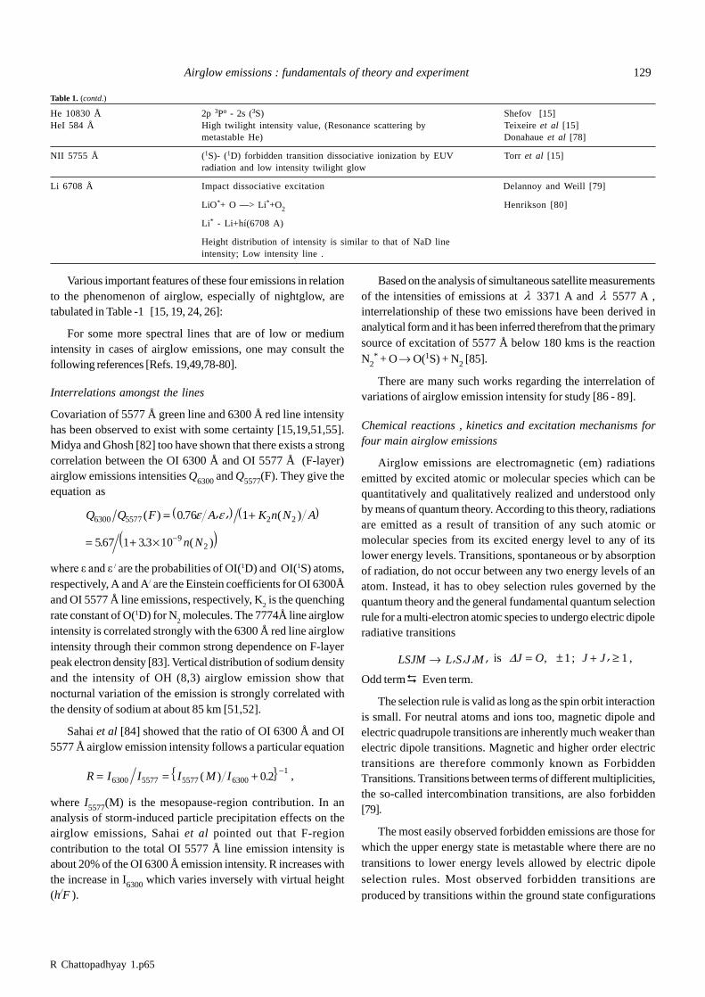
Various important features of these four emissions in relationto the phenomenon of airglow, especially of nightglow, aretabulated in Table -1 [15, 19, 24, 26]:
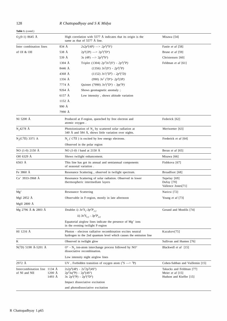
For some more spectral lines that are of low or mediumintensity in cases of airglow emissions, one may consult thefollowing references [Refs. 19,49,78-80].
Interrelations amongst the lines
Covariation of 5577 Å green line and 6300 Å red line intensityhas been observed to exist with some certainty [15,19,51,55].Midya and Ghosh [82] too have shown that there exists a strongcorrelation between the OI 6300 Å and OI 5577 Å (F-layer)airglow emissions intensities Q6300 and Q5577(F). They give theequation as
Q Q F A K n N A6300 5577 2 20 76 1( ) . ( )= ¢ ¢ +e ea f a f
= + ´ -567 1 33 1092. . ( )n Nd i
where å and å / are the probabilities of OI(1D) and OI(1S) atoms,respectively, A and A/ are the Einstein coefficients for OI 6300Åand OI 5577 Å line emissions, respectively, K
2 is the quenching
rate constant of O(1D) for N2 molecules. The 7774Å line airglow
intensity is correlated strongly with the 6300 Å red line airglowintensity through their common strong dependence on F-layerpeak electron density [83]. Vertical distribution of sodium densityand the intensity of OH (8,3) airglow emission show thatnocturnal variation of the emission is strongly correlated withthe density of sodium at about 85 km [51,52].
Sahai et al [84] showed that the ratio of OI 6300 Å and OI5577 Å airglow emission intensity follows a particular equation
R I I I M I= = +-
6300 5577 5577 63001
0 2( ) .l q ,
where I5577(M) is the mesopause-region contribution. In ananalysis of storm-induced particle precipitation effects on theairglow emissions, Sahai et al pointed out that F-regioncontribution to the total OI 5577 Å line emission intensity isabout 20% of the OI 6300 Å emission intensity. R increases withthe increase in I6300 which varies inversely with virtual height(h/F ).
Based on the analysis of simultaneous satellite measurementsof the intensities of emissions at l 3371 A and l 5577 A ,interrelationship of these two emissions have been derived inanalytical form and it has been inferred therefrom that the primarysource of excitation of 5577 Å below 180 kms is the reactionN2
* + O ® O(1S) + N2 [85].
There are many such works regarding the interrelation ofvariations of airglow emission intensity for study [86 - 89].
Chemical reactions , kinetics and excitation mechanisms forfour main airglow emissions
Airglow emissions are electromagnetic (em) radiationsemitted by excited atomic or molecular species which can bequantitatively and qualitatively realized and understood onlyby means of quantum theory. According to this theory, radiationsare emitted as a result of transition of any such atomic ormolecular species from its excited energy level to any of itslower energy levels. Transitions, spontaneous or by absorptionof radiation, do not occur between any two energy levels of anatom. Instead, it has to obey selection rules governed by thequantum theory and the general fundamental quantum selectionrule for a multi-electron atomic species to undergo electric dipoleradiative transitions
LSJM L S J M® ¢ ¢ ¢ ¢ is DJ O J J= ± + ¢ ³, ; ,1 1
Odd term D Even term.
The selection rule is valid as long as the spin orbit interactionis small. For neutral atoms and ions too, magnetic dipole andelectric quadrupole transitions are inherently much weaker thanelectric dipole transitions. Magnetic and higher order electrictransitions are therefore commonly known as ForbiddenTransitions. Transitions between terms of different multiplicities,the so-called intercombination transitions, are also forbidden[79].
The most easily observed forbidden emissions are those forwhich the upper energy state is metastable where there are notransitions to lower energy levels allowed by electric dipoleselection rules. Most observed forbidden transitions areproduced by transitions within the ground state configurations
Table 1. (contd.)
R Chattopadhyay 1.p65
130 R Chattopadhyay and S K Midya
because for most of the atom and ions, all levels of the groundstate configurations lie below all corresponding excited stateconfigurations and consequently, are all metastable. Airglowemissions are produced both through allowed and forbiddentransitions although most important ones are produced throughforbidden transitions. Transitions are possible only when theatomic or molecular species undergo the process of excitation.The action-reaction schemes via energetics that paves the wayof excitation are collectively known as the excitation-mechanism.
Chemical Kinetics is the branch of Physical Chemistry whichdeals with the speed of reaction or reaction rate, factors thatinfluence the rate and reaction mechanism. The reaction ratedepends on the nature of reacting species, concentration ofeach such species, ambient temperature, presence of extraneousbodies and energising em waves.
Reactions occurring entirely within one phase are knowncollectively as homogeneous reaction while reactions, in whichphase transformation takes place on the surface of catalyst orof the container wall, are collectively known as heterogenousreactions [90] . Rate of a reaction is defined as
R dc dt dx dt= - =l q l q ,
where ‘c’ is the concentration of the reacting species at anytime ‘t’ and ‘x’ is the concentration of the product-species atthe same time ‘t’ . The order of reaction is the number ofconcentration terms on which reaction rate depends. The firstorder reaction rate is ‘kc’ where ‘k’ is the rate constant and ‘c’ isthe concentration of a reacting species ; similarly, second orderreaction rate is ‘kc2’ and so on.
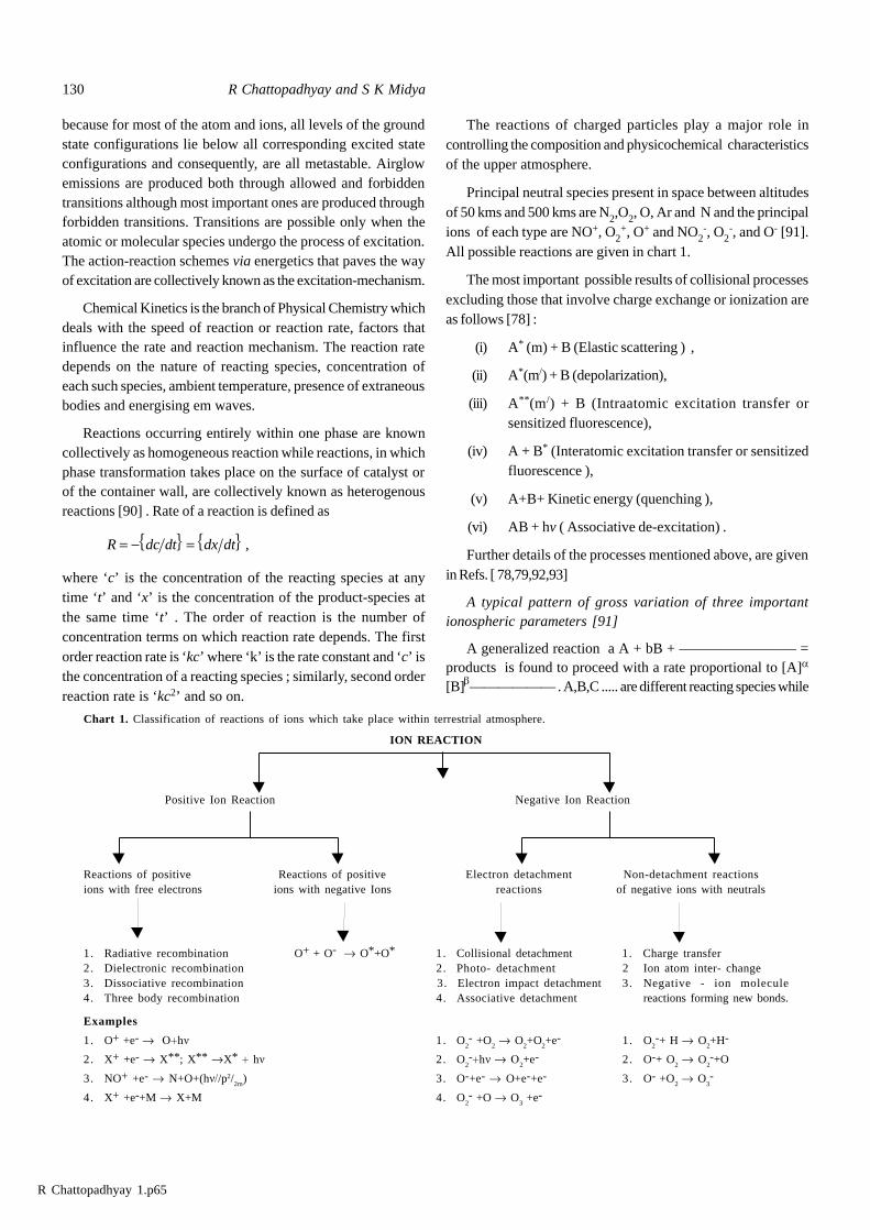
Chart 1. Classification of reactions of ions which take place within terrestrial atmosphere.
ION REACTION
Positive Ion Reaction Negative Ion Reaction
Reactions of positive Reactions of positive Electron detachment Non-detachment reactionsions with free electrons ions with negative Ions reactions of negative ions with neutrals
1. Radiative recombination O+ + O- ® O*+O* 1. Collisional detachment 1. Charge transfer2. Dielectronic recombination 2.Photo- detachment 2 Ion atom inter- change3. Dissociative recombination 3. Electron impact detachment 3.Negative - ion molecule4. Three body recombination 4. Associative detachment reactions forming new bonds.
Examples
1. O+ +e- ® O+hí 1. O2- +O
2 ® O
2+O
2+e- 1. O
2-+ H ® O
2+H-
2. X+ +e- ® X** ; X** ®X* + hí 2. O2-+hí ® O
2+e- 2. O-+ O
2 ® O
2-+O
3. NO+ +e- ® N+O+(hí//p2/2m
) 3. O-+e- ® O+e-+e- 3. O- +O2 ® O
3-
4. X+ +e-+M ® X+M 4. O2- +O ® O
3 +e-
The reactions of charged particles play a major role incontrolling the composition and physicochemical characteristicsof the upper atmosphere.
Principal neutral species present in space between altitudesof 50 kms and 500 kms are N2,O2, O, Ar and N and the principalions of each type are NO+, O2
+, O+ and NO2-, O2
-, and O- [91].All possible reactions are given in chart 1.
The most important possible results of collisional processesexcluding those that involve charge exchange or ionization areas follows [78] :
(i) A* (m) + B (Elastic scattering ) ,
(ii) A *(m/) + B (depolarization),
(iii) A ** (m/) + B (Intraatomic excitation transfer orsensitized fluorescence),
(iv) A + B* (Interatomic excitation transfer or sensitizedfluorescence ),
(v) A+B+ Kinetic energy (quenching ),
(vi) AB + hv ( Associative de-excitation) .
Further details of the processes mentioned above, are givenin Refs. [ 78,79,92,93]
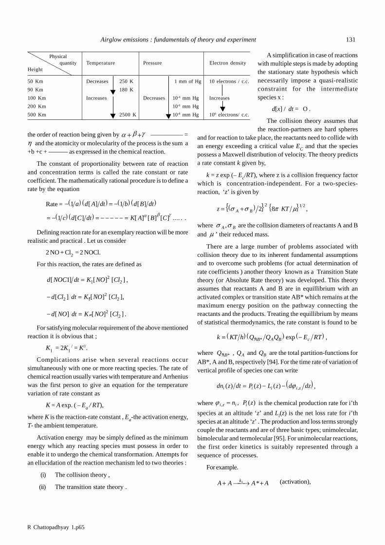
A typical pattern of gross variation of three importantionospheric parameters [91]
A generalized reaction a A + bB + ———————— =products is found to proceed with a rate proportional to [A]a
[B]b—————— . A,B,C ..... are different reacting species while
R Chattopadhyay 1.p65
Airglow emissions : fundamentals of theory and experiment 131
the order of reaction being given by a b g+ + ————— =h and the atomicity or molecularity of the process is the sum a+b +c + ——— as expressed in the chemical reaction.
The constant of proportionality between rate of reactionand concentration terms is called the rate constant or ratecoefficient. The mathematically rational procedure is to define arate by the equation
Rate = - = -1 1a d A dt b d B dta f a f a f a f[ ] [ ]
= - = - - - - - =1 c d C dt K A B Ca f a f[ ] [ ] [ ] [ ] .... .a b g .
Defining reaction rate for an exemplary reaction will be morerealistic and practical . Let us consider
2 NO + Cl2 = 2 NOCl.
For this reaction, the rates are defined as
d NOC dt K NO Cl[ ] [ ] [ ] ,1 12
2=
- = ¢d Cl dt K NO Cl[ ] [ ] [ ],2 12
2
- = ¢¢d NO dt K NO Cl[ ] [ ] [ ] .22
For satisfying molecular requirement of the above mentionedreaction it is obvious that ;
K1 = 2K1 / = K//.
Complications arise when several reactions occursimultaneously with one or more reacting species. The rate ofchemical reaction usually varies with temperature and Arrheniuswas the first person to give an equation for the temperaturevariation of rate constant as
K = A exp. ( – Ea / RT),
where K is the reaction-rate constant , Ea-the activation energy,T- the ambient temperature.
Activation energy may be simply defined as the minimumenergy which any reacting species must possess in order toenable it to undergo the chemical transformation. Attempts foran ellucidation of the reaction mechanism led to two theories :
(i) The collision theory ,
(ii) The transition state theory .
A simplification in case of reactionswith multiple steps is made by adoptingthe stationary state hypothesis whichnecessarily impose a quasi-realisticconstraint for the intermediatespecies x :
d[x] / dt = O .
The collision theory assumes thatthe reaction-partners are hard spheres
and for reaction to take place, the reactants need to collide withan energy exceeding a critical value EC and that the speciespossess a Maxwell distribution of velocity. The theory predictsa rate constant k given by,
k = z exp (– Ec/RT), where z is a collision frequency factorwhich is concentration-independent. For a two-species-reaction, ‘z’ is given by
z KTA B= +s s p ma fm r l q2 82 1 2
,
where s sA B, are the collision diameters of reactants A and Band m ’ their reduced mass.
There are a large number of problems associated withcollision theory due to its inherent fundamental assumptionsand to overcome such problems (for actual determination ofrate coefficients ) another theory known as a Transition Statetheory (or Absolute Rate theory) was developed. This theoryassumes that reactants A and B are in equillibrium with anactivated complex or transition state AB* which remains at themaximum energy position on the pathway connecting thereactants and the products. Treating the equillibrium by meansof statistical thermodynamics, the rate constant is found to be
k KT h Q Q Q E RTAB A B c= ¢ -a f a f a f* exp ,
where ¢QAB* , QA and QB are the total partition-functions for
AB*, A and B, respectively [94]. For the time rate of variation ofvertical profile of species one can write
dn z dt P z L z d dzi i i i z( ) ( ) ( ) ,= - - jc h ,
where j i z i in P z, , ( )= is the chemical production rate for i’th
species at an altitude ‘z’ and Li(z) is the net loss rate for i’thspecies at an altitude ‘z’ . The production and loss terms stronglycouple the reactants and are of three basic types; unimolecular,bimolecular and termolecular [95]. For unimolecular reactions,the first order kinetics is suitably represented through asequence of processes.
For example.
A A A Ak+ ¾ ®¾ +1 * (activation),
Physical quantity Temperature Pressure Electron densityHeight
50 Km Decreases 250 K 1 mm of Hg 10 electrons / c.c.
90 Km 180 K
100 Km Increases Decreases 10-4 mm Hg Increases
200 Km 10-6 mm Hg
500 Km 2500 K 10-8 mm Hg 106 electrons/ c.c.
R Chattopadhyay 1.p65
132 R Chattopadhyay and S K Midya
A A A Ak* *+ ¾ ®¾ +2 (deactivation),
A A hvk* 3¾ ®¾ + productions + radiations
(reaction).
Application of the stationary state hypothesis for [A*] givesthe result
- = +d A dt k k A k A k[ ] [ ] [ ]1 32
2 3d i a f .
Normally, the system obeys the law of first order kinetics;but at sufficiently low pressure, the reaction becomes secondorder. Most of the chemical processes that take place within theatmosphere follow a third order kinetics and may be representedby a termolecular chemical reaction. A symbolical representationof such process is
A B M AB M+ + ¾ ®¾ + ,
where M is the third body. This process can be thought tocomprise a sequence of steps such as,
A B ABk+ ¾ ®¾4 * ,
AB M AB Mk* ,+ ¾ ®¾ +5
AB A Bk* .6¾ ®¾ +
Steady state transition theory gives the rate as [96].
d AB dt k k A B M k M k[ ] [ ][ ][ ] [ ]= +4 5 5 6a f a f .
This equation shows that the process is an equivalent secondorder reaction. But if k5 [M] << k6, this reaction becomes a thirdorder reaction while if k5[M] >> k6, the reaction becomesequivalent to a first order reaction.
In cases of fluorescence or similar radiation phenomena, thefollowing scheme is a representative one :
A hv AI abs+ ¾ ®¾ * (absorption)
A M A Mkq* + ¾ ®¾ + (quenching),
A A hvkr* ¾ ®¾ + (fluorescence).
Here, quenching means the process of coming down of anexcited species to ground state by means of reaction with anotherbody M called quencher and the quenching rate depends onthe concentrations of both, excited species and quencher.
Quenching renders the intensity of emission or to say morepractically, the volume emission rate decreased. In steady state,the quenched fluorescence-intensity is given by
I k A k I k k Mfluorescence r r abs r q= = +[ *] ( ) [ ]c h .
Reactions which depend on the required threshold energymay, in general, be divided into two types :
(i) Thermal or dark reactions that occurs at the thresoldof the order of 10 - 100 K. calorie (mainly kinetic energyof colliding species)
(ii) Photochemical reactions occur due to absorption ofphotons having l ranging from 100 A to 10000 Å.
There are two basic rules which govern all the photochemicalreactions :
(a) Grothus - Draper law : Only those radiations whichare absorbed , can be effective in producing thechemical change.
(b) Einstein’s Law : Each quantum of radiation absorbedby a molecule, activates one molecule in the primarystep of a photochemical process.
The rate of production of i’th species per unit volume ofions at an altitude ‘h’ by photoionization is given by [15]
q h h Q l n hi i( ) ( , ) ( , ) ( ) ,= åj l ll
(4)
where ni is the concentration of neutral atoms or molecules of
i’th species, j l( , )h is the flux of solar radiation of wavelengthl per unit area per second at height h, Q( l , l) is thephotoionization crosssection of the neutral species for radiationof wavelength l . If the solar zenith angle is y , then
j l j l y lt( , ) ( ) exp sec ( , ) ( ) .h Q m n h dhm
h
m= - åL
NMM
O
QPP
¥
z0 (5)
Q mt l( , ) is the total absorption crosssection of the neutralspecies m for radiation of wavelength l , absorptions of radiation
by all neutral species encountered are allowed, j l0( ) is the
incident flux of wavelength l per unit area. It was shown byBates and Massey [97] that the dissociative recombination isthe most significant of all processes involving ion- electronrecombination that occur within the terrestrial ionosphere.
XY+ + e ® X + Y.
In this reaction, the electron recombines with a molecularion and the excess energy released, dissociates the molecules.Variation of rate coefficient with temperature for such a reaction,depends on the shapes of potential energy curves for XY andXY+ [98].
Chemical kinetic rate constants are primarily determined bylaboratory experiments. Many of these rates are not determinedwith a great precision because of the difficulties of performingthe experiments. Comprehensive tabulation of rate constant dataare obtainable from the Refs. [99-106].
R Chattopadhyay 1.p65
Airglow emissions : fundamentals of theory and experiment 133
Excitation mechanism for four main airglow emissions
Each of the airglow lines has one or more specific mechanism ofexcitation. Amongst all probable and proposed mechanisms.only those are considered for which the rate coefficient and thevolume emission rate are maximum.
Excitation mechanism for OI 6300 Å airglow emissions
OI6300 Å line emission is produced due to a forbidden transition[48]
O D O P hv( ) ( ) ( ) .1 32 6300® + Å
(O1D) may be produced in three different ways as follows :
(i) Dissociative O2+ + e ® O2 ® O* + O*
Recombination (Unstable)
(ii) Photodissociation
(Schuman Rungedissociation) [19] O2 + hv (l < 1750 Å)
® O (1S) + O*
(iii) PhotodetachmentO- + hv ® O(1D) + e.
Amongst the above three processes, the dissociativerecombination is the most significant process to contribute tothe production of OI 6300Å emission (airglow). Besides, thefollowing are the principal reactions involved in the productionof O* and O2
+ and subsequent quenching [ 107, 108].
O+ + O2 ® O2+ + O*, O+ + N2 ® NO+ + N, O2
+ + e ® O* + O*,
O2+ + N ® NO+ + O*, O(1D) + N2 ® O(3P) + N2 ,
O(1D) + O2 ® O(3P) + O2 , O(1D) + e ® O(3P) + e,
O(1D) + O ® O(3P) + O,
N(2D) + e ® N(4S) + e , N(2D) + O ® N(4S) + O,
N(2D) + O2 ® NO + O*.
Excitation mechanism for 5577 Å airglow emission :
OI 5577 Å line emission is produced due to the forbiddentransition [ 48]
O (1S) ® O(1D) + hv (5577 Å).
O(1S) may be produced in the following different ways (asproposed ) :
Chapman’s mechanism [ 109]
O+ + ® å < +O O O O23 14X g v S, ( ) .d i
Barth’s mechanism [110]
O O M O M+ + ® +2 * ,
O O O X g v O S2 23 14* , ( ) .+ ® å £ +d i
Quenching occurs in either of the three ways :
O M O M O O O O D or P2 2 2 21 3* , * ,+ ® + + ® + d i
O O hv2 2* .® +
Other processes are as follows [111] :
Dissociative recombination ® + ®+O e O2 2*
® +O O S( ) ,1
Dissociative collisional excitation ® +O e2 (high-energy)
® + ® + +O e O O S e21* d i (low energy),
Collisional deactivation of N N A O Pu2 23 3® å ++( ) ( )
® å +N X O Sg21 1d i ( ) .
Photodissociation ® + ® +O hv O S O21( ) * (O* means
oxygen in 1S or 1D or 3P state,
Collisional ion-atom interaction ® + ®+ +N O NO2
+ O S( )1 [112],
Dissociative recombination ® å ++ +NO X e1d i® +N O S( ) .1
Evidences from aeronomical and chemical kinetic points ofview show that Barth’s mechanism is the most important sourceof O(1S) [113]
Excitation mechanism for Na 5893 Å airglow emission :
Na I 5893 Å line emission is produced due to allowed transition
Na P Na S hv Å( ) ( ) ( ) .2 2 5893® +
The followings are the most probable mechanism ofproduction of Na (2P) ;
(i) Resonance scattering by atmospheric sodium [114]
Na Na( ) ( ) ( )2 25893S hv Å P+ ®l (Sun to
atmosphere )
Na Na( ) ( ) ( )2 2 5893P S hv Å® + l (atmosphere to
Earth surface )
(ii) An alternative explanation was given in the works ofVegard and coworkers [ 115, 116]. Na atoms arereleased in the photodissociation of some compoundof Na.
U
V
||||
W
|||| O
* d
en
ote
s o
xyg
en
ato
min
1 S o
r in
1 D o
r in
3 P
R Chattopadhyay 1.p65
134 R Chattopadhyay and S K Midya
(iii) Free sodium is possibly formed by reductionmechanism [117, 118]
Na O O NaO X P X Pg* ( ) ( ) ( ) ( )2 32
3 2Õ + ® å +
(endothermic).
NaO* is formed following any one of the schemes givenbelow :
Na O Na O( ) *( ) ,23
22S O X+ ® Õ +
Na O NaO( ) ( )2 2S x X x+ + ® Õ +
Na O NaO22
32S X M Mgd i d i+ å + ® + ,
NaO O NaO O23
2+ ® +( ) * .P
NaH + O2
Moreover, NaO2 + H
NaO* + OH
(iv) Another mechanism is also possible (Bates & Nicolet)[119] :
NaH O OH Na( ) ( ) ( ) ( ) .X P X P1 3 2 2å + ® Õ +
(v) Bates gave another possible mechanism ; [120,121]
NaH H H Na( ) ( ) ( ) .X S X g p1 22
1 2å + ® å ++d i(exothermic)
On the basis of the rate coefficients and their dependenceon temperature, the altitudinal distribution of relativeabundances of different species and temperature are found out.Comparing those values with the observed values the mostsuitable mechanism is chosen for consideration while explainingvarious features concerned. Chapman’s mechanism is the mostimportant of all those mechanisms.
Excitation mechanism for OH airglow emission :
OH band emission occurs at different wavelengths due to thetransition from vibrationally excited state down to vibrationalground states.
OH* ® OH + hv.
OH* may, most practically, be formed in either of thefollowing ways;
(i) Bates Nicolet theory [119]
O +O2 + M ® O3 + M,
O3 + H ® OH* (3.32 ev) + O2.
(ii) Krassovsky theory [122]
O2 + O + M ® O3 + M,
O + O3 ® O2* + O2*.
O2* + H ® OH* + O
(iii) Breig theory [ 123]
H + M + O2 ® HO2 + M,
HO2 + O* ® OH* + O2.
2. Ionospheric activities and their relation with airglowemissions
2.1 Classification of terrestrial atmosphere and ionosphere
2(1)(i) Nomenclature for different layers of atmosphere :
Attempts were made by many scientists to classify and namethe different layers of atmosphere primarily on the basis ofthermal properties and of responses to thermal energy- transfer.Among those scientists T.D. Bort was the pioneer [124]. Asearly as 1898, with the help of balloon flights Bort became ableto specify different sources of error in pressure-altitude-andtemperature-determination and radiation- errors at some heightof atmosphere. Bort showed for the first time that above about11 kms., the temperature of the atmosphere during daytimebecomes constant and for that reason, the layer above 11 kms(approximately) was named by Bort himself as ‘isothermal layer’.Soon after that, Bort realized that the ‘isothermal layer’ was notperfectly isothermal and was found to show some kind ofstratification. Therefore, it could be better named as the‘stratosphere’. In this way, the different layers and sublayers ofterrestrial atmosphere were identified and named. A comparisonof different standard nomenclatures which are in use, is givenbelow [ Table 2 and Figure 12] [125] ;
Originally, two kinds of nomenclatures were proposed by apanel appointed by the special subcommittee on the UpperAtmosphere of the National Advisory Committee forAeronautics (NACA) of the U.S.A. These were
(i) General nomenclature (ii) Special nomenclature
Layer’s Name Approximate Specification /range of height characteristics
(i) General nomenclature [22]
Troposphere 0 - 12 km
Stratosphere 12 - 80 km
Mesosphere 80 - 100 km The region of majorminimum of
temperature
Ionosphere 80 - 400 km
Suprasphere 400 - 1000 km
Exosphere > 1000 km Appreciable escapeof air to outer space.
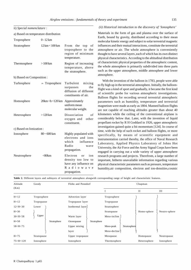
R Chattopadhyay 1.p65
Airglow emissions : fundamentals of theory and experiment 135
ii) Special nomenclature :
a) Based on temperature distribution
Troposphere 0 - 12 km
Stratosphere 12 km < 100 km From the top oftroposphere to theregion of minimumtemperature.
Thermosphere > 100 km Region of increasingtemperature, abovethe stratosphere.
b) Based on Composition :
Turbosphere » Troposphere Turbulent mixingsurpasses thediffusion of differentconstituents of air.
Homosphere 20km <h <120 kmApproximatelyuniform meanmolecular weight.
Heterosphere > 120 km Dissociation ofoxygen and otherconstituent.
c) Based on Ionization :
Ionosphere 80 ~ 600 km Highly populated withelectrons and ionswhich influenceRadio wavepropagation.
Neutrosphere <80km Electron or iondensity too low tohave any influence onR a d i o w a v epropagation.
(ii) Historical introduction to the discovery of ‘Ionosphere’
Materials in the form of gas and plasma over the surface ofEarth, bound by gravity, distributed according to their meanmolecular kinetic energy and subject to solar terrestrial magneticinfluences and their mutual interactions, constitute the terrestrialatmosphere or air. The whole atmosphere is convenientlythought to have several layers ,each of which has its own distinctphysical characteristics. According to the altitudinal distributionof characteristic physical properties of the atmospheric content,the whole atmosphere is primarily subdivided into three partssuch as the upper atmosphere, middle atmosphere and loweratmosphere.
With the invention of the balloon in 1783, people were ableto fly high up in the terrestrial atmosphere. Initially, the balloon-flight was a kind of sport and gradually, it became the first kindof scientific probe for various atmospheric investigations.Balloon flights for recording several terrestrial atmosphericparameters such as humidity, temperature and terrestrialmagnetism were made as early as 1804. Manned balloon flightsare not capable of reaching altitudes greater than about 40kilometers while the ceiling of the conventional airplane isconsiderably below that. Later, with the invention of liquidpropellant rocket by R H Goddard in 1926, upper atmosphericinvestigation gained quite a bit momentum [124]. In course oftime, with the help of such rocket and balloon flights, or morespecifically, by means of scientific equipment andinstrumentation carried thereby, the office of Naval ResearchLaboratory, Applied Physics Laboratory of Johns HotUniversity, the Air Force and the Army Signal Corps have beenengaged in carrying out a wide variety of upper atmosphereresearch programs and projects. Therefrom, a large number ofimportant, hitherto unavailable information regarding variousphysical characteristic parameters such as pressure, temperaturehumidity,air composition, electron and ion-densities,cosmic
Table 2. Different layers and sublayers of terrestrial atmosphere alongwith corresponding range of height and characteristic features.
Altitude Goody Flohn and Penndorf Chapman
(Km)I II III
H<12 Troposphere Advection layer Troposphere
H=12 Tropopause Tropopause layer Tropopause
12<H<30 Lower Isothermal layer Stratosphere
H=30 Stratopause Homo-sphere Neutro-sphere
30<H<58 Upper Warm layer Meso-incline
H=58 Stratophere Ozonopause Stratophere
58<H<75 Upper mixing Meso-peak Stratosphere
layer Meso-decline
H=75 Stratopause Upper tropopause Mesopause Homopause Neutropause
75<H<120 Ionosphere Ionosphere Thermosphere Heterosphere Ionosphere
UVW
U
V
|||
W
|||
U
V
|||
W
|||
U
V||
W||
U
V
|||||
W
|||||
U
V
|||||
W
|||||
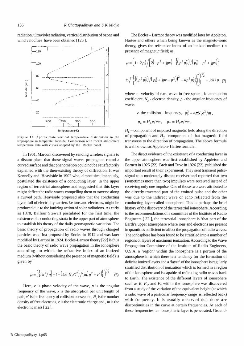
R Chattopadhyay 1.p65
136 R Chattopadhyay and S K Midya
radiation, ultraviolet radiation, vertical distribution of ozone andwind velocities have been obtained [125 ].
Figure 12. Approximate vertical temperature distribution in thetroposphere in temperate latitude. Comparison with rocket atmospheretemperature data with curves adopted by the Rocket panel.
In 1901, Marconi discovered by sending wireless signals toa distant place that those signal waves propagated round acurved surface and that phenomenon could not be satisfactorilyexplained with the then-existing theory of diffraction. It wasKennelly and Heaviside in 1902 who, almost simultaneously,postulated the existence of a conducting layer in the upperregion of terrestrial atmosphere and suggested that this layermight deflect the radio waves compelling them to traverse alonga curved path. Heaviside proposed also that the conductinglayer, full of electricity carriers i.e ions and electrons, might beproduced due to the ionizing action of solar radiations. As earlyas 1878, Balfour Stewart postulated for the first time, theexistence of a conducting strata in the upper part of atmosphereto establish his theory of the daily geomagnetic variation. Thebasic theory of propagation of radio waves through chargedparticles was first proposed by Eccles in 1912 and was latermodified by Larmor in 1924. Eccles-Larmor theory [22] is thusthe basic theory of radio wave propagation in the ionosphereaccording to which the refractive index of an ionizedmedium (without considering the presence of magnetic field) isgiven by
m p= + - +FH IKck p N C m p vc2 2 2 2
12
1 4o t d i d i{ } (6)
Here, c is phase velocity of the wave, p is the angularfrequency of the wave, k is the absorption per unit length ofpath, v’ is the frequency of collision per second, Ne is the numberdensity of free electrons, e is the electronic charge and , m is theelectronic mass [ 22 ].
The Eccles – Larmor theory was modified later by Appleton,Hartee and others which being known as the magneto-ionictheory, gives the refractive index of an ionized medium (inpresence of magnetic field) as,
m = + - + - - +LNM
FH1 2 20
2 2 2 202 2p p jpv p p p p jpvTd i d i d i{ }
± + - +RST
UVWOQPIKJ
+p p p jpv p p p jck pT L2 2
02 2
22 2
12
4d i d ie j , (7)
where c- velocity of e.m. wave in free space , k- attenuationcoefficient, Ne - electron density, p - the angular frequency ofwave,
v- the collision – frequency, p N e me02 24= p ,
p H e mc p H e mcL L T T= =, ,
HL – component of imposed magnetic field along the directionof propagation and HT- component of that magnetic fieldtransverse to the direction of propagation. The above formulais well known as Appleton- Hartee formula.
The direct evidence of the existence of a conducting layer inthe upper atmosphere was first established by Appleton andBarnett in 1925 [22]. Breit and Tuve in 1926 [22], published theimportant result of their experiment. They sent transient pulse-signal to a moderately distant receiver and reported that two(sometimes more than two) impulses were received instead ofreceiving only one impulse. One of those two were attributed tothe directly traversed part of the emitted pulse and the otherwas due to the indirect wave or echo reflected from theconducting layer called ionosphere. This is perhaps the briefhistory of the discovery of the terrestrial ionosphere. Accordingto the recommendations of a committee of the Institute of RadioEngineers [ 22 ], the terrestrial ionosphere is ‘that part of theEarth’s upper atmosphere where ions and electrons are presentin quantities sufficient to affect the propagation of radio waves.The ionosphere has been found to be stratified into a number ofregions or layers of maximum ionization. According to the WavePropagation Committee of the Institute of Radio Engineers,U.S.A, a ‘region’ within the ionosphere is a portion of theatmosphere in which there is a tendency for the formation ofdefinite ionized layers and a ‘layer’ of the ionosphere is regularlystratified distribution of ionization which is formed in a regionof the ionosphere and is capable of reflecting radio waves backto Earth. The existence of the different layers of ionospheresuch as E, F1, and F2 within the ionosphere was discoveredfrom a study of the variation of the equivalent height (at whicha radio wave of a particular frequency range is reflected back)with frequency. It is usually observed that there arediscontinuities in the curve at certain frequencies. At each ofthese frequencies, an ionospheric layer is penetrated. Ground-
Temperature (oK)
Alti
tude
(km
.)
120
100
80
60
40
20
200 250 300 350
F
E
D
C
B
A
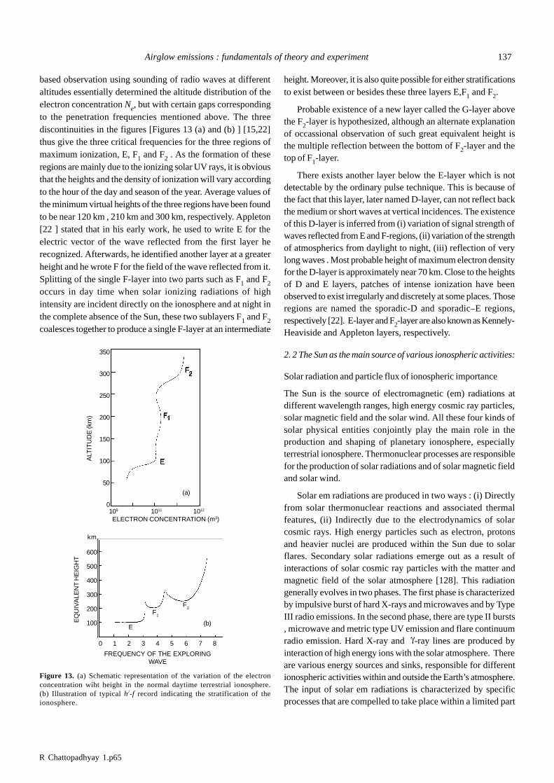
R Chattopadhyay 1.p65
Airglow emissions : fundamentals of theory and experiment 137
based observation using sounding of radio waves at differentaltitudes essentially determined the altitude distribution of theelectron concentration Ne, but with certain gaps correspondingto the penetration frequencies mentioned above. The threediscontinuities in the figures [Figures 13 (a) and (b) ] [15,22]thus give the three critical frequencies for the three regions ofmaximum ionization, E, F1 and F2 . As the formation of theseregions are mainly due to the ionizing solar UV rays, it is obviousthat the heights and the density of ionization will vary accordingto the hour of the day and season of the year. Average values ofthe minimum virtual heights of the three regions have been foundto be near 120 km , 210 km and 300 km, respectively. Appleton[22 ] stated that in his early work, he used to write E for theelectric vector of the wave reflected from the first layer herecognized. Afterwards, he identified another layer at a greaterheight and he wrote F for the field of the wave reflected from it.Splitting of the single F-layer into two parts such as F1 and F2occurs in day time when solar ionizing radiations of highintensity are incident directly on the ionosphere and at night inthe complete absence of the Sun, these two sublayers F1 and F2coalesces together to produce a single F-layer at an intermediate
height. Moreover, it is also quite possible for either stratificationsto exist between or besides these three layers E,F1 and F2.
Probable existence of a new layer called the G-layer abovethe F2-layer is hypothesized, although an alternate explanationof occassional observation of such great equivalent height isthe multiple reflection between the bottom of F2-layer and thetop of F1-layer.
There exists another layer below the E-layer which is notdetectable by the ordinary pulse technique. This is because ofthe fact that this layer, later named D-layer, can not reflect backthe medium or short waves at vertical incidences. The existenceof this D-layer is inferred from (i) variation of signal strength ofwaves reflected from E and F-regions, (ii) variation of the strengthof atmospherics from daylight to night, (iii) reflection of verylong waves . Most probable height of maximum electron densityfor the D-layer is approximately near 70 km. Close to the heightsof D and E layers, patches of intense ionization have beenobserved to exist irregularly and discretely at some places. Thoseregions are named the sporadic-D and sporadic–E regions,respectively [22]. E-layer and F2-layer are also known as Kennely-Heaviside and Appleton layers, respectively.
2. 2 The Sun as the main source of various ionospheric activities:
Solar radiation and particle flux of ionospheric importance
The Sun is the source of electromagnetic (em) radiations atdifferent wavelength ranges, high energy cosmic ray particles,solar magnetic field and the solar wind. All these four kinds ofsolar physical entities conjointly play the main role in theproduction and shaping of planetary ionosphere, especiallyterrestrial ionosphere. Thermonuclear processes are responsiblefor the production of solar radiations and of solar magnetic fieldand solar wind.
Solar em radiations are produced in two ways : (i) Directlyfrom solar thermonuclear reactions and associated thermalfeatures, (ii) Indirectly due to the electrodynamics of solarcosmic rays. High energy particles such as electron, protonsand heavier nuclei are produced within the Sun due to solarflares. Secondary solar radiations emerge out as a result ofinteractions of solar cosmic ray particles with the matter andmagnetic field of the solar atmosphere [128]. This radiationgenerally evolves in two phases. The first phase is characterizedby impulsive burst of hard X-rays and microwaves and by TypeIII radio emissions. In the second phase, there are type II bursts, microwave and metric type UV emission and flare continuumradio emission. Hard X-ray and g-ray lines are produced byinteraction of high energy ions with the solar atmosphere. Thereare various energy sources and sinks, responsible for differentionospheric activities within and outside the Earth’s atmosphere.The input of solar em radiations is characterized by specificprocesses that are compelled to take place within a limited part
Figure 13. (a) Schematic representation of the variation of the electronconcentration wiht height in the normal daytime terrestrial ionosphere.(b) Illustration of typical h/-f record indicating the stratification of theionosphere.
(a)
(b)
ALT
ITU
DE
(km
)
350
300
250
200
150
100
50
0
F2
F1
E
109 1011 1012
ELECTRON CONCENTRATION (m3)
EQ
UIV
ALE
NT
HE
IGH
T
km
600
500
400
300
200
100
0 1 2 3 4 5 6 7 8
FREQUENCY OF THE EXPLORINGWAVE
E
F1
F2
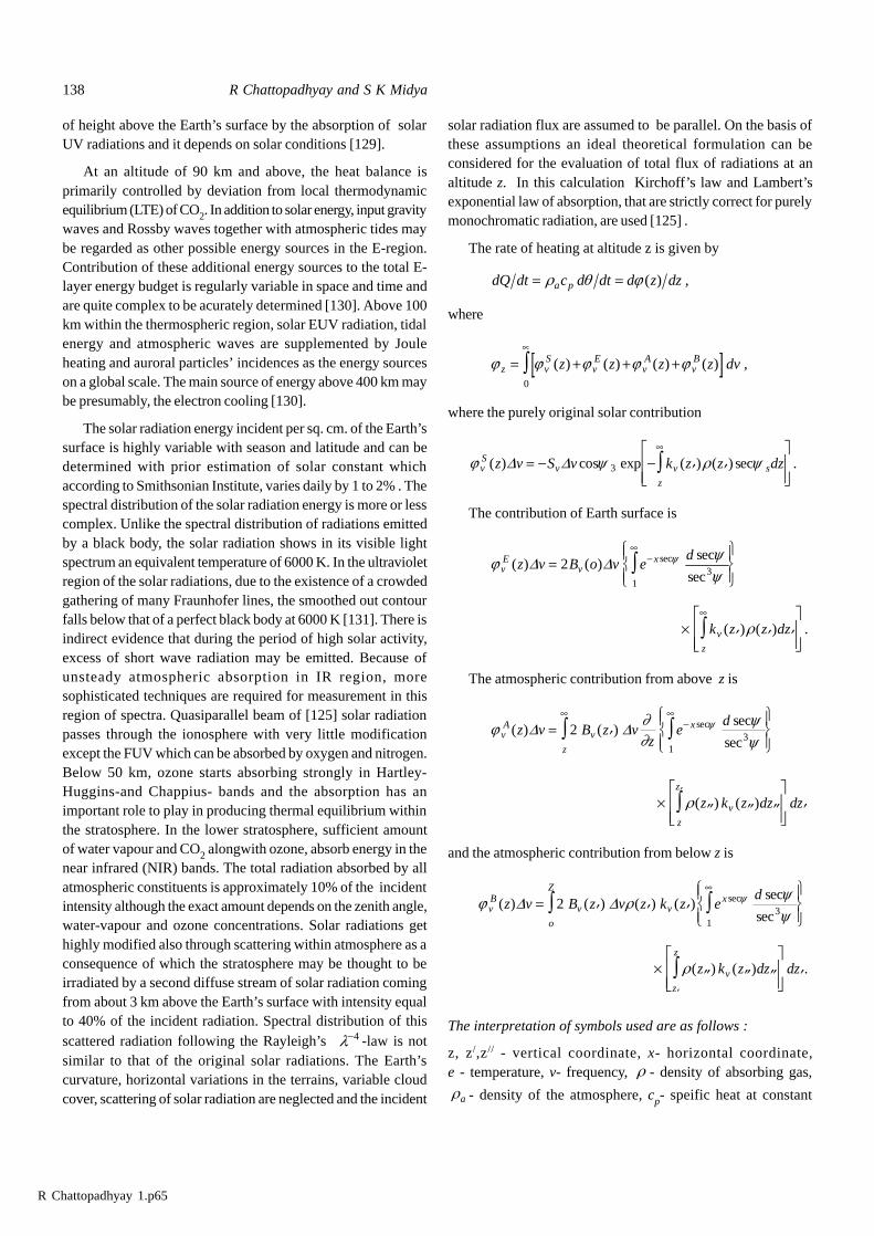
R Chattopadhyay 1.p65
138 R Chattopadhyay and S K Midya
of height above the Earth’s surface by the absorption of solarUV radiations and it depends on solar conditions [129].
At an altitude of 90 km and above, the heat balance isprimarily controlled by deviation from local thermodynamicequilibrium (LTE) of CO2. In addition to solar energy, input gravitywaves and Rossby waves together with atmospheric tides maybe regarded as other possible energy sources in the E-region.Contribution of these additional energy sources to the total E-layer energy budget is regularly variable in space and time andare quite complex to be acurately determined [130]. Above 100km within the thermospheric region, solar EUV radiation, tidalenergy and atmospheric waves are supplemented by Jouleheating and auroral particles’ incidences as the energy sourceson a global scale. The main source of energy above 400 km maybe presumably, the electron cooling [130].
The solar radiation energy incident per sq. cm. of the Earth’ssurface is highly variable with season and latitude and can bedetermined with prior estimation of solar constant whichaccording to Smithsonian Institute, varies daily by 1 to 2% . Thespectral distribution of the solar radiation energy is more or lesscomplex. Unlike the spectral distribution of radiations emittedby a black body, the solar radiation shows in its visible lightspectrum an equivalent temperature of 6000 K. In the ultravioletregion of the solar radiations, due to the existence of a crowdedgathering of many Fraunhofer lines, the smoothed out contourfalls below that of a perfect black body at 6000 K [131]. There isindirect evidence that during the period of high solar activity,excess of short wave radiation may be emitted. Because ofunsteady atmospheric absorption in IR region, moresophisticated techniques are required for measurement in thisregion of spectra. Quasiparallel beam of [125] solar radiationpasses through the ionosphere with very little modificationexcept the FUV which can be absorbed by oxygen and nitrogen.Below 50 km, ozone starts absorbing strongly in Hartley-Huggins-and Chappius- bands and the absorption has animportant role to play in producing thermal equilibrium withinthe stratosphere. In the lower stratosphere, sufficient amountof water vapour and CO2 alongwith ozone, absorb energy in thenear infrared (NIR) bands. The total radiation absorbed by allatmospheric constituents is approximately 10% of the incidentintensity although the exact amount depends on the zenith angle,water-vapour and ozone concentrations. Solar radiations gethighly modified also through scattering within atmosphere as aconsequence of which the stratosphere may be thought to beirradiated by a second diffuse stream of solar radiation comingfrom about 3 km above the Earth’s surface with intensity equalto 40% of the incident radiation. Spectral distribution of thisscattered radiation following the Rayleigh’s l-4 -law is notsimilar to that of the original solar radiations. The Earth’scurvature, horizontal variations in the terrains, variable cloudcover, scattering of solar radiation are neglected and the incident
solar radiation flux are assumed to be parallel. On the basis ofthese assumptions an ideal theoretical formulation can beconsidered for the evaluation of total flux of radiations at analtitude z. In this calculation Kirchoff’s law and Lambert’sexponential law of absorption, that are strictly correct for purelymonochromatic radiation, are used [125] .
The rate of heating at altitude z is given by
dQ dt c d dt d z dza p= =r q j( ) ,
where
j j j j jz vS
vE
vA
vBz z z z dv= + + +
µ
z ( ) ( ) ( ) ( ) ,0
where the purely original solar contribution
j y r yvS
v v s
z
z v S v k z z dz( ) cos exp ( ) ( ) sec .D D= - - ¢ ¢L
NMM
O
QPP
¥
z3
The contribution of Earth surface is
j yy
yvE
vxz v B o v e
d( ) ( )
sec
secsecD D=
RS|T|
UV|W|
-¥
z23
1
´ ¢ ¢ ¢L
NMM
O
QPP
¥
z k z z dzv
z
( ) ( ) .r
The atmospheric contribution from above z is
j ¶¶
yy
yvA
v
z
xz v B z vz
ed
( ) ( )sec
secsecD D= ¢
RS|T|
UV|W|
¥-
¥
z z21
3
´ ¢¢ ¢¢ ¢¢L
NMM
O
QPP
¢
¢
z r ( ) ( )z k z dz dzv
z
z
and the atmospheric contribution from below z is
j r yy
yvB
v
o
Z
vxz v B z v z k z e
d( ) ( ) ( ) ( )
sec
secsecD D= ¢ ¢ ¢
RS|T|
UV|W|
z z¥
21
3
´ ¢¢ ¢¢ ¢¢L
NMM
O
QPP
¢
¢
z r ( ) ( ) .z k z dz dzv
z
z
The interpretation of symbols used are as follows :
z, z/,z// - vertical coordinate, x- horizontal coordinate,e - temperature, v- frequency, r - density of absorbing gas,
ra - density of the atmosphere, cp- speific heat at constant
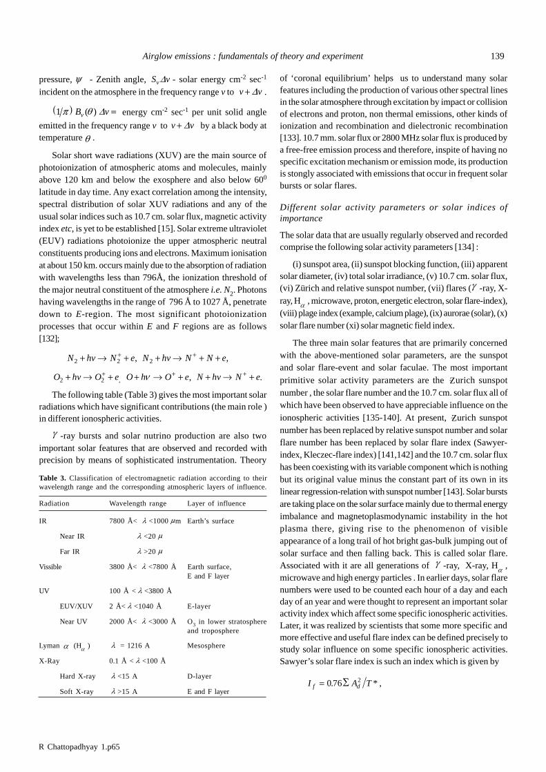
R Chattopadhyay 1.p65
Airglow emissions : fundamentals of theory and experiment 139
Table 3. Classification of electromagnetic radiation according to theirwavelength range and the corresponding atmospheric layers of influence.
Radiation Wavelength range Layer of influence
IR 7800 Å< l <1000mm Earth’s surface
Near IR l <20 m
Far IR l >20 m
Vissible 3800 Å< l <7800 Å Earth surface,E and F layer
UV 100 Å < l <3800 Å
EUV/XUV 2 Å< l <1040 Å E-layer
Near UV 2000 Å< l <3000 Å O3 in lower stratosphereand troposphere
Lyman a (Ha ) l = 1216 A Mesosphere
X-Ray 0.1 Å <l <100 Å
Hard X-ray l <15 A D-layer
Soft X-ray l >15 A E and F layer
pressure, y - Zenith angle, S vvD - solar energy cm-2 sec-1
incident on the atmosphere in the frequency range v to v v+ D .
1 p qa f B vv ( ) D = energy cm-2 sec-1 per unit solid angle
emitted in the frequency range v to v v+ D by a black body attemperature q .
Solar short wave radiations (XUV) are the main source ofphotoionization of atmospheric atoms and molecules, mainlyabove 120 km and below the exosphere and also below 600
latitude in day time. Any exact correlation among the intensity,spectral distribution of solar XUV radiations and any of theusual solar indices such as 10.7 cm. solar flux, magnetic activityindex etc, is yet to be established [15]. Solar extreme ultraviolet(EUV) radiations photoionize the upper atmospheric neutralconstituents producing ions and electrons. Maximum ionisationat about 150 km. occurs mainly due to the absorption of radiationwith wavelengths less than 796Å, the ionization threshold ofthe major neutral constituent of the atmosphere i.e. N2. Photonshaving wavelengths in the range of 796 Å to 1027 Å, penetratedown to E-region. The most significant photoionizationprocesses that occur within E and F regions are as follows[132];
N hv N e N hv N N e2 2 2+ ® + + ® + ++ +, ,
O hv O e O h O e N hv N e2 2+ ® + + ® + + ® ++ + +, , .n
The following table (Table 3) gives the most important solarradiations which have significant contributions (the main role )in different ionospheric activities.
g -ray bursts and solar nutrino production are also twoimportant solar features that are observed and recorded withprecision by means of sophisticated instrumentation. Theory
of ‘coronal equilibrium’ helps us to understand many solarfeatures including the production of various other spectral linesin the solar atmosphere through excitation by impact or collisionof electrons and proton, non thermal emissions, other kinds ofionization and recombination and dielectronic recombination[133]. 10.7 mm. solar flux or 2800 MHz solar flux is produced bya free-free emission process and therefore, inspite of having nospecific excitation mechanism or emission mode, its productionis stongly associated with emissions that occur in frequent solarbursts or solar flares.
Different solar activity parameters or solar indices ofimportance
The solar data that are usually regularly observed and recordedcomprise the following solar activity parameters [134] :
(i) sunspot area, (ii) sunspot blocking function, (iii) apparentsolar diameter, (iv) total solar irradiance, (v) 10.7 cm. solar flux,(vi) Zürich and relative sunspot number, (vii) flares (g -ray, X-ray, Ha , microwave, proton, energetic electron, solar flare-index),(viii) plage index (example, calcium plage), (ix) aurorae (solar), (x)solar flare number (xi) solar magnetic field index.
The three main solar features that are primarily concernedwith the above-mentioned solar parameters, are the sunspotand solar flare-event and solar faculae. The most importantprimitive solar activity parameters are the &&Zurich sunspotnumber , the solar flare number and the 10.7 cm. solar flux all ofwhich have been observed to have appreciable influence on theionospheric activities [135-140]. At present, &&Zurich sunspotnumber has been replaced by relative sunspot number and solarflare number has been replaced by solar flare index (Sawyer-index, Kleczec-flare index) [141,142] and the 10.7 cm. solar fluxhas been coexisting with its variable component which is nothingbut its original value minus the constant part of its own in itslinear regression-relation with sunspot number [143]. Solar burstsare taking place on the solar surface mainly due to thermal energyimbalance and magnetoplasmodynamic instability in the hotplasma there, giving rise to the phenomenon of visibleappearance of a long trail of hot bright gas-bulk jumping out ofsolar surface and then falling back. This is called solar flare.Associated with it are all generations of g -ray, X-ray, Ha ,microwave and high energy particles . In earlier days, solar flarenumbers were used to be counted each hour of a day and eachday of an year and were thought to represent an important solaractivity index which affect some specific ionospheric activities.Later, it was realized by scientists that some more specific andmore effective and useful flare index can be defined precisely tostudy solar influence on some specific ionospheric activities.Sawyer’s solar flare index is such an index which is given by
I A Tf d= å0 76 2. * ,
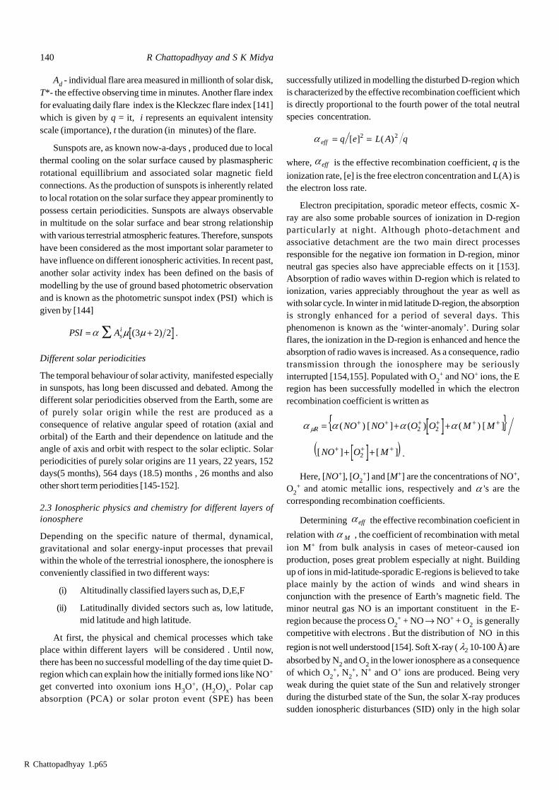
R Chattopadhyay 1.p65
140 R Chattopadhyay and S K Midya
Ad - individual flare area measured in millionth of solar disk,T*- the effective observing time in minutes. Another flare indexfor evaluating daily flare index is the Kleckzec flare index [141]which is given by q = it, i represents an equivalent intensityscale (importance), t the duration (in minutes) of the flare.
Sunspots are, as known now-a-days , produced due to localthermal cooling on the solar surface caused by plasmasphericrotational equillibrium and associated solar magnetic fieldconnections. As the production of sunspots is inherently relatedto local rotation on the solar surface they appear prominently topossess certain periodicities. Sunspots are always observablein multitude on the solar surface and bear strong relationshipwith various terrestrial atmospheric features. Therefore, sunspotshave been considered as the most important solar parameter tohave influence on different ionospheric activities. In recent past,another solar activity index has been defined on the basis ofmodelling by the use of ground based photometric observationand is known as the photometric sunspot index (PSI) which isgiven by [144]
PSI Asi= +åa m m( ) .3 2 2
Different solar periodicities
The temporal behaviour of solar activity, manifested especiallyin sunspots, has long been discussed and debated. Among thedifferent solar periodicities observed from the Earth, some areof purely solar origin while the rest are produced as aconsequence of relative angular speed of rotation (axial andorbital) of the Earth and their dependence on latitude and theangle of axis and orbit with respect to the solar ecliptic. Solarperiodicities of purely solar origins are 11 years, 22 years, 152days(5 months), 564 days (18.5) months , 26 months and alsoother short term periodities [145-152].
2.3 Ionospheric physics and chemistry for different layers ofionosphere
Depending on the specific nature of thermal, dynamical,gravitational and solar energy-input processes that prevailwithin the whole of the terrestrial ionosphere, the ionosphere isconveniently classified in two different ways:
(i) Altitudinally classified layers such as, D,E,F
(ii) Latitudinally divided sectors such as, low latitude,mid latitude and high latitude.
At first, the physical and chemical processes which takeplace within different layers will be considered . Until now,there has been no successful modelling of the day time quiet D-region which can explain how the initially formed ions like NO+
get converted into oxonium ions H3O+, (H2O)x. Polar cap
absorption (PCA) or solar proton event (SPE) has been
successfully utilized in modelling the disturbed D-region whichis characterized by the effective recombination coefficient whichis directly proportional to the fourth power of the total neutralspecies concentration.
aeff q e L A q= =[ ] ( )2 2
where, aeff is the effective recombination coefficient, q is the
ionization rate, [e] is the free electron concentration and L(A) isthe electron loss rate.
Electron precipitation, sporadic meteor effects, cosmic X-ray are also some probable sources of ionization in D-regionparticularly at night. Although photo-detachment andassociative detachment are the two main direct processesresponsible for the negative ion formation in D-region, minorneutral gas species also have appreciable effects on it [153].Absorption of radio waves within D-region which is related toionization, varies appreciably throughout the year as well aswith solar cycle. In winter in mid latitude D-region, the absorptionis strongly enhanced for a period of several days. Thisphenomenon is known as the ‘winter-anomaly’. During solarflares, the ionization in the D-region is enhanced and hence theabsorption of radio waves is increased. As a consequence, radiotransmission through the ionosphere may be seriouslyinterrupted [154,155]. Populated with O2
+ and NO+ ions, the Eregion has been successfully modelled in which the electronrecombination coefficient is written as
a a a amR NO NO O O M M= + ++ + + + + +( ) [ ] ( ) ( ) [ ]2 2{ }
[ ] [ ]NO O M+ + ++ +2e j .
Here, [NO+], [O2+] and [M+] are the concentrations of NO+,
O2+ and atomic metallic ions, respectively and a 's are the
corresponding recombination coefficients.
Determining aeff the effective recombination coeficient in
relation with a M , the coefficient of recombination with metalion M+ from bulk analysis in cases of meteor-caused ionproduction, poses great problem especially at night. Buildingup of ions in mid-latitude-sporadic E-regions is believed to takeplace mainly by the action of winds and wind shears inconjunction with the presence of Earth’s magnetic field. Theminor neutral gas NO is an important constituent in the E-region because the process O2
+ + NO ® NO+ + O2 is generallycompetitive with electrons . But the distribution of NO in this
region is not well understood [154]. Soft X-ray (l2 10-100 Å) areabsorbed by N2 and O2 in the lower ionosphere as a consequenceof which O2
+, N2+, N+ and O+ ions are produced. Being very
weak during the quiet state of the Sun and relatively strongerduring the disturbed state of the Sun, the solar X-ray producessudden ionospheric disturbances (SID) only in the high solar
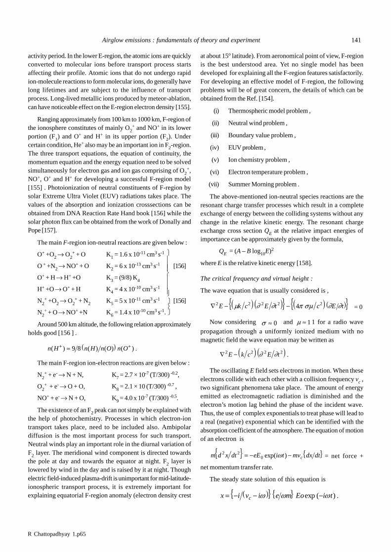
R Chattopadhyay 1.p65
Airglow emissions : fundamentals of theory and experiment 141
activity period. In the lower E-region, the atomic ions are quicklyconverted to molecular ions before transport process startsaffecting their profile. Atomic ions that do not undergo rapidion-molecule reactions to form molecular ions, do generally havelong lifetimes and are subject to the influence of transportprocess. Long-lived metallic ions produced by meteor-ablation,can have noticeable effect on the E-region electron density [155].
Ranging approximately from 100 km to 1000 km, F-region ofthe ionosphere constitutes of mainly O2
+ and NO+ in its lowerportion (F1) and O+ and H+ in its upper portion (F2). Undercertain condition, He+ also may be an important ion in F2-region.The three transport equations, the equation of continuity, themomentum equation and the energy equation need to be solvedsimultaneously for electron gas and ion gas comprising of O2
+,NO+, O+ and H+ for developing a successful F-region model[155] . Photoionization of neutral constituents of F-region bysolar Extreme Ultra Violet (EUV) radiations takes place. Thevalues of the absorption and ionization crosssections can beobtained from DNA Reaction Rate Hand book [156] while thesolar photon flux can be obtained from the work of Donally andPope [157].
The main F-region ion-neutral reactions are given below :
O+ +O2 ® O2+ + O K1 = 1.6 x 10⁻¹¹ cm3 s-1
O + +N2 ® NO+ + O K2 = 6 x 10-13 cm3 s-1 [156]
O+ + H ® H+ +O K3 = (9/8) K4
H+ +O ® O+ + H K4 = 4 x 10⁻¹⁰ cm3 s-1
N2+ +O2 ® O2
+ + N2 K5 = 5 x 10-11 cm3 s-1 [156]
N2+ + O ® NO+ +N K6 = 1.4 x 10⁻¹⁰ cm3 s-1.
Around 500 km altitude, the following relation approximatelyholds good [156 ] .
n H n H n O n O( ) ( ) ( ) ( ) .+ +» 9 8a f
The main F-region ion-electron reactions are given below :
N2+ + e- ® N + N, K7 = 2.7 × 10⁻⁷ (T/300) -0.2,
O2+ + e- ® O + O, K8 = 2.1 × 10 (T/300) -0.7 ,
NO+ + e- ® N + O, K9 = 4.0 x 10⁻⁷ (T/300) -0.5.
The existence of an F2 peak can not simply be explained withthe help of photochemistry. Processes in which electron-iontransport takes place, need to be included also. Ambipolardiffusion is the most important process for such transport.Neutral winds play an important role in the diurnal variation ofF2 layer. The meridional wind component is directed towardsthe pole at day and towards the equator at night. F2 layer islowered by wind in the day and is raised by it at night. Thoughelectric field-induced plasma-drift is unimportant for mid-latitude-ionospheric transport process, it is extremely important forexplaining equatorial F-region anomaly (electron density crest
at about 15o latitude). From aeronomical point of view, F-regionis the best understood area. Yet no single model has beendeveloped for explaining all the F-region features satisfactorily.For developing an effective model of F-region, the followingproblems will be of great concern, the details of which can beobtained from the Ref. [154].
(i) Thermospheric model problem ,
(ii) Neutral wind problem ,
(iii) Boundary value problem ,
(iv) EUV problem ,
(v) Ion chemistry problem ,
(vi) Electron temperature problem ,
(vii) Summer Morning problem .
The above-mentioned ion-neutral species reactions are theresonant charge transfer processes which result in a completeexchange of energy between the colliding systems without anychange in the relative kinetic energy. The resonant chargeexchange cross section QE at the relative impact energies ofimportance can be approximately given by the formula,
QE = (A – B log10E)2
where E is the relative kinetic energy [158].
The critical frequency and virtual height :
The wave equation that is usually considered is ,
Ñ - -2 2 2 2 24E k c E t c E tm ¶ ¶ p sm ¶ ¶d i d i{ } d i a f{ } = 0
Now considering s » 0 and m » 11 for a radio wave
propagation through a uniformly ionized medium with nomagnetic field the wave equation may be written as
Ñ -2 2 2 2E k c E td i d i¶ ¶ .
The oscillating E field sets electrons in motion. When theseelectrons collide with each other with a collision frequency vc ,two significant phenomena take place. The amount of energyemitted as electromagnetic radiation is diminished and theelectron’s motion lag behind the phase of the incident wave.Thus, the use of complex exponentials to treat phase will lead toa real (negative) exponential which can be identified with theabsorption coefficient of the atmosphere. The equation of motionof an electron is
m d x dt eE i t mv dx dtc2 2
0o t l q= - -exp( )w = net force +
net momentum transfer rate.
The steady state solution of this equation is
x i v i e m Eo i tc= - - -w w wa fm rl q exp ( ) .
UVW
U
V|||
W|||
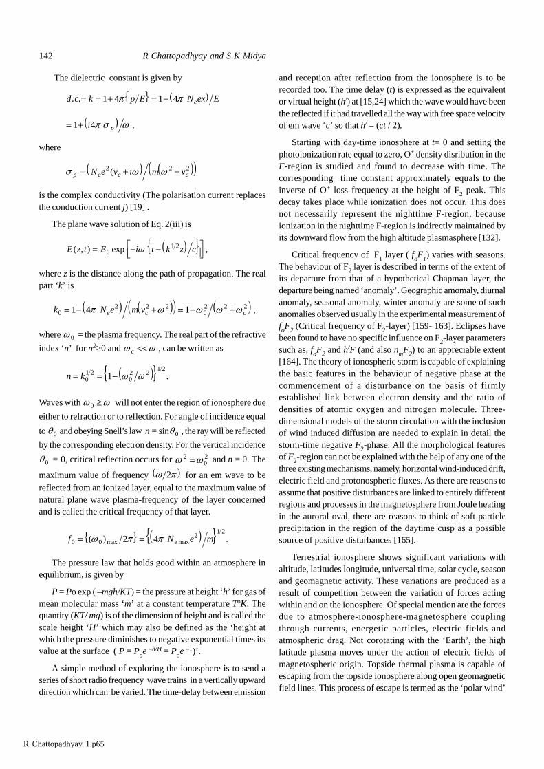
R Chattopadhyay 1.p65
142 R Chattopadhyay and S K Midya
The dielectric constant is given by
d c k p E N ex Ee. .= = + = -1 4 1 4p pl q a f
= +1 4i pp s wc h ,
where
s w wp e c cN e v i m v= + +2 2 2(d i d ie j
is the complex conductivity (The polarisation current replacesthe conduction current j) [19] .
The plane wave solution of Eq. 2(iii) is
E z t E i t k z c( , ) exp ,= - -LNM
OQP0
1 2w d i{ }
where z is the distance along the path of propagation. The realpart ‘k’ is
k N e m ve c c02 2 2
02 2 21 4 1= - + = - +p w w w wd i d ie j d i ,
where w0 = the plasma frequency. The real part of the refractive
index ‘n’ for n2>0 and w wc << , can be written as
n k= = -01 2
02 2
1 21 w wd i{ } .
Waves with w w0 ³ will not enter the region of ionosphere due
either to refraction or to reflection. For angle of incidence equal
to q0 and obeying Snell’s law n = sinq0 , the ray will be reflected
by the corresponding electron density. For the vertical incidence
q0 = 0, critical reflection occurs for w w202= and n = 0. The
maximum value of frequency w p2a f for an em wave to bereflected from an ionized layer, equal to the maximum value ofnatural plane wave plasma-frequency of the layer concernedand is called the critical frequency of that layer.
f N e me0 02
1 22 4= =( ) .max maxw p pl q d i{ }
The pressure law that holds good within an atmosphere inequilibrium, is given by
P = Po exp ( –mgh/KT) = the pressure at height ‘h’ for gas ofmean molecular mass ‘m’ at a constant temperature ToK. Thequantity (KT/ mg) is of the dimension of height and is called thescale height ‘H’ which may also be defined as the ‘height atwhich the pressure diminishes to negative exponential times itsvalue at the surface ( P = Poe –h/H = Poe –1)’.
A simple method of exploring the ionosphere is to send aseries of short radio frequency wave trains in a vertically upwarddirection which can be varied. The time-delay between emission
and reception after reflection from the ionosphere is to berecorded too. The time delay (t) is expressed as the equivalentor virtual height (h/) at [15,24] which the wave would have beenthe reflected if it had travelled all the way with free space velocityof em wave ‘c’ so that h/ = (ct / 2).
Starting with day-time ionosphere at t= 0 and setting thephotoionization rate equal to zero, O+ density disribution in theF-region is studied and found to decrease with time. Thecorresponding time constant approximately equals to theinverse of O+ loss frequency at the height of F2 peak. Thisdecay takes place while ionization does not occur. This doesnot necessarily represent the nighttime F-region, becauseionization in the nighttime F-region is indirectly maintained byits downward flow from the high altitude plasmasphere [132].
Critical frequency of F1 layer ( foF1) varies with seasons.The behaviour of F2 layer is described in terms of the extent ofits departure from that of a hypothetical Chapman layer, thedeparture being named ‘anomaly’. Geographic amomaly, diurnalanomaly, seasonal anomaly, winter anomaly are some of suchanomalies observed usually in the experimental measurement offoF2 (Critical frequency of F2-layer) [159- 163]. Eclipses havebeen found to have no specific influence on F2-layer parameterssuch as, foF2 and h/F (and also nmF2) to an appreciable extent[164]. The theory of ionospheric storm is capable of explainingthe basic features in the behaviour of negative phase at thecommencement of a disturbance on the basis of firmlyestablished link between electron density and the ratio ofdensities of atomic oxygen and nitrogen molecule. Three-dimensional models of the storm circulation with the inclusionof wind induced diffusion are needed to explain in detail thestorm-time negative F2-phase. All the morphological featuresof F2-region can not be explained with the help of any one of thethree existing mechanisms, namely, horizontal wind-induced drift,electric field and protonospheric fluxes. As there are reasons toassume that positive disturbances are linked to entirely differentregions and processes in the magnetosphere from Joule heatingin the auroral oval, there are reasons to think of soft particleprecipitation in the region of the daytime cusp as a possiblesource of positive disturbances [165].
Terrestrial ionosphere shows significant variations withaltitude, latitudes longitude, universal time, solar cycle, seasonand geomagnetic activity. These variations are produced as aresult of competition between the variation of forces actingwithin and on the ionosphere. Of special mention are the forcesdue to atmosphere-ionosphere-magnetosphere couplingthrough currents, energetic particles, electric fields andatmospheric drag. Not corotating with the ‘Earth’, the highlatitude plasma moves under the action of electric fields ofmagnetospheric origin. Topside thermal plasma is capable ofescaping from the topside ionosphere along open geomagneticfield lines. This process of escape is termed as the ‘polar wind’
R Chattopadhyay 1.p65
Airglow emissions : fundamentals of theory and experiment 143
[132]. The cross-tail potential (CTP) difference is the electricalpotential difference generated across the magnetospheric tailby means of interaction of shocked solar wind with thegeomagnetic field. CTP can vary typically from 20 kV to 120 kVdepending on the level of geomagnetic activity. Most of thetime, the ring current effectively shields the plasma, within theplasmasphere and therefore, only the high latitude ionosphereis influenced by magnetospheric electric field. At all ionosphericaltitudes, the frequency of electron-neutral atom collision is muchless than the electron cyclotron frequency and therefore, thecombined effect of the perpendicular field E and geomagneticfield B is to induce an electron drift in E × B direction. At F-region altitude, both ions and electrons drift in the E × B direction[132]. The corotation velocity, although much low, is added withdrift for the E-field-induced two-cell drift pattern which isappreciable within the high latitude ionospheric plasma. Thereoccurs an ionization hole, a low density-low temperature-regionthat appears during quiet geomagnetic activity.
At mid-latitudes, the geomagnetic field lines are inclined tothe vertical direction. The effect of meridional wind (north south)is to compel the F-region ionization to move up or down thefield lines depending on the direction of wind. The equator-ward wind at night therefore, has an important role to play inmaintaining F-layer ionization. Mid-latitude ionosphere exhibitsanother type of transport process which is the plasma-flow alongdifferent geomagnetic field lines. During geomagnetic storms,high density cold plasma in the plasmasphere comes into contactwith low density hot plasma in the ring current. Energy, either ofany one or of both of the Coulombic collision and wave-particleinteraction, transforms ring current particles into thermalelectrons within the interaction region. This energy is thenconducted to the lower ionosphere along geomagnetic field lineswhich gives rise to an elevated electron temperature. Hotelectrons at an altitude range of 300-400 km. have got sufficientenergy to collisionally excite atomic oxygen as a result of whichOI 6300 Å red line is emitted. Produced in this way, the oxygenred line emission is generally found over a narrow band of latitudeon the equatorial side of the auroral oval which is well known asstable auroral red arc (SAR-arc).
At low latitudes, the quasi-horizontal geomagnetic field linesproduce some unique transport processes, the most interestingof which is the equatorial fountain [132]. Another source oftransportation is the expansion and cooling of ionosphericplasma on the summer side of the equator and compression andheating of the same on the winter side of the equator.
The existence of ionospheric structures with scale sizes oftens of kilometers or smaller than that are collectively known asthe small scale irregularities [166]. These can be primarily causedby the onset and evolution of different types of instability.Evolving from large scale ionospheric configurations, these
instabilities are generally mutually superimposed. The two mostimportant small scale irregulatities are:
(i) The steepening and subsequent recurrential splittingof barium clouds released in the ionosphere, afterbeing driven by the gradient drift instability.
(ii) The formation and buoyant rise of low density‘bubbles’ of plasma, after being driven by thecollisional Rayleigh-Taylor instability in the nighttimeequatorial ionosphere, is known as equatorial speadF (ESF) .
These effects have bearing on the magnetic field intensityand are therefore latitude dependent too [166] .
Peak electron density nm(e) is another important ionosphericparameter which affects airglow emission significantly, becauseof its intrinsic relation with the critical frequency and to someextent, with the virtual height . The peak electron density nm(e)or nmF2 is related to foF2 according to the well known equation[167]
nm(e) (cc-1) = 1.24 × 10⁴ [foF2(MHz)]2 . (9)
Peak electron density nmF2 is so strongly correlated to foF2both from purely theoretical and empirical points of view thatone is computed from the value of the other. nm(e) is very oftencomputed from foF2 [ 168, 169] . Sometimes, zenith airglowintensity for different important airglow emissions are directlycomputed from their relation with nm(e) [170] . Ionization profilein the F1 region is different from that of F2 because of thefollowing reasons [80];
(i) F2-region ionosphere is optically thin to most ionizingradiations and if the atmosphere in this region can beconsidered to be isothermal, the general rate ofphotoionization for incident monochromatic radiation(for single ionizable constituent) can be written as,
q z F N z z z Hv v( , ) ( ) exp .m p s= - -0 0a f (10)
(ii) The recombination term being directly proportionalto ne , the electron density under the chemicalequillibrium would increase indefinitely withheight.
(iii) But indefinite increase of ne with altitude can not berealistic . Hence, F2 can not be treated with chemicalequilibrium only. Dynamics is also an essential featurein F2-region. Ambipolar diffusion stops that indefiniteincrease of ne with height .
Kimura et al [171] have shown on the basis of DiffusiveEquilibrium (DE) model and SUPIM analysis ( discussed later)that the latitude dependence of global electron can approximatelybe represented by an oscillatory function of latitude.
R Chattopadhyay 1.p65
144 R Chattopadhyay and S K Midya
2 .4 Interrelation between ionospheric activities and airglowemissions:
From our previously discussed sections regarding the basicphysics of airglow, related chemical kinetics and excitationmechanism and above all, the ionospheric physics and chemistry,it is obvious and easy to comprehend that there exists a directrelationship, either of complex or of straightforward naturebetween ionospheric parameters and airglow emissions.Considering eqs. Eq. 1- 4,8 and 9 simultaneously, one canmathematically prove that,
airglow intensity µ - -f F z z H0 22
0exp ( ) .
Barbier [172] was the first to establish a semiempirical formulafor OI 6300 Å airglow emission which is given by,
Q6300 = A (foF2)2 exp [ – (h’ F – 200) / H ] + B,
where H is the scale height in terms of oxygen and was assumedby Barbier himself to be equal to 41.3 . Later, this relation due toBarbier was verified to an extraordinary level of satisfaction byCarman et al [173]. Barbier’s equation has been used by severalworkers in their analysis of OI 6300 Å and OI 5577 Å airglowintensity variation with different solar geophysical parameters[174, 175 ]. Actually, the volume emission rate of different airglowradiations, which is directly proportional to the correspondingintensity, depends in general, on the electron density and therelative abundances of different atomic and molecular ionicspecies involved in all possible dominant modes of excitation.For oxygen green and red line airglow emissions , it is thereforededucible from the experimentally determined values of differentrate-constants, quenching coefficients and transitionprobabilities that the airglow intensity for those two emissionsis proportional only to the electron density and so the patternof variation of OI 6300 Å and OI 5577 Å airglow emissions ismainly governed by the electron density profile, [ 48, 167, 169,174] . Besides, there are many more works regarding the analysisof interrelation between different airglow emissions andcorresponding ionospheric parameters [ 176 - 180].
2 .5 Ozone chemistry and its importance in airglow study :
In the UV and visible regions of solar spectrum between 2000 Åand 6600 Å , O3 is the naturally occurring major atmosphericabsorber. Intense Hartley band and weak Huggins and Chappiusbands are among the principal spectral features of O3 . Photolysisof O3 in the visible spectral region leads to ground state products
O2 (3 å-
g) and O (3P) [181]. Photolytic production of O(1D) in the
reaction
O hv O O3 2+ ® + * ,
is possible in a spin conserved process at wavelengths l £ 310nm. This reaction is the major source of O(1D) , which on one
hand, gives oxygen red and green lines emissions throughforbidden transitions and on the other hand, is involved inreaction with H2O, CH4 and N2O [ 182] . The basic atmosphericO3 photochemistry theory, as developed by Chapman [182],involves two photochemical and three chemical reactions ;
O3 + hv ® O2 + O, O2+ hv ® O + O , O + O2 + M ® O3 + M,
O + O3 ® O2 + O2, O + O+ M ® O2 + M .
Approximately, 80% of stratospheric O3 produced by solarirradiation is not balanced by Chapman’s removal scheme or bytransport to lower altitudes. Reactions with trace amounts of N,H, C or halogen are important [182,183]. Midya [184] reportsthat O3 plays an important role in the emission of OH ( 8,3) bandairglow and there is a correlation between the two. Midya et al[185] have found out that both chemical kinetically andpractically, Li 6708 Å line intensity decreases proportionallywith dramatic depletion of ozone at two antarctic survey stations(Halley-Bay and Mc- Murdo) .
3. Well known features of terrestrial airglow emissions
Airglow intensity variation is one of the most significant airglowfeatures which can be broadly classified into two different types:
(i) Spatial variation ,
(ii) Temporal variation.
Spatial variation again has some specific varieties; Theseare (a) Altitudinal variation or vertical profile, (b) Latitudinalvariation and (c) Longitudinal variation. Temporal variation toohas certain varieties ; (d) Hourly and diurnal variation, (e) Meanmonthly or seasonal, (f) Semiannual and annual; all these typesof variations are described briefly.
3.1 Altitudinal distribution or vertical profile :
Altitudinal distribution or vertical distribution of upperatmospheric pressure, mean density, temperature, electrondensity and density of different neutral and ionic species havebeen determined through several rocket launching and satellitelaunching missions, several times at different latitudes andlongitudes. Each time, the data have been modified to someextent. Based on these data, several airglow fluctuation modelshave been developed by many scientists. F-region nightglowemission, dominated by oxygen green and red line emissionshas been found to increase with altitude, being maximum above200 km and then to decrease again upto a certain height [48,186].Solomon et al [187] compared their model for 6300 Å airglowemission with corresponding satellite mission observation givingspecial stress to emission -altitude profile and they too showedthat the intensity of emissions increases with altitude to reach amaximum at about 250 km and then decreases with altitude. Meloet al [ 188 ] analyse the different mission experimental results ofaltitude profile of volume emission rate for 5577 Å , O2( 0 - 0)
R Chattopadhyay 1.p65
Airglow emissions : fundamentals of theory and experiment 145
band and O2 Herzberg band in which the same has been foundto increase with height reaching a maximum above 100 km, andthen to decrease. Takahashi et al [30] described in details, thealtitude profile of all important airglow lines obtained fromMULTIFOT experiment. Shepherd et al [189] describes theobserved vertical distribution of 5577 Å emission neargeographic equator.
3. 2 Latitudinal variation of airglow intensity :
The latitudinal variation of airglow intensity is difficult to bedetermined properly [24]. Many problems in determining thelatitude-dependence of airglow emission intensity have beensorted out by many scientists in the early period of the study ofairglow emissions.
Davis and Smith studied observed latitudinal variations ofall important airglow emission lines and found that [190 ] 5577 Åand 6300 Å line intensities have in general, an oscillatory natureof variation with latitude, having a minimum at the geomagneticequator. The maximum values of intensities of those lines innorthern hemisphere is much greater than those in southernhemisphere. In case of Na 5893 Å line intensity, the findings aresimilar to those mentioned above except the fact that themaximum value of intensity in southern hemisphere is muchmore than that in northern hemisphere. Chandra et al [170] toostudied latitudinal variations of airglow emission coupled withseasonal and other variations and they inferred that electroncontent profile has little to control OI 6300 Å airglow emissionvalues. Zuzic et al [191] use (N2/O) ratio to indicate thethermospheric composition changes and isolating geomagneticactivity effect from ESRO4 satellite data, they find out the latitudeprofile of that ratio. This may give useful data for obtaininganalytically latitudinal structure of airglow emission profile.Kimura et al [172], in their model-based calculations, havecomputed and studied the latitudinal variation of electrondensity and other ion densities, which may help us to develop amodel for latitude variation of different airglow emissions. Hickeyet al [192] discuss the latitudinal variations of geocoronal hotoxygen and compared it with other type of variations. Ghoshand Midya [193] explained the latitudinal variation of 5577 Ånight airglow emission with the help of latitudinal variation ofair density.
3 .3 Longitudinal variation :
Mukherjee [194] identifies a westward penetrating electric fieldat low and equatorial latitudes that affects the excursions in ‘H’which may indirectly influence the corresponding airglowemissions. Su et al [195] made a modelling study of thelongitudinal variations in the north south asymmetries of theionospheric equatorial anomaly. Actually, the longitudinalvariation of airglow emission is both theoretically and practically,
insignificant and little work on that type of variation has thereforebeen done.
3.4 Hourly and diurnal variation of airglow intensity andSZA :
Regular temporal observations of airglow emissions have beendominated by such temporal recording of airglow data all overthe world. Ghosh and Midya [196] reported their observation ofmorning twilight airglow emissions at Kolkata where all threeairglow lines’ intensities [ 5577 Å , 5893 Å & 6300 Å ] werefound to be increase exponentially with time and then reachinga peak within 15-20 minutes from the start of enhancement, decaydown to an average range of intensity. Only the 6300 Å lineintensity did not show any peak .Ghosh and Midya [90] studiedalso the evening twilight enhancement of 5893 Å line intensityat Kolkata and obtained successive enhancements and decaysas exponential fuctions of time. But for this case, they obtaineda typically prominent two-peak feature, one of which occurredbefore the local sunset and the other, a little lower than firstpeak, occurred with certainty after the local sunset time. Similarobservations were discussed in the perspective of differentexcitation mechanisms by the same authors [81] . Low et al [197]discussed the INDII/ UARS observations of twilight hydroxylairglow at mid-latitude equinox in which they observed thatduring the early hours after sunset, the volume emission rate onthe bottom side of the layers appears to decay exponentiallywith time having a time constant that varies from 1.1 h at 78 kmto 2.9 h at 82 km. They also showed that the value of this timeconstant is related to the process of excitations involved.Mukherjee et al [198] studied 6300 Å nightglow they observedmade from 17o latitude and showed that in the geomagneticallyquiet night, the 630nm airglow intensity varies more or lesssimilarly at two stations, Kolhapur (lat. 16o8 N, long. 74o2E) andAhmedabad (lat. 23o.0 N long. 72o6E). The intensities were foundto decay almost exponentially with time showing a two peakfeature. But it is interesting to see that during geomagneticallydisturbed night, the 6300 Å airglow intensity oscillates withtime and decays exponentially. The dawn to dusk asymmetry involumetric intensity of 5577 Å airglow emission was identifiedfrom AE-C satellite-measurements. Kiselev [199] explained thatassymmetry on the basis of an analysis of the excitationmechanism and its dependence on solar zenith angle (SZA) . Inhis model-based- calculations of the OI 844.6 nm airglowemission during the period of evening twilight, Singh (200) foundthat the calculation as a function of solar zenith angle (SZA)gives the corresponding line intensity in fair, agreement withthe measurementm, only for a range of SZA. Tanabe et al [201]disscussed in detail, the airglow observation program of TokyoAstronomical Observatory where observation was maderegularly on Moonless clear nights of every month since theInternational Geophysical Year (IGY), (1957-8) at Mainuyama,
R Chattopadhyay 1.p65
146 R Chattopadhyay and S K Midya
Dodaira, and Kiso stations. Hickey et al [ 192] described thediurnal variation of geocoronal hot oxygen in details. Kaganand Frolov [202] reported the diurnal variations of decay time ofheater-induced small- scale irregularities in the mid-latitudeionospheric F-layer measured by means of diagnostic stimulatedem emissions (DSEE) and analysed the results.
Bhaumik et al [203] reported their observation on morningtwilight airglow emissions of OH [7,2] and Li 6708 Å line, inwhich the intensity for both emissions was found to increaseexponentially with time.
3.5 Dynamical coupling :
Variety of dynamical processes are involved in coupling themotions of middle atmosphere with that of lower ionosphere.Classifying in general those processes as either advective, wave-like or diffusive, Hocking (204) discussed various aspects ofthe those process detail.
3.6 Barium cloud feature :
Detailed investigations on the ionization and airglow of Ba inthe early stage have been made and expansion of the Ba cloudin the field of solar radiation has been reported by Priyatkin et al[205] . Kinetic processes involved in the excitation and ionizationof barium atoms by suprathermal electrons formed at the time ofshort radio waves, influence on barium cloud and have beenanalysed by Grebnev et al [206] .
3.7 Seasonal variation of airglow intensity:
Monthly mean values of airglow emission intensities, oftentermed as seasonal airglow data, are of great importance inairglow research. Ghosh and Midya explained the seasonalvariations of 5577 Å and 5893 Å night airglow emission atCalcutta on the basis of their consideration of density of air andrelated compositions as functions of time. For explaining theseasonal variations, they considered Chapman’s mechanism andJacchia’s relations [207]. Seasonal variation of the low latitudeOI 630.0 nm nightglow and its strong correlation with solaractivity and solar cycle have been presented by Sahai et al[208] . Seasonal variation of 6300 Å airglow line intensity hasbeen obtained by Midya and Ghosh [82] who found an oscillatorymode of variation against month. Seasonal variation of OH(8,3)airglow band intensity distribution has been considered andexplained in terms of air density fluctuations by Bhaumik et al[209]. Midya et al [210] considered seasonal variation of 5893 Åairglow intensity at Calcutta and found that the same is correlatedwith solar flare index Hickey et al [192] discussed the seasonalvariations of geocoronal hot oxygen in terms of fluctuations ofits new sources. McNeil et al [211] found that the maincontribution to the seasonal variation of sodium nightglowcomes from the temperature dependence of the reaction that
recycles atomic sodium from NaHCO3 . Seasonal variations inthe atmospheric minor species including ozone are secondaryeffects at best. With the help of calculations based onspectrographic observation of the OH atmospheric emission(9,4) , (6,2) , (5,1) and O2 (0,1) bands, seasonal variation oftemperature at 88.95 km height has been established byToroshelidze [212].
3.8 Semi-annual and annual variations :
Estimating variation of wind velocity due to turbulence in inertialsubrange, the vertical eddy diffusivity in the troposphere,stratosphere and also in mesosphere have been studied andseasonal, semi- annual and annual variations of diffusivityparameter K has been confirmed by Kurosaki et al [213]. Theeffect of O3 depletion on OH (8,3) band emission on the basis ofBates - Nicolet theory has been described and the annualvariation of the same at Halley Bay station during the period1973 to 1984 has been presented by Midya [184]. Takahashi etal [214] found that 5577 Å , 5893 Å and OH (9,4) band emissionsin upper mesospheric and lower thermospheric airglow showstrong semi-annual oscillations with maxima at equinoxes andminima during the solstices. They suggested that suchoscillations may be caused by the effects either of one or ofboth seasonal variations in vertical eddy transport andmeridional circulation. Burnside and Tepley [215] in theirmeridian- scanning observations of the intensities of the OIemissions 558 nm and 557.7 nm, noticed that the ratio between558 nm intensity to the North and to the South of Sutherland,underwent an annual variation with the largest ratios beingobserved during Southern winter.
3.9 Hydrodynamical oscillation type variation :
Pertsev reports the identification of a new types ofhydrodynamic oscillations revealed by airglow fluctuations[216].
3.10 Rotational and doppler temperatures :
Molecular rotational energy expressed in terms of equivalentgas kinetic temperature is known as Rotational temperature.Similarly, the airglow spectral line broadening due to Dopplereffect may be looked upon as to be conveniently expressed interms of an equivalent temperature called the Dopplertemperature. They are of immense significance in aeronomy andairglow study [10].
3.11 Limb view of Earth’s airglow spectra :
Earth’s airglow layer observed in the limb view, appears to be acomposite spectral layer. Mende et al [217] described in detail,such limb view spectrum of Earth’s airglow and compared itwith a model of limb view spectrum.
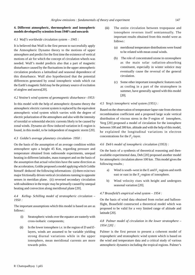
R Chattopadhyay 1.p65
Airglow emissions : fundamentals of theory and experiment 147
4. Different atmospheric, thermospheric and ionosphericmodels developed by scientists from 1940’s and onwards
4.1 Wulf ’s worldwide circulation system – 1945 :
It is believed that Wulf is the first person to successfully applythe Atmospheric Dynamo theory to the motions of upperatmosphere and predict for the first time the existence of verticalmotions of air for which the concept of circulation wheels wasneeded. Wulf’s model predicts also that a part of magneticdisturbance caused by the fluctuations in the upper atmosphericcirculation produces a latitudinal and seasonal dependence ofthis disturbance. Wulf also hypothesized that the potentialdifferences generated by zonal ionospheric winds which cutthe Earth’s magnetic field may be the primary source of excitationof airglow and aurora[20].
4.2 Vestine’s wind systems of geomagnetic disturbance -1953:
In this model with the help of atmospheric dynamo theory theatmospheric electric current system is replaced by the equivalentatmospheric wind system which varries with the degree ofelectric polarization of the atmosphere and also with the intensityof toroidal or solenoidal electric currents likely to be caused byzonal winds. Dynamo air-flow-induced variation in E-region isfound, in this model, to be independent of magnetic storm [20].
4.3 Goldie’s average planetary circulation- 1950 :
On the basis of the assumption of an average condition withinatmosphere upto a height 45 Km, regarding pressure andtemperature obtained from radiosonde experiments, unequalheating in different latitudes, mass transport and on the basis ofthe assumption that actual velocities have the same direction asthe acceleration, Goldie proposed a model applying which Goldiehimself deduced the following informations : (i) there exist twomajor frictionally driven vertical circulations running in oppositesenses in meridian plane. (ii) reversed secondary circulationwith subsidence in the tropic may be primarily caused by unequalheating and convection along meridional plane [20].
4.4 Kellog- Schilling model of stratospheric circulation –1950 :
The important assumptions which this model is based on are asfollows :
(i) Stratospheric winds over the equator are easterly withcross-isobaric components;
(ii) In the lower ionosphere i.e. in the region of D and E-layers, winds are assumed to be variable yieldingstrong diurnal variations while in the upperionosphere, mean meridional currents are moretowards poles.
(iii) The entire circulation between tropopause andionosphere reverses itself semiannually. Theimportant results obtained from this model were asfollows :
(a) meridional temperature distributions were foundto be related with mean zonal winds.
(b) The role of concentrated ozone in ozonosphereas the main solar radiation-absorbingconstituent, especially in winter solstice mayeventually cause the reversal of the generalcirculation.
(c) Some other important ionospheric features suchas cooling in a part of the stratosphere insummer, have generally agreed with this model[20].
4.5 Yerg’s ionospheric wind system (1951) :
Based on the observation of temperature lapse-rate from electronrecombination coefficient and a proposed large scale verticaldistribution of viscous stress in the F-region of ionosphere,Yerg [20] proposed a model of circulation for the ionospherebetween 100 and 300 km. altitude and with the help of this model,he explained the longitudinal variations in electronconcentrations for the F2-layer.
4.6 Deb’s model of ionospheric circulation (1953) :
On the basis of a synthesis of theoretical reasoning and then-available experimental data, Deb [20] proposed another modelfor atmospheric circulation above 100 km . This model gives thefollowing results ;
a) Wind is south–west in the E and F1 regions and northeast or east in the F2-region of ionosphere.
b) Wind velocity rises with height and undergoesseasonal variation [20].
4.7 Brasefield’s empirical wind system – 1954 :
On the basis of wind data obtained from rocket and balloon-flight, Brasefield constructed a theoretical model which wasproposed to be valid for a very limited range of altitude andlatitude [20].
4.8 Palmer model of circulation in the lower stratosphere –1954 [20] :
Palmer is the first person to present a coherent model oftropospheric and stratospheric wind system which is based onthe wind and temperature data and a critical study of variousatmospheric dynamics including the tropical regions. Palmer’s
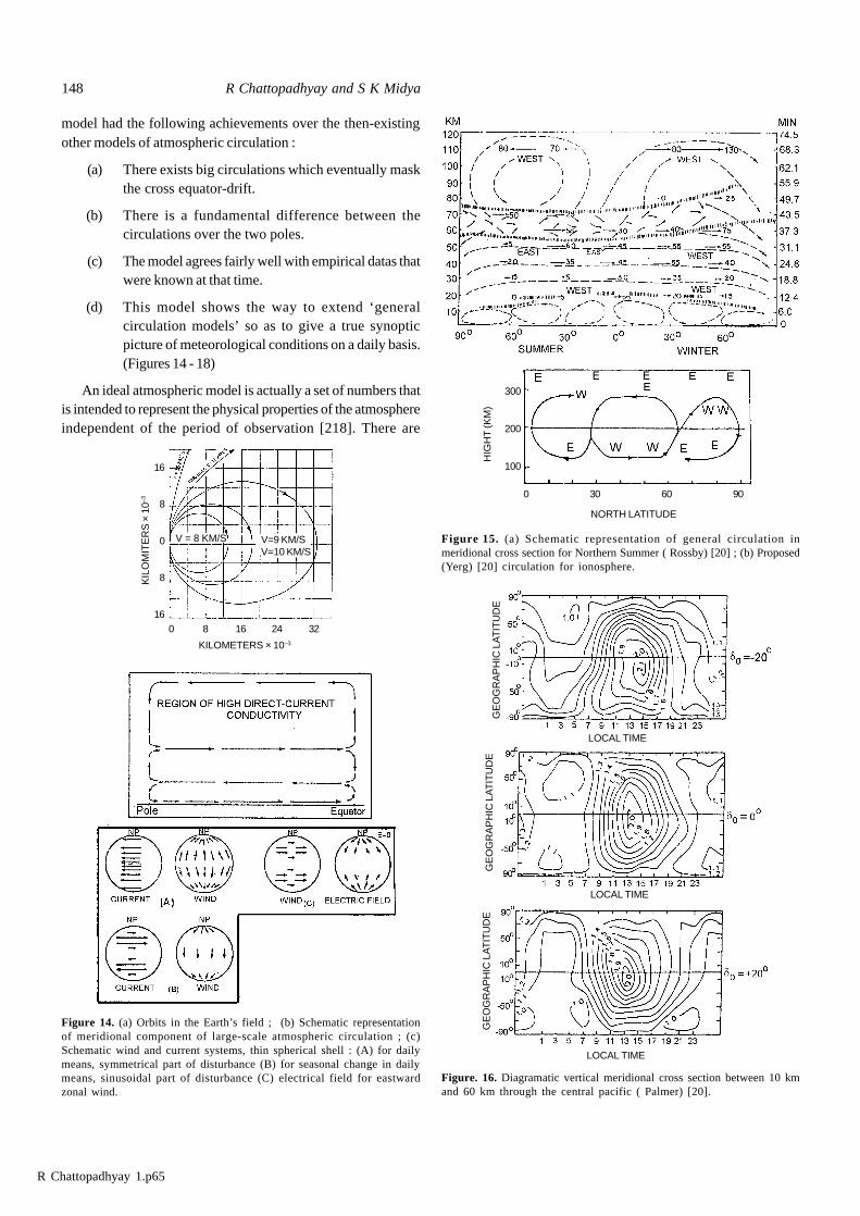
R Chattopadhyay 1.p65
148 R Chattopadhyay and S K Midya
Figure 15. (a) Schematic representation of general circulation inmeridional cross section for Northern Summer ( Rossby) [20] ; (b) Proposed(Yerg) [20] circulation for ionosphere.
Figure. 16. Diagramatic vertical meridional cross section between 10 kmand 60 km through the central pacific ( Palmer) [20].
Figure 14. (a) Orbits in the Earth’s field ; (b) Schematic representationof meridional component of large-scale atmospheric circulation ; (c)Schematic wind and current systems, thin spherical shell : (A) for dailymeans, symmetrical part of disturbance (B) for seasonal change in dailymeans, sinusoidal part of disturbance (C) electrical field for eastwardzonal wind.
model had the following achievements over the then-existingother models of atmospheric circulation :
(a) There exists big circulations which eventually maskthe cross equator-drift.
(b) There is a fundamental difference between thecirculations over the two poles.
(c) The model agrees fairly well with empirical datas thatwere known at that time.
(d) This model shows the way to extend ‘generalcirculation models’ so as to give a true synopticpicture of meteorological conditions on a daily basis.(Figures 14 - 18)
An ideal atmospheric model is actually a set of numbers thatis intended to represent the physical properties of the atmosphereindependent of the period of observation [218]. There are
KIL
OM
ITE
RS
× 1
0–3
16
8
0
8
160 8 16 24 32
KILOMETERS × 10–3
V = 8 KM/S V=9 KM/SV=10 KM/S
NORTH LATITUDE
HIG
HT
(KM
)0 30 60 90
300
200
100
GE
OG
RA
PH
IC L
AT
ITU
DE
LOCAL TIME
GE
OG
RA
PH
IC L
AT
ITU
DE
LOCAL TIME
LOCAL TIME
GE
OG
RA
PH
IC L
AT
ITU
DE
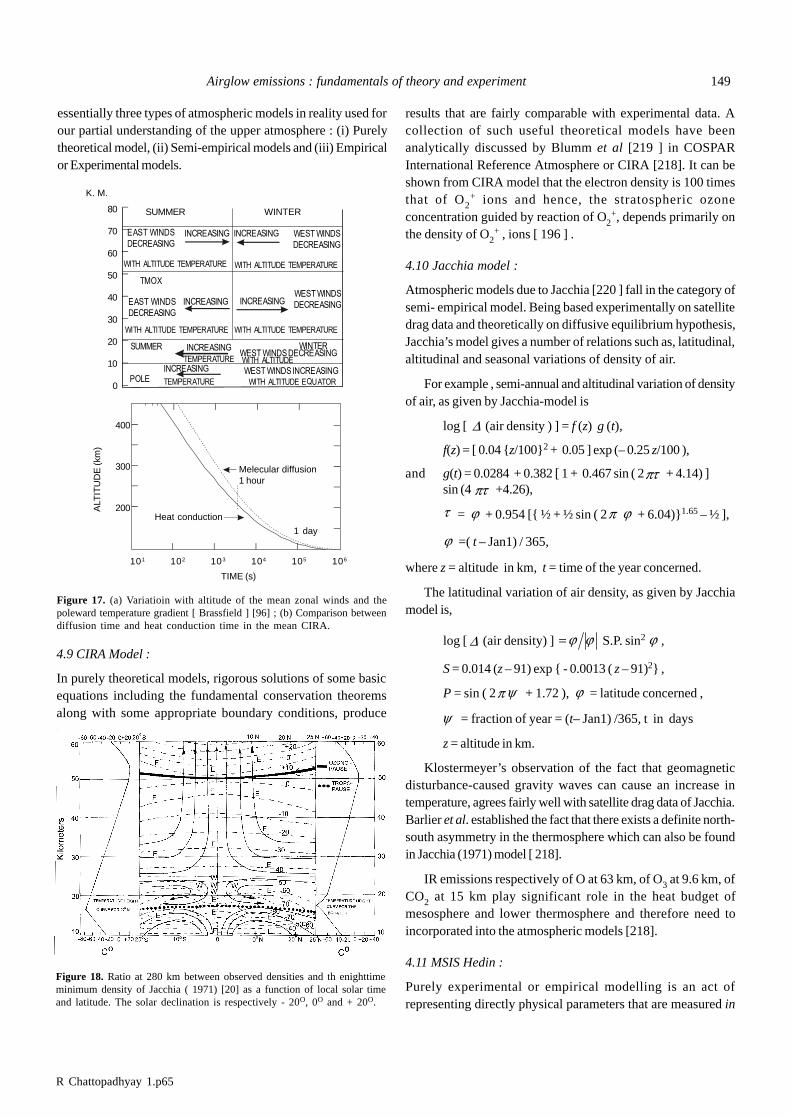
R Chattopadhyay 1.p65
Airglow emissions : fundamentals of theory and experiment 149
results that are fairly comparable with experimental data. Acollection of such useful theoretical models have beenanalytically discussed by Blumm et al [219 ] in COSPARInternational Reference Atmosphere or CIRA [218]. It can beshown from CIRA model that the electron density is 100 timesthat of O2
+ ions and hence, the stratospheric ozoneconcentration guided by reaction of O2
+, depends primarily onthe density of O2
+ , ions [ 196 ] .
4.10 Jacchia model :
Atmospheric models due to Jacchia [220 ] fall in the category ofsemi- empirical model. Being based experimentally on satellitedrag data and theoretically on diffusive equilibrium hypothesis,Jacchia’s model gives a number of relations such as, latitudinal,altitudinal and seasonal variations of density of air.
For example , semi-annual and altitudinal variation of densityof air, as given by Jacchia-model is
log [ D (air density ) ] = f (z) g (t),
f(z) = [ 0.04 {z/100}2 + 0.05 ] exp (– 0.25 z/100 ),
and g(t) = 0.0284 + 0.382 [ 1 + 0.467 sin ( 2pt + 4.14) ]sin (4 pt +4.26),
t = j + 0.954 [{ ½ + ½ sin ( 2p j + 6.04)}1.65 – ½ ],
j =( t – Jan1) / 365,
where z = altitude in km, t = time of the year concerned.
The latitudinal variation of air density, as given by Jacchiamodel is,
log [ D (air density) ] = j j S.P. sin2 j ,
S = 0.014 (z – 91) exp { - 0.0013 ( z – 91)2} ,
P = sin ( 2p y + 1.72 ), j = latitude concerned ,
y = fraction of year = (t– Jan1) /365, t in days
z = altitude in km.
Klostermeyer’s observation of the fact that geomagneticdisturbance-caused gravity waves can cause an increase intemperature, agrees fairly well with satellite drag data of Jacchia.Barlier et al. established the fact that there exists a definite north-south asymmetry in the thermosphere which can also be foundin Jacchia (1971) model [ 218].
IR emissions respectively of O at 63 km, of O3 at 9.6 km, ofCO2 at 15 km play significant role in the heat budget ofmesosphere and lower thermosphere and therefore need toincorporated into the atmospheric models [218].
4.11 MSIS Hedin :
Purely experimental or empirical modelling is an act ofrepresenting directly physical parameters that are measured in
Figure 18. Ratio at 280 km between observed densities and th enighttimeminimum density of Jacchia ( 1971) [20] as a function of local solar timeand latitude. The solar declination is respectively - 20O, 0O and + 20O.
Figure 17. (a) Variatioin with altitude of the mean zonal winds and thepoleward temperature gradient [ Brassfield ] [96] ; (b) Comparison betweendiffusion time and heat conduction time in the mean CIRA.
essentially three types of atmospheric models in reality used forour partial understanding of the upper atmosphere : (i) Purelytheoretical model, (ii) Semi-empirical models and (iii) Empiricalor Experimental models.
4.9 CIRA Model :
In purely theoretical models, rigorous solutions of some basicequations including the fundamental conservation theoremsalong with some appropriate boundary conditions, produce
||
||
||
||
|
K. M.
80
70
60
50
40
30
20
10
0
SUMMER WINTER
EAST WINDSDECREASING
INCREASING INCREASING WEST WINDSDECREASING
WITH ALTITUDE TEMPERATURE WITH ALTITUDE TEMPERATURE
EAST WINDSDECREASING
INCREASING INCREASINGWEST WINDSDECREASING
WITH ALTITUDE TEMPERATURE WITH ALTITUDE TEMPERATURE
TMOX
SUMMER WINTERINCREASINGTEMPERATURE
WEST WINDS DECREASINGWITH ALTITUDE
INCREASINGTEMPERATURE WITH ALTITUDE EQUATOR
WEST WINDS INCREASINGPOLE
ALT
ITU
DE
(km
)
400
300
200
101 102 103 104 105 106
TIME (s)
Heat conduction
Melecular diffusion1 hour
1 day
||
||
|
||
||
||
| | | |
| | | |
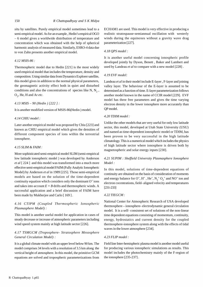
R Chattopadhyay 1.p65
150 R Chattopadhyay and S K Midya
situ by satellites. Purely empirical model sometimes lead to asemi-empirical model. As for an example , Hedin’s empirical OGO– 6 model gives a worldwide distribution of temperature andconcentration which was obtained with the help of sphericalharmonic analysis of measured data. Similarly, ESRO-4 data dueto von Zahn presents another empirical model.
4.12 MSIS-86 :
Thermospheric model due to Hedin [221] is the most widelyused empirical model that includes the temperature, density andcomposition. Using similar data from Dynamics Explorer satellite,this model gives in addition to the normal physical parameters,the geomagnetic activity effect both in quiet and disturbedconditions and also the concentrations of species like N, N2 ,O2, He, H and Ar etc.
4.13 MSIS – 90 (Hedin ) [222 ] :
It is another modified version of MSIS-86(Hedin ) model.
4.14 CHIU model :
Later another empirical model was proposed by Chiu [223] andknown as CHIU empirical model which gives the densities ofdifferent component species of ions within the terrestrialionosphere.
4.15 SLIM & FAIM :
More sophisticated semi-empirical model SLIM (semi-empiricallow latitude ionospheric model ) was developed by Andersonet al [ 224 ] and this model was transformed into a much moreeffective semi-empirical model FAIM (Fully Analytic IonosphericModel) by Anderson et al in 1989 [225]. Those semi-empiricalmodels are based on the solution of the time-dependentcontinuity equation which considers only the dominant O+ ionsand takes into account E × B drifts and thermospheric winds. Asuccessful application and a brief discussion of FAIM havebeen made by Mukherjee and Carlo [ 169 ] .
4.16 CTIPM (Coupled Thermospheric IonosphericPlasmasphere Model) :
This model is another useful model for application in cases ofsteady decrease or increase of atmospheric parameters includingwind speed system mainly at high latitude sector [226].
4.17 TSMGCM (Troposphere- Stratosphere MesosphereGeneral Circulation Model) :
It is a global climate model with an upper level below 90 km. Themodel comprises 34 levels with a resolution of 3.5 km along thevertical height of atmosphere. In this model, the primitive GCMequations are solved and tropospheric parameterizations from
ECHAM1 are used. This model is very effective in producing arealistic stratospause-semiannual oscillation with westerlywinds during the equinoxes without a gravity wave dragparameterization [227].
4.18 QPS model :
It is another useful model concerning ionospheric profiledeveloped jointly by Dyson, Benett , Baker and Lambert andused by Landeau et al to compare with a new model [228] .
4.19 EVF model:
Landeau et al in their model include E-layer , F-layer and joiningvalley layer. The behaviour of the E-layer is assumed to bedetermined as a function of time. E-layer parameterization followsanother model known in the name of CCIR model [229]. EVFmodel has three free parameters and gives the time varyingelectron density in the lower ionosphere more accurately thanQP model.
4.20 TDIM model :
Unlike the other models that are very useful for only low latitudesector, this model, developed at Utah State University (USU)and named as time-dependent ionospheric model or TDIM, hasbeen proven to be very successful in the high latitudeclimatology. This is a numerical model which includes the physicsof high latitude sector where ionosphere is driven both bymagnetospheric and solar energy inputs [230].
4.21 SUPIM : Sheffield University Plasmasphere IonosphereModel :
In this model, solutions of time-dependent equations ofcontinuity are obtained on the basis of consideration of momentsand energy balance for O+, H+ , He+, N2
+ O2+ and NO+ ion and
electron cocentrations, field- aligned velocity and temperatures[231-233]
4.22 TIEGCM :
National Center for Atmospheric Research of USA developedthermosphere – ionosphere- electrodynamic general circulationmodel. It is a self- consistent set of solutions of the non-lineartime dependent equations consisting of momentum, continuity,energy, hydrostatics and current density for the coupledthermosphere-ionosphere system along with the effects of tidalwaves in the lower atmosphere [234].
4.23 FLIP model :
Field line Inter-hemispheric plasma model is another model usefulfor producing various ionospheric simulations as results. Thismodel includes the photochemistry mainly of the F-region ofthe ionosphere [235-237] .
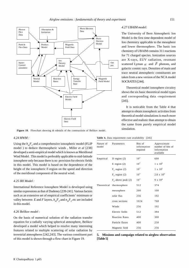
R Chattopadhyay 1.p65
Airglow emissions : fundamentals of theory and experiment 151
4.24 MWM :
Using the hmF2 and a comprehensive ionospheric model (FLIPmodel ) to deduce thermospheric winds , Miller et al [238]developed a semi-empirical model which is known as MeridionalWind Model . This model is preferably applicable to mid-latitudeionosphere only because there is no provision for electric fieldsin this model. This model is based on the dependence of theheight of the ionospheric F-region on the speed and directionof the meridional component of the neutral wind.
4.25 IRI Model :
International Reference Ionosphere Model is developed usingsimilar expressions as that of Dudeney [239-241]. Various factorssuch as an extensive set of empirical coefficients’ minimum orvalley between E and F layers, hmF2 and nmF2 etc are includedin this model.
4.26 Belikov model :
On the basis of numerical solution of the radiation transferequation for a radially varying spherical atmosphere, Belikovdeveloped a model which helped to resolve many interestingfeatures related to multiple scattering of solar radiation byterrestrial atmospheres [242,243]. The various constituent partof this model is shown through a flow chart in Figure 19.
4.27 UBAIM model:
The University of Bern Atmospheric IonModel is the first time dependent model ofIon chemistry applicable to the mesophereand lower thermosphere. The basic ionchemistry of UBAIM contains 311 reactionsfor 71 charged species. Ionization sourcesare X-rays, EUV radiation, resonantscattered Lyman a and b photons, andgalactic cosmic rays. Densities of main andtrace neutral atmospheric constituents aretaken from a new version of the NCA modelSOCRATES [244].
Theoretical model ionosphere circuitryshows the six basic theoretical model typesand corresponding data -requirement[245].
It is noticable from the Table 4 thatattempt to obtain ionospheric activities fromtheoretical model simulations is much moreeffective and realistic than attempt to obtainthe same from purely empirical modelsimulation.
Table 4. Data requirement cum availability [245]
Nature of Parameters Bits of Approximatemodel information number of bits of
required informationavailable
Empirical D region (2) 107 600
E region (2) 107 1 x 10⁵
F1 region (2) 107 1 x 10⁵
F2 region (2) 107 2.8 x 10⁵
F2 above peak (2) 107 9 x 10⁴
Theoretical thermosphere 512 374
mesosphere 200 100
solar flux 256 192
cross sections 1024 768
Winds 256 192
Electric fields 512 384
Reaction Rates 400 300
Particle fluxes 400 250
Magnetic field 256 256
5. Missions and campaign related to airglow observation[Table 5]
PhotonFluxData
ParticleFlux Data
InpactControlparameter
Absorption &Ionizat ion
ProductModel
NeutralModel
MagneticField Data
ReactionRates
IonDensityModel
EnergyTransferRate
MagneticField Model
Output
Electric FieldModel
Electric FieldData
Photo ElectronData
PhotoElectronModel
Figure 19. Flowchart showing th edetails of the comtructioin of Belikov model.
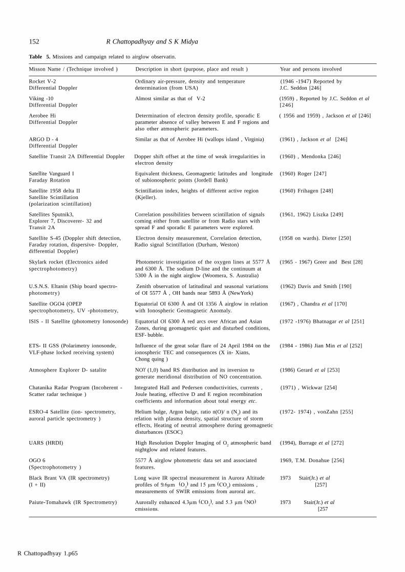
R Chattopadhyay 1.p65
152 R Chattopadhyay and S K Midya
Table 5. Missions and campaign related to airglow observatin.
Misson Name / (Technique involved ) Description in short (purpose, place and result ) Year and persons involved
Rocket V-2 Ordinary air-pressure, density and temperature (1946 -1947) Reported byDifferential Doppler determination (from USA) J.C. Seddon [246]
Viking -10 Almost similar as that of V-2 (1959) , Reported by J.C. Seddon et alDifferential Doppler [246]
Aerobee Hi Determination of electron density profile, sporadic E ( 1956 and 1959) , Jackson et al [246]Differential Doppler parameter absence of valley between E and F regions and
also other atmospheric parameters.
ARGO D - 4 Similar as that of Aerobee Hi (wallops island , Virginia) (1961) , Jackson et al [246]Differential Doppler
Satellite Transit 2A Differential Doppler Dopper shift offset at the time of weak irregularities in(1960) , Mendonka [246]electron density
Satellite Vanguard I Equivalent thickness, Geomagnetic latitudes and longitude(1960) Roger [247]Faraday Rotation of subionospheric points (Jordell Bank)
Satellite 1958 delta II Scintillation index, heights of different active region (1960) Frihagen [248]Satellite Scintillation (Kjeller).(polarization scintillation)
Satellites Sputnik3, Correlation possibilities between scintillation of signals (1961, 1962) Liszka [249]Explorer 7, Discoverer- 32 and coming either from satellite or from Radio stars withTransit 2A spread F and sporadic E parameters were explored.
Satellite S-45 (Doppler shift detection, Electron density measurement, Correlation detection, (1958 on wards). Dieter [250]Faraday rotation, dispersive- Doppler, Radio signal Scintillation (Durham, Weston)differential Doppler)
Skylark rocket (Electronics aided Photometric investigation of the oxygen lines at 5577 Å(1965 - 1967) Greer and Best [28]spectrophotometry) and 6300 Å. The sodium D-line and the continuum at
5300 Å in the night airglow (Woomera, S. Australia)
U.S.N.S. Eltanin (Ship board spectro- Zenith observation of latitudinal and seasonal variations (1962) Davis and Smith [190]photometry) of OI 5577 Å , OH bands near 5893 Å (NewYork)
Satellite OGO4 (OPEP Equatorial OI 6300 Å and OI 1356 Å airglow in relation (1967) , Chandra et al [170]spectrophotometry, UV -photometry, with Ionospheric Geomagnetic Anomaly.
ISIS - II Satellite (photometry Ionosonde)Equatorial OI 6300 Å red arcs over African and Asian (1972 -1976) Bhatnagar et al [251]Zones, during geomagnetic quiet and disturbed conditions,ESF- bubble.
ETS- II GSS (Polarimetry ionosonde, Influence of the great solar flare of 24 April 1984 on the (1984 - 1986) Jian Min et al [252]VLF-phase locked receiving system) ionospheric TEC and consequences (X in- Xians,
Chong quing )
Atmosphere Explorer D- satalite NOg (1,0) band RS distribution and its inversion to (1986) Gerard et al [253]generate meridional distribution of NO concentration.
Chatanika Radar Program (Incoherent - Integrated Hall and Pedersen conductivities, currents , (1971) , Wickwar [254]Scatter radar technique ) Joule heating, effective D and E region recombination
coefficients and information about total energy etc.
ESRO-4 Satellite (ion- spectrometry, Helium bulge, Argon bulge, ratio n(O)/ n (N2) and its (1972- 1974) , vonZahn [255]
auroral particle spectrometry ) relation with plasma density, spatial structure of stormeffects, Heating of neutral atmosphere during geomagneticdisturbances (ESOC)
UARS (HRDI) High Resolution Doppler Imaging of O2 atmospheric band (1994), Burrage et al [272]
nightglow and related features.
OGO 6 5577 Å airglow photometric data set and associated 1969, T.M. Donahue [256](Spectrophotometry ) features.
Black Brant VA (IR spectrometry) Long wave IR spectral measurement in Aurora Altitude1973 Stair(Jr.) et al(I + II) profiles of 9.6ìm (O
3) and 15 ìm (CO
2) emissions , [257]
measurements of SWIR emissions from auroral arc.
Paiute-Tomahawk (IR Spectrometry) Aurorally enhanced 4.3ìm (CO2), and 5.3 ìm (NO) 1973 Stair(Jr.) et al
emissions. [257
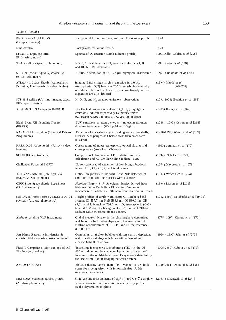
R Chattopadhyay 1.p65
Airglow emissions : fundamentals of theory and experiment 153
Black BrantVA (III & IV) Background for auroral case, Auroral IR emission profile.1974(IR spectrometry)
Nike-Javelin Background for auroral cases. 1974
SPIRIT 1 Expt. (Spectral Spectra of O3 emission (Limb radiance profile) 1990, Adler Golden et al [258]
IR Interferometry)
S3-4 Satellite (Spectro photometry) NO, d, g band emissions, O2 emissions, Herzberg I, II 1992, Eastes et al [259]
and III, N2 LBH emissions.
S-310-20 (rocket liquid N2 cooled Ge Altitude distribution of O
2 1.27 ìm nightglow observation 1992, Yamamoto et al [260]
sensor radiometry)
ATLAS - 1 Space Shuttle (Atmospheric Imaging Earth’s night airglow emission in the O2, (1994) Mende et al.
Emission, Photometric Imaging device) Atmospheric [O,O] bands at 702.0 nm which eventually [262-265]absorbs all the Earth-reflected emissions. Gravity waves’signatures are also detected.
STS-39 Satellite (UV limb imaging expt., H, O, N, and N2 dayglow emissions’ observations (1991-1994) Budzien et al [266]
FUV Spectrometer)
AIDA ACT ’89 Campaign (MORTI) The fluctuations in atmospheric O2(b 1Ó
g+) nightglow (1993) Hickey et al [267]
emissions induced respectively by gravity waves,evanescent waves and acoustic waves, are analysed.
Black Brant XII Sounding Rocket EUV emissions of atomic oxygen , molecular nitrogen (1988 - 1993) Cotton et al [268](BEARS) dayglow features etc. (Wallop Island, Virginia)
NASA CRRES Satellite (Chemical Release Emissions from spherically expanding neutral gas shells,(1990-1994) Woscott et al [269]Programme) released near perigee and below solar terminator were
observed.
NASA DC-8 Airborne lab. (All sky video. Observations of upper atmospheric optical flashes and (1993) Sentman et al [270]imaging) consequences (American Midwest).
SPIRE (IR spectrometry) Comparison between non- LTE radiative transfer (1994), Nebel et al [271]calculation and 4.3 ìm Earth limb radiance data.
Challenger Space lab2 (IRT) IR consequences of excitation of low lying vibrational (1994),Maycrott et al [273]levels of H
2O by O (3P) and implications
ACTIVNY- Satellite (low light level Optical diagnostics in the visible and NIR detection of (1992) Wescott et al [274]imagers & Spectrograph) emission from satellite releases were examined.
CIRRIS 1A Space shuttle Experiment Absolute NO(v = 1, J, Ù) column density derived from (1994) Lipson et al [261](IR Spectrometry) high resolution Earth limb IR spectra. Production
mechanism of subthermal NO spin orbit distribution tested.
SONDA III rocket borne , MULTIFOT 92 Height profiles of airglow emissions O2 Herzberg-band (1992-1995) Takahashi et al [29-30]
payload (Airglow photometry) system, OI 557.7 nm NaD 589.3nm, OI 630.0 nm OH(8,3) band R branch at 724.0 nm , O
2 Atmospheric (O,O)
band at 762 nm, sky background at 578 nm and 710nm ,Sodium Lidar measured atomic sodium.
Akebono satellite VLF instruments Global electron density in the plasmasphere determined (1775- 1997) Kimura et al [172]and found to be L value dependent. Determination ofrelative concentrations of H+, He+ and O+ the referencealtitude etc
San Marco 5 satellite Ion density & Correlation of airglow bubbles with ion density depletion, (1988 - 1997) Jahn et al [275]electric field measuring instrumentation) and of additional airglow bubbles with enhanced AC
electric field fluctuations.
FRONT Campaign (Radio and optical All Travelling Ionospheric Disturbances (TID) in the OI (1998-2000) Kubota et al [276]Sky Imaging devices) 630 nm nightglow images over Japan and its structure’s
location in the mid-latitude lower F-layer were detected bythe use of multipoint imaging network system.
ARGOS (HIRAAS) Electron density determination by inversion of UV limb (1999-2001) Dymond et al [38]scans for a comparison with ionosonde data. A fairagreement was noticed.
METEORS Sounding Rocket project Simultaneous measurements of O2(1 D ) and O
2(1 å ) airglow (2001 ) Miynczak et al [277]
(Airglow photometry) volume emission rate to derive ozone density profilein the daytime mesosphere.
Table 5. (contd.)
R Chattopadhyay 1.p65
154 R Chattopadhyay and S K Midya
6. Newly discovered airglow lines’ features, newly proposedexcitation mechanism and newly determined constants andcoefficients.
Some of the relatively recently discovered airglow lines’ features,newly proposed excitation mechanisms and newly determinedconstants and coefficients are described below :
6.1 O (1D) rate constants and their temperature dependence:
Streit et al [104] gave absolute rate constants and theirtemperature-dependence for the deactivation of O(1D) by fiveatmospheric gases O2, N2, CO2, O3 and H2O. Photolysis of O3at 266 nm [104] produces O (1D), which in the transition O(1D)® O(3p) gives 630 nm radiation. Gases O2, N2 and CO2 ,thequenchers of O(1D) are found to have a small negativetemperature-dependence. Arrhenius expressions for thereactions measured and given by Streit et al [104] are O2 (T= 104– 354K) 0.29 exp (134/RT), N2 (T = 104 –354k) 0.20 exp(214/RT),CO2(T = 139 -200 K) 1.2 and (T= 200–354K) 0.68 exp(233/RT).The rate constants for O3 and H2O are 2.4 × 10⁻¹⁰ and 2.3 × 10⁻¹⁰ cm3/ molecule, and over the ranges of 103-393K and 253 - 353K , respectively.
6.2 New values of rate constants and branching ratio for N2+
+ O reaction :
The branching ratio and the rate constant for the reaction N2+ +
O were remeasured by Knutsen et al [278]. The resulting rateconstant was found to be equal to 1.8(± 0.7) x 10-10 cm3 s-1 andbranching ratio of NO+ : O+ = 90( ± 3) : 10( ± 3) were found to bein good agreement with earlier measurements.
6.3 New value of Einstein’s coefficient for spontaneous emissionof the O
2 ( a 1 D g
) state :
For the transition O2( X 3å g - a 1 D g) at 1.2 mm, Einstein
coefficient A for spontaneous emission of radiation has beenfound by Mlynczak et al [279] to be equal to 1.47 × 10⁻⁴ s-1. Theconventionally used value has been 2.58 × 10⁻⁴ s-1. The newvalue of A coefficient implies that ozone concentrations, inferredfrom O2 ( a 1 D g) emission, must increase significantly in existingdata bases [ 279].
6.4 Revised cross-sections of O+ 834 Å dayglow:
Assessment of O(3P) photoionization, N2 photoabsorptioncrosssections, O+ oscillator strength and transition probabilitieson OII 834 Å airglow emissions were made by Link et al [280].The 834 Å intensities computed using the new parameters asmentioned above, agrees fairly well with rocket data. Incontradicton to data that were used earlier, there new data indicatethat besides being unique, NmF2 and hmF2 can vary by factors2 and 50 km, respectively.
6.5 Carroll- Yoshino band problem :
Terrestrial airglow emissions near 958 Å and 980 Å
corresponding to N2 Carroll- Yoshino c’4 1 å u
+ – x 1 å g+ (O, O),
I(OP) and (O, 1) Rydberg bands are found to be weaker thanthese inferred from c’4 (O) excitation rate . For resolving thisproblem, Stevens et al [281] developed and discussed theirresonant fluorescent scattering model for CY(0,0) and (0,1).
6.6 New finding about OI 844.6 nm emission mechanism :
Experimentally obtained twilight decay curves for thermosphericOI 844.6 nm emission was also represented by the field lineinterhemispheric plasma model. This model assumes onlyphotoelectron-impact-excitation to be the only [282] productionmechanism with a crosssection appropriate to an optically thinatmosphere. The model calculations were found to agree withthe experimentally obtained results.
6.7 New quenching value of O(1D) :
New value of rate coefficient for quenching of O(1D) by O(3P)was found out [283] as a function of temperature. which doesnot agree with the usually considered value.
6.8 Self absorption theory :
A self-absorption model using Holstein transmission functionwas developed [284] and applied successfully to UV fluorescentNO (1,0) g - band emission.
6.9 New inference about Na nightglow excitation :
The potential energy surfaces of NaO+O reactionlead to excitedNa* (2P) atoms which involve doublet rather than quartet spinconfigurations and have the branching ratio f~ 2/3 for the excitedstate of NaO [285].
6.10 On the analysis of geophysical data for an unknownconstant :
Uncritical use of least square method of analysis of geophysicaldata is inappropriate and must be supplemented [286] with anerror analysis. This fact has been exemplified with O+ - O collisioncross-section.
6.11 Inference about quenching rates for O2 Herzberg I bands:
In agreement with the laboratory measurements, the values ofquenching rates for O2 Herzberg I band , O2 Atmospheric band(O, O) and the green line have been newly found and is greaterthan 1 x 10-11, the value usually considered [187].
6.12 Measurerment of rate constant for quenching CO2 by
atomic oxygen at low temperature :
Laboratory measurement of the rate constant for quenchingCO2 (OI 1O) state during collisions of CO2 molecules with O
R Chattopadhyay 1.p65
Airglow emissions : fundamentals of theory and experiment 155
atoms at temperatue range of 206-358 K has been made. The useof these new values of rate constant significantly decreased therate of cooling by CO2 15 ìm emission in the terrestrial lowerthermosphere as compared to the previously obtained rate [287].
7. Effect of different physical factors on airglow emissions
Classification of factors that affect airglow emissions :
The factors that the terrestrial airglow emissions depend on,may be broadly classified into four types :
(i) Purely of solar origin
(ii) Lunar effects
(iii) Effects of other cosmic bodies
(iv) Terrestrial atmospheric features.
7.1 Purely solar effect :
Solar activities are the main sources of terrestrial ionososphericfeatures and have already been discussed in Sections 2.2 and2.3. Study of correlations of terrestrial airglow and associatedphenomen a with specific solar parameters started relativelylater and has gathered momentum in recent past. Sahai et al[288] have shown that OI 630.0 nm low-latitude nightglowintensity is very strongly correlated with 10.7 cm solar flux andsunspot number. The correlations are generally found to bealmost seven times in high solar activity period than in low solaractivity period . Midya et al [289] have shown that Na 5893 Ånightglow intensity showed an oscillatory variation with solarflare number, relative sunspot number and variable componentof 10.7 cm solar flux both in peak phase of 20th solar cycle at Mt.Abu and in non-peak phase of 21st solar cycle at Kolkata. Theyinterpreted this variation in terms of similar variation of ozoneas ozone’s concentration is a major factor on which atmosphericsodium concentration and associated emission intensity depend.Terez and Terez [290] have established that the variation of globaltotal ozone content is mostly the result of 10.7 cm. solar fluxvariation [291]. Labitzke and Loon [291] have established thatthe statistical correlation between ozone concentration and 10.7cm. solar flux is highest between 5o and 30o latitude and thegeopotential heights in ozone layer has a good correlation with11 year sunspot cycle. Clemensha et al [292] analysed theatmospheric sodium measurements and concluded that thecentroid height of the sodium layer shows its covariation with10 year (?) solar cycle related oscillations. A good correlation of(OH) (8,3) band rotational temperature with 10.7 cm. solar fluxhas been obtained by Sahai et al [293] . Midya et al [210] obtainedan oscillatory mode of variation in 5893 Å nightglow intensityas plotted against solar flare index given by Sawyer. Silbergeit[294] found a correlation between the geomagnetic storm andsolar cycle length. Kolomittsev et al [295] studies theoreticallythe dependence of F-region electron density profile on solar
activity expressed in terms of 10.7 cm. solar flux. Adler et al[296] established the fact that along with 10.7 cm solar flux andsunspot number, solar cycle length (SCL) is also a good indicatorof long term changes in solar EUV radiations that affect stronglythe terrestrial ionosphere, particularly the IEC. Midya and Midya[196] studied the correlation of monthly mean values of h/ F andfoF2 with each of three solar parameters, solar flare number,sunspot number and 10.7 cm solar flux. They studies thedependence of 5577 Å airglow intensity on solar parametersand found some useful regression equations. Smith and King[297] described in detail the long term relationships of sunspotsand solar faculae with different ionospheric parameters.Correlation between O3 concentration and solar flare index(Sawyer) has been found to be poor. Midya et al [298] foundoscillatory modes of variations of 5577 Å line airglow intensitywith each of sunspot number and 10.7 cm. solar flux both inpeak phase (of 20th solar cycle at Mt. Abu) and in non-peakphase (of 21st solar cycle at Kolkata). Mikhailov et al [299]studied the dependence of post-midnight winter NmF2enhancements on solar activity. Borovsky et al [300] exploredthe correlation between the amplitude of the MHD turbulencein the upstream solar wind and the amplitude of the Earth’sgeomagnetic activity indices. From fluid flow experiment, theterbulence effect is interpreted as an enhanced viscous couplingof the solar wind flow to the Earth’s magnetosphere caused byan eddy viscosity that is controlled by the amplitude of MHDturbulence.
7.2 Purely lunar effects :
Lunar effects on Terrestrial airglow phenomena may broadly beclassified into three types ; (a) Effect of background moon light,(b) L-variation and tidal effect (c) Effect of terrestrial magnetotailand reversal of electric field and related E × B drift. OI 6300 Ånightglow emission has been found to be affected by Moon’sage less than 7 days or more than 23 days for D > 50o [301].Approximately, 7% of the incident light gets reflected from lunarsurface; an appreciable amount of lunar thermal emission comesout of it [302-303]. Lunar radiations undergo short-period fadingdue to scintillation proportional to lunar libration and also long-period fading which is presumed to be caused by ionosphericirregularities associated with absorption, Doppler effect andFaraday effect within the atmosphere [304]. Lunar tidal variationof magnetic field (L-Variation ) is high at the Newmoon phase atequinox and summer solstice. The electric current responsiblefor L-variation on the sunlit side of the Earth have intensityusually one tenth of that for Sq. [22,24] . Inspite of being weakerrelative to the solar tidal effect, the lunar tidal effect is morereadily determined and has been observed in D, E, F1 and F2regions of the ionosphere [20]. Lunar tides leave signature inthe mesopause region of upper atmosphere which is revealedby the characteristics of the variation of atmospheric emissionwith Moon’s age [234] . The Earth on its night-side, has a
R Chattopadhyay 1.p65
156 R Chattopadhyay and S K Midya
magnetic field extended beyond the lunar orbit and may therefore,interact with the lunar magnetic field [305] . The strong local-time-dependence of O(1S) airglow emission at the geographicequator is presumed to be the result of tidal effect [ 189 ] . In thelocal solar time domain, the volume emission rate of oxygen andhydroxyl band airglow and their peak-height at the equator,undergo large tidal perturbation [44]. Fesen [234] has shownthrough TIEGCM simulation that F2 peak electron densitydepends partially on the vertically propagating tide [234].
7.3 Effects of other cosmic bodies :
Meteoritic effects :
Analysis of IR airglow data obtained from on board USA FISTAaircraft indicates a small yet significant enhancement in OHairglow emission during the peak of the storm related to Leonid1999 meteror shower [306] although no such influence on Na Dairglow emissions was observed during the same meteor storm[307].
7.4 Terrestrial atmospheric features which the terrestrialairglow emissions depends on are mainly the following :
Gravity wave effects :
Mercier [ 308 ] reports some statistical results of observation ongravity waves within the ionosphere. This observation was madewith the help of ground based radio inter- ferometers. Tarassickand Hines [309] explored the influence of gravity waves onairglow emissions elucidating the observable effects of suchwaves. Methods of distinguishing between evanescent wavesand internal gravity wave modes and of determination of verticalwavelength were proposed by Tarassic et al Isler et al [310]obtained a closed-form solution for the integrated airglowresponse to linear gravity wave where all the higher ordernonlinear response terms are retained. Wave-induced airglowfluctuations were shown to be much greater than thecorresponding density fluctuations for major atomic species.Sobral et al [33] reported winter-time photometric perturbationof the nocturnal F-region atomic oxygen 630 nm red line intensityon southern hemisphere which they observed to be concurrentwith apparent ionogram signatures of F-region gravity waves .Gravity waves act as a source of perturbation for initiating plasmabubble events during the month when the ambient ionosphericconditions provide favourable chances for growth of instability.Hines [311] proved a fundamental theorem of airglowfluctuations that are induced by gravity waves and also showedthat gravity wave-induced airglow fluctuations do not dependon the minor species involved in the photochemistry of thecorresponding emission process. Wang et al [312] generalizedHines-Tarassick’s theory of gravity waves induced airglowfluctuations and compare their results of analysis with observed
variations. Five years of photometric data of the 630 nm oxygenairglow emissions over Davis, Antarctica, have been searchedby Innis et al [313] for obtaining evidence of periodic oscillationsdue to atmospheric gravity waves. Hetch et al [314] analysedthe instability features in airglow caused by atmospheric gravitywaves and found that if same is characterized by the aligment ina direction perpendicular to the atmospheric gravity wave (AGW)wavefronts. Observation made with the help of multicomponentinstrument confirms the fact that such features are caused byconvective instability.
Yao [315] established a two dimensional time-dependentnonlinear photochemical dynamical coupling gravitationalwaves model and he solved it using FICE method. Results ofsimulation from this model show that the gravity wavepropagation can induce large change of the mean profiles ofoxygen compound and hydrogen compound in the mesopauseregion.
Geomagnetic effects:
Numerical simulation of Monte Carlo (MC) solution of nonlinearBoltzman equation for chemically produced hot oxygen atomsis found to give number density and temperature of nonthermaloxygen atoms at equatorial latitudes which fairly agree with theobserved results under the condition of low solar andgeomagnetic activities [316,251]. The thermospherictemperatures obtained from Doppler broadening of OI 630. nmemissions and the mesospheric rotational temperatures obtainedfrom OH (9,4) and O2A(0,1) band emissions during the recoveryphase of geomagnetic storms were found to be lower than thecorresponding values in the quiet geomagnetic conditions,respectively [317] . Field and Rishbeth [318] express the disturbedto quiet ratio of NmF2 in terms of mean (DC) and local time (AC)variations for over 20 years’ data from each of 53 stations between70o N and 80o S and they found some important implicationsincluding a long term effect. They interpreted their results interms of change of composition of F2-layer due to storms . Saha[319] describes enhancement in the equatorial peak atomic oxygendensity in the lower thermosphere and also the rise in OH (7-2)nightglow intensity following a geomagnetic substorm althoughno such enhancement of OI 6300 Å could be observed ascompared to OI 5577 Å intensity rise. He interpreted theobservational results on the basis of the concept that extra-ionospheric current increases the recombination rate. Regularall sky imaging observations of the F-region nightglow emissionand mesospheric band emission during geomagnetic storm ofFebruary 12,2000 show that both OI 6300 Å airglow emissionsand band emissions are enhanced along with several small scaleintensity depletional structures which, as Sahai et al [320]suggest , might be caused by nonlinear interactions betweenTID and enhanced ionospheric anomaly.
R Chattopadhyay 1.p65
Airglow emissions : fundamentals of theory and experiment 157
Effects of lightning:
Boeck et al [321] described a transient luminosity observed atthe height of airglow layer (~95 km) in coincidence with alightning flash that took place directly beneath the layer in atropical oceanic thunderstorm. Providing a new evidence ofcoupling between lightning and ionospheric events , thisluminous event in the ionosphere was the only kind of its ownobserved during an examination of several thousand images oflightning records under suitable viewing conditions with spaceshuttle cameras.
Effect of earthquake :
Seismic activity produces F2 region heating and thereby leavingsignature of earthquake phenomena in the 5577 Å , 6300 Å andOH airglow emissions [322-324]. Seismogravity oscillations areenhanced before and at the time of earthquake and thoseoscillations affect the atmosphere immediately beforeearthquake. Internal gravity waves are generated and their groupvelocities have vertical components that may hit the ionosphere.A strong seismic radio emission may induce disturbance in theF-region aeronomical structures.
Non-LTE contribution :
Excess of atomic oxygen UV dayglow emissions which couldnot be obtained from standard thermosphere model calculationsat exospheric altitudes, have been explained in terms of breakdown of the relative transfer model due to nonlocal thermalequilibrium above the exobase and a hot atomic oxygengeocorona [325] .
Thermosphere-ionosphere coupling :
Measurements of line shape of OI 630 nm and 557.7 nmemissions were used to obtain velocities of neutral atomicspecies and ion velocities in the E and F regions. Frictionalheating obtained therefrom was interpreted as a result ofdynamical coupling between ionosphere and thermosphere[322].
8. Newly indentified airglow related features
8.1 Light Pollution :
‘Light pollution’, relatively newer discovery an interestingfeature with nightsky brightness, is a term given to thephenomenon of emissions from the sky in excess of naturalnightglow. This phenomenon has been observed in severalmetropoliton cities and in their surroundings throughout theworld, where artificial light, scattered and reflected by the lowerregion of the atmosphere exceeds a certain limit so as to share asignificant portion of nightsky-emissions observed there. Lightpollution, from the viewpoint of its origin, depends quantitativelyon two probable factors :
(a) Number and intensity of artificially produced lightand
(b) Light reflecting air-pollutants.
Cinzano [327] studied the growth of light pollution innorthern Italy for a period between 1960 and 1995 (35 years) andconcluded that the mean annual increase in nightglowbrightness was found to be 10% per year. Yet, as the airglowphenomena depend on the solar activity and as the lightpollution is measured along with the airglow intensity, the actualincrease in light pollution remains unresolvable during the solarminimum or solar maximum. Xiao-Jun et al [328] too studied thelight pollution at Xinglong station and have inferred that thelight pollution is not yet significant there.
8.2 Sprites :
Sprites’ images were recorded by Nielsen et al [329] at 1 msresolution and these images revealed several new spriteproperties. Sprites appear to occur in a highly structuredmesosphere and Nielsen et al suggested that the origin of someof those sprite structures are the sprites’ activity themselves.Sprites can be large with horizontal widths of more than 40 km,and they can extend from the clouds upto the lower ionosphereaffecting a large volume of the atmosphere. Bell et al [330]mentioned that large quasi-electrostatic (QE) fields abovethunderclouds produce an upward travelling beam of 1 Mevrunaway electrons which may contribute to the production ofoptical emissions above thunderclouds called red sprites.
8.3. Radiation belt-particle contamination :
During the daytime flight of rocket skylark 12 upto an apogee of830 km. over Natal (Brazil) specific non-electromagneticcontaminations of the concentrates in the detectors of EUVabsorption cell spectrometers carried on board rocket skylark12 were registered in addition to He I / HeII and O II emissions.Those were shown [331] to be caused by the particle-inducedevents associated probably with one or both of middle-energeticelectrons and protons.
8.4 Disturbance of airglow measurements:
Spots in the Earth’s upper atmosphere have been detected fromwhich [332] airglow emissions are found to come with decreasedintensity. It is shown that for observations from above adeposition rate of 1 kg/ sec. of gas approximately along the flux-direction, is sufficient to produce a substantial decrease ofintensity in a spot ~ 50 km in diameter and those gas mass maybe discharged from a space vehicle or the evaporated substanceof a mini-comet. Three chemical groups of primary ‘silicate’spheres, each less than 30ìm in diameter, of cometary originwere collected in the lower stratosphere [333].
R Chattopadhyay 1.p65
158 R Chattopadhyay and S K Midya
8.5 Artificial satellite - space-vehicle -glow and laboratorymodelling :
A glow around exposed surfaces of the space-shuttle facingthe direction of orbital motion was first observed in 1983. Theextension of this shuttle-glow was approximately 10 cm from thesurface of the shuttle and was found to be maximum at thewavelength of 6800 Å. This, with a resolution of about 350 Å,formed a continuum. The most probable cause of such glowwas found to be recombination [334] of fast oxygen atoms in theupper atmosphere with NO absorbed on the shuttle’s surface.This forms excited NO2 which radiates light as it desorbs. Onthe shuttle mission STS-39, four gases NO, CO2, Xe and Newere released for a plasma experiment. Unintentionally, so muchgas was scattered on the surface of the shuttle-tail that whenNO was released, a much more intense glow was observed.Under normal conditions the absorbed NO that causes the glowprobably comes either from the surrounding or from the reactionsthat took place in the exhaust gas.
The N2 LBH band is the only N2 band system which hasbeen identified in space-craft glow and is thought to be producedby recombination of N(4s) atoms on the spacecraft surface [335]. The absence of other bands is attributed to the higher kineticenergy in case of the spacecraft. Surface-mediated O + NOrecombination, a key reaction in spacecraft-glow wasinvestigated in the laboratory and the results obtained therefromwas used to provide a re-evaluation of Atmosphere Explorerglow [336]. A fast oxygen atom source was used to investigatethe glow phenomena in the laboratory [337]. The hypothesizedmechanism of recombination of O with surface-bound NO wasverified positively. Spacecraft glow has also been observed infar ultraviolet region [338].
8.6 Space-shuttle-induced optical contamination :
The data obtained from CIRRIS 1A interferometric andradiometric experiments during the flight of STS-39 implies thatwater outgassed from the shuttle is highly excited by collisionswith atmospheric O classifying it as a type of shuttle-inducedglow [339]. Similar reporting about the optical contamination ofnatural airglow with shuttle-induced cloud glow has been madeby other workers too [340] . An infrared contaminant model (IRmodel) had been developed by Zhou et al [341] for studyingshuttle-induced excitation of and emission from water moleculesoutgassed from space shuttle. This model has been utilised inexplaining various shuttle-induced glow-contamination featuresobtained from a large number of other missions. Kurskov et al[342] have shown that the calculations of efficiency of variousmechanisms for the luminescence of the gaseous componentsof the intrinsic atmosphere of a spacecraft in IR band agreefairly well with the experimental result.
8.7 Travelling ionospheric disturbances :
Propagation of a medium scale travelling ionosphericdisturbance in the OI 6300 nm nightglow imaging was observedin a campaign experiment with five all sky imagers that wereused for F-region radio and optical measurement. Thedisturbance was observed to travel 2500 km a night in the newmoon period [276]
8.8 SNE or South to North propagating events :
Sobral et al [33] reports that there exists a feature of majorimportance in case of airglow perturbations and that is travellingof airglow valleys or minima from South towards North. Theysuggest that this South to North propagations of airglow minimaare caused partially by the gravity wave modulation of airglowintensity. It is also mentioned that [321] travelling atmosphericdisturbances may contribute to an early onset of the low-latitudeperturbation. Thus, the delay between the disturbance peakand the associated effect on the atmosphere in an equatorialstation, may cause the absence of OI 6300 Å peak as observedusually is.
8.9. Vertical propagation of atmospheric waves ordisturbances:
Observations regarding the wavelength of atmosphericoscillation using Doppler shifts of OI 557 nm and OH ( 6 - 2) inWINDII experiment indicate changes in atmospheric structureat the peak height of those emissions. This favours the presenceof long vertical wave mode near austral autumn equinox [343].Simultaneous measurements of large vertical winds in the upperand lower thermosphere using a scanning F-P spectrometer weremade by Price et al [344] which showed the existence of anupwelling region with large horizontal scale.
8.10 SSL or sudden sodium layers :
Inspite of having sufficient knowledge of excitations and ratecoefficients for loss processes of sodium for about a decade,circumstances responsible for the sporadic occurrence of narrowintense layers of Na are not well understood. Driven by dynamicalprocesses, ion-ion recombination between coincident layers ofNa+ and O+ ions formed by e + O2 reaction or a mixing betweenatomic oxygen layer and the layer of sodium makes the formationof SSL or (sudden sodium layers) possible [345] .
8.11 Features of ionospheric plasma depletion or IPD :
In an experiment with the help of all sky optical imaging system,operated from Sriharikota rocket range, ionospheric plasmadepletion was determined by means 630 nm and 777nm nightglowemission observations. Estimation of a number of plasmadepletion parameters, such as degree of depletion, east -westextent, tilt with respect to the geomagnetic field interdepletiondistance, drift velocity and plasma enhancements or brightnesspatterns were also made [346].
R Chattopadhyay 1.p65
Airglow emissions : fundamentals of theory and experiment 159
9. Application of airglow phenomena
9.1 Atomic oxygen profiles at midlatitude and equator derivedfrom airglow observation :
Transition of lower thermospheric atomic oxygen in the Spring,has been searched with the help of long-term mid latitude airglowdata and its statistical regression analysis . It has been inferredtherefrom that rapid intensity changes do occur in other seasonstoo [347] . The volume emission rate was obtained from rocketobservations of OI 5577 Å night airglow in the lowerthermosphere at equatorial stations [348] and its large variabilitycaused by the dynamical control of the atmomic oxygen wasdetected. Atomic oxygen density profiles were deducedfrom airglow data and were compared with available experimentaldata.
9.2 Recovering ionization frequency and oxygen atom densitywith the help of airglow data :
Using a synthetic data set and an inversion algorithm on asimple photochemical model involving O+ (2D –2P) transition,the possibility of obtaining informations about thethermospheric atomic oxygen density had been explored [344].The unattenuated O+(2P) ionization frequency was also obtainedby inverting twilight observation of O+ (2D – 2P) 732 nm airglowemission data [349].
9.3 Analysis of vibrational states of oxygen Herzberg I systemusing nightglow :
UV nightglow between 2670 And 3040 Å was observed fromWhitesand missile range and was speculated from a syntheticspectra-data set of 41 spectral scans of the nightglow with the
brightest feature given by O2 (A3
å u+ - X3
å g-) Herzberg I
system . The distribution of vibrational states observedtherefrom, indicates that the vibrational levels were depletedand magnitude of vibrational shift much less than was predictedtheoretically [350].
9.4 Atomic oxygen concentration from airglow data :
The atomic oxygen profiles were obtained from emissions fromatomic oxygen and were used to test the photochemicalmechanisms usually considerd for explaining the differentemissions in the scenario of atomic oxygen recombination. Thederived concentration data were compared with theconcentrations actually observed in the same campaign [351] .
9.5 UV airglow and the knowledge of upper atmosphericconditions :
The fact that the Earth’s UV airglow contains fundamentaldiagnostic information about the state of upper atmosphere andionosphere has been reviewed on the basis of UVphenomenology within Earth’s atmosphere. Concepts of variousexcitation mechanisms of atomic and molecular energy states
are developed and discussed from the first principle and appliedto selected examples of day and night airglow alongwith, adetailed review of radiation transport theory. A comprehensiveexamination of the current status of knowledge of the individualemission features seen in the airglow, alongwith their relationshipto atomic physical theories relevant to atmospheric observationshave been discussed. The use of airglow features as remotesensing observables has also been examined so thatdiagnostically useful species can be selected for collectinginformation about the state of thermosphere and ionosphere[352].
9.6 Procedure for extraction of precise airglow data inpresence of strong background radiation :
Realizing the importance of ground -based measurement ofterrestrial airglow for many applications in the field of aeronomy,a procedure for extracting automatically even very weak airglowemissions in the presence of strong background radiation hasbeen described [353].
9.7 Ozone data from airglow observation :
Simultaneous measurements of the O2 (1D ) and O2 (
1å ) airglow
volume emission rates were made in the daytime mesospheresand were used to derive ozone concentration separately fromeach airglow . The derived ozone profiles were found to be infair agreement with the measured values within the measurementuncertainties [277]. There are several other reports the use ofairglow data about the different states of the mesosphere andthe ionosphere [ 354,35,31].
9.8 Electron density determination:
The inversion of electron density from Total ElectronContent(TEC) measurement of Global Positioning System (GPS)radio occultation was investigated by means of simulated datafrom IRI-2001 and observations by the GPS/MET satelliteexperiment [355].
10. Non-terrestrial solar planetary aeronomy : facts andspeculations
10.1 Mercury :
Having rlatively smaller gravitational mass and relatively muchhigher incident radiation temperature, the planet mercurypossesses virtually no atmosphere [356] . Mercury has anappreciable magnetic field and an escape velocity of 4.4 km s-1 .It may contain Na in its atmosphere possibly derived from impactvaporization [357].
10.2 Venus :
Typical daytime exospheric temperature (TDET) of Venus is 280K [358]. In addition to the major neutral component CO2, theupper atmosphere of Venus contains also H, He ,O, C, CO and
R Chattopadhyay 1.p65
160 R Chattopadhyay and S K Midya
probably N2, Cl and S [359] . Venusian ionosphere has a prominentpeak near 140 km identitied as F1 layer which appears both onthe day and night side. An E layer near 125 km and possibly anF2 layer near 179 km are also found to appear. Daytime ionosphereis explained in terms of absorption of solar radiation by CO2,Oand He. Direct interaction of Venusian atmosphere results in theformation of a bowshock [359]. UV spectra of Venusionnightglow is found to be dominated by the d and g band ofNO which are speculated to be emitted in radiative collisionsbetween N and O essentially by inverse predissociation , N(4S)
+ O(3P) ® NO (a 4 Õ ) ® NO(C2Õ , v/=0) [356] . Unstable
neutral species such as CO and O are created in the venusianatmosphere by photodissociation of CO2 [357] . Model-basedcalculations involving observational information regardingionospheric constituents such as C+, CO+, N+, N2
+ , NO+ producepromising agreement with airglow observations on venus[356,359] .
10.3 Mars :
Having TDET approximately equal to 150 k and CO2 as the majorneutral atmospheric constituent of its own, Mars interacts withthe solar wind to produce a bowshock, the shock point of whichvaries in position. Possessing an O2
+ ion- dominated ionosphere,Mars has got an equivalent F1 layer right at the vertical heightof about 140 km . The source of HOx which catalyses to produceCO2 recombination on Mars is H2O and H2 . Observations ofUV dayglow spectra made in the Mariner Missions, reveal thatintense features on Mars are Cameron band of CO
A X3 1Õ ® å+d i , the fourth positive bands of CO
A X1 1Õ ® å+d i , CO2+ band system A Xu g
2 2Õ ® Õd iand B Xu g
2 2Õ - Õ+d i ,OI (1S, 3S, 5S ® 3P) and the resonance
lines of Cl at 156.1 and 105.7 nm [ 356-358 ].
10.4 Jupiter :
It has a probable value of TDET equal to 130 K if solar radiationis considered to be the only source of heat. But directmeasurements by Voyger UVS stellar occultation measuringdevices indicate that 1100K < TDET < 1600 K . Solar UV radiationis not the only source of heat for Jovian thermosphere. Someother possible sources of heat are upwardly propagating gravitywaves, electrons’ and ions’ precipitations, frictional Jouleheating due to electric fields generated in the magnetosphereby departure of the magnetospheric plasma from corotation [357].The neutral components of Jovian atmosphere are H2, He,CH4,NH3, CH3D, C2H6, C2H2, PH3, H2O [360]. Jupiter has astrong magnetic field . C2H6, C2H2 and H2 produced in differentphotochemical processes are transported downward and areeventually converted to CH4 at high temperature that prevailsbelow the visible cloud deck. The most abundant and important
ion on Jupiter is H+. The various important reactions that takeplace in the Jovian atmosphere or ionosphere (more specifically)may be classified into three categories : ion production byphotolysis or electron impact, ion exchange reaction, ion removalor electron-ion recombination. Airglow radiation from Jovianatmosphere is yet to be detected prominently. ‘He’ has beendetected in Jovian atmosphere from dayglow observations ofresonace line at 584 Å.
10.5 Jupiter’s satellite IO :
Being innermost of all satellites of Jupiter, IO is most exposed toJovian radiation belt and magnetospheric interaction as aconsequence of which Io modulates the Jovian decametric radiobursts [356,361]. Intense sodium D line emission has beenobserved to come from Io and its surrounding cloud. The Na ismost likely sputtered from the satellite surfaces by intermittentbombardement of low energy protons. [361] . Pioneer 10measured an electron density of almost 105 cm -3 on IO [358].The ionosphere of Io contains probably Na+ and SO2
+ andelectrons which are formed by photoionization of neutral speciessuch as Na and SO2 [358,362] . He 10830 Å line emission hasalso been observed to come from Io [362] .
10.6 Saturn :
H2 is the most abundant neutral species in Saturnian atmosphere.He, CH4 and NH3 are minor constituents of Saturn’s neutralatmosphere [363]. TDET of Saturn’s atmosphere was found tobe approximately 900 K. Solar EUV radiation and impactinoization by energetic particles are the sources of ionization onSaturn. Electron density in the Saturnian ionosphere is of theorder of 104 cm-3 .
10.7 Saturn’s satellite Titan :
Voyger confirmed that Titan has a dense N2 atmosphere. CH4 /N2 mixing ratio on Titan, as measured by Voyger is about .05 andmany other hydrocarbons have been detected in the Titan’satmosphere. Ionization, either by photolysis or by electron impactproduces UV spectrum of excited N2. A major ion in Titan’satmosphere is H2CN+ [358] . Limb brightening with N+ ( 1085 Å)and N2C4
- band emission caused 970 Å features are alsoobserved [358] .
10.8 Comet :
One of the remarkable features of the cometary spectra is thatthey consist mainly of emission bands of molecular ions. Bandsof H2O
+, CO+, CO2+, OH+, N2
+ and CH+ have been detected inthe cometary spectra. Of all these, CO+ bands are the strongestin the tail. H2O
+, CH+ and OH+ bands are concentrated in coma.Na D lines, OI 6300 Å and bands of CN have also been detectedin the cometary spectra [357].
R Chattopadhyay 1.p65
Airglow emissions : fundamentals of theory and experiment 161
10.9 Moon :
Na and K in lunar atmosphere may be produced by impactvaporization of the regolith by meteoritic collision. The calculatedrate and observation together indicate that Na and K areprobably lost mainly by escape of the hot impact product. Atomicoxygen is produced mainly by solar wind sputtering anddesorption induced by solar photons’ absorption. OH bandemission at 2085 Å with intensity as much as 50 R at the sub-solar limb is predicted. Local Interstellar Medium (LISM) Ly a -photodissociation may limit the lifetime of H2O ice in theshadowed region of moon [364,365].
10.10 Meteors :
Strong hydrogen emissions along with NO2 yellow continuum,thermal red continuum and 50 atomic lines between 3700 - 9000Å have been detected in the spectra of Leonid meteor train. Theatomic lines within the meteor trace decayed in seconds. LinesFeI, MgI, CaI, CaI, CrI, MnI, KI and ALI along with OI 5577 Åwere present [366] . Resonance Lidar measurements of Nadensity and consistent Na airglow observations were also madein the Leonid meteor train 2 [367].
References
[1] L Yntema Publ. Ast. Groningen No. 22 1 (1909)
[2] C T Elvy Astrophys. J. 111 432 (1950)
[3] S Newcomb Astrophys. J . 14 297 (1901)
[4] G J Burns Astrophys. J. 16 166 (1902)
[5] S D Townley Publ. Ast. Soc. Pacif 15 13 (1903)
[6] C Fabry Astrophys. J. 31 394 ( 1910)
[7] P J vanRhijn Astrophys. J. 50 356 (1919)
[8] Lord Rayleigh (R J Strutt) Proc. Roy, Soc.(London) A29 458(1930)
[9] J S Bowen Astrophys. J. 67 1 (1928)
[10] J W Chamberlain Physics of the Aurora and Airglow (New York: Academic) (1961)
[11] R Chattopadhyay Bull. IAPT (India) 11 9 275 (1994)
[12] D Barbier, J Dufay and D Williams Ann. Astrophys. 14 99 (1951)
[13] K Chuvayev Doklady Akad. Nauk. (S.S.S.R) 87 551 (1952)
[14] V I Krassovky Doklady Akad. Nauk. (S.S.S.R) 78 669 (1951)
[15] D R Bates Applied Atomic Collision Physics Vol. I : AtmosphericPhysics and Chemistry eds. H S W Massey and D R Bates, (NewYork: Academic) (1982)
[16] D R Bates and M Nicolet J. Geophy. Res. 55 301 (1950)
[17] D R Bates and M Nicolet Compt. rend. 230 1943 (1950)
[18] A Vallance Jones and A W Harrison J. Atmos. Terr. Phys. 13 45(1958)
[19] Solar Terrestrial Physics, Principles and Theoretical Foundations(eds.) R L Carovillano and J M Forbes (Dordrecht : D Riedel)(1983)
[20] Geophysical Research Papers No. 43 Methods and Results ofUpper Atmosphere Research (ed) J Kaplan, (Geophysics ResearchDirectorate, Airforce, Cambridge Research Centre)
[21] Night Sky Radiations from the Upper Atmosphere (Compendiumof Meterology), (ed.) T F Malone, (1951)
[22] S K Mitra The Upper Atmosphere (2nd edn.) (Calcutta : TheAsiatic Society) (1953)
[23] The Spectra of the Night Sky and the Aurora (The Atmosphereof the Earth and Planets) (ed.) G P Kuiper (Univ. Chicago Press)(1952)
[24] Physics of the Upper Atmosphere (ed.) J A Ratcliffe (New York :Academic) (1950)
[25] F E Roach and L L Smith Absolute Photometry of the Light of theNight Sky, the zenith intensity of Halekala [ latitude N 20.7o] andat Fritz Peak [ latitude N 39.9o], Technical Note, No. 214, (USDepartment of commerce, National Bureau of Standands) (1964)
[26] a) S N Ghosh, S K Midya and S Purkait Mahavisva 3 31 (1982);b) S N Ghosh and S K Midya Mahavisva 6 (1985)
[27] G J Hernandez and A L Carrigan (eds.) Airglow Calibrationssymposium (Airforce Cambridge Research Laboratories, UpperAtmosphere Physics Laboratory, Project 7661, Special Reports,No. 22 AFCEL 65- 114, Office of Aerospace Research, UnitedStates Air Force) (1994)
[28] D Marlow and J C Pemberton Rev. Sci. Instrum. 20 724 (1946)
[29] F E Roach and D Barbier Publ. Astr. Soc. Pacif. 61 80 (1949)
[30] R G H Greer and G T Best Planet. Space. Sci. 15 1857 (1967)
[31] H Takahashi, Y Sahai, B R Clemensha, D M Simonich, N RTeixeira, R M Lobo and A Eras Planet Space Sci. 37 640 (1989)
[32] H Takahashi, B R Clemensha, D M Simonich, Stella M L Melo, NR Teixeira, A Eras, J Stegman and G Witt J. Atmos. Terr. Phys.58 16 1943 (1996)
[33] Stella M L Melo, H Takahashi, B R Clemensha, P P Batista and DM Simonich J. Atmos. Terr. Phys. 58 16 1935 (1996)
[34] M Mendillo, J Baumgardner, M Colerico and D Nottingham J.Atoms. Sol. Terr. Phys. 59 13 1587 (1997)
[35] J H A Sobral, G L Borba, M A Abdu, I S Batista, H Sawant, C-JZamlutti, H Takahashi and Y Nakamura J. Atmos. Sol. Terr. Phys.59 33 1611 (1997)
[36] C B Cosmovici and R Stalio NuovoCim 15C 703 (1992)
[37] S Chakraborti, T P Sasseen, M Lampton and S Bowyer Geophys,Res. Lett. 20 335 (1993)
[38] D J W Kendall, E J Leewellyn M R C, S B Mende, G R Swensonand R L Gattinger Can. J. Phys. 69 209 (1991)
[39] M Yanhua, R N Peterson, S P Zhang, I C McDade, R H Wiens andG G Shepherd Ann. Geophys. 13 189 (1995)
[40] K F Dymond, S A Budzion, S E Thonnard, R P Mcloy and R JThomas Geophys Res. Lett. 28 927 (2001)
[41] J Bishop, J Harlander, S Nossal, F L Roesler J. Atmos. Sol. Terr.Phys. 63 341 (2001)
[42] J W Duff and D R Smith J. Atmos. Sol. Terr. Phys. 62 1199(2000)
[43] J L Innis F A Philips, G B Burns, P A Greet, W J R French and PL Dyson Ann. Geophys. (Germany) 19 359 (2001)
[44] W Gant Proc. SPIE - Int. Soc. Opt. Engg. (USA) 430 266(2001)
[45] K Lierpka, M J Kosch, H Holma, A J Kavangly and T HogforsGeophys. Res. Lett. 30 6 (2003)
[46] S P Zhans, R Roble and G G Shepherd J. Geophys. Res. 106 A1021381 (2001)
[47] R Chattopadhyay, S K Midya and U K De Indian J. Phys. 74B133 (2000)
[48] V L Peterson, T E Vanzandt and R B Norton J. Geophys. Res. 712255 (1966)
[49] V I Krassovsky, N N Shefov and V I Yarin Planet. Space. Sci. 9883 (1962)
R Chattopadhyay 1.p65
162 R Chattopadhyay and S K Midya
[50] P D Feldman and P Z Takacs J. Geophys. Res. 81 260 (1976)
[51] K Misawa Ionos Space. Res. Jpn. 29 199 (1975)
[52] J W Meriwether (Jr.), D Torr, J C G Walker and A-O Nier, J.Geophys. Res. 83 3311 (1978)
[53] J F Noxon Planet and Space Sci. 26 199 (1978)
[54] K Misawa and I Takeuchi J.Geophys. Res. 82 2410 (1976)
[55] W G Fastie and T M Donahaue Space Res. 4 (Amsterdam : NorthHolland) p304 (1964)
[56] W H Brune, P D Feldman, R C Anderson, W G Fastie and R CHenry Geophys. Res. Lett. 5 383 (1978)
[57] A B Christenson Planet. Space. Sci. (Irb) 23 4 831 (1975)
[58] P D Feldman, D E Anderson (Jr.), R R Meir and E P Gention J.Geophys. Res. 86 3583 (1981)
[59] J Frederick and D W Rusch Astron Astrophys. 61 635 (1977)
[60] J W Meriwether and J C G Walker J. Geophy. Res. 82 1855(1977)
[61] J E Frederick and P B Hays Planet and Space Sci. (GB) 26 339(1978)
[62] D Beran and E Suckfull J. Geophys. 44 155 (1977)
[63] K Misawa Report of Ionosphere and Space Research in Japan 28134 (1974)
[64] L M Fishkova Geomagn. Aeron. (USA) 16 530 (1976)
[65] A L Broadfoot and A E Johanson J. Geophys. Res. 81 1331(1976)
[66] C A Tepley J. Geophys. Res. 86 7781 (1981)
[67] M Dufay Ann. Geophys. 14 391 (1958)
[68] A Vallance Jones Ann. Geophys. 14 179 (1958)
[69] R S Narcisi Proceedings of the Tenth Meeting of Air Committeeon Space Research (London) (1967)
[70] J M Young, C S Waller, C Y Johnson and J C Holmes J. Geophys.Res. 76 3170 (1971)
[71] J C Gerald and A Monfils J. Geophys. Res. 83 4389 (1978)
[72] K M Kazakov C. R. Acad. Bulg. Sci. 31 1301 (1978)
[73] A Vallance Jones Planet. Space. Sci. 10 117 (1963)
[74] P Z Takacks and P D Reldman J. Geophys. Res. 82 5011 (1977)
[75] T M Donahaue and J B Kumar J. Geophys. Res. 76 145 (1971)
[76] J Delannoy and G Weill Compt. Rend. 247 806 (1958)
[77] K Henrikson, C G Sivjee and C S Deehr J. Geophys. Res. 85 5153(1980)
[78] W Hanle and H Kleinpoppen (eds.) Progress in AtomicSpectroscopy (NewYork : Plenum) (1978)
[79] G Herzberg Molecular Spectra and Molecular, Structure Vol.ISpectra of Diatomic Molecules (New Jersey : D Van Nostrand)(1950)
[80] J W Chamberlain Theory of Planetary Atmospheres : AnIntroduction to their Physics and Chemistry (New York :Academic) (1978)
[81] S N Ghosh and S K Midya Indian J. Radio Space. Phys. 16 277(1987)
[82] S K Midya and S N Ghosh Earth, Moon and Planets 66 145(1994)
[83] Y Sahai J. Geophys. Res. 86 3657 (1981)
[84] Y Sahai, J A Bittencourt, H Takahashi, N R Teixeira, B A Tinsleyand R P Rohrbaugh J. Atmos. Terr. Phys. 52 749 (1990)
[85] V A Kiselev Geomagn. Aeron. 31 294 (1991)
[86] V Ramachandra Rao Ann. Geophys (France) 30 291 (1974)
[87] H Takahashi Planet. Space Sci. 27 (1979)
[88] P Kulkarni and V R Rao Indian J. Radio Space Phys. 2 269(1973)
[89] K Misawa and I Takenely Inons. Space. Res. Jpn. 30 109 (1976)
[90] P C Rakshit Physical Chemistry (Kolkata : Sarat Book House)(1980)
[91] W W Hunt (Jr) Research Note 80 (Reactions of Ions in the UpperAtmosphere), (Photochemistry Lab. Project 7635, AirforceCambridge Research laboratory. Office of Aerospace ResearchUnited State Airforce)
[92] I I Sobbelman Atomic Spectra and Raidative Transitions (NewYork : Springer-verlag) (1979)
[93] R D Cowan The Theory of Atomic Structure and Spectra(University of California press) (1981)
[94] R P Wayne in Comprehensive Chemical Kinetics Vol. 182 (eds.)C H Bamford and C F H Tipper, (Amsterdam : Elsvier) (1969)
[95] J R Winick Solar Terrestrial Physics p677 (eds.) R L Carovillanoand J M Forbes (Dordrecht : D Reidel) (1982)
[96] Atmospheres of Earth and the Planets (ed.) B M McCormac :(Dordrecht : D Reidel) (1974)
[97] D R Bates and H S W Massey Proc. Roy Soc. A192 (1947)
[98] H S W Massey and H B Gilboy Electronic and Ionic ImpactPhenomena (2nd edn.) Vol. 14 chap 20 (Oxford University Press)(1974)
[99] D L Baulch, R G Cox, R F Hampson (Jr. ) J A Kerr, J Troe and RT Watson Physics and Chemistry Reference Data I 295 (1979)
[100] NASA 1981 Chemical Kinetic and Photochemical Data for Usein Stratospheric Modelling Evaluation No. 4 JPL 81 (1981)
[101] P J Crutzen J. Geophys. Res. 76 7311 (1971)
[102] S C Solomon, P B Hays and V J Abreu J. Geophys. Res. 93 A99867 (1988)
[103] D D Cleary J. Geophys. Res. 91 A10 11337 (1986)
[104] G E Streit, C J Howard, A L Schmeltekopf, J A Davidson and H ISchiff J. Chem. Phys. 65 11 (1976)
[105] D Smith and R A Fouracre Planet. Space Sci. 16 243 (1968)
[106] H I Schiff Neutral Atmospheric Chemistry (Introduction and reviewpapers presented at the Summer Advanced Study, Institution ofPhysics and Chemistry of Upper Atmosphere) (University ofOrleans, France) (1972)
[107] R Link and L L Cogger J. Geophys. Res. 93 A9 9883 (1988)
[108] D R Bates Planet. Space Sci. 26 897(1978)
[109] S Chapman Proc. Roy. Soc. A132 353(1931)
[110] C A Barth J. Geophys. Res. 69 3301 (1964)
[111] R G A Greer Planet.Space. Sci. 27 7 925 (1979)
[112] J E Frederick J. Geophys. Res. 81 3923 (1976)
[113] D R Bates Planet. Space Sci. 29 1061 (1981)
[114] J W Chamberlain and B J Ngaard J. Atmos. Terr. Phys. 9 169(1956)
[115] L Vegard Nature 62 300 (1948)
[116] L Vegard, G Kvifte, A Omholt and S Larsen Geophys. Publik. 191 (1955)
[117] S Chapman Meterorol. Mag. 73 137 (1938)
[118] S A Chapman Astrophys. J. 90 309 (1939)
[119] D R Bates and M Nicolet J. Geophys. Res. 55 235 (1950)
[120] D R Bates Terr. Mag. 52 71 (1947)
[121] D R Bates J. Geophys. Res. 55 347 (1950)
[122] V I Krassovsky Airglow and the Aurorae (eds.) B Armstrong andA Dalgarno 197 (London : Pergamon) (1956)
[123] E L Breig Planet Space Sci. 18 1271 (1970)
[124] J Gordon Vaeth 200 Miles Up (New York : The Ronald Press)
R Chattopadhyay 1.p65
Airglow emissions : fundamentals of theory and experiment 163
[125] R M Good The Physics of the Stratosphere (University Press :Cambridge) (1954)
[126] Institute of Radio Engineers Standard on wave propagation,Definition of terms 1950 Proc. IRE. 38 1264 (1950)
[127] R Silberstein J. Atmos. Terr. Phys. 13 382 (1959)
[128] L A Fisk Solar Terrestrial Physics (eds.) R L Carovillano and J MForbes (Dordrecht : D Riedel) (201) (1983)
[129] A Egeland Atmospheres of Earth and the Planets (ed.) B MMcCormac (Dordrecht : D Reidel) (1974)
[130] H I Schiff (ed.) B M McCormac Atmospheres of Earth and thePlanets (Dordrecht : D Reidel) (1974)
[131] E Durand The Atmospheres of the Earth and Planets (Chicago :University Press) (1949)
[132] R W Schunk Solar Terrestrial Physics (eds.) R L Carovillano andJ M Forbes (Dordrecht : D Reidel) (1983)
[133] A H Gabriel and H E Mason Applied Atomic Collision PhysicsVol 1 (eds.) H S W Massey and D R Bates (New York : Academic)(1982)
[134] M Carbonell and J L Ballester Astron. Astrophys 255 350 (1992)
[135] H W Newton Geophys. Suppl. Mon. Not. Roy. Astron. Soc. 5 321(1948)
[136] E Tandberg Hanssen Astrophys. J. 121 367 (1955)
[137] J F Denisse Ann. Geophys. 8 55 (1952)
[138] H W Dodson and E R Hedeman J. Geophys Res. 63 77 (1958)
[139] C S Warwick and R T Hansen J. Atm. Terr. Phys. 14 287 (1959)
[140] D P Kanellakos Radio Astronomical and Satellite Studies of theAtmosphere (ed.) J Aarons (Amsterdom: North Holland) (1963)
[141] C B Sawyer J. Geophys Res. 72 385 (1967)
[142] T Atac Astrophys and Space Sci. 135 201 (1987)
[143] Solar Geophysical Data Book (NOAA, Department of commerce,USA)
[144] G A Chapman, A M Cookson and J J Dobias Astrophys J. 432 403(1994)
[145] A Ozguc and T Atac Solar Phys. 123 357 (1989)
[146] R E Howard Solar Phys. 131 327 (1991)
[147] R Oliver and J L Ballester Solar Phys. 156 145 (1995)
[148] J Javaraiah and M H Gokhale Solar Phys. 170 389 (1997)
[149] R Oliver, J L Ballester and F Bandin Nature 394 552 (1998)
[150] G W Lockwood, A S Brian, L B Sallie and R R Radick Nature 360653 (1992)
[151] S D’silva and R Howard Solar Phys. 151 213 (1994)
[152] J Javaraiah and M H Gokhale Solar Phys. 154 173 (1995)
[153] H S W Massey Applied Atomic Collision Physics Vol. 1 (eds.) HS W Massey and D R Bates (New York : Academic) (1982)
[154] W Swider Atmospheres of Earth and the Planets (ed.) B MMcCormac (Dordrecht : D Reidel) (1974)
[155] P Stubbe Atmospheres of Earth and the Planets (ed.) B MMcCormac (Doordrecht : D Reidel) (1974)
[156] DNA Reaction Rate Handbook 1972 DOD (Nuclear InformationCentre, General Electric, California) 93 102 (1972)
[157] R F Donally and J H Pope NOAA Technical Report ERL 276(1973)
[158] A Dalgarno Phil. Trans. R. Soc. London Ser. A250 426 (1958)
[159] J A Ratcliffe, E R Schmerling, C S G K Setty and J O Thomas Phil.Trans. Roy. Soc. A248 621 (1956)
[160] D F Martyn Proc. IRE 47 147 (1959)
[161] D F Martyn Phys. Soc. Rept. Ionosphere Conf. 212 (1955)
[162] H L Lung J. Geophys. Res. 54 177 (1949)
[163] F Mariani J. Atmos. Terr. Phys. 10 239 (1957)
[164] J A Ratcliffe Solar Eclipses and the Ionosphere (Pergamon :London) (1956)
[165] A D Danilov and L D Morozova Geomag. Aeron. 25 593 (1985)
[166] S T Zalesak Solar Terrestrial Physics (eds.) R L Carovillano and JM Forbes 781 (Dordrecht : D Reidel) (1982)
[167] Y Sahai, J A Bittencourt, N R Teixeira and H Takahashi J. Atmos.Terr. Phys. 51 433 (1989)
[168] J G Moore and E J Weber J. Atmos. Terr. Phys. 43 851 (1981)
[169] G K Mukherjee and L Carlo J. Geomag. Geoelectr. 46 1029(1994)
[170] S Chandra, E I Reed and B E Troy (Jr) J. Geophys. Res. 78 4630(1973)
[171] I Kimura, K Tsunehara, A Hikuma, Y- Z, Su, Y Kasahara and HOya J. Atmos Sol. Terr. Phys. 59 1569 (1997)
[172] D Barbier Compt. Rend. 245 1559 (1957)
[173] E H Carman and B P Kilfoyle J. Geophys. Res. 68 5606 (1963)
[174] B S Salaria, N S Chauhan and H S Gurm Indian J. Radio andSpace Phys. 16 221 (1987)
[175] S K Midya and D Midya Earth, Moon and Planet 71 1 (1995)
[176] D Barbier Ann. Geophys. 15 179 (1959)
[177] P Lagos, W Bellew and S M Silverman J. Atmos. Terr. Phys. 25581 (1963)
[178] V L Peterson and W R Steiger J. Geophy. Res. 71 9 2267 (1966)
[179] S Jain, S D Mishra, S K Vijay and A K Gwal Indian J. Phys. 72B(1) (1998)
[180] G K Mukherjee Terr. Atmos. Oce. Sci. (TAO) 10 265 (1999)
[181] R P Wayne Physics and Chemistry of Upper Atmosphere (ed.) BM McCormac (Dordrecht : D Reidel) 125 (1973)
[182] I T N Jones Atmospheres of the Earth and the Planets (ed.) B MMcCormac (Dordrecht : D Reidel) (1974)
[183] S N Ghosh and S K Midya Indian J. Phys. 68B (6) 473 (1994)
[184] S K Midya Earth, Moon and Planets 65 1 (1994)
[185] S K Midya and H Sarkar Czech. J. Phys. 51 6 609 (2001)
[186] D M Packer Ann. Geophys. 17 67 (1961)
[187] S C Solomon, P B Hays and V J Abreu J. Geophys. Res. 93A 9867(1988)
[188] S M L Melo, H Takahashi, B P Clemensha and J Stegman J.Atmos. Sol. Terr. Phys. 59, 295(1997)
[189] G G Shepherd, C Mclandress and B H Solheim Geophys. Res. Lett.22 275 (1995)
[190] T N Davis and L L Smith J. Geophys. Res. 70 1127 (1965)
[191] M Zuzic, L Scherliess and G W Prolss J. Atmos. Sol. Terr. Phys. 59711 (1997)
[192] M P Hickey, P G Richards and D G Torr J. Geophys. Res. 100 A917377 (1995)
[193] S N Ghosh and S K Midya Indian J. Phys. 63B (2) 212 (1989)
[194] G K Mukherjee Indian J. Radio Space Phys. 23 393 (1994)
[195] Y Z Su, G J Bailey, K L Oyama and N Balan J. Atmos. Sol. Terr.Phys. 59 1299 (1997)
[196] S N Ghosh and S K Midya Indian J. Phys. 60B 418 (1986)
[197] R P Lowe, L M LeBlanc and K L Gilbert J. Atmos. Terr. Phys. 581863 (1996)
[198] G K Mukherjee, L Carlo and S H Mahajan Earth, Planets Space(Japan) 52 (2000)
[199] V A Kiselev Geomag. Aeron 31 379 (1991)
[200] V Singh Indian J. Radio Space Phys. 21 370 (1992)
[201] H Tanabe, A Takuchi, A Miyashita and K Tanaka Ref. Nat. Astron.Obs. Jpan. 1 309 (1992)
R Chattopadhyay 1.p65
164 R Chattopadhyay and S K Midya
[202] L M Kagan and V L Frolov J. Atmos. Terr. Phys. 58 1465 (1996)
[203] D Bhaumik, J N Chakraborty, S K Midya and S R ChakrabortyEarth, Moon and Planets 75 169 (1996)
[204] W K Hocking J. Atmos. Terr. Phy. 58 735 (1996)
[205] S N Priyatkm and E L Stupitskii Cosm. Res. 30 204 (1992)
[206] I A Grebnev, A-V Gurvich, G P Millinevich and S Sh NikolaishivilliCosm. Res. 31 92 (1993)
[207] S N Ghosh and S K Midya Indian J. Phys. 63B 913 (1989)
[208] Y Sahai, H Takahashi, J A Bittencourt, J H A Sobral and N RTeixeira J. Atmos. Terr. Phys. 50 135 (1988)
[209] D Bhaumik, R Chattopadhyay, J N Chakraborty, S K Midya, KSengupta and S N Ghosh Proc. Int. Symp. Radio, Remote Sensingof the Atmos. Environ. CSIR, NPL 385 (1990)
[210] S K Midya, G Tarafdar and T K Das Indian J. Pure and Appl.Phys. 5 183 (1993)
[211] W J McNeil, E Murad and S T Lai J. Geophys. Res. 100 D8 16847(1995)
[212] T I Toroshelidze Astophys. Space. Sci. 215 11 (1993)
[213] S Kurosaki, M D Yamanaka, H Hashiguchi, T Sato and S Fukao J.Atmos. Terr. Phys. 58 727 (1996)
[214] H Takahashi, B R Clemensha and P P Batista J. Atmos. Terr.Phys. 57 407 (1995)
[215] R G Burnside and C A Tepley Planet Space. Sci. 38 77 (1990)
[216] N N Pertshev Akad. Nauk, Fiz. Atmos. Okona (Russia) 29 608(1993)
[217] S B Mende, S P Geller, E Murad and C P Pike J. Geophys Res. 9819117 (1998)
[218] G Kockarts Atmospheres of the Earth and the Planets B MMcCormac (Dordrecht : D Reidel) (1974)
[219] P Blum, I Haris and W Priester Cospar International ReferenceAtmosphere (1972)
[220] L G Jacchia i) Smithsonian Contribution to Astrophysics 8 215(1965); ii) Smithsonian Institute Astrophysics Observatory,Special Report 332 (1971)
[221] A E Hedin J. Geophys. Res. 92 A5 4649 (1987)
[222] A E Hedin J. Geophys. Res. 96 A2 1159 (1991)
[223] Y T Chiu J. Atmos. Terr. Phys. 37 1563 (1975)
[224] D N Anderson, M Mendillo and B Herniter Radio Sci. 92 292(1987)
[225] D N Anderson, J M Forbes and M Coderescu J. Geophys. Res. 901520 (1989)
[226] STEP Handbook of Ionospheric Models (ed.) R N Schunk (UtahState University) p217 (1996)
[227] K M Muller, U Langematz and S Pawson J. Atmos. Sci. 54 2749(1997)
[228] T Landeau, F Gauthier and N Ruclle J. Atmos. Sol. Terr. Phys. 59125 (1997)
[229] CCIR model 1980 Kyoto, Supplement No.3 to Report 340 (IUT,Geneva) (1978)
[230] J J Sojka and R W Schunk J. Atmos. Sol. Terr. Phys. 59 207(1997)
[231] G J Bailey and R Cellek Ann. Geophys. 8 171 (1990)
[232] G J Bailey, R Sellek and Y Rippeth Ann. Geophys. 11 263 (1993)
[233] G J Bailey and N Ballan STEP Hand Book on Ionospheric Model(ed.) R W Schunk 173 (1996)
[234] C G Fesen J. Atmos. Sol. Terr. Phys. 59 1521 (1997)
[235] P G Richards and D G Torr J. Geophys. Res. 91 9017 (1986)
[236] P G Richards and D G Torr J. Geophys. Res. 93 4060 (1988)
[237] P G Richards J. Geophys. Res. 96 17839 (1991)
[238] K L Miller, M Lemon and P G Richards J. Atmos. Sol. Terr. Phys.59 1805 (1997)
[239] J R Dudeney J. Atmos. Terr. Phys. 45 629 (1983)
[240] D Bilitza Radio. Science 21 343 (1986)
[241] D Bilitza 90-22 National Space Science Data Centre (Green BeltMD) (1990)
[242] Yu E Belikov, Sh S Nikolaishvili and R K Peradze Cosmic Res.108 (1993)
[243] Yu E Belikov J. Atmos. Terr. Phys. 58 1843 (1996)
[244] J Kazil, E K Opp., S Chabrillat and J Bishop J. Geophys. Res. 108ACH-11-1-15 (2003)
[245] J S Nisbet Atmospheres of the Earth and the Planets (ed.) B MMcCormac (Dordrecht : D Reidel) (1974)
[246] F de Mendonka Radio Astronomical and Satellite Studies of theAtmosphere (ed.) J Aarons (Amsterdam : North Holland) (1963)
[247] R S Roger Radio Astronomical and Satellite Studies of theAtmosphere (ed.) J Aarons (Amsterdam : North Holland) (1963)
[248] J Frihagen Radio Astronomical and Satellite Studies of theAtmosphere (ed.) J Aarons (Amsterdam : North Holland) (1963)
[249] L Liszka Radio Astronomical and Satellite Studies of theAtmosphere (ed.) J Aarons (Amsterdam : North Holland) (1963)
[250] C L Dieter Radio Astronomical and Satellite Studies of theAtmosphere (ed.) J Aarons (Amsterdam : North Holland) (1963)
[251] V P Bhatnagar and G G Shepherd J. Atmos. Terr. Phys. 49 959(1987)
[252] M Jian Min and L Qi- Li Chin. J. Space. Sci. 6 137 (1986)
[253] J C Gerard and C E Noel J. Geophys. Res. 91 A9 10136 (1986)
[254] V B Wickwar Atmospheres of Earth and the Planets (ed.) B MMcCormac (Dordrecht : D Rcidel) (1974)
[255] U Von Zahn Atmospheres of Earth and the Planets (ed.) B MMcCormac (Dordrech : D Rcidel) (1974)
[256] T M Danahue Atmospheres of Earth and the Planets (ed.) B MMcCormac (Dordrecht : D Rcidel) (1974)
[257] A T Stair (Jr), J C Ulwick, K D Baker and D J Bakar, Atmospheresof Earth and the Planets (ed.) B M McCormac (Dordrecht : DReidel) (1974)
[258] S M Adles -Golden, M W Matthend, D R Smith and A J RatKoushi J. Geophys. Res. 95 A9 15243 (1990)
[259] R W Eastes, R E Huffman and F J Leblanc Planet. Space Sci. 40481 (1992)
[260] H Yamamidto, I Naito, T Makino and H Sekiguchi J. Geomagn.Geoelect. 44 207 (1992)
[261] S J Lipson, P S Armstrong, J A Dodd, J R Lowell, W A M Blumbergand R M Nadile Geophys. Res. Lett. 21 2421 (1994)
[262] S E Mende, G R Swenson, S P Geller and K A Spear Geophys.Res.Lett. 21 283 (1994)
[263] D G Torr, M R Torr and P G Richards Geophys. Res. Lett. 20 519(1993)
[264] S Chakraborti, T P Sasseen, M Lamptors and S Bowyer Geophys.Res. Lett. 20 535 (1993)
[265] M R Torr, D G Torr and P G Richards Geophys. Res. Lett. 20 531(1993)
[266] S A Budzien, P D Feldman and R R Conway J. Geophys. Res. 99A12 23275 (1994)
[267] M P Hickey, G Schubert and R L Walterscheid J. Geophys. Res.98 A8 13717 (1993)
[268] B M Cotton, S Chakraborti and G R Gladstone J. Geophys. Res.98 A12 21627 (1993)
R Chattopadhyay 1.p65
Airglow emissions : fundamentals of theory and experiment 165
[269] E M Wescott, H C Stenback-Nielser, D L Hampton and P ADelamere J.Geophy. Res. 99 A2 2145 (1994)
[270] D D Sentman and E M Wescott Geophys. Res. Lett. 20 24 2857(1993)
[271] H Nebel, P P Wintersteiner, R H Picards, J R Winick and R DSharma J. Geophys. Res. 99 D5 10409 (1994)
[272] M D Burrage, N Arrin, W R Skinner and P B Hays J. Geophys.Res. 39 A8 15017 (1994)
[273] R E Maycrott, G R Swenson, E L Sweitzer and D G Koch J.Geophys. Res. 99 A9 17559 (1994)
[274] E M Wescott, H C Stenback-Nielsen and D L Humpton Geophys.Res. Lett. 19 20 2079 (1992)
[275] J M Jahn, J LaBelle, J H A Sobral, T L Aggson and W B HansonJ. Atmos. Sol. Terr. Phys. 59 1601 (1997)
[276] M Kubota, K Shio Kawa, M K Ejiri, Y Otsuka, T Ogawa, TSakanoi, H Fukunishi, M Yainamoto, S Fukao and A Sait Geophys.Res. Lett. 27 4037 (2000)
[277] M G Miynczak, F Morgan, J-H.Yee, P Espy, D Murtagh, BMarshall and F Schmidlin Geophys. Res. Lett. 28 999 (2001)
[278] K Knutsen et al, Planet. Space. Sci. 36 307 (1988)
[279] M G Mlynczak and D J Nesbitt Geophys. Res. Lett. 22 1381(1995)
[280] R Link, J S Evans and G R Gladstone J. Geophys. Res. 99 2121(1994)
[281] M H Stevens, R R Meier, R R Conway and D E Strobel J. Geophys.Res. 99 A1 417 (1994)
[282] F Bahsoma Hamade, R H Weings, G G Shepherd and P G RichardsJ. Geophys. Res. 99 A4 6289 (1994)
[283] M J Jamieson, M Finch, R S Friedman and A Dalgarno Planet.Space. Sci. 40 11719 (1992)
[284] F G Eparvier and C A Earth J. Geophys. Res. 97 A9 1372 (1992)
[285] D R Hershbach, C F Kolb, D R Worsnop and X Shi Nature 3566368 414 (1992)
[286] C O Hines, H G Mayr and C A Reddy J. Atmos. Terr. Phys. 59 181(1997)
[287] G M Shred, L E Khvorostovskaya Igop, Yu Potekhin, V P Ogibalovand T V Vzyakova Proc. SPIE-Int. SOC. Opt. Eng. (USA) 482106 (2003)
[288] Y Sahai, H Tashashi, J A Bittencourt, J H A Sobral and N RTeixeira J. Atmos. Terr. Phys. 50 135 (1988)
[289] S K Midya, G Tarafdar and T K Das Earth, Moon and Planets 75177 (1996)
[290] E I Terez and G A Terez J. Atmos. Terr. Phys. 58 1849 (1996)
[291] K Labitzke and H VanLoon J. Atmos. Sol. Terr. Phys. 59 9(1997)
[292] B R Clemensha, P P Batista and D M Simonich J. Atmos. Sol.Terr. Phys. 59 131673 (1997)
[293] Y Saha, D H Giers, L L Cogger, P R Fagundes and G P Garbe J.Atmos. Terr. Phys. 58 1927 (1996)
[294] V M Silbergleit J. Atmos. Sol. Terr. Phys. 59 259 (1997)
[295] O P Kolomiitsev, B M Reddy and V A Surotkin J. Atmos. Sol.Terr. Phys. 59 1287 (1997)
[296] N O de Adler, A G Elias and J R Manzano J. Atmos Sol. Terr. Phys.59 159 (1997)
[297] P A Smith and J W King J. Atmos. Terr. Phys. 43 1057 (1981)
[298] S K Midya, G Tarafdar and T K Das Earth, Moon and Planets 70135 (1997-1998)
[299] A V Mikhailov, M Froster and T K Legehins Koya Ann. Geophys.18 1422 (2000)
[300] J E Borovsky and W O Funsten J. Geophys. Res. 108 SMP 13-1-25 (2003)
[301] K Misawa Ref. Ionosph. Res. 29 162 (1975)
[302] O Struve Elementary Astronomy (New York : Oxford UniversityPress) (1959)
[303] J W Warwic Radio Astronomical and Satellites Studies of theAtmosphere (ed.) J Aarons (Amsterdom : North Holland) (1963)
[304] G N Taylor Radio Astronomical and Satellites Studies of theAtmosphere (ed.) J Aarons (Amsterdom : North Holland) (1963)
[305] V M Vsylinuas Solar Terrestrial Physics (eds.) R L Carovillanoand J M Forbes (Dordrechet : D R Reidel) (1983)
[306] J Kristl, M Esplin, T Hudson, M Taylor and C L Siefring Earth,Moon and Planets 82-83 525 (2000)
[307] K Brosch and O Shemmer Earth, Moon and Planets 82-83 1 535(2000)
[308] C Mercier J. Atmos. Terr. Phys. 48 7 605 (1968)
[309] D W Tarassic and C O Hines Planet. Space Sci. 38 1105 (1990)
[310] J R Isler, T F Tuan, R H Picard and VcMaklouf J. Geophys. Res.96 A8 14141 (1991)
[311] C O Hines J. Atmos. Sol. Terr. Phys. 59 319 (1997)
[312] D Y Wang, W E Ward, Y J Rochou, G G Shepherd, S P Zhang, RH Weins, D Y Liang, W A Gault and B H Slheim J. Atmos. Sol.Terr. Phys. 63 35 (2001)
[313] J L Innis, P A Greet and D L Dyson J. Geophys. Res. 106 A815489 (2001)
[314] J H Hetch, R L Wallterschila and R H Viscent J. Geophys. Res.106 D22 28189 (2001)
[315] Xu and Ji Yao Proc. SPIE-Int. Soc. Opt. Eng. (USA) 4678 622(2002)
[316] V I Shematovich, D V Bisikalo and J C Gerard J. Geophys. Res. 99A12 23217 (1994)
[317] P R Fagundes, Y Sahai, H Takahashi, D Gobbi and J A Bitten-court J. Atmos. Terr. Phys. 58 1963 (1996)
[318] P R Field and H Rishbeth J. Atmos. Sol. Terr. Phys. 59 163 (1997)
[319] S K Saha Indian J. Phys. 75B 285 (2001)
[320] Y Sahai, K Shiokawa, Y Otsuka, G Thara, T Ogauda, K Igarashi,S Miyazaki and A Saito J. Geophys. Res. 98 A12 21651 (1993)
[321] W L Boeck, O H Vaughan (Jr.), R Blakeslec, B Vonnegut and MBrook, Geophys. Res. Lett. 19 99 (1992)
[322] L M Fiskova, M B Gokhberg and V A Pilipenko Ann. Geophys. 3689 (1985)
[323] K Akmamedov Geomag. Aeron. 33 135 (1993)
[324] G K Mukherjee Bull. IAPT (India) 16 303 (1999)
[325] D M Cotton, G R Gladstone and S Chakraborty J. Geophys. Res.98 A12, 21651 (1993)
[326] R J Sica, J P St. Maurice, G Hernandez, G J Romick and T SunodaJ. Geophys Res. 98 A9 18667 (1993)
[327] P Cinzano Mem. Soc. Astron. Ital 71 159 (2000)
[328] J Xiao-Jun, X Da -Wei and H Jing -Yao Acta. Astro. Phys. Sin 19220 (1999)
[329] H C S- Nielsen, D R Moudry, E M Wescott, D D Sentman and F TS Sabbas Geophys. Res. Lett. 27 3829 (2000)
[330] T F Bell, V P Pasko and U S Inan Geophys. Res. Lett. 22 2127(1995)
[331] H J Fahr et al, J. Geophys. (Germany) 54 219 (1984)
[332] Yu I Galperin and E I Gol’ braikn Cosm. Res. 28 619 (1990)
[333] F J M Rietmeijer Earth, Moon and Planets 82-83 505 (1998)
[334] R A Viereck and E Murad Nature 354 48 (1991)
[335] R E Meyerott and G R Swenson Planet. Space. Sci. 39 469(1991)
R Chattopadhyay 1.p65
166 R Chattopadhyay and S K Midya
[336] W A D Greer, N H Pratt and J P W Stark Geophys. Res. Lett. 201731 (1993)
[337] G E Caledonia, K W Hotzclaw, B D Green and R H Krech Geophys.Res. Lett. 17 1881 (1990)
[338] R G West, M R Sims and R Willingale Planet. Space. Sci 42 71-80 (1994)
[339] D A Dean, E R Huppi, D R Smith and R M Nadile Geophys.Res.Lett. 21 609 (1994)
[340] D K Zhou, W R Pendleton (Jr. ), G B Bingham, A J Stend and DA Dean Geophys. Res. Lett. 21 613 (1994)
[341] D K Zhou, W R Pendleton (Jr.), G B Binghan, D C Thanson, URaitt and R M Nadile Geophys. Res.Lett. 99 A10 19585 (1994)
[342] A A Kurskov, A A Kirillov and A V Afonin Sov. J. Opt. Technol59 8 472 (1992)
[343] G Hernandez, R Weins, R P Lowe, G G Shepherd, G J Fraser, R WSmith, L M Leblanc and M Clark Geophys. Res. Lett. 22 2389(1995)
[344] G D Price, R N Smith and G Hernandez J. Atmos. Terr. Phys. 57631 (1995)
[345] W Swider Planet. Space. Sci 40 247 (1992)
[346] H S S Sinha and S Raizads Earth, Planets Space 52 549 (2000)
[347] K Shio Kawa and Y Kiyama J. Atmos. Sol. Terr. Phys. 62 1215(2000)
[348] D Gobbi, H Takahashi, B R Clemensha and P P Batista Planet.Space. Sci. 40 775 (1992)
[349] I C McDade, W E Sharp, P G Richards and D G Torr J. Geophys.Res. 96 259 (1991)
[350] D E Siskind and W E Sharp Plant, Space. Sci. 38 1399 (1990)
[351] M J Lopez- Gonzalez, U J Lopez-Moreno and R Rodrigo Planet.Space. Sci. 40 929 (1992)
[352] R R Mier Space. Sci. Rev. 58 1 (1991)
[353] W R Swift, D G Torr, M R Torr., C Hamilton, H Dongani, P GRichards and G G Sivjee J. Geophys. Res. 95 15227 (1990)
[354] D Pallamraju, J Baumgardner, S Chakraborti and T R Pedersen J.Geophys. Res. 106 5543 (2001)
[355] K Hocke and K Igarashi Earth,Planets Space 54 947 (2002)
[356] H S W Massey Applied Atomic Collision Physics Vol. 1 (eds.) (HS W Massey and D R Bates (New York : Academic Press) (1982)
[357] T E Cravens Solar Terrestrial Physics (eds.) R L Carovillano andJ M Forbes (Doradrecht : D Reidel) (1983)
[358] S Kumar Atmospheres of the Earth and the Planets (ed.) B MMcCormac (Dordrecht : D Reidel) (1974)
[359] L J Paxton J. Geophys. Res. 93 8473 (1988)
[360] M B Mcelroy Atmospheres of the Earth and the Planets (eds.) BM McCormac (Dordrecht : D Reidel) (1974)
[361] T D Parkinson Atmospheres of the Earth and the Planets (ed.) BM McCormac (Dordrecht : D Reidel) (1974)
[362] Y L Young Atmospheres of the Earth and the Planets (eds.) B MMcCormac (Dordrecht : D Reidel) (1974)
[363] G E Hunt Atmospheres of the Earth and the Planets (eds.) B MMcCormac (Dordrecht : D Reidel) (1974)
[364] D F Strobel, R R Meier, M E Summers and D J Strickland Geophys.Res. Lett. 18 689 (1991)
[365] T H Morgan and D E Shemansky J. Geophys. Res. 96 A2 1351(1991)
[366] J Borovicka and R Jenniskens Earth, Moon and Planets. 82 399(1998)
[367] C A Kruschavitz, M C Kettey, C S Gardner, G Swenson, A-Z Liu,X Chiu, J D Drum, W T Armstrong, J M C Plane, B W Grime andP Jenniskens J. Geophys. Res. 106 21525 (2001)
About the Reviewers
R Chattopadhyay
Dr. Rabindranath Chattopadhyay obtained M.Sc. ( Physics ) degree from CalcuttaUniversity in 1987 and Ph.D. degree in Upper Atmospheric Research fromJadavpur University in 2004. His field of specialization is airglow, solar terrestrialrelationship and their consequences as rgistered in Terrestrial Ionosphericchanges. He is at present an assistant teacher of Physics in Haripal G.D.Institution, Khamarchandi, Hooghly, West Bengal.
S K Midya
Dr. Subrata Kumar Midya is a senior Reader in Physics in the Department ofPhysics, Serampore College, Srampore, Hooghly. His field of specializaiton isairglow, O3 depletion and interstellar molecules. He has published more thanseventy research papers in different international journals. He is also an Honoraryscientist at the Centre for Space Physics, 43 Chalantika, Garia station Road,Kolkata-84. He has supervised three successful Ph.D scholars and at present isengaged as referee of different research journals.


![ULTRAVIOLET IMAGING SPECTROGRAPH Final Report - Volume... · Titan Airglow and Aurora Stevens et al. [2011, 2015] and Lavvas et al. [2015] characterize the Titan airglow and compare](https://img.pdfslide.us/doc/110x75/604b2c312ead7847c61911dc/ultraviolet-imaging-spectrograph-final-report-volume-titan-airglow-and-aurora.jpg)