Aircraft trace element pollution around London Gatwick Airport

BY: Dawn Thomas

1989

ACKNOWLEDGEMENTS

My thanks go to my family for all their help, to Mark for his help and encouragement throughout and Nic

for her help.

My thanks also to my supervisor, Tim Jickells. I am grateful for technical and practical help from Marcus

and Geoff Moore; Julian Andrews for his help with X-ray interpretation.

I would like to express my gratitude to Mr I Ockenden, Mr F. Adsett from Arun FOE and Mike Foster for

supplying me with so much information.

ABSTRACT

A sector of land was sampled around Gatwick Airport with the aim of seeing whether the trace metal

concentration gave any indication of pollution. The samples were digested by concentrated nitric acid and analysed for seven metals: Al, Cd, Cr, Cu, Fe, Pb and Zn by atomic absorption spectroscopy. Analysis

was performed to calculate the amount of organic carbon present and to find the soil texture of the

samples. x-ray diffraction was performed on a number of samples.

The results show there is an increase in concentration of all the metals investigated from west to east,

with a region of higher concentration protruding from the end of the runway. Some variation in the values can be accounted for by soil type, but by no means all. The findings of this report show good agreement

with those of other studies in the area. It seems that Gatwick Airport is responsible for some trace metal

pollution.

GENERAL INTRODUCTION

Gatwick Airport has long been in the news due to overuse of the runway and concern over pollution and

over recent years the volume of air traffic has sharply increased. An observer watching planes take-off

and land would assume the black exhaust emitted by the aircraft causes damaging pollution. However, J. Parker (1970) argued that the nature of these emissions is not comparable to other known sources of

pollution such as factory chimneys, because the rapid movement of the source has a tendency to stretch

the plume and contain it, as does the vortex in the existing wake of the jet exhaust. These factors contribute towards an increase in the apparent density of the plume (S Rundle 1976). The relationship

between the rate pollutants are emitted by jet aircraft and their concentration near an airport is

determined by the mixing of the exhaust with the surrounding atmosphere (J Heywood 1971). Several physical effects will simultaneously act to determine ground level concentrations:

(a) the entrainment of surrounding air and its mixing with exhaust gases caused by the turbulent

motion of the jet trail

(b) the gradual rise of the trail due to its buoyancy

(c) the additional mixing of the trail and the surrounding air caused by turbulence present in the

atmosphere

(d) the convection of the trail due to wind

In early mixing stages the first two processes dominate. Initially trail behavior is determined by jet momentum, but eventually buoyancy effects predominate. Based on the theory of jet trail growth due to

its own turbulent motion, the trail grows quickly to a radius of about 100 feet in 1/2 minute at take-off, then

more slowly, requiring 10 minutes to grow to a radius of 1000. This does not account for effects of high-speed jet mixing near the jet engine, interactions of multiple engines, nor motions induced by plane

wings.

L Mortimer (1978) stated that there was at that time no significant pollution problem caused by aircraft

engine emissions, but added that this may not always be so. The exhaust from all forms of combustion

engine contains environmentally undesirable constituents, including aircraft engines. Two areas exist where aircraft engine emissions might be a problem: the environment in and around the airport and the

stratosphere. There are a number of specific pollutants related to aircraft operation about which there is

concern.

These include smoke (including particulates), carbon monoxide, hydrocarbons, oxides of nitrogen and

ozone (from photochemical synthesis).

There are complicating factors in measuring aircraft pollution (I Williams 1988). Emissions data based on

aircraft engine emissions are not always representative of air quality effects. Emissions will be distributed throughout the airport and surrounding area and are subject to considerable atmospheric dilution.

Airports consist of a multitude of individual sources: aircraft, service vehicles and cars, heating plants, fuel

storage and aircraft maintenance facilities (E.S.T.Bastress 1973). Variations in local concentrations due to plane and ground vehicle movements are of little concern as their characteristic times of movement are

short compared to air quality standard time periods. However, variation in their traffic levels will affect

pollutant concentrations and must be considered. These activity levels will vary over time periods comparable to those specified in short term air quality standards. Emissions from airport surroundings will

create background pollution concentrations, varying with time and meteorological conditions. They

combine with airport emissions to produce higher concentrations and a greater impact. Errors are liable in any data due to the large number of sources, the calculations involved and difficulties in siting sampling

instruments. Despite this, many studies have been carried out in and around the vicinity of airports

(Warren Spring Laboratory 1981, 3½ Parker 1973, S. Rundle 1976, B. Lyons et al. 1983, T.P. Nichols et al. 1981, I. Williams 1988, E.S.T. Bastress 1973, J. Heywood et al. 1971, L. Shabad & G. Smirnov 1971,

A. Clark et al. 1983, I Ockenden 1988, A McIntyre et al. 1982). These show general agreement that

emissions from aircraft are only a small percentage of the total emissions from all sources on a national scale. The majority of surveys looking at air quality indicate that concentrations of air pollutants are

generally low and do not exceed current Aircraft emissions, especially during approach, taxi and take-off

operations are confined to a small segment of a metropolis area, rather than being widely distributed. A common belief is that particle formation occurs in the rich primary combustion zone of the combustor and

that particulate emissions are usually greatest during take-off and landing (J Heywood 1971). Since the

introduction of turbojet aircraft in the 1950’s highly visible smoke plumes, eye irritation and the stench of unburnt hydrocarbons have become familiar (Science Research Council 1976). Due to the increase in

size of airports and aircraft, and change in aircraft flight patterns, pollution problems will continue to

increase until exhaust emissions are reduced. Clearly, the total quantity of pollutants generated by an aircraft during a ‘landing and take-off cycle’ depends on its duration and on emission rates.

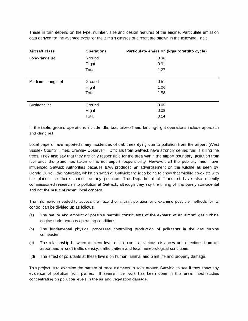
These in turn depend on the type, number, size and design features of the engine, Particulate emission

data derived for the average cycle for the 3 main classes of aircraft are shown in the following Table.

Aircraft class Operations Particulate emission (kg/aircraft/lto cycle)

Long-range jet Ground 0.36

Flight 0.91

Total 1.27

Medium—range jet Ground 0.51

Flight 1.06 Total 1.58

Business jet Ground 0.05 Flight 0.08

Total 0.14

In the table, ground operations include idle, taxi, take-off and landing-flight operations include approach

and climb out.

Local papers have reported many incidences of oak trees dying due to pollution from the airport (West

Sussex County Times, Crawley Observer). Officials from Gatwick have strongly denied fuel is killing the

trees. They also say that they are only responsible for the area within the airport boundary; pollution from fuel once the plane has taken off is not airport responsibility. However, all the publicity must have

influenced Gatwick Authorities because BAA produced an advertisement on the wildlife as seen by

Gerald Durrell, the naturalist, whilst on safari at Gatwick; the idea being to show that wildlife co-exists with the planes, so there cannot be any pollution. The Department of Transport have also recently

commissioned research into pollution at Gatwick, although they say the timing of it is purely coincidental

and not the result of recent local concern.

The information needed to assess the hazard of aircraft pollution and examine possible methods for its

control can be divided up as follows:

(a) The nature and amount of possible harmful constituents of the exhaust of an aircraft gas turbine

engine under various operating conditions.

(b) The fundamental physical processes controlling production of pollutants in the gas turbine combuster.

(c) The relationship between ambient level of pollutants at various distances and directions from an

airport and aircraft traffic density, traffic pattern and local meteorological conditions.

(d) The effect of pollutants at these levels on human, animal and plant life and property damage.

This project is to examine the pattern of trace elements in soils around Gatwick, to see if they show any evidence of pollution from planes. It seems little work has been done in this area; most studies

concentrating on pollution levels in the air and vegetation damage.

Lateral variations in the chemical composition of surface sediments can act as a guide to local pollution

centres (Forstner & Wittman). Similarly qualitative profiles of sediment data can be used to evaluate characteristic influences from industrial, municipal and agricultural sources, provided that grain-size

effects - which strongly influence metal values - are accounted for. Sediment cores provide a historical

record of events occurring in the area. In the sampling and storage of soils strict precautionary measures are necessary. The use of an ordinary spade is preferable to that of an auger, and tools encased in teflon

are recommended. In all cases, material selected for analysis should be collected from the inner part of

the sample material, which has not been in direct contact with metal of the sampling device. Air drying samples will have little effect on the total trace metal concentrations. However, if speciation, organic

extractable trace elements, etc., are of interest, any drying procedure may lessen the validity of the

sample analysis. The longer a soil sample is kept air-dried the greater the amount of water-soluble and organic matter that can be extracted. It is advised that the best sample storage temperature is -20 to300C

- i.e. below their freezing point to minimise effects of microbial activity (I.L. Marr and M.S. Cresser).

xxxx

established ambient air quality standards or guidelines.

However, Warren Springs Laboratory s found that the non-methane hydrocarbons at Gatwick did exceed these standards at all sites, although some were attributed to motorcars. They also found that airborne

lead concentrations were similar to UK urban areas. The lead is probably derived from internal

combustion engines rather than aviation fuel, kerosene.

Kerosene is purely hydrocarbon based and is ashless. Fuel cannot pick up any contaminants until put

into the tanks, when it can breathe and so pick up airborne dust, etc. The antistatic additives used in fuel are ASA3 and Stadis 450, both are chromium based at up to 3 ppm of chromium (B.P. Labs).

J Heywood (1971) states that in the vicinity of air terminals the density of pollutant emission and the resulting pollutant concentrations are comparable to these same pollutants from other sources in adjacent

local communities. Thus the principle impact of aircraft emissions is local in nature and it is more likely

that these emissions will constitute a more significant portion of community-wide pollutant loadings as new aircraft are introduced and emissions from other sources reduced. The severity of emissions around

Gatwick will increase if the second runway is built, as the CAA is proposing, resulting in increased local

concern.

Evidence of damage was claimed by Mr W Jeal, an orchid grower, whose nursery was situated less than

half a mile from the airport and in the direct flightpath. ‘Orchids ruined by jet fumes, says grower’ was the title in the Daily Telegraph (18/1/72). He claimed his orchids started to be destroyed from 1967, a year

associated with rapid increase in the use of jets, whose engines were inefficient in fuel combustion. More

recently, a local conservationist, Mr I Ockenden, reported that air pollution was causing severe tree damage in the area.

He completed a survey with the Friends of the Earth, showing that the areas situated under the flightpath

showed significantly more damage than the rest of the survey area (Horsham Oak Tree Survey, 1966). Although they could not state definitely that Gatwick was the cause, they defined it as ‘a definite suspect’.

Mr Qckenden also reported the outcome of a public inquiry on Gatwick’s Second Terminal, at which a

spokesman failed to answer questions about pollution from jet fuel. He knew nothing of jettisoned fuel as a pollutant, nor at what distance from the airport it was jettisoned, an issue which caused the sacking of 1

man and the subsequent striking of 3,700 others at San Diego (San Diego Union 21/10/70).

Local people have also reported the smell and taste of kerosene and exhaust fumes at all times, unburnt

fuel deposits on their ponds and fuel spattered over paths from aircraft (You and Yours 1988). This has

also been observed around other airports such as Heathrow, Manchester and military airports.

There is a belief that damage is being done under the flightpath, not only to people and plants, but also

animals.

M. Hayaski (1980) found a difference in concentration of trace elements in dogs surrounding Osaka

Airport, Japan, to those living further away.

To determine the concentration of metals in soils it is necessary first to bring them into solution.

Extraction methods involve either fusion or acid dissolution. The latter has several advantages and was employed. It does not allow large amounts of salt to be introduced into the solution which can cause

instability and lead to high instrument background readings. Nitric acid has been widely used in

extraction and can be used separately or with hydrochloric acid. This method provides a high degree of metal extraction, but does not dissolve silicates completely. It does, however, destroy organic matter, all

precipitated and adsorbed metals and leaches a certain amount of metals from the silicate lattice (H

Agernuam & A.S.Y. Chau 1976). Such acid extraction methods are reasonably rapid and inexpensive, but little is known about their accuracy. Reproducibility is of paramount importance in monitoring

programmes such as this to determine the changes at one locality. S.A. Sinex et al. (1980) studied the

completeness, precision and accuracy of an acid extraction - atomic absorption spectroscopy (ASS) method. They found that the nitric acid extraction was not as efficient as with aqua regia. Their results

showed that boiling conditions maximise the recovery of metals. M A Hasan (1967) found that the metal

concentrations obtained by nitric/perchloric acid and nitric acid were about equal, although the former treatment gave higher concentrations for some metals. He found both gave quick and complete

destruction without loss of volatile elements such as cadmium, lead and zinc. Numerous investigations

have shown that it is unnecessary to obtain full digestion of all soil components, including metals bound into internal structures of silicates and other detrital minerals, as pollution effects usually occur at the

surface of the soil particles (Forstner and Wittmann). The simple HNO3-HC1 digestion also circumvents

the need to redissolve the lead precipitates of the filtration residue when determining the lead. Losses of chromium with nitric acid due to the low boiling point of chromyl chloride will not occur because the boiling

point of nitric acid is lower. It is widely agreed that leaching with nitric acid will only give partial extraction,

but does extract 75-85% of zinc and 60-85% of cadmium (A.S.G. Jones 1973, C.W. Holmes 1974). For these reasons, together with that of cost and safety (concentrated hydrofluoric acid might have been a

better acid to use for digestion, but owing to its high toxicity and corrosive properties was eliminated) the

method employed was that of concentrated nitric acid, boiled to dryness then an equal volume of 1% hydrochloric acid added.

AAS is a popular metal determination technique because it is relatively sensitive, specific and simple to

operate.

Methods based on atomic absorption are potentially highly specific because atomic absorption lines are

remarkably narrow (0.002 — 0.005 nm) and electronic transition energies are unique for each element. First introduced as an analytical tool by Walsh in 1955, the principles have been well documented (A L

Page et al. 1982, K Smith 1983, D A Skoog 1985, H H Willard et al. M A Hasan 1987, I. Williams 1988).

In its simplest sense AAS makes use of the fact that free atoms of an element absorb light at wavelengths characteristic of that element and the extent of the absorption is a measure of the concentration of these

atoms in the light path. In theory, AAS should follow the Beer-Lambert Law, ie A=EcL, where:

A = Absorbance

E = Molar extinction co-efficient

C = Concentration of sample

I = Optical pathlength through the sample

but, departures from linearity are often encountered. To determine whether or not linearity does exist a

calibration curve covering the range of concentrations in the sample should be prepared (D A Skoog 1985). In the linear region of the calibration curve, one standard and a blank are sufficient to define the

relationship; in non-linear regions at least 3 standards and a blank are required (H H Willard et al.). At

high concentrations deviations from the Beer-Lambert Law occur because the atomised sample absorbs more emitted radiation, and the previously negligible background radiation becomes significant. Thus

transmission of the emitted radiation is artificially high and absorbance low, since absorbance = log (T-1).

AAS has the advantages of high reproducibility and rapid analysis. Disadvantages include the fact that

analysis is generally mono-elemental. Two main types of interference occur; spectral-arising when

absorption of an interfering species lies so close to, or overlaps, the analyte absorbance that resolution is impossible; and chemical interferences-various chemical processes occurring during atomozation that

alter absorbance characteristics of the analyte. The spectral interferences result from the presence of

combustion products that exhibit broad-band absorbance or of particular products that scatter radiation. Both diminish the power of the transmittance beam, leading to positive errors. When fuel or the oxidant

mixture alone is the source, corrections are readily obtained from the blanks being aspirated into

theflame. A sample matrix source results in a positive error in concentration and absorbance. Interference from matrix products are not widely encountered with flame atomization and are avoided by

varying analytical parameters such as temperature and fuel-oxidant ratio. Chemical interferences are

more common. They can be minimised by suitable choice of operating conditions. Most commonly it is the result of anions which form compounds of low volatility with the analyte and so reduce the rate of

atomisation, resulting in low values (D A Skoog 1965). Aluminum is expected to volatilize to aluminum

oxide species prior to atomization at about 27000C, but residual compounds will affect this (R Cornelis & P Schutyser 1984). Chloride-rich samples could produce volatile aluminium chlorides, having a high

dissociation energy and leading to loss by lack of atomization. However, by use of flame AAS this effect

will be negligible.

After calculation of the metal concentrations, account had to be made for grain size fractions (U Forstner

& W. Salomons). The finer grained fractions (mainly clays) show relatively high metal contents. In silt and fine sand fractions, concentrations generally decrease due to domination by quartz components with low

metal contents. In coarser fractions the presence of heavy minerals may cause the metal portion to

increase again. Thus it is obvious that grain size exercises a determining influence on metal concentrations.

Although the best method might have been to separate the clay/silt fraction and fine silt fraction by sieving and calculating the amounts in each there was insufficient time for this. Instead the percentage of organic

carbon was calculated, as this leads to similar results - the more carbon present, the smaller the particles

and the greater surface area to which the metals can adhere. It is difficult quantitatively to estimate the amount of organic matter in soil. Previously the change in weight of soil resulting from destruction of

organic compounds by hydrogen peroxide or ignition at high temperatures has been used. Both are

subject to errors - hydrogen peroxide does not quantitatively remove organic matter and ignition gives an over-estimate, because both organic and inorganic constituents lose weight during heating (A L Page et

al.). previously loss-on-ignition has been widely dismissed as crude and inadequate due to additional

losses of CO2 from carbonates in calcareous soils; to loss of elemental C and to loss of structural water from clay minerals. However, error from loss of CO2 from carbonates is likely to be either eliminated or

substantially reduced in low temperature ignition.

The contribution resulting from loss of structural water from clays varies according to the percentage of

clay and its mineralogical nature. Ignition at 3750C eliminates this water loss, because the main loss

occurs at 450 - 6000C. Because of the variation in amount of organic matter destroyed in relation to temperature and time of ignition’ it is necessary to have a closely controlled furnace temperature.

Work by D.F. Ball (1964) has shown that: = 0.458 x —0.4

where x is the loss on ignition at 3750C.

He found ignition at this temperature reduced weight loss due to non-organic material. The prediction

limits are narrower for this temperature at all values of organic matter than at 8500C. Due to this greater

accuracy and the fact that loss-on-ignition is a simple and rapid method of assessing organic matter in soils, the loss-on-ignition at 3750C method was employed.

X-ray diffraction can be used to examine samples to identify constituents. The reason can then be seen for any anomalous values of concentrations of metals due to the different fractions, or to pollution. Gibbs

(1965) compared methods previously used to prepare oriented specimens of 2um clays for quantative X-

ray diffractometry and found only smear, rapid suction and pressure methods were acceptable (G W Brindley & G. Brown). The powder print of a substance forms a unique fingerprint. Thus an unknown

may be identified by preparing its diffraction pattern and comparing it to known patterns. The Hanawalt

system was devised so that the known patterns can be located quickly. Each pattern is described by listing the d and I values of its diffraction lines onto a card file (Figure 1), where d is the spacing of the

lattice planes and I the intensity of each line. Once the diffraction pattern of the unknown has been made

and the plane spacing d corresponding to each line calculated, the unknown can be identified (B D Cullity). If the sample is a mixture, as was the case in this project, each component must be identified

individually.

Once one component has been identified, all lines corresponding to it are omitted and the intensity of the

remainder are re-scaled so the strongest is equal to 100. This procedure is repeated until all lines have been accounted for (H.H. Willard et al.). Analysis of mixtures becomes difficult when lines from different

phases are superimposed, and when the resulting composite line is one of the 3 strongest in the pattern

of the unknown. The usual procedure leads only to a very tentative identification of one phase, as agreement is obtained for some d values, but not all corresponding intensities. In theory, the Hanawalt

method should lead to a positive identification of any substance whose diffraction pattern is included in

the card file.In practice, however, various difficulties arise, usually due to errors in the diffraction pattern of the unknown. The possibility of abnormal intensities due to preferred orientation may arise.

This may be reduced if a mixture is employed containing a mineral, such as quartz, which does not show preferential orientation (G W Brindley). A limitation of the preliminary examination is that mixed layer

clays may be unrecognisable.

Usually they are characterised by non-integral diffractions-peaks are broad and often have asymmetrical

profiles. They often contain swelling layers combined with non-swelling layers. Ethylene glycol saturation

impresses a standard condition on the swelling component and integral or non-integral spacings should be looked for as a pointer to a smectite or mixed-layer clay respectively. Dispersion of X-rays may be

hindered by particles being coated and bound together by iron oxides or hydroxides, or organic matter.

The organic matter can usually be removed by treatment with hydrogen peroxide (G Brown).

Thus X-ray diffraction provides a rapid, accurate method for identification of crystalline phases in a

material; sometimes it may be the only method available for determining which polymorphic forms of substances are present.

A relatively quick method by which to classify soils is by texture. Texture influences a wide variety of pedological, physical, chemical and biological processes. Thus its property is a natural criterion to use in

soil classification schemes. It was used, with the x-rays, in the identification of the soil types. It was not

possible to take x-ray diffractions of all the samples. Assessment of soil is made by rubbing moistened soil between fingers and thumb. With experience it is possible to estimate confidently the particle size

distribution. This technique gives an outline of organic matter content, particle size distribution of the

mineral fraction, grade, size, shape and development of soil fragments and strength, stickiness, plasticity, porosity, packing density and stoniness of soil (J M Hodgson et al. 1976). F E Foss et al. (1975) found

that greatest accuracy was achieved for sand, clay, sandy loam and silt loam classes. The errant texture

was generally associated with high contents of coarse fragments, free iron, organic matter and very fine or coarse sands. This shows higher accuracies are obtained where one soil separate dominates — as

mixing of separates increases, field texture becomes more difficult. Compensation should be made for the

silty feel of organic matter when estimating particle size distribution of mineral fractions of surface horizons. When top and subsoils are combined clay estimates have higher accuracy than silt -mostly

because when soil is moistened and worked to its maximum plasticity, its stickiness and polish are more

easily related to clay content than the slippery feel or feathering is to the silt present. Despite conscious attempts to allow for the presence of variable amounts of organic carbon or calcium carbonate

J M Hodgson et al. (1976) found these two factors are potential sources of error. K Simpson (1983)

recommended that soils containing more than 20% of either organic matter or calcium carbonate should not be assessed by this method.

Moderate quantities of organic matter tend to make soil feel ‘loamy’, and well-decomposed humus feels

somewhat like silt, but can usually be distinguished by its dark colour and tendency, unlike silt, to break up when smeared on the palm. Moderate quantities of fine calcium carbonate also tend to make the soil

feel silty. High levels of organic matter are normally associated with dark colour, smoother feel, better

aggregation in sandy soils and weaker clods and finer silt in clays (MAFF 1984).

This project was aimed at finding whether there was a link between pollution from Gatwick and the

concentration of trace metals in the soil of the surrounding area. The concentrations were measured by flame atomic absorption spectroscopy and, rather than distinguishing different particle sizes, the

percentage of organic carbon was determined. Thus it was hoped to account for differences in

concentration that might have been encountered. X-ray diffraction and soil texture were also determined to see whether any of the anomalous readings were due to a difference in soil type rather than some form

of pollution.

METHOD

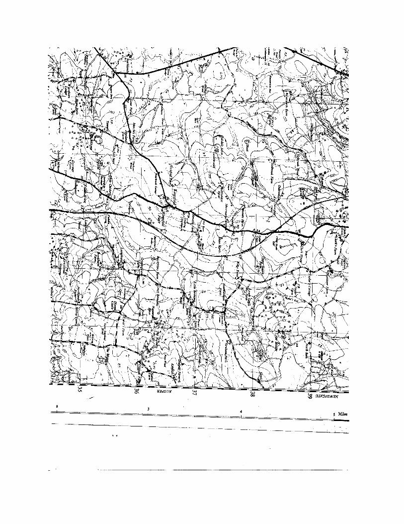
Site Selection

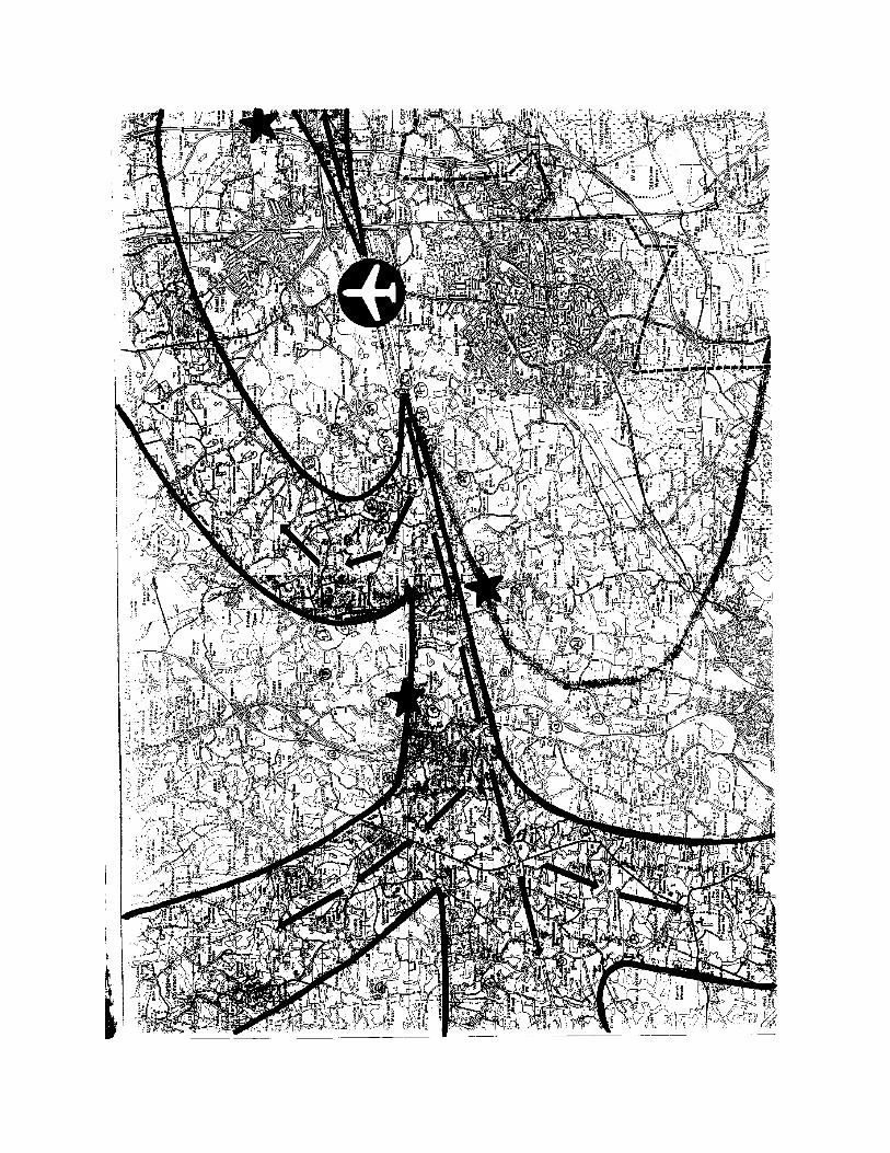
Sites were chosen within the sector of a circle, whose centre was the western end of Gatwick Airport

runway. This sector was chosen so the flightpath ran through its centre. Within it sites were selected so they lay, as nearly as possible, along the arcs of circles with decreasing radii-forty-two sites were chosen

in all. In an attempt to form some sort of reference, each site was chosen to be at least 30 metres from

the road to avoid undue pollution. All were taken from grassy areas on unploughed land. If necessary, where the only land was farmland, samples were taken from under hedgerows so they would contain the

least amount of fertilisers, pesticides, etc., and would be unploughed. A stainless steel trowel was used

for digging samples, which were stored in a freezer in sealed plastic bags until tests were performed. Cores were obtained by driving a hollow stainless steel tube into the ground and the soil removed by

pushing it out with a stainless steel disc of the same diameter as the inside of the tube. These samples

were stored in an identical manner. All were carefully labelled.

Extraction of the metals

Soil was selected from the centre of each sample to ensure that it was uncontaminated. After drying in a

pickstone thermostatic 30/300 oven at 105 C the samples were sieved. To obtain a representative sample, they were partitioned by the quarter system. Approximately 15.0000 grams of soil were weighed

out accurately, to this was added 37 ml. of laboratory grade concentrated IWO3 and boiled to dryness.

Once dry and cool they were mixed with an equal volume of laboratory grade 1% HC1. As all samples could not be treated on the same day, one sample from each run was repeated in the next practical

session, allowing any variation between runs to be seen. Three blanks were prepared in exactly the

same way as the samples the HNO3 was boiled to dryness and the 1% HC1 added. All samples were filtered on Whatman OF/C filter paper.

For speed, reduction of sample loss and contamination by exposure to air for extended periods the solutions were filtered under vacuum and stored in glass stoppered glass bottles.

Standard samples were prepared using 1000 mg—l metal standard solutions supplied by BDH chemicals and distilled water. The standards used for each element were chosen so the instrument worked within

its linear operating range (Table

2). Concentrations were measured for: Pb, Al, Cu, Cr, Cd, Fe, Zn — where necessary samples were

diluted. Operating conditions used for the spectrometer are given in Table 3.

The instrument had to be recalibrated every S samples for Al to allow for changes in absorption

characteristics. If left for longer the baseline began to drift. The blanks were analysed to check for

contamination, the levels were usually below the detection limits of the Flame Atomic Absorption.

All apparatus was acid washed before use.

Table 2

Element Conc. (ppm)

A1 10 20 50

Pb 1 5 10 20 50

Zn 10 100 200 400 600

Fe 10 20 50 100 200

Cd 0.5 1 3 5 10

Cr 1 10 30 50

Cu 0.5 1 5 10 20

Table 3

Operating conditions for Lab AAS

Fe Zn Cd Cu Pb Cr A1

Lamp current

(mA)

5 9 4 4 5 7 10

Flame A i r – a c e t y l e n e N20/ acetylene

Wavelength

(nm)

372.0 213.9 228.8 324.8 217.0 357.9 309.3

|Measurement time (s)

1 1 1 1 1 1 1

Replicates 3 3 3 3 3 3 3

DETERMINATION OF ORGANIC CARBON

The loss on ignition method was used. A crucible was weighed, about 5.0000 grams of air-dried soil added and the weight recorded. The crucibles were placed in a Gallenkamp muffle furnace at 1050C for 3

hours. After this they were placed in a desiccator to cool and weighed. The samples were then placed

into the preheated muffle furnace at 3750C for 16 hours. At the end of this period they were removed and, after preliminary cooling, transferred to a desiccator to cool to room temperature and again weighed.

X-RAY DIFFRACTION

Approximately 50 grammes of each sample were broken down and mixed with a little water. Mechanical

grinding was kept to a minimum because it tends to disorder the crystalline materials and reduce

diffracted intensities, thus crushing was preferred. Removal of finer powders prevented excess grinding while coarser material was left to be crushed further. The suspension was wet sieved to remove particles

greater than 63 um. The samples were treated with 10% H202 to remove organic matter, some heating

was required before effervescence ceased. The samples were washed several times with a iN MgC12 solution; they were centrifuged between each washing on a GSR centrifuge. This causes some

floculation so samples were washed several times with distilled water until the liquid, decanted after

centrifuging, produced no white precipitate of silver chloride when treated with a solution of silver nitrate.

Several samples, even after repeated centrifugation, did not settle completely, so this top layer was

removed, placed into new centrifuge tubes and drops of lN MgCl2 solution added until, following centrifuging, settlement occurred. The sample was labeled accordingly. All samples were smeared onto

X-ray diffraction slides and taken for X-ray. A very thin layer on a glass slide can have a high degree of

preferential orientation, but alignment is less perfect when thicker layers are used, as is required inquantitative analysis and when clay material contains minerals such as quartz.

SOIL TEXTURE

Each sample was moistened and worked in the hand until it reached its greatest stickiness and plasticity

(could be easily moulded, but showed no free water) and so aggregates were broken down. Relative proportions of sand, silt and clay were assessed by feeling between finger and thumb and by the

propensity to form a ball or thread when rolled between the palms. Table 4 shows the general criteria on

which judgement was made to place a soil into the appropriate textural class.

Table 4 Assessment of soil texture

Grittiness Smoothness Stickiness Ball and worm

formation

Texture

Not gritty Not smooth Extremely sticky Forms a long

worm, easily bent

into a ring

Clay

Moderate and

soapy

Very sticky Forms a long

worm, bends into a

ring

Silty

clay

Moderately sticky Forms a worm, will

not bend into a

ring

Silty

clay

loam

Extreme and

soapy

Very slightly sticky Forms a ball,

forms a worm with

difficulty

Silt

Grittiness Smoothness Stickiness Ball and worm

formation

Texture

Very smooth and

soapy

Slightly sticky Forms a ball, but

worm breaks

Silt

loam

Slight to moderate Slightly smooth Moderately sticky Forms a worm,

bends into a ring

Clay

loam

Moderate Not smooth Very sticky Forms long worms, bends,

forms rings with

difficulty

Sandy clay

loam

Moderately sticky Forms long worms, bends do

not form rings

Loam

Not sticky Forms a ball, forms worms with

difficulty

Loam

Very gritty Just forms a ball, does not form a

worm

Sandy

loam

Extremely gritty Barely forms a ball which collapses

easily

Loamy sand

Does not form a

ball

Sand

RESULTS

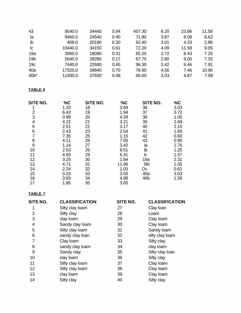
Table 5 shows the soil content of Al, Cd, Cr, Cu, Fe, Pb and Zn for the 43 collection sites. It also shows

values for these metals for the 3 depth profiles.

The percentage of organic carbon is given in Table 6, for the various samples. Some of the X-ray

diffraction spectra are shown in Appendix 1 - for samples 6, 34 and 43.

Table 7 shows the classification of soil textures derived from the ‘hand texturing method’.

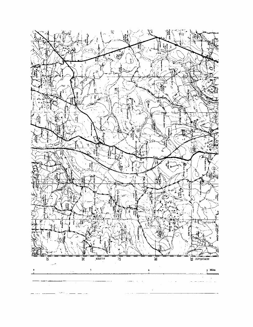
Isohaline maps were drawn so that a clearer picture of metal concentrations in relation to the position of

the runway at Gatwick could be seen (Appendix 2).

In addition, plots were made of the concentration of metal against distance of each site from the most

western end of the runway, allowing any relationship between the two to be seen (Appendix 3).

To find any relationship between the metals themselves-i.e. to see if one metal varied in the same way as

another and if that variation could be predicted - a plot was made of each metal against every other metal

(Appendix 4). The strength of the relationship bet ween them is then measured by an index known as the correlation coefficient. The graphs give a good visual impression of the strength of an association, but

such a subjective estimate may be unreliable, so an objective one is used instead - the correlation

coefficient. When the distribution approximates to a straight line, one variable is highly predictable from the other. Thus the distance of the points from the best fitting straight line is a good index of the strength

of the relationship (R. Haynes). The correlation coefficient, r, has a value between -l and 1. Numbers

close to 1 or -l indicate a very high correlation, those close to 0 indicate no relationship at all. A positive correlation is one in which an increase in one variable is matched by an increase in another. The opposite

is true for a negative correlation - as one variable increases, the other decreases.

The correlation between two variables is the amount they vary together expressed as a proportion of the

amount they vary in total. The formula used to calculate the correlation coefficient was:

r = XY -X Y

[( X2-X X)( Y2 -Y Y)]

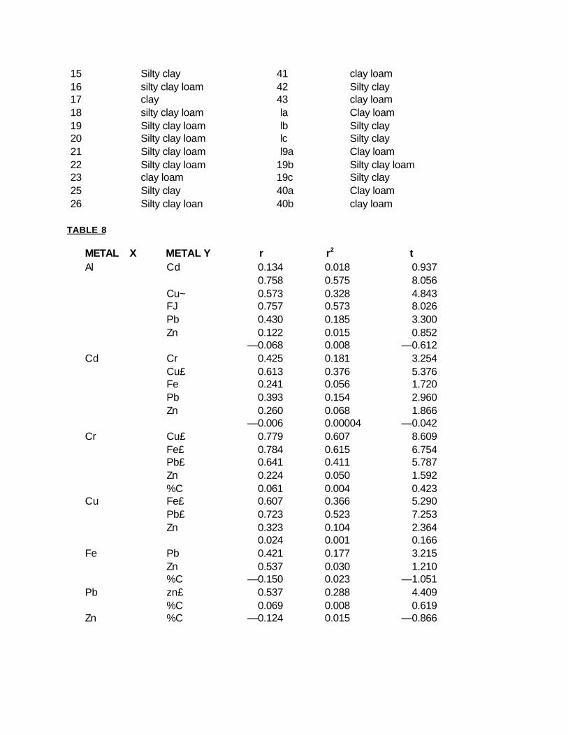
The results are given in Table 8. The square of the correlation coefficient is the coefficient of

determination. This gives the proportion of the variation of Y, associated with variations in X. It ranges

from 0 to 1, as shown in Table 8, together with values of t, which shows how reliable the sample correlation coefficient is. The correlation found is based on the samples obtained during field work. Had

other samples been taken, the coefficient may have been different. The null hypothesis is that there is no

correlation between the two variables - the population correlation coefficient is 0.

Then sample values come from a t distribution with a mean of 0. If the calculated value of t is near the

centre of the distribution, it could easily come from a distribution where this population coefficient is 0 and the null hypothesis cannot be rejected. If the calculated value of t falls in one of the tails of the distribution

(is higher than given critical values) then it is extremely unlikely that the sample r has come from this

distribution and the null hypothesis is rejected.

The values of t were calculated by:

t = r (N – 2)

(1 - r2)

where N number of samples.

Some of the values for the correlation coefficients seemed very low when the graph suggested they should be high.

This occurred when one point showed great deviation. In these cases r was recalculated (Table 9), along with new values for the coefficient of determination and t.

Key to Tables

a, b and c = 1st, 2nd and 3rd 3” of the depth profiles respectively.

* = averaged values of concentrations for repeated samples.

£ = significant at 0.2% level.

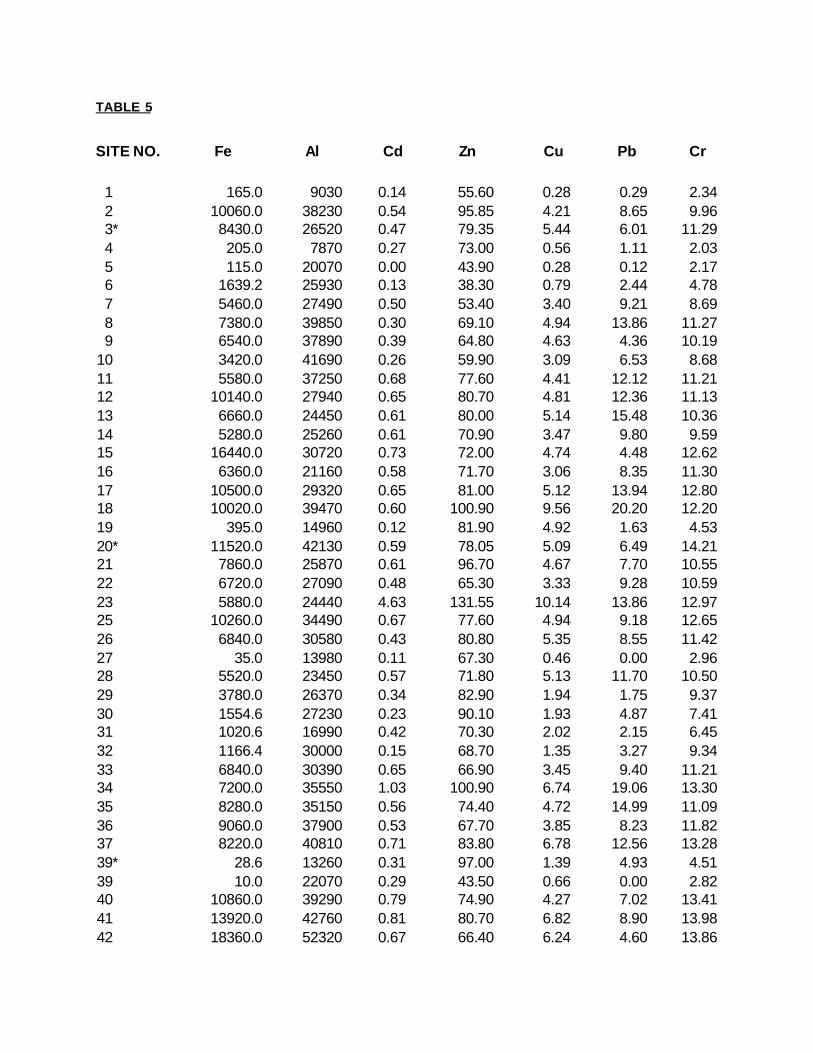
TABLE 5

SITE NO. Fe Al Cd Zn Cu Pb Cr 1 165.0 9030 0.14 55.60 0.28 0.29 2.34 2 10060.0 38230 0.54 95.85 4.21 8.65 9.96 3* 8430.0 26520 0.47 79.35 5.44 6.01 11.29 4 205.0 7870 0.27 73.00 0.56 1.11 2.03 5 115.0 20070 0.00 43.90 0.28 0.12 2.17 6 1639.2 25930 0.13 38.30 0.79 2.44 4.78 7 5460.0 27490 0.50 53.40 3.40 9.21 8.69 8 7380.0 39850 0.30 69.10 4.94 13.86 11.27 9 6540.0 37890 0.39 64.80 4.63 4.36 10.19 10 3420.0 41690 0.26 59.90 3.09 6.53 8.68 11 5580.0 37250 0.68 77.60 4.41 12.12 11.21 12 10140.0 27940 0.65 80.70 4.81 12.36 11.13 13 6660.0 24450 0.61 80.00 5.14 15.48 10.36 14 5280.0 25260 0.61 70.90 3.47 9.80 9.59 15 16440.0 30720 0.73 72.00 4.74 4.48 12.62 16 6360.0 21160 0.58 71.70 3.06 8.35 11.30 17 10500.0 29320 0.65 81.00 5.12 13.94 12.80 18 10020.0 39470 0.60 100.90 9.56 20.20 12.20 19 395.0 14960 0.12 81.90 4.92 1.63 4.53 20* 11520.0 42130 0.59 78.05 5.09 6.49 14.21 21 7860.0 25870 0.61 96.70 4.67 7.70 10.55 22 6720.0 27090 0.48 65.30 3.33 9.28 10.59 23 5880.0 24440 4.63 131.55 10.14 13.86 12.97 25 10260.0 34490 0.67 77.60 4.94 9.18 12.65 26 6840.0 30580 0.43 80.80 5.35 8.55 11.42 27 35.0 13980 0.11 67.30 0.46 0.00 2.96 28 5520.0 23450 0.57 71.80 5.13 11.70 10.50 29 3780.0 26370 0.34 82.90 1.94 1.75 9.37 30 1554.6 27230 0.23 90.10 1.93 4.87 7.41 31 1020.6 16990 0.42 70.30 2.02 2.15 6.45 32 1166.4 30000 0.15 68.70 1.35 3.27 9.34 33 6840.0 30390 0.65 66.90 3.45 9.40 11.21 34 7200.0 35550 1.03 100.90 6.74 19.06 13.30 35 8280.0 35150 0.56 74.40 4.72 14.99 11.09 36 9060.0 37900 0.53 67.70 3.85 8.23 11.82 37 8220.0 40810 0.71 83.80 6.78 12.56 13.28 39* 28.6 13260 0.31 97.00 1.39 4.93 4.51 39 10.0 22070 0.29 43.50 0.66 0.00 2.82 40 10860.0 39290 0.79 74.90 4.27 7.02 13.41 41 13920.0 42760 0.81 80.70 6.82 8.90 13.98 42 18360.0 52320 0.67 66.40 6.24 4.60 13.86

43 9540.0 34440 0.94 457.30 6.20 23.96 11.56 la 8460.0 29540 0.40 71.80 3.87 8.08 8.62 lb 408.0 20190 0.30 62.40 3.01 4.33 2.86 lc 10440.0 34150 0.61 72.20 4.09 11.58 9.05 19a 3060.0 18090 0.31 65.20 2.72 8.43 7.26 19b 5640.0 28280 0.17 67.70 2.80 9.00 7.33 19c 7440.0 22690 0.45 96.30 3.42 6.46 7.91 40a 17520.0 39640 0.70 78.90 4.56 7.46 10.96 40b* 11930.0 37830 0.48 65.60 3.03 4.87 7.89

TABLE 6

SITE NO. %C SITE NO. %C SITE NO. %C 1 1.33 18 3.69 36 3.03 2 6.43 19 1.94 37 3.72 3 0.99 20 4.34 38 1.05 4 4.22 21 3.21 39 1.69 5 2.51 22 3.17 40 2.15 6 2.43 23 2.54 41 1.69 7 7.35 25 1.15 42 0.83 8 4.11 26 7.55 43 0.90 9 1.14 27 3.42 la 2.76 10 2.53 26 8.51 lb 1.25 11 4.50 29 6.41 lc 1.57 12 3.25 30 1.84 19a 2.31 13 4.71 31 11.96 l9b 1.05 14 2.24 32 1.03 Dc 0.61 15 0.23 33 3.55 40a 3.03 16 3.93 34 4.98 40b 1.59 17 1.85 35 3.65 TABLE 7

SITE NO. CLASSIFICATION SITE NO. CLASSIFICATION 1 Silty clay loam 27 Clay loan 2 Silty clay 28 Loam 3 clay loam 29 Clay loam 4 Sandy clay loam 30 Clay loam 5 Silty clay loam 31 Sandy loam 6 sandy clay loan 32 silty clay loam 7 Clay loam 33 Silty clay 8 sandy clay loam 34 clay loam 9 Sandy clay 35 Silty clay loan 10 clay loam 36 Silty clay 11 Silty clay loam 37 Clay loam 12 Silty clay loam 38 Clay loam 13 clay loam 39 Clay loam 14 Silty clay 40 Silty clay

15 Silty clay 41 clay loam 16 silty clay loam 42 Silty clay 17 clay 43 clay loam 18 silty clay loam la Clay loam 19 Silty clay loam lb Silty clay 20 Silty clay loam lc Silty clay 21 Silty clay loam l9a Clay loam 22 Silty clay loam 19b Silty clay loam 23 clay loam 19c Silty clay 25 Silty clay 40a Clay loam 26 Silty clay loan 40b clay loam

TABLE 8

METAL X METAL Y r r2 t Al Cd 0.134 0.018 0.937 0.758 0.575 8.056 Cu~ 0.573 0.328 4.843 FJ 0.757 0.573 8.026 Pb 0.430 0.185 3.300 Zn 0.122 0.015 0.852 —0.068 0.008 —0.612 Cd Cr 0.425 0.181 3.254 Cu£ 0.613 0.376 5.376 Fe 0.241 0.056 1.720 Pb 0.393 0.154 2.960 Zn 0.260 0.068 1.866 —0.006 0.00004 —0.042 Cr Cu£ 0.779 0.607 8.609 Fe£ 0.784 0.615 6.754 Pb£ 0.641 0.411 5.787 Zn 0.224 0.050 1.592 %C 0.061 0.004 0.423 Cu Fe£ 0.607 0.366 5.290 Pb£ 0.723 0.523 7.253 Zn 0.323 0.104 2.364 0.024 0.001 0.166 Fe Pb 0.421 0.177 3.215 Zn 0.537 0.030 1.210 %C —0.150 0.023 —1.051 Pb zn£ 0.537 0.288 4.409 %C 0.069 0.008 0.619 Zn %C —0.124 0.015 —0.866

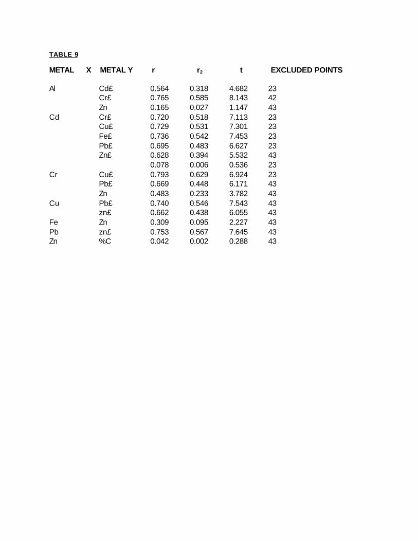
TABLE 9 METAL X METAL Y r r2 t EXCLUDED POINTS Al Cd£ 0.564 0.318 4.682 23 Cr£ 0.765 0.585 8.143 42 Zn 0.165 0.027 1.147 43 Cd Cr£ 0.720 0.518 7.113 23 Cu£ 0.729 0.531 7.301 23 Fe£ 0.736 0.542 7.453 23 Pb£ 0.695 0.483 6.627 23 Zn£ 0.628 0.394 5.532 43 0.078 0.006 0.536 23 Cr Cu£ 0.793 0.629 6.924 23 Pb£ 0.669 0.448 6.171 43 Zn 0.483 0.233 3.782 43 Cu Pb£ 0.740 0.546 7.543 43 zn£ 0.662 0.438 6.055 43 Fe Zn 0.309 0.095 2.227 43 Pb zn£ 0.753 0.567 7.645 43 Zn %C 0.042 0.002 0.288 43

CONCLUSION

The concentrations of metals found in this study seem to indicate that Gatwick Airport is having some

effect on the surrounding area. There is an increase in concentration from west to east for all metals. An area of high concentration protrudes from the runway, the size of which varies between metals, but is

evident for all. Further evidence that these elevated concentrations arise from the airport is that as metal

density increases, the size of this area decreases, suggesting larger particles fall first whilst lighter elements are carried further. The distribution pattern shows agreement with those of other reports on

vegetation damage.

What effects land use in the area has on distribution patterns is uncertain and more investigation is

needed before definite conclusions can be drawn. To see the full effect of the airport on the region, a

larger area would need to be investigated, including more sites farther from the flightpath. More work is required on constituents in the soil than was possible in this study, so that the extent of their influence can

be seen. The need to combine the results of studies around Gatwick is evident. The consolidation of

findings, if in agreement, would provide conclusive evidence of pollution. Work on meteorological effects on emissions may help to explain the patterns found and would be useful.

DISCUSSION

Soil is a very difficult substance to analyse, often results are not easy to interpret due to variability of

elemental content at any site. Inevitably errors will occur in preparation of soils and measurement of their

content. It is often sample preparation - the decomposition and solution steps - which introduce more errors than actual spectroscopic measurement. Efforts were made to minimise errors, but there are many

possible sources. Reagents used in sample decomposition may have introduced some traces of the

elements under consideration as these may have been present as an impurity. It is hoped that the use of blanks will have removed this particular source of error. Contamination can arise from the air, which is

why samples were stored in stoppered bottles and filtration performed under vacuum-making it as rapid

as possible. However, the possibility of contamination whilst open to air still exists. Chemical laboratories are one of the worst places for carrying out trace analysis because so many compounds are present at

concentrations much greater than is found elsewhere. Fume cupboards can worsen the situation as

there is a flow of laboratory air into the working space and over the samples.

As mentioned, the errors involved with AAS are small.

The greatest errors occurred in measurement of aluminium, despite recalibration every five samples -

probably due to the high flame temperature required. To discover the extent of variation the ‘standard

addition method’ could be used (M Bader 1980, D A Skoog 1985), but due to lack of time was not attempted. This involves the addition of one or more increments of standard solution to sample aliquots

of identical size. Each solution is diluted to a fixed volume before measurement. Successive

introductions can be made of standard to the unknown. Measurements are made on the original solution and after each addition. Thus it can be seen if the instrument is measuring accurately. Here it was

assumed that errors were snail, or, that if a significant amount was being lost, it was the same for each

sample.

Concentrations obtained for Cd, Pb and Zn are comparable with literature values for typical British soils

(K A Smith, W Salomons & U Forstner). Values for Cr and Cu, however, are slightly lower - by a factor of about S and 9 respectively. The values found for Al are in agreement with those found by I Williams

(1988).

The contour maps were drawn to enable distribution of trace elements to be seen in relation to the

runway. In general a similar pattern can be seen. As the runway is neared, the elemental concentration

increases. The effect is smaller with Al and Zn, which have more uniform patterns. Pb has a less well-defined pattern, probably due to the fact that roads are an additional source of Pb, disrupting any pattern

that may arise from the aeroplanes. The pattern does appear to follow roads to some extent, despite

precautions taken to try and minimise this. From the runway, moving towards higher ground, concentrations of Pb are high, reaching a peak at site 42, which is on the edge of the high ground. The

area immediately behind shows low concentration of Pb - probably because the land, although about

100’, is actually beginning to descend on the far side of the ridge and also because most of these sites are to the west of woodland. Trees may shelter the topsoil from pollutants to some extent. Beyond this

ridge is an area of relatively flat ground, showing relatively high Pb concentrations. The A.24 runs

through the centre of this area and could be a source of pollutants, and possibly concentrations are increased because there is less to prevent trace element dispersion. Both sites 18 and 43 show elevated

concentrations, 18 is in this central region and 43 slightly north of the runway near Horley and at the edge

of the flightpath, which sweeps around to the north, where planes are ‘stacked before landing.

The map for Zn shows a more uniform pattern, but with a slight increase towards the runway. Again the

high ground 0.3 km from the runway shows low values, whilst on the lower ground just beyond, values are higher. Site 43 has the highest Zn concentration, whilst 39 again is low. Site 2 shows enrichment

compared to other sites at a similar distance possibly because of a nearby dump. Also evident is an area

of high Zn concentration protruding from the runway, which is more prominent than that for Pb.

The pattern for Cr is similar, there seems to be a gradual increase towards the runway from the west.

Again there is this area of low concentration around 0.3 km from the runway, with an area of high concentration beyond. An area of high concentration extends out from the runway over sites 34, 37, 40,

41 and 42 directly below the flightpath as the others suggest.

These same sites show high concentrations on the Cu profile. Just beyond is the region of low values on

higher land, and beyond that the higher concentrations again. This too shows a general increase from

west to east. The site with greatest concentration is again site 23.

The trend is the same for Cd as for the others - a general increase in concentration from west to east.

The area of high concentration from the runway does not extend so far out, but is still in evidence. There is again this band of low concentrations over the area of higher ground and the area of higher

concentrations beyond. Site 23 again shows the highest enrichment.

As expected, A1 does not show a great deal of variation across the sample area, because it is present in

the ground in such large quantities that it would take a massive amount to perturb it. However, there does seem to be a region of higher concentration protruding from the end of the runway, culminating in

the site of highest concentration - site 42. The region of low concentration does exist, but is less well

defined than for other metals. A ridge of higher values exists further from the runway than for other elements - at around 1 km from the runway.

The same is expected of Fe as it is of A1. However, Fe bears more resemblance to the other elements than Al does. It shows the gradual increase in concentration from west to east, with the region of higher

concentration extending away from the runway. A region of lower concentration exists on the raised land

followed by a region of higher concentration behind, although in this region the centre site 19 shows much lower concentration than the rest.

The concentration contours, in general, show an increase in concentration from west to east towards the runway.

Extending out from the runway is a region of high concentration, beyond this an area of lower concentration, which is on land of 100’ or more in height. Behind that is a region of higher concentration,

in an area which contains less woodland and is more open. Most frequently the sites with anomalously

high concentrations are 23 and 43, although site 42 is generally enriched as well.

The graphs of elemental concentration against distance from the runway (Appendix 3) illustrate the same

point. They all show some increase on nearing the runway, even though the results are scattered.

A possible explanation for the low values on top of the hill is that they are just beyond the ridge of high

ground and are slightly sheltered. It could also be a result of woodland providing some shelter. The soil content will influence the metal concentration — the more clay, the smaller the particles and the more

surface area to which the metals can adhere. Thus from the naps it is expected that this region should

contain less clay in its soils than other areas. The wind direction and meteorological conditions will also have some effect on distribution - the prevailing wind being south-westerly. It would be expected that the

highest concentrations occur in the north east, however, the exact effect of ridges and dips is unknown.

The activities of landowners could be of major importance to some elements investigated, for example Cu is used in a spray for potatoes.

Site 43 seems to show generally high concentrations, which could result from land use, wind direction, or its position on a hill making a prime site on which pollutants can collect. It could also be because it is

directly under the path taken by planes whilst stacked, waiting to land. If planes emit more pollutants

whilst flying slowly in the stack, this could be a major cause of enrichment.

The depth profiles seem to reveal little information. To learn more it would have been better to have

taken more samples with finer divisions. As it is the profiles were taken at regular intervals beneath the centre of the flightpath, the farthest being 1.6 km from the runway. Site 1 shows in all cases that the

lowest 3” had the highest concentration, the centre 3” the lowest and the top 3” sampled was intermediate

in nature. The profile at site 19 for Cu, Zn, Fe and Cr shows a general increase in concentration with depth, but for the remaining metals the situation is different. For Al the middle section shows the highest

concentration with the top having the least, for Cd the lowest 3” shows the highest concentration whilst

the top shows the intermediate level; with Pb it is again the middle section which shows the highest concentration, while the bottom shows the lowest amount.

At site 40, closest to the runway, all metals show a decrease in concentration with depth. The situation found at site 1 almost agrees with the findings of J.R. Butler (1954) for Cr and Fe, the findings of B. Lyons

et al. (1983) for Cd is also in agreement. However, R Levi-Minzi et al. (1969) found the reverse to be true

— a decrease of Cd with depth. Cu, Zn and Pb have all been shown in literature to decrease with depth the opposite effect to the findings at site 1. Site 19 shows agreement for Cr, Fe and Pb with literature - an

increase in concentration with depth. Cd increases in depth at this site, agreeing with the findings of B.

Lyons, but contrary to those of R Levi-Minzi et al. The results for Cu and Zn - an increase with depth - are contrary to literature findings. Site 40 shows more general agreement with the observations of others.

There is a decrease from the surface layer for Cu, Zn, Pb and Cd - the results for Cd agree with that of R.

Levi -Minzi et al. The results for Cr and Fe are in disagreement with literature observations as they show a decrease in depth not an increase. It seems that Cd is expected to decrease with depth under natural

conditions, but organic matter can contribute to an increase, so observed differences could result from

this or from pollution, quite which it is impossible to say from the findings of this report.

Soil organic matter has been defined as the organic fraction of soil, including plant, animal and microbial

residues. However, it includes only that organic material which accompanies soil particles through a 2 mm sieve and it is difficult to quantify the amount present. One procedure is to calculate the amount of

organic carbon and multiply by a constant factor. There is some disagreement as to what this factor

should be, although it is widely believed that carbon comprises 48-56% of soil organic matter. In this project organic carbon was found and used as an indicator of the amount of organic matter present -

although not actually calculated. The organic matter is expected to have a profound influence on the

binding of metallic cations - the cation exchange capacity is largely due to organic matter. However, as the amount of organic carbon, and so the amount of organic matter, was so small it was found to have

had little influence on the soil concentration.

A statistical approach was adopted to study the association between the different trace elements in soil.

Examination of r, r2 and t revealed the associations between the metals. Points showing anomalous

behaviour were disregarded, the values of r, r2 and t recalculated, and it was found that more associations became highly significant. The excluded points were either 23, 42 or 43 - the sites showing the highest

concentration of elements. The result was that both Al and Fe showed significant association with Cr, Cu

and Cd, but not Pb and Zn. However, they both showed a significance with Pb at the 1% level. Cd, Cr and Cu were shown to be associated with Zn and Pb at the 0.2% significance level. It would appear that

Al relates best to Cd, Cu relates best to Cr, as does Fe, whilst Pb is most highly correlated to Zn.

Although %C shows no particular association with any of the elements, the strongest relationship was a

negative one with Fe.

Work by K P Prabhakaran Nair & A Cottenie (1971) found that Zn and Pb were best related to a particle

size diameter of l0-20um, Fe to the clay fraction and A1 and Cu to the fraction 2-10um. If the association found here is correct, it could imply Cd will also be associated with the fraction 2-10um, whilst Cr may be

intermediate between the 2 and 2-10um fraction. Thus elevated concentrations of Pb and Zn should

occur naturally where particles are lO-2Oum diameter, Fe and possibly Cr with the clay fraction and Al, Cd and Cu with particles of 2-lOum. So if concentrations are elevated in other cases, it could be as a

result of pollution.

The x-rays give information on soil content and from the peaks it is possible to calculate the relative

quantities of clay minerals. The different clays have different effects on metals. Smectites have a high

capacity for cation exchange, whilst kaolinites have a very small propensity; illites show an intermediary effect. Smectites undergo much isomorphous substitution, leaving a deficiency of positive charge in the

layers; compensation is by replacement of 02 by OH- introduction of excess cations and adsorption of

cations onto the surface of individual layers. This last method always occurs to some degree and so presence of these ions is a characteristic of smectites. The ions are held loosely to the clay structure and

so are readily extracted. Thus if the clay contains much smectite it should show a high metal

concentration. As kaolinite has a structure approaching an ideal formula, it undergoes little isomorphous substitution and so has little metal cations associated with it (K B Krauskopf 1985).

Although 20 samples were prepared for analysis, only 18 were returned, of these 2 were incomplete and 2, although given the same sample number, were actually different samples - the spectra were different -

as it was unknown which was which they had to be disregarded. Thus only 17 could be used. Where

there were no X-rays, the soil texture results were used.

These can only be used as a rough guide to the true contents of soil - they give no information of different

types of clay present, so differences in associated cations are unknown.

However, they do act as a guide and also give some indication of the particle size of soil, which also

affects trace element concentration.

The sites which showed particularly low concentrations on the ridge about 0.3 km from the runway were

investigated first. From the X-ray of site 31 it could be seen that the constituents were quartz and calcite. Quartz shows no association with trace metals and so the concentration should be low. Site 30 contains

mostly kaolinite, with a small amount of illite and a tiny amount of smectite. Thus a fairly low concentration

of metals would be expected as illite has less tendency to be bound together by cations - it holds potassium ions especially tightly and only part of the charge is replaceable by other ions.

The relative quantities of each clay can be estimated from the peak areas. Once these have been found the value for the kaolinite peak is divided by 2, that for smectite by 4-the illite peak is left unchanged.

Site 32 should show slightly higher concentrations than it does, because it contains more illite than

kaolinite, with a little smectite. Site 27 has almost equal quantities of illite and kaolinite with a smaller amount of smectite, so it too would be expected to show higher values than it actually does. Sites 19, 26

and 39 also show low concentrations in this area, but there is no X-ray information on them. The soil

textures show site 39 to be a clay loam and the other two to be silty clay loams. The clay loam should have slightly larger particles and so should have the lower concentration of the three. The site did indeed

show low concentrations for all metals and this could be the reason.

Sites which showed enrichment throughout were 23, 34, 37, 41, 42 and 43. X-ray data was available for 2

of these. Site 43 contained a large amount of illite, with little smectite, and would be expected to show

high concentrations, but not so high as found throughout. Site 34 contained almost twice as much illite as kaolinite, with a relatively small quantity of smectite in comparison. Thus concentrations would be thought

to be high, but not as high as they are.

Sites 23, 37 and 41 are all clay loams. As such they have an intermediate particle size and so would not

be expected to show the high concentrations they do. This suggests evidence of pollution. The particle

size at site 42 is smaller - here the soil is a silty clay, thus a higher concentration of metals may be expected. Without knowing which clays are present it is difficult to say whether concentrations found here

are those which may be expected naturally from the soil type, or if it is due to some sort of pollution.

What these results do seem to show is that sites which continually show elevated concentrations of

metals are, in some way, polluted and are not the result of natural levels of the soil.

If the different metals do show natural enrichment with different particle sizes as is suggested by K P

Prabhakaran Nair & A.Cottenie (1971) then it may be expected that Pb and Zn will show slightly higher

concentrations in clay loams and silty clay loams. This may account for the high concentrations at sites 13, 23, 34 and 43. It is, however, very unlikely to account for all this enrichment. For Fe to be associated

with the clay particles and for there to be no other pollution the highest concentrations would have to be

where the soil is clay, or at least silty clay. This clearly is not the case for all such sites - for instance sample lb is a silty clay, but has a very low Fe concentration. However, site 17 is a clay and does show a

relatively high Fe concentration, sites with the highest concentrations of Fe are also silty clays. So it

would appear that it is having some effect, but cannot be in any way responsible for all that is found. A1, Cr, Cu and Cd should all show high values in silty clays and silty clay loams if the theory is believed, but

this does not seem to be the case, suggesting either pollution or that the association is not strong.

Work carried out by S Rundle (1976) found conclusive proof that air collected from behind aircraft

positively damages plants. Whether ambient air levels reach this concentration was not determined. It

was thought that anticyclones would allow little air movement forming temperature inversions, which would result in a ground level mist allowing emissions to accumulate. She also found that trees and

plants near the car parks at the end of the runway and by the fuel farm showed growth rate decreases

above that normally expected.

This report led to further work by I Ockenden and the Friends of the Earth (FoE). They found the worst

tree damage occurred in straight lines corresponding to the flightpaths from Gatwick. The Horsham oak tree survey found trees on high ground faired best - this corresponds to the low level of pollutants found on

high ground in this study. The average damage to trees under the flightpath was found to be 57%, but

away from the flightpaths it was 40%. Trees on sand were found to fair better than those on clay, despite oaks preference for heavier soil, possibly because the flightpaths occur over clay. This could be attributed

to the fact that clay will have a greater concentration of adsorbed cations due to the smaller particle size.

The areas they found to have worst tree damage coincide well with areas of highest trace metals found in this study, although the agreement becomes less well defined at greater distances from the runway. The

work by I. Williams (1988) shows high A1 concentrations and a Ca deficiency in soils in the area. A

decreasing Ca2+:A13+ ratio in soils is thought to damage trees fine root systems. This could be another explanation of the agreement between the findings of this study - where high A1 concentrations occur, and

that of the FoE - where the most oak tree damage occurs.

BIBLIOGRAPHY

Agerniam, H. & Chau A.S.Y. (1976), Evaluation Techniques for the Determination of Metals in Aquatic

Sediments, The Analyst 101, pp.761—767

Bader, 1W. (1980), A Systematic Approach to Standard Addition Methods in Instrumental Analysis, J.

Chem Education 57, pp.7O3—706

Ball, D.F. (1964), Loss on Ignition as an Estimate of Organic Matter arid Organic Carbon in iron—

calcareous Soils, J. Soil Science 15, pp.84—92

Bastress, E.S.T. (1973), Impact of Aircraft Exhaust Emissions at Airports, Environ. Sci. Technol. 7,

pp.811—816

B.P. Laboratories, Private Communication

Brindley, G W & Brown, 0. (1980), Crystal Structures of Clay Minerals and their X—ray Identification,

Mineralogical Society, London

Brindley, G W (1951), The X-ray Identification and Crystal Structures of Clay Minerals, Mineralogical

Society, London

Brown, G (1951), The X-ray Identification and Crystal Structures of Clay Minerals, Mineralogical Society,

London

Butler, J.R. (1954), Trace Element Distribution in some Lancashire Soils,

J. Soil Science ~, pp.156—166

Clark, A .1. et al. (1983), Air quality Measurement in the Vicinity of Airports, Env. Pollution 6(B), pp.245—

251

Cornelis, H & Schutyser, P. (1984), Analytical Problems Related to A1 - Determination in Body Fluids,

Water and Dialysate, Contr. Kephrol 38, pp.1

Crawley Observer, Wed 8/3/89, pp.13

Cullity, B.D. (1978), Elements of X-ray Diffraction, Addison—Wesley Publ. Co., Philippines

Daily Telegraph, 18/1/72

Daily Telegraph., 16/1/89, pp.5

Forstner, U. & Salomens, W. (1984), Metals in the Hydrocycle, Springer— Verlag, Berlin

Forstner, U. & Wittmann, 0.T.W. (1981), Metal Pollution in the Aquatic Environment, Springer-Verlag,

Berlin

Foss, F.E. et al. (1975), Testing the Accuracy of Field Textures, Soil Sci. Soc. Amer. Proc. 22. PP.800 -

802

Friends of the Earth, (1986), The Horsham Oak Tree Survey Friends of the Earth, (1988), The Story of

Robert Jeal

Hasan, M.A. (1987), Determination of Metals in Aerosols by Atomic Absorption Spectrophotometry, flEA

MSc Thesis

Hayaska, N (1980), Pollution Abstracts 81 - 01968

Haynes, H (1982), Environmental Science Methods, Chapman & Hall, London

Heywood, J. et al. (1971), Jet Aircraft Air Pollution Production and Metals in Sediments, Anal. Chem. -

pp.2342—2346

Skoog, D.A. (1985), Principles of Instrumental Analysis, Saunders College

Smith, K.A. (1983), Soil Analysis, Marcel Dekker Inc., N.Y.

Warren Springs Laboratory, Report on Air Pollution at Gatwick Airport, Document BAA119 at the Oatwick

T2 Inquiry

West Sussex County Times, 1988—89

Willard, H H et al. (1988), Instrumental Methods of Analysis, Wadsworth Publishing Co., California

Williams, I D (1988), Elemental Status of Oak Tree Damage in Relation to Pollution from Gatwick Flight

Activities, Uni. of Surrey 3rd Year Proiect

You and Yours (1988), BBC. Radio Programme, November