Atmos. Meas. Tech., 7, 3487–3496, 2014www.atmos-meas-tech.net/7/3487/2014/doi:10.5194/amt-7-3487-2014© Author(s) 2014. CC Attribution 3.0 License.

Airborne Multiwavelength High Spectral Resolution Lidar(HSRL-2) observations during TCAP 2012: vertical profiles ofoptical and microphysical properties of a smoke/urban haze plumeover the northeastern coast of the USD. Müller 1,2, C. A. Hostetler3, R. A. Ferrare3, S. P. Burton3, E. Chemyakin2, A. Kolgotin4, J. W. Hair 3, A. L. Cook3,D. B. Harper3, R. R. Rogers3, R. W. Hare3, C. S. Cleckner3, M. D. Obland3, J. Tomlinson5, L. K. Berg5, andB. Schmid5

1University of Hertfordshire, Hatfield, Hertfordshire, UK2Science Systems and Applications, Inc., NASA Langley Research Center, Hampton, VA, USA3NASA Langley Research Center, Hampton, VA, USA4Physics Instrumentation Center, Troitsk, Russia5Pacific Northwest National Laboratory, Richland, WA, USA

Correspondence to:D. Müller (d.mueller@herts.ac.uk)

Received: 14 January 2014 – Published in Atmos. Meas. Tech. Discuss.: 6 February 2014Revised: 25 August 2014 – Accepted: 26 August 2014 – Published: 10 October 2014

Abstract. We present measurements acquired by the world’sfirst airborne 3 backscatter (β)+2 extinction (α) High Spec-tral Resolution Lidar (HSRL-2). HSRL-2 measures particlebackscatter coefficients at 355, 532, and 1064 nm, and par-ticle extinction coefficients at 355 and 532 nm. The instru-ment has been developed by the NASA Langley ResearchCenter. The instrument was operated during Phase 1 of theDepartment of Energy (DOE) Two-Column Aerosol Project(TCAP) in July 2012. We observed pollution outflow fromthe northeastern coast of the US out over the western At-lantic Ocean. Lidar ratios were 50–60 sr at 355 nm and 60–70 sr at 532 nm. Extinction-related Ångström exponents wereon average 1.2–1.7, indicating comparably small particles.Our novel automated, unsupervised data inversion algorithmretrieved particle effective radii of approximately 0.2 µm,which is in agreement with the large Ångström exponents.We find good agreement with particle size parameters ob-tained from coincident in situ measurements carried out withthe DOE Gulfstream-1 aircraft.

1 Introduction

We developed an automated, unsupervised inversion algo-rithm. We tested the performance of the algorithm for thefirst time with data acquired with the world’s first airborne3 backscatter (β) + 2 extinction (α) multiwavelength HighSpectral Resolution Lidar (HSRL-2). The instrument ac-quired data during the first intensive observation period (7–30 July 2012) of the Department of Energy (DOE) Two-Column Aerosol Project (TCAP) (Berg et al., 2014).

TCAP goals included quantifying aerosol properties andradiation and cloud characteristics at a location subject toboth clear and cloudy conditions, and both clean and pollutedconditions. HSRL-2 is the successor of HSRL-1, which hasbeen operating in various field campaigns since 2006 (Hairet al., 2008). Like HSRL-1, HSRL-2 measures backscat-ter, extinction, and depolarization at 532 nm and backscat-ter and depolarization at 1064 nm. In addition, HSRL-2 alsomeasures extinction, backscattering, and depolarization at355 nm.

Raman lidar and high spectral resolution lidar providehigh-quality backscatter and extinction coefficients. Mul-tiwavelength lidar (MWL) allows, e.g., for aerosol typ-ing (Burton et al., 2012). Aerosols of specific types show

Published by Copernicus Publications on behalf of the European Geosciences Union.

3488 D. Müller et al.: HSRL-2 measurements during TCAP 2012

characteristic values of extinction-related and/or backscatter-related Ångström exponents and extinction-to-backscatter(lidar) ratios and particle depolarization ratios. Aerosol typ-ing information provides the climate modeling communitywith information on aerosol properties. Aerosol types can berelated to their aerosol microphysical properties. Pure aerosoltypes possess a limited parameter range (particle size dis-tribution, complex refractive index). Recently, attempts havebeen made to split mixtures of different aerosol types intopure types (Tesche et al., 2009; Burton et al., 2014; Noh,2014), which can then be processed individually by inversionalgorithms as described in the following.

The 3β + 2α lidar techniques are the basis for micro-physical retrieval algorithms, e.g., inversion with regular-ization (Qing et al., 1989; Müller et al., 1999a; Veselovskiiet al., 2002; Böckmann et al., 2005), singular-value decom-position, linear estimation, and principal component analysistechniques (Donovan and Carswell, 1997; Veselovskii et al.,2012; de Graaf et al., 2013), and the latest development,dubbed the “Arrange & Average Algorithm” (Chemyakin etal., 2014). These algorithms allow for inverting the mea-sured optical quantities into microphysical properties, suchas particle size distribution or their integral properties andthe complex refractive index. First successful applications ofthe method of inversion with regularization can be found inMüller et al.(1998), Veselovskii et al.(2002), andBöckmannet al.(2005).

In the case of inversion with regularization, the retrievedparticle size distributions and the complex refractive indexcan be used to compute single-scattering albedo (scattering-to-extinction ratio), which is one of the most important pa-rameters in climate forcing studies (Bond et al., 2013). Re-cently, simulation studies were carried out with the goal ofinvestigating how accurately absorption and scattering coef-ficients can be inferred from the microphysical parameters.The results of these simulation studies will be presented intwo contribution that are in preparation (Müller et al., 2014a,b).

With regard to multiwavelength Raman lidar the technol-ogy has matured to the point that ground based systems canbe operated in a reliable manner at nighttime. EARLINETsuccessfully operates a network of Raman lidars. Several ofthese systems are multiwavelength systems, which allow fordetailed aerosol studies over Europe. Regardless of this ca-pability, investigations of aerosol properties on the globalscale cannot be done with ground-based systems. Compara-bly long signal-averaging times make these systems unsuit-able for operation aboard fast-flying platforms, e.g., aircraftand satellites.

Thus, HSRL is the method of choice for airborne andspace-borne applications in order to retrieve aerosol micro-physical properties. Space missions of HSRL systems will belaunched by NASA (http://www.nasa-usa.de/mission_pages/station/research/experiments/1037.html) and ESA (Stoffelenet al., 2005; Ansmann et al., 2007; Flamant et al., 2008) in the

next couple of years and . These lidar missions however donot provide the necessary number of measurement channelsin order to carry out detailed investigations of particle mi-crophysical properties. Multiwavelength HSRL is needed forproviding high-quality microphysical data products. NASALangley Research Center has developed two such systems,dubbed HSRL-1 (Hair et al., 2008) and HSRL-2.

HSRL-2 is the first airborne system capable of providing3β+ 2α data. This contribution aims at showing the results ofmicrophysical particle properties that can be obtained fromthis instrument. The inversion method used for the retrievalsis based on the concepts presented byMüller et al. (1999a)andVeselovskii et al.(2002). It has however been modified inorder to allow for fast, unsupervised, automated data process-ing. Details on the inversion methodology will be presentedin the aforementioned contributions that are in preparation.

These first results of HSRL-2 3β+ 2α measurements showpollution that was transported from the US and Canada outover the western Atlantic Ocean during TCAP. Our prototypesoftware delivered profiles of particle microphysical parame-ters in near-real time from the inversion of the optical profilesmeasured by HSRL-2 aboard the NASA B-200 King Air air-craft. We show a comparison of our results to coincident insitu measurements of particle size parameters acquired by theDOE (Department of Energy) Gulfstream-1 (G-1) aircraft.Section 2 summarizes the methodologies. Section 3 presentsmeasurement examples. Section 4 closes with a summary.

2 Methodology

The DOE G-1 aircraft was equipped to measure particle sizedistributions, chemical composition, and optical properties(Berg et al., 2014). The NASA King Air was equippedwith HSRL-2 (http://abstractsearch.agu.org/meetings/2012/FM/sections/A/sessions/A13K/abstracts/A13K-0336.html).HSRL-2 is the second-generation airborne HSRL de-veloped at the NASA Langley Research Center. Itis an airborne prototype for the lidar on the futureAerosol-Cloud-Ecosystem (ACE) mission recommendedfor implementation by NASA in the National Re-search Council’s Decadal Survey for Earth Science(http://science.nasa.gov/earth-science/decadal-surveys/). Itbuilds on the heritage of the HSRL-1 system (Hair et al.,2008) that has flown on more than 20 field campaigns since2006.

2.1 HSRL-2

HSRL-2 operates at laser wavelengths of 355, 532, and1064 nm. HSRL-2 measures profiles of particle backscat-ter coefficients and linear particle depolarization ratios at355, 532, and 1064 nm, and particle volume extinction co-efficients at 355 and 532 nm. The extinction and backscattercoefficients at 355 and 532 nm are derived using the HSRL

Atmos. Meas. Tech., 7, 3487–3496, 2014 www.atmos-meas-tech.net/7/3487/2014/

D. Müller et al.: HSRL-2 measurements during TCAP 2012 3489

technique (Grund and Eloranta, 1991). An iodine-vapor fil-ter is used for the extinction-coefficient measurements at532 nm. The backscatter coefficient at 1064 nm is measuredusing the standard backscatter technique (Fernald, 1984), butwith the benefit of transfer of calibration using the 532 nmHSRL retrievals in clear-air regions of the profile (Hair et al.,2008). The measurements presented in this contribution didnot indicate the presence of a significant amount of depolar-izing aerosol particles. The channels used for the depolariza-tion measurements will be described in a separate publica-tion.

The uncertainties of the data are governed by various fac-tors, like hardware and its calibration, signal calibration,signal-to-noise ratio, and signal averaging in time and space.A detailed description of calibration techniques and sourcesof error for the 532 and 1064 nm channels are given byHair et al.(2008). The new feature of HSRL-2 compared toHSRL-1 is that it measures the particle volume extinctioncoefficient not only at 532 nm, but also at 355 nm, using aninterferometric technique.

Data were sampled at 100 m horizontal and 15 m verticalresolutions and averaged to achieve the desired level of ran-dom uncertainty. For standard products, this is typically 1 kmhorizontally and 30 m vertically for backscatter and depolar-ization and 1 km horizontally and 150 m vertically for aerosolextinction. However, for the input to the microphysics re-trieval for this study, data were averaged to 5 minutes and150 m vertically to make the random error insignificant (0.1–3 %); studies are underway with regard to quantifying sys-tematic errors. Thus we had had optimum conditions forthis first test of the automated software as these errors aremore than adequate for trustworthy microphysical retrievals(Müller et al., 1999b; Veselovskii et al., 2002; Böckmannet al., 2005).

2.2 Automated, unsupervised inversion algorithm

HSRL-2 is the motivation for developing the next genera-tion of inversion methodology that allows us to process ahigh volume of data in an unsupervised, automated manner inreal time with significantly enhanced accuracy of the inver-sion data products. Our ultimate goal is to develop softwarefor application with a space-borne version of the multiwave-length HSRL.

The automated, unsupervised inversion software has beenused for the analysis of the measurements. Details of the soft-ware package and results of simulations studies including un-certainty analysis will be presented in two contributions thatare in preparation (Müller et al., 2014a, b). In the followingwe summarize the algorithm and some results of the simula-tion studies.

The mathematical equations that are used for solving theinverse ill-posed problem are the same used for the man-ual version of the inversion algorithm. The manual versionhas been applied in a multitude of studies by different lidar

groups since 1997 (e.g.,Müller et al., 1998, 2001; Murayamaet al., 2004; Balis et al., 2010; Alados-Arboledas et al.,2011; Noh et al., 2011; Navas-Guzmán et al., 2013; Nico-lae et al., 2013). The equations that connect the measuredbackscatter and extinction coefficients to the underlying mi-crophysical particle properties, i.e., the particle size distribu-tion and complex refractive index, are solved by the use ofeight triangular-shaped basis functions that are logarithmic-equidistantly distributed in an inversion window (Mülleret al., 1999a, b). In this study we set the minimum particleradius of the inversion window to 30 nm and the maximumvalue to 8 µm. This size range was sufficient for the data an-alyzed in this study.

We use the data of 3β+ 2α systems in the way describedby Müller et al. (2001) and Veselovskii et al.(2002). Wesolve the equations by determining weight factors for thebase functions (triangles), which then allow us to reconstructapproximations of the particle size distributions. The posi-tion of the triangles on the radius scale and their geometricalwidth is varied, such that we have several hundred differentinversion windows within which the eight basis functions aredistributed. An example that shows this distribution of trian-gle functions is shown in Fig. 1 inMüller et al.(1999a). Wesolve the equations for 91 inversion windows and for each in-version window the inversion is carried out for a grid of com-plex refractive indices. The real part varies between 1.325and 1.8. The step size is 0.025. The imaginary part variesbetween 0 and 0.1. The step size is 0.003.

We apply parallelization in the computations, which in-creases data processing speed. For each 3β+ 2α data set,we run the algorithm for the error-free data, and we carryout eight runs in which the data are distorted by a ran-dom noise of 15 %; see alsoVeselovskii et al.(2002) andSawamura et al.(2014). Details on error analysis will be pre-sented by Müller et al. (2014a).

In the manual version of the algorithm we used to aver-age all individual solutions that fell within a prescribed value(threshold value) of the discrepancy, as described byMülleret al.(1999b) andVeselovskii et al.(2002). This discrepancythreshold was determined from simulation studies. We opti-mized the automated scheme, compared to the manual ver-sion, using simulation studies. We found that using the 500solutions with the lowest discrepancies provide us with bet-ter inversions results. Details will be presented by Müller etal. (2014a).

All in all, 573 300 individual solutions were generated foreach data point on 17 July 2012 (see Fig. 4). The data pro-cessing time was 22 s for each optical data point, i.e., theerror-free and eight error runs combined with each of the 91inversion windows and the grid of 700 complex refractiveindices. These results were used to produce the profiles ofmicrophysical properties shown in Fig. 4. We obtain meanvalues and uncertainties that are defined in terms of 1 stan-dard deviation.

www.atmos-meas-tech.net/7/3487/2014/ Atmos. Meas. Tech., 7, 3487–3496, 2014

3490 D. Müller et al.: HSRL-2 measurements during TCAP 2012

Simulation studies were carried out for the automated ver-sion to test the performance. A sensitivity analysis was donefor two different error model in order to test the robustness ofthe automated software from the mathematical point of viewand for testing if the knowledge of the error models that de-scribes the measurement errors of the optical input data issignificant. One error model is based on extreme error simu-lations in which each measurement channel is given the max-imum value of an assumed measurement error, e.g., 5, 10,15, or 20 %. This kind of sensitivity analysis with respect tomeasurement errors had previously been done for the man-ual inversion algorithm. In the automated version, we usedthe same measurement error scenarios, but we introduced aGauss error-distribution model in addition. This means that,for example, for a measurement error of 15 % in a measure-ment channel, this 15 % measurement error has a Gauss-likeprobability distribution. A weighting of the measurement er-ror is thus introduced.

To give an impression on the simulation results, we sum-marize a few numbers. We tested 2880 optical data sets thatare representative of 48 mono-modal particle size distribu-tions: mean radii are between 20 and 300 nm. Geometricalstandard deviation (mode width) was 1.5, 1.7, 1.9, 2.1, 2.3,2.5. Effective radii were between 30 nm and 2.44 µm. Wetested real parts of 1.4, 1.5, 1.6, and 1.7 and we will include1.3 in the next round of simulations. Imaginary parts were0, 0.0001, 0.001, 0.0025, 0.005, 0.0075, 0.01, 0.015, 0.02,0.025, 0.03, 0.035, 0.04, 0.045, and 0.05. We tested measure-ment errors in which each channel of the 3β+ 2α system has5, 10, 15, and 20 % error. We tested the extreme error model(Müller et al., 1999b) and the model in which the errors havea Gauss-like probability distribution. We also tested four er-ror scenarios in which measurement uncertainties differ be-tween the different measurement channels.

The preliminary analysis shows the following results. Ef-fective radius can on average be retrieved to 30 % uncer-tainty. Uncertainty in the volume concentration can reach50 %, but in most cases stays within 30 %. An exact quan-tification of the meaning of “most cases” will be given inour future contributions. Surface-area concentration can beretrieved to 30 % or better. Number concentration shows anuncertainty of 70 % or less in approximately 50 % of the sim-ulations. Most of the simulations stay within 100 % uncer-tainty, but we find outliers. The real part can be retrieved to0.05 in approximately 50–70 % of the cases. The main chal-lenge is the imaginary part. It is less than 50 % in 50 % of thesimulations. The other 50 % of simulated cases shows uncer-tainties that can reach several 100 % uncertainty. We are cur-rently analyzing these cases. We also look into difference ofretrieval errors with regard to the use of the two error modelsapplied to the optical input data.

We assume that we will not be able to retrieve the imag-inary part to better than 0.005i. We believe than any betteraccuracy is unrealistic in view of the limited optical data setof 3β+ 2α data, measurement errors, data averaging in time

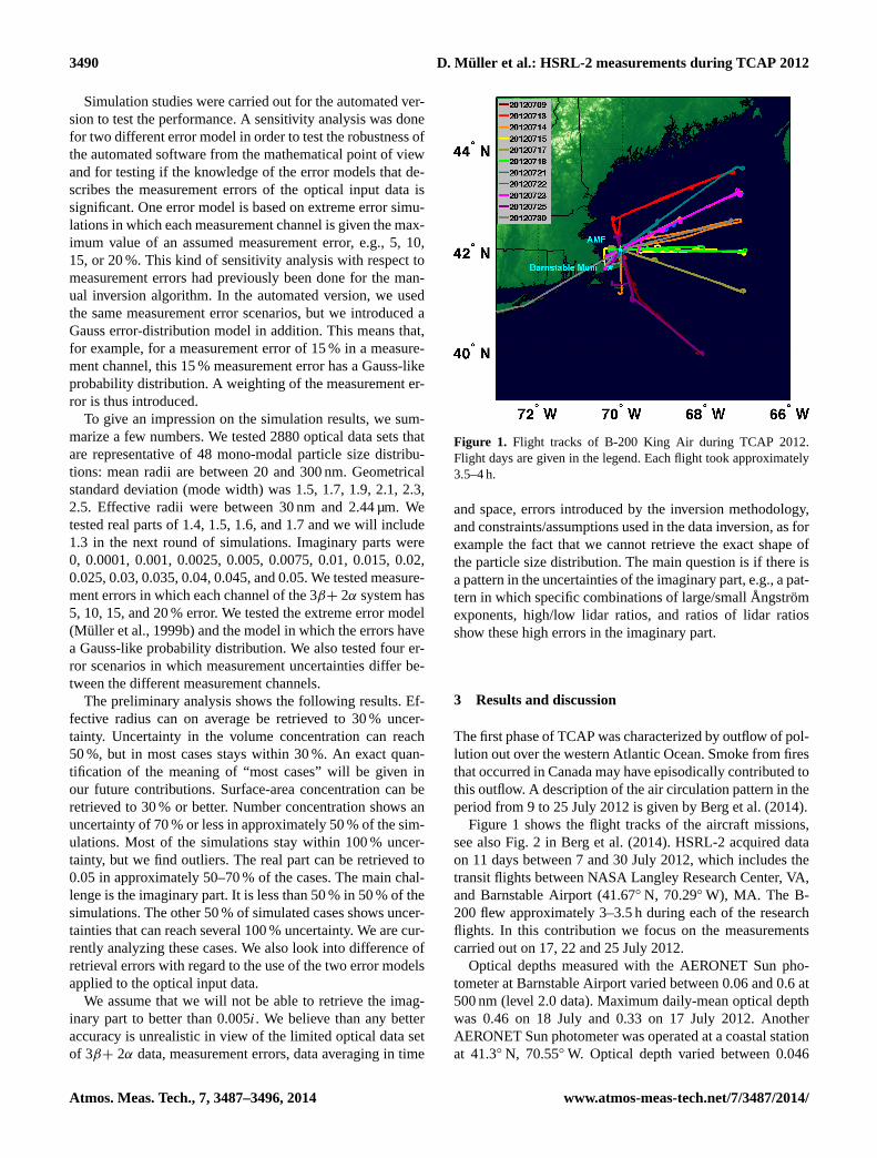
Figure 1. Flight tracks of B-200 King Air during TCAP 2012.Flight days are given in the legend. Each flight took approximately3.5–4 h.

and space, errors introduced by the inversion methodology,and constraints/assumptions used in the data inversion, as forexample the fact that we cannot retrieve the exact shape ofthe particle size distribution. The main question is if there isa pattern in the uncertainties of the imaginary part, e.g., a pat-tern in which specific combinations of large/small Ångströmexponents, high/low lidar ratios, and ratios of lidar ratiosshow these high errors in the imaginary part.

3 Results and discussion

The first phase of TCAP was characterized by outflow of pol-lution out over the western Atlantic Ocean. Smoke from firesthat occurred in Canada may have episodically contributed tothis outflow. A description of the air circulation pattern in theperiod from 9 to 25 July 2012 is given byBerg et al.(2014).

Figure 1 shows the flight tracks of the aircraft missions,see also Fig. 2 inBerg et al.(2014). HSRL-2 acquired dataon 11 days between 7 and 30 July 2012, which includes thetransit flights between NASA Langley Research Center, VA,and Barnstable Airport (41.67◦ N, 70.29◦ W), MA. The B-200 flew approximately 3–3.5 h during each of the researchflights. In this contribution we focus on the measurementscarried out on 17, 22 and 25 July 2012.

Optical depths measured with the AERONET Sun pho-tometer at Barnstable Airport varied between 0.06 and 0.6 at500 nm (level 2.0 data). Maximum daily-mean optical depthwas 0.46 on 18 July and 0.33 on 17 July 2012. AnotherAERONET Sun photometer was operated at a coastal stationat 41.3◦ N, 70.55◦ W. Optical depth varied between 0.046

Atmos. Meas. Tech., 7, 3487–3496, 2014 www.atmos-meas-tech.net/7/3487/2014/

D. Müller et al.: HSRL-2 measurements during TCAP 2012 3491

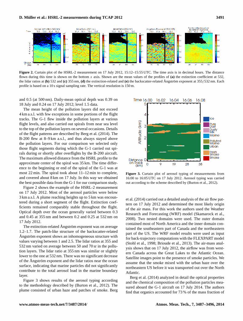
Figure 2. Curtain plot of the HSRL-2 measurement on 17 July 2012, 15:12–15:55 UTC. The time axis is in decimal hours. The distanceflown during this time is shown on the bottomx axis. Shown are the mean values of the profiles of(a) the extinction coefficient at 532,the lidar ratios at(b) 532 and(c) 355 nm,(d) the extinction-related and(e) the backscatter-related Ångström exponent at 355/532 nm. Eachprofile is based on a 10 s signal sampling rate. The vertical resolution is 150 m.

and 0.5 (at 500 nm). Daily-mean optical depth was 0.39 on18 July and 0.24 on 17 July 2012; level 1.5 data.

The mean height of the pollution layers did not exceed4 km a.s.l. with few exceptions in some portions of the flighttracks. The G-1 flew inside the pollution layers at variousflight levels, and also carried out spirals from near sea levelto the top of the pollution layers on several occasions. Detailsof the flight patterns are described byBerg et al.(2014). TheB-200 flew at 8–9 km a.s.l., and thus always stayed abovethe pollution layers. For our comparison we selected onlythose flight segments during which the G-1 carried out spi-rals during or shortly after overflights by the B-200 aircraft.The maximum allowed distance from the HSRL profile to theapproximate center of the spiral was 35 km. The time differ-ence to the beginning or end of the spiral of the G-1 was atmost 22 min. The spiral took about 11–12 min to complete,and covered about 8 km on 17 July. In this way we obtainedthe best possible data from the G-1 for our comparison study.

Figure 2 shows the example of the HSRL-2 measurementon 17 July 2012. Most of the aerosol particles were below3 km a.s.l. A plume reaching heights up to 5 km was encoun-tered during a short segment of the flight. Extinction coef-ficients remained comparably stable throughout the flight.Optical depth over the ocean generally varied between 0.3and 0.45 at 355 nm and between 0.2 and 0.25 at 532 nm on17 July 2012.

The extinction-related Ångström exponent was on average1.2–1.7. The patch-like structure of the backscatter-relatedÅngström exponent shows an inhomogeneous structure withvalues varying between 1 and 2.5. The lidar ratios at 355 and532 nm varied on average between 50 and 70 sr in the pollu-tion layers. The lidar ratio at 355 nm was similar or slightlylower to the one at 532 nm. There was no significant decreaseof the Ångström exponent and the lidar ratios near the oceansurface, indicating that marine particles did not significantlycontribute to the total aerosol load in the marine boundarylayer.

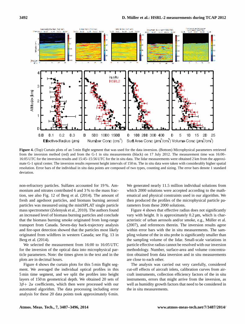
Figure 3 shows results of the aerosol typing accordingto the methodology described by (Burton et al., 2012). Theplume consisted of urban haze and patches of smoke.Berg

Figure 3. Curtain plot of aerosol typing of measurements from16:00 to 16:05 UTC on 17 July 2012. Aerosol typing was carriedout according to the scheme described by (Burton et al., 2012).

et al.(2014) carried out a detailed analysis of the air flow pat-tern on 17 July 2012 and determined the most likely originof the air mass. For this work the authors used the WeatherResearch and Forecasting (WRF) model (Skamarock et al.,2008). Two nested domains were used. The outer domaincontained most of North America and the inner domain con-tained the southeastern part of Canada and the northeasternpart of the US. The WRF model results were used as inputfor back-trajectory computations with the FLEXPART model(Stohl et al., 1998; Brioude et al., 2013). The air-mass anal-ysis shows that on 17 July 2012, the airflow was from west-ern Canada across the Great Lakes to the Atlantic Ocean.Satellite images point to the presence of smoke particles. Weassume that the smoke mixed with the urban haze over thenortheastern US before it was transported out over the NorthAtlantic.

Berg et al.(2014) analyzed in detail the optical propertiesand the chemical composition of the pollution particles mea-sured aboard the G-1 aircraft on 17 July 2014. The authorsfind that organics accounted for 73 % of the mass fraction of

www.atmos-meas-tech.net/7/3487/2014/ Atmos. Meas. Tech., 7, 3487–3496, 2014

3492 D. Müller et al.: HSRL-2 measurements during TCAP 2012

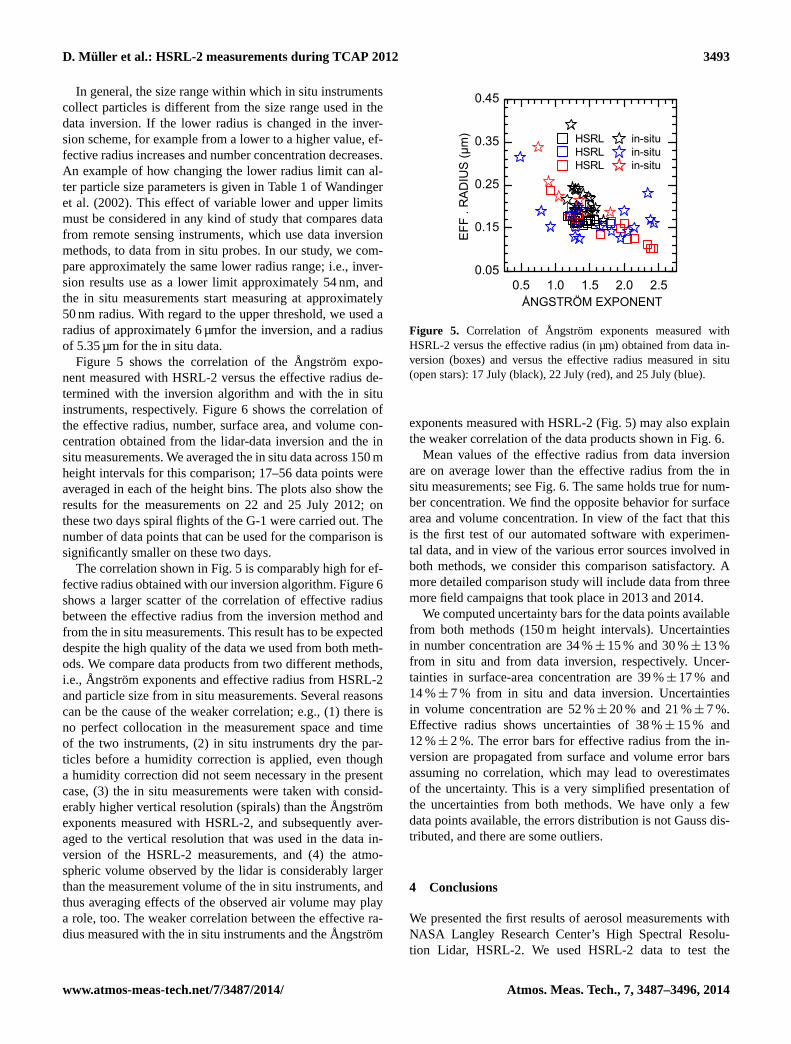
Figure 4. (Top) Curtain plots of an 5 min flight segment that was used for the data inversion. (Bottom) Microphysical parameters retrievedfrom the inversion method (red) and from the G-1 in situ measurements (black) on 17 July 2012. The measurement time was 16:00–16:05 UTC for the inversion results and 15:45–15:56 UTC for the in situ data. The lidar measurements were obtained 2 km from the approxi-mate G-1 spiral center. The inversion results represent height intervals of 150 m. The in situ data were taken with considerably higher spatialresolution. Error bars of the individual in situ data points are composed of two types, counting and sizing. The error bars denote 1 standarddeviation.

non-refractory particles. Sulfates accounted for 19 %. Am-monium and nitrates contributed 6 and 3 % to the mass frac-tion, see also Fig. 12 ofBerg et al.(2014). The amount offresh and agedsoot particles, and biomass burning aerosolparticles was measured using the miniSPLAT single particlemass spectrometer (Zelenyuk et al., 2010). The authors foundan increased level of biomass burning particles and concludethat the biomass burning smoke originated from long-rangetransport from Canada. Seven-day back-trajectory analysisand fire-spot detection showed that the particles most likelyoriginated from wildfires in western Canada; see Fig. 13 inBerg et al.(2014).

We selected the measurement from 16:00 to 16:05 UTCfor the inversion of the optical data into microphysical par-ticle parameters. Note: the times given in the text and in theplots are in decimal hours.

Figure 4 shows the curtain plots for this 5 min flight seg-ment. We averaged the individual optical profiles in this5 min time segment, and we split the profiles into heightlayers of 150 m geometrical depth. We obtained 20 sets of3β+ 2α coefficients, which then were processed with ourautomated algorithm. The data processing including erroranalysis for these 20 data points took approximately 6 min.

We generated nearly 11.5 million individual solutions fromwhich 2000 solutions were accepted according to the math-ematical and physical constraints used in our algorithm. Wethen produced the profiles of the microphysical particle pa-rameters from these 2000 solutions.

Figure 4 shows that effective radius does not significantlyvary with height. It is approximately 0.2 µm, which is char-acteristic of urban aerosols and/or smoke, e.g.,Müller et al.(2007), and references therein. The inversion results agreewithin error bars with the in situ measurements. The sam-pling volume of the in situ probe is significantly smaller thanthe sampling volume of the lidar. Small-scale variations inparticle effective radius cannot be resolved with our inversionmethodology. Number, surface-area and volume concentra-tion obtained from data inversion and in situ measurementsare close to each other.

The analysis was carried out very carefully, consideredcut-off effects of aircraft inlets, calibration curves from air-craft instruments, collection efficiency factors of the in situinstruments, errors that might arrive from the inversion, aswell as humidity growth factors that need to be considered inthe in situ measurements.

Atmos. Meas. Tech., 7, 3487–3496, 2014 www.atmos-meas-tech.net/7/3487/2014/

D. Müller et al.: HSRL-2 measurements during TCAP 2012 3493

In general, the size range within which in situ instrumentscollect particles is different from the size range used in thedata inversion. If the lower radius is changed in the inver-sion scheme, for example from a lower to a higher value, ef-fective radius increases and number concentration decreases.An example of how changing the lower radius limit can al-ter particle size parameters is given in Table 1 ofWandingeret al. (2002). This effect of variable lower and upper limitsmust be considered in any kind of study that compares datafrom remote sensing instruments, which use data inversionmethods, to data from in situ probes. In our study, we com-pare approximately the same lower radius range; i.e., inver-sion results use as a lower limit approximately 54 nm, andthe in situ measurements start measuring at approximately50 nm radius. With regard to the upper threshold, we used aradius of approximately 6 µmfor the inversion, and a radiusof 5.35 µm for the in situ data.

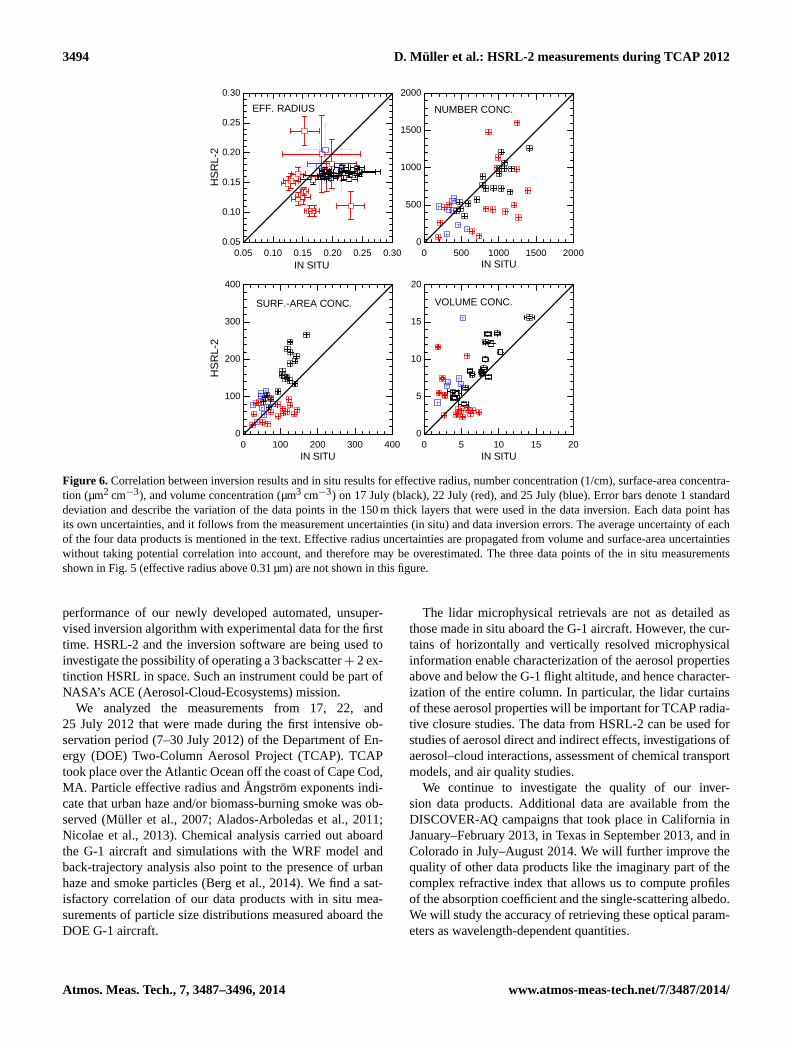
Figure 5 shows the correlation of the Ångström expo-nent measured with HSRL-2 versus the effective radius de-termined with the inversion algorithm and with the in situinstruments, respectively. Figure 6 shows the correlation ofthe effective radius, number, surface area, and volume con-centration obtained from the lidar-data inversion and the insitu measurements. We averaged the in situ data across 150 mheight intervals for this comparison; 17–56 data points wereaveraged in each of the height bins. The plots also show theresults for the measurements on 22 and 25 July 2012; onthese two days spiral flights of the G-1 were carried out. Thenumber of data points that can be used for the comparison issignificantly smaller on these two days.

The correlation shown in Fig. 5 is comparably high for ef-fective radius obtained with our inversion algorithm. Figure 6shows a larger scatter of the correlation of effective radiusbetween the effective radius from the inversion method andfrom the in situ measurements. This result has to be expecteddespite the high quality of the data we used from both meth-ods. We compare data products from two different methods,i.e., Ångström exponents and effective radius from HSRL-2and particle size from in situ measurements. Several reasonscan be the cause of the weaker correlation; e.g., (1) there isno perfect collocation in the measurement space and timeof the two instruments, (2) in situ instruments dry the par-ticles before a humidity correction is applied, even thougha humidity correction did not seem necessary in the presentcase, (3) the in situ measurements were taken with consid-erably higher vertical resolution (spirals) than the Ångströmexponents measured with HSRL-2, and subsequently aver-aged to the vertical resolution that was used in the data in-version of the HSRL-2 measurements, and (4) the atmo-spheric volume observed by the lidar is considerably largerthan the measurement volume of the in situ instruments, andthus averaging effects of the observed air volume may playa role, too. The weaker correlation between the effective ra-dius measured with the in situ instruments and the Ångström

0.5 1.0 1.5 2.0 2.50.05

0.15

0.25

0.35

0.45

EFF

. R

AD

IUS

(µm

)

ÅNGSTRÖM EXPONENT

Figure 5. Correlation of Ångström exponents measured withHSRL-2 versus the effective radius (in µm) obtained from data in-version (boxes) and versus the effective radius measured in situ(open stars): 17 July (black), 22 July (red), and 25 July (blue).

exponents measured with HSRL-2 (Fig. 5) may also explainthe weaker correlation of the data products shown in Fig. 6.

Mean values of the effective radius from data inversionare on average lower than the effective radius from the insitu measurements; see Fig. 6. The same holds true for num-ber concentration. We find the opposite behavior for surfacearea and volume concentration. In view of the fact that thisis the first test of our automated software with experimen-tal data, and in view of the various error sources involved inboth methods, we consider this comparison satisfactory. Amore detailed comparison study will include data from threemore field campaigns that took place in 2013 and 2014.

We computed uncertainty bars for the data points availablefrom both methods (150 m height intervals). Uncertaintiesin number concentration are 34 %± 15 % and 30 %± 13 %from in situ and from data inversion, respectively. Uncer-tainties in surface-area concentration are 39 %± 17 % and14 %± 7 % from in situ and data inversion. Uncertaintiesin volume concentration are 52 %± 20 % and 21 %± 7 %.Effective radius shows uncertainties of 38 %± 15 % and12 %± 2 %. The error bars for effective radius from the in-version are propagated from surface and volume error barsassuming no correlation, which may lead to overestimatesof the uncertainty. This is a very simplified presentation ofthe uncertainties from both methods. We have only a fewdata points available, the errors distribution is not Gauss dis-tributed, and there are some outliers.

4 Conclusions

We presented the first results of aerosol measurements withNASA Langley Research Center’s High Spectral Resolu-tion Lidar, HSRL-2. We used HSRL-2 data to test the

www.atmos-meas-tech.net/7/3487/2014/ Atmos. Meas. Tech., 7, 3487–3496, 2014

3494 D. Müller et al.: HSRL-2 measurements during TCAP 2012

0 . 0 5 0 . 1 0 0 . 1 5 0 . 2 0 0 . 2 5 0 . 3 00 . 0 5

0 . 1 0

0 . 1 5

0 . 2 0

0 . 2 5

0 . 3 0

HSRL

-2

I N S I T U0 5 0 0 1 0 0 0 1 5 0 0 2 0 0 0

0

5 0 0

1 0 0 0

1 5 0 0

2 0 0 0

HSRL

-2

N U M B E R C O N C .E F F . R A D I U S

I N S I T U

0 1 0 0 2 0 0 3 0 0 4 0 00

1 0 0

2 0 0

3 0 0

4 0 0

S U R F . - A R E A C O N C .

I N S I T U0 5 1 0 1 5 2 0

0

5

1 0

1 5

2 0

V O L U M E C O N C .

I N S I T UFigure 6. Correlation between inversion results and in situ results for effective radius, number concentration (1/cm), surface-area concentra-tion (µm2 cm−3), and volume concentration (µm3 cm−3) on 17 July (black), 22 July (red), and 25 July (blue). Error bars denote 1 standarddeviation and describe the variation of the data points in the 150 m thick layers that were used in the data inversion. Each data point hasits own uncertainties, and it follows from the measurement uncertainties (in situ) and data inversion errors. The average uncertainty of eachof the four data products is mentioned in the text. Effective radius uncertainties are propagated from volume and surface-area uncertaintieswithout taking potential correlation into account, and therefore may be overestimated. The three data points of the in situ measurementsshown in Fig. 5 (effective radius above 0.31 µm) are not shown in this figure.

performance of our newly developed automated, unsuper-vised inversion algorithm with experimental data for the firsttime. HSRL-2 and the inversion software are being used toinvestigate the possibility of operating a 3 backscatter+ 2 ex-tinction HSRL in space. Such an instrument could be part ofNASA’s ACE (Aerosol-Cloud-Ecosystems) mission.

We analyzed the measurements from 17, 22, and25 July 2012 that were made during the first intensive ob-servation period (7–30 July 2012) of the Department of En-ergy (DOE) Two-Column Aerosol Project (TCAP). TCAPtook place over the Atlantic Ocean off the coast of Cape Cod,MA. Particle effective radius and Ångström exponents indi-cate that urban haze and/or biomass-burning smoke was ob-served (Müller et al., 2007; Alados-Arboledas et al., 2011;Nicolae et al., 2013). Chemical analysis carried out aboardthe G-1 aircraft and simulations with the WRF model andback-trajectory analysis also point to the presence of urbanhaze and smoke particles (Berg et al., 2014). We find a sat-isfactory correlation of our data products with in situ mea-surements of particle size distributions measured aboard theDOE G-1 aircraft.

The lidar microphysical retrievals are not as detailed asthose made in situ aboard the G-1 aircraft. However, the cur-tains of horizontally and vertically resolved microphysicalinformation enable characterization of the aerosol propertiesabove and below the G-1 flight altitude, and hence character-ization of the entire column. In particular, the lidar curtainsof these aerosol properties will be important for TCAP radia-tive closure studies. The data from HSRL-2 can be used forstudies of aerosol direct and indirect effects, investigations ofaerosol–cloud interactions, assessment of chemical transportmodels, and air quality studies.

We continue to investigate the quality of our inver-sion data products. Additional data are available from theDISCOVER-AQ campaigns that took place in California inJanuary–February 2013, in Texas in September 2013, and inColorado in July–August 2014. We will further improve thequality of other data products like the imaginary part of thecomplex refractive index that allows us to compute profilesof the absorption coefficient and the single-scattering albedo.We will study the accuracy of retrieving these optical param-eters as wavelength-dependent quantities.

Atmos. Meas. Tech., 7, 3487–3496, 2014 www.atmos-meas-tech.net/7/3487/2014/

D. Müller et al.: HSRL-2 measurements during TCAP 2012 3495

Acknowledgements.The authors thank the NASA Langley B-200King Air flight crew or their outstanding work and support duringthe research flights. Support for the HSRL-2 flight operationsduring TCAP was provided by the DOE ARM program: Intera-gency Agreement DE-SC0006730. Support for data analysis wasprovided in part by the DOE Atmospheric System Research (ASR)program. Support for the development of HSRL-2 was providedby the NASA Science Mission Directorate, ESTO, AITT, andRadiation Science Program. We thank C. Flynn, R. Wagener, L.Gregory, and P. Russell at the Barnstable AERONET station forproviding data. The AERONET data at MVCO are provided by H.Feng and H. M. Sosik.

Edited by: V. Amiridis

References

Alados-Arboledas, L., Müller, D., Navas-Guzmán, J. L. G.-R.,Pérez-Ramírez, D., and Olmo, F. J.: Optical and microphysi-cal properties of fresh biomass burning aerosol retrieved by Ra-man lidar, and star- and sun-photometry, Geophys. Res. Lett., 38,L01807, doi:10.1029/2010GL043004, 2011.

Ansmann, A., Wandinger, U., Rille, O. L., Lajas, D., and Straume,A. G.: Particle backscatter and extinction profiling with thespaceborne high-spectral-resolution Doppler lidar ALADIN:methodology and simulations, Appl. Opt., 46, 6606–6622, 2007.

Balis, D., Giannakaki, E., Müller, D., Amiridis, V., Kelektsoglou,K., Rapsomanikis, S., and Bais, A.: Estimation of the mi-crophysical aerosol properties over Thessaloniki, Greece, dur-ing the SCOUT-O3 campaign with the synergy of Raman li-dar and sunphotometer data, J. Geophys. Res., 115, D08202,doi:10.1029/2009JD013088, 2010.

Berg, L. K., Fast, J. D., Barnard, J. C., Burton, S. P., Cairns, B.,Chand, D., Comstock, J. M., Dunagan, S., Ferrare, R. A., Flynn,C. J., Hair, J. W., Hostetler, C. A., Hubbe, J., Johnson, R., Kas-sianov, E. I., Kluzek, C. D., Kollias, P., Lamer, K., Lantz, K.,Mei, F., Miller, M. A., Michalsky, J., Ortega, I., Pekour, M.,Rogers, R. R., Russell, P. B., Redemann, J., III, A. J. S., Segal-Rosenheimer, M., Schmid, B., Shilling, J. E., Shinozuka, Y.,Springston, S. R., Tomlinson, J. M., Tyrrell, M., Wilson, J. M.,Volkamer, R., Zelenyuk, A., and Berkowitz, C. M.: The Two-Column Aerosol Project: phase I overview and impact of ele-vated aerosol layers on aerosol optical depth, J. Geophys. Res.,submitted, 2014.

Böckmann, C., Miranova, I., Müller, D., Scheidenbach, L., andNessler, R.: Microphysical aerosol parameters from multiwave-length lidar, J. Opt. Soc. America-A, 22, 518–528, 2005.

Bond, T. C., Doherty, S. J., Fahey, D. W., Forster, P. M., Berntsen,T., DeAngelo, B. J., Flanner, M. G., Ghan, S., Karcher, B., Koch,D., Kinne, S., Kondo, Y., Quinn, P. K., Sarofim, M. C., Schultz,M. G., Schulz, M., Venkataraman, C., Zhang, H., Zhang, S., Bel-louin, N., Guttikunda, S. K., Hopke, P. K., Jacobson, M. Z.,Kaiser, J. W., Klimont, Z., Lohmann, U., Schwarz, J. P., Shin-dell, D., Storelvmo, T., Warren, S. G., and Zender, C. S.: Bound-ing the role of black carbon in the climate system: A scientificassessment, J. Geophys. Res., 118, 5380–5552, 2013.

Brioude, J., Arnold, D., Stohl, A., Cassiani, M., Morton, D.,Seibert, P., Angevine, W., Evan, S., Dingwell, A., Fast, J. D.,Easter, R. C., Pisso, I., Burkhart, J., and Wotawa, G.: The La-

grangian particle dispersion model FLEXPART-WRF version3.1, Geosci. Model Dev., 6, 1889–1904, doi:10.5194/gmd-6-1889-2013, 2013.

Burton, S. P., Ferrare, R. A., Hostetler, C. A., Hair, J. W., Rogers, R.R., Obland, M. D., Butler, C. F., Cook, A. L., Harper, D. B., andFroyd, K. D.: Aerosol classification using airborne High Spec-tral Resolution Lidar measurements – methodology and exam-ples, Atmos. Meas. Tech., 5, 73–98, doi:10.5194/amt-5-73-2012,2012.

Burton, S. P., Vaughan, M. A., Ferrare, R. A., and Hostetler, C.A.: Separating mixtures of aerosol types in airborne High Spec-tral Resolution Lidar data, Atmos. Meas. Tech., 7, 419–436,doi:10.5194/amt-7-419-2014, 2014.

Chemyakin, E., Müller, D., Burton, S., Kolgotin, A., Hostetler, C.,and Ferrare, R.: Arrange & Average algorithm for the retrieval ofaerosols parameters from multiwavelength HSRL/Raman lidardata, Appl. Opt., in press, 2014.

de Graaf, M., Apituley, A., and Donovan, D.: Feasibility study ofintegral property retrieval for tropospheric aerosol from Ramanlidar data using principle component analysis, Appl. Opt., 52,2173–2186, 2013.

Donovan, D. P. and Carswell, A. I.: Principal component analysisapplied to multiwavelength lidar aerosol backscatter and extinc-tion measurements, Appl. Opt., 36, 9406–9424, 1997.

Fernald, F. G.: Analysis of atmospheric lidar observations: Somecomments, Appl. Opt., 23, 652–653, 1984.

Flamant, P., Cuesta, J., Denneulin, M.-L., Dabas, A., and Huber,D.: ADM-Aeolus retrieval algorithms for aerosol and cloud prod-ucts, 60, 273–268, 2008.

Grund, C. J. and Eloranta, E. W.: The University of Wisconsin HighSpectral Resolution Lidar, Opt. Eng., 30, 6–12, 1991.

Hair, J. W., Hostetler, C. A., Cook, A. L., Harper, D. B., Ferrare,R. A., Mack, T. L., Welch, W., Izquierdo, L. R., and Hovis, F. E.:Airborne high-spectral-resolution lidar for profiling aerosol opti-cal profiles, Appl. Opt., 47, 6734–6752, 2008.

Müller, D., Wandinger, U., Althausen, D., Mattis, I., and Ansmann,A.: Retrieval of physical particle properties from lidar observa-tions of extinction and backscatter at multiple wavelengths, Appl.Opt., 37, 2260–2263, 1998.

Müller, D., Wandinger, U., and Ansmann, A.: Microphysical parti-cle parameters from extinction and backscatter lidar data by in-version with regularization: Theory, Appl. Opt., 38, 2346–2357,1999a.

Müller, D., Wandinger, U., and Ansmann, A.: Microphysical parti-cle parameters from extinction and backscatter lidar data by in-version with regularization: Simulation, Appl. Opt., 38, 2358–2368, 1999b.

Müller, D., Wandinger, U., Althausen, D., and Fiebig, M.: Compre-hensive particle characterization from three-wavelength Raman-lidar observations, Appl. Opt., 40, 4863–4869, 2001.

Müller, D., Mattis, I., Ansmann, A., Wandinger, U., Ritter, C., andKaiser, D.: Multiwavelength Raman lidar observations of par-ticle growth during long-range transport of forest-fire smokein the free troposphere, Geophys. Res. Letts., 34, L05803,doi:10.1029/2006GL027936, 2007.

Müller, D., Chemyakin, E., and Kolgotin, A.: Automated and Unsu-pervised Inversion of Multiwavelength Lidar Data, Part 1: Micro-physical Parameters and Uncertainties Derived from SimulationStudies, in preparation, 2014a.

www.atmos-meas-tech.net/7/3487/2014/ Atmos. Meas. Tech., 7, 3487–3496, 2014

3496 D. Müller et al.: HSRL-2 measurements during TCAP 2012

Müller, D., Chemyakin, E., and Kolgotin, A.: Automated and Un-supervised Inversion of Multiwavelength Lidar Data, Part 2: Op-tical Parameters and Derived From Microphysical Data Uncer-tainties Inversion Products, in preparation, 2014b.

Murayama, T., Müller, D., Wada, K., Shimizu, A., Sekigushi,M., and Tsukamato, T.: Characterization of Asian dust andSiberian smoke with multi-wavelength Raman lidar over Tokyo,Japan in spring 2003, Geophys. Res. Letts., 31, L23103,doi:10.1029/2004GL021105, 2004.

Navas-Guzmán, F., Müller, D., Bravo-Aranda, J. A., Guerrero-Rascado, J. L., Granados-Muñoz, M. J., Pérez-Ramírez, D.,Olmo, F. J., and Alados-Arboledas, L.: Eruption of the Eyjafjal-lajökull Volcano in spring 2010: Multiwavelength Raman lidarmeasurements of sulphate particles in the lower troposphere, J.Geophys. Res., 118, 1804–1813, doi:10.1002/jgrd.50116, 2013.

Nicolae, D., Nemuc, A., Müller, D., Talianu, C., Vasilescu, J., Bel-egante, L., and Kolgotin, A.: Characterization of fresh and agedbiomass burning events using multiwavelength Raman lidar andmass spectrometry, J. Geophys. Res., 118, 1–10, 2013.

Noh, Y. M.: Single-scattering albedo profiling of mixed Asian dustplumes with multiwavelength Raman lidar, Atmos. Environ., 95,305–317, 2014.

Noh, Y. M., Müller, D., Mattis, I., Lee, H., and Kim, Y. J.: Verti-cally resolved light-absorption characteristics and the influenceof relative humidity on particle properties: Multiwavelength Ra-man lidar observations of East Asian aerosol types over Korea, J.Geophys. Res., 116, D06206, doi:10.1029/2010JD014873, 2011.

Qing, P., Nakane, H., Sasano, Y., and Kitamura, S.: Numerical sim-ulation of the retrieval of aerosol size distribution from mul-tiwavelength laser radar measurements, Appl. Opt., 28, 5259–5265, 1989.

Sawamura, P., Müller, D., Hoff, R. M., Hostetler, C. A., Ferrare, R.A., Hair, J. W., Rogers, R. R., Anderson, B. E., Ziemba, L. D.,Beyersdorf, A. J., Thornhill, K. L., Winstead, E. L., and Holben,B. N.: Aerosol optical and microphysical retrievals from a hybridmultiwavelength lidar dataset – DISCOVER-AQ 2011, Atmos.Meas. Tech. Discuss., 7, 3113–3157, doi:10.5194/amtd-7-3113-2014, 2014.

Skamarock, W. C., Klemp, J. B., Dudhia, J., Gill, D. O., Barker,D. M., Duda, M. G., Huang, X.-Y., Wang, W., and Powers, J. G.:A Description of the Advanced Research WRF Version 3, Rep.NCAR/TN-475+STR, Tech. rep., Boulder, CO, USA, 2008.

Stoffelen, A., Pailleux, J., Källn, E., Vaughan, J. M., Isaksen, L.,Flamant, P., Wergen, W., Andersson, E., Schyberg, H., Culoma,A., Meynart, R., Endemann, M., and Ingmann, P.: The Atmo-spheric Dynamics Mission for global wind field measurement,Bull. Am. Meteorol. Soc., 86, 73–87, 2005.

Stohl, A., Hittenberger, M., and Wotawa, G.: Validation of theLagrangian particle dispersion model FLEXPART against largescale tracer experiment data, Atmos. Environ., 32, 4245–4264,1998.

Tesche, M., Ansmann, A., Müller, D., Althausen, D., Engelmann,R., Freudenthaler, V., and Groß, S.: Vertically resolved separationof dust and smoke over Cape Verde by using multiwavelengthRaman and polarization lidar during SAMUM 2008, J. Geophys.Res., 114, D13202, doi:10.1029/2009JD011862, 2009.

Veselovskii, I., Kolgotin, A., Griaznov, V., Müller, D., Wandinger,U., and Whiteman, D. N.: Inversion with regularization for the re-trieval of tropospheric aerosol parameters from multiwavelengthlidar sounding, Appl. Opt., 41, 3685–3699, 2002.

Veselovskii, I., Dubovik, O., Kolgotin, A., Korenskiy, M., White-man, D. N., Allakhverdiev, K., and Huseyinoglu, F.: Linear es-timation of particle bulk parameters from multi-wavelength li-dar measurements, Atmos. Meas. Tech. Discuss., 4, 7499–7528,doi:10.5194/amtd-4-7499-2011, 2011.

Wandinger, U., Müller, D., Böckmann, C., Althausen, D., Matthias,V., Bösenberg, J., Weiss, V., Fiebig, M., Wendisch, M., Stohl,A., and Ansmann, A.: Optical and microphysical characteriza-tion of biomass-burning and industrial-pollution aerosols frommultiwavelength lidar and aircraft measurements, J. Geophys.Res., 107, 8125, doi:10.1029/2000JD000202, 2002.

Zelenyuk, A., Imre, D., Earle, M., Easter, R., Korolev, A., Leaitch,R., Liu, P., Macdonald, A. M., Ovchinnikov, M., and Strapp, W.:In situ characterization of cloud condensation nuclei, interstitial,and background particles using the single particle mass spec-trometer, SPLAT II, 82, 7943–7951, 2010.

Atmos. Meas. Tech., 7, 3487–3496, 2014 www.atmos-meas-tech.net/7/3487/2014/