i

Air void analysis of hardened concrete via flatbed scanner

By

Karl Peterson

A THESIS

Submitted in partial fulfillment of the requirements

for the degree of

MASTER OF SCIENCE IN CIVIL ENGINEERING

MICHIGAN TECHNOLOGICAL UNIVERSITY

May 2001

iii

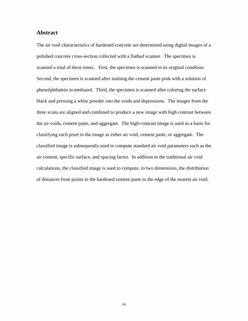
Abstract

The air void characteristics of hardened concrete are determined using digital images of a

polished concrete cross-section collected with a flatbed scanner. The specimen is

scanned a total of three times. First, the specimen is scanned in its original condition.

Second, the specimen is scanned after staining the cement paste pink with a solution of

phenolphthalein in methanol. Third, the specimen is scanned after coloring the surface

black and pressing a white powder into the voids and depressions. The images from the

three scans are aligned and combined to produce a new image with high contrast between

the air voids, cement paste, and aggregate. The high-contrast image is used as a basis for

classifying each pixel in the image as either air void, cement paste, or aggregate. The

classified image is subsequently used to compute standard air void parameters such as the

air content, specific surface, and spacing factor. In addition to the traditional air void

calculations, the classified image is used to compute, in two dimensions, the distribution

of distances from points in the hardened cement paste to the edge of the nearest air void.

iv

Acknowledgments

I want to thank Dr. Mark Snyder for introducing me to the science of concrete. It was Dr.

Snyder who suggested to me years ago that an automated method of quantifying air

bubbles in concrete would make a good thesis topic. I want to thank the folks at the

MnDOT Office of Materials and Road Research for the opportunity to perform dozens of

linear traverses and point counts on concrete specimens. I want to thank Ann MacLean

of the Forestry Department for the insight that software developed for processing remote

sensing imagery could be used to count air bubbles in concrete. I want to thank George

Dewey, Stan Vitton, and Bill Rose for serving on my committee, and Tom Van Dam, my

thesis advisor, for his help and support.

I would especially like to thank Larry Sutter for planting me in the fertile research

environment of the Keweenaw. Larry provided me with the lab equipment, macros, and

encouragement necessary to blossom and grow into a Master of Science. Thanks also to

Andy Swartz, Jennifer Felger, and Karl Hanson for their help in the lab, to Robert

Landsperger and Shane Christ for their professional computer support, and to the

Keweenaw Food Co-op for the delicious defense-day deli tray.

Thanks also to my family and friends, but most of all, I want to thank Anne

Walter for her love and support.

v

Contents

Abstract iii

Acknowledgements iv

List of Figures vi

List of Tables vi

1 Introduction 1

2 Background 3

2.1 Capillary Pores of Hardened Concrete 3

2.2 History of Air Entrainment 4

2.3 Freeze-Thaw Deterioration 5

2.4 Computing the Spacing Factor 5

2.5 The Spacing Distribution 8

3 Experimental 9

3.1 Introduction 9

3.2 Surface Preparation 9

3.3 Manually Performed Modified Point-Count 11

3.4 Scanning of the Surface 12

3.5 Geometric Rectification 13

3.6 Classification 15

3.7 Accuracy Assessment 20

3.8 Automated Modified Point-Count 22

3.9 The Spacing Distribution 23

4 Conclusions 35

4.1 Conclusions and Recommendations for Future Work 35

References 38

vi

List of Figures

1 Current practice of evaluating frost resistance from air-void parameters 2

2 A comparison of resolution between microscope and scanner 14

3 Flow-sheet of image processing to yield false color image 16

4 Two dimensional feature space plots from false color image 18

5 Classified scanner images compared to microscope images 21

6a False color image 25

6b Classified image 26

6c Results of a point count on a binary image of aggregate 27

6d Results of a point count on a binary image of air voids 28

6e Results of a linear traverse on a binary image of air voids 29

7 Example of cost surface accumulation 31

8 Accumulated cost surface image 32

9 Spacing distribution 34

10 Cumulative paste to void proximity distribution 34

List of Tables

1 Numerical band assignments for scanned images 17

2 Training set statistics 19

3 Accuracy assessment 20

4 Results from Modified Point-Counts 24

1

Chapter 1

Introduction

Concrete is a building material that is accessible to everyone. Combine three scoops of

rock, two scoops of sand, one scoop of cement, and add water to yield desired

consistency. Place the mixture in a form, and wait for it to harden. To make the final

product even more durable, it is considered good practice to include an air entraining

admixture. Air entraining admixtures are sometimes present in the cement powder, or

may be added to the water prior to mixing. As the name suggests, air entraining

admixtures encourage the formation of tiny air bubbles, (with diameters on the order of

one tenth of a millimeter) in the cement paste. The exact mechanisms responsible for the

enhanced durability of air entrained concrete are not completely understood. However, it

is generally accepted that each individual air bubble “protects” the hardened cement paste

in the immediate vicinity (1,2,3,4). Thus, the size distribution and spatial distribution of

the air bubbles in concrete has been a topic of great interest. The most widely used

method to determine whether or not a sufficient amount of entrained air is present is

ASTM C 457-90 “Standard Test Method for Microscopical Determination of Parameters

of the Air-Void System in Hardened Concrete” (5). To perform the test, a cross-sectional

polished slab is prepared from the concrete specimen, placed on a mechanical stage, and

illuminated with an oblique light source. The operator observes the polished surface

through a microscope, and distinguishes air voids by the shadows cast in the depressions.

The operator must systematically examine the slab, and record statistics about the air

bubbles, aggregates, and cement paste. The test is time consuming and tedious. Within

the scope of this work, efforts to automate this procedure are described.

2

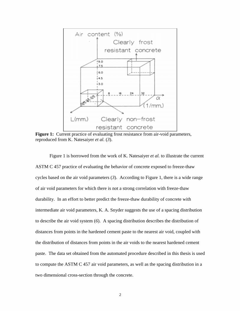
Figure 1: Current practice of evaluating frost resistance from air-void parameters,reproduced from K. Natesaiyer et al. (3).

Figure 1 is borrowed from the work of K. Natesaiyer et al. to illustrate the current

ASTM C 457 practice of evaluating the behavior of concrete exposed to freeze-thaw

cycles based on the air void parameters (3). According to Figure 1, there is a wide range

of air void parameters for which there is not a strong correlation with freeze-thaw

durability. In an effort to better predict the freeze-thaw durability of concrete with

intermediate air void parameters, K. A. Snyder suggests the use of a spacing distribution

to describe the air void system (6). A spacing distribution describes the distribution of

distances from points in the hardened cement paste to the nearest air void, coupled with

the distribution of distances from points in the air voids to the nearest hardened cement

paste. The data set obtained from the automated procedure described in this thesis is used

to compute the ASTM C 457 air void parameters, as well as the spacing distribution in a

two dimensional cross-section through the concrete.

3

Chapter 2

Background

2.1 Capillary Pores of Hardened Concrete

The information presented in this section is of a general nature, and can be found in most

textbooks that deal with concrete as building material. Two suggested textbooks are

included in the references (7,8).

Traditionally, concrete is a mixture of sand, rock, cement powder, water, and air.

Cement powder is the only ingredient that does not occur naturally. Cement powder is

produced by combining a source of calcium, (usually limestone) with a source of silicon,

aluminum, and iron, (usually shale or clay) at temperatures in the neighborhood of

1400°C. As the semi-molten mixture cools, four new minerals are present: primarily

tricalcium silicate and dicalcium silicate, and to a lesser degree, tricalcium aluminate and

tetracalcium aluminoferrite. In portland cement, the cement minerals are generally mixed

with gypsum, and ground into a powder. In concrete, most of the water combines with

the cement powder to produce hydration products. There are several hydration products,

but the two most prevalent are calcium silicate hydrate gel and calcium hydroxide. The

water not consumed remains as a highly alkaline solution in the spaces between the

hydration products. The spaces between the hydration products are referred to as

capillary pores. The collection of hydration products and capillary pores is referred to as

the hardened cement paste. The durability of the concrete during freeze-thaw cycles is

related to the behavior of the solution present in the capillary pores.

4

2.2 History of Air Entrainment

In the mid 1930s, the New York State Division of Highways built thirteen experimental

sections of concrete to investigate what was considered to be a “salt-scale” problem with

their highways (9). Different types and blends of cement were used. Cores were taken

from the pavements, and subjected to freeze-thaw cycles in a solution of calcium

chloride. Only those cores that contained a particular type of “natural cement” produced

in Ulster County, New York proved resistant to the damaging effect of freeze-thaw

cycles. The term natural cement implies that the limestone used to produce the cement

did not need to be blended with additional sources of aluminum, iron, and silicon before

firing in the kiln. It was speculated that the use of small amounts of fat or grease during

the grinding of the cement clinker was related to the unusual durability of the natural

cement. Further experimentation by the Universal Atlas Cement Company found that the

addition of small amounts of fat or grease, fish-oil stereate, or vinsol resin resulted in

concrete with more entrained air. Subsequent collaboration between the New York State

Division of Highways, the Universal Atlas Cement Company, and the Portland Cement

Association eventually led to the wide use of air entrained admixtures in concrete.

It is also worth mentioning that ancient Roman concrete appears to be air

entrained. It is believed that the addition of blood or milk to the mixture may be

responsible for the presence of entrained air (10).

5

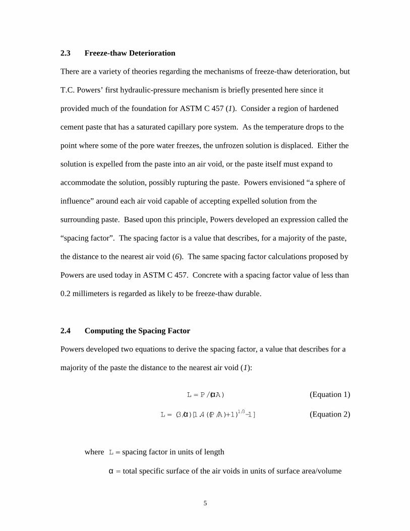
2.3 Freeze-thaw Deterioration

There are a variety of theories regarding the mechanisms of freeze-thaw deterioration, but

T.C. Powers’ first hydraulic-pressure mechanism is briefly presented here since it

provided much of the foundation for ASTM C 457 (1). Consider a region of hardened

cement paste that has a saturated capillary pore system. As the temperature drops to the

point where some of the pore water freezes, the unfrozen solution is displaced. Either the

solution is expelled from the paste into an air void, or the paste itself must expand to

accommodate the solution, possibly rupturing the paste. Powers envisioned “a sphere of

influence” around each air void capable of accepting expelled solution from the

surrounding paste. Based upon this principle, Powers developed an expression called the

“spacing factor”. The spacing factor is a value that describes, for a majority of the paste,

the distance to the nearest air void (6). The same spacing factor calculations proposed by

Powers are used today in ASTM C 457. Concrete with a spacing factor value of less than

0.2 millimeters is regarded as likely to be freeze-thaw durable.

2.4 Computing the Spacing Factor

Powers developed two equations to derive the spacing factor, a value that describes for a

majority of the paste the distance to the nearest air void (1):

L = P/(αA) (Equation 1)

L = (3/α)[1.4((P/A)+1)1/3-1] (Equation 2)

where L = spacing factor in units of length

α = total specific surface of the air voids in units of surface area/volume

6

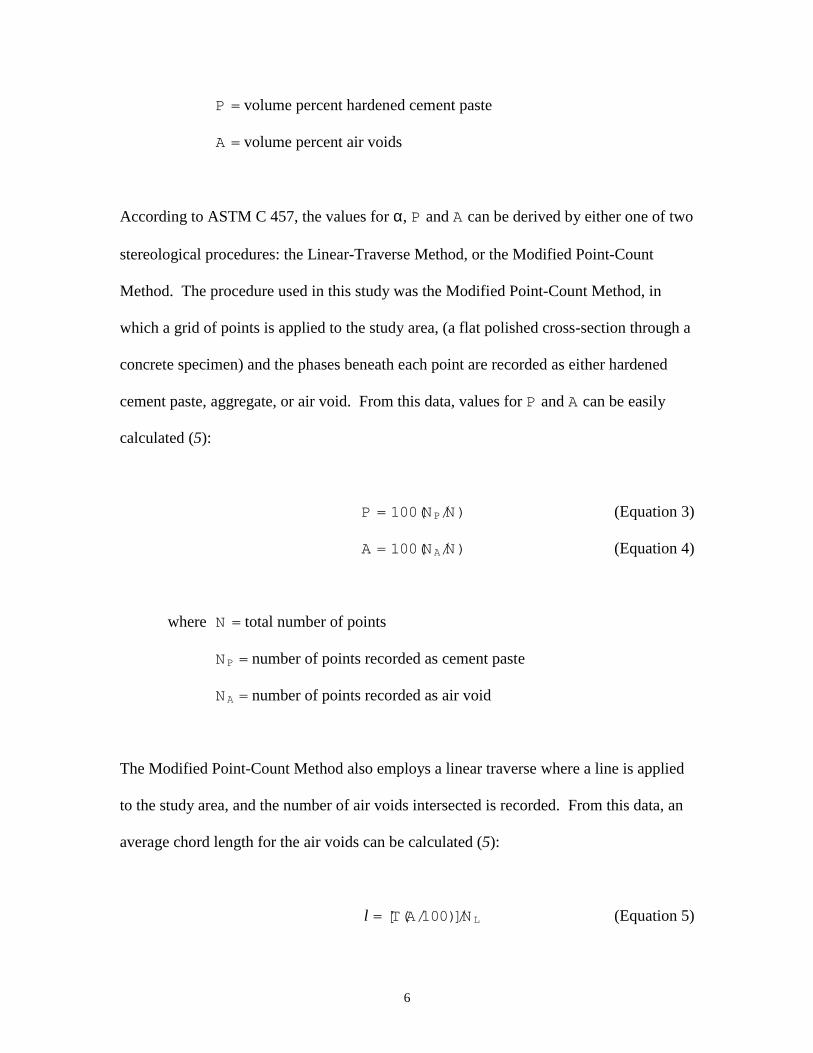
P = volume percent hardened cement paste

A = volume percent air voids

According to ASTM C 457, the values for α, P and A can be derived by either one of two

stereological procedures: the Linear-Traverse Method, or the Modified Point-Count

Method. The procedure used in this study was the Modified Point-Count Method, in

which a grid of points is applied to the study area, (a flat polished cross-section through a

concrete specimen) and the phases beneath each point are recorded as either hardened

cement paste, aggregate, or air void. From this data, values for P and A can be easily

calculated (5):

P = 100(NP/N) (Equation 3)

A = 100(NA/N) (Equation 4)

where N = total number of points

NP = number of points recorded as cement paste

NA = number of points recorded as air void

The Modified Point-Count Method also employs a linear traverse where a line is applied

to the study area, and the number of air voids intersected is recorded. From this data, an

average chord length for the air voids can be calculated (5):

l = [T(A/100)]/NL (Equation 5)

7

where l = average chord length

T = total line length

NL = number of air voids intersected by the line

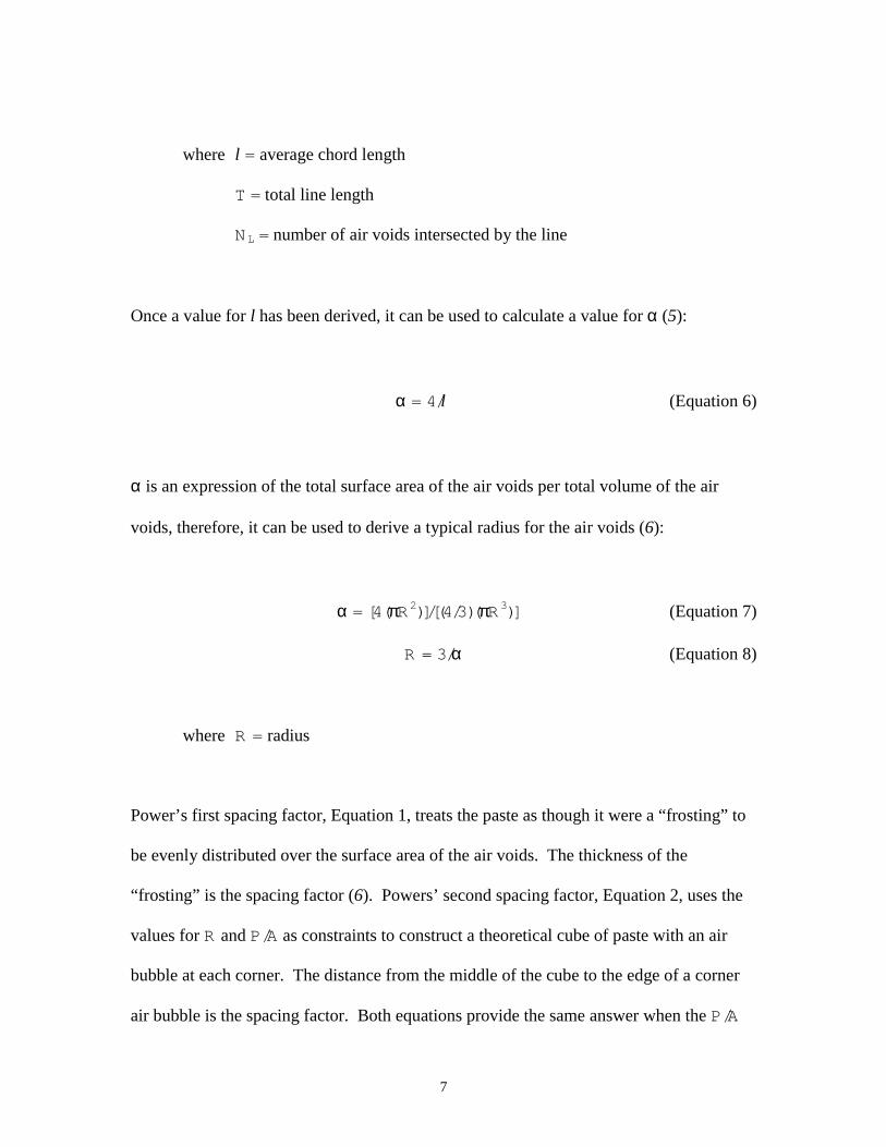
Once a value for l has been derived, it can be used to calculate a value for α (5):

α = 4/l (Equation 6)

α is an expression of the total surface area of the air voids per total volume of the air

voids, therefore, it can be used to derive a typical radius for the air voids (6):

α = [4(πR2)]/[(4/3)(πR3)] (Equation 7)

R = 3/α (Equation 8)

where R = radius

Power’s first spacing factor, Equation 1, treats the paste as though it were a “frosting” to

be evenly distributed over the surface area of the air voids. The thickness of the

“frosting” is the spacing factor (6). Powers’ second spacing factor, Equation 2, uses the

values for R and P/A as constraints to construct a theoretical cube of paste with an air

bubble at each corner. The distance from the middle of the cube to the edge of a corner

air bubble is the spacing factor. Both equations provide the same answer when the P/A

8

ratio equals 4.342. For P/A values less than 4.342 Equation 1 yields smaller values for L

than does Equation 2. Powers suggested the use of whichever equation yields the smaller

value for L (11).

2.5 The Spacing Distribution

Recently, a clever numerical experiment was conducted by K. A. Snyder to test the

performance of various air void spacing equations (6). The premise of the test was that in

a concrete system some points in the paste are closer to air voids than other points in the

paste, thus, the best way to think of the spacing is to treat it as a distribution of distances.

In the test, a hypothetical cube of paste is filled with randomly placed air bubbles. The

location and size of all of the air bubbles are known, so an accurate distribution of

spacing distances can be constructed. Powers’ spacing factor L came close to predicting

the 95th percentile of the distribution, that is, 95 percent of the paste was within the

distance L of the nearest void. However, none of the spacing equations, nor the

numerical test, take into account the presence of aggregate in the concrete. The

obstruction of a grain of sand between a point in the hardened cement paste and the

nearest air void will have an effect on the distance between the two. Instead, the spacing

equations are based on the premise that there are enough air bubbles in the concrete that

an aggregate will not generally be encountered when traveling from any given point in

the paste to the nearest air void (6). The data collected in the automated ASTM C 457

procedure described in this thesis is used to explore the effect of the presence of

aggregate on the spacing distribution on a two-dimensional slice through a concrete

specimen.

9

Chapter 3

Experimental

3.1 Introduction

The ability to make the distinction between air void, hardened cement paste, and

aggregate relies on methods of increasing the contrast between the three phases. When

manually performing ASTM C 457, the operator makes distinctions between hardened

cement paste and aggregate by variations in color and texture. By illuminating the

polished surface with an oblique light source, the operator distinguishes air voids by the

shadows cast in the depressions. In the method described here, the contrast between

hardened cement paste and aggregate is enhanced by staining the hardened cement paste

pink with a solution of phenolphthalein in alcohol (12). Air voids are distinguished by

using the popular technique of painting the polished surface black, and forcing white

powder into the depressions (11,13,14). Through the use of a flatbed scanner, digital

images of the surfaces are used to produce a new image where each pixel is classified as

either air void, hardened cement paste, or aggregate. The technology used to accomplish

this task is the same technology the remote sensing community has used for years to

analyze digital images collected by satellites. Specialized software has been developed to

process digital satellite images and to classify features according to their spectral

signatures (15). The same software is applied here to classify the digital images of

polished concrete collected with a flatbed scanner.

3.2 Surface Preparation

A concrete specimen, measuring 115 x 115 x 8 millimeters, (4.5 x 4.5 x 0.3 inches) was

cut with a water-cooled diamond saw from a 150 millimeter (6 inch) diameter core

10

retrieved from an airport runway pavement at Lubbock International Airport. Special

precautions were made to avoid sampling from the exterior portions of the core, which

may have experienced carbonation. One face of the slab was polished on a water-cooled

rotating lap. The face was polished in six steps. The first five polishing steps utilized

magnetic-backed fixed-diamond abrasive wheels that adhere to the iron platen of the

rotating lap. The grit sizes were as follows: 60, 100, 200, 325, and 500. The final

polishing step utilized an adhesive-backed 600 grit fixed-silicon carbide paper that

adheres to the iron platen of the rotating lap. Polishing residues were removed from the

specimen surface between each step and after the final step by gently blowing on the

surface with an air hose and rinsing with water. After cleaning, the sample was blotted

dry and placed in a 40°C oven for 30 minutes. After drying, twelve steel reference pins,

(fabricated from common paper staples) were fixed via cyanoacrylate to the sides of the

specimen, three pins per side. The pins were placed along the sides of the slab, but

perpendicular to the polished surface, such that the tip of each pin was flush with the

polished surface. The polished surface was then scanned on a flatbed scanner, the details

of which are described later.

After the initial scan, the polished surface was stained with a 0.5%

phenolphthalein solution in alcohol. Portions of the surface with a pH greater than 8.3

turn a pink to red color when exposed to phenolphthalein. To stain the specimen, a small

amount of solution was sprayed onto the surface. The solution was allowed to sit for a

period of 20 seconds, after which, the excess was blotted away. The specimen was dried

in a 40°C oven for 30 minutes, and then placed on a flatbed scanner and scanned in the

same manner as the non-stained surface.

11

It is important to note that the hardened cement paste will turn pink when exposed

to phenolphthalein, unless the hardened cement paste has carbonated. Hence, it is

important to conduct the staining as soon as possible after cutting and polishing the

specimen in order to avoid excessive carbonation. Most conventional aggregates will be

unaffected by the phenolphthalein stain.

After the second scan, an 18 mm wide felt-tipped black permanent marker was

used to color the surface black. A series of slightly overlapping parallel lines were used

to color the surface. The specimen was dried in a 40°C oven for 15 minutes before

applying the second coating of black ink. The second coat was applied at an orientation

of 90° to the first coat, and dried again in a 40°C oven for 15 minutes. After the ink had

dried, 2 micrometer wollastonite powder was generously piled onto the polished surface,

and gently worked into the voids with the flat face of a glass slide. Next, most of the

excess powder was scraped away with a single edged razor blade. The remaining powder

was wiped away with a lightly oiled fingertip, leaving only the powder that had been

worked into the recesses or voids. The black and white treated surface was placed on a

flatbed scanner, and scanned in as before.

3.3 Manually Performed Modified Point-Count

A Modified Point-Count was performed on the non-stained surface according to ASTM C

457 on a motorized stage with a zoom stereo microscope equipped with a video camera.

Both the motorized stage and the video camera were connected to a computer and

controlled by a macro written for NIH Image, a public domain image analysis program

developed at the National Institutes of Health and available on the internet at

12

http://www.scioncorp.com/ (16). In addition to performing the Modified Point-Count, a

total of 570 digital images of the polished surface were captured from the microscope,

along with the x and y stage coordinates of a crosshairs located at the center of each

image. Digital images were also captured of the reference pins, along with the

accompanying x and y stage coordinates. The digital images of the reference pins were

used to align the digital images from the scanner to the same coordinate system used by

the motorized stage. The 570 digital images of the polished surface were used later to

compare the classification scheme of the scanned images to features observed with the

microscope.

3.4 Scanning of the Surface

The initial non-stained surface, the phenolphthalein stained surface, and the black and

white treated surface were placed on a flatbed scanner, scanned in RGB color at a pixel

resolution of 16.9 x 16.9 micrometers, (1500 dpi) and saved in a tagged image file

format, (TIFF). The area scanned was slightly larger than the polished surface, so as to

ensure that the reference pins would be included in the scan. Special precautions were

taken to ensure that the polished concrete surface and the glass flatbed scanner surface

were both free of any stray particles of lint or dust that might prevent the sample from

resting perfectly flat upon the scanner.

The optical resolution of the scanner used, in terms of pixel size, is 10.6 x 42.3

micrometers, (600 x 2400 dpi). However, since rectangular pixels would complicate the

analysis of the image, square pixels were used instead. If the dimensions of the square

pixels were set equal to the axis of lower resolution, that is, 42.3 x 42.3 micrometers,

13

(600 dpi) then some of the resolution would be lost. Conversely, if the dimensions of the

square pixels were set equal to the axis of higher resolution, that is, 10.6 x 10.6

micrometers, (2400 dpi) some of the resolution would be interpolated, hence artificial.

The 16.9 x 16.9 micrometer pixel resolution used in the experiment was chosen as a

compromise, and interpolated from the 10.6 x 42.3 micrometer pixel data. According to

ASTM C 457, the microscope used to perform an air void analysis should be able to

resolve features of 10 micrometers in size (5). Although the scanner used in this

experiment does not quite achieve this resolution, there are commercially available

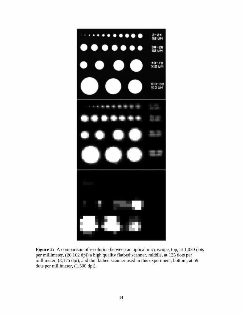
scanners capable of this kind of resolution. Figure 2 compares the performance of the

scanner used in this experiment to an optical microscope and to a high quality flatbed

scanner used in the publishing industry. As can be seen in Figure 2, the high quality

flatbed scanner falls short of the optical microscope, but is capable of resolving features

of 10 micrometers. The scanner used in this experiment is only capable of resolving

features of 100 micrometers.

3.5 Geometric Rectification

Features common between the three images, such as dark specks in the hardened cement

paste or small entrained air voids, were used to align the non-stained image and the black

and white treated image to the phenolphthalein stained image. Simply stated, to align an

image, the x and y coordinates of a pixel that define a feature in the image are correlated

with the x and y coordinates of a pixel that define the same feature in the reference

image. The process is repeated until coordinate sets are well distributed over the two

images. The geometric relationship between the two sets of coordinates is used to

14

Figure 2: A comparison of resolution between an optical microscope, top, at 1,030 dotsper millimeter, (26,162 dpi) a high quality flatbed scanner, middle, at 125 dots permillimeter, (3,175 dpi), and the flatbed scanner used in this experiment, bottom, at 59dots per millimeter, (1,500 dpi).

15

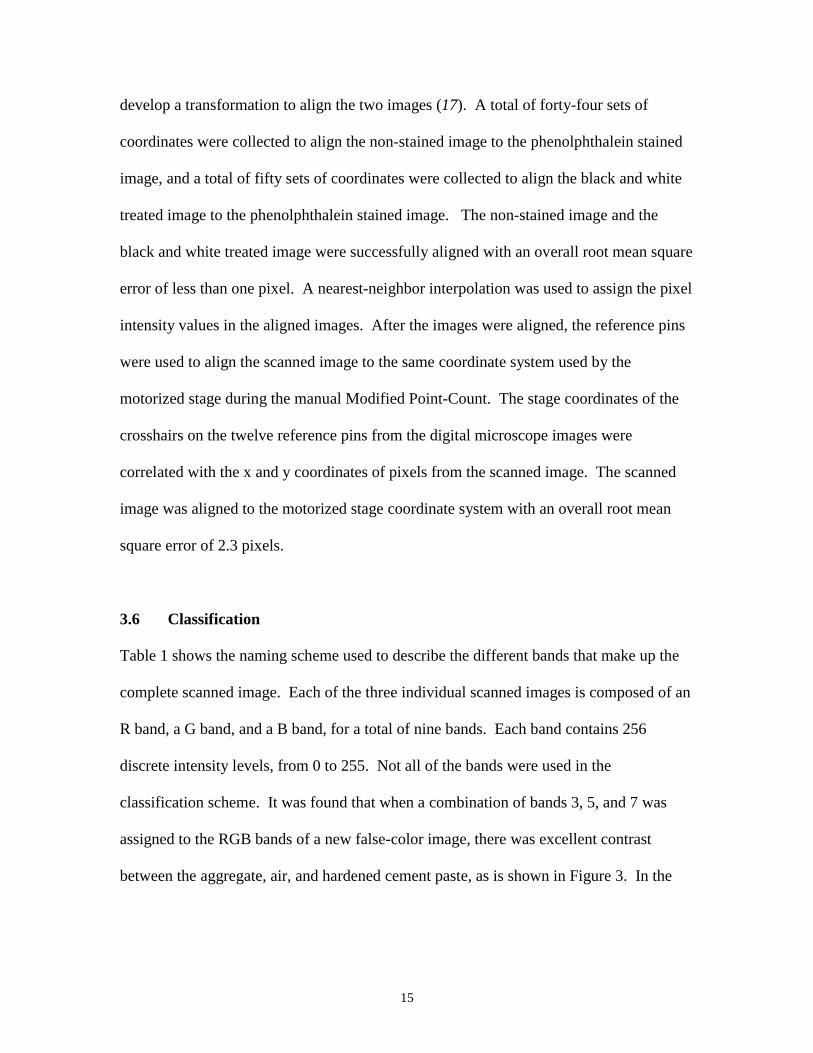
develop a transformation to align the two images (17). A total of forty-four sets of

coordinates were collected to align the non-stained image to the phenolphthalein stained

image, and a total of fifty sets of coordinates were collected to align the black and white

treated image to the phenolphthalein stained image. The non-stained image and the

black and white treated image were successfully aligned with an overall root mean square

error of less than one pixel. A nearest-neighbor interpolation was used to assign the pixel

intensity values in the aligned images. After the images were aligned, the reference pins

were used to align the scanned image to the same coordinate system used by the

motorized stage during the manual Modified Point-Count. The stage coordinates of the

crosshairs on the twelve reference pins from the digital microscope images were

correlated with the x and y coordinates of pixels from the scanned image. The scanned

image was aligned to the motorized stage coordinate system with an overall root mean

square error of 2.3 pixels.

3.6 Classification

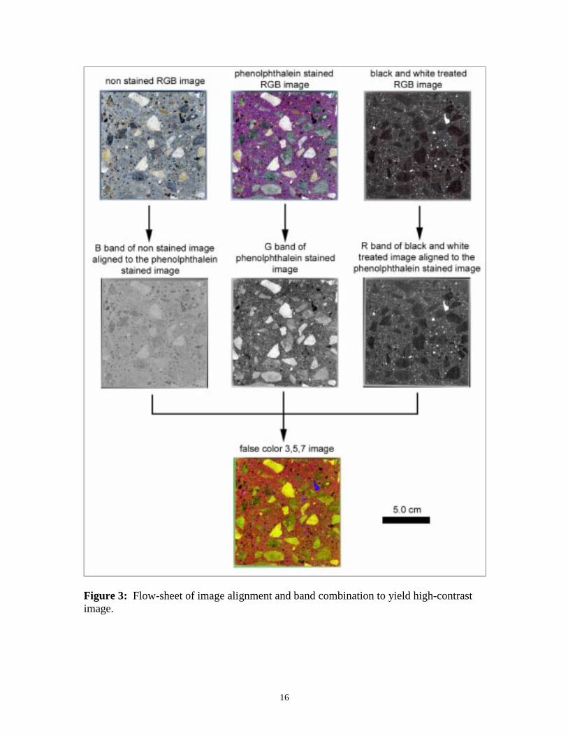
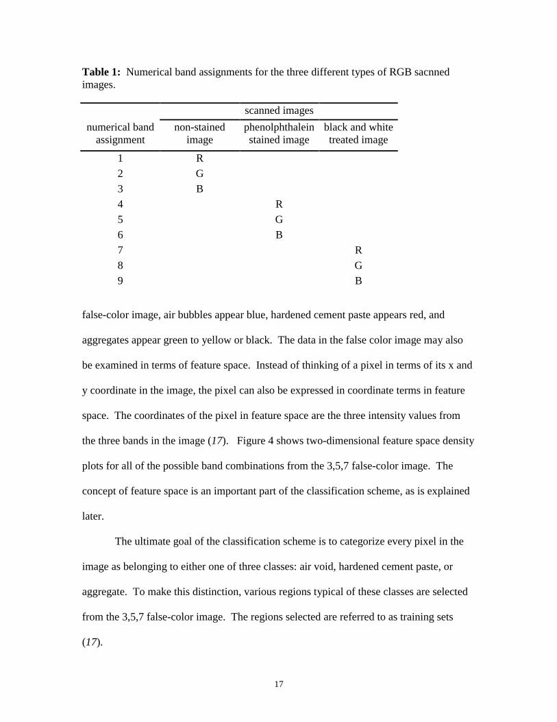
Table 1 shows the naming scheme used to describe the different bands that make up the

complete scanned image. Each of the three individual scanned images is composed of an

R band, a G band, and a B band, for a total of nine bands. Each band contains 256

discrete intensity levels, from 0 to 255. Not all of the bands were used in the

classification scheme. It was found that when a combination of bands 3, 5, and 7 was

assigned to the RGB bands of a new false-color image, there was excellent contrast

between the aggregate, air, and hardened cement paste, as is shown in Figure 3. In the

16

Figure 3: Flow-sheet of image alignment and band combination to yield high-contrastimage.

17

Table 1: Numerical band assignments for the three different types of RGB sacnnedimages.

scanned images

numerical bandassignment

non-stainedimage

phenolphthaleinstained image

black and whitetreated image

1 R

2 G

3 B

4 R

5 G

6 B

7 R

8 G

9 B

false-color image, air bubbles appear blue, hardened cement paste appears red, and

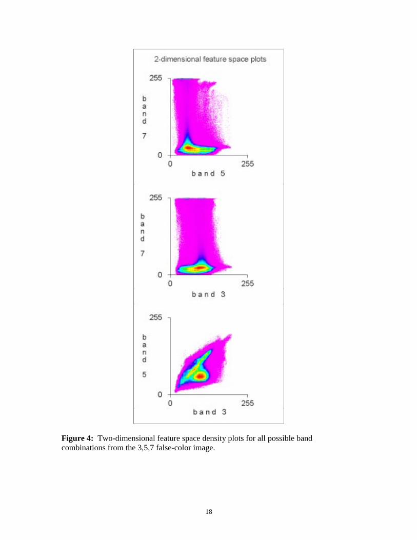
aggregates appear green to yellow or black. The data in the false color image may also

be examined in terms of feature space. Instead of thinking of a pixel in terms of its x and

y coordinate in the image, the pixel can also be expressed in coordinate terms in feature

space. The coordinates of the pixel in feature space are the three intensity values from

the three bands in the image (17). Figure 4 shows two-dimensional feature space density

plots for all of the possible band combinations from the 3,5,7 false-color image. The

concept of feature space is an important part of the classification scheme, as is explained

later.

The ultimate goal of the classification scheme is to categorize every pixel in the

image as belonging to either one of three classes: air void, hardened cement paste, or

aggregate. To make this distinction, various regions typical of these classes are selected

from the 3,5,7 false-color image. The regions selected are referred to as training sets

(17).

18

Figure 4: Two-dimensional feature space density plots for all possible bandcombinations from the 3,5,7 false-color image.

19

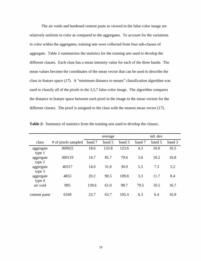
The air voids and hardened cement paste as viewed in the false-color image are

relatively uniform in color as compared to the aggregates. To account for the variations

in color within the aggregates, training sets were collected from four sub-classes of

aggregate. Table 2 summarizes the statistics for the training sets used to develop the

different classes. Each class has a mean intensity value for each of the three bands. The

mean values become the coordinates of the mean vector that can be used to describe the

class in feature space (17). A “minimum distance to means” classification algorithm was

used to classify all of the pixels in the 3,5,7 false-color image. The algorithm compares

the distance in feature space between each pixel in the image to the mean vectors for the

different classes. The pixel is assigned to the class with the nearest mean vector (17).

Table 2: Summary of statistics from the training sets used to develop the classes.

average std. dev.

class # of pixels sampled band 7 band 5 band 3 band 7 band 5 band 3

aggregatetype 1

369925 18.6 133.8 123.6 4.3 10.0 10.5

aggregatetype 2

300119 14.7 85.7 79.6 5.6 18.2 16.8

aggregatetype 3

40317 14.0 31.0 30.0 5.3 7.3 5.2

aggregatetype 4

4853 20.2 90.5 109.8 3.3 11.7 8.4

air void 895 139.6 61.0 98.7 79.5 10.5 16.7

cement paste 6169 23.7 63.7 105.4 6.3 6.4 16.9

20

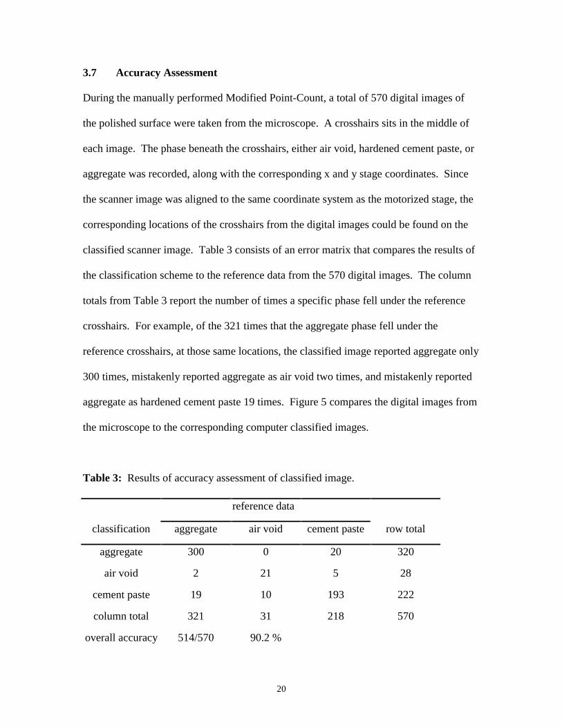
3.7 Accuracy Assessment

During the manually performed Modified Point-Count, a total of 570 digital images of

the polished surface were taken from the microscope. A crosshairs sits in the middle of

each image. The phase beneath the crosshairs, either air void, hardened cement paste, or

aggregate was recorded, along with the corresponding x and y stage coordinates. Since

the scanner image was aligned to the same coordinate system as the motorized stage, the

corresponding locations of the crosshairs from the digital images could be found on the

classified scanner image. Table 3 consists of an error matrix that compares the results of

the classification scheme to the reference data from the 570 digital images. The column

totals from Table 3 report the number of times a specific phase fell under the reference

crosshairs. For example, of the 321 times that the aggregate phase fell under the

reference crosshairs, at those same locations, the classified image reported aggregate only

300 times, mistakenly reported aggregate as air void two times, and mistakenly reported

aggregate as hardened cement paste 19 times. Figure 5 compares the digital images from

the microscope to the corresponding computer classified images.

Table 3: Results of accuracy assessment of classified image.

reference data

classification aggregate air void cement paste row total

aggregate 300 0 20 320

air void 2 21 5 28

cement paste 19 10 193 222

column total 321 31 218 570

overall accuracy 514/570 90.2 %

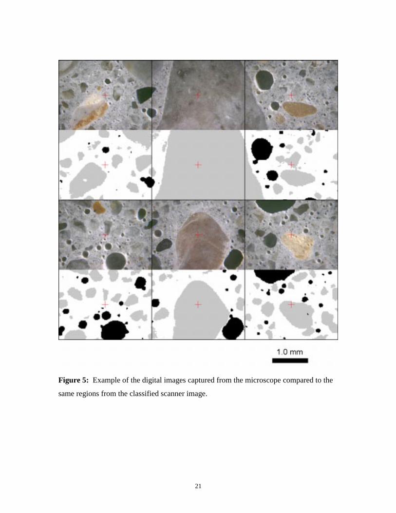
21

Figure 5: Example of the digital images captured from the microscope compared to the

same regions from the classified scanner image.

22

3.8 Automated Modified Point-Count

In order to perform a Modified Point-Count according to ASTM C 457, the classified

image data was imported into NIH Image. However, the 5000 x 5000 pixel image was

too large for NIH Image to process, so it was subdivided into four 2500 x 2500 pixel

images. From the classified data, two new binary images were created. The first binary

image consists only of aggregate particles, and the second binary image consists only of

air voids in the hardened paste. To create the binary aggregate image, the gray aggregate

pixels were selected from the classified image, and any voids within the aggregates were

automatically filled in. To create the binary air void image, the black air void pixels were

selected from the classified image, and subtracted from the aggregate binary image,

leaving only those air voids in contact with the hardened cement paste.

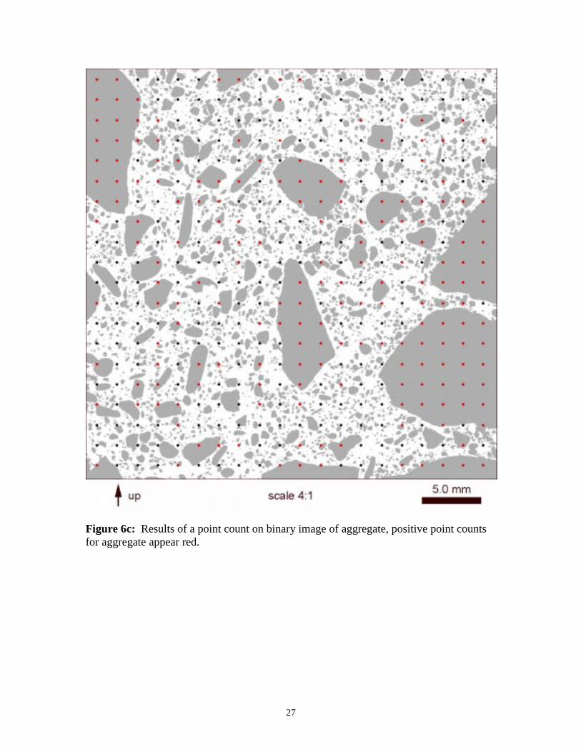
To perform the modified point count, a 2500 x 2500 pixel binary image was

constructed with a regular array of 400 single pixel black dots. A Boolean AND

operation was performed between the array of black dots and the binary aggregate

images. The number of black dots in the resulting images was automatically tabulated,

representing the number of aggregate particles encountered during the point count. A

Boolean AND operation was also performed between the array of black dots and the

binary air void images. The number of black dots in the resulting images was

automatically tabulated, representing the number of air voids encountered during the

point count. To derive the number of points that intersect with hardened cement, the total

number of points used in the experiment, (1600) was subtracted from the sum of the

number of aggregates encountered plus the number of air voids encountered.

23

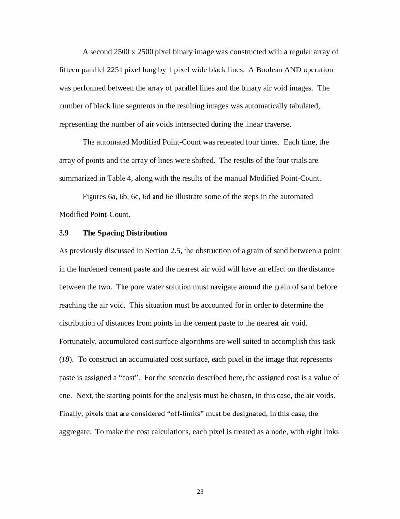
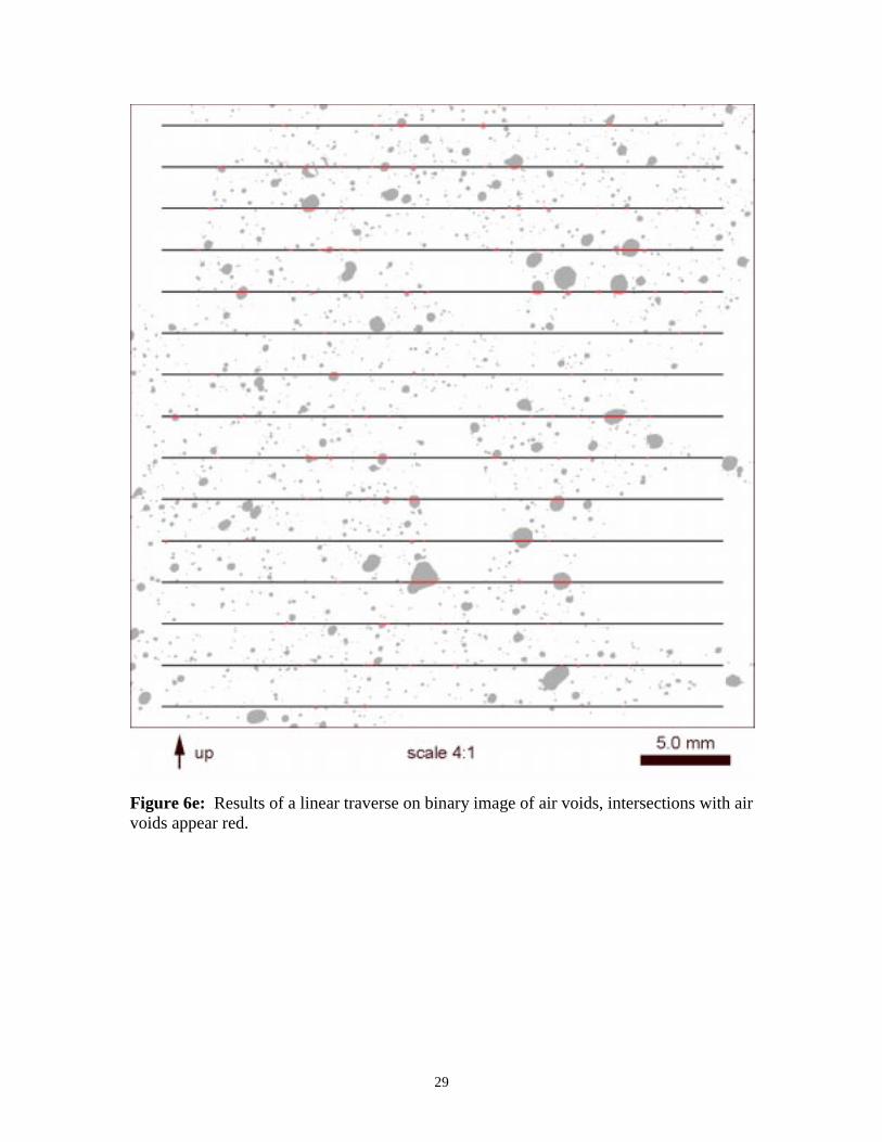
A second 2500 x 2500 pixel binary image was constructed with a regular array of

fifteen parallel 2251 pixel long by 1 pixel wide black lines. A Boolean AND operation

was performed between the array of parallel lines and the binary air void images. The

number of black line segments in the resulting images was automatically tabulated,

representing the number of air voids intersected during the linear traverse.

The automated Modified Point-Count was repeated four times. Each time, the

array of points and the array of lines were shifted. The results of the four trials are

summarized in Table 4, along with the results of the manual Modified Point-Count.

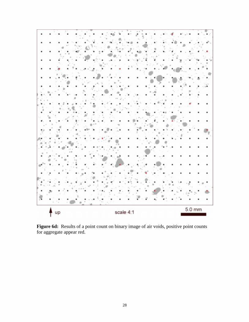
Figures 6a, 6b, 6c, 6d and 6e illustrate some of the steps in the automated

Modified Point-Count.

3.9 The Spacing Distribution

As previously discussed in Section 2.5, the obstruction of a grain of sand between a point

in the hardened cement paste and the nearest air void will have an effect on the distance

between the two. The pore water solution must navigate around the grain of sand before

reaching the air void. This situation must be accounted for in order to determine the

distribution of distances from points in the cement paste to the nearest air void.

Fortunately, accumulated cost surface algorithms are well suited to accomplish this task

(18). To construct an accumulated cost surface, each pixel in the image that represents

paste is assigned a “cost”. For the scenario described here, the assigned cost is a value of

one. Next, the starting points for the analysis must be chosen, in this case, the air voids.

Finally, pixels that are considered “off-limits” must be designated, in this case, the

aggregate. To make the cost calculations, each pixel is treated as a node, with eight links

24

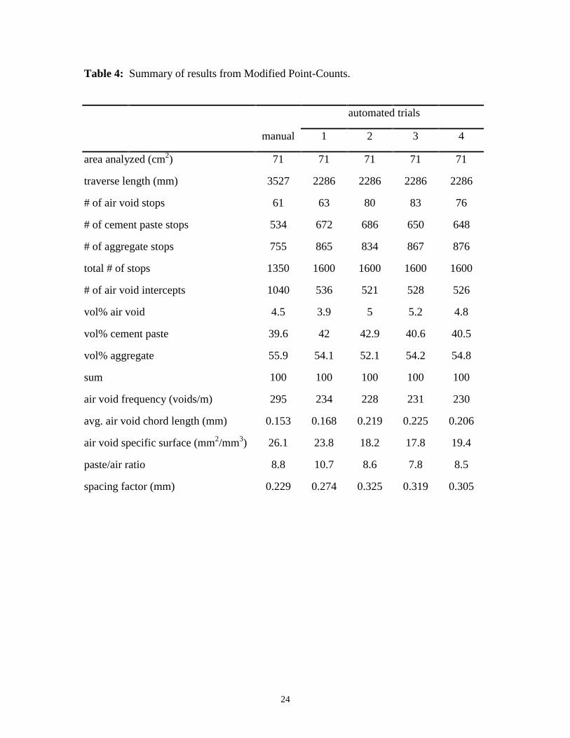
Table 4: Summary of results from Modified Point-Counts.

automated trials

manual 1 2 3 4

area analyzed (cm2) 71 71 71 71 71

traverse length (mm) 3527 2286 2286 2286 2286

# of air void stops 61 63 80 83 76

# of cement paste stops 534 672 686 650 648

# of aggregate stops 755 865 834 867 876

total # of stops 1350 1600 1600 1600 1600

# of air void intercepts 1040 536 521 528 526

vol% air void 4.5 3.9 5 5.2 4.8

vol% cement paste 39.6 42 42.9 40.6 40.5

vol% aggregate 55.9 54.1 52.1 54.2 54.8

sum 100 100 100 100 100

air void frequency (voids/m) 295 234 228 231 230

avg. air void chord length (mm) 0.153 0.168 0.219 0.225 0.206

air void specific surface (mm2/mm3) 26.1 23.8 18.2 17.8 19.4

paste/air ratio 8.8 10.7 8.6 7.8 8.5

spacing factor (mm) 0.229 0.274 0.325 0.319 0.305

25

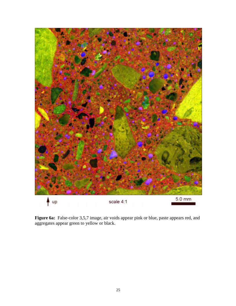
Figure 6a: False-color 3,5,7 image, air voids appear pink or blue, paste appears red, andaggregates appear green to yellow or black.

26

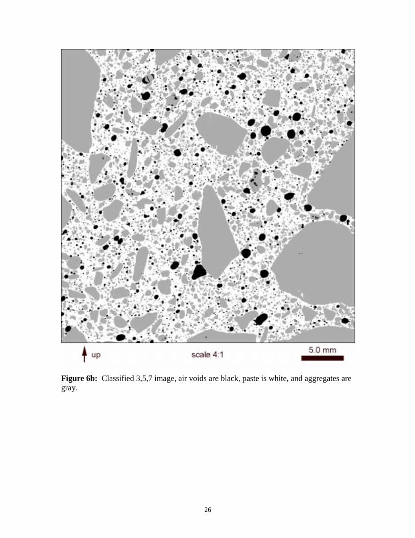
Figure 6b: Classified 3,5,7 image, air voids are black, paste is white, and aggregates aregray.

27

Figure 6c: Results of a point count on binary image of aggregate, positive point countsfor aggregate appear red.

28

Figure 6d: Results of a point count on binary image of air voids, positive point countsfor aggregate appear red.

29

Figure 6e: Results of a linear traverse on binary image of air voids, intersections with airvoids appear red.

30

connecting to the surrounding pixels. The cost to move across a link is calculated as

follows:

c = a + (b1 + b2)/2 (Equation 9)

where a = the length of the link between the neighboring pixels

b1 = the cost of the originating pixel

b2 = the cost of the destination pixel

c = the accumulated cost

The value for a depends on the location of the destination pixel relative to the originating

pixel. If the destination pixel is directly north, south, east, or west of the originating

pixel, the value for a is one. If the destination pixel is located diagonally relative to the

originating pixel, the value for a is the square root of two. Accumulated costs are

calculated for pixels that neighbor the starting-point pixels. These pixels are assigned the

new accumulated cost value. These immediate neighbors have a direct path to the

starting-point pixels, so their values are output to the accumulated cost surface. An

iterative process ensues where subsequent pixels are assigned a least accumulated cost

value. A detailed description of the workings of the accumulated cost surface algorithm

used in this research can be found in the help files of the software used to process the data

(19).

Figure 7 shows an example of an accumulated cost surface. For the final step

illustrated in Figure 7, the cost values for each pixel are rounded to the nearest whole

number. This step was undertaken so that the accumulated cost surface could be treated

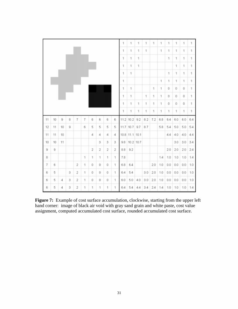
31

Figure 7: Example of cost surface accumulation, clockwise, starting from the upper lefthand corner: image of black air void with gray sand grain and white paste, cost valueassignment, computed accumulated cost surface, rounded accumulated cost surface.

32

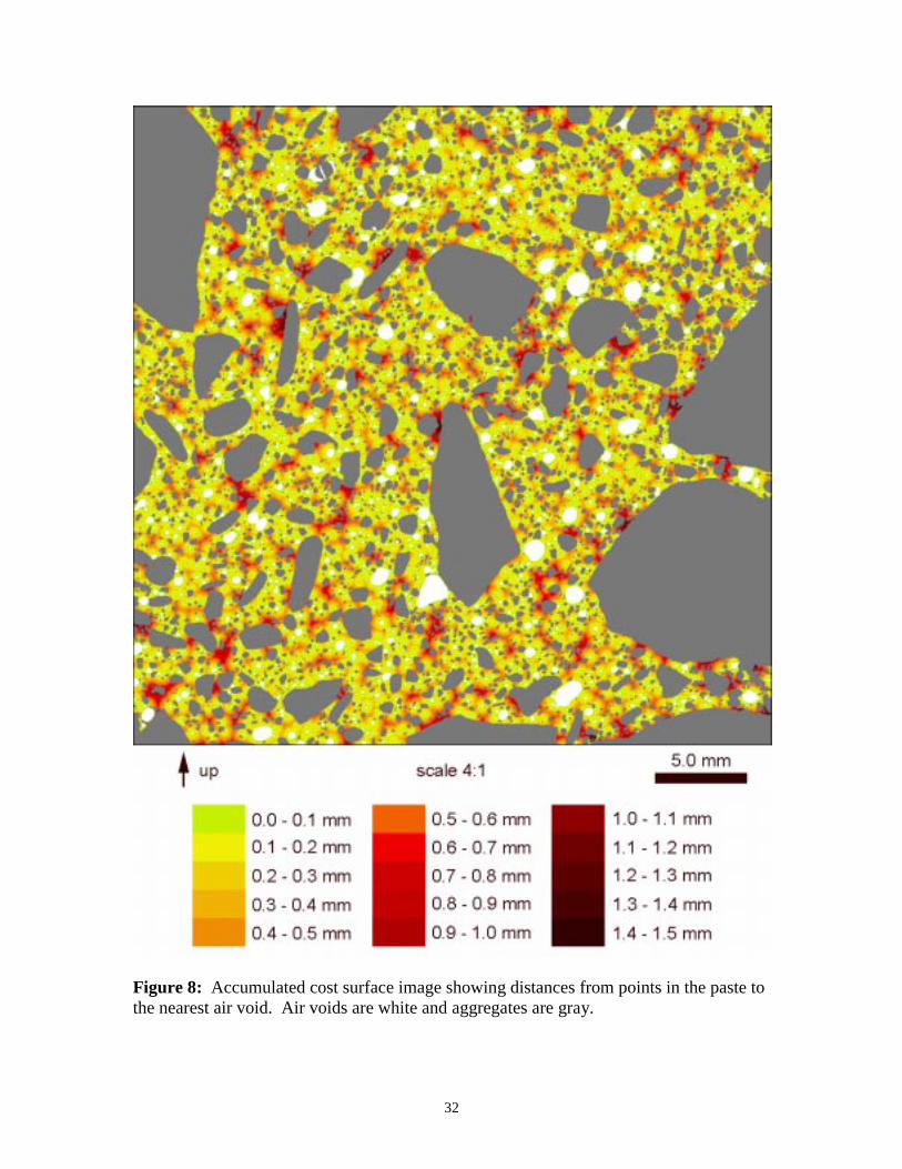
Figure 8: Accumulated cost surface image showing distances from points in the paste tothe nearest air void. Air voids are white and aggregates are gray.

33

as an 8-bit image. Figure 8 depicts the results of the accumulated cost surface analysis on

the concrete sample. In Figure 8, the cement paste is color coded in terms of the distance

to the nearest air void. The shades of yellow and green in Figure 8 represent paste that is

within 0.2 mm of the nearest air void. The value of 0.2 mm was selected because it is the

spacing factor distance generally accepted as “safe” in terms of freeze-thaw durability

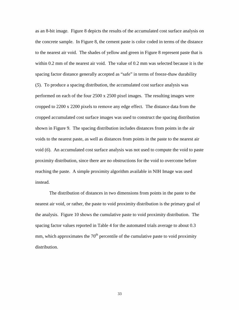
(5). To produce a spacing distribution, the accumulated cost surface analysis was

performed on each of the four 2500 x 2500 pixel images. The resulting images were

cropped to 2200 x 2200 pixels to remove any edge effect. The distance data from the

cropped accumulated cost surface images was used to construct the spacing distribution

shown in Figure 9. The spacing distribution includes distances from points in the air

voids to the nearest paste, as well as distances from points in the paste to the nearest air

void (6). An accumulated cost surface analysis was not used to compute the void to paste

proximity distribution, since there are no obstructions for the void to overcome before

reaching the paste. A simple proximity algorithm available in NIH Image was used

instead.

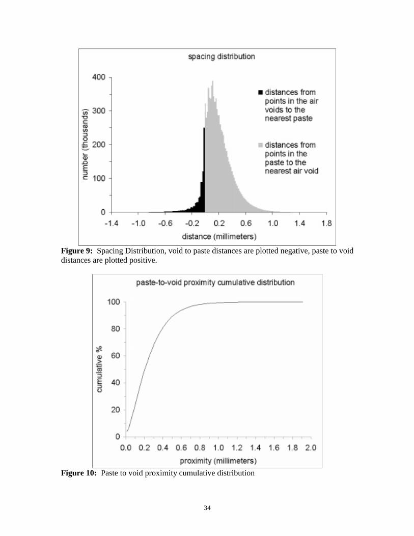
The distribution of distances in two dimensions from points in the paste to the

nearest air void, or rather, the paste to void proximity distribution is the primary goal of

the analysis. Figure 10 shows the cumulative paste to void proximity distribution. The

spacing factor values reported in Table 4 for the automated trials average to about 0.3

mm, which approximates the 70th percentile of the cumulative paste to void proximity

distribution.

34

Figure 9: Spacing Distribution, void to paste distances are plotted negative, paste to voiddistances are plotted positive.

Figure 10: Paste to void proximity cumulative distribution

35

Chapter 4

Conclusions

4.1 Conclusions and Recommendations for Future Work

According to the error matrix presented in Table 3, the classification scheme had an

overall accuracy of 90.2% as compared to the 570 digital microscope images. Table 4

demonstrates that the automated method came close to duplicating the results of the

manually performed Modified Point-Count, as the overall volume percent values for the

different phases are relatively similar. However, differences become apparent in the air

void statistics and the spacing factor. The values for the air void frequency and air void

specific surface are slightly lower in the automated trials as compared to the manual

method. The values for the average air void chord length are slightly higher in the

automated trials as compared to the manual method.

There are two plausible explanations for this. First, as can be seen in Figures 2

and 5, the resolution of the scanner is too poor to detect the smallest of air voids.

Second, the resolution may have been too poor to discern between air voids in close

proximity to each other, thereby lumping them together as one air void. A better quality

scanner of the type used in Figure 2 would likely correct these problems. Close scrutiny

of Figure 5 also reveals that aggregate is occasionally classified as paste. In addition,

some of the misclassification may also be due to the 2.3 pixel alignment error between

the motorized stage coordinate system and the scanned image. More experimentation

with other types of classification schemes is warranted.

The information contained in a classified scanner image can be used for purposes

other than the standard ASTM C 457 procedures. In this thesis, the distribution in two

36

dimensions of distances from points in the cement paste to the nearest air void is

calculated. However, the results of the paste to void proximity analysis are based on

some simplifications. First, with a two-dimensional cross-section, it is possible for a

region of hardened cement paste to appear to be completely surrounded by aggregate,

making it impossible to reach an air void. To eliminate this situation, any air void or

hardened cement paste regions completely enclosed by an aggregate were filled in and

reclassified as aggregate. This solution, while simple, worked well in this situation, but

might eliminate too much data in concrete where dimpled or more complex-shaped

aggregates are used. Second, the data set is unavoidably two-dimensional. Ultimately,

only a three-dimensional data set can provide an accurate approximation for the spacing

distribution. Recently, three-dimensional x-ray computed tomography digital images

have been collected from hardened concrete for the purpose of air void analysis (20).

With a three-dimensional data set, it would be possible to achieve a better understanding

of the influence aggregate has on the spacing distribution.

In this study, only one concrete specimen was examined. The experiment should

be repeated with multiple concrete prisms to represent a variety of air void systems.

Furthermore, measurements of the two dimensional paste to void proximity distributions

should be correlated with laboratory freeze-thaw tests performed on the same concrete

prisms.

In this study, the automated Modified Point-Count was performed only four times

on the data set. Ideally, the automated Modified Point-Count could be repeated hundreds

of times on the same sample, shifting the position of the test lines and points each time, to

yield a better approximation of the air void parameters. However, any future work using

37

a flatbed scanner approach should take advantage of commercially available high

resolution scanners.

The two dimensional paste to void proximity distribution data obtained in this

study could be used, with some effort, to indirectly test the equations currently available

for predicting three dimensional paste to void proximity distributions. None of the

equations currently available take into account the influence of the presence of aggregate

on the distribution (6). The methods described in this study do account for the presence

of aggregate, but only in two dimensions. The equations used to predict three

dimensional paste-to-void proximity distributions require the input of one dimensional

linear traverse data. Since equations have already been derived to project one

dimensional traverse data into three dimensions, it follows that related equations could be

derived for two dimensions. The two dimensional paste to void proximity distributions

obtained by the methods described in this thesis could then be compared to the two

dimensional paste to void proximity distributions derived by equation.

38

References

1. Powers, T.C. The Air Requirement of Frost-Resistant Concrete. Highway Research

Board Proceedings 29th Annual Meeting, Washington D.C., December 13-16, pp.

184-211, 1949.

2. Philleo, R.E. A Method for Analyzing Void Distribution in Air-Entrained Concrete.

Cement, Concrete, and Aggregates, Vol. 5, No. 2, pp. 128-130, 1983.

3. Natesaiyer, K. Hover, K.C., Snyder, K.A. Protected-Paste Volume of Air-Entrained

Cement Paste. Part 1. Journal of Materials in Civil Engineering, Vol. 4, No. 2, pp.

166-184, 1992.

4. Pleau, R. Pigeon, M. The Use of the Flow Length Concept to Assess the Efficiency of

Air Entrainment with Regards to Frost Durability: Part I – Description of the Test

Method. Cement, Concrete, and Aggregates, Vol. 18, No. 1, pp. 19-29, 1996.

5. C 457-98 Standard Test Method for Microscopical Determination of Parameters of

the Air-Void System in Hardened Concrete. American Society for Testing and

Materials, West Conshohocken, Pennsylvania, 2000.

6. Snyder, K. A. A Numerical Test of Air-Void Spacing Equations. Advances in Cement

Based Materials, Vol. 8, No. 28, pp. 28-44, 1998.

7. Mindness, S. Young, J.F. Concrete. Prentice-Hall, Inc. Englewood Cliffs, New

Jersey, 1981, 671 p.

8. Mehta, P.K. Monteiro, P.J.M. Concrete, Structure, Properties, and Materials, 2nd Ed.

Prentice-Hall, Inc. Englewood Cliffs, New Jersey, 1993, 548 p.

9. Moore, O.L. Pavement Scaling Successfully Checked. Engineering News Record,

Vol. 125, No. 15, pp. 471-474, 1940.

10. Idorn, G.M. The History of Concrete Technology Through a Microscope. Beton

Teknik, Vol. 25, No. 4, pp. 119-141, 1959.

11. Dewey, G. R., and Darwin, D. Image Analysis of Air Voids in Air Entrained

Concrete. SM Report No. 29, The University of Kansas Center For Research,

Lawrence, Kansas, August 1991, 331 p.

39

12. Muethel, R. W. Investigation of Calcium Hydroxide Depletion as a Cause of

Concrete Pavement Deterioration. Research Report R-1353, Michigan Department of

Transportation Construction and Technology Division, November 1997, 39 p.

13. Chatterji, S., and Gudmundsson, H. Characterization of Entrained Air Bubble

Systems in Concrete by Means of an Image Analyzing Microscope. Cement and

Concrete Research, Vol. 7, No. 4, August 1977, pp. 423-428.

14. MacInnis, C. and Racic, D. The Effect of Superplasticizers on the Air-Void System in

Concrete. Cement and Concrete Research, Vol. 16, No. 3, May 1986, pp. 345-352.

15. Research Systems Inc., Envi 3.2, September 3, 2000, http://www.envi-sw.com/.

16. Sutter, L. L. Modified Point Count Macro for NIH Image. November 16, 2000.

http://techsrv1.tech.mtu.edu/~llsutter/.

17. Jensen, J. R. Introductory Digital Image Processing : A Remote Sensing Perspective.

Prentice-Hall, Inc. Upper Saddle River, New Jersey, 1996, 316 p.

18. Chrisman, N. Exploring Geographic Information Systems. John Wiley & Sons, Inc.

New York, 1997, 298 p.

19. ESRI, ArcView GIS 3.2, January 30, 2001,

http://www.esri.com/software/arcview/index.html.

20. Wiese, D. Thomas M. D. A. Thornton, M. and Peng D. A New Method of Air Void

Analysis for Structural Concrete. Proceedings of the 22nd International Conference

on Cement Microscopy, International Cement Microscopy Association, Montreal,

Canada, pp. 389-398, 2000.