Air quality standards–a statistician’s perspective

Peter Guttorp

Northwest Research Center for Statistics and the Environment

peter@stat.washington.edu

www.stat.washington.edu/peter

Clean Air Act

First federal air pollution laws 1955

Clean Air Act 1970

EPA formed to enforce CAA

Requires EPA to set National Ambient Air Quality Standards (1970)

primary: public health

secondary: public welfare

States are responsible for meeting standards

State Implementation Plan must be approved by EPA

Exposure issues for particulate matter (PM)

Personal exposures vs. outdoor and central measurements

Composition of PM (size and sources)

PM vs. co-pollutants (gases/vapors)

Susceptible vs. general population

Phoenix particulate matter and respiratory deaths

Main question:

Are respiratory deaths among elderly caused by particulate matter air pollution?

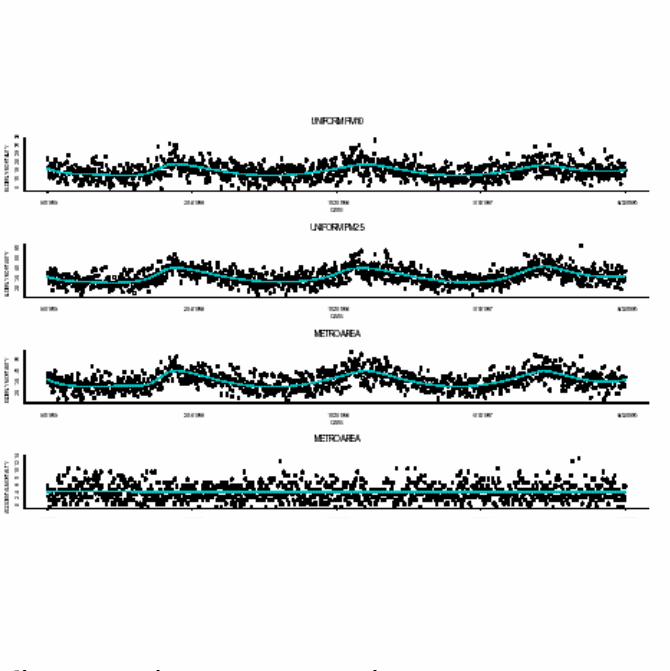
Data: Single site PM10,PM2.5 5/95 – 6/98

Mortality

Meteorology (temperature, specific humidity)

Incl. baseline, lags 0-3, quadratic functions of met, total of 29 variables

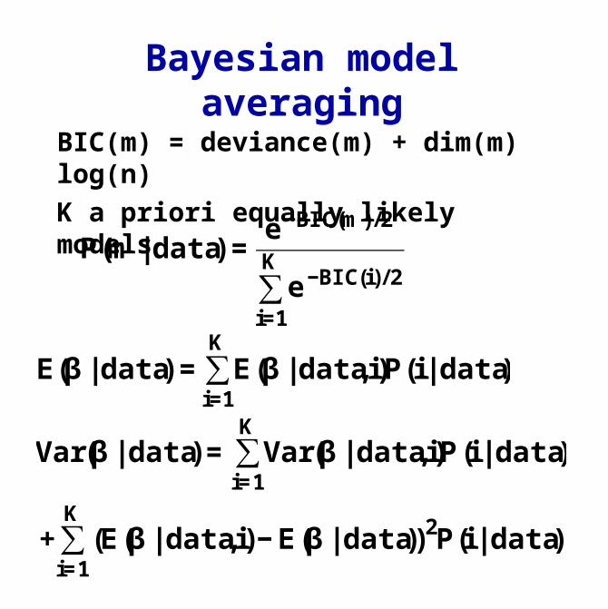
Bayesian model averaging

BIC(m) = deviance(m) + dim(m) log(n)

K a priori equally likely models

€

P(m | data) =e−BIC(m)/2

e−BIC(i)/ 2

i=1

K

∑

€

E(β | data) = E(β | data,i)P(i | data)i=1

K

∑

€

Var(β | data) = Var(β | data,i)P(i | data)i=1

K∑

+ E(β | data,i)− E(β | data)( )2

i=1

K∑ P(i | data)

BMA, cont.

Uses all models considered, rather than the best model

Often several models are nearly equally good

Can use prior information about models

Leaps and bounds algorithm to find best models of each size

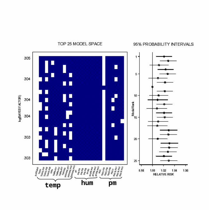
temp hum pm

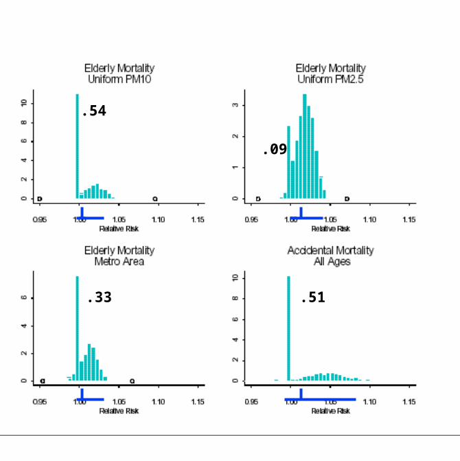
.54

.09

.33 .51

Is PM a pollutant?

The same concentration of PM has had different health effects in Boston and SeattleSome evidence that sulphates better predictor of health effectsPM is probably many pollutants

–Size–Chemical composition–Co-pollutants

Classification due to measurement technique?

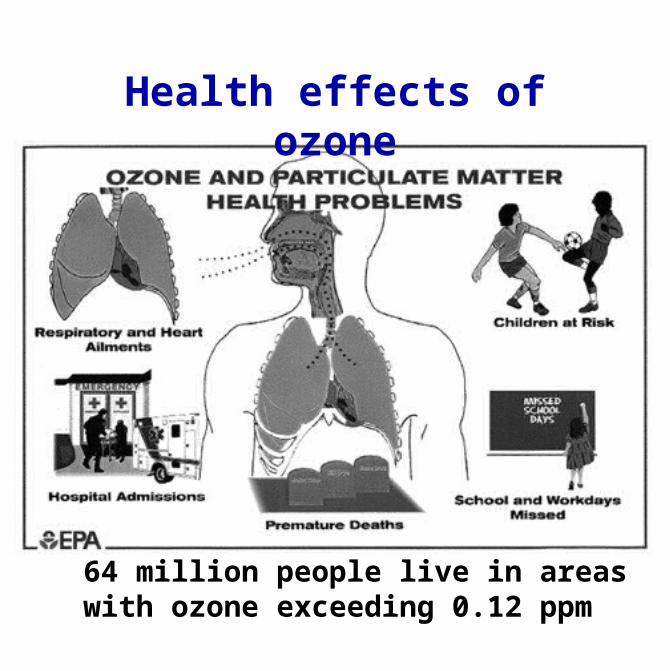
Health effects of ozone

64 million people live in areas with ozone exceeding 0.12 ppm

Biological effects of ozone

Adversely affects the ability of plants to produce and store food

Leaf loss

Severe forest dieback

Precursors part of acid rain

Ozone standard

In each region the expected number of daily maximum 1-hr ozone concentrations in excess of 0.12 ppm shall be no higher than one per year

Implementation: A region is in violation if 0.12 ppm is exceeded at any monitoring site in the region more than 3 times in 3 years

A hypothesis testing framework

The EPA is required to protect human health. Hence the more serious error is to declare a region in compliance when it is not.

The correct null hypothesis therefore is that the region is violating the standard.

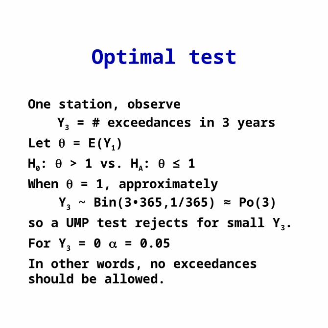
Optimal test

One station, observe

Y3 = # exceedances in 3 years

Let = E(Y1)

H0: > 1 vs. HA: ≤ 1

When = 1, approximately

Y3 ~ Bin(3•365,1/365) ≈ Po(3)

so a UMP test rejects for small Y3.

For Y3 = 0 = 0.05

In other words, no exceedances should be allowed.

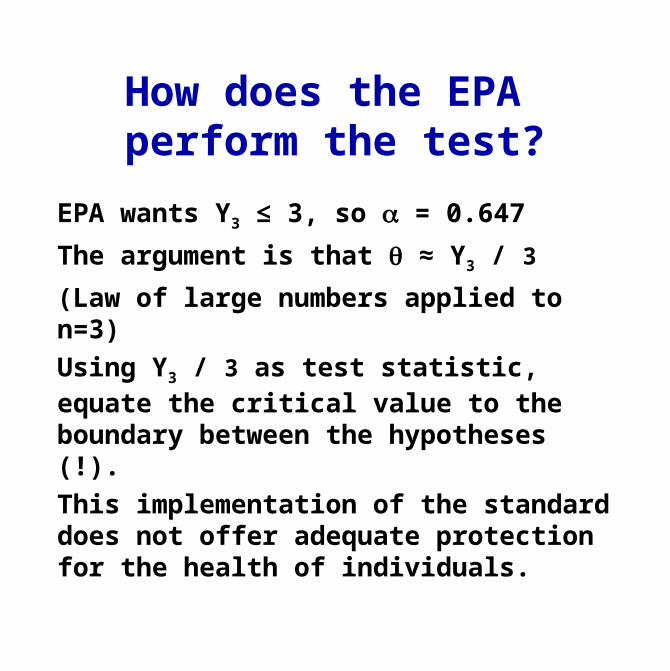
How does the EPA perform the test?

EPA wants Y3 ≤ 3, so = 0.647

The argument is that ≈ Y3 / 3

(Law of large numbers applied to n=3)

Using Y3 / 3 as test statistic, equate the critical value to the boundary between the hypotheses (!).

This implementation of the standard does not offer adequate protection for the health of individuals.

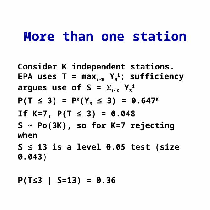
More than one station

Consider K independent stations. EPA uses T = maxi≤K Y3

i; sufficiency argues use of S = i≤K Y3

i

P(T ≤ 3) = PK(Y3 ≤ 3) = 0.647K

If K=7, P(T ≤ 3) = 0.048

S ~ Po(3K), so for K=7 rejecting when

S ≤ 13 is a level 0.05 test (size 0.043)

P(T≤3 | S=13) = 0.36

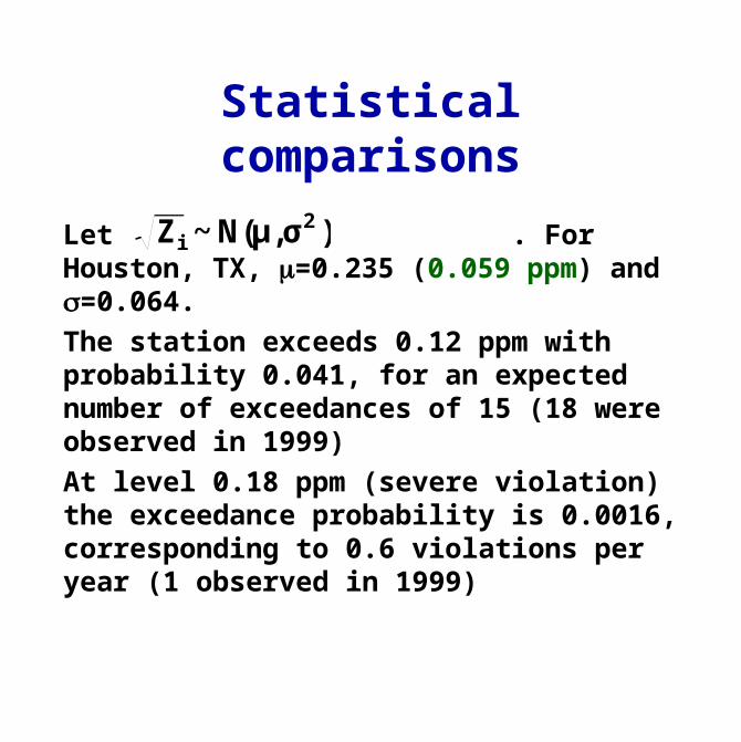
Statistical comparisons

Let . For Houston, TX, =0.235 (0.059 ppm) and =0.064.

The station exceeds 0.12 ppm with probability 0.041, for an expected number of exceedances of 15 (18 were observed in 1999)

At level 0.18 ppm (severe violation) the exceedance probability is 0.0016, corresponding to 0.6 violations per year (1 observed in 1999)

Zi ~N(μ,σ2)

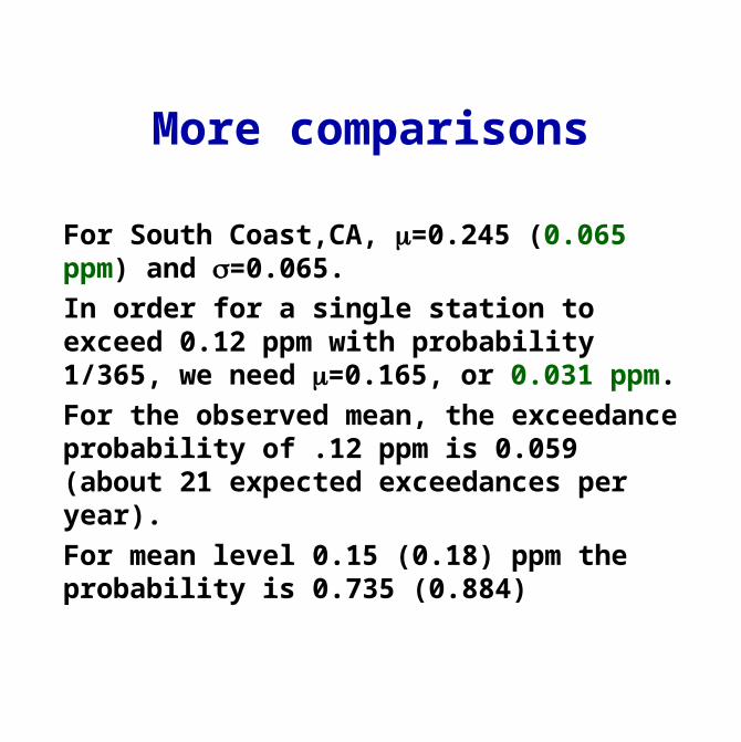
More comparisons

For South Coast,CA, =0.245 (0.065 ppm) and =0.065.

In order for a single station to exceed 0.12 ppm with probability 1/365, we need =0.165, or 0.031 ppm.

For the observed mean, the exceedance probability of .12 ppm is 0.059 (about 21 expected exceedances per year).

For mean level 0.15 (0.18) ppm the probability is 0.735 (0.884)

The Barnett-O’Hagan setup

Ideal standard: bound on level of pollutant in an area over a time period

Realizable standard: a standard for which one can determine without uncertainty where it is satisfied

Statistically verifiable standard: ideal standard augmented with operational procedure for assessing compliance

Consequences for hypothesis tests

One option: set values of and at the design level and a “safe” level, respectively.

For example, the “safe” level could be the highest level for which the relative risk of health effects on some susceptible population is not significantly different from one

A new ozone standard

Summer 1997:

8-hour averages instead of 1-hour

Limit 0. 08 ppm instead of 0.12 increases non-attainment counties from 104 to 394

Instead of expected number of exceedances, limit is put on a 3-year average of fourth-highest ozone concentration

change from ideal to realizable standard

Legal challenges of the new air quality standards

The new 8-hr standard for ozone was challenged to the Supreme Court.

The US Court of Appeals directed EPA to consider potential positive health effects of ground-level ozone. The EPA has not found any.

Spatial and temporal dependence

Daily maxima of ozone show some temporal structure

There is substantial spatial correlation between daily maxima at different monitors in a region

Simulations indicate that 10 sites in the Chicago area behaves similar to 2 independent sites

Network bias

Many health effects studies useair quality data from compliance networks

health outcome data from hospital records

Compliance networks aim at finding large values of pollution

Actual exposure may be lower than network values

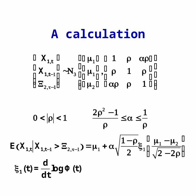
A calculation

X1,t

X1,t−1

X2,t−1

⎛

⎝

⎜⎜⎜

⎞

⎠

⎟⎟⎟~N3

1

1

2

⎛

⎝

⎜⎜

⎞

⎠

⎟⎟,

1 ρ ρρ 1 ρρ ρ 1

⎛

⎝

⎜⎜

⎞

⎠

⎟⎟

⎡

⎣

⎢⎢⎢

⎤

⎦

⎥⎥⎥

0 < ρ < 12ρ2 −1

ρ≤ ≤

1ρ

E X1,t X1,t−1 > X2,t−1( ) =1 + 1−ρ2

ξ1

1 −2

2 −2ρ

⎛

⎝⎜

⎞

⎠⎟

ξ1(t) =d

dtlogΦ(t)

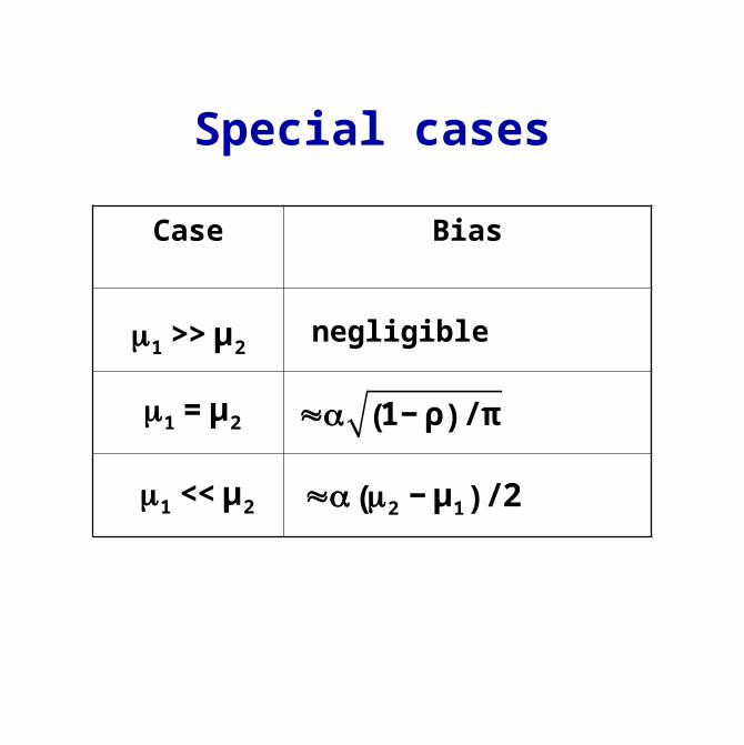
Special cases

Case Bias

negligible1 >> μ2

1 = μ2 ≈ 1− ρ( ) / π

1 << μ2 ≈ 2 − μ1( ) / 2

-5 -4 -3 -2 -1 0 1 2 3 4 50

0.05

0.1

0.15

0.2

0.25

0.3

0.35

0.4

0.45Densities of conditional distributions

alpha1=-0.7; rho=-0.8

alpha=-0.7; rho=0.8 alpha1=0.7; rho=0.8

alpha1=0.7; rho=-0.8

A more complete picture?

Health effects studies need actual exposure.

Standards can only be set on ambient air.

PNW PM Center studies personal exposure in elderly

Much of personal exposure, especially in elderly, comes from indoor sources. Only about 5% of variability due to ambient sources. Most of ambient variability due to time (not space).

A conditional calculation

Given an observation of .120 ppm in the Houston region, what is the probability that an individual in the region is subjected to more that .120 ppm?

Need to calculate supremum of Gaussian process (after transformation) over a region that is highly correlated with measurement site, taking into account measurement error.

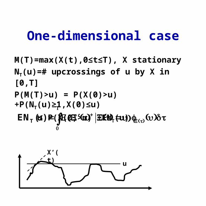
One-dimensional case

M(T)=max(X(t),0≤t≤T), X stationary

NT(u)=# upcrossings of u by X in [0,T]

P(M(T)>u) = P(X(0)>u)+P(NT(u)≥1,X(0)≤u)

≤ P(X(0)>u) +ENT(u)

ENT (u) = E ′X (t)+ X(t) =u( ) fX(t) (u)dt0

T

∫

u

X‘(t)

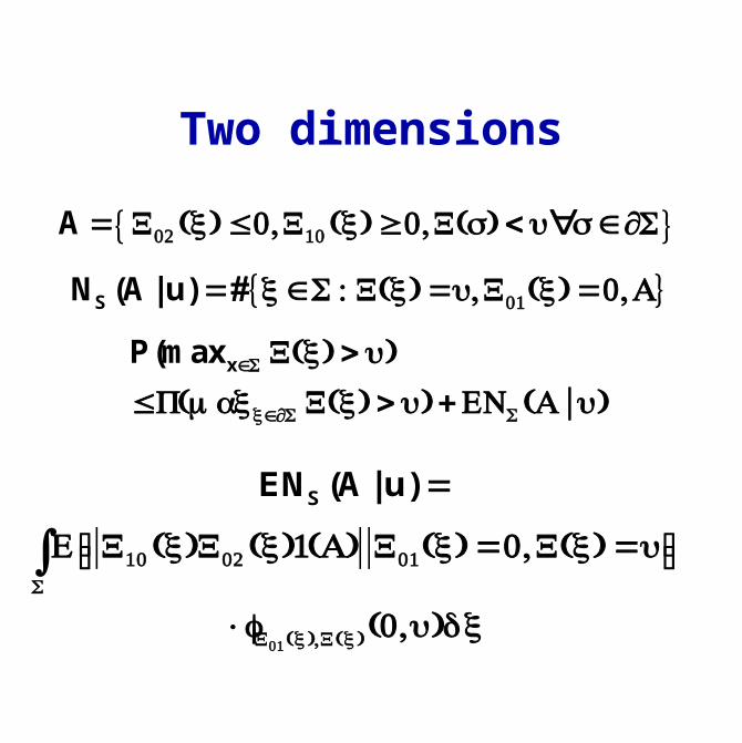
Two dimensions

P(maxx∈S X(x) > u)≤P(maxx∈∂S X(x) > u) +ENS (A |u)

ENS (A | u) =

E X10 (x)X02 (x)1(A) X01(x) =0,X(x) =u⎡⎣ ⎤⎦S∫

×fX01 (x),X(x)(0,u)dx

A = X02 (x) ≤0,X10 (x) ≥0,X(s) < u∀s ∈∂S{ }

NS (A | u) =#{x∈S : X(x) =u,X01(x) =0,A}

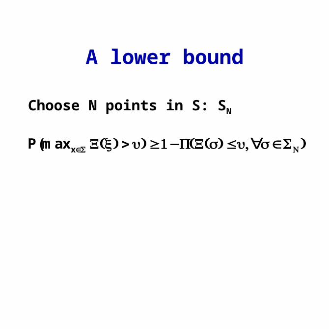
A lower bound

Choose N points in S: SN

P(maxx∈S X(x) > u) ≥1−P(X(s) ≤u,∀s ∈SN )

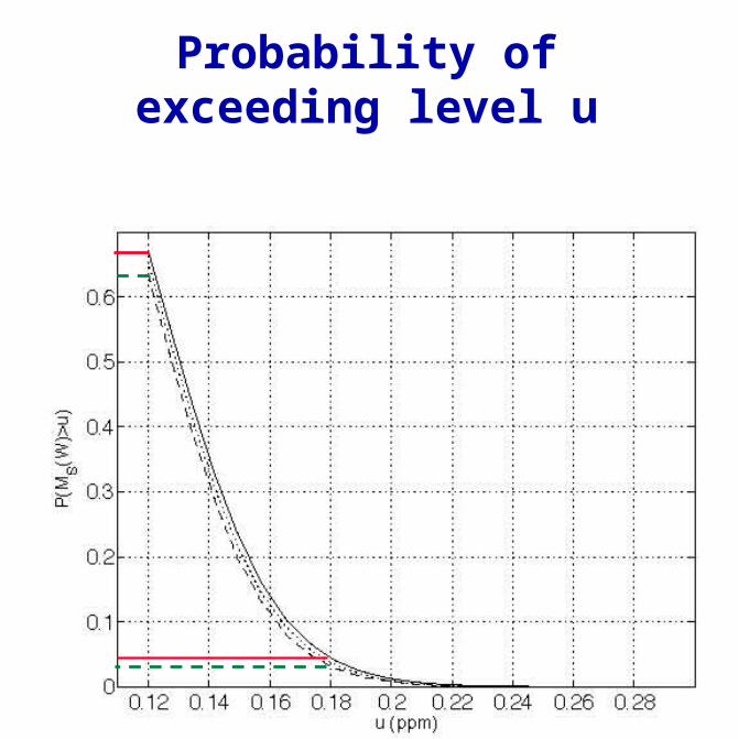
Probability of exceeding level u

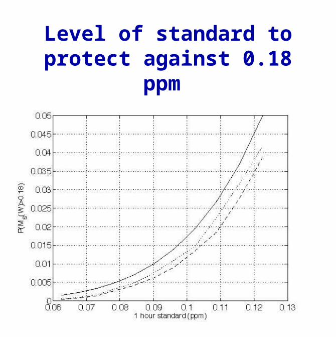
Level of standard to protect against 0.18 ppm

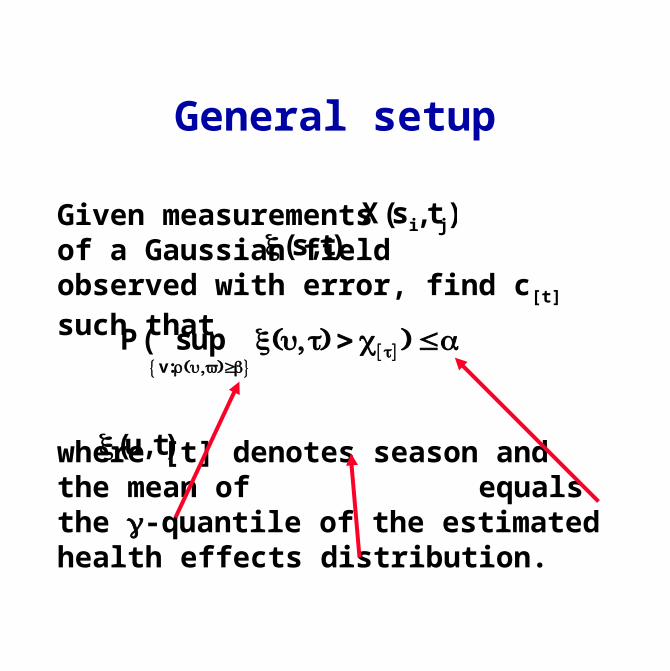
General setup

Given measurements of a Gaussian field observed with error, find c[t] such that

where [t] denotes season and the mean of equals the -quantile of the estimated health effects distribution.

X(si, t j )ξ(s, t)

P( supv:ρ(u,v)≥{ }

ξ(u, t) > c[ t] ) ≤

ξ(u, t)

Other approches to setting standards

Standard relative to natural variability

Areal average standards

Multi-pollutant standards

All require substantial statistical input.

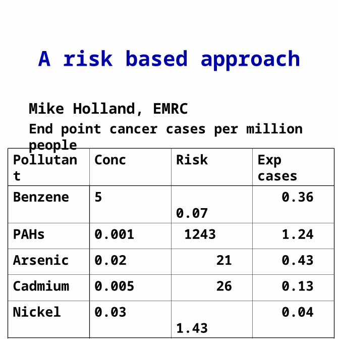
A risk based approach

Mike Holland, EMRCEnd point cancer cases per million people

Pollutant Conc Risk Exp cases

Benzene 5 0.07 0.36

PAHs 0.001 1243 1.24

Arsenic 0.02 21 0.43

Cadmium 0.005 26 0.13

Nickel 0.03 1.43 0.04

Total 2.20

Some difficulties with the risk based approach

Are risks additive?

There can be more than one endpoint

Uncertainties in risk estimates and in concentrations need to propagate through the analysis

Cost-benefit analysis not necessarily politically appropriate

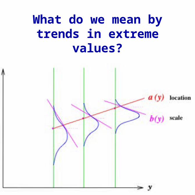
What do we mean by trends in extreme values?

Multiple variables

Extreme in one, not extreme in others?

Interesting scenario:

Medium temperature, about 0C

Large snowfall

Extreme winds

What to do?

“Standard” extreme value asymptotics works for values high in all variables

Heffernan approach:

Model: for x large, where Z comes from extreme value theory.

E Y X =x( ) =x+ xZ