Air Quality Modeling

Rosa Sohn and Sun-Kyoung Park

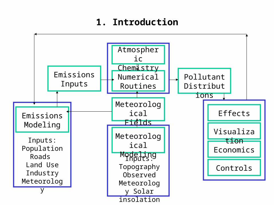
1. Introduction

Emissions Modeling

Controls

Economics

Visualization

Effects

Pollutant Distributions

Meteorological Fields

Numerical Routines

Atmospheric Chemistry

Meteorological Modeling

Emissions Inputs

Inputs:Population

Roads Land Use Industry

Meteorology

Inputs:Topography

Observed Meteorology

Solar insolation

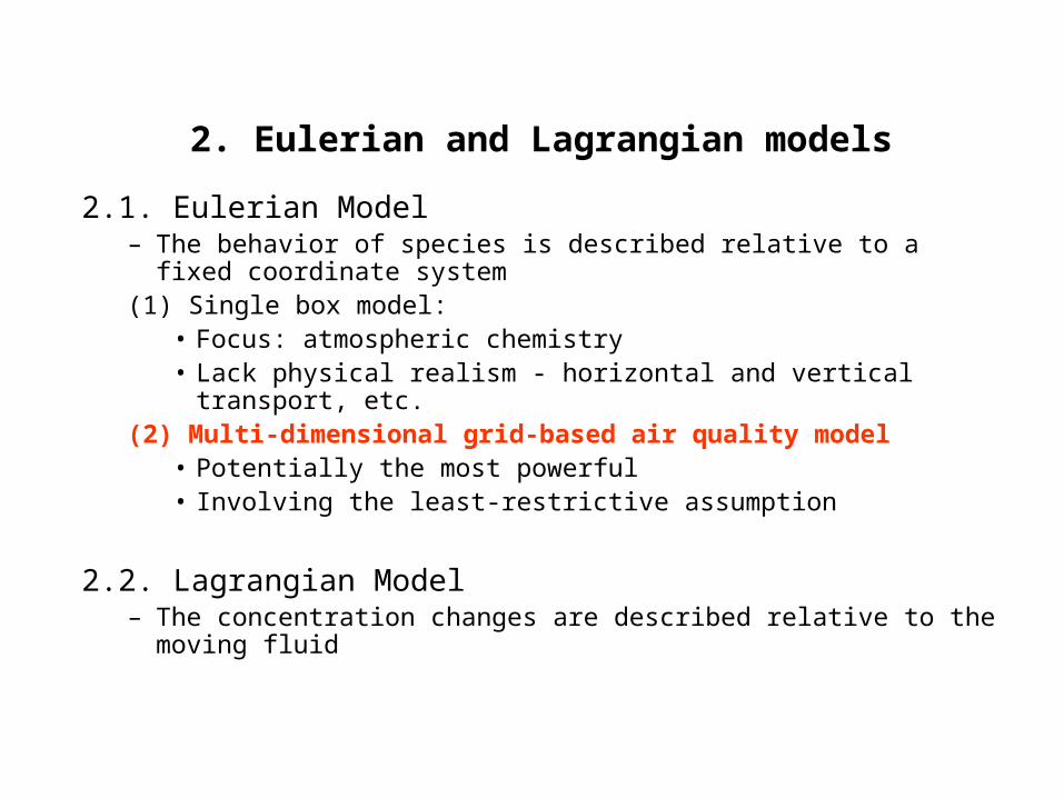
2. Eulerian and Lagrangian models

2.1. Eulerian Model– The behavior of species is described relative to a

fixed coordinate system(1) Single box model:

• Focus: atmospheric chemistry • Lack physical realism - horizontal and vertical transport, etc.

(2) Multi-dimensional grid-based air quality model• Potentially the most powerful• Involving the least-restrictive assumption

2.2. Lagrangian Model– The concentration changes are described relative to the

moving fluid

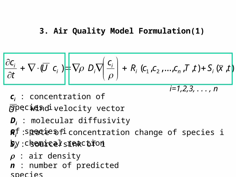
3. Air Quality Model Formulation(1)

),(),,,...,,()( 21 txStTcccRc

DcUt

cini

iii

i

ci : concentration of species i.

U : wind velocity vector

Di : molecular diffusivity of species i

Ri : rate of concentration change of species i by chemical reaction

Si : source/sink of i

: air densityn : number of predicted species

i=1,2,3, . . . , n

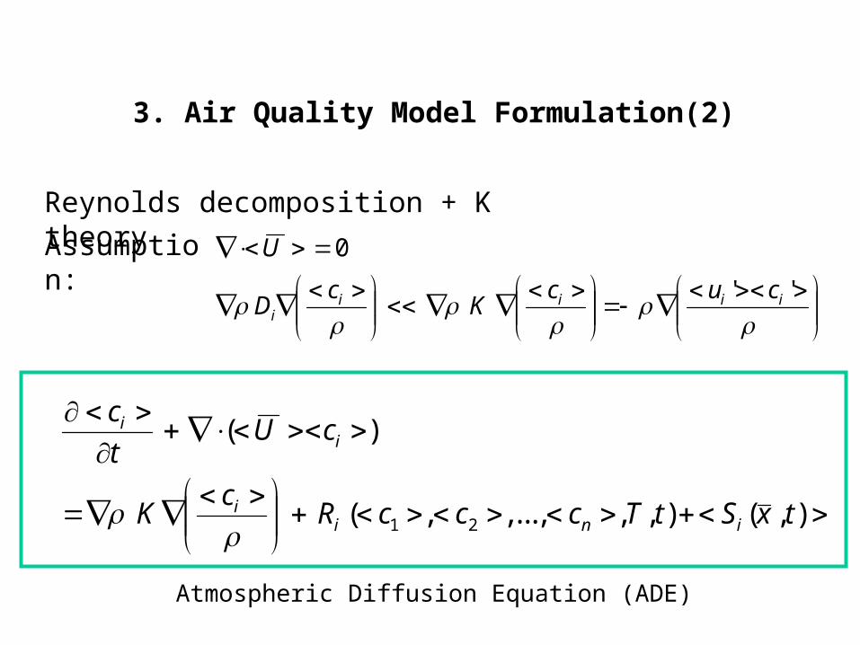
3. Air Quality Model Formulation(2)

''

0

iiiii

cucK

cD

UAssumption:

),(),,,...,,(

)(

21 txStTcccRc

K

cUt

c

inii

ii

Reynolds decomposition + K theory

Atmospheric Diffusion Equation (ADE)

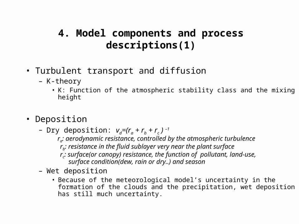
• Turbulent transport and diffusion– K-theory

• K: Function of the atmospheric stability class and the mixing height

• Deposition– Dry deposition: vd=(ra + rb + rc ) –1

ra: aerodynamic resistance, controlled by the atmospheric turbulence rb: resistance in the fluid sublayer very near the plant surface rc: surface(or canopy) resistance, the function of pollutant, land-use, surface condition(dew, rain or dry..) and season

– Wet deposition • Because of the meteorological model’s uncertainty in the formation of the

clouds and the precipitation, wet deposition has still much uncertainty.

4. Model components and process descriptions(1)

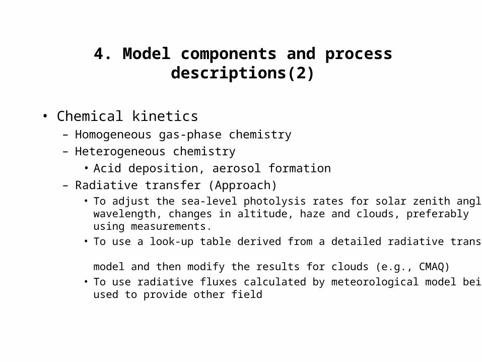
• Chemical kinetics– Homogeneous gas-phase chemistry– Heterogeneous chemistry

• Acid deposition, aerosol formation– Radiative transfer (Approach)

• To adjust the sea-level photolysis rates for solar zenith angle, wavelength, changes in altitude, haze and clouds, preferably using measurements.

• To use a look-up table derived from a detailed radiative transfer model and then modify the results for clouds (e.g., CMAQ)

• To use radiative fluxes calculated by meteorological model being used to provide other field

4. Model components and process descriptions(2)

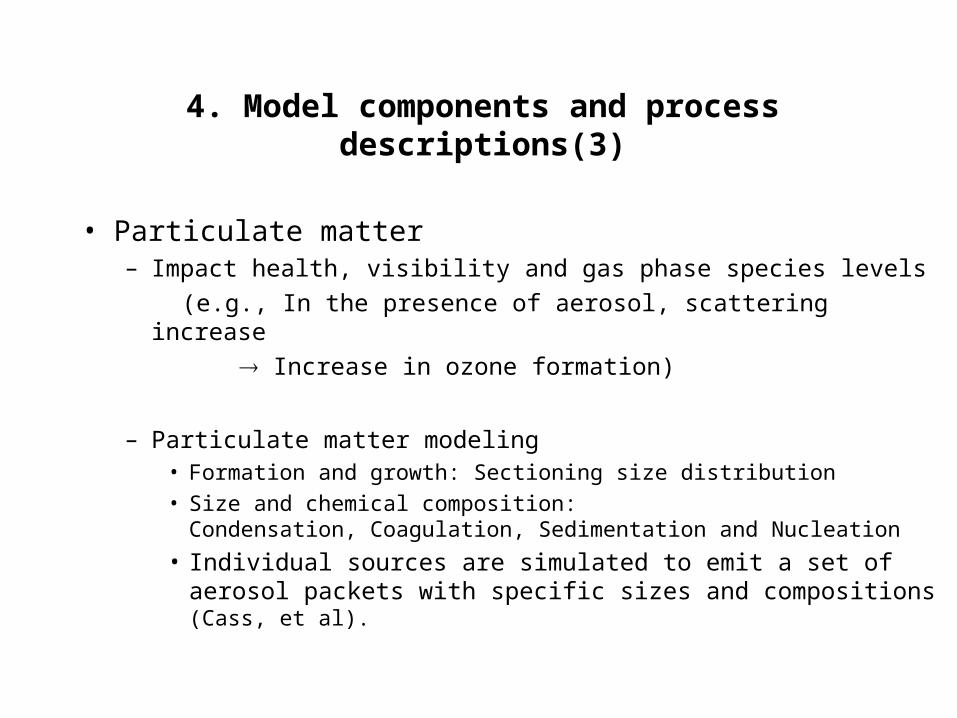
• Particulate matter – Impact health, visibility and gas phase species levels

(e.g., In the presence of aerosol, scattering increase

Increase in ozone formation)

– Particulate matter modeling• Formation and growth: Sectioning size distribution

• Size and chemical composition:Condensation, Coagulation, Sedimentation and Nucleation

• Individual sources are simulated to emit a set of aerosol packets with specific sizes and compositions (Cass, et al).

4. Model components and process descriptions(3)

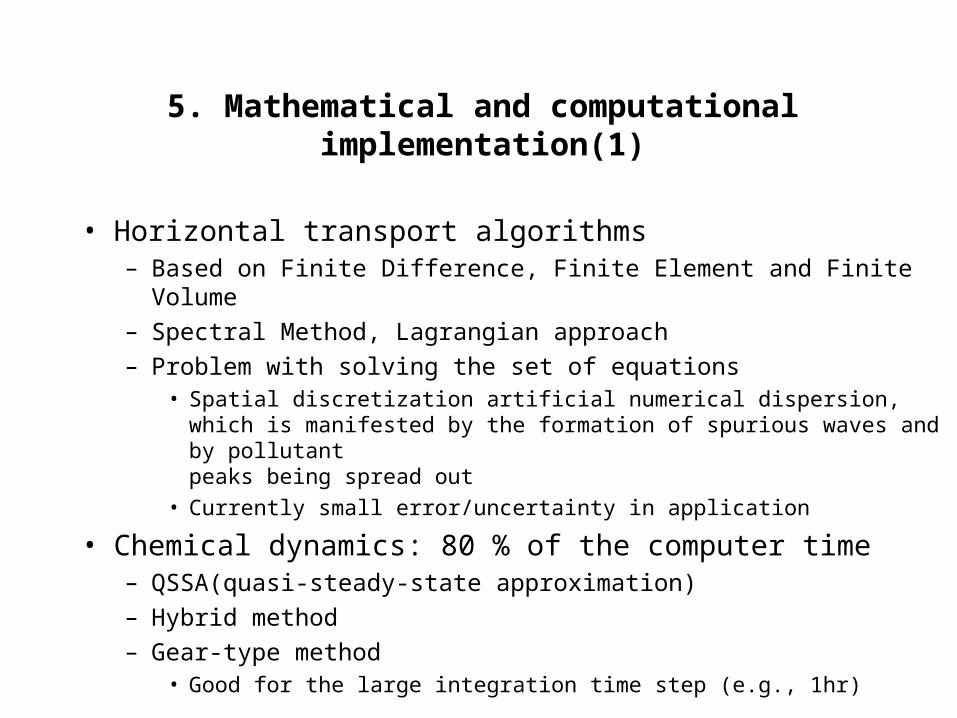
• Horizontal transport algorithms– Based on Finite Difference, Finite Element and Finite Volume– Spectral Method, Lagrangian approach– Problem with solving the set of equations

• Spatial discretization artificial numerical dispersion, which is manifested by the formation of spurious waves and by pollutant peaks being spread out

• Currently small error/uncertainty in application

• Chemical dynamics: 80 % of the computer time– QSSA(quasi-steady-state approximation)– Hybrid method– Gear-type method

• Good for the large integration time step (e.g., 1hr)

5. Mathematical and computational implementation(1)

5. Mathematical and computational implementation(2)

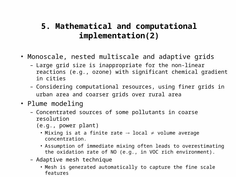
• Monoscale, nested multiscale and adaptive grids– Large grid size is inappropriate for the non-linear reactions (e.g.,

ozone) with significant chemical gradient in cities

– Considering computational resources, using finer grids in urban

area and coarser grids over rural area • Plume modeling

– Concentrated sources of some pollutants in coarse resolution(e.g., power plant)

• Mixing is at a finite rate local volume average concentration.

• Assumption of immediate mixing often leads to overestimating the oxidation rate of NO (e.g., in VOC rich environment).

– Adaptive mesh technique• Mesh is generated automatically to capture the fine scale features

5. Mathematical and computational implementation(3)

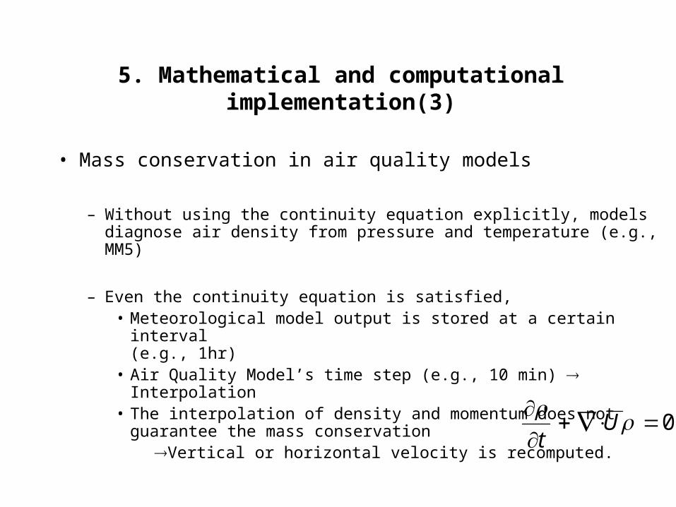
• Mass conservation in air quality models

– Without using the continuity equation explicitly, models diagnose air density from pressure and temperature (e.g., MM5)

– Even the continuity equation is satisfied, • Meteorological model output is stored at a certain interval

(e.g., 1hr)• Air Quality Model’s time step (e.g., 10 min) Interpolation • The interpolation of density and momentum does not

guarantee the mass conservation Vertical or horizontal velocity is recomputed. 0

Ut

5. Mathematical and computational implementation(4)

• Advanced Analysis routines

– Integration of specific physical and chemical processes terms • Applied to Lagrangian Box Modeling studies

– Direct sensitivity analysis• Brute Force• Decoupled Direct Method(DDM)• Adjoint Approach

– Limitation: cannot capture nonlinear response

• Meteorological Input– Horizontal and Vertical Wind fields, Temperature, Humidity, Mixing

depth, Solar insolation fields, Vertical diffusivities, cloud characteristics(liquid water content, droplet size, cloud size, etc.), rain fall

• How to prepare input fields?– Interpolating relatively sparse observations over the modeling

domain using the objective analysis– Meteorological Model (e.g., MM5) output because of the

sparseness of data

6. Model Input (1) - Meteorology

• Emission– CO, NO, NO2, SO2, VOCs, SO3, NH3, PM2.5 and PM10– Emissions are one of the most uncertain, but the most

important inputs into air quality models

• Temporal Processing– The inventory is the yearly averaged data, but the AQM

needs short interval emission input(e.g., hourly).

• Spatial Processing– The inventory is county based data, but the AQM needs

gridded emission inventory if you are doing the multi-dimensional grid-based air quality model

6. Model Input (2) – Emission

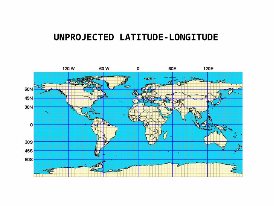
UNPROJECTED LATITUDE-LONGITUDE

• “Grid” defined in the AQM depends on the map projection.

• Map Projection – Attempt to portray the surface of the earth or a portion of the earth on

a flat surface

• Cylindrical• Psuedo-cylindrical• Conical• Azimuthal• Other

Map Projection

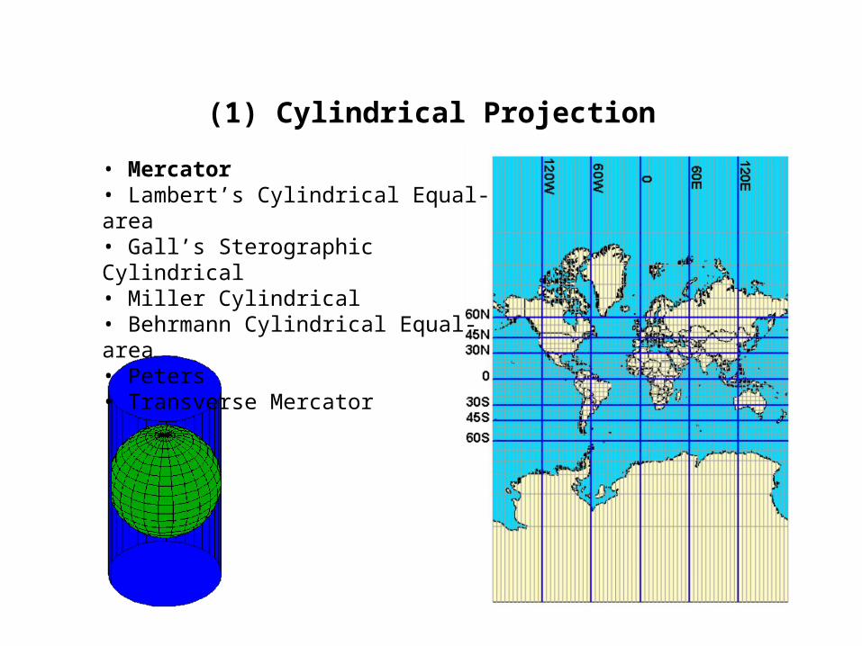
(1) Cylindrical Projection

• Mercator• Lambert’s Cylindrical Equal-area • Gall’s Sterographic Cylindrical• Miller Cylindrical• Behrmann Cylindrical Equal-area• Peters• Transverse Mercator

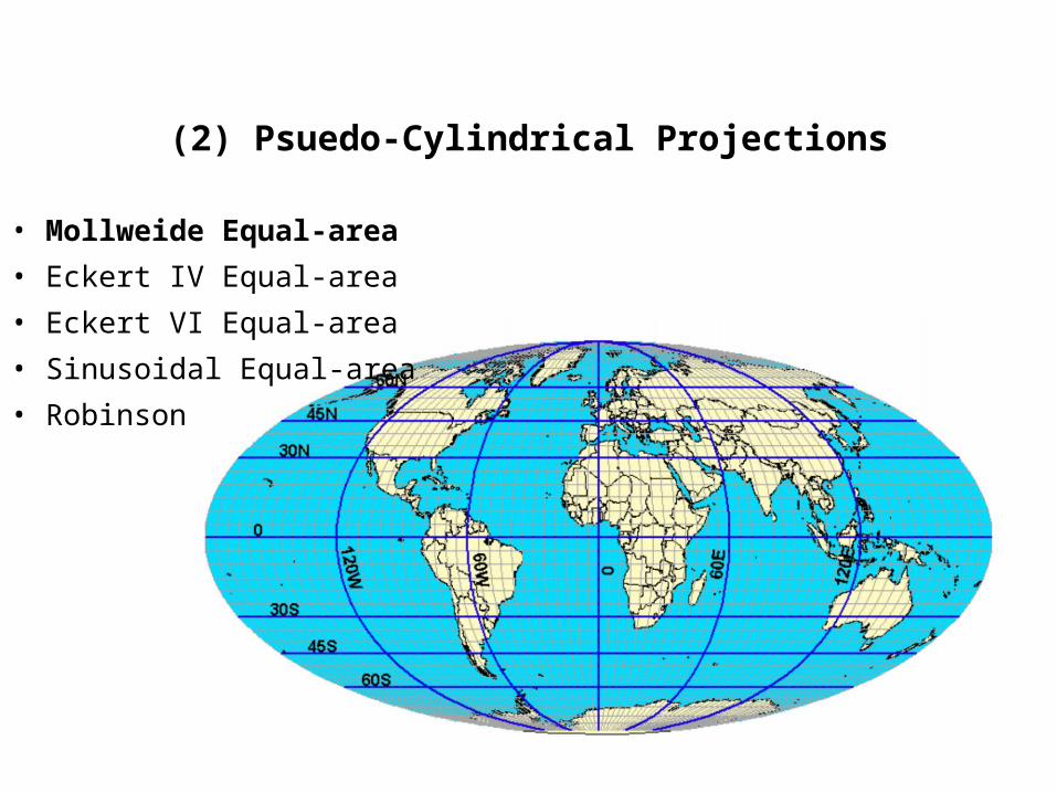
• Mollweide Equal-area

• Eckert IV Equal-area

• Eckert VI Equal-area

• Sinusoidal Equal-area

• Robinson

(2) Psuedo-Cylindrical Projections

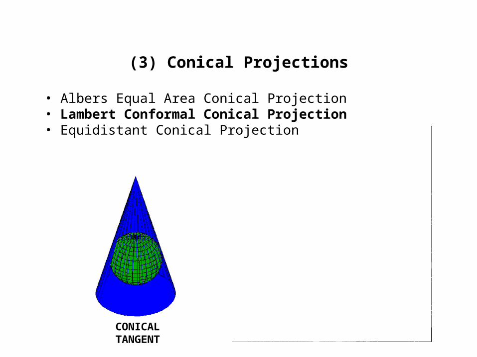
• Albers Equal Area Conical Projection• Lambert Conformal Conical Projection• Equidistant Conical Projection

CONICALTANGENT

(3) Conical Projections

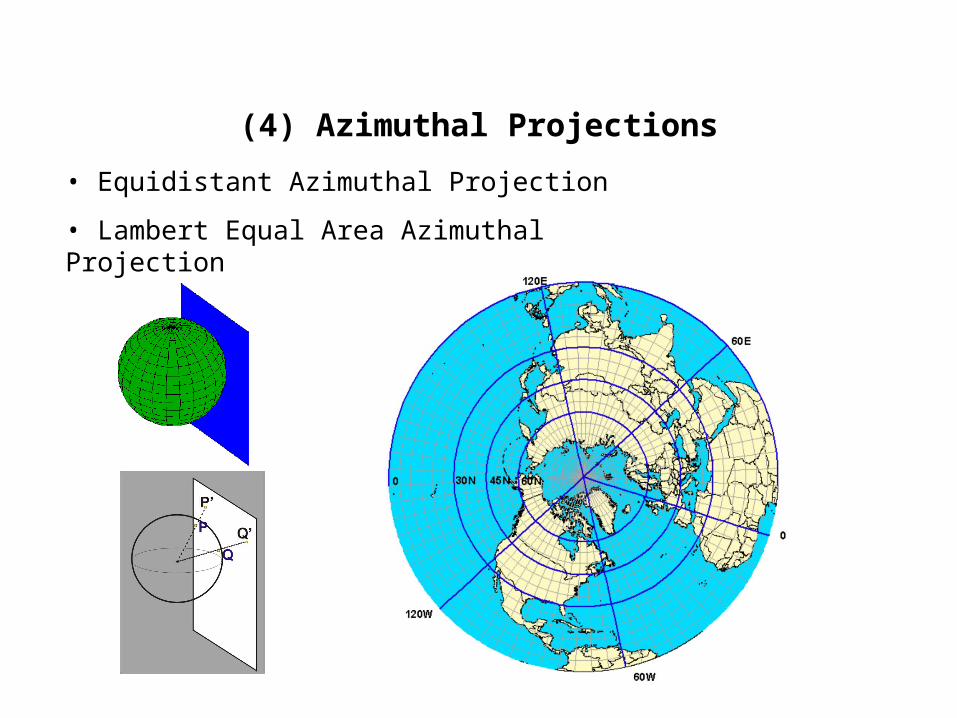
(4) Azimuthal Projections

• Equidistant Azimuthal Projection

• Lambert Equal Area Azimuthal Projection

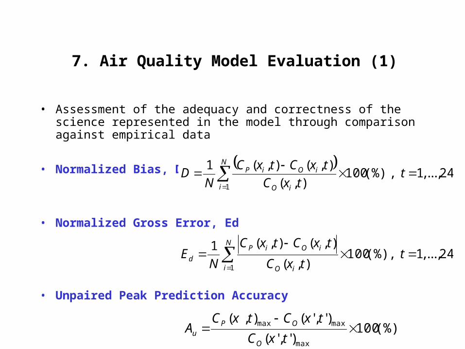
• Assessment of the adequacy and correctness of the science represented in the model through comparison against empirical data

• Normalized Bias, D

• Normalized Gross Error, Ed

• Unpaired Peak Prediction Accuracy

24,...,1,(%)100

),(

),(),(1

1

ttxC

txCtxC

ND

N

i iO

iOiP

(%)100)','(

)','(),(

max

maxmax

txC

txCtxCA

O

OPu

24,...,1,(%)100),(

),(),(1

1

ttxC

txCtxC

NE

N

i iO

iOiP

d

7. Air Quality Model Evaluation (1)

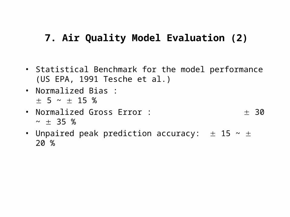
• Statistical Benchmark for the model performance (US EPA, 1991 Tesche et al.)

• Normalized Bias : 5 ~ 15 %• Normalized Gross Error : 30 ~ 35 %• Unpaired peak prediction accuracy: 15 ~ 20 %

7. Air Quality Model Evaluation (2)

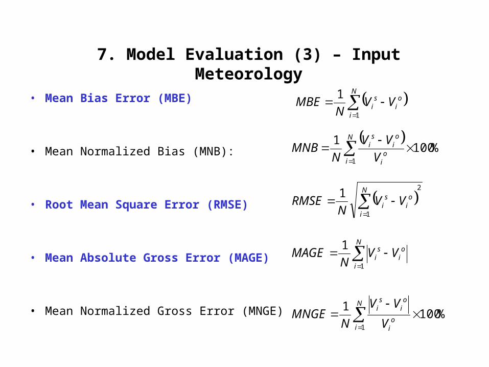
• Mean Bias Error (MBE)

• Mean Normalized Bias (MNB):

• Root Mean Square Error (RMSE)

• Mean Absolute Gross Error (MAGE)

• Mean Normalized Gross Error (MNGE)

N

i

oi

si VV

NMBE

1

1

2

1

1

N

i

oi

si VV

NRMSE

%100

1

1

N

io

i

oi

si

V

VV

NMNB

%1001

1

N

io

i

oi

si

V

VV

NMNGE

N

i

oi

si VV

NMAGE

1

1

7. Model Evaluation (3) – Input Meteorology

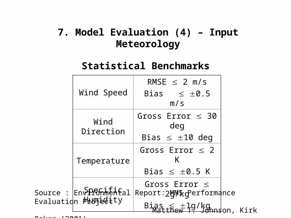
Statistical Benchmarks

Wind SpeedRMSE 2 m/s

Bias 0.5 m/s

Wind DirectionGross Error 30 deg

Bias 10 deg

TemperatureGross Error 2 K

Bias 0.5 K

Specific Humidity

Gross Error 2g/kg

Bias 1g/kg

Source : Environmental Report: MM5 Performance Evaluation Project Matthew T. Johnson, Kirk Baker (2001)

7. Model Evaluation (4) – Input Meteorology

8. Application (1)

• Sensitivity to Process Parameterizations

• Sensitivity to Model Numerics/Structure– Small uncertainty in numerical technique– Grid size, number of the vertical layers.

(e.g., Difference in ozone prediction Horizontal grid size: 5 km, 10 km and 20km Number of the vertical layers : 6 ~ 15 layers)

• Sensitivity to Model Input– Emissions, meteorological conditions, boundary conditions,

initial conditions, HONO formation rate and deposition

– Emission control Ozone and PM control (e.g., SO2 control sulfate decrease, but nitrate increases)

– VOCs with different reactivity Ozone, PM, …(e.g., Methanol based fuels would be beneficial for ozone control because of its atmospheric low reactivity)

8. Application (2)

9. Current Status of AQM

• 1st generation: simple chemistry at local scales

• 2nd generation: local, urban, regional addressing each scale with a separate model and often focusing on a single pollutant.

• 3rd generation: multiple pollutants simultaneously up to continental scales and incorporate feedbacks between chemical and meteorological components. – Models3 (SMOKE, MM5 and CMAQ(Community Multiscale Air

Quality) Modeling system: urban to regional scale air quality simulation of tropospheric ozone, acid deposition, visibility and fine particulate).

• 4th generation (Future): extend linkages and process feedback to include air, water, land, and biota to simulate the transport and fate of chemical and nutrients throughout an ecosystem.

• Download the existing model with free of charge• Models3

– MM5 (http://www.mmm.ucar.edu/mm5/mm5-home.html)• PSU/NCAR mesoscale model version 5• Meteorological Field

– SMOKE (http://edge.emc.mcnc.org/uihelp/docs/smoke.html)• Sparse Matrix Operator Kernel Emissions modeling system

• Converting emissions inventory data into the formatted emission files required by an AQM

– CMAQ (http://www.epa.gov/asmdnerl/models3/)• Community Multiscale Air Quality Modeling System• Atmospheric chemistry combined with the numerical routine

Step 1. Getting Started with AQM

• MM5 (PSU/NCAR mesoscale model version 5) download

– http://www.mmm.ucar.edu/mm5/mm5-home.html

– MM5 Input Data: http://dss.ucar.edu/catalogs/

• Topography and Landuse data• Gridded atmospheric data with sea-level pressure, wind, temperature, relative

humidity and geopotential height • Observation data that contains soundings and surface reports

Step 2. Meteorological Input – MM5 (1)

Step 2. Meteorological Input – MM5 (2)

• MM5 Output Manipulation for the evaluation, etc.

– MM5toGrADS http://www.mmm.ucar.edu/mm5/mm5v3/tutorial/mm5tograds/mm5tograds.html

– GrADS(Grid Analysis and DisplaySystem) http://grads.iges.org/grads/

• Converting the MM5 output to the format required in SMOKE and CMAQ (NetCDF format)

– MCIP2(Meteorology-Chemistry Interface Processor Version 2): Inside of the CMAQ model system

• National Emission Inventory (1996 yr, 1999 yr) (http://www.epa.gov/ttn/chief/net/index.html)

• Projection to the model year– EGAS 4.0 (http://www.epa.gov/ttn/chief/emch/projection/egas40/)

• Spatial Processing– Converting the county based inventory data to the gridded emission inventory

which fits to the multi-dimensional grid-based air quality model– ESRI ArcGIS – ArcView, ArcInfo, ArcMap, ArcToolbox and ArcCatalog (Architecture Computer Lab (Rm 359))

• SMOKE (http://edge.emc.mcnc.org/uihelp/docs/smoke.html)– Converting emissions inventory into the formatted emission files required by an

AQM (NetCDF format)

Step 3. Emission Input – SMOKE

• CMAQ Modeling system– (Community Multiscale Air Quality)– http://www.epa.gov/asmdnerl/models3/

• CMAQ Document– http://www.epa.gov/asmdnerl/models3/doc/science/science.html

• CMAQ Tutorial– http://www.epa.gov/scram001/cmaq.htm

Step 4. Air Quality Modeling - CMAQ

• PAVE– The Package for Analysis and Visualization of Environmental Data– Visualization and the analysis of NetCDF data– http://www.epa.gov/asmdnerl/models3/vistutor/pave.html

• NetCDF IO/API– The Models-3 Input/Output Applications Programming Interface– The standard data access library for EPA's Models-3 available from both C

and Fortran. (ASCII or Binary NetCDF)– http://www.emc.mcnc.org/products/ioapi/AA.html– AQM testing with arbitrary input (e.g., zero emission)– Evaluation

Step 5. Tools

QuestionsComments

Reference: NARSTO critical review of photochemical models and modeling, Armistead Russell and Robin Dennis, 2000 Atmospheric Environment 34. 2283 - 2324