Embed Size (px)
Citation preview

i
Air Pollution from Motor Vehicles
Standards and Technologies for Controlling Emissions

ii
Air Pollution from Motor Vehicles
blank

iii
Asif FaizChristopher S. WeaverMichael P. Walsh
With contributions by
Surhid P. GautamLit-Mian Chan
The World BankWashington, D.C.
Air Pollution from Motor Vehicles
Standards and Technologies for Controlling Emissions


v
Preface xiiiAcknowledgments xviiParticipants at the UNEP Workshop xix
Chapter 1 Emission Standards and Regulations 1
International Standards 2
U.S. Standards
2U.N. Economic Commission for Europe (ECE) and European Union (EU) Standards
6
Country and Other Standards 9
Argentina
11Australia
11Brazil
12Canada
13Chile
14China
15Colombia
15Eastern European Countries and the Russian Federation
15Hong Kong 16India
17Japan
18Republic of Korea
18Malaysia
19Mexico
19Saudi Arabia
19Singapore
19Taiwan (China)
20Thailand
20
Compliance with Standards 21
Certification or Type Approval
21Assembly Line Testing
22In-Use Surveillance and Recall
22Warranty
23On-Board Diagnostic Systems
23
Alternatives to Emission Standards 23References 24
Chapter 2 Quantifying Vehicle Emissions
25
Emissions Measurement and Testing Procedures 25
Exhaust Emissions Testing for Light-Duty Vehicles
25Exhaust Emissions Testing for Motorcycles and Mopeds
29Exhaust Emissions Testing for Heavy-Duty Vehicle Engines
29
Contents

vi
Air Pollution from Motor Vehicles
Crankcase Emissions
32Evaporative Emissions
32Refueling Emissions
33On-Road Exhaust Emissions
33
Vehicle Emission Factors 33
Gasoline-Fueled Vehicles
37Diesel-Fueled Vehicles
39Motorcycles
43
References 46
Appendix 2.1 Selected Exhaust Emission and Fuel Consumption Factors for Gasoline-Fueled Vehicles 49Appendix 2.2 Selected Exhaust Emission and Fuel Consumption Factors for Diesel-Fueled Vehicles 57
Chapter 3 Vehicle Technology for Controlling Emissions
63
Automotive Engine Types 64
Spark-Ignition (Otto) Engines
64Diesel Engines
64Rotary (Wankel) Engines
65Gas-Turbine (Brayton) Engines
65Steam (Rankine Engines)
65Stirling Engines
65Electric and Hybrid Vehicles
65
Control Technology for Gasoline-Fueled Vehicles (Spark-Ignition Engines) 65
Air-Fuel Ratio
66Electronic Control Systems
66Catalytic Converters
67Crankcase Emissions and Control
67Evaporative Emissions and Control
67Fuel Dispensing/Distribution Emissions and Control
69
Control Technology for Diesel-Fueled Vehicles (Compression-Ignition Engines) 69
Engine Design
70Exhaust Aftertreatment
71
Emission Control Options and Costs 73
Gasoline-Fueled Passenger Cars and Light-Duty Trucks
73Heavy-Duty Gasoline-Fueled Vehicles
76Motorcycles
76Diesel-Fueled Vehicles
76
References 79
Appendix 3.1 Emission Control Technology for Spark-Ignition (Otto) Engines 81Appendix 3.2 Emission Control Technology for Compression-Ignition (Diesel) Engines 101Appendix 3.3 The Potential for Improved Fuel Economy 119
Chapter 4 Controlling Emissions from In-Use Vehicles
127
Inspection and Maintenance Programs 127Vehicle Types Covered 129Inspection Procedures for Vehicles with Spark-Ignition Engines 130
Exhaust Emissions
131Evaporative Emissions
133Motorcycle White Smoke Emissions
133
Inspection Procedures for Vehicles with Diesel Engines 133Institutional Setting for Inspection and Maintenance 135
Centralized I/M
136Decentralized I/M
137Comparison of Centralized and Decentralized I/M Programs
138Inspection Frequency
140Vehicle Registration
140
Roadside Inspection Programs 140

Contents
vii
Emission Standards for Inspection and Maintenance Programs 141Costs and Benefits of Inspection and Maintenance Programs 144
Emission Improvements and Fuel Economy
149Impact on Tampering and Misfueling
151Cost-Effectiveness
153
International Experience with Inspection and Maintenance Programs 154Remote Sensing of Vehicle Emissions 159
Evaluation of Remote-Sensing Data
162
On-Board Diagnostic Systems 164Vehicle Replacement and Retrofit Programs 164
Scrappage and Relocation Programs
165Vehicle Replacement
165Retrofit Programs
166
Intelligent Vehicle-Highway Systems 167References 168
Appendix 4.1 Remote Sensing of Vehicle Emissions: Operating Principles, Capabilities, and Limitations 171
Chapter 5 Fuel Options for Controlling Emissions
175
Gasoline 176
Lead and Octane Number
176Fuel Volatility
179Olefins
180Aromatic Hydrocarbons
180
Distillation Properties
181Oxygenates
182Sulfur
183Fuel Additives to Control Deposits 184Reformulated Gasoline 184
Diesel 186Sulfur Content 187Cetane Number 188Aromatic Hydrocarbons 188Other Fuel Properties 189Fuel Additives 190Effect of Diesel Fuel Properties on Emissions: Summary of EPEFE Results 191
Alternative Fuels 193Natural Gas 195Liquefied Petroleum Gas (LPG) 200Methanol 202Ethanol 204Biodiesel 206Hydrogen 210
Electric and Hybrid-Electric Vehicles 211Factors Influencing the Large-Scale Use of Alternative Fuels 213
Cost 213End-Use Considerations 215Life-Cycle Emissions 216Conclusions 218
References 219
Appendix 5.1 International Use of Lead in Gasoline 223Appendix 5.2 Electric and Hybrid-Electric Vehicles 227Appendix 5.3 Alternative Fuel Options for Urban Buses in Santiago, Chile: A Case Study 237
Abbreviations and Conversion Factors 241
Country Index 245

viii Air Pollution from Motor Vehicles
Boxes
Box 2.1 Factors Influencing Motor Vehicle Emissions 34Box 2.2 Development of Vehicle Emissions Testing Capability in Thailand 36
Box 3.1 Trap-Oxidizer Development in Greece 72
Box A3.1.1 Compression Ratio, Octane, and Fuel Efficiency 90
Box 4.1 Effectiveness of California’s Decentralized “Smog Check” Program 128Box 4.2 Experience with British Columbia’s AirCare I/M Program 129Box 4.3 On-Road Smoke Enforcement in Singapore 142Box 4.4 Replacing Trabants and Wartburgs with Cleaner Automobiles in Hungary 167
Box 5.1 Gasoline Blending Components 176Box 5.2 Low-Lead Gasoline as a Transitional Measure 178Box 5.3 Use of Oxygenates in Motor Gasolines 182Box 5.4 CNG in Argentina: An Alternative Fuel for Buenos Aires Metropolitan Region 196Box 5.5 Brazil’s 1990 Alcohol Crisis: the Search for Solutions 207Box 5.6 Electric Vehicle Program for Kathmandu, Nepal 214Box 5.7 Ethanol in Brazil 216Box 5.8 Compressed Natural Gas in New Zealand 217
Figures
Figure 2.1 Exhaust Emissions Test Procedure for Light-Duty Vehicles 26Figure 2.2 Typical Physical Layout of an Emissions Testing Laboratory 27Figure 2.3 U.S. Emissions Test Driving Cycle for Light-Duty Vehicles (FTP-75) 27Figure 2.4 Proposed U.S. Environmental Protection Agency US06 Emissions Test Cycle 28Figure 2.5 European Emissions Test Driving Cycle (ECE-15) 30Figure 2.6 European Extra-Urban Driving Cycle (EUDC) 30Figure 2.7 European Emissions Test Driving Cycle for Mopeds 31Figure 2.8 Relationship between Vehicle Speed and Emissions for Uncontrolled Vehicles 35Figure 2.9 Effect of Average Speed on Emissions and Fuel Consumption for European Passenger Cars without
Catalyst (INRETS Driving Cycles; Fully Warmed-Up In-use Test Vehicles) 39Figure 2.10 Cumulative Distribution of Emissions from Passenger Cars in Santiago, Chile 40Figure 2.11 Effect of Average Speed on Emissions and Fuel Consumption for Heavy-Duty Swiss Vehicles 42Figure 2.12 Effect of Constant Average Speed and Road Gradient on Exhaust Emissions and Fuel Consumption
for a 40-ton Semi-Trailer Truck 43Figure 2.13 Cumulative Distribution of Emissions from Diesel Buses in Santiago, Chile 44Figure 2.14 Smoke Opacity Emissions from Motorcycles in Bangkok, Thailand 46
Figure 3.1 Effect of Air-Fuel Ratio on Spark-Ignition Engine Emissions 66Figure 3.2 Types of Catalytic Converters 68Figure 3.3 Effect of Air-Fuel Ratio on Three-Way Catalyst Efficiency 69Figure 3.4 Hydrocarbon Vapor Emissions from Gasoline Distribution 70Figure 3.5 Nitrogen Oxide and Particulate Emissions from Diesel-Fueled Engines 71
Figure A3.1.1 Combustion in a Spark-Ignition Engine 81Figure A3.1.2 Piston and Cylinder Arrangement of a Typical Four-Stroke Engine 84Figure A3.1.3 Exhaust Scavenging in a Two-Stroke Gasoline Engine 85Figure A3.1.4 Mechanical Layout of a Typical Four-Stroke Engine 86Figure A3.1.5 Mechanical Layout of a Typical Two-Stroke Motorcycle Engine 86Figure A3.1.6 Combustion Rate and Crank Angle for Conventional and Fast-Burn Combustion Chambers 89

Contents ix
Figure A3.2.1 Diesel Combustion Stages 102Figure A3.2.2 Hydrocarbon and Nitrogen Oxide Emissions for Different Types of Diesel Engines 103Figure A3.2.3 Relationship between Air-Fuel Ratio and Emissions for a Diesel Engine 106Figure A3.2.4 Estimated PM-NOx Trade-Off over Transient Test Cycle for Heavy-Duty Diesel Engines 109Figure A3.2.5 Diesel Engine Combustion Chamber Types 110Figure A3.2.6 Bus Plume Volume for Concentration Comparison between Vertical and Horizontal Exhausts 116Figure A3.2.7 Truck Plume Volume for Concentration Comparison between Vertical and Horizontal Exhausts 116
Figure A3.3.1 Aerodynamic Shape Improvements for an Articulated Heavy-Duty Truck 120Figure A3.3.2 Technical Approaches to Reducing Fuel Economy of Light-Duty Vehicles 121
Figure 4.1 Effect of Maintenance on Emissions and Fuel Economy of Buses in Santiago, Chile 130Figure 4.2 Schematic Illustration of the IM240 Test Equipment 132Figure 4.3 Bosch Number Compared with Measured Particulate Emissions for Buses in Santiago, Chile 134Figure 4.4 Schematic Illustration of a Typical Combined Safety and Emissions Inspection Station: Layout and
Equipment 137Figure 4.5 Schematic Illustration of an Automated Inspection Process 138Figure 4.6 Cumulative Distribution of CO Emissions from Passenger Cars in Bangkok 143 Figure 4.7 Cumulative Distribution of Smoke Opacity for Buses in Bangkok 143Figure 4.8 Illustration of a Remote Sensing System for CO and HC Emissions 160Figure 4.9 Distribution of CO Concentrations Determined by Remote Sensing of Vehicle Exhaust in Chicago
in 1990 (15,586 Records) 161Figure 4.10 Distribution of CO Concentrations Determined by Remote Sensing of Vehicle Exhaust
in Mexico City 161Figure 4.11 Distribution of HC Concentrations Determined by Remote Sensing of Vehicle Exhaust
in Mexico City 161
Figure 5.1 Range of Petroleum Products Obtained from Distillation of Crude Oil 186Figure 5.2 A Comparison of the Weight of On-Board Fuel and Storage Systems for CNG and Gasoline 199
Figure A5.2.1 Vehicle Cruise Propulsive Power Required as a Function of Speed and Road Gradient 228
Tables
Table 1.1 Progression of U.S. Exhaust Emission Standards for Light-Duty Gasoline-Fueled Vehicles 3Table 1.2 U.S. Exhaust Emission Standards for Passenger Cars and Light-Duty Vehicles Weighing Less than 3,750
Pounds Test Weight 4Table 1.3 U.S. Federal and California Motorcycle Exhaust Emission Standards 5Table 1.4 U.S. Federal and California Exhaust Emission Standards for Medium-Duty Vehicles 6Table 1.5 U.S. Federal and California Exhaust Emission Standards for Heavy-Duty and Medium-Duty Engines 7Table 1.6 European Emission Standards for Passenger Cars with up to 6 Seats 9Table 1.7 European Union 1994 Exhaust Emission Standards for Light-Duty Commercial Vehicles (Ministerial
Directive 93/59/EEC) 10Table 1.8 ECE and Other European Exhaust Emission Standards for Motorcycles and Mopeds 10Table 1.9 Smoke Limits Specified in ECE Regulation 24.03 and EU Directive 72/306/EEC 11Table 1.10 European Exhaust Emission Standards for Heavy-Duty Vehicles for Type Approval 11Table 1.11 Exhaust Emission Standards (Decree 875/94), Argentina 12Table 1.12 Exhaust Emission Standards for Motor Vehicles, Australia 13Table 1.13 Exhaust Emission Standards for Light-Duty Vehicles (FTP-75 Test Cycle), Brazil 13Table 1.14 Exhaust Emission Standards for Heavy-Duty Vehicles (ECE R49 Test Cycle), Brazil 14Table 1.15 Exhaust Emission Standards for Light- and Heavy-Duty Vehicles, Canada 14Table 1.16 Exhaust Emission Limits for Gasoline-Powered Heavy-Duty Vehicles (1983), China 15Table 1.17 Proposed Exhaust Emission Limits for Gasoline-Powered Heavy-Duty Vehicles, China 16Table 1.18 List of Revised or New Emission Standards and Testing Procedures, China (Effective 1994) 16

x Air Pollution from Motor Vehicles
Table 1.19 Emission Limits for Gasoline-Fueled Vehicles for Idle and Low Speed Conditions, Colombia 16Table 1.20 Exhaust Emission Standards for Gasoline- and Diesel-Fueled Vehicles, Colombia 17Table 1.21 Summary of Vehicle Emission Regulations in Eastern Europe 17Table 1.22 Exhaust Emission Standards for Gasoline-Fueled Vehicles, India 18Table 1.23 Motorcycle Emission Standards, Republic of Korea 18Table 1.24 Emission Standards for Light-Duty Vehicles, Mexico 19Table 1.25 Exhaust Emission Standards for Light-Duty Trucks and Medium-Duty Vehicles by Gross Vehicle Weight,
Mexico 20Table 1.26 Exhaust Emission Standards for Motorcycles, Taiwan (China) 21Table 1.27 Exhaust Emission Standards, Thailand 21
Table 2.1 Estimated Emission Factors for U.S. Gasoline-Fueled Passenger Cars with Different Emission Control Technologies 37
Table 2.2 Estimated Emission Factors for U.S. Gasoline-Fueled Medium-Duty Trucks with Different Emission Control Technologies 38
Table 2.3 Estimated Emission and Fuel Consumption Factors for U.S. Diesel-Fueled Passenger Cars and Light-Duty Trucks 41
Table 2.4 Estimated Emission and Fuel Consumption Factors for U.S. Heavy-Duty Diesel-Fueled Trucks and Buses 41
Table 2.5 Emission and Fuel Consumption Factors for Uncontrolled U.S. Two- and Four-Stroke Motorcycles 45
Table 2.6 Emission Factors for Uncontrolled European Motorcycles and Mopeds 45Table 2.7 Emission and Fuel Consumption Factors for Uncontrolled Thai Motorcycles 45
Table A2.1.1 Exhaust Emissions, European Vehicles, 1970–90 Average 49Table A2.1.2 Exhaust Emissions, European Vehicles, 1995 Representative Fleet 49Table A2.1.3 Estimated Emissions and Fuel Consumption, European Vehicles, Urban Driving 50Table A2.1.4 Estimated Emissions and Fuel Consumption, European Vehicles, Rural Driving 51Table A2.1.5 Estimated Emissions and Fuel Consumption, European Vehicles, Highway Driving 52Table A2.1.6 Automobile Exhaust Emissions, Chile 53Table A2.1.7 Automobile Exhaust Emissions as a Function of Test Procedure and Ambient Temperature,
Finland 53Table A2.1.8 Automobile Exhaust Emissions as a Function of Driving Conditions, France 53Table A2.1.9 Automobile Exhaust Emissions and Fuel Consumption as a Function of Driving Conditions and
Emission Controls, Germany 53Table A2.1.10 Exhaust Emissions, Light-Duty Vehicles and Mopeds, Greece 54Table A2.1.11 Hot-Start Exhaust Emissions, Light-Duty Vehicles, Greece 54Table A2.1.12 Exhaust Emissions, Light-Duty Vehicles and 2-3 Wheelers, India 54
Table A2.2.1 Exhaust Emissions, European Cars 57Table A2.2.2 Estimated Emissions and Fuel Consumption, European Cars and Light-Duty Vehicles 57Table A2.2.3 Estimated Emissions, European Medium- to Heavy-Duty Vehicles 58Table A2.2.4 Exhaust Emissions, European Heavy-Duty Vehicles 58Table A2.2.5 Exhaust Emissions and Fuel Consumption, Utility and Heavy-Duty Trucks, France 58Table A2.2.6 Exhaust Emissions, Santiago Buses, Chile 59Table A2.2.7 Exhaust Emissions, London Buses, United Kingdom 59Table A2.2.8 Exhaust Emissions, Utility and Heavy-Duty Vehicles, Netherlands 59Table A2.2.9 Automobile Exhaust Emissions as a Function of Driving Conditions, France 59Table A2.2.10 Automobile Exhaust Emissions and Fuel Consumption as a Function of Testing Procedures,
Germany 60Table A2.2.11 Exhaust Emissions, Cars, Buses, and Trucks, Greece 60Table A2.2.12 Exhaust Emissions, Light-Duty Vehicles and Trucks, India 60

Contents xi
Table 3.1 Automaker Estimates of Emission Control Technology Costs for Gasoline-Fueled Vehicles 74Table 3.2 Exhaust Emission Control Levels for Light-Duty Gasoline-Fueled Vehicles 75Table 3.3 Recommended Emission Control Levels for Motorcycles in Thailand 76Table 3.4 Industry Estimates of Emission Control Technology Costs for Diesel-Fueled Vehicles 77Table 3.5 Emission Control Levels for Heavy-Duty Diesel Vehicles 78Table 3.6 Emission Control Levels for Light-Duty Diesel Vehicles 78
Table A3.1.1 Effect of Altitude on Air Density and Power Output from Naturally Aspirated Gasoline Engines in Temperate Regions 87
Table A3.1.2 Cold-Start and Hot-Start Emissions with Different Emission Control Technologies 91Table A3.1.3 Engine Performance and Exhaust Emissions for a Modified Marine Two-Stroke Engine 93Table A3.1.4 Exhaust Emissions and Fuel Economy for a Fuel-Injected Scooter 94Table A3.1.5 Moped Exhaust Emissions 97
Table A3.3.1 Energy Efficiency of Trucks in Selected Countries 122Table A3.3.2 International Gasoline and Diesel Prices 124Table A3.3.3 Gasoline Consumption by Two- and Three-Wheelers 125
Table 4.1 Characteristics of Existing I/M Programs for Heavy-Duty Diesel Vehicles in the United States, 1994 136Table 4.2 Estimated Costs of Centralized and Decentralized I/M Programs in Arizona, 1990 139Table 4.3 Schedule of Compulsory Motor Vehicle Inspection in Singapore by Vehicle Age 141Table 4.4 Inspection and Maintenance Standards Recommended for Thailand 145Table 4.5 Distribution of Carbon Monoxide and Hydrocarbon Emissions from 17,000 Short Tests on Gasoline
Cars in Finland 145Table 4.6 In-Service Vehicle Emission Standards in the European Union, 1994 146Table 4.7 In-Service Vehicle Emission Standards in Argentina, New Zealand, and East Asia, 1994 147Table 4.8 In-Service Vehicle Emission Standards in Poland, 1995 148Table 4.9 In-Service Vehicle Emission Standards for Inspection and Maintenance Programs in Selected U.S.
Jurisdictions, 1994 148Table 4.10 U.S. IM240 Emission Standards 149Table 4.11 Alternative Options for a Heavy-Duty Vehicle I/M Program for Lower Fraser Valley, British Columbia,
Canada 150Table 4.12 Estimated Emission Factors for U.S. Gasoline-Fueled Automobiles with Different Emission Control
Technologies and Inspection and Maintenance Programs 151Table 4.13 Estimated Emission Factors for U.S. Heavy-Duty Vehicles with Different Emission Control Technologies
and Inspection and Maintenance Programs 152Table 4.14 U.S. EPA’s I/M Performance Standards and Estimated Emissions Reductions from Enhanced I/M
Programs 153Table 4.15 Effect of Engine Tune-Up on Emissions for European Vehicles 153Table 4.16 Tampering and Misfueling Rates in the United States 154Table 4.17 In-Use Emission Limits for Light-Duty Vehicles in Mexico 158Table 4.18 Remote Sensing CO and HC Emissions Measurements for Selected Cities 163
Table 5.1 Incremental Costs of Controlling Gasoline Parameters 185Table 5.2 Influence of Crude Oil Type on Diesel Fuel Characteristics 187Table 5.3 Influence of Diesel Fuel Properties on Exhaust Emissions 190Table 5.4 Properties of Diesel Test Fuels Used in EPEFE Study 192Table 5.5 Change in Light-Duty Diesel Vehicle Emissions with Variations in Diesel Fuel Properties 192Table 5.6 Change in Heavy-Duty Diesel Vehicle Emissions with Variations in Diesel Fuel Properties 193Table 5.7 Toxic Emissions from Gasoline and Alternative Fuels in Light-Duty Vehicles with Spark-Ignition
Engines 194

xii Air Pollution from Motor Vehicles
Table 5.8 Wholesale and Retail Prices of Conventional and Alternative Fuels in the United States, 1992 194Table 5.9 Properties of Conventional and Alternative Fuels 195Tables 5.10 Inspection and Maintenance (Air Care) Failure Rates for In-Use Gasoline, Propane, and Natural Gas
Light-Duty Vehicles in British Columbia, Canada, April 1993 195Table 5.11 Emissions Performance of Chrysler Natural Gas Vehicles 198Table 5.12 Emissions from Diesel and Natural Gas Bus Engines in British Columbia, Canada 198Table 5.13 Emissions from Diesel and Natural Gas Bus Engines in the Netherlands 198Table 5.14 Comparison of Emissions and Fuel Consumption for Five Modern Dual-Fueled European Passenger
Cars Operating on Gasoline and LPG 201Table 5.15 Pollutant Emissions from Light- and Heavy-Duty LPG Vehicles in California 201Table 5.16 Standards and Certification Emissions for Production of M85 Vehicles Compared with Their Gasoline
Counterparts 203Table 5.17 Average Emissions from Gasohol and Ethanol Light-Duty Vehicles in Brazil 205Table 5.18 Physical Properties of Biodiesel and Conventional Diesel Fuel 208Table 5.19 Costs of Substitute Fuels 214Table 5.20 Comparison of Truck Operating Costs Using Alternative Fuels 215Table 5.21 Alternative Fuel Vehicles: Refueling Infrastructure Costs and Operational Characteristics 217Table 5.22 Aggregate Life-Cycle Emissions for Gasoline-Fueled Cars with Respect to Fuel Production, Vehicle
Producion, and In-Service Use 218Table 5.23 Aggregate Life-Cycle Emissions from Cars for Conventional and Alternative Fuels 218
Table A5.1.1 Estimated World Use of Leaded Gasoline, 1993 224
Table A5.2.1 Characteristics of Electric Motors for EV Applications 229Table A5.2.2 Goals of the U.S. Advanced Battery Coalition 231Table A5.2.3 Specific Energies Achieved and Development Goals for Different Battery Technologies 232Table A5.2.4 Relative Emissions from Battery-Electric and Hybrid-Electric Vehicles 234Table A5.2.5 Examples of Electric Vehicles Available in 1993 234
Table A5.3.1 Emissions of Buses with Alternative Fuels, Santiago, Chile 238Table A5.3.2 Economics of Alternative Fuel Options for Urban Buses in Santiago, Chile 238

xiii
Because of their versatility, flexibility, and low initialcost, motorized road vehicles overwhelmingly domi-nate the markets for passenger and freight transportthroughout the developing world. In all but the poorestdeveloping countries, economic growth has triggered aboom in the number and use of motor vehicles. Al-though much more can and should be done to encour-age a balanced mix of transport modes—includingnonmotorized transport in small-scale applications andrail in high-volume corridors—motorized road vehicleswill retain their overwhelming dominance of the trans-port sector for the foreseeable future.
Owing to their rapidly increasing numbers and verylimited use of emission control technologies, motor ve-hicles are emerging as the largest source of urban airpollution in the developing world. Other adverse im-pacts of motor vehicle use include accidents, noise,congestion, increased energy consumption and green-house gas emissions. Without timely and effective mea-sures to mitigate the adverse impacts of motor vehicleuse, the living environment in the cities of the develop-ing world will continue to deteriorate and become in-creasingly unbearable.
This handbook presents a state-of-the-art review ofvehicle emission standards and testing procedures andattempts to synthesize worldwide experience with ve-hicle emission control technologies and their applica-tions in both industrialized and developing countries. Itis one in a series of publications on vehicle-related pol-lution and control measures prepared by the WorldBank in collaboration with the United Nations Environ-ment Programme to underpin the Bank's overall objec-tive of promoting transport development that isenvironmentally sustainable and least damaging to hu-man health and welfare.
Air Pollution in the Developing World
Air pollution is an important public health problem inmost cities of the developing world. Pollution levels inmegacities such as Bangkok, Cairo, Delhi and MexicoCity exceed those in any city in the industrialized coun-tries. Epidemiological studies show that air pollution indeveloping countries accounts for tens of thousands ofexcess deaths and billions of dollars in medical costsand lost productivity every year. These losses, and theassociated degradation in quality of life, impose a signif-icant burden on people in all sectors of society, but es-pecially the poor.
Common air pollutants in urban cities in developingcountries include:
• Respirable particulate matter from smoky diesel ve-hicles, two-stroke motorcycles and 3-wheelers,burning of waste and firewood, entrained roaddust, and stationary industrial sources.
• Lead aerosol from combustion of leaded gasoline.• Carbon monoxide from gasoline vehicles and burn-
ing of waste and firewood.• Photochemical smog (ozone) produced by the re-
action of volatile organic compounds and nitrogenoxides in the presence of sunlight; motor vehicleemissions are a major source of nitrogen oxides andvolatile organic compounds.
• Sulfur oxides from combustion of sulfur-containingfuels and industrial processes.
• Secondary particulate matter formed in the atmo-sphere by reactions involving ozone, sulfur and ni-trogen oxides and volatile organic compounds.
• Known or suspected carcinogens such as benzene,1,3 butadiene, aldehydes, and polynuclear aromatic
Preface

xiv Air Pollution from Motor Vehicles
hydrocarbons from motor vehicle exhaust and oth-er sources.
In most cities gasoline vehicles are the main sourceof lead aerosol and carbon monoxide, while diesel vehi-cles are a major source of respirable particulate matter.In Asia and parts of Latin America and Africa two-strokemotorcycles and 3-wheelers are also major contributorsto emissions of respirable particulate matter. Gasolinevehicles and their fuel supply system are the mainsources of volatile organic compound emissions in near-ly every city. Both gasoline and diesel vehicles contrib-ute significantly to emissions of oxides of nitrogen.Gasoline and diesel vehicles are also among the mainsources of toxic air contaminants in most cities and areprobably the most important source of public exposureto such contaminants.
Studies in a number of cities (Bangkok, Cairo, Jakar-ta, Santiago and Tehran, to name five) have assigned pri-ority to controlling lead and particulate matterconcentrations, which present the greatest hazard tohuman health. Where photochemical ozone is a prob-lem (as it is, for instance, in Mexico City, Santiago, andSão Paulo), control of ozone precursors (nitrogen ox-ides and volatile organic compounds) is also importantboth because of the damaging effects of ozone itself andbecause of the secondary particulate matter formationresulting from atmospheric reactions with ozone. Car-bon monoxide and toxic air contaminants have been as-signed lower priority for control at the present time,but measures to reduce volatile organic compounds ex-haust emissions will generally reduce carbon monoxideand toxic substances as well.
Mitigating the Impacts of Vehicular Air Pollution
Stopping the growth in motor vehicle use is neither fea-sible nor desirable, given the economic and other ben-efits of increased mobility. The challenge, then, is tomanage the growth of motorized transport so as to max-imize its benefits while minimizing its adverse impactson the environment and on society. Such a managementstrategy will generally require economic and technicalmeasures to limit environmental impacts, together withpublic and private investments in vehicles and transportinfrastructure. The main components of an integratedenvironmental strategy for the urban transport sectorwill generally include most or all of the following:
• Technical measures involving vehicles and fuels.
These measures, the subject of this handbook, candramatically reduce air pollution, noise, and otheradverse environmental impacts of road transport.
• Transport demand management and market in-centives. Technical and economic measures to dis-courage the use of private cars and motorcyclesand to encourage the use of public transport andnon-motorized transport modes are essential for re-ducing traffic congestion and controlling urbansprawl. Included in these measures are market in-centives to promote the use of cleaner vehicle andfuel technologies. As an essential complement totransport demand management, public transportmust be made faster, safer, more comfortable, andmore convenient.
• Infrastructure and public transport improvements.Appropriate design of roads, intersections, and traf-fic control systems can eliminate bottlenecks, ac-commodate public transport, and smooth trafficflow at moderate cost. New roads, carefully targetedto relieve bottlenecks and accommodate publictransport, are essential, but should be supportedonly as part of an integrated plan to reduce trafficcongestion, alleviate urban air pollution, and im-prove traffic safety. In parallel, land use planning,well-functioning urban land markets, and appropri-ate zoning policies are needed to encourage urbandevelopment that minimizes the need to travel, re-duces urban sprawl, and allows for the provision ofefficient public transport infrastructure and services.
An integrated program, incorporating all of these el-ements, will generally be required to achieve an accept-able outcome with respect to urban air quality. Focuson only one or a few of these elements could conceiv-ably make the situation worse. For example, buildingnew roads, in the absence of measures to limit transportdemand and improve traffic flow, will simply result inmore roads full of traffic jams. Similarly, strengtheningpublic transport will be ineffective without transportdemand management to discourage car and motorcycleuse and traffic engineering to give priority to publictransport vehicles and non-motorized transport (bicy-cles and walking).
Technical Measures to Limit Vehicular AirPollution
This handbook focuses on technical measures for con-trolling and reducing emissions from motor vehicles.Changes in engine technology can achieve very large re-ductions in pollutant emissions—often at modest cost.Such changes are most effective and cost-effective whenincorporated in new vehicles. The most common ap-proach to incorporating such changes has been throughthe establishment of vehicle emission standards.

Preface xv
Chapter 1 surveys the vehicle emission standards thathave been adopted in various countries, with emphasison the two principal international systems of standards,those of North America and Europe. Chapter 2 discussesthe test procedures used to quantify vehicle emissions,both to verify compliance with standards and to esti-mate emissions in actual use. This chapter also includesa review of vehicle emission factors (grams of pollutantper kilometer traveled) based on investigations carriedout in developing and industrial countries.
Chapter 3 describes the engine and aftertreatmenttechnologies that have been developed to enable newvehicles to comply with emission standards, as well asthe costs and other impacts of these technologies. Animportant conclusion of this chapter is that major re-ductions in vehicle pollutant emissions are possible atrelatively low cost and, in many cases, with a net sav-ings in life-cycle cost as a result of better fuel efficiencyand reduced maintenance requirements. Although thefocus of debate in the industrial world is on advanced(and expensive) technologies to take emission controllevels from the present 90 to 95 percent control to 99or 100 percent, technologies to achieve the first 50 to90 percent of emission reductions are more likely to beof relevance to developing countries.
Hydrocarbon, carbon dioxide, and nitrogen oxideemissions from gasoline fueled cars can be reduced by50 percent or more from uncontrolled levels throughengine modifications, at a cost of about U.S.$130 percar. Further reductions to the 80 to 90 percent level arepossible with three-way catalysts and electronic enginecontrol systems at a cost of about U.S.$600 - $800 percar. Excessive hydrocarbon and particulate emissionsfrom two-stroke motorcycles and three-wheelers can belowered by 50 to 90 percent through engine modifica-tions at a cost of U.S.$60 - $80 per vehicle. For diesel en-gines, nitrogen oxide and hydrocarbon emissions canbe reduced by 30 to 60 percent and particulate matteremissions by 70 to 80 percent at a cost less thanU.S.$1,500 per heavy-duty engine. After-treatment sys-tems can provide further reductions in diesel vehicleemissions although at somewhat higher cost.
Measures to control emissions from in-use vehiclesare an essential complement to emission standards fornew vehicles and are the subject of chapter 4.Appropriately-designed and well-run in-use vehicle in-spection and maintenance programs, combined withremote-sensing technology for roadside screening oftailpipe emissions, provide a highly cost-effectivemeans of reducing fleet-wide emissions. Retrofitting en-gines and emission control devices may reduce emis-sions from some vehicles. Policies that accelerate theretirement or relocation of uncontrolled or excessivelypolluting vehicles can also be of value in developingcountries where the high cost of vehicle renewal and
the low cost of repairs result in a very slow turnover ofthe vehicle fleet, with large numbers of older pollutingvehicles remaining in service for long periods of time.
The role of fuels in reducing vehicle emissions is re-viewed in chapter 5, which discusses both the benefitsachievable through reformulation of conventional gaso-line and diesel fuels and the potential benefits of alterna-tive cleaner fuels such as natural gas, petroleum gas,alcohols, and methyl/ethyl esters derived from vegeta-ble oils. Changes in fuel composition (for example, re-moval of lead from gasoline and of sulfur from diesel)are necessary for some emission control technologies tobe effective and can also help to reduce emissions fromexisting vehicles. The potential reduction in pollutantemissions from reformulated fuels ranges from 10 to 30percent. Fuel modifications take effect quickly and be-gin to reduce pollutant emissions immediately; in addi-tion, they can be targeted geographically (to highlypolluted areas) or seasonally (during periods of elevatedpollution levels). Fuel regulations are simple and easy toenforce because fuel refining and distribution systemsare highly centralized. The use of cleaner alternative fu-els such as natural gas, where they are economical, candramatically reduce pollutant emissions when com-bined with appropriate emission control technology.Hydrogen and electric power (in the form of batteriesand fuel cells ) could provide the cleanest power sourc-es for running motor vehicles with ultra-low or zeroemissions. Alternative fuel vehicles (including electricvehicles) comprise less than 2 percent of the global ve-hicle fleet, but they provide a practical solution to urbanpollution problems without imposing restrictrions onpersonal mobility.
Technical emission control measures such as those de-scribed in this handbook do not, by themselves, consti-tute an emission control strategy, nor are they sufficientto guarantee environmentally acceptable outcomes overthe long run. Such measures can, however, reduce pollut-ant emissions per vehicle-kilometer traveled by 90 per-cent or more, compared with in-use uncontrolledvehicles. Thus a substantial improvement in environmen-tal conditions is feasible, despite continuing increases innational vehicle fleets and their utilization. Althoughtechnical measures alone are insufficient to ensure thedesired reduction of urban air pollution, they are an in-dispensable component of any cost-effective strategy forlimiting vehicle emissions. Employed as part of an inte-grated transport and environmental program, these mea-sures can buy the time necessary to bring about theneeded behavioral changes in transport demand and thedevelopment of environmentally sustainable transportsystems.

xvi Air Pollution from Motor Vehicles
xvii
This handbook is a product of an informal collabora-tion between the World Bank and the United NationsEnvironment Programme, Industry and Environment(UNEP IE), initiated in 1990. The scope and contents ofthe handbook were discussed at a workshop on Auto-motive Air Pollution—Issues and Options for Develop-ing Countries, organized by UNEP IE in Paris in January1991. The advice and guidance provided by the work-shop participants, who are listed on the next page, isgratefully acknowledged.
It took nearly five years to bring this work to comple-tion, and in the process the handbook was revised fourtimes to keep up with the fast-breaking developmentsin this field. The final revision was completed in June1996. This process of updating was greatly helped bythe contributions of C. Cucchi (Association des Con-structeurs Europeans d’Automobiles, Brussels); Juan Es-cudero (University of Chile, Santiago); Barry Gore(London Buses Ltd., United Kingdom); P. Gargava (Cen-tral Pollution Control Board, New Delhi, India); A.K.Gupta (Central Road Research Institute, New Delhi, In-dia); Robert Joumard (Institute National de Recherchesur les Transports et leur Sécurité, Bron, France); Ricar-do Katz (University of Chile, Santiago); Clarisse Lula(Resource Decision Consultants, San Francisco); A.P.G.Menon (Public Works Department, Singapore); LaurieMichaelis (Organization for Economic Co-operation andDevelopment/International Energy Agency, Paris); PeterMoulton (Global Resources Institute, Kathmandu);Akram Piracha (Pakistan Refinery Limited, Karachi); Zis-sis Samaras (Aristotle University, Thessaloniki, Greece);A. Szwarc (Companhia de Tecnologia de SaneamentoAmbiental, São Paulo, Brazil); and Valerie Thomas (Prin-ceton University, New Jersey, USA). We are speciallygrateful to our many reviewers, particularly the threeanonymous reviewers whose erudite and compellingcomments induced us to undertake a major updatingand revision of the handbook. We hope that we havenot disappointed them. Written reviews prepared by
Emaad Burki (Louis Berger International, Washington,D.C., USA); David Cooper (University of Central Florida,Orlando); John Lemlin (International Petroleum Indus-try Environmental Conservation Association, London);Setty Pendakur (University of British Columbia, Canada);Kumares Sinha (Purdue University, Indiana, USA);Donald Stedman (University of Colorado, Denver); andby Antonio Estache, Karl Heinz Mumme, Adhemar Byl,and Gunnar Eskeland (World Bank) proved invaluable inthe preparation of this work. In addition, we made gen-erous use of the literature on this subject published bythe Oil Companies’ European Organization for Environ-mental and Health Protection (CONCAWE) and the Or-ganization for Economic Cooperation and Development(OECD).
We owe very special thanks to José Carbajo, John Flo-ra, and Anttie Talvitie at the World Bank, who kept faithwith us and believed that we had a useful contributionto make. We gratefully acknowledge the support and en-couragement received from Gobind Nankani to bringthis work to a satisfactory conclusion. Our two collabo-rators, Surhid P. Gautam and Lit-Mian Chan spent end-less hours keeping track of a vast array of backgroundinformation, compiling the data presented in the book,and preparing several appendices. Our debt to them isgreat.
We would like to acknowledge the support of JeffreyGutman, Anthony Pellegrini, Louis Pouliquen, RichardScurfield and Zmarak Shalizi at the World Bank, whokept afloat the funding for this work despite the delaysand our repeated claims that the book required yet an-other revision. Jacqueline Aloisi de Larderel, HeleneGenot, and Claude Lamure at UNEP IE organized and fi-nanced the 1991 Paris workshop and encouraged us tocomplete the work despite the delays. We would like torecord the personal interest that Ibrahim Al Assaf, untilrecently the Executive Director for Saudi Arabia at theWorld Bank, took in the conduct of the work and the en-couragement he offered us.
Acknowledgments

xviii Air Pollution from Motor Vehicles
Paul Holtz provided editorial assistance and advice.Jonathan Miller, Bennet Akpa, Jennifer Sterling, BeatriceSito, and Catherine Ann Kocak, were responsible for art-work and production of the handbook.
In closing we are grateful for the patience andsupport our families have shown us while we toiledto finish this book. Many weekends were consumedby this work and numerous family outings were can-celed so that we could keep our self-imposed dead-
lines. Without their understanding, this would stillbe an unfinished manuscript. Very special thanks toour wives, Surraya Faiz, Carolyn Weaver, and EvelynWalsh.
Asif FaizChristopher S. WeaverMichael P. Walsh
November 1996

xix
Marcel BidaultChief, Directorate of Studies and ResearchRenault Industrial Vehicles, France
David BrittonInternational Petroleum Industry Environmental Conservation Association IPIECA, United Kingdom
Asif FaizHighways AdviserInfrastructure and Urban Development DivisionThe World Bank, U.S.A.
Hélène GenotSenior ConsultantUNEP IE, France
Barry GoreVehicle EngineerLondon Buses Ltd., United Kingdom
M. HublinPresident, Expert Group on Emissions and EnergyEuropean Automobile ManufacturersAssociation, France
Claude LamureDirectorNational Institute for Transportand Safety Research (INRETS),France
Jaqueline Aloisi de LarderelDirectorUNEP IE, France
Tamas MereteiProfessor, Institute of TransportationSciences, Hungary
Juan Escudero OrtuzarExecutive SecretarySpecial Commission for theDecontamination of the SantiagoMetropolitan Region, Chile
Peter PetersonDirector, Monitoring Assessment and Research Centre (MARC)UNEP/GEMS, United Kingdom
John PhelpsTechnical Manager, European AutomobileManufacturers Association, France
Claire van RuymbekerStaff Scientist, Administration for AirQuality, Mexico
Zissis C. SamarasAssociate ProfessorAristotle University, Thessaloniki, Greece
Kumares C. SinhaProfessor of Transport Engineering,Purdue University, Indiana, U.S.A.
Michael P. WalshInternational ConsultantArlington, Virginia, U.S.A.
The workshop on Automotive Air Pollution — Issues and Options for Developing Countries, sponsored by the UnitedNations Environment Programme, Industry and Environment (UNEP IE), was held in Paris, January 30-31, 1991. Thetitles of the particpants reflect the positions held at the time of the workshop.
Participants at the UNEP Workshop


1
Motor vehicle emissions can be controlled most effec-tively by designing vehicles to have low emissions fromthe beginning. Advanced emission controls can reducehydrocarbon and carbon monoxide emissions by morethan 95 percent and emissions of nitrogen oxides by 80percent or more compared with uncontrolled emissionlevels. Because these controls increase the cost andcomplexity of design, vehicle manufacturers require in-ducements to introduce them. These inducements mayinvolve mandatory standards, economic incentives, or acombination of the two. Although mandatory standardshave certain theoretical disadvantages compared witheconomic incentives, most jurisdictions have chosenthem as the basis for their vehicle emissions controlprograms. Vehicle emission standards, now in effect inall industrialized countries, have also been adopted inmany developing countries, especially those where rap-id economic growth has led to increased vehicular traf-fic and air pollution, as in Brazil, Chile, Mexico, theRepublic of Korea, and Thailand.
Because compliance with stricter emission standardsusually involves higher initial costs, and sometimeshigher operating costs, the optimal level of emissionstandards can vary among countries. Unfortunately, thedata required to determine optimal levels are often un-available. Furthermore, economies of scale, the lead-time required and the cost to automakers of developingunique emission control systems, and the cost to gov-ernments of establishing and enforcing unique stan-dards all argue for adopting one of the set ofinternational emission standards and test procedures al-ready in wide use.
The main international systems of vehicle emissionstandards and test procedures are those of North Amer-ica and Europe. North American emission standards andtest procedures were originally adopted by the UnitedStates, which was the first country to set emission stan-dards for vehicles. Under the North American Free TradeAgreement (NAFTA), these standards have also been
adopted by Canada and Mexico. Other countries and ju-risdictions that have adopted U.S. standards, test proce-dures or both include Brazil, Chile, Hong Kong, Taiwan(China), several Western European countries, the Re-public of Korea (South Korea), and Singapore (for mo-torcycles only). The generally less-stringent standardsand test procedures established by the United NationsEconomic Commission for Europe (ECE) are used in theEuropean Union, in a number of former Eastern bloccountries, and in some Asian countries. Japan has alsoestablished a set of emission standards and testing pro-cedures that have been adopted by some other EastAsian countries as supplementary standards.
In setting limits on vehicle emissions, it is important todistinguish between
technology-forcing
and
technology-following
emission standards. Technology-forcing stan-dards are at a level that, though technologically feasible,has not yet been demonstrated in practice. Manufactur-ers must research, develop, and commercialize new tech-nologies to meet these standards. Technology-followingstandards involve emission levels that can be met withdemonstrated technology. The technical and financialrisks involved in meeting technology-following standardsare therefore much lower than those of technology-forc-ing standards. In the absence of effective market incen-tives to reduce pollution, vehicle manufacturers havelittle incentive to pursue reductions in pollutant emis-sions on their own. For this reason, technology-forcingemission standards have provided the impetus for nearlyall the technological advances in the field.
The United States has often set technology-forcingstandards, advancing emissions control technologyworldwide. Europe, in contrast, has generally adoptedtechnology-following standards that require new emis-sion control technologies only after they have beenproven in the U.S. market.
Incorporating emission control technologies andnew-vehicle emission standards into vehicle productionis a necessary but not a sufficient condition for achieving
Emission Standards and Regulations
1

2
Air Pollution from Motor Vehicles
low emissions. Measures are also required to ensure thedurability and reliability of emission controls throughoutthe vehicle’s lifetime. Low vehicle emissions at the timeof production do little good if low emissions are notmaintained in service. To ensure that vehicle emissioncontrol systems are durable and reliable, countries suchas the United States have programs to test vehicles in ser-vice and recall those that do not meet emission stan-dards. Vehicle emission warranty requirements have alsobeen adopted to protect consumers.
International Standards
Vehicle emission control efforts have a thirty-year histo-ry. Legislation on motor vehicle emissions first ad-dressed visible smoke, then carbon monoxide, andlater on hydrocarbons and oxides of nitrogen. Reduc-tion of lead in gasoline and sulfur in diesel fuel receivedincreasing attention. In addition, limits on emissions ofrespirable particulate matter from diesel-fueled vehi-cles were gradually tightened. Carcinogens like ben-zene and formaldehyde are now coming under control.For light-duty vehicles, crankcase hydrocarbon controlswere developed in the early 1960s, and exhaust carbonmonoxide and hydrocarbon standards were introducedlater in that decade. By the mid-1970s most industrial-ized countries had implemented some form of vehicleemission control program.
Advanced technologies were introduced in new U.S.and Japanese cars in the mid- to late 1970s. These tech-nologies include catalytic converters and evaporativeemission controls. As these developments spread andthe adverse effects of motor vehicle pollution were rec-ognized, worldwide demand for emission control sys-tems increased. In the mid-1980s, Austria, the FederalRepublic of Germany and the Netherlands introducedeconomic incentives to encourage use of low-pollutionvehicles. Australia, Denmark, Finland, Norway, Sweden,and Switzerland adopted mandatory vehicle standardsand regulations. A number of rapidly industrializingcountries such as Brazil, Chile, Hong Kong, Mexico, theRepublic of Korea, Singapore, and Taiwan (China) alsoadopted emission regulations.
In 1990, the European Council of EnvironmentalMinisters ruled that all new, light-duty vehicles sold inthe EU in 1993 meet emission standards equivalent to1987 U.S. levels. They also proposed future reductionsto reflect technological progress. While Europe movedtoward U.S. standards, the United States, particularlyCalifornia, moved to implement even more stringentlegislation. Also, in 1990, the U.S. Congress adoptedamendments to the Clean Air Act that doubled the du-rability requirement for light-duty vehicle emission con-trol systems, tightened emission standards further,
mandated cleaner fuels, and added cold temperaturestandards. The California Air Resources Board (CARB)established even more stringent regulations under itsLow-Emission Vehicle (LEV) program.
Efforts are now being made to attain global harmoni-zation of emission standards. Emissions legislation is be-ing tightened in many member countries of theOrganization for Economic Co-operation and Develop-ment (OECD). Harmonization of emission standardsamong countries can reduce the costs of compliance byavoiding duplication of effort. Development of a newemission control configuration typically costs vehiclemanufacturers tens of millions of dollars per vehiclemodel, and takes from two to five years. By eliminatingthe need to develop separate emission control configu-rations for different countries, harmonization of emis-sion standards can save billions of dollars indevelopment costs. Such harmonization would greatlyfacilitate international exchange of experience with re-spect to standards development and enforcement activ-ities, particularly between industrialized anddeveloping countries.
The independent standards development and en-forcement activities of the California Air ResourcesBoard require a staff of more than 100 engineers, scien-tists, and skilled technicians, along with laboratory op-erating costs in the millions of dollars per year. The totalstate budget for Califormia’s Mobile Source Program isU.S.$65 million a year. This figure substantially exceedsthe entire environmental monitoring and regulatorybudget of most developing nations.
Harmonization of emission standards in North Amer-ica was an important aspect of the NAFTA involvingCanada, Mexico, and the United States. The ECE and theEU have established common emission regulations formuch of Europe. The United Nations Industrial Devel-opment Organization (UNIDO) is supporting work toharmonize emission regulations in southeast Asia. Aproposal submitted by the United States would expandthe ECE’s functions by creating an umbrella agreementunder which any country could register its emissionstandards, testing procedures, and other aspects of itsvehicle emission regulations as international standards.A mechanism would also work toward regulatory com-patibility and the eventual development of consensusregulations. Agreement has already been reached onharmonized emission requirements for some enginesused in off-highway mobile equipment.
U.S. Standards
California was the first U.S. state to develop motor vehi-cle emission standards and, because of the severe airquality problems in Los Angeles, remains the only statewith the authority to establish its own emission stan-
Emission Standards and Regulations
3
dards. In the past several decades California has oftenestablished vehicle emission requirements that were lat-er adopted at the U.S. federal level. The national effortto control motor vehicle pollution can be traced to the1970 Clean Air Act, which required a 90 percent reduc-tion in emissions of carbon monoxide, hydrocarbons,and nitrogen oxides from automobiles. The Act was ad-justed in 1977 to delay and relax some standards, im-pose similar requirements on trucks, and mandatevehicle inspection and maintenance programs in areaswith severe air pollution. Further amendments to theAct, passed in 1990, further tightened vehicle emissionrequirements.
Because of the size of the U.S. auto market, vehiclesmeeting U.S. emission standards are available from mostinternational manufacturers. For this reason, and be-cause U.S. standards are generally considered the mostinnovative, many other countries have adopted U.S.standards.
1
Light-duty vehicles
. The U.S. emission standards for pas-senger cars and light trucks that took effect in 1981 werelater adopted by several countries including Austria,Brazil, Canada, Chile, Finland, Mexico, Sweden, andSwitzerland. Compliance with these standards usuallyrequired a three-way catalytic converter with closed-loop control of the air-fuel ratio, and it provided the im-petus for major advances in automotive technologyworldwide. The 1990 Clean Air Act amendments man-dated even stricter standards for light-duty and heavy-duty vehicles, and also brought emissions from nonroadvehicles and mobile equipment under regulatory con-trol for the first time.
The evolution of U.S. exhaust emission standards forlight-duty, gasoline-fueled vehicles is traced in table1.1. In addition to exhaust emission standards, U.S. reg-ulations address many other emission-related issues, in-cluding control of evaporative emissions, fuel vaporemissions from vehicle refueling, emissions durabilityrequirements, emissions warranty, in-use surveillanceof emissions performance, and recall of vehicles foundnot to be in compliance. Regulations that require on-board diagnostic systems that detect and identify mal-functioning emission systems or equipment are alsobeing implemented.
The 1990 Clean Air Act amendments mandated im-plementation of federal emission standards identical to1993 California standards for light-duty vehicles. TheseTier 1 emission standards (to be phased in between1994 and 1996) require light-duty vehicle emissions ofvolatile organic compounds to be 30 percent less and
1. As U.S. standards are used by many other countries and are con-sidered a benchmark for national standards around the world, theyare treated as de-facto international standards.
emissions of nitrogen oxides to be 60 percent less thanthe U.S. federal standards applied in 1993. Useful-life re-quirements are extended from 80,000 to 160,000 kilo-meters to further reduce in-service emissions.Requirements for low-temperature testing of carbonmonoxide emissions and for on-board diagnosis of emis-sion control malfunctions should also help reduce in-service emissions.
In response to the severe air pollution problems inLos Angeles and other California cities, CARB in 1989 es-tablished stringent, technology-forcing vehicle emis-sion standards to be phased in between 1994 and 2003.These rules defined a set of categories for low-emissionvehicles, including
transitional low-emission vehicles(TLEV)
,
low-emission vehicles (LEV)
,
ultra low-emission vehicles (ULEV)
, and
zero-emission vehicles(ZEV)
. These last two categories are considered as fa-voring natural gas and electric vehicles, respectively.Table 1.2 summarizes the emission limits for passengercars and light-duty vehicles corresponding to these low-emission categories.
In addition to being far more stringent than any pre-vious emission standards, the new California standardsare distinguished by having been designed specificallyto accommodate alternative fuels. Instead of hydrocar-bons, the new standards specify limits for organic emis-sions in the form of non-methane organic gas (NMOG)which is defined as the sum of non-methane hydrocar-
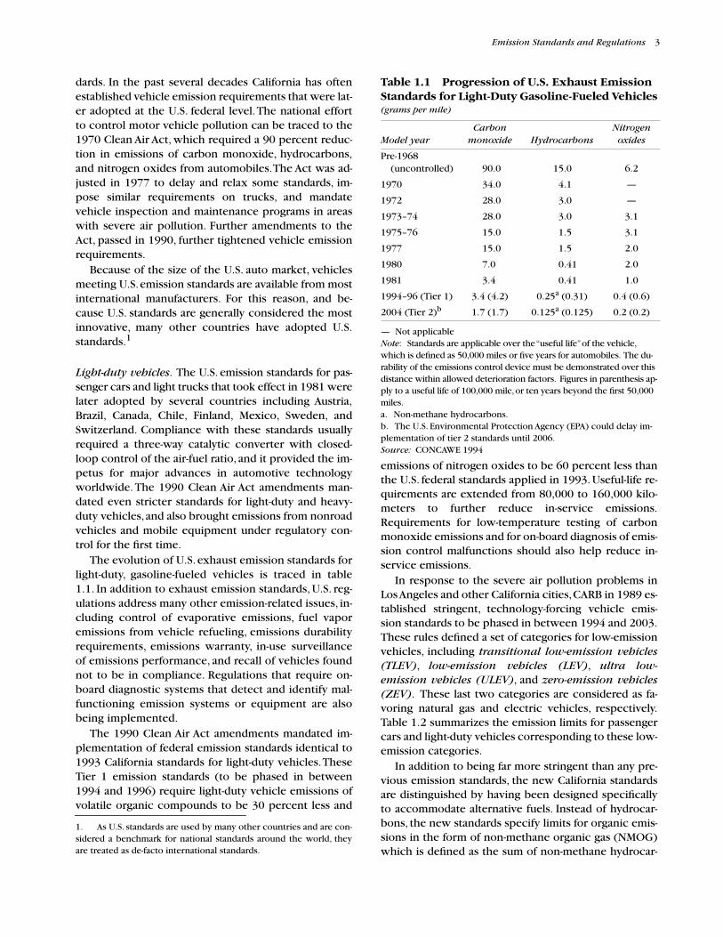
Table 1.1 Progression of U.S. Exhaust Emission Standards for Light-Duty Gasoline-Fueled Vehicles
(grams per mile)
— Not applicable
Note
: Standards are applicable over the “useful life” of the vehicle, which is defined as 50,000 miles or five years for automobiles. The du-rability of the emissions control device must be demonstrated over this distance within allowed deterioration factors. Figures in parenthesis ap-ply to a useful life of 100,000 mile, or ten years beyond the first 50,000 miles.a. Non-methane hydrocarbons.b. The U.S. Environmental Protection Agency (EPA) could delay im-plementation of tier 2 standards until 2006.
Source:
CONCAWE 1994
Model yearCarbon
monoxide HydrocarbonsNitrogenoxides
Pre-1968(uncontrolled) 90.0 15.0 6.2
1970 34.0 4.1 —
1972 28.0 3.0 —
1973–74 28.0 3.0 3.1
1975–76 15.0 1.5 3.1
1977 15.0 1.5 2.0
1980 7.0 0.41 2.0
1981 3.4 0.41 1.0
1994–96 (Tier 1) 3.4 (4.2) 0.25
a
(0.31) 0.4 (0.6)
2004 (Tier 2)
b
1.7 (1.7) 0.125
a
(0.125) 0.2 (0.2)

4
Air Pollution from Motor Vehicles
bons, aldehydes, and alcohol emissions, and thus ac-counts for the ozone-forming properties of aldehydesand alcohols tests that are not measured by standard hy-drocarbon tests. The new standards also provide for thenon-methane organic gas limit to be adjusted with reac-tivity adjustment factors. These factors account for thedifferences in ozone-forming reactivity of the NMOGemissions produced by alternative fuels, comparedwith those produced by conventional gasoline. Thisprovision gives an advantage to clean fuels such as nat-ural gas, methanol, and liquified petroleum gas, whichproduce less reactive organic emissions.
The 1990 Clean Air Act amendments also clarified therights of other states to adopt and enforce the morestringent California vehicle emission standards in placeof federal standards. New York and Massachusetts havedone so. In addition, the other states comprising the“Ozone Transport Region” along the northeastern sea-board of the United States (from Maine to Virginia) haveagreed to pursue the adoption of the California stan-dards in unison. This has prompted the auto industry todevelop a counter-offer, which is to implement Califor-nia’s LEV standard throughout the U.S. The auto indus-
try offer would not include California’s more-restrictiveULEV and ZEV standard, which are required under Mas-sachusetts and New York law.
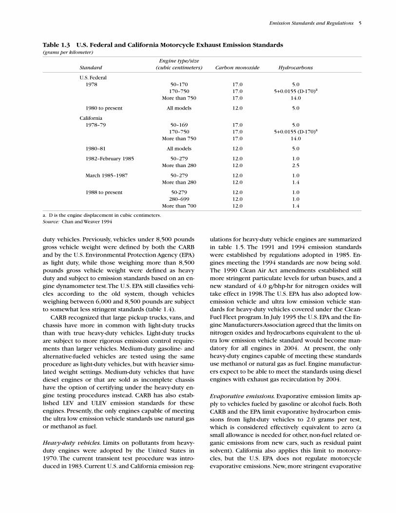
Motorcycles.
Current U.S. and California emission stan-dards for motorcycles are summarized in table 1.3. Un-like other vehicles, motorcycles used in the U.S. canmeet these emission standards without a catalytic con-verter. The most important effect of the U.S. federalemission standards has been the elimination of two-stroke motorcycles, which emit large volumes of hydro-carbons and particulate matter. California standards,though more stringent than the federal ones, can still bemet without a catalytic converter. Motorcycle standardsin the United States are lenient compared with stan-dards for other vehicles because the number of motor-cycles in use is small, and their emissions areconsidered insignificant compared with other mobileemission sources.
Medium-duty vehicles.
In 1989, CARB adopted regula-tions that redefined vehicles with gross vehicle weightratings between 6,000 and 14,000 pounds as medium-
Table 1.2 U.S. Exhaust Emission Standards for Passenger Cars and Light-Duty Vehicles Weighing Less than 3,750 Pounds Test Weight
(grams per mile)
— Not applicableNMHC = non-methane hydrocarbonsNMOG = non-methane organic gases
Note:
The federal Tier 1 standards also specify a particulate matter limit of 0.08 gram per mile at 50,000 miles and 0.10 gram per mile at 100,000 miles. The California standards also specify a maximum of 0.015 gram per mile for formaldehyde emissions for 1993 standard, transitional low-emission, and low-emission vehicles, and 0.008 grams per mile for ultra low-emission vehicles. Likewise, for benzene, a limit of 0.002 gram per mile is specified for low-emission and ultra low-emission vehicles. For diesel vehicles, a particulate matter limit of 0.08 gram per mile is specified for 1993 standard, transitional low-emission, and low-emission vehicles, and 0.04 gram per mile for ultra low-emission vehicles at 100,000 miles.a. Except for California.b. Equivalent to California 1993 model year standard.c. To be phased in over a ten-year period; expected year of phase-in.
Source:
CONCAWE 1994, Chan and Weaver 1994
50,000 miles or five years 100,000 miles or ten years
StandardYear
implemented
Carbonmonoxide75°/20°F Hydrocarbons
Nitrogen oxides
Carbonmonoxide
75°F HydrocarbonsNitrogen oxides
Passenger car
a
(Tier 0) 1981 3.4/— 0.41 1.0 — — —
Light-duty truck
a
(Tier 0) 1981 10/— 0.80 1.7 — — —
Tier 1
b
1994–6 3.4/10.0 0.25 NMHC 0.4 4.2 0.31 NMHC 0.6
Tier 2 2004 1.7/3.4 0.125 NMHC 0.2 — — —
California Low-Emission Vehicle/Federal Clean-fuel Fleet programs
Transitional low-emission vehicle (TLEV) 1994
c
3.4/10 0.125 NMOG 0.4 4.2 0.156 NMOG 0.6
Low-emission vehicle (LEV) 1997
c
3.4/10 0.075 NMOG 0.2 4.2 0.090 NMOG 0.3
Ultra low-emission vehicle (ULEV) 1997
c
1.7/10 0.040 NMOG 0.2 2.1 0.055 NMOG 0.3
Zero-emission vehicle (ZEV) 1998
c
0 0 0 0 0 0
Emission Standards and Regulations
5
duty vehicles. Previously, vehicles under 8,500 poundsgross vehicle weight were defined by both the CARBand by the U.S. Environmental Protection Agency (EPA)as light duty, while those weighing more than 8,500pounds gross vehicle weight were defined as heavyduty and subject to emission standards based on an en-gine dynamometer test. The U.S. EPA still classifies vehi-cles according to the old system, though vehiclesweighing between 6,000 and 8,500 pounds are subjectto somewhat less stringent standards (table 1.4).
CARB recognized that large pickup trucks, vans, andchassis have more in common with light-duty trucksthan with true heavy-duty vehicles. Light-duty trucksare subject to more rigorous emission control require-ments than larger vehicles. Medium-duty gasoline- andalternative-fueled vehicles are tested using the sameprocedure as light-duty vehicles, but with heavier simu-lated weight settings. Medium-duty vehicles that havediesel engines or that are sold as incomplete chassishave the option of certifying under the heavy-duty en-gine testing procedures instead. CARB has also estab-lished LEV and ULEV emission standards for theseengines. Presently, the only engines capable of meetingthe ultra low emission vehicle standards use natural gasor methanol as fuel.
Heavy-duty vehicles.
Limits on pollutants from heavy-duty engines were adopted by the United States in1970. The current transient test procedure was intro-duced in 1983. Current U.S. and California emission reg-
ulations for heavy-duty vehicle engines are summarizedin table 1.5. The 1991 and 1994 emission standardswere established by regulations adopted in 1985. En-gines meeting the 1994 standards are now being sold.The 1990 Clean Air Act amendments established stillmore stringent particulate levels for urban buses, and anew standard of 4.0 g/bhp-hr for nitrogen oxides willtake effect in 1998. The U.S. EPA has also adopted low-emission vehicle and ultra low emission vehicle stan-dards for heavy-duty vehicles covered under the Clean-Fuel Fleet program. In July 1995 the U.S. EPA and the En-gine Manufacturers Association agreed that the limits onnitrogen oxides and hydrocarbons equivalent to the ul-tra low emission vehicle standard would become man-datory for all engines in 2004. At present, the onlyheavy-duty engines capable of meeting these standardsuse methanol or natural gas as fuel. Engine manufactur-ers expect to be able to meet the standards using dieselengines with exhaust gas recirculation by 2004.
Evaporative emissions.
Evaporative emission limits ap-ply to vehicles fueled by gasoline or alcohol fuels. BothCARB and the EPA limit evaporative hydrocarbon emis-sions from light-duty vehicles to 2.0 grams per test,which is considered effectively equivalent to zero (asmall allowance is needed for other, non-fuel related or-ganic emissions from new cars, such as residual paintsolvent). California also applies this limit to motorcy-cles, but the U.S. EPA does not regulate motorcycleevaporative emissions. New, more stringent evaporative
Table 1.3 U.S. Federal and California Motorcycle Exhaust Emission Standards
(grams per kilometer)
a. D is the engine displacement in cubic centimeters.
Source:
Chan and Weaver 1994
StandardEngine type/size
(cubic centimeters) Carbon monoxide Hydrocarbons
U.S. Federal 1978 50–170
170–750More than 750
17.017.017.0
5.05+0.0155 (D-170)
a
14.0
1980 to present All models 12.0 5.0
California 1978–79 50–169
170–750More than 750
17.017.017.0
5.05+0.0155 (D-170)
a
14.0
1980–81 All models 12.0 5.0
1982–February 1985 50–279More than 280
12.012.0
1.02.5
March 1985–1987 50–279More than 280
12.012.0
1.01.4
1988 to present 50-279280–699
More than 700
12.012.012.0
1.01.01.4

6
Air Pollution from Motor Vehicles
test procedures scheduled to take effect during the mid-1990s will have the same limit of 2.0 grams per test, butrunning-loss emissions will be limited to 0.05 grams permile. The new standard is nominally the same as the oldone, but more severe test conditions under the new testprocedures will impose much greater compliance re-quirements on manufacturers.
Evaporative and refueling emissions have become amore significant fraction of total emissions as a conse-quence of the steady decline in exhaust hydrocarbonemissions. To address this problem, and to encouragethe introduction of vehicles using cleaner fuels, the U.S.EPA has defined a special category of vehicles called in-herently low-emission vehicles (ILEVs). These vehiclesmust meet the ultra low-emission standard for emissionsof nitrogen oxides and the low-emission vehicle stan-dards for carbon monoxide and non-methane organicgas. They must also exhibit inherently low evaporativeemissions by passing an evaporative test with the evap-orative control system disabled. Gasoline-fueled vehiclescannot meet this standard. Inherently low-emission vehi-cles are eligible for certain regulatory benefits, includingexemption from “no-drive” days and other time-based
transportation control measures. As of mid-1995, justtwo vehicle models were certified as inherently low-emission vehicles, and both were fueled by compressednatural gas (CNG).
U.N. Economic Commission for Europe (ECE)and European Union (EU) Standards
The vehicle emission standards established by the ECEand incorporated into the legislation of the EU (former-ly the European Community) are not directly compara-ble to those in the United States because of differencesin the testing procedure.
2
The relative emissions mea-sured using the two procedures vary with the vehicle’s
2. Besides the member states of the EU, China, the Czech Republic,Hong Kong, Hungary, India, Israel, Poland, Romania, Saudi Arabia, Sin-gapore, Thailand, the Slovak Republic, and countries in the formerU.S.S.R. and the former Yugoslavia require compliance with ECE reg-ulations. Austria, Denmark, Finland, Norway, Sweden, and Switzer-land have adopted U.S. standards. Following their admission into theEuropean Union in 1995, Austria, Finland, and Sweden must complywith EU regulations; a four-year transitional period has been agreed af-ter which national emission standards must either be harmonizedwith EU regulations or renegotiated.
Table 1.4 U.S. Federal and California Exhaust Emission Standards for Medium-Duty Vehicles
(grams per mile)
50,000 miles or five years 120,000 miles or eleven years
Standard (FTP-75)Year
implementedCarbon
monoxide HydrocarbonsNitrogen oxides
Carbonmonoxide Hydrocarbons
Nitrogen oxides
U.S. federal 1983 10.0 0.80 1.7 — — —
California/U.S. Tier 10–3,750 pounds3,751–5,750 pounds5,751–8,500 pounds8,500–10,000 pounds
b
10–14,000 pounds
b
1995/1996
a
3.44.45.05.57.0
0.25 NMHC0.32 NMHC0.39 NMHC0.46 NMHC0.60 NMHC
0.40.71.11.32.0
5.06.47.38.1
10.3
0.36 NMHC0.46 NMHC0.56 NMHC0.66 NMHC0.86 NMHC
0.550.981.531.812.77
California Low-Emission Vehicle/Federal Clean-Fuel Fleet programs
Low-emission vehicle (LEV)0–3,750 pounds3,751–5,750 pounds5,751–8,500 pounds8,501–10,000 pounds
b
10–14,000 pounds
b
1998
a
3.44.45.05.57.0
0.125 NMOG0.160 NMOG0.195 NMOG0.230 NMOG0.300 NMOG
0.40.71.11.32.0
5.06.47.38.1
10.3
0.180 NMOG0.230 NMOG0.280 NMOG0.330 NMOG0.430 NMOG
0.61.01.51.82.8
Ultra low-emission vehicle (ULEV)0–3,750 pounds3,751–5,750 pounds5,751–8,500 pounds8,501–10,000 pounds
b
10–14,000 pounds
b
1998
a
1.72.22.52.83.5
0.075 NMOG0.100 NMOG0.117 NMOG0.138 NMOG0.180 NMOG
0.20.40.60.71.0
2.53.23.74.15.2
0.107 NMOG0.143 NMOG0.167 NMOG0.197 NMOG0.257 NMOG
0.30.50.80.91.4
— Not applicable
Note:
NMHC–Non-methane hydrocarbons, NMOG–Non-methane organic gas. Emission standards for medium-duty vehicles also include limits for particulate matter and aldehyde emissions.a. Expected year of phase-in.b. California non-diesel vehicles only. All U.S. and California diesel-fueled vehicles weighing more than 8,500 pounds are subject to heavy-duty testing procedures and standards.
Source:
CONCAWE 1994

Emission Standards and Regulations
7
Table 1.5 U.S. Federal and California Emission Standards for Heavy-Duty and Medium-Duty Engines
—
Not applicableNR = Not regulated; HDV= Heavy-duty vehicle; LHDV= Light heavy-duty vehicle (<14,000 lb. GVW); MHDV= Medium heavy-duty vehicle (>14,000 lb. GVW); ILEV= Inherently low-emission vehicle; LEV= Low-emission vehicle; ULEV= Ultra low-emission vehicle; SULEV= Super ultra low-emission vehicle.a Acceleration/lug/peak smoke opacity.b Non-methane hydrocarbon (NMHC) standard applies instead of total hydrocarbion (THC) for natural gas engines only.c Replaced by “medium duty” vehicle classification beginning 1995.d These standards (NMHC+NO
x
) limit the sum of NMHC and NO
x
emissions.e NMHC limited to 0.5 g/bhp-hr.f Use of NMHC instead of THC standard is optional for diesel, LPG, and natural gas engines.g Methanol-fueled engines only. From 1993-95, limited to 0.10 g/bhp-hr, subsequently to 0.05 g/bhp-hr.h Includes spark-ignition gasoline and alternative fuel engines, except those derived from heavy-duty diesels.i Optional standards. Engines certified to these standards may earn emission credits.j Optional standards for diesel and diesel-derived engines and engines sold in incomplete medium-duty vehicle chassis.
Source:
CONCAWE 1995
Exhaust emissions (g/bhp-hr)
Totalhydrocarbons
Hydrocarbons(non-methane)
Nitrogenoxides
Carbonmonoxide
Particulate matter Formaldehyde
Smoke
opacitya
U.S. Federal heavy-duty regulation
1991 HDV diesel 1.3 — 5.0 15.5 0.25 — 20/15/50
1991 LHDV gasoline 1.1 — 5.0 14.4 — — —
1991 MHDV gasoline 1.9 1.2b
5.0 37.1 — — —
1994 HDV diesel 1.3 0.9b
5.0 15.5 0.10 — 20/15/50
1994 LHDV ottoc
1.1 1.7 b
5.0 14.4 — — —
1994 MHDV ottoc
1.9 1.2 b
5.0 37.1 — — —
1994 transit bus 1.3 1.2 b
5.0 15.5 0.07 — 20/15/50
1996 transit bus 1.3 1.2 b
5.0 15.5 0.05 — 20/15/50
1998 HDV diesel 1.3 1.2 b
4.0 15.5 0.10 — 20/15/50
1998 transit bus 1.3 1.2 b
4.0 15.5 0.05 — 20/15/50
2004 (proposed) HDV Opt. A 1.3 2.4 d
15.5 0.10 — 20/15/50
2004 (proposed) HDV Opt. B 1.3 2.5 d, e
15.5 0.10 — 20/15/50
Federal clean fuel fleet standards regulation
LEV - Federal fuel NR 3.8 d
14.4 0.10 — 20/15/50
LEV - California fuel NR 3.5 d
14.4 0.10 — 20/15/50
ILEV NR 2.5 d
14.4 0.10 0.050 20/15/50
ULEV NR 2.5 d
7.2 0.05 0.025 20/15/50
California heavy-duty regulation
1991 HDV diesel 1.3 1.2 f
5.0 15.5 0.25 0.10 g
20/15/50
1991 LHDV ottoc,h
1.1 0.9 5.0 14.4 — 0.10 g
—
1991 MHDV ottoh
1.9 1.7 f
5.0 37.1 — 0.10 g
—
1994 HDV diesel 1.3 1.2 f
5.0 15.5 0.10 0.10 g
20/15/50
1994 urban bus 1.3 1.2 f
5.0 15.5 0.07 0.10 g
20/15/50
Optional bus std. 1994i
1.3 1.2 f
0.5-3.5 15.5 0.07 0.10 g
20/15/50
1996 urban bus 1.3 1.2 f
4.0 15.5 0.05 0.05 g
20/15/50
Optional bus std. 1996i
1.3 1.2 f
0.5-2.5 15.5 0.05 0.05 g
20/15/50
California medium-duty regulation j
Tier 1 NR 3.9d
14.4 0.10 — 20/15/50
LEV 1992-2001 NR 3.5 d
14.4 0.10 0.05 20/15/50
2002-2003 NR 3.0 d
14.4 0.10 0.05 20/15/50
ULEV 1992-2003 NR 2.5 d
14.4 0.10 0.05 20/15/50
2004+Opt. A. NR 2.5 d, e
14.4 0.10 0.05 20/15/50
2004+Opt. B NR 2.4 d
14.4 0.10 0.05 20/15/50
SULEV NR 2.0 d
7.2 0.05 0.05 20/15/50
8
Air Pollution from Motor Vehicles
emission control technology, but test results in gramsper kilometer are generally of the same order.
Until the mid-1980s, motor vehicle emission regula-tions in Europe were developed by the ECE for adop-tion and enforcement by individual member countries.It had been a common practice for the EU to adopt stan-dards and regulations almost identical to those issuedby the ECE. In terms of stringency (i.e. level of emissioncontrol technology required for compliance) the Euro-pean standards have lagged considerably behind theU.S. standards. Much of this lag has been caused by thecomplex, consensus-based approach to standard settingused by the ECE and by the difficulty of obtaining agree-ment between so many individual countries, each withits own interests and concerns. With the recent shift todecision procedures requiring less-than-unanimousagreement within the European Union, it has been pos-sible to adopt more stringent emission standards. Thestringency of the most recent EU emission standards isnow closer to that of the U.S. standards. For all practicalpurposes the ECE no longer promulgates standards thathave not been agreed first by the EU.
Unlike the U.S. standards, the ECE emission standardsapply to vehicles only during type approval and whenthe vehicle is produced (conformity of production).Once the vehicle leaves the factory and enters service,the manufacturer has no liability for its continued com-pliance with emission limits. Surveillance testing, recallcampaigns, and other features of U.S. emissions regula-tion are not incorporated in the European regulatorystructure. As a result, manufacturers of such vehicleshave little incentive to ensure that the emission controlsystems are durable enough to provide good controlthroughout the vehicle’s lifetime.
Light-duty vehicles.
These vehicles were the first to beregulated, beginning in 1970, to conform to the originalECE Regulation 15. The regulation was amended fourtimes for type approval (ECE 15-01, implemented in1974, ECE 15-02 in 1977, ECE 15-03 in 1979, and ECE15-04 in 1984) and twice for conformity of production(1981 and 1986). Regulation ECE 15-04 was applied toboth gasoline and diesel-fueled light-duty vehicles,whereas earlier regulations applied only to gasoline-fu-eled vehicles. The emission limits included in these reg-ulations were based on the ECE 15 driving cycle (vanRuymbeke and others 1992).
The ECE did not adopt emission standards requiringthree-way catalytic converters until 1988 (ECE regula-tion 83), and then only for vehicles with engine dis-placement of 2.0 liters or more. Less stringent standardswere specified for smaller vehicles, in order to encour-age the use of lean-burn engines. Although ECE 83 wasalso adopted as European Community Directive 88/76/
EEC, this regulation was not implemented in nationallegislation by any European country, in anticipation ofthe adoption of the Consolidated Emissions Directive,91/441/EEC. This latter directive was adopted by theCouncil of Ministers of the European Community inJune 1991. Under the Consolidated Emission Directives,exhaust emission standards for passenger cars (includ-ing diesel cars) are certified on the basis of the newcombined ECE-15 (urban) cycle and extra-urban drivingcycle (EUDC). In contrast to previous directives, a com-mon set of exhaust emission standards (including dura-bility testing) were applied to all private passenger cars(both gasoline and diesel-engined) irrespective of en-gine capacity. The standard also covers vehicle evapo-rative emissions. Limit values for passenger caremissions are shown in table 1.6. These limits becameeffective July 1, 1992 for new models, and on December31, 1992 for all production.
In March 1994, the Council of Ministers of the Euro-pean Community adopted Directive 94/12/EC whichprovides for more stringent emission limits for passen-ger cars from 1996 onwards (table 1.6). These standardsagain differentiate between gasoline and diesel vehicles,but require significant emission reductions from bothfuel types. These standards make separate provisions fordirect-injection (DI) diesel engines to meet less-stringentstandards for hydrocarbons plus oxides of nitrogen andfor particulate matter, until September 30, 1999.
In contrast to previous directives, production vehi-cles must comply with the type approval limits. There isalso a durability requirement for vehicles fitted with pol-lution control devices. Implementation of these emis-sion standards by EU member States is mandatory andunlike previous directives, not left to the discretion ofindividual national governments. Directive 94/12/ECalso required that new proposals must be prepared be-fore June 30, 1996 to implement further reductions inexhaust emissions by June 1, 2000
3
(CONCAWE 1995).Limit values for emissions of gaseous pollutants from
light-duty trucks and commercial vehicles were alsoestablished in the Consolidated Emissions Directive,but the actual limits were identical to the limits estab-lished in ECE 15.04, and did not include a limitation on
3. In June 1996, the European Commission proposed to adopt thefollowing exhaust emission limits for cars to become effective in years2000 and 2005 (Walsh 1996a; Plaskett 1996).
•
Gasoline-fueled (g/km)
2000 2005
CO 2.30 1.00HC 0.20 0.10NO
x
0.15 0.08
•
Diesel-fueled (g/km)CO 0.64 0.50HC+NO
x
0.56 0.30NO
x
0.50 0.25PM 0.05 0.025

Emission Standards and Regulations
9
particulate matter emissions. Ministerial Directive 93/59/EEC did finally modify the emission limits for lighttrucks and commercial vehicles. Table 1.7 shows theemission standards established for light trucks and com-mercial vehicles by this directive. These standards be-came effective with the 1994 model year. For lighttrucks with reference mass less than 1,250 kg, the stan-dards are equivalent to those established for passengercars by the Consolidated Emissions Directive; heaviervehicles are allowed somewhat higher emissions. Lighttruck standards comparable in strictness to the passen-ger car standards of 93/59/EEC have not yet been pro-posed.
The present European emissions standards for passen-ger cars and light commercial vehicles are comparable tothe U.S. standards adopted in the early 1980s. The emis-sion control technologies required to meet thesestandards are similar. The main emission controlrequirements for gasoline vehicles include three-waycatalytic converters with feedback control of the air-fuelratio through an exhaust gas oxygen sensor. The 1996European emissions standards for passenger cars aremore stringent, following the example set by the U.S.Tier 1 standards.
Motorcycles.
Although the ECE has issued emissionstandards for motorcycles (ECE regulation 40.01) andmopeds (ECE Regulation 47), these regulations are onlynow being adopted in the EU (table 1.8). In addition,Austria and Switzerland have established their owntechnology-forcing emission standards for motorcyclesand mopeds. The moped standards are sufficiently strict
to require catalytic converters, at least on two-strokeengines.
Heavy-duty engines.
European regulation of heavy-dutyvehicle engines has lagged behind U.S. standards for thesame reasons as that for light-duty engines. ECE regula-tion 49.01, for gaseous emissions and ECE regulation24.03 for black smoke emissions (table 1.9), in effect un-til July 1992, was comparable in stringency to U.S. regu-lations from the 1970s, and could be met with little or noeffort by diesel-engine manufacturers. The Clean LorryDirective (91/542/EEC), compulsory throughout the EU,reduces particulate and gaseous emissions for heavy-dutyvehicles in two stages. The first-stage standards (Euro 1),which took effect in July 1992, are comparable in strin-gency to 1988 U.S. standards, while the second-stagestandards (Euro 2) are comparable to 1991 U.S. levels (ta-ble 1.10). An even more stringent third-stage standard isunder discussion, as is a change from the current steady-state emissions testing procedure to a transient cycle sim-ilar to the one used in the United States (Baines 1994).
Country and Other Standards
This section summarizes the vehicle emission standardsadopted by a number of individual countries, as of early1995. Because emission standards often change, readerswho require precise information are advised to obtainup-to-date information from the legal authorities of thecountry involved. The Oil Companies’ European Orga-nization for Environmental Protection and Health
Table 1.6 European Union Emission Standards for Passenger Cars with up to 6 Seats
(ECE15+EUDC test procedure, grams per kilometer)
— Not applicableNote: Directive 94/12/EC applies to both type approval and conformity of production.a. Effective dates: (i) All light-duty vehicles except direct-ignition (DI) diesels; new models July 1, 1992, all models Dec. 31, 1992. (ii) DI diesels, July 1, 1994.b. Effective dates: (i) Gasoline and IDI diesels; new models Jan 1, 1996, all models Jan 1 1997. (ii) DI diesels Oct 1, 1999.c. DI diesel limits until June 30, 1994 were 1.36 g/km (HC+NOx) and 0.19 g/km (PM).d. Less stringent standards apply to DI diesel until Sept 30, 1999: 0.9 g/km (HC+NOx) and 0.10 g/km (PM).
Source
: CONCAWE 1995
91/441/EECa
94/12/ECb
Type approvalConformity of
production Gasoline Diesel
CO
2.72 3.16 2.2 1.0
HC + NO
x
0.97c
1.13 0.5 0.7d
PM
0.14c
0.18 — 0.08d
Evap. Emissions (g/test)
2.0 2.0 2.0 —

10
Air Pollution from Motor Vehicles
Table 1.8 ECE and Other European Exhaust Emission Standards for Motorcycles and Mopeds
(grams per kilometer)
— Not applicableNote: This table does not show ECE40 and ECE40.1 limits for Reference Weight, R (motocycle weight+75 kg) of more than 100 kg and less than 300 kg. Furthermore only limits for type approval are shown in this table. See CONCAWE (1995) for additional information and applicable limits for conformity of production.Source: CONCAWE 1992; 1994; 1995
Regulation, engine type Carbon monoxide Hydrocarbons Nitrogen oxidesTesting
procedure
ECE 40Two-stroke, less than 100 kilogramsTwo-stroke, more than 300 kilogramsFour-stroke, less than 100 kilogramsFour-stroke, more than 300 kilograms
16.040.025.050.0
10.015.0
7.010.0
————
ECE cycleECE cycleECE cycleECE cycle
ECE 40.01Two-stroke, less than 100 kilogramsTwo-stroke, more than 300 kilogramsFour-stroke, less than 100 kilogramsFour-stroke, more than 300 kilograms
12.832.017.535.0
8.012.0
4.26.0
————
ECE cycleECE cycleECE cycleECE cycle
ECE 47 for mopedsTwo-wheelThree-wheel
8.015.0
5.010.0
——
ECE cycleECE cycle
SwitzerlandTwo-strokeFour-strokeMoped
8.013.0
0.5
3.03.00.5
0.100.300.10
ECE 40ECE 40ECE 40
AustriaMotorcycles (<50 cc and >40 km/h)
Two stroke (before Oct. 1, 1991)Two stroke (from Oct. 1, 1991)
Four stroke (before Oct. 1, 1991)Four stroke (from Oct. 1, 1991)
Motorcycles (<50 cc)Two stroke (before Oct. 1, 1990)Two stroke (from Oct. 1, 1990)
Four stroke (before Oct. 1, 1990)Four stroke (from Oct. 1, 1990)
Mopeds (<50 cc and <40 km/h)From Oct. 1, 1988
13.08.0
18.013.0
12.0–32.08.0
17.5–35.013.0
1.2
6.57.5
6.53.0
8.0–12.07.5
4.2–6.03.0
1.0
2.00.1
1.00.3
1.00.1
0.80.3
0.2
ECE 40ECE 40
ECE 40ECE 40
ECE 40ECE 40
ECE 40ECE 40
ECE 40
Table 1.7 European Union 1994 Exhaust Emission Standards for Light-Duty Commercial Vehicles (Ministerial Directive 93/59/EEC)
(grams per kilometer)
a. Reference mass (RM) means the mass of the vehicle in running order less the uniform mass of a driver of 75 kg and increased by a uniform mass of 100 kg.b. Diesel vehicles only.c. Includes passenger vehicles with seating capacity greater than six persons or reference mass greater than 2,500 kg.
Source
: CONCAWE 1995
Exhaust emissions
Vehicle category Reference
mass (kg)
a
Carbon monoxide
Hydrocarbons +nitrogen oxides
Particulate
matter
b
Light trucks
c
RM
≤
1,250 Type-approvalConformity of production
2.723.16
0.971.13
0.140.18
1,250
≤
RM
≤
1700 Type-approvalConformity of production
5.176.0
1.41.6
0.190.22
RM > 1,700 Type-approvalConformity of production
6.98.0
1.72.0
0.250.29

Emission Standards and Regulations
11
(CONCAWE) in Brussels, has also published a series ofreports summarizing vehicle emission and fuel stan-dards worldwide. The most recent such report (CON-CAWE 1994) is a comprehensive source of informationon motor vehicle emission regulations and fuel specifi-cations worldwide.
Argentina
Decree 875/94 of National Law 2254/92 issued in 1994establishes national emission standards for new and usedmotor vehicles (table 1.11). The Decree also assigns theSecretaría de Recursos Naturales y Ambiente Humano asthe responsible agency for enforcing and updating thesestandards. These emission limits were reinforced by theJoint Resolutions 96/94 and 58/94 issued by the Secretar-ies of Transport and Industry in March 1994. Emissionlimits are established with a different compliance sched-ule for trucks and urban passenger transport vehicles. Inaddition, emission limits for particulate matter are beingestablished for the years 1996 and 2000. The exhaustemission standards for new light-duty gasoline-fueled ve-hicles, new heavy-duty vehicles, diesel-fueled vehicles,
and for all used vehicles appear to be based on ECE regu-lations. Another regulation required the retirement ofbuses older than 10 years (about 3,500 buses) in 1995.Municipal emission standards in the Capital Federal areembodied in Ordinance No. 39,025 and appear to betighter than national emission limits. It is understood thatArgentine standards conform closely to Brazilian stan-dards although implementation is delayed because of thecurrent limited availability of unleaded gasoline.
Australia
In Australia’s federal system of government, the powerto introduce motor vehicle legislation, including emis-sion regulations, lies with state governments. This is theopposite of the situation in the United States. The Aus-tralian Transport Advisory Council (ATAC) is composedof federal and state transport ministers who meet twicea year. The Council can agree to adopt emission andsafety standards which, while not binding on the states,are usually adopted in state legislation. States have actedunilaterally when agreement is not reached within theCouncil, however.
Table 1.9 Smoke Limits Specified in ECE Regulation 24.03 and EU Directive 72/306/EEC
(smoke emission limits under steady state conditions)
Note:
Intermediate values are also specified. Opacity under free acceleration should not exceed the approved level by more than 0.5 m
-1
Although the free acceleration test was intended as a means of checking vehicles in service it has not proved entirely successful. A number of different methods have been proposed by various countries, but there is no generally accepted alternative method of in-service checking.
Source
: CONCAWE 1994
Nominal flow (liters/second) Absorption coefficient (m-
1
)
42100200
2.261.4951.065
Table 1.10 European Exhaust Emission Standards for Heavy-Duty Vehicles for Type Approval
(grams per kilowatt hour)
Effective date Carbon monoxide
Nitrogen oxides Hydrocarbons
ParticulatematterRegulation New models All production
ECE 49 (13-mode) 14.0 18.0 3.5
a
ECE 49.01 (88/77/EEC) April 1988 October 1990 11.2(13.2)
14.4(15.8)
2.4
(2.6)
b a
Clean lorry directive (91/542/EEC)Stage 1 (Euro 1)
Stage 2 (Euro 2)
Stage 3 (Euro 3)
July 1992
October 1995
1999 (tentative)
October 1993
October 1996
n.a.
4.5(4.9)
4.0(4.0)
2.5
8.0(9.0)
7.0(7.0)
5.0
1.1(1.23)
1.1(1.10)
0.7
0.36–0.61
c
(0.40–0.68)
0.15–0.25
c
(0.15–0.25)
less than 0.12
n.a. = Not availablea. Smoke according to ECE Regulation 24.03, EU Directive 72/306/EEC.b. Figures in parentheses are emission limits for conformity of production.c. Depending on engine rating.
Source:
Havenith and others 1993; CONCAWE 1994
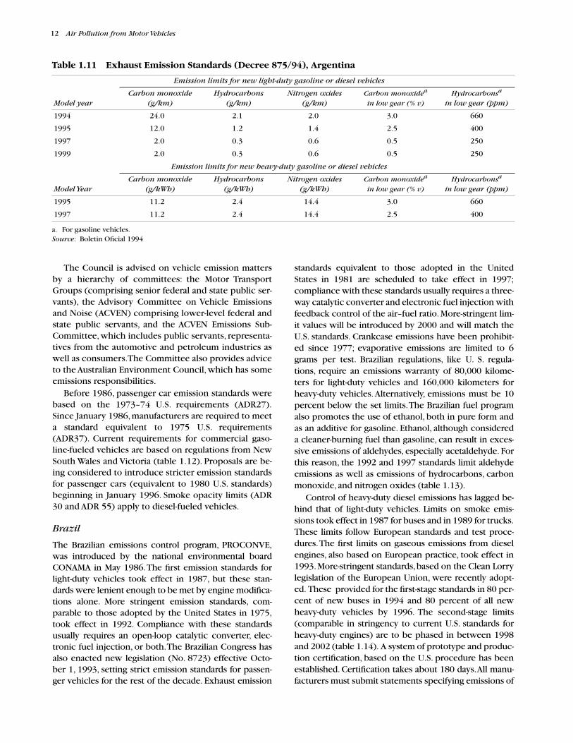
12
Air Pollution from Motor Vehicles
The Council is advised on vehicle emission mattersby a hierarchy of committees: the Motor TransportGroups (comprising senior federal and state public ser-vants), the Advisory Committee on Vehicle Emissionsand Noise (ACVEN) comprising lower-level federal andstate public servants, and the ACVEN Emissions Sub-Committee, which includes public servants, representa-tives from the automotive and petroleum industries aswell as consumers. The Committee also provides adviceto the Australian Environment Council, which has someemissions responsibilities.
Before 1986, passenger car emission standards werebased on the 1973–74 U.S. requirements (ADR27).Since January 1986, manufacturers are required to meeta standard equivalent to 1975 U.S. requirements(ADR37). Current requirements for commercial gaso-line-fueled vehicles are based on regulations from NewSouth Wales and Victoria (table 1.12). Proposals are be-ing considered to introduce stricter emission standardsfor passenger cars (equivalent to 1980 U.S. standards)beginning in January 1996. Smoke opacity limits (ADR30 and ADR 55) apply to diesel-fueled vehicles.
Brazil
The Brazilian emissions control program, PROCONVE,was introduced by the national environmental boardCONAMA in May 1986. The first emission standards forlight-duty vehicles took effect in 1987, but these stan-dards were lenient enough to be met by engine modifica-tions alone. More stringent emission standards, com-parable to those adopted by the United States in 1975,took effect in 1992. Compliance with these standardsusually requires an open-loop catalytic converter, elec-tronic fuel injection, or both. The Brazilian Congress hasalso enacted new legislation (No. 8723) effective Octo-ber 1, 1993, setting strict emission standards for passen-ger vehicles for the rest of the decade. Exhaust emission
standards equivalent to those adopted in the UnitedStates in 1981 are scheduled to take effect in 1997;compliance with these standards usually requires a three-way catalytic converter and electronic fuel injection withfeedback control of the air–fuel ratio. More-stringent lim-it values will be introduced by 2000 and will match theU.S. standards. Crankcase emissions have been prohibit-ed since 1977; evaporative emissions are limited to 6grams per test. Brazilian regulations, like U. S. regula-tions, require an emissions warranty of 80,000 kilome-ters for light-duty vehicles and 160,000 kilometers forheavy-duty vehicles. Alternatively, emissions must be 10percent below the set limits. The Brazilian fuel programalso promotes the use of ethanol, both in pure form andas an additive for gasoline. Ethanol, although considereda cleaner-burning fuel than gasoline, can result in exces-sive emissions of aldehydes, especially acetaldehyde. Forthis reason, the 1992 and 1997 standards limit aldehydeemissions as well as emissions of hydrocarbons, carbonmonoxide, and nitrogen oxides (table 1.13).
Control of heavy-duty diesel emissions has lagged be-hind that of light-duty vehicles. Limits on smoke emis-sions took effect in 1987 for buses and in 1989 for trucks.These limits follow European standards and test proce-dures. The first limits on gaseous emissions from dieselengines, also based on European practice, took effect in1993. More-stringent standards, based on the Clean Lorrylegislation of the European Union, were recently adopt-ed. These provided for the first-stage standards in 80 per-cent of new buses in 1994 and 80 percent of all newheavy-duty vehicles by 1996. The second-stage limits(comparable in stringency to current U.S. standards forheavy-duty engines) are to be phased in between 1998and 2002 (table 1.14). A system of prototype and produc-tion certification, based on the U.S. procedure has beenestablished. Certification takes about 180 days. All manu-facturers must submit statements specifying emissions of
Table 1.11 Exhaust Emission Standards (Decree 875/94), Argentina
a. For gasoline vehicles.
Source
: Boletin Oficial 1994
Emission limits for new light-duty gasoline or diesel vehicles
Model yearCarbon monoxide
(g/km)Hydrocarbons
(g/km)Nitrogen oxides
(g/km)Carbon monoxidea
in low gear (% v)Hydrocarbonsa
in low gear (ppm)
1994 24.0 2.1 2.0 3.0 660
1995 12.0 1.2 1.4 2.5 400
1997 2.0 0.3 0.6 0.5 250
1999 2.0 0.3 0.6 0.5 250
Emission limits for new heavy-duty gasoline or diesel vehicles
Model YearCarbon monoxide
(g/kWh)Hydrocarbons
(g/kWh)Nitrogen oxides
(g/kWh)Carbon monoxidea
in low gear (% v)Hydrocarbonsa
in low gear (ppm)
1995 11.2 2.4 14.4 3.0 660
1997 11.2 2.4 14.4 2.5 400

Emission Standards and Regulations 13
all models. Manufacturers of light-duty trucks (over 2,000kg GVW) have the option to choose either the LDV orHDV test procedures for certification.
Canada
New standards for cars, light-duty trucks, and heavyduty trucks were introduced in 1987, bringing Canadi-an standards in line with then current U.S. limits (table
1.15). Limits for heavy-duty trucks are expected to betightened in line with U.S. standards between 1994 and1996. The Canadian federal government has announcedplans to bring passenger car emission standards in linewith the limits established in the U.S. Clean Air Act, pur-suant to the provisions of NAFTA. Standards of 0.25grams per mile for hydrocarbons, 3.4 grams per mile forcarbon monoxide, and 0.4 grams per mile for nitrogen
Table 1.13 Exhaust Emission Standards for Light-Duty Vehicles (FTP-75 Test Cycle), Brazil(grams per kilometer)
— Not applicableNotes: Effective January 1, 1988, no crankcase emissions permitted. Effective January 1, 1990, evaporative emissions limited to 6 grams per test(SHED). Exemptions possible for manufacturers with production less than 2,000 vehicles per year.a. New cars only.b. For certain specified models.c. For all models, except those not derived from light-duty vehicles.d. For models not derived from light-duty vehicles.e. For models not covered in footnote d.f. For alcohol-fueled vehicles only.g. For diesel-fueled vehicles only.h. Idle CO for alcohol in gasohol-fueled vehicles.i. Evaporative emissions expressed as propane for gasohol-fueled and ethanol for alcohol-fueled vehicles.Source: CETESB 1994; CONCAWE 1994
Year effec-tive
Carbonmonoxide Hydrocarbons Nitrogen oxides Aldehydesf
ParticulateMatterg
Carbon monoxide at idle (% v)h
Evaporative(grams per test)i
1988a
1989b
1990c
1992d
1992e
19941997
242424241212
2
2.12.12.12.11.21.20.3
2.02.02.02.01.41.40.6
————
0.150.150.03
————
0.050.050.05
3.03.03.03.02.52.50.5
——6.06.06.06.06.0
2000 Limits in line with U.S. standards
Table 1.12 Exhaust Emission Standards for Motor Vehicles, Australia(grams per kilometer)
Regulation Effective dateCarbon
monoxide HydrocarbonsNitrogen oxides
Particulatematter
Testprocedure
Evaporative emissions
(grams per test)
Passenger carsADR 27A/B/C
ADR 37a
Proposed standards
July 1976January 1982January 1986
January 1996January 2000
24.222.0
9.3(8.45)
4.342.11
2.11.910.93
(0.85)
0.260.26
1.91.731.93
(1.75)
1.240.63
————
2.02.0
FTP 75FTP 75FTP 75
(FTP 75)
FTP 75FTP 75
2.0 (Canister)6.0 (SHED)b
2.0 (SHED)(1.9 SHED)
Commercial vehicles (gasoline)NSW (Clean Air Act) andVictoria (statutory rules) 1992 9.3 0.93 1.93 — FTP 75 2.0 (SHED)
— Not applicableNote: Figures in parentheses apply to certification vehicles.a. The higher figures apply to production vehicles, which must meet the limits from 150 kilometers to 80,000 kilometers or for five years, which-ever occurs first.b. SHED = Sealed Housing for Evaporative Determinations.Source: CONCAWE 1994

14 Air Pollution from Motor Vehicles
oxides will probably be required as of 1996. The Feder-al Transport Minister and representatives of the automo-tive industry have agreed that cars sold in Canada from1994 to 1996 will meet the same emissions standards asthose sold in the United States. The U.S. manufacturershave committed themselves to market 1991 and subse-quent model heavy-duty engines meeting U.S. standardsin Canada in the absence of specific regulations.
Air quality legislation enacted by British Columbia in1994 gives the province the authority to set standards
for vehicle emissions and fuels. Based on the Californiamodel, the provincial standards applicable to the dense-ly populated southern regions of the province are themost stringent in Canada.
Chile
Chilean authorities have adopted regulations requiringall new light-duty vehicles to meet 1983 U.S. emissionlimits. These regulations have been applied to the Santi-ago metropolitan area and surrounding regions since
Table 1.14 Exhaust Emission Standards for Heavy-Duty Vehicles (ECE R49 Test Cycle), Brazil(grams per kilowatt hour)
— Not applicableNote: * k=soot (g/m3) *x gas flow (l/sec), applies to all vehicles.a. Particulate emissions (PM) 0.7 g/kWh for engines up to 85 kWh; 0.4 g/kWh for engines above 85 kWh. Crankcase emissions must be nil, exceptfor some turbocharged diesel engines if there is a technical justification.b. Applies from this date onwards.Source: CETESB 1994; CONCAWE 1994
Vehicle class Effective datePercentvehicles
Carbonmonoxide Hydrocarbons Nitrogen oxides
Particulate matter Smoke K
All vehicles January 1, 1989January 1, 1996
January 1, 2000
January 1, 2002
—20802080
100
—11.2
4.94.94.04.0
—2.451.21.21.11.1
—14.4
9.09.07.07.0
—
0.7/0.4a
0.7/0.4a
0.150.15
2.5b
All imports January 1, 1994January 1, 1996January 1, 1998
100100100
4.94.94.0
1.21.21.1
9.09.07.0
0.7/0.4a
0.7/0.4a
0.15
2.5b
Urban buses January 10, 1987January 3, 1994
January 1, 1996January 1, 1998
January 1, 2002
—208020802080
100
—11.2
4.911.2
4.94.94.04.0
—2.451.22.41.21.21.11.1
—14.4
9.014.4
9.09.07.07.0
————
0.7/0.4a
0.7/0.4a
0.150.15
2.5b
2.5b
Table 1.15 Exhaust Emission Standards for Light- and Heavy-Duty Vehicles, Canada
Vehicle typeYear
effectiveCarbon
monoxide HydrocarbonsNitrogen oxides
Dieselparticulates
Testing procedure
Light-duty vehicles (grams per kilometer)
Cars and light-duty trucks 1975–87 25.00 2.00 3.10 — FTP 75
Cars 1988 2.11 0.25 0.62 0.12 FTP 75
Trucks less than 1,700 kilograms 1988 6.20 0.20 0.75 0.16 FTP 75
Trucks more than 1,700 kilograms 1988 6.20 0.50 1.10 0.16 FTP 75
Heavy-duty vehicles (grams per brake horsepower-hour)
Less than 6,350 kilograms 1988 14.4 1.1 6.0 — U.S. transient
More than 6,350 kilograms 1988 37.1 1.9 6.0 — U.S. transient
Diesels 19881994
15.515.5
1.31.3
6.05.0
0.60.1
U.S. transientU.S. transient
— Not applicableSource: CONCAWE 1994

Emission Standards and Regulations 15
September 1992, and were extended nationally in Sep-tember 1994. Regulations have also been adopted re-quiring new heavy-duty trucks and buses to beequipped with engines meeting U.S. or European emis-sion standards. U.S. 1991 or Euro 1 standards were re-quired for buses in Santiago beginning September 1993,and for all heavy-duty vehicles in September 1994. U.S.1994 or Euro 2 standards will be required for Santiagobuses in 1996, and nationwide in 1998. An emissionstest facility for certification and enforcement purposesis under development.
China
Regulation of motor vehicle emission in China has beenguided by legislation enacted by the Standing Commit-tee of the National People’s Congress in 1979 and 1987and the State Council in 1991: the “EnvironmentalProtection Law of the People’s Republic of China”(1979), the “Law of the People’s Republic of China onthe Prevention and Control of Air Pollution” (1987), andthe “Detailed Rules and Regulations for the Law of thePeople’s Republic of China on the Prevention and Con-trol of Air Pollution” (1991). Based on these laws, theNational Environmental Protection Agency, which isresponsible for formulating emission standards and test-ing procedures, has issued 11 motor vehicle emissioncontrol standards and formulated a Management Proce-dure and Technical Policy to control emissions.
Standards for light-duty vehicles, adopted in 1979,are equivalent to ECE regulation 15-03 and includetesting procedures for type approval and conformityof production. The standard test procedure lasts 13minutes and has four cycles with no intermission.Each cycle covers 15 working phases (idling, accelera-tion, deceleration, steady speed, and so on). Thesestandards were developed by the Changchun Automo-tive Research Institute and submitted to the State Envi-ronmental Protection Administration by the ChineseAutomotive Industry Federation (CSEPA 1989). The En-vironmental Protection Administration adopted perfor-mance targets for motorcycles in 1985 (GB 5366-85),and exhaust emission standards for light-duty vehiclesin 1989 (GB11641-89). The light-duty vehicle stan-dards apply to cars, passenger vans, and light-dutyfreight vehicles (reference mass 3,500 kilograms orless) operating at a minimum speed of 50 kilometersan hour.
Exhaust emission standards for heavy-duty vehicles,adopted in 1983 (Regulations No. GB 3842-83, 3843-83, and 3844-83) consist only of carbon monoxide andhydrocarbon limits determined at idle and apply bothto new and in-use vehicles (table 1.16). China is con-sidering legislation for heavy-duty gasoline-engine ve-hicles based on two runs of the U.S. 9-mode cycle usedby U.S. EPA during 1970-1983. Proposed limits are giv-en in table 1.17. Idle emission standards have also
been adopted for heavy-duty gasoline engines, andconsideration is being given to establishing mass emis-sion limits for these engines in grams per kilowatthour. Revised or new emission standards and testingprocedures that came into force in 1994 are listed intable 1.18.
Chinese motor vehicle regulations require that all do-mestically produced vehicle models must be listed inthe “Index of Enterprises Producing Motor Vehicles andtheir Products” issued annually by China National Auto-motive Industry Corporation (CNAIC) and the Ministryof Public Security. Before a vehicle model is listed in theIndex, the vehicle should pass an approval test carriedout by “The Type Approval Organization for New MotorVehicle Products.” Recently, the responsibility for issu-ing the index and type approvals has been transferred tothe Auto Industry Bureau of the Ministry of Machinery.Included in the approval tests are idling emissions testsfor gasoline-fueled vehicles and free acceleration smoketests for diesel-fueled vehicles. In addition, a full loadsmoke test is required for diesel engines. In case ofimported motor vehicles, the type approval tests, areconducted by authorized laboratories of the StateAdministration for Import and Export CommodityInspection.
Colombia
New emission standards for gasoline- and diesel-fueledvehicles were established in 1996 by Resolution 5 of theMinistry of the Environment and Transport. These stan-dards establish carbon monoxide and hydrocarbonsemission limits for two mean-sea-level ranges of 0 to1,500 meters, and 1,501 to 3,000 meters (table 1.19).
Additional emission standards have been adopted bythe Ministry of the Environment for light, medium, andheavy-duty gasoline- and diesel-fueled vehicles to comeinto effect with model year 1997 (table 1.20).
Eastern European Countries and the Russian Federation
Most eastern European and central Asian countries in-cluding Russia use some combinations of ECE and EUregulations, as shown in table 1.21.
Table 1.16 Exhaust Emission Limits for Gasoline-Powered Heavy-Duty Vehicles (1983), China
Source: CONCAWE 1994
Idle
Carbon monoxide Hydrocarbons
Vehicles (% v) (ppm)
New 5.0 2500
In-use 6.0 3000
Imports 4.5 1000

16 Air Pollution from Motor Vehicles
Hong Kong
New cars sold in Hong Kong are required to meet eitherU.S. or Japanese emission standards or the new consol-idated European limits (91/441/EEC). Each of these reg-ulations requires the use of three-way catalyticconverters with electronic control systems. All newcars were required to meet these standards as of January1992. Light-duty diesel vehicle emission standards were
also tightened effective April 1, 1995. All new passengercars and taxis must comply with 1990 U.S. standards orequivalent EU and Japanese standards. Similar require-ments will apply to medium goods vehicles and lightbuses. For goods vehicles and buses with a designweight of 3.5 tonnes or more either the 1990 U.S. stan-dards or the Euro 1 standards will apply. Emissions stan-dards have not been established for motorcycles.
Table 1.17 Proposed Exhaust Emission Limits for Gasoline-Powered Heavy-Duty Vehicles, China(grams per kilowatt hour)
Source: CONCAWE 1994
Year VehicleCarbon
monoxide (g/kWh)Hydrocarbons + Nitrogen oxides
(g/kWh)
Up to 1997 Certified before 1992Produced after 1992Type approved after 1992
805040
322016
1997 Certified before 1992Produced after 1992Type approved after 1992
503428
2013.611
Table 1.18 List of Revised or New Emission Standards and Testing Procedures, China (Effective 1994)
Source: Walsh 1995
Number Title
GB 14761.1-93
GB 14761.2-93
GB 14761.3-93
GB 14761.4-93
GB 14761.5-93
GB 14761.6-93
GB 14761.7-93
GB/T 14762-93
GB/T 14763-93
GB/T 3845-93
GB/T 3846-93
GB/T 3847-93
GB 14621-93
GB/T 14622-93
GB/T 5466-93
Emission standard for exhaust pollutants from light-duty vehicles
Emission standard for exhaust pollutants from gasoline engine of road vehicles
Emission standard for fuel evaporative emissions from road vehicle with gasoline engine
Emission standard for pollutants from crankcase of vehicle engines
Emission standard for pollutants at idle speed from road vehicle with gasoline engine
Emission standard for smoke at free acceleration from road vehicles with diesel engine
Emission standard for smoke at full load from automotive diesel engines
Measurement method for exhaust pollutants from gasoline engine of road vehicles
Measurement method of fuel evaporative emissions from road vehicles with gasoline engine
Measurement method for pollutants at idle speed from road vehicles with diesel engine
Measurement method for smoke at free acceleration from road vehicles with diesel engine
Measurement method for smoke at full load from automotive diesel engines
Emission standard for exhaust emissions from motorcycles
Measurement method for exhaust emissions from motorcycles under running mode
Measurement method for exhaust emissions from motorcycles under idle speed
Table 1.19 Emission Limits for Gasoline-Fueled Vehicles for Idle and Low Speed Conditions, Colombia
msl = mean sea levelSource: Onursal and Gautam 1996
Carbon monoxide (%) Hydrocarbons (ppm)
Model year above msl: 0–1500 m 1501–3000 m above msl: 0–1500 m 1501–3000 m
2001 or newer 1.0 1.0 200 200
1998–2000 2.5 2.5 300 300
1997–1996 3.0 3.5 400 450
1995–1991 4.5 5.5 750 900
1990–1975 5.5 6.5 900 1000
1974 or older 6.5 7.5 1000 1200
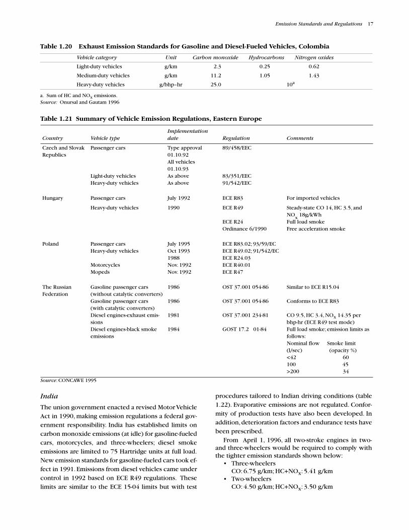
Emission Standards and Regulations 17
India
The union government enacted a revised Motor VehicleAct in 1990, making emission regulations a federal gov-ernment responsibility. India has established limits oncarbon monoxide emissions (at idle) for gasoline-fueledcars, motorcycles, and three-wheelers; diesel smokeemissions are limited to 75 Hartridge units at full load.New emission standards for gasoline-fueled cars took ef-fect in 1991. Emissions from diesel vehicles came undercontrol in 1992 based on ECE R49 regulations. Theselimits are similar to the ECE 15-04 limits but with test
procedures tailored to Indian driving conditions (table1.22). Evaporative emissions are not regulated. Confor-mity of production tests have also been developed. Inaddition, deterioration factors and endurance tests havebeen prescribed.
From April 1, 1996, all two-stroke engines in two-and three-wheelers would be required to comply withthe tighter emission standards shown below:
• Three-wheelersCO: 6.75 g/km; HC+NOx: 5.41 g/km
• Two-wheelersCO: 4.50 g/km; HC+NOx: 3.50 g/km
Table 1.20 Exhaust Emission Standards for Gasoline and Diesel-Fueled Vehicles, Colombia
a. Sum of HC and NOx emissions.Source: Onursal and Gautam 1996
Vehicle category Unit Carbon monoxide Hydrocarbons Nitrogen oxides
Light-duty vehicles g/km 2.3 0.25 0.62
Medium-duty vehicles g/km 11.2 1.05 1.43
Heavy-duty vehicles g/bhp–hr 25.0 10a
Table 1.21 Summary of Vehicle Emission Regulations, Eastern Europe
Source: CONCAWE 1995
Country Vehicle typeImplementation date Regulation Comments
Czech and Slovak Republics
Passenger cars
Light-duty vehiclesHeavy-duty vehicles
Type approval01.10.92All vehicles01.10.93As aboveAs above
89/458/EEC
83/351/EEC91/542/EEC
Hungary Passenger cars July 1992 ECE R83 For imported vehicles
Heavy-duty vehicles 1990 ECE R49
ECE R24Ordinance 6/1990
Steady-state CO 14, HC 3.5, and NOx 18g/kWhFull load smokeFree acceleration smoke
Poland Passenger carsHeavy-duty vehicles
MotorcyclesMopeds
July 1995Oct 19931988Nov. 1992Nov. 1992
ECE R83.02; 93/59/ECECE R49.02; 91/542/ECECE R24.03ECE R40.01ECE R47
The Russian Federation
Gasoline passenger cars(without catalytic converters)Gasoline passenger cars(with catalytic converters)Diesel engines-exhaust emis-sionsDiesel engines-black smoke emissions
1986
1986
1981
1984
OST 37.001 054-86
OST 37.001 054-86
OST 37.001 234-81
GOST 17.2 01-84
Similar to ECE R15.04
Conforms to ECE R83
CO 9.5, HC 3.4, NOx 14.35 per bhp-hr (ECE R49 test mode)Full load smoke; emission limits as follows:Nominal flow Smoke limit(l/sec) (opacity %)<42 60100 45>200 34

18 Air Pollution from Motor Vehicles
Japan
Japan revised its emissions test procedures for light-dutyvehicles in 1991. The new test procedure, resemblingthe new ECE emissions test cycle, consists of a series oflow- and moderate-speed accelerations and decelera-tions at 20 kilometers per hour to 40 kilometers perhour, as well as a higher-speed component reaching upto 70 kilometers per hour. It will apply to passenger carsand light- and medium-duty trucks (up to 2.5 tons grossweight). The test procedure for heavy-duty engines hasalso been modified from the previous six-mode test toanother steady-state, engine dynamometer test involving13 operating modes (these modes are different from theECE 13-mode test). The units of measurement have alsobeen changed, from grams per test and ppm to gramsper kilometer and grams per kilowatt hour, making iteasier to compare Japanese standards with U.S. and ECEemission standards. In addition to these changes, emis-sion limits on nitrogen oxides (already among the moststringent worldwide) are to be further tightened, andlimits on diesel particulate emissions have been intro-duced. Smoke limits were reduced by 20 percent in1993 for light- and medium-duty diesel vehicles andmore stringent smoke limits were expected for heavy-duty passenger vehicles. Detailed information on Japa-nese emission standards is available in CONCAWE 1994.
Because of the differences in test procedures, a directcomparison of Japanese emission standards with thoseapplied to the U.S. and Europe cannot be made.
Republic of Korea
Passenger car and light-truck emission standards equalto current U.S. standards have been in effect since1987. These standards apply to passenger cars using ei-ther gasoline or liquified petroleum gas, with enginedisplacement greater than 0.8 liter and gross vehicleweight less than 2.7 tons. Standards for heavy-duty gas-oline and liquified petroleum gas engines, based on theU.S. heavy-duty transient test procedure, are similar tothose in effect for heavy-duty gasoline engines in theUnited States before 1990. Heavy-duty diesel test pro-cedures and emission standards are similar to those ofJapan. The Korean government is also moving to dis-courage the use of diesel engines in medium-dutytrucks in favor of gasoline or liquified petroleum gas en-gines with more effective emissions control. Legisla-tion has also been introduced for two-stroke and four-stroke motorcycles that would require the use of cata-lytic converters. Emission limits for two- and four-stroke motorcycles are summarized in table 1.23; thetest procedure however, is not known (CONCAWE1994; UNIDO 1990).
Table 1.22 Exhaust Emission Standards for Gasoline-Fueled Vehicles, India(grams per kilometer)
Reference mass (kilograms) Carbon monoxide Hydrocarbons
Two- and three-wheel vehiclesLess than 150150–350More than 350
1212+(18*(R-150)/200)
30
88+(4*(R-150)/200)
12
Light-duty vehiclesLess than 1,0201,020–1,2501,250–1,4701,470–1,7001,700–1,9301,930–2,150More than 2,150
14.316.518.820.722.924.927.1
2.02.12.12.32.52.72.9
R = Reference mass.Source: India 1989
Table 1.23 Motorcycle Emission Standards, Republic of Korea
a. Proposed.Source: CONCAWE 1994
Two-stroke Four-stroke
Period Carbon monoxide (% v) Hydrocarbons (ppm) Carbon monoxide (% v) Hydrocarbons (ppm)
1/91 to 12/921/93/12/951/96 onwarda
5.54.63.6
11001100
450
5.54.53.6
450450400

Emission Standards and Regulations 19
Malaysia
In Malaysia, vehicle emission regulations based on ECE15.04 were introduced in September 1992. A further re-quirement that all new gasoline-fueled vehicles beequipped with catalytic converters has been temporari-ly postponed.
Mexico
New passenger cars and light-duty trucks sold in Mexi-co have been subject to exhaust emission standards(generally based on U.S. standards) since 1975 (table1.24). Until the 1991 model year, however, these stan-dards were loose enough to be met without the use ofa catalytic converter or other advanced emission con-trol technology. The 1991 and 1992 model years werea transition during which standards were made suffi-ciently stringent to require catalytic converters but notthe full range of emission control technology requiredin the United States. Despite the transition period, mostMexican automakers equipped their vehicles with U.S.-model emission controls instead of a less-sophisticatedsystem that would be used for only two years. New carsand light trucks since model year 1993 have been re-quired to meet exhaust emission standards that areequivalent to 1987 U.S. standards. Starting in 1995, allcars, light commercial vehicles and light trucks were re-quired to meet an evaporative emissions standard of 2.0grams per test as well. Mexico has not yet adopted otherelements of the U.S. regulations: emissions durability,emissions warranty requirements, and in-service testingwith recall of vehicle models found to be violating emis-sion standards in service. As part of the NAFTA, the Unit-ed States, Canada, and Mexico are in the process ofharmonizing vehicle emission standards.
In the past few years, Mexican authorities have estab-lished emission standards for medium- and heavy-dutyvehicles (table 1.25). In 1991 authorities and manufac-
turers agreed on catalyst-forcing standards for gasoline-fueled microbuses. New microbuses are required tomeet these standards. Similar standards will apply to allnew medium-duty vehicles in 1994. As of June 1992,new heavy-duty diesel vehicles were required to beequipped with engines meeting 1991 U.S. emission stan-dards at sea level, with an additional test of smoke opac-ity conducted at Mexico City’s altitude (2,000 meters).Work on evaluating the feasibility of meeting 1994 U.S.emission standards at Mexico City’s altitude is planned.
Saudi Arabia
Saudi Arabia has adopted emission standards equivalentto ECE R15.03. Annual inspections of vehicle emissioncontrol systems is required in Jeddah, Riyadh, and Dam-man. Evaporative emissions are limited to 6.0 grams pertest (SHED).
Singapore
Singapore introduced European (ECE R 15-04) emissionstandards for passenger cars in 1986. Since July 1, 1992,all new gasoline-fueled vehicles registered in Singaporehave been required to comply either with ECE 83 orcurrent Japanese emission regulations. In July 1993, thelimits of the Consolidated Emissions Directive replacedECE 83. New diesel-fueled vehicles have been requiredto meet the smoke limits of ECE R 24.03 since January1991, and used diesel vehicles imported to Singaporehave been required to meet the same standard since Jan-uary 1992. New motorcycles have been required sinceOctober 1991 to comply with U.S. emission standardsstipulated in the U.S. Code of Federal Regulations (40CFR 86.410-80) before they can be registered for use inSingapore.
Since 1982, all in-use vehicles have been required toundergo a periodic, compulsory mechanical inspec-tion. This is to ensure that vehicles on public roads aremaintained properly, are roadworthy, and do not pol-
Table 1.24 Emission Standards for Light-Duty Vehicles, Mexico(grams per kilometer)
Year Carbon monoxide Hydrocarbons Nitrogen oxides
Pre-1975 (uncontrolled) 54.0 5.5 2.3
1975 29.2 2.5 2.3
1976 24.2 2.1 2.3
1977 24.2 2.6 2.3
1988 22.2 2.0 2.3
1990 18.0 1.8 2.0
1991 7.0 0.7 1.4
1993 2.11 0.25 0.62
Note: Evaporative hydrocarbon emissions are not regulated.Source: World Bank 1992

20 Air Pollution from Motor Vehicles
lute the environment. Exhaust emissions are checkedduring these inspections. Enforcement inspection isalso conducted daily by spot checking vehicles on theroad. Detailed information on Singapore emission stan-dards is given in CONCAWE 1994.
Taiwan (China)
All new cars sold in Taiwan (China) have been requiredto meet ECE regulation 15.04 emission standards sinceJuly 1987. In July 1990, the regulation was tightened torequire compliance with 1983 U.S. emission standards.New models and all imports were required to meetthese standards immediately, and existing domesticallyproduced models were allowed waivers of up to threeyears. Beginning July 1994, all car models sold in Tai-wan (China) were required to meet U.S. standards.Emission standards for new motorcycle engines havealso been established—1991 standards are some of themost stringent in the world (table 1.26). Compliancewith motorcycle standards has required significant en-gine modifications, including the use of air injection infour-stroke engines and the installation of catalytic con-verters on two-stroke engines. Electric motorcycleshave been available since May 1992 but with modestsales.
Motorcycle durability requirements have been in forcesince November 1991. All new motorcycles are requiredto demonstrate that they can meet the relevant standardsfor a minimum of 6,000 kms. It is expected that the dura-bility requirement will be increased to 20,000 kms fromJanuary 1, 1998 and that the share of electric poweredmotorcycles will be mandated at 5 percent.
Diesel engines have been required to comply withsmoke emission limits since 1984. Since July 1993, die-sel engines have been required to meet emission limitsof 6.0 grams per bhp-hour for nitrogen oxides and 0.7grams per bhp-hour for particulate matter, based on theU.S. heavy-duty transient cycle. The nitrogen oxidesstandard is the same as the 1988 U.S. standard, whilethe standard for particulate matter is slightly morelenient.
Thailand
The rapid growth in the vehicle fleet has compelled theRoyal Thai Government to quickly establish emissionstandards. New gasoline-fueled vehicles have been re-quired to be fitted with catalytic converters since 1993.Thailand has adopted test cycles and emission standardsconforming to ECE/EEC regulations for light-duty gaso-line and light- and heavy-duty diesel vehicles (table1.27). Emission standards for motorcycles equivalent toECE R40 were introduced in August 1993 and soon afterrevised to comply with ECE R40.01 regulations. Third-phase controls similar to the Taiwanese regulations arebeing introduced over the period 1994–1997.
In addition to the standards themselves, proceduresfor verifying compliance and for corrective action todeal with non complying vehicles also need to be de-veloped. The Thai Institute of Standards has establishedlaboratory facilities to measure emissions from light-duty gasoline-and diesel-fueled vehicles and motocy-cles. Facilities for diesel engines are scheduled to becompleted soon after. They will be used only to verifycompliance by new vehicles—as in Europe, but unlike
Table 1.25 Exhaust Emission Standards for Light-Duty Trucks and Medium-Duty Vehicles by Gross Vehicle Weight, Mexico(grams per kilometer)
Vehicle type Carbon monoxide Hydrocarbons Nitrogen oxides
Light-duty trucks, less than 2,727 kilograms1991–931994
22.08.75
2.00.63
2.31.44
Light-duty trucks, 2,728–3,000 kilograms19911992–931994
35.022.0
8.75
3.02.00.63
3.52.31.44
Medium-duty vehicles, 3,000–3,857 kilograms199219931994
28.022.0
8.75
2.82.00.63
2.82.31.44
Urban transport minibuses, 3,001–5,500 kilogramsa
19911992
10.03.0
0.60.3
1.51.0
Note: Evaporative emissions are not regulated.a. Standards applied only to highly polluted areas through 1992; minibuses outside critical areas were not regulated until 1993.Source: World Bank 1992

Emission Standards and Regulations 21
in the United States, manufacturers will bear no re-sponsibility for continuing emissions compliance inconsumer use.
Compliance with Standards
Stringent emission standards are of little value withouta program to ensure that vehicle sellers and buyers com-ply with them. A comprehensive compliance programshould cover both new and in-use vehicles; it should as-sure that attention is given to emission standards at thevehicle design stage prior to mass production; it shouldensure quality on the assembly line; and it should deterthe manufacture of non-conforming vehicles throughan enforceable warranty and recall system. Further-more, vehicle owners should be encouraged to carryout maintenance on emission control devices as re-quired by the manufacturer, and the service industry
should be regulated to perform this maintenance prop-erly. A comprehensive compliance program should in-clude the items outlined in the following sections.
Certification or Type Approval
Most countries require some form of certification or typeapproval by vehicle manufacturers to demonstrate thateach new vehicle sold is capable of meeting applicableemission standards. Usually, type approval requires emis-sion testing of prototype vehicles representative ofplanned production vehicles. Under ECE and Japaneseregulations, such compliance is required only for new ve-hicles (though new regulations require manufacturers todemonstrate in each case the durability of catalytic con-verters up to 80,000 kilometers). U.S. regulations requirethat vehicles comply with emission standards through-out their useful lives when maintained according to themanufacturers specifications.
Table 1.27 Exhaust Emission Standards, Thailand
Source: CONCAWE 1994
Vehicle Effective date Cycle Equivalent limits
Gasoline
Light diesel
Heavy diesel
Motorcycles
Jan. 1, 1995
Jan. 1, 1995
Jan. 1, 1993Jan. 1, 2000
Jan. 1, 1994Jan. 1, 1997
ECE 83
ECE 83
ECE 49ECE 49
ECE 40ECE 40
ECE 91/411/EEC
ECE 91/411/EEC
ECE 91/542/ (A)/EEC (Euro 1)ECE 91/542 (B)/EEC (Euro 2)
see table 1.26 footnote (a)
Table 1.26 Exhaust Emission Standards for Motorcycles, Taiwan (China)
ECE 40 (driving cycle) ECE 40 (idle)
Year implemented Classification
Carbonmonoxide(grams perkilometer)
Hydrocarbons + nitrogen oxides
(grams perkilometer)
Carbon monoxide
(percent byvolume)
Hydrocarbons(ppm)
Acceleration smoke
(opacity percentage)
1984 New 8.8 6.5 4.5 7,000 —
In-use — — 4.5 9,000 —
1988 Prototype 7.3 4.4 4.5 7,000 15
Production 8.8 5.5 4.5 7,000 15
In-use(inspection) — — 4.5 9,000 30
1991 Prototype 3.75 2.4 4.5 7,000 15
Production 4.50 3.0 4.5 7,000 15
In-use(inspection) — — 4.5 9,000 30
1997 (proposed) Prototype 0.75a 0.8a 4.5 7,000 15
— Not applicablea. From January 1994 onwards, the limits are CO (1.5 g/km), HC (1.2 g/km), and NOx (0.4 g/km). It is proposed to reduce the 1994 limits byhalf as of January 1997.Source: Chan and Weaver 1994; CONCAWE 1992

22 Air Pollution from Motor Vehicles
As part of the U.S. certification process, vehiclemanufacturers are required to operate a prototype ve-hicle in an accelerated durability test driving program,for distances ranging from 6,000 kilometers (for smallmotorcycles) to 160,000 kilometers (for passengercars) or 192,000 kilometers (for light trucks). Heavy-duty engines are similarly tested, using an accelerateddurability procedure on an engine dynamometer. Emis-sion tests on the prototype vehicle or engine undergo-ing this accelerated testing are used to establishdeterioration factors for each pollutant for a given en-gine family. To determine compliance with the regula-tions, the emissions from low-mileage prototypevehicles are multiplied by the established deteriorationfactor; the result is required to be less than the applica-ble standard. Durability demonstrations, maintenance,and emissions testing are normally conducted by vehi-cle manufacturers, but national testing authorities willoccasionally test certification vehicles on a spot checkbasis.
The advantage of a certification program is that it caninfluence vehicle design prior to mass production. Ob-viously, it is more cost-effective if manufacturers identi-fy and correct problems before production actuallybegins. As a practical matter, the certification processdeals with prototype cars (sometimes almost hand-made) in an artificial environment of careful mainte-nance, perfect driving conditions, and well-trained driv-ers using ideal roads or dynamometers. As a result,vehicles that fail to meet emission standards during cer-tification will almost certainly fail to meet standards inuse. The converse, however, is not true—it cannot besaid with confidence that vehicles that pass certificationwill inevitably perform well in use.
Assembly Line Testing
The objectives of assembly line testing are to enable reg-ulatory authorities to identify certified production vehi-cles that do not comply with applicable emissionstandards, to take remedial actions (such as revokingcertification and recalling vehicles) to correct the prob-lem, and to discourage the manufacture of noncomply-ing vehicles.
Assembly line testing provides an additional checkon mass-produced vehicles to assure that the designsfound adequate in certification are satisfactorily translat-ed into production, and that quality control on the as-sembly line is sufficient to provide reasonable assurancethat cars in use will meet standards. The main advan-tage of assembly line testing over certification is that itmeasures emissions from real production vehicles.However, assembly line testing provides no measure ofvehicle performance over time or mileage—a substan-tial and inevitable shortcoming.
In-Use Surveillance and Recall
U.S. emission regulations require vehicles to continueto meet emission standards throughout their usefullives, if maintained according to manufacturers’ specifi-cations. U.S. authorities have instituted extensive test-ing programs to guard against increases in emissionsresulting from defective emission controls in customeruse. Several hundred vehicles per year are temporarilyprocured from consumers for testing. A questionnaireand physical examination of the vehicle are used to de-termine whether the vehicle has been properly main-tained. The vehicles are then adjusted to specificationsand tested for emissions. Average emissions from allproperly maintained vehicles of a given make and mod-el tested must comply with the applicable emissionsstandard within a range that allows for statistical uncer-tainty. Otherwise, the manufacturer may be ordered torecall the vehicles for repairs or modifications to bringthem within the standard. Hundreds of thousands of ve-hicles are recalled in this manner each year.
The expense and consumer dissatisfaction generatedby emission recalls have induced manufacturers to de-velop far more durable and effective emission controlsystems and to establish internal emission targets fornew vehicles that are much stricter than legal standards.Most manufacturers design for a margin of at least 30percent (and preferably 50 percent) between the certi-fied emissions and the standard in order to provide areasonable allowance for in-use deterioration. Thus, toensure in-use compliance with a standard of 0.2 gramsper mile for nitrogen oxides, most manufacturers wouldset a development target of 0.1 grams per mile. As a re-sult, the emissions performance of vehicles in use hasimproved significantly.
Emissions surveillance programs provide extensivedata on vehicle emissions in the real world, as opposedto the artificial world of prototype development andcertification. They thus provide important informationto air quality planning authorities, vehicle regulators,and vehicle manufacturers on the actual effectivenessof emission control programs and technologies. The im-portance of such real-world data cannot be overestimat-ed. Surveillance programs in the United States havebeen instrumental in identifying the causes of high ve-hicle emissions in use, which in turn has led regulatorsand manufacturers to take actions to correct these prob-lems. In the absence of systematic measurements of ac-tual vehicle emissions in use, government and industrycan all too easily assume that no problems exist.
Surveillance and recall programs have had their diffi-culties. Surveillance programs are expensive and poten-tially are subject to sampling bias, because citizens mustbe induced to lend their vehicles to the government fortesting. Surveillance testing of heavy-duty engines re-quires that they be removed from the vehicle and tested

Emission Standards and Regulations 23
on an engine dynamometer—an extremely expensiveprocedure. As a result, very little of this type of testinghas been done to date, and data on in-use emissionsfrom heavy-duty vehicles are correspondingly sparse.Recalls are not fully effective either—in the UnitedStates, on average, only 55 percent of the vehicles re-called are actually brought in by their owners for repair.The lag time between identification of a nonconform-ing class and the manufacturer’s recall notice can bewell over a year. Mandatory recalls are possible onlywhen a substantial number of vehicles in a class or cat-egory exceeds the standards limit; this may preclude re-calls of serious but less frequent failures.
Warranty
Warranty programs are intended to provide effective re-course to consumers against manufacturers when indi-vidual vehicles fail to meet in-use standards, and todiscourage the manufacture of such vehicles. Warran-ties attempt to assure the remedy of defects in design orworkmanship that cause high emissions.
On-Board Diagnostic Systems
Increasingly complicated vehicle engine and emissionscontrol systems have made the diagnosis and repair ofmalfunctioning systems more difficult. With present in-spection and maintenance program designs, many emis-sions-related malfunctions can go undetected inmodern vehicles. This is especially true for malfunc-tions related to nitrogen oxides, because present in-spection and maintenance programs do not test forthese emissions. To improve the effectiveness of emis-sions control diagnosis, the United States has recentlyadopted second-generation requirements for on-boarddiagnosis of emissions-related malfunctions.
Alternatives to Emission Standards
Because they are mandatory and universal, traditionalvehicle emission standards lack flexibility and may thusimpose higher costs in return for lower benefits thanmore flexible approaches. To avoid disrupting the mar-ket, universal standards must be set at a level that nearlyall vehicles can meet, which implies that some vehiclesare capable of meeting stricter standards but have no in-centive to do so. In most cases, standards do not differ-entiate between vehicles according to use—the taxicabin a highly polluted urban center meets the same stan-dards as a car used in a remote rural area. Emissions con-trol for the latter vehicle has little or no social utility andsocial resources are wasted.
A number of approaches have been taken to reducethese drawbacks. In the United States, for example, pro-grams for emissions averaging, trading, and banking
have been introduced in which manufacturers who areable to do better than the emission standards on one ve-hicle or engine model can generate credits that can beused to offset higher-than-standard emissions from an-other model of vehicle or engine. The manufacturer canchoose whether to use the credits in the same year (av-eraging), sell them to another manufacturer (trading),or save them against possible need in a subsequent year(banking).
Another promising strategy for achieving maximumemission reductions at minimum cost is to establish dif-ferentiated emission standards for heavily used vehiclesin highly-polluted areas. In the United States, for exam-ple, fleet vehicles in major urban areas will be coveredby the “Clean Fuel Vehicle” program, a special programthat requires vehicles certified to lower emission stan-dards. Special strict emission standards have also beenestablished for gasoline-fueled minibuses in highly pol-luted areas in Mexico. In Chile, buses in Santiago wererequired to meet emission standards earlier than othervehicles.
An extension of the differentiated emission standardapproach would be to offer economic incentives for ur-ban vehicles to adopt more stringent emission controls.By calibrating the size of the incentive to the expecteduse of the vehicle, the most stringent and expensiveemission controls could be applied where they wouldbe most effective.
Some countries in Western Europe, notably Germany,have made effective use of tax incentives to encouragebuyers to choose vehicles certified to more stringentemission standards than the minimum requirements. Inthe United States, consumers are being encouraged topurchase low-emitting vehicles by making these vehi-cles exempt from transportation control measures, suchas mandatory no-drive days. This approach is also beingused in Mexico City to encourage owners of commercialvehicles to switch to cleaner fuel systems, such as liqui-fied petroleum gas and natural gas.
From a theoretical standpoint, a vehicle emissions taxwould be an ideal economic incentive for controllingemissions. Although such a tax would pose formidableimplementation problems, a properly implementedemission tax could encourage vehicle owners to pur-chase clean cars (leading manufacturers to compete incleanliness as they now compete in fuel economy), andit would encourage them to maintain their cars properlyso that they continue to be clean in use. An alternativeto the emissions tax that might be easier to implementwould be to impose a high indirect tax (e.g. on fuel), andthen to offer a rebate on this tax based on a vehicle’semission performance in a representative test such asthe IM240 described in Chapter 4. This would create anincentive for drivers to undergo the test (in order to re-ceive the rebate) rather than to avoid it.

24 Air Pollution from Motor Vehicles
Very similar in theoretical effect to a vehicle emis-sions tax would be the provision of mobile-source emis-sion reduction credits, which could be traded tostationary sources or other vehicle owners in lieu ofmeeting emission regulations. If combined with a suffi-ciently tight limit on overall emissions, such a programwould provide an incentive for those who could reduceemissions cost-effectively to do so, in order to sell theresulting reductions (or rights to emit) to others forwhom reducing emissions would be more costly. Creditprograms of this kind are now being implemented in anumber of jurisdictions in the United States.
References
Baines, T.M. 1994. Personal Communication. U.S. Envi-ronmental Protection Agency, Washington, D.C.
Boletin Oficial. 1994. Section No. 27.919. Buenos Aires,Argentina.
CETESB. 1994. Relatorio de Qualidade do Ar no Esta-do de São Paulo - 1993. Companhia de Tecnologiade Saneamento Ambiental, São Paulo, Brazil.
Chan, L.M. and C.S. Weaver. 1994. “Motorcycle EmissionStandards and Emission Control Technology.” Depart-mental Paper Series No. 7, Asia Technical Depart-ment, The World Bank, Washington, D.C.
CONCAWE (Conservation of Clean Air and Water in Eu-rope). 1992. Motor Vehicle Emission Regulationsand Fuel Specifications—1992 Update. Report 2/92, Brussels.
_____. 1994. Motor Vehicle Emission Regulations andFuel Specifications—1994 Update. Report 4/94,Brussels.
_____. 1995. Motor Vehicle Emission Regulations andFuel Specifications in Europe and the UnitedStates—1995 Update. Brussels.
CSEPA (China State Environmental Protection Adminis-tration). 1989, “Emission Standards for Exhaust Pollu-tion from Light-Duty Vehicles.” National StandardGB11641-89, Beijing.
Havenith, C., J.R. Needham, A.J. Nicol, and C.H. Such.1993. “Low Emission Heavy-Duty Diesel Engine for Eu-rope.” SAE Paper 932959. Warrendale, Pennsylvania.
India, Ministry of Surface Transport. 1989. “Report ofThe Working Group on Road Transport for the EighthPlan (1990-95).” Government of India, New Delhi.
Onursal, B. and S. Gautam. 1996. “Vehicular Air Pollu-tion: Experience from Seven LAC Urban Centers.” AWorld Bank Study (forthcoming), Washington, D.C.
Plaskett, L. 1996. “Airing the Differences.” Fina ncialTimes, June 26, 1996, London.
UNIDO (United Nations Industrial Development Orga-nization). 1990. “Control and Regulatory MeasuresConcerning Motor Vehicle Emissions in the Asia-Pa-cific Region.” Report from a Meeting at the Korea In-stitute of Science and Technology, Seoul.
van Ruymbeke, C., R. Joumard, R. Vidon, and C. Provost.1992. “Representativity of Rapid Methods for Measur-ing Pollutant Emissions from Passenger Cars.” IN-RETS Report LEN9219. Bron, France.
Walsh, M.P. 1995. “Technical Notes.” 3105 N. DinwiddieStreet, Arlington, Virginia.
_____. 1996a. “Car Lines.” Issue 96-3, 3105 N. DinwiddieStreet, Arlington, Virginia.
World Bank. 1992. “Transport Air Quality Managementin the Mexico City Metropolitan Area.” Sector ReportNo. 10045-ME. The World Bank, Washington, D.C.

25
There are several procedures for measuring vehicleemissions for regulatory purposes. The most commonlyused are the U.S. federal, the United Nations EconomicCommission for Europe (ECE), and the Japanese test pro-cedures. The U.S. and European tests are also used ex-tensively in other countries. These test procedures havemany common elements. For light-duty vehicles, includ-ing motorcycles, emissions are measured by operatingthe vehicle on a chassis dynamometer while collectingits exhaust in a constant-volume sampling system. Test-ing for heavy-duty vehicle engines is done on an enginedynamometer.
The main difference among the procedures is thedriving cycle (for vehicles) or operating cycle (forheavy-duty engines). The European and Japanese pro-cedures test in a series of steady-state operating condi-tions, while the U.S. procedures involve transientvariations in speed and load more typical of actual driv-ing. None of the tests fully reflect real-world drivingpatterns, however. More representative driving cycleshave been developed, and are being considered foradoption in the United States (AQIRP 1996).
Vehicle emissions are affected by driving patterns,traffic speed and congestion, altitude, temperature, andother ambient conditions; by the type, size, age, andcondition of the vehicle’s engine; and, most important-ly, by the emissions control equipment and its mainte-nance. Emission factors are estimates of the pollutantemissions produced per kilometer traveled by vehiclesof a given class. Computer models estimate vehicleemission factors as functions of speed, ambienttemperature, vehicle technology, and other variables.The U.S. EPA’s MOBILE5 is probably the most widelyused. It is based on emission tests carried out on in-usevehicles as part of the U.S. EPA’s emissions surveillanceprogram. The European Union’s COPERT model in-cludes a wide cross-section of European vehicles and isbased on an extensive program of emission tests carriedout in several European countries.
Vehicle emission factors for a given jurisdictionshould ideally be based on emission measurements per-formed on a representative sample of in-use vehiclesfrom that area. Such data collection is expensive, how-ever, and requires facilities that few countries possess.Without specific data, preliminary planning can bebased on MOBILE5 or COPERT estimates for similartechnologies, or on data from countries with similarvehicle fleet characteristics.
Emissions Measurement and Testing Procedures
Motor vehicle emissions are highly variable. In additionto differences among vehicles, differences in operatingconditions can cause emissions from a given vehicle tochange by more than 100 percent. A consistent and rep-licable test procedure is required if emission regulationsor incentive systems are to be enforceable. To ensure im-provement in emissions, testing should be repre-sentative of in-use conditions or severe enough toensure effective emission control system performanceunder all conditions. Current procedures do not alwaysachieve this objective. This chapter includes the key fea-tures of the various emission test procedures. Detaileddescriptions of these procedures can be found in officialdocuments -- Part 86 of the Code of Federal Regulationsfor the U.S. procedures and the various ECE standardsavailable through the United Nations ECE secretariat inGeneva.
Exhaust Emissions Testing for Light-Duty Vehicles
Three test procedures are presently used to measurethe emissions of light-duty vehicles: the U.S. federal testprocedure (FTP), the European test procedure estab-lished by the United Nations Economic Commission forEurope (ECE) regulation 83, and the Japanese test pro-cedure. The U.S. procedure has now been adopted
Quantifying Vehicle Emissions
2

26
Air Pollution from Motor Vehicles
throughout North America, and is also used in Brazil,Chile, Republic of Korea, Taiwan (China), and someWestern European countries. The European test proce-dure and emissions standards are used in the EuropeanUnion, most Eastern European countries, China, andIndia, where it includes an Indian driving cycle. Thoughprimary used in Japan, the Japanese procedure and stan-dards are accepted by several East Asian countries.
All three test procedures measure exhaust emis-sions produced while the vehicle is driven through aprescribed driving cycle on a chassis dynamometer.Emissions are sampled by means of a constant volumesampling (CVS) system (figure 2.1). The specific driv-ing cycle differs, however. Because emissions in urbanareas are the principal concern of control programs,all testing is based on vehicles operating in stop-and-godriving conditions typical of urban areas. The layout ofa typical emissions testing laboratory is shown in fig-ure 2.2.
U.S. procedure
. In the U.S. federal test procedure (FTP-75), the vehicle is driven on a chassis dynamometer ac-cording to a predetermined speed-time trace (drivingcycle) while exhaust emission samples are diluted,cooled, and collected in the constant volume samplingsystem. The driving cycle, lasting 2,475 seconds, re-flects the varying nature of urban vehicle operation (fig-ure 2.3). The average driving speed is 31.4 kilometersper hour (excluding the ten-minute “hot soak” between1,370 and 1,970 seconds when the engine is shut off).The test begins with a cold start (at 20º to 30º Celsius)after a minimum 12-hour soak. The emission results re-ported are calculated as the weighted average of emis-sions measured during three phases: cold start, hotstabilized, and hot start.
Although it is intended to represent typical urbandriving (based on a transient cycle representative ofdriving patterns in Los Angeles, California), the drivingcycle used for the U.S. test procedure does not coverthe full range of speed and acceleration conditions thatvehicles experience. When the cycle was adopted in theearly 1970s, chassis dynamometers had limited capabil-ities that made it necessary to use low speeds andacceleration rates. The top speed in the U.S. cycle is 91kilometers per hour and maximum acceleration is 5.3kilometers per hour per second (1.47 m/sec
2
), both arelower than what most vehicles can achieve on the road.
As the FTP cycle does not cover the full range of pos-sible speed and acceleration conditions, emissionsunder off-cycle conditions are effectively uncontrolled(AQIRP 1996). Manufacturers can and do take advan-tage of this to increase the power output and perfor-mance of their vehicles under off-cycle conditions. As aresult, vehicle emissions may increase dramatically un-der these conditions. For example, most gasoline pas-senger car engines use a rich mixture and shut offexhaust gas recirculation at or near full throttle, causinghuge increases in CO emissions. Such increases associ-ated with high power and load conditions (such as hardacceleration, high speed operations, or use of accesso-ries), can soar as high as 2,500 times the emission ratenoted for stoichiometric operations. Although most ve-hicles spend less than 2 percent of their total drivingtime in severe enrichment conditions, this can accountfor up to 40 percent of total CO emissions (Guensler1994). NO
x
and HC are also increased. The U.S. EPA and CARB have studied in-use driving
patterns and found that high speed and high accelera-tion driving are not uncommon, and their inclusion in atest procedure can greatly affect overall emission mea-
Figure 2.1 Exhaust Emissions Test Procedure for Light-Duty Vehicles
Source:
Weaver and Chan 1995

Quantifying Vehicle Emissions
27
Figure 2.3 U.S. Emissions Test Driving Cycle for Light-Duty Vehicles (FTP-75)
Source:
CONCAWE 1994
Figure 2.2 Typical Physical Layout of an Emissions Testing Laboratory
Source:
Weaver and Chan 1995

28
Air Pollution from Motor Vehicles
surements. CARB further concluded that these effectsmay be responsible for emissions in the South Coast AirBasin of California being as much as 7 percent higherfor nitrogen oxides, 20 percent higher for hydrocar-bons, and 80 percent higher for carbon monoxide thanprojected by the current emission models.
Another failing of the FTP-75 is the poor simulationof air conditioner operation. The air conditioner doesnot run during the FTP; instead, dynamometer load isincreased to simulate the additional load on the enginedue to the air conditioner compressor. EPA tests of sev-eral vehicles with the air conditioner running showedNO
x
emissions nearly double those without the air con-ditioner, although fuel consumption increased only 20percent. Apparently, manufacturers have not optimizedfor low emissions with the air conditioner on, sincethey know that the vehicle will not be tested in thatcondition.
A revised version of the U.S. test procedure has beendeveloped and proposed for adoption by the U.S. EPA.This procedure includes an additional driving cycle,called the US06, constructed so that when combinedwith the existing FTP (figure 2.4) it includes the fullrange of speed and load conditions found in actual driv-ing. The US06 cycle includes higher speeds and moreaggressive driving patterns than in the current U.S. pro-
cedure. The proposed revisions also include testingwith the air conditioner on, to better reflect actual emis-sions during warm weather.
Until recently the U.S. emissions test was onlycarried out at ambient temperatures of about 20 to30°C. Although it was known that hydrocarbons and es-pecially carbon monoxide emissions increase greatly atlow temperatures because of increased cold start en-richment and slower catalyst light-off, these low tem-perature emissions were unregulated. As a result lowtemperature carbon monoxide emissions are five to tentimes the emissions of carbon monoxide at normal am-bient conditions. Recent legislation in the United States,however, requires carbon monoxide emissions testingat both –7°C and normal ambient temperature, bringingthis source of excess emissions under control for allnew vehicle models by 1996.
European procedure
. The emissions test procedure forEuropean passenger cars was defined by ECE regulation15 and consists of three tests. Like the U.S. procedure,the first test measures the exhaust emissions producedin a driving cycle on a chassis dynamometer. The differ-ence is the driving cycle used. The European test proce-dure is a simplified representation of the driving cyclein a typical European urban center (such as Rome), with
Figure 2.4 Proposed U.S. Environmental Protection Agency US06 Emissions Test Cycle
Source
: Weaver and Chan 1995

Quantifying Vehicle Emissions
29
15 linked driving modes (figure 2.5). The maximumspeed for the European test cycle is 50 kilometers perhour. The vehicle is allowed to soak for at least sixhours at a temperature between 20 and 30°C. It is thenstarted and, after idling for 40 seconds, is driventhrough the test cycle four times without interruption.The cycle lasts 780 seconds and totals 4.052 kilometers,making the average speed 18.7 kilometers per hour.The second test samples tailpipe carbon monoxide con-centrations immediately after the last cycle of the firsttest. The third test measures crankcase emissions.
Compared with the U.S. procedure, the Europeandriving cycle is simple, consisting of stable speedslinked by uniform accelerations and decelerations. Theabsence of real-world driving effects reduces the se-verity of the test. The Institut National de Recherchesur les Transports et Leur Securité (INRETS) in Francehas determined that the European test cycle, charac-terized by uniform transitions between steady states,underestimates actual emissions by 15-25 percentwhen compared with more realistic driving at thesame average speed (Joumard and others 1990). Also,the maximum acceleration rate in the Europeanprocedure is 3.75 kilometers per hour per second(1.04 m/sec
2
)—significantly less than the U.S. proce-dure, and thus even less representative of real driving.This rate is sustained for just four seconds during thefirst brief peak in the driving cycle; rates for the othertwo accelerations in the cycle are 2.61 and 1.92 kilo-meters per hour per second (0.73 and 0.53 m/sec
2
, re-spectively), less than one fifth the rate commonlyobserved in actual driving.
To account for higher vehicle speeds outside of ur-ban centers, EU emission test procedures now includean extra-urban driving cycle (figure 2.6). The extra-urban driving cycle (EUDC) lasts 400 seconds at an av-erage speed of 62.6 kilometers per hour, with a maxi-mum speed of 120 kilometers per hour. The maximumacceleration rate, however, is only 3 kilometers perhour per second (0.83 m/sec
2
). Since the maximumspeed and the maximum acceleration rate are still con-siderably less than in actual driving, emissions at off-cy-cle conditions remain uncontrolled. As testing is onlyconducted between 20° and 30°C, low-temperature car-bon monoxide emissions are not controlled.
Japanese procedure
. The Japanese test procedure is sim-ilar to the European one. Until 1991 the main test forlight-duty vehicles was a 10-mode driving cycle simulat-ing congested urban driving. This was replaced with the10.15 mode cycle, which adds a segment reaching 70 ki-lometers per hour. Both tests are hot-start procedures(i.e. the vehicle is already warmed up). A separate, 11-mode test cycle measures cold-start emissions.
Exhaust Emissions Testing for Motorcycles and Mopeds
The emissions test procedure for motorcycles in theUnited States is the same as for light-duty passengercars, except that the maximum speed is reduced formotorcycles with an engine displacement of less than170 cc engine displacement (figure 2.7). For passengercars and motorcycles with displacement over 170 cc,the maximum speed is 91 kilometers per hour, while formotorcycles under 170 cc it is 58.7 kilometers per hour.Testing is done on a single-roll dynamometer equippedwith a flywheel to simulate the inertia of motorcycleand rider, and with a clamp to hold the motorcycle up-right. The European test procedure for motorcycles isthe same as for light-duty vehicles, but does not includethe extra-urban driving cycle.
As with passenger cars, present emission test cyclesfor motorcycles are inadequate. The operating charac-teristics of many motorcycles make acceleration ratesparticularly significant. Observations in Bangkokindicate that motorcycle acceleration rates in trafficoften exceed 12 kilometers per hour per second (3.3m/sec
2
), more than twice the maximum accelerationrate in the U.S. procedure, and three times that in theEuropean procedure (Chan and Weaver 1994).
ECE regulation 47 defines the test procedure for emis-sions from vehicles with less than 50 cc engine displace-ment and an unladen weight of less than 400 kilograms(figure 2.7). Such vehicles are almost entirely mopeds.The maximum speed in this test cycle is 50 kilometersper hour, or the maximum speed the vehicle can reachat wide-open throttle if less than 50 kilometers per hour.The United States does not regulate emissions from mo-torcycles with less than 50 cc engine displacement, butthe U.S. EPA has recently proposed doing so. The test cy-cle would be the same as for motorcycles with an enginedisplacement between 50 and 170 cc.
Exhaust Emissions Testing for Heavy-Duty Vehicle Engines
Heavy-duty, on-highway vehicles are also tested by U.S.,European, and Japanese test procedures. The U.S. pro-cedure (1985) tests under transient conditions while theEuropean (ECE 49) and Japanese (13-mode test) proce-dures use steady state tests. (These procedures are de-scribed in detail in CONCAWE 1994, and in officialdocuments.) All three procedures measure exhaust emis-sions from the engine alone (removed from the vehicle),operating over a specified cycle on an engine dynamom-eter. The U.S. procedure involves transient changes inspeed and load to mimic actual road operation. The Euro-pean and Japanese procedures measure emissions at anumber of specified steady-state conditions, and com-bine these according to a weighting scheme. Results of

30
Air Pollution from Motor Vehicles
Figure 2.5 European Emissions Test Driving Cycle (ECE–15)
(repeated four times)
Source
: CONCAWE 1994
Figure 2.6 European Extra-Urban Driving Cycle (EUDC)
Source
: CONCAWE 1994

Quantifying Vehicle Emissions
31
the U.S. and European tests are reported in mass of pol-lutant emissions per unit of work output rather thanemissions per vehicle-kilometer. This is because of thewide range of sizes and applications in heavy-duty vehi-cles, each of which would otherwise have to be tested in-dividually on a chassis dynamometer. Emissions perkilometer are strongly affected by vehicle size and fuelconsumption and would require different standards foreach vehicle category. Regulation based on work outputallows one set of standards to be applied to engines usedin a broad range of vehicles. The Japanese test is reportedin terms of pollutant concentration corrected to standardconditions, which has a similar effect.
The U.S. heavy-duty transient test consists of enginespeed and load transients that were selected to simulateintracity truck operations. This is because trucks greatlyoutnumber buses in U.S. urban areas. Engine testingyields pollutant emissions per unit of work output of theengine (in grams per horsepower-hour). The U.S. EPA for-mula for converting grams per horsepower-hour tograms per mile utilizes a conversion factor of about threehorsepower-hours to a mile, based on fuel consumption.However, tests by the U.S. EPA and other organizationssuggest that using the U.S. EPA transient test for bus en-gines may underestimate actual bus chassis emissions bya factor of three to six (Alson, Adler, and Baines 1989).
Testing in-use vehicles with engine dynamometers isdifficult since the engine must be removed from the ve-hicle. Accordingly, emissions from in-service heavy-duty vehicles are usually measured with the whole vehi-cle operating on a chassis dynamometer. A number oftest cycles have been developed for this purpose, in-cluding a chassis version of the U.S. heavy-duty transienttest cycle and various cycles simulating bus operations.These include the New York City cycle and the Santiagobus cycle developed in Chile (Steiner 1989).
The comparative advantages of transient and steady-state test procedures have often been debated during thepast few decades (Cornetti and others 1988). U.S. author-ities adopted the transient procedure (replacing an earli-er 13-mode steady-state test) in 1985, arguing that steady-state tests do not adequately measure the air-fuel ratioduring transient operations such as acceleration. Dieselparticulate matter and hydrocarbon emissions are sensi-tive to the test cycle used, particularly in transient condi-tions. Particulate matter and hydrocarbon emissions intransient tests are generally found to be higher than insteady state tests. Emissions of nitrogen oxides show bet-ter correlation between the two types of tests.
Regulations based on a specific emissions test usu-ally only control emissions in the operating modes ex-perienced during that procedure. Since vehicles
Figure 2.7 European Emissions Test Driving Cycle for Mopeds
Source
: CONCAWE 1994

32
Air Pollution from Motor Vehicles
operate in a variety of speed-load conditions, it is im-portant that testing procedures reflect these condi-tions. Emission control strategies based on aprocedure that measures emissions at a limited num-ber of operating conditions may be insufficient. Elec-tronic engine control systems can be programmed toundermine a steady state test cycle, by minimizingemissions only at the test points. This is much more dif-ficult in a transient test cycle. In response to these ar-guments, European authorities are developing anappropriate transient test cycle (Baines 1994).
Adopting the U.S. test cycle in Europe would pro-mote international standardization, but it may not bethe optimal solution. Most of the work during the U.S.test cycle is produced near rated speed and load (Cor-netti and others 1988). While the U.S. EPA considersthis to be typical of truck operations in U.S. cities, it isnot typical of European driving patterns or long dis-tance driving patterns in the United States. Thedevelopment of high torque-rise engines, overdrivetransmissions, road speed governors, and the increasingconcern for fuel economy are resulting in U.S. trucksspending more time operating near peak torque speed,even in urban areas. Since the transient test contains lit-tle operation at this speed, manufacturers are able tocalibrate their engines for best performance and fueleconomy at peak torque, rather than for least emissions.Trucks that run mostly near peak torque conditionsrather than near rated speed will produce more pollut-ant emissions than estimated from the emission test re-sults. Thus, the argument is strong for a revised testcycle that would give increased emphasis to peaktorque operating conditions. Given the significantlyhigher proportion of trucks and buses in the trafficstreams in developing countries, there may be a case todevelop test cycles that are more representative of op-erating conditions (low power to weight ratio and slow-er speeds) in developing countries.
Crankcase Emissions
There is no common procedure for measuring crank-case emissions across countries. European regulationsspecify a functional test to confirm the absence of vent-ing from the crankcase, while U.S. regulations simplyprohibit crankcase emissions. Uncontrolled crankcaseemissions have been estimated from measurements ofvolatile organic compound concentrations in blowbygases. On vehicles with closed crankcase ventilationsystems, crankcase emissions are assumed to be zero.
Adoption of European standards for controllingcrankcase emissions may be more appropriate for de-veloping countries, given the similarities of enginetechnology.
Evaporative Emissions
United States and California
. The U.S. procedure forlight-duty vehicles measures evaporative emissionsfrom simulated diurnal heating and cooling and evapo-ration from the carburetor under hot-shutdown condi-tions. Evaporative emission requirements apply topassenger cars, light-duty trucks, and heavy-duty vehi-cles using gasoline or other volatile fuels (but not die-sel). California also tests motorcycles.
Evaporative emissions are measured by placing thevehicle in an enclosure called Sealed Housing for Evap-orative Determination (SHED), which captures all va-pors emitted from the vehicle. The diurnal portion ofthe evaporative test measures emissions from the vehi-cle as the temperature in the gasoline tank is increasedfrom 15.6 to 28.9°C. This simulates the warming thatoccurs as the temperature rises during the course of aday.
The
hot soak
portion of the evaporative test mea-sures emissions from the vehicle for one hour followingthe exhaust emissions test. The vehicle is moved fromthe dynamometer into the SHED as soon as the drivingtest is complete. The sum of diurnal and hot-soak emis-sions total
grams per test
, which is the regulated quan-tity. Individual diurnal and hot soak test results can alsobe used to translate grams per test into grams per kilo-meter. The formula is:
grams/kilometer =
diurnal grams/test
+
N
∗
(hot soak grams/test) (2.1) average kilometers driven per day
where N is the average number of trips per day.
Evaporative test procedures have recently beenreevaluated in the United States. This is because testingprograms indicate that fuel evaporation is a largersource of emissions of volatile organic compounds thanhad previously been recognized and that under somecircumstances significant evaporative emissions werecoming even from vehicles equipped with evaporativecontrol systems meeting U.S. EPA and CARB standards.In failing to test the evaporative control system underconditions as severe as in actual use, existing diurnaland hot-soak test procedures may have limited the de-gree of evaporative control achieved.
These issues have been addressed in the latest Cali-fornia and U.S. EPA regulations, which have establishedmore elaborate evaporative test procedures. These pro-cedures are intended to be more representative of real-world vehicle evaporative emissions. The Californiaprocedure includes a 72-hour triple diurnal test cycle ina SHED that ranges between 18 and 41ºC. Running loss-es are measured by operating the vehicle on a chassisdynamometer through three consecutive U.S. drivingcycles in the SHED at 41ºC. The U.S. EPA test cycle is

Quantifying Vehicle Emissions
33
similar but involves less extreme temperatures. Thesetests have required manufacturers to design higher-ca-pacity evaporative emissions control systems thatachieve better in-use control even under extremeconditions.
Both the CARB and the U.S. EPA limit evaporativehydrocarbon emissions to 2.0 grams per test, which isconsidered effectively equivalent to zero (a smallallowance is needed for other, non-fuel related organicemissions from new cars, such as residual paint sol-vent). The new test procedures have the same 2.0 gramsper test limit, with a separate limit on running-loss emis-sions of 0.05 gram per mile. Although the standards arenominally the same as before, the more severe testingconditions impose more stringent requirements onmanufacturers.
European Union
. Until recently the European testingprocedures did not provide for evaporative emissionmeasurements as evaporative hydrocarbon emissionswere not regulated. This was remedied by the Consoli-dated Emissions Directive issued by the Council ofMinisters of the European Community in June 1991. Thedirective established evaporative emission limits basedon tests similar to the former U.S. SHED test procedure.
Japan
. The Japanese evaporative test procedure mea-sures hot-soak emissions only; diurnal emissions, run-ning losses, and resting losses are not measured. Thetest uses carbon traps connected to the fuel system atpoints where fuel vapors may escape into the atmo-sphere. The vehicle is driven at 40 kilometers per houron a chassis dynamometer for 40 minutes, then the en-gine is stopped, the exhaust is sealed, and preweighedcarbon traps are connected to the fuel tank vent, aircleaner, and any other possible vapor sources. After onehour, the traps are reweighed.
Refueling Emissions
Testing for refueling emissions involves measuringconcentrations of volatile organic compounds in thevapors vented from gasoline tanks during the refuelingprocess and observing spillage frequency and volume.Emissions from the underground storage tank vent aremonitored by measuring the flow rate and concentra-tions of volatile organic compounds in gases emittedfrom the vent.
On-Road Exhaust Emissions
To obtain emissions data that is directly representative ofactual traffic conditions and driving patterns, a numberof on-board systems have been developed and tested. Asystem developed by the Flemish Institute for Techno-logical Research includes a miniature constant volume
sampler (CVS), gas analyzers, a sensor and measuringsystem for fuel consumption, an optical sensor to mea-sure vehicle speed and distance travelled, and a data pro-cessor on a laptop computer for online collection, withreal-time processing and evaluation of data. This systemhas been used to measure vehicle exhaust emissions inmotorway and rural highway traffic. Measured emissionshave been within 10 percent of laboratory data. The sys-tem can be used with all carbon fuels to directly measureexhaust emissions of carbon monoxide, hydrocarbons,nitrogen oxides, and carbon dioxide in either grams persecond or grams per kilometer (Lenaers 1994).
Vehicle Emission Factors
Pollutant emission levels from in-service vehicles varydepending on vehicle characteristics, operating condi-tions, level of maintenance, fuel characteristics, and am-bient conditions such as temperature, humidity, andaltitude. The
emission factor
is defined as the estimatedaverage emission rate for a given pollutant for a givenclass of vehicles. Estimates of vehicle emissions are ob-tained by multiplying an estimate of the distance trav-eled by a given class of vehicles by an appropriateemission factor.
Because of the many variables that influence vehicleemissions (see box 2.1), computer models have been de-veloped that estimate emission factors under any combi-nation of conditions. Two of the most advanced modelsare the U.S. EPA’s MOBILE series (the current version isMOBILE5a), and the EMFAC model developed by CARB.Both models use statistical relationships based on thou-sands of emission tests performed on both new and usedvehicles. In addition to standard testing conditions,many of these vehicles have been tested at other tem-peratures, with different grades of fuel, and under differ-ent driving cycles. Relationships have been developedfor vehicles at varying emission control levels, rangingfrom no control to projections of in-use performance offuture low-emission vehicle fleets.
Although accurate emission factors and an under-standing of the conditions that affect them are obviouslyimportant for air quality planning and management, datafor in-service vehicles are surprisingly poor. Even in theUnited States, where systematic emission measurementshave been carried out on in-service vehicles for morethan a decade, there is considerable uncertainty aboutthe applicability of the results. The most importantsources of uncertainty are the sensitivity of vehicle emis-sions to the driving cycle, the wide variety of driving pat-terns, and the effects of sampling error, given the highlyskewed distribution of emission levels among vehiclesequipped with emission controls. The U.S. sampling sur-veys indicate that a small fraction of “gross” emitters in

34
Air Pollution from Motor Vehicles
the vehicle fleet are responsible for a large fraction of to-tal emissions. These are generally vehicles in whichemission controls are malfunctioning, tampered with, ordamaged. It is difficult to represent this minority accu-rately in a sample of reasonable size. Another concern isthe potential for sampling bias: owners must agree tohave their vehicles tested, and owners of the worst vehi-cles may be less likely to do so. A consensus is develop-ing that the combined effect of these problems hascaused existing models to underestimate motor vehicleemission factors by a substantial margin.
A study under the U.S. Air Quality Improvement Re-search Program (AQIRP 1995) compared real world vehi-cle emissions to values calculated using the U.S. EPAMOBILE computer models (MOBILE4.1 and MOBILE5).In general, the MOBILE models predicted emissions rateswithin + 50 percent although at one site MOBILE5 over-predicted rates to a much greater extent. MOBILE5’s pre-dictions were consistently higher than those ofMOBILE4.1 at both test sites (Fort McHenry tunnel underBaltimore Harbor and Tuscarora tunnel in the mountainsof Pennsylvania). Both MOBILE modes underpredictedlight-duty non-exhaust emission rates, which constitutedapproximately 15-20 percent of the total light-duty non-methane hydrocarbon emissions. For light-duty vehicles,
MOBILE 4.1 predictions of CO/NO
x
and NMHC/NO
x
ra-tios were in closer agreement with the observed ratiosthan were MOBILE5 predictions.
Emission factors calculated by the MOBILE models arebased on average speeds, ambient temperature, diurnaltemperature range, altitude, and fuel volatility; changes inthese input assumptions alter the resulting emission fac-tors. Exhaust pollutant emission factors increase mark-edly at low temperatures, while evaporative emissions ofvolatile organic compounds increase with increasingtemperature. Evaporative emissions of volatile organiccompounds also increase as gasoline volatility and diurnaltemperature range increase. Hydrocarbon and carbonmonoxide emissions per vehicle-kilometer tend to in-crease at low average speeds, such as in congested citydriving, while emissions of nitrogen oxides tend to in-crease at high speeds, which corresponds to higher loadconditions. The relationship between average speed andemissions estimated by MOBILE5 for uncontrolled motorvehicles is shown in figure 2.8. Low average speeds aredue to traffic congestion, and the increase in emissionsunder these conditions is due to the stop-and-go patternof traffic flow in congested condition.
Other emission models have been developed, thoughnone incorporates as much data on in-use emissions as
Box 2.1 Factors Influencing Motor Vehicle Emissions
1. Vehicle/Fuel Characteristics• Engine type and technology—two-stroke, four-stroke; Diesel, Otto, Wankel, other engines; fuel injection, turbocharging,
and other engine design features; type of transmission system• Exhaust, crankcase, and evaporative emission control systems in place—catalytic converters, exhaust gas recirculation, air
injection, Stage II and other vapor recovery systems• Engine mechanical condition and adequacy of maintenance• Air conditioning, trailer towing, and other vehicle appurtenances• Fuel properties and quality—contamination, deposits, sulfur, distillation characteristics, composition (e.g., aromatics, olefin
content) additives (e.g., lead), oxygen content, gasoline octane, diesel cetane• Alternative fuels• Deterioration characteristics of emission control equipment• Deployment and effectiveness of inspection/maintenance (I/M) and anti-tampering (ATP) program
2. Fleet Characteristics• Vehicle mix (number and type of vehicles in use)• Vehicle utilization (kilometers per vehicle per year) by vehicle type.• Age profile of the vehicle fleet• Traffic mix and choice of mode for passenger/goods movements• Emission standards in effect and incentives/disincentives for purchase of cleaner vehicles• Adequacy and coverage of fleet maintenance programs• Clean fuels program
3. Operating Characteristics• Altitude, temperature, humidity (for NO
x
emissions)• Vehicle use patterns—number and length of trips, number of cold starts, speed, loading, aggressiveness of driving behavior• Degree of traffic congestion, capacity and quality of road infrastructure, and traffic control systems• Transport demand management programs
Source
: Faiz and others 1995; Faiz and Aloisi de Larderel 1993

Quantifying Vehicle Emissions
35
Figure 2.8 Relationship between Vehicle Speed and Emissions for Uncontrolled Vehicles
Source
: Chan and Weaver 1995

36
Air Pollution from Motor Vehicles
MOBILE5 and EMFAC. The COPERT model (Andrias andothers 1992) applies a methodology developed by theCORINAIR working group on emission factors to calcu-late emissions from road traffic in the EU (Eggleston andothers 1991). COPERT can be used to estimate vehicleemission factors for carbon monoxide, non-methane hy-drocarbons, methane, oxides of nitrogen, total particulatematter, ammonia, and nitrous oxide. Fuel consumptionestimates are also provided. Emission factors are estimat-ed for urban, rural, and highway driving with an averageautomobile speed of 25 kilometers per hour, 75 kilome-ters per hour, and 100 kilometers per hour, respectively.COPERT accounts for cold-start emissions and evapora-tion losses, and uses an average trip length of 12 kilome-ters. Less extensive emission factor models have alsobeen developed for vehicles in Chile (Turner and others1993), Indonesia (IGRP 1991), and Thailand (Chongpeer-apien and others 1990). The MOBILE4 model has beenadapted to estimate emissions from the Mexican vehiclefleet (Radian Corporation 1993).
The Swiss Federal Environment Department has com-missioned the development of a data bank of vehicle ex-haust and evaporative emissions for both regulated andunregulated pollutants. Information on nearly 300 differ-ent compounds, including specific hydrocarbons, alde-hydes, phenols, polycyclic aromatic hydrocarbons, andseveral inorganic compounds, is available in the databank (Brunner and others 1994). The data bank current-ly contains about 16,000 emission factors, classified bysix main vehicle categories (gasoline-fueled, diesel-fu-eled, and other light-duty vehicles; gasoline-fueled, die-sel-fueled, and other heavy-duty vehicles; and two-wheelers).
Extensive emissions testing of in-use vehicles is re-quired to develop and validate an emission factor model.For lack of better data, the MOBILE5 emissions have fre-
quently been used to estimate vehicle emission factorsfor uncontrolled vehicles in such countries as Chile, In-donesia, and Mexico. This provides only a rough esti-mate, however, since the technologies andcharacteristics of today’s vehicles, even without emis-sion controls, are significantly different from the uncon-trolled (pre-1970) U.S. vehicles that were used todevelop the MOBILE models. In addition, emission fac-tors for motorcycles and heavy-duty vehicles have re-ceived little attention in the past and are supported bylimited data. They should be considered rough estimatesfor vehicles in the United States, and even less represen-tative of vehicles in developing countries. One weak-ness of MOBILE5 is that it does not estimate particulatematter (PM) emissions. Although a PM model based onMOBILE5a became available in 1994, this model doesnot account for particulate emissions deterioration inuse, and thus underestimates real-world emissions.
Since motorcycles and heavy-duty vehicles are amongthe most significant vehicular sources of air pollution inmany developing countries, and PM emissions are amongthe most pressing concerns, it is clear that continued re-liance on MOBILE5 will be insufficient. Vehicle emissionfactor models should be developed on the basis of emis-sion tests carried out under local conditions and shouldreflect actual in-use performance of vehicles.
A key requirement for effective long-run emissionscontrol is an ongoing program that monitors in-servicevehicle emissions in an appropriate emissions laborato-ry. It is essential to measure actual vehicle emissions be-fore and after control measures are implemented toknow whether they are effective and how they could beimproved. As mentioned elsewhere, surveillance testingis an important element of U.S. in-service emissions test-ing. This testing is performed to verify compliance withemissions durability requirements. Testing programs
Box 2.2 Development of Vehicle Emissions Testing Capability in Thailand
The Royal Thai government has adopted an action plan that addresses the air pollution and noise problems caused by road ve-hicles. Among the measures included in this plan is the provision of a vehicle emissions laboratory. The primary purpose ofthis laboratory is the measurement and development of in-use vehicle emission factors. Another important function is to de-velop improved vehicle emission short tests for use in the planned inspection and maintenance program. The laboratory willbe capable of measuring (using constant volume sampling under simulated transient driving conditions) exhaust emissions ofcarbon monoxide, oxides of nitrogen, hydrocarbons, and particulate matter from two- and four-stroke motorcycles, three-wheel taxis (
tuk-tuks
), light-duty gasoline and diesel vehicles, and heavy-duty diesel vehicles weighing up to 21 metric tons.The laboratory will also analyze driving patterns so that Bangkok-specific driving cycles can be established. The laboratory isexpected to cost about $2 million. Equipment costs will be financed by the World Bank.
Plans call for three test cells, one each for motorcycle, light-duty vehicle/light truck, and heavy-duty truck/bus testing. Test-ing equipment will include chassis dynamometers, constant volume sampling and dilution tunnel units, gas analyzer instru-ments, and data acquisition and control hardware. Each test cell will have its own dynamometer, so the entire weight and powerrange of vehicles can be tested. Three-wheelers will be tested on the motorcycle dynamometer.
A set of driving cycles representative of Bangkok and other Thai traffic conditions will be developed, to provide representa-tive emission factors for the local vehicle population. The laboratory will provide the flexibility to run standard tests (such asthe U.S., European, and Japanese certification cycles) as well as custom-designed cycles.
Source
: Chan and Weaver 1994

Quantifying Vehicle Emissions
37
have also been carried out on in-use vehicles in Chile (Es-cudero 1991; Sandoval, Prendez, and Ulriksen 1993),Finland (Laurikko 1995), and Greece (Pattas, Kyriakis,and Samaras 1985), among others. Development or ex-pansion of emission laboratories for such testing is pro-ceeding in several developing countries, includingBrazil, Iran, Mexico, and Thailand (box 2.2). The resultsobtained by these laboratories are expected to add sig-nificantly to the knowledge of vehicle emission charac-teristics and compilation of appropriate emission factorsfor use in developing countries.
Gasoline-Fueled Vehicles
Emission factor estimates for U.S. gasoline-fueled pas-senger cars and medium-duty trucks equipped with dif-ferent levels of emission control technology arepresented in tables 2.1 and 2.2. These estimates incor-porate MOBILE5a results for methane, non-methane
hydrocarbons, nitrogen oxides, and carbon monoxide.Emissions of the greenhouse gases carbon dioxide andnitrous oxide were also estimated: the former based ontypical fuel economy and fuel carbon content, the latterbased on the data available for different types of emis-sions control systems.
An inventory of emission factors for gasoline-fueledvehicles derived from the COPERT model and individualstudies in Europe and several developing countries ispresented in appendix 2.1. These emission factors arelikely to be more representative of conditions in devel-oping countries, although there is considerable variationamong emission factor measurements, even for similarvehicles and test conditions. This variation indicates theimportance of basing emission factor estimates on actualmeasured emissions for a vehicle fleet rather than rely-ing on data or estimates from other sources. This notonly ensures accurate emission factors, it provides an
Table 2.1 Estimated Emission Factors for U.S. Gasoline-Fueled Passenger Cars with Different Emission Control Technologies
(grams per kilometer)
Note:
Estimated with the U.S. EPA MOBILE5a model for the following conditions: temperature, 24 ºC; speed, 31 kilometers per hour; gasoline Reid Vapor Pressure, 62 kPa (9 PSI); and no inspection and maintenance program in place.
Source:
Chan and Reale 1994; Weaver and Turner 1991
Type of control
Carbon monoxide
Non-methanevolatile organic
compounds Methane
N
itrogen oxides
Nitrous oxide
Carbon dioxide
Fuel efficiency (liters per
100 kilometers)
Advanced three-way catalyst controlExhaustEvaporativeRunning lossRestingTotal emissions
6.20
6.20
0.380.090.160.040.67
0.04
0.04
0.52
0.52
0.019
0.019
200
200
8.4
Early three-way catalystExhaustEvaporativeRunning lossRestingTotal emissions
6.86
6.86
0.43 0.14 0.16 0.06 0.79
0.05
0.05
0.66
0.66
0.046
0.046
254
254
10.6
Oxidation catalystExhaustEvaporativeRunning lossRestingTotal emissions
22.37
22.37
1.870.390.170.062.49
0.10
0.10
1.84
1.84
0.027
0.027
399
399
16.7
Non-catalyst controlExhaustEvaporativeRunning lossRestingTotal emissions
27.7
27.7
2.160.700.170.063.09
0.15
0.15
2.04
2.04
0.005
0.005
399
399
16.7
UncontrolledExhaustEvaporativeRunning lossRestingTotal emissions
42.67
42.67
3.381.240.940.065.62
0.19
0.19
2.7
2.7
0.005
0.005
399
399
16.7
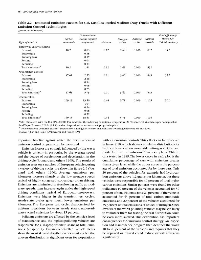
38
Air Pollution from Motor Vehicles
Table 2.2 Estimated Emission Factors for U.S. Gasoline-Fueled Medium-Duty Trucks with Different Emission Control Technologies
(grams per kilometer)
Type of control
Carbon monoxide
Non-methane volatile organic
compounds MethaneNitrogenoxides
Nitrous oxide
Carbon dioxide
Fuel efficiency(liters per
100 kilometers)
Three-way catalyst controlExhaustEvaporativeRunning lossRestingRefuelingTotal emissions
a
10.2
10.2
0.830.380.170.040.241.41
0.12
0.12
2.49
2.49
0.006
0.006
832
832
34.5
Non-catalyst controlExhaustEvaporativeRunning lossRestingRefuelingTotal emissions
a
47.61
47.61
2.552.160.940.080.255.73
0.21
0.21
3.46
3.46
0.006
0.006
843
843
35.7
UncontrolledExhaustEvaporativeRunning lossRestingRefuelingTotal emissions
a
169.13
169.13
13.563.930.940.080.32
18.51
0.44
0.44
5.71
5.71
0.009
0.009
1,165
1,165
50.0
Note:
Estimated with the U.S. EPA’s MOBILE5a model for the following conditions: temperature, 24 ºC; speed, 31 kilometers per hour; gasoline Reid Vapor Pressure, 62 kPa (9 PSI); and no inspection and maintenance program in place.
a
Total emissions comprise exhaust, evaporative, running loss, and resting emissions; refueling emissions are excluded.
Source:
Chan and Reale 1994; Weaver and Turner 1991
important baseline against which the effectiveness ofemission control programs can be measured.
Emission factors are strongly influenced by the way avehicle is driven—in particular, by the average speedand the degree of acceleration and deceleration in thedriving cycle (Joumard and others 1995). The results ofemission tests on a number of European vehicles, usinga variety of driving cycles, are shown in figure 2.9 (Jou-mard and others 1990). Average emissions perkilometer increase sharply at the low average speedstypical of highly congested stop-and-go urban driving.Emissions are minimized in free-flowing traffic at mod-erate speeds, then increase again under the high-speeddriving conditions typical of European motorways.Emissions were higher in the transient test cycles;steady-state cycles gave much lower emissions perkilometer. The European test cycle, characterized byuniform transitions between steady states, underesti-mates actual emissions by about 15 percent.
Pollutant emissions are affected by the vehicle’s levelof maintenance, and the highest-polluting vehicles areresponsible for a disproportionate share of total emis-sions (chapter 4). Emission-controlled vehicle fleetsshow the most skewed distribution of emissions, but theuneven distribution is significant even for populations
without emission controls. This effect can be observedin figure 2.10, which shows cumulative distributions forhydrocarbons, carbon monoxide, nitrogen oxides, andparticulate matter emissions from a sample of Chileancars tested in 1989. The lower curve in each plot is thecumulative percentage of cars with emissions greaterthan a given level, while the upper curve is the percent-age of total emissions accounted for by these cars. Only20 percent of the vehicles, for example, had hydrocar-bon emissions above 1.2 grams per kilometer, but thesevehicles were responsible for 40 percent of total hydro-carbon emissions. Similar patterns were found for otherpollutants: 10 percent of the vehicles accounted for 37percent of total PM emissions, 20 percent of the vehiclesaccounted for 43 percent of total carbon monoxideemissions, and 20 percent of the vehicles accounted for35 percent of total emissions of oxides of nitrogen. Sinceowners of the worst polluting vehicles may be less likelyto volunteer them for testing, the real distribution couldbe even more skewed. This distribution has importantconsequences for emissions control strategy. An inspec-tion and maintenance program that identifies the worst10 to 20 percent of the vehicles and requires that theybe repaired or retired could reduce overall emissionssignificantly.
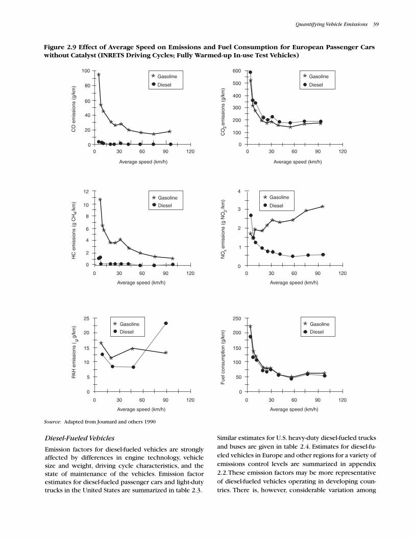
Quantifying Vehicle Emissions
39
Figure 2.9 Effect of Average Speed on Emissions and Fuel Consumption for European Passenger Carswithout Catalyst (INRETS Driving Cycles; Fully Warmed-up In-use Test Vehicles)
Source
: Adapted from Joumard and others 1990
Diesel-Fueled Vehicles
Emission factors for diesel-fueled vehicles are stronglyaffected by differences in engine technology, vehiclesize and weight, driving cycle characteristics, and thestate of maintenance of the vehicles. Emission factorestimates for diesel-fueled passenger cars and light-dutytrucks in the United States are summarized in table 2.3.
Similar estimates for U.S. heavy-duty diesel-fueled trucksand buses are given in table 2.4. Estimates for diesel-fu-eled vehicles in Europe and other regions for a variety ofemissions control levels are summarized in appendix2.2. These emission factors may be more representativeof diesel-fueled vehicles operating in developing coun-tries. There is, however, considerable variation among

40
Air Pollution from Motor Vehicles
Figure 2.10 Cumulative Distribution of Emissions from Passenger Cars in Santiago, Chile
Source:
Turner and others 1993
the estimates and measurements in the tables and ap-pendix because of differences in cycle conditions, differ-ences in the sample population, and different estimationtechniques. This indicates again the importance of actualemission measurements on the population of interest inorder to develop realistic emission factors.
The emission factor estimates for diesel-fueled pas-senger cars and light trucks in table 2.3 are comparableto the estimates for gasoline-fueled vehicles in table 2.1
and appendix 2.1. This is not true for the estimates forheavy-duty vehicles. Although heavy-duty diesel-fueledand gasoline-fueled vehicles are covered by similar emis-sion standards and test procedures, the average charac-teristics of the vehicles themselves differ considerably.Unlike heavy-duty gasoline-fueled vehicles, heavy-dutydiesel-fueled vehicles are primarily large trucks withgross vehicle weight ratings of 10 to 40 tons. The emis-sion factors in table 2.4 are therefore more representa-

Quantifying Vehicle Emissions
41
tive of large trucks (and buses) than smaller medium-duty trucks and vans. The opposite is true for the gaso-line-fueled vehicle emission factors in table 2.2.
Average pollutant emissions from heavy-duty diesel-fueled vehicles are especially sensitive to the speedand acceleration characteristics of the driving cycle.Emissions per kilometer vary according to the averagecycle speed. For heavy-duty diesel-fueled vehicles,emissions of carbon monoxide, hydrocarbons, andparticulate matter increase at low average speeds, dueto the stop-and-go driving associated with congestedtraffic. Emissions of nitrogen oxides and fuel consump-tion increase between 40 and 50 kilometers per hour(figure 2.11).
The effects of steady-state vehicle speed and road gra-dient on emissions and fuel consumption of a 40-ton semi-trailer truck are shown in figure 2.12. On negative grades,the emissions of all pollutants are insignificant, but they
increase sharply with increasing grades, particularly fornitrogen oxides and hydrocarbons. There is also somecorrelation of carbon monoxide and particulate emis-sions with speed and road gradient (Roumegoux 1995).
There are also large variations in particulate and hy-drocarbon emission factors for uncontrolled vehicles.This is partly the result of differences in maintenance,which can have a tremendous effect on particulate emis-sions. In testing buses in Chile, for example, particulatematter emissions from well-maintained buses were morethan 80 percent less than the average particulate emis-sions for the entire bus fleet. Cumulative probability dis-tributions for particulate matter, hydrocarbon, andnitrogen oxides emissions from the Chilean bus fleetillustrate the nature of the problem (figure 2.13). The 10percent of the buses with highest emissions are respon-sible for 25 percent of total particulate emissions, while20 percent of the buses produced 40 percent of the
Table 2.3 Estimated Emission and Fuel Consumption Factors for U.S. Diesel-Fueled Passenger Cars and Light-Duty Trucks
(grams per kilometer)
— Not applicable
Note:
MOBILE5 estimates.
Source:
Chan and Reale 1994; Weaver and Turner 1991; Weaver and Klausmeier 1988
Vehicle typeCarbon
monoxide HydrocarbonsNitrogen oxides
Particulatematter
Carbondioxide
Fuel consumption(liters/100 km)
Passenger carsAdvanced controlModerate controlUncontrolled
0.830.830.99
0.270.270.47
0.630.900.99
———
258403537
9.414.719.6
Light-duty trucksAdvanced controlModerate controlUncontrolled
0.940.941.52
0.390.390.77
0.731.011.37
———
358537559
13.019.623.3
Table 2.4 Estimated Emission and Fuel Consumption Factors for U.S. Heavy-Duty Diesel-Fueled Trucks and Buses
(grams per kilometer)
Vehicle typeCarbon
monoxide HydrocarbonsNitrogen oxides
Particulate matter
Carbondioxide
Fuel consumption(liters/100 km)
U.S. heavy-duty diesel trucksAdvanced controlModerate controlUncontrolled
6.337.247.31
1.321.722.52
5.0911.56
15.55
———
982991
1,249
35.735.745.5
U.S. 1984 measurementsSingle-axle tractorsDoubleaxle tractorsBuses
3.757.19
27.40
1.941.741.71
9.3717.012.40
1.071.472.46
1,0561,4641,233
———
New York City vehiclesMedium-heavy trucksTransit buses
——
2.845.22
23.28 34.89
2.462.66
——
53.880.7
— Not applicable
Note:
MOBILE5 estimates.
Source:
Chan and Reale 1994; Weaver and Turner 1991; Weaver and Klausmeier 1988

42
Air Pollution from Motor Vehicles
Figure 2.11 Effect of Average Speed on Emissions and Fuel Consumption for Heavy-Duty Swiss Vehicles
Source:
OFPE 1988

Quantifying Vehicle Emissions
43
Figure 2.12 Effect of Constant Average Speed and Road Gradient on Exhaust Emissions and Fuel Consumption for a 40-ton Semi-Trailer Truck
Note:
Figures in percent refer to road gradient.
Source:
Roumegoux 1995
emissions. The 20 percent of the buses with lowest emis-sions (generally those with the best maintenance) pro-duced only 7 percent of particulate emissions.
Motorcycles
Two- and three-wheeled vehicles, such as motorcyclesand auto-rickshaws, constitute a large portion of motor-
ized vehicles in developing countries, particularly inEast and South Asia. While they are responsible for a rel-atively small fraction of the total vehicle kilometers trav-eled in most countries, they are major sources of airpollution–particularly two-stroke engines running on amixture of gasoline and lubricating oil. It has been esti-mated that uncontrolled motorcycles in industrialized

44
Air Pollution from Motor Vehicles
countries emit 22 times the mass of hydrocarbons and10 times as much carbon monoxide as automobiles con-trolled to U.S. 1978 levels (OECD 1988). In Taiwan (Chi-na), hydrocarbon emissions from two-stroke enginemotorcycles were 13 times higher than the hydrocar-bon emissions from new four-stroke motorcycles andmore than 10 times higher than the hydrocarbon emis-sions from in-use passenger cars. Carbon monoxideemissions from two-stroke motorcycle engines weresimilar to those from four-stroke engines (Shen and Hua-ng 1991).
Data on motorcycle emissions are scarce. Availabledata pertain mostly to uncontrolled U.S. motorcycles,though limited information is also available fromEurope and Thailand.
United States
. Between 1970 and 1980, considerablestudy of motorcycle emissions was prompted by motor-
cycle emission regulations developed by U.S. EPA andCARB. Data on uncontrolled emissions from U.S. motor-cycles are from this period (table 2.5). These datainclude the only particulate emission measurements onmotorcycles available in the technical literature, andthey allow an assessment of the relationship betweensmoke opacity and particulate emissions. The data aremostly for high- powered, large-displacement touringmotorcycles, which are common in the United Statesbut not in most developing countries. Motorcycles usedin developing countries seldom exceed 250 cc in en-gine displacement. Due to their smaller size and weight,these motorcycles would be expected to have loweremissions than large touring motorcycles.
The average emissions for uncontrolled two-strokemotorcycles were 9.9 grams per kilometer of hydrocar-bons, 16.1 grams per kilometer of carbon monoxide,0.022 grams per kilometer of nitrogen oxides, and
Figure 2.13 Cumulative Distribution of Emissions from Diesel Buses in Santiago, Chile
Source:
Turner and others 1993
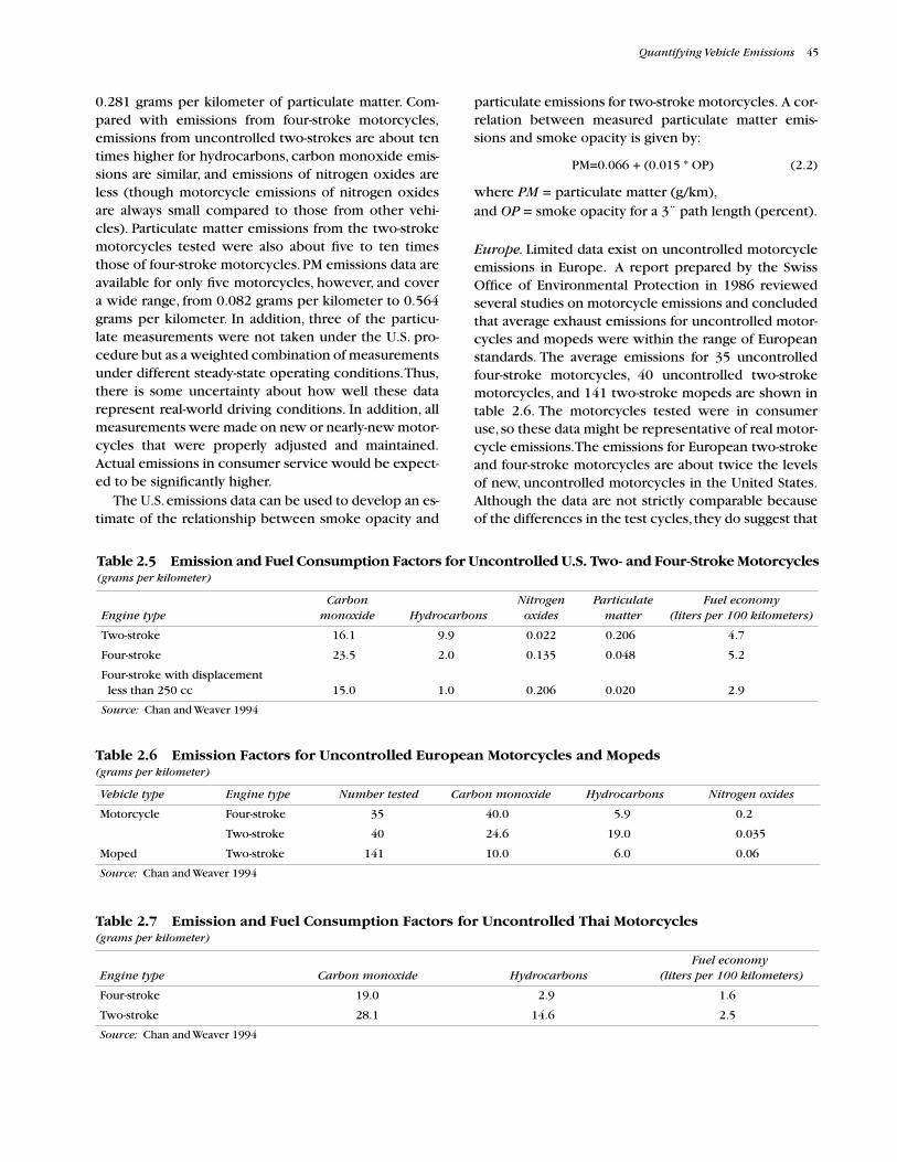
Quantifying Vehicle Emissions
45
0.281 grams per kilometer of particulate matter. Com-pared with emissions from four-stroke motorcycles,emissions from uncontrolled two-strokes are about tentimes higher for hydrocarbons, carbon monoxide emis-sions are similar, and emissions of nitrogen oxides areless (though motorcycle emissions of nitrogen oxidesare always small compared to those from other vehi-cles). Particulate matter emissions from the two-strokemotorcycles tested were also about five to ten timesthose of four-stroke motorcycles. PM emissions data areavailable for only five motorcycles, however, and covera wide range, from 0.082 grams per kilometer to 0.564grams per kilometer. In addition, three of the particu-late measurements were not taken under the U.S. pro-cedure but as a weighted combination of measurementsunder different steady-state operating conditions. Thus,there is some uncertainty about how well these datarepresent real-world driving conditions. In addition, allmeasurements were made on new or nearly-new motor-cycles that were properly adjusted and maintained.Actual emissions in consumer service would be expect-ed to be significantly higher.
The U.S. emissions data can be used to develop an es-timate of the relationship between smoke opacity and
particulate emissions for two-stroke motorcycles. A cor-relation between measured particulate matter emis-sions and smoke opacity is given by:
PM=0.066 + (0.015 * OP) (2.2)
where
PM
= particulate matter (g/km), and
OP
= smoke opacity for a 3¨ path length (percent).
Europe.
Limited data exist on uncontrolled motorcycleemissions in Europe. A report prepared by the SwissOffice of Environmental Protection in 1986 reviewedseveral studies on motorcycle emissions and concludedthat average exhaust emissions for uncontrolled motor-cycles and mopeds were within the range of Europeanstandards. The average emissions for 35 uncontrolledfour-stroke motorcycles, 40 uncontrolled two-strokemotorcycles, and 141 two-stroke mopeds are shown intable 2.6. The motorcycles tested were in consumeruse, so these data might be representative of real motor-cycle emissions. The emissions for European two-strokeand four-stroke motorcycles are about twice the levelsof new, uncontrolled motorcycles in the United States.Although the data are not strictly comparable becauseof the differences in the test cycles, they do suggest that
Table 2.6 Emission Factors for Uncontrolled European Motorcycles and Mopeds
(grams per kilometer)
Vehicle type Engine type Number tested Carbon monoxide Hydrocarbons Nitrogen oxides
Motorcycle Four-stroke 35 40.0 5.9 0.2
Two-stroke 40 24.6 19.0 0.035
Moped Two-stroke 141 10.0 6.0 0.06
Source:
Chan and Weaver 1994
Table 2.7 Emission and Fuel Consumption Factors for Uncontrolled Thai Motorcycles
(grams per kilometer)
Engine type Carbon monoxide HydrocarbonsFuel economy
(liters per 100 kilometers)
Four-stroke 19.0 2.9 1.6
Two-stroke 28.1 14.6 2.5
Source:
Chan and Weaver 1994
Table 2.5 Emission and Fuel Consumption Factors for Uncontrolled U.S. Two- and Four-Stroke Motorcycles(grams per kilometer)
Engine typeCarbon
monoxide HydrocarbonsNitrogen oxides
Particulate matter
Fuel economy(liters per 100 kilometers)
Two-stroke 16.1 9.9 0.022 0.206 4.7
Four-stroke 23.5 2.0 0.135 0.048 5.2
Four-stroke with displacement less than 250 cc 15.0 1.0 0.206 0.020 2.9
Source: Chan and Weaver 1994

46 Air Pollution from Motor Vehicles
Figure 2.14 Smoke Opacity Emissions from Motorcycles in Bangkok, Thailand
Source: Chan and Weaver 1994
average in-use emissions from uncontrolled motorcy-cles are higher than emissions from new, properly ad-justed motorcycles (Chan and Weaver 1994).
Thailand. A cumulative distribution plot of accelera-tion smoke opacity for 167 randomly selected motorcy-cles in Bangkok is shown in figure 2.14. More than 95percent of the motorcycles tested were equipped withtwo-stroke engines. The mean smoke opacity, correctedto a three-inch path length, was 61 percent—four timesthe opacity for the smokiest of the uncontrolled U.S.motorcycles with opacity measurements ranging from 3to 18 percent. By extrapolating the correlation in equa-tion 2.2 it can be estimated that the 61 percent averagesmoke opacity in Bangkok is equivalent to average par-ticulate matter emissions of about 1.0 grams per kilome-ter (figure 2.14).
The Thai Department of Pollution Control has gath-ered data on hydrocarbon and carbon monoxide emis-sions for 17 Thai-produced motorcycles based on theEuropean test cycle. These data were obtained frommanufacturers and thus probably represent new, prop-erly-adjusted motorcycles (table 2.7). Of the 17 motor-cycles, two had four-stroke engines and the rest hadtwo-strokes. Average hydrocarbon and carbon monox-ide emissions for the two-stroke motorcycles were 14.6
and 28.1 grams per kilometer, respectively; the averagesfor the four-stroke motorcycles were 2.9 and 19.0 gramsper kilometer, respectively. These values are similar tobut lower than the average for European motorcyclesreported in table 2.6. Since the Thai data are for newmotorcycles and the European data are for motorcyclesin use, this is not surprising. In addition to having loweremissions, four-stroke motorcycles also had much bet-ter fuel economy than the two-strokes, averaging 1.6liters per 100 kilometers compared with 2.5 liters per100 kilometers for the two-stroke motorcycles.
References
Alson, J., J. Adler, and T. Baines. 1989. “Motor VehicleEmission Characteristics and Air Quality Impacts ofMethanol and Compressed Natural Gas.” in D. Sper-ling, ed. Alternate Transportation Fuels: An Envi-ronmental and Energy Solution. Greenwood Press,Wesport, Connecticut.
Andrias, A., D. Zafiris, Z. Samras, and K-H. Zierock.1992. “Computer Program to Calculate Emissionsfrom Road Traffic—User’s Manual,” COPERT, EC Con-tract No. B4-3045 (91) 10 PH (DG XI/B/3), EuropeanCommission, Brussels.

Quantifying Vehicle Emissions 47
AQIRP. 1995. “Real World Automotive Emissions – Re-sults of Studies in the Fort McHenry and TuscaroraMountain Tunnels.” Air Quality Improvement Re-search Program, Technical Bulletin No. 14. Auto/OilIndustry Research Council, Atlanta, Georgia.
_____. 1996. “Dynamometer Study of Off-Cycle ExhaustEmissions.” Air Quality Improvement Research Pro-gram, Technical Bulletin No. 19. Auto/Oil IndustryCouncil, Atlanta, Georgia.
Baines, T. 1994. “Personal Communication.” U.S. Envi-ronmental Protection Agency, Office of Mobile Sourc-es, Washington, D.C.
Brunner, D., K. Sclapfer, M. Ros, and F. Dinkel. 1994.“Data Bank on Unregulated Vehicle Exhaust andEvaporative Emissions.” 3rd International Sympo-sium on Transport and Air Pollution, Poster Proceed-ings, INRETS, Arcueil, France.
Chan, L.M. and M. Reale. 1994. “Emissions Factors Gen-erated from In-House MOBILE5a.” Engine, Fuel, andEmissions Engineering. Sacramento, California.
Chan, L.M. and C.S. Weaver. 1994. “Motorcycle EmissionStandards and Emission Control Technology.”Departmental Paper Series, No. 7, Asia Technical De-partment, The World Bank, Washington, D.C.
Chan, L.M. and C.S. Weaver. 1995. “Figures Generatedwith the Use of MOBILE5a,” Engine, Fuel, and Emis-sions Engineering, Sacramento, California.
Chongpeerapien, T., S. Sungsuwan, P. Kritiporn, S. Bura-nasajja. 1990. “Energy and Environment, Choosingthe Right Mix.” Resource Management Associates Re-search Report No. 7, Thailand Development Re-search Institute, Bangkok.
CONCAWE (Conservation of Clean Air and Water in Eu-rope). 1994. Motor Vehicle Emission Regulationsand Fuel Specifications–1994 Update. Report 4/94.
Cornetti, G., K. Klein, G. Frankle, and H. Stein. 1988.“U.S. Transient Cycle Versus ECE R.49 13 – ModeCycle.” SAE Paper 880715, Society of AutomotiveEngineers, Warrendale, Pennsylvania.
Eggleston, H., N. Gorissen, R. Joumard, R. Rijkeboeer, Z.Samaras, and K. Zierock. 1991. “CORINAIR WorkingGroup on Emission Factors for Calculating 1990Emissions From Road Traffic.” Volume 1. Methodolo-gy and Emission Factors. Final Report, EC Study Con-tract B4-3045(91)10PH. Commission of theEuropean Communities. Brussels.
Escudero, J. 1991. “Notes on Air Pollution Issues in San-tiago Metropolitan Region,” Letter #910467, datedMay 14, 1991. Comisión Especial de Descontami-nación de la Region Metropolitana. Santiago.
Faiz, A., S. Gautam, and E. Burki. 1995. “Air Pollutionfrom Motor Vehicles: Issues and Options for LatinAmerican Countires.” The Science of the Total Envi-ronment, 169:303-310.
Faiz, A., and J. Aloisi de Larderel. 1993. “Automotive AirPollution in Developing Countries: Outlook and Con-trol Strategies”. The Science of the Total Environ-ment, 134: 325–344.
Guensler, R. 1994. “Loop Holes for Air Pollution,” ITS Re-view, Volume 18, Number 1. University of California,Berkeley.
IGRP (Indonesian German Research Project). 1991. “En-vironmental Impacts of Energy Strategies for Indone-sia.” VWS Report on Assessment of the EmissionCoefficients of the Traffic Sector in Jawa. Jakarta.
Joumard, R., L. Paturel, R. Vidon, J. P. Guitton, A. Saber,and E. Combet. 1990. Emissions Unitaires de Pollu-ants des Véhicules Légers. Report 116 (2nd ed.) Insti-tut National du Recherche sur les Transports et LeurSecurite (INRETS), Bron, France.
Joumard, R., P. Jost, J. Hickman, and D. Hassel. 1995.“Hot Passenger Car Emissions Modelling as aFunction of Instantaneous Speed and Acceleration.”The Science of the Total Environment, 169: 167-174.
Laurikko, J. 1995. “Ambient Temperature Effect on Auto-motive Exhaust Emissions: FTP and ECE Test CycleResponses.” The Science of the Total Environment,169: 195-204.
Lenaers, G. 1994. “A Dedicated System for On-the-roadExhaust Emissions Measurements on Vehicles.” 3rdInternational Symposium on Transport and Air Pollu-tion, Poster Proceedings, INRETS, Arcueil, France.
OECD (Organization for Economic Cooperation & De-velopment). 1988. Transport and the Environment.Paris.
OFPE (l’Office federal de la protection de l’environne-ment). 1988. “Emissions Polluantes du Trafic RoutierPrive de 1950 a 2000.” Les cahiers de l'environne-ment 55, Berne, Switzerland.
Pattas, K., N. Kyriakis, and Z. Samaras. 1985. “ExhaustEmission Study of the Current Vehicle Fleet in Athens(Phase II).” Final Report. 3 volumes. University ofThessaloniki, Greece.
Radian Corporation. 1993. “Revision of the MOBILE-MEXICO (Mobile Mexico) Model Report.” Departa-mento del Distrito Federal, Mexico City, Mexico.
Roumegoux, J.P. 1995. “Calcul des Emissions Unitairesde Polluants des Véhicules Utilitaires”, The Science ofthe Total Environment, 169: 273-82.
Sandoval, H., M. Prendez, and P. Ulriksen eds. 1993. Con-taminacion Atmosferica de Santiago: Estado Actualy Soluciones, University of Chile, Santiago.
Shen, S., and Huang, K. 1991. “Response to Transport-In-duced Air Pollution: The Case of Taiwan.” in M.L. Birkand D.L. Bleviss, eds., Driving New Directions:Transportation Experiences and Options in Devel-oping Countries. International Institute for EnergyConservation, Washington, D.C.

48 Air Pollution from Motor Vehicles
Steiner, A. 1989. “Operacion y Resultados del Programade Mediciones de la UMEVE.” Paper Presented at theSeminar on Contaminacion Atmosferica Debido aMotores de Combustion Interna, Santa Maria Univer-sity, Valparaiso, Chile.
Turner, S.H., C.S. Weaver, and M.J. Reale. 1993. “Costand Emissions Benefits of Selected Air Pollution Con-trol Measures in Santiago, Chile.” Engine, Fuel, andEmissions Engineering, Inc. Sacramento, California
Weaver, C.S., and R. Klausmeier. 1988. “Heavy-DutyDiesel Vehicle Inspection and Maintenance Study.”
Report to the California Air Resources Board, Engine,Fuel, and Emissions Engineering Inc., Sacramento,California.
Weaver, C.S., and S. Turner. 1991. “Mobile SourceEmission Factors for Global Warming Gases.” Reportto U.S. EPA Contract 68-W8-0113. Sacramento,California.
Weaver, C.S., and L.M. Chan. 1995. “Company Archives”Multiple Sources. Engine, Fuel, and Emissions Engi-neering Inc., Sacramento, California.

49
Selected Exhaust Emission and Fuel Consumption Factorsfor Gasoline-Fueled Vehicles
Appendix 2.1
Table A2.1.1 Exhaust Emissions, European Vehicles, 1970–90 Average
(grams per kilometer)
Traffic type and engine/emission control characteristics Carbon monoxide Hydrocarbons Nitrogen oxides Particulate matter
Urban
Two-stroke 32.9 20.2 0.26 0.00
More than 2,000 cc 32.0 3.0 2.00 0.01
1,400–2,000 cc 31.0 2.9 1.80 0.10
Less than 1,400 cc 30.0 2.8 1.70 0.14
Catalyst without O
2
sensor 6.6 0.9 1.00 0.00
Catalyst with O
2
sensor 1.5 0.2 0.27 0.00
Rural highway
Two-stroke 21.6 13.0 0.33 0.00
More than 2,000 cc 21.0 2.2 2.49 0.01
1,400–2,000 cc 20.0 2.1 2.29 0.01
Less than 1,400 cc 19.0 2.0 2.09 0.01
Catalyst without O
2
sensor 4.5 0.5 1.15 0.00
Catalyst with O
2
sensor 1.2 0.1 0.24 0.00
Motorway
Two-stroke 22.7 13.0 0.42 0.00
More than 2,000 cc 21.5 2.3 3.03 0.01
1,400–2,000 cc 20.5 2.2 2.83 0.01
Less than 1,400 cc 19.5 2.1 2.63 0.01
Catalyst without O
2
sensor 5.0 0.5 1.35 0.00
Catalyst with O
2
sensor 1.3 0.1 0.32 0.00
Source:
Metz 1993
Table A2.1.2 Exhaust Emissions, European Vehicles, 1995 Representative Fleet
(grams per kilometer)
Emission regulations/controls Carbon monoxide Hydrocarbons Nitrogen oxides Carbon dioxide Particulate matter
ECE 15-03 31.5 3.57 2.29 188 —
ECE 15-04 24.1 2.97 2.40 192 —
Three-way catalytic converter 5.2 0.32 0.40 247 —
Diesel
a
0.7 0.13 1.22 188 0.14
— Not applicablea. Included for comparison.
Source:
Joumard and others 1995

50
Air Pollution from Motor Vehicles
Table A2.1.3 Estimated Emissions and Fuel Consumption, European Vehicles, Urban Driving
(grams per kilometer)
n.a. = Not available— Not applicable
Notes:
• Average driving speed 25 kilometers per hour.• Emission factors in g/km are derived from the COPERT model for 1990, utilizing the CORINAIR methodology for road traffic emissions. The pollutants included are:CO, NMVOC, NO
x
, CH
4
, N
2
O, NH
3
. Fuel consumption is also estimated. Total VOC (or HC) emission factors may be obtained by adding NM-VOC and CH
4
factors.• Cold-start emissions are calculated for urban driving conditions only, taking into account the monthly variation of the average minimum and maximum temperatures.For this specific application, average temperatures in Brussels (Belgium) were used, with the following monthly distribution:
• Evaporative losses are estimated in g/km; REID vapor pressure of gasoline 80 kPa (from October to March) and 65 kPa (from April to September) with monthlytemperatures given in note 3. • For cold-starts and evaporation losses, average trip length equals 12 km.
Source:
Samaras 1992
Vehicle type
Carbon monoxide
(CO)
Non-methanevolatile org. compounds
(NM-VOC)
Nitrogen oxides(NO
x
)Methane
(CH
4
)
Nitrous oxide(N
2
O)Ammonia
(NH
3
)Evap.
emissions
Fuel consumption(liter/100 km)
Passenger Cars
Two-stroke 20.7 15.2 0.3 0.150 0.005 0.002 1.13 14.93
LPG 6.9 11.8 1.9 0.122 0.000 0.000 — 8.78
Pre-1971 (Pre ECE)
Less t..han 1,400 cc 56.8 4.2 1.7 0.224 0.005 0.002 1.13 12.99
1,400-2,000 cc 56.8 4.2 1.9 0.224 0.005 0.002 1.13 15.38
More than 2,000 cc 56.8 4.2 2.4 0.224 0.005 0.002 1.13 19.23
1972-76 (ECE15/00-01)
Less than 1,400 cc 41.6 3.3 1.7 0.224 0.005 0.002 1.13 11.63
1,400-2,000 cc 41.6 3.3 1.9 0.224 0.005 0.002 1.13 13.89
More than 2,000 cc 41.6 3.3 2.4 0.224 0.005 0.002 1.13 15.63
1977-79 (ECE15/02)
Less than 1,400 cc 35.4 3.3 1.5 0.224 0.005 0.002 1.13 10.64
1,400-2,000 cc 35.4 3.3 1.7 0.224 0.005 0.002 1.13 12.82
More than 2,000 cc 35.4 3.3 2.0 0.224 0.005 0.002 1.13 15.87
1980-84 (ECE15/03)
Less than 1,400 cc 22.3 3.3 1.6 0.224 0.005 0.002 1.13 10.64
1,400-2,000 cc 22.3 3.3 1.9 0.224 0.005 0.002 1.13 12.82
More than 2,000 cc 22.3 3.3 2.5 0.224 0.005 0.002 1.13 15.87
1985-89 (ECE15/04)
Less than 1,400 cc 21.4 2.6 1.6 0.224 0.005 0.002 1.13 5.71
1,400-2,000 cc 21.4 2.6 1.9 0.224 0.005 0.002 1.13 10.53
More than 2,000 cc 21.4 2.6 2.3 0.224 0.005 0.002 1.13 18.29
Improved conventional
Less than 1,400 cc 13.5 1.8 1.4 0.224 0.005 0.002 1.13 7.94
1,400-2,000 cc 7.8 1.5 1.5 0.224 0.005 0.002 1.13 10.53
Oxidizing catalyst without l sensor
Less than 1,400 cc 15.7 1.6 1.1 0.224 0.005 0.002 1.13 8.70
1,400-2,000 cc 7.6 0.4 0.9 0.224 0.005 0.002 1.13 10.53
3 way catalyst with l sensor
Less than 1,400 cc 4.1 0.4 0.4 0.062 0.050 0.070 0.23 8.47
1,400-2,000 cc 4.1 0.4 0.4 0.062 0.050 0.070 0.23 10.31
More than 2,000 cc 4.1 0.4 0.4 0.062 0.050 0.070 0.23 12.99
Light-duty vehicles 46.1 4.7 3.1 0.230 0.006 0.002 1.03 17.86
Motorcycles
Less than 50 cm3 10.0 5.9 0.1 0.100 0.001 0.001 0.28 2.40
More than 50 cm3, two-stroke 22.0 14.9 0.1 0.150 0.002 0.002 0.45 4.00
More than 50 cm3, four-stroke 20.0 2.8 0.3 0.200 0.002 0.002 0.45 5.08
Month 01 02 03 04 05 06 07 08 09 10 11 12
Tmin (°C) -1.2 0.3 2.2 5.1 7.9 10.9 12.1 12.2 10.6 7.3 3.1 0.2
Tmax (°C) 4.3 6.7 10.3 14.2 18.4 22.0 22.7 22.3 20.5 15.4 8.9 5.6

Selected Exhaust Emission and Fuel Consumption Factors for Gasoline-Fueled Vehicles
51
Table A2.1.4 Estimated Emissions and Fuel Consumption, European Vehicles, Rural Driving
(grams per kilometer)
— Not applicablen.a. = Not available
Notes:
• Average driving speed, 75 kilometers per hour.• Emission factors in g/km are derived from the COPERT model for 1990, utilizing the CORINAIR methodology for road traffic emissions. The pollutants included are:CO, NMVOC, NO
x
, CH
4
, N
2
O, NH
3
. Fuel consumption is also estimated. Total VOC (or HC) emission factors may be obtained by adding NMVOC and CH
4
factors.• Cold-start emissions are calculated for urban driving conditions only, taking into account the monthly variation of the average minimum and maximum temperatures.For this specific application, average temperatures in Brussels (Belgium) were used, with the following monthly distribution:
• Evaporative losses are estimated in g/km; REID vapor pressure of gasoline 80 kPa (from October to March) and 65 kPa (from April to September) with monthlytemperatures given in note 3. • For cold-starts and evaporation losses, average trip length equals 12 km.
Source:
Samaras 1992
Vehicle type
Carbon monoxide
(CO)
Non-methanevolatile org. compounds
(NM-VOC)
Nitrogen oxides(NO
x
)Methane(CH
4
)
Nitrous oxide(N
2
O)Ammonia
(NH
3
)Evap.
emissions
Fuel consumption(liter/100 km)
Passenger Cars
Two-stroke 7.5 7.24 1.0 0.040 0.005 0.002 0.14 8.77
LPG
3.1 0.6 2.6 0.035 0.000 0.000 – 6.02
Pre-1971 (Pre ECE)
Less than 1,400 cc 18.5 1.53 2.1 0.025 0.005 0.002 0.14 7.35
1,400-2,000 cc 18.5 1.53 2.8 0.025 0.005 0.002 0.14 8.93
More than 2,000 cc 18.5 1.53 4.3 0.025 0.005 0.002 0.14 10.64
1972-76 (ECE 15/00-01)
Less than 1,400 cc 14.8 1.23 2.1 0.025 0.005 0.002 0.14 5.88
1,400-2,000 cc 14.8 1.23 2.8 0.025 0.005 0.002 0.14 6.94
More than 2,000 cc 14.8 1.23 4.3 0.025 0.005 0.002 0.14 7.75
1977-79 (ECE 15/02)
Less than 1,400 cc 7.9 1.03 2.2 0.025 0.005 0.002 0.14 6.02
1,400-2,000 cc 7.9 1.03 2.5 0.025 0.005 0.002 0.14 6.85
More than 2,000 cc 7.9 1.03 2.8 0.025 0.005 0.002 0.14 8.47
1980-84 (ECE 15/03)
Less than 1,400 cc 8.3 1.03 2.3 0.025 0.005 0.002 0.14 6.02
1,400-2,000 cc 8.3 1.03 2.8 0.025 0.005 0.002 0.14 6.45
More than 2,000 cc 8.3 1.03 3.4 0.025 0.005 0.002 0.14 8.00
1985-89 (ECE 15/04)
Less than 1,400 cc 4.7 0.83 2.2 0.025 0.005 0.002 0.14 5.78
1,400-2,000 cc 4.7 0.83 2.7 0.025 0.005 0.002 0.14 6.45
More than 2,000 cc 4.7 0.83 2.9 0.025 0.005 0.002 0.14 8.00
Improved conventional
Less than 1,400 cc 6.5 0.73 2.2 0.025 0.005 0.002 0.14 6.37
1,400-2,000 cc 2.3 0.63 2.7 0.025 0.005 0.002 0.14 7.25
Oxidizing catalyst without l sensor
Less than 1,400 cc 5.5 0.53 1.7 0.025 0.005 0.002 0.14 6.58
1,400-2,000 cc 3.6 0.13 1.5 0.025 0.005 0.002 0.14 7.52
3-way catalyst with l sensor
Less than 1,400 cc 1.4 0.12 0.3 0.020 0.050 0.100 0.03 6.25
1,400-2,000 cc 1.4 n.a. 0.3 n.a. 0.050 0.100 0.03 7.30
More than 2,000 cc 1.4 0.12 0.3 0.020 0.050 0.100 0.03 8.85
Light-duty vehicles 15.0 1.7 2.7 0.040 0.006 0.002 0.14 9.03
Motorcycles
Less than 50 cm
3
10.0 6.00 0.1 0.100 0.001 0.001 0.00 2.40
More than 50 cm
3
, two-stroke 22.0 15.05 0.1 0.150 0.002 0.002 0.06 4.00
More than 50 cm
3
, four-stroke 20.0 3.00 0.3 0.200 0.002 0.002 0.06 5.08
Month 01 02 03 04 05 06 07 08 09 10 11 12
Tmin (ºC) -1.2 0.3 2.2 5.1 7.9 10.9 12.1 12.2 10.6 7.3 3.1 0.2
Tmax (ºC) 4.3 6.7 10.3 14.2 18.4 22.0 22.7 22.3 20.5 15.4 8.9 5.6

52
Air Pollution from Motor Vehicles
Table A2.1.5 Estimated Emissions and Fuel Consumption, European Vehicles, Highway Driving
(grams per kilometer)
— Not applicable
Notes:
• Average driving speed, 100 kilometers per hour.• Emission factors in g/km are derived from the COPERT model for 1990, utilizing the CORINAIR methodology for road traffic emissions. The pollutants included are:CO, NMVOC, NO
x
, CH
4
, N
2
O, NH
3
. Fuel consumption is also estimated. Total VOC (or HC) emission factors may be obtained by summing up NMVOC and CH4.• Cold-start emissions are calculated for urban driving conditions only, taking into account the monthly variation of the average minimum and maximum temperatures.For this specific application, average temperatures in Brussels (Belgium) were used, with the following monthly distribution:
• Evaporative losses are estimated in g/km; REID vapor pressure of gasoline from 80 kPa (from October to March) and 65 kPa (from April to September) with monthlytemperatures given in note 3. • For cold-starts and evaporation losses, average trip length equals 12 km.
Source:
Samaras 1992
Vehicle type
Carbon monoxide
(CO)
Non-methanevolatile org. compounds
(NM-VOC)
Nitrogen oxides(NO
x
)Methane(CH
4
)
Nitrous oxide(N
2
O)Ammonia(NH
3
)Evap.
emissions
Fuel consumption(liter/100 km)
Passenger Cars
Two-stroke 8.7 0.93 0.7 0.025 0.005 0.002 0.14 7.58
LPG 9.8 0.5 2.9 0.025 0.000 0.000 — 7.23
Pre-1971 (Pre-ECE)
Less than 1,400 cc 15.5 1.23 2.0 0.026 0.005 0.002 0.14 8.33
1,400-2,000 cc 15.5 1.23 3.1 0.026 0.005 0.002 0.14 10.20
More than 2,000 cc 15.5 1.23 5.5 0.026 0.005 0.002 0.14 11.76
1972-76 (ECE 15/00-01)
Less than 1,400 cc 18.6 1.13 2.0 0.026 0.005 0.002 0.14 6.49
1,400-2,000 cc 18.6 1.13 3.1 0.026 0.005 0.002 0.14 8.06
More than 2,000 cc 18.6 1.13 5.5 0.026 0.005 0.002 0.14 8.85
1977-79 (ECE 15/02)
Less than 1,400 cc 8.3 0.93 2.9 0.026 0.005 0.002 0.14 6.85
1,400-2,000 cc 8.3 0.93 3.3 0.026 0.005 0.002 0.14 7.94
More than 2,000 cc 8.3 0.93 3.7 0.026 0.005 0.002 0.14 9.43
1980-84 (ECE 15/03)
Less than 1,400 cc 7.9 0.93 3.3 0.026 0.005 0.002 0.14 6.85
1,400-2,000 cc 7.9 0.93 3.8 0.026 0.005 0.002 0.14 7.94
More than 2,000 cc 7.9 0.93 4.5 0.026 0.005 0.002 0.14 9.43
1985-89 (ECE 15/04)
Less than 1,400 cc 4.3 0.73 2.7 0.026 0.005 0.002 0.14 6.37
1,400-2,000 cc 4.3 0.73 3.5 0.026 0.005 0.002 0.14 6.98
More than 2,000 cc 4.3 0.73 3.7 0.026 0.005 0.002 0.14 9.35
Improved conventional
Less than 1,400 cc 10.5 0.83 2.4 0.026 0.005 0.002 0.14 9.26
1,400-2,000 cc 6.7 0.73 3.7 0.026 0.005 0.002 0.14 10.42
Oxidizing catalyst without
λ
sensor
Less than 1,400 cc 8.4 0.53 1.9 0.026 0.005 0.002 0.14 9.01
1,400-2,000 cc 6.7 0.23 1.6 0.026 0.005 0.002 0.14 10.87
3-way catalyst with
λ
sensor
Less than 1,400 cc 3.1 0.12 0.5 0.020 0.050 0.001 0.03 8.70
1,400-2,000 cc 3.1 0.12 0.5 0.020 0.050 0.001 0.03 10.20
More than 2,000 cc 3.1 0.12 0.5 0.020 0.050 0.001 0.03 12.99
Light-duty vehicles 12.0 1.0 3.2 0.025 0.002 0.006 0.14 8.54
Motorcycles
Less than 50 cm
3
10.0 6.00 0.1 0.100 0.001 0.001 0.00 2.40
More than 50 cm
3
, two-stroke 22.0 15.05 0.1 0.150 0.002 0.002 0.06 4.00
More than 50 cm
3
, four-stroke 20.0 3.00 0.3 0.200 0.002 0.002 0.06 5.08
Month 01 02 03 04 05 06 07 08 09 10 11 12
Tmin (ºC) -1.2 0.3 2.2 5.1 7.9 10.9 12.1 12.2 10.6 7.3 3.1 0.2
Tmax (ºC) 4.3 6.7 10.3 14.2 18.4 22.0 22.7 22.3 20.5 15.4 8.9 5.6

Selected Exhaust Emission and Fuel Consumption Factors for Gasoline-Fueled Vehicles
53
Table A2.1.6 Automobile Exhaust Emissions, Chile
(grams per kilometer)
Vehicle type Carbon monoxide Hydrocarbons Nitrogen oxides Particulate matter
Private car 26.0 1.00 1.2 0.07
Taxi 28.0 1.50 1.4 0.06
Note:
Measured using the U.S. federal testing procedure.
Source:
Escudero 1991
Table A2.1.7 Automobile Exhaust Emissions as a Function of Test Procedure and Ambient Temperature, Finland
(grams per kilometer)
53 5 Hydrocarbons Nitrogen oxides
ECE-1522°C-7°-20°C
2.6011.2217.81
0.271.092.79
0.270.650.62
FTP-7522°C-7°C-20°C
1.405.348.58
0.130.501.25
0.160.290.31
Note:
Based on emission tests on cars with a three-way catalytic converter.
Source:
Laurikko 1995
Table A2.1.8 Automobile Exhaust Emissions as a Function of Driving Conditions, France
(grams per kilometer)
Traffic type Carbon monoxide Hydrocarbons Nitrogen oxides Carbon dioxide
Congested urban 94.1 10.70 1.6 520.73
Free-flowing urban 29.3 3.52 1.8 189.54
Highway 19.4 2.45 2.2 149.05
Motorway 16.0 1.09 3.0 153.48
Source:
Joumard and others 1990
Table A2.1.9 Automobile Exhaust Emissions and Fuel Consumption as a Function of Driving Conditions and Emission Controls, Germany
(grams per kilometer)
Vehicle typeCarbon
monoxide HydrocarbonsNitrogenoxides
Carbondioxide
Fuel consumption (li-ters/100km)
European test procedure (low-speed urban driving with cold start)
Catalyst with O
2
sensor 6.27 0.81 0.59 274 11.90
Catalyst without O
2
sensor 15.34 1.93 0.94 234 9.80
No catalyst 17.67 2.62 1.29 243 10.50
U.S. federal test procedure (mixed urban driving)
Catalyst with O
2
sensor 3.02 0.27 0.39 204 8.90
Catalyst without O
2
sensor 11.76 1.35 0.88 180 7.80
No catalyst 12.14 1.84 1.63 182 7.90
Rural highway
Catalyst with O
2
sensor 0.98 0.06 0.28 136 5.90
Catalyst without O
2
sensor 3.98 0.42 1.15 130 5.60
No catalyst 4.89 0.76 1.94 126 5.50
Motorway
Catalyst with O
2
sensor 5.13 0.14 0.75 193 8.30
Catalyst without O
2
sensor 12.72 0.60 1.74 189 8.20
No catalyst 12.78 0.94 3.18 178 7.70
Source:
Hassel and Weber 1993

54
Air Pollution from Motor Vehicles
Table A2.1.10 Exhaust Emissions, Light-Duty Vehicles and Mopeds, Greece
(grams per kilometer)
Vehicle type Carbon monoxide Hydrocarbons Nitrogen oxides
Light-duty 45.8 1.6 1.60
Motorcycle 21.4 3.4 0.11
Moped 14.0 10.4 0.05
Note:
Measured using the ECE-15 testing procedure.
Source:
Pattas, Kyriakis, and Nakos 1993
Table A2.1.11 Hot-Start Exhaust Emissions, Light-Duty Vehicles, Greece
(grams per kilometer
)
Engine capacity/Emission standard Carbon monoxide Hydrocarbons Nitrogen oxides
Less than 1,400 ccPre-control (1971)ECE 15-00 (1971–75)ECE 15-02 (1975–79)ECE 15-03 (1980–84)ECE 15-04 (1985–present)
60.0258.1744.3731.3325.50
5.154.803.773.602.08
1.231.421.581.812.08
1,400–2,000 ccPre-controlECE 15-00ECE 15-02ECE 15-03ECE 15-04
73.6154.5151.2035.9427.99
4.874.673.653.272.11
1.061.821.751.952.06
More than 2,000 ccPre-controlECE 15-00ECE 15-02ECE 15-03ECE 15-04
77.1291.9721.2881.5030.18
5.605.851.623.322.14
1.400.772.281.022.04
Note:
Measured using the ECE-15 testing procedure, average speed 18.7 kilometers per hour.
Source:
Pattas, Kyriakis, and Nakos 1993
Table A2.1.12 Exhaust Emissions, Light-Duty Vehicles and 2-3 Wheelers, India
(grams per kilometer)
— Not applicable
n.a. = Not available
Sources:
Biswas and Dutta 1994; Bose 1994; Gargava and Aggarwal 1994
Vehicle typeCarbon
monoxideHydro-carbons
Nitrogen oxides
Sulfurdioxide
Car/Jeep 23.8 3.5 1.6 0.1
Taxi 29.1 4.3 1.9 0.1
Two-wheeler 8.2 5.1 — —
Auto-rickshaw (3-wheeler) 12.5 7.8 — 0.0
Light-duty vehicles 40.0 6.0 3.2 0.08
Motorcycles 17.0 10.0 0.07 0.02

Selected Exhaust Emission and Fuel Consumption Factors for Gasoline-Fueled Vehicles
55
References
Biswas, D. and S.A. Dutta. 1994. “Strategies for Controlof Vehicular Pollution in Urban Areas of India.” Pro-ceedings of a Workshop on The Energy Nexus—In-dian Issues & Global Impacts (April 22–23, 1994),University of Pennsylvania, Philadelphia.
Escudero, J. 1991. “Notes on Air Pollution Issues in San-tiago Metropolitan Region”, Letter # 910467, datedMay 14, 1991. Comisión Especial de Descontami-nación de la Region Metropolitana. Santiago, Chile.
Gargava, P., and A. Aggarwal. 1994. “Prediction of Im-pact of Air Environment on Planning the ControlStrategies for Automobile Pollution in an IndianCoastal City.”
Poster Proceedings
, 3rd InternationalInternational Symposium on Transport and Air Pollu-tion, INRETS, Arcueil, France.
Hassel, D. and F-J. Weber. 1993. “Mean Emissions andFuel Consumption of Vehicles in Use with DifferentEmission Reduction Concepts.”
The Science of theTotal Environment
134: 189-95.Joumard, R., L. Paturel, R. Vidon, J. P. Guitton, A. Saber,
and E. Combet. 1990.
Emissions Unitaires de Pollu-
ants des Véhicules Légers.
Report 116 (2nd ed.) Insti-tut National du Recherche sur les Transports et leurSecurite (INRETS), Bron, France.
Joumard, R., P. Jost, J. Hickman, and D. Hassel. 1995.“Hot Passenger Car Emissions Modelling as a Func-tion of Instantaneous Speed and Acceleration.”
TheScience of the Total Environment
, 169: 167-74.Laurikko, J. 1995. “Ambient Temperature Effect on Auto-
motive Exhaust Emissions: FTP and ECE Test CycleResponses.”
The Science of the Total Environment
,169: 195-204.
Metz, N. 1993. “Emission Characteristics of DifferentCombustion Engines in City, on Rural Roads, and onHighways.”
The Science of the Total Environment
,134: 225-35.
Pattas, K., N. Kyriakis, and C. Nakos. 1993. “Time De-pendence of Traffic Emissions in the Urban Area ofThessaloniki.”
The Science of the Total Environment
134: 273-84. Samaras, Z. 1992. “COPERT Emission Factors.” Informal
Communication. Directorate-General for Environ-ment, Nuclear Safety, and Civil Protection, Commis-sion of the European Communities, Brussels.


57
Selected Exhaust Emission and Fuel Consumption Factorsfor Diesel-Fueled Vehicles
Appendix 2.2
Table A2.2.1 Exhaust Emissions, European Cars
(grams per kilometer)
Traffic type/emission control Carbon monoxide Hydrocarbons Nitrogen oxides Particulate matter
Urban
with catalyst 0.05 0.08 0.70 0.20
without catalyst 1.30 0.10 0.90 0.30
Rural
with catalyst 0.02 0.10 0.61 0.18
without catalyst 0.60 0.10 0.79 0.29
Highway
with catalyst 0.20 0.10 0.77 0.27
without catalyst 0.70 0.10 0.97 0.37
Source:
Metz 1993
Table A2.2.2 Estimated Emissions and Fuel Consumption, European Cars and Light-Duty Vehicles
(grams per kilometer)
Notes:
• Average driving speeds for urban, rural and motorway are 25 km/hour, 75 km/hour and 100 km/hour, respectively.• Emission factors in g/km are derived from the COPERT model for 1990, utilizing the CORINAIR methodology for road traffic emissions. Thepollutants included are: CO, HC, NO
x
, TPM. Fuel consumption is also estimated.
Source:
Samaras 1992
Traffic and vehicle type Carbon monoxide Hydrocarbons Nitrogen oxidesParticulate
matterFuel consumption
(liters/100km)
Urban
Passenger cars Less than 2,000 cc More than 2,000 ccLight-duty vehicles
1.01.02.4
0.3060.3060.506
0.71.01.7
0.3620.3620.333
10.010.014.08
Rural
Passenger cars Less than 2,000 cc More than 2,000 ccLight-duty vehicles
0.50.50.8
0.1050.1050.205
0.40.71.2
0.1310.1310.131
5.055.058.40
Motorway
Passenger cars Less than 2,000 cc More than 2,000 ccLight-duty vehicles
0.40.40.6
0.1050.1050.105
0.50.91.3
0.1700.1700.160
6.176.177.87

58
Air Pollution from Motor Vehicles
Table A2.2.3 Estimated Emissions, European Medium- to Heavy-Duty Vehicles
(grams per kilometer)
Notes:
• Average driving speed for urban: 25 km/h; rural: 75 km/h; and highway: 100 km/h.
• Emission factors in g/km are derived from the COPERT model for 1990, utilizing the CORINAIR methodology for road traffic emissions. Thepollutants included are: CO, NO
x
, TPM. Fuel consumption is also estimated.
Source:
Samaras 1992
Vehicle typeCarbon
monoxide HydrocarbonsNitrogen
oxidesParticulate
matter CH
4
N
2
O NH
3
Fuel consumption
(liters/100km)
Urban 3.5-16.0 tons More than 16.0 tons
18.818.8
2.795.78
8.716.2
0.951.60
0.0850.175
0.0300.030
0.0030.003
27.0343.48
Rural 3.5-16.0 tons More than 16.0 tons
7.37.3
0.762.58
7.414.8
0.821.40
0.0100.080
0.0300.030
0.0030.003
22.2238.46
Motorway 3.5-16.0 tons More than 16.0 tons
4.24.2
0.622.27
6.013.5
1.671.25
0.0200.070
0.0300.030
0.0030.003
18.1834.48
Table A2.2.4 Exhaust Emissions, European Heavy-Duty Vehicles
(grams per kilometer)
Engine type and vehicle loading Carbon monoxide Hydrocarbons Nitrogen oxides Particulate matter
Natural aspiration, 3.5–16.0 tons 3.41 0.61 6.58 0.55
Turbo-charged3.5–16.0 tons16.0–38.0 tons
2.004.21
0.571.06
13.0726.90
0.370.71
Turbo-charged with inter-cooling, 16.0–38.0 tons 5.37 1.00 16.90 0.61
Source:
Sawer 1986
Table A2.2.5 Exhaust Emissions and Fuel Consumption, Utility and Heavy-Duty Trucks, France
(grams per kilometer)
Vehicle typeAvg. Speed
km/hFuel Consmp.
km/lCarbon
monoxide HydrocarbonsNitrogenoxides
Particulate matter
Empty Utility truck (3.5t), IDI
Heavy-duty truck (19t), DI
Semi-trailer (40t), DI
76.5123.7
68.988.469.288.0
11.06.14.33.94.03.7
1.01.72.62.81.91.7
0.61.60.80.71.11.0
1.61.9
15.512.0
6.77.4
0.52.00.50.40.90.9
Loaded Utility truck (3.5t), IDI
Heavy-duty truck (19t), DI
Semi-trailer (40t), DI
74.2117.7
66.884.762.275.6
9.35.83.53.42.32.4
1.21.73.13.83.23.0
0.91.80.80.71.11.0
1.61.9
16.413.410.710.1
0.92.30.50.51.41.3
Source:
Roumegoux 1995

Selected Exhaust Emission and Fuel Consumption Factors for Diesel-Fueled Vehicles
59
Table A2.2.6 Exhaust Emissions, Santiago Buses, Chile
(grams per kilometer)
Testing procedure Carbon monoxide Hydrocarbons Nitrogen oxides Particulate matter
Santiago cycle (CADEBUS) 5.70 1.40 5.40 2.50
Source:
Escudero 1991
Table A2.2.7 Exhaust Emissions, London Buses, United Kingdom
(grams per kilometer)
Testing procedure Carbon monoxide Hydrocarbons Nitrogen oxides Particulate matter
London Bus LimitedIn-service simulation
LadenUnladen
Test cycleLadenUnladen
7.096.61
5.645.64
1.190.92
0.670.62
28.8932.37
22.5014.07
1.691.47
1.360.58
Source:
Gore 1991
Table A2.2.8 Exhaust Emissions, Utility and Heavy-Duty Vehicles, Netherlands
(grams per kilometer)
Testing procedure and loading Carbon monoxide Hydrocarbons Nitrogen oxides Particulate matter
UrbanLess than 3.5 tons3.5–5.5 tons5.5–12.0 tons12.0–15.0 tonsMore than 15.0 tons
3.04.0
10.013.016.0
1.32.07.09.0
12.0
1.36.0
10.013.020.0
1.21.53.55.07.0
RuralLess than 3.5 tons3.5–5.5 tons5.5–12.0 tons12.0–15.0 tonsMore than 15.0 tons
1.52.04.04.55.0
0.71.02.53.03.5
1.36.0
10.013.020.0
0.61.02.02.53.0
HighwayLess than 3.5 tons3.5–5.5 tons5.5–12.0 tons12.0–15.0 tonsMore than 15.0 tons
0.91.01.52.02.0
0.50.82.02.32.5
1.47.0
13.015.025.0
0.50.91.82.02.5
Source:
Veldt 1986
Table A2.2.9 Automobile Exhaust Emissions as a Function of Driving Conditions, France
(grams per kilometer)
Traffic type Carbon monoxide Hydrocarbons Nitrogen oxides Particulate matter Carbon dioxide
Congested urban 3.29 1.04 2.70 0.68 588
Free-flowing urban 1.05 0.29 0.76 0.29 225
Highway 0.61 0.16 0.57 0.19 179
Motorway 0.61 0.09 0.56 0.25 166
Source:
Joumard and others 1990

60
Air Pollution from Motor Vehicles
Table A2.2.10 Automobile Exhaust Emissions and Fuel Consumption as a Function of Testing Procedures, Germany
(grams per kilometer)
Testing procedureCarbon
monoxide HydrocarbonsNitrogenoxides
Particulatematter
Carbondioxide
Fuel consumption (liters/100km)
European (ECE-15)With cold start (ETK)Extra urban driving cycle (EUDC)ETK + EUDC
1.001.000.270.54
0.170.170.050.10
0.910.190.550.68
0.1150.1150.0810.093
215215128160
38.3038.30
4.906.70
U.S. federal (FTP-75) 0.61 0.10 0.70 0.092 166 6.40
Highway 0.25 0.04 0.48 0.052 115 4.40
Motorway 0.33 0.05 0.83 0.119 179 6.90
Source:
Hassel and Weber 1993
Table A2.2.11 Exhaust Emissions, Cars, Buses, and Trucks, Greece
(grams per kilometer)
Vehicle type Carbon monoxide Hydrocarbons Nitrogen oxides
Passenger car 1.34 1.81 0.69
Urban bus 21.16 5.57 10.40
Other buses 4.95 2.15 5.94
Trucks 6.19 2.68 7.43
Source:
Pattas, Kyriakis, and Nakos 1993
Table A2.2.12 Exhaust Emissions, Light-Duty Vehicles and Trucks, India
(grams per kilometer)
Vehicle type Carbon monoxide Hydrocarbons Nitrogen oxides Sulfur dioxide Particulate matter
Light-duty vehicles 1.1 0.28 0.99 0.39 2.0
Heavy-duty truck 12.70 2.10 21.0 1.50 3.0
Source:
Biswas and Dutta 1994; Gargava and Aggarwal 1994

Selected Exhaust Emission and Fuel Consumption Factors for Diesel-Fueled Vehicles
61
References
Biswas, D. and S.A. Dutta. 1994. “Strategies for Controlof Vehicular Pollution in Urban Areas of India,” Pro-ceedings of a the Workshop on The Energy Nexus—Indian Issues & Global Impacts (April 22–23,1994), University of Pennsylvania, Philadelphia.
Escudero, J. 1991. “Notes on Air Pollution Issues in San-tiago Metropolitan Region”, Letter# 910467, datedMay 14, 1991, Comisión Especial de Decontami-nación de la Region Metropolitana, Santiago.
Gargava, P., and A. Aggarwal. 1994. “Prediction of Im-pact of Air Environment on Planning the ControlStrategies for Automobile Pollution in an IndianCoastal City.” 3rd International Symposium on Trans-port and Air Pollution,
Poster Proceedings
, INRETS,Arcueil, France.
Gore, B.M. 1991 (draft). “Vehicle Exhaust EmissionEvaluations.” Office of the Group of Engineers, Lon-don Buses Limited, London.
Hassel, D. and F-J. Weber. 1993. “Mean Emissions andFuel Consumption of Vehicles in Use with DifferentEmission Reduction Concepts.”
The Science of theTotal Environment,
134: 189–95.Joumard, R., L. Paturel, R. Vidon, J. P. Guitton, A. Saber,
and E. Combet. 1990.
Emissions Unitaires de Pollu-
ants des Véhicules Légers.
Report 116 (2nd ed.) Insti-tut National du Recherche sur les Transports et leurSecurite (INRETS), Bron, France.
Metz, N. 1993. “Emission Characteristics of DifferentCombustion Engines in City, on Rural Roads, and onHighways.”
The Science of the Total Environment
134: 225–35.Pattas, K., N. Kyriakis, and C. Nakos. 1993. “Time De-
pendence of Traffic Emissions in the Urban Area ofThessaloniki.”
The Science of the Total Environment
134: 273-84. Roumegoux, J.P. 1995. “Calcul des Emissions Unitaires
de Polluants des Véhicules Utilitaires,”
The Science ofthe Total Environment,
169: 273-82.Samaras, Z. 1992. “COPERT Emission Factors.” Informal
Communication. Directorate-General for Environ-ment, Nuclear Safety, and Civil Protection, Commis-sion of the European Communities, Brussels.
Sawer, J.M. 1986. “A Review of Diesel Engine Emissionsin Europe,” Report DP 86/1946, Ricardo ConsultingEngineers, Shoreham-by-Sea, England.
Veldt, C. 1986. “Emissions from Road Transport”, Dis-cussion Paper for the OECD Workshop on Compari-son of Emission Inventory Data, MT-TNO,Apeldoorn, Netherlands (October 22–24).


63
The principal pollutant emissions from vehiclesequipped with spark-ignition gasoline engines includeunburned hydrocarbons, carbon monoxide, and nitro-gen oxides in the exhaust. Emissions of respirable par-ticulate matter (PM) can also be considerable,particularly from two-stroke engines. Lead aerosol emis-sions from combustion of leaded gasoline are also signif-icant and have important impacts on public health.Evaporation of gasoline in the fuel system, the escape ofgasoline vapors during refueling, and the escape ofblowby losses from the crankcase contribute additionalhydrocarbon emissions.
In new automobiles, carbon monoxide, hydrocar-bon, and nitrogen oxide emissions can be reduced by50 percent or more from uncontrolled levels throughengine modifications, at a cost of about U.S.$130 percar. Fuel consumption may increase slightly. Hydrocar-bon and carbon monoxide reductions of 90 to 95 per-cent and nitrogen oxide reductions of 80 to 90 percentare possible with three-way catalysts and electronic en-gine control systems that cost about U.S.$600 toU.S.$800 per car. Such devices have little impact on fueleconomy. Lean-burn techniques combined with an oxi-dation catalytic converter can achieve comparablehydrocarbon and carbon monoxide reductions, a 60 to75 percent reduction in nitrogen oxides, and a 10 to 15percent improvement in fuel economy.
Two-stroke gasoline engines—used in motorcyclesand three-wheelers, predominantly in Asia and Europe,and formerly in some automobiles in Eastern Europe—are a special case. Hydrocarbon emissions from two-stroke engines are high because a significant part of theair-fuel mixture escapes unburned into the exhaust. Par-ticulate emissions from two-strokes are also excessivebecause oil is mixed with the fuel, and recondenses intooil particles in the exhaust. Hydrocarbon emissions froma single two-stroke motorcycle can exceed those fromthree uncontrolled passenger cars and particulate mat-ter emissions can exceed those from a heavy-duty diesel
truck. These emissions can be controlled by substitutinga four-stroke engine or an advanced two-stroke designthat uses fuel injection, at a cost of about U.S.$60 toU.S.$80 per vehicle. This change also reduces fuel con-sumption by 30 to 40 percent. Further control of motor-cycle and three-wheeler emissions can be achieved withcatalytic converters.
The most significant emissions from diesel-fueledvehicles are particulate matter, nitrogen oxides, and hy-drocarbons. Particulate matter emissions from uncon-trolled diesel engines are six to ten times those fromgasoline engines. Diesel smoke is also a visible publicnuisance. Emissions of other pollutants from diesel en-gines are generally lower than those for comparable gas-oline engines. Compared with similar vehicles withuncontrolled gasoline engines, light-duty diesel vehicleswithout emission controls emit about 90 percent lesshydrocarbons and carbon monoxide and about 50 to 70percent less nitrogen oxides. Heavy-duty diesel vehiclesemit 50 to 100 percent more nitrogen oxides than theirgasoline counterparts, but 90 to 95 percent less hydro-carbons and 98 percent less carbon monoxide. Bothlight- and heavy-duty diesel- fueled vehicles are consid-erably more fuel efficient than their gasoline counter-parts (15 to 40 percent for light-duty diesels, as much as100 percent for heavy-duty ones) and therefore emitless carbon dioxide.
Diesel engine emissions of nitrogen oxides andhydrocarbons can be reduced by more than 50 percentand emissions of particulate matter by more than 75percent from uncontrolled levels through enginedesign changes, improved fuel injection systems, turbo-charging, and charge air cooling. These changesimprove fuel economy (diesel fuel-efficiency has im-proved by 30 percent since the 1970s) but increaseengine costs. Particulate matter and hydrocarbonemissions can be further reduced through the use oflow-sulfur fuel and an oxidation catalytic converter. Thelowest particulate matter emissions (a 95 percent reduc-
Vehicle Technology for Controlling Emissions
3

64
Air Pollution from Motor Vehicles
tion from uncontrolled levels) are possible with the useof trap-oxidizers, but the reliability of these systems hasnot been proven conclusively.
Automotive Engine Types
Pollutant emissions from motor vehicles are determinedby the vehicle's engine type and the fuel it uses. Spark-ig-nition and diesel engines are the two most common en-gines. Engine technology, emission characteristics, andemission control technologies for these two basic enginetypes are discussed in detail in appendices 3.1 and 3.2.Measures to improve fuel economy and directly reduceemissions of carbon dioxide are presented in appendix3.3. Other engine technologies and advanced vehicle pro-pulsion systems have been reviewed by Watkins (1991),Brogan and Venkateswaran (1993), Kimbom (1993), Ma-son (1993), MacKenzie (1994), and OTA (1995).
Spark-Ignition (Otto) Engines
Most passenger cars and light-duty trucks use spark-igni-tion (Otto cycle) gasoline engines. These engines are alsoused in heavy-duty trucks and buses in some countries,including China, Mexico, the Russian Federation and oth-er republics of the former Soviet Union, and the UnitedStates. Other fuels used in spark-ignition engines includenatural gas, liquified petroleum gas, alcohols, and hydro-gen (see chapter 5).
Spark-ignition gasoline engines have either a two-stroke or four-stroke design. Two-stroke engines arecheaper, lighter, and can produce greater power outputper unit of displacement, so they are widely used insmall motorcycles, outboard motors, and small powerequipment. Two-stroke engines emit 20 to 50 percent oftheir fuel unburned in the exhaust, resulting in highemissions and poor fuel economy. Because the crank-case pumps the air-fuel mixture through the engine,two-stroke engines require that oil be mixed with theair-fuel mixture to lubricate bearings and pistons. Someof this oil appears as white smoke in the exhaust, result-ing in high emissions of particulate matter.
All gasoline engines currently used in automobilesand larger vehicles use the four-stroke design, althoughadvanced two-stroke engines are being developed.These advances pertain to fuel injection, combustion,and the lubrication system. Advanced two-stroke en-gines under development would achieve lower emis-sions and fuel consumption than four-stroke enginesand retain the two-stroke’s advantages of lower weightand cost per unit of power output.
The main pollutant emissions from spark-ignition gas-oline engines are hydrocarbons, carbon monoxide, andnitrogen oxides. Carbon monoxide and nitrogen oxidesare only emitted in the vehicle exhaust, while hydrocar-
bon emissions occur in the vehicle exhaust, the enginecrankcase, the fuel system, and from atmospheric vent-ing of vapors during fuel distribution and dispensing.
Particulate matter emissions from gasoline enginesare caused by the condensation of oil vapor in the ex-haust. These particulate matter emissions are usuallysmall for four-stroke engines. Two-stroke engines andfour- strokes with excess oil consumption can exhibithigh particulate matter emissions.
The use of lead as an antiknock additive in gasolineis being discontinued in many countries for environ-mental reasons. Where these compounds are still in use,lead aerosol emissions from gasoline engines are themajor source of airborne lead in the environment. A re-view of lead additives in gasoline is presented in an ap-pendix to chapter 5.
Diesel Engines
Most heavy-duty trucks and buses have diesel engines,as do some light-duty vehicles and passenger cars. Die-sel engines in light-duty vehicles are common in Eu-rope, (about 20 percent of the light-duty fleet) and inparts of southeast Asia. Diesel engines, unlike spark-ig-nition engines, do not premix fuel with air before it en-ters the cylinder. Instead, the fuel is injected at highpressure near the top of the compression stroke. Onceinjected, the fuel is heated to ignition by the com-pressed air in the cylinder, eliminating the need for aseparate spark-ignition system.
There are two types of diesel engine: indirect and di-rect injection. In an
indirect injection
(IDI) diesel en-gine the fuel is injected into a pre-chamber whereignition occurs and combustion then spreads to themain combustion chamber. Indirect injection technolo-gy is mainly used for small, high-speed applicationssuch as passenger cars, where low noise and high per-formance are important.
In a
direct injection
(DI) engine the fuel is sprayeddirectly into and ignited in the combustion chamber.These engines are generally used in medium and largetrucks and give higher power output and better fueleconomy but they are considerably noisier. Develop-ments in reducing noise and improving performancehave led to the use of these engines in passenger cars,although there is considerably less experience withthese engines in small applications (Holman 1990).
Compared with gasoline spark-ignition engines,heavy-duty diesel engines have lower carbon monoxideand hydrocarbon emissions but higher nitrogen oxideemissions. They are up to 100 percent more fuel-effi-cient, resulting in lower emissions of carbon dioxide.Light-duty diesels exhibit better fuel efficiency and low-er carbon monoxide, hydrocarbon, and nitrogen oxideemissions than their gasoline counterparts.

Vehicle Technology for Controlling Emissions
65
Particulate matter emissions from diesel engines areconsiderably higher than from gasoline engines. Dieselemissions—in the form of black smoke—are a majorsource of high ambient concentrations of particulatematter in most large cities of the developing world. Oth-er pollutant emissions from diesel vehicles include sulfurdioxide and noise. Particulate matter and noise emissionsresult from the combustion process. These emissions canbe reduced by modifying the engine and combustion sys-tem (appendix 3.1). Diesel engines meeting current U.S.and future European emission standards are smokelesswhen properly maintained, have better fuel efficiency,are less noisy, and emit less nitrogen oxides and hydrocar-bons than the uncontrolled diesel engines sold in devel-oping countries.
Rotary (Wankel) Engines
A rotary engine utilizes a triangular rotor which turnswithin an elliptical combustion chamber. The motion ofthe triangular rotor varies the volume of the space be-tween the rotor and the chamber wall and performs thecompression and expansion functions of a piston in aconventional engine. Rotary engines are smaller, lighterand simpler than reciprocating piston engines. Carbonmonoxide and hydrocarbon emissions are significantlyhigher from rotary engines as compared to conventionalengines; emissions of nitrogen oxides are about thesame. Production models of passenger cars and motorcy-cles have been built with rotary engines.
Gas-Turbine (Brayton) Engines
Gas-turbine engines are used in aircraft, stationaryapplications, high-speed trains, and marine vessels.These engines have high output in relation to enginesize and low emissions because of a low-pressure com-bustion process. Gas-turbine engines have been testedin road vehicles since the 1960s, but no commerciallyviable vehicle system has been developed. Drawbacksof gas turbines for road vehicles include high costs,poor transient response, and inefficiency, particularly atlight loads. The problem of poor efficiency at light loadsis especially severe in passenger vehicles, which com-monly use less than 10 percent of the maximum poweroutput in highway cruise conditions.
Steam (Rankine) Engines
Steam engines were used in early automobiles. Theseengines lost favor to spark-ignition engines because ofthe efficiency of gasoline engines, the time required toraise steam pressure, the need to refill with both high-purity water and fuel, and safety concerns over thehigh-pressure boiler. Like other engines using externalcombustion, steam engines exhibit low pollutant emis-sions compared with uncontrolled internal combustion
engines. Some research has been done on closed-cir-cuit, low-temperature Rankine engines as a bottomingcycle for internal combustion engines in heavy-dutytrucks. These engines would use the wasted heat in thetruck's exhaust to produce additional power, therebyincreasing overall efficiency.
Stirling Engines
Stirling engines have been of interest for many years. Theyare theoretically capable of achieving high fuel efficiency,and have demonstrated low emission levels. Currentlyavailable Stirling engines are not practical for automotiveuse, however, because of their high cost, poor transientresponse, and poor power-to-weight and power-to-vol-ume ratios.
Electric and Hybrid Vehicles
Electric vehicles have been pursued because of theirmechanical simplicity and the absence of direct pollut-ant emissions, although emissions from the powersource should be taken into account. The potential torecover kinetic energy during braking can contribute toincreased fuel efficiency. Electric vehicles are used inspecialized applications, but current battery technolo-gy is inadequate for electric vehicles to compete withinternal combustion vehicles in most applications.Although improved batteries are being researched, abreakthrough that would make electric vehicles com-petitive appears unlikely in the near future (OTA 1995).
Hybrid vehicle designs, in which an internal combus-tion Brayton or Stirling engine would supplement thebatteries, are being developed. In this design, the enginesupplies average power while batteries supply surgepower for acceleration and absorb power duringbraking. Running under steady state conditions at itsmost efficient point, the engine in a hybrid vehicle couldhave very low emissions, and such vehicles could morethan double the fuel efficiency of present vehicledesigns. Electric and hybrid vehicles are discussed inappendix 5.2.
Control Technology for Gasoline-Fueled Vehicles (Spark-Ignition Engines)
Emissions from spark-ignition engines can be reducedthrough changes in engine design, combustion condi-tions, and catalytic aftertreatment. Some of the engineand combustion variables that affect emissions are theair-fuel ratio, ignition timing, turbulence in the combus-tion chamber, and exhaust gas recirculation. Of these,the most important is the air-fuel ratio. These topics arediscussed briefly below, and in detail in appendix 3.1.
Engine-out pollutant emissions can be reduced sub-stantially from uncontrolled levels through appropriate

66
Air Pollution from Motor Vehicles
engine design and control strategies. This involvestradeoffs among engine complexity, fuel economy, pow-er, and emissions. The use of catalytic aftertreatment al-lows a further order-of-magnitude reduction inpollutant emissions and, by reducing the need for en-gine-out control, an improvement in power and fueleconomy at a given emissions level.
Air-Fuel Ratio
The air-fuel ratio has an important effect on enginepower, efficiency, and emissions. The ratio of air tofuel in the combustible mixture is a key design param-eter for spark-ignition engines. An air-fuel mixture thathas exactly enough air to burn the fuel, with neitherair nor fuel left over, is
stoichiometric
, and has anormalized air-fuel ratio (
λ
) of 1.0
1
. Mixtures withmore air than fuel are lean, with
λ
s higher than 1.0;those with more fuel are rich, with
λ
s less than 1.0. Amixture with a
λ
of 1.5 has 50 percent more air thanneeded to burn all the fuel. Engines using lean mix-tures are more efficient than those using stoichiomet-ric mixtures. There are a number of reasons for this,including less heat loss, higher compression ratios(lean mixtures knock less readily), lower throttlinglosses at part load, and favorable thermodynamicproperties in burned gases. Engines designed to burnvery lean mixtures—
λ
more than 1.2 (numeric air-fuel
ratio of 17.60:1)—are
lean burn
. The generalized vari-ation of emissions with air–fuel ratio for a spark-igni-tion engine is shown in figure 3.1.
Electronic Control Systems
Electronic control technology for stoichiometric en-gines using three-way catalysts has been extensively de-veloped. Nearly all engine emission control systemsused in the United States since 1981 incorporate com-puter control of the air-fuel ratio. Similar systems havebeen used in Japan since 1978 and in Europe since thelate 1980s. These systems measure the air-fuel ratio inthe exhaust and adjust the air-fuel mixture going intothe engine to maintain stoichiometry. In addition to theair-fuel ratio, computer systems control features thatwere controlled by vacuum switches or other devices inearlier emission control systems. These include sparktiming, exhaust gas recirculation, idle speed, air injec-tion systems, and evaporative canister purging.
The stringent air-fuel ratio requirements of three-waycatalysts made advanced control systems necessary. Butthe precision and flexibility of the electronic control sys-tem can reduce emissions even in the absence of a cata-lytic converter. Many control systems can self-diagnoseengine and control system problems. Such diagnosticsare mandatory in the United States. The ability to warnthe driver of a malfunction and assist the mechanic in itsdiagnosis can improve maintenance quality. Self-diagnos-tic capabilities are becoming increasingly sophisticatedand important as engine control systems become more
1. The numerical value of the stoichiometric air-fuel ratio for gaso-line is 14.7:1, corresponding to a
λ
of 1.00.
Figure 3.1 Effect of Air-Fuel Ratio on Spark-Ignition Engine Emissions
Source:
Weaver and Chan 1995
CONOx Lean Misfire
Limit
HC
Richer Leaner1.0
decr
ease
incr
ease
Rel
ativ
e em
issi
ons
Normalized air/fuel ratio (λ)

Vehicle Technology for Controlling Emissions
67
complex. Computer-controlled engine systems are alsomore resistant to tampering and maladjustment than me-chanical controls. The tendency for emissions to increaseover time is thus reduced in computer-controlledvehicles.
Catalytic Converters
The catalytic converter is one of the most effectiveemission control devices available. The catalytic con-verter processes exhaust to remove pollutants, achiev-ing considerably lower emissions than is possible within-cylinder techniques. Vehicles with catalytic convert-ers require unleaded fuel, since lead forms deposits that“poison” the catalytic converter by blocking the accessof exhaust gases to the catalyst. A single tank of leadedgasoline can significantly degrade catalyst efficiency.Sulfur and phosphorous in fuel can also poison the cat-alytic converter. Converters can also be damaged by ex-cessive temperature, which can arise from excessoxygen and unburned fuel in the exhaust.
The catalytic converter comprises a ceramic sup-port, a washcoat (usually aluminum oxide) to provide avery large surface area and a surface layer of preciousmetals (platinum, rhodium, and palladium are mostcommonly used) to perform the catalyst function. Cata-lysts containing palladium are more sensitive to the sul-fur content of gasoline than platinum/rhodium catalysts(ACEA/EUROPIA 1995).
Two types of catalytic converters are commonly usedin automotive engines: oxidation (
two-way
) catalystscontrol hydrocarbon and carbon monoxide emissionsand oxidation–reduction (
three-way
) catalysts controlhydrocarbons, carbon monoxide, and nitrogen oxides(figure 3.2). A new type of catalytic converter is the
leannitrogen-oxide
catalyst, which reduces nitrogen oxideemissions in lean conditions where a three-way catalystis ineffective.
Two-way catalysts
. Oxidation catalysts use platinum,palladium, or both to increase the rate of reaction be-tween oxygen, unburned hydrocarbons, and carbonmonoxide in the exhaust. This reaction would normallyproceed slowly. Catalyst effectiveness depends on itstemperature, the air-fuel ratio of the mixture, and themix of hydrocarbons present. Highly reactive hydrocar-bons such as formaldehyde and olefins are oxidizedmore effectively than less-reactive ones. Short-chainparaffins like methane, ethane, and propane are amongthe least reactive hydrocarbons and are difficult to oxi-dize.
Three-way catalysts
. Three-way catalysts generally use acombination of platinum, palladium, and rhodium. Inaddition to promoting the oxidation of hydrocarbons and
carbon monoxide, palladium and rhodium promote thereduction of nitric oxide (NO) to nitrogen and oxygen.For efficient NO reduction, a rich or stoichiometric air-fuel ratio is required. At optimal conditions a three-waycatalyst can oxidize hydrocarbons and carbon monoxideand reduce nitrogen oxides. The window of air-fuel ratiosin which this occurs is narrow, and there is a tradeoff be-tween nitrogen oxide and hydrocarbon/carbon monox-ide control even within this window. The variation ofthree-way catalyst efficiency with the normalized air–fuelratio (
λ
) is shown in figure 3.3. To maintain the preciseair-fuel ratio required, gasoline cars use exhaust (
λ
)
sen-sors (also known as oxygen sensors) with electronic con-trol systems for feedback control of the air-fuel ratio.
Lean nitrogen-oxide catalysts
. Conventional three-waycatalysts are ineffective at reducing nitrogen oxides un-der lean conditions. This has restricted the use of ad-vanced lean-burn engines in passenger vehicles.Because of their superior fuel efficiency and low carbonmonoxide emissions, lean-burn engines are otherwisean attractive technology. Researchers have developedzeolite catalytic materials that reduce nitrogen oxideemissions, using unburned hydrocarbons in the exhaustas the reductant. Although the lean nitrogen-oxide cat-alyst is typically about 50 percent effective—consider-ably less than a three-way catalyst under stoichiometricconditions—the benefit is still significant. A few auto-mobile models using lean nitrogen-oxide catalysts havebeen introduced in Japan.
Crankcase Emissions and Control
The blowby of compressed gases past the piston ringsconsists mostly of unburned or partly-burned hydrocar-bons. In uncontrolled vehicles, the blowby gases werevented to the atmosphere. Crankcase emission controlsinvolve closing the crankcase vent port and venting thecrankcase to the air intake system via a check valve. Con-trol of these emissions is no longer considered a signifi-cant technical issue.
Evaporative Emissions and Control
Gasoline is a relatively volatile fuel. Even at normaltemperatures, significant gasoline evaporation occurs ifgasoline is stored in a vented tank. The most commonmeasure of gasoline volatility is the Reid vapor pressure(RVP), which is the vapor pressure measured understandard conditions at an air-to-liquid ratio of 4:1 and atemperature of 37.8ºC. Gasoline volatility is normallyadjusted to compensate for variations in ambient tem-perature. When temperatures are below freezing 0ºC,gasoline is usually adjusted to an RVP of about 90 kPa(13 psi) to increase fuel vaporization. This level of vol-atility would cause vapor lock in vehicles at tempera-

68
Air Pollution from Motor Vehicles
Figure 3.2 Types of Catalytic Converters
Source:
Wijetilleke and Karunaratne 1992
Secondary air
OxidationcatalystHC, CO
SINGLE BED OXIDATION CATALYTIC CONVERTER
Mixture-formationsystem
DUAL BED OXIDATION CATALYTIC CONVERTER
Mixture-formationsystem
OxidationcatalystHC, CO
ReductioncatalystNOx
Secondary air
SINGLE BED THREE-WAY CATALYTIC CONVERTER
Mixture-formationsystem
Three-waycatalystNOx, HC, CO
Lambdasensor
Electroniccontrol unit

Vehicle Technology for Controlling Emissions
69
tures exceeding 30ºC. At these temperatures, gasolineRVP is ideally kept below 70 kPa (10 psi). Gasoline withan RVP of 75 kPa (11 psi) will produce about twice theevaporative emissions of gasoline with an RVP of 60 kPa(8.7 psi).
The four primary sources of evaporative emissions fromvehicles are diurnal (daily) emissions, hot-soak emissions,resting losses, and running losses.
Diurnal and hot-soak emissions have been controlled forsome time in the United States, and such controls were in-cluded in the Consolidated Emissions Directive adopted bythe European Community in 1991. Evaporative emissionsare controlled by venting the fuel tank (and, in carburetedvehicles, the carburetor bowl) to the atmosphere through acanister of activated charcoal. Hydrocarbon vapors are ad-sorbed by the charcoal, so little vapor escapes to the air. Thecharcoal canister is regenerated or “purged” by drawing airthrough it into the intake manifold when the engine is run-ning. Adsorbed hydrocarbons are stripped from the char-coal and burned in the engine.
Fuel Dispensing/Distribution Emissions and Control
As with evaporative emissions, emissions from fuel dis-tribution are significant only for vehicles using volatilefuels, such as gasoline. These emissions result from fuelvapor contained in the headspace of the vehicle fueltank. This vapor is displaced as fuel is added during re-fueling. Vapor emissions also occur when the servicestation tank is refilled from a tank truck, and when the
tank truck is refilled at the bulk terminal. Sources andmagnitude of hydrocarbon vapor emissions from gaso-line distribution and dispensing are shown in figure 3.4.
Technology to reduce gasoline distribution emis-sions involves two types of controls. One method con-trols vapors displaced from the receiving tank byventing them to the delivery truck tank. This is knownas
Stage I
and is about 95 percent effective, reducing va-por emissions from 1.14 grams per liter dispensed to0.06 grams per liter. International experience showsthat the cost of retrofitting fuel storage tanks, deliverytrucks, and service stations with vapor recovery devicesis small and the payback period based on the benefit offuel savings alone, is two to three years. Two alterna-tives are available to control fuel vapors displaced fromthe vehicle tank during refueling (
Stage II
control). Onealternative modifies the gasoline dispensing system tocapture vapors. The other alternative captures vapor onboard the vehicle in a charcoal canister similar to thatused for controlling evaporative emissions.
Control Technology for Diesel-FueledVehicles (Compression–Ignition Engines)
The principal pollutants emitted by diesel engines arenitrogen oxides, sulfur dioxide, particulate matter, andhydrocarbons. Diesels also produce carbon monoxide,smoke, odors, and noise. Fuel quality affects dieselemissions, the main factors being fuel density, sulfurcontent, aromatic content, and certain distillation char-
Figure 3.3 Effect of Air-Fuel Ratio on Three-Way Catalyst Efficiency
Source:
Weaver and Chan 1995
Cat
alys
t effi
cien
cy (
perc
ent)
100
80
NOx
HC
CO60
40 window ofoperation
Normalized air/fuel ratio (λ)
Numerical air/fuel ratio (λ)
20
100.97
14.3
0.98
14.4
0.99
14.5
1.00
14.7
1.01
14.8
1.02
15.0
1.03
15.1

70
Air Pollution from Motor Vehicles
acteristics. Engine variables with the greatest effect ondiesel emission rates are the combustion chamber de-sign, air-fuel ratio, rate of air-fuel mixing, fuel injectiontiming, compression ratio, and the temperature andcomposition of the charge in the cylinder. These factorsare discussed in detail in appendix 3.2.
Engine Design
There is a tradeoff between nitrogen oxide and par-ticulate control measures in diesel vehicles. Thistradeoff is shown in figure 3.5 for three different levelsof diesel technology. The tradeoff is not absolute—bothnitrogen oxides and particulate matter emissions can bereduced simultaneously. There are limits on the extentto which either can be reduced, however, without in-creasing the other. To minimize all pollutants simulta-neously requires optimization of fuel injection, fuel-airmixing, and combustion processes over the range ofoperating conditions.
Reduced nitrogen oxide and particulate emissionshave resulted from an improved understanding of thediesel combustion process and the factors affectingpollutant formation and destruction in the cylinder.Modifying the diesel combustion process is complex; ithas a direct impact on cost, fuel economy, power andtorque output, cold starting, and visible smoke, and it
involves complex tradeoffs among nitrogen oxide, hy-drocarbon, and particulate matter (PM) emissions.
Most engine manufacturers have followed a broadlysimilar approach to reducing diesel emissions, althoughthe specific techniques used differ considerably fromone manufacturer to the next. This typical approach in-cludes the following major elements:
• Reducing parasitic hydrocarbon and PM emissions(those not directly related to the combustion pro-cess) by minimizing injection nozzle sac volumeand oil consumption
• Reducing PM emissions and improving fuel effi-ciency and power output through turbochargingand by refining the match between the turbocharg-er and the engine
• Reducing emissions of PM and nitrogen oxides bycooling the compressed-charge air with aftercoolers
• Further reducing nitrogen oxides to meet regulato-ry targets by retarding fuel injection timing overmost of the speed–load range. A flexible timing sys-tem minimizes the adverse effects of retarded tim-ing on smoke, starting, and light-load hydrocarbonemissions
• Further reducing nitrogen oxides in light-duty vehi-cles by recirculating exhaust gas under light-loadconditions
Figure 3.4 Hydrocarbon Vapor Emissions from Gasoline Distribution
Source:
Weaver and Chan 1995

Vehicle Technology for Controlling Emissions
71
• Reducing the PM increase resulting from retardedtiming by increasing the fuel injection pressure andinjection rate
• Improving air utilization (and reducing hydrocar-bon and PM emissions) by minimizing parasitic vol-umes in the combustion chamber–such as theclearance between piston and cylinder head andthe clearance between the piston and the walls ofthe cylinder
• Optimizing in-cylinder air motion through changesin combustion chamber geometry and intake airswirl to provide adequate mixing at low speeds (tominimize smoke and PM) without over-rapid mix-ing at high speeds (which would increase hydrocar-bons, nitrogen oxides, and fuel consumption); and
• Controlling smoke and PM emissions in full-poweroperation and transient accelerations by improvingthe governor curve shape and limiting transientsmoke (frequently through electronic governorcontrols).
These changes have reduced PM emissions from die-sel engines by more than 80 percent and emissions of ni-trogen oxides by 50 to 70 percent compared withuncontrolled levels. Fuel efficiency has increased mark-edly compared with older engines. These emission re-ductions and fuel economy improvements haverequired complete redesign of large parts of the engine
and combustion system, and costs to manufacturers andengine purchasers have been sizable. But the benefits inthe form of cleaner and more efficient engines havebeen significant.
Exhaust Aftertreatment
Another approach to reducing pollutant emissions is touse a separate process to eliminate pollutants from theexhaust after it leaves the engine, but before it is emit-ted into the air. Aftertreatment systems include particu-late trap-oxidizers and diesel catalytic converters, bothof which have been used in vehicles. Work is under wayon lean nitrogen oxide catalysts for diesel engines, butsuccess has been limited.
Trap-oxidizers
. A trap-oxidizer system has a particulatefilter (the
trap
) in the engine exhaust stream and somemeans of burning (
oxidizing
) collected particulate mat-ter from the filter. Manufacturing a filter capable of col-lecting soot and other particulate matter from theexhaust stream is straightforward, and effective trappingmedia have been developed and demonstrated. Themain problem of trap-oxidizer system development ishow to remove the soot effectively and regenerate thefilter. Diesel particulate matter consists of solid carboncoated with heavy hydrocarbons. This mixture ignites at500 to 600ºC, well above the normal range of diesel en-gine exhaust temperatures (150–400ºC). Special means
Figure 3.5 Nitrogen Oxide and Particulate Matter Emissions from Diesel-Fueled Engines
Source:
Weaver and Chan 1995
U.S. 1991 ENGINE
Nitrogen oxides (g/bhp-hr)
U.S. 1994 ENGINE
1985 ENGINE
1988 Standards
1991 Standards
1994 Standards
Par
ticul
ate
mat
ter
(g/b
hp-h
r)
1
0.9
0.8
0.7
0.6
0.5
0.4
0.3
0.2
0.1
0
0 2 4 6 8

72
Air Pollution from Motor Vehicles
are therefore needed to ensure ignition. Once ignited,however, this material burns at temperatures that canmelt or crack the particulate filter. Initiating and control-ling regeneration without damaging the trap is the cen-tral problem of trap-oxidizer development.
A number of trapping media have been tested or pro-posed, including cellular ceramic monoliths, woven ce-ramic-fiber coils, ceramic foams, corrugated multi-fiberfelts, and catalyst-coated, stainless-steel wire mesh. Themost successful trap-oxidizer systems use either the ce-ramic monolith or the ceramic-fiber coil traps (Feutlin-ske 1989; Holman 1990; Knecht 1991).
Many techniques for regenerating particulate trap-oxidizers have been proposed, and much developmenteffort has been invested. Regeneration techniques canbe divided into passive and active approaches.
Passive
systems attain the conditions required for regenerationas a result of normal vehicle operation. This requires acatalyst (as either a coating on the trap or a fuel addi-tive) to reduce the ignition temperature of the collectedparticulate matter. Regeneration temperatures of 420 ºChave been reported with catalytic coatings, and lowertemperatures can be achieved with fuel additives.
Ac-tive
systems monitor particulate matter in the trap andtrigger specific actions to regenerate it when needed. Avariety of approaches to trigger regeneration have beenproposed, including diesel-fuel burners, electric heat-ers, and catalyst injection systems.
Passive regeneration is difficult on heavy-duty vehi-cles. Regeneration temperatures must be attained innormal operation, even under light-load conditions.Currently, no purely passive regeneration system is un-der consideration for heavy-duty applications. Some
manufacturers are working on quasi-passive systems, inwhich the system usually regenerates passively withoutintervention, but the active system remains as a backup.
No catalytic coating has sufficiently reduced trap re-generation temperature to permit reliable passive regen-eration in heavy-duty diesel service. But catalyst coatingshave a number of advantages in active systems. The re-duced ignition temperature and increased combustionrate resulting from the catalyst imply that less energy isneeded from the regeneration system. Regeneration willalso occur spontaneously under most duty cycles, greatlyreducing the number of times the regeneration systemmust operate. Spontaneous regeneration also providesinsurance against regeneration system failure. Finally, atrap catalyst may simplify a regeneration system.
To date, trap-oxidizer systems have been used in onlya few engine and vehicle models. Traps were installedon one diesel passenger car model sold in California inthe early 1990s, but the systems were not durable andwere withdrawn after two years. Trap-oxidizer systemswere standard devices on new, heavy-duty, U.S. busengines certified to meet 1993 PM standards, and theyhave been retrofitted to buses in a number of U.S. urbanareas, including New York City and Philadelphia. Theyhave also been deployed in a number of demonstrationprojects in Europe, including transit buses in Germanyand Athens, Greece (Pattas and others 1990). The Athensprogram was so successful that proposals were made tofit trap-oxidizers to all buses in the city (box 3.1).
Addition of a trap-oxidizer would add substantially tothe initial cost of a diesel engine, and would increasefuel consumption and maintenance costs. Engine man-ufacturers anticipate strong market resistance to this
Box 3.1 Trap-Oxidizer Development in Greece
Urban buses are responsible for more than half the traffic-produced smoke in downtown areas of major Greek cities. Sincethe service life of these vehicles often approaches 15 years, the possibility of retrofitting urban buses with trap-oxidizer sys-tems was considered by the Athens Bus Corporation, utilizing the following features:
• Wall-flow ceramic monoliths for filtration, with more than 90 percent filtration efficiency,• A regeneration system using cerium-based fuel additives and exhaust gas throttling, and• Bypass control of the regeneration system for protection against filter melting or cracking.
A pilot phase was initiated in 1989 to determine the service life of the filters and the feasibility of the trap-oxidizer system.A Greek manufacturer produced the systems, and 110 buses were retrofitted and put in normal service. Two years of pilotoperation indicated that the normal service life of the filter exceeded 100,000 kilometers—more than a year of bus opera-tion. The trap-oxidizer system represented 3 to 5 percent of the market price of a new bus. And the operational cost (fuelpenalty plus fuel additive) was 2 percent of the cost of fuel.
On the basis of these findings, the Greek Ministry for the Environment recommended retrofitting the entire Athens urbanbus fleet with traps, sponsoring similar actions in other major Greek cities, and adopting U.S. regulations for particulateemissions for all new urban buses sold in Athens. Unfortunately, the Greek Ministry of Transport was unable to raise the 1billion drachmas needed to fit the remaining 1,700 city buses.
Source:
Pattas and others 1990; Hope 1992

Vehicle Technology for Controlling Emissions
73
technology. Their success in reducing engine-out PMemissions from new diesel engines has greatly dimin-ished the interest in trap-oxidizers.
In-cylinder diesel PM control has greatly reduced PMemission levels. Progress has been most effective in re-ducing the soot portion of PM emissions, so the solubleorganic portion of particulate matter now accounts fora much larger share. Depending on engine and operat-ing conditions, the soluble organic portion may ac-count for 30 to 70 percent of PM emissions.
Oxidation catalysts
. Like a catalytic trap, a diesel catalyt-ic converter oxidizes a large portion of the hydrocar-bons present in the soluble organic portion of PMemissions, as well as gaseous hydrocarbons, carbonmonoxide, odor (from organic compounds such as alde-hydes), and mutagenic emissions. Unlike a catalytic trap,the oxidizing catalytic converter does not collect solidparticulate matter, which passes through in the exhaust.This eliminates the need for a regeneration system.
Oxidation catalytic converters have been used inlight-duty vehicles and demonstrated to be effective forheavy-duty applications. They have little effect on nitro-gen oxide emissions, but can reduce volatile organiccompound and carbon monoxide emissions by up to 80percent. The durability of oxidation catalytic converterson heavy-duty engines has yet to be determined, but itis likely to be acceptable. These catalysts have a negligi-ble effect on fuel consumption.
The main difficulty with using oxidation catalyticconverters on heavy-duty diesel engines is that they cancause the formation of sulfuric acid and sulfates fromsulfur dioxide in the exhaust. If fuel sulfur levels are sig-nificant, these compounds can add considerably to par-ticulate mass. Fuel with less than 0.05 percent sulfur byweight is required for diesel catalysts to perform well.However, the linkage between fuel sulfur content andthe higher conversion rates of SO
2
(gaseous) to SO
3
(particulate matter) in vehicles equipped with oxida-tion catalysts may be due to the high operating temper-ature of the catalyst (above 350ºC) obtained duringstatic dynometer tests. Actual on-the-road operatingconditions tend to result in lower catalyst temperatureand hence a lower rate of sulphate particle emissions(CONCAWE Review 1994).
Lean nitrogen-oxide catalysts
. Since diesel engines op-erate with lean air-fuel ratios, three-way catalytic con-verters do not reduce the emissions of nitrogen oxides.Research is underway on zeolite-based, lean nitrogen-oxide catalysts that reduce nitrogen oxide emissionsusing unburned hydrocarbons in the exhaust. A 20 per-cent reduction in nitrogen oxide emissions has been
achieved, but results have been discouraging, partly be-cause water in the exhaust inhibits the catalyst and part-ly because the sulfur in diesel poisons the catalyst.Current catalyst formulations also require that the ex-haust be hydrocarbon-enriched to achieve reasonableefficiency, thus increasing fuel consumption and possi-bly emissions. Despite these problems, some analystsexpect viable lean nitrogen-oxide catalysts for dieselengines to be developed by the late 1990s.
Vertical exhausts.
The exhaust pipes on heavy-duty ve-hicles are either vertical (so that the exhaust is emittedabove the vehicles) or horizontal. Although the choiceof exhaust location does not affect overall pollutantemissions, it can have a significant effect on local con-centrations of pollutants. A vertical exhaust pipe reduc-es the concentration of exhaust pollutants at breathinglevel, reducing human exposure to high local concen-trations. Vertical exhausts can reduce exposure to highlocal concentrations of pollutants by 65 to 87 percent(Weaver and others 1986). Vertical exhausts also makeit easier to enforce on-road smoke limitations.
Many heavy-duty trucks and some buses are designedwith vertical exhausts from the beginning. There is notechnical reason why all trucks and buses could not beso equipped. Retrofitting vertical exhausts to trucksoriginally equipped with horizontal exhausts is feasiblein many cases, but can be impractical because of limitsimposed by truck design or use. Retrofitting buses ismore complex, but also feasible. In Santiago, Chile, reg-ulations adopted in 1987 required vertical exhausts onall buses, and led to a large number of retrofits.
Emission Control Options and Costs
This section discusses motor vehicle emission controlsachievable with current and foreseeable technology,and estimates the costs of achieving these controls. Thefocus is on technology rather than regulations (seeChapter 1 for a discussion of vehicle emission standardsand regulations).
Gasoline-Fueled Passenger Cars and Light-Duty Trucks
Many technologies that improve automotive fuelefficiency such as fuel injection, electronic control ofspark timing, advanced choke systems, and improvedtransmissions, also reduce exhaust emissions. And someemission control requirements have improved fuelefficiency. In the absence of tight emission standardsand controls, it is unlikely that these advanced enginetechnologies would have been applied to automobiles.

74
Air Pollution from Motor Vehicles
In industrialized countries, passenger cars and light-duty trucks are responsible for a larger share of total mo-bile source pollutant emissions than any other vehiclecategory. Many jurisdictions have adopted strict limits onemissions from new light-duty vehicles (chapter 1). As aresult of these emission regulations, several levels of con-trol technology have been developed that can be classi-fied according to effectiveness, complexity, and cost.Emission controls range from those achievable throughsimple air- fuel ratio and timing adjustments to standardsrequiring feedback-controlled fuel injection systems withexhaust gas recirculation and three-way catalysts.
The costs of emission control systems are controver-sial. Industry estimates of cost and fuel consumptionchanges for gasoline vehicles in various engine andtreatment configurations are given in table 3.1. Esti-mates by other parties give somewhat different results(compare table 3.2, based on estimates developed byChristopher Weaver for the U.S. EPA).
As vehicle technology is pushed to achieve lowpollution levels, common international elements areemerging. In every case, the least polluting vehicles usecatalytic converters. Since these systems are poisonedby lead and the phosphorous in most engine oils, theyfoster the introduction of unleaded gasoline and cleaneroils, reducing overall lead pollution. To optimize thesesystems, better air–fuel and spark management systemshave evolved, leading to increased use of both electron-ics and fuel injection. These advances also increase fuelefficiency and lower carbon dioxide emissions.
Improved emissions in the United States have beenaccompanied by improved fuel economy. The weightedfleet average in 1967 was 14.9 miles per gallon, com-pared with 27.3 miles per gallon in 1987, an increase of83 percent. Correcting for vehicle weight reductions,the improvement was about 47 percent. The introduc-
tion of unleaded fuel and catalytic converters in 1975coincided with substantial fuel economy gains.
Table 3.2 summarizes six possible levels of emissioncontrol for light-duty vehicles which range from thesimple controls used in the United States and Japan inthe 1970s (and, until the early 1990s, in Europe) to themost sophisticated systems now available.
Non-catalyst controls
. Emissions standards at this controllevel can be met by four-stroke gasoline engines withoutemissions aftertreatment and correspond to U.S. stan-dards of the early 1970s. Exhaust emission controls forgasoline vehicles involve modification in carburetor de-sign and setting the air-fuel ratio to minimize carbonmonoxide and hydrocarbon emissions, while nitrogenoxide control is achieved by retarding ignition timing, ex-haust gas recirculation, or both. Diesel vehicles requireno modifications to meet these standards. Two-stroke gas-oline engines would either be eliminated or forced toadopt fuel injection. Crankcase and evaporative emissioncontrols for gasoline vehicles are also needed.
The non-catalyst approach avoids the complexitiesand costs of catalysts and unleaded fuel. Total systemcost would be about U.S.$130 for a passenger car—U.S.$60 for air injection, U.S.$20 for evaporative con-trols, and U.S.$5 for crankcase controls. The remainingU.S.$45 covers engine modifications and cold-startemission controls.
Oxidation catalyst
. Unleaded gasoline increases the tech-nological feasibility of more stringent exhaust emissionscontrol. With two-way catalysts, air injection, and me-chanical air-fuel ratio controls (such as a standard carbure-tor), total system cost is about U.S.$380–$205 for thecatalytic converter, U.S.$60 for the air injection system,and U.S.$25 for crankcase and evaporative controls. The
Table 3.1 Automaker Estimates of Emission Control Technology Costs for Gasoline-Fueled Vehicles
(percent)
Technology Engine cost increase Fuel consumption change
Lean-burn engine with carburetor and conventional ignition 1.0 –2
Pulse air and exhaust gas recirculation 4.5 3
Lean-burn engine with carburetor and programmed ignition 2.0 1
Recalibrated conventional engine with electronic fuel injection 8.0 2
Lean-burn engine with electronic fuel injection 9.0 –7
Lean-burn engine with oxidation catalyst 4.5 –3
Open loop, three-way catalyst carburetor 4.1 2
Lean-burn engine, closed loop, electronic fuel injection, variable intake oxidation catalyst 15.0 –7
Closed loop, electronic fuel injection, three-way catalyst 13.0 3
Note:
Baseline is a small vehicle with 1.4-liter conventional carburetor engine meeting ECE 15/04 standard.
Source:
ECMT 1990
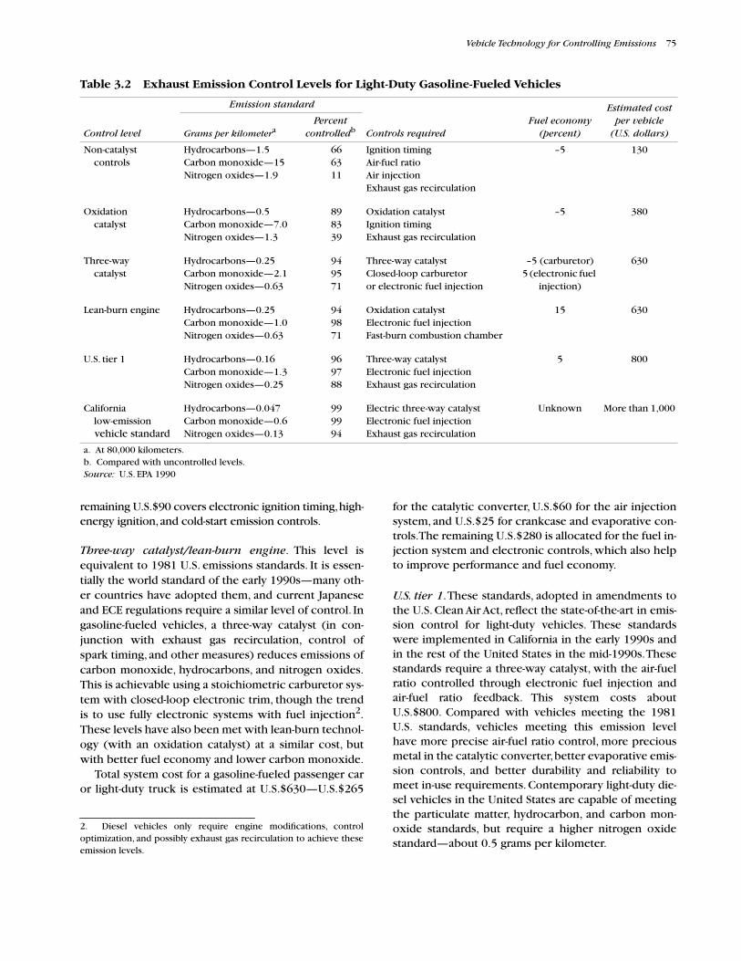
Vehicle Technology for Controlling Emissions
75
remaining U.S.$90 covers electronic ignition timing, high-energy ignition, and cold-start emission controls.
Three-way catalyst/lean-burn engine
. This level isequivalent to 1981 U.S. emissions standards. It is essen-tially the world standard of the early 1990s—many oth-er countries have adopted them, and current Japaneseand ECE regulations require a similar level of control. Ingasoline-fueled vehicles, a three-way catalyst (in con-junction with exhaust gas recirculation, control ofspark timing, and other measures) reduces emissions ofcarbon monoxide, hydrocarbons, and nitrogen oxides.This is achievable using a stoichiometric carburetor sys-tem with closed-loop electronic trim, though the trendis to use fully electronic systems with fuel injection
2
.These levels have also been met with lean-burn technol-ogy (with an oxidation catalyst) at a similar cost, butwith better fuel economy and lower carbon monoxide.
Total system cost for a gasoline-fueled passenger caror light-duty truck is estimated at U.S.$630—U.S.$265
2. Diesel vehicles only require engine modifications, controloptimization, and possibly exhaust gas recirculation to achieve theseemission levels.
for the catalytic converter, U.S.$60 for the air injectionsystem, and U.S.$25 for crankcase and evaporative con-trols. The remaining U.S.$280 is allocated for the fuel in-jection system and electronic controls, which also helpto improve performance and fuel economy.
U.S. tier 1
. These standards, adopted in amendments tothe U.S. Clean Air Act, reflect the state-of-the-art in emis-sion control for light-duty vehicles. These standardswere implemented in California in the early 1990s andin the rest of the United States in the mid-1990s. Thesestandards require a three-way catalyst, with the air-fuelratio controlled through electronic fuel injection andair-fuel ratio feedback. This system costs aboutU.S.$800. Compared with vehicles meeting the 1981U.S. standards, vehicles meeting this emission levelhave more precise air-fuel ratio control, more preciousmetal in the catalytic converter, better evaporative emis-sion controls, and better durability and reliability tomeet in-use requirements. Contemporary light-duty die-sel vehicles in the United States are capable of meetingthe particulate matter, hydrocarbon, and carbon mon-oxide standards, but require a higher nitrogen oxidestandard—about 0.5 grams per kilometer.
Table 3.2 Exhaust Emission Control Levels for Light-Duty Gasoline-Fueled Vehicles
Emission standard
Fuel economy(percent)
Estimated costper vehicle
(U.S. dollars)Control level
Grams per kilometer
a
Percentcontrolled
b
Controls required
Non-catalystcontrols
Hydrocarbons—1.5Carbon monoxide—15Nitrogen oxides—1.9
666311
Ignition timingAir-fuel ratioAir injectionExhaust gas recirculation
–5 130
Oxidationcatalyst
Hydrocarbons—0.5Carbon monoxide—7.0Nitrogen oxides—1.3
898339
Oxidation catalystIgnition timingExhaust gas recirculation
–5 380
Three-waycatalyst
Hydrocarbons—0.25Carbon monoxide—2.1Nitrogen oxides—0.63
949571
Three-way catalystClosed-loop carburetoror electronic fuel injection
–5 (carburetor)5 (electronic fuel
injection)
630
Lean-burn engine Hydrocarbons—0.25Carbon monoxide—1.0Nitrogen oxides—0.63
949871
Oxidation catalystElectronic fuel injectionFast-burn combustion chamber
15 630
U.S. tier 1 Hydrocarbons—0.16Carbon monoxide—1.3Nitrogen oxides—0.25
969788
Three-way catalystElectronic fuel injectionExhaust gas recirculation
5 800
Californialow-emissionvehicle standard
Hydrocarbons—0.047Carbon monoxide—0.6Nitrogen oxides—0.13
999994
Electric three-way catalystElectronic fuel injectionExhaust gas recirculation
Unknown More than 1,000
a. At 80,000 kilometers.b. Compared with uncontrolled levels.
Source:
U.S. EPA 1990

76
Air Pollution from Motor Vehicles
Table 3.3 Recommended Emission Control Levels for Motorcycles in Thailand
Emission standard
Fuel economy(percent)
Estimated costper vehicle
(U.S. dollars)Control level
Grams per kilometer
a
Percent controlled
b
Controls required
Eliminatetwo-stroke
Hydrocarbons—5.0Carbon monoxide—12.0Nitrogen oxides—NRParticulate matter—0.15
6650—
50–90
Four-stroke engine or advancedtwo-stroke
30–40
60–80
Non-catalyst controls
Hydrocarbons—1.0Carbon monoxide—12.0Nitrogen oxides—0.5Particulate matter—0.15
9050
20050–90
Four-stroke or two stroke withcatalyst, ignition timing, air-fuel ratio control
0
80–100
Oxidation catalyst or advanced technology
Hydrocarbons—0.5Carbon monoxide—2.0Nitrogen oxides—0.5Particulate matter—0.05
9880
20085
Four-stroke or advanced two- stroke, ignition timing, air-fuel ratio control, catalytic converteror electronic fuel injection
–5
80–100
— Not applicableNR = Not regulated.a. At 80,000 kilometers.b. Compared with uncontrolled two-stroke.
Source:
Weaver and Chan 1994
California low-emission vehicle (LEV)
. These stan-dards, to be implemented in California beginning in1997, and in other parts of the United States in 2001, ex-ceed the current state-of-the-art in emission control forgasoline vehicles. Compliance with these standards willrequire even more precise control of the air-fuel ratio,heavier catalyst loadings, and better engine-out emis-sion controls than the current state-of-the-art, and pos-sibly new technologies or alternative fuels. For largevehicles, it appears that preheated catalytic convertersmay be required to reduce emissions when the vehicleis started cold. This will pose a significant challenge toautomakers. The total cost is unknown, but will mostlikely exceed U.S.$1,000.
Heavy-Duty Gasoline-Fueled Vehicles
Heavy-duty vehicles with gasoline engines can use theemission control technologies outlined above. Becauseof differences in vehicle size and testing procedures,however, emissions standards cannot be directly com-pared. Because of their smaller numbers, heavy-duty gas-oline vehicles receive less regulatory attention, andemissions standards are less strict. Emission standards forthese vehicles are also lax because they typically operateat high loads, making it difficult to ensure catalyst dura-bility. Design solutions for the catalyst durability problemexist, and recent California regulations will require vehi-cles under 14,000 pounds gross vehicle weight to meetlow-emission vehicle standards. The cost of meetingemissions standards in larger vehicles is expected to be50 to 100 percent more than for passenger cars becauseof the larger size of the equipment required.
Motorcycles
In the past, motorcycles were subject to lenient emis-sion controls or none at all. This reflects their minor con-tribution to emissions in most industrial countries andthe difficulty and expense of installing emission controlson small, heavily-loaded engines. In many Asian cities,however, motorcycles and three- wheelers are responsi-ble for a large fraction of hydrocarbon and PM emissions.Recommended emission control levels based on an as-sessment of motorcycle emissions in Thailand are sum-marized in table 3.3 (Weaver and Chan 1994).
The first step in controlling emissions from motorcy-cles vehicles is eliminating the excessive emissionsfrom two-stroke engines. This can be done by switchingto a four-stroke design or to a two- stroke design incor-porating timed fuel injection and crankcase lubrication.This would reduce hydrocarbon and particulate matteremissions by about 90 percent, at a cost of aboutU.S.$60 per vehicle. Additional emission reductions arepossible with improved four-stroke engine design andcalibration and through the use of catalytic converters.Catalytic converters are used on two-stroke motorcy-cles in Taiwan (China) and on mopeds in Austria andSwitzerland. Catalyst-forcing standards for four-strokeengines have not been adopted in any jurisdiction.
Diesel-Fueled Vehicles
As with gasoline-fueled vehicles, diesel engine emis-sion reductions have accompanied improvements infuel efficiency. Although measures such as retarding in-jection timing increase fuel consumption, these havebeen offset by gains from turbocharging, charge-air

Vehicle Technology for Controlling Emissions
77
cooling, and improved fuel injection equipment. Thecosts of these features are offset by lower fuel con-sumption. Industry estimates of cost increases for en-gine modifications to meet emission standards areshown in table 3.4.
Uncontrolled emissions of nitrogen oxides fromheavy-duty diesel engines range from 12 to 21 grams perkilowatt-hour (9 to 16 grams per brake horsepower-hour) when measured using the U.S. transient or Euro-pean 13-mode cycle. Particulate matter emissions onthe transient cycle are typically 1–5 g/kWh (0.75–3.7 g/bhp-hr), but are significantly lower on the Europeansteady-state cycle. Engines that have been tamperedwith or poorly maintained may emit higher PM emis-sions in the form of smoke.
By moderately retarding fuel injection timing fromthe optimal point, nitrogen oxides can be reduced toless than 11.0 g/kWh (8 g/bhp-hr). This may require up-graded fuel-injection equipment. Particulate matteremissions can be limited through smoke opacity stan-dards under acceleration and full-load conditions. Achi-evable peak acceleration smoke opacity levels rangefrom 25 to 35 percent, while steady- state smoke opaci-ty of less than 5 percent (the limit of visibility) is readilyachievable. This minimal control level is comparable tothat required of California engines in the 1970s and Eu-ropean engines until the early 1990s.
Moderate control of 8 g/kWh (6 g/bhp-hr) of nitro-gen oxides and 0.7 g/kWh (0.5 g/bhp-hr) of particulatematter requires further optimization of the injectiontiming and the overall combustion system. This corre-sponds to 1990 U.S. federal standards. The next level ofcontrol corresponds to the 1991 U.S. standards, whichhave also been adopted in Canada and Mexico. Achiev-ing this level of nitrogen oxides control while meetingPM emission standards requires major engine designmodifications. These include variable fuel-injection tim-ing, high-pressure fuel injection, combustion optimiza-
tion, and charge- air cooling. A tighter U.S. particulatematter standard (0.13 g/kWh; 0.10 g/bhp-hr) took ef-fect in 1994. This standard applied to diesel engines inurban buses in 1993, and a limit of 0.07 g/bhp-hr wasadopted for 1994 and 1995. After 1995, U.S. urban bus-es will be required to meet an emission standard of 0.07g/kWh (0.05 g/bhp-hr).
Further reductions are being contemplated. The1990 U.S. Clean Air Act amendments require reducedemissions of nitrogen oxides for all heavy-duty truckand bus engines (5.4 g/kWh; 4.0 g/bhp-hr) in 1998.
The stringent nitrogen oxides and PM standardsadopted by the United States would not have been possi-ble for diesel engines until very recently. Developmentsin fuel-injection rate-shaping, and the potential use of ex-haust gas recirculation mean that nitrogen oxide emis-sion levels of 2.6 g/kWh (2.0 g/bhp-hr) may now beachievable, in combination with low PM emissions. Us-ing selective exhaust gas recirculation and extensive en-gine optimization, nitrogen oxide levels as low as 2.6 g/kWh (2.0 g/bhp-hr) have been achieved in the laboratory(Needham, Doyle, and Nicol 1991). Translating researchresults into marketable engines takes time, but this maybe feasible by the end of the 1990s.
Further reductions in nitrogen oxide and particulatematter emissions are possible with alternative fuels.Pre-production methanol direct-injection engines us-ing glow-plug assisted compression ignition have pro-duced nitrogen oxide emissions below 2.9 g/kWh (2.1g/bhp-hr), with efficiency comparable to that of a reg-ulated diesel engine. Heavy-duty, lean-burn, natural-gasengines have achieved nitrogen oxide levels below 2.5g/kWh (1.9 g/bhp-hr), with energy efficiency about 10percent worse than the diesel. Spark-ignition enginesusing natural gas, liquefied petroleum gas, and gasolinewith three-way catalysts, stoichiometric air-fuel ratios,and closed-loop control have achieved nitrogen oxideemissions below 1.5 g/kWh (1.1 g/bhp-hr) at low mile-
Table 3.4 Industry Estimates of Emission Control Technology Costs for Diesel-Fueled Vehicles
(percent)
Technology Engine cost increase
Baseline engine, no emission control equipment 0
Injection timing retard 0
Low sac volume and valve covering nozzle Minimal
Turbocharging 3–5
Charge cooling 5–7
Improved fuel injection 13–15
High-pressure fuel injection with electronic control 14–16
Variable geometry turbocharging 1–3
Particulate trap 4–25
Source:
ECMT 1990 (based on Tonkin and Etheridge 1987)

78 Air Pollution from Motor Vehicles
Table 3.5 Emissions Control Levels for Heavy-Duty Diesel Vehicles
Emissions limit at full useful life
Fueleconomya
(percent)
Estimated cost perengine
(U.S. dollars)Control level Grams per kilowatt-hour
Gramsper brake
horsepower-hour Controls required
Uncontrolled Nitrogen oxides—12.0 to 21.0Particulate matter—1.0 to 5.0
9.0 to 16.00.75 to 3.70
None (PM level depends on smoke controls & maintenance level)
0 0
Minimal control Nitrogen oxides—11.0Particulate matter—0.7 to 1.0Peak smoke—20 to 30 percent opacity
8.00.5 to 0.75
Injection timingSmoke limiter
–3 to 0 0–200
Moderate control Nitrogen oxides—8.0Particulate matter—0.7
6.00.5
Injection timingCombustion optimization
–5 to 0 0–1,500
1991 U.S. standard(Euro 2)
Nitrogen oxides—6.7 (7.0)Particulate matter—0.34 (0.15)b
5.00.25
Variable injection timingHigh-pressure fuel injectionCombustion optimizationCharge-air cooling
–5 to 5 1,000–3,000
Lowest dieselstandards underconsideration
Nitrogen oxides—2.7 to 5.5c
Particulate matter—0.07 to 0.132.0 to 4.0
0.05 to 0.10Electronic fuel injectionCharge-air coolingCombustion optimizationExhaust gas recirculationCatalytic converter or particulate trap
–10 to 0 2,000–6,000
Alternative-fuelforcing
Nitrogen oxides—less than 2.7Particulate matter—less than 0.07
2.00.04
Gasoline/three-way catalystNatural gas lean-burnNatural gas/three-way catalystMethanol-diesel
–30 to 0 0–5,000
Note: Kilowatt-hours are converted to brake horsepower-hours by multiplying by 0.7452.a. Potential fuel economy improvements result from addition of turbocharging and intercooling to naturally aspirated engines.b. Euro-2 emissions are measured on a steady-state cycle that underestimates PM emissions in actual driving. Actual stringency of control require-ments is similar to that of U.S. 1991.c. Not yet demonstrated in production vehicles.Source: Weaver 1990
Table 3.6 Emission Control Levels for Light-Duty Diesel Vehicles
Control levelEmissions limit at full useful life
(grams per kilometer)Reductiona
(percent) Controls required
Fuel economy(percent)
Estimated cost per engine
(U.S. dollars)
Uncontrolled Nitrogen oxides—1.0 to 1.5Particulate matter—0.6 to 1.0
00
None (PM level dependson smoke controls &maintenance level)
0 0
Moderate control Nitrogen oxides—0.6Particulate matter—0.4
4033
Injection timingCombustion optimization
–5 to 0 0–500
1988 U.S. standard (EU Directive 91/441/EEC)
Nitrogen oxides—0.6(HC+NOx:0.97)Particulate matter—0.13 (0.14)
4078
Variable injection timingCombustion optimizationExhaust gas recirculation
–5 to 0 100–200
Advanced diesel technology
Nitrogen oxides—0.5Particulate matter—0.05–0.08
4092
Electronic fuel injectionCombustion optimizationExhaust gas recirculationCatalytic converter or
particulate trap
–10 to 0 200–500
a. Compared with uncontrolled levels.Source: Weaver 1990

Vehicle Technology for Controlling Emissions 79
age, and acceptable catalyst durability has been demon-strated in some cases. Particulate matter emissionswith these fuels are also low. Since they do not formsoot or condensable organic compounds, particulateemissions derive only from the lubricating oil. With acatalytic converter, these are less than 0.05 g/kWh(0.04 g/bhp-hr).
The emission control levels achievable for heavy-duty diesel engines, the costs of achieving these levels,and the corresponding effects on fuel economy areshown in table 3.5. These estimates prepared for anOECD study differ from those based on industrysources.
Potential emission controls for light-duty diesel vehi-cles range from none to moderate control (applied inEurope until recently) to the stringent controls typicalof California and the rest of the United States. Given thecollapse in demand for diesel vehicles in the U.S., nomanufacturer considered it worthwhile to develop anemissions control system to meet the California limits.Similar emission standards for diesel-fueled passengercars have recently been adopted in Europe, where die-sel cars are a large part of the market. Vehicles meetingthese control levels are thus likely to be developed inthe near future. Estimates of cost and emission controleffectiveness for light-duty diesel-fueled automobilesare provided in table 3.6.
References
ACEA/EUROPIA (European Automobile Manufacturer’sAssociation/European Petroleum Industry Associa-tion). 1995. European Program on Emissions, Fu-els, and Engine Technologies. EPEFE Report,Brussels.
Brogan, J.J. and S.R. Venkateswaran. 1993. “Fuel-Effi-cient Low-Emission Propulsion Technology” in To-wards Clean & Fuel Efficient Automobiles.Proceedings of an International Conference held inBerlin (March 25-27, 1991), OECD, Paris.
CONCAWE Review. 1994. “Oxidation Catalysts for Die-sel Cars,” Volume 3, Number 2, October, Brussels.
ECMT (European Conference of Ministers of Transport).1990. Transport Policy and the Environment. Or-ganisation for Economic Cooperation and Develop-ment (OECD). Paris.
Feutlinske, H. 1989. “Possibilities for Reducing PollutantEmissions from Diesel Engines–Comments on theDevelopment Status of Particle Filters.” Report 4,48th International Congress, International Union ofPublic Transport. Brussels.
Holman, C. 1990. “Pollution from Diesel Vehicles.” Brief-ing Document, Friends of the Earth, London.
Hope, K. 1992. “Urban Air Pollution: Greeks Battle toDefeat the Nefos.” Financial Times, March 11, 1992.London.
Kimbom, G. 1993. “Some Examples of Alternative En-gines” in Towards Clean & Fuel Efficient Automo-biles. Proceedings of an International Conferenceheld in Berlin (March 25-27, 1991), OECD, Paris.
Knecht, W. 1991. “Reduction of Heavy-duty Diesel Emis-sions and Application of Particulate Traps and Oxida-tion Catalysts.” in The Diesel Engine–Energy Stakeand Environment Constraints, TÜV Brussels, Rhein-land/OPET.
MacKenzie, J.J. 1994. The Keys to the Car—Electric andHydrogen Vehicles for the 21st Century. WorldResources Institute, Washington, D.C.
Mason, J.L. 1993. IC Engines & Fuels for Cars & LightTrucks: 2015.” in Transportation & Global ClimateChange, eds. L. Greene & D.J. Santini, AmericanCouncil for an Energy Efficient Economy, Washing-ton, D.C.
Needham, J.R., D.M. Doyle, and A.J. Nicol. 1991. “TheLow Nitrogen Oxide Truck Engine.” SAE Paper910731, Society of Automotive Engineers, Warren-dale, Pennsylvania.
OTA (Office of Technology Assessment, U.S. Congress).1995. Advanced Automotive Technology: Visions ofa Super-Efficient Family Car. OTA-ETI-638. U.S. Gov-ernment Printing Office, Washington, D.C.
Pattas, K., Z. Samaras, N. Patsatzis, C. Michalopoulous, O.Zogou, A. Stamatellos, and M. Barkis. 1990. “On-RoadExperience with Trap Oxidiser Systems Installed onUrban Buses.” SAE Paper 900109, Presented at the So-ciety of Automotive Engineers (SAE) InternationalCongress and Exposition, Detroit, Michigan.
Tonkin, P.R. and P. Etheridge. 1987. “A New Study of theFeasibility and Possible Impact of Reduced EmissionLevels from Diesel Engined Vehicles,” Report No.DP87/0927, Shoreham by Sea, Ricardo ConsultingEngineers, U.K.
U.S. EPA (United States Environmental Protection Agen-cy). 1990. “Volatile Organic Compounds from On-Road Vehicles: Sources and Control Options.” Reportprepared for the Long-range Transboundary Air Pollu-tion Convention. United Nations Economic Commis-sion for Europe. Washington, D.C. (Draft)
Watkins, L.H. 1991. Air Pollution from Motor Vehicles.State-of-the-Art Review/1. Transport and Road Re-search Laboratory. HMSO. London.
Weaver, C.S., R.J. Klausmeier, L.M. Erickson, J. Gallagh-er, and T. Hollman. 1986. “Feasibility of Retrofit Tech-nology for Diesel Emissions Control.” SAE Paper860296, Society of Automotive Engineers, Warren-dale, Pennsylvania.

80 Air Pollution from Motor Vehicles
Weaver, C.S. 1990. “Emissions Control Strategies forHeavy-Duty Diesel Engines.” EPA report 460/3- 90-001. U.S. Environmental Protection Agency. (Draft)Ann Arbor, Michigan.
Weaver, C.S. and L.M. Chan. 1994. “Motorcycle Emis-sion Standards and Emission Control Technology.”Report to the Royal Thai Ministry of Science, Tech-nology, and the Environment, and The World Bank.
Sacramento, California, Engine, Fuel, and EmissionsEngineering, Inc.
Weaver, C.S. and L.M. Chan. 1995. “Company Archives”Multiple Sources. Engine, Fuel and Emissions Engi-neering, Inc. Sacramento, California.
Wijetilleke, L and S. Karunaratne. 1992. “Control andManagement of Petroleum Related Air Pollution.”The World Bank, Washington, D.C. (Draft)

81
This appendix provides a more detailed technical dis-cussion to supplement the general information onspark-ignition engine emissions and control technolo-gies in chapter 3.
Combustion and Pollutant Formation inSpark-Ignition Engines
Gasoline engines emit carbon monoxide (CO), nitrogenoxides (NO
x
), hydrocarbons (HC), particulate matter
(PM), and lead (where leaded gasoline is used), as wellas other toxics such as benzene, 1,3 butadiene, andformaldehyde.
Exhaust Emissions
Exhaust emissions are caused by the combustion pro-cess. Figure A3.1.1 shows the combustion process in anOtto-cycle engine. After the initial spark, there is an igni-tion delay while the flame kernel created by the sparkgrows. The flame then spreads through the combustion
Emission Control Technology for Spark-Ignition (Otto) Engines
Appendix 3.1
Figure A3.1.1 Combustion in a Spark-Ignition Engine
Source:
Weaver and Chan 1995
Ignition

82
Air Pollution from Motor Vehicles
chamber. The rate of spread is determined by the flamespeed, which is a function of air-fuel ratio, temperature,and turbulence level. The increase in volume of the hotburned gases behind the flame front presses the un-burned charge outward. Overall cylinder pressure in-creases, increasing the temperature of the unburnedcharge. Finally, the remaining elements of the unburnedmixture burn out as the piston descends. The main ex-haust pollutants are discussed below.
Nitrogen oxides
. The two main nitrogen oxides emittedfrom combustion engines are nitric oxide (NO) and ni-trogen dioxide (NO
2
). Most nitrogen oxides fromcombustion engines—90 percent—are nitric oxide.This gas is formed from nitrogen and free oxygen athigh temperatures. The rate of formation is a function ofoxygen availability, and is exponentially dependent onthe temperature. Most nitrogen oxide emissions formearly in the combustion process, when the piston isnear the top of its stroke (
top-dead- center
) and temper-atures are highest. Nitrogen oxide emissions are con-trolled by reducing the flame temperature (by retardingcombustion, diluting the reacting mixture, or both) andby minimizing the time that burned gases stay at hightemperatures.
Carbon monoxide.
Carbon monoxide emissions arecaused by the combustion of rich mixtures, where theair-fuel ratio,
λ
is less than 1.0. In such mixtures, thereis insufficient oxygen to convert all the carbon to car-bon dioxide. A small amount of carbon monoxide is alsoemitted under lean conditions because of chemical ki-netic effects. Carbon monoxide emissions are con-trolled in the engine by adjusting the air-fuel ratio of thecharge entering the cylinder.
Hydrocarbons
. Hydrocarbon emissions result from ele-ments of the air-fuel mixture that have not finished burn-ing at the time the exhaust valve opens. Hydrocarbonemissions are composed of unburned fuel and productsof partial combustion, such as ethylene and formalde-hyde. Hydrocarbon sources include crevice volumes,such as the space between the piston and cylinder wallabove the piston ring, and the quenched layer immediate-ly next to the combustion chamber walls. Unburned mix-ture is forced into these crevices during compression andcombustion, and emerges late in the expansion and dur-ing the exhaust stroke. This is the major source of hydro-carbon emissions from four-stroke engines. In two-strokeengines, fuel mixing with the exhaust during scavengingand misfire at light loads are sources of hydrocarbons. Ab-normal operation in a four-stroke engine, such as a misfir-ing cylinder, can cause significant quantities of unburnedfuel to pass into the exhaust. In lean mixtures, flame
speeds may be too low for combustion to be completedduring the power stroke, or combustion may not occur.These conditions also cause high hydrocarbon emissions.
Unburned hydrocarbons emitted from the cylindercontinue to react in the exhaust only if the temperatureis above 600°C and oxygen is present. So hydrocarbonemissions from the tailpipe may be significantly lowerthan the hydrocarbons leaving the cylinder. This effectis important at stoichiometric or near-stoichiometricconditions because of the higher exhaust temperaturesexperienced.
Particulate matter
. Unlike diesel engines, PM emissionsfrom spark-ignition engines are generally not regulated.They frequently are not measured or reported, leadingmany to assume they are negligible. This is not the case.Particulate matter emissions from four-stroke spark-igni-tion engines result from unburned lubricating oil in theexhaust and from ash-forming fuel and oil additivessuch as tetra-ethyl lead. Although PM emission rates forspark-ignition engines are low compared with diesels,emissions can be significant when poor maintenance orengine wear lead to high oil consumption, or when oilis mixed with the fuel, as in two-stroke engines.
Toxic pollutants
. Toxic chemicals emitted by spark-igni-tion engines include lead compounds, benzene, 1,3butadiene, and aldehydes. Lead emissions are caused bytetra-ethyl lead, used as an octane enhancer in leadedgasoline. Benzene is one of the many hydrocarbons ingasoline-engine exhaust, accounting for about 4 per-cent of total hydrocarbons. Benzene in the exhaust iscaused by fuel coming through unburned and by de-alkylation of other aromatic compounds. 1,3 butadieneis a product of partial hydrocarbon combustion. Bothbenzene and 1,3 butadiene are carcinogens, so expo-sure to them is cause for concern. Studies in the UnitedStates indicate that motor vehicles are responsible formost human exposure to benzene and 1,3 butadiene(U.S. EPA 1990).
Aldehydes are intermediate products of hydrocarboncombustion. Highly reactive, they form other productsduring combustion. The small amounts of aldehydeemissions found in gasoline, diesel, and other enginesusing hydrocarbon fuels are caused by the quenching ofpartially reacted mixture (because of contact with acold surface, for instance). For fuels containing ethanoland methanol, the primary oxidation reactions proceedthrough formaldehyde and acetaldehyde, respectively,so these compounds are often found in significant con-centrations in the exhaust. Both formaldehyde and ace-taldehyde are irritants and suspected carcinogens.
Nitrous oxide.
Uncontrolled auto engines emit a fewmilligrams per kilometer of nitrous oxide (N
2
O). If the

Emission Control Technology for Spark-Ignition (Otto) Engines
83
engine has a catalytic converter, increased nitrous oxideformation occurs because of the reaction of nitric oxideand ammonia with the platinum in the catalyst. Nomore than 5 to 10 percent of the nitric oxide in exhaustis converted into nitrous oxide in this way. The conver-sion in the catalyst is highly temperature dependent. Asthe catalyst warms up after a cold start, nitrous oxidelevels increase to about 5.5 times the inlet level at360°C. Emissions then decrease to the inlet level at460°C. At higher temperatures, the catalyst destroys ni-trous oxide instead of forming it (Prigent and Soete1989). Nitrous oxide is thus formed primarily duringcold starts of catalyst-equipped vehicles.
Crankcase Emissions
All piston engines experience leakage or blowby ofcompressed gas past the piston rings. In spark-ignitionengines, this leakage consists of unburned or partlyburned air-fuel mixture and contains unburnedhydrocarbons. In older vehicles, blowby gases werevented to the atmosphere. Hydrocarbon emission levelsfrom the crankcase were about half the level of uncon-trolled exhaust emissions. These emissions are now con-trolled by venting the crankcase to the air intake systemby means of a positive crankcase ventilation (PCV)valve. The unburned hydrocarbons in the blowby gasare recycled to the engine and burned. The flow of airthrough the crankcase also helps to prevent condensa-tion of fuel and water in the blowby gases, thus reduc-ing oil contamination and increasing engine life. Onesignificant drawback of the PCV system is that the recy-cling of blowby gases tends to foul the intake manifold.An effective gasoline detergent can eliminate this prob-lem.
Evaporative and Refueling Emissions
Gasoline-fueled vehicles emit a significant amount of hy-drocarbons as evaporative emissions from their fuel sys-tem. Four main sources of evaporative emissions havebeen identified:
breathing
(diurnal) losses from fueltanks caused by the expansion and contraction of gas inthe tank with changes in air temperature;
hot-soak
emissions from the fuel system when a warm engine isturned off;
running losses
from the fuel system duringvehicle operation; and
resting losses
from permeationof plastic and rubber materials in the fuel system.
Refu-eling emissions
consist of gasoline vapor displacedfrom the fuel tank when it is filled.
Evaporative and refueling emissions are strongly affect-ed by fuel volatility. Diurnal emissions also vary dependingon the daily temperature range and the amount of vaporspace in the fuel tank. Hot-soak emissions result from theconduction of heat from the warm engine to the carbure-tor, which is open to the atmosphere. Hot-soak losses are
greatly reduced in sealed fuel systems, such as those usedwith fuel injection systems. Such systems may have higherrunning losses, however, due to the recirculation of hotfuel from the engine back to the fuel tank.
Evaporative emissions can be reduced by venting thefuel tank and the carburetor to a canister containing ac-tivated carbon. This material adsorbs volatile emissionsfrom the fuel system when the engine is not running.When the engine is running, intake air is drawn throughthe canister, purging it of hydrocarbons, which thenform part of the fuel mixture fed to the engine. A largercanister can also be used to control refueling vaporemissions, or these emissions can be controlled by cap-turing them through the refueling nozzle and conduct-ing them back to the service station tank.
Engine Design
Spark-ignition vehicle engines are either two stroke orfour stroke. The distinction is important for emissionssince two-stroke engines emit more hydrocarbons andparticulate matter than four-stroke engines of similarsize and power. Two-stroke engines are less fuel effi-cient than four strokes, but have higher power output,quicker acceleration, and lower manufacturing costs.Because of their performance and cost advantages, two-stroke engines are used extensively in motorcycles andin small power equipment such as chainsaws and out-board motors. They are particularly common in smallmotorcycles (50 to 150 cc engine displacement), wheretheir poor fuel economy is of less importance to a con-sumer. They were also used in some small automobiles,particularly in Eastern Europe.
The piston and cylinder of a typical four-stroke en-gine are shown in figure A3.1.2. Engine operation takesplace in four distinct steps: intake, compression, power,and exhaust, with each step corresponding to one
stroke
of the piston (180 degrees of crankshaft rota-tion). During intake, the intake valve admits a mixtureof air and fuel, which is drawn into the cylinder by thevacuum created by the downward motion of the piston.Figure A3.1.2 shows the piston near the end of the in-take stroke, approaching
bottom-dead-center
. Duringcompression, the intake valve closes, and the upwardmotion of the piston compresses the air-fuel mixtureinto the combustion chamber between the top of thepiston and the cylinder head.
The compression stroke ends when the piston reach-es top-dead-center. Just before this point, the air-fuelmixture is ignited by a spark from the spark plug and be-gins to burn. Combustion of the air-fuel mixture takesplace near top-dead-center, increasing the temperatureand pressure of the trapped gases. During the powerstroke, the pressure of the burned gases pushes the pis-

84
Air Pollution from Motor Vehicles
ton down, turning the crankshaft and producing power.As the piston approaches bottom-dead-center again, theexhaust valve opens, releasing the burned gases. Duringthe exhaust stroke the piston ascends toward top-dead-center, pushing the remaining burned gases out theopen exhaust port. The exhaust valve then closes andthe intake valve opens for the next intake stroke.
In a four-stroke engine, combustion and the resultingpower stroke occur once every two revolutions of thecrankshaft. In a two-stroke engine, combustion occursin every revolution of the crankshaft. Two-strokeengines eliminate the intake and exhaust strokes, leav-ing only the compression and power strokes. Ratherthan occupying distinct phases of the cycle, exhaustand intake occur simultaneously (figure A3.1.3). As thepiston approaches bottom-dead-center in the powerstroke, it uncovers exhaust ports in the wall of the cylin-der. The high-pressure combustion gases blow into theexhaust manifold. As the piston gets closer to the bot-tom of its stroke, intake ports are uncovered, and freshair-fuel mixture is forced into the cylinder while the ex-haust ports are still open. Exhaust gas is
scavenged
(forced) from the cylinder by the pressure of the incom-
ing charge. In the process, mixing between exhaust gasand the charge takes place, so some of the fresh chargeis also emitted in the exhaust. If fuel is already mixedwith the air in the charge (as in all current two-strokemotorcycle engines), this fuel will be lost in the ex-haust. The loss of fuel during scavenging is one of themain causes of high hydrocarbon emissions from two-stroke motorcycle engines.
The other reason for high hydrocarbon emissionsfrom two strokes is their tendency to misfire under low-load conditions. At low loads, the amount of freshcharge available to scavenge the burned gases from thecylinder is small, so a significant amount of the burnedgas remains in the cylinder to dilute the incomingcharge. The resulting mixture of air, fuel, and exhaustburns less readily and is more difficult to ignite than anair-fuel mixture alone. At light loads, the mixture some-times fails to ignite, allowing the fuel vapor in the cylin-der to pass unburned into the exhaust. These occasionalmisfires are the cause of the popping sound made bytwo-stroke engines under light-load conditions.
The mechanical systems required by four-stroke en-gines to open and close their intake and exhaust valves
Figure A3.1.2 Piston and Cylinder Arrangement of a Typical Four-Stroke Engine
Source:
Weaver and Chan 1995

Emission Control Technology for Spark-Ignition (Otto) Engines
85
at the right time make these engines relatively complexto manufacture. The mechanical layout of one commontype of four-stroke engine, with an overhead camshaft,is shown in figure A3.1.4. The valves are opened bylobes on the camshaft, which is driven at one-half en-gine speed by a sprocket and chain arrangement fromthe crankshaft. The camshaft lobes press on the valvefollowers, pushing up the rocker arms, and make thevalves open at the appropriate time in every secondcrankshaft revolution. The camshaft, valve linkage,crankshaft bearings, and pistons are lubricated by oilpumped from the oil sump at the bottom of the crank-case. The other common design, with the camshaft lo-cated lower in the engine and driving the valvesthrough pushrods, is even more complicated.
A two-stroke engine is much simpler (figure A3.1.5).As the piston rises during the compression stroke, itcreates a vacuum in the crankcase, which draws the air-fuel mixture from the carburetor into the crankcase. Asthe piston descends during the power stroke, the air-fuel mixture in the crankcase is prevented by the reedvalve from going out the intake port, and instead isforced up into the cylinder, where it displaces theburned gases in the cylinder into the exhaust in the
scavenging process diagrammed in figure A3.1.3, asshown. The complex valve gear, camshaft, and relatedmechanisms of the four-stroke engine are not needed inthe two stroke. For small motorcycles with two-strokeengines, the cost difference between two-stroke andfour-stroke engines is U.S.$60 to U.S.$80 per unit(Weaver and Chan 1994).
Since the crankcase in a two-stroke engine serves asthe pump for the scavenging process, it cannot be usedas an oil sump; gasoline would mix with the oil and di-lute it. Lubrication for two-stroke engines is providedby mixing two-stroke oil with the fuel. As the fuel-oilmixture is atomized and mixes with the air, the light hy-drocarbons in the fuel evaporate, leaving a mist of oildroplets or particles. Some of this mist contacts the in-ternal parts of the engine, lubricating them, but most ofit passes into the cylinder with the fresh charge. A sig-nificant part of the frest charge passess unburned intothe exhaust, carrying the oil droplets with it. Some oilmay also escape unburned from the combustion pro-cess. Since the oil particles scatter light that strikesthem, they are visible as white or blue smoke. Thissmoke is one of the distinguishing features of two-
Figure A3.1.3 Exhaust Scavenging in a Two-Stroke Gasoline Engine
Source:
Weaver and Chan 1995

86
Air Pollution from Motor Vehicles
Figure A3.1.5 Mechanical Layout of a Typical Two-Stroke Motorcycle Engine
Source:
Weaver and Chan 1995
Figure A3.1.4 Mechanical Layout of a Typical Four-Stroke Engine
Source:
Weaver and Chan 1995

Emission Control Technology for Spark-Ignition (Otto) Engines
87
stroke engines, and the reason for their high particulatematter emissions.
Emission Control Technology for Four-Stroke Engines
Fuel Metering Systems
Because of the importance of air-fuel ratio control foremissions, fuel metering systems are crucial in the emis-sion control systems of Otto-cycle engines. Two types ofmetering systems are common: carburetors and fuel in-jection systems. Both are affected by altitude.
Carburetors
. These systems were used almost universal-ly before the advent of emission regulations and are stillcommon where stringent emission controls are not ineffect. In a carburetor, air going into the engine is accel-erated in one or more venturis. The pressure differentialin the venturi throat is used to draw fuel into the air-stream and atomize it. In advanced carburetors, this issupplemented by devices that provide mixture en-richment at idle and light-load conditions, and duringcold starts.
Carburetors cannot maintain precise air-fuel ratiocontrol under all conditions and are subject to changeover time. They are not suitable for applications thatrequire precise and invariant air-fuel ratio control. Toaddress these problems, carburetors with electronicair-fuel ratio adjustment were marketed in the early1980s for use with three-way catalyst systems. Suchsystems are inferior to electronic fuel injection, how-ever, and they are no longer produced in significantnumbers.
Fuel injection systems
. During the 1980s, air-fuel ratiocontrol systems for light-duty gasoline vehicles evolvedfrom mechanical systems such as carburetors to directcontrol of fuel quantity through electronic fuel injec-tion. These systems provide rapid and precise control ofthe air-fuel ratio. There are two basic types of fuel injec-
tion systems: central (
throttle-body
) injection systems,with one or two centrally-located fuel injectors; andmulti-port fuel injection systems, with one fuel injectorlocated at the inlet to each cylinder. The multi-port sys-tems reduce cylinder-to-cylinder variations in air-fuel ra-tio and simplify intake manifold design, since formationof fuel puddles in the intake manifold is no longer aproblem. Because they have fewer parts, central fuel in-jection systems are cheaper, while multi-port systemshave better emissions and performance.
The first widely used fuel injection systems were de-veloped and marketed by Robert Bosch AG (Bosch1986). In these systems, fuel is injected continuouslythrough nozzles at each intake port. The rate of injec-tion is controlled by varying the pressure supplied tothe nozzles by an electric fuel pump. Fuel injection sys-tems now use fully electronic control. Fuel is providedto the injectors at constant pressure by a pump andpressure regulating valve. The injectors are solenoidvalves, which are controlled by the engine computer.The computer controls the quantity of fuel injected byvarying the length of time the valve remains open dur-ing each revolution of the crankshaft.
Electronic multi-port fuel injection systems eitherfire all the fuel injectors at once, or each injector is firedsequentially at the optimal time during engine rotation.All-at-once systems are simpler and cheaper, while se-quential fuel injection gives the most precise and flexi-ble control over the injection process. Sequentialsystems allow better air-fuel mixing and thus better per-formance and emissions. As vehicle emission standardsgrow more demanding in industrialized countries, morevehicles are being equipped with multi-port, sequentialfuel injection systems.
Altitude effects on air-fuel ratio
. Atmospheric pressure,air temperature, and air density vary with changes in al-titude (table A3.1.1). Reduced air density at high alti-tudes reduces the power of a naturally aspiratedgasoline engine and upsets normal operating character-istics, resulting in excessive pollutant emissions. Fuel
Table A3.1.1 Effect of Altitude on Air Density and Power Output from Naturally Aspirated Gasoline Engines in Temperate Regions
Source:
Babkov and Zamakhayev 1967
Altitude (meters)Air pressure
(mm of mercury)Air density
(kilograms per cubic meter)Air temperature(degrees Celsius)
Excess aircoefficient
Engine powerreduction (percent)
0 760.0 1.225 15.0 1.00 0
1,000 674.1 1.112 8.5 0.89 11.3
2,000 596.1 1.007 2.0 0.80 21.5
3,000 525.8 0.999 -4.5 0.71 30.8
4,000 452.3 0.819 -11.0 0.63 39.2
5,000 405.1 0.736 -17.5 0.56 46.7

88
Air Pollution from Motor Vehicles
mixture composition is characterized by its
excess aircoefficient
, which is the ratio of air supplied to thequantity required. Gasoline-fueled automobile enginesusually operate with an excess air coefficient rangingfrom 0.8 to 1.2. Air density decreases with altitude, withthe air admitted to the engine reducing by about 4 to 5percent per 100 meters of altitude and, with it, enginepower. As a result of the reduced air density the fuel-airmixture becomes richer, leading to a further decrease inengine power and an increase in emissions of carbonmonoxide and hydrocarbons.
For example, at 2,000 meters (the altitude of MexicoCity), air pressure is only 80 percent of that at sea level,so a given volume of air contains only 80 percent asmuch oxygen. For vehicles using carburetors or continu-ous fuel injection systems, the change in atmosphericpressure from one elevation to another affects the air-fuelratio. If a carburetor is set for stoichiometric operation atsea level, it will mix the same mass of fuel with the samevolume of air at 2,000 meters. But the same volume of aircontains 20 percent less oxygen, so the resulting air-fuelmixture is 25 percent too rich. Conversely, a carburetorset for stoichiometric operation at 2,000 meters will pro-duce too lean a mixture at sea level.
It is important that vehicles be adjusted for the alti-tude at which they operate. This is a problem at high al-titudes, since vehicles are often preset for operationnear sea level. When vehicles are driven to high-altitudeareas, the resulting rich mixture has little effect on vehi-cle performance, though it increases fuel consumptionand carbon monoxide emissions. Since performance isnot affected, the vehicle owner may not find it necessaryto have the engine adjusted. With proper adjustment, ve-hicle emissions at high altitudes are similar to those atsea level (although engine power falls in proportion toair pressure). Adjustments are not necessary in vehiclesequipped with modern electronic fuel injection sys-tems, since these systems automatically compensate foraltitude changes.
Exhaust Gas Recirculation
Dilution of the incoming charge with spent exhaust af-fects pollutant formation, and can be useful in control-ling nitrogen oxide emissions. In four-stroke engines,this dilution is achieved through exhaust gas recircula-tion. Exhaust gas recirculation can be used in twostrokes, but a more convenient alternative is to reducethe scavenging ratio, thus increasing the amount ofspent gas in the cylinder. The effect of exhaust gas dilu-tion is similar to that of excess combustion air—dilutingthe combustion reactants reduces flame temperatureand flame speed. Exhaust gas has a greater effect onflame speed and nitrogen oxide emissions than thesame quantity of excess air (Heywood 1988). This is
caused by the greater heat capacity of the carbon diox-ide and water contained in the exhaust and the reducedoxygen content of the charge. As with excess combus-tion air, too much exhaust leads to unacceptable vari-ation in combustion and increased hydrocarbonemissions. The degree of exhaust gas dilution that canbe tolerated depends on the ignition system, combus-tion chamber design, and engine speed. Ignition sys-tems and combustion chamber designs that improveperformance with lean mixtures (
lean burn—fast burncombustion systems
) also improve perfor mance withhigh levels of exhaust gas recirculation.
Combustion Timing
The relationship between the motion of the piston andthe combustion of the charge has a major effect on pol-lutant emissions and engine efficiency. Combustionshould be timed so that most of the combustible mix-ture burns near or slightly after the piston reaches top-dead-center. Mixtures that burn late in the expansionstroke do less work on the piston, decreasing fuel effi-ciency. Mixtures that burn before top- dead-center in-crease the compression work done by the piston, alsodecreasing efficiency. Since combustion takes time tocomplete, it is necessary to compromise between thesetwo effects.
The timing of the combustion process is determinedby the timing of the initial spark, the length of the igni-tion delay, and the rate of flame propagation throughthe mixture. Flame propagation is controlled by the ge-ometry and turbulence level in the combustion cham-ber. Only the timing of the initial spark can becontrolled without redesigning the engine. The greaterthe ignition delay and the slower the flame propagationrate, the earlier the initial spark must be to maintain op-timal combustion timing. For typical gasoline engines,the optimal spark advance is 20 to 40 degrees crank-shaft rotation before top-dead-center. The optimal sparkadvance is also a function of engine speed—at higherspeeds, a larger angular advance is required, since theignition delay time remains roughly constant.
The portion of the air-fuel mixture that burns at orbefore top-dead-center accounts for a disproportionateshare of nitrogen oxide emissions, since the burned gas-es remain at high temperatures for long periods. To re-duce nitrogen oxide emissions, it is common to retardthe ignition timing somewhat in emission-controlledengines. Excessively retarded ignition timing can in-crease hydrocarbon emissions, reduce power output,and increase fuel consumption.
With lean mixtures, the ignition delay becomes long-er and the flame speed becomes slower, so optimalspark timing is further advanced than for a stoichiomet-ric mixture. For this reason, design features to increase

Emission Control Technology for Spark-Ignition (Otto) Engines
89
flame speeds and reduce combustion time are impor-tant for lean-burn engines. Several combustion systemsto achieve these goals have been developed.
Fast-burn techniques.
To reduce knocking and improveefficiency, the time required for combustion should beminimized. This can be done by designing the com-bustion chamber to maximize flame speed and burningrate or minimize the distance the flame has to travel, orboth.
The fraction of fuel burned and its derivative, thecombustion rate, are shown for conventional and fast-burn combustion chambers in figure A3.1.6. In the con-ventional chamber, the flame spreads at a relatively slowrate, giving a long combustion time. To avoid having toomuch fuel burn late in the expansion stroke, it is neces-sary to advance the timing so that a significant part ofthe fuel burns before top-dead-center. The hot gasesproduced in this combustion, instead of expanding,must be further compressed. This subtracts from the network output of the engine, and also increases nitrogenoxide emissions.
With the fast-burn chamber, the flame spreads rapid-ly because of turbulence, giving a higher combustionrate and shorter combustion duration. This means thatthe start of combustion can be later than in a conven-tional engine. Since very little combustion takes placeuntil after top-dead-center, the burned gases are notrecompressed, efficiency is increased, and nitrogenoxide emissions are lower. There is also less fuel burnedduring the later stages of the expansion stroke, whichalso contributes to better efficiency. Finally, reducing
the combustion time reduces the time available for theremaining unburned mixture to undergo pre-flamereactions and self-ignite, causing knock. Reducing thetendency to knock allows an increase in compressionratio, further increasing efficiency (box A3.1.1).
Ignition systems
. The type of ignition system used andthe amount of energy delivered have an important ef-fect on the ignition delay and subsequent combustion.For any flammable mixture, there is a minimum sparkenergy required for ignition. Both the minimum igni-tion energy and the ignition delay are lowest for stoichi-ometric mixtures, and increase greatly as the mixturebecomes leaner or more diluted. The minimum ignitionenergy also increases with increasing gas velocity pastthe spark plug. Increasing the spark energy beyond theminimum required for ignition helps reduce both thelength and the variability of the ignition delay. Lean-burn engines and engines with high exhaust gas recir-culation require much higher energy ignition systemsthan conventional stoichiometric engines.
High-ignition energies are attained by increasing thespark gap (and thus the breakdown voltage) or thestored energy available to supply the arc. The firstapproach is more effective. Transistorized coil and dis-tributorless electronic ignition systems are increasinglyused. Driven by a computer chip, these can provideflexible control of ignition timing.
Stratified charge.
To obtain reliable ignition of lean ordiluted air-fuel mixtures, it is advantageous to have a
Figure A3.1.6 Combustion Rate and Crank Angle for Conventional and Fast-Burn Combustion Chambers
Source:
Weaver and Chan 1995
Conventional
Fast-Burn

90
Air Pollution from Motor Vehicles
more easily ignitable mixture in the space near thespark plug. Combustion of this mixture ignites themore difficult-to-ignite mixture in the rest of the cham-ber. This charge stratification is achieved by placingthe spark plug in a separate prechamber with its ownfuel feed, or by stratifying the charge in the main com-bustion chamber through a combination of fluid dy-namics and the timing of fuel injection. Becausestratified charge systems are complex and costly, theyare rarely used in automotive engines. They are com-mon in large lean-burn engines used in stationaryapplications.
Cold-Start Emission Control
Engines using gasoline and other liquid fuels requirespecial systems to start under cold conditions. In coldconditions, fuel does not fully evaporate. It is neces-sary to enrich the mixture, providing more fuel thannormal so that even partial fuel vaporization producesan ignitable mixture. In carbureted vehicles, this is ac-complished by the choke; in vehicles with fuel injec-tion, extra fuel must be injected to provide thenecessary enrichment.
The rich mixture and poor combustion under cold-start conditions cause high hydrocarbon and carbonmonoxide emissions (table A3.1.2). This problem is ag-gravated in vehicles with catalytic converters becausethe catalyst has not reached operating temperature, andis thus ineffective in reducing these emissions. In mod-ern emission-controlled vehicles, cold starting accounts
for more than 80 percent of total hydrocarbon and car-bon monoxide emissions (Hellman and others 1989). Itis important to reduce the time spent operating in thismode. Cold-start emission control devices include auto-matic chokes (under thermostatic or electronic con-trol) and inlet air heaters. These heaters divert exhaustgas past the inlet manifold or pull engine intake airthrough a shroud surrounding the exhaust. This reduceswarmup time but does not affect the need for initial en-richment to start the engine. A few recent engines in-clude an electronically controlled electric heater grid inthe air intake to assist in fuel evaporation.
To comply with the stringent low-emission vehicle(LEV) emission standards adopted in California, suppli-ers have focused on reducing cold-start hydrocarbonemissions. The simplest approach, and the most pur-sued, is to design the catalytic converter system to light-off quickly, which requires that either the main catalyticconverter or a smaller “precatalyst” be positioned closeto the engine, and that the heat capacity of the interven-ing exhaust system be minimized. This can make thecatalyst more vulnerable to thermal damage under highloads. Emissions of hydrocarbons and nitrogen oxidesare significantly lowered for close-coupled catalystswhereas carbon monoxide emissions remain un-changed (ACEA/EUROPEA 1995).
A number of other technologies have been devel-oped to reduce cold start emissions. Of these, the elec-trically heated catalyst (EHC) system is the mosteffective. By preheating the catalytic converter, cold
Box A3.1.1 Compression Ratio, Octane, and Fuel Efficiency
The efficiency that is theoretically possible for an internal-combustion engine is a function of its
compression ratio
. A high-er compression ratio increases efficiency, though improvement is less for ratios larger than 12:1. Frictional losses also in-crease with the compression ratio, so the optimal compression ratio for most engines is between 12:1 and 16:1.Compression ratios are limited in spark-ignition engines by the problem of
knock
. As unburned air-fuel mixture in the enginecylinder is compressed ahead of the flame front, its temperature increases, and it undergoes pre-flame reactions. Given suf-ficient time and temperature, the mixture self-ignites. The resulting shock waves can damage the engine or cause it to over-heat.
The ability of a fuel to resist self-ignition is measured by its octane level. There are two octane measurements, the researchoctane number (RON) and the motor octane number (MON). Compared with other fuels for spark-ignition engines, gasolinehas poor anti-knock performance. Typical RON for refined gasoline ranges from 91 to 97, and gasoline obtained directly fromcrude oil distillation can have a RON as low as 70. The RON for methanol is about 106, for propane 112, and more than 130for natural gas.
Knocking increases with compression ratio. Fuel knock resistance therefore determines the compression ratio that canbe used, and thus the fuel efficiency of the engine. Because diesel engines do not premix air and fuel in the cylinder, theydo not suffer from knock, and can use higher compression ratios. This is one of the main reasons that diesel engines aremore fuel-efficient than gasoline engines. Because of gasoline’s poor knock resistance, gasoline engines are mostly limitedto compression ratios of 8:1 or 9:1. More knock-resistant fuels, such as methanol and natural gas, use compression ratios of11:1 or greater.Fast-burn techniques are especially important for engines using lean mixtures. Faster combustion and highercompression ratio allow lean mixtures to be burned, reducing emissions and improving efficiency. This is the basis of thelean-burn/fast-burn engine. These engines have a 15 to 20 percent advantage in fuel consumption compared with stoi-chiometric engines. Pre-catalyst emissions of carbon monoxide and nitrogen oxides are also lower, though hydrocarbonemissions from these engines may be higher than with a conventional stoichiometric engine.
Source:
Weaver and Chan 1995

Emission Control Technology for Spark-Ignition (Otto) Engines
91
start hydrocarbon and carbon monoxide emissions canbe reduced by more than two-thirds. Although effectivein reducing cold-start emissions, the EHC has manydrawbacks, including cost, weight, and energyconsumption. In addition to the heated catalyst, an EHCsystem requires additional battery capacity, heavy ca-bles, and expensive electronics to handle the amperag-es involved, an air pump and air injection system tosupply oxygen to the catalyst, and most likely a larger al-ternator. Other approaches to preheating the catalystinclude the use of separate burners igniting the exhaustitself. This last requires air injection combined with arich air-fuel ratio to form an ignitable mixture. Anotherapproach that has been developed has been to capturethe hydrocarbon emissions temporarily by adsorbtionon specially designed materials when the engine iscold. As the exhaust temperature increases, the ad-sorbed hydrocarbons are released. The catalytic con-verter by then is warmed up and operational.
Idling Emission Control and Fuel Cut-Off Systems
Where the idling period is a large portion of the totaldriving period, as in many congested cities in develop-ing countries (half of the driving time in Delhi is spentin the idling range of engine operation during peaktraffic hours), total exhaust emissions of carbon mon-oxide and hydrocarbons may be reduced by loweringthe idling speed (say, from 900 rpm to 600 rpm) andadjusting the ignition timing to achieve a stable idlingoperation. Similarly, where deceleration constitutes asignificant portion of the driving period (20 to 25percent), exhaust emissions may be reduced by cut-ting off the fuel supply during deceleration through asolenoid valve installed in the primary idling circuit ofthe carburetor. Use of such a fuel cut-off system dur-ing deceleration can reduce exhaust emissions by 90percent, while vehicle handling in downhill driving isimproved (Khatri and others 1994). Electronic fuel in-
jection systems incorporate fuel cutoffs as a matter ofcourse.
Exhaust Aftertreatment
A useful alternative to controlling emissions within theengine cylinder is to reduce them instead with subse-quent treatment of the exhaust gas. This allows the com-bustion process within the cylinder to be optimized(within some limits) for best power and fuel economy,rather than for lowest emissions. The two aftertreatmenttechnologies that have seen wide use on spark-ignitionvehicles are air injection and the various types of catalyt-ic converters. In addition, thermal reactors have beenused to promote oxidation of engine-out carbon monox-ide and hydrocarbon emissions but systems of this typehave faded from use (Faiz and others 1990).
Air injection
. The exhaust gases expelled from the cyl-inder of an Otto-cycle engine contain significantamounts of unburned hydrocarbons and carbon mon-oxide. If sufficient oxygen is present, these gases willcontinue to react in the exhaust system, reducing thequantities of these pollutants that are ultimately emittedfrom the tailpipe. The reaction rate is extremely sensi-tive to temperature—a minimum of 600°C is needed tooxidize hydrocarbons significantly, and a minimum of700°C for carbon monoxide. To provide the neededoxygen under rich or stoichiometric conditions, addi-tional air is injected into the exhaust manifold. This airis provided either by a separate air pump or by a systemof check valves that use the normal pressure pulsationsin the exhaust manifold to draw in air from outside. Thelatter system, pulse air injection, is cheaper butprovides a smaller quantity of air.
Air injection was first used as an emissions controltechnique in itself. It is still used for this purpose inheavy-duty gasoline engines and four-stroke motorcy-cles (both engine types operate under rich conditions at
Table A3.1.2 Cold-Start and Hot-Start Emissions with Different Emission Control Technologies
(grams per test)
Carbon monoxide Hydrocarbons Nitrogen oxides
Fuel consumption(liters per 100
kilometers)
TechnologyHotstart
Coldstart
CS:HS
a
Hotstart
Coldstart
CS:HS
a
Hotstart
Coldstart
CS:HS
a
Hotstart
Coldstart
CS:HS
a
Uncontrolled 49.7 100.6 2.0 32.2 25.1 0.8 12.2 11.8 0.97 10.1 12.9 1.3
Lean-burn 9.6 29.8 3.1 11.1 11.1 1.0 8.6 8.7 1.0 9.0 10.2 1.1
Three-way catalyst 11.1 32.0 2.9 1.8 3.8 2.1 3.4 4.8 1.4 9.8 11.3 1.2
Lean-burn andoxidation catalyst 1.8 22.9 12.7 2.5 6.2 2.5 7.2 8.2 1.1 8.9 10.4 1.2
Note:
Based on ECE-15 testing procedure. All vehicles tested had a 1.6 liter engine.a. Ratio of cold-start to hot-start emissions and fuel consumption.
Source:
Pearce and Davies 1990

92
Air Pollution from Motor Vehicles
full load). Air injection is also used with oxidizing cata-lytic converters to ensure the mixture entering the cat-alyst has an air–fuel ratio greater than stoichiometer. Invehicles with three-way catalytic converters, air injec-tion before the catalyst must be avoided for it to controlnitrogen oxide emissions. So in three-way catalyst vehi-cles, air injection is used primarily during cold starts,and is cut off during normal operation.
Catalytic converters.
To perform their function, catalystmaterials in the catalytic converter must be in close con-tact with exhaust gas. The most common catalyst designis a single piece of ceramic (ceramic monolith), extrud-ed to form numerous small parallel channels. Exhaustgases flow lengthwise through the parallel channels,which provide a high surface area. Other types includeceramic bead beds and cellular structures comprised ofmetal alloys. Alloys are mostly used in situations wheremechanical or thermal shock would damage ceramic.
Chemical reactions in the catalytic converter takeplace at the catalyst surface. The average catalytic con-verter contains only a fraction of a gram of the catalyticmetals. To make efficient use of this expensive material,it must have a high surface area readily accessible to theexhaust gases. The most common and damaging main-tenance problem with catalytic converters is the reduc-tion of the surface area of the exposed catalyst. Forexample, lead in fuel and phosphorus from fuel or en-gine oil can form deposits on the surface of the catalystmaterial, blocking the pores and destroying its efficien-cy. Excess temperatures can make the metal crystalssinter together, losing surface area, or even melting theceramic monolith. This causes a loss of porosity and adrop in conversion efficiency. Such high temperaturesare commonly caused by excessive combustible mate-rials and oxygen in the exhaust (due to a misfiring cyl-inder, for instance). These materials react in thecatalytic converter and can raise its temperatureenough to cause permanent damage. Correcting thecause of the misfire will not restore emissions perfor-mance unless the catalyst is replaced. Reliable fuel andignition systems are vital to the effective performanceof catalyst systems.
Emission Control Technology forTwo-Stroke Engines
Compared with four-stroke spark-ignition engines, twostrokes exhibit vastly higher hydrocarbon and particulatematter emissions. Carbon monoxide emissions are com-parable to four-stroke engines, while nitrogen oxideemissions are somewhat less. The major sources of hydro-carbon emissions in two strokes are the loss of unburnedair-fuel mixture into the exhaust during scavenging and
emissions caused by misfire or partial combustion at lightloads. Studies indicate that fresh-charge losses into theexhaust can be as high as 30 percent for conventionaltwo-stroke engines (Hare and others 1974; Batoni 1978;Nuti and Martorano 1985). Under light-load conditions,the flow of fresh charge is reduced, and substantialamounts of exhaust gas are retained in the cylinder. Thisresidual gas leads to incomplete combustion or misfire.Misfiring causes the popping sound produced by two-stroke engines at idle and light loads and the problemsthese engines often have in maintaining stable idle. Un-stable combustion is a major source of unburned hydro-carbon exhaust emissions at idle or light-load conditions(Tsuchiya and others 1980; Abraham and Prakash 1992;Aoyama and others 1977).
Technologies to reduce two-stroke engine emissionsinclude advanced fuel metering systems, improvedscavenging characteristics, combustion chamber modi-fications, improved ignition systems, exhaust aftertreat-ment technologies, and improvements in enginelubrication. The application of these technologies tosmall utility, moped, and motorcycle engines to reduceexhaust emissions has been reported in a number ofstudies, and there is real-world experience with some ofthese techniques, particularly in Taiwan (China).
Advanced Fuel Metering
Air and fuel metering can improve engine performanceand fuel consumption and reduce exhaust emissions.Conventional carburetor systems for two-stroke motor-cycle engines are designed to provide smooth and sta-ble operation under a variety of speed and loadconditions, but give little consideration to fuel con-sumption or exhaust emissions. The advantages of fuelinjection in two-stroke engines are twofold—precisecontrol of the air-fuel ratio, and the ability to reduce theloss of fresh charge into the exhaust by in-cylinder injec-tion or properly timed injection into the transfer port.
Electronic fuel injection systems in current four-stroke automobiles provide a metered amount of fuelbased on a measure of the air flow into the engine. Thefuel supply system consists of a fuel pump, fuel filter,and pressure regulator. The fuel injector is a high-speedsolenoid valve connecting the pressurized fuel supplyto the engine air intake. By opening the valve, the elec-tronic control unit permits pressurized fuel to sprayinto the air intake, where it mixes with air, vaporizes,and is inducted into the engine.
Similar fuel injection systems have been developedfor use in advanced two-stroke engines. These systemstypically inject fuel into the transfer port rather than di-rectly into the cylinder. With precise injection timing, itis possible to reduce the hydrocarbon content of the airthat short-circuits the combustion chamber during scav-

Emission Control Technology for Spark-Ignition (Otto) Engines
93
enging. Because of the need to assure a combustiblemixture at the spark plug, it is not possible to complete-ly eliminate short-circuiting by this means.
An alternative fuel injection approach eliminatesshort-circuiting entirely by injecting the fuel directlyinto the cylinder near or after the time the exhaust portcloses. Because direct injection into the cylinder pro-vides little time for fuel mixing and vaporization, directfuel injection systems must inject quickly to achievefuel atomization. This generally requires the use of air-blast injection, in contrast to the fuel-only atomizationused in indirect injection systems. For direct-injectionsystems, an air pump is required to supply compressedair for the air-blast injection. A fuel injection systemshould deliver extremely small fuel droplets to controlspray penetration and fuel distribution. It must mix fueladequately with available air in the available time at thehigh engine speeds typical of two-stroke operation.Also, the fuel droplet size must be consistent through-out the fuel spray to ensure minimum coalescence ofthe droplets toward the end of the spray plume.
Atomization quality is based on the size of the drop-lets, measured in terms of the Sauter Mean Diameter(SMD). To vaporize the fuel spray quickly, a fuel dropletSMD of 10 to 20 microns is required for direct fuel injec-tion. For indirect injection, a fuel droplet SMD of 100microns is acceptable, since the fuel vaporizes in the in-take port and during the compression stroke.
Because of the achievements reported for enginesusing the Orbital Combustion Process (OCP) and simi-lar direct-injection approaches, two-stroke engines arecurrently a major area of automotive research and devel-opment. Some prototype two-stroke engines havereached emissions levels comparable to four-stroke en-gines (Duret and Moreau 1990; Huang and others 1991;Monnier and Duret 1991; Laimbock and Landerl 1990;Douglas and Blair 1982; Plohberger and others 1988;Blair and others 1991). Limited studies have been car-ried out on the application of direct fuel-injection sys-tems in small two-stroke engines. In one such study, theInstitute Francais du Petrole (IFP) designed and devel-
oped a marine outboard two-stroke engine based on aconverted production engine, using a direct air-assistedfuel-injection system with compressed air supplied bythe pumping action of the crankshaft (Monnier and Du-ret 1991). This system, named IAPAC, includes a surgetank that stores the compressed air from the crankcase.This surge tank serves as a reservoir to supply com-pressed air to the pneumatic fuel injection device.
Several versions of the IAPAC engine system weretested for performance and exhaust emissions (tableA3.1.3). These included engines with the original andwith a newly designed intake manifold, and an enginewith an external compressor for supplying the com-pressed air. A 1.2 liter, 85-horsepower engine had 27percent lower fuel consumption and reductions in hy-drocarbon and carbon monoxide emissions of 84 per-cent and 79 percent, respectively. Although nitrogenoxide emissions increased by 133 percent, these levelsare still low compared with four-stroke nitrogen oxideemissions.
Researchers at the Industrial Technology ResearchInstitute (ITRI) of Taiwan (China) have demonstrated alow-pressure, air-assisted, direct fuel injection system ina two-stroke scooter engine (Huang and others 1991;1993). Prior to this system, ITRI tested a cylinder-wallfuel injection system with and without air assist for fuelatomization. Exhaust emissions and fuel economy re-sults for two 82 cc, two-stroke scooters with carburetedengines under best-tuned conditions are shown in tableA3.1.4.
ITRI researchers achieved a fuel droplet SMD of 70microns for the cylinder-wall injection system withoutair assist. This was done using an injector nozzle withspiral grooves. Emissions were reduced by 25 percentfor hydrocarbons and 8 percent for carbon monoxide,and fuel economy increased 14 percent. As expected,nitrogen oxide emissions increased substantially be-cause of leaner combustion.
With low-pressure air assist in the cylinder-wall injec-tion system, fuel droplet SMD decreased to 35 microns.Compared with the carburetor system, this air-assisted
Table A3.1.3 Engine Performance and Exhaust Emissions for a Modified Marine Two-Stroke Engine
(grams per kilowatt hour)
Emissions
ConfigurationCarbon
monoxide Hydrocarbons Nitrogen oxides BSFC
a
Power(kilowatts)
Production 211.0 164 1.5 514 59.2
IAPAC with original intake system 69.9 55 3.5 396 56.8
IAPAC with new intake system 61.5 44 3.5 365 56.8
IAPAC with new intake system andexternal compressed air (HIPAC) 43.9 26 3.5 373 56.8
a. Break specific fuel consumption.
Source:
Monnier and Duret 1991
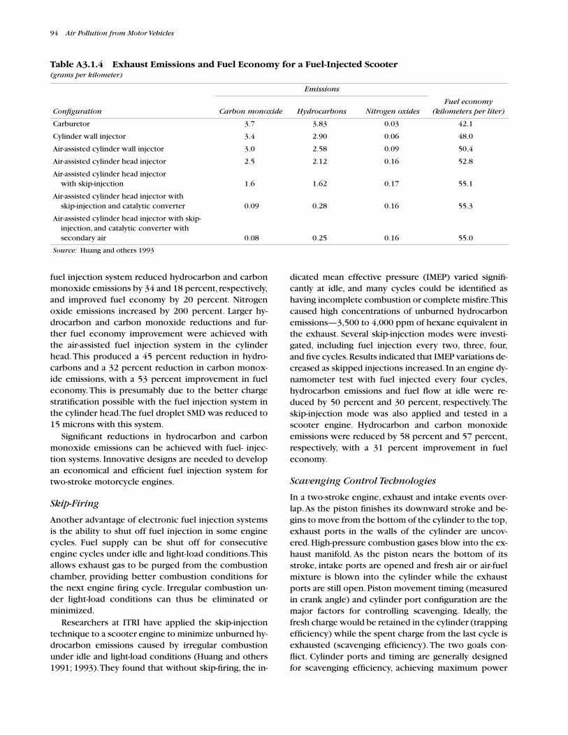
94
Air Pollution from Motor Vehicles
fuel injection system reduced hydrocarbon and carbonmonoxide emissions by 34 and 18 percent, respectively,and improved fuel economy by 20 percent. Nitrogenoxide emissions increased by 200 percent. Larger hy-drocarbon and carbon monoxide reductions and fur-ther fuel economy improvement were achieved withthe air-assisted fuel injection system in the cylinderhead. This produced a 45 percent reduction in hydro-carbons and a 32 percent reduction in carbon monox-ide emissions, with a 53 percent improvement in fueleconomy. This is presumably due to the better chargestratification possible with the fuel injection system inthe cylinder head. The fuel droplet SMD was reduced to15 microns with this system.
Significant reductions in hydrocarbon and carbonmonoxide emissions can be achieved with fuel- injec-tion systems. Innovative designs are needed to developan economical and efficient fuel injection system fortwo-stroke motorcycle engines.
Skip-Firing
Another advantage of electronic fuel injection systemsis the ability to shut off fuel injection in some enginecycles. Fuel supply can be shut off for consecutiveengine cycles under idle and light-load conditions. Thisallows exhaust gas to be purged from the combustionchamber, providing better combustion conditions forthe next engine firing cycle. Irregular combustion un-der light-load conditions can thus be eliminated orminimized.
Researchers at ITRI have applied the skip-injectiontechnique to a scooter engine to minimize unburned hy-drocarbon emissions caused by irregular combustionunder idle and light-load conditions (Huang and others1991; 1993). They found that without skip-firing, the in-
dicated mean effective pressure (IMEP) varied signifi-cantly at idle, and many cycles could be identified ashaving incomplete combustion or complete misfire. Thiscaused high concentrations of unburned hydrocarbonemissions—3,500 to 4,000 ppm of hexane equivalent inthe exhaust. Several skip-injection modes were investi-gated, including fuel injection every two, three, four,and five cycles. Results indicated that IMEP variations de-creased as skipped injections increased. In an engine dy-namometer test with fuel injected every four cycles,hydrocarbon emissions and fuel flow at idle were re-duced by 50 percent and 30 percent, respectively. Theskip-injection mode was also applied and tested in ascooter engine. Hydrocarbon and carbon monoxideemissions were reduced by 58 percent and 57 percent,respectively, with a 31 percent improvement in fueleconomy.
Scavenging Control Technologies
In a two-stroke engine, exhaust and intake events over-lap. As the piston finishes its downward stroke and be-gins to move from the bottom of the cylinder to the top,exhaust ports in the walls of the cylinder are uncov-ered. High-pressure combustion gases blow into the ex-haust manifold. As the piston nears the bottom of itsstroke, intake ports are opened and fresh air or air-fuelmixture is blown into the cylinder while the exhaustports are still open. Piston movement timing (measuredin crank angle) and cylinder port configuration are themajor factors for controlling scavenging. Ideally, thefresh charge would be retained in the cylinder (trappingefficiency) while the spent charge from the last cycle isexhausted (scavenging efficiency). The two goals con-flict. Cylinder ports and timing are generally designedfor scavenging efficiency, achieving maximum power
Table A3.1.4 Exhaust Emissions and Fuel Economy for a Fuel-Injected Scooter
(grams per kilometer)
Emissions
Configuration Carbon monoxide Hydrocarbons Nitrogen oxidesFuel economy
(kilometers per liter)
Carburetor 3.7 3.83 0.03 42.1
Cylinder wall injector 3.4 2.90 0.06 48.0
Air-assisted cylinder wall injector 3.0 2.58 0.09 50.4
Air-assisted cylinder head injector 2.5 2.12 0.16 52.8
Air-assisted cylinder head injector with skip-injection 1.6 1.62 0.17 55.1
Air-assisted cylinder head injector with skip-injection and catalytic converter 0.09 0.28 0.16 55.3
Air-assisted cylinder head injector with skip- injection, and catalytic converter with secondary air 0.08 0.25 0.16 55.0
Source:
Huang and others 1993

Emission Control Technology for Spark-Ignition (Otto) Engines
95
output and smoother idle at the expense of increasedshort-circuiting and hydrocarbon emissions. It is possi-ble to reconfigure intake and exhaust ports to fine- tunescavenging characteristics for lower emissions, but thisinvolves performance tradeoffs. Another way to in-crease trapping efficiency, with minimum impact onperformance, is applying exhaust charge controltechnology.
Exhaust charge control technology modifies exhaustflow by introducing control valves in the exhaust or byusing the exhaust pressure pulse wave. Using the ex-haust pressure pulse wave to control intake and exhaustflow requires a long exhaust pipe, and is effective onlyfor a restricted range of engine speeds. Control valvesare usually used to control the exhaust flow rate in smallengines. The critical variable for exhaust charge controltechniques is the contraction ratio, defined as the ratioof the unrestricted exhaust passage area to the restrict-ed exhaust passage area regulated by the valve. The ef-fectiveness of these techniques is measured by thedelivery ratio, which is the ratio between the mass ofair-fuel mixture actually delivered to the engine and themass of air-fuel mixture contained by the engine dis-placement volume at ambient conditions.
Research has demonstrated the potential of exhaustcharge control valves in small two-stroke engines(Hsieh and others 1992; Tsuchiya and others 1980; Du-ret and Moreau 1990). Significant reductions in hydro-carbon emissions and fuel consumption can beachieved, as can a reduction in unstable combustion atlight load. The delivery ratio where rapid increase in ir-regular combustion occurs (defined as the critical de-livery ratio) is 0.2 (Tsuchiya and others 1980). This issimilar to a recent finding of 0.25 as the critical deliveryratio (Hsieh and others 1992). With exhaust chargecontrol, the critical delivery ratio decreases from 0.25to 0.20 and 0.15 at low and medium engine speeds(1,500 and 3,000 rpm), respectively (Hsieh and others1992). The exhaust charge control technique reducesirregular combustion under light-load conditions. Hy-drocarbon emissions and fuel consumption were re-duced by 30 percent and 6 percent, respectively, whenthe exhaust charge control technique was used in a testengine. At the same delivery ratio, the engine with ex-haust charge control produced higher power output. A60 percent reduction in hydrocarbon emissions and a20 percent reduction in fuel consumption can beachieved with an exhaust charge control valve (Duretand Moreau 1990).
Honda has incorporated a “Revolutionary ControlledExhaust Valve (RC Valve)” in a 150 cc, two-stroke motor-cycle equipped with a capacitive-discharge ignition,computerized controller, and servo motor to attain highpower efficiency at low- and high-speed conditions(Tan and Chan 1993). Although the RC Valve is intended
to improve engine performance, it can also serve as anemissions control device.
Other Engine Modifications
Other engine modifications and techniques include im-proved combustion chamber and piston configurations,improved lean–dilute combustion to prevent misfire,and changes in ignition timing and design.
Combustion chamber
. Combustion chamber and pis-ton configurations can be improved to induce more tur-bulent motions during the compression stroke and tocontrol the direction of the fresh charge to minimizeshort-circuiting. Improved combustion chamber andpiston configurations can also minimize the formationof pockets or dead zones in the cylinder. Researchers atGraz University of Technology (GUT) in Austria de-signed a combustion chamber that concentrated thesquish area above the exhaust port (Laimbock andLanderl 1990). This design forces the fresh charge tooverflow the spark plug, which improves cooling andallows the engine to run leaner without pre-ignition.
Lean–dilute combustion technology
. Lean-burn en-gines can develop low nitrogen oxide and carbon mon-oxide emissions and good fuel economy, but theyrequire a high-energy ignition system or stratifiedcharge to avoid misfire and cyclic instability, resulting inhigh hydrocarbon emissions. Stratified-charge two-stroke engines with fuel injection systems include theOCP, PROCO, and DISC engines developed by Orbital,Ford, and General Motors, respectively. Another con-cept is the two-step, stratified-charge for a crankcase-scavenged, two-stroke engine (Blair and others 1991).In this system, air is introduced to scavenge the burnedgas in the cylinder, then a rich mixture is delivered tothe cylinder just after scavenging.
Ignition timing
. Ignition timing on two-stroke motor-cycle engines is usually chosen to optimize power out-put rather than fuel economy or exhaust emissions. Theeffects of ignition timing on combustion and emissionsin two-stroke engines are similar to the effects in four-stroke engines. Retarding ignition timing reduces pow-er and increases fuel consumption, but reduces nitro-gen oxide and hydrocarbon emissions. Retardingignition timing, especially at high loads, may recoverthe increased nitrogen oxide emissions that otherwiseresult from a lean mixture in low-emission, two-strokeengines.
The effect of ignition timing on direct-injected,spark-ignition engines is different from that in otherspark-ignition engines. In direct-injection systems, ad-vancing ignition timing at light load reduces hydrocar-

96
Air Pollution from Motor Vehicles
bon emissions by reducing the dispersion of the fuelcloud. This cloud is less likely to contact the walls of thecombustion chamber. This reduces the hydrocarbonsproduced by the quenching effect at the combustionchamber walls, as well as the filling of crevice volumeswith unburned mixture. Unburned hydrocarbonscaused by flame quenching and crevice volumes are ma-jor sources of hydrocarbon exhaust emissions. With bet-ter combustion quality at advanced ignition timing,carbon monoxide emissions are also reduced. Nitrogenoxide emissions, however, are increased with advancedignition timing.
Dual spark-plug ignition
. Researchers at ITRI haveused a dual spark-plug ignition in a scooter two-strokeengine to determine the effects on engine torque andunburned hydrocarbon emissions (Huang and others1991). The engine with dual spark plugs had lower hy-drocarbon emissions and better engine torque at low-and medium-load. Improvements were thought to bethe result of increased combustion speed and decreasedmixture bulk quenching when the dual-plug ignitionwas used. ITRI’s findings also showed that additionalspark plugs did not improve the hydrocarbon emissionsunder idling or light-load conditions.
Exhaust Aftertreatment Technologies
Aftertreatment technologies such as thermal oxidationand catalytic converters provide emission control be-yond that achievable with engine and fuel-meteringtechnologies alone. Catalytic converters are used exten-sively in automobiles and have also been demonstratedin two-stroke motorcycles and other small engines (Bur-rahm and others 1991; Laimbock and Landerl 1990;Hsien and others 1992).
Thermal oxidation
. Thermal oxidation is used to re-duce hydrocarbon and carbon monoxide emissions bypromoting oxidation in the exhaust. This oxidationtakes place in the exhaust port or pipe and may requireadditional air injection. Substantial reductions in hydro-carbon and carbon monoxide emissions can beachieved if the exhaust temperature is high enough fora long period. The temperatures required for hydrocar-bon and carbon monoxide oxidation are 600 and700°C, respectively. These requirements are difficult tomeet in small engines with short exhaust systems, butthey have been demonstrated with a four-stroke engineby introducing secondary air into the stock exhaustmanifold upstream of the engine muffler. Air injection atlow rates into the stock exhaust system was found to re-duce hydrocarbon emissions by 77 percent and carbonmonoxide emissions by 64 percent (White and others1991). This was only effective under high-power operat-
ing conditions. The temperatures required to achieveoxidation substantially increase the external tempera-ture of the exhaust pipe.
Oxidation catalyst
. Like thermal oxidation, the oxida-tion catalyst is used to promote oxidation of hydrocar-bon and carbon monoxide emissions in the exhauststream. It also requires sufficient oxygen for the reac-tion to occur. Some of the requirements for a catalyticconverter to be used in two-stroke engines include highhydrocarbon conversion efficiency, resistance to ther-mal damage, resistance to poisoning by sulfur and phos-phorus compounds in the lubricating oil, and low light-off temperature. Additional requirements for catalystsin motorcycle engines include extreme vibration resis-tance, compactness, and light weight.
Using catalytic converters in two-stroke engines isdifficult because of the high concentration of hydrocar-bons and carbon monoxide in their exhaust. If com-bined with sufficient air, these concentrations causecatalyst temperatures that easily exceed the tempera-ture limits of the catalyst, and also pose the risk of fireor injury to motorcycle users. Catalytic converters intwo strokes require engine modifications to reduce pol-lutant concentrations in the exhaust, and may requirethat air supply be limited to the exhaust before thecatalyst.
Oxidation catalytic converters have been applied tosmall engines. Researchers at GUT and ITRI have pub-lished data on the application of catalytic converters insmall two- stroke engines. The Graz researchers focusedon reducing exhaust emissions from two-stroke moped,motorcycle, and chainsaw engines by using catalyticconverters, and on improving the thermodynamic char-acteristics of the engine, such as gas exchange and fuelhandling systems, cylinder and piston geometry andconfigurations, and exhaust and cooling systems. Theeffects of catalytic converters on two moped enginestested under the ECE-15 driving cycle are shown in ta-ble A3.1.5. In the 1.2 horsepower engine, the catalyticconverter reduced hydrocarbon and carbon monoxideemissions by 96.7 and 98.5 percent, respectively. Therewas no change in nitrogen oxides. For the 2.7 horse-power engine, hydrocarbon, carbon monoxide, and ni-trogen oxide emissions were reduced by 96.4, 87.9, and27.8 percent, respectively. Hydrocarbon and carbonmonoxide emissions were reduced even further whenan advanced engine with a watercooled cylinder andfour scavenger ports was used with the catalytic con-verter. Data on catalyst temperatures and emissions du-rability are not available.
ITRI researchers retrofit a catalytic converter to a125 cc, two-stroke motorcycle engine and demon-strated effective emissions control and durability

Emission Control Technology for Spark-Ignition (Otto) Engines
97
(Hsien and others 1992). The researchers evaluated theeffects of catalyst composition and substrate, the celldensity of the substrate, the converter size and installa-tion location, and the use of secondary air injection onthe catalytic effectiveness and engine performance.Their conclusions were: (i) metal substrate is superiorto ceramic substrate for converter efficiency and en-gine performance, since the thin walls of the metal sub-strate have a larger effective area and lower backpressure; (ii) exhaust temperature profile, space avail-ability, and the effects on engine exhaust tuning mustbe considered when installing the catalytic converter;(iii) additional catalyst would improve the carbon mon-oxide conversion efficiency in the rich air–fuel mixturetypical of two-stroke motorcycle engines; (iv) the celldensity of the substrate should be less than 200 cpsi tominimize pressure loss and maintain engine power; (v)hydrocarbon and carbon monoxide conversion effi-ciency increases significantly when secondary air issupplied; and (vi) exhaust smoke opacity was reducedwith the use of the catalytic converter. Reduced opaci-ty was probably the result of catalytic oxidation of thelubricating oil vapor. This has been observed in otherengines.
ITRI also retrofit a catalytic converter to a two-strokescooter along with fuel injection and skip- firing at idle.Adding the catalytic converter improved overall emis-sions control efficiency from 58.2 percent to 92.8 per-cent for hydrocarbons, and from 56.8 to 97.6 percentfor carbon monoxide emissions. Efficiency improvedonly slightly with the use of secondary air. This is be-cause the fuel-injected engine operated at lean condi-tions, so oxygen was available in the catalytic convertereven without air injection.
Catalytic converters have been used for several yearson two-stroke motorcycles and mopeds to meetemission standards in Austria, Switzerland, and Taiwan(China). In-use experience indicates they are accept-able, although special heat shielding is needed to pro-tect passengers from contact with the catalyst housing,
which can reach 500°C. Conclusive data on the durabil-ity of these converter systems are not available.
Lubricating Oil Technologies
Lubricating oil is the major source of particulate matteremissions from two-stroke engines. Since the crankcaseof a two-stroke engine is used for pumping air or the air-fuel mixture into the combustion chamber, it cannot bea lubricant-oil reservoir. Oil mist is therefore injectedinto the incoming air stream. As this stream passesthrough the crankcase, lubrication is provided for cylin-der walls, crankshaft bearings, and connecting-rod bear-ings. Ball or roller bearings are typically used instead ofthe plain bearings of a four-stroke engine. The oil mistcontinues to the combustion chamber, where it is partlyburned. Remaining unburned oil recondenses in the ex-haust plume and creates blue or white smoke. Becausephosphorus or other deposit-forming additives in theoil would poison a catalytic converter, two-stroke oilsfor catalyst- equipped motorcycles need to be formulat-ed without these compounds.
Lubrication system
. Three approaches are used to sup-ply lubricating oil to two-stroke engines: pre-mixingwith the fuel when it is added to the tank; line-mixing,in which oil is metered into the fuel between the fueltank and the engine; and oil injection, in which the oil ismetered directly into the intake manifold or other pointsusing a pump controlled by engine speed or throttle set-ting. The second and third approaches are the mostcommon in current motorcycles since they control theflow rate of the oil and provide reliable lubrication. In-jection provides the best control. Orbital has designedan electronic lubrication system for their OCP two-stroke engines that reduces the amount of oil requiredby the engine. Several Yamaha two-stroke motorcyclesmarketed in Asia have also used an electronic oil meter-ing system to alter the oil flow to the carburetor accord-ing to engine load. The Yamaha Computer-ControlledLubrication System (YCLS) supplies required lubricating
Table A3.1.5 Moped Exhaust Emissions
(grams per kilometer)
Engine configuration Carbon monoxide Hydrocarbons Nitrogen oxides
1.2 horsepower
Without catalyst 2.716 1.013 0.049
With catalyst 0.09 0.015 0.049
2.7 horsepower
Without catalyst 3.205 0.771 0.09
With catalyst 0.116 0.093 0.065
Advanced engine with catalyst 0.037 0.022 0.067
Source
: Douglas and Blair 1982

98
Air Pollution from Motor Vehicles
oil to the engine according to engine speed using anelectronic control unit and three-way control valve (Tanand Chan 1993). In a fuel injected two-stroke engine,this function could be handled by the same electroniccontrol unit as the fuel injection system.
Low-smoke oil. Conventional two-stroke lubricating oilsare based on long-chain paraffin or naphthene mole-cules that break down slowly and are resistant to com-bustion. Using synthetic, long-chain polyolefin materialsinstead of naphthenes and paraffins can significantly re-duce smoke opacity from two-stroke engines. Becauseof the double carbon bonds in the polyolefin chain,these chains break down more quickly and burn morecompletely. Studies have proven that substituting poly-isobutylene for bright stock or other heavy lube-oil frac-tions in two-stroke lubricating oils can reduce enginesmoke levels (Sugiura and Kagaya 1977; Kagaya and Ish-imaru 1988; Eberan- Eberhorst and others 1979; Brownand others 1989). Lubricity is the same for polyisobuty-lene and bright stock. Low-smoke, polyisobuyltene-based lubricating oil is now required for two-stroke mo-peds and motorcycles in some countries in southeastAsia, including Thailand.
Low-smoke oils will not solve the particulate prob-lem for two strokes. Oil in the 20 to 30 percent of thefresh charge that short-circuits the cylinder will beunaffected by combustion. There is also a possibilitythat combustion of polyisobutene may increase emis-sions of toxic air contaminants, particularly 1,3 butadi-ene. Research is needed to assess the effect of these oilson particulate matter and other emissions.
References
Abraham, M. and S. Prakash. 1992. “Cyclic Variations ina Small Two-Stroke Cycle Spark-Ignited Engine—AnExperimental Study.” SAE Paper 920427. Society ofAutomotive Engineers, Warrendale, Pennsylvania.
ACEA/EUROPIA (European Automobile Manufacturer’sAssociation). 1995. European Program on Emis-sions, Fuels, and Engine Technologies. EPEFE Re-port, Brussels.
Aoyama, T., M. Nakajima, M. Onishi, and S. Nakahiko.1977. “Abnormal Combustion in Two-Stroke Motor-cyle Engines.” SAE Paper 770189, Society of Automo-tive Engineers, Warrendale, Pennsylvania.
Babkov, V., and M. Zamakhayev. 1967. Highway Engi-neering. MIR Publishers, Moscow.
Batoni, G. 1978. “Investigations into the Two-StrokeMotorcycle Engine.” SAE Paper 780170, Society ofAutomotive Engineers, Warrendale, Pennsylvania.
Blair, G.P., R.J. Kee, C.E. Carson, and R. Douglas. 1991.“The Reduction of Emissions and Fuel Consump-
tion by Direct Air-Assisted Fuel Injection into a Two-Stroke Engine.” Paper prepared for the 4th GrazTwo-Wheeler Symposium, Technical University,Graz, Austria.
Bosch, Robert AG. 1986. Automotive Handbook. 2ndedition. Stuttgart.
Brown, R.M., D.A. Fog, and D.H. Garland. 1989. “SmokeReduction In Two-Stroke Gasoline Engines.” Paperprepared for the 5th International Pacific Conferenceon Automotive Engineering. Beijing, China.
Burrahm, R.W., J.J. White, and J.N. Carroll. 1991. “SmallUtility Engine Emissions Reduction Using Automo-tive Technology.” SAE Paper 911805, Society of Auto-motive Engineers, Warrendale, Pennsylvania.
Douglas, R. and G.P. Blair. 1982. “Fuel Injection of aTwo-Stroke Cycle Spark Ignition Engine.” SAE Paper820952, Society of Automotive Engineers, Warren-dale, Pennsylvania.
Duret, P. and J.F. Moreau. 1990. “Reduction of PollutantEmissions of the IAPAC Two-Stroke Engine withCompressed Air Assisted Fuel Injection.” SAE Paper900801. Society of Automotive Engineers, Warren-dale, Pennsylvania.
Eberan-Eberhorst, C.G., and H. Martin. 1979. “Perfor-mance Test Methods For Two-Stroke-Cycle Engine Lu-bricants Including Lean Fuel-Oil Ratio Conditions.”SAE Paper 790078, Society of Automotive Engineers,Warrendale, Pennsylvania.
Faiz A., K. Sinha, M. Walsh, and A. Varma 1990. “Auto-motive Air Pollution – Issues and Options for Devel-oping Countries.” Working Paper Series 492, WorldBank, Washington, D.C.
Hare, C.T., K.J. Springer, W.R. Houtman, and T. Huls,1974. “Motorcycle Emissions, Their Impact, andPossible Control Techniques.” SAE Paper 740267,Society of Automotive Engineers, Warrendale,Pennsylvania.
Hellman, K.H., R.I. Bruetsch, G.K. Piotrowski, and W.D.Tallen. 1989. “Resistive Materials Applied to QuickLightoff Catalysts.” SAE Paper 890799, Society of Au-tomotive Engineers, Warrendale, Pennsylvania.
Heywood, J.B. 1988. Internal Combustion Engine Fun-damentals. New York: McGraw Hill.
Hsieh, P.H., R.F. Horng, H.H. Huang, Y.Y. Peng, and J.Wang. 1992. “Effects of Exhaust Charge Control Valveon Combustion and Emissions of Two-Stroke CycleDirect-Injection S.I. Engine.” SAE Paper 922311.Society of Automotive Engineers, Warrendale,Pennsylvania.
Hsien, P.H., L.K. Hwang, and H.W. Wang. 1992. “Emis-sion Reduction by Retrofitting a 125cc Two- StrokeMotorcycle with Catalytic Converter.” SAE Paper922175, Society of Automotive Engineers, Warren-dale, Pennsylvania.

Emission Control Technology for Spark-Ignition (Otto) Engines 99
Huang, H.H., Y.Y. Peng, M.H. Jeng, and J.H. Wang. 1991.“Study of a Small Two-Stroke Engine with Low-Pres-sure Air-Assisted Direct-Injection System.” SAE Paper912350. Society of Automotive Engineers, Warren-dale, Pennsylvania.
Huang, H.H., M.H. Jeng, N.T. Chang, Y.Y. Peng, J.H.Wang, and W.L. Chang. 1993. “Improvement of Ex-haust Emissions on Two-Stroke Engine by Direct-In-jection System.” SAE Paper prepared for the March1993 Society of Automotive Engineers Congress,Warrendale, Pennsylvania.
Kagaya, M., and M. Ishimaru. 1988. “A New ChallengeFor High Performance Two-Cycle Engine Oils.” SAEPaper 881619. Society of Automotive Engineers,Warrendale, Pennsylvania.
Khatri, D.S., A. Ramesh, M.K.G. Babu, and F. Fallahza-deh. 1994. “Simple Techniques for Emission Controlin a Passenger Car Engine.” 3rd International Sympo-sium on Transport and Air Pollution, Poster Proceed-ings, INRETS, Arcueil, France.
Laimbock, F.J. and C.J. Landerl. 1990. “50cc Two-StrokeEngines for Mopeds, Chainsaws, and Motorcycleswith Catalysts.” SAE Paper 901598, Society ofAutomotive Engineers, Warrendale, Pennsylvania.
Monnier, G., and P. Duret. 1991. “IAPAC Compressed AirAssisted Fuel Injection for High Efficiency Low Emis-sions Marine Outboard Two-Stroke Engines.” SAE Pa-per 911849, Society of Automotive Engineers,Warrendale, Pennsylvania.
Nuti, M. and L. Martorano. 1985. “Short-Circuit RatioEvaluation in the Scavenging of Two-Stroke S.I. En-gines.” SAE Paper 850177, Society of Automotive En-gineers, Warrendale, Pennsylvania.
Pearce, T.C. and G.P. Davies. 1990. “The Efficiency ofAutomotive Exhaust Catalysts and the Effects ofComponent Failure.” Research Report 287. TRRL.Crowthorne, Berkshire.
Plohberger and others. 1988. “Development of a Fuel-Injected Two-Stroke Gasoline Engine.” SAE Paper
880170, Society of Automotive Engineers, Warren-dale, Pennsylvania.
Prigent, M. and G. De Soete. 1989. “Nitrous Oxide N2Oin Engines Exhaust Gases - A First Appraisal of Cata-lyst Impact”, SAE Paper 890492, SAE International,Warrendale, Pennsylvania.
Sugiura, K. and M. Kagaya. 1977. “A Study of VisibleSmoke Reduction From a Small Two-Stroke EngineUsing Various Engine Lubricants.” SAE Paper770623, Society of Automotive Engineers, Warren-dale, Pennsylvania.
Tan, M. and T. Chan. 1993. “Technical Handout” HongLeong Sdn. Bhd., Distributor of Yamaha Motorcyclesin Malaysia.
Tsuchiya, K., S. Hirano, M. Okamura, and T. Gotoh.1980. “Emission Control of Two-Stroke MotorcycleEngines by the Butterfly Exhaust Valve.” SAE Paper800973, Society of Automotive Engineers, Warren-dale, Pennsylvania.
U.S. EPA (United States Environmental Protection Agen-cy). 1990. “Volatile Organic Compounds from On-Road Vehicles: Sources and Control Options.” Reportprepared for the Long-range Transboundary Air Pollu-tion Convention. United Nations Economic Commis-sion for Europe. Washington, D.C. (Draft.)
Weaver, C.S. and L.M. Chan. 1994. “Motorcycle EmissionStandards and Emission Control Technology.” Reportto the Royal Thai Ministry of Science, Technology, andthe Environment and The World Bank. Engine, Fuel,and Emissions Engineering, Inc. Sacramento,California.
Weaver, C.S. and L.M. Chan. 1995. “Company Archives”Multiple Sources. Engine, Fuel and Emissions Engi-neering, Inc., Sacramento, California.
White, J.J., J.N. Carroll, C.T. Hare, and J.G. Lourenco.1991. “Emission Control Strategies for Small UtilityEngines.” SAE Paper 911807, Society of AutomotiveEngineers, Warrendale, Pennsylvania.

Emission Control Technology for Spark-Ignition (Otto) Engines 100

101
This appendix provides a more detailed technical dis-cussion to supplement the general information on die-sel engine emissions and control technologies inchapter 3.
Diesel Combustion and Pollutant Formation
Diesel engine emissions are determined largely by thecombustion process. During the compression stroke, adiesel engine compresses only air. The process of com-pression heats the air to about 700–900ºC, which is wellabove the self-ignition temperature of diesel fuel. Nearthe top of the compression stroke, liquid fuel is injectedinto the combustion chamber under tremendous pres-sure through a number of small orifices in the tip of theinjection nozzle.
Figure A3.2.1 shows the stages of diesel injection andthe subsequent combustion process. As fuel is injectedinto the combustion chamber just before the pistonreaches top-dead-center, the periphery of each jet mixeswith the hot compressed air already present. After a briefperiod known as the ignition delay, this fuel-air mixtureignites. In the
premixed combustion
phase, the fuel-airmixture formed during the ignition delay period burnsvery rapidly, causing a rapid rise in cylinder pressure. Thesubsequent rate of burning is controlled by the rate atwhich the remaining fuel and air can mix. Combustion al-ways occurs at the interface between the air and the fuel.Most of the fuel injected is burned in this
mixing-con-trolled combustion
phase, except under very light loads,when the premixed combustion phase dominates.
Nitrogen Oxides
Diesel engines are a significant source of nitrogen oxideemissions, primarily in the form of nitric oxide (NO).This gas results from the reaction between nitrogen andfree oxygen at the high temperatures close to the flame
front. The rate of NO formation in diesels is a functionof oxygen availability, and increases exponentially withflame temperature. Emissions of nitrogen oxides (NO
x
)can be reduced effectively by actions which reduce theflame temperature. These include delaying combustioninto the expansion phase, cooling the air charge goinginto the cylinder, and exhaust gas recirculation (EGR).Since combustion always occurs under near-stoichio-metric conditions, reducing the flame temperature bylean-burn techniques, as in spark-ignition engines, isimpractical.
Most of the NO
x
emitted is formed early in the com-bustion process, when the piston is still near the top ofits stroke. This is when the flame temperature is highest.Work by several researchers (Wade and others 1987;Cartellieri and Wachter 1987) indicates that a largeshare of diesel NO
x
is formed during the premixed com-bustion phase. It has been found that reducing theamount of fuel burned in this phase can significantly re-duce these emissions. An effective way of reducing NO
x
emissions is to retard the injection timing such thatburning occurs later in the cycle. However, this may in-crease smoke and fuel consumption. Since NO
x
emis-sions are highest at high loads, a flexible timing plancould be introduced. This would vary the injection tim-ing in accordance with the engine conditions to obtaina better tradeoff among different pollutant emissions.This type of system would require the use of electroniccontrols, which are considerably more expensive thanconventional fuel injection equipment.
Charge cooling reduces NO
x
emissions by reducingthe charge temperature. This technique is particularlyattractive owing to the additional benefit of increasedpower. In the absence of emission controls, the range ofNO
x
emissions from turbocharged charge-cooled DI en-gines (7-17 g/kWh) is lower than for naturally aspirated(11-23 g/kWh) and turbocharged (13-28 g/kWh) DI en-gines (figure A3.2.2).
Emission Control Technology for Compression Ignition (Diesel) Engines
Appendix 3.2

102
Air Pollution from Motor Vehicles
Figure A3.2.1 Diesel Combustion Stages
Source:
Heywood 1988
Start of injection Premixed combustion
Mixing-controlled combustion Late combustion
Premixed combustion phase
Ignitiondelayperiod Mixing-controlled combustion phase
Latecombustionphase
dEOI
e
210200190180170160
SOI
C
a bCrank angle, degrees SOI = start of ignition
EOI = end of ignition
Rat
e of
hea
t rel
ease

Emission Control Technology for Compression Ignition (Diesel) Engines
103
A better tradeoff between NO
x
emissions and fuelconsumption can be achieved by optimizing the mixingprocess. The use of higher injection pressures reducesthe heat release period, which allows the use of moreretarded timings and leads to a better NO
x
emission-fuelconsumption tradeoff. Other methods of NO
x
reduc-tion include chemical removal, water injection, and ex-haust gas recirculation. However, these techniques mayintroduce durability problems.
Particulate Matter
Diesel particulate matter
1
consists mostly of three com-ponents: soot formed during combustion, heavyhydrocarbons condensed or adsorbed on the soot, andsulfates. In older diesels soot was typically 40 to 80percent of the total particulate mass, but soot emissionsfrom modern emission-controlled engines are muchlower. Most of the remaining particulate mass consistsof heavy hydrocarbons adsorbed or condensed on thesoot. This is referred to as the soluble organic fraction
(SOF) of the particulate matter. The SOF is derived partlyfrom the lubricating oil, partly from unburned fuel, andpartly from compounds formed during combustion.
Diesel soot is formed primarily during the mixing-controlled combustion phase. Primary soot particlesare small spheres of graphitic carbon approximately0.01 millimeter in diameter. These are formed by the re-action of gaseous hydrocarbons such as acetylene un-der conditions of moderately high temperature andoxygen deficiency. The primary particles then agglom-erate to form chains and clusters of linked particles, giv-
1. The diesel combustion process results in fuel-rich zones inwhich carbon particles are formed. These particles adsorb organiccompounds (primarily aliphatic and polycyclic aromatic hydrocar-bons) and sulfuric acid during the exhaust gas cooling and dilutionprocess. The hydrocarbons originating from the unburnt lubricatingoil contribute significantly (up to 40 percent) to heavy-duty diesel PMemissions. Although PM emissions are related to smoke and hydrocar-bon emissions, there is no direct correlation. Particulate matter emis-sions are assessed gravimetrically while smoke is measured by a lightobscuration technique.
Figure A3.2.2 Hydrocarbon and Nitrogen Oxide Emissions for Different Types of Diesel Engines
(European 13-mode test)
Note: D.I.NA = direct injection naturally aspirated; D.I.TC = direct injection turbocharged; D.I.TCA = direct injection turbocharged aftercooled, I.D.INA = indirect injection naturally aspirated.
Source:
Latham and Tomkin 1988
D.I. NA
D.I. TC
D.I. TCAI.D. INA
NOx (g/kWh)
HC
(g/
kWh)
3.0
2.0
2.0
0.00 5 10 15 20 25 30

104
Air Pollution from Motor Vehicles
ing the soot its characteristic fluffy appearance. Duringmixing-controlled combustion, the local gas composi-tion at the flame front is close to stoichiometric, with anoxygen-rich region on one side and a fuel-rich region onthe other. The moderately high temperatures and oxy-gen deficiency required for soot formation are thus al-ways present.
Most of the soot formed during diesel combustion issubsequently burned during the later portions of the ex-pansion stroke. Typically, less than 10 percent of thesoot formed in the cylinder survives to be emitted intothe atmosphere; in modern emission-controlled dieselengines, less than one percent may be emitted. Soot ox-idation is much slower than soot formation, however,and the amount of soot oxidized is dependent on theavailability of high temperatures and adequate oxygenduring the late stages of combustion. Conditions that re-duce the availability of oxygen (such as poor mixing oroperation at low air-fuel ratios), or which reduce thetime available for soot oxidation (such as retarding thecombustion timing) can cause a very large increase insoot emissions.
Hydrocarbons and Related Emissions
Diesel engines normally emit low levels of hydrocarbons.Diesel HC emissions are mainly due to incomplete com-bustion of the fuel or the lubricating oil. Hydrocarbonemissions can be controlled by the correct matching ofthe air-fuel mixing process and injection equipment. Fur-ther mechanical developments have reduced oil- derivedhydrocarbon levels by reducing the amount of oil enter-ing the cylinder. In extreme cases major structural chang-es may be required. Other reductions can be made byreducing the nozzle sac/hole volume and avoiding sec-ondary injections. In general diesel engine hydrocarbonemissions are fairly easy to control.
Diesel hydrocarbon emissions (as well as the un-burned-fuel portions of the particulate SOF) occur pri-marily at light loads. The major source of light-loadhydrocarbon emissions is excessive air-fuel mixing,which results in air-fuel mixture(s) that are too lean toburn. Other hydrocarbon sources include fuel deposit-ed on the combustion chamber walls or in combustionchamber crevices by the injection process, fuel retainedin the orifices of the injector which vaporizes late in thecombustion cycle, partly reacted mixture quenched bytoo-rapid mixing with air, and vaporized lubricating oil.Aldehydes and ketones (as partially-reacted hydrocar-bons) and the small amount of carbon monoxide pro-duced by diesels are probably formed in the sameprocesses as the hydrocarbon emissions.
In addition to aldehydes and ketones, unregulatedpollutants from diesel engines include polycyclic andnitro-polycyclic aromatic compounds (PAH and nitro-
PAH), and small quantities of hydrogen cyanide, cyano-gen, and ammonia. The presence of polycyclic aromatichydrocarbons and their nitro-derivatives in diesel ex-haust is of special concern, since these compounds in-clude many known mutagens and suspectedcarcinogens. A significant portion of these compounds(especially the smaller two- and three-ring compounds)are apparently derived directly from diesel fuel. Typicaldiesel fuel contains a significant fraction of PAH by vol-ume. Most of the larger and more dangerous PAH ap-pear to form during the combustion process, possiblyvia the same acetylene polymerization reaction that pro-duces soot (Williams and others 1987). Indeed, the sootparticle itself can be viewed as a very large PAH mole-cule. PAH and nitro-PAH can be reduced by decreasingthe aromatic content of the fuel.
Diesel engines emit significantly more aldehydesand ketones than comparable gasoline engines. Alde-hyde emissions are largely responsible for diesel odorand cause irritation of the nasal passages and eyes.These emissions are strongly related to total hydrocar-bon emissions and can be controlled by the same tech-niques. Sulfur dioxide emissions are the result ofnaturally occurring sulfur in the fuel and can only be re-duced by lowering the fuel sulfur content. Hydrogen cy-anide, cyanogen, and ammonia are present only in smallquantities in diesel exhaust and are unlikely to becomeregulated.
Visible Smoke
Black smoke from diesel engines is due to the soot com-ponent of diesel particulate matter. Under most operat-ing conditions, nearly all of this soot is oxidized in thecylinder, so the exhaust plume from a properly adjusteddiesel engine is normally invisible—with a total opacity(absorbance plus reflectance) of 2 percent or less. Visi-ble black smoke is generally due to injecting too muchfuel for the amount of air available in the cylinder, or topoor mixing between fuel and air. These conditions canbe prevented by proper design. The PM reductions re-quired to comply with U.S. 1994 and Euro 1 emissionstandards have resulted in the virtual elimination ofvisible smoke emissions from properly functioningengines.
Under some conditions, diesel engines may alsoemit white, blue, or gray smoke. These are due to thepresence of condensed hydrocarbon droplets in the ex-haust. Unlike soot, these droplets scatter light, thus giv-ing the smoke a bluish or whitish cast. Blue or graysmoke is generally due to vaporized lubricating oil andindicates an oil leak into the cylinder or exhaust system.White smoke is common when engines are first startedin cold weather and usually goes away when the enginewarms up.

Emission Control Technology for Compression Ignition (Diesel) Engines
105
Noise
Diesel engine noise is due mostly to the rapid combus-tion (and resulting rapid pressure rise) in the cylinderduring the premixed burning phase. The greater the igni-tion delay, and the more fuel is premixed with air, thegreater this pressure rise and the resulting noise emis-sions. Noise emissions and NO
x
emissions thus tend tobe related—reducing the amount of fuel burned in thepremixed burning phase will tend to reduce both. Othernoise sources include those common to all engines, suchas mechanical vibration, fan noise, and so forth. Thesecan be minimized by appropriate mechanical design.
Odor
The characteristic diesel odor is due primarily to partial-ly oxygenated hydrocarbons (aldehydes and similar spe-cies) in the exhaust resulting from slow oxidationreactions in air-fuel mixtures too lean to burn normally.Unburned aromatic hydrocarbons may also play a signif-icant role. The most significant aldehyde species arebenzaldehyde, acetaldehyde, and formaldehyde, butother aldehydes such as acrolein (a powerful irritant)are significant as well. Aldehyde and odor emissions areclosely linked to total hydrocarbon emissions—experi-ence has shown that modifications that reduce total hy-drocarbons also tend to reduce aldehydes and odor aswell.
Toxic Air Contaminants
Diesel exhaust contains many organic species that areknown or suspected of causing cancer or other healthproblems. These include formaldehyde, benzene, andpolynuclear aromatic hydrocarbons, as well as other uni-dentified mutagenic compounds. Organic extracts of die-sel particulate have repeatedly been shown to bemutagenic in the Ames test, a commonly used screeningtechnique for potential carcinogens. California, based ona number of epidemiological studies, has proposed toregulate diesel exhaust itself as a suspected carcinogen.In general, measures that tend to reduce diesel hydrocar-bon and particulate matter emissions also seem to reducemutagenic (and presumed carcinogenic) activity.
Influence of Engine Variables on Emissions
The engine variables having the greatest effects on dieselemission rates are the air-fuel ratio, rate of air- fuel mixing,fuel injection timing, compression ratio, and the tem-perature and composition of the charge in the cylinder.
Air-Fuel Ratio
The ratio of air to fuel in the combustion chamber hasan extremely important effect on emission rates for hy-
drocarbons and particulate matter. In diesel engines,the fact that fuel and air must mix before burning meansthat a substantial amount of excess air is needed to en-sure complete combustion of the fuel within the limitedtime allowed by the power stroke. Diesel engines,therefore, operate with overall air- fuel ratios that areconsiderably lean of stoichiometric (
λ
greater thanone). The minimum air-fuel ratio for complete combus-tion is about
λ
= 1.5. This ratio is known as the smokelimit, since smoke increases dramatically at air-fuel ra-tios lower than this limit. For a given amount of air inthe cylinder, the smoke limit establishes the maximumamount of fuel that can be burned per stroke, and thusthe maximum power output of the engine.
Figure A3.2.3 shows the typical relationship be-tween air-fuel ratio and emissions in a diesel engine. Atvery high air-fuel ratios (corresponding to very lightload), the temperature in the cylinder after combustionis too low to burn out residual hydrocarbons, so emis-sions of gaseous hydrocarbons and particulate SOF arehigh. At lower air-fuel ratios, less oxygen is available forsoot oxidation, so soot emissions increase. As long as
λ
remains above 1.6, this increase is relatively gradual.Soot and visible smoke emissions show a strong non-lin-ear increase below the smoke limit (at about
λ
= 1.5).In naturally aspirated engines (those without a turbo-
charger), the amount of air in the cylinder is independentof the power output. Maximum power output for theseengines is normally smoke-limited, that is, limited by theamount of fuel that can be injected without exceedingthe smoke limit. Maximum fuel settings on naturally aspi-rated engines represent a compromise between smokeemissions and power output. Where diesel smoke is regu-lated, this compromise must result in smoke opacity be-low the regulated limit. Otherwise, opacity is limited bythe manufacturer's judgment of the commercially ac-ceptable smoke level, which varies significantly fromcountry to country.
In conventional turbocharged engines, an increase inthe amount of fuel injected per stroke increases the ener-gy in the exhaust gas, causing the turbocharger to spinmore rapidly and pump more air into the combustionchamber. For this reason, power output from turbo-charged engines is not usually smoke-limited. Instead, itis limited by design limits such as the allowable turbo-charger speed and mechanical and thermal loading of theengine components.
Turbocharged engines do not normally experiencelow air-fuel ratios during steady-state conditions, andtherefore tend to exhibit low steady-state smoke even atfull power. Low air-fuel ratios can occur in turbochargedengines under transient conditions, however. This is be-cause the inertia of the turbocharger rotor keeps it fromresponding instantly to an increase in fuel input. Thus

106
Air Pollution from Motor Vehicles
the air supply during the first few seconds of full-poweracceleration is less than would be supplied by the turbo-charger in steady-state operation. Unless the fuel is sim-ilarly limited during this period, the air-fuel ratio will bebelow the smoke limit, resulting in a black ‘puff’ ofdense smoke. The resulting excess particulate emissionscan be significant under urban driving conditions. Toovercome this problem, turbocharged engines in high-way vehicles commonly incorporate an accelerationsmoke limiter. This device modulates the fuel flow to theengine according to the boost pressure to allow theturbocharger time to respond.
The setting on the smoke limiter must compromisebetween acceleration performance (drivability) andlow smoke emissions. In the United States, accelerationsmoke emissions are regulated. ECE R24 also limits free-acceleration smoke opacity. Elsewhere, accelerationsmoke opacity is limited by the manufacturer's judg-ment of commercial acceptability, or by the need topass free-acceleration smoke tests.
The high transient smoke emissions observed fromturbocharged engines not equipped with adequate ac-celeration smoke limiters have led some parties to con-clude that turbocharged engines produce worseemissions than naturally aspirated engines. For exam-ple, an opacity test (ECE Regulation 24) carried out by
London Buses Limited (LBL) on 254 buses in its opera-tional fleet showed that 68 percent of the naturally aspi-rated buses passed the test compared with a 36 percentpass rate for turbocharged buses (Gore 1991). Whenproperly controlled, however, turbocharged enginestend to have lower emissions of particulate matter andoxides of nitrogen than naturally- aspirated engines ofsimilar power output. Indeed, the strict emissions limitsnow effective in the United States have nearly eliminat-ed naturally-aspirated engines from the U.S. market, anda similar trend in Europe with the advent of stricter die-sel emission standards. High efficiency turbochargingsuch as variable geometry turbochargers (VGT) andcharge cooling increase the air-fuel ratio and so lead to afurther reduction in PM emissions under most engineconditions.
Air-Fuel Mixing
The rate of mixing between the compressed charge inthe cylinder and the injected fuel is among the most im-portant factors in determining diesel performance andemissions. The mixing rate during the ignition delay peri-od determines how much fuel is burned in the premixedburning phase. The higher the mixing rate, the greaterthe amount of fuel burning in the premixed mode, andhigher the noise and NO
x
emissions. In the subsequent
Figure A3.2.3 Relationship between Air-Fuel Ratio and Emissions for a Diesel Engine
Source:
Weaver and Chan 1995
NOx
HC
Particulate matter
Air-fuel ratio
Increasing power output
1 2 4 8 16 32 64
Incr
easi
ng e
mis
sion
s (g
/kW
h)

Emission Control Technology for Compression Ignition (Diesel) Engines
107
mixing-controlled combustion phase, the rate of com-bustion is limited by the mixing rate. The more rapid andcomplete this mixing, the greater the amount of fuel thatburns near the top-dead-center, the higher the efficiency,and the lower the PM emissions.
In engine design practice, it is necessary to strike abalance between the rapid and complete mixing re-quired for low soot emissions and best fuel economy, asthe too-rapid mixing results in high NO
x
emissions. Theprimary factors affecting the mixing rate are the fuel in-jection pressure, the number and size of injection orific-es, any swirling motion imparted to the air as it entersthe cylinder during the intake stroke, and air motionsgenerated by combustion chamber geometry duringcompression. Much of the progress in in-cylinder emis-sion control over the last decade has come through im-proved understanding of the interactions betweenthese different variables and emissions, leading to im-proved design of fuel injection systems and combustionchambers.
Air-fuel mixing rates in current emission-controlledengines are the product of extensive optimization to as-sure rapid and complete mixing under nearly all operat-ing conditions. Poor mixing may still occur during ‘lug-down’–high-torque operation at low engine speeds.Turbocharger boost, air swirl level, and fuel injectionpressure are typically poorer in these ‘off-design’ condi-tions. Significant improvements can be made in smokeemission and fuel consumption by optimizing the swirlratio as a function of engine speed. Maintenance prob-lems such as injector tip deposits can also degrade air-fuel mixing and result in greatly increased emissions.This is a common cause of high smoke emissions.
Fuel Injection and Combustion Timing
The timing relationship between the beginning of fuelinjection and the top of the compression stroke has animportant effect on diesel engine emissions and fueleconomy. For best fuel economy, it is preferable thatcombustion begin at or somewhat before top-dead-cen-ter. Since there is a finite delay between the beginningof injection and the start of combustion, it is necessaryto inject the fuel somewhat before this point (generally5 to 15 degrees of crankshaft rotation before). The earli-er fuel is injected, the less compression heating willhave occurred, and the longer the ignition delay. Thelonger ignition delay provides more time for air and fuelto mix, increasing the amount of fuel that burns in thepremixed combustion phase. More fuel burning at orjust before top-dead-center also increases the maximumtemperature and pressure attained in the cylinder. Bothof these effects tend to increase NO
x
emissions. On theother hand, earlier injection timing tends to reduce PM
and light-load hydrocarbon emissions. Fuel burning inpremixed combustion forms little soot, while the sootformed in mixing-controlled combustion near top-dead-center experiences a relatively long period of high tem-peratures and intense mixing, and is thus mostly oxi-dized. The end-of-injection timing also has a major effectupon soot emissions—fuel injected more than a few de-grees after TDC burns more slowly, and at a lower tem-perature, so that less of the resulting soot has time tooxidize during the power stroke. For a fixed injectionpressure, orifice size, and fuel quantity, the end-of-injec-tion timing is determined by the timing of the begin-ning of injection.
The result of these effects is that injection timingmust compromise between PM emissions and fueleconomy on the one hand and noise, NO
x
emissions,and maximum cylinder pressure on the other. The termsof the compromise can be improved to a considerableextent by increasing injection pressure, which increas-es mixing and advances the end-of-injection timing. An-other approach under development is split injection, inwhich a small amount of fuel is injected early in orderto ignite the main body of fuel quantity injected neartop-dead-center. Some fuel injection systems can nowvary the injection rate, within limits, under electroniccontrol.
Compared to uncontrolled diesel engines, moderndiesel engines with emission controls generally havemoderately retarded injection timing to reduce NO
x
, inconjunction with high injection pressure to limit the ef-fects of retarded timing on PM emissions and fuel econ-omy. The response of fuel economy and PM emissions toretarded timing is not linear—up to a point, the effectsare relatively small, but beyond that point deteriorationis rapid. Great precision in injection timing thus be-comes necessary—a change of one degree crank anglecan have a significant impact on emissions. The optimalinjection timing is a complex function of engine design,engine speed and load, and the relative stringency ofemission standards for different pollutants. Attaining therequired flexibility and precision of injection timing hasposed a major challenge to fuel injection manufacturers.
Charge Temperature
The process of compressing the intake air in turbo-charged engines increases its temperature. Reducing thetemperature of the compressed air charge going into thecylinder has benefits for both PM and NO
x
emissions.Reducing the charge temperature directly reduces theflame temperature during combustion, and thus helps toreduce NO
x
emissions. In addition, the relatively colderair is denser, so that (at the same pressure) a greater massof air can be contained in the same fixed cylinder vol-

108
Air Pollution from Motor Vehicles
ume. This increases the air-fuel ratio in the cylinder andthus helps to reduce soot emissions. By increasing theair available while decreasing piston temperatures,charge-air cooling can also make possible a significant in-crease in power output while remaining within the en-gine thermal limits. For this reason, many high-poweredturbocharged engines incorporate charge-air coolerseven in the absence of emission controls. Charge-aircoolers are almost universal on low-emission engines,many of which use air-to-air aftercooling to achieve thelowest possible temperature. However, excessively coldcharge air can reduce the burnout of hydrocarbons, andthus increase light-load hydrocarbon emissions. This canbe counteracted by advancing injection timing, or by re-ducing charge air cooling at light loads.
Charge Composition
Nitrogen oxide emissions are heavily dependent onflame temperature. By altering the composition of theair charge to increase its specific heat and the concen-tration of inert gases, it is possible to decrease the flametemperature significantly. The most common way of ac-complishing this is through exhaust gas recirculation(EGR). At moderate loads, EGR has been shown to be ca-pable of reducing NO
x
emissions by a factor of two ormore with little effect on PM emissions. Although sootemissions are increased by the reduced oxygen concen-tration, the soluble organic portion of the PM and gas-eous HC emissions are reduced due to the higher in-cylinder temperature caused by the hot exhaust gas.EGR has been used for some time in light-duty diesel en-gines in order to reduce NO
x
. Preliminary results of astudy of EGR effects in advanced heavy-duty diesel en-gines have shown the potential to achieve extremelylow NO
x
emissions (less than 3 g/kWh) combined withextremely low PM emissions (Needham and others1991; Havenith and others 1993). EGR is consideredone of the most promising NO
x
control technologies.Extensive development, however, is needed with re-gard to combustion system designs, the recirculationand admission system, cooling at high load, rematchingof turbo machinery, wear limitation, and transient con-trol (OECD/IEA 1993).
Compression Ratio
Diesel engines rely on compression heating to ignite thefuel, so the engine's compression ratio has an importanteffect on combustion. A higher compression ratio re-sults in a higher temperature for the compressedcharge, and thus in a shorter ignition delay and higherflame temperature. The effect of a shorter ignition delayis to reduce NO
x
emissions, while the higher flame tem-perature would be expected to increase them. In prac-tice, these two effects nearly cancel each other out, so
that changes in compression ratio have little effect onNO
x
.Engine fuel economy, cold starting, and maximum
cylinder pressures are also affected by the compressionratio. For an idealized diesel cycle, the thermodynamicefficiency is an increasing function of compression ra-tio. In a real engine, however, the increased thermody-namic efficiency is offset after some point by increasingfriction so that a point of maximum efficiency isreached. With most heavy- duty diesel engine designs,this optimal compression ratio is about 12 to 15. To en-sure adequate starting ability under cold conditions,however, most diesel engine designs require a some-what higher compression ratio—in the range of 15–20or more. Generally, higher-speed engines with smallercylinders require higher compression ratios for ade-quate cold starting.
Emissions Tradeoffs
There is an inherent conflict between some of the mostpowerful diesel NO
x
control techniques and PM emis-sions. This is the basis for the much-discussed “tradeoff”relationship between diesel NO
x
and PM emissions. Thetradeoff is not absolute—a combination of technical ad-vances can make it possible to reduce both NO
x
andparticulate emissions (figure A3.2.4). These tradeoffs doplace limits on the extent to which any one pollutantcan be reduced, however. To minimize emissions of allpollutants simultaneously requires careful optimizationof the fuel injection, fuel-air mixing, and combustionprocesses over the full range of engine operatingconditions.
Improvements in Engine Technology
Diesel engine emissions are determined by the com-bustion process within the cylinder. This process iscentral to the operation of the diesel engine. Virtuallyevery characteristic of the engine affects combustionin some way, and thus has some direct or indirect ef-fect on emissions. Some of the engine systems affect-ing diesel emissions are the fuel injection system, theengine control system, air intake and combustionchamber, and the air charging system. Actions to re-duce lubricating oil consumption can also impact hy-drocarbon and PM emissions. Finally, some advancedtechnologies now under development may give evenlower pollutant emissions in the future (Walsh and Bra-dlow 1991).
Combustion System Types
The geometries of the combustion chamber and the airintake port control the air motion in the diesel combus-

Emission Control Technology for Compression Ignition (Diesel) Engines
109
tion chamber, and thus play an important role in air-fuelmixing and emissions. A number of different combus-tion chamber designs are used in diesel engines. Virtual-ly all commercial diesel engines make use of one of thecommon combustion chamber designs shown in figureA3.2.5. The most fundamental difference between thecombustion chambers is between the indirect-injection(IDI) and direct-injection (DI) designs. In an indirect-in-jection engine, fuel is injected into a separate ‘precham-ber,’ where it mixes and partly burns before jetting intothe main combustion chamber above the piston. In themore common direct-injection engine, fuel is injecteddirectly into a combustion chamber hollowed out of thetop of the piston. DI engines can be further divided intohigh-swirl, low-swirl (quiescent chamber), and wall-wetting designs. The latter has many characteristics incommon with indirect-injection systems.
Fuel-air mixing in the direct-injection engine is lim-ited by the fuel injection pressure and any motion im-parted to the air entering the chamber. In high-swirl DIengines, a strong swirling motion is imparted to the airentering the combustion chamber by the design of the
intake port. These engines typically use moderate-to-high injection pressures, and three to five spray holesper nozzle. Low-swirl engines rely primarily on the fuelinjection process to supply the mixing. They typicallyhave very high fuel injection pressures and six to ninespray holes per nozzle. Wall-wetting DI engines alsohave fairly high swirl, but the injection system isdesigned to deposit the fuel on the combustion cham-ber wall, where it vaporizes and burns relatively slowly.
In the IDI engine, the mixing between air and fuel isdriven primarily by air swirl induced in the prechamberas air is forced into it during compression, and by the tur-bulence induced by the expansion out of the precham-ber during combustion. These engines typically havebetter high-speed performance than DI engines, and canuse cheaper fuel injection systems. For this reason, theyhave been used extensively in passenger car and lighttruck applications. Historically, IDI diesel engines havealso exhibited lower emission levels than DI engines.With recent developments in DI engine emission con-trols, however, this is no longer the case. Disadvantagesof the IDI engine are the extra heat and frictional losses
Figure A3.2.4 Estimated PM-NO
x
Trade-Off Over Transient Test Cycle for Heavy-Duty Diesel Engines
Note:
Current engines improve significantly on these trends meeting U.S. 1998 standards without a trap.
Source:
Adapted from Latham and Tomkin 1988

110
Air Pollution from Motor Vehicles
due to the prechamber. These result in a 5 to 15 percentreduction in fuel efficiency compared to a DI engine. Be-cause of this, nearly all heavy-duty truck engines are ofthe DI type, and there is an increasing trend toward DIengines in passenger cars and light trucks.
DI Combustion Chamber Design
Changes in the engine combustion chamber and relatedareas have demonstrated a major potential for emissioncontrol. Design changes to reduce the crevice volumein DI diesel cylinders increase the amount of air avail-able in the combustion chamber. Changes in combus-tion chamber geometry —such as the use of a reentrantlip on the piston bowl—can markedly reduce emissionsby improving air-fuel mixing and minimizing wall im-pingement by the fuel jet. Optimizing the intake portshape for best swirl characteristics has also yieldedsignificant benefits. A number of light- and medium-dutyengines now incorporate variable air intake systems tooptimize swirl characteristics across a broader range ofengine speeds.
Crevice volume
. The crevice volume includes the clear-ance between the top of the piston and the cylinderhead, and the ‘top land’—the space between the side ofthe piston and the cylinder wall above the top com-pression ring. The air in these spaces contributes littleto the combustion process. The smaller the crevice vol-ume, the larger the combustion chamber volume can befor a given compression ratio. Thus, reducing the crev-ice volume increases the amount of air available for
combustion. To reduce these volumes, engine makershave reduced the clearance between the piston and cyl-inder head through tighter production tolerances, andhave moved the top compression ring toward the top ofthe piston. This increases the temperature of the topring and poses design problems for the piston top andcooling system. These problems have been addressedthrough redesign and the use of more expensive mate-rials. The higher piston ring temperature also requireshigher quality engine oil to avoid formation of damag-ing deposits.
Combustion chamber shape
. Numerous test results in-dicate that, for high swirl DI engines, a reentrant com-bustion chamber shape (in which the lip of thecombustion chamber protrudes beyond the walls of thebowl) provides a substantial improvement in perfor-mance and emissions over the previous straight-sidedbowl designs. Nearly all of the manufacturers of high-swirl engines are developing or using this approach.Similar improvements in the performance of low-swirlDI engines have come primarily through refinements tothe classic ‘mexican hat’ combustion chamber shape.
Intake air swirl
. Optimal matching of intake air swirlwith combustion chamber shape and other variables iscritical for emissions control in high-swirl engines.Swirl is determined mostly by the design of the air in-take port. Unfortunately, the selection of a fixed swirllevel involves some tradeoffs between low-speed andhigh-speed performance. At low speeds, higher swirl
Figure A3.2.5 Diesel Engine Combustion Chamber Types
Source:
Weaver and Chan 1995
Indirect injection

Emission Control Technology for Compression Ignition (Diesel) Engines
111
provides better mixing, permitting more fuel to be in-jected and thus greater torque output at the samesmoke level. However, this can result in too much swirlat higher speeds, impairing the airflow to the cylinder.
Attaining an optimal swirl level is most difficult insmaller light-duty and medium-duty DI engines, as theseexperience a wider range of engine speeds than doheavy-duty engines. One solution to this problem is tovary the swirl ratio as a function of engine speed. Anumber of production light- and medium-duty enginesnow use this approach with a noticeable reduction inPM and NO
x
emissions (Shimada, Sakai, and Kurihara1986).
Fuel Injection
The fuel injection system in a diesel engine includes themachinery by which the fuel is transferred from the fueltank to the engine, then injected into the cylinders atthe right time for optimal combustion, and in the cor-rect amount to provide the desired power output. Thequality, quantity, and timing of fuel injection determinethe engine's power, fuel economy, and emission charac-teristics so that the fuel injection system is one of themost important components of the engine.
The fuel injection system normally consists of a low-pressure pump to transfer fuel from the tank to the sys-tem, one or more high-pressure fuel pumps to createthe pressure pulses that actually send the fuel into thecylinder, the injection nozzles through which fuel is in-jected into the cylinder, and a governor and fuel meter-ing system. These determine how much fuel is to beinjected on each stroke, and thus the power output ofthe engine.
The major areas of concentration in fuel injectionsystem development have been on increased injectionpressure, increasingly flexible control of injection tim-ing, and more precise governing of the fuel quantity in-jected. Systems offering electronic control of thesequantities, as well as fuel injection rate, have been intro-duced. Some manufacturers are also pursuing technolo-gy to vary the rate of fuel injection over the injectionperiod, in order to reduce the amount of fuel burning inthe premixed combustion phase. Reductions in NO
x
and noise emissions and maximum cylinder pressureshave been demonstrated using this approach (Gill1988). Other changes have been made to the injectionnozzles themselves, to reduce or eliminate sac volumeand to optimize the nozzle hole size and shape, numberof holes, and spray angle for minimum emissions.
Injection system types
. The most common diesel fuel in-jection system consists of a single fuel pump (typicallymounted at the side of the engine) driven by gears from
the crankshaft and connected to individual injectionnozzles at the top of each cylinder by special high-pres-sure fuel lines. These pump-line-nozzle injection sys-tems can be further divided into two subclasses:“distributor” fuel pumps, in which a single pumping el-ement is mechanically switched to connect to the high-pressure fuel lines for each cylinder in turn, and “in-line”pumps having one pumping element per cylinder, eachconnected to its own high-pressure fuel line. Distribu-tor-type systems are less costly and are commonly usedin light- duty engines. In-line fuel injection pumps havebetter durability and can reach higher injection pres-sures. They are much more common in engines used forheavy-duty vehicles.
The most common alternative to the pump-line noz-zle injection systems are systems using unit injectors, inwhich the individual fuel metering and pumping ele-ment for each cylinder is combined in the same unitwith the injection nozzle at the top of the cylinder. Thepumping elements in a unit injector system are general-ly driven by the engine camshaft.
Worldwide, many more engines are made withpump-line-nozzle injection systems than with unit injec-tors. This is primarily due to the higher cost of unit in-jector systems. Due to the absence of high- pressurefuel lines, however, unit injectors are capable of higherinjection pressures than pump-line-nozzle systems.With improvements in electronic control, these systemsoffer better fuel economy at low emission levels thanthe pump-line-nozzle systems. For this reason, most ofthe new heavy-duty engines produced in the UnitedStates are now equipped with unit injectors (Balek andHeitzman 1993).
A new type of fuel injection system has recently beenintroduced. This system uses electro-hydraulic actuatorssupplied with fuel from a “common rail” instead of me-chanically driven pumping elements. These systems al-low great flexibility in control of fuel injection rate andtiming.
Fuel injection pressure and injection rate
. High fuelinjection pressures are desirable to improve fuelatomization and fuel-air mixing, and to offset the effectsof retarded injection timing by increasing the injectionrate. A number of studies have been published on the ef-fects of higher injection pressures on PM or smoke emis-sions. All show marked reductions as injection pressureis increased. High injection pressures are most impor-tant in low-swirl, direct-injection engines, since the fuelinjection system is responsible for most of the fuel-airmixing in these systems. For this reason, low-swirl en-gines tend to use unit injector systems, which canachieve peak injection pressures in excess of 1,500 bar.

112
Air Pollution from Motor Vehicles
The injection pressures achievable in pump-line-nozzle fuel injection systems are limited by the mechan-ical strength of the pumps and fuel lines, as well as bypressure wave effects, to about 800 bar. Improvementsin system design to minimize pressure wave effects, andincreases in the size and mechanical strength of the linesand pumping elements have increased the injectionpressures achievable in pump-line-nozzle systems sub-stantially from those achievable a few years ago.
The pumping elements in nearly all present fuel in-jection systems are driven by a fixed mechanical linkagefrom the engine crankshaft. This means that the pump-ing rate, and thus the injection pressure, are strongfunctions of engine speed. At high speeds, the pumpingelement moves rapidly, and injection pressures and in-jection rates are high. At lower speeds, however, the in-jection rate is proportionately lower, and injectionpressure drops off rapidly. This can result in poor atom-ization and mixing at low speeds, and is a major causeof high smoke emissions during lugdown. Increasingthe pump rate to provide adequate pressure at lowspeeds is impractical, as this would exceed the systempressure limits at high speed.
A new type of in-line injection pump provides a par-tial solution to this problem (Ishida, Kanamoto, andKurihara 1986). The cam driving the pumping elementsin this pump has a non-uniform rise rate, so that pump-ing rate at any given time is a function of the cam angle.By electronically adjusting a spill sleeve, it is possible toselect the portion of the cam's rotation during whichfuel is injected, and thus to vary the injection rate. Injec-tion timing varies at the same time, but the system is de-signed so that desired injection rate and injectiontiming correspond fairly well. A 25 percent reductionin PM emissions and a 10 percent reduction in HC emis-sions has been obtained using this system, with virtuallyno increase in NO
x
emissions. Fuel injection pumps in-corporating this technology are now used in a numberof production engines. The same approach has alsobeen applied to unit injector systems, using an electron-ically controlled spill valve.
Another approach to increasing injection pressure atlow engine speeds is the use of electro-hydraulic “com-mon rail” injection systems. Through appropriate de-sign and control schemes, such systems can control andmaintain fuel injection pressures nearly independentlyof engine speed (Hower and others 1993).
Initial injection rate and premixed burning
. Reducingthe amount of fuel burned in the premixed combustionphase can significantly reduce total NO
x
emissions. Thiscan be achieved by reducing the initial rate of injection,while keeping the subsequent rate of injection high toavoid high PM emissions due to late burning. This re-
quires varying the rate of injection during the injectionstroke. This represents a difficult design problem formechanical injection systems, but should be possibleusing electro-hydraulic injectors. Another approach tothe same end is split injection, in which a small amountof fuel is injected in a separate event ahead of the mainfuel injection period. Experimental data show a markedbeneficial effect from reducing the initial rate of injec-tion (Gill 1988). A substantial reduction in NO
x
emis-sions could be achieved through this technique with nosignificant adverse impacts on HC or PM emissions. Asan additional benefit, engine noise and maximum cylin-der pressures for a given power output are reduced.
Low sac/sacless nozzles
. The nozzle sac is a small inter-nal space in the tip of the injection nozzle. The nozzle or-ifices open into the sac so that fuel flowing past theneedle valve first enters the sac and then sprays out ofthe orifices. The small amount of fuel remaining in thesac tends to burn or evaporate late in the combustion cy-cle, resulting in significant PM and HC emissions. The sacvolume can be minimized or eliminated by redesigningthe injector nozzle. One manufacturer reported nearly a30 percent reduction in PM emissions through elimina-tion of the nozzle sac. It is also possible to retain someof the sac while designing the injector nozzle so that thetip of the needle valve covers the injection orifices whenit is closed. This valve-covers-orifice (VCO) injector de-sign is now common on production engines designedfor North American emissions standards.
Engine Control Systems
Traditionally, diesel engine control systems have beenclosely integrated with the fuel injection system, andthe two systems are often discussed together. These ear-lier control systems (still in use on many engines) areentirely mechanical. In recent years an increasing num-ber of computerized electronic control systems havebeen introduced in diesel engines. With the introduc-tion of these systems, the scope of the engine controlsystem has been greatly expanded.
Mechanical controls
. Most current diesel engines stillrely on mechanical engine control systems. The basicfunctions of these systems include basic fuel metering,engine speed governing, maximum power limitation,torque curve “shaping”, limiting smoke emissions dur-ing transient acceleration, and (sometimes) limited con-trol of fuel injection timing. Engine speed governing isaccomplished through a spring and flyweight systemwhich progressively (and quickly) reduces the maxi-mum fuel quantity as engine speed exceeds the ratedvalue. The maximum fuel quantity itself is generally setthrough a simple mechanical stop on the rack control-
Emission Control Technology for Compression Ignition (Diesel) Engines
113
ling injection quantity. More sophisticated systems al-low some “shaping” of the torque curve to change themaximum fuel quantity as a function of engine speed.
Acceleration smoke limiters are needed to preventexcessive black smoke emissions during transient accel-eration of turbocharged engines. Most are designed tolimit the maximum fuel quantity injected as a functionof turbocharger boost, so that full engine power is de-veloped only after the turbocharger comes up to speed.
Many pump-line-nozzle fuel injection systems incor-porate mechanical injection timing controls. Since theinjection pump is driven by a special shaft geared to thecrankshaft, injection timing can be adjusted within alimited range by varying the phase angle between thetwo shafts, using a sliding spline coupling. A mechanicalor hydraulic linkage slides the coupling back and forthin response to engine speed and load signals.
In mechanical unit injector systems, the injectors aredriven by a direct mechanical linkage from the cam-shaft, making it very difficult to vary the injection tim-ing. Formerly, some California engines with unitinjectors used a mechanical timing control that operat-ed by moving the injector cam followers back and forthwith respect to the cam. Although effective in limitinglight load hydrocarbon and PM emissions, these sys-tems have proved to be troublesome and unpopularamong users.
Electronic controls
. The advent of computerized elec-tronic engine control systems has greatly increased thepotential flexibility and precision of fuel metering andinjection timing controls. In addition, it has made possi-ble whole new classes of control function, such as roadspeed governing, alterations in control strategy duringtransients, synchronous idle speed control, and adap-tive learning, including strategies to identify and com-pensate for the effects of wear and component-to-component variation in the fuel injection system.
By continuously adjusting the fuel injection timing tomatch a stored “map” of optimal timing vs. speed andload, an electronic timing control system can signifi-cantly improve on the NO
x
/PM emissions and NO
x
emission/fuel consumption tradeoffs possible with stat-ic or mechanically-variable injection timing. Most elec-tronic control systems also incorporate the functions ofthe engine governor and the transient smoke limiter.This helps to reduce excess PM emissions due to me-chanical friction and lag time during engine transients,while simultaneously improving engine performance.Potential reductions in PM emissions of up to 40 per-cent have been demonstrated with this approach (Wadeand others 1987).
Other electronic control features, such as cruise con-trol, upshift indication, and communication with an
electronically controlled transmission also help to re-duce fuel consumption, and will thus likely reduce in-use emissions. Since the effect of these technologies isto reduce the amount of engine work necessary per ki-lometer, rather than the amount of pollution per unit ofwork, these effects are not necessarily reflected in dyna-mometer emissions test results.
Turbocharging and Intercooling
A turbocharger consists of a centrifugal air compressormounted on the same shaft as an exhaust gas turbine.By increasing the mass of air in the cylinder prior tocompression, turbocharging correspondingly increasesthe amount of fuel that can be burned without exces-sive smoke, and thus increases the potential maximumpower output. The fuel efficiency of the engine is im-proved as well. The process of compressing the air,however, increases its temperature, increasing the ther-mal load on critical engine components. By cooling thecompressed air in an intercooler before it enters the cyl-inder, the adverse thermal effects can be reduced. Thisalso increases the density of the air, allowing an evengreater mass of air to be confined within the cylinder,and thus further increasing the maximum power poten-tial. Turbocharging and intercooling offer an inexpen-sive means to simultaneously improve power-weightratios, fuel economy, and control of NO
x
and PM emis-sions (OECD/IEA 1993).
Increasing the air mass in the cylinder and reducingits temperature can reduce both NO
x
and PM emissionsas well as increase fuel economy and power from a givenengine displacement. Most heavy-duty diesel engines areequipped with turbochargers, and most of these have in-tercoolers. In the United States virtually all engines wereequipped with these systems by 1991, and in Europeturbocharging and aftercooling are expected to becomestandard feature on all heavy-duty engines. Recent devel-opments in air charging systems for diesel engines havebeen primarily concerned with increasing the turbo-charger efficiency, operating range, and transient re-sponse characteristics; and with improved intercoolersto further reduce the temperature of the intake charge.Tuned intake air manifolds (including some with vari-able tuning) have also been developed to maximize airintake efficiency in a given speed range.
Turbocharger refinements
. Turbochargers for heavy-duty diesel engines are already highly developed, but ef-forts to improve their performance continue. The majorareas of emphasis are improved matching of turbo-charger response characteristics to engine require-ments, improved transient response, and higherefficiencies. Engine/turbocharger matching is especial-ly critical because of the inherent conflict between the

114
Air Pollution from Motor Vehicles
response characteristics of the two types of machines.Engine boost pressure requirements are greatest nearthe maximum torque speed, and most turbochargersare matched to give near optimal performance at thatpoint. At higher speeds, however, the exhaust flow rateis greater, and the turbine power output is correspond-ingly higher. Boost pressure under these circumstancescan exceed the engine's design limits, and the excessiveturbine backpressure increases fuel consumption. Thussome compromise between adequate low speed boostand excessive high speed boost must be made.
Variable geometry turbocharger
. Because of the inher-ent mismatch between engine response characteristicsand those of a fixed geometry turbocharger, a number ofengine manufacturers are considering the use of variablegeometry turbines instead (Wallace and others 1986). Inthese systems the turbine nozzles can be adjusted tovary the turbine pressure drop and power level in orderto match the engine's boost pressure requirements.Thus, high boost pressures can be achieved at low en-gine speeds without wasteful overboosting at highspeed. The result is a substantial improvement in lowspeed torque, transient response, and fuel economy,and a reduction in smoke, NO
x
, and PM emissions.Prototype variable geometry turbochargers (VGT)
have been available for some time, but they have notbeen used in production vehicles until recently. The ma-jor reasons for this are their cost (which could be 50percent more than a comparable fixed geometry turbo-charger), reliability concerns, and the need for a sophis-ticated electronic control system to manage them. Withthe recent deployment of electronic engine controls onmost new engines in North America, these argumentshave lost much of their force, and the fuel economy andperformance advantages of the VGT are great enough tooutweigh the costs in many applications. As a result,variable geometry turbochargers are beginning to enterthe market in limited numbers.
Other superchargers
. A number of alternative forms ofsupercharging have been considered, with a view toovercome the mismatch between turbocharger and en-gine response characteristics. The gas dynamic super-charger, for example, has the major advantages ofsuperior low-speed performance and improved tran-sient response.
Aftercoolers
. Most aftercoolers rely on the engine cool-ing water as a heat sink, since this minimizes the com-ponents required. The relatively high temperature ofthis water (about 90ºC) limits the benefits available,however. For this reason, many heavy-duty diesel en-gines are now being equipped with low-temperaturecharge-air cooling systems.
The most common type of low-temperature charge-air cooler rejects heat directly to the atmospherethrough an air-to-air heat exchanger mounted on thetruck chassis in front of the radiator. Although bulky andexpensive these charge air coolers are able to achievethe lowest charge air temperatures—in many cases, only10 or 15ºC above ambient. An alternative approach islow- temperature air to water intercooling, in which thebasic water-air intercooler is retained, but with drastical-ly reduced radiator flow rates to lower the water temper-ature. This water is then passed through the intercoolerbefore it is used for cooling the rest of the engine.
Intake manifold tuning
. Tuned intake manifolds havebeen used for many years to enhance airflow rates onhigh performance gasoline engines, and are now usedon some diesel engines as well A tuned manifold pro-vides improved airflow and volumetric efficiency atspeeds near its resonant frequency at the cost of re-duced volumetric efficiency at other speeds. A variable-resonance manifold has been shown to improve airflowcharacteristics at both low and high speeds for light-duty engines (Thoma and Fausten 1993).
Lubricating Oil Control
A significant fraction of diesel particulate matter con-sists of oil-derived hydrocarbons and related solid mat-ter; estimates range from 10 to 50 percent. Reduced oilconsumption has been a design goal of heavy-duty die-sel engine manufacturers for some time, and the cur-rent generation of diesel engines already uses relativelylittle oil compared to their predecessors. Further reduc-tions in oil consumption are possible through careful at-tention to cylinder bore roundness and surface finish,optimization of piston ring tension and shape, and at-tention to valve stem seals, turbocharger oil seals, andother possible sources of oil loss. Some oil consumptionin the cylinder is required with present technology,however, for the oil to perform its lubricating and cor-rosion retarding functions.
The reduction in diesel fuel sulfur content has re-duced the need for corrosion protection, and hasopened the way for still greater reductions in lubricat-ing oil consumption. Changes in oil formulation canalso help to reduce PM emissions by 10 to 20 percent(Dowling 1992).
Key Elements in Controlling Engine-OutEmissions
In the last decade, engine manufacturers have madeenormous progress in reducing emissions of NO
x
andparticulate matter from diesel engines. Most enginemanufacturers have followed a broadly similar ap-

Emission Control Technology for Compression Ignition (Diesel) Engines
115
proach to reducing diesel emissions, although the spe-cific techniques used differ considerably from onemanufacturer to the next. This typical approach in-cludes the following major elements:
• Minimize parasitic hydrocarbon and PM emissions(those not directly related to the combustionprocess) by minimizing injection nozzle sac volumeand reducing oil consumption to the extentpossible.
• Reduce PM emissions, improve fuel-efficiency, andincrease power and torque output by turbochargingnaturally-aspirated engines, and increasing theboost pressure and improving the match betweenturbocharger and engine in already-turbochargedengines.
• Reduce PM and NO
x
(with some penalty in HC) bycooling the compressed charge air as much as pos-sible, via air-air or low temperature air-water after-coolers.
• Further reduce NO
x to meet regulatory targets byseverely retarding fuel injection timing over most ofthe speed/load range. Minimize the adverse effectsof retarded timing on smoke, starting, and light-load hydrocarbon emissions by means of a flexibletiming system to advance the timing under theseconditions.
• In light-duty diesels only, further reduce NOx by theuse of exhaust gas recirculation under light-loadconditions. EGR is not yet used in commercialheavy-duty diesel engines, but likely will be used tomeet future NOx standards less than 5 g/kWh.
• Recover the PM increase due to retarded timing byincreasing the fuel injection pressure and control-ling the fuel injection rate.
• Improve air utilization (and reduce hydrocarbonand PM emissions) by minimizing parasitic volumesin the combustion chamber, such as the clearancebetween piston and cylinder head clearance andbetween the piston and the walls of the cylinder.
• Optimize in-cylinder air motion through changes incombustion chamber geometry and intake air swirlto provide adequate mixing at low speeds (to mini-mize smoke and PM) without over-rapid mixing athigh speeds (which would increase hydrocarbonand NOx, emissions, and fuel consumption).
• Control smoke and PM emissions in full-power op-eration and transient accelerations through im-proved control of fuel injection, under both steady-state and (especially) transient conditions, fre-quently through electronic control of the fuel injec-tion system.
Taken together, the changes made to diesel enginesused in North America to limit their emissions have re-
duced PM emissions by more than 80 percent and NOxemissions by 50 to 70 percent compared to uncon-trolled levels. Similar changes are now being made inEuropean engines to meet the new EU emission stan-dards. At the same time that emissions have been re-duced, engine power output per unit of weight orengine displacement has increased by more than 30percent. Fuel efficiency has also improved by 20 per-cent compared to the engines of two decades ago.Achieving these emission reductions and fuel economyimprovements has required the complete redesign oflarge portions of the engine and combustion system,with significant costs to manufacturers and engine pur-chasers. A detailed technical review of control measuresinvolving multi-valve technology, improved turbocharg-ing and exhaust gas recirculation, and electronic igni-tion control is provided in TUV Rheinland/OPET 1991and OECD/IEA 1993.
Vertical Vehicle Exhausts for DispersingEmissions
The exhaust pipes on heavy-duty vehicles may be eithervertical (so that the exhaust is emitted above the vehi-cle) or horizontal. Although the choice of exhaust loca-tion does not affect overall pollutant emissions, it cansignificantly affect local concentrations of pollutants.Use of a vertical exhaust reduces the concentration ofexhaust pollutants at breathing level. thus reducing hu-man exposure to high local concentrations.
In the United States nearly all heavy-heavy trucks andmany medium-heavy trucks are outfitted with verticalexhausts. Where horizontal exhausts are fitted, this is of-ten due to some feature of the design that rules out avertical exhaust. For instance, many medium-duty vanshave too little clearance between the van body and thecab door for an exhaust pipe to be fitted. Trucks usedfor automobile transportation usually have horizontalexhausts to prevent smoke from blowing back over thecars being transported and damaging their finish. Othercases where truck design or use rule out vertical ex-hausts include garbage trucks with hydraulic lifts for“dumpsters” and specialized construction vehicles suchas truck cranes. There appears to be no engineering rea-son for preferring horizontal over vertical exhausts intransit buses, except for front-engined buses or articu-lated models with the engine located in the middle.Some bus transit operators prefer the low stack sincethe exhaust plume then is less visible to the public.
Colucci and Barnes (1986) investigated the effects ofvertical and horizontal exhausts on pollutant concentra-tions in a bus-stop situation and found that the pollutantconcentration in the “breathing zone” near a bus stopaveraged about eight times higher with a horizontal

116 Air Pollution from Motor Vehicles
Figure A3.2.6 Bus Plume Volume for Concentration Comparison between Vertical and HorizontralExhausts
Source: Weaver and others 1986
Figure A3.2.7 Truck Plume Volume for Concentration Comparison between Vertical and Horizontal Exhausts
Source: Weaver and others 1986
40'
13'
3'
40'
3.5'
10'
10'
40'3.5'
40'
3.5'
10'
3' 40'
18'
10'

Emission Control Technology for Compression Ignition (Diesel) Engines 117
than with a vertical exhaust. In order to estimate the ef-fects of exhaust geometry on pollutant concentrationsin other situations, Weaver and others (1986) conduct-ed field observations of plume dispersion behind anumber of smoky trucks and buses. Based on these“eyeball” measurements and simple geometric assump-tions, rough estimates of the relative pollutant concen-trations behind vehicles of each type moving on acrowded roadway were made. The geometric assump-tions used in this calculation are shown in figures A3.2.6and A3.2.7. These assumptions tend to understate theimprovements due to the vertical exhaust. Despite thisunderstatement, the calculated reduction in exposureto high local concentrations of pollutants due to verticalexhaust ranged from 65 to 87 percent.
Retrofitting vertical exhausts to trucks originallyequipped with horizontal exhausts is feasible in mostcases, with an estimated cost of about U.S.$300—U.S.$500 in an easy installation and up to U.S.$1,000 ina more difficult one. Retrofitting vertical exhausts tobuses is also feasible in many cases. For the front-en-gine buses commonly used in developing countries,the modifications are similar to those required for atruck. A mandatory program of retrofitting existing bus-es was undertaken in Santiago, Chile in 1987, with con-siderable success. For rear engine buses, verticalexhaust retrofits may be more difficult. The back of arear-engine bus is usually crowded with plumbing, airducts, and other obstructions, many of which wouldneed to be relocated in order to route the exhaust up-ward. These modifications are best undertaken whenthe bus is designed. It is recommended that rear enginebuses be specified with vertical exhausts when theyare ordered. Most bus manufacturers offer a choice ofexhaust locations.
References
Balek, S.J. and R.E. Heitzman. 1993. “Caterpillar 3406EHeavy-Duty Diesel Engines.” SAE Paper 932969, SAEInternational, Warrendale, Pennsylvania.
Cartellieri, W.P., and W.F. Wachter. 1987. “Status Reporton a Preliminary Survey of Strategies to Meet US-1991 HD Diesel Emission Standards Without ExhaustGas Aftertreatment.” SAE Paper 870342, SAE Inter-national, Warrendale, Pennsylvania.
Colucci, J.M. and G.J. Barnes. 1986. “The Effect of Ex-haust System Geometry on Exhaust Dilution andOdor Intensity.” SAE Paper 710219, Warrendale,Pennsylvania.
Dowling, M. 1992. “The Impact of Oil Formulation onEmissions from Diesel Engines”, SAE Paper 922198,SAE International, Warrendale, Pennsylvania.
Gill, A.P. 1988. “Design Choices for 1990s Low EmissionDiesel Engines.” SAE Paper 880350, SAE Internation-al, Warrendale, Pennsylvania.
Gore, B.M. 1991. “Vehicle Exhaust Emission Evalua-tions.” Office of the Group of Engineers, London Bus-es Limited, London (Draft).
Havenith, C. J.R. Needham, A.J. Nicol, C.H. Such. 1993.“Low Emission Heavy Duty Diesel Engine for Eu-rope.” SAE Paper 932959, Society of Automotive En-gineers, Warrendale, Pennsylvania.
Heywood, J.B. 1988. Internal Combustion EngineFundamentals. New York: McGraw Hill.
Hower, M.J., R.A. Mueller, D.A. Oehlerking, and M.R.Zielke. 1993. “The New Navistart T 444E Direct-Injec-tion Turbocharged Diesel Engine.” SAE Paper 930269,SAE International, Warrendale, Pennsylvania.
Ishida, A. T. Kanamoto, and S. Kurihara. 1986. “Improve-ments of Exhaust Gas Emissions and Cold Startabilityof Heavy Duty Diesel Engines by New Injection-Rate-Control Pump”. SAE Paper 861236, in Combustion,Heat Transfer, and Analysis. SAE International, War-rendale, Pennsylvania.
Latham, S. and P.R. Tomkin. 1988. “A Study of the Feasi-bility and Possible Impact of Reduced Emissions Lev-els from Diesel-Engined Vehicles” Research ReportNo. 158, Transport and Road Research Laboratory,Crowthorne, Berkshire, U.K.
Needham, J.R., D.M. Doyle, and A.J. Nicol. 1991. “TheLow Nitrogen Oxide Truck Engine.” SAE Paper910731, Society of Automotive Engineers, Warren-dale, Pennsylvania.
OECD (Organization for Economic Cooperation and De-velopment)/IEA (International Energy Agency).1993. Cars and Climate Change. Paris.
Shimada, T.K. K. Sakai, and S. Kurihara. 1986. “VariableSwirl Inlet System and Its Effect on Diesel Perfor-mance and Emissions”, SAE Paper 861185 in Com-bustion, Heat Transfer and Analysis. Society ofAutomotive Engineers, Warrendale, Pennsylvania.
Thomas, F. and H. Fausten. 1993. “The New 4-Valve 6 Cyl-inder 8.0 Liters Mercedes-Benz Diesel Engine for theExecutive Class Passenger Vehicle.” SAE Paper932875, SAE International, Warrendale, Pennsylvania.
TUV Rheinland-OPET. 1991. The Diesel Engine EnergyStake and Environment Constraints, Proceedingsof an International Seminar held in Cologne, 22-23May 1991, Germany.
Wade, W.R., C.E. Hunter, F.H. Trinker, and H.A. Cikanek.1987. “The Reduction of NOx and Particulate Emis-sions in the Diesel Combustion Process.” ASME Pa-per 87-ICE-37 American Society of MechanicalEngineers, New York, NY.
Wallace, F.J., D. Howard, E.W. Roberts, and U. Anderson.1986. “Variable Geometry Turbocharging of a Large

118 Air Pollution from Motor Vehicles
Truck Diesel Engine”. SAE Paper 860452, SAE Inter-national, Warrendale, Pennsylvania.
Walsh M.P. and R. Bradlow. 1991. “Diesel ParticulateControl Around the World.” SAE Paper 910130, Soci-ety of Automotive Engineers, Warrendale, Pennsylva-nia.
Weaver, C.S., R.J. Klausmeier, L.M. Erickson, J. Gallagher,and T. Hollman. 1986. “Feasibility of Retrofit Technol-ogies for Diesel Emissions Control”, SAE Paper
860452, SAE International, Warrendale, Pennsylvania.Weaver, C.S. and L.M. Chan. 1995. “Company Archives”
Multiple Sources. Engine, Fuel And Emissions Engi-neering, Sacramento, California.
Williams, P.T., G.E. Andrews, and K.D. Bartle. 1987. “Die-sel Particulate Emissions: The Role of Unburnt Fuel inthe Organic Fraction Composition,” SAE Paper870554, SAE International, Warrendale, Pennsylvania.

119
This appendix provides a general overview of possiblefuel economy improvements in the automotive sectorin developing countries. It is based mostly on informa-tion in several reports on energy use in developingcountries, prepared by the Office of Technology Assess-ment (OTA) of the U.S. Congress.
Background
In most developing countries the transportation sectoraccounts for one-third of total commercial energy con-sumption and more than one-half of total oil consump-tion. China and India are exceptions; in these countriestransportation accounts for less than 10 percent of com-mercial energy consumption, though this share is grow-ing rapidly because of economic growth and theconcomitant increase in motorization (OTA 1991a; Faiz1993). Application of available technologies could sig-nificantly improve transport energy efficiency in devel-oping countries. Retrofits—including turbochargers,radial tires, rebuilt motors using diesel fuel injection sys-tems, and cab-mounted air deflectors to reduce wind re-sistance—could yield substantial energy savings. Themain vehicle design factors affecting fuel consumptionare weight, rolling resistance and aerodynamic drag(OTA 1995). Figure A3.3.1 shows how the aerodynamicshape of a heavy-duty truck can be improved with side-skirts, fill-in panels, and a roof- mounted deflector. Theassociated reduction in drag can produce fuel savings ofabout 10-14 percent (Waters 1990).
In passenger transport, automobiles in developingcountries would benefit from such technologies as radi-al tires, improved aerodynamics, fuel injection, andelectronic control of spark timing. Many other efficien-cy improvements are at various stages of developmentand commercialization (OTA 1991b). However, mostimprovements in vehicle fuel economy and perfor-mance over the next decade will come from the diffu-
sion of technology already existing in prototypes andsome new vehicles.
Opportunities for fuel economy improvements inlight-duty vehicles are shown in figure A3.3.2. The twomost important areas for improvements involve increas-ing the efficiency of the drivetrain (engine, transmis-sion, and axles) and reducing the work needed to movethe vehicle (tractive effort). The efficiency of the rapidlygrowing fleet of two- and three-wheelers could also beimproved by using improved carburetors, electronic ig-nition, and four-stroke rather than two-stroke engines(OTA 1992).
These technologies are highly cost-effective, andcould result in energy savings of 20 to 50 percent overcurrent levels. Improved carburetors and electronic ig-nition in two-wheelers, for example, can increase ener-gy efficiency by 10 to 15 percent, while using four-stroke rather than two-stroke engines increases energyefficiency by 25 percent.
Because of the small size of their markets, however,developing countries have little influence over the de-velopment and commercialization of these technolo-gies. And several factors impede the adoption of thesetechnologies or the full harnessing of their potential forimproved fuel economy, including:
•
Poor infrastructure
. Aerodynamic and turbocharg-ing benefits accrue only at higher speeds, which of-ten are not possible on the rough, congested roadsin developing countries. Similarly, poor and deteri-orated pavements deter the use of larger and moreenergy efficient trucks. Many new technologies de-pend on high quality fuels and are incompatiblewith the variable quality of fuels often found in de-veloping countries.
•
Maintenance and training
. Several technologiesrequire maintenance skills that may not be availablein developing countries. Forcing truck owners to
The Potential for Improved Fuel Economy
Appendix 3.3

120
Air Pollution from Motor Vehicles
Figure A3.3.1 Aerodynamic Shape Improvements for an Articulated Heavy-Duty Truck
Source:
Waters 1990
seek out specialized firms for routine maintenancereduces the benefits of improved energy efficiency.Poor driving habits can also reduce efficiency gains.
•
High costs
. As in other sectors, potential users aredeterred by the additional cost of improved tech-nology. For many users, energy costs constitute asmall part of total operating costs, so the efficiencybenefit may be small in relation to the effort in-volved in finding and maintaining a more efficientvehicle and the various attendant uncertainties. En-
ergy efficient technologies are adopted more rapid-ly in transportation modes where fuel is a largeshare of total cost (such as in air and maritime trans-port) and where financial decisions are made onthe basis of discount rates closer to commercialbank rates.
•
Fuel costs
. The willingness to pay for new technolo-gies is also closely related to fuel costs. In oil-exporting developing countries, fuel prices are oftenlower than international prices, offering little incen-

The Potential for Improved Fuel Economy
121
tive to economize on their use. In the oil-importingcountries, gasoline prices are generally higher thaninternational costs. Diesel prices, however, are oftenconsiderably lower than gasoline and internationalprices, again discouraging conservation.
•
Import duties
. High import duties on retrofit equip-ment and on vehicles with higher initial costs dueto more efficient equipment deter the diffusion ofsuch technologies, despite their potential to reduceoil (and refinery equipment) imports.
•
Low scrappage rates
. The vehicle fleet is older, lessefficient, and less likely to be scrapped in developingcountries because road vehicles are in great demand,maintenance is cheap, and replacement is expen-sive. While old vehicles can be retrofit to improvefuel efficiency, their owners are likely to be unable toafford the additional cost. Replacing old vehicleswith new, while contributing to the improved effi-ciency of the fleet, can incur large capital outlays.
Figure A3.3.2 Technical Approaches to Reducing Fuel Economy of Light-Duty Vehicles
Source:
OECD/IEA 1993

122
Air Pollution from Motor Vehicles
Trucks
The potential for improving the energy efficiency oftruck fleets in developing countries is considerable. Thetruck fleets in developing countries are generally older,smaller, and less technologically sophisticated—andtherefore less energy efficient—than those found in theindustrialized countries (table A3.3.1)
Furthermore, truck fleet scrappage rates are muchlower than in industrialized countries. Since repairs arerelatively inexpensive, it is usually cheaper and easierto repair a vehicle than to replace it. It is generally noteasy to retrofit trucks with efficiency improvementsonce they are in operation. One exception is periodicengine rebuilding. If done with modern technology,such as improved fuel injectors and injection pumps,rebuilding can improve engine efficiency by up to 5percent.
However, most repair shops in developing countrieslack the technical expertise to rebuild engines withimproved technologies. If engines have to be sent to thefactory for rebuilding, downtime and transport costsincrease, making energy-saving investments lessattractive.
The size of a truck affects its overall energy efficien-cy. Small trucks generally require more energy thanlarge trucks to perform the same task, Chinese trucks,for example, average 4 to 5 tons, and the largest Indiantrucks are rated at 8 to 9 tons. In the United States, most-ly 40-ton trucks are used for freight haulage while 10–20 ton trucks are used for short-haul distribution. Thepoor highway infrastructure in many developing coun-tries constrains the use of larger trucks. Improved truckcarrying capacity and energy efficiency cannot be im-plemented without corresponding improvements inroad carrying capacity.
As noted, trucks in developing countries are gener-ally less technologically sophisticated. For example,most truck manufacturers in India build diesel enginescomparable in technological sophistication and effi-
ciency to those built in industrialized countries in the1960s. This situation is slowly changing. Some Indiantruck manufacturers now offer Japanese engines withimproved fuel efficiency. Brazil assembles trucks basedon a Western European design and exports themthroughout Latin America. And many countries in Afri-ca import trucks from Europe and Japan. Still, giventhe local conditions in developing countries (roadconditions, maintenance challenges, variable fuel qual-ity, and energy pricing policies), total diesel fuel econ-omy stays quite low. As the share of developingcountries in markets for trucks increases, they may beable to increase their leverage on industrial manufac-turers to provide technologies more suitable for theirconditions.
Technology alone may thus have a limited role in im-proving truck energy efficiency in developing coun-tries. Proven efficiency improvements such asturbochargers, larger vehicles, and aerodynamic im-provements, require smooth, uncongested, heavy-dutyroads. Diesel vehicle efficiency drops sharply underconditions of varying load and speed such as are oftenfound in developing countries.
Road construction and maintenance, however, areexpensive, and the energy efficiency benefits are oftendifficult to measure. In the short term, improved roadsincrease energy efficiency by allowing for higher sus-tained speeds. Truck operating costs drop 15 to 40 per-cent when a road is paved. In the longer term,improved roads allow for turbochargers, aerodynamicimprovements, and larger, heavier trucks. Improvedroads may increase traffic (and therefore energy use),but additional traffic may contribute to overall econom-ic development in an efficient manner.
Operational improvements also have the potentialto improve efficiency. Since load factors are often low,improved communications, route scheduling, andoverall coordination of freight transport can improveenergy efficiency by ensuring full loads and reducingwaste. Low loads, however, are often dictated by reg-
Table A3.3.1 Energy Efficiency of Trucks in Selected Countries
Note:
OECD and Indian trucks use diesel, Chinese trucks use gasoline.
Source:
Yenny and Uy 1985
Country/region Truck nameCapacity
(metric tons)
Energy consumption(megajoules per metric ton
per kilometer)
OECD Mercedes Benz 1217 (1979) 7.0 1.0
OECD Man-VW9136 (1980) 5.9 1.0
India TATA 1201 SE/42 5.0 2.1
India Ashok Leyland Beaver 7.5 1.6
China Jiefang CA-10B 4.0 2.3
China Dongeng EQ140 5.0 1.8

The Potential for Improved Fuel Economy
123
ulatory and institutional factors. Many enterprises indeveloping countries do their own shipping ratherthan rely on commercial fleets that may be less reli-able. These “own account” shippers are usually li-censed to carry their own products only, resulting inempty backhauls and low average load factors. Entryand price regulations also contribute to low-load fac-tors and high fuel consumption per unit of cargohauled.
Automobiles
Automobile ownership levels are increasing rapidly. Asthe most energy intensive form of passenger transport,automobile energy efficiency is of critical importance.As with trucks, the scrappage rate of the automobilefleet in many developing countries is quite low. The rea-sons are much the same—low repair costs, minimalquality requirements for annual registration, and thehigh cost and limited availability of new vehicles. Gov-ernment measures to increase scrappage rates—by pur-chasing old cars, establishing emission standards, orimposing registration fees that are inversely proportion-al to age—would increase the average energy efficiencyof the auto fleet, but at a cost to users. In addition, thelong useful life of the average car in developing coun-tries indicates that new cars have sustainably high stan-dards of energy efficiency.
The energy efficiency of vehicles sold in developingcountries varies widely, mainly as a result of whetherthe vehicle is manufactured domestically or imported.The most popular car in India until recently had fuelconsumption about twice that of a comparably sizedJapanese or German car. The energy efficiency of carsproduced in China is similarly low. But new automotivetechnologies have been introduced in both countries inrecent years, increasing the fuel efficiency of domesti-cally manufactured cars. The fuel efficiency of cars pro-duced in other developing countries—Brazil, Mexico,and Republic of Korea—meet international standards af-ter accounting for their size, accessories, and otherfactors.
Most developing countries, however, import theirautos from the industrialized world, either in finishedform (as in small African and Central American nations)or in the form of kits from which cars and light-dutytrucks are assembled. Automobiles produced in indus-trialized countries and exported to developing coun-tries are similar but not identical to those sold in theindustrialized countries. Models sent to developingcountries have smaller engines, fewer luxury accesso-ries (such as air conditioning), lower compressions ra-tios (to allow for lower octane gasoline), and often donot use technologies such as fuel injection and electron-
ic engine controls. The lack of luxury accessories in-creases efficiency, but the lack of electronic enginecontrols and other technologies decreases it. The net ef-fect is that autos exported to developing countries areof comparable efficiency to similar models producedand sold in the industrialized countries.
The energy efficiency of these vehicles would bene-fit from readily available technologies, though at an in-creased cost. The electronic control of spark timing andidle speed found in almost all industrialized country ve-hicles, for example, increases fuel efficiency by 4 to 5percent at a cost of about U.S.$75–100. Radial tires, im-proved aerodynamics, and fuel injection offer similarenergy savings.
Though such calculations do not account for environ-mental and safety benefits, they do illustrate that invest-ments in increased efficiency can provide a reasonablereturn. Evidence from industrialized countries, howev-er, indicates that consumers demand a payback periodof two years or less from efficiency investments; con-sumers in developing countries could be expected todemand even shorter payback period. In oil-importingdeveloping countries gasoline prices tend to be aboveinternational levels, and there is a limit to how much gas-oline prices can be increased without unduly wideningthe gap between gasoline and diesel prices (tableA3.3.2). Purchase taxes in most countries are alreadystructured to discourage the purchase of large autos,suggesting a role for auto efficiency standards.
Efficiency features such as fuel injection are consid-erably more complex than what is currently in place(carburetors) and require skilled labor for repair. Butsome efficiency features offer benefits in addition tofuel savings. Fuel injection is more reliable, does not re-quire adjustment, and results in lower emissions thancarburetors. Radial tires improve handling and safetyand increase tire life.
Developing countries depend on industrializedcountries for vehicle design. Further improvement infuel efficiency thus depends on automotive technologyadvances in the industrialized countries. Vehicles cur-rently sold in both the developing and the industrializedworld are not nearly as efficient as is technically possi-ble. Several manufacturers, including General Motors,Volkswagen, and Volvo have built prototype automo-biles that achieve from 66 miles per gallon (3.5 liters/100 km) to 70 miles per gallon (3.3 liters/100 km). Aprototype four-seater automobile introduced by Toyotain 1985 achieved 98 miles per gallon (2.4 liters/100km). This vehicle uses a direct-injection diesel engine, acontinuously variable transmission (CVT), and plasticsand aluminum to reduce weight. While these vehiclesare not in production, the long-term technical potentialfor efficiency improvements is large, and improvements

124
Air Pollution from Motor Vehicles
Table A3.3.2 International Gasoline and Diesel Prices
Source:
World Bank 1996
(U.S. cents per liter)
Gasoline Diesel Gasoline Diesel
North America (first half 1996 unless noted) Europe (first half 1996 unless noted)
Canada 51 37Mexico 39 26
Western
United States 39 35 Austria Dec '95 115 87Belgium 119 80
Latin America and the Caribbean (first quarter 1996 unless noted)
Denmark 113 89
England 92 85Antigua & Barbuda 1994 56 53 Finland 120 85Argentina 84 28 France 118 82Barbados Dec '95 77 64 Germany 111 74Bolivia 60 40 Greece 93 62Brazil 65 37 Iceland Dec '95 105 35Chile 55 34 Ireland 104 90Colombia 34 23 Italy 122 91Costa Rica 41 28 Luxembourg 95 67Curacao 66 25 Netherlands 116 80Dominica 40 28 Norway 134 116Ecuador 33 28 Portugal 103 70El Salvador 47 27 Spain 91 68Grenada 71 57 Sweden Dec '95 117 101Guatemala 45 35 Switzerland Dec '95 102 101Honduras 40 27Jamaica 27 24
Central and Eastern (last quarter 1995 unless noted)
Nicaragua 89 32 Bulgaria 46 26Panama 49 33 Croatia 75 64Paraguay Dec '95 44 28 Czech Republic 85 60Peru 77 39 Estonia 33 33Puerto Rico 36 31 Hungary 74 65Trinidad & Tobago 48 22 Latvia 41 34Uruguay 95 44 Lithuania 62 30Venezuela 12 9 Macedonia 93 59
Poland 55 42
Africa (last quarter 1995 unless noted)
Romania 29 19Algeria 40 23 Russia Jan. '96 40 22Benin 36 28 Slovakia 66 40Botswana 38 35 Slovenia 59 50Burkina Faso 81 62 Turkey Jul '96 63 37Burundi 52 48 Yugoslavia/Serbia 76 84Cameroon 68 50Central African Republic 82 64
Asia (1994 unless noted)
Chad 80 70 Bangladesh Mar. '96 36 31Cote d' Ivoire 83 56 China 28 25Egypt 29 12 Hong Kong 105 71Ethiopia 32 24 India Mar. '96 54 22Ghana 38 33 Israel 62 16Kenya Apr '96 56 37 Japan Jul '96 108 69Madagascar 47 32 Kuwait Oct '96 15 13Mali 82 57 Nepal Mar. '96 52 22Morocco 94 47 Pakistan Jul '96 45 20Mozambique 53 32 Saudi Arabia Sep '96 16 10Niger 79 55 Sri Lanka Mar. '96 74 22Nigeria 13 3 Republic of Korea Jan. '96 79 33Sengal 94 62 Taiwan (China) 61 43South Africa Apr '96 48 48 Thailand 31 29Sudan 50 25 Vietnam 34 34Tanzania 56 44Togo 47 40
Other (1995 unless noted)
Uganda 98 85 Australia 54 52Zambia 60 57 New Zealand 63 35

The Potential for Improved Fuel Economy
125
made by the major producers could quickly become theglobal standard.
Buses
Buses are the backbone of urban passenger transport inthe developing world, providing essential low-costtransport, particularly for low-income groups. In manycities buses account for more than half of all motorizedtrips.
As with other road vehicles, a variety of technologiesare available to improve the energy efficiency of bustransport, including turbochargers, smaller engines, au-tomatic timing advances, and lighter frames (using alu-minum or plastic rather than steel). However, fuelconservation technologies in buses are constrained bytheir operating environment. Most urban buses operateon congested streets, and low speeds and frequentspeed changes are associated with low operating effi-ciency. To the extent that inefficient bus service hascontributed to the use of automobiles and two- andthree-wheelers, more efficient bus service could slowthe increase in private vehicle ownership.
Some cities have introduced bus priority lanes in aneffort to improve bus service. The most successful pri-ority busways are in Brazil, notably in Curitiba, PortoAlegre, and São Paulo. These busways have increasedbus speeds by more than 20 percent, created smoothertraffic flows, and reduced fuel consumption.
Two- and Three-Wheelers
Two-wheelers are widely used in many Asian and otherdeveloping nations as an inexpensive mode of personaltransportation for a growing urban middle class. Two-and three-wheelers vastly outnumber automobiles inmany Asian cities and consume a large fraction of totalgasoline (table A3.3.3). Two- wheelers fall between au-tomobiles and buses in terms of energy efficiency perpassenger-mile.
Two-wheeler engines are designed as either two-stroke or four-stroke. In the past, all but the largest mo-torcycles had two-stroke engines, since manufacturingthese engines is simple and inexpensive. They also pro-duce more power for a given displacement and requirelittle maintenance. However, emissions from two-strokeengines (largely unburned gasoline) are ten times thoseof four-stroke engines of equal power, and fuel efficien-cy is 20 to 25 percent lower.
The problems of the two-stroke engine are madeeven worse when used on a three-wheeler vehicle.Such vehicles are underpowered, so the engine is usu-
ally operated near wide-open throttle. Two-stroke en-gines operating under these conditions produce highemissions and have poor fuel economy, with fuel con-sumption comparable to that of some small cars. Yetthere is a widespread perception in India and parts ofAsia that three-wheelers are efficient modes of publictransport.
Improved technologies are available that can drasti-cally reduce emissions and fuel consumption, though atsome cost to the user. Improved carburetors and elec-tronic ignition can improve fuel efficiency by 10 to 15percent. Replacing two-stroke with four-stroke enginesincreases fuel efficiency by 25 percent. This technologycosts about U.S.$100. Based on a gasoline price ofU.S.$1.50/gallon (U.S.$0.40/liter), this investment is re-couped in about 1.6 years, even without consideringenvironmental benefits (OTA 1992).
References
Faiz, A. 1993. “Automotive Emissions in DevelopingCountries—Relative Implications for Global Warm-ing, Audification and Urban Air Quality.”
TransportResearch, 27 (3): 167–86
.OECD (Organization for Economic Cooperation and De-
velopment)/IEA (International Energy Agency).1993.
Cars and Climate Change
. Paris. OTA (Office of Technology Assessment). 1991a.
Energyin Developing Countries
. Report No. OTA-E-486,Washington, D.C. U.S. Government Printing Office.
_____. 1991b.
Improving Automobile Fuel Economy:New Standards, New Approaches
. Report No. OTA-E-504, Washington, D.C.: U.S. Government PrintingOffice.
Table A3.3.3 Gasoline Consumption by Two- and Three-Wheelers
Source:
OTA 1992
CountryPercentage of total
consumption
Bolivia 8
Brazil 2
Cameroon 12
China 12
India 45
Japan 14
Kenya Less than 2
Taiwan (China) 50
Thailand 30
United States Less than 1

126
Air Pollution from Motor Vehicles
_____. 1992.
Fueling Development: Energy Technolo-gies for Developing Countries
. Report No. OTA-E-516, Washington, D.C. U.S. Government Printing Of-fice, Washington, D.C.
_____. 1995.
Advanced Automotive Technology, Vi-sions of a Super-Efficient Family Car.
OTA-ETI-638,U.S. Government Printing Office, Washington, D.C.
Waters, M.H.L. 1990. “UK Road Transport’s Contribu-tion to Greenhouse Gases: A Review of TRRL and oth-
er Research.” Transport Road Research Laboratory(TRRL) Contract Report No. 223, Crowthorne, Berk-shire, U.K.
World Bank. 1996. International Gas Prices, InternalMemo Transportation, Water and Urban Division, TheWorld Bank, Washington, D.C.
Yenny, J. and L. Uy. 1985. “Transport in China.”
WorkingPaper 723
, World Bank, Washington, D.C.

127
Inspection and maintenance (I/M) measures to controlemissions from in-use vehicles are an essential comple-ment to emission standards for new vehicles. Althoughdifficult to implement, an effective inspection andmaintenance program can significantly reduce emis-sions from uncontrolled vehicles. I/M programs are alsoneeded to ensure that the benefits of new-vehicle con-trol technologies are not lost through poor mainte-nance and tampering with emission controls.
I/M programs for gasoline vehicles commonly in-clude measurement of hydrocarbon and carbon monox-ide concentrations in the exhaust. These have limitedeffectiveness but can identify gross malfunctions inemission control systems. Newer programs such as theIM240 procedure developed in the United States use dy-namometers and constant volume sampling to measureemissions in grams per kilometer over a realistic drivingcycle. Inspection and maintenance of high-technology,computer-controlled vehicles can be enhanced substan-tially with on-board diagnostic systems. For diesel vehi-cles, smoke opacity measurements in free accelerationare the most common inspection method. This ap-proach also has limited effectiveness but can identify se-rious emission failures. Opacity measurements can alsobe used to control white smoke emissions from two-stroke motorcycles.
On-road emission checks can improve the effective-ness of periodic I/M programs. Checks for smoke emis-sions from two-stroke and diesel vehicles can be mademore effective by visual prescreening. The effective-ness of on-road checks for hydrocarbons and carbonmonoxide can be enhanced by remote sensing the con-centrations of these pollutants in the vehicle exhaust.
There are two main types of I/M programs: central-ized programs, in which all inspections are done inhigh-volume test facilities operated by the governmentor contracted to competitively-selected private opera-tors, and decentralized programs, in which both emis-sions testing and repairs are done in private garages.
The decentralized arrangement is generally less effec-tive because of fraud and improper inspections (box4.1). Centralized programs operated by private con-tractors yield better results (box 4.2) and are recom-mended for most developing countries.
Inspection and maintenance programs are an impor-tant part of motor vehicle emissions control efforts.When I/M programs identify non-complying vehicles,this information can be fed back to recall and assemblyline test programs, allowing regulatory authorities tofocus investigations and test orders on vehicles withconsistently high emissions. Inspection and mainte-nance programs help identify equipment defects andfailures covered by vehicle warranty schemes. Theseprograms also discourage tampering with emissioncontrols or misfueling; the threat of failing inspectionis considered a strong deterrent. Without effective I/Mprograms, compliance with standards is significantlyweakened.
Where emission standards have recently been intro-duced, measures are needed to address existing uncon-trolled and high-emitting vehicles. Retrofit programsfor some vehicles may reduce in-use emissions. Poli-cies that accelerate the retirement or relocation ofworn-out and inefficient vehicles and vehicles notequipped with emission controls can also be of value,particularly in developing countries where the highcost of vehicle replacement combined with the lowcost of labor for repairs results in large numbers of old-er vehicles continuing in service well beyond their nor-mal lifespan.
Inspection and Maintenance Programs
To ensure a reasonable level of maintenance and properfunctioning of emission controls, many jurisdictions inEurope, Japan, the United States, and an increasingnumber of developing countries have established peri-
Controlling Emissions from In-Use Vehicles
4

128
Air Pollution from Motor Vehicles
odic inspection and maintenance programs for light-duty cars and trucks. Some jurisdictions have extendedthese programs to include heavy-duty trucks and, in afew cases, motorcycles. These programs often are sup-plemented by programs that identify and cite pollutingvehicles on the road.
Inspection and maintenance serve two purposes in avehicle emission control program. First, they help iden-tify vehicles in which maladjustments or other mechan-ical problems are causing high emissions. Inpopulations of modern, emission-controlled vehicles, alarge fraction of total emissions is due to a minority ofvehicles with malfunctioning emission control systems.Various researches have shown that 5 percent of the ve-hicle fleet causes 25 percent of all emissions, that 15percent of the fleet is responsible for 43 percent of totalemissions, and that 20 percent of the vehicles are re-sponsible for 60 percent of emissions (Guensler 1994).The problem is aggravated by super emitters -- vehicleswith emission rates greater than five times the certifica-tion standard. Among uncontrolled vehicles, the differ-ence in hydrocarbon and carbon monoxide emissionsbetween a properly adjusted and maintained engineand one that is poorly adjusted can amount to a factorof four or more. Carbon monoxide emissions can in-crease by up to 400 percent through normal drift of en-gine settings between routine services (Potter andSavage 1986).
The second important role of I/M programs is to iden-tify malfunctions and discourage tampering with emis-sion control equipment, so that the emission controlscontinue to be effective over the useful life of the vehicle.A damaged catalytic converter or malfunctioning oxygensensor can increase hydrocarbon and carbon monoxideemissions from modern emission-controlled vehicles bya factor of 20 or more, often without seriously affectingdrivability. Similar malfunctions can increase nitrogenoxide emissions three to five fold as well. In diesel vehi-cles, a worn or damaged fuel injection system can in-crease emissions of particulate matter at least twentyfold. It has been shown that by identifying vehicles thathave maintenance problems and requiring that they berepaired, an effective I/M program should be able to re-duce average vehicle emissions by 30 to 50 percent.There are major political and institutional constraints toestablishing such programs, however, and few I/M pro-grams now in place are achieving their full potential.
A comprehensive I/M program requires the follow-ing major elements:
• A suitable test procedure, supplemented by inspec-tion of emission control systems where necessary.
• Effective enforcement of vehicle compliance (forexample, through the vehicle registration process).
• Adequate attention to repair procedures and me-chanic training.
Box 4.1 Effectiveness of California’s Decentralized “Smog Check” Program
The first wide-ranging test and repair I/M program was implemented in California in 1984, requiring gasoline-fueled light-dutyvehicles to pass inspection every two years. Inspections were performed at decentralized, state-licensed private garages. Cal-ifornia's Smog Check Program demonstrates the inherent weakness of decentralized test and repair I/M, and also the politicaldifficulty of changing such a program once adopted. Despite rigorous enforcement efforts by the California Bureau of Auto-motive Repair (BAR), an independent audit of the Smog Check Program found that improper inspection and repairs were wide-spread and seriously reduced its potential effectiveness. Failure to carry out complete visual and functional checks of emissioncontrol systems, and falsification of after-repair emission tests to show that vehicles had been repaired to meet the emissionstandards, were identified as major problems. Covert audits carried out by BAR have shown that only about half of the vehiclestested receive proper visual and functional checks.
According to a 1995 review of the program by U.S. EPA, falsification of retest data had compromised the program's effec-tiveness to achieve reductions in HC emissions by at least 30 percent and CO emissions by about 39 percent. Such falsificationis an inherent problem in test-and-repair systems, due to the conflict of interest in having a repair facility check its own work.Several reasons are attributed to the less than expected effectiveness of the California Smog Check Program: inspection sta-tions do not identify problem vehicles; the stations engage in corruption and fraud; mechanics have difficulty in fixing brokencars—indeed, about half the cars repaired following an inspection have increased emissions; and motorists tamper with theircars to make them clean on inspection day.
The experience with California's Smog Check Program convinced the U.S. EPA to require test-only inspections for en-hanced I/M programs in the U.S. But in California, the implementation of a test-only program has been blocked because ofpolitical resistance by the existing Smog Check inspection facilities. Instead, California is seeking to implement a complex “hy-brid” program that would retain the costly and ineffective test-and-repair system for most vehicles and make increased use ofremote sensing to identify possibly high-emitting vehicles on the road. The technical and political feasibility of this hybrid pro-gram is yet to be established.
Source:
U.S. EPA 1995

Controlling Emissions from In-Use Vehicles
129
Box 4.2 Experience with British Columbia’s AirCare I/M Program
In 1992, the Canadian province of British Columbia implemented a centralized emissions inspection and maintenance (I/M)program in the Lower Fraser Valley to control excess emissions from in-use cars and light duty trucks. The program, known asAirCare, utilized state-of-the-art inspection procedures. It was the first I/M program to measure HC, CO and NO
x
emissions us-ing the acceleration simulation mode (ASM), a steady-state loaded mode test that simulates vehicle acceleration. The inspectionalso included an idle test and an anti-tampering check to assure high emitting vehicles were identified and repaired. Shownbelow are average exhaust emission test results, before and after repair for HC, CO, and NO
x
for the indicated model yeargroups.
Repairs significantly reduced HC, CO, and NO
x
emissions from failed vehicles in all model year groups; overall, about 88percent of the repairs were effective in reducing emissions. Based on the audit results, it was estimated that emissions werereduced approximately 20 percent for HC, 24 percent for CO, and 2.7 percent for NO
x
, results that correlate well with thereductions predicted by the U.S. EPA’s MOBILE5a model—20 percent for HC, 20 percent for CO, and one percent for NO
x
. Inaddition, the audit program found that fuel economy for the failed vehicles improved by approximately 5.5 percent correspond-ing to an estimated annual savings of C$72 per year per vehicle.
An audit program has demonstrated that the centralized AirCare program has resulted in very high quality inspections. Forexample, after reviewing over 2 million tests, the auditor concluded that incorrect emission standards were applied in only onepercent of the inspections. Not one instance was found where a vehicle was given a conditional pass or waiver inappropriately.Waivers are given after at least C$200 has been spent on repairs at a certified repair facility. About one percent of the failedvehicles were found to be receiving waivers even though their emissions were excessive, i.e. they exceeded either 10 percentCO, 2,000 ppm HC or 4,000 ppm NO
x
. Available data also indicated that vehicles are repaired sufficiently well so that they re-main low emitting. For example, almost 53,000 vehicles which failed the test the first year were repaired adequately to passthe following year.
In summary, the British Columbia experience confirms that well-designed I/M programs, properly implemented at central-ized facilities using a loaded mode test can achieve a substantial reduction in emissions. These reductions are approximatelyequal to those predicted by the MOBILE5a model. An added benefit is the substantial fuel savings. Improvements to the pro-gram such as including evaporative testing, reducing or eliminating cost waivers, adding the IM240 test or tightening the stan-dards could further increase program effectiveness and benefits.
Carbon monoxide (g/km) Hydrocarbons (g/km) Nitrogen oxides (g/km)
Model year Before repair After repair Before repair After repair Before repair After repair
Pre-1981 33 17 3.5 1.9 3.3 1.4
1981-1987 29 12 2.2 1.2 2.8 2.1
Post-1987 8.6 2.9 0.49 0.24 3.0 1.7
• Routine quality control.• Enforcement of program requirements for inspec-
tors and mechanics, especially in decentralized pro-grams, through such means as undercover vehiclescontaining known defects.
• Periodic evaluation and review to identify problemareas and develop solutions.
• Comprehensive vehicle model year coverage thatincludes older vehicles.
• Minimization of repair cost waivers and other waiv-ers and exemptions.
These requirements call for a properly designed pro-gram that is well funded, politically supported, andstaffed with technically competent personnel. In most
cases, it has proven difficult to sustain these elementsover the long term, resulting in less effective programs.
Vehicle Types Covered
The tendency in industrialized countries such as theUnited States has been to design I/M programs aroundprivate passenger cars, with other vehicle classes includ-ed as an afterthought, if at all. This is inappropriate evenin industrialized countries where passenger cars ac-count for most pollutant emissions, and is even less ap-propriate in developing nations. Because of their largershare of the vehicle fleet and relatively high utilization,commercial vehicles such as buses, minibuses, taxis, andtrucks account for a large share of motor vehicle emis-
130
Air Pollution from Motor Vehicles
sions in developing countries. More frequent and morestringent inspections may therefore be justified for thesevehicles, and such measures are likely to meet less polit-ical resistance than inspections of passenger cars. Con-centrating on these vehicles may also be justified wheregovernments, because of limited institutional capacityor political concerns, are unable to implement a moreextensive I/M program. As these vehicles have impactson public safety, it may also be appropriate to includesafety inspections (brakes, tires, and so on) at the sametime as the emissions inspection. Where safety inspec-tions are already in effect, emissions inspection can beadded to the program.
Inspection and maintenance programs and test proce-dures should target the vehicle types and pollutants ofgreatest concern. For example, if particulate emissionsfrom diesel vehicles and two-stroke motorcycles are themost important vehicle-related air quality concern (asthey are in much of the developing world), I/M programsinitially should focus on controlling smoke emissionsfrom such vehicles. There has been a tendency amongdeveloping countries to model their I/M programs afterthose in the industrialized countries, such as concentrat-ing on hydrocarbon and carbon monoxide emissionsfrom passenger cars. This is often inappropriate.
The potential emission benefits of improving mainte-nance for diesel vehicles are shown in figure 4.1, whichcompares the emissions and fuel economy from severalbuses tested as part of a Chilean field study. Among the
diesel buses, four had their engines rebuilt to manufac-turers' specifications. One was tested in that condition,one was maintained in accordance with manufacturer’sspecifications, one was maintained according to aver-age maintenance standards, and one received no main-tenance. Additional tests were carried out on a poorlymaintained in-service bus without rebuilding the en-gine. Emissions, especially of particulate matter, weremany times higher for the engine that received no main-tenance, and even higher for the poorly maintained in-service bus. The potential reduction in diesel emissionsthrough adequate maintenance remains substantial inmost developing countries. Further, the improvementin fuel economy from adequate maintenance shouldmore than recoup the added costs.
Inspection Procedures for Vehicles with Spark-Ignition Engines
For vehicles with spark-ignition engines, the inspec-tion element of an I/M program typically includes ameasurement of tailpipe hydrocarbon and carbon mon-oxide concentrations. Some jurisdictions perform a vi-sual check of the emission control systems, and someareas conduct a functional check of certain systems,such as the exhaust gas recirculation (EGR) system andignition timing. Checks of evaporative control systemshave recently been introduced in the United States. Ve-
Figure 4.1 Effect of Maintenance on Emissions and Fuel Economy of Buses in Santiago, Chile
Source:
Escudero 1991
Em
issi
ons
(g/k
m)

Controlling Emissions from In-Use Vehicles
131
hicles with malfunctioning or disabled emission con-trols or excessive exhaust pollution must be repairedand retested. Often there is provision for a cost waiv-er—a limit on the amount the vehicle owner is re-quired to spend for repairs, except in the case ofdeliberate tampering. About 75 percent of the I/M pro-grams in the United States include provision for waiv-ers. Under the U.S. Clean Air Act, repair cost limits maynot be less than U.S.$450 for vehicles subject to en-hanced inspection and maintenance. For vehicles inless-polluted areas subject only to basic inspection andmaintenance, the repair cost limits are U.S.$75 for pre-1981 vehicles and U.S.$200 for 1981 and later vehicles,adjusted for inflation.
Exhaust Emissions
Idle tests
. The most common emission test in I/Mprograms is a measurement of hydrocarbon and carbonmonoxide concentrations in the exhaust while the vehi-cle is idling. Many inspections in Finland, Germany,Sweden, and the United States supplement this mea-surement with a second measurement carried out withthe engine running at 2,500 rpm with no load. Austriahas adopted a 3,000 rpm high idle (Laurikko 1994).These measurements do not require a dynamometer orother expensive equipment.
The idle test was originally developed for vehicleswith little or no emission control, and for these vehiclesit can detect a large proportion of malfunctioning ormaladjusted engines. These vehicles are normallyequipped with mechanical carburetors or fuel injectionsystems, where the air-fuel ratio at idle is related to theair-fuel ratio under load. Thus measurements of hydro-carbon and carbon monoxide emissions at idle and2,500 rpm provide a reasonable indication of the emis-sions under normal operating conditions for vehicleswith mechanical air-fuel ratio control systems. Thesevehicles include older technology cars and light trucks,and most heavy-duty gasoline vehicles commonly usedin developing countries.
The
idle/2,500 rpm test
procedure does not give sat-isfactory results for vehicles using electronic air-fuel ratiocontrol systems. Despite the widespread use of this testprocedure in I/M programs, the correlation is poor be-tween idle/2,500 rpm test results and emissions mea-sured under more realistic conditions. For example,Laurikko (1994) found that a reasonably good correlationexisted between U.S. FTP results and the idle/2,500 rpmtest for carbon monoxide emissions, but not for hydro-carbons. The test was also ineffective in detecting highNO
x
emissions, as might be caused by a defective or dis-connected oxygen sensor. Meaningful measurements ofNO
x
emissions require that the engine be under load.
The idle/2,500 rpm procedure passes many vehiclesthat have high emissions when measured in a morecomprehensive emissions test. Passing a vehicle thathas high emissions is referred to as an error of omis-sion. The idle/2,500 rpm test sometimes fails vehiclesthat do not have excessive emissions when measuredon the FTP and that are not malfunctioning. This isknown as an error of commission. Errors of omissionreduce the effectiveness of the I/M program, while er-rors of commission unnecessarily increase costs to theconsumer and may even increase emissions, as me-chanics try to fix an emissions control system that isnot broken.
In the past a number of car models suffered fromchronic errors of commission in the idle/2,500 rpm testprocedure, usually because of the interaction betweencatalyst protection strategies (such as turning off air in-jection after a specified period at idle) and the I/M testprocedure. These failures were a significant issue in thelate 1980s, but most vehicles are now designed to avoidthis problem. Regulations adopted by the U.S. Environ-mental Protection Agency require new vehicles to passall applicable I/M tests with a significant margin fordeterioration.
To help reduce the false failures associated with theidle test, some I/M programs require
preconditioning
at2,500 rpm with no load for three minutes before a finalidle test failure determination is made. This precondi-tioning helps ensure that the control system is in normalclosed-loop operation and the catalytic converter is ade-quately warmed up. Tests in Finland have shown that 95percent of the vehicles equipped with three-way catalyt-ic converters reach stabilized readings within three min-utes, and in Austria three-minute conditioning prior tomeasurement is mandatory (Laurikko 1994). Because ofthe increased noise resulting from running the engine athigh speed, the Finnish testing procedure requires thatmeasurements start at 2,500 rpm. If the readings stabi-lize before the three minutes have elapsed, the vehiclepasses the high idle portion of the test. After passing thehigh-idle test, the conditioning is normally sufficient formeasurement at normal idle. More than one-third of thevehicles that fail the initial test pass after extended pre-conditioning (Tierney 1991). Even though adequate pre-conditioning minimizes false failures, the correlationbetween idle/2,500 rpm results and FTP emissions re-mains poor.
Loaded dynamometer tests.
Studies in California(Austin and Sherwood 1989) and Germany (OECD1989) indicate that more representative test proce-dures, requiring dynamometer loading of the vehicles,give substantially better results, especially for NO
x
emis-sions. An acceleration simulation mode test called the
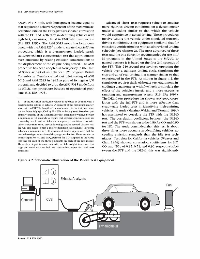
132
Air Pollution from Motor Vehicles
ASM5015 (15 mph, with horsepower loading equal tothat required to achieve 50 percent of the maximum ac-celeration rate on the FTP) gives reasonable correlationwith the FTP and is effective in identifying vehicles withhigh NO
x
emissions, related to EGR valve malfunction(U.S. EPA 1995). The ASM 5015 mode has been com-bined with the ASM2525
1
mode to create the
ASM2 test
procedure, which is a dynamometer loaded, steadystate, raw exhaust concentration test that approximatesmass emissions by relating emission concentrations tothe displacement of the engine being tested. The ASMprocedure has been adopted in New Jersey in the Unit-ed States as part of an enhanced I/M program. BritishColumbia in Canada carried out pilot testing of ASM5015 and ASM 2525 in 1992 as part of its regular I/Mprogram and decided to drop the ASM 5015 mode fromits official test procedure because of operational prob-lems (U.S. EPA 1995).
Advanced “short” tests require a vehicle to simulatemore rigorous driving conditions on a dynamometerunder a loading similar to that which the vehiclewould experience in actual driving. These proceduresinvolve testing the vehicle under simulated transientdriving conditions, using equipment similar to that foremissions certification but with an abbreviated drivingschedule (see chapter 2). The most advanced of thesetests and the one currently recommended for use in I/M programs in the United States is the
IM240
, sonamed because it is based on the first 240 seconds ofthe FTP. This 240-second test involves operating thevehicle over a transient driving cycle, simulating thestop-and-go of real driving in a manner similar to thatexperienced in the FTP. As shown in figure 4.2, thesimulation requires fairly elaborate test equipment, in-cluding a dynamometer with flywheels to simulate theeffect of the vehicle's inertia, and a more expensivesampling and measurement system (U.S. EPA 1993).The IM240 test procedure has shown very good corre-lation with the full FTP and is more effective thansteady-state loaded tests in identifying high-emittingvehicles. A study (Martino, Wakim and Westand 1994)has attempted to correlate the FTP with the IM240test. The correlation coefficient between the IM240test and the FTP was shown to be 0.86 for CO and 0.90for HC. The study concluded that this test is aboutthree times more accurate in identifying vehicles ex-ceeding emission standards than the idle test tech-niques. Test data for California vehicles (Weaver andChan 1994) showed correlation coefficients for HC,CO, and NO
x
of 0.95, 0.71, and 0.96, respectively, be-tween the FTP and the IM240; this was significantly
1. In the ASM2525 mode, the vehicle is operated at 25 mph with adynamometer setting to achieve 25 percent of the maximum acceler-ation rate on FTP. The length of the modes used in the test procedurehas not been fully specified by U.S. EPA or by any state. Based on pre-liminary analysis of the California results, each mode will need to lasta minimum of 30 seconds to ensure that exhaust concentrations arereasonably stable and vehicles are adequately conditioned. As withother steady-state tests, preconditioning and/or second chance test-ing will also need to play a role to minimize false failures. For somevehicles, a minimum of 180 seconds of loaded operations will beneeded to trigger operation of the purge mechanism. There are six cutpoints (ppm for HC and NO
x
, percent for CO) applied in the ASM2test, one for each of the three pollutants on each of the two modes.These six cut points must vary with vehicle weight, to ensure thatlarge and small cars are held to comparable targets for total massemissions.
Figure 4.2 Schematic Illustration of the IM240 Test Equipment
Source:
U.S. EPA 1995
Fan
Exhaust Analyzers
CVS
Dynamometer
Computer

Controlling Emissions from In-Use Vehicles
133
better than the correlation with either of the ASM testprocedures.
Compared to earlier tests, the IM240 and similar shorttest cycles have many advantages. Since they are basedon realistic driving cycles, they correlate better with theresults of complete emissions tests but are considerablyshorter and less complex to perform. Since the emis-sions measured in the test procedure are representativeof those produced in actual driving, errors of omissionand commission are greatly reduced. The low likelihoodof errors of commission makes it possible to establishmore stringent standards, thereby reducing errors ofomission. The test procedure also provides realistic mea-surement of NO
x
, HC, and CO emissions, making visualand functional checks of EGR, spark timing, and catalystpresence unnecessary. This reduces the opportunitiesfor fraud and error in the inspection program.
The disadvantages of the IM240 test are the longertesting time (which reduces throughput) and the cost(U.S.$80,000–120,000) and complexity of the equip-ment required to perform it. A dynamometer with iner-tial simulation used for the IM240 test costs aboutU.S.$20,000, and the cost of the associated sampling andmeasuring equipment can exceed U.S.$100,000. Bycomparison, the cost of equipment to perform theASM5015 test is about U.S.$40,000, while the simpleidle/2,500 rpm test requires an analyzer costingU.S.$5,000-12,000. Competition and economies of massproduction may reduce the cost of IM240 systems in thefuture by as much as 50 percent (U.S. EPA 1995).
To increase the effectiveness of I/M testing, especial-ly for nitrogen oxides, many jurisdictions require sup-plementary visual and functional checks of theemission controls. For instance, the mechanic is re-quired to confirm the presence of the catalytic convert-er, check that the fillpipe restrictor is in place, check forlead in the tailpipe (indicative of misfueling), confirmoperation of the EGR valve, check ignition timing, en-sure that there are no leaks in the exhaust system, andso on. Because these checks are time-consuming, manymechanics in decentralized I/M programs do not per-form all of them.
Evaporative Emissions
Evaporative emissions account for about half the totalhydrocarbon emissions from current vehicles. Twocommon failures of evaporative systems are vapor leak-ing from the fuel system and failure of the canisterpurge system, which results in an ineffective, saturatedcanister. U.S. EPA specifications for enhanced I/M pro-grams require a pressure test for fuel vapor leakage anda functional check of the canister purge system (U.S.EPA 1993). Few vehicles are programmed to purge un-der idle or 2,500 rpm/no-load conditions, so there is no
way to check the proper operation of the purge systemin the idle tests. Evaporative purge systems are opera-tive in both the IM240 and ASM test procedures.
Motorcycle White Smoke Emissions
Measuring white smoke on two-stroke vehicles is evenmore problematic than measuring black smoke fromdiesels. This is because motorcycles exhibit greatervariation in exhaust pipe configuration than trucks.Where white smoke and particulate emissions fromtwo-stroke motorcycles are a significant problem (as inmuch of Asia), white smoke testing programs should beestablished to reduce these emissions.
Appropriate procedures for white smoke testing havebeen developed for application in Thailand (McGregorand others 1994). A similar procedure is applied for newvehicle certification in Taiwan (China). Smoke opacitymeasurements are carried out using an in-line smokeopacity meter similar to that used to measure dieselsmoke opacity. The opacity meter is connected to anadapter attached to the motorcycle exhaust pipe. Theadapter standardizes the path length through which theopacity measurement is taken. The motorcycle is‘revved’ repeatedly by suddenly opening and closing thethrottle with the engine at idle. The maximum smokeopacity measured is taken as the emission measurement.
Inspection Procedures for Vehicles with Diesel Engines
Emissions inspection procedures for diesel vehiclesusually focus on smoke emissions. Smoke can be mea-sured in a number of ways, including the Bosch and Har-tridge methods or with a full-flow opacity meter. In the
Bosch
method, a spring-loaded sampler pulls a fixed vol-ume of smoke through filter paper, depositing thesmoke particles on the paper (Bosch 1986). The paperis then read by a photoelectric device, which producesa number indicating the degree of blackness of the col-lected particulate matter. The higher the number, thedarker the smoke.
The Bosch method provides an accurate measure ofsoot and other dark material in the smoke, but it re-sponds poorly, if at all, to smoke particles that are notblack. Lubricating oil droplets, for instance, produce abluish or grayish smoke (because of light scattering) buthave little color in themselves. When collected on theBosch filter, these droplets make the filter wet, but notblack, and are not detected. This is a major drawback,since excessive oil smoke is a major contributor to totalparticulate emissions from diesel vehicles in use, partic-ularly in developing countries. Because it fails to detectthis smoke, the Bosch method correlates poorly withactual particulate emissions from in-use vehicles (figure

134
Air Pollution from Motor Vehicles
4.3). Another problem with the Bosch method is thatgreat skill is needed by the operator to trigger the sam-pling system at exactly the right moment to catch theresults of the snap acceleration. Triggering the samplertoo soon or too late (the common case) will give an er-roneously low value.
For purposes of inspection and maintenance, a bet-ter measure of excessive particulate emissions is givenby a light-transmission opacity meter (opacimeter).This measures the attenuation of a beam of light shiningacross the smoke plume in percent opacity. Since theseopacimetric measurements include both the effects oflight absorption (by soot) and light scattering (by oil orfuel droplets), they provide a better indicator of emis-sions of both types of smoke. Light-transmission opaci-ty meters include full-flow, end-of-pipe opacity meters,and partial-flow, sampling meters such as the commonlyused Hartridge meter. The
Hartridge
and other partial-flow meters draw a continuous sample of the exhaustinto a chamber and measure the attenuation of a beamof light shining through the chamber. Exposure toheavy oil smoke may contaminate the Hartridge meter,requiring that it be cleaned.
For light-transmission opacity meters, the opacitymeasurement depends on the density of the smoke andthe width of the plume of smoke that the light beammust pass through. This width is known as the pathlength. The path length is related to the light attenua-tion by the Beer-Lambert law:
N = 100 (1-e
-kl
) (4.1)
where N is the opacity (in percent),
e
is the base of nat-ural logarithms,
k
is the absorption coefficient (smokedensity), and
l
is the effective path length through thesmoke (in meters). This equation can be used to correctsmoke opacity measurements made at different pathlengths to a single comparable basis.
This relationship applies both to full-flow and par-tial-flow opacity meters. For the full-flow meter, thepath length can usually be approximated as the diame-ter of the exhaust pipe, which is typically in the rangefrom 50 to 150 mm. For partial-flow meters, it is thelength of the measuring chamber built into the instru-ment. This length varies depending on the meter: forthe Hartridge meter, it is 457 mm (18 inches). This rel-atively long path length makes the Hartridge meter sen-sitive to low levels of smoke but impairs its ability todistinguish between moderate and extreme smoke lev-els. Other partial-flow meters use shorter measuringchambers.
In 1989, Chile switched from a Bosch-type filtermethod for measuring diesel smoke emissions to a testprocedure utilizing a full-flow, end-of-pipe opacitymeter. The Chilean experience has confirmed the great-er effectiveness of the opacimeter. This technique isused in most I/M programs in the United States that in-clude diesel smoke measurement. The most commonmeter is a portable, battery-operated system made up ofa light transmitter/receiver assembly that fits over theengine exhaust pipe and is connected by a cable to ahand-held digital readout unit. This system can also beconnected to a strip-chart recorder to produce a perma-
Figure 4.3 Bosch Number Compared with Measured Particulate Emissions for Buses in Santiago, Chile
Source:
Weaver and Chan 1995
Bos
ch N
umbe
r
Particulate matter (grams/kilometer)
00
8
9
7
6
5
4
3
2
1
1 2 3 4 6 7 8 95 10

Controlling Emissions from In-Use Vehicles
135
nent record. Other opacimeter designs are available foruse in fixed installations.
To be meaningful, diesel smoke measurementsshould be taken with the engine under load. Smokelevels under light-load conditions and at idle are normal-ly very low, so that it is not possible to distinguish be-tween clean vehicles and most smoky vehiclesoperating under light-load conditions. Only a small mi-nority of seriously malfunctioning diesel vehicles exhib-it measurable smoke opacity under idle or light-loadconditions.
One commonly used technique for loading the en-gine to achieve a meaningful smoke measurement is theso-called
snap acceleration
or
free-acceleration
test.This test loads the engine with its own inertia, as the en-gine is rapidly accelerated from idle to full (governor-limited) speed. Test results are very sensitive to properconduct of the test. The test is fast and convenient,however, and is therefore widely used for on-road en-forcement.
In order to reduce the variability and improve the ac-curacy of the snap acceleration procedure, a committeeorganized by the Society of Automotive Engineers (SAE)has been working to develop a standardized Recom-mended Practice for this test. The core of the procedure(SAE J1667) is a
snap-idle
sequence that is administeredby the inspector in the course of the opacity measure-ment. SAE J1667 differs from earlier versions of thesnap-acceleration test procedure mostly in its calcula-tion of the final result. The snap- acceleration test proce-dure, however, is very sensitive to operator style. It isimportant that the procedure conform exactly to thewritten directions in order to obtain the most accurateresults (McGregor and others 1994).
Although simple, convenient, and widely used, thistest does not always give a reliable measure of smokeemissions in actual use, since the operating conditioninvolved (rapid acceleration under no load) is not char-acteristic of normal engine operation. Tests in Califor-nia showed poor correlation between this test andmore representative test procedures such as full-load ac-celeration (Weaver and Klausmeier 1988). This lack ofcorrelation makes it necessary to set somewhat looserstandards to avoid failing properly functioning engines.Like the idle test for gasoline vehicles, the snap acceler-ation is most useful as a crude indicator of serious emis-sion malfunctions.
A more representative smoke value can be obtainedby measuring opacity under stabilized, full-load condi-tions. These can be achieved either by using a dyna-mometer or by placing the drive wheels on a set of freerollers and loading the engine by using the vehicle’s ser-vice brake. The
free-roller approach
is an ISO standard.It has an advantage in safety and convenience over thedynamometer, since a vehicle that slips off the rollers isrestrained by its own brake and does not keep moving.
A disadvantage of the free-roller technique is that it maybe difficult to control engine loading, especially intrucks equipped with air brakes. Another disadvantageis that drivers are often reluctant to apply the brakewhile running the engine at full power. Although a ve-hicle's brakes should be able to absorb the full poweroutput of the engine for a considerable time beforeoverheating, drivers often fear the vehicle will bedamaged.
To control transient smoke emissions (especially aproblem with turbocharged engines) it is desirable toinclude a
transient acceleration test
mode in the I/Mprocedure. Various technical options exist for perform-ing such a test. For most engines, however, the snap-ac-celeration test provides a reasonable indicator ofacceleration smoke performance.
Heavy-duty diesel vehicles (HDDV) are expected tobe able to meet stricter exhaust standards through im-provements in engine design, electronic controls, andthe use of low-sulfur fuel. As commercial fleets are re-placed with newer models, HDDV emissions are likelyto decrease substantially. This does not imply thatthere is no need for I/M programs for heavy-duty vehi-cles. In California, CARB has estimated that about 42percent of HC, and 56 percent of PM, and 6 percent ofNO
x
emissions emitted by HDDVs in 1990 resultedfrom engine tampering and maladjustment (Jacobsand others 1991). The primary causes of excess smokeemissions were found to be improper air-fuel ratiocontrol settings, incorrect fuel injection timing, andinadequate intake air (e.g. from dirty air filters). Ex-cess emissions from HDDVs occur to a large extent asa result of improper maintenance and deliberate en-gine tampering to coax more power out of an enginebeyond its rated capacity. This tampering results inoverfuelling and large amounts of excess hydrocar-bons and smoke emissions. Reduction of these excessemissions has been the main target of I/M programs forHDDVs. Several such programs have been implement-ed in the United States, especially in the western states(table 4.1) and in some European and developingcountries. The effectiveness of these programs has notbeen fully established although experience with suchprograms in Santiago and Singapore appears quitepromising.
Institutional Setting for Inspection and Maintenance
The cost-effectiveness of I/M programs depends on thetesting procedure and institutional setting. I/M pro-grams are commonly either centralized (see box 4.1) ordecentralized (see box 4.2), although some hybrid pro-grams have also been adopted.

136
Air Pollution from Motor Vehicles
Table 4.1 Characteristics of Existing I/M Programs for Heavy-Duty Diesel Vehicles in the United States, 1994
a. Smoke emission standard—all trucks, 55 percent opacity; 1991 and later models, 40 percent opacity.
State/area Program type Vehicles subject Test procedure Enforcement Repair cost limits
Arizona Centralized; based on annual registration
All locally registered HDDVs
Dynamometer lug down
Registration Waiver granted for repairs over U.S.$300
California Random roadside program for fleet vehicles
All HDDVs
Snap-idle
(a)
Citation (ticket) with mandatory penalties
None
Southern Califor-nia
Smoke patrol All HDDVs Visual opacity Citation (ticket) Not applicable
Smoking vehicle reporting program
All HDDVs None Public reports of smoking vehicles result in letters sent to operators requesting that they repair their vehicles
None
Colorado Decentralized; with annual fleet self testing
Locally registered HDDVs and other HDDVs which generally operate in program areas
Dynamometer lug down, on-road acceleration, on-road lug down and stall idle
Certificate of emissions compliance required, decal-based enforcement, snap-idle testing performed for data collection purpos-es not enforcement
Waivers granted after repair costs exceed U.S.$1,500
Nevada Smoke patrol All HDDVs Visual opacity Citation (ticket) None
Washington Centralized; based on annual registra-tion with fleet self testing
Locally registered 1968 and later models HDDVs
Snap-idle Registration Waivers granted after repair costs exceed U.S.$50 for 1980 and older vehicles, and U.S.$150 for 1981 and newer vehicles
Centralized I/M
In centralized programs, vehicles must be inspected atone of a small number of high-volume inspection facili-ties. These facilities are regulated by the government,and run either by public employees or by independentcontractors. In a typical program, the government fran-chises a single contractor to build and operate the in-spection centers in a given area, while charging a set feeto the public. These franchises are normally awardedon a competitive basis, taking into account both thetechnical competence and experience of the biddersand the proposed fee. The fee is normally set at a levelthat allows the contractor to recover its capital and op-erating costs and make a profit over the time period
covered by the franchise. In some cases, governmentshave issued multiple franchises for the same area. InMexico City, for instance, franchises have been awardedto five different consortia, reducing the government'sdependence on any one organization.
Centralized, fixed-lane inspection centers designedspecifically for high-volume inspection of vehicles per-mit the cost-effective use of more sophisticated andcomprehensive inspection procedures and equipment.A typical layout of a combined safety and emissions in-spection station is shown in figure 4.4. These centersuse automated and computerized inspection equip-ment and procedures and include consumer-orientedfeatures, such as:

Controlling Emissions from In-Use Vehicles
137
Figure 4.4 Schematic Illustration of a Typical Combined Safety and Emissions Inspection Station: Layoutand Equipment
Source:
Weaver and Chan 1995
• Subjective decisions are automated, minimizing thepotential for human error or tampering with thetest results.
• Inspection standards, test results, and pass-faildecisions can be computer-stored and printed outfor the consumer.
• Diagnostic information suggesting the probablecause of failure can also be printed—helping themotorist and the mechanic, and lowering repaircosts.
• Independent reinspection and evaluation of the effec-tiveness of vehicle repairs and costs allow the govern-ment to determine the effectiveness of the programand to upgrade repair industry performance.
In general, inspections in centralized programs aremore effective because of better oversight, standardizedtraining, and more experienced inspection personnel.
Decentralized I/M
In a decentralized program, vehicles are inspected atprivate service stations and garages, which also makerepairs on vehicles that fail the emissions test. Whilethese inspection and repair stations are generally li-censed and authorized by regional or local government,they are not operated under direct government control.
This presents opportunities for fraud, both against theconsumer (failing vehicles that should have passed inorder to “repair” them) and against the system (passingvehicles that should have failed in return for a bribe orto keep the customer happy). To deter fraud, decentral-ized I/M programs in the United States require the useof emission analyzers, such as BAR90, which incorpo-rate extensive automation of the inspection process.
2
Aschematic illustration of an automated inspection pro-cess utilizing a four-gas (carbon monoxide, hydrocar-bons, oxygen, and carbon dioxide) analyzer is shown infigure 4.5. Automation is intended to make fraud moredifficult. In addition, well-run decentralized programsincorporate extensive overt and covert audits of inspec-
2. Specifications for the automated emission analyzers were firstdeveloped by the California Bureau of Automotive Repair (BAR) in1984 to support that state’s Smog Check Program. These BAR84 ana-lyzer specifications were widely adopted in other U.S. jurisdictionsand in several other countries. In response to studies showing contin-ued widespread fraud, BAR in 1990 adopted more stringent automa-tion requirements, including the printing of the inspectioncertificates on a remote printer not accessible to the inspector. Use ofanalyzers meeting this specification became mandatory in Californiain 1990. Because of their extensive automation, data recording, andother features, the BAR90 analyzers are fairly expensive—aboutU.S.$12,000 to U.S.$15,000 for a basic machine, compared with lessthan U.S.$5,000 for a simple CO and HC measurement system.

138
Air Pollution from Motor Vehicles
tion stations to make fraud more risky. This implies thata large surveillance team is needed in the regulatoryagency to supervise inspection programs and ensurequality control. Fraud and poor performance are, none-theless, still possible and common. Although theBAR90 analyzer itself reads the pollutant concentrationsand makes the pass-fail decision, there is no way to en-sure that the analyzer is inserted in the tailpipe correct-ly. Similarly, there is no way for the analyzer to detectwhether mechanics have carried out the visual andfunctional checks they are prompted to perform, andmany mechanics do not do so in order to save time.
Although many—perhaps the majority—of privategarages performing inspections in decentralized pro-grams are competent and conscientious, there is a ten-dency for the bad inspectors to drive out the good.Inspectors who pass vehicles that should fail are patron-ized by consumers wishing to avoid expensive repair.Inspectors who do not carry out a full under-hood in-spection can complete an inspection in less time, andtherefore at lower cost, than their more conscientiouscounterparts. Studies by the U.S. EPA have found ratesof improper inspections exceeding 50 percent in de-centralized I/M programs (Tierney 1991; U.S. EPA1995), even in states such as California that have madestrong enforcement and oversight efforts.
An undercover investigation of California's decen-tralized Smog Check program, a model program in
many respects, showed that fewer than 60 percent ofthe stations identified any defect in the defective carspresented at the station and only 25 percent found allthe defects in the cars. A 1990 U.S. EPA undercover in-vestigation presented cars with missing catalytic con-verters at 25 inspection stations in Virginia. Only 10 ofthe 35 inspectors discovered that the converter wasmissing. These two undercover investigations as wellas other evaluations suggest that less than one-fourthof vehicles inspected in decentralized programs re-ceived thorough and accurate inspections (Glazer andothers 1995).
Comparison of Centralized and Decentralized I/M Programs
Personnel and training requirements differ significantlybetween centralized and decentralized programs. De-pending on the size of the system, the number of li-censed inspectors in a decentralized program can rangefrom a few hundred to over 10,000. Centralized pro-grams on the other hand, require from a few dozen to acouple of hundred inspectors. The physical magnitudeof training requirements for anti-tampering inspectionscan be daunting in a decentralized system (Tierney1991).
Since the number of inspection locations and inspec-tors is smaller in a centralized program, the skills andcompetence of the inspectors can be much higher, and
Figure 4.5 Schematic Illustration of an Automated Inspection Process
Source:
University of Central Florida 1991
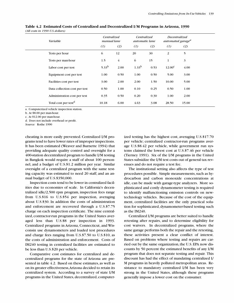
Controlling Emissions from In-Use Vehicles
139
cheating is more easily prevented. Centralized I/M pro-grams tend to have lower rates of improper inspections.It has been estimated (Weaver and Burnette 1994) thatproviding adequate quality control and oversight for a400-station decentralized program to handle I/M testingin Bangkok would require a staff of about 100 person-nel, and a budget of U.S.$1.2 million per year. Similaroversight of a centralized program with the same test-ing capacity was estimated to need 20 staff, and an an-nual budget of U.S.$350,000.
Inspection costs tend to be lower in centralized facil-ities due to economies of scale. In California's decen-tralized idle/2,500 rpm program, inspection fees rangefrom U.S.$16 to U.S.$54 per inspection, averagingabout U.S.$30. In addition the costs of administrationand enforcement are recovered through a U.S.$7.75charge on each inspection certificate. The nine central-ized, contractor-run programs in the United States aver-aged less than U.S.$8 per inspection in 1993.Centralized programs in Arizona, Connecticut, and Wis-consin use dynamometers and loaded test proceduresand charge fees ranging from U.S.$7.50 to U.S.$10, asthe costs of administration and enforcement. Costs ofIM240 testing in centralized facilities are estimated tobe less than U.S.$20 per vehicle.
Comparative cost estimates for centralized and de-centralized programs for the state of Arizona are pre-sented in table 4.2. Based on these estimates, as well ason its greater effectiveness, Arizona decided to retain itscentralized system. According to a survey of state I/Mprograms in the United States, decentralized, computer-
ized testing has the highest cost, averaging U.S.$17.70per vehicle; centralized contractor-run programs aver-age U.S.$8.42 per vehicle, while government run sys-tems claimed the lowest cost at U.S.$7.46 per vehicle(Tierney 1991). Six of the I/M programs in the UnitedStates subsidize the I/M test costs out of general tax rev-enues and do not require a test fee.
The institutional setting also affects the type of testprocedures possible. Simple measurements, such as hy-drocarbon and carbon monoxide concentrations atidle, can be made with garage-type analyzers. More so-phisticated and costly dynamometer testing is requiredto identify malfunctioning emission controls on new-technology vehicles. Because of the cost of the equip-ment, centralized facilities are the only practical solu-tion for sophisticated, dynamometer-based testing suchas the IM240.
Centralized I/M programs are better suited to handleretesting after repairs, and to determine eligibility forcost waivers. In decentralized programs, where thesame garage performs both the repair and the retesting,these activities present a clear conflict of interest.Based on problems where testing and repairs are car-ried out by the same organization, the U.S. EPA now dis-counts by 50 percent the estimated benefits of any I/Mprogram that does not separate testing and repair. Thisdiscount has had the effect of mandating centralized I/M programs in heavily polluted metropolitan areas. Re-sistance to mandatory centralized I/M has been verystrong in the United States, although these programsgenerally impose a lower cost on the consumer.
Table 4.2 Estimated Costs of Centralized and Decentralized I/M Programs in Arizona, 1990
(All costs in 1990 U.S. dollars)
a. Computerized vehicle inspection station.b. At $8.00 per man-hour.c. At $12.00 per man-hour.d. Does not include overhead or profit.
Source:
Rothe 1990
VariableCentralized
manual lane Centralized
automatic laneDecentralized
automated garage
a
(1) (2) (1) (2) (1) (2)
Tests per hour 6 12 20 30 2 5
Tests per man-hour 1.5 4 6 15 1 3
Labor cost per test 5.33
b
2.00 1.33
b
0.53 12.00
c
4.00
Equipment cost per test 1.00 0.50 1.00 0.50 5.00 3.00
Facilities cost per test 3.00 2.00 2.00 1.50 10.00 5.00
Data collection cost per test 0.50 1.00 0.10 0.25 0.50 1.00
Administration cost per test 0.35 0.50 0.20 0.30 1.00 2.00
Total cost per test
d
10.18 6.00 4.63 3.08 28.50 15.00

140
Air Pollution from Motor Vehicles
It has been argued that the effectiveness of centralI/M programs is offset by increased inconvenience tothe vehicle owner, since it is necessary to drive to oneof a limited number of facilities and, if the vehicle fails,drive it elsewhere to be repaired and then return tohave it reinspected.
However, dissatisfaction with existing centralizedprograms has been minimal—many consumers seemto prefer centralized inspections. Before Mexico Cityswitched entirely to centralized, contractor-operatedI/M, 20 percent of the public chose to have their vehi-cles inspected at the 16 public stations, despite signif-icantly greater inconvenience (the public stationsoften had lines and did not accept cash; consumershad first to go to an agency of the Treasury and makethe payment, then take the receipt to the inspectionfacility). This preference was apparently due to theperception that the public stations were more honestand did better inspections, thus protecting the con-sumer against possible fraud by the private garage andensuring that the vehicle owner contributed to thefight against air pollution. In New Jersey (UnitedStates), where vehicle owners have a choice of freecentralized inspections or paying for inspections inprivate garages, 80 percent of the public chooses cen-tralized inspection. Integrating fee payment, vehicleregistration, and vehicle inspection in the same facilitycould reduce any inconvenience associated with cen-tralized inspections (U.S. EPA 1995).
Centralized inspection programs are sometimes op-posed by the private automotive repair industry, whichstands to gain customers and revenues from decentral-ized programs (increasingly complex testing proce-dures and equipment requirements in the United Stateshave blunted some of this opposition). They may alsobe opposed by automotive user groups (either becauseof the convenience issue discussed above or becausecentralized inspections are harder to circumvent). Fleetoperators dislike centralized testing because it oftenmeans that they can no longer self-inspect. Because ofthis opposition, the majority of I/M programs in theUnited States used decentralized inspection until re-cently. The Clean Air Act Amendments of 1990 mandat-ed the use of enhanced I/M—utilizing the IM240 test(or an equally effective procedure) in a centralized pro-gram — for highly polluted areas. Because of the chal-lenge that effective, centralized test procedures pose toexisting vested interests, this requirement has createdgreat political resistance, and many states are openly de-fying U.S. EPA regulations on this issue. As a result, ef-fective I/M programs and the resulting air qualitybenefits have been seriously delayed.
Centralized inspection programs are more commonin Latin American countries. Chile has a highly effec-tive program of centralized I/M for passenger cars and
commercial vehicles, while Mexico has adopted a simi-lar program, initially confined to commercial vehicles.Until recently, passenger cars were allowed to continueusing the decentralized facilities in Mexico City as a po-litical expedience. Centralized I/M programs are sched-uled to start in several metropolitan regions in Brazilover the next few years.
Inspection Frequency
Until recently, most I/M programs in the United Statesrequired annual testing of vehicles, but the U.S. EPAnow recommends testing every two years as being al-most as effective while having much lower cost. In Ja-pan, vehicles must be submitted for testing when theyare three years old and every two years thereafter. Eu-ropean requirements for in-service testing vary by vehi-cle type; annual testing is mandatory for heavy-dutydiesel vehicles, spark-ignition automobiles are tested an-nually once they are three years old, and testing for lightdiesel vehicles begins at age four and is required everytwo years thereafter (CONCAWE 1994). The schedulefor compulsory motor vehicle testing in Singapore isshown in table 4.3; it varies by type and age of vehicle.
Vehicle Registration
To simplify administration of I/M and guard against eva-sion of program requirements, the system should belinked with the vehicle registration system. Ideally, ve-hicles should be identified by license plate, engine andchassis numbers, and physical description (make, mod-el, year, body type), and this information should beavailable at the vehicle testing location. Informationshould also be kept on vehicle test results, retrofitequipment installed, and vehicle disposition. This willrequire considerable strengthening of vehicle registra-tion programs in many developing countries.
Roadside Inspection Programs
Roadside or on-road vehicle inspection programs pro-vide an important supplement to periodic inspectionand maintenance. Periodic inspection is predictablyscheduled, giving vehicle owners an opportunity toevade the program. For instance, one common cause ofhigh smoke emissions in diesel engines is tampering withthe maximum fuel setting on the fuel injection pump.This provides more fuel to the engine, increasing poweroutput and smoke. Since owners know when the vehi-cle will be inspected, they can adjust the pump to itsproper setting immediately before the inspection, thenreturn it to the higher power setting afterward. Anotherway of reducing visible smoke is putting a handful ofgravel in the exhaust pipe just before the inspection.

Controlling Emissions from In-Use Vehicles
141
Similar tricks are possible, and reportedly common, formeeting carbon monoxide emissions standards with gas-oline vehicles, and it is conceivable that a motorcyclewhite smoke inspection can be passed by similar means.
Since a vehicle owner cannot predict whether he willbe targeted by an on-road or roadside inspection, such in-spections are difficult to evade. On-road and roadside in-spections are especially useful for enforcing vehiclesmoke limits, since the visible nature of smoke emissionsallows enforcement efforts to target the worst offenders.This reduces the costs and increases the effectiveness ofthe program and minimizes inconvenience to owners ofvehicles that are not polluting excessively.
A roadside smoke inspection program has been im-plemented in California to control smoke emissionsfrom heavy trucks. Smoke inspection teams are de-ployed at weight and safety inspection stations and atother roadside locations. A member of the inspectionteam observes oncoming trucks visually, waving overthose producing excessive smoke. These are then sub-jected to a free-acceleration smoke test using a smokeopacity meter. A truck fails if smoke opacity is in excessof 50 percent for half a second. Vehicles that pass aresent on their way; those that fail receive a citation thatcan be cleared only after the vehicle is repaired. Theminimum penalty is U.S.$300 if proof of correction (re-pair) is provided in 15 days; otherwise the fine isU.S.$500. A second citation during the same year car-ries a much larger fine (U.S.$1,800) and requires thatthe vehicle be presented at a smoke test location forsmoke measurement after repairs. Vehicles with out-standing violations may be removed from service by theCalifornia Highway Patrol. In southern California, theroadside smoke inspection program is supplementedby a Smoking Vehicle Reporting Program (SVRP) where-by members of the public can report suspected viola-tors to the regulatory agency, which, after verifying thevehicle identity, sends a letter to the vehicle owner
warning that the operation of the smoking vehicle is il-legal and that appropriate repairs must be made. Thereis no follow-up enforcement.
Roadside checks for smoke opacity are also appropri-ate for control of excess white smoke emissions fromtwo-stroke motorcycles. These emissions are believedto result, in many cases, from using too much or thewrong type of lubricating oil. Such practices are morelikely to be detected by visual screening on the roadthan by a periodic I/M test.
Roadside checks for hydrocarbon and carbon mon-oxide emissions from gasoline vehicles have also beenimplemented in a number of countries, including Mexi-co and Thailand. Singapore has one of the most effec-tive on-road smoke enforcement program, using both I/M inspections and mobile inspection teams (box 4.3).Since vehicles with high hydrocarbon and carbon mon-oxide emissions are not usually as obvious as those pro-ducing excessive smoke, these programs must rely onstopping vehicles at random. This reduces the efficien-cy of the program and increases the inconvenience todrivers of low-emitting vehicles. The development ofpractical remote-sensing systems for vehicle emissionsoffers the potential for roadside inspection programs tobe targeted more effectively. Remote sensing is dis-cussed later in this chapter.
Emission Standards for Inspection and Main-tenance Programs
Implementation of an I/M program requires that stan-dards be established for emissions from in-service vehi-cles. Ideally, test procedures should be defined basedon a strong correlation with actual on-road emissions,and cutpoints for each procedure should be establishedby taking into account both the technical capabilities ofthe vehicles and the emissions standards for which they
Table 4.3 Schedule of Compulsory Motor Vehicle Inspection in Singapore by Vehicle Age
— Not applicable
Note:
Life span of all private hire cars and taxis is seven years.
Source:
Registry of Vehicles 1993
Vehicle age
Type of vehicle Less than three years Three to ten years More than ten years
Motorcycles and scooters Exempt Annually AnnuallyCars and station wagons Exempt Every two years AnnuallyTuition cars Annually Annually AnnuallyPrivate hire cars Annually Annually —Public service vehicles Taxis Public buses (SBS, TIB, CSS) Other buses
Every six monthsEvery six months
Annually
Every six monthsEvery six months
Annually
Every six monthsEvery six months
AnnuallyTrucks and goods vehicles Annually Annually Every six monthsAll other heavy vehicles Annually Annually Every six months

142
Air Pollution from Motor Vehicles
Box 4.3 On-Road Smoke Enforcement in Singapore
Under Section 72 of the Road Traffic Act, if smoke or visible vapor is emitted from any motor vehicle used on a public road andthe emission causes or is likely to cause annoyance or danger to the public or injury or damage to any person or property, theowner and the driver of the vehicle is guilty of an offense. The smoke test is a key component of emissions inspection andenforcement. The passing standard for the diesel smoke is 50 Hartridge Smoke Units (HSU). While the routine smoke test duringperiodic inspections is retained for diagnostic purposes, it is more effective to concentrate on roadside enforcement as aneffective deterrent to smoke emissions, particularly from heavy-duty vehicles. The Registry of Vehicles has introduced mobilesmoke test units to control smoke emissions from diesel vehicles. These units, deployed at a number of strategic locations, con-duct on-the-spot smoke tests on passing diesel-powered vehicles.
The enforcement standard and penalties imposed are as follows:
Smoke level (HSU) Penalty
Less than 50 Pass (no penalty)51-70 Fines (owner and driver, S$100 each)
71-85 Fines (owner and driver, S$100 each)Vehicle prohibited from the road until faults rectified
86 or more Owner and driver charged in court. Vehicle prohibited from road until faults rectified.
The emphasis of enforcement inspection is not on hefty fines and penalties (though these serve a deterrent effect), but onthe need for vehicle owners to pay attention to the overall condition of their vehicles. The roadside inspections are supplement-ed by periodic island-wide visual surveys of vehicles to monitor the effectiveness of roadside smoke testing and enforcementprograms.
Source:
Registry of Vehicles 1993
were designed. Emissions measured by basic I/M testprocedures do not correlate well with emissions mea-sured by the more sophisticated tests used to establishvehicle emissions standards, or with actual on-roademissions. These procedures are primarily effective inidentifying vehicles with grossly excessive emissions inorder to require that these be repaired.
In-use vehicle emission standards are set at severallevels to accommodate current and future emissioncontrol technologies, as well as the required levels ofemission reductions.
Emission standards for I/M programs must considerboth the statistical distribution of vehicle emission lev-els and the maximum failure rate that can be consideredpolitically acceptable. The worst 10 or 20 percent ofthe vehicles (gross emitters) generally account for a sub-stantial fraction of total emissions. For example, thehighest emitting 20 percent of cars in Bangkok account-ed for about 50 percent of measured carbon monoxideemissions (figure 4.6). Likewise, 20 percent of the bus-es accounted for 50 percent of the measured smokeemissions (figure 4.7). By measuring the actual distribu-tion of emissions in the target population, it is possibleto set emission standards such that the highest-emittingvehicles fail and must be repaired, without producing
such a high failure rate that the program becomes polit-ically unsustainable. With continued monitoring of ve-hicle emission levels and failure rates, it should bepossible to tighten standards as vehicle conditions im-prove over time, creating a progressive improvement invehicle emission levels.
The emission standards recommended by McGregorand others (1994) for Thailand and the failure rates re-sulting from enforcing these standards on the existingvehicle fleet are shown in table 4.4. Based on the on-road measurements in Bangkok, one would expect fail-ure rates, given these standards, to be extremely highand perhaps politically unacceptable. However, it wasalso considered that anticipatory maintenance wouldreduce the failure rate, and that higher failure rateswould be politically acceptable for commercial vehiclessuch as trucks and taxis.
Setting cutpoints (in-use vehicle emission standards)was a major decision in the establishment of the Finnishin-use emissions control program. Gasoline-fueled pas-senger cars were the only group of motor vehicles sub-ject to in-use control, using the two-speed idle test. Type-specific values from emissions certification data wereused in setting standards. Much of the fleet was certifiedunder ECE Regulation 15, which provides carbon mon-

Controlling Emissions from In-Use Vehicles
143
Figure 4.6 Cumulative Distribution of CO Emissions from Passenger Cars in Bangkok
Source:
McGregor and others 1994
Figure 4.7 Cumulative Distribution of Smoke Opacity for Buses in Bangkok
Source:
McGregor and others 1994
Carbon monoxide (percent)
Cum
ulat
ive
dist
ribut
ion
(per
cent
)
0
10
20
30
40
50
60
70
80
90
100
Vehicles
Emissions
0 1 2 3 4 5 6 7 8 9 10 11 12
Passenger Cars at Normal Idle (Sample size = 253)
Pre
sent
CO
Sta
ndar
d =
6.0
%
Ave
rage
= 3
.30%
Buses (Sample size = 94)
Smoke opacity (percent: corrected to 3" dia. tailpipe)
Vehicles
Emissions
Cum
ulat
ive
dist
ribut
ion
(per
cent
)
Ave
rage
= 3
1.4%
1000 10 20 30 40 50 60 70 80 90
0
10
20
30
40
50
60
70
80
90
100

144
Air Pollution from Motor Vehicles
oxide standards at idle (4.5 percent in 15/03 and 3.5 per-cent in 15/04), but no idle hydrocarbon standard. Inlater model years (since 1989), low-emission vehicleswere certified mostly according to Swedish RegulationA13, which includes idle standards for carbon monoxide(0.5 percent) and hydrocarbons (100 ppm). Cutpointswere also based on experience with existing in-use con-trol programs, particularly those in Europe. Three cut-points were evaluated using the results obtained from afew prototype test stations making inspections duringthe 18 months prior to full implementation of the I/Mprogram. The results from these 17,000 short-tests aresummarized in table 4.5 (Laurikko 1994).
In-service vehicle emission standards mostly basedon two-speed idle and smoke opacity tests, are summa-rized in table 4.6 (for European Union and selectedmember states), table 4.7 (Argentina, New Zealand, andEast Asia), table 4.8 (Poland), and table 4.9 (selectedU.S. jurisdictions).
Unlike the idle and smoke opacity test procedures,the U.S. EPA's IM240 test procedure correlates wellwith actual vehicle emissions. Such procedures haveonly recently been used for routine I/M testing and havebeen adopted by several jurisdictions in the U.S. Thesetests make it possible to relate emissions from in-servicevehicles to new-vehicle emission standards. Failure cri-teria for these programs are generally set at levels suchthat any vehicle significantly exceeding the applicablenew-vehicle emissions standard would fail. The U.S.EPA’s recommended design for enhanced I/M programs(U.S. EPA 1995) is summarized below:
Network Type: CentralizedTest frequency: BiennialModel year coverage: 1968 and newerVehicle types: Light-duty vehicles and trucksExhaust tests: IM240 on all vehicles (at specified
cut-points)Evaporative system tests: Purge test on 1971 and newer
vehiclesPressure test on 1981 and newer vehicles
Visual test: NoneWaiver rate: 3 percentCompliance rate: 96 percen
t
The performance standard actually adopted for en-hanced I/M programs, requires annual centralized test-ing for all 1968 and later model passenger cars and light-duty trucks in non-attainment metropolitan areas begin-ning in 1995. The two-speed idle and loaded steady-statetests can be used for 1968–1985 models but the high-tech IM240 test is required for 1986 and later model ve-hicles. Besides the exhaust emission tests, this perfor-mance standard requires a visual inspection of thecatalyst and fuel inlet checks on 1984 and newer vehi-
cles. Pressure and purge checks are also required to testthe efficacy of the evaporative system.
IM240 emission standards for in-use vehicles, shownin table 4.10, have been set at levels 2–3 times above thecertification standards. The IM240 program is designedto be phased-in over 2–3 annual test cycles. The recom-mended phase-in standards are even more lenient tokeep failure rates at an acceptable level, so that the re-pair industry is not overwhelmed with vehicles requir-ing repair.
Stringent emission standards and testing proceduresfor in-use vehicles should be adopted in countries withsevere mobile source air quality problems. This wouldensure continuing effectiveness of vehicle emissioncontrols in service (possibly reducing the need for elab-orate durability and recall programs such as those in theUnited States) and accelerate the replacement or retro-fitting of highly polluting. The owner of a vehicle notmeeting the standards could be offered technical and fi-nancial assistance to retrofit the polluting vehicle withemission controls such as a catalytic converter or an al-ternative fuel (natural gas, propane) kit, to re-engine it,or to replace it with a new, low-emission vehicle. An al-ternative approach would use vehicle emission taxesrather than standards. This would offer greater flexibil-ity, while creating an incentive to reduce emissionseven below the legislated standards.
Costs and Benefits of Inspection and Maintenance Programs
Two major costs are associated with an I/M program:
• The cost of operating the program -- which generallyapplies to all inspected vehicles, since it tends to bea function of the total number of vehicles examined.
• Repair costs -- which apply only to vehicles that failthe inspection test.
The operating costs of I/M programs vary widely, de-pending on local conditions such as land and laborcosts, the existence of safety inspection stations, andthe type of inspection performed.
A centralized program is likely to have higher start-up costs than a decentralized program because ofcosts associated with constructing centralized inspec-tion stations. As these costs are often financed private-ly, they have no impact on the government budget. InMaryland (United States), for example, a private con-tractor was selected through a competitive biddingprocess to construct ten new inspection stations, withan average of five lanes each, to inspect approximately1.6 million vehicles annually. The contractor retained
Controlling Emissions from In-Use Vehicles
145
Table 4.5 Distribution of Carbon Monoxide and Hydrocarbon Emissions from 17,000 Short Tests onGasoline Cars in Finland
a. Corresponding to following cutpoints: CO (4.5 percent) and HC (1,000 ppm) for ECE 15-03; and CO (3.5 percent) and HC (6,000 ppm) for ECE15-04.
Source:
Laurikko 1994
Share of total (percent) Share of total (percent)
Carbon monoxideconcentration on idle
(percent)ECE regulation
15-03ECE regulation
15-04
Hyrocarbon concentration on idle
(ppm)ECE regulation
15-03ECE regulation
15-04
0 – 3 57.8 78.7 0 – 400 71.1 90.0
3 – 4 12.8 10.1 400 – 600 16.2 8.2
4 – 5 8.3 4.2 600 – 800 4.6 0.6
5 – 6 6.0 3.0 800 – 1,000 2.4 0.3
More than 6 15.0 4.0 More than 1,000 5.7 1.0
Total 100.0 100.0 Total 100.0 100.0
Failure rate
a
25 percent 15 percent Failure rate 5.7 percent 1.9 percent
Table 4.4 Inspection and Maintenance Standards Recommended for Thailand
— Not applicable
Source:
McGreogor and others 1994
Type of vehicleCO at idle (percent)
CO at high idle (percent)
HC at idle (ppm)
HC at high idle
(ppm)
Opacity at peak
(percent)
Opacity at high idle (percent)
Failure rate
(percent)
Motorcycles and side-car delivery
6 6 14,000 14,000 70 40 56
Tuk-tuks and three-wheeled delivery vehicles
2 n.a. 14,000 n.a. 70 — 19
Passenger cars, see-lors, gasoline pickups
5 5 300 300 — — 40
Taxis 5 5 300 300 — — 73
Medium and heavy-duty trucks (diesel)
— — — — 65 — 75
Buses (BMTA) — — — — 25 — 26
Buses (mini-bus) — — — — 25 — 46
Pickups (diesel), pickups as taxis & buses
— — — — 65 — 58
U.S.$7.50 of the U.S.$9 inspection fee to recoup the in-vestment in inspection stations and to cover the oper-ating costs, while U.S.$1.50 was returned to the stateto cover the administrative costs of the program.Implementation of a centralized program does not al-
ways result in high construction costs; New Jersey(United States) incorporated its emissions testing pro-gram into an existing centralized safety inspection pro-gram, thus avoiding the cost of constructing entirelynew facilities.

146 Air Pollution from Motor Vehicles
Table 4.6 In-Service Vehicle Emission Standards in the European Union, 1994
a. The cutpoint for a three-way catalyst equipped car (1990) is at high idle (2,500 rpm); there is also a limit on excess air/fuel ratio of 1±0.03 athigh idle.b. Finland also has standards for hydrocarbon emissions as follows: before 1978, exempted; 1978–85, 1,000 ppm; 1986–1990, 600 ppm; and 1990and after, 100 ppm.c. HC = 0.12 percent after August 1, 1983.Source: CONCAWE 1994
Location/vehicle typeCarbon monoxide
(percent) Smoke
AustriaSpark-ignition vehicle (idle speed) Without catalyst With three-way catalystDiesel
3.5<0.3
Bacharach number≤4.5 (±1.0 tolerance)
for soot measurement
DenmarkGasoline-fueled vehicles Before 1984 1984 and later With three-way catalystDiesel-fueled vehicles
5.54.50.5
3.8 Bosch
FinlandGasoline-fueled cars, registration years Before 1978 1978–85 1986–90 1990 and latera, b
Diesel-fueled vehicles, registration years Before 1990 1990 and later
1980 and later (effective 1995) naturally aspirated turbo-charged
Exempted4.53.50.3
--_
7.0 Bosch3.5 Bosch
2.5 m-1
3.0 m-1
ItalyGasoline-fueledDiesel-fueled busesOther diesel-fueled vehicles
4.565 percent70 percent
NetherlandsGasoline-fueled & LPG vehicles (since 1974)Cars with 3-way catalyst (since 1976)
4.50.5
United KingdomGasoline-fueled vehiclesc
First used between Aug 1, 1975 & July 31, 1983First used on or after Aug 1, 1983
6.04.5
European Union (recommended application)Gasoline-fueled vehicles Manufactured up to October 1, 1986 Manufactured after October 1, 1986 All models fitted with 3-way, closed-loop catalytic convert-er Idle
2000 rpmDiesel-fueled vehicles Naturally aspirated Turbocharged
4.53.5
0.50.3
2.5 m-1
3.0 m-1

Controlling Emissions from In-Use Vehicles 147
Table 4.7 In-Service Vehicle Emission Standards in Argentina, New Zealand, and East Asia, 1994
— Not applicableLPG = Liquefied Petroleum Gas.Source: CONCAWE 1994
Country/vehicle characteristicsCarbon monox-
ide (percent)Hydrocarbons
(ppm) Smoke
ArgentinaGasoline-fueled vehicles 1983–1991 1992 1994Diesel-fueled vehicles 1994
4.53.02.5
900600400
5 Bacharrach index and 2.62 m-1
New ZealandVehicle Model Pre-1982 1982–1992 1992 and later
4.53.52.5
800400400
ChinaDiesel-fueled vehicles (before 1984) Free acceleration Full loadDiesel-fueled vehicles (after 1984) Free acceleration Full load
5.0 Bosch4.5 Bosch
4.0 Bosch3.5 Bosch
JapanGasoline-fueled vehicles Four-stroke engine Two-stroke engine
4.52.5
1,2007,800
Republic of KoreaGasoline and LPG-fueled vehicles (1987) Rectification Until Sept. 1990 From Oct. 1990 Penalty Until Sept. 1990 From Sept. 1990Gasoline and LPG-fueled vehicles (1988) Rectification Until Sept. 1990 From Oct. 1990 Penalty Until Sept. 1990 From Sept. 1990Diesel-fueled vehicles Until Sept. 1990 From Oct. 1990
1.3–9.01.3–4.4
9.1 and above4.5 and above
1.3–9.01.3–4.4
9.1 and above4.5 and above
1,200–4,8001,200
—above 4,800
200–880220
—above 880
50 percent opacity40 percent opacity
SingaporeGasoline-fueled vehicles 2.5 —

148 Air Pollution from Motor Vehicles
Table 4.9 In-Service Vehicle Emission Standards for Inspection and Maintenance Programs in Selected U.S. Jurisdictions, 1994
Note: In the United States, gasoline emission standards apply at both idle and 2,500 rpm. See table 4.10 for IM240 emission standards.Source: CONCAWE 1992; CONCAWE 1994; Rothe 1990
Jurisdiction/vehicle type/model yearCarbon monoxide
(percentage)Hydrocarbons
(ppm)Smoke
(percent opacity)
U.S. EPA basic I/M programPassenger cars (1981 and later models)
1.2 220
ArizonaPassenger cars and light trucks 1967–71 1972–74 1975–78 1979 1980 and later modelsDiesel-fueled vehicles
5.55.02.22.21.2
500400250220220
50
FloridaGasoline-powered vehicles Gross vehicle weight up to 6,000 pounds 1975–77 1978–79 1980 1981 and later models Gross vehicle weight of 6,001 to 10,000 pounds 1975–77 1978–79 1980 1981–1984 1985 and later modelsDiesel-fueled vehicles Cruise mode Idle mode
5.04.03.01.2
6.55.54.53.01.2
500400300220
750600400300220
205
Table 4.8 In-Service Vehicle Emission Standards in Poland, 1995
a. Includes all heavy-duty vehicles.b. Excluding heavy-duty vehicles.c. At free acceleration from low idle speed.
Vehicle typeCarbon monoxide
(percent)Hydrocarbons
(ppm) Smoke
Vehicles with spark-ignition engines Registered before October 1, 1986 Motorcycles Other Vehiclesa
Registered after October 1, 1986 and before July 1, 1995 Motorcycles Other Vehicles Registered after July 1, 1995 Motorcycles Other vehiclesb (at idle) Other vehiclesb (at 2000–3000 rpm raised idle) Vehicles with diesel enginesc
Naturally aspirated Turbocharged
5.54.5
4.53.5
4.50.50.3
100100
2.5 m-1
3.0 m-1

Controlling Emissions from In-Use Vehicles 149
British Columbia (Canada) has evaluated the cost ofseveral alternatives for a heavy-duty vehicle I/M program;of the various options available, roadside smoke inspec-tion appeared to be the least capital intensive (table 4.11)and arguably the most cost effective (GVRD 1994).
Decentralized programs are less expensive to set upthan centralized programs but are more expensive tooperate. Cost elements include licensing for numerousinspection stations, certification of repair facilities,emission test equipment, audit vehicles, and programmanagement (data processing, quality assurance, publicinformation, training, supplies, and so on). Programmanagement costs should generally be borne by thegovernment but it may be advantageous to contract pro-gram management to a specialized firm.
Repair expenditures are a legitimate cost of I/M pro-grams. Much of the repair cost information reported inthe literature is dated and not too reliable (Faiz and oth-ers 1990). Non-uniform reporting methods and the in-ability to segregate the costs of I/M-related repairs makeit difficult to obtain reliable and accurate repair cost da-ta. Repair costs may be distorted by warranty coverageprovisions in U.S. emission regulations, which can re-quire the vehicle manufacturer to pay for all repairsneeded to pass the I/M test. The warranty coverage,however, remains in effect only under the condition
that the vehicle has not been tampered with or misusedand that the vehicle owner follows the maintenancepractices prescribed by the manufacturer. U.S. EPA esti-mates suggest that repair costs associated with the en-hanced I/M program (IM240) would range betweenU.S.$40–$250 depending on the tests that are failed(U.S. EPA 1995).
Experience with Colorado’s I/M program shows av-erage repair costs of U.S.$186 for vehicles failing theIM240 test and U.S.$86 for older vehicles tested by the2-speed idle procedure. For diesel-fueled vehicles, theaverage repair cost was U.S.$97, and no vehicles re-quired waivers to pass (Colorado 1996).
Emission Improvements and Fuel Economy
The U.S. EPA's MOBILE5a model provides estimates ofvehicle emission reductions due to different I/M pro-grams. Estimated emission reductions from I/M pro-grams for U.S. gasoline-fueled automobiles and heavy-duty vehicles (derived from the MOBILE5 model) forvarious levels of emissions control technology are pre-sented in tables 4.12 and 4.13. Emission reductions at-tributed by the U.S. EPA to enhanced I/M programs aregiven in table 4.14. Among European programs, Swe-den estimates that its I/M program has reduced carbonmonoxide by 20 percent and hydrocarbons by 7 per-cent based on the ECE test procedure, and Switzerlandestimates reductions in hydrocarbons and carbon mon-oxide of 20 to 30 percent (Berg 1989). Researchers atthe Institut National de Recherche sur les Transports etLeur Securite (INRETS) in France tested vehicles “be-fore” (as received from the owner) and “after” they hadbeen tuned to manufacturer's specifications. As shownin table 4.15, carbon monoxide and hydrocarbon emis-sions and fuel consumption fell significantly followingproper tuning, but nitrogen oxide emissions increasedespecially for gasoline-fueled vehicles (Joumard andothers 1990). Where effective nitrogen oxide controlsare in place, I/M programs help to reduce nitrogen ox-ide emissions as well. Current I/M programs yield smallreductions in NOx emissions and these are mostly theresult of lower tampering rates. With the advent (in theUnited States) of advanced I/M programs based on load-ed testing, nitrogen oxide emissions are expected to de-cline substantially.
It is important to note that emission reductions startout slowly and increase gradually over time because I/M programs tend to retard the overall deterioration rateof fleet emissions. Maximum benefits are achieved byadopting the I/M program as early as possible. Fuel sav-ings have been attributed to the improved vehicle main-tenance practices associated with an effective I/Mprogram. Fuel savings range from 0 to 7 percent. In cal-
Table 4.10 U.S. IM240 Emission Standards(grams per mile)
Note: The standards become fully effective in 1997 following a phase-in period during 1995–1997.a. 1994 and later models.b. Non-methane hydrocarbons.c. Not meeting Tier 1 emission standards.Source: U.S. EPA 1992
Vehicle type/model year
Carbon monoxide Hydrocarbons
Nitrogen
oxides
Light-duty vehicle
Tier 1 (94/95/96)a
1994–1995c
1986–1993
152020
0.7b
0.80.8
1.42.02.0
Light-duty truck (≤6000lb GVW)
Tier 1 (94/95/96)a
1994–1995c
1986–1993
152020
0.7b
1.21.2
2.03.53.5
Light-duty truck (>6000lb GVW)
Tier 1 (94/95/96)a
1994–1995c
1986–1993
152020
0.8b
1.21.2
2.53.53.5

150 Air Pollution from Motor Vehicles
Table 4.11 Alternative Options for a Heavy-Duty Vehicle I/M Program for Lower Fraser Valley, BritishColumbia, Canada(Canadian dollars)
a. Training and education would be a necessary first component of all full-scale programs; with an estimated cost of C$ 400,000.b. Annual program cost = all operating costs + amortization of total capital costs.c. LFV = Lower Fraser Valley.Source: GVRD 1994
Program category
Training/
educationa Smoking vehicle road testingCentralizedtest stations
On-road smoke patrol
Roadside opacity testing
Dynamometer testing facility
LFVc registered heavy-duty
vehicles
All heavy-duty vehicles
operating in LFV
Program alternative (1) (2A) (2B) (2C) (3A) (3B)
Program elements a) Develop appropriate regulations
b) Industry training and public educa-tion
c) Smoking vehicle reporting pro-gram
Alternative 1 plus:
d) On-road test-ing
e) Enforcement (tickets)
f) Voluntary vehicle repair
g) Repair incen-tives
Alternative 1 plus:
d) Random road-side testing
e) Enforcement (tickets)
f) Voluntary vehicle repair
g) Repair incen-tives
Alternative 1 plus alternatives 2A or 2B plus:
h) On road or roadside inspec-tion plus dyna-mometer testing
i) Mandatory repair and dyna-mometer retest-ing
Alternative 1 plus:
d) Dynamome-ter testing of LFV registered vehicles only
e) Enforcement via registration
f) Mandatory repair and dyna-mometer retest-ing
Alternative 1 plus
d) Dynamome-ter testing of all HDVs operating in LFV
e) Enforcement via registration for local vehi-cles, tickets for others
f) Mandatory repair and dyna-mometer retest-ing for locally registered HDVs
Test type None Visual (smoke) opacity plus opacity meter
Opacity meter Dynamometer and analyzers
Dynamometer and analyzers
Dynamometer and analyzers
Regulated pollutants Smoke, PM10, hydro-
carbons
Smoke, PM10,
hydrocarbons
Smoke, PM10,
hydrocarbons
Smoke, PM10,
hydrocarbons
Smoke, PM10,
carbon monox-ide, nitrogen oxides, hydro-carbons
Smoke, PM10,
carbon monox-ide, nitrogen oxides, hydro-carbons
Program cost analysis Capital costs Annual operating costs Smoking vehicle
reporting program
Annual program costb
Vehicle repair cost Vehicle downtime cost Total annual cost
$200,000$1,450,000
$120,000$1,620,000$6,200,000$4,300,000
$12,120,000
$1,200,000$1,200,000
$120,000$1,520,000$4,200,000$2,400,000$9,120,000
$5,400,000$4,400,000
$120,000$5,320,000$6,200,000$4,600,000
$16,120,000
$5,300,000$3,500,000
$120,000$4,620,000$3,500,000$3,000,000
$11,120,000
$11,200,000$6,300,000
$120,000$8,520,000
$11,500,000$10,300,000$30,320,000
Pollutants reduced (tonnes/year)
PM10
HC NOx
1995 2005 93 50 92 77 0 0
1995 2005 62 33 61 51 0 0
1995 2005 119 63 117 98 0 0
1995 2005 100 53 141 116 137 226
1995 2005 133 70 174 143 178 296

Controlling Emissions from In-Use Vehicles 151
Table 4.12 Estimated Emission Factors for U.S. Gasoline-Fueled Automobiles with Different EmissionControl Technologies and Inspection and Maintenance Programs(grams per kilometer)
Note: U.S. EPA MOBILE5a estimates for: ambient temperature 24°C; speed 31kph; and gasoline RVP 62 kPa (9.0 psi).a. Centralized, biennal testing; 2,500 rpm and idle test procedure; emission cutpoints at 220 ppm for hydrocarbons and 1.2 percent for carbonmonoxide. Visual inspection of catalyst and fuel inlet restrictor for catalyst-equipped vehicles. Assumed 96 percent compliance rate with a 3 percentwaiver rate.b. Centralized, annual testing; transient IM240 test procedure; emissions cutpoints at 0.5 gram per kilometer for hydrocarbons, 12.5 grams perkilometer for carbon monoxide, and 1.25 grams per kilometer for nitrogen oxides. Visual inspection of catalyst and fuel inlet restrictor for catalyst-equipped vehicles. Assumed 96 percent compliance rate with a 3 percent waiver rate.
Source: Chan and Reale 1994
Emission control (fuel consumption)Carbon
monoxide MethaneNon-methane volatime
organic compoundsNitrogen oxides
Advanced three-way catalyst control (11.9 kilometers per liter)No I/M program
Basic I/M programa
Enhanced I/M programb
Basic program compared with no program (percent difference)Enhanced program compared with basic program(percent difference)
6.205.364.39
16
23
0.0400.0400.030
0
33
0.670.620.51
8
22
0.520.510.46
2
11
Early three-way catalyst (9.4 kilometers per liter)No I/M program
Basic I/M programa
Basic program compared with no program (percent difference)
6.865.95
15
0.0500.044
14
0.780.71
10
0.660.64
3
Oxidation catalyst (6.0 kilometers per liter)No I/M program
Basic I/M programa
Basic program compared with no program (percent difference)
22.3717.15
30
0.1000.093
7
2.482.14
16
1.841.68
10
Non-catalyst control (6.0 kilometers per liter)No I/M program
Basic I/M programa
Basic program compared with no program (percent difference)
27.7021.95
26
0.150.14
7
3.082.86
8
2.041.94
5
Uncontrolled (6.0 kilometers per liter)No I/M program
Basic I/M programa
Basic program compared with no program (percent difference)
42.6734.47
24
0.190.19
0
5.625.46
3
2.72.7
0
culating the cost effectiveness of its programs, the U.S.EPA uses a figure of 3.5 percent for basic I/M programs.For enhanced high-tech I/M programs fuel economy im-provements are estimated to range between 6 and 19percent.
Impact on Tampering and Misfueling
The U.S. EPA has been collecting data on tamperingand misfueling to assess the magnitude of the problem.These activities can increase hydrocarbon emissions

152 Air Pollution from Motor Vehicles
Table 4.13 Estimated Emission Factors for U.S. Heavy-Duty Vehicles with Different Emission ControlTechnologies and Inspection and Maintenance Programs(grams per kilometer)
Note: U.S. EPA MOBILE5a estimates for: ambient temperature 24°C; speed 31 kph; and gasoline RVP 62 kPa (9.0 psi).a. Centralized, biennial testing; 2,500 rpm and idle test procedure; emission cutpoints at 220 ppm for hydrocarbons and 1.2 percent for carbonmonoxide. Visual inspection of catalyst and fuel inlet restrictor for catalyst-equipped vehicles. Assumed 96 percent compliance rate with a 3 per-cent waiver rate.b. Centralized, annual testing; transient IM240 test procedure; emissions cutpoints at 0.5 grams per kilometer for hydrocarbons, 12.5 grams perkilometer for carbon monoxide, and 1.25 grams per kilometer for nitrogen oxides. Visual inspection of catalyst and fuel inlet restrictor for catalyst-equipped vehicles. Assumed 96 percent compliance rate with a 3 percent waiver rate.
Source: Chan and Reale 1994
Emission control (fuel consumption)Carbon
monoxide Methane
Non-methane volatile organic
compoundsNitrogen oxides
Three-way catalyst control (2.9 kilometers per liter)No I/M programBasic I/M programa
Enhanced I/M programb
Basic program compared with no program (percent difference)Enhanced program compared with basic program (percent difference)
10.209.158.69
11
5
0.1240.1120.106
11
6
1.411.341.17
5
15
2.492.462.42
1
2
Non-catalyst control (6.0 kilometers per liter)No I/M programBasic I/M program
Basic program compared with no program (percent difference)
47.6143.04
11
0.210.19
10
5.735.57
3
3.463.46
0
Uncontrolled (6.0 kilometers per liter)No I/M programBasic I/M program
Basic program compared with no program (percent difference)
169.13161.21
5
0.440.42
5
18.518.11
2
5.715.44
4
tenfold and carbon monoxide emissions twentyfold.Surveys by the U.S. EPA in the 1980s showed that near-ly one in five vehicles had at least one emission controldisablement and that a significant number of vehicleowners had poisoned their catalytic converters by us-ing leaded fuel. Widespread use of leaded fuel in cata-lyst-equipped vehicles was also observed in Mexicowhen the difference in price between the two fuelswas large. Fortunately, many countries have adoptedtax policies that make the price of unleaded gasolinesimilar to that of leaded gasoline; this should restrainthe tendency to switch fuels that occurred in the Unit-ed States and Mexico.
Investigations by the U.S. EPA suggest that I/M pro-grams can reduce the rates of tampering and misfuelingby half (table 4.16), though they have no significant ef-fect on disablement of the exhaust gas recirculation(EGR) system. Since the I/M programs surveyed in 1982addressed only hydrocarbon and carbon monoxide
problems, it is not surprising that the programs had noeffect on tampering with EGR systems, which are de-signed to reduce nitrogen oxide emissions. By minimiz-ing tampering and misfueling of newer model cars thatuse catalysts to control nitrogen oxide emissions, I/Mprograms should prove effective in reducing nitrogenoxide emissions as well.
Tampering surveys conducted by agencies in theUnited States suggest that older vehicles have higherrates of tampering than newer vehicles. Furthermore,the under hood visual inspection portion, if carriedout diligently, was found to be effective in identifyingmany elements of a vehicle emission control systemthat may have been tampered with or modified. It isextremely difficult to ensure adequate visual inspec-tion in decentralized I/M programs, however. Tamper-ing and misfuelling rates tend to be significantly lowerin centralized I/M programs

Controlling Emissions from In-Use Vehicles 153
Table 4.14 U.S. EPA’s I/M Performance Standards and Estimated Emission Reductions from Enhanced I/M Programs
Source: Walsh 1995
Estimated reductions in emissions (percent)
Test procedureCarbon
monoxide HydrocarbonNitrogenoxides
Low enhanced I/M performance standard 16.1 9.3 1.5
High enhanced I/M performance standard 35.4 31.9 13.4
Low performance I/M programsBiennial idle test Without technician training and certification With technician training and certificationAnnual 2-speed idle test and repair Without ASM+pressure and purge+technician
training & certification With ASM+pressure and purge+technician training
& certification
16.222.3
15.7
24.9
9.812.6
10.2
21.1
2.46.6
2.6
11.6
High enhanced I/M performance standardsComprehensive biennial test—IM240 program Without technician training and certification With technician training and certificationBiennial test—ASM Without technician training and certification With technician training and certification
37.843.9
33.739.8
34.537.3
31.734.5
14.618.9
14.318.6
Table 4.15 Effect of Engine Tune-Up on Emissions for European Vehicles(ratio of emissions after tuning to before tuning)
— Not applicablen.a. = Not available or not significantly different.Source: Joumard and others 1990
Vehicle type/testing procedureCarbon
monoxide HydrocarbonsNitrogen oxides
Polycyclic aromatic
hydrocarbonsParticulate
matterCarbon dioxide
Fuel consumption
Light-duty gasoline-fueled vehiclesMean of four hot cyclesECE 15 hot cycleECE 15 cold cycle
0.800.850.78
0.890.851.18
1.061.041.02
—0.81—
———
1.010.961.00
0.960.930.98
Light-duty diesel-fueled vehiclesMean of four hot cyclesECE 15 hot cycleECE 15 cold cycle
0.970.960.84
0.780.810.65
1.051.111.12
n.a.1.14n.a.
0.750.640.66
0.940.860.89
1.021.000.93
Cost-Effectiveness
The U.S. EPA has estimated the cost-effectiveness of hy-drocarbon emission reductions from the United Statesvehicle fleet using enhanced I/M at about U.S.$500 perton — a very cost-effective option. For less-effective andmore expensive decentralized programs, the estimatedcosts were as high as U.S.$15,000 per ton (U.S. EPA1995).
The estimated cost per ton of PM-10 reduced in thefirst year of a centralized I/M program for heavy-dutydiesel vehicles varied from C$17,000 for an on-roadsmoke patrol to C$64,000 for a centralized test stationwith a dynamometer testing facility (GVRD 1994).
Few cost-effectiveness estimates have been made forI/M programs in developing countries, and none ofthese have had the benefit of actual test data. A World

154 Air Pollution from Motor Vehicles
Bank study for Mexico estimated the cost per ton of hy-drocarbons, nitrogen oxides, and particulate matter re-duced by a centralized I/M program in Mexico City. Theestimated cost-effectiveness was U.S.$839 per ton for acentralized program addressing high-use commercial ve-hicles, U.S.$1,720 per ton for a centralized program ad-dressing private passenger cars, and U.S.$2,056 per tonfor a decentralized passenger car program. In additionto being more cost-effective, the centralized passengercar program was projected to achieve nearly double thereduction in emissions of the decentralized program.
International Experience with Inspectionand Maintenance Programs
Inspection and maintenance programs have been an in-tegral element of air pollution control programs in manyindustrialized countries, but special care is required indesigning the inspection and enforcement mechanismsof I/M programs in developing countries. Otherwise,weak administrative and regulatory arrangements couldresult in massive evasion of I/M programs or corruptpractices on the part of I/M officials and inspectors. Ex-perience with traffic and safety regulation enforcementin developing countries has shown many instances ofthese types of problems. If possible, vehicle I/M testingshould be carried out in centralized, high-volume, test-only facilities. Automated reading of emission measure-ments and computerization of the pass-fail decision canhelp to minimize opportunities for fraud. Close linksshould also be established between the vehicle registra-tion process and emissions testing in order to avoid thepotential for counterfeiting of vehicle inspection certifi-cates and stickers. Finally, inspection facilities should be
operated by a small number of private contractors, withthe government's role limited to oversight of the con-tractor's performance. Since the government could can-cel the contract if corruption is discovered, thecontractor has a strong incentive to establish pay, man-agement, and supervision practices that minimize thispossibility. This is more difficult in situations where thegovernment operates the inspection facility. A brief sur-vey of the international experience with I/M programs ispresented in the following sections.
Argentina. At present, about 400,000 buses andtrucks operating in the Gran Buenos Aires area andabout 250,000 taxis and other commercial vehicles reg-istered in the Capital Federal area are subject to period-ic inspections as explained below:
• Buses, both CNG and diesel-fueled, are inspected at6-month intervals at one of the 12 inspection sta-tions owned and operated by the private firm CENTunder the supervision of CONTA (Comision Nacio-nal del Transporte Automotor), an agency of the na-tional Ministry of Transport. Emission checks areperformed visually. A new regulation will requireall inspection stations to have the basic equipmentfor carrying out emission checks.
• Taxis and commercial vehicles are inspected bySACTA, a private sector concessionaire under thejurisdiction of the Federal Capital Administration.Inspection charges are U.S.$42 per vehicle andU.S.$21.50 for re-inspection upon rejection. Oneof the objectives of the technical control is to en-sure compliance with exhaust and noise emissionsstandards. Exhaust emission controls are limited to
Table 4.16 Tampering and Misfueling Rates in the United States( percent)
n.a. = Not availableSource: Faiz and others 1990; Tierney 1991
1982 1987–89
Type of tampering No I/M With I/M Decentralized I/M Centralized I/M
Overall 16.7 13.9 n.a. n.a.
Catalytic converter 4.4 1.7 8.0 4.0
Inlet restrictor 5.9 3.1 12.0 6.0
Air pump system 4.6 2.3 15.0 12.0
Exhaust gas recirculation (EGR) system 9.8 10.1 n.a. n.a.
Evaporative canister n.a. n.a. 11.0 8.0
Fuel switching 15.1 6.2 13.0 8.0

Controlling Emissions from In-Use Vehicles 155
carbon monoxide and hydrocarbons for CNG andgasoline-fueled vehicles; diesel-fueled cars are test-ed for smoke opacity.
The vehicle inspection program suffers from severenon-compliance. While non-compliance with the man-datory annual inspection for taxis is relatively low at lessthan 5 percent (out of 38,500 vehicles), it is significant-ly more common among trucks and passenger transportvehicles: only 10 percent of 170,000 registered trucksand about 8 percent of the 21,000 registered passengertransport vehicles show up for annual inspections.
To reduce non-compliance, the municipal Secretariatfor Urban Planning and Environment together with themunicipal police carry out sporadic road checks. Theirresults indicate that 25 percent of all vehicles operatedin the Federal Capital Area violate emission norms. In1991, two-thirds of the surveyed cars in circulationwere found to be in non-compliance with the CO emis-sion limit of 4.5 percent. In April 1994, 235 out of 898randomly stopped vehicles, (almost 25 percent) failedto meet emission limits. In addition it was found that 15percent of the checked buses (80 out of 483 buses),nearly 40 percent of the tested trucks (96 out of 252trucks), and more than one-third of the inspected cars(59 out of 163 cars) violated the standards. To strength-en enforcement CONTA has introduced a hot line for re-porting buses emitting excessive smoke. SACTA alsocarries out random roadside checks.
Both the provincial and the Federal Capital adminis-trations plan to introduce mandatory inspections forprivate vehicles. The Province of Buenos Aires has al-ready solicited tenders from private inspection firms.In contrast to Buenos Aires, recent experiences inMendoza and Cordoba suggest that air pollution can bereduced significantly through improved vehicle mainte-nance. These cities are reported to have achieved sig-nificant improvements in air quality by enforcingcompliance with emission standards.
Austria. All cars are subject to an annual safety andcarbon monoxide emission inspection.
Brazil. Vehicle inspection and maintenance pro-grams are still at an early stage of development. TheState of São Paulo and some other states have had on-road smoke enforcement programs for diesel vehicles,but these programs have had only limited effectiveness.Plans are now underway to implement centralized, con-tractor-operated I/M inspection in São Paulo, Recife andBelo Horizonte. The centralized I/M program in Sao Pau-lo is scheduled to start in 1996 and is aimed to identifymaladjusted or poorly maintained light duty vehicleswith excessive emissions and needing proper mainte-
nance, and to ensure that emission control systems arein place and in good operational conditions. Prelimi-nary estimates show that a centralized I/M program forthe São Paulo Metropolitan Region could reduce carbonmonoxide, unburned fuel and particulate matter emis-sions by 10 to 20 percent. This is based on preliminaryinspections of vehicles and measurements of emissionreductions following repair of failed vehicles. In addi-tion, fuel economy is expected to improve between 5 to10 percent.
Canada. The Federal Government regulates new ve-hicle emissions; provinces exercise control over in-usevehicles. Ontario, British Columbia, and several otherprovinces have evaluated various options for I/M pro-grams for in-use vehicles, in conjunction with safety in-spection programs. One of the issues is whether theprogram should be voluntary or mandatory; some of thefactors against a mandatory program in the sparselypopulated territories are the high costs of travel for in-spection, negative public response to mandatory in-spection, and lack of qualified personnel to performinspections in some communities. Box 4.2 provides anevaluation of British Columbia's AirCare I/M program.
Chile. Technical inspection for all diesel vehicles hasbeen mandatory for several years. Inspection stationsand procedures have been recently upgraded, especial-ly for buses. The bus inspection procedure is based ona dynamic test that uses opacimeters. The maximumopacity standard at idle is 2 percent and at full load is 30percent. Mandatory hydrocarbons and carbon monox-ide checks of gasoline-fueled vehicles have been intro-duced as well. Selective roadside inspections are alsocarried out by the police to control carbon monoxideemissions from cars and opacity levels of bus emissions(Escudero 1991).
China. At the time of registration each motor vehicleis checked for idling emissions (gasoline-fueled) or freeacceleration smoke (diesel-fueled) at local inspectionstations. Periodic inspections are required annually forall vehicles and are conducted by the local vehicle man-agement office in centralized inspection lanes utilizingthe idle test or the free acceleration test. The quality andeffectiveness of these inspections vary significantlyfrom one jurisdiction to another.
Costa Rica. In February 1993 a law specifying vehi-cle emission standards was enacted by the Congress.Regulations came into force at the end of 1994. Besidesthe compulsory use of the catalytic converters in newcars (from 1995 only lead-free gasoline is sold) a decen-

156 Air Pollution from Motor Vehicles
tralized I/M program is being implemented with thehelp of private garages. In addition, traffic police makesroadside random checks with mobile equipment. How-ever the inspectors are not well trained and do not han-dle the equipment properly, so that even highlypolluting cars pass the controls. An important elementof the I/M program has been the training of mechanicsand certification of garages to perform proper tune-upof gasoline- and diesel-engined vehicles. The public isregularly informed of measures taken through a publicinformation campaign.
Finland. After an 18-month lead-time the in-use con-trol program was initiated on January 1, 1993. Both state-owned inspection stations and private repair garages anddealerships perform the short test (two-speed idle) andissue inspection certificates. Each sector has received anequal share of the workload. If emissions certificates areless than eight months old, cars are exempted from theemissions test when performing the technical inspec-tion. Actual failure rates have been much lower thanthose calculated from preliminary tests.
About 10 percent of the cars have been ordered tocorrect carbon monoxide settings. Only about 3 per-cent of the decisions to fail a vehicle have been made onthe basis of excessive hydrocarbon emissions. The fail-ure rate on air-fuel ratio is low, but this indicates onlythat a small number of catalyst-equipped vehicles havebeen tested. Regular, non-catalyst cars must be inspect-ed every year, but low-emission vehicles (usually three-way catalyst equipped) are subject to inspection notearlier than the third year of their service life. After thatthey are exempted for two more years, but after thesixth year they must be inspected annually.
The Finnish program does not permit any waivers, awidely used practice in U.S. programs. However, nocase has emerged where a car could not pass the shorttest after a reasonable tune-up or repair. The decision toexempt cars made before 1978 was probably wise inthis respect, since such vehicles are not widely used.The overall response of motorists to this control pro-gram has so far been positive.
Until 1995, only gasoline-fueled passenger cars werecovered under the control program. Diesel-fueled carsand trucks are only checked if they emitted consider-able visible smoke. The program have since been ex-panded to test diesel-fueled vehicles using the freeacceleration method (Laurikko 1994).
Germany. Biennial inspection of automobiles hasbeen required for many years; the program was recentlyexpanded to an annual test. As Germany introducesmore rigorous emission standards with increased use ofcatalyst technology, it is evaluating a variety of tech-niques to improve its I/M test requirements. If the Ger-
man program is implemented, it will likely serve as amodel for other European countries, particularly coun-tries interested in reducing nitrogen oxide and dieselparticulate emissions. Details of the German in-serviceemission test requirements are summarized in CON-CAWE 1994.
Hong Kong. In an effort to address the diesel partic-ulate problem, observer teams issue citations to smok-ing vehicles, requiring such vehicles to report to acentral testing station for instrumented (Hartridge)tests. Vehicles that fail the 60 HSU standard must re-ceive necessary repairs or face fines. With the openingof an automated inspection facility, annual inspectionswill be required for all goods vehicles (only those over11 years old were tested before), taxis, and buses. Pri-vate cars are tested for roadworthiness in private garag-es if they are more than six years old, but this has littleif any impact on emissions. A mandatory I/M programis planned for introduction in 1996.
India. The first stages of a vehicle pollution controlprogram have been completed. Major elements in-clude a 3 percent limit (by volume) on idle carbonmonoxide emissions for all four-wheel, gasoline-fueledvehicles, a 4.5 percent limit (by volume) on idle car-bon monoxide emissions for all two- and three-wheelgasoline-fueled vehicles, and a 75 HSU limit on smokedensity for diesel vehicles at full load (60 to 70 percentof maximum rated engine speed); the limit on the freeacceleration test is 65 HSU. These standards went intoeffect on October 1, 1989. Automobile standards sim-ilar to ECE Regulation 15-04 but tailored to Indian driv-ing conditions went into effect in 1991. Diesel vehiclerequirements were also tightened at that time. Theneed for a comprehensive I/M program has increasedsubstantially with the requirement that all new cars inthe four major metropolitan areas (Bombay, Calcutta,Delhi and Madras) be fitted with catalysts, from April1, 1995.
Italy. Since 1989, the Italian Department of Environ-ment has invited all vehicle owners to have their vehicleschecked on a voluntary basis. A network of test centershas been setup with the cooperation of motor-manufac-turers and the oil industry. After testing, the owner is ad-vised that the vehicle requires adjustments if it exceedscarbon monoxide limits for gasoline-fueled vehicles andsmoke opacity limits for diesel-fueled vehicles.
Japan. The history of motor vehicle emission stan-dards, including those for in-use vehicles, is similar tothat in the United States. In Japan, inspection programsfor carbon monoxide have been in effect since 1970,and hydrocarbon measurements and limits were added

Controlling Emissions from In-Use Vehicles 157
in 1975. Vehicles must be submitted for testing oncethey are three years old and every two years thereafter.
Republic of Korea. An active air pollution controlprogram is in place that includes a system of randomroadside inspections. As part of a study on motor vehi-cle pollution control, a task force has been organized todevelop a set of recommendations to improve I/M.While there is an I/M program in place, standards arelax. The government is planning substantial improve-ments to the I/M program, including the possible addi-tion of the IM240 test.
Mexico. A rudimentary I/M program was initiated in1988, with pass-fail decisions left to individual mechan-ics. This approach resulted in a high percentage of im-proper inspections. To rectify the problem, concessionswere granted for 24 high-volume, inspection-only facili-ties (macrocentros) utilizing computerized emission an-alyzers. It was mandatory for all high-use commercialvehicles (taxis, minibuses) and government vehicles tobe inspected at these facilities, although private auto-mobiles could use them, too. In addition, private garag-es inspecting private automobiles were required to usecomputerized analyzers and were subject to surveil-lance and enforcement activities. Programs to improvemechanic training and repair quality were alsodeveloped.
By the end of 1995, however, it became increasinglyclear that the private garage system under the dual I/Msystem, was not working. As one indicator, for example,the failure rate in the private garages averaged about 9percent whereas in the centralized lanes, the failure ratewas about 16 percent. Stations conducting improper orfraudulent inspections were taken to court on severaloccasions and were subsequently shut down. As a re-sult, the government decided to close all the private ga-rage inspection stations and to switch to a completelycentralized system.
The upgraded I/M program has the following keyelements:
• Since January 2, 1996 all I/M tests in the FederalDistrict are conducted at one of the existing cen-tralized facilities-- 26 facilities with about 142 lanes.It is intended to add 36 new facilities with 3 laneseach by January 1997.
• Standards (cut points) were tightened so that theaverage failure rate increased to 26 percent.
• The inspection frequency for all but high mileagevehicles was reduced to once per annum to relievecongestion at the lanes; taxicabs and other high usevehicles continue to be tested twice per annum.
• The inspection stations are being upgraded so thatall will have a dynamometer and be capable of run-ning the ASM (25/50/15) test by end 1996.
• Private cars receive the two stage idle test whereasthe high use vehicles receive a steady state loadedtest.
• Independent auditors monitor the tests carried outat each station. These auditors are rotated monthlyand their contracts are funded by the companiesoperating the stations. In addition, each test is re-corded on video in real time and the tapes and com-puter print outs are spot checked to assure that thetests are valid.
• The funding for the centralized facilities will be en-tirely private with cost recovery from inspection/test fees. Fees will be 70 pesos (U.S.$9.30) for carsand 100 (U.S.$13.25) pesos for high-use vehicles;10 pesos of the fee will go to the government to payfor the stickers.
• In designing the I/M program, the government hasexercised close coordination with the automobilemanufacturers.
• In use vehicle standards were tightened by approx-imately 30 percent. The standards applicable in theDDF prior to January 1995 (old) and January 1,1995 (new) summarized in table 4.17.
The Philippines. Diesel smoke control has three ele-ments: information, education, and communications,coupled with strong enforcement. Teams operate onkey routes in Manila and on the basis of Ringlemannchart readings issue citations and revoke the registra-tion plates of offending vehicles. To reclaim plates, ve-hicles must be presented to the central testing facilityfor a more technically-sound Hartridge instrument test.This test must be passed (67 HSU or less) to avoid a fine(200 pesos for the first failure, 500 for the second, and1,000 for the third). The citation rate was 5,000 vehi-cles a month in 1990. These limits are quite lenient, sothat vehicles passing the test still emit visible smoke(Walsh and Karlsson 1990).
Poland. Motor vehicle emission standards have beengradually tightened over the last five years with a viewto harmonize the national requirements with the Euro-pean Union. A revised regulation specifying emissionrequirements to be satisfied by new and in-use motorvehicles in Poland came into effect on July 1, 1995. Thenew regulation requires emission checks for in-use vehi-cles. The compliance with in-use requirements ischecked during mandatory periodic inspections andrandom road-side checks; the frequency of periodic in-

158 Air Pollution from Motor Vehicles
spections is a function of vehicle category and age, asindicated below:
• For passenger cars and light duty vehicles subjectto type approval: three years after the first registra-tion, then after two years, and subsequently onceevery year.
• For passenger cars and light duty vehicles not sub-ject to type approval: once every year.
• For trucks having a maximum mass exceeding3,500 kg: once every year, then every six months.
Singapore. Cars are tested for idle carbon monox-ide and hydrocarbon emissions, but standards are notyet enforced because the I/M program has not beenfully implemented. Standards are lenient—800 ppmfor hydrocarbons and 4.5 percent for carbon monox-ide. Diesel smoke testing is carried out using the free-acceleration test; mobile vans are employed by the po-lice who stop smoking vehicles and administer a Har-tridge smoke test. If the vehicle fails to meet astandard of 50 Hartridge Smoke Units (HSU), the own-er must pay a fine and repair the vehicle (Registry ofVehicles 1993).
Sweden. An annual I/M program is limited to mea-surement of carbon monoxide emissions at idle with le-nient standards. However, a more comprehensive butnon-sophisticated I/M program has been evaluated forimplementation. Catalyst-equipped passenger cars agedtwo years or older have to be inspected annually by theSwedish Motor Vehicle Inspection Company. Older ve-
hicles (1976-1988 car models) must be submitted for theannual test until they are five years old or have reached80,000 kilometers, whichever occurs first. It is expect-ed that this limit will be extended to 160,000 kilometers.Failed vehicles have to be rectified and retested within amonth. Vehicles not retested within the one month limitare not permitted to ply on the roads.
Switzerland. A mandatory I/M program has been ineffect since 1986. This program requires compulsorytesting; gasoline-fueled light-duty vehicles are tested an-nually at authorized garages, while all vehicles with die-sel engines must undergo a regular check at an officialtest station administered by the local canton. Diesel ve-hicles are tested at three-year intervals except for truckstransporting hazardous materials, which are testedannually.
Taiwan (China). Random roadside inspections havebeen implemented by local Environmental ProtectionAdministration bureaus. A free motorcycle emissionstest and maintenance program has also been promoted.In large cities buses are tested for free. The Environ-mental Protection Administration (EPA) has set up state-of-the-art vehicle inspection and maintenance stationsthroughout the island. In addition, inspection licensesare issued to qualified privately-owned garage stations(Shen and Huang 1991).
In order to reduce the pollution from motorcycles,the EPA is actively promoting a motorcycle I/M pro-gram. In the first phase, from February through May1993, the EPA tested 113,147 motorcycles in Taipei City.
Table 4.17 In-Use Emission Limits for Light-Duty Vehicles in Mexico
Note: Old prior to January 1995; New from January 1, 1995.Source: Onursal and Gautam 1996
CO (%) HC (ppm)
Model year Old New Old New
Passenger cars
1979 and older 6.0 4.0 700 450
1980-1986 4.0 3.5 500 350
1987-1993 3.0 2.5 400 300
1994 and later 2.0 1.0 200 100
Combis and light trucks
1979 and older 6.0 5.0 700 600
1980-1985 5.0 4.0 600 500
1986-1991 4.0 3.5 500 400
1992-1993 3.0 3.0 400 350
1994 and later 2.0 2.0 200 200

Controlling Emissions from In-Use Vehicles 159
Of these, 49 percent were given a blue card indicatingthat they were clean, 21 percent a yellow card indicat-ing that their emissions were marginal, and 30 percentfailed the test. Between December 1993 and May 1994,142,287 motorcycles were inspected, with 55 percentreceiving blue cards, up 6 percent from the earlier pro-gram, and 27 percent failing, a drop of 3 percent in thefailure rate. The major repair for failing motorcycles wasreplacement of the air filter.
Thailand. Teams from the Department of PollutionControl and the Bangkok Police carry out roadsidechecks of carbon monoxide emissions from passengercars, hydrocarbons from motorcycles, and smoke fromdiesel vehicles. The motorcycle hydrocarbon standardis 14,000 ppm, which means that most two-stroke mo-torcycles can pass the test. The smoke opacity limit isBosch number 5, measured in a free-acceleration test.Commercial vehicles are also subject to annual checksof smoke opacity (for diesels) or carbon monoxide (forspark-ignition vehicles) as part of the licensing process,but these inspections are of limited effectiveness. InBangkok, the rate of failure for smoke opacity was just2 percent, whereas on-road emission measurementssuggest that more than 50 percent of the trucks havesmoke opacity exceeding the established limits. TheLand Transport Department is in the early stages of im-plementing a decentralized periodic I/M test for alltypes of vehicles in the Bangkok Metropolitan Region.Efforts to improve I/M test procedures and appropriateemissions standards are also under way.
United States. The I/M program is administered bythe states and consists of periodic emission testing of in-use vehicles. Inspection and maintenance programs arerequired as part of the State Implementation Plans (SIP)for those states unable to achieve compliance with car-bon monoxide or ozone air quality standards in non-attainment areas.
Inspection and maintenance programs have been es-tablished in 140 regions comprising parts or all of 36states and the District of Columbia. Only four states(Connecticut, Massachusetts, Rhode Island, and NewJersey) and the District of Columbia have state-wide(city-wide in the case of D.C.) programs; the rest con-centrate on major population centers. While most U.S.I/M programs have been adopted in response to federalrequirements, they differ significantly in terms of imple-mentation. This is because the U.S. EPA, in specifyingthe program requirements, recognized the wide diversi-ty of existing local conditions. Rather than attemptingto dictate the specific details of the program, the U.S.EPA chose to set out performance requirements. Thesewere based on emissions reductions, which were pre-
dicted by evaluating the program details using the MO-BILE emission factor models.
The type of I/M program, enforcement mechanisms,frequency of inspections, and other features are gener-ally left to the discretion of the responsible state or localadministration, subject to U.S. EPA's approval that therequisite performance criteria would be achieved.About 86 million vehicles are subject to I/M programsin the United States (U.S. EPA 1995).
United Kingdom. Emission testing has been intro-duced as part of the roadworthiness test applied to allfour-wheel gasoline-fueled cars three years or older.Standards and testing methods for light-duty diesel vehi-cles and two-stroke engines are being developed. In-spection tests are conducted with the engine warmed-up and at idle, with the test results compared to theemission standards.Vehicles fail the complete DOTroadworthiness test even if the emissions performanceis the only item of failure. A free re-test is allowed pro-vided the vehicle is returned to the same testing stationwithin 10 days.
Emission checks also include roadside testing. Vehi-cles that fail the roadside check are required to be recti-fied within ten days or become subject to a fine of up toUK£5000. In extreme cases, the vehicle may be subjectto an immediate ban. In a 1994 roadside check in Cen-tral London, 20 percent of the gasoline-fueled vehiclesand one in three diesel vehicles gave off illegal emis-sions (Ahuja 1994). Roadside emission checks havebeen included in the roadworthiness test sinceNovember 1991.
Remote Sensing of Vehicle Emissions
Remote sensing of vehicle emissions is a new technolo-gy that could improve the effectiveness of vehicle emis-sions control programs. The technique works bymeasuring the absorption of a beam of infrared light bythe carbon dioxide, carbon monoxide, and hydrocar-bons in a vehicle's exhaust plume (figure 4.8). Based onthe absorption, a computer is able to calculate the ra-tios of carbon monoxide and hydrocarbons to carbondioxide in the exhaust. From this information it is pos-sible to calculate the concentrations of hydrocarbonsand carbon monoxide in the exhaust at the instant thevehicle passes the remote sensing device (Stedman andBishop 1991). This system has been used to character-ize the statistical distribution of vehicle emissions in anumber of cities, including Chicago and Mexico City(figures 4.9, 4.10, and 4.11). It is expected that a re-mote sensing system for NOx emissions would utilize ei-ther a beam of ultraviolet light or light from a turnable

160 Air Pollution from Motor Vehicles
diode laser projected across the road (U.S. EPA 1995). Aprototype system capable of measuring nitrogen oxideconcentrations has been developed. A technical assess-ment of the use of remote sensing for I/M programs isprovided in appendix 4.1.
Although remote sensing offers significant potentialfor vehicle emissions monitoring and control, the tech-nique has limitations. Remote sensor technology mea-sures the instantaneous concentration of hydrocarbonand carbon monoxide in a vehicle's exhaust at the timeit passes the sensor. This measurement is a snapshot ofemissions and thus not a reliable indicator of overall ve-hicle emission levels or even “gross emitter” status,since emissions measured by the remote sensing deviceoften do not correlate with the Federal Test Procedure(FTP) measurements or other measures of actual emis-sions over realistic driving cycles. Even properly func-tioning vehicles may exhibit high carbon monoxide andhydrocarbon concentrations in the tailpipe under driv-ing conditions such as hard acceleration or cold start-ing. Many vehicles also exhibit moderately high carbonmonoxide concentrations at idle. Some older vehiclesexperience high hydrocarbon concentrations duringdeceleration, while newer vehicles cut off fuel duringdeceleration, making the hydrocarbon to carbon diox-ide ratio hard to predict.
Since the air-fuel ratio at normal cruise should beclose to stoichiometric (very close for closed-loop vehi-cles, less so for vehicles without closed-loop control), ahigh hydrocarbon or carbon monoxide concentrationin normal cruise conditions indicates a likely emissionsproblem. Still, the hydrocarbon or carbon monoxideconcentration that would indicate a problem in a vehi-cle with electronic closed-loop air-fuel ratio control may
be normal for a vehicle without such control. In addi-tion, gasoline-fueled, heavy-duty vehicles may haveanomalously high readings because of their heavier en-gine loading and more lax emissions standards. Also, hy-drocarbon concentrations exhibited by two-strokemotorcycles in normal operation would indicate grossmalfunction in a four-stroke engine.
Another limitation on current remote sensing devic-es is that they can measure only one lane, requiring ve-hicles to pass in single file. Furthermore, no practicalmethod is available for sensing of evaporative and othernon-tailpipe emissions. The system does not work onvehicles with elevated exhaust pipe discharge and in-valid readings result when the sensor beam is blockedby pedestrians, bicycles, or trailers.
For remote sensing to be reliable and useful, extra-neous sources of variation should be eliminated. It isimportant to distinguish between emission signals thatindicate a high emissions malfunction and those thatresult from normal operation. Aberrant readingscaused by acceleration or deceleration can be screenedout by adding a leading and trailing photocell to thephotocell that triggers data acquisition in the sensor.By comparing the time-distance ratios between the firstand second and the second and third detectors, it ispossible to determine whether the vehicle is accelerat-ing or decelerating and to reject the data for these con-ditions. Cases of intrinsically dirty vehicles, such astwo-stroke motorcycles and heavy-duty gasolinetrucks, can be screened out by capturing the vehicle'simage on film and sorting the data into categoriesbased on vehicle type. Similarly, newer vehicles thatmay have been subject to more stringent emissionsstandards can be distinguished from older vehicles that
Figure 4.8 Illustration of a Remote Sensing System for CO and HC Emissions
Source: U.S. EPA 1995
IR Source
Video I.D. Camera
Detector
Computer
Radar Gun
Controlling Emissions from In-Use Vehicles 161
Figure 4.10 Distribution of CO Concentrations Determined by Remote Sensing of Vehicle Exhaust in Mexico City
Source: Beaton and others 1992
Figure 4.9 Distribution of CO Concentrations Determined by Remote Sensing of Vehicle Exhaust in Chicago in 1990 (15,586 records)
Source: Beaton and others 1992
Figure 4.11 Distribution of HC Concentrations Determined by Remote Sensing of Vehicle Exhaust in Mexico City
Source: Beaton and others 1992

162 Air Pollution from Motor Vehicles
were not subject to such standards. In cases of doubt,the year of manufacture of the vehicle can be deter-mined by checking the license plate number againstthe vehicle registration data.
Identifying cases in which unusually high hydrocar-bon and carbon monoxide conditions are caused bynormal cold-start enrichment is more difficult. It maybe possible to identify this condition from the remote-sensing “signature.” Alternately, it may be more practicalsimply to locate the sensors where vehicles would haveoperated for several minutes before passing the sensorlocation.
The main advantage of remote sensing is that it canscreen a large number of vehicles quickly and cheaply.This is useful for improving vehicle emissions invento-ries, since it provides an unbiased indication of the frac-tion of vehicles on the road that fall into differentemission classes. Remote sensing can thus comple-ment the results of more detailed surveillance testingusing dynamometer measurements. Such testing pro-vides more accurate measurement of total emissionsover the driving cycle than does remote sensing but suf-fers from potential sampling bias and lack of represen-tation of the cycle test of real world emissions.
Potentially the most useful application of remotesensing is direct identification of high-emitting vehicleson the road so they can be targeted for testing and re-pairs. This could ultimately take the form of a compre-hensive surveillance system, incorporating numerousdetectors operating continuously and unattended at stra-tegic locations throughout an urban area. High emissionreadings would be linked to individual vehicles, eitherthrough video monitoring of license plates or throughelectronic vehicle identification as part of an intelligenthighway system. Owners of high emission vehicleswould be notified to present them for inspection. Thisarrangement could supplement or, if sufficiently devel-oped, replace routine I/M testing. Targeting inspectionsat likely high emitters would significantly reduce the so-cial costs of I/M programs. Several recent studies in theU.S. have examined this possibility (Austin and others1994; California I/M Review Committee 1993; Walsh andothers 1993). The main findings of these studies can besummarized as follows:
• Remote sensing to identify gross-emitting vehicleson the road could be a useful supplement to in-crease the effectiveness of an enhanced vehicle in-spection and maintenance (I/M) program. Remotesensing could help to identify some gross-emittingvehicles that evade the I/M tests as well as vehiclesthat pass the I/M test because of tampering withthe emission controls. In addition, remote sensingoffers an effective approach to early identification
and correction of vehicles that become gross emit-ters between successive scheduled inspections.
• Neither remote sensing alone nor the use of re-
mote sensing as a “screen” would be a viable sub-stitute for an effective periodic I/M program.Remote sensing presently is less effective than ad-vanced I/M tests in identifying vehicles with highexhaust HC and CO emissions, and cannot identifyvehicles with high NOx or evaporative HC emis-sions. In order to avoid failing a large number of“clean” vehicles, the failure criteria used for re-mote sensing must be set at a level that allowsmany “dirty” vehicles to pass undetected.
For remote sensing to achieve its potential, a numberof technical issues need to be addressed. The most criti-cal of these is improving the accuracy of remote sensorsin identifying high emitters. Another problem that needsto be solved is sampling across multiple lanes of trafficwithout creating conspicuous structures or causing asafety hazard. The remote sensing system should also becapable of operating for long periods unattended in or-der to save labor costs, reduce conspicuousness of thetesting system, and avoid roadside driver distraction.One possible solution to the multi-lane sampling prob-lem would be to locate the sensor units behind gratingsin the road surface, with the receivers located overhead,behind a traffic sign or in some inconspicuous place.
Evaluation of Remote-Sensing Data
A summary of on-road CO and HC emission statisticsderived from remote sensing surveys at several loca-tions around the world is presented in table 4.18.(Zhang and others 1994).
The median values are substantially lower than themean. This indicates that the distribution of emissions ishighly skewed, with a relatively small number of highemission values having a disproportionate impact on themean. Such a skewed distribution is to be expected,since pollutant concentrations may be quite high butcannot be less than zero. As shown in table 4.18 shows,the mean and median emission values in cities such asBangkok, Kathmandu, and Mexico City are significantlyhigher than those measured in most European andAmerican cities, while the difference between the meanand median values is proportionately less. In U.S. andsome European countries, nearly all cars have emissioncontrols, so that tailpipe pollutant emissions are usuallylow. High pollutant emissions are due to either unusualoperating conditions or emission control system failure.The distribution of pollutant emissions is highly skewed,as the few vehicles with high pollutant levels account fora large fraction of the measured emissions.

Controlling Emissions from In-Use Vehicles 163
Where average pollutant emissions are high, the ef-fect of the highest-emitting vehicles on the overall aver-age is proportionately less. The two cities in Asia,Bangkok and Kathmandu, stand out with respect to hy-drocarbon emissions, due to the high percentage of mo-torcycles and three-wheelers equipped with two-strokegasoline and LPG engines. These engines have extreme-ly high hydrocarbon emissions, even when properlytuned and operating normally. The wide range of grosspolluter cutpoints depicted in table 4.18 suggests that
emission standards for in-use vehicles should be basedon an evaluation of local conditions and not derivedfrom general international practice. Based on the resultsof remote sensing emission surveys, there may be a caseto vary both the stringency of in-use emission standardsand the frequency of vehicle inspections by vehiclemodel, vehicle age and geographical location. This maybe particularly relevant to developing countries.
Observations like those in table 4.18 have sometimesbeen used to support arguments such as that “10 per-
Table 4.18 Remote Sensing CO and HC Emission Measurements for Selected Cities
a. Percentage of vehicles responsible for half of the emissions.b. CO and HC emissions values (in percent) corresponding to the gross polluter threshold.Source: Zhang and others 1994
Carbon monoxide Hydrocarbons
Location DateNo. of
recordsMean (%)
Median (%)
Percentage of gross
pollutersa
Gross polluter cutpointb
(%)Mean (%)
Median (%)
Percentage of gross
pollutersa
Gross polluter
cutpointb
(%)
Bangkok Aug-93 5,260 3.04 2.54 21.65 5.24 0.95 0.57 17.93 1.98
Chicago Jun-92 8,733 1.04 0.25 7.50 4.20 0.09 0.06 15.89 0.13
Denver Oct-91 35,945 0.74 0.11 6.68 3.42 0.06 0.03 10.92 0.10
Edinburgh Nov-92 4,524 1.48 0.69 13.40 3.44 0.13 0.08 11.87 0.23
Gothenburg Sep-91 10,285 0.71 0.14 8.80 2.58 0.06 0.05 19.71 0.09
Hamburg May-94 11,128 0.57 0.12 6.80 2.43 0.04 0.02 9.88 0.09
Hong Kong Aug-93 5,891 0.96 0.18 9.17 3.41 0.05 0.04 15.87 0.08
Kathmandu Aug-93 11,227 3.85 3.69 24.88 5.85 0.76 0.36 11.05 1.06
Leicester Nov-92 4,992 2.32 1.61 18.15 4.33 0.21 0.13 13.78 0.33
Lisbon May-94 10,426 1.48 0.38 12.00 4.21 0.06 0.03 10.42 0.12
London Nov-92 11,666 0.96 0.17 8.38 3.58 0.14 0.07 10.00 1.98
Los Angeles Jun-91 42,546 0.79 0.15 6.97 3.46 0.07 0.04 10.27 0.15
Lyon May-94 14,276 0.97 0.22 8.79 3.52 0.07 0.04 11.07 0.14
Melbourne May-92 15,908 1.42 0.57 12.43 3.52 0.11 0.06 11.05 0.19
Mexico City Feb-91 31,838 4.30 3.81 24.29 6.58 0.21 0.11 10.20 0.41
Milan May-94 13,943 1.25 0.39 11.99 3.42 0.06 0.04 10.74 0.12
Rotterdam May-94 12,882 0.55 0.13 6.99 2.31 0.04 0.02 9.91 0.08
Seoul Aug-93 3,104 0.82 0.26 9.83 2.62 0.04 0.02 4.80 0.15
Taipei Aug-93 12,062 1.49 0.88 16.78 3.09 0.06 0.05 20.09 0.09
Thessaloniki Sep-92 10,536 1.40 0.55 13.32 3.46 0.16 0.08 9.86 0.33
Zurich Mar-94 11,298 0.83 0.17 6.93 3.66 0.03 0.02 9.34 0.06

164 Air Pollution from Motor Vehicles
cent of the vehicles are responsible for 50 percent ofthe emissions” and that if these “gross polluters” couldonly be identified and repaired, air quality could be im-proved substantially at little cost. This argument is onlypartly valid. Although the distribution of real-world ve-hicle emissions is certainly skewed, with a majority ofemissions produced by a minority of the vehicles, thedegree of skewness is exaggerated by remote sensingdata. That is because these data confound the variabilityin emissions between vehicles with the variability inemissions from the same vehicle under different operat-ing conditions3. Remote sensing does not distinguishbetween the variability in instantaneous measurementsof emissions and variability in total emissions per kilo-meter over the vehicle's driving cycle. This can lead toerroneous conclusions regarding the contribution ofgross emitters to pollutant emissions.
On-Board Diagnostic Systems
The objective of an on-board diagnostic (OBD) systemis to, identify and diagnose emission-related malfunc-tions in vehicles equipped with sophisticated electron-ic engine control systems, as such malfunctions cangreatly increase emissions. As vehicle engine and emis-sion control systems have grown more complicated, di-agnosis and repair of malfunctioning systems hasbecome increasingly difficult. Many emissions-relatedmalfunctions can go undetected in modern vehiclestested with current I/M programs. This is especiallytrue for NOx related malfunctions, since basic I/M pro-grams do not test for NOx emissions.
Regulations requiring on-board diagnostic systemshave been in effect in California for some time, and wererecently strengthened with many additional require-ments. These second-generation requirements areknown as OBD2. Under the revised requirements, thevehicle's computer system is required to detect failuresor loss of efficiency in the major emissions-related com-ponents and systems, including the catalytic converter,air-fuel ratio sensor, EGR system, evaporative purge sys-tem, and all emissions-related sensors and actuators con-nected to the computer. The system is also required todetect engine misfire (a common cause of catalytic con-verter failure). When a failure is detected, the system ac-tivates internal malfunction codes and lights a specialmalfunction indicator light, warning the driver to have
the vehicle repaired. A check of the codes and the mal-function indicator light is included in the California I/Mprogram; vehicles do not pass if the light is illuminated.
The U.S. EPA has also adopted regulations similar toOBD2. On-board diagnostic systems meeting the U.S.EPA regulations were first introduced in light-duty vehi-cles in 1994 with a phase-in period extended to the 1998model year. These regulations require that manufacturersprotect engine calibrations and operational softwarefrom tampering. For light-duty vehicles with diesel en-gines, the federal OBD rule does not require monitoringof the oxygen sensor or detection of engine misfire butcatalyst malfunctions or deterioration must be detected.There are presently no OBD requirements for heavy-dutyspark-ignition or diesel engines.
Since the OBD system monitors engine and emissioncontrol system functioning over the full range of drivingconditions, it covers a much broader range of checksthan any I/M test. If successful, these systems couldconceivably reduce the I/M process to a simple check ofthe malfunction indicator light. The status and pros-pects of technology to meet these requirements are con-troversial, however. It remains to be seen how effectiveand tamper-proof these systems will be in large-scale de-ployment. Effective I/M test procedures will continueto be required for at least the foreseeable future.
An additional benefit of an OBD system is in assistingthe service industry to quickly and properly diagnoseand repair malfunctions in the vehicle's Emission Con-trol System (ECS). Since the OBD system is an integralpart of the vehicle's engine control system, it sensescomputer electronic signals under a variety of operat-ing speed and load modes and can thus detect and storeintermittent faults that are difficult to duplicate in theservice garage.
Vehicle Replacement and Retrofit Programs
Although new vehicle emission standards can help capthe growth in vehicle emissions and I/M programs canreduce emissions from in-use vehicles, levels of air pol-lution are nonetheless likely to remain unacceptablyhigh in many cities in the developing world, because ofthe large number of uncontrolled vehicles already in op-eration. Where the severity of the air quality problemso warrants, it may be appropriate to consider vehicleretrofit and replacement programs. Such measures arelikely to be most cost-effective when applied tointensively-used vehicles such as taxis, minibuses, bus-es, and trucks. These vehicles have high emission levelsin proportion to their numbers in the vehicle fleet. Ret-rofitting existing vehicles with new engines or emissioncontrol systems or replacing them with new, low-emit-ting vehicles can often reduce emissions from these ve-
3. Consider, for example, a car that normally emits 1 gram per kilo-meter of CO but produces 200 grams per kilometer under hard accel-eration. This is typical of modern emission-controlled vehicles. Nowconsider a remote sensing sample of 20 such identical vehicles, ofwhich 19 were captured in normal operation, and one under hard ac-celeration. A naive analysis would suggest that the one vehicle (5 per-cent of the sample) accounted for more than 80 percent of total COemissions; this is an absurd result.
Controlling Emissions from In-Use Vehicles 165
hicles by 70 percent or more. Even where activevehicle retrofit and replacement programs are not war-ranted, care should be taken to ensure that the vehicletax structure does not encourage the retention of oldvehicles in service, and preferably, that it acts to encour-age purchase of new, emission-controlled vehicles.
Scrappage and Relocation Programs
Vehicle fleets in many developing countries are charac-terized by a large number of old, poorly maintained, andhigh-emitting vehicles. Although the value of these ve-hicles may not be high, low labor costs for repairs makeit feasible to keep them in operation. The value of suchmarginal vehicles can be affected by tax policies, some-times in unexpected ways. For example, many develop-ing countries impose high luxury taxes on purchase ofnew vehicles, which increases the value of vehicles al-ready in the fleet. Similarly, high taxes on ownership ofnew vehicles, with declining tax rates as the vehicle ag-es, also tend to increase the value of older vehicles andreduce their scrappage rate. From an emissions per-spective, flat or even increasing taxes on vehicle owner-ship as a function of age would be preferable to adeclining tax rate. Even better would be a tax based onvehicle emissions levels.
Other policies can also affect vehicle scrappagerates. Perhaps the most effective way to induce scrap-page of older vehicles is to institute a strict inspectionand maintenance program, possibly covering bothemissions and safety requirements. Flat limits on theage of vehicles permitted to circulate are also possiblebut not advisable except in unusual cases, as they un-fairly discriminate against older vehicles that are prop-erly maintained (Beaton and others 1995). A possibleexception might be where new vehicles have signifi-cantly stricter emission standards than older vehicles inthe fleet. In this case, it may be permissible to allow old-er vehicles to continue to circulate provided they areretrofitted to meet the same standards as new vehicles.
The Union Oil Company of California (UNOCAL) hasdemonstrated a successful program in Southern Califor-nia to retire 1970 and earlier vintage automobiles bybuying them from their owners for U.S.$700 each andscrapping them. Nearly 8400 old automobiles were re-moved from the vehicle fleet in 1990 (U.S. Congress/OTA 1992).
UNOCAL’s latest program (SCRAP IV) initiated in Jan-uary 1995, specifically targets pre-1975 model year ve-hicles, which can emit 50–100 times more pollutantsper mile than new vehicles and account for a dispropor-tionately high volume of all mobile emission sources inthe Los Angeles Basin. Vehicles acquired through theprogram are scrapped and made available for self-ser-vice parts dismantling. Vehicles with special collector
value are sold to the public. To qualify for the program,vehicles must be fully functional, not partially disman-tled, and driven under their own power. They must havebeen registered in the local area for at least two years.UNOCAL will use most of the emission credits earnedfrom scrapping older vehicles under SCRAP IV to offsetsome of the emissions from its Los Angeles marine ter-minal (Oil and Gas Journal 1995). Removing all high-emitting cars through this approach offers a cost-effec-tive approach to reducing emissions as a substitute forcontrols on stationary sources or increasingly stringentemissions standards for new cars.
Where the existing vehicle fleet retains significanteconomic value, relocation of the vehicles to smallertowns and villages outside major urban areas may be auseful approach. This makes it possible to retain muchof the economic value of the vehicle for society whilestill removing it from the major cities, where air pollu-tion is worst. While total emissions remain the same,the lower vehicle ownership and use in the countrysideresults in lower pollutant concentrations, and the lowerhuman population density means that fewer people areexposed to pollutants. Measures to encourage such ashift include differential vehicle taxes between urbanand rural areas, age limits on vehicle registration in ur-ban areas, and the application of differential taxes basedon vehicle emissions in urban areas.
Vehicle Replacement
Vehicle replacement is generally the most practical solu-tion where the existing vehicle fleet is old, in poor con-dition, or difficult to retrofit. Such replacements can notonly reduce emissions but can improve traffic safety. Inthe case of buses and minibuses, replacement can alsohelp to improve the quality and comfort of public trans-port, possibly helping to encourage a mode shift fromprivate cars. A key concern in evaluating the cost-effec-tiveness of a vehicle replacement program is the disposi-tion of the vehicles replaced. If the old vehicle isallowed to continue operating as before (with a differentowner), emissions will not decrease. Requiring that theold vehicle be scrapped ensures that the full emission re-duction is achieved but may greatly increase the cost ofthe program, depending on the old vehicle's value. Aless costly alternative is to require that the old vehicle besold and re-registered outside the urban area, thus in-creasing the supply of transport in rural areas and ensur-ing that the vehicle's emissions do not add to pollutionin the city. In the case of taxis, it is probably sufficientto allow the old vehicles to be used as private cars, sincethese are used much less intensively than taxis.
An example of an emissions-related vehicle replace-ment program is the Taxi Modernization Program under-taken in Mexico City. Based on an agreement signed in

166 Air Pollution from Motor Vehicles
March 1991 between the Mexican authorities, the taxiassociations, and the automotive manufacturers, thisprogram is providing some U.S.$700 million, throughthe commercial banks, as a line of credit to fund the taxiprogram. Automobile manufacturers have agreed tomake available specified numbers of vehicles permonth, at agreed prices. The aim is to replace all pre-1985 taxis with new vehicles meeting Mexican 1991 or1993 emission standards. Up to 63,000 taxis (93 percentof the fleet) could be replaced under the program. Thisprogram includes a combination of regulatory measures(taxicab licenses are denied for pre-1985 vehicles) andeconomic incentives (special prices have been negotiat-ed with manufacturers and financing will be providedon favorable terms but at a positive real rate of interest).
Hungary has taken a step toward the elimination oftwo-stroke engines often found in the heavily pollutingTrabant and Wartburg automobiles, the East Germanproducts common to many countries in the former So-viet bloc. In 1994, businesses that owned two-strokeengined vehicles were required to scrap them. Individ-ual owners were encouraged to replace two-stroke ve-hicles with four-stroke engines or to install catalyticconverters for the two-stroke engines (box 4.4).
Retrofit Programs
Where a vehicle was originally manufactured withoutemission controls but remains in reasonable condition,retrofitting emission controls may be a cost-effective op-tion to reduce emissions. Depending on the situation,this retrofit may be accomplished by installing addition-al components, such as air pumps or catalytic convert-ers; replacing the engine with one designed for lowemissions; or retrofitting a separate system, such as a liq-uefied petroleum gas or natural gas conversion kit. Ret-rofitting is most practical where the control measure inquestion can be implemented without changing the ba-sic engine design, as in the case of a catalytic converter.A catalytic converter retrofit program was implementedin Germany for several years. This program, driven bytax incentives for vehicle modification, has been consid-ered a modest success. A similar program has been im-plemented in Sweden, and programs are beingconsidered in Chile and Taiwan (China). In Hungary,the government has initiated a five-year program to per-suade owners of older cars to install catalytic converterswith financial assistance up to 60 percent of the cost ofretrofitting with catalytic converters (Walsh 1995). Onthe other hand, a program of engine control retrofit inCalifornia in the 1960s intended to reduce nitrogen ox-ide emissions suffered implementation difficulties andwas abandoned after a few years.
Retrofit strategies are especially appropriate forheavy-duty vehicles such as trucks, buses, and minibus-
es. This is because these vehicles have high levels ofemissions, long lives, and high usage levels and thusproduce large amounts of pollution, particularly visiblesmoke and particulate matter, per vehicle. Retrofittingthese vehicles can therefore be reasonably cost-effec-tive. Also, heavy-duty vehicles are normally designed sothat extra space is available and major components suchas engines are interchangeable, thus simplifying the ret-rofit process. Passenger cars, in contrast, tend to be de-signed as an integrated system, making them moredifficult to retrofit.
Since strict emissions standards for new heavy-dutyengines have been adopted only recently (and not at allin most countries), most engines in service are effective-ly uncontrolled. To improve air quality in the short term,it may be desirable in some cases to retrofit these en-gines for lower nitrogen oxide emissions. By retardingdiesel fuel injection timing, a simple procedure withmost engine designs, nitrogen oxide emissions can bereduced significantly. While retarding injection timingdoes increase fuel consumption and particulate matteremissions, it is often possible to achieve reductions of 20to 30 percent in NOx emisions without marked effectson particulate emissions and fuel consumption. In manycases, further reductions in both nitrogen oxide and par-ticulate emissions can be achieved by upgrading enginetechnology at the time of major overhauls, either by re-building the engine with more advanced components orby replacing it with an engine designed for low emis-sions. Given that the overhaul is required in any event,the incremental cost of upgrading technology is relative-ly small, and the emission reductions can be significant.
For medium- and heavy-duty gasoline vehicles, onepractical and effective means of reducing emissions isto convert them to burn liquefied petroleum gas (LPG)or compressed natural gas (CNG). This can result insubstantial reductions in emissions (especially with theuse of high-technology LPG or CNG systems incorporat-ing feedback control and three-way catalysts). These fu-els can also offer substantial cost savings. Where theyare available from domestic sources, both LPG and CNGare usually less costly than gasoline. Natural gas is usu-ally cheaper than LPG and has superior characteristicsas an engine fuel. Although natural gas vehicle conver-sions are more expensive than those for LPG, thesecosts can normally be recovered through lower fuel andmaintenance costs.
A successful retrofit requires considerable care andengineering development work. Proper design, proto-type testing (including emissions testing), and manufac-turing are required. Because of the expense involved indevelopment, retrofitting will generally be most cost-ef-fective where a large number of vehicles of similar typeand design are available for retrofit. Examples includetransit bus fleets, garbage collection fleets, and urban
Controlling Emissions from In-Use Vehicles 167
delivery fleets. The highest priority for retrofit pro-grams should go to transit buses and other vehicles op-erating in congested urban areas, particularly thosewith high-emission, stop-and-go driving cycles. Suchprograms could be undertaken, at least initially, on a vol-untary or quasi-voluntary basis. Government-owned ve-hicle fleets are especially suitable for such programs.
An example of a large-scale emissions retrofit programis planned in Mexico City. The Environmental Commis-sion for the Mexico City Region has developed a plan toretrofit more than 100,000 gasoline-fueled minibuses andgasoline trucks with LPG and CNG systems. Vehicles tobe retrofitted will be those built between 1977 (1982 inthe case of minibuses) and 1991 (when catalyst-forcingemissions standards for gasoline vehicles came into ef-fect). Older vehicles will be forcibly retired; younger ve-hicles are already equipped with catalytic converters,and have much lower emissions. A highly successful pro-gram to retrofit taxis with LPG and CNG systems hasbeen implemented in Buenos Aires. Such retrofit pro-grams are also popular in Asian countries and have beenused to convert motorized three-wheelers with twostroke engines (variously called helicopters, rickshaws,tempos, tuk-tuks, and, in Bangladesh, Indonesia, Nepal,and the Philippines respectively) to run on LPG.
Intelligent Vehicle-Highway Systems
There has been interest in recent years in the applica-tion of advanced information and control technology toimprove the efficiency and safety of road transport.Many competing proposals for intelligent vehicle-high-way systems (IVHS) have been floated, research and de-velopment is underway, and a number of prototypesystems are being constructed. To the extent that it in-creases the carrying capacity of the road system, andtherefore increases vehicle kilometers travelled, IVHS ismore likely to contribute to increased vehicle emis-sions. Nevertheless, appropriate application of IVHStechnology could contribute to reducing emissions andimproving the cost-effectiveness of emissions control ina number of ways, including (Weaver 1991):
• Implementation of road use/emissions charges.• Implementation of transportation control measures.• Selective activation of emission controls.• Navigation assistance to drivers in avoiding conges-
tion and minimizing VMT.• Assistance in minimizing stop-and-go operation.• On-board diagnostics and condition monitoring.• Vehicle registration enforcement.
Box 4.4 Replacing Trabants and Wartburgs with Cleaner Automobiles in Hungary
The city government of Budapest provides public transportation passes to motorists who have turned in their highly pollutingtwo-stroke-engine automobiles. A second provision of the same program has allowed motorists to sell their Trabants and Wart-burgs to the city for a price higher than the going market rate and to use the proceeds as part of a down payment on a new,Western-made, environmentally friendly car.
Under this program, 1,451 owners of these polluting cars—two-thirds own Trabants and one-third own Wartburgs—haveapplied to exchange their cars for passes to use in the city's transportation system. For each Trabant, the city will award fouryear long passes; for each Wartburg, six year long passes will be issued. Pass holders can use them on any of the city's publictransport systems. The program is expected to cost the city 90 million forints (U.S.$900,000).
About 120,000 Trabants and Wartburgs were on Budapest’s streets in the early 1990s. The two cars, made in the formerEast Germany, are notorious for spewing pollutants into the environment. Because of their low price, they were cars of choicein Hungary.
At the time of the program's launching in September 1993, the administration displayed five selected car models in thecity hall's courtyard. Dealers for 43 car models had submitted vehicles for consideration by the city administration. A commit-tee chose the finalists on the basis of engine characteristics, the existence of a catalytic converter, availability of service, price,and credit conditions. It negotiated with the banks in the city to set up purchase terms. The cars chosen for the program werethe SEAT Marbella, Suzuki Swift, Opel Corsa, Renault, and Volkswagen Polo. More than 700 owners of Trabants and Wartburgssold their cars to the city for coupons worth 20,000 forints (U.S.$200) and 33,000 forints (U.S.$330), respectively. The motor-ists could add these coupons to cash for a one-third down payment on the purchase price of a new car with the remainingpayments spread over five years at annual interest rates of 13 to 15 percent (considered highly favorable in Hungary). The carprices were 60,000 forints to 190,000 forints (U.S.$600-$1,900) lower than their showroom prices.
The Trabants and Wartburgs turned in by the motorists were destroyed. The cost of the program was about 17 millionforints (U.S.$170,000). Taking more than 2,000 Trabants and Wartburgs off the streets would eliminate 331,000 kilograms ofpollutants per year.
Public transportation will also be a target. Already, the city of Budapest has made plans to buy as many as 400 buses fueledby natural gas. The buses will be purchased over the next two years and will replace existing polluting diesel buses. The useof natural gas instead of diesel fuel will also save money, enabling the city to recover its investment in new buses in about fouryears.
Source: Walsh 1994

168 Air Pollution from Motor Vehicles
Some of these applications (notably driver assis-tance) are already contemplated as part of the ongoingresearch and development in IVHS. The proposal to re-quire on-board computer systems to notify air qualityauthorities when the OBD system indicates a malfunc-tion was mentioned earlier in the discussion of OBD.
To assess the potential benefits of IVHS for reducingvehicle emissions, it is essential to understand the fac-tors that determine vehicle emissions. Potential impactsof IVHS include changes in the number of vehicle-milestravelled, changes in average speed, changes in drivingpatterns (reduced acceleration and deceleration), andchanges in trip patterns (more short trips). The effectsof these changes will vary depending on the vehicletype and the rapidly-evolving emission control technol-ogy which is evolving rapidly. A California low-emissionvehicle, for instance, reacts very differently to changesin operating patterns than a typical European vehicle,or even a U.S. vehicle of three years ago. This is antici-pated to be a fertile field for emissions research in thedecade ahead.
References
Ahuja A. 1994. “Fume Check Starts in Puff of Smoke.”The Times, Nov. 3, 1994, London.
Austin, T. and L. Sherwood. 1989. “Development of Im-proved Loaded-Mode Test Procedures for Inspectionand Maintenance Programs.” SAE Paper 891120, SAEInternational, Warrendale, Pennsylvania.
Austin, T.C., F.J. DiGenova, and T.R. Carlson. 1994. “Anal-ysis of the Effectiveness and Cost-Effectiveness of Re-mote Sensing Devices.” Report to the U.S.Environmental Protection Agency, Sierra Research,Inc., Sacramento, California.
Beaton, S.P., G.A. Bishop, and D.H. Stedman. 1992.“Emission Characteristics of Mexico City Vehicles,”University of Denver, Colorado.
Beaton, S.P., G.A. Bishop, Y. Zhang, L.L. Ashbaugh, D.R.Lawson, and D.H. Stedman. 1995. “On-Road VehicleEmissions; Regulations, Cost, and Benefits” Science,268: 991-93.
Berg, W. 1989. “Strategies and Experience with VehicleEmissions Inspection and Maintenance.” Daimler-Benz AG, Stuttgart, Germany.
Bosch, Robert AG. 1986. Automotive Handbook. 2nded. Stuttgart, Germany.
California I/M Review Committee. 1993. “Evaluation ofthe California Smog Check Program and Recommen-dations for Program Improvements.” Fourth Reportof the California I/M Review Committee to the Legis-lature, February 16, 1993, California.
Chan, L. and M. Reale. 1994. “Emissions Factors Gener-ated from MOBILE5a.” Engine, Fuel, and EmissionsEngineering, Inc., Sacramento, California.
Colorado. 1996. “Annual Report to the General Assem-bly of the State of Colorado on Vehicle Emission In-spection and Maintenance Programs.” ColoradoDepartment of Public Health and Environment, Den-ver, Colorado.
CONCAWE (Conservation of Clean Air and Water inEurope). 1992. Motor Vehicle Emission Regulationsand Fuel Specifications–1992 Update. Report 2/92.Brussels.
_____. 1994. Motor Vehicle Emission Regulations andFuel Specifications–1994 Update. Report 4/94.Brussels.
Escudero, J. 1991. “Notes on Air Pollution Issues in San-tiago Metropolitan Region.” Letter #168910467.Comision Especial de Descontaminacion de la Re-gion Metropolitana, Santiago, Chile.
Faiz A., K. Sinha, M. Walsh, and A. Varma 1990. “Automo-tive Air Pollution–Issues and Options for DevelopingCountries.” Working Paper No. 492, World Bank,Washington, D.C.
Glazer A., D.B. Kline, C. Lave. 1995. “Clean on Paper,Dirty on the Road: Troubles with California’s SmogCheck.” Journal of Transport Economics and Policy,29(1): 85–92.
Guensler, R. 1994. “Loop Holes for Air Pollution.” ITSReview No. 1, Volume 18. University of California.Berkeley.
GVRD (Greater Vancouver Regional District, Provinceof British Columbia). 1994. “Heavy Duty VehicleEmission Inspection and Maintenance Program Im-plementation in the Lower Fraser Valley.” Environ-ment Canada, Canada
Jacobs, P.E., D.J. Cheznica, and J.D. Kowalski. 1991.“California’s Heavy-Duty Vehicle Smoke and Tamper-ing Inspection Program.” SAE Paper 911669, SAE In-ternational, Warrendale, Pennsylvania.
Joumard, R., L. Paturel, R. Vidon, J-P. Guitton, A-I. Saber,and E. Combet, 1990. Emissions Unitaires de Pollu-ants des Vehicules Legers. Report 116 (2nd ed.). In-stitut National de Recherche sur les Transports etLeur Securite (INRETS), Bron, France.
Laurikko, J. 1994. In-use Vehicle Emissions Control inFinland: Introduction and Practical Experience. TheScience of the Total Environment, 169: 195-204.
Martino, Wakim, and Westand. 1994. “Comparison ofthe HC and CO Emissions Estimates Using FTP andM240, and Remote Sensing.” Paper presented at the6th CRC On-Road Vehicle Emissions Workshop,March 16–18, San Diego, California.
McGregor, D., C. Weaver, L. Chan, and M. Reale. 1994.“Vehicle I/M Test Procedures and Standards.” Reportto the World Bank and the Royal Thai Ministry of Sci-ence, Technology and the Environment. Engine, Fu-el, and Emissions Engineering, Inc., Sacramento,California (Draft).

Controlling Emissions from In-Use Vehicles 169
OECD (Organization for Economic Cooperation and De-velopment). 1989. “Control of Emissions from Vehi-cle in Use.” ENV/AIR/88.11 (second revision), Paris.
Oil and Gas Journal. 1995. “Unocal Extends CaliforniaClean Air Campaign” Comment. Vol. 93. No. 2 p.22.
Onursal, B and S. Gautam. 1996. Vehicular Air Pollution:Experience from Seven LAC Urban Centers. A WorldBank Study (Forthcoming), Washington, D.C.
Potter, C. and C. Savage. 1986. “An Inspection of theVariation of In-Service Vehicle Emissions and FuelEconomy With Age and Mileage Accumulation: Stage1. Report.” LR562 (AP), Warren Spring Laboratory,Department of Trade and Industry.
Registry of Vehicles. 1993. “Measures Introduced toControl Vehicle Emissions in Singapore.” Singapore.
Radian. 1994. “Audit results: Air Care I/M Program”, Re-port prepared for British Columbia Ministry of Envi-ronment, Lands and Parks and B.C. Ministry ofTransportation and Highways, Canada.
Rothe, V. 1990. “Motor Vehicle Inspection Effective-ness.” Report Prepared for Arizona Department ofEnvironment Air Quality, Tempe, Arizona.
Shen, S. and Huang, K. 1991. “Taiwan Air Pollution Con-trol Program–Impact of and Control Strategies forTransportation-Induced Air Pollution.” Bureau of AirQuality Protection and Noise Control, EnvironmentalProtection Administration, Taiwan (China).
Stedman, D. and G. Bishop. 1991. “Evaluation of a Re-mote Sensor for Mobile Source CO Emissions.” Re-port No. EPA 600/4-90/032, U.S. EPA EnvironmentalMonitoring Systems Laboratory, Las Vegas, Nevada.
Tierney, G. 1991. “I/M Network Type: Effects on Emis-sion Reductions, Cost, and Convenience.” ReportNo. EPA-AA-TSS-I/M-89-2, U.S. Environmental Protec-tion Agency, Washington, D.C.
University of Central Florida. 1991. “Air Quality in UrbanTransportation.” Course Notes, International RoadFederation, Washington, D.C.
U.S. Congress/Office of Technology Assessment (OTA).1992. Retiring Old Cars: Program to Save Gasolineand Reduce Emissions. OTA-E-536, U.S. Govern-ment Printing Office, Washington, D.C.
U.S. EPA. 1992. “Inspection and Maintenance ProgramRequirements”, Final Rule. Federal Register, Part VII,Volume 57, No. 215, United States EnvironmentalProtection Agency, Washington, D.C.
_____. 1993. “High-Tech I/M Test Procedures, EmissionStandards, Quality Control Requirements and Equip-ment Specifications – Revised Technical Guidance.”
Report No. EPA-AA-EPSD-IM-93-1, United States Envi-ronmental Protection Agency, Washington, D.C.
_____. 1995. “EPA I/M Briefing Book: Everything YouEver Wanted to Know About Inspection and Mainte-nance”, Report No. EPA-AA-EPSD-IM-94-1226, UnitedStates Environmental Protection Agency, Office of Airand Radiation Washington, D.C.
Walsh, M. and J. Karlsson. 1990. “Motor Vehicle Pollu-tion Control in Asia: The Lessons of Europe.” SAETechnical Paper 900613. Presented at the SAE Inter-national Congress and Exposition, Detroit, MI., Feb-ruary 26-March 2.
Walsh, M.P., R.F. Klausmeier, and J.H. Seinfeld. 1993.“Report of the Peer Review Panel, Fourth Annual Re-port on the California Inspection and MaintenanceProgram”, Memorandum to J.H. Presley, Chairman,California Senate Special Committee on Vehicle Emis-sions and Vehicle Inspection and Maintenance,Jananne Sharpless, Chairwoman, California Air Re-sources Board.
Walsh, M. 1994. “Technical Notes.” 3105 N. DinwiddieSt, Arlington, VA 22207, mimeo.
_____. 1995. “Technical Notes.” 3105 N. DinwiddieStreet, Arlington, VA 22207, mimeo.
Weaver, C.S. and A. Burnette. 1994. “Organizational Re-quirements, Planning and Budget for Quality Assur-ance and Quality Control for the Privatized VehicleInspection and Maintenance Program”, Report to theRoyal Thai Department of Land Transport and theWorld Bank, Radian Corporation, Texas.
Weaver, C. 1991. “Smart Vehicle Contributions to AirQuality Attainment.” Report to the U.S. EPA undercontract 68-W8-0113. Engine, Fuel, and EmissionsEngineering, Inc., Sacramento, California.
Weaver, C. and R. Klausmeier. 1988. Heavy-Duty DieselVehicle Inspection and Maintenance Study. (4 vol-umes). Report to the California Air Resources Board.Radian Corporation, Sacramento, California.
Weaver, C.S. and L.M. Chan. 1994. “Analysis of CARBASM and IM240 Data”, Memorandum, Engine, Fuel,and Emissions Engineering, Inc., Sacramento,California.
_____. 1995. “Company Archives” Multiple Sources, En-gine, Fuel and Emissions Engineering, Inc., Sacra-mento, California.
Zhang, Y., D.H. Stedman, G.A. Bishop, P.L. Guenthes, andS.P. Beaton. 1994. “Worldwide On-Road Vehicle Ex-haust Emissions Study by Remote Sensing.” Depart-ment of Chemistry, University of Denver, Colorado.

170 Air Pollution from Motor Vehicles

171
Appendix 4.1
Operating Principles
The technology for remote sensing of vehicle exhaustsis based on non-dispersive infra-red (NDIR) spectrosco-py. It measures the carbon monoxide to carbon dioxideratio (CO/CO
2
) and the hydrocarbon to carbon dioxideration (HC/CO
2
) in the exhaust of any on-road vehicle.The remote sensing system consists of an infra-red (IR)source that emits a horizontal beam of radiation across asingle traffic lane, approximately 25 cm above the roadsurface, into a receiver on the opposite side. The beamis split in the receiver into four channels having wave-length specific detectors for CO, CO
2
, HC, and a refer-ence signal. The IR absorption caused by CO, HC, andCO
2
in the exhaust plume is determined using separateband pass optical filters centered at 4.6, µm, 3.4 µm, and4.3 µm, respectively, and compared to a reference ab-sorption at 3.9 µm (that does not absorb vehicle exhaustgases), to eliminate any effects related to source fluctua-tions or dust and smoke behind the vehicle. The datafrom all four channels are fed to a computer which con-verts the radiation absorbed by CO, CO
2
, and HC intoCO/CO
2
and HC/CO
2
ratios. A video camera system isinterfaced for the purposes of vehicle identification. On-site calibration is performed daily with a certified gas cyl-inder containing known concentration ratios of CO,CO
2
, propane (for HC), and nitrogen (Zhang and others1994). The details of the instrumentation have been de-scribed elsewhere (Guenther and others 1991). A sim-ple way to conceptualize the remote sensing system is toimagine a typical garage-type NDIR instrument in whichthe separation of the IR source and detector is increasedfrom 10 cm to several (6-12) meters. Instead of exhaustgas passing through a flow cell, a car now drives be-tween the source and the detector.
As a vehicle passes through the infra-red beam, theremote sensing device measures the ratio of CO (andexhaust HC) to CO
2
in front of the vehicle and in the ex-haust plume behind. The “before” measurement is used
as a base and the vehicle’s CO emission rate is calculat-ed by comparing the “behind” measurement with theexpected CO to CO
2
ratio for ideal combustion. Ex-haust HC is calculated in a similar manner by comparingthe total carbon content of exhaust HC, CO, and CO
2
tothe carbon content of the fuel burned by the vehicle(U.S. EPA 1995).
As the effective plume path length and the amount ofplume observed depend on air turbulence and wind, thesensor can only directly measure ratios of CO or HC toCO
2
. These ratios, termed Q for CO/CO
2
and Q' for HC/CO
2
, are useful parameters to describe the combustionsystem. Using fundamental principles of combustionchemistry, it is possible to determine many parametersof the engine and the emissions control system includ-ing the instantaneous air-fuel ratio, the grams of CO orHC emitted per unit of gasoline burned and the volumepercent CO and HC in the exhaust gas. Most vehicleequipped with advanced emission control systems willhave near-zero Q and Q' since they emit little CO or HC.To obtain a Q greater than near-zero, the engine must op-erate on the fuel-rich side of stoichiometry and the emis-sion control system, if present, must not be fullyoperational. A high Q' can be associated with either fuel-rich or fuel-clean air-fuel ratios combined with a missingor malfunctioning emission control system. A lean airfuel ratio, while impairing driveability, does not produceCO in the engine. If the air-fuel ratio is lean enough toinduce misfire then a large amount of unburned fuel inthe form of hydrocarbons (HC) is present in the exhaustmanifold. If the catalyst is absent or non-functional, thenhigh HC will be observed in the exhaust without thepresence of high CO. To the extent that the exhaust sys-tem of the misfiring vehicle contains some residual cata-lytic activity, the HC may be partially or completelyconverted to a CO-CO
2
mixture.The remote sensor is effective across traffic lanes
up to 15 meters in width. It can be operated acrossdouble lanes of traffic with additional video hardware;
Remote Sensing of Vehicle Emissions: Operating Principles, Capabilities, and Limitations

172
Remote Sensing of Vehicle Emissions: Operating Principles, Capabilities, and Limitations
however, the normal operating mode is for single lanetraffic. It operates most effectively on dry pavement,as rain, snow, and very wet pavement scatter the IRbeam. These interferences can increase the frequencyof invalid readings, ultimately to the point that all dataare rejected as being contaminated by too much“noise.”
Capabilities and Limitations of RemoteSensing
Tailpipe CO and HC Emission
Remote sensing can provide reliable measurements ofon-road CO and HC emissions. In a seminal experimentin Los Angeles (Lawson and others 1990) to test the ca-pability of remote sensing to measure tailpipe CO emis-sions, the following relationship was obtained byregressing percent tailpipe CO against percent remotesensor CO:
Tailpipe %CO = 1.03 [Remote sensor % CO] + 0.08 (A4.1.1)
with a correlation coefficient of 0.97 for a sample sizeof 34. This experiment confirmed the ability of remotesensing to measure instantaneous CO tailpipe values atdifferent vehicle speeds. It was observed that remotesensing CO measurements were generally higher thanno-load idle CO measurements obtained during road-side smog checks, as shown by the following relation-ship, with a correlation coefficient of 0.67:
Remote sensor %CO = 0.73 [Roadside idle %CO] + 2.51 (A4.1.2)
In a follow-on study (University of Denver 1994), theroadside measurements were compared in a blind test tothose measured by a vehicle equipped with a tailpipeprobe, trunk mounted CO and HC monitors, and com-puter control of the vehicle's air-fuel ratio. Compared tothe vehicle with known emissions, the remote sensingmeasurements were found to be accurate within + 5 per-cent for CO and + 15 percent for HC. In an experimentinvolving remote sensing of 58,063 individual vehiclesin Los Angeles in 1991, a sample of 307 vehicles identi-fied as high emitters was subjected to a more detailed in-spection—41 percent of these vehicles had emissioncontrol equipment that had definitely been tamperedwith, and an additional 25 percent had defective equip-ment, although not necessarily the result of deliberatetampering. Furthermore, 85 percent of these high emit-ters failed the tailpipe test and overall 92 percent failedthe roadside inspection. Of the 25 vehicles which wereidentified by remote sensing as high emitters but passedthe roadside inspection, four subsequently failed theIM240 test (indicating they were correctly identified ashigh emitters) and 10 were in cold start mode. Of the
74 vehicles which failed the remote sensing test andwere subsequently given an IM240 test, 23 emitted morethan 100 grams of CO per mile; 6 emitted more than 20grams of HC per mile; and 3 emitted more than 10 gramsof NO
x
per mile.These pilot studies and several other experiments
conducted worldwide (Zhang and others 1994) have es-tablished remote sensing as a reasonably reliable andlow-cost technology—about U.S.$0.50 a test—for rapidassessment of CO and HC exhaust emissions and for thedetection of gross emitters for more detailed evaluationand testing.
Instantaneous Versus Drive Cycle Emissions
Remote sensing has the advantage of being able to testlarge numbers of vehicles quickly and relatively cheaply.One of the greatest strengths of remote sensing technol-ogy may also be its intrinsic weakness, i.e. the ability totake an instantaneous reading or snapshot of what iscoming out of a vehicle's exhaust pipe. This can be a li-ability because a given vehicle has widely variable in-stantaneous emission rates depending on how it isbeing operated at any given moment, whether the en-gine is cold or warm, and whether the catalyst iswarmed up, among other things.
HC and CO emissions in the exhaust manifold are afunction of the air-fuel ratio at which the engine is op-erating. These “engine-out” emissions are altered bytailpipe emission controls.
CO emissions are caused by the lack of sufficient airfor complete combustion. If the air-fuel mix is uniform,CO is formed uniformly throughout the volume of thecombustion chamber.
For HC the situation is more complex. In the mainpart of the combustion chamber, away from the walls,essentially all the HC is burned; however, the flamefront initiated by the spark plug cannot propagate with-in about one millimeter of the relatively cold cylinderwalls. This phenomenon causes a “quench layer”, a thinlayer of unburned fuel, next to the walls and in the cyl-inder orifices. Upon opening the exhaust valve, the ris-ing piston scrapes this quench layer containingunburned HC and excess HC is emitted. Unburned HCemissions increase significantly if the vehicle is operat-ing with a rich mixture. There is a second peak in HCemissions which occurs in the fuel-lean zone. This phe-nomenon is known as “lean burn misfire” or “lean miss”;it is the cause of hesitation experienced at idle before acold vehicle has fully warmed up. When this misfiringoccurs a whole cylinder full of unburned air-fuel mix isdischarged into the exhaust manifold. Misfiring also oc-curs if a spark plug lead is missing or if the ignition sys-tem in one cylinder is otherwise fatally compromised.Severe fuel economy losses occur when significant mis-firing is taking place.

Remote Sensing of Vehicle Emissions: Operating Principles, Capabilities, and Limitations
173
The fact that there are two regions of high HC andonly one of high CO indicates that one would not ex-pect a high correlation between HC and CO exhaustemissions measured by remote sensing. High HC wouldbe expected for some very low CO vehicles as well asfor high CO vehicles. One would not expect to seemany very low HC readings in the presence of high CO.This conclusion is confounded however, by the pres-ence of catalytic converters in the exhaust system. If avehicle running with a rich mixture has a functioningair injection system and catalyst then both the HC andCO will be removed. If the catalyst is functioning, butthere is no air injection, then some or all of the HC willbe converted to CO. In this case, the CO will remain inthe exhaust since there is inadequate oxygen for its ox-idation. Similarly, it is possible for a catalyst-equippedvehicle operating in the lean burn misfire region to emitCO into the air, even though it was not emitting CO intoits own exhaust manifold.
To deal with this wide range of emissions, the US Fed-eral Test Procedure (FTP) attempts to simulate emis-sions from a vehicle under both cold and warmconditions, with engine operation ranging from idlingto accelerating and steady-state driving at variousspeeds. The emission measurements are averaged to ob-tain a composite emissions rate. Even this test, whichtypically costs more than U.S.$1000 to run and takes al-most a full day, has been criticized as inadequately sim-ulating the full range of important driving conditions,such as hard acceleration, high speeds, heavy loads,short trips that begin and end before the engine haswarmed fully. Normal, clean vehicles operating overthe FTP cycle will occasionally have high CO, HC andNO
x
emissions, albeit not as frequently or as high asdirty vehicles; conversely, very dirty vehicles drivenover the FTP cycle will occasionally have low emissions,although not as frequently as clean vehicles.
A short test procedure, no matter how accurate itsreadings, will only be able to discriminate between highand low emitters if it tests vehicles under conditions suf-ficiently broad to identify overall emissions. For a longtime, it was believed that a simple idle test was a goodindicator of emissions because in typical stop and gocity driving, average speeds were quite low and for alarge proportion of the time the engine was idling orthe idle jets on the carburetor were dominating the air-fuel mixture—an important determinant of engine-outemissions from precontrolled cars. It is now knownthat while the idle test does a fairly good job of identify-ing vehicles with excessive HC and CO emissions as de-termined by the FTP, it is possible to lower the idleemissions of a vehicle without significantly impactingFTP emissions. Also the idle test cannot measure NO
x
emissions or evaporative emissions.In a study by Martino and others (1994), it was noted
that the correlation between the FTP and remote sens-
ing is widely variable (highly dependent upon the driv-ing mode at the time that remote sensing was carriedout), and frequently quite low. For example, at light andheavy accelerations, the correlations for CO were 0.05and 0.08 respectively; for HC under the same condi-tions, the correlations were 0.23 and 0.19, respectively.For idle conditions, the CO correlation between remotesensing and the FTP was quite good at 0.86 and it waseven better for a 30 miles per hour cruise, 0.93. For HC,however, under the same conditions the correlationswere poorer, 0.21 and 0.68, respectively.
This correlation data should be interpreted cautious-ly, however, because they are based on a relatively smallsample of vehicles. While recognizing this limitation,the results are not very encouraging in terms of the abil-ity of remote sensing to accurately estimate a vehicle’srate of emissions unless the driving conditions can becarefully controlled.
Recognizing the good correlation between theIM240 and the FTP, other researchers have been at-tempting to predict IM240 emissions using one ormore remote sensing measurements; these resultshave also been mixed (General Motors and others1994). The criteria used in this study was the ability ofremote sensing to predict whether a vehicle was ahigh emitter or not
1
. For CO, a high emitter was de-fined as any vehicle emitting more than 20 grams permile (gpm) on the IM240; 3 percent CO was the corre-sponding remote sensing cut point. For HC, a highemitter was defined as any vehicle emitting above 1gpm on the IM240; the corresponding remote sensingcut point was 0.1 percent. It was found that the re-mote sensors seemed to be quite unreliable, if onlyone remote sensing reading was used for an individualvehicle. For example, for CO, 9 out of the 24 “clean”vehicles were inappropriately failed, an error of com-mission rate of 38 percent while 2 out of 20 “dirty” ve-hicles were passed inappropriately, an error ofomission rate of 10 percent. An examination of thedata showed that if the remote sensing cut points wereraised to reduce the errors of commission, the propor-tion of dirty vehicles missed by the test would increasesignificantly. For hydrocarbons, the errors of omissionwere quite high (54 percent), while the errors of com-mission were very low, 4 percent. If the number of re-mote sensing tests on each vehicle is increased tothree or more, the performance improves. For CO, theerrors of commission dropped to 3 percent but the er-rors of omission increased to 33 percent. For HC, theerrors of commission remained low at 3 percent butthe errors of omission increased to 75 percent.
1. If a truly clean vehicle is predicted to be a high emitter, thiswould be an error of commission. If a truly dirty vehicles is predictedto be clean, this would be an error of omission.

174
Remote Sensing of Vehicle Emissions: Operating Principles, Capabilities, and Limitations
Tailpipe NO
x
Emissions
Remote sensing currently is not effective in identifyingvehicles emitting excessive quantities of oxides of nitro-gen (NO
x
). However, appropriate devices have beendeveloped and are in the demonstration stage; it is ex-pected that NO
x
identification will be possible in the fu-ture. The remote sensing system for NO
x
will use eithera beam of ultraviolet light, or light from a turnable diodelaser (U.S. EPA 1995). A NO
x
unit has been constructedand tested in Denver (Colorado), Dearborn (Michigan),and El Paso (Texas). The CO to CO
2
ratio determined byIR remote sensing systems would still be needed to cal-culate NO
x
emissions.
Evaporative Hydrocarbon Emissions
Remote sensing is unable to identify vehicles with ex-cessive quantities of evaporative emissions. This tech-nique cannot be used for under the hood inspection totest for evaporative and other non-tailpipe emissions.Fuel evaporation is a significant source of HC emissionsthat can exceed tailpipe emissions from controlled carsin hot climates.
Conclusions
It is clear that remote sensing offers the advantage of test-ing emissions from a large numbers of vehicles quicklyand relatively cheaply. However, the critical issue is howwell it can be used to test a broad representative cross-section of the overall vehicle population for all pollutantson a routine basis without excessively disrupting the freemovement of goods and people. There are several logis-tical and technical concerns in this respect. In its currentuse, remote sensing requires that vehicles pass the sensorin single file. It is not practical to constrict heavily trav-eled roadways to a single lane during rush hours. Con-cepts of how remote sensors could be used in multiple-lane traffic situations have yet to be tested. Placement onsingle-lane on and off ramps is a possibility, but this raisesconcerns over the proportion of the vehicle populationthat could be covered by such a scheme. Locating re-mote sensors in risky areas is also a concern from a secu-rity standpoint. The cost of creating a remote sensingnetwork would not be small. Many permanent stationswould be needed for adequate coverage and they wouldhave to operate over extended time periods.
Remote sensing test results appear to be poorly cor-related with average emissions during stop-and-go driv-ing as measured by the IM240 test. The proportion ofvehicles that are falsely failed by remote sensing tend tobe high and could lead to unnecessary repairs and causeinconvenience to car owners. Unless fairly stringentcutpoints are used, only a small portion of gross emit-ters are likely to be detected by remote sensing. How-ever, use of a “high emitter profile” could rectify thisproblem as well as reduce false failures. Furthermore,
remote sensing technology is incapable of detectingeven the most common forms of tampering.
In addition to concerns over identifying excess emit-ters, there are concerns about repairing “dirty” vehiclesdetected by remote sensing tests. Repairs could be in-effective unless a good confirmatory test such as theIM240 is performed after the repair.
Despite its limitations, remote sensing can play avery useful role in identifying gross polluters for furthertesting and in better targeting I/M programs, by reduc-ing the need for testing the entire vehicle fleet at regularintervals. Remote sensing is a powerful data gatheringtool and offers unique opportunities for future emissionreductions. Its role as an adjunct to periodic I/M pro-gram could be highly cost effective. The relatively low-cost of acquiring and operating remote sensing tech-nology makes it particularly attractive for use in devel-oping countries.
References
Guenther, P.L., D.H. Stedman, J. Hannigan, J. Bean, andR. Quine. 1991.
“Remote Sensing of Automobile Ex-haust.”
American Petroleum Institute PublicationNo. 4538
, Washington, D.C.General Motors, Ford, Chrysler, and Michigan Depart-
ment of State. 1994.
“
Real-World Emissions Variabili-ty as Measured by Remote Sensors.” Paper presentedat the 4th CRC On-road Vehicle Emissions Workshop,March 16-18, 1994, San Diego, California.
Lawson, D.R., P. Groblicki, D.H. Stedman, G.A. Bishop,and P. Guenther. 1990. “Emissions from In-Use MotorVehicles in Los Angeles: A Pilot Study of Remote Sens-ing and Inspection and Maintenance Program.”
Jour-nal of the Air and Waster Management AssociationVol. 40. No.8
Martino, Wakim, and Welstand. 1994.
“Comparison ofHC and CO Emissions Estimates Using FTP, IM240,and Remote Sensing.” Paper presented at the 4thCRC On-Road Vehicle Emissions Workshop, March16-18 1994, San Diego, California
University of Denver. 1994. “On-Road Remote Sensingof CO and HC Emissions in California”. Final Report,Contract No. A032-093, Research Division, CaliforniaAir Resources Board, Los Angeles.
U.S. EPA. 1995. “EPA I/M Briefing Book: Everything YouEver Wanted to Know About Inspection and Mainte-nance”, Report No. EPA-AA-EPSD-IM-96-1226, UnitedStates Environmental Protection Agency, Office of Air& Radiation, Washington, D.C.
Zhang, Y., D.H. Stedman, G.A. Bishop, P.L. Guenther,and S.P. Beaton. 1994.
“Worldwide On Road VehicleExhaust Emissions Study by Remote Sensing.” De-partment of Chemistry, University of Denver,Colorado.

175
Fuel composition and characteristics play an importantrole in engine design and emissions performance.Changes in the composition and properties of gasolineand diesel fuel can affect vehicle emissions significant-ly, although the relationships among fuel properties,engine technologies and exhaust emissions are com-plex (ACEA/EUROPIA 1994; 1995a). Changes in onefuel characteristic may lower emissions of one pollut-ant but may increase those of another (for example, de-creasing aromatics content in gasolines lowers CO andHC emissions but increases NO
x
emissions). In someinstances, engines in different vehicles classes respondvery differently to changes in fuel properties (e.g. in-creasing the cetane number in diesel fuels lowers NO
x
emissions for both light and heavy duty DI engines, butnot for light duty IDI engines). In response to environ-mental concerns, conventional automotive fuels haveundergone substantial modifications in recent decadesand are expected to be improved further. Fuel reformu-lation is an important element of air quality programsin many jurisdictions. The potential for reduction inpollutant emissions through cost-effective fuel modifi-cations is typically in the order of 10 to 30 percent—less than what can be achieved through vehicle emis-sion controls, but still significant. A major advantage offuel modifications for emissions control is that they of-ten can take effect quickly and begin reducing pollut-ant emissions immediately, whereas vehicle emissioncontrols generally must be phased in with the turnoverin the vehicle fleet. Another advantage of fuel modifica-tions is that they can be targeted geographically or sea-sonally by requiring the more expensive “clean” fuelsonly in highly polluted areas or during seasons with ahigh incidence of elevated pollution episodes. In addi-tion, fuel modifications are usually easier to enforce,since fuel refining and distribution systems are highlycentralized.
Major efforts have been made worldwide to gradual-ly remove lead from gasoline, both to reduce lead emis-
sions and to make possible the use of vehicle emissioncontrol technologies such as catalytic converters. Possi-ble further changes to reduce emissions from gasolineinclude reduced volatility, increased oxygen content,reduced aromatics, and more widespread use of deter-gent additives. Conventional diesel fuel also can be im-proved by reducing the sulfur and aromatic content andby using detergent additives.
The substitution of cleaner-burning alternative fuelsfor conventional gasoline and diesel fuel has attractedgreat attention during the past two decades. Motiva-tions for this substitution include conservation of oilproducts and energy security, as well as the reductionof gaseous and particulate emissions and visiblesmoke. Care is needed in evaluating the air qualityclaims for alternative fuels, however. While many alter-native fuels do reduce emissions considerably, this isnot always the case. In some cases CO, HC, NO
x
, andaldehyde emissions may increase with the use of alter-native fuels.
Alternative fuels commonly considered for vehicu-lar use are natural gas (in compressed or liquefiedform), liquefied petroleum gas (LPG), methanol (madefrom natural gas, coal, or biomass), ethanol (madefrom grain or sugar), vegetable oils, hydrogen, synthet-ic liquid fuels derived from the hydrogenation of coal,and various blends such as gasohol. Although the po-tential benefits of many of these fuels have been great-ly overstated, others (notably natural gas and LPG) dohave significant emission advantages and may have sig-nificant economic advantages as well. Hydrogen, al-though potentially a very clean fuel, is difficult to storeand requires large amounts of energy to produce. Elec-tricity (although not strictly a fuel) can reduce pollut-ant emissions dramatically if used for vehiclepropulsion, although this reduction often comes at ahigh cost, both financially and in flexibility of opera-tion. Although the pollutant emissions produced ingenerating electricity should not be ignored, these are
Fuel Options For Controlling Emissions
5

176
Air Pollution from Motor Vehicles
generally less than those produced by internal com-bustion engines in road vehicles.
Environmental assessment of alternative fuelsshould not be based solely on vehicle end-use emis-sion characteristics but should account for pollutantemissions associated with the production, storage,and distribution of these fuels. This is especially truefor assessment of emissions contributing to globalwarming.
Gasoline
Gasoline is a mixture of 200 to 300 hydrocarbons thatevaporates between ambient temperature and 200ºC(Celsius). The mixture is produced by the distillationand chemical processing of crude oil; in addition, vari-ous chemicals and blending agents are added to im-prove its properties as a motor fuel (box 5.1). Gasolinecharacteristics having an important effect on enginesand emissions include its knock resistance rating or oc-tane number, volatility characteristics, and chemicalcomposition. The use of tetra-ethyl lead as a gasoline
additive is especially important because of its implica-tions for catalytic converters, gasoline composition,antiknock performance, valve wear, engine life, andlead emissions. Worldwide, motor vehicles consumeover 2 billion liters of gasoline every day, about two-thirds of which is unleaded.
Lead and Octane Number
A fuel's octane number is a measure of its resistance todetonation and “knocking” in a spark-ignition engine.Knock reduces engine power output, and severe or pro-longed knock damages the engine. The tendency toknock increases with increasing engine compression ra-tio. Higher octane fuels are more resistant to knockingand thus can be used in engines with higher compres-sion ratios. This is desirable because higher compres-sion ratios improve thermodynamic efficiency andpower output.
Typically, raising the compression ratio of an enginefrom 7.5 to 9 increases the octane requirement byabout 10 units (numbers) and results in a 10 percent in-crease in engine efficiency (Armstrong and Wilbraham1995). The engine octane requirement is also influ-
Box 5.1 Gasoline Blending Components
Gasoline is produced by blending the output from several refinery processes, each containing different hydrocarbons. Theproperties of gasoline can be modified by changing the proportions of the blending components, which include:
• Butane—a gas often sold as liquefied petroleum gas (LPG), which has a high octane number and can be used as motorfuel. Butane is dissolved in other gasoline components and provides volatility for cold starts.
• Straight-run gasoline—from the primary distillation of crude oil; has a low octane number.• Isomerate—produced by converting straight-chain paraffins to branched-chain paraffins by isomerising straight-run gas-
oline fractions. Provides clean-burning, higher-octane quality.• Reformate—from the catalytic reforming of n-alkanes into iso-alkanes, and cyclo-alkanes into aromatics. The process,
known as platforming when the catalyst contains platinum, produces high-octane gasoline, but the yields fall as the oc-tane number of the product increases. Catalytic reforming is the most important process for producing gasoline; a typicalsummer-grade premium gasoline contains about 70 percent reformate.
• Catcracked gasoline—from catalytic cracking of residual oil containing large molecules with boiling points above 370ºCto form unsaturated olefins and branched molecules with high octane rating.
• Hydrocracked gasoline—from the hydrocracker which breaks up large molecules but also adds hydrogen. Contains main-ly low-octane alkanes and is unsuitable for gasoline but is a good feedstock for the catalytic reformer.
• Polymerate—produced by reacting light alkenes (olefins such as propene and butene) to give heavier olefins, which havea good octane quality and do not increase the vapor pressure of gasoline.
• Alkylate—from processes where light iso-alkanes from primary distillation, such as isobutane, are coupled with light alk-enes (olefins such as butene) from the catcracker to make high-octane components.
• Oxygenates—certain alcohols and ethers containing carbon, hydrogen, and generally one oxygen atom. Can be used asoctane boosters or gasoline extenders.
Conventional thermal cracking, which requires heating the feed to 500ºC at pressure of up to 70 bars, is now virtuallyobsolete for producing motor gasoline. Breaking and coking are two forms of thermal cracking used to convert marginal fueloils and other residual products into more profitable products such as gasoline, naphtha, and gas oil.
Source:
Owen and Coley 1990; Shell 1989
Fuel Options For Controlling Emissions
177
enced by environmental and engine operating charac-teristics, such as:
• An increase in humidity from 20 to 90 percent (at20°C) decreases octane demand by about 5 units(numbers).
• An increase in altitude from sea level to 1,000 m re-duces octane demand by about 10 units.
• An increase in engine spark advance by 4 degreescan increase octane requirement by about 5 units.
• An increase in engine cooling jacket temperaturefrom 60°C to 90°C can increase octane require-ment by 6-7 units.
• Engine deposit accumulation at 10,000 miles canincrease the octane requirement by as much as 10units (Eager 1995).
Engines designed for use with high-octane fuels canproduce more power and have lower fuel consumptionthan engines designed for lower-octane fuels. For a giv-en engine design, however, there is no advantage in us-ing a higher octane fuel than the engine requires.Higher-octane “premium” gasoline—unless it is re-quired to avoid knocking—is not necessarily of higherquality and provides no benefit in most cases. Certainhigh-performance cars are an exception to this rule;they are designed for high-octane gasoline but areequipped with knock sensors that permit operation onregular gasoline by retarding the ignition timing ifknock is detected. Such vehicles exhibit better perfor-mance and fuel economy if operated on the high-octanegasoline for which they are designed.
Octane number is measured by the research and mo-tor octane tests. The results of these tests are expressedas either the research octane number (RON) or the mo-tor octane number (MON) of the fuel. Both tests involvecomparing the antiknock performance of the fuel tothat of a mixture of two primary reference fuels, iso-oc-tane (octane rating of 100) and n-heptane (octane ratingof 0), with the octane number defined as the percent-age of iso-octane in the reference octane-heptane mix-ture that gives the same antiknock performance as thefuel being tested. For fuels with octane numbers above100, mixtures of iso-octane and tetra-ethyl lead are usedto extend the octane scale to 130. The research and mo-tor tests differ in detail: the research test reflects prima-rily low-speed, mild driving, while the motor testreflects high-speed, intensive driving. Most fuels have ahigher RON than MON, and the difference betweenthese two values is known as the sensitivity. In the Unit-ed States and parts of Latin America gasoline antiknockratings are combined in an Anti Knock Index (AKI),which is expressed as the average of RON and MON, de-noted by (R + M)/2. Elsewhere it is common to use RONas the antiknock rating.
In order to ensure that vehicle fuels have octanequality compatible with end-user expectations, the oiland automotive industries have cooperated to definestandards for automotive gasoline. The octane value se-lected as a standard represents a compromise betweenthe greater engine power and efficiency achievablewith a higher compression ratio (calling for higher-oc-tane fuel) and the greater costs and energy consump-tion involved in producing higher octane. In the UnitedStates, this compromise resulted in a standard value of87 for (R+M)/2 for unleaded regular gasoline, equiva-lent to about 91 RON. In Europe, where high fuel taxesmake engine efficiency important, the standard is 95RON.
Tetra-ethyl lead (TEL) and tetra-methyl lead (TML) asfuel additives have been used to reduce the knockingtendencies of gasoline since 1922. A typical lead con-tent of 0.4 gram per liter (g/l) boosts a gasoline's RONby about six units. In the days before advanced refiningtechnology, the antiknock properties imparted to gaso-line by tetra-ethyl lead made possible the developmentof efficient, high-compression gasoline engines. Withthe development of advanced refining technologies,lead compounds are no longer needed to achieve highoctane levels, although lead is still by far the cheapestmeans of producing high-octane gasoline. Based ontypical experience in the United States, Australia, Eu-rope, and elsewhere, the added refining cost of produc-ing gasoline of adequate octane quality without lead isabout 0.5 to 3.0 U.S. cents per liter, or equivalent to 2-10 percent of the gasoline price before tax. The cost indeveloping countries with simpler hydroskimming re-fineries could be somewhat higher because of the largercapital investment required (Jamal 1995).
The past fifteen years have seen a substantial reduc-tion in the use of lead in gasoline as the adverse healthimpacts of lead have become better known. Lead de-posits poison catalytic converters and exhaust oxygensensors—a single tankful of leaded fuel is enough to re-duce converter efficiency significantly. Lead in the envi-ronment is poisonous to humans, and lead antiknocksin gasoline are by far the largest source of lead aerosol—among the most toxic air pollutants in many developingcountries. An impressive array of evidence has linkedeven subacute blood lead levels with a variety of ills, in-cluding reduced mental capacity in children and highblood pressure in adults (Schwartz and others 1985).The U.S. Surgeon General has lowered the allowablelevel of lead in blood, above which medical action isrecommended, from 25 mg/deciliter to 10 mg/decil-iter—a level comparable to the average blood lead levelamong urban dwellers in many developing countries.
The demonstrated link between lead use in gasolineand average blood lead levels in humans caused the U.S.Environmental Protection Agency (EPA) in 1985 to limit

178
Air Pollution from Motor Vehicles
Box 5.2 Low-Lead Gasoline as a Transitional Measure
Vehicles equipped with catalytic converters require unleaded gasoline to prevent the catalyst from being poisoned by lead de-posits. Vehicles without catalytic converters do not require unleaded gasoline but generally can use it without harm. Even en-gines without hardened valve seats can be run on unleaded fuel provided that leaded fuel is used every fourth or fifth tank fill;in addition, some adjustment of engine timing may be needed. Reducing or eliminating gasoline lead is desirable for publichealth reasons, but in the short term (three to five years) reductions in lead use may be constrained by refining capacity. Someof the octane shortfall may be recovered by importing high-octane blending components such as methyl tertiary-butyl ether(MTBE), ethanol, or high-octane hydrocarbon blendstocks, or by importing unleaded gasoline.
The octane boost due to lead does not increase linearly with lead concentration. The first 0.1 g/liter of lead additive pro-vides the largest octane boost, with subsequent increases in lead concentration giving progressively smaller returns. Less leadis required to produce two units of low-lead gasoline as compared to one unit of high-lead and one unit of unleaded gasolineof the same octane value. Thus if octane capacity is limited, the quickest and most economical way to reduce lead emissionsgenerally is to reduce the lead content of all leaded gasoline grades as much as possible, rather than to encourage the ownersof non-catalyst cars to use unleaded fuel. This also helps to reserve supplies of unleaded gasoline (which may be difficult toproduce and distribute in sufficient quantities) for catalyst-equipped vehicles. Decreasing the lead content in leaded gasolinealso reduces the difference in refining cost between leaded and unleaded gasoline. If this is reflected in retail prices, it willreduce the temptation for owners of catalyst-equipped vehicles to misfuel with leaded gasoline.
Source:
Weaver 1995
the lead content of gasoline in the United States to 0.1gram per gallon, or about 1/30th the typical lead con-centration before control. In 1990 the U.S. Congressprohibited the addition of lead to gasoline effective Jan-uary 1, 1995. Canada banned the use of leaded gasolinein road vehicles in 1990, Colombia and Guatemala in1991, and Austria (the first European country) in 1993.The Republic of Korea and Sweden eliminated lead ingasoline in 1994. Slovakia and Thailand banned leadedgasoline in 1995. Antigua and Suriname reportedly havebanned the use of leaded gasoline as well. Brazil and Ja-pan eliminated leaded gasoline in the 1980s. Nearly allEuropean countries and many of the more industrial-ized countries of Asia have limited the lead content ofgasoline to 0.15 g/l (which yields a 2-3 unit boost in agasoline’s RON). Many European countries have eitherbanned the use of leaded regular gasoline (while con-tinuing to allow more-expensive leaded premium gaso-line for high-performance vehicles) or driven it out ofthe market through tax incentives. Unleaded gasoline isgradually starting to penetrate developing country mar-kets. Unleaded gasoline is marketed in nearly all thecountries in Latin America and the Caribbean, and inEastern Europe. Regular unleaded gasoline is also avail-able in most countries in East Asia and has been intro-duced in the large metropolitan cities in India.Worldwide, the unleaded share of the gasoline marketincreased from about 50 percent in 1991 to over 67 per-cent in 1996. A survey of the international use of lead ingasoline is presented in appendix 5.1. The typical leadcontent of gasoline sold in Europe, East Asia and the Pa-cific varies from 0.15 to 0.45 g/l; in Latin America andthe Caribbean from 0.1 to 0.84 g/l; in South Asia, Mid-dle East, and North Africa from 0.2 to 0.82 g/l; and inSub-Saharan Africa from 0.4 to 0.84 g/l (NRDC and
CAPE 21 1994). As of 1994, unleaded gasoline was notmarketed in any Sub-Saharan African country.
In addition to its effects on fuel octane level, lead ingasoline has many other effects in the engine (Weaver1986). It serves as a lubricant between exhaust valvesand their seats made from soft metals in some older mod-el cars, thus helping to prevent excessive wear, known asvalve seat recession. This protective function is the rea-son the U.S. EPA limited lead content to 0.1 gram per gal-lon rather than banning it outright and that Europeanspecifications require a minimum of 0.15 g/l (box 5.2).
The danger of valve seat recession due to unleadedgasoline use has been overstated in many cases by leadadditive companies seeking to protect their markets.Valve seat recession is only likely to occur when engineswith soft cast-iron valve seats are driven for long periodsat very high speed, as on an Autobahn or a U.S. Inter-state Highway. Few developing countries have highwaynetworks that would permit such driving. In the UnitedStates, the experience of numerous fleets that convert-ed to unleaded gasoline in the early 1970s shows thatthe incidence of valve-seat recession was very low, oc-curring in only a small proportion of vehicles (Weaver1986). Where valve seat recession does occur, it can beremedied, and recurrence prevented by machining outthe valve seats and replacing them with hardened in-serts. The cost of this operation is typically a few hun-dred dollars. Protection may also be provided tovulnerable vehicles by using potassium or sodium-basedvalve seat protection additives in gasoline. Such addi-tives have been used in several countries where thephase-out period for leaded gasoline has been short(Armstrong and Wilbraham 1995).
Although they protect soft valve seats from reces-sion, lead deposits have a number of negative effects.

Fuel Options For Controlling Emissions
179
These include corroding exhaust valve materials, foul-ing spark plugs, and increasing hydrocarbon emissions.To prevent the buildup of excessive deposits, tetra-ethyllead is used in combination with lead “scavengers” (eth-ylene dichoride and ethylene dibromide). These scaven-gers form corrosive acids upon combustion and aremajor contributors to engine and exhaust system rust-ing, corrosive wear, and reduced oil life. On balance,the negative maintenance effects of lead and its scaven-gers outweigh the positive effects, since the use of un-leaded gasoline typically reduces maintenance costs.Switching from leaded to unleaded gasoline may in-crease engine life by as much as 150 percent. Thus thereis little technical argument for retaining lead in gasolineif the refining capacity exists to provide the required oc-tane in some other manner.
The cost savings associated with maintenance reduc-tions from unleaded gasoline could be significant. A Ca-nadian analysis estimated savings—from spark plugchanges every other year with unleaded gasoline in-stead of every year with leaded gasoline, oil and filterchange once a year instead of twice a year, muffler re-placements once instead of twice in five years, and noreplacement of exhaust pipes compared with every fiveyears with leaded gasoline—at Canadian 2.4 cents perliter, for 16,000 km yearly driving. Oil industry esti-mates of maintenance savings ranged from Canadian 0.3to 2.1 cents per liter, all expressed in terms of 1980 Ca-nadian dollars (OECD 1988).
Refiners have used a number of techniques to re-place the octane value formerly contributed by lead ad-ditives (see box 5.1). Catalytic cracking and reformingare used to increase the concentrations of high-octanehydrocarbons such as benzene, toluene, xylene, andother aromatic species, and olefins. Alkylation andisomerization are used to convert straight-chain paraf-fins (which have relatively low octane) to higher-octanebranched paraffins. In the past increased quantities oflight hydrocarbons such as butane also were blended.Use of oxygenated blending agents such as ethanol,methanol (with cosolvent alcohols), and especially me-thyl tertiary-butyl ether (MTBE) has increased greatly. Inaddition, the antiknock additive methylcyclopentadie-nyl manganese tricarbonyl (MMT) is permitted in lead-ed gasoline in the United States and in both leaded andunleaded fuel in Canada. In Sweden lead has been re-placed by sodium- and potassium-based additives.
Some of these solutions have created environmentalproblems of their own. For example, the increased useof benzene and other aromatics has led to concern overhuman exposure to benzene and to controls on gasolinearomatic content. Xylenes, other alkyl-aromatic hydro-carbons, and olefins are much more reactive in produc-ing ozone than most other hydrocarbons. Use ofoxygenates may result in increased emissions of alde-
hydes, which are toxic and may raise exhaust reactivity.Increased use of light hydrocarbons in gasoline produc-es a higher Reid vapor pressure (RVP)—a measure of va-por pressure at a fixed temperature (100ºF/37.8ºC) andvapor to liquid ratio (4:1)—and increased evaporativeemissions. Average RVP levels in U.S. gasoline increasedsignificantly when lead was phased out until regulationswere adopted to limit gasoline RVP levels. The potentialfor expanded use of MMT as an antiknock has raisedconcerns in the United States about the potential toxic-ity of manganese in the environment. Authorities inCanada have concluded, however, that the resultingmanganese concentrations are not a health threat.
Fuel Volatility
Fuel volatility, as measured by RVP, has a marked effecton evaporative emissions from gasoline vehicles bothwith and without evaporative emission controls. In testsperformed on European vehicles without evaporativeemission controls, it was found that increasing the fuelRVP from 62 to 82 kPa (9 to 11.9 psi) roughly doubledevaporative emissions (McArragher and others 1988).The effect is even greater in controlled vehicles. In goingfrom 62 to 82 kPa RVP fuel, average diurnal emissions invehicles with evaporative controls increased by morethan five times, and average hot-soak emissions by 25 to100 percent (U.S. EPA 1987). The large increase in diur-nal emissions from controlled vehicles is due to satura-tion of the charcoal canister, which allows subsequentvapors to escape to the air. Vehicle refueling emissionsare also strongly affected by fuel volatility. In a compara-tive test on the same vehicle, fuel with RVP of 79 kPa(11.5 psi) produced 30 percent more refueling emis-sions than gasoline with RVP of 64 kPa (9.3 psi)—1.89 g/liter versus 1.45 g/liter dispensed (Braddock 1988).
Based on these investigations, the U.S. EPA has estab-lished nationwide summertime RVP limits for gasoline.These limits are 7.8 psi (54 kPa) in warm climates and9.0 psi (62 kPa) in cooler regions. Still lower RVP levelswere required as of January 1, 1995, in “reformulated”gasoline sold in areas with serious air pollution prob-lems—7.2 psi (49.6 kPa) for warm areas and 8.1 psi(55.8 kPa) in cooler areas. Sweden and Finland alsohave introduced environmental gasolines with maxi-mum caps on RVP; 70-80 kPa in summer and 90-100 kPain winter (CONCAWE 1994).
An important advantage of gasoline volatility controlsis that they can reduce emissions from in-use vehiclesand from the gasoline distribution system. Unlike newvehicle emissions standards, it is not necessary to waitfor the fleet to turn over before they take effect. Theemission benefits and cost-effectiveness of lower volatil-ity are greatest where few of the vehicles in use areequipped with evaporative controls, as in most develop-ing countries. In uncontrolled cars without a carbon

180
Air Pollution from Motor Vehicles
canister, evaporative emissions increase exponentiallywith increasing fuel RVP and ambient temperatures.Even where evaporative controls are common, as in theUnited States, volatility control may still be beneficial toprevent in-use volatility levels from exceeding the con-trol levels.
According to Phase 1 results of the U.S. Air QualityImprovement Research Program (AQIRP)
1
, a reductionin fuel volatility (RVP) of 1 psi (6.9 kPa) from 9 psi to 8psi lowered total evaporative emissions by 34 percentwith no significant effect on fuel economy. LoweringRVP by 1 psi also reduced exhaust hydrocarbon emis-sions by 4 percent and CO by 9 percent. NO
x
was unaf-fected (AQIRP 1993; AQIRP 1991a). The lowering ofvapor pressure had no significant effect on emissions ofexhaust toxics (benzene, 1, 3 butadiene, formaldehyde,acetaldehyde, and polycyclic organic matter).
In its analysis of the RVP regulation, the U.S. EPA(1987) estimated that the long-term refining costs ofmeeting a 62 kPa (9 psi) RVP limit throughout the UnitedStates would be about 0.38 U.S. cents per liter, assumingcrude oil cost U.S.$20 a barrel. These costs were largelyoffset by credits for improved fuel economy and reducedfuel loss through evaporation, so that the net cost to theconsumer was estimated at 0.12 U.S. cents per liter.
Gasoline volatility reductions are limited by the needto maintain adequate fuel volatility for good vaporiza-tion under cold conditions; otherwise, engines are diffi-cult to start. Volatility reductions below 58 kPa (8.4 psi)have been shown to impair cold starting and driveabili-ty and increase exhaust VOC emissions, especially atlower temperatures. For this reason volatility limits arenormally restricted to the warm months, when evapo-rative emissions are most significant. The range of ambi-ent temperatures encountered also must be consideredin setting gasoline volatility limits. Gasoline volatilitycontrols could prove particularly beneficial in hot trop-ical countries with high temperatures but low ranges ofdiurnal and seasonal variations in temperature.
Olefins
Olefins, or alkenes, are a class of hydrocarbons thathave one or more double bonds in their carbon struc-ture. Examples include ethylene, propylene, butene,and butadiene. Olefins in gasoline are usually createdduring the refining process by cracking naphthas or
other petroleum fractions at high temperatures. Olefinsare also created by partial combustion of paraffinic hy-drocarbons in the engine. Compared with paraffins, vol-atile light olefins have very high ozone reactivity.Because of their higher carbon content, they also havea slightly higher flame temperature than paraffins, andthus NO
x
emissions may be increased somewhat.The AQIRP examined the impacts of reducing olefins
in gasoline from 20 to 5 percent by volume (Hochhaus-er and others 1991; AQIRP 1993). The results show thatwhile there tends to be a reduction in NO
x
emissionsfrom both current and older catalyst-equipped vehicles(about 6 percent), volatile organic compound (VOC)emissions tended to rise by 6 percent in both vehicleclasses. This was ascribed to the fact that a reduction inolefin content implies an increase in paraffins. The ole-fins react much more readily in a catalytic converterthan do paraffins. Increasing the paraffin content of thefuel therefore tends to reduce the overall VOC efficien-cy of the catalytic converter. The result of this change ishigher paraffinic VOC emissions (which have substan-tially reduced reactivity compared with olefinic VOCemissions) and an associated reduction in vehicle ex-haust reactivity. Olefin reduction had no significant ef-fect on total exhaust toxic level but lowered 1,3butadiene by 30 percent.
For non-catalyst cars, the effect of reduced olefins onemissions is small and not fully documented (ACEA/EU-ROPIA 1994).
Aromatic Hydrocarbons
Aromatic hydrocarbons are hydrocarbons that containone or more benzene rings in their molecular structure.In order to meet octane specifications, unleaded gaso-line normally contains 30 to 50 percent aromatic hydro-carbons. Aromatics, because of their high carboncontent, have slightly higher flame temperatures thanparaffins and are therefore thought to contribute tohigher engine-out NO
x
emissions. Aromatics in the en-gine exhaust also raise the reactivity of the exhaust VOCbecause of the high reactivity of the alkyl aromatic spe-cies such as xylenes and alkyl benzenes. Reducing thecontent of aromatic hydrocarbons in gasoline has beenshown to reduce NO
x
emissions, exhaust reactivity, andbenzene emissions. Of the fuel properties tested byAQIRP, reduced aromatic content had the largest effecton total toxics due to the lowering of exhaust benzeneemissions. Reduction of aromatics from 45 percent to20 percent lowered the total air toxic emissions fromcatalyst-equipped cars by 23 to 38 percent. Benzenecomprised 74 percent of the toxic emissions from cur-rent U.S. model cars with fuel-injected engines and newemission-control technology and 56 percent from oldercatalyst-equipped cars with carbureted engines (AQIRP1990; 1991b; 1993).
1. The AQIRP was established in 1989 by fourteen oil companiesand three domestic automakers to develop data to help U.S.legislatorsand regulators meet national clean air goals. The U.S.$40 millionAQIRP program includes three components: extensive vehicle emis-sion measurements using statistically designed experiments, air qual-ity modeling studies to predict the effect of measured emissions onozone formation, and economic analysis of the fuel-vehicle systems.The vehicles tested in the program are primarily late-model U.S. carsequipped with fuel injection systems, catalytic converters, and car-bon canisters.

Fuel Options For Controlling Emissions
181
Statistically controlled test carried out under the Eu-ropean Program on Emissions, Fuels and Engine Tech-nologies (EPEFE)
2
show that reducing the aromaticcontent in gasolines reduced HC and CO emissions butincreased NO
x
emissions over the full European drivingcycle. The response of NO
x
emissions to increasing ar-omatic content, however, varied with the driving cy-cle—over the ECE (urban) cycle, NO
x
emissionsincreased with increasing aromatics but over EUDC (ex-tra-urban), there was a decrease in NO
x
emissions withincreasing aromatics. A reduction in the aromatic con-tent of gasoline lowered benzene emissions but in-creased aldehyde emissions slightly. The EPEFEinvestigation also concluded that the catalyst light-offtime was substantially reduced by lowering the aromat-ic content of gasoline. (ACEA/EUROPIA 1994; ACEA/EUROPIA 1995a).
Vehicle exhaust accounts for 85-90 percent of ben-zene emissions; the remainder is from evaporative anddistribution losses. Benzene from fuel and dealkylationof higher aromatics in the combustion process contrib-ute about equally to benzene emissions. A third smallsource comprises the partial combustion products ofother hydrocarbons. Limiting the benzene content offuel remains the most effective and widely used ap-proach to controlling benzene emissions. Lowering thebenzene fraction in gasoline from 3 to 2 percent re-duced benzene emissions by about 17 percent (ACEA/EUROPIA 1994).
In the United States the benzene content in reformu-lated gasoline has been limited to 1 percent by volumemaximum, effective January 1, 1995. Total aromatics areindirectly controlled by the requirement that emissionsof air toxics be reduced by 15 percent. In California thereformulated gasoline required from March 1996 will
have a 1 percent volume benzene limit, while total aro-matics will be limited to 25 percent. In the EuropeanUnion a 5 percent limit on benzene content has been ineffect since 1989. In some countries, notably Austria,Finland, Germany, Italy, and Sweden, lower benzene (1to 3 percent) and aromatic limits (Italy has limited totalaromatics to 33 percent) have been introduced or areunder consideration (CONCAWE 1995). The benzenecontent in gasoline is limited to 5 percent in Australiaand New Zealand also. The Republic of Korea limits thebenzene content to 6 percent and total aromatics to 55percent by volume. Thailand has limited benzene to 3.5percent volume since 1993; aromatics were reduced to50 percent maximum in 1994 and are expected to be re-duced to 35 percent by 2000 (CONCAWE 1994).
Unleaded gasoline typically has a significantly highercontent of benzene (3 to 5 percent) and aromatics (35to 56 percent) than leaded gasoline. The cost of reduc-ing the benzene and aromatic content of gasoline de-pends on the refinery configuration. Simple refineriesproduce gasoline by reforming and isomerization, andtheir output is determined by the type of crude oil used.Complex refineries increase the total yield of gasolineby cracking residues otherwise only useful as fuel oil.
According to oil industry estimates, the incrementalcost (in 1989 U.S. dollars) of producing gasoline with a3 percent benzene content and 30 percent aromatics,was about 0.1 U.S. cent per liter for European refineries;for gasoline with 1 percent benzene content and 30 per-cent aromatics, the incremental cost was between 0.6and 1.35 U.S. cents per liter (CONCAWE 1989a).
Distillation Properties
3
Gasoline contains a wide range of hydrocarbons con-taining from four to eleven carbon atoms and thereforeexhibits a wide boiling range. The “front-end” volatilityof a gasoline is the temperature at which 10 percent ofthe fuel evaporates (T10) and is important because it isrelated to cold-start and vapor lock (a hot weather prob-lem). The temperature at which 50 percent is evaporat-ed (T50) or “mid-range” volatility has been related toshort-trip fuel economy, warm-up, and cool weatherdriveability. “Back-end” volatility, expressed as the tem-perature at which 90 percent of the fuel is evaporated(T90), has been related to engine deposits and engineoil dilution (Aguila and others 1991). The allowable
2. EPEFE is a major collaborative research program by the Europe-an automotive and oil industries with the active support of the Euro-pean Commission to establish correlations among fuel quality, enginedesign, emissions, and air quality. The main objective of EPEFE is toidentify cost-effective measures to meet rational air quality objectivesbased on scientifically sound information. A further purpose is to pro-vide information and data to support European emissions legislationfor the year 2000 and beyond. The research program aims to quantifythe reduction in traffic emissions that can be achieved by combiningadvanced fuels with the vehicle/engine technologies under develop-ment in Europe for the year 2000. The set of test vehicles and enginesused in the study reflect the wide range in vehicle sizes and enginedisplacements available in Europe. Some of the vehicles wereequipped with prototype emission technologies currently under de-velopment (e.g. close-coupled catalysts for gasoline vehicles, oxida-tion catalysts for light-duty diesel vehicles, and high-pressure ignitionsystems for heavy-duty diesel engines). All light duty vehicles exceed-ed the requirements of the 1996 European emission standards whileheavy-duty diesel engines exceeded the Euro 2 emission standardsthat came into force in EU in October 1995. In total, EPEFE examined12 test gasolines with 16 gasoline-powered vehicles, and 11 test dieselfuels with 19 light-duty vehicles and 5 heavy-duty engines (ACEA/EU-ROPIA 1995a).
3. The distillation curve of a fuel can be analyzed in terms of tem-perature (T) or evaporative (E) values. For example, T50 is the temper-ature at which 50 percent of the fuel volume is evaporated, whileE100 is the portion of the fuel evaporated at 100°C, in the standarddistillation test. These two measures are representative of mid-rangevolatility and are inversely related. A gasoline with a high E100 valuewill have a low T50 value. Both measures are widely used in interna-tional gasoline specifications (Armstrong and Wilbraham 1995).Front-end volatility is characterized by E70 or T10 values while back-end volatility is represented by E150 or T90 values.

182
Air Pollution from Motor Vehicles
Box 5.3 Use of Oxygenates in Motor Gasolines
Oxygenated supplements, which cover a range of lower alcohols and ethers, can substitute for lead additives in gasoline. Oxy-genates are produced from a variety of feedstocks; ethanol is derived mostly from renewable agricultural feedstocks, and meth-anol is derived primarily from natural gas. Ether production facilities are integrated within a refinery. Large-scale units use butaneisomerization/dehydrogeneration technology, where both the butane and methanol feedstocks are derived from lower-value gassources. The behavior of oxygenates in terms of blending and vehicle performance is different from hydrocarbons-only gasolines.The commonly used oxygenates in gasoline blends are methanol, ethanol, isopropanol, tertiary butyl alcohol (TBA), methyl ter-tiary butyl ether (MTBE), ethyl tertiary butyl ether (ETBE), di-isoprophyl ether (DIPE), and iso-butyl alcohol. Tertiary amyl methylether (TAME) also has been used in small amounts. The volume of oxygenates in gasoline blends varies from 3 to 22 percent,although commonly-used blends have 10-15 percent oxygenates. The oxygen content of the blend is generally about 1 to 2 per-cent by weight. Oxygenates serve three basic objectives: extending the gasoline stock or serving as a fuel substitute (for example,ethanol in Brazil), boosting octane value, and providing an effective means of reducing harmful emissions (for example, MTBEin unleaded gasoline in Mexico City). Some of the important vehicle performance characteristics of oxygenated fuels include:
Antiknock performance.
Oxygenated fuels perform better than hydrocarbon-only fuels at low olefin levels. They give betterantiknock performance in unleaded gasolines; this is particularly the case with increasing MTBE content. MTBE has proven tobe an effective substitute for lead in gasoline because it has a high octane rating (RON 119, MON 101) and is less water-sensitivethan alcohol. It is not clear, however, whether oxygenates give better antiknock performance under lean-burn conditions.
Driveability.
Vehicles fitted with fuel injection systems have better tolerance in cold weather conditions for low-volatility fuelscontaining oxygenates. At high altitudes and in hot weather, oxygenated fuels (except for certain methanol blends) give similaror better handling performance compared with wholly hydrocarbon fuels.
Fuel economy.
In the case of commercial oxygenated gasoline (which must comply with existing gasoline specifications), fueleconomy is essentially unchanged with increasing amounts of oxygen. There could be marginal benefits in terms of reducedenergy consumption with increased fuel oxygenate content.
Exhaust emissions.
CO and HC levels are progressively reduced as oxygen content is increased, while NO
x
emissions may in-crease, particularly when oxygenates are blended with fuels with low aromatic content. Ethanol blends increase aldehyde emis-sions with increasing concentration; with other oxygenates there is only a marginal increase, which may be corrected withexhaust oxidation or three-way catalysts. Oxygenates are particularly useful in lowering emissions from older vehicles, espe-cially toxic emissions such as benzene. For the same fuel oxygenate content, MTBE and ETBE exhibit similar exhaust emissioncharacteristics.
Source:
Lang and Palmer 1989; ARCO 1993; AQIRP 1993; Hutcheson 1995
range of gasoline distillation properties is generally de-fined by national fuel specifications, many of which arebased on American Society for Testing and Materials(ASTM) Standard D 439. Efforts to reduce the allowablerange of distillation properties are sometimes advocatedto reduce emissions. Such modifications can be ex-tremely expensive, however, because they shrink theavailable pool of gasoline blending components. In oneAQIRP investigation, lowering T90 from 360ºF to 280ºFreduced HC emissions but increased CO emissions inolder catalyst-equipped vehicles. In general, loweringT90 always reduced hydrocarbon emissions, but the re-duction was much larger when the aromatic contentwas high (AQIRP 1993; 1991c).
Another AQIRP study on the effects of gasoline T50and T90 on exhaust emissions of fuel-injected catalyst-equipped U.S. cars and advanced technology proto-types showed that non-methane hydrocarbon emissionsdecreased significantly when T50 was lowered from215°F to 185°F or T90 reduced from 325°F to 280°F. CO
emissions also decreased when T50 was reduced but in-creased when T90 was lowered; a significant interac-tion was found between T50 and T90 with the effect ofone parameter dependent on the level of the other.NO
x
emissions tended to increase somewhat when T50was reduced in the current catalyst-equipped cars. To-tal toxic emissions (benzene, 1,3 butadiene, formalde-hyde, and acetaldehyde) decreased significantly with alowering of T90 (AQIRP 1995a). EPEFE experimentshave shown that increasing the content of mid-rangedistillates (E100) reduced total HC and benzene emis-sions but increased NO
x
emissions. Carbon monoxideemissions were lowest at E100 of 50 percent (v/v), fora given aromatic content. (ACEA/EUROPIA 1995a).
Oxygenates
Blending small percentages of oxygenated compoundssuch as ethanol, methanol, tertiary butyl alcohol (TBA),and methyl tertiary-butyl ether (MTBE) with gasoline re-duces the volumetric energy content of the fuel while

Fuel Options For Controlling Emissions
183
improving the antiknock performance and thus makespossible a potential reduction in lead and harmful aro-matic compounds. Assuming no change in the settingsof the fuel metering system, lowering the volumetricenergy content will result in a leaner air-fuel mixture,thus helping to reduce exhaust CO and HC emissions(box 5.3). This approach has attracted considerable at-tention in the United States and has been adopted by anumber of jurisdictions to reduce wintertime CO emis-sions. (CO emissions are highest at low temperatures,with low traffic speeds, and at high altitude).
Exhaust HC and CO emissions are reduced by the useof oxygenates, but NO
x
emissions may be increasedslightly by the leaner operation. AQIRP experimentstested the effects of adding 10 percent ethanol (3.5 wt.percent oxygen) and 15 percent MTBE (2.7 wt. percentoxygen) to industry-average gasoline. The ethanol addi-tion lowered non-methane hydrocarbon (NMHC) andCO emissions in late-model catalyst-equipped, gasoline-fueled vehicles by 5.9 and 13.4 percent, respectively,and increased NO
x
emissions by 5.1 percent. The MTBEaddition lowered NMHC and CO emissions by 7.0 and9.3 percent, respectively, and increased NO
x
emissionsby 3.6 percent (Hochhauser and others 1991; AQIRP1991a, 1991b, 1992a). For a cross-section of Europeancars without catalysts, adding 15 percent MTBE to gas-oline reduced CO emissions by 4 – 43 percent and HCemissions by up to 14 percent. For catalyst-equippedcars, the average reduction was 10 percent in CO emis-sions and 6 percent in HC emissions whereas NO
x
emis-sions increased by 5 percent (ACEA/EUROPIA 1994). Intests performed in Mexico City, the addition of 5 per-cent MTBE to leaded gasoline produced a 14.7 percentreduction in CO and an 11.6 percent reduction in HCemissions from non-catalyst gasoline vehicles. The oc-tane boost due to the MTBE also made possible a 0.066g/l reduction in lead.
Colorado (United States) initiated a program to man-date the addition of oxygenates to gasoline during win-ter months, when high ambient CO levels tend tooccur. The mandatory oxygen requirement for January-March 1988 was 1.5 percent by weight, equivalent toabout 8 percent MTBE. In the following years the mini-mum oxygen content was 2 percent by weight, equiva-lent to 11 percent MTBE. These requirements wereestimated to reduce CO exhaust emissions by 24 to 34percent in vehicles already fitted with three-way cata-lyst systems. This program led the U.S. Congress to man-date the use of oxygenated fuels (minimum 2.7 percentoxygen by weight) in areas with serious winter COproblems. Other countries that require mandatory useof oxygenates in gasoline are Brazil (22 percent etha-nol), South Africa (8 to 12 percent alcohol), Thailand(5.5 to 10 percent MTBE), and Korea (0.5 percent min-imum oxygen). Reformulated gasolines used in Sweden
and Finland have specific oxygen requirements (2 to 2.7percent).
Although exhaust HC emissions tend to be lowerwith oxygenate blended fuels, the use of alcohols asblending agents may increase evaporative emissions con-siderably. Because of their non-ideal behavior in solu-tion, blends of ethanol and methanol with gasoline havehigher vapor pressure than either component alone.Evaporative emissions from alcohol-gasoline blends alsotend to be 50 to 65 percent higher, even when the gaso-line composition has been adjusted to keep RVP thesame. This is due to the effect of alcohol blending on theshape of the distillation curve. The alcohols also reducethe effectiveness of the charcoal canister. The alcoholsare more strongly retained by the evaporative canisterand are difficult to strip during purging, thus reducingthe canister's adsorptive capacity.
Due to the increased evaporative emissions, alcoholblends tend to produce higher total HC emissions thanstraight gasoline unless ambient temperatures are solow that evaporative emissions are negligible. Similaradverse effects have not been reported for MTBE andother ethers. Corrosion, phase separation on contactwith water, and materials compatibility problems some-times experienced with alcohol fuels—are much lessserious for the ethers. For this reason MTBE and otherethers are strongly preferred as oxygenated blendingagents by many fuel marketers, as well as for air qualitypurposes. The costs of using ethers are also relativelymoderate (about 1-3 U.S. cents per liter in 1993 prices),so this can be a cost-effective approach as well.
Sulfur
Sulfur in gasoline is undesirable for several reasons. Themost important of these is that it can bind to the pre-cious metals in the catalytic converter under rich condi-tions, temporarily poisoning it. Although this poisoningis reversible, the efficiency of the catalyst is reducedwhile operating on high-sulfur fuel. A 1981 study byGeneral Motors showed emission reductions of 16.2percent for HC, 13.0 percent for CO, and 13.9 percentfor NO
x
with old catalysts by switching from fuel con-taining 0.09 percent sulfur to fuel with 0.01 percent sul-fur (Furey and Monroe 1981). Even larger reductionswere seen in vehicles with relatively new catalysts. Inthe EPEFE study, a reduction of sulfur content from 328to 18 ppm resulted in emission reductions of 9.2 per-cent for HC, 9.4 percent for CO, and 11.2 percent forNO
x
for European catalyst-equipped light-duty vehicles.(ACEA/EUROPIA 1995a).
Similar results have been reported from modern,fuel-injected vehicles with three-way catalysts, tested aspart of the AQIRP (AQIRP 1993). This study showed thatreducing fuel sulfur content can contribute directly toreductions in mass emissions (HC, CO, and NO
x
), toxic

184
Air Pollution from Motor Vehicles
emissions (benzene, 1,3-butadiene, formaldehyde, andacetaldehyde), and potential ozone formation. The sul-fur reduction study used test fuels with nominal fuel sul-fur levels of 50, 150, 250, 350, and 450 ppm in ten late-model U.S. vehicles. Reductions in HC, NMHC, CO, andNO
x
were 18, 17, 19, and 8 percent, respectively, whenthe fuel sulfur level was dropped from 450 ppm to 50ppm. Reducing the fuel sulfur level also reduced ben-zene emissions by 21 percent and acetaldehyde emis-sions by 35 percent. Formaldehyde emissions wereincreased by 45 percent, while changes in 1,3-butadi-ene emissions were insignificant. Reactivity per gram ofnon-methane organic gas (NMOG) increased slightly,but this was counterbalanced by the decrease in NMOGmass, so that total ozone-reactivity per mile was re-duced by 9 percent (AQIRP 1992b). The EPEFE resultscorroborate the AQIRP findings except that emissionsof 1,3 butadine, formaldehyde, and acetaldehyde wereunaffected by changes in the sulfur content of gasolinesused in EPEFE test (ACEA/EUROPIA 1995a).
In addition to its effects on catalyst efficiency, sulfurin gasoline contributes directly to sulfur dioxide, sul-fate, and hydrogen sulfide emissions. Under lean condi-tions fuel sulfur forms particulate sulfates and sulfuricacid in catalytic converters. Under rich conditions hy-drogen sulfide is formed by the reduction of sulfur diox-ide and sulfates stored on the catalyst substrate. Theoffensive odor of hydrogen sulfide in the exhaust con-tributes to a popular perception that catalysts do notwork and may lead to increased tampering with emis-sion controls. In 1989, 41 percent of the gasoline pro-duced in the United States had a sulfur content above300 ppm and about 9 percent above 700 ppm. The costof removing sulfur, a nonlinear function of the sulfurcontent, has been estimated by AQIRP as follows:
• 0.4 U.S. cent a gallon (0.1 U.S. cent per liter) to re-duce the sulfur content of gasoline from 340 ppmto 160 ppm,
• 2.1 to 2.9 U.S. cents a gallon (0.5 to 0.8 U.S. centper liter) to reduce sulfur from 340 ppm to 50 ppm,
• 4.6 to 5.1 U.S. cents a gallon (1.2 to 1.3 U.S. centsper liter) to reduce sulfur from 340 ppm to 20 ppm.
The cost of reduction to the 20 ppm level is almosttwice that of the 50 ppm level because essentially all ofthe gasoline blending components must be hydrotreat-ed to remove sulfur (AQIRP 1992c).
Fuel Additives to Control Deposits
Deposits on inlet valves and fouling of fuel injectors canbe reduced significantly through the use of gasoline ad-ditives, with a beneficial impact on emissions. Emis-sions from light-duty vehicles were significantlylowered by the use of gasoline with deposit-control ad-
ditives -- CO emissions by 10-15 percent, HC by 3-15percent, and NO
x
by 6-15 percent (ACEA/EUROPIA1995b).
Reformulated Gasoline
The potential for reformulating gasoline to reduce pol-lutant emissions has attracted considerable attentionworldwide, and is the subject of major cooperative re-search programs between the oil and auto industries inthe United States and Europe. The most significant po-tential emission reductions for gasoline reformulationthus far have been through reducing volatility (to re-duce evaporative emissions), reducing sulfur (to im-prove catalyst efficiency), and adding oxygenatedblendstocks (with a corresponding reduction in toxic,high-octane aromatic hydrocarbons, which otherwisewould be required). There is also evidence that changesin mid-range distillation characteristics may reduceemissions in fuel-injected catalyst-equipped vehicles,but the effects are relatively small and have not beendemonstrated in vehicles with carburetors. These samechanges led to large increases in hot-soak evaporativeemissions from older vehicles, so that the net effect ofreducing distillation temperatures in these vehicles wasto increase HC emissions.
Research by AQIRP on the effects of gasoline refor-mulation on exhaust emissions of catalyst-equipped old-er, current, and advanced (U.S. tier 1) cars has shownthat non-methane hydrocarbon (NMHC) emissionswere 12-27 percent lower with reformulated gasolinethan with industry-average gasoline; furthermore COemissions were reduced by 21 to 28 percent and NO
x
emission by 7 to 16 percent.
4
This study also demon-strated that the differences in exhaust emissions be-tween reformulated gasoline with MTBE (11 percent)and a similar gasoline without oxygenates were general-ly not significant. Formaldehyde emissions however,were 13 percent lower with the oxygenate-free refor-mulated gasoline (AQIRP 1991c; 1995b).
Gasoline reformulation, however, is a somewhatvague concept that could include any or all of the mod-ifications discussed above. Such reformulations are like-ly to have the greatest effect—as well as the greatestcost-effectiveness—when applied to the fuel normallyused by existing vehicles without emission controls. Inmost instances this fuel is leaded gasoline. Modernemission-controlled vehicles require unleaded gasoline,
4. Properties of California Phase 2 reformulated gasoline used inAQIRP study: aromatics (25.4 vol%), olefins (4.1 vol%) benzene (0.93wt%), sulfur (31 ppm), MTBE (11.2 vol%), RVP (6.8 psi), T10 (142°F),T50 (202°F), T90 (239°F), API Gravity (59.9).Properties of industry - average gasoline used in the AQIRP study: ar-omatics (32 vol%), olefins (9.2 vol%) benzene (1.53 wt%), sulfur (339ppm), RVP (8.7 psi), T10 (114°F), T50 (218°F), T90 (330°F), API Grav-ity (57.4).

Fuel Options For Controlling Emissions
185
are less sensitive to changes in gasoline parameters, andhave relatively low emissions to start with, so that evena large percentage reduction in emissions may be insig-nificant in absolute terms. This suggests that a “two gas-oline” policy might be the most advantageous, with thefuel (whether leaded or a special unleaded blend) usedby the older, uncontrolled vehicles being specially for-mulated to reduce their emissions, and the unleadedgasoline intended for emission-controlled vehicles sub-ject to less stringent restrictions.
The AQIRP has estimated the costs of modifying cer-tain gasoline properties, such as aromatics, oxygenates,olefins, T90, and sulfur (AQIRP 1992c). The incrementalcosts of controlling individual gasoline parameters, aswell as the costs of controlling multiple parameters, aresummarized in table 5.1. Some combinations can becontrolled at little or no cost beyond the cost of control-ling a single parameter, while the cost of controllingother combinations is higher. This is due to the synergythat occurs among gasoline properties when one is con-trolled and others are allowed to change. It should benoted that single-property cost comparisons do not rep-resent optimal or even likely solutions but may facilitatethe ranking of options when fuel reformulation propos-als are considered. For most fuels studied, the potentialfuel economy penalty is 2 – 5 U.S. cents per gallon, re-sulting from the lower energy content of these fuels(AQIRP 1993).
In the United States strict requirements have been es-tablished for reformulated gasolines to be sold in areaswith serious air pollution. The U.S. EPA has modeled theeffect of changes in gasoline composition on emissionsof hydrocarbons and toxic air contaminants. Phase I re-
formulated gasoline is required to reduce these emis-sions by 15 percent. Phase II gasoline, to be required in2000, must achieve a 25 percent reduction. Californiahas adopted its own gasoline reformulation require-ments; Phase II California gasoline is expected to yielda reduction of about 30 percent compared with the fu-els sold in 1990. The costs of these changes are high,however: federal Phase II gasoline is expected to costabout 3 U.S. cents per liter extra, and California Phase IIfuel may cost as much as 5 U.S. cents more per liter torefine.
In Europe, the overall effect of reformulated gaso-lines, achieved by adding 10 to 15 percent oxygenates(by volume) and reducing the concentration of aromat-ics, has been a car-weighted average reduction of 11percent in both HC and NO
x
emissions and a 23 percentreduction in CO emissions. These reductions pertainprimarily to cars without catalytic converters or carboncanisters. The additional cost of producing these clean-er gasolines is estimated at about 0.5 to 1.0 percent ofthe retail price (ARCO 1993).
The major benefit of gasoline reformulation is to re-duce emissions (especially evaporative emissions) fromvehicles with little or no emission control. Reformula-tion of unleaded gasoline intended for modern emis-sion-controlled vehicles is unlikely to be cost-effective,compared with most other potential emission controlmeasures, and should therefore be considered onlywhere more cost-effective measures are insufficient.For instance, the cost of reducing emissions with Cali-fornia reformulated gasoline is estimated atU.S.$125,000 per ton of NMOG emissions eliminatedfor vehicles meeting current Tier 1 standards, and
Table 5.1 Incremental Costs of Controlling Gasoline Parameters
(1989 U.S. dollars)
Note:
1 U.S. gallon = 3.79 liters
Source:
AQIRP 1993
Property controlled Control levelManufacturing cost
(cents/gallon)
Aromatics 20% 2.3–4.7
MTBE 15% 2.2–3.1
Olefins 5% 2.2–3.1
T90 280°F (155°C) 5.0–8.8
Sulfur 50 ppm 2.1–4.6
T90 and aromatics 280° F (155°C) and 20% 5.0–9.4
Olefins and aromatics 5% and 20% 3.8–7.9
Aromatics, MTBE, olefins, T90 20%/15%/5%/280°F (155°C) 7.0–11.6
Aromatics, MTBE, olefins, T90 20%/15%/9%/310°F (173°C) 2.3–4.7

186
Air Pollution from Motor Vehicles
U.S.$420,000 per ton for future low-emission vehicles.The estimated cost of reducing NMOG emissions withfederal reformulated gasoline range from U.S.$50,000per ton for Tier 1 vehicles to U.S.$168,000 per ton forlow-emission vehicles (LEVs). By comparison, the costof modest reformulation of leaded gasoline intended foruncontrolled vehicles in Mexico was estimated at lessthan U.S.$5,000 per ton (Weaver and Turner 1994).
Diesel
Automotive gas oil or high-speed diesel consists of acomplex mixture of hydrocarbons evaporating typical-ly between 180°C and 400°C. Diesel fuels are mademainly from straight-run refinery components—hydro-carbons derived directly from the distillation of crudeoil. Two main hydrocarbon fractions are used to makediesel fuels—the middle distillates or gas oils, and theresidual oils. To these are added small quantities of com-ponents from other refining processes such as catcrack-ing and hydrocracking. High-speed diesel engines usedin road vehicles run on distillate fuel from gas oil, whilelow-speed diesel engines used in ships and electric gen-eration use heavy residual fuel oil. Diesel fuels are usu-ally blends because the pattern of fuel demand does notmatch the output of a simple distillation refinery, andmore complex refining patterns have to be used. Also,there is competition between products because the
fractions yielding diesel fuels are also used to make do-mestic and industrial heating oils and aviation fuel, asshown in figure 5.1 (Shell 1988). Diesel fuel propertiesare highly dependent on the type of crude oil fromwhich the diesel fuel is refined (table 5.2).
The relationship between fuel characteristics, en-gine performance, and exhaust emissions is complex,and there often is a tradeoff between measures to con-trol one pollutant and its effect on others. Diesel en-gines are generally quite robust and tolerant of a widerange in fuel characteristics and quality. Thus fuel prop-erties tend to have a minor influence on emissions com-pared with the influence of engine design andoperating conditions. Nevertheless, the quality andcomposition of diesel fuel can have important effectson pollutant emissions. The effects of fuel on dieselemissions have received a great deal of study in the pastdecade, and a large amount of new information has be-come available. These data indicate that the fuel vari-ables having the most important effects on emissionsare sulfur content, cetane number, and the fraction ofaromatic hydrocarbons contained in the fuel. Cetanenumber and aromatic hydrocarbon content are them-selves closely related—fuels with high cetane tend tohave low aromatic hydrocarbon content, and vice ver-sa. Other fuel properties such as density, back-end vola-tility and viscosity, also affect emissions, but generally toa much lesser extent. In addition, the use of fuel addi-tives may have a significant impact on emissions.
Figure 5.1 Range of Petroleum Products Obtained from Distillation of Crude Oil
Source:
Shell 1988

Fuel Options For Controlling Emissions
187
Sulfur Content
Diesel fuel for highway use normally contains between0.1 and 0.5 percent sulfur by weight, although some,mostly developing countries (for example, Brazil, India,Pakistan) allow 1.0 percent or even higher amounts ofsulfur in diesel oil. Sulfur in diesel fuel contributes to en-vironmental deterioration both directly and indirectly.Most of the sulfur in the fuel burns to SO
2
, which isemitted to the atmosphere in diesel exhaust. Because ofthese emissions, diesel vehicles are significant contribu-tors to ambient SO
2
levels in some areas.Most of the fuel sulfur that is not emitted as SO
2
isconverted to various metal sulfates and to sulfuric acidduring or immediately after the combustion process.Both materials are emitted in particulate form. The typi-cal rate of conversion in a heavy-duty diesel engine isabout 1 to 3 percent of the fuel sulfur; in a light-duty en-gine it is 3 to 5 percent. Even at this rate sulfate particlestypically account for 0.05 to 0.10 g/kWh of particulatesin heavy-duty engines, equivalent to about 10 percent oftotal particulate emissions. The effect of sulfate particlesis increased by their hygroscopic nature—they tend toabsorb significant quantities of water from the air.
Certain precious-metal exhaust catalysts such as plat-inum can oxidize SO
2
to SO
3
, which combines with wa-ter in the exhaust to form sulfuric acid. The rate ofconversion with the catalyst is dependent on the tem-perature, space velocity, and oxygen content of the ex-haust and on the activity of the catalyst. Generally,catalyst formulations that are most effective at oxidizinghydrocarbons and CO are also most effective at oxidiz-ing SO
2
. The presence of a significant amount of sulfur(greater than0.05 percent) in diesel fuel thus limits thepotential use of catalytic converters or catalytic trap-ox-idizers for oxidization controlling PM, CO, and HC emis-sions from diesel vehicles.
Aside from its particulate-forming tendencies, SO
2
isrecognized as a hazardous pollutant in its own right.The health and welfare effects of SO
2
emissions fromdiesel vehicles are probably much greater than those ofan equivalent quantity emitted from a utility stack or in-dustrial boiler, since diesel exhaust is emitted close tothe ground in the vicinity of roads, buildings, and con-centrations of people.
In order to reduce SO
2
and particulate emissionsand to ensure compatibility with advanced diesel emis-sion control systems such as trap oxidizers and oxida-tion catalysts, diesel engine manufacturers, the U.S. oilindustry, and the U.S. EPA agreed to limit diesel fuelsulfur content to 0.05 percent by weight starting inOctober 1993. Measures to progressively reduce dieselfuel sulfur content to 0.05 percent by October 1996have been adopted in the European Union as well. Afurther reduction to 0.03 percent is expected by 2000(Walsh 1996). Switzerland adopted a sulfur limit of0.05 percent in 1994, and Austria reduced the allow-able sulfur limit from 0.15 percent to 0.05 percent in1995. Japanese industry has agreed to reduce sulfurcontent of diesel fuels from 0.2 percent to 0.05 per-cent by 1997. Thailand has adopted a phased reduc-tion of sulfur in diesel from the current level of 0.5percent to 0.25 percent in 1996 and 0.05 percent in2000. Finland and Sweden have introduced virtuallysulfur-free diesel fuels (0.001-0.005 percent sulfur),backed by tax incentives to encourage their produc-tion and use, particularly in urban areas (CONCAWE1994). There has been little progress in reducing thesulfur content of diesel fuel in most developing coun-tries, although India, Pakistan, Philippines, and SriLanka planned to reduce the sulfur content of dieselfrom 1.0 percent to 0.5 percent by 1996, initially inthe metropolitan areas.
Table 5.2 Influence of Crude Oil Type on Diesel Fuel Characteristics
n.a. = Not available
Source:
Owen and Coley 1990
Crude oil source Hydrocarbon type Cetane numberSulfur content
(percent) Calorific value
North Sea Paraffinic High 0.10–3.0 Low
Middle East Paraffinic High 0.86–1.40 Low
Nigeria Napthenic Low 0.12–0.34 Medium
Venezuela/Mexico Napthenic/aromatic Very low 0.30–1.3 High
Indonesia/Australia Paraffinic High 0.10–0.30 Low
Russia n.a. n.a. 0.69 n.a.

188
Air Pollution from Motor Vehicles
Sulfur is removed from fuel through a hydro-desulfu-rization (HDS) process. Low-pressure HDS plants canremove 65 to 75 percent of sulfur, reduce aromatic lev-els by 5 to 10 percent, and increase cetane number by1 to 2. Newer HDS plants operating at medium to highpressures can remove more than 95 percent of sulfurand 20 to 30 percent of aromatics.
The costs of reducing the sulfur content of diesel to0.05 percent are considered moderate—less than oneU.S. cent per liter—and the estimated cost-effectivenessis attractive compared with other diesel control mea-sures. A 1989 study by CONCAWE concluded that thecosts of reducing diesel-fuel sulfur content to 0.05 per-cent in Europe would be between 0.9 and 1.4 U.S. centsper liter, equivalent to U.S.$6,000–$9,000 per ton of sul-fur removed (CONCAWE 1989b). The fixed costs of re-tooling refineries to produce low-sulfur diesel,however, can be quite large, requiring substantial up-front investment. For example, hardware modificationsto an Asian refinery to reduce the sulfur content of die-sel from 0.5 to 0.2 percent were estimated to raise theproduction cost of diesel by 1.6 to 1.9 U.S. cents per li-ter (Barakat 1995).
Cetane Number
The cetane number is a measure of a fuel's ignition qual-ity and indicates the readiness of a diesel fuel to ignitespontaneously under the temperature and pressureconditions in the engine's combustion chamber. Thehigher the cetane number, the shorter the delay be-tween injection and ignition and the better the ignitionquality. The cetane number of a fuel is determined bycomparing its ignition quality under standard operatingconditions with a blend of two reference fuels—thestraight chain—paraffin n-cetane (with a value of 100 bydefinition), which ignites very quickly, and a branchedparaffin, heptamethyl nonane (with an assigned valueof 15), which has a long ignition delay. Cetane numberis determined by the composition of the diesel fuel. Re-search has shown that higher-cetane fuel is associatedwith improved combustion, improved cold starting, re-duced white smoke, less noise, and reduced HC, CO,and particulate emissions particularly during the vehi-cle warm-up phase (IEA 1993). The time to start, thetime to achieve a stable idle, and time to reach 50 per-cent of the initial smoke level all increase progressivelywith decreasing cetane number. Black smoke and gas-eous emissions increase with lower cetane fuels, espe-cially at cetane levels below 45. Variations in cetanenumber have a less pronounced effect on passenger caremissions (IDI engines) compared to heavy-duty truckemissions (DI engines) (Owen and Coley 1990)
European diesel fuel has cetane numbers rangingfrom 43 to 57, with an average of 50. U.S. diesel fueltends to have lower cetane, with a minimum of 40 and
an average around 43. The difference is due to the factthat European diesel contains primarily straight-run hy-drocarbons, while U.S. diesel contains a higher percent-age of cracked products. Since October 1993, dieselfuel used in road vehicles in the United States has beensubject to a minimum cetane index
5
requirement of 45.This has helped to limit the aromatic content and main-tain the cetane value of U.S. diesel fuel. The cetane rat-ing of diesel fuel used in developing countries variesconsiderably, but is commonly closer to the Europeanthan the U.S. practice. For example, diesel fuel pro-duced in Pakistan (by the Pakistan Refinery in Karachi)has a typical cetane number of 52, comparable in quali-ty to European diesel fuels (Piracha 1993), whereas Bra-zil's diesel fuel tends to be of lower quality because ofthe higher content of heavy distillates. As in Europe,diesel fuel in most developing countries contains most-ly straight-run hydrocarbons.
There is a tradeoff between cetane number and emis-sion benefits. Given the nonlinearity of the relationship,emission improvements beyond a certain cetane levelmay not materialize. There is little evidence that emis-sions would improve significantly with fuel cetane num-bers above current European levels. In the mostadvanced diesel formulations (Finland, Sweden) the ce-tane number is in the 47 to 50 range. High cetane fuelstend to be paraffinic and exhibit relatively high cloudpoints,
6
which could be problematic in terms of coldweather operability. Also, cetane-rich paraffinic crudestend to be high in sulfur content (Hutcheson and vanPassen 1990). It is estimated that a two-point reductionin the cetane number (from a median European value of50 to 48) could increase NO
x
emissions by 2 percentand PM emissions by up to 6 percent. Such a two-pointlowering of the cetane number could result from the in-creased use of cracked components in diesel fuel in Eu-rope (Holman 1990).
Aromatic Hydrocarbons
Aromatic hydrocarbons are hydrocarbon compoundscontaining one or more “benzene-like” ring structures.They are distinguished from paraffins and napthenes,the other major hydrocarbon constituents of diesel fuel,which lack such structures. Compared with these othercomponents, aromatic hydrocarbons are denser, havepoorer self-ignition qualities, and produce more soot in
5. The term cetane index is an approximation of cetane numberbased on an empirical relationship with density and volatility param-eters. The cetane index is not a good estimate of the cetane numberof diesel fuels containing ignition-improver organic nitrate additivessuch as 2-ethyl hexyl nitrate (2-EHN).6. The cloud point is the temperature at which wax starts to sepa-rate out of solution as the fuel cools. Pour point is the temperature atwhich the amount of wax out of solution is sufficient to gel the fuel.These measure have been used to define the low-temperature proper-ties of diesel fuels.

Fuel Options For Controlling Emissions
189
burning. Ordinarily, straight-run diesel fuel produced bysimple distillation of crude oil is fairly low in aromatichydrocarbons. Catalytic cracking of residual oil to in-crease gasoline and diesel production results in in-creased aromatic content. A typical straight-run dieselmight contain 20 to 25 percent aromatics by volume,while a diesel blended from catalytically cracked stockscould have 40 to 50 percent aromatics.
Aromatic hydrocarbons have poor self-ignition quali-ties, so that diesel fuels containing a high fraction of ar-omatics tend to have low cetane numbers. Typicalcetane values for straight-run diesel are in the 50 to 55range; those for highly aromatic diesel fuels are typically40 to 45 and may be even lower. This produces more dif-ficulty in cold starting and increased combustion noiseand HC and NO
x
emissions due to the increased igni-tion delay.
Increased aromatic content is correlated with highercarbonaceous particulate emissions. Aromatic hydro-carbons have a greater tendency to form soot in burn-ing, and the poorer combustion quality also appears toincrease particulate soluble organic fraction (SOF) emis-sions. Much of the increase in PM and other emissionswith increasing aromatic content appears to be due tothe accompanying deterioration in cetane quality. Much(but not all) of this deterioration can be recoveredthrough the use of cetane-enhancing additives. Sincethe cost of these additives is much less than the cost ofthe extra processing needed to reduce aromatic con-tent, this may be a cost-effective solution. Performancewith additives, however, does not always match resultsobtained with natural cetane values (Owen and Coley1990).
The content of polyaromatic hydrocarbons may alsobe an important factor affecting soot formation. In-creased aromatic content also is correlated with in-creased SOF mutagenicity, possibly due to increasedpolynuclear aromatic (PNA) hydrocarbon and nitro-PNA emissions. There is also evidence that highly aro-matic fuels have a greater tendency to form deposits onfuel injectors and other critical components. Such de-posits can interfere with proper fuel-air mixing, greatlyincreasing PM and HC emissions.
To reduce diesel emissions, the California Air Re-sources Board recently adopted regulations limiting thearomatic hydrocarbon content of diesel fuel in Califor-nia to 10 percent by volume (the previous value was 30percent). This regulation has been fairly expensive—costs have exceeded 3 U.S. cents per liter of fuel—andthe cost-effectiveness of reducing aromatic hydrocar-bons is relatively poor. The new low-aromatic Californiafuel also has been blamed for a rash of fuel pump sealleaks that occurred in California shortly after it was in-troduced—apparently as a result of shrinkage of theelastomers making up the seals when exposed to the
lower-aromatic fuel. A number of European countriesare introducing compositional specifications for dieselfuels to enhance emissions performance. Finland's re-formulated diesel limits the aromatics content to 20 per-cent by volume. Swedish diesel fuels for use in urbanareas are limited to an aromatic content of 5 to 20 per-cent (CONCAWE 1995). The total aromatic content ofdiesel fuel tends to have a strong correlation with cet-ane quality and fuel density and by itself may not have asignificant effect on PM emissions (Armstrong and Wil-braham 1995).
Other Fuel Properties
Diesel fuel consists of a mixture of hydrocarbons withdifferent molecular weights and boiling points. As a re-sult, as some of the fuel boils away on heating, the boil-ing point of the remainder increases. This fact is used tocharacterize the range of hydrocarbons in the fuel in theform of a “distillation curve” specifying the temperatureat which 10 percent, 20 percent, and so on of the hydro-carbons have boiled away. A low 10 percent boilingpoint (T10) is associated with a significant content ofrelatively volatile hydrocarbons. Fuels with this charac-teristic tend to exhibit somewhat higher HC emissionsthan others. Formerly, a high 90 percent boiling point(T90) was associated with higher particulate emissions.More recent studies (Wall and Hoekman 1984) haveshown that this effect is spurious—the apparent statis-tical linkage was due to the higher sulfur content ofthese high-boiling fuels. A high 90 percent boiling pointmay have an effect on cold starting, however, becausethe heavier hydrocarbons readily form wax crystals atlow temperatures, and these crystals can block fuel fil-ters, cutting off fuel flow to the engine.
Other fuel properties also may have an effect onemissions. Fuel density, for instance, may affect themass of fuel injected into the combustion chamber andthus the air-fuel ratio. This is because fuel injectionpumps meter fuel by volume, not by mass, and the dens-er fuel has a greater mass for the same volume. Too higha density will result in over-fueling (richer air-fuel ratio),black smoke and excessive particulate emissions. Toolow a density leads to power loss as measured by fuelconsumption (Hutcheson and Van Passen 1990). Inheavy-duty engines, fuel density can affect injectiontiming and hence engine performance and emissions.
Fuel viscosity can affect fuel injection characteristics(timing and amount of fuel injected) and the mixingrate as a function of the spray shape and droplet size ofthe injected fuel. An increase in viscosity increasessmoke and CO emissions but tends to have little effecton HC and NO
x
emissions (Owen and Coley 1990). Thecorrosiveness, cleanliness, and lubricating properties ofthe fuel can all affect the service life of the fuel injectionequipment—possibly contributing to excessive in-use
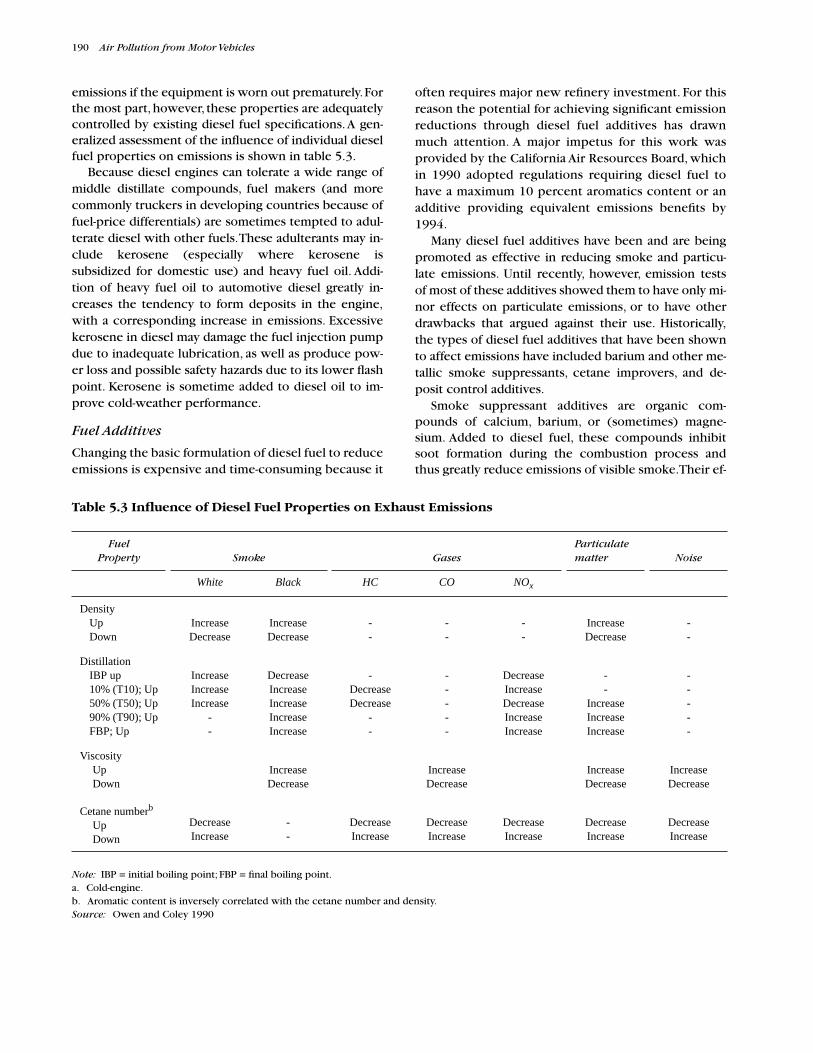
190
Air Pollution from Motor Vehicles
emissions if the equipment is worn out prematurely. Forthe most part, however, these properties are adequatelycontrolled by existing diesel fuel specifications. A gen-eralized assessment of the influence of individual dieselfuel properties on emissions is shown in table 5.3.
Because diesel engines can tolerate a wide range ofmiddle distillate compounds, fuel makers (and morecommonly truckers in developing countries because offuel-price differentials) are sometimes tempted to adul-terate diesel with other fuels. These adulterants may in-clude kerosene (especially where kerosene issubsidized for domestic use) and heavy fuel oil. Addi-tion of heavy fuel oil to automotive diesel greatly in-creases the tendency to form deposits in the engine,with a corresponding increase in emissions. Excessivekerosene in diesel may damage the fuel injection pumpdue to inadequate lubrication, as well as produce pow-er loss and possible safety hazards due to its lower flashpoint. Kerosene is sometime added to diesel oil to im-prove cold-weather performance.
Fuel Additives
Changing the basic formulation of diesel fuel to reduceemissions is expensive and time-consuming because it
often requires major new refinery investment. For thisreason the potential for achieving significant emissionreductions through diesel fuel additives has drawnmuch attention. A major impetus for this work wasprovided by the California Air Resources Board, whichin 1990 adopted regulations requiring diesel fuel tohave a maximum 10 percent aromatics content or anadditive providing equivalent emissions benefits by1994.
Many diesel fuel additives have been and are beingpromoted as effective in reducing smoke and particu-late emissions. Until recently, however, emission testsof most of these additives showed them to have only mi-nor effects on particulate emissions, or to have otherdrawbacks that argued against their use. Historically,the types of diesel fuel additives that have been shownto affect emissions have included barium and other me-tallic smoke suppressants, cetane improvers, and de-posit control additives.
Smoke suppressant additives are organic com-pounds of calcium, barium, or (sometimes) magne-sium. Added to diesel fuel, these compounds inhibitsoot formation during the combustion process andthus greatly reduce emissions of visible smoke. Their ef-
Table 5.3 Influence of Diesel Fuel Properties on Exhaust Emissions
Note:
IBP = initial boiling point; FBP = final boiling point.a. Cold-engine.b. Aromatic content is inversely correlated with the cetane number and density.
Source:
Owen and Coley 1990
Fuel Property Smoke Gases
Particulatematter Noise
White Black HC CO NO
x
DensityUpDown
IncreaseDecrease
IncreaseDecrease
--
--
--
IncreaseDecrease
--
DistillationIBP up10% (T10); Up50% (T50); Up90% (T90); UpFBP; Up
IncreaseIncreaseIncrease
--
DecreaseIncreaseIncreaseIncreaseIncrease
-DecreaseDecrease
--
-----
DecreaseIncreaseDecreaseIncreaseIncrease
--
IncreaseIncreaseIncrease
-----
ViscosityUpDown
IncreaseDecrease
IncreaseDecrease
IncreaseDecrease
IncreaseDecrease
Cetane number
b
UpDown
DecreaseIncrease
--
DecreaseIncrease
DecreaseIncrease
DecreaseIncrease
DecreaseIncrease
DecreaseIncrease

Fuel Options For Controlling Emissions
191
fects on SOF are not fully documented, but one study(Draper, Phillips, and Zeller 1988) has shown a signifi-cant increase in polycyclic aromatic hydrocarbon(PAH) content and mutagenicity of SOF with a bariumadditive. Particulate sulfate emissions are greatly in-creased with these additives because they all form sta-ble solid metal sulfates that are emitted in the exhaust.The overall effect of reducing soot and increasing metalsulfate emissions may be either an increase or decreasein the total particulate mass, depending on the sootemissions level at the beginning and the amount of ad-ditive used. The principal smoke-suppressant additive,barium, is a highly toxic heavy metal, raising additionalconcerns about its possible widespread use. Copperbased additives in diesel fuel can be effective in reduc-ing particulate emissions but may result in significantincrease in dioxin emissions. Trace amounts of chlo-rides (0.9 ppm) in diesel fuel form dioxins (2,3,7,8 tet-racholorodibenzo-p-dioxin) when catalyzed by thecopper additives.
Cetane enhancers are used to improve the self-igni-tion properties of diesel fuel. These compounds (gener-ally organic nitrates) are added to low-grade diesel fuelsto reduce the adverse impact of poor cetane quality oncold starting, combustion noise, and emissions. Cetaneimprovers have been shown to reduce particulateemissions when added to substandard fuels to bringtheir cetane levels up to the normal diesel range. With-in the normal range, however, they tend to have lesseffect.
Deposit control additives can prevent or reverse theincrease in smoke and particulate emissions (and fuelconsumption) that results from the formation of depos-its on fuel injectors and also can reduce the need formaintenance for the same reason. These additives (oftenpackaged in combination with a cetane-enhancer) helpprevent and remove coke deposits on fuel injector tipsand other vulnerable locations—thus maintaining new-engine injection and mixing characteristics. A study forthe California Air Resources Board estimated that the in-crease in PM emissions due to fuel injector problemsfrom trucks in use was more than 50 percent of new-ve-hicle emissions levels (Weaver and Klausmeier 1988). Alarge share of this excess is unquestionably due to fuelinjector deposits. Although their use is quite likely justi-fied for their long-term benefits alone, deposit controladditives typically have little or no direct effect on par-ticulate emissions.
Information is also available on a new class of dieselfuel additives which reduce smoke and particulateemissions without using barium or other metals. Theseall-organic smoke suppressant additives may offer sig-
nificant scope for reducing particulate emissions fromexisting vehicles in a simple and cost-effective manner.Andrews and Charalambous (1991) have documentedtheir tests on such an additive, which was shown to actas a cetane improver and as a detergent—helping tokeep injectors clean. Most importantly, it produced a40 to 60 percent direct and immediate reduction in die-sel particulate emissions over the entire load rangewhen mixed at 0.2 percent (v/v) concentration in thefuel. Both the solid carbon (soot) and the soluble organ-ic fraction of the particulate matter were reduced bythe additive. Although the precise actions of the addi-tive are not known, it is suspected that it may functionby inhibiting soot formation during the combustionprocess.
Similar results were reported for an (apparently) dif-ferent additive by Smith and others (1991). The teamstudied the effects of a proprietary ashless fuel additivedeveloped by Exxon. Measurements were taken in anumber of heavy-duty truck engines and light-duty pas-senger car engines, including both naturally aspiratedand turbocharged models. Significant particulate reduc-tions were found, ranging from 15 to 40 percent de-pending on the engine and test cycle. Again, thesereductions were immediate (and thus not the result ofcleaning up injector deposits, although the additive isclaimed to do that as well).
Some refiners have received permission to meet theCalifornia diesel fuel requirements by marketing dieselfuel blends having higher aromatic levels than the 10percent allowed in the regulation but lower sulfurthan the regulatory limit of 0.05 percent. These fuelsalso incorporate proprietary fuel additives to attain thesame emissions benefits as the 10 percent aromaticfuel.
Effect of Diesel Fuel Properties on Emissions:Summary of EPEFE Results
The European Programme on Emissions, Fuels, and En-gine Technologies (EPEFE) has examined the effect ofvariations in European diesel fuel properties on emis-sions of light duty diesel vehicles and heavy-duty die-sel engines (Camarsa and Hublin 1995, ACEA/EUROPIA 1995a). The test vehicles and engines usedin the EPEFE study conformed to EU 1996 emissionlimits (based on the complete European driving cycle)for light-duty diesel vehicles, and Euro 2 limits (basedon the 13 -mode test) for heavy-duty diesel engines.Properties of the diesel test fuels are summarized intable 5.4.
With respect to emissions from light-duty diesel vehi-cles, the results of the EPEFE study are summarized in

192
Air Pollution from Motor Vehicles
Table 5.4 Properties of Diesel Test Fuels Used in EPEFE Study
Diesel fuel type Density (g/l) Polyaromatics Cetane number T90 (°C) Sulfur (ppm)
Low polyaromatics and low densityLow polyaromatics and high densityHigh polyaromatics and high densityHigh polyaromatics and low density
826–829857855829
0.9–1.11.1
7.3–8.07.1–7.7
49.5–58.050.0
50.2–59.150.2–50.6
326–347348
344–371346–349
404–469415
420–442402–416
Source:
Camarsa and Hublin 1995
table 5.5. The main conclusions pertaining to light-dutydiesel fuel effects are:
•
Particular matter.
Reducing fuel density is themost significant factor in lowering PM emissions.Reductions in polyaromatic content, T95, and sul-fur also lowered PM emissions but to a lesser de-gree, whereas an increase in cetane numberincreased PM emissions.
•
Carbon monoxide.
Increasing cetane number ordecreasing density is a major factor in reducing COemissions; decreasing polyaromatic content in-creased CO emissions, but this effect was less pro-nounced compared to cetane number and density.
•
Nitrogen oxides.
Decreasing polyaromatic contentreduced NO
x
emissions, whereas decreasing T95and density increased NO
x
emissions; cetane num-ber had no significant effect on NO
x
emissions.•
Volatile organic compounds.
Increasing cetanenumber or decreasing density reduced HCemissions significantly, including toxic emissions ofbenzene, 1,3 butadane, formaldehyde, and acetal-dehyde; decreasing polyaromatic content increasedHC emissions including benzene emissions, whileformaldehyde and acetaldehyde emissions were re-duced; decreasing T95 also lowered formaldehydeand acetaldehyde emissions.
Reducing diesel fuel density and increasing cetanenumber are the two most important parameters in re-ducing light-duty diesel vehicle emissions (Camarsa andHublin 1995).
With respect to emissions from heavy-duty diesel en-gines, results of the EPEFE study are summarized in ta-ble 5.6. The main conclusions with respect to heavy-duty diesel fuel effects are:
•
Particulate matter. Reducing the content of polyar-omatics or sulfur reduced PM emissions; lighter-density diesel fuel had lower PM emissions but thiseffect was not statistically significant.
• Nitrogen oxides. All fuel parameters in the EPEFEstudy affected emissions; reducing density, polyar-omatics or T95 decreased NOx emissions, so didan increase in cetane number but the effect wasnot very strong; these effects, however, were notas large as those measured for CO and HCemissions.
• Carbon monoxide. Increasing cetane number wasthe only factor that reduced CO emissions; reduc-ing T95 and density increased CO emissions.
• Hydrocarbons. Reducing T95 or density increasedHC emissions, while a reduction in polyaromaticcontent or an increase in cetane number reducedHC emissions.
Table 5.5 Change in Light-Duty Diesel Vehicle Emissions with Variations in Diesel Fuel Properties(percent)
— Not applicableNS = Non-significant.a. Baseline properties: density 855 g/l; polyaromatic content 8 percent; cetane number 50; T95 370°C; sulfur 2000 ppm.b. Negative values indicate a decrease in emission.c. Positive values indicate an increase in emission.
Diesel fuel propertya CO HC NOx PM CO2
Density855 to 828 g/l –17.1b –18.9c +1.4 –19.4 –0.9
Polyaromatics8 to 1 percent +4.0c +5.5 –3.4 –5.2 –1.08
Cetane50 to 58 –25.3 –26.3 –0.18 (NS) +5.2 –0.37 (NS)
T95370 to 325°C –1.8 +3.4 +4.6 –6.9 +1.59
Sulfur2000 to 500 ppm — — — –2.4 —

Fuel Options For Controlling Emissions 193
Increasing cetane number and decreasing polyaro-matics are the two most significant parameters in reduc-ing heavy-duty diesel engine emissions (Camarsa andHublin 1995). The absence of any effect on PM emis-sion from changes in cetane number is different fromthe results of a number of U.S. studies. This differencemost likely is due to the higher cetane number of theEPEFE test fuels compared to the diesel fuels in the Unit-ed States. Increasing cetane number from 50 to 58seems to have little effect on PM emissions, but increas-ing it from 40 to higher levels such as 45 or 50 has a sig-nificant effect.
Individual vehicles and engines showed a wide rangeof response to the fuel properties investigated in theEPEFE study. In general DI and IDI light-duty vehiclesshowed the same trend concerning the effect of fuelproperties on regulated emissions except for the NOxresponse to cetane number. The lowest sensitivity tofuel property changes was associated with light-dutyIDI engines with mechanical injection controls; light-duty diesel vehicles equipped with IDI enginesachieved consistently low absolute emission rates ingrams per kilometer.
The EPEFE test results for light-duty diesel vehiclesshow that the effect of fuel density on engine emissions,to some extent, was caused by the physical interactionof fuel density with the fuel management system. Vehi-cle sensitivity to variations in fuel density can be influ-enced by the choice of a specific engine tuning/calibration set; sensitivities were lowest when the en-gines were set to high density tuning and highest at lowdensity tuning. Except for NOx lowest emissions weregenerally observed using low density fuels with low den-sity engine tuning. When engines were appropriately
tuned to use fuel of a given density, emissions were gen-erally lower than when density and tuning were notmatched. At both high and low density tunings, massemissions of PM, HC, and CO were higher with highdensity fuels although high density fuels gave lower NOxemissions.
In case of heavy-duty diesel engines, reducing fueldensity lowered engine power and increased fuel con-sumption. Adjustments of the injection system to thesame mass fuel delivery and dynamic injection timingeliminated the difference in emission levels betweenthe low and high density fuels tested in the EFEFEstudy. The effect of fuel density on engine performanceand emissions was caused by the physical interactionwith the fuel injection system, which is purely hydrau-lic in nature. Fuel density did not appear to have any ef-fect on the combustion process (ACEA/EUROPIA1995a).
Alternative Fuels
The possibility of substituting cleaner-burning alterna-tive fuels for gasoline and diesel has drawn increasingattention over the past decade. A vast array of scientificand popular literature has been devoted to the subjectof alternative fuels (OECD 1995; Hutcheson 1995; OTA1995; EIA 1994; Maggio and others 1991; OTA 1990;Transnet 1990; Sperling 1989; World Bank 1981). Alter-native fuels have the potential to conserve oil productsand preserve energy sources, as well as reduce or elim-inate pollutant emissions. Some alternative fuels havethe potential for large, cost-effective reductions in emis-sions of regulated pollutants (CO, HC, NOx) but may
Table 5.6 Change in Heavy-Duty Diesel Vehicle Emissions with Variations in Diesel Fuel Properties(percent)
— Not applicableNS = Non-significant.a. Baseline properties: density 855 g/l; polyaromatic content 8 percent cetane number 50; T95 370°C; sulfur 2000 ppm.b. Negative values indicate a decrease in emissions.c. Positive values indicate an increase in emissions.Source: Camarsa and Hubbin 1995; ACEA/EUROPIA 1995a
Diesel fuel propertya CO HC NOx PM CO2
Density855 to 828 g/l +5.0b +14.25c –3.57 –1.59 +0.07
Polyaromatics8 to 1 percent 0.08 (NS) –4.02 –1.66 –3.58 –0.60
Cetane50 to 58 –10.26 –6.25 –0.57 0 (NS) –0.41
T95370 to 325°C +6.54 +13.22 –1.75 0 (NS) +0.42
Sulfur2000 to 500 ppm — — — –13.0 —

194 Air Pollution from Motor Vehicles
Table 5.7 Toxic Emissions from Gasoline and Alternative Fuels in Light-Duty Vehicles with Spark-Ignition Engines(mg/km)
Compound Gasoline RFG M85 M100 E85 CNG LPG
Benzene 7.95 4.88 4.38 0.32 1.21 0.242 0.242
Toluene 33.66 3.45 8.66 2.11 0.75 0.695 0.695
m&p Xylenes 4.57 4.77 1.54 0.30 1.30 0.705 0.033
0-Xylenes 1.95 1.58 0.46 0.16 0.39 0.399 0.101
1,3-Butadiene 0.19-0.50 0.24 0.44 2.05a
0.12 0.093-0.404 —
Formaldehyde 4.78 0.60 13.87 21.76 3.15 2.712 4.870
Acetaldehyde 0.94 0.50 10.02 0.27 13.32 0.529 0.641
Acrolein 1.12 — 4.44 0.09 — 0.330 0.118
— Not availableNotes: RFG = reformulated gasoline; M85 = 85 percent methanol blend; M100 = pure methanol; E85 = 85 percent ethanol blend; CNG = com-pressed natural gas; LPG = liquefied petroleum gas.a. Other sources suggest that emissions of 1,3 butadiene from M100 could be virtually nil.Source: U.S. EPA 1993; OECD 1995
cause a sharp increase in emissions of toxic pollutants(table 5.7). Care is needed, however, in evaluating theair quality claims for alternative fuels—in many casesthe same or even greater emission reductions could beachieved using a conventional fuel with an advancedemissions control system. Which approach is the morecost-effective will depend on the relative costs of con-ventional and alternative fuels.
In many parts of the world at present, natural gas andLPG are competitive (in resource terms) with gasolineor diesel fuel and may therefore be attractive from aneconomic as well as an environmental perspective. Eth-anol, methanol, and hydrogen are generally more ex-pensive than gasoline. Table 5.8 compares the costs ofthe main alternative fuels in the United States with thatof gasoline in 1992.
The basic physical properties of the main alternativefuels are compared with gasoline and diesel fuel in table5.9. As this table shows, all of the main alternative fuelshave lower energy density, and therefore require agreater volume of on-board storage than gasoline or die-sel fuel to achieve a given operating range.
While the use of alternative fuels can make low emis-sions easier to achieve, a vehicle using “clean” alternativefuels will not necessarily have low pollutant emissions.Much depends on the level of emission control technol-ogy employed. While strict “technology-forcing” emis-sion standards have produced advances in gasoline anddiesel engine emission control technology, alternative fu-els have not been subjected to similar regulatory over-sight and control until recently. This is especially true ofretrofit equipment for converting existing vehicles to run
Table 5.8 Wholesale and Retail Prices of Conventional and Alternative Fuels in the United States, 1992
Source Gasolinea
Methanolb
Ethanolc
LPGc
CNGd
LNGe
Hydrogenf
Wholesale (U.S.$/gal) 0.51-0.68 0.32-0.42 1.29-1.45 0.25-0.45 0.25-0.50 0.40-0.55 0.25g
Wholesale (U.S.$/thermh
) 0.41-0.54 0.56-0.74 1.70-1.91 0.29-0.53 0.26-0.52 0.53-0.72 0.85
Retail (U.S.$/gal) 0.97-1.32 0.80-0.92 n.a. 0.95-1.10 0.40-0.90 n.a. 9.60-16.00
Retail (U.S.$/therm) 0.78-1.06 1.41-1.62 n.a.i
1.12-1.29 0.41-0.93 n.a. 33.10-55.17
Note: 1 US gallon = 3.79 litersn.a. = Not availablea. Wholesale and retail prices - Oil & Gas Journal, December 21, 1992, page 114.b. Wholesale prices - Oxy-Fuel News, October 5, 1992, page 9. Retail prices - California 1992.c. Ethanol and LPG wholesale prices - Oxy-Fuel News, October 5, 1992, pp. 8-9. Retail prices - California 1992.d. Wholesale and retail prices - industry estimates.e. Wholesale prices - industry estimates.f. Wholesale and retail prices are based on quotes from industrial gas suppliers.g. Natural gas and hydrogen are priced in dollars per 100 ft
3.
h. 1 therm = 100,000 Btu.i. Not available at retail outlets.Source: Seisler and others 1993

Fuel Options For Controlling Emissions 195
on alternative fuels. Regulations requiring emissions cer-tification for such equipment are presently effective onlyin California and Mexico; a similar requirement will applyin the rest of the United States beginning in 1997. Be-cause of the absence of regulation, many vehicle conver-sion kits are sold with relatively poor air-fuel ratiocontrol, resulting in unnecessarily high emissions. In-stalled in a modern, emission controlled gasoline vehicle,such kits can even increase emissions compared to thosethat the vehicle produced before being converted (table5.10). Regulatory pressure, however, has resulted in theintroduction of a number of retrofit kits incorporatingelectronic controls and well-designed emission controlsystems. Vehicles equipped with these kits have demon-strated the ability to comply with California LEV emissionstandards. Of course, the lowest emissions and the mostefficient operation are obtained where an engine is de-signed by the manufacturer for alternative fuel use.
Natural Gas
Natural gas, which is 85 to 99 percent methane, hasmany desirable qualities as a fuel for spark-ignition en-
gines. Clean-burning, cheap, and abundant in manyparts of the world, it already plays a significant role asa motor fuel in Argentina (box 5.4), Canada, Italy, NewZealand, Russia, and the United States. Recentadvances in the technology for natural gas vehicles andengines, new technologies and international standard-ization for storage cylinders, and the production oforiginal equipment manufacture (OEM) natural gas ve-hicles in a number of countries have combined toboost the visibility and market potential of natural gasas a vehicle fuel.
There are over one million natural gas vehicles in op-eration worldwide; Argentina and Italy account formore than 50 percent of the global fleet. The penetra-tion of natural gas vehicles in heavy-duty fleets is still mi-nuscule. A CNG fleet of 2,000 buses and trucks inSichuan Province, China is a notable example (IANGV/IGU 1994).
Most of the natural gas vehicles (NGVs) in operationworldwide are retrofits, converted from gasoline vehi-cles. The physical properties of natural gas make such aconversion relatively easy. Conversion costs typically
Table 5.9 Properties of Conventional and Alternative Fuels
Property Gasoline Diesel Methanol EthanolPropane(LPG)
Methane(CNG) RME
H/C ratio 1.9 1.88 4.0 3.0 2.7 4.0 n.a.
Energy content (LHV) (MJ/kg) 44.0 42.5 20.0 26.9 46.4 50.0 36.8
Liquid density (kg/l) 0.72–0.78 0.84–0.88 0.792 0.785 0.51 0.422 0.86–0.90
Liquid energy density (MJ/l) 33.00 36.55 15.84 21.12 23.66a 21.13 b 32.4–33.1
Boiling point (°C) 37–205 140–360 65 79 –42.15 –161.6 n.a.
Research Octane Numbers 92-98 ~25 106 107 112 120 n.a.
Motor Octane Numbers 80-90 – 92 89 97 120 n.a.
Cetane Numbers 0–5 45–55 5 5 ~2 0 45–59
Stoichiometric air-fuel ratio 14.7 14.6 6.5 9.0 15.7 17.2 13.0
Reid Vapor Pressure (psi) 8–15 0.2 4.6 2.3 208 2,400 0.5
n.a. = Not availableNotes: LHV = lower heating value; LPG = liquefied petroleum gas; RME = rapeseed methyl ether; CNG = compressed natural gas.a. Energy density of propane at standard temperature and pressure: 0.093MJ/l.b. Energy density of methane at standard temperature and pressure: 0.036MJ/l; at 200 bar pressure: 70.4MJ/l.Source: EIA 1994; OECD 1995; Hutcheson 1995
Table 5.10 Inspection and Maintenance (Air Care) Failure Rates for In-Use Gasoline, Propane, andNatural Gas Light-Duty Vehicles in British Columbia, Canada, April 1993
Source: B.C. Ministry of Energy, Mines and Petroleum Resources 1994
(percent)
Model year Gasoline Propane Natural gas
1974 or older 31 19 11
1975–81 37 42 24
1982–87 25 47 23
1988–93 6 44 34
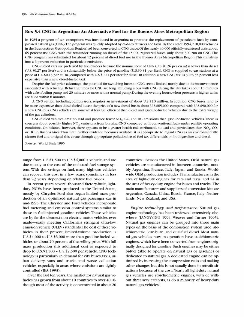
196 Air Pollution from Motor Vehicles
range from U.S.$1,500 to U.S.$4,000 a vehicle, and aredue mostly to the cost of the on-board fuel storage sys-tem. With the savings on fuel, many high-use vehiclescan recover this cost in a few years, sometimes in lessthan 2-3 years, depending on relative fuel prices.
In recent years several thousand factory-built, light-duty NGVs have been produced in the United States,mostly by Chrysler. Ford also began limited mass pro-duction of an optimized natural gas passenger car inmid-1995. The Chrysler and Ford vehicles incorporatefuel metering and emission control systems similar tothose in fuel-injected gasoline vehicles. These vehiclesare by far the cleanest non-electric motor vehicles evermade—easily meeting California's stringent ultra-lowemission vehicle (ULEV) standards. The cost of these ve-hicles in their present, limited-volume production isU.S.$4,000 to U.S.$6,000 more than gasoline-fueled ve-hicles, or about 20 percent of the selling price. With fullmass production this additional cost is expected todrop to U.S.$1,500 – U.S.$2,500 per vehicle. CNG tech-nology is particularly in demand for city buses, taxis, ur-ban delivery vans and trucks and waste collectionvehicles, especially in areas where emissions are tightlycontrolled (IEA 1993).
Over the last ten years, the market for natural gas ve-hicles has grown from about 10 countries to over 40, al-though most of the activity is concentrated in about 20
countries. Besides the United States, OEM natural gasvehicles are manufactured in fourteen countries, nota-bly Argentina, France, Italy, Japan, and Russia. World-wide OEM production includes 15 manufacturers in thearea of light-duty engines for cars and taxis, and 24 inthe area of heavy-duty engine for buses and trucks. Themain manufacturers and suppliers of conversion kits areArgentina, Canada, China, Russia, France, Italy, Nether-lands, New Zealand, and USA.
Engine technology and performance. Natural gasengine technology has been reviewed extensively else-where (IANGV/IGU 1994; Weaver and Turner 1995).Natural gas engines can be grouped into three maintypes on the basis of the combustion system used: sto-ichiometric, lean-burn, and dual-fuel diesel. Most natu-ral gas vehicles now in operation have stoichiometricengines, which have been converted from engines orig-inally designed for gasoline. Such engines may be eitherbi-fuel (able to operate on natural gas or gasoline) ordedicated to natural gas. A dedicated engine can be op-timized by increasing the compression ratio and makingother changes, but this is not usually done in retrofit sit-uations because of the cost. Nearly all light-duty naturalgas vehicles use stoichiometric engines, with or with-out three-way catalysts, as do a minority of heavy-dutynatural gas vehicles.
Box 5.4 CNG in Argentina: An Alternative Fuel for the Buenos Aires Metropolitan Region
In 1985 a program of tax exemptions was introduced in Argentina to promote the replacement of petroleum fuels by com-pressed natural gas (CNG). The program was quickly adopted by mid-sized trucks and taxis. By the end of 1994, 210,000 vehiclesin the Buenos Aires Metropolitan Region had been converted to CNG usage. Of the nearly 40,000 officially-registered taxis, about65 percent use CNG, with the remainder running on diesel; of the 15,000 registered buses, only about 300 run on CNG. TheCNG program has substituted for about 12 percent of diesel fuel use in the Buenos Aires Metropolitan Region. This translatesinto a 6 percent reduction in particulate emissions.
CNG-fueled cars are preferred by taxi owners because the nominal cost of CNG (U.S.$0.26 per cu.m) is lower than diesel(U.S.$0.27 per liter) and is substantially below the price of gasoline (U.S.$0.81 per liter). CNG is supplied to gas stations at aprice of U.S.$0.13 per cu. m., compared with U.S.$0.21 per liter for diesel. In addition, a new CNG taxi is 30 to 35 percent lessexpensive than a new diesel-fueled taxi.
Despite the fuel price advantage, the potential for switching buses to CNG seems limited, mostly due to the inconvenienceassociated with refueling. Refueling times for CNG are long. Refueling a bus with CNG during the day takes about 15 minuteswith a fast-fueling pump and 20 minutes or more with a normal pump. During the evening hours, when pressure is higher, tanksare filled within 8 minutes.
A CNG station, including compressors, requires an investment of about U.S.$1.5 million. In addition, CNG buses tend tobe more expensive than diesel-fueled buses: the price of a new diesel bus is about U.S.$85,000, compared with U.S.$90,000 fora new CNG bus. CNG vehicles are somewhat less fuel efficient than diesel and gasoline-fueled vehicles, due to the extra weightof the gas cylinders.
CNG-fueled vehicles emit no lead and produce fewer NOx, CO, and HC emissions than gasoline-fueled vehicles. There isconcern about possibly higher NOx emissions from burning CNG compared with conventional fuels under real-life operatingconditions. On balance, however, there appears to be a greater health risk attributable to lead and particulates than NOx, CO,or HC in Buenos Aires. Thus until further evidence becomes available, it is appropriate to regard CNG as an environmentallycleaner fuel and to signal this virtue through appropriate pollution-based fuel tax differentials on both gasoline and diesel.
Source: World Bank 1995

Fuel Options For Controlling Emissions 197
Lean-burn engines use an air-fuel mixture withmore air than is required to burn all of the fuel. Theextra air dilutes the mixture and reduces the flametemperature, thus reducing engine-out NOx emissionsand exhaust temperatures. Because of reduced heatlosses and various thermodynamic advantages, lean-burn engines are generally 10 to 20 percent more effi-cient than stoichiometric engines. Without turbo-charging, however, the power output of a lean-burnengine is less than that of a stoichiometric engine.With turbocharging the situation is reversed. Becauselean mixtures knock less readily, lean-burn enginescan be designed for higher levels of turbochargerboost than stoichiometric engines and thus canachieve higher power output. The lower tempera-tures experienced in these engines also contribute tolonger engine life and reliability. For these reasons,most heavy-duty natural gas engines are of the lean-burn design. These include a rapidly growing numberof heavy-duty, lean-burn engines developed and mar-keted specifically for vehicular use.
Dual-fuel diesel engines are a special type of lean-burn engine in which the air-gas mixture in the cylinderis ignited not by a spark plug but by the injection of asmall amount of diesel fuel, which self-ignites. Most die-sel engines can readily be converted to dual-fuel opera-tion, retaining the option to run on 100 percent dieselfuel if gas is not available. Because of the flexibility thisallows, the dual-fuel approach has been popular forheavy-duty retrofit applications. Until recently dual-fuelengine systems tended to have very high HC and COemissions due to the production of mixtures too lean toburn at light loads. Developments such as timed gas-eous fuel injection systems have overcome these prob-lems (Weaver and Turner 1994).
Emissions. Because natural gas is mostly methane,natural gas vehicles have lower exhaust emissions ofnon-methane hydrocarbons than gasoline vehicles, buthigher emissions of methane. Controlled tests conduct-ed by AQIRP on catalyst-equipped light-duty vehicles(U.S. 1992 and 1993 production models) showed thatnon-methane emissions of CNG vehicles were aboutone-tenth those of their counterpart gasoline-fueled ve-hicles, while methane emissions were ten times higher.CO and NOx emissions varied significantly among thethree pairs of test vehicles (passenger car, van, and pick-up truck). CO emissions were 20 to 80 percent lowerwith CNG compared to gasoline; NOx emissions rangedfrom 80 percent lower with CNG (for the pick-up truck)to about the same levels for both CNG and gasoline (forthe medium-duty van). Toxic air pollutant emissionswere dramatically lower with CNG; formaldehyde emis-sions were reduced by 50 percent and acetaldehyde
emissions by 80 percent for CNG vehicles compared totheir gasoline counterparts. Benzene and 1,3 butadieneare virtually nonexistent in CNG exhaust (AQIRP1995c). Since the fuel system is sealed, there are noevaporative or running-loss emissions, and refuelingemissions are negligible. Cold-start emissions from nat-ural gas vehicles also are low, since cold-start enrich-ment is not required, and this reduces both non-methane hydrocarbon and carbon monoxide emissions.Natural gas vehicles are normally calibrated with some-what leaner fuel-air ratios than gasoline vehicles, whichalso reduces CO emissions. Given equal energy efficien-cy, CO2 emissions from natural gas vehicles will be low-er than for gasoline vehicles, since natural gas has alower carbon content per unit of energy. In addition,the high octane value for natural gas (RON of 120 ormore) makes it possible to attain increased efficiency byincreasing the compression ratio. Optimized heavy-duty natural gas engines can approach diesel efficiencylevels. Emissions of nitrogen oxides from uncontrollednatural gas vehicles may be higher or lower than com-parable gasoline vehicles, depending on the enginetechnology but are typically somewhat lower. Light-duty natural gas vehicles equipped with modern elec-tronic fuel control systems and three-way catalytic con-verters have achieved NOx emissions more than 75percent below the stringent California ULEV standards(table 5.11).
In the past few years a number of heavy-duty enginemanufacturers have developed diesel-derived lean-burnnatural gas engines for use in emissions-critical applica-tions such as urban transit buses and delivery trucks.These engines incorporate the low-NOx technologyused in stationary natural gas engines, and typically anoxidation catalyst as well. They are capable of achievingvery low levels of NOx, and particulate matter (less than2.0 g/bhp-hr NOx and 0.03 g/bhp-hr PM) with high effi-ciency, high power output, and (it is anticipated) longlife. Five such engines—the Cummins L10 and DetroitDiesel Series 50 engines for transit buses and the Her-cules 5.6l and 3.7l and Cummins 6B engines for school-buses and medium trucks—have been certified inCalifornia. A comparison of emissions from a two-strokediesel engine and a Cummins L10 natural gas engine isshown in table 5.12. The emissions performance of DAFGKL1160 diesel engines converted to lean-burn natural-ly-aspirated CNG engines (with an oxidation catalyst)for use in city and regional bus services in the Nether-lands is presented in table 5.13.
Fuel storage and refueling. Pipeline-quality naturalgas is a mixture of several different gases. The primaryconstituent is methane (CH4), which typically makes up85 to 99 percent of the total. The rest is primarily ethane

198 Air Pollution from Motor Vehicles
(C2H6), with smaller amounts of propane, butane, andinert gases such as nitrogen, argon, and carbon dioxide.The mix of minor constituents varies considerably de-pending on the source and processing of the gas. TheSociety of Automotive Engineers (SAE) has recommend-ed acceptable compositional limits for natural gas in-tended for introduction into the fuel container ofnatural gas vehicles and for use as an automotive fuel.
Refueling technology is one of the key elements indeveloping a successful market for natural gas vehicleswhich, on average, require refueling twice as frequentlyas gasoline vehicles. Refueling stations are categorizedas either slow-fill or fast-fill. The fast-fill station operatesin a manner comparable to gasoline stations with the ve-hicle refueling in 3-5 minutes. The slow-fill station ac-complishes the refueling of one or more vehicles over a
Table 5.13 Emissions from Diesel and Natural Gas Bus Engines in the Netherlands(g/kwh)
Bus type NOx HC CO PM
CNG city bus 4.3 2.1 0.4 <0.05
CNG regional bus 2.9 3.1 2.5 <0.05
Diesel bus 14.0 1.2 4.0 0.55
EU 1996 standards 7.0 1.1 4.0 0.15
Source: IANGV/IGU 1994
Table 5.12 Emissions from Diesel and Natural Gas Bus Engines in British Columbia, Canada(grams per mile)
Pollutant Current two-stroke engine diesela Natural gasb Difference Percent reduction
HC 0.79 0.02 0.77 97.5
CO 20.85 0.03 20.82 99.9
NOx 20.36 10.26 10.10 49.6
PM 3.32 0.12 3.20 96.4
a. A Detroit Diesel 6V-92TA two-stroke diesel engine.b. A Cummins L10 natural gas engine.Source: B.C. Ministry of Energy, Mines, and Petroleum Resources 1994
Table 5.11 Emissions Performance of Chrysler Natural Gas Vehicles(grams per mile)
Mileage NMOG CO NOx HCHO
LEV Stda 50,000 0.195 5.0 1.1 0.022
120,000 0.280 7.3 1.5 0.032
ULEV Stdb 50,000 0.050 2.2 0.4 0.009
100,000 0.070 2.8 0.5 0.013
Chrysler B350 Ramvan (5,751–8,500 lbs)
Gasoline 50,000 0.19 3.4 0.51 n.a.
CNG 50,000 0.031 2.3 0.05 0.002
(LEV) 120,000 0.040 3.1 0.05 0.003
Chrysler Minivan (3,751–5,750 lbs)
Gasoline 50,000 0.20 1.2 0.19 n.a.
CNG 50,000 0.021 0.4 0.04 0.0002
(ULEV) 100,000 0.035 0.4 0.05 0.0002
n.a. = Not availableNotes: NMOG = Non-methane organic gases. HCHO = Formaldehydea. LEV standard for medium-duty vehicles: 5,751–8,500 lbs.b. ULEV standard for light-duty trucks: 3,751–5,750 lbs.Source: California Air Resources Board 1994

Fuel Options For Controlling Emissions 199
period of several hours, typically 12-14 hours. The costof a slow-fill station is about U.S.$3000--4000 while afast-fill station may cost between U.S.$100,000--250,000. A Vehicle Refueling Appliance (the home com-pressor) has been developed in the United States for theresidential home market for refueling one passenger carovernight. The cost of the Vehicle Refueling Applianceis about U.S.$2,500 (IANGV/IGU 1994).
Natural gas under normal temperature and pressurecreates significant problems with fuel storage aboardthe vehicle. At present, natural gas is stored either as agas (CNG) in high-pressure cylinders or as a cryogenicliquid (LNG) in an insulated tank. Both forms of storageare considerably heavier, more expensive, and bulkierthan storage for an equivalent amount of gasoline or die-sel. The costs of compressing or liquefying natural gasin order to store it are also substantial. The high-pres-sure cylinders needed for CNG weigh more and occupymore space than the vacuum-cryogenic tanks used forLNG, but the cost of the two storage systems is aboutthe same. Nearly all the natural gas vehicles now in userely on CNG rather than on LNG. This is due to thegreater cost of liquefaction and the handling difficulties
involved with LNG. Use of LNG may be attractive in cas-es where large quantities are available at little or no in-cremental cost (as in LNG-importing countries), and forvehicles such as locomotives and long-haul trucks,which need to carry large amounts of fuel.
Figure 5.2 compares the weight of different CNG cyl-inders and fuel with a gasoline tank containing the sameamount of energy. As this figure shows, the early plainsteel CNG cylinders were far heavier than a gasolinetank. The additional weight resulted in a fuel economypenalty of 0.5 liters per 100 km for a CNG passenger carfitted with steel cylinders (Hutcheson 1995). With ad-vances in cylinder technology, however, this weight dis-advantage has been greatly reduced.
Fuel price and supply. After coal, natural gas is themost abundant fossil fuel. The ratio of proven gas re-serves to annual production is double that of petroleum,and a larger proportion of world gas reserves than petro-leum reserves is found outside the Middle East. Today,most major urban centers and many minor ones in indus-trial countries are served by a large network of gas pipe-lines. Other technologies for natural gas transportation
Figure 5.2 A Comparison of the Weight of On-Board Fuel and Storage Systems for CNG and Gasoline
Source: Weaver and Chan 1995
Type of CNG container
Wei
ght (
kg/li
ter,
of g
asol
ine
equi
vale
nt)
Storage
Fuel
6.0
5.0
4.0
3.0
2.0
1.0
0.0
Plain steel Wrappedsteel
Wrappedaluminum
Allcomposite
Gasoline
0.9
1.8
2.9
4.0
5.2

200 Air Pollution from Motor Vehicles
and distribution include liquefaction and shipment in liq-uid form (LNG), and short-distance transport of CNG inlarge banks of cylinders. Japan, Korea, Taiwan (China),and many countries of Western Europe now import sig-nificant quantities of natural gas in the form of LNG.
Owing to transportation difficulties, the cost of natu-ral gas varies greatly from country to country and evenwithin countries. Where gas is available by pipelinefrom the field, its price is normally set by competitionwith residual fuel oil or coal as a burner fuel. The mar-ket-clearing price of gas under these conditions is typi-cally about U.S.$3.00 per million BTU (equivalent toabout 0.41 U.S. cents per gallon of diesel fuel equiva-lent). Compression costs for CNG can add anotherU.S.$0.50 to U.S.$2.00 per million BTU, depending onthe size of the facility and the natural gas supplypressure.
The cost of LNG also varies considerably, dependingon specific contract terms (there is no effective “spot”market for LNG). The cost of small-scale liquefaction ofnatural gas is about U.S.$2.00 per million BTU, makingit uneconomic compared with CNG in most cases.Where low-cost remote gas is available, however, LNGproduction can be quite economic. Typical 1987 costsfor LNG delivered to Japan were about U.S.$3.20 toU.S.$3.50 per million BTU. The costs of terminal re-ceipt and transportation would probably add anotherU.S.$0.50 per million BTU, at the wholesale level.
Safety. CNG vehicles are as safe as gasoline vehicles.Compressed natural gas storage cylinders are built torigorous quality standards. Except for trace contami-nants such as hydrogen sulfide (H2S), natural gas is non-toxic and biologically inert. Due to the high ignitiontemperature of natural gas, simple exposure to a hotsurface (such as an exhaust manifold) is unlikely to leadto a fire. Overall, the risk of fire as a result of uncon-trolled release of CNG is much lower than that from gas-oline, and comparable to that which might be expectedwith diesel fuel (OECD 1995).
The safety record of LNG vehicles is not as well estab-lished as that of CNG, due to the much smaller numberof LNG vehicles in use. As with compressed natural gas,vaporized LNG is non-toxic and biologically inert. Beinga cryogenic fluid, LNG (with a boiling point of –160ºC)tends to vaporize quickly when spilled. Experience hasshown that the vapor cloud above a pool of spilled LNGis very difficult to ignite, due to the narrow range of in-flammability of natural gas vapor. One of the major con-cerns with the use of LNG in vehicles is the possibilitythat excess vapor pressure might be vented from inac-tive vehicles left in an enclosed area such as a garage forlong periods of time, possibly causing an explosion.LNG tanks are equipped with pressure relief valves, andnewer technology fuel tanks guarantee fuel storage for
up to eight to ten days without pressure relief valves be-ing activated. Another danger associated with the use ofLNG is the possibility of cryogenic burns due to contactwith spilled LNG during refueling or as the result of anaccident. LNG nozzles, hoses, and dispenser, however,are equipped with valves to prevent excessive release ofLNG in the event of an accident. The fact that LNG tanksare tough and designed to fail predictably reduces thelikelihood of contact with spilled fuel during an acci-dent (Hutcheson 1995).
Liquefied Petroleum Gas (LPG)
Liquefied petroleum gas, at present the most wide-spread of gaseous fuels, powers an estimated four mil-lions vehicles in several countries, notably the Australia,Canada, Italy, Japan, Korea, Netherlands, New Zealand,Thailand, and the United States. As a fuel for spark-igni-tion engines, it has many of the same advantages as nat-ural gas with the additional advantage of being easier tocarry aboard the vehicle. Its major disadvantage is thelimited supply, which rules out any large-scale conver-sion to LPG fuel.
LPG is typically a mixture of several gases in varyingproportions. Major constituent gases are propane(C3H8) and butane (C4H10), with minor quantities ofpropene (C3H6), various butenes (C4H8), iso-butane,and small amounts of ethane (C2H6). The compositionof commercial LPG is quite variable. In countries withcolder climates, LPG has a higher proportion of pro-pane and propene (as high as 100 percent) in order toprovide adequate vapor pressure in winter, while inwarmer countries LPG consists mostly of butane andbutenes. LPG composition may also be varied seasonal-ly with a higher percentage of propane and propene inthe winter months. Being a gas at normal temperatureand pressure LPG mixes readily with air in any propor-tion. Cold starting is not a problem and therefore cold-start enrichment is not necessary.
Because of its superior knock-resistance, propane ispreferred to butane as an automotive fuel. Propane's oc-tane rating of 112, while somewhat lower than that ofnatural gas, is still much higher than typical gasoline val-ues, and permits the use of compression ratios in therange of 11-12:1. The lean combustion limit of propane-gasoline mixtures is considerably leaner than for gaso-line, allowing the use of lean-burn calibrations, whichincrease efficiency and reduce emissions. These mix-tures are more resistant to knocking and permit the useof still higher compression ratios.
Engine technology and performance. Engine technolo-gy for LPG vehicles is similar to that for natural gas vehi-cles, with the exception that LPG is not commonly usedin dual-fuel diesel applications due to its relatively poorknock resistance (Hutcheson 1995). Both stoichiomet-

Fuel Options For Controlling Emissions 201
ric and lean-burn LPG engines have been developedwith good results. Nearly all LPG vehicles currently inoperation are aftermarket retrofits of existing gasolinevehicles, mostly using mechanical (as opposed to elec-tronic) conversion systems. The costs of convertingfrom gasoline to LPG are considerably less than those ofconverting to natural gas, due primarily to the lowercost of the fuel tanks. For a light-duty vehicle, conver-sion costs of U.S.$800-U.S.$1,500 are typical. As withnatural gas, the cost of conversion for high-use vehiclescan typically be recovered within a few years throughlower fuel costs. Owing to the lack of strong industrysupport, research on LPG as a vehicle fuel has been lim-ited in comparison to natural gas.
Emissions. LPG has many of the same emission char-acteristics as natural gas. On an energy basis LPG has alower carbon content than gasoline or diesel fuel. Whenused in spark-ignition engines, LPG produces near-zeroparticulate emissions, very little CO and moderate HCemissions. Variations in the concentration of differenthydrocarbons in LPG can affect the species composi-tion and reactivity of HC exhaust emissions. As olefins(such as propene and butene) are much more reactivein contributing to ozone formation than paraffins (suchas propane and the butanes), an increase in the olefincontent of LPG is likely to result in increased ozone-forming potential of exhaust emissions. Due to the gas-tight seals required on the fuel system, evaporativeemissions are negligible. LPG emissions during refuel-ing are significant, and U.S. codes require a vapor venton the tank to be opened to avoid overfilling. Technol-ogy to eliminate these emissions exists, however. Ex-haust NMHC and CO emissions are lower with LPG thangasoline. The carbon dioxide emissions typically arealso somewhat lower than those for gasoline due to the
lower carbon-energy ratio and the higher octane qualityof LPG. NOx emissions are similar to those from gaso-line vehicles, and can be effectively controlled usingthree-way catalysts. Overall, LPG provides less air quali-ty benefits then CNG mainly because the hydrocarbonemissions are photochemically more reactive and emis-sions of carbon monoxide are higher.
Modern European dual-fueled LPG cars haveachieved impressive results in reducing emissions. Av-erage emissions and fuel consumption test results forfive dual-fueled passenger cars fitted with closed-loopthree-way catalysts and third generation LPG equip-ment are summarized in table 5.14. The tests were con-ducted over the ECE+EUDC cycle. Table 5.15 showsthe limited emissions data available for LPG vehicles inCalifornia.
Modern spark-ignition LPG-fueled engines equippedwith a three-way catalyst can easily meet (Euro 2 and 3)stringent heavy-duty emission standards. Lean burn en-gines in combination with an oxidation catalyst can alsoachieve very low emission results (Hutcheson 1995).The very low levels of particulate emissions with bothstoichiometric and lean-burning LPG engines continueto be their strongest point, particularly as this is attain-able with low NOx emissions. With respect to CO2 emis-sions and energy consumption, LPG-fueled heavy-dutyvehicles typically consume 20-30 percent more energy.As LPG has a higher energy content per kilogram thandiesel and a lower carbon mass fraction, the CO2 emis-sions of LPG in heavy-duty use are roughly comparableto diesel. LPG also has an advantage over CNG in that itis stored at relatively low pressure in lighter tanks,which impose a lower energy penalty.
Fuel storage. LPG is stored on the vehicle as a liquidunder pressure. LPG tanks, since they must contain an
Table 5.14 Comparison of Emissions and Fuel Consumption for Five Modern Dual-Fueled EuropeanPassenger Cars Operating on Gasoline and LPG
Source: Hutcheson 1995
Emissions and fuel consumption Gasoline LPG
CO (g/km) 0.87 0.72
HC (g/km) 0.14 0.12
NOx (g/km) 0.12 0.16
Fuel consumption (l/100km) 8.7 11.3
Energy consumption (MJ/km) 2.8 2.7
Table 5.15 Pollutant Emissions from Light- and Heavy-Duty LPG Vehicles in California
Source: CARB 1991
Vehicle type NOx NMHC CO
Passenger car (g/mile) 0.2 0.15 1.0
Heavy-duty engine (g/bhp-hr) 2.8 0.5 23.2

202 Air Pollution from Motor Vehicles
internal pressure of 20–40 atmospheres, are generallycylindrical with rounded ends and are much strongerthan the tanks used for storing gasoline or diesel fuel (al-beit much less so than those used for CNG). Propanecan be pumped from one tank to another like any liq-uid, but the need to maintain pressure requires a gas-tight seal. Except for the need for a standardized, gas-tight connection, LPG used as vehicle fuel can be dis-pensed in much the same way as gasoline or diesel fuel.So that some vapor space is always available for expan-sion, LPG tanks used in automotive service must neverbe filled to more than 80 percent capacity. Automatic filllimiters are incorporated in the tanks for this purpose.
Fuel price and supply. LPG is produced in the extrac-tion of heavier liquids from natural gas and as a by-prod-uct in petroleum refining. LPG supply exceeds thedemand in most petroleum-refining countries, so theprice is low compared with other hydrocarbons.Wholesale prices for consumer-grade propane in theUnited States have ranged between 0.25 and 0.30 U.S.cents a gallon for several years, or about 30 percent lessthan the wholesale cost of diesel on an energy basis. De-pending on the locale, however, the additional costs ofstoring and transporting LPG may more than offset thisadvantage.
Because the supply of LPG is limited (about 5-10 per-cent of the amount of petroleum produced and approx-imately 3 percent of the quantity of natural gas), andsmall in relation to other hydrocarbon fuels, any large-scale conversion of heavy-duty vehicles to LPG usewould likely absorb the existing glut, causing prices torise. For this reason LPG probably makes the most senseas a special fuel for use in vehicles—such as rickshaws,taxis, urban buses and delivery trucks—operating in es-pecially pollution-sensitive areas. LPG is used in urbantaxis in many Asian cities, and is also a popular fuel foundin converted three-wheelers. Several hundred LPG-fu-eled city buses have been in use in Vienna, Austria.
Safety. LPG poses a greater safety risk than CNG. Un-like natural gas, LPG vapors are heavier than air, so thatleaks from the fuel system tend to “pool” at ground lev-el, where they might contact ignition sources. To someextent, the same considerations apply to conventionalliquid fuels, although their volatility is somewhat lower.The flammability limits of LPG vapor in the air are alsobroader than those for natural gas. However, where ap-propriate ventilation systems and work practices areemployed, LPG vehicles can be parked and maintainedin enclosed premises without any problems. In addi-tion, the risk of leaks from modern fuel systems is verysmall. Nevertheless, vehicles fitted with LPG systemsmay be subject to restrictions on parking in enclosedspaces and may be prohibited from using underground
communal parking facilities. Like natural gas, LPG isnon-toxic. Also like natural gas, LPG is stored on the ve-hicle in sealed pressure vessels which are much stron-ger than typical gasoline fuel tanks. The probability of atank rupturing and releasing fuel is thus less than forgasoline (Hutcheson 1995).
Methanol
Widely promoted in the United States as a “clean fuel,”methanol has many desirable combustion and emis-sions characteristics, including good lean-combustioncharacteristics, low flame temperature (leading to lowNOx emissions), and low photochemical reactivity.Methanol is dispensed from fuel pumps in a mannersimilar to gasoline. The major drawback of methanol asa fuel is its cost and the volatility of pricing. While meth-anol prices have been highly volatile in the past, thereis little prospect for it to become price-competitivewith conventional fuels unless world oil prices increasegreatly.
With an octane number of 112 and excellent leancombustion properties, methanol is a good fuel for lean-burn Otto-cycle engines. Its lean combustion limits aresimilar to those of natural gas, while its low energy den-sity results in a low flame temperature compared withhydrocarbon fuels, and in lower NOx emissions. To thiscan be added its low vapor pressure, a characteristicthat contributes to a significant reduction in evapora-tive losses.
Engine technology and performance. The low ener-gy density of methanol means that a large amount(roughly twice the mass of gasoline) is required toachieve the same power output. This intrinsic disadvan-tage is partially compensated by the high octane num-ber of methanol and its charge cooling capability, sothat 1.5 liters of methanol give the same mileage as oneliter of gasoline in a dedicated use vehicle. The highheat of vaporization of methanol, combined with thelarge amounts required, makes it difficult to ensurecomplete vaporization and requires special attention tothe design of intake manifolds and cold-start proce-dures. Otto-cycle engines using pure methanol (M100)become nearly impossible to start below 5ºC withoutspecial pilot fuels or supplemental heating techniques.
The low-temperature starting and other problemswith pure methanol have led the developers of light-duty methanol vehicles to specify an 85 percent metha-nol/15 percent gasoline blend (M85) for the currentgeneration of methanol vehicles. The added gasoline in-creases the vapor pressure of the mixture, improvingstarting and making the headspace mixture too rich toburn. It also makes the flame luminous. Most of theemissions benefits of methanol (such as low evapora-tive emissions) are lost with the switch to M85, howev-

Fuel Options For Controlling Emissions 203
er. If the fuel mixture contains even a small percentageof methanol, the vapor pressure rises dramatically.
Flexible fuel vehicles—capable of running on anycombination of gasoline and up to 85 percent metha-nol—have been developed, and fleets of these vehiclesare being tested. The engines and emission control sys-tems on these vehicles are similar to those for advanced-technology gasoline vehicles, and the overall energy ef-ficiency and emission properties are also similar. The in-cremental cost of the flexible-fuel vehicle, comparedwith one designed for gasoline only, is estimated to beabout U.S.$300-400 in large-scale production.
Heavy-duty engines also can be operated on metha-nol, using a variety of technical approaches. A numberof heavy-duty methanol engines have been developedand are reported in the literature. The most promisingapproach is to inject the methanol in liquid form, as ina diesel engine. Engines using this approach can attaindiesel-like efficiencies. Detroit Diesel Corporation inthe United States certified its heavy-duty transit bus en-gine, the 6V-92TA, for methanol use in 1991, and a num-ber of buses using this fuel are now in operation. Thisengine uses direct injection of methanol in liquid form.
Maintenance costs with methanol-fueled enginescould be higher compared to gasoline-fueled engines.Methanol combustion products are fairly corrosive, andcertain engine designs tested to date suggest that theengine life of these designs is likely to be considerablyshorter. Other designs have experienced no significantadded wear. Oil change intervals also may need to beshortened to counteract the increased corrosiveness ofthe combustion products.
Emissions. While the potential emissions benefits ofneat methanol (M100) remain a matter of some conjec-ture, the use of M85 offers some advantages. As metha-nol contains no complex organic compounds, it
promises two air quality benefits over gasoline: lowerozone-forming potential in some areas and reduced emis-sions of a number of toxic air contaminants (especiallybenzene and other polycyclic aromatic hydrocarbons).Emissions of formaldehyde (a primary combustion prod-uct of methanol), however, can be significantly higher;more than five times the amount emitted by comparablegasoline-fueled vehicles. Formaldehyde is toxic and prob-ably a carcinogenic. In confined spaces such as garagesand tunnels, emissions from methanol-fueled vehiclescould result in harmful concentration levels of formalde-hyde. The difficult cold-starting characteristics of metha-nol also lead to high unburned fuel and CO emissionsduring cold starts. HC emissions from methanol enginesare mostly unburned methanol and formaldehyde. Sincemethanol shows less photochemical reactivity than mosthydrocarbons, it was long thought that methanol vehi-cles could help reduce urban ozone problems. More re-cent studies, however, have shown that the highreactivity of the formaldehyde offsets the low reactivityof methanol, so that net ozone benefits are small.
The use of M85 results in reduced emissions of form-aldehyde and 1,3 butadiene, but acetaldehyde emis-sions (not significant with neat methanol) approach thelevels associated with ethanol-gasoline blends (OECD1995). Certification emissions of NMHC, CO, and NOxare compared for gasoline and M85 flexible fuel vehi-cles (FFVs) in table 5.16, which also shows the applica-ble 1994 U.S. emission standards and transitional lowemission vehicle (TLEV), low-emission vehicle (LEV),and ultra-low emission vehicle (ULEV) standards forflexible fuel vehicles. The use of M85 in FFV’s resultedin significantly reduced NMHC and NOx emissions com-pared to equivalent gasoline models. CO emission weresimilar for both M85 and gasoline-fueled vehicles.
AQIRP investigations have shown that, compared togasoline, the use of M85 in earlier (pre-1990) prototype
Table 5.16 Standards and Certification Emissions for Production of M85 Vehicles Compared with Their Gasoline Counterparts(g/mile)
Source: CARB 1994
Vehicle type NMHC CO NOx
Standard Current TLEV LEV ULEV
0.3900.2500.1250.075
0.40.40.20.2
7.03.43.41.7
Certification Gasoline Ford Taurus Chrysler/Dodge Spirit M85 Ford Taurus Chrysler/Dodge Spirit
0.1700.130
0.0910.040
0.110.1
0.10.3
2.32.1
1.41.1

204 Air Pollution from Motor Vehicles
flexible fuel and variable fuel vehicles (VFVs) reducedCO emissions (by 31 percent), increased NOx emissions(by 23 percent), while exhaust NMHC emissions re-mained about the same. Exhaust benzene, 1,3 butadi-ene, and acetaldehyde emissions were lower with M85than gasoline, while formaldehyde emissions were fivetimes higher. Evaporative NMHC also increased signifi-cantly with M85. The use of M10 (a blend of 10 percentmethanol and 90 percent gasoline) in the prototypeFFVs and VFVs reduced all exhaust emissions but in-creased evaporative emissions (AQIRP 1993).
Heavy-duty methanol engines produce significantlylower NOx and PM emissions than similar heavy-dutybus diesel engines, while NMHC, CO, and formalde-hyde emissions, tend to be much higher. These emis-sions, however, have been controlled successfully bycatalytic converters.
Safety. Methanol exhibits a number of safety and han-dling problems which have led to concerns over its pos-sible widespread use. Unlike hydrocarbon fuels,methanol burns with a nearly non-luminous flame thatis impossible to see in daylight. This has generated con-cern over effects on firefighters and passers-by in theevent of a fire. Methanol's vapor pressure is also suchthat it can form a flammable mixture in the headspaceof its fuel tank at normal ambient temperatures. The tox-icity of methanol, and its lack of taste or odor, indicatethat poisoning may be a much greater problem thanwith gasoline (Maggio and others 1991; EIA 1994;Hutcheson 1995).
Fuel price and supply. Methanol can be producedfrom natural gas, crude oil, coal, biomass or cellulose. Atcurrent prices the most economical feedstock for meth-anol production is natural gas, especially natural gasfound in remote regions where it has no ready market.The current world market for methanol is for a com-modity chemical rather than a fuel. World methanol pro-duction capacity is limited (about 7 billion gallons perannum) and projected to be tight at least through the1990s. Methanol is used as feedstock in the productionof MTBE, and the huge increase in MTBE demand for re-formulated gasoline caused methanol prices to reachhigh levels in 1994. AQIRP analysis indicates that M85is likely to be more costly than conventional gasoline inthe short to medium term. Estimates range fromU.S.$0.15 – 0.17 per liter in the short term. Transactioncosts for methanol attaining a significant m arket pene-tration are likely toe high (AQIRP 1993). Methanol maybe best used in specialized, ultra-low-emission applica-tions such as urban buses and trucks. Any large-scaleconversion of vehicles to methanol would require ex-tensive new methanol production capacity if priceswere not to rise significantly.
The price of methanol on the world market has fluc-tuated dramatically in the past decade, from aboutU.S.$0.06 per liter in the early 1980s to U.S.$0.16-0.18in the late 1980s, to as much as U.S.$0.47 in 1994. Thelower prices reflect oversupply; the higher prices re-flect shortages. Estimates of the long-term supply priceof methanol for the next decade range from U.S.$0.11 –0.15 per liter (Wagner and Tatterson 1987; DiFiglio andLawrence 1987; AQIRP 1993; Hutcheson 1995). Thiswould be equal to U.S.$0.27 – 0.31 per liter on an ener-gy-equivalent basis compared to a spot gasoline price ofU.S.$0.18 – 0.20 per liter. In addition to new methanolsupply capacity, any large-scale use of methanol as a ve-hicle fuel would require substantial investments in fuelstorage, transportation, and dispensing facilities, whichwould further increase the delivered cost of the fuel.
Ethanol
Ethanol has attracted considerable attention as a motorfuel due to the success of the Brazilian Pro-alcohol pro-gram initiated in 1975 as a response to the global oil cri-sis of the 1970s. Despite the technical success of thisprogram — around one-third of Brazil’s 12 million carsare powered by ethanol fuel — the high cost of produc-ing ethanol (compared with hydrocarbon fuels) has re-quired large direct and indirect subsidies amounting toover U.S.$1.0 billion per annum.
As the next higher of the alcohols in molecularweight, ethanol resembles methanol in most combus-tion and physical properties, except that it is consider-ably cleaner, less toxic and less corrosive. In addition,ethanol has a higher volumetric energy content. Etha-nol or grain alcohol can be produced by processing ag-ricultural crops such as sugar cane or corn but it is moreexpensive to produce than methanol and requires largeharvest of these crops and large amounts of energy forits production. This can lead to environmental prob-lems, particularly soil degradation (OECD 1995).
Ethanol is most conveniently manufactured in one ofthe two forms: a 95 percent mixture with water, knownas hydrous or hydrated ethanol, and a 99.5 percent mix-ture with benzene, known as anhydrous or absoluteethanol. Fuel grade ethanol, as produced in Brazil, ismanufactured by distillation, and contains several partswater (by volume).
When ethanol is blended with ordinary gasoline inproportions up to 22 percent, the resulting mixtureknown as gasohol, may be burned in ordinary spark-igni-tion automobile engines. Pure ethanol is used extensivelyas a blendstock for gasoline in Brazil, South Africa, andthe United States. While ethanol is completely miscible ingasoline, the presence of even a small amount of watercan result in phase separation. Hence, only anhydrousethanol is used in the gasohol mixture. Gasohol blendsform azeotropes which cause a disproportionate in-

Fuel Options For Controlling Emissions 205
crease in vapor pressure together with a reduction infront-end distillation temperature. This effect varies withethanol concentration but is particularly significant atlow ethanol concentrations up to around 10 percent.Such an increase in vapor pressure can cause hot drive-ability problems in vehicles. As a consequence, the basegasoline must be tailored to accept ethanol. Compared tothe base gasoline, gasohol has a higher RON while theMON is about the same. Under low speed and accelera-tion conditions, road performance of gasohol is generallysimilar to or better than gasoline with the same octanequality. The high-speed, high-load performance of gaso-hol, however, tends to be inferior to that of an equivalent- octane quality gasoline (Hutcheson 1995; Weiss 1990).
Engine technology and performance. Anhydrousethanol has about 65 percent of the heat energy con-tent of an equal volume of gasoline. However, the phys-io-chemical and combustion characteristics of alcoholpermit it to achieve a higher thermal efficiency in an in-ternal combustion engine. Up to a proportion of about20 percent anhydrous ethanol this increase in efficiencycompensates almost fully for the slightly lower energycontent of gasohol blend, so that there are no notice-able mileage penalties in substituting gasohol for gaso-line. The fuel economy of vehicles using gasohol isdependent mostly on the engine type and driving con-ditions. Dynamometer test results and road trials onnon-catalyst cars show no change in fuel economy forethanol contents up to 5 percent volume. For closed-loop catalyst-equipped cars there is a noticeable reduc-tion in fuel economy associated with gasohol(Hutcheson 1995).
A special engine is required to burn mixtures richerthan 22 percent ethanol. “All-alcohol” cars bearing suchengines normally burn hydrated ethanol and requirespecial adaptations mainly to prevent corrosion. Theseadaptations costing about U.S.$500 per vehicle, includecoating the insides of the fuel tank with tin, the fuellines with copper and nickel, and the carburetor withzinc. The pistons also have to be strengthened to permitthe use of higher compression ratios possible with theuse of alcohol. Such engines cannot compensate for thelower energy content of a given volume of ethanol com-pared to gasohol, even though their higher compres-sion ratios achieve even higher thermal efficiency than
those achieved with gasohol in an ordinary engine.About 1.25 litres of pure hydrated alcohol give the samemileage as one liter of gasoline—a significant fuel econ-omy penalty. Ethanol-powered cars tend to be poorstarters in cold weather (Homewood 1993; Weiss1990). To ease this problem, flexible-fuel vehicles havebeen developed in the United States to operate on anyblend of gasoline and ethanol up to 85 percent ethanolby volume.
Emissions. By blending 22 percent anhydrous etha-nol with gasoline to produce gasohol, Brazil has beenable to eliminate completely the requirement for lead asan octane enhancer. Emissions from a sample of non-catalyst Brazilian vehicles using ethanol and gasohol fu-els are compared in table 5.17.
Emissions from ethanol-powered vehicles are not aswell characterized as for other alternative fuels, but arebelieved to be high in unburnt ethanol, acetaldehyde(more than 12 times compared to gasoline vehicles), andformaldehyde. These emissions, however, can be effec-tively controlled with a catalytic converter. Ethanol-runvehicles generate 20 to 30 percent less CO and roughly15 percent less NOx compared to gasoline-fueled vehi-cles. As the vapor pressure of pure ethanol is much low-er than gasoline, evaporative emissions from ethanol-powered vehicles are significantly lower. The low vaporpressure of ethanol, however, could cause cold-startingproblems in colder climates and result in higher cold-start exhaust emissions. Emissions of benzene, 1,3 buta-diene and particulate matter are also substantially lowerfor ethanol-powered vehicles (Homewood 1993;Pitstick 1993). Limited ozone modeling of speciatedemissions from ethanol-fueled vehicle suggests that theozone-forming potential of neat ethanol is less than thatof gasoline and diesel, about the same as that of refor-mulated gasoline, and higher than that of LPG, metha-nol, and CNG.
Some of the limitations of pure ethanol such as cold-start problems and the need for dedicated OEM vehiclescan be addressed by blending ethanol with gasoline toform E85 fuel (85 percent ethanol and 15 percent gaso-line) for use in dedicated Variable Fuel Vehicles (VFVs)/Flexible Fuel Vehicles (FFVs). The gasoline componentvaporizes more readily than ethanol, and makes coldstarting possible. But ethanol blended with gasoline di-
Table 5.17 Average Emissions from Gasohol and Ethanol Light-Duty Vehicles in Brazil(g/km)
Source: Murgel and Szwarc 1989
Fuel type CO HC NOx
Gasohol 40.5 3.8 1.4
Ethanol 18.8 1.6 1.1

206 Air Pollution from Motor Vehicles
minishes some of the inherent benefits of using ethanolin the first instance such as low volatility, no benzene infuel, and lower CO emissions. FFV/VFVs running onethanol-gasoline blends are likely to have higher evapo-rative emissions (with greater ozone-forming potential)than gasoline vehicles as well as increased emissions ofCO and benzene (Pitstick 1993; OECD 1995).
A limited investigation by AQIRP to compare the ex-haust emissions of catalyst-equipped FFV/VFVs operat-ed on E85 fuel and gasoline showed that NOx emissionswere significantly reduced with E85, by as much as 50percent. Total toxic emissions were two to three timesgreater with E85 compared to gasoline due to a large in-crease in acetaldehydes. Formaldehyde emissions withE85 also increased to twice the level of gasoline whilebenzene and 1,3 butadiene were greatly reduced. COemissions also increased with E85. Energy specific fueleconomy changed less than one percent while volumet-ric fuel economy was 25 percent lower with E85(AQIRP 1995d).
Safety. In much the same manner as other fuels, etha-nol presents a fire hazard if handled improperly. The ex-plosion hazard of ethanol is rated as moderate whenexposed to flame. Although ethanol is less volatile thangasoline, it is considered to be more explosive. Vaporsthat form above a pool of ethanol are potentially explo-sive. Repeated overexposure to ethanol will cause red-ness and irritation of the skin. The fuel is not consideredto be particularly hazardous and inhalation of smallamounts of ethanol vapor are not considered toxic. Ex-cessive ingestion of ethanol is dangerous and will requiremedical care. As an intoxicating beverage, ethanol pre-sents a special supervisory challenge. Supplies of ethanolmust be carefully monitored (Maggio and others 1991).
Fuel prices and supply. Ethanol is produced primari-ly by fermentation of starch from grains or sugar fromsugar cane. As a result the production of ethanol for fuelcompetes directly with food production in most coun-tries. The resulting high price of ethanol (ranging fromU.S.$0.26 – 0.41 per liter equivalent to U.S.$0.40 – 0.65per liter of gasoline on an energy basis) has effectivelyruled out its use as a motor fuel except where (as in Bra-zil and the United States) it is heavily subsidized. TheBrazilian Pro-alcohol program has attracted worldwideattention as the most successful example of implement-ing an alternative fuel program. Despite the availabilityof a large and inexpensive biomass resource, this pro-gram has required massive government subsidies for itsviability. To address a severe shortage of ethanol in1990, a blend of methanol, ethanol, and gasoline wasdeveloped for use in dedicated alcohol vehicles (box5.5). Because of earlier disruptions in supply of fuel al-cohol and reductions in direct subsidies, the share of
ethanol-powered cars in new car sales in Brazil droppedto less than one percent in 1996.
Biodiesel
Vegetable oils considered as possible substitutes for die-sel fuel can be produced from a variety of sources in-cluding rape (also known as canola or colza), sunflower,sesame, cotton, peanut, soya, coconut, and oil palm.Vegetable oils have been promoted as possible replace-ment for diesel fuel because of their good ignition qual-ity. However, their high viscosity (about 20 times that ofdiesel), which results in poor fuel atomization, fuel in-jector blockage, ring stickings, and contamination of lu-bricating oil, makes them best used as blends withdiesel fuels in mixtures of up to 50 percent. When usedin blends, vegetable oils produce higher emissions ofCO, HC, and PM as compared to pure diesel fuels(OECD 1995; IEA 1993). Biodiesel is produced by react-ing vegetable or animal fats with methanol or ethanol(trans-esterification) to produce a lower viscosity fuel(oil ester) that is similar in physical characteristics todiesel, and can be used neat or blended with petroleumdiesel. Care must be exercised to completely removethe glycerin residues produced as a by-product. Enginesrunning on neat biodiesel or blended with petroleumdiesel tend to have lower black smoke and CO emis-sions but higher NOx and possibly higher emissions ofparticulate matter. These differences are not large, how-ever. Other advantages of biodiesel include high cetanenumber, low viscosity, very low sulfur content, and thefact that it is a renewable resource. Disadvantages in-clude high cost (U.S.$0.39 – 0.91 per liter before tax)and reduced energy density (resulting in lower enginepower output). The effects of biodiesel on engine per-formance and emissions over a long period in actual ser-vice are not well documented.
Although the use of vegetable oils in diesel enginesdates to 1900, the modern use of biodiesel fuel started inthe early 1980s, when vegetable oils—soybean oil, sun-flower oil, corn oil, cottonseed oil, and rapeseed oil—were first used as experimental substitutes for diesel fuelin farm tractors. Interest in biodiesel plunged along withthe price of oil in 1983. Recently, interest in cleaner airand renewable energies has led to renewed private andpublic focus on biodiesel fuel. A small-scale program toconvert palm oil to methyl ester for use in taxis has beensuccessful in Malaysia (Ani, Lal, and Williams 1990).
Properties. The properties of biodiesel are comparedwith those of diesel fuel in table 5.18. The importantproperties include viscosity, which indicates the flowcharacteristics of the fuel; pour point, which describesthe cold-flow characteristics of the fuel; alkaline con-tent or acid number (soap content), which measures

Fuel Options For Controlling Emissions 207
the amounts of deposit-forming sodium and potassiumin the fuel; sulfur and nitrogen contents, which affectthe amount of PM and NOx emissions formed; and io-dine number, which indicates the fuel stability (level ofsaturation of the fuel). Biodiesel has many physicalproperties (such as the cetane number) quite similar toconventional diesel. It differs from ordinary diesel fuelin terms of its lower energy content (due to its higheroxygen content), which reduces engine power output;it has a higher density and a lower volatility comparedwith diesel, and a stronger affinity for water; and it con-tains no aromatics and only trace amounts of sulfur.Both the low sulfur content and the significant oxygen
content should help to reduce soot formation and emis-sions from biodiesel. Low volatility and poor cold flowproperties could constrain the use of biodiesel in colderclimates. Being hydrophilic, biodiesel requires specialcare in storage. It is fully biodegradable -- 98 percent ofthe spilled material is broken down within three weeksand the remainder within five weeks (Hutcheson 1995).
Use. Owing to the high price of conventional dieselfuel in Europe (U.S.$3 to U.S.$4 a gallon including tax-es), a sizeable number of diesel vehicles in Austria, Bel-gium, France, and Italy run on biodiesel fuel madeprimarily from rape-seed oil (U.S. DOE 1994). In the
Box 5.5 Brazil’s 1990 Alcohol Crisis: The Search for Solutions
A one billion liter shortage of ethanol in 1990 - the result of a 50 percent drop in sugarcane prices over the past several yearsand the corresponding reduction in sugarcane acreage from 1987 to 1989—compelled Brazilian government agencies and pri-vate organizations to search for an emergency solution to guarantee fuel supply for the 4.2 million ethanol-fueled vehicle fleet.The initial recommendations were to:
• Reduce ethanol content in gasohol from 22 to 12 percent• Add up to 5 percent gasoline to the hydrated ethanol fuel.
Because these recommendation fell short of satisfying the ethanol shortfall, the use of methanol as a supplementary alcoholwas considered. After an intensive investigation, a new fuel blend of 60 percent hydrated ethanol (E), 33 percent methanol(M), and 7 percent gasoline (G), by volume, was identified as a suitable substitute for ethanol in Original Equipment Manufac-ture (OEM) vehicles designed to run on ethanol and gasohol mixtures. The addition of methanol tended to compensate forgasoline in the E60/M33/G7 blend: the methanol in the blend resulted in leaner air-to-fuel ratio and a low caloric value; thegasoline fraction in the blend fully compensated for this effect by providing a richer air-to-fuel ratio and a high caloric value.The volatility of this blend, however, was 80 percent higher than ethanol fuel in terms of Reid Vapor Pressure (RVP). Althougha high RVP improves cold starts (less exhaust emissions and better fuel economy), the 80 percent rise in RVP resulted in a two-to threefold increase in evaporative emissions, particularly for pre- 1970 Brazilian vehicles. Fuel economy improved by 2 per-cent with this blend. Exhaust emissions from the new methanol/ethanol/gasoline (MEG) blend are compared below with eth-anol and other other fuel blends evaluated as part of this investigation:
a. Emissions in grams per kilometer (FTP cycle) for this blend were 17 g/km CO; 2g/km HC; 1.1g/km NOx, and 0.07 g/km aldehydes. n.a. = Not available(e) = Estimate
In summary, the ethanol-methanol gasoline blend helped to meet a critical fuel shortage without compromising thecountry’s vehicle pollution control program (PROCONVE) or requiring special tuning, recalibration, or conversion of thededicated alcohol engines. There have been no adverse effects reported from the use of this blended fuel.
Source: Szwarc and others 1991
Relative emissions (base=100)
Stoichiometricair/fuel ratio
Density (kg/l) CO HC NOx Aldehydes
Hydrous ethanol(E100) 8.3 0.79 100 100 100 100
95% ethanol-5% gasoline (E95/G5) n.a. 0.78 125 110 100 n.a
22% ethanol-78% gasoline (E22/G78) 8.9 0.77 175 122 138 36
12% ethanol-88% gasoline (E12/G88) n.a. 0.76 282 134 106 n.a.
100% gasoline (G100) 14.8 0.74 350 140 115 (e) 10 (e)
60% ethanol-33% methanol-7% gasoline (E60/M33/G7)a/ 8.2 0.79 98 90 112 54

208 Air Pollution from Motor Vehicles
Table 5.18 Physical Properties of Biodiesel and Conventional Diesel Fuel
n.a. = Not availableSource: Reed 1994; Ziejewski, Goettler, and Pratt 1986; Alfuso and others 1993; Tritthart and Zelenka 1990; Perkins, Peterson, and Auld 1991, Scholl and Sorenson 1993; U.S. DOE 1994
Property Methyl ester (biodiesel) Common diesel fuel
Viscosity @ 40°C 4.1 – 4.5 2.3 –2.8
Pour point, °C –4 –29
Cloud point, °C –6.7 –20
API gravity @ 15.6 °C 27.8 35.5
Net heat of combustion, MJ/kg 37.1–37.7 42.8
Cetane number 46–52 47–51
Oxydation stability, mg/1000ml 0.06 0.11
Carbon, % weight 77–78 86
Hydrogen, % weight 11–12 13
Oxygen, % weight 10–11 0
Sulfur, % weight 0.002 –0.03 0.15–0.2
Water, mg/kg 500 50
Nitrogen, ppm 29 0
Total acid no., mg KOH/g 0.14–0.45 n.a.
Flash point, °C 152–171 61–92
Iodine value 133 n.a.
Density at 15°C, (kg/m3) 882–885 850–860
Distillation T10, °C T50, °C T95, °C
334336345
227283348
United States biodiesel fuel has been used mostly indemonstration projects in which it is blended with con-ventional diesel fuel to reduce sulfur and particulateemissions from diesel vehicles. Some limited demon-stration projects using neat biodiesel in diesel vehicleshave also been initiated (U.S. DOE 1994; Reed 1994).
Engine emissions, performance, and durability. Re-sults from laboratory studies (Alfuso and others 1993;Pagowski and others 1994; Scholl and Sorenson 1993;Tritthart and Zelenka 1990; Reed 1994; Perkins, Peter-son, and Auld 1994; Ziejewski, Goettler, and Pratt 1986generally agree that blended or neat biodiesel has thepotential to reduce diesel CO emissions (although theseare already low), smoke opacity, and HC emissions par-ticularly polycyclic aromatic hydrocarbons. But thesestudies show an increase in NOx emissions for biodieselfuel compared with diesel fuel at normal engine condi-tions. The higher NOx emissions from biodiesel-fueledengines are partly due to the higher cetane number ofbiodiesel, which causes a shorter ignition delay andhigher peak cylinder pressure. Some of this increasemay be due to the nitrogen content of the fuel. The re-duction in smoke emissions is believed to be the result
of better combustion of the short-chain hydrocarbonsfound in biodiesel, as well as the effects of the oxygencontent. Other data have shown that mixing oxygen-ates with diesel fuel helps reduce smoke.
Several European studies have also investigated theemissions performance of rape-seed methyl ester (RS-ME) as a neat fuel or as a blend with conventional dieselfuel up to 20 percent. As reported by Hutcheson (1995),RSME compared to conventional diesel fuel has the fol-lowing emission characteristics:
• Lower HC and CO emissions.• Consistently higher NOx emissions.• Generally lower particulate emissions particularly
under high-speed and moderately high-load condi-tions but a dramatic increase under low-speed andlight-load conditions (Cold ECE 15).
The increased NOx emissions may be attributed toincreased combustion temperatures due to better avail-ability of oxygen within the combustion zone. This phe-nomena may also influence the formation of soot.
As for the HC emissions, research by Scholl and So-renson (1993) shows a reduction in HC emissions when

Fuel Options For Controlling Emissions 209
biodiesel is used. There is some concern, however, thatthe organic acids and oxygenated compounds in biodie-sel may affect the response of the flame ionization de-tector, thus understating the actual HC emissions.Scholl and Sorenson also mention that the behavior ofthese compounds with respect to adsorption and des-orption on the surfaces of the gas sampling system is un-known. Thus more studies are needed to understandthe organic constituents in the exhaust from biodiesel-fueled engines before firm conclusions can be drawn re-garding the effects on HC emissions.
There is controversy concerning the effect ofbiodiesel on particulate matter emissions. Alfuso andothers (1993) report that some studies claim a reduc-tion of particulate emissions when biodiesel is used,while some studies show an increase. Alfuso and othersfound that the particulate matter produced by biodie-sel was higher than that produced by diesel fuel inlight-duty transient driving (ECE 15 testing cycle). Thiseffect may depend on the selection of the injection tim-ing. According to an analysis of particulate compositionreported by Hutcheson (1995), soot emissions (insolu-bles) were significantly reduced with RSME but theproportion of the emissions composed of fuel-derivedhydrocarbons (fuel solubles) condensed on the sootwas much higher (a five to six fold increase comparedto diesel). This suggests that RSME may not burn tocompletion as readily as diesel fuel. Although the totalPM emissions for diesel (0.275 g/mile) were significant-ly higher than RSME (0.224 g/mile), the soluble organicfraction (16 percent) in diesel emissions was substan-tially lower compared to RSME (51 percent). In addi-tion, a general trend toward lower emissions of PAHand aldehydes has been found with RSME, although incold FTP and ECE tests, an increase in these emissionswas observed.
In general, no engine, ignition system, or fuel injec-tor modification is necessary for diesel engines to oper-ate on biodiesel. However, the solvent characteristics ofthe fuel require the replacement of the hoses and fuellines that contact the fuel. Furthermore, the work ofScholl and Sorenson (1993) has shown that a 5 degreeretardation of injection timing is required to lower NOxemissions using biodiesel. Scholl's research also showedthat the peak cylinder pressure and the peak rate ofpressure rise were higher for biodiesel-fueled enginesthan for diesel-fueled engines. This suggests that biodie-sel engine carrying higher stress than components en-gines using diesel, and this may affect their durabilityand reliability. These findings imply that some engineadjustments or modifications may be needed with theuse of bio-diesel to optimize engine performance, emis-sions, and durability.
Research has shown that the combustion character-istics of biodiesel are comparable to diesel fuel (Scholl
and Sorenson 1993; Alfuso and others 1993), but the so-dium and potassium atoms in biodiesel fuel can formdeposits in the combustion chamber. As these depositsbuild up, they can affect combustion characteristics,and influence engine performance and operability aswell as increase exhaust emissions. Substantial depositbuild-up in the combustion chamber can also degradeengine durability.
Another common finding on the use of biodiesel asa vehicle fuel is that biodiesel tends to dilute engine oil.More frequent oil changes may be required with biodie-sel fuel. Prolonged engine operation with diluted en-gine oil may cause the oil to break down and the engineto seize. Other concerns regarding the use of biodieselfuel are that the vehicle is likely to have problems op-erating in cold weather, due to the fuel's relatively highcloud and pour point (Perkins, Peterson, and Auld1991). Although pour point depressant and cold-flowimprovers may help alleviate this problem, such addi-tives might affect the biodegradability of the fuel,which is an important advantage of biodiesel (U.S. DOE1994).
Fuel cycle emissions and fuel cost. OECD/IEA(1994) includes a detailed evaluation of the economicsof biofuels. The production of vegetable oil–basedbiodiesel fuel involves plowing the ground (tillage),planting the crops (rape, soybean, sunflower, corn),and fertilizing and harvesting the crops. These process-es require the use of motorized farm equipment, whichproduce exhaust emissions and use fossil energy. In ad-dition, methanol or ethanol are needed in the trans-esterification process, and the emissions emitted to pro-duce these compounds should be taken into account.In a life-cycle study on rape-seed oil and its esters, theGerman Federal Environmental Agency has noted thatother factors such as odor generated by fuel combus-tion and large emissions of nitrous oxide (N2O) in theproduction cycle render the use of this fuel less attrac-tive (OECD 1995). Therefore the overall energy con-sumption and full fuel cycle emissions for biodiesel fuelmight be as high as those from conventional diesel fuel.Thus biodiesel fuel might not be as attractive as other al-ternative fuels, such as natural gas, as a substitute forconventional diesel fuel.
The cost of biodiesel fuel is one of the principal bar-riers making it less attractive as a substitute for diesel.The cost of vegetable oils is U.S.$2 – 3 a gallon. If thecredit for glycerol, which is a by-product of the biodie-sel trans-esterification process and a chemical feedstockfor many industrial processes, is taken into account, thecost of converting vegetable oils to biodiesel is approx-imately U.S.$0.50 a gallon (Reed 1994). Thus the totalcost for biodiesel fuel is U.S.$2.50 – 3.50 a gallon. Thisis substantially higher than the cost of conventional die-

210 Air Pollution from Motor Vehicles
sel, about U.S.$0.75 – 0.85 a gallon before tax. If wastevegetable oil is used, the cost of biodiesel could be re-duced to about U.S.$1.50 a gallon (Reed 1994). Sincethe heating value for biodiesel is less than that for diesel,more fuel must be burned to provide the same workoutput as diesel. This adds further to the cost disadvan-tage of biodiesel. Considering these limitations and theavailability of less greenhouse gas intensive alternativesat similar cost, the use of rape-seed oil or its derivativescannot be justified from the standpoint of environmen-tal protection.
Hydrogen
Although hydrogen has the potential to be the cleanest-burning motor fuel, it has many properties that make itextremely difficult to use in motor vehicles. Hydrogen'spotential for reducing exhaust emissions stems from theabsence of carbon atoms in its molecular structure. Be-cause of the absence of carbon, the only pollutant pro-duced in the course of hydrogen combustion is NOx (ofcourse, the lubricating oil may still contribute smallamounts of HC, CO, and PM). Hydrogen combustionalso produces no direct emissions of CO2. Indirect CO2emissions depend on the nature of the energy sourceused to produce the hydrogen. In the long-term eventof drastic measures to reduce CO2 emissions (to help re-duce the effects of global warming), the use of hydro-gen fuel produced from renewable energy sourceswould be a possible solution. Mackenzie (1994) pro-vides an excellent review of the prospects and potentialof hydrogen vehicles.
Fuel supply. Hydrogen suffers from two major prob-lems: production and storage. Hydrogen is not a fossilfuel, and is not found in significant quantities in na-ture. It therefore must be manufactured. Hydrogen canbe produced by a number of methods, of which themost common are electrolysis of water, reforming nat-ural gas, or partial oxidation and steam reforming ofother fossil fuels. (It should be noted that hydrogenproduced by reforming fossil fuels does not reducegreenhouse emissions because the CO2 emitted in thereforming process is comparable to that which wouldhave been emitted if the fossil fuels were used directlyin a vehicle.) The most economical source of hydrogenis from reforming natural gas. Hydrogen is currentlymanufactured in limited quantities as an industrialchemical, as rocket fuel, and in larger quantities foruse in petroleum refineries and chemical plants. Elec-trolysis is sometimes used to produce high-purity hy-drogen for special purposes but cannot competeeconomically with natural gas reforming for large-scaleproduction.
Advocates of a future “sustainable” hydrogen econo-my have proposed many ideas for renewable sources of
hydrogen. These potential future sources include elec-trolysis of water using large-scale, cheap photoelectricor solar-electric systems, or cheap, abundant, and envi-ronmentally benign hydroelectric or nuclear-electricplants. In the nearer term, renewable hydrogen couldbe produced from biomass using any of several process-es. It is unclear, however, why hydrogen would be pro-duced from biomass instead of easier-to-handle fuelssuch as methanol, ethanol, or methane. Hydrogen alsocould be produced on a large scale through in-situ gas-ification of coal, but this would result in large emissionsof CO2, as well as localized environmental damage dueto subsidence, possible groundwater contamination,and so on.
In order for hydrogen to become available as a motorfuel, significant investments would be needed in the in-frastructure for the delivery, storage, and dispensing ofthe fuel. These investments are unlikely to occur as longas the costs of hydrogen production and use exceedthose of other available motor fuels.
Fuel storage. Hydrogen can be stored on-board a ve-hicle as a compressed gas or as a liquid, or in chemicalstorage in the form of metal hydrides. Hydrogen alsocan be manufactured on-board the vehicle by reformingnatural gas, methanol, or other fuels, or by the reactionof water with sponge iron. In the latter case the spongeiron is oxidized and must be regenerated periodically.Compressed hydrogen occupies roughly fourteen timesthe space of an equivalent amount of gasoline. Thuscompressed gas storage would add significant bulk andweight to a vehicle—about three times the bulk andweight of an equivalent volume of compressed naturalgas. Vehicle range and refueling frequency would be sig-nificant constraints.
Hydrogen can also be stored on-board a vehicle as aliquid, but this requires that it be cooled below its boil-ing point of –423°F (at 36°F above absolute zero, thelowest boiling point of any substance except helium).Even as a liquid, however, hydrogen would still occupyroughly four times the volume of an equivalent amountof gasoline. Furthermore, the energy required for refrig-eration to liquefy the hydrogen could easily exceed theenergy value of the fuel itself, resulting in an extremelyinefficient system.
The third option for hydrogen storage is in the formof metal hydrides. Current metal hydride storage sys-tems are heavy and bulky, but less so than the storagecylinders required for compressed hydrogen (Billings1993). This is considered the leading technology forstoring hydrogen for vehicular use. Research is underway in several countries to improve these characteris-tics, and some vehicle manufacturers in Germany andJapan are developing prototype vehicles.

Fuel Options For Controlling Emissions 211
Engine and vehicle technology. Aside from its low-emission characteristics, hydrogen is a poor fuel for in-ternal combustion engines. This is due to its poor knockresistance compared with other gaseous fuels (such asnatural gas or propane). Hydrogen-fueled spark-ignitionengines are susceptible to detonation or knock, whichlimits the compression ratios that can be used and thusthe efficiency attainable. Rotary engines have met withlimited success in past engine research. Some researchalso has studied the possibility of using hydrogen in anignition-assisted diesel engine, which would avoid theproblem of knock.
The most promising approach to the use of hydrogenfor vehicular propulsion is to react it with oxygen in afuel cell to supply electric energy to a hybrid-electric ve-hicle. Fuel cells are extremely efficient compared withinternal combustion engines, and hydrogen-air fuelcells produce no pollutant emissions. Thus this systemwould be similar to a battery-electric propulsion sys-tem, except that the fuel cell and fuel supply would re-quire significantly less weight and bulk than a batterysystem for the same energy storage. The fuel could besupplied and stored as hydrogen or could be producedon-board by the reformation of methanol, natural gas,or other hydrocarbon fuels, or by the reaction of waterwith sponge iron. Producing hydrogen for the fuel cellby reforming hydrocarbon fuels may be especially at-tractive—both because of the increased ease of han-dling compared with pure hydrogen and because thisapproach could continue to use the fuel supplyinfrastructure already in place.
Research and development work on hydrogen-pow-ered vehicles is progressing in several countries includ-ing Canada, Germany, Japan, and the United States. Oneof the most promising developments is a prototype 60-passenger hydrogen bus produced by Canada’s BallardPower Systems, a leader in fuel cell technology. The pro-ton-exchange-membrane (PEM) fuel-cell bus has beenput in service in Vancouver, Canada. It travels at normaloperating speeds and can go more than 400 km on a sin-gle hydrogen charge. The Ballard prototype, however,costs three times as much to operate as a comparablediesel bus. Economies of scale and improved fuel cellsmight make it competitive with conventional dieselbuses beyond 2000 (AASHTO 1996; MacKenzie 1994).
Emissions. Hydrogen has the potential to be thecleanest-burning motor fuel. With the virtual elimina-tion of CO and HC exhaust emissions, only nitrogen ox-ide emissions would be present in any significantquantity in the vehicle exhausts; NOx emissions fromexisting prototype hydrogen vehicles are similar tothose from gasoline vehicles (Kukkonen and Shelef1994).
Economics. Due to the high cost of production, lackof storage reserves, and the large quantities required forhydrogen to be used as a motor fuel, it is unlikely thathydrogen will be a cost-effective fuel in the near future.New production and storage techniques will be re-quired before hydrogen fuel becomes economically—much less technologically—feasible.
Safety. There are numerous safety concerns using hy-drogen as a motor fuel. These concerns are associatedprimarily with its extreme flammability. Although hy-drogen is lighter than air, it mixes rapidly with air to cre-ate a combustible or explosive mixture. Hydrogen alsois difficult to store as a gas because its molecules arequite small, which enables them to diffuse out throughmost common containment materials. Special materialsfor tanks and fuel lines are required to contain the fueland to minimize leakage.
Electric and Hybrid-Electric Vehicles
Electric vehicles—in the form of trolleys used7 for pub-lic transit—were a familiar sight in many cities in LatinAmerica, Asia, and Eastern Europe. Although they arequiet and emit virtually no pollution, they have high op-erating costs, and very high capital costs comparedwith diesel-fueled buses. The flexibility of operationswith trolley buses is also limited due to the need to fol-low overhead wires, which are vulnerable to accidentsand sabotage. As a result they have been replaced byconventional diesel buses in most developing countriesover the past 30 years. A few battery-electric buses havebeen built as demonstration projects, but these have ex-tremely limited range and are suitable only for short“shuttle” routes. Because of the disadvantages of elec-tric buses, the use of emission-controlled diesel or alter-native-fuel buses is frequently a better and more cost-effective solution to the problem of diesel bus emis-sions in urban areas.
The major focus at present is on the development ofbattery-powered electric passenger cars and light vans
7. Worldwide there are over 370 trolleybus systems. Western na-tions (including the American hemisphere), operate 73 systems total-ing some 5,400 vehicles, the largest system is in São Paulo, Brazil, with480 trolley buses. Eastern countries, including China and the succes-sor states of the former Soviet Union, account for about 300 systemswith an estimated 25,000 vehicles. The largest of these systems is inMoscow with an estimated 2,000 vehicles. All of Western Europe has52 systems with 2,200 trolleybuses. The United States has five sys-tems, (Boston, Dayton, Philadelphia, San Francisco, and Seattle) witha total of 727 vehicles. Canada has two systems in Vancouver and Ed-monton with 355 trolleybuses. Trolleybuses cost between 50-100 per-cent more than diesel buses of comparable size and are economicalto operate only in cities with steep streets and substantial height dif-ferences (AASHTO 1995).
212 Air Pollution from Motor Vehicles
for commuter and pickup-and-delivery services in ur-ban areas. With improvements in electric motor and bat-tery technology, a number of vehicle designs havingacceptable performance characteristics have been de-veloped. A brief review of electric and hybrid electricvehicle technology is presented in appendix 5.2. The re-sources expended on electric vehicle developmenthave increased greatly since 1990, when the CaliforniaAir Resources Board (CARB) adopted new emission reg-ulations requiring a minimum of two percent of vehiclesales in California (about 20,000 cars) to be zero emis-sion vehicles (ZEVs) beginning in 1998. This percentagewas to rise 5 percent in 2001 and 10 percent in 2003
8
.The current state-of-the-art in battery technology stilllimits battery-electric vehicles to short ranges—on theorder of 100-150 kilometers under the most favorableconditions. Under less favorable conditions the achiev-able range may be much less. Factors contributing to re-duced range include use of heaters or air conditioners,use of lights for night driving, and rain, snow, wind, orother factors that increase rolling resistance or air drag.
Despite their limitations, electric vehicles are poten-tially attractive in some kinds of vehicle service—espe-cially those, such as commuting and urban pickup anddelivery, where short range is not a problem. Ofcourse, the main advantage of electric vehicles is the ab-sence of pollutant emissions at the point of use, al-though the incremental emissions from the power plantto produce the electricity may be significant. In addi-tion, electric vehicles have a potential efficiency advan-tage in applications—such as buses—that involverepeated stopping and starting. This is because of thepotential for regenerative braking. By using the motorsas generators to decelerate, it is possible to recover forlater use much of the kinetic energy of the vehicle, rath-er than dissipating this energy as heat as is done in a tra-ditional friction brake.
Battery technology is now the subject of intensive re-search and development aimed at increasing energy andpower density/efficiency, increasing useful life, reduc-ing manufacturing costs, and finding substitutes for en-vironmentally undesirable materials such as lead andcadmium. Other on-board energy storage devices suchas high-speed flywheels and ultracapacitors are also un-dergoing intensive research and development and mayultimately provide a better solution than electrochemi-cal batteries (OTA 1995; Mackenzie 1994).
8. In January 1996, CARB decided to suspend this regulation as thetechnology to produce battery-powered ZEV’s is not adequately ad-vanced in terms of vehicle range, cost or performance for the industryto achieve these targets. Despite rescinding its 1998 deadline, CARBremains committed to imposing targets for the number of ZEVs andhas obtained a commitment from the motor industry to sell about2000 electric vehicles in Los Angeles and Sacramento (which have theworst smog records) between 1998 and 2000.
Another promising electric-vehicle technology is thehybrid-electric vehicle, which would combine many ofthe advantages of the battery-electric vehicle (regenera-tive braking, quiet operation), with much longer rangeand greater energy efficiency overall. These vehiclescould also be designed to have very low emissions, pos-sibly less than those of the power plant supplying thebattery-electric vehicle. The motor in a hybrid-electricvehicle would be designed to give the best emissionsand fuel economy at one or two specific operatingpoints and would then always operate at these points.The motors themselves might be advanced internalcombustion engine designs or could include such othertechnologies such as gas turbines and Stirling engines.The motor would turn a generator and would be sizedto supply the average electric power required by the ve-hicle, while an on-board electric energy storage systemwould supply surge power for acceleration and wouldaccept the power returned by regenerative braking. Inaddition to avoiding the broad range of engine operat-ing conditions experienced by current vehicle engines,this arrangement would avoid engine transients, a majorcontrol problem and a significant source of pollutantemissions (Sperling 1995; OTA 1995).
Electric vehicles are very expensive compared toother clean-vehicle technologies. Low-production mod-els such as the Chrysler TEVan sell for more thanU.S.$100,000 each. General Motor’s EV1, the first elec-tric car in modern times to have been specifically de-signed by a major car maker for the mass market, ispriced at U.S.$35,000. Estimates of the costs of battery-electric vehicles in volume production are heavily influ-enced by assumptions regarding battery cost and effi-ciency. Estimates of the incremental cost (comparedwith a gasoline-fueled vehicle meeting current U.S.emission standards) range from U.S.$3,000 to morethan U.S.$20,000 per vehicle. To these costs need to beadded the costs of the electric-charging infrastructure,and the incremental capital costs of new power plants.OTA (1995), Sperling (1995), Mackenzie (1994), andIEA (1993) provide detailed assessments of the technol-ogy and economics of electric vehicles. Barring a crisisthat could accelerate the development schedules, itmight be 2020 or 2025 before advanced electric vehi-cles produced for the mass market have fully penetratedthe new vehicle fleet, and it would be another 10 to 15years before penetration of the entire fleet takes place(OTA 1995). Despite these limitations, electric vehicleshave become popular in some European countries andare beginning to penetrate the motorcycle/moped mar-ket in Asia.
In France, buyers of electric cars qualify for aFF15,000 (U.S.$2,500) government grant to offset theadditional cost compared to conventional cars. Francehas operated the world’s biggest trial program for elec-
Fuel Options For Controlling Emissions 213
tric cars, involving Peugot-Citröen. A major demonstra-tion project has been in progress in the port city of LaRochelle. Under an agreement involving the city, theFrench electricity authority and the automaker, 50 bat-tery-powered Citroen Ax and Peugeot 106 cars havebeen rented to private users from FF900 to FF1000(U.S.$150 to $110) a month, including insurance, main-tenance and rental of nickel-cadmiums batteries. In addi-tion to the availability of public recharge bays with“quick charge” dispensers, participants with their owngarages may plug into a recharger overnight; this allowsthem to drive 75 to 100 km for about 8–9 francs(U.S.$1.50) of electricity (AASHTO 1994). A new exper-iment in Tours will test the demand for specifically-de-signed urban electric cars, which can be rented andreturned after short periods, similar to taxis. Potentialbacking for electric cars in France has been influencedby the cheap nuclear-generated power (Simonian 1996).
Despite their limited range, there are about 250,000electric vehicles in France; compared to just 3,000 suchvehicles in the United States. Sweden has also experi-mented with electric cars for use by municipal organi-zations under the auspices of Newtek, a Swedish Stateagency. In Finland the postal service has more than 40electric vans in daily use. In England, a bus fleet pow-ered by electricity and guided by a satellite navigationsystem has been launched in London. The 12-seater bus-es use an electric drive system developed and suppliedby Wavedriver, a joint venture between the TechnologyPartnership, a research company, and PowerGen, theUK power generator. The batteries, which can run for50 miles, can be re-charged in less than an hour. The Ox-ford County Council (U.K.) has also successfully operat-ed four 18-seater, battery-powered electric buses toprovide inner city shuttle service over a two-year peri-od. Electric vehicle (EV) demonstration projects havebeen sponsored by other jurisdictions in U.K., such asCamden, Conventry, and Ipswich.
Germany’s Ministry of Research and Development inassociation with the automotive industry and batterymanufactures is supporting a four-year demonstrationprogram on the Baltic Sea Island of Ruegen to test a fleetof 37 new private cars, 20 vans, and 3 minibuses retro-fitted with electric motors. The experiment includesboth new nickel-cadmium and conventional batteries.The demonstration program, besides assessing the tech-nical performance of the latest generation of battery-powered vehicles, expects to determine the degree ofdriver acceptance and accommodation to the opera-tional characteristics of electrical vehicles. In Japan, theNational Environment Agency has offered to subsidize50 percent of the cost of electric vehicles (mini vansand delivery vehicles) purchased by local governments.The objective is to raise environmental awareness andencourage local businesses to purchase electric vehi-
cles. The electric delivery van has a top speed of 85 km/hr and can travel nearly a hundred miles after beingcharged overnight (AASHTO 1993).
In Nepal, electric three-wheelers (Safa Tempos9
)have been introduced in Kathmandu as a replacementfor conventional diesel-fueled tempos under a joint pro-gram supported by the national government, the UnitedStates Agency for International Development (USAID),and the private sector. The program is managed by Ne-pal Electric Vehicle Industry (NEVI) and has receivedstrong government support in the form of reduced im-port duties and other tax incentives (box 5.6).
Factors Influencing the Large-Scale Use ofAlternative Fuels
Cost
Large scale introduction of alternative transport fuelsdepends on the cost of production and the additionalcosts of fuel storage, distribution, and end use. Produc-tion costs are a function of the abundance or scarcity ofthe resources from which the fuel is produced, as wellas the technology available for extracting those resourc-es. Gasoline and diesel substitutes made from heavyoils, natural gas or biomass require relatively minorchanges to existing distribution and end-use systems,whereas CNG, LPG, and alcohol fuels require largermodifications.
Alternative fuel costs (inclusive of production, distri-bution, and end-use) as estimated by OECD and basedon 1987 prices and technology are shown in table 5.19.According to the OECD's International Energy Agency(IEA), CNG and LPG could be economically competitivewith conventional gasoline. Methanol and synthetic gas-oline made from natural gas could become marginallycompetitive under optimistic assumptions about gasprices. Methanol from coal or biomass and ethanol frombiomass were estimated to cost at least twice as muchas gasoline (IEA 1990).
A study by the World Bank (Moreno and Bailey 1989)found that at crude oil prices of U.S.$10 per barrel orlower (in 1988 prices) alternative fuels were generallyuncompetitive. With crude oil cost between U.S.$10and U.S.$20 per barrel, custom-built, high-mileage LPGvehicles and retrofitted, slow-fill CNG vehicles (mostlycaptive fleets of urban buses, taxis, and delivery vehi-
9. The Safa Tempo (electric three-wheeler) runs on a 72-volt directcurrent (D.C.) motor (8.5 hp @3,800 rpm), powered by a pack of 12(6-volt, 220 amp. hr) or 36 (2-volt, 150 amp. hr) batteries. The maxi-mum speed is set at 40 km/hr and range per charge of batteries is 60kilometers. The daily duty range (with exchange of batteries) is 150kilometers. The average power consumption is 150-200 watt-hr per ki-lometer. The maximum pay load is 600 kg, equivalent to about 10 pas-sengers plus driver.

214 Air Pollution from Motor Vehicles
cles with high annual mileage but restricted range) be-come competitive. Between U.S.$20 and U.S.$30 perbarrel, fast-fill CNG and propane-fueled low-mileage ve-hicles would be competitive. Methanol from naturalgas becomes competitive above U.S.$50 per barrel.Synthetic gasoline and diesel do not become competi-
tive until the price of crude oil reaches U.S.$70 per bar-rel. In view of the high cost of fuel transport in tubetrailers, CNG as a motor fuel becomes competitive atthe crude oil prices noted above only if filling stationsare located near a natural gas pipeline or distributionnetwork.
Box 5.6 Electric Vehicle Program for Kathmandu, Nepal
Kathmandu suffers from severe air pollution due to vehicle emissions and provides ideal circumstances for the introductionof zero emission electric vehicles. With a population of approximately 1.5 million people, the city occupies an area roughly12 kilometers wide. Thus distances traveled are quite short. Speeds seldom exceed 40 kilometers per hour and are generallybelow 30 kilometers per hour. Inexpensive, non-polluting hydroelectric power is available. And the total number of motorvehicles including motorcycles is under 100,000. Because they are on the streets all day, the 3,500 three-wheelers providingpublic transportation account for 25 percent of the road traffic and, because they are poorly maintained, more than their shareof the air pollution. Thus, at a relatively small cost and in a short time, a dramatic change can be made in Kathmandu’s airquality.
Global Resources Institute initiated the first phase of the electric vehicle program for Kathmandu in September 1993 withthe conversion of a diesel three-wheeler to electric power. The Vikram three-wheeler was chosen because of its reputation asthe worst polluter in Kathmandu. Following extensive tests on the initial vehicle to optimize the drive system, seven newthree-wheelers were built and the first converted vehicle was retrofitted with the new drive system. In August 1995, theseeight vehicles were placed into service as a six-month demonstration project with a company providing public transportation.Ongoing work is focused on developing a sustainable electric vehicle industry in Nepal.
The Electric Vehicle Program for Kathmandu has gone well. Since its inception in September 1993, the Safa Tempo (“safa”means clean and “tempo” is the local generic name for a three-wheeler) program has become widely recognized and supportedby the public. It has been featured in the press and on local and worldwide television and radio. In July 1995, the governmentreduced import duties on components for local assembly of electric three--wheelers from 60 percent to 5 percent and on fully-assembled electric vehicles of all types from as much as 150 percent to 10 percent.
During the first six months of service the demonstration fleet of Safa Tempos carried over 200,000 people and traveled175,000 kilometers. Within four months of operation on a new route, the fleet reached 95 percent of its target revenue figuresto make it more profitable than diesel three-wheelers. Public response has been overwhelmingly favorable -- the only criticismbeing the presence of too few Safa Tempos. Two companies have formed to assemble, manufacture, import, and service elec-tric vehicles in Nepal. In addition several transport companies plan to operate fleets of 30 to 50 electric three-wheelers. Addi-tional companies have expressed interest in manufacturing components and supporting services for the electric vehicles.Banks in Nepal and Bangladesh have indicated interest in providing loans to the electric vehicle industry.
Other cities in South and East Asia have become aware of the developments in Kathmandu and have asked for guidanceto promote electric vehicle programs to reduce air pollution.
Table 5.19 Costs of Substitute Fuels, 1987(1987 U.S. dollars)
Source: IEA 1990
FuelCost per barrel of gasoline
energy equivalent
Crude oil (assumed price) $18
Conventional gasoline $27
Compressed natural gas $20-46
Very heavy oil products $21-34
Methanol (from gas) $30-67
Synthetic gasoline (from gas) $43-61
Diesel (from gas) $69
Methanol (from coal) $63-109
Methanol (from biomass) $64-126
Ethanol (from biomass) $66-101

Fuel Options For Controlling Emissions 215
A 1990 study for the American Trucking Associationscompared vehicle operating costs for heavy-duty trucksusing alternative fuels (table 5.20). The study concludedthat for U.S. conditions the use of alternative fuelswould increase truck operating costs by 1 to 24 per-cent, compared with diesel costs. New fueling facilitieswere considered a significant (although not a major)contributor to the higher cost of alternative fuels (Bat-telle and Ganett Fleming 1990). An investigation of al-ternative fuel options for urban buses in Santiago, Chile,concluded that LPG-, methanol- and gasoline-fueled bus-es were unlikely to gain a substantial share of the urbantransport market. Well-maintained diesel-fueled buseshad a strong competitive advantage while CNG-fueledbuses could become competitive (appendix 5.3).
Compared to gasoline or diesel, the cost of biofuels(bioethanol and rape-seed methyl ester) is 3-4 timeshigher. As the energy and emissions benefits from theuse of biofuels are relatively small, widespread adoptionof biofuels does not appear to be justified. Electric andhybrid-electric cars, even under the most favorable sce-narios, are expected to cost U.S.$5,000-20,000 morethan comparable conventionally-fueled cars, on a life-cy-cle cost basis. The additional cost of electric vehicletechnology, however, has a substantial payoff in near-zero emissions and increased fuel economy (OTA 1995).
End-Use Considerations
Alternative fuels require changes in distribution,marketing, and end-use systems. Regardless of the eco-nomics, inadequate fuel supply or unreliable distribu-tion systems could inhibit consumer acceptance ofalternative transportation fuels. Experience with etha-nol in Brazil and CNG in New Zealand suggests that themain factors influencing large-scale introduction ofCNG and alcohol fuels are price competitiveness, avail-
ability, cost of feedstock (sugarcane for ethanol, naturalgas for CNG), fuel safety and quality standards, the reli-ability of distribution systems, and the technical qualityof vehicles (driveability, durability, safety). Brazil’s expe-rience with ethanol (box 5.7) and New Zealand’s expe-rience with CNG (box 5.8) clearly show that it ispossible to develop a large market for alternative fuelswithin a reasonable time frame if the financial incen-tives are favorable and efforts are made to overcome un-certainty on the part of industry and consumers(Sathaye and others 1989). In both instances substantialsubsidies were provided to fuel producers and to pri-vate motorists to induce the transition to alternative fu-els (Moreno and Bailey 1989).
Substantial market penetration by alternative fuel ve-hicles may not occur if the refueling infrastructure is in-adequate, as is often the case. The early evidence fromNew Zealand suggests that lack of fueling stations was asignificant barrier to vehicle conversions to CNG andLPG. A rapid buildup of the retail network for a new fuelto a level approximately 15 percent of the retail gaso-line network is likely to allay consumer concerns re-garding fuel availability (Kurani and Sperling 1993).Alternative fuel vehicles, in addition, face disadvantagesin terms of range, weight, and vehicle space relative togasoline and diesel vehicles, as demonstrated by theBritish Columbia (Canada) experience (table 5.21).
Many of the disadvantages of alternative-fuel vehi-cles—including incremental vehicle costs—could beminimized with original equipment manufacture(OEM) vehicles, provided that there is sufficient marketdemand to permit mass production (5,000-10,000 vehi-cles of a particular make and model are required for anormal production run). Production of alternative-fuelOEM vehicles, however, is influenced significantly bythe ability of conventional gasoline- and diesel-fueled
Table 5.20 Comparison of Truck Operating Costs Using Alternative Fuels(constant 1987 U.S. dollars)
a. Costs are based on a drayage operation, excluding training and dispatching. Two new fueling and maintenance bays are provided for every twen-ty-five alternative-fuel trucks in the fleet (each traveling 100,000 miles annually). Applicable depreciation schedules for tractors and facilities areused in the cost analysis. Fuel costs are based on U.S.$1.26 per gallon of ordinary diesel and five miles per gallon for each tractor.b. The base cost is about U.S.$1.00 per mile.Source: Battelle and Ganett Fleming 1990
CostaCurrentdiesel
Reformulateddiesel
Methane(M-100) CNG LNG LPG
Tractor price $70,000 $71,850 $74,990 $86,320 $73,200 $73,550
Fuel (annual cost) $25,200 $25,800 $46,400 $26,400 $29,200 $24,600
Fuel (cents/mile) 25.2 25.8 46.4 26.4 29.2 24.6
Engine maintenance (cents/mile) 2.0 2.3 2.4 2.1 2.1 1.3
New facilities (cents/mile) Base (0) Base (0) 1.8 3.5 2.5 1.3
Net increase (cents/mile) Base (0) 1.2 24.2 7.6 7.1 1.5
Total increase in cost Baseb 1% 24% 8% 7% 2%

216 Air Pollution from Motor Vehicles
Box 5.7 Ethanol in Brazil
Ethanol as a neat fuel or as a fuel additive, has been used extensively in Brazil, and also in the United States, Sweden, Kenya,South-Africa and Zimbabwe. The Brazilian experience has been extensively researched and shows the critical importance ofconsistent government support for the promotion of alternative fuel technologies.
Brazil has used small amounts of ethanol for decades as an enhancer in gasoline and to provide a by-product market forthe sugar industry. In the late 1970s, rising oil prices coupled with high interest rates and a crash in the world sugar marketcreated a foreign debt-service crisis. This compelled the Brazilian government to look at options to reduce petroleum imports.
During 1975-79, the government-sponsored Pro-alcohol program increased the ethanol percentage in gasohol to 20 per-cent (and after 1984 to 22 percent). From 1979 to 1986, Pro-alcohol promoted dedicated ethanol vehicles and in 1985, ethanolvehicles comprised 95 percent of new car sales. From 1986 onwards, however, alcohol production could not keep pace withthe demand. This reflected mainly a lag between sugarcane and fuel alcohol prices. Brazil produced 11.7 million cubic metersand consumed 12.5 million cubic meters of fuel alcohol in 1988. In the first phase of the Pro-alcohol program, the governmentprovided up to 75 percent subsidies for ethanol producer investments and assured a 6 percent return on investment. At thisstage, however, car manufacturers were unwilling to produce ethanol-only vehicles. During the second phase consumer incen-tives were introduced for vehicle purchases, and the pump price of ethanol was guaranteed to be no more than 65 percent thatof gasoline. The car industry was encouraged by the government’s commitment and started producing ethanol vehicles. Despitethe poor redesign and inadequate performance of alcohol-powered vehicles initially, the consumer take-up was massive.
The world sugar market began improving in the late 1980s, and the government increased the ethanol price from 54 per-cent of the gasoline price toward the 65 percent limit. After 1989, this ratio was further raised to 75 percent. In addition, creditsubsidies for distilleries were suspended. The combination of vigorous demand and a production level which repeatedly fellshort of the projections and commitments made by distilleries led to the depletion of strategic inventories in 1988 and to dis-ruptions in fuel alcohol supply in the following years. In 1990 a new fuel blend, referred to as MEG (methanol-ethanol-gasoline)was introduced in São Paulo and some cities in the State of Minas Gerais, made up of a volumetric blend of about 60 percenthydrated alcohol, 33 percent methanol, and 7 percent gasoline, to substitute for neat ethanol in alcohol-powered vehicles (box5.5). The disruption in alcohol fuel supply produced a rapid fall in purchases of ethanol vehicles. The government later regainedpublic confidence by restoring incentives but Pro-alcohol’s credibility was irreparably damaged. By 1996 the share of ethanolcars had dropped to less than one percent of new car sales.
The opportunity cost of ethanol production in Brazil was claimed to be about $30-35/toe. This would require sugar pricesbelow U.S.$100 per ton. Sugar prices often have exceeded U.S.$200 per ton and independent analyses have put the Brazilianethanol cost at nearer U.S.$70/toe. At U.S.$0.43 per liter this exceeds the net-of-tax price of gasoline in most countries by alarge margin. The economic subsidy attributed to the alcohol fuel program in 1995 was about U.S.$1.9 billion (alcohol fuelconsumption of 12.3 billion liters and an estimated subsidy of U.S.$0.15 per liter).
Although an outstanding technical success, the Pro-alcohol program became an economic liability when the world energyprices plunged in mid-1980s. Oil prices would have to return to U.S.$25-30 a barrel for the program to cover even the operatingcosts making it a costly insurance policy against an unlikely contingency. Pro-alcohol offered extremely generous investmentincentives and price guarantees to expand sugarcane production and distillery capacity. These arrangements, however, placeda heavy implicit tax on the Brazilian motorist (compared to the price of imported gasoline), and encouraged the productionof alcohol-fueled cars well past any possible economic justification. With ethanol production costs at U.S.$30-40 per barrel(159 liters) and no immediate risk of a hike in world oil prices, it is quite likely that production of ethanol cars may cease byyear 2000 with ethanol becoming simply a gasoline additive. Until then, there remains of fleet of about 4.5 million ethanol-fueled cars in Brazil that will continue to require a steady and reliable supply of fuel alcohol.
Source: Michaelis 1991; Weiss 1990; 1993; Petrobras 1996
vehicles to meet increasingly strict emission standardsat reasonable cost.
Life-Cycle Emissions
End-use emissions constitute only a part of the life-cycleemissions associated with the production and use ofmotor vehicles. Automotive life-cycle emissions may bedivided into three major stages: production of the mo-tor vehicle, production of the fuel to run the vehicle,and the use of the vehicle on the road.
The energy use and emissions related to the manu-facture of comparable vehicles designed to run on dif-
ferent fuels do vary significantly, with at most a 10percent variation among various fuels. A greater varia-tion occurs among vehicles of different size and be-tween vehicles with different specifications within thesame model type and range. The life cycle emissionsfrom fuel production and end-use have received con-siderable attention in recent years with the emergenceof a variety of alternative fuels for which the end-useemissions are considerably lower or approach zero asin the case of electric vehicles. For electric and hydro-gen-fueled vehicles, the emissions are heavily depen-dent on the source of electricity. The emissions from
Fuel Options For Controlling Emissions 217
the production and distribution of fossil-derived alter-native fuels (e.g, LPG or CNG) are similar to those forgasoline although there may be major differences withrespect to specific pollutants e.g., low SO2 emissionsbut high methane (CH4) emissions from the produc-tion of CNG (Lewis and Gover 1996; OECD 1993;OECD 1995).
Emissions from vehicle use comprise the largest partof life-cycle emissions, and depend on many factors, in-cluding engine technology, emissions control technolo-gy, the type of trip-making (congested urban or free-flowing motorway), the driving style (aggressive orsteady), and the level and quality of vehicle mainte-nance. Estimated life-cycle emissions for gasoline-fueledlight-duty vehicles are shown in table 5.22. Vehicle useis the largest lifetime contributor to CO2, CO, and NOx
emissions, fuel production the greatest contributor tohydrocarbon emissions, while vehicle production isdominant in SO2 and PM emissions. The relative share ofvehicle use to fuel production and distribution emis-sions in the gasoline life-cycle depends mainly on thelifetime distance traveled by the vehicle.
Estimated life-cycle emissions from cars for a varietyof fuels is presented in table 5.23. While there is a largevariation among various fuel types with respect to thestage (vehicle production, fuel production and distribu-tion, vehicle use) at which emissions occur, the range inaggregate life-cycle emissions is much smaller. By chang-ing fuels, it is possible to transfer the source of emissionsfrom the vehicle-use stage to the fuel production/distri-bution stage but it is more difficult to reduce the overallmagnitude of emissions (Lewis and Gover 1996). This is
Table 5.21 Alternative Fuel Vehicles: Refueling Infrastructure Costs and Operational Characteristics(Canadian dollars)
a. Compared to an equivalent gasoline-powered car.Source: British Columbia, Ministry of Energy, Mines, and Petroleum Resources 1994
Fuel typeInfrastructure
costsVehicle
retrofit cost
Incremental OEM vehicle cost; current and future
mass production
Vehicle range (with equal cargo
space)a
Weight of fuel and tank (equivalent
75 liter capacity)a
Natural gas(CNG)
$300,000 (quick fill)$3,500 (5-hr fill) $2,500-3,000
$3,000-4000$1,000 (mass) 20%
5 times higher (299 kg)
Propane (LNG)
$40,000-80,000$50,000 (new pump)
$1,500-2,000No conversion
available
$2,000$600 (mass)
$2,00070%
1.7 times higher (102 kg)
2.2 times higher
Methanol $10,000 (station retrofit) $200 (mass) 60% (131 kg)
Gasohol No additional infra. needed
No adjustment needed
Special vehicle not needed
Slightly lower No difference
Ethanol Same as methanol No conversion available
Same as methanol 67% 1.65 times higher (99 kg)
Box 5.8 Compressed Natural Gas in New Zealand
The New Zealand government launched a CNG program in 1979, aiming to convert 150,000 vehicles to CNG by the end of1985. By 1986, 110,000 vehicles (11 percent of all cars and light trucks) had been converted, and New Zealand had 400 fillingstations dispensing CNG. In 1979, CNG sold for NZ$0.29 per liter compared to NZ$0.42 per liter for premium gasoline. Theprice advantage for CNG peaked in 1984 when CNG cost about 40 percent the price of gasoline. Following deregulation offuel prices in 1986, gasoline prices fell more rapidly in real terms than CNG prices, significantly narrowing the price differencebetween the two fuels. Incentives were provided in the form of vehicle conversion grants. The cost of conversion at the timewas about NZ$1,500 (U.S.$750 in 1984 prices), of which the government provided NZ$150. Initial take-up was poor, but itwas improved in late 1980 by an increase in the grant to NZ$200 and increased subsidies to fueling stations, along with taxbenefits to consumers. The average payback period for car conversion was about two years. Motorists, however, were reluctantto convert to the new technology and were concerned about fuel availability. Some poor conversions contributed to consumerdoubts. A large increase in government support in 1983 included a low-interest loan for conversions.
The increase in conversions was halted in 1985 when a new administration reduced support for the program. The con-version rate fell from 2,400 a month in 1984 to 150 a month in 1987. By 1988, sales of conversion kits had slumped to levelsbelow the earliest years of the program.
Source: Michaelis 1991; Kurani and Sperling 1993

218 Air Pollution from Motor Vehicles
Table 5.23 Aggregate Life-Cycle Emissions from Cars for Conventional and Alternative Fuels(grams per kilometer)
Note: Vehicle utilization based on a vehicle lifetime of 12 years at 9,500 miles per annum.Source: Lewis and Gover 1996
CO2 CO NOx HC SO2 PM N20
Gasoline 287.8 3.453 0.558 0.792 0.699 0.032 0.0611
Diesel 227.1 0.489 0.981 0.384 0.702 0.131 0.005
LPG 239.0 3.889 0.482 0.443 0.649 0.027 0.505
CNG 242.0 0.863 0.457 1.137 0.575 0.022 0.815
Methanol 233.7 3.292 0.729 0.914 0.549 0.023 0.038
Biomethanol 292.0 3.419 0.784 0.597 0.646 0.039 0.046
Electricity 228.1 0.068 0.520 0.451 1.005 0.040 0.008
of particular relevance to greenhouse gas emissions. Bytransferring the source of emissions from vehicle use tofuel production, as in the case of electric vehicles, localpollutants such as CO, HC, and NOx may be eliminatedentirely but there may be a considerable increase in CO2,SO2, and PM emissions (e.g., from coal-fired power gen-eration plants).
Conclusions
Although alternative fuels (including electricity) powerless than two percent of the global motor vehicle fleet,they have the potential to reduce urban air pollutionwhen used in vehicles with dedicated engines and opti-mized emission control systems. Among the alternativefuels, the greatest emission reductions are obtainedwith hydrogen, followed by natural gas and LPG. Elec-tric vehicles have zero emissions at the point of use, al-though emissions of NOx and SO2 associated with
power generation for electric vehicle use can exceedthose from conventional gasoline and diesel vehicles.
Commercial vehicle fleets with high annual mileage(taxis, urban buses, pick-ups, and delivery vehicles) arelikely to remain the main niche market for alternative fu-els, with CNG capturing a major share of the market indeveloping countries. Inconveniences associated withgaseous fuel and electric vehicles—slow refueling,bulky fuel storage, reduced range—tend to limit theirappeal in the consumer vehicle market. Increasing con-sumer familiarity with the technology and the establish-ment of more extensive fuel dispensing networksshould make alternative-fuel vehicles attractive toconsumers.
In developing countries after-market conversions toLPG or CNG use will remain the primary mode of alter-native fuel use. The depth of market penetration will de-pend on retail fuel prices, inclusive of taxes. The fuelprice differential should allow recovery of retrofit costsin three to four years. A potential market for alternative
Table 5.22 Aggregate Life-Cycle Emissions for Gasoline-Fueled Cars with Respect to Fuel Production, Vehicle Production, and In-Service Use(grams per kilometer)
a. Hydrocarbon figures include VOC emissions from paint and adhesive operations.Note: Vehicle utilization based on a vehicle lifetime of 12 years at 9,500 miles per annum.Source: Lewis and Gover 1996
CO2 CO NOx HCa SO2 PM N2O
Fuel production 47.0 0.061 0.174 0.388 0.185 0.011 0.0066
Vehicle production 54.5 0.021 0.160 0.105 0.493 0.016 0.0007
Vehicle use 186.3 3.371 0.224 0.299 0.020 0.005 0.0538
Total 287.8 3.453 0.558 0.792 0.699 0.032 0.0611
Percent of total emissions
Fuel production 16.3 1.8 31.1 49.1 26.5 35.7 10.9
Vehicle production 18.9 0.6 28.7 13.2 70.6 48.8 1.2
Vehicle use 64.7 97.6 40.2 37.7 2.9 15.5 88.0
Fuel Options For Controlling Emissions 219
fuels in developing countries could be as additives orfeedstocks for reformulated gasolines. MTBE and ETBE(produced from methanol and ethanol), are the pre-ferred additives because they require no change in vehi-cle technology. With reasonable fiscal incentives,appropriate fuel pricing, and technical support, electrictwo-and three-wheelers could substitute for their gaso-line-fueled counterparts in many highly congested ur-ban areas in the developing world.
References
AASHTO (American Association of State Highway andTransportation Officials). 1993. “Major Electric Vehi-cle Test on Baltic Island” and “Electric Vehicle Subsi-dy Programs: U.S., Japan, and France”.International Transportation Observer (Summer1993), AASHTO and International Center of theAcademy for State and Local Government (ASLG),Washington, D.C.
____. 1994. “La Rochelle (France) Starts Major EVDemo”. International Transportation Observer(Spring 1994), Washington, D.C.
____. 1995. “Trolleybuses - A Trolleybus Renaissance?”.International Transportation Observer (Spring1995), Washington, D.C.
____. 1996. “Energy Alternatives - the Bus that ShedsWater” International Transportation Observer(Spring 1996), Washington, D.C.
ACEA/EUROPIA (European Automobile ManufacturersAssociation/European Petroleum Industry Associa-tion). 1995a. European Programme on Emissions,Fuels, and Engine Technologies Report, Brussels.
_____. 1995b. “Fuel Additives, Deposit Formation, andEmissions: An Evaluation of Existing Literature.” Re-port of European Commission — Industry WorkingGroup (February 2,1995), European Commission,Brussels.
_____. 1994. “Effects of Fuel Qualities and Related Vehi-cle Technologies on European Vehicle Emissions: AnEvaluation of Existing Literature and Proprietary Da-ta”, Report of European Commission—IndustryWorking Group (February 24,1994), European Com-mission, Brussels.
Aguila, J., N. Chan, and J. Courtis. 1991. “Proposed Reg-ulations for California Phase 2 Reformulated Gaso-line.” Technical Support Document, California AirResources Board, Sacramento, California.
Alfuso, S., M. Aurlemma, G. Police, and M.V. Prati. 1993.“The Effect of Methyl-Ester of Rapeseed Oil on Com-bustion and Emissions of DI Diesel Engines.” SAE Pa-per 932801. SAE International, Warrendale,Pennsylvania.
Andrews, G.E., and L.A. Charalambous. 1991. “An Or-ganic Diesel Fuel Additive for the Reduction of Partic-ulate Emissions.” SAE Paper 912334. SAEInternational, Warrendale, Pennsylvania.
Ani F., M. Lal, and A. Williams. 1990. “The CombustionCharacteristics of Palm Oil and Palm Oil Ester.” Paperpresented at the Third International Conference onSmall Engines and Their Fuels for Use in Small Areas(July 17), University of Reading, U.K.
AQIRP (Air Quality Improvement Research Program).1990. “Inertial Mass Exhaust Emissions Results fromReformulated Gasolines.” Technical Bulletin 1, Auto/Oil Coordinating Research Council Inc., Atlanta,Georgia.
_____. 1991a. “Emissions Results of Oxygenated Gaso-lines and Changes in RVP.” Technical Bulletin 6, Auto/Oil Coordinating Research Council Inc., Atlanta,Georgia.
_____. 1991b. “Exhaust Emissions of Toxic Air PollutantsUsing Reformulated Gasolines.” Technical Bulletin 5,Auto/Oil Coordinating Research Council Inc., Atlan-ta, Georgia.
_____. 1991c. “Mass Exhaust Emissions Results fromReformulated Gasolines in Older Vehicles.” TechnicalBulletin 4, Auto/Oil Coordinating Research CouncilInc., Atlanta, Georgia.
_____. 1992a. “Comparison of Effects of MTBE andTAME on Exhaust and Evaporate Emissions, Air Tox-ics, and Reactivity.” Technical Bulletin 9, Auto/Oil Co-ordinating Research Council Inc., Atlanta, Georgia.
_____. 1992b. “Effects of Fuel Sulfur on Mass ExhaustEmissions, Air Toxics, and Reactivity.” Technical Bulle-tin 8, Auto/Oil Coordinating Research Council Inc.,Atlanta, Georgia.
_____. 1992c. “Estimated Costs of Modifying GasolineProperties.” Economics Bulletin 2, Auto/Oil Coordi-nating Research Council Inc., Atlanta, Georgia.
_____. 1993. Auto/Oil Air Quality Improvement Re-search Program Phase I Final Report. Auto/OilCoordinating Research Council Inc., Atlanta,Georgia.
_____. 1995a. “Effects of Gasoline T50, T90, and Sulfuron Exhaust Emissions of Current and FutureVehicles”, Technical Bulletin 18, Auto/Oil Coordinat-ing Research Council Inc., Atlanta, Georgia.
_____. 1995b. “Gasoline Reformulation and VehicleTechnology Effects on Exhaust Emissions”, TechnicalBulletin 19, Auto/Oil Coordinating Research CouncilInc., Atlanta, Georgia.
_____. 1995c.“Exhaust Emissions of Compressed Natu-ral Gas Vehicles Compared with Gasoline Vehicles.”Technical Bulletin 15, Auto/Oil Coordinating Re-search Council Inc., Atlanta, Georgia.

220 Air Pollution from Motor Vehicles
_____. 1995d. “Exhaust Emissions of E85 Ethanol Fueland Gasoline Flexible/Variable Fuel Vehicles.” Techni-cal Bulletin 16, Auto/Oil Coordinating ResearchCouncil Inc., Atlanta, Georgia.
ARCO Chemical Europe. 1993. “European Clean Gaso-line.” Maidenhead, Berk., U.K.
Armstrong, J.D. and Wilbraham, K. 1995. “Fuels - TheirProperties and Respective International Standards”,Paper Presented at the Seminar on EnvironmentallyFriendly Petroleum Fuels (Nov. 18-19, 1995), Direc-torate General of Oil, Ministry of Petroleum and Nat-ural Resources, Islamabad, Pakistan.
British Columbia, Ministry of Energy, Mines, and Petro-leum Resources. 1994. “Cleaner Fuels for Cleaner Air:The Role of Alternative Transportation Fuels in Brit-ish Columbia.” Victoria, British Columbia, Canada.
Barakat, M.A. 1995. “Availability of Improved PetroleumProducts as a Function of Quality”. Paper Presentedat the Seminar on Environmentally Friendly Petro-leum Fuels (Nov. 18-19, 1995), Directorate Generalof Oil, Ministry of Petroleum and Natural Resources,Islamabad, Pakistan.
Battelle and Gannett Fleming. 1990. “Effects of Alterna-tive Fuels on the U.S. Trucking Industry.” AmericanTrucking Association Research Foundation, Alexan-dria, Virginia.
Billings, R.E. 1993. “The Hydrogen World View.” ProjectEnergy 1993, Conference Proceedings, InternationalAcademy of Science, Independence, Montana.
Braddock, J.N. 1988. “Factors Influencing the Composi-tion and Quantity of Passenger Car Refueling Emis-sions - Part II.” SAE Paper 880712, SAE International,Warrendale, Pennsylvania.
Camarsa, M. and M. Hublin. 1995. “Preliminary Results -Diesel Fuel”, European Programme on Emissions, Fu-els, and Engines (EPEFE), Brussels.
CARB (California Air Resources Board). 1991. “TechnicalSupport Document for Proposed Reactivity Adjust-ment Factors for Transitional Low-Emission Vehicles.”Mobile Source Division, Research Division, El Monte,California.
_____. 1994. “Zero Emission Vehicle Update.” DraftTechnical document for the Low-emission Vehicleand Zero Emission Vehicle Workshop, March 25.
CONCAWE (Conservation of Clean Air and Water in Eu-rope). 1987. “Diesel Fuel Quality and its Relationshipwith Emissions for Diesel Engines.” Report 10/87.The Hague, Netherlands.
_____. 1989a. “Economic Consequences of LimitingBenzene/Aromatics in Gasoline.” The Hague.
_____. 1989b. “Costs to Reduce the Sulfur Content ofDiesel Fuel.” Report 10/89. The Hague.
_____. 1992. “Motor Vehicle Emission Regulations andFuel Specifications - 1992 Update.” Report 2/92.Brussels.
_____. 1994. “Motor Vehicle Emission Regulations andFuel Specifications - 1994 Update.” Report 4/94.Brussels.
_____. 1995. “Motor Vehicle Emission Regulations andFuel Specifications in Europe and the United State -1995 Update.” Report 5/95. Brussels.
COST302. 1988. Prospects for Electric Vehicles in Eu-rope. F. Fabre and A. Klose, eds. Commission of theEuropean Communities, Luxembourg.
DiFiglio, C., and M.F. Lawrence. 1987. “Economic andSecurity Issues of Methanol Supply.” In METHA-NOL—Promise and Problems. SAE Paper 872062.SAE International, Warrendale, Pennsylvania.
Draper, W.M., J. Phillips, and H.W. Zeller. 1988. “Impactof a Barium Fuel Additive on the Mutagenicity andPolycyclic Aromatic Hydrocarbon Content of DieselExhaust Particulate Emissions.” SAE Paper 881651.SAE International, Warrendale, Pennsylvania.
Eager, J. 1995. “The Potential of High Quality Fuels fromConsumer’s Point of View”, Paper Presented at theSeminar on Environmentally Friendly Petroleum Fu-els (Nov. 18-19, 1995), Directorate General of Oil,Ministry of Petroleum and Natural Resources, Islam-abad, Pakistan.
EIA (Energy Information Administration). 1994. Alter-natives to Traditional Transportation Fuels—AnOverview. U.S. Department of Energy, Washington,D.C.
Furey, R.L., and D.R. Monroe. 1981. “Fuel Sulfur Effectson the Performance of Automotive Three-Way Cata-lysts During Vehicle Emissions Tests.” SAE Paper811228. SAE International, Warrendale, Pennsylva-nia.
Lewis, C.A. and M.P. Gover. 1996. “Life-Cycle Analysis ofMotor Fuel Emissions”, Estimation of Pollutant Emis-sions from Transport, COST 319, Interim Report andProceedings Workshop Nov 27-28, 1995, CEC/DGVII, European Commission, Brussels.
Hochhauser, A.M., J.D. Benson, V. Burns, R.A. Grose, W.S.Koehl, L.J. Painter, B.H. Rippon, R.M. Reuter, and J.A.Rutherford. 1991. “The Effect of Aromatics, MTBE,Olefins, and T90 on Mass Exhaust Emissions fromCurrent and Other Vehicles.” The Auto/Oil Air QualityImprovement Research Program, Atlanta, Georgia.
Holman C. 1990. Pollution from Diesel Vehicles.Friends of the Earth Ltd., U.K.
Homewood, B. 1993. “Will Brazil’s Cars Go to the Wag-on?” New Scientist, Jan 9, 1993 (pp 22–23).
Hutcheson R.C., and C. van Paasen. 1990. “Diesel FuelQuality into the Next Century.” Paper presented atthe Institute of Petroleum Conference on the Europe-an Auto Diesel Challenge. Shell International Petro-leum Company, London.
Hutcheson, R.C. 1995. “Alternative Fuels in the Automo-tive Market” CONCAWE Report No. 2/95. Brussels.

Fuel Options For Controlling Emissions 221
IANGV/IGU (International Association of Natural GasVehicles/International Gas Union). 1994. “Task ForceReport, Milan 1994”. Natural Gas Vehicle Task Force,Auckland, New Zealand.
IEA (International Energy Agency). 1990. Substitute Fu-els for Road Transport: A Technology Assessment.Organization for Economic Cooperation and Devel-opment, Paris.
_____. 1993. Electric Vehicles: Technology, Perfor-mance, and Potential, Organization for EconomicCooperation and Development, Paris.
Jamal, M.Q. 1995. “Impact of Lead Phase-Out”, PaperPresented at the Seminar on Environmentally Friend-ly Petroleum Fuels (Nov. 18-19, 1995), DirectorateGeneral of Oil, Ministry of Petroleum and Natural Re-sources, Islamabad, Pakistan.
Kukkonen, C.A., and M. Shelef. 1994. “Hydrogen as an Al-ternative Automotive Fuel: 1993 Update.” SAE Paper940766. SAE International, Warrendale, Pennsylvania.
Kurani, S.K. and D. Sperling. 1993. “Fuel Availability andDiesel Fuel Vehicles in New Zealand”, TRB ReprintPaper No. 930992, Institute of Transportation Stud-ies, University of California, Davis.
Lang, C. J., and F. H. Palmer. 1989. “The Use of Oxygen-ates in Motor Gasolines.” In K. Owen ed., Gasolineand Diesel Fuel Additives. John Wiley and Sons, NewYork.
Mackenzie, J.J. 1994. The Keys to the Car: Electric andHydrogen Vehicles for the 21st Century. World Re-search Institute, Washington, D.C.
Maggio, M.E., T.H. Maze, and K.M. Waggoner. 1991. Al-ternative Fuels: What You Need to Know. AmericanPublic Works Association, Chicago.
McArragher, J.S., W.E. Betts, J. Brandt, D. Kiessling, G.F.Marchesi, K. Owen, J.K. Pearson, K.P. Schug, andD.G. Snelgrove. 1988. “Evaporative Emissions fromModern European Vehicles and their Control.” SAEPaper 880315, SAE International, Warrendale, Penn-sylvania.
Michaelis, L. 1991. “Air Pollution from Motor Vehicles.”Draft position Paper Prepared for the World Bank,Washington, D.C.
_____. 1995. “The Abatement of Air Pollution from Mo-tor Vehicles, The Role of Alternative Fuels”, Journalof Transport Economics and Policy, Volume XXIX,No.1 (pp 71-84).
Moreno, R. Jr., and D.G. Fallen Bailey. 1989. AlternativeTransport Fuels from Natural Gas. World BankTechnical Paper 96. Washington, D.C.
Moulton, P. 1996. “The Electric Vehicle TransportationProgram for Kathmandu-A Brief Status Report”, Glo-bal Resources Institute, Eugene, Oregon.
Murgel, E.M., and A. Szwarc. 1989. “Condições deTráfego e a Emissão de Poluentes.” Ambiente 3 (1),São Paolo, Brazil.
NRDC and CAPE 21. 1994. “Four in '94: Assessing Na-tional Actions to Implement Agenda 21: A Country-by-Country Report.” National Resources DefenseCouncil, Washington, DC.
OECD (Organization for Economic Development andCooperation). 1988. Transport and Environment.Paris.
_____. 1993. Choosing an Alternative TrasnportationFuel, Air Pollution and Greenhouse Gas Impacts,Paris.
_____. 1995. Motor Vehicle Pollution Reduction Strate-gies Beyond 2010. Paris.
OTA (Office of Technology Assessment, U.S. Congress).1990. Replacing Gasoline: Alternative Fuels forLight-Duty Vehicles, U.S. Government Printing Of-fice, Washington, D.C.
_____. 1995. Advanced Automotive Technology: Vi-sions of a Super-Efficient Family Car, OTA-ETI-638,U.S. Government Printing Office, Washington, D.C.
Owen K., and T. Coley. 1990. Automobile Fuels Hand-book. SAE International, Warrendale, Pennsylvania.
Pagowski, Z., S. Oleksy, B. Wislicki, J. Szczecinski, and B.Zdrodowska. 1994. “An Investigation of Polish Biofu-el Used in High-Speed Diesel Car Engines.” 3rd PosterProceedings, INRETS, Arcueil, France.
Perkins, L.A., Peterson, C.L., and Auld, D.L. 1991. “Dura-bility Testing of Transesterified Winter Rape Oil (Bras-sica Napus L.) as Fuel in Small Bore, Multi-Cylinder,DI, CI Engines.” SAE Paper 911764. SAE Internation-al, Warrendale, Pennsylvania.
Petrobras (Brazilian Oil Company). 1996. “PersonalCommunications.” Rio de Janeiro, Brazil
Piracha, M. A. 1993. “Fuel Quality in Pakistan - ProductSpecifications and Typical Values.” Personal Commu-nication, Pakistan Refinery Limited, Karachi.
Post, R. 1993. “Flywheel Technology”, in AdvancedComponents for Electric and Hybrid Electric Vehi-cles: Workshop Proceedings. NIST Special Publica-tion 860, National Institute of Standards andTechnology, Gaithersburg, Maryland.
Reed, T.B. 1994. “An Overview of The Current Status ofBiodiesel.” Department of Chemical Engineering,Colorado School of Mines, Golden, Colorado.
Sathaye J., B. Atkinson, and S. Meyers. 1989. “PromotingAlternative Transportation Fuels: The Role of Govern-ment in New Zealand, Brazil, and Canada.” Energy:Vol. 14 (10): 575–84. Pergamon Press.
Scholl, K.W., and Sorenson, S.C. 1993. “Combustion ofSoybean Oil Methyl Ester in a Direct Injection DieselEngine.” SAE Paper 930934. SAE International, War-rendale, Pennsylvania.
Schwartz, J., H. Pitcher, R. Levin, B. Ostro, and A.L.Nichols. 1985. “Costs and Benefits of Reducing Leadin Gasoline: Final Regulatory Impact Analysis.” Re-port EPA-230-05-85-006. U.S. EPA, Washington, D.C.:.

222 Air Pollution from Motor Vehicles
Seisler, J., G. Sperling, C.S. Weaver, and S.H. Turner.1993. “Alternative Fuel Vehicles”, in Energy Law andTransactions. Oakland, California: Matthew Benderand Co.
Shell. 1988. “Diesel.” Shell Science and Technology,Shell International Petroleum Company, London.
_____. 1989. “Gasoline.” Shell Science and Technology,Shell International Petroleum Company, London.
Simonain, H. 1996. “Smog Clears over Carmakers”,Financial Times (January 11, 1996), London.
Smith, A.K., M. Dowling, W.J. Fowler, and M.G. Taylor.1991. “Additive Approaches to Reduced Diesel Emis-sions”, SAE Paper 912327. SAE International,Warrendale, Pennsylvania.
Sperling, D., ed. 1989. Alternative Transportation Fu-els: Environmental and Energy Solutions. West-port, Conn.: Quorom Books.
Sperling, D. 1995. Future Drive: Electric Vehicles andSustainable Transportation, Island Press, Washing-ton, D.C.
Szwarc, A., G. Murgel Branco, E.L. Farah, and W. Costa.1991. “Alcohol Crisis in Brazil: The Search for Alterna-tives.” Paper Presented at the Ninth InternationalSymposium on Alcohol Fuels, November 12-15, Flo-rence, Italy.
Transnet. 1990. Energy, Transport, and the Environ-ment. Innovation in Transport, London.
Tritthart, P., and Zelenka, P. 1990. “Vegetable Oils andAlcohols: Additive Fuels for Diesel Engines.” SAEPaper 905112. SAE International, Warrendale,Pennsylvania.
U.S. DOE (Department of Energy). 1994. “Biofuels Up-date 2 (1).” National Alternative Fuels Hotline,Arlington, Virginia.
U.S. EPA (Environmental Protection Agency). 1987.“Draft Regulatory Impact Analysis: Control of Gaso-line Volatility and Evaporative Hydrocarbon Emis-sions From New Motor Vehicles.” Office of MobileSources, Washington, D.C.
_____. 1988. “Mobile Source Emission Standards Sum-mary.” Office of Air and Radiation, Washington, D.C.
_____. 1993. “Motor Vehicle-Related Air Toxic Study,”Public Review Draft, Washington, D.C.
Wagner, T.O., and D.F. Tatterson. 1987. “ComparativeEconomics of Methanol and Gasoline.” SAE Paper871579. SAE International, Warrendale, Pennsylvania.
Wall, J.C., and S.K. Hoekman. 1984. “Fuel CompositionEffects on Heavy-Duty Diesel Particulate Emissions.”SAE Paper 841364. SAE International, Warrendale,Pennsylvania.
Walsh, M.P. 1996b. “Car Lines.” Issue 96–4, 3105 N. Din-widdie Street, Arlington, Virginia.
Weaver, C.S. 1986. “The Effects of Low-Lead and Unlead-ed Fuels on Gasoline Engines.” SAE Paper 860090.SAE International, Warrendale, Pennsylvania.
_____. 1989. Natural Gas Vehicles: A Review of theState of the Art. Natural Gas Vehicle Coalition.Arlington, Virginia.
Weaver, C.S. 1995. “Low-Lead as a Transition Measure”,Informal Technical Note, Engine, Fuel, and EmissionsEngineering, Inc., Sacramento, California. (mimeo)
Weaver, C.S., and R. Klausmeier. 1988. “Heavy-Duty Die-sel Vehicle Inspection and Maintenance Study.” (4volumes). Report to the California Air ResourcesBoard. Radian Corporation, Sacramento, California.
Weaver, C.S. and S.H. Turner. 1994. “Dual Fuel NaturalGas/Diesel Engines: Technology, Performance, andEmissions”, Report to the Gas Research Institute, En-gine, Fuel, and Emissions Engineering, Inc., Sacra-mento, California.
Weaver, C.S. and S.H. Turner. 1995. “Natural Gas Vehi-cles: State of the Art, 1995,” Report to the Natural GasVehicle Coalition.” Engine, Fuel, and Emissions Engi-neering, Inc., Sacramento, California.
Weaver, C.S. and L.M. Chan. 1995. “Company Archives:Multiple Sources.” Engine, Fuel and Emissions Engi-neering, Inc., Sacramento, California.
World Bank. 1981. “Alternative Fuels for Use in InternalCombustion Engines.” Energy Department Paper 4.Washington, D.C.
World Bank. 1995. “Argentina - Managing Environmen-tal Pollution: Issues and Options”, Volume II- Techni-cal Report (14070-AR), Environment and UrbanDevelopment Division, Country Dept. I, The WorldBank, Washington, D.C.
Ziejewski, M., H. Goettler, and G. L. Pratt. 1986. “Com-parative Analysis of the Long-Term Performance of aDiesel Engine on Vegetable Oil Based Alternate Fu-els.” SAE Paper 860301. SAE International, Warren-dale, Pennsylvania.

223
Worldwide, leaded gasoline has been estimated to ac-count for three quarters or more of atmospheric leademissions. (Nriagu and Pacyna 1988). Octel Ltd. (88percent owned by Great Lakes Chemical and 12 per-cent owned by Chevron) is the main producer of leadgasoline additives worldwide. The other producers arein Germany—less than 4,000 tons of lead per year, andin Russia—about 5,000 tons per year. Ethyl Corporationwas, until March 1994, the world’s other major produc-er of lead additives. Ethyl has ceased production of tet-ra-ethyl lead (TEL) and has entered into an agreementwith Octel for its supply, so that Ethyl and Octel will re-main the the two main suppliers of TEL. Ethyl suppliesabout a third of the world market for TEL; this accountsfor about 70 percent of Ethyl's earnings (Ottenstein andTsuei 1994).
The total annual sales of lead additives are in the or-der of U.S.$1 billion (TEL sells for U.S.$7 per kg, equiv-alent to U.S.$0.023 per g Pb). The TEL market isestimated to be decreasing at about 7 percent annually.Great Lakes and Ethyl have priced ahead of TEL volumedeclines to maintain earnings. Thus annual price in-creases of 7 percent or more can be expected in comingyears (Ottenstein and Tsuei 1994).
Annual world use of lead in gasoline additives wasestimated to be about 70,000 tons in 1993. An estimat-ed one half of this was used in the former SovietUnion, Eastern Europe and the Far East. The rest wasused, in approximately equal amounts, in Western Eu-rope, Africa, the Middle East, and the Americas (Tho-mas 1995).A number of countries have effectivelyeliminated the use of leaded gasoline. In Japan, reduc-tion of lead in gasoline began in the 1970s, and leadedgasoline has now been eliminated (OECD 1993). InCanada, the use of leaded gasoline was banned in
1990, except in farm, marine and commercial trans-port and aviation, in which lead content is limited to0.026 g/liter (OECD 1993). Brazil uses no leaded gas-oline, with its vehicle fleet operating entirely on fuelalcohol and gasohol. Colombia eliminated leaded gas-oline in 1991. As of 1994, leaded gasoline accountedfor about one percent of total U.S. automotive gasolineuse. The addition of lead to gasoline has been prohib-ited in the United States since January 1, 1995.Austriabanned leaded gasoline in 1993 (NRDC and CAPE1994). In Sweden and South Korea, use of leaded gas-oline was eliminated in 1994. Slovakia and Thailandbanned leaded gasoline in 1995.
A number of other countries are in the process ofphasing out leaded gasoline. In Mexico, as of 1993, allnew cars must have catalytic converters, and thus mustuse unleaded gasoline (Driscoll and others 1992). InAustralia, the government is urging all motorists toswitch to unleaded gasoline, and the concentrations oflead in gasoline are being reduced (Australian CEPA1994). In the European Union, the lead content of gas-oline is limited to 0.15g/l, and all new cars are requiredto have catalytic converters, which require use of un-leaded gasoline. Unleaded gasoline accounted for 62percent of gasoline sales in the European Union as awhole, in 1994. A full ban on the use of leaded gasolinein the European Union will become effective in 2000.China also plans to ban production of leaded gasolineby 2000 (Walsh 1996b).
Table A5.1.1 shows the available data on worldwideuse of leaded gasoline. The reliability of some of thedata, regarding both concentrations of lead in gasolineand the leaded fraction of gasoline sold, is low. Inmany cases, the maximum concentration and not theaverage is reported. Overall, however, the table showsthat leaded gasoline continues to be used heavily in Af-rica, Central and South America, Asia and Eastern Eu-rope; in many countries, unleaded gasoline remainsunavailable.
International Use of Lead in Gasoline
Appendix 5.1
This appendix was prepared by Ms. Valerie M. Thomas, ResearcherStaff, Princeton University and is based on her paper published in the
Annual Review of Energy and Environment
20:301-24.

224
Air Pollution from Motor Vehicles
Not listed in Table A5.1.1 is aviation gasoline, usedby aircraft with piston engines (nor jet engines). Avia-tion gasoline is typically leaded, but there is little infor-mation on the lead content of aviation gasoline in mostcountries. In Switzerland, lead in aviation gasoline islimited to 0.56 g/l (OECD1993). In the United States,lead in aviation gasoline is typically 0.5-0.8g/l. About1.2 billion liters of aviation gasoline are used in theUnited States annually, for a total lead emission of about840 tons per year. This is about eight times the amountof lead contained in the highway gasoline still used inthe US in 1993. Many piston aircraft do not have hard-
ened exhaust valve seats, and so may risk valve seat re-cession if lead is not used. However, in tests ofautomobile engines, the risk of valve seat recession ap-pears to have been exaggerated, and even in the moststrenuous tests, valve seat recession is prevented atlead concentrations of 0.05 g/l, an order of magnitudeless than is apparently used in aviation gasolines(Thomas 1995).
Table A5.1.1 includes gasoline used for boat engines.While in most countries this is a minor market, in smallisland nations it could represent a significant fraction ofgasoline consumption. Leaded gasoline is used for car
Table A5.1.1 Estimated World Use of Leaded Gasoline, 1993*
* Unless indicated otherwise
Region/countries Motor gasoline
consumption, 10
9
l/yr Lead content of
leaded gasoline, g/lTotal added lead, tons/yr
Leaded gasolineshare, percent
North America
Canada 32.0 – – 0Mexico 26.0 0.07 1,300 70United States 430.0 0.026 100 1Total 488.0 – 1,400
Central & South America and Caribbean
Antigua 0.02 – – 0Argentina 4.50 0.10 600 70Brazil 17.00 – – 0Chile 1.60 0.42 660 99Colombia 6.40 – – 0Ecuador 1.50 0.84 1,200 >95Peru 1.20 0.84 920 91Puerto Rico 2.90 0.13 380 0Surinam 0.06 – – 0Trinidad & Tobago 0.36 0.40 140 100Venezuela 7.70 0.37 2,600 90Virgin Islands 0.23 1.12 260 0Other a 8.00 0.40 3,000Total 51.47 9,760
Western Europe
Austria 3.5 – – 0Belgium 3.7 0.15 240 43Denmark 2.2 0.15 79 24Finland 2.7 0.15 120 30 (1992)France 27.0 0.15 2,400 59Germany 42.0 0.15 699 11Greece 3.3 0.15 380 –Ireland 1.2 0.15 110 62Italy 19.0 0.15 2,200 76Luxemborg 5.2 0.15 240 31Netherlands 4.7 0.15 180 25Norway 2.4 0.15 140 40Portugal 1.9 0.40 600 79Spain 11.0 0.15 1,600 94Sweden 5.7 0.15 9 1Switzerland 5.0 0.15 260 35 (1992)United Kingdom 33.0 0.15 2,300 47Otherb 0.2 0.15 30Total 173.7 11,587

International Use of Lead in Gasoline
225
Table A5.1.1 (Continued)
* Unless otherwise indicated.a. Honduras 100% of gasoline is leaded, 0.84g Pb/l; unleaded gasoline introduced in Barbados on June 1, 1994.b. Iceland-the share of leaded gasoline is 70% (1993), lead content: 0.15g Pb/l.c. Bulgaria-unleaded gasoline available; 0.15g Pb/l (1993) in leaded gasoline.d. No unleaded gasoline available in Sub-Saharan Africa (1993); lead content as follows: Benin 0.84g Pb/l, Botswana 0.44g Pb/l, Ethiopia 0.76 gPb/l, Kenya 0.40g Pb/l, Namibia 0.40g Pb/l, Nigeria 0.66g Pb/l, Malawi 0.53g Pb/l,South Africa 0.49g Pb/l, Uganda 0.80g Pb/l, and Zimbabwe 0.84gPb/l.e. Unleaded gasoline expected to be introduced by 1996 in South Africa.f. Morocco – 0.3% of gasoline unleaded (1991), 0.5g Pb/l in leaded gasoline; Tunisia-no unleaded (1991), 0.5g Pb/l.g. India-lead content to be reduced to 0.5g Pb/l by 1996.h. Pakistan-no unleaded gasoline; 0.42 - 0.82 g Pb/l to be reduced to 0.35g Pb/l in 1996; Philippines-unleaded gasoline available in Metro Manila,Cebu, and Davao; 0.15g Pb/l in leaded gasoline with a market share of 90 percent (1994); Myanmar-no unleaded gasoline available, 0.56g Pb/l;Indonesia-the only ASEAN country not using unleaded gasoline; average lead content in gasoline, 0.15g Pb/l.
Source:
Shah 1994; Thomas 1995;
Oil and Gas Journal
1995; Walsh 1996b
Region/countries Motor gasoline
consumption, 10
9
l/yr Lead content of
leaded gasoline, g/lTotal added lead, tons/yr
Leaded gasolineshare, percent
Eastern Europec and Former Soviet Union
Former Czechoslovakia
2.3 0.15 330 91 (1991)
Former Soviet Union
100.0 0.20 10,000 60 (1994)
Former Yogoslavia
3.6 0.50 1,800 98
Hungary
2.1 0.15 240 75
Poland
3.7 0.15 490 88
Romania
2.8 0.60 1,700 100
Turkey
4.4 0.15 650 90
Total
118.9 15,210
Middle East
Iran
8.1 0.19 1,500 100
Iraq
4.4 0.40 1,700 100
Israel
2.1 0.15 310 100
Kuwait
1.2 0.53 620 100
Qatar
0.4 0.40 75 47 (1992)
Saudi Arabia
9.3 0.40 3,700 100
Syria
1.5 0.24 360 100
United Arab Emirates
1.3 0.40 530 100
Other
4.6 0.40 1,900
Total
28.5 8,995
Africa
d
Algeria
2.6 0.60 1,700 100
Egypt
2.0 0.35 700 100
Libya
2.0 0.80 1,600 100
Nigeria
6.4 0.66 4,200 100South Africa e 6.4 0.40 2,600 100Other
f
6.4 0.40 2,600 100
Total
25.8 13,400
Far East and Oceania
Australia
17.0 0.40 2,700 55 (1994)
China
30.0 0.70 900 41 (1994)
Hong Kong
0.4 0.15 32 32India
g
4.8 0.70 700 95 (1994)
Japan
44.0 – – 0
Malaysia
3.8 0.15 300 46 (1994)
New Zealand
2.8 0.40 640 57 (1994)
Singapore
0.6 0.12 35 42 (1994)
Sri Lanka
0.2 0.20 50 100
Taiwan (China)
4.9 0.10 70 41 (1994)
Thailand
3.7 0.15 440 58 (1994)
Republic of Korea
3.8 – – 0Other
h
15.0 0.40 3,167
Total
114.0
World
1,000.3 60,352

226
Air Pollution from Motor Vehicles
racing, although unleaded racing gasoline is available inCanada (Mally 1993).
While in many countries the refineries may not be ca-pable of producing unleaded gasoline with sufficientoctane, this is not always the case. For example, in Ven-ezuela and in Trinidad and Tobago (both oil producers),unleaded gasoline is made for export, while leaded gas-oline is produced for the domestic market (Garip-Ber-tuol 1994). Oman has the capacity to produceunleaded gasoline, but, due to lack of demand, does notyet do so (MEED 1994).
In Table A5.1.1 the former Soviet Union is shown asthe largest user of lead gasoline additives. While somelead additives are manufactured in Russia, they aremostly purchased from Octel, making the former Sovi-et Union one of Octel's major markets for lead addi-tives (Great Lakes Chemical 1992). In a number ofcountries, use of leaded gasoline has been reduced inmajor cities. For example, while the lead content ofleaded gasoline in most of Greece is 0.4g/l, in Athensit is 0.15 g/l (OECD 1993). Only unleaded gasoline isreported to be sold in Moscow and St. Petersburg.Lower concentrations of lead are used in Caracas thanin the rest of Venezuela (Garip-Bertuol 1994). In Mex-ico City, use of leaded gasoline has been eliminated forthe most part, but its use will continue in the rest ofMexico. India introduced unleaded gasoline in its fourlargest metropolitan cities (Bombay, Calcutta, Delhiand Madras) on April 1, 1995. By the end of 1998, allcommercial gasoline sold in Beijing, Tianzing, Shang-hai, Guangzhou and Shenzhen in China will be unlead-ed (Walsh 1996b).
A number of other countries have introduced un-leaded gasoline, although there is no available infor-mation on its market share. These include Chile(1991), Israel (1991), Peru (1992), Morocco (1994)and the Philippines (1994). The Philippines also re-duced the lead content of its leaded gasoline from0.6g/l to 0.15g/l.
Other countries, including South Africa, India, SaudiArabia and Bahrain plan to introduce unleaded gasolinein the near future (1995-96). Kuwait plans to have com-pletely eliminated the use of leaded fuel by 1997 (Jans-en 1994), and Argentina well before that deadline(Lloyd's list 1993). Ecuador will stop production ofleaded gasoline in 1996 (Inter Press Service 1993),while Taiwan (China) will eliminate its use by 1999(CENS 1992).
References
CENS (China Economic News Service). 1992. “Taiwan:Government to Advance Mandatory Unleaded Gas byTwo Years.” (December 15).
Driscoll W. Muschak J. Garfias J. Rothenberg SJ. 1992.“Reducing Lead in Gasoline: Mexico's Experience.”
Environmental Science and Technology 26(9):1702-05.
Garip-Bertuol P. 1994. “Leaded Gasoline: Waiting for aChoice.” Venectomy Monthly (April).
Great Lakes Chemical Corporation. 1992. “1991 AnnualReport.” West Lafyette, Indiana.
Inter Press Service. 1993. Ecuador: “Alarming Levels ofLead Poisoning in Quito.” (September 27).
Janssen N. 1994. “Cars Must Switch for Unleaded Ku-wait by '97.” Moneyclips (March 10).
Lloyd's List 1993. “Argentina: Petrol Plan.” YPF (August21), London.
Natural Resources Defense Council (NRDC) and Cam-paign for Action to Protect Earth (CAPE 21). 1994.“Four in ’94: Assessing National Actions to Imple-ment Agenda 21: A Country-by-Country Report.”NRDC, Washington, DC.
Oil & Gas Journal. 1995. “Asian Product SpecificationsTighten by 2000.” 93(32): 63-65.
OECD (Organization for Economic Cooperation and De-velopment). 1993.
Risk Reduction Monograph No.1: Lead
. Environmental Directorate, OECD, Paris.Ottenstein R and Tsuei A. 1994. “Ethyl Corporation.” CS
First Boston Corporation, New York.Nriagu, J.O. and J.M. Pacyna. 1988. “Quantitative Assess-
ments of Worldwide Contamination of Air, Water andSoils by Trace Metals.”
Nature 333:134-139.
Malloy G. 1993. “Firm Scores with Unleaded Race Fuel.”
Toronto Star. Oct. 9, p.L13.
MEED (Middle East Economic Digest). 1994. “Oman; OilRefining Company Denies Report of Unleaded PetrolProduction.” (August 1).
Shah, J. 1994. “Fact Sheet for Unleaded, Low-leaded Gas-oline and Diesel.” Asia Technical Department, WorldBank, Washington, D.C. (mimeo)
Thomas, V.M. 1995. “The Elimination of Lead in Gaso-line.”
Annual Review of Energy and Environment20:301-24.
Walsh, M.P. 1996b. “Car Lines.” Issue 96-4, 3105 N. Din-widdie Street, Arlington, Virginia, U.S.A.

227
The distinguishing feature of an electric vehicle (EV) isthat it is propelled by one or more electric motors, rath-er than by an internal-combustion engine. Electric ve-hicles can be separated into three groups, based on thehow and where the electricity is produced:
• Vehicles relying on
continuous electric supply
from an off-board generation system. These includetrolley buses supplied by overhead wires, as wellas most electric rail transportation systems.Because of their dependence on continuous elec-tric supply, these vehicles are suitable only for verylimited niches, and they will not be discussed fur-ther in this appendix.
• Vehicles relying on
stored electricity
from an off-board generation system. These include battery-electric vehicles, as well as vehicles using otherenergy storage media such as flywheels. These arefrequently referred to as zero-emission vehicles(ZEVs), but this is true only if emissions from theoff-board power generation system are ignored.
• Vehicles relying on
on-board electric generation
to supply their needs. These include series electrichybrids, in which a small engine drives an electricgenerator while the wheels are powered exclu-sively by an electric motor, parallel electrichybrids, in which both the engine and the electricmotor can drive the wheels, and fuel-cell electricvehicles.
The major advantage of electric propulsion is that itallows the two processes of propelling the vehicle andconverting the chemical energy in the fuel into usefulwork to be separated. If the electrical energy to drivethe vehicle is produced off-board, as in a battery-elec-tric vehicle or a trollybus supplied by overhead wires,there is no pollution at the point of use. Of course, pol-lution may still be created at the power plant, but pollu-
tion control for a single, centralized power plant isoften easier and cheaper than for a multitude of vehi-cles. Even where the electric power is generated on-board the vehicle, as in a hybrid or fuel-cell vehicle, thepollution produced is typically much less than would beproduced by a vehicle with a conventional internal-combustion engine (ICV).
Because electric motors are capable of generatinghigh torque at low speed, and can operate efficientlyover a greater range of speeds than internal-combustionengines, the drivetrain of an EV can be simpler than thatof an ICV. It can also be more efficient. The engine inan ICV must be designed to meet the peak power de-mand for acceleration, which is far more than requiredfor normal driving. Figure A5.2.1 shows the cruisingpower required by a typical large passenger car as afunction of speed and grade. Under straight-and-levelconditions, an IC engine capable of producing morethan 100 kW will typically be producing 10 kW or less.As a result, the engine's efficiency will typically be lessthan half of its efficiency under optimum conditions.The need to accommodate large, rapid variations inspeed and load also impairs IC engine efficiency andemissions. While electric motors are also less efficientunder light load than at full power, the reduction in ef-ficiency is much less.
Electric vehicles can also save energy in stop-and-godriving through
regenerative braking
. In this tech-nique, the electric motor is used as a generator, convert-ing the kinetic energy of the vehicle's motion back intoelectric energy, rather than dissipating it as heat in thebrakes. Provided there is sufficient on-board storage, re-generative braking can recover 50 to 80 percent of thekinetic energy of the vehicle for later use, while savingwear on the mechanical brakes. This is especially valu-able for transit buses and other vehicles that stop andstart frequently.
Electric and Hybrid-Electric Vehicles
Appendix 5.2

228
Air Pollution from Motor Vehicles
Electric Propulsion Technology
Electric motors used in EV's are of three main types:DC motors, AC induction motors, and AC permanent-magnet synchronous motors. Table A5.2.1 comparesthe characteristics of these motor types. Most electricroad vehicles produced up to this point have used DCmotors, because this type of motor permits the use ofa simpler and less expensive control system. Com-pared to AC motors producing the same power, DC mo-tors are heavier and less efficient. The requirement forperiodic servicing of the motor brushes is also a disad-vantage. AC induction and permanent-magnet synchro-nous motors are lighter and more efficient, but canoperate only at a rotational speed that is close to (in-duction motors) or equal to (synchronous motors) thefrequency of the AC power source. For automotiveuse, they require a sophisticated and expensive controlsystem to synthesize variable-frequency AC power.With recent developments in power semiconductortechnology, the costs of variable-frequency AC motorcontrollers have been reduced considerably, and manynew EV designs now incorporate AC propulsion. Per-manent-magnet synchronous motors offer the highestpower density and efficiency of the three motor types,but the exotic materials required for their magnetsmake them fairly expensive.
Energy Requirements of Electric Vehicles
Much confusion exists regarding the energy require-ments of electric vehicles, and many published state-ments regarding EV energy requirements and range arehalf-truths, at best. EVs require energy for propulsion,to operate essential auxiliary systems such as headlightsand windshield wipers, and for climate control. Withthe possible exception of a fuel-fired heater for climatecontrol, all of this energy must be provided by the on-board storage or generation system.
Propulsion
- Energy required for propulsion dependson the characteristics of the propulsion system; themass, aerodynamic characteristics, and rolling resis-tance of the vehicle; the driving cycle; and the environ-mental conditions. The need to minimize on-boardbattery storage has led to considerable research on re-ducing propulsion energy requirements. Propulsive en-ergy is required to overcome three main energy losses:aerodynamic drag, rolling resistance, and kinetic energyin the brakes when a vehicle slows down or stops. Ki-netic energy is proportional to the vehicle mass and tothe square of the speed, so that four times as much en-ergy is required to accelerate a vehicle to 100 km/hr asto 50 km/hr. When a vehicle is slowed or stopped usingconventional friction brakes, this energy is dissipated as
Figure A5.2.1 Vehicle Cruise Propulsive Power Required as a Function of Speed and Road Gradient
Source: Weaver and Chan 1995
wer
Req
uire
d (K
W)
40
60
80
100

Electric and Hybrid-Electric Vehicles
229
heat. The use of regenerative braking makes it possibleto recover much of the vehicle's kinetic energy onceagain as electricity, but electrical losses in the motor/generator and electric storage medium mean that someenergy is still lost. The amount of this loss dependsheavily on the driving pattern—jerky, start-and-stopdriving wastes much more energy than gradual acceler-ation and deceleration.
Aerodynamic drag increases as the cube of velocity.At highway speeds, aerodynamic drag accounts formost of the energy loss from the vehicle, but this effectis negligible in city traffic. Headwinds and crosswindscan increase drag forces considerably. Aerodynamicdrag is also proportional to the product of the
drag co-efficient
CD and the frontal area of the vehicle. It canbe minimized by reducing the frontal area - making thevehicle thinner and flatter - and by designing the vehicleto have as low a CD as possible, consistent with its in-tended use. This generally involves streamlining, elimi-nating protrusions and other disturbances in theairstream, and designing the rear of the vehicle to createa minimum of turbulence in its wake. Typical CD valuesfor vehicles are from 0.4 to 0.7 for cars, and up to 1.5for trucks, but some advanced designs such as the GMImpact prototype vehicle have CD values as low as 0.18(Bartholomew 1993).
Rolling resistance is due mostly to energy lost in de-formation of the tires in their contact with the road sur-face (and in deformation of the road surface itself, if it isother than clean, dry pavement). Friction in bearingsand other moving parts of the vehicle contributes aswell. Energy lost in the tires can be reduced by increas-ing the air pressure and reducing the cross-section ofthe tires, as well as by internal changes in tire construc-tion. These changes may conflict with other tire-designgoals such as safety and handling, however. Rolling re-sistance is lowest on clean, smooth, dry pavement.Rough pavement rain, snow, dirt or gravel on the roadimproperly inflated tires or improper tire alignment re-
sult in rolling resistance coefficients many times higherthan the minimum.
The electrical energy required for propulsion is alsoaffected by the efficiency of the propulsion system.Electrical losses in the motor controller and in the mo-tor itself mean that this system is less than perfectly ef-ficient. The combined efficiency of the electriccontroller and motor(s) in converting electrical energyfrom the battery into kinetic energy of the vehicle istypically in the range of 80 to 90 percent. Losses tend toincrease with the
maximum
power capacity of the pro-pulsion system, so that a large electric motor (allowingrapid acceleration) is likely to be less efficient undernormal cruise conditions than a smaller and less power-ful one. This is one of several reasons that EVs tend tobe underpowered compared to ICVs.
Overall propulsive energy requirements for electricvehicles are usually quoted for idealized conditions ofclean, dry pavement, no crosswinds or headwinds, anda moderate driving cycle. Under these conditions, pro-pulsive energy requirements for a typical light-duty pas-senger vehicle are around 0.25 kWh per kilometer(measured at the output from the battery). Consump-tion levels for a van are about double this. Advanced en-ergy-efficient small cars such as the GM Impact haveachieved propulsive energy consumption levels around0.1 kWh/km under these ideal conditions. Adverseweather and road conditions can increase this con-sumption by factors of two or more, however.
Auxiliary loads
- In addition to propulsive power,vehicles require electrical or mechanical power for es-sential safety-related functions such as lights, wind-shield wipers, window defoggers, and - in largevehicles - power steering. These loads can amount to afurther 0.3 to 0.7 kW for lights and other auxiliaries,while power steering may consume 0.2 to 1.5 kW (Bar-tholomew 1993). These essential auxiliary loads can
Table A5.2.1 Characteristics of Electric Motors for EV Applications
Note: (-) = low, (+) = moderate, and (++) = high.
Source:
Institute of Applied Energy, Japan 1992
DC Brushed AC Induction AC Synchronous
Efficiency (Max)
Weight
Motor Cost
Controller Cost
80-85%
—
—
++
85-90%
+
+
—
90-95%
++
—
—

230
Air Pollution from Motor Vehicles
easily amount to 5 or 10 percent of the propulsive en-ergy requirement.
Climate control
- Climate control (cabin heatingand cooling) is a critical issue for electric vehicles. De-pending on climatic conditions, adequate heating maybe essential for vehicle safety (keeping windows de-fogged, etc.). Air-conditioning, although not critical tosafety, may be essential for consumer acceptance. Ad-equate heating requires about 6 kW of thermal energy,which in ICVs is supplied from the engine waste heat.Hybrid and fuel-cell vehicles could also use waste heatfor cabin comfort, but vehicles relying on off-boardgeneration need to supply this either from the electric-ity stored on board or from a separate fuel-fired heater.The GM Impact uses an electric heat pump for bothheating and cooling, depending on the ambient condi-tions. When air-conditioning is in use, the compressorconsumes between 1.5 and 6 kW (Bartholomew1993). At 60 km/hr, 3 kW for climate control would beequivalent to 0.05 kWh/km. Depending on the driv-ing speed and ambient conditions, it is clear that theenergy consumed by the climate control system couldeasily equal or exceed the energy required to propelthe vehicle.
Electric energy consumption
- All of the precedingdiscussion has referred to the demand for energy
sup-plied by the battery
(or other on-board electric supplysystem). For vehicles using off-board generation, addi-tional losses will be incurred in electric transmission, inconverting from AC line power to DC, voltage drops inthe battery (or other storage system) during chargingand discharging, and self-discharge (the gradual loss ofcharge experienced by batteries as they stand unused).For typical battery-electric systems, these lossesamount to 30 percent to 50 percent of the electricitysupplied
1
, so that powerplant emissions per kWh ofelectricity actually provided to the propulsion systemwill be correspondingly greater.
Battery Technology
Battery technology is presently the main obstacle towidespread use of electric vehicles. If one takes 0.25kWh/km as a
realistic
estimate of the stored energy re-quirement for a passenger vehicle under typical (non-ideal) operating conditions, attaining a minimally ac-ceptable range of 200 km would require storage of 50
kWh of electrical energy. Present lead-acid batteriescan store about 25 Wh per kg, so that storing 50 kWhwould require about two tons of batteries. This is clear-ly impractical. For this reason, present EVs using lead-acid batteries have significantly shorter range than mostconsumers consider acceptable, especially under non-ideal (but realistic) operating conditions such as rain,night-driving, use of air-conditioning, etc. Major effortsto develop better batteries are under way around theworld. Table A5.2.2 summarizes the mid-term and long-term goals of the U.S. Advanced Battery Consortium(ABC). These goals have not yet been attained. Evenwhen the mid-term goals are attained, the batteries re-quired to achieve 200 km range under realistic condi-tions would weigh 625 kg, would cost U.S.$7,500,would have a maximum power output of 94 kW, and alife of 5 years or 600 cycles. It is unclear whether a ve-hicle acceptable to consumers could be based on suchbatteries. U.S. ABC's far more ambitious long-termgoals, if met, could result in commercially-acceptableelectric vehicles, but the technological feasibility ofmeeting these goals is questionable. Table A5.2.3 sum-marizes the specific energy levels already achieved andthe development goals for a number of battery technol-ogies. As this table shows, only the lithium and alumi-num-air batteries show significant promise of meetingthe 200 Wh/kg goal of the U.S. ABC.
Other Energy Storage Media
Other energy storage media besides batteries couldconceivably be used in an EV. Two of the most promis-ing non-battery storage media are advanced flywheelsystems and ultracapacitors. However, neither of thesetechnologies is presently mature enough to offer a via-ble alternative to batteries as a primary energy storagemedium. They may see their major applications in pro-viding surge power and storage for regenerative brakingin hybrid and fuel-cell electric vehicles.
Flywheel energy storage
- A flywheel stores energy inthe form of rotational kinetic energy, rather than theelectrochemical potential energy of a battery. An elec-tric motor/generator system combined with the fly-wheel serves to convert this rotational kinetic energyinto electricity, and vice-versa. The use of high-strengthmaterials allows the flywheel to rotate at extremely highspeed, and thus to store a great deal of energy for its sizeand weight. Advantages of flywheels include highcharge/discharge efficiency, high specific energy, andhigh specific power. Values quoted by a flywheel devel-oper are 100 to 150 Whr/kg specific energy, and 5-10kW/kg for specific power (Post 1993). The latter valueis orders of magnitude higher than present electro-
1. See, for instance, G.D. Whitehead and A.S. Keller, "PerformanceTesting of the Vehma G Van Electric Vehicle", SAE Paper No. 910242.Between 42 and 49 percent of total AC electric power supplied waslost between the AC input to the charger and the DC output from thebatteries (Whitehead and Keller 1991).

Electric and Hybrid-Electric Vehicles
231
Table A5.2.2 Goals of the U.S. Advanced Battery Coalition
Note:
Wh/kg = Watt hour per kilogram; Wh/l = Watt hours per liter; C/3 = One third of capacity; DOD = Depth of discharge.
Source:
Jemerson and others 1991
Mid term Long term
Specific energy Wh/kg(C/3 discharge rate)
80(100 desired)
200
Energy density Wh/l(C/3 discharge rate)
135 300
Specific power W/kg(80% DOD/30 sec)
150(200 Desired)
400
Power density W/l 250 600
Life (years) 5 10
Cycle life (80% DOD cycles) 600 1000
Ultimate price (US$/kWh) <$150 $50
Operating environment –30 to 65˚C –40 to 85˚C
Recharge time <6 hours 3 to 6 hours
Continuous discharge in oneHour (No failure)
75%(of rated energy capacity)
75%(of rated energy capacity)
Power & capacity degradation (Percent of rated spec)
20% 20%
Efficiency(C/3 discharge, 6 hour charge)
75% 80%
Self-discharge <15% in 48 hours <15% per month
Maintenance No maintenanceService by qualified personnel
only
No maintenanceService by qualified personnel
only
Thermal loss(For high temp batteries)
Abuse resistance
3.2 W/kWh15% of capacity, 48-hour period
TolerantMinimized by on-board controls
3.2 W/kWh15% of capacity, 48-hour period
TolerantMinimized by on-board controls
chemical batteries, making flywheels especially suitablefor surge power applications. Charge/discharge effi-ciency, at 90 to 95 percent, is also considerably highercomparable to electrochemical batteries.
The major drawbacks of flywheel technology are anenergy density little better than advanced battery sys-tems, and very high costs. The projected cost of a mod-ular 1 kW flywheel assembly is more than U.S.$400after the 10,000th unit has been produced (Post 1993).To be economically viable, these costs would need tobe reduced to U.S.$50 to U.S.$100 per kW at the veryhighest.
Ultracapacitors
- Ultracapacitors are very high-ca-pacity electronic charge storage devices. Because oftheir all-electronic design, they are extremely simple,and capable of generating very high specific power.Specific power in excess of 4 kW/kg has beenachieved. These characteristics may make them usefulfor surge power applications in hybrid and fuel-cell ve-
hicles. Specific energy is presently 10-25 Wh/kg,which is no better than present lead-acid batteries.Thus, barring a significant breakthrough, these devicesare unlikely to be useful for primary energy storage inEV applications.
Fuel cells
. A fuel cell converts chemical energy di-rectly into electrical energy, (same as a battery) but itdiffers from both a rechargeable (or secondary) storagebattery and from a heat engine. While fuel cells and bat-teries are both electrochemical devices, the main differ-ence is that in a battery, the electricity-producingreactants are regenerated in the battery by the recharg-ing process, whereas in a fuel cell, the electricity-pro-ducing reactants are continually supplied from anexternal source such as air and a hydrogen storage tank.
A fuel cell system consists of the fuel-cell stack it-self, which produces the electricity; a container tostore the hydrogen or hydrogen-containing com-pound; an air-compressor to provide pressurized oxy-

232
Air Pollution from Motor Vehicles
gen to the fuel cell; a cooling system to maintain theproper operating temperature; and a water manage-ment system to keep the fuel-cell membrane saturatedand also to prevent product water from accumulatingat the cathode. It will also have a reformer to convertthe methanol into hydrogen and CO
2
, if the vehiclestores hydrogen in the form of methanol (OECD/IEA1993).
There are four types of fuel cells that could be usedin motor vehicles: phosphoric acid, alkaline, solid ox-ide, and proton-exchange membrane. Phosphoric-acidfuel cells use a corrosive electrolyte, are too large andheavy to be used in light-duty motor vehicles, but maybe satisfactory for use in heavy-duty vehicles. Alkalinefuel cells perform very well, but the electrolyte is intol-erant of CO
2
and the system must be supplied with ei-ther bottled oxygen or air scrubbed of CO
2
. Solid-oxidefuel cells appear promising with respect to perfor-mance, but it will take time before they become com-mercially available. On cold-start, they require arelatively long warm-up period to reach their operatingtemperature, although a battery could provide the ener-gy required at start up.
Proton-exchange membrane (PEM) fuel cells offerrelatively good performance and are able to provide asubstantial amount of power at ambient temperatures.They contain no corrosive fluids, are relatively simple inconstruction, have a long life, and are potentially inex-
pensive to manufacture. Most electric vehicle research,development and demonstration programs are focusingon PEM fuel cells. It is believed that PEM fuel cells,which are expected to be commercially available withina few years are best suited for use in highway vehiclesin the short term.
Several challenges face the development of PEMfuels cells; a detailed discussion of developments infuel-cell technology in presented in OECD/IEA(1993):
• Improving the performance and reducing the cost of the membrane, without compromising its mechanical properties or making it susceptible to impurities in the gas stream.
• Finding a simple and effective way to keep the membrane moist but at the same time not allow-ing product water to build up at the cathode.
• Reducing the size and energy consumption of the air-compression system—by using a variable-speed “smart” air-compressor programmed to operate at the optimal efficiency point depending on the load.
• Reducing the weight, bulk, and manufacturing cost of the stack plates and assembly.
• Improving gas diffusion at low current densities and increasing the activity and active area of the catalyst.
Table A5.2.3 Specific Energies Achieved and Development Goals for Different Battery Technologies
(Wh/kg)
Source:
OECD/IEA 1993
Type of battery Specific energy
Achieved Goal
Lead-acid batteries Sealed Vented
35 Battery 40 Battery
40-45 Battery 45-55 Battery
Alkaline batteries Ni/Cd Ni/Fe Ni/MH Ni/Zn
35 Battery 55 Battery 55 Cell 70 Battery
55-60 Battery 55-60 Battery 70-80 Battery 70-80 Battery
Flow through batteries Zn/Br 70 Battery 70-80 Battery
High temp. batteries Na/S Na/NiCl
2
LiAl/FeS
110 Battery 80 Battery 95 Module
120-130 Battery100-120 Battery100-120 Battery
Ambient temp. lithium batteries Li/MnO
2
Li/LiCoO
2
100 Cell 115 Cell
160-180 Module170-190 Module
Metal-air batteries Fe/Air Al/Air
70 Cell250 Cell
100 Battery250 Module

Electric and Hybrid-Electric Vehicles
233
Hybrid- and Fuel-Cell Electric Vehicles
A hybrid-electric vehicle combines electric propulsionwith an on-board energy conversion system. Views ofthe relative roles of battery storage and on-board powerappropriate for a hybrid vehicle vary. Two polar casescan be defined, type A and type C, to match the nomen-clature used by the California Air Resources Board. Atype A hybrid is essentially a battery-electric vehicle,with an on-board battery charger to extend its drivingrange. The expectation is that this vehicle would oper-ate most of the time on battery power, with the batter-ies recharged from the electric utility grid. The on-board engine would be used only when the batterycharge was near exhaustion - primarily on extra-urbantrips. In this view, which appears to be that of the Cal-ifornia Air Resources Board, a hybrid vehicle is essential-ly a way to make battery-electrics acceptable to thepublic by extending their driving range.
A type C hybrid, on the other hand, would not relyon the batteries for primary energy storage to any greatextent. Instead, the engine would run continuously, ata more-or-less constant load, and the batteries, ultraca-pacitor bank, flywheel system, or other energy storagemedium would function as an accumulator - smoothingout the load on the prime mover, and accepting the en-ergy recovered by regenerative braking. This would al-low the prime mover to be sized for the
average
powerdemand over the driving cycle (with some reserve),rather than the
peak
power demand, as it must be in amechanical drive system without energy storage. Sincethe prime mover would operate at 50-100 percent of itsdesigned power output most of the time, its average ef-ficiency over the driving cycle would be much greaterthan that of present engines (for which the average loadover the driving cycle is typically less than 10 percentof maximum power rating). The higher efficiency andthe decoupling of engine and wheels should result inmuch lower emissions than a conventional vehicle. De-coupling the engine from the wheels (and thus from theneed to respond to rapid changes in speed and poweroutput) would also make possible the use of new, low-er-emitting and possibly more efficient prime moverssuch as stirling engines, ultra-lean burn IC engines, andgas turbines. To eliminate evaporative emissions, thesevehicles would probably be fueled by natural gas orneat methanol (M100). Ultimately, the primary energyconversion could be accomplished by a fuel cell, if fu-ture R&D results in fuel cell systems inexpensiveenough for automotive use.
Unfortunately, none of these advanced electric vehi-cle technologies would qualify for ZEV status, and it isthus uncertain whether they will be developed fully.Even though emissions from each of these technologieswould be comparable to or less than the powerplant
emissions due to a battery-electric vehicle, the emis-sions from the vehicle itself would not be mathematical-ly zero. In the Stirling and gas-turbine engines, non-zeroemissions would result from catalytic combustion ofnatural gas or M100, while in the case of fuel cells, re-forming of natural gas or M100 to produce the hydro-gen required for the fuel cell would generate small butmeasurable amounts of NO
x
and CO.Table A5.2.4 shows the calculation of relative emis-
sions from battery-electric, Stirling, gas-turbine, andfuel-cell technologies in heavy-duty engines. The firstfour columns in the table show the emissions fromeach technology per kilowatt-hour of electric poweroutput. These are compared with projected averageemissions from electric generation in the northeastUnited States. The fifth column shows the estimatedloss in going from the electricity source to the motorinput on the vehicle. In the case of the on-board gen-eration technologies, these losses would be negligible.For the battery-electric alternative, it is assumed thatcumulative losses due to AC-DC conversion and electri-cal losses in the battery would amount to 40 percent.Columns 6 through 9 show the emissions produced bythe energy conversion system per bhp-hr of work out-put by the electric propulsion system. These values arecomparable both with each other and with the emis-sions (in g/bhp-hr) from conventional engines over thetransient test cycle.
As shown in table A5.2.4, NO
x
and SO
x
emissionsfrom the power-plants supplying the battery-electricvehicle are much higher than the corresponding emis-sions from the on-board energy conversion systems.Since the energy-efficiency, range, and payload of thesesystems would also be better than those of a battery-electric, they clearly represent a superior alternative.
Electric Vehicle Costs and Availability
In-use electric vehicles around the world are mostly de-ployed in demonstration programs (IEA 1993). This ex-cludes specialized, low-speed vehicles such as golfcarts, milk delivery vans, and forklifts. Due to commer-cialization efforts in Japan, California, and elsewhere,this number of EVs is projected to increase to severalhundred thousand by 2000, but the realism of theseprojections is open to question. Table A5.2.5 summariz-es the characteristics and prices of some electric vehi-cles that are currently available. As this table indicates,the prices of present EVs are extremely high comparedto those of ICVs.
The high costs of present EVs are due in part to thevery low production volumes involved. These costswould presumably be reduced by mass production. Onthe other hand, the features and range required to make

234
Air Pollution from Motor Vehicles
Table A5.2.4 Relative Emissions from Battery-Electric and Hybrid-Electric Vehicles
n.a. Not available— Not applicable
Source
: Hirschenhofer 1992; Weaver and Chan 1992; MacKay 1992; Tennis 1992
Emissions (g/kWh elec.)Battery
loss Emissions (g/bhp-hr mech)
NO
x
CO NMHC SO
x
NO
x
CO NMHC SO
x
Hybrid vehicles: on-board generation
Natural gas fuel cell
Phosphoric acid 0.066 n.a. n.a. 0.00 0% 0.049 — — 0.00
Solid oxide 0.156 n.a. n.a. 0.00 0% 0.116 — — 0.00
Natural gas stirling engines
MTI stirling 0.097 0.425 0.0005 0.00 0% 0.073 0.317 0.0004 0.00
DDC-STM 0.201 2.856 0.038 0.00 0% 0.150 2.131 0.028 0.00
Natural gas turbine (24 KW)
0.046 0.03 0.025 0.00 0% 0.034 0.022 0.019 0.00
Battery-electric vehicles: fixed power plants
Future Northeast power plants (NESCAUM 1992)
Avg. 1995 1.9 0.15 0.15 5.1 40% 2.387 0.187 0.187 6.32
Avg. 2000 0.4 0.15 0.013 3.9 40% 0.497 0.187 0.016 4.85
Avg. 2015 0.6 0.15 0.013 1.5 40% 0.746 0.187 0.016 1.87
Table A5.2.5 Examples of Electric Vehicles Available in 1993
Note:
1. City driving2. Constant speed of 40 km/h3. Constant speed of 40 km/h using Ni/Cd battery4. Constant speed of 40 km/h using Pb/Acid battery5. Speed of 50 km/h
Source:
Institute of Applied Energy, Japan 1993
Model Manufacturer Type of vehicle Battery Motor Range Top speed Price
G-Van Conceptor, Canada Full-sizedvan
Pb-Acid DC 100 km1 83 km/h US$50,000
J5/C25 Peugeot/Citroen, France Full-sized van Pb-Acid DC 75 km1 90 km/h not available
Hi-Jet Daihatsu, Japan Micro-Van Pb-Acid DC 90 km2 75 km/h Y 2,170,000
Panda Fiat, Italy Two-seatercar
Pb-Acid DC 70 km2 70 km/h L 30,000,000
Volta SEER, France Mini-van Pb-Acid DC 80 km2 73 km/h FF 125,000
Mini-elCity
CityCorn, Denmark Commuter car Pb-Acid DC 40 km2 35 km/h KDr 40,000
Town Toyota Motor Co., Japan Van Pb-Acid AC 160 km2 110 km/h Y 8,000,000
Libero Mitsubishi, Japan Four-seater station wagon
Ni/Cd or Pb-Acid
AC 250 km3
166 km4130 km/h Y 10,000,000
Elcat Elcat, Finland Van Pb-Acid DC 100 km5
60-70 km172 km/h not available

Electric and Hybrid-Electric Vehicles
235
EVs acceptable to consumers are likely to increase costssignificantly, due to the increased battery capacity andother added requirements. Estimates of the future pricedifferential between EVs and ICVs range from little orno difference (California Air Resources Board 1994) toU.S.$21,000 per vehicle (Austin and Lyons 1994). SomeU.S. auto manufacturers have estimated even highercost differentials.
In addition to the difference in vehicle cost, it is im-portant to take into account the differences in vehicleperformance between feasible EVs and present ICVs.Consumers place a significant value on vehicle charac-teristics such as range and acceleration. Henderson andRusin (1994) have calculated that -based on U.S. con-sumers' demonstrated willingness-to-pay for these char-acteristics in ICVs, the value provided to consumers byEVs would be between U.S.$6,700 and U.S.$7,700 lessper vehicle. In other words, EVs would have to bepriced between U.S.$6,700 and U.S.$7,700
lower
thancomparable ICVs in order to be attractive to a typicalconsumer.
It can be assumed that the
initial
purchasers of EVswould be consumers who do not value range and accel-eration highly, so that this difference in values would bemuch less for those individuals. For EVs to make a sig-nificant contribution to air quality or energy savings,however, it would be necessary for them to be attrac-tive to the typical consumer as well.
References
Austin, T.C. and J.M. Lyons. 1994. "Cost Effectiveness ofthe California Low Emission Vehicle Standards",
SAEPaper
No. 940471, SAE International, Warrendale,Pennsylvania.
Bartholomew, R.W. 1993. "Opening Remarks for theParallel Session on Energy Conversion Systems" in
Advanced Components for Electric and HybridElectric Vehicles: Workshop Proceedings
, NIST Spe-cial Publication 860, National Institute of Standardsand Technology, Gaithersburg, Maryland.
Bortone, C. 1992. "Outcomes of the Workshop on Elec-tric Vehicles and Advanced Batteries" in
The UrbanElectric Vehicle - Policy Options, Technology Trends,and Market Prospects
, Organization for EconomicCo-Operation and Development (OECD), Paris,France.
CARB. 1994. “Zero Emission Vehicle Update,” DraftTechnical Document for the Low-emission Vehicleand Zero Emission Vehicle Workshop (March 25,1994), California Air Resources Board, Los Angeles,California.
Fukino, Masato, Namio Irie, and Hideo Ito. 1992. "De-velopment of an Electric Concept Vehicle with a Su-per Quick Charging System"
SAE Paper
No. 920442,SAE International, Warrendale, Pennsylvania.
Henderson, T.P. and M. Rusin. 1994.
Electric Vehicles:Their Technical and Economic Status
, ResearchStudy No. 073, American Petroleum Institute, Wash-ington, D.C.
Hirschenhofer, J.J. 1992. "Commercialization of FuelCell Technology",
Mechanical Engineering.
Institute of Applied Energy, Japan. 1993.Jemerson, F.E., M.A. Dzieciuch, and D.R. Smith. 1991.
"United States Advanced Battery Consortium", Annu-al Automotive Technology Development Contractor'sCoordination Meeting, Dearborn, Michigan (Octo-ber, 1991).
MacKay, R. 1992. “Hybrid Vehicle Gas Turbines,”
SAE Pa-per
No. 930044, SAE International, Warrendale,Pennsylvania.
OECD/IEA. 1993.
Electric Vehicles: Technology, Perfor-mance, and Potential
, Organization for EconomicCo-operation and Development and International En-ergy Agency, Paris.
Post, R. 1993. "Flywheel Technology" in
AdvancedComponents for Electric and Hybrid Electric Vehi-cles: Workshop Proceedings
, NIST Special Publica-tion 860, National Institute of Standards andTechnology, Gaithersburg, Maryland.
Tennis, M.W. 1992. “Impact of Battery-Powered ElectricVehicles on Air Quality in the Northeast States,” Re-port to NESCAUM, Boston.
Weaver, C.S. and L.M. Chan. 1992. “Technical Memoran-dum under GRI Contract.” Engine, Fuel, and Emis-sions Engineering, Inc., Sacramento, California.
Weaver, C.S. and L.M. Chan. 1995. “Company Archives”Multiple Sources. Engine, Fuel and Emissions Engi-neering, Inc., Sacramento, California.
Whitehead, G.D. and A.S. Keller. 1991. “PerformanceTesting of the Vehma G Van Electric Vehicle.”
SAE Pa-per
No. 910242, SAE International, Warrendale,Pennsylvania.

237
Alternative Fuel Options for Urban Buses in Santiago, Chile: A Case Study
In 1989 the National Commission for Energy in Chile or-ganized a pilot program with the objective of verifyingunder local conditions the conversion costs, energy ef-ficiency, and impact on air pollution of using “cleaner”fuels in public transport buses in Santiago (CNE 1988).
The experiments were carried out over six monthson thirteen buses—eleven representative of the regularfleet and two new vehicles. As originally designed, theprogram called for the use of properly maintainedbuses complying with factory specifications beforeconversion to alternative fuels. These requirementswere impossible to meet due to the poor condition ofthe fleet, so a conditioning stage was introduced tobring the engines up to “first repair” specifications.Important conclusions were reached before the pilotprogram even started. First, the existing engines didnot operate properly as diesels and were not suited fordirect conversion to alternative fuels. Second, dramaticimprovements in performance and emissions could beobtained with standard engine overhaul andmaintenance.
Following a conditioning stage, six buses weremodified to run on LPG and methanol, and two newbuses (one gasoline-fueled, another CNG-fueled) pro-vided by private owners were added to the experi-ment. Four conventional diesel-fueled buses, afteroverhaul, were used as controls under various busmaintenance regimes. A fifth diesel-fueled bus (oneyear old) was allowed to operate under its owner'srules, and an old diesel bus representing actual operat-ing and maintenance conditions was added to the ex-
periment. For the emissions test, the gasoline-fueledbus and a diesel bus were tested with and without acatalytic converter. Characteristics of the buses aresummarized below:
Converted to liquefied petroleum gas (LPG)
•
LPG-1; spark-ignited (converted diesel engine)
•
LPG-2; spark-ignited (new spark ignition V-8 Otto-cycle engine)
•
LPG-3; spark-ignited (factory-converted)
Converted to methanol
•
Methanol-1; spark-ignited (converted diesel engine)
•
Methanol-2; spark-ignited (new ethanol-adapted en-gine)
•
Methanol-3; reconditioned engine (diesel engineusing methanol with additives to facilitate ignition).
Gasoline
•
Gasoline; spark-ignited (new Otto-cycle enginewith an oxidation catalytic converter; unleaded gas-oline)
Compressed natural gas (CNG)
•
CNG; spark-ignited (new Otto-cycle engine)
Conventional diesel (reconditioned)
•
Diesel-1; fitted with a ceramic filter (trap) and a re-generation system
•
Diesel-2; with manufacturer-recommended mainte-nance
•
Diesel-3; with average Santiago maintenance
•
Diesel-4; without maintenance
•
Diesel-5; reference bus (base case)
Appendix 5.3
This appendix was contributed by Mr. Juan Escudero, University ofChile, Santiago. He was formerly the Executive Secretary of the Spe-cial Commission for the Decontamination of the Santiago Metropoli-tan Region.

238
Air Pollution from Motor Vehicles
Table A5.3.1 Emissions of Buses with Alternative Fuels, Santiago, Chile
(grams per kilometer)
— Not applicablea. All tests performed on a chassis dynamometer.b. With a catalytic converter.
Source
: Escudero 1991; CNE 1988
CADEBUS (Santiago driving cycle)a
Bus I.D./fuel type Particulate matter CO
NO
x
VOC Aldehydes
LPG-1LPG-2LPG-3
0.0760.0610.047
31.543166.253115.294
11.4913.7278.949
2.6266.2643.617
0.01270.00680.0050
METHANOL-1METHANOL-2METHANOL-3
0.1640.0330.154
116.43884.35416.598
4.7466.0594.150
11.8666.4947.227
0.06000.04710.0328
GASOLINE-1A
b
GASOLINE-10.1950.304
2.56823.423
3.7053.857
0.84215.341
0.0003—
CNG-1 0.043 28.976 7.937 5.136 0.0033
DIESEL-1A
b
DIESEL-1DIESEL-2DIESEL-3DIESEL-4DIESEL-5DIESEL-6
0.3851.6210.7050.5981.5180.3413.050
1.7963.6562.1362.5564.6061.8339.660
3.8214.2054.6324.5227.7795.3627.000
0.6401.2911.4221.4472.2950.8851.730
—0.00290.00160.0022
—0.0028
—
Table A5.3.2 Economics of Alternative Fuel Options for Urban Buses in Santiago, Chile
— Not applicablea. Compared to base case (DIESEL-5), and includes engine conversion/replacement, fuel and maintenance costs.b. New engine costs in Chile were: LPG-3: U.S.$13,011; METHANOL-1: U.S.$7,250; GASOLINE-1: U.S.$6,894; CNG-1: U.S.$9,715. Engine replace-ment cost for LPG-2 was U.S.$6,097; for all other buses U.S.$7,250.c. CNG in km/m
3.
d. Optimized diesel.
*
not significantly different from base case
Source
: Escudero 1991; CNE 1990
Bus I.D./fuel typeEngine conversion
(U.S.$)Fuel system
conversion (U.S.$)Fuel efficiency
(km/l)Fuel cost
(U.S.$/km)Total incremental cost (U.S.$/year)
a
LPG-1LPG-2LPG-3
4,4893,132
b/
1,2531,0091,427
1.931.641.65
0.1490.1740.173
6,2347,2758,273
METHANOL-1METHANOL-2METHANOL-3
4,495b
450
303303303
0.811.161.30
0.1830.1280.114
8,6274,0844,386
GASOLINE-1 4,784 + b/ — 2.11 0.169 7,415
CNG-1 3,973 + b/ 2,385 3.30
c/
0.080 2,437
DIESEL-1DIESEL-2DIESEL-3DIESEL-4DIESEL-5 (Base case)
d
1,288 (trap)130130130130
—————
4.094.564.343.354.58
0.0760.0690.0720.0930.068
2,015
***
0

Alternative Fuel Options for Urban Buses in Santiago, Chile: A Case Study
239
Old diesel
•
Diesel-6; poorly maintained Santiago bus
The bus emission characteristics of alternative fueloptions are summarized in table 5.3.1. All alternativefuel options were effective in reducing particulate emis-sions, with the highest reductions achieved with LPG,CNG, and methanol (with additives to facilitate com-pression ignition). All fuel alternatives increased COemissions compared with diesel, to the point that cata-lytic converters were required (compare GASOLINE-1Awith GASOLINE-1). In terms of reduced diesel emis-sions, the importance of maintenance is paramount;buses with overhauled and well-maintained diesel en-gines had three to seven times lower emissions than thetypical Santiago bus.
An economic evaluation of alternative fuel optionsfor Santiago buses (table 5.3.2) confirmed that diesel-fu-eled buses had a strong competitive advantage, whilethe CNG-fueled buses could become competitive. Thisevaluation demonstrated that LPG-, methanol-, and gas-
oline-fueled buses were unlikely to gain a substantialmarket share in the Santiago metropolitan region. Inlight of the results of this pilot program, bus emissionscontrol policy in Chile was targeted at maintenance im-provement programs for diesel-fueled buses and con-version of public transport buses to natural gas.
References
CNE (Comisión Nacional de Energía). 1988. “Contami-nación Atmosférica: Análisis de Alternativas de uso dePetroleo Diesel en Vehículos de Locomoción Colec-tive de Santiago.” Santiago, Chile.
_____. 1990. “Informe Final: Resultados, Conclusionesy Recomendaciones,” Programa Piloto: Uso Combus-tibles Alternativos en Vehiculos de LocomocionColectiva Urbana en Santiago, Santiago.
Escudero, J. 1991. “Notes on Air Pollution Issues in San-tiago Metropolitan Region” Letter #910467, datedMay 14. Comisión Especial de Descontaminación dela Region Metropolitana. Santiago, Chile.


241
Abbreviations
AASHTO American Association of State Highway and Transportation OfficialsABC Advanced Battery ConsortiumACEA European Automobile Manufacturers’ AssociationACVEN Advisory Council on Vehicle Emissions and NoiseAKI Anti Knock IndexAQIRP Air Quality Improvement Research ProgramASLG Academy for State and Local GovernmentASM Acceleration Simulation ModeASTM American Society for Testing and MaterialsATAC Australian Transport Advisory Council
C$ Canadian Dollar°C Degrees CelsiusCAPE Campaign for Action to Protect the EarthCARB California Air Resources BoardCETESB Companhia de Tecnologia de Saneamento Ambiental, São Paulo, BrazilCH
4
MethaneCNAIC China National Automotive Industry CorporationCNG Compressed Natural GasCO Carbon MonoxideCO
2
Carbon DioxideCONAMA Brazilian National Environmental BoardCONCAWE Oil Companies’ European Organization for Environmental Protection and HealthCONTA Comision Nacional del Transporte AutomotorCSEPA China State Environmental Protection AdministrationCVS Constant Volume SamplingCVT Continuously Variable Transmission
DC Engine Displacement (cubic centimeters)DI Direct InjectionDIPE Di-Isopropyl Ether
EC European CommunityECE Economic Commission for EuropeECMT European Conference of Ministers of TransportECS Emission Control SystemEEC European Economic Community
Abbreviations and Conversion Factors

242
Air Pollution from Motor Vehicles
EGR Exhaust Gas RecirculationEHC Electrically Heated CatalystEHN Ethyl Hexyl NitrateEOI End of IgnitionEPEFE European Programme on Emissions, Fuels, and Engine TechnologiesETBE Ethyl Tertiary Butyl EtherEU European UnionEUDC Extra Urban Driving CycleEUROPIA European Petroleum Industry AssociationEV Electric VehicleFBP Final Boiling PointFTP Federal Test Procedure
g/bhp-hr grams per brake horse power per hourg/km grams per kilometerg/l grams per literg/mile grams per mileGUT Graz University of Technology, AustriaGVRD Greater Vancouver Regional DistrictGVW Gross Vehicle Weight
HC HydrocarbonsHDV Heavy-Duty VehicleHSU Hartridge Smoke Unit
IBP Initial Boling PointICV Internal Combustion Engine VehicleI/M Inspection and MaintenanceIDI Indirect InjectionIEA International Energy AgencyIFP Institut Francais du PetroleIGRP Indonesian German Research ProjectILEV Inherently Low-Emission VehicleINRETS Institut National de Recherche sur les Transports et Leur Securité, FranceIR Infra-redITRI Industrial Technology Research Institute, Taiwan (China)IVHS Intelligent Vehicle-Highway Systems
kWh kilowatt-hourkPa kilopascal
IAPAC Injection Assisté par Air CompriméLDV Light-Duty VehicleLEV Low-Emission VehicleLHDV Light Heavy-Duty VehicleLHV Lower Heating ValueLNG Liquefied Natural GasLPG Liquefied Petroleum Gas
MBT Minimum for Best TorqueMEG Methanol/Ethanol/GasolineMHDV Medium Heavy-Duty VehicleMMT Methylcyclopentadienyl Manganese Tricarbonyl MON Motor Octane Number

Abbreviations and Conversion Factors
243
mpg miles per gallonmsl mean sea levelMTBE Methyl Tertiary Butyl EtherMVMA Motor Vehicle Manufacturer's Association
n.a. not availableN.A. Naturally AspiratedNAFTA North American Free Trade AgreementNDIR Non-Dispersive Infra-RedNEVI Nepal Electric Vehicle IndustryN
2
O Nitrous OxideNGV Natural Gas VehicleNMHC Non-methane HydrocarbonsNMOG Non-Methane Organic GasNO Nitric OxideNO
2
Nitrogen DioxideNO
x
Nitrogen OxidesNR Not RegulatedNRDC Natural Resources Defense CouncilNZ$ New Zealand Dollar
O
3
OzoneOBD On-Board DiagnosticOCP Orbital Combustion ProcessOECD Organization for Economic Cooperation and DevelopmentOFPE l’Office Federal de la Protection de l’Environnement, SwitzerlandOTA Office of Technology Assessment, U.S. Congress
PAH Polycyclic and Nitro-Polycyclic Aromatic CompoundsPb LeadPCV Positive Crankcase VentilationPEM Proton-Exchange MembranePM Particulate MatterPNA Polynuclear Aromatics (Hydrocarbons)PROCONVE Brazilian Vehicle Emissions Control Programpsi pounds per square inchppm parts per million
R&D Research and DevelopmentRFG Reformulated GasolineRM Reference Massrpm revolutions per minuteRVP Reid Vapor PressureRON Research Octane Number
SAE Society of Automotive EngineersSHED Sealed Housing for Evaporative DeterminationsSIP State Implementation Plans SMD Sauter Mean DiameterSOF Soluble Organic FractionSOI Start of IgnitionSO
2
Sulfur DioxideSO
x
Sulfur OxidesSOF Soluble Organic Fraction

244
Air Pollution from Motor Vehicles
SPM Suspended Particulate MatterSULEV Super Ultra Low-Emission VehicleSVRP Smoking Vehicle Reporting Program
TAME Tertiary Amyl Methyl EtherTBA Tertiary Butyl AlcoholTC Turbo-chargedTCA Turbo-charged After-cooledTDC Top-Dead-CenterTEL Tetra Ethyl LeadTHC Total HydrocarbonsTLEV Transitional Low-Emission VehicleTML Tetra Methyl LeadTPM Total Particulate MatterTSP Total Suspended Particulate Matter
ULEV Ultra Low-Emission VehicleUN United NationsUNCHS United Nations Center for Human SettlementUNDP United Nations Development ProgrammeUNEP United Nations Environment ProgrammeUNIDO United Nations Industrial Development OrganizationUNOCAL Union of Oil Companies of CaliforniaU.S. EPA United States Environmental Protection AgencyU.S.$ United States Dollar
VCO Valve-Covers-OrificeVDT Vehicle Distance Traveled VGT Variable Geometry TurbochargersVKT Vehicles Kilometers of TravelVOC Volatile Organic Compounds
WHO World Health OrganizationWRI World Resources Institute
ZEV Zero Emission Vehicle
Conversion Factors
1 gallon = 3.785 liters1 mile = 1.609 kilometers1 psi = 6.893 kPa1 bhp = 0.745 kW1 lb = 0.373 kg

245
Algeria124,225Antigua & Barbuda 124, 178, 224Argentina 11, 124, 144, 147, 154, 195, 196, 224, 226Australia 2, 11, 13, 124, 177, 181, 200, 223, 225Austria 2, 3, 76, 95, 97, 98, 124, 131, 146, 155, 178, 181,187, 223, 224Baharain 226Bangladesh 124, 167Barbados 124, 225Belgium 124, 224Benin 124, 225Bolivia 124, 125Botswana 124, 225Brazil 1, 2, 3, 12, 13, 14, 24, 37, 122, 123, 124, 125, 140,155, 178, 183, 187, 204, 205, 206, 207, 211, 215, 217,223, 224Bulgaria 124, 225Burkina Faso 124Burundi 124Cameroon 124, 125Canada 1, 2, 3, 13, 14, 19, 77, 124, 129, 132, 149, 150,155, 178, 179, 195, 196, 198, 200, 211, 215, 223, 224,234Central African Republic 124Chad 124Chile 1, 2, 3, 14, 26, 31, 36, 38, 40, 41, 44, 73, 123, 124,130, 134, 155, 214, 224, 226, 237, 238, 239China 15, 16, 26, 64, 122, 124, 125, 147, 155, 195, 196,211, 223, 226Colombia 15, 16, 17, 124, 178, 224Costa Rica 124, 155Cote d’ Ivoire 124Croatia 124Curacao 124Czech Republic 17, 124, 225Denmark 2, 124, 146, 224, 234Dominica 124ECE 1, 6, 8, 9, 10, 11, 15, 25, 28, 106, 142, 156, 181Egypt 124, 225
England/U.K. 124, 146, 159, 213, 224Ecuador 124, 224, 226El Salvador 124Estonia 124Ethiopia 124, 225EU 6, 8, 15, 16, 26, 33, 146, 181, 187, 191, 223Finland 2, 3, 36, 124, 131, 145, 146, 156, 181, 183, 187,213, 224, 234France 29, 124, 149, 196, 212, 219, 221, 224, 234Germany 2, 72, 123, 124, 156, 166, 181, 210, 211, 213,223, 224Ghana 124Greece 37, 72, 124, 224, 225Grenada 124Guatemala 124, 178Honduras 124, 225Hong Kong 1, 2, 16, 124, 156, 225Hungary 17, 124, 166, 167, 225Iceland 124, 225India 17, 18, 26, 122, 124, 125, 156, 178, 187, 188, 225,226Indonesia 36, 167, 225Iran 37, 225Iraq 225Ireland 124, 224Israel 124, 225, 226Italy 124, 146, 181, 195, 196, 200, 224, 234Jamaica 124Japan 1, 18, 26, 29, 33, 66, 74, 75, 122, 123, 124, 125,127, 147, 156, 178, 187, 196, 199, 200, 210, 211, 223,225, 229, 234Kenya 124, 125, 225Kuwait 124, 225, 226Latvia 124Libya 225Lithuania 124Luxembourg 124, 224Macedonia 124Madagascar 124
Country Index
246
Air Pollution from Motor Vehicles
Malawi 225Malaysia 19, 98, 206, 225Mali 124Mexico 1, 2, 3, 19, 20, 36, 37, 64, 77, 88, 123, 124, 136,140, 152, 154, 157, 158, 223, 224, 226Morocco 124, 225, 226Mozambique 124Myanmar 225Namibia 225Nepal 124, 167, 213, 214Netherlands 2, 124, 146, 196, 198, 200, 224New Zealand 124, 144, 147, 181, 195, 196, 200, 215,218, 225Nicaragua 124Niger 124Nigeria 124, 225Norway 2, 124, 224Oman 226Pakistan 124, 187, 188, 221, 225Paraguay 124Peru 124, 224, 226Philippines 157, 167, 188Poland 17, 124, 144, 148, 157, 225Portugal 124, 224Puerto Rico 124, 224Qatar 225Republic of Korea 1, 2, 18, 26, 123, 124, 147, 157, 178,181, 183, 199, 200, 223, 225Romania 124, 225Saudi Arabia 19, 124, 225, 226Senegal 124Singapore 1, 2, 19, 141, 142, 147, 158, 225Slovak Republic 17, 124, 178Slovenia 124South Africa 124, 183, 225, 226
Spain 124, 224Sri-Lanka 124, 188, 225Surinam 178, 224Sweden 2, 3, 124, 144, 158, 181, 183, 187, 213, 223,224Switzerland 2, 3, 42, 47, 76, 97, 124, 158, 187, 224Syria 225Taiwan (China) 1, 2, 20, 21, 26, 44, 76, 93, 97, 124, 125,133, 158, 199, 225, 226Tanzania 124Thailand 1, 20, 21, 36, 37, 44, 45, 46, 47, 76, 98, 124,142, 145, 159, 178, 181, 183, 187, 200, 223, 225The Russian Federation 17, 64, 124, 195, 196, 226Togo 124Trinidad and Tobago 124, 224Tunisia 225Turkey 124, 225Uganda 124, 225United Arab Emirates 225United States/U.S. 1, 2, 3, 4, 5, 6, 7, 8, 9, 12, 13, 14, 15,16, 18, 19, 20, 21, 22, 23, 25, 26, 27, 28, 29, 31, 32, 33,34, 36, 37, 38, 39, 41, 44, 45, 64, 66, 69, 72, 74, 75, 76,77, 79, 85, 106, 109, 117, 119, 122, 124, 125, 127, 128,131, 132, 133, 134, 136, 139, 144, 148, 149, 151, 152,153, 154, 159, 165, 177, 179, 180, 181, 183, 184, 188,189, 192, 194, 195, 196, 198, 200, 202, 203, 206, 207,211, 212, 214, 223, 224Uruguay 124Venezuela 124, 224Vietnam 124Virgin Islands 224Yugoslavia/Serbia 124, 225Zambia 124Zimbabwe 225