AIR FORCE INSTITUTEOF TECHNOLOGY

SATELLITE EPHEMERIS CORRECTION VIAREMOTE SITE OBSERVATION FOR STARTRACKER NAVIGATION PERFORMANCE

IMPROVEMENT

THESIS

Capt Jorge E. Dıaz

AFIT-ENG-MS-16-M-013

DEPARTMENT OF THE AIR FORCEAIR UNIVERSITY

AIR FORCE INSTITUTE OF TECHNOLOGY

Wright-Patterson Air Force Base, Ohio

DISTRIBUTION STATEMENT AAPPROVED FOR PUBLIC RELEASE; DISTRIBUTION UNLIMITED.

The views expressed in this document are those of the author and do not reflect theofficial policy or position of the United States Air Force, the United States Departmentof Defense or the United States Government. This material is declared a work of theU.S. Government and is not subject to copyright protection in the United States.


SATELLITE EPHEMERIS CORRECTION VIA REMOTE SITE OBSERVATION

FOR STAR TRACKER NAVIGATION PERFORMANCE IMPROVEMENT

THESIS

Presented to the Faculty

Department of Electrical and Computer Engineering

Graduate School of Engineering and Management

Air Force Institute of Technology

Air University

Air Education and Training Command

in Partial Fulfillment of the Requirements for the

Degree of Master of Science in Electrical Engineering

Capt Jorge E. Dıaz, B.S.E.E.

March 2016

DISTRIBUTION STATEMENT AAPPROVED FOR PUBLIC RELEASE; DISTRIBUTION UNLIMITED.




THESIS

Capt Jorge E. Dıaz, B.S.E.E.

Committee Membership:

Maj Scott J. Pierce, PhDChair

John F. Raquet, PhDMember

Richard G. Cobb, PhDMember


Abstract

In order for celestial navigation observing satellites to provide accurate positioning

estimates, precise ephemerides of the observed satellites are necessary. This work

analyzed a method to correct for satellite ephemeris to be used in celestial navigation

applications. This correction is the measured angle differences between the expected

location of the satellite, which is given by propagating publicly available Two-Line

Elements (TLE), and their observed angles from a precisely known reference site.

Therefore, the angle difference can be attributed completely to satellite ephemeris

error assuming instrument error was accounted for. The intent is to calculate this

correction from the reference site and relate it to remote sites that have visibility

of the same satellite, but where its own location is known with some uncertainty.

The effects of increased baseline distances from the reference site, in addition to time

delays when the correction was calculated are studied.

Satellite observations were simulated and propagated using TLEs. This simulated

data was manipulated to calculate the angle difference and transform that angle to

the viewpoint of the remote sites. This corrected observed angle was integrated using

an extended Kalman Filter (EKF) with an inertial measurement unit (IMU) and a

barometric altimeter. The performance of the position solution in the navigation

filter was calculated as the error from simulated truth.

The satellite ephemeris error measured at a reference location becomes less ob-

servable by a remote user according to the line-of-sight transformation due to the

reference-satellite-remote geometry. A mathematical formula for calculating the ap-

plicability of projecting the remote site observation to other locations is developed

and compared to simulated ephemeris errors. This formula allows a user to de-

iv

fine geographic regions of validity through ephemeris error tolerance. Estimating

the ephemeris error with regular updates from a reference site resulted in a reduc-

tion of inertial measurement unit (IMU) drift and reducing the distance root mean

squared (DRMS) error by a maximum of 98% under certain conditions.

v


To my wife, daughter and son.

vi

Acknowledgements

I would like to thank my advisor, Maj Pierce, for his guidance, support and

mentoring throughout this process. I also want to express my gratitude to Dr. Raquet

and Dr. Cobb, my thesis committee members, for sharing their advice and expertise

that helped keep me on track and fine tune this work. Special thanks to the great

ANT center staff for providing the equipment, technical assistance, and admin support

needed during this research.

I would also like to extend my thanks to my friends and mentors from my previous

unit at Patrick AFB, since it was there where they encouraged and motivated me to

pursue my graduate degree here at AFIT. Finally, I wish to thank my family, especially

my wife for her support and constant encouragement during these last 18 months.

Without their support, none of the work presented in this thesis would have been

possible.

Capt Jorge E. Dıaz

vii

Table of Contents

Page

Abstract . . . . . . . . . . . . . . . . . . . . . . . . . . . . . . . . . . . . . . . . . . . . . . . . . . . . . . . . . . . . . . . iv

Acknowledgements . . . . . . . . . . . . . . . . . . . . . . . . . . . . . . . . . . . . . . . . . . . . . . . . . . . . . vii

List of Abbreviations . . . . . . . . . . . . . . . . . . . . . . . . . . . . . . . . . . . . . . . . . . . . . . . . . . . . . x

List of Figures . . . . . . . . . . . . . . . . . . . . . . . . . . . . . . . . . . . . . . . . . . . . . . . . . . . . . . . . . xii

List of Tables . . . . . . . . . . . . . . . . . . . . . . . . . . . . . . . . . . . . . . . . . . . . . . . . . . . . . . . . . . xiii

I. Introduction . . . . . . . . . . . . . . . . . . . . . . . . . . . . . . . . . . . . . . . . . . . . . . . . . . . . . . . . 1

1.1 Objective . . . . . . . . . . . . . . . . . . . . . . . . . . . . . . . . . . . . . . . . . . . . . . . . . . . . . . 21.2 Assumptions and Applicability . . . . . . . . . . . . . . . . . . . . . . . . . . . . . . . . . . . . 21.3 Thesis Overview. . . . . . . . . . . . . . . . . . . . . . . . . . . . . . . . . . . . . . . . . . . . . . . . . 3

II. Background . . . . . . . . . . . . . . . . . . . . . . . . . . . . . . . . . . . . . . . . . . . . . . . . . . . . . . . . 5

2.1 Angles Only Navigation . . . . . . . . . . . . . . . . . . . . . . . . . . . . . . . . . . . . . . . . . . 52.2 Coordinate Systems . . . . . . . . . . . . . . . . . . . . . . . . . . . . . . . . . . . . . . . . . . . . . 72.3 Observations . . . . . . . . . . . . . . . . . . . . . . . . . . . . . . . . . . . . . . . . . . . . . . . . . . . . 82.4 Differential Site Ephemeris Correction . . . . . . . . . . . . . . . . . . . . . . . . . . . . . 112.5 Navigation Estimation . . . . . . . . . . . . . . . . . . . . . . . . . . . . . . . . . . . . . . . . . . 14

2.5.1 State Model . . . . . . . . . . . . . . . . . . . . . . . . . . . . . . . . . . . . . . . . . . . . . 152.5.2 Kalman Filter . . . . . . . . . . . . . . . . . . . . . . . . . . . . . . . . . . . . . . . . . . . . 16

2.6 Summary . . . . . . . . . . . . . . . . . . . . . . . . . . . . . . . . . . . . . . . . . . . . . . . . . . . . . 17

III. Computer Modeling . . . . . . . . . . . . . . . . . . . . . . . . . . . . . . . . . . . . . . . . . . . . . . . . 18

3.1 Introduction . . . . . . . . . . . . . . . . . . . . . . . . . . . . . . . . . . . . . . . . . . . . . . . . . . . 183.2 Systems Took Kit (STK) Simulation . . . . . . . . . . . . . . . . . . . . . . . . . . . . . . 183.3 STK Baseline Distance Variant . . . . . . . . . . . . . . . . . . . . . . . . . . . . . . . . . . . 213.4 STK Time Variant . . . . . . . . . . . . . . . . . . . . . . . . . . . . . . . . . . . . . . . . . . . . . 223.5 EKF Model . . . . . . . . . . . . . . . . . . . . . . . . . . . . . . . . . . . . . . . . . . . . . . . . . . . . 23

3.5.1 IMU Model . . . . . . . . . . . . . . . . . . . . . . . . . . . . . . . . . . . . . . . . . . . . . . 233.5.2 Barometric Altimeter Model . . . . . . . . . . . . . . . . . . . . . . . . . . . . . . . 313.5.3 Star Tracker Model . . . . . . . . . . . . . . . . . . . . . . . . . . . . . . . . . . . . . . . 313.5.4 Complete System Dynamics Model . . . . . . . . . . . . . . . . . . . . . . . . . 333.5.5 Measurement Model . . . . . . . . . . . . . . . . . . . . . . . . . . . . . . . . . . . . . . 34

3.6 SPIDER . . . . . . . . . . . . . . . . . . . . . . . . . . . . . . . . . . . . . . . . . . . . . . . . . . . . . . 393.7 Summary . . . . . . . . . . . . . . . . . . . . . . . . . . . . . . . . . . . . . . . . . . . . . . . . . . . . . 39

viii

Page

IV. Results . . . . . . . . . . . . . . . . . . . . . . . . . . . . . . . . . . . . . . . . . . . . . . . . . . . . . . . . . . . 40

4.1 Introduction . . . . . . . . . . . . . . . . . . . . . . . . . . . . . . . . . . . . . . . . . . . . . . . . . . . 404.2 Distance Variant Results . . . . . . . . . . . . . . . . . . . . . . . . . . . . . . . . . . . . . . . . 404.3 Time Variant Results . . . . . . . . . . . . . . . . . . . . . . . . . . . . . . . . . . . . . . . . . . . 434.4 EKF Results . . . . . . . . . . . . . . . . . . . . . . . . . . . . . . . . . . . . . . . . . . . . . . . . . . . 45

4.4.1 Free INS . . . . . . . . . . . . . . . . . . . . . . . . . . . . . . . . . . . . . . . . . . . . . . . . 474.4.2 Angles Only . . . . . . . . . . . . . . . . . . . . . . . . . . . . . . . . . . . . . . . . . . . . 484.4.3 Angles and Ephemeris Updates . . . . . . . . . . . . . . . . . . . . . . . . . . . . 484.4.4 EKF Bias State . . . . . . . . . . . . . . . . . . . . . . . . . . . . . . . . . . . . . . . . . . 51

4.5 Position Error . . . . . . . . . . . . . . . . . . . . . . . . . . . . . . . . . . . . . . . . . . . . . . . . . 544.6 Summary . . . . . . . . . . . . . . . . . . . . . . . . . . . . . . . . . . . . . . . . . . . . . . . . . . . . . 56

V. Conclusion . . . . . . . . . . . . . . . . . . . . . . . . . . . . . . . . . . . . . . . . . . . . . . . . . . . . . . . . 58

5.1 Introduction . . . . . . . . . . . . . . . . . . . . . . . . . . . . . . . . . . . . . . . . . . . . . . . . . . . 585.2 Summary of Document . . . . . . . . . . . . . . . . . . . . . . . . . . . . . . . . . . . . . . . . . . 585.3 Summary of Contributions . . . . . . . . . . . . . . . . . . . . . . . . . . . . . . . . . . . . . . . 595.4 Future Work . . . . . . . . . . . . . . . . . . . . . . . . . . . . . . . . . . . . . . . . . . . . . . . . . . . 60

Appendix A. Star Tracker Angle Measurement Linearization . . . . . . . . . . . . . . . . . 62

Bibliography . . . . . . . . . . . . . . . . . . . . . . . . . . . . . . . . . . . . . . . . . . . . . . . . . . . . . . . . . . . 75

ix

List of Abbreviations

LOP line of position

RA right ascension

DEC declination

COTS Commercial off-the-shelf

AFRL Air Force Research Laboratory

CCD charged-coupled device

LEO low-Earth orbit

SSN Space Surveillance Network

RSO resident space object

JSpOC Joint Space Operations Center

TLE Two-Line Element sets

FOV field of view

SGP4 Simplified General Perturbations-4

STK System Tool Kit

GPS Global Positioning System

COM Component Object Model

GNSS Global Navigation Satellite System

IMU inertial measurement unit

x

EKF extended Kalman filter

DoD Department of Defense

INS Inertial Navigation System

FOGM first-order Gauss Markov

ECEF Earth-Centered, Earth-Fixed

NED North-East-Down

DCM direction cosine matrix

AWGN additive white Gaussian noise

ANT Autonomy & Navigation Technology

ICD interface control document

SPIDER Sensor Processing for Inertial Dynamics Error Reduction

AFIT Air Force Institute of Technology

DRMS distance root mean squared

RMS root mean squared

GCRF Geocentric Celestial Reference Frame

xi

List of Figures

Figure Page

1 Geometry of single observation. . . . . . . . . . . . . . . . . . . . . . . . . . . . . . . . . . . . . 6

2 Celestial sphere. . . . . . . . . . . . . . . . . . . . . . . . . . . . . . . . . . . . . . . . . . . . . . . . . . 7

3 STK and MATLAB simulation flow chart. . . . . . . . . . . . . . . . . . . . . . . . . . 19

4 Angle projections for co-located site and 100 km . . . . . . . . . . . . . . . . . . . . 41

5 Residual angle comparison for co-located and 100 km . . . . . . . . . . . . . . . . 41

6 Angle residual averages for increasing distances . . . . . . . . . . . . . . . . . . . . . 42

7 Co-located site angle residuals for varying time delays . . . . . . . . . . . . . . . 44

8 Average residual angles for varying distances and timedelays . . . . . . . . . . . . . . . . . . . . . . . . . . . . . . . . . . . . . . . . . . . . . . . . . . . . . . . . . 45

9 Average residual angles for distances under 600km andtime delays . . . . . . . . . . . . . . . . . . . . . . . . . . . . . . . . . . . . . . . . . . . . . . . . . . . . 46

10 EKF position error with INS and baro . . . . . . . . . . . . . . . . . . . . . . . . . . . . . 47

11 EKF position error with INS, baro and star trackerwithout ephemeris update . . . . . . . . . . . . . . . . . . . . . . . . . . . . . . . . . . . . . . . 49

12 EKF position error with INS, baro and star tracker withephemeris update . . . . . . . . . . . . . . . . . . . . . . . . . . . . . . . . . . . . . . . . . . . . . . . 50

13 Right ascension bias state estimate . . . . . . . . . . . . . . . . . . . . . . . . . . . . . . . . 51

14 Declination bias state estimate . . . . . . . . . . . . . . . . . . . . . . . . . . . . . . . . . . . 52

15 Right ascension and declination bias state estimatesseparated by 100 km . . . . . . . . . . . . . . . . . . . . . . . . . . . . . . . . . . . . . . . . . . . . 54

16 EKF position error estimates without scaling factor . . . . . . . . . . . . . . . . . 55

17 EKF position error estimates with scaling factor . . . . . . . . . . . . . . . . . . . . 55

18 Average DRMS error for LEO for distances under 600 km . . . . . . . . . . . . 57

xii

List of Tables

Table Page

1 Sensors parameters. . . . . . . . . . . . . . . . . . . . . . . . . . . . . . . . . . . . . . . . . . . . . . 35

xiii



I. Introduction

In a world heavily dependent on Global Navigation Satellite System (GNSS),

predominantly Global Positioning System (GPS), the navigation community has been

actively exploring new methods of navigation to use where and when GPS is degraded.

The Department of Defense (DoD) also has an interest in finding alternatives for

navigating in GPS denied or degraded environments as directed by the National Space

Policy of 2010. President Obama’s National Space Policy of 2010 states, “Invest in

domestic capabilities and support international activities to detect, mitigate, and

increase resiliency to harmful interference to GPS, and identify and implement, as

necessary and appropriate, redundant and back-up systems or approaches for critical

infrastructure, key resources, and mission-essential functions.”[16].

Celestial navigation is a viable option when operating in GPS degraded environ-

ments, especially when imaging illuminated satellites. Combining stars and a passing

satellite in the same image, a line of position (LOP) can be calculated using the precise

cataloged position of stars and resident space object (RSO) ephemeris [8]. In order

for this method to provide accurate positioning estimates, precise ephemerides of the

observed satellites are necessary. A clear advantage of celestial navigation is that

stars are not jammable, and with GPS and communications satellite constellations,

there is always a satellite visible. For example, the Iridium satellite constellation

which resides in low-Earth orbit (LEO), consist of 6 orbital planes with 11 active

satellites in each plane. These 66 active satellites provide coverage over the entire

1

Earth’s surface at every moment.

This thesis focuses on a particular mathematical method of correcting ephemeris

error by imaging a known RSO from a reference site, measuring the angle difference

when compared to its expected location, and projecting that difference to remote sites

for correction. The effects of applying this correction at different time epochs and at

different baseline distances from the remote site are the primary focus of our work.

The work performed does not include the image processing techniques to obtain those

angles, that has been explained and demonstrated in [13], [22] and [11]. There are

limitations to the RSO that can be imaged based on the RSO magnitude and sensor

selection. During this research it was assumed the observations were made and the

pointing angles to the RSO were extracted from the images.

1.1 Objective

When estimating an observer’s position in celestial navigation by imaging satel-

lites, inaccurate satellite ephemeris is the primary cause of error [19]. For this reason,

this research intended to determine the performance improvement of an Inertial Nav-

igation System (INS) coupled with a star tracker when correcting for the observed

RSO ephemeris via observation from a reference site. This correction is intended for

a regional geographical area near the reference site and with a relatively short time of

relevance. The reason for this geographical and time restriction is because the entire

orbit of the RSO is not corrected (i.e. velocity and other data is not determined).

Instead the position of the RSO at a specific time epoch is corrected.

1.2 Assumptions and Applicability

This work assumes Two-Line Element sets (TLE) are publicly available for the

observed RSOs. In addition to having acTLEs available to make the observations,

2

the right ascension (RA) and declination (DEC) angles to the RSO are assumed

to be previously extracted via image processing techniques. Errors from the image

processing techniques to include the star catalog errors, were determined not to be a

significant factor in our work since sensor noise was added. Additionally, time delays

were introduced when analyzing the transformation matrix, but this delay does not

account for system time errors. The TLE error introduced in this work is limited to

an initial bias of ±0.005 in inclination and the right ascension of the ascending node

values. This error remains constant throughout the different scenarios simulated.

This method of correcting for the ephemeris from a differential site first proposed

by Pierce [19], could be used with RSOs with prior knowledge of its position and

bright enough to be imaged with Commercial off-the-shelf (COTS) hardware. Prior

knowledge of the RSO being imaged is a limiting factor in this method because the

main idea is to measure the angle difference between the RSO’s expected location

and its observed location . However, the theory presented in this thesis should also

be applicable to dimmer objects imaged by specialized equipment given its expected

position.

1.3 Thesis Overview

Chapter II of this document describes previous related research which our work

leverages. Chapter III details the modeling approach taken in our research and de-

velops the dynamics and measurement models of the star tracker, along with the

algorithms used to calculate navigation estimates. Chapter IV describes and ana-

lyzes the performance of the navigation states estimation using the proposed method

of correcting for RSO ephemeris in simulated scenarios. Chapter V explains conclu-

sions drawn from the results obtained in this research, presents possible applications

and additional work of interest on this topic.

3

Appendix A derives the linearized measurement equations for the star tracker as

applied to the position error states in the extended Kalman filter (EKF).

4

II. Background

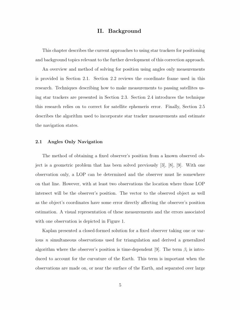
This chapter describes the current approaches to using star trackers for positioning

and background topics relevant to the further development of this correction approach.

An overview and method of solving for position using angles only measurements

is provided in Section 2.1. Section 2.2 reviews the coordinate frame used in this

research. Techniques describing how to make measurements to passing satellites us-

ing star trackers are presented in Section 2.3. Section 2.4 introduces the technique

this research relies on to correct for satellite ephemeris error. Finally, Section 2.5

describes the algorithm used to incorporate star tracker measurements and estimate

the navigation states.

2.1 Angles Only Navigation

The method of obtaining a fixed observer’s position from a known observed ob-

ject is a geometric problem that has been solved previously [3], [8], [9]. With one

observation only, a LOP can be determined and the observer must lie somewhere

on that line. However, with at least two observations the location where those LOP

intersect will be the observer’s position. The vector to the observed object as well

as the object’s coordinates have some error directly affecting the observer’s position

estimation. A visual representation of these measurements and the errors associated

with one observation is depicted in Figure 1.

Kaplan presented a closed-formed solution for a fixed observer taking one or var-

ious n simultaneous observations used for triangulation and derived a generalized

algorithm where the observer’s position is time-dependent [9]. The term βi is intro-

duced to account for the curvature of the Earth. This term is important when the

observations are made on, or near the surface of the Earth, and separated over large

5

Figure 1. Geometry of a single observation. Both the observed direction of the objectand the object’s coordinates are assumed to have some error[9]

distances (tens of kilometers). The observer’s position X and velocity vector V can

be calculated using this algorithm, given the known position of the observed object

P, and the unit vector d of the object from the observer. It is important to ensure

the observed object’s coordinates P and the unit vector of the observation d to be

in the same reference frame. The resulting solution for the observer’s position and

velocity vector will be expressed in that particular reference frame. For the intended

application in this thesis, the observer position will not be limited to a fixed location

and the observations are not separated over large distances.

The work presented by Kaplan involves triangulation, which requires a sequence of

angles-only measurements. In his paper, he introduced the idea of imaging satellites

against a star background taking advantage of their finite slant range [9]. However,

in this thesis the method does not involve triangulation because an accurate LOP

6

can be obtained by using image processing techniques to extract pointing angles and

precise ephemerides from the satellites.

2.2 Coordinate Systems

As presented in the previous section it is necessary to have the observations and the

position of the observed objects in a common coordinate system. However, ultimately

we’re interested in representing position, velocity and attitude in the local level frame.

he location of celestial objects are given by RA and DEC in the celestial sphere. The

Geocentric Celestial Reference Frame (GCRF) is the standard geocentric frame that

measures the RA east in the plane of the equator from the vernal equinox Υ. DEC

angles northward from the equator are positive and angles southward are negative.

Figure 2 depicts the celestial sphere and the references used for measuring RA and

DEC. However, when observing objects orbiting near Earth a distinction must be

Figure 2. Right ascension (α) and declination (δ) in the celestial sphere[6]

7

made between geocentric and topocentric angles. Geocentric is referred to frame

systems which the origin is at the center of the earth. Topocentric, on the other

hand, are those that the origin is on or near the surface of the Earth. For distant

celestial objects, like stars, the difference between geocentric and topocentric are

negligible because those objects appear to be in the same direction anywhere from

Earth, but that is not the case for near-Earth objects. For topocentric observations it

is important to know the origin of the observation [25] and time of the observations.

These two parameters are important to know when converting from topocentric to

geocentric, and vice versa. In this research the angle measurements received from the

star tracker are topocentric.

Similar to the GCRF, the Earth-Centered, Earth-Fixed (ECEF) frame has its

origin at the center of the Earth. However, this frame is fixed to the rotating Earth

with the first axis in the direction of the Prime Meridian, the second axis orthogonal

to the first and within the equatorial plane, and the third axis in the direction of the

North pole orthogonal to the equatorial plane. Typically, location in the ECEF are

expressed as [x, y, z] vectors.

2.3 Observations

Over the past decade there have been several publication [11, 20, 22], demonstrat-

ing the capability of COTS telescopes and charged-coupled device (CCD) sensors,

used to obtain high accuracy angular observations of space objects. The Raven pro-

gram [22] developed by the Air Force Research Laboratory (AFRL), demonstrated

this capability by using COTS hardware and software to track, image and obtain

accurate angular observations of space objects with a standard deviation of approx-

imately one arcsecond. The advantage of using COTS hardware and software is the

reduction in cost, schedule and the flexibility to change the system configuration based

8

on particular requirements. These Raven-class systems have been used to collect as-

trometric and photometric data on LEO satellites, to include 1 kg picosatellites [11].

Primarily, these Raven-class systems have been used to support the Space Surveil-

lance Network (SSN) to track and estimate the orbit of RSO, but in this thesis the

primary goal is to obtain astrometric data of the RSO at a given time and not to

estimate its entire orbit.

These astrometric data which are precise positions of objects in the celestial

sphere, are obtained by processing images of satellites in a background of precisely

known stars [2]. The open source package Astrometry.net [12] processes astronom-

ical images and provides astrometric data. The authors claim a success rate above

99.9% with no false positive [12]. The output obtained from Astrometry.net is used to

convert from pixel coordinates in the images to topocentric RA DEC in the celestial

sphere. With this data it is now possible to estimate the satellite’s position in the

celestial sphere.

Levesque [13] presented a technique to obtain this RA DEC measurement of satel-

lite streaks by processing astronomical images and using a software package similar

to Astrometry.net. His detection algorithm consisted of removing the background

from the image through an iterative process, removing stars and finally identifying

the streak by convolving the expected streak with the remaining objects in the im-

age. The algorithm detection rate is dependent on both the brightness and the length

of the streak. Another algorithm to automatically detect LEO object streaks is de-

veloped by Oniga [17]. Oniga’s method differs from Levesque primarily in how the

background is removed. The algorithm presented removes most stars as part of the

background removal process, claiming their method is less complex than Levesque’s

algorithm. The results from these image processing techniques, is to obtain point-

ing vectors to the RSO from the observer’s position. This data extracted from the

9

images in combination with other data from the RSO (i.e. ephemeris), is possible

to determine the observer’s position using Kaplan’s algorithm [9] presented earlier in

Equation (??).

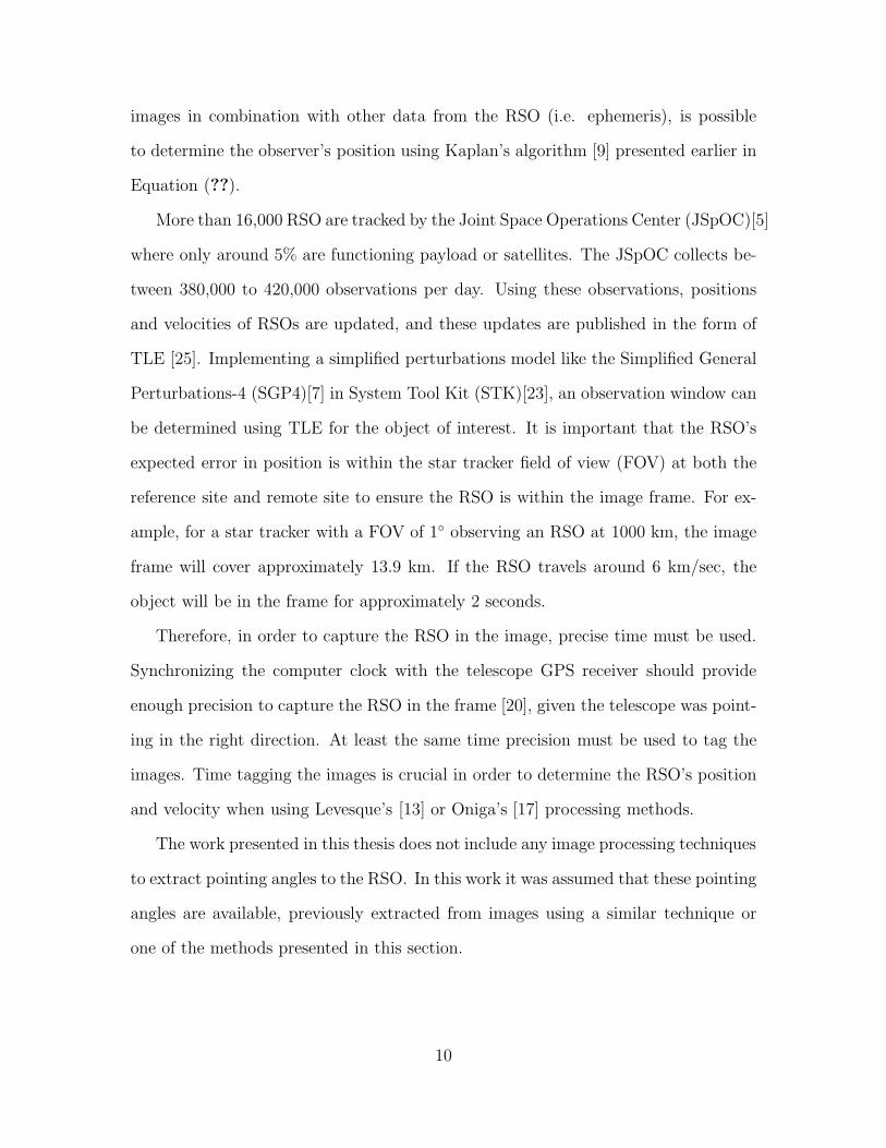
More than 16,000 RSO are tracked by the Joint Space Operations Center (JSpOC)[5]

where only around 5% are functioning payload or satellites. The JSpOC collects be-

tween 380,000 to 420,000 observations per day. Using these observations, positions

and velocities of RSOs are updated, and these updates are published in the form of

TLE [25]. Implementing a simplified perturbations model like the Simplified General

Perturbations-4 (SGP4)[7] in System Tool Kit (STK)[23], an observation window can

be determined using TLE for the object of interest. It is important that the RSO’s

expected error in position is within the star tracker field of view (FOV) at both the

reference site and remote site to ensure the RSO is within the image frame. For ex-

ample, for a star tracker with a FOV of 1 observing an RSO at 1000 km, the image

frame will cover approximately 13.9 km. If the RSO travels around 6 km/sec, the

object will be in the frame for approximately 2 seconds.

Therefore, in order to capture the RSO in the image, precise time must be used.

Synchronizing the computer clock with the telescope GPS receiver should provide

enough precision to capture the RSO in the frame [20], given the telescope was point-

ing in the right direction. At least the same time precision must be used to tag the

images. Time tagging the images is crucial in order to determine the RSO’s position

and velocity when using Levesque’s [13] or Oniga’s [17] processing methods.

The work presented in this thesis does not include any image processing techniques

to extract pointing angles to the RSO. In this work it was assumed that these pointing

angles are available, previously extracted from images using a similar technique or

one of the methods presented in this section.

10

2.4 Differential Site Ephemeris Correction

When determining position using RSO observations against a star background, it

is important to precisely know the RSO’s position. As showed previously in ??, the

accuracy of this data has a direct impact in the calculated observer’s position. In

this thesis the position of the RSO is determined using publicly available TLE and

propagating forward in time to the desired time epoch using SGP4 in STK. Typically,

TLE propagated using SGP4 for RSOs in LEO experience a positional error rate of

approximately, 1.5 km/day [14]. This positional error theoretically can be removed

by making observations from a reference site with known position. With the reference

site’s known position and an estimation of the RSO’s range, a position estimate of the

RSO can be calculated. This approach assumes all other sources of error are accounted

for and any difference in the measurements is a direct result of the RSO positional

error. Pierce presented a method [19] for calculating this angle difference called ∆θ,

and to project it from the reference site to the remote observer’s frame. The idea is

that the observer can apply this projected difference to the observed measurements

and correct for the RSO’s position, improving the accuracy of its position estimate.

The equations presented in [19] for projecting the measured angle difference from

the expected are presented below in Equations (2.1) to (2.12). The angle difference

from the expected to the truth (observed) is calculated at the reference site repre-

sented by ∆θ in Equation (2.1). This residual is calculated in radians and can be

converted to meters by multiplying the expected slant range ρd in meters as depicted

in Equation (2.2)[19].

∆θ =

∆α

∆δ

=

αtruth − αexpected

δtruth − δexpected

(2.1)

where, ∆α is the RA residual given by the difference between truth αtruth and expected

11

αexpected. Similarly, ∆δ is the DEC residual given by the difference between truth δtruth

and expected δexpected.

∆θm = ∆θ · ρd =

∆αm

∆δm

(2.2)

For the equations listed below, the estimated range is used because the scenario

assumes the reference site does not have the capability to measure range to the RSO.

Equation (2.3) represents the unit vector along the line of sight from the reference site

to the RSO. The unit vector in the direction of the right ascension is calculated using

Equation (2.7), and in the direction of declination is given by Equation (2.9)[19].

u1d =Pd

ρd(2.3)

where the pointing vector P from the differential site is defined by,

P =

Px

Py

Pz

=

xs − xo

ys − yo

zs − zo

(2.4)

and slant range ρ by,

ρ =√P 2x + P 2

y + P 2z (2.5)

u2temp = u1d × [0 0 − 1]T (2.6)

u2d =u2temp

‖u2temp‖(2.7)

u3temp = u1d × u2d (2.8)

u3d =u3temp

‖u3temp‖(2.9)

12

These unit vectors from the reference site are multiplied by their respective angle

residuals as showed in Equation (2.10). This projects the observation angle residuals

from the reference site’s image frame to the RA DEC frame [19].

∆θpm = ∆αm · u2d +∆δm · u3d (2.10)

∆θpm is used in Equation (2.11) by multiplying it with the unit vectors from the

remote site to project the residual from the RA DEC frame to the remote site’s image

frame. The unit vectors for the remote uo site are also calculated using Equations (2.3)

to (2.9)[19].

∆θem,o =

∆αem,o

∆δem,o

=

∆θpm · u2o

∆θpm · u3o

(2.11)

To convert the projected residual to radians, ∆θem,o is divided by the expected

slant range ρo from the remote site to the RSO as showed in Equation (2.12)[19].

∆θo =∆θ

em,o

ρo(2.12)

Combining Equations (2.10) to (2.12) and rearranging these equations, yields

Equation (2.13) which is the angle residual from the expected and observed angle at

the reference site.

∆θo =ρd

ρo

∆αd(u2d · u2o) + ∆δd(u3d · u2o)

∆αd(u2d · u3o) + ∆δd(u3d · u3o)

(2.13a)

=ρd

ρo

(u2d · u2o) (u3d · u2o)

(u2d · u3o) (u3d · u3o)

∆αd

∆δd

(2.13b)

13

From Equation (2.13), W is defined as the transformation matrix, which when left

multiplied to the reference site’s corrections projects it to the remote’s image frame.

W =ρd

ρo

(u2d · u2o) (u3d · u2o)

(u2d · u3o) (u3d · u3o)

(2.14)

With the correction ∆θo properly projected to the remote site, it can be applied

to the remote’s observations. Using the same Equations (2.3) to (2.9) the unit vectors

from the remote site’s image frame are calculated, in order to apply the correction

from the reference site.

Various baseline distances and RSO orbits were simulated and evaluated in [19].

Further investigation to this method was recommended by Pierce in his dissertation

[19] as a viable solution to correct for ephemeris error and improve position accuracy.

This method of projecting angle residual from reference to remote site will be studied

in this thesis. The focus of this work was on the effects of varying baseline distance of

the remote site from the reference site and time delay between time of the observation

and time of applying the residual correction at the remote site.

2.5 Navigation Estimation

Navigation state errors were estimated using an extended Kalman filter (EKF)

which is a recursive data processing algorithm used when the dynamics or measure-

ment models are non-linear. A key reason for its optimality is that Kalman filters

incorporate all information that is made available [18]. The EKF uses the same two

step process of propagate and update of the linear Kalman filter, and implements

the same equations for those steps. The propagation step uses the dynamics and

measurement model to propagate the state estimates and the state covariance matrix

forward in time. Similarly, the update step updates the state estimates and covari-

14

ance matrix whenever a measurement from the sensors is available. The Kalman

filter equations use the state space representation. States are represented as an n-

dimensional vector x. The system dynamics are represented by F, with control inputs

u and dynamic driving noise w. Measurements of those states are represented by z,

with measurement corruption noise v.

2.5.1 State Model

For a linear system, the dynamic and measurement model are represented in state

space by Equation (2.15) and Equation (2.16) [18].

x(t) = F(t)x(t) +B(t)u(t) +G(t)w(t) (2.15)

z(t) = H(t)x(t) + v(t) (2.16)

B and G in Equation (2.15) map the control input and dynamic noise to the

states, respectively. H in Equation (2.16) is the measurements matrix. For systems

with either non-linear dynamics or non-linear measurement models, the system is

represented as follows [18].

x(t) = f [x(t),u(t), t] +G(t)w(t) (2.17)

z(ti) = h [x(ti), ti] + v(ti) (2.18)

For both linear and non-linear systems, the dynamics and measurements noises are

assumed to be zero-mean additive white and Gaussian with cross covariance matrices

given by Equations (2.19) and (2.20), respectively.

Ew(t)w(t+ τ)T = Q(t)δ(τ) (2.19)

15

Ev(ti)v(tj)T = R(ti)δij (2.20)

where E is the expectation operator and δ(τ) is a Dirac delta function.

In order to use the same linear Kalman filter equations, the non-linear equations

describing the system were linearized about the state estimates using a first-order

Taylor series expansion. Higher terms (non-linear) are neglected, leaving a linear

approximation of the non-linear function.

2.5.2 Kalman Filter

As stated in the previous section, the Kalman filter consist of two main steps;

propagation and update. For linear systems, the states are propagated forward by

multiplying the states by the state transition matrix Φ [18]

Φ(ti+1, ti) = eF∆t (2.21)

where ∆t is given by the time interval from ti to ti+1. Using the state transition

matrix, the state estimates and the state cross covariance matrix are propagated

forward in time with Equation (2.22) and Equation (2.23), respectively [18].

x(t−i+1) = Φ(ti)x(t+i ) (2.22)

P(t−i+1) = Φ(ti)P(t+i )Φ(ti)T +Qdi (2.23)

where Qdi is given by

Qdi ,

∫ ti+1

ti

Φ(ti+1, τ)G(τ)Q(τ)G(τ)TΦ(ti+1, τ)Tdτ (2.24)

The non-linear matrix f(·) and h(·) are linearized by taking the Jacobian in order

to use the linear Kalman filter equations to propagate and update the state estimates.

16

Fi ,∂f [x(t),u(t), t]

∂x(t)

∣∣∣∣x=x(t+i )

(2.25)

Hi+1 ,∂h[x(ti), ti]

∂x(ti)

∣∣∣∣x=x(t−i+1

)

(2.26)

With the linearized matrices calculated using Equations (2.25) and (2.26), the

states and cross covariance matrix are propagated from ti to t−

i+1 using Equations (2.22)

and (2.23). Similarly the states and cross covariance matrix are updated from t−i+1 to

t+i+1 with the following equations [18].

x(t+i+1) = x(t−i+1) +K(ti+1)[z(ti+1)− h(x(t−i+1), ti+1)] (2.27)

P(t+i+1) = [I−K(ti+1)H(ti+1)]P(t−i+1) (2.28)

where K is the Kalman gain, defined by Equation (2.29) [18].

Ki+1 = P(t−i+1)HT (ti+1)

[R(ti+1) +H(ti+1)P(t−i+1)H

T (ti+1)]−1

(2.29)

Maybeck [18] provides further detail and complete derivations of these equations

for the linear Kalman filter as well as for the EKF.

2.6 Summary

This chapter described previous research relevant to the use of star tracker imag-

ing of LEO passing satellites for navigation on Earth. Additionally, the reference

frame used in this research is explained, along with the mathematical technique for

correcting satellite ephemeris that is studied in this research. Finally, it introduced

an overview of the Kalman filter algorithm, along with the equations used for the

propagation and update steps.

17

III. Computer Modeling

3.1 Introduction

This chapter details the simulation setup and approach used to simulate and ana-

lyze the data. Section 3.2 describes how the ephemeris data was acquired, simulated

and used for analysis. Sections 3.3 and 3.4, explain the process used for correcting

satellite ephemeris when the remote and reference site have distance differences and

delay by the time the correction is applied. Finally, Section 3.5 describes the dynam-

ics and measurment models for sensors used by the EKF to estimate the navigation

states.

3.2 Systems Took Kit (STK) Simulation

A scenario was created in STK [23] with the reference site given by the initial

location of the remote site’s trajectory plus the baseline distance specified in the

scenario. The observations were made from this reference site to measure the angle

difference between the expected and truth angles. The RSO’s TLEs used in STK

for the simulations were downloaded from CelesTrak [4]. To generate the difference

between the expected and the observed angles, a bias was added to the TLE in

the scenario. This bias was introduced in the form of a constant bias of ±0.005

in the right ascending node and inclination to the TLE, which was then labeled as

truth. This added bias in the TLE resulted approximately in 1 mili radians difference

between the truth and expected RSO, which translates to approximately 1 km in

distance at a range of 1000 km. This modification to the TLE was made using a text

editor manually before importing it to STK. This resulted in two distinct objects in

STK to generate separate data sets for analysis, one labeled as truth (i.e. TLE plus

bias) and expected (i.e. TLE). A flow chart diagram of this process is depicted in

18

Figure 3. STK and MATLAB simulation flow chart.

Figure 3.

A minimum elevation angle of 10 above the horizon was set for the reference

site as a constraint, to clear any possible line of sight obstruction. With the TLEs

and reference loaded in the scenario, access from the site to the RSO was calculated

using STK. This data can be extracted creating custom reports in STK and export

the necessary data via comma separated value (.csv) files. In this research the data

was extracted from STK via MATLAB®[15] by establishing a Component Object

Model (COM) connection to STK. This method was preferred since all the calcu-

19

lations were performed in MATLAB® and to maximize process automation. The

data extracted from STK to perform the calculations were the ECEF coordinates for

both the expected and the truth positions. With the coordinates of the RSO and the

observer’s position, the pointing vector was calculated and transformed to topocen-

tric RADEC using Vallado’s Algorithm 26 [25]. The algorithm uses Equation (3.1)

for calculating the topocentric right ascension and Equation (3.2) for topocentric

declination.

α = tan−1

(Py

Px

)= atan2(Py, Px) (3.1)

δ = sin−1

(Pz

ρ

)(3.2)

To calculate the unit vector of the observed RSO, the slant range is needed as

showed in Equation (2.3). As simulated, neither the reference nor the remote site

have the capability of measuring range to the RSO. Therefore, the slant range used

for the observed calculations is the same as the range for the expected. An example

calculation of the topocentric and unit vectors for the reference site are shown below.

Given an observer located at (6378.137, 0, 0) km and satellite passing overhead

at (7368.084, 0, 383.91) km

ρ =√P 2x + P 2

y + P 2z =

√(xRSO − xsite)2 + (yRSO − ysite)2 + (zRSO − zsite)2

=√

(989.947)2 + (0)2 + (383.91)2

= 1061.782 km

α = tan−1

(0

989.947

)= 0 rad

δ = sin−1

(383.91

1061.782

)= 0.370 rad

All the necessary data are available to calculate the pointing vector Pd and the

20

corresponding unit vectors u1d,u2d,u3d.

u1d =Pd

ρ=

[989.947, 0, 383.91]

1061.782

= [.932344, 0, 0.361571]

u2d =u1d × [0 0 − 1]T

|u1d × [0 0 − 1]T |= [0, 0.93234, 0]

u3d =u1d × u2d

|u1d × u3d|= [−0.33711, 0, 0.86926]

With the unit vectors calculated the angle difference ∆θ can be projected to the

observer’s frame and then with another site’s unit vectors, project it to that site’s

image frame using Equations (2.10) to (2.12) and (2.13).

3.3 STK Baseline Distance Variant

Using the scenario constraints and following the same process presented in Section

3.2, the baseline distance from the reference to the remote site was increased in 50 km

increments in a iterative process, to a maximum of 2000 km. 2000 km is approximately

the radius of the access area for a RSO in LEO and a minimum elevation angle of

10. In the simulations, the geodetic latitude and longitude of the remote site are

calculated using the haversine equations [21].

The haversine equations provide great-circle distances between two locations as-

suming the Earth is a sphere. These equations were used to determine the latitude

and longitude of the remote site given a baseline distance and bearing from the ref-

erence site. A MATLAB® function was created to calculate this new reference site

location. The inputs required for this function are geodetic latitude and longitude

in radians, bearing in degrees clockwise from North, and distance in meters. The

outputs of this function are the geodetic latitude and longitude of the remote site in

21

both radians and degrees. A sample MATLAB® call would be,

[lat2,lon2,lat2 d,lon2 d]= haversine(lat1,lon1,bearing,distance)

The haversine equations used in this function assume the Earth has radius of 6371

km. Using the haversine equations, latitude for the remote site is calculated using

Equation (3.3) and longitude using Equation (3.4). In both these equations ∆ = dR,

where d is the baseline distance in meters from the reference to the remote site, R is

the Earth radius and ϕ is the bearing in radians. Within the MATLAB® function

the input bearing is converted to radians before being used in Equation (3.3) and

Equation (3.4).

lat2 = arcsin(sin(lat1) · cos(∆) + cos(lat1) · sin(∆) · cos(ϕ)) (3.3)

lon2 = lon1 + atan2(sin(ϕ) · sin(∆) · cos(lat1), cos(∆)− sin(lat1) · sin(lat2)) (3.4)

This new geodetic latitude and longitude was used to calculate the topocentric

RA DEC from STK for the remote site. This process of calculating latitude, longitude

and obtaining line of sight measurements for the new remote site was repeated in

MATLAB®. The objective was to analyze the accuracy of the transformation matrix

W showed in Equation (2.14) with increased distances. Acquiring simulation data

with this information will validate the Differential Site Ephemeris Correction method

presented in Section 2.4, and provide performance information at different distances.

3.4 STK Time Variant

We followed a similar approach when analyzing the effects of time delay in the

performance of the transformation matrix W. First, both the remote site and the

22

reference site were co-located. With the two sites co-located the time delay was

increased from 0 seconds to 30 seconds.

Basically, the time delay affects the transformation matrix by calculating W using

an old (stale) angle correction ∆θ along with the reference site unit vectors associated

with that ∆θ. When the measurements received by the EKF are the reference site

unit vectors and the angle correction ∆θ. To calculate W the filter then uses the

measured angles from the remote site. These old measurements coming from the

reference site are used in combination with the reference site real-time measurements

to calculate W using Equation (2.14). This accomplished the desired objective of

calculating W using old (stale) angle corrections, and applying it at a current time.

The effects of combining these two variables (distance and time) in the position

estimates are presented in the next chapter.

3.5 EKF Model

With the methodology presented in Section 3.3 for distance variant measurements

and Section 3.4 for time variant, a model for incorporating these measurements in

the EKF is presented in this section. The sensors integrated in the EKF are an IMU,

a barometric altimeter and a star tracker. The dynamics and measurement models

for these sensors are presented in this section. The EKF estimates the error states

using a Pinson error model [24]. The Pinson error model provides the continuous-time

dynamics equations for the IMU errors. This was augmented with altimeter and the

star tracker dynamic and measurement models to completely describe our system.

3.5.1 IMU Model

IMU provides changes in velocity ∆v, and attitude ∆θ, which when integrated

over a time interval and provided the initial conditions, result in an estimate of

23

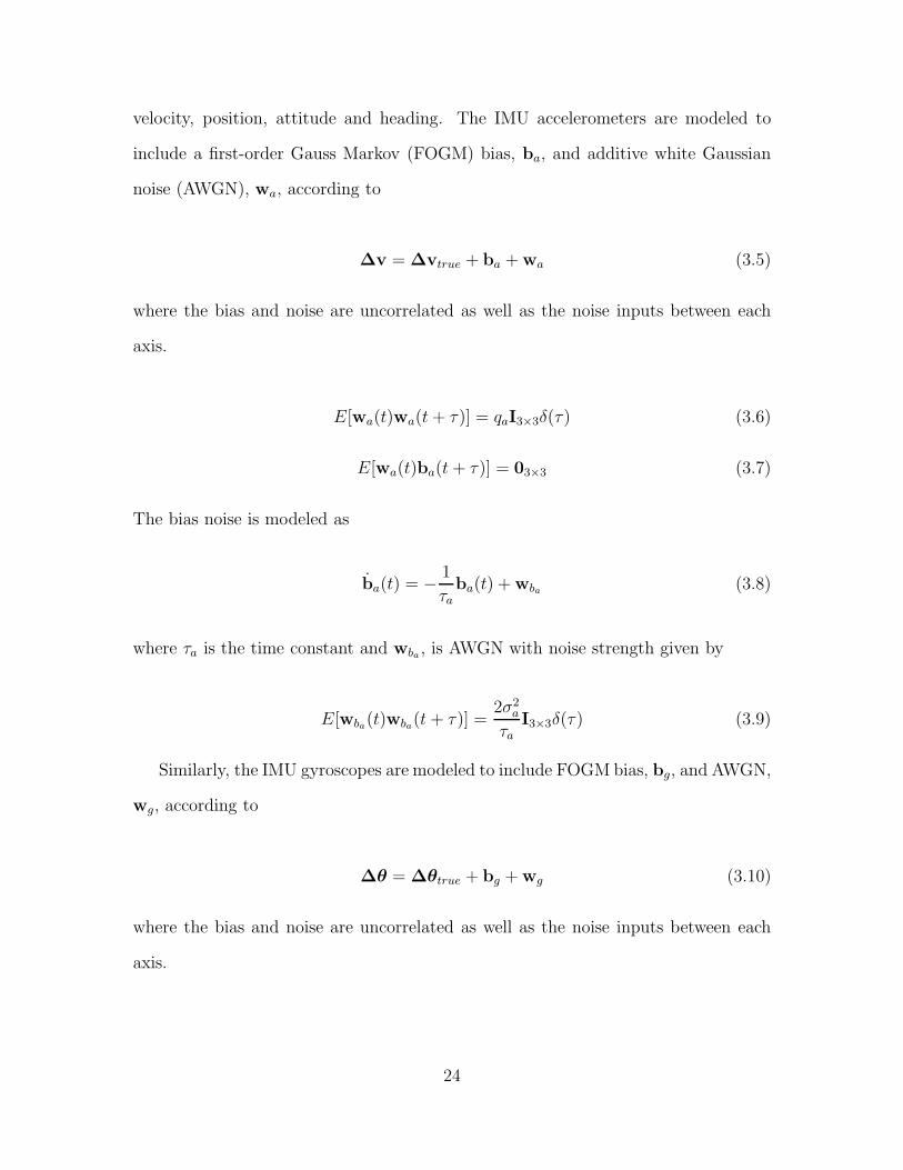
velocity, position, attitude and heading. The IMU accelerometers are modeled to

include a first-order Gauss Markov (FOGM) bias, ba, and additive white Gaussian

noise (AWGN), wa, according to

∆v = ∆vtrue + ba +wa (3.5)

where the bias and noise are uncorrelated as well as the noise inputs between each

axis.

E[wa(t)wa(t+ τ)] = qaI3×3δ(τ) (3.6)

E[wa(t)ba(t+ τ)] = 03×3 (3.7)

The bias noise is modeled as

ba(t) = −1

τaba(t) +wba (3.8)

where τa is the time constant and wba , is AWGN with noise strength given by

E[wba(t)wba(t + τ)] =2σ2

a

τaI3×3δ(τ) (3.9)

Similarly, the IMU gyroscopes are modeled to include FOGM bias, bg, and AWGN,

wg, according to

∆θ = ∆θtrue + bg +wg (3.10)

where the bias and noise are uncorrelated as well as the noise inputs between each

axis.

24

E[wg(t)wg(t+ τ)] = qgI3×3δ(τ) (3.11)

E[wg(t)bg(t + τ)] = 03×3 (3.12)

Similar to the accelerometers, the gyroscopes’ biases are modeled as

bg(t) = −1

τgbg(t) +wbg (3.13)

where τg is the time constant and wbg , is AWGN with noise strength given by

E[wbg(t)wbg(t+ τ)] =2σ2

g

τgI3×3δ(τ) (3.14)

With the model describing the IMU accelerometers and gyroscopes, the state

vector used in the EKF can be defined. The first error states are the ones related to

the information provided by the IMU.

xINS = [Lat, lon, h, vN , vE , vD, θ, φ, ψ]T (3.15a)

xINS = [pINS, vINS, θnINS]

T (3.15b)

where, position p is given by geodetic latitude, longitude and altitude. Velocity v is

defined as the velocity in the local level North-East-Down (NED) frame, relative to

the Earth. Attitude θ is represented by three angles, θ, φ, ψ along the three body

axes.

xINS

= [δLat, δlon, δh, δvN , δvE, δvD, ǫx, ǫy, ǫz ]T (3.16a)

xINS

= [δp, δv, ǫ]T (3.16b)

25

where, ǫ, describes tilt errors about the three axes, and Cnn is the direction cosine

matrix (DCM) estimated from ǫ, which correct the attitude provided by the IMU.

Tracking the error provides better filter stability, because the errors change slowly

when compared to the actual system dynamics. Therefore, to obtain an estimate of

position, velocity and attitude the EKF vector in Equation (3.16a) needs to be added

to the data provided by the IMU. Combining the filter state error estimates xINS

and the data provided by the IMU xINS, an estimate on the true position, velocity

and attitude, xtrue is obtained.

xINStrue=

ptrue

vtrue

θntrue

=

pINS + δp

vINS + δv

Cnn(ǫ)θ

nINS

(3.17)

To determine the position on Earth using inertial measurement data, it is neces-

sary to make some assumptions regarding the shape of the Earth [24]. The Earth

is assumed to be an ellipsoid with meridian radius of curvature RN , given by Equa-

tion (3.18), with rotation rate Ω and transverse radius of curvature C⊕, given by

Equation (3.19), at latitude L.

RN = R⊕

1− e2

(1− e2 sin2 L)3/2(3.18)

C⊕ = RE =R⊕√

1− e2 sin2 L(3.19)

where R⊕ is the Earth radius and e is the eccentricity of the Earth.

With the state vector and assumptions regarding the shape of the Earth, Pinson’s

error model can be used to obtain the dynamics equations describing the INS. The

Pinson error model detailed in [24] was rearranged to match the INS state vector

xINS showed in Equation (3.15a), which resulted in Equation (3.20).

26

FINS =

Fpp Fpv Fpǫ

Fvp Fvv Fvǫ

Fǫp Fǫv Fǫǫ

(3.20)

where the subscripts of the matrix Fp,v,ǫ denote the position, velocity and tilt error,

respectively. The matrices of FINS describing the position error dynamics are defined

as

Fpp =

0 0 −vN

C2⊕

vE tanL

C⊕ cosL0 −

vE

C2⊕ cosL

0 0 0

(3.21)

Fpv =

1

C⊕

0 0

01

C⊕ cosL0

0 0 −1

(3.22)

Fpǫ = 03×3 (3.23)

The velocity error dynamics equations are defined as

Fvp =

−vE

(2Ω cosL+

vE

C⊕ cos2 L

)0

1

C2⊕

(v2E tanL− vNvD)

2Ω(vN cosL− vD sinL) +vNvE

C⊕ cos2 L0 −

vE

C2⊕

(vN tanL+ vD)

2ΩvE sinL 01

C2⊕

(v2N + v2E)

(3.24)

27

Fvv =

vD

C⊕

−2(Ω sinL+vE

C⊕

tanL)vN

C⊕

2Ω sinL+vE

C⊕

tanL1

C⊕

(vN tanL+ vD) 2Ω cosL+vE

C⊕

−2vNC⊕

−2(Ω cosL+vE

C⊕

) 0

(3.25)

Fvǫ =

0 −fD fE

fD 0 −fN

−fE fN 0

(3.26)

where, fNED are the specific acceleration forces in the navigation frame. To calcu-

late these forces the rate of change of the latitude, L, and longitude, l, defined by

Equations (3.27) and (3.28) are needed. These rates are calculated using the known

velocity v, expressed in the navigation frame.

L =vN

RN + h(t)(3.27)

l =vE secL(t)

C⊕ + h(t)(3.28)

To subsequently calculate the acceleration, the change in position, ∆x is calculated

as

∆x =

(L(t+∆t)− L(t))(RN + h(t))

(l(t +∆t)− l(t))(RE + h(t)) cos(L(t))

−(h(t +∆t)− h(t)

(3.29)

where ∆t is the time interval. From the change in position and the velocity, the

acceleration, a, and the forces fNED that cause that acceleration are calculated as

a = v = 2∆x− v∆t

∆t2(3.30)

28

fNED =

aN + vE(2Ω + l) + sin(L)− vDL

aE − vN(2Ω + l) sin(L)− vD(2Ω + l) cos(L)

az + vy(2Ω + l) cos(L)− vN L− g

(3.31)

The equations describing the tilt error dynamics as a function of the states is defined

as

Fǫp =

−Ω sinL 0 −vE

C2⊕

0 0vN

C2⊕

−ΩcosL−vE

C⊕ cos2 L0

vE tanL

C2⊕

(3.32)

Fǫv =

01

C⊕

0

−1

C⊕

0 0

0 −tanL

C⊕

0

(3.33)

Fǫǫ =

0 −Ω sinL−vE

C⊕

tanLvN

C⊕

Ω sinL+vE

C⊕

tanL 0 Ω cosL+vE

C⊕

−vN

C⊕

−ΩcosL−vE

C⊕

0

(3.34)

To completely model the errors generated by the IMU, the three accelerometer

biases, ba, three gyroscope biases, bg, are modeled as showed in Equations (3.8)

and (3.13), respectively.

Augmenting the state vector from Equation (3.16a) with these biases yields the

new augmented state vector as

xIMU = [δp, δv,Cnn(ǫ),ba,bg]

T (3.35)

Using the model shown in Equations (3.8) and (3.13), the continuous-time dy-

29

namics matrices describing it are defined as

Fba = I3×3 · −1

τa(3.36)

Fbg = I3×3 · −1

τg(3.37)

Combining these new continuous-time dynamics Equations (3.36), (3.37) and (3.47)

with FINS from Equation (3.20), results in FIMU , which describes the continuous-time

dynamics of the error propagation for the IMU.

FIMU =

FINS 09×3 09×3

03×9 Fba 03×3

03×9 03×3 Fbg

(3.38)

With the continuous-time dynamic matrix defined, it is necessary to combine the

continuous-time noise equations into a matrix to form QIMU . Which is obtained by

combining Equations (3.6), (3.9), (3.11) and (3.14).

QIMU =

03×3 03×3 03×3 03×3 03×3

03×3 CbnqaI3×3C

bnT

03×3 03×3 03×3

03×3 03×3 CbnqgI3×3C

bnT

03×3 03×3

03×3 03×3 03×3

2σ2ba

τaI3×3 03×3

03×3 03×3 03×3 03×3

2σ2bg

τgI3×3

(3.39)

with its distribution matrix, GIMU .

GIMU = I15×15 (3.40)

30

3.5.2 Barometric Altimeter Model

The barometric altimeter measures the altitude of the sensor. This system can be

modeled as the sum of the true altitude, a FOGM bias and AWGN.

hbaro(t) = htrue(t) + bb(t) + wb(t) (3.41)

where the AWGN is defined by

E[wb(t)] = 0 (3.42)

E[wb(t)wb(t + τ)] = σ2b δ(τ) (3.43)

and the FOGM process defined by

bb(t) = −1

τbbb(t) + wbb (3.44)

E[wbb(t)] = 0 (3.45)

E[wbb(t)wbb(t+ τ)] =2σ2

bb

τbδ(τ) (3.46)

From Equation (3.44) we defined Fbb , and from Equation (3.46), Qbb , as

Fbb = −1

τb(3.47)

Qbb = σ2b (3.48)

3.5.3 Star Tracker Model

Star tracker provides topocentric RA and DEC angles, Λ. The star tracker is

modeled as the sum of the true angles, a FOGM bias and zero-mean AWGN. The

bias, bs, represents the bias due to the RSO ephemeris error which the reference site

is measuring. The noise, ws, is the noise introduced by the sensor, which it was

31

assumed both sites (reference and remote) use same quality sensor with same noise

strength.

Λ = Λtrue + bs +ws (3.49)

where the AWGN is defined by

E[ws(t)] = 0 (3.50a)

E[ws(t)ws(t + τ)] = qsI2×2δ(τ) (3.50b)

E[ws(t)bs(t+ τ)] = 02×2 (3.51)

and the bias FOGM process defined by

bs(t) = −1

τsbs(t) +wbs (3.52)

E[wbs(t)] = 0 (3.53a)

E[wbs(t)wbs(t + τ)] =2σ2

bs

τsI2×2δ(τ) (3.53b)

With the star tracker bias model presented in Equation (3.52) we defined, Fbs ,

and with the noise strength shown in Equation (3.53b), we defined Qbs , as

Fbs =

−1

τs0

0 −1

τs

(3.54)

Qbs =

2σ2bs

τs0

02σ2

bs

τs

(3.55)

32

3.5.4 Complete System Dynamics Model

Combining the dynamics models presented in Sections 3.5.1 to 3.5.3, we combine

the state vectors presented in those sections to define the system state vector, x, as

x = [δLat, δlon, δh, δvN , δvE, δvD, ǫx, ǫy, ǫz, bax , bay , baz , bgx , bgy , bgz , bα, bδ, bb]T

(3.56a)

x = [δp, δv, ǫ,ba,bg,bs, bb]T (3.56b)

where δp is the error in position given by geodetic latitude, longitude and altitude.

Velocity error in the local level NED frame, relative to the Earth is described by

δv. The tilt errors about the three axis are described by, ǫ and Cnn is the DCM

estimated from ǫ, which correct the attitude provided by the IMU. The biases for

the accelerometers, gyroscopes, star tracker and altimeter are represented by, ba, bg,

bs, and bb, respectively. With the state vector for the entire system defined, the F

matrix that describes the continuous-time dynamics and the continuous-time noise

strength matrix, Q, are described by

F =

FINS 09×3 09×3 09×2 09×1

03×9 Fba 03×3 03×2 03×1

03×9 03×3 Fbg 03×2 03×1

02×9 02×3 02×3 Fbs 02×1

01×9 01×3 01×3 01×2 Fbb

(3.57)

33

Q =

03×3 03×3 03×3 03×3 03×3 03×2 03×1

03×3 CbnqaI3×3C

bnT

03×3 03×3 03×3 03×2 03×1

03×3 03×3 CbnqgI3×3C

bnT

03×3 03×3 03×2 03×1

03×3 03×3 03×3

2σ2ba

τaI3×3 03×3 03×2 03×1

03×3 03×3 03×3 03×3

2σ2bg

τgI3×3 03×2 03×1

02×3 02×3 02×3 02×3 02×3

2σ2bs

τsI2×2 02×1

01×3 01×3 01×3 01×3 01×3 03×2

2σ2bb

τb

(3.58)

with its distribution matrix, G.

G = I18×18 (3.59)

Using Equation (2.21) to calculate Φ and Q can be discretized using Equa-

tion (2.24), generating Qd. With Qd, the covariance of the system can be propagated

forward in time by the EKF. The parameters used in our work for the IMU and star

tracker needed to simulate data, are listed in Table 1. These parameters typical for

tactical grade IMU and currently available COTS star trackers. The equations pre-

sented in this section described the dynamics of the system, in the following section

the measurement model used for the EKF is presented.

3.5.5 Measurement Model

The three measurements incorporated by the EKF are altitude from barometric

altimeter, angles measured from observer to imaged satellite, and angle correction

from the reference site. The angle measurements from the observer to the imaged

satellite are independent from the reference site corrections. The measurement model

for the barometric altimeter was defined from Equation (3.41) and using the model

34

Table 1. Sensors parameters.

Name Symbol Value Units

AccelerometerBias

σba 9.8× 10−3 m/s2

Gyroscope Bias σbg 4.84× 10−6 rad/s

Gyro/Accel TimeCorrelation

τa,g 3600 s

Barometric Al-timeter Bias

σb 5 m

Star Tracker Ac-curacy

σbs,st1 4.84× 10−6 rad

Star Tracker TimeCorrelation

τs 120 s

presented in Equation (2.16).

zbaro(ti) = Hbaro(ti)x(ti) + bb + vb(ti) (3.60)

The measurement model for the barometric altimeter is linear. Therefore, the

mapping to the corresponding state Hbaro was done directly without linearizing.

Hbaro =

[0 0 1 01×14 1

](3.61)

with its measurement uncertainty Rbaro given by

Rbaro(ti) = E[vb(ti)vb(tj)] = σ2bm (3.62)

The star tracker will be modeled with two distinct models. The first model zst1,

describes the measured topocentric right ascension and declination, as

zst1(ti) = hst1(ti)[x(ti), ti] + bst + vst1(ti) (3.63)

35

Rst1(ti) = E[vst1(ti)vTst1(ti)] =

σ2st1 0

0 σ2st1

(3.64)

where the variance σst1 = σbs , as listed in Table 1, which is the accuracy of the star

tracker. The measurement model hst1, is described by the non-linear Equation (3.65).

The measurement equations are a function of ρ, which is the magnitude of the pointing

vector P from the observer to the RSO in the ECEF frame, as explained in Section 3.2

[25].

hst1(ti) =

α

δ

=

tan−1

(Py

Px

)

sin−1

(Pz

ρ

)

(3.65)

The angles are non-linear functions of the state. In order to implement this model

in the EKF algorithm, the equations must be linearized around the current state as

showed in Equation (2.26). Linearizing hst1 around the current state, yields Hst1

shown below

Hst1(ti+1) ,∂hst1(δx, t)

∂δx(t)

∣∣∣∣δx=x(t−i+1

)

(3.66a)

=

∂α

∂δL

∂α

∂δl

∂α

∂δh01×12 1 0 0

∂δ

∂δL

∂δ

∂δl

∂δ

∂δh01×12 0 1 0

(3.66b)

the complete derivation of Hst1 are found in Appendix A. The linearization Hst1 de-

rived in the appendix and presented here differs from the one presented by Pierce [19].

The difference between the two is how hst1 was defined, particularly the trigonometric

equation used for the right ascension. As depicted in Equation (3.65), the right ascen-

36

sion equation used in this thesis involves arctan, where Pierce used arcsin

(Py√

P 2x + P 2

y

)

[19]. Both equations are equivalent to calculate the right ascension and can be found

in [25]. However, when linearizing this non-linear equations information about the

quadrant is lost. Since RA is defined from 0 − 2π, quadrant information is critical.

For this reason arctan was used in this thesis in lieu of arcsin. To retain the quadrant

information when linearizing hst1, arctan was treated as a function of two variables,

in this case Py and Px. Treating the trigonometric function as a function of two

variables result in two partial derivatives, retaining information about the quadrant.

This approach of treating arctan as a function of two variable is equivalent of using

atan2 in computer language. Therefore, when implementing this measurement model

in MATLAB®the atan2 function was used. To emphasize this difference atan2 was

used in the notation at the beginning of this chapter and in the appendix.

The second measurement model for the star tracker zst2, describes the angle cor-

rection received from the reference site, which is a direct measurement of the bias, bs

in addition to AWGN, vst2.

zst2(ti) = hst2(ti)[x(ti), ti] + vst2(ti) (3.67)

Rst2(ti) = E[vst2(ti)vTst2(ti)] =

σ2st2 0

0 σ2st2

(3.68)

σst2 is dependent on the reference site sensor noise since the bias is measured

at the reference site. The transformation matrix W is used on the white Gaussian

noise from the sensor at the reference site Vd and taking the expected value, yields

37

Equation (3.69)which is the reference site’s variance projected to the remote site.

E[(Wvd)(Wvd)T ] = WE[vdv

Td ]W

T (3.69)

It was assumed the reference site and the remote site use same quality sensor.

Therefore, the variance for the reference site is also given by σst1 and when projected

to the remote is given by σst2 defined by Equation (3.70).

σ2st2 = Wσ2

st1IWT (3.70)

As stated before, ∆θremote is directly related to bs, which this bias represents

the ephemeris error. This measurement consists of the ∆θreference projected to the

remote site using W showed in Equation (2.14). This bias is included in the state

vector x, for this reason Hst2 becomes a direct mapping to those states, as shown in

Equation (3.72b).

hst2(ti) =

∆αremote

∆δremote

=

bsα

bsδ

(3.71)

Hst2(i+ 1) ,∂hst2(δx, t)

∂δx(t)

∣∣∣∣δx=x(t−i+1

)

(3.72a)

=

01×15 1 0 0

01×15 0 1 0

(3.72b)

38

3.6 SPIDER

The Kalman filter algorithm was implemented using Sensor Processing for Inertial

Dynamics Error Reduction (SPIDER). SPIDER is a navigation based Kalman filter-

ing software developed by the Autonomy & Navigation Technology (ANT) center at

the Air Force Institute of Technology (AFIT)[10]. The benefit of using SPIDER rather

than developing an independent algorithm for this thesis is that SPIDER is modular,

relatively easy to introduce additional sensors, and most importantly it is a proven

tool. Most sensors used in this research are options currently modeled and available

for use in SPIDER. The only sensor not currently modeled is the star tracker with its

two form of measurement previously described in Section 3.5.3. Following SPIDER

interface control document (ICD)[1], the required MATLAB® functions were written

to incorporate the star tracker sensor to SPIDER.

3.7 Summary

This chapter developed the model of integrating a star tracker, IMU and baro

measurement with an EKF to evaluate the performance improvement of correcting

for satellite ephemeris with the presented technique. The next chapter compares and

analyzes the results of the navigation states estimates for the different scenarios with

different combinations of distance and time delays.

39

IV. Results

4.1 Introduction

This chapter presents the results obtained from simulations of the model described

in Chapter III. First, the results obtained from varying the baseline distance from the

reference site and remote site are shown. Secondly, following the same methodology,

results depicting the effects of adding time delay to the transformation matrix are

compared. The time delay effects are also combined with varying distances between

the reference and remote sites. Finally, the results of the navigation states from the

EKF are presented in this chapter. The results of the EKF are compared between

free INS and incorporating star tracker measurements.

4.2 Distance Variant Results

First, we used the simulated data to validate the transformation matrix W pre-

sented in Equation (2.14). The method compared the remote site’s measured angles

with the reference site’s angles projected to the remote site’s image frame using W.

To validate W, the transformation matrix must accurately project the angle correc-

tion δθ to the remote site. The results obtained from applying the transformation

matrix W are shown in Figure 4. The results validate the methodology proposed by

Pierce [19] and presented earlier in Section 2.4. The projected angles are not exactly

equal as shown in Figure 5 , this difference was attributed to the AWGN with variance

σbs , being introduced by the sensor accuracy at the reference site. When the two sites

are co-located this residual is expected to be minimum and within the variance of the

sensor.

With the transition matrix W validated for the co-located scenario more investi-

gation was done to analyze the effects of increasing the baseline distance between the

40

0 500 1000 1500 2000 2500 3000 3500

Time (sec)

2

3

4

5

6

7

8

Rig

ht A

scen

sion

Ang

le (

rad)

Measured AngleProjected Angle

0 500 1000 1500 2000 2500 3000 3500

Time (sec)

-1

-0.5

0

0.5

1

1.5

Dec

linat

ion

Ang

le (

rad)

Measured AngleProjected Angle

Figure 4. Topocentric right ascension (top) and declination (bottom) angles from 100km separated sites. Solid lines are simulated angles at remote site, while dotted line isthe expected angle at the remote plus the correction from the remote projected.

0 500 1000 1500 2000 2500 3000 3500

Time (sec)

-2.5

-2

-1.5

-1

-0.5

0

0.5

1

Rig

ht A

scen

sion

Res

idua

l Ang

le (

rad)

×10-4

Co-located2-σ100 km

0 500 1000 1500 2000 2500 3000 3500

Time (sec)

-8

-6

-4

-2

0

2

4

6

Dec

linat

ion

Res

idua

l Ang

le (

rad)

×10-5

Co-located2-σ100 km

Figure 5. Topocentric right ascension (top) and declination (bottom) angles residualsfrom co-located site and 100 km separated site. Black lines are the residuals anglesfrom the co-located site, while blue are the residuals from the site separated by 100km and dotted magenta lines is 2−σ from the noise introduced by the sensor. At largeseparation distances, the projected correction does not correct for all angle error.

reference and remote sites. A variety of scenarios started with the remote co-located

with the reference, to a maximum distance of 2000 km. 2000 km is approximately the

radius of the access area for a RSO in LEO and a minimum elevation angle of 10. In

addition to the distance increase, the heading angle relative to the reference site was

41

0 200 400 600 800 1000 1200 1400 1600 1800 2000

Distance (km)

0

0.2

0.4

0.6

0.8

1

∆ R

ight

Asc

ensi

on E

rror

(ra

d)

×10-3

Residual

0 200 400 600 800 1000 1200 1400 1600 1800 2000

Distance (km)

0

0.5

1

1.5

2

2.5

3

3.5

4

∆ D

eclin

atio

n E

rror

(ra

d)

×10-4

Residual

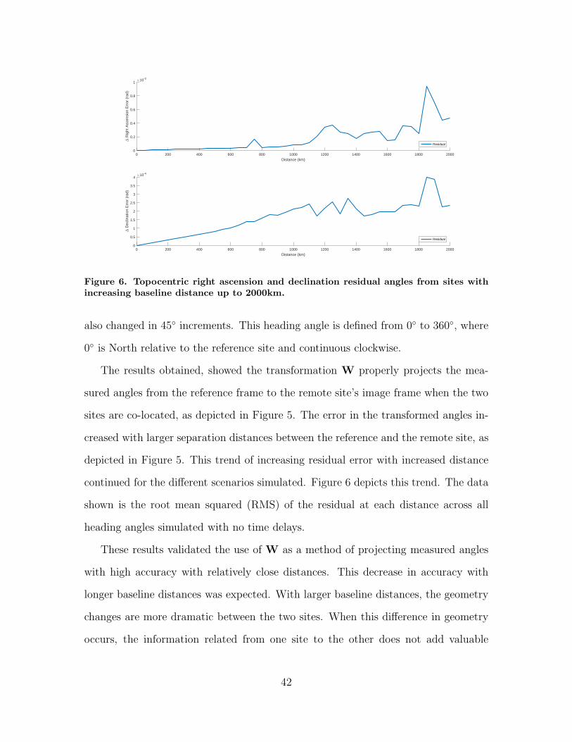
Figure 6. Topocentric right ascension and declination residual angles from sites withincreasing baseline distance up to 2000km.

also changed in 45 increments. This heading angle is defined from 0 to 360, where

0 is North relative to the reference site and continuous clockwise.

The results obtained, showed the transformation W properly projects the mea-

sured angles from the reference frame to the remote site’s image frame when the two

sites are co-located, as depicted in Figure 5. The error in the transformed angles in-

creased with larger separation distances between the reference and the remote site, as

depicted in Figure 5. This trend of increasing residual error with increased distance

continued for the different scenarios simulated. Figure 6 depicts this trend. The data

shown is the root mean squared (RMS) of the residual at each distance across all

heading angles simulated with no time delays.

These results validated the use of W as a method of projecting measured angles

with high accuracy with relatively close distances. This decrease in accuracy with

longer baseline distances was expected. With larger baseline distances, the geometry

changes are more dramatic between the two sites. When this difference in geometry

occurs, the information related from one site to the other does not add valuable

42

information. Depending on the application and error tolerance the results shown

Figure 6 can be used to determine the threshold distance not to exceed when using

this method.

4.3 Time Variant Results

Similar to the effect of distance to the transformation, simulated data was used to

analyze the effects of applying the transformation matrix W when calculated using

observations made at a previous time. RSOs in LEO orbit travel at high velocity,

which result in a short window of visibility for an observer on the surface of the

Earth. The RSO used in these simulations had an average visibility window of 10

minutes. With this relatively short visibility window, it was expected for time delays

to have a greater impact on the transformation when compared to increasing distance,

because the pointing angle to the RSO will change significantly in a short period of

time. Figure 7 shows how for a particular simulation with the two sites co-located

time delays affect the transformation matrix accuracy. During the simulations the

transformation matrix was calculated using time delays ranging from 0 to 30 seconds

with 10 seconds increments. These results were expected and this trend was expected

to continue for larger baseline distances.

Based on the the scenario setup assumed for this research, it is more likely that the

reference site is not co-located with the remote. Therefore, the effects of applying an

angle correction observed at a previous time, varying from 0 to 30 seconds in the past,

in addition to baseline distance were compared. Figure 7 shows a linear growth of the

residual for both RA and DEC. It is of interest to show how this error translates when

the sites are not co-located. Figure 8 depicts the residual of the transformed angle

for distances up to 2000 km and up to 30 s time delays. These results showed that on

average an increase of time delay in the calculation of the transformation matrix W,

43

0 5 10 15 20 25 30

Time Delay (s)

0

0.2

0.4

0.6

0.8

1

∆ R

ight

Asc

ensi

on E

rror

(ra

d)

×10-5

0 5 10 15 20 25 30

Time Delay (s)

0

0.5

1

1.5

2

2.5

3

∆ D

eclin

atio

n E

rror

(ra

d)

×10-6

Figure 7. Topocentric right ascension (top) and declination (bottom) residual anglesin radians from co-located sites with time delays from 0-30 seconds.

also increases the error in the transformed angles. Figure 8 shows the residual for both

RA and DEC linearly growing up to approximately 600 km. For distances greater

than 600 km the residual continues to grow in an unpredictable manner. In addition

the residual at 600 km is approximately 3.3× 10−5 which results in large positioning

error. To put the magnitude in of the residual in perspective, 4.8× 10−6 rad error in

the pointing angle for satellites at 1000 km, results in approximately 20 m of error in

the observer’s position error [19]. For these reasons the area of analysis was limited

to distances under 600 km, as depicted in Figure 9.

44

0 200 400 600 800 1000 1200 1400 1600 1800 2000

Distance (km)

0

0.2

0.4

0.6

0.8

1

∆ R

ight

Asc

ensi

on E

rror

(ra

d)

×10-3

0s Delay15s Delay30s Delay

0 200 400 600 800 1000 1200 1400 1600 1800 2000

Distance (km)

0

1

2

3

4

∆ D

eclin

atio

n E

rror

(ra

d)

×10-4


Figure 8. Topocentric right ascension and declination residual angles from sites withincreasing baseline distance up to 2000km and time delays from 0s to 30s.

The following section will present and analyze how this increase in error of the

transformed angles affects the navigation states calculated by the EKF.

4.4 EKF Results

Sections 4.2 and 4.3 showed the effects of applying the transformation matrix W

at different distances and time delays. In this section, the results of incorporating

45

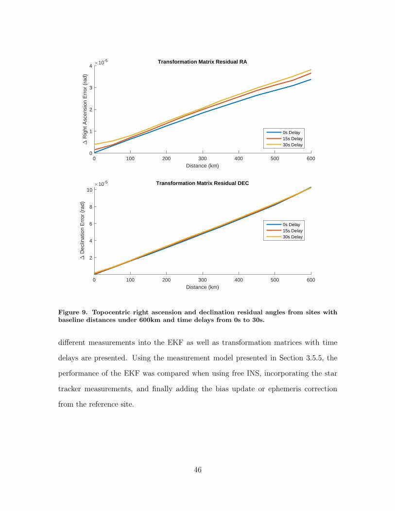
0 100 200 300 400 500 600

Distance (km)

0

1

2

3

4

∆ R

ight

Asc

ensi

on E

rror

(ra

d)

×10-5 Transformation Matrix Residual RA


0 100 200 300 400 500 600

Distance (km)

2

4

6

8

10

∆ D

eclin

atio

n E

rror

(ra

d)

×10-5 Transformation Matrix Residual DEC


Figure 9. Topocentric right ascension and declination residual angles from sites withbaseline distances under 600km and time delays from 0s to 30s.

different measurements into the EKF as well as transformation matrices with time

delays are presented. Using the measurement model presented in Section 3.5.5, the

performance of the EKF was compared when using free INS, incorporating the star

tracker measurements, and finally adding the bias update or ephemeris correction

from the reference site.

46

0 100 200 300 400 500 600 700 800 900

tgps (sec)

-1.5

-1

-0.5

0

0.5

1

1.5

Pos

ition

Err

or (

m)

×104

N errorE errorN sigE sig

Figure 10. EKF North (blue) and East (red) position estimate errors with only baro-metric altimeter updates. Dotted lines denote 2-σ variances in each direction.

4.4.1 Free INS

Table 1 shows the parameters used for the EKF simulations. Figure 10 depicts

the position error on both North and East axis for the free INS simulation. This sim-

ulation run was labeled as free INS, because it is the INS coupled with a barometric

altimeter without incorporating any star tracker measurements. A barometric altime-

ter was included to constrain the vertical drift of the INS, while allowing horizontal

drift. The error on the Down axis was omitted in Figure 10 because it was kept rela-

tively constant by the baro within the standard deviation specified in Table 1. With

no additional measurements providing updates to the East and North axis, free INS

results are consistent with a drifting INS. The simulation was run for 15 min. For

this particular simulation the DRMS error was approximately 6333 m. This much

error in the navigation states are too large for practical applications. These results

are compared in the next section to the same trajectory, but integrating star tracker

47

angle only measurements without the bias updates.

4.4.2 Angles Only

The position estimate was further evaluated when including measurements from

the star tracker. The measurements follow the model presented in Section 3.5.5, zst1,

which measures the topocentric right ascension and declination from the observer to a

RSO of interest. As presented and derived in that section, these measurements provide

an update on the position states. Therefore, when incorporating these measurements

an improvement in the position estimation was expected. Since there is still a bias in

the measurement model due to satellite position error, which is not being updated by

this measurement update, error in the form of FOGM process is still expected to be

present in the results in addition to the sensor noise. Figure 11 shown below depicts

the position error of the navigation states estimated by the EKF incorporating the

star tracker pointing angles at 1 Hz.

The DRMS error for this particular simulation run is approximately 2670 m.

When these results are compared to the results shown in Figure 10, the position error

is reduced by 58%. Even with this significant reduction in the position error, it is

still high for navigation applications. It is important to note after approximately 300

seconds the East and North error are outside the 2-σ bound, which indicates the EKF

is overconfident. After 700 seconds it appears as the error is reducing to be within

the variance bounds, but with such large covariance is not practical for navigation

purposes.

4.4.3 Angles and Ephemeris Updates

Using the same trajectory as the one for the previous scenarios, the model was

further refined to include measurements from the reference site containing updates for

48

0 100 200 300 400 500 600 700 800 900

tgps (sec)

-5000

-4000

-3000

-2000

-1000

0

1000

2000

3000

4000

5000P

ositi

on E

rror

(m

)N errorE errorN sigE sig

Figure 11. EKF North (blue) and East (red) position estimate errors with baro and1 Hz star tracker angle updates without ephemeris updates. Dotted lines denote 2-σvariances in each direction.

the bias in the measurement model. Figure 12 depicts the position error in the North

and East axis as estimated by the EKF. The parameters used in the filter are the

same as for the previous simulations, which are listed in Table 1. For this simulation,

the EKF incorporates angles only updates at 1 Hz as in the previous simulation, and

the ephemeris correction or bias update is measured at 60 second intervals. In this

particular simulation, the transition matrix W has no time delay and the reference

site is offset from the remote by 25 km. Introducing a transition matrix with no

time delay, results in transformed angle corrections with minimum error. For this

reason, the results shown in Figure 12 are the baseline and the EKF estimation

is expected to have the minimum error when compared to estimation including time

49

0 100 200 300 400 500 600 700 800 900

tgps (sec)

-200

-150

-100

-50

0

50

100

150

200

Pos

ition

Err

or (

m)


Figure 12. EKF North (blue) and East (red) position estimate errors with baro, 1 Hzstar tracker angle updates and 60s ephemeris correction from reference site. Referencesite separated by 25 km with remote and no time delay. Dotted lines denote 2-σvariances in each direction.

delays. The DRMS error for this particular simulation, is approximately 55 m. When

we compared these results to the error previously obtained when integrating angles

only measurements without the bias update, the DRMS error was reduced by 98%.

This reduction in the DRMS error showed a significant improvement in the estimate

of the navigation solution, when incorporating the star tracker measurements and the

ephemeris correction from the reference site.

However, due to the behavior previously observed in Figure 5, interest was placed

in tracking the behavior of the bias state, as it appears to be dynamic and increasing

in magnitude as the baseline distance is increased. The next section analyzes the

filter estimation of these bias states.

50

0 100 200 300 400 500 600 700 800 900

tgps (s)

-4

-2

0

2

4

RA

Ang

le (

rad)

×10-4

0 100 200 300 400 500 600 700 800 900

tgps (sec)

-1

-0.5

0

0.5

1

RA

Ang

le (

rad)

×10-4

Figure 13. Right ascension bias estimate (blue) with 60 second ephemeris correctionupdates with noiseless TLE. Dotted lines denote 2-σ variances.

4.4.4 EKF Bias State

As shown earlier in the previous section, the error in position was significantly

reduced when adding the reference site corrections as another measurement to the

EKF in addition to the pointing angles. In addition of the reduced error, it is of

interest to determine if the EKF is estimating the bias, bs, in the measurement

model presented in Equation (3.49) correctly.

To validate the dynamics and measurement models used in the EKF, simulations

were conducted without any TLE propagation error and both sites co-located. By not

having noise in the TLE, the only source of noise in the results are the noise introduced

by the sensor. The results of this simulation are analyzed in this section by focusing

51

0 100 200 300 400 500 600 700 800 900

tgps (sec)

-4

-2

0

2

4

DE

C A

ngle

(ra

d)

×10-4

0 100 200 300 400 500 600 700 800 900

tgps (sec)

-1

-0.5

0

0.5

1

DE

C A

ngle

(ra

d)

×10-4

Figure 14. Declination bias estimate (blue) with 60 second ephemeris correction up-dates with noiseless TLE. Dotted lines denote 2-σ variances.

on the states added to the SPIDER framework. The other states in the SPIDER

model have been studied and verified in previous research work [10], for this reason

several simulations were run with SPIDER built in sensors to verify its performance.

However, full detailed analysis was not included in this section. This section analyzes

the filter’s performance in estimating the added states related to the star tracker

sensor, with emphasis in the satellite ephemeris bias states. The results depicting the

state estimates for the bias in the right ascension with no ephemeris error is shown in

Figure 13 and in declination shown in Figure 14. The subplots shown in Figures 13

and 14 is the same data but represented differently. In the top plots the covariance

has a wide bound which is constantly changing. The covariance value is constantly

changing from the maximum which in part is driven by the noise strength specified

52

in the dynamics model, given by Equation (3.55). Using the parameters previously

specified the theoretical value for the maximum value of the covariance is 4.8× 10−4

and the value obtained in the simulation was 3.55 × 10−4. This value is updated

every second indirectly by the Hst1 as defined in Equation (3.66a) which relate the

measured angles from the remote site to the states. Some information regarding the

bias states is in this measurement update. For this reason the covariance is driven

down with each measurement because the covariance of the sensor is 1 arc second.

However, the direct measurement for that bias state is integrated by the EKF every 60

seconds. As depicted in Figures 13 and 14, the covariance is properly updated every

60 seconds. In addition to the covariance propagation and update of the bias state,

on average the state estimate is bounded by the covariance. Based on these results

we validated the star tracker models used for the system dynamics and measurements

when the two sites are co-located. Additionally, the DRMS achieved, of 39 m, is the

lowest value achieved in the scenarios simulated. To clearly show these results on the

bias states, the bottom plot of Figures 13 and 14 are the a posteriori value of the

covariance.

With noise introduced again to the TLE and with a separation distance of 100 km

between the reference site and remote site, Figure 15 shows the filter estimate of the

RA and DEC bias states. At distances of 100 km an greater the filter bias states

starts to become overconfident, and during periods of times the state estimates are

outside the covariance bounds, as depicted in Figure 15. This degradation of the filter

estimation of the bias states continues for larger baseline distances. This degradation

of the filter estimates was related to the increase in DRMS error for the same large

distances.

Attempting to improve the estimation of the bias states, a scaling factor was

applied to the noise strength of the measurement of the bias state Rst2 for a distance

53

0 100 200 300 400 500 600 700 800 900

tgps (sec)

-3

-2

-1

0

1

2

3

RA

Ang

le (

rad)

×10-4

0 100 200 300 400 500 600 700 800 900

tgps (sec)

-3

-2

-1

0

1

2

DE

C A

ngle

(ra

d)

×10-4

Figure 15. Satellite bias state RA(top) and DEC(bottom) when reference site andremote are separated by 100 km. Estimate (blue) and state variance (2-σ, black).

of 500 km, with the objective of reducing the DRMS error. The reason for this scale

factor was due to the linear residual growth discussed in Section 4.3 and depicted in

Figure 8, in an attempt to bound the state estimates by the increased covariance.

Preliminary results of a particular simulation show a reduction of DRMS error at a

distance of 500 km, from 1276 m with no scaling depicted in Figure 16, to 553 m with

a scale factor of 1× 103 depicted in Figure 17.

4.5 Position Error

Section 4.4 showed results and discussed DRMS values for specific scenarios. This

section will combine those results under a variety of conditions into one chart that

54

0 100 200 300 400 500 600 700 800 900

tgps (sec)

-5000

-4000

-3000

-2000

-1000

0

1000

2000

Pos

ition

Err

or (

m)


Figure 16. EKF North (blue) and East (red) position estimate errors with baro and 1Hz star tracker angle updates and ephemeris updates without scaling factor. Dottedlines denote 2-σ variances in each direction.

0 100 200 300 400 500 600 700 800 900

tgps (sec)

-1500

-1000

-500

0

500

1000

Pos

ition

Err

or (

m)

Position Error (m)


Figure 17. EKF North (blue) and East (red) position estimate errors with baro and1 Hz star tracker angle updates and ephemeris updates with scaling factor of 1 × 103.Dotted lines denote 2-σ variances in each direction.

55

depicts how the DRMS is affected by distance and time delays in Figure 18. Multiple

simulations were completed at each distance from 0 to 2000 km, along several heading

angles 0 to 2π, with time delays ranging from 0 to 30 seconds. The DRMS error was

calculated from the output of the EKF for each of those simulations, then averaged

along the heading angle for that distance and time delay.

From the results obtained and shown in Figure 18, distances under 200 km the

DRMS values are under 500 m and may be of used in some navigation applications.

The DRMS error up to that distance appears to be growing linearly. The effects of

time delays in the DRMS error are greater at closer distances. For distances greater

than 300 km the effects of time delays are negligible. At that point the DRMS error

is over 1 km.

At 400 km there is a noticeable spike in the DRMS in particular for time delays

of 15 seconds and 30 seconds. At those large distances the geometry is significantly

different between the two sites and the transformation may not be projecting the angle

corrections properly, in addition at those large distances the filter bias state estimates

starts to degrade. Since Figure 18 is the average DRMS, and heading angle relative

to the reference affects the transformation residual, several of those simulations may

have affected the averages due to poor error observability caused by satellite geometry

and producing that spike.

4.6 Summary

This chapter reviewed the results of calculating the transition matrix under vary-

ing conditions and the impact in the navigation state calculated by the EKF. The

parameters varied include the distances between the reference and remote site, as

well as the time between when the angle bias measurement was made and applied

to the angles transformed. As expected, the results showed that the closer the two

56

0 100 200 300 400 500 600

Distance (km)

0

500

1000

1500

2000

2500

3000D

RM

S E

rror

(m

)

DRMS Error


Figure 18. Average DRMS error as calculated from the EKF navigation solution fordistances up to 600km and time delays from 0s to 30s.

sites are and the shorter the time delay, the transformation matrix more accurately

transformed the angles. As a result, more accurate transition matrices reduced the

EKF position estimate error.

Finally, the combination of increasing distance as well as time delay were simu-

lated. These results show how both distance and time delay have a direct negative

effect in the accuracy of the transformation matrix. These results are depicted in

Figure 18 and provide the expected DRMS error according to the distance separation

and time delay, based on the system model presented in this thesis.

Chapter V contains conclusions drawn from this research, further research that

can be done to improve this correction method for obtaining better results, as well

as identifying possible applications where this method could be of benefit.

57

V. Conclusion

5.1 Introduction

A summary of the document and the analysis of our work are discussed in this

chapter. The contributions made to the body of knowledge in the field of star tracker

navigation are presented. Lastly, several remarks regarding areas of further research

are given as well as possible applications.

5.2 Summary of Document

Chapter I introduced the motivation for this research, the research objectives

and the structure of this document. Chapter II described the current approaches to

using star tracker for positioning, including using satellite observations as navigational

aids. Additionally, Chapter II also presented background subject matter regarding

reference frames, a technique for correcting satellite ephemeris error, and estimation

using a Kalman filter. Chapter III detailed the simulation setup and approach used to

analyze the data in this research. Chapter III presented the integration of the IMU,

barometric altimeter, and star tracker in the EKF framework. It developed the model

for the star tracker dynamics and measurements. Results are presented in Chapter IV,

which include the effects of distance and time delays in the transformation matrix W

and the position error estimated by the EKF. A mathematical method of projecting

observed angles from one location to another was analyzed using simulated data and

scenarios.

The simulated data supported the mathematical model, and provided insight on

how that projection degraded with distance and time delays. For distances greater

than 300 km, different time delays have less impact on DRMS error. At distances

smaller than 300 km, those same time delays result in greater estimated position error.

58

A degradation of the transformation matrix with distance translates to a dynamic

variance of the sensor receiving the bias update and it is not a fixed value when

using the model presented in this paper. The results of estimating the bias as a

FOGM process show it to be a poor approximation of the true bias state. A simple

scaling method of increasing the covariance of that bias state, resulted in improved

estimation of the bias, however for the limited simulations attempted the DRMS error

was increased by using this method for relatively close distance (25 km) but reducing

the error for larger distances (500 km). In most navigation applications, minimizing

DRMS error is desirable. Therefore, with the results obtained and presented in this

paper, separation distances used should be less than 200 km to obtain DRMS error

under 500 m.

5.3 Summary of Contributions

The work presented in this paper provides a method of correcting for ephemeris

error, when precise ephemerides are not available for the RSO observed and improve

the performance of the navigation states. The measurement model for the star tracker

was derived in previous work, but the derivation presented in detail in Appendix A

takes into account the quadrant for the angles which is important when linearizing

the measurement equations.

A method of correcting for satellite ephemeris error from a reference site by mea-

suring angle difference which was previously proposed, was analyzed and validated

in this research. A framework for incorporating satellite ephemeris corrections in the

form of angles from another site was analyzed and it showed improvement in the

navigation solution when using simulated data.

The results obtained in this research showed the angle bias states are not properly

modeled by a FOGM. Using a FOGM for the angle measurement bias performs well

59

for relatively close distances, but as the residual in the transformed angles grows the

FOGM does not properly estimate the biases.

5.4 Future Work

During the course of this research it was identified that several aspects could

be further investigated and elements of this performance model improved. First,

further research in modeling the ephemeris bias state should be explored. It was

shown how the transformation matrix residual increases with larger baseline distances,

this limits the ability of the FOGM to correctly estimate the bias in association

with the ephemeris error. A refinement in the dynamics model of these bias angles

should provide significant improvement in the filter navigation solution. Applying a

scaling factor to the measurement noise as the distance is increased was proposed and

preliminary tested in this research. This method might be a viable alternative for

improving the performance for distances over 100 km, when using the model presented

in this thesis. Applying this scaling method should be explored further as well as a

different bias dynamic model that can track the bias more efficiently without the filter

being overconfident. In addition a backward-smoothing algorithm may also improve

the estimates of the bias states, and should be explored.

Additionally, the error in the TLE was restricted by a constant bias of ±0.005

in the inclination and the right ascending node. Therefore, the results obtained

in this work are limited to this very specific type of error. To further analyze the

performance of the transformation matrix different types of errors should be explored.

An alternative can be introducing random Gaussian error with a standard deviation

of ±0.005 to the same parameters of the TLE. Performing the analysis on a broader

set of errors helps in determining a generalized performance of the transformation

matrix, consequently the performance of the filter estimation.

60

In addition to the varying the error introduced in the TLE, converting the observed

angles from topocentric RA and DEC to other frames might provide insight on how

the position error is actually represented and how it is propagating. Converting

RA and DEC angle differences to cross-track and along-track error might improve

categorizing the error. However, observability on these errors is also highly dependent

on the geometry. At low elevations the along-track errors are difficult to resolve, and

when directly above, cross-track errors tend to dominate [25].

The observations of passing satellites were made from only one reference site.

A second area to further investigate is whether improvement in the accuracy of the

transformation matrix could be obtained by adding a second site. Having observations

from two distinct separate sites, could result in improved overall observability of the

errors. This increase in observability potentially will result in improved navigation

solution. Additionally, including a second reference site will provide information on

the error on all three axis and improve the satellite’s position measurement, which

could be use for orbit estimation.

Finally, the setup chosen for this work establishes the reference site as being at

different physical location from the remote. However, this same approach could be

used to represent a system equipped with GNSS, that gets intermittent or partial

updates. For example, if positioning via GNSS is available to the remote, it can

correct for the bias state itself. This should improve the DRMS error because it has

GNSS positioning for a period of time and all ephemeris error can be corrected except

the measurement noise.

61

Appendix A. Star Tracker Angle Measurement Linearization

The measurement model presented in Equation (3.65) was linearized around a

nominal value by taking the Jacobian as depicted in Equation (3.66a) in order to be

applied in the EKF algorithm. The linearized simplified solution was shown in Equa-

tion (3.66b). The complete derivation is shown here. The non-linear measurements

are given by Equation (3.65), also shown here.

hst1(ti) =

α

δ

=

tan−1

(Py

Px

)

sin−1

(Pz

ρ

)

(A.1)

where, P is the pointing vector from the observer to the RSO with Px, Py and Pz

components in ECEF frame and ρ is the slant range from observer to RSO.

P =

Px

Py

Pz

=

xs − xo

ys − yo

zs − zo

(A.2)

ρ =√P 2x + P 2

y + P 2z (A.3)

The observer’s position is given in geodetic latitude, longitude and altitude (L,l,h),

with units of radians, radians and meters, respectively. These geodetic coordinates

are converted to ECEF by [25]

xecefo = f(xn

o ) =

x

y

z

=

R cos(l)

R sin(l)

(C⊕(1− e2) + h) sin(L)

(A.4)

where the observer’s state in the navigation frame, xno , and the coefficient R and C⊕

62

are given by Equations (A.5) to (A.7) [25].

xno = [L l h]T (A.5)

C⊕ = RE =R⊕√

1− e2 sin2 L(A.6)

R = (C⊕ + h) cos(L) (A.7)

with R⊕ and e describing the equatorial radius and the Earth’s eccentricity, respec-

tively.

Taking the Jacobian of the star tracker angle measurement model, the linearized

measurement model matrix becomes

Hst1(ti+1) ,∂hst1(δx, t)

∂δx(t)

∣∣∣∣δx=x(t−i+1

)

(A.8a)

=

∂α

∂δL

∂α

∂δl

∂α

∂δh01×12 1 0 0

∂δ

∂δL

∂δ

∂δl

∂δ

∂δh01×12 0 1 0

(A.8b)

Each element of the H matrix are described and derived here. To retain the

quadrant information when linearizing hst1, arctan was treated as a function of two

variables, in this case Py and Px. Treating the trigonometric function as a function of

two variables result in two partial derivatives, retaining information about the quad-

rant. This approach of treating arctan as a function of two variable is equivalent of

using atan2 in computer language. Therefore, when implementing this measurement

model in MATLAB®the atan2 function was used. To emphasize this difference atan2

was used in the notation.

63

First, the partial derivatives with respect to the 18 state vector are shown below.

∂α

∂δL=

∂

∂δL

(atan2

(Py

Px

))(A.9a)

=∂

∂Px

(tan−1

(Py

Px

))∂Px

∂δL+

∂

∂Py

(tan−1

(Py

Px

))∂Py

∂δL(A.9b)

=−Py

P 2x + P 2

y

∂Px

∂δL+

Px

P 2x + P 2

y

∂Py

∂δL(A.9c)

∂α

∂δl=

∂

∂δl

(atan2

(Py

Px

))(A.10a)

=∂

∂Px

(tan−1

(Py

Px

))∂Px

∂δl+

∂

∂Py

(tan−1

(Py

Px

))∂Py

∂δl(A.10b)

=−Py

P 2x + P 2

y

∂Px

∂δl+

Px

P 2x + P 2

y

∂Py

∂δl(A.10c)

∂α

∂δh=

∂

∂δh

(atan2

(Py

Px

))(A.11a)

=∂

∂Px

(tan−1

(Py

Px

))∂Px

∂δh+

∂

∂Py

(tan−1

(Py

Px

))∂Py

∂δh(A.11b)

=−Py

P 2x + P 2

y

∂Px

∂δh+

Px

P 2x + P 2

y

∂Py

∂δh(A.11c)

64

∂δ

∂δL=

∂

∂δL

(sin−1

(Pz

ρ

))(A.12a)

=1√

1−

(Pz

ρ

)2

∂

∂δL

(Pz

ρ

)(A.12b)

=1√

1−

(Pz

ρ

)2

ρ∂Pz

∂δL− Py

∂ρ

∂δLρ2

(A.12c)

∂δ

∂δl=

∂

∂δl

(sin−1

(Pz

ρ

))(A.13a)

=1√

1−

(Pz

ρ

)2

∂

∂δl

(Pz

ρ

)(A.13b)

=1√

1−

(Pz

ρ

)2

ρ0

∂Pz

∂δl− Py

∂ρ

∂δlρ2

(A.13c)

=1√

1−

(Pz

ρ

)2

−Py

∂ρ

∂δlρ2

(A.13d)

65

∂δ

∂δh=

∂

∂δh

(sin−1

(Pz

ρ

))(A.14a)

=1√

1−

(Pz

ρ

)2

∂

∂δh

(Pz

ρ

)(A.14b)

=1√

1−

(Pz

ρ

)2

ρ∂Pz

∂δh− Py

∂ρ

∂δhρ2

(A.14c)

=1√

1−

(Pz

ρ

)2

−ρ sin(L)− Py

∂ρ

∂δhρ2

(A.14d)

Next the partial derivatives needed to completely solve the partials with respect to

the state vector presented earlier, are derived below. These are the partial derivatives

of the pointing vector from the observer to the satellite.

66

∂Px

∂δL=

∂

∂δL(xs − xo) (A.15a)

= 0−∂xo

∂δL(A.15b)

= −∂

∂δL(R cos(l + δl)) (A.15c)

= − cos(l + δl)∂R

∂δL−R

0∂

∂δLcos(l + δl) (A.15d)


∂δL(A.15e)

= − cos(l + δl)

[cos(L+ δL)

R⊕e2 cos(L+ δL) sin(L+ δL)

(1− e2sin2(L+ δL))3/2− sin(L+ δL)(C⊕ + h)

]

(A.15f)

= cos(l + δl) sin(L+ δL)(C⊕ + h)−R⊕e

2 cos2(L+ δL) cos(l + δl) sin(L+ δL)

(1− e2sin2(L+ δL))3/2

(A.15g)

∂Px

∂δl=

∂

∂δl(xs − xo) (A.16a)

= 0−∂xo

∂δl(A.16b)

= −∂

∂δl(R cos(l + δl)) (A.16c)

= − cos(l + δl)0

∂R

∂δl−R

∂

∂δlcos(l + δl) (A.16d)

= R sin(l + δl) (A.16e)

67

∂Px

∂δh=

∂

∂δh(xs − xo) (A.17a)

= 0−∂xo

∂δh(A.17b)

= −∂

∂δh(R cos(l + δl)) (A.17c)


∂δh−R

∂

∂δhcos(l + δl) (A.17d)

= − cos(l + δl) cos(L+ δL) (A.17e)

∂Py

∂δL=

∂

∂δL(ys − yo) (A.18a)

= 0−∂yo

∂δL(A.18b)

= −∂

∂δL(R sin(l + δl)) (A.18c)

= − sin(l + δl)∂R

∂δL− R

∂

∂δLsin(l + δl) (A.18d)


∂δL− 0 (A.18e)

= − sin(l + δl)

[cos(L+ δL)


(1− e2sin2(L+ δL))3/2− sin(L+ δL)(C⊕ + h)

]

(A.18f)

= sin(l + δl) sin(L+ δL)(C⊕ + h)−R⊕e

2 cos2(L+ δL) sin(l + δl) sin(L+ δL)

(1− e2sin2(L+ δL))3/2

(A.18g)

68

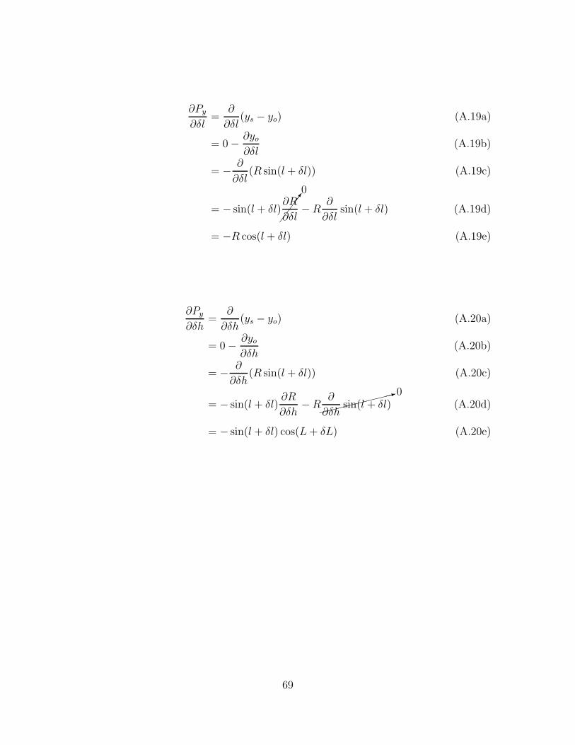
∂Py

∂δl=

∂

∂δl(ys − yo) (A.19a)

= 0−∂yo

∂δl(A.19b)

= −∂

∂δl(R sin(l + δl)) (A.19c)

= − sin(l + δl)0

∂R

∂δl−R

∂

∂δlsin(l + δl) (A.19d)

= −R cos(l + δl) (A.19e)

∂Py

∂δh=

∂

∂δh(ys − yo) (A.20a)

= 0−∂yo

∂δh(A.20b)

= −∂

∂δh(R sin(l + δl)) (A.20c)


∂δh−R

0∂

∂δhsin(l + δl) (A.20d)

= − sin(l + δl) cos(L+ δL) (A.20e)

69

∂Pz

∂L=

∂

∂δL(zs − zo) (A.21a)

= 0−∂zo

∂δL(A.21b)

= −∂

∂δL(((C⊕(1− e2)) + h) sin(l + δl)) (A.21c)

= −(1− e2) sin(L+ δL)∂C⊕

∂δL− cos(L+ δL)(C⊕(1− e2) + h+ δh) (A.21d)

= −(1− e2) sin(L+ δL)R⊕e

2 cos(L+ δL) sin(L+ δL)

(1− e2sin2(L+ δL))3/2−

cos(L+ δL)(C⊕(1− e2) + h + δh)

(A.21e)

∂Pz

∂δl=

∂

∂δl(zs − zo) (A.22a)

= 0−∂zo

∂δl(A.22b)

= −∂

∂δl(((C⊕(1− e2)) + h + δh) sin(l + δl)) (A.22c)

= −(1− e2) sin(L)0

∂C⊕

∂δl− (C⊕(1− e2) + h+ δh)0∂ sin(L+ δL)

∂δl(A.22d)

= 0− 0 = 0 (A.22e)

70

∂Pz

∂δh=

∂

∂δh(zs − zo) (A.23a)

= 0−∂zo

∂δh(A.23b)

= −∂

∂δh(((C⊕(1− e2)) + h + δh) sin(l + δl)) (A.23c)

= −

(1− e2)

0

∂C⊕

∂δh+ 1

sin(L+ δL)− (C⊕(1− e2) + h+ δh)0∂ sin(L+ δL)

∂δh

(A.23d)

= − sin(L+ δL) (A.23e)

Below, the partial derivatives of the slant range with respect to the states.

∂ρ

∂L=

∂

∂δL

√P 2x + P 2

y + P 2z (A.24a)

=1

2ρ

∂

∂δL(P 2

x + P 2y + P 2

z ) (A.24b)

=1

2ρ

[2Px

∂Px

∂δL+ 2Py

∂Py

∂δL+ 2Pz

∂Pz

∂δL

](A.24c)

=1

ρ

[Px∂Px

∂δL+ Py

∂Py

∂δL+ Pz

∂Pz

∂δL

](A.24d)

=1

ρ

[Px

(cos(l + δl) sin(L+ δL)(C⊕ + h+ δh)−

R⊕e2 cos2(L+ δL) cos(l + δl) sin(L+ δL)

(1− e2sin2(L+ δL))3/2

)+

Py

(sin(l + δl) sin(L+ δL)(C⊕ + h + δh)−

R⊕e2 cos2(L+ δL) sin(l + δl) sin(L+ δL)

(1− e2sin2(L+ δL))3/2

)+

Pz

(−(1− e2) sin(L+ δL)


(1− e2sin2(L+ δL))3/2−

cos(L+ δL)(C⊕(1− e2) + h + δh))]

(A.24e)

71

∂ρ

∂δl=

∂

∂δl

√P 2x + P 2

y + P 2z (A.25a)

=1

2ρ

∂

∂δl(P 2

x + P 2y + P 2

z ) (A.25b)

=1

2ρ

[2Px

∂Px

∂δl+ 2Py

∂Py

∂δl+ 2Pz

∂Pz

∂δl

](A.25c)

=1

ρ

Px

∂Px

∂δl+ Py

∂Py

∂δl+ Pz

0

∂Pz

∂δl

(A.25d)

=1

ρ[Px (R sin(L+ δL)) + Py (−R cos(l + δl))] (A.25e)

∂ρ

∂δh=

∂

∂δh

√P 2x + P 2

y + P 2z (A.26a)

=1

2ρ

∂

∂δh(P 2

x + P 2y + P 2

z ) (A.26b)

=1

2ρ

[2Px

∂Px

∂δh+ 2Py

∂Py

∂δh+ 2Pz

∂Pz

∂δh

](A.26c)

=1

ρ

[Px∂Px

∂δh+ Py

∂Py

∂δh+ Pz

∂Pz

∂δh

](A.26d)

=1

ρ[Px (− cos(l + δl) cos(L+ δL)) + Py (− cos(L+ δL) sin(l + δl)) + Pz (− sin(L+ δL))]

(A.26e)

Finally, the partial derivatives of the ECEF conversion coefficient with respect to

the error states are derived.

72

∂C⊕

∂δL=

∂

∂δL

(R⊕√

1− e2 sin2(L)

)(A.27a)

= 0−R⊕

2(1− e2 sin2(L))−1/2 ∂

∂δL(1− e2 sin2(L)) (A.27b)

=(0−

R⊕

2(1− e2 sin2(L))−1/2) (0− 2e2 cos(L) sin(L))

(√1− e2 sin2(L))2

(A.27c)

=R⊕e

2 cos(L) sin(L)

(1− e2sin2(L))3/2(A.27d)

∂C⊕

∂δl=

∂

∂δl

(R⊕√

1− e2 sin2(L)

)= 0 (A.28)

∂C⊕

∂δh=

∂

∂δh

(R⊕√

1− e2 sin2(L)

)= 0 (A.29)

∂R

∂δL=

∂

∂δL((C⊕ + h) cos(L)) (A.30a)

= cos(L)∂

∂δL(C⊕ + h)− sin(L)(C⊕ + h) (A.30b)

= cos(L)R⊕e

2 cos(L) sin(L)

(1− e2sin2(L))3/2− sin(L)(C⊕ + h) (A.30c)

∂R

∂l=

∂

∂δl((C⊕ + h) cos(L)) (A.31a)

= cos(L)0∂

∂δl(C⊕ + h) + (C⊕ + h)

0∂

∂δlcos(L) (A.31b)

= 0 (A.31c)

73

∂R

∂δh=

∂

∂δh((C⊕ + h) cos(L)) (A.32a)

= cos(L)(0 + 1) + (C⊕ + h)0∂

∂δhcos(L) (A.32b)

= cos(L) (A.32c)

Combining the partial derivatives presented in this Appendix, the linearized mea-

surement model can be implemented in the EKF filter.

74

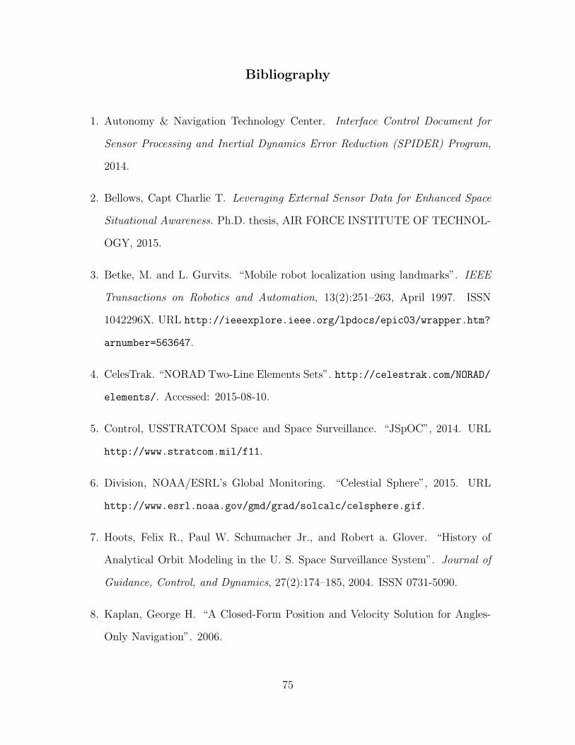
Bibliography

1. Autonomy & Navigation Technology Center. Interface Control Document for

Sensor Processing and Inertial Dynamics Error Reduction (SPIDER) Program,

2014.

2. Bellows, Capt Charlie T. Leveraging External Sensor Data for Enhanced Space

Situational Awareness. Ph.D. thesis, AIR FORCE INSTITUTE OF TECHNOL-

OGY, 2015.

3. Betke, M. and L. Gurvits. “Mobile robot localization using landmarks”. IEEE

Transactions on Robotics and Automation, 13(2):251–263, April 1997. ISSN

1042296X. URL http://ieeexplore.ieee.org/lpdocs/epic03/wrapper.htm?

arnumber=563647.

4. CelesTrak. “NORAD Two-Line Elements Sets”. http://celestrak.com/NORAD/

elements/. Accessed: 2015-08-10.

5. Control, USSTRATCOM Space and Space Surveillance. “JSpOC”, 2014. URL

http://www.stratcom.mil/f11.

6. Division, NOAA/ESRL’s Global Monitoring. “Celestial Sphere”, 2015. URL

http://www.esrl.noaa.gov/gmd/grad/solcalc/celsphere.gif.

7. Hoots, Felix R., Paul W. Schumacher Jr., and Robert a. Glover. “History of

Analytical Orbit Modeling in the U. S. Space Surveillance System”. Journal of

Guidance, Control, and Dynamics, 27(2):174–185, 2004. ISSN 0731-5090.

8. Kaplan, George H. “A Closed-Form Position and Velocity Solution for Angles-

Only Navigation”. 2006.

75

9. Kaplan, George H. “Angles-Only Navigation: Position and Velocity Solution

from Absolute Triangulation”. Navigation, 58(3):187–201, 2011.

10. Kawecki, James E.C. “Initial Implementation And Testing Of A Tightly-Coupled

IMU/Pseudolite System”, 2015.

11. Kervin, Paul, Vicki S Hoo, Daron Nishimoto, and Dennis Liang. Rapidly de-

ployable Raven-class systems SSA Support in the Field. Technical report, DTIC

Document, 2009.

12. Lang, D., D. W. Hogg, K. Mierle, M. Blanton, and S. Roweis. “Astrometry.net:

Blind Astrometric Calibration of Arbitrary Astronomical Images”. 139:1782–

1800, May 2010.

13. Levesque, M. “Automatic Reacquisition of Satellite Positions by Detecting Their

Expected Streaks in Astronomical Images”. Advanced Maui Optical and Space

Surveillance Technologies Conference, 81. 2009.

14. Levit, Creon and William Marshall. “Improved orbit predictions using two-line

elements”. Advances in Space Research, 47(7):1107–1115, 2011. ISSN 02731177.

URL http://dx.doi.org/10.1016/j.asr.2010.10.017.

15. MATLAB. version 8.5.0.197613 (R2015a). The MathWorks Inc., 2015.

16. Obama, President Barack. “National Space Policy of the United States of

America”, 2010. URL https://www.whitehouse.gov/sites/default/files/

national_space_policy_6-28-10.pdf.

17. Oniga, Florin, Melania Miron, Radu Danescu, and Sergiu Nedevschi. “Automatic

recognition of low earth orbit objects from image sequences”. IEEE International

Conference on Intelligent Computer Communication and Processing. 2011.

76

18. Peter, S Maybeck. Stochastic Models, Estimation, and Control. Vol. 1. New York,

NY: Academic Press, 1979.

19. Pierce, Scott J. Modeling Navigation System Performance of a Satellite-Observing

Star Tracker Tightly Integrated with an Inertial Measurement Unit. Ph.D. thesis,

Air Force Institute of Technology, 2015.

20. Schmunk, Matthew M. Initial Determination of Low Earth Orbits Using Com-

mercial Telescopes. Master’s thesis, Air Force Institute of Technology, 2008.

21. Sinnott, Roger. “Virtues of the Haversine”. 1984.

22. Sydney, Paul F., John L. Africano, Amy Fredericks, Kris M. Hamada, Vicki

SooHoo, Daron L. Nishimoto, Paul W. Kervin, Steve Bisque, and Matthew

Bisque. “Raven automated small telescope systems”. volume 4091, 237–247.

2000.

23. Systems Tool Kit (STK). version 10.1.3. Analytical Graphics, Inc. (AGI), 2014.

24. Titterton, David and John L Weston. Strapdown inertial navigation technology,

volume 17. IET, 2004.

25. Vallado, David A and Wayne D McClain. Fundamentals of Astrodynamics and

Applications. Kluwer Academic Publishers, 2nd edition, 2001.

77

REPORT DOCUMENTATION PAGE Form ApprovedOMB No. 0704–0188

The public reporting burden for this collection of information is estimated to average 1 hour per response, including the time for reviewing instructions, searching existing data sources, gathering andmaintaining the data needed, and completing and reviewing the collection of information. Send comments regarding this burden estimate or any other aspect of this collection of information, includingsuggestions for reducing this burden to Department of Defense, Washington Headquarters Services, Directorate for Information Operations and Reports (0704–0188), 1215 Jefferson Davis Highway,Suite 1204, Arlington, VA 22202–4302. Respondents should be aware that notwithstanding any other provision of law, no person shall be subject to any penalty for failing to comply with a collectionof information if it does not display a currently valid OMB control number. PLEASE DO NOT RETURN YOUR FORM TO THE ABOVE ADDRESS.

1. REPORT DATE (DD–MM–YYYY) 2. REPORT TYPE 3. DATES COVERED (From — To)

4. TITLE AND SUBTITLE 5a. CONTRACT NUMBER

5b. GRANT NUMBER

5c. PROGRAM ELEMENT NUMBER

5d. PROJECT NUMBER

5e. TASK NUMBER

5f. WORK UNIT NUMBER

6. AUTHOR(S)

7. PERFORMING ORGANIZATION NAME(S) AND ADDRESS(ES) 8. PERFORMING ORGANIZATION REPORTNUMBER

9. SPONSORING / MONITORING AGENCY NAME(S) AND ADDRESS(ES) 10. SPONSOR/MONITOR’S ACRONYM(S)

11. SPONSOR/MONITOR’S REPORTNUMBER(S)

12. DISTRIBUTION / AVAILABILITY STATEMENT

13. SUPPLEMENTARY NOTES

14. ABSTRACT

15. SUBJECT TERMS

16. SECURITY CLASSIFICATION OF:

a. REPORT b. ABSTRACT c. THIS PAGE

17. LIMITATION OFABSTRACT

18. NUMBEROFPAGES

19a. NAME OF RESPONSIBLE PERSON

19b. TELEPHONE NUMBER (include area code)

Standard Form 298 (Rev. 8–98)Prescribed by ANSI Std. Z39.18

24–03–2016 Master’s Thesis Sept 2014 — Mar 2016

Satellite Ephemeris Correction via Remote Site Observation for StarTracker Navigation Performance Improvement

Dıaz, Jorge E., Capt, USAF

Air Force Institute of TechnologyGraduate School of Engineering and Management (AFIT/EN)2950 Hobson WayWPAFB OH 45433-7765


Intentionally Left Blank

DISTRIBUTION STATEMENT A:APPROVED FOR PUBLIC RELEASE; DISTRIBUTION UNLIMITED.

This material is declared a work of the U.S. Government and is not subject to copyright protection in the United States.

This thesis analyzed a method to correct for satellite ephemeris to be used in celestial navigation applications. Thiscorrection is the measured angle difference between the expected location of the satellite, which is given by propagatingpublicly available Two-Line Element sets (TLE), and their observed angles from a precisely known reference site.Therefore, the angle difference can be attributed completely to satellite ephemeris error assuming instrument error wasaccounted for. The intent is to calculate this correction from the reference site and relate it to remote sites that havevisibility of the same satellite, but where its own location is known with some uncertainty. The effects of increasedbaseline distances from the reference site are studied, as well as time delays.

extended Kalman filter, star tracker, celestial navigation, satellite observation, ephemeris correction, image-aidednavigation

U U U U 92

Maj Scott J. Pierce, AFIT/ENG

(937) 255-3636, x3419; [email protected]

Documents

AIR FORCE INSTITUTEOF TECHNOLOGY