MATHEMATICAL PROGRAMMING MODEL FOR FIGHTER TRAINING SQUADRON PILOT SCHEDULING

THESIS

Thomas M. Newlon, Lt, USAF

AFIT/GOR/ENS/07-17

DEPARTMENT OF THE AIR FORCE AIR UNIVERSITY

AIR FORCE INSTITUTE OF TECHNOLOGY

Wright-Patterson Air Force Base, Ohio

APPROVED FOR PUBLIC RELEASE; DISTRIBUTION UNLIMITED.

The views expressed in this thesis are those of the author and do not reflect the official policy or position of the United States Air Force, Department of Defense, or the United States Government.

AFIT/GOR/ENS/07-17

MATHEMATICAL PROGAMMING MODEL FOR FIGHTER TRAINING SQUADRON PILOT SCHEDULING

THESIS

Presented to the Faculty

Department of Operational Sciences

Graduate School of Engineering and Management

Air Force Institute of Technology

Air University

Air Education and Training Command

In Partial Fulfillment of the Requirements for the

Degree of Master of Science in Operations Research

Thomas M. Newlon, BS

Lieutenant, USAF

March 2007

APPROVED FOR PUBLIC RELEASE; DISTRIBUTION UNLIMITED.

AFIT/GOR/ENS/07-17

MATHEMATICAL PROGAMMING MODEL FOR FIGHTER TRAINING SQUADRON PILOT SCHEDULING

Thomas M. Newlon, BS Lieutenant, USAF

Approved: ____________________________________ ___ Dr. James T. Moore (Chairman) date ____________________________________ ___ Maj Shane A. Knighton, Ph.D. (Member) date

AFIT/GOR/ENS/07-17

Abstract

The United States Air Force fighter training squadrons build weekly schedules

using a long and tedious process. Very little of this process is automated and optimality

of any kind is nearly impossible. Schedules are built to a feasible condition only to be

changed with consideration of Wing level requirements. Weekly flying schedules are

restricted by requirements for crew rest, days since a pilot’s last sortie, sorties in the last

30 days, and sorties in the last 90 days. By providing a scheduling model to the pilot

charged with creating the schedule, valuable pilot hours could be spent in the cockpit,

simulator, or other required duty. This research effort presents a mathematical

programming (MP) approach to the fighter squadron pilot training scheduling problem.

The methodology presented is based on binary variables that will provide integer

solutions to every feasible set of inputs. A simulator heuristic developed specifically for

this problem assigns pilots to simulator sorties based on the feasible solutions obtained

from two different formulation and solving approaches. One approach assigns training

mission sorties and duties for the entire week, while the other approach breaks the week

into ten successive sub-problems. The model constructs two feasible schedules in

approximately 2.5 minutes.

iv

AFIT/GOR/ENS/07-17

DEDICATION

I would like to dedicate this effort to my grandfather who has always encouraged me to work hard while displaying honor and integrity. My grandfather has been and will

always be my mentor, my pastor, and my hero.

v

Acknowledgments

First I would like to thank my wife and kids for their understanding of long hours

and the loving support they gave me. Next, I would like to thank my parents for always

pushing me to excel. I would like to express my sincere appreciation to my faculty

advisor, Dr. James T. Moore, for his guidance and support throughout the course of this

thesis effort. The insight and experience was certainly appreciated. I would also like to

thank Maj. Shane A. Knighton, of the Air Force Institute of Technology faculty for the

support provided to me in this endeavor. Additionally, I would like to thank Maj. Ian

Phillips and Maj. Bradley Oliver for fighter pilot insights on this research.

Thomas M. Newlon

vi

Table of Contents

Page

Abstract .................................................................................................................. iv

Dedication ....................................................................................................................v

Acknowledgments........................................................................................................... vi List of Figures ................................................................................................................. ix List of Tables ....................................................................................................................x I. Introduction .............................................................................................................1 Background..............................................................................................................1 Problem Objectives and Limitations........................................................................6 Problem Modeling ...................................................................................................9 Scope......................................................................................................................13 Methodology..........................................................................................................14 Summary ................................................................................................................15 II. Literature Review...................................................................................................16 General...................................................................................................................16 Scheduling Theory .................................................................................................16 Scheduling Requirements ......................................................................................17 Previous Methods...................................................................................................20 Similar Problems....................................................................................................24 Summary ................................................................................................................27 III. Methodology..........................................................................................................28 Overview................................................................................................................28 Objectives ..............................................................................................................28 Assumptions...........................................................................................................30 Decision Variables .................................................................................................32 Parameters..............................................................................................................34 Constraints .............................................................................................................35 Problem Formulation……………………………………………………………..37 Simulator Heuristic……………………………………………………………….60 Network Representation.........................................................................................61 Future Research .....................................................................................................67 Summary ................................................................................................................70

vii

Page IV. Testing, Results, and Analysis ...............................................................................72 General...................................................................................................................72 Test Plan.................................................................................................................72 Test Results............................................................................................................75 Analysis of Test Results.........................................................................................76 Follow On Testing and Results..............................................................................79 Summary ................................................................................................................81 V. Conclusion .............................................................................................................82 General...................................................................................................................82 Key Elements .........................................................................................................82 Research Conclusions ............................................................................................83 Recommendations for Future Research .................................................................83 Recommendations for Model Usage......................................................................84 Appendix A. Acronyms .................................................................................................85 Appendix B. Sample Documents and Schedules...........................................................88 Appendix C. User Manual .............................................................................................95 Bibliography ...................................................................................................................99 Vita ..............................................................................................................................101

viii

List of Figures

Page Figure 1. Sample Syllabus .............................................................................................9 Figure 2. Regression Flow Chart..................................................................................19 Figure 3. Feasible Initial Solution Construction Heuristic...........................................23 Figure 4. Software Implementation of Construction Heuristic ....................................24 Figure 5. The Standard Crew Network ........................................................................26 Figure 6. Single Day Network Representation.............................................................62 Figure 7. SOF Duty Network Representation ..............................................................65 Figure 8. Sortie and Simulator Network Representation .............................................66 Figure 9. FLUG Mission Network Representation ......................................................67 Figure 10. Half Normal Plot...........................................................................................76 Figure 11. Single Factor Plot..........................................................................................77

ix

List of Tables

Page Table 1. Typical Daily Sorties In A Fighter Squadron………………………………....7 Table 2. Annual F-15 RAP Sortie Requirements...........................................................18 Table 3. Test Plan 23 Full Factorial................................................................................74 Table 4. Test Results for Full Week Formulation..........................................................75 Table 5. Test Results for Sub-Problems Formulation....................................................75 Table 6. ANOVA Table .................................................................................................77 Table 7. Follow On Test Results for Full Week Formulation .......................................79 Table 8. Follow On Test Results for Sub-Problems Formulation..................................80

x

MATHEMATICAL PROGAMMING MODEL FOR FIGHTER TRAINING SQUADRON PILOT SCHEDULING

I. Introduction

1.1 Background Scheduling the required training for fighter squadron personnel is a time

consuming and mostly manual process that must take into account numerous factors.

Due to the resource constraints and pilot requirements, building a monthly, weekly, and

daily schedule can be challenging and require hours of time. The weekly flying schedule

is restricted by requirements for crew rest, days since a pilot’s last sortie, number of

sorties in the last 30 days, and number of sorties in the last 90 days. Often, a lesser

ranked and inexperienced pilot is tasked to build the weekly schedule. The development

of a scheduling model is important and requires a great deal of analytical problem solving

to overcome the complexities associated with the scheduling problem. By providing a

scheduling model to the pilot charged with creating the schedule, valuable pilot hours

could be spent in the cockpit, simulator, or other required duty.

A squadron is defined as the basic administrative aviation unit of the Army, Navy,

Marine Corps, and the Air Force consisting of two or more flights of aircraft. Normally,

all the aircraft are of the same type (i.e. an F-15 squadron). A flight is defined as the

basic tactical unit in the Air Force consisting of four or more aircraft in two or more

elements. A sortie is defined as an operational flight by one aircraft (DoD, 2001). Thus,

1

Air Force squadrons generally consist of 12 to 24 aircraft and 25 – 45 pilots which

perform 10 – 24 sorties per day.

The pilot building the schedule (i.e. the scheduler) must account for the

squadron’s training requirements and ensure that pilots are only scheduled for appropriate

training missions. A pilot should not be scheduled to fly a training sortie for a

qualification level he/she has already acquired. Additionally, the pilot should not be

scheduled for training missions well above their current qualification level. Many

training missions have prerequisite training missions. The scheduler should ensure that

prerequisites are successfully met before a pilot is scheduled for a training mission. Then

the schedule is built with an assumption of available resources and existing manpower.

The schedule should reflect the Director of Operations (DO) preferences as much as

possible. Additionally, the schedule must be flexible and adapt to meet real-time

operational conditions. The weekly schedule may change drastically if anything prevents

the success of all scheduled missions. The scheduler may spend valuable hours

developing a feasible schedule that will later be changed to meet real-time demands and

coordination constraints. The initial feasible solution is merely a starting point for the

weekly schedule. A well-designed model that optimizes any portion of the scheduling

process and provides an optimal or near optimal solution in fractions of an hour would

vastly improve the existing process.

Training Background Training is one of the most important aspects of any career. For United States Air

Force (USAF) pilots, it could very well be the difference between life and death, gain or

2

loss of air superiority, and therefore the ability to defend the nation. Therefore, training

must be accomplished in the most effective and efficient manner possible. Pilot training

is required for USAF pilots to progress from Initial Qualification Training (IQT), which

occurs prior to the first squadron assignment, to Mission Qualification Training (MQT),

which begins at the first operational squadron assignment. Afterwards, Continuation

Training (CT) is used to maintain a pilot’s current qualification status.

Mission readiness is the ultimate goal of MQT. MQT is used to get new or

transferred pilots to a Basic Mission Capable (BMC) status within their current

assignment. A pilot that completes the minimum requirement of MQT is at the Combat

Mission Ready (CMR) status. Finally, re-qualification of previously CMR qualified

pilots is accomplished with MQT. Continuation Training (CT) is the process used to

maintain the BMC and CMR status of pilots. (DAF, 2004)

In order to preserve CMR status once qualified, pilots must pass periodic flight and ground evaluations, fly a certain number of training sorties per month, accomplish a number of specific training events on these sorties, and attend a number of ground training events. These ground training events include physiological training, instrument refresher course, life support training (egress, ejection, water survival, etc.), handgun training, intelligence training, combat survival training, chemical warfare defense training, situational emergency procedures training, and weapons and tactics academics (Boyd et. al., 2006).

Operational squadrons have additional requirements for specialized training as well.

Specialized training programs are used to prepare pilots with the following capabilities:

Flight Lead Upgrade (FLUG), Instructor Pilot Upgrade (IPUG), Mission Commander,

Night Vision Goggles (NVG), and Helmet Mounted Cueing System (Boyd et. al., 2006).

3

Specialized training, IQT, MQT, and CT, is outlined in AFI 11-2F-15V1, 19 July

2004, and the specific training missions are further detailed in the related upgrade

program syllabus. Pilots may have different training requirements due to their specific

qualification level or due to the subsequent level they are striving to achieve. The DO

may request a specific pilot or group of pilots to fly a certain type of mission or to fly at a

specific day or time. The schedule must account for additional duties, such as Designated

Squadron Supervisor known as TOP 3 in AF vernacular and Supervisor of Flying-

Operations (SOF). These duties are scheduling requirements which further restrict the

problem. Schedules must also account for factors such as sortie rate, necessary ground

and simulator training, unforeseen Duty to Not Include Flying (DNIF) status, leave, or

other duties.

The total number of Ready Aircrew Program (RAP) sorties is the basic

requirement for maintaining a qualification level. The number of RAP sorties and

corresponding events that build pilot status for each qualification level are determined by

Major Commands (MAJCOM) and unit commanders. Successful tactical mission profile

or building block sorties are labeled effective RAP training sorties.

The Aviation Resource Management System (ARMS) Database is used to

maintain all the data required to track RAP currencies and requirements. In each fighter

squadron, the Operations Data Management (ODM) personnel manage the ARMS

Database. All accomplished events are logged by the pilots and then passed to the ODM

personnel. The ODM personnel then transfer the accomplished events information into

the ARMS Database. Printed spreadsheet reports are prepared for the commander and

squadron supervisors in order to ease tracking of squadron training activities.

4

Evaluation Background Completed training does not always lead to successful preparation. There is a

need to evaluate the success of the training program and the overall readiness of the

individuals exposed to the training program. In the fighter squadron community, this is

accomplished with the Stan/Eval program. The Stan/Eval programs in every unit are

outlined by AFI 11-202 Vol 2 – Aircrew Standardization/Evaluation Program as well as

aircraft specific AFI 11-2MDS-V2 series. Squadron flight examiners, designated as such

by the squadron commander, are responsible for conducting a two phase evaluation for

readiness specified by flight and ground responsibilities. Instrument Evaluation and

Mission Evaluation are the most common types of aircrew evaluations.

Instrument Evaluation is used to verify that pilots are able to operate in conditions

that restrict the ability to visually identify the horizon and thus require instrument

utilization. For the flight phase of this type of evaluation, a pilot must demonstrate the

ability to fly the aircraft by instrument flight rules including approaches at airfields other

than home. The evaluator will be in a chase airframe or in the backseat of the fighter

aircraft flown by the pilot (in airframes with two seats). The ground phase of Instrument

Evaluation requires Instrument Refresher Course (IRC), IRC examination, closed and

open book portions of the aircraft qualification examination, an Emergency Procedures

Evaluations (EPE) Simulator, and a check of the pilot’s flight publications. (Boyd et. al.,

2006)

The flight phase of Mission Evaluation involves a scenario that is representative

of the squadron’s expected mission. Evaluators typically fly in another airframe, while

the pilot’s highest qualification dictates where he/she will fly the checkride utilizing the

5

airframe formations and tactics of the unit’s primary mission. During the ground phase

of Mission Evaluation, pilots will complete an EPE simulation that emphasizes

emergencies impacting the pilot’s ability to employ weapons or operate in a tactical

manner for the ground phase of Mission Evaluation. (Boyd et. al., 2006)

Scheduling The scheduling process has seen little change in the past 25 years (Boyd et. al.,

2006). However, technology has improved greatly and the resources are available to

improve this process (Boyd et. al., 2006). As Force Shaping continues to be a standard

practice, the United States Air Force must take advantage of the opportunity to achieve

more with less. Decreasing the number of airmen requires jobs to be accomplished in a

more efficient manner. Thus, building a model that accomplishes this time consuming

task rapidly and effectively has value. Using technological advances to automate the

scheduling process would provide a more efficient schedule building process and provide

the possibility of optimally scheduling some or all of the weekly events.

1.2 Problem Objective and Limitations The objective of the research is to create a model that produces a feasible training

schedule for a fighter squadron. The following problem characteristics must be

considered and modeled to the greatest extent possible. Creating the weekly flying

schedule can be very time intensive and may require corrective action after the first

weather cancellation, failed mission or other event that disrupts the schedule and causes a

chain-reaction of schedule changes to occur. The weekly flying schedule is restricted by

6

requirements for crew rest, days since a pilot’s last sortie, number of sorties in the last 30

days, and number of sorties in the last 90 days. The feasibility of multiple sorties in a

single day is limited by the requirement of a 12-hour flight duty period (FDP). This

requirement prevents pilots from flying the airframe after 12 hours of duty. A typical

fighter squadron may have a total of 22 sorties every day. These sorties are broken into

configuration types and two time periods. Daily flying schedules usually consist of two

sections. Each section is called a “GO” and contains the following information for that

portion of the flying schedule: pilot to plane assignments, meeting schedule, simulator

schedule, and additional duties. The first section is referred to as the AM GO and the

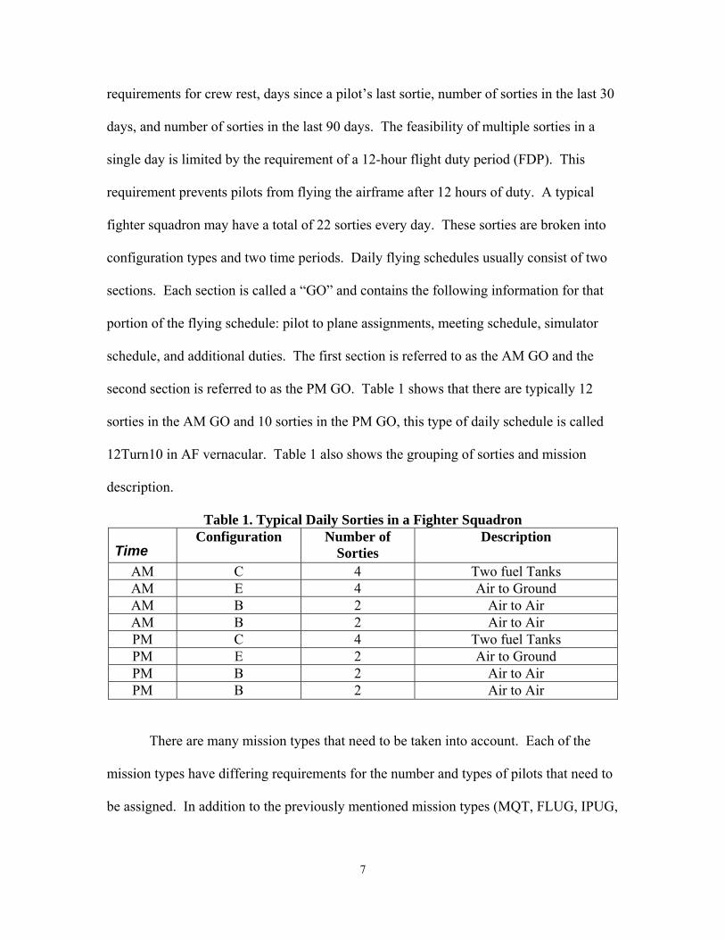
second section is referred to as the PM GO. Table 1 shows that there are typically 12

sorties in the AM GO and 10 sorties in the PM GO, this type of daily schedule is called

12Turn10 in AF vernacular. Table 1 also shows the grouping of sorties and mission

description.

Table 1. Typical Daily Sorties in a Fighter Squadron

Time Configuration Number of

Sorties Description

AM C 4 Two fuel Tanks AM E 4 Air to Ground AM B 2 Air to Air AM B 2 Air to Air PM C 4 Two fuel Tanks PM E 2 Air to Ground PM B 2 Air to Air PM B 2 Air to Air

There are many mission types that need to be taken into account. Each of the

mission types have differing requirements for the number and types of pilots that need to

be assigned. In addition to the previously mentioned mission types (MQT, FLUG, IPUG,

7

NVG, and helmet mounted cueing systems), the schedule should account for Mission

Check (MSN CHK), Instrument Check (INST CHK), and CT in the following three

areas: Basic Fighter Maneuvers (BFM), Situational Awareness Training (SAT), and

Suppression of Enemy Air Defenses (SEAD). The specified crews for each type of

mission consists of combinations of instructor pilots (IP), flight leads (FL), upgrade pilots

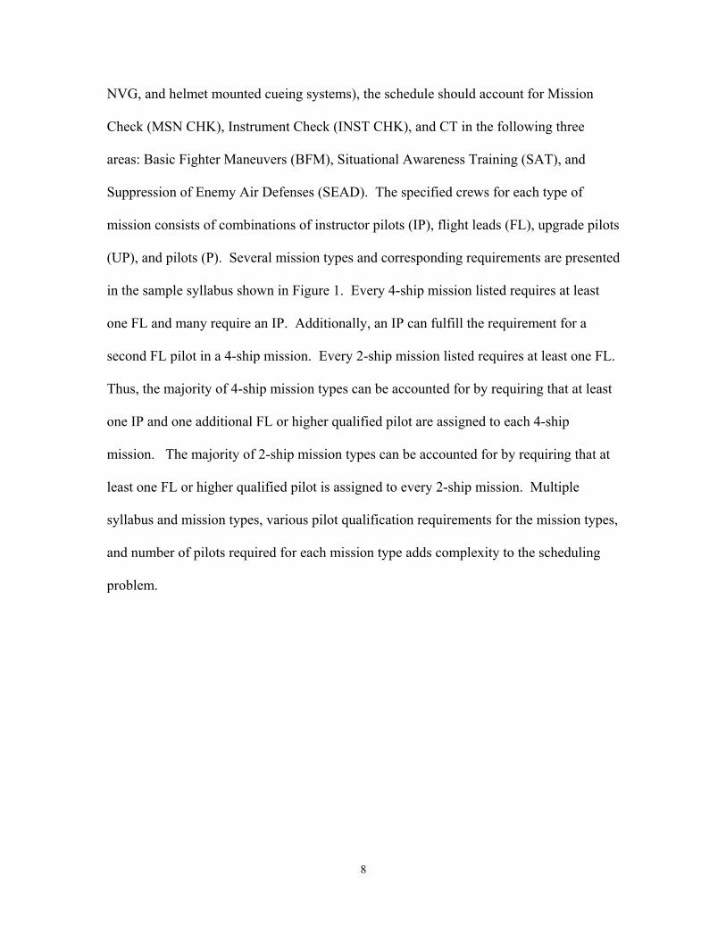
(UP), and pilots (P). Several mission types and corresponding requirements are presented

in the sample syllabus shown in Figure 1. Every 4-ship mission listed requires at least

one FL and many require an IP. Additionally, an IP can fulfill the requirement for a

second FL pilot in a 4-ship mission. Every 2-ship mission listed requires at least one FL.

Thus, the majority of 4-ship mission types can be accounted for by requiring that at least

one IP and one additional FL or higher qualified pilot are assigned to each 4-ship

mission. The majority of 2-ship mission types can be accounted for by requiring that at

least one FL or higher qualified pilot is assigned to every 2-ship mission. Multiple

syllabus and mission types, various pilot qualification requirements for the mission types,

and number of pilots required for each mission type adds complexity to the scheduling

problem.

8

Figure 1. Sample Syllabus (Boyd et. al., 2006)

1.3 Problem Modeling A complete model would account for a priority list of DO specified requests,

syllabus requirements, upgrade requirements, continuation training requirements and

sortie count requirements. The syllabus defines all pre-requisites and training

requirements needed for the successful completion of a specific course. A pilot involved

9

in the FLUG program would need to complete all the training requirements outlined by

the FLUG syllabus. A complete model would also account for the present qualification

levels of each pilot and whether or not all prerequisite training had been accomplished

prior to each scheduled mission. The model must be in accordance with (IAW) all

governing AFIs and squadron level requirements. The scope of this problem is well

beyond the capabilities of the basic Excel solver, which can only handle 200 integer

variables in a single problem. Additionally, building a model with expensive solver

software would not be useful to fighter squadrons without the purchase of that software

package. Therefore, building a model that uses an affordable Excel based solver capable

of handling larger problems makes sense.

The problem is further complicated by various sortie counts (15-day, 30-day, and

90-day), which have significant implications to the fighter pilot training mission. A pilot

that exceeds 15 days without flying a sortie will be required to fly an additional sortie

before returning to the training program. A pilot that fails to meet the 90-day

requirement will lose that qualification. Therefore, finding appropriate priority weighting

for these events is another difficulty associated with this problem.

Another area of difficulty is dealing with pilot availability. A pilot that is on

leave, temporary duty (TDY), or deployed would be unavailable for any duty in the

squadron. However, a pilot that is restricted to Duty to Not Include Flying (DNIF) would

be available to perform TOP3, SOF, or other duties that do not involve flying. All other

pilots are assumed to be available for any and all duties. However, availability may also

be limited by the required crew rest of 12 hours.

10

Further complicating the problem formulation is the need to model various types

of daily flight possibilities for each pilot. A pilot may be assigned to fly a single sortie,

two sorties with separate briefings (Double Turn), or multiple sorties (2-3) from a single

briefing each day. In the later case, the pilot remains in the aircraft with engines running

and the aircraft is refueled between missions (Pit-N-Go). A key concern is that a pilot

who flies a sortie later in the duty day must be able to be on the ground with engines shut

down when they reach the twelve-hour point for the day. Therefore, special

consideration must be taken for multiple events in a duty day which could include, but is

not limited to, the combination of TOP3, SOF, simulator sorties, ground training, and

mission/event sorties.

Additionally, assignment of pilots to aircraft becomes more complicated when

two-seat fighters are included in the scheduling and when simulator check rides occur.

Both of these events will require two pilots being assigned to a scheduled event that

normally requires one pilot. Also, when scheduling a pilot for a double turn, a

compound issue must be considered. If the flights are scheduled too far apart, the

schedule is infeasible because the pilot cannot exceed a twelve-hour duty day and still be

in the cockpit. Similarly, if the flights are scheduled too close together, the pilot will be

unable to complete the first flight, debrief, and be ready for the next mission in time for

take-off.

A weekly schedule can be formed in a number of ways. First, a model may be

developed with the intent of building the entire schedule with a single run of a solver

platform. However, there may be advantages to breaking the problem into smaller

sub-problems. For example, the schedule could be built one day at a time. Each method

11

has benefits and disadvantages. A single run of solver can account for a pilot’s

availability for the entire week. This approach benefits the final schedule when a pilot

may be unavailable later in the week and needs to complete requirements earlier in the

week. However, a disadvantage for this method is the complexity of modeling an

“if-then” penalty scenario involved with the 15-day sortie count. The penalty increases

until a pilot is assigned to a training mission sortie; then the penalty would reset to zero.

A day by day method allows the model to account for what has been scheduled on the

previous day(s), but it has increased complexity involved when trying to account for a

pilot’s availability for the entire week. Smaller periods of time allow a model to account

for each GO, but adds complexity when accounting for the scheduled times for AM GO

and PM GO as events may overlap and some duties may extend from AM GO to PM GO.

A prioritized list of requests from the DO may add an additional level of

complexity. A DO request that identifies all of the pilots, specific mission/event and day

is easier to account for in a model than a request that two pilots are assigned to a certain

type of mission at some point during the week. The model would need to account for

numerous combinations of missions that may accommodate the less specific request.

Additionally, since DO requests will vary in information given, the model must be able to

accept various types of DO request inputs.

Given a need for the automation and optimization of weekly flight schedules for

fighter pilot training, a few questions need answers. What work has been accomplished

toward this goal? How can the research build on this foundation work? Is it feasible to

construct a mathematical programming (MP) model that will meet the various needs of a

12

USAF fighter squadron? Is the benefit of such a model worthy of the expected cost to

implement such a model?

1.4 Scope The scope of this thesis is to build a MP model to generate a weekly flying

schedule for one fighter training squadron. The model accounts for two different areas of

training (MQT and CT) and three different training arenas (flight, simulator, and

other/ground) and allows for other responsibilities within the squadron such as Top 3 and

SOF. One key area of focus is pilot availability to perform one sortie, one SOF or Top 3

duty, a combination of a SOF or Top 3 duty and sortie, or multiple sorties each day.

Ensuring pilot availability is accomplished by sectioning the day into smaller time

intervals and building a staggered schedule in which pilots have twelve-hour workdays

during the squadron’s sixteen-hour day. Schedules can be developed based on pilot

availability, event start times, and expected length of time required by sorties, simulator

sorties, and duties. The model should account for all requirements for each pilot’s

qualification level and pilots that are attempting to upgrade. Also, the model should

allow for quick changes for unforeseen problems such as weather cancellation,

non-effective missions, airframe availability, or airspace availability. Finally, the model

must be user friendly. This is accomplished with the use of a Graphical User Interface

(GUI) and spreadsheet fields that would ideally be populated automatically from a

database.

13

1.5 Methodologies A model is ideally constructed to find an optimal solution. However, in some

instances, models that provide feasible solutions in a timely manner have value. The

overall size and computation time required to solve the problem can be reduced by

reducing the number of variables. One way of accomplishing this reduction is to

combine variables. Another method is to remove some variables from the optimization

process and use preprocessing or heuristic methods to account for those variables either

before or after the optimization. Thus, optimizing parts of the weekly schedule and using

scheduling principles can provide a feasible solution in a timely manner.

Ideally, the MP model would allow for changes to be made at any point in the

existing schedule. Once changes are made, the model could be rerun and it would

provide a solution for the remaining time in the week that continues to meet all

constraints.

Additionally, the model must have a GUI. The model should be user friendly and

thus allow for simple inputs such as number of pilots, unavailable pilots (leave, other

duty), qualification level, BMC or CMR status, experienced or inexperienced pilot,

mission times, simulator times, days since last sortie, 30-day sortie count, and 90-day

sortie count.

The model is constructed in Excel utilizing the Premium Frontline Solver

software. Additionally, VBA coding is used for the GUI and is also used in

preprocessing and heuristic efforts.

14

1.6 Summary Chapter 1 provides background for the scheduling of fighter pilot continuation

and upgrade training. Additionally, the research objective was addressed and a scope for

this thesis was outlined. Chapter 2 gives a literature review for sources of information

helpful in addressing the problem. Chapter 3 explains how the problem was approached

and modeled. Chapter 3 also details areas for future research. Chapter 4 provides a test

plan, test results, and analysis of test results. The scenario is altered to verify that the

model works on a variety of operational fighter squadron scenarios. Chapter 5 provides

the conclusion and summarizes the research effort and results and restates

recommendations for future research.

15

II. Literature Review 2.1 General A great deal of review was necessary in order to provide a basis of information

for the general operations and scheduling practices of a fighter squadron. Additionally,

research was required to find previous methods addressing the scheduling problem and

alternative approaches to similar types of problems. The review presents information

from theses, articles, textbooks and Air Force Instructions (AFI).

2.2 Scheduling Theory The scheduling textbook by Pinedo is an excellent resource for basic scheduling

concepts. Of particular interest to this research is the scheduling of constrained events

within a scheduling process and optimizing the benefits gained when scheduling the

flexible events. The specific concepts of interest are tardiness, processing times,

preemption, and precedence.

The tardiness of a job j is defined as the maximum value of lateness or zero,

Tj = max(Cj-dj, 0) = max(Lj, 0). Lateness (Lj) is the difference of the actual job

completion time (Cj) and the due date (dj). Thus, while Lj < 0 the tardiness (Tj) = 0. The

unit penalty is defined to equal one when Cj > dj and equals zero otherwise. The total

weighted tardiness is an additional cost function that can be utilized to penalize tardiness.

The total weighted tardiness is defined as ∑wjTj where wj is the weight associated with

job j (Pinedo, 2000).

The processing time (pij) is the amount of time required to complete job j on

machine i. When the processing time is the same for any machine, the i subscript may be

16

dropped. When preemptions are allowed, a job may be interrupted to process another

job. The processing time on the preempted job is not lost and only the remaining

processing time is required when the original job returns to the machine (Pinedo, 2000).

Precedence constraints require that one or more jobs may have to be completed

before another job is allowed to begin its processing. If each job has no more than one

predecessor and one successor, then the constraints are referred to as chains (Pinedo,

2000).

2.3 Scheduling Requirements After pilots complete IQT and MQT, they will be assigned to a CMR or BMC

position (DAF, 2004). CMR pilots are required to be proficient in all primary missions

of their unit and weapon systems, while BMC pilots are required to be familiarized in all

primary missions of their unit and weapon system (DAF, 2004). The Ready Aircrew

Program (RAP) is the CT designed to focus training on capabilities needed to accomplish

a unit’s core tasked missions (DAF, 2004). All active duty wing positions are CMR or

BMC positions (DAF, 2004). Table 3 shows the RAP sortie requirements for F-15 pilots.

For example, an experienced ACC pilot in a CMR slot would need to have flown 9

sorties in a 30-day lookback, 24 sorties in a 90-day lookback, and 98 sorties in a one year

lookback. Experienced pilots are pilots with 500 hours logged flight time on the primary

aircraft inventory (PAI), or 1000 hours logged flight time, of which 300 are PAI, or 600

fighter hours, of which 200 are PAI, or previously fighter experienced and 100 hours PAI

(DAF, 2004). All other pilots are considered inexperienced pilots.

17

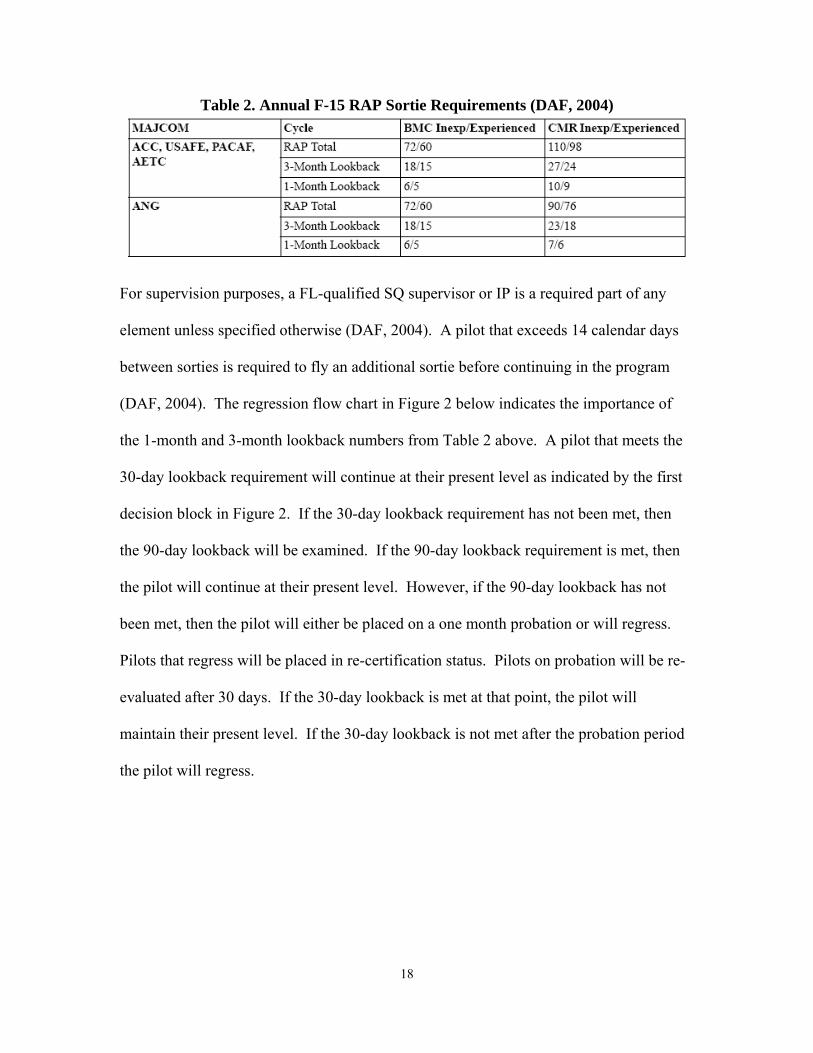
Table 2. Annual F-15 RAP Sortie Requirements (DAF, 2004)

For supervision purposes, a FL-qualified SQ supervisor or IP is a required part of any

element unless specified otherwise (DAF, 2004). A pilot that exceeds 14 calendar days

between sorties is required to fly an additional sortie before continuing in the program

(DAF, 2004). The regression flow chart in Figure 2 below indicates the importance of

the 1-month and 3-month lookback numbers from Table 2 above. A pilot that meets the

30-day lookback requirement will continue at their present level as indicated by the first

decision block in Figure 2. If the 30-day lookback requirement has not been met, then

the 90-day lookback will be examined. If the 90-day lookback requirement is met, then

the pilot will continue at their present level. However, if the 90-day lookback has not

been met, then the pilot will either be placed on a one month probation or will regress.

Pilots that regress will be placed in re-certification status. Pilots on probation will be re-

evaluated after 30 days. If the 30-day lookback is met at that point, the pilot will

maintain their present level. If the 30-day lookback is not met after the probation period

the pilot will regress.

18

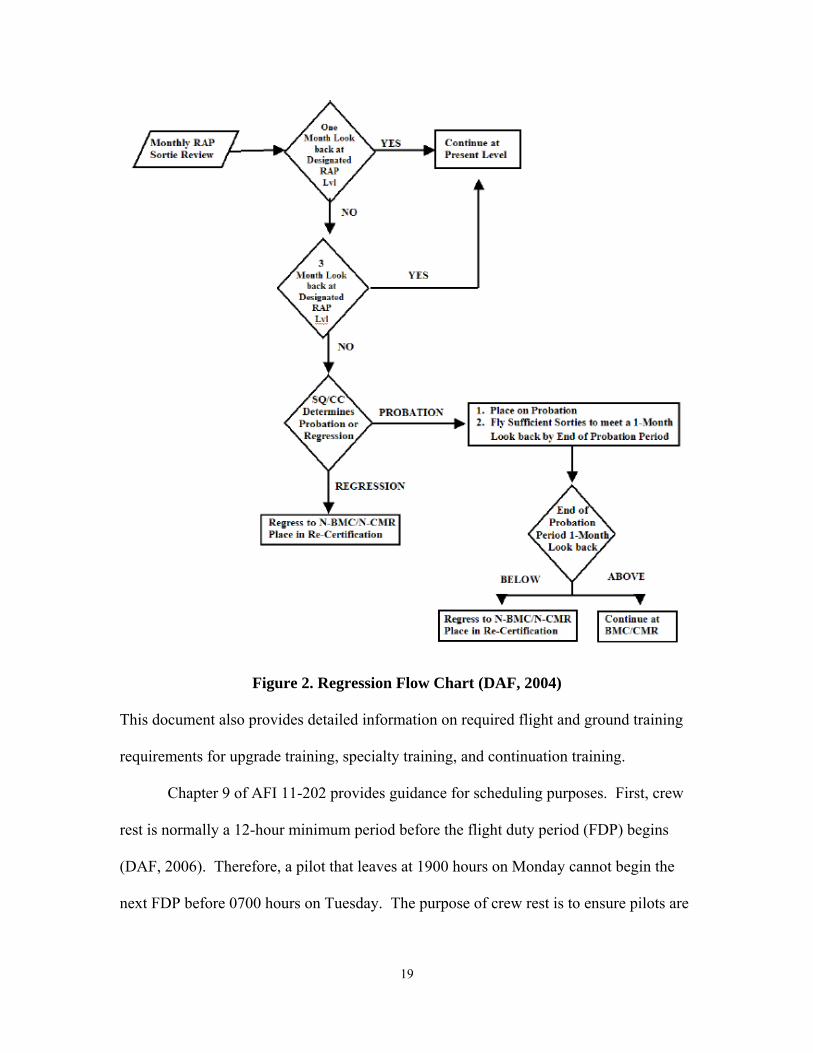
Figure 2. Regression Flow Chart (DAF, 2004)

This document also provides detailed information on required flight and ground training

requirements for upgrade training, specialty training, and continuation training.

Chapter 9 of AFI 11-202 provides guidance for scheduling purposes. First, crew

rest is normally a 12-hour minimum period before the flight duty period (FDP) begins

(DAF, 2006). Therefore, a pilot that leaves at 1900 hours on Monday cannot begin the

next FDP before 0700 hours on Tuesday. The purpose of crew rest is to ensure pilots are

19

well rested before engaging in flying duties by providing an opportunity for the pilot to

sleep (DAF, 2006). However, crew rest includes the following activities: meals,

transportation, and sleep (DAF, 2006). Additionally, maximum flying limits are defined

in AFI 11-202 as 56 hours logged flight time per seven consecutive days, 125 hours

logged flight time per 30 consecutive days and 330 hours logged flight time per 90

consecutive days (DAF, 2006). The maximum FDP is 12 hours for all single seat aircraft

or any other instance where only one pilot has access to the flight controls (DAF, 2006).

If a pilot performs other duties beyond the 12-hour FDP, then crew rest begins at the

termination of those duties (DAF, 2006).

2.4 Previous Methods The feasibility of constructing a network flow model to build a weekly schedule

for a fighter squadron is demonstrated in research accomplished by Boyd, Cunningham,

Gray, and Parker in 2006. The use of a network flow model for scheduling problems is a

fairly new approach. Their proof of concept model required 1990 variables, 3463

constraints, 1730 bounds and 260 integer variables. This was a minimum cost network

flow model utilizing Premium Solver Platform Version 6.5 created by Frontline Systems

(Boyd et. al., 2006). Figure 4 shows the network flow model for Monday’s AM GO.

According to the authors, this model is very simplistic and needs further research and

development before it can be implemented in the USAF fighter squadron community.

The authors indicate limitations and areas for further research. However, all

suggested items may not be necessary in developing a useful model and there may be

unmentioned areas of research. First, this model divided the workday into AM and PM

20

sections. This does limit the availability of the pilots for other assignments if they are

scheduled for a mission sortie, simulator sortie, SOF duty, or Top 3 duty during one of

the two periods. The suggested improvement is to divide the day into more than two

parts. The authors recommend hourly increments and a sixteen-hour workday where

each pilot is scheduled for a twelve-hour day. This would significantly increase the

number of variables and constraints required to build the model. The solver platform

used will only allow 8000 variables and 8000 constraints. Therefore, multiplying the

time period variables by a factor of eight would exceed the capabilities of the Premium

Solver Platform.

The next limitation addressed by the authors is the fact that the model only

accounts for a small portion of the data that is required to build a fully effective

scheduling process. The model, used by the authors, accounts for the 90-day sortie count,

and pilot status as related to Combat Mission Ready (CMR) or Basic Mission Capable

(BMC) and whether or not the pilot is flying at his/her highest qualification level (Boyd

et. al., 2006). It is recommended that the operationally effective model would account for

15, 30, 60 and 90-day sortie counts. Additionally, the model should schedule pilots based

on training and RAP requirements as well as the SAT mission requirements.

The authors also indicate a need for “hard schedule” priorities. This should be

accomplished with a DO only input page which will add additional constraints to the

model. This feature is not a part of the proof of concept model. The Letter of Xs is the

source document for which pilots are qualified to fulfill specific tasks. A sample Letter

of Xs appears in Appendix B. However, a flight commander or DO may desire to have a

specific IP assigned to fly a specific student’s training mission. Addressing this

21

limitation early may reduce the complexity of the overall problem. Pilots already

assigned to missions may be removed from the formulation for that time period and those

cockpits no longer have to be filled by the model (Boyd et. al., 2006).

There is an author concern that a pilot who has less flying time would be

scheduled multiple times in a week. This would yield a “feast or famine” cycle in the

scheduling process. This would occur because in the authors’ model, the schedule is built

based on recent flying that does not include the week being scheduled. There is no

suggestion for solving this current limitation. Their research found that changing costs

associated with flying later in the week based on previous flying affected the linearity of

the model (Boyd et. al., 2006).

The final concern mentioned by the authors is that the model does not benefit by

scheduling a pilot that is well ahead of his/her sortie count. The suggestion by the

authors here is to use goal programming in an attempt to fly all available pilots at the

BMC/CMR weekly requirement or greater each week (Boyd et. al., 2006). A successful

method for this limitation may also remedy the “feast or famine” cycle.

Nguyen’s research focused directly on IQT, so this research deals with a smaller

set of requirements than the fighter squadron environment. However, some of the

applications used in the model may be an excellent resource for model development in

the fighter training squadron problem. Nguyen’s model uses VBA to provide a GUI and

to develop scheduling rules such that an initial feasible solution can be found. An

attrition environment was created to account for the common occurrence that scheduled

missions are not completed as scheduled (Nguyen, 2002).

22

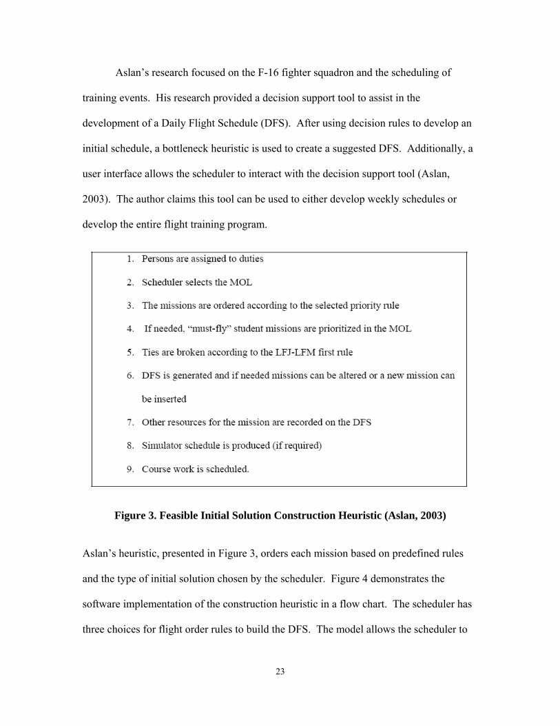
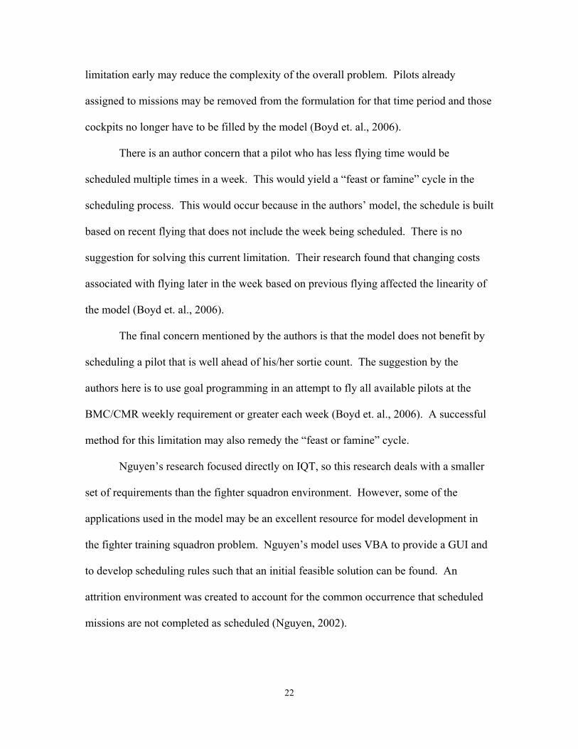
Aslan’s research focused on the F-16 fighter squadron and the scheduling of

training events. His research provided a decision support tool to assist in the

development of a Daily Flight Schedule (DFS). After using decision rules to develop an

initial schedule, a bottleneck heuristic is used to create a suggested DFS. Additionally, a

user interface allows the scheduler to interact with the decision support tool (Aslan,

2003). The author claims this tool can be used to either develop weekly schedules or

develop the entire flight training program.

Figure 3. Feasible Initial Solution Construction Heuristic (Aslan, 2003)

Aslan’s heuristic, presented in Figure 3, orders each mission based on predefined rules

and the type of initial solution chosen by the scheduler. Figure 4 demonstrates the

software implementation of the construction heuristic in a flow chart. The scheduler has

three choices for flight order rules to build the DFS. The model allows the scheduler to

23

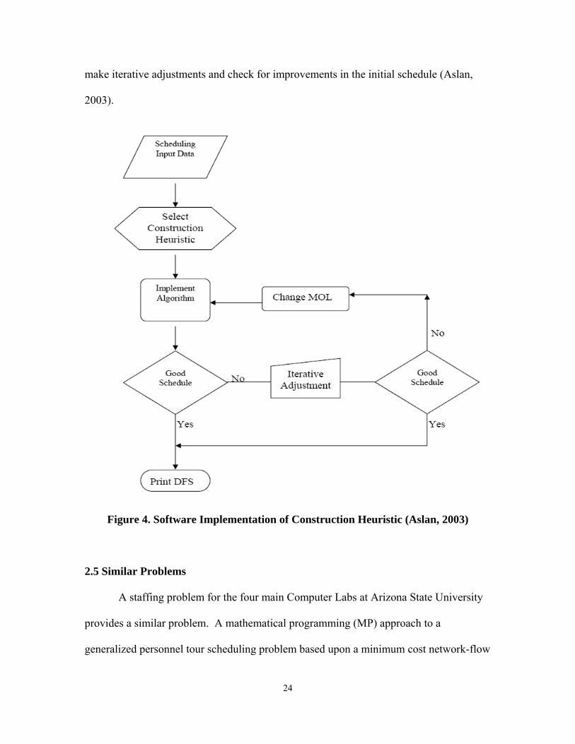
make iterative adjustments and check for improvements in the initial schedule (Aslan,

2003).

Figure 4. Software Implementation of Construction Heuristic (Aslan, 2003)

2.5 Similar Problems A staffing problem for the four main Computer Labs at Arizona State University

provides a similar problem. A mathematical programming (MP) approach to a

generalized personnel tour scheduling problem based upon a minimum cost network-flow

24

formulation with specialized side constraints is presented for this problem. The

decomposition of personnel scheduling provides three primary sub-problems: demand

modeling, shift selection, and rostering. The heterogeneous work force is a key factor in

this problem. A heterogeneous workforce is a collection of personnel who have

significantly different availabilities, skill sets, and seniorities. Additionally, rest between

consecutive shifts is a realistic requirement in tour-scheduling continuous operations.

Tour scheduling problems are essentially binary set-covering problems and as problem

size increases, the efficiency of the associated integer program (IP) decreases rapidly.

The formulation used for this problem allows very large problem instances to be solved

extremely efficiently compared to the corresponding IP solution. The formulation allows

for specialized constraints to accommodate continuous operations. This model can be

modified to deal with varying availabilities. A network arc may be removed to prevent

an unavailable employee from being scheduled. This is easy to program and has no

effect on the integrality of solutions from the LP-network solution (Knighton et al.,

2007). Knighton’s research demonstrates the fairly new approach of using a network

flow model to solve a scheduling problem.

Tanker Crew Scheduling provides a similar problem in that it deals with the

effective scheduling of limited resources of pilots and aircraft. In this case, a hybrid tabu

search approach is used with a set partitioning optimization approach (Combs 2002,

Combs and Moore 2004). The vocabulary building scheme within the metaheuristic

search is effective and can be applied to any set partitioning or set covering solution

structure (Combs 2002, Combs and Moore 2004).

25

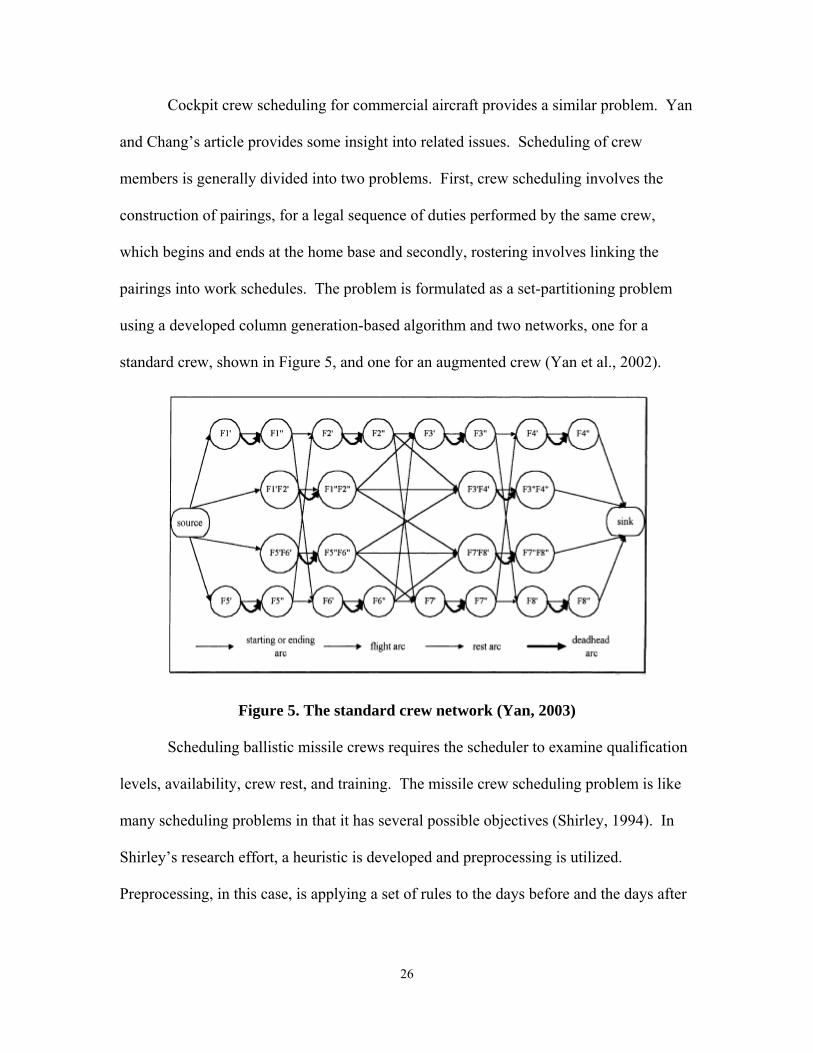
Cockpit crew scheduling for commercial aircraft provides a similar problem. Yan

and Chang’s article provides some insight into related issues. Scheduling of crew

members is generally divided into two problems. First, crew scheduling involves the

construction of pairings, for a legal sequence of duties performed by the same crew,

which begins and ends at the home base and secondly, rostering involves linking the

pairings into work schedules. The problem is formulated as a set-partitioning problem

using a developed column generation-based algorithm and two networks, one for a

standard crew, shown in Figure 5, and one for an augmented crew (Yan et al., 2002).

Figure 5. The standard crew network (Yan, 2003)

Scheduling ballistic missile crews requires the scheduler to examine qualification

levels, availability, crew rest, and training. The missile crew scheduling problem is like

many scheduling problems in that it has several possible objectives (Shirley, 1994). In

Shirley’s research effort, a heuristic is developed and preprocessing is utilized.

Preprocessing, in this case, is applying a set of rules to the days before and the days after

26

a day that is being considered for an alert. Thus, preprocessing helps reduce the

complexity of the problem by eliminating infeasible results from the solution space

before attempting to solve the problem.

Gronkvist also utilizes a preprocessing technique in the NP-hard Tail Assignment

problem (Gronkvist, 2006). The generalized preprocessing technique is based on

constraint propagation. This can dramatically reduce the size of the flight network.

Unfortunately, column generation only solves the LP relaxation. The integration of

constraint programming and column generation has great potential and may be very

useful since the column generation process only looks at a restricted part of the problem

at any given time and the constraint model has a global feasibility-focused view.

2.6 Summary The methods and problems presented in this chapter provide a foundation for this

research. The scheduling principles are directly applied to the MP model presented in

Chapter 3. Preprocessing allows an overall reduction in the number of variables and

constraints. The methodology of this research is described and then presented in a

mathematical formulation. The heuristic for assigning pilots to simulators is presented.

Also, a network representation of the problem is presented. Finally, suggestions for

further research are discussed in detail.

27

III. Methodology

3.1 Overview This chapter explains the details associated with the fighter training squadron

scheduling problem. First, the overall objectives are outlined. Second, the assumptions

for model development are specified. Next, the decision variables are defined. The

decision variables affect many other parameters within the model. The function of each

of these parameters is described by the decision variables associated to that parameter

and the constraint the parameter establishes for building the schedule. Finally, the model

constraints are defined in the context of a general formulation. These constraints vary

based on the inputs to the model. However, the constraints are driven by the

requirements as found in AFI 11-2F-15V1.

This chapter also presents the problem formulation and gives a detailed

explanation of the penalties that are built into the model. A network diagram is provided

to better show the flow of pilots to assignments. Finally, the simulator assignments and

off-duty portions of the schedule are explained in detail.

3.2 Objectives There are many ways to approach these types of problems. First, a feasible

solution may suffice in a highly constrained problem with limited resources. However,

optimality is often desired if it can be achieved with a reasonable amount of time, cost,

and resources. In other cases, it may be preferable to solve portions of a problem or

sub-problems to be combined into a complete answer. For example, some problems may

28

remove constraints if certain requirements have already been met. For the fighter pilot

scheduling problem, feasibility is a concern as current manually generated schedules

necessitate pilots being pulled from other squadrons in order to meet the sortie demands.

With the assumptions mentioned above, this model can be broken into ten

sub-problems. The first sub-problem would solve the Monday AM portion of the weekly

schedule to optimality within the given constraints. There are sub-problems for the AM

GO and the PM GO Monday through Friday. In using preprocessed penalties for each

sub-problem, a penalty for a specific pilot can be removed in subsequent sub-problems

after the requirements for that pilot have been met. However, any one of the

sub-problems could require more pilots than are currently available within the squadron.

Therefore, the model allows additional non-squadron pilots into the model for the

specific sub-problems where infeasibility due to a lack of available pilots may occur.

There is an associated cost with the use of non-squadron pilots. The model reports

mission needs for additional pilots on the schedule sheets below each day’s schedule.

The user would need to find non-squadron pilot(s) available to fly the sorties scheduled to

the generic pilot(s).

Therefore, the first objective is to make the scheduling process more efficient.

The second objective is to make the pilot training squadron efficient and effective in the

overall mission. The model objective used to accomplish the first two objectives is to

minimize the penalties for pilots exceeding fifteen days without sorties, pilots falling

below their 30-day sortie count requirement, and pilots falling below their 90-day sortie

count requirement while effectively filling every cockpit with as many squadron pilots as

possible. The penalties are a function of tardiness for each pilot in achieving their

29

respective requirements for each of the RAP sortie count requirements. The penalty

functions in the sub-problem formulation differ from the full week formulation.

The overall objectives of this research are to minimize the cost of utilizing non-

squadron pilots and to minimize the penalties associated with non-compliance of 15-day,

30-day, and 90-day sortie requirements. Thus, the overall objective is to build a feasible

schedule by solving for pilot assignments (training mission sorties, Top 3, and SOF),

using as few non-squadron pilots as possible, based on sortie counts (15-day, 30-day, and

90-day), and filling simulator sorties with a heuristic developed for this problem as a

response to the mission sortie, SOF duty and Top 3 duty assignments. This research

attempts to meet these objectives by utilizing two approaches. The first approach is to

solve the entire week as a single MP problem. The second approach divides the overall

problem into several smaller problems which allows results from the previous

sub-problem to be used as inputs for the successive sub-problem.

3.3 Assumptions As with many problems, assumptions were made in order to achieve the overall

objectives. The first assumptions define the time involved in events on the schedule. A

sortie is approximately 1.5 hours in duration. However, in the model, a scheduled flying

event begins with the pre-flight briefing and ends with the flight debrief. Thus, a flying

event on the schedule is assumed to require at least 4.0 hours and no more than 6.0 hours

of a pilot’s schedule. Additionally, the simulator events were assumed to require 3.0 to

4.0 hours of the pilot’s schedule. Briefings before consecutive simulator sorties are

assumed to be 3.0 hours apart. TOP3 and SOF positions are generally an 8.0-hour duty.

30

However, the TOP3 and SOF positions are scheduled in 6.0-hour blocks to relax the

constraint and provide increased opportunity for pilots assigned to these duties to be

assigned to sorties and simulators. Thus, the daily schedule may require a pilot to

perform TOP3/SOF duties and also fly a sortie. Therefore, the timing of the two events

requires some flexibility. A 12Turn10 flying schedule is assumed to be in place

everyday, and omitted missions would be treated as incomplete missions. It is also

assumed that other pilots are available to fill any shortfalls the squadron has in filling the

cockpits for the week.

The parameters that aid in building model constraints have differing levels of

importance. The 15-day sortie count for instance may be more important than the 30-day

sortie count. However, there is no specific guidance to the importance or priority levels

for any of these parameters. If a pilot does not fly a sortie in 15 days, then that pilot must

fly a CT sortie before returning to normal training activities. Therefore, this model

assumes that the 15-day sortie count is the first priority and the scheduling constraints are

driven by this parameter for each of the squadron’s pilots. It is also assumed that

simulator sorties should be evenly dispersed if possible. The model also assumes no pilot

can fly more than two sorties on the same day. A pilot may be scheduled to fly a sortie

and perform an extra SOF or Top 3 duty or fill a simulator seat on the same day. The

schedule is built around the assumption that in a sixteen-hour day, every pilot will have

four hours of the day off. The assumption of simulator availability requires that four

simulators are available during two distinct and consistent time frames every duty day.

Finally, each 4-ship or 2-ship training mission is limited to a maximum of one TOP3

qualified pilot.

31

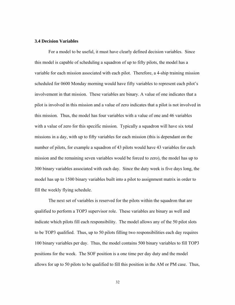
3.4 Decision Variables

For a model to be useful, it must have clearly defined decision variables. Since

this model is capable of scheduling a squadron of up to fifty pilots, the model has a

variable for each mission associated with each pilot. Therefore, a 4-ship training mission

scheduled for 0600 Monday morning would have fifty variables to represent each pilot’s

involvement in that mission. These variables are binary. A value of one indicates that a

pilot is involved in this mission and a value of zero indicates that a pilot is not involved in

this mission. Thus, the model has four variables with a value of one and 46 variables

with a value of zero for this specific mission. Typically a squadron will have six total

missions in a day, with up to fifty variables for each mission (this is dependant on the

number of pilots, for example a squadron of 43 pilots would have 43 variables for each

mission and the remaining seven variables would be forced to zero), the model has up to

300 binary variables associated with each day. Since the duty week is five days long, the

model has up to 1500 binary variables built into a pilot to assignment matrix in order to

fill the weekly flying schedule.

The next set of variables is reserved for the pilots within the squadron that are

qualified to perform a TOP3 supervisor role. These variables are binary as well and

indicate which pilots fill each responsibility. The model allows any of the 50 pilot slots

to be TOP3 qualified. Thus, up to 50 pilots filling two responsibilities each day requires

100 binary variables per day. Thus, the model contains 500 binary variables to fill TOP3

positions for the week. The SOF position is a one time per day duty and the model

allows for up to 50 pilots to be qualified to fill this position in the AM or PM case. Thus,

32

the model has 100 binary variables per day to fill the SOF position or 500 binary

variables for the SOF position for the week. Additionally, generic pilots are added to

allow non-squadron pilots to be used when necessary. The model has 10 additional pilot

slots (5 IP and 5 FL). Which are available as needed for any of the six missions each

day. This provides an additional 60 variables per day or 300 variables for the week.

Therefore, the model uses up to 560 variables per day, or 280 variables per GO. Thus,

the week would require 2800 binary decision variables to complete the weekly schedule.

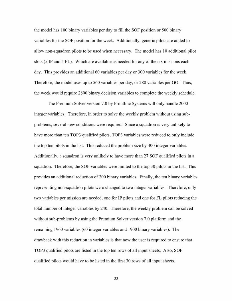
The Premium Solver version 7.0 by Frontline Systems will only handle 2000

integer variables. Therefore, in order to solve the weekly problem without using sub-

problems, several new conditions were required. Since a squadron is very unlikely to

have more than ten TOP3 qualified pilots, TOP3 variables were reduced to only include

the top ten pilots in the list. This reduced the problem size by 400 integer variables.

Additionally, a squadron is very unlikely to have more than 27 SOF qualified pilots in a

squadron. Therefore, the SOF variables were limited to the top 30 pilots in the list. This

provides an additional reduction of 200 binary variables. Finally, the ten binary variables

representing non-squadron pilots were changed to two integer variables. Therefore, only

two variables per mission are needed, one for IP pilots and one for FL pilots reducing the

total number of integer variables by 240. Therefore, the weekly problem can be solved

without sub-problems by using the Premium Solver version 7.0 platform and the

remaining 1960 variables (60 integer variables and 1900 binary variables). The

drawback with this reduction in variables is that now the user is required to ensure that

TOP3 qualified pilots are listed in the top ten rows of all input sheets. Also, SOF

qualified pilots would have to be listed in the first 30 rows of all input sheets.

33

Extending the reduction to the single go, the 1960 weekly variables implies 392

variables per day or 196 variables per GO. Thus, the model may be altered to work in a

limited capacity without the Premium Solver platform to solve the weekly schedule using

ten sub-problems. However, modifications would be required and a significant increase

in time to solve would result. The modifications would include reduction of total

variables from 280 to 196 per GO and rewriting the VBA code for the standard solver.

On a test run of two sub-problems, the standard solver found a solution in seconds.

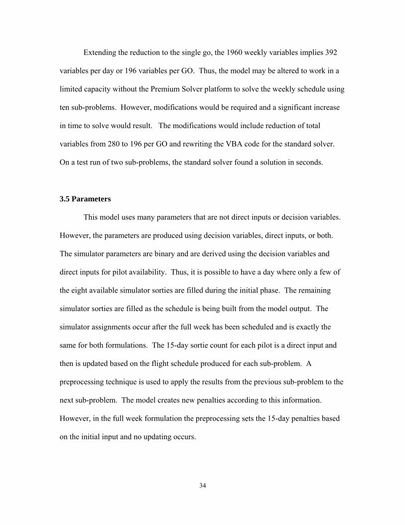
3.5 Parameters

This model uses many parameters that are not direct inputs or decision variables.

However, the parameters are produced using decision variables, direct inputs, or both.

The simulator parameters are binary and are derived using the decision variables and

direct inputs for pilot availability. Thus, it is possible to have a day where only a few of

the eight available simulator sorties are filled during the initial phase. The remaining

simulator sorties are filled as the schedule is being built from the model output. The

simulator assignments occur after the full week has been scheduled and is exactly the

same for both formulations. The 15-day sortie count for each pilot is a direct input and

then is updated based on the flight schedule produced for each sub-problem. A

preprocessing technique is used to apply the results from the previous sub-problem to the

next sub-problem. The model creates new penalties according to this information.

However, in the full week formulation the preprocessing sets the 15-day penalties based

on the initial input and no updating occurs.

34

The remaining parameters within the model are used within the model constraints.

In both formulations, parameters are utilized to prevent assigning pilots to more than one

activity at a time and to prevent assigning unavailable pilots to activities. Another

parameter is used to prevent exceeding a twelve-hour work day for the sub-problem

formulation.

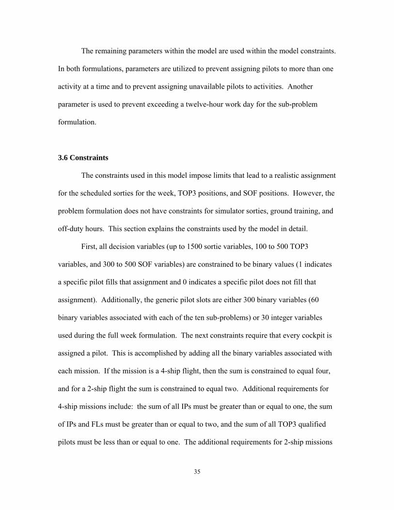
3.6 Constraints

The constraints used in this model impose limits that lead to a realistic assignment

for the scheduled sorties for the week, TOP3 positions, and SOF positions. However, the

problem formulation does not have constraints for simulator sorties, ground training, and

off-duty hours. This section explains the constraints used by the model in detail.

First, all decision variables (up to 1500 sortie variables, 100 to 500 TOP3

variables, and 300 to 500 SOF variables) are constrained to be binary values (1 indicates

a specific pilot fills that assignment and 0 indicates a specific pilot does not fill that

assignment). Additionally, the generic pilot slots are either 300 binary variables (60

binary variables associated with each of the ten sub-problems) or 30 integer variables

used during the full week formulation. The next constraints require that every cockpit is

assigned a pilot. This is accomplished by adding all the binary variables associated with

each mission. If the mission is a 4-ship flight, then the sum is constrained to equal four,

and for a 2-ship flight the sum is constrained to equal two. Additional requirements for

4-ship missions include: the sum of all IPs must be greater than or equal to one, the sum

of IPs and FLs must be greater than or equal to two, and the sum of all TOP3 qualified

pilots must be less than or equal to one. The additional requirements for 2-ship missions

35

include: the sum of all IPs and FLs must be greater than or equal to one and the sum of

all TOP3 qualified pilots must be less than or equal to one.

For each of the ten TOP3 positions during the week, the next set of constraints

requires that the sum of all TOP3 qualified pilots assigned to each position is equal to

one. Additionally, there is a constraint that for each TOP3 qualified pilot, the sum of

each day’s TOP3 and SOF position assignments is less than or equal to one. Also, the

sum of all SOF qualified pilots, including the TOP3 qualified pilots, for the SOF

assignment each day equals one. It is important that no SOF or Top 3 duty overlaps

directly with a sortie; thus, a constraint is added that for all pilots qualified for SOF and

TOP3 duties, the sum of the variables associated with those duties and the variables

associated with sorties occurring in the same timeframe of the day is less than or equal to

one. Additionally, there is a constraint that for each pilot, the sum of the variables

associated with a single day’s sorties is less than or equal to two.

Finally, the model is constrained by timing requirements. A pilot may perform an

AM GO SOF or Top 3 duty and fly a PM GO sortie provided that the sortie will not

require the pilot to be flying the aircraft at a point twelve hours later than the pilot’s day

started. Similarly, a pilot may fly an AM GO sortie and perform a PM GO SOF or Top 3

duty provided that the sortie does not require the pilot to be flying the aircraft during the

SOF or Top 3 duty timeframe. Thus, the constraints require that the AM GO SOF or

Top 3 duty scenario is linked only to a sortie that begins no later than eight hours into the

pilot’s daily schedule. For the PM SOF or Top 3 duty scenario, the AM GO flight

briefing must begin at least four hours prior to the PM GO SOF or Top 3 duty.

36

The squadron’s duty day for this model is defined as 0500 to 2100. In order to

meet the timing requirements, every pilot would ideally be scheduled for four hours of

off-duty time during this sixteen-hour period. The four hours of off-duty time should

leave a consecutive grouping of twelve one hour time slots that make up the pilot’s duty

day. Thus, a pilot may have the first four 1-hour blocks (0500-0859) or the last four

1-hour blocks (1700-2100) designated as off-duty. Additionally, a pilot may have

off-duty scheduled at both the beginning and end of the day. For example, 0700-1900 is

a valid twelve-hour duty day with two hours of off-duty time scheduled at each end of the

squadron’s daily hours.

3.7 Problem Formulation

The overall formulation for this problem has 1960 variables and 2735 constraints.

However, by solving the problem one GO at a time, the formulation for each GO has 280

variables and less than 450 constraints. The number of constraints for each GO will vary

depending on circumstances. Monday’s AM GO is not restricted by crew rest from the

previous duty day or the need to work around events already scheduled for the day and

thus only requires 114 constraints. However, the PM GO for each day must take into

account the AM GO schedule to avoid conflicts and thus requires 443 constraints. The

AM GO for every day other than Monday must account for crew rest from the previous

duty day and therefore requires 164 constraints. The overall formulation is presented first

and an individual GO formulation follows. In both cases, the purpose of each section of

the formulation is briefly described.

37

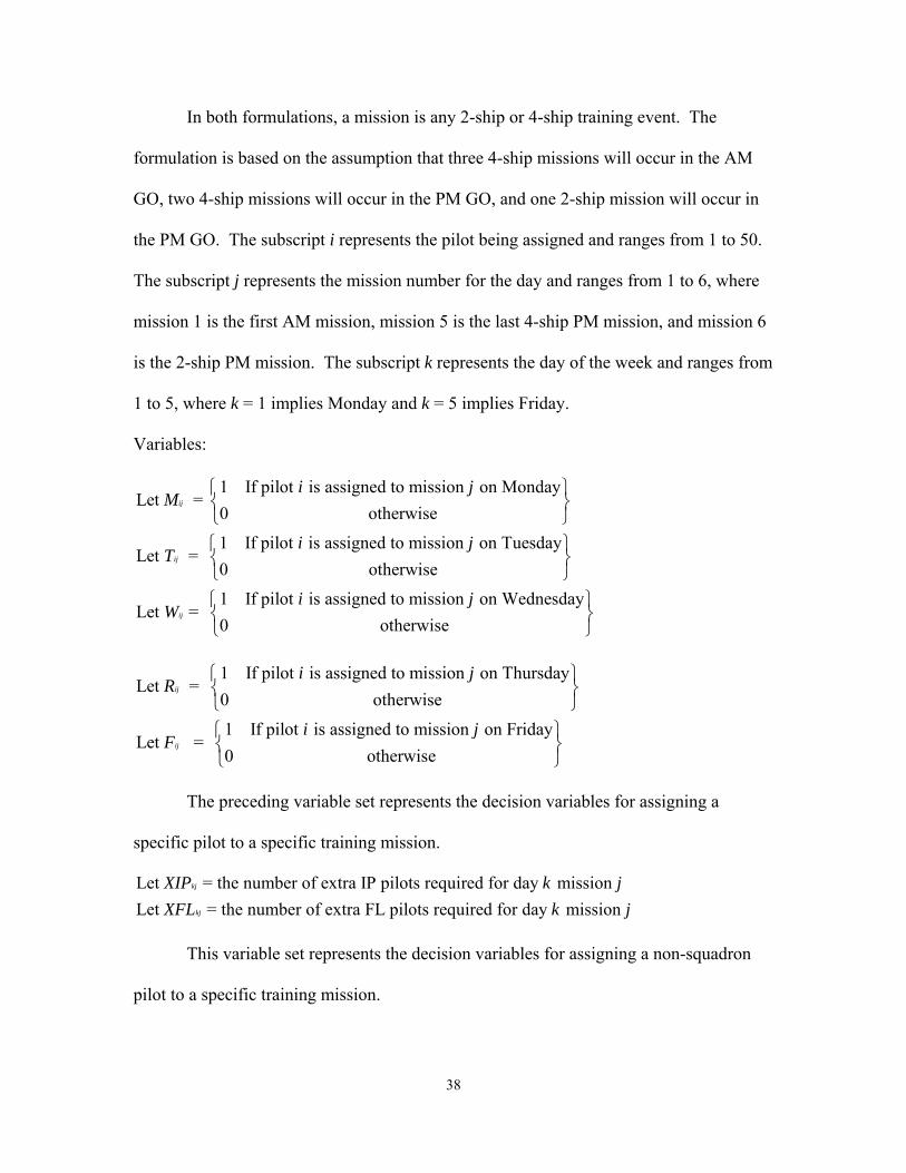
In both formulations, a mission is any 2-ship or 4-ship training event. The

formulation is based on the assumption that three 4-ship missions will occur in the AM

GO, two 4-ship missions will occur in the PM GO, and one 2-ship mission will occur in

the PM GO. The subscript i represents the pilot being assigned and ranges from 1 to 50.

The subscript j represents the mission number for the day and ranges from 1 to 6, where

mission 1 is the first AM mission, mission 5 is the last 4-ship PM mission, and mission 6

is the 2-ship PM mission. The subscript k represents the day of the week and ranges from

1 to 5, where k = 1 implies Monday and k = 5 implies Friday.

Variables:

1 If pilot is assigned to mission on MondayLet =

0 otherwise

1 If pilot is assigned to mission on TuesdayLet =

0 otherwise

1 If pilot is assigned to mission on WLet =

ij

ij

ij

i jM

i jT

i jW

⎧ ⎫⎨ ⎬⎩ ⎭⎧ ⎫⎨ ⎬⎩ ⎭

ednesday0 otherwise⎧ ⎫⎨ ⎬⎩ ⎭

1 If pilot is assigned to mission on ThursdayLet =

0 otherwise

1 If pilot is assigned to mission on FridayLet =

0 otherwise

ij

ij

i jR

i jF

⎧ ⎫⎨ ⎬⎩ ⎭⎧ ⎫⎨ ⎬⎩ ⎭

The preceding variable set represents the decision variables for assigning a

specific pilot to a specific training mission.

Let = the number of extra IP pilots required for day mission Let = the number of extra FL pilots required for day mission

kj

kj

XIP k jXFL k j

This variable set represents the decision variables for assigning a non-squadron

pilot to a specific training mission.

38

1 If pilot is assigned as Monday AM GO TOP3

Let = 0 otherwise

1 If pilot is assigned as Monday PM GO TOP3Let =

0 otherwise

1 If pilot is assigned as Monday Let =

i

i

i

iMAMT3

iMPMT3

iMAMSOF

⎧ ⎫⎨ ⎬⎩ ⎭⎧ ⎫⎨ ⎬⎩ ⎭

AM GO SOF0 otherwise

1 If pilot is assigned as Monday PM GO SOFLet =

0 otherwise

1 If pilot is assigned as Tuesday AM GO TOP3Let =

0 otherwise

1 If pilLet =

i

i

i

iMPMSOF

iTAMT3

TPMT3

⎧ ⎫⎨ ⎬⎩ ⎭⎧ ⎫⎨ ⎬⎩ ⎭⎧ ⎫⎨ ⎬⎩ ⎭

ot is assigned as Tuesday PM GO TOP30 otherwise

1 If pilot is assigned as Tuesday AM GO SOFLet =

0 otherwise

1 If pilot is assigned as Tuesday PM GO SOFLet =

0 otherwise

i

i

i

iTAMSOF

iTPMSOF

⎧ ⎫⎨ ⎬⎩ ⎭⎧ ⎫⎨ ⎬⎩ ⎭⎧⎨

⎫⎬

⎩ ⎭

1 If pilot is assigned as Wednesday AM GO TOP3Let =

0 otherwise

1 If pilot is assigned as Wednesday PM GO TOP3Let =

0 otherwise

i

i

iWAMT3

iWPMT3

⎧ ⎫⎨ ⎬⎩ ⎭⎧ ⎫⎨ ⎬⎩ ⎭

1 If pilot is assigned as Wednesday AM GO SOFLet =

0 otherwise

1 If pilot is assigned as Wednesday PM GO SOFLet =

0 otherwise

i

i

iWAMSOF

iWPMSOF

⎧ ⎫⎨ ⎬⎩ ⎭⎧ ⎫⎨ ⎬⎩ ⎭

1 If pilot is assigned as Thursday AM GO TOP3Let =

0 otherwisei

iRAMT3 ⎧ ⎫

⎨ ⎬⎩ ⎭

1 If pilot is assigned as Thursday PM GO TOP3Let =

0 otherwise

1 If pilot is assigned as Thursday AM GO SOFLet =

0 otherwise

i

i

iRPMT3

iRAMSOF

⎧ ⎫⎨ ⎬⎩ ⎭⎧ ⎫⎨ ⎬⎩ ⎭

1 If pilot is assigned as Thursday PM GO SOFLet =

0 otherwisei

iRPMSOF ⎧ ⎫

⎨ ⎬⎩ ⎭

39

1 If pilot is assigned as Friday AM GO TOP3Let =

0 otherwise

1 If pilot is assigned as Friday PM GO TOP3Let =

0 otherwise

1 If pilot is assigned as FLet =

i

i

i

iFAMT3

iFPMT3

iFAMSOF

⎧ ⎫⎨ ⎬⎩ ⎭⎧ ⎫⎨ ⎬⎩ ⎭

riday AM GO SOF0 otherwise

1 If pilot is assigned as Friday PM GO SOFLet =

0 otherwisei

iFPMSOF

⎧ ⎫⎨ ⎬⎩ ⎭⎧ ⎫⎨ ⎬⎩ ⎭

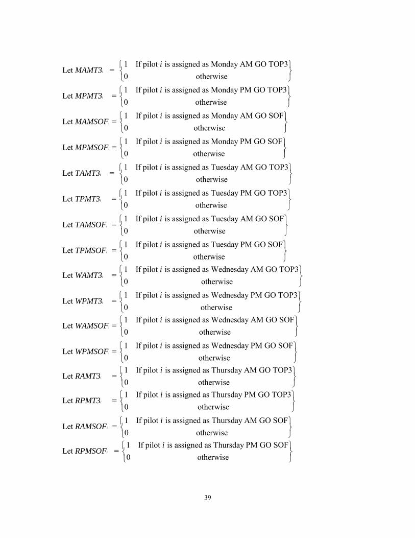
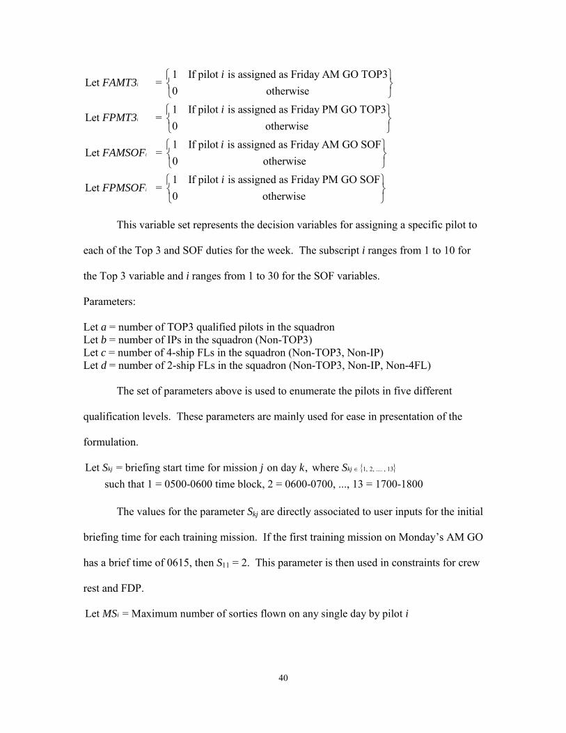
This variable set represents the decision variables for assigning a specific pilot to

each of the Top 3 and SOF duties for the week. The subscript i ranges from 1 to 10 for

the Top 3 variable and i ranges from 1 to 30 for the SOF variables.

Parameters:

Let a = number of TOP3 qualified pilots in the squadron Let b = number of IPs in the squadron (Non-TOP3) Let c = number of 4-ship FLs in the squadron (Non-TOP3, Non-IP) Let d = number of 2-ship FLs in the squadron (Non-TOP3, Non-IP, Non-4FL) The set of parameters above is used to enumerate the pilots in five different

qualification levels. These parameters are mainly used for ease in presentation of the

formulation.

{ }1, 2, .... , 13Let = briefing start time for mission on day , where such that 1 = 0500-0600 time block, 2 = 0600-0700, ..., 13 = 1700-1800

kj kjS j k S ∈

The values for the parameter Skj are directly associated to user inputs for the initial

briefing time for each training mission. If the first training mission on Monday’s AM GO

has a brief time of 0615, then S11 = 2. This parameter is then used in constraints for crew

rest and FDP.

Let = Maximum number of sorties flown on any single day by pilot iMS i

40

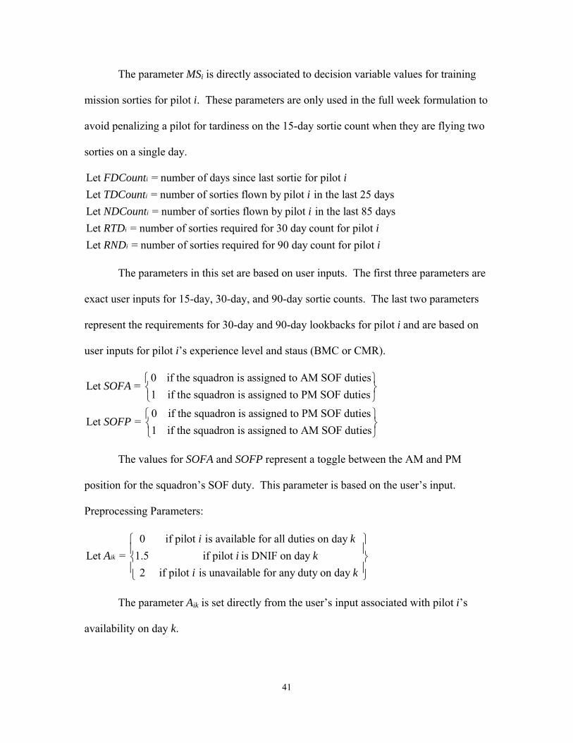
The parameter MSi is directly associated to decision variable values for training

mission sorties for pilot i. These parameters are only used in the full week formulation to

avoid penalizing a pilot for tardiness on the 15-day sortie count when they are flying two

sorties on a single day.

Let = number of days since last sortie for pilot Let = number of sorties flown by pilot in the last 25 daysLet = number of sorties flown by pilot in the last 85 daysLet

i

i

i

FDCount iTDCount iNDCount i

= number of sorties required for 30 day count for pilot Let = number of sorties required for 90 day count for pilot

i

i

RTD iRND i

The parameters in this set are based on user inputs. The first three parameters are

exact user inputs for 15-day, 30-day, and 90-day sortie counts. The last two parameters

represent the requirements for 30-day and 90-day lookbacks for pilot i and are based on

user inputs for pilot i’s experience level and staus (BMC or CMR).

0 if the squadron is assigned to AM SOF dutiesLet =

1 if the squadron is assigned to PM SOF duties

0 if the squadron is assigned to PM SOF dutiesLet =

1 if the squadron is assigned to AM SO

SOFA

SOFP

⎧ ⎫⎨ ⎬⎩ ⎭

F duties⎧ ⎫⎨ ⎬⎩ ⎭

The values for SOFA and SOFP represent a toggle between the AM and PM

position for the squadron’s SOF duty. This parameter is based on the user’s input.

Preprocessing Parameters:

0 if pilot is available for all duties on day Let = 1.5 if pilot is DNIF on day

2 if pilot is unavailable for any duty on day ik

i kA i k

i k

⎧ ⎫⎪ ⎪⎨ ⎬⎪ ⎪⎩ ⎭

The parameter Aik is set directly from the user’s input associated with pilot i’s

availability on day k.

41

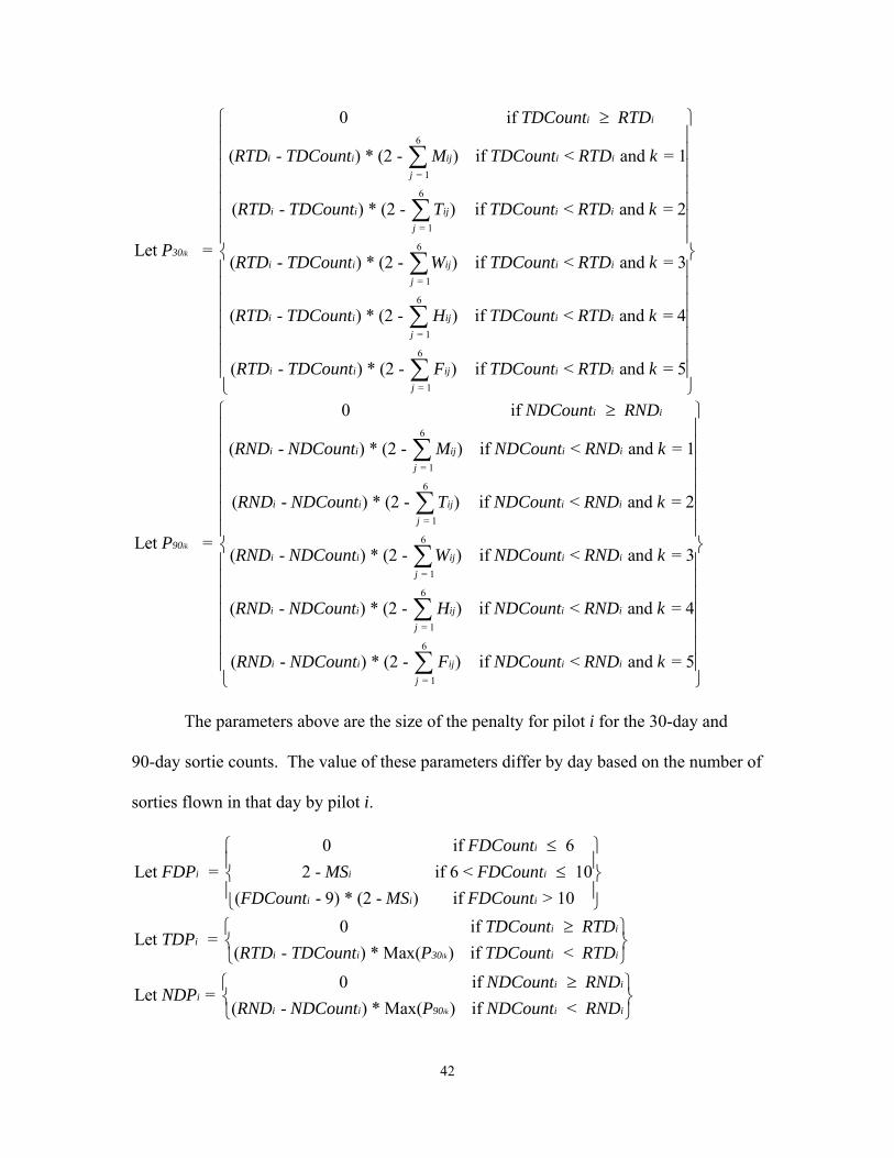
6

= 1

6

= 1

6

= 1

0 if

( - ) * (2 - ) if < and = 1

( - ) * (2 - ) if < and = 2

Let = ( - ) * (2 - ) if

ik

i i

i i ij i i

j

i i ij i i

j

30i i ij

j

TDCount RTD

RTD TDCount M TDCount RTD k

RTD TDCount T TDCount RTD k

PRTD TDCount W

≥

∑

∑

∑6

= 1

6

= 1

< and = 3

( - ) * (2 - ) if < and = 4

( - ) * (2 - ) if < and = 5

i i

i i ij i ij

i i ij i i

j

TDCount RTD k

RTD TDCount H TDCount RTD k

RTD TDCount F TDCount RTD k

⎧ ⎫⎪ ⎪⎪ ⎪⎪ ⎪⎪ ⎪⎪ ⎪⎪ ⎪⎪ ⎪⎨ ⎬⎪ ⎪⎪ ⎪⎪ ⎪⎪ ⎪⎪ ⎪⎪ ⎪⎪ ⎪⎩ ⎭

∑

∑

6

= 1

6

= 1

6

= 1

0 if

( - ) * (2 - ) if < and = 1

( - ) * (2 - ) if < and = 2

Let = ( - ) * (2 - ) if

ik

i i

i i ij i i

j

i i ij i i

j

90i i ij

j

NDCount RND

RND NDCount M NDCount RND k

RND NDCount T NDCount RND k

PRND NDCount W

≥

∑

∑

∑6

= 1

6

= 1

< and = 3

( - ) * (2 - ) if < and = 4

( - ) * (2 - ) if < and = 5

i i

i i ij i i

j

i i ij i i

j

NDCount RND k

RND NDCount H NDCount RND k

RND NDCount F NDCount RND k

⎧ ⎫⎪ ⎪⎪ ⎪⎪ ⎪⎪ ⎪⎪ ⎪⎪ ⎪⎪ ⎪⎨ ⎬⎪ ⎪⎪ ⎪⎪ ⎪⎪ ⎪⎪ ⎪⎪ ⎪⎪ ⎪⎩ ⎭

∑

∑

The parameters above are the size of the penalty for pilot i for the 30-day and

90-day sortie counts. The value of these parameters differ by day based on the number of

sorties flown in that day by pilot i.

0 if Let = 2 - if 6 < 10

( - 9) * (2 - ) if > 10

i

i i

i i i

FDCountFDP MS FDCount

FDCount MS FDCount

≤⎧ ⎫⎪ ⎪≤⎨ ⎬⎪ ⎪⎩ ⎭

6i

i

i

0 if Let =

( - ) * Max( ) if <

0 if Let =

( - ) * Max( ) if <

ik

ik

i ii

i i 30 i

i ii

i i 90 i

TDCount RTDTDP

RTD TDCount P TDCount RTD

NDCount RNDNDP

RND NDCount P NDCount RND

≥⎧ ⎫⎨ ⎬⎩ ⎭

≥⎧ ⎫⎨ ⎬⎩ ⎭

42

These parameters are the actual penalty values in the objective function and are

based on the inputs for 15-day, 30-day, and 90-day sortie counts and either maximum

number of sorties in a single day or the maximum P30 or P90 values for pilot i during the

week.

For the above, i = 1, 2,…, 50; j = 1, 2,…, 6; k = 1 (Monday), 2 (Tuesday),…, 5 (Friday).

Objective Function:

5 6 50 50 50

= 1 = 1 = 1 =1 = 1

Min = 10 * ( + ) + + 5 * + 10 * kj kj i i i

k j i i i

W XIP XFL FDP TDP NDP∑∑ ∑ ∑ ∑

The objective function is the minimum sum of the following: ten times the

number of non-squadron pilots used in the weekly schedule, the sum of 15-day penalty

parameters for all squadron pilots, five times the sum of all 30-day penalty parameters for

all squadron pilots, and ten times the 90-day penalty parameters for all squadron pilots.

s.t. Constraint Set 1

50

= 1

50

= 1

50

= 150

= 1

+ + = 4 for = 1, 2, 3, 4, 5

+ + = 2

+ + = 4 for = 1, 2, 3, 4, 5

+ + = 2

ij

i6

ij

i6

1j 1ji

16 16i

2j 2j

i

26 26

i

M XIP XFL j

M XIP XFL

T XIP XFL j

T XIP XFL

∑

∑

∑

∑

50

= 1

50

= 1

+ + = 4 for = 1, 2, 3, 4, 5

+ + = 2

ij

i6

3j 3ji

36 36i

W XIP XFL j

W XIP XFL

∑

∑

43

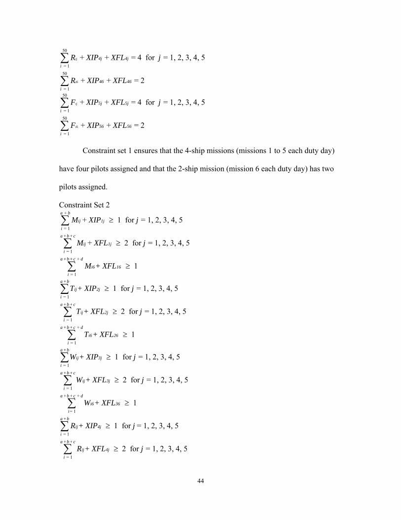
50

= 150

= 1

+ + = 4 for = 1, 2, 3, 4, 5

+ + = 2

ij

i6

4j 4ji

46 46i

R XIP XFL j

R XIP XFL

∑

∑

50

= 1

50

= 1

+ + = 4 for = 1, 2, 3, 4, 5

+ + = 2

ij

i6

5j 5ji

56 56i

F XIP XFL j

F XIP XFL

∑

∑

Constraint set 1 ensures that the 4-ship missions (missions 1 to 5 each duty day)

have four pilots assigned and that the 2-ship mission (mission 6 each duty day) has two

pilots assigned.

Constraint Set 2 +

= 1

= 1

+

= 1

+ 1 for = 1, 2, 3, 4, 5

+ 2 for = 1, 2, 3, 4, 5

1

a b

ij 1jia + b + c

ij 1ji

a + b + c d

i6 16i

M XIP j

M XFL j

M + XFL

≥

≥

≥

∑

∑

∑

= 1

= 1 +

= 1

1 for = 1, 2, 3, 4, 5

2 for = 1, 2, 3, 4, 5

1

a + b

ij 2jia + b + c

ij 2ji

a + b + c d

i6 26i

T + XIP j

T + XFL j

T + XFL

≥

≥

≥

∑

∑

∑

= 1

= 1 +

= 1

= 1

1 for = 1, 2, 3, 4, 5

2 for = 1, 2, 3, 4, 5

1

1 for = 1, 2, 3, 4, 5

2

a + b

ij 3jia + b + c

ij 3ji

a + b + c d

i6 36i

a + b

ij 4ji

ij 4j

W + XIP j

W + XFL j

W + XFL

R + XIP j

R + XFL

≥

≥

≥

≥

≥

∑

∑

∑

∑

= 1 for = 1, 2, 3, 4, 5

a + b + c

ij∑

44

+

= 1

1a + b + c d

i6 46

i

R + XFL ≥∑

= 1

= 1 +

= 1

1 for = 1, 2, 3, 4, 5

2 for = 1, 2, 3, 4, 5

1

a + b

ij 5ji

a + b + c

ij 5ji

a + b + c d

i6 56i

F + XIP j

F + XFL j

F + XFL

≥

≥

≥

∑

∑

∑

Constraint set 2 ensures that every 4-ship mission has at least one pilot qualified

at the IP level and one additional pilot qualified at the 4-ship FL level or higher assigned.

This constraint set also ensures that every 2-ship mission has at least one pilot qualified

as a 2-ship FL or higher.

Constraint Set 3

= 1

1 for = 1, 2, 3, 4, 5, 6a

ij

i

M j≤∑

= 1 1 for = 1, 2, 3, 4, 5, 6

a

iji

T j≤∑

= 1

1 for = 1, 2, 3, 4, 5, 6a

ij

i

W j≤∑

= 1 1 for = 1, 2, 3, 4, 5, 6

a

iji

R j≤∑

= 1

1 for = 1, 2, 3, 4, 5, 6a

ij

i

F j≤∑

Constraint set 3 prevents the model from assigning two or more TOP3 qualified

pilots to any single mission.

Constraint Set 4

= 1

= 1

= 1

= 1

a

ii

a

ii

MAMT3

MPMT3

∑

∑

= 1

= 1a

i

i

TAMT3∑

45

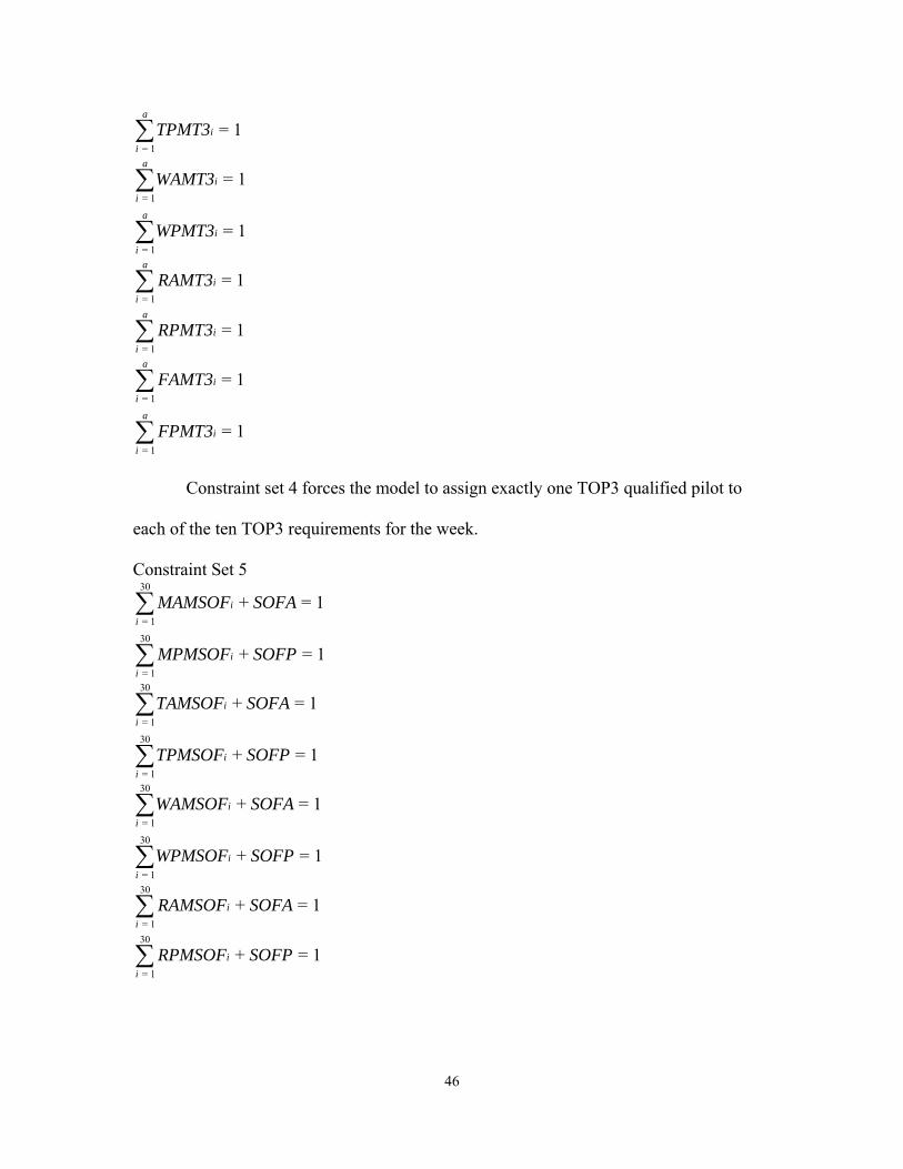
= 1

= 1a

i

i

TPMT3∑

= 1

= 1

= 1

= 1

a

ii

a

ii

WAMT3

WPMT3

∑

∑

= 1 = 1

a

ii

RAMT3∑

= 1

= 1a

i

i

RPMT3∑

= 1

= 1

= 1

= 1

a

ii

a

ii

FAMT3

FPMT3

∑

∑

Constraint set 4 forces the model to assign exactly one TOP3 qualified pilot to

each of the ten TOP3 requirements for the week.

Constraint Set 5 30

= 1

30

= 1

+ = 1

+ = 1

ii

ii

MAMSOF SOFA

MPMSOF SOFP

∑

∑

30

= 130

= 1

+ = 1

+ = 1

ii

ii

TAMSOF SOFA

TPMSOF SOFP

∑

∑

30

= 1

30

= 1

+ = 1

+ = 1

ii

ii

WAMSOF SOFA

WPMSOF SOFP

∑

∑

30

= 1 + = 1i

iRAMSOF SOFA∑

30

= 1

+ = 1i

i

RPMSOF SOFP∑

46

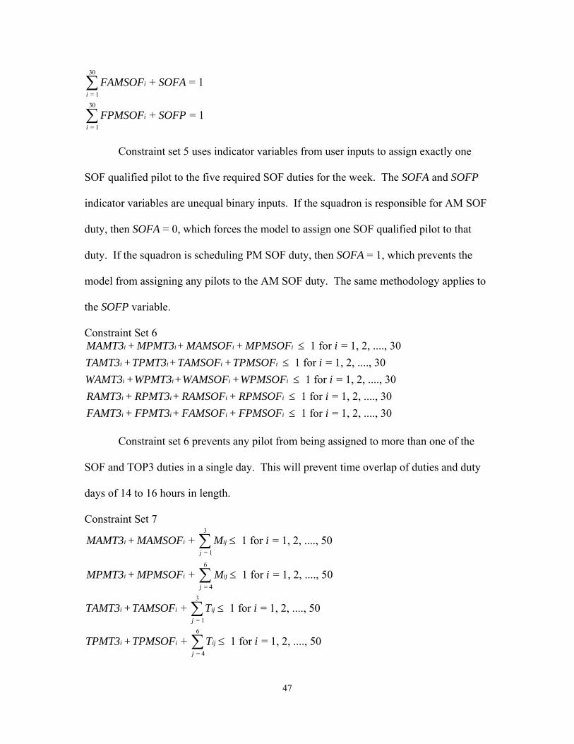
30

= 130

= 1

+ = 1

+ = 1

ii

ii

FAMSOF SOFA

FPMSOF SOFP

∑

∑

Constraint set 5 uses indicator variables from user inputs to assign exactly one

SOF qualified pilot to the five required SOF duties for the week. The SOFA and SOFP

indicator variables are unequal binary inputs. If the squadron is responsible for AM SOF

duty, then SOFA = 0, which forces the model to assign one SOF qualified pilot to that

duty. If the squadron is scheduling PM SOF duty, then SOFA = 1, which prevents the

model from assigning any pilots to the AM SOF duty. The same methodology applies to

the SOFP variable.

Constraint Set 6

1 for = 1, 2, ...., 30 1 for = 1, 2, ...., 30

1 for = 1, 2, ...., 30

i i i i

i i i i

i i i i

i

MAMT3 + MPMT3 + MAMSOF + MPMSOF iTAMT3 + TPMT3 + TAMSOF + TPMSOF iWAMT3 + WPMT3 + WAMSOF + WPMSOF iRAMT3 + RPMT3

≤≤≤

1 for = 1, 2, ...., 301 for = 1, 2, ...., 30

i i i

i i i i

+ RAMSOF + RPMSOF iFAMT3 + FPMT3 + FAMSOF + FPMSOF i

≤≤

Constraint set 6 prevents any pilot from being assigned to more than one of the

SOF and TOP3 duties in a single day. This will prevent time overlap of duties and duty

days of 14 to 16 hours in length.

Constraint Set 7 3

= 1

6

= 4

+ 1 for = 1, 2, ...., 50

+ 1 for = 1, 2, ...., 50

i i ijj

i i ijj

MAMT3 + MAMSOF M i

MPMT3 + MPMSOF M i

≤

≤

∑

∑

3

= 1

+ 1 for = 1, 2, ...., 50i i ij

j

TAMT3 + TAMSOF T i≤∑

6

= 4 + 1 for = 1, 2, ...., 50i i ij

jTPMT3 + TPMSOF T i≤∑

47

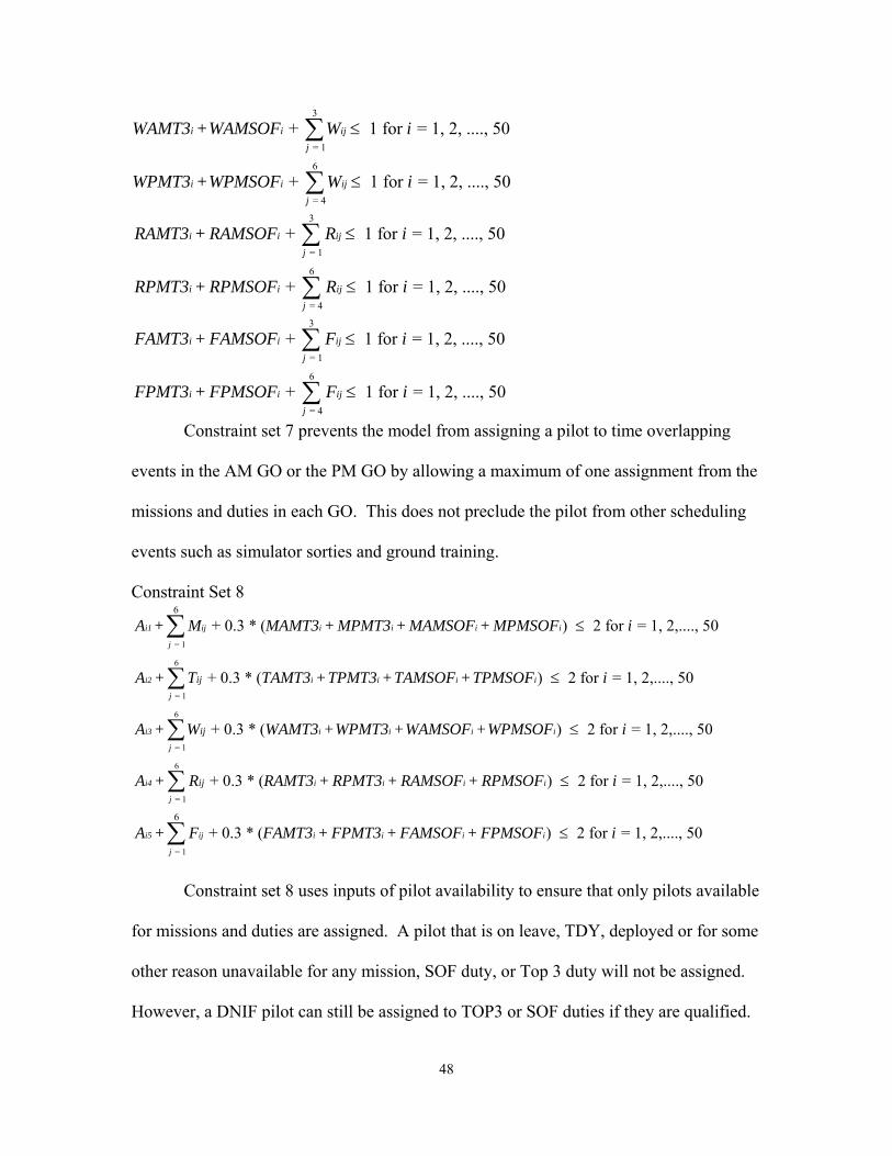
3

= 1

6

= 4

+ 1 for = 1, 2, ...., 50

+ 1 for = 1, 2, ...., 50

i i ijj

i i ijj

WAMT3 + WAMSOF W i

WPMT3 + WPMSOF W i

≤

≤

∑

∑

3

= 1

6

= 4

+ 1 for = 1, 2, ...., 50

+ 1 for = 1, 2, ...., 50

i i ijj

i i ijj

RAMT3 + RAMSOF R i

RPMT3 + RPMSOF R i

≤

≤

∑

∑

3

= 1

6

= 4

+ 1 for = 1, 2, ...., 50

+ 1 for = 1, 2, ...., 50

i i ijj

i i ijj

FAMT3 + FAMSOF F i

FPMT3 + FPMSOF F i

≤

≤

∑

∑

Constraint set 7 prevents the model from assigning a pilot to time overlapping

events in the AM GO or the PM GO by allowing a maximum of one assignment from the

missions and duties in each GO. This does not preclude the pilot from other scheduling

events such as simulator sorties and ground training.

Constraint Set 8

= 1

6

= 1

6

= 1

6

+ 0.3 * ( ) 2 for = 1, 2,...., 50

+ 0.3 * ( ) 2 for = 1, 2,...., 50

+ 0.3 *

i1 ij i i i i

j

i2 i i i i

j

i3

j

ij

ij

A + M MAMT3 + MPMT3 + MAMSOF + MPMSOF i

A + T TAMT3 + TPMT3 + TAMSOF + TPMSOF i

A + W

≤

≤∑

∑

∑

6

= 1

= 1

6

( ) 2 for = 1, 2,...., 50

+ 0.3 * ( ) 2 for = 1, 2,...., 50

+ 0.3 * (

i i i i

i4 i i i i

j

i5 ij i i

j

ij

WAMT3 + WPMT3 + WAMSOF + WPMSOF i

A + R RAMT3 + RPMT3 + RAMSOF + RPMSOF i

A + F FAMT3 + FPMT3 + FAMS

≤

≤∑

∑ ) 2 for = 1, 2,...., 50i iOF + FPMSOF i≤

Constraint set 8 uses inputs of pilot availability to ensure that only pilots available

for missions and duties are assigned. A pilot that is on leave, TDY, deployed or for some

other reason unavailable for any mission, SOF duty, or Top 3 duty will not be assigned.

However, a DNIF pilot can still be assigned to TOP3 or SOF duties if they are qualified.

48

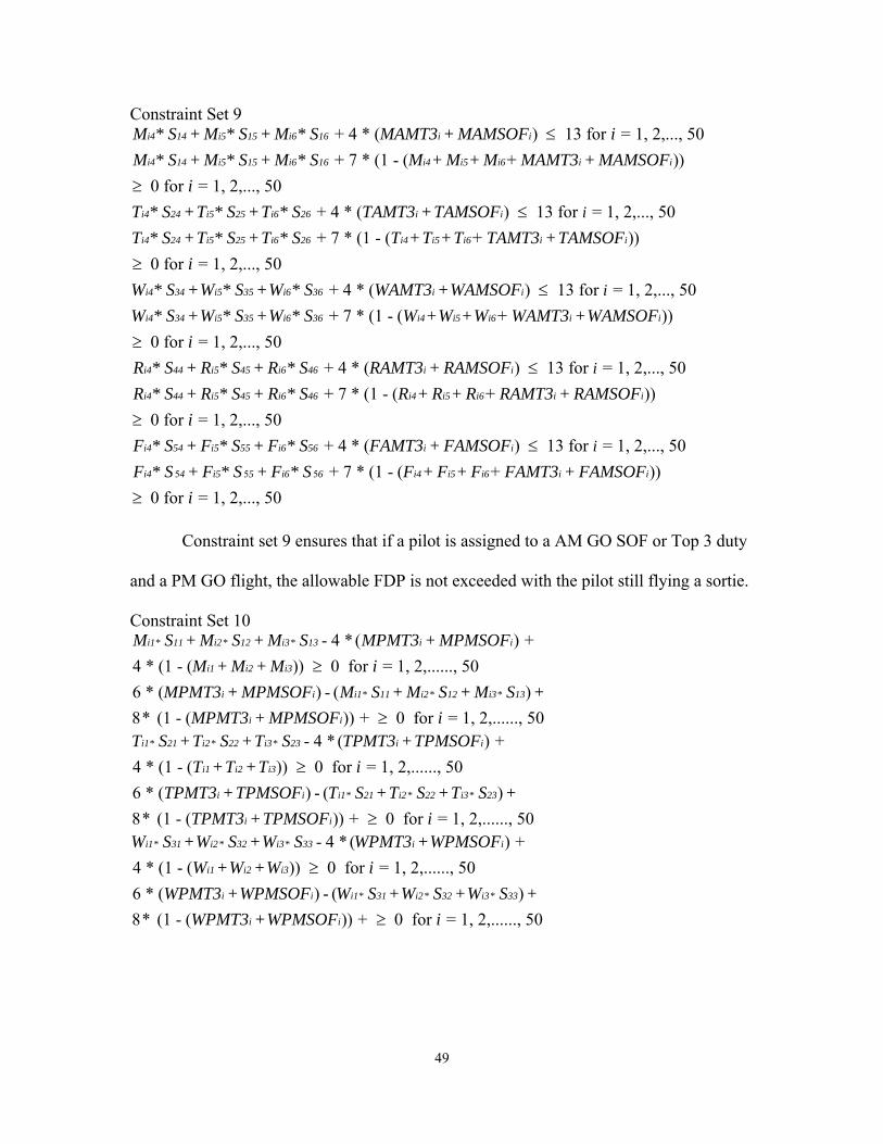
Constraint Set 9 + 4 * ( ) 13 for = 1, 2,..., 50 + 7 * (1 - ( + ))

0 for = 1, 2,..., 50

i4 14 i5 15 i6 16 i i

i4 14 i5 15 i6 16 i4 i5 i6 i i

i4 24

M * S + M * S + M * S MAMT3 + MAMSOF iM * S + M * S + M * S M + M + M MAMT3 + MAMSOF

iT * S

≤

≥ + 4 * ( ) 13 for = 1, 2,..., 50 + 7 * (1 - ( + ))

0 for = 1, 2,..., 50

i5 25 i6 26 i i

i4 24 i5 25 i6 26 i4 i5 i6 i i

i4 34 i5 3

i+ T * S + T * S TAMT3 + TAMSOFT * S + T * S + T * S T + T + T TAMT3 + TAMSOF

iW * S + W * S

≤

≥ + 4 * ( ) 13 for = 1, 2,..., 50 + 7 * (1 - ( + ))

0 for = 1, 2,..., 50

5 i6 36 i i

i4 34 i5 35 i6 36 i4 i5 i6 i i

i4 44 i5 45 i6

i + W * S WAMT3 + WAMSOFW * S + W * S + W * S W + W + W WAMT3 + WAMSOF

iR * S + R * S + R *

≤

≥ + 4 * ( ) 13 for = 1, 2,..., 50 + 7 * (1 - ( + ))

0 for = 1, 2,..., 50 + 4 *

46 i i

i4 44 i5 45 i6 46 i4 i5 i6 i i

i4 54 i5 55 i6 56

iS RAMT3 + RAMSOFR * S + R * S + R * S R + R + R RAMT3 + RAMSOF

iF * S + F * S + F * S

≤

≥

5 5 5

( ) 13 for = 1, 2,..., 50 + 7 * (1 - ( + ))

0 for = 1, 2,..., 50

i i

i4 4 i5 5 i6 6 i4 i5 i6 i i

iFAMT3 + FAMSOFF * S + F * S + F * S F + F + F FAMT3 + FAMSOF

i

≤

≥ Constraint set 9 ensures that if a pilot is assigned to a AM GO SOF or Top 3 duty

and a PM GO flight, the allowable FDP is not exceeded with the pilot still flying a sortie.

Constraint Set 10 - 4 * ( ) +

4 * (1 - ( )) 0 for = 1, 2,......, 506 * ( ) - ( )8* (1 - (

i1 * 11 i2 * 12 i3 * 13 i i

i1 i2 i3

i i i1 * 11 i2 * 12 i3 * 13

i

M S + M S + M S MPMT3 + MPMSOFM + M + M i

MPMT3 + MPMSOF M S + M S + M S + MPMT3 + MP

≥

)) + 0 for = 1, 2,......, 50iMSOF i≥

- 4 * ( ) + 4 * (1 - ( )) 0 for = 1, 2,......, 506 * ( ) - ( )8* (1 - (

i1 * 21 i2 * 22 i3 * 23 i i

i1 i2 i3

i i i1 * 21 i2 * 22 i3 * 23

i

T S + T S + T S TPMT3 + TPMSOFT + T + T i

TPMT3 + TPMSOF T S + T S + T S + TPMT3 + TP

≥

)) + 0 for = 1, 2,......, 50iMSOF i≥

- 4 * ( ) + 4 * (1 - ( )) 0 for = 1, 2,......, 506 * ( ) - ( )8* (1 - (

i1 * 31 i2 * 32 i3 * 33 i i

i1 i2 i3

i i i1 * 31 i2 * 32 i3 * 33

i

W S + W S + W S WPMT3 + WPMSOFW + W + W i

WPMT3 + WPMSOF W S + W S + W S + WPMT3 + WP

≥

)) + 0 for = 1, 2,......, 50iMSOF i≥

49

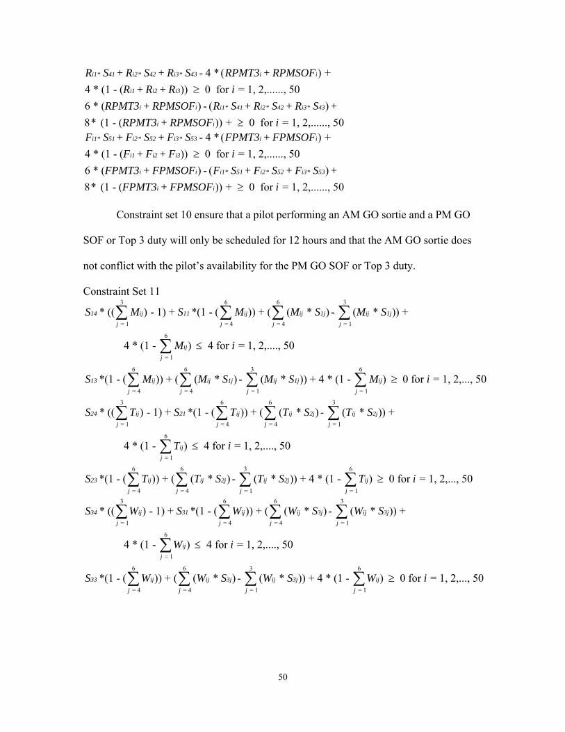
- 4 * ( ) + 4 * (1 - ( )) 0 for = 1, 2,......, 506 * ( ) - ( )8* (1 - (

i1 * 41 i2 * 42 i3 * 43 i i

i1 i2 i3

i i i1 * 41 i2 * 42 i3 * 43

i

R S + R S + R S RPMT3 + RPMSOFR + R + R i

RPMT3 + RPMSOF R S + R S + R S + RPMT3 + RP

≥

)) + 0 for = 1, 2,......, 50iMSOF i≥

- 4 * ( ) + 4 * (1 - ( )) 0 for = 1, 2,......, 506 * ( ) - ( )8* (1 - (

i1 * 51 i2 * 52 i3 * 53 i i

i1 i2 i3

i i i1 * 51 i2 * 52 i3 * 53

i

F S + F S + F S FPMT3 + FPMSOFF + F + F i

FPMT3 + FPMSOF F S + F S + F S + FPMT3 + FP

≥

)) + 0 for = 1, 2,......, 50iMSOF i≥

Constraint set 10 ensure that a pilot performing an AM GO sortie and a PM GO

SOF or Top 3 duty will only be scheduled for 12 hours and that the AM GO sortie does

not conflict with the pilot’s availability for the PM GO SOF or Top 3 duty.

Constraint Set 11 3 6 6 3

= 1 = 4 = 4 = 1

6

= 1

6 6

= 4 = 4

* (( ) - 1) + *(1 - ( )) + ( ( * ) - ( * )) +

4 * (1 - ) 4 for = 1, 2,...., 50

*(1 - ( )) + ( ( *

14 ij 11 ij ij 1j ij 1j

j j j j

ij

j

13 ij ij 1

j j

S M S M M S M S

M i

S M M S

≤

∑ ∑ ∑ ∑

∑

∑ ∑3 6

= 1 = 1

) - ( * )) + 4 * (1 - ) 0 for = 1, 2,..., 50j ij 1j ij

j j

M S M i≥∑ ∑3 6 6 3

= 1 = 4 = 4 = 1

6

= 1

* (( ) - 1) + *(1 - ( )) + ( ( * ) - ( * )) +

4 * (1 - ) 4 for = 1, 2,...., 50

24 ij 21 ij ij 2j ij 2j

j j j j

ij

j

S T S T T S T S

T i≤

∑ ∑ ∑ ∑

∑

6 6 3 6

= 4 = 4 = 1 = 1

*(1 - ( )) + ( ( * ) - ( * )) + 4 * (1 - ) 0 for = 1, 2,..., 5023 ij ij 2j ij 2j ijj j j j

S T T S T S T i≥∑ ∑ ∑ ∑

3 6 6 3

= 1 = 4 = 4 = 1

6

= 1

6 6

= 4 = 4

* (( ) - 1) + *(1 - ( )) + ( ( * ) - ( * )) +

4 * (1 - ) 4 for = 1, 2,...., 50

*(1 - ( )) + ( ( *

34 ij 31 ij ij 3j ij 3j

j j j j

ij

j

33 ij ij 3

j j

S W S W W S W S

W i

S W W S

≤

∑ ∑ ∑ ∑

∑

∑ ∑3 6

= 1 = 1

) - ( * )) + 4 * (1 - ) 0 for = 1, 2,..., 50j ij 3j ij

j j

W S W i≥∑ ∑

50

3 6 6 3

= 1 = 4 = 4 = 1

6

= 1

6 6

= 4 = 4

* (( ) - 1) + *(1 - ( )) + ( ( * ) - ( * )) +

4 * (1 - ) 4 for = 1, 2,...., 50

*(1 - ( )) + ( ( *

44 ij 41 ij ij 4j ij 4j

j j j j

ij

j

43 ij ij 4

j j

S R S R R S R S

R i

S R R S

≤

∑ ∑ ∑ ∑

∑

∑ ∑3 6

= 1 = 1

) - ( * )) + 4 * (1 - ) 0 for = 1, 2,..., 50j ij 4j ij

j j

R S R i≥∑ ∑

3 6 6 3

= 1 = 4 = 4 = 1

6

= 1

6 6

= 4 = 4

* (( ) - 1) + *(1 - ( )) + ( ( * ) - ( * )) +

4 * (1 - ) 4 for = 1, 2,...., 50

*(1 - ( )) + ( ( *

54 ij 51 ij ij 5j ij 5j

j j j j

ij

j

53 ij ij 5

j j

S F S F F S F S

F i

S F F S

≤

∑ ∑ ∑ ∑

∑

∑ ∑3 6

= 1 = 1

) - ( * )) + 4 * (1 - ) 0 for = 1, 2,..., 50j ij 5j ij

j j

F S F i≥∑ ∑

Constraint set 11 ensures that any pilot assigned to fly in both an AM GO mission

and a PM GO mission has a minimum of four hours between mission start times and a

maximum of eight hours between mission start times.

Constraint Set 12 3 6

= 1 = 4

( ) + - ( ( * ( - 8)) + * 2 +

* 4) 0 for = 1, 2,..., 50

ij 2j i i ij 1j i

j j

i

T * S TAMSOF + TAMT3 M S MPMSOF

MPMT3 i≥

∑ ∑

3 6

= 1 = 4

( ) + - ( ( * ( - 8)) + * 2 +

* 4) 0 for = 1, 2,..., 50

ij 3j i i ij 2j i

j j

i

W * S WAMSOF + WAMT3 T S TPMSOF

TPMT3 i≥

∑ ∑

3 6

= 1 = 4

( ) + - ( ( * ( - 8)) + * 2 +

* 4) 0 for = 1, 2,..., 50

ij 4j i i ij 3j i

j j

i

R * S RAMSOF + RAMT3 W S WPMSOF

WPMT3 i≥

∑ ∑

3 6

= 1 = 4

( ) + - ( ( * ( - 8)) + * 2 +

* 4) 0 for = 1, 2,..., 50

ij 5j i i ij 4j i

j j

i

F * S FAMSOF + FAMT3 R S RPMSOF

RPMT3 i≥

∑ ∑

Constraint set 12 ensures that every pilot has a minimum of twelve hours crew

rest from every weekday PM GO (except Friday) to the following day’s AM GO.

All , , and 0 and integer, All other variables are binarykj kj kjXIP XFL S ≥

51

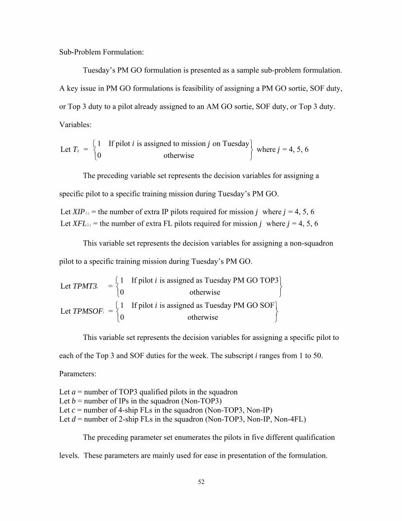
Sub-Problem Formulation:

Tuesday’s PM GO formulation is presented as a sample sub-problem formulation.

A key issue in PM GO formulations is feasibility of assigning a PM GO sortie, SOF duty,

or Top 3 duty to a pilot already assigned to an AM GO sortie, SOF duty, or Top 3 duty.

Variables:

1 If pilot is assigned to mission on TuesdayLet = where = 4, 5, 6

0 otherwiseij

i jT j⎧ ⎫

⎨ ⎬⎩ ⎭

The preceding variable set represents the decision variables for assigning a

specific pilot to a specific training mission during Tuesday’s PM GO.

2

2

Let = the number of extra IP pilots required for mission where = 4, 5, 6Let = the number of extra FL pilots required for mission where = 4, 5, 6

j

j

XIP j jXFL j j

This variable set represents the decision variables for assigning a non-squadron

pilot to a specific training mission during Tuesday’s PM GO.

1 If pilot is assigned as Tuesday PM GO TOP3Let =

0 otherwise

1 If pilot is assigned as Tuesday PM GO SOFLet =

0 otherwise

i

i

iTPMT3

iTPMSOF

⎧ ⎫⎨ ⎬⎩ ⎭⎧ ⎫⎨ ⎬⎩ ⎭

This variable set represents the decision variables for assigning a specific pilot to

each of the Top 3 and SOF duties for the week. The subscript i ranges from 1 to 50.

Parameters:

Let a = number of TOP3 qualified pilots in the squadron Let b = number of IPs in the squadron (Non-TOP3) Let c = number of 4-ship FLs in the squadron (Non-TOP3, Non-IP) Let d = number of 2-ship FLs in the squadron (Non-TOP3, Non-IP, Non-4FL) The preceding parameter set enumerates the pilots in five different qualification

levels. These parameters are mainly used for ease in presentation of the formulation.

52

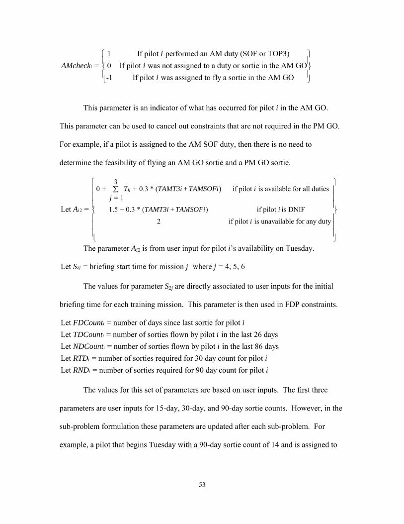
1 If pilot performed an AM duty (SOF or TOP3) = 0 If pilot was not assigned to a duty or sortie in the AM GO

-1 If pilot was assigned to fly a sortie in the AM GOi

iAMcheck i

i

⎧ ⎫⎪ ⎪⎨ ⎬⎪ ⎪⎩ ⎭

This parameter is an indicator of what has occurred for pilot i in the AM GO.

This parameter can be used to cancel out constraints that are not required in the PM GO.

For example, if a pilot is assigned to the AM SOF duty, then there is no need to

determine the feasibility of flying an AM GO sortie and a PM GO sortie.

2

30 + + 0.3 * ( ) if pilot is available for all duties

= 11.5 + 0.3 * ( ) if pilot is DNIF

2 if pilot is unavailable for any duty Let =

ij

i

T TAMT3i + TAMSOFi ij

TAMT3i + TAMSOFi i i

A

∑⎧ ⎫⎪ ⎪⎪ ⎪⎪ ⎪⎨ ⎬⎪ ⎪⎪ ⎪⎪ ⎪⎩ ⎭

The parameter Ai2 is from user input for pilot i’s availability on Tuesday.

Let = briefing start time for mission where = 4, 5, 62jS j j The values for parameter S2j are directly associated to user inputs for the initial

briefing time for each training mission. This parameter is then used in FDP constraints.

Let = number of days since last sortie for pilot Let = number of sorties flown by pilot in the last 26 daysLet = number of sorties flown by pilot in the last 86 daysLet

i

i

i

FDCount iTDCount iNDCount i

= number of sorties required for 30 day count for pilot Let = number of sorties required for 90 day count for pilot

i

i

RTD iRND i

The values for this set of parameters are based on user inputs. The first three

parameters are user inputs for 15-day, 30-day, and 90-day sortie counts. However, in the

sub-problem formulation these parameters are updated after each sub-problem. For

example, a pilot that begins Tuesday with a 90-day sortie count of 14 and is assigned to

53

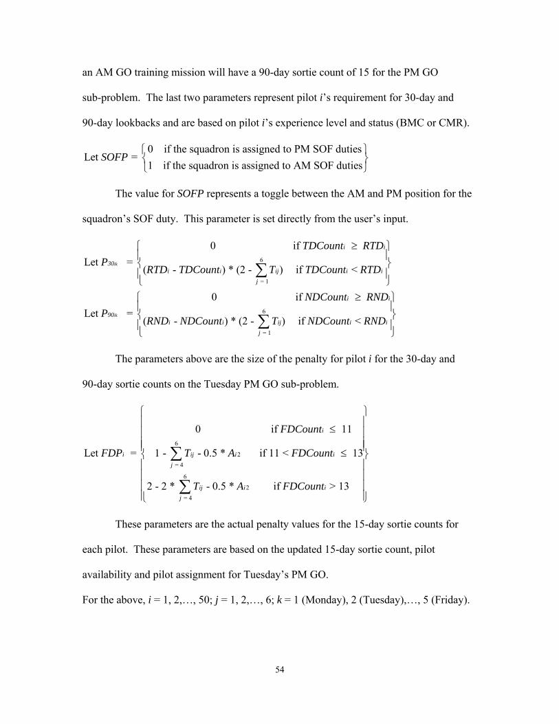
an AM GO training mission will have a 90-day sortie count of 15 for the PM GO

sub-problem. The last two parameters represent pilot i’s requirement for 30-day and

90-day lookbacks and are based on pilot i’s experience level and status (BMC or CMR).

0 if the squadron is assigned to PM SOF dutiesLet =

1 if the squadron is assigned to AM SOF dutiesSOFP ⎧ ⎫

⎨ ⎬⎩ ⎭

The value for SOFP represents a toggle between the AM and PM position for the

squadron’s SOF duty. This parameter is set directly from the user’s input.

6

= 1

6

= 1

0 if Let =

( - ) * (2 - ) if <

0 if Let =

( - ) * (2 - ) if <

ik

ik

i i

30i i ij i

j

i i

90i i ij i

j

TDCount RTDP

RTD TDCount T TDCount RTD

NDCount RNDP

i

iRND NDCount T NDCount RND

≥⎧ ⎫⎪ ⎪⎨ ⎬⎪ ⎪⎩ ⎭

≥⎧ ⎫⎪ ⎪⎨ ⎬⎪ ⎪⎩ ⎭

∑

∑

The parameters above are the size of the penalty for pilot i for the 30-day and

90-day sortie counts on the Tuesday PM GO sub-problem.

6

2 = 4

6

2 = 4

0 if

Let = 1 - - 0.5 * if 11 < 13

2 - 2 * - 0.5 * if > 13

i

i ij i ij

ij i ij

FDCount

FDP T A FDCount

T A FDCount

⎧ ⎫⎪ ⎪≤⎪ ⎪⎪ ⎪⎪ ⎪≤⎨ ⎬⎪ ⎪⎪ ⎪⎪ ⎪⎪ ⎪⎩ ⎭

∑

∑

11

These parameters are the actual penalty values for the 15-day sortie counts for

each pilot. These parameters are based on the updated 15-day sortie count, pilot

availability and pilot assignment for Tuesday’s PM GO.

For the above, i = 1, 2,…, 50; j = 1, 2,…, 6; k = 1 (Monday), 2 (Tuesday),…, 5 (Friday).

54

Objective Function:

6 50 50

= 4 = 1 =1 = 1Min = 10 * ( + ) + 25 * + 10 * + 25 * i2 i22j 2j i 30 90

j i iW XIP XFL FDP P P∑ ∑ ∑

50

i∑

The objective function is the minimum sum of the following: ten times the

number of non-squadron pilots used in Tuesday’s PM GO, 25 times the sum of Tuesday

PM GO 15-day penalties for all squadron pilots, ten times the sum of Tuesday PM GO

30-day penalties for all squadron pilots, and 25 times the sum of Tuesday PM GO 90-day

penalties for all squadron pilots.

s.t. Constraint Set 1

50

= 150

= 1

+ + = 4 for = 4, 5

+ + = 2

ij

i6

2j 2ji

26 26i

T XIP XFL j

T XIP XFL

∑

∑

Constraint set 1 ensures that the 4-ship missions (missions 4 and 5) have four

pilots assigned and that the 2-ship mission (mission 6) has two pilots assigned.

Constraint Set 2

= 1

= 1

+

= 1

1 for = 4, 5

2 for = 4, 5

1

a + b

ij 2j

i

a + b + c

ij 2j

i

a + b + c d

i6 26

i

T + XIP j

T + XFL j

T + XFL

≥

≥

≥

∑

∑

∑

Constraint set 2 ensures that each 4-ship mission has at least one pilot qualified at

the IP level and one additional pilot qualified at the 4-ship FL level or higher assigned.

This constraint set also ensures that the 2-ship mission has at least one pilot qualified as a

2-ship FL or higher assigned.

55

Constraint Set 3

= 1

1 for = 4, 5, 6a

ij

i

T j≤∑

This constraint set ensures at most one Top 3 pilot is assigned to each mission. Constraint Set 4

= 1

= 1a

i

i

TPMT3∑

This constraint requires that one Top 3 qualified pilot is assigned to the Tuesday

PM GO Top 3 duty.

Constraint Set 5 30

= 1

+ = 1i

i

TPMSOF SOFP∑

Constraint set 5 ensures that the Tuesday PM SOF duty is filled for a squadron

performing PM SOF duties.

Constraint Set 6 1 for = 1, 2, ...., 30i i i iTAMT3 + TPMT3 + TAMSOF + TPMSOF i≤

Constraint set 6 prevents any pilot from being assigned to more than one of the

SOF and TOP3 duties during Tuesday. This will prevent time overlap of duties and a

duty day on Tuesday of 14 to 16 hours in length.

Constraint Set 7 6

= 4 + 1 for = 1, 2, ...., 50i i ij

jTPMT3 + TPMSOF T i≤∑

Constraint set 7 prevents the model from assigning a pilot to time overlapping

events in the PM GO by allowing a maximum of one assignment from the training

missions and SOF or Top 3 duties in the PM GO. This does not prevent the pilot from

other scheduling events such as simulator sorties and ground training.

56

Constraint Set 8 6

= 4 + 0.3 * ( ) 2 for = 1, 2,...., 50i2 ij i i

jA + T TPMT3 + TPMSOF i≤∑

Constraint set 8 uses inputs of pilot availability to ensure that only pilots available

for missions and duties are assigned.

Constraint Set 9 + 4 * ( ) 13 for = 1, 2,..., 50i4 24 i5 25 i6 26 i i iT * S + T * S + T * S TAMT3 + TAMSOF ≤

Constraint set 9 ensures that if a pilot is assigned to a Tuesday AM GO SOF or

Top 3 duty and a Tuesday PM GO flight, the allowable FDP is not exceeded with the

pilot still flying a sortie.

Constraint Set 10

6 6

= 4 = 4* (1 - 0.5 * (1 - )) * ( ) - 7 * 2i i ij 2j ij

j j

AMcheck AMcheck T * S T⎛ ⎞

≤⎜ ⎟⎝ ⎠∑ ∑

6 6

= 4 = 4* (1 - 0.5 * (1 - )) * ( ) - 7 * 0i i ij 2j ij

j j

AMcheck AMcheck T * S T⎛ ⎞

≥⎜ ⎟⎝ ⎠∑ ∑

3 3

= 1 = 1

3 3

= 1 = 1

* (-1) * (0.5 * (1 + ) - 1) * ( ) - 4 * 1

* (-1) * (0.5 * (1 + ) - 1) * ( ) - 4 * 0

i i ij 2jj j

i i ij 2j

j j

AMcheck AMcheck T * S T

AMcheck AMcheck T * S T

⎛ ⎞≤⎜ ⎟

⎝ ⎠⎛ ⎞

≥⎜ ⎟⎝ ⎠

∑ ∑

∑ ∑

ij

ij

Constraint set 10 ensures a pilot performing a Tuesday AM GO sortie and a

Tuesday PM GO SOF or Top 3 duty will only be scheduled for 12 hours and the AM GO

sortie does not conflict with the pilot’s availability for the PM GO SOF or Top 3 duty.

Constraint Set 11

6 3 6

= 4 = 1 = 4

6 3 6

= 4 = 1 = 4

0.5 * * ( 1) * - ( * ) - 4 * 5

0.5 * * ( 1) * - ( * ) - 4 * 0

( )

( )

( )

( )

i i ij 2j ij 2j ijj j j

i i ij 2j ij 2j ij

j j j

AMcheck AMcheck T * S T S T

AMcheck AMcheck T * S T S T

⎛ ⎞− ≤⎜ ⎟

⎝ ⎠⎛ ⎞

− ≥⎜ ⎟⎝ ⎠

∑ ∑ ∑

∑ ∑ ∑

57

Constraint set 11 ensures that any pilot assigned to fly in both a Tuesday AM GO

mission and a Tuesday PM GO mission has a minimum of four hours between mission

start times and a maximum of eight hours between mission start times.

All , , and 0 and integer, All other variables are binarykj kj kjXIP XFL S ≥

This formulation is representative of all PM GO sub-problems. The constraint

sets are labeled to allow a side by side comparison with the formulation of the entire

week. Constraint set 1, for example, is used to ensure that four pilots are assigned to

every 4-ship mission and two pilots are assigned to every 2-ship mission. The full week

formulation has twelve constraint sets and the Tuesday PM GO formulation above has

eleven constraint sets. Constraint set 12 is used to ensure that 12 hours of crew rest

occurs from the end of a PM GO on one day to the start of AM GO duties the next day.

Therefore, the PM GO formulation above does not require this constraint set. However,

in the AM GO formulations (except Monday’s AM GO), constraint set twelve is required

and other constraint sets may be omitted. The advantage of using sub-problems is found

in the constraints relating to multiple assignments in a duty day. For example, a pilot

may fly both AM GO and PM GO sorties in the same duty day. In the weekly

formulation, constraint set 11 ensures the feasibility of a pilot flying any two sorties.

Each of these constraints depend on six variables (three AM GO and three PM GO).

However, the PM GO sub-problem only uses three variables and the known result of the

AM GO sub-problem. Thus, the other three variables are now constants. This constraint

ensures feasibility of a single pilot flying two sorties based on a known time frame for the

58

first of the two sorties. Therefore, constraint set 11 has the same purpose in both

formulations (weekly and PM GO), but the constraints themselves are different.

The indicator variable AMcheck is used to indicate what has occurred in the AM

GO. If a pilot is assigned to an AM GO SOF or Top 3 duty, then AMcheck = 1 and

constraint set 9 ensures the feasibility of the same pilot being assigned to a PM GO sortie.

Constraint sets 10 and 11 for that pilot equal zero and are irrelevant since the pilot did not

fly in the AM GO. If a pilot is unassigned in the AM GO, then AMcheck = 0 and

constraint sets 10 and 11 for that pilot equal zero and are irrelevant. If the pilot is

assigned to an AM GO sortie, then AMcheck = -1 and constraint set 9 for that pilot is

irrelevant since the pilot did not perform an AM GO SOF or Top 3 duty. Constraint sets

10 and 11 are used to ensure the feasibility of the same pilot being assigned to a PM GO

SOF or Top 3 duty (constraint set 10) or flying a sortie in the PM GO (constraint set 11).

Another advantage of using sub-problems is the ability to update sortie counts.

The updated values of these parameters are compared with sortie count requirements.

Using simple programming, preprocessing of the sortie count penalty functions can be

accomplished. For example, a pilot’s 30-day sortie count is 4 and the requirement is 6.

Thus, the pilot must fly at least two sorties during the week to fulfill the requirement. If

the requirement is met on Tuesday, then the penalty function for this pilot’s 30-day sortie

count goes to zero for the remainder of the week. In the sub-problem, this is a linear

function based on known results of previous sub-problems. In the full week formulation,

this penalty function could not be based on known results from early points in the week.

The penalty functions for pilot sortie counts in the full week formulation are smooth

nonlinear functions. The penalty terms are ∑TDPi and ∑NDPi for i = 1 to 50 where:

59

0 if Let =

( - ) * Max( ) if <

0 if Let =

( - ) * Max( ) if <

ik

ik

i ii

i i 30 i

i ii

i i 90 i

TDCount RTDTDP

i

i

RTD TDCount P TDCount RTD

NDCount RNDNDP

RND NDCount P NDCount RND

≥⎧ ⎫⎨ ⎬⎩ ⎭

≥⎧ ⎫⎨ ⎬⎩ ⎭

Since a maximum value formula is associated with these parameters, the penalty terms

are clearly nonlinear. However, the P30 and P90 parameters will have a value of 0, 1, or 2.

Thus, the full week formulation has smooth nonlinear 30 and 90-day penalty functions.

3.8 Simulator Heuristic

In both formulations of this problem, the number of variables is reduced by

excluding the simulator sorties from the problem. However, a simulator heuristic was

developed to ensure the simulator sorties are populated with pilots. The heuristic is

designed using VBA programming and is applied to the overall problem after the

previously mentioned formulations have been solved. Thus, training mission, SOF duty,

and Top 3 duty assignments are used as inputs for the heuristic. The heuristic is designed

to spread the simulator sorties to as many of the squadron pilots as possible. Thus,

Monday’s simulator sorties are assigned first and each successive day is scheduled such

that available pilots with the fewest simulator sorties for the week are assigned first.

The initial phase of the simulator heuristic looks for available pilots that have not

been assigned to a training mission on a given duty day. A pilot meeting this criteria is

assigned to a simulator sortie provided they have not already been assigned to two

simulator sorties for the week. After the initial phase, the weekly schedule is populated

with simulator and training mission sorties, Top 3 and SOF duties, and off-duty time.

60

The second phase of the simulator heuristic counts the number of simulator sorties

filled for each day. If any day has not been filled, then the schedule for that day is

examined. Beginning with the first pilot and proceeding down the list, the heuristic

searches for pilots with the required block of time unscheduled. If a pilot has the time

available and has fewer simulator sorties than the incremented variable for each pass,

then that pilot is assigned to a simulator. The incremented variable simtot starts at three

and is incremented to ten. No pilot can fill more than ten simulator sorties in a week.

However, the heuristic should disperse the simulator assignments such that no pilot

exceeds four simulator sorties for the week. If all simulator sorties have not been filled,

then no squadron pilots are available to fill the requirement and the simulator slot is lost.

3.9 Network Representation

The network representation for a single day is shown in Figure 6. The source

nodes (T3 1, T3 2,…,P d) and the “Other Pilots” node represent the available pilots.

Flow moves toward the sink node (“Ground Training”). The sink node also includes

activities such as: TDY, deployment, leave, ground training, classes, professional military

education (PME), and relief of non-squadron pilots. There are several side constraints to

the MP model. First, no pilot can be assigned to multiple events occurring at the same

time. Therefore, a pilot acting as the TOP3 in the AM GO cannot then be assigned as the

IP pilot for a 0900 AM GO sortie. However, the 12Turn10 does not have set time

restrictions. Thus, AM GO sorties could be scheduled after noon, or PM GO sorties

could be scheduled before noon. Therefore, a pilot may perform PM GO SOF or Top 3

duties after a PM GO flight that begins at 0900. However, the current model does not

61

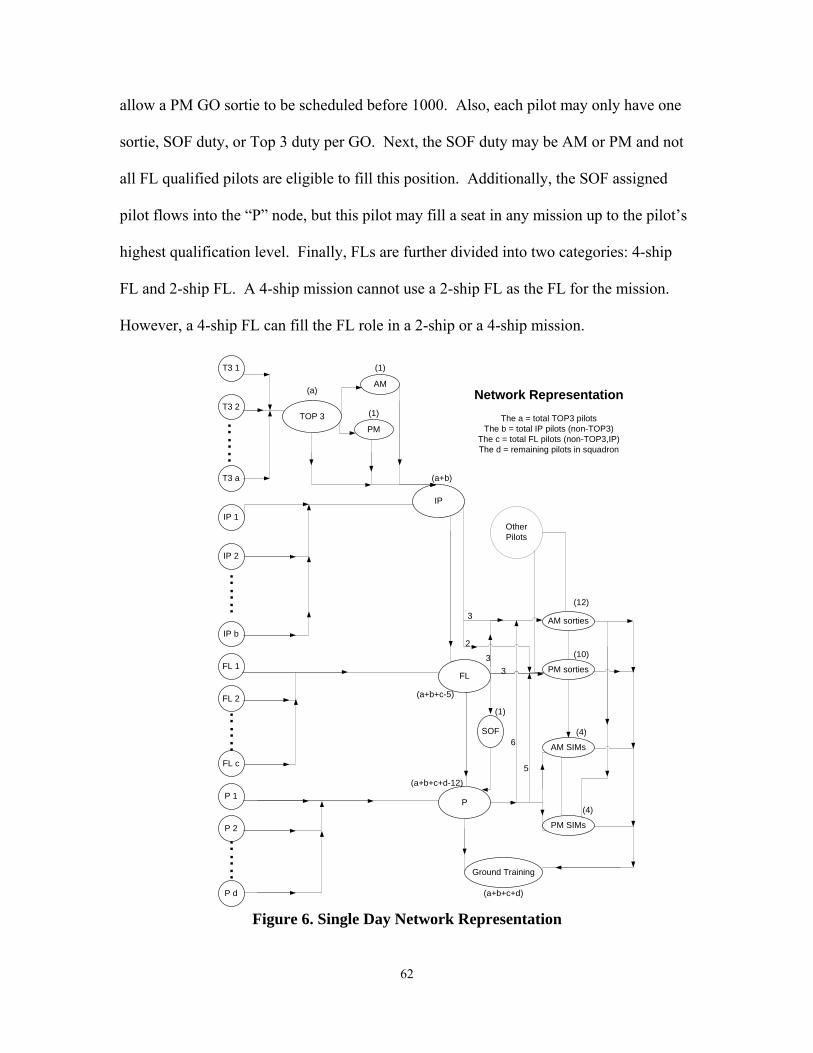
allow a PM GO sortie to be scheduled before 1000. Also, each pilot may only have one

sortie, SOF duty, or Top 3 duty per GO. Next, the SOF duty may be AM or PM and not

all FL qualified pilots are eligible to fill this position. Additionally, the SOF assigned

pilot flows into the “P” node, but this pilot may fill a seat in any mission up to the pilot’s

highest qualification level. Finally, FLs are further divided into two categories: 4-ship

FL and 2-ship FL. A 4-ship mission cannot use a 2-ship FL as the FL for the mission.

However, a 4-ship FL can fill the FL role in a 2-ship or a 4-ship mission.

T3 1

T3 2

T3 a

IP 1

IP 2

IP b

FL 1

FL 2

FL c

P 1

P 2

P d

TOP 3

AM

PM

IP

FL

AM sorties

PM sorties

AM SIMs

PM SIMs

P

Ground Training

Network RepresentationThe a = total TOP3 pilots

The b = total IP pilots (non-TOP3)The c = total FL pilots (non-TOP3,IP)The d = remaining pilots in squadron

:::

:::

:::

:::

SOF

(a)

(1)

(1)

(a+b)

(1)

(12)

(10)

(a+b+c-5)

(a+b+c+d-12)

(a+b+c+d)

(4)

(4)

3

2

33

6

5

OtherPilots

Figure 6. Single Day Network Representation

62

The network representation in Figure 6 also shows demands on certain nodes and

arcs. The min and max capacity on all arcs from the pilot nodes to the qualification

nodes (TOP3, IP, FL, and P) is 1. There is exactly one pilot at each pilot node, and each

pilot must flow to a qualification level. The squadron has “a” pilots qualified at the

TOP3 level and thus the “TOP3” node has a demand of “a.” Additionally, the “AM” and

“PM” TOP3 nodes have a demand of 1. Therefore, the arc from “TOP3” to “IP” has a

flow of “a-2” and arcs “AM” to “IP” and “PM” to “IP” both have a flow of 1. Thus, all

of the TOP3 qualified pilots flow into the “IP” node and all IP pilots that are not TOP3

qualified flow into the “IP” node. Since the squadron has “b” IP pilots that are not TOP3

qualified, the demand at the “IP” node is “a+b.”

There are three missions in the AM sorties which require an IP pilot and two

missions in the PM sorties which require an IP pilot. Thus, the arc from “IP” to “AM

sorties” has a maximum capacity of 3 and the arc from “IP” to “PM sorties” has a

maximum capacity of 2. The total IP demand for the day is five, but a single IP pilot may

fly an AM sortie and a PM sortie in that role. All remaining pilots in the “IP” node will

flow to the “FL” node as they are qualified for FL duty. Thus, the minimum demand at

the “FL” node is “a+b-5” plus the number of FL (non-IP and non TOP3) pilots in the

squadron, “c.”

The arcs from “FL” to “AM sorties” and “FL” to “PM sorties” both have a

maximum capacity of 3. However, a FL pilot may fill the FL role in both an AM sortie

and a PM sortie. The total FL demand for the day is six. Additionally, one pilot

qualified to fill the SOF position will fill the SOF demand and flow from the “FL” node

to the “SOF” node and on to the “P” node. All remaining pilots in the “FL” node will

63

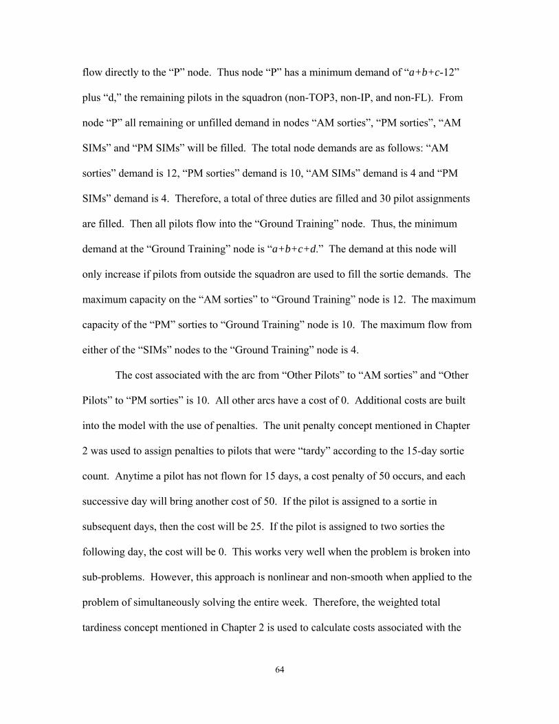
flow directly to the “P” node. Thus node “P” has a minimum demand of “a+b+c-12”

plus “d,” the remaining pilots in the squadron (non-TOP3, non-IP, and non-FL). From

node “P” all remaining or unfilled demand in nodes “AM sorties”, “PM sorties”, “AM

SIMs” and “PM SIMs” will be filled. The total node demands are as follows: “AM

sorties” demand is 12, “PM sorties” demand is 10, “AM SIMs” demand is 4 and “PM

SIMs” demand is 4. Therefore, a total of three duties are filled and 30 pilot assignments

are filled. Then all pilots flow into the “Ground Training” node. Thus, the minimum

demand at the “Ground Training” node is “a+b+c+d.” The demand at this node will

only increase if pilots from outside the squadron are used to fill the sortie demands. The

maximum capacity on the “AM sorties” to “Ground Training” node is 12. The maximum

capacity of the “PM” sorties to “Ground Training” node is 10. The maximum flow from

either of the “SIMs” nodes to the “Ground Training” node is 4.

The cost associated with the arc from “Other Pilots” to “AM sorties” and “Other

Pilots” to “PM sorties” is 10. All other arcs have a cost of 0. Additional costs are built

into the model with the use of penalties. The unit penalty concept mentioned in Chapter

2 was used to assign penalties to pilots that were “tardy” according to the 15-day sortie

count. Anytime a pilot has not flown for 15 days, a cost penalty of 50 occurs, and each

successive day will bring another cost of 50. If the pilot is assigned to a sortie in

subsequent days, then the cost will be 25. If the pilot is assigned to two sorties the

following day, the cost will be 0. This works very well when the problem is broken into

sub-problems. However, this approach is nonlinear and non-smooth when applied to the

problem of simultaneously solving the entire week. Therefore, the weighted total

tardiness concept mentioned in Chapter 2 is used to calculate costs associated with the

64

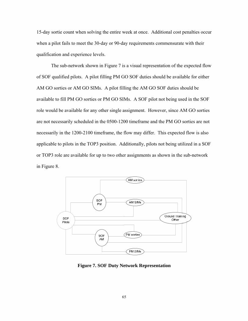
15-day sortie count when solving the entire week at once. Additional cost penalties occur

when a pilot fails to meet the 30-day or 90-day requirements commensurate with their

qualification and experience levels.

The sub-network shown in Figure 7 is a visual representation of the expected flow

of SOF qualified pilots. A pilot filling PM GO SOF duties should be available for either

AM GO sorties or AM GO SIMs. A pilot filling the AM GO SOF duties should be

available to fill PM GO sorties or PM GO SIMs. A SOF pilot not being used in the SOF

role would be available for any other single assignment. However, since AM GO sorties

are not necessarily scheduled in the 0500-1200 timeframe and the PM GO sorties are not

necessarily in the 1200-2100 timeframe, the flow may differ. This expected flow is also

applicable to pilots in the TOP3 position. Additionally, pilots not being utilized in a SOF

or TOP3 role are available for up to two other assignments as shown in the sub-network

in Figure 8.

Figure 7. SOF Duty Network Representation

65

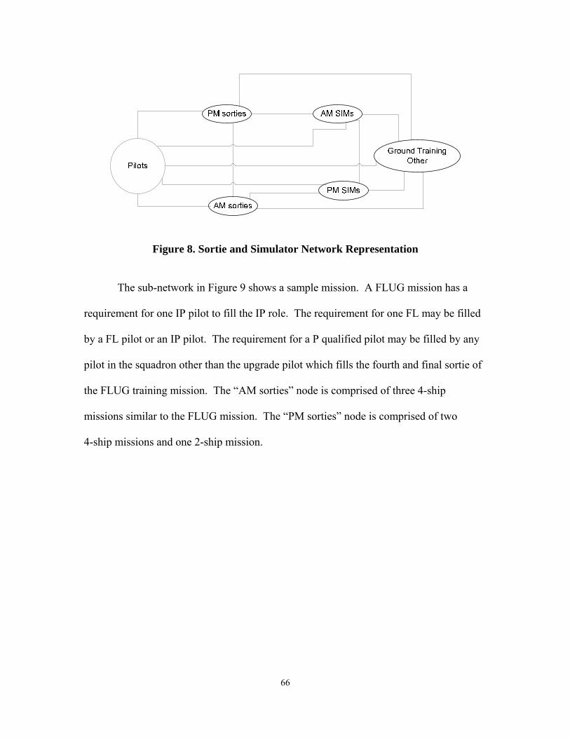
Figure 8. Sortie and Simulator Network Representation

The sub-network in Figure 9 shows a sample mission. A FLUG mission has a

requirement for one IP pilot to fill the IP role. The requirement for one FL may be filled

by a FL pilot or an IP pilot. The requirement for a P qualified pilot may be filled by any

pilot in the squadron other than the upgrade pilot which fills the fourth and final sortie of

the FLUG training mission. The “AM sorties” node is comprised of three 4-ship

missions similar to the FLUG mission. The “PM sorties” node is comprised of two

4-ship missions and one 2-ship mission.

66

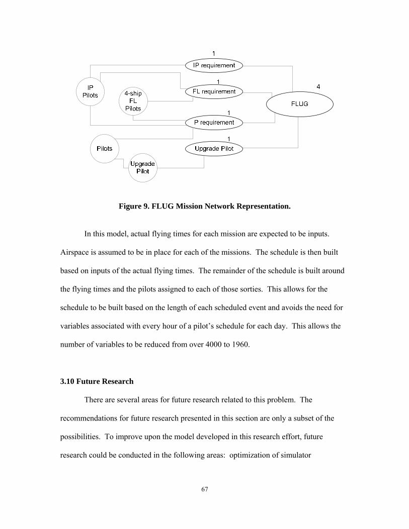
Figure 9. FLUG Mission Network Representation.

In this model, actual flying times for each mission are expected to be inputs.

Airspace is assumed to be in place for each of the missions. The schedule is then built

based on inputs of the actual flying times. The remainder of the schedule is built around

the flying times and the pilots assigned to each of those sorties. This allows for the

schedule to be built based on the length of each scheduled event and avoids the need for

variables associated with every hour of a pilot’s schedule for each day. This allows the

number of variables to be reduced from over 4000 to 1960.

3.10 Future Research

There are several areas for future research related to this problem. The

recommendations for future research presented in this section are only a subset of the

possibilities. To improve upon the model developed in this research effort, future

research could be conducted in the following areas: optimization of simulator

67

assignments, more extensive breakdown of pilot qualifications, incorporation of airspace

assignments and requirements, more pilot availability options, and development of a DO

input page.

The model developed in this research effort optimizes pilot assignments to

training mission sorties, TOP3 duties, and SOF duties. Simulator sorties are assigned

with VBA code based on training mission assignments and duties. This method allowed

for a decrease in the number of variables required to solve the weekly formulation.

Frontline’s Premium Solver Platform provides a LP/QP engine with a limit of 8000

variables and 8000 constraints. However, the LP/QP engine is limited to 2000 integer

variables. Therefore, possible ways to implement optimization of the simulator sorties

would include: a reduction of integer variables by utilizing up to 6000 non-integer

variables, an additional sub-problem for simulator optimization, or upgrading to

Frontline’s Large Scale LP/QP Solver. The Large Scale LP/QP solver provides two

options. A standard option with limits of 32,000 variables and 32,000 constraints is

available. However, the extended version has no set limits. Therefore, the limitation is

only time and computer memory (Frontline Systems, 2007).

The breakdown of pilot qualifications in this research is limited by time and lack

of subject matter experience. Specialized training provides additional qualifications that

are not accounted for in this model. A few of the qualifications not used in this research

effort include: Joint Helmet Mounted Cueing Systems (JHMCS) IP, Night Vision

Goggles (NVG) FL, NVG IP, and Mission Commander (MCC). Pilots with these

qualifications may be required in certain training missions.

68

A weighted matching of mission type to assigned training missions would provide

a name for each training mission. In the current model, training missions are numbered 1

through 6 each day. Each of these training missions should be named according to the

individuals assigned to the mission and their respective training program. For example, a

pilot in the FLUG program may be ready for FLUG-3 (Night Intercepts). The FLUG-3

mission requires a 4-ship mission with the UP, an IP, a 4-ship FL, and an additional pilot.

This mission also requires a night time sortie and either a F-15A or F-15B configuration.

Thus, this mission cannot be accomplished in a week where the UP is only assigned to

daytime AM sorties. If the UP is in a night time sortie that qualifies for the mission, it

may not be the highest priority training mission that can be accomplished with the given

set of pilots. Another pilot assigned to the same mission may be ready for a NVG

mission with a higher priority. This could be accomplished with extensive programming

to account for all the various mission types and respective requirements. Additional

formulations to solve the weighted matching problem after each GO would also be

required.

In addition to assigning mission types based on qualification of the assigned

pilots, number of aircraft in the mission, training priorities, and aircraft configuration,

some airspace restrictions eliminate the possibility of accomplishing certain training

missions. The airspace restrictions will vary from base to base. Additionally, some

squadrons may have to share limited airspace resources with other base units. Therefore,

this research area may be squadron specific or base specific.

In this research effort, pilot availability is characterized in three ways (Available,

Unavailable and DNIF). However, pilot availability is not always that easily defined.

69

Some pilots may be available for only portions of a duty day. Additionally, some pilots

may be available for only day time sorties, simulator sorties, or duties. Therefore, it may

be necessary to further breakdown pilot availabilities in order to ensure a feasible

solution is realized.

Finally, DO inputs into the scheduling process are not accounted for in this

research effort. This should be accomplished with a DO only page. A DO input of

specific pilot to specific training mission on a specified day is easier to incorporate than a

vague request that the new pilot needs to be assigned to a mission with a specified IP

sometime this week. For example, pilot 7 is to fly mission 2 on Monday. Preprocessing

this request, Mi2 = 1 and solver will fill the remaining three sorties in mission 2.

However, the vague request is harder to preprocess. One possible method would be to

iteratively assign the two pilots to each of the thirty possible missions for the week. Then

run solver on each combination, keeping only the best schedule after each successive

combination. Another possibility would be to use the underlying code to add additional

constraints to the model based on the DO inputs. Then run the solver application based

on the existing model with the additional DO input constraints.

3.11 Summary

In this chapter, a general presentation of the methodology was given. The

objectives of this research effort were presented along with the assumptions used to meet

those objectives. The decision variables were presented along with related parameters

and constraints required for the problem formulation. Two approaches to problem

formulation were provided along with detailed descriptions. The problem was

70

graphically displayed in a network representation with sub networks for more detail.

Finally, future research areas were presented. The simulator heuristic was introduced and

explained. Chapter 4 presents the test plan, test events, and results of the testing.

71

IV. Testing, Results, and Analysis

4.1 General In this chapter, the test plan and rational are presented. The results of the testing

are presented and analyzed. Corrections to the model based on test results are explained

in detail. Follow on testing is presented. Finally, the results and analysis of the follow on

testing are presented.

4.2 Test Plan In order to effectively test the model, design of experiments (DOE) was utilized.

First, the factors were listed. Then, the list of factors was reduced to a smaller set that is

considered representative of the main effects. A full factorial will test all possible

combinations for all settings of the remaining factors.

In development of the test plan, 11 factors were considered. The initial values of

the factors are based on user inputs. The factors include: number of pilots, availability of

pilots, 15-day sortie count, 30-day sortie count, 90-day sortie count, scheduled training

mission times, scheduled simulator times, SOF (AM or PM), pilot qualifications, pilot

experience levels, and CMR status. The model utilizes two methods of building the

weekly schedule (full week formulation and sub-problems). Thus, the model is really

two models rolled into one application as explained in Chapter 3. Therefore, the method

used could be a factor. Additionally, the method that utilizes sub-problems allows the

user to indicate a subset of the sub-problems to solve. However, in this case a

comparison of the two methods is preferred. Therefore, all ten sub-problems were

selected for each test run. Thus, in both cases, a full weekly schedule is developed.

72

In an effort to develop a reasonable test plan, four factors (SOF AM/PM,

experience, BMC/CMR status, and qualification level) were excluded from the formal

testing and the remaining factors were aggregated into three factors (number of available

pilots, level of difficulty imposed by mission times, and percentage of pilots eligible for

sortie count penalties) for the formal testing. Many of the factors have several

combinations of possible inputs. Therefore, a full factorial of all the factors would be

tedious and time consuming. The SOF input was eliminated from the factors and set as

an AM GO duty for the formal testing. Additionally, pilot qualification, pilot experience,

and pilot status (BMC or CMR) were eliminated from the formal testing. Pilot

qualifications, experience, and CMR status were set proportional to the number of pilots

at a level such that feasible schedules should be attainable. The number of pilots and

pilot availability were aggregated into a two-level factor (Factor A, number of available

pilots). Thus, for testing, all pilots were assumed to be available for duty each day. The

two-levels of pilots used were 23 and 43 to represent extreme cases. Both methods

optimally assign 22 sorties and three duties per day to the available pilots. Thus 23 pilots

is less than the number of daily assignments, while 43 is an excess setting. The three

sortie count factors were aggregated into a two-level factor (Factor C, percentage of

pilots eligible for sortie count penalties) such that either 25% of the available pilots may

be penalized for failing to meet sortie count requirements or 75% of the available pilots

may be penalized for failing to meet sortie count requirements. These pilots need to fly

soon and may need multiple sorties during the week to meet 30-day and 90-day

requirements. Finally, the scheduled training mission times and the scheduled simulator

times were aggregated into a two-level factor (Factor B, level of difficulty imposed by

73

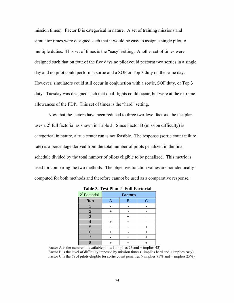
mission times). Factor B is categorical in nature. A set of training missions and

simulator times were designed such that it would be easy to assign a single pilot to

multiple duties. This set of times is the “easy” setting. Another set of times were

designed such that on four of the five days no pilot could perform two sorties in a single

day and no pilot could perform a sortie and a SOF or Top 3 duty on the same day.

However, simulators could still occur in conjunction with a sortie, SOF duty, or Top 3

duty. Tuesday was designed such that dual flights could occur, but were at the extreme

allowances of the FDP. This set of times is the “hard” setting.

Now that the factors have been reduced to three two-level factors, the test plan

uses a 23 full factorial as shown in Table 3. Since Factor B (mission difficulty) is

categorical in nature, a true center run is not feasible. The response (sortie count failure

rate) is a percentage derived from the total number of pilots penalized in the final

schedule divided by the total number of pilots eligible to be penalized. This metric is

used for comparing the two methods. The objective function values are not identically

computed for both methods and therefore cannot be used as a comparative response.

Table 3. Test Plan 23 Full Factorial 23 Factorial Factors

Run A B C 1 - - - 2 + - - 3 - + - 4 + + - 5 - - + 6 + - + 7 - + + 8 + + +

Factor A is the number of available pilots (- implies 23 and + implies 43) Factor B is the level of difficulty imposed by mission times (- implies hard and + implies easy) Factor C is the % of pilots eligible for sortie count penalties (- implies 75% and + implies 25%)

74

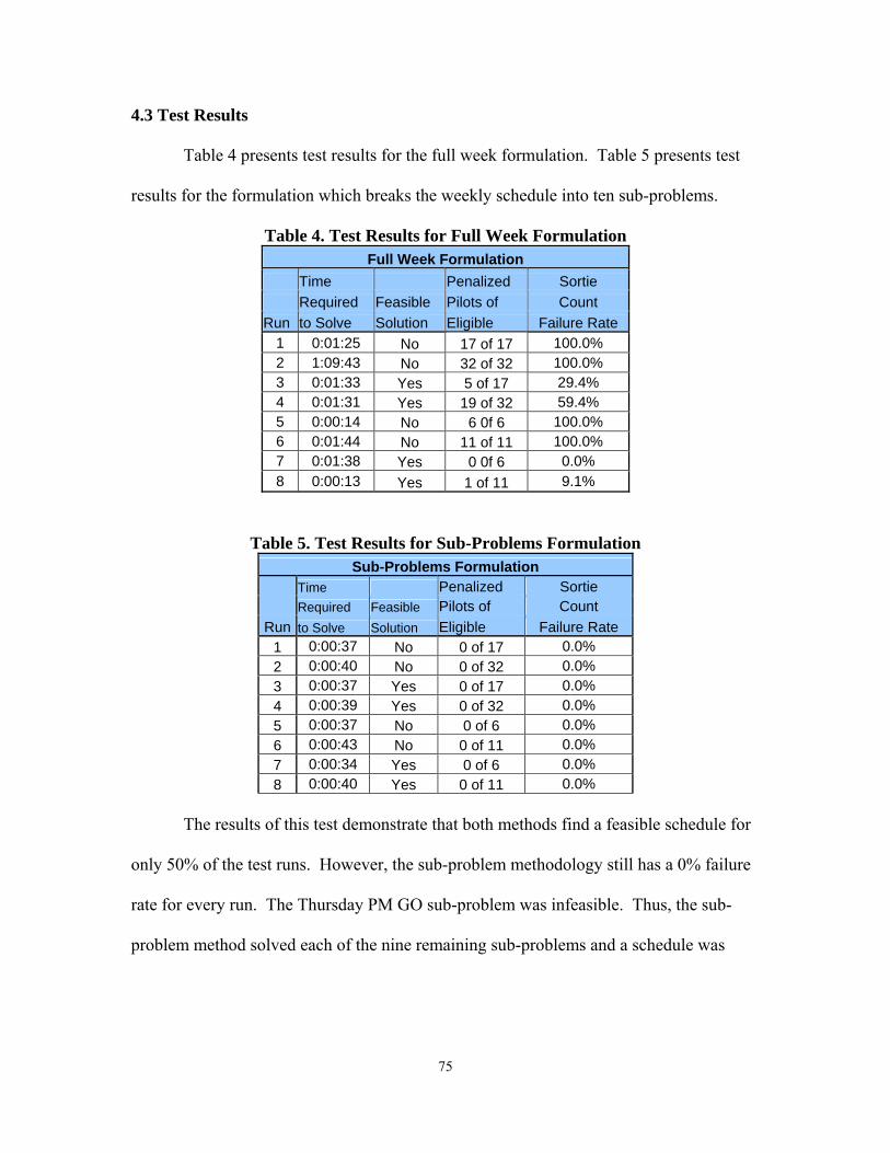
4.3 Test Results Table 4 presents test results for the full week formulation. Table 5 presents test

results for the formulation which breaks the weekly schedule into ten sub-problems.

Table 4. Test Results for Full Week Formulation Full Week Formulation

Time Penalized Sortie Required Feasible Pilots of Count Run to Solve Solution Eligible Failure Rate

1 0:01:25 No 17 of 17 100.0% 2 1:09:43 No 32 of 32 100.0% 3 0:01:33 Yes 5 of 17 29.4% 4 0:01:31 Yes 19 of 32 59.4% 5 0:00:14 No 6 0f 6 100.0% 6 0:01:44 No 11 of 11 100.0% 7 0:01:38 Yes 0 0f 6 0.0% 8 0:00:13 Yes 1 of 11 9.1%

Table 5. Test Results for Sub-Problems Formulation Sub-Problems Formulation

Time Penalized Sortie Required Feasible Pilots of Count Run to Solve Solution Eligible Failure Rate

1 0:00:37 No 0 of 17 0.0% 2 0:00:40 No 0 of 32 0.0% 3 0:00:37 Yes 0 of 17 0.0% 4 0:00:39 Yes 0 of 32 0.0% 5 0:00:37 No 0 of 6 0.0% 6 0:00:43 No 0 of 11 0.0% 7 0:00:34 Yes 0 of 6 0.0% 8 0:00:40 Yes 0 of 11 0.0%

The results of this test demonstrate that both methods find a feasible schedule for

only 50% of the test runs. However, the sub-problem methodology still has a 0% failure

rate for every run. The Thursday PM GO sub-problem was infeasible. Thus, the sub-

problem method solved each of the nine remaining sub-problems and a schedule was

75

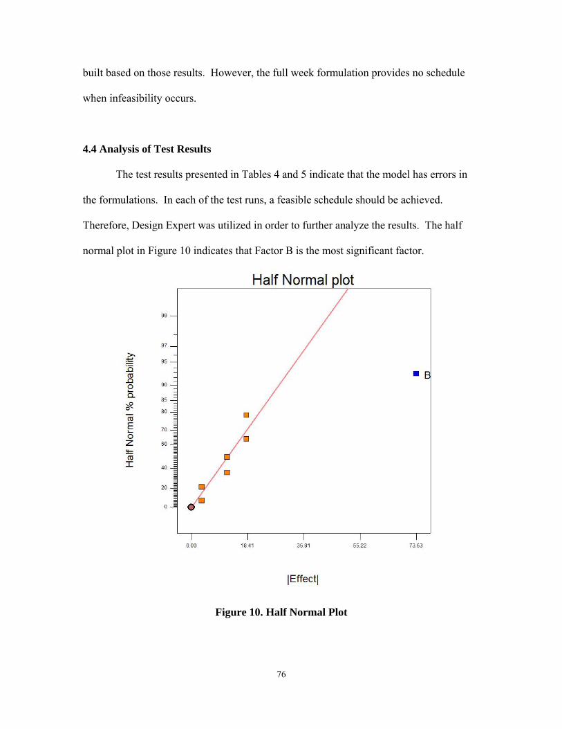
built based on those results. However, the full week formulation provides no schedule

when infeasibility occurs.

4.4 Analysis of Test Results The test results presented in Tables 4 and 5 indicate that the model has errors in

the formulations. In each of the test runs, a feasible schedule should be achieved.

Therefore, Design Expert was utilized in order to further analyze the results. The half

normal plot in Figure 10 indicates that Factor B is the most significant factor.

Figure 10. Half Normal Plot

76

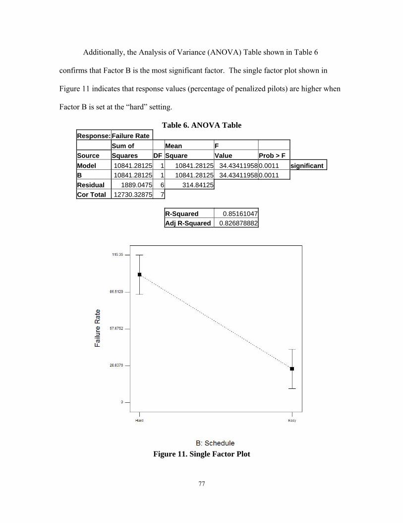
Additionally, the Analysis of Variance (ANOVA) Table shown in Table 6

confirms that Factor B is the most significant factor. The single factor plot shown in

Figure 11 indicates that response values (percentage of penalized pilots) are higher when

Factor B is set at the “hard” setting.

Table 6. ANOVA Table Response: Failure Rate Sum of Mean F Source Squares DF Square Value Prob > F Model 10841.28125 1 10841.28125 34.43411958 0.0011 significant B 10841.28125 1 10841.28125 34.43411958 0.0011 Residual 1889.0475 6 314.84125 Cor Total 12730.32875 7 R-Squared 0.85161047 Adj R-Squared 0.826878882

Figure 11. Single Factor Plot

77

Since the “hard” setting for Factor B is identified as the problem, and specifically

on Thursday’s PM GO, the training mission times for Thursday’s PM GO were examined

further. The times assigned to Thursday’s PM GO did not appear to have any impact on

the infeasibility of that particular sub-problem. However, the sub-problem for

Thursday’s PM GO is dependent upon results from Thursday’s AM GO. Therefore,

Thursday AM GO training times were examined further. This is the only point at which

an AM GO training mission is scheduled later than 0959. According to the formulation

presented in Chapter 3, this should not be a problem. However, the formula in the model

used to determine the feasibility of a pilot performing two sorties in a single day

contained an extra element which added the time stamp of the AM GO flight. The time

stamp used in the formulation is 1 = 0500-0559, 2 = 0600-0659, …..16 = 2000-2100.

Therefore, any AM GO sortie before 1000 is not a problem as it adds 5 or less to a

formula that is constrained to be less than or equal to 5. However, any AM GO flight

after 0959 would add 6 or more to the formula which is constrained in the PM GO. Thus,

the PM GO sub-problem becomes infeasible.

The full week formulation did not have the same problem. The formula used in

the full week formulation for the feasibility of a pilot to perform two sorties in a single

day is different than the one used in the sub-problems. Therefore, further investigation

was required to identify the problem with the full week method. The formula used to

ensure that crew rest requirements were met did not properly account for the timing of

the AM GO sortie. Therefore, when the AM GO sortie occurred at a later time, the

78

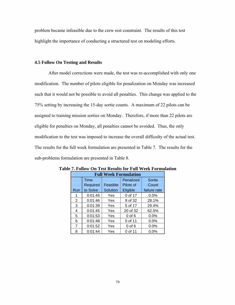
problem became infeasible due to the crew rest constraint. The results of this test

highlight the importance of conducting a structured test on modeling efforts.

4.5 Follow On Testing and Results After model corrections were made, the test was re-accomplished with only one

modification. The number of pilots eligible for penalization on Monday was increased

such that it would not be possible to avoid all penalties. This change was applied to the

75% setting by increasing the 15-day sortie counts. A maximum of 22 pilots can be

assigned to training mission sorties on Monday. Therefore, if more than 22 pilots are

eligible for penalties on Monday, all penalties cannot be avoided. Thus, the only

modification to the test was imposed to increase the overall difficulty of the actual test.

The results for the full week formulation are presented in Table 7. The results for the

sub-problems formulation are presented in Table 8.

Table 7. Follow On Test Results for Full Week Formulation Full Week Formulation

Time Penalized Sortie Required Feasible Pilots of Count Run to Solve Solution Eligible failure rate

1 0:01:45 Yes 0 of 17 0.0% 2 0:01:46 Yes 9 of 32 28.1% 3 0:01:39 Yes 5 of 17 29.4% 4 0:01:45 Yes 20 of 32 62.5% 5 0:01:53 Yes 0 of 6 0.0% 6 0:01:48 Yes 0 of 11 0.0% 7 0:01:52 Yes 0 of 6 0.0% 8 0:01:44 Yes 0 of 11 0.0%

79

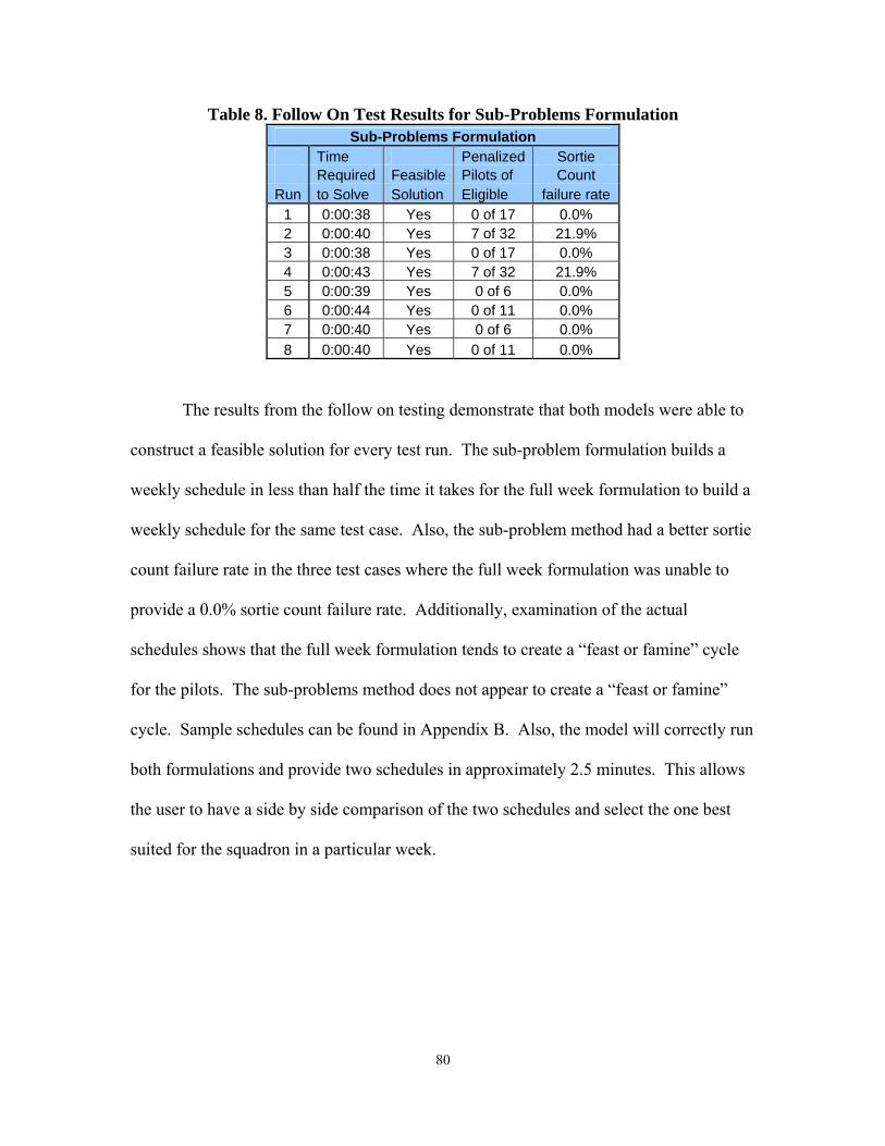
Table 8. Follow On Test Results for Sub-Problems Formulation Sub-Problems Formulation

Time Penalized Sortie Required Feasible Pilots of Count Run to Solve Solution Eligible failure rate

1 0:00:38 Yes 0 of 17 0.0% 2 0:00:40 Yes 7 of 32 21.9% 3 0:00:38 Yes 0 of 17 0.0% 4 0:00:43 Yes 7 of 32 21.9% 5 0:00:39 Yes 0 of 6 0.0% 6 0:00:44 Yes 0 of 11 0.0% 7 0:00:40 Yes 0 of 6 0.0% 8 0:00:40 Yes 0 of 11 0.0%

The results from the follow on testing demonstrate that both models were able to

construct a feasible solution for every test run. The sub-problem formulation builds a

weekly schedule in less than half the time it takes for the full week formulation to build a

weekly schedule for the same test case. Also, the sub-problem method had a better sortie

count failure rate in the three test cases where the full week formulation was unable to

provide a 0.0% sortie count failure rate. Additionally, examination of the actual

schedules shows that the full week formulation tends to create a “feast or famine” cycle

for the pilots. The sub-problems method does not appear to create a “feast or famine”

cycle. Sample schedules can be found in Appendix B. Also, the model will correctly run

both formulations and provide two schedules in approximately 2.5 minutes. This allows

the user to have a side by side comparison of the two schedules and select the one best

suited for the squadron in a particular week.

80

4.6 Summary

In Chapter 4 test plans were explained, test results were presented, test failures

were addressed, and follow on testing with results were presented. Chapter 5 provides

conclusions from the overall research effort and the testing.

81

V. Conclusions

5.1 General

This chapter reviews the key elements of this research effort and discusses the

research conclusions. This chapter also makes recommendations for future research and

for model usage. The fighter training squadron pilot scheduling problem is complex.

The current process is tedious and mostly manual. Often, inexperienced pilots are

charged with the task of building the weekly schedule. These inexperienced pilots lose

hours of valuable training time.

The problem background is presented in Chapter 1. A list of factors and

scheduling considerations are also presented in Chapter 1. Scheduling problems exists in

many areas and a great deal of research has been conducted on the various types of

scheduling problems. Chapter 2 presents the literature reviewed for this research. The

problems presented in Chapter 2 reflect scheduling research related to the fighter training

squadron pilot scheduling problem. Two methodologies are presented in Chapter 3. A

full week methodology with a single formulation is presented. Then a sub-problem

methodology that consists of ten sub-problems is presented. Chapter 3 also presents a

formulation for each methodology. Then Chapter 4 presents the test plan and results.

5.2 Key Elements

The idea of building a solution based on partial solutions as presented by Combs

and Moore presents an approach for dealing with large scale scheduling problems

(Combs 2002, Combs and Moore 2004). Preprocessing is a key element used to define

82

the costs associated with penalties and with assigning non-squadron pilots to sorties.

Preprocessing is presented in Chapter 2 in the discussion of Shirley’s research (Shirley,

1994). In the two methodologies presented in Chapter 3, preprocessing is used to set the

parameters for each formulation (full week and each of the ten sub-problems). The ten

sub-problems provide partial solutions that are combined to provide an overall solution.

5.3 Research Conclusions

This research effort provides an approach for dealing with the many complexities

of the fighter training squadron pilot scheduling problem. The approach used here

minimized the overall size of the problem with the use of preprocessing and development

of a heuristic to assign pilots to simulator sorties. Additionally, the MP model is relaxed

to ensure that a feasible solution will be found. The test results demonstrate the models

ability to solve both formulations (full week and sub-problems) and construct a feasible

schedule based on those solutions and the simulator heuristic. However, a violation of

any of the assumptions presented in Chapter 3 may make finding a feasible solution

impossible.

5.4 Recommendations for Future Research

Recommended areas of future research include the following: optimization of

simulator assignments, more extensive breakdown of pilot qualifications, incorporation

of airspace assignments and requirements, more pilot availability options, and

development of a DO input page. Each of these areas of research is discussed in more

detail in Chapter 3. Future research is not limited to these areas. However, the

83

incorporation of these problem characteristics along with a heuristic to set up a weighted

matching problem for assigning specific training mission types (i.e. FLUG-2, IPUG-3,

NVG-3) missions should result in a highly effective and useful model.

The sub-problem methodology is recommended for use with future research. The

sub-problem methodology appears to be more efficient and prevents the “feast or famine”

cycle. Additionally, the 280 integer variables used in each sub-problem will allow

incorporation of new integer variables. The Premium Solver platform from Frontline

Systems has a limit of 2000 integer variables. The full week formulation uses 1960

integer variables and is very close to the limit.

5.4 Recommendations for Model Usage

The model developed in this research, inclusive of both formulations, may be

useful in its current state. However, the pilot responsible for building the weekly

schedule must assign names to the missions on the final schedule. This model is

designed to schedule a single squadron of up to 50 pilots for training missions, TOP3 and

SOF duties, and simulator sorties only. A user manual is presented in Appendix C to

address the specific details for using this model.

84

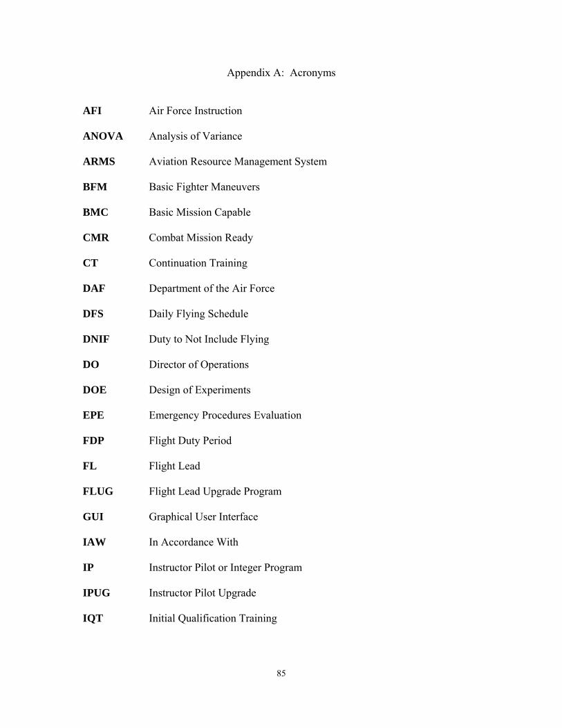
Appendix A: Acronyms

AFI Air Force Instruction ANOVA Analysis of Variance ARMS Aviation Resource Management System BFM Basic Fighter Maneuvers BMC Basic Mission Capable CMR Combat Mission Ready CT Continuation Training DAF Department of the Air Force DFS Daily Flying Schedule DNIF Duty to Not Include Flying DO Director of Operations DOE Design of Experiments EPE Emergency Procedures Evaluation FDP Flight Duty Period FL Flight Lead FLUG Flight Lead Upgrade Program GUI Graphical User Interface IAW In Accordance With IP Instructor Pilot or Integer Program IPUG Instructor Pilot Upgrade IQT Initial Qualification Training

85

IRC Instrument Refresher Course JHMCS Joint Helmet Mounted Cueing System LFJ Least Flexible Job LFM Least Flexible Machine LP Linear Program MAJCOM Major Command MCC Mission Commander MOL Mission Order List MP Mathematical Programming MQT Mission Qualification Training NP Nondeterministic Polynomial-time NVG Night Vision Goggles ODM Operations Data Management PEP Production Eagle Package PEX Patriot Excalibur Scheduling Software PME Professional Military Education QP Quadratic Program RAP Ready Aircrew Program SAT Surface Attack Tactics SEAD Suppression of Enemy Air Defenses SIM Simulator SOF Supervisor of Flying TDY Temporary Duty

86

TOP 3 Designated Daily Squadron Supervisor UP Upgrade Pilot VBA Visual Basic for Applications

87

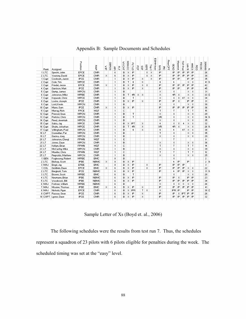
Appendix B: Sample Documents and Schedules

Sample Letter of Xs (Boyd et. al., 2006) The following schedules were the results from test run 7. Thus, the schedules

represent a squadron of 23 pilots with 6 pilots eligible for penalties during the week. The

scheduled timing was set at the “easy” level.

88

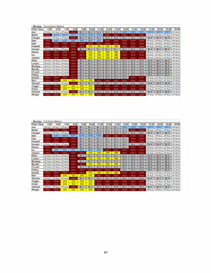
89

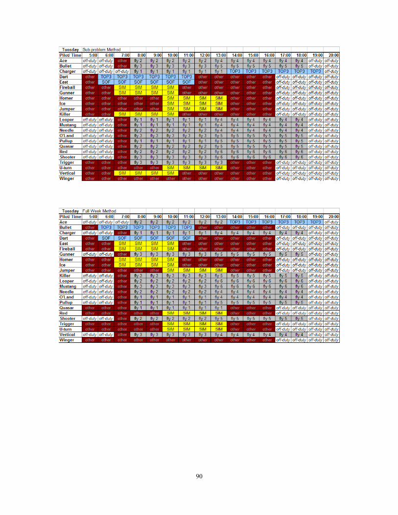
90

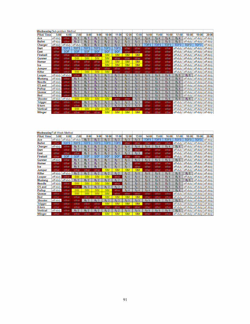
91

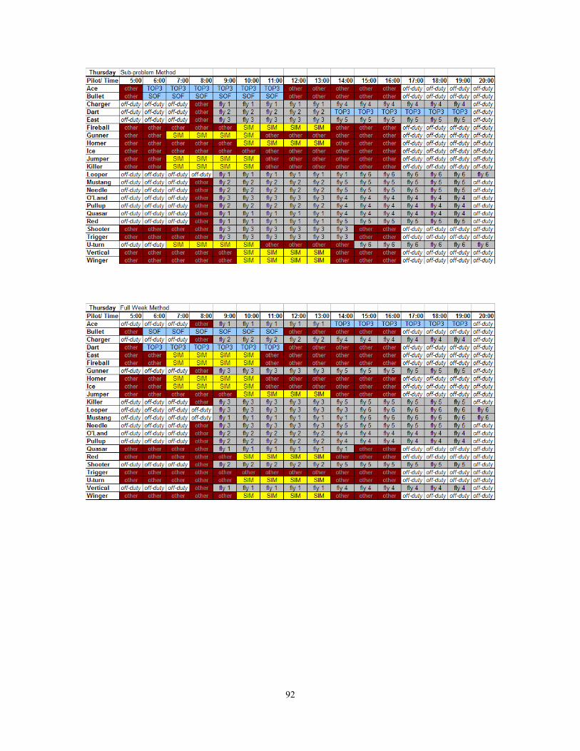
92

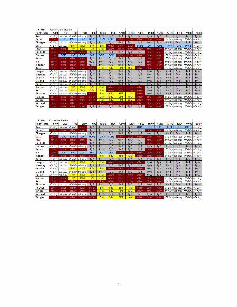
93

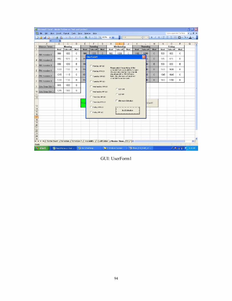
GUI: UserForm1

94

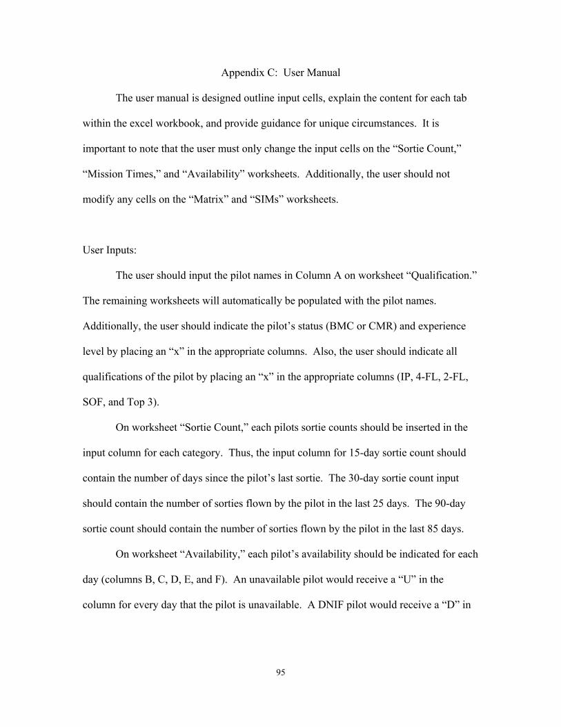
Appendix C: User Manual

The user manual is designed outline input cells, explain the content for each tab

within the excel workbook, and provide guidance for unique circumstances. It is

important to note that the user must only change the input cells on the “Sortie Count,”

“Mission Times,” and “Availability” worksheets. Additionally, the user should not

modify any cells on the “Matrix” and “SIMs” worksheets.

User Inputs:

The user should input the pilot names in Column A on worksheet “Qualification.”

The remaining worksheets will automatically be populated with the pilot names.

Additionally, the user should indicate the pilot’s status (BMC or CMR) and experience

level by placing an “x” in the appropriate columns. Also, the user should indicate all

qualifications of the pilot by placing an “x” in the appropriate columns (IP, 4-FL, 2-FL,

SOF, and Top 3).

On worksheet “Sortie Count,” each pilots sortie counts should be inserted in the

input column for each category. Thus, the input column for 15-day sortie count should

contain the number of days since the pilot’s last sortie. The 30-day sortie count input

should contain the number of sorties flown by the pilot in the last 25 days. The 90-day

sortie count should contain the number of sorties flown by the pilot in the last 85 days.

On worksheet “Availability,” each pilot’s availability should be indicated for each

day (columns B, C, D, E, and F). An unavailable pilot would receive a “U” in the

column for every day that the pilot is unavailable. A DNIF pilot would receive a “D” in

95

the column for every day that the pilot is DNIF. Any other input or a blank cell indicates

the pilot is available.

On worksheet “Mission Times,” the user should indicate the start times for

mission briefings and simulator briefings. Additionally, the user should input mission

times, simulator times, and configurations. Simulator configuration is optional.

Additionally, the model will indicate an error for the inputs on this page when an initial

brief time is scheduled later than the take-off time, when the mission times exceed the

schedule boundaries (0500-2000), when there is missing information, and when there is

less than 15 minutes between brief time and take-off time. These errors will be indicated

by red blocks and an error message. When the times are set for the model message will

change to “Times are set for the model” and the block will turn green. However, the

model will still run with the error message. However, the results may or may not be

useful.

Running the Model:

After all the inputs are correctly made, the user will click the “START” button on

the “Mission Times” worksheet. The model will then clear all cells used by the solver.

After the cells are cleared, a GUI will appear. The user will select what portion of the

weekly schedule the model should build, AM or PM SOF setting, and alternate schedule

(if desired). After completing the selections, the use will click the “Build Schedule”

button. The schedules will be constructed and may be viewed on worksheets “Schedule”

and “Schedule 2.” The alternate schedule is the full week method and will be presented

on worksheet “Schedule 2.” Once the schedules are built it is recommended to copy and

96

paste the schedules into another spreadsheet for any modifications. The user may move

off-duty time and other time. Additionally, the user may choose to move a simulator

assignment from one pilot to another. However, if flight times need to change it is

recommended that the model is rerun with the correct times.

Schedules:

The resulting schedules are independent of each other. Thus, it is recommended

that the user does NOT use days from one schedule with days from the other schedule.

This may result in violations of crew rest. If the model is unable to fill all of the mission

sortie demands with the pilots listed by the user, then below that days schedule will be a

message indicating which mission needs a pilot and what qualification level that is

required. Ultimately, it is the responsibility of the scheduler and the individual pilots to

ensure that the schedule is acceptable and that FDP and crew rest restrictions are not

violated.

Unique Circumstances:

There are unique circumstances in which the model will not produce a useful

schedule. A few cases are presented with suggestions for resolving the issue. If a

squadron has only one Top 3 qualified pilot available, the model will fail to solve the

weekly schedule. However, if the user places this pilot in the list twice and marks the

availability as DNIF. The model will then assign the first occurrence of this pilot to one

Top 3 duty (AM GO or PM GO) and the second occurrence will be assigned to the other

Top 3 duty.

97

Next, if the model is assigning all the Top 3 qualified pilots to AM GO mission

sorties and Top 3 or SOF duty. A circumstance may result that the model does not solve

the PM GO for that day because there are no available Top 3 pilots for the PM GO Top 3

duty. The user may select one of the Top 3 qualified pilots being assigned to an AM GO

sortie and set the availability of that pilot to “D”. Then the model should assign that pilot

in the PM GO Top 3 duty.

Finally, one or more pilots in the squadron may require additional time in the

simulator. The model may be assigning this pilot to other activities that prevent

simulator time. To resolve this issue the user can mark this pilot as DNIF or unavailable

on the “Availability” worksheet. Then, after the model has finished running, copy the

final schedule into another spreadsheet and manually move simulator sorties to the

required pilot(s).

98

Bibliography 1. Aslan, Davut. A Decision Support System for Effective Scheduling in an F-16 Pilot

Training Squadron, MS thesis, AFIT/GOR/ENS 03-01. Graduate School of Management and Engineering, Air Force Institute of Technology (AU), Wright-Patterson AFB OH, March 2003.

2. Boyd, Jay A. H., Case A. Cunningham, Darren P. Gray, and John L. Parker.

Network Flow Model For Optimizing Fighter Squadron Scheduling, Graduate Research Project, AFIT/ENV ISL-06J. Graduate School of Management and Engineering, Air Force Institute of Technology (AU), Wright-Patterson AFB OH, June 2006.

3. Combs, Todd E. “A Hybrid Tabu Search/Set Partitioning Approach to Tanker Crew

Scheduling,” Military Operations Research, Volume 9 Number 1: 43-56 (2004). 4. Department of the Air Force, F-15 Aircrew Training, AFI 11-2F-15V1.

Washington: HQ USAF, 19 Jul 2004. 5. Department of the Air Force, Flying Hour Program Management. AFI 11-202.

Washington: HQ USAF, 05 Apr 2006. 6. Department of Defense, Dictionary of Military and Associated Terms, Joint

Publication 1-02, 12 April 2001. 7. Gronkvist, Mattias. “Accelerating column generation for aircraft scheduling using

constraint propagation,” Computers & Operations Research, 33: 2918-2934 (2006). 8. Knighton, Shane A., Jeffery K. Cochran, Ira A. Fulton. A Network-flow Based

Mathematical Programming Approach to Optimal Rostering of Continuous Heterogeneous Workforces, Submitted to Computers and Operations Research.

9. Nquyen, Cuong T. An Interactive Decision Support System For Scheduling Fighter

Pilot Training, MS thesis, AFIT/GOR/ENS/02-12. Graduate School of Management and Engineering, Air Force Institute of Technology (AU), Wright-Patterson AFB OH, March 2002.

10. Pinedo, Michael. Scheduling: Theory, Algorithms, and Systems, 2nd Edition, 2000. 11. Shirley, Michael D. Jr. An Improved Heuristic for Intercontinental Ballistic

Missile Crew Scheduling, MS thesis, AFIT/GOA/ENS 94D-01. Graduate School of Management and Engineering, Air Force Institute of Technology (AU), Wright-Patterson AFB OH, March 1994.

99

12. Yan, Shangyao, Jei-Chi Chang. “Airline cockpit crew scheduling,” European Journal of Operational Research 136: 501-511 (2002).

100

Vita Lieutenant Thomas M. Newlon graduated from Buckhannon-Upshur High School

in Buckhannon, West Virginia. He entered undergraduate studies at West Virginia

Wesleyan College in Buckhannon, West Virginia but left the school after completing his

sophomore year. Three years later he returned to undergraduate studies at Fairmont State

College (now a university) in Fairmont, West Virginia where he graduated with a

Bachelor of Science degree in Mathematics and a Bachelor of Arts degree in Education,

specializing in Mathematics 5-12, May 1999. He was commissioned through the Officer

Training School at Maxwell Air Force Base on 4 April 2003.

His first assignment was at Eglin AFB as an operations analyst for Air Force

Operational Test and Evaluation Center (AFOTEC) Detachment 2 in April 2003. During

this period of time he worked mostly with the Operational testing of the Large Aircraft

Infrared Countermeasures (LAIRCM) System. He also Flew 16 testing sorties as a Flight

Test Engineer (FTE) in support of the testing effort. He also worked with the Advanced

Strategic and Tactical Expendable (ASTE) and Miniature Air Launch Decoy (MALD)

programs. In August 2005, he entered the Graduate School of Engineering and

Management, Air Force Institute of Technology. Upon graduation, he will be assigned to

Air Combat Command Headquarters (ACC/HQ) at Langley AFB.

101

REPORT DOCUMENTATION PAGE Form Approved OMB No. 074-0188

The public reporting burden for this collection of information is estimated to average 1 hour per response, including the time for reviewing instructions, searching existing data sources, gathering and maintaining the data needed, and completing and reviewing the collection of information. Send comments regarding this burden estimate or any other aspect of the collection of information, including suggestions for reducing this burden to Department of Defense, Washington Headquarters Services, Directorate for Information Operations and Reports (0704-0188), 1215 Jefferson Davis Highway, Suite 1204, Arlington, VA 22202-4302. Respondents should be aware that notwithstanding any other provision of law, no person shall be subject to an penalty for failing to comply with a collection of information if it does not display a currently valid OMB control number. PLEASE DO NOT RETURN YOUR FORM TO THE ABOVE ADDRESS. 1. REPORT DATE (DD-MM-YYYY)

20-03-2007 2. REPORT TYPE

Master’s Thesis 3. DATES COVERED (From – To)

Sep 2005 - Mar 2007 5a. CONTRACT NUMBER

5b. GRANT NUMBER

4. TITLE AND SUBTITLE MATHEMATICAL PROGRAMMING MODEL FOR FIGHTER TRAINING SQUADRON PILOT SCHEDULING

5c. PROGRAM ELEMENT NUMBER

5d. PROJECT NUMBER 5e. TASK NUMBER

6. AUTHOR(S) Newlon, Thomas, M., Lieutenant, USAF

5f. WORK UNIT NUMBER

7. PERFORMING ORGANIZATION NAMES(S) AND ADDRESS(S) Air Force Institute of Technology Graduate School of Engineering and Management (AFIT/EN) 2950 Hobson Street, Building 642 WPAFB OH 45433-7765

8. PERFORMING ORGANIZATION REPORT NUMBER AFIT/GOR/ENS/07-17

10. SPONSOR/MONITOR’S ACRONYM(S)

9. SPONSORING/MONITORING AGENCY NAME(S) AND ADDRESS(ES) AFOSR/NM Attn: Fariba Fahroo, Ph.D. 875 North Randolph Street Suite 325, Room 3112 Arlington, VA 22203 DSN: 426-8429

11. SPONSOR/MONITOR’S REPORT NUMBER(S)

12. DISTRIBUTION/AVAILABILITY STATEMENT APPROVED FOR PUBLIC RELEASE; DISTRIBUTION UNLIMITED. 13. SUPPLEMENTARY NOTES 14. ABSTRACT The United States Air Force fighter training squadrons build weekly schedules using a long and tedious process. Very little of this process is automated and optimality of any kind is nearly impossible. Schedules are built to a feasible condition only to be changed with consideration of Wing level requirements. Weekly flying schedules are restricted by requirements for crew rest, days since a pilot’s last sortie, sorties in the last 30 days, and sorties in the last 90 days. By providing a scheduling model to the pilot charged with creating the schedule, valuable pilot hours could be spent in the cockpit, simulator, or other required duty. This research effort presents a mathematical programming (MP) approach to the fighter squadron pilot training scheduling problem. The methodology presented is based on binary variables that will provide integer solutions to every feasible set of inputs. A simulator heuristic developed specifically for this problem assigns pilots to simulator sorties based on the feasible solutions obtained from two different formulation and solving approaches. One approach assigns training mission sorties and duties for the entire week, while the other approach breaks the week into ten successive sub-problems. The model constructs two feasible schedules in approximately 2.5 minutes. 15. SUBJECT TERMS Integer Programming, Scheduling, Preprocessing, Heuristic Methods, Penalties

16. SECURITY CLASSIFICATION OF: 19a. NAME OF RESPONSIBLE PERSON James T Moore, Dr. (ENS)

a. REPORT

U

b. ABSTRACT

U

c. THIS PAGE

U

17. LIMITATION OF ABSTRACT

UU

18. NUMBER OF PAGES

113 19b. TELEPHONE NUMBER (Include area code) (937) 255-3636, ext 4528; e-mail: James.Moore@afit.edu

Standard Form 298 (Rev. 8-98) Prescribed by ANSI Std. Z39-18