WEIGHTED MAHALANOBIS DISTANCE FOR

CO-J HYPER-ELLIPSOIDAL CLUSTERING

THESISKhaled S. YounisCaptain, RJAF

AFIT/GE/ENG/96D-22

DTIC QUALITY INSPEC7M 3

DEPARTMENT OF THE AIR FORCEAIR UNIVERSIY

AIR FORCE INSTITUTE OF TECHNOLOGY

Wri ght-Potteqipr ~ a~~q j

IAPProve for publIc r~mI Dt3I~iUuulOD U31

AFIT/GE/ENG/96D-22

WEIGHTED MAHALANOBIS DISTANCE FOR

HYPER-ELLIPSOIDAL CLUSTERING

THESISKhaled S. YounisCaptain, RJAF

AFIT/GE/ENG/96D-22

, DMC QUAI = II PEt D 3

Approved for public release; distribution unlimited

AFIT/GE/ENG/96D-22

WEIGHTED MAHALANOBIS DISTANCE FOR

HYPER-ELLIPSOIDAL CLUSTERING

THESIS

Presented to the Faculty of the Graduate School of Engineering

of the Air Force Institute of Technology

Air University

In Partial Fulfillment of the

Requirements for the Degree of

Master of Science in Electrical Engineering

Khaled S. Younis, B.S.E.E

Captain, RJAF

December, 1996

Approved for public release; distribution unlimited

The views expressed in this thesis are those of the author and do not reflect the official policy or position

of the Department of Defense or the U. S. Government.

Acknowledgements

At first, I thank God for giving me the ability to finish this research effort and to

learn a little more about one small aspect of His universe. I would like also to thank the

Royal Jordanian Air Force for giving me the great opportunity to study at the Air Force

Institute of Technology.

This thesis could not have been done without the help of few individuals who deserve

thanks and credit. First of all, I owe a great deal of thanks to my advisor, Dr. Steven

Rogers, for his sharp insight, expertise, and enthusiasm. He provided me with plenty of

rope, but still kept me from hanging myself. I thank him for the constant encouragement

during the last few months. The comments of the other committee members, Dr. Martin

DeSimio and Dr. Mathew Kabriski, have been extremely helpful to me in bringing this

report to its finished form. Thanks to Dr DeSimio for providing friendly encouragement

and many interesting discussions on new and bizarre clustering methods. I would like to

thank my sponsor, Maj. Tom Burns from Wright Labs, for his support and guidance. I am

also grateful for the network support provided so ably by Dan Zambon and Dave Doak.

I wish to acknowledge the support of the International Military Students Office and

the assistance of Mr. Vic Grazier who helped me and other international students and our

families since we arrived here.

Most importantly, I owe the greatest amount of gratitude to my wife, Maha. Her

contribution to this project by her willing sacrifice of time and effort to support me may

never be fully assessed. I feel lucky that God has chosen me to be your husband. Last but

not least, I owe a special thanks for my beautiful daughter, Mira, and my son, Mostafa,

for the joy that they add to my life. I hope that one day you will realize how many times

I wanted to be with you but I couldn't.

Khaled S. Younis

ii

Table of Contents

Page

Acknowledgements .. .. .. .. ... ... ... ... ... ... .... ... . ......

List of Figures. .. .. .. ... ... ... .... ... ... ... ... ... ..... vi

List of Tables. .. .. .. .. ... .... ... ... ... ... ... ... ... .... viii

Abstract .. .. .. .. .. .... ... ... ... ... ... ... ... ... ... ... ix

I. Introduction .. .. .. .. .. ... .... ... ... ... ... ... ... ... 1

1.1 Background .. .. .. .. ... ... ... ... ... ... ... ... 1

1.2 Problem Statement .. .. .. ... ... ... ... .... ...... 3

1.3 Summary of Current Knowledge. .. .. .. ... ... ... ..... 3

1.4 Scope. .. .. .. ... ... ... ... ... ... ... ... .... 4

1.5 Approach .. .. .. .. ... ... ... ... ... ... ... .... 4

1.6 Research Objectives .. .. .. .. ... ... .... ... ... ... 5

1.7 Thesis Organization .. .. .. .. ... ... ... .... ... ... 5

1.8 Summary .. .. .. .. ... ... ... ... ... ... .... ... 5

II. Theory .. .. .. .. .. .... ... ... ... ... ... ... ... ... ... 6

2.1 Introduction .. .. .. ... ... ... ... ... ... ... ..... 6

2.2 Pattern Classification. .. .. .. ... ... ... ... ... .... 6

2.3 The Clustering Problem. .. .. .. .. ... ... ... ... .... 8

2.3.1 Similarity Measures .... .. .. .. .. .. .. .. 10

2.3.2 Optimality Criterion .. .. .. .. ... ... ... ..... 12

2.4 The Batch k-means Algorithm. .. .. .. ... ... ... ..... 14

2.4.1 The LBG Algorithm .. .. .. .. ... ... ... ..... 15

2.4.2 The Fuzzy c-means Algorithm. .. .. ... ... ...... 15

iii

Page

2.5 Principal Component Analysis ..... ................... 17

2.6 Clustering Based on The Mahalanobis Distance .............. 19

2.6.1 Problems with Integrating The Mahalanobis Distance in

Clustering ....... .......................... 19

2.6.2 The Hyperellipsoidal Clustering (HEC) Neural Network 20

2.6.3 The Weighted Mahalanobis Distance Clustering Algorithm 25

2.6.4 Relation to Maximum Likelihood Estimate in The Gaus-

sian Mixture Model (GMM) ..................... 28

2.7 Summary ........ ............................... 33

III. Methods ......... ...................................... 34

3.1 Introduction ........ ............................. 34

3.2 A General Approach for Batch k-means Clustering ........... 34

3.2.1 Preprocessing .............................. 35

3.2.2 Initialization ....... ........................ 35

3.2.3 Partitioning ............................... 39

3.2.4 Codebook Update ...... ..................... 39

3.2.5 Clustering Evaluation ..... ................... 39

3.3 The LBG Algorithm Implementation ..................... 40

3.4 The Fuzzy c-means Algorithm Implementation ............. 40

3.5 The WMD Algorithm Implemetation .... ............... 41

3.6 Principal Component Analysis Network .................. 42

3.7 Hyperellipsoidal Clustering Algorithm ................... 43

3.8 Summary ........ ............................... 43

IV. Results ......... ....................................... 45

4.1 Introduction ........ ............................. 45

4.2 Two-Dimensional Test Cases ...... .................... 46

4.3 Clustering of The Iris Data ...... ..................... 49

iv

Page

4.4 Vector Quantization Coding of Image Data. .. .. .. ... .... 51

4.5 Summary. .. .. .. ... ... ... ... ... ... ... ..... 55

V. Conclusion .. .. .. ... ... ... ... .... ... ... ... ... .... 56

5.1 Introduction. .. .. .. ... ... .... ... ... ... ...... 56

5.2 Contributions .. .. .. .. .. .... ... ... ... ... ...... 56

5.3 Follow-on Research .. .. .. .. .. ... .... ... ... ...... 57

5.4 Summary of Results. .. .. .. ... ... ... ... ... ..... 57

5.5 Conclusions. .. .. .. .. ... ... ... .... ... ... .... 58

Appendix A. Clustering Codes. .. .. .. .. ... ... ... ... ... ..... 59

A.1 cluster.m. .. .. .. ... ... ... ... ... .... ... .... 59

A.1.1 getdata.m .. .. .. .. ... ... ... ... ... ..... 72

A.1.2 KLI.m. .. .. .. .. ... ... .... ... ... ...... 74

A.1.3 plotclusters.m. .. .. .. .. ... ... ... ... ..... 78

A.2 Hyperellipsoidal Clustering (HEC) algorithm .. .. .. .. ..... 80

A.2.1 HEC.m .. .. .. ... ... ... ... ... ... ..... 80

A.2.2 HECVQ.II. .. .. .. .... ... ... ... ... .... 85

A.2.3 PCA.m .. .. .. ... ... ... ... ... ... ..... 88

Appendix B. Vector Quantization Code .. .. .. ... .... ... ... .... 90

B.1 ImageVQ.m. .. .. .. .. ... ... ... ... ... ... ..... 90

Bibliography .. .. .. ... ... ... ... ... ... ... ... ... .... .... 94

Vita. .. .. .. ... ... ... ... ... ... ... ... ... ... .... ...... 97

v

List of Figures

Figure Page

1. Projection of the Iris data set onto the plane spanned by the first two prin-

cipal components ........ ................................ 11

2. Results of clustering the shown patterns into two classes using the Euclidean

and the Mahalanobis distance metrics .......................... 12

3. The case where a large cluster engulfs a neighboring smaller cluster. (a) The

first cluster has more samples than the second class. (b) More samples are

assigned to the cluster of the left as the iterative process continues . . . . 19

4. The results of clustering using the Mahalanobis distance in subsequent iter-

ations. JGMSE is smaller in the first iteration (a) than in the next iteration

(b ) .. . . . . . . . . . . . . . . . . . . . . . . . . . . . . . . . . . . . . . . . 21

5. Principal component analysis neural network ..................... 22

6. Architecture of the neural network for Hyperellipsoidal clustering (HEC) . 24

7. The four different Gaussians detected using the GMM/EM approach using

initial parameters estimated from applying the LBG algorithm with Eu-

clidean distance ........ ................................. 32

8. Flowchart of the general approach to perform batch k-means clustering . . 34

9. Scatter plot for the Daisy data set ............................. 38

10. Flowchart of the HEC algorithm .............................. 43

11. Gaussians data set (a) and location of cluster centers upon convergence (b)

LBG, (c) FCM, (d) WMD ................................... 47

12. Original and computed partitioning of a mixture of Gaussian data using the

different clustering methods. (a) Original classes. (b)-(f): Resultant One-

nearest neighbor classification using the codebook generated by HEC, LBG,

FCM, WMDC, and WMDVC methods, respectively. ............... 48

13. Original and computed partitioning of Iris data using the different clustering

methods. (a) Original classes. (b)-(f): Resultant One-nearest neighbor

classification using the codebook generated by LBG, FCM, HEC , WMD

with conscience, and WMD with volume constraint methods, respectively. 50

vi

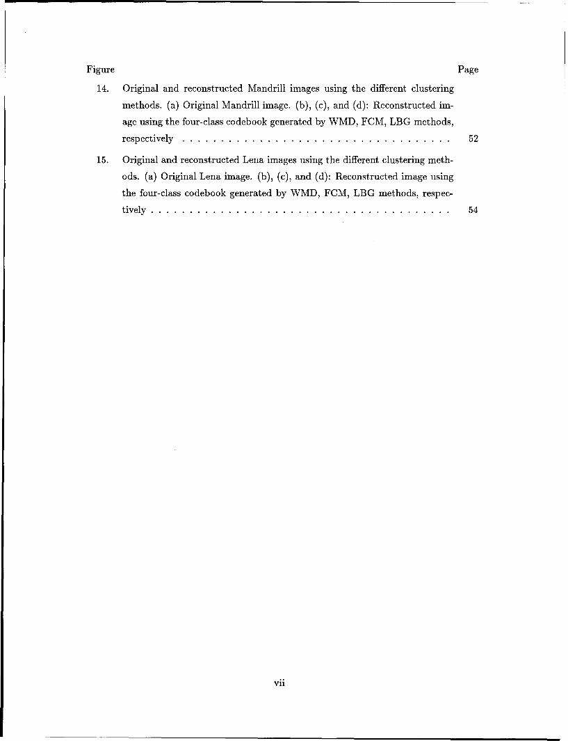
Figure Page

14. Original and reconstructed Mandrill images using the different clustering

methods. (a) Original Mandrill image. (b), (c), and (d): Reconstructed im-

age using the four-class codebook generated by WMD, FCM, LBG methods,

respectively ......... ................................... 52

15. Original and reconstructed Lena images using the different clustering meth-

ods. (a) Original Lena image. (b), (c), and (d): Reconstructed image using

the four-class codebook generated by WMD, FCM, LBG methods, respec-

tively ......... ....................................... 54

vii

List of Tables

Table Page

1. Table of the required initial and final distortion and the number of iterations

required by the LBG algorithm to cluster the Daisy data set into eight clusters 38

2. Results of clustering the 2-dimensional mixture of Gaussians data into three

clusters by the different clustering methods ....................... 46

3. Results of clustering the Iris data into three clusters by the different cluster-

ing methods ........ ................................... 49

viii

AFIT/GE/ENG/96D-22

Abstract

Cluster analysis is widely used in many applications, ranging from image and speech

coding to pattern recognition. A new method that uses the weighted Mahalanobis distance

(WMD) via the covariance matrix of the individual clusters as the basis for grouping is

presented in this thesis. In this algorithm, the Mahalanobis distance is used as a measure

of similarity between the samples in each cluster. This thesis discusses some difficulties as-

sociated with using the Mahalanobis distance in clustering. The proposed method provides

solutions to these problems. The new algorithm is an approximation to the well-known

expectation maximization (EM) procedure used to find the maximum likelihood estimates

in a Gaussian mixture model. Unlike the EM procedure, WMD eliminates the requirement

of having initial parameters such as the cluster means and variances as it starts from the

raw data set. Properties of the new clustering method are presented by examining the

clustering quality for codebooks designed with the proposed method and competing meth-

ods on a variety of data sets. The competing methods are the Linde-Buzo-Gray (LBG)

algorithm and the Fuzzy c-means (FCM) algorithm, both of them use the Euclidean dis-

tance. The neural network for hyperellipsoidal clustering (HEC) that uses the Mahalnobis

distance is also studied and compared to the WMD method and the other techniques as

well. The new method provides better results than the competing methods. Thus, this

method becomes another useful tool for use in clustering.

ix

WEIGHTED MAHALANOBIS DISTANCE FOR

HYPER-ELLIPSOIDAL CLUSTERING

L Introduction

1.1 Background

One of the most primitive and common activities of man consists of sorting like

things into categories. The objective is to group either the data units (tanks, persons,

images) or the variables (attributes, characteristics, measurements) into clusters such that

the elements within a cluster have a high degree of "natural association" while the clusters

are "relatively distinct" from one another.

Cluster analysis is very important in solving pattern recognition problems, especially

when there are only unlabeled data points. Lacking the knowledge of the class membership

of the data points, one cannot estimate the statistical properties of each class. Cluster

analysis is also useful when the actual distribution of the sample is multimodal or can be

characterized as a mixture of several unimodal distributions.

Many applications of pattern recognition and neural networks require clustering as a

tool of learning and designing a pattern classifier based on the minimum distance concept.

Unsupervised or self-organized learning algorithms have played a central part in mod-

els of neural computation. Examples are Hebbian learning, ART, and Kohonen feature

maps [9]. Unsupervised models have been proposed as front ends for supervised learn-

ing problems [29]. Different approaches to clustering appear in Gersho and Gray [15],

Bezdek [4], and Duda and Hart [12]. In spite of the numerous research efforts, data clus-

tering remains a difficult and essentially an unsolved problem [18].

Clustering can be hard, where each data point is assigned to only one cluster, or soft,

where clustering is basically a function assigning to each sample a degree of membership

u E [0, 1] to each cluster [7]. An example of the hard clustering is the algorithm proposed

by Linde, Buzo, and Gray, commonly known as the LBG algorithm [24]. On the other

hand, the most common algorithm in fuzzy clustering is the fuzzy c-means (FCM) outlined

in Bezdek's paper [7].

One of the most important issues pertaining to clustering is the choice of the similarity

measure. A form of the geometrical distance metric between points in the feature space is

considered a logical choice. A general form of the distance between vectors x and m is

D = 11X - ro12 = (x - m) T A - ' ( x - m), (1)

where d is the dimensionality of the feature vector and A is any positive definite d x d

matrix [24]. The effect of A is to scale the distance along each feature axis. One of the

most commonly used distance measures is the Euclidean distance, DE = I Ix - m I II, where

I is the identity matrix, and where equal weight is given to distance along each feature

axis.

Partitional clustering algorithms and competitive neural networks for unsupervised

learning which use the Euclidean distance metric to compute the distance between a pattern

and the assigned cluster center are suitable primarily for detecting hyperspherically-shaped

clusters [19]. Hence, clustering algorithms with the Euclidean distance metric have the

undesirable property of splitting large or elongated (i.e., non-hyperspherical) clusters.

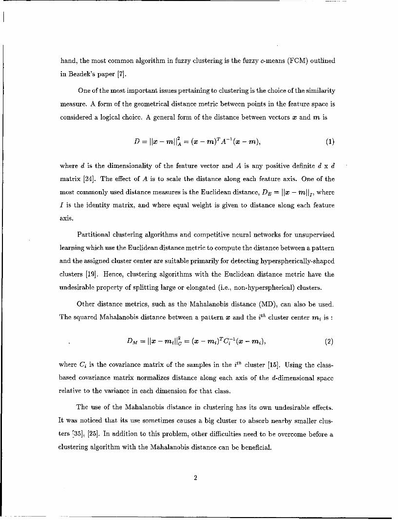
Other distance metrics, such as the Mahalanobis distance (MD), can also be used.

The squared Mahalanobis distance between a pattern x and the ith cluster center mi is :

Dm = llx - m~il'= (x - mi)TC (x - i), (2)

where Ci is the covariance matrix of the samples in the ith cluster [15]. Using the class-

based covariance matrix normalizes distance along each axis of the d-dimensional space

relative to the variance in each dimension for that class.

The use of the Mahalanobis distance in clustering has its own undesirable effects.

It was noticed that its use sometimes causes a big cluster to absorb nearby smaller clus-

ters [35], [25]. In addition to this problem, other difficulties need to be overcome before a

clustering algorithm with the Mahalanobis distance can be beneficial.

2

1.2 Problem Statement

This thesis integrates the class-based Mahalanobis distance as a similarity measure

in partitional clustering.

1.3 Summary of Current Knowledge

Even though the Mahalanobis distance is well known in the pattern recognition

literature, the idea of measuring the Mahalanobis distance to each cluster based on its

covariance matrix and using these measurements as a basis for partitioning is not common.

Patrick and Shen [27] suggested an interactive approach for hyperellipsoidal cluster-

ing. They used the problem knowledge to provide the computer with the initial center

of the hyperellipsoidal clusters and the covariance matrix for the data in that cluster in

addition to the "expert's" confidence level in those values. Their approach sequentially

detects clusters, so there is no competition between different clusters, and the output clus-

ters are affected by the order in which a cluster center is defined. This approach requires a

supervisory knowledge of the data that rarely occurs, especially when visualization of the

data is difficult or impossible.

In 1991, Jolion et al. [20] proposed an iterative clustering algorithm based on the

minimum volume ellipsoid (MVE) robust estimator. At each iteration in this algorithm,

the best fitting hyperellipsoidal-shaped cluster is detected by comparing the distribution

of the pattern inside a minimum volume hyper-ellipsoid to a cluster generated from a

Gaussian distribution. The authors realized the computational burden of finding the best-

fitting hyperellipsoid in the entire feature space, so they employed a random subsampling

technique and performed the clustering based on these few samples. Their approach also

detects clusters sequentially which may result in a nonoptimal clustering.

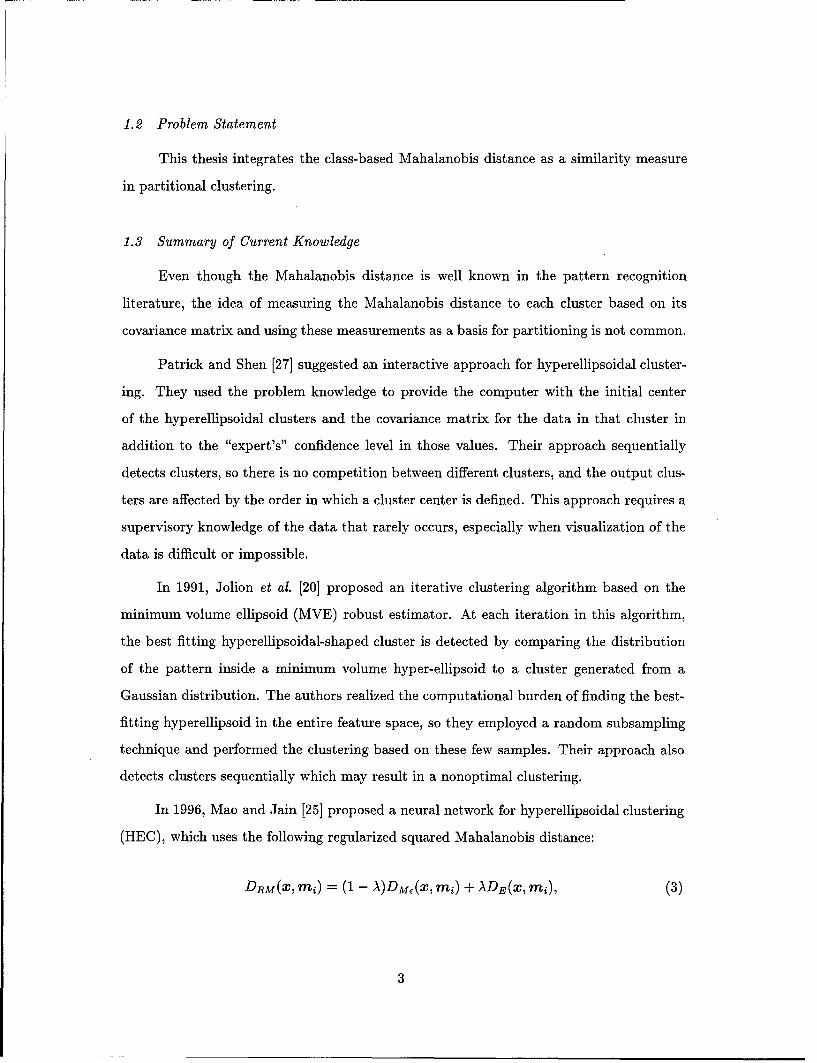
In 1996, Mao and Jain [25] proposed a neural network for hyperellipsoidal clustering

(HEC), which uses the following regularized squared Mahalanobis distance:

DRM(X, mi) = (1 - A)DM,(x, mi) + ADE(X, mi), (3)

3

where DE is the Euclidean distance and DM, is the Mahalanobis distance when a small

number e is added to the diagonal elements of the class covariance matrix Ci. For 0 < A < 1,

DRM is a linear combination of the squared Mahalanobis distance and the squared Eu-

clidean distance. Introducing the regularized Mahalanobis distance results in a tradeoff

between the previously mentioned complementary properties associated with using either

the Euclidean distance or the Mahalanobis distance by itself.

This thesis analyzes the HEC algorithm and introduces another clustering method

based on the Mahalanobis distance to each cluster, weighted by a factor that depends on

the population of that cluster [35].

1.4 Scope

In this thesis, a new clustering technique based on the class-based Mahalanobis dis-

tance is implemented and compared with the Mahalanobis distance based HEC algorithm.

Both hard and fuzzy algorithms using Euclidean distance are used as a baseline for com-

parison. Problems that face the use of Mahalanobis distance in clustering are analyzed

and solved. The data are two-dimensional Gaussian and the well-known Iris data. Vector

quantization coding of images is also considered as a practical application.

1.5 Approach

The approach taken in this investigation is composed of three steps. The first step

is to implement both the LBG technique, described by Linde et al. [24], and the FCM, as

outlined by Bezdek [7]. These techniques are validated with similar test problems to those

shown in the references. The second step of the approach is to implement HEC as a neural

network technique for hyper-ellipsoidal clustering using regularized Mahalanobis distance.

This technique will also be tested with the same test problems as the LBG and the FCM

techniques. Finally, the weighted Mahalanobis distance (WMD) algorithm is implemented

and compared with the previous techniques.

4

1.6 Research Objectives

The research objectives for this thesis are as follows:

1. Implement the LBG and the FCM approaches and verify their performance.

2. Build a neural network algorithm for performing principal component analysis (PCA)

necessary for implementing the HEC algorithm.

3. Implement a neural network-based HEC algorithm and compare its performance with

the LBG and the FCM approaches.

4. Build a better Mahalanobis distance based clustering algorithm that is capable of

solving the problems associated with using the Mahalanobis distance in clustering.

5. investigate the theoretical justification for the proposed method.

6. Develop sufficient understanding of how each method works to be able to draw ap-

propriate inferences from the results, beyond simply the output partitioning.

1.7 Thesis Organization

The remainder of this thesis is organized as follows: Chapter II draws upon a detailed

review of pertinent theory and methods relating to clustering to develop four techniques

for clustering, LBG, FCM, HEC, and WMD. Chapter III describes the implementation

of these techniques. Chapter IV presents and discusses the results obtained by applying

these techniques to several real and synthetic data sets. Finally, Chapter V summarizes the

results obtained in this investigation and provides recommendations for further research.

1.8 Summary

It is difficult for some problems to obtain labeled data, such as in the case of speech

recognition and speaker identification. Hence, finding natural concentrations in data with-

out supervision is necessary. Since real-life data are not isotropically distributed around

well-separated centers, a system that can detect hyperellipsoidal shaped clusters is needed.

II. Theory

2.1 Introduction

This chapter focuses on the theoretical concepts necessary to understand the methods

developed and used for clustering. In the sections that follow, these areas are treated:

" Background of statistical pattern classification.

" Benefits and description of clustering.

" General k-means algorithm and its hard and fuzzy variations.

" Principal component analysis

" Clustering based on the Mahalanobis distance to allow for hyperellipsoidally shaped

clusters.

" Theoretical foundation of the weighted Mahalanobis distance clustering algorithm.

2.2 Pattern Classification

In statistical pattern classification, the goal is to assign a d-dimensional input pattern

x to one of c classes, w1,w 2 ,... ,wc. If the class conditional densities, p(xlwi), and the

a priori class probabilities, P(wi), i = 1, 2,... , c; are completely known, the optimum

strategy for making the assignment is the Bayes decision rule [12]: Assign a pattern x into

class wj if

P(wjlx) >P(wilx), i = 1, 2,..., c; i j

where

P(Wjx) =P(w3 )p(xlw3 )p(x)

is called the a posteriori probability of class wj, given the pattern vector x and p(x) is

the probability distribution function (PDF) of the measurements. This rule minimizes the

overall probability of error.

Bayes rule is a special case of a more general decision rule that can be formulated

as a set of c discriminant functions, gi(x),i = 1, 2, ... ,c. We assign x to class wj if

6

gj(x) > gj(x), for all i 0 j. The output nodes of feedforward networks, such as multi-

layer perceptrons and radial basis function networks, can be used to compute discriminant

functions and therefore can be used as classifiers [32].

As implied before, the best discriminant functions are the a posteriori probabilities.

However, in most practical applications neither the a priori probability nor the conditional

PDF's for all classes are known, and only a finite amount of data is available from each

class. This means that the class conditional density functions need to be estimated using

just a finite number of data points. Given a collection of labeled samples, two approaches

may be used to estimate the a posteriori probability of each class. The first is to assume

values for the a priori probabilities, then estimate the probability distribution functions

at each point. Alternatively, the a posteriori probabilities may be estimated directly from

the labeled samples [12].

One class of procedures for estimating density functions entails assuming a func-

tional form for each PDF, and then estimating parameters to fit that form to the data.

One of the estimation techniques is the maximum likelihood estimation (MLE) [12]. In

practice, however, it may be unjustifiable to assume the correct form for each PDF. In

addition, many practical problems involve multimodal densities, while nearly all of the

classical parametric densities are unimodal. The alternative to this class of procedures is

to estimate the density functions directly from the data, without assuming a functional

form. Because they do not involve estimates of functional parameters, these procedures

are generally referred to as non-parametric techniques [12]. Examples of the well-known

non-parametric density estimation techniques are k-nearest neighbor (k-NN) and Parzen

window estimators. The estimated class conditional density functions can be used to cal-

culate the discriminant functions. Neural networks also take this approach. It was shown

that a multilayer perceptron (MLP) approximates the a posteriori probabilities of the

classes being trained [31].

In many practical cases the data are of limited sample size and also unlabeled. This

is because the class memberships are not available or because collection and labeling of

a large set of sample patterns can be very costly and time consuming. For instance,

recorded speech is virtually free, but labeling the speech, marking what word or phoneme

7

is being uttered at each instant, is very expensive and time consuming [12]. In this case

classification can be accomplished by finding groups in the data and then labeling these

categories as specific classes by supervision.

Clustering can also be used to save time by designing a crude classifier on a small,

labeled set and then modifying the design by allowing it to run without supervision on a

large, unlabeled set. In addition, clustering can give the analyst insight into the nature or

structure of the data especially when no prior knowledge is assumed or the data cannot

be visualized. Finally, another important application of clustering is feature selection. It

is important to eliminate redundant features to reduce the dimensionality of the prob-

lem. Taking into account those distinct and well separated features saves time and makes

parameter estimation more accurate. For all of the above reasons, clustering is a very

important tool in pattern recognition and shall be defined in the next section.

2.3 The Clustering Problem

Cluster analysis is one of the basic tools for identifying structure in data. Clustering

usually implies partitioning of a collection of objects (tanks, stock market reports, images,

cancerous areas in a mammogram) into c disjoint subsets. That is, to partition a set I

of n samples X = {Xl, X2, .. , Xn} C "' into subsets I-i, .. , -Lc. Each subset is to represent

a cluster, with objects in the same cluster being somehow "more similar" than samples

in different clusters. In other words, objects in a cluster should have common properties

which distinguish them from the members of the other clusters.

In fuzzy clustering, the clusters are not subsets of the collection but are instead fuzzy

subsets as introduced by Zadeh [36]. That is, the "clusters" are functions assigning to each

object a number between zero and one which is called the membership of the object in the

cluster. Objects which are similar to each other are identified by the fact that they have

high memberships in the same cluster. It is also assumed that the memberships are chosen

so that their sum for each object is one. So, the fuzzy clustering is, in this sense, also a

partition of the set of objects.

8

Each cluster may be represented by a reproduction vector, mi, that is usually chosen

to be the Euclidean center of gravity, or the centroid of the samples in that cluster. Hence,

it is called the cluster center.

To measure a clustering algorithm performance, one defines a criterion function that

measures the clustering quality of any partition of the data. The goal is to find the

partition that minimizes the criterion function. The approach most frequently used in

seeking optimal partitions is iterative optimization [12]. The basic idea is to start with

an initial partition and iteratively change the location of cluster centers and reassign data

points to the different clusters in a way that maximizes the criterion function.

Clustering or unsupervised learning algorithms can be grouped into two categories:

hierarchical and partitional. A hierarchical clustering is a nested sequence of partitions,

whereas a partitional clustering is a single partition [18]. Commonly used partitional

clustering algorithms are the k-means algorithm and its variations (e.g., ISODATA [2])

which incorporates some heuristics for merging and splitting clusters and for handling

outliers. Competitive neural networks are also used to cluster input data. The well-known

examples are Kohonen's Learning Vector Quantization (LVQ) and self-organizing map [23],

and Adaptive Resonance Theory (ART) models [8].

A clustering algorithm in this context is equivalent to a vector quantizer (VQ) where

the object is to find a system for mapping a sequence of continuous or discrete vectors

into a digital sequence suitable for communication or storage in a digital channel [17]. The

goal of vector quantizers is data compression. They are used to reduce the bit rate while

maintaining the necessary fidelity of the data [17]. When used in a vector quantization

context, cluster centers are termed codewords and the set of all codewords is called a

codebook. To define the performance of a quantizer in producing the "best" possible

reproduction sequence requires the idea of a distortion measure. Despite the differences

between clustering algorithms and vector quantizers, their ultimate goal of exploiting the

similarity between the samples allows us to use the terms clustering and vector quantization

interchangeably throughout this thesis.

9

Most variations in the design of a vector quantizer or a clustering algorithm are in

the choice of a quantitative measure of similarity and in the definition of the criterion

function, or distortion. Hence, these two critical topics are the subject of the following

subsections.

2.3.1 Similarity Measures. The first important question in a clustering algorithm

design is how to determine "more similar". Similarity measures can be in a form of non-

metric similarity functions or distance metrics. Duda and Hart [12] list a number of

functions s(x, m) whose values are higher if the vectors x and m are somehow similar. An

example measure is the normalized inner product which is the cosine of the angle between

the two vectors. Other similarity functions include the two-sided tangent distance and

Tanimoto distance which is especially useful if the features are binary [12].

Distance measures are more often used to measure similarity. The smaller the dis-

tance between two patterns, the greater the similarity. The assumption made in using

these measures is that similarity between objects is measured by the distance between

their corresponding data vectors. So, if the distances to the mean of a cluster are small,

the points in the cluster are also close to each other and therefore assumed to be "similar".

Mao and Jain [25] suggest that Euclidean distance is the most commonly used dis-

tance metric in practice. However, choosing the Euclidean distance to measure similarity

implies an isotropic feature space weighting. Consequently, a clustering algorithm with

Euclidean distance favors hyperspherically shaped clusters of equal size. The clusters in a

data set are not always compact and isolated in the sense that the between-cluster vari-

ation is much higher than the within-cluster variation. Therefore, using the Euclidean

distance has the undesirable effect of splitting large as well as elongated clusters under

some circumstances [25]. It is easy to find examples of data sets in real applications which

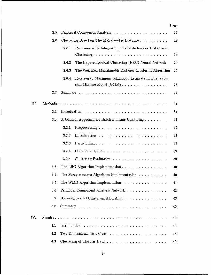
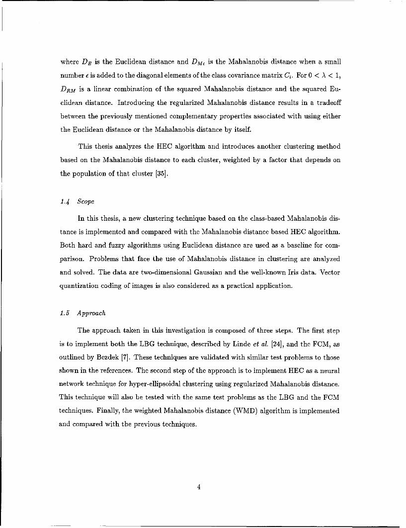
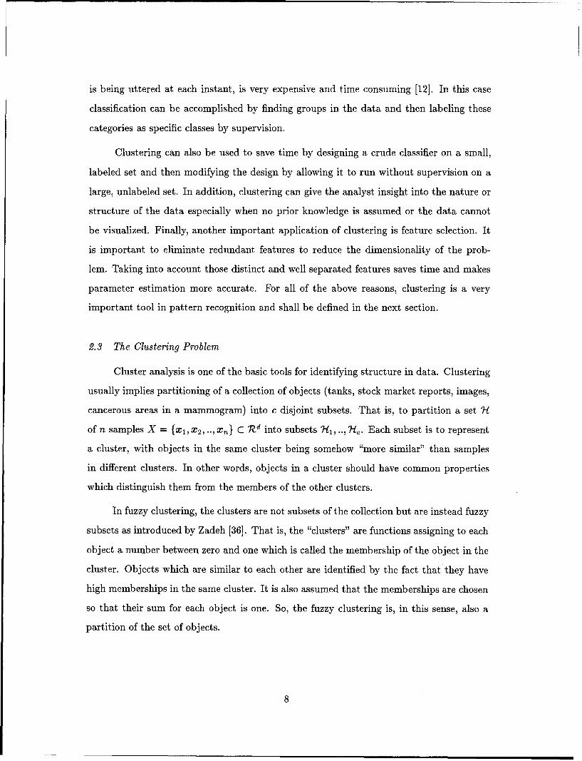
do not have spherically shaped clusters of equal size. For example, Fig. 1 shows the two-

dimensional projection of the well-known Iris data onto a plane spanned by the first two

principal eigenvectors. Since we know the category information of the patterns in the Iris

data set, we label each pattern by its category in the projection map. There are two ob-

vious clusters, but neither of them has a spherical shape. From Fig. 1, we can see that

10

oO CLASS i

0 X CLASS2 +

+ CLASS3 +

2-

S00 +0 x +0. ++E 1 )<+ +

oo

ox000+ CU0 X

-2x+

x

-3

-3 -2 -1 0 1 2 3First Principal Component

Figure 1. Projection of the Iris data set onto the plane spanned by the first two principalcomponents

the larger cluster is a mixture of two classes (Iris Versicolor and Iris Virginica) which have

nonspherical distributions.

An alternative distance metric that depends on the distribution of the data itself is

the Mahalanobis distance defined in Eqn. (2) and rewritten here for convenience.

DM = - mll ( - m) T C-(x - m) (4)

where C is the covariance matrix of a pattern population, m is the mean vector, and x

represents a variable pattern. The Mahalanobis distance is especially useful if the statistical

properties of the population are to be considered.

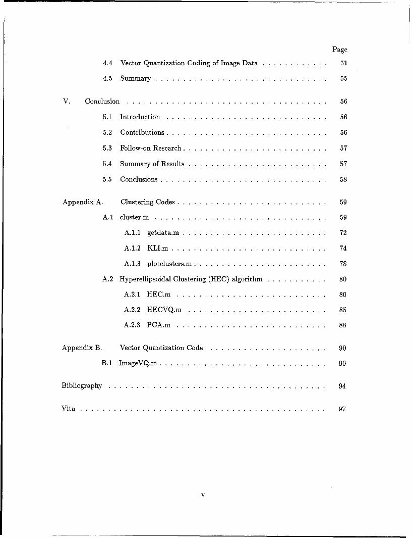
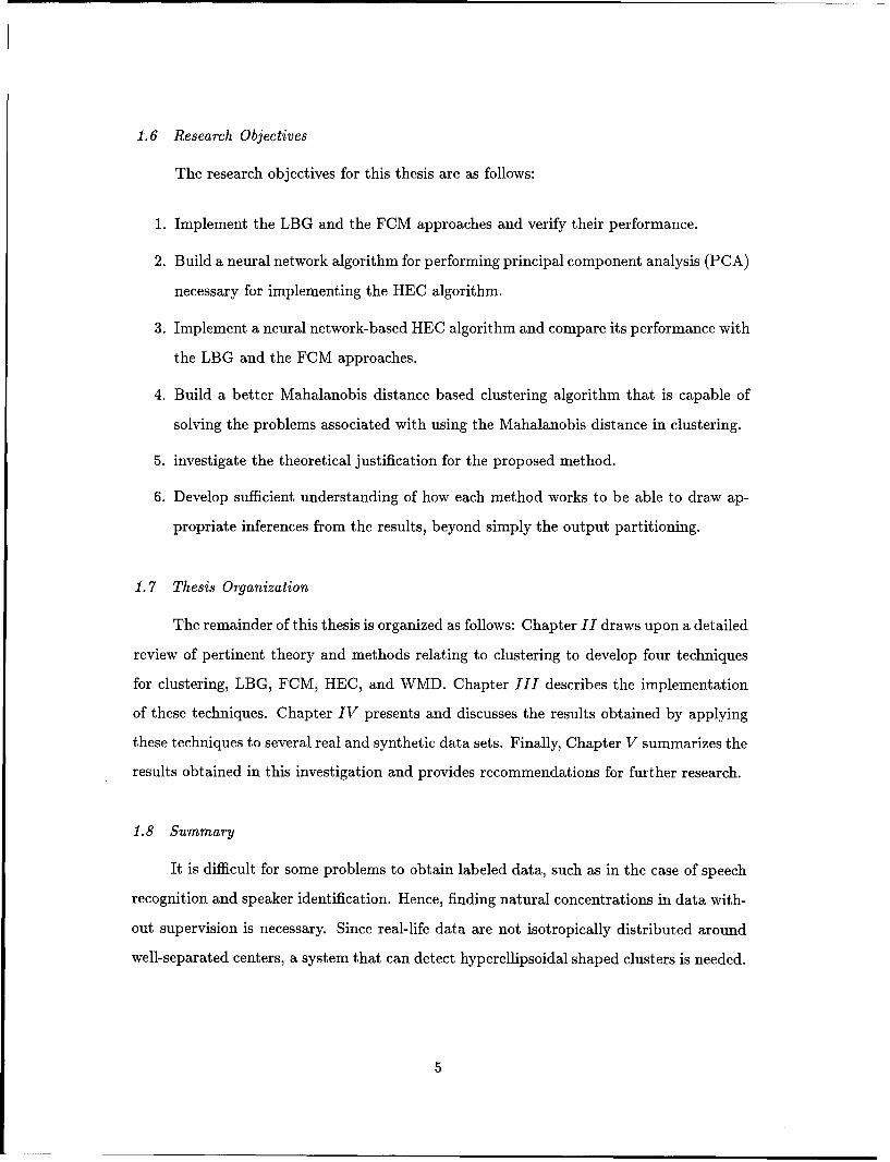
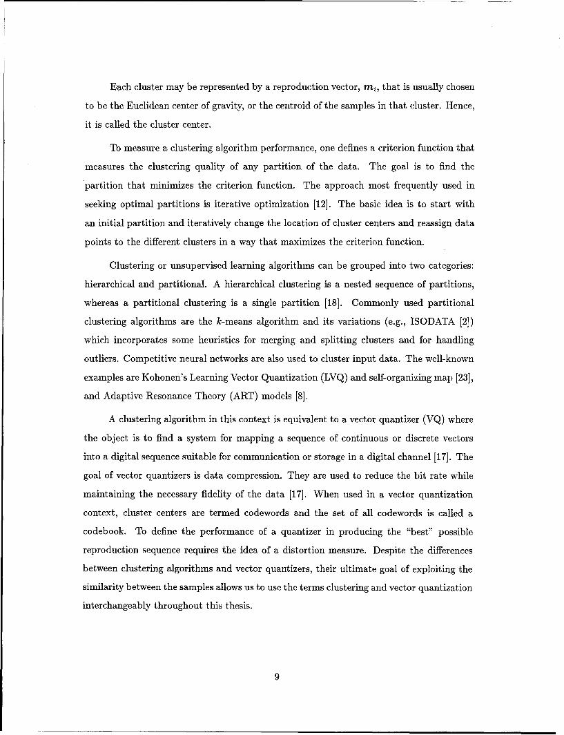
Figure 2 shows a scenario of two-cluster solutions by vector quantization using the

Euclidean and Mahalanobis distance measures. It is clear from the figure that using the

Euclidean distance results in undesired grouping of the two classes. On the other hand,

using the Mahalanobis distance allows the natural grouping of the two clusters.

The equi-Euclidean distance surface defines a hyper-sphere of unity aspect ratio,

which is the ratio between the major axis to the minor axis in an ellipse. On the other

hand, the equi-Mahalanobis distance surface defines a hyperellipsoid of any shape which

11

x2 -- Eucridean

Feature(2) - Mahalanobis

o 10 1 0

0, 0

0 A

Feature (1)

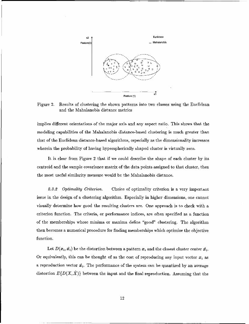
Figure 2. Results of clustering the shown patterns into two classes using the Euclideanand the Mahalanobis distance metrics

implies different orientations of the major axis and any aspect ratio. This shows that the

modeling capabilities of the Mahalanobis distance-based clustering is much greater than

that of the Euclidean distance-based algorithms, especially as the dimensionality increases

wherein the probability of having hyperspherically shaped cluster is virtually zero.

It is clear from Figure 2 that if we could describe the shape of each cluster by its

centroid and the sample covariance matrix of the data points assigned to that cluster, then

the most useful similarity measure would be the Mahalanobis distance.

2.3.2 Optimality Criterion. Choice of optimality criterion is a very important

issue in the design of a clustering algorithm. Especially in higher dimensions, one cannot

visually determine how good the resulting clusters are. One approach is to check with a

criterion function. The criteria, or performance indices, are often specified as a function

of the memberships whose minima or maxima define "good" clustering. The algorithm

then becomes a numerical procedure for finding memberships which optimize the objective

function.

Let D(xi, &) be the distortion between a pattern xi and the closest cluster center i.

Or equivalently, this can be thought of as the cost of reproducing any input vector xi as

a reproduction vector &i. The performance of the system can be quantized by an average

distortion E{D(X, ±)} between the input and the final reproduction. Assuming that the

12

process is stationary and ergodic, then the mathematical expectation is, with probability

one, equal to the long term sample average [17]

1 n-1

E{D(X,X)} = lim n ZD(xj, &) (5)j=0

Equation (5) implies that if the input source statistics do not change with time and if

the time average equals the ensemble average then the resulting sample average distortion

should be nearly the expected value, and the same codebook used on future data should

yield approximately the same averages.

As for the choice of distortion measure, it ought to to be tractable, computable, and

subjectively meaningful so that large or small quantitative distortion measures correlate

with bad and good subjective quality [17].

The simplest and most widely used distortion measure, although lacking the above

properties, is the squared error distortion measure,

d-1

D(x,.) = lix - ll' = -(xi - i)2 . (6)i=O

Substituting Eqn. (6) in Eqn. (5) yields the mean squared error (MSE) criterion

function. Dunn [13] developed the first fuzzy extension to the least mean square error

approach to clustering and this was generalized by Bezdek [6] to a family of algorithms.

Let n be the total number of samples, ni the number of samples in 7i, and mi be the

mean of those samples. The generalized mean squared error is then defined by:

JGMSE =n = j=- A (7)

where uij is the membership of the ith pattern to the jth cluster, m is a weighting exponent

strictly greater than one, and A is any positive definite matrix [7].

Many algorithms were designed based on minimizing JGMSE. In these algoritms, the

JGMSE is monotonically nonincreasing function as the number of iterations increases.

13

Modifying the criterion function to allow the use of a generalized distance as a dis-

tance metric is possible by defining A. Linde et al. [24] and Bezdek [7] generalized A to

any d x d positive definite matrix. They showed that if the covariance matrix for all the

data is used, the Mahalanobis distance is the basis for the partitioning.

Clustering using the global covariance matrix results in a monotonically decreasing

objective function. However, all the clusters may not have the same distribution (shape)

as that of the whole data set. Hence, using the global covariance matrix for each cluster

may not give the best grouping of the data.

Other common criterion functions are the average squared distances between samples

in a cluster domain and the average squared distances between samples in different cluster

domains [33].

Backer and Jain [1] suggested a goal-directed approach to the cluster validity problem.

The goal can be minimizing the classification error rate. Alternatively, the clustering

performance can be considered good if the clusters were dense, which means minimum

volume of the equi-Mahalanobis distance ellipsoids, or the clusters were far apart. Gath

and Geva [14] also considered a large number of the data points in the vicinity of the

cluster center as an indication of good clustering. In Section 2.6.4 we will see that the goal

is maximizing the likelihood function.

2.4 The Batch k-means Algorithm

A well known algorithm for the design of a locally optimal codebook with iterative

codebook improvement is the generalized Lloyd algorithm (GLA) [15]. The two steps in

each iteration of this algorithm are:

Step 1: Given a codebook M = {mi ; i = 1,... ,k } obtained from the 1 th iteration, assign

each data point to the closest codeword.

Step 2: Obtain the codebook M1+1 by computing the centroid of each cluster based on

the partitioning of Step 1.

14

where the closest codeword is typically found with a distance metric based on the as-

sumption that similar feature vectors are likely to lie close to each other in the feature

space. The above algorithm is usually terminated when the codewords stop moving or the

difference between their locations in consecutive iterations is below a threshold.

The GLA algorithm is widely known as the batch k-means algorithm when the dis-

tortion measure used is the sum of squared distances from all points in a cluster domain

to the cluster center [33]. A sequential k-means, where the update to the cluster centers

occurs after each pattern being classified, is proposed by McQueen [26].

In the next sections, two methods that use variations on the described k-means

algorithm are presented. We will discuss how these methods differ in calculating the

membership function of the data to the reproduction vectors.

2..1 The LBG Algorithm. The first algorithm is described by Linde, Buzo, and

Gray in 1980 [24], and is also known as the LBG algorithm for short. The LBG Algorithm

is similar to k-means, but the distortion measure is general. A survey of different distortion

measures is provided in the paper. It was shown that the best partition is obtained by

choosing the nearest-neighbor codeword to each input, and no reproduction alphabet can

yield a smaller average distortion than that containing the centroids of the subsets. The

GLA iterative method with these rules is guaranteed to result in a non-increasing average

distortion (based on the distance from the cluster centers to the data points within the

clusters) after each iteration, and it terminates in a local minimum when the average

distortion stops changing significantly.

2.4.2 The Fuzzy c-means Algorithm. In a "hard" clustering algorithm such

as the k-means algorithm, each pattern is to be assigned to only one cluster. However,

this "All-or-None" membership constraint is not realistic, since many pattern vectors may

have characteristics of more than one class. Hence came the idea of assigning a set of

membership function values for each pattern to every one of the different classes. This

results in a fuzzy boundary rather than a hard one.

15

The first and most widely used fuzzy clustering algorithm is the fuzzy c-means al-

gorithm [34]. It is an iterative procedure for finding a membership matrix, U, and a set

of cluster centers, M, to minimize the generalized mean squared error objective function,

see Eqn. (7). By minimizing JGMSE, one should obtain high memberships in cluster j for

data which are close to the vector m.

The vectors M 1 , m 2 ,... , M, can be interpreted as prototypes for the clusters rep-

resented by the membership functions, and are also called cluster centers. In order to

minimize the objective function, the cluster centers and membership functions are chosen

so that high memberships occur for points close to the corresponding cluster centers. The

number m is called the exponent weight. It can be chosen to "tune out" noise in the data.

The higher the value of m, the less the contribution of those data points whose member-

ships are uniformly low to the objective function. Consequently, such points tend to be

ignored in determining the centers and membership functions [34]. The actual construc-

tion of the FCM algorithm is based on the following set of equations which are necessary

conditions for M 1 , m 2 ,... , m, and the membership matrix U to produce a local minimum:

En l(ij)m , (8)

andii= 2 (9)

((Xr-m)rA-(Xj-m,) )-E]k=1 k(X~j-mk)1A-1(Xj-mk)]

The update equations are obtained by differentiating the objective function with

respect to the components of V and U subject to the constraint that E=l uij = 1. No

closed form solution has been found for this differentiation, but these equations are the

basis for an iterative procedure which converges to a local minimum for the objective

function [34]. One could start with an initial guess of the value for the membership values,

U, for a specific choice of m and c. Using these memberships and Eqn. (8), one computes

cluster centers, then using these cluster centers and Eqn. (9) recomputes memberships and

so forth, iterating back and forth between Eqn. (8) and Eqn. (9) until the memberships or

cluster centers for successive iterations differ by no more than some prescribed value.

16

In the cases where classification is the goal, Eqn. (9) can be used as the basis where

maximum membership function value uij means smaller distance and higher likelihood

that the data point xi is a member of the j" cluster. The class membership function

values provide a measure of similarity by which a soft decision can be made with a degree

of confidence.

2.5 Principal Component Analysis

One of the topics that is used in signal processing and used in the techniques to be

presented in the next sections is the principal components analysis (PCA). The goal is to

find the maximum variance in the data and to transform the data into a space where the

features are uncorrelated.

Let C., be the covariance matrix of the data set X. Since C, is real and symmetric, it

is possible to find a set of orthonormal eigenvectors [16]. Let ej and 0j, i = 1, 2,... , d, be

the eigenvectors and the eigenvalues of C,. If we arrange the eigenvalues in decreasing order

so that, 01 > 0 2 > ... > Od, a transformation matrix whose rows are the corresponding

eigenvectors of C,; is defined to be D.

If m,, is the mean of the samples X, the transformation

y = D(x - ma,) (10)

is called principal component, Karhunen-Lo~ve, or Hotelling transformation.

It can be shown that, the mean of Y is zero and its covariance matrix is given by [16]:

CZ, = DT cD = T = diagl',..., 10}, (11)

which means that the features of Y are uncorrelated. Furthermore, if we divide each

eigenvector by the square root of the corresponding eigenvalue, the resultant covariance

matrix, C., will be the identity. Hence, this scaled principal component analysis is called

the whitening transform.

17

Another interesting property of this transform can be seen if we let

y p-1 /2 x, (12)

and

v = -1 /2pm', (13)

for any vector x E X. Computing the Euclidean distance between v and y yields

DE(y,v) = (y - v)'(y - V). (14)

Substituting Eqn. (12) and Eqn. (13) and using the fact that for any orthonormal

matrix

= (15)

it can be shown that Eqn. (14) becomes

DE(y, v) = (x - mx)TC.l (X - m.), (16)

which is the definition of the Mahalanobis distance between a vector x and a cluster center

mx. In other words, this says that the Mahalanobis distance between an input pattern x

and a cluster center mx in the input space is equivalent to the Euclidean distance between

them in the transformed space, i.e.,

DM(x, mx) = DE(y,v). (17)

For any q d, the projection of x onto the span of {el, e2,... ,eq} accounts for

the maximum fraction of the total sample variance in x that can be accounted for by a

linear projection onto a q-dimensional vector subspace. Plotting the first few principal

components allows us to visually examine the data that account for most of its variance.

These properties of the principal component analysis will be utilized in the Mahalanobis

distance based algorithms.

18

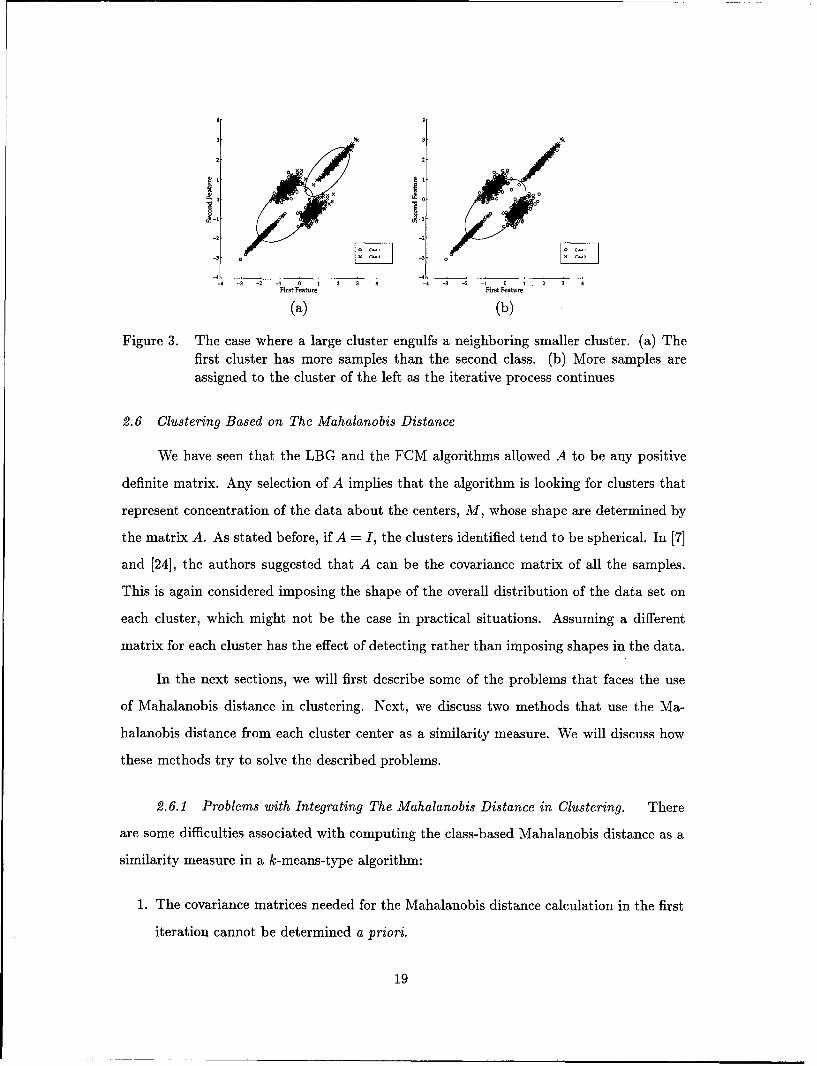
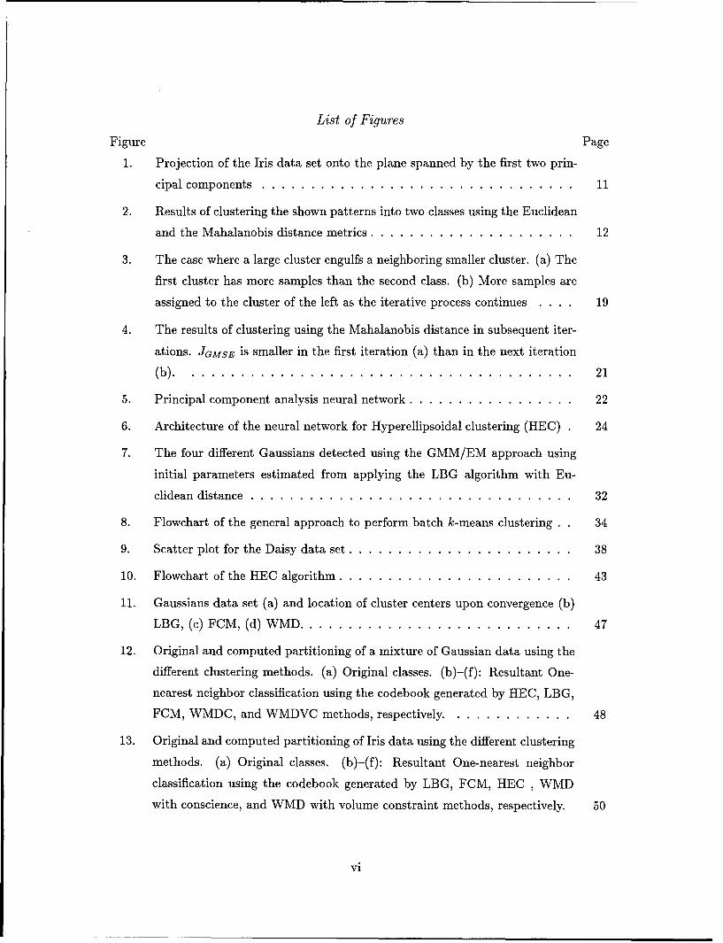
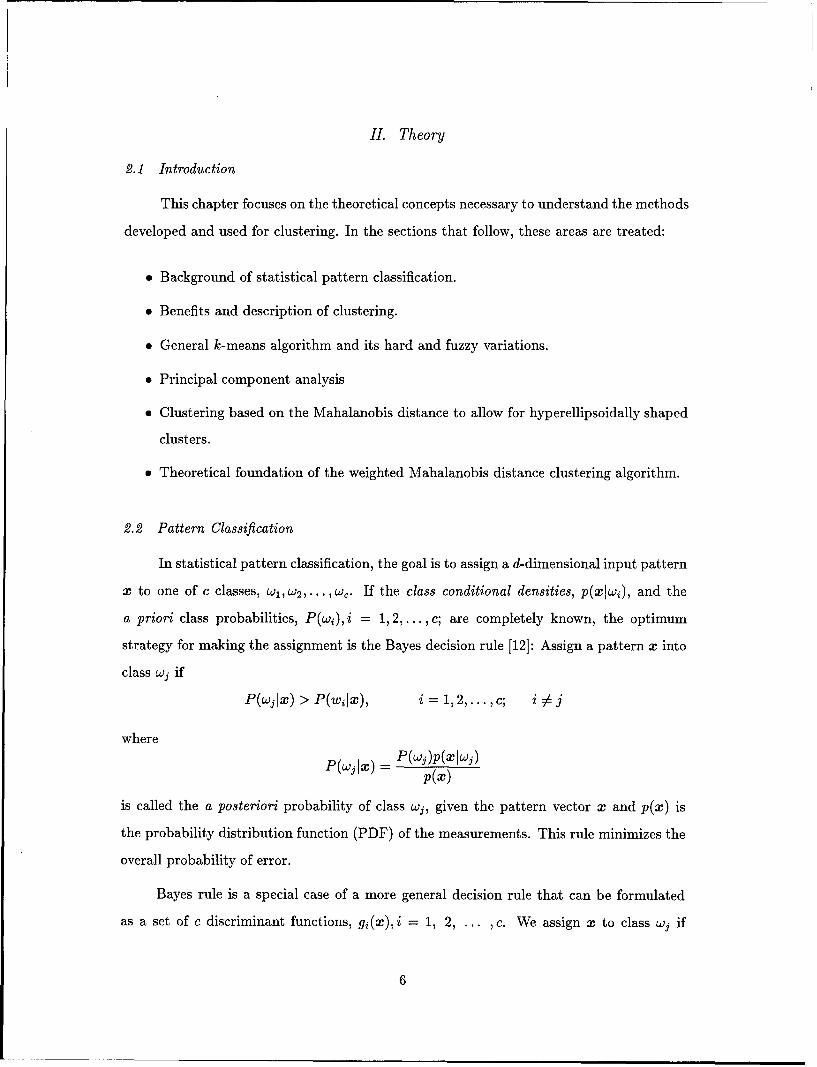
4 4

2 2

-2 -2

-4 -3 -2 -1 0 1 2 3 4 -3 -2 -1 0 1 2 3 4First Feature First Feature

(a) (b)

Figure 3. The case where a large cluster engulfs a neighboring smaller cluster. (a) Thefirst cluster has more samples than the second class. (b) More samples areassigned to the cluster of the left as the iterative process continues

2.6 Clustering Based on The Mahalanobis Distance

We have seen that the LBG and the FCM algorithms allowed A to be any positive

definite matrix. Any selection of A implies that the algorithm is looking for clusters that

represent concentration of the data about the centers, M, whose shape are determined by

the matrix A. As stated before, if A = I, the clusters identified tend to be spherical. In [7]

and [24], the authors suggested that A can be the covariance matrix of all the samples.

This is again considered imposing the shape of the overall distribution of the data set on

each cluster, which might not be the case in practical situations. Assuming a different

matrix for each cluster has the effect of detecting rather than imposing shapes in the data.

In the next sections, we will first describe some of the problems that faces the use

of Mahalanobis distance in clustering. Next, we discuss two methods that use the Ma-

halanobis distance from each cluster center as a similarity measure. We will discuss how

these methods try to solve the described problems.

2.6.1 Problems with Integrating The Mahalanobis Distance in Clustering. There

are some difficulties associated with computing the class-based Mahalanobis distance as a

similarity measure in a k-means-type algorithm:

1. The covariance matrices needed for the Mahalanobis distance calculation in the first

iteration cannot be determined a priori.

19

2. If the number of patterns in a cluster is small compared to the input dimensionality

d, then the d x d sample covariance matrix of the cluster may be singular.

3. The k-means clustering algorithm with the Mahalanobis distance tends to generate

unusually large or unusually small clusters [35], [25]. Figure 3 shows the case of

large cluster engulfing the neighboring cluster. Points on the perimeter are of equal

Mahalanobis distance to the cluster centers. Since the first cluster exhibits more

variations in both directions, its covariance matrix is larger. Hence the Mahalanobis

distance to the cluster center with a larger A is more likely to be smaller and more

samples are assigned to that cluster in subsequent iterations.

4. When performing the clustering based on the individual covariance matrices to allow

for each cluster to have its distinct shape, JGMSE does not result in a monotonically

decreasing function as the number of iterations increases.

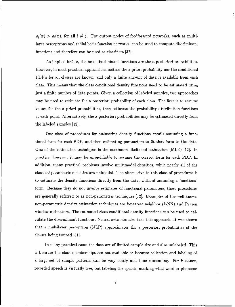
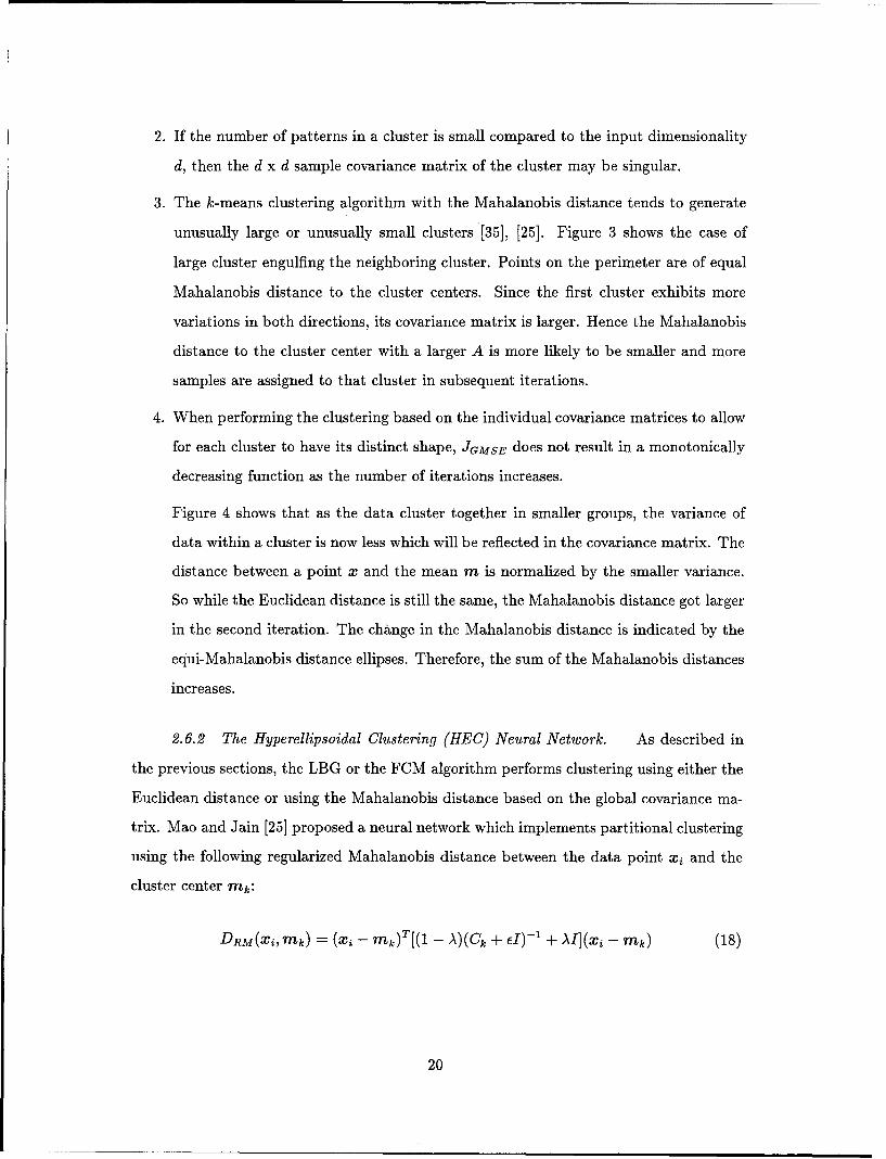
Figure 4 shows that as the data cluster together in smaller groups, the variance of

data within a cluster is now less which will be reflected in the covariance matrix. The

distance between a point x and the mean m is normalized by the smaller variance.

So while the Euclidean distance is still the same, the Mahalanobis distance got larger

in the second iteration. The change in the Mahalanobis distance is indicated by the

equi-Mahalanobis distance ellipses. Therefore, the sum of the Mahalanobis distances

increases.

2.6.2 The Hyperellipsoidal Clustering (HEC) Neural Network. As described in

the previous sections, the LBG or the FCM algorithm performs clustering using either the

Euclidean distance or using the Mahalanobis distance based on the global covariance ma-

trix. Mao and Jain [25] proposed a neural network which implements partitional clustering

using the following regularized Mahalanobis distance between the data point xi and the

cluster center Mk:

DRM(X,mk) =(x - mk)T[(1 - A)(Ck + cI)- + AI](x, - ink) (18)

20

15 x

15 X

00

1o

aX 0

-10 X++

-10

-15-15

-15 -10 5 0 5 10 15

First Feature First Featue

(a) (b)

Figure 4. The results of clustering using the Mahalanobis distance in subsequent itera-tions. JGMSE is smaller in the first iteration (a) than in the next iteration (b).

where A and E are called the regularization parameters. Note that this regularized Ma-

halanobis distance takes the shape of each cluster into consideration. When A=O and

E=O, DRM becomes the squared Mahalanobis distance. When A= 1, DRM reduces to the

squared Euclidean distance. When 0 < A < 1, DRM is a linear combination of the squared

Mahalanobis distance and the squared Euclidean distance. Therefore, A can be used as a

parameter to control the degree that the distance measure deviates from the commonly

used squared Euclidean distance. On the other hand,E is added to prevent the singularity

of the covariance matrix Ck as shall be discussed later.

Equation (17) indicates that the computation of the Mahalanobis distance can be

decomposed into two steps; first, projecting the input pattern into the whitened space and

second, computing the Euclidean distance in the whitened space.

Neural networks provide a suitable architecture for implementation of many signal

processing techniques. hence, the authors implemented the two-step computation using a

two-layer network whose first and second layers compute the whitening transform and the

Euclidean distance, respectively. Then, the regularized distance can be computed by the

weighted sum of two Euclidean distances: one in the original input space and one in the

whitened space.

21

W ld W1 2 h

oW2d A2 d •

0 h •

xa

0Wdl Wd2

XdWdd

Figure 5. Principal component analysis neural network

Since it is necessary to find the eigenvectors and eigenvalues before such a regularized

Mahalanobis distance can be calculated, a neural network version of principal component

analysis algorithm was chosen to perform the whitening. In the next sections, a description

of the PCA neural network algorithm is outlined. Then, the architecture for the HEC

network is described. Finally, a discussion of the HEC algorithm is provided.

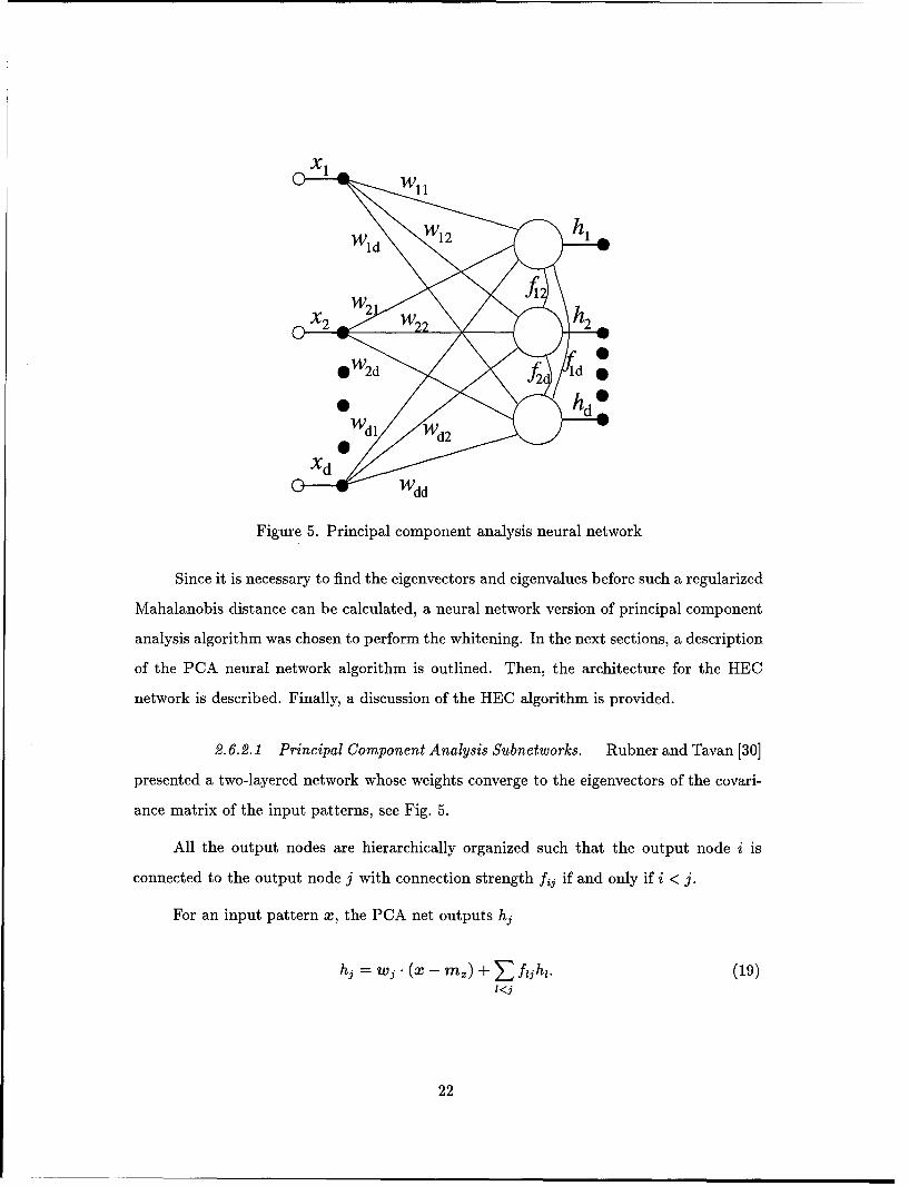
2.6.2.1 Principal Component Analysis Subnetworks. Rubner and Tavan [30]

presented a two-layered network whose weights converge to the eigenvectors of the covari-

ance matrix of the input patterns, see Fig. 5.

All the output nodes are hierarchically organized such that the output node i is

connected to the output node j with connection strength fij if and only if i < j.

For an input pattern x, the PCA net outputs hj

hj = w. (x - mx) + 1 fight. (19)1<j

22

The weights on the connections between the input nodes and the output nodes of

the PCA subnetwork are adjusted according to the Hebbian rule, i.e.,

Awij = '/(xi - mi)hj, i,j = 1,2,... ,d; (20)

where y is the learning rate. The lateral weights are updated according to the anti-Hebbian

rule

Afij = -hihj, l,j = 1,2,...,d, l <j; (21)

where A is another positive learning rate. Rubner and Tavan demonstrated that following

the above update equations forces the lateral weights to vanish and the activities of the

output cells to become uncorrelated. Then the weights on the connections to the jth

output layer, wj, are the eigenvector corresponding to the jth largest eigenvalue. The jih

eigenvalue is estimated by the variance of hi after the network converges.

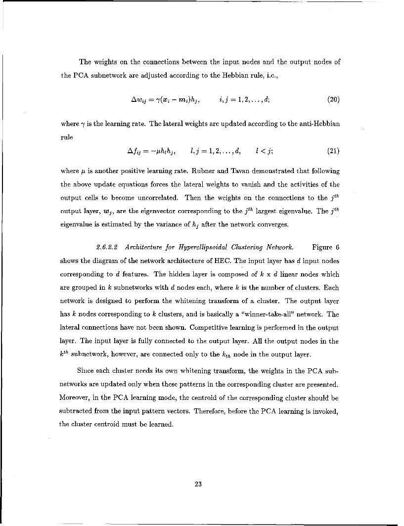
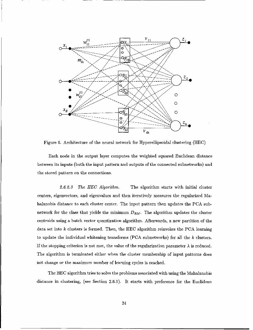
2.6.2.2 Architecture for Hyperellipsoidal Clustering Network. Figure 6

shows the diagram of the network architecture of HEC. The input layer has d input nodes

corresponding to d features. The hidden layer is composed of k x d linear nodes which

are grouped in k subnetworks with d nodes each, where k is the number of clusters. Each

network is designed to perform the whitening transform of a cluster. The output layer

has k nodes corresponding to k clusters, and is basically a "winner-take-all" network. The

lateral connections have not been shown. Competitive learning is performed in the output

layer. The input layer is fully connected to the output layer. All the output nodes in the

kth subnetwork, however, are connected only to the kth node in the output layer.

Since each cluster needs its own whitening transform, the weights in the PCA sub-

networks are updated only when these patterns in the corresponding cluster are presented.

Moreover, in the PCA learning mode, the centroid of the corresponding cluster should be

subtracted from the input pattern vectors. Therefore, before the PCA learning is invoked,

the cluster centroid must be learned.

23

.. .. - --------

V~ dk

Figure 6. Architecture of the neural network for Hyperellipsoidal clustering (HEC)

Each node in the output layer computes the weighted squared Euclidean distance

between its inputs (both the input pattern and outputs of the connected subnetworks) and

the stored pattern on the connections.

2.6.2.3 The HEC Algorithm. The algorithm starts with initial cluster

centers, eigenvectors, and eigenvalues and then iteratively measures the regularized Ma-

halanobis distance to each cluster center. The input pattern then updates the PCA sub-

network for the class that yields the minimum DRM. The algorithm updates the cluster

centroids using a batch vector quantization algorithm. Afterwards, a new partition of the

data set into k clusters is formed. Then, the HEC algorithm reinvokes the PCA learning

to update the individual whitening transforms (PCA subnetworks) for all the Ic clusters.

If the stopping criterion is not met, the value of the regularization parameter A is reduced.

The algorithm is terminated either when the cluster membership of input patterns doesnot change or the maximum number of learning cycles is reached.

The HEC algorithm tries to solve the problems associated with using the Mahalanobis

distance in clustering, (see Section 2.6.1). It starts with preference for the Euclidean

24

distance to address the first problem concerning initial values for the individual covariance

matrices. After the data have been partitioned using a batch vector quantization algorithm

with Euclidean distance, the means and the covariance matrices of the individual clusters

are calculated and used for upcoming iterations.

The second problem of dealing with ill-posed conditions is solved by the introduction

of the regularization parameter c. The role of E is to convert a singular covariance matrix

to a nonsingular matrix by adding a diagonal matrix with small elements. This actually

forces the cluster to have a non-zero extent in all dimensions.

The authors suggested the use of larger value of A when the covariance matrix C

cannot be reliably estimated or learned. In addition, this regularized MD was hoped to

solve the problem of large clusters swallowing smaller nearby ones. However, the algorithm

starts with initial value of A = 1 and decreases with each iteration. This suggests that this

problem is more likely to occur very often only during the first few cycles of learning.

In this algorithm the performance was not evaluated by minimization of the cost

function defined in the paper as the JGMSE with m = 1. However, the quality of the

resultant clustering is assumed to correlate with the compactness of the output clusters.

The compactness of a cluster is measured by the significance level of the Kolmogorov-

Smirnov test on the distribution of the Mahalanobis distances of patterns in a cluster to

the cluster center under the Gaussian cluster assumption. Moreover, it was not shown how

this is incorporated in the algorithm

2.6.3 The Weighted Mahalanobis Distance Clustering Algorithm. The idea be-

hind the proposed method is to allow each cluster to have its own shape implied by the

covariance matrix of the samples within that cluster. A cluster would attract those data

points which enhance its shape and reject those which do not fit. In other words, each vec-

tor x will be assigned to the cluster to which it best integrates regardless of the Euclidean

separation between that data point and that cluster's centroid.

In this algorithm, we modify the GLA described in Section 2.4 such that in each iter-

ation we assign a pattern x to the cluster that yields the minimum weighted Mahalanobis

distance, Di = wi * Ix - mI 12,, where wi is the cluster weight and its computations will

25

be discussed later. In the second step, we update mi and Ci by computing the mean and

the covariance matrix of the data points of each cluster based on the partitioning of the

first step. The algorithm is terminated when the codewords stop moving.

Two ways to get an initial codebook are discussed here. The first method treats the

whole data set as a unique cluster and grows the codebook to the desired number of clusters,

k, by splitting. In splitting, small perturbation vectors p are added to every codeword.

We made pi for the i h cluster to be in the direction of the eigenvector corresponding to

the maximum eigenvalue of Ai. This provides a systematic approach of distributing the

codewords since each cluster center splits in a particular direction based on the cluster's

shape. The second approach to get an initial codebook is used when the desired codebook

size is not an integer power of two. This method uses the Karhunen-Lo~ve transformation

to place the initial codewords along the principal component axes of the data's covariance

matrix. For the first iteration, we use the global covariance matrix as Ai for all the

codewords.

If the number of data points in any cluster is less than the dimensionality of the data,

then Ai might be singular which prevents computing the inverse. Thus, we add a matrix

with small diagonal elements to the covariance matrix to prevent the singularity.

The introduction of the weight w is due to the fact that the use of Mahalanobis

distance alone in clustering sometimes causes a large cluster to attract members of neigh-

boring clusters. This leads to unusually large and unusually small clusters. We evaluate wi

as the ratio of the number of samples in i to the size of the training set. This approach is

appealing as it does not rely on an arbitrary constant or user adjustable parameter. Even

though this weight penalizes large clusters, it does not prevent a cluster from having more

samples if they are much closer to it than other codewords. This is similar to conscience

in neural networks which rewards a balanced representation of the data points [10], [29].

In trying to deal with the problem of nondecreasing JGMSE, one can suggest the use

of another goal-oriented criterion function such as the sum of the volume of the ellipsoids.

Nevertheless, we recall that the update equations for the LBG and the FCM algorithms

were computed based on minimizing JGMSE when A was fixed for all iterations and clusters.

26

However, as the data cluster together in smaller groups, the variances decrease and the

Mahalanobis distance increases as was explained before. Looking at the JGMSE criterion

function again and allowing Ai to be variable

C 2i

JGMSE E n Z E( 1 j)m(x - m)T A i l (x - m) (22)"=1 j'=1

it is clear that there is a need to restrict Ai somehow in order to obtain a nontrivial solution.

Otherwise, the minimum of JGMSE would be given by A71=0, which corresponds to a huge

cluster with infinite variation in all directions.

One way to solve this problem is to force the determinant of all clusters to have a

unity value. In d-dimensional space, a surface of constant Mahalanobis distance DM is a

hyperellipsoid. The volume of this d-dimensional hyperellipsoid is [12:24]

v = vdICIl/ 2D d , (23)

where Vd is the volume of an d-dimensional unit radius hypersphere, which only depends

on the dimensionality of the space:

Vd= d/ d even, (24)(d/2)!' n

Vd = 22'd-l)/2N9) d odd. (25)d!

Hence, by restricting ICI = 1, constant Mahalanobis distance surfaces now enclose constant

volumes.

This choice of this constraint has been criticized because it seemed somewhat ar-

bitrary [34]. However, it has the effect of normalizing the volume enclosed by the equi-

Mahalanobis distance hyperellipsoid to a constant volume for all clusters while maintaining

the distinct shape of each cluster.

After the normalization of the determinants, the JGMSE distortion has become mono-

tonically decreasing as a function of clustering iterations. This means that now we can

use the criterion function in Mahalanobis distance based algorithms to find the number of

27

clusters k or to define a stopping criterion. In the next section, we will give an analysis of

the weighted Mahalanobis distance algorithm as an approximation to the famous expec-

tation maximization method as applied to the problem of maximum likelihood estimation

in the Gaussian mixture model.

2.6.4 Relation to Maximum Likelihood Estimate in The Gaussian Mixture Model

(GMM). The use of different covariance matrices for different clusters was a motivation

to investigate the similarity between the WMD algorithm and the Gaussian mixture model.

This presentation of GMM will follow the outline of Reynolds [28], to which the reader is

referred for a more extensive treatment of the subject.

A Gaussian mixture density is a weighted sum of L component densities as given by

the equation:L

p(xlG) = Epibi(x), (26)i=l

where x is a d-dimensional random vector, bi(x) are the component densities and pi are the

mixture weights for i = 1,..., L. Each component density is a d-variate Gaussian function

of the form

bi(x) = exp 2 Mi)TCl Mi) (27)i27l /2 exp

where mi represents the mean vector and Ci is the covariance matrix [12:23].

The mixture weights satisfy the constraint that ELpi = 1, which ensures the

mixture is a true probability density function. The complete Gaussian mixture density

is parameterized by the mean vectors, covariance matrices and mixture weights from all

component densities which is represented by the notation

e = (PmC, =1,...,L. (28)

It is known that sometimes the observation density is not well represented by any

one parametric PDF, such as a single Gaussian or Laplacian density. Hence, the GMM can

be viewed as a parametric PDF based on a linear combination of Gaussian basis functions

28

capable of representing a large class of arbitrary densities. One of the powerful attributes

of the GMM is its ability to form smooth approximations to arbitrarily shaped densities.

Whereas the classical uni-modal Gaussian model could model a feature distribution only by

a position (mean vector) and an elliptic shape (covariance matrix), the GMM has L mean

vectors, covariance matrices and weight parameters which allow it much greater modeling

capabilities.

Maximum likelihood parameter estimation is a general and powerful method for

estimating the parameters of a stochastic process from a set of observed samples. It is

based on finding the model parameters, e, which are the most likely to have produced the

set of observed samples. This is accomplished by finding the parameters which maximize

the model's likelihood function over a set of observations. For a set of observations referred

to collectively as X = (x1, x 2, ... , x n), the likelihood function for a model E is defined

as the joint probability density of X treated as a function of E. Thus, the probability

density p(XIE) is called a likelihood function when it is considered as a function of e.

This likelihood function can be calculated as:

p(XIE) = Ep(X, IIO), (29)I

wheren

p(x,IfE) = IIpitb.i(xi), (30)t=1

is the joint PDF of X and I, and the notation Ej denotes the sum over all possible

assignments of the data set.

A necessary condition for the maximum likelihood parameter estimates is that they

satisfy the likelihood equationp(Xl) (31)

aE 0.(

Unfortunately, attempting to solve Eqn. (31) directly for the GMM parameters does not

yield a closed form solution [28]. However, an iterative parameter estimation procedure

which is a special case of the Expectation Maximization (EM) algorithm can be imple-

mented to find the Maximum likelihood estimates [3]. The EM algorithm is the basis

29

for several parameter estimation procedures in the area of statistical data analysis. The

widespread use of the EM algorithm stems from the fact that it guarantees a non-decreasing

likelihood function after each iteration. The basic idea of the EM algorithm is, beginning

with an initial model, E, estimate a new model, 6, such that p(X16) _ p(XIO). The new

model then becomes the current model and the process is repeated until some convergence

threshold is reached.

Reynolds [28] stated that Baum [3] has derived an auxiliary function,

Q(E, 6) = _p(X, IIE) logp(X, 11), (32)I

which exhibits the property that finding 6 that maximizes Q(E, 6), results in an increase

in the observed data likelihood, which is the goal. Reynolds [28] showed that the estimation

equations for the model's parameters are as follows:

The mixture weights are obtained by:

1 n

Pi = - E P(wiIxt, E). (33)n t=l

The component density means are estimated as:

E t'=, P (w ilx t, O)x ( 4m' E, P(wi xt, E))"(4

The component density covariance matrices are computed as follows:

= 1-P(wlxt, E)(x - mi)(x - m.)Tt'=1 P(wilxt, E))(5

Where in all of the previous equations

P(wixt,O) E= ECpibi(x) (36)

Using the above equations, the EM algorithm now consists of the following steps:

Initialize Start with initial model parameters, E°

30

E-Step Estimate new model parameters 6 using the estimation equations

M-Step Replace current model parameters with the new model parameters

Iterate Iterate between the E and the M steps until the likelihood function stops increas-

ing

Looking closely at Eqn. (36), which can be rewritten as

ICj1-1 2 exp [-I(xt - mi)TC (Xt - mi)] PiP , = kI 1-1/2 exp [-I(Xt - mk)TC; (Xt - Mk)] Pk' (37)

it can be noted that when the Mahalanobis distance between xt and the cluster mean, mi,

is small and between xt and the other means is large, the a posteriori probability is high

(approaching the upper limit which is one). Using the approximation that

1 i = arg [m DM(xt, m)] j = 1,... ,cP(wi Ixt, 8) ..ztj (38)

0 otherwise.

then Equations (33)-(35) become:

71 flPi 1 =-,i (39)n nxE'Hi

where ni is the number of data points in the ith cluster. The component density means

become:M Z x (40)

n'i xET~i

and the component density covariance matrices are:

1 _ (x - mj)(x - mi) T (41)

ni cH

which are the same equations used to calculate the weights, the means, and the covariance

matrices in WMD.

This shows that the WMD method is actually an approximate method of finding the

actual distribution of the data set as a mixture of Gaussian distributions. Its theoretical

31

4-

+ Class 3

• Class 4

2

-3

-1

-2-

-3-

-4 -3 -2 -1 0 1 2 3 4Feature 1

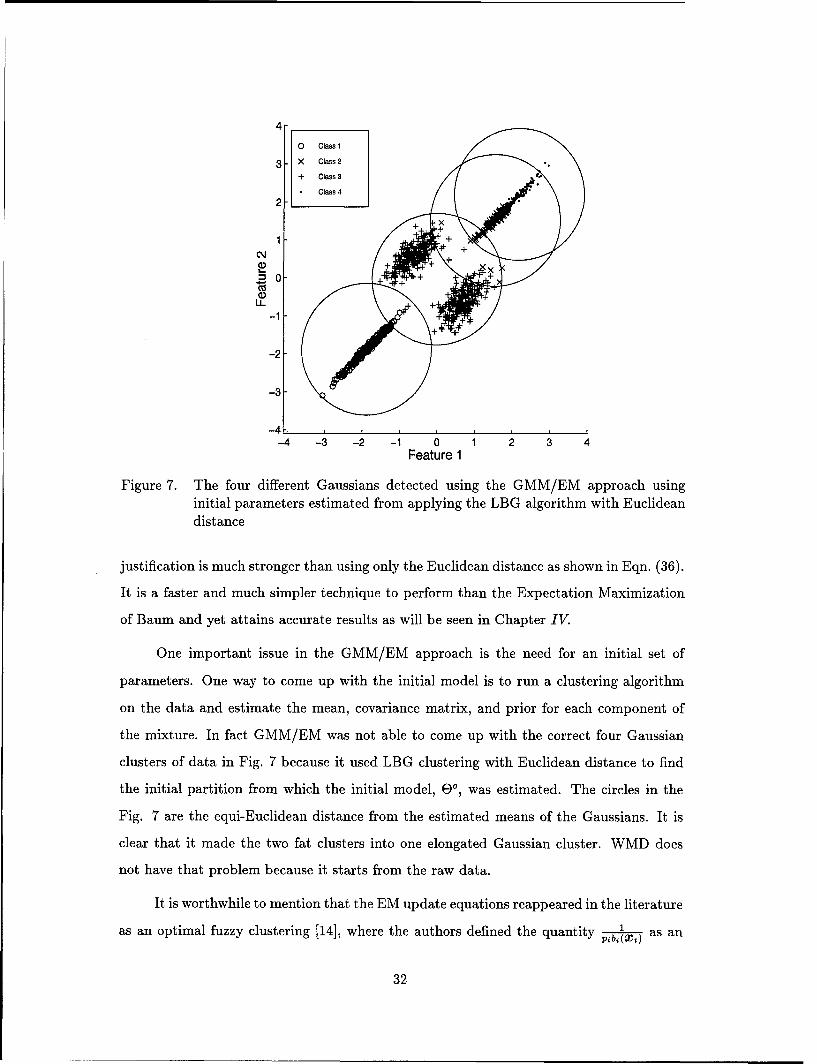
Figure 7. The four different Gaussians detected using the GMM/EM approach usinginitial parameters estimated from applying the LBG algorithm with Euclideandistance

justification is much stronger than using only the Euclidean distance as shown in Eqn. (36).

It is a faster and much simpler technique to perform than the Expectation Maximization

of Baum and yet attains accurate results as will be seen in Chapter IV.

One important issue in the GMM/EM approach is the need for an initial set of

parameters. One way to come up with the initial model is to run a clustering algorithm

on the data and estimate the mean, covariance matrix, and prior for each component of

the mixture. In fact GMM/EM was not able to come up with the correct four Gaussian

clusters of data in Fig. 7 because it used LBG clustering with Euclidean distance to find

the initial partition from which the initial model, 8 0, was estimated. The circles in the

Fig. 7 are the equi-Euclidean distance from the estimated means of the Gaussians. It is

clear that it made the two fat clusters into one elongated Gaussian cluster. WMD does

not have that problem because it starts from the raw data.

It is worthwhile to mention that the EM update equations reappeared in the literature

as an optimal fuzzy clustering [14], where the authors defined the quantity I as anpibi(X3)

32

"exponential" distance measure d2(xt, mi) and the component covariance matrices were

called fuzzy covariance matrices. In this paper, Gath and Geva realized that the initial

model selection has an important effect on the overall results. Therefore, they grew the

codebook to the desired number of codewords, one codeword at a time, by a procedure that

places the new codeword in a region where the data points have low degree of membership

in the existing clusters. This is similar to the way splitting in the direction of maximum

variance would ensure systematic distribution of the codewords.

The optimal fuzzy approach gave very good results that captured the shape of un-

derlying substructures in many cases including the Iris data set, linear distributions, and

clustering of sleep EEG recordings in order to classify the signal into various sleep stages.

However, the required computation associated with calculating the a posteriori probabili-

ties for each pattern after every iteration can become exorbitant.

2.7 Summary

This chapter has provided a background on clustering and has presented the theo-

retical justification for the approaches used in this thesis. The key ideas are summarized

as follows:

1. Some clusters fall naturally in hyperellipsoids in the feature space rather than in

hyperspheres.

2. The WMD algorithm allows for individually shaped hyperellipsoidal clusters with

constraints on the covariance matrices.

3. The WMD algorithm is related to the expectation maximization algorithm.

33

III. Methods

3.1 Introduction

Having discussed in Chapter 11 the concepts used in the four clustering techniques

(LBG, FCM, WMD, and HEC), this chapter presents the details of implementing these

methods. First, Section 3.2 discusses the general approach followed in batch k-means-type

clustering with variations in all stages of the algorithm. Next, Section 3.3 describes the

implementation of the LBG algorithm. Next, Section 3.4 describes how the FCM ap-

proach was implemented. In Section 3.5, the details of the weighted Mahalanobis distance

algorithm are presented. The first three methods are described together because they

are similar in following the general structure of the k-means algorithm, so they may be

implemented together to realize significant savings in computation and time. Section 3.6

outlines the methodology used in building the neural network for performing the principal

component analysis. Finally, Section 3.7 describes the HEC network for integrating the

Mahalanobis distance in partitional clustering.

3.2 A General Approach for Batch k-means Clustering

As discussed in Chapter II, the LBG, FCM, and WMD techniques are all based on

the generalized Lloyd algorithm. This section presents the general approach taken by these

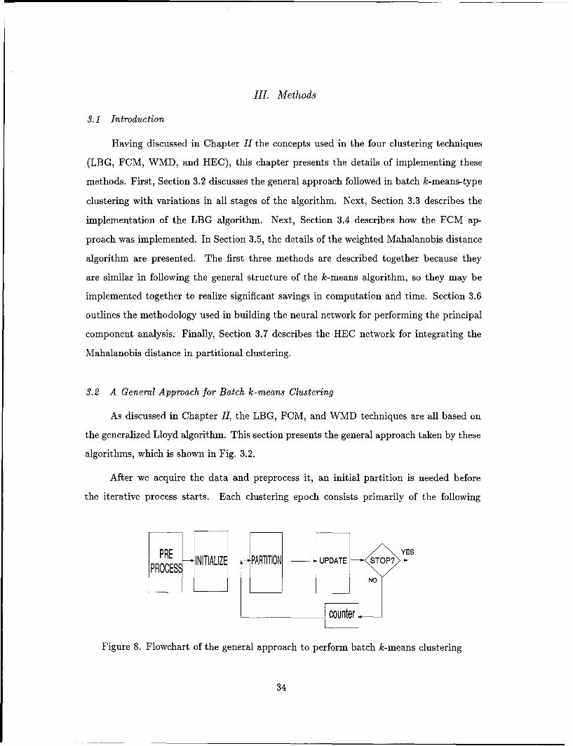
algorithms, which is shown in Fig. 3.2.

After we acquire the data and preprocess it, an initial partition is needed before

the iterative process starts. Each clustering epoch consists primarily of the following

NO

Figure 8. Flowchart of the general approach to perform batch k-means clustering

34

steps: partitioning according to a specific distortion measure, codebook update based on

the results of the first step, and finally, evaluation of the current partition quality before

another iteration is initiated.

The algorithms described here are implemented in MATLAB®. Appendix A contains

the code named CLUSTER used to implement the LBG, FCM, and WMD techniques. A

description of its operation and a list of its subroutines are also provided. The following

sections will describe each stage of this general code.

3.2.1 Preprocessing. A normalization procedure that is composed of two steps

is performed for all cases. First, the mean of the data set is subtracted from it which

is equivalent to forcing the mean of the input patterns to equal zero. This is especially

important for the PCA network. Second, we scale all the data sets to make the maximum

length of feature vectors to be one without changing the shape of clusters or the relative

location or ratio between the features. By doing so, the same set of parameters can be

applied to all the data sets, and any initial codebook with small length is guaranteed to

be in the middle of the data points in the feature space.

3.2.2 Initialization. As stated in Section 2.6.4, the choice of the initial model

is critical for the quality of the results. The parameters needed to start each epoch of

the iterative process depend on the clustering algorithm under study. Nevertheless, all

clustering techniques require an initial codebook to improve. Therefore, this section will

describe the different ways of finding the initial codebook while initialization for different

parameters required for the Mahalanobis distance-based algorithms is discussed later.

A variety of codebook initialization schemes have been investigated in hopes of pro-

viding accelerated convergence of the k-means algorithm, achieving a better local minimum,

and providing flexibility in terms of the number of clusters. In the following sections, some

of the techniques that are incorporated in CLUSTER are described.

3.2.2.1 Initialization by Splitting. Linde et al. [24] suggested a splitting

method whereby one starts by finding the centroid of all the training data which is the

optimum codebook of size one. This single codeword, ino, is then split to form two

35

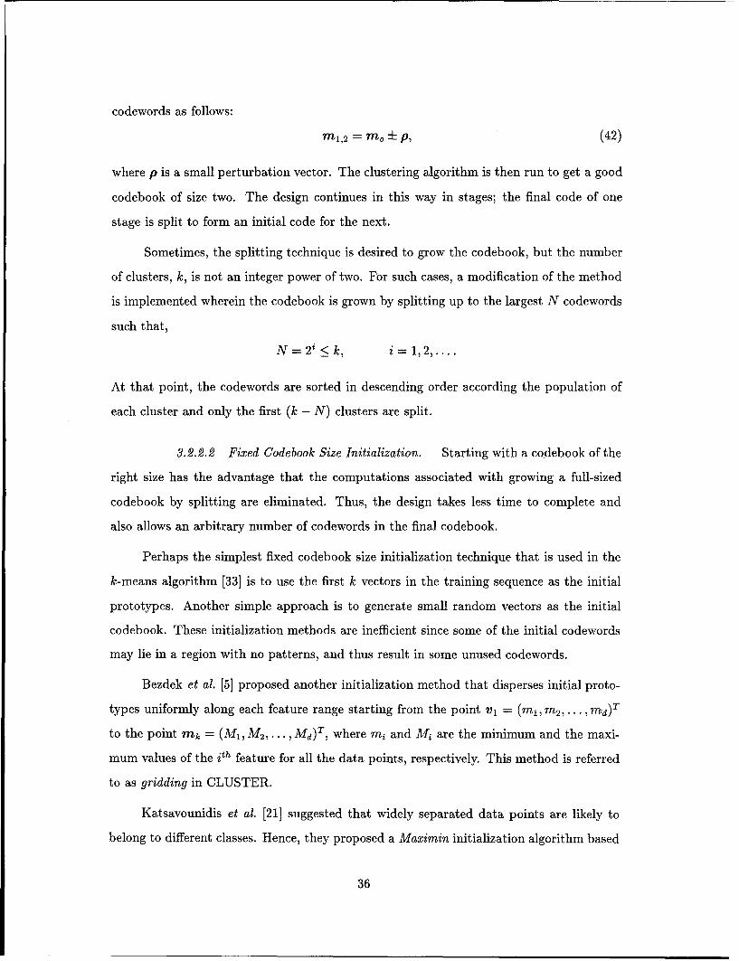
codewords as follows:

M 1 ,2 =m o ± P, (42)

where p is a small perturbation vector. The clustering algorithm is then run to get a good

codebook of size two. The design continues in this way in stages; the final code of one

stage is split to form an initial code for the next.

Sometimes, the splitting technique is desired to grow the codebook, but the number

of clusters, k, is not an integer power of two. For such cases, a modification of the method

is implemented wherein the codebook is grown by splitting up to the largest N codewords

such that,

N = 2' < k, i = 1,2....

At that point, the codewords are sorted in descending order according the population of

each cluster and only the first (k - N) clusters are split.

3.2.2.2 Fixed Codebook Size Initialization. Starting with a codebook of the

right size has the advantage that the computations associated with growing a full-sized

codebook by splitting are eliminated. Thus, the design takes less time to complete and

also allows an arbitrary number of codewords in the final codebook.

Perhaps the simplest fixed codebook size initialization technique that is used in the

k-means algorithm [33] is to use the first k vectors in the training sequence as the initial

prototypes. Another simple approach is to generate small random vectors as the initial

codebook. These initialization methods are inefficient since some of the initial codewords

may lie in a region with no patterns, and thus result in some unused codewords.

Bezdek et al. [5] proposed another initialization method that disperses initial proto-

types uniformly along each feature range starting from the point v, = (m 1 ,m 2 ,... ,eMd)T

to the point mk = (M 1, M 2,..., Md)T, where mi and Mi are the minimum and the maxi-

mum values of the ith feature for all the data points, respectively. This method is referred

to as gridding in CLUSTER.

Katsavounidis et al. [21] suggested that widely separated data points are likely to

belong to different classes. Hence, they proposed a Maximin initialization algorithm based

36

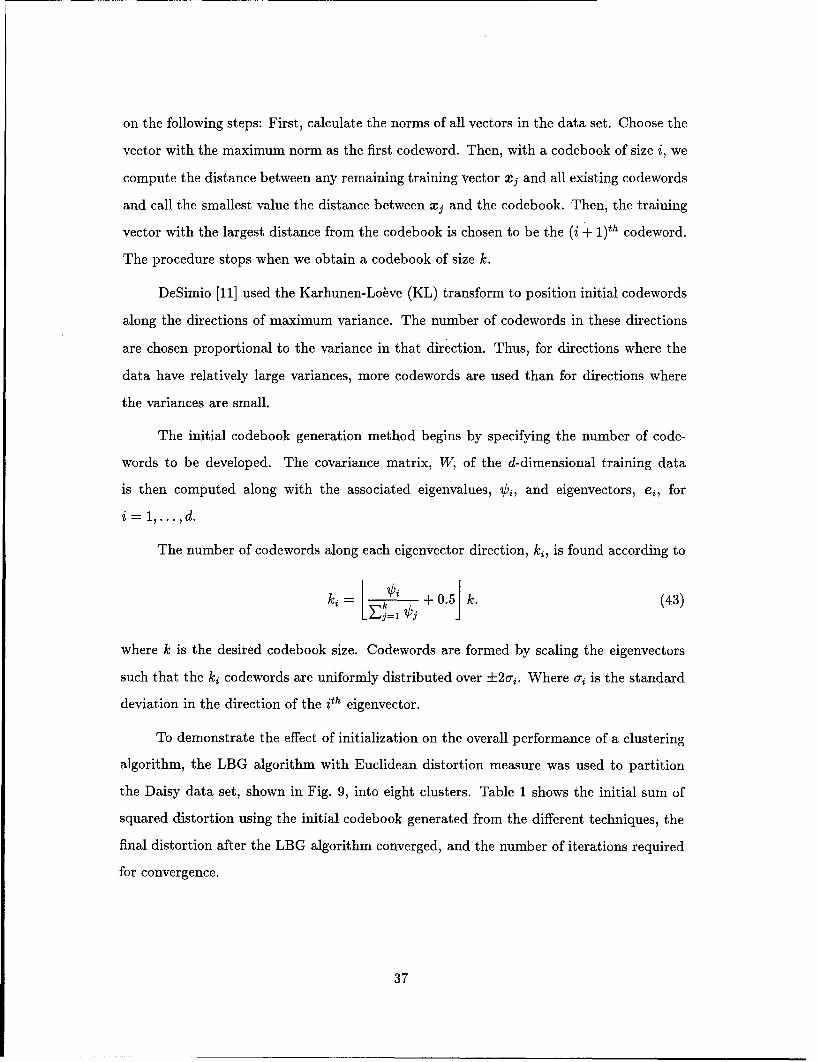
on the following steps: First, calculate the norms of all vectors in the data set. Choose the

vector with the maximum norm as the first codeword. Then, with a codebook of size i, we

compute the distance between any remaining training vector xj and all existing codewords

and call the smallest value the distance between xj and the codebook. Then, the training

vector with the largest distance from the codebook is chosen to be the (i + 1)1h codeword.

The procedure stops when we obtain a codebook of size k.

DeSimio [11] used the Karhunen-Lo~ve (KL) transform to position initial codewords

along the directions of maximum variance. The number of codewords in these directions

are chosen proportional to the variance in that direction. Thus, for directions where the

data have relatively large variances, more codewords are used than for directions where

the variances are small.

The initial codebook generation method begins by specifying the number of code-

words to be developed. The covariance matrix, W, of the d-dimensional training data

is then computed along with the associated eigenvalues, 0j, and eigenvectors, ej, fori=l..d

The number of codewords along each eigenvector direction, ki, is found according to

I j=1 Oj I

where k is the desired codebook size. Codewords are formed by scaling the eigenvectors

such that the ki codewords are uniformly distributed over ±20-. Where O- is the standard

deviation in the direction of the ith eigenvector.

To demonstrate the effect of initialization on the overall performance of a clustering

algorithm, the LBG algorithm with Euclidean distortion measure was used to partition

the Daisy data set, shown in Fig. 9, into eight clusters. Table 1 shows the initial sum of

squared distortion using the initial codebook generated from the different techniques, the

final distortion after the LBG algorithm converged, and the number of iterations required

for convergence.

37

Scatter plot for Daisy data set20

15"

10 45O ",% . "

5-

-5"

-15:, .

-20-20 -15 -10 -5 0 5 10 15 20

Feature 1

Figure 9. Scatter plot for the Daisy data set

Table 1. Table of the required initial and final distortion and the number of iterationsrequired by the LBG algorithm to cluster the Daisy data set into eight clusters

Initialization Method I Initial Distortion Final Distortion I Number of Iterations

Splitting 21550 15880 17First-k-samples 295700 26430 7

Maximin 79710 15960 12Gridding 97890 14690 8

KLI 41860 13610 7

38

As can be seen from the results, the worst is the "First-k-samples" approach because

all the initial codewords may be of the same cluster. Splitting took more iterations to give

better initial distortion, but it is not guaranteed to give the best final distortion.

For the purpose of simulations in the next chapter, LBG's splitting was used. For the

cases where the required codebook size is not an integer power of two, the KL initialization

(KLI) technique was preferred to the other techniques as it gives the best overall results

as shown in Table 1.

3.2.3 Partitioning. The partitioning step consists basically of assigning each data

point to the cluster whose centroid is nearest to that data point in d space, where d is the

dimensionality of the data set. The minimum distance criterion can be used to determine

the point membership of each centroid.

Hence, partitioning of X into k clusters is better described by a n x k matrix, U,

whose entry, uij, is the membership of the ith pattern in the jth cluster. Therefore, the

entries of U are numbers between zero and one and the sum of the entries in each row is

one.

Note that in hard clustering the range of uij is {O,1}, which means that in cases of

equal distances to more than one cluster center a tie-breaking rule is needed. In CLUSTER,

the least numbered cluster is considered a winner.

3.2.4 Codebook Update. There are two ways for updating cluster centers, the

sequential approach, where the codewords are updated after each sample, and the batch

method, where the update takes place after all the data points are assigned to the different

cluster centers. Even though the HEC algorithm adjusts the weights adaptively to estimate

the eigenvectors and eigenvalues, the actual update to the cluster centers are done by a

batch vector quantization algorithm [25]. Therefore, we restrict our analysis in this thesis

to the batch mode.

3.2.5 Clustering Evaluation. The final logical step within an iteration is the

evaluation of the clusters produced by the previous steps. Once formed, clusters must be

39

evaluated to determine if the present configuration is optimal or whether modifications are

necessary.

The following sections discuss in detail the implementation of each of the three clus-

tering algorithms. For each technique, the specifics about which initialization technique

is used, what distance measure is implemented, how to perform the update, and what

criterion for cluster evaluation is necessary are clearly identified.

3.3 The LBG Algorithm Implementation

We followed the algorithm described in [24] using the Euclidean distance as a ba-

sis for partitioning. The codebook was grown by splitting, where a fixed small random

perturbation vector is added to each codeword after each splitting stage.

The n x c distance matrix containing the Euclidean distance from the data points to

each codeword is calculated using Eqn. (6). The optimality criterion is the mean squared

error (MSE). The algorithm is terminated when (MSE) stops decreasing significantly.

3.4 The Fuzzy c-means Algorithm Implementation

There is no specific initialization technique suggested for the FCM algorithm [7].

Bezdek suggested starting with a random codebook but for the purpose of comparison,

the same method for initialization was used for all algorithms. The Euclidean distance

was also used as a basis for partitioning to compare with the Mahalanobis distance-based

algorithms.

While in LBG only data points which are assigned to a specific cluster will update

its codeword, in FCM all the data points will affect the update of the codewords. In other

words, every data point is assigned to all the codewords but with different degrees. Recall

that if u e{O,1} the calculation of M reduces to computing the means for the different

clusters. Hence this same equation, Eqn. (8), is used for updating the cluster center for

both the LBG and the FCM algorithms.

Different values for the exponential weight, m, were tried. It was found that as m gets

larger, the effect of far points on the cluster center becomes clearer by shifting its location

40

towards them. Keller et al. found that, in general, a value of m = 2 is appropriate [22].

However, a value of m = 3 was used for the simulations to allow for more fuzziness.

When using the fuzzy membership functions to perform classification, one considers

the degree of class membership for each test vector. The class membership function values,

U, computed with Eqn. (9), provide a measure of similarity by which a decision can be

made to assign the pattern to the class that yields the highest membership value.

3.5 The WMD Algorithm Implemetation

The algorithm starts with measuring the mean and covariance of the whole data set.

As suggested by [24] the required c codewords can grow by splitting. Splitting can be done

randomly or according to other considerations. However, we think that the best splitting

is that which will put the new codewords for a specific cluster far apart in the direction of

the maximum variance of that cluster. We made the perturbation for each cluster based

on eigenvalues and eigenvectors of its covariance matrix as

1b i (44)

where im and e' are the maximum eigenvalue and the corresponding eigenvector of Ci,

respectively. The benefit of this approach is that there is a systematic approach of dis-

tributing the codebook vectors and each cluster will split in different directions based on

the distribution in that cluster independent from other clusters.

In cases where the number of codewords is not an integer power of two, the KLI

algorithm was used with the covariance matrix for all data points is used as Ci for all

clusters.

Two ways to compute the Mahalanobis distance are possible, using C,71 as in Eqn. (4)

or using the eigenvectors and eigenvalues of Ci as suggested by Eqn. (17). The second

method avoids the need to compute the distance to each data point separately so matrix

multiplication can be used instead of the loops which results in huge savings. Moreover,

the second method turns away from inverting the different covariance matrices after each

41

iterations and with proper implementation, we can keep the eigenvalues and eigenvectors

so we can also obtain the new codewords after each splitting stage as the byproduct.

After all the data is presented, the codeword for each cluster will be computed as

the average of the data points assigned to that cluster. The covariance matrix of these

data points forms the A matrix for that group. The weight, wi, can be calculated as the

ratio of the number of samples in the ith cluster to the size of the training samples for the

WMD with conscience (WMDC). For the WMD with volume constraint (WMDVC)

= (45)

where ICil is the determinant of Ci.

The algorithm is terminated when the difference between the location of the code-

words in consecutive iterations falls below a threshold or JGMSE stops decreasing signifi-

cantly for the case of WMDVC.

3.6 Principal Component Analysis Network

The proposed neural network was built as shown in Fig. 5. In using the update

equations, Eqn. (20) and Eqn. (21), it should be noted that it is required to have the mean

of the input patterns equal zero. In addition, the weights should be normalized after every

update.

The weight vector w, converges to the eigenvector with the largest eigenvalue of the

covariance matrix C of the pattern set. Subsequently, the eigenvector corresponding to

the next largest eigenvalue is computed and so on up the number of the output nodes.

This network was able to find the eigenvectors for the covariance matrix of several

data sets accurately and quickly. However, it was noticed that this algorithm doesn't

converge easily when the eigenvalues are small. A modification of the learning rules was

implemented by Mao and Jain [25]. However, since the authors didn't have theoretical

justification and introduced ad hoc parameters that might not generalize to other data

sets, the modified learning rules were not implemented.

42

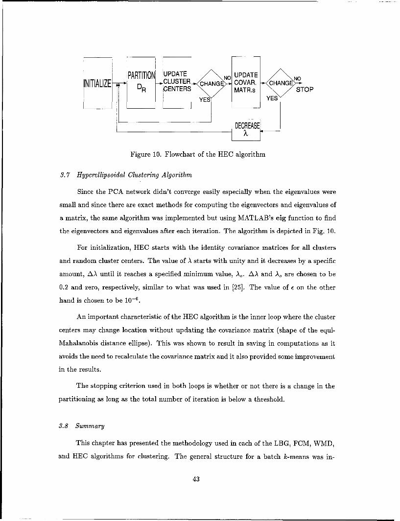
PARTITION UPDATE NOUPDATE N_CLUSTER CHNE COVAR. CHANG

NIILIE -- R CENTERS MATR.s STOP

YESYE

DER7EASE _

Figure 10. Flowchart of the HEC algorithm

3.7 Hyperellipsoidal Clustering Algorithm

Since the PCA network didn't converge easily especially when the eigenvalues were

small and since there are exact methods for computing the eigenvectors and eigenvalues of

a matrix, the same algorithm was implemented but using MATLAB's eig function to find

the eigenvectors and eigenvalues after each iteration. The algorithm is depicted in Fig. 10.

For initialization, HEC starts with the identity covariance matrices for all clusters

and random cluster centers. The value of A starts with unity and it decreases by a specific

amount, AA until it reaches a specified minimum value, A,. AA and A, are chosen to be

0.2 and zero, respectively, similar to what was used in [25]. The value of E on the other

hand is chosen to be 10-6.

An important characteristic of the HEC algorithm is the inner loop where the cluster

centers may change location without updating the covariance matrix (shape of the equi-

Mahalanobis distance ellipse). This was shown to result in saving in computations as it

avoids the need to recalculate the covariance matrix and it also provided some improvement

in the results.

The stopping criterion used in both loops is whether or not there is a change in the

partitioning as long as the total number of iteration is below a threshold.

3.8 Summary

This chapter has presented the methodology used in each of the LBG, FCM, WMD,

and HEC algorithms for clustering. The general structure for a batch k-means was in-

43

troduced with a description of each stage of this general algorithm. A neural network

for principal component analysis was discussed. The following chapter presents results

obtained by applying these techniques to several pattern recognition and Image coding

problems.

44

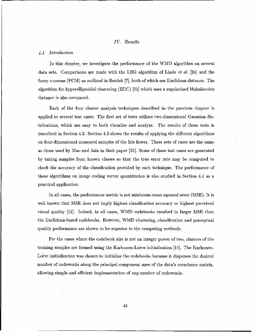
IV. Results

4.1 Introduction

In this chapter, we investigate the performance of the WMD algorithm on several

data sets. Comparisons are made with the LBG algorithm of Linde et al. [24] and the

fuzzy c-means (FCM) as outlined in Bezdek [7], both of which use Euclidean distance. The

algorithm for hyperellipsoidal clustering (HEC) [25] which uses a regularized Mahalanobis

distance is also compared.

Each of the four cluster analysis techniques described in the previous chapter is

applied to several test cases. The first set of tests utilizes two-dimensional Gaussian dis-

tributions, which are easy to both visualize and analyze. The results of these tests is

described in Section 4.2. Section 4.3 shows the results of applying the different algorithms

on four-dimensional measured samples of the Iris flower. These sets of cases are the same

as those used by Mao and Jain in their paper [25]. Some of these test cases are generated

by taking samples from known classes so that the true error rate may be computed to

check the accuracy of the classification provided by each technique. The performance of

these algorithms on image coding vector quantization is also studied in Section 4.4 as a

practical application.

In all cases, the performance metric is not minimum mean squared error (MSE). It is

well known that MSE does not imply highest classification accuracy or highest perceived

visual quality [12]. Indeed, in all cases, WMD codebooks resulted in larger MSE than

the Euclidean-based codebooks. However, WMD clustering, classification and perceptual

quality performance are shown to be superior to the competing methods.

For the cases where the codebook size is not an integer power of two, clusters of the

training samples are formed using the Karhunen-Lo~ve initialization [11]. The Karhunen-

Lo~ve initialization was chosen to initialize the codebooks because it disperses the desired

number of codewords along the principal component axes of the data's covariance matrix,

allowing simple and efficient implementation of any number of codewords.

45

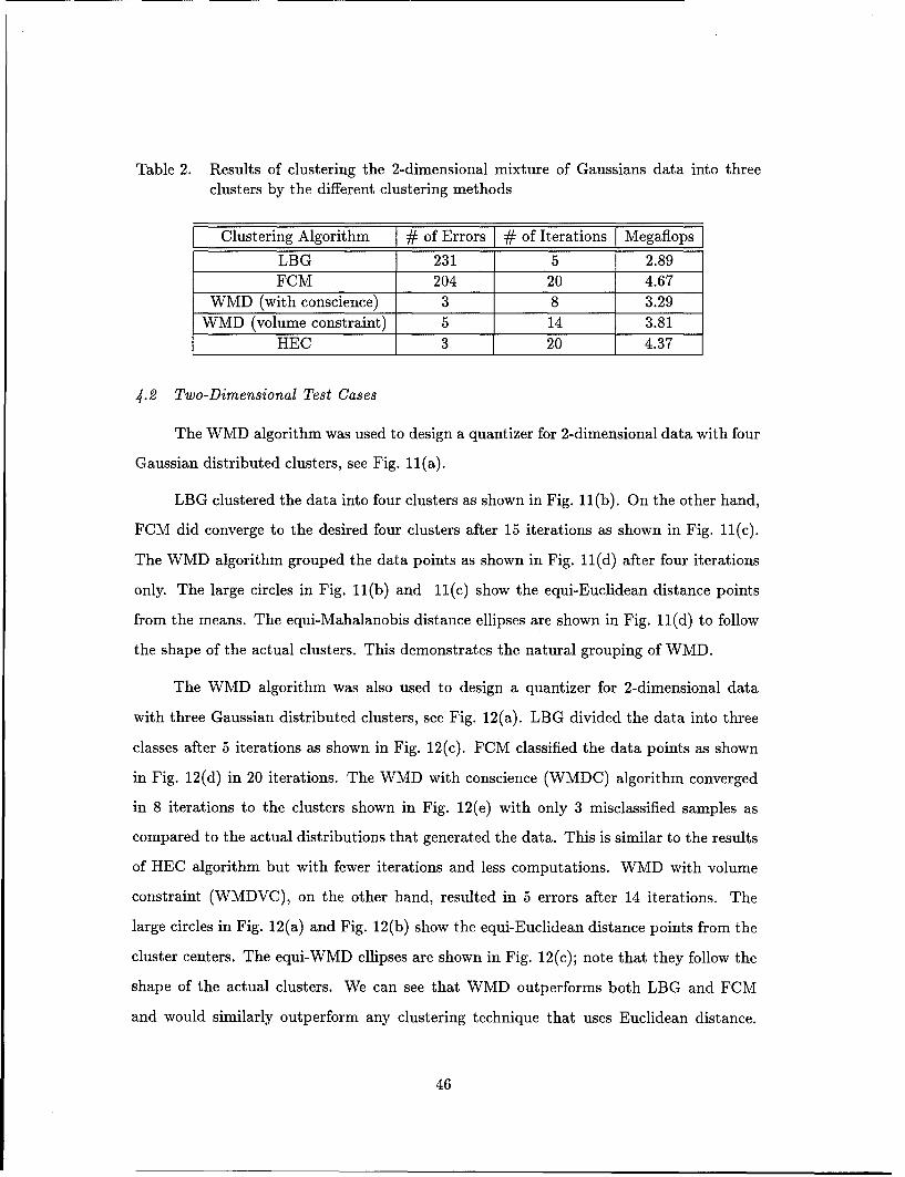
Table 2. Results of clustering the 2-dimensional mixture of Gaussians data into threeclusters by the different clustering methods

Clustering Algorithm # of Errors # of Iterations Megaflops

LBG 231 5 2.89FCM 204 20 4.67

WMD (with conscience) 3 8 3.29WMD (volume constraint) 5 14 3.81

HEC 3 20 4.37

4.2 Two-Dimensional Test Cases

The WMD algorithm was used to design a quantizer for 2-dimensional data with four

Gaussian distributed clusters, see Fig. 11(a).

LBG clustered the data into four clusters as shown in Fig. 11(b). On the other hand,

FCM did converge to the desired four clusters after 15 iterations as shown in Fig. 11(c).

The WMD algorithm grouped the data points as shown in Fig. 11(d) after four iterations

only. The large circles in Fig. 11(b) and 11(c) show the equi-Euclidean distance points

from the means. The equi-Mahalanobis distance ellipses are shown in Fig. 11(d) to follow

the shape of the actual clusters. This demonstrates the natural grouping of WMD.

The WMD algorithm was also used to design a quantizer for 2-dimensional data

with three Gaussian distributed clusters, see Fig. 12(a). LBG divided the data into three

classes after 5 iterations as shown in Fig. 12(c). FCM classified the data points as shown

in Fig. 12(d) in 20 iterations. The WMD with conscience (WMDC) algorithm converged

in 8 iterations to the clusters shown in Fig. 12(e) with only 3 misclassified samples as

compared to the actual distributions that generated the data. This is similar to the results

of HEC algorithm but with fewer iterations and less computations. WMD with volume

constraint (WMDVC), on the other hand, resulted in 5 errors after 14 iterations. The

large circles in Fig. 12(a) and Fig. 12(b) show the equi-Euclidean distance points from the

cluster centers. The equi-WMD ellipses are shown in Fig. 12(c); note that they follow the

shape of the actual clusters. We can see that WMD outperforms both LBG and FCM

and would similarly outperform any clustering technique that uses Euclidean distance.

46

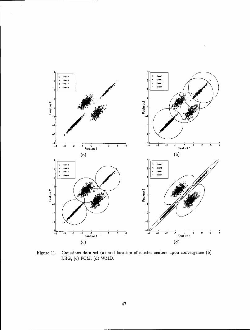
4 4

3 X t3o

+ C + x

04 OIo 2

1 1

-2 -2

-3 0 -3-

-h 1-4 L-__________________________

-4 -3 2 -1 0 1 2 3 4 -4 -3 -2 -1 0 1 2 3 4Feature 1 Feature 1

(a) (b)4 4

2 2

1 1x114)

76

a 0

-46 -4

-4 3 -2 -1 0 1 2 3 4 -4 -3 -2 -1 0 1 2 3 4Feature 1 Feature 1

(c) (d)

Figure 11. Gaussians data set (a) and location of cluster centers upon convergence (b)LBG, (c) FCM, (d) WMD.

47

15 X0.0

100.

+ +

-1 LL+

+ +++ + + .

5 -02.

-0~-15 -10 -5 0 5 10 15 ..6 -0.4 -0.2 0 0.2 0.4 0.6 0.8First Feature First Feature

(a) (b)15 1

10 X10

5 X X5X

I@ 00U

54 5) Oo 0

-00 ++ + -1 C= +i+ + ++ +C.S

_f +X~ I+

-50 0 1101

First Feature First Feature

(c) (d)15 X15 X

10 10

am 5

X +0

5 0 CL5AX

X+5 + XL S

0 -0 + *

r r+

-15 1

-15 -10 -5 0 5 10 15 -15 -10 -5 0 5 10 15First Feature First Feature

(e) Mf

Figure 12. Original and computed partitioning of a mixture of Gaussian data using thedifferent clustering methods. (a) Original classes. (b)-(f): Resultant One-nearest neighbor classification using the codebook generated by HEC, LBG,FOM, WMDC, and WMDVC methods, respectively.

48

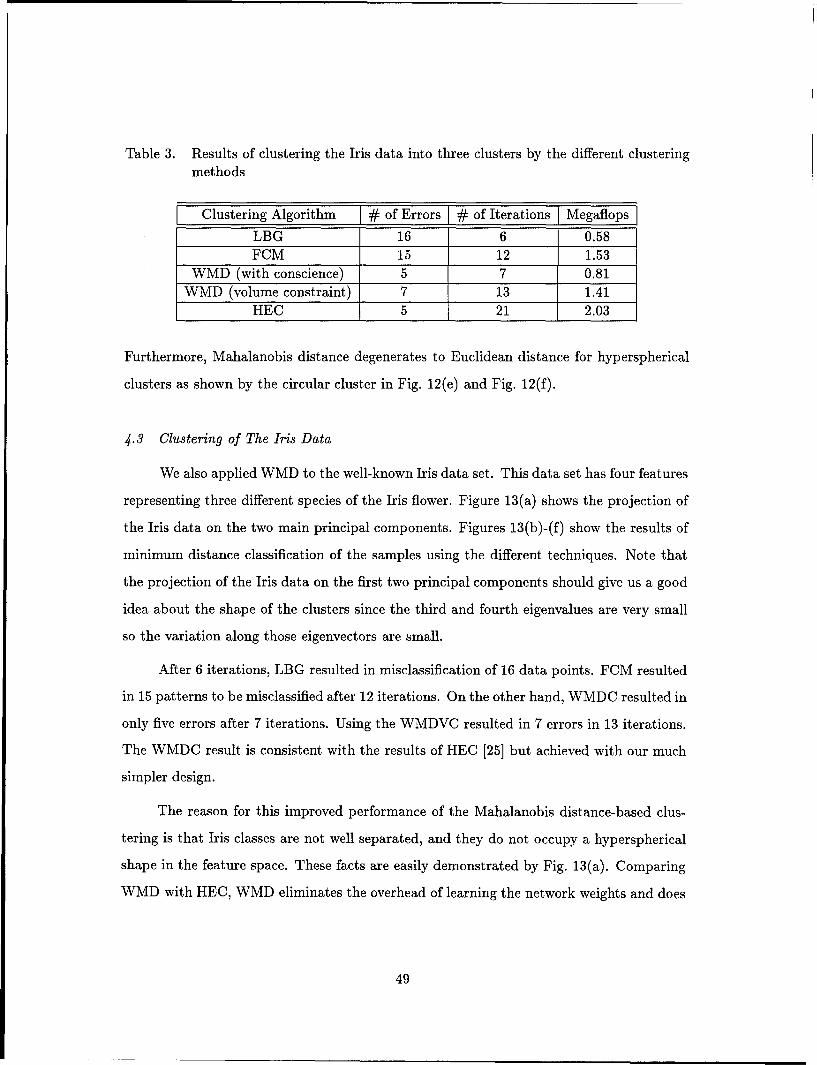
Table 3. Results of clustering the Iris data into three clusters by the different clusteringmethods

Clustering Algorithm # of Errors # of Iterations Megaflops

LBG 16 6 0.58FCM 15 12 1.53

WMD (with conscience) 5 7 0.81WMD (volume constraint) 7 13 1.41

HEC 5 21 2.03

Furthermore, Mahalanobis distance degenerates to Euclidean distance for hyperspherical

clusters as shown by the circular cluster in Fig. 12(e) and Fig. 12(f).

4.3 Clustering of The Iris Data

We also applied WMD to the well-known Iris data set. This data set has four features

representing three different species of the Iris flower. Figure 13(a) shows the projection of

the Iris data on the two main principal components. Figures 13(b)-(f) show the results of

minimum distance classification of the samples using the different techniques. Note that

the projection of the Iris data on the first two principal components should give us a good

idea about the shape of the clusters since the third and fourth eigenvalues are very small

so the variation along those eigenvectors are small.

After 6 iterations, LBG resulted in misclassification of 16 data points. FCM resulted

in 15 patterns to be misclassified after 12 iterations. On the other hand, WMDC resulted in

only five errors after 7 iterations. Using the WMDVC resulted in 7 errors in 13 iterations.

The WMDC result is consistent with the results of HEC [25] but achieved with our much

simpler design.

The reason for this improved performance of the Mahalanobis distance-based clus-

tering is that Iris classes are not well separated, and they do not occupy a hyperspherical

shape in the feature space. These facts are easily demonstrated by Fig. 13(a). Comparing

WMD with HEC, WMD eliminates the overhead of learning the network weights and does

49

0 CLASS 1 0 CLASS 13 X CRASS2 + + X CLASS2 X0 + CLASS 3 + + CLASS 3 x

oD 00 a) ++0 : ++ & + o0 x

i + FL 0 xoq o+ +o +

cctixL20 %-0 +

*0'x 0

0P 0X ~ +

x W 0 + P

-2 0 x -2 + 0

x+ 0 0

-3 -3

-3 -2 -I 0 1 2 3 3 -2 -1 0 1 2 3

First Principal Component First Principal Component

(a) (b)

+ ~~~; x 7s x+xct ,s2 xo CLAS, 0 CLASS'+ CLA SS x + CLASS 3 x

+ + + + C

+ 3 + 0

0 x x 0

-3<E 3 1 2 01 O 1 X >2 0 1 0 1X 2

0 0lA8 0+0 0 V+ 8

+ 0 1o . x

0 +3<h)- 00 0 O

co -2 + 0 -2- + O

-3 -3

-2 -1 0 1 2 3 -3 -2 -1 0 1 2 3First Principal Component First Principal Component

(c) (d)

+ CLASS 5+ CLF+ +

mos(a) Orgia clsss (D)) Reutn n-eretniho ls

0 3< + 0 3

+ -0

8 ifcaio usn8h oeokgnrtd yLG CHCWDwt

E. 1+ 00.xX.E10 x

x &0

-24- 1+ 2x 33- + to

-i 04

conscience1 and WMD with volume constraint methods1 respectively.

50

not require an upper limit on the number of iterations (100,000 was used in HEC) [25].

Furthermore, no ad hoc parameters are required for WMD.

4.4 Vector Quantization Coding of Image Data

In this section, we evaluate the WMD clustering algorithm in a realistic application,

specifically, vector quantization coding of an image. We have chosen this application,

in part, because the computation is very intensive due to the large amount of data to

be processed. In addition, the evaluation results can be expressed both numerically and

visually, providing better insight of the differences among the algorithms.

Vector quantization image coding is used to reduce transmission bit rate or data

storage while maintaining acceptable image quality. In this application, the mandrill image

from the University of Southern California (USC) image database was used, see Fig. 14(a).

It consists of 480 x 500 pixel digitized into 8-bit gray levels. Due to the large size of

the image, it was down-sampled by a factor of four along both axes resulting in a more

manageable problem. In this experiment we try to partition the images into 4 clusters

and then define the centroids of resulting clusters as the codewords. Blocks of 4 x 4 pixels

defining 16-dimensional vectors were then used to design the codebooks.

For the purpose of comparison, we test the performance of the WMD algorithm ver-

sus both LBG clustering and Fuzzy c-means on computing the codebooks for the images.

Figures 14(b), 14(c), and 14(d) show the reconstructed images using the four-class code-

book generated by WMD, FCM, and LBG clustering methods, respectively. Comparing

these figures, we find obvious degradation of the visual quality in LBG and FCM recon-

structed images especially in the nose area. Only the WMD image shows the three-level

change in the nose pixels and the continuity of the dark gray level all around the nose. The

covariance matrix of the pixels corresponding to this gray level was found to be different

from the identity which implies a non-hyperspherical shape. WMD groups the vectors

naturally, which provides the clear improvement in the quality of the reconstructed image.

The proposed algorithm adapts to the local characteristics and preserves the features of

the face.

51

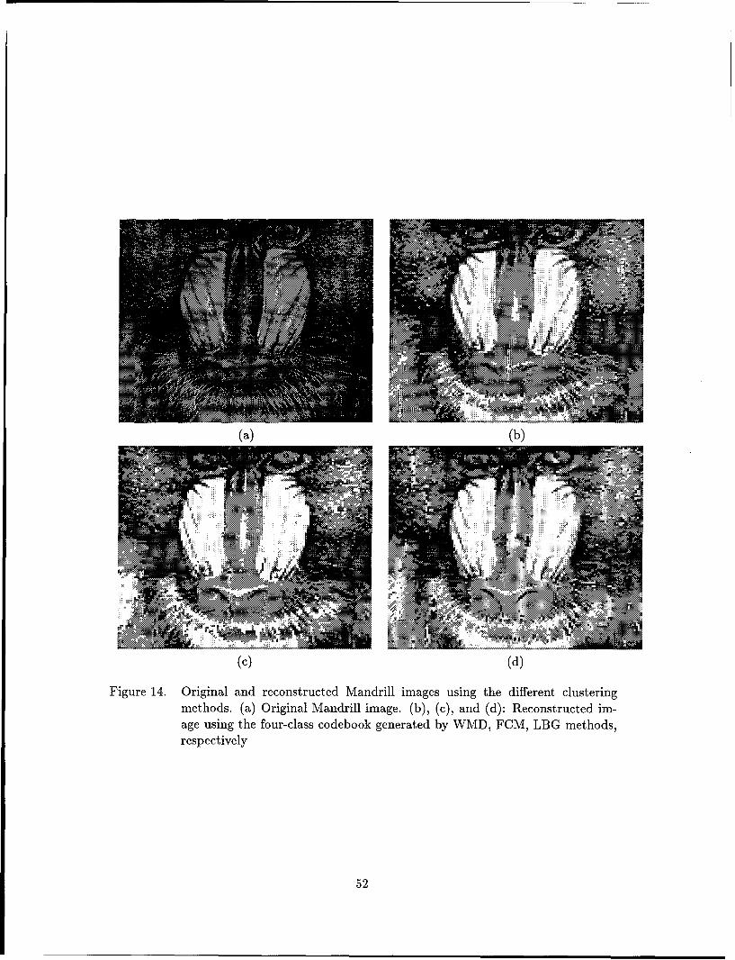
(a) (b)

(c) (d)

Figure 14. Original and reconstructed Mandrill images using the different clustering

methods. (a) Original Mandrill image. (b), (c), and (d): Reconstructed im-

age using the four-class codebook generated by WMD, FCM, LBG methods,

respectively

52

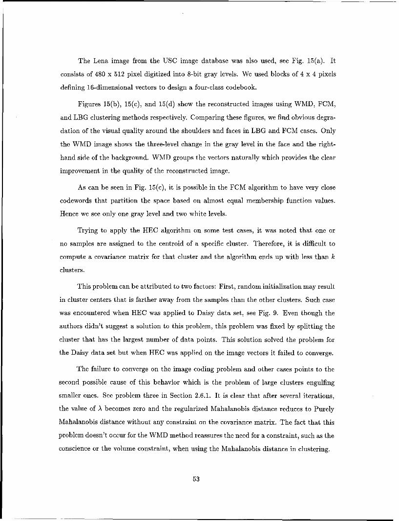
The Lena image from the USC image database was also used, see Fig. 15(a). It

consists of 480 x 512 pixel digitized into 8-bit gray levels. We used blocks of 4 x 4 pixels

defining 16-dimensional vectors to design a four-class codebook.

Figures 15(b), 15(c), and 15(d) show the reconstructed images using WMD, FCM,

and LBG clustering methods respectively. Comparing these figures, we find obvious degra-

dation of the visual quality around the shoulders and faces in LBG and FCM cases. Only

the WMD image shows the three-level change in the gray level in the face and the right-

hand side of the background. WMD groups the vectors naturally which provides the clear

improvement in the quality of the reconstructed image.

As can be seen in Fig. 15(c), it is possible in the FCM algorithm to have very close

codewords that partition the space based on almost equal membership function values.

Hence we see only one gray level and two white levels.

Trying to apply the HEC algorithm on some test cases, it was noted that one or

no samples are assigned to the centroid of a specific cluster. Therefore, it is difficult to

compute a covariance matrix for that cluster and the algorithm ends up with less than k

clusters.

This problem can be attributed to two factors: First, random initialization may result

in cluster centers that is farther away from the samples than the other clusters. Such case

was encountered when HEC was applied to Daisy data set, see Fig. 9. Even though the

authors didn't suggest a solution to this problem, this problem was fixed by splitting the

cluster that has the largest number of data points. This solution solved the problem for

the Daisy data set but when HEC was applied on the image vectors it failed to converge.

The failure to converge on the image coding problem and other cases points to the

second possible cause of this behavior which is the problem of large clusters engulfing

smaller ones. See problem three in Section 2.6.1. It is clear that after several iterations,

the value of A becomes zero and the regularized Mahalanobis distance reduces to Purely

Mahalanobis distance without any constraint on the covariance matrix. The fact that this

problem doesn't occur for the WMD method reassures the need for a constraint, such as the

conscience or the volume constraint, when using the Mahalanobis distance in clustering.

53

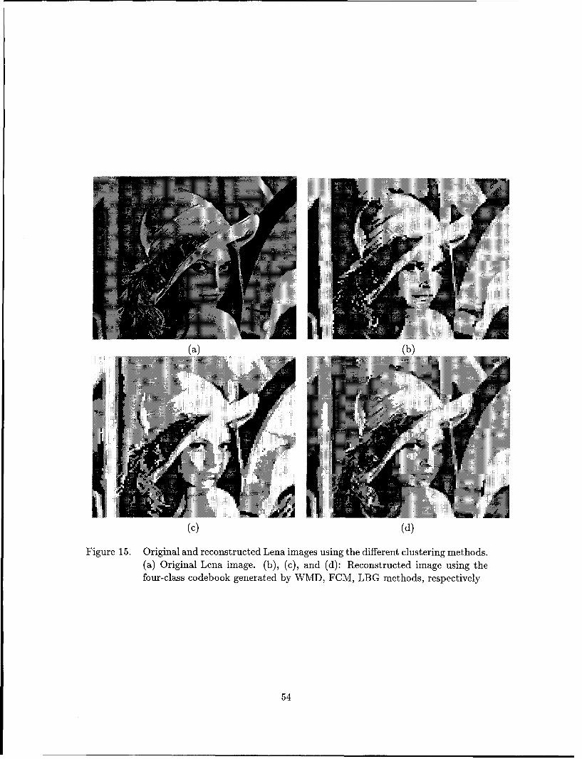
ii X 2

(a) (b)

LA(c) AV(d)

Figure 15. Original and reconstructed Lena images using the different clustering methods.(a) Original Lena image. (b), (c), and (d): Reconstructed image using thefour-class codebook generated by WMD, FCM, LBG methods, respectively

54

4.5 Summary

This chapter has shown the results obtained by applying each of the four techniques to

two two-dimensional and one four-dimensional test cases. In addition, vector quantization

coding of two images were intried. In general, these results indicate that the Mahalanobis

distance is a useful metric to be used as a similarity measure. Nevertheless, it was shown

that there exists a necessity to control the covariance matrix of each cluster in order to

obtain good results. The next chapter summarizes the results obtained in this investigation

and provides some recommendations for further research.

55

V. Conclusion

5.1 Introduction

The primary objective of this research was to examine the use of the class-based

Mahalanobis distance in clustering and develop a method to solve the problems associated

with such a use. The second objective was to compare its performance to Euclidean

distance based algorithms and other Mahalanobis distance based algorithms. Both of the

objectives were met.

5.2 Contributions

" This thesis introduced a method for integrating the Mahalanobis distance into batch

k-means-type algorithm. This algorithm has several attributes that make it well

suited for more general clustering problems: First, the system is robust in that

it achieved similar success in all of the test cases studied. Second, the algorithm

is related to the expectation maximization process so it has the same theoretical

foundation as the Gaussian mixture models. Third, it builds the codebook starting

from the data itself using an improved splitting method that takes the different shapes

of clusters into account.

" The analysis showed that the covariance matrices in the Mahalanobis distance based

algorithms need to be constrained in order to reach a non-trivial solution. Two

different constraints were discussed and implemented.

" As a tool for follow-on research, this thesis intentionally provides a significant amount

of background information in the area of clustering. Chapter H was specifically

written to assist a novice to the field in learning many of the clustering problem

fundamentals. The software developed in this effort contains numerous selections of

clustering techniques and parameters. This provides ease in application or replication

of this work for further research.

56

5.3 Follow-on Research

The research discussed in this thesis is by no means exhaustive. As with any large

undertaking, there are many areas left for further research. Some possible enhancements

are listed below:

" Preliminary results showed that the mutual Mahalanobis distances between the clus-

ter centers mi and mj using both Ci and Cj are good indicators of the similarity

between the two clusters in terms of shape and orientation. These indicators can be

the basis for merging similar clusters.

" Exploring the possibilities for finding the appropriate number of clusters, k, by means

of merging clusters based on the Mahalanobis distance between their centroids and

finding a monotonically decreasing criterion function as the number of clusters k

increases, such as JGMSE in WMD with volume constraint. The best number of

clusters will correspond to the "knee" of the curve where further increase in k results

in only a slight decrease in the criterion function.

" Developing a way to handle outliers which affect the covariance matrix and hence

the overall performance of a Mahalanobis distance based algorithm.

5.4 Summary of Results

Mahalanobis Distance is a very useful tool which is believed to give a better measure

of similarity than the Euclidean distance. It was shown that for certain data sets, the

Euclidean distance based clustering algorithms do not group the data points naturally.

The weighted Mahalanobis distance clustering, on the other hand, results in codebooks

that represent the data better than codebooks generated with either the LBG or the FCM

algorithms.

Even though the neural network for hyperellipsoidal clustering (HEC) uses the Ma-

halanobis distance, it failed to perform as well as the WMD algorithm. This is because it

could not solve the problems associated with using the Mahalanobis distance in clustering.

The WMD algorithm has been demonstrated using both artificial data and real data

to outperform existing methods in maintaining the natural distribution of the feature space.

57

It was also shown that WMD clustering accounts for variability in cluster shapes, cluster

densities, and the number of data points in each of the subsets.

The techniques developed for this thesis should be applicable not only to other syn-

thetic data, but to any data sets which are characterized by non-spherical cluster shapes.

5.5 Conclusions

The results obtained in this thesis lead to several interesting conclusions:

" Hyperellipsoidal clusters are more general and more likely to be encountered in real-

life applications than hyperspherical clusters.

" Increased generality allows better classification and perceptual image quality than

Euclidean distance based algorithms.

" Unlike HEC, WMD was able to overcome the difficulties associated with using the

Mahanobis disance in clustering.

" WMD has been related to the EM algorithm for finding the parameters in a Gaussian

Mixture Model

58

Appendix A. Clustering Codes

This appendix contains the MATLAB® codes which implement the LBG, FCM,

WMD, and HEC approaches.

To allow for saving in time and computation, a system for clustering is generated with

numerous selections of data sets, codebook size, distance metrics, initialization techniques,

and partitioning rules (hard or fuzzy). Therefore, a user can study the results of using these

algorithms with different parameters. In combining the algorithms together in CLUSTER,

some redundant operations are eliminated, such as reloading the data, normalization, and

codebook initialization. In fact, it is possible to have the code run all the algorithms with

all different choices or parameters and save the results and figures with different file names

without supervision. This automatic storing of output files and figures saves a lot of time

and enables the user to either start looking at the results while the code is running or leave

the code running and examine the results later.

A.1 cluster.m

function [cluscentr-new,A-inv,lisdist,asigned-classl=...

Cluster (Datachoice, codbksize ,hard.fuzzy....

Mpara,Distnce, init_ clus,weight)

% [clus-centr-new, A-inv, lisdist]=...

Cluster(Data-choice, codbksize ,hard-fuzzy,Mpara,Distnce,init-clus ,weight)

% Capt Khaled Younis, RJAF

% Aug 26, 1996

% A clustering package that perform Hard/Fuzzy c-means

% using Euclidean/Weighted Euclidean/Mahalanobis distance

% Initialization by Splitting/KLI/Min-max/Gridding or Randomly

%%%%%%% Get parameters %%%%%%%%%%%

59

% Datachoice= input('Data set ...

(1) XOR data (2) Gaussians (3) IRIS (4) Daisy (5) Mandrill ...

(6) uniform (7) flir (8) Lenna (9) sub-manifold (10) Linear: ');

% codbksize input('Codebook size : ');

% hard-fuzzy = input('Clustering Algorithm ...

(1) LBG ( HCM) (2) Fuzzy Cmeans : 1);

% init-clus = input('Codebook Generation ...

(1) Splitting (2) Fixed size (first C samples) (3) Maximin ...

(4) Bezdek (5) Desimio (6) get-then-split (7) random :

% Distnce = input('Similarity Measure ...

(1) Euclidean Distance (2) Diagonal covariance...

(3) changing Mahalanobis : ');

% weight = input ('Weighting ...

(0) No weight (1) Conscience (2) Determinant constraint :

% Mpara=O; % to set it zero if not fuzzy

% if hard_fuzzy==2

% Mpara = input('M parameter for Fuzzy C-means

% end

% end %if nargin

-End get parameters

if nargin==6

weight=l;

end

flops (0)

tic

rsq=2;

close all

plt=l;

%%%Y%%% Initalize parameters for the whole program %%

lisdist=[]; %To record the distortion vs. number of iterations

60

epsl=O.OO1; %~required change rate in Distotion

epsl2=le-6; %Required min change in cc location Cf cn of data)

savplt=l; %(1) saves (0) Not to save the plots

savres=2; M(0) No save

(1) saves in ASCII ...

(2) save in variables in .mat

M=1; %For splitting

cls-totzeros (codbksize , );

---- End Initialize parameters

//%%%%%*% Get data %%%%%%*%%%%%%%%%%%%%%

data-in=getdata(Data-choice);

[row, col] size (data-in);

av=mean(data-in);

norm-datadata-n-ones (row,1) *av;

maxlength=max(diag(normdata*normdata'));

data- in==norm-.data. /(ones (row, col) *sqrt (max..length));

asignd..class=ones (row, 1);

data-cl=[asignd-class datajin];

covr=cov(data-.in);

covr-allcovr;

mx..data=max(datajin);

mn-.data=min(data-in);

mxmax (mx..Aata) +1;

mnmin(mn-data) -1;

% ----- -end get data

%%%%%%% Suitable matrix for ellipse drawing %%D:disnce

if Distnce==1,

elps..cov=reshape(eye(size(covr)) ,1,col-2);

61

elseif Distnce==2,

elps-.covzeros (size (covr));

elps-.cov=reshape(diag(diag(covr) ,O) ,1,col'2);

elseif Distnce==3,

elps-.cov=reshape(inv(covr),l,colV2); % initially Global covariance matrix

%elps-cov=reshape(eye(col),1,colV2); %. initially Euclidean distance

else error('invalid choice')

end %h if dist

A-invelps-cov; %redundant for other than WMD

% For automatic savings of the figures and the results

Which=[Datachoice codbksize hard~fuzzy Mpara Distnce init-clus weight]

%%%%Get initial cluster centers %%7.%%%%%%%%

if init-.clus==1 %splitting

AOav;

clus-.centr-.oldAO; %.initial codebook vector (centroid)

elseif init-.clus2 %. C samples

clus-centr-new=data~n(:codbksize,:)+1O^(-6); % first c samples

elseif init...clus==3 %Minimax

% eta=.2; % min percetage of the distance to last cc

% clus-centr-new=minmax(data-in,codbksize,eta);

clus-centr-new=turbo-mm(data-in, codbksize)+eps;

elseif init-.clus4 % Bezdek's Gridding

dif...overN=/(codbksize-1)* (mx-.data-mnn-dataL);

for i1l:codbksize

cluscentr~new(i,:)=mn~data+(i-)*dif~over.N;

62

end %/f or i

clus-.centrnew=clus-centr-new+1O0 (-6);

elseif init-clus5 %KLI

clus-centr-new=kli (data-in, codbksize);

elseif init-clus==6

load . /autosaves/mandxnah4splt2

giv-clus-centr = clus-centr-new;

load ./autosavespert

giv-pert = pert;

H=length(giv-.pert (:, 1));

elseif init-.clus==7 % random

clus-.centr-.new=randn(codbksize ,col);

else error('invalid choice')

end %/if init_clus

while M<codbksize

%### Start splitting loop ####################

if init-.clus==l %splitting

if M==.

[vec,valleig(covr all);

pert=(vec*sqrt(diag(val)))';

end

pertlbg=(randn(1,col)-.5)*le-1*mean(mean(data-in));

%7%%% Get cc & pert after splitting %%%%7%%%%%%%%%%

if 2*M<=codbksize % Splitting by two

if Distnce ==3

clus-centr-new=...

63

[clus..centr-old+pert/M/2; clus-entr-.old-pert/M/2];

else

clus-centr-new=...

[clus-centr.old+ones CM,1) *pertlbg; ...

clus-centr-.old-ones CM,1) *pertlbgl;

end

A~inv=[A..inv; A~nv];

M=2*M;

elseif 2*M>codbksize % add required number

nuin-sp=codbksize-M;

[Srt ,IND] =sort (cls..tot);

if Distnce==3

clus..centr..new(IND(M:-1:M-nuin~sp+1), :)...

clus..centr..old(IND(M:-1:M-nun..sp+l), :)+...

pert(IND(M:-:M-num-.sp+l), :)/M/2;

clus-.centr-.new= [clus-.centr-.new; ...

clus..centr..old(IND(M:-1:M-nun..sp+1), :)-...

pert (IND(M:-1:H-num-.sp+1) ,:/2;

else

clus~centr~new(IND(M:-1:M-num~sp+l), :)=...

clus-centr.old(IND(M:-:M-num-sp+l), :)+...

ones (num-.sp, 1)*pertlbg;

clus-centr-.new= [clus-centr-new; ...

clus..centr..old(IND(M:-i:M-nun..sp+1),:) ...

-ones(num-.sp, 1)*pertlbg];

end

A-nv=[A-nv;A-inv(IND(M:-:M-nu..sp+1),:)];

M=M+num.sp;

end % if 2*M

---- End Get cc & pert

64

elseif init...clus==6

pert=giv-pert;

clus..centr-oldgiv-clus.centr;

else

Mcodbksize;

A-inv=ones(codbksize,1)*reshape(Ainv,1,colV2);

end %if initsclus

% ---- -- End splitting loop

%%.%%% find suitable A mtx f or distance calc X%%%

if Distnce==1 %Euclidean

A-matrixones (col ,M);

elseif Distnce2 %Diagonal coy (Ecld divided by std)

A-matrixdiag(covr) *ones (1,M);

end % if Dis

Y%%%%%%%%.Y initialization for distortion calc loop

m=O; %counter for iterations each sp-stag

oldmxmov=O;var=O; %to control the number of iterations

Dist...old=realmax; %initialize distortion each sp-stage

Dist-new=99-49;

mx-movcc=100; %To check stability of moving cc in WMD

Distancezeros(row,M); % Distance matrix

list=[];

consc=ones(l,M);

%######### Start Distortion Calculations loop #############

while ((Dist-old-Distnew)/Dist~new>epsl) & mx-movcc>epsl2

clus-centr-old=clus-centr-new;

Uzeros(row,M); % Membership matrix update each iter

65

i=O;

%%.%% find new distance matricies then U mtx /%%%%

while i<row

ii+1;

if Distnce -=3

Distance(i, :)=sum(((clus-.centr-.new-(datain(i,:)))'.

else

for k1I:M

Distance(i,k)=[clus..centr-new(k, :)-data-in(i, :)]* ...

reshape (A-inv(k, :) ,col,col)* ...

[cluscentr.new(k, :)-data-in(i, :)J';

Distance..wocon(i,k)=Distance(i,k)/consc(k);

end %/f or k

end %if Dis

if hard-fuzzy==1 % HCM ( LBG)

Mpara=3;

[nn,ii]=min(Distance(i,:));

U(i,ii)1I;

elseif harc-fuzzy==2 % Fuzzy C-.means

for j1I:M

U(i,j)=1/sum((ones(M,I)*sqrt(Distance(i,j))./ ...

sqrt(Distance(i,:)'))."'(2/(Mpara-1)));

end % for j

else error('invalid choice')

end % end if hard

end % end for i

%---- -end Distance & U calc

66

%%%% Update the covariance mtx, pert, clus-centr Y%%%%%%%%

[dummy,asignd-classj ~max(U');

clear dummy

clus-centr-new=((1./sum(U.JMpara))'*ones(1,col)).* ...

((U. -Mpara) '*data-in);

for pl:M

indx=find(asignd-.class==p);

len-.class=length(indx);

cls-.tot (p)=len..class;

if len..class>1

covr=cov(data..in(indx,:));

if len..class<col, covr=covr+eps*eye(col); 'eps', end

inv-.covr=inv(covr);

if Distnce==3

if weight=0O

consc(p)=1; % no conscience

elseif weight==.

consc(p)=len-.class/row; % conscience

elseif weight==2

consc(p)=1/(det(inv-.covr))Y(1/col); % volume constraint

end

A-inv(p, :)=consc(p)*reshape(inv-.covr,1,colV2);

det(reshape(A.inv(p, :) ,col,col));

end

else

covr=covr-.all;

end %if len

[vec,val]=eig(covr);

[mval ,inval] =max(diag(val));

67

pert(p, :)=sqrt(mval)*vec(: ,inval)'; % nix vrnce dirctn

% pert(p,:)=(vec*sqrt(diag(val)))'; % sum of scaled e-vec

end % for p

if hard-fuzzyl

indfind(sum(U)= I sum(U)0=);

len=length(ind);

if len>O

[mI~i,indI=max(suin(U));

clus..centr-.new(ind, :)=(randn(len,l)+1)*clus-centrnew(ind,:);

end %/if len

end % end if hard

% ----------- End update

%%%% Check stopping criteria, Distortion or mxmov2

if Distnce3 I hard-fuzzy==2

mxmovcc=max(sum(clus-centr.new'-clus-centr-old'). 2)

JMD (m+l)=sum(sum( (U. -Mpara) .*Distance));

if m<3, znx-.movcc=mxjovcc+le-6;end

else

Dist-.old=Dist-new;

Dist-.new=sum(sum( (U. Mpara) .*Distance));

end %if Dis

% --------------- End check

%%. Distance(1:row,asignd-class')

%JMD(m+l)=sum(Distance(l:row,asignd.class'))

m--m+1;

lisdist=[lisdist;M mi Dist-new mx-movccl;

var=var+sign(ix.movcc-oldmxmov);

list=[list;var reshape(clus..centr-new,l,M*col) reshape(pert,1,M*col)];

oldixmov=mx-movcc;

if m=40

68

[aa,bb1=min(list(: ,1));

clus..centr.new=reshape (list (bb,2:M*col+l) ,M,col);

pert=reshape (list (bb ,M*col+2:2*M*col+1) , , col);

mxmovcc=Q;

end % if m

%Y'%%%%%%%% To display results in 2D case

if plt==1

if col>2,data2d=eigtrans(data-.in,2);

else data2d=data-in;

end

if M<=6

plotclusters(data2d,M,asigndclass,Anv,col,cluscentr.new...

Distnce ,elps...cov,rsq,elps..cov,Which, savplt)

elseif M>6 & co1=2

plotclusters2(data2d,H,asignd-class,A-nv,col,clus.centr-new,...

Distnce,elps..cov,rsq,mn,mx,elps..cov,Which, savplt)

end %if M

end %if col

% --- -- end display results

end % end while D

% ---- --- End distortion calc loop

if init-clus-=l,break,'p',end % quit in case of no splitting

end % end while M (splitting)

%----- --End main loop

tot-timetoc

69

itern=length(lisdist (:, 1))

megaflops=flops/toc/1 e6

if savresl

eval(['save ./autosaves/' int2str(Which) 'res clus..centr.new A..inv

lisdist tot-.time asigned-class megaf lops -ascii'])

elseif savres==2

eval(['save ./autosavesl' int2str(Which) 'res clus~centr..new A~inv

lisdist tot-.time asigned-class megaf lops'])

end

% leave space when you use save command (save ')

%%%%% Iris data display

if Data-choice==3

[a,b]=max(U');

b

end

------ End Iris

% To measure the mutual MD between clusters

% dist=zeros(codbksize,codbksize);

for i=1:codbksize

for j=1:codbksize

if i-=j

dist(i,j)=mah-dist(clus.centr.new(i, :) ,clus..centr..new(j,:),...

reshape(A-inv(i, :) ,col,col));

end

end

end

70

%%.% To run a movie of clustering until ctrl-c is pressed

if col==2 & pltl

% while 1>0

for k=1:itern;

figure (k)

pause (1)

end

% end

end

71

A.1.1 getdata.m. Any data set to be partitioned is stored in a specific subdirec-

tory called datasets and included in the choices of the main program.

function data-n=getdata(Data-choice)

if Data..choice==1

load /home/hawkeye6/96d/96d/kyounis/dataset/xorData. asc

data-in~xorData(: ,2:3);

elseif Data-.choice==2

load /home/hawkeye6/96d/96d/kyounis/dataset/gaussians3

dataingaussians3;

elseif Data-choice3

load /homelhawkeye6l96dl96d/kyounisldataset/irisall

elseif Datachoice4

load /hore/hawkeye6/96d/96d/kyounis/dataset/daisy .train

% This ignores the first colm which is supposed to give class

jjj=length(daisy(l,:));

data-in~daisy(:,2:jjj);

elseif Data-.choice==5

load /home/hawkeye6/96d/96d/kyounis/dataset/intens-vec

data-in~intens-vec;

elseif Data-choice==6

load /home/hawkeye6/96d/96d/kyounis/dataset/unif

data-in~unif(1:1OOO,:);

elseif Data-choice==7

load /home/hawkeye6/96d/96d/kyounis/dataset/flir .dat

data-in=flir(:,2:18);

elseif Data-choice==8

load /home/hawkeye6/96d/96d/kyounis/dataset/8dec44

data- in=intens-.vec;

elseif Data..choice==9

72

load /home/hawkeye6/96d/96d/kyounis/dataset/s-shaped

data-n~s.shaped;

elseif Data-choicelO1

load /home/hawkeye6l96dl96d/kyounisldatasetllinear2

data-n~lin.data;

else error('invalid choice')

end

73

A.1.2 KLLm. This KLI initialization code implemented here was written by Dr.

Martin DeSimio.

% kli.m

% Dr. Martin deSimio

% 22 august 1995

use this routine to get an initial codebook of any size

% function klicbk = kli2(y,Ncdw);

% where

% y = the set of data, one fv per row

% Ncdw = the number of codewords to generate

function klicbk = kli2(y,Ncdw);

% make data set zero mean

% first find number of fv's (# rows)

ndrows = size(y,1);

meany = mean(y);

allmeany = ones(ndrows,1)*meany;

y = y - allmeany;

% compute covariance of zero mean data, then find eigenvectors of

% covariance matrix

covy = cov(y);

[v,d] = eig(covy);

% find the total power

P = trace(d);

74

% get the number of dimensions

dims = size(covy,l);

% N(i) is the number of initial codewords along dimension i

N = zeros(dims,l);

for dimindx = 1:dims % for each dimension

N(dimindx) = round( Ncdw * d(dimindx,dimindx)/P );

end

ncheck = sum(N);

if(ncheck -= Ncdw)

warning = 'not right number of codewords!'

delta-ncdw = ncheck - Ncdw

if (delta-ncdw > 0) % find dimension with most codewords and subtract

[a,b] = max(N)

N(b) = N(b) - delta-ncdw;

end

if(delta-ncdw < 0) % find dimenstion with least codewords and add

[a,b] = min(N);

N(b) = N(b) - deltancdw; % note that this will increase N(b)

end

end

N;

newcheck=sum(N);

now spread codewords out along eigenvectors;

assume spread of +/- 2sigma; this keeps codwords within the data

row = i;

75

for i = 1:dims

if (N(i) -=O)

sigm = sqrt(d(i,i));

if (rem( N(i),2)) == 0 % then even number of codewords

oddity = 'no'; % in this dimension

cell =4*sigm/N(i);

for j :N(i)/2

icbk(row,:) =v(:,i)'* (1/2)*(2*j -1)*cell;

icbk(row+i,:) = -1*icbk(row,:);

row = row+2;

end

end

if (rem( N(i),2)) == 1 % then odd number of codewords

oddity = 'yes'; % in this dimension

if (Ni) == 1)

icbk(row,:) =sigm*O.001* randn(1,dims);

row = row+1; % added this fix on 26 july

else

icbk(row,:) = sigm*0.001*randn(1,dims);

row = row+1;

cell =4*sigm/(N(i)-l);

for j=1: (N(i)-l)12

icbk(row,:) = v(:,i)'*j*cell;

icbk(rowi-,:) = -1*icbk(row,:);

row =row+2

end

end

end

end % for N(i) not =0

76

end

% now add the mean value to the codebook vectors

addmn =ones(Ncdw,l)*meany;

klicbk =icbk + addmn;

77

A.1.3 plotclusters.m.

function plotclusters(data-n,M,asignd-class,A-nv,col,clus.centr-new,..

Distnce ,elps-cov,rsq,elps-cov,Which, savplt)

mx-datamax (data-in);

mn~datamin (data..jn);

mx=max(mx-data)i-;

mn=min(mn-data) -1;

figure('Position',[630, 700, 400 ,4001)

hold on

llI=find(asignd-class==1);

plot(data..in(ll1,1) ,data..in(ll1,2), 'o')

l12=find(asignd.class==2); plot(data..in(1l2,1) ,data-in(112,2) , x')

set (gca, 'FontSize' ,8)

if M=2, legend('Class 1','Class 2');

elseif M>2,113=find(asignd.class==3);

plot(data-in(113,I) ,data-in(1l3,2) ,'+')

if M==3, legend('CLASS 1','CLASS 2','CLASS 3')

elseif M>3,114=find(asign..class==4);

plot (datajin(114,I) ,data..in(114,2),'.')

if M==4,legend('Class 1','Class 2','Class 3','Class 4');

elseif M>4,115=find(asignd..class==5);

plot(data..in(1l5,1) ,data-in(115,2), 'ro')

if M==5, legend('CLASS 1','CLASS 2','CLASS 3','CLASS 4','CLASS 5')

elseif M>5,116=find(asignd-class==6);

plot(datajin(116,1) ,data-in(116,2) ,)r

legend('CLASS 1',ICLASS 2','CLASS 3','CLASS 4','CLASS 5','CLASS 6')

end

end

78

end

end

% grid

axis([mn mx inn mxj)

axis ('square')

set (gca, 'FontSize' ,15)

if col==2

for j=1:M

elps-covreshape(A-inv(j, :) ,col,col);

ellipse(clus.centr..new(j, :) ,elps-cov,rsq)

xlabel( 'First Feature')

ylabel ('Second Feature')

end %f or j

else

xlabel ('First Principal Component')

ylabel( 'Second Principal Component')

end %if col

set (gca, 'FontSize' ,12);

hold off

if savplt==i

plt-.naie=['datal int2str(Which)];

eval( ['print -deps /home/hawkeye6/96d/96d/kyounis/PR/images/' plt-naie])

end %if savplt

79

A.2 Hyperellipsoidal Clustering (HEC) algorithm

Following are the MATLAB ® codes used to implement the HEC algorithm. The

code HECVQ.m implements the batch vector quantization algorithm described in HEC.

Finally, the code PCA.m implements the neural network for principal component analysis.

A.2.1 HEC.m.

% HEC;

function class=HEC(Datachoice,codbksize);

%clear

close all

tic

flops(0)

con-flag=O;

plt.flag=1;

%%%7%%%% load input data and substract the mean then normalize

%Data-choice= input('Data set (1) XOR data (2) Gaussians (3) IRIS (4) Daisy

(5) Mandrill (6) uniform (7) flir (8) Lenna ...

(9) sub-manifold (10) linear

%codbksize = input('Codebook size

data.in=getdata(Data_.choice);

[row, col] =size (data.in);

mn=mean(datain);

data_in=data_in-ones (row, 1) *mn;

max.lengthmax(diag(data_in*data_in'));

data-in=data-in. / (ones (row, col) *sqrt (max-length));

mxdata=max (data_in);

mn-data=min (data.in);

rx=max(mx-data)+i;

mn=min(mn-data)-1;

liml=[mn mx mn mx];

80

%%%%%%% initialize

W=ones(codbksize,l)*reshape(eye(col) ,1,colV2);

%eval=ones (codbksize, col);

%deal with column vectors in cc

cc-.old=O. 1*randn(col ,codbksize);

7.cc.old.l*[1 2;2 3 ;1 2;3 1];

Vcc-old;

Y=data.in;

lambda=O;

Delt-lambda=. 2;

lambdamin=O;

epsl=le-6;

S=ones (codbksize ,col);

cons=ones (1,codbksize);

thresh=le-4;

diff=1;

m=0;

oldclass=zeros(1 ,row);

inv..cov.mtx=ones(codbksize,l)*reshape(eye(col) ,l,colV2);

------ End initialization

7%%%7%%%%%%% St art main loop

while diff>thresh

[cc-new,class,B,mvq]=HECVQ(data~n,Y,cc-old,V,W,S,lanbda,m,lim1,con-flag,...

cons, inv-.covmtx);

if Data-choice==3,class

end %if data

if col==2 & plt-.flag==l

h3=figure('Position , [1, 600, 400 ,400]);

81

h4=figure('Position',[1, 100, 400 ,400]);

end %/if col

%%%%%%%%%.7 compute new mean, coy according to the new partitioning

for i1l:codbksize

[val2 ,ind2j =find(class==i);

len=length (ind2);

if con-flag==1 ,cons (i)=len/row;end.

if len>1

%.%%%%%%%%. Get eve c,eval,mean and covr

[trans,M4,covr,vec,val]=eigtrans(data-in(ind2, :) ,2,0,0);

cc..new(: ,i)=M(:);

inv-.cov=inv(covr);

inv-.cov.mtx(i, :)=reshape(inv..cov,1,col-2);

W(i, :)=reshape(vec,1,col^2);

eval~i, :)val;

V(: ,i)=S(i,:)' .*(vec'*cc-new(: ,i));

Y(ind2, :)=(ones(len,l)*S(i, :)) .*(data-in(ind2, :)*vec);

else

)error'

if len=1l

cc...new(: ,i)=data.in(ind2,:)I;

else

cend Y i lenl nn~olI

end %if lenth1

%*.%%%%%%.' plot partitioning

82

if col==2 & plt-flag==

figure (h3)

title(['m = ,int2str(m)])

if i==1, plot(data-n(ind2,),data-in(ind2,2),'.')

elseif i==2,plot(data-.in(ind2,1) ,datajin(ind2,2), 'x')

elseif i==3,plot(data-.in(ind2,1) ,datajin(ind2,2) ,')

elseif i==4,plot(data-in(ind2,1) ,data-in(ind2,2) , o')

end % if i1=

hold on

plot(cc..new(l,i) ,cc-new(2,i) ,*'

ellipse (M,inv...cov, 1)

end %if col

------ End plotting

end %f or i

%--- --End computation

if col==2 & plt-flag==l

figure (h3) ,hold off

% figure(h4),hold off

end % if col

if class==oldclass ,break,else ,oldclass=class;

end %if class

lambdamax (lambdaxnin, lambda-Delt-anbda);

m-m+mvq

% if m==1O,break,end

cc...old=cc..new;

end % while diff

%---- -End main loop

tttoc

megaflops=flops/tt/I e6

83

%%%%%%%Display results after rearranging

num.figgcf;

%while 1>0

%or i~l:num..fig

%figure(i) ,pause(l)

%end

%(end

84

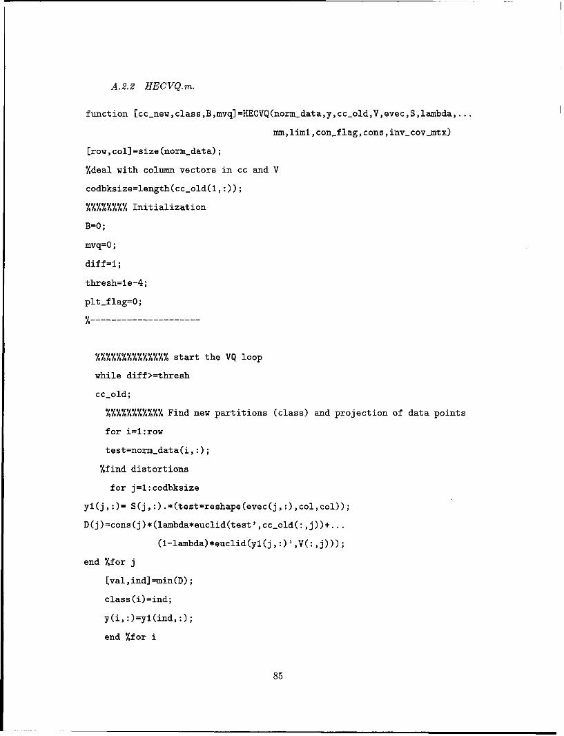
A.2.2 HECVQ.m.

function [cc-new,class,B,mvq]=HECVQ(norn-ata,y,cc-old,V,evec,S,larbda....

mm,liml,conjflag,cons,inv-coy-mtx)

Erow, coil size (norm-data);

%deal with column vectors in cc and V

codbksizelength(cc..old(l,:));

Y%%%%%%% Initialization

B=O;

mvq-O;

diff=1;

thresh=le-4;

pltjflag=O;

%%%///%***%%%% start the VQ loop

while diff>=thresh

cc-.old;

%%%.7%%%%%%% Find new partitions (class) and projection of data points

for i=1:row

test=norm.data(i,:);

%find distortions

for j1l:codbksize

yi(j,:)= S(j,:).*(test*reshape(evec(j,:),col,col));

D(j)=cons(j)*(laxnbda*euclid(test' ,cc...old(: ,j))+...

(1-lambda)*euclid(yl(j,:)',V(:,j)));

end %~for j

Eval ,ind] min CD);

class (i)=ind;

y(i, :)=y1(ind,:);

end %/f or i

85

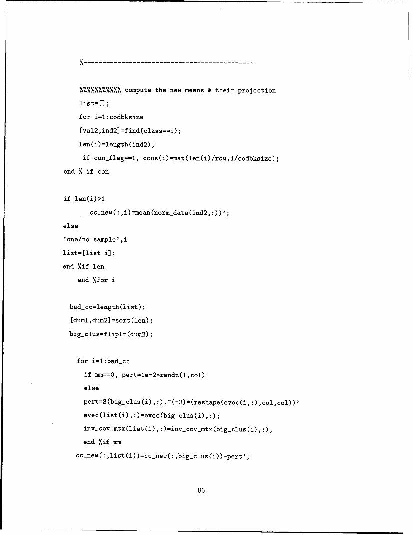
%%%%%%%%%% compute the new means & their projection

list=[];

for i=1:codbksize

[val2,ind2]=find(class==i);

len(i)=length(ind2);

if conflagl=, cons(i)=maxc(len(i)/row,1/codbksize);

end % if con

if len(i)>1

cc-new(: ,i)=mean(norm-data(ind2,:))';

else

'one/no sainple',i

end %if len

end %/f or i

ba&..cc=length(list);

IdumI ,dum2] =sort (len);

big..clus=fliplr (dum2);

for i~l:bad..cc

if mm==O, pert~1e-2*randn(1,col)

else

evec(list(i), :)=evec(big..clus(i),:);

inv-cov-mtx(list(i) ,:)=inv-cov-mtx(big-.clus(i),:);

end %if mm

cc..new(: ,list(i))=cc-new(: ,big..clus(i))-pert';

86

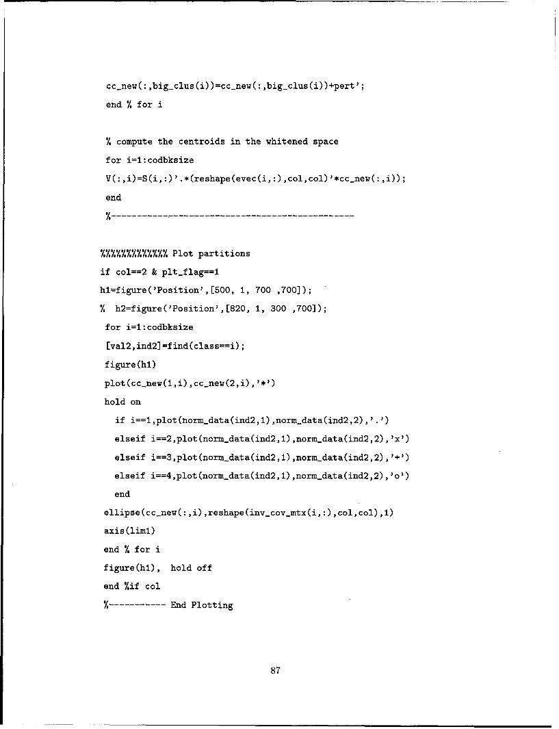
cc..new(: ,big.clus(i))=cc.new(: ,big-clus(i))+pert';

end %h for i

% compute the centroids in the whitened space

for i=i:codbksize

V(: ,i)=S(i,:)' .*(reshape(evec(i, :) ,col,col) '*cc..new(: ,i));

end

%-------------------------------------

%%%%%%%%%%%Plot partitions

if col==2 & plt-flagi=

hl=figure('Position',[500, 1, 700 ,700]);

% h2=figure('Position',[820, 1, 300 ,700]);

for i=l:codbksize

Lval2, ind2] =find(class==i);

figure (hi)

plot(cc..new(i,i),cc-new(2,i),'*')

hold on

if i==l,plot(norm-data(ind2,I) ,norm...data(ind2,2),' .3)

elseif i==2,plot(norm-.data(ind2,I) ,norm-.data(ind2,2) ,'x')

elseif i==3,plot(norm-data(ind2,I) ,norm-data(ind2,2) ,')

elseif i==4,plot(norm.data(ind2,I) ,norm-data(ind2,2) ,'o')

end

ellipse(cc..new(:,i),reshape(inv...covjtx(i,:),col, col),1)

axis (limi)

end % for i

figure(hi), hold off

end %if col

------- End Plotting

87

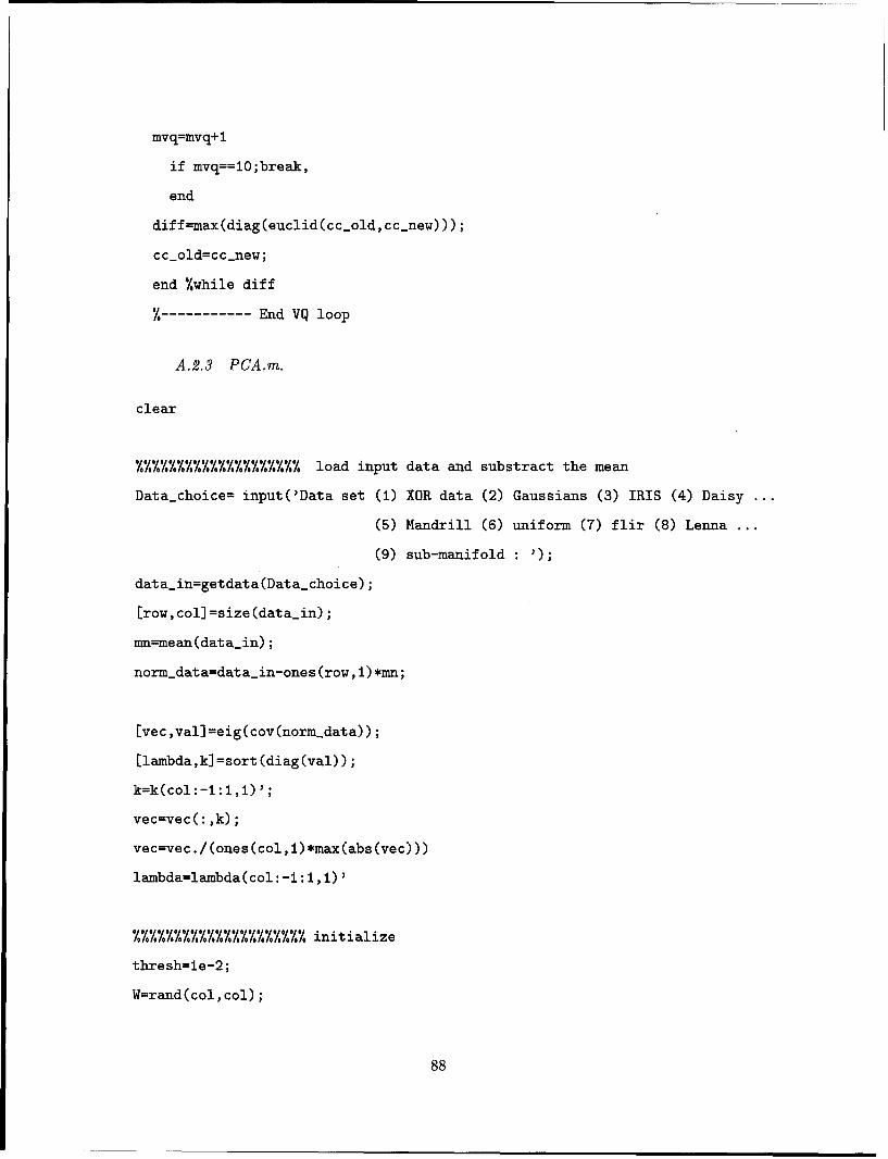
mvqmvq+ 1

if mvqlO1;break,

end

diff~max(diag(euclid(cc-old, cc-new)));

cc-old=cc.new;

end %while diff

% ---- -End VQ loop

A.2.3 PCA.m.

clear

%%%%%%%%Y%% hh/%%%%%%% load input data and substract the mean

Data-choice= input('Data set (1) XOR data (2) Gaussians (3) IRIS (4) Daisy

(5) Mandrill (6) uniform (7) flir (8) Lenna ...

(9) sub-manifold

data-in=getdata (Data-choice);

[row, col] =size (data-in);

rn=mean(data-in);

norm-.data=data-.in-ones (row,1) *mn;

[vec ,val1=eig(cov(normdata));

[lambda,k] =sort (diag(val));

k=k(col:-1:1,1);

vec=vec(: ,k);

vec=vec./(ones(col, 1)*max(abs(vec)))

laibdalambda(col:-1:1,1)'

%%Y%%%%%%%%%%%%%%%%%Y initialize

threshle-2;

W=rand(col,col);

88

i=O;

H=zeros(1,col);

U=triu(rand(col,col) ,1);

eta=4e-2;

Mu=9e-2;

epoch=O;

while max(max(abs (U)) )>thresh

ii+1;

pattern=iorm-data(i,:)';

if i==row,i=O;epoch=epoch+l,W./(ones(col,l)*max(abs(W))) ,end

for j=l:col;

H(j)=W(: ,j) '*pattern+H*U(: ,j);

end % for j

Delt_.W=eta*pattern*H;

Delt-U=-Mu*triu(H' *H, 1);

W=W+Delt-W;

U=U+Delt-U;

W=W./(ones(col,col)*max(max(abs(W)))); % normalize W

if epoch==100,break,end

end % while max

89

Appendix B. Vector Quantization Code

The following MATLAB® code is used to perform vector quantization coding of

images.

B.1 Image VQ.m

% Vector quantization

%function [Xnew,kh] =ImageVQ(Data_choice, codbksize,hard-fuzzy,Mpara,Distnce, initclus)

tm=clock;

M=4; % codebook size

R=log(M)/log(2); %no. of bits to represent codebook ( M= 2-R )

% if nargin<1

Mpara=O; % to set it zero if not fuzzy

%%%%%%% Get parameters %%%%%%Y %%% %Data-choice= input(' Data set (1) XOR data (2) Gaussians (3) IRIS (4)Daisy...

(5) Mandrill (6) uniform (7) flir (8) Lenna ...

(9) sub-manifold :');

codbksize = input('Codebook size : ');

hard-fuzzy = input('Clustering Algorithm (1) LBG ( HCM) (2) Fuzzy C-means

Distnce = input('Similarity Measure (1) Euclidean Distance ...

(2) Diagonal covariance ...

(3) changing Mahalanobis : 1);

init-clus = input('Codebook Generation (1) Splitting (2) first C samples ...

(3) Minimax (4) Bezdek (5) Desimio (6) get-then-split

if hardfuzzy==2

mm = input('M parameter for Fuzzy C-means

end

% endif nargin

--------------------------------------------

Which=[Data-choice codbksize hard_fuzzy Mpara Distnce init-clus]

90

%%%%%%% load the test image %%%%%%%%%%%%%%%%%%%%%%%%

clear dis-test

if Data-choice==5

load ./autosaves/mandrill

[rom,com]=size(X);

ival = mean(map')'; % the average of the 3 values of colormap (B&W intensity)

newmap=[ ival ival ival];

for i=l:rom

for j=l:com

X_intens(i,j)=ival(X(i,j));

% Matrix of 480x500 of intensity rather than indecies as in X

end

end

elseif Data-choice==8

load ./autosaves/lenna

X_intens=lenna;

else error('invalid choice')

end

[ro,co]=size(X-intens);

%%%%%%%% % Z Decimate the image %%%%%%%%%%%%%%%%%%%%

% Get upper-left pixel from 4x4 block, and and arrange each 4x4 of them in a row

% [intens-vec,x-intens]=decimate(X-intens,4,4);

% Or get saved decimated image directly

eval(['load /home/hawkeye6/96d/96d/kyounis/dataset/' int2str(Data-choice) 'dec44'])

91

%%%%%%%%% Find codebook %%%%%%%%%%%%%%%7.%7.

%[A2,lis2l=Cluster(intensvec,M);

% Or you can load predetermined codebook (and A-inv matrix if needed)

% to load the codebook of the same image

load /home/hawkeye6/96d/96d/kyounis/PR/clustering/autosaves/8410352res

% to load a specific codebook

%load /home/hawkeye6/96d/96d/kyounis/PR/clustering/autosaves/541035res

%%%%%%%%% Perform VQ to reconstruct the image %%%%%%%%%%

A2=clus-centr-new;

for i=1:4:ro

for j=1:4:co

x-test=reshape(X-intens(i:i+3,j:j+3),1,16);

diff=ones(M,1)*x-test-A2;

distest=sum(diff.^2');

[R,ind]=min(dis-test);

Xnew(i:i+3,j:j+3)=reshape(A2(ind,:),4,4);

end

end

eval(['save ./autosaves/' int2str(Which) ' Xnew'])

%%%%%%%%%%%%%% compute distortion / view image %%%%%%%%%%%%%%%%%

dist=mean(mean((X-intens-Xnew).-2))

mmm=max (max (Xnew));

Xnew3=Xnew*65/mmm; %scale such that max grey level is 65

figure('Position',[750, 700, 300 ,300])

92

image (Xnew3)

axis off

colormap (gray)

plt..naxne=[Irecons' int2str (Which)]

eval(['print -deps /home/hawkeye6/96d/96d/kyounis/PR/VQ/images/I plt-nane])

tot-time=etime (clock,tm)

93

Bibliography

1. Backer, E. and A. K. Jain. "A Clustering Performance Measure Based on FuzzySet Decomposition," IEEE Trans. Pattern Anal. Machnine Intell., PAMI-3(1):66-74(1981).

2. Ball, G. H. and D. G. Hall. "Some fundamental Concepts and Synthesis Procedures forPattern Recognition Preprocessors," In Proc. Int. Conf. Microwaves, Circuit Theory,Information Theory, 281-297 (September 1964). Tokyo, Japan.

3. Baum, L., et al. "A maximization Technique Occuring in the Statistical Analysis ofProbailistic Functions of Markov Chains," Ann. Math Statistics, 164-171 (1970).

4. Bezdek, James. Pattern Recognition with Fuzzy Objective Function Algorithm.Plenum Press, New York, 1981.

5. Bezdek, James, et al. "Some New Competitive Learning Schemes," SPIE, 2492(1995).

6. Bezdek, James C. Fuzzy Mathematics in Pattern Classification. PhD dissertation,Cornell Univ., Ithaca, NY, 1973.

7. Bezdek, James C. Self-Organization and Clustering Algorithms. Technical Report,Defense Technical Information Center (DTIC) N91-21783, 1991.

8. Carpenter, G. and S. Grossberg. "Adaptive Resonance Theory: Stable Self Organiza-tion of Neural Recognition Code in Response to Arbitrary Lists of Input Patterns,"In Proc. 8th Annual Conf. Cognitive Science, 45-62 (1986).

9. Darken, Christian and John Moody. Fast Adaptive k-means Clustering: Some Imper-ical Results. Technical Report, AFOSR Grant 89-0478, 1989.

10. DeSieno, D. "Adding Conscience to Competitive Learning," IEEE Proceedings Int.Conf. in Neural Networks (ICNN-88), 117-124 (1988). San Deigo, CA.

11. DeSimio, Martin, "AFIT/EENG 817 Class Notes and Personal Interviews." The AirForce Institute of Technology, 1995.

12. Duda, Richard 0. and Peter E. Hart. Pattern Classification and Scene Analysis. JohnWiley and Sons, 1973.

13. Dunn, J. C. "A Fuzzy Relative of the ISODATA Process," Cybernetics, 32-57 (March1974).

14. Gath, I. and A. B. Geva. "Unsupervised Optimal fuzzy Clustering," IEEE Trans. onPattern Analysis and Machine Intelligence, PAMI-11 (7):773-781 (July 1989).

15. Gersho, Allen and Robert M. Gray. Vector Quantization and Signal Compression.Boston, MA: Kluwer, 1992.

16. Gonzalez, Rafael C. and Paul Wintz. Digital Image Processing (2nd Edition). AddisonWesley, 1987.

17. Gray, Robert M. "Vector Quantization," IEEE ASSP Magazine, 1:4-29 (1989).

94

18. Jain, A. K. and R. C. Dubes. Algorithms for Clustering Data. Englewood Cliffs, NJ:Prentice-Hall, 1988.

19. Jain, Anil K. and Jianchang Mao. Computational Intelligence Imitating Life. IEEEPress Marketing, 1994.

20. Jolion, J. M., et al. "Robust Clustering with Applications in Computer Vision," IEEETrans. Pattern Anal. Machine Intell., PAMI-13(8):791-802 (1991).

21. Katsavounidis, Ioannis, et al. "A New Initialization Technique for Generalized LloydIteration," IEEE Signal Processing Letters, 1 (10):144-146 (October 1994).

22. Keller, James M., et al. "A Fuzzy K-Nearest Neighbor Algorithm," IEEE Transactionson Systems, Man, and Cybernetics, SMC-15(4):580-585 (July/August 1985).

23. Kohonen, Tuevo T. Self-Organization and Associative Memory. Springer-Verlag,Berlin, 1989.

24. Linde, Y., et al. "An Algorithm for Vector Quantizer Design," IEEE Trans. Commun.,COM-28:84-95 (1980).

25. Mao, Jianchang and Anil K. Jain. "A Self-Organizing Network for HyperellipsoidalClustering," IEEE Transactions on Neural Networks, 7(1):16-29 (January 1996).

26. McQueen, J. B. "Some Methods of Classification and Analysis of Multivariate Ob-servations," In Proc. 5th Berkeley Symp. Math. Statis. Probability, 281-297 (1967).

27. Patrick, Edward A. and Leon Y. L. Shen. "Interactive Use of Problem knowledgefor Clustering and Decision Making," IEEE Tran. on Computers, 216-222 (February1971).

28. Reynolds, Douglas A. A Gaussian Mixture Modeling Approach to Text-IndependentSpeaker Identification. PhD dissertation, Georgia Institute of Technology, August1992.

29. Rogers, Steven K., et al. An Introduction to Biological and Artificial Neural Networks.Bellingham, Washington: SPIE Optical Engineering Press, 1991.

30. Rubner, J. and P. Tavan. "A Self Organizing Network for Principal ComponentAnalysis," Europhysics letters, 10:693-698 (1989).

31. Ruck, Dennis W. and Steven Rogers. "The Multilayer Perceptron as an Approxi-mation to a Bayes Optimal Discriminant Function," IEEE Transactions on NeuralNetworks, 1 (2):296-298 (December 1990).

32. Ruck, Dennis W., et al. "The Multilayer Perceptron as an Approximation to a BayesOptimal Discriminant Function," IEEE Transactions on Neural Networks (1990).

33. Tou, Julius T. and Rafael C. Gonzalez. Pattern Recognition Principles. Reading,MA: Addison-Wesley Publishing Company, 1974.

34. Windham, M. P. "Cluster Validity of the Fuzzy c-means Clustering Algorithm," IEEETrans. Pattern Analysis and Machine Intelligence, PAMI-4 (4):357-363 (1982).

35. Younis, Khaled S., et al. "Vector Quantization Based on Dynamic Adjustment ofMahalanobis Distance," IEEE National Aerospace and Electronics Conference (NAE-CON), 2:858-862 (May 1996).

95

36. Zadeh, Lotfi A. "Fuzzy Sets," Information and Control, 8:338-353 (1965).

96

VitaCaptain Khaled S. Younis - He graduated First

in the 1986 high school clams at Dirar Ibnel Azwar School in Amman, Jordan. In 1990,he graduated from Mu'tah University with a Bachelor of Science Degree in ElectricalEngineering and be was awarded a Royal prize granted for the first of the Engineeringgraduates. Upon graduation, Capt. Younis received his commission as a Second Lieutenanin the Royal Jordanian Air Force (RJAF). In 1994, he was selected by the RJAF to earn hisMaster of Science Degree in Electrical Engineering at the Air Force Institute of Technology(AFIT) at Wright-Patterson AFB, Ohio. Capt Younis was awarded a scholarship by theDayton Area Graduate Studies Institute (DAGSI) to pursue a Doctorate of PhilosophyDegree in Electrical Engineering after completion of his Master's program at AFIT.

97

REPORT DOCUMENTATION PAGE Form Approved

I 0MB No. 0704-0 188Public reporting burden for this collection of information is estimated to average 1 hour per response, including the time for reviewing instructions, searching existing data sources,gathering and maintaining the data needed, and completing and reviewing the collection of information. Send comments regarding this burden estimate or any other aspect of thiscollection of information, including suggestions for reducing this burden, to Washington Headquarters Services, Directorate for Information Operations and Reports, 1215 JeffersonDavis Highway, Suite 1204, Arlington, VA 22202-4302. and to the Office of Management and Budget, Paperwork Reduction Project (0704-0188), Washington. DC 20503.

1. AGENCY USE ONLY (Leave blank) I REPORT DATE 3. REPORT TYPE AND DATES COVEREDIDecember 1996 Master's Thesis.

4. TITLE AND SUBTITLE S5. FUNDING NUMBERSWEIGHTED MAHALANOBIS DISTANCE FORHYPER-ELLIPSOIDAL CLUSTERING

6. AUTHOR(S)Khaled S. YounisCaptain, RJAF

7. PERFORMING ORGANIZATION NAME(S) AND ADDRESS(ES) 8. PERFORMING ORGANIZATIONAir Force Institute of Technology REPORT NUMBER

WPAFB OH 45433-6583 AFIT/GE/ENG/96D-22

9. SPONSORING / MONITORING AGENCY NAME(S) AND ADDRESS(ES) 10. SPONSORING / MONITORING

Major Thomas Burns, WL/AARA AGENCY REPORT NUMBER

2010 fifth Street, Bldg. 23WPAFB, OH 45433

11. SUPPLEMENTARY NOTES

12a. DISTRIBUTION /AVAILABILITY STATEMENT 12b. DISTRIBUTION CODEApproved for public release; Distribution Unlimited

13. ABSTRACT (Maximum 200 words)

Abstract

Cluster analysis is widely used in many applications, ranging from image and speech coding to pattern recog-nition. A new method that uses the weighted Mahalanobis distance (WMD) via the covariance matrix of theindividual clusters as the basis for grouping is presented in this thesis. In this algorithm, the Mahalanobis dis-tance is used as a measure of similarity between the samples in each cluster. This thesis discusses some difficultiesassociated with using the Mahalanobis distance in clustering. The proposed method provides solutions to theseproblems. The new algorithm is an approximation to the well-known expectation maximization (EM) procedureused to find the maximum likelihood estimates in a Gaussian mixture model. Unlike the EM procedure, WMDeliminates the requirement of having initial parameters such as the cluster means and variances as it starts fromthe raw data set. Properties of the new clustering method are presented by examining the clustering quality forcodebooks designed with the proposed method and competing methods on a variety of data sets. The compet-ing methods are the Linde-Buzo-Gray (LBG) algorithm and the Fuzzy c-means (FCM) algorithm, both of themuse the Euclidean distance. The neural network for hyperellipsoidal clustering (HEC) that uses the Mahalnobisdistance is also studied and compared to the WMD method and the other techniques as well. The new methodprovides better results than the competing methods. Thus, this method becomes another useful tool for use in

14. SUBJECT TERMS 15. NUMBER OF PAGES

Clustering, Unsupervised Learning, Mahalanobis Distance, Neural Networks, Pat- 109tern Recognition 16. PRICE CODE

17. SECURITY CLASSIFICATION 18. SECURITY CLASSIFICATION 19. SECURITY CLASSIFICATION 20. LIMITATION OF ABSTRACTOF REPORT OF THIS PAGE OF ABSTRACT

UNCLASSIFIED UNCLASSIFIED UNCLASSIFIED UL

NSN 7540-01-280-5500 Standard Form 298 (Rev. 2-89)Prescribed by ANSI Std. Z39-18298-102