D

DEPOT-LEVEL SIMULATION AND

MULTIVARIATE ANALYSIS ON B-1 HIGH VELOCITY MAINTENANCE

THESIS

Florence K. Yee, First Lieutenant, USAF

AFIT-OR-MS-ENS-11-26

DEPARTMENT OF THE AIR FORCE AIR UNIVERSITY

AIR FORCE INSTITUTE OF TECHNOLOGY

Wright-Patterson Air Force Base, Ohio

DISTRIBUTION STATEMENT A. APPROVED FOR PUBLIC RELEASE; DISTRIBUTION UNLIMITED.

The views expressed in this thesis are those of the author and do not reflect the official policy or position of the United States Air Force, Department of Defense, or the United States Government.

AFIT-OR-MS-ENS-11-26

DEPOT-LEVEL SIMULATION AND MULTIVARIATE ANALYSIS ON B-1 HIGH VELOCITY MAINTENANCE

THESIS

Presented to the Faculty

Department of Operational Sciences

Graduate School of Engineering and Management

Air Force Institute of Technology

Air University

Air Education and Training Command

In Partial Fulfillment of the Requirements for the

Degree of Master of Science in Operations Research

Florence K. Yee, BS

First Lieutenant, USAF

March 2011

APPROVED FOR PUBLIC RELEASE; DISTRIBUTION UNLIMITED.

AFIT-OR-MS-ENS-11-26

DEPOT-LEVEL SIMULATION AND MULTIVARIATE ANALYSIS ON B-1 HIGH VELOCITY MAINTENANCE

Florence K. Yee, BS First Lieutenant, USAF

Approved: _________//SIGNED// _________________ MARCH 11, 2011 Dr. J. O. Miller (Chairman) date ________//SIGNED// __________________ MARCH 11, 2011 Dr. Kenneth W. Bauer (Member) date

iv

AFIT-OR-MS-ENS-11-26

Abstract

The objective of this thesis is to gain insights on the B-1B depot maintenance

operations, with a focus on direct maintenance hours or burn rate, under the

implementation of High Velocity Maintenance (HVM). Based on historical depot

maintenance data and the current B-1 depot HVM prototype data, a discrete-event

simulation model is developed using Arena 12.0. Some United States Air Force supply

chain influences, such as manning levels and kitting characteristics of the B-1 depot

operations, are incorporated in our models as design factors. The model captures the

stochastic nature of 30 HVM tasks performed on one B-1 aircraft in a representative

HVM cycle at the B-1 depot located in Oklahoma City Air Logistics Center, Tinker Air

Force Base.

To examine the impact of HVM, we vary the levels of the design factors and

conduct a design of experiment (DOE). The DOE analysis reveals that manning levels

and kitting characteristics have statistically significant impact on some HVM task

completion times, which are used collectively as a surrogate measure for burn rate. In

particular, manning schedule with a centric focus on direct maintenance, high task kit

availability, and small kit deficiency produce the highest burn rate. Additionally, by

performing multivariate analysis, we are able to reduce the dimensionality of the output

statistics and conclude that kit deficiency is the main driver for HVM task duration with

our simulation.

v

AFIT-OR-MS-ENS-11-26

To my husband, who supports and believes in me every day. To my mom, who is always there for me.

vi

Acknowledgments

First and foremost, from the bottom of my heart, I would like to thank Dr. J.O.

Miller for his patience, guidance, and support on both the technical and grammatical

fronts of this thesis. Dr. Miller has not only helped me through many simulation

obstacles but also encouraged me to work outside my cocoon and actually start writing

the longest paper I have even written in my life. Without his help, I would still be

taunted by the blinking Microsoft Word cursor on the top left-hand corner of my first

blank page. I would also like to thank my reader, Dr. Kenneth Bauer, for his valuable

comments and inputs as I thrive to complete this thesis. Dr. Bauer’s keen insights on

multivariate analysis have rescued me from the bottomless analysis rabbit hole that I was

trapped for countless hours…

I also owe special thanks to the maintenance and logistics gurus, Ms. Angie

Ceyler, Mr. Mark Fryman, SMSgt Frank Michaliszyn, and Mr. Edwin Milnes for helping

me to get a better understanding of aircraft maintenance and providing vast information

and data that made this research possible.

Florence K. Yee

vii

Table of Contents Page

Abstract .............................................................................................................................. iv

Acknowledgments.............................................................................................................. vi List of Figures .................................................................................................................... ix

List of Tables ..................................................................................................................... xi 1. Introduction ..................................................................................................................... 1

1.1 Background ............................................................................................................... 1

1.2 Problem Statement .................................................................................................... 3

1.3 Problem Approach .................................................................................................... 3

1.4 Research Scope ......................................................................................................... 5

1.5 Literature Review...................................................................................................... 6

1.5.1 USAF Supply Chain Modeling .......................................................................... 6

1.5.2 Background of HVM ......................................................................................... 8

1.5.3 History of HVM ............................................................................................... 12

1.6 Methodology ........................................................................................................... 16

1.7 Thesis Outline ......................................................................................................... 17

2. Discrete-event Simulation of High Velocity Depot Maintenance Process for B-1 ...... 19

2.1 Introduction ............................................................................................................. 19

2.2 Overview ................................................................................................................. 19

2.3 Model Development................................................................................................ 21

2.3.1 General Cycle................................................................................................... 22

2.3.2 Resource Set Up ............................................................................................... 24

2.3.3 Arena Measures of Effectiveness (MOEs) Collection ..................................... 26

2.3.4 Assumptions ..................................................................................................... 27

2.3.5 Supporting Data ............................................................................................... 29

2.4 Verification and Validation..................................................................................... 30

2.5 Design of Experiment Methodology ....................................................................... 33

2.6 DOE Analysis and Results ...................................................................................... 34

2.6.1 DOE Screening ................................................................................................ 35

2.6.2 Full Factorial Design........................................................................................ 36

2.7 Conclusion .............................................................................................................. 40

3. Case Study .................................................................................................................... 41

viii

Multivariate Analysis on Outputs from the B-1 HVM Simulation................................... 41

3.1 Introduction ............................................................................................................. 41

3.2 B-1 HVM Simulation .............................................................................................. 43

3.3.1 Model Development......................................................................................... 43

3.3.2 Supporting Data, Verification, and Validation ................................................ 46

3.4 Multivariate Analysis .............................................................................................. 49

3.4.1 Analysis Background ....................................................................................... 49

3.4.2 Analysis and Results ........................................................................................ 51

3.4.3 Multivariate Analysis Conclusion.................................................................... 60

3.5 Conclusion .............................................................................................................. 61

4. Conclusion .................................................................................................................... 62

4.1 Summary ................................................................................................................. 62

4.2 Future Research ...................................................................................................... 63

Appendix A. Generator Harness DSW Sequence ............................................................ 65

Appendix B. GH Kit Delivery Sequence ......................................................................... 66

Appendix C. GH Task Kit Requirement List................................................................... 67

Appendix D. Historical Data of AFUS and Flush Tasks ................................................. 69

Appendix E. Experimental Design Matrix....................................................................... 70

Appendix F. Summary of Screening Test ........................................................................ 71

Appendix G. Diagnostics of DOE for AvgGHTime ........................................................ 72

Appendix H. Diagnostics of DOE for AvgSimTime ....................................................... 74

Appendix I. Matlab Programming Code .......................................................................... 77

Appendix J. Blue Dart...................................................................................................... 84

Appendix K. ENS Quad Chart ......................................................................................... 86

Bibliography ..................................................................................................................... 87

ix

List of Figures Page

Figure 1. Maintenance Cycle of Commercial and USAF Aircraft .................................... 9

Figure 2. HVM vision diagram (Robin AFB Factsheet, 2010)........................................ 10

Figure 3. Example of a task kit used by B-1 HVM team in Oklahoma City ALC .......... 11

Figure 4. C-130 Maintenance Life Cycle Comparison (Robin AFB Factsheet, 2010) .... 14

Figure 5. General Logic Flow for an Op.......................................................................... 17

Figure 6. Conceptual Representation of an Aircraft Cycle .............................................. 23

Figure 7. Simulation Logic of an Op ............................................................................... 24

Figure 8. An Example of the Arena Failure Process ....................................................... 25

Figure 9. Partition of Maintenance Time within an Op ................................................... 28

Figure 10. Summary of AvgGHTime DOE Statistics ..................................................... 37

Figure 11. Cube Plot for AvgGHTime DOE Analysis .................................................... 37

Figure 12. Residual vs. Predicted of AvgSimTime ......................................................... 38

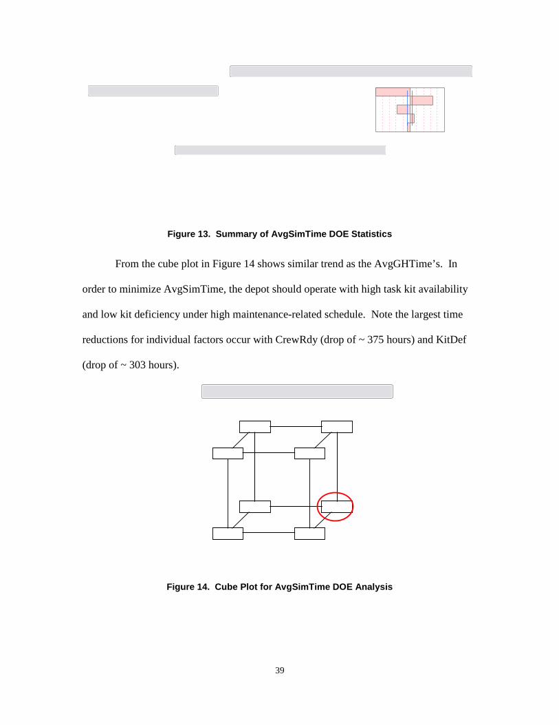
Figure 13. Summary of AvgSimTime DOE Statistics ..................................................... 39

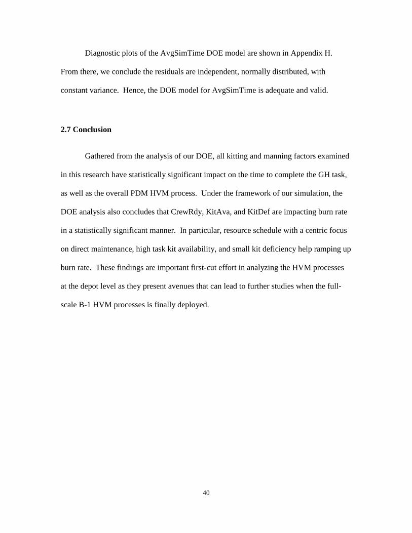
Figure 14. Cube Plot for AvgSimTime DOE Analysis.................................................... 39

Figure 15. Generalized B-1 HVM Model ........................................................................ 45

Figure 16. Generalized Simulation Logic Within an Op ................................................. 45

Figure 17. Scree Plot ........................................................................................................ 52

Figure 18. Three-dimensional Factor Plot (KitDef Coded) ............................................. 54

Figure 19. Task Duration vs. PEs Effectiveness .............................................................. 55

Figure 20. Three-dimensional Factor Plot (KitAva Coded) ............................................ 56

Figure 21. Task Duration vs. No-kit Occurrences ........................................................... 57

x

Figure 22. No-kit occurrences (F2) vs. task duration (F1) .............................................. 57

Figure 23. %AvgNoKit vs. task duration (F1) ................................................................. 58

Figure 24. F2 vs. F1 ......................................................................................................... 59

Figure 25. %AvgNoKit vs. F1 ......................................................................................... 59

Figure 26. Legend of Design Levels ................................................................................ 60

xi

List of Tables

Page Table 1. Simulation MOE Statistics……………………………………………………. 27

Table 2. Maintenance Process Distribution Summary…………………………………. 30

Table 3. Response Table of AvgGHTime……………………………………………… 31

Table 4. GH DSW Results……………………………………………………………… 32

Table 5. Simulated GH Statistics……………………………………………………….. 32

Table 6. Design Levels of Three Factors……………………………………………….. 34

Table 7. Selected Simulation Outputs Statistics………………………………………... 35

Table 8. Summary of Screening Test…………………………………………………... 36

Table 9. Maintenance Process Distribution Summary…………………………………. 46

Table 10. Response Table of AvgGHTime……………………………………………...47

Table 11. GH DSW Results…………………………………………………………….. 48

Table 12. Simulated GH Statistics……………………………………………………… 48

Table 13. Design Levels of Three Design Factors………………………………………49

Table 14. Simulation Output Statistics…………………………………………………. 50

Table 15. List of Reduced Variables…………………………………………………….51

Table 16. PCA Loading Matrix………………………………………………………… 52

Table 17. Rotated Factor Loadings……………………………………………………... 53

1

DEPOT-LEVEL SIMULATION AND MULTIVARIATE ANALYSIS ON B-1 HIGH

VELOCITY MAINTENANCE

1. Introduction

1.1 Background

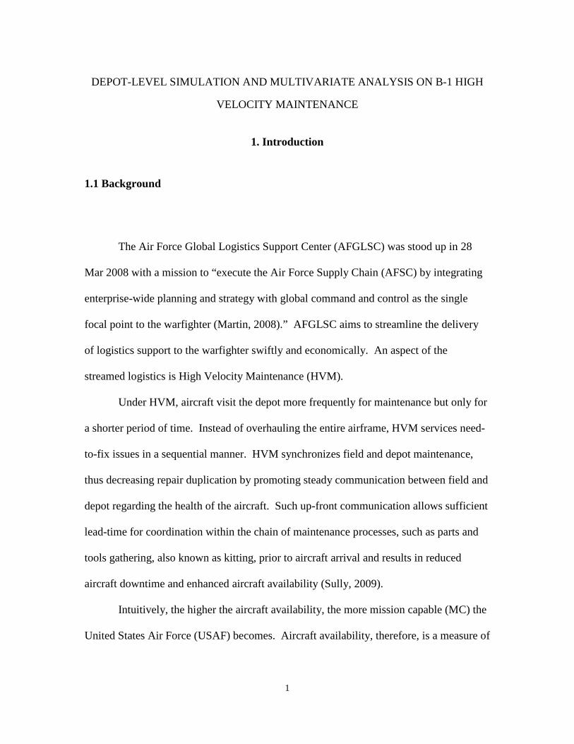
The Air Force Global Logistics Support Center (AFGLSC) was stood up in 28

Mar 2008 with a mission to “execute the Air Force Supply Chain (AFSC) by integrating

enterprise-wide planning and strategy with global command and control as the single

focal point to the warfighter (Martin, 2008).” AFGLSC aims to streamline the delivery

of logistics support to the warfighter swiftly and economically. An aspect of the

streamed logistics is High Velocity Maintenance (HVM).

Under HVM, aircraft visit the depot more frequently for maintenance but only for

a shorter period of time. Instead of overhauling the entire airframe, HVM services need-

to-fix issues in a sequential manner. HVM synchronizes field and depot maintenance,

thus decreasing repair duplication by promoting steady communication between field and

depot regarding the health of the aircraft. Such up-front communication allows sufficient

lead-time for coordination within the chain of maintenance processes, such as parts and

tools gathering, also known as kitting, prior to aircraft arrival and results in reduced

aircraft downtime and enhanced aircraft availability (Sully, 2009).

Intuitively, the higher the aircraft availability, the more mission capable (MC) the

United States Air Force (USAF) becomes. Aircraft availability, therefore, is a measure of

2

the USAF’s operational strength. Commercial airlines routinely maintain over 90%

aircraft availability; whereas the USAF has 60% availability rates on average (Dement,

2009). It is, therefore, not surprising that the concept of HVM emerged from the

competitive nature of commercial airlines to raise revenue by maximizing aircraft

availability. Burn rate or direct touch labor working hours per day is closely tied to

aircraft downtime due to maintenance and, therefore, aircraft availability. The higher the

burn rate, the less time the aircraft is grounded for maintenance and hence, the higher the

aircraft availability. Currently, the burn rate of the B-1 fleet is 145 to 150 hours per day.

Under HVM management, burn rate is expected to ramp up to 400 hours a day (Canaday,

2010).

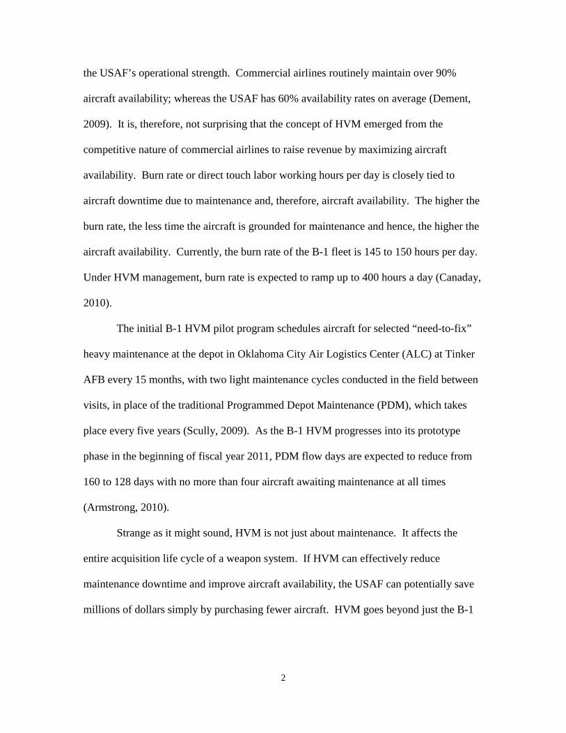
The initial B-1 HVM pilot program schedules aircraft for selected “need-to-fix”

heavy maintenance at the depot in Oklahoma City Air Logistics Center (ALC) at Tinker

AFB every 15 months, with two light maintenance cycles conducted in the field between

visits, in place of the traditional Programmed Depot Maintenance (PDM), which takes

place every five years (Scully, 2009). As the B-1 HVM progresses into its prototype

phase in the beginning of fiscal year 2011, PDM flow days are expected to reduce from

160 to 128 days with no more than four aircraft awaiting maintenance at all times

(Armstrong, 2010).

Strange as it might sound, HVM is not just about maintenance. It affects the

entire acquisition life cycle of a weapon system. If HVM can effectively reduce

maintenance downtime and improve aircraft availability, the USAF can potentially save

millions of dollars simply by purchasing fewer aircraft. HVM goes beyond just the B-1

3

fleet. The impact of HVM can be potentially unlimited for it is designed to be scalable,

repeatable, and deployable on all weapon systems in the USAF inventory (Adams, 2008).

1.2 Problem Statement

The goal of this thesis research is to gain insights on B-1 depot maintenance

operations, with a focus on burn rate, under the implementation of HVM considering

some key USAF supply chain influences. In particular, this study focuses on the impact

of three factors; the effectiveness of kitting, the availability of kits, and the increased

readiness of maintenance crews, on burn rate. With limited data available on actual

number of maintenance workers available and how additional workers affect task

completion times, we model a set number of workers and use the task completion time

(TC) as a surrogate measure for burn rate. With this framework, an increased burn rate

results in a lower TC.

1.3 Problem Approach

In this study, discrete-event simulation (DES) is hand-picked to analyze the B-1

depot maintenance burn rate under HVM considering some key USAF supply chain

influences. First and foremost, quantitative data is limited since a full-scale B-1 HVM

process is currently non-existent and the HVM prototype phase is still being modified.

4

As of Jan 2011, only three B-1 prototypes have gone through two specific maintenance

tasks defined under HVM (Ceyler, 2011). It is, therefore, infeasible to study the impact

of HVM on burn rate analytically. Secondly, the USAF supply chain is arguably a

massive and complex system, hence, it is impractical to explicitly measure the impact of

the USAF supply chain on burn rate within this thesis. An Arena simulation model is

built to capture an abstraction of part of the envisioned B-1 HVM depot process and its

interaction with the USAF supply chain.

As mentioned before, data on the B-1 HVM process is limited. Hence, in order to

add creditability, we sought advice from subject matter experts and used the process flow

of the only B-1 HVM depot task for which some actual data was available. According to

personal correspondence with Ms. Angie Ceyler, B-1 AFGLSC HVM Materiel Team

Lead at Tinker AFB, in terms of manpower under the current work force construct of the

B-1 prototype phase, there are four personnel equivalences (PEs) for each of the two

eight-hour shifts per day. However non-maintenance related, indirect, or non-value

added hours, such as breaks, training, and admin requirements, can take up to two to

three hours per PE per shift. This results in net direct hand-on working hours of about

five to six hours per PE per shift on average. Hence we model the availability of PEs

using a distribution that models the amount of direct and indirect hours throughout the

workday.

A single simulation model is created using ARENA 12.0 to examine the impact of

HVM and the influence of the USAF supply chain on the depot’s TC. A design of

experiment (DOE) is conducted on simulation outputs to assess the impact of the

effectiveness of kitting, the availability of kits, and increased readiness of maintenance

5

crews. We embed the levels of our DOE factors with the Arena model as variables.

They are adjusted accordingly to represent a baseline model that reflects the operation

tempo and kitting specifics of the current practice of the B-1 HVM prototypes.

Embellished models are set up centering off the baseline factors to assess the sensitivity

of TC and other responses, with respect to the change to our selected USAF supply chain

influences. Multivariate analysis is also used to examine the relationship and variability

amongst the observed MOEs.

1.4 Research Scope

The full-scale B-1 HVM life cycle is currently still in development and the B-1

HVM prototype only covers maintenance sustainment at the depot level. The scope of

this research is, therefore, confined within maintenance at the depot while base level

logistics, such as time spent at the base prior to returning to depot for HVM, is not

considered.

As of 30 Sep 09, the USAF managed 113,897 recoverable and consumable items.

These items are procured, inventoried, stored, and transported from one hub to another

within the broad network of the USAF supply chain (Parson, 2010). The depot at Tinker

AFB where B-1 HVM is performed is just one hub. Therefore, a considerable amount of

abstraction is adopted in our Arena model to capture supply chain influences through

kitting as a key enabler of HVM. The scenario we consider in this study is a single PDM

6

visit consisting of ten cycles of a set of maintenance tasks performed at a single dock

using HVM B-1 prototype manning levels and kitting characteristics.

General concepts of the proposed HVM for the B-1B fleet are well-documented

and some initial work has been conducted to analyze the behavior of such processes at

the base level (Park, 2010). The purpose of this research is to develop a flexible

framework for modeling HVM at the depot and to provide insights on improving HVM

depot maintenance operations, not to provide an exact measurement of changes in burn

rate or other MOEs with respect to changes in modeled supply chain influences. Once

the full-scale B-1B HVM process is underway and more data is available, fitted

distributions of processes, ranges of input parameters, and logic flows within the DES

model can be refined to mirror a more accurate representation of the real system.

1.5 Literature Review

1.5.1 USAF Supply Chain Modeling

Traditionally speaking, USAF supply chain models are tailored to analyze

mission capable (MC) rate, which serves as a direct measure of the USAF’s operational

strength. Ramey (2008, pg xxii) defines MC as “the status of an aircraft that can perform

some or all of its assigned mission; may be FMC [fully mission capable] or PMC

[partially mission capable].” MC is closely tied to aircraft availability, which is a direct

product of aircraft maintenance capabilities, including burn rate, which, in turn, is

significantly affected by the logistics support structure.

7

In 2007, RAND launched Project Air Force (PAR) per the request of the Deputy

Chief of Staff for Logistics, Installations, and Mission Support and the Vice Commander

of Air Force Materiel Command (AFMC) (Tripp et, 2010). PAR aims to improve

effectiveness and efficiency of the logistics enterprise by designing and evaluation a set

of lean and agile logistic options that meet that USAF’s growing demand of air

superiority. The scope of PAR encompasses not only maintenance processes, but also

policies and posture; command and control; information systems; and inventory stockage

policies for three specific platforms: F-16, C-130, and KC-135. The size and complexity

of PAR called for various operations research (OR) analysis techniques including use of

the campaign level Logistics Composite Model (LCOM).

LCOM is a detailed simulation model that detects the sensitivity of sortie

generation due to changes in logistics resources, such as maintenance personnel,

equipment, facilities, and spare parts (Tripp et al, 2010). For the C-130 platform, LCOM

concludes that large component repair and isochronal (ISO) – inspection facilities

(CRFs), which conducted 200 or more ISOs annually, had a 30% higher labor utilization

rate than small CRFs that conducted about 20 ISOs year round. In other words, small

CRFs require two-to-three times as much manpower per ISO as larger CRFs. In

conjunction with labor utilization, LCOM also concluded that ISO flow times were 60%

less in larger CRFs than in small CRFs. LCOM findings were validated by the historical

data from Little Rock AFB, AR and Air Force Special Operations Command (AFSOC).

One significantly overarching conclusion of PAR was that maintenance consolidation and

integration, such as HVM, could improve aircraft maintenance capabilities and in turn,

aircraft availability.

8

As opposed to LCOM that encompasses most of the USAF supply chain

elements, 2Lt Anson R. Park, USAF, developed a flexible stand-alone model that

examines the impact of HVM on the availability of the B-1B Lancer at the base level.

Based on B-1 data collected from two B-1B squadrons of the 28th Bombardment Wing

located at Ellsworth AFB, SD, Park used DES and created two simulation models in

ARENA 12.0. The models captured the B-1B maintenance and supply process at base

level under both the current state of operations (i.e. no HVM) and with the

implementation of HVM. Park’s finding concluded that HVM can potentially improve

aircraft availability significantly if coupled with expected reductions in aircraft failure

rates and improvement in base stockage effectiveness.

1.5.2 Background of HVM

The concept of HVM was first outlined in Fiscal Year 2007. It emerged from the

competitive nature of commercial airlines to maximize revenue by minimizing aircraft

maintenance downtime and thus, maximizing aircraft availability. Commercial

maintenance, repair, and overhaul (MRO) is up to eight times more efficient than the

USAF MRO performed under PDM. Commercial airlines consistently uphold a touch-

hour maintenance rate or burn rate of 500 to 900 hours per day; whereas the ALCs

support 145 to 220 touch hours per day during PDM (Warner Robin ALC, 2009). As a

result, commercial airlines maintain over 90% aircraft availability rates; whereas the

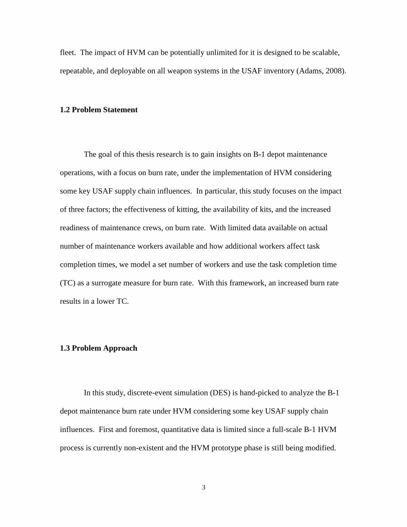
USAF has, on average, 60% availability rates (Dement, 2009). Figure 1 shows the

maintenance cycles of commercial and USAF aircraft from Warner Robin ALC.

9

Figure 1. Maintenance Cycle of Commercial and USAF Aircraft

(Robin AFB Factsheet, 2010)

With such high success rates in the commercial sector, it is no wonder the USAF

seeks ways to emulate the maintenance processes used in commercial airlines and to

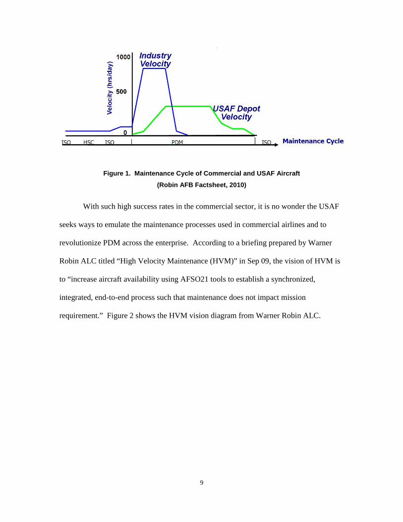
revolutionize PDM across the enterprise. According to a briefing prepared by Warner

Robin ALC titled “High Velocity Maintenance (HVM)” in Sep 09, the vision of HVM is

to “increase aircraft availability using AFSO21 tools to establish a synchronized,

integrated, end-to-end process such that maintenance does not impact mission

requirement.” Figure 2 shows the HVM vision diagram from Warner Robin ALC.

10

Figure 2. HVM vision diagram (Robin AFB Factsheet, 2010)

The HVM vision is supported by the three basic HVM tenants that aim to

significantly reduce aircraft downtime. The first tenant is to inspect the aircraft prior to

arrival at the depot (Crenshaw, 2010). Under HVM, aircraft visit the depot more

frequently for heavy maintenance but for a shorter period of time. ISO maintenance and

PDM are integrated and synchronized to minimize duplication. Inspection is performed

routinely in the field and the conditions of the aircraft are consistently reported to the

depot. Constant communication between field and depot allows continuous planning at

the depot level to identify deferrable tasks vs. need-to-fix tasks, so that proper parts,

tools, and personnel support are scheduled accordingly for those need-to-fix maintenance

11

issues prior to the aircraft arrival. This results in reduced aircraft downtime and thus,

enhances aircraft availability (Warner Robin ALC, 2009).

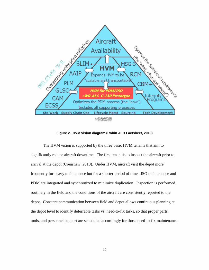
The second HVM tenant as suggested by Crenshaw is kitting. It is the assembly

of tools and parts into “task kits” for major maintenance jobs. Figure 3 shows an

example of a task kit for part of the Generator Wiring Harness maintenance task of the B-

1 prototype as defined by the HVM team at Oklahoma City ALC, Tinker AFB (Ceyler,

2010). Kitting derives from the mechanic-centric focus of HVM. The idea behind

kitting is that all parts, tools, data, etc. are pre-positioned for the mechanics before

maintenance begins. Kitting is expected to reduce aircraft downtime by eliminating time

wasted in resource gathering while the planes are grounded for maintenance.

Consumables

Noun QTY

Wax tie cord 1 roll

S Wre. .020-.032 1 roll

Tef tape 2" 1roll

Razor Blades 3

Sharpie 1

12" Wire tie 1 bag

Tools

TOOL # Description

#6 Crimpers

Multimeter & Probes

Heat Gun

Ratcheting cable cutters

Zip tie gun

Barrell Crimper Lg dies

Wire stripper w/dies

Tape Measure

Scissors

Side Cutters

S.Wre. Pliers 8"

Box Knife

Hook Scribe

Large Crimper

Figure 3. Example of a task kit used by B-1 HVM team in Oklahoma City ALC

12

The third HVM tenant calls for clear mapping of day-to-day maintenance tasks

and staying on track with the schedule. This has proven to be a challenge in the

beginning of the C-130 HVM program. The high-resolution detailed breakdown of the

day-to-day maintenance tasks inflated the number of daily tasks into the hundreds and

made it logistically difficult to accomplish everything according to schedule (Crenshaw,

2010). Learning from the downfall, the C-130 HVM program repackaged the tasks into

more manageable pieces at a higher level prior to day-to-day schedule mapping.

Together with routine field inspection and kitting, maintenance is more likely to stay on

track with less downtime, and hence, aircraft availability goes up.

1.5.3 History of HVM

In an effort to increase aircraft availability, the USAF has launched a series of

studies to emulate the commercial aircraft MRO over the years. One of the HVM pioneer

studies is for the C-5 Galaxy airlift aircraft conducted by the Resources Management and

System Acquisition program of Project AIR FORCE in the early 90’s (Ramey, 1999).

The study explored changes in logistics infrastructure in relation to the changes in

operational capability in terms of three primary performance measures, MC status,

departure reliability, and issue effectiveness for the C-5 Galaxy. A simulation model of

the C-5 operation and support construct was built using RAND’s Dyna-METRIC, a DES

tool designed specifically for military logistics systems. The model was later verified and

validated by the Air Mobility Command (AMC).

The scope of the C-5 study included data collected from 20 bases, six

intermediate support facilities, one depot complex, and 109 aircraft with 1,980 reparable

13

line items. Ten replications of a 360-day operation were simulated. The model

compared simulated performances of the C-5 under standard logistic infrastructure and

high-velocity infrastructure (HVI), which emphasized the speed of processing rather than

the mass of the inventory. The findings concluded that HVI upheld the same C-5

performances as (or in some cases better than) the standard infrastructure but HVI

required only one-sixth and one-third of the inventory and inventory value of the (then)

current infrastructure, respectively (Ramey, 1999).

Another study titled “The C-5 High Velocity Regionalized Isochronal (HVRISO)

Inspection Concept: An Evaluation of Future Performance” was conducted in 2009 by an

AFIT master student, MSgt Theodore K. Heiman. The study explored the impact on C-5

availability with isochronal inspection site consolidation from the four docks that are

currently in use (as of 2009) to three HVRISO docks operating based on centralized

maintenance schedules provided by Air Mobility Command (AMC). Heiman concluded

that HVRISO could drive C-5 availability to the highest level under specific dock

selection methods and consolidation requirements.

Following the high-velocity footprints of the C-5 Galaxy is the C-130 Hercules.

In Aug 2009, a pilot HVM program took place at Warner Robin ALC in Robin AFB, GA.

According to Ellen Griffith, the chief of Depot Operations Division at AFMC, the C-130s

are “a low density, high-demand fleet, and they [AFSOC] need every bit of flying time

we can give back to them… we desperately want to reduce the amount of time that we

have aircraft like gunships down at depot” (Adams, 2008).

In order to better accommodate the needs of the war fighters, HVM requires the

C-130 fleet to visit Warner Robin ALC for integrated ISO and PDM every 18 months but

14

only for 12 to 15 days as opposed to a 160-day PDM every five years (Khan, 2010).

According to Doug Keen, HVM Product Team lead at Warner Robin ALC, HVM could

reduce the number of C-130 grounded for maintenance from as many as 70 to as low as

15, saving as much as $1.6 billion in assets. HVM seeks to raise the C-130 burn rate

from 145 to 220 hours per day to the commercial airlines level of 500 to 900 hours per

day. Figure 4 shows the comparison of the C-130 maintenance life cycle under current

and HVM state as defined by Warner Robins ALC.

Figure 4. C-130 Maintenance Life Cycle Comparison (Robin AFB Factsheet, 2010)

After the C-130 Hercules, the B-1 Lancers was selected to enter the HVM

program. The B-1B is the world record holder for speed, payload, and distance. It is no

wonder that the Lancers have been a valuable asset to the USAF in combat operations

since 1980s (Park, 2010). However, in 2007, over half the fleet was down for

maintenance issues. In 2008, there were on average, only 28 B-1 aircraft available with

15

36 grounded due to maintenance at any given time. The rate is “unacceptable, and that’s

why we’re doing HVM,” said the Sam Malone, deputy director of the 427th Aircraft

Sustainment Group at Tinker AFB, whose unit is responsible for the B-1 depot

maintenance and repair (Sully, 2009).

Similar to the HVM program of the C-130, the initial B-1 HVM pilot program

schedules aircraft for selected “need-to-fix” heavy maintenance at the depot in Oklahoma

City ALC, Tinker AFB every 15 months, with two light maintenance cycles conducted in

the field between visits, in place of the traditional PDM, which takes place every five

years (Scully, 2009). As the B-1 HVM progresses into its prototype phase in the

beginning of fiscal year 2011, PDM flow days are expected to reduce from 160 to 128

days with no more than four aircraft awaiting maintenance at all times (Armstrong,

2010).

According to Ms. Angie Ceyler, B-1 AFGLSC HVM Materiel Team Lead, at

Tinker AFB, OK, the B-1 prototype is in development phase, which consists of detailed

evaluation of a sequence of maintenance processes that leads to the full-scale HVM

deployment. Processes such as outlining the Bill of Work (BOW), evaluating

supportability, performing daily standard planning, tool kitting, and task kitting for each

HVM maintenance task are executed sequentially and assessed prior to being molded into

the final HVM process. As of Nov 2010, there are over 30 maintenance tasks in the B-

1B prototype capability development calendar.

The B-1 HVM program also addresses some of the challenges from unscheduled

maintenance, the biggest maintenance driver. Mahesh Reddy, Boeing’s B-1 program

director, estimated that 86% of maintenance events in military aviation are unscheduled

16

(Canaday, 2010). HVM promotes consistent communication between field and depot

regarding the health of the aircraft; predictability and supportability are added to the B-1

maintenance life cycle. Fewer surprises means a smoother, more responsive and better

catered maintenance lifecycle even when maintenance are unscheduled.

1.6 Methodology

The conceptual model for our research begins with a B-1 arriving at the depot for

a single HVM PDM visit. We model three maintenance tasks based upon three prototype

tasks and manning levels where some data existed. Each task consists of several distinct

operations, some of which can occur in parallel. We then cycle the B-1 through this set

of tasks ten times. This results in a total 30 tasks being modeled during a representative

HVM PDM visits. Time to complete (TCs) is captured for each operation and task as a

function of three factors: kit deficiency (KitDef), crew readiness (CrewRdy), and kit

availability (KitAva). We explore the impact on HVM operations by varying the levels

of these factors using DOE and some multivariate techniques.

The HVM modeled consists of three HVM tasks defined by the HVM team at

Oklahoma City ALC. The three tasks are Generator Wiring Harness (GH), ADG/IDG

Heat Exchange Flush (Flush), and Aft Fuselage Upper Shoulder (AFUS). Each task is

further broken into manageable operations (ops). As of Jan 2011, only the detailed

breakdown of GH is available. Hence, Flush and AFUS are each broken down into three

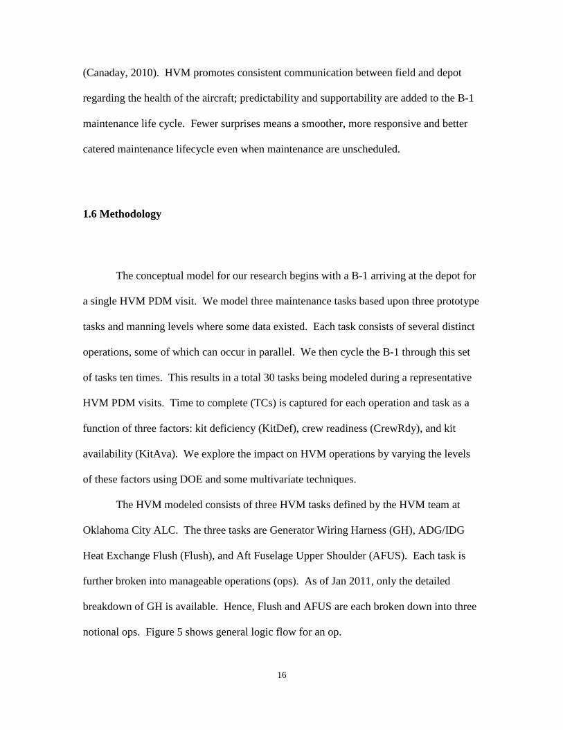
notional ops. Figure 5 shows general logic flow for an op.

17

Figure 5. General Logic Flow for an Op

Once an aircraft arrives to the depot, it is immediately split into three entities

which proceed to the first op station of each task (the GH task has priority). Upon arrival

at an op station, the aircraft seizes the appropriate resources and enters a specific logic

chain based on kit availability. If the required kit is available, the aircraft enters the chain

where only value-added (VA) time is allotted. However, if the required kit is not

available, the aircraft enters the chain where both value-added and maintenance-related

non-value-added (NA) times are allotted to account for the inefficiency of gathering parts

and tools on the spot. The process without a kit results in a longer TC. When

maintenance is completed at the op station, the aircraft travels to another op until 30 total

tasks are completed.

1.7 Thesis Outline

Chapter 2 includes detailed description of the conceptual model development, the

final DES model implementation, and the DOE used to study the joint effect of various

factors on TC and other MOEs. Chapter 3 is a case study of our Arena model using

Seize EE(s) Task Kit Available?

VA time with Kit

VA time without Kit

MX-related NA time

Route to Next Op

YES

NO

Op 1Release

EE(s)

Release EE(s)

18

multivariate techniques to examine the relationship and variability amongst the

simulation outputs statistics. Chapter 4 is the thesis conclusion that re-emphasizes

significant findings and offers recommendations for future study. Chapters 2 and 3 are

written in journal paper and conference proceeding formats.

19

2. Discrete-event Simulation of High Velocity Depot Maintenance Process for B-1 2.1 Introduction

Since the delivery of the 100 B-1B Lancers during the Reagan administration in

the 1980s, the Lancers have been valuable to the United States Air Force in combat

operations. In recent campaigns, such as Operation Allied Force, six B-1Bs flew two

percent of the total combat sorties but were responsible for over 20 percent tonnage of

bombs dropped on targets throughout the entire campaign. Other than combat efficiency,

the Lancer is also the world record holder for over 100 avionic titles including speed,

payload, and distance (Park, 2010). However, the B-1B operation was severely

hampered in 2008 when on average only 28 aircraft were available with 36 grounded due

to maintenance at any given time (Scully, 2009). In order to raise aircraft availability and

to maintain air superiority, the United States Air Force (USAF) has initiated High

Velocity Maintenance (HVM) on the B-1 fleet in the beginning of fiscal year 201l.

2.2 Overview

Presently, commercial airlines routinely maintain over 90 percent aircraft

availability; whereas the USAF has 60 percent availability rates on average (Dement,

2009). Considering that mission capable rate (MC) is closely tied to aircraft availability,

the USAF was inspired by commercial practices and has launched studies tailored to

improve aircraft availability and ultimately, air superiority. Ranging from fleet level

efforts, such as Project Air Force (PAR) conducted by RAND in 2007, to standalone

20

analyses dedicated for specific airframe such as Park (2010); it has reached the

conclusion that HVM has significant potential to improve aircraft availability.

The goal of HVM is to reduce aircraft downtime due to maintenance and enhance

aircraft availability by synchronizing field and depot maintenance and thus, minimizing

repair duplication. Under HVM, aircraft visit the depot more frequently for heavy

maintenance but for a shorter period of time. Instead of overhauling the entire airframe,

HVM services need-to-fix maintenance issues using kitting, pre-assembly of parts and

tools for major maintenance tasks (Sully, 2009). Burn rate or direct touch labor working

hours per day of the proposed B-1 HVM program at the depot is expected to ramp up to

400 hours per day versus the current Programmed Depot Maintenance (PDM) level of

145 to 150 direct hours per day (Canaday, 2010).

Intuitively, the higher the burn rate, the higher the aircraft availability. As such,

the goal of this research is to gain insights on B-1 depot maintenance operations, with a

focus on burn rate, under the implementation of HVM considering some key USAF

supply chain influences. While the concepts of the proposed B-1B HVM program are

well-documented and some initial analyses has been conducted at the base level (Park,

2010); full-scale B-1 HVM program is still in development. In fact only three B-1

prototypes have undergone two specific maintenance tasks in the B-1 HVM prototype

stage, which started in Oct 2010 (Ceyler, 2011).

Due to data limitation on the specifics of the proposed B-1 HVM processes and

the complexity of the USAF supply chain, discrete-event simulation (DES) is chosen to

model the B-1 HVM processes at the depot in Oklahoma City Air Logistics Center

(ALC), Tinker AFB, OK. A considerable amount of abstraction is adopted in our DES

21

model to capture supply chain influences on a single PDM visit consisting of 30 HVM

tasks. A surrogate measure for burn rate, time to complete (TC) a maintenance task, is

used as a key metric to assess the B-1 HVM processes. With this framework, an

increased burn rate results in a lower TC.

Understanding the impact of HVM is crucial since it can potentially affect the

entire acquisition life cycle of a weapon system. If HVM can effectively reduce

maintenance downtime and improve aircraft availability, the USAF can potentially save

millions of dollars simply by purchasing fewer aircraft. HVM goes beyond just the B-1

fleet for it is designed to be scalable, repeatable, and deployable on all weapon systems in

the USAF inventory (Adams, 2008). Hence, the methodologies used in this study

encompasses both simulation modeling and numerical experiment, such as design of

experiment (DOE) and multivariate analysis, to provides a way to better understand the

impact of HVM on burn rate and its overarching effect on aircraft availability.

2.3 Model Development

This research models the behavior of one B-1 aircraft going through a single

HVM PDM visit at the B-1 depot in Oklahoma City Air Logistics Center (ALC), Tinker

AFB, OK. The aircraft cycles through a composite of three HVM tasks ten times,

creating a representative series of 30 HVM tasks, as outlined in the B-1 HVM prototype

capability rollout calendar from Nov 2010 (Ceyler, 2011). Each HVM task is modeled

as a single-dock operation using HVM B-1 prototype manning levels and kitting

characteristics. The next section describes the general conceptual flow of our model.

22

2.3.1 General Cycle In order to create a representative series of 30 HVM tasks performed on one B-1

aircraft using data from three specific tasks, our model generates an aircraft as ten distinct

HVM entities (conceptually for sets of tasks that need to be completed sequentially), with

each entity completing one cycle through the three tasks. To allow parallel maintenance

operations, the first HVM entity is immediately split into three task entities, each of

which proceed to one of the modeled HVM tasks: Generator Harness (GH), Aft Fuselage

Upper Shoulder (AFUS), or ADG/IDG Heat Exchange Flush (Flush) while the rest of the

HVM entities stay put in a “Hold” block. Once each task entity is finished with its HVM

task, the three entities are batched back together and the HVM entity is disposed. Once

the sum of HVM entities disposed and the HVM entities in the “Hold” block equals ten

(indicating all previous tasks complete), another HVM entity is released from the “Hold”

block for split and parallel maintenance. Such mechanism guarantees only one set of

tasks is being performed at any given time and creates a single-dock operation that

mirrors the prototype processes at the B-1 depot. The process repeats until a total of 30

HVM tasks are completed representing a single HVM visit at the depot for one aircraft.

A conceptual representation of an aircraft cycle is shown below in Figure 6.

23

Figure 6. Conceptual Representation of an Aircraft Cycle

GH, AFUS, and Flush are each broken down into several manageable distinct

operations (ops), some of which occur in parallel. As of Jan 2011, only the detailed ops

sequence of the GH daily standard of work (DSW) was available and is shown in

Appendix A (Ceyler, 2011). AFUS and Flush are each broken down into three notional

ops. As mentioned before, a HVM entity is split into three task entities in order to

accomplish the three HVM tasks in parallel. GH, however, has priority in manpower or

personnel equivalences (PEs), which are seized upon aircraft arrival at an ops station.

Then, based on task kit availability, the task entity accumulates either only value-added

(VA) time as a result of direct hands-on maintenance facilitated by kitting; or VA time

and maintenance-related non-value-added (NA) time representing direct hours and

indirect hours spent on gathering parts and tools due to the absence of kitting. When

maintenance is completed, PEs are released and the task entity is routed to the next ops

station. The process continues till all ops of a HVM task are done. Once all three HVM

HVM Entity Arrival

Data Assignment

Task Set in Process?

Hold

Duplicate HVM Entity for parallel

MX tasks processing

GH

AFUS

Flush

Batch back to a single

entity

Signal to Release next HVM Entity

from Hold

HVM Entity

Disposal

YES

NO

24

tasks are finished, another HVM entity cycle begins. Simulation terminates after ten

cycles are executed. Figure 7 shows the simulation logic of an op.

Figure 7. Simulation Logic of an Op

2.3.2 Resource Set Up The PE schedule is modeled based on the manning requirement of the GH task

specified in the B-1 HVM DSW phase. Starting from 0800 to midnight, there are two

consecutive eight-hour PE shifts per day with four PEs per shift. The rest of the day is

considered inactive. Other non-maintenance related indirect hours, such as breaks,

training, shift changes, and admin requirements, can take up to two to three hours per PE

per shift. This results in average net working hours of roughly five to six hours per PE

per shift. These non-touch hours are captured in our model by inducing breaks, via the

Arena Failure Module, in the PE schedules as periods of randomly distributed up time

and down time. PEs engage in maintenance activities during up times and disengage

from any maintenance processes immediately when down times occur. An Arena

StateSet, WorkingDay, is created to ensure that breaks only occur during scheduled PE

shifts. Figure 8 shows an example of the Arena Failure Module with a one-to-three ratio

of up and down times, representing an average six hours per PE per shift of available

Seize EE(s) Task Kit Available?

VA time with Kit

VA time without Kit

MX-related NA time

Route to Next Op

YES

NO

Op 1Release

EE(s)

Release EE(s)

25

touch hours. Note that modeled down times do not include any non-maintenance related

NA times accrued when a kit is not available.

Figure 8. An Example of the Arena Failure Process

For ease of analysis, a variable called Crew Readiness (CrewRdy) is created to

allow easy modification of the distribution of up and down times. When referring to a

level of CrewRdy, we use the average number of up time, which includes both VA and

NA maintenance-related hours per PE per shift.

Another resource requirement gathered from the GH task is task kit

characteristics. The Kit Delivery Sequence of the GH task is shown in Appendix B

(Ceyler, 2011). It indicates that three out of ten ops of the GH task do not require a kit.

The rest of the ops require one of three task kits: the 14210 build-up kit, the 14211 FOM

kit, and the 14206 harness installation kit. Detailed breakdown of parts and tools

requirements for each GH task kit is listed in Appendix C (Ceyler, 2011). Since the kit

details of the AFUS and Flush tasks are unavailable, notional kits are created for all ops

under those two tasks. Kit characteristics are captured by modeling kit availability

26

(KitAva) and deficiency (KitDef) as variables in our Arena model. KitAva ranges from

0-100%, representing the probability of a kit being available. KitDef is a positive

numeric value that indicates the level of deficiency of a task kit. KitDef of 1.0 implies

the kit is neutral. KitDef less than 1.0 means the task kit is less deficient (i.e. more

effective) in getting the maintenance done and vice versa.

2.3.3 Arena Measures of Effectiveness (MOEs) Collection The goal of our research is to understand the impact of HVM on burn rate.

However, other than the GH task, burn rate data, which encompasses the total number of

VA hours spread over a known duration of time, is unavailable on all maintenance tasks

scheduled for the B-1 HVM prototype processes. Based on the VA hours available, one

of the MOEs our simulation captures is TC, which is used as a surrogate measure for

burn rate. With this framework, an increased burn rate results in a lower TC. Twenty

TCs, including one for the overall simulation (ten sets of the three HVM tasks), one for

each of the three HVM tasks, and one for each of the 16 ops embedded within the tasks,

are collected.

Other than using TCs to capture the impact of HVM on burn rate, other MOEs are

used to understand the effect of manning and kitting characteristics at the depot. The

average utilization of all PEs is captured to show resource usage of the system based on a

specific manning requirement. The average percentage of the non-maintenance related

indirect hours of all PEs is captured as well to show how much non-maintenance related

activities affect TCs. Finally, the observed percentage of unavailable kit occurrences of

27

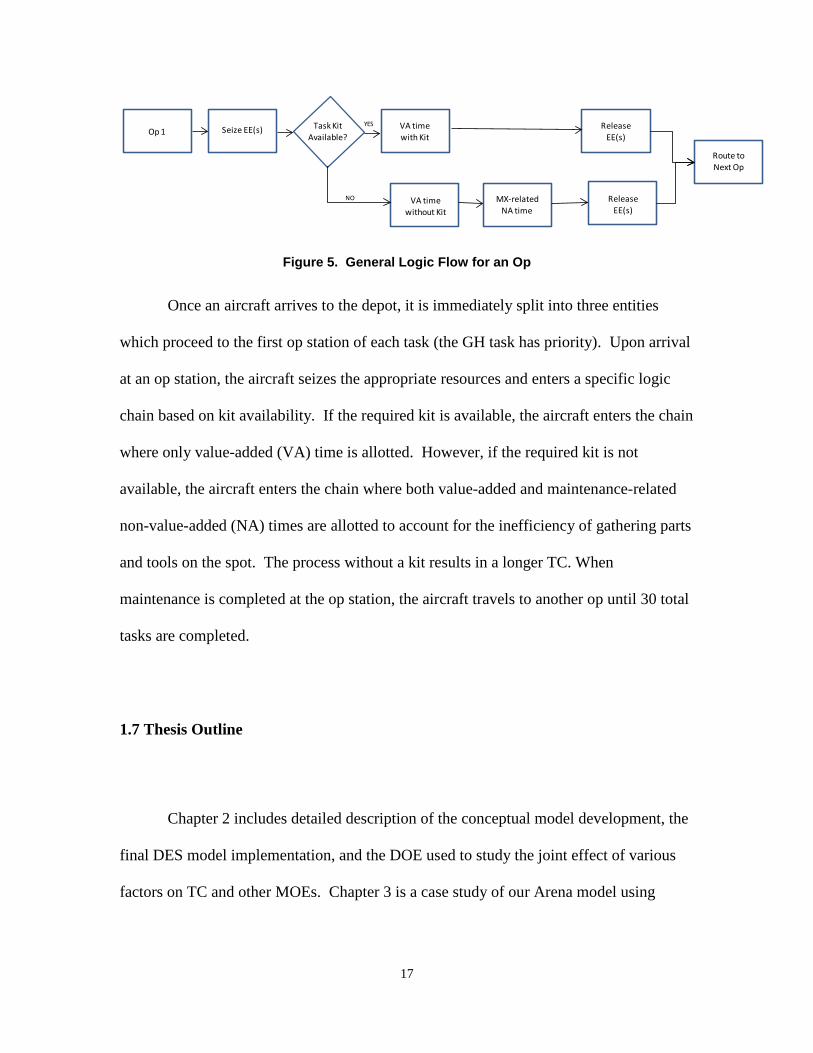
each HVM task is recorded to show how kit availability drives TCs. Table 1 shows the

simulation MOE statistics.

Table 1. Simulation MOE Statistics

MOE Expression Description

**AvgOP# Average TC of OP#

AvgGHTime Average TC of GH task

AvgAFUSTime Average TC of AFUS task

AvgFlushTime Average TC of Flush task

AvgSimTime Average TC of simulation

*AvgUteEE Average utilization of all PEs

% AvgBreakEE Average percentage of non-maintenance hours of all PEs

% NoKit_GH Observation percentage of unavailable kit in GH when needed

% NoKit_AFUS Observation percentage of unavailable kit in AFUS when needed

% NoKit_Flush Observation percentage of unavailable kit in Flush when needed

* AvgUteEEi = Average utilization of EEi for i = 1, …, 4 **AvgOP# = Average TC of OP# for # = any ops number

2.3.4 Assumptions

Assumptions are made in the development of this study in order to keep our

simulation within the scope of the research and provide meaningful analysis. Some key

assumptions follow:

The model is a terminating simulation that represents one cycle of a PDM HVM visit

under single-dock operation, serving only one aircraft at any given time.

28

Ten cycles of our current model of three prototype HVM tasks is a representative

PDM HVM visit consisting of 30 tasks.

The three selected HVM tasks can be carried out simultaneously since they are all

off-power procedures (Michaliszyn, 2011), while their respective ops are performed

sequentially with some parallel processes embedded within.

The model captures only an abstraction of depot level maintenance while base level

logistics, such as time spent at the base prior to revisiting depot for HVM, is ignored.

The manpower resource simulated accounts for only one logistics specialty,

electrician (EE).

Kit availability is not modeled explicitly such that the logistics of parts and tools are

not accounted for.

All EEs are identical in terms of efficiency.

The maintenance structures, including manning and kitting specifics, of AFUS and

Flush mirror those of the GH DSW, using 2 EEs and one kit per op.

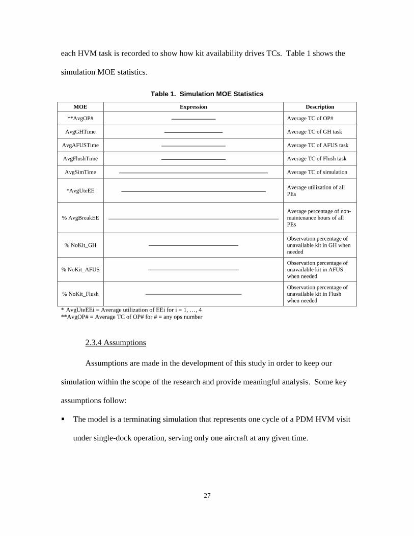
Maintenance time without kitting is about 1.5 times longer than the one with kitting.

Figure 9 shows the partition of maintenance time within an op.

Figure 9. Partition of Maintenance Time within an Op

Seize EE(s) Task Kit Available?

VA time with Kit

VA time without Kit

MX-related NA time

Route to Next Op

YES

NO

Op 1Release

EE(s)

Release EE(s)

MX time (with kit) = VA time =KitDef* X

VA time (no kit) ≈ XMX-related NA time (no kit) ≈ 0.5XMX time (no kit) ≈ 1.5X

29

2.3.5 Supporting Data One of the challenges we faced in this research is the limited supporting data on

the proposed HVM processes since it is still under development. However, the B-1

AFGLSC HVM Materiel Team provided us with some details of the GH DSW processes

and some historical data in regards to direct maintenance hours of the AFUS and Flush

tasks. Therefore, we were able to develop distributions that capture the stochastic nature

of depot maintenance processes under HVM in our model. Mean planned hours

(PHr_mu) of maintenance for each op of GH are available in the GH DSW Sequence

worksheet in Appendix A. We model each GH op time using an uniform distribution

with parameters set at minus 10% to plus 10% from the PHr_mu. Note that the hours

cited in the GH DSW Sequence are the estimated hours to complete each op and should

be divided evenly among all PEs assigned to that op.

Historical data of direct maintenance hours of AFUS and Flush are shown in

Appendix D. Because of the very small sample size of data for these tasks, we modeled

total task times for AFUS and Flush using triangular distributions with parameters taken

directly as the minimum (min), median, and maximum (max) values for the respective

task. Since we broke each of these tasks into three representative ops, we divided the

triangular parameters by three for each op with the respective tasks.

Finally, reflecting back on the assumption we made in the previous section:

maintenance time without kit is about 1.5 times longer than the one with kit. Therefore,

we model the maintenance process without kit in two parts – VA and the NA times. In

this case, VA is similar to the process distribution with kit (i.e. VA is developed as the

product of an uniform distribution with parameters set at 1 to 1.1 and the original process

30

distribution) and NA is roughly half of the process distribution with kit (i.e. NA is

developed as the product of an uniform distribution with parameters set at 0.4 to 0.5 and

the original process distribution). Under this framework, the total process time without

kit is approximately 1.5 times longer than the one with kit. Table 2 is a summary of

distributions use in the maintenance process modules within our model.

Table 2. Maintenance Process Distribution Summary

Description Expression GH VA process for op i with kit KitDef*UNIF(-10%PHr_mu of op i, +10%PHr_mu of op i) GH VA process for op i with no kit req. UNIF(-10%PHr_mu of op i, +10%PHr_mu of op i) GH VA process for op i without kit UNIF(0.4, 0.5)*UNIF(-10%PHr_mu of op i, +10%PHr_mu of op i) GH NA process for op i without kit UNIF(1, 1.1)*UNIF(-10%PHr_mu of op i, +10%PHr_mu of op i) AFUS VA process for op i with kit KitDef*TRIA(AFUS_min/3, AFUS_median/3, AFUS_max/3) AFUS VA process for op i without kit UNIF(0.4, 0.5)* TRIA(AFUS_min/3, AFUS_median/3, AFUS_max/3) AFUS NA process for op i without kit UNIF(1, 1.1)* TRIA(AFUS_min/3, AFUS_median/3, AFUS_max/3) Flush VA process for op i with kit KitDef*TRIA(Flush _min/3, Flush _median/3, Flush _max/3) Flush VA process for op i without kit UNIF(0.4, 0.5)* TRIA(Flush _min/3, Flush _median/3, Flush _max/3) Flush NA process for op i without kit UNIF(1, 1.1)* TRIA(Flush _min/3, Flush _median/3, Flush _max/3) UNIF – Uniform distribution TRIA – Triangular distribution AFUS_min – minimum of the AFUS historical hours AFUS_median - median of the AFUS historical hours AFUS_max – maximum of the AFUS historical hours Flush_min – minimum of the Flush historical hours Flush _median – median of the Flush historical hours Flush _max – maximum of the Flush historical hours 2.4 Verification and Validation

Verification and validation are essential in adding creditability to any simulation-

based research. Verification ensures that the simulation model is built correctly whereas

validation ensures that the correct model is built. To verify the simulation logic, we

visually monitor several animated Arena runs and observed that the animated entities are

routed to all maintenance stations as planned. One by one, every HVM entity is split into

three to join the simultaneous maintenance of GH, AFUS, and Flush until a total of 30

HVM tasks are completed. The routing logic is further verified by examining the output

31

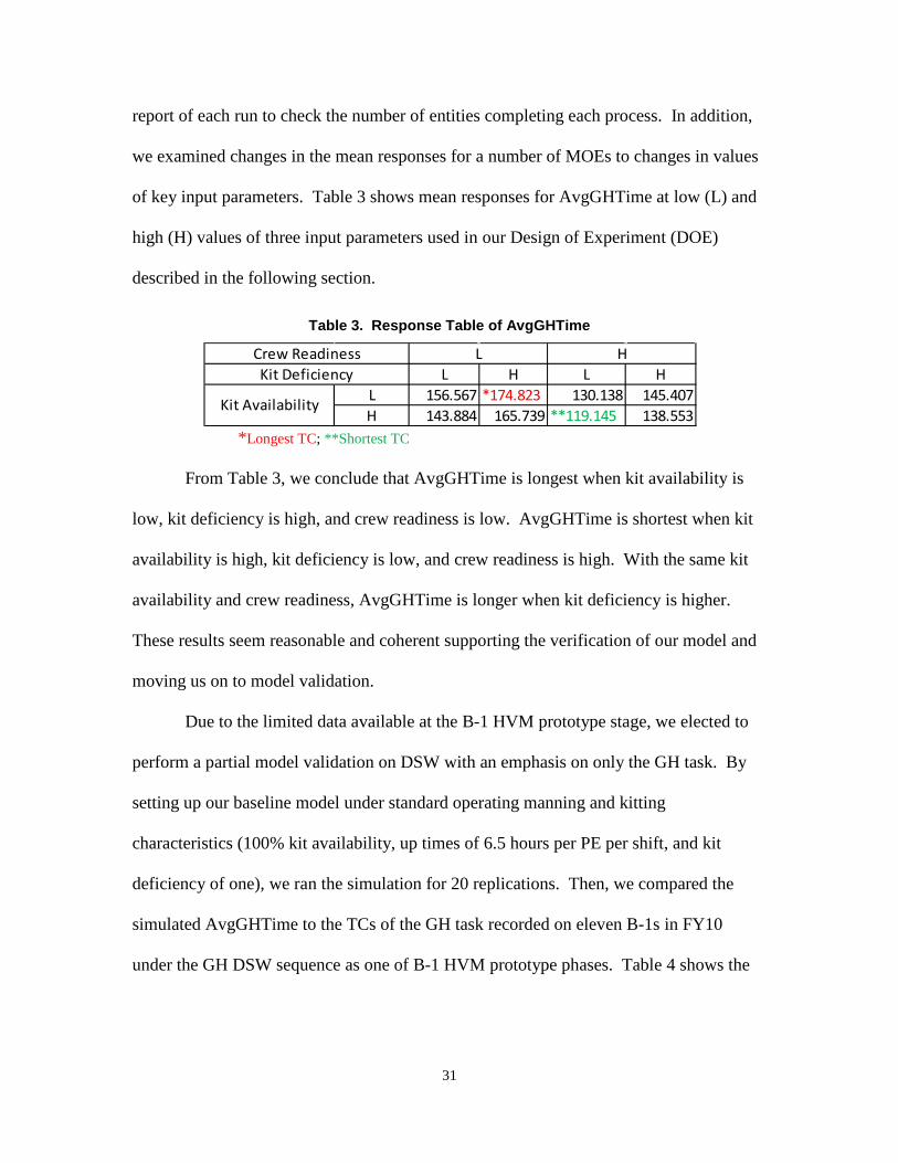
report of each run to check the number of entities completing each process. In addition,

we examined changes in the mean responses for a number of MOEs to changes in values

of key input parameters. Table 3 shows mean responses for AvgGHTime at low (L) and

high (H) values of three input parameters used in our Design of Experiment (DOE)

described in the following section.

Table 3. Response Table of AvgGHTime

*Longest TC; **Shortest TC

From Table 3, we conclude that AvgGHTime is longest when kit availability is

low, kit deficiency is high, and crew readiness is low. AvgGHTime is shortest when kit

availability is high, kit deficiency is low, and crew readiness is high. With the same kit

availability and crew readiness, AvgGHTime is longer when kit deficiency is higher.

These results seem reasonable and coherent supporting the verification of our model and

moving us on to model validation.

Due to the limited data available at the B-1 HVM prototype stage, we elected to

perform a partial model validation on DSW with an emphasis on only the GH task. By

setting up our baseline model under standard operating manning and kitting

characteristics (100% kit availability, up times of 6.5 hours per PE per shift, and kit

deficiency of one), we ran the simulation for 20 replications. Then, we compared the

simulated AvgGHTime to the TCs of the GH task recorded on eleven B-1s in FY10

under the GH DSW sequence as one of B-1 HVM prototype phases. Table 4 shows the

L H L HL 156.567 *174.823 130.138 145.407H 143.884 165.739 **119.145 138.553

L H

Kit Availability

Crew ReadinessKit Deficiency

32

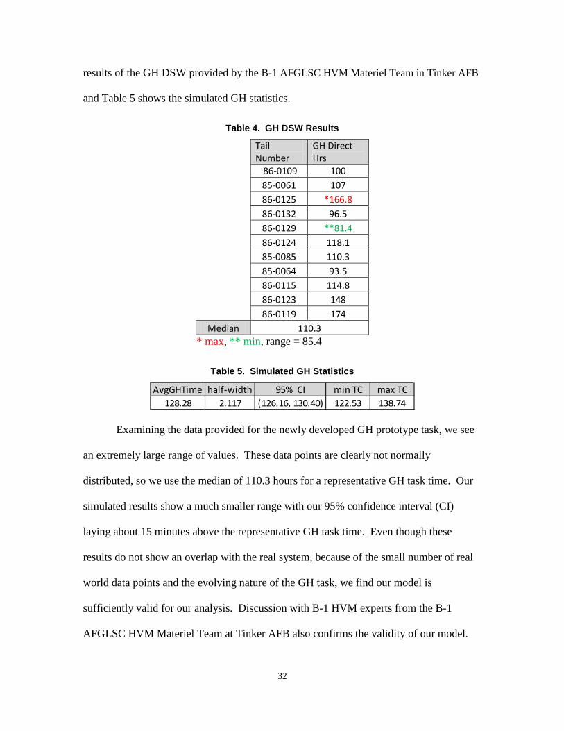
results of the GH DSW provided by the B-1 AFGLSC HVM Materiel Team in Tinker AFB

and Table 5 shows the simulated GH statistics.

Table 4. GH DSW Results

Tail Number

GH Direct Hrs

86-0109 100 85-0061 107 86-0125 *166.8 86-0132 96.5 86-0129 **81.4 86-0124 118.1 85-0085 110.3 85-0064 93.5 86-0115 114.8 86-0123 148 86-0119 174

Median 110.3 * max, ** min, range = 85.4

Table 5. Simulated GH Statistics

Examining the data provided for the newly developed GH prototype task, we see

an extremely large range of values. These data points are clearly not normally

distributed, so we use the median of 110.3 hours for a representative GH task time. Our

simulated results show a much smaller range with our 95% confidence interval (CI)

laying about 15 minutes above the representative GH task time. Even though these

results do not show an overlap with the real system, because of the small number of real

world data points and the evolving nature of the GH task, we find our model is

sufficiently valid for our analysis. Discussion with B-1 HVM experts from the B-1

AFGLSC HVM Materiel Team at Tinker AFB also confirms the validity of our model.

AvgGHTime half-width 95% CI min TC max TC128.28 2.117 (126.16, 130.40) 122.53 138.74

33

2.5 Design of Experiment Methodology

The purpose of this DOE is to identify the factors that drive TC and, ultimately,

burn rate under the impact of HVM with some key USAF supply chain influences at the

depot level. We are examining three factors: kit availability (KitAva), crew readiness

(CrewRdy), and kit deficiency (KitDef) with two levels each. KitAva (%) is the

probability that the kit is available for a maintenance op. KitDef is a positive numeric

value that indicates the level of deficiency of a task kit and is used as a multiplier of op

time with kit. KitDef of 1.0 implies the kit is neutral. KitDef less than 1.0 means the

task kit is less deficient (i.e. more effective) in getting the maintenance done and vice

versa. CrewRdy is defined as the average number of maintenance-related hours,

including both VA and NA maintenance hours, per PE per shift.

KitAva and KitDef are selected for our DOE because they are important kitting

characteristics derived from the tenants of HVM. As for CrewRdy, it might seem rather

straightforward that CrewRdy is inversely related to TCs. However, the interaction

effects of CrewRdy and other kitting characteristics might not be so intuitive. Hence,

CrewRdy is included in the DOE as well. Within our Arena model all the factors are

embedded as variables. Levels of all factors can be easily modified by changing the

values of the variables. The two levels of each factor are scaled to approximately ±10%

of the base level or center point. Completing the set up of our DOE, two simulation

outputs, AvgTimeGH and AvgSimTime, are selected as responses. Table 6 outlines the

design levels used in this DOE.

34

Table 6. Design Levels of Three Factors

2.6 DOE Analysis and Results

Since our model is a terminating simulation representing a PDM HVM visit for a

single aircraft, no warm up period is required. In determining an appropriate number of

replications, ( , we used procedure from Law (2007) to ensure the half-width of

the mean response is not greater than an absolute error, β, of the mean response. Using

our baseline model as described in Section 2.4, we ran the simulation 21 times,

incrementing the number of replications one at a time from 10 to 30. Iteratively, we

determine the appropriate such that the mean response half-width of (1-α)% CI is

less than or equal to β. Or as outlined in Law (2007) equation (9.2),

Applying the above principle to AvgGHTime with 95% CI and β of 2.5 hours, we

conclude that 20 replications are sufficiently large such that about 5% of the time,

AvgGHTime would have an absolute error at most 2.5 hours.

Over 20 replications, other than the two DOE responses, we have also collected

other MOEs. Table 7 summarizes the response statistics of AvgGHTime and

AvgSimTime and some other MOEs statistics collected under the baseline model.

FactorLow Level

(-)Center Point

(0)High Level

(+)KitAva(%) 80% 90 100%

KitDef 0.9 1 1.1CrewRdy (Hrs) 5.5 1 6.5

35

Table 7. Selected Simulation Outputs Statistics

The above statistics agree with the baseline model set up. Average overall

utilization rate, AvgEEUte, is high because the PEs are expected to finish all tasks

scheduled, with no compensation, prior to wrapping up their workday. Hence, the PEs

work longer than scheduled (over the average 6.5 hours they are available). The average

overall non-maintenance related NA hours, %AvgBreakEE, is lower than the expected

18.75%. However, such outcome fits the notion that the PEs work during some modeled

down time, thus lowering the percentage of non-maintenance related NA time out of a

longer workday. The TCs for AvgGHTime and AvgSimTime also look reasonable.

2.6.1 DOE Screening After completing a validation of the baseline model, we proceed to DOE using

JMP 8.0. We begin with a screening test, with α level of 0.05, of the full model

consisting of three two-level factors as detailed in Table 6. A randomized design matrix,

including a center point, is shown in Appendix E. Both individual p-values and half

normal plots (see Appendix F) of the two responses, AvgGHTime and AvgSimTime,

suggest that the three main effects are significant for AvgGHTime while the three main

effects plus the KitDef and KitAva interaction effect are significant for AvgSimTime.

Table 8 shows a summary of the screening test.

Min Mean Max half-widthAvgGHTime 122.53 128.28 138.74 2.117AvgSimTime 1320 1415 1584 36.058AvgEEUte 0.99678 1.0503 1.0958 0.01316%AvgBreakEE 13.346 14.532 15.377 0.26205%NoKit_Flush 0 0 0 0

36

Table 8. Summary of Screening Test

p-value

Factor AvgGHTime AvgSimTime CrewRdy 0.0004* 0.0003*

KitDef 0.0013* 0.0007* KitAva 0.0103* 0.0036*

CrewRdy*CrewRdy 0.4607 0.9165 CrewRdy*KitDef 0.5159 0.1727 CrewRdy*KitAva 0.6788 0.5159

KitDef*KitAva 0.2923 0.0369* CrewRdy*KitDef*KitAva 0.9562 0.8576

*significant factors CrewRdy*CrewRdy, KitDef*KitDef, KitAva*KitAva are aliases

2.6.2 Full Factorial Design Based on the results of the screening test, only significant factors of each response

are kept for their respective 23 full factorial DOE. The model for AvgGHTime is

statistically significant with R2adj equals to 0.993. At an α level of 0.05, all three main

effects are significant. In descending order of significance, the order is CrewRdy,

KitDef, and KitAva. As expected, CrewRdy plays a major role in driving AvgGHTime.

This makes sense because the more maintenance-related hours are allotted to the

processes, the faster things get done. Also, it turns out the kitting does have a significant

impact on AvgGHTime. Therefore, the HVM manning and kitting characteristics do

show a significant impact on burn rate as well. Figure 10 shows the ANOVA, parameter

estimates, and the effect test.

37

Figure 10. Summary of AvgGHTime DOE Statistics

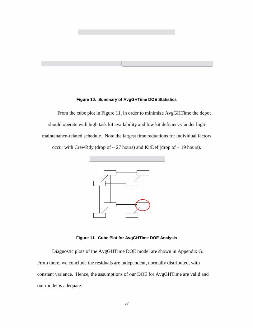
From the cube plot in Figure 11, in order to minimize AvgGHTime the depot

should operate with high task kit availability and low kit deficiency under high

maintenance-related schedule. Note the largest time reductions for individual factors

occur with CrewRdy (drop of ~ 27 hours) and KitDef (drop of ~ 19 hours).

Figure 11. Cube Plot for AvgGHTime DOE Analysis

Diagnostic plots of the AvgGHTime DOE model are shown in Appendix G.

From there, we conclude the residuals are independent, normally distributed, with

constant variance. Hence, the assumptions of our DOE for AvgGHTime are valid and

our model is adequate.

38

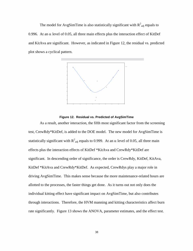
The model for AvgSimTime is also statistically significant with R2adj equals to

0.996. At an α level of 0.05, all three main effects plus the interaction effect of KitDef

and KitAva are significant. However, as indicated in Figure 12, the residual vs. predicted

plot shows a cyclical pattern.

Figure 12. Residual vs. Predicted of AvgSimTime

As a result, another interaction, the fifth most significant factor from the screening

test, CrewRdy*KitDef, is added to the DOE model. The new model for AvgSimTime is

statistically significant with R2adj equals to 0.999. At an α level of 0.05, all three main

effects plus the interaction effects of KitDef *KitAva and CrewRdy*KitDef are

significant. In descending order of significance, the order is CrewRdy, KitDef, KitAva,

KitDef *KitAva and CrewRdy*KitDef. As expected, CrewRdys play a major role in

driving AvgSimTime. This makes sense because the more maintenance-related hours are

allotted to the processes, the faster things get done. As it turns out not only does the

individual kitting effect have significant impact on AvgSimTime, but also contributes

through interactions. Therefore, the HVM manning and kitting characteristics affect burn

rate significantly. Figure 13 shows the ANOVA, parameter estimates, and the effect test.

39

Figure 13. Summary of AvgSimTime DOE Statistics

From the cube plot in Figure 14 shows similar trend as the AvgGHTime’s. In

order to minimize AvgSimTime, the depot should operate with high task kit availability

and low kit deficiency under high maintenance-related schedule. Note the largest time

reductions for individual factors occur with CrewRdy (drop of ~ 375 hours) and KitDef

(drop of ~ 303 hours).

Figure 14. Cube Plot for AvgSimTime DOE Analysis

40

Diagnostic plots of the AvgSimTime DOE model are shown in Appendix H.

From there, we conclude the residuals are independent, normally distributed, with

constant variance. Hence, the DOE model for AvgSimTime is adequate and valid.

2.7 Conclusion

Gathered from the analysis of our DOE, all kitting and manning factors examined

in this research have statistically significant impact on the time to complete the GH task,

as well as the overall PDM HVM process. Under the framework of our simulation, the

DOE analysis also concludes that CrewRdy, KitAva, and KitDef are impacting burn rate

in a statistically significant manner. In particular, resource schedule with a centric focus

on direct maintenance, high task kit availability, and small kit deficiency help ramping up

burn rate. These findings are important first-cut effort in analyzing the HVM processes

at the depot level as they present avenues that can lead to further studies when the full-

scale B-1 HVM processes is finally deployed.

41

3. Case Study

Multivariate Analysis on Outputs from the B-1 HVM Simulation

3.1 Introduction

In Mar 2008, the Air Force Global Logistics Support Center (AFGLSC) was

stood up with a mission to “execute the Air Force Supply Chain (AFSC) by integrating

enterprise-wide planning and strategy with global command and control as the single

focal point to the warfighter (Martin, 2008).” AFGLSC aims to streamline logistics such

as aircraft maintenance, in order to deliver support to warfighter swiftly and

economically. An aspect of the streamlined logistics adapts a lean and agile aircraft

maintenance process known as High Velocity Maintenance (HVM).

Under HVM, aircraft visit the depot more frequently but for a shorter period of

time. HVM synchronizes field and depot maintenance, minimizing repair duplication.

Instead of overhauling the entire airframe, HVM uses kitting, pre-assembly of parts and

tools, to service need-to-fix maintenance issues in a sequential manner (Sully, 2009).

Burn rate or direct touch labor working hours per day is expected to ramp up under the

HVM construct. Intuitively, the higher the burn rate, the higher the aircraft availability.

The higher the aircraft availability, the more mission capable (MC) the United States Air

Force (USAF) is. Therefore, improving aircraft availability is crucial to maintaining air

superiority.

Since 1980s, the Lancers have been valuable to the USAF in combat operations.

In recent campaigns, such as Operation Allied Force, six B-1Bs flew two percent of the

42

total combat sorties but were responsible for over 20 percent tonnage of bombs dropped

on targets throughout the entire campaign (Park, 2010). However, the B-1B operation

was severely hampered in 2008 when on average only 28 aircraft were available with 36

grounded due to maintenance at any given time (Scully, 2009). In an effort to increase B-

1B availability, USAF initiated HVM on the B-1 fleet in fiscal year 2011, expecting to

ramp up burn rate from the current Programmed Depot Maintenance (PDM) of 145 hours

per day to the proposed B-1 HVM of 400 hours per day at the B-1 depot in Oklahoma

City ALC, Tinker AFB (Canaday, 2010).

While the concepts of the proposed B-1 HVM program are well-documented and

some initial analyses have been performed at the base level (Park, 2010); studies have not

been extensively conducted at the depot level. Therefore, the goal of this research is to

gain insights on B-1 depot maintenance operations, with a focus on burn rate, under the

implementation of HVM considering some key USAF supply chain influences. Based on

the discrete-event simulation (DES) model we constructed, this study uses multivariate

analysis to reduce the dimensionality of the simulation output statistics to a few

representative factors. Factor analysis is specifically chosen to study the relationship

among those representative factors in order to assess system performance.

This reminder of this chapter provides concise description of our B-1 HVM

simulation model and a detailed discussion of multivariate analysis on various simulation

outputs.

43

3.2 B-1 HVM Simulation

This research models the behavior of one B-1 aircraft going through a single

HVM visit consisting of 30 HVM tasks at the B-1 depot in Oklahoma City ALC. Each

HVM task is modeled as a single-dock operation using some HVM B-1 prototype

manning levels and kitting characteristics provided by the B-1 AFGLSC HVM Materiel

Team at Tinker AFB. A considerable amount of abstraction is used in the model

development in order to sufficiently capture a representative B-1 HVM structure at the

depot within the scope of the research. The focus of this study is to examine the impact

of HVM under some USAF supply chain influences on burn rate using a surrogate

measure, time to complete (TC) a maintenance task. With this framework, an increased

burn rate results in a lower TC.

3.3.1 Model Development Using Arena 12.0, a DES model is developed under several key assumptions:

Only one set of three HVM prototype tasks is performed at any given time.

Ten cycles of our current model (of three prototype HVM tasks) is a

representative PDM HVM visit consisting of 30 tasks.

The three modeled HVM tasks are carried out simultaneously while their

respective operations (ops) are performed either in sequence or parallel.

Only depot level maintenance is modeled. Base logistics is ignored.

Only electrician (EE) is modeled as the simulated manpower resource.

All EEs are identical in terms of efficiency.

Part and tool availabilities are not modeled explicitly.

44

Maintenance without kit takes about 1.5 times longer than the one with kit

Maintenance structures of all three HVM tasks mirror off the daily standard of

work (DSW) sequence of the generator harness task defined by the depot,

using 2 EEs and one kit per op (Appendix A).

Figure 15 shows a generalized representation of our model. Using data from three

specific B-1 HVM prototype tasks: Generator Harness (GH), Aft Fuselage Upper

Shoulder (AFUS), and ADG/IDG Heat Exchange Flush (Flush), our model generates one

aircraft as ten distinct HVM entities (conceptually as ten sets of tasks that need to be

completed sequentially). Each HVM entity completes one cycle as shown in Figure 15

totaling a series of 30 HVM tasks. When the first HVM entity enters the system, it is

immediately split into three task entities, each of which proceeds to one of the modeled

HVM tasks while the rest of the HVM entities stay put in a “Hold” block. Once each

task entity is finished with its HVM task, the three entities are batched back together and

the HVM entity is disposed. Once the sum of the HVM entities disposed and the HVM

entities in the “Hold” block equals ten (indicating all previous tasks complete), another

HVM entity is released from the “Hold” block for split and parallel maintenance. The

process repeats until a total of 30 HVM tasks are completed. Under this framework, we

created a representative series of 30 HVM tasks performed on one B-1 aircraft mirroring

45

the B-1 HVM prototype phase at the depot.

Figure 15. Generalized B-1 HVM Model

GH, AFUS, and Flush are each broken down into several manageable distinct ops.

At the beginning of each op, the required EE are seized. Then, based on task kit

availability at each op, the task entity accumulates either only value-added (VA) time as a

result of direct hands-on maintenance facilitated by kitting; or VA time and maintenance-

related non-value-added (NA) time representing direct hours and indirect hours spent on

gathering parts and tools due to the absence of kitting. Before being routed to the next

op, the EEs are released. Figure 16 shows the generalized simulation logic within an op.

Figure 16. Generalized Simulation Logic Within an Op

The completion of a series of 30 HVM tasks signals the end of a replication.

Twenty replications are run to ensure the variations of the mean responses are within

HVM Entity Arrival

Data Assignment

Task Set in Process?

Hold

Duplicate HVM Entity for parallel

MX tasks processing

GH

AFUS

Flush

Batch back to a single

entity

Signal to Release next HVM Entity

from Hold

HVM Entity

Disposal

YES

NO

Seize EE(s) Task Kit Available?

VA time with Kit

VA time without Kit

MX-related NA time

Route to Next Op

YES

NO

Op 1Release

EE(s)

Release EE(s)

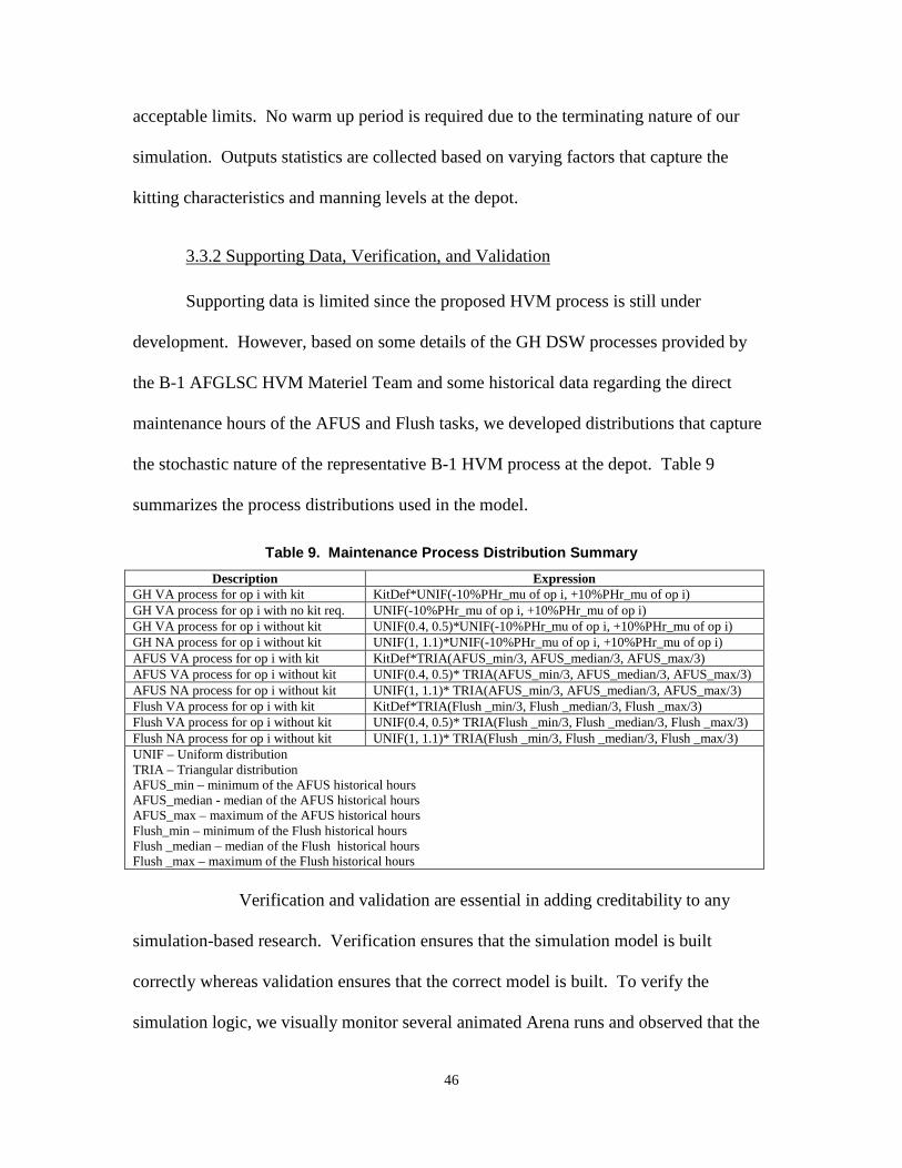
46

acceptable limits. No warm up period is required due to the terminating nature of our

simulation. Outputs statistics are collected based on varying factors that capture the

kitting characteristics and manning levels at the depot.

3.3.2 Supporting Data, Verification, and Validation Supporting data is limited since the proposed HVM process is still under

development. However, based on some details of the GH DSW processes provided by

the B-1 AFGLSC HVM Materiel Team and some historical data regarding the direct

maintenance hours of the AFUS and Flush tasks, we developed distributions that capture

the stochastic nature of the representative B-1 HVM process at the depot. Table 9

summarizes the process distributions used in the model.

Table 9. Maintenance Process Distribution Summary

Description Expression GH VA process for op i with kit KitDef*UNIF(-10%PHr_mu of op i, +10%PHr_mu of op i) GH VA process for op i with no kit req. UNIF(-10%PHr_mu of op i, +10%PHr_mu of op i) GH VA process for op i without kit UNIF(0.4, 0.5)*UNIF(-10%PHr_mu of op i, +10%PHr_mu of op i) GH NA process for op i without kit UNIF(1, 1.1)*UNIF(-10%PHr_mu of op i, +10%PHr_mu of op i) AFUS VA process for op i with kit KitDef*TRIA(AFUS_min/3, AFUS_median/3, AFUS_max/3) AFUS VA process for op i without kit UNIF(0.4, 0.5)* TRIA(AFUS_min/3, AFUS_median/3, AFUS_max/3) AFUS NA process for op i without kit UNIF(1, 1.1)* TRIA(AFUS_min/3, AFUS_median/3, AFUS_max/3) Flush VA process for op i with kit KitDef*TRIA(Flush _min/3, Flush _median/3, Flush _max/3) Flush VA process for op i without kit UNIF(0.4, 0.5)* TRIA(Flush _min/3, Flush _median/3, Flush _max/3) Flush NA process for op i without kit UNIF(1, 1.1)* TRIA(Flush _min/3, Flush _median/3, Flush _max/3) UNIF – Uniform distribution TRIA – Triangular distribution AFUS_min – minimum of the AFUS historical hours AFUS_median - median of the AFUS historical hours AFUS_max – maximum of the AFUS historical hours Flush_min – minimum of the Flush historical hours Flush _median – median of the Flush historical hours Flush _max – maximum of the Flush historical hours

Verification and validation are essential in adding creditability to any

simulation-based research. Verification ensures that the simulation model is built

correctly whereas validation ensures that the correct model is built. To verify the

simulation logic, we visually monitor several animated Arena runs and observed that the

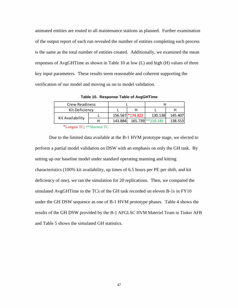
47

animated entities are routed to all maintenance stations as planned. Further examination

of the output report of each run revealed the number of entities completing each process

is the same as the total number of entities created. Additionally, we examined the mean

responses of AvgGHTime as shown in Table 10 at low (L) and high (H) values of three

key input parameters. These results seem reasonable and coherent supporting the

verification of our model and moving us on to model validation.

Table 10. Response Table of AvgGHTime

*Longest TC; **Shortest TC Due to the limited data available at the B-1 HVM prototype stage, we elected to

perform a partial model validation on DSW with an emphasis on only the GH task. By

setting up our baseline model under standard operating manning and kitting

characteristics (100% kit availability, up times of 6.5 hours per PE per shift, and kit

deficiency of one), we ran the simulation for 20 replications. Then, we compared the

simulated AvgGHTime to the TCs of the GH task recorded on eleven B-1s in FY10

under the GH DSW sequence as one of B-1 HVM prototype phases. Table 4 shows the

results of the GH DSW provided by the B-1 AFGLSC HVM Materiel Team in Tinker AFB

and Table 5 shows the simulated GH statistics.

L H L HL 156.567 *174.823 130.138 145.407H 143.884 165.739 **119.145 138.553

L H

Kit Availability

Crew ReadinessKit Deficiency

48

Table 11. GH DSW Results

Tail Number

GH Direct Hrs

86-0109 100 85-0061 107 86-0125 *166.8 86-0132 96.5 86-0129 **81.4 86-0124 118.1 85-0085 110.3 85-0064 93.5 86-0115 114.8 86-0123 148 86-0119 174

Median 110.3 * max, ** min

Table 12. Simulated GH Statistics

Examining the data provided for the newly developed GH prototype task, we see

an extremely large range of values. These data points are clearly not normally

distributed, so we use the median of 110.3 hours for a representative GH task time. Our

simulated results show a much smaller range with our 95% confidence interval (CI)

laying about 15 minutes above the representative GH task time. Even though these

results do not show an overlap with the real system, because of the small number of real

world data points and the evolving nature of the GH task, we find our model is

sufficiently valid for our analysis. Discussion with B-1 HVM experts from the B-1

AFGLSC HVM Materiel Team at Tinker AFB also confirms the validity of our model.

AvgGHTime half-width 95% CI min TC max TC128.28 2.117 (126.16, 130.40) 122.53 138.74

49

3.4 Multivariate Analysis

Adopting the idea from performing multivariate analysis on military aircraft

maintenance for performance assessment purposes (Miller et al, 2007), we apply the

techniques of multivariate analysis to our simulation output statistics to reduce the

dimensionality of system outputs and to identity key system measures that drive system

performance.

3.4.1 Analysis Background A 43 simulation design structure (yielding 64 design points) is created using three

design factors with four levels each. The three design factors are kit availability

(KitAva), kit deficiency (KitDef), and crew readiness (CrewRdy). KitAva represents the

probability of a task kit being available at any op. KitDef is a numeric value that

indicates the level of deficiency of a task kit. KitDef of 1.0 implies the kit is neutral.

KitDef less than 1.0 means the task kit is less deficient (i.e. more effective) in getting

maintenance done and vice versa. CrewRdy refers to the average number of maintenance

hours, including both VA and NA times, per personnel equivalence (PE) per shift. Table

10 shows the actual values of the four levels used by the three design factors.

Table 13. Design Levels of Three Design Factors

At each design point, 20 replications of the simulation are ran to generate mean

responses of 25 output statistics at the end of each replication. Among the 25 outputs, 20

level 1 level 2 level 3 level 4KitAva (%) 45 60 75 90

KitDef 0.8 0.9 1 1.1CrewRdy (Hrs) 5.5 6 6.5 7

50

are TCs, including one for the overall simulation (ten sets of the three HVM tasks), one

for each of the three HVM tasks, and one for each of the 16 ops embedded within the

tasks. Table 11 summarizes the simulation output statistics collected.

Table 14. Simulation Output Statistics

MOE Expression Description

**AvgOP# Average TC of OP#

AvgGHTime Average TC of GH task

AvgAFUSTime Average TC of AFUS task

AvgFlushTime Average TC of Flush task

AvgSimTime Average TC of simulation

*AvgUteEE Average utilization of all PEs

% AvgBreakEE Average percentage of non-maintenance hours of all PEs

% NoKit_GH Observation percentage of unavailable kit in GH when needed

% NoKit_AFUS Observation percentage of unavailable kit in AFUS when needed

% NoKit_Flush Observation percentage of unavailable kit in Flush when needed

*AvgUteEEi = Average utilization of EEi for i = 1, …, 4 **AvgOP# = Average TC of OP# for # = any ops number

25 output statistics imply there are 25 dimensions in our output data, which makes

it cumbersome and inefficient in assessing system performance. By using multivariate

analysis, our goal is to reduce the dimensionality of the data and yet still be able to

sufficiently explain the variation of the data.

51

3.4.2 Analysis and Results

Prior to proceeding to the actual multivariate analysis, we filtered the 25 output

statistics by eliminating MOEs with collinearity. Table 15 shows a reduced list of

variables.

Table 15. List of Reduced Variables

MOE Expression Description

AvgGHTime Average TC of GH task

AvgAFUSTime Average TC of AFUS task

AvgFlushTime Average TC of Flush task

*AvgUteEE Average utilization of all PEs

% AvgBreakEE Average percentage of non-maintenance hours of all EEs

% AvgNoKit Observation percentage of unavailable kit in all three tasks

*AvgUteEEi = Average utilization of EEi for i = 1, …, 4

The reduced list of variables contains six output statistics. We proceed to perform

principal component analysis (PCA) on the six variables using Matlab 7.9.0. The Matlab

programming code used for multivariate analysis is shown in Appendix I. Table 16

shows the PCA loadings, the eigenvalues, and cumulative variance corresponded to each

eigenvector within the loading matrix. Based on the cumulative variance, we conclude

that the first three principal components (PCs) account for 99.75% of the total output

statistics variance. In other words, together, the first three PCs explain approximately

99.75% of the total variance.

52

Table 16. PCA Loading Matrix

Using the eigenvalues, we constructed a scree plot as shown in Figure 17. Using

Cattell’s test (Bauer, 2010), we concluded the reduced dimensionality of the data is three

since there are three points on or above the scree line.

Figure 17. Scree Plot

Once we have determined the reduced dimensionality of the output statistics is

three, we used Matlab 7.9.0 to perform factor analysis on the first three PCs using

4.5328 1.2405 0.2119 0.0095 0.0035 0.0018cumulative

variance 75.54667 96.22167 99.75333 99.91167 99.97 100AvgGHTime -0.9778 0.1316 0.1486 -0.0602 -0.0261 0.0129

AvgAFUSTime -0.9799 0.1373 0.1361 0.0355 -0.0152 -0.0297AvgFlushTime -0.9701 0.1761 0.1589 0.0327 0.0348 0.0183%AvgBreakEE -0.8932 -0.4188 -0.154 -0.0446 0.0287 -0.015

%AvgNoKit -0.3609 0.8953 -0.2612 -0.0045 0.0016 -0.0009AvgEEUte 0.8644 0.4432 0.2326 -0.0392 0.0225 -0.0143

eigvalues

Component loading = loading matrix

- scree line

53

varimax rotation. Table 17 shows the rotated factor loadings. The first factor is

dominated by the loadings of the average time to complete each individual HVM task.

We call this factor “task duration.” The second factor is simply the average percentage

occurrence of no kit available at an op when needed. We call this “no-kit occurrences.”

The third factor is a contrast between the average percentage of EE down time (non-

maintenance related indirect hours) and the average EE utilization. We call this “PEs

effectiveness.” Note that after we factor analyzed the original reduced output data, it can

now be represented in terms of the three retained rotated factor scores.

Table 17. Rotated Factor Loadings

To further explore the relationship of the rotated factors, we plot the three retained

rotated factor scores. In Figure 18, the data points are coded according to the four levels

of KitDef: 0.8, 0.9, 1.0, and 1.1. Based on the clear grouping by KitDef, the figure

reveals that KitDef is a significant driver on task duration. Along the task duration

dimension, we observed that the more deficient a kit is, the longer the task takes. In other

words, based on the task duration factor, we can predict the deficiency of kit used in the

system and vice versa. Furthermore, we observed that there is roughly a linear

relationship between factor 1 and factor 3. As indicated by the solid arrow in Figure 18,

variable Factor 1* Factor 2* Factor 3*AvgGHTime 0.8383 0.2596 -0.4748

AvgAFUSTime 0.8327 0.271 -0.4804AvgFlushTime 0.8478 0.2899 -0.4411%AvgBreakEE 0.474 -0.0692 -0.8761

%AvgNoKit 0.2632 0.9613 0.0807AvgEEUte -0.397 0.0569 0.9148

* = rotated factors

54

the KitDef-coded three-dimensional plot, and Figure 19, a two-dimensional plot of PEs

effectiveness vs. task duration, more effective PEs lead to shorter task duration.

Figure 18. Three-dimensional Factor Plot (KitDef Coded)

-2

-1

0

1

2

-4-2

02

4-4

-2

0

2

4

F2, No-kit Occurrences

Three-dimensional Factor Plot, coded by KitDef

F1, Task Duration

F3, P

Es

Effe

ctiv

enes

s

KitDef=0.8KitDef=0.9KitDef=1.0KitDef=1.1

55

Figure 19. Task Duration vs. PEs Effectiveness

Another interesting factor score plot is shown in Figure 20. The data points are

coded according to the levels of KitAva. Clear grouping by KitAva is observed. The

figure reveals that KitAva is not a significant driver on task duration. Along the task

duration dimension, we observed that while low kit availability (say, 45%) guarantees

longer task duration; high kit availability spreads task duration to a wide range.

Nevertheless, KitAva clearly drives no-kit occurrences since the no-kit occurrences

dimension distinctively separates the data into four clusters by KitAva.

Furthermore, we observed that there is roughly a linear relationship between

factor 1 and factor 2. As indicated by the solid arrow in Figure 20, the KitAva-coded

three-dimensional plot, and Figure 21, a two-dimensional plot of task duration vs. no-kit

occurrences, more no-kit occurrences lead to shorter task duration. This finding

contradicts the very premise of the HVM concept stating that kitting reduces maintenance

-2.5 -2 -1.5 -1 -0.5 0 0.5 1 1.5 2 2.5-2.5

-2

-1.5

-1

-0.5

0

0.5

1

1.5

2

2.5

F3, PEs Effectiveness

F1, T

ask

Dur

atio

n

F1 vs. F3 coded by KitDef

KitDef=0.8KitDef=0.9KitDef=1.0KitDef=1.1

56

time. To further explore such seeming inconsistency, we plot and compare the basic un-

coded no-kit occurrences (F2) vs. task duration (F1) and %AvgNoKit vs. task duration

(F1) as shown in Figure 22 and Figure 23, respectively.

Figure 20. Three-dimensional Factor Plot (KitAva Coded)

-2

-1

01

2

-4

-2

0

2

4-4

-2

0

2

4

F2, No-kit Occurrences

Three-dimensional Factor Plot, coded by KitAva

F1, Task Duration

F3, P

Es

Effe

ctiv

enes

sKitAva=45KitAva=60KitAva=75KitAva=90

57

Figure 21. Task Duration vs. No-kit Occurrences

Figure 22. No-kit occurrences (F2) vs. task duration (F1)

-2 -1.5 -1 -0.5 0 0.5 1 1.5 2-2.5

-2

-1.5

-1

-0.5

0

0.5

1

1.5

2

2.5

F2, No-kit Occurrences

F1, T

ask

Dur

atio

n

F1 vs. F2 coded by KitAva

KitAva=45KitAva=60KitAva=75KitAva=90

Fig 14.

58

Figure 23. %AvgNoKit vs. task duration (F1)

Since no-kit occurrences (F2) originated from the factor loading of a single

variable, %AvgNoKit, we expected F2 vs. F1 and %AvgNoKit vs. F1 to exhibit similar

pattern. However, as indicated by the solid arrows in Figure 22 and Figure 23, it is clear

that F2 vs. F1 shows a negative linear relationship; whereas %AvgNoKit vs. F1

demonstrates roughly a zero-sloped pattern. Such discovery not only suggests that we

might have over-interpreted F2 but also proves that F1 is driven by more than just F2 or

%AvgNoKit. To confirm our suspicions, we proceed to reaccomplish F2 vs. F1 and

%AvgNoKit vs. F1 by indicating all three design levels of each design points in Figure

24 and Figure 25, respectively, followed by the legend of various design levels in Figure

26.

Fig 13.

59

Figure 24. F2 vs. F1

Figure 25. %AvgNoKit vs. F1

-2.5 -2 -1.5 -1 -0.5 0 0.5 1 1.5 2 2.5-2

-1.5

-1

-0.5

0

0.5

1

1.5

2

F1 - task duration

F2 -

No-

kit o

ccur

renc

es

F1 vs. F2

-2.5 -2 -1.5 -1 -0.5 0 0.5 1 1.5 2 2.55

10

15

20

25

30

35

40

45

50

55

Task duration

%A

vgN

oKit

F1 vs. %AvgNoKit

60

Figure 26. Legend of Design Levels

Both Figures 24 and 25 show clear grouping of KitAva. In accordance to our

previous findings, KitAva clearly is not a significant driver on task duration. However,

based on KitAva alone, we can cast fairly accurate predictions on no-kit occurrences (or

%AvgNoKit) and vice versa. Furthermore, with every design point fully decoded (by

CrewRdy, KitDef, and KitAva), we observe a positive relationship between no-kit

occurrences (or %AvgNoKit) and task duration as indicated by the solid arrow in both

Figure 24 and Figure 25 stating that task duration raises as no-kit occurrences (or

%AvgNoKit) increase. Such discovery has rectified our previous inconsistency as shown

in Figure 20 and 21.

3.4.3 Multivariate Analysis Conclusion Based on the examination of the various factor score plots obtained as a result of

our factor analysis, we concluded that the dimensionality of simulation output statistics

can be largely reduced to three: task duration, no-kit occurrences, and PEs effectiveness.

Task duration (Factor 1) is strongly affected by KitDef - the more deficient a kit is, the

longer the task takes; no-kit occurrences (Factor 2) is strongly affected by KitAva; PEs

effectiveness (Factor 3) is strongly affected by CrewRdy; the more maintenance hours

available (i.e. more CrewRdy) per shift, the more effective the PEs are. Based on the

level of KitDef, we can predict task duration and vice versa.

Legend:* = CrewRdy 5.5Hrs red = KitDef 0.8 = KitAva 45%+ = CrewRdy 6 Hrs blue = KitDef 0.9 = KitAva 60%= CrewRdy 6.5 Hrs green = KitDef 1 = KitAva 75%

O = CrewRdy 7 Hrs black = KitDef 1.1 = KitAva 90%

61

3.5 Conclusion

In this section, we have explored the relationship among various output statistics

from our B-1 HVM simulation modeled at the depot level. By employing the techniques

of multivariate analysis, we have discovered that there are three interpretable factors:

task duration, no-kit occurrences, and PEs effectiveness; as well as the design factors that

drive them. We are also able to determine some relationships among the factors. Such

conclusion provides further insights of the impact of HVM under some USAF supply

chain influences. When the full-scale B-1 HVM processes is finally deployed and more

sophisticated simulation outputs are available, multivariate analysis can be re-

accomplished to further explore the relationships among those simulation outputs and

gain insights of the HVM simulation input structures.

62

4. Conclusion

4.1 Summary

This research provides some initial insights on improving B-1 HVM operations at

the depot level via the use of DES. The stochastic nature of our model was captured by

various simulation elements using both historical depot maintenance data and the most

current B-1 HVM data collected from the B-1 prototype process at Oklahoma City ALC,

Tinker AFB. Under such framework, this research uses DOE to investigate factors that

drive the performance of depot HVM, which has not been extensively studied in prior

researches. It shows that resource schedule with a centric focus on direct maintenance

and small kit deficiency are significant in improving burn rate.

Other than DOE, we have also performed multivariate analysis to examine the

simulation output statistics in order to further assess system performance by exploring the

impact of depot HVM processes from the system output perspective. It shows the

dimensionality of the output statistics can be largely reduced to three factors: task

duration, no-kit occurrences, and PEs effectiveness. Kit deficiency turns out to be the

most significant driver of task duration or burn rate. Based on the level of kit deficiency,

we can successfully predict task duration.

Simulation together with the techniques of DOE and multivariate analysis are

crucial in the assessment of the B-1 HVM process, which is still under development.

This study is set up such that updates can be made to the original simulation with relative

63

ease. Analyses can also be re-accomplished under this framework to further gain insights

of the B-1 HVM process as it grows.

4.2 Future Research

The B-1 bombers are valuable combat asset to the USAF. The availability of the

B-1 fleet is, therefore, crucial to assert air superiority and support the USAF mission of

fly, fight, and win. Nevertheless, current published work that examines the availability of

the B-1 fleet from the depot maintenance standpoint is limited. This research serves as a

first-cut effort to gain some initial insights of the impact of depot HVM on B-1

availability. As more data becomes available regarding the B-1 HVM prototype process,

our research can definitely be expanded.

First and foremost, the details within a task, such as the various maintenance

specialties assigned, or a more precise description of process distributions, should be

expanded to include more HVM tasks that are outlined in the B-1 prototype schedule.

This simulation stems from data of only three completed HVM B-1 prototype tasks (three

tails per tasks at most). Expand our data set to include more HVM tasks and their

associate details as the B-1 HVM prototype process continues to grow can add fidelity to

the output statistics being reported in this research.

Secondly, when the general details of how the full-scale B-1 HVM process

interacts with individual bases become available, the model should be expanded to

include some base-level logistics, such as cycle times between field maintenance and

depot HVM and the task differentiation between field and depot. Doing so can gain

64

better understanding of the HVM impacts on the entire life cycle of the B-1 fleet and

possibly provide some guidelines in establishing some aircraft maintenance policies.

Granted, it is impossible to model the coming and going of every tool and part

explicitly within the Air Force supply chain. However, if we can expand the scope of this

research to encompass more supply chain influences at the stock level, say bench

stockage of some important task kits, we can then explore the impact of certain stock on

HVM and ultimately, B-1 availability. This can potentially shed lights on the acquisition

life cycle of the Lancers.

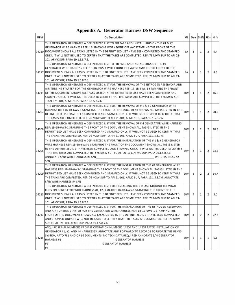
65

Appendix A. Generator Harness DSW Sequence

OP # Op Description MJ Day Shift PE's Hr's

14210

THIS OPERATION GENERATES A DEFINITIZED LIST TO PREPARE AND INSTALL LUGS ON THE #1 & #2 GENERATOR WIRE HARNESS REF: 1B-1B-6WS-1 WORK DONE OFF A/C STAMPING THE FRONT OF THE DOCUMENT SHOWS ALL TASKS LISTED IN THE DEFINITIZED LIST HAVE BEEN COMPLETED AND STAMPED ONLY. IT WILL NOT BE USED TO CERTIFY THAT THE TASKS ARE COMPLETED. REF: 76 MXW SUP TO AFI 21-101, AFMC SUP, PARA 19.1.5.8.7.6.

BA 1 1 2 9.4

14217

THIS OPERATION GENERATES A DEFINITIZED LIST TO PREPARE AND INSTALL LUGS ON THE #4 GENERATOR WIRE HARNESS REF: 1B-1B-6WS-1 WORK DONE OFF A/C STAMPING THE FRONT OF THE DOCUMENT SHOWS ALL TASKS LISTED IN THE DEFINITIZED LIST HAVE BEEN COMPLETED AND STAMPED ONLY. IT WILL NOT BE USED TO CERTIFY THAT THE TASKS ARE COMPLETED. REF: 76 MXW SUP TO AFI 21-101, AFMC SUP, PARA 19.1.5.8.7.6.

BA 1 1 2 4.5

14211

THIS OPERATION GENERATES A DEFINITIZED LIST FOR THE REMOVAL OF THE NITROGEN RESERVOIR AND AIR TURBINE STARTER FOR THE GENERATOR WIRE HARNESS REF: 1B-1B-6WS-1 STAMPING THE FRONT OF THE DOCUMENT SHOWS ALL TASKS LISTED IN THE DEFINITIZED LIST HAVE BEEN COMPLETED AND STAMPED ONLY. IT WILL NOT BE USED TO CERTIFY THAT THE TASKS ARE COMPLETED. REF: 76 MXW SUP TO AFI 21-101, AFMC SUP, PARA 19.1.5.8.7.6.

DW 1 1 2 16.5

14207

THIS OPERATION GENERATES A DEFINITIZED LIST FOR THE REMOVAL OF # 1 & # 2 GENERATOR WIRE HARNESS REF: 1B-1B-6WS-1 STAMPING THE FRONT OF THE DOCUMENT SHOWS ALL TASKS LISTED IN THE DEFINITIZED LIST HAVE BEEN COMPLETED AND STAMPED ONLY. IT WILL NOT BE USED TO CERTIFY THAT THE TASKS ARE COMPLETED. REF: 76 MXW SUP TO AFI 21-101, AFMC SUP, PARA 19.1.5.8.7.6.

DW 2 1 2 20.5

14208

THIS OPERATION GENERATES A DEFINITIZED LIST FOR THE REMOVAL OF # 4 GENERATOR WIRE HARNESS REF: 1B-1B-6WS-1 STAMPING THE FRONT OF THE DOCUMENT SHOWS ALL TASKS LISTED IN THE DEFINITIZED LIST HAVE BEEN COMPLETED AND STAMPED ONLY. IT WILL NOT BE USED TO CERTIFY THAT THE TASKS ARE COMPLETED. REF: 76 MXW SUP TO AFI 21-101, AFMC SUP, PARA 19.1.5.8.7.6.

DW 2 2 2 10.5

14206

THIS OPERATION GENERATES A DEFINITIZED LIST FOR THE INSTALLATION OF THE # 1 & # 2 GENERATOR WIRE HARNESS REF: 1B-1B-6WS-1 STAMPING THE FRONT OF THE DOCUMENT SHOWS ALL TASKS LISTED IN THE DEFINITIZED LIST HAVE BEEN COMPLETED AND STAMPED ONLY. IT WILL NOT BE USED TO CERTIFY THAT THE TASKS ARE COMPLETED. REF: 76 MXW SUP TO AFI 21-101, AFMC SUP, PARA 19.1.5.8.7.6. ANNOTATE S/N: WIRE HARNESS #1 S/N______________________________________ WIRE HARNESS #2 S/N______________________________________

DW 3 1 2 23.5

14209

THIS OPERATION GENERATES A DEFINITIZED LIST FOR THE INSTALLATION OF THE #4 GENERATOR WIRE HARNESS REF: 1B-1B-6WS-1 STAMPING THE FRONT OF THE DOCUMENT SHOWS ALL TASKS LISTED IN THE DEFINITIZED LIST HAVE BEEN COMPLETED AND STAMPED ONLY. IT WILL NOT BE USED TO CERTIFY THAT THE TASKS ARE COMPLETED. REF: 76 MXW SUP TO AFI 21-101, AFMC SUP, PARA 19.1.5.8.7.6. ANNOTATE S/N: WIRE HARNESS #4 S/N______________________________________

DW 3 2 2 14.7

14213

THIS OPERATION GENERATES A DEFINITIZED LIST FOR INSTALLING THE 3 PHASE GROUND TERMINAL LUGS ON GENERATOR WIRE HARNESS #1, #2, & #4 REF: 1B-1B-6WS-1 STAMPING THE FRONT OF THE DOCUMENT SHOWS ALL TASKS LISTED IN THE DEFINITIZED LIST HAVE BEEN COMPLETED AND STAMPED ONLY. IT WILL NOT BE USED TO CERTIFY THAT THE TASKS ARE COMPLETED. REF: 76 MXW SUP TO AFI 21-101, AFMC SUP, PARA 19.1.5.8.7.6.

DW 4 1 2 5.0

14212

THIS OPERATION GENERATES A DEFINITIZED LIST FOR THE INSTALLATION OF THE NITROGEN RESERVOIR AND AIR TURBINE STARTER FOR THE GENERATOR WIRE HARNESS REF: 1B-1B-6WS-1 STAMPING THE FRONT OF THE DOCUMENT SHOWS ALL TASKS LISTED IN THE DEFINITIZED LIST HAVE BEEN COMPLETED AND STAMPED ONLY. IT WILL NOT BE USED TO CERTIFY THAT THE TASKS ARE COMPLETED. REF: 76 MXW SUP TO AFI 21-101, AFMC SUP, PARA 19.1.5.8.7.6

DW 4 2 2 22.3

14215

ACQUIRE SERIAL NUMBERS FROM JE OPERATION NUMBERS 14206 AND 14209 AFTER INSTALLATION OF GENERATOR #1, #2, AND #4 HARNESSES. ANNOTATE AND FORWARD TO RECORDS TO UPDATE THE REMIS SYSTEM, AFTO 781 AND OR 95 DOCUMENTS. NO TECH DATA REQUIRED ANNOTATE S/N GENERATOR HARNESS #1___________________________________ GENERATOR HARNESS #2___________________________________ GENERATOR HARNESS #4___________________________________

DW 5 1 1 0.1

66

Appendix B. GH Kit Delivery Sequence

OP # Op Description KitDel Day

Del Before Shift

Pickup

Day

Pickup

After Shift

14210

THIS OPERATION GENERATES A DEFINITIZED LIST TO PREPARE AND INSTALL LUGS ON THE #1 & #2 GENERATOR WIRE HARNESS REF: 1B-1B-6WS-1 WORK DONE OFF A/C STAMPING THE FRONT OF THE DOCUMENT SHOWS ALL TASKS LISTED IN THE DEFINITIZED LIST HAVE BEEN COMPLETED AND STAMPED ONLY. IT WILL NOT BE USED TO CERTIFY THAT THE TASKS ARE COMPLETED. REF: 76 MXW SUP TO AFI 21-101, AFMC SUP, PARA 19.1.5.8.7.6.

14210 Bui ld Up Ki t

1 1 1 1

14217

THIS OPERATION GENERATES A DEFINITIZED LIST TO PREPARE AND INSTALL LUGS ON THE #4 GENERATOR WIRE HARNESS REF: 1B-1B-6WS-1 WORK DONE OFF A/C STAMPING THE FRONT OF THE DOCUMENT SHOWS ALL TASKS LISTED IN THE DEFINITIZED LIST HAVE BEEN COMPLETED AND STAMPED ONLY. IT WILL NOT BE USED TO CERTIFY THAT THE TASKS ARE COMPLETED. REF: 76 MXW SUP TO AFI 21-101, AFMC SUP, PARA 19.1.5.8.7.6.

14210 1 1 1 1

14211

THIS OPERATION GENERATES A DEFINITIZED LIST FOR THE REMOVAL OF THE NITROGEN RESERVOIR AND AIR TURBINE STARTER FOR THE GENERATOR WIRE HARNESS REF: 1B-1B-6WS-1 STAMPING THE FRONT OF THE DOCUMENT SHOWS ALL TASKS LISTED IN THE DEFINITIZED LIST HAVE BEEN COMPLETED AND STAMPED ONLY. IT WILL NOT BE USED TO CERTIFY THAT THE TASKS ARE COMPLETED. REF: 76 MXW SUP TO AFI 21-101, AFMC SUP, PARA 19.1.5.8.7.6.

14211 FOM Kit

1 1 1 1

14207

THIS OPERATION GENERATES A DEFINITIZED LIST FOR THE REMOVAL OF # 1 & # 2 GENERATOR WIRE HARNESS REF: 1B-1B-6WS-1 STAMPING THE FRONT OF THE DOCUMENT SHOWS ALL TASKS LISTED IN THE DEFINITIZED LIST HAVE BEEN COMPLETED AND STAMPED ONLY. IT WILL NOT BE USED TO CERTIFY THAT THE TASKS ARE COMPLETED. REF: 76 MXW SUP TO AFI 21-101, AFMC SUP, PARA 19.1.5.8.7.6.

no ki t

14208

THIS OPERATION GENERATES A DEFINITIZED LIST FOR THE REMOVAL OF # 4 GENERATOR WIRE HARNESS REF: 1B-1B-6WS-1 STAMPING THE FRONT OF THE DOCUMENT SHOWS ALL TASKS LISTED IN THE DEFINITIZED LIST HAVE BEEN COMPLETED AND STAMPED ONLY. IT WILL NOT BE USED TO CERTIFY THAT THE TASKS ARE COMPLETED. REF: 76 MXW SUP TO AFI 21-101, AFMC SUP, PARA 19.1.5.8.7.6.

no ki t

14206

THIS OPERATION GENERATES A DEFINITIZED LIST FOR THE INSTALLATION OF THE # 1 & # 2 GENERATOR WIRE HARNESS REF: 1B-1B-6WS-1 STAMPING THE FRONT OF THE DOCUMENT SHOWS ALL TASKS LISTED IN THE DEFINITIZED LIST HAVE BEEN COMPLETED AND STAMPED ONLY. IT WILL NOT BE USED TO CERTIFY THAT THE TASKS ARE COMPLETED. REF: 76 MXW SUP TO AFI 21-101, AFMC SUP, PARA 19.1.5.8.7.6. ANNOTATE S/N: WIRE HARNESS #1 S/N______________________________________ WIRE HARNESS #2 S/N______________________________________

14206 Insta l Harness

3 1 3 2

14209

THIS OPERATION GENERATES A DEFINITIZED LIST FOR THE INSTALLATION OF THE #4 GENERATOR WIRE HARNESS REF: 1B-1B-6WS-1 STAMPING THE FRONT OF THE DOCUMENT SHOWS ALL TASKS LISTED IN THE DEFINITIZED LIST HAVE BEEN COMPLETED AND STAMPED ONLY. IT WILL NOT BE USED TO CERTIFY THAT THE TASKS ARE COMPLETED. REF: 76 MXW SUP TO AFI 21-101, AFMC SUP, PARA 19.1.5.8.7.6. ANNOTATE S/N: WIRE HARNESS #4 S/N______________________________________

14206 3 2 4 1

14213

THIS OPERATION GENERATES A DEFINITIZED LIST FOR INSTALLING THE 3 PHASE GROUND TERMINAL LUGS ON GENERATOR WIRE HARNESS #1, #2, & #4 REF: 1B-1B-6WS-1 STAMPING THE FRONT OF THE DOCUMENT SHOWS ALL TASKS LISTED IN THE DEFINITIZED LIST HAVE BEEN COMPLETED AND STAMPED ONLY. IT WILL NOT BE USED TO CERTIFY THAT THE TASKS ARE COMPLETED. REF: 76 MXW SUP TO AFI 21-101, AFMC SUP, PARA 19.1.5.8.7.6.

14206 4 1 4 1

14212

THIS OPERATION GENERATES A DEFINITIZED LIST FOR THE INSTALLATION OF THE NITROGEN RESERVOIR AND AIR TURBINE STARTER FOR THE GENERATOR WIRE HARNESS REF: 1B-1B-6WS-1 STAMPING THE FRONT OF THE DOCUMENT SHOWS ALL TASKS LISTED IN THE DEFINITIZED LIST HAVE BEEN COMPLETED AND STAMPED ONLY. IT WILL NOT BE USED TO CERTIFY THAT THE TASKS ARE COMPLETED. REF: 76 MXW SUP TO AFI 21-101, AFMC SUP, PARA 19.1.5.8.7.6

14211 FOM Kit

4 2 4 2

14215

ACQUIRE SERIAL NUMBERS FROM JE OPERATION NUMBERS 14206 AND 14209 AFTER INSTALLATION OF GENERATOR #1, #2, AND #4 HARNESSES. ANNOTATE AND FORWARD TO RECORDS TO UPDATE THE REMIS SYSTEM, AFTO 781 AND OR 95 DOCUMENTS. NO TECH DATA REQUIRED ANNOTATE S/N GENERATOR HARNESS #1___________________________________ GENERATOR HARNESS #2___________________________________ GENERATOR HARNESS #4___________________________________

no ki t

67

Appendix C. GH Task Kit Requirement List

68

69

Appendix D. Historical Data of AFUS and Flush Tasks

Afte Fuselage Upper Shoulder Tail Number Hrs

109 5.1

61 14.4

125 12.4

132 20.1

129 22.1

124 23.3

ADG/IDG Flush Tail Number Hrs

109 40.7

61 110.9

125 49.1

132 31.7

70

Appendix E. Experimental Design Matrix

**Actual Values of Levels - +

Kit Availability 80% 100% Kit Deficiency 0.9 1.1

Crew Readiness

5.5 6.5

Run KitAva Crew Readiness KitDef AvgGHTim AvgSimTime

3 - - - 156.567 1811.772

5 - - + 174.823 2020.576

6 - + - 130.138 1469.619

8 - + + 145.407 1637.307

2 0 0 0 148.954 1672.316

1 + - - 143.884 1618.406

4 + - + 165.739 1925.527

7 + + - 119.145 1308.544

9 + + + 138.553 1559.163

71

Appendix F. Summary of Screening Test Response – AvgGHTime

Response – AvgSimTime

72

Appendix G. Diagnostics of DOE for AvgGHTime

The lack of cyclical pattern in residual vs. predicted plot suggests that the residuals are linear.

High p-value in the Durbin-Watson test suggests that the residuals are independent.

The lack of megaphone shape in every residual vs. variable suggests the residuals have constant variance.

73

The normal quantile plot shows that all residuals lie within acceptable region.

All semistudentized residuals are within the ±4 range. Hence, there are no outliers.

74

Appendix H. Diagnostics of DOE for AvgSimTime

The lack of cyclical pattern in residual vs. predicted plot suggests that the residuals are linear.

High p-value in the Durbin-Watson test suggests that the residuals are independent.

75

The lack of megaphone shape in every residual vs. variable plot suggests the residuals have constant variance.

The normal quantile plot shows that all residuals lie within acceptable region.

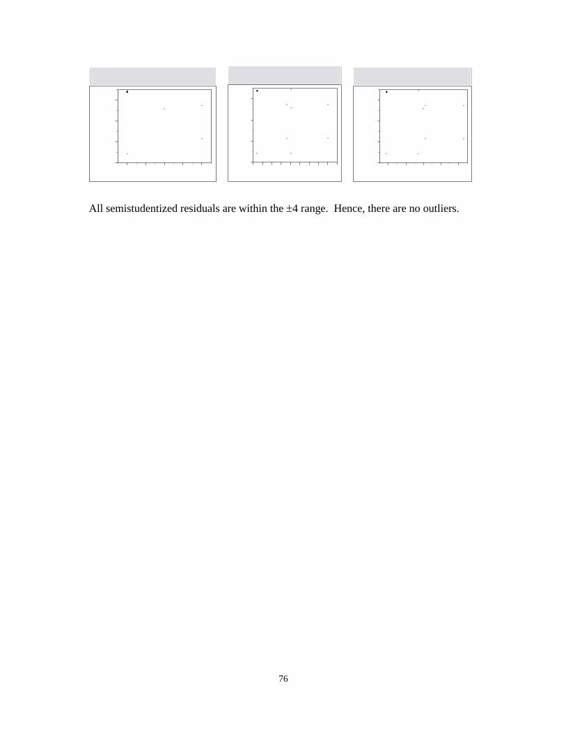
76

All semistudentized residuals are within the ±4 range. Hence, there are no outliers.

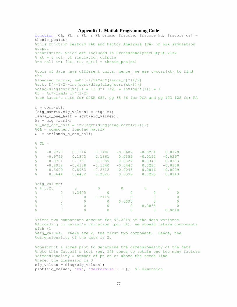
77

Appendix I. Matlab Programming Code function [CL, FL, r_FL, r_FL_prime, frscore, frscore_kd, frscore_cr] = thesis_pca(xt) %this function perform PAC and Factor Analysis (FA) on six simulation output %statistics, which are included in ProcessAnalyzerOutput.xlsx % xt = 6 col. of simulation outputs %to call it: [CL, FL, r_FL] = thesis_pca(xt) %cols of data have different units, hence, we use c=corr(xt) to find the %loading matrix, L=D^(-1/2)*Ac*(lamda_c)^(1/2) %s.t. D^(-1/2)=inv(sqrt(diag(diag(corr(xt))))) %diag(diag(corr(xt))) = I; D^(-1/2) = inv(sqrt(I)) = I %L = Ac*(lamda_c)^(1/2) %see Bauer's note for OPER 685, pg 38-56 for PCA and pg 103-122 for FA r = corr(xt); [eig_matrix,eig_values] = eigs(r); lamda_c_one_half = sqrt(eig_values); Ar = eig_matrix; %D_neg_one_half = inv(sqrt(diag(diag(corr(x))))); %CL = component loading matrix CL = Ar*lamda_c_one_half; % CL = % % -0.9778 0.1316 0.1486 -0.0602 -0.0261 0.0129 % -0.9799 0.1373 0.1361 0.0355 -0.0152 -0.0297 % -0.9701 0.1761 0.1589 0.0327 0.0348 0.0183 % -0.8932 -0.4188 -0.1540 -0.0446 0.0287 -0.0150 % -0.3609 0.8953 -0.2612 -0.0045 0.0016 -0.0009 % 0.8644 0.4432 0.2326 -0.0392 0.0225 -0.0143 %eig_values: % 4.5328 0 0 0 0 0 % 0 1.2405 0 0 0 0 % 0 0 0.2119 0 0 0 % 0 0 0 0.0095 0 0 % 0 0 0 0 0.0035 0 % 0 0 0 0 0 0.0018 %first two components account for 96.221% of the data variance %According to Kaiser's Criterion (pg. 54), we should retain components with >1 %eig_values. There are 2, the first two component. Hence, the %dimensionality of the data is 2. %construct a scree plot to determine the dimensionality of the data %note this Cattell's test (pg. 54) tends to retain one too many factors %dimensionality = number of pt on or above the scree line %here, the dimension is 3 eig_values = diag(eig_values); plot(eig_values, 'bx', 'markersize', 10); %3-dimension

78

figure; dimension = 3; index = 1; %factor loading pg. 115, using 3-dimension for index = 1:1:dimension FL(:, index) = sqrt(eig_values(index))*eig_matrix(:, index); end % FL % -0.9778 0.1316 0.1486 % -0.9799 0.1373 0.1361 % -0.9701 0.1761 0.1589 % -0.8932 -0.4188 -0.1540 % -0.3609 0.8953 -0.2612 % 0.8644 0.4432 0.2326s %but really, only need two dimension according to Kaiser's Criterion %here, we use 3-dimension since the 2-D r_FL shows no interesting pattern %find the rotated FL r_FL = rotatefactors(FL); %flipped the signs of the first col of r_FL r_FL_prime = [-1*r_FL(:, 1), r_FL(:, 2:end)]; % r_FL = % % -0.8383 0.2596 -0.4748 % -0.8327 0.2710 -0.4804 % -0.8478 0.2899 -0.4411 % -0.4740 -0.0692 -0.8761 % -0.2632 0.9613 0.0807 % 0.3970 0.0569 0.9148 % r_FL_prime = % % 0.8383 0.2596 -0.4748 % 0.8327 0.2710 -0.4804 % 0.8478 0.2899 -0.4411 % 0.4740 -0.0692 -0.8761 % 0.2632 0.9613 0.0807 % -0.3970 0.0569 0.9148 %F1 - Task Duration %F2 - No-kit Occurrences %F3 - PEs Effectivenss %find the unrotated factor scores fscore = zscore(xt)*inv(r)*FL; %find the rotated factor scores (pg. 125)

79

%note the frscore here is sorted accd. to KitAva s.t. 1-16 rows represent %KitAva = 45%; 17-32 rows represent KitAva = 60%, etc frscore = zscore(xt)*inv(r)*r_FL_prime; %sort the frscore according to KitDef. Group the frscore s.t. 1-16 rows %represent KitDef = 0.8, 17-32 rows represent KitDef = 0.9, etc count = 0; for m = 0:3 for index = 1+16*m:4:16*(m+1)-3 frscore_kd(index:index+3, :)= frscore(count*16+(1+4*m):count*16+4*(1+m), :); count = count +1; end count = 0; end %sort the frscore according to CrewRdy. Group the frscore s.t. 1-16 rows %represent CrewRdy = 5.5; 17-32 rows represent CrewRdy = 6, etc count = 0; for m = 0:3 for index = 1+16*m:16*(m+1) frscore_cr(index, :)= frscore((m+1)+count*4, :); count = count +1; end count = 0; end % plot F1 vs F2 - grouped by KitAva plot(frscore(1:16, 2), frscore(1:16,1), 'r*', frscore(17:32, 2), frscore(17:32,1), 'b+', frscore(33:48, 2), frscore(33:48,1), 'g.', frscore(49:64, 2), frscore(49:64,1), 'ko'); xlabel('F2, No-kit Occurrences'); ylabel('F1, Task Duration'); legend('KitAva=45','KitAva=60','KitAva=75', 'KitAva=90'); title('F1 vs. F2 coded by KitAva'); figure; % plot F1 vs F2 - grouped by KitDef plot(frscore_kd(1:16, 2), frscore_kd(1:16,1), 'r*', frscore_kd(17:32, 2), frscore_kd(17:32,1), 'b+', frscore_kd(33:48, 2), frscore_kd(33:48,1), 'g.', frscore_kd(49:64, 2), frscore_kd(49:64,1), 'ko'); xlabel('F2, No-kit Occurrences'); ylabel('F1, Task Duration'); legend('KitDef=0.8','KitDef=0.9','KitDef=1.0', 'KitDef=1.1'); title('F1 vs. F2 coded by KitDef'); figure; % plot F1 vs F2 - grouped by CrewRdy plot(frscore_cr(1:16, 2), frscore_cr(1:16,1), 'r*', frscore_cr(17:32, 2), frscore_cr(17:32,1), 'b+', frscore_cr(33:48, 2),

80

frscore_cr(33:48,1), 'g.', frscore_cr(49:64, 2), frscore_cr(49:64,1), 'ko'); xlabel('F2, No-kit Occurrences'); ylabel('F1, Task Duration'); legend('CrewRdy=5.5','CrewRdy=6.0','CrewRdy=6.5', 'CrewRdy=7.0'); title('F1 vs. F2 coded by CrewRdy'); figure; %________________________________________________________________________% % plot F1 vs F3 - grouped by KitAva plot(frscore(1:16, 3), frscore(1:16,1), 'r*', frscore(17:32, 3), frscore(17:32,1), 'b+', frscore(33:48, 3), frscore(33:48,1), 'g.', frscore(49:64, 3), frscore(49:64,1), 'ko'); xlabel('F3, PEs Effectiveness'); ylabel('F1, Task Duration'); legend('KitAva=45','KitAva=60','KitAva=75', 'KitAva=90'); title('F1 vs. F3 coded by KitAva'); figure; % plot F1 vs F3 - grouped by KitDef plot(frscore_kd(1:16, 3), frscore_kd(1:16,1), 'r*', frscore_kd(17:32, 3), frscore_kd(17:32,1), 'b+', frscore_kd(33:48, 3), frscore_kd(33:48,1), 'g.', frscore_kd(49:64, 3), frscore_kd(49:64,1), 'ko'); xlabel('F3, PEs Effectiveness'); ylabel('F1, Task Duration'); legend('KitDef=0.8','KitDef=0.9','KitDef=1.0', 'KitDef=1.1'); title('F1 vs. F3 coded by KitDef'); figure; % plot F1 vs F3 - grouped by CrewRdy plot(frscore_cr(1:16, 3), frscore_cr(1:16,1), 'r*', frscore_cr(17:32, 3), frscore_cr(17:32,1), 'b+', frscore_cr(33:48, 3), frscore_cr(33:48,1), 'g.', frscore_cr(49:64, 3), frscore_cr(49:64,1), 'ko'); xlabel('F3, PEs Effectiveness'); ylabel('F1, Task Duration'); legend('CrewRdy=5.5','CrewRdy=6.0','CrewRdy=6.5', 'CrewRdy=7.0'); title('F1 vs. F3 coded by CrewRdy'); figure; %_________________________________________________________________________% % plot F2 vs F3 - grouped by KitAva plot(frscore(1:16, 3), frscore(1:16,2), 'r*', frscore(17:32, 3), frscore(17:32,2), 'b+', frscore(33:48, 3), frscore(33:48,2), 'g.', frscore(49:64, 3), frscore(49:64,2), 'ko'); xlabel('F3, PEs Effectiveness'); ylabel('F2, No-kit Occurrences'); legend('KitAva=45','KitAva=60','KitAva=75', 'KitAva=90'); title('F2 vs. F3 coded by KitAva'); figure;

81

% plot F2 vs F3 - grouped by KitDef plot(frscore_kd(1:16, 3), frscore_kd(1:16,2), 'r*', frscore_kd(17:32, 3), frscore_kd(17:32,2), 'b+', frscore_kd(33:48, 3), frscore_kd(33:48,2), 'g.', frscore_kd(49:64, 3), frscore_kd(49:64,2), 'ko'); xlabel('F3, PEs Effectiveness'); ylabel('F2, No-kit Occurrences'); legend('KitDef=0.8','KitDef=0.9','KitDef=1.0', 'KitDef=1.1'); title('F2 vs. F3 coded by KitDef'); figure; % plot F2 vs F3 - grouped by CrewRdy plot(frscore_cr(1:16, 3), frscore_cr(1:16,2), 'r*', frscore_cr(17:32, 3), frscore_cr(17:32,2), 'b+', frscore_cr(33:48, 3), frscore_cr(33:48,2), 'g.', frscore_cr(49:64, 3), frscore_cr(49:64,2), 'ko'); xlabel('F3, PEs Effectiveness'); ylabel('F2, No-kit Occurrences'); legend('CrewRdy=5.5','CrewRdy=6.0','CrewRdy=6.5', 'CrewRdy=7.0'); title('F2 vs. F3 coded by CrewRdy'); figure; %_________________________________________________________________________% %plot F1 vs F2 using unrotated factor scores % plot(fscore(1:16, 2), fscore(1:16,1), 'r.', fscore(17:32, 2), fscore(17:32,1), 'b.', fscore(33:48, 2), fscore(33:48,1), 'g.', fscore(49:64, 2), fscore(49:64,1), 'c.'); % xlabel('F2, No-kit Occurrences'); % ylabel('F1, Task Duration'); % legend('KitAva45','KitAva60','KitAva75', 'KitAva90'); % title('unrotated factor scores grouped by KitAva'); % figure; %3-D factor plot plot3(frscore(1:16, 2), frscore(1:16,1), frscore(1:16,3), 'r*', frscore(17:32, 2), frscore(17:32,1), frscore(17:32,3),'b+',frscore(33:48, 2), frscore(33:48,1), frscore(33:48,3),'g.', frscore(49:64, 2), frscore(49:64,1), frscore(49:64,3),'ko'); xlabel('F2, No-kit Occurrences'); ylabel('F1, Task Duration'); zlabel('F3, PEs Effectiveness'); grid on axis square legend('KitAva=45','KitAva=60','KitAva=75', 'KitAva=90'); title('Three-dimensional Factor Plot, coded by KitAva'); figure; %3-D factor plot plot3(frscore_kd(1:16, 2), frscore_kd(1:16,1), frscore_kd(1:16,3), 'r*', frscore_kd(17:32, 2), frscore_kd(17:32,1), frscore_kd(17:32,3),'b+',frscore_kd(33:48, 2), frscore_kd(33:48,1),

82

frscore_kd(33:48,3),'g.', frscore_kd(49:64, 2), frscore_kd(49:64,1), frscore_kd(49:64,3),'ko'); xlabel('F2, No-kit Occurrences'); ylabel('F1, Task Duration'); zlabel('F3, PEs Effectiveness'); grid on axis square legend('KitDef=0.8','KitDef=0.9','KitDef=1.0', 'KitDef=1.1'); title('Three-dimensional Factor Plot, coded by KitDef'); figure; %3-D factor plot plot3(frscore_cr(1:16, 2), frscore_cr(1:16,1), frscore_cr(1:16,3), 'r*', frscore_cr(17:32, 2), frscore_cr(17:32,1), frscore_cr(17:32,3),'b+',frscore_cr(33:48, 2), frscore_cr(33:48,1), frscore_cr(33:48,3),'g.', frscore_cr(49:64, 2), frscore_cr(49:64,1), frscore_cr(49:64,3),'ko'); xlabel('F2, No-kit Occurrences'); ylabel('F1, Task Duration'); zlabel('F3, PEs Effectiveness'); grid on axis square legend('CrewRdy=5.5','CrewRdy=6.0','CrewRdy=6.5', 'CrewRdy=7.0'); title('Three-dimensional Factor Plot, coded by CrewRdy'); figure; % % plot F1 vs F3 % plot(frscore(:, 3), frscore(:,1), 'b.'); % xlabel('F3, PEs Effectiveness'); % ylabel('F1, Task Duration'); % %legend('male','female','best'); % figure; % % plot F2 vs F3 % plot(frscore(:, 3), frscore(:,2), 'b.'); % xlabel('F3, PEs Effectiveness'); % ylabel('F2, No-kit Occurrences'); % %legend('male','female','best'); % figure; mean_xt = mean(xt); %col mean %centering x for col = 1:1:size(xt, 2) %vary col from 1 to 6, num col for row = 1:1:size(xt, 1) %vary col from 1 to 64, num row xt_mean_std (row, col)= xt(row, col) - mean_xt(col); end end D_neg_one_half = inv(sqrt(diag(diag(cov(xt))))); %D_one_half = diagonal matrix of variances (ref. pg. 47) %Y = "standardized" component scores Y = xt_mean_std*D_neg_one_half*Ar; %xt_mean_std*D_neg_one_half = xt_mean_std/D_one_half = standardizing xt

83

%principal component score for each class KitAva45 = Y(1:16, 1:6); KitAva60 = Y(17:32, 1:6); KitAva75 = Y(33:48, 1:6); KitAva90 = Y(49:64, 1:6); %component score for the first two principal components Y_first_2_comp = Y(:, 1:2); % scatter(KitAva45(:,1),KitAva45(:,2),3,'r'); % hold on; % scatter(KitAva60(:,1),KitAva60(:,2),3,'b'); % scatter(KitAva75(:,1),KitAva60(:,2),3,'g'); % scatter(KitAva90(:,1),KitAva60(:,2),3,'c'); % xlabel('CP1'); % ylabel('CP2'); % title('PCA - Plot of CP2 vs CP1'); % legend('KitAva45','KitAva60','KitAva75', 'KitAva90'); % hold off; % figure; end

84

Appendix J. Blue Dart How does High Velocity Maintenance Support the USAF Mission to Fly, Fight, and Win?

In Operation Allied Force, the B-1 Lancers secured over 20 percent bombs

dropped on targets throughout the entire campaign (Park, 2010). Less than a decade

later, by 2008, more than half the B-1 fleet were grounded due to maintenance at any

given time (Scully, 2009). Such decay drives mission capability rate down and

ultimately alarms the USAF leadership that the B-1 maintenance paradigm needs changes

gearing towards being lean and agile. In the beginning of fiscal year 2011, the USAF has

initiated a revolutionized maintenance concept called High Velocity Maintenance (HVM)

on the B-1 Bomber to boost aircraft availability.

Under HVM, aircraft pay frequent but brief maintenance visits to the depot.

HVM minimizes repair duplication by synchronizing field and depot maintenance.

Instead of overhauling the entire airframe, HVM uses kitting, pre-assembly of parts and

tools, to service only need-to-fix maintenance issues (Sully, 2009). Burn rate or direct

touch labor working hours per day for the B-1 fleet is expected to ramp up to 400 hours

per day versus the current Programmed Depot Maintenance (PDM) level of 145 to 150

direct hours per day (Canaday, 2010). Intuitively, the higher the burn rate, the higher the

aircraft availability and the more mission capable the USAF is.

The objective of this research was to examine the impact of HVM on B-1 depot

maintenance operations and gain insights on B-1 availability rates under some USAF

supply chain influences. A high-level simulation was developed to model some HVM

processes for the B-1 Bomber at its depot located in Oklahoma City Air Logistics Center,

Tinker Air Force Base. Among other measure of effectiveness, our model tracked the

85

completion times of various HVM tasks and used those collectively as a surrogate

measure for depot burn rate. With this framework, an increased burn rate would result in

lower completion times. Analysis performed on model outputs revealed that HVM task

completion times decrease (i.e. burn rate increases) noticeably when the depot operates at

the optimal HVM levels – high task kit availability, low kit deficiency, and high crew

participation in maintenance. Additional analysis confirmed that task completion times

were driven significantly by the quality (or deficiency) of the task kits. In other words,

when mechanics are given the right parts and tools ahead of time, burn rate and

inherently, the Lancer’s availability have the potential to increase significantly.

Strange as it might sound, HVM is not just about maintenance. It affects the entire

acquisition life cycle of a weapon system. If HVM can effectively reduce maintenance

downtime and improve aircraft availability, the USAF can potentially save millions of

dollars simply by purchasing fewer aircraft. HVM goes beyond just the B-1 fleet. The

impact of HVM can be potentially unlimited for it is designed to be scalable, repeatable,

and deployable on all weapon systems in the USAF inventory (Adams, 2008). Studies on

maintenance practices such as HVM can subsequently lead us to find better ways to

support our aging fleet and continue to fly, fight, and win in the foreseeable future.

86

Appendix K. ENS Quad Chart

87

Bibliography

1. Adams, Charlotte. “Reinventing USAF Depot Maintenance.” Aviation Today. 1 Dec 2008. Last retrieved 13 Oct 2010 from http://www.aviationtoday.com/am/categories/military/Reinventing-USAF-Depot-Maintenance_27947.html

2. Armstrong, Brandice J. “B-1 HVM prototype phase next step in program.” Air Force Print News Today. 24 Sep 2010. Last retrieve 13 Oct 2010 from http://www.tinker.af.mil/news/story_print.asp?id=123223693

3. Bauer, Kenneth.W. OPER 685 class notes from Spring 2010. Department of

Operational Sciences, Air Force Institute of Technology (AU), Wright-Patterson AFB, OH. March 2010.

4. Canaday, Henry. “Trading Downtime For Burn Rate.” Military Logistics Forum

2010, Volume 4, Issue 1. February 2010. Last retrieved 12 Oct 2010 from http://geospatial-intelligence-forum.com/military-logistics-forum/226-mlf-2010-volume-4-issue-1-february/2525-trading-downtime-for-burn-rate.html

5. Ceyler, Angie. B1 AFGLSC HVM Materiel Team Lead. Personal Correspondence. Nov 2010 – Mar2011.

6. Crenshaw, Wayne. “HVM journey continues with help from lessons learned.” Air Force Print News Today. 8 Jan 2010. Last retrieved 13 Oct 2010 from http://www.robins.af.mil/news/story_print.asp?id=123184666

7. Dement, Frank, Doug Keene, and Gary O’Neill. “Handbook of Military Industrial Engineering.” CRC Press, 2009.

8. Department of the Air Force. “High Velocity Maintenance.” Robin AFB Fact Sheet, 24 Feb 2010. Last retrieved 12 Oct 2010 from http://www.robins.af.mil/library/factsheets/factsheet.asp?id=10795

9. Heiman, Theodore K. Simulation Modeling of the C-5 Galaxy High Velocity Regionalized Isochronal (HVRISO) Inspection Concept. MS thesis, AFIT/GLM/ENS/09-6. Graduate School of Engineering and Management, Air Force Institute of Technology (AU), Wright-Patterson AFB OH, March 2009 (ADA500454).

10. Khan, Azfar A. “High-Velocity Air Force Maintenance.” Air Force Technology. 06 May 2010. Last retrieved 11 Oct 2010 from http://www.airforce-technology.com/features/feature84237/

88

11. Law, Averill M. Simulation Modeling and Analysis (4th Edition). New York: The McGraw-Hill Companies, Inc., 2007.

12. Martin, Patricia R. 638 SCMG/CL. “AF Global Logistics Support Center Update.” 19 Nov 2008. Last retrieve 8 Dec 2010 from http://www.wrcoc-aic.org/Archive/RS/RS08/RS08-martin.pdf

13. Michaliszyn, Frank L. USAF ACC 28MXG/MXEM1. Personal Correspondence. Nov 2010 – Mar2011.

14. Miller, J.O., K.W. Bauer, Jr, P. Faas, C.R. Pawling, and S.E. Sterling. "Multivariate Analysis of a Simulation Prognostics and Health Management System for Military Aircraft Maintenance," International Journal of Logistics: Research and Applications, Vol. 10, No. 1, March 2007, 1-10.

15. Park, Anson R. Simulation Analysis of High Velocity Maintenance for the B-1B. MS Thesis, AFIT-OR-MS-ENS-10-09. Department of Operational Sciences, Air Force Institute of Technology (AU), Wright-Patterson AFB, OH. March 2010.

16. Parson, Carl R. Simulation Modeling and Analysis of TNMCS for the B-1 Strategic Bomber. MS Thesis, AFIT-OR-MS-ENS-10-09. Department of Operational Sciences, Air Force Institute of Technology (AU), Wright-Patterson AFB, OH. June 2010.

17. Ramey, Timothy L. Lean Logistics. RAND, 1999.

18. Scharven, Ron. “Global support center officially stands up March 28.” Air Force Print News Today. 14 Mar 2008. Last retrieve 3 Jan 2011 from http://www.af.mil/news/story.asp?id=123090324

19. Scully, Megan. “High Velocity Maintenance.” Air Force Magazine, Vol. 92, No.

8. Aug 2009. Last retrieved 13 Oct 2010 from http://www.airforce-magazine.com/MagazineArchive/Pages/2009/August%202009/0809maintenance.aspx

20. Stout, Howdy. “Proposed B-1 program aims to speed maintenance.” Air Force Print News Today. 17 Apr 2009. Last retrieve 11 Oct 2010 from http://www.af.mil/news/story_print.asp?id=123144906

21. Tripp, Robert S, Ronald G. McGarvey, Ben D. Van Roo, James M. Masters, and Jerry M. Sollinger. “A Repair Network Concept for Air Force Maintenance.” RAND, 2010.

89

REPORT DOCUMENTATION PAGE Form Approved OMB No. 074-0188

The public reporting burden for this collection of information is estimated to average 1 hour per response, including the time for reviewing instructions, searching existing data sources, gathering and maintaining the data needed, and completing and reviewing the collection of information. Send comments regarding this burden estimate or any other aspect of the collection of information, including suggestions for reducing this burden to Department of Defense, Washington Headquarters Services, Directorate for Information Operations and Reports (0704-0188), 1215 Jefferson Davis Highway, Suite 1204, Arlington, VA 22202-4302. Respondents should be aware that notwithstanding any other provision of law, no person shall be subject to an penalty for failing to comply with a collection of information if it does not display a currently valid OMB control number. PLEASE DO NOT RETURN YOUR FORM TO THE ABOVE ADDRESS. 1. REPORT DATE (DD-MM-YYYY)

24-03-2011 2. REPORT TYPE

Master’s Thesis 3. DATES COVERED (From – To)

Sep 2010 – Mar 2011 4. TITLE AND SUBTITLE DEPOT-LEVEL SIMULATION AND MULTIVARIATE ANALYSIS ON B-1 HIGH VELOCITY MAINTENANCE

5a. CONTRACT NUMBER

5b. GRANT NUMBER

5c. PROGRAM ELEMENT NUMBER

6. AUTHOR(S) Yee, Florence, K, First Lieutenant, USAF

5d. PROJECT NUMBER 5e. TASK NUMBER

5f. WORK UNIT NUMBER

7. PERFORMING ORGANIZATION NAMES(S) AND ADDRESS(S) Air Force Institute of Technology Graduate School of Engineering and Management (AFIT/EN) 2950 Hobson Street, Building 642 WPAFB OH 45433-7765

8. PERFORMING ORGANIZATION REPORT NUMBER AFIT-OR-MS-ENS-11-26

9. SPONSORING/MONITORING AGENCY NAME(S) AND ADDRESS(ES) AFMC 591st SCMG/CL Attn: Col. Ray Lindsay 2515 Thurlow Dr. DSN: 787-2069 Bldg 70 Suite 5 e-mail: Ray.Lindsay@wpafb.af.mil WPAFB OH 45433

10. SPONSOR/MONITOR’S ACRONYM(S) 11. SPONSOR/MONITOR’S REPORT NUMBER(S)

12. DISTRIBUTION/AVAILABILITY STATEMENT APPROVED FOR PUBLIC RELEASE; DISTRIBUTION UNLIMITED.

13. SUPPLEMENTARY NOTES

14. ABSTRACT The objective of this thesis is to gain insights on the B-1B depot maintenance operations, with a focus on direct maintenance hours or burn rate, under the implementation of High Velocity Maintenance (HVM). Based on historical depot maintenance data and the current B-1 depot HVM prototype data, a discrete-event simulation model is developed using Arena 12.0. Some United States Air Force supply chain influences, such as manning levels and kitting characteristics of the B-1 depot operations, are incorporated in our models as design factors. The model captures the stochastic nature of 30 HVM tasks performed on one B-1 aircraft in a representative HVM cycle at the B-1 depot located in Oklahoma City Air Logistics Center, Tinker Air Force Base. To examine the impact of HVM, we vary the levels of the design factors and conduct a design of experiment (DOE). The DOE analysis reveals that manning levels and kitting characteristics have statistically significant impact on some HVM task completion times, which are used collectively as a surrogate measure for burn rate. In particular, manning schedule with a centric focus on direct maintenance, high task kit availability, and small kit deficiency produce the highest burn rate. Additionally, by performing multivariate analysis, we are able to reduce the dimensionality of the output statistics and conclude that kit deficiency is the main driver for HVM task duration with our simulation. 15. SUBJECT TERMS Modeling and Simulation, Discrete-Event Simulation, ARENA, B-1B Lancer, High Velocity Maintenance, Oklahoma City Air Logistics Center, supply chain, kitting 16. SECURITY CLASSIFICATION OF: 17. LIMITATION OF

ABSTRACT

UU

18. NUMBER OF PAGES

101

19a. NAME OF RESPONSIBLE PERSON Dr. John O. Miller (ENS)

a. REPORT

U

b. ABSTRACT

U

c. THIS PAGE

U

19b. TELEPHONE NUMBER (Include area code) (937) 255-6565, ext 4326; e-mail: John.Miller@afit.edu

Standard Form 298 (Rev. 8-98) Prescribed by ANSI Std. Z39-18