and

A SECURE AND EFFICIENT COMMUNICATIONS ARCHITECTURE FOR GLOBAL INFORMATION GRID USERS VIA COOPERATING SPACE ASSETS

DISSERTATION

Victor P. Hubenko, Jr., Major, USAF

AFIT/DCE/ENG/08-02

DEPARTMENT OF THE AIR FORCE AIR UNIVERSITY

AIR FORCE INSTITUTE OF TECHNOLOGY

Wright-Patterson Air Force Base, Ohio

APPROVED FOR PUBLIC RELEASE; DISTRIBUTION UNLIMITED

The views expressed in this dissertation are those of the author and do not reflect the

official policy or position of the United States Air Force, Department of Defense, or the

U.S. Government.

AFIT/DCE/ENG/08-02

A SECURE AND EFFICIENT COMMUNICATIONS ARCHITECTURE FOR GLOBAL INFORMATION GRID USERS VIA COOPERATING SPACE ASSETS

DISSERTATION

Presented to the Faculty

Graduate School of Engineering and Management

Air Force Institute of Technology

Air University

Air Education and Training Command

In Partial Fulfillment of the Requirements for the

Degree of Doctor of Philosophy

Victor P. Hubenko, Jr., BS EE, MS EE

Major, USAF

June 2008

APPROVED FOR PUBLIC RELEASE; DISTRIBUTION UNLIMITED

AFIT/DCE/ENG/08-02

A SECURE AND EFFICIENT COMMUNICATIONS ARCHITECTURE FORGLOBAL INFORMATION GRID USERS VIA COOPERATING SPACE ASSETS

Victor P. Hubenko, Jr., BS EE, MS EE

Major, USAF

Approved:

~a-t.~Richard A. Raines, PhDCommittee Chairman

~Date

~~06~

Rusty . Baldwin, PhDCommittee Member

~611f1A

~~\&Q~Barry E. M l' s, PhD 'Co ittee ember../J

. oJ. I~

Committee Member

~Av(R/~gMichael A. Grimaila, PhDCommittee Member

-0. C4-7Robert A. Canfield, PDean's Representative

c)''! :rv f'J 08Date

J!faU7t 8ate

Accepted:

Marlin U. Thomas, PhDDean

/0 .r~05

Date

iv

AFIT/DCE/ENG/08-02

A SECURE AND EFFICIENT COMMUNICATIONS ARCHITECTURE FOR GLOBAL INFORMATION GRID USERS VIA COOPERATING SPACE ASSETS

by

Victor P. Hubenko, Jr., BS EE, MS EE

Major, USAF

Dr. Richard A. Raines, Advisor

Abstract

With the Information Age fully in place and still experiencing rapid development,

users expect to have global, seamless, ubiquitous, secure, and efficient communications

that provide access to real-time applications and collaboration. The United States

Department of Defense’s (DoD) Network-Centric Enterprise Services initiative, along

with the notion of pushing the “power to the edge,” will provide end-users with

maximum situational awareness, a comprehensive view of the battlespace, all within a

secure networking environment.

This research develops a novel security framework architecture to provide

efficient and scalable secure multicasting in the low earth orbit satellite network

environment. This security framework architecture combines several key aspects of other

secure group communications architectures in a way that increases efficiency and

scalability, while maintaining the overall system security level. This security architecture

in a deployed environment with heterogeneous communications users will reduce re-

keying. Less frequent re-keying means more resources are available for user data rather

v

than security overhead. This translates to greater performance for the end user; it will

seem as if they have a “larger pipe” for their network links.

This research develops and analyzes multiple mobile communication environment

scenarios to demonstrate the superior re-keying offered by the novel “Hubenko Security

Framework Architecture” compared to traditional and clustered multicast security

architectures. For example, in the scenario containing a heterogeneous mix of user types

(Stationary, Ground, Sea, and Air), the Hubenko Architecture achieves a minimum ten-

fold reduction in total keys distributed compared to other known architectures. For

another scenario, the Hubenko Architecture operates at 6% capacity while other

architectures consumed 98% of capacity. With 80% user mobility for 40% Air users, re-

keying in other architectures increased 900%, whereas the Hubenko Architecture only

increased 65%. By reducing overall system re-keying, the Hubenko Architecture

increases system efficiency and scalability.

This new architecture is extensible to numerous secure group communications

environments beyond the low earth orbit satellite network environment, including

unmanned aerial vehicle swarms, wireless sensor networks, and mobile ad hoc networks.

At the time of publication, the Hubenko Architecture was the basis for several current

Master’s level research efforts in the aforementioned areas.

vi

Acknowledgments

Just as they are first in my life, my wife and children are first to be thanked.

Thank you for enduring the many nights and weekends that we shared together, yet apart,

as I worked towards graduation. I can never express enough how much gratitude I have

for my wife continually resetting and putting her career on hold so I could advance in

mine. She is the reason I was able to focus on this degree, and is the pillar of my success.

I also thank my parents for giving me the best opportunities for success as they could.

I thank Dr. Richard Raines, my advisor, for allowing me to spread my wings, yet

keeping me on the path to graduation. I also thank my committee (Drs. Raines, Mullins,

Baldwin, Mills, and Grimaila) for the numerous document reviews, feedback, and

support of my research, publications, and dissertation.

Academics aside, I thank Ms. Stacey Johnston, the unsung hero of the Center for

Cyber Research for always selflessly taking care of the CCR students (and staff!), making

our lives at AFIT that much less stressful.

Thanks to my AFIT Dining Out 2006 Committee for helping reestablish the

grandeur of AFIT spirit and camaraderie as we “Experienced the Excellence,” achieving

miracles and a sold-out event in seven weeks time. Also, my fellow staff of the 2005-

2006 AFIT Student Association are owed many thanks for the long hours put in to make

the lives of our fellow AFIT students more enjoyable, from Doolittle’s and beyond!

Speaking of camaraderie and friends, thanks to Major Chris Augeri for teaching

me that MatLab can run inside of Word inside of Excel and for all that help with getting

my MatLab code (and any software app) to work properly. Thanks to Major Kevin

vii

Cousin and family for always volunteering to help us out. Thanks to Major Ken Edge

and Captain Mark Kleeman for keeping things interesting in the PhD Penthouse. A

special thanks to Major George Dalton for always looking out for me, for being a great

friend, and sharing his 24 years of leadership experience with me so I can grow into a

better leader.

My journey down the road to AFIT started with Mr. John Cunningham, who

personally nominated me for an Advanced Academic Degree slot and then made sure I

had the best shot possible for being selected. Finally, I owe a debt of gratitude to the “C-

Cubed Aerospace Mafia” (John Overton, Chris Pate, Mike Wenkel) for making me look

good while I reigned as Mayor of C-Cubeville at NPOESS. They shared three lifetimes

of experiences, wisdom, and lessons that I carry with me today. They gave me the

opportunity and support to stand out as a shining star and get noticed.

It takes the support of many people to achieve success. I thank all those people,

named and unnamed, now and in the past, for their help in getting me this far in life. I

am fortunate to have such a caring assemblage of people touch my life.

viii

Table of Contents

Page

Abstract .............................................................................................................................. iv

Acknowledgments.............................................................................................................. vi

Table of Contents............................................................................................................. viii

List of Figures ................................................................................................................... xii

List of Tables .....................................................................................................................xv

List of Acronyms ............................................................................................................ xvii

I. Introduction ......................................................................................................................1

1.1 Background .........................................................................................................1

1.2 Problem Statement ..............................................................................................3

1.3 Research Goal .....................................................................................................3

1.4 Research Contributions .......................................................................................4

1.4.1 Coherent, Secure, and Efficient Architecture for LEOSat Environment ..4

1.4.2 Extension of Hubenko Architecture to Other Highly Mobile Environments.............................................................................................6

1.5 Assumptions/Limitations ....................................................................................6

1.6 Dissertation Organization....................................................................................7

II. Literature Review............................................................................................................8

2.1 Chapter Overview ...............................................................................................8

2.2 Communication Satellite Systems ......................................................................8

2.2.1 Global Information Grid..........................................................................11

2.2.2 Highlights of the IRIDIUM® LEO Satellite System ...............................20

2.2.3 Other Satellite Communications Systems ...............................................22

2.2.4 Inter-Satellite Links and On-orbit Routing..............................................23

2.3 Multicasting Technologies ................................................................................25

ix

2.3.1 Multicast Overview .................................................................................25

2.3.2 Link State and Distance Vector Routing Algorithms Overview .............26

2.3.3 Dense and Sparse Types of Multicast .....................................................30

2.3.4 Some Options for Multicast Networks ....................................................31

2.3.5 Group Management Protocols .................................................................33

2.3.6 Multicast Satellite Networks: Architectures and Multicast Protocols.....34

2.3.7 Issues Surrounding Multicast Communications......................................36

2.4 Multicasting Security ........................................................................................38

2.4.1 General Security Services........................................................................39

2.4.2 Issues Surrounding Multicast Security ....................................................41

2.4.3 Scalable, Secure Multicast Systems and Architectures ...........................46

2.4.4 Deficiencies of Known Scalable, Secure Multicast Systems and Architectures............................................................................................53

2.5 Summary ...........................................................................................................54

III. Methodology ................................................................................................................55

3.1 Chapter Overview .............................................................................................55

3.2 Hubenko LEOSat Security Framework Architecture Motivation.....................55

3.3 LEOSat Network Environment Validation .......................................................57

3.4 Continued Viability of PIM-DM.......................................................................62

3.5 Hubenko Security Framework Architecture Development...............................64

3.5.1 Baseline Security Architecture for the LEO Satellite Environment........65

3.5.2 Clusterized Security Architecture............................................................68

3.5.3 Hubenko Security Framework Architecture............................................73

3.5.4 Demonstrate Improved System Security Performance............................79

3.6 Simulation Environment and Architecture Models...........................................80

x

3.6.1 Simulation Environment..........................................................................80

3.6.2 Architecture Models ................................................................................87

3.6.3 Confidence Interval .................................................................................95

3.7 Simulation Equipment.......................................................................................96

3.8 Metrics for Security Performance Evaluation and Analysis .............................97

3.9 Time Scaling for Modeling Expediency ...........................................................98

3.10 Model Verification ............................................................................................98

3.11 Model Validation ............................................................................................105

3.12 Summary .........................................................................................................111

IV. Performance Results and Analysis ............................................................................112

4.1 Chapter Overview ...........................................................................................112

4.2 Model Scenarios..............................................................................................112

4.2.1 Highly Mobile User Environment (Four Different RoM).....................112

4.2.2 Short versus Long Duration...................................................................120

4.2.3 Increasing Aircraft over Stationary Users .............................................130

4.2.4 Varied Air Content Rate of Mobility.....................................................137

4.3 Performance Conclusions ...............................................................................141

4.3.1 Re-Keying Performance Results ...........................................................141

4.3.2 Hubenko Saturation ...............................................................................146

4.3.3 RoM Sensitivity.....................................................................................146

4.4 Analysis of Variance.......................................................................................150

4.5 Summary .........................................................................................................154

V. Conclusion ..................................................................................................................156

5.1 Summary of Research .....................................................................................156

xi

5.2 Research Contributions ...................................................................................157

5.3 Publications .....................................................................................................158

5.4 Recommendations for Future Research ..........................................................158

5.4.1 Adapt Hubenko Security Framework Architecture to Other Environments.........................................................................................158

5.4.2 Incorporate Features from the Integrated Architecture Concept ...........158

5.4.3 Re-establish Original LEOSat Baseline with Hubenko Architecture....160

VI. Appendix....................................................................................................................162

6.1 Short versus Long Duration Scenario 1 (Section 4.2.2).................................163

6.2 Short versus Long Duration Scenario 2 (Section 4.2.2).................................167

6.3 Increasing Aircraft Over Stationary Users Scenario 2 (Section 4.2.3) ..........171

6.4 Analysis of Variance Data ..............................................................................175

6.5 MatLab Code from Increasing Aircraft Over Stationary Users Scenario 2 (Section 4.2.3).................................................................................................175

VII. Bibliography.............................................................................................................196

VIII. Vita..........................................................................................................................206

xii

List of Figures

Page

Figure 1 - Relative Re-keying Performance ....................................................................... 5

Figure 2 - Global Information Grid Layers [SMC06a]..................................................... 12

Figure 3 - The Gothic Architecture [JuA02]..................................................................... 47

Figure 4 - Example of a Secure Distribution Tree [Mit97] .............................................. 50

Figure 5 - GSA Multicast Forwarding Performance [Mit97] ........................................... 51

Figure 6 - Baseline LEOsat Security Architecture ........................................................... 66

Figure 7 - Initialize Baseline Architecture Example......................................................... 67

Figure 8 - Baseline Example - Two .................................................................................. 67

Figure 9 - Baseline Example - Three ................................................................................ 67

Figure 10 - Baseline Example - Four................................................................................ 67

Figure 11 - Baseline Example - Finish ............................................................................. 68

Figure 12 - Clusterized Security Architecture .................................................................. 70

Figure 13 - Initialize Cluster Example.............................................................................. 71

Figure 14 - Cluster Example - Two .................................................................................. 71

Figure 15 - Cluster Example - Three ................................................................................ 72

Figure 16 - Cluster Example - Four .................................................................................. 72

Figure 17 - Cluster Example - Finish................................................................................ 72

Figure 18 - Hubenko Architecture Flow Chart ................................................................. 75

Figure 19 - Hubenko Security Framework Architecture .................................................. 76

Figure 20 - Initialize Hubenko Architecture..................................................................... 78

Figure 21 - Hubenko Example - Two ............................................................................... 78

Figure 22 - Hubenko Example - Three ............................................................................. 78

xiii

Figure 23 - Hubenko Example - Four ............................................................................... 78

Figure 24 - Flow Diagram for MatLab Simulation Code ................................................. 91

Figure 25 - User Satellite Assignments .......................................................................... 100

Figure 26 - User Cluster Assignments ............................................................................ 100

Figure 27 - User Mobility Assignments.......................................................................... 100

Figure 28 - User Mobility Verification........................................................................... 100

Figure 29 - User Join Time Assignments ....................................................................... 100

Figure 30 - User Duration Assignments ......................................................................... 100

Figure 31 - User Activity Verification............................................................................ 101

Figure 32 - Cluster Trigger Verification......................................................................... 102

Figure 33 - Average Per-User Re-keying ....................................................................... 103

Figure 34 - Total System Keys ....................................................................................... 103

Figure 35 - Group Key Management Overhead - Actual Trace [JuA02] ....................... 106

Figure 36 - Group Key Management Overhead - Simulated Trace [JuA02].................. 106

Figure 37 - Average Keys Distributed in a Highly Mobile Environment....................... 108

Figure 38 - Spatial Clustering- Varying the Number of Hosts Leaving [BaB02] .......... 109

Figure 39 - Hubenko Model - Varying the Number of Hosts Leaving........................... 109

Figure 40 - Rates of Mobility for Highly Mobile Scenario ............................................ 113

Figure 41 - Average Times Each User is Re-Keyed (from 10 to 2000 Users, 2000 Time Steps, Highly Mobile User Environment Scenario)....................................... 116

Figure 42 - Total Keys Distributed in Each Architecture (from 10 to 2000 Users, 2000 Time Steps, Highly Mobile User Environment Scenario) ............................. 119

Figure 43 - Total Keys Distributed - 1% Mobility (from 10 to 1000 Users, 1000 Time Steps, Short versus Long Duration Scenario 1) ............................................. 123

Figure 44 - Average Per-User Re-Key - 50% Mobility (from 10 to 1000 Users, 1000 Time Steps, Short versus Long Duration Scenario 1).................................... 125

xiv

Figure 45 - Average Per-User Re-Key - 50% Mobility (from 10 to 10,000 Users, 10,000 Time Steps, Short versus Long Duration Scenario 2).................................... 127

Figure 46 - Total Keys Distributed - All Users (from 10 to 10,000 Users, 10,000 Time Steps, Short versus Long Duration Scenario 2) ............................................. 128

Figure 47 - Total Keys Distributed - Control Group (from 10 to 10,000 Users, 10,000 Time Steps, Short versus Long Duration Scenario 2).................................... 129

Figure 48 - Average Per-User Re-Key - All Users (from 10 to 1000 Users, 1000 Time Steps, Increasing Aircraft Scenario 1) ........................................................... 132

Figure 49 - Average Per-User Re-Key - Control Group (from 10 to 1000 Users, 1000 Time Steps, Increasing Aircraft Scenario 1) .................................................. 132

Figure 50 - Total Keys Distributed - All Users (from 10 to 1000 Users, 1000 Time Steps, Increasing Aircraft Scenario 1) ...................................................................... 133

Figure 51 - Total Keys Distributed - Control Group (from 10 to 1000 Users, 1000 Time Steps, Increasing Aircraft Scenario 1) ........................................................... 134

Figure 52 - Total Keys Distributed - All Users (from 10 to 10,000 Users, 10,000 Time Steps, Increasing Aircraft Scenario 2) ........................................................... 136

Figure 53 - Average Per-User Re-Key - All Users (from 10 to 10,000 Users, 10,000 Time Steps, Increasing Aircraft Scenario 2) ........................................................... 137

Figure 54 - Per-User Average Re-Key Results - All Users (from 10 to 2000 Users, 2000 Time Steps, Varied Air Content Scenario) .................................................... 139

Figure 55 - Varied Air Content RoM Scenario Revisited (from 10 to 2000 Users, 2000 Time Steps) .................................................................................................... 149

Figure 56 - Integrated Architecture Services Added ...................................................... 160

xv

List of Tables

Page

Table 1 - Data-to-Overhead Comparison.......................................................................... 58

Table 2 - Received-to-Sent Comparison........................................................................... 59

Table 3 - End-to-End Delay Comparison ......................................................................... 60

Table 4 - System, Scenario, and Iteration Level Parameters and Factors......................... 83

Table 5 - Highly Mobile User Environment Parameters ................................................ 114

Table 6 - First Short vs. Long Duration Scenario Parameters ........................................ 122

Table 7 - Second Short vs. Long Duration Scenario Parameters.................................... 124

Table 8 - Increasing Aircraft Parameters - Scenario 1.................................................... 131

Table 9 - Increasing Aircraft Parameters - Scenario 2.................................................... 135

Table 10 - Rates of Mobility (Varied Air Content) ........................................................ 138

Table 11 - Varied Air Content RoM Parameters ............................................................ 138

Table 12 - Per-User Average Re-Keying Summary ....................................................... 141

Table 13 - Total Keys Distributed Summary.................................................................. 144

Table 14 - Mobility Content for Varied Air Content Scenario....................................... 148

Table 15 - ANOVA with Duration = 0.2 ........................................................................ 152

Table 16 - ANOVA with Duration = 0.5 ........................................................................ 153

Table 17 - ANOVA with Duration = 0.8 ........................................................................ 154

Table 18 - Total Keys Distributed (All Users, Short vs. Long Duration Scenario 1)..... 163

Table 19 - Total Keys Distributed (Control Group Users, Short vs. Long Duration Scenario 1) ..................................................................................................... 164

Table 20 - Average Per-User Re-Key (All Users, Short vs. Long Duration Scenario 1)165

Table 21 - Average Per-User Re-Key (Control Group Users, Short vs. Long Duration Scenario 1) ..................................................................................................... 166

xvi

Table 22 - Total Keys Distributed (All Users, Short vs. Long Duration Scenario 2)..... 167

Table 23 - Total Keys Distributed (Control Group Users, Short vs. Long Duration Scenario 2) ..................................................................................................... 168

Table 24 - Average Per-User Re-Key (All Users, Short vs. Long Duration Scenario 2)169

Table 25 - Average Per-User Re-Key (Control Group Users, Short vs. Long Duration Scenario 2) ..................................................................................................... 170

Table 26 - Total Keys Distributed (All Users, Increasing Aircraft Over Stationary Users Scenario 2) ..................................................................................................... 171

Table 27 - Total Keys Distributed (Control Group Users, Increasing Aircraft Over Stationary Users Scenario 2).......................................................................... 172

Table 28 - Average Per-User Re-Key (All Users, Increasing Aircraft Over Stationary Users Scenario 2) ........................................................................................... 173

Table 29 - Average Per-User Re-Key (Control Group Users, Increasing Aircraft Over Stationary Users Scenario 2).......................................................................... 174

Table 30 - Data in Raw Format for use in ANOVA....................................................... 175

xvii

List of Acronyms

ACS Access Control Server

AEHF Advanced Extremely High Frequency

AFIT Air Force Institute of Technology

AJ Anti-Jam

ANOVA Analysis of Variance

AOR Area of Responsibility

AS Anti-Scintillation

AWACS Airborne Warning and Control System

BACN Battlefield Airborne Communications Node

BGMP Border Gateway Multicast Protocol

BGP Border Gateway Protocol

CBT Core Based Trees

CIO Chief Information Officer

COV Coefficient of Variance

CRT Chinese Remainder Theorem

CWDM Coarse Wave Division Multiplexing

DBST Delay-Bounded Steiner Tree

DES Discrete Event Simulation

DiRK Distributed Registration and Key Distribution

DISN Defense Information Systems Network

DoD Department of Defense

DoS Denial of Service

DSCS Defense Satellite Communications Systems

DtO Data-to-Overhead ratio

DV Distance Vector

DVBMT Delay-Variation-Bounded Multicast Tree

DVB-S Digital Video Broadcast – Satellite

DVMRP Distance Vector Multicast Routing Protocol

DWDM Dense Wave Division Multiplexing

EHF Extremely High Frequency

EIGRP Enhanced IGRP

EPS Enhanced Polar System

EtE End to End

FAB-T Family of Advanced Beyond Line-of-sight Terminals

FAI International Aeronautical Federation

GAC Group Access Control

GACA Group Access Control Awareness

GACA-GKM Group Access Control Aware-Group Key Management

GBS Global Broadcast Service Satellite System

GEO Geostationary earth orbit

GEO Geosynchronous earth orbit

GIG Global Information Grid

GIG-BE Global Information Grid – Bandwidth Expansion

GKM Group Key Management

xviii

GMAS Group Member Authorization System

GMNF-DVMRP Group Membership Near First DVMRP

GPMS Group Policy Management System

GPS Navistar Global Positioning System

GSA Group Security Agents

GSC Group Security Controller

GSI Group Security Intermediaries

HEO Highly elliptical orbit

HSRP Hierarchical Satellite Routing Protocol

ICO Intermediate Circular Orbit

IEEE The Institute for Electrical and Electronics Engineers

IETF Internet Engineering Task Force

IGMP Internet Group Management Protocol

IGRP Interior Gateway Routing Protocol

IOS Cisco’s Internetwork Operating System

IP Internet Protocol

IS-IS Intermediate System to Intermediate System

ISL Inter-Satellite Links

ISP Internet Service Provider

ISR Intelligence, Surveillance, Reconnaissance

J-STARS Joint Surveillance and Target Attack Radar System

JTRS Joint Tactical Radio System

KEK Key-Encryption-Keys

LEO Low earth orbit

LEOsat LEO Satellite-based networks

LKH Logical Key Hierarchy

LPI/D Low Probability of Intercept/Detection

LS Link State

MAC Message Authentication Codes

MANET Mobile ad hoc network

MAODV Multicast extension to Ad hoc On demand Distance Vector routing protocol

MBone Multicast Backbone

MEF Marine Expeditionary Force

MEO Medium earth orbit

Milstar Military Strategic and Tactical Relay Satellite

MLD Multicast Listener discovery

MOSPF Multicast Open Shortest Path First

MUOS Mobile User Objective System

NCW Network Centric Warfare

NLSP Novell's NetWare Link State Protocol

NMT Navy Multiband Terminals

NPOESS National Polar-orbiting Operational Environmental Satellite System

ODMRP On-demand Distance Multicast Routing Protocol

OPNET OPNET, Inc.

OSPF Open Shortest Path First

xix

P2P Point-to-point

PIM-Bidir Bi-directional PIM

PIM-DM Protocol Independent Multicast – Dense Mode

PIM-SM Protocol Independent Multicast – Sparse Mode

PKI Public-Key Infrastructure

QoS Quality of Service

RF Radio Frequency

RFC Request For Comments

RIP Routing Information Protocol

RoM Rate of Mobility

RtS Received-to-Sent ratio

RTT Round Trip Time

SCAMP Single Channel Anti-Jam Man Portable

SGRP Satellite Grouping and Routing Protocol

SMART-T Secure Mobile Anti-Jam Reliable Tactical-Terminal

SOS Satellite Over Satellite Network

STK Satellite Tool Kit

S-UMTS Satellite-Universal Mobile Telecommunications System

TCA Transformational Communications Architecture

TCP Transmission Control Protocol

TSAT Transformational Satellite System

UAV Unmanned Aerial Vehicle

UFO UHF Follow-On Satellite System

UHF Ultra High Frequency

VoIP Voice over IP

VPN Virtual Private Network

WGS Wideband Gapfiller Satellite

WSN Wireless Sensor Network

1

A SECURE AND EFFICIENT COMMUNICATIONS ARCHITECTURE FOR GLOBAL INFORMATION GRID USERS VIA COOPERATING SPACE ASSETS

I. Introduction

1.1 Background

The Information Age is in a stage of rapid growth. As soon as new technologies

are introduced, users expect even more capability, more speed, and greater flexibility.

Rarely does any new technology exist as a stand-alone entity. Rather, society advances

together, through sharing of knowledge, techniques, and technology. At the heart of this

information sharing society is a communications network that always seems to be one

step behind the needs of its users. Physical communications technologies, whether in the

form of terrestrial or satellite systems, are also rapidly advancing in capacity and

capabilities to meet the needs of bandwidth-hungry users. From the users’ perspective,

however, it seems “more” is never enough.

One way of addressing the problem of insufficient communications capacity is to

focus on the actual data generation and usage of communications. At the dawn of the

Information Age, the relatively small numbers of users were able to communicate in a

point-to-point (P2P) fashion between local areas. Today, users need more capabilities

than P2P systems can provide. Users expect to communicate in a one-to-many and even

many-to-many fashion.

The United States Department of Defense (DoD) recognizes the need to change

the data-sharing paradigm from a “stove-piped” point-to-point fashion to more of a group

data sharing environment:

2

“Across the DoD, broad leadership goals are transforming the way information is managed to accelerate decision-making, improve joint warfighting, and create intelligence advantages…

Net-centricity compels a shift to a “many-to-many” exchange of data, enabling many users and applications to leverage the same data—extending beyond the previous focus on standardized, predefined, point-to-point interfaces.” [Ste03] -John P. Stenbit, Former DoD Chief Information Officer

The enabling infrastructure that will deliver this “network-centric” environment

for the DoD is the Global Information Grid (GIG). The GIG is “The globally

interconnected, end-to-end set of information capabilities, associated processes, and

personnel for collecting, processing, storing, disseminating, and managing information on

demand to war-fighters, policy makers, and support personnel. The GIG includes all

owned and leased communications and computing systems and services, software

(including applications), data, security services and other associated services necessary to

achieve Information Superiority.” [DoD02]. As noted in [AlH03], the GIG enables the

aforementioned change in mindset, termed “power to the edge,” that delivers vast

computing power to all DoD entities, regardless of their physical location, so long as they

are “net-ready, meaning connected to the GIG.”

Satellites are an indispensable component of the GIG’s approach to connecting

every warfighter with the information they need to make rapid, well-informed decisions.

As is the case in all communications systems, secure, efficient, and effective methods for

transferring information are essential. Multicasting in a satellite environment can provide

the necessary performance and security while improving the efficient use of critical

bandwidth.

3

1.2 Problem Statement

Throughout the GIG, as well as the Internet in general, communications

predominantly flow in a point-to-point fashion, which is inefficient when large groups of

users are accessing or sharing the same information. Additionally, secure group

communications architectures face several issues, including limited scalability for very

large groups of users, and excessive time and processing overhead to achieve a secure

system. A secure group communications environment that must accommodate highly

mobile users exacerbates these issues. Finally, users in the field, whether they are

terrestrial or airborne, typically need bulky equipment to access limited, low-rate

connectivity. Those users should not have to worry about excessive security overhead

further hindering their communications as well. Proposals in the research literature

address some of the issues. However, a solution that meets both the security and

scalability needs of highly mobile users has yet to be proposed.

1.3 Research Goal

This research develops a novel security architecture, dubbed the “Hubenko

Security Framework Architecture,” (Hubenko Architecture for short) to secure group

communications (namely, multicast) in the low earth orbit satellite network environment

more efficiently than currently proposed architectures. To achieve this goal, the Hubenko

Architecture combines key aspects of different secure group communications

architectures in a way that increases efficiency and scalability.

Implementing the Hubenko Architecture in a deployed environment with

heterogeneous communications users will reduce the frequency of re-keying. Less

4

frequent re-keying equates to more resources available for data throughput versus

security overhead. This translates to performance to the end user; it will seem as if they

have a “larger pipe” for their network links.

1.4 Research Contributions

1.4.1 Coherent, Secure, and Efficient Architecture for LEOSat Environment

The primary objective of this research is to develop a coherent security

framework architecture that improves the scalability of secure group communications for

highly mobile users. This framework architecture is then applied to the LEO satellite

network environment.

This research results in a scalable system security architecture capable of handling

large groups of users (e.g., ten thousand or more) without loss of efficiency or

significantly affecting data throughput. The architecture allows the system to handle at

least an order of magnitude more highly mobile users while providing superior re-keying

performance over the traditional and clustered architectures.

Multiple mobile communication environment scenarios are developed and

analyzed to demonstrate the superior re-keying advantage offered by the Hubenko

Architecture over traditional and clustered multicast security architectures. The first

scenario compares the performance for different levels of user mobility. The second

scenario compares the performance for different levels of user persistence in a multicast

group. The third scenario compares the performance for increasing the number of aircraft

flying over stationary users. The final scenario compares the performance of varied

numbers of aircraft in a heterogeneous user environment. A sampling of the results

5

includes the following. In the scenario containing a heterogeneous mix of user types

(Stationary, Ground, Sea, and Air), the Hubenko Architecture achieved a minimum ten-

fold reduction in total keys distributed compared to the Cluster and Baseline

architectures. In the “Increasing Aircraft over Stationary Users” scenario, the Hubenko

Architecture operated at 6% capacity while the Cluster and Baseline architectures

operated at 98% capacity. In the 80% overall mobility experiment with 40% Air users,

the Cluster and Baseline architecture re-keying increased 900% over the Stationary case,

whereas the Hubenko Architecture only increased 65%. A relative performance example

for each of the scenarios is plotted in Figure 1 for illustrative purposes. The amount of

re-keying was independently normalized for each scenario (i.e., the amount of re-keying

in scenario one does not directly correlate to the amount of re-keying in scenario two). In

each scenario, the Hubenko Architecture required less re-keying than the Cluster

Architecture, as illustrated in the figure by the lower amount of relative re-keying.

0

2

4

6

8

10

12

14

16

18

20

Re-k

eyin

g Am

ount

Scenario One Scenario Two Scenario Three Scenario Four

HubenkoCluster

Figure 1 - Relative Re-keying Performance

6

1.4.2 Extension of Hubenko Architecture to Other Highly Mobile Environments

The unique topological and environmental challenges of the LEO satellite

network originally motivated the development of the Hubenko Architecture. Once the

benefits of the research materialized, it became obvious that the topology could be

collapsed to a single terrestrial plane (versus a hybrid satellite-terrestrial topology), and

the architecture could be extended to accommodate a variety of environments.

The Hubenko Architecture can easily adapt to multicast protocols and security

architectures in numerous operational and deployed environments. Other research in the

design stages is adapting the Hubenko Architecture for use in secure multicast

communications of unmanned aerial vehicle (UAV) swarms. Additionally, the

architecture could be used in mobile ad hoc networks (MANET), wireless sensor

networks (WSN), and other heterogeneous mobile communications environments.

1.5 Assumptions/Limitations

The Hubenko Architecture’s advantage is limited in environments where the

communicating users are predominantly stationary, or where the users’ movements are

localized within a single area (i.e., a single cluster). In these environments, the Hubenko

Architecture has the same performance as the clustered environment, but has extra

overhead from an access control awareness feature implementation. Therefore, in a

homogenous wireless sensor network where the sensors are immobile and extremely

limited in battery and processing power, an implementation of the Hubenko Architecture

for this environment would be detrimental. The overhead would unnecessarily decrease

battery life through increased computational and communications cycles required to

7

support the access control awareness functions, which provide no benefit in this case.

However, in a heterogeneous environment where the wireless sensor network is part of a

larger network with mobile communications units passing through, and communicating

with, the wireless sensor network, the reduced re-keying will greatly improve scalability

and efficiency, and therefore battery life.

1.6 Dissertation Organization

This document is divided into five chapters. Chapter II reviews relevant literature

for satellite systems, multicasting technologies, and multicasting security. Chapter III

discusses the development and the details of the Hubenko Security Framework

Architecture, along with the motivation for pursuing this architecture. This chapter also

discusses the simulations and models that support the performance claims. Chapter IV

presents the results and analysis of the numerous simulations performed during the course

of this research. Chapter V concludes the document with a brief summary of the

research, highlights of the contributions this research provides to the network

communications community, and recommendations for future research.

8

II. Literature Review

2.1 Chapter Overview

This chapter presents a literature review covering three broad areas related to: 1)

communication satellite systems, 2) multicasting technologies, and 3) multicasting

security. The first area of research includes: low earth orbit, medium earth orbit, and

geosynchronous earth orbit (and hybrids thereof) communication satellite systems and

architectures; and the modeling, simulation, and analysis of such systems. The second

area covers multicasting protocols and algorithms suitable for adaptation to satellite

network environments, along with relevant modeling, simulation, and analysis of the

protocols and algorithms. Finally, the third area of review pertains to multicasting

security.

2.2 Communication Satellite Systems

Before discussing communication satellite systems, a brief overview of the four

main satellite orbits is presented including: the low earth orbit (LEO), the medium earth

orbit (MEO), the highly elliptical orbit (HEO), and the geosynchronous earth orbit

(GEO).

The first orbit, the low earth orbit, places the satellite at an altitude between 200

to about 2,000 kilometers above the surface of the earth. Depending on the angle of the

orbit with respect to the equator, the orbit can be classified as either prograde (0 to 90

degrees, “with” the rotation of the earth) or retrograde (90 to 180 degrees, “against” the

rotation of the earth). LEO satellites that pass over the polar regions of earth are often

referred to as “polar-orbiting.” Since LEO satellites orbit relatively closely to the earth,

9

radio frequency propagation round trip times (one link up, and one link down) are about

1.33 to 13.33 milliseconds, depending on the orbit altitude.

The medium earth orbit is also known as the intermediate circular orbit (ICO).

MEOs are typically circular at an altitude of around 10,000 kilometers. This orbital

height places the satellites between the two Van Allen radiation belts and therefore leads

to longer satellite life as compared to an elliptical orbit where satellites pass through the

radiation belts. Due to their altitude, MEOs provide coverage to the same ground

location for several hours, and have a radio frequency propagation round trip time of

about 67 milliseconds. One of the best-known examples of a MEO satellite system is the

United States Navistar Global Positioning System (GPS).

A highly elliptical orbit’s altitude varies, bringing a satellite relatively close to the

earth at its perigee, and relatively far from the earth at its apogee. The HEO typically

serves a very specialized purpose, as with the Molnya satellite system (which gave the

name to its specific orbit). The Molnya system has an orbit that varies from an altitude of

about 1,000 kilometers to about 40,000 kilometers, and is highly inclined, thus providing

long periods of coverage to the northern latitudes of Russia.

Finally, the geosynchronous earth orbit places a satellite in a near-stationary

position above the earth’s surface. However, this is a common point of confusion, since a

geosynchronous satellite technically only requires a rotation in the direction of the earth,

and need not appear stationary from the ground. The Geostationary orbit, at an altitude

of approximately 35,768 kilometers above the surface of the earth, is a subcategory of

geosynchronous orbits, and is generally used when GEO satellites are referenced. Based

10

on this altitude, the radio frequency propagation round trip time for a GEO satellite is

approximately 238.45 milliseconds. A comprehensive discussion of these orbits can be

found in [Rod01, Sae03].

Existing long haul satellite communications systems primarily use geostationary

earth orbit (GEO) satellites. GEO satellite systems allow full earth coverage below ~78

degrees latitude with as few as three satellites. Drawbacks to using these systems include

the long propagation delay and the large propagation loss. The transmission power

required to overcome the propagation loss of a 35,768 kilometers path makes GEO user

handheld terminals impractical compared to LEO user handheld terminals. Therefore,

the primary advantages associated with LEO satellites are a lower transmission power, a

lower propagation delay, and polar coverage.

One aspect of defining a communications satellite system is its orbit. From a data

handling perspective, communications satellite systems typically process data in two

ways: “bent-pipe” or “store-and-forward.” When communication satellites operate in a

bent-pipe fashion, they receive a signal from a terrestrial user and then echo the same

signal back to the earth for further processing by some other entity. A store-and-forward

satellite makes processing decisions on where to send a received signal, either back to the

same geographical location, or to some other location on another transmitter [BeF99].

This includes being able to route signals to other satellites in a crosslink manner, where

supported.

In addition to categorizing satellite systems based on their orbits and data

handling characteristics, communication satellite systems can be divided according to the

11

different types of communications services they provide: narrowband, wideband, and

protected communications services. To illustrate this, consider the Global Information

Grid (GIG) and its subsystems as an example of a communications architecture that

incorporates each of these services in its “layers.”

2.2.1 Global Information Grid

The DoD defines the GIG as a “globally interconnected, end-to-end set of

information capabilities, associated processes, and personnel for collecting, processing,

storing, disseminating, and managing information” [GAO04]. Furthermore, the GIG

incorporates almost all of DoD’s information systems, services, applications, and data

into a single seamless, reliable, and secure Internet-like network. The GIG promotes

interoperability by using standards-based technologies across all platforms. The GIG will

integrate most, if not all, of DoD’s weapon systems, command, control, and

communications systems, as well as business systems. When complete, the GIG will

have a new core network consisting of both a Satellite Layer and a Surface Layer. There

is also an Aerospace Layer populated with mobile users and weapons systems. Finally,

there is a “Near-Space Layer” between the altitudes of air flight and space, which may

eventually make its way into the final architecture.

2.2.1.1 The GIG Satellite Layer

As depicted in Figure 2, the majority of the GIG’s communication assets in the

Satellite Layer, either operational or in development, are geosynchronous earth orbit

(GEO) satellites. The different systems provide the military with narrowband, wideband,

and protected communications capabilities. In general, the narrowband capabilities

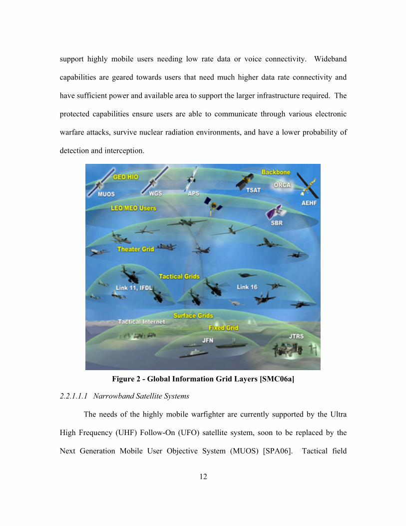
12

support highly mobile users needing low rate data or voice connectivity. Wideband

capabilities are geared towards users that need much higher data rate connectivity and

have sufficient power and available area to support the larger infrastructure required. The

protected capabilities ensure users are able to communicate through various electronic

warfare attacks, survive nuclear radiation environments, and have a lower probability of

detection and interception.

Figure 2 - Global Information Grid Layers [SMC06a]

2.2.1.1.1 Narrowband Satellite Systems

The needs of the highly mobile warfighter are currently supported by the Ultra

High Frequency (UHF) Follow-On (UFO) satellite system, soon to be replaced by the

Next Generation Mobile User Objective System (MUOS) [SPA06]. Tactical field

13

equipment has to be small, light, and rugged to survive the harsh environments faced by

the typical warfighter. To support increased mobility, tactical terminals typically have

much smaller antennas and less processing power than users that are stationary. Because

of these constraints, low rate voice or data communications are the usual services

provided to the warfighter on the move. Utilizing the UHF spectrum allows signals to

penetrate buildings, harsh weather, and thick vegetation. In addition, UHF frequencies

are well-suited for use in low-power, inexpensive, lightweight, rugged communication

systems [SMC06b].

2.2.1.1.2 Wideband Satellite Systems

Tactical forces in the field rely upon wideband satellite systems to reach back to

the surface portions of the GIG. The Defense Satellite Communications Systems Phase

III (DSCS III) wideband satellites use a portion of the X-band frequency to provide

secure voice and high data rate communications for the military’s typical long-haul, high-

capacity communications needs when a high speed, high capacity terrestrial network is

not available [SMC06b].

In the near future, the Wideband Gapfiller Satellite (WGS) system will replace

DSCS as the next generation of high capacity communications connectivity. Notionally,

there will be three to five WGS’s on orbit, depending on the development pace of the

Transformational Satellite System (TSAT). WGS will augment and then replace the

DSCS support in X-band, as well as augment and replace the one-way Ka-band broadcast

of the Global Broadcast Service Satellite System (GBS). WGS will also provide a new

two-way Ka-band communication capability for the warfighter.

14

As the name implies, the Global Broadcast Service provides a high speed, high

volume “broadcast-from-the-sky” service for the military. The GBS will augment, as

well as interface with, other communication services to provide a medium for continuous

information flow to users. The GBS platforms are hosted on three of the UFO satellites,

and will fly on three WGS’s. Additionally, future requirements for the broadcast service

will be met by hosting GBS packages on TSAT platforms [SMC06b].

TSAT rounds out the capabilities of all the previous DoD wideband

communication satellite systems and is the ultimate enabler of the Transformational

Communications Architecture (TCA). TSAT will provide another source of high data

rate satellite communications along with services modeled after the Internet. Notionally,

five operational satellites will be connected in a ring through laser crosslinks, and will

provide laser and radio frequency (RF) connections to the Surface layer. TSAT will

extend routing capabilities of the previous wideband satellite systems and be able to route

packets in space rather than provide bent-pipe, point-to-point connections between

ground users. The satellite crosslinking reduces the need for packets to make multiple

ground/satellite hops to reach distant users. This reduces end-to-end latency, and allows

for near-real time communications speeds [DTI05].

2.2.1.1.3 Protected Satellite Systems

Protected communications are serviced by a global extremely high frequency

(EHF) system, composed of the Military Strategic and Tactical Relay Satellite (Milstar)

system, the Advanced Extremely High Frequency System and Enhanced Polar System.

Protected communications offer Low Probability of Intercept/Detection (LPI/D), Anti-

15

Jam (AJ), and Anti-Scintillation (AS) protection, as well as being encrypted. The main

methods of protecting the communication links originate from operating in the Ka-band

as well as using advanced communications techniques, such as frequency hopping and

active phased array antennas. This combination offers resilience against electronic

warfare and reduces the probability of physical attacks.

The first in the series of satellite systems to provide protected communications for

the DoD is the Military Strategic and Tactical Relay Satellite (Milstar). Launched in

1994, Milstar provides connectivity to ships, submarines, aircraft, and other terrestrial

users through five geosynchronous satellites. Since the satellites are crosslinked and can

process traffic rather than simply transpond signals between two ground users, Milstar

satellites establish circuits between themselves and the ground, based on dynamic user

needs [SMC06b].

In the next few years, the Advanced Extremely High Frequency (AEHF) System

will launch three geosynchronous satellites, continuing and enhancing the protected

services offered by Milstar. The AEHF enhancements over Milstar include a 100-times

capacity increase, as well as enhanced anti-jam and LPI/D capabilities, and advanced

encryption systems. Once a single TSAT is operational, DoD will have achieved

continuous 24-hour communications coverage between the latitudes of +/- 65 degrees

with the three AEHF satellites and one TSAT.

To augment the current northern polar coverage gap in Milstar services, the

Interim Polar EHF system places protected communications packages on three classified

spacecraft that occupy highly elliptical orbits. This system provides protected

16

communications services similar to Milstar, but in the northern polar region. When

AEHF comes online, the Enhanced Polar System (EPS) will provide protected

communications that are comparable to AEHF, but will be on a classified spacecraft, just

like the Interim Polar EHF system. However, unlike Interim Polar, EPS will have

crosslink capabilities, enabling cross connections to not only other EPS packages, but to

AEHF and TSAT as well [SMC06b].

There has been a steady progression of capabilities in each of the different types

of satellite communications systems, as well as a move towards a highly cooperative

Satellite layer to maximize communications support to the warfighter. Each piece of the

Satellite layer contributes directly to achieving the concept of Network Centric

communications for the DoD user.

Operating in the realm of the Satellite layer is well understood by the DoD, with

mature technologies deployed and well-developed operational concepts in place. To

follow the intent of the Transformational mantra means taking a fresh look at how best to

utilize available resources for providing information to the warfighter. Using lessons

learned in the Satellite layer and applying them to the Near-Space layer may greatly

enhance the DoD’s capabilities for a fraction of the cost.

2.2.1.2 The GIG Near-Space Layer

Near space begins at an altitude of 22.86 kilometers and ends at the beginning of

space or at 100.58 kilometers according to the International Aeronautical Federation

(FAI) [Tom05]. Near-Space is the region between the traditional realms of satellites and

air-breathing assets such as unmanned aerial vehicles (UAVs) and typical airplanes.

17

Though not formally incorporated as a layer in the GIG, research into exploiting the

Near-Space layer is gaining support within the DoD. When the Near-Space technologies

mature, this layer will most likely find a home in the GIG. Examples of “nearcraft”

platforms for carrying sensors or communications packages include balloons, gliders,

special motorized nearcraft, all of which are currently under development.

There are several key advantages to operating in the Near-Space layer over the

Satellite layer [Tom05]. The first advantage is significantly reduced developmental and

operational cost, since the assets do not have to be space hardened and space qualified.

Another advantage is the reduced component sizes of sensors and communications

equipment needed to achieve performance levels similar to like systems in the Satellite

layer since sensors are significantly closer than those placed on satellites. On the other

hand, if the same satellite sensors or communications packages are used on platforms in

the Near-Space layer, large increases (10-20 fold) in image resolution, sensitivity, and

accuracy can be achieved. In addition to the cost and component advantages, Near-Space

atmospheric conditions allow sensors and communications equipment to operate with less

interference and/or distortion. For example, “nearcraft” operate at altitudes low enough

to avoid most space weather effects. In addition, they are below the wave-refracting or

blocking ionosphere, which allows better sensor performance, and yet are high enough to

avoid most atmospheric weather effects, like high winds or rain. With the development

of Near-Space vehicles comes the potential to achieve true continuous, persistent

Intelligence, Surveillance, and Reconnaissance (ISR) or communications coverage of

18

specific tactical areas. While Near-Space offers unique opportunities, the Aerospace

layer contains many of the contemporary platforms needed for military operations.

2.2.1.3 The GIG Aerospace Layer

The conventional Aerospace layer is by far the most familiar layer above the

Surface layer. New technologies and applications are continuously developed to enhance

and improve capabilities. This layer is dominated by aircraft such as helicopters, fighters,

tankers, and cargo jets. However, the impact of the unmanned aerial vehicles is being felt

due to increased operational capabilities.

Familiar equipment using the Aerospace layer includes the Airborne Warning and

Control System (AWACS) and the Joint Surveillance and Target Attack Radar System (J-

STARS). These assets are used for long-range surveillance and target acquisition, as well

as command and control functions for both ground and aerospace assets. The

employment of the Aerospace layer goes beyond conventional ISR collection and

delivery of munitions and supplies. This layer is emerging to take on new roles in the

communications arena with the development of the Battlefield Airborne Communications

Node (BACN). The BACN will provide communications connections to both legacy

radio systems as well as advanced Internet Protocol (IP) communications (data as well as

voice).

2.2.1.4 The GIG Surface Layer

Bridging the Aerospace layer and the Surface layer is a new communication

system called Joint Tactical Radio System (JTRS) [GAO04]. This software radio system

will bridge interoperability gaps between current user terminals and new IP terminals for

19

mobile users on the ground, at sea, or in the air, as well as connect those same users to the

permanent terrestrial network. In instances when a JTRS is not available, users can

directly access the Satellite layer systems for their communications needs. Examples of

user terminals supported by AEHF include Secure Mobile Anti-Jam Reliable Tactical-

Terminal (SMART-T), Single Channel Anti-Jam Man Portable (SCAMP), Family of

Advanced Beyond Line-of-sight Terminals (FAB-T), and Navy Multiband Terminals

(NMT).

As part of the core backbone, the terrestrial networks of the GIG are also being

enhanced to provide maximum information sharing between entities. The Defense

Information Systems Network (DISN) was recently upgraded through an effort known as

“Global Information Grid-Bandwidth Expansion,” or GIG-BE [GAO04]. GIG-BE

provides fiber optic connectivity to several key military installations, as well as upgraded

the network capacity to about 90 DoD installations.

2.2.1.5 The GIG’s “Missing” Layer

The Satellite layer is typically associated with GEO satellites. Because of the

steadily increasing usage of the GEO belt (to near saturation), new approaches for using

orbital assets are needed. Non-GEO orbits were proposed in the early 1990s and fielded

in the late 1990s. Particular emphasis was placed on fielding low earth orbit (LEO)

systems of cooperating assets. The LEO belt can be considered the GIG’s “Missing”

layer.

LEOs typically reside 200 to 2,000 kilometers above the earth’s surface. Because

of this orbit, communications between a terrestrial observer and a LEO satellite may last

20

for only 8 to 20 minutes, but with up to 45 times less latency compared to a GEO

satellite. Because of the short viewing time, multiple satellites must be placed into

multiple orbital planes to provide extended viewing coverage. Perhaps two of the best-

known LEO satellite systems are IRIDIUM® and GlobalStar®. IRIDIUM® uses 66

satellites and has store-and-forward capabilities, while GlobalStar® uses 40 satellites and

operates as a bent-pipe.

2.2.2 Highlights of the IRIDIUM® LEO Satellite System

The Air Force Institute of Technology’s (AFIT) initial venture into the realm of

low earth orbit (LEO) satellite network architectures began with an investigation on the

packet delays, convergence speeds, and protocol overhead of the Extended Bellman-Ford

and Darting unicast routing protocols adapted to a satellite network and modeled and

simulated on the IRIDIUM® and GlobalStar® satellite systems [RaJ97]. Following this

effort, a higher fidelity model of the IRIDIUM® LEO satellite network was developed

[FoR98, PrR99].

The information in this section was derived from [FoR98, Hub97, PrR99, RaJ97,

Sae03]. The IRIDIUM® system is a worldwide LEO satellite communications system

designed to support voice, data, facsimile, and paging. The IRIDIUM® satellite

constellation has six orbital planes with eleven satellites in each plane. The satellites are

in a circular orbit at an altitude of approximately 780 kilometers and an inclination of

86.4 degrees. Orbital planes one and six are counter-rotating and separated by

approximately 22 degrees. The remaining orbital planes are co-rotating and are separated

by approximately 31.6 degrees.

21

The velocity of a LEO satellite relative to earth is 26,804-kilometers/hour and

results in an orbital period of 100.13 minutes. The minimum inclination angle for a user

to see a given satellite is 8.2 degrees. At a fixed location on earth, the average in-view

time for a satellite is approximately nine minutes and either one or two satellites are

visible at a time.

A link is established from an earth station to the satellite with the strongest signal.

There are 48 spot beams per satellite, with 80 circuits per spot beam. Each spot beam is

approximately 30 miles in diameter, depending on the satellite’s current position. Since

the satellites are moving much faster than the mobile users, the mobile users are

considered stationary with respect to the velocity of the satellites, as even a mobile user

in an airplane is traveling much slower than a satellite. As the satellites pass overhead,

the link from user to satellite is handed off from a satellite leaving the users area to one

entering the user’s area, much like a cellular phone user hands off between cellular phone

towers when passing from one cell to the next.

Each IRIDIUM® satellite maintains up to four inter-satellite links (ISL). Intra-

plane links (crosslinks to satellites in the same orbital plane) are maintained permanently,

while inter-plane links (crosslinks to satellites in different orbital planes) are dynamically

established and terminated to avoid excessive overlap near the polar regions. Satellites

along the counter-rotating seams do not establish ISLs between each other due to the

rapid angular change.

22

2.2.3 Other Satellite Communications Systems

The GIG is an excellent example of multiple systems cooperating to deliver

services to customers. The satellite systems within the GIG, however, are but a small

subset of the total number of worldwide communications satellite systems planned, in the

development stages, or are currently in operation. The late 1990s saw a flurry of activity

from numerous entities to meet the needs projected for satellite users. As a result, much

research and development money went into the area of satellite communications. For

example, 17 companies filed for EHF spectrum to operate their proposed satellite systems

[FrH99]. Still others proposed and investigated systems ranging from LEO systems to

MEO to GEO, and even hybrid systems [BhH02, CaL99, GhS99, JaK99, Yam97]. This

created extensive development of non-geostationary orbital analysis as well as much-

needed research in intra- and inter-satellite routing techniques, satellite network

architectures, business models, and user terminal technologies [AkE02, Bar04, WuS05].

The first known research efforts regarding LEO constellations date back to the early

1970s [RaD99, Wal70, Wal71].

Despite the extensive research and investment, the majority of the 1990s-

proposed satellite systems never launched, while a few systems, like ICO®, were

successfully placed into orbit, yet did not succeed commercially. Fortunately, most of the

research efforts were not in vain. One technology that is still being developed, and

fielded is the Digital Video Broadcast – Satellite (DVB-S) [BeH05, BeQ05, CaD04,

ChK04, ChT03, CoB05, CoM00, CrH05, MoR04, Rei06, RiV04, SkL04, SkV05, SuJ04].

23

However, this technology is not applicable to the focus of this research due to its one-

way, broadcast-type technology.

Another technology that is gaining interest (at least from a research perspective) is

the Universal Mobile Telecommunications System (UMTS) [BaL03, KaH04, LoL04,

NaK04, SuE02]. The main focus of this effort is the deployment of an extensive

downlink capability from the LEO and GEO satellites (Satellite-Universal Mobile

Telecommunications System, or S-UMTS), with relatively little satellite uplink capability

except for remote users. The UMTS uplink will most often be handled by the Terrestrial-

Universal Mobile Telecommunications System (T-UMTS) portion of the network. As

such, the UMTS system does not fall within the scope and intent of this research.

2.2.4 Inter-Satellite Links and On-orbit Routing

From a communications network standpoint, the most critical research areas

derived from the systems developed in the 1990’s is that of the inter-satellite links (ISLs)

which enable on-orbit routing capabilities. Numerous constellations and architectures

have been analyzed, validating the proposed use of LEO satellite constellations instead of

GEO satellites in communications networks [FoR98, MoS02, PrR99, RaD99], as well as

comparing different constellations to minimize the impacts of the non-communicating

counter-rotating seams of the near-polar star pattern constellations [WeF01]. Other

issues related to satellite networking are caused by the high mobility of the satellites, and

their constant, rapidly changing topology. Fortunately, satellites maintain regular, highly

predictable, periodic orbits which allow convenient adaptations of terrestrial routing

algorithms and protocols to a satellite network [HuR06a, RaD99, RaJ97, ThR02,

24

WoC01]. In addition to adapting the routing protocol, there are other methods of using a

terrestrial protocol in a satellite environment. For example, dividing the network between

terrestrial and orbit assets using tunneling, network address translation, or an exterior

gateway protocol prevents the propagation of too many IP routing table updates from the

satellite portion of the network from entering the terrestrial network [WoC01].

Extensive research has investigated the effects of transmission control protocol

(TCP) and routing strategies in satellite constellations. Some focus on improving the

GEO communications systems with their long latencies rather than improvements for

LEO systems, but benefits derived for GEO systems can be adapted to make

improvements in LEO systems [AkJ04, AkM01a, AkM01b, AkX02, BhB01, GoJ01,

JiA02, KaT04, Kot05, MaP03, Mar01, MiS01, TsO05, WoP01, ZhB02].

Since existing long-haul satellite communications systems primarily use GEO

satellites at altitudes of approximately 35,768 kilometers, GEO satellite systems provide

full earth coverage below ~78 degrees latitude with as few as three satellites. However,

the one-way (ground to satellite or satellite to ground) signal propagation delay is

approximately 119.23 milliseconds as compared to approximately 0.67 to 6.67

milliseconds for a LEO. While the GEO systems in the GIG use crosslinks to route

traffic from one part of the world to another with end-to-end latencies of at least 238.45

milliseconds, LEO communications systems can achieve average end-to-end latencies of

less than 100 milliseconds for intercontinental communications using satellite crosslinks

[HuR06a]. Thus, LEO communication satellite systems with lower transmission power

25

requirements, shorter propagation delays, and global coverage are worth including in the

overall GIG architecture.

If low-latency voice and video communications are important requirements for

tactical users in the field, the LEO communications system are the better choice. If

seconds matter in Network Centric military communications, an extra 138 milliseconds

latency could mean the difference between meeting or missing an objective. However,

realizing these communication capabilities will require efficient transmission strategies.

2.3 Multicasting Technologies

Most Internet communication uses a one-to-one (unicast) approach for source-

destination communications. Unicast requires a node to send an individual message to

every recipient. This approach works well until a single message needs to be sent to

multiple nodes. In this case, separate copies of the message must be sent. This approach

is obviously inefficient as it wastes bandwidth and resources. It would be especially

inefficient in a multi-layered, long-haul communications environment such as the GIG.

An approach that improves efficiency and alleviates possibly significant traffic on long-

haul links is multicast routing to groups of users that are receiving the same data. This

concept was first proposed by Stephen Deering [DeC90, Dee91].

2.3.1 Multicast Overview

Multicast routing fits in between unicast routing and broadcast routing. Broadcast

routing sends one message to each node in the entire broadcast domain (similar to a bent-

pipe satellite operation). While this is a very effective method of ensuring all users on

the network receive an important message, it is quite wasteful, especially if the message

26

is actually intended for a small subset of the available users. Multicast routing, as

compared to unicast routing, sends a single message per link instead of sending a copy

for each node accessing the information on the link. This single copy is reproduced

across multiple links as close to the individual receiving nodes as possible. In this way,

multicasting enables a large amount of information to be efficiently distributed between a

large group of interested users. Satellites, because of their large coverage areas, are an

ideal means of implementing multicast.

There are several dozen different multicasting protocols proposed in the literature,

some of which warrant further investigation. When selecting a multicasting protocol,

desirable properties are: low cost; low end-to-end delay; scalability; ability to support

dynamic group membership; survivable in terms of network, link, or node outages; and

some level of fairness to all members [SaM00]. In addition to these properties, it is also

important to ensure a high level of efficiency (maximum data transmitted for the least

overhead) and a high level of effectiveness (maximum received-to-sent ratio), indicating

few lost packets throughout the system [HuR06a, ThR02]. A final consideration is the

viability of the protocol either in the commercial world or as a developing or established

standard. Before exploring the various multicasting protocols, two major types of unicast

routing protocols in use today are examined.

2.3.2 Link State and Distance Vector Routing Algorithms Overview

When a host sends a packet to a user on another host, the packet is sent down the

protocol stack to the physical network, where it is carried to its intended destination.

Several key tasks must be performed to ensure this happens correctly. One such task is

27

obtaining the destination’s address. The other is to direct the packet towards that address.

Assuming the address is already known (by some unspecified means), network routers

communicate among themselves to determine the best path to the destination node. The

two most prevalent routing algorithm categories used throughout the Internet are Link

State and Distance Vector. Both algorithms provide a means to route packets towards

intended destinations using Dijkstra's algorithm [Dij59] to determine the shortest paths.

Both algorithms use routing tables stored in the routers, and they both share at least some

of their routing tables with other routers in the network. Distance Vector algorithms are

well-suited for small, simple networks, and Link State algorithms are better at handling

larger, more complex networks.

Link State-based algorithms include Open Shortest Path First (OSPF),

Intermediate System to Intermediate System (IS-IS), Border Gateway Protocol (BGP),

and Novell's NLSP (NetWare Link State Protocol). The best known Distance Vector

algorithm is the Bellman-Ford algorithm, which is used in many routing protocols such as

Routing Information Protocol (RIP v1 and v2), Interior Gateway Routing Protocol

(IGRP), Internet BGP, Novell IPX, and the original ARPAnet. Enhanced IGRP (EIGRP)

is a well-known Cisco proprietary routing protocol that integrates the capabilities of link-

state protocols into distance vector protocols.

One of the most obvious differences between the Link State (LS) and Distance

Vector (DV) routing algorithms is the way information is shared between routers in the

respective networks. Each LS router periodically floods the entire network with the state

of its own local connections. From this flooding, each LS router calculates routes for the

28

entire network because it has knowledge of all connectivity and link costs. In this

respect, LS algorithms have a “global view” of the network, i.e., the routers exchange

information to make informed decisions on the best routes for the entire network.

Ideally, all routers would have identical routing tables.

Distance Vector routing algorithms share much more information (possibly their

entire routing tables instead of only their local connections) than LS algorithms, but the

routers only share this information with their neighbors. While LS algorithms share the

information with a regular period, DV algorithms send the information only when there

are changes. Once the network reaches a steady state, the routers will no longer share

data if there are no more changes. To build a complete routing table, DV routers

iteratively build the tables as they receive information. Router tables store which router

is the next hop in the route and what the trip cost will be. Unlike the LS algorithm, the

DV routing tables do not have complete route information for every link in the route.

Assuming there are n nodes and L links in the network, the worst case

computational complexity of a LS network is O(n2), with approximately O(nL) messages

sent to achieve full network convergence. DV networks converge at varying rates,

depending on the topology of the network. When a link cost is reduced, that information

flows quickly throughout the network. On the other hand, when a cost is increased, the

information travels much slower through the network, and a phenomenon known as the

“count to infinity problem” could arise. Count to infinity occurs when two nodes

iteratively increase their cost information based on their direct neighbor, resulting in an

inaccurately increasing cost. This is similar to what occurs if a clockmaker adjusts his

29

clocks based on the town clock tower, and the keeper of the clock tower sets his time

based on the clockmaker’s clocks.

DV algorithms converge slower than LS algorithms, and are likely to have routing

loops while converging. LS algorithms, because they converge more quickly, are

somewhat less prone to routing loops than distance vector algorithms. DVs typically do

not experience route oscillation, whereas LS algorithms are likely to oscillate on occasion

because they respond so quickly to routing changes.

Link-state algorithms require more CPU power and memory than distance vector

algorithms. LS algorithms, therefore, can be more expensive to implement and support.

LS protocols are generally more scalable than distance vector protocols.

LS networks are continually refreshed with the latest information, so failure

notification spreads quickly throughout a large network, whereas a failure in a large DV

network may take a relatively long time to propagate to all routers. Again, this comes at

the cost of more message traffic overhead from the frequent flooding of connectivity

data. Since LS algorithms only flood their own connection information, this reduces the

effect of errors propagating throughout the network. Should a link state router fail, or

have its routing table corrupted and send out incorrect link information, only the local

area and traffic destined for that specific location is jeopardized. In the case of DV

algorithms, a corrupted link status would propagate throughout the whole network since

routers depend on data from each other to gather the network connectivity beyond their

neighborhood. Incorrect information passed from one router to the next will eventually

make its way throughout the network.

30

The Link State and Distance Vector routing algorithms are not only used in

unicast routing; the design concepts are used in multicasting protocols as well. For

example, Multicast Open Shortest Path First (MOSPF) [Moy94] is a link-state algorithm,

while Distance Vector Multicast Routing Protocol (DVMRP) [FiD01, Pus04, ThR02],

On-demand Distance Multicast Routing Protocol (ODMRP) [YiS03], and Multicast

extension to Ad hoc On demand Distance Vector routing protocol (MAODV) [RoP00]

are distance vector algorithms. Since Protocol Independent Multicast – Dense Mode

(PIM-DM) [AdN05, DeE96, HuR06a, Sae03] and Protocol Independent Multicast –

Sparse Mode (PIM-SM) [FeH06] are “protocol independent” as their names indicate,

they inherit the underlying routing tables and are neither link-state nor distance vector

algorithms. Aside from the LS or DV categorization, multicasting protocols can be

classified as Dense or Sparse.

2.3.3 Dense and Sparse Types of Multicast

Multicast protocols support two modes of operation: dense mode and sparse

mode. Dense Mode protocols perform best when the topology is densely populated with

group members. Routers assume there are group members downstream, and continue to

forward packets unless a prune message (indicating no members exist or remain in the

group) is received. Dense Mode protocols, also known as broadcast-and-prune protocols,

are typically source-based, meaning the root of the multicast tree starts at the source.

Examples of Dense Mode protocols include DVMRP, Group Membership Near First

DVMRP (GMNF-DVMRP) [LaD98], and Protocol Independent Multicast – Dense Mode

(PIM-DM). ODMRP is a mesh-type protocol that provides maximum connectivity and

31

robustness for highly mobile networks. While not specifically classified as a dense

protocol, the broadcasting characteristic of ODMRP safely places it in this category.

Sparse Mode protocols work more efficiently with a small, widely distributed

group membership. Members are expected to explicitly join groups by way of a core

router that is typically located in a central portion of the network. Source members

communicate with the core router as a “meeting place,” and build the multicast tree from

there. Examples include Protocol Independent Multicast – Sparse Mode (PIM-SM), and

Core Based Trees (CBT) [Bal97]. MAODV is a hybrid of dense and sparse modes. An

MAODV user broadcasts to find the multicast trees, and joins the nearest tree discovered.

MAODV multicast groups also establish group leaders to initiate and maintain group

sequence numbers.

2.3.4 Some Options for Multicast Networks

To support the aforementioned multicast protocols, a network must have

multicast-aware routers in the network. The obvious way to achieve this is to deploy an

entire network of routers that are multicast-aware. However, that may be impractical for

numerous reasons, such as fiscal limitations or not having control of the entire network.

A solution for the first requirement is to deploy virtual private networks (VPNs) across

the Internet, and even departmentalized VPNs within a corporate network [KaK01]. In

March 1992, the Multicast Backbone (MBone) network became the first operational

multicasting network, using IP-encapsulated tunnels to multicast (via DVMRP) video

conferencing between 20 geographically separated sites through the Internet [Alm00].

Aside from tunneling across domains to connect multicast domains, a host can contact a

32

“multicast reflector” or participate in an “overlay multicast” group [ElR03]. If a host

only has access to unicast capabilities, that host can contact another host on the edge of

its unicast domain and the desired multicast domain. The reflector host acts as a proxy

for the first host. This concept is similar to tunneling, except the tunnels are not

permanent as they are in MBone. In the overlay case, the end systems take control of the

multicasting functionalities such as group membership and packet handling. Directed

virtual graphs connect each of the participating nodes, thus masking the actual physical

connection information. To achieve this, the overlay multicast group needs complete

control of the network. This contrasts with traditional multicasting where the core routers

handle the routing, replication, membership; manage the physical connections; and retain

control of the network across the various domains [ElR03].

The new 802.1a(x) standards groups are carrier-grade Ethernet adaptations to

allow Internet Service Providers the ability to offer widespread Layer 3 multicast and

broadcast services to their customers across a shared medium [Ela05]. This differs from

Layer 3 multicast and broadcast technologies that ultimately rely on point-to-point

connections between users and not a shared medium. While some of the ideas for

enhancing efficiency in the shared multicast arena have some benefit to the proposed

research topic, the standards groups are only in their first drafts, and are mostly forward-

looking. The scope of the 802.1a(x) research does not specifically include multicasting

on shared access medium such as Ethernet or ad hoc sensor networks, although the

findings may support adaptation to these technologies.

33

Besides being able to connect to other multicast routers, the various multicast

groups must be managed. Currently, two Internet standards address this requirement, and

they are discussed in the next section.

2.3.5 Group Management Protocols

Internet Group Management Protocol (IGMP) [CaD02, Fen02] and Multicast

Listener Discovery (MLD) [DeF99, Hab03, ViC04] are protocols that assist the

multicasting protocol users in managing groups. IGMP was developed primarily for use

in IPv4 multicast systems, while MLD was developed for IPv6 multicast systems. Since

the two are closely related, several other standards documents address their common

functionalities [FeH04, HaM03, HoC04].

IGMP is an asymmetric protocol that handles group members and multicast

routers separately within the same specification [CaD02]. IPv4 systems use IGMP to

share local IP multicast group membership information with their neighbor multicast

routers along with other IP multicast management functions. Joins, Leaves, Queries and

Reports are all provided by IGMP [CaD02, Fen02, Sae03].

IPv6 routers use MLD to maintain a list of multicast listeners attached to its local

interfaces, as well as communicate with neighboring multicast routers to share those

multicast addresses of interest to each other [ViC04]. Much like IGMP, MLD is also an

asymmetric protocol, specifying separate behaviors for multicast address listeners and

multicast routers.

34

Having covered the basics of multicasting, the next section discusses multicasting

systems that have either been proposed or implemented in a satellite network

environment.

2.3.6 Multicast Satellite Networks: Architectures and Multicast Protocols

There are several communications satellite architectures with varying

constellation designs across the LEO, MEO, and GEO realms. The first relevant satellite

architecture has a LEO and a MEO layer of satellites [LeK00, LeL00]. LEO-only

architectures with numerous satellites (72, 288, and 1,152) in the constellation suffered

significant delays due to large numbers of hops when traversing the LEO network. To

preclude this, the MEO layer is added as well as the Hierarchical Satellite Routing

Protocol (HSRP). This protocol minimizes hop counts for long distance routes by

sending traffic from the LEO layer up to the MEO layer that has a smaller node count,

and then back to the LEO layer down instead of traversing through the extensive LEO

layer with its large node count. HSRP simulation results show a 75 milliseconds delay

and are on par with those found in [HuR06a].

The fundamental shortcomings of typical connectionless routing schemes in

satellite networks are due to path metric calculations that do not properly account for the

total delay [ChE02]. The Satellite Grouping and Routing Protocol (SGRP) evaluates the

overall path delays, to include processing, transmission, and propagation in a LEO/MEO

satellite architecture. The MEO’s main function is to perform the route and delay

calculations for the LEOs, thereby offsetting significant amounts of processing and power

utilization on the LEOs. MEOs can also perform routing if necessary. Metrics have been

35

reported on Path Optimality, Link Congestion, and Satellite Failures, but the end-to-end

performance of this new protocol has not been evaluated [ChE02].

The “Multi-Layered Satellite Routing” Algorithm, or MLSR, assumes a satellite

network with LEO, MEO, and GEO satellite layers [AkE02]. The bulk of the routing is

handled by the LEO layer, while the GEO layer is used primarily for handling the routing

protocol calculations. The GEO routers use route aggregation from one layer to the next,

and make routing decisions based on link delays and the status of the total topology. The

GEO layer does not route data traffic. Simulation studies in [AkE02] compare the

performance of MLSR to a network using only LEO satellites and found when the LEO

layer ISL utilization approached roughly 96%, a significant decrease in end-to-end delay

was achieved by sending the data traffic up to the MEO layer to route using a different

path. Once stabilized, the end-to-end (EtE) delay was estimated to be about 130

milliseconds between 105° W, 45° N (Montana/Wyoming border) and 15° W, 15° N

(Senegal, Africa). For comparison, the estimated EtE delay for similar distances was

approximately 86 milliseconds using only a LEO network, under different loading

conditions [HuR06a].

Using the same satellite constellation, an enhancement to the MLSR protocol was

adapted to the network [YuE02]. The GEO layer manages groups as well as constructs

trees for the LEO and MEO layers. Multicasting using shortest path trees (rooted at the

source node on the ground) resulted in a slightly increased delay to gain higher

bandwidth efficiency. Using the nearest LEO as the core node for a core based tree

multicast, the network and algorithm had worse delay performance and increased link

36

cost over a non-uniform distribution of members compared to a uniform distribution.

However, without further details on the densities and layout of the member nodes, it is

difficult to determine if the poor performance is due to the Sparse Mode protocol when a

Dense Mode protocol would be more effective, or if the proposed multicasting protocol

has a deficiency.

It has been claimed that none of the proposed terrestrial multicast protocols (such

as MOSPF, DVMRP, CBT, and the two PIM protocols) are well-suited for use in satellite

networks [EkA02]. The main reason is the limited ability for the satellites to establish or

maintain the multicast trees in the rapidly changing satellite environment. To the

contrary, [HuR06a, Sae03] indicates that with few changes to the protocol, PIM-DM can

be adapted to a LEO satellite environment with relatively good performance.

2.3.7 Issues Surrounding Multicast Communications

The two previous sections reflect the results from a significant number of on-

going research efforts in the area of satellite communications architectures and

multicasting technologies. However, there are still several areas that impede the

extensive deployment of multicast throughout the Internet. There are many reasons why

multicasting has been slow to develop.

2.3.7.1 Scalability

The first issue is high scalability [SaM00]. The network must be able to support a

large number of users, but without causing excessive delays due to resource limitations or

excessively large tree structures (either shared or source-rooted). The overhead of

37

multiple membership groups, plus multiple trees should not overburden the routing

infrastructure.

2.3.7.2 Dynamic Multicast Groups

Multicast protocols should allow members to join and leave groups as necessary,

as well as allow members to participate in more than one group at a time. The joining

and leaving processes should not burden the existing multicast tree or group members by

increasing cost, delays, since the groups can be highly dynamic with numerous joins and

leaves occurring throughout a session [SaM00].

2.3.7.3 Survivability

Survivability of a routing protocol is its ability to re-establish connectivity in the

event of link or node failures [SaM00]. If the multicasting protocol has its own unicast

routing mechanism to establish connectivity, the multicast protocol is as survivable as its

unicast counterpart. For multicast protocols that are independent of the unicast routing,

such as the PIM protocols, they must implement their own means of protection or

restoration in the event of failures.

2.3.7.4 Fairness and Jitter

Depending on the user or customer base of the implemented network, fairness is

an issue that has to be addressed [SaM00]. In most cases, each user should receive the

same basic quality of service (such as consistent delays), as well access to data at roughly

the same time. These can be accomplished by finding delay- and delay-variation-

bounded trees for the multicast network. Algorithms that compute the Delay-Bounded

38

Steiner Tree (DBST) and the Delay-Variation-Bounded Multicast Tree (DVBMT) are

beyond the scope of this research [MaG04].

Delay variation is also known as jitter. One cause of jitter is found within the

LEO satellite architecture itself [LoL04]. Depending on the instantaneous configuration

of satellites, the available routes for a single session may change numerous times, with a

different number of hops for each topology change. TCP applications may not be able to

tolerate these changes in delays and therefore might timeout or drop connections.

2.3.7.5 Other Related Issues

Still several other issues need to be addressed in multicast protocols. Examples

include: IGMP Feedback Implosion, where the multicast receivers send back so many

ACKs for the received packets such that memory and processor capacity are exhausted

[AkH04, FiD01, SuH03]; asymmetric multicast paths due to terrestrial based-uplinks,

where users do not directly uplink to the serving satellite thereby increasing response

time [SuH03]; unreliable satellite links due to high bit error rates [AkH04, SuH03]; and

flow/congestion control (similar to terrestrial TCP networks). There are numerous

research efforts that address TCP flow and congestion control performance in both LEO

and GEO satellite network environments [AkJ04, AkM01a, AkM01b, AkX02, BhB01,

CrH01, GoJ01, JiA02, KaT04, MaP03, Mar01, MiS01, TsO05, WoP01, ZhB02].

2.4 Multicasting Security

In the early development of multicast, the goals were to provide a means of open

communications for a group of interested users that was more efficient than broadcasting.

Ease of access and openness were critical to its development [Alm00, DeC90, Dee91].

39

Ideally, any user could join a multicast group given the multicast address. The user could

forward a message with this address to multicast routers that would delivery it to the

proper group. Therefore, groups can receive messages from anyone, at anytime, without

knowing who sent the messages since registration was not a requirement. Supporting

users that joined and left at will gave multicast great flexibility as a means of group

communications, but also left it vulnerable to attack.

There has been significant improvement in network security since the early

1990’s, much of which has benefited multicast communications. Germane to this

discussion are scalability enhancements for security measures. Key management

received much attention in the literature, as there are numerous methods of efficiently re-

keying a large group, all with benefits and drawbacks depending on the usage model and

system requirements [RaH03]. Keying, however, is only one aspect of the multicast

system that affects efficiency and scalability. Design of the network topography, both

logical and physical, can enhance the overall system security performance of a multicast

network.

This subsection discusses the different services required; issues related to

scalability for secure multicasting; issues related to Group Membership; and finally

relevant secure group communications architectures found in the literature.

2.4.1 General Security Services

Throughout the literature [AgC01, AlE03, AmN05, AvL04, BaB02, BrR02,

CaG99, CaW98, DiL00, ElR03, JuA03, KeR05, Kru98, Mit97, PaK98, ShG99, SuH03,

XiP05, YaF01], there is general agreement that common network security services are

40

essential to multicast security including: Confidentiality, Integrity, Access Control, Non-

repudiation, Authentication, Traffic Forward Secrecy, Traffic Backward Secrecy,

Anonymity, Group Key Management, Group Access Control, and Group Policy. These

services can apply to both unicast and multicast networks.

• Confidentiality: only the intended parties may read the data. Typically, this is

enforced by using one of the many encryption schemes available.

• Integrity or Data Authentication: ensures the data that is sent is the same as that

which is received (i.e., not altered during transmission). Encrypted checksums or

hash functions or keyed hash functions can provide this service.

• Access control: only authorized parties may join multicast groups, send messages to

multicast groups, or receive data from multicast groups. Methods to control access to

the established groups include access control lists and digital signatures.

• Non-repudiation: this is the ability of the recipient to prove the sender sent a message

even if the sender denies sending it. The typical method used for non-repudiation is a

public key infrastructure cryptography, where the sender signs each of the messages

with their own private key.

• Authentication: ensures that the source of the received message truly is who they

claim to be.

• Key Independence: ensures that if an outsider can get a set of group keys, he does not

have enough information to create either a past or a future key.

• Traffic Forward Secrecy: when members leave a group, they should no longer have

access to any future group communications.

41

• Traffic Backward Secrecy: when joining a group, a member should not have access

to messages that were sent prior to joining the group.

• Anonymity: protects both the individual members from knowing who the other

members of the group are, as well as preventing outsiders from discovering who the

multicast group members are. This, however, conflicts with non-repudiation.

• Group Key Management: This is a topic of great interest throughout the literature,

since this can greatly affect the scalability and performance of the system. There are

numerous proposals for different methods of generating and managing keys [ChB04,

HaB01, HaC00, HeS05, HoI04, HuM03, JuL06, JuY06, NgZ05, PaO06, RaH03,

RoB01, ScL02, ShG99, WeS03, YaS01, Yuh03].

• Group Access Control: This is another area that can affect the scalability and overall

performance of the multicast protocol. Group Access Control permits or denies

membership into multicast groups according to the particular architecture designs.

• Group Policy: this establishes which users have access to which functions, such as

signing certificates, key generation and distribution, and maintenance of access

control lists.

2.4.2 Issues Surrounding Multicast Security

Some of the issues discussed in Section 2.3.7 are directly affected by the level of

security implemented in the multicast system. Two of the main concerns that need to be

managed are maintaining scalability, and maintaining dynamic group membership in

multicasting.

42

2.4.2.1 Issues Relating to Multicast Scalability

Many issues hinder widespread scalability of secure multicast systems. Limited

end node capabilities such as processing power and available storage capacity are one

contributor. Another is the Group Key Management protocol, which can consume a lot

of bandwidth in a large system.

2.4.2.1.1 Satellite On-board Processing Capabilities

Typical constraints of on-board processing capabilities of many satellite systems

are limited memory (for processing and storing), as well as limited processing power

[SuH03].

As a related concern, the end users may face a similar limitation on processing

and storage capabilities. Any enhancements to the system that benefit the satellite

segment should translate to benefits for the end users as well. The terrestrial routers are

less constrained than either the satellite or the user nodes. Again, any benefits will apply

to the terrestrial routers as well.

2.4.2.1.2 Group Key Management

Perhaps the most critical issue that limits widespread scalability is the group key

management scheme used in the system [AgC01, AmN05, JuA02, JuA03, Mit97,

ShG99]. Public key infrastructure digital signatures are a secure way of protecting a

system; however, they are also computationally expensive. MACs (Message

Authentication Codes) with secret keys are less expensive computationally, but are less

secure.

43

If secret keys are loaded onto a satellite before launch, there must be sufficient

storage available to have enough keys on board to last the expected lifetime of the

satellite. If keys are loaded once a satellite is on orbit, a system of securely re-keying

over the air must be implemented.

2.4.2.1.3 Group Key Distribution

To secure a group of users, some type of encryption is generally used. Encryption

schemes require key generation and distribution. An overview of several different

methods are presented here, adapted from [Kru98]:

• Manual Key Distribution: In a manual key distribution scheme, a communications

security custodian receives, distributes, stores, and loads keys for all of the

cryptographic equipment in a given unit. Since keys are manually distributed, key

requirements must be set far in advance, with a sufficient supply requested for a given

period of time. A major benefit of this system is that this grade of cryptographic

equipment typically operates at line speeds, and hence there is no overhead or delay

for using a robust encryption system. The obvious drawback is the labor required to

distribute and re-key the equipment. As such, the system has limited scalability.

Another downside to the manual system is a significant delay in issuing new keys in

the event of compromised keys.

• Pairwise Keying: This method of distribution relies on a central entity to generate,

distribute, and manage unique keys for each end user of the system. Using public-key

infrastructure (PKI) cryptography to establish a secure channel for the distribution of

secret group keys to each of the end users is an example of such a system. How well

44

this system scales depends on the computational power in the central entity and each

of the end users that are joining the group. Unless the work of the central entity is

distributed to other trusted entities, Pairwise Keying is not efficient enough to scale

well.

• Hierarchical Trees: This method creates a hierarchical tree of key-encryption-keys

(KEKs) for users in the multicast tree. Members are leaves in the tree and have their

own KEK. This scheme derives its efficiency by dividing the k-ary tree into smaller

subsections. The smaller the subsection of the tree that needs to be re-keyed, the less

computationally intensive the re-key will be. This means it will scale very well for

large user groups.

• Secure Lock: The secure lock uses multicast properties to distribute the keys to

interested users. Using the Chinese Remainder Theorem (CRT) [Sti95], a secure lock

is constructed to “lock” the deciphering group session key. Those already in the

secure group can unlock the group session key, while others cannot. Secure Locks,

however, are inherently centralized, and do not scale well.

• Distributed Registration and Key Distribution (DiRK): This architecture spreads the

burden of key distribution over several trusted members. Because the system is

distributed, it scales well in large networks.

2.4.2.2 Issues Relating to Group Membership

Another aspect of group management is determining who the members of the

group are. The multicast routing protocol must be aware of group members in the

network to deliver packets to them [JuA02, JuA03]. The typical mechanism for this is

45

the Internet Group Membership Protocol (IGMP), discussed in Section 2.3.5. In the

generic group management model, any host can use IGMP to become a member of any IP

multicast group, thus exposing the group to eavesdropping or theft of service.

Information can be protected by encrypting the multicast data and providing decryption

keys to authorized members. Despite the use of encryption, unauthorized users could

receive the encrypted data and determine its contents via traffic analysis and/or

cryptanalysis. Furthermore, malicious users could launch denial-of-service attacks by

either joining several multicast groups and extending the trees, or be filling up the

network by sending useless data to known multicast groups. An examination of the

Logical Key Hierarchy (LKH) secure multicast protocol revealed security weaknesses in

the reliability of the re-keying authentication process [DiC05]. The authors showed that a

Denial of Service (DoS) attack could result in a session hijack, but proposed a reliable

key authentication scheme that addresses the weaknesses without resorting to public key

signatures. In addition, the use of distillation codes have been proposed to detect and

resist certain DoS attacks in multicast environments were the end-user devices are

resource constrained [DiD03].

One approach to addressing these problems is either to control access to the

multicast group, or to control the senders’ ability to send data to the established groups.

The Gothic architecture provides this type of access control [JuA02]. Gothic’s design

goals include maintaining or increasing the level of security while providing a scalable

system with low computation overhead at the routers, low message overhead, and low

support infrastructure requirements by reducing the security processes based on

46

knowledge of a user’s previous or future ability to obtain group data. Relative to two

previously proposed systems, Gothic maintained or increased the level of security while

increasing scalability. Gothic will be discussed in the following section.

A similar concept is called “GAC/GKM” [XiP05]. GAC/GKM increased overall

system efficiency by approximately five times compared to Gothic. This was achieved

by using short host identification numbers and group access control server identification

numbers instead of digital certificates for authentication and reauthorization. Since the

size of the ID numbers is about 40 bits versus the typical 1024 bit digital signatures, the

GAC/GKM system uses weaker security to achieve better scalability.

2.4.3 Scalable, Secure Multicast Systems and Architectures

This subsection presents relevant architectures selected from the literature. Each

of these proposed architectures improves system scalability and security in different

ways.

2.4.3.1 GOTHIC

The functions necessary to provide controlled access to a group are [JuA02]:

1. Group policy specification functions

2. Access request functions

3. Access control functions

The first set of functions is used when a host is designated a group owner. Once

designated, that host may set policies for the newly established group. The second set of

functions is used to become a member of one or more multicast groups. The third set of

functions establishes whether the host can become a member of a particular group.

47

The functions are divided into two systems: the group policy management system

and the group member authorization system. Figure 3 shows the Gothic architecture and

its two subsystems. The group policy management system contains the first set of

functions, and the group member authorization system contains the last two sets of

functions. Gothic interfaces with the routing system as well as any potential group key

management systems. Furthermore, Gothic assumes a public-key infrastructure (PKI)

complete with a trusted certificate authority is available; however, it can be used without

PKI if necessary.

Figure 3 - The Gothic Architecture [JuA02]

2.4.3.1.1 Group Member Authorization System

The group member authorization system (GMAS) controls access to the multicast

groups [JuA02]. The main subsystem of the GMAS is an access control server (ACS).

Any host that wishes to join or establish a group is authorized and authenticated based on

48

the host’s credentials, such as host IP address (to confirm the user’s machine), host

certificate and private key (to confirm the individual user), as well as the host’s right to

join the desired group [JuA02].

2.4.3.1.2 Group Policy Management System

Once a multicast group is established, the group policy management system

(GPMS) controls the membership of the established groups based on the group owner’s

list of authorized users. To ensure the group owner is not corrupted, two methods of

determining and authorizing the group owner are proposed: group owner certificates and

a group ownership service [JuA02]. The “Group Owner Determination and

Authentication Systems,” GODAS, ensures the correct host retains the overall access

authority to his or her multicast group.

2.4.3.1.3 Reducing Group Keying Overhead

There are literally hundreds of proposals in the literature for various group key

management (GKM) schemes; Section 2.4.1 references a small subset of the available

literature. Group re-keying can be one of the most expensive operations on the network,

and wastes considerable network resources (like bandwidth and processing power) if the

groups are dynamic. Generally, most GKMs are designed to efficiently key and re-key

large groups of users as their respective groups change either by the addition of new

users, departures of former users, or expelling users for various reasons. Depending on

the security requirements of the groups, a change in group membership calls for either a

full or a partial group re-key to preserve a desired security level for the group.

49

Some of the burden on the GKM can be alleviated if the system leverages the

policies imposed by the GAC to reduce the number of times the system has to re-key

[JuA02]. For example, in a typical GKM system, whenever a user joins or leaves a

multicast group, the entire system is re-keyed based on the assumption that the new user

could have gained access to either the old encrypted data prior to arrival, or to new

encrypted data after departure. By leveraging the services of the GAC to ensure no

unwanted users have access to the data prior to their validated join or after their

departure, the GKM does not have to re-key in either of these situations. As a result,

significant overall system efficiency is gained [JuA02].

The feature that is unique to Gothic and applicable to a satellite network, is its use

of the “Group Access Control Aware – Group Key Management” system. Gothic’s

GACA-GKM can increase the scalability of the proposed architecture. Another feature

that can increase scalability is covered in the following section.

2.4.3.2 Iolus

Iolus increases system scalability by breaking up the flat, secure multicast

architecture, and creating a hierarchy of independent, secure subgroups [Mit97]. The

hierarchy is dubbed a “secure distribution tree,” and acts like a single virtual secure

multicast group. There is a single group security controller (GSC) which manages the

overall security of the group along with the group security intermediaries (GSI).

Generally, GSC and the GSIs are referred to as “group security agents” (GSAs). The

subgroups, denoted by clouds in Figure 4, are interconnected by the GSIs, which work

together to bridge the local multicast traffic from each subgroup into all of the other

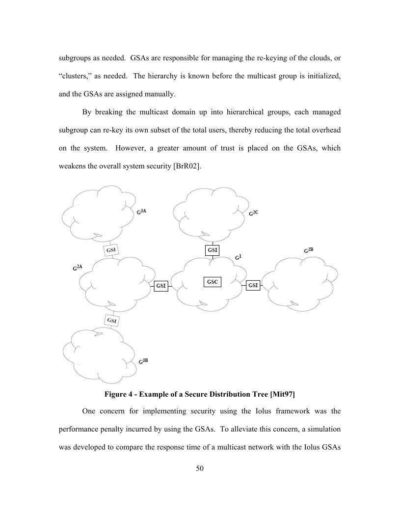
50

subgroups as needed. GSAs are responsible for managing the re-keying of the clouds, or

“clusters,” as needed. The hierarchy is known before the multicast group is initialized,

and the GSAs are assigned manually.

By breaking the multicast domain up into hierarchical groups, each managed

subgroup can re-key its own subset of the total users, thereby reducing the total overhead

on the system. However, a greater amount of trust is placed on the GSAs, which

weakens the overall system security [BrR02].

Figure 4 - Example of a Secure Distribution Tree [Mit97]

One concern for implementing security using the Iolus framework was the

performance penalty incurred by using the GSAs. To alleviate this concern, a simulation

was developed to compare the response time of a multicast network with the Iolus GSAs

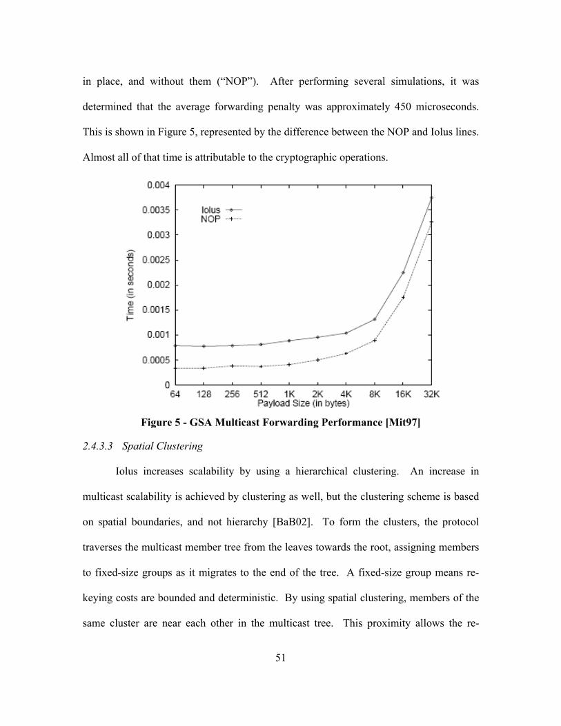
51

in place, and without them (“NOP”). After performing several simulations, it was

determined that the average forwarding penalty was approximately 450 microseconds.

This is shown in Figure 5, represented by the difference between the NOP and Iolus lines.

Almost all of that time is attributable to the cryptographic operations.

Figure 5 - GSA Multicast Forwarding Performance [Mit97]

2.4.3.3 Spatial Clustering

Iolus increases scalability by using a hierarchical clustering. An increase in

multicast scalability is achieved by clustering as well, but the clustering scheme is based

on spatial boundaries, and not hierarchy [BaB02]. To form the clusters, the protocol

traverses the multicast member tree from the leaves towards the root, assigning members

to fixed-size groups as it migrates to the end of the tree. A fixed-size group means re-

keying costs are bounded and deterministic. By using spatial clustering, members of the

same cluster are near each other in the multicast tree. This proximity allows the re-

52

keying scheme to be more efficient. Like Iolus, each cluster has a cluster leader that

interfaces with other clusters and manages re-keying for the cluster.

The differences between Iolus and Spatial Clustering are subtle [BaB02]. In fact,

Spatial Clustering could be used to model Iolus. The two main differences between the

architectures are the way the subgroup leaders are assigned and how subgroups are

formed. In Iolus, the GSAs are special nodes assigned upon the establishment of the

multicast group. In Spatial Clustering, leaders are dynamically assigned, can easily

change as the groups change, and are ordinary nodes that happened to be on a cluster

boundary in the multicast tree. Regarding the formation of the subgroups, Iolus assigns

subgroups based on administrative boundaries, while Spatial Clustering groups are

assigned by proximity on the multicast trees [BaB02].

2.4.3.4 Secure Spread

Secure Spread increases the efficiency and scalability of secure multicast

[AmN05]. The client-server architecture assigns “heavy-weight” activities to servers,

and leaves “light-weight” services to the clients. This architecture is called an “integrated

architecture,” where computationally intensive security services are implemented in the

servers. A “layered architecture,” in contrast, implements such intensive services in the

clients.

To increase performance and scalability, the integrated architecture coupled a

small number of servers to execute the computationally expensive services of the

distributed protocols, thus removing the burden from the clients. The group key

agreement protocols are distributed protocols, and are the most resource intensive of the

53

services. With a small number of servers in a relatively stable configuration, heavy-

weight re-keying between the servers occurs less frequently than the client re-keying.

The servers do not need to be re-keyed when a client joins or leaves the group. Servers

only re-key if one of the servers leave or join the server group. Also, the server re-keying

can be quicker due to needing less keys generated for a small number of servers as

compared to a large number of keys for numerous clients.

2.4.4 Deficiencies of Known Scalable, Secure Multicast Systems and Architectures

Most Group Key Management systems are designed to efficiently key and re-key

large groups of users as the multicast group membership changes. Even the most

efficient GKM, however, will have a fixed cost per user or system to perform the key

updates.

Gothic makes use of group membership knowledge and control to reduce re-

keying. This provides over an order of magnitude less GKM traffic as compared to a

traditional GKM scheme [JuA02]. However, the GACA-GKM is employed across the

entire domain, and does not take advantage of physical or logical separation to further

enhance the scalability.

Iolus improves re-keying efficiency by dividing the various multicast groups into

layered, hierarchical subgroups, connected by GSAs. Spatial Clustering divides the

multicast groups into spatial clusters based on proximity in the multicast tree to reduce

join and leave re-keying overhead. Neither architecture, however, maintains any Group

Access Control Awareness information to reduce the re-keying in the clusters when a

previously authenticated and trusted user moves from one cluster to the next. Both

54

architectures demonstrated improved performance over traditional architectures in fairly

static environments where the users primarily join or leave, and not where they move

from cluster to cluster.

2.5 Summary

This chapter provides an in-depth look at satellite communications systems as

well as the Global Information Grid architecture. This is followed by a discussion on

multicast and group management protocols, along with examples of proposed satellite

architectures that use multicast. Finally, multicast security was addressed to include

required services, group and key management, and architectures germane to the focus of

this research. The closing section addresses limitations that the current multicast security

architectures faced in a highly mobile user environment.

55

III. Methodology

3.1 Chapter Overview

This chapter presents the methodology for the development of the secure, scalable

Hubenko Security Framework Architecture for LEO satellite-based (LEOsat) networks.

The Hubenko Architecture addresses the shortfalls of previous architectures, namely the

lack of a secure multicast architecture that scales well for very large numbers (10,000 or

more) of highly mobile users. Highly Mobile Users change satellite spot beams often,

and/or very rapidly. A person walking down the street talking on a satellite telephone

would not be considered highly mobile, but the same user in an automobile or an airplane

would. A Highly Mobile Environment is defined as a group of users in a network that

collectively change satellite spot beams often. For example, this could be a large group

of slow-moving users, or a small group of rapidly moving users. This chapter begins

with the motivation for developing the Hubenko Architecture. The validity of employing

a LEO satellite communications network is presented, along with the viability of the

PIM-DM multicasting protocol. Next, the development of the Hubenko Security

Framework Architecture is presented followed by a detailed discussion of the modeling

and simulation environment, along with the descriptions and specific parameters for each

of the developed scenarios. The metrics collected and analyzed are defined in this

chapter as well. The chapter concludes with the model verification and validation.

3.2 Hubenko LEOSat Security Framework Architecture Motivation

A review of current literature indicates relatively few research efforts can secure

group communications while simultaneously scale to very large groups of users (over

56

10,000 users). A few of the architectures noted earlier make contributions to an overall

framework for secure group communications in a multicast network. None, however,

specifically addresses a LEOsat network environment, nor do they completely address the

issues facing a global user base such as that found in the GIG.

The foundation of any secure group communications is some type of group key

distribution and management scheme. As mentioned before, this field is well populated

with various concepts for different scenarios and applications, with no one solution

meeting all needs. From the standpoint of this research, the actual keying architecture

piece, be it a centralized, decentralized, or distributed keying agreement protocol, is

transparent to the overall research [ChB04, RaH03]. Therefore, the Hubenko

Architecture allows the system developers to insert the group key protocol(s) that best fit

their needs.

Several secure group communications architectures improve overall system

performance and scalability by dividing the multicast group in various ways. However,

breaking the group into progressively smaller units will ultimately reach a point that will

begin to negatively affect scalability rather than improve it. Therefore, small cluster sizes

alone will not provide sufficient security performance improvement. The developers of

the Group Access Control Awareness (GACA) scheme acknowledge that, while capable

of improving security performance for a system, GACA is suitable as a module to a

larger system, and not a stand-alone solution to security and scalability on its own.

Alone, each of the concepts presented solve parts of the complex security

environment faced in the global environment of the GIG. The novel Hubenko Security

57

Framework Architecture combines several of the features into a coherent solution,

presenting a secure architecture adapted to the unique LEOSat environment.

3.3 LEOSat Network Environment Validation

This section establishes the LEO satellite architecture as a viable unsecured

baseline solution for meeting the needs of the DoD user community. To assess the

relative performance of PIM-DM versus other multicasting protocols (DVMRP and

ODMRP), a set of performance metrics are established [Tho01, ThR01, ThR02]. These

metrics include: the Data-to-Overhead (DtO) ratio; the Received-to-Sent (RtS) ratio; and

the End-to-End (EtE) delay. The Data-to-Overhead ratio indicates how efficiently data is

transmitted throughout the network. The higher the ratio, the higher the amount of data

as compared to overhead information. The only packet types that contain data are the

PIM Packet, RIP Probe, and RIP Report; all other packets are counted as overhead. The

Received-to-Sent ratio is an indicator of packet loss, either due to an invalid route, time-

to-live expiration, or no next hop available (e.g., a satellite loses communications with

the ground station and drops the packet). Packets received compared to total packets

transmitted (precv/ptot_tx) is a simple means of determining how successfully the multicast

system performed. While the sent packet count should always be greater than or equal to

the number received, an occasional duplicated packet means this ratio could be slightly

greater than one. For example, a source sends a single packet that is later duplicated

during a satellite handoff and instead of one of the duplicated packets being properly

discarded in the network, both packets are received (which of course the receiver would

then be able to discard on of the duplicates). End-to-End delay is a “lower-better” metric,

58

which indicates the average time a packet was in transit from the source to the

subscribers. While each multicasting algorithm may use a different route, the most

efficient route is the shortest route with the least number of hops and minimal network

congestion along the way.

The PIM-DM protocol’s effectiveness can be illustrated by comparing the average

values from the simulations for the three defined metrics to earlier work on DVMRP and

ODMRP. All three protocols were implemented using the same satellite network model

validated in previous work [Tho01, ThR01, ThR02]. However, directly comparing the

implementations of PIM-DM, DVMRP, and ODMRP is not possible as the protocols

differed considerably in their implementation and execution. This comparison can be

accomplished by examining the metrics ranges and bounds of the protocols at comparable

loading levels. Table 1 shows the Data-to-Overhead ratio comparison for the target

protocols. All of the PIM-DM simulation experiments were repeated three times and a

90% confidence level used. Since the results for DVMRP and ODMRP were gathered

from previous work, confidence interval overlap analysis was not performed to ascertain

statistical independence.

Table 1 - Data-to-Overhead Comparison DtO DVMRP ODMRP PIM-DM

Min 0.291817 0.111433 0.645125Average 0.561919 0.229997 0.82285

Max 0.766399 0.37276 0.910808

As is shown by Table 1, the DtO measurements illustrate that PIM-DM has a 16%

higher DtO ratio than DVMRP, and a 59% higher DtO ratio than ODMRP. This is the

expected result and is caused by the separation of the routing protocol from the

59

multicasting protocol. Both DVMRP and ODMRP have the routing protocol information

embedded in the multicasting packet. This increases the overall size of the packet, and

therefore increases the amount of overhead for the multicasting portion of the protocol.

Since PIM-DM simply interfaces with the existing routing protocol and does not have the

routing information embedded in the multicasting packets, there is less overhead from the

multicasting perspective. The benefit of separating the routing protocol from the

multicasting protocol is clear as the DtO ratio increases.

A second strength of PIM-DM is seen from the RtS ratio. Using the “orders of

magnitude” reliability terminology from the telecommunications industry, each decimal

place in a reliability statistic represents an order of magnitude. For example, a reliability

metric of 0.999 is one order of magnitude better than 0.99. Table 2 shows PIM-DM has

two orders of magnitude better maximum reliability than ODMRP, and three orders of

magnitude better maximum reliability than DVMRP. In addition, the near perfect

transmission capability exhibited by PIM-DM is ideal when data integrity is crucial. A

protocol with higher RtS not only reliably delivers packets, but decreases retransmission

of missed packets. PIM-DM had a tighter range for RtS (99.93%-99.99%) than both

DVMRP and ODMRP, regardless of the loading on the network.

Table 2 - Received-to-Sent Comparison RtS DVMRP ODMRP PIM-DM

Min 0.845103 0.865764 0.999285Average 0.8950897 0.956833 0.999853

Max 0.9435325 0.996637 0.999939

The EtE delay factor was lower for both ODMRP and DVMRP compared to PIM-

DM, as shown in Table 3. This result is surprising, especially when considering that both

60

DVMRP and PIM-DM build approximately the same length tree structure. The

difference can be explained by two factors. First, the additional layer between PIM and

RIP introduces a slight delay. Since PIM does not maintain its own routing tables like

ODMRP and DVMRP, PIM-DM queries the routing tables to determine the next hop

before actually sending the packet, rather than performing the lookup in its own tables.

Second, the 99.98% RtS ratio is achieved by PIM-DM at the price of non-optimal paths

while the connection between the source and the subscriber was being renegotiated. To

avoid dropping packets, an old satellite node would forward packets to the new satellite

node until the connection was removed. This forwarding increases the reliability but

introduces additional hops along the path leading to higher EtE delays. Therefore, the

penalty for the DtO and RtS performance of PIM-DM is, on average, a seven millisecond

increase in EtE delays compared to DVMRP and 12 milliseconds increase compared to

ODMRP.

Table 3 - End-to-End Delay Comparison EtE (msec) DVMRP ODMRP PIM-DM

Min 65.9055 56.237 69.488Avg 69.1706 64.254 76.393Max 77.326 73.098 86.862

The EtE delays above are well within the typical real-time voice requirements.

For example, Nortel research has determined that a delay of 250 milliseconds is the upper

delay limit for conversations. If delays exceed that limit, the conversation between two

people will be disrupted [NOR05]. Additionally, the EuroSkyWay test-bed analyzed

VoIP performance and determined geostationary satellites are capable of providing good

quality of service (QoS) in terms of jitter and packet loss, and medium to poor QoS in

61

terms of packet delay [CrS01]. According to a study on one-way Internet delays,

[CoP02] demonstrated that the average delay value for international routes is

approximately 110 milliseconds. Consider the case of a global PIM-DM multicast

environment, with integrated terrestrial and LEO satellite PIM-DM network segments.

Given the EtE performance shown in Table 3, the PIM-DM LEO satellite segment would

be transparent to the users in terms of both delay and operation.

Overall, the preliminary work shows that the PIM-DM protocol adapts well to a

satellite network environment. The modified PIM-DM protocol provides a scalable

framework in a satellite communications environment. The protocol scales with load and

provides equivalent performance characteristics regardless of the load on the system.

The Data-to-Overhead ratio is on average approximately 80% and increases with a more

stable network configuration (i.e., the network converges, with few changes during the

simulation period). The Received-to-Sent ratio is 99.98% across all loading levels, so

very few packets are dropped with the majority of packets being delivered successfully.

Finally, with the End-to-End delay of approximately 76 milliseconds, PIM-DM compares

well with longer-range terrestrial networks, and is meets quality of service requirements

for packet-based network communications. PIM-DM compares favorably to both

DVMRP and ODMRP and surpasses the performance of both protocols. The separation

of routing and multicast data simplifies the network and allows the incorporation of other

multicast protocols. PIM-DM gives the user superior transmission capability and

provides a reliable, scalable network configuration with very little packet loss and

excellent responsiveness.

62

Multicast protocols adapted to a GlobalStar®-like LEO satellite environment

concluded that multicasting in a LEOSat network provided upwards of 300% increase in

efficiency over unicast routing [EkA02].

While the GIG GEO systems use crosslinks to route traffic from one part of the

world to another with delays of 250 milliseconds or more, LEO communications systems

achieve average end-to-end latencies of less than 100 milliseconds for intercontinental

communications using satellite crosslinks [HuR06a, Sae03]. This performance indicates

LEO communication satellite systems should be included in an overall GIG architecture

to improve end-to-end performance.

3.4 Continued Viability of PIM-DM

PIM-DM has a large following in the commercial world as well as an active

Internet Engineering Task Force (IETF) working group [Sav06]. PIM-DM is an

excellent choice for adapting to the LEO satellite environment since the protocol is a

dense mode protocol, and satellites are capable of interfacing with a large group of users

simultaneously. Further, the protocol independence of PIM-DM permits an easier

adaptation to a satellite environment, requiring only the multicast portion of the protocol

be modified while using the well-established RIP protocol (with minor modifications) for

the underlying routing support. From a commercial standpoint, Cisco has incorporated

PIM-DM in its routers and Internetwork Operating System (IOS) [CIS07], and the

OPNET Modeler [OPN06] software package now has PIM-DM and SM models

available. This is not true for other multicast protocols.

63

Recently, there was a proposal to the IETF to re-classify several of the multicast

protocols as historic, indicating they are no longer actively developed and supported

[Sav06]. These protocols include Border Gateway Multicast Protocol (BGMP), Core

Based Trees (CBT), and Multicast OSPF (MOSPF). In addition, this same document

sought to retire the following RFCs: [RFC3913], [RFC2189], [RFC2201], [RFC1584],

and [RFC1585] and thus was not considered as the basis of new research.

Despite the fact that PIM-DM is regarded as a protocol that will not work in ISP

networks, PIM-DM is a good option in dense end-user environments [Sav06].

Additionally, the comments on the reliance of the complicated Assert timing issues

causing numerous dropouts and poor routing during satellite handoffs have been

satisfactorily addressed in [Sae03]. In the satellite network environment, the satellite

routers frequently transition, or “hand-off,” their users to neighboring satellites as the

satellites move about their orbits. Typical terrestrial applications of PIM-DM do not

experience, and do not account for, the frequent hand-offs encountered in the satellite

environment. Therefore, the specified functions of the Assert had to be modified to

rebuild the links after satellite transitions. The specification uses the Assert message to

choose between alternate routes to force a specific route configuration, or to determine

which node should be the forwarder for the group [AdN05]. The satellite adaptation uses

the Assert to build a new route since the current route has changed due to satellite

movement. Therefore, the Assert is accomplishing the same basic function as the

specification, but the approach is unique to this satellite network model. Additionally,

the RIP Ground message was added to assist with the transition capability. Without these

64

application-specific modifications, PIM-DM performance in a satellite network would be

severely degraded, as noted in the literature.

While not yet obsolete, the use of Distance Vector Multicast Routing Protocol

(DVMRP) [RFC1075], first used in the MBone, is on the decline. Most DVMRP

applications have been replaced with PIM-SM, leaving DVMRP only in legacy

applications for the near term [Sav06].

MOSPF [RFC1584] was used by several vendors in intra-domain networks.

Since MOSPF does not scale to the inter-domain case, it is no longer actively deployed.

BGMP [RFC3913] appears to have been supported only in documents. No

known implementations or deployments exist [Sav06].

CBT [RFC2201] was an academic project that provided the basis for PIM sparse

mode shared trees. As soon as PIM was able to establish the shared tree capability, CBT

was no longer needed [Sav06] and hence has not been deployed.

3.5 Hubenko Security Framework Architecture Development

This effort is comprised of three elements: adapt a flat key multicast security

architecture to the baseline LEOsat model; enhance this generic architecture by

progressively adapting relevant portions of three secure group communications

architectures/frameworks (Iolus, Spatial Clustering, and Gothic) to the model; and

finally, demonstrate the expected increase in efficiency and overall system scalability

performance through discrete event simulation and analysis.

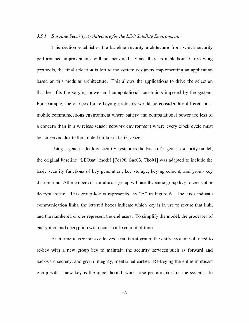
65

3.5.1 Baseline Security Architecture for the LEO Satellite Environment

This section establishes the baseline security architecture from which security

performance improvements will be measured. Since there is a plethora of re-keying

protocols, the final selection is left to the system designers implementing an application

based on this modular architecture. This allows the applications to drive the selection

that best fits the varying power and computational constraints imposed by the system.

For example, the choices for re-keying protocols would be considerably different in a

mobile communications environment where battery and computational power are less of

a concern than in a wireless sensor network environment where every clock cycle must

be conserved due to the limited on-board battery size.

Using a generic flat key security system as the basis of a generic security model,

the original baseline “LEOsat” model [Fos98, Sae03, Tho01] was adapted to include the

basic security functions of key generation, key storage, key agreement, and group key

distribution. All members of a multicast group will use the same group key to encrypt or

decrypt traffic. This group key is represented by “A” in Figure 6. The lines indicate

communication links, the lettered boxes indicate which key is in use to secure that link,

and the numbered circles represent the end users. To simplify the model, the processes of

encryption and decryption will occur in a fixed unit of time.

Each time a user joins or leaves a multicast group, the entire system will need to

re-key with a new group key to maintain the security services such as forward and

backward secrecy, and group integrity, mentioned earlier. Re-keying the entire multicast

group with a new key is the upper bound, worst-case performance for the system. In

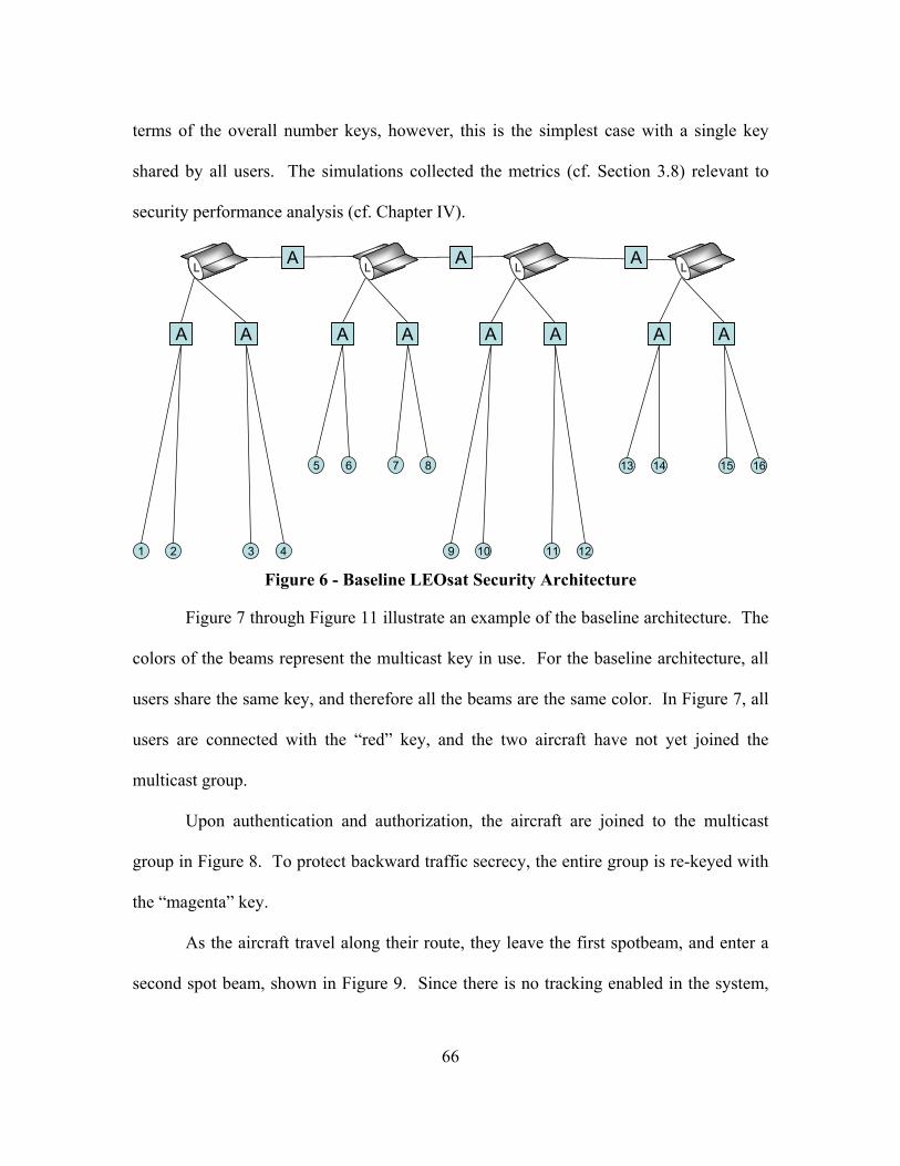
66

terms of the overall number keys, however, this is the simplest case with a single key

shared by all users. The simulations collected the metrics (cf. Section 3.8) relevant to

security performance analysis (cf. Chapter IV).

1 2 4

7

3

5 8

11

6

9 12

14

10

13 15 16

A AAA A AAA

LL LL LL LLA AA

Figure 6 - Baseline LEOsat Security Architecture

Figure 7 through Figure 11 illustrate an example of the baseline architecture. The

colors of the beams represent the multicast key in use. For the baseline architecture, all

users share the same key, and therefore all the beams are the same color. In Figure 7, all

users are connected with the “red” key, and the two aircraft have not yet joined the

multicast group.

Upon authentication and authorization, the aircraft are joined to the multicast

group in Figure 8. To protect backward traffic secrecy, the entire group is re-keyed with

the “magenta” key.

As the aircraft travel along their route, they leave the first spotbeam, and enter a

second spot beam, shown in Figure 9. Since there is no tracking enabled in the system,

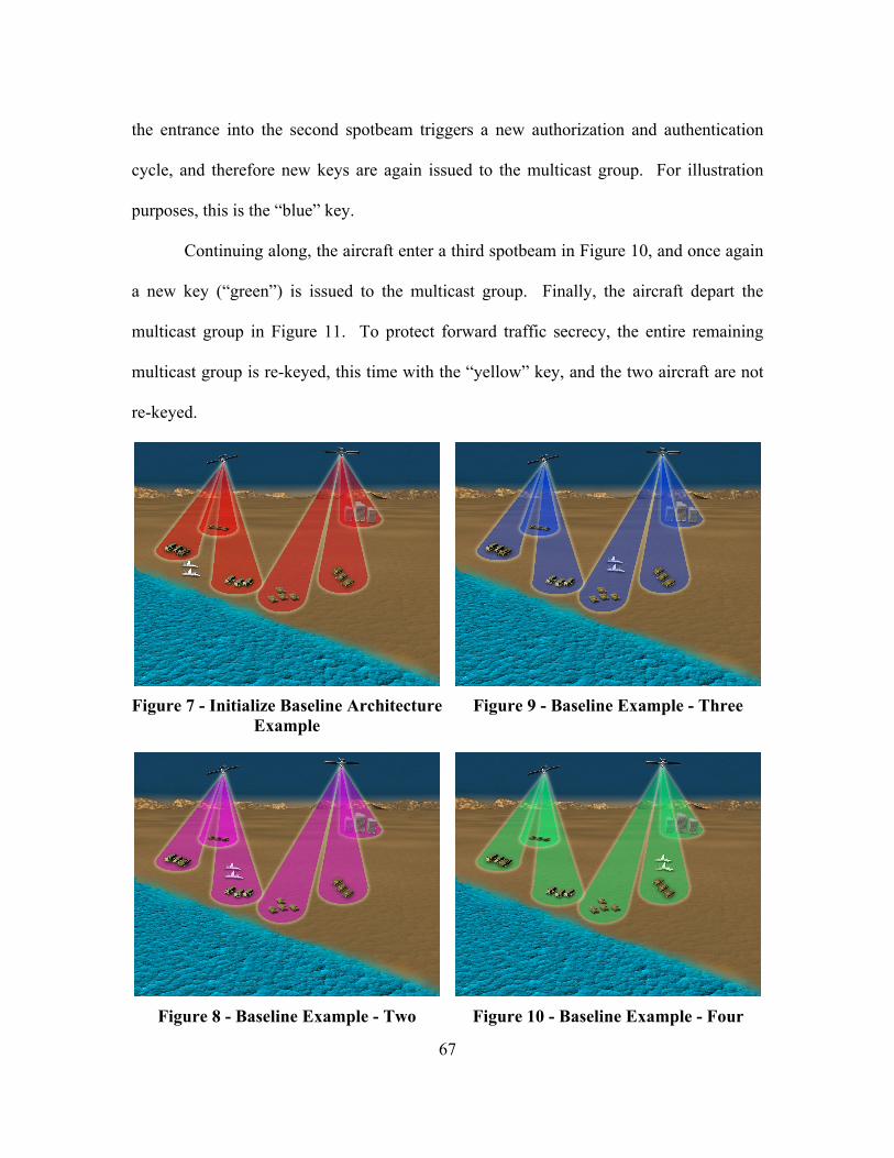
67

the entrance into the second spotbeam triggers a new authorization and authentication

cycle, and therefore new keys are again issued to the multicast group. For illustration

purposes, this is the “blue” key.

Continuing along, the aircraft enter a third spotbeam in Figure 10, and once again

a new key (“green”) is issued to the multicast group. Finally, the aircraft depart the

multicast group in Figure 11. To protect forward traffic secrecy, the entire remaining

multicast group is re-keyed, this time with the “yellow” key, and the two aircraft are not

re-keyed.

Figure 7 - Initialize Baseline Architecture

Example

Figure 8 - Baseline Example - Two

Figure 9 - Baseline Example - Three

Figure 10 - Baseline Example - Four

68

Figure 11 - Baseline Example - Finish

3.5.2 Clusterized Security Architecture

With a baseline and minimal security features in place, this section describes how

the LEOsat network security architecture was enhanced by using key features of several

secure group communications architecture proposals [AmN05, BaB02, JuA02, Mit97].

The first enhancement applies clustering proposed by [BaB02, Mit97].

Iolus, due to its predetermined, static clusters and Group Security Agents (GSA)

assignment scheme, adapts well to the satellite environment where satellites follow

predetermined orbits with repeating ground tracks, and deterministically hand off users

from one satellite to another. The penultimate leaves of the multicast tree, namely the

LEO satellites in view of the users, are also static, in a sense, and pre-determined.

Although the satellites are actually rapidly moving in and out of view overhead, the user

will always be connected to a single satellite. This single satellite, regardless of exactly

which satellite unit it is, will appear constant. Furthermore, the satellites naturally act as

GSAs, bridging the traffic between clusters (spot beams) and managing the re-keying for

each of the clusters.

69

By dividing the network into two distinct hierarchical groups (“satellites” and

“users”) as proposed in the Iolus system, a leave or join by a user will trigger a re-key in

the user cluster, but not in the satellite cluster. Similarly, a leave or join by a satellite will

trigger a satellite cluster re-key, and not affect the users. However, it is presumed that a

leave or join by a satellite is triggered by the need for a satellite’s end-user to leave or

join a multicast group since satellites generally are not end users as well as intermediary

routers. Therefore, satellite joins or departures independent of user joins or departures

should rarely occur. The Satellite Cluster group key is represented by “V” in Figure 12.

To further increase the efficiency of the clustering concept, Spatial Clustering is

implemented. Spatial Cluster’s spatial boundaries adapt well to a satellite environment,

though the concept of clustering is applied in a slightly different manner from the

perspective of the leaves and their relative proximity. In Spatial Cluster, the geographic

distances covered within a single cluster vary greatly since fixed-sized clusters are

maintained despite variances in user density. Maintaining a fixed-size cluster in the

satellite-adapted network, however, is impractical due to the dynamic nature of the

mobile user environment. Except in cases with significant spot beam overlap (e.g., in the

higher latitudes), users could not switch clusters to modify the cluster sizes. Thus, while

the satellite environment can still benefit from the Spatial Cluster concept, fixed

geographical boundaries are used rather than fixed cluster user size. The ovals in Figure

12 represent the geographic clustering, with each cluster sharing a user group cluster key,

lettered “A” through “H.” This reduces the impact to the system when a new user joins a

group, or when a group member leaves. In the initial architecture, the entire system

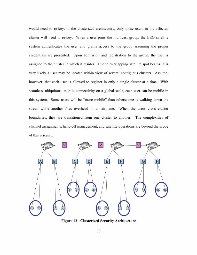
70

would need to re-key; in the clusterized architecture, only those users in the affected

cluster will need to re-key. When a user joins the multicast group, the LEO satellite

system authenticates the user and grants access to the group assuming the proper

credentials are presented. Upon admission and registration to the group, the user is

assigned to the cluster in which it resides. Due to overlapping satellite spot beams, it is

very likely a user may be located within view of several contiguous clusters. Assume,

however, that each user is allowed to register in only a single cluster at a time. With

seamless, ubiquitous, mobile connectivity on a global scale, each user can be mobile in

this system. Some users will be “more mobile” than others; one is walking down the

street, while another flies overhead in an airplane. When the users cross cluster

boundaries, they are transitioned from one cluster to another. The complexities of

channel assignments, hand-off management, and satellite operations are beyond the scope

of this research.

1 2 4

7

3

5 8

11

6

9 12

14

10

13 15 16

A AAA A AAA

LL LL LL LLA AAV VV

A DCB E HGF

Figure 12 - Clusterized Security Architecture

71

Figure 13 through Figure 17 illustrate the same scenario as the Baseline example,

but with the Clusterized Security Architecture in place. Figure 13 illustrates the initial

state of the clusterized multicast group. All users depicted in this figure are

communicating in the same multicast group. Each spotbeam, however, is utilizing a

different multicast key, represented by a different beam color for illustration purposes.

All users within each spotbeam share the same key. The two aircraft are not joined to the

multicast group.

When the aircraft join the multicast group and fly into the first spotbeam, only

that “teal” cluster needs to re-key, as shown in Figure 14 by the spotbeam turning to a

“dark blue” key. Note only those users in the single cluster are now affected by the join,

compared to the entire multicast group in the Baseline example.

Figure 13 - Initialize Cluster Example

Figure 14 - Cluster Example - Two

When the aircraft fly to the next spotbeam in Figure 15, the old spotbeam changes

key to “dark green,” and the new cluster changes key to “tan.” The clusters need to re-

key for the same reason as the Baseline example: there is no tracking enabled in the

system, the entrance into the second spotbeam triggers a new authorization and

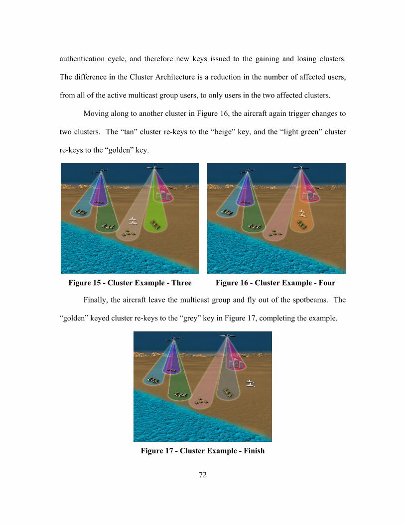
72

authentication cycle, and therefore new keys issued to the gaining and losing clusters.

The difference in the Cluster Architecture is a reduction in the number of affected users,

from all of the active multicast group users, to only users in the two affected clusters.

Moving along to another cluster in Figure 16, the aircraft again trigger changes to

two clusters. The “tan” cluster re-keys to the “beige” key, and the “light green” cluster

re-keys to the “golden” key.

Figure 15 - Cluster Example - Three

Figure 16 - Cluster Example - Four

Finally, the aircraft leave the multicast group and fly out of the spotbeams. The

“golden” keyed cluster re-keys to the “grey” key in Figure 17, completing the example.

Figure 17 - Cluster Example - Finish

73

A further enhancement to this scheme divides the satellites into smaller clusters as

well. However, it is assumed that the satellites are controlled by a single, trusted entity

(in this case the DoD) and there is no need to re-key when a satellite leaves or joins the

satellite group.

3.5.3 Hubenko Security Framework Architecture

With the “clusterizing” of the multicast network established, the following

enhancement adds the “Group Access Control Aware-Group Key Management” feature

from Gothic [JuA02]. The satellite environment is an ideal medium capable of centrally

sharing the group access awareness information, making Gothic readily adaptable.

When the key functions of Gothic are incorporated into the Hubenko Security

Framework Architecture, security performance increases (i.e., re-keying decreases). For

example, consider a multicast group established in a deployed location consisting of air-,

sea-, and land-based tactical units. The occupied locations spread across an area larger

than 50 kilometers in diameter, and therefore is covered by more than a single satellite

spot beam. All of the multicast enabled users join the same multicast group. Each of the

sea- or land-based users joins the group, clustered in their respective areas. The aircraft

flying sorties throughout the region enter and exit the user clusters at a rate much quicker

than their ground or sea counterparts. For example, an aircraft flying at 800 kilometers

per hour will cross a 50 kilometer spot beam in about three and three quarter minutes at

its widest point. During the same period of time, terrestrial users will either appear fixed

relative to the spot beam, or occasionally cross into a new spot beam.

74

Without clustering, the entire Baseline system would have to re-key when users

join or leave a group. With clustering, each cluster is keyed with a separate cluster key.

Adding a new user to the cluster, even if it is already joined to the same multicast group

in another cluster, requires a re-keying of that new cluster. However, with GACA-GKM

support, if the system can establish that a registered user who moves to a new cluster did

not have access to data prior to its joining, or will no longer have access after its

departure, then the cluster would not need to re-key to incorporate the new user or

remove it from the group. Instead, either the new user would be issued a new key upon

entry, or the system would simply continue as before so long as the principles of forward-

and backward secrecy are maintained.

Figure 18 depicts the flow of the Hubenko Architecture. The top section depicts

the initialization process, which follows from the discussion in Sections 2.4.3.1.1 and

2.4.3.1.2. The middle section summarizes the re-keying effects of Joins and Leaves as

described in the above paragraphs. The bottom section summarizes the process for re-

keying when a user moves to a new cluster.

75

Check GACA-GKM:User Still Authorized?

No

Multicast Group Established using GMAS, GPMS SubsystemsCriteria established on who can join group,

either by explicit list of users, or list of criteria

Users Join GroupIn the nearest Cluster

-Authenticated, Validated, Authorized

Re-Key ClusterAny Users Active and Registered in the

Cluster are Re-keyed due to Join or Leave

Eject User

Yes

Users Leave GroupBy own volition or

Are ejected

GACA-GKMUpdated

Accordingly

Established User Moves to New Cluster

Issue User Cluster Key- Only the User that is New to this Cluster Requires the key

- All Other Users Continue Unaffected, Including Users from Previous Cluster

Group Initialization

Group Membership Changes

Group Member Movement

Figure 18 - Hubenko Architecture Flow Chart

76

Figure 19 depicts the key features of the Hubenko Architecture. The dotted lines

represent the Satellite Layer sharing global knowledge of active users through the

GACA-GKM. As before, multiple users in the same cluster who are participating in the

same multicast group share the same cluster key.

1 2 4

7

3

5 8

11

6

9 12

14

10

13 15 16

A DCB E HGF

LL LL LL LLV VV

Rapid Mobility

User

GACA-GKM GACA-GKM GACA-GKMGACA-GKM

Figure 19 - Hubenko Security Framework Architecture

Assume a mobile user (e.g., User 4 in Figure 19) is registered in cluster “B” in a

multicast group, then moves to cluster “C” and joins a different multicast group. With

GACA-GKM support, the system would issue the cluster “C” key to User 4 without re-

keying the other users in “C” since the system knows that User 4 did not collect any data

from the new multicast group in “C” prior to it being granted the “C” key. Further, the

system would not need to re-key the users in cluster “B” since User 4 is no longer able to

receive the “B” data. For added security, User 4 should destroy the “B” key since it is no

longer needed. Since GACA-GKM tracks the locations and group memberships of the

77

users in the system, it knows when users transition from one cluster to another and are

still registered in the same multicast group. Therefore, when registered members of a

multicast group move from cluster to cluster, they are issued the new cluster keys without

impacting the new or old clusters. Since the user is already a member of the multicast

group, and already has the same old data collected in the previous cluster, there is no

need to re-key the new cluster since Traffic Backward Secrecy is not violated. Further,

there is no need to re-key the old cluster since Traffic Forward Secrecy would not be

violated either.

Using the previous sample scenario from the Baseline and Cluster examples,

Figure 20 through Figure 23 illustrate the potential savings in re-keying by employing the

Hubenko Architecture in a mobile environment. The Hubenko Architecture effectively

initializes much like the Cluster Architecture did in Figure 13, with each cluster in Figure

20 utilizing a different key. However, when the two aircraft fly into the first spot beam in

Figure 21 and join the multicast group, the system is able to issue the current “dark

green” key to the two aircraft, and not have to re-key the whole cluster. This is because

the system is able to determine that neither of the two aircraft were previously in a

location that was covered by the multicast spotbeams, and therefore would not have been

able to collect data from the past.

Upon transitioning to the next cluster in Figure 22, the system again tracks the

whereabouts of the aircraft, and is able to issue the “tan” keys to the aircraft, without

having to re-key the tan cluster. In addition, the system does not need to re-key the dark

78

green cluster because the system not only knows that the aircraft are no longer in that

cluster, but also to which cluster they are currently assigned.

Figure 20 - Initialize Hubenko

Architecture

Figure 21 - Hubenko Example - Two

The same situation holds true as the aircraft move into the “grey” cluster in Figure

23. The “tan” cluster does not need to re-key, nor does the “grey” cluster. Finally, as the

aircraft leave the multicast group and fly out of the “grey” cluster, they deregister from

the multicast group. This Leave triggers the “grey” cluster to re-key to protect forward

traffic secrecy.

Figure 22 - Hubenko Example - Three

Figure 23 - Hubenko Example - Four

79

To ensure the integrity of the system, “physical separation” alone cannot be used

when a previously unregistered user joins a group due to the broadcast nature of satellite

communications and the inability to determine if anyone is “listening” to the transmitted

data. Despite the use of relatively small spot beams, a large geographical area is still

contained within view of the satellite. Therefore, a user may be out of view of any of the

registered users, but well within view of the data transmissions in the cluster. This user

can conceivably collect data, and then join the group. If the system did not re-key the

cluster upon this new user’s join, the new user would now be able to decrypt the

previously collected data with the key it just received. This violates the Traffic

Backward Secrecy service provided by the network security system.

The previous cases do not apply if there is only one multicast group on the

system. All of the registered users, while communicating with different cluster keys,

would be receiving the same multicast data. Therefore, local transitions from spot beam

to spot beam without cluster re-keying would be acceptable. However, in a system

capable of handling multiple, concurrent, and distinct multicast groups, the former cases

would most likely apply.

3.5.4 Demonstrate Improved System Security Performance

The final element of the research and development of the Hubenko Security

Framework Architecture demonstrates the overall security performance improvements

(i.e., less overall re-keying for the individual users and for the system as a whole) of the

enhanced architecture by way of discrete time simulation using MatLab. Architecture

models were developed based on the architectures defined above. The design of the

80

models are discussed in Section 3.6. The results and respective analysis of the

simulations are discussed in Chapter IV.

3.6 Simulation Environment and Architecture Models

A discrete time computer simulation was created using MatLab® version R2006b

[MAT07] to compare the efficiency and scalability performance of three representative

architectures. Efficiency is defined as a measure of average re-keying experienced by the

individual users. That is, the basis for determining efficiency was the number of times

each user, on average, had to re-key during a given simulation period. Scalability is

defined as the overall system-level key count. The more keys distributed per simulation,

the less scalable the architecture. Since the number of keys, and not actual packet traffic,

was the focus for determining efficiency and scalability, complex event simulators with

packet-generation capabilities were not necessary. Instead, the simulation tracks all of

the required performance statistics on each of the individual users, and aggregates the

results to establish system level performance.

3.6.1 Simulation Environment

In this model, all multicast groups and active users (those registered in the

multicast groups) are managed by the satellite infrastructure. If a user decides to initiate

a new multicast group, the request is made to the satellite network, and the necessary

group ownership information is transferred to the satellite layer for group establishment

and subsequent management. For the performance results and analysis discussed in

Chapter IV, however, the simulations focused on the steady-state performance, i.e., users

joining, leaving, and moving within established multicast groups. When a user joins a

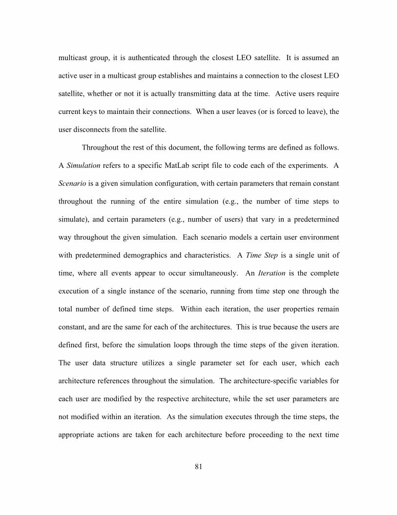
81

multicast group, it is authenticated through the closest LEO satellite. It is assumed an

active user in a multicast group establishes and maintains a connection to the closest LEO

satellite, whether or not it is actually transmitting data at the time. Active users require

current keys to maintain their connections. When a user leaves (or is forced to leave), the

user disconnects from the satellite.

Throughout the rest of this document, the following terms are defined as follows.

A Simulation refers to a specific MatLab script file to code each of the experiments. A

Scenario is a given simulation configuration, with certain parameters that remain constant

throughout the running of the entire simulation (e.g., the number of time steps to

simulate), and certain parameters (e.g., number of users) that vary in a predetermined

way throughout the given simulation. Each scenario models a certain user environment

with predetermined demographics and characteristics. A Time Step is a single unit of

time, where all events appear to occur simultaneously. An Iteration is the complete

execution of a single instance of the scenario, running from time step one through the

total number of defined time steps. Within each iteration, the user properties remain

constant, and are the same for each of the architectures. This is true because the users are

defined first, before the simulation loops through the time steps of the given iteration.

The user data structure utilizes a single parameter set for each user, which each

architecture references throughout the simulation. The architecture-specific variables for

each user are modified by the respective architecture, while the set user parameters are

not modified within an iteration. As the simulation executes through the time steps, the

appropriate actions are taken for each architecture before proceeding to the next time

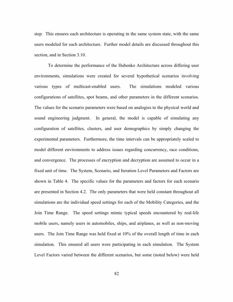
82

step. This ensures each architecture is operating in the same system state, with the same

users modeled for each architecture. Further model details are discussed throughout this

section, and in Section 3.10.

To determine the performance of the Hubenko Architecture across differing user

environments, simulations were created for several hypothetical scenarios involving

various types of multicast-enabled users. The simulations modeled various

configurations of satellites, spot beams, and other parameters in the different scenarios.

The values for the scenario parameters were based on analogies to the physical world and

sound engineering judgment. In general, the model is capable of simulating any

configuration of satellites, clusters, and user demographics by simply changing the

experimental parameters. Furthermore, the time intervals can be appropriately scaled to

model different environments to address issues regarding concurrency, race conditions,

and convergence. The processes of encryption and decryption are assumed to occur in a

fixed unit of time. The System, Scenario, and Iteration Level Parameters and Factors are

shown in Table 4. The specific values for the parameters and factors for each scenario

are presented in Section 4.2. The only parameters that were held constant throughout all

simulations are the individual speed settings for each of the Mobility Categories, and the

Join Time Range. The speed settings mimic typical speeds encountered by real-life

mobile users, namely users in automobiles, ships, and airplanes, as well as non-moving

users. The Join Time Range was held fixed at 10% of the overall length of time in each

simulation. This ensured all users were participating in each simulation. The System

Level Factors varied between the different scenarios, but some (noted below) were held

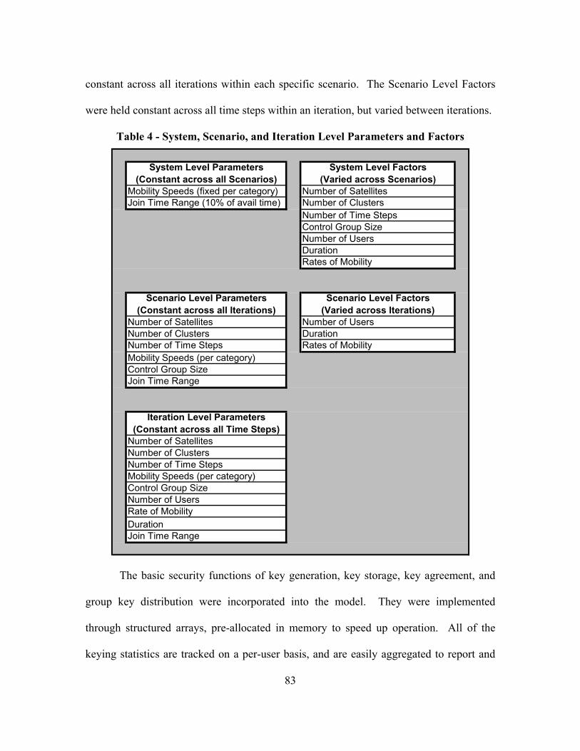
83

constant across all iterations within each specific scenario. The Scenario Level Factors

were held constant across all time steps within an iteration, but varied between iterations.

Table 4 - System, Scenario, and Iteration Level Parameters and Factors

Scenario Level Factors(Varied across Iterations)

Iteration Level Parameters (Constant across all Time Steps)

Control Group Size

Number of UsersDuration

Scenario Level Parameters (Constant across all Iterations)

Number of SatellitesNumber of Clusters

Control Group Size

DurationJoin Time Range

Number of UsersRate of Mobility

Number of Time StepsMobility Speeds (per category)

Rates of Mobility

Join Time Range

Number of SatellitesNumber of ClustersNumber of Time StepsMobility Speeds (per category)

Number of UsersDurationRates of Mobility

Join Time Range (10% of avail time) Number of ClustersNumber of Time StepsControl Group Size

System Level Parameters (Constant across all Scenarios)

Mobility Speeds (fixed per category)

System Level Factors(Varied across Scenarios)

Number of Satellites

The basic security functions of key generation, key storage, key agreement, and

group key distribution were incorporated into the model. They were implemented

through structured arrays, pre-allocated in memory to speed up operation. All of the

keying statistics are tracked on a per-user basis, and are easily aggregated to report and

84

analyze system-level statistics. In addition, multiple fields with multi-dimensional arrays

within each structure represented each user’s parameters, as described below.

The users are divided into four representative Mobility categories, assigned with

varying percentages of each as needed to model each scenario (cf. Section 4.2). The

categories were chosen to represent the main types of users commonly operating in a

deployed environment. “Stationary” (i.e., non-moving) users represent fixed

infrastructure, such as a command post. “Sea” users have slow mobility (e.g., movement

between clusters occurs at a relatively slow pace (e.g., several time steps)), and represent

ships and amphibious units. “Ground” users move twice as fast as Sea users, and

represent vehicles such as tanks, trucks, automobiles. “Air” users move four times as fast

as Ground users, and represent airplanes, helicopters, and unmanned aerial vehicles

(UAVs). The relative speeds of the categories were derived by analogy to real-world

operators, which were then generalized into four distinct groups for simplicity. A ship

typically has top speeds near 45 kilometers per hour. Smaller craft can move faster,

while some ships have slower top speeds. An automobile or truck can easily reach 90

kilometers per hour, while most tanks cannot. Additionally, 360 kilometers per hour is

an easy feat for a jet, but more difficult for UAVs and helicopters to achieve. Should an

analysis require a finer granularity of Mobility Categories, each category can easily be

broken into subcategories (e.g., “Air” can be divided into UAVs, Helicopters, and Jet

Planes for instance). Related to the user Mobility categories is a system-level “Rate of

Mobility” (RoM) parameter. A “Rate of Mobility” is defined as the overall percentage of

users that are mobile (i.e., Sea, Ground or Air type) for each iteration. For example, a 1%

85

RoM means that out of one thousand users, an average of ten users would be assigned

one of the three mobility categories, with the remaining users assigned a stationary

category.

When the simulation initializes an iteration, each user is randomly assigned (using

a uniform distribution) to an initial Satellite and respective Cluster; a Join Time; a

Duration; and one of the four Mobility categories. In most of the scenarios, the uniform

distribution ensured even loading across all of the factors. To investigate targeted areas

of interest, certain scenarios reduced the range of factor values to simulate a more

concentrated factor loading. For example, in scenarios with numerous satellites, using

the uniform distribution allowed level loading across the system, without “overcrowding”

any one cluster. Some of the scenarios, however, have only a single satellite for a high

user density.

If the node is mobile, it may change to a new cluster during the iteration. The

Join Times are uniformly distributed to activate all users within a specified time period,

typically within the first one-third of the iteration’s time steps. In general, the Durations

(length of time the user is active in the multicast group) are uniformly distributed

between one time step to the time remaining until the end of the simulation. Certain

scenarios, however, investigated the performance with specified duration lengths, as

noted below.

The distributions used ensure a highly active user group with numerous joins and

leaves spread throughout the iteration. Besides the joining and leaving activities, the

users are able to move between clusters at a rate dependent on their mobility category.

86

Each user’s mobility category is also assigned randomly within the constraint of the

overall Rate of Mobility for the given scenario. Once the overall RoM is achieved (e.g.,

10% of all active users are Sea, Ground, or Air types), all subsequent users are assigned

to the Stationary category. Each of the scenarios used different RoM to simulate

different real-life situations. The RoM were derived from knowledge of typical troop,

fleet, and squadron sizes found operating within an operational area of responsibility

(AOR). For example, a Marine Expeditionary Force (MEF) typically has between 7,000

and 20,000 troops deployed to a region. Along with the troops, the MEF deploys a few

squadrons of aircraft and several amphibious units. Additionally, the Marines frequent

deploy with the Navy, thus increasing the number of sea vessels and aircraft in the AOR.

Out of the total number of troops, not all are in motion simultaneously. Hence, the

scenarios all have less than 100% RoM. If, on the other hand, a scenario were to focus

specifically on the efficiency and scalability of a mobile ad hoc network (MANET), it

would be feasible to have 100% of the users be mobile.

To model the impact each event has on re-keying, the events are logically

categorized into two levels. Joins and leaves are categorized as Level 2 events, and

movement between clusters is categorized as a Level 1 event. If multiple events occur

within a single time step, the highest-level event (i.e., Level 2 > Level 1 > None) takes

priority, and only one consequence is modeled for the affected cluster or system as

appropriate. In typical multicast systems, the only level that is modeled is Level 2 since

movement was not a design criteria as multicast was being developed. Therefore, Level

1 was implemented to account for the movement not seen in other models. As a generic

87

example, if there are two leaves and a join within the same time step, only one round of

re-keying is required to account properly for all three changes in the multicast group

instead of three rounds of keying. The sizing of the time step will determine the level of

fidelity of multiple events occurring near-simultaneously within a time step.

3.6.2 Architecture Models

3.6.2.1 Baseline Architecture

The first architecture, referred to as the “Baseline” architecture, is a generic

multicast network that uses a flat keying system (i.e., all keys shown in Figure 6 are the

same). There is no provision for clustering, so a user joining or leaving the network

requires a new group key be established and distributed to all users in the system. As a

user travels from one location to another, it deregisters from one spot beam, and re-

registers in a new one. This is a new join, and again all users need to be re-keyed.

In the Baseline architecture, all events are handled the same since a user joining

the multicast group, leaving the multicast group, or moving between satellite spot beams

produces the same effect: trigger the multicast group to re-key. When the multicast

group re-keys, all active users require a new key, regardless of their spot beam.

3.6.2.2 Cluster Architecture

The second architecture, referred to as the “Cluster” architecture, enables

clustering, where each cluster is keyed with a separate cluster key (as shown in Figure

12). Adding a new user to the cluster, even if already joined to the same multicast group

but in another cluster, required a re-keying of that cluster. Highly mobile users (e.g.,

aircraft), enter and exit the user clusters at a much greater rate than their terrestrial

88

counterparts. Therefore, even a single airplane flying into and out of heavily populated

clusters induces a significant amount of re-keying on the cluster users.

In the Cluster architecture, all events again produce the same effect of inducing a

re-key; however, the impacts are limited to the users within the same cluster where the

event occurs. Therefore, when a user joins or leaves a multicast group, or moves to a

new cluster, only that cluster requires the re-key, and not the entire multicast group as in

the Baseline architecture.

3.6.2.3 Hubenko Architecture

The third architecture, referred to as the “Hubenko Architecture,” incorporates the

GACA-GKM support into the Clustered architecture and is shown in Figure 19. If the

system can establish a registered user does not have access to data prior to its joining a

cluster, or would no longer have access after its departure, the cluster does not need to re-

key. Instead, either the new user is issued a new key upon entry, or the system simply

continues as before upon exit.

It is important to note that this implies a level of trust in the GACA subsystem, as

well as sufficient trust in the authenticated user. A user will retain old keys for a certain

amount of time, and could return to a previous cluster and continue to receive messages.

If the user is a legitimate member of the multicast group anyway, the impact is minimal

for returning to an old cluster that has not been re-keyed since that user would have

collected the same data through another cluster. As a precaution, however, the whole

system should establish a policy to re-key periodically, thus ensuring old keys are not

used longer than the policy dictates.

89

Finally, in the Hubenko Architecture, the Level 1 and Level 2 events affect the

system differently. Level 2 events (joins and leaves) have the same impacts as the

Cluster architecture: the multicast group users in the affected cluster are re-keyed. Level

1 events (movement between clusters), however, do not require a re-key since the

movement is tracked within the Group Access Control Awareness (GACA) subsystem.

This differs from the Cluster architecture, which does not have the GACA subsystem and

therefore cannot correlate a leave in one cluster and a join in another cluster as movement

between the two. When multiple events occur within the same cluster and time step in

the Hubenko Architecture, the highest Level event will drive how the cluster responds. If

there are multiple joins or leaves within the same time step, the entire cluster will re-key

once for that time step, and not once per join or leave. If there is movement into or out of

the cluster along with a leave or a join in the same time step, then the cluster must re-key

once to accommodate the new or departed user. If there are multiple movements that

meet the criteria for merely issuing keys to the moved user, then no other user (other than

the one that just arrived) within the cluster is affected for that time step.

The complete Hubenko Architecture requires that the ownership determination

functions and the group policy specification functions from the Gothic architecture be

implemented. Together, these control access to the established multicast groups.

However, since the analysis was focused on the long-term, steady-state system, and not

the initialization, these functions were not explicitly modeled and simulated. Instead, it

was assumed that the complete set of functions were in place, and no distinction was

90

made between either a user leaving the multicast group of its own volition, or a user

being ejected for some other reason.

The following pages depict the flow of the MatLab simulation code (Figure 24).

A sample of the complete code is included in Section 6.5. While the specific iteration

structure and plotting functions varied between scenarios, the core of the simulation

remained the same.

91

Establish Scenario Experimental ParametersControlGroupSize, MaxNumUsers, numTimeSteps, numSats,

numClusters, Mobility Categories and associated speeds,DurationFactor, MobilityProfile, JoinTimeSetter,

Confidence Interval Statistics

Pre-Allocate Applicable Multi-dimensional Arrays in MemoryTotal Keys Distributed, Control Group Keys Distributed,

Total Average Key Counts, Control Group Average Key Counts,Confidence Interval Statistics Arrays

Begin Iterations LoopRepeat Loop numIterations Times

Begin Confidence Interval LoopRepeat Loop SampleSize Times

Initialize System Status ArraysClusterTriggers, ClusterActivity

Pre-Allocate User Structure

Begin User Structure Initialization LoopRepeat Loop numUsers Times

Is User inControl Group orMobility Group?

InitializeMobilityGroup

InitializeControlGroup

InitializeMobilityGroup

InitializeControlGroup

(a)

(b)

(c)

Figure 24 - Flow Diagram for MatLab Simulation Code

92

Initialize Control GroupAssign Random Satellite, Cluster;

Set: JoinTime=1, Duration=numTimeSteps,Mobility=Stationary

Initialize Mobility GroupAssign Random Satellite, Cluster,

JoinTime, Duration, Mobility(Mobility Assigned per RoM)

Initialize Control GroupAssign Random Satellite, Cluster;

Set: JoinTime=1, Duration=numTimeSteps,Mobility=Stationary

Initialize Mobility GroupAssign Random Satellite, Cluster,

JoinTime, Duration, Mobility(Mobility Assigned per RoM)

All users assigned?ReturnTo (c)

No

Yes

Begin SimTime LoopRepeat Loop numTimeSteps Times (d)

Begin User Activity LoopRepeat Loop numUsers Times (e)

Is User Active?No Yes

Set ClusterActivity,User.Active flags

Is this a new User?

Set ClusterTrigger,Initialize Mobility Counter

if User is Mobile

Did User JustLeave?

No

Set ClusterTriggerFlag

Yes

Yes

Eject User

Are CredentialsValid?

No

NoYes

Is UserMobile?

ReturnTo (e)

No

MobileUser

Update

Yes

Figure 24 - Flow Diagram for MatLab Simulation Code (Continued)

93

Mobile User UpdateIncrement User.Waiting

Did UserJust Move?

No

Yes

ReturnTo (e)

No

No

Yes

Yes

Yes

- Reset User.Waiting;- Set ClusterTrigger to Level 1

Event unless already set to Level 2;- Update Location;

- Set ClusterTrigger to Level 1Event unless already set to Level 2

All Users checkedfor this Time Step?

ReturnTo (e)

Was a ClusterTriggered?

No ReturnTo (d)

Determine User Re-KeyingRepeat Loop numUsers Times(f)

Is UserActive?

Increment User’sBaseline Key Counter

Level 2Event?

All Time StepsCompleted?

No

Yes

Figure 24 - Flow Diagram for MatLab Simulation Code (Continued)

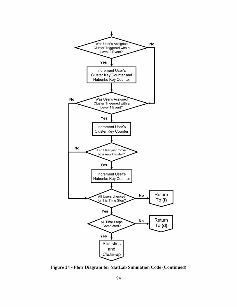
94

NoWas User’s AssignedCluster Triggered with a

Level 2 Event?

Increment User’sCluster Key Counter and

Hubenko Key Counter

Yes

Was User’s AssignedCluster Triggered with a

Level 1 Event?

Increment User’sCluster Key Counter

No

Yes

Did User just moveto a new Cluster?

Increment User’sHubenko Key Counter

No

Yes

No

Yes

All Users checkedfor this Time Step?

ReturnTo (f)

No

Yes

All Time StepsCompleted?

ReturnTo (d)

Statisticsand

Clean-up

Figure 24 - Flow Diagram for MatLab Simulation Code (Continued)

95

Statistics and Clean-up- Calculate Iteration Statistics

- Clean-up Variables and Multi-Dimensional Arrays as Applicable

No

Yes

All SampleSizeIterations Complete?

ReturnTo (b)

No

Yes

All Iterations Complete?ReturnTo (a)

Final Statistics and Data- Calculate Final Statistics

- Produce Figures- Export Data

Figure 24 - Flow Diagram for MatLab Simulation Code (Continued)

3.6.3 Confidence Interval

The confidence level for this research is 95%. When an experiment has a 95%

confidence level with an interval of plus or minus 10%, there is a 95% probability that

the actual mean value of the experiment lies within a range 10% above and 10% below

the experimental mean [Jai91]. The confidence interval is given by

1 1

2 2

,s sx z x zn nα α

− −

⎛ ⎞⎛ ⎞ ⎛ ⎞− +⎜ ⎟⎜ ⎟ ⎜ ⎟

⎝ ⎠ ⎝ ⎠⎝ ⎠ (1)

where x is the sample mean, 1

2

z α−

is the (1 )2α

− quantile of a unit normal variate (1.960

for 95% confidence if more than 30 samples are used), s is the standard deviation, and n

96

is the number of samples. If the means of two experiments fall within the confidence

intervals of each other, then the two items being compared are statistically not different.

If the confidence interval does not contain the mean, then the items being compared may

be statistically different at this confidence level and a t-test would need to be performed.

The Coefficient of Variation (C.O.V.) [Jai91], is the ratio of the sample standard

deviation to the sample mean

. . . sC OVx

= (2)

A C.O.V. of less than 10% is generally used as the stopping criteria for simulations.

Results collected for analysis in Section 4.2 indicated three repetitions were sufficient to

achieve non-overlapping interval bounds for the scenarios with 10,000 users at 95%

confidence, while five repetitions were necessary for the scenarios with fewer users.

3.7 Simulation Equipment

The research and development computer was a XEON workstation with two

three-gigahertz “Dual-Core” Hyper Threaded XEON CPUs, along with 4 gigabytes of

random access memory and dual 75 gigabyte hard drives. This computer is typically

capable of running upwards of eight simultaneous MatLab simulations, due to its eight

virtual CPUs, with no apparent slowdown.

The elapsed time for simulations to complete varied from as little as less than a

day, to more than four weeks. The longest simulations were the ones that modeled

10,000 users for 10,000 time steps, with three repetitions to achieve the desired non-

overlapping 95% confidence interval bounds. The only technical issue that arose due to

97

computer equipment and/or software occurred during the execution of the 10,000

user/10,000 time step simulations. MatLab running on Microsoft Windows®-based

computers has a two billion data element limitation. The simulations were coded in such

a way as to maximize the full set of available data elements, without exceeding the limit.

However, after approximately three weeks into the execution, the workstation

experienced a memory error and reboot, thereby not completing the simulation. The page

file statistics never surpassed two gigabytes during the executions; however, Windows

XP does not have a native utility to track actual system memory usage or history, so there

may have been an error that was not tracked. The only logged error that was reported

related to the Symantec “quarantine scan” operation. The machine was removed from the

local area network, and all anti-virus and security software was uninstalled. This solved

the problem.

3.8 Metrics for Security Performance Evaluation and Analysis

The overall objective of this research effort is the development of an efficient and

scalable multicast security framework architecture for a LEOsat environment that

provides improved performance over current secure group communications architectures.

Efficiency is defined as a measure of average re-keying experienced by the individual

users. That is, the basis for determining efficiency is the number of times each user, on

average, has to re-key during a given simulation period. Scalability is defined as a

measure of the overall system-level key count. The more keys that have to be distributed

per simulation, the less scalable the architecture. Therefore, the following metrics are

used throughout the following simulations and analysis:

98

- Average number of times each user is re-keyed during an iteration.

- Total number of keys distributed in the system during an iteration

These metrics are similar in concept to related research efforts and are germane to

determining potential security performance improvements [HoI04, RaH03].

3.9 Time Scaling for Modeling Expediency

Time scaling is a technique that has been successfully used in the past to reduce

simulation times by appropriately adjusting packet sizes, delays, etc [Fos98, Sae03,

Tho01]. This was helpful for analyzing end-to-end delays in prior research. The focus of

this research, however, was on the effects joining, leaving, and moving of users had on

re-keying operations. In this research, time was normalized to uniform time steps, and all

events occurred within those steps. The time steps can be enlarged to the order of

seconds or even minutes to model broad, large-scale environments such as the global

LEOSat network, or reduced to milliseconds to analyze small, localized networks in

greater detail.

3.10 Model Verification

Model verification was accomplished using a systematic approach. MatLab code

was used for the modeling and simulation of the Hubenko Security Framework

Architecture. A spiral testing and verification method was employed on the architecture.

Problems with syntax and illegal statements were identified and corrected after each

section of code was written. Further, each section of code was checked for proper,

expected execution to ensure each progressive feature was correct before the next section

was developed.

99

During development, most of the errors involved logical issues with the boundary

conditions, such as properly accounting for the start or finish of a user’s duration,

incorrectly incrementing re-key counts just before a user’s joining, or just after a user’s

leaving the multicast group. These errors were identified by stepping through the code

by hand, using the results of the user structure population and comparing the output of

functions with the expected output. Figure 25 through Figure 30 (excluding Figure 28)

graphically display contents of the Satellite, Cluster, Mobility, Join Time, and Duration

fields for each of the individual users’ random assignments, summarized from the

structured array. Plots similar to these were used throughout the development and testing

to ensure the expected randomization occurred, ensure the assignments were within the

expected bounds, and to verify that the code was executing properly given certain values

in the user structured arrays. Figure 25 shows the satellites that each user is assigned to

at the start of the simulation. Figure 26 shows the respective cluster assignments for each

user. Combining the cluster assignment with the satellite assignment, each user’s

location can be identified throughout the simulation. Figure 28 is an aggregate of the

data from the User.Mobility field (plotted as a bar plot in Figure 27), and verifies the

distribution of the user Mobility Categories. The distribution of the user mobility is used

to define the specific “Rate of Mobility” for each of the model scenarios. Each user’s

Join Time and Duration assignments are shown in Figure 29 and Figure 30, respectively.

These two fields dictate when the users join, and how long they remain active, thus

allowing a verification of each user’s activity (or lack thereof) for each time slot.

100

1 2 3 4 5 6 7 8 9 100

0.5

1

1.5

2

2.5

3

User

Sat

ellit

e #

User Satellite Assignments

Figure 25 - User Satellite Assignments

1 2 3 4 5 6 7 8 9 100

0.5

1

1.5

2

2.5

3

User

Clu

ster

#

User Cluster Assignments

Figure 26 - User Cluster Assignments

1 2 3 4 5 6 7 8 9 100

0.5

1

1.5

2

2.5

3

3.5

4

User

Mob

ility

Typ

e

User Mobility Assignments

Figure 27 - User Mobility Assignments

Stationary Ground Sea Air0

0.5

1

1.5

2

2.5

3

User Mobility Type

Num

ber o

f Use

rs

User Mobility Type Demographics for 10 Users

Figure 28 - User Mobility Verification

1 2 3 4 5 6 7 8 9 100

5

10

15

20

25

30

35

40

User

Join

Tim

e

User Join Time Assignments

Figure 29 - User Join Time Assignments

1 2 3 4 5 6 7 8 9 100

5

10

15

20

25

User

Dur

atio

n (#

Tim

e S

teps

)

User Duration Assignments

Figure 30 - User Duration Assignments

101

Critical to the operation of the code is the identification of when users are active

and when they are not. As discussed in Section 3.6.1, all active users receive new keys

upon the appropriate system or cluster re-key, whether or not they are transmitting data at

that time. Therefore, it is imperative to ensure the system is properly tracking each user’s

current state of activity. To verify the correct operation of simulated user activity, the

user structure was examined with the help of spreadsheets, along with graphical plots

such as Figure 31. This figure shows the Join Times (positive slopes) as well as the

Departures (negative slopes) of the ten users being examined. Join Time plus Duration

equals Departure Time.

0 10 20 30 40 50 600

0.2

0.4

0.6

0.8

1

Time

0=N

ot A

ctiv

e, 1

=Act

ive

Individual User Activity

0 10 20 30 40 50 600

0.2

0.4

0.6

0.8

1

Time

0=N

ot A

ctiv

e, 1

=Act

ive

Individual User Activity

Figure 31 - User Activity Verification

To illustrate, User 10, depicted with the bold red line, had a Join Time of six (cf.

Figure 29) and a Duration of sixteen (cf. Figure 30) for a Departure Time of twenty-two.

Note the first descending line in Figure 31. This line is associated with User 3. User 3’s

Join Time was set at Time Step one, and therefore there is no ascending line associated

with the Join since the user initialized as active. However, User 3 in the plotted example

case had a Departure of Time Step four, and its respective descending line is clearly

102

identified. Therefore, the plot shows nine ascending lines (indicating the Joins) and ten

descending lines (indicating the Departures).

Along with Joins and Departures, Mobile users can move between clusters. This

information was tracked in another multidimensional array and combined with the Join

and Departure information to yield a set of “triggers” used to establish when clusters or

systems would need to re-key. Plots similar to Figure 32, along with exporting the arrays

to a spreadsheet, were used to verify the correct operation of the Join, Leave, and

Movement triggers. Figure 32 is the aggregate of all users across all clusters in the

system, for the sixty simulated Time Steps. The height of the bars (either one or two)

correlate to the Level One and Level Two events described earlier in Section 3.6.1. Note

that there are only nineteen Level Two events (Joins or Leaves) since there is a

simultaneous Join and Leave at Time Step Thirty Five. In addition, any movement that

occurs within the same Time Step that a Join or Leave occurs will be masked by the

higher priority event (i.e., a Join or a Leave).

0 10 20 30 40 50 60 700

0.5

1

1.5

2

Time

1=C

Lust

er M

ove,

2=j

oin/

leav

e

Cluster Triggers

Figure 32 - Cluster Trigger Verification

103

Returning to the examples of Users 3 and 10, Figure 32 was used to verify the

Joins and Departures. The Level 2 events shown at Time Steps 1, 4, 6, and 22

correspond to the User 3 Join, User 3 Departure, User 10 Join, and User 10 Departure,

respectively.

Each successive step in the development ultimately led to the final performance

statistics, namely, Average Per-User re-keying, and Total System Keys Distributed,

shown in Figure 33 and Figure 34, respectively. For the development and testing phases,

the data was drawn in bar graphs for simplicity of analysis. Further, there was only one

iteration at a time under investigation. Therefore, line plots similar to those shown in

Section 4.2, which represent multiple iterations demonstrating the performance of the

systems as the number of users grow, were unnecessary and impractical. Bar graphs for

each iteration would have been prohibitively cluttered for analysis beyond a few

iterations.

Baseline Cluster Hubenko0

1

2

3

4

5

6

7

8

Architecture

Ave

rage

Tim

es R

ekey

ed

Average Number of Times Each User is Rekeyed for the Different Archtiectures

Figure 33 - Average Per-User Re-keying

Baseline Cluster Hubenko0

10

20

30

40

50

60

70

80

Tim

es R

ekey

ed

Total Keys Distributed for the Simulation Period

Figure 34 - Total System Keys

During the initial stages of model development, there were multiple active

multicast groups in each iteration. This modeled multiple multicast groups co-existing

104

within the same satellites and clusters. This allows accurate modeling of the physical

properties (e.g., time, frequency, and/or code division multiple access technologies)

available on current and future satellite systems. However, as the number of users and

time steps increased, this method became too resource intensive in terms of the number

of MatLab data elements required to execute the code. The number of MatLab data

elements is roughly two billion when operating on a Windows-based computing platform.

The removal of the concurrent multicast groups conserved sufficient data space to allow

the execution of larger numbers of concurrent users over longer simulated periods of

time.

Another tool used to verify the model development was the random number

generator state control. There are several options available in MatLab for manipulating

the pseudorandom events. Only two methods, however, were used in this model. They

were resetting the state to zero, and choosing a random seed for each simulation, as

shown below.

% Return RAND to its default initial state to allow for repeatability rand('state',0); % Initialize RAND to a different state each time. rand('state',sum(100*clock))

Setting the random number generator back to the same state on successive

simulation executions allowed testing of certain functions, features, and changes in

parameters through replication of the user assignments. This was especially helpful when

removing sections of code (such as the multiple multicast group feature), or adding the

next successive feature. The simulations could be run using the same user population on

105

the before and after code, and the results compared to verify the correct operation of the

new features.

Enabling different states between successive executions ensured different user

initialization parameters, thereby generating slightly different results. MatLab can ensure

a new seed each time by utilizing the current time of the system clock as a function for

seed generation. The MatLab function “clock” outputs the current time as a six element

date vector with the year, month, day, hour, minute, and seconds, each in decimal form.

Each element is multiplied by 100 to ensure integer values, and then are summed into a

single scalar value to be used as the seed. Since time is monotonically increasing, the

seed does not duplicate on successive iterations.

3.11 Model Validation

Model validation was difficult since there are no known physical implementations

of similar secure multicasting group architectures. Therefore, the Hubenko Security

Framework Architecture model was validated against one of the other architectures found

in the literature, namely the Spatial Cluster architecture. A comparison with the Iolus

architecture was not possible since the article discussing the Iolus architecture did not

perform any simulations examining average or total system re-keying. Instead, time

delays incurred by using the group security agents (GSA) were measured.

Full replication of the simulation experiments to validate the Hubenko model with

the Gothic architecture model was not possible due to lack of complete environment data

(e.g., user parameters, mission trace data) used in [JuA02]. Additionally, the

exceptionally long periods of simulated time (almost 700,000 time steps) used in the

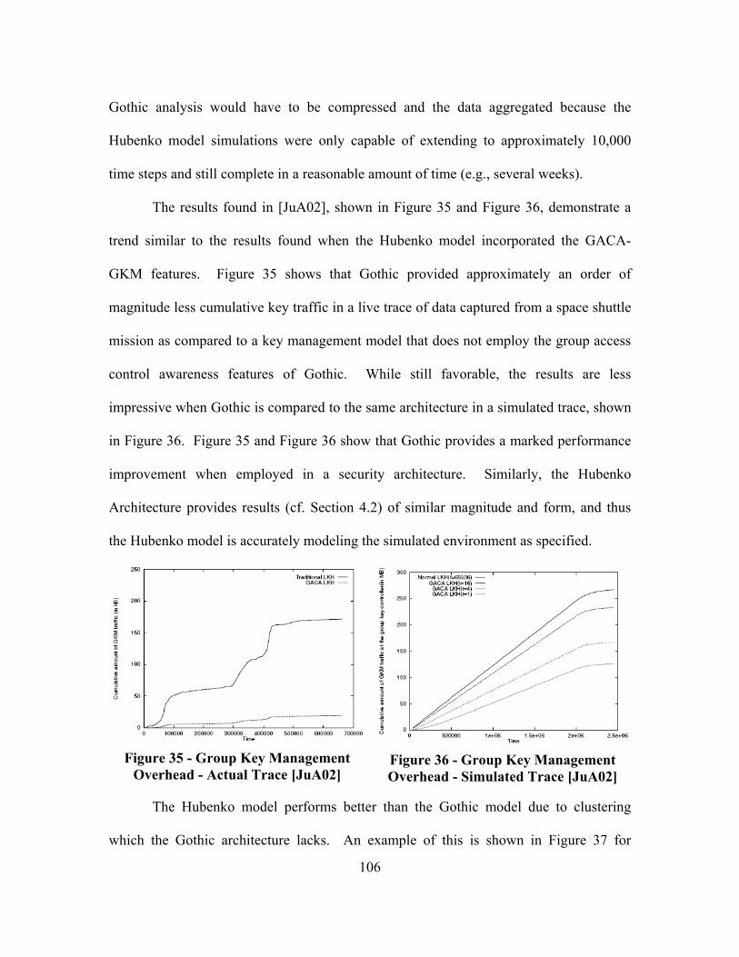
106

Gothic analysis would have to be compressed and the data aggregated because the

Hubenko model simulations were only capable of extending to approximately 10,000

time steps and still complete in a reasonable amount of time (e.g., several weeks).

The results found in [JuA02], shown in Figure 35 and Figure 36, demonstrate a

trend similar to the results found when the Hubenko model incorporated the GACA-

GKM features. Figure 35 shows that Gothic provided approximately an order of

magnitude less cumulative key traffic in a live trace of data captured from a space shuttle

mission as compared to a key management model that does not employ the group access

control awareness features of Gothic. While still favorable, the results are less

impressive when Gothic is compared to the same architecture in a simulated trace, shown

in Figure 36. Figure 35 and Figure 36 show that Gothic provides a marked performance

improvement when employed in a security architecture. Similarly, the Hubenko

Architecture provides results (cf. Section 4.2) of similar magnitude and form, and thus

the Hubenko model is accurately modeling the simulated environment as specified.

Figure 35 - Group Key Management

Overhead - Actual Trace [JuA02]

Figure 36 - Group Key Management Overhead - Simulated Trace [JuA02]

The Hubenko model performs better than the Gothic model due to clustering

which the Gothic architecture lacks. An example of this is shown in Figure 37 for

107

comparison. The Hubenko Architecture provides a greater degree of improvement over

the Clustered architecture (Figure 37) than the Gothic architecture provides over the

Normal LKH architecture (Figure 36). As an aside, the effect of increasing mobility in

the simulations is apparent in Figure 37. The average keys distributed in the 1%

(iterations 1 through 200) and 10% (iterations 201 through 400) RoM sets begin at or

near zero, while the average keys distributed starts off higher in the 25% (iterations 401

through 600) and the 75% (iterations 601 through 800) RoM sets. From the very first

iterations (401 and 601, respectively), there is significantly more movement throughout

the 25% and 75% RoM sets as compared to the 1% and 10% RoM beginning iterations (1

and 201, respectively).

Note in all figures created during the course of this research, the transitions

between different “iteration sets” (e.g., between two consecutive RoM sets) are drawn.

This transition appears as a drop in key counts, but it is due only to the graphical process

used to create each figure. The most logical presentation for the data was using line

graphs. MatLab plotted the data as continuous functions rather than breaking the lines at

each set transition. At each transition point within the scenarios, the lines dip in the

Hubenko plot due to the resetting of the user population. When the user population drops

from the maximum number of users in the last iteration of one set, to the minimum

number of users in the first iteration of the next set, the Hubenko key counts all go down

as well. In the scenarios where the RoM changes, the Baseline and Cluster plot lines also

drop at the transition. However, in the Short versus Long Duration scenarios, the

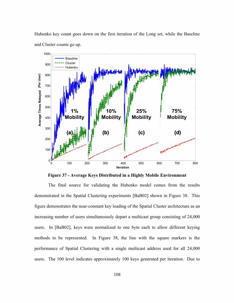
108

Hubenko key count goes down on the first iteration of the Long set, while the Baseline

and Cluster counts go up.

0 100 200 300 400 500 600 700 8000

100

200

300

400

500

600

700

800

900

1000

Iteration

Ave

rage

Tim

es R

ekey

ed

BaselineClusterHubenko

(a) (b) (c) (d)

1%Mobility

10%Mobility

25%Mobility

75%Mobility

(Per

Use

r)

0 100 200 300 400 500 600 700 8000

100

200

300

400

500

600

700

800

900

1000

Iteration

Ave

rage

Tim

es R

ekey

ed

BaselineClusterHubenko

(a) (b) (c) (d)(a) (b) (c) (d)

1%Mobility

10%Mobility

25%Mobility

75%Mobility

(Per

Use

r)

Figure 37 - Average Keys Distributed in a Highly Mobile Environment

The final source for validating the Hubenko model comes from the results

demonstrated in the Spatial Clustering experiments [BaB02] shown in Figure 38. This

figure demonstrates the near-constant key loading of the Spatial Cluster architecture as an

increasing number of users simultaneously depart a multicast group consisting of 24,000

users. In [BaB02], keys were normalized to one byte each to allow different keying

methods to be represented. In Figure 38, the line with the square markers is the

performance of Spatial Clustering with a single multicast address used for all 24,000

users. The 100 level indicates approximately 100 keys generated per iteration. Due to

109

clustering, as the number of users simultaneously departing the multicast group increases,

the key counts remain approximately the same.

The validation simulations had the following characteristics. The Hubenko

Architecture had 2,112 clusters while Spatial Clustering states it had approximately 3,100

clusters (and approximately 17,000 routers). The Hubenko experiments used 23,323

users (versus 24,000 users) for an average of eleven users per cluster. The simulation

focused on the steady state (i.e., all users already joined to group) just like Spatial

Cluster, with no other events occurring except the noted departures. There was no

movement for this validation experiment, and hence no observed difference between the

Cluster and Hubenko performance results.

Under similar conditions as the experiments in [BaB02], the Hubenko

Architecture also has a near-constant key loading for increased simultaneous departing

users as shown in Figure 39.

Figure 38 - Spatial Clustering- Varying the Number of Hosts Leaving [BaB02]

1 4 16 64 256 1024 3000104

105

106

107

108

Number of Simultaneous Leaves Per Time Step

Tota

l Key

s Di

stri

bute

d in

the

Syst

em (l

og s

cale

)

BaselineClusterHubenko

8

1 4 16 64 256 1024 3000104

105

106

107

108

Number of Simultaneous Leaves Per Time Step

Tota

l Key

s Di

stri

bute

d in

the

Syst

em (l

og s

cale

)

BaselineClusterHubenko

8

Figure 39 - Hubenko Model - Varying

the Number of Hosts Leaving Close inspection of Figure 38 and Figure 39 reveals several differences. First and

foremost, the demonstrated key loading (on the log10 scale) for the Spatial Cluster

110

architecture is approximately 102 keys, while the loading for the Hubenko results is

approximately 104 keys. The reason for this difference is due to which keys are being

considered in each case. The Spatial Clustering experiments measured the keys

distributed through the tree routers which does not include the final leaf routers, or the

end users (hosts). On the other hand, the Hubenko experiments measure the keys

distributed through to the end users. Furthermore, Spatial Clustering does not count any

replicated keys sent to the individual users in each cluster. This accounts for one order of

magnitude of the difference since the approximate loading of each cluster is between

eight and fifteen users. The Hubenko Architecture assumes that across the domain of the

24,000 users, the overall cluster loading average is eleven (which is roughly 101).

The second order of magnitude difference is not as clearly explained due to

insufficient information on the Spatial Cluster implementation, network topology, and

other key parameters. Therefore, it is assumed that unique keys are counted for the key

hierarchy (where several users utilize the same sets of keys), and not the total number of

keys distributed to each individual user. Even so, since the keys are multicast to the

group, there is no additional load on the network for sending multiple keys. The values

reported by Spatial Cluster are normalized byte loads, and not necessarily the number of

keys distributed to all users. In Figure 38, for example, one hundred keys are clearly not

sufficient to re-key the remaining 12,000 users when 12,000 users simultaneously depart.

Assuming a uniform distribution of users departing the group, there is no way to have

12,000 users distributed among different clusters, with an average loading of

approximately eleven users per cluster, and yet only require one hundred keys for said

111

users and clusters. However, it is possible to contrive scenarios where the users that are

simultaneously departing are all leaving from the same clusters. In this case, all of the

empty clusters would simply be pruned from the multicast tree rather than require any

new keys to be issued. It might then be possible that of the 12,000 users that departed,

only 100 clusters of the remaining users were affected (i.e., only one or two users from a

select few clusters left the group). The Hubenko simulation did not contrive such a

scenario; rather, it employed a uniform random distribution for the user departures.

The trend of the results shown in Figure 39, compared to the results shown in

Figure 38, validates the clustering portion of the Hubenko Security Framework

Architecture model. Similarly, the trends of the Gothic architecture, shown in Figure 35

and Figure 36 above, validate the GACA portion of the Hubenko model results.

3.12 Summary

This chapter presents the methodology for the development of the secure, scalable

Hubenko Security Framework Architecture for LEO satellite-based networks (LEOsat),

and addresses the lack of a secure multicast architecture that scales well for very large

numbers (10,000 or more) of highly mobile users. The motivation for developing the

Hubenko Architecture, along with the validity of employing a LEO satellite

communications network is presented. Additionally, the metrics that were collected and

analyzed were defined in this chapter as well. This chapter concludes with the model

verification and validation.

112

IV. Performance Results and Analysis

4.1 Chapter Overview

This chapter discusses the modeling and simulation performance results.

Analysis of the results confirms the re-keying advantages provided by the Hubenko

Architecture over other secure group communications architectures in all of the simulated

user environments. Various user environment scenarios are presented with their

corresponding simulation performance results, along with analysis and discussion.

Finally, the performance results are summarized.

4.2 Model Scenarios

To determine the performance of the Hubenko Architecture over the Baseline and

Clustered architectures, several scenarios are developed and analyzed. In each scenario,

the basic models are the same as those discussed in Section 3.6.2. The only changes are

to the values in the specified parameters for each scenario, as noted in each scenario

discussion below.

4.2.1 Highly Mobile User Environment (Four Different RoM)

The first simulation scenario represented four independent Rates of Mobility

(RoM) for a moderate user population size. To contain the user movement in a relatively

small geographical area, only a single satellite with ten active spot beams (clusters) is

simulated. This models a geographical coverage area that would encompass a typical

theater of operations (e.g., deployed military operations overseas, or a widespread

disaster recovery area). In general, the model is capable of simulating any configuration

of satellites and clusters by simply changing the experimental parameters. However,

113

these scenarios used a single satellite because aircraft do not typically fly with sufficient

speed or range to significantly impact terrestrial-based users over a larger area. The first

RoM, 1%, represents a user environment with little mobility, such as when all users are in

garrison, and their movements do not cause them to cross into neighboring clusters.

Subsequent RoM incrementally increase the user mobility (10%, and 25%), ending with a

75% RoM to characterize the Hubenko Architecture in a highly mobile environment.

Figure 40 shows the representative distribution of the users’ mobility categories (from the

final iteration of each iteration set) for each of the four different Rates of Mobility,

marked (a) through (d).

Stationary Ground Sea Air0

200

400

600

800

1000

1200

1400

1600

1800

2000

(a)

Num

ber o

f Use

rs

User Mobility Distribution for 2000 Users. (Iteration 200)

Stationary Ground Sea Air0

200

400

600

800

1000

1200

1400

1600

1800

2000

(b)

Num

ber o

f Use

rs

User Mobility Distribution for 2000 Users. (Iteration 400)

Stationary Ground Sea Air0

200

400

600

800

1000

1200

1400

1600

(c)

Num

ber

of U

sers

User Mobility Distribution for 2000 Users. (Iteration 600)

Stationary Ground Sea Air0

100

200

300

400

500

600

(d)

Num

ber

of U

sers

User Mobility Distribution for 2000 Users. (Iteration 800)

1%Mobility

25%Mobility

10%Mobility

75% Mobility

Stationary Ground Sea Air0

200

400

600

800

1000

1200

1400

1600

1800

2000

(a)

Num

ber o

f Use

rs

User Mobility Distribution for 2000 Users. (Iteration 200)

Stationary Ground Sea Air0

200

400

600

800

1000

1200

1400

1600

1800

2000

(b)

Num

ber o

f Use

rs

User Mobility Distribution for 2000 Users. (Iteration 400)

Stationary Ground Sea Air0

200

400

600

800

1000

1200

1400

1600

(c)

Num

ber

of U

sers

User Mobility Distribution for 2000 Users. (Iteration 600)

Stationary Ground Sea Air0

100

200

300

400

500

600

(d)

Num

ber

of U

sers

User Mobility Distribution for 2000 Users. (Iteration 800)

1%Mobility

25%Mobility

10%Mobility

75% Mobility

Figure 40 - Rates of Mobility for Highly Mobile Scenario

114

The distinct sections (“iteration sets”) marked (a) through (d) in Figure 41 and

Figure 42 correspond to the four different Rates of Mobility (1%, 10%, 25%, and 75%),

respectively. Section (a) has iterations 1 through 200, section (b) iterations 201 through

400, and so on. From left to right in Figure 41 and Figure 42, as the iteration count

increased, the number of users in the system also increased. For example, iterations 1,

201, 401, and 601 had ten users total, for an average cluster density of one user per

cluster. The maximum average cluster density for each simulation set (iterations 200,

400, 600, and 800) was two hundred users, for a total of two thousand users across the ten

satellite clusters. The RoM was constant for all iterations within each iteration set.

When the two hundredth iteration within each set completed, the RoM was increased to

the next level and the number of users reset to an average cluster density of one user per

cluster. The key simulation parameters are summarized in Table 5.

Table 5 - Highly Mobile User Environment Parameters

Satellites 1Clusters 10Maximum Users 2000Time Steps 2000Rates of Mobility (%) 1, 10, 25, 75

Features Mobile users evenly divided between Sea, Ground, and Air

With low overall mobility, both the Cluster and the Hubenko Architectures

demonstrated significant improvement over the Baseline architecture in terms of average

re-keys per user (Figure 41) and total keys distributed in each system (Figure 42). Since

there was relatively little movement with the 1% RoM, the Hubenko Architecture offered

little improvement over the Cluster architecture. The Group Access Control Awareness –

115

Group Key Management (GACA-GKM) did not have an opportunity to provide any

benefits for supporting mobile users. However, as the Rate of Mobility increased (shown

in Figure 41 and Figure 42 (b) through (d)), the performance gains due to the inclusion of

the GACA-GKM in the Hubenko Architecture also increased. This is demonstrated by

observing the difference in re-keying between the Cluster and the Hubenko architectures

in the 1% mobility sections (~150 average re-keys), to the difference in the 75% mobility

sections (~625 average re-keys). The performance gain from the Hubenko Architecture

is approximately 400%.

Saturation is defined as each user being re-keyed at every time step. The

Baseline architecture results in saturation which a re-key of each user occurs per each

time step. Adding more users increases the Total Keys Distributed, but does not increase

the Per-User Average Re-key result, which equals the number of time steps. This is

because at least one event occurs in each time step, and one or more events trigger a re-

key, and at most one re-key can occur per time step. Therefore, the maximum number of

keys that can be distributed in a system in a single iteration is the number of active users

times the number of time steps. Additionally, Maximum Capacity of an architecture is

defined as the number of users that drives the respective architecture to its saturation

point. Beyond the maximum capacity, the architecture continues to re-key each user at

each time step. The per-user average re-keying will remain constant, roughly equal to the

number of Time Steps (dependent on the average Duration for the users). The Total Keys

Distributed, however, will continue to increase as the number of users increases.

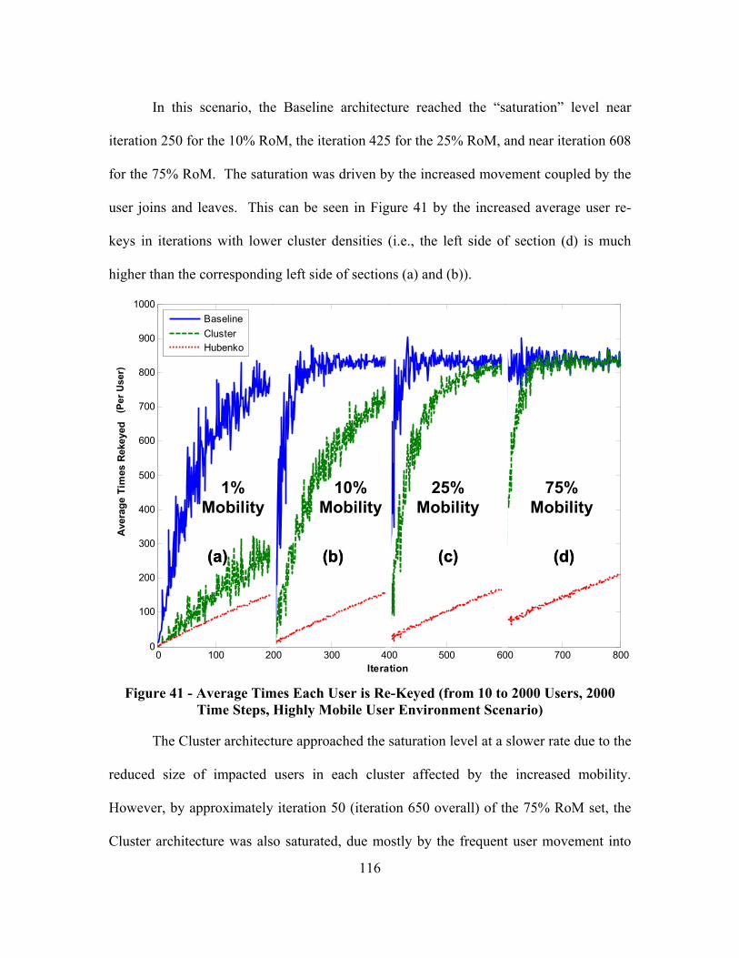
116

In this scenario, the Baseline architecture reached the “saturation” level near

iteration 250 for the 10% RoM, the iteration 425 for the 25% RoM, and near iteration 608

for the 75% RoM. The saturation was driven by the increased movement coupled by the

user joins and leaves. This can be seen in Figure 41 by the increased average user re-

keys in iterations with lower cluster densities (i.e., the left side of section (d) is much

higher than the corresponding left side of sections (a) and (b)).

0 100 200 300 400 500 600 700 8000

100

200

300

400

500

600

700

800

900

1000

Iteration

Aver

age

Tim

es R

ekey

ed

BaselineClusterHubenko

(a) (b) (c) (d)

1%Mobility

10%Mobility

25%Mobility

75%Mobility

(Per

Use

r)

0 100 200 300 400 500 600 700 8000

100

200

300

400

500

600

700

800

900

1000

Iteration

Aver

age

Tim

es R

ekey

ed

BaselineClusterHubenko

(a) (b) (c) (d)(a) (b) (c) (d)

1%Mobility

10%Mobility

25%Mobility

75%Mobility

(Per

Use

r)

Figure 41 - Average Times Each User is Re-Keyed (from 10 to 2000 Users, 2000

Time Steps, Highly Mobile User Environment Scenario)

The Cluster architecture approached the saturation level at a slower rate due to the

reduced size of impacted users in each cluster affected by the increased mobility.

However, by approximately iteration 50 (iteration 650 overall) of the 75% RoM set, the

Cluster architecture was also saturated, due mostly by the frequent user movement into

117

and out of the clusters. This means that the Cluster system reaches maximum capacity

with only five hundred active users. Meanwhile, in the final iteration (iteration 800), the

Hubenko system was operating at approximately 22% capacity with four times as many

users. The values in the final iteration of the 75% RoM are: 2,000 Users, 137 Average

Hubenko Keys, and 825 Average Cluster Keys. Extrapolating this performance (shown

in Equation 3), an estimate of approximately 12,000 users may be sufficient to saturate

the Hubenko Architecture. This is a 650% performance increase given a highly mobile

user environment.

2000137 825

Users xUsersAverage Keys Average Keys

= (3)

Had the Cluster and Baseline systems not saturated due to the MatLab simulation

code limitations, the Hubenko Architecture improvement likely would have been

demonstrated to be considerably larger. In an attempt to demonstrate this improvement,

sensitivity analysis was performed. The size of the system (e.g., number of clusters) was

increased to reduce the overall cluster densities. However, as the density was reduced,

the Hubenko Architecture once again performed better. As the number of users was

increased, the Cluster architecture saturated again. The cycle of increasing the number of

clusters to reduce the amount of Cluster re-keying, followed by increasing the overall

cluster densities was repeated until the maximum number of Matlab elements was

attained. At this point (35,494 users, 5,000 clusters) the Hubenko Architecture could still

not be saturated.

Recall the transitions from last iteration of a RoM set to the first of the next RoM

set (e.g., 200 to 201) is seen as a sharp drop. This apparent transition is an artifact of the

118

MatLab graphical process of plotting the lines as continuous functions, and not allowing

breaks between sets.

Confidence Intervals are not plotted in the scenarios that have several hundred

iterations due to visual cluttering. Confidence Intervals are plotted in scenarios that

contain 10,000 users and were executed with only thirty or so iterations because they

were more visually reasonable.

The overall performance improvements can also be seen in total number of keys

distributed in each system, shown in Figure 42. Again, the Baseline architecture

approaches the saturation point quickly where the number of keys distributed is no longer

affected by movement since the joins and leaves are enough to cause the frequent re-

keying of the system. With increased movement in the 2,000 user iterations, the Cluster

architecture suffers an order of magnitude more re-keying than the Hubenko

Architecture.

Note that the Hubenko Architecture has a slow growth in the total number of keys

distributed. This growth is due to the high number of users that are individually keyed as

they move into new clusters. With large numbers of mobile users, the issuance of single

keys begins to add up to a significant amount. This, of course, is still a much slower

growth of total system keys than that experienced in either the Baseline or Cluster

architectures.

119

0 100 200 300 400 500 600 700 8000

2

4

6

8

10

12

14

16

18

Iteration

Tota

l Key

s D

istri

bute

d in

the

Sys

tem

BaselineClusterHubenko

(a) (b) (c) (d)

(x10

5 )

1%Mobility

10%Mobility

25%Mobility

75%Mobility

0 100 200 300 400 500 600 700 8000

2

4

6

8

10

12

14

16

18

Iteration

Tota

l Key

s D

istri

bute

d in

the

Sys

tem

BaselineClusterHubenko

(a) (b) (c) (d)(a) (b) (c) (d)

(x10

5 )

1%Mobility

10%Mobility

25%Mobility

75%Mobility

Figure 42 - Total Keys Distributed in Each Architecture (from 10 to 2000 Users,

2000 Time Steps, Highly Mobile User Environment Scenario)

As seen in Figure 42, section (a), with only 1% mobility, the Hubenko

Architecture issues approximately 300,000 keys in iteration 200. Since there is little

movement (i.e., 1%), the vast majority of the keys are issued due to the join or leave of

users in each of the clusters, and not from movement. Since the join and leave

distribution are statistically the same across all iterations, the iteration 800 of Figure 42,

section (d), with 75% mobility, would also have approximately 300,000 keys issued in

the Hubenko Architecture due to joins and leaves. Therefore, the additional 100,000 keys

(for a total of 400,000 Hubenko Architecture keys) are due to individual key updates to

mobile users as the mobile users travel to new clusters. Comparing the same iterations of

120

the Cluster Architecture, there were 500,000 keys issued in iteration 200, and 1.6 million

keys issued in iteration 800. The difference due to the increased mobility is 1.1 million

more Cluster Architecture keys. The Hubenko Architecture, therefore, has a ten-fold

improvement over the Cluster architecture with the same user joins, leave, and mobility.

4.2.2 Short versus Long Duration

The next simulation modeled two scenarios that also had a single satellite with ten

spot beams, each spot beam representing a different cluster. Using Total Keys

Distributed and Per-User Average Re-keying as the figures of merit for comparison, the

two scenarios demonstrate the performance improvements offered by the Hubenko

Architecture with varying user duration characteristics. The first scenario modeled a

Rate of Mobility (RoM) of 1%, and the second scenario modeled a RoM of 50%. The

1% RoM is the low mobility environment, and 50% RoM is the high mobility

environment. The focus of this investigation is the impact of changing the Duration

factor of the mobile users rather than increasing the Rate of Mobility. The longer the

users persist, the larger the number of re-keys is expected.

Due the length of time to accomplish each experiment, a full factorial design was

not used in all scenarios. However, a full factorial design was used for the analysis of

variance to investigate interactions.

To investigate the impact a few aircraft flying over numerous terrestrial users

have on re-keying, a “Control Group” of users is set aside in each scenario. The users in

the control group were assigned: a Join Time of one (became active in the first time step);

a Duration equal to the number of Time Steps that kept the users active until the last time

121

step; and a Mobility category of Stationary. The size of the control group varied across

the scenarios, as noted below. During the course of the simulations, the metrics were

tracked for all users combined, as well as for just the control group users.

For the first scenario, the number of users increase from as low as ten users in the

system, to as high as one thousand. With ten clusters in the system, there is a maximum

average cluster density of 100 users per cluster in the 1000 user case. In this case,

increasing the user density beyond this number saturates the system for the Cluster

architecture.

The first scenario models a user population with 1% overall mobility The control

group size was held constant at 50% of the total user population. In this scenario, the

Stationary mobility category was used to model the ground troop component of a

deployed contingency, and not a stationary infrastructure. With respect to fast-moving

vehicles and aircraft, troops appear stationary. The value of 50% of the population

allows the non-control group users to generate significant movement, and therefore

mimic real-life situations where aircraft and vehicles are continuously moving throughout

a theater of operations. This scenario ran for two hundred iterations. During each

iteration, the user assignments remained constant for all three architectures. For each

successive iteration, the user population received an entirely new set of uniformly

distributed assignments. In the first one hundred iterations, the number of users increased

from ten users to one thousand users in steps of ten. In addition, each user’s Duration

was set to a relatively “Short” period of time (approximately 20% of the total simulation

time). Within the second set of one hundred iterations, the number of users was reset to

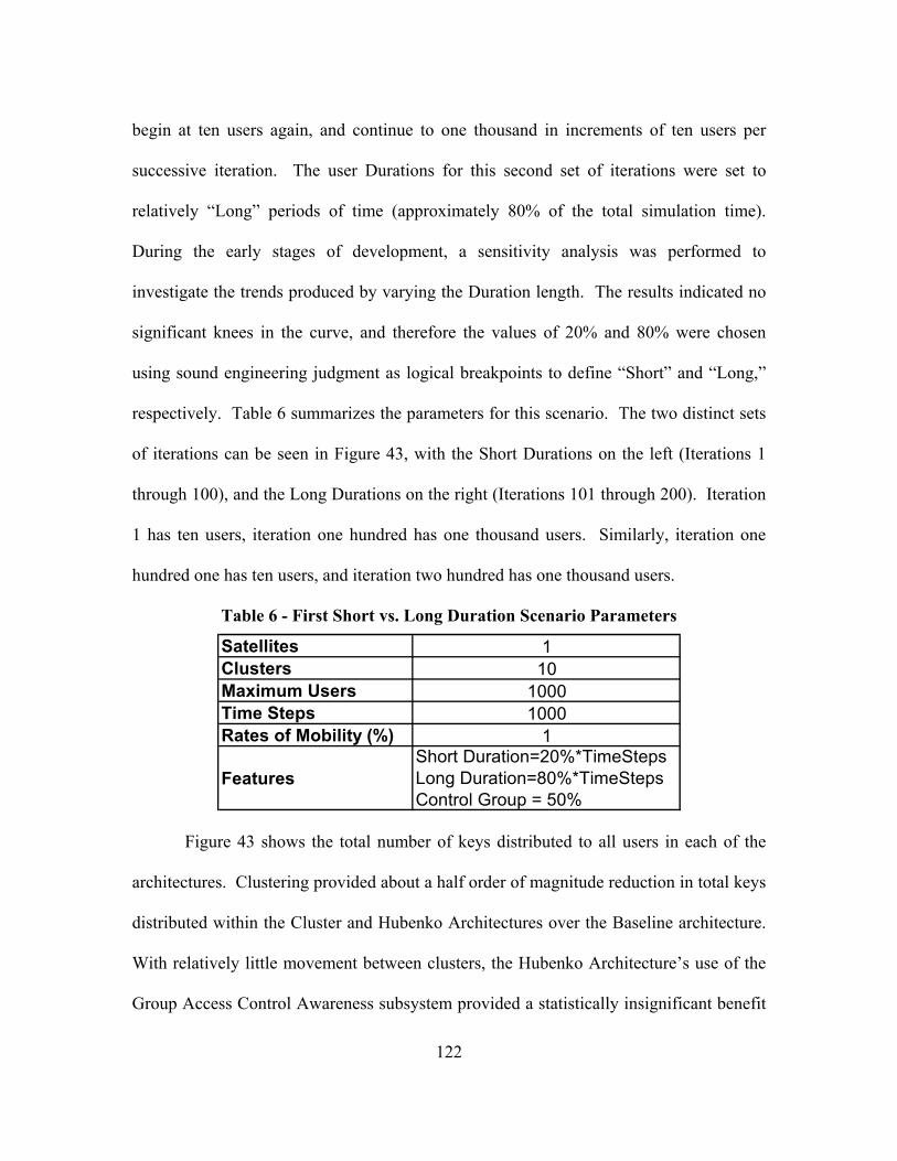
122

begin at ten users again, and continue to one thousand in increments of ten users per

successive iteration. The user Durations for this second set of iterations were set to

relatively “Long” periods of time (approximately 80% of the total simulation time).

During the early stages of development, a sensitivity analysis was performed to

investigate the trends produced by varying the Duration length. The results indicated no

significant knees in the curve, and therefore the values of 20% and 80% were chosen

using sound engineering judgment as logical breakpoints to define “Short” and “Long,”

respectively. Table 6 summarizes the parameters for this scenario. The two distinct sets

of iterations can be seen in Figure 43, with the Short Durations on the left (Iterations 1

through 100), and the Long Durations on the right (Iterations 101 through 200). Iteration

1 has ten users, iteration one hundred has one thousand users. Similarly, iteration one

hundred one has ten users, and iteration two hundred has one thousand users.

Table 6 - First Short vs. Long Duration Scenario Parameters

Satellites 1Clusters 10Maximum Users 1000Time Steps 1000Rates of Mobility (%) 1

FeaturesShort Duration=20%*TimeStepsLong Duration=80%*TimeStepsControl Group = 50%

Figure 43 shows the total number of keys distributed to all users in each of the

architectures. Clustering provided about a half order of magnitude reduction in total keys

distributed within the Cluster and Hubenko Architectures over the Baseline architecture.

With relatively little movement between clusters, the Hubenko Architecture’s use of the

Group Access Control Awareness subsystem provided a statistically insignificant benefit

123

over the Cluster architecture in the Short Duration iterations. The benefits of the GACA

subsystem emerged in the Long Duration iterations where there was slightly more

movement due to users being active long enough to make a slight impact. One percent

mobility was not sufficient to saturate the Baseline architecture with re-keying activity

since there is less than (number of users) x (one thousand time steps) total keys

distributed in each iteration.

0 20 40 60 80 100 120 140 160 180 200101

102

103

104

105

106

Iteration

Tota

l Key

s D

istri

bute

d in

the

Sys

tem

(log

sca

le)

IterFactor: 100, IterSteps: 1 RunVersion = Milcom Short Long Duration 1pct Mobile 2007 05 18 WS 20-May-2007 01:00:14

BaselineClusterHubenko

Short Duration Long Duration

0 20 40 60 80 100 120 140 160 180 200101

102

103

104

105

106

Iteration

Tota

l Key

s D

istri

bute

d in

the

Sys

tem

(log

sca

le)

IterFactor: 100, IterSteps: 1 RunVersion = Milcom Short Long Duration 1pct Mobile 2007 05 18 WS 20-May-2007 01:00:14

BaselineClusterHubenko

0 20 40 60 80 100 120 140 160 180 200101

102

103

104

105

106

Iteration

Tota

l Key

s D

istri

bute

d in

the

Sys

tem

(log

sca

le)

IterFactor: 100, IterSteps: 1 RunVersion = Milcom Short Long Duration 1pct Mobile 2007 05 18 WS 20-May-2007 01:00:14

BaselineClusterHubenko

Short Duration Long Duration(20% of the Time Steps) (80% of the Time Steps)

0 20 40 60 80 100 120 140 160 180 200101

102

103

104

105

106

Iteration

Tota

l Key

s D

istri

bute

d in

the

Sys

tem

(log

sca

le)

IterFactor: 100, IterSteps: 1 RunVersion = Milcom Short Long Duration 1pct Mobile 2007 05 18 WS 20-May-2007 01:00:14

BaselineClusterHubenko

Short Duration Long Duration

0 20 40 60 80 100 120 140 160 180 200101

102

103

104

105

106

Iteration

Tota

l Key

s D

istri

bute

d in

the

Sys

tem

(log

sca

le)

IterFactor: 100, IterSteps: 1 RunVersion = Milcom Short Long Duration 1pct Mobile 2007 05 18 WS 20-May-2007 01:00:14

BaselineClusterHubenko

0 20 40 60 80 100 120 140 160 180 200101

102

103

104

105

106

Iteration

Tota

l Key

s D

istri

bute

d in

the

Sys

tem

(log

sca

le)

IterFactor: 100, IterSteps: 1 RunVersion = Milcom Short Long Duration 1pct Mobile 2007 05 18 WS 20-May-2007 01:00:14

BaselineClusterHubenko

Short Duration Long Duration(20% of the Time Steps) (80% of the Time Steps)

Figure 43 - Total Keys Distributed - 1% Mobility (from 10 to 1000 Users, 1000 Time

Steps, Short versus Long Duration Scenario 1)

The three data lines on the left side of Figure 43 (iterations 1 through 100, “Short

Duration”) are relatively smooth since at most only 1% of the users were mobile, and

they were active for only a short time. This limited the overall mobility and therefore

124

variability across the iterations. The lines on the right side (iterations 101 through 200,

“Long Duration”) fluctuated more due to increased variability in the mobility between

iterations. The mobile users were not only active for longer periods of time, but the

speeds at which they moved between clusters varied based on the mobility category.

Therefore, if one iteration had five ground or sea users and only one aircraft, it would

have fewer movement triggers than an iteration with five aircraft users.

For the second Short versus Long Duration scenario, the number of users was

increased to 10,000, the number of time steps was increased to 10,000, and the Rate of

Mobility was increased to 50%. The control group size was held constant at 50% of the

total user population like the previous scenario. Therefore, the remaining 50% of the

users were randomly assigned to the three mobility categories. Table 7 summarizes the

parameters for this scenario.

Table 7 - Second Short vs. Long Duration Scenario Parameters

Satellites 1Clusters 10Maximum Users 10,000Time Steps 10,000Rates of Mobility (%) 50

FeaturesShort Duration=20%*TimeStepsLong Duration=80%*TimeStepsControl Group = 50%

The performance of the Cluster architecture thus far was following a trend of

saturating long before the Hubenko Architecture. In Figure 44, for example, with one

thousand users maximum simulated over one thousand time steps, with a 50% RoM.

Even with a relatively small user population, the Cluster architecture approaches

saturation, while the Hubenko Architecture performs at approximately one-ninth

125

capacity. Therefore, increasing the number of users and time steps will determine the

Hubenko performance under stress.

0 5 10 15 20 25 300

100

200

300

400

500

600

700

800

900

1000

Iteration

Aver

age

Tim

es R

ekey

ed

BaselineClusterHubenko

Short Duration(20% of the Time Steps)

Long Duration(80% of the Time Steps)

(Per

Use

r)

0 5 10 15 20 25 300

100

200

300

400

500

600

700

800

900

1000

Iteration

Aver

age

Tim

es R

ekey

ed

BaselineClusterHubenko

Short Duration(20% of the Time Steps)

Long Duration(80% of the Time Steps)

(Per

Use

r)

Figure 44 - Average Per-User Re-Key - 50% Mobility (from 10 to 1000 Users, 1000

Time Steps, Short versus Long Duration Scenario 1)

The apparent step increase that occurs in Iterations 16 through 30 is due to the

increased length of time a mobile user remains active. On average, they remain active

four times longer in the Long Duration than the Short Duration. Correspondingly, the

average re-keying experienced per user also increases an average of four times as

compared to the respective Short Duration iteration (e.g., Iterations 5 and 20 have the

same number of users).

126

Note the difference in the plots between Figure 43 and Figure 44. In preparation

for simulating a much larger user population for a much larger number of time steps, the

number of iterations is decreased (from 200 in Scenario 1 to 30 in Scenario 2). The

decrease was necessary to allow the simulations to complete in a reasonable amount of

time (measured in weeks). The decrease in step resolution, however, still produced

sufficient data points to analyze the trends and detect significant changes. Based on the

results from previous scenarios, the trends had only minor variations due to random

distributions as the population size grew. Little certainty, if any, is lost by the decrease in

granularity. Along with the increased user population and increased time steps, the

number of replications was increased from one simulation to three. Running three

replications of the 10,000 user simulations resulted in non-overlapping bounds at a 95%

confidence interval (illustrated as dotted lines of the same color surrounding the main

plot lines of interest). The scenarios with 2,000 or less users required a sample size of

five for non-overlapping confidence interval bounds, and therefore resulted in statistically

different performance for the different architectures. In the scenarios with 10,000 mobile

users, three replications generally yielded Coefficients of Variance of less than 0.1%.

Figure 45 demonstrates that the Short Duration iterations still do not have enough

event activity to saturate the Baseline architecture which is operating at only about one-

third capacity. However, the Long Duration iterations approach the maximum possible

total keys distributed (approximately 8,700 out of 10,000 possible). With increased

mobility, the Cluster architecture shows significant increases in total keys distributed for

both the Short and Long Durations from the 1% mobility scenario. Despite the benefits

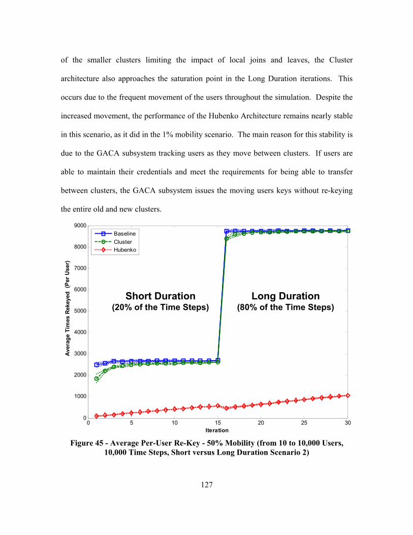
127

of the smaller clusters limiting the impact of local joins and leaves, the Cluster

architecture also approaches the saturation point in the Long Duration iterations. This

occurs due to the frequent movement of the users throughout the simulation. Despite the

increased movement, the performance of the Hubenko Architecture remains nearly stable

in this scenario, as it did in the 1% mobility scenario. The main reason for this stability is

due to the GACA subsystem tracking users as they move between clusters. If users are

able to maintain their credentials and meet the requirements for being able to transfer

between clusters, the GACA subsystem issues the moving users keys without re-keying

the entire old and new clusters.

0 5 10 15 20 25 300

1000

2000

3000

4000

5000

6000

7000

8000

9000

Iteration

Ave

rage

Tim

es R

ekey

ed

BaselineClusterHubenko

Short Duration(20% of the Time Steps)

Long Duration(80% of the Time Steps)

(Per

Use

r)

0 5 10 15 20 25 300

1000

2000

3000

4000

5000

6000

7000

8000

9000

Iteration

Ave

rage

Tim

es R

ekey

ed

BaselineClusterHubenko

Short Duration(20% of the Time Steps)

Long Duration(80% of the Time Steps)

(Per

Use

r)

Figure 45 - Average Per-User Re-Key - 50% Mobility (from 10 to 10,000 Users,

10,000 Time Steps, Short versus Long Duration Scenario 2)

128

The Total Keys Distributed count in Figure 46 demonstrates nearly an order of

magnitude fewer keys distributed between the Hubenko Architecture and the Baseline

and Cluster architectures at Iteration 30. Figure 46 shows all of the keys distributed for

each of the architectures in the second Short versus Long Duration scenario. The results

for the Cluster and Baseline key counts are statistically equivalent due to their

overlapping confidence interval bounds. The Hubenko Architecture, however, distributes

almost 80 million less keys to all users in the same span of time.

0 5 10 15 20 25 300

1

2

3

4

5

6

7

8

9

Iteration

Tota

l Key

s D

istri

bute

d in

the

Sys

tem

BaselineClusterHubenko

(x10

7 )

Short Duration(20% of the Time Steps)

Long Duration(80% of the Time Steps)

0 5 10 15 20 25 300

1

2

3

4

5

6

7

8

9

Iteration

Tota

l Key

s D

istri

bute

d in

the

Sys

tem

BaselineClusterHubenko

(x10

7 )

Short Duration(20% of the Time Steps)

Long Duration(80% of the Time Steps)

Figure 46 - Total Keys Distributed - All Users (from 10 to 10,000 Users, 10,000 Time

Steps, Short versus Long Duration Scenario 2)

Figure 47 shows the number of keys distributed to the Control Group (50% of the

user population). Since the Control Group persists for the entire simulation while the

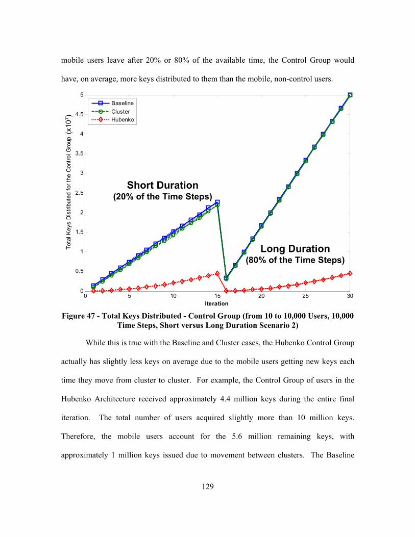
129

mobile users leave after 20% or 80% of the available time, the Control Group would

have, on average, more keys distributed to them than the mobile, non-control users.

0 5 10 15 20 25 300

0.5

1

1.5

2

2.5

3

3.5

4

4.5

5

Iteration

Tota

l Key

s D

istri

bute

d fo

r the

Con

trol G

roup

BaselineClusterHubenko

(x10

7 )

Short Duration(20% of the Time Steps)

Long Duration(80% of the Time Steps)

0 5 10 15 20 25 300

0.5

1

1.5

2

2.5

3

3.5

4

4.5

5

Iteration

Tota

l Key

s D

istri

bute

d fo

r the

Con

trol G

roup

BaselineClusterHubenko

(x10

7 )

Short Duration(20% of the Time Steps)

Long Duration(80% of the Time Steps)

Figure 47 - Total Keys Distributed - Control Group (from 10 to 10,000 Users, 10,000

Time Steps, Short versus Long Duration Scenario 2)

While this is true with the Baseline and Cluster cases, the Hubenko Control Group

actually has slightly less keys on average due to the mobile users getting new keys each

time they move from cluster to cluster. For example, the Control Group of users in the

Hubenko Architecture received approximately 4.4 million keys during the entire final

iteration. The total number of users acquired slightly more than 10 million keys.

Therefore, the mobile users account for the 5.6 million remaining keys, with

approximately 1 million keys issued due to movement between clusters. The Baseline

130

and Cluster architectures, on the other hand, have 50 million keys issued to the Control

Groups, but only about 37 million keys issued to the mobile users. Therefore,

implementing the Hubenko Architecture reduces the re-keying burden on the Control

Group as well as reducing the overall re-keying for the system. This reduced re-keying

overall enhances scalability and increases the efficiency of the system.

4.2.3 Increasing Aircraft over Stationary Users

This set of scenarios determines any reduction in re-keying for terrestrial-based

users provided by the Hubenko Architecture in a highly mobile environment. A Highly

Mobile Environment is a group of users in a network that collectively change satellite

spot beams often. These scenarios simulated a large population of terrestrial users with

several aircraft flying overhead, continuously moving between the clusters. The control

group size was held constant at 85% of the total user population, and their Duration lasts

for the entire number of time steps. The Control Group’s Mobility Category is Stationary

Users. The Duration for the remaining 15% of users is at Long (up to 80% of the total

possible time steps). Six iteration sets were run with increasing overall average mobility

as follows: 1%, 3%, 5%, 7%, 10%, and 15%. If a user is mobile, its mobility category is

set to Aircraft. The first scenario was run with 1,000 users for 1,000 time steps to

observe the behavior of the Cluster architecture in addition to the Hubenko Architecture.

Table 8 summarizes the scenario parameters. The sample size of five replications

prevents significant overlap in the confidence interval bounds of the three architectures

under the lower RoM. The second scenario was run with 10,000 users and 5,000 time

steps to demonstrate the performance of the Hubenko Architecture in a heavily populated

131

environment. Due to the significantly larger number of users and time steps, three

replications were sufficient.

Table 8 - Increasing Aircraft Parameters - Scenario 1

Satellites 1Clusters 10Maximum Users 1,000Time Steps 1,000Rates of Mobility (%) 1, 3, 5, 7, 10, 15

Features Control Group = 85%Mobile User Duration = Long

Observing the per-user average re-keying for all of the users in Figure 48, the

Baseline architecture quickly saturates in all but the first iteration set (1% mobility). The

Cluster architecture shows modest improvement under low mobility. By 7% mobility,

clustering alone is insufficient to prevent re-keying saturation. The Hubenko

Architecture provides the most stable operation in the heavily mobile environment, with

approximately one and a half orders of magnitude less average user re-keying. The slow

growth in the average number of re-keys in the respective iterations across the iteration

sets was due to the increasing amount of movement in the mobile user population.

By comparison, Figure 49 shows that the results are nearly identical for the

Control Group under all simulated RoM, as demonstrated by the same average re-keying

per user for each of the different RoM. This is due to the randomization of the mobile

users’ joins and departures that, with a uniform distribution, appear constant over the

course of numerous iterations. What is absent is the excessive re-keying caused by the

frequent movement of the mobile users due to the GACA-GKM sub-system. The trend is

similar for the Control Group results of the Total Keys Distributed, shown in Figure 51.

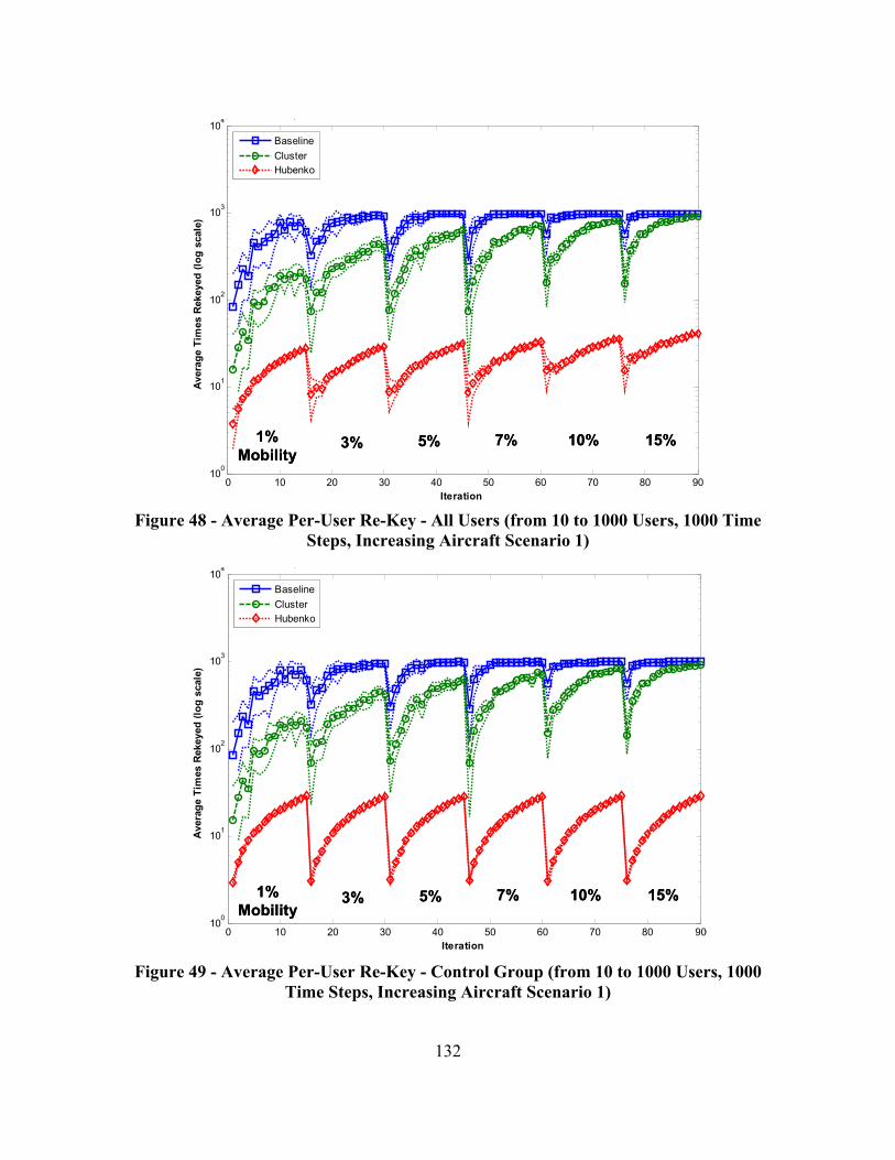
132

0 10 20 30 40 50 60 70 80 90100

101

102

103

104

Iteration

Aver

age

Tim

es R

ekey

ed (l

og s

cale

)

,

BaselineClusterHubenko

1%Mobility

3% 5% 7% 10% 15%

0 10 20 30 40 50 60 70 80 90100

101

102

103

104

Iteration

Aver

age

Tim

es R

ekey

ed (l

og s

cale

)

,

BaselineClusterHubenko

1%Mobility

3% 5% 7% 10% 15%1%Mobility

3% 5% 7% 10% 15%

Figure 48 - Average Per-User Re-Key - All Users (from 10 to 1000 Users, 1000 Time

Steps, Increasing Aircraft Scenario 1)

0 10 20 30 40 50 60 70 80 90100

101

102

103

104

Iteration

Ave

rage

Tim

es R

ekey

ed (l

og s

cale

)

,

BaselineClusterHubenko

1%Mobility

3% 5% 7% 10% 15%

0 10 20 30 40 50 60 70 80 90100

101

102

103

104

Iteration

Ave

rage

Tim

es R

ekey

ed (l

og s

cale

)

,

BaselineClusterHubenko

1%Mobility

3% 5% 7% 10% 15%1%Mobility

3% 5% 7% 10% 15%

Figure 49 - Average Per-User Re-Key - Control Group (from 10 to 1000 Users, 1000

Time Steps, Increasing Aircraft Scenario 1)

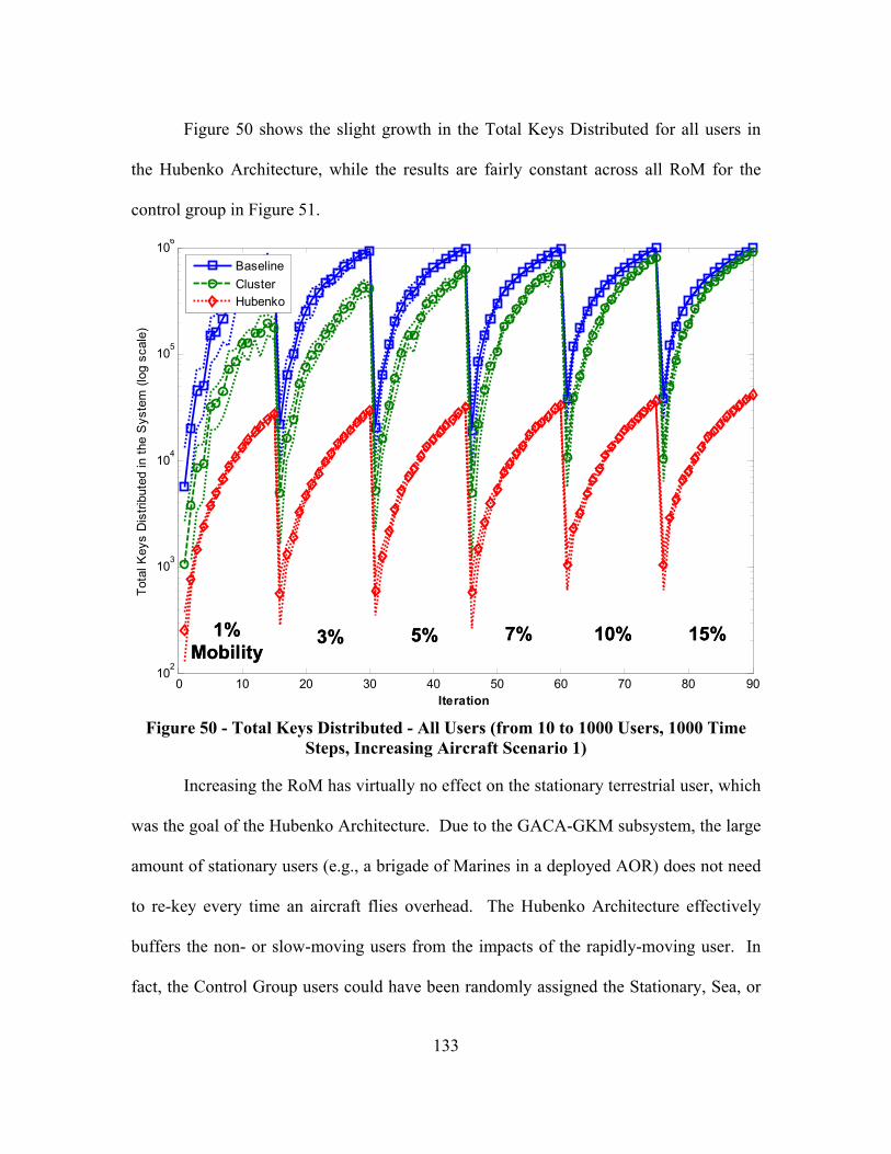
133

Figure 50 shows the slight growth in the Total Keys Distributed for all users in

the Hubenko Architecture, while the results are fairly constant across all RoM for the

control group in Figure 51.

0 10 20 30 40 50 60 70 80 90102

103

104

105

106

Iteration

Tota

l Key

s D

istri

bute

d in

the

Sys

tem

(log

sca

le)

BaselineClusterHubenko

1%Mobility

3% 5% 7% 10% 15%

0 10 20 30 40 50 60 70 80 90102

103

104

105

106

Iteration

Tota

l Key

s D

istri

bute

d in

the

Sys

tem

(log

sca

le)

BaselineClusterHubenko

1%Mobility

3% 5% 7% 10% 15%1%Mobility

3% 5% 7% 10% 15%

Figure 50 - Total Keys Distributed - All Users (from 10 to 1000 Users, 1000 Time

Steps, Increasing Aircraft Scenario 1)

Increasing the RoM has virtually no effect on the stationary terrestrial user, which

was the goal of the Hubenko Architecture. Due to the GACA-GKM subsystem, the large

amount of stationary users (e.g., a brigade of Marines in a deployed AOR) does not need

to re-key every time an aircraft flies overhead. The Hubenko Architecture effectively

buffers the non- or slow-moving users from the impacts of the rapidly-moving user. In

fact, the Control Group users could have been randomly assigned the Stationary, Sea, or

134

Ground Mobility Category instead of just Stationary, and the results would have been

approximately the same. There would be little change with the exception of the

additional keys incurred by the individual Control Group users moving from one cluster

to another. The Air users flying overhead would not induce any additional re-keying on

the non-stationary users, just as they induce no re-keying on the Stationary users

(assuming those fast-moving aircraft have the proper credentials such that the GACA-

GKM subsystem can transparently authenticate, validate, and authorize them into the new

clusters).

0 10 20 30 40 50 60 70 80 90102

103

104

105

106

Iteration

Tota

l Key

s D

istri

bute

d fo

r the

Con

trol G

roup

(log

sca

le)

BaselineClusterHubenko

1%Mobility

3% 5% 7% 10% 15%

0 10 20 30 40 50 60 70 80 90102

103

104

105

106

Iteration

Tota

l Key

s D

istri

bute

d fo

r the

Con

trol G

roup

(log

sca

le)

BaselineClusterHubenko

1%Mobility

3% 5% 7% 10% 15%1%Mobility

3% 5% 7% 10% 15%

Figure 51 - Total Keys Distributed - Control Group (from 10 to 1000 Users, 1000

Time Steps, Increasing Aircraft Scenario 1)

135

The Baseline architecture is saturated, and therefore no change is observed with

increased RoM. The Cluster architecture saturates on the higher number iterations within

each iteration set (the ones with a higher number of active users), and increasingly

approaches the saturation point in the iterations with lower RoM. The overall results

indicate that if the system designers implemented the Hubenko Architecture, terrestrial-

based users would experience reduced re-keying in environments where numerous

aircraft are flying overhead. If the Hubenko Architecture were not employed, each over-

flight would cause a re-key in the local cluster, thus increasing overhead and reducing

system efficiency and scalability.

In an effort to analyze the Hubenko Architecture under a higher user loading

level, Scenario 2 with 10,000 users for 5,000 time steps was executed. A sample size of

three replications was sufficient to generate statistically different results for the Baseline

and Cluster architectures, even for the 1% RoM. The parameters are summarized in

Table 9.

Table 9 - Increasing Aircraft Parameters - Scenario 2

Satellites 1Clusters 10Maximum Users 10,000Time Steps 5,000Rates of Mobility (%) 1, 3, 5, 7, 10, 15

Features Control Group = 85%Mobile User Duration = Long

As expected, the Cluster and Baseline architectures quickly saturate in the 3%

RoM and beyond, while the Hubenko Architecture experiences linear growth in the Total

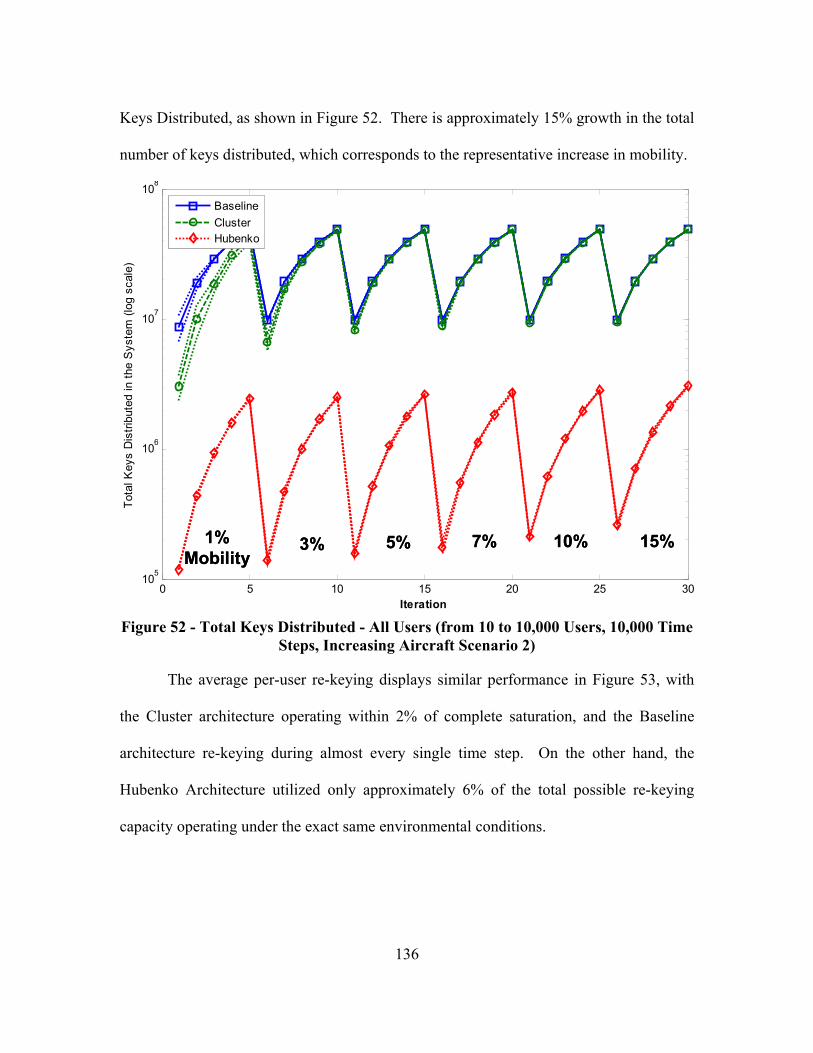
136

Keys Distributed, as shown in Figure 52. There is approximately 15% growth in the total

number of keys distributed, which corresponds to the representative increase in mobility.

0 5 10 15 20 25 30105

106

107

108

Iteration

Tota

l Key

s D

istri

bute

d in

the

Sys

tem

(log

sca

le)

BaselineClusterHubenko

1%Mobility

3% 5% 7% 10% 15%

0 5 10 15 20 25 30105

106

107

108

Iteration

Tota

l Key

s D

istri

bute

d in

the

Sys

tem

(log

sca

le)

BaselineClusterHubenko

1%Mobility

3% 5% 7% 10% 15%1%Mobility

3% 5% 7% 10% 15%

Figure 52 - Total Keys Distributed - All Users (from 10 to 10,000 Users, 10,000 Time

Steps, Increasing Aircraft Scenario 2)

The average per-user re-keying displays similar performance in Figure 53, with

the Cluster architecture operating within 2% of complete saturation, and the Baseline

architecture re-keying during almost every single time step. On the other hand, the

Hubenko Architecture utilized only approximately 6% of the total possible re-keying

capacity operating under the exact same environmental conditions.

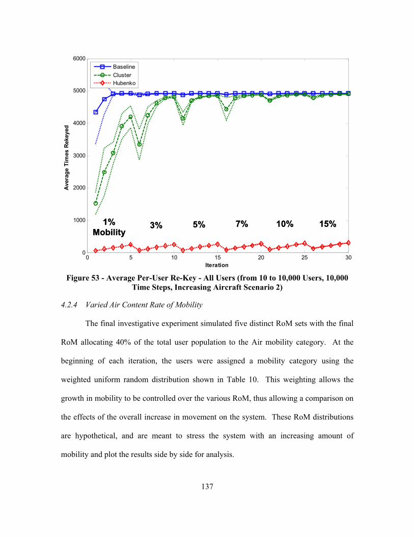
137

0 5 10 15 20 25 300

1000

2000

3000

4000

5000

6000

Iteration

Aver

age

Tim

es R

ekey

ed

BaselineClusterHubenko

1%Mobility

3% 5% 7% 10% 15%

0 5 10 15 20 25 300

1000

2000

3000

4000

5000

6000

Iteration

Aver

age

Tim

es R

ekey

ed

BaselineClusterHubenko

1%Mobility

3% 5% 7% 10% 15%1%Mobility

3% 5% 7% 10% 15%

Figure 53 - Average Per-User Re-Key - All Users (from 10 to 10,000 Users, 10,000

Time Steps, Increasing Aircraft Scenario 2)

4.2.4 Varied Air Content Rate of Mobility

The final investigative experiment simulated five distinct RoM sets with the final

RoM allocating 40% of the total user population to the Air mobility category. At the

beginning of each iteration, the users were assigned a mobility category using the

weighted uniform random distribution shown in Table 10. This weighting allows the

growth in mobility to be controlled over the various RoM, thus allowing a comparison on

the effects of the overall increase in movement on the system. These RoM distributions

are hypothetical, and are meant to stress the system with an increasing amount of

mobility and plot the results side by side for analysis.

138

Table 10 - Rates of Mobility (Varied Air Content)

Iteration User Type Demographics1 through 100 All Stationary101 through 200 ~1/2 Stationary, 1/2 Ground201 through 300 ~1/3 Stationary, Ground, Sea301 through 400 ~1/4 Stationary, Ground, Sea, Air401 through 500 ~1/5 Stationary, Ground, Sea; 2/5 Air

Within each RoM set, the user population is steadily increased from one through

one hundred average users per cluster, for a total maximum user population of 2,000

users. Table 11 summarizes the scenario parameters. This scenario analyzes the

Hubenko Architecture performance in a heavily mobile environment with increasing air

assets. This scenario had the heaviest amount of mobility of all the modeled scenarios,

with only 20% of the users stationary in the final RoM.

Table 11 - Varied Air Content RoM Parameters

SatellitesClustersMaximum UsersTime StepsRates of Mobility (%)

1 through 100 All Stationary101 through 200 ~1/2 Stationary, 1/2 Ground201 through 300 ~1/3 Stationary, Ground, Sea301 through 400 ~1/4 Stationary, Ground, Sea, Air401 through 500 ~1/5 Stationary, Ground, Sea; 2/5 Air

0, 50, 66, 75, 80

Features

210

20002000

Since there is no movement in the first iteration set (iterations 1 through 100 in

Figure 54), the GACA-GKM provides no additional benefit in the Hubenko system

compared to the Clustered system. The steady growth in re-keying for all three

architectures is due to the steady growth in overall number of active users in each system

and their respective joins and leaves.

139

0 50 100 150 200 250 300 350 400 450 5000

100

200

300

400

500

600

700

800

900

Iteration

Ave

rage

Tim

es R

ekey

ed

BaselineClusterHubenko

100% Stationary

50% Stationary/

50%Ground

33% Stationary/

Ground/Sea

25% Stationary/

Ground/Sea/Air

20% Stationary/

Ground/Sea;

40% Air

(Per

Use

r)

0 50 100 150 200 250 300 350 400 450 5000

100

200

300

400

500

600

700

800

900

Iteration

Ave

rage

Tim

es R

ekey

ed

BaselineClusterHubenko

100% Stationary

50% Stationary/

50%Ground

33% Stationary/

Ground/Sea

25% Stationary/

Ground/Sea/Air

20% Stationary/

Ground/Sea;

40% Air

(Per

Use

r)

Figure 54 - Per-User Average Re-Key Results - All Users (from 10 to 2000 Users,

2000 Time Steps, Varied Air Content Scenario)

As mobility increases from left to right in Figure 54, so does the amount of

average re-keying for the Baseline and Clustered architectures. The flat architecture

reaches its maximum due to the numerous joins and leaves throughout the system as early

as the 50% RoM with only the relatively slow moving Ground users. Beyond this level

of mobility, the re-keying only gets worse if the system is not already saturated.

The Clustered architecture, while performing under the saturation level in the first

three RoM, saturates in the 75% RoM. The Cluster architecture is able to avoid

saturation in the 50% and 66% RoM sets because the movers were relatively slow

(numerous time steps pass before the user moves to a new cluster). None of the mobile

users was the Air category. Therefore, while the overall RoM for this scenario was the

140

same or higher than the scenario RoM in Sections 4.2.2 and 4.2.3, the speed at which the

users changed clusters was considerably slower on average with no Air users.

Correspondingly, the per-user average re-keying experience was lower in this scenario

for the second and third RoM sets than in the previous scenarios. With the introduction

of the Air category of users in the fourth RoM (iterations 301 through 400), the Cluster

architecture once again saturates beyond an average cluster density of fifty users per

cluster. The same is also true when the RoM increases to 80% and the allocation of Air

users increases to 40%.

The Hubenko Architecture experiences a considerably smaller rate of increase in

per-user average re-keying in the respective RoM sets, clearly demonstrating the

combined benefits of the clustering and GACA-GKM features. Having a 50% mobile

user population only increases average re-keying 10% over the all stationary case

(iterations 1 through 100). This relatively small increase is due to the mobile users

changing clusters rather slowly, since none of the mobile users were rapidly moving

users. The 66% RoM has an increase of 15%; again a small increase due to the lack of

Air users in the RoM allocation. Increasing the RoM to 75% with 25% of the total user

population being allocated to the rapid moving user category (Air) increases the average

re-keying by about 50%. Similarly, increasing the RoM to 80% with 40% of the total

population becoming Air users increased the average re-keying by about 65% over the

stationary case. While this performance compared to the Stationary RoM appears

significantly impacted, comparing the Hubenko performance to the respective Cluster

performance demonstrates an improvement in re-keying performance. The true

141

performance increase is masked by the Cluster architecture saturating under the given

scenario parameters.

4.3 Performance Conclusions

Reducing the number of total keys distributed in each architecture to increase

scalability was one focus for this research, while minimizing the re-keying impact (and

hence increasing efficiency) for the individual terrestrial user was another.

4.3.1 Re-Keying Performance Results

First and foremost, regardless of the scenario, the Hubenko Architecture always

performed better than either the Cluster or the Baseline architectures. Table 12

summarizes the average re-keying counts of the individual users in the different

scenarios. The data is from the iteration of each scenario with the maximum number of

users simulated.

Table 12 - Per-User Average Re-Keying Summary

AllUsers

Control Group All Users

Control Group All Users

Control Group

Short 55 89 63 102 230 382Long 68 90 190 216 738 841Short 574 884 2,609 4,382 2,689 4,541Long 1,058 900 8,736 9,956 8,757 9,997

1% 244 259 4,206 4,248 4,921 4,9943% 254 259 4,818 4,876 4,926 4,9995% 264 260 4,859 4,921 4,924 4,9977% 274 260 4,883 4,949 4,925 4,99810% 288 259 4,897 4,964 4,927 4,99915% 309 257 4,906 4,976 4,926 4,999

85% Long 10,000 5,000

Baseline

50%1% 1,000 1,000

50% 10,000 10,000

ControlGroupSize

Rateof

Mobility DurationMax #Users

TimeSteps

Hubenko Cluster

For the first scenario with 1% RoM, there is an extremely low overall mobility.

In the Short duration iterations, All Users averaged less individual re-keying than the

Control Group because the non-control group was active for a relatively short time, and

therefore only re-keyed a few times. Only active users re-key. The Control Group, on

142

the other hand, was always active and so gathered many more keys. Averaging the two

groups together lowered the overall average number. There was very little change in the

Long duration iterations since there was very little movement overall.

In the 50% RoM scenario, the Short duration again produced a lower average re-

keying for All Users compared to the Control Group in the Hubenko Architecture for

similar reasons to the 1% RoM scenario. However, the Long duration had significantly

more movement for a longer period of time. Therefore, more keys were distributed, on

average, to All Users as compared to the Control Group. This occurred because each

individual mobile user would acquire a new key upon entry to a cluster (due to

movement, not a new Join), whereas the Control Group was stationary and did not gain

any more keys other than those which were assigned to the clusters as a whole (for a Join

or a Leave). The mobile users in the same clusters also receive a new key as well, and

therefore the net sum for that case is the same between the two groups. Comparing the

Long to the Short durations for the 50% RoM, the All Users average doubles while the

Control Group remains effectively the same. The difference between the two All Users

statistics is due to the increased individual movement. The difference between the two

Control Group statistics is due to the random distribution of Join and Leave times. The

number of time steps (i.e., 10,000) gives sufficient range for the users to individually join

and leave at different time steps. The difference of sixteen keys falls within the

confidence interval bounds at a 95% confidence level, and therefore the two results are

not different.

143

In the Increasing Aircraft scenario with the 85% Control Group size, extrapolating

the results gives the crossover point to be about 4% Rate of Mobility for the Control

Group and the All Users averages to be even, despite the 15/85 split in user population

size. With more than 4% RoM, however, the All Users average is larger than the Control

Group average due to the extra keys generated by the moving users. Compared to the

other scenarios, similar trends are observed as the overall RoM increases: the Control

Group averages remain statistically equivalent between RoM, and the All User average

increases as the RoM increases.

In all scenarios, the Hubenko Control Group average re-keying count was

virtually unaffected by increasing Rates of Mobility, which was the research goal of the

Hubenko Architecture. In contrast, the Control Group averages doubled for both the

Cluster and the Baseline architectures in the Short/Long scenarios. The number would

have been larger for the Cluster and the Baseline counts had those systems not saturated.

Using the same scenarios as above, Table 13 summarizes the Total Keys

Distributed for the three architectures. The first observation to note is that, unlike the

averages in Table 12, the All Users entries are always higher than the corresponding

Control Group entries. This is expected since the All Users value includes the key count

for the Control Group. The difference between the All Users value and the Control

Group value is the number of keys distributed to the mobile users in each of the

simulations.

144

Table 13 - Total Keys Distributed Summary

AllUsers

Control Group All Users

Control Group All Users

Control Group

Short 54,698 44,428 62,980 50,960 230,019 191,000Long 67,523 44,883 189,988 108,249 737,977 420,500Short 5,740,023 4,417,780 26,090,714 21,909,020 26,891,443 22,703,333Long 10,577,002 4,499,922 87,363,595 49,782,164 87,568,289 49,985,000

1% 2,444,874 2,200,596 42,055,851 36,107,938 49,214,102 42,449,0003% 2,536,541 2,200,724 48,179,126 41,450,189 49,257,760 42,488,6675% 2,638,523 2,206,712 48,593,570 41,831,655 49,244,917 42,471,6677% 2,742,361 2,208,028 48,830,033 42,069,857 49,251,433 42,485,83310% 2,877,280 2,201,124 48,965,305 42,190,781 49,268,474 42,491,50015% 3,087,913 2,185,256 49,057,807 42,293,289 49,257,078 42,491,500

ControlGroupSize

10,000 10,000

5,00010,000

50%50%

85% Long

BaselineClusterHubenko

1% 1,000 1,000

TimeSteps

Max #UsersDuration

Rateof

Mobility

In the 1% RoM scenario, with low mobility and short duration, the Hubenko

Architecture All Users count has 25% growth over the Control Group count. Although

50% of the total users were active at some point during the iteration, they were only

active for at most 20% of the total available number of Time Steps. This was not long

enough either to allow the mobile users to generate significant cluster activity, or to

collect numerous keys as they moved between clusters. Similarly, the key count for All

Users in the Long duration does not increase significantly. While those mobile users

were active for up to 80% of the total available time, the 1% mobility still limits the

potential number of keys that could have been generated. Even with the limited mobility,

the Hubenko Architecture collected one-third as many keys in the same iteration as the

Cluster architecture, and one-tenth as many as the Baseline architecture. Therefore, the

Hubenko Architecture begins to improve scalability and efficiency even with extremely

low mobility.

In the 50% RoM scenario, the Hubenko Architecture’s All Users key count

experiences a 30% growth over the Control Group key count for the Short Duration

iteration, and 135% growth for the Long Duration iteration. Comparing the same

statistics for the Cluster and Baseline architectures, they both experienced only 18% key

145

growth for the Short Duration, and only 76% key growth for the Long Duration. The

reason for the comparatively low percentage increases is that the two systems reached the

saturation points, as discussed earlier, and therefore the counts ceased to increase. The

efficiency and scalability benefits of the Hubenko Architecture are obvious when the total

counts of the three systems are compared. The Hubenko Architecture produced four and

a half times less keys overall for the Short Duration, and eight and a quarter times less

keys for the Long Duration. Again, if the model’s data element limitations could be

lifted, these numbers would have been even better.

The Hubenko Architecture has modest growth as the RoM steadily increases from

1% to 15% in the “Increasing Aircraft” scenario. The growth is strictly due to the mobile

users moving to new clusters and gathering new keys as they enter each new cluster

(assuming, of course, the users are properly authorized to do so). The results are similar

to the Per User Average Re-keying just discussed. With the exception of the 1% RoM,

there is no further increase in total key count in either the Cluster or Baseline architecture

for the increased RoM due to the saturation of those architectures.

Though the results were not tabularized, the performance in the “Varied Air

Content” scenario also demonstrates the superior performance of the Hubenko

Architecture, this time in an excessively (80%) mobile scenario. Even in the most mobile

case simulated in that scenario, the Hubenko Architecture still did not double the amount

of re-keying, while the Cluster and Baseline architectures saturated with the introduction

of the Air users.

146

4.3.2 Hubenko Saturation

In all simulated scenarios, the Hubenko Architecture outperformed the Baseline

and the Cluster architectures with fewer re-keys individually and at the system level. By

observing the trend of increased re-keying with increasing numbers of users, one can

predict that the Hubenko Architecture too will eventually saturate. Due to the two billion

data element limit of MatLab, however, it was not possible to simulate a scenario with

any appreciable length of time where the Hubenko Architecture saturates. This was

because of the need for very large numbers of users (e.g., in the “Varied Air Content”

scenario, beyond 50,000 users). At that point, though, there would no longer be any

benefit to implementing either a Hubenko or a Clustered architecture. Therefore, in the

case of an excessively saturated system, the simplest solution becomes the most efficient:

re-key the entire system simultaneously on a pre-determined scheduled that meets the

required security level. For any system loading less than this, however, the Hubenko

Architecture is the superior choice for systems with highly mobile users.

4.3.3 RoM Sensitivity

From the validation simulation (Section 3.11) where all users were set to

Stationary, and the 0% RoM iteration set in the Varied Air Content RoM scenario

(Section 4.2.4), it is clear that without movement, the Hubenko Architecture provides no

re-keying performance increase over the Cluster architecture. With the introduction of

mobility come the scalability and efficiency benefits provided by the Hubenko

Architecture.

147

In the Short versus Long Duration scenario with 1% RoM (Section 4.2.2), the

Short Duration iteration set demonstrated statistically insignificant differences in the

Cluster and Hubenko performances. This was due to the Short Duration parameter not

allowing the mobile users to move between clusters often enough to impact the re-keying

results. Keeping the RoM at 1% while increasing the Duration to Long yielded

approximately a half order of magnitude performance increase for the Hubenko

Architecture. Movement was not the only factor to influence the performance of the

Hubenko Architecture. Increasing the length of time that users were active increased the

amount of overall movement throughout the simulation led to the observation of the

increased re-keying performance in the Hubenko Architecture. Therefore, overall

movement is the main contributor to being able to discern the benefits of implementing

the Hubenko Architecture.

The results of the other scenarios corroborate this conclusion. In all simulated

scenarios, the more movement that occurred during the simulation, the better the

Hubenko Architecture performed compared to the Baseline and Cluster architectures.

The increase in movement could come from either an increase in the RoM (more users

moving throughout the simulation period), or an increase in the length of time the moving

users are allowed to move about, or the overall relative speeds at which the mobile users

are allowed to move. Consider the case shown in Figure 54. Iterations 101 through 200

have 50% Stationary/50% Ground users, and iterations 201 through 300 having one third

each Stationary, Ground, and Sea users. While the overall RoM for the sets are 50% and

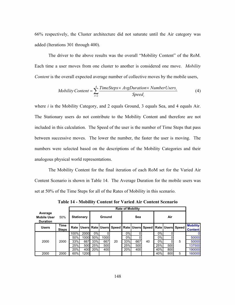
148

66% respectively, the Cluster architecture did not saturate until the Air category was

added (Iterations 301 through 400).

The driver to the above results was the overall “Mobility Content” of the RoM.

Each time a user moves from one cluster to another is considered one move. Mobility

Content is the overall expected average number of collective moves by the mobile users,

4

2

i

i i

TimeSteps AvgDuration NumberUsersMobility ContentSpeed=

× ×=∑ (4)

where i is the Mobility Category, and 2 equals Ground, 3 equals Sea, and 4 equals Air.

The Stationary users do not contribute to the Mobility Content and therefore are not

included in this calculation. The Speed of the user is the number of Time Steps that pass

between successive moves. The lower the number, the faster the user is moving. The

numbers were selected based on the descriptions of the Mobility Categories and their

analogous physical world representations.

The Mobility Content for the final iteration of each RoM set for the Varied Air

Content Scenario is shown in Table 14. The Average Duration for the mobile users was

set at 50% of the Time Steps for all of the Rates of Mobility in this scenario.

Table 14 - Mobility Content for Varied Air Content Scenario

Average Mobile User

Duration50%

Users Time Steps Rate Users Rate Users Speed Rate Users Speed Rate Users Speed Mobility

Content100% 2000 0% 0 0% 0 0% 0 050% 1000 50% 1000 0% 0 0% 0 5000033% 667 33% 667 33% 667 0% 0 5000025% 500 25% 500 25% 500 25% 500 13750020% 400 20% 400 20% 400 40% 800 190000

2000 2000 60% 1200 40% 800 5 160000

Air

Rate of Mobility

Stationary Ground Sea

20002000 20 540

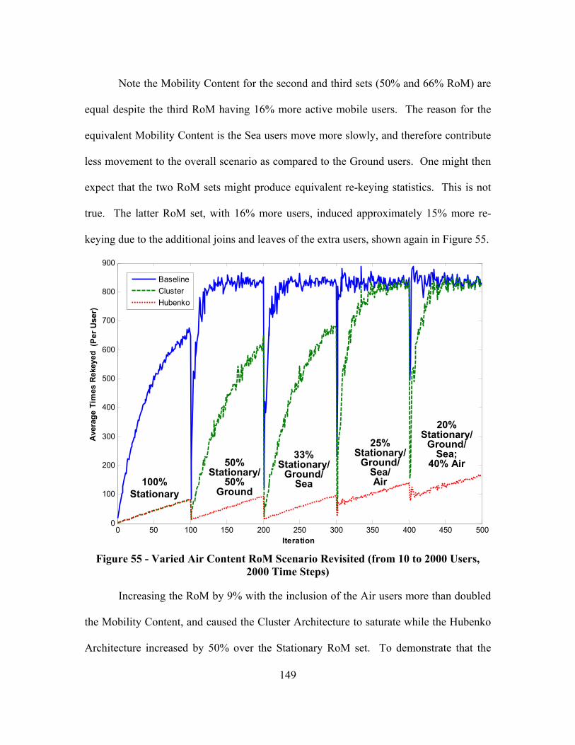
149

Note the Mobility Content for the second and third sets (50% and 66% RoM) are

equal despite the third RoM having 16% more active mobile users. The reason for the

equivalent Mobility Content is the Sea users move more slowly, and therefore contribute

less movement to the overall scenario as compared to the Ground users. One might then

expect that the two RoM sets might produce equivalent re-keying statistics. This is not

true. The latter RoM set, with 16% more users, induced approximately 15% more re-

keying due to the additional joins and leaves of the extra users, shown again in Figure 55.

0 50 100 150 200 250 300 350 400 450 5000

100

200

300

400

500

600

700

800

900

Iteration

Ave

rage

Tim

es R

ekey

ed

BaselineClusterHubenko

100% Stationary

50% Stationary/

50%Ground

33% Stationary/

Ground/Sea

25% Stationary/

Ground/Sea/Air

20% Stationary/

Ground/Sea;

40% Air

(Per

Use

r)

0 50 100 150 200 250 300 350 400 450 5000

100

200

300

400

500

600

700

800

900

Iteration

Ave

rage

Tim

es R

ekey

ed

BaselineClusterHubenko

100% Stationary

50% Stationary/

50%Ground

33% Stationary/

Ground/Sea

25% Stationary/

Ground/Sea/Air

20% Stationary/

Ground/Sea;

40% Air

(Per

Use

r)

Figure 55 - Varied Air Content RoM Scenario Revisited (from 10 to 2000 Users,

2000 Time Steps)

Increasing the RoM by 9% with the inclusion of the Air users more than doubled

the Mobility Content, and caused the Cluster Architecture to saturate while the Hubenko

Architecture increased by 50% over the Stationary RoM set. To demonstrate that the

150

main contributor to the Cluster’s saturation was the Air user, this scenario should have

included a RoM with 40% Air users and the rest Stationary. The last row in Table 14 is

the expected Mobility Content. The Cluster architecture would have saturated due to the

more than tripling of Mobility Content as compared to the 50% Ground RoM iteration.

Therefore, the main contributor to the increased re-keying is the Mobility Content of each

Scenario.

4.4 Analysis of Variance

In general, experiments are used to study the performance of processes and

systems. Experiments consist of several inputs, of which some variables are controllable,

and others are not. These inputs are processed by the system, and a response is observed.

To increase the fidelity of the system analysis, multiple replications of the same

experiment can be processed, and the observations recorded and analyzed. One method

of analyzing the data is through the Analysis of Variance, or ANOVA. This allows the

complexities of the numerous observations to be divided into manageable groups with

definable impacts on the system.

There are three main Factors that were controlled throughout the simulations:

Duration, RoM, and Number of Users. In the ANOVA analysis that follows, the three

factors each had three levels of input: Duration (0.2, 0.5, 0.8); RoM (25%, 50%, 75%);

and Number of Users (200, 600, 1000). Alone, each Factor may have an effect, or

Factors may combine through interactions.

In the following ANOVA tables, the observations are the total keys distributed for

the Baseline, Cluster, and Hubenko architectures, respectively. The raw data collected is

151

listed in Table 30. For the first ANOVA table, the Duration was held constant at 20% of

the available simulation time, giving the users a short period in which to interact. With

the Join Time held at 10% to ensure all users would be active at some point during each

simulation, having a Duration of 20% means all users will Join and Leave a multicast

group during the simulation. Therefore, the Joins and Leaves had more of an impact than

the amount of movement. Unfortunately, the amount of re-keying due to Joins and

Leaves versus the amount of re-keying due to movement was not captured during the

simulations, so there is no definite proof that this statement is true. However, observing

the F-statistics and the P-values the Summary ANOVA table in Table 15, we see that the

Number of Users in the Baseline architecture is a significant factor, while the RoM and

the interaction of the RoM and Number of Users are not. A significant factor at the 95%

confidence level is one having a P-value less than or equal to 0.05. For the Hubenko and

Cluster Architectures, where the systems are less sensitive to motion, both the Number of

Users and the RoM are significant factors, as well as their interactions.

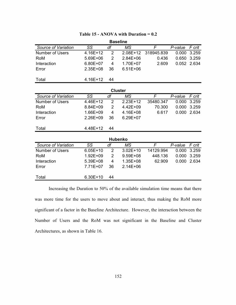
152

Table 15 - ANOVA with Duration = 0.2

Source of Variation SS df MS F P-value F critNumber of Users 4.16E+12 2 2.08E+12 318945.839 0.000 3.259RoM 5.69E+06 2 2.84E+06 0.436 0.650 3.259Interaction 6.80E+07 4 1.70E+07 2.609 0.052 2.634Error 2.35E+08 36 6.51E+06

Total 4.16E+12 44

Source of Variation SS df MS F P-value F critNumber of Users 4.46E+12 2 2.23E+12 35480.347 0.000 3.259RoM 8.84E+09 2 4.42E+09 70.300 0.000 3.259Interaction 1.66E+09 4 4.16E+08 6.617 0.000 2.634Error 2.26E+09 36 6.29E+07

Total 4.48E+12 44

Source of Variation SS df MS F P-value F critNumber of Users 6.05E+10 2 3.02E+10 14129.994 0.000 3.259RoM 1.92E+09 2 9.59E+08 448.136 0.000 3.259Interaction 5.39E+08 4 1.35E+08 62.909 0.000 2.634Error 7.71E+07 36 2.14E+06

Total 6.30E+10 44

Hubenko

Cluster

Baseline

Increasing the Duration to 50% of the available simulation time means that there

was more time for the users to move about and interact, thus making the RoM more

significant of a factor in the Baseline Architecture. However, the interaction between the

Number of Users and the RoM was not significant in the Baseline and Cluster

Architectures, as shown in Table 16.

153

Table 16 - ANOVA with Duration = 0.5

Source of Variation SS df MS F P-value F critNumber of Users 3.57E+12 2 1.79E+12 120246.946 0.000 3.259RoM 1.91E+08 2 9.56E+07 6.430 0.004 3.259Interaction 2.04E+08 4 5.11E+07 3.439 0.018 2.634Error 5.35E+08 36 1.49E+07

Total 3.57E+12 44

Source of Variation SS df MS F P-value F critNumber of Users 3.67E+12 2 1.84E+12 39613.784 0.000 3.259RoM 1.35E+10 2 6.73E+09 145.058 0.000 3.259Interaction 4.59E+08 4 1.15E+08 2.472 0.062 2.634Error 1.67E+09 36 4.64E+07

Total 3.69E+12 44

Source of Variation SS df MS F P-value F critNumber of Users 5.71E+10 2 2.86E+10 15831.566 0.000 3.259RoM 1.24E+09 2 6.19E+08 342.914 0.000 3.259Interaction 3.46E+08 4 8.65E+07 47.939 0.000 2.634Error 6.50E+07 36 1.80E+06

Total 5.88E+10 44

Cluster

Hubenko

Baseline

Finally, the Duration was increased to 80%, and the Number of Users and the

RoM were significant factors for all three architectures. The interactions, however, were

only significant for the Hubenko Architecture, as shown in Table 17.

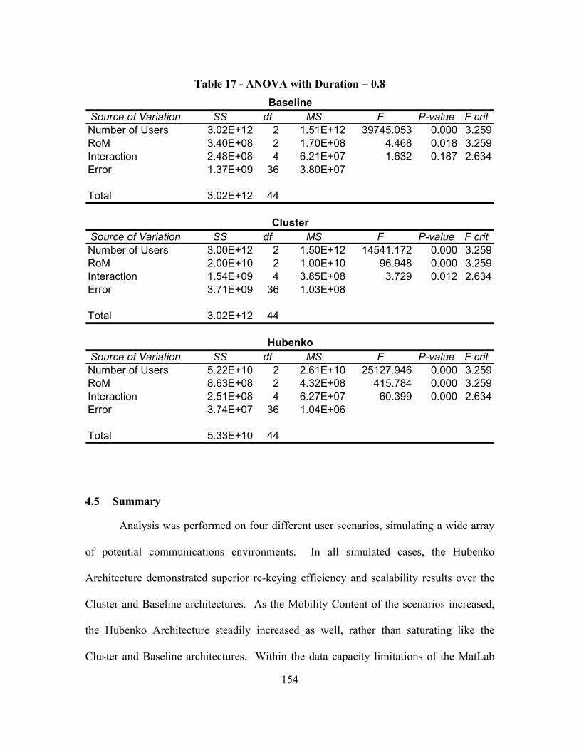
154

Table 17 - ANOVA with Duration = 0.8

Source of Variation SS df MS F P-value F critNumber of Users 3.02E+12 2 1.51E+12 39745.053 0.000 3.259RoM 3.40E+08 2 1.70E+08 4.468 0.018 3.259Interaction 2.48E+08 4 6.21E+07 1.632 0.187 2.634Error 1.37E+09 36 3.80E+07

Total 3.02E+12 44

Source of Variation SS df MS F P-value F critNumber of Users 3.00E+12 2 1.50E+12 14541.172 0.000 3.259RoM 2.00E+10 2 1.00E+10 96.948 0.000 3.259Interaction 1.54E+09 4 3.85E+08 3.729 0.012 2.634Error 3.71E+09 36 1.03E+08

Total 3.02E+12 44

Source of Variation SS df MS F P-value F critNumber of Users 5.22E+10 2 2.61E+10 25127.946 0.000 3.259RoM 8.63E+08 2 4.32E+08 415.784 0.000 3.259Interaction 2.51E+08 4 6.27E+07 60.399 0.000 2.634Error 3.74E+07 36 1.04E+06

Total 5.33E+10 44

Hubenko

Baseline

Cluster

4.5 Summary

Analysis was performed on four different user scenarios, simulating a wide array

of potential communications environments. In all simulated cases, the Hubenko

Architecture demonstrated superior re-keying efficiency and scalability results over the

Cluster and Baseline architectures. As the Mobility Content of the scenarios increased,

the Hubenko Architecture steadily increased as well, rather than saturating like the

Cluster and Baseline architectures. Within the data capacity limitations of the MatLab

155

software operating on a Windows platform, the Hubenko Architecture could not be

saturated, whereas the Cluster and Baseline architectures readily saturated with moderate

Mobility Content. The primary objective of the Hubenko Architecture was achieved, as

shown by the minimal re-keying impact on the Control Group users when numerous

rapidly moving users were present in the system.

156

V. Conclusion

5.1 Summary of Research

Relatively few research efforts are aimed at securing group communications while

scaling well to large groups of highly mobile users. A few of the architectures noted in

Chapter II contribute pieces to an overall framework for secure group communications in

a multicast network. None of the research, though, specifically addressed a LEOsat

network environment, nor do they completely address the issues facing a global, highly

mobile user base dependent on a LEO communications satellite system as their best

means for infrastructure.

After a rigorous search through the literature to survey the history and determine

the state-of-the-art of satellite multicasting and secure group communications, this

research provides an efficient and scalable secure multicasting in the LEO satellite

network environment by developing the novel “Hubenko Security Framework

Architecture.”

This research develops and analyzes the Baseline, Cluster, and Hubenko

Architectures in multiple mobile communication environment scenarios, and consistently

demonstrates the superior re-keying advantage offered by the “Hubenko Security

Framework Architecture.”

This research was the basis for several publications, as noted in Section 5.3.

Further, this research has been used in the development of an application of the Hubenko

Architecture to the unmanned aerial vehicle environment at the Master’s degree level.

157

5.2 Research Contributions

In today’s highly mobile world of deployed communications, security and

efficiency are critical requirements that must be met. Employing a security scheme that

negatively impacts the user’s network experience is undesirable. Leveraging multicast

architectures that provide disparate scalability benefits in non-mobile environments, the

Hubenko Architecture provides efficient security in a mobile multicast environment using

a low earth orbit satellite-based infrastructure. The aforementioned simulations

demonstrate the Hubenko Architecture’s results in significantly less re-keying for both

the individual user and the overall system. Less re-keying means less system overhead

which corresponds to better network throughput and lower mean delay. An example of

the increased efficiency is the 835% reduction of individual re-keying in the Varied Air

Content scenario. An example of the increased scalability is the Hubenko Architecture

operating at 22% capacity with four times the number of users that caused the Cluster

architecture to saturate.

This research produced a novel architecture that can be applied to numerous

group communications environments to reduce the re-keying overhead (increased

efficiency) and increase the number of supportable users (increased scalability).

Increased efficiency means smaller devices that are battery-dependent can re-key less

often, which translates to longer battery life for performing more sensing operations.

Users in the field connected via low-rate secure links will effectively have more

bandwidth due to less time wasted on repeatedly transferring new keys. Larger numbers

of supportable users means the network can support a larger number of sensors, or

accommodate an order of magnitude of more users in the same network.

158

5.3 Publications

The number of refereed publications in international journals and conference

proceedings demonstrates the novelty of this research. To date, five papers have been

published including two journal articles [HuR06a, HuR06b, HuR07a, HuR07b, HuR08].

Specific titles and publication venues are listed at the end of this chapter.

5.4 Recommendations for Future Research

5.4.1 Adapt Hubenko Security Framework Architecture to Other Environments

With relatively minor adjustments, the Hubenko Architecture can be applied to

several other areas of communications, namely unmanned aerial vehicle (UAV) swarms,

wireless sensor networks (WSN), and mobile ad hoc networks. Master’s level research is

currently underway in applying the Hubenko Architecture to a UAV environment, with a

goal of assessing battery life and communications overhead performance gains.

Additionally, the Hubenko Architecture could be applied to wireless sensor

networks in a heterogeneous environment to reduce the amount of re-keying on the WSN

when mobile units pass through the WSN field. Another potential application is to use an

Air Battle Node instead of a LEO satellite network. This would bring the main

infrastructure closer to the tactical theater network, reducing propagation delays even

more.

5.4.2 Incorporate Features from the Integrated Architecture Concept

Another area of potential interest for increasing system scalability and efficiency

makes use of the “integrated architecture” concept from [AmN05]. This concept

removes some of the security processing burden from the users, as shown in Figure 56.

By centralizing the key agreement and distribution across the satellite group versus the

159

user group, a further increase in system scalability should be achieved due to less

processing requirements being placed on the end users. Incidentally, a corollary benefit

from implementing the integrated architecture is the potential for bringing the GIG’s

“Power to the Edge” by allowing the end users to upload heavyweight processing tasks to

the satellites for computation. The radio frequency propagation time for the user to send

data to the LEO system and receive a reply (a single round trip; up once and down once)

is between 1.33 and 13.33 milliseconds. This shifts ground-based processing tasks

performed by deployed tactical users to more capable orbital resources. This corollary is

based on the assumption that the next generation LEO satellite system processes and

downloads large amounts of data more quickly than the tactical ground system and

independently of satellite handoff delays. Leveraging the capabilities of the satellite

infrastructure to perform the “heavy lifting” computations for reduced-capability mobile

terrestrial users is a potential benefit inherent in the overall system with minimal

adaptation required.

160

1 4

7

3

5 8

11

6

9 12

1413 15 16

A DCB E HGF

LL LL LL LLV VV

Security Processing

Key Generation

Offload heavy processing

requirements to satellites

102

Figure 56 - Integrated Architecture Services Added

5.4.3 Re-establish Original LEOSat Baseline with Hubenko Architecture

With the Hubenko Security Framework Architecture complete, a port of the

MatLab simulations to the OPNET [OPN06] environment for more detailed analysis at

the packet level would be beneficial. One could re-investigate the End-to-End, Received-

to-Sent, and Data-to-Overhead ratio performance with a more detailed packet- and

system-level analysis of the architecture.

161

Publications

Published (5):

[HuR06a] Hubenko Jr., Victor P., Richard A. Raines, Michael A. Temple, Robert F. Mills, and Mark D. Saeger, "Adaptation, Modeling, and Analysis of PIM-DM in a LEO Satellite Network Environment," Proceedings of the IEEE Aerospace Conference, Big Sky, Montana, 2006.

[HuR06b] Hubenko Jr., Victor P., Richard A. Raines, Robert F. Mills, Rusty O. Baldwin, Barry E. Mullins, and Michael R. Grimaila, "Improving the Global Information Grid’s Performance Through Satellite Communications Layer Enhancements," IEEE Communications, vol. 44, no. 11, pp. 66-72, 2006. (Approximately 5% Acceptance Rate)

[HuR07a] Hubenko Jr., Victor P., Richard A. Raines, Rusty O. Baldwin, Barry E. Mullins, Robert F. Mills, and Michael R. Grimaila, "Improving Satellite Multicast Security Scalability by Reducing Re-keying Requirements," IEEE Network, vol. 21, no. 4, pp. 51-56, 2007. (Approximately 5% Acceptance Rate)

[HuR07b] Hubenko Jr., Victor P., Richard A. Raines, Rusty O. Baldwin, Barry E. Mullins, Robert F. Mills, and Michael R. Grimaila, "Applying a Secure and Efficient Low Earth Orbit Satellite-Based Multicast Architecture in a Deployed Environment," Proceedings of the MILCOM 2007, pp. 1-7, Orlando, Florida, 2007

[HuR08] Hubenko Jr., Victor P., Richard A. Raines, Rusty O. Baldwin, Barry E. Mullins, Robert F. Mills, and Michael R. Grimaila, "A Secure and Efficient Satellite-based Multicast Architecture," Proceedings of the IEEE Radio and Wireless Symposium, pp. 227-230, Orlando, Florida, 2008 (Winner, Third Best Student Paper)

162

VI. Appendix

This section presents the raw data tables and a printout of the MatLab code. The

only tables included here are for the three scenarios that had thirty iterations. Due to their

large size, each of the tables for the other scenarios, with ninety or more iterations, are

available in softcopy. A sample printout of the MatLab code is also attached in this

section. Numerous versions of the code were used throughout development. Within each

version, the outer loops of the code (illustrated in Figure 24) were modified as needed to

accommodate the parameter changes for each scenario. The core architectural portion of

the code, however, was not modified after verification and validation, and was carried

through in each version unaltered.

163

6.1 Short versus Long Duration Scenario 1 (Section 4.2.2)

Table 18 - Total Keys Distributed (All Users, Short vs. Long Duration Scenario 1)

Iteration Baseline Cluster Hubenko Baseline Cluster Hubenko Baseline Cluster Hubenko1 0.1134 0.0785 0.0446 1,148 221 30 10,131 2,818 6622 0.1649 0.2358 0.0892 4,482 2,340 164 27,178 9,923 1,8423 0.0345 0.0932 0.0389 1,582 1,801 136 45,889 19,324 3,4854 0.0351 0.0553 0.0190 2,268 1,781 107 64,630 32,198 5,6505 0.0168 0.0287 0.0230 1,370 1,264 185 81,764 43,979 8,0406 0.0313 0.0364 0.0131 3,069 2,247 150 98,073 61,804 11,5067 0.0423 0.0707 0.0080 4,870 5,195 118 115,201 73,432 14,7438 0.0150 0.0366 0.0117 2,012 3,280 221 133,960 89,656 18,8349 0.0299 0.0261 0.0111 4,523 2,765 254 151,078 105,908 22,916

10 0.0192 0.0321 0.0215 3,304 4,091 610 171,998 127,295 28,31311 0.0243 0.0287 0.0055 4,564 4,125 183 187,664 143,656 33,33112 0.0188 0.0208 0.0110 3,877 3,350 427 206,772 160,803 38,71213 0.0076 0.0377 0.0143 1,691 6,596 630 223,545 175,030 44,09914 0.0111 0.0283 0.0059 2,734 5,685 306 247,133 200,620 51,57215 0.0065 0.0188 0.0077 1,687 4,076 443 261,293 216,475 57,76716 0.1329 0.2125 0.2180 6,632 5,419 688 49,913 25,495 3,15617 0.0173 0.0446 0.0337 1,974 3,333 215 114,203 74,794 6,38918 0.0025 0.0355 0.0380 430 4,784 418 171,567 134,790 11,00419 0.0067 0.0203 0.0224 1,555 4,074 364 230,844 200,323 16,26820 0.0092 0.0379 0.0459 2,677 9,747 979 290,027 257,069 21,31121 0.0062 0.0138 0.0469 2,162 4,483 1,345 348,178 324,141 28,68822 0.0037 0.0122 0.0341 1,521 4,699 1,274 406,813 385,056 37,31623 0.0006 0.0070 0.0179 270 3,116 765 465,786 442,460 42,65424 0.0022 0.0015 0.0370 1,168 747 1,807 522,956 497,912 48,76025 0.0022 0.0040 0.0341 1,309 2,257 2,031 584,313 563,508 59,51126 0.0008 0.0047 0.0235 486 2,904 1,565 642,065 621,087 66,61727 0.0022 0.0007 0.0254 1,540 459 1,903 697,785 674,657 74,85928 0.0025 0.0049 0.0111 1,925 3,599 952 756,834 733,793 86,07729 0.0039 0.0057 0.0038 3,230 4,519 369 818,866 799,647 96,53130 0.0004 0.0031 0.0105 366 2,617 1,115 874,995 853,895 106,548

Coeff of Variance Sample Standard Dev Mean

164

Table 19 - Total Keys Distributed (Control Group Users, Short vs. Long Duration Scenario 1)

Iteration Baseline Cluster Hubenko Baseline Cluster Hubenko Baseline Cluster Hubenko1 0.1185 0.0739 0.0520 963 150 14 8,129 2,034 2632 0.1646 0.2328 0.0381 3,628 1,769 37 22,043 7,599 9713 0.0394 0.0979 0.0049 1,480 1,489 10 37,600 15,203 2,0584 0.0389 0.0601 0.0147 2,066 1,539 53 53,111 25,594 3,5845 0.0281 0.0155 0.0134 1,899 547 72 67,691 35,251 5,3866 0.0246 0.0304 0.0082 2,000 1,518 65 81,400 49,887 7,8877 0.0444 0.0718 0.0079 4,252 4,250 82 95,763 59,196 10,3918 0.0239 0.0364 0.0021 2,674 2,653 29 112,051 72,860 13,6629 0.0359 0.0317 0.0102 4,543 2,741 172 126,400 86,420 16,919

10 0.0200 0.0325 0.0180 2,884 3,366 376 143,856 103,631 20,87211 0.0302 0.0387 0.0160 4,733 4,533 398 156,831 117,220 24,87212 0.0194 0.0232 0.0159 3,355 3,056 465 173,067 131,829 29,26613 0.0127 0.0373 0.0170 2,385 5,372 574 188,211 144,196 33,71514 0.0091 0.0261 0.0161 1,887 4,321 637 208,126 165,638 39,61415 0.0068 0.0251 0.0068 1,500 4,457 301 219,000 177,836 44,38816 0.1251 0.2180 0.0247 3,363 2,770 7 26,884 12,708 26317 0.0153 0.0439 0.0031 981 1,736 3 64,030 39,554 92718 0.0052 0.0327 0.0243 503 2,380 49 97,167 72,692 2,02219 0.0047 0.0204 0.0089 609 2,208 31 130,473 108,280 3,47920 0.0047 0.0376 0.0094 771 5,275 52 164,606 140,387 5,55921 0.0048 0.0181 0.0074 945 3,243 58 197,733 178,941 7,79122 0.0020 0.0105 0.0055 466 2,249 59 231,602 213,295 10,65623 0.0020 0.0086 0.0129 534 2,106 175 265,131 245,582 13,60124 0.0012 0.0038 0.0109 346 1,058 187 298,300 276,737 17,14625 0.0015 0.0049 0.0224 509 1,534 473 331,779 313,363 21,11526 0.0025 0.0061 0.0137 924 2,099 343 365,410 346,826 25,05227 0.0015 0.0032 0.0098 611 1,206 291 397,867 377,165 29,70328 0.0025 0.0066 0.0150 1,090 2,729 518 431,124 410,427 34,51429 0.0006 0.0026 0.0147 270 1,160 582 465,755 448,308 39,58630 0.0006 0.0038 0.0070 289 1,812 315 499,167 479,751 45,032

Coeff of Variance Sample Standard Dev Mean

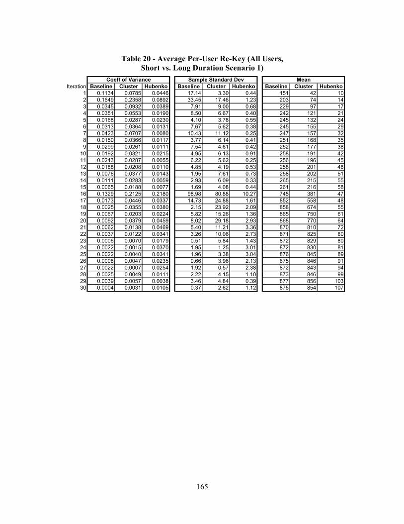
165

Table 20 - Average Per-User Re-Key (All Users, Short vs. Long Duration Scenario 1)

Iteration Baseline Cluster Hubenko Baseline Cluster Hubenko Baseline Cluster Hubenko1 0.1134 0.0785 0.0446 17.14 3.30 0.44 151 42 102 0.1649 0.2358 0.0892 33.45 17.46 1.23 203 74 143 0.0345 0.0932 0.0389 7.91 9.00 0.68 229 97 174 0.0351 0.0553 0.0190 8.50 6.67 0.40 242 121 215 0.0168 0.0287 0.0230 4.10 3.78 0.55 245 132 246 0.0313 0.0364 0.0131 7.67 5.62 0.38 245 155 297 0.0423 0.0707 0.0080 10.43 11.12 0.25 247 157 328 0.0150 0.0366 0.0117 3.77 6.14 0.41 251 168 359 0.0299 0.0261 0.0111 7.54 4.61 0.42 252 177 38

10 0.0192 0.0321 0.0215 4.95 6.13 0.91 258 191 4211 0.0243 0.0287 0.0055 6.22 5.62 0.25 256 196 4512 0.0188 0.0208 0.0110 4.85 4.19 0.53 258 201 4813 0.0076 0.0377 0.0143 1.95 7.61 0.73 258 202 5114 0.0111 0.0283 0.0059 2.93 6.09 0.33 265 215 5515 0.0065 0.0188 0.0077 1.69 4.08 0.44 261 216 5816 0.1329 0.2125 0.2180 98.98 80.88 10.27 745 381 4717 0.0173 0.0446 0.0337 14.73 24.88 1.61 852 558 4818 0.0025 0.0355 0.0380 2.15 23.92 2.09 858 674 5519 0.0067 0.0203 0.0224 5.82 15.26 1.36 865 750 6120 0.0092 0.0379 0.0459 8.02 29.18 2.93 868 770 6421 0.0062 0.0138 0.0469 5.40 11.21 3.36 870 810 7222 0.0037 0.0122 0.0341 3.26 10.06 2.73 871 825 8023 0.0006 0.0070 0.0179 0.51 5.84 1.43 872 829 8024 0.0022 0.0015 0.0370 1.95 1.25 3.01 872 830 8125 0.0022 0.0040 0.0341 1.96 3.38 3.04 876 845 8926 0.0008 0.0047 0.0235 0.66 3.96 2.13 875 846 9127 0.0022 0.0007 0.0254 1.92 0.57 2.38 872 843 9428 0.0025 0.0049 0.0111 2.22 4.15 1.10 873 846 9929 0.0039 0.0057 0.0038 3.46 4.84 0.39 877 856 10330 0.0004 0.0031 0.0105 0.37 2.62 1.12 875 854 107

Coeff of Variance Sample Standard Dev Mean

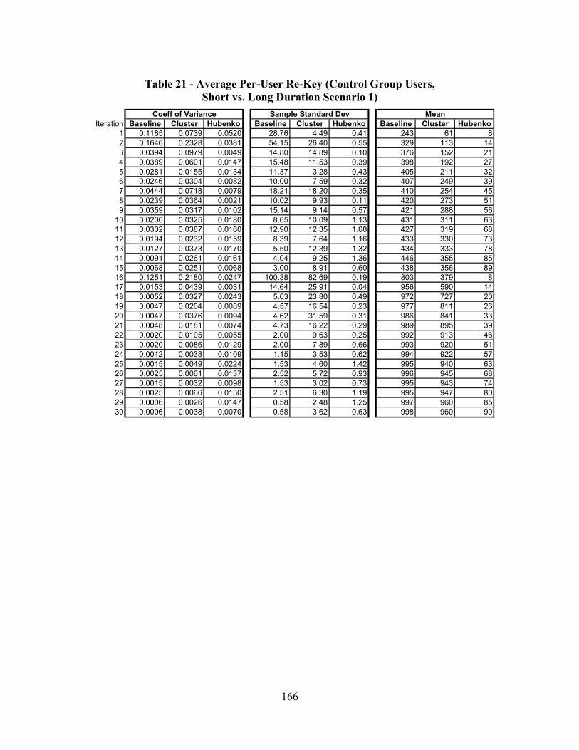
166

Table 21 - Average Per-User Re-Key (Control Group Users, Short vs. Long Duration Scenario 1)

Iteration Baseline Cluster Hubenko Baseline Cluster Hubenko Baseline Cluster Hubenko1 0.1185 0.0739 0.0520 28.76 4.49 0.41 243 61 82 0.1646 0.2328 0.0381 54.15 26.40 0.55 329 113 143 0.0394 0.0979 0.0049 14.80 14.89 0.10 376 152 214 0.0389 0.0601 0.0147 15.48 11.53 0.39 398 192 275 0.0281 0.0155 0.0134 11.37 3.28 0.43 405 211 326 0.0246 0.0304 0.0082 10.00 7.59 0.32 407 249 397 0.0444 0.0718 0.0079 18.21 18.20 0.35 410 254 458 0.0239 0.0364 0.0021 10.02 9.93 0.11 420 273 519 0.0359 0.0317 0.0102 15.14 9.14 0.57 421 288 56

10 0.0200 0.0325 0.0180 8.65 10.09 1.13 431 311 6311 0.0302 0.0387 0.0160 12.90 12.35 1.08 427 319 6812 0.0194 0.0232 0.0159 8.39 7.64 1.16 433 330 7313 0.0127 0.0373 0.0170 5.50 12.39 1.32 434 333 7814 0.0091 0.0261 0.0161 4.04 9.25 1.36 446 355 8515 0.0068 0.0251 0.0068 3.00 8.91 0.60 438 356 8916 0.1251 0.2180 0.0247 100.38 82.69 0.19 803 379 817 0.0153 0.0439 0.0031 14.64 25.91 0.04 956 590 1418 0.0052 0.0327 0.0243 5.03 23.80 0.49 972 727 2019 0.0047 0.0204 0.0089 4.57 16.54 0.23 977 811 2620 0.0047 0.0376 0.0094 4.62 31.59 0.31 986 841 3321 0.0048 0.0181 0.0074 4.73 16.22 0.29 989 895 3922 0.0020 0.0105 0.0055 2.00 9.63 0.25 992 913 4623 0.0020 0.0086 0.0129 2.00 7.89 0.66 993 920 5124 0.0012 0.0038 0.0109 1.15 3.53 0.62 994 922 5725 0.0015 0.0049 0.0224 1.53 4.60 1.42 995 940 6326 0.0025 0.0061 0.0137 2.52 5.72 0.93 996 945 6827 0.0015 0.0032 0.0098 1.53 3.02 0.73 995 943 7428 0.0025 0.0066 0.0150 2.51 6.30 1.19 995 947 8029 0.0006 0.0026 0.0147 0.58 2.48 1.25 997 960 8530 0.0006 0.0038 0.0070 0.58 3.62 0.63 998 960 90

Coeff of Variance Sample Standard Dev Mean

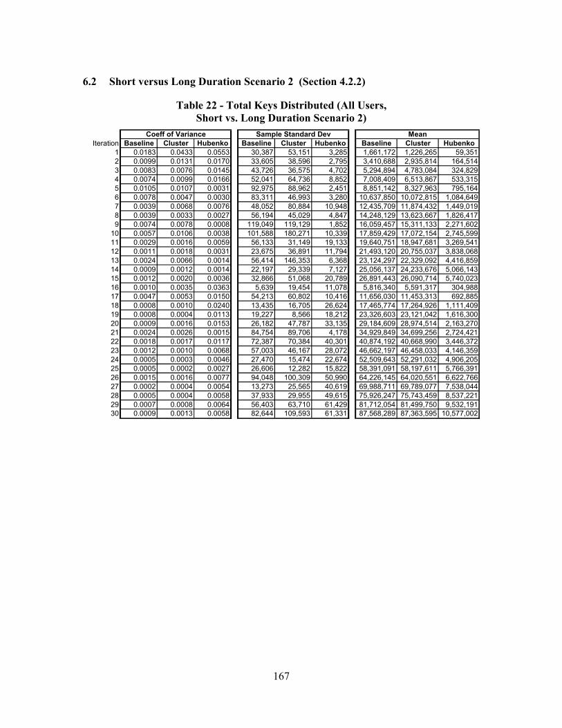
167

6.2 Short versus Long Duration Scenario 2 (Section 4.2.2)

Table 22 - Total Keys Distributed (All Users, Short vs. Long Duration Scenario 2)

Iteration Baseline Cluster Hubenko Baseline Cluster Hubenko Baseline Cluster Hubenko1 0.0183 0.0433 0.0553 30,387 53,151 3,285 1,661,172 1,226,265 59,3512 0.0099 0.0131 0.0170 33,605 38,596 2,795 3,410,688 2,935,814 164,5143 0.0083 0.0076 0.0145 43,726 36,575 4,702 5,294,894 4,783,084 324,8294 0.0074 0.0099 0.0166 52,041 64,736 8,852 7,008,409 6,513,867 533,3155 0.0105 0.0107 0.0031 92,975 88,962 2,451 8,851,142 8,327,963 795,1646 0.0078 0.0047 0.0030 83,311 46,993 3,280 10,637,850 10,072,815 1,084,6497 0.0039 0.0068 0.0076 48,052 80,884 10,948 12,435,709 11,874,432 1,449,0198 0.0039 0.0033 0.0027 56,194 45,029 4,847 14,248,129 13,623,667 1,826,4179 0.0074 0.0078 0.0008 119,049 119,129 1,852 16,059,457 15,311,133 2,271,602

10 0.0057 0.0106 0.0038 101,588 180,271 10,339 17,859,429 17,072,154 2,745,59911 0.0029 0.0016 0.0059 56,133 31,149 19,133 19,640,751 18,947,681 3,269,54112 0.0011 0.0018 0.0031 23,675 36,891 11,794 21,493,120 20,755,037 3,838,06813 0.0024 0.0066 0.0014 56,414 146,353 6,368 23,124,297 22,329,092 4,416,85914 0.0009 0.0012 0.0014 22,197 29,339 7,127 25,056,137 24,233,676 5,066,14315 0.0012 0.0020 0.0036 32,866 51,068 20,789 26,891,443 26,090,714 5,740,02316 0.0010 0.0035 0.0363 5,639 19,454 11,078 5,816,340 5,591,317 304,98817 0.0047 0.0053 0.0150 54,213 60,802 10,416 11,656,030 11,453,313 692,88518 0.0008 0.0010 0.0240 13,435 16,705 26,624 17,465,774 17,264,926 1,111,40919 0.0008 0.0004 0.0113 19,227 8,566 18,212 23,326,603 23,121,042 1,616,30020 0.0009 0.0016 0.0153 26,182 47,787 33,135 29,184,609 28,974,514 2,163,27021 0.0024 0.0026 0.0015 84,754 89,706 4,178 34,929,849 34,699,256 2,724,42122 0.0018 0.0017 0.0117 72,387 70,384 40,301 40,874,192 40,668,990 3,446,37223 0.0012 0.0010 0.0068 57,003 46,167 28,072 46,662,197 46,458,033 4,146,35924 0.0005 0.0003 0.0046 27,470 15,474 22,674 52,509,643 52,291,032 4,906,20525 0.0005 0.0002 0.0027 26,606 12,282 15,822 58,391,091 58,197,611 5,766,39126 0.0015 0.0016 0.0077 94,048 100,309 50,990 64,226,145 64,020,551 6,622,76627 0.0002 0.0004 0.0054 13,273 25,565 40,619 69,988,711 69,789,077 7,538,04428 0.0005 0.0004 0.0058 37,933 29,955 49,615 75,926,247 75,743,459 8,537,22129 0.0007 0.0008 0.0064 56,403 63,710 61,429 81,712,054 81,499,750 9,532,19130 0.0009 0.0013 0.0058 82,644 109,593 61,331 87,568,289 87,363,595 10,577,002

Coeff of Variance Sample Standard Dev Mean

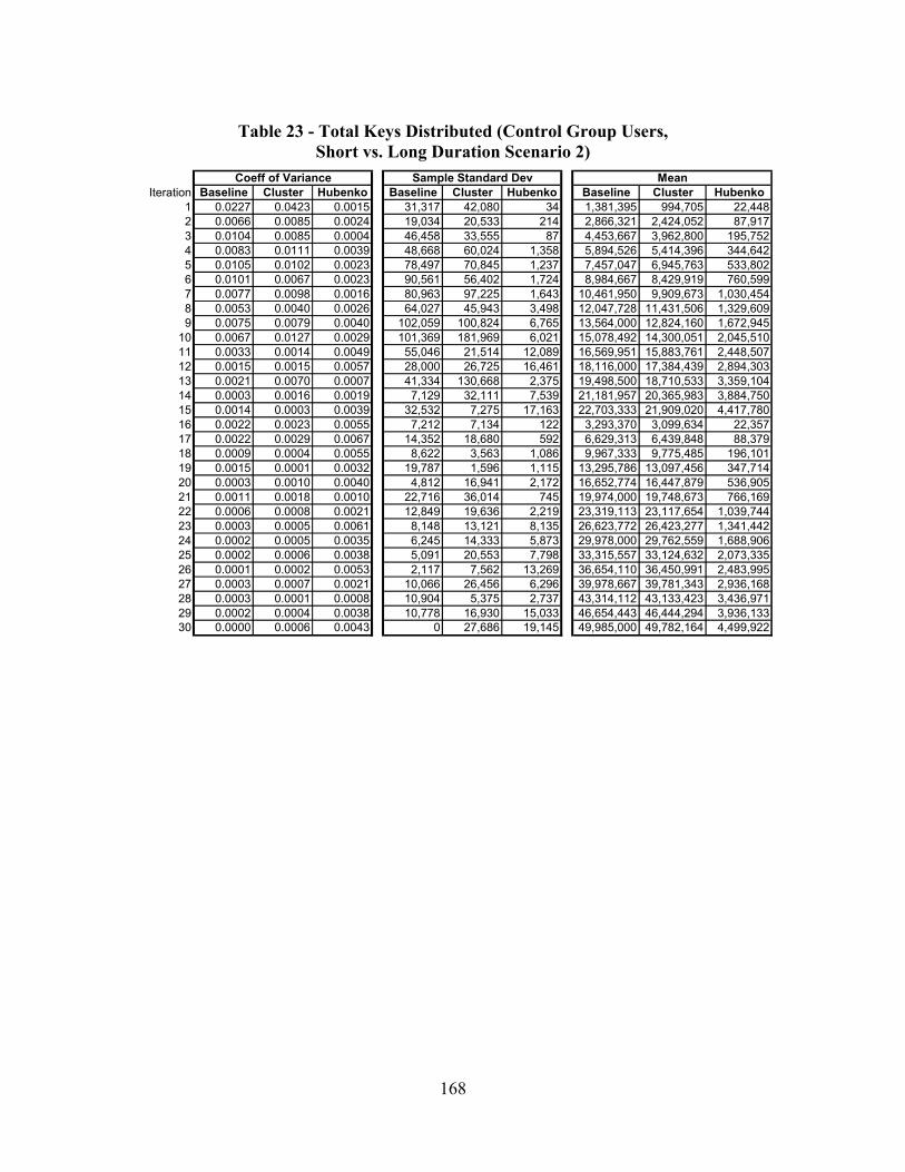
168

Table 23 - Total Keys Distributed (Control Group Users, Short vs. Long Duration Scenario 2)

Iteration Baseline Cluster Hubenko Baseline Cluster Hubenko Baseline Cluster Hubenko1 0.0227 0.0423 0.0015 31,317 42,080 34 1,381,395 994,705 22,4482 0.0066 0.0085 0.0024 19,034 20,533 214 2,866,321 2,424,052 87,9173 0.0104 0.0085 0.0004 46,458 33,555 87 4,453,667 3,962,800 195,7524 0.0083 0.0111 0.0039 48,668 60,024 1,358 5,894,526 5,414,396 344,6425 0.0105 0.0102 0.0023 78,497 70,845 1,237 7,457,047 6,945,763 533,8026 0.0101 0.0067 0.0023 90,561 56,402 1,724 8,984,667 8,429,919 760,5997 0.0077 0.0098 0.0016 80,963 97,225 1,643 10,461,950 9,909,673 1,030,4548 0.0053 0.0040 0.0026 64,027 45,943 3,498 12,047,728 11,431,506 1,329,6099 0.0075 0.0079 0.0040 102,059 100,824 6,765 13,564,000 12,824,160 1,672,945

10 0.0067 0.0127 0.0029 101,369 181,969 6,021 15,078,492 14,300,051 2,045,51011 0.0033 0.0014 0.0049 55,046 21,514 12,089 16,569,951 15,883,761 2,448,50712 0.0015 0.0015 0.0057 28,000 26,725 16,461 18,116,000 17,384,439 2,894,30313 0.0021 0.0070 0.0007 41,334 130,668 2,375 19,498,500 18,710,533 3,359,10414 0.0003 0.0016 0.0019 7,129 32,111 7,539 21,181,957 20,365,983 3,884,75015 0.0014 0.0003 0.0039 32,532 7,275 17,163 22,703,333 21,909,020 4,417,78016 0.0022 0.0023 0.0055 7,212 7,134 122 3,293,370 3,099,634 22,35717 0.0022 0.0029 0.0067 14,352 18,680 592 6,629,313 6,439,848 88,37918 0.0009 0.0004 0.0055 8,622 3,563 1,086 9,967,333 9,775,485 196,10119 0.0015 0.0001 0.0032 19,787 1,596 1,115 13,295,786 13,097,456 347,71420 0.0003 0.0010 0.0040 4,812 16,941 2,172 16,652,774 16,447,879 536,90521 0.0011 0.0018 0.0010 22,716 36,014 745 19,974,000 19,748,673 766,16922 0.0006 0.0008 0.0021 12,849 19,636 2,219 23,319,113 23,117,654 1,039,74423 0.0003 0.0005 0.0061 8,148 13,121 8,135 26,623,772 26,423,277 1,341,44224 0.0002 0.0005 0.0035 6,245 14,333 5,873 29,978,000 29,762,559 1,688,90625 0.0002 0.0006 0.0038 5,091 20,553 7,798 33,315,557 33,124,632 2,073,33526 0.0001 0.0002 0.0053 2,117 7,562 13,269 36,654,110 36,450,991 2,483,99527 0.0003 0.0007 0.0021 10,066 26,456 6,296 39,978,667 39,781,343 2,936,16828 0.0003 0.0001 0.0008 10,904 5,375 2,737 43,314,112 43,133,423 3,436,97129 0.0002 0.0004 0.0038 10,778 16,930 15,033 46,654,443 46,444,294 3,936,13330 0.0000 0.0006 0.0043 0 27,686 19,145 49,985,000 49,782,164 4,499,922

MeanSample Standard DevCoeff of Variance

169

Table 24 - Average Per-User Re-Key (All Users, Short vs. Long Duration Scenario 2)

Iteration Baseline Cluster Hubenko Baseline Cluster Hubenko Baseline Cluster Hubenko1 0.0183 0.0433 0.0553 45.56 79.69 4.93 2,491 1,838 892 0.0099 0.0131 0.0170 25.19 28.93 2.10 2,557 2,201 1233 0.0083 0.0076 0.0145 21.86 18.29 2.35 2,647 2,392 1624 0.0074 0.0099 0.0166 19.51 24.27 3.32 2,628 2,442 2005 0.0105 0.0107 0.0031 27.89 26.68 0.74 2,655 2,498 2396 0.0078 0.0047 0.0030 20.83 11.75 0.82 2,659 2,518 2717 0.0039 0.0068 0.0076 10.30 17.33 2.35 2,665 2,544 3108 0.0039 0.0033 0.0027 10.54 8.44 0.91 2,671 2,554 3429 0.0074 0.0078 0.0008 19.84 19.85 0.31 2,677 2,552 379

10 0.0057 0.0106 0.0038 15.24 27.04 1.55 2,679 2,561 41211 0.0029 0.0016 0.0059 7.65 4.25 2.61 2,678 2,584 44612 0.0011 0.0018 0.0031 2.96 4.61 1.47 2,687 2,594 48013 0.0024 0.0066 0.0014 6.51 16.89 0.73 2,668 2,576 51014 0.0009 0.0012 0.0014 2.38 3.14 0.76 2,684 2,596 54315 0.0012 0.0020 0.0036 3.29 5.11 2.08 2,689 2,609 57416 0.0010 0.0035 0.0363 8.45 29.17 16.61 8,720 8,383 45717 0.0047 0.0053 0.0150 40.64 45.58 7.81 8,738 8,586 51918 0.0008 0.0010 0.0240 6.72 8.35 13.31 8,733 8,632 55619 0.0008 0.0004 0.0113 7.21 3.21 6.83 8,746 8,669 60620 0.0009 0.0016 0.0153 7.85 14.33 9.94 8,754 8,691 64921 0.0024 0.0026 0.0015 21.19 22.43 1.04 8,732 8,675 68122 0.0018 0.0017 0.0117 15.51 15.08 8.64 8,758 8,714 73823 0.0012 0.0010 0.0068 10.69 8.66 5.26 8,748 8,710 77724 0.0005 0.0003 0.0046 4.58 2.58 3.78 8,752 8,715 81825 0.0005 0.0002 0.0027 3.99 1.84 2.37 8,758 8,729 86526 0.0015 0.0016 0.0077 12.82 13.68 6.95 8,757 8,729 90327 0.0002 0.0004 0.0054 1.66 3.20 5.08 8,749 8,724 94228 0.0005 0.0004 0.0058 4.38 3.46 5.72 8,760 8,739 98529 0.0007 0.0008 0.0064 6.04 6.83 6.58 8,754 8,731 1,02130 0.0009 0.0013 0.0058 8.26 10.96 6.13 8,757 8,736 1,058

Coeff of Variance Sample Standard Dev Mean

170

Table 25 - Average Per-User Re-Key (Control Group Users, Short vs. Long Duration Scenario 2)

Iteration Baseline Cluster Hubenko Baseline Cluster Hubenko Baseline Cluster Hubenko1 0.0227 0.0423 0.0015 93.90 126.18 0.10 4,142 2,983 672 0.0066 0.0085 0.0024 28.54 30.78 0.32 4,297 3,634 1323 0.0104 0.0085 0.0004 46.46 33.55 0.09 4,454 3,963 1964 0.0083 0.0111 0.0039 36.50 45.01 1.02 4,420 4,060 2585 0.0105 0.0102 0.0023 47.09 42.50 0.74 4,473 4,167 3206 0.0101 0.0067 0.0023 45.28 28.20 0.86 4,492 4,215 3807 0.0077 0.0098 0.0016 34.70 41.66 0.70 4,483 4,247 4428 0.0053 0.0040 0.0026 24.01 17.23 1.31 4,517 4,286 4999 0.0075 0.0079 0.0040 34.02 33.61 2.25 4,521 4,275 558

10 0.0067 0.0127 0.0029 30.41 54.59 1.81 4,523 4,290 61411 0.0033 0.0014 0.0049 15.01 5.87 3.30 4,519 4,332 66812 0.0015 0.0015 0.0057 7.00 6.68 4.12 4,529 4,346 72413 0.0021 0.0070 0.0007 9.54 30.15 0.55 4,499 4,318 77514 0.0003 0.0016 0.0019 1.53 6.88 1.62 4,539 4,364 83215 0.0014 0.0003 0.0039 6.51 1.45 3.43 4,541 4,382 88416 0.0022 0.0023 0.0055 21.62 21.39 0.37 9,875 9,294 6717 0.0022 0.0029 0.0067 21.52 28.01 0.89 9,939 9,655 13318 0.0009 0.0004 0.0055 8.62 3.56 1.09 9,967 9,775 19619 0.0015 0.0001 0.0032 14.84 1.20 0.84 9,971 9,822 26120 0.0003 0.0010 0.0040 2.89 10.16 1.30 9,990 9,867 32221 0.0011 0.0018 0.0010 11.36 18.01 0.37 9,987 9,874 38322 0.0006 0.0008 0.0021 5.51 8.41 0.95 9,993 9,907 44623 0.0003 0.0005 0.0061 3.06 4.92 3.05 9,983 9,907 50324 0.0002 0.0005 0.0035 2.08 4.78 1.96 9,993 9,921 56325 0.0002 0.0006 0.0038 1.53 6.17 2.34 9,994 9,937 62226 0.0001 0.0002 0.0053 0.58 2.06 3.62 9,996 9,940 67727 0.0003 0.0007 0.0021 2.52 6.61 1.57 9,995 9,945 73428 0.0003 0.0001 0.0008 2.52 1.24 0.63 9,995 9,953 79329 0.0002 0.0004 0.0038 2.31 3.63 3.22 9,997 9,952 84330 0.0000 0.0006 0.0043 0.00 5.54 3.83 9,997 9,956 900

Coeff of Variance Sample Standard Dev Mean

171

6.3 Increasing Aircraft Over Stationary Users Scenario 2 (Section 4.2.3)

Table 26 - Total Keys Distributed (All Users, Increasing Aircraft Over Stationary Users Scenario 2)

Iteration Baseline Cluster Hubenko Baseline Cluster Hubenko Baseline Cluster Hubenko1 0.0904 0.0897 0.0023 784,829 274,033 275 8,681,369 3,055,333 117,7322 0.0407 0.1177 0.0152 772,818 1,173,413 6,646 18,976,685 9,970,518 437,4553 0.0018 0.0431 0.0025 53,566 800,236 2,317 29,433,570 18,562,466 940,1884 0.0003 0.0404 0.0044 10,262 1,263,530 7,033 39,320,710 31,313,357 1,608,1105 0.0007 0.0324 0.0071 34,017 1,361,841 17,303 49,214,102 42,055,851 2,444,8746 0.0035 0.0569 0.0231 34,400 380,817 3,230 9,770,308 6,687,975 139,8617 0.0011 0.0251 0.0195 22,200 425,981 9,252 19,609,750 16,984,644 473,9008 0.0009 0.0075 0.0036 26,589 208,018 3,619 29,520,563 27,701,209 1,006,6109 0.0002 0.0025 0.0055 9,491 96,303 9,387 39,379,345 38,265,499 1,702,262

10 0.0002 0.0032 0.0012 7,713 154,483 2,920 49,257,760 48,179,126 2,536,54111 0.0010 0.0202 0.0218 9,728 167,167 3,459 9,761,333 8,293,889 158,68212 0.0008 0.0025 0.0099 15,507 46,824 5,109 19,659,593 18,822,068 518,12113 0.0006 0.0011 0.0072 16,456 31,920 7,623 29,535,431 28,846,826 1,060,09114 0.0002 0.0008 0.0114 5,989 29,226 20,325 39,391,169 38,757,835 1,783,21415 0.0003 0.0014 0.0025 16,778 68,131 6,575 49,244,917 48,593,570 2,638,52316 0.0006 0.0314 0.0420 5,667 279,120 7,442 9,788,197 8,876,319 177,39017 0.0000 0.0052 0.0099 976 99,539 5,534 19,676,719 19,142,139 556,93818 0.0002 0.0012 0.0082 4,753 35,696 9,177 29,534,553 29,074,184 1,122,98719 0.0003 0.0002 0.0045 11,313 8,768 8,248 39,395,378 38,967,151 1,839,46320 0.0004 0.0009 0.0116 17,796 41,728 31,904 49,251,433 48,830,033 2,742,36121 0.0009 0.0025 0.0096 8,935 23,533 2,026 9,822,170 9,404,468 211,79622 0.0001 0.0026 0.0066 1,976 49,842 4,105 19,688,321 19,352,214 622,00923 0.0002 0.0008 0.0035 5,392 22,836 4,155 29,553,302 29,207,472 1,201,79324 0.0004 0.0002 0.0024 13,963 8,793 4,646 39,393,821 39,096,376 1,969,19225 0.0001 0.0012 0.0047 7,355 60,835 13,404 49,268,474 48,965,305 2,877,28026 0.0011 0.0036 0.0213 11,052 34,605 5,545 9,831,126 9,575,730 259,77627 0.0005 0.0009 0.0055 10,650 18,365 3,900 19,682,966 19,467,606 709,54228 0.0000 0.0002 0.0102 1,191 6,918 13,743 29,545,568 29,301,262 1,349,40229 0.0003 0.0007 0.0084 12,390 26,241 18,085 39,409,317 39,218,908 2,145,05730 0.0001 0.0006 0.0040 5,036 28,360 12,442 49,257,078 49,057,807 3,087,913

Coeff of Variance Sample Standard Dev Mean

172

Table 27 - Total Keys Distributed (Control Group Users, Increasing Aircraft Over Stationary Users Scenario 2)

Iteration Baseline Cluster Hubenko Baseline Cluster Hubenko Baseline Cluster Hubenko1 0.0904 0.0901 0.0126 674,779 235,371 1,256 7,465,833 2,613,564 99,8202 0.0402 0.1173 0.0106 657,918 1,001,880 4,076 16,348,333 8,542,335 385,2103 0.0017 0.0428 0.0039 42,466 681,868 3,254 25,375,900 15,916,084 841,7884 0.0002 0.0403 0.0027 6,800 1,083,386 3,878 33,904,800 26,874,601 1,440,8935 0.0007 0.0326 0.0060 29,445 1,176,173 13,210 42,449,000 36,107,938 2,200,5966 0.0038 0.0570 0.0125 32,300 326,376 1,244 8,418,400 5,728,202 99,7197 0.0014 0.0254 0.0130 24,122 369,534 5,050 16,903,667 14,565,260 387,4658 0.0010 0.0079 0.0068 25,669 188,972 5,765 25,460,900 23,789,119 848,7949 0.0002 0.0028 0.0055 6,800 90,976 7,965 33,959,200 32,900,293 1,455,898

10 0.0001 0.0035 0.0029 4,907 143,850 6,306 42,488,667 41,450,189 2,200,72411 0.0011 0.0202 0.0102 8,833 143,706 1,021 8,409,900 7,102,288 100,13412 0.0007 0.0025 0.0035 11,940 39,913 1,337 16,951,267 16,165,912 384,37513 0.0006 0.0011 0.0017 15,581 27,851 1,419 25,471,100 24,805,061 838,69214 0.0001 0.0009 0.0061 3,926 28,921 8,929 33,975,067 33,354,936 1,457,82315 0.0001 0.0015 0.0028 4,907 62,574 6,271 42,471,667 41,831,655 2,206,71216 0.0011 0.0325 0.0028 8,996 247,237 277 8,437,100 7,610,948 100,46717 0.0003 0.0055 0.0020 5,194 89,699 763 16,971,667 16,457,992 389,31018 0.0002 0.0013 0.0043 5,100 33,277 3,668 25,474,500 25,023,431 847,14119 0.0003 0.0002 0.0058 10,387 8,326 8,332 33,984,133 33,562,246 1,443,86020 0.0001 0.0011 0.0111 4,907 46,662 24,403 42,485,833 42,069,857 2,208,02821 0.0010 0.0027 0.0065 8,500 21,593 649 8,467,700 8,074,409 100,62422 0.0002 0.0030 0.0129 3,926 49,773 4,970 16,985,267 16,655,744 386,20523 0.0002 0.0010 0.0035 5,100 25,709 2,977 25,489,800 25,148,962 845,16524 0.0003 0.0002 0.0087 10,387 5,070 12,642 33,984,133 33,689,599 1,445,42525 0.0000 0.0013 0.0037 0 54,912 8,253 42,491,500 42,190,781 2,201,12426 0.0009 0.0037 0.0013 7,852 30,083 132 8,475,633 8,228,259 100,67727 0.0005 0.0011 0.0058 8,996 18,061 2,244 16,976,200 16,763,702 384,03928 0.0001 0.0002 0.0046 2,944 4,016 3,852 25,486,400 25,244,285 840,83829 0.0002 0.0006 0.0026 7,852 20,685 3,715 33,988,667 33,799,540 1,443,18830 0.0000 0.0005 0.0027 0 23,186 5,843 42,491,500 42,293,289 2,185,256

Coeff of Variance Sample Standard Dev Mean

173

Table 28 - Average Per-User Re-Key (All Users, Increasing Aircraft Over Stationary Users Scenario 2)

Iteration Baseline Cluster Hubenko Baseline Cluster Hubenko Baseline Cluster Hubenko1 0.0904 0.0897 0.0023 392.41 137.02 0.14 4,341 1,528 592 0.0407 0.1177 0.0152 193.20 293.35 1.66 4,744 2,493 1093 0.0018 0.0431 0.0025 8.93 133.37 0.39 4,906 3,094 1574 0.0003 0.0404 0.0044 1.28 157.94 0.88 4,915 3,914 2015 0.0007 0.0324 0.0071 3.40 136.18 1.73 4,921 4,206 2446 0.0035 0.0569 0.0231 17.20 190.41 1.62 4,885 3,344 707 0.0011 0.0251 0.0195 5.55 106.50 2.31 4,902 4,246 1188 0.0009 0.0075 0.0036 4.43 34.67 0.60 4,920 4,617 1689 0.0002 0.0025 0.0055 1.19 12.04 1.17 4,922 4,783 213

10 0.0002 0.0032 0.0012 0.77 15.45 0.29 4,926 4,818 25411 0.0010 0.0202 0.0218 4.86 83.58 1.73 4,881 4,147 7912 0.0008 0.0025 0.0099 3.88 11.71 1.28 4,915 4,706 13013 0.0006 0.0011 0.0072 2.74 5.32 1.27 4,923 4,808 17714 0.0002 0.0008 0.0114 0.75 3.65 2.54 4,924 4,845 22315 0.0003 0.0014 0.0025 1.68 6.81 0.66 4,924 4,859 26416 0.0006 0.0314 0.0420 2.83 139.56 3.72 4,894 4,438 8917 0.0000 0.0052 0.0099 0.24 24.88 1.38 4,919 4,786 13918 0.0002 0.0012 0.0082 0.79 5.95 1.53 4,922 4,846 18719 0.0003 0.0002 0.0045 1.41 1.10 1.03 4,924 4,871 23020 0.0004 0.0009 0.0116 1.78 4.17 3.19 4,925 4,883 27421 0.0009 0.0025 0.0096 4.47 11.77 1.01 4,911 4,702 10622 0.0001 0.0026 0.0066 0.49 12.46 1.03 4,922 4,838 15623 0.0002 0.0008 0.0035 0.90 3.81 0.69 4,926 4,868 20024 0.0004 0.0002 0.0024 1.75 1.10 0.58 4,924 4,887 24625 0.0001 0.0012 0.0047 0.74 6.08 1.34 4,927 4,897 28826 0.0011 0.0036 0.0213 5.53 17.30 2.77 4,916 4,788 13027 0.0005 0.0009 0.0055 2.66 4.59 0.98 4,921 4,867 17728 0.0000 0.0002 0.0102 0.20 1.15 2.29 4,924 4,884 22529 0.0003 0.0007 0.0084 1.55 3.28 2.26 4,926 4,902 26830 0.0001 0.0006 0.0040 0.50 2.84 1.24 4,926 4,906 309

Coeff of Variance Sample Standard Dev Mean

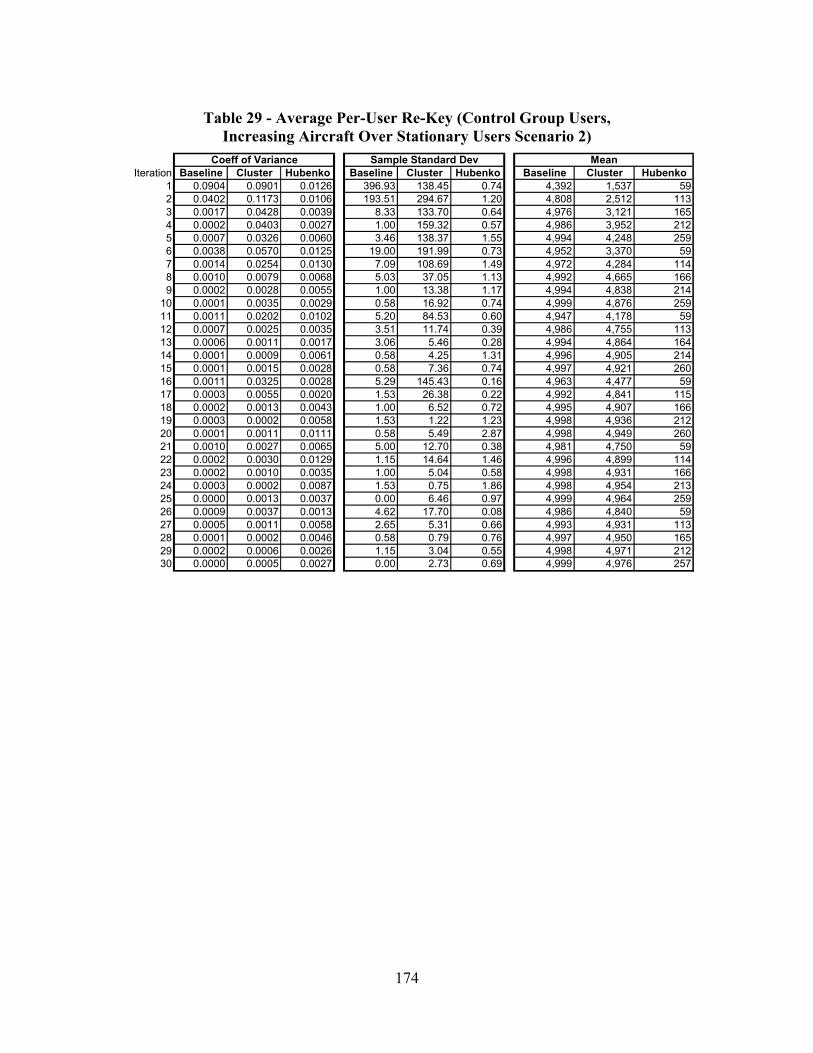
174

Table 29 - Average Per-User Re-Key (Control Group Users, Increasing Aircraft Over Stationary Users Scenario 2)

Iteration Baseline Cluster Hubenko Baseline Cluster Hubenko Baseline Cluster Hubenko1 0.0904 0.0901 0.0126 396.93 138.45 0.74 4,392 1,537 592 0.0402 0.1173 0.0106 193.51 294.67 1.20 4,808 2,512 1133 0.0017 0.0428 0.0039 8.33 133.70 0.64 4,976 3,121 1654 0.0002 0.0403 0.0027 1.00 159.32 0.57 4,986 3,952 2125 0.0007 0.0326 0.0060 3.46 138.37 1.55 4,994 4,248 2596 0.0038 0.0570 0.0125 19.00 191.99 0.73 4,952 3,370 597 0.0014 0.0254 0.0130 7.09 108.69 1.49 4,972 4,284 1148 0.0010 0.0079 0.0068 5.03 37.05 1.13 4,992 4,665 1669 0.0002 0.0028 0.0055 1.00 13.38 1.17 4,994 4,838 214

10 0.0001 0.0035 0.0029 0.58 16.92 0.74 4,999 4,876 25911 0.0011 0.0202 0.0102 5.20 84.53 0.60 4,947 4,178 5912 0.0007 0.0025 0.0035 3.51 11.74 0.39 4,986 4,755 11313 0.0006 0.0011 0.0017 3.06 5.46 0.28 4,994 4,864 16414 0.0001 0.0009 0.0061 0.58 4.25 1.31 4,996 4,905 21415 0.0001 0.0015 0.0028 0.58 7.36 0.74 4,997 4,921 26016 0.0011 0.0325 0.0028 5.29 145.43 0.16 4,963 4,477 5917 0.0003 0.0055 0.0020 1.53 26.38 0.22 4,992 4,841 11518 0.0002 0.0013 0.0043 1.00 6.52 0.72 4,995 4,907 16619 0.0003 0.0002 0.0058 1.53 1.22 1.23 4,998 4,936 21220 0.0001 0.0011 0.0111 0.58 5.49 2.87 4,998 4,949 26021 0.0010 0.0027 0.0065 5.00 12.70 0.38 4,981 4,750 5922 0.0002 0.0030 0.0129 1.15 14.64 1.46 4,996 4,899 11423 0.0002 0.0010 0.0035 1.00 5.04 0.58 4,998 4,931 16624 0.0003 0.0002 0.0087 1.53 0.75 1.86 4,998 4,954 21325 0.0000 0.0013 0.0037 0.00 6.46 0.97 4,999 4,964 25926 0.0009 0.0037 0.0013 4.62 17.70 0.08 4,986 4,840 5927 0.0005 0.0011 0.0058 2.65 5.31 0.66 4,993 4,931 11328 0.0001 0.0002 0.0046 0.58 0.79 0.76 4,997 4,950 16529 0.0002 0.0006 0.0026 1.15 3.04 0.55 4,998 4,971 21230 0.0000 0.0005 0.0027 0.00 2.73 0.69 4,999 4,976 257

Coeff of Variance Sample Standard Dev Mean

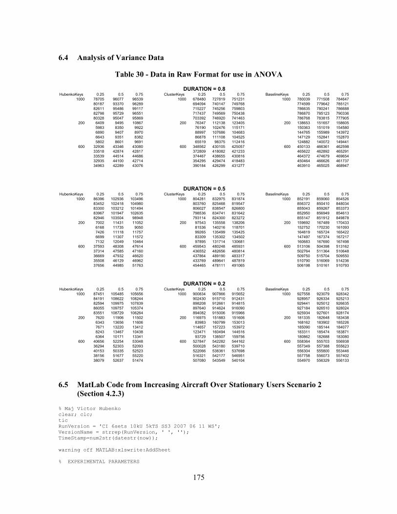
175

6.4 Analysis of Variance Data

Table 30 - Data in Raw Format for use in ANOVA

HubenkoKeys 0.25 0.5 0.75 ClusterKeys 0.25 0.5 0.75 BaselineKeys 0.25 0.5 0.751000 78705 96077 96539 1000 678480 727819 751231 1000 780039 771508 784647

80187 93370 96289 694094 740147 749768 774599 779642 78512182611 95486 99117 715227 745256 759803 786635 780241 78668882798 95729 96551 717437 749569 750438 786870 785123 79033680328 95047 95869 703392 746920 741463 786768 783815 777905

200 6409 9495 10867 200 76347 112138 123405 200 138653 151657 1586055983 8350 9922 76190 102476 115171 150363 151019 1545806890 9407 8970 88997 107686 104683 144765 155989 1439726643 9351 8382 86878 111108 104525 147129 152841 1528705802 8601 9691 65519 98375 112416 124882 140072 149441

600 32936 43346 43080 600 348562 430105 425057 600 450133 466361 46259833518 42874 42817 372809 418082 421233 465622 462892 46529133539 44514 44686 374467 438655 430816 464372 474679 46965432935 44100 42714 354295 429474 418483 450464 466626 46173734963 42289 43076 390184 426299 431277 463910 465025 468947

HubenkoKeys 0.25 0.5 0.75 ClusterKeys 0.25 0.5 0.75 BaselineKeys 0.25 0.5 0.751000 86396 102936 103496 1000 804281 832975 831874 1000 852191 859060 854526

83452 102418 104980 803760 825468 819547 856372 850410 84803483300 103212 101494 806027 838547 826800 855043 859267 85337383967 101947 102635 798536 834741 831642 852950 856949 85461382946 103504 98948 793114 824300 823272 855147 851912 849878

200 7002 11431 11052 200 97543 135558 138206 200 159692 167489 1704336168 11735 9050 81536 140216 118701 152752 170230 1610937426 11118 11757 99265 135499 135425 164819 165724 1654226699 11307 11572 83309 135302 134502 147497 167374 1672177132 12049 10464 97895 131714 130681 160683 167690 167498

600 37593 48308 47614 600 459543 480248 485931 600 513106 504398 51316237314 47585 47160 436552 482656 480814 502764 511364 51064836669 47932 46620 437864 489190 483317 509750 515704 50955035508 46129 46962 433769 489641 487819 510790 516069 51423637656 44985 51763 454465 478111 491065 506198 510161 510793

HubenkoKeys 0.25 0.5 0.75 ClusterKeys 0.25 0.5 0.75 BaselineKeys 0.25 0.5 0.751000 87451 105485 105656 1000 900834 907866 915652 1000 927558 923079 928342

84191 108622 108244 902430 915710 912431 928957 926334 92521382594 109975 107839 898208 912661 914815 929441 925012 92663586055 109757 105374 897640 914624 916090 927184 926510 92802483551 108729 106264 894082 915006 915966 925934 927601 928174

200 7620 11906 11502 200 116975 151883 151606 200 181335 182648 1834386343 13656 11606 83983 160799 153013 168162 183902 1852267671 13220 13412 114657 157223 153972 185090 185144 1840778243 13467 10438 123471 160494 144516 183311 185474 1838716364 10171 13341 93729 138507 159756 180862 182688 183080

600 40656 52254 53048 600 527847 542282 544162 600 558364 555703 55693836294 52303 52093 500028 543180 539710 557349 557388 55562340153 50335 52523 522066 538361 537698 556304 555800 55344638156 51677 55220 516321 542177 546951 557758 556073 55740238079 52637 51474 507080 543549 540104 554970 556329 556133

DURATION = 0.8

DURATION = 0.5

DURATION = 0.2

6.5 MatLab Code from Increasing Aircraft Over Stationary Users Scenario 2 (Section 4.2.3)

% Maj Victor Hubenko clear; clc; tic RunVersion = 'CI 6sets 10kU 5kTS SS3 2007 06 11 WS'; VersionName = strrep(RunVersion, ' ', ''); TimeStamp=num2str(datestr(now)); warning off MATLAB:xlswrite:AddSheet % EXPERIMENTAL PARAMETERS

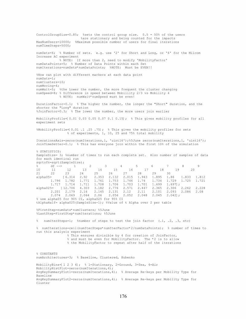
176

ControlGroupSize=0.85; %sets the control group size. 0.5 = 50% of the users %are stationary and being counted for the impacts MaxNumUsers=10000; %Maximum possible number of users for final iterations numTimeSteps=5000; numSets=6; % Number of sets. e.g. use '2' for Short and Long, or '6' for the Milcom Increase AC experiment % NOTE: If more than 2, need to modify 'MobilityFactor' numDataPoints=5; % Number of Data Points within each Set numIterations=numSets*numDataPoints; %NOTE: Must be EVEN!! %Now can plot with different markers at each data point numSats=1; numClusters=10; numMoving=4; numWait=5; %the Lower the number, the more frequent the cluster changing numSpeed=8; % Difference in speed between Mobililty 2/3 vs Mobility 4 % NOTE: numWait*numSpeed must be even! DurationFactor=0.1; % The higher the number, the longer the "Short" duration, and the shorter the "Long" duration %JoinFactor=0.3; % The lower the number, the more users join earlier MobilityProfile=[0.01 0.03 0.05 0.07 0.1 0.15]; % This gives mobility profiles for all experiment sets %MobilityProfile=[0.01 .1 .25 .75]; % This gives the mobility profiles for sets % of experiments, 1, 10, 25 and 75% total mobility IterationsAxis=zeros(numIterations,1, 'uint16');%5June zeros(numIterations,1, 'uint16'); JoinTimeSetter=0.1; % This has everyone join within the first 10% of the simulation % STATISTICS: SampleSize= 3; %number of times to run each complete set. Also number of samples of data for each identical run sqrtofn=sqrt(SampleSize); % df --> 1 2 3 4 5 6 7 8 9 10 11 12 13 14 15 16 17 18 19 20 21 22 23 24 25 26 27 28 29 30 alpha05= [6.314 2.92 2.353 2.132 2.015 1.943 1.895 1.86 1.833 1.812 1.796 1.782 1.771 1.761 1.753 1.746 1.74 1.734 1.729 1.725 1.721 1.717 1.714 1.711 1.708 1.706 1.703 1.701 1.699 1.697]; alpha025= [12.706 4.303 3.182 2.776 2.571 2.447 2.365 2.306 2.262 2.228 2.201 2.179 2.16 2.145 2.131 2.12 2.11 2.101 2.093 2.086 2.08 2.074 2.069 2.064 2.06 2.056 2.052 2.048 2.045 2.042]; % use alpha05 for 90% CI, alpha025 for 95% CI tAlphaHalf= alpha025(SampleSize-1); %Value of t Alpha over 2 per table %FirstStep=numSats*numClusters; %5June %LastStep=FirstStep*numIterations; %5June % numIterSteps=1; %number of steps to test the join factor (.1, .2, .3, etc) % numIterations=ceil(numIterSteps*numIterFactor*2/numDataPoints); % number of times to run this analysis experiment % This ensures divisible by 4 for creation of JoinFactor, % and must be even for MobilityFactor. The *2 is to allow % the MobilityFactor to repeat after half of the iterations % CONSTANTS numArchitectures=3; % Baseline, Clustered, Hubenko MobilityBins=[1 2 3 4]; % 1=Stationary, 2=Ground, 3=Sea, 4=Air MobilityHistPlot=zeros(numIterations,4); AvgKeySummaryPlot1=zeros(numIterations,4); % Average Re-keys per Mobility Type for Baseline AvgKeySummaryPlot2=zeros(numIterations,4); % Average Re-keys per Mobility Type for Cluster

177

AvgKeySummaryPlot3=zeros(numIterations,4); % Average Re-keys per Mobility Type for Hubenko TotalKeysDistribCount=zeros(numIterations,numArchitectures,SampleSize); % Total Number of keys distributed in a MCast Group for the simulation % period. Single dimension array, running tally. Count all of the new keys % that are distributed to all users, satellites each time a new key is % distributed for the MCast Group. 1=baseline, 2=clusters, 3=Hubenko TotalHalfKeysDistribCount=zeros(numIterations,numArchitectures,SampleSize); % Total Number of keys distributed for the Stationary "control group" users DensityVsRekeys=zeros(numIterations,numArchitectures,SampleSize); DensityVsHalfRekeys=zeros(numIterations,numArchitectures,SampleSize); % [+ B - + C - + H - ...] Where B, C, H are the means for the SampleSize, % + is the Top of the confidence interval, - is the Bottom of the % Confidence Interval TotalKeysDistribCountPlot=zeros(numIterations,3*numArchitectures); TotalHalfKeysDistribCountPlot=zeros(numIterations,3*numArchitectures); DensityVsRekeysPlot=zeros(numIterations,3*numArchitectures); DensityVsHalfRekeysPlot=zeros(numIterations,3*numArchitectures); %xMeanArray is the mean array for each of the above arrays TKDMeanArray=zeros(numIterations,numArchitectures); THKDMeanArray=zeros(numIterations,numArchitectures); DVRMeanArray=zeros(numIterations,numArchitectures); DVHRMeanArray=zeros(numIterations,numArchitectures); % xSampleSDArray is the sample standard deviation array for each of the above arrays TKDSampleSDArray=zeros(numIterations,numArchitectures); THKDSampleSDArray=zeros(numIterations,numArchitectures); DVRSampleSDArray=zeros(numIterations,numArchitectures); DVHRSampleSDArray=zeros(numIterations,numArchitectures); % % The Coefficient of Variation (C.O.V.) [Jai91], is the ratio of standard % deviation to sample mean: xSampleSDArray/xMeanArray. COVTKD=zeros(numIterations,numArchitectures); COVTHKD=zeros(numIterations,numArchitectures); COVDVR=zeros(numIterations,numArchitectures); COVDVHR=zeros(numIterations,numArchitectures); FigNum=0; index = datestr(clock); index = strrep(index, ' ', '-'); index = strrep(index, ':', '-'); % % Return RAND to its default initial state to allow for repeatability % rand('state',0); % Initialize RAND to a different state each time. rand('state',sum(100*clock)) for IterAxisMaker=1:numIterations IterationsAxis(IterAxisMaker,1)=IterAxisMaker; end MobilityFactor=zeros(numIterations,1); MFactorCount=1; for MobilityMaker=1:numIterations %(numIterations/2) MobilityFactor(MobilityMaker,1)=MobilityProfile(MFactorCount); if mod(MobilityMaker,numDataPoints)==0 MFactorCount=MFactorCount+1; end end % JoinFactor=zeros(numIterations,1); % multiplier=0.1; % for JoinMaker=1:numIterations % JoinFactor(JoinMaker,1)=multiplier; % if mod(JoinMaker,numDataPoints)==0

178

% multiplier=multiplier+0.1; % end % end % Note: FirstStep=numSats*numClusters; LastStep=FirstStep*numIterations; for h=1:numIterations %FirstStep:hStepSize:LastStep % ModTest1=h/FirstStep; ModTest2=mod(h,numDataPoints); if ModTest2==0 IterRep=numDataPoints; else IterRep=ModTest2; end % numUsers=h; numUsers=ceil(IterRep*MaxNumUsers/numDataPoints) % Rate of Mobility is held for numDataPoints times for g=1:SampleSize % Start Loop for run repetition for Statistics calculations pause(0); ClusterActivity=zeros((numSats*numClusters)+1,numTimeSteps, 'uint16'); %ClusterActivity=zeros((numSats*numClusters)+1,numMCGroups,numTimeSteps, 'uint16'); % Tracks when a user joins or leaves a specific Cluster within a Multicast % Group. As a user joins or leaves, increment/decrement as appropriate. % The last element {(numSats*numClusters)+1} in each set is the % total count of Active Users in that MCGroup across all satellites and % clusters. ClusterTriggers=zeros((numSats*numClusters)+1,numTimeSteps, 'uint8'); %ClusterTriggers=zeros((numSats*numClusters)+1,numMCGroups,numTimeSteps, 'uint8'); % Tracks when a cluster needs to be rekeyed. When a new user first joins % or leaves the system, the corresponding cluster element is set to 1. If % a registered mobile user enters or leaves the cluster, the cluster % element is set to 2. The last % element {(numSats*numClusters)+1} in each set is the "MCGroup Rekey % Trigger Flag," which is set to the max of that MCGroup (0, 1, or 2). 0 % means no joins, leaves, or mobile users entering/exiting; 1 means a user % registered or deregistered from the system; 2 means a mobile user entered % or left the cluster. % Initialize Users UserMoverPercent=0; MFcalc=MobilityFactor(h); %Initialize User Structure User=repmat(struct('Satellite',int8(0),'Cluster',int8(0),... 'TimesRekeyed1',0,'TimesRekeyed2',0,'TimesRekeyed3',0,'JoinTime',int16(0),... 'Duration',int16(0),'Mobility',int8(0),'Waiting',int8(0),'Active',zeros(numTimeSteps,1, 'uint8')),1,numUsers); for i=1:numUsers pause(0); User(i).Satellite = ceil(rand*numSats); User(i).Cluster = ceil(rand*numClusters); % The following were initialized in the repmat(struct) statement % User(i).TimesRekeyed1 = 0; % Baseline System Rekey Count % User(i).TimesRekeyed2 = 0; % Cluster System Rekey Count % User(i).TimesRekeyed3 = 0; % Hubenko System Rekey Count if i<=(numUsers*ControlGroupSize) % For the first half of the users, set them to Join at one, and % stay the whole time. Also set them to Stationary User(i).JoinTime = 1; %ceil(rand*numTimeSteps*JoinTimeSetter); User(i).Duration = numTimeSteps-1; User(i).Mobility = 1; else % Otherwise, set them to Join randomly in 1st third, Short and Long Durations, % and random mobility up to the Mobility Profile User(i).JoinTime = ceil(rand*numTimeSteps*JoinTimeSetter); % if h <= (numIterations/2) % User(i).Duration = ceil(rand*DurationFactor*(numTimeSteps-User(i).JoinTime)); % "Short" % else

179

User(i).Duration = ceil((1-rand*DurationFactor)*(numTimeSteps-User(i).JoinTime)); % "Long" % end %if for Duration assignment % Uniformly assign durations to be within remaining time, under the % constraint of "Short" or "Long" DurationFactor if UserMoverPercent < (MFcalc*numUsers) % UserMover=rand; % if UserMover > MFcalc % if UserMover is greater than the Mobility Profile % %for this increment, then set the user to Stationary % User(i).Mobility = 1; % else % Otherwise, uniformly assign it to either Sea, Ground, or Air User(i).Mobility = 1+ceil(rand*3); UserMoverPercent=UserMoverPercent+1; %end % if/else UserMover > MFcalc else User(i).Mobility = 1; end %if/else UserMoverPercent < (MFcalc*numUsers) end %Of the if/else for i<=(numUsers*ControlGroupSize) % Both of the following were initialized in the repmat(struct) statement % User(i).Waiting = 0; %holder for how long to wait until moving to next cluster % User(i).Active=zeros(numTimeSteps,1, 'uint8'); % Initialize to all % zeros indicating not active. When Active, each slot will be set to 1. % if mod(i,1800)==0 % InitializeUsersLoopsTaken=i % end end %for i=numUsers Loop MobilityHist=[User.Mobility]; MobilityHistPlot(h,:)=hist(MobilityHist,MobilityBins); % Below is to check to ensure random spread in the correct ranges % Lo=Locator; % figure, mesh(Lo); %meshc gives contour plot under mesh %figure,surf(Lo); % Sa = [User.Satellite] % Cl = [User.Cluster] % MC = [User.MCGroup] % JT = [User.JoinTime] % Du = [User.Duration]; % Mo = [User.Mobility] % figure,bar(Du) % xlabel('User #'); % ylabel('Duration Value'); % title({['User.Duration for iteration ',num2str(ModTest1)]}) % Start stepping through "Time." % Array indexing starts at "1"; nomenclature is (rows, columns) % Joins and leaves are edge triggered. Can not join and leave in % same time step. Can have join duration of one time step, but not less. for simTime=1:numTimeSteps % timeis=simTime for j=1:numUsers % First check if each User is Active if ((User(j).JoinTime <= simTime) && (simTime <= (User(j).JoinTime + User(j).Duration - 1))) % changed from & to && based on auto-recommendation % If Active, load the User's location based on the Satellite and Cluster % Line below assumes User can only be in one MCGroup at a time ClusterActivity(((User(j).Satellite-1)*numClusters)+User(j).Cluster,simTime)=ClusterActivity(((User(j).Satellite-1)*numClusters)+User(j).Cluster,simTime)+1; %ClusterActivity(((User(j).Satellite-1)*numClusters)+User(j).Cluster,User(j).MCGroup,simTime)=ClusterActivity(((User(j).Satellite-1)*numClusters)+User(j).Cluster,User(j).MCGroup,simTime)+1; User(j).Active(simTime,1)=1; % Set User Active Flag since it is active

180

% Then check if user just became active during this time slot. If % so, then process the rekeying as appropriate. if (User(j).JoinTime == simTime) % if true, this is a new user to the group/cluster % Set the flag for the new user ClusterTriggers(((User(j).Satellite-1)*numClusters)+User(j).Cluster,simTime)=2; %ClusterTriggers(((User(j).Satellite-1)*numClusters)+User(j).Cluster,User(j).MCGroup,simTime)=2; if User(j).Mobility >1 User(j).Waiting=1; end end % Check if just became Active if User(j).Mobility >1 User(j).Waiting=User(j).Waiting+1; if (User(j).Mobility==2) % This is the Ground User; 2xfaster than Sea User if User(j).Waiting ==(numWait*numSpeed*0.5) User(j).Waiting=1; %if ClusterTriggers(((User(j).Satellite-1)*numClusters)+User(j).Cluster,User(j).MCGroup,simTime)~=2 if ClusterTriggers(((User(j).Satellite-1)*numClusters)+User(j).Cluster,simTime)~=2 %This triggers the current cluster for the %departing user. %ClusterTriggers(((User(j).Satellite-1)*numClusters)+User(j).Cluster,User(j).MCGroup,simTime)=1; ClusterTriggers(((User(j).Satellite-1)*numClusters)+User(j).Cluster,simTime)=1; end %Now get a new location, and set the trigger User(j).Satellite = ceil(rand*numSats); User(j).Cluster = ceil(rand*numClusters); %if ClusterTriggers(((User(j).Satellite-1)*numClusters)+User(j).Cluster,User(j).MCGroup,simTime)~=2 %ClusterTriggers(((User(j).Satellite-1)*numClusters)+User(j).Cluster,User(j).MCGroup,simTime)=1; if ClusterTriggers(((User(j).Satellite-1)*numClusters)+User(j).Cluster,simTime)~=2 ClusterTriggers(((User(j).Satellite-1)*numClusters)+User(j).Cluster,simTime)=1; %This triggers the new cluster for the user end end%if User Waiting elseif (User(j).Mobility==3) % This is the Sea User; half as fast as Ground User if User(j).Waiting ==(numWait*numSpeed) User(j).Waiting=1; if ClusterTriggers(((User(j).Satellite-1)*numClusters)+User(j).Cluster,simTime)~=2 %if ClusterTriggers(((User(j).Satellite-1)*numClusters)+User(j).Cluster,User(j).MCGroup,simTime)~=2 %This triggers the current cluster for the %departing user. ClusterTriggers(((User(j).Satellite-1)*numClusters)+User(j).Cluster,simTime)=1; end %Now get a new location, and set the trigger User(j).Satellite = ceil(rand*numSats); User(j).Cluster = ceil(rand*numClusters); if ClusterTriggers(((User(j).Satellite-1)*numClusters)+User(j).Cluster,simTime)~=2 ClusterTriggers(((User(j).Satellite-1)*numClusters)+User(j).Cluster,simTime)=1; %This triggers the new cluster for the user end end%if User Waiting

181

elseif User(j).Mobility==4 % This is the Air Mover, so moves in fewest # of TimeSteps if User(j).Waiting ==numWait User(j).Waiting=1; if ClusterTriggers(((User(j).Satellite-1)*numClusters)+User(j).Cluster,simTime)~=2 %This triggers the current cluster for the %departing user. ClusterTriggers(((User(j).Satellite-1)*numClusters)+User(j).Cluster,simTime)=1; end %Now get a new location, and set the trigger User(j).Satellite = ceil(rand*numSats); User(j).Cluster = ceil(rand*numClusters); if ClusterTriggers(((User(j).Satellite-1)*numClusters)+User(j).Cluster,simTime)~=2 ClusterTriggers(((User(j).Satellite-1)*numClusters)+User(j).Cluster,simTime)=1; %This triggers the new cluster for the user end end%if User Waiting end%if & elseif end%if User Mobility >1 % Check to see if User just left the MCGroup/System elseif (simTime == (User(j).JoinTime + User(j).Duration)) % Set the flag for the leaving user ClusterTriggers(((User(j).Satellite-1)*numClusters)+User(j).Cluster,simTime)=2; % Decrement the User's instant key count. If the user leaves, % it will definitely drop the key regardless if the % Group/Cluster rekeys or not end %if & elseif end %j pause(0); % Check for joins and leaves. If either a join, a leave, or both % in the MC Group, then rekey. Otherwise, no need to rekey. ClusterActivity((numSats*numClusters)+1,simTime)=sum(ClusterActivity(1:(numSats*numClusters),simTime)); ClusterTriggers((numSats*numClusters)+1,simTime)=max(ClusterTriggers(1:(numSats*numClusters),simTime)); if ClusterTriggers((numSats*numClusters)+1,simTime)>=1 % If true, this means there was some kind of activity in % the MCGroup,so all active users must rekey for the Baseline system. % if ClusterTriggers((numSats*numClusters)+1,NewKeyCheckLoop,simTime)==2 % %If true, there was a new or departing user, so all % %active users must rekey for the Baseline system. % TotalKeysDistribCount(NewKeyCheckLoop,1)=TotalKeysDistribCount(NewKeyCheckLoop,1)+ClusterActivity((numSats*numClusters)+1,NewKeyCheckLoop,simTime); % end % First check which users were active, then see who was % affected. for k=1:numUsers if User(k).Active(simTime,1)==1 %If the user is Active, continue. Otherwise move %on to next user. if ClusterTriggers((numSats*numClusters)+1,simTime)>=1 %If true, this means a new user joined or left %the MCGroup, and therefore all users in the %baseline must rekey, as well as all users in %the Cluster must key

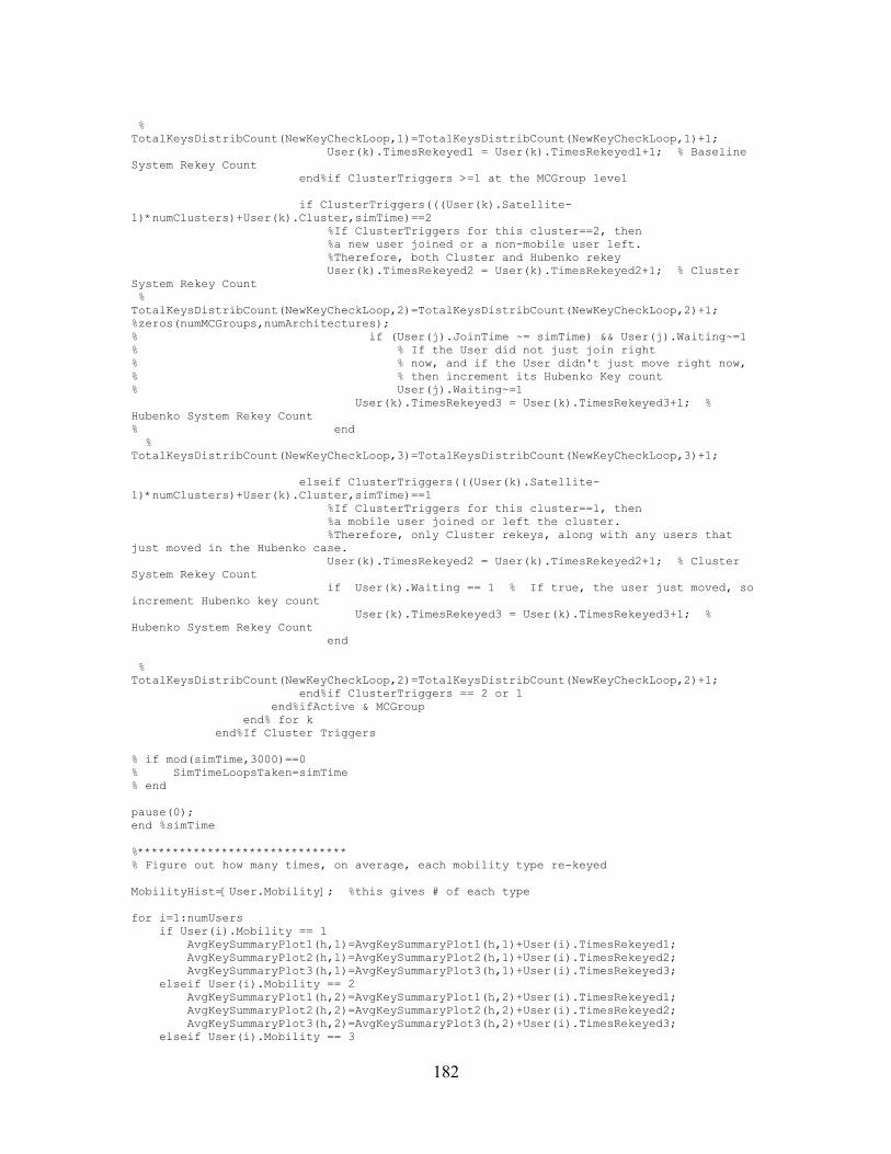
182

% TotalKeysDistribCount(NewKeyCheckLoop,1)=TotalKeysDistribCount(NewKeyCheckLoop,1)+1; User(k).TimesRekeyed1 = User(k).TimesRekeyed1+1; % Baseline System Rekey Count end%if ClusterTriggers >=1 at the MCGroup level if ClusterTriggers(((User(k).Satellite-1)*numClusters)+User(k).Cluster,simTime)==2 %If ClusterTriggers for this cluster==2, then %a new user joined or a non-mobile user left. %Therefore, both Cluster and Hubenko rekey User(k).TimesRekeyed2 = User(k).TimesRekeyed2+1; % Cluster System Rekey Count % TotalKeysDistribCount(NewKeyCheckLoop,2)=TotalKeysDistribCount(NewKeyCheckLoop,2)+1; %zeros(numMCGroups,numArchitectures); % if (User(j).JoinTime ~= simTime) && User(j).Waiting~=1 % % If the User did not just join right % % now, and if the User didn't just move right now, % % then increment its Hubenko Key count % User(j).Waiting~=1 User(k).TimesRekeyed3 = User(k).TimesRekeyed3+1; % Hubenko System Rekey Count % end % TotalKeysDistribCount(NewKeyCheckLoop,3)=TotalKeysDistribCount(NewKeyCheckLoop,3)+1; elseif ClusterTriggers(((User(k).Satellite-1)*numClusters)+User(k).Cluster,simTime)==1 %If ClusterTriggers for this cluster==1, then %a mobile user joined or left the cluster. %Therefore, only Cluster rekeys, along with any users that just moved in the Hubenko case. User(k).TimesRekeyed2 = User(k).TimesRekeyed2+1; % Cluster System Rekey Count if User(k).Waiting == 1 % If true, the user just moved, so increment Hubenko key count User(k).TimesRekeyed3 = User(k).TimesRekeyed3+1; % Hubenko System Rekey Count end % TotalKeysDistribCount(NewKeyCheckLoop,2)=TotalKeysDistribCount(NewKeyCheckLoop,2)+1; end%if ClusterTriggers == 2 or 1 end%ifActive & MCGroup end% for k end%If Cluster Triggers % if mod(simTime,3000)==0 % SimTimeLoopsTaken=simTime % end pause(0); end %simTime %****************************** % Figure out how many times, on average, each mobility type re-keyed MobilityHist=[User.Mobility]; %this gives # of each type for i=1:numUsers if User(i).Mobility == 1 AvgKeySummaryPlot1(h,1)=AvgKeySummaryPlot1(h,1)+User(i).TimesRekeyed1; AvgKeySummaryPlot2(h,1)=AvgKeySummaryPlot2(h,1)+User(i).TimesRekeyed2; AvgKeySummaryPlot3(h,1)=AvgKeySummaryPlot3(h,1)+User(i).TimesRekeyed3; elseif User(i).Mobility == 2 AvgKeySummaryPlot1(h,2)=AvgKeySummaryPlot1(h,2)+User(i).TimesRekeyed1; AvgKeySummaryPlot2(h,2)=AvgKeySummaryPlot2(h,2)+User(i).TimesRekeyed2; AvgKeySummaryPlot3(h,2)=AvgKeySummaryPlot3(h,2)+User(i).TimesRekeyed3; elseif User(i).Mobility == 3

183

AvgKeySummaryPlot1(h,3)=AvgKeySummaryPlot1(h,3)+User(i).TimesRekeyed1; AvgKeySummaryPlot2(h,3)=AvgKeySummaryPlot2(h,3)+User(i).TimesRekeyed2; AvgKeySummaryPlot3(h,3)=AvgKeySummaryPlot3(h,3)+User(i).TimesRekeyed3; else AvgKeySummaryPlot1(h,4)=AvgKeySummaryPlot1(h,4)+User(i).TimesRekeyed1; AvgKeySummaryPlot2(h,4)=AvgKeySummaryPlot2(h,4)+User(i).TimesRekeyed2; AvgKeySummaryPlot3(h,4)=AvgKeySummaryPlot3(h,4)+User(i).TimesRekeyed3; end %end if end %for i=numUsers Loop % Now average each of the sumarries out using the precalculated number in % each mobility type pause(0); AvgKeySummaryPlot1(h,:)=AvgKeySummaryPlot1(h,:)./MobilityHistPlot(h,:); AvgKeySummaryPlot2(h,:)=AvgKeySummaryPlot2(h,:)./MobilityHistPlot(h,:); AvgKeySummaryPlot3(h,:)=AvgKeySummaryPlot3(h,:)./MobilityHistPlot(h,:); %************************************** % All of the User's different Keys UserKeys1=[User.TimesRekeyed1]; UserKeys2=[User.TimesRekeyed2]; UserKeys3=[User.TimesRekeyed3]; % Only the Control Group's keys HalfUserKeys1=UserKeys1(1:(numUsers*ControlGroupSize)); HalfUserKeys2=UserKeys2(1:(numUsers*ControlGroupSize)); HalfUserKeys3=UserKeys3(1:(numUsers*ControlGroupSize)); SumUserKeys1=sum(UserKeys1); SumUserKeys2=sum(UserKeys2); SumUserKeys3=sum(UserKeys3); SumHalfUserKeys1=sum(HalfUserKeys1); SumHalfUserKeys2=sum(HalfUserKeys2); SumHalfUserKeys3=sum(HalfUserKeys3); TotalKeysDistribCount(h,:,g)=[SumUserKeys1 SumUserKeys2 SumUserKeys3]; TotalHalfKeysDistribCount(h,:,g)=[SumHalfUserKeys1 SumHalfUserKeys2 SumHalfUserKeys3]; AverageUserKeys1=SumUserKeys1/numUsers; AverageUserKeys2=SumUserKeys2/numUsers; AverageUserKeys3=SumUserKeys3/numUsers; AvearageUserKeys=[AverageUserKeys1 AverageUserKeys2 AverageUserKeys3]; AverageHalfUserKeys1=SumHalfUserKeys1/(numUsers*ControlGroupSize); AverageHalfUserKeys2=SumHalfUserKeys2/(numUsers*ControlGroupSize); AverageHalfUserKeys3=SumHalfUserKeys3/(numUsers*ControlGroupSize); AvearageHalfUserKeys=[AverageHalfUserKeys1 AverageHalfUserKeys2 AverageHalfUserKeys3]; figure,bar(AvearageUserKeys) xlabel('Architecture'); set(gca,'XTickLabel',{'Baseline';'Cluster';'Hubenko'}) ylabel('Average Times Rekeyed'); % XMinorTick off % YMinorTick off title({['Average Number of Times Each User is Rekeyed'];['for the Different Archtiectures'];['Time Steps:',num2str(numTimeSteps),', Users:',num2str(numUsers),', MCGroups:',num2str(numMCGroups),', Sats:',num2str(numSats),', Clust:',num2str(numClusters)];[' Baseline:',num2str(AverageUserKeys1),', Cluster:',num2str(AverageUserKeys2),', Hubenko:',num2str(AverageUserKeys3)]}) set(gcf, 'PaperPositionMode', 'manual'); set(gcf, 'PaperUnits', 'inches'); set(gcf, 'PaperPosition', [1 1 4.9 3.7]); PlotJoinTimeUserKeys=[User.TimesRekeyed1; User.TimesRekeyed2; User.TimesRekeyed3; User.JoinTime]; figure,bar(PlotJoinTimeUserKeys') title({['Join Time Vs User Times Rekeyed']}) legend('Baseline Keys','Cluster Keys','Hubenko Keys','Time Joined'); PlotClusterActivity=zeros(1,numTimeSteps); PlotClusterActivity(:,:)=ClusterActivity((numSats*numClusters)+1,1,:); figure,plot(PlotClusterActivity)

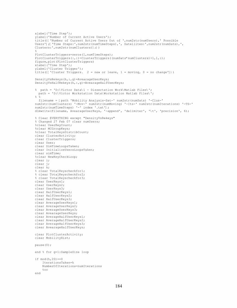
184

xlabel('Time Step'); ylabel('Number of Current Active Users'); title({['Number of Current Active Users Out of ',num2str(numUsers),' Possible Users'];['Time Steps:',num2str(numTimeSteps),', Satellites:',num2str(numSats),', Clusters:',num2str(numClusters)];}) % PlotClusterTriggers=zeros(1,numTimeSteps); PlotClusterTriggers(:,:)=ClusterTriggers((numSats*numClusters)+1,1,:); figure,plot(PlotClusterTriggers) xlabel('Time Step'); ylabel('Cluster Trigger'); title({['Cluster Triggers. 2 = new or leave, 1 = moving, 0 = no change']}) DensityVsRekeys(h,:,g)=AvearageUserKeys; DensityVsHalfRekeys(h,:,g)=AvearageHalfUserKeys; % path = 'D:\Victor Data\1 - Dissertation Work\Matlab Files\'; path = 'D:\Victor Workstation Data\Workstation Matlab Files\'; % % filename = [path 'Mobility Analysis-Sat-' num2str(numSats) '-Clus-' num2str(numClusters) '-Mov-' num2str(numMoving) '-Its-' num2str(numIterations) '-TS-' num2str(numTimeSteps) '-' index '.txt']; dlmwrite(filename, AvearageUserKeys, '-append', 'delimiter', '\t', 'precision', 6); % Clear EVERYTHING except "DensityVsRekeys" % Changed 27 Feb 07 clear numUsers; %clear UserKeyCount; %clear MCGroupKeys; %clear TotalKeysDistribCount; clear ClusterActivity; clear ClusterTriggers; clear User; clear SimTimeLoopsTaken; clear InitializeUsersLoopsTaken; clear simTime; %clear NewKeyCheckLoop; clear i; clear j; clear k; % clear TotalKeyscheckfor1; % clear TotalKeyscheckfor2; % clear TotalKeyscheckfor3; clear UserKeys1; clear UserKeys2; clear UserKeys3; clear HalfUserKeys1; clear HalfUserKeys2; clear HalfUserKeys3; clear AverageUserKeys1; clear AverageUserKeys2; clear AverageUserKeys3; clear AvearageUserKeys; clear AverageHalfUserKeys1; clear AverageHalfUserKeys2; clear AverageHalfUserKeys3; clear AvearageHalfUserKeys; clear PlotClusterActivity; clear MobilityHist; pause(0); end % for g=1:SampleSize loop if mod(h,20)==0 IterationsTaken=h NumberOfIterations=numIterations toc end

185

UpdateNote=strcat('cmd /c "net send /domain:enxp401x "Iteration #',num2str(iter),' completed.""'); system(UpdateNote); %USE THIS ONE FOR AN UPDATE ON EACH TRIAL if mod(h,numDataPoints)==0 UpdateNote=strcat('cmd /c "net send /domain:enxp401x "Iter# ',num2str(h),' of ',num2str(numIterations),'-',VersionName,'.""'); system(UpdateNote); end %end "h" loop here for iterations of number of users, then plot out results end % Now Compute the Confidence Intervals: % % [+ B - + C - + H - ...] Where B, C, H are the means for the SampleSize, % % + is the Top of the confidence interval, - is the Bottom of the % % Confidence Interval % TotalKeysDistribCountPlot=zeros(numIterations,3*numArchitectures); % TotalHalfKeysDistribCountPlot=zeros(numIterations,3*numArchitectures); % DensityVsRekeysPlot=zeros(numIterations,3*numArchitectures); % DensityVsHalfRekeysPlot=zeros(numIterations,3*numArchitectures); % xMeanArray is the mean array for each of the above arrays % NOTE: mean(x,3) produces the mean in the third dimension, namely the repeated samples TKDMeanArray=mean(TotalKeysDistribCount,3); THKDMeanArray=mean(TotalHalfKeysDistribCount,3); DVRMeanArray=mean(DensityVsRekeys,3); DVHRMeanArray=mean(DensityVsHalfRekeys,3); % % xSampleSDArray is the sample standard deviation array for each of the above arrays % NOTE: s = std(X,flag,dim) computes the standard deviations along the % dimension of X specified by scalar dim. Set flag to 0 to normalize % Y by n-1; set flag to 1 to normalize by n. % Using std(x,0,3) for ssd across the sample size TKDSampleSDArray=std(TotalKeysDistribCount,0,3); THKDSampleSDArray=std(TotalHalfKeysDistribCount,0,3); DVRSampleSDArray=std(DensityVsRekeys,0,3); DVHRSampleSDArray=std(DensityVsHalfRekeys,0,3); % % The Coefficient of Variation (C.O.V.) [Jai91], is the ratio of standard % deviation to sample mean: xSampleSDArray/xMeanArray. COVTKD=TKDSampleSDArray./TKDMeanArray; COVTHKD=THKDSampleSDArray./THKDMeanArray; COVDVR=DVRSampleSDArray./DVRMeanArray; COVDVHR=DVHRSampleSDArray./DVHRMeanArray; %XBar= ; %means for each set of identical runs %n=SampleSize %sqrtofn=sqrt(SampleSize) %SampleSD= Sample Standard Deviation %use alpha05 for 90% CI, alpha025 for 95% CI %tAlphaHalf= alpha025(SampleSize-1); %Value of t Alpha over 2 per table % Confidence Interval (+) = Xbar + (tAlphaHalf*SampleSD/sqrtofn) % Confidence Interval (-) = Xbar - (tAlphaHalf*SampleSD/sqrtofn) for statA=1:numArchitectures %Put the Means in place: TotalKeysDistribCountPlot(:,(3*statA)-1)=TKDMeanArray(:,statA); TotalHalfKeysDistribCountPlot(:,(3*statA)-1)=THKDMeanArray(:,statA); DensityVsRekeysPlot(:,(3*statA)-1)=DVRMeanArray(:,statA); DensityVsHalfRekeysPlot(:,(3*statA)-1)=DVHRMeanArray(:,statA); %Now Calculate the + CI Bounds TotalKeysDistribCountPlot(:,(3*statA)-2)=TotalKeysDistribCountPlot(:,(3*statA)-1)+(tAlphaHalf*TKDSampleSDArray(:,statA)/sqrtofn); TotalHalfKeysDistribCountPlot(:,(3*statA)-2)=TotalHalfKeysDistribCountPlot(:,(3*statA)-1)+(tAlphaHalf*THKDSampleSDArray(:,statA)/sqrtofn);

186

DensityVsRekeysPlot(:,(3*statA)-2)=DensityVsRekeysPlot(:,(3*statA)-1)+(tAlphaHalf*DVRSampleSDArray(:,statA)/sqrtofn); DensityVsHalfRekeysPlot(:,(3*statA)-2)=DensityVsHalfRekeysPlot(:,(3*statA)-1)+(tAlphaHalf*DVHRSampleSDArray(:,statA)/sqrtofn); %Now Calculate the - CI Bounds TotalKeysDistribCountPlot(:,(3*statA))=TotalKeysDistribCountPlot(:,(3*statA)-1)-(tAlphaHalf*TKDSampleSDArray(:,statA)/sqrtofn); TotalHalfKeysDistribCountPlot(:,(3*statA))=TotalHalfKeysDistribCountPlot(:,(3*statA)-1)-(tAlphaHalf*THKDSampleSDArray(:,statA)/sqrtofn); DensityVsRekeysPlot(:,(3*statA))=DensityVsRekeysPlot(:,(3*statA)-1)-(tAlphaHalf*DVRSampleSDArray(:,statA)/sqrtofn); DensityVsHalfRekeysPlot(:,(3*statA))=DensityVsHalfRekeysPlot(:,(3*statA)-1)-(tAlphaHalf*DVHRSampleSDArray(:,statA)/sqrtofn); end % for statA pause(0); figurebox = figure; subplot(2,2,1),bar(MobilityHistPlot(ceil(numDataPoints*0.25),:))%,MobilityBins) Changed from Hist to Bar xlabel('(a)', 'FontWeight','bold'); set(gca,'XTickLabel',{'Stationary';'Ground';'Sea';'Air'}, 'FontWeight','bold') ylabel('Number of Users', 'FontWeight','bold'); title(['User Mobility Distribution for ???',num2str(numSats*numClusters*numDataPoints*0.25),' Users. (Iteration ',num2str(numDataPoints*0.25),')'], 'FontWeight','bold'); %See if need to reset numUsers with numUsers=FirstStep*numDataPoints hfinder = findobj(gca,'Type','patch'); set(hfinder,'FaceColor','b','EdgeColor','w') subplot(2,2,2),bar(MobilityHistPlot(ceil(numDataPoints*0.5),:))%,MobilityBins) xlabel('(b)', 'FontWeight','bold'); set(gca,'XTickLabel',{'Stationary';'Ground';'Sea';'Air'}, 'FontWeight','bold') ylabel('Number of Users', 'FontWeight','bold'); title(['User Mobility Distribution for ???',num2str(numSats*numClusters*numDataPoints*0.5),' Users. (Iteration ',num2str(numDataPoints*0.5),')'], 'FontWeight','bold'); hfinder = findobj(gca,'Type','patch'); set(hfinder,'FaceColor','b','EdgeColor','w') subplot(2,2,3),bar(MobilityHistPlot(ceil(numDataPoints*0.75),:))%,MobilityBins) xlabel('(c)', 'FontWeight','bold'); set(gca,'XTickLabel',{'Stationary';'Ground';'Sea';'Air'}, 'FontWeight','bold') ylabel('Number of Users', 'FontWeight','bold'); title(['User Mobility Distribution for ???',num2str(numSats*numClusters*numDataPoints*0.75),' Users. (Iteration ',num2str(numDataPoints*0.75),')'], 'FontWeight','bold'); hfinder = findobj(gca,'Type','patch'); set(hfinder,'FaceColor','b','EdgeColor','w') subplot(2,2,4),bar(MobilityHistPlot(numDataPoints,:))%,MobilityBins) xlabel('(d)', 'FontWeight','bold'); set(gca,'XTickLabel',{'Stationary';'Ground';'Sea';'Air'}, 'FontWeight','bold') ylabel('Number of Users', 'FontWeight','bold'); title(['User Mobility Distribution for ???',num2str(numSats*numClusters*numDataPoints),' Users. (Iteration ',num2str(numDataPoints),')'], 'FontWeight','bold'); hfinder = findobj(gca,'Type','patch'); set(hfinder,'FaceColor','b','EdgeColor','w') % Create textbox annotation1 = annotation(... figurebox,'textbox',... 'LineStyle', 'none',... % no outline box 'Position',[0.417 0.96 0.2 0.02],... % [left, bottom, width, height] 'HorizontalAlignment', 'center',... 'FontWeight', 'bold',... 'FitHeightToText','off',...

187

'String',{num2str(TimeStamp)}); DateStamp=num2str(datestr(now,30)); FigNum=FigNum+1; FigName=strcat(DateStamp,VersionName,num2str(FigNum),'.fig'); saveas(gcf,FigName) %print('-dmeta', '-r1200', FigName); tickmarksforx=zeros(1,numIterations); for tickmaker=1:numIterations tickmarksforx(1,tickmaker)=tickmaker; end %figure,[AX,H1,H2] = plotyy(X,Y1,X,Y2,DensityVsRekeys,JoinFactor); %,'plot'); % Turn Plot Colors on and off %set(0,'DefaultAxesLineStyleOrder',{'-',':','--'}) % setting a default value for the axes LineStyleOrder property % s = square, o = o, d = diamond %set(0,'DefaultAxesColorOrder',[0,0,0]) % Sets default line color to black (see "ColorSpec" for colors) % set(0,'DefaultAxesLineStyleOrder','-|--|:',... % 'DefaultLineLineWidth',1.5) %'DefaultAxesColorOrder',[1 0 0;0 1 0;0 0 1],... % '-',':o','--x' {'-*',':','o'} ,'LineWidth',2 % % Dual plot on single axes % figure,[ax,h1,h2] = plotyy(IterationsAxis, JoinFactor, IterationsAxis, DensityVsRekeys); % % grid on % ylabel('Rate of Mobility','FontWeight','bold'); % puts a label on the left axis. % axes(ax(2)) % makes the 2nd yaxis the current axis. % xlabel('Iteration','FontWeight','bold'); % puts a label on the X axis % ylabel('Average Times Rekeyed','FontWeight','bold'); % puts a label on the right axis % legend('Baseline','Cluster','Hubenko'); % %title({['Average Number of Times Each User is Rekeyed vs. increasing Join Factor (Higher JF=Slower Join Rate)'];['JoinFactor Varies and Nobody Leaves. Last Iteration Average Users per Cluster= ',num2str(numUsers/(numSats*numClusters))];['Time Steps:',num2str(numTimeSteps),', Satellites:',num2str(numSats),', Clusters:',num2str(numClusters),', numMoving:',num2str(numMoving)];['IterFactor: ',num2str(numDataPoints),', IterSteps:',num2str(numIterSteps),', numWait:',num2str(numWait),', numSpeed:',num2str(numSpeed)]}) % % title({['Average Number of Times Each User is Rekeyed vs. increasing Join Factor (Higher JF=Slower Join Rate)'];['JoinFactor Varies and Nobody Leaves. Last Iteration Average Users per Cluster= ',num2str(numUsers/(numSats*numClusters))];['Time Steps:',num2str(numTimeSteps),', Satellites:',num2str(numSats),', Clusters:',num2str(numClusters),', numMoving:',num2str(numMoving),', numWait:',num2str(numWait),', numSpeed:',num2str(numSpeed)];['IterFactor: ',num2str(numDataPoints),', IterSteps:',num2str(numIterSteps),' RunVersion=',RunVersion]}) % title({['Average Number of Times Each User is Rekeyed vs. Increasing Mobility and Increasing User Density'];['Last Iteration Average Users per Cluster = ',num2str(numUsers/(numSats*numClusters)),'. JoinFactor held constant at ',num2str(JoinTimeSetter)];['Time Steps: ',num2str(numTimeSteps),', Satellites: ',num2str(numSats),', Clusters: ',num2str(numClusters),', numMoving: ',num2str(numMoving),', numWait: ',num2str(numWait),', numSpeed: ',num2str(numSpeed)];['IterFactor: ',num2str(numDataPoints),', IterSteps: ',num2str(numIterSteps),' RunVersion = ',RunVersion,' ',num2str(TimeStamp)]},'FontWeight','bold') set(0,'DefaultLineLineWidth',1.5) %figure,plot(IterationsAxis, DensityVsRekeys); %************************************************** % These lines below name each on of the lines, and gives them their % linestyles. They will then show up in the legend with the given names. % set(plot2(2),'DisplayName','Baseline'); % set(plot2(5),'DisplayName','Cluster','LineStyle','--'); % set(plot2(8),'DisplayName','Hubenko','LineStyle',':'); % % xlabel('Iteration','FontWeight','bold'); % ylabel('Average Times Rekeyed','FontWeight','bold');

188

% % %These lines below turn off the HandleVisibility for the lines that I don't % %want to show up in the legend. Be sure to call Legend after the lines are % %"shut off" otherwise the lines will still end up in the legend. % set(plot2(1),'HandleVisibility','off'); % set(plot2(3),'HandleVisibility','off'); % set(plot2(4),'HandleVisibility','off'); % set(plot2(6),'HandleVisibility','off'); % set(plot2(7),'HandleVisibility','off'); % set(plot2(9),'HandleVisibility','off'); % legend('Location','NorthWest'); %************************************************** % s = square, o = o, d = diamond %set(0,'DefaultAxesColorOrder',[0,0,0]) % Sets default line color to black (see "ColorSpec" for colors) % set(0,'DefaultAxesLineStyleOrder','-|--|:',... % 'DefaultLineLineWidth',1.5) %'DefaultAxesColorOrder',[1 0 0;0 1 0;0 0 1],... % '-',':o','--x' {'-*',':','o'} style color marker figure,plot2 = plot(IterationsAxis, DensityVsRekeysPlot); set(plot2(2),'DisplayName','Baseline','LineStyle','-','Marker','s','Color','b'); set(plot2(5),'DisplayName','Cluster','LineStyle','--','Marker','o','Color',[0 0.5 0]); set(plot2(8),'DisplayName','Hubenko','LineStyle',':','Marker','d','Color','r'); set(plot2(1),'LineStyle',':','Color','b','HandleVisibility','off'); set(plot2(3),'LineStyle',':','Color','b','HandleVisibility','off'); set(plot2(4),'LineStyle',':','Color',[0 0.5 0],'HandleVisibility','off'); set(plot2(6),'LineStyle',':','Color',[0 0.5 0],'HandleVisibility','off'); set(plot2(7),'LineStyle',':','Color','r','HandleVisibility','off'); set(plot2(9),'LineStyle',':','Color','r','HandleVisibility','off'); legend('Location','NorthWest'); xlabel('Iteration','FontWeight','bold'); ylabel('Average Times Rekeyed','FontWeight','bold'); %legend('Baseline','Cluster','Hubenko','Location','NorthWest'); %title({['Average Number of Times Each User is Rekeyed vs. increasing Join Factor (Higher JF=Slower Join Rate)'];['JoinFactor Varies and Nobody Leaves. Last Iteration Average Users per Cluster= ',num2str(numUsers/(numSats*numClusters))];['Time Steps:',num2str(numTimeSteps),', Satellites:',num2str(numSats),', Clusters:',num2str(numClusters),', numMoving:',num2str(numMoving)];['IterFactor: ',num2str(numDataPoints),', IterSteps:',num2str(numIterSteps),', numWait:',num2str(numWait),', numSpeed:',num2str(numSpeed)]}) % title({['Average Number of Times Each User is Rekeyed vs. increasing Join Factor (Higher JF=Slower Join Rate)'];['JoinFactor Varies and Nobody Leaves. Last Iteration Average Users per Cluster= ',num2str(numUsers/(numSats*numClusters))];['Time Steps:',num2str(numTimeSteps),', Satellites:',num2str(numSats),', Clusters:',num2str(numClusters),', numMoving:',num2str(numMoving),', numWait:',num2str(numWait),', numSpeed:',num2str(numSpeed)];['IterFactor: ',num2str(numDataPoints),', IterSteps:',num2str(numIterSteps),' RunVersion=',RunVersion]}) title({['Average Number of Times Each User is Rekeyed (All Users)'];['Last Iteration Average Users per Cluster = ',num2str(numUsers/(numSats*numClusters)),'. JoinFactor held constant at ',num2str(JoinTimeSetter)];['Time Steps: ',num2str(numTimeSteps),', Satellites: ',num2str(numSats),', Clusters: ',num2str(numClusters),', numMoving: ',num2str(numMoving),', numWait: ',num2str(numWait),', numSpeed: ',num2str(numSpeed)];['Number of Data Points: ',num2str(numDataPoints),', Number of Sets: ',num2str(numSets),' RunVersion = ',RunVersion,' ',num2str(TimeStamp)]},'FontWeight','bold') FigNum=FigNum+1; FigName=strcat(DateStamp,VersionName,num2str(FigNum),'.fig'); saveas(gcf,FigName) %print('-dmeta', '-r1200', FigName); %figure,semilogy(IterationsAxis, DensityVsRekeys); figure,semilogy3 = semilogy(IterationsAxis, DensityVsRekeysPlot); set(semilogy3(2),'DisplayName','Baseline','LineStyle','-','Marker','s','Color','b'); set(semilogy3(5),'DisplayName','Cluster','LineStyle','--','Marker','o','Color',[0 0.5 0]); set(semilogy3(8),'DisplayName','Hubenko','LineStyle',':','Marker','d','Color','r');

189

set(semilogy3(1),'LineStyle',':','Color','b','HandleVisibility','off'); set(semilogy3(3),'LineStyle',':','Color','b','HandleVisibility','off'); set(semilogy3(4),'LineStyle',':','Color',[0 0.5 0],'HandleVisibility','off'); set(semilogy3(6),'LineStyle',':','Color',[0 0.5 0],'HandleVisibility','off'); set(semilogy3(7),'LineStyle',':','Color','r','HandleVisibility','off'); set(semilogy3(9),'LineStyle',':','Color','r','HandleVisibility','off'); legend('Location','NorthWest'); xlabel('Iteration','FontWeight','bold'); ylabel('Average Times Rekeyed (log scale)','FontWeight','bold'); %legend('Baseline','Cluster','Hubenko','Location','NorthWest'); %title({['Average Number of Times Each User is Rekeyed vs. increasing Join Factor (Higher JF=Slower Join Rate)'];['JoinFactor Varies and Nobody Leaves. Last Iteration Average Users per Cluster= ',num2str(numUsers/(numSats*numClusters))];['Time Steps:',num2str(numTimeSteps),', Satellites:',num2str(numSats),', Clusters:',num2str(numClusters),', numMoving:',num2str(numMoving)];['IterFactor: ',num2str(numDataPoints),', IterSteps:',num2str(numIterSteps),', numWait:',num2str(numWait),', numSpeed:',num2str(numSpeed)]}) % title({['Average Number of Times Each User is Rekeyed vs. increasing Join Factor (Higher JF=Slower Join Rate)'];['JoinFactor Varies and Nobody Leaves. Last Iteration Average Users per Cluster= ',num2str(numUsers/(numSats*numClusters))];['Time Steps:',num2str(numTimeSteps),', Satellites:',num2str(numSats),', Clusters:',num2str(numClusters),', numMoving:',num2str(numMoving),', numWait:',num2str(numWait),', numSpeed:',num2str(numSpeed)];['IterFactor: ',num2str(numDataPoints),', IterSteps:',num2str(numIterSteps),' RunVersion=',RunVersion]}) title({['Average Number of Times Each User is Rekeyed (All Users)'];['Last Iteration Average Users per Cluster = ',num2str(numUsers/(numSats*numClusters)),'. JoinFactor held constant at ',num2str(JoinTimeSetter)];['Time Steps: ',num2str(numTimeSteps),', Satellites: ',num2str(numSats),', Clusters: ',num2str(numClusters),', numMoving: ',num2str(numMoving),', numWait: ',num2str(numWait),', numSpeed: ',num2str(numSpeed)];['Number of Data Points: ',num2str(numDataPoints),', Number of Sets: ',num2str(numSets),' RunVersion = ',RunVersion,' ',num2str(TimeStamp)]},'FontWeight','bold') FigNum=FigNum+1; FigName=strcat(DateStamp,VersionName,num2str(FigNum),'.fig'); saveas(gcf,FigName) %print('-dmeta', '-r1200', FigName); %figure,plot(IterationsAxis, DensityVsHalfRekeys); figure,plot4 = plot(IterationsAxis, DensityVsHalfRekeysPlot); set(plot4(2),'DisplayName','Baseline','LineStyle','-','Marker','s','Color','b'); set(plot4(5),'DisplayName','Cluster','LineStyle','--','Marker','o','Color',[0 0.5 0]); set(plot4(8),'DisplayName','Hubenko','LineStyle',':','Marker','d','Color','r'); set(plot4(1),'LineStyle',':','Color','b','HandleVisibility','off'); set(plot4(3),'LineStyle',':','Color','b','HandleVisibility','off'); set(plot4(4),'LineStyle',':','Color',[0 0.5 0],'HandleVisibility','off'); set(plot4(6),'LineStyle',':','Color',[0 0.5 0],'HandleVisibility','off'); set(plot4(7),'LineStyle',':','Color','r','HandleVisibility','off'); set(plot4(9),'LineStyle',':','Color','r','HandleVisibility','off'); legend('Location','NorthWest'); xlabel('Iteration','FontWeight','bold'); ylabel('Average Times Rekeyed','FontWeight','bold'); %legend('Baseline','Cluster','Hubenko','Location','NorthWest'); %title({['Average Number of Times Each User is Rekeyed vs. increasing Join Factor (Higher JF=Slower Join Rate)'];['JoinFactor Varies and Nobody Leaves. Last Iteration Average Users per Cluster= ',num2str(numUsers/(numSats*numClusters))];['Time Steps:',num2str(numTimeSteps),', Satellites:',num2str(numSats),', Clusters:',num2str(numClusters),', numMoving:',num2str(numMoving)];['IterFactor: ',num2str(numDataPoints),', IterSteps:',num2str(numIterSteps),', numWait:',num2str(numWait),', numSpeed:',num2str(numSpeed)]}) % title({['Average Number of Times Each User is Rekeyed vs. increasing Join Factor (Higher JF=Slower Join Rate)'];['JoinFactor Varies and Nobody Leaves. Last Iteration Average Users per Cluster= ',num2str(numUsers/(numSats*numClusters))];['Time Steps:',num2str(numTimeSteps),', Satellites:',num2str(numSats),', Clusters:',num2str(numClusters),', numMoving:',num2str(numMoving),', numWait:',num2str(numWait),', numSpeed:',num2str(numSpeed)];['IterFactor: ',num2str(numDataPoints),', IterSteps:',num2str(numIterSteps),' RunVersion=',RunVersion]})

190

title({['Average Number of Times Each User is Rekeyed (Control Group= ',num2str(ControlGroupSize*100),'% of all Users)'];['Last Iteration Average Users per Cluster = ',num2str(numUsers/(numSats*numClusters)),'. JoinFactor held constant at ',num2str(JoinTimeSetter)];['Time Steps: ',num2str(numTimeSteps),', Satellites: ',num2str(numSats),', Clusters: ',num2str(numClusters),', numMoving: ',num2str(numMoving),', numWait: ',num2str(numWait),', numSpeed: ',num2str(numSpeed)];['Number of Data Points: ',num2str(numDataPoints),', Number of Sets: ',num2str(numSets),' RunVersion = ',RunVersion,' ',num2str(TimeStamp)]},'FontWeight','bold') FigNum=FigNum+1; FigName=strcat(DateStamp,VersionName,num2str(FigNum),'.fig'); saveas(gcf,FigName) %print('-dmeta', '-r1200', FigName); %figure,semilogy(IterationsAxis, DensityVsHalfRekeys); figure,semilogy5 = semilogy(IterationsAxis, DensityVsHalfRekeysPlot); set(semilogy5(2),'DisplayName','Baseline','LineStyle','-','Marker','s','Color','b'); set(semilogy5(5),'DisplayName','Cluster','LineStyle','--','Marker','o','Color',[0 0.5 0]); set(semilogy5(8),'DisplayName','Hubenko','LineStyle',':','Marker','d','Color','r'); set(semilogy5(1),'LineStyle',':','Color','b','HandleVisibility','off'); set(semilogy5(3),'LineStyle',':','Color','b','HandleVisibility','off'); set(semilogy5(4),'LineStyle',':','Color',[0 0.5 0],'HandleVisibility','off'); set(semilogy5(6),'LineStyle',':','Color',[0 0.5 0],'HandleVisibility','off'); set(semilogy5(7),'LineStyle',':','Color','r','HandleVisibility','off'); set(semilogy5(9),'LineStyle',':','Color','r','HandleVisibility','off'); legend('Location','NorthWest'); xlabel('Iteration','FontWeight','bold'); ylabel('Average Times Rekeyed (log scale)','FontWeight','bold'); %legend('Baseline','Cluster','Hubenko','Location','NorthWest'); %title({['Average Number of Times Each User is Rekeyed vs. increasing Join Factor (Higher JF=Slower Join Rate)'];['JoinFactor Varies and Nobody Leaves. Last Iteration Average Users per Cluster= ',num2str(numUsers/(numSats*numClusters))];['Time Steps:',num2str(numTimeSteps),', Satellites:',num2str(numSats),', Clusters:',num2str(numClusters),', numMoving:',num2str(numMoving)];['IterFactor: ',num2str(numDataPoints),', IterSteps:',num2str(numIterSteps),', numWait:',num2str(numWait),', numSpeed:',num2str(numSpeed)]}) % title({['Average Number of Times Each User is Rekeyed vs. increasing Join Factor (Higher JF=Slower Join Rate)'];['JoinFactor Varies and Nobody Leaves. Last Iteration Average Users per Cluster= ',num2str(numUsers/(numSats*numClusters))];['Time Steps:',num2str(numTimeSteps),', Satellites:',num2str(numSats),', Clusters:',num2str(numClusters),', numMoving:',num2str(numMoving),', numWait:',num2str(numWait),', numSpeed:',num2str(numSpeed)];['IterFactor: ',num2str(numDataPoints),', IterSteps:',num2str(numIterSteps),' RunVersion=',RunVersion]}) title({['Average Number of Times Each User is Rekeyed (Control Group= ',num2str(ControlGroupSize*100),'% of all Users)'];['Last Iteration Average Users per Cluster = ',num2str(numUsers/(numSats*numClusters)),'. JoinFactor held constant at ',num2str(JoinTimeSetter)];['Time Steps: ',num2str(numTimeSteps),', Satellites: ',num2str(numSats),', Clusters: ',num2str(numClusters),', numMoving: ',num2str(numMoving),', numWait: ',num2str(numWait),', numSpeed: ',num2str(numSpeed)];['Number of Data Points: ',num2str(numDataPoints),', Number of Sets: ',num2str(numSets),' RunVersion = ',RunVersion,' ',num2str(TimeStamp)]},'FontWeight','bold') FigNum=FigNum+1; FigName=strcat(DateStamp,VersionName,num2str(FigNum),'.fig'); saveas(gcf,FigName) %print('-dmeta', '-r1200', FigName); % set(0,'DefaultLineLineWidth',1.5) % figure,plot(IterationsAxis, DensityVsRekeys); % % ylabel('Rate of Mobility','FontWeight','bold'); % puts a label on the left axis. % % axes(ax(2)) % makes the 2nd yaxis the current axis. % xlabel('Iteration','FontWeight','bold'); % ylabel('Average Times Rekeyed','FontWeight','bold'); % legend('Baseline','Cluster','Hubenko'); % %title({['Average Number of Times Each User is Rekeyed vs. increasing Join Factor (Higher JF=Slower Join Rate)'];['JoinFactor Varies and Nobody Leaves. Last Iteration

191

Average Users per Cluster= ',num2str(numUsers/(numSats*numClusters))];['Time Steps:',num2str(numTimeSteps),', Satellites:',num2str(numSats),', Clusters:',num2str(numClusters),', numMoving:',num2str(numMoving)];['IterFactor: ',num2str(numDataPoints),', IterSteps:',num2str(numIterSteps),', numWait:',num2str(numWait),', numSpeed:',num2str(numSpeed)]}) % % title({['Average Number of Times Each User is Rekeyed vs. increasing Join Factor (Higher JF=Slower Join Rate)'];['JoinFactor Varies and Nobody Leaves. Last Iteration Average Users per Cluster= ',num2str(numUsers/(numSats*numClusters))];['Time Steps:',num2str(numTimeSteps),', Satellites:',num2str(numSats),', Clusters:',num2str(numClusters),', numMoving:',num2str(numMoving),', numWait:',num2str(numWait),', numSpeed:',num2str(numSpeed)];['IterFactor: ',num2str(numDataPoints),', IterSteps:',num2str(numIterSteps),' RunVersion=',RunVersion]}) % title({['Average Number of Times Each User is Rekeyed vs. Increasing Mobility and Increasing User Density'];['Last Iteration Average Users per Cluster = ',num2str(numUsers/(numSats*numClusters)),'. JoinFactor held constant at ',num2str(JoinTimeSetter)];['Time Steps: ',num2str(numTimeSteps),', Satellites: ',num2str(numSats),', Clusters: ',num2str(numClusters),', numMoving: ',num2str(numMoving),', numWait: ',num2str(numWait),', numSpeed: ',num2str(numSpeed)];['IterFactor: ',num2str(numDataPoints),', IterSteps: ',num2str(numIterSteps),' RunVersion = ',RunVersion,' ',num2str(TimeStamp)]},'FontWeight','bold') % % plot(DensityVsRekeys) % % % Plotting Multiple Plots with Different Axis Limits on same Plot % % ax1 = gca; % % ax2 = axes('Position',get(ax1,'Position'),... % % 'XAxisLocation','bottom',... % % 'YAxisLocation','right'); %,... % % % 'Color','none',... % % % 'XColor','k','YColor','k'); % % plot(JoinFactor,ax2) % xlabel('Average Number of Users per Cluster'); % ylabel('Average Times Rekeyed'); % legend('Baseline','Cluster','Hubenko'); % title({['Average Number of Times Each User is Rekeyed'];['Versus increasing User Cluster Density'];['JoinFactor Varies and Nobody Leaves'];['Time Steps:',num2str(numTimeSteps),', Satellites:',num2str(numSats),', Clusters:',num2str(numClusters)];['numMoving:',num2str(numMoving),', numWait:',num2str(numWait),', numSpeed:',num2str(numSpeed)]}) %set(gca, 'xtick',tickmarksforx,'xminortick', 'off') %set(gca, 'yminortick', 'off') % figure,bar(DensityVsRekeys) % %title({['Average Number of Times Each User is Rekeyed vs. increasing Join Factor (Higher JF=Slower Join Rate)'];['JoinFactor Varies and Nobody Leaves. Last Iteration Average Users per Cluster= ',num2str(numUsers/(numSats*numClusters))];['Time Steps:',num2str(numTimeSteps),', Satellites:',num2str(numSats),', Clusters:',num2str(numClusters),', numMoving:',num2str(numMoving),', numWait:',num2str(numWait),', numSpeed:',num2str(numSpeed)];['IterFactor: ',num2str(numDataPoints),', IterSteps:',num2str(numIterSteps),' RunVersion=',RunVersion]}) % title({['Average Number of Times Each User is Rekeyed vs. Increasing Mobility and Increasing User Density'];['Last Iteration Average Users per Cluster = ',num2str(numUsers/(numSats*numClusters)),'. JoinFactor held constant at ',num2str(JoinTimeSetter)];['Time Steps: ',num2str(numTimeSteps),', Satellites: ',num2str(numSats),', Clusters: ',num2str(numClusters),', numMoving: ',num2str(numMoving),', numWait: ',num2str(numWait),', numSpeed: ',num2str(numSpeed)];['IterFactor: ',num2str(numDataPoints),', IterSteps: ',num2str(numIterSteps),' RunVersion = ',RunVersion,' ',num2str(TimeStamp)]},'FontWeight','bold') % %title({['Average Number of Times Each User is Rekeyed vs. increasing Join Factor (Higher JF=Slower Join Rate)'];['JoinFactor Varies and Nobody Leaves. Last Iteration Average Users per Cluster= ',num2str(numUsers/(numSats*numClusters))];['Time Steps:',num2str(numTimeSteps),', Satellites:',num2str(numSats),', Clusters:',num2str(numClusters),', numMoving:',num2str(numMoving)];['IterFactor: ',num2str(numDataPoints),', IterSteps:',num2str(numIterSteps),', numWait:',num2str(numWait),', numSpeed:',num2str(numSpeed)]}) % % XMinorTick off % % YMinorTick off

192

% xlabel('Iteration','FontWeight','bold'); % puts a label on the X axis % ylabel('Average Times Rekeyed','FontWeight','bold'); % puts a label on the right axis % legend('Baseline','Cluster','Hubenko'); % figure,bar(DensityVsRekeys') % title({['Average Number of Times Each User is Rekeyed vs. Increasing Mobility and Increasing User Density'];['Last Iteration Average Users per Cluster = ',num2str(numUsers/(numSats*numClusters)),'. JoinFactor held constant at ',num2str(JoinTimeSetter)];['Time Steps: ',num2str(numTimeSteps),', Satellites: ',num2str(numSats),', Clusters: ',num2str(numClusters),', numMoving: ',num2str(numMoving),', numWait: ',num2str(numWait),', numSpeed: ',num2str(numSpeed)];['IterFactor: ',num2str(numDataPoints),', IterSteps: ',num2str(numIterSteps),' RunVersion = ',RunVersion,' ',num2str(TimeStamp)]},'FontWeight','bold') % set(gca,'XTickLabel',{'Baseline';'Cluster';'Hubenko'}) %figure,plot(TotalKeysDistribCount) figure,plot6 = plot(TotalKeysDistribCountPlot); set(plot6(2),'DisplayName','Baseline','LineStyle','-','Marker','s','Color','b'); set(plot6(5),'DisplayName','Cluster','LineStyle','--','Marker','o','Color',[0 0.5 0]); set(plot6(8),'DisplayName','Hubenko','LineStyle',':','Marker','d','Color','r'); set(plot6(1),'LineStyle',':','Color','b','HandleVisibility','off'); set(plot6(3),'LineStyle',':','Color','b','HandleVisibility','off'); set(plot6(4),'LineStyle',':','Color',[0 0.5 0],'HandleVisibility','off'); set(plot6(6),'LineStyle',':','Color',[0 0.5 0],'HandleVisibility','off'); set(plot6(7),'LineStyle',':','Color','r','HandleVisibility','off'); set(plot6(9),'LineStyle',':','Color','r','HandleVisibility','off'); legend('Location','NorthWest'); xlabel('Iteration','FontWeight','bold'); ylabel('Total Keys Distributed in the System'); %legend('Baseline','Cluster','Hubenko','Location','NorthWest'); % set(gca,'XTickLabel',{'Baseline';'Cluster';'Hubenko'}) title({['Total Keys Distributed in the System'];['Users:',num2str(numUsers),', Sats:',num2str(numSats),', Clust:',num2str(numClusters)];[' Mobility:',num2str(numMoving),', Wait:',num2str(numWait),', Speed:',num2str(numSpeed)];['Number of DataPoints: ',num2str(numDataPoints),', Number of Sets: ',num2str(numSets),' RunVersion = ',RunVersion,' ',num2str(TimeStamp)]}) % set(gcf, 'PaperPositionMode', 'manual'); % set(gcf, 'PaperUnits', 'inches'); % set(gcf, 'PaperPosition', [1 5 4.9 3.7]); % space from left edge, space % from bottom, width, height FigNum=FigNum+1; FigName=strcat(DateStamp,VersionName,num2str(FigNum),'.fig'); saveas(gcf,FigName) %print('-dmeta', '-r1200', FigName); %figure,semilogy(TotalKeysDistribCount) figure,semilogy7 = semilogy(TotalKeysDistribCountPlot); set(semilogy7(2),'DisplayName','Baseline','LineStyle','-','Marker','s','Color','b'); set(semilogy7(5),'DisplayName','Cluster','LineStyle','--','Marker','o','Color',[0 0.5 0]); set(semilogy7(8),'DisplayName','Hubenko','LineStyle',':','Marker','d','Color','r'); set(semilogy7(1),'LineStyle',':','Color','b','HandleVisibility','off'); set(semilogy7(3),'LineStyle',':','Color','b','HandleVisibility','off'); set(semilogy7(4),'LineStyle',':','Color',[0 0.5 0],'HandleVisibility','off'); set(semilogy7(6),'LineStyle',':','Color',[0 0.5 0],'HandleVisibility','off'); set(semilogy7(7),'LineStyle',':','Color','r','HandleVisibility','off'); set(semilogy7(9),'LineStyle',':','Color','r','HandleVisibility','off'); legend('Location','NorthWest'); xlabel('Iteration','FontWeight','bold'); ylabel('Total Keys Distributed in the System (log scale)'); %legend('Baseline','Cluster','Hubenko','Location','NorthWest'); % set(gca,'XTickLabel',{'Baseline';'Cluster';'Hubenko'}) title({['Total Keys Distributed in the System'];['Users:',num2str(numUsers),', Satellites:',num2str(numSats),', Clusters:',num2str(numClusters)];['Mobility:',num2str(numMoving),', Wait:',num2str(numWait),', Speed:',num2str(numSpeed)];['Number of DataPoints: ',num2str(numDataPoints),', Number of Sets: ',num2str(numSets),' RunVersion = ',RunVersion,' ',num2str(TimeStamp)]})

193

FigNum=FigNum+1; FigName=strcat(DateStamp,VersionName,num2str(FigNum),'.fig'); saveas(gcf,FigName) %print('-dmeta', '-r1200', FigName); %figure,plot(TotalHalfKeysDistribCount) figure,plot8 = plot(TotalHalfKeysDistribCountPlot); set(plot8(2),'DisplayName','Baseline','LineStyle','-','Marker','s','Color','b'); set(plot8(5),'DisplayName','Cluster','LineStyle','--','Marker','o','Color',[0 0.5 0]); set(plot8(8),'DisplayName','Hubenko','LineStyle',':','Marker','d','Color','r'); set(plot8(1),'LineStyle',':','Color','b','HandleVisibility','off'); set(plot8(3),'LineStyle',':','Color','b','HandleVisibility','off'); set(plot8(4),'LineStyle',':','Color',[0 0.5 0],'HandleVisibility','off'); set(plot8(6),'LineStyle',':','Color',[0 0.5 0],'HandleVisibility','off'); set(plot8(7),'LineStyle',':','Color','r','HandleVisibility','off'); set(plot8(9),'LineStyle',':','Color','r','HandleVisibility','off'); legend('Location','NorthWest'); xlabel('Iteration','FontWeight','bold'); ylabel('Total Keys Distributed for the Control Group'); %legend('Baseline','Cluster','Hubenko','Location','NorthWest'); % set(gca,'XTickLabel',{'Baseline';'Cluster';'Hubenko'}) title({['Total Keys Distributed for the Control Group (',num2str(ControlGroupSize*100),'% of all Users)'];['Users:',num2str(numUsers),', Sats:',num2str(numSats),', Clust:',num2str(numClusters)];[' Mobility:',num2str(numMoving),', Wait:',num2str(numWait),', Speed:',num2str(numSpeed)];['Number of DataPoints: ',num2str(numDataPoints),', Number of Sets: ',num2str(numSets),' RunVersion = ',RunVersion,' ',num2str(TimeStamp)]}) % set(gcf, 'PaperPositionMode', 'manual'); % set(gcf, 'PaperUnits', 'inches'); % set(gcf, 'PaperPosition', [1 5 4.9 3.7]); % space from left edge, space % from bottom, width, height FigNum=FigNum+1; FigName=strcat(DateStamp,VersionName,num2str(FigNum),'.fig'); saveas(gcf,FigName) %print('-dmeta', '-r1200', FigName); %figure,semilogy(TotalHalfKeysDistribCount) figure,semilogy9 = semilogy(TotalHalfKeysDistribCountPlot); set(semilogy9(2),'DisplayName','Baseline','LineStyle','-','Marker','s','Color','b'); set(semilogy9(5),'DisplayName','Cluster','LineStyle','--','Marker','o','Color',[0 0.5 0]); set(semilogy9(8),'DisplayName','Hubenko','LineStyle',':','Marker','d','Color','r'); set(semilogy9(1),'LineStyle',':','Color','b','HandleVisibility','off'); set(semilogy9(3),'LineStyle',':','Color','b','HandleVisibility','off'); set(semilogy9(4),'LineStyle',':','Color',[0 0.5 0],'HandleVisibility','off'); set(semilogy9(6),'LineStyle',':','Color',[0 0.5 0],'HandleVisibility','off'); set(semilogy9(7),'LineStyle',':','Color','r','HandleVisibility','off'); set(semilogy9(9),'LineStyle',':','Color','r','HandleVisibility','off'); legend('Location','NorthWest'); xlabel('Iteration','FontWeight','bold'); ylabel('Total Keys Distributed for the Control Group (log scale)'); %legend('Baseline','Cluster','Hubenko','Location','NorthWest'); % set(gca,'XTickLabel',{'Baseline';'Cluster';'Hubenko'}) title({['Total Keys Distributed for the Control Group (',num2str(ControlGroupSize*100),'% of all Users)'];['Users:',num2str(numUsers),', Satellites:',num2str(numSats),', Clusters:',num2str(numClusters)];['Mobility:',num2str(numMoving),', Wait:',num2str(numWait),', Speed:',num2str(numSpeed)];['Number of DataPoints: ',num2str(numDataPoints),', Number of Sets: ',num2str(numSets),' RunVersion = ',RunVersion,' ',num2str(TimeStamp)]}) FigNum=FigNum+1; FigName=strcat(DateStamp,VersionName,num2str(FigNum),'.fig'); saveas(gcf,FigName) %print('-dmeta', '-r1200', FigName); % figure,bar(AvgKeySummaryPlot1) % title({['Average Number of Times Each User Type is Rekeyed for the Baseline Architecture'];['Last Iteration Average Users per Cluster = ',num2str(numUsers/(numSats*numClusters)),'. JoinFactor held constant at ',num2str(JoinTimeSetter)];['Time Steps: ',num2str(numTimeSteps),', Satellites:

194

',num2str(numSats),', Clusters: ',num2str(numClusters),', numMoving: ',num2str(numMoving),', numWait: ',num2str(numWait),', numSpeed: ',num2str(numSpeed)];['IterFactor: ',num2str(numDataPoints),', IterSteps: ',num2str(numSets),' RunVersion = ',RunVersion,' ',num2str(TimeStamp)]},'FontWeight','bold') % % figure,bar(AvgKeySummaryPlot2) % title({['Average Number of Times Each User Type is Rekeyed for the Clustered Architecture'];['Last Iteration Average Users per Cluster = ',num2str(numUsers/(numSats*numClusters)),'. JoinFactor held constant at ',num2str(JoinTimeSetter)];['Time Steps: ',num2str(numTimeSteps),', Satellites: ',num2str(numSats),', Clusters: ',num2str(numClusters),', numMoving: ',num2str(numMoving),', numWait: ',num2str(numWait),', numSpeed: ',num2str(numSpeed)];['IterFactor: ',num2str(numDataPoints),', IterSteps: ',num2str(numSets),' RunVersion = ',RunVersion,' ',num2str(TimeStamp)]},'FontWeight','bold') % % figure,bar(AvgKeySummaryPlot3) % title({['Average Number of Times Each User Type is Rekeyed for the Hubenko Architecture'];['Last Iteration Average Users per Cluster = ',num2str(numUsers/(numSats*numClusters)),'. JoinFactor held constant at ',num2str(JoinTimeSetter)];['Time Steps: ',num2str(numTimeSteps),', Satellites: ',num2str(numSats),', Clusters: ',num2str(numClusters),', numMoving: ',num2str(numMoving),', numWait: ',num2str(numWait),', numSpeed: ',num2str(numSpeed)];['IterFactor: ',num2str(numDataPoints),', IterSteps: ',num2str(numSets),' RunVersion = ',RunVersion,' ',num2str(TimeStamp)]},'FontWeight','bold') %***************************** %NOW WRITE ALL ARRAYS TO Excel TO SAVE THE RAW DATA XLFileName=strcat(DateStamp,VersionName,'.xls'); % % % CONFIDENCE INTERVALS: % % % % [+ B - + C - + H - ...] Where B, C, H are the means for the SampleSize, % % % % + is the Top of the confidence interval, - is the Bottom of the % % % % Confidence Interval; "half" = control group InfoRow1={'Each Row is an Iteration'}; HeaderRow1={'Baseline + CI','Baseline','Baseline - CI','Cluster + CI','Cluster','Cluster - CI','Hubenko + CI','Hubenko','Hubenko - CI'}; HeaderRow2={'Baseline','Cluster','Hubenko'}; xlswrite(XLFileName, InfoRow1,'TotalKeysDistribCountPlot','C4'); xlswrite(XLFileName, HeaderRow1,'TotalKeysDistribCountPlot','C5'); xlswrite(XLFileName, TotalKeysDistribCountPlot, 'TotalKeysDistribCountPlot','C6'); xlswrite(XLFileName, {'Coeff of Variance'},'TotalKeysDistribStats','C4'); xlswrite(XLFileName, HeaderRow2,'TotalKeysDistribStats','C5'); xlswrite(XLFileName, COVTKD, 'TotalKeysDistribStats','C6'); xlswrite(XLFileName, {'Sample Standard Dev'},'TotalKeysDistribStats','I4'); xlswrite(XLFileName, HeaderRow2,'TotalKeysDistribStats','I5'); xlswrite(XLFileName, TKDSampleSDArray, 'TotalKeysDistribStats','I6'); xlswrite(XLFileName, {'Mean'},'TotalKeysDistribStats','O4'); xlswrite(XLFileName, HeaderRow2,'TotalKeysDistribStats','O5'); xlswrite(XLFileName, TKDMeanArray, 'TotalKeysDistribStats','O6'); xlswrite(XLFileName, InfoRow1,'TotalHalfKeysDistribCountPlot','C4'); xlswrite(XLFileName, HeaderRow1,'TotalHalfKeysDistribCountPlot','C5'); xlswrite(XLFileName, TotalHalfKeysDistribCountPlot, 'TotalHalfKeysDistribCountPlot','C6'); xlswrite(XLFileName, {'Coeff of Variance'},'TotalHalfKeysDistribStats','C4'); xlswrite(XLFileName, HeaderRow2,'TotalHalfKeysDistribStats','C5'); xlswrite(XLFileName, COVTHKD, 'TotalHalfKeysDistribStats','C6'); xlswrite(XLFileName, {'Sample Standard Dev'},'TotalHalfKeysDistribStats','I4'); xlswrite(XLFileName, HeaderRow2,'TotalHalfKeysDistribStats','I5'); xlswrite(XLFileName, THKDSampleSDArray, 'TotalHalfKeysDistribStats','I6');

195

xlswrite(XLFileName, {'Mean'},'TotalHalfKeysDistribStats','O4'); xlswrite(XLFileName, HeaderRow2,'TotalHalfKeysDistribStats','O5'); xlswrite(XLFileName, THKDMeanArray, 'TotalHalfKeysDistribStats','O6'); xlswrite(XLFileName, InfoRow1,'DensityVsRekeysPlot','C4'); xlswrite(XLFileName, HeaderRow1,'DensityVsRekeysPlot','C5'); xlswrite(XLFileName, DensityVsRekeysPlot, 'DensityVsRekeysPlot','C6'); xlswrite(XLFileName, {'Coeff of Variance'},'DensityVsRekeysStats','C4'); xlswrite(XLFileName, HeaderRow2,'DensityVsRekeysStats','C5'); xlswrite(XLFileName, COVDVR, 'DensityVsRekeysStats','C6'); xlswrite(XLFileName, {'Sample Standard Dev'},'DensityVsRekeysStats','I4'); xlswrite(XLFileName, HeaderRow2,'DensityVsRekeysStats','I5'); xlswrite(XLFileName, DVRSampleSDArray, 'DensityVsRekeysStats','I6'); xlswrite(XLFileName, {'Mean'},'DensityVsRekeysStats','O4'); xlswrite(XLFileName, HeaderRow2,'DensityVsRekeysStats','O5'); xlswrite(XLFileName, DVRMeanArray, 'DensityVsRekeysStats','O6'); xlswrite(XLFileName, InfoRow1,'DensityVsHalfRekeysPlot','C4'); xlswrite(XLFileName, HeaderRow1,'DensityVsHalfRekeysPlot','C5'); xlswrite(XLFileName, DensityVsHalfRekeysPlot, 'DensityVsHalfRekeysPlot','C6'); xlswrite(XLFileName, {'Coeff of Variance'},'DensityVsHalfRekeysStats','C4'); xlswrite(XLFileName, HeaderRow2,'DensityVsHalfRekeysStats','C5'); xlswrite(XLFileName, COVDVHR, 'DensityVsHalfRekeysStats','C6'); xlswrite(XLFileName, {'Sample Standard Dev'},'DensityVsHalfRekeysStats','I4'); xlswrite(XLFileName, HeaderRow2,'DensityVsHalfRekeysStats','I5'); xlswrite(XLFileName, DVHRSampleSDArray, 'DensityVsHalfRekeysStats','I6'); xlswrite(XLFileName, {'Mean'},'DensityVsHalfRekeysStats','O4'); xlswrite(XLFileName, HeaderRow2,'DensityVsHalfRekeysStats','O5'); xlswrite(XLFileName, DVHRMeanArray, 'DensityVsHalfRekeysStats','O6'); pause(0); % The rawest of the raw data. Multidimensional arrays with depth "SampleSize" for XL=1:SampleSize NameOfSheet=strcat('TotalKeysDistribCount',num2str(XL)); xlswrite(XLFileName, InfoRow1,NameOfSheet,'C4'); xlswrite(XLFileName, HeaderRow2,NameOfSheet,'C5'); xlswrite(XLFileName, TotalKeysDistribCount(:,:,XL), NameOfSheet,'C6'); NameOfSheet1=strcat('TotalHalfKeysDistribCount',num2str(XL)); xlswrite(XLFileName, InfoRow1,NameOfSheet1,'C4'); xlswrite(XLFileName, HeaderRow2,NameOfSheet1,'C5'); xlswrite(XLFileName, TotalHalfKeysDistribCount(:,:,XL), NameOfSheet1,'C6'); NameOfSheet2=strcat('DensityVsRekeysCount',num2str(XL)); xlswrite(XLFileName, InfoRow1,NameOfSheet2,'C4'); xlswrite(XLFileName, HeaderRow2,NameOfSheet2,'C5'); xlswrite(XLFileName, DensityVsRekeys(:,:,XL), NameOfSheet2,'C6'); NameOfSheet3=strcat('DensityVsHalfRekeysCount',num2str(XL)); xlswrite(XLFileName, InfoRow1,NameOfSheet3,'C4'); xlswrite(XLFileName, HeaderRow2,NameOfSheet3,'C5'); xlswrite(XLFileName, DensityVsHalfRekeys(:,:,XL), NameOfSheet3,'C6'); pause(0); end% for XL=1:SampleSize xlswrite(XLFileName, HeaderRow, DateStamp,'A4') xlswrite(XLFileName, ResultsTable, DateStamp,'A8') toc system('cmd /c "net send /domain:enxp401x "Finished!""'); FinishedNote=strcat('cmd /c "net send /domain:enxp401x "Finished ',RunVersion,'! TS-',num2str(numTimeSteps),' , IF-',num2str(numDataPoints),'.""'); system(FinishedNote);

196

VII. Bibliography

[AdN05] Protocol Independent Multicast - Dense Mode (PIM-DM): Protocol Specification (Revised) (RFC 3973), http://tools.ietf.org/wg/pim/draft-ietf-pim-dm-new-v2/rfc3973.txt, Accessed: May 15, 2006.

[AgC01] Agarwal, D. A., O. Chevassut, M. R. Thompson, and G. Tsudik, "An integrated solution for secure group communication in wide-area networks," Proceedings of the Sixth IEEE Symposium on Computers and Communications, 2001, Hammamet, 2001.

[AkE02] Akyildiz, I. F., E. Ekici, and M. D. Bender, "MLSR: a novel routing algorithm for multilayered satellite IP networks," Networking, IEEE/ACM Transactions on, vol. 10, no. 3, pp. 411-424, 2002.

[AkH04] Akkor, Gun, Michael Hadjitheodosiou, and John S. Baras, "Transport protocols in multicast via satellite," International Journal of Satellite Communications and Networking, vol. 22, no. 6, pp. 611-627, 2004.

[AlH03] Alberts, David S. and Richard E. Hayes, Power to the Edge: Command and Control in the Information Age. Washington, DC: DoD Command and Control Research Project, 2003.

[Alm00] Almeroth, Kevin C., "The evolution of multicast: from the MBone to interdomain multicast to Internet2 deployment," IEEE Network, vol. 14, no. 1, pp. 10-20, 2000.

[AmN05] Amir, Yair, Cristina Nita-Rotaru, Jonathan Stanton, and Gene Tsudik, "Secure Spread: An Integrated Architecture for Secure Group Communication " IEEE TDSC, vol. 2, no. 3, pp. 248-261, 2005.

[BaB02] Banerjee, Suman and Bobby Bhattacharjee, "Scalable secure group communication over IP multicast," IEEE Journal on Selected Areas in Communications, vol. 20, no. 8, pp. 1511-1527, 2002.

[BaL03] Barnett, C. A. and K. J. R. Liu, "Resource efficient multicast for 3G UMTS wireless networks," Proceedings of the VTC, 2003.

[Bal97] Core Based Trees (CBT version 2) Multicast Routing (RFC 2189), http://www.ietf.org/rfc/rfc2189.txt?number=2189, Accessed: May 15, 2006.

[Bar04] Barani, Bernard, "Satellite communications: the contribution of the 5th framework programme and future perspectives," International Journal of Satellite Communications and Networking, vol. 22, no. 1, pp. 5-18, 2004.

[BeF99] Bever, Mark, Joseph Freitag, Stuart Linsky, James M. Myers, Raymond M. Nuber, Jaime L. Prieto Jr, and Eric R. Wiswell, "Fast-packet vs circuit switch

197

and bent pipe satellite network architectures," International Journal of Satellite Communications, vol. 17, no. 2-3, pp. 83-105, 1999.

[BhH02] Bhasin, Kul and Jeffrey L. Hayden, "Space Internet architectures and technologies for NASA enterprises," International Journal of Satellite Communications, vol. 20, no. 5, pp. 311-332, 2002.

[BrR02] Bruschi, Danilo and Emilia Rosti, "Secure multicast in wireless networks of mobile hosts: protocols and issues," Mobile Networks and Applications, vol. 7, no. 6, pp. 503-511, 2002.

[CaD02] IETF, RFC 3376: Internet Group Management Protocol, Version 3, http://www.ietf.org/rfc/rfc3376.txt, Accessed: May 22, 2006.

[CaL99] Carducci, F. and G. Losquadro, "The EuroSkyWay worldwide system providing broadband service to fixed and mobile end-users," International Journal of Satellite Communications, vol. 17, no. 2-3, pp. 143-154, 1999.

[ChB04] Challal, Yacine, Hatem Bettahar, and Abdelmadjid Bouabdallah, "SAKM: a scalable and adaptive key management approach for multicast communications," ACM SIGCOMM Computer Communication Review, vol. 34, no. 2 (April 2004), pp. 55-70, 2004.

[ChE02] Chao, Chen, Ekici Eylem, and F. Akyildiz Ian, "Satellite grouping and routing protocol for LEO/MEO satellite IP networks," Proceedings of the 5th ACM international workshop on Wireless mobile multimedia, Atlanta, Georgia, USA, 2002.

[CIS07] Cisco Systems, Inc., Cisco Internetwork Operating System (Cisco IOS), San Jose, CA, http://www.cisco.com, Accessed: August 30, 2007.

[CoP02] 53rd IETF, Statistics of One-Way Internet Packet Delays, Minneapolis, MN

[CrS01] Cruickshank, H., Z. Sun, F. Carducci, and A. Sanchez, "Analysis of IP voice conferencing over EuroSkyWay satellite system," IEEE Communications, vol. 148, no. 4, pp. 202-206, 2001.

[DeC90] Deering, Stephen and D. Cheriton, "Multicast Routing in Datagram Internetworks and Extended LANs," ACM Transactions on Computer Systems, pp. 85-111, 1990.

[Dee91] Deering, Stephen, "Multicast Routing in a Datagram Internetwork," Ph.D., Stanford University, 1991.

[DeE96] Deering, S., D. L. Estrin, D. Farinacci, V. Jacobson, Liu Ching-Gung, and Wei Liming, "The PIM architecture for wide-area multicast routing," Networking, IEEE/ACM Transactions on, vol. 4, no. 2, pp. 153-162, 1996.

198

[DeF99] IETF, Multicast Listener Discovery (MLD) for IPv6, http://tools.ietf.org/html/2710, Accessed: May 22, 2006.

[DiC05] Di Pietro, Roberto, Stefano Chessa, and Piero Maestrini, "Computation, Memory and Bandwidth Efficient Distillation Codes to Mitigate DoS in Multicast," Proceedings of the First International Conference on Security and Privacy for Emerging Areas in Communications Networks (SECURECOMM’05), Athens, Greece, 2005.

[DiD03] Di Pietro, Roberto, Antonio Durante, and Luigi V. Mancini, "A reliable key authentication schema for secure multicast communications," Proceedings of the 22nd International Symposium on Reliable Distributed Systems (SRDS’03), Florence, Italy, 2003.

[Dij59] Dijkstra, E. W., "A Note on Two Problems in Connexion with Graphs," Numerische Mathematik, vol. 1, pp. 269-271, 1959.

[DoD02] Department of Defense, Global Information Grid (GIG) Overarching Policy, DoD Directive 8100.1, (Arlington, VA).

[DTI05] Transformational SATCOM (TSAT) - PE NUMBER: 0603845F, http://www.dtic.mil/descriptivesum/Y2006/AirForce/0603845F.pdf, Washington, DC, Accessed: April 17, 2006.

[EkA02] Ekici, E., I. F. Akyildiz, and M. D. Bender, "A multicast routing algorithm for LEO satellite IP networks," Networking, IEEE/ACM Transactions on, vol. 10, no. 2, pp. 183-192, 2002.

[Ela05] Elangovan, A., "Efficient multicasting and broadcasting in layer 2 provider backbone networks," IEEE Comm, vol. 43, no. 11, pp. 166-170, 2005.

[ElR03] El-Sayed, A., V. Roca, and L. Mathy, "A survey of proposals for an alternative group communication service," IEEE Network, vol. 17, no. 1, pp. 46-51, 2003.

[FeH04] IETF, IGMP/MLD-based Multicast Forwarding ("IGMP/MLD Proxying"), http://tools.ietf.org/pdf/draft-ietf-magma-igmp-proxy-06.pdf, Accessed: 2006.

[FeH06] Protocol Independent Multicast - Sparse Mode (PIM-SM): Protocol Specification (Revised), http://tools.ietf.org/wg/pim/draft-ietf-pim-sm-v2-new/draft-ietf-pim-sm-v2-new-12.txt, Accessed: May 15, 2006.

[Fen02] IETF, RFC 3228: IANA Considerations for IPv4 Internet Group Management Protocol (IGMP), http://tools.ietf.org/pdf/rfc3228.pdf, Accessed: 2006.

[FiD01] Filali, F. and W. Dabbous, "Issues on the IP multicast service behaviour over the next-generation satellite-terrestrial hybrid networks," Proceedings of the Sixth IEEE Symposium on Computers and Communications, 2001.

199

[FoR98] Fossa Jr., C. E., R. A. Raines, G. H. Gunsch, and M. A. Temple, "An overview of the IRIDIUM (R) low Earth orbit (LEO) satellite system," Proceedings of the IEEE 1998 National Aerospace and Electronics Conference, Dayton, OH, USA, 1998.

[Fos98] Fossa Jr, Carl E., "A Performance Analysis of the IRIDIUM Low Earth Orbit Satellite System," Master's thesis, Air Force Institute of Technology, 1998, AFIT/GE/ENG/98J-01.

[FrH99] Freitag, Joe, Peter Hadinger, Hau Ho, and Eric Wiswell, "Global EHF satellite network for delivering fibre optic capacity world wide," International Journal of Satellite Communications, vol. 17, no. 2-3, pp. 73-81, 1999.

[GAO04] United States Government Accountability Office, Defense Acquisitions: the Global Information Grid and challenges facing its implementation, GAO-04-858, (Washington, DC: July 28, 2004).

[GhS99] Ghedia, Lalji, Keith Smith, and Gary Titzer, "Satellite PCN - the ICO system," Intl Journal of Satellite Communications, vol. 17, no. 4, pp. 273-289, 1999.

[HaB01] Hardjono, T., M. Baugher, and H. Harney, "Group Key Management for IP Multicast: Model & Architecture," Proceedings of the 10th IEEE International Workshops on Enabling Technologies, 2001.

[Hab03] IETF, RFC 3590: Source Address Selection for the Multicast Listener Discovery (MLD) Protocol, http://tools.ietf.org/html/3590, Accessed: 2006.

[HaC00] Hardjono, T. and B. Cain, "Key establishment for IGMP authentication in IP multicast," Proceedings of the ECUMN 2000, 2000.

[HaM03] IETF, IGMPv3/MLDv2 and Multicast Routing Protocol Interaction, http://tools.ietf.org/pdf/draft-ietf-magma-igmpv3-and-routing-05.pdf, Accessed: May 22, 2006.

[HeS05] Heeyoul, Kim, Hong Seong-min, H. Yoon, and J. W. Cho, "Secure group communication with multiplicative one-way functions," Proceedings of the International Conference on Information Technology, 2005.

[HoC04] IETF, IGMPv3/MLDv2 for SSM, http://tools.ietf.org/pdf/draft-holbrook-idmr-igmpv3-ssm-08.pdf, Accessed: May 22, 2006.

[HoI04] Howarth, M. P., S. Iyengar, Z. Sun, and H. Cruickshank, "Dynamics of key management in secure satellite multicast," Selected Areas in Communications, IEEE Journal on, vol. 22, no. 2, pp. 308-319, 2004.

[Hub97] Hubbel, Y. C., "A comparison of the IRIDIUM and AMPS systems," IEEE Network, vol. 11, no. 2, pp. 52-59, 1997.

200

[HuM03] Huang, J. H. and S. Mishra, "Mykil: a highly scalable key distribution protocol for large group multicast," Proceedings of the GLOBECOM 2003, 2003.

[HuR06a] Hubenko Jr., Victor P., Richard A. Raines, Michael A. Temple, Robert F. Mills, and Mark D. Saeger, "Adaptation, Modeling, and Analysis of PIM-DM in a LEO Satellite Network Environment," Proceedings of the IEEE Aerospace Conference, Big Sky, Montana, 2006.

[HuR06b] Hubenko Jr., Victor P., Richard A. Raines, Robert F. Mills, Rusty O. Baldwin, Barry E. Mullins, and Michael R. Grimaila, "Improving the Global Information Grid’s Performance Through Satellite Communications Layer Enhancements," IEEE Communications, vol. 44, no. 11, pp. 66-72, 2006.

[HuR07a] Hubenko Jr., Victor P., Richard A. Raines, Rusty O. Baldwin, Barry E. Mullins, Robert F. Mills, and Michael R. Grimaila, "Improving Satellite Multicast Security Scalability by Reducing Re-keying Requirements," IEEE Network, vol. 21, no. 4, pp. 51-56, 2007.

[HuR07b] Hubenko Jr., Victor P., Richard A. Raines, Rusty O. Baldwin, Barry E. Mullins, Robert F. Mills, and Michael R. Grimaila, "Applying a Secure and Efficient Low Earth Orbit Satellite-Based Multicast Architecture in a Deployed Environment," Proceedings of the MILCOM 2007, Orlando, Florida, 2007.

[HuR08] Hubenko Jr., Victor P., Richard A. Raines, Rusty O. Baldwin, Barry E. Mullins, Robert F. Mills, and Michael R. Grimaila, "A Secure and Efficient Satellite-based Multicast Architecture," Proceedings of the IEEE Radio and Wireless Symposium, Orlando, Florida, 2008.

[Jai91] Jain, Raj, The Art of Computer Systems Performance Analysis. New York, New York: John Wiley & Sons, 1991.

[JaK99] Jancso, James D. and Bruce Kraselsky, "The Constellation LEO satellite system: a wide-area solution to telecom needs in underserved areas worldwide," International Journal of Satellite Communications, vol. 17, no. 4, pp. 257-271, 1999.

[JuA02] Judge, Paul and Mostafa Ammar, "Gothic: a group access control architecture for secure multicast and anycast," Proceedings of the IEEE INFOCOM, New York City, NY, USA, 2002.

[JuA03] Judge, Paul and Mostafa Ammar, "Security issues and solutions in multicast content distribution: a survey," IEEE Network, vol. 17, no. 1, pp. 30-36, 2003.

201

[JuL06] Jung, Eunjin, Alex X. Liu, and Mohamed G. Gouda, "Key bundles and parcels: Secure communication in many groups," Computer Networks, vol. 50, no. 11, pp. 1781-1798, 2006.

[JuY06] Jun, Zhang, Zhou Yu, Ma Fanyuan, Gu Dawu, and Bai Yingcai, "An extension of secure group communication using key graph," Information Sciences, vol. 176, no. 20, pp. 3060-3078, 2006.

[KaH04] Karaliopoulos, M., P. Henrio, K. Narenthiran, E. Angelou, and B. G. Evans, "Packet scheduling for the delivery of multicast and broadcast services over S-UMTS," International Journal of Satellite Communications and Networking, vol. 22, no. 5, pp. 503-532, 2004.

[KaK01] Kamata, Minoru, Tetsuya Kawase, Akira Watanabe, and Iwao Sasase, "Proposal and analysis of multicast communication method in a department VPN," Electronics and Communications in Japan (Part I: Communications), vol. 84, no. 7, pp. 45-56, 2001.

[Kru98] Kruus, Peter S., "A Survey of Multicast Security Issues and Architectures," Proceedings of the 21st National Information Systems Security Conference, Arlington, Virginia, USA, 1998.

[LaD98] Lai, Yuan-Cheng, Ying-Dar Lin, and Wei-Che Yu, "GMNF-DVMRP: an enhanced version of distance vector multicast routing protocol," International Journal of Communication Systems, vol. 11, no. 2, pp. 93-101, 1998.

[LeK00] Lee, Jaeook and Sun Kang, "Satellite over satellite (SOS) network: a novel architecture for satellite network," Proceedings of the IEEE INFOCOM 2000; Nineteenth Annual Joint Conference of the IEEE Computer and Communications Societies, Tel Aviv, Israel, 2000.

[LeL00] Lee, Jae-Wook, Jun-Woo Lee, Tae-Wan Kim, and Dae-Ung Kim, "Satellite over satellite (SOS) network: a novel concept of hierarchical architecture and routing in satellite network," Proceedings of the 25th Annual IEEE Conference on Local Computer Networks, 2000 (LCN 2000), Tampa, FL, 2000.

[LoL04] Loreti, P., M. Luglio, R. Kapoor, J. Stepanek, M. Gerla, F. Vatalaro, and M. A. Vazquez-Castro, "Mobile internet access using satellite networks," International Journal of Satellite Communications and Networking, vol. 22, no. 6, pp. 587-610, 2004.

[MaG04] Macq, Jean-François and Michel X. Goemans, "Trade-offs on the location of the core node in a network," Networks, vol. 44, no. 3, pp. 179-186, 2004.

[MAT07] The MathWorks, Inc.®, MatLab, Natick, Massachusetts, http://www.mathworks.com, Accessed: July 30, 2007.

202

[Mit97] Mittra, Suvo, "Iolus: a framework for scalable secure multicasting," Proceedings of the ACM SIGCOMM '97, Cannes, France, 1997.

[MoS02] Mohorcic, Mihael, Ales Svigelj, Gorazd Kandus, and Markus Werner, "Performance evaluation of adaptive routing algorithms in packet-switched intersatellite link networks," International Journal of Satellite Communications, vol. 20, no. 2, pp. 97-120, 2002.

[Moy94] Multicast Extensions to OSPF, http://tools.ietf.org/html/1584, Accessed: May 15, 2006.

[NaK04] Narenthiran, K., M. Karaliopoulos, B. G. Evans, W. De-Win, M. Dieudonne, P. Henrio, M. Mazzella, E. Angelou, I. Andrikopoulos, P. I. Philippopoulos, D. I. Axiotis, N. Dimitriou, A. Polydoros, G. E. Corazza, and A. Vanelli-Coralli, "S-UMTS access network for broadcast and multicast service delivery: the SATIN approach," International Journal of Satellite Communications and Networking, vol. 22, no. 1, pp. 87-111, 2004.

[NgZ05] Ng, W. H. D. and Sun Zhili, "Multi-layers balanced LKH," Proceedings of the IEEE International Conference on Communications, 2005.

[NOR05] http://www.nortel.com/corporate/pressroom/feature_article/2005a/03_07 _05_realtime.html, Accessed: 2005.

[OPN06] OPNET Technologies, Inc.®, OPNET®, Bethesda, MD, http://www.opnet.com, Accessed: May 17, 2006.

[PaO06] Park, Mirang, Naonobu Okazaki, and Shoichiro Seno, "A proposal and its evaluations of a re-keying system for dynamic secure group communications," Systems and Computers in Japan, vol. 37, no. 2, pp. 11-24, 2006.

[PrR99] Pratt, Stephen R., Richard A. Raines, Carl E. Fossa Jr., and Michael A. Temple, "An operational and performance overview of the IRIDIUM low earth orbit satellite system," in IEEE Communications Surveys & Tutorials, vol. 2, 1999, pp. 2-10.

[Pus04] Distance Vector Multicast Routing Protocol Internet Draft, http://tools.ietf.org/wg/idmr/draft-ietf-idmr-dvmrp-v3/draft-ietf-idmr-dvmrp-v3-11.txt, Accessed: May 15, 2006.

[RaD99] Raines, Richard A. and Nathaniel J. Davis I. V., "The simulation modelling and performance analysis of low earth orbit satellite communication networks for personal communications," International Journal of Communication Systems, vol. 12, no. 3, pp. 197-215, 1999.

203

[RaH03] Rafaeli, Sandro and David Hutchison, "A survey of key management for secure group communication," ACM Computing Surveys, vol. 35, no. 3, pp. 309-329, 2003.

[RaJ97] Raines, R. A., R. F. Janoso, D. M. Gallagher, and D. L. Coulliette, "Simulation of two routing protocols operating in a low Earth orbit satellite network environment," Proceedings of the IEEE MILCOM, Monterey, California, 1997.

[RoB01] Rodeh, Ohad, Kenneth P. Birman, and Danny Dolev, "The Architecture and Performance of Security Protocols in the Ensemble Group Communication System: Using Diamonds to Guard the Castle," ACM Transactions on Information and System Security (TISSEC), vol. 4, no. 3, pp. 289-319, 2001.

[Rod01] Roddy, Dennis, Satellite Communications, Third ed. New York, NY: McGraw-Hill, 2001.

[RoP00] Multicast Ad hoc On-Demand Distance Vector (MAODV) Routing Internet Draft, http://tools.ietf.org/wg/manet/draft-ietf-manet-maodv/draft-ietf-manet-maodv-00.txt, Accessed: May 15, 2006.

[Sae03] Saeger, Mark D., "Performance Analysis of Protocol Independent Multicasting - Dense Mode in Low Earth Orbit Satellite Networks," Master's thesis, Air Force Institute of Technology, 2003, AFIT/GCE/ENG/03-03.

[SaM00] Sahasrabuddhe, L. H. and B. Mukherjee, "Multicast routing algorithms and protocols: a tutorial," IEEE Network, vol. 14, no. 1, pp. 90-102, 2000.

[Sav06] Internet Engineering Task Force, Overview of the Internet Multicast Routing Architecture (draft-ietf-mboned-routingarch-03.txt), Accessed: May 26, 2006.

[ScL02] Scheikl, O., J. Lane, R. Boyer, and M. Eltoweissy, "Multi-level secure multicast: the rethinking of secure locks," Proceedings of the IPPW, 2002.

[ShG99] Shields, Clay and J. J. Garcia-Luna-Aceves, "KHIP—a scalable protocol for secure multicast routing," Proceedings of the Conference on Applications, technologies, architectures, and protocols for computer communication, Cambridge, Massachusetts, United States, 1999.

[SMC06a] MILSATCOM Joint Program Office, http://www.losangeles.af.mil/SMC/MC/, Los Angeles Air Force Base, CA, Accessed: April 17, 2006.

[SMC06b] Space and Missile Systems Center, http://www.losangeles.af.mil/SMC/PA/Fact_Sheets/, Los Angeles Air Force Base, CA, Accessed: April 17, 2006.

204

[SPA06] Space & Naval Warfare Systems Command, http://enterprise.spawar.navy.mil/UploadedFiles/next_gen_muos.pdf, San Diego, CA, Accessed: April 17, 2006.

[Ste03] John P. Stenbit, DoD Net-Centric Data Strategy, (Washington, DC: May 9, 2003).

[Sti95] Stinson, Douglas R., Cryptography: Theory and Practice. Boca Raton, Florida: CRC Press, Inc., 1995.

[SuE02] Sumanasena, M. A. K., B. G. Evans, A. Vanelli-Coralli, and G. E. Corazza, "SATIN approach in W-CDMA adaptation for broadcast and multicast based S-UMTS," Proceedings of the Vehicular Technology Conference, 2002.

[SuH03] Sun, Z., M. P. Howarth, H. Cruickshank, S. Iyengar, and L. Claverotte, "Networking issues in IP multicast over satellite," International Journal of Satellite Communications and Networking, vol. 21, no. 4-5, pp. 489-507, 2003.

[Tho01] Thomas, Ryan W., "Multicast Algorithms for Mobile Satellite Communication Networks," Master's thesis, Air Force Institute of Technology, 2001, AFIT/GCE/ENG/01M-04.

[ThR01] Thomas, R. W., R. A. Raines, R. O. Baldwin, and M. A. Temple, "Simulation, modeling, and evaluation of satellite-based multicasting protocols," Proceedings of the Fall 2001 IEEE Vehicular Technology Conference, Atlantic City, NJ, 2001.

[ThR02] Thomas, Ryan W., Richard A. Raines, Rusty O. Baldwin, and Michael A. Temple, "Performance analysis of multicast algorithms for mobile satellite communication networks," Computer Communications Journal, Special Issue on Advances in Performance Evaluation of Computer and Telecommunications Networking, vol. 25, no. 11-12, pp. 1085-1093, 2002.

[Tom05] Tomme, Edward B., "The Paradigm Shift to Effects-Based Space: Near-Space as a Combat Space Effects Enabler," Airpower Research Institute, Maxwell AFB, AL, 2005.

[ViC04] IETF, RFC 3810: Multicast Listener Discovery Version 2 (MLDv2) for IPv6, http://tools.ietf.org/html/3810, Accessed: May 22, 2006.

[Wal70] Walker, J.G., "Circular Orbit Patterns Providing Whole Earth Coverage," Technical Report 70211, November 1970, 1970.

[Wal71] Walker, J.G., "Some circular orbit patterns providing continuous whole earth coverage," Journal of the British Interplanetary Society, vol. 24, pp. 369-384, 1971.

205

[WeF01] Werner, Markus, Jochen Frings, Frédéric Wauquiez, and Gérard Maral, "Topological design, routing and capacity dimensioning for ISL networks in broadband LEO satellite systems," International Journal of Satellite Communications, vol. 19, no. 6, pp. 499-527, 2001.

[WeS03] Wei-Chi, Ku and Chen Shuai-Min, "An improved key management scheme for large dynamic groups using one-way function trees," Proceedings of the International Conference on Parallel Processing Workshops, 2003.

[WoC01] Wood, L., A. Clerget, I. Andrikopoulos, G. Pavlou, and W. Dabbous, "IP routing issues in satellite constellation networks," International Journal of Satellite Communications, vol. 19, no. 1, pp. 69-92, 2001.

[WuS05] Wu, Feng-Ge, Fu-Chun Sun, Ke Yu, and Chang-Wen Zheng, "Performance evaluation on a double-layered satellite network," International Journal of Satellite Communications and Networking, vol. 23, no. 6, pp. 359-371, 2005.

[XiP05] Xin, Li, Zhang Peng, and Ye Chengqing, "GAC/GKM: a group access control architecture for secure multicast," Proceedings of the International Conference on Communications, Circuits and Systems, China, 2005.

[Yam97] Yamashita, Tomoyoshi, "The low-/medium-earth orbit constellations for global satellite systems," Electronics and Communications in Japan (Part I: Communications), vol. 80, no. 4, pp. 106-114, 1997.

[YaS01] Yang, Wen-Her and Shiuh-Pyng Shieh, "Secure key agreement for group communications," International Journal of Network Management, vol. 11, no. 6, pp. 365-374, 2001.

[YiS03] On-Demand Multicast Routing Protocol (ODMRP) for Ad Hoc Networks Internet Draft, http://tools.ietf.org/wg/manet/draft-ietf-manet-odmrp/draft-ietf-manet-odmrp-04.txt, Accessed: May 15, 2006.

[YuE02] Yue, Gaofeng, E. Ekici, and I. F. Akyildiz, "A new multicast routing algorithm in hierarchical satellite networks," Proceedings of the IEEE Global Telecommunications Conference 2002 (GLOBECOM '02), 2002.

[Yuh03] Yuh-Min, Tseng, "A scalable key-management scheme with minimizing key storage for secure group communications," International Journal of Network Management, vol. 13, no. 6, pp. 419-425, 2003.

206

VIII. Vita

Major Victor P. Hubenko, Jr. graduated Valedictorian from Brentwood High

School in Brentwood, New York. He entered undergraduate studies at Cornell University

in Ithaca, New York where he graduated with a Bachelors of Science degree in Electrical

Engineering and was commissioned a Second Lieutenant, United States Air Force, in

December 1996.

His first assignment was at Maxwell Air Force Base (Gunter Annex), Alabama,

where he was a network engineer for Air Force Systems Networking. He designed,

installed, configured, and maintained classified networks for Air Force, Air Force

Reserve, and Air National Guard units throughout the continental United States and

Alaska. He also managed the classified network connectivity deployment for the Air

Force Defense Messaging System. In December 1999, he was assigned to the tri-agency

National Polar-orbiting Operational Environmental Satellite System (NPOESS)

Integrated Program Office, Silver Spring, Maryland. There he served as the Command,

Control, and Communications Segment Integrated Product Team lead, managing all

aspects of communications for NPOESS to include terrestrial and satellite

telecommunications, network security, network operations, antenna and ground station

development, Mission Management Center development, and software development.

While assigned to NPOESS, he completed his Master of Science degree in Electrical

Engineering at Johns Hopkins University, Baltimore, Maryland. In August 2004, he

entered the Graduate School of Engineering and Management, Air Force Institute of

Technology, Wright-Patterson Air Force Base, Ohio.

REPORT DOCUMENTATION PAGE Form Approved OMB No. 074-0188

The public reporting burden for this collection of information is estimated to average 1 hour per response, including the time for reviewing instructions, searching existing data sources, gathering and maintaining the data needed, and completing and reviewing the collection of information. Send comments regarding this burden estimate or any other aspect of the collection of information, including suggestions for reducing this burden to Department of Defense, Washington Headquarters Services, Directorate for Information Operations and Reports (0704-0188), 1215 Jefferson Davis Highway, Suite 1204, Arlington, VA 22202-4302. Respondents should be aware that notwithstanding any other provision of law, no person shall be subject to an penalty for failing to comply with a collection of information if it does not display a currently valid OMB control number. PLEASE DO NOT RETURN YOUR FORM TO THE ABOVE ADDRESS. 1. REPORT DATE (DD-MM-YYYY)

19-06-2008 2. REPORT TYPE

Doctoral Dissertation 3. DATES COVERED (From – To)

August 2004 – June 2008 5a. CONTRACT NUMBER 5b. GRANT NUMBER

4. TITLE AND SUBTITLE A Secure and Efficient Communications Architecture For Global Information Grid Users Via Cooperating Space Assets 5c. PROGRAM ELEMENT NUMBER

5d. PROJECT NUMBER 5e. TASK NUMBER

6. AUTHOR(S) Hubenko, Victor, P. Jr., Major, USAF

5f. WORK UNIT NUMBER

7. PERFORMING ORGANIZATION NAMES(S) AND ADDRESS(S) Air Force Institute of Technology Graduate School of Engineering and Management (AFIT/EN) 2950 Hobson Way, Building 640 WPAFB OH 45433-7765

8. PERFORMING ORGANIZATION REPORT NUMBER AFIT/DCE/ENG/08-02

10. SPONSOR/MONITOR’S ACRONYM(S)

9. SPONSORING/MONITORING AGENCY NAME(S) AND ADDRESS(ES)

11. SPONSOR/MONITOR’S REPORT NUMBER(S)

12. DISTRIBUTION/AVAILABILITY STATEMENT

APPROVED FOR PUBLIC RELEASE; DISTRIBUTION UNLIMITED. 13. SUPPLEMENTARY NOTES 14. ABSTRACT With the Information Age in full and rapid development, users expect to have global, seamless, ubiquitous, secure, and efficient communications capable of providing access to real-time applications and collaboration. The United States Department of Defense’s (DoD) Network-Centric Enterprise Services initiative, along with the notion of pushing the “power to the edge,” aims to provide end-users with maximum situational awareness, a comprehensive view of the battlespace, all within a secure networking environment. Building from previous AFIT research efforts, this research developed a novel security framework architecture to address the lack of efficient and scalable secure multicasting in the low earth orbit satellite network environment. This security framework architecture combines several key aspects of different secure group communications architectures in a new way that increases efficiency and scalability, while maintaining the overall system security level. By implementing this security architecture in a deployed environment with heterogeneous communications users, reduced re-keying frequency will result. Less frequent re-keying means more resources are available for throughput as compared to security overhead. This translates to more transparency to the end user; it will seem as if they have a “larger pipe” for their network links. As a proof of concept, this research developed and analyzed multiple mobile communication environment scenarios to demonstrate the superior re-keying advantage offered by the novel “Hubenko Security Framework Architecture” over traditional and clustered multicast security architectures. For example, in the scenario containing a heterogeneous mix of user types (Stationary, Ground, Sea, and Air), the Hubenko Architecture achieved a minimum ten-fold reduction in total keys distributed as compared to other known architectures. Another experiment demonstrated the Hubenko Architecture operated at 6% capacity while the other architectures operated at 98% capacity. In the 80% overall mobility experiment with 40% Air users, the other architectures re-keying increased 900% over the Stationary case, whereas the Hubenko Architecture only increased 65%. This new architecture is extensible to numerous secure group communications environments beyond the low earth orbit satellite network environment, including unmanned aerial vehicle swarms, wireless sensor networks, and mobile ad hoc networks. 15. SUBJECT TERMS Secure Multicast Architecture, Low Earth Orbit Satellite, Satellite Communications 16. SECURITY CLASSIFICATION OF:

19a. NAME OF RESPONSIBLE PERSON Dr. Richard A. Raines (ENG)

a. REPORT

U

b. ABSTRACT

U

c. THIS PAGE

U

17. LIMITATION OF ABSTRACT

UU

18. NUMBER OF PAGES

226

19b. TELEPHONE NUMBER (Include area code) (937) 255-6565, ext 4278 e-mail: Richard.Raines@afit.edu

Standard Form 298 (Rev. 8-98) Prescribed by ANSI Std. Z39-18