Embed Size (px)
Citation preview

A COMPARISON OF RF-DNA FINGERPRINTING USING HIGH/LOW VALUE
RECEIVERS WITH ZIGBEE DEVICES
THESIS
Tyler D. Stubbs, Captain, USAF
AFIT-ENG-14-M-74
DEPARTMENT OF THE AIR FORCEAIR UNIVERSITY
AIR FORCE INSTITUTE OF TECHNOLOGY
Wright-Patterson Air Force Base, Ohio
DISTRIBUTION STATEMENT A:APPROVED FOR PUBLIC RELEASE; DISTRIBUTION UNLIMITED

The views expressed in this thesis are those of the author and do not reflect the officialpolicy or position of the United States Air Force, the Department of Defense, or the UnitedStates Government.
This material is declared a work of the U.S. Government and is not subject to copyrightprotection in the United States.
AFIT-ENG-14-M-74
A COMPARISON OF RF-DNA FINGERPRINTING USING HIGH/LOW VALUE
RECEIVERS WITH ZIGBEE DEVICES
THESIS
Presented to the Faculty
Department of Electrical and Computer Engineering
Graduate School of Engineering and Management
Air Force Institute of Technology
Air University
Air Education and Training Command
in Partial Fulfillment of the Requirements for the
Degree of Master of Science in Electrical Engineering
Tyler D. Stubbs, B.S.E.E.
Captain, USAF
March 2014
DISTRIBUTION STATEMENT A:APPROVED FOR PUBLIC RELEASE; DISTRIBUTION UNLIMITED

AFIT-ENG-14-M-74
A COMPARISON OF RF-DNA FINGERPRINTING USING HIGH/LOW VALUE
RECEIVERS WITH ZIGBEE DEVICES
Tyler D. Stubbs, B.S.E.E.Captain, USAF
Approved:
//signed//
Michael A. Temple, PhD (Chairman)
//signed//
Lt Col. Jeffrey D. Clark, PhD (Member)
//signed//
Robert F. Mills, PhD (Member)
11 Mar 2014
Date
11 Mar 2014
Date
11 Mar 2014
Date
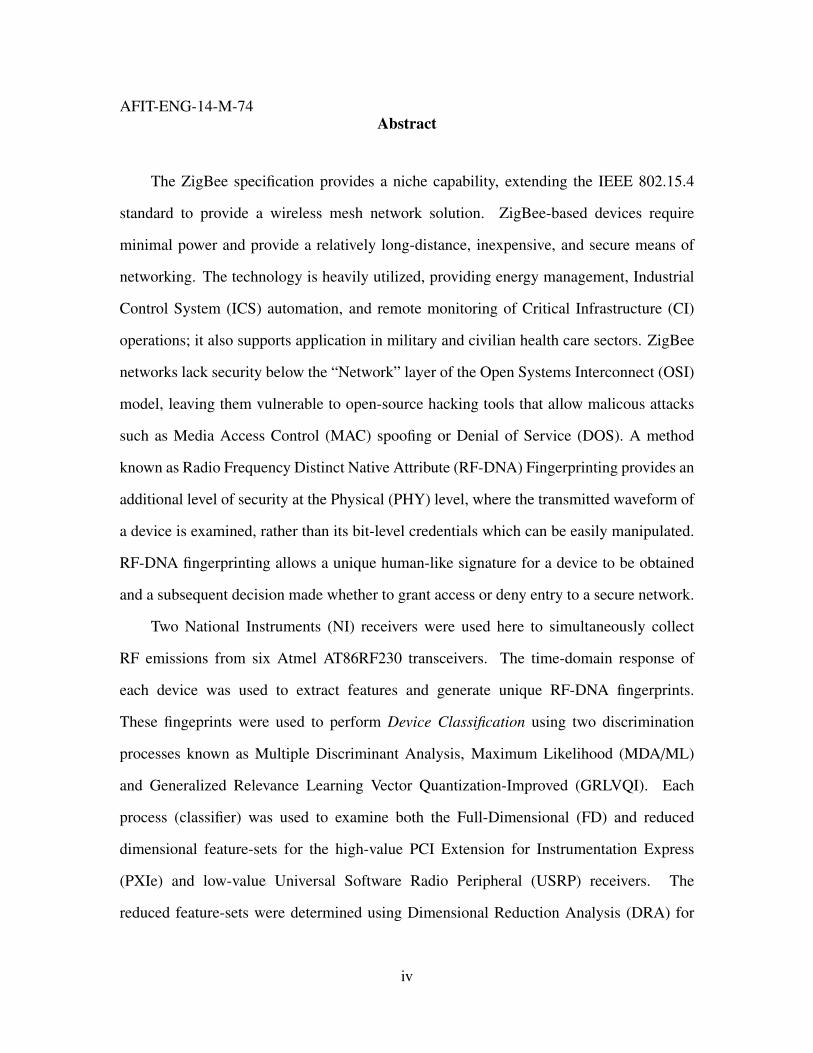
AFIT-ENG-14-M-74Abstract
The ZigBee specification provides a niche capability, extending the IEEE 802.15.4
standard to provide a wireless mesh network solution. ZigBee-based devices require
minimal power and provide a relatively long-distance, inexpensive, and secure means of
networking. The technology is heavily utilized, providing energy management, Industrial
Control System (ICS) automation, and remote monitoring of Critical Infrastructure (CI)
operations; it also supports application in military and civilian health care sectors. ZigBee
networks lack security below the “Network” layer of the Open Systems Interconnect (OSI)
model, leaving them vulnerable to open-source hacking tools that allow malicous attacks
such as Media Access Control (MAC) spoofing or Denial of Service (DOS). A method
known as Radio Frequency Distinct Native Attribute (RF-DNA) Fingerprinting provides an
additional level of security at the Physical (PHY) level, where the transmitted waveform of
a device is examined, rather than its bit-level credentials which can be easily manipulated.
RF-DNA fingerprinting allows a unique human-like signature for a device to be obtained
and a subsequent decision made whether to grant access or deny entry to a secure network.
Two National Instruments (NI) receivers were used here to simultaneously collect
RF emissions from six Atmel AT86RF230 transceivers. The time-domain response of
each device was used to extract features and generate unique RF-DNA fingerprints.
These fingeprints were used to perform Device Classification using two discrimination
processes known as Multiple Discriminant Analysis, Maximum Likelihood (MDA/ML)
and Generalized Relevance Learning Vector Quantization-Improved (GRLVQI). Each
process (classifier) was used to examine both the Full-Dimensional (FD) and reduced
dimensional feature-sets for the high-value PCI Extension for Instrumentation Express
(PXIe) and low-value Universal Software Radio Peripheral (USRP) receivers. The
reduced feature-sets were determined using Dimensional Reduction Analysis (DRA) for
iv
both quantitative and qualitative subsets. Additionally, each classifier performed Device
Classification using a “hybrid” interleaved set of fingerprints from both receivers.
The FD feature-set used for Device Classification included NF=297 features. When
examining each single receiver seperately and averaging over both classifiers, FD analysis
achieved an arbitrary benchmark of average correct classification %C>90% (cross-device
average) at S NR≈11.0 dB and S NR≈16.0 dB for PXIe and USRP receivers respectively.
MDA/ML performed better for FD feature sets, with GRLVQI requiring S NR≈2.0 dB in
additional gain to match MDA/ML performance. DRA was used to evaluate performance
using both quantitatively (NF=5, 10, 33, 66, 99) and qualitatively (NF=99) reduced feature
sets. Quantitative DRA performance favored the PXIe receiver which consistently achieved
%C>90% at S NR≈12.0 dB for NF∈[10 297]. Qualitative DRA showed that irrespective
of the receiver used, the Phz-only feature-set outperformed the Frq-only and Amp-only
feature-sets. Additionally, when using FD NF=297 and NF=99 for both quantitative and
qualitative feature-sets, %CFD ≈ %C99Qnt ≈ %C99Phz. Finally, when developing a Hybrid
Cross-Receiver model using fingerprints from both receivers, testing with PXIe-only
fingerprints proved to be the most effective method for performing Device Classification.
Both classifiers performed better than in any other hybrid case, achieving the %C>90%
benchmark for NF∈[5 297] and NF∈[10 297] using GRLVQI and MDA/ML, respectively.
v

Acknowledgments
I would first and foremost like to thank my amazing wife and son. Without their love,
patience, and encouragement, this dream never would have come to fruition.
I also would like to thank my advisor Dr. Temple for his guidance, wisdom and support
throughout this research.
Tyler D. Stubbs
vi
Table of Contents
Page
Abstract . . . . . . . . . . . . . . . . . . . . . . . . . . . . . . . . . . . . . . . . . iv
Acknowledgments . . . . . . . . . . . . . . . . . . . . . . . . . . . . . . . . . . . . vi
Table of Contents . . . . . . . . . . . . . . . . . . . . . . . . . . . . . . . . . . . . vii
List of Figures . . . . . . . . . . . . . . . . . . . . . . . . . . . . . . . . . . . . . . ix
List of Tables . . . . . . . . . . . . . . . . . . . . . . . . . . . . . . . . . . . . . . xi
List of Symbols . . . . . . . . . . . . . . . . . . . . . . . . . . . . . . . . . . . . . xii
List of Acronyms . . . . . . . . . . . . . . . . . . . . . . . . . . . . . . . . . . . . xiii
I. Introduction . . . . . . . . . . . . . . . . . . . . . . . . . . . . . . . . . . . . . 1
1.1 Operational Motivation . . . . . . . . . . . . . . . . . . . . . . . . . . . . 11.2 Technical Motivation . . . . . . . . . . . . . . . . . . . . . . . . . . . . . 31.3 Previous vs. Current Research . . . . . . . . . . . . . . . . . . . . . . . . 41.4 Document Organization . . . . . . . . . . . . . . . . . . . . . . . . . . . . 4
II. Background . . . . . . . . . . . . . . . . . . . . . . . . . . . . . . . . . . . . . 8
2.1 ZigBee Signal Characteristics . . . . . . . . . . . . . . . . . . . . . . . . . 82.2 RF-Fingerprint Generation . . . . . . . . . . . . . . . . . . . . . . . . . . 10
2.2.1 Time Domain Signal Responses . . . . . . . . . . . . . . . . . . . 102.2.2 Statistical Metrics . . . . . . . . . . . . . . . . . . . . . . . . . . 11
2.3 MDA/ML Processing . . . . . . . . . . . . . . . . . . . . . . . . . . . . . 132.3.1 Multiple Discriminant Analysis (MDA) Model Development . . . . 142.3.2 Maximum Likelihood (ML) Classification . . . . . . . . . . . . . . 16
2.4 GRLVQI Processing . . . . . . . . . . . . . . . . . . . . . . . . . . . . . 18
III. Methodology . . . . . . . . . . . . . . . . . . . . . . . . . . . . . . . . . . . . 21
3.1 Signal Collection . . . . . . . . . . . . . . . . . . . . . . . . . . . . . . . 223.2 Post-Collection Processing . . . . . . . . . . . . . . . . . . . . . . . . . . 25
3.2.1 Burst Detection . . . . . . . . . . . . . . . . . . . . . . . . . . . . 253.2.2 Down Conversion and Filtering . . . . . . . . . . . . . . . . . . . 27
vii

Page
3.2.3 SNR Scaling . . . . . . . . . . . . . . . . . . . . . . . . . . . . . 273.3 RF Fingerprint Generation . . . . . . . . . . . . . . . . . . . . . . . . . . 293.4 Dimensional Reduction Analysis . . . . . . . . . . . . . . . . . . . . . . . 31
3.4.1 Quantitative DRA . . . . . . . . . . . . . . . . . . . . . . . . . . 323.4.2 Qualitative DRA . . . . . . . . . . . . . . . . . . . . . . . . . . . 33
3.5 Device Discrimination . . . . . . . . . . . . . . . . . . . . . . . . . . . . 343.5.1 MDA/ML Model Development and Classification . . . . . . . . . . 343.5.2 GRLVQI Model Development and Classification . . . . . . . . . . 373.5.3 Comparative Assesment Test Matrix . . . . . . . . . . . . . . . . . 39
IV. Results and Analysis . . . . . . . . . . . . . . . . . . . . . . . . . . . . . . . . 42
4.1 Classification Model Development . . . . . . . . . . . . . . . . . . . . . . 434.2 Single Receiver Classification: Full-Dimensional (MDA/ML and GRLVQI) 434.3 Single Receiver Classification: DRA Performance (GRLVQI) . . . . . . . . 44
4.3.1 Quantitative DRA Performance . . . . . . . . . . . . . . . . . . . 454.3.2 Qualitative DRA Performance . . . . . . . . . . . . . . . . . . . . 47
4.4 Hybrid Cross-Receiver Classification: Full-Dimensional and QuantitativeDRA . . . . . . . . . . . . . . . . . . . . . . . . . . . . . . . . . . . . . . 484.4.1 Case 1: Hybrid Cross-Receiver Testing . . . . . . . . . . . . . . . 504.4.2 Case 2: PXIe Only Testing . . . . . . . . . . . . . . . . . . . . . . 524.4.3 Case 3: USRP Only Testing . . . . . . . . . . . . . . . . . . . . . 52
V. Conclusion . . . . . . . . . . . . . . . . . . . . . . . . . . . . . . . . . . . . . 55
5.1 Summary . . . . . . . . . . . . . . . . . . . . . . . . . . . . . . . . . . . 555.2 Findings and Contributions . . . . . . . . . . . . . . . . . . . . . . . . . . 56
5.2.1 Single Receiver Assessment . . . . . . . . . . . . . . . . . . . . . 565.2.2 Hybrid Receiver Assessment . . . . . . . . . . . . . . . . . . . . . 57
5.3 Recommendations for Future Research . . . . . . . . . . . . . . . . . . . . 58
Bibliography . . . . . . . . . . . . . . . . . . . . . . . . . . . . . . . . . . . . . . 61
viii

List of Figures
Figure Page
1.1 Seven-layer Open Systems Interconnect (OSI) Network Model . . . . . . . . . 3
1.2 AFIT RF-DNA Fingerprinting Process . . . . . . . . . . . . . . . . . . . . . . 5
2.1 Physical Layer and MAC Sublayer Structure for a ZigBee Packet . . . . . . . . 9
2.2 IEEE 802.15.4 Standard PHY Protocol Data Unit (PPDU) Packet Structure . . 10
2.3 Fingerprint Generation . . . . . . . . . . . . . . . . . . . . . . . . . . . . . . 13
2.4 MDA Projection Representation for NCl=3 Classes . . . . . . . . . . . . . . . 16
2.5 GRLVQI Projection Representation for =3 Classes . . . . . . . . . . . . . . . 20
3.1 RF Fingerprinting Process . . . . . . . . . . . . . . . . . . . . . . . . . . . . 22
3.2 Signal Collection Setup . . . . . . . . . . . . . . . . . . . . . . . . . . . . . . 23
3.3 Normalized PSD of Collections Showing Clock Skew . . . . . . . . . . . . . . 24
3.4 Normalized Atmel RZUSBstick PSD with Offset . . . . . . . . . . . . . . . . 24
3.5 Normalized Atmel RZUSBstick PSD Down-Converted and Filtered . . . . . . 28
3.6 ZigBee Transmission Specifying SHR . . . . . . . . . . . . . . . . . . . . . . 30
3.7 Burst Magnitude Response Divided Into Subregions . . . . . . . . . . . . . . . 32
3.8 Device Discrimination Process Block Diagram . . . . . . . . . . . . . . . . . 35
3.9 K-fold Cross-Validation Training Process for MDA Model Development . . . . 40
3.10 Block Diagram of Signal Collection, Post-Collection Processing, and K-fold
MDA Model Development . . . . . . . . . . . . . . . . . . . . . . . . . . . . 41
4.1 Full-Dimensional Receiver and Method Comparison . . . . . . . . . . . . . . 45
4.2 Full-Dimensional Receiver Cross-Device Averages . . . . . . . . . . . . . . . 46
4.3 Quantitative DRA Receiver Comparison . . . . . . . . . . . . . . . . . . . . . 48
4.4 Qualitative DRA Receiver Comparison . . . . . . . . . . . . . . . . . . . . . . 49
4.5 Hybrid Case 1 Full-Dimensional and Quantitative DRA Comparison . . . . . . 51
ix

Figure Page
4.6 Hybrid Case 2 Full-Dimensional and Quantitative DRA Comparison . . . . . . 52
4.7 Hybrid Case 3 Full-Dimensional and Quantitative DRA Comparison . . . . . . 54
x

List of Tables
Table Page
1.1 Previous Work vs Current Contributions . . . . . . . . . . . . . . . . . . . . . 7
3.1 Burst detection parameters for ZigBee transmission collections . . . . . . . . . 26
3.2 Comparative Assesment Test Matrix . . . . . . . . . . . . . . . . . . . . . . . 39
4.1 Full-Dimensional Receiver Cross-Device Averages Benchmark Comparison . . 46
4.2 Hybrid Case Description . . . . . . . . . . . . . . . . . . . . . . . . . . . . . 50
4.3 Hybrid Case 1: MDA/ML vs. GRLVQI Gain . . . . . . . . . . . . . . . . . . 51
4.4 Hybrid Case 2: MDA/ML vs. GRLVQI Gain . . . . . . . . . . . . . . . . . . 53
4.5 Hybrid Case 3: MDA/ML vs. GRLVQI Gain . . . . . . . . . . . . . . . . . . 53
xi

List of Symbols
Symbol Definition
a amplitude
%C99Amp 99-Feature Amplitude-Only Classification Benchmark
%C99Frq 99-Feature Frequency-Only Classification Benchmark
%C99Phz 99-Feature Phase-Only Classification Benchmark
%C99Qnt 99-Feature Quantitative Classification Benchmark
%CFD Full-Dimensional Classification Benchmark
F Fingerprint
fs Sample Rate
NC Number of Samples Collected
NCh Number of Instantaneous Responses
NCl Number of Classes
ND Number of Dimensions
NDev Number of Devices
NF Number of Features
NIR Number of Independent Realizations
NM Number of Statistical Metrics
NNz Number of Noise Realizations
NP Number of Prototype Vectors
NR Number of Regions
NS HR Number of Synchronization Header Responses
φ phase
∆t Sample Duration
xii
List of Acronyms
Acronym Definition
A/D Analog-to-Digital Converter
AFIT Air Force Institute of Technology
AWGN Additive White Gaussian Noise
DRA Dimensional Reduction Analysis
GRLVQI Generalized Relevance Learning Vector Quantization-Improved
ICS Industrial Control System
IEEE Institue of Electrical and Electronics Engineers
IP Internet Protocol
I/Q In-Phase and Quadrature
MAC Media Access Control
MDA Multiple Discriminant Analysis
MDA/ML Multiple Discriminant Analysis, Maximum Likelihood
ML Maximum Likelihood
MVG Multivariate Guassian
NI National Instruments
OSI Open Systems Interconnect
PXIe PCI Extension for Instrumentation Express
RF-DNA Radio Frequency Distinct Native Attribute
ROI Region of Interest
SFD Start-of-Frame-Delimiter
SHR Synchronization Header Response
USRP Universal Software Radio Peripheral
WPAN Wireless Personal Area Network
xiii
A COMPARISON OF RF-DNA FINGERPRINTING USING HIGH/LOW VALUE
RECEIVERS WITH ZIGBEE DEVICES
I. Introduction
This chapter provides a brief introduction to the operationally motivated research of
the ZigBee protocol and its applications in Section 1.1. Additionally, Section 1.2
provides the technical motivation for using the Air Force Institute of Technology (AFIT)’s
Radio Frequency Distinct Native Attribute (RF-DNA) process. Specifically, Section 1.3
provides the current state of AFIT’s RF-DNA fingerprinting process based on previous
research [2–4, 6, 10, 11, 15, 20–23, 25–27, 29, 31–37, 39, 40, 45, 46] and advancements
from the contributions of this research [30]. Finally, a breakdown of the document
organization is presented in Section 1.4.
1.1 Operational Motivation
The Institue of Electrical and Electronics Engineers (IEEE) 802.15 standard provides
guidance for establishing a Wireless Personal Area Network (WPAN) [24]. WPAN pro-
vide a an effective way for anyone to establish a personal network to which a multitude
of wireless devices can be connected for buisness or home use. The ZigBee specification
provides a niche capability, quickly growing in popularity, within this standard as dictated
by IEEE standard 802.15.4 [48]. ZigBee provides a low energy, low cost alternative that
is relatively simple to set up. ZigBee devices also boast long battery life and the ability to
perform secure networking. For these reasons, ZigBee is used in many industries, includ-
ing commercial, military, and healthcare. Commercial industries [13, 43, 44] use ZigBee
for Industrial Control System (ICS) and building automation, energy management and the
1

monitoring of critical infrastructure. The military has begun to utilize ZigBee for location
and positioning [10] while medical usage includes life-support and patient monitoring [5].
Given the strong probability that personal, critical, and even military national security in-
formation could traverse ZigBee networks on a day-to-day basis, the requirement for strong
network security remains high.
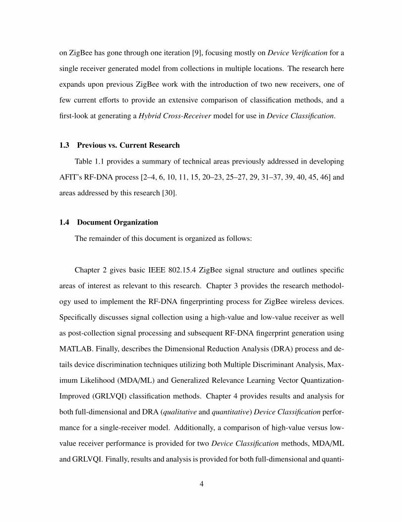
Wireless networks, such as ZigBee, all run off of the same basic premise of a seven
layer model known as the Open Systems Interconnect (OSI) model , shown in Fig. 1.1 [1].
The focus for security tends to rely soley on the “Network” and “Data Link” layers. This
basic security is where a network relies on device Media Access Control (MAC) or Internet
Protocol (IP) information to be submitted and verified as authorized prior to being allowed
into a network. There are various open source hacking tools that detect these mechanisms
by spoofing (replicating and presenting) specific device bit-level credentials and gaining
unauthorized network access. Once inside, a malicous device can perform various attacks
such as denial or service, network key sniffing, or hostile takeover of the whole network.
Of these hacking tools, there are a few that specifically target vulnerabilities of ZigBee
devices including KillerBee [47] and Api-Do [38].
This increasing threat to WPANs, specifically ZigBee, has constituted establishing
security at the most basic “Physical” level of the OSI model. This level deals with the
the actual physical waveform a device emits when it transmits or receives information.
Ongoing research at AFIT has attempted to establish a process known as RF-DNA
fingerprinting whereby a specific device can be described by features unique only to it.
A network can then use this prior-known information to compare to a device requesting
entry into the secure network, assess its bit-level credentials, and deem it as authorized or
unauthorized to enter. This process describes each device with a unique human-like RF
2

signature that allows for highly accurate Device Classification and makes replication of or
faking identities very difficult. It is for this reason that additional RF-DNA security at the
“Physical” layer is important to supplement existing “Network” and “Data Link” security,
which may be easier to bypass.
Figure 1.1: Seven-layer Open Systems Interconnect (OSI) Network Model [1].
1.2 Technical Motivation
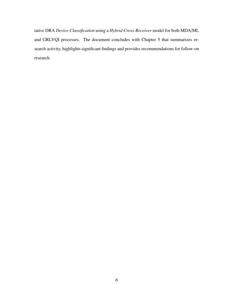
This RF-DNA process has gone through multiple generations of evolution and
currently stands as shown in Fig. 1.2 [9]. Each evolution of the process has incorporated
different classification and verification methods, model development techniques, as well as
introduced new receivers, signal types, and feature-sets. Each of these new or modified
methods and hardware have been specifically addressed through previous work at AFIT
[4, 6, 10, 11, 15, 20–23, 25–27, 29, 31–37, 39, 40, 45, 46], with the aim of supplementing
research conducted outside of AFIT as well [2, 3, 6–8, 14–17]. Previous work specifically
3
on ZigBee has gone through one iteration [9], focusing mostly on Device Verification for a
single receiver generated model from collections in multiple locations. The research here
expands upon previous ZigBee work with the introduction of two new receivers, one of
few current efforts to provide an extensive comparison of classification methods, and a
first-look at generating a Hybrid Cross-Receiver model for use in Device Classification.
1.3 Previous vs. Current Research
Table 1.1 provides a summary of technical areas previously addressed in developing
AFIT’s RF-DNA process [2–4, 6, 10, 11, 15, 20–23, 25–27, 29, 31–37, 39, 40, 45, 46] and
areas addressed by this research [30].
1.4 Document Organization
The remainder of this document is organized as follows:
Chapter 2 gives basic IEEE 802.15.4 ZigBee signal structure and outlines specific
areas of interest as relevant to this research. Chapter 3 provides the research methodol-
ogy used to implement the RF-DNA fingerprinting process for ZigBee wireless devices.
Specifically discusses signal collection using a high-value and low-value receiver as well
as post-collection signal processing and subsequent RF-DNA fingerprint generation using
MATLAB. Finally, describes the Dimensional Reduction Analysis (DRA) process and de-
tails device discrimination techniques utilizing both Multiple Discriminant Analysis, Max-
imum Likelihood (MDA/ML) and Generalized Relevance Learning Vector Quantization-
Improved (GRLVQI) classification methods. Chapter 4 provides results and analysis for
both full-dimensional and DRA (qualitative and quantitative) Device Classification perfor-
mance for a single-receiver model. Additionally, a comparison of high-value versus low-
value receiver performance is provided for two Device Classification methods, MDA/ML
and GRLVQI. Finally, results and analysis is provided for both full-dimensional and quanti-
4

Figure 1.2: AFIT RF-DNA Fingerprinting Process [9].
5
tative DRA Device Classification using a Hybrid Cross-Receiver model for both MDA/ML
and GRLVQI processes. The document concludes with Chapter 5 that summarizes re-
search activity, highlights significant findings and provides recommendations for follow-on
research.
6
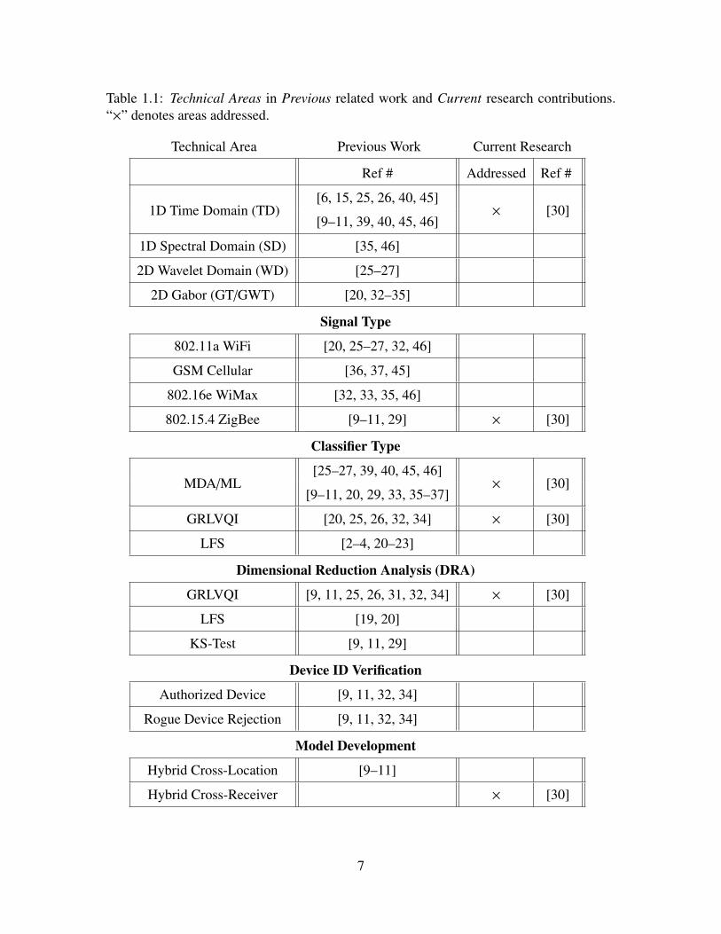
Table 1.1: Technical Areas in Previous related work and Current research contributions.“×” denotes areas addressed.
Technical Area Previous Work Current Research
Ref # Addressed Ref #
1D Time Domain (TD)[6, 15, 25, 26, 40, 45]
× [30][9–11, 39, 40, 45, 46]
1D Spectral Domain (SD) [35, 46]
2D Wavelet Domain (WD) [25–27]
2D Gabor (GT/GWT) [20, 32–35]
Signal Type
802.11a WiFi [20, 25–27, 32, 46]
GSM Cellular [36, 37, 45]
802.16e WiMax [32, 33, 35, 46]
802.15.4 ZigBee [9–11, 29] × [30]
Classifier Type
MDA/ML[25–27, 39, 40, 45, 46]
× [30][9–11, 20, 29, 33, 35–37]
GRLVQI [20, 25, 26, 32, 34] × [30]
LFS [2–4, 20–23]
Dimensional Reduction Analysis (DRA)
GRLVQI [9, 11, 25, 26, 31, 32, 34] × [30]
LFS [19, 20]
KS-Test [9, 11, 29]
Device ID Verification
Authorized Device [9, 11, 32, 34]
Rogue Device Rejection [9, 11, 32, 34]
Model Development
Hybrid Cross-Location [9–11]
Hybrid Cross-Receiver × [30]
7

II. Background
This chapter contains the technical background that serves as the framework for
methodology described in Chap. 3. Section 2.1 describes the basic ZigBee signal
structure as used in WPANs under IEEE 802.15.4. Section 2.2 introduces details for
Air Force Institute of Technology (AFIT)’s Radio Frequency Distinct Native Attribute
(RF-DNA) fingerprinting process, including fingerprint generation and calculation of
statistical metrics from instantaneous time-domain signal responses. Section 2.3 describes
elements of the Multiple Discriminant Analysis, Maximum Likelihood (MDA/ML) process
and Section 2.4 describes the Generalized Relevance Learning Vector Quantization-
Improved (GRLVQI) process.
2.1 ZigBee Signal Characteristics
ZigBee-based networks adhere to guidelines provided in IEEE 802.15.4 [24], which
specifies structure of “Physical” and “Data-Link” (specifically Media Access Control
(MAC)-sublayer) layers for ZigBee device transmission. As shown in Fig.2.1 [24], ZigBee
packets exhibit the data frame specification as provided in standards. The MAC sublayer
contains the actual transmission including the associated addressing fields, sequence
numbers, data being transmitted, etc. This research focuses on a specific Region of
Interest (ROI) for exploitation known as the Synchronization Header Response (SHR)
as shown in the “Physical” layer in Fig.2.1. This region is composed of a 5-octet, two
sequence structure as shown in Fig.2.2. The SHR includes:
1. Preamble: A 4-octet (32-bit) binary string of 0’s that is designed to provide symbol
chip timing for the transmitting device.
2. Start-of-Frame-Delimiter (SFD): A 1-octet (8-bit) binary string that is predefined as
(1 1 1 0 0 1 0 1). It is designed to signify the end of the preamble and thus the
8
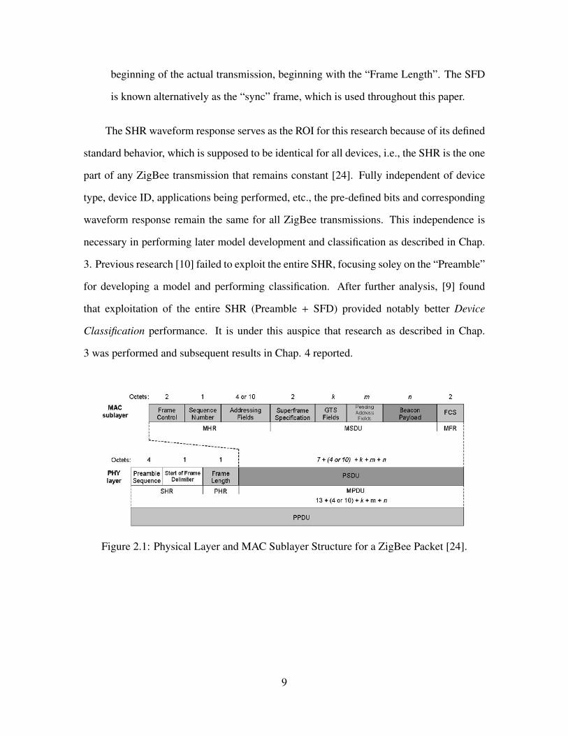
beginning of the actual transmission, beginning with the “Frame Length”. The SFD
is known alternatively as the “sync” frame, which is used throughout this paper.
The SHR waveform response serves as the ROI for this research because of its defined
standard behavior, which is supposed to be identical for all devices, i.e., the SHR is the one
part of any ZigBee transmission that remains constant [24]. Fully independent of device
type, device ID, applications being performed, etc., the pre-defined bits and corresponding
waveform response remain the same for all ZigBee transmissions. This independence is
necessary in performing later model development and classification as described in Chap.
3. Previous research [10] failed to exploit the entire SHR, focusing soley on the “Preamble”
for developing a model and performing classification. After further analysis, [9] found
that exploitation of the entire SHR (Preamble + SFD) provided notably better Device
Classification performance. It is under this auspice that research as described in Chap.
3 was performed and subsequent results in Chap. 4 reported.
Figure 2.1: Physical Layer and MAC Sublayer Structure for a ZigBee Packet [24].
9

Figure 2.2: Physical Protocol Data Unit (PPDU) packet structure for IEEE 802.15.4 [24].
The SHR as specified on the left is the ROI for this research
2.2 RF-Fingerprint Generation
An RF-DNA fingerprint is the collective term used to describe a unique, human-like
signature for a specific wireless device. Each fingerprint is generated in a two-step process
that includes calculation of instantaneous time domain signal responses, and calculation of
statistical metrics of those signal responses. Each step is further discussed below:
2.2.1 Time Domain Signal Responses.
The ZigBee SHR contains a unique time-domain waveform in which instantaneous
signal responses that describe it can be calculated. This research, as described and exe-
cuted in [9–11, 27, 30, 31, 36, 37, 40, 46] focused on NCh = 3 characteristic instantaneous
responses (a = amplitude, φ = phase, f = frequency) in a burst. Each collected signal
is represented as complex In-Phase and Quadrature (I/Q) component pairs which both re-
ceivers collect and store in the form of 16-bit integers [28]:
[I0,Q0, I1,Q1, ..., INC ,QNC ] ,
where NC represents the total number of collected sample I/Q pairs. The corresponding
instantaneous time-domain responses (a, φ, f ) are calculated as [30]:
a[n] =√
I[n]2 + Q[n]2, (2.1)
10

φ[n] = tan−1[Q[n]I[n]
], for I[n] , 0, (2.2)
f (n) =1
2π
[dφ(n)
dt
], (2.3)
for a given sample number n = 1, 2, 3, . . . ,NC.
These calculated elements of the SHR are then normalized [27, 40] and their mean
value removed. This is done by first removing the mean value for each element within a
single response and then dividing (normalizing) the collection of remaining elements by
the maximum value. This is accomplished for each response in (2.1), (2.2), and (2.3) and
yields:
ac(n) =a[n] − µa
maxn{ac[n]}
, (2.4)
φc[n] =φ[n] − µφ
maxn{φc[n]}
, (2.5)
fc[n] =f [n] − µ f
maxn{ fc[n]}
. (2.6)
where (2.4), (2.5), (2.6) show the respective mean (µa, µφ and µ f ) being removed and
“max” notes the value by which each response is normalized; these are the normalized
signal responses used for RF-DNA fingerprint generation.
2.2.2 Statistical Metrics.
After each response is centered and normalized, statistical metrics are calculated.
Following [9–11, 27, 30, 31, 36, 37, 40, 46], NM = 4 statistical metrics can be calculated
(σ = standard deviation ,σ2 = variance, γ = skewness, κ = kurtosis) for each response.
This is done by:
1. Dividing the SHR into NR equal subregions subject to the constraint that NC/NR is
an integer. Additionally, the entire SHR is examined and treated as a region itself,
yielding a total of NR+1 regions.
11

2. Calculating σ, σ2, γ, and κ (as selected) for each response sequence ac(n), φc[n], and
fc[n] according to
µ =1N
N∑n=1
x[n] , (2.7)
σ =
√√1N
N∑n=1
(x[n] − µ)2 , (2.8)
σ2 =1N
N∑n=1
(x[n] − µ)2 , (2.9)
γ =1
Nσ3
N∑n=1
(x[n] − µ)3 , (2.10)
κ =1
Nσ4
N∑n=1
(x[n] − µ)4 , (2.11)
where NC represents the total number of collected samples.
3. Arranging selected (2.8)-(2.11) metrics in a vector for each specific region as,
FRi = [σRi σ2RiγRi κRi]1×4, (2.12)
where i = 1, 2, 3, . . . ,NR+1. An example of this process is shown in Fig. 2.3 [31].
In total, for each fingerprint composed of NCh instantaneous responses and NM
statistical metrics per response, over an SHR of NR+1 regions, the number of “full-
dimensional” (FD) features (NFD) is calculated as,
NFD = NCh × NM × NR+1, (2.13)
where each full-dimensional fingerprint F is composed of the calculated statistics for
each of the three instantaneous responses and shown as
12

Figure 2.3: Process to generate a unique fingerprint utilizing statistical metrics for each
instantaneous response over NR+1 subregions [31].
F = [Fa ... Fφ ... F f ]1×NFD , (2.14)
These full-dimensional RF-DNA fingerprints are then used for model development and
classification for all devices (classes) using the two methods as described below.
2.3 MDA/ML Processing
The MDA/ML model development and classification process is comprised of two
seperate processes including Multiple Discriminant Analysis (MDA) and Maximum
Likelihood (ML) estimation. The description included here is based largely upon [9], with
selected elements included here for completeness. MDA serves as a method to develop a
model utilzing the Training RF-DNA fingerprints as will be discussed in Chap. 3. ML is
a classification method that uses the Testing RF-DNA fingerprints to compare to the model
generated by MDA and subsequently perform Device Classification. Both processes are
presented in further detail below.
13

2.3.1 Multiple Discriminant Analysis (MDA) Model Development.
This section describes how a model, later used for classification, is developed using
MDA. MDA is a process, based on Fisher’s Linear Discriminant, that linearly projects a
high-dimensional data space into a lower-dimensional one. The desired effect is to follow
the method of least-squares whereby a generalized linear model can be generated [12].
Unlike the Fisher method, which only works for discrimination of a NCl ≤ 2 class prob-
lem, MDA works to reduce the feature dimensionality describing an RF-DNA fingerprint
through projection for NCl > 2. MDA takes a specified number of feature (NF)-dimensional
described input, and projects it into a subspace that is characterized by ND dimensions. It
is noted that through the remainder of this document, the term “class” is interchangable
with a single “device” and accordingly with NDev = 6 devices as described in Section 3.1,
NCl = 6 classes. The overall goal of this projection is to maximize the distance of the space
describing each class from another while simultaneously minimizing the spread within a
class. Mathematically, this directly translates to a desired maximum distance between the
mean of each class, while minimizing the variance within a single class [12].
Two scatter matrices required for MDA are the out-of-class (inter-class, Sb) and in-
class (intra-class, Sw) matrices [42]. These two matrices are used to assemble the required
projection matrix, referred to as W. It is this matrix that is used to project a fingerprint F,
and maintain an optimal balance ratio between inter-class means and intra-class variances
as described in [12]. These scatter matrices, as well as their components are computed
as [42],
Sb =
NCl∑i=1
PiΣi , (2.15)
Sw =
NCl∑i=1
Pi(µi − µ0)(µi − µ0)T , (2.16)
14
where class covariance (Σi) and the global mean of all classes (µ0) are calculated as
Σi = E[(x − µi)(x − µi)T ] , (2.17)
µ0 =
NCl∑i=1
Piµi . (2.18)
µi and Pi as referenced in (2.18) are the mean and prior probability for each class
respectively. The intra-class scatter matrix in (2.16) provides a measure of the sum of
probability-weighted class feature variances for each individual class while the inter-class
scatter matrix in (2.15) provides a measure of the average distance (over all of the classes
combined) between individual class means from the respective calculated global mean of
all classes combined.
The NF-dimensional input RF-DNA fingerprint vectors, shown as F from (2.14), are
then projected into the lower (ND)-dimensional subspace using the projection operator
matrix, shown below as
f = WT F . (2.19)
W is the NF×ND projection matrix formed from the NCl−1 eigenvectors of S−1w Sb, and f is
the resulting RF-DNA fingerprint after projection into the new subspace [42]. Each of these
fingerprints f will then be split into Training and Testing sets as described in methodology
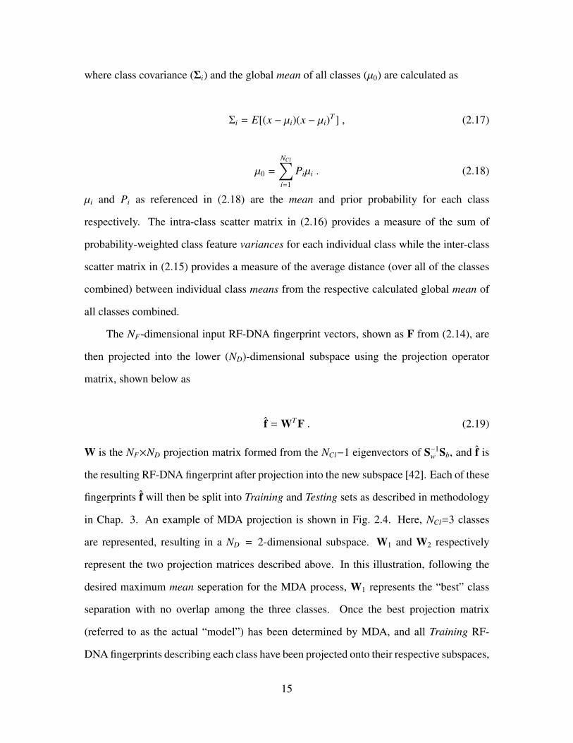
in Chap. 3. An example of MDA projection is shown in Fig. 2.4. Here, NCl=3 classes
are represented, resulting in a ND = 2-dimensional subspace. W1 and W2 respectively
represent the two projection matrices described above. In this illustration, following the
desired maximum mean seperation for the MDA process, W1 represents the “best” class
separation with no overlap among the three classes. Once the best projection matrix
(referred to as the actual “model”) has been determined by MDA, and all Training RF-
DNA fingerprints describing each class have been projected onto their respective subspaces,
15

model creation is finished and the process of Device Classification begins using ML and
the projected Testing RF-DNA fingerprints.
Figure 2.4: MDA Projection Representation for NCl=3 Classes corresponding to projectiononto 2-dimensional subspaces using W1 and W2 [12] operators; Showing maximumseperation (no overlap among the different classes), W1 is the optimal projection matrix(model) in this case.
2.3.2 Maximum Likelihood (ML) Classification.
ML is a method of Device Classification that uses the model developed with MDA.
As previously stated, after a model is created using the Training RF-DNA fingerprints, ML
takes the remaining (and unused) fingerprints describing the Testing data set, and performs
Device Classification. ML classification begins once the best “model” or projection matrix
(W) is determined, and the Testing fingerprints for each class are projected onto the
subspace. At this point in the process, the Training fingerprints have been projected,
and the mean (µi), and covariance (Σi) for each individual class have been computed
for i=1, 2, . . . ,NCl. ML operates off the assumption that all of the projected data is a
Multivariate Guassian (MVG) distribution and hence each class can be described by its own
class-dependent µi and Σi. Additionally, the ML process can assume that the covariance for
16

each class is identical and thus, a collective estimated covariance describing all classes can
be shown as
ΣP =1
NCl
NCl∑i=1
Σi . (2.20)
With the assumption of each class as a MVG distribution, posterior conditional
probabilities can be calculated for each Testing fingerprint f and used to provide a
measurement of class (ci) likelihood. Following the MVG distribution and collective
covariance (2.20) estimate, likelihood estimation can be implemented as [31, 42],
P(f|NCli
)=
1
(2π)(NCl−1)/2 det(ΣP
)1/2 · exp(Fe) , (2.21)
where Fe is calculated as
Fe = −12
(f − µi
)T (ΣP
)−1 (f − µi
). (2.22)
ci likelihood values as used for ML are based on a Bayesian decision theory. Each f from
the Testing data set is assigned to a specific ci by
P(ci|f
)> P
(c j|f
)∀ j , i . (2.23)
Again, i=1, 2, . . . ,NCl and here, P(ci|f
)is known as the the conditional posterior
probability that a given f belongs to a specific class ci. The conditional posterior probability
P(ci|f
)in (2.23) is calculated using Bayes’ Rule using specific ci likelihood values as shown
below [31, 42]:
17

P(ci|f
)=
P(f|ci
)P(ci)
P(f) . (2.24)
It is assumed that P(ci)=1/NCl, meaning that all prior probabilities are equal for all classes.
This, coupled with the fact that for any given f fingerprint, P(f)
is the same for all ci
as applied to (2.24), allows for simplication when making a comparison using (2.23).
Classification is then performed on a single Testing f using criteria in (2.23). Each f
is assigned a specific ci “label” based on maximum posterior probability. A “correct
classification” occurs if the assigned ci label matches the true or known ci label. This
process is repeated on all Testing fingerprints.
2.4 GRLVQI Processing
The second method considered for model development and classification is GRLVQI.
The description included here is based largely upon [31], with selected elements included
here for completeness. Unlike MDA/ML which is a two-stage process of model
development and classification, GRLVQI is a one-stage process that develops a model
and performs classification simultaneously. GRLVQI provides some advantages over
MDA/ML, including:
1. No required assumption of MVG distribution; GRLVQI does not require knowledge
of or assumption of any specific statistical distribution.
2. Model Development and Device Classification are performed jointly, rather than as
independent processes.
3. Each input feature is assigned a relevance value (λ) that allows for feature ranking
and Dimensional Reduction Analysis (DRA), as described in Section 3.4.
The model generated by GRLVQI utilizes prototype vectors that describe a specific
space for each class. The number of prototype vectors NP is pre-defined before model
18

development and classification take place. NP is the same for all classes and each prototype
vector used is comprised of NF features. The collection of all prototype vectors that
describe the classes is represented by pn, and given by [18]
pn = [P](NCl·NP)×NF , (2.25)
where NCl is the number of classes and P is a matrix that defines the classification
boundaries for the prototype vectors. The overall goal is to minimize Bayesian risk by
iteratively shifting the intra-class (pn) and inter-class (po) prototype vectors that describe
the space for all classes until a “best fit model” is achieved. This shift, dnλ, is computed
as [18]
dnλ =
NF∑i=1
λi(fmi − pn
i )2 , (2.26)
where fmis a randomly chosen Training input fingerprint to start the process, and n is the
prototype vector from (2.25) such that n = 1, 2, 3, . . . ,NP. λi is also randomly chosen when
the process is started.
This iterative process continues [31] until the prototype vectors are arranged in a best-
fit model and the corresponding λi values determined. Each λi receives a ranking (number)
that indicates its importance in classification; each i is known as an “index number” and
directly corresponds to a single feature. All λi’s are organized into a single vector known
as λB where it is possible for different index numbers (different features) to have the same
relevance ranking (λ) value, however,
NF∑i=1λi = λB ≡ 1.
19

The higher the λi value, the more important or relevant it is in performing Device
Classification as will later be discussed in Section 3.4. Finally, the Testing fingerprints
(f) are placed in 2.26 one at a time according to the best model, and the euclidean-distance,
between each f and the prototype vectors, is calculated as shown in Fig. 2.5 [31]. The
classification (assignment of that particular f to a specific ci) follows according to [31]
ci : mini, j
(dpλ(pi, j, f)) (2.27)
Figure 2.5: GRLVQI Projection Representation for a single fingerprint f for NCl=3Classes[31].
20

III. Methodology
This chapter contains the methodology utilized while conducting this research in order
to obtain the results as presented in Chap. 4. Simultaneous emissions collections
were taken by both receivers for a single device at a time. These emissions, stored by
the receivers as basic In-Phase and Quadrature (I/Q) components, were then converted
into complex values for ease in signal processing. MATLAB was then used to compute
instantaneous responses of detected bursts over the entirety of the Region of Interest
(ROI) and used to detect and extract “bursts.” The ROI, or ZigBee Synchronization
Header Response (SHR), was then down-converted to base-band and filtered with a 8th-
order Butterworth filter to remove background channel noise. Simultaneously, Additive
White Gaussian Noise (AWGN) was generated, like-filtered, and added to the filtered
SHR to appropriately power-scale and achieve S NR∈[0 24] dB. This resulting signal,
comprised of the sum of the down-converted and filtered SHR and AWGN, was then
broken into NR subregions. These subregions were then used to calculate statistical
metrics based off of the instantaneous time-domain signal responses. These are statistical
“features” used to generate a unique Radio Frequency Distinct Native Attribute (RF-DNA)
fingerprint that was used in Device Classification using both Multiple Discriminant
Analysis, Maximum Likelihood (MDA/ML) and Generalized Relevance Learning Vector
Quantization-Improved (GRLVQI) processes. Section 4.1 describes the setup for collecting
emissions. Section 4.2 discusses all post-signal collection processing, including burst
detection, filtering, and AWGN-aided S NR scaling. Section 4.3 discusses how an RF
fingerprint was generated for a full-dimensional feature-set, while Section 4.4 discusses
the process known as Dimensional Reduction Analysis (DRA). Finally, Section 4.4
discusses device discrimination, using both MDA/ML and GRLVQI model generation and
21

classification techniques. Accounting for specific receivers used here, AFIT’s entire RF-
DNA Fingerprinting process is as shown in Fig. 3.1 [9].
Figure 3.1: AFITs Fingerprinting Process [9]
3.1 Signal Collection
Two receivers, the National Instruments (NI) PCI Extension for Instrumentation Ex-
press (PXIe)-1085 and Universal Software Radio Peripheral (USRP)-2921, each with a 16-
bit Analog-to-Digital Converter (A/D), were used to collect RF emissions from six Atmel
AT86RF230 KillerBee ZigBee transceivers transmitting at 2.48 GHz per IEEE 802.15.4.
Each device (collectively referred to henceforth as Atmel RZUSBstick or seperately as
22
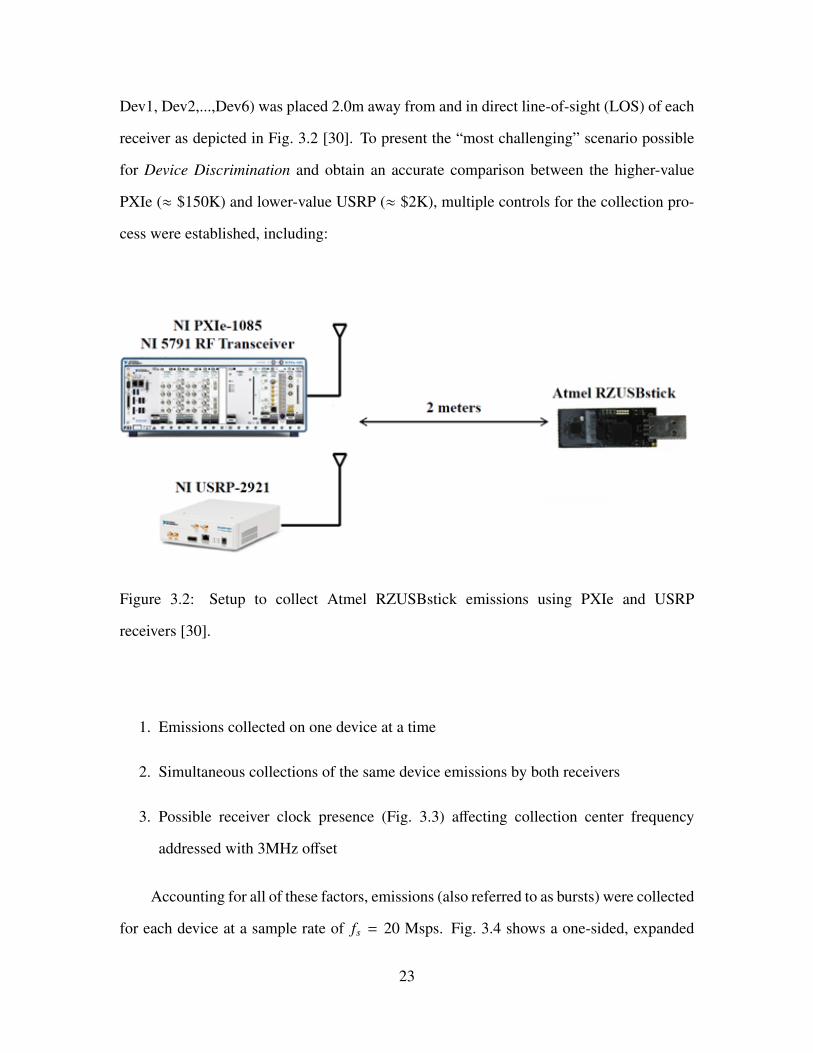
Dev1, Dev2,...,Dev6) was placed 2.0m away from and in direct line-of-sight (LOS) of each
receiver as depicted in Fig. 3.2 [30]. To present the “most challenging” scenario possible
for Device Discrimination and obtain an accurate comparison between the higher-value
PXIe (≈ $150K) and lower-value USRP (≈ $2K), multiple controls for the collection pro-
cess were established, including:
Figure 3.2: Setup to collect Atmel RZUSBstick emissions using PXIe and USRP
receivers [30].
1. Emissions collected on one device at a time
2. Simultaneous collections of the same device emissions by both receivers
3. Possible receiver clock presence (Fig. 3.3) affecting collection center frequency
addressed with 3MHz offset
Accounting for all of these factors, emissions (also referred to as bursts) were collected
for each device at a sample rate of fs = 20 Msps. Fig. 3.4 shows a one-sided, expanded
23
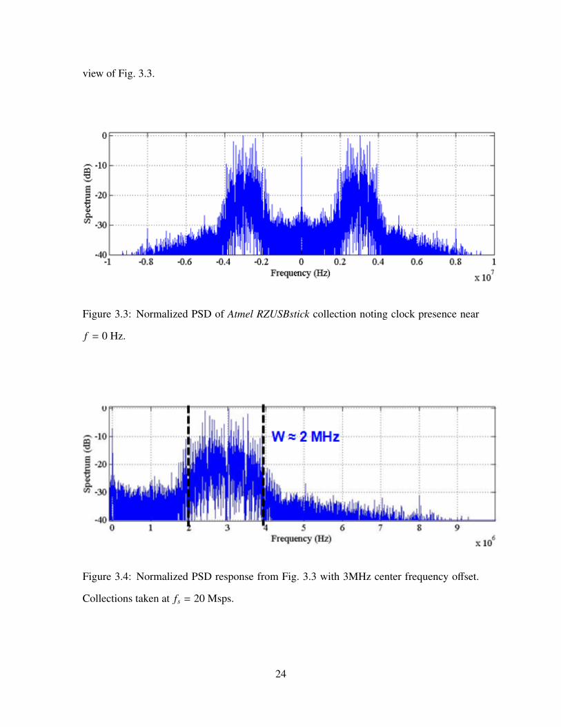
view of Fig. 3.3.
Figure 3.3: Normalized PSD of Atmel RZUSBstick collection noting clock presence near
f = 0 Hz.
Figure 3.4: Normalized PSD response from Fig. 3.3 with 3MHz center frequency offset.
Collections taken at fs = 20 Msps.
24

3.2 Post-Collection Processing
Following emission collections on all ZigBee devices using both receivers, a series
of post-collection processing steps were performed using MATLAB before RF-DNA
fingerprint generation. Collected bursts were first put through an amplitude-based
detection process, with bursts meeting specific criteria “extracted,” and those not discarded.
Extracted bursts were down-converted (center frequency shifted to f = 0), and subsequently
placed through a baseband filter to remove background noise. Finally AWGN was
generated, like-filtered, power-scaled, and added to the bursts to achieve a desired
S NR∈[0 24] dB. Each of these steps followed those from previous work [9, 30, 31], and
are described specific to this research next.
3.2.1 Burst Detection.
As discussed in Section 2.2.1, collected emissions from both receivers were stored as
interleaved I/Q components according to [28]:
[I0,Q0, I1,Q1, ..., INC ,QNC ]; (3.1)
where NC is the total number of collected samples. For easier processing in MATLAB,
each I/Q pair was converted into its corresponding complex format as:
[(I0 + jQ0), (I1 + jQ1), ..., (INC + jQNC )]. (3.2)
The collected bursts were then put through an amplitude-based detection process to extract
usable bursts out of the background noise. Bursts that met specific detection criteria were
determined as suitable to subsequently turn into fingerprints for later Device Classification,
while others were discarded. Specific requirements for detected bursts included specific
leading (tL) and trailing (tT ) edge thresholds, as well as minimum (TMin) and maximum
(TMax) time duration, shown in Table. 3.1.
25
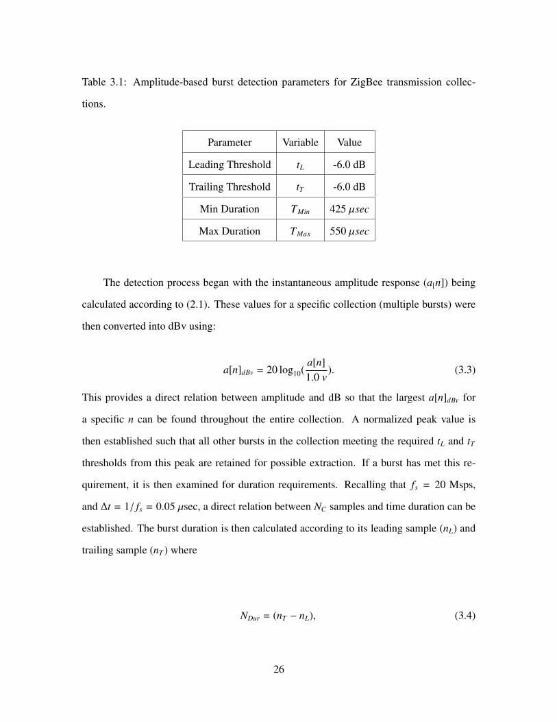
Table 3.1: Amplitude-based burst detection parameters for ZigBee transmission collec-
tions.
Parameter Variable Value
Leading Threshold tL -6.0 dB
Trailing Threshold tT -6.0 dB
Min Duration TMin 425 µsec
Max Duration TMax 550 µsec
The detection process began with the instantaneous amplitude response (a[n]) being
calculated according to (2.1). These values for a specific collection (multiple bursts) were
then converted into dBv using:
a[n]dBv = 20 log10(a[n]1.0 v
). (3.3)
This provides a direct relation between amplitude and dB so that the largest a[n]dBv for
a specific n can be found throughout the entire collection. A normalized peak value is
then established such that all other bursts in the collection meeting the required tL and tT
thresholds from this peak are retained for possible extraction. If a burst has met this re-
quirement, it is then examined for duration requirements. Recalling that fs = 20 Msps,
and ∆t = 1/ fs = 0.05 µsec, a direct relation between NC samples and time duration can be
established. The burst duration is then calculated according to its leading sample (nL) and
trailing sample (nT ) where
NDur = (nT − nL), (3.4)
26

TMin < (NDur ∗ ∆t) < TMax. (3.5)
If threshold and duration requirements are met, a burst is retained and “extracted” for use
in classification; if it does not meet the requirements it is discarded.
3.2.2 Down Conversion and Filtering.
After burst extraction was completed, the retained bursts were subsequently placed
through a two-stage process where each was down-converted to baseband ( fc = 0) and
filtered. Each process is outlined below:
1. MATLAB was used to down-convert each extracted burst to baseband using its
own center frequency estimate derived from a gradient-based frequency estimation
process [9, 30].
2. The down-converted burst was placed through a baseband filter to remove back-
ground noise and minimize fluctuations in Device Classification. This was done
as in [9, 30], using a 8th-order Butterworth filter having a baseband bandwidth of
WBB = 1MHz. The result was a single burst, centered at fc = 0, with minimal ef-
fect from noise outside of the collected IEEE 802.15.4 channel. This process was
repeated for all extracted bursts, with one such burst shown in Fig.3.5 [30].
3.2.3 SNR Scaling.
Finally, to provide a desired analysis range of S NR∈[0 24] dB (S NRA) for Device
Classification, AWGN was created using MATLAB and like-filtered before addition to
each burst to form the collective SHR used to generate fingerprints.
The collected S NR (S NRC) is a function of both power in the collected signal (without
background noise) (PC), and the power in the background noise during collection (PN). PN
27
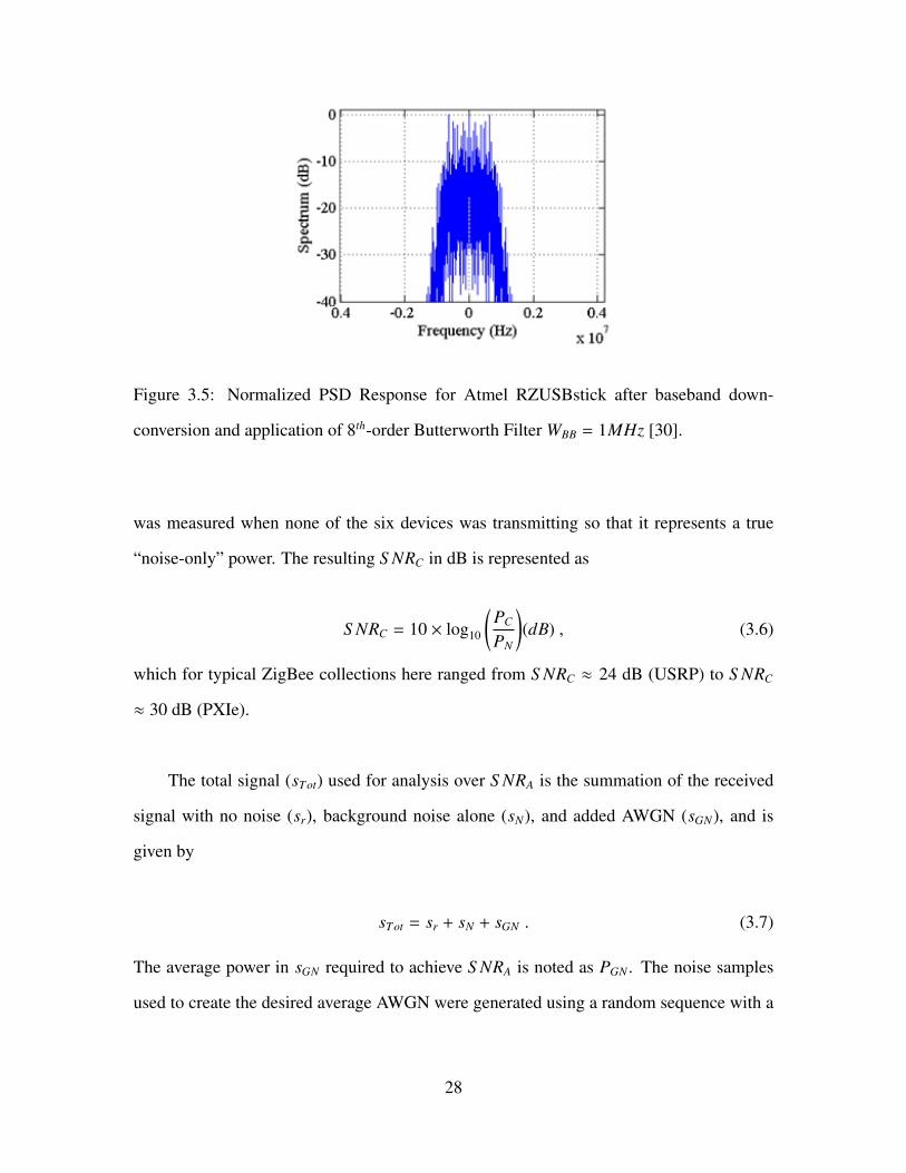
Figure 3.5: Normalized PSD Response for Atmel RZUSBstick after baseband down-
conversion and application of 8th-order Butterworth Filter WBB = 1MHz [30].
was measured when none of the six devices was transmitting so that it represents a true
“noise-only” power. The resulting S NRC in dB is represented as
S NRC = 10 × log10
(PC
PN
)(dB) , (3.6)
which for typical ZigBee collections here ranged from S NRC ≈ 24 dB (USRP) to S NRC
≈ 30 dB (PXIe).
The total signal (sTot) used for analysis over S NRA is the summation of the received
signal with no noise (sr), background noise alone (sN), and added AWGN (sGN), and is
given by
sTot = sr + sN + sGN . (3.7)
The average power in sGN required to achieve S NRA is noted as PGN . The noise samples
used to create the desired average AWGN were generated using a random sequence with a
28

normal distribution that was complex with zero mean. With PGN = 1, the associated scale
factor (S F) required to obtain the desired analysis S NRA is given by
S F =
√10
−S NRA10 × PC . (3.8)
Following the definition of S NR as the ratio of total signal (without noise) to total noise
(without signal), (3.6) can be rewritten to incorporate PGN , shown as
S NRA = 10 × log10
(PC
PN + PGN
)(dB) , (3.9)
where it is noted that generally, the scaled AWGN power is far greater than the collected
background noise power (PGN>>PN). This allows for (3.9) to be simplified, reducing it to
S NRA = 10 × log10
(PC
PGN
)(dB) . (3.10)
Finally, the total estimated average power for PGN can be calculated following the
expression for the total of any given arbitrary complex sequence as shown below
PGN =1
NC
NC∑i=1
S F · nGN(i)S F · n∗GN(i) . (3.11)
where nGN(i) is the real power, and n∗GN(i) is the complex conjugate or reactive power,
over i=1, 2, . . . ,NC total samples. As described above, this process of generating AWGN
and appropriately scaling it such that Device Classification could be performed over
S NRA∈[0 24] dB, was repeated and subsequently added to each extracted burst before
RF-DNA fingerprint generation. Finally, it is noted that S NRA henceforth is referred to as
S NR∈[0 24] dB throughout this document.
3.3 RF Fingerprint Generation
The overall ZigBee SHR as described in Section 3.2.3 (SHR + AWGN), while similar
in structure when defined in terms of transmitted bits, is slightly different for each device
29

in terms of the physical waveform. The SHR therefore contains each device’s unique
signature. This unique signature comes from manufacturing tolerances, device aging
characteristics, and differences in the manufacturing process. It is this unique, device-
dependent signature that is exploited to generate RF-DNA fingerprints and perform Device
Classification.
IEEE 802.15.4 defines the first 5 octets for all ZigBee signals. The first TP = 128
µsec of each transmission corresponds to the preamble, and the following TS yn = 32 µsec
contains the synchronization information [24]. The collective preamble and sync informa-
tion (128 µsec +32 µsec) makes up the total TS HR = = 160 µsec) SHR, as illustrated in
Fig.3.6. Accordingly, the duration of collected emissions, given ∆t = 1/ fs = 0.05 µsec in
each sample, is given by:
Figure 3.6: ZigBee transmission showing the SHR (highlighted in red) and the payload
(highlighted in blue).
30

NPre =128µsec.05µsec
= 2560samples. (3.12)
NS yn =32µsec.05µsec
= 640samples. (3.13)
NS HR = 2560 + 640 = 3200samples. (3.14)
Recalling the constraint that NC/NR must be an integer per Section 2.2.2, the SHR was
divided into NR = 32 equal subregions of 100 samples each, beginning at the start of the
transmission (burst) and ending after the last sync sample as depicted in Fig. 3.7.
Each subregion of 100 samples contained three instantaneous signal responses (a, φ,
f ) that uniquely described that subregion. Each instantaneous response was described by
three RF-DNA statistics (σ2, γ, κ). Accordingly, σ2, γ, and κ were calculated per (2.9)-
(2.11) for each a, φ, and f for each of the NR = 32 subregions as well as over the entire
SHR for one final region such that the total number of regions was NR+1 = 33. Each statistic
calculation represents a single RF-DNA “feature.” It is these specific features that uniquely
generated the RF-DNA fingerprints used for MDA/ML and GRLVQI Device Classification.
In the case that all features were used to describe a unique fingerprint, known as “full-
dimensional” (FD), the number of features is shown as
NFD = (a, φ, f) × (σ2, γ, κ) × (NR+1) = NF = 297. (3.15)
3.4 Dimensional Reduction Analysis
A process known as DRA was performed to reduce the number of features contained
within each RF-DNA fingerprint for a given device. The overall DRA goal is to effectively
reduce computational time and complexity, while maintaining a desired comparable
31

Figure 3.7: Magnitude response of a single burst SHR divided in to NR = 32 subregions
for subsequent RF-DNA fingerprinting. 100 samples are represented between each vertical
red dashed line.
classification performance regardless of the receiver used. Two types, Quantitative DRA
and Qualitative DRA are discussed next.
3.4.1 Quantitative DRA.
The first method of DRA is enabled through GRLVQI and deals with the actual
number of features NF . Recall from Section 3.3 that the full-dimensional set of features
describing an RF-DNA fingerprint for the Atmel RZUSBstick is NFD = NF = 297
32
features. This research followed the method in [9, 31] to iteratively reduce NF to a level
that maintains the %C=90% performance benchmark as will be described in Chap. 4.
Quantitative DRA takes the GRLVQI relevance vector λB from Section 2.4 and selects a
specified number of salient features such that only the top-ranked λi values are retained and
used to represent the characteristic “space” of a particular class. These values are relevance
ranked, meaning that the top-ranked (highest-valued λi) features have the greatest impact on
Device Classification. Quantitative DRA can be performed using any desired NF provided
the chosen value adheres to
NFD ≤ NF > 0. (3.16)
Selection of specific values used for NF here are described in Chap. 4, where results for
NF = 5, 10, 33, 66, and 99 features are provided.
3.4.2 Qualitative DRA.
The other method of DRA selects feature-sets as a given instantaneous signal response
subset as described in Section 2.2. Again the full-dimensional feature-set for a given RF-
DNA fingerprint included NFD = NF = 297 features. These features were composed
of statisticas (σ2, γ, κ) calculated for the instantaneous (a, φ, f) responses of a given burst.
Given three responses for each full-feature RF-DNA fingerprint,
NF(a) = NF(φ) = NF( f ) = 99, (3.17)
where during RF-DNA fingerprint generation, response features were organized sequen-
tially in RF-DNA fingerprints according to
F = [F(a)...F(φ)
...F( f )]1×297, (3.18)
where indices in F are given by:
33
a : i ∈ [1 99]; φ : i ∈ [100 198]; f : i ∈ [199 297]. (3.19)
Each subset was analyzed seperately, meaning that in one case for example, φ-only
features were used. In each case, relevance rankings (1 − 99 with “1” being noted as the
“top feature” and thus having the biggest effect on Device Classification) were assigned to
the given subset of λi values. This process was repeated for each instantaneous response
(a, φ, f) to obtain an accurate comparison among the subsets of their effects on Device
Classification. Additionally, this enabled direct comparison with Quantitative DRA for
NF = 99 (where the number of features may be composed of features from any and all of
the a, φ, or f subsets).
3.5 Device Discrimination
As described in Chap. 2, two methods of Device Discrimination were performed
using identical sets of RF-DNA fingerprints, MDA/ML and GRLVQI. Fig. 3.8 [41]
shows the basic discrimination process (in block diagram form) that all classifiers follow.
Additionally, DRA was performed using a model generated from GRLVQI and its
associated λ values; all methods of Device Classification performed will be shown in
Section 3.5.3.
3.5.1 MDA/ML Model Development and Classification.
The development here is taken exclusively from [9] and presented here for complete-
ness. MDA/ML as described in Section 2.3 is a two-step discrimination process that in-
volves both MDA model development and ML Device Classification. It is an extension
of Fisher’s Linear Discriminant and used for NCl > 2. This research was conducted
for six devices (classes), NDev = NCl = 6, and it thus follows from Section 2.3.1 that
ND = (NCl = 6) − 1 = 5 dimensions.
34

Figure 3.8: Block diagram of device discrimination process showing model development,usage of test statistics, and subesequent classification [41]. It is noted that “verification” ispossible after model development as well but not addressed in this research and thereforegrayed out.
MDA/ML was performed using RF-DNA fingerprints from both the PXIe and USRP
NI receivers for three different models:
35

1. Single Receiver: PXIe-only Training fingerprints
2. Single Receiver: USRP-only Training fingerprints
3. Hybrid Cross-Receiver: Combined PXIe and USRP Training fingerprints
Each model was developed by MDA through input feature dimensional reduction. The
full-dimensional feature-set, NF=297, RF-DNA Training fingerprints were projected onto
the ND=5-dimensional subspace. This was done using an iterative method known as
a K-fold process as described in detail in [9]. K-fold is a method that uses cross-
validation to develop the “best” model for use in Device Classification as shown in Fig. 3.9
[9]. The best model, as discussed in Section 2.3.1, refers to the model that leaves the
maximum distance between the mean of each class and simultaneously minimizes the
variance within any single class [12]. This research utilized a K=5 approach for model
development. Once the best model (WB) was selected, that model formed the projection
matrix (W) as discussed in Section 2.3.1. The fingerprints (F j) were then projected
according to (2.19), with the resulting f representing the lowered-dimensional projected
RF-DNA fingerprints. Following projection of all RF-DNA fingerprints, the feature space
describing each class was “mapped” accordingly into the Fisher Space (Fig.3.10) such that
the “decision boundaries” defining each respective class were formed. ML was then used
to perform Device Classification.
ML classification, as described in Section 2.3.2, was accomplished using the
remaining Testing fingerprints that were set aside during MDA model development. Each
of the NDev = 6 devices were represented and the process again assumed Multivariate
Guassian (MVG) distributions. The distributions were each described by their class-
specific means (µi) where i = 1, 2, ...(NCl = 6), and a collective covariance for all devices
(ΣP) as calculated in (2.20). Additionally, all prior probabilities and device likelihoods
36

were assumed to be equal. Each Testing fingerprint was classified one at a time following
the iterative process [9]:
1. Input Testing fingerprint F j from an unknown class c j.
2. Project F j into the Fisher space using (2.19) to generate projected fingerprint f j.
3. Associate f j to one of the known classes (devices) based on its maximum conditional
likelihood probability according to
ci : arg maxi
[p(ci|f j)
], (3.20)
where i=1, 2, . . . , (NCl = 6) and p(ci|f j) is the conditional likelihood probability that
projected fingerprint f j belongs to class ci. The overall measure of effectiveness for
the classifier (%C) is the percentage of the time the classifier correctly assigns the
fingerprint to its true device or class over all trials performed. “Correct” classification
notes when f j is classified as its known ci for a single trial.
3.5.2 GRLVQI Model Development and Classification.
The development here is taken exclusively from [18, 31] and presented here for com-
pleteness. GRLVQI processing follows the same basic process shown in Fig. 3.8 [41].
Unlike MDA/ML though, GRLVQI, as described in Section 2.4, performs model develop-
ment and Device Classification jointly, rather than as two independent processes.
GRLVQI requires no prior assumption of MVG distribution and additionally,
requires no knowledge of or assumption of any specific statistical distribution for model
development. It uses a specified number of prototype vectors to “shape” the space of each
class. This research utilized NP = 10 prototype vectors to describe each class, with each
prototype vector being comprised of NF = 297 features for full-dimensional analysis. The
37

collection of all prototype vectors, pn as derived in (2.25) [18], was used to iteratively shift
intra-class (pn) and inter-class (po) prototype vectors until a “best model” was achieved
according to (2.26) [18]. Model development and subsequent classification followed the
process as shown below:
1. Randomly choose a Training fingerprint (fm) and relevance-ranked feature (λi) and
input to (2.26).
2. Shift prototype vectors describing class “space” by distortion factor dnλ
3. Continue to iteratively shift protype vectors by dnλ and update corresponding
relevance-rankings (λi) until “best-fit model” is achieved by defined smallest dnBias
as described in [31]
4. Define “best-fit” relevance ranking vector (λB) as the vector containing λi for
i = 1, 2, 3, . . . ,NF; higher-valued λi correspond to most relevant features used in
describing a class.
5. Measure euclidian distance from a single Testing fingerprint (f) to each of the
prototype vectors as defined by the best model.
6. Associate the unknown f to one of the known ci based on the smallest euclidean
distance to the prototype vectors of a specified ci following
ci : mini, j
(dpλ(pi, j, f)) (3.21)
where i=1, 2, . . . , (NCl = 6) and j=1, 2, . . . , (NP = 10). As with MDA/ML,
%C provides the measurement of classifier effectiveness and “correct” classification
occurs when f j is classified as the true known ci.
38

3.5.3 Comparative Assesment Test Matrix.
The full spectrum of assesments performed, including full-dimensional and DRA
(quantitative and qualitative) using both MDA/ML and GRLVQI is shown in Table. 3.2.
The results of these tests, which allow for an accurate comparison of both classification
methods, as well both receivers are further discussed in Chap. 4.
Table 3.2: Comparative Assesment Test Matrix: 1 Full-Dimensional Baseline (MDA/ML &
GRLVQI), 2 Quantitative DRA (GRLVQI), 3 Quantitative vs. Qualitative DRA (GRLVQI),
and X denotes Test Not Performed
39
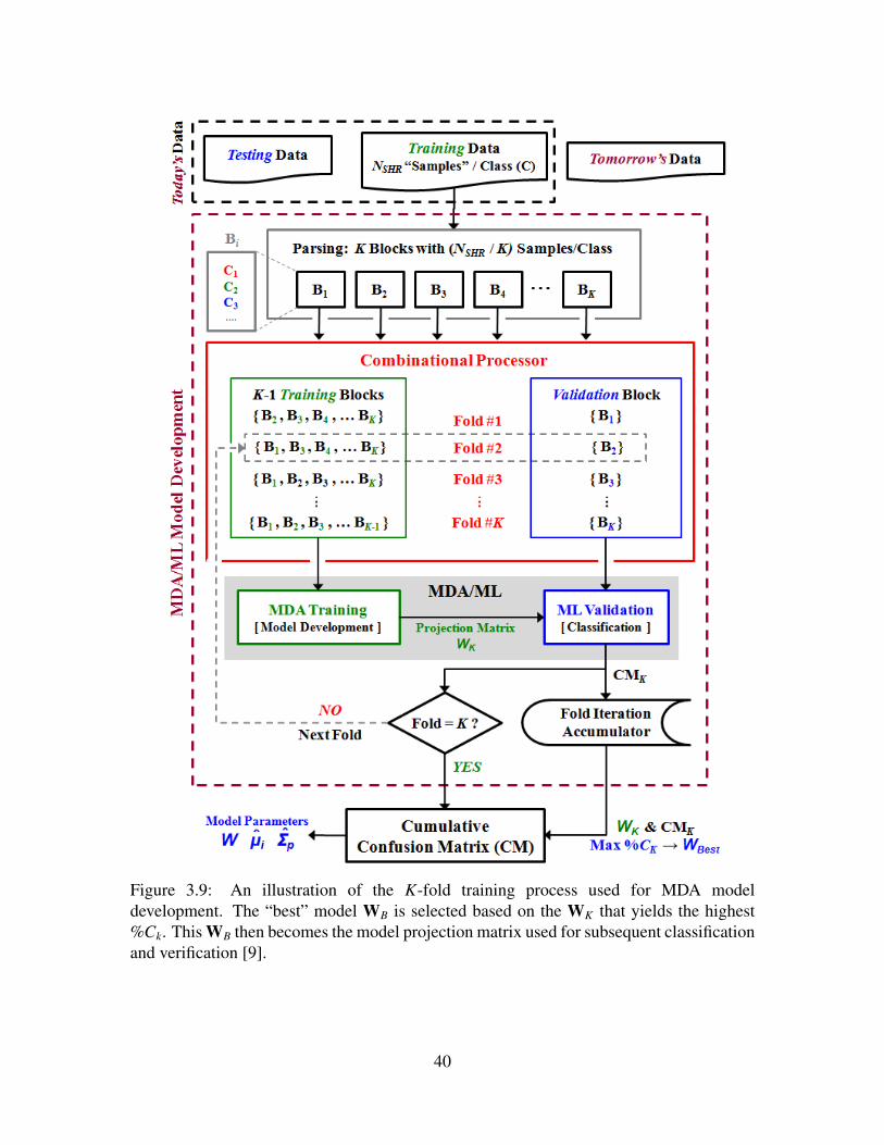
Figure 3.9: An illustration of the K-fold training process used for MDA modeldevelopment. The “best” model WB is selected based on the WK that yields the highest%Ck. This WB then becomes the model projection matrix used for subsequent classificationand verification [9].
40

Figure 3.10: Signal collection, post-collection processes and K-fold cross-validationtraining for MDA model development. This depicts a representative NDev=3 ZigBeedevices (classes) and the corresponding 2D Fisher Space. Each (o) represents a projectedtraining fingerprint f clustered around the respective class means shown as (•) [9].
41
IV. Results and Analysis
This chapter contains device discrimination results for six ZigBee devices using emis-
sions collected on National Instruments (NI) PCI Extension for Instrumentation Ex-
press (PXIe) and Universal Software Radio Peripheral (USRP) receivers. Device Classi-
fication was performed on both full-dimensional as well as qualitative and quantitative
Dimensional Reduction Analysis (DRA) feature-sets. DRA was performed using Gen-
eralized Relevance Learning Vector Quantization-Improved (GRLVQI) relevance-ranked
features. Subsequent classification of fingerprints from both receivers using DRA was only
performed using the GRLVQI method previously discussed in Section 3.4. Finally, De-
vice Classification was executed on the Hybrid fingerprints. Here, the term Hybrid is used
in different context from [9] and describes Cross-Receiver model development using RF-
DNA fingerprints derived from PXIe and USRP collections. As with the single-receiver
setup described above, both full-dminesional and quantitative only DRA feature-sets were
used for Device Classification. Section 4.1 describes how the model was developed after
dividing the prints into Training and Testing sets. Section 4.2 discusses full-dimensional
fingerprint Device Classification using both Multiple Discriminant Analysis, Maximum
Likelihood (MDA/ML) and GRLVQI methods and compares performance of PXIe and
USRP. Section 4.3 details the DRA process, including specific quantitative NF selection
and comparison of qualitative versus quantitative features for PXIe and USRP receivers.
Section 4.4 presents Hybrid Cross-Receiver model development and shows MDA/ML and
GRLVQI Device Classification performance results for full-dimensional fingerprints while
Section 4.5 compares quantitative DRA Device Classification results for MDA/ML and
GRLVQI models.
42

4.1 Classification Model Development
The classification model for single-receiver assessment was developed using PXIe
and USRP collections seperately. Specifically, a number of Synchronization Header Re-
sponse (SHR) from ZigBee emissions from each receiver were split into Training (NS HR
= 300) and Testing (NS HR = 300) for NCl = 6 classes. Further, a given number of noise
realizations were like-filtered and used for Monte Carlo simulation. The total of NIR used
for Monte Carlo simulation for each device included:
NIR = (NS HR = 600) × (NNz = 15) = 9000 Independent Realizations.
Of this total, NIR = 4500 independent realizations for each device were used for
“Training,” to develop the model via projection (MDA/ML) and with prototype vectors
(GRLVQI) as described in Section 3.5.1 and Section 3.5.2. The remaining NIR = 4500
were set aside for “Testing,” and assessing Device Classification.
4.2 Single Receiver Classification: Full-Dimensional (MDA/ML and GRLVQI)
Both classification methods were used for full-dimensional Device Classification where
in this case, NF = 297. This was derived from the fact that each SHR was described by
three instantaneous responses (a = amplitude, φ = phase, f = frequency), each of which
were in turn described by three statistics (σ2 = variance, γ = skewness, κ = kurtosis).
Further, each SHR divided into a fixed NR = 32 subregions across the entire SHR. The
statistics of each response were taken withinin each subregion resulting in a total of:
NFullFeat = (a, φ, f) × (σ2, γ, κ) × (NR+1 = 33) = NF = 297. (4.1)
Each RF-DNA fingerprint used for either model development of classification thus
contains NF = 297. Classification was performed on both PXIe and USRP using both
43

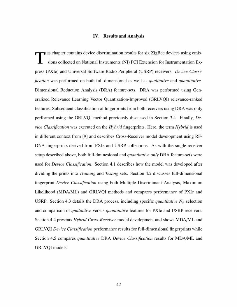
MDA/ML and GRLVQI. Fig. 4.1 shows full-dimensional classification performance for
fingerprints used for Testing. This was done for S NR∈[0 24] dB, keeping in context of
[30]. The performance of each device at each S NR is shown as well as the cross-device av-
erage performance for all devices noted as “Average.” A desired benchmark of %C=90%
was set for easy comparison of full-dimensional and DRA performance. It can be seen in
Fig. 4.1 that while it requires a range of S NR∈[8.5 24] dB to do so, each device as well as
their average achieves the benchmark for both receivers and both methods.
With the baseline for full-dimensional classification established, the remainder of
this paper will drop device-specific comparison and provide analysis only on the “Cross-
Device Average” performance of all given devices. Fig. 4.2 shows the same classification
performance as Fig. 4.1 with the devices removed, leaving only the cross-device average for
each receiver and method for comparison. Table. 4.1 provides a quick-reference chart for
Fig. 4.2, showing the S NR value at which each cross-device average achieves the arbitrary
%C=90% benchmark. When averaging performance for each individual receiver across
both methods, it can be seen that the higher end PXIe receiver clearly outperforms the lower
end USRP receiver by S NR ≈ 4.9 dB. Additionally, GRLVQI, when averaged across both
receivers, performs consistently poorer, requiring S NR ≈ 2.0 dB gain to match MDA/ML
performance.
4.3 Single Receiver Classification: DRA Performance (GRLVQI)
Due to the nature in which it is calculated, MDA/ML does not allow for DRA to
be performed as it does not provide relevance-ranking values for specific features as
does GRLVQI. Refering back to GRLVQI performance in Table. 4.1, PXIe achieved the
%C=90% benchmark at S NR ≈ 12.0 dB and USRP at S NR ≈ 18.0 dB. It is from these
two S NR values that DRA was performed respectively for each receiver.
44
Figure 4.1: Full-dimensional (NF = 297) classification comparing PXIe and USRP using
both MDA/ML and GRLVQI processes for NCl = 6. This shows all device averages as well
as the aggregated cross-device average
4.3.1 Quantitative DRA Performance.
Quantitative DRA was first performed in order to see how far of a reduction in features
the model could be developed with before Testing performance suffered signifigantly.
45

Figure 4.2: Full-dimensional (NF = 297) Cross-Device Averages for both receivers and
both classifiers.
Table 4.1: Full-dimensional (NF = 297) Cross-Device Average Benchmark Performance
Comparison.
46
Signifigant degradaded performance is defined as a shift in S NR at which meeting the
%C=90% benchmark either requires more gain (positive dB) from the full-dimensional
case, or where the benchmark is never achieved for S NR∈[0 24] dB. Refering to Section
4.2 where each fingerprint is made up of three responses (a, φ, f ), each providing NF
= 99 features, quantitative DRA began with NF = 99. DRA was subsequently repeated
over all S NR values as before, reducing by 33% first to ensure performance was not
degraded. It was then repeated with increased % reduction each time until performance
for either PXIe or PXIe began to suffer. Overall, quantitative DRA was performed for
(NF = 5, 10, 33, 66 and 99) features. Fig. 4.3 shows both receivers’ cross-device average
for the full-dimensional feature-set as well as each NF DRA. It is observed that as in
full-dimensional analysis in Section 4.2, high-value PXIe outperforms low-value USRP as
DRA is increased and NF is decreased. PXIe in fact consistently achieves the %C=90%
benchmark at the full-dimensional prescribed S NR ≈ 12.0 dB for all except NF = 5. PXIe
does however, unlike USRP, always achieve the benchmark overall. At NF = 10 features,
USRP performance begins to suffer, requiring an additional gain of S NR ≈ 6.0 dB. It then
quickly degrades to where the benchmark isn’t even achieved at NF = 5 features.
4.3.2 Qualitative DRA Performance.
Qualitative DRA, describing features by their signal responses (a, φ, f ) was then
performed on both receivers using GRLVQI. Previous research [9] has suggested that
unique RF-DNA signatures of ZigBee devices tend to be easier distinguished when looking
at the phase (φ) features of the SHR. Response-specific DRA was performed such that NF
= 99 each for (a, φ, f ). A model was created for each response feature-set seperately. A
comparison of these qualitative features as well as the quantitative DRA for NF = 99 is
seen in Fig. 4.4. Along with the full-dimensional feature set for each receiver from Section
4.2, it is clear that for the Atmel ZigBee devices used, (φ)-only features far outperform
a and f. Additionally, φ-only feature-set for both receivers performs just as well as full-
47

Figure 4.3: Quantitative DRA (NF = 5, 10, 33, 66, 99 and 297) Cross-Device Averages
Benchmark Comparison
dimensional and quantitative DRA for NF = 99 features. It is no surprise that PXIe
continues to outperform USRP, achieving the %C=90% benchmark with an S NR ≈ 6.2
dB gain
4.4 Hybrid Cross-Receiver Classification: Full-Dimensional and Quantitative DRA
The model for the cross-receiver setup was developed in a similar fashion to the single-
receiver model described in Section 4.1. In the Hybrid Cross-Receiver setup though, the
model was developed by combining PXIe and USRP fingerprints. Again, each receiver
provided NS HR = 600 ZigBee responses, which were divided into Training and Testing.
The Hybrid Cross-Receiver model though, containing fingerprints from both receivers, was
split, with Training = NS HR = 600 and two sets (one for each receiver) of Testing = NS HR
= 300 for each of the NCl = 6 classes. As in the single-receiver model, NNz = 15 like-
filtered, independent Monte Carlo Noise realizations were added to each ZigBee response
48

Figure 4.4: Quantitative DRA (NF = 99 & 297) versus Qualitative DRA (NF (a, φ, f ) = 99)
Cross-Device Averages Benchmark Comparison.
for each device to develop NIR independent realizations given by:
NIR = (NS HR = 600) × (NNz = 15) × (2 Receivers) = 18000.
The Hybrid Cross-Receiver was then, in contrast to Section 4.1, developed with NIR = 9000
independent realizations labeled “Training.” The remaining “Testing,” fingerprints were
split into three cases as summarized in Table. 4.2.
In Case 1, the “Testing” fingerprints were a combination of the reserved fingerprints
for both receivers, thus NIR = 4500 for each device. Case 2 and Case 3 tested the same
Hybrid Cross-Receiver model on only one receiver at a time. The reserved NIR = 2250 per
device for PXIe and NIR = 2250 for USRP were used as “Testing” fingerprints for Device
49

Table 4.2: Case Descriptions for Hybrid Cross-Receiver Training (Model Development)
and Device Classification Testing
Classification in Case 2 and Case 3 respectively.
Both Full-Dimensional and Quantitative DRA Device Classification were performed
using both MDA/ML and GRLVQI. It is important to note though, that while DRA was
performed using MDA/ML, the relevance-ranked features used to allow this, were actually
taken from the models developed using GRLVQI. Additionally, DRA for both MDA/ML
and GRLVQI for all three cases shown in Table. 4.2, was performed at S NR = 18.0 dB.
This value was determined by recalling from Section 4.3 that the %C=90% benchmark was
achieved in the worst case, for both receivers, at S NR ≈ 18.0 dB.
4.4.1 Case 1: Hybrid Cross-Receiver Testing.
The Hybrid Cross-Receiver fingerprints used for Testing were again a combination of
reserved, interleaved PXIe and USRP fingerprints. Fig. 4.5 shows a Full-Dimensional (NF
= 297) and Quantitative DRA (NF = 5, 10, 33, 66, 99) Device Classification comparison of
MDA/ML and GRLVQI. Table. 4.3 shows clearly that for a Full-Dimensional feature-set,
MDA/ML is superior to GRLVQI, requiring nearly S NR ≈ 2.0 dB less gain to achieve
%C=90%. GRLVQI immediately surpasses MDA/ML for Quantitative DRA, providing a
S NR ≈ 3.5 dB gain for NF = 99. Subsequent MDA/ML DRA performance fails to even
50

meet the %C=90% benchmark as GRLVQI DRA remains mostly consistent even as NF
decreases.
Figure 4.5: Case 1: Full-Dimensional (NF = 297) and Quantitative DRA (NF =
5, 10, 33, 66, 99) Device Classification using Hybrid Cross-Receiver model and Hybrid
Cross-Receiver testing.
Table 4.3: Case 1: GRLVQI “Gain” relative to MDA/ML. “X” indicates an incalculable
value given the %C=90% benchmark is never achieved within S NR∈[0 24] dB.
51

4.4.2 Case 2: PXIe Only Testing.
Fingerprints used for Case 2 Testing were entirely from PXIe fingerprints held out
of model development. Fig. 4.6 compares Full-Dimensional (NF = 297) and Quantitative
DRA (NF = 5, 10, 33, 66, 99) Device Classification, again for MDA/ML and GRLVQI.
Table. 4.4 show that while MDA/ML initially is marginally better when running Full-
Dimensional features, GRLVQI performance remains consistent as NF decreases and far
outperforms MDA/ML. It is noted also, that unlike in Case 1, MDA/ML performance on
its own is much better, meeting the %C=90% benchmark for all but NF = 5.
Figure 4.6: Case 2: Full-Dimensional (NF = 297) and Quantitative DRA (NF =
5, 10, 33, 66, 99) Device Classification using Hybrid Cross-Receiver model and PXIe only
testing.
4.4.3 Case 3: USRP Only Testing.
Case 3 Testing fingerprints are comprised of only USRP fingerprints held out of model
development. Fig. 4.7 compares Full-Dimensional (NF = 297) and Quantitative DRA (NF
52
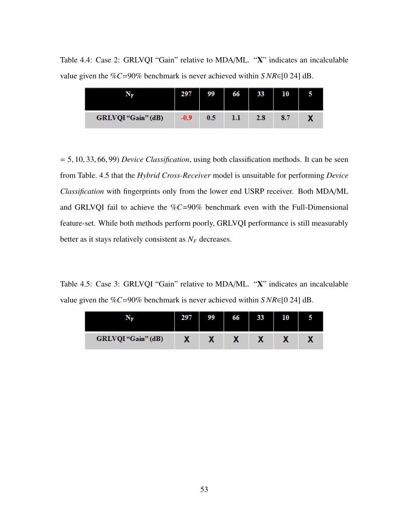
Table 4.4: Case 2: GRLVQI “Gain” relative to MDA/ML. “X” indicates an incalculable
value given the %C=90% benchmark is never achieved within S NR∈[0 24] dB.
= 5, 10, 33, 66, 99) Device Classification, using both classification methods. It can be seen
from Table. 4.5 that the Hybrid Cross-Receiver model is unsuitable for performing Device
Classification with fingerprints only from the lower end USRP receiver. Both MDA/ML
and GRLVQI fail to achieve the %C=90% benchmark even with the Full-Dimensional
feature-set. While both methods perform poorly, GRLVQI performance is still measurably
better as it stays relatively consistent as NF decreases.
Table 4.5: Case 3: GRLVQI “Gain” relative to MDA/ML. “X” indicates an incalculable
value given the %C=90% benchmark is never achieved within S NR∈[0 24] dB.
53

Figure 4.7: Case 3: Full-Dimensional (NF = 297) and Quantitative DRA (NF =
5, 10, 33, 66, 99) Device Classification using Hybrid Cross-Receiver model and USRP only
testing.
54
V. Conclusion
This chapter provides a summary of reseach performed, findings and contributions to
the Radio Frequency Distinct Native Attribute (RF-DNA) fingeprinting process, and
recommendations for follow-on research.
5.1 Summary
ZigBee-based networks are an affordable, widely-used option for accomplishing a
multitide of tasks within Wireless Personal Area Network (WPAN) applications. Due to
their low energy requirements, commercial availability, and low implementation complex-
ity, ZigBee WPANs are found in many buisnesses, hospitals, and homes. They are also
used in very important applications for Industrial Control System (ICS) automation, en-
ergy management, and by the military for location and positioning [10]. These sensors
are becoming increasingly exploited and the systems they are designed to protect remain
vulnerable to malicous attacks such as spoofing, denial of service, and key sniffing. These
attacks aim to gain unauthorized access by spoofing the bit level credentials required to
enter a secure network.
The security of ZigBee systems must be increased to prevent unauthorized persons
from entering networks and gaining access to critical information or control of critical
systems or infrastructure. One method for doing this is by exploiting known behavior and
RF fingerprint signature for known network devices. From this collection, an Authorized
and Unauthorized list can be created that upon request to enter a network, a device must
submit its bit-level credentials and be verified prior to being granted access. One method
considered here is RF-DNA fingerprinting, which provides an added level of security by
examining the actual physical waveform features emitted by a device. This provides a way
55

to single out a device and prevent something as simple as changing bit level credentials, or
spoofing a Media Access Control (MAC) address and entering a network.
5.2 Findings and Contributions
This research expanded the capabilities of AFIT’s RF-DNA fingerprinting process.
Specifically, earlier work in [9] was expanded with and knowledge of ZigBee device behav-
ior increased by introducting and investigating RF-DNA fingerprinting performance using
two new receivers and a new set of devices. Accurate comparisons between two different
classification methods, Multiple Discriminant Analysis, Maximum Likelihood (MDA/ML)
and Generalized Relevance Learning Vector Quantization-Improved (GRLVQI), were made
for both full-dimensional and Dimensional Reduction Analysis (DRA) (quantitative and
qualitative) feature-sets. Finally, a Hybrid Cross-Receiver model for Device Classification
was introduced and a first-ever comparison made using a model developed with RF-DNA
fingerprints from both a high-value PCI Extension for Instrumentation Express (PXIe) re-
ceiver and low-value Universal Software Radio Peripheral (USRP) receiver; both receivers
are commercial products manufactured by National Instruments (NI).
5.2.1 Single Receiver Assessment.
Full-dimensional Device Classification was performed with both receivers using MDA/ML
and GRLVQI methods. Regardless of the receiver, MDA/ML consistently dominated GRLVQI,
with the latter requiring an average S NR ≈ 2.0 dB increase in gain to match performance.
When averaging across classification methods however, the high-end PXIe receiver outper-
formed the low-end USRP receiver, requiring S NR ≈ 5.1 dB less to reach the arbitrary
%C=90% benchmark.
Quantitative DRA Device Classification, again only performed using GRLVQI, exhib-
ited a notable difference in performance between PXIe and USRP. While PXIe achieved
%C=90% at S NR ≈ 12.0 dB consistently, for NF∈[10 297], USRP performance suffered
56
and failed to meet the benchmark for NF ≤ 10. Qualitative DRA using NF = 99 features
proved that regardless of the receiver used, the Phz-only feature set far outperformed the
Frq-only and Amp-only feature sets. In fact, when compared to quantitative DRA perfor-
mance using the top-ranked NF = 99 features (combination of Amp, Phz, and Frq features)
for both receivers,
%CFD ≈ %C99Qnt ≈ %C99Phz > %C99Frq >> %C99Amp,
where %CFD is the average correct classification using the full-dimensional (FD) feature
set. Finally, on a comparison of receiver-only performance, regardless of classification
method or feature-set, high-value PXIe outpaced performance of low-value USRP by
S NR ≈ 6.0 dB.
5.2.2 Hybrid Receiver Assessment.
For “hybrid” receiver assessment, the MDA/ML and GRLVQI models were developed
using fingerprints from both receivers for both full-dimensional and Quantitative DRA
Device Classification. Three specific cases were examined where the Testing fingerprint
set included: 1) a hybrid combination of both PXIe and USRP fingerprints, 2) PXIe-only
fingerprints, and 3) USRP-only fingerprints.
Case 1: “Hybrid Cross-Receiver” (PXIe and USRP)
When Testing fingerprints were comprised of both receivers (Hybrid Cross-
Receiver), %C performance was mixed. While both classification methods met
the %C=90% benchmark for full-dimensional features, MDA/ML %C performance
immediately dropped off for NF < 99. Although MDA/ML was the clear winner for
full-dimensional classification, edging out GRLVQI by S NR ≈ 2.3 dB less required
gain, subsequent reduction of NF favored GRLVQI by S NR ≈ 3.5 dB less required
gain than that of MDA/ML to meet %C=90%. In fact, when NF ≤ 66, MDA/ML
failed to achieve the %C=90% benchmark over the specified S NR∈[0 24] dB range.
57

Case 2: PXIe Only Testing
Utilizing only PXIe fingerprints for Testing greatly increased %C performance for
both full-dimensional and DRA feature sets using MDA/ML and GRLVQI. While
MDA/ML performed better for full-dimensional classification, when averaged across
calcuable values (NF = 10, 33, 66, 99), GRLVQI required S NR ≈ 3.27 dB less gain
to match MDA/ML %C=90% benchmark performance. The Hybrid Cross-Receiver
model is well-suited for use soley with the PXIe receiver.
Case 3: USRP Only Testing
Utilizing only USRP fingerprints for Testing with full-dimensional and DRA feature
sets, regardless of classification method, failed to meet the %C=90% benchmark over
the S NR∈[0 24] dB range. The Hybrid Cross-Receiver model is deemed unsuitable
for use soley with the USRP receiver.
Overall when comparing classification methods, as in the single-receiver assessment,
MDA/ML outperformed GRLVQI for a full-dimensional feature-set. Averaged among
Case 1 and Case 2 (Case 3 full-dimensional analysis failed to achieve %C=90% benchmark
over the S NR∈[0 24] dB range), GRLVQI required an additional S NR ≈ 1.6 dB to match
MDA/ML %C performance. Quantitative DRA performance favored GRLVQI though,
providing relatively consistent %C over S NR∈[0 24] dB for NF > 10. Again, when
averaged across calcuable values for Case 1 and Case 2, MDA/ML required S NR ≈ 3.32
dB additional gain to match GRLVQI %C=90% benchmark performance.
5.3 Recommendations for Future Research
This research has shown that a high-value receiver (PXIe) generally provides better
classification performance than a lower-valued receiver (USRP). Further, it was shown that
by combining RF-DNA fingerprints from high and low value receivers, a Hybrid Cross-
Receiver model can be developed and when utilized properly, provide classification per-
58

formance results consistent with models developed solely from fingerprints for a single
receiver. This work is not complete and further benefit could be realized by investigating:
1. Alternative Classifiers - There are numerous other classifiers already in existence.
Device Classification should be investigated further by developing models and
performing classification with these alternative classifiers. Results varied in this
research, based mostly off of the classification method used and the NF chosen to
perform classification with. Choosing a different classifier other than MDA/ML or
GRLVQI may provide a single method that is the clear winner, outperforming all
other classifiers regardless of whether Full-Dimensional or DRA is used.
2. Different RF-DNA Features - There are endless possiblities of how to define the
features that are used to describe each RF-DNA fingerprint. Further work should be
performed to change the feature sets that are used for classification. Specifically
alternatives can include changing the size and number of subregions, developing
models that perform quantitative DRA within a specified time domain instantaneous
signal response (φ-only for example), and performing fingerprint generation using
different statistical metrics or combinations thereof. All these alternatives may
provide a different set of features that can more consistently meet or exceed
%C=90% at a lower dB value.
3. Alternative (non-ZigBee) Signals - The ZigBee protocol is a very small portion of
the mass of existing RF signals capable of performing device classification on. The
comparison of high versus low value receivers as well as creation of a Hybrid Cross-
Receiver may be found to be more suitable if performing Device Classification on
any of these other non-ZigBee signals.
59
4. Different devices within the ZigBee protocol - The Atmel AT86RF230 is but one
ZigBee device capable of being researched in terms of its signal responses. As
the ZigBee protocol is relatively inexpensive and widely used in a myriad of
applications, new devices will come to the forefront, and spoofing will remain a
concern. Investigating alternative devices with the same receivers will help to further
create a known pool of the behavior of all devices running the ZigBee protocol. This
information could be used to heighten security within critical networks that rely on
ZigBee every day.
60
Bibliography
[1] “OSI Reference Model”, May 2009. URL http://www.ccnaguru.com/
osi-reference-model.html.
[2] Buckner M.A. Learning From Data with Localized Regression and DifferentialEvolution. Ph.D. thesis, University of Tennessee, Knoxville, May 2003.
[3] Buckner M.A., A.M. Urmanov, A.V. Gribok and J.W. Hines. “Application ofLocalized Regularization Methods for Nuclear Power Plant Sensor CalibrationMonitoring”, Technical Correspondence, 2002.
[4] Buckner M.A., M. Bobrek, E.E. Farquahar, Harmer P.K. and M.A. Temple. “Enhanc-ing Network Security Using ’Learning-From-Signals’ and Fractioinal Fourier Trans-form Based RF-DNA Fingerprints”. SDR’11- Wireless Innovation Conference. Dec2011.
[5] Chen, S.K., T. Kao, C.T. Chan, C.N. Huang, C.Y. Chiang, C.Y. Lai, T.H. Tung, andP.C. Wang. “A Reliable Transmission Protocol for ZigBee-Based Wireless PatientMonitoring”. IEEE Trans on Information technology in Biomedicine, 16(1):6–16, Jan2012.
[6] Danev B. and S. Kapkun. “Transient-Based Identification of Wireless Sensor Nodes”.Proc of the 8th ACM/IEEE Int’l Conf on Information Processing in Sensor Networks(IPSN09). Apr 2009.
[7] Danev B., H. Luecken, S. Capkun, and K. El Defrawy. “Attacks on Physical-layer Identification”. Proc of the 3rd ACM Int’l Conf on Wireless Network Security(WiSec10). Mar 2010.
[8] Danev B., Heydt-Benjamin, S. Thomas and S. Capkun. “Physical-layer Identificationof RFID Devices”. Proc of the 18th conference on USENIX security symposium,SSYM’09, 199–214. 2009.
[9] Dubendorfer C.K. Using RF-DNA Fingerprints To Discriminate ZigBee Devices in anOperational Environment. Master’s thesis, Air Force Institute of Technology, March2013.
[10] Dubendorfer C.K., B.W. Ramsey and M.A. Temple. “An RF-DNA VerificationProcess for ZigBee Networks”. Proc of Military Communications Conference(MILCOM12). Oct 2012.
[11] Dubendorfer C.K., B.W. Ramsey and M.A. Temple. “ZigBee PHY-Based Device IDVerification: Security Enhancement for Industrial Control and Building AutomationSystems”. Proc of IFIP Working Group 11.10 Int’l Conf on Critical InfrastructureProtection (IFIP13). Mar 2013.
61

[12] Duda R., P. Hart and D. Stork. Pattern Classification. John Wiley & Sons, Inc., NewYork, second edition, 2001.
[13] Egan D. “The Emergence of ZigBee in Building Automation and Industrial Control”.Computing & Control Engineering Journal, 16(2):14–19, April-May 2005.
[14] Hall J., et. al. “Detection of Transient in Radio Frequency Fingerprinting Using SignalPhase”. IASTED Int’l Conf on Wireless and Optical Communications, May 2003.
[15] Hall J., et. al. “Using Transceiverprints for Anomaly Based Intrusion Detection”.3rd IASTED Int’l Conf on Communications, Internet and Information Technology(CIIT), November 2004.
[16] Hall J., M. Barbeau and E. Kranakis. “Radio Frequency Fingerprinting for IntrusionDetection in Wireless Networks”, Jul 2005. DRAFT.
[17] Hall J., M. Barbeau and E. Kranakis. “Detecting Rogue Devices In BluetoothNetworks Using Radio Frequency Fingerprinting”. Communications and ComputerNetworks, 108–113. 2006.
[18] Hammer B. and T. Villmann. “Generalized Relevance Learning Vector Quantization”.Neural Networks, 15:1059–1068, 2002.
[19] Harmer P.K. Development of Learning from Signals Classifier for Cognitive SoftwareDefined Radio Applications. Ph.D. thesis, Air Force Institute of Technology, March2013.
[20] Harmer P.K., D.R. Reising and M.A. Temple. “Classifier Selection for Physical LayerSecurity Augmentation in Cognitive Radio Networks”. Proc of IEEE Int’l Conf onCommunications (ICC13), Jun 2013.
[21] Harmer P.K., M.A. Temple, M.A. Buckner and E.E. Farquahar. “4G SecurityUsing Physical Layer RF-DNA with DE-Optimized LFS Classificatioin”. Jourof Communications, Special Issue: Advances in Communications and Networking,9(6):671–681, Dec 2011.
[22] Harmer P.K., M.A. Temple, M.A. Buckner and E.E. Farquahar. “Using DifferentialEvolution to Optimize ’Learning from Signals’ and Enhance Network Security”.Submitted to: Genetic and Evolutionary Computation Conference (GECCO). JulyJul 2011.
[23] Harmer P.K., M.D. Williams and M.A. Temple. “Using DE-Optimized LFSProcessing to Enhance 4G Communication Security”. 20th International Conferenceon Computer Communication and Networks (ICCCN). Aug 2011.
[24] Institute of Electrical and Electronics Engineers. IEEE 802.15.4, Standard, WirelessMedium Access Control (MAC) and Physical Layer (PHY) Specifications for Low-Rate WPANS, 2006.
62

[25] Klein R.W. Application of Dual-Tree Complex Wavelet Transforms to Burst Detectionand RF Fingerprint Classification. Ph.D. thesis, Air Force Institute of Technology,September 2009.
[26] Klein R.W., M.A. Temple and M.J. Mendenhall. “Application of Wavelet-Based RFFingerprinting to Enhance Wireless Network Security”. Jour of Communications andNetworks, Vol. 11, No. 6, Dec 2009.
[27] Klein R.W., M.A. Temple, M.J. Mendenhall and D.R. Reising. “Sensitivity Analysisof Burst Detection and RF Fingerprinting Classification Performance”. Proc of IEEEInt’l Conf on Communications (ICC09). Jun 2009.
[28] National Instruments. National Instruments Record and Playback Demo With NIUSRP, 2012.
[29] Ramsey B.W., M.A. Temple and B.E. Mullins. “PHY Foundation for Multi-Factor ZigBee Node Authentication”. Proc of IEEE Global Communications Conf(GLOBECOM12). Dec 2012.
[30] Ramsey B.W., T.D. Stubbs, B.E. Mullins, M.A. Temple, M.A. Buckner. “WirelessCritical Infrastructure Protection Using Low-Cost RF Fingerprinting Receivers”.Journal of Computers and Electrical Engineering. Submitted Feb 2013, UnderReview.
[31] Reising, D.R. Exploitation of RF-DNA for Device Classification and VerificationUsing GRLVQI Processing. Ph.D. thesis, Air Force Institute of Technology,December 2012.
[32] Reising, D.R., and M.A. Temple. “Verification of Localized OFDM-Based DevicesUsing Dimensionally Efficient GRLVQI Processing”. Systems Journal, IEEE, 2012.
[33] Reising D.R. and M.A. Temple. “WiMAX Mobile Subscriber Verification UsingGabor-Based RF-DNA Fingerprints”. 2012 IEEE International CommunicationsConference (ICC12). Jun 2012.
[34] Reising D.R., M.A. Temple, and J.A. Jackson. “Detecting Rogue Devices at CloudWireless Access Points Using RF Air Monitors”. Information Forensics and Security,IEEE Transactions on, 2012.
[35] Reising D.R., M.A. Temple and M.E. Oxley. “Gabor-Based RF-DNA Fingerprintingfor Classifying 802.16e WiMAX Mobile Subscribers”. 2012 IEEE Int’l Conf onComputing, Networking & Communications (ICNC), Jan 2012.
[36] Reising D.R., M.A. Temple and M.J. Mendenhall. “Improved Wireless Security forGMSK-Based Devices Using RF Fingerprinting”. Int. J. Electronic Security andDigital Forensics, Vol. 3, No. 1, pp. 41-59,2010.
63

[37] Reising D.R., M.A. Temple and M.J. Mendenhall. “Improving Intra-CellularSecurity Using Air Monitoring with RF Fingerprints”. Proc of 2010 IEEE WirelessCommunications & Networking Conf (WCNC10). Apr 2010.
[38] Speers R., J. Wright and R. Melgares. “Api-do: Tools for ZigBee and 802.15.4Security Auditing”. URL http://code.google.com/p/zigbeesecurity/.
[39] Suski W.M. II, M.A. Temple, M.J. Mendenhall and R.F. Mills. “RF FingerprintingCommercial Communication Devices to Enhance Electronic Security”. Int. J.Electronic Security and Digital Forensics, Vol. 1, No. 3, pp. 301-322, 2008.
[40] Suski W.M. II, M.A. Temple, M.J. Mendenhall and R.F. Mills. “Using SpectralFingerprints to Improve Wireless Network Security”. Proc of IEEE GlobalCommunications Conf (GLOBECOM08). Mar 2008.
[41] Temple M.A. “RF-DNA Fingerprinting: Distinct Native Attributes”, Lecture Notes,EENG 699, Jan 2013.
[42] Theodoridis S. and K. Koutoumbas. Pattern Recognition. Academic Press, fourthedition, 2009.
[43] Tihon I. and V. Croitoru. “ZigBee Sensor Networks Telesurveillance”. 1–4. 10thInternational Symposium on Signals, Circuits and Systems (ISSCS’11), Jun 2011.
[44] Whittaker T. “Final Word”. 18(3):48, Jun-July 2007.
[45] Williams M.D., M.A. Temple and D.R. Reising. “Augmenting Bit-Level networkSecurity Using Physical Layer RF DNA Fingerprinting”. Proc of IEEE GlobalCommunications Conf (GLOBECOM10). Dec 2010.
[46] Williams M.D., S.A. Munns, M.A. Temple and M.J. Mendenhall. “RF-DNAFingerprinting for Airport WiMax Communications Security”. Proc of 4th Int’l Confon Net and Sys Security (NSS10). Sep 2010.
[47] Wright J. “KillerBee: Framework and Tools for Exploiting ZigBee and IEEE 802.15.4Networks”, Version 1.0, 2010. URL http://code.google.com/p/killerbee/.
[48] ZigBee Alliance. ZigBee Specification, 2008.
64

REPORT DOCUMENTATION PAGE Form ApprovedOMB No. 0704–0188
The public reporting burden for this collection of information is estimated to average 1 hour per response, including the time for reviewing instructions, searching existing data sources, gathering andmaintaining the data needed, and completing and reviewing the collection of information. Send comments regarding this burden estimate or any other aspect of this collection of information, includingsuggestions for reducing this burden to Department of Defense, Washington Headquarters Services, Directorate for Information Operations and Reports (0704–0188), 1215 Jefferson Davis Highway,Suite 1204, Arlington, VA 22202–4302. Respondents should be aware that notwithstanding any other provision of law, no person shall be subject to any penalty for failing to comply with a collectionof information if it does not display a currently valid OMB control number. PLEASE DO NOT RETURN YOUR FORM TO THE ABOVE ADDRESS.
1. REPORT DATE (DD–MM–YYYY) 2. REPORT TYPE 3. DATES COVERED (From — To)
4. TITLE AND SUBTITLE 5a. CONTRACT NUMBER
5b. GRANT NUMBER
5c. PROGRAM ELEMENT NUMBER
5d. PROJECT NUMBER
5e. TASK NUMBER
5f. WORK UNIT NUMBER
6. AUTHOR(S)
7. PERFORMING ORGANIZATION NAME(S) AND ADDRESS(ES) 8. PERFORMING ORGANIZATION REPORTNUMBER
9. SPONSORING / MONITORING AGENCY NAME(S) AND ADDRESS(ES) 10. SPONSOR/MONITOR’S ACRONYM(S)
11. SPONSOR/MONITOR’S REPORTNUMBER(S)
16. SECURITY CLASSIFICATION OF:
a. REPORT b. ABSTRACT c. THIS PAGE
17. LIMITATION OFABSTRACT
18. NUMBEROFPAGES
19a. NAME OF RESPONSIBLE PERSON
19b. TELEPHONE NUMBER (include area code)
Standard Form 298 (Rev. 8–98)Prescribed by ANSI Std. Z39.18
27–03–2014 Master’s Thesis Oct 2013–Mar 2014
A Comparison of RF-DNA Fingerprinting Using High/Low ValueReceivers with ZigBee Devices
Stubbs, Tyler D., Captain, USAF
Air Force Institute of TechnologyGraduate School of Engineering and Management (AFIT/EN)2950 Hobson WayWPAFB, OH 45433-7765
AFIT-ENG-14-M-74
Intentionally Left Blank
12. DISTRIBUTION / AVAILABILITY STATEMENTDISTRIBUTION STATEMENT A:APPROVED FOR PUBLIC RELEASE; DISTRIBUTION UNLIMITED
13. SUPPLEMENTARY NOTESThis work is declared a work of the U.S. Government and is not subject to copyright protection in the United States.
14. ABSTRACTThe ZigBee specification provides a niche capability, extending the IEEE 802.15.4 standard to provide a wireless mesh networksolution. ZigBee-based devices require minimal power and provide a relatively long-distance, inexpensive, and secure meansof networking. The technology is heavily utilized, providing energy management, ICS automation, and remote monitoring ofCritical Infrastructure (CI) operations; it also supports application in military and civilian health care sectors. ZigBee networkslack security below the “Network” layer of the OSI model, leaving them vulnerable to open-source hacking tools that allowmalicous attacks such as MAC spoofing or Denial of Service (DOS). A method known as RF-DNA Fingerprinting provides anadditional level of security at the Physical (PHY) level, where the transmitted waveform of a device is examined, rather than itsbit-level credentials which can be easily manipulated. RF-DNA fingerprinting allows a unique human-like signature for a deviceto be obtained and a subsequent decision made whether to grant access or deny entry to a secure network. Two NI receiverswere used here to simultaneously collect RF emissions from six Atmel AT86RF230 transceivers. The time-domain responseof each device was used to extract features and generate unique RF-DNA fingerprints. These fingeprints were used to performDevice Classification using two discrimination processes known as MDA/ML and GRLVQI. Each process (classifier) was usedto examine both the Full-Dimensional (FD) and reduced dimensional feature-sets for the high-value PXIe and low-value USRPreceivers. The reduced feature-sets were determined using DRA for both quantitative and qualitative subsets. Additionally, eachclassifier performed Device Classification using a “hybrid” interleaved set of fingerprints from both receivers.15. SUBJECT TERMSRF-DNA Fingerprinting, ZigBee, Classification, Hybrid Receiver
U U U UU 79
Dr. Michael A. Temple (ENG)
(937) 255-3636 x4279 [email protected]