AIR FORCE INSTITUTE OF TECHNOLOGY · Air Force Institute of Technology ... The MIF Project and Interpolating Specific Range ... fuel loaded. For example: 1,500 lbs of fuel is burned

C-5M FUEL EFFICIENCY THROUGH MFOQA DATA ANALYSIS

THESIS

Michael P. Mariotti, Major, USAF

AFIT-ENS-MS-15-M-116

DEPARTMENT OF THE AIR FORCE AIR UNIVERSITY

AIR FORCE INSTITUTE OF TECHNOLOGY

Wright-Patterson Air Force Base, Ohio

DISTRIBUTION STATEMENT A. APPROVED FOR PUBLIC RELEASE; DISTRIBUTION UNLIMITED.

The views expressed in this thesis are those of the author and do not reflect the official policy or position of the United States Air Force, Department of Defense, or the United States Government. This material is declared a work of the U.S. Government and is not subject to copyright protection in the United States.



THESIS

Presented to the Faculty

Department of Operational Sciences

Graduate School of Engineering and Management

Air Force Institute of Technology

Air University

Air Education and Training Command

In Partial Fulfillment of the Requirements for the

Degree of Master of Science in Operations Research

Michael P. Mariotti, BS

Major, USAF

March 2015

DISTRIBUTION STATEMENT A. APPROVED FOR PUBLIC RELEASE; DISTRIBUTION UNLIMITED.



Michael P. Mariotti, BS

Major, USAF

Committee Membership:

Dr. Jeffery D. Weir Chair

Dr. Kenneth W. Bauer Member

Lt Col Adam D. Reiman, PhD Member

iv


Abstract

This study investigates the usage of Military Flight Operations Quality Assurance

(MFOQA) data as a means to obtain precise, aircraft-specific fuel loads. Currently,

USAF C-5M aircraft include a 4% “degrade” value in their fueling practices. MFOQA

data are analyzed in an attempt to refine this value. Case study data are analyzed from a

single C-5M. A model is constructed using smoothing techniques which compare

MFOQA actual observations to a baseline flight test model. The resulting figures are

applicable to fuel planning and fuel efficiency concepts. Validation is presented through

comparison with computerized flight planning software output. Results from the case

study analysis are presented within the framework of fleet-wide implementation and

maintenance practices.

v

Acknowledgments

To my faculty advisor, Dr. Jeff Weir: your guidance, expertise, and insight were

invaluable and truly appreciated. I thank Mr. Don Anderson at Air Mobility Command

for sponsoring and supporting this research. Finally, I thank Mr. Jack Doremus at the

Lockheed Corporation for pioneering this sort of study and for his belief in its potential.

Michael P. Mariotti

vi

Table of Contents

Page

Abstract .............................................................................................................................. iv

Table of Contents ............................................................................................................... vi

List of Figures .................................................................................................................. viii

List of Tables ..................................................................................................................... ix

I. Introduction .....................................................................................................................1

II. Literature Review ............................................................................................................7

Chapter Overview .........................................................................................................7

Fleet Health Monitoring ...............................................................................................9

FOQA/QAR Data Analysis ........................................................................................10

Engine Diagnostic Tools ............................................................................................12

Fuel Consumption ......................................................................................................13

Filtering, Smoothing, and Estimation .........................................................................14

III: Methodology ...............................................................................................................18

Case Study Data and Autocorrelation ........................................................................18

Specific Range and the Baseline Engineering Model ................................................22

The MIF Project and Interpolating Specific Range Values ........................................25

Establishing Stable Cruise Criteria and Parsing Data ................................................26

Actual Fuel Burn Estimate and LOESS Smoothing ...................................................26

LOESS Smoothing Parameters for C-5M MFOQA Fuel Flow ..................................28

LOESS Residual Diagnostics .....................................................................................30

Comparison and Summary .........................................................................................36

IV. Analysis and Results ...................................................................................................40

Quantifying the fuel degrade value ............................................................................40

vii

Computer Flight Plan Validation................................................................................43

V. Conclusions and Recommendations ............................................................................45

Using MFOQA to Quantify Fuel Degrade .................................................................45

Fleet Fuel Efficiency and Maintenance/Operations Implications ..............................46

Future Work................................................................................................................48

Recommendations for Action .....................................................................................49

Summary.....................................................................................................................49

Appendix A: Algorithms...................................................................................................50

Appendix B: Quad Chart ..................................................................................................52

Bibliography ......................................................................................................................53

viii

List of Figures

Page

Figure 1 - Relevant Sources ................................................................................................ 8

Figure 2 - OLS Residual Plots .......................................................................................... 21

Figure 3 - Nominal Specific Range Curves ...................................................................... 24

Figure 4 - Residual Dependency Plots for the Linear Fit ................................................. 32

Figure 5 - Residual Dependency Plots for the Quadratic Fit ............................................ 33

Figure 7 - Normal Quantile Plots for the Quadratic Fit .................................................... 35

Figure 8 - Methodology Summary .................................................................................... 36

Figure 9 - Smoothing Example ......................................................................................... 38

ix

List of Tables

Page

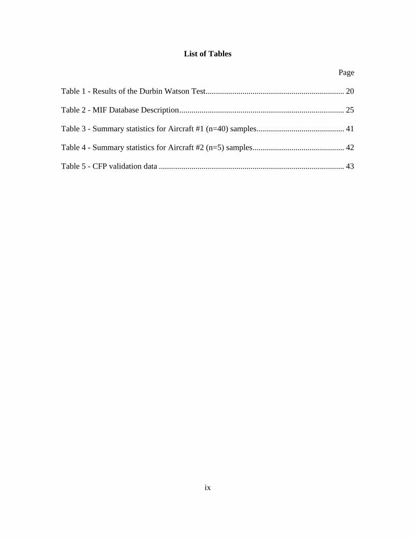
Table 1 - Results of the Durbin Watson Test .................................................................... 20

Table 2 - MIF Database Description ................................................................................. 25

Table 3 - Summary statistics for Aircraft #1 (n=40) samples ........................................... 41

Table 4 - Summary statistics for Aircraft #2 (n=5) samples ............................................. 42

Table 5 - CFP validation data ........................................................................................... 43

1


I. Introduction

The United States Air Force (USAF) operates an enormous fleet of aircraft.

Within the USAF structure, Air Mobility Command (AMC) operates a fleet of large

transport aircraft designed for heavy airlift missions. These so-called “heavies” consume

large amounts of aviation fuel. Rising fuel costs combined with austere fiscal conditions

are a significant challenge for AMC airlift operations. Efforts to reduce AMC fuel

consumption while maintaining mission effectiveness are of utmost concern for the

command.

Given that AMC consumed roughly 63% of all the fuel used in the entire USAF

in 2011 (and therefore a large portion of the DoD fuel usage), ongoing efforts aimed at

improving fuel efficiency resulted in many changes to policies and procedures at AMC

(United States Department of Energy, 2012). Fleet-wide fuel consumption and fuel

efficiency is a complex problem which requires investigation into both the aircraft

systems and the fleet’s operational procedures (Lee et al., 2004). Instituting standardized

fleet-wide policies regarding fuel usage is critical not only for cost savings but also for

addressing environmental concerns (Lee, 2010). Reiman (2014) notes the importance of

a holistic enterprise approach to fuel efficiency. The concept of fuel efficiency regarding

a fleet of aircraft requires analysis of a dizzying array of factors: fuel loading, cargo

loading, routing, flight duration, etc. Quantifying the various aspects contributing to fleet

fuel efficiency is not an easy task. Despite the challenges, there is a vast body of research

2

indicating that proper data analysis can contribute to improved fuel efficiency in a fleet of

aircraft.

This study focuses on a very specific aspect of fuel efficiency: engine fuel

consumption at cruise. Properly quantifying the actual fuel burn of each individual

engine permits flight planners to calculate a more precise fuel load for a specific aircraft

on a specific mission. It is a deceptively complex question: How much fuel goes on an

aircraft to complete a mission? The answer to this question is critical. Excess fuel leads

to costly waste while a shortage could result in a costly diversion to an alternate

destination. An optimal “ramp” fuel load is critical since any excess fuel acts as “cargo”.

In other words, any surplus fuel beyond that needed to safely complete the mission

simply increases the gross weight of the aircraft and decreases the overall fuel efficiency

for the flight. AMC publications estimate a loss of 3% per hour per pound of excess

fuel loaded. For example: 1,500 lbs of fuel is burned during a 5 hour flight to

accommodate an extra 10,000 lbs of fuel (AMC Pamphlet 11-3, 2007). Reiman et al.

(2011) suggest the use of a fueling accuracy metric to quantify this phenomenon and

ensure no excess fuel is loaded. Clearly, optimizing ramp fuel loads is critical to the

efficient operation of an aircraft fleet.

Inherent to the concept of an optimized ramp fuel load is an engine-specific (and

therefore aircraft-specific) measurement of fuel burn. The atmospheric and mechanical

factors affecting fuel burn rate in jet engines are well researched and understood. It is

also well understood that aircraft engines deteriorate over time and associated variation in

the fuel burn rates of individual engines can be drastic (Mehalic & Ziemianski, 1980).

3

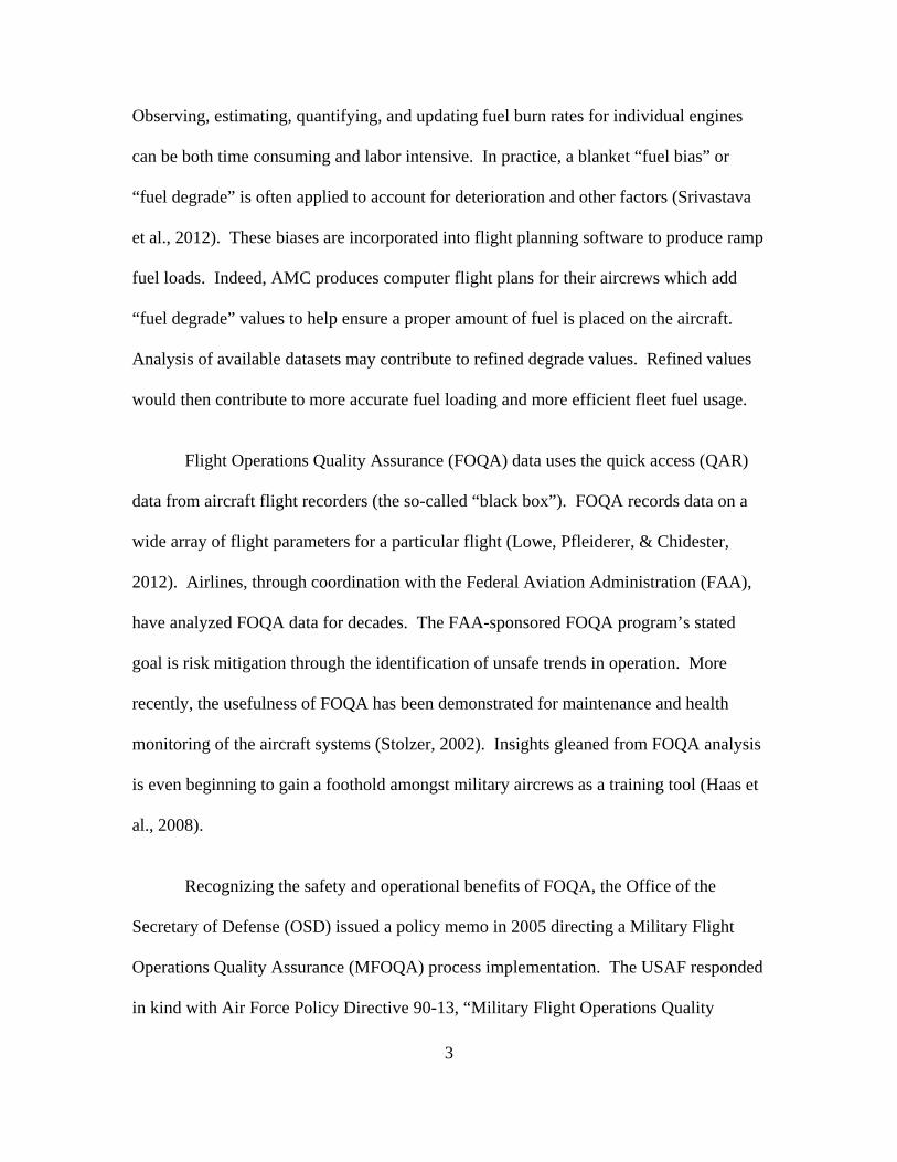
Observing, estimating, quantifying, and updating fuel burn rates for individual engines

can be both time consuming and labor intensive. In practice, a blanket “fuel bias” or

“fuel degrade” is often applied to account for deterioration and other factors (Srivastava

et al., 2012). These biases are incorporated into flight planning software to produce ramp

fuel loads. Indeed, AMC produces computer flight plans for their aircrews which add

“fuel degrade” values to help ensure a proper amount of fuel is placed on the aircraft.

Analysis of available datasets may contribute to refined degrade values. Refined values

would then contribute to more accurate fuel loading and more efficient fleet fuel usage.

Flight Operations Quality Assurance (FOQA) data uses the quick access (QAR)

data from aircraft flight recorders (the so-called “black box”). FOQA records data on a

wide array of flight parameters for a particular flight (Lowe, Pfleiderer, & Chidester,

2012). Airlines, through coordination with the Federal Aviation Administration (FAA),

have analyzed FOQA data for decades. The FAA-sponsored FOQA program’s stated

goal is risk mitigation through the identification of unsafe trends in operation. More

recently, the usefulness of FOQA has been demonstrated for maintenance and health

monitoring of the aircraft systems (Stolzer, 2002). Insights gleaned from FOQA analysis

is even beginning to gain a foothold amongst military aircrews as a training tool (Haas et

al., 2008).

Recognizing the safety and operational benefits of FOQA, the Office of the

Secretary of Defense (OSD) issued a policy memo in 2005 directing a Military Flight

Operations Quality Assurance (MFOQA) process implementation. The USAF responded

in kind with Air Force Policy Directive 90-13, “Military Flight Operations Quality

4

Assurance”. Although gathered, analyzed, and maintained mostly for safety and

readiness issues, AFPD 90-13 acknowledges the potential for “enhanced maintenance

operations”. Stolzer (2003) outlines how this is possible:

Typically, modern digital aircraft capture and store between 200 and 500

parameters per second…including gauge readings, switch positions, control wheel

deflections, control positions, engine performance, hydraulic and electrical system

status, and many others (p. 6).

In other words, MFOQA records almost everything of interest going on with the aircraft.

Although massive and unwieldy, the raw MFOQA represents a gold mine of aircraft data.

Within the framework of fuel efficiency and aircraft-specific fuel burn rates, MFOQA

data has great analysis potential.

The USAF C-5M “Super Galaxy” is the latest modification to AMC’s C-5 cargo

aircraft. The C-5 is the largest aircraft in the USAF fleet and performs a wide array of

airlift missions across the globe. AMC records indicate the C-5 fleet flew well over

30,000 hours in both fiscal year 2011 and 2012 (Air Mobility Command, 2014). AMC’s

Tanker/Airlift Control Center (TACC) at Scott Air Force Base produces most of the

optimized flight plans for C-5M crews. These flight plans include ramp fuel loads

calculated with computer flight planning software in a process similar to most airline

dispatch centers. These flight plans are optimized for various input parameters: sortie

type, duration, cargo, weather, etc. The flight planning software also plans the fuel load

based on the technical order data provided to the USAF by Lockheed (the aerospace

5

corporation that builds the C-5M). Currently, AMC flight planners add a 4% fuel

degrade to the baseline fuel burn quantities when calculating the ramp fuel loads for the

C-5M aircraft. This 4% “pad” accounts for the variation in engine performance discussed

earlier. Proper examination of the available MFOQA could contribute to a more refined

degrade quantity for an individual C-5M.

This study determines if MFOQA gathered from the C-5M is a viable method of

quantifying a highly accurate fuel degrade figure for an individual aircraft. Recall that

any extra fuel (even if added as part of the 4% “pad”) acts as cargo and decreases the

overall fuel efficiency of a given sortie. Consider, for instance, if the burn rate on a

particular C-5M is more accurately described at 3.9% instead of 4% from the baseline

technical order fuel burn rate. On long haul missions, the C-5M carries roughly 160,000

lbs of jet fuel for an 8 hour flight (Lockheed Martin, 2012). In this case, the revised

padding factor reduces the ramp fuel load by 160 lbs (one tenth of one percent). This

may seem to be a “drop in the bucket”, but consider that a C-5M easily flies several

hundred such missions in a year (C-5 aircraft logged over 30,000 hours in FY 11) (Air

Mobility Command, 2014). Also, based on the “3% rule” outlined above, the C-5M

burns another estimated 38.4 lbs of fuel to accommodate the 160 lbs of excess ramp fuel.

AMC estimates a cost of $3.79 per gallon of fuel in FY12 (Air Mobility Command,

2014). A baseline density for military grade JP-8 fuel is 6.8 lbs per gallon (Lockheed

Martin, 2012). With these figures, an estimated cost for 198.4 lbs of wasted fuel is

roughly $110. The carrying costs alone constitute approximately $21 of the $110.

6

The figures compound quickly for an entire fleet over a year of operations. AMC

databases show C-5 aircraft flew roughly 16,000 hours in FY 12. Given this information,

a mere one tenth of one percent translates into roughly $200,000 in overall fuel costs.

The carrying costs alone constitute $42,000. The $42,000 could be considered an

immediate cost savings, whereas the overall cost of $200,000 represents an inventory

reallocation. Consider also the cost of underestimating the degrade value. Suppose an

engine is over-consuming fuel at a rate of 5-6% degrade instead of the advertised 4%. In

this case, fuel conservation practices leading to razor thin fuel reserve margins could

cause inadvertent and costly diversions and mission delays. Accurately quantifying the

fuel degrade figure for an individual aircraft has massive fuel and cost savings potential.

Chapter I framed the overall scope of this thesis: exploring the use of MFOQA to

provide refined fuel degrade values for the C-5M aircraft. Chapter II will provide further

details on the project by outlining the applicable literature surrounding the subject.

7

II. Literature Review

Chapter Overview

As discussed in Chapter I, FOQA lends itself to in-depth data analysis due to the

wealth of information contained in the data. Research into the use of FOQA for aircraft

engine diagnostics emerged in the last decade as a natural extension of the quality control

and safety monitoring originally intended for the FOQA program. A subset of this

research surrounds fuel efficiency through FOQA analysis.

To understand the current state of research in the realm of FOQA analysis on fuel

efficiency, a host of online research databases, article repositories, conference

proceedings, scholarly texts, and online search engines were examined. Keywords in the

searches included “FOQA”, “Fuel Efficiency”, “Fuel Consumption”, “Aircraft Fleet”,

“Data Analysis”, “Data Mining”, and others. Various combinations of the above

keywords yielded many of the same sources suggesting these to be the more seminal

works on the subject.

Figure 1 is representative of the body of work surrounding FOQA and fuel

efficiency. The literature is broken down by subtopics which will be discussed in this

chapter.

8

Figure 1 - Relevant Sources

Fleet H

ealth

Mon

itorin

g

FOQA/QAR D

ata A

nalysis

Engine D

iagon

sitc T

ools

Fuel Con

sum

ption

Filter

ing/S

moo

thin

g/Esti

mat

ion

Advance

d Tec

hniques

Anomaly

Dete

ction

Related WorksBabikian et al (2002) ● ●

Chang (2014) ● ● ●

Chu et al (2011) ● ● ●

Chu et al (2010) ● ● ●

Cleveland (1979) ●

Collins (1982) ●

Garbi (2007) ●

Grewal and Andrews (2008) ●

Gorinevsky et al (2012) ● ● ●

Kalman (1960) ●

Kobayashi and Simon (2003) ● ●



Kwan et al (2014) ● ●

Li (2010) ● ● ● ●

Li et al (2011) ● ● ●

Lockheed Martin (2014) ● ● ● ●

Mehalic and Ziemianski (1980) ● ●

Monnin et al (2011) ● ● ●

Schilling (1997) ● ●

Simon (2008) ● ●

Simon and Simon (2010) ● ●

Simon and Garg (2010) ● ●

Simon and Armstrong (2013) ● ●

Srivastava et al (2012) ● ● ● ● ●

Staszewski et al (2004) ● ●

Stolzer (2003) ● ● ● ●

Stolzer and Halford (2007) ● ● ● ● ●

Torenbeek (1997) ●

Woodbury and Srivastava (2012) ● ● ● ● ●

Related Works

9

Fleet Health Monitoring

Examining a complex concept such as fuel efficiency begins by examining the

fleet as a whole. The engineering effects within the fleet are the most straightforward.

The fact that older engines are less fuel efficient is well known. Quantifying such effects

is vital to fleet fuel efficiency. Serious research into the degradation of aircraft engines in

terms of fuel efficiency has gone on for decades (Mehalic and Ziemanski, 1980). As

technology improved, researchers explored both the physical factors as well as the

operational policies that influenced fuel burn rates in aircraft fleets (Babikan et al., 2002).

These practices gave rise to the concept of fleet health monitoring.

The main purpose of this thesis is utilizing FOQA to learn about the fuel

consumption behavior of individual aircraft. Specifically for the C-5M, the goal is to

obtain precise, aircraft-specific fuel loads through the application of a precise fuel

degrade figure. This process can be seen as very specific form of fleet health monitoring.

Monnin et al. (2011) underscore the importance of fleet-wide health monitoring. They

offer several models which demonstrate the synergistic effects arising from analysis of

individual units within the operations framework of the entire fleet. Kwan et al. (2014)

provide a report for the international council on clean transportation by ranking major

U.S. airlines using a “fuel efficiency” score gleaned from various fleet-wide policies and

procedures implemented by the companies. Aircraft-specific fuel loading (the tailored

“ramp” loads described in Chapter I) is one of a myriad of considerations accounting for

the overall fuel efficiency score. Several studies examine FOQA and other data sources

for fuel burn rates and other fleet health information. For example, Chu et al. (2011)

10

describe adaptable and scalable models within the framework of statistical process

control. The intended use of these models is overall fleet health monitoring (not just fuel

efficiency). Stolzer (2003) and several others listed in Figure 1 focus specifically on fuel

efficiency but their work is aimed at fleet-wide monitoring and implementation. These

trends in the research clearly suggest that FOQA analysis is rarely, if ever, conducted in a

vacuum. Researchers are considering the fleet-wide ramifications of the outcomes of

their studies.

FOQA/QAR Data Analysis

FOQA fits nicely into the fleet health monitoring framework and works well for

many different forms of analysis. There are several reasons for this. First, it is collected

regularly per both FAA and USAF policy as described in Chapter I. It is an existing data

source that requires no additional resources to produce (Stolzer, 2003). The raw FOQA

is readily available; however, manipulating the raw FOQA does require effort and skill.

Another reason FOQA is so useful is the massive amount of information it contains.

FOQA captures the entire flight envelope and almost any imaginable relevant parameter.

This makes FOQA a very adaptable data source. For example, Chu et al. (2010) propose

models for fleet-wide anomaly detection. They build the models by focusing upon a

limited set of variables examined on the cruise portion of sampled FOQA flights. Stolzer

(2003) and Stolzer and Halford (2007) also reduce the FOQA down to a very limited

subset for their study on fuel consumption. Lockheed Martin (the aerospace company

that manufactures the C-5M), conducted a study aimed at quantifying the specific range

(cruise fuel burn) of individual aircraft. This study incorporated QAR-derived data

11

similar to FOQA (Lockheed Martin, 2014). Li et al. (2011) utilize FOQA in a more

traditional manner: they employ cluster analysis to identify anomalous flight parameters

(airspeed, pitch, etc). Studies of this type abound. Gorinevsky et al. (2012) provide

similar analyses to Li et al. (2011) by using FOQA for anomaly detection. Hailing from

the NASA Ames Research Center, the authors propose various multivariate data

reduction techniques to reduce terabytes of FOQA data to megabytes of scatter matrices.

The implementation is through Hotelling T2 Statistics which are based upon empirical

means and empirical covariances of the data. This is done within the framework of

anomaly detection, but can be adapted to regression parameters. These studies

demonstrate the wide applicability of FOQA to fleet health monitoring, but also illustrate

the enormous and unwieldy nature of the data. Oftentimes a large portion of the research

project goes toward data reduction or filtering. FOQA-derived research abounds despite

its cumbersome nature.

Although data reduction is often applied to FOQA databases, they are also often

used in their entirety. Srivastava et al. (2012) is another Ames Center study advocating

the use of the entire dataset. Several exotic methods (ensemble regressions, bootstrap

and kriging models, neural nets, etc) are applied to produce fuel consumption models.

The goal is again anomaly detection, but specifically anomalous fuel consumption. This

work was derived from a previous study (Srivastava, 2010) dealing with general linear

models and Gaussian regression techniques to model anomalous fuel consumption.

Woodbury and Srivastava (2012) summarize the previous works. The journal article

focuses more upon comparing the regression models and introduces a time element. The

12

basic concepts involve regression models built upon limited FOQA inputs and analysis of

time series relationships. The approach is closely related to the methodology applied in

Chapter III (although the underlying models differ). Finally, Li (2010) presents a broad

overview of techniques useful in managing the entire FOQA dataset. He references work

in the fields of machine learning and data mining. This harkens back to the Stolzer and

Halford (2007) study that echoes the same praise for such techniques. Pulling FOQA (or

any other data source) with the intention of identifying or estimating anomalous engine

performance is only one possible application of this highly adaptable dataset. Overall,

there is a clear trend toward utilizing FOQA for anomaly detection. There are precious

few studies dealing with parameter estimation. It is worthwhile to examine non-FOQA

based studies that provide engine health parameter estimation.

Engine Diagnostic Tools

Data-driven estimates of engine health parameters often begin with models of the

internal processes of the engines themselves. For example, Kobayashi and Simon (2005)

employ a nonlinear simulation of engine components for use in their analysis. A similar

approach is taken in their previous studies, although the analysis techniques themselves

differ (Neural Networks and Genetic Algorithms for the 2005 study versus Kalman Filter

techniques for the previous studies). Simon (2008) offers a brief summary of algorithms

proposed for engine health monitoring listing regressions, filtering, and smoothing

techniques alongside other advanced techniques including neural networks, fuzzy logic,

and genetic algorithms. Indeed, various researchers have applied each of these methods

within various frameworks to produce estimable parameters. Taken as a whole, there is a

13

wide array of available techniques to estimate engine health parameters. Kobayashi and

Simon (2003), Kobayashi and Simon (2004), Simon (2008), Simon and Simon (2010),

and Simon and Garg (2010) all build upon classical filtering techniques (Kalman, 1960)

coupled with various associated optimization schemes within the filter to obtain results.

Kobayashi and Simon (2005) utilize a neural network-genetic algorithm, and Chang

(2014) approaches the problem with a fuzzy logic model. Clearly, there are many

applicable algorithms employed in the problem of data analysis of engine health. For the

scope of this thesis, it is prudent to examine a subset of engine health parameters –

specifically fuel consumption.

Fuel Consumption

Similar to the studies on engine components in general, studies focusing

specifically on fuel consumption also model the internal working of the engine. One

such model was derived by Collins (1982) based upon his work at MITRE. He outlines

the functional relationships between the classical aeronautical engineering equations and

translates them into forms easily implemented for data analysis. Future research such as

Schilling’s (1997) neural network model relies on Collins (1982) equations. An

underlying engineering model driving the data analysis is a persistent theme in the

research. Fuel consumption models often employ such baseline models which are

grounded in aeronautics.

On the topic of estimating fuel consumption, Stolzer (2003) and Lockheed Martin

(2014) both advocate examining the fuel burn during the cruise portion of the flight.

14

Garbi (2007) follows suit with a reference cruise model for a specific aircraft and analysis

through a longitudinal motion model. Torenbeek (1997) presents an excellent treatment

of the concept of cruise flight in relation to range (this concept is detailed in Chapter III).

Woodbury and Srivastava (2012) performed linear discriminant analysis on FOQA data

and verified that vertical speed corresponded to a higher fuel flow, whereas cruise flight

tended toward values with a central mean and normal distribution. The reasoning for

focusing upon cruise flight is simple: the cruise portion is usually the longest and most

stable phase of any flight. The pitch, roll, and airspeed of the aircraft are intentionally

close to constant. Since many other factors contributing to fuel consumption are nearly

constant, the cruise portion represents the most stable flight region to observe engine fuel

consumption. The concept of cruise flight data as a source for engine fuel consumption

rounds out the research into the realm of FOQA analysis for fuel efficiency purposes.

Chapter II closes with an examination of the techniques utilized to perform the research.

Filtering, Smoothing, and Estimation

A number of studies outlined in this chapter deal with advanced techniques

(Artificial Neural Nets, Advanced Regression, Classification Trees, Cluster Analysis,

etc). These techniques are aimed at anomaly detection within a fleet either for fuel

consumption specifically, or one or several engine parameters in general. Although

useful and effective, the goal of this study is neither classification nor anomaly detection

(although anomalous fuel burn rates become evident in the analysis). The goal of this

study is to quantify fuel burn rates for specific aircraft. In order to provide an estimate

for fuel consumption, one should consider different algorithms. Simon (2008) offers a

15

brief summary of algorithms proposed for engine health monitoring which includes

weighted least squares, expert systems, Kalman filters, neural networks, fuzzy logic, and

genetic algorithms. The key difference between the data presented in this thesis and

those examined by Simon (2008) and others is the existence of positive autocorrelation

within the data. Herein lays a key difference between smoothing and filtering techniques.

Simon (2008) states smoothing has no benefit over filtering on datasets with constant

bias. Unfortunately, the datasets utilized in this thesis are massively autocorrelated which

drives the analysis toward smoothing techniques to provide estimates.

Staszewski et al. (2004) compose an entire text centered on concepts of signal

processing for health monitoring. Their work harkens back to the earlier discussion on

fleet health monitoring and diagnostic tools. Although centered more upon digital signals

concerned with structural damage detection, the authors note the importance of

considering noise reduction in a given dataset in a later chapter (pp. 165-173). They

frame the concept of noise reduction in terms of classical smoothing techniques such as

Fourier transforms, Wiener filters, and various other techniques. They also advocate the

use of a simple moving average procedure computed using nearest neighbors.

Additionally, they recognize that the classical techniques (Fourier transforms, etc.) can

break down when the signal is non-stationary (time-dependent) (p. 171). They suggest

the use of a windowed Fourier transform over a span of data that can be considered

stationary. Based on the works of Staszewski et al. (2004), Simon (2008), and others, it

is clear that the autocorrelated MFOQA fuel flow data provided for this study would

require a smoothing technique capable of handling non-stationary, time-dependent data.

16

Cleveland (1979) introduced the concept of local regression on scatterplots, which

he abbreviated LOESS. Much like the concept of windowed Fourier transforms

described by Staszewski et al. (2004), the LOESS procedure uses weighted least squares

over a localized span (sometimes called bandwidth) of data. The procedure is a

nonparametric model which utilizes neighborhood weights about each point in the span

(Martinez and Martinez, 2008, p. 520). The weights are derived from the bandwidth

based upon a tricube function:

3 3(1 ) ; 0 1( )

0; otherwise

u uW u

(1)

These weights are applied to either a first order weighted least squares fit or a

second order polynomial fit. Higher order polynomials are possible, but rarely used

(Cleveland, 1979). Cleveland’s (1993) text defines the two parameters for LOESS: =

bandwidth (expressed as a percentage of the total number of data points ), and = the

order of the polynomial used in the Weighted Least Squares procedure (pp. 96-101). The

choice of and for the MFOQA fuel flow data is detailed in Chapter III.

Furthermore, Cleveland (1994) advocates the use of the LOESS smoother on time series

data (p. 154) noting the ability to fit trends while smoothing oscillations in time series

data.

In summary, this chapter explored the body of work surrounding the use of FOQA

data for aircraft fuel efficiency analysis. Chapter II also scoped the specific problem of

quantifying an aircraft-specific fuel consumption figure. Beginning within the

17

framework of fleet health monitoring and moving to the more specific topics of engine

diagnostics and fuel consumption, the literature suggests different methods to harness

FOQA data for fuel efficiency. On the specific topic of aircraft-specific fuel burn

estimation, research points toward smoothing techniques as a viable methodology. With

the relevant literature properly outlined, Chapter III moves on to the Methodology

employed for the case study itself.

18

III: Methodology

Chapter I and Chapter II outlined the general philosophy behind utilizing

MFOQA to realize gains in fuel efficiency and included an outline of the research in this

arena. This Chapter outlines the specific methodology utilized toward an overall goal of

extracting C-5M fuel burn estimates from noisy MFOQA data.

Case Study Data and Autocorrelation

Previous chapters discussed the large and unwieldy nature of FOQA data.

AMC’s MFOQA database is no exception. Analysts at AMC Headquarters at Scott Air

Force Base provided the author with thirty test missions extracted from two aircraft (29

missions from one aircraft and one mission from a different aircraft). AMC contracted

out the task of reducing and cleansing the raw MFOQA for the individual flights down to

manageable file sizes. Serendipitously, the aircraft sensors which detect fuel flow

readings record on one second intervals which matched the intervals on the cleansed files.

The contracting team reduced down redundant and missing rows of data. The resulting

datasets contain records of aircraft parameters and external environmental readings at one

sample per second. Since the bulk of the provided data is from a single aircraft, the

overall methodology approach is a case study on this single aircraft. As will be

demonstrated, the methodology is applicable to the entire C-5M fleet.

Chapter II discussion noted cruise as most applicable flight regime for estimating

fuel consumption. A simple model for capturing fuel burn during cruise flight associates

the Gross Weight and Airspeed of the aircraft to the Fuel Flow rate. Details on this

phenomenon will be discussed in later sections. To establish an initial framework,

19

consider how Stolzer (2003) discovered both Airspeed and Gross Weight to be significant

predictor variables on Fuel Flow rates for a FOQA-based study using ordinary least

squares (OLS) regression techniques. It is worth noting that Stozler’s (2003) dataset

consisted of a single sample across several hundred FOQA datasets (missions), whereas

this study utilizes many samples across only 30 FOQA datasets (missions). Thus,

Stolzer’s (2003) data is automatically independently distributed. The same assumption

cannot be made for the data in this study. Nevertheless, running a simple linear

regression still provides insights. The Stolzer (2003) study was rigorous and included

several iterations of stepwise regression and resulted in uncorrelated predictors with

excellent properties (low variance inflation factors, etc). From these results, it is

reasonable to build an initial framework around a simple model which includes Stolzer’s

(2003) significant predictor variables.

OLS techniques are a natural starting point for data analysis. Using Gross Weight

and Airspeed as regressors and Fuel Flow as the response, multiple linear regressions

were performed in MATLAB software’s “regstats” function on the associated columns of

four specific MFOQA samples. The four samples represent “stable cruise” segments

culled from the 30 test missions. They include the longest observed cruise (3.04 hours),

the shortest observed cruise segment (0.84 hours), and two at-large samples near the

mean cruise time of 1.5 hours. Details on the construction of these stable cruise segments

are provided in the appendix. The resulting models exhibit low R-squared values,

indications of lack of fit, and most importantly, significant values for the Durbin-Watson

Statistic. These are all clear indications of autocorrelation. This is to be expected when

examining MFOQA fuel flows over time. As the aircraft burns fuel, it becomes lighter

20

thus reducing the overall Gross Weight. Since the fuel burn is a function of the Gross

Weight of the aircraft, an overall trend exists but is masked by True Airspeed deviations.

These Airspeed deviations are manifestations of throttle excursions occurring as the

autopilot/autothrottle system corrects for Altitude deviations (Lockheed Martin, 2014).

Such throttle excursions introduce autocorrelated noise into the system. The

autocorrelated errors are evident through various statistical means. Bowerman, et al.

(2005) provides the definition of the Durbin-Watson statistic on p. 291:

2

12

2

1

( )n

t tt

n

tt

e ed

e

(2)

Table 1 below lists the values for the Durbin-Watson Statistic on the sample MFOQA

datasets clearly indicating significant positive autocorrelation. It is worth noting that the

p-values produced in Table 1 are normal approximations1, but the result is clear. Notice

the sample sizes are in seconds corresponding to the cruise times described in the

previous paragraph.

Table 1 - Results of the Durbin Watson Test

1 See http://www.mathworks.com/help/stats/linearmodel.dwtest.html for details

Durbin-Watson Statistic Value p-value Sample Size

0.048662424 0 10955

0.051726953 0 3022

0.043579036 0 5051

0.044840468 0 5952

21

The plots of the residuals of the four regressions shown in Figure 2 also exhibit the tell-

tale signs of autocorrelation. They exhibit “sine wave” patterns as a clear violation of

non-constant variance assumptions:

Figure 2 - OLS Residual Plots

Several of the studies discussed in Chapter II addressed the time series aspect of

FOQA analysis. Li et al. (2011) and Woodbury and Srivastava (2012), in particular,

speak to the time element as they attempt to model the entire flight envelope for anomaly

detection. Their models are based upon cluster analysis and general linear

models/Gaussian processes respectively. This study relies more upon smoothing

techniques associated with time series analysis. Smoothing techniques are essential to

this study in terms of understanding the actual fuel burn during cruise flight. Before

22

examining the actual fuel burn and applicable smoothing techniques, a baseline fuel burn

model must be established.

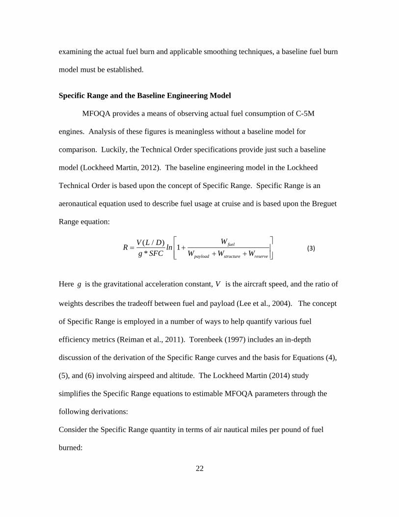
Specific Range and the Baseline Engineering Model

MFOQA provides a means of observing actual fuel consumption of C-5M

engines. Analysis of these figures is meaningless without a baseline model for

comparison. Luckily, the Technical Order specifications provide just such a baseline

model (Lockheed Martin, 2012). The baseline engineering model in the Lockheed

Technical Order is based upon the concept of Specific Range. Specific Range is an

aeronautical equation used to describe fuel usage at cruise and is based upon the Breguet

Range equation:

( / )1

*fuel

payload structure reserve

WV L DR ln

g SFC W W W

(3)

Here g is the gravitational acceleration constant, V is the aircraft speed, and the ratio of

weights describes the tradeoff between fuel and payload (Lee et al., 2004). The concept

of Specific Range is employed in a number of ways to help quantify various fuel

efficiency metrics (Reiman et al., 2011). Torenbeek (1997) includes an in-depth

discussion of the derivation of the Specific Range curves and the basis for Equations (4),

(5), and (6) involving airspeed and altitude. The Lockheed Martin (2014) study

simplifies the Specific Range equations to estimable MFOQA parameters through the

following derivations:

Consider the Specific Range quantity in terms of air nautical miles per pound of fuel

burned:

23

Nautical Miles

fuel

SRW

(4)

Dividing each term through by time, we have:

Nautical Miles/hr

/ hrfuel

SRW

(5)

(1)

Which is re-written in terms of MFOQA observable terms as:

KTASV

FSR

F

(6)

(1)

where KTASV is the True Airspeed of the aircraft, and FF is the fuel flow reading in lbs/hr.

Both are observable MFOQA parameters. Equation (6) offers a means to calculate a

Specific Range value at a fixed Altitude and a given Gross Weight simply from observing

the True Airspeed value (which is the Nautical Miles/hour value adjusted for altitude and

temperature) (Lockheed Martin, 2014). Since the True Airspeed is a function of altitude

and temperature, the C-5M Technical Order presents flight-tested charts providing plots

of Specific Range values at a fixed altitude for a given Gross Weight and Mach Number

(True Airspeed in terms of percentage of the speed of sound) (Lockheed Martin, 2011).

Figure 3 is an example of a Specific Range chart similar to the one in the Technical

Order. Families of curves are printed for a fixed Altitude with respect to Gross Weight

values at 10,000 pound intervals. The curves plot Specific Range versus Airspeed in

Mach. Figure 3 displays the curves for five Gross Weights valued from 700,000 lbs to

740,000 lbs. Notice the non-linear relationship between Airspeed and Specific Range

24

which indicates an “optimal” airspeed is quantifiable for every combination of Gross

Weight and Altitude.

Figure 3 - Nominal Specific Range Curves

Finally, notice that Equation (6) can be re-written in terms of Fuel Flow:

KTASV

RFF

S

(7)

(1)

Thus, for a given set of MFOQA observations (Altitude, Gross Weight, True Airspeed), it

is possible to obtain a Technical Order “baseline” Fuel Flow measure. This quantity can

then be compared to the actual MFOQA Fuel Flow observation at a specific point in time.

Integration over time of the observed cruise portion provides a total fuel burn estimate for

25

both the baseline (derived from Specific Range values based on MFOQA Altitude, Gross

Weight, and Airspeed) and the observed (the actual MFOQA Fuel Flow reading).

The MIF Project and Interpolating Specific Range Values

The Technical Order charts such as the example in Figure 3 are useful for

understanding the concept of Specific Range visually, but are not ideal for obtaining

precise Specific Range values. Simply plotting the inputs (Airspeed and Gross Weight)

requires a keen eye and provides only rough estimates at best. Also, the precise MFOQA

readings naturally require interpolation between the curves since the Gross Weight values

are only plotted at 10,000 lb increments. Luckily, through the efforts of an ongoing fuel

efficiency project titled “Mission Index Flying” (MIF), the charts themselves were

converted over to tabulated values. MIF is based upon industry best practices of

quantifying the optimal airspeeds (i.e., flying airspeeds corresponding to the maximum

on the Specific Range curve) discussed earlier and plotted on Figure 3 (Mirtich, 2011). A

MIF database of approximately 26,000 records which contains tabulated values for a

Specific Range for a given Altitude, Mach speed, and Gross Weight was obtained. The

tabulated values are easily interpolated to provide precise Specific Range estimates.

Table 2 below outlines the ranges on the MIF database:

Table 2 - MIF Database Description

Input MIF Database Ranges MIF Database Increments

Altitude 27,000'-45,000' 1000'Mach Airspeed 0.39-0.825 0.005Gross Weight 400,000 lbs - 840,000 lbs 10,000 lbs

26

Using Equation (7) above, the baseline Specific Range values are easily converted into

instantaneous Fuel Flows for comparison with the actual Fuel Flow observations. An

interpolating function can be used or the values can be rounded to the nearest entry

among the 26,000 available combinations. For this study, an interpolation scheme was

implemented using MATLAB’s “scatteredInterpolant” function.

Establishing Stable Cruise Criteria and Parsing Data

The 30 test samples provided by AMC yielded 45 MFOQA cruise portions which

fall into the ranges in Table 2. Visual Basic (VBA) code was written to quickly parse an

entire mission (one of the thirty samples) into usable cruise segments within the Altitude

ranges of Table 2. The logic for focusing upon stable cruise flight segments was outlined

in Chapter II. The VBA code limits “stable cruise” to the following criteria: 1) At least

one hour of cruise (3600 records), 2) Of the one hour cruise, the first and last five

minutes are discarded to allow for level-off from climbs and preclude capturing initial

climb to the next altitude, 3) A steady altimeter reading (25’) to reduce noise. Pseudo-

code is provided in Appendix A. Precise Specific Range values for each record in a

stable cruise sample arise from plugging in observed MFOQA Altitudes, Gross Weights,

and Mach speeds. The stable cruise segments also record the observed Fuel Flow during

flight. These data are used to calculate the actual fuel burn estimate for comparison to

the baseline.

Actual Fuel Burn Estimate and LOESS Smoothing

This section returns to the concept of quantifying the specific fuel burn for a

specific engine (which aggregates into an estimate for the fuel burn of the aircraft as a

27

whole). With the autocorrelation detailed, stable cruise samples parsed, and a baseline

fuel burn calculated, the actual fuel burn estimate can be established and compared to the

baseline. The result is a good estimation of the true fuel burn “degrade” of the engine.

Implementation of the LOESS smoother upon noisy MFOQA fuel flow data is the

method employed in this study.

The section on autocorrelation and the introduction of the smoothing technique

known as LOESS set the stage for the methodology involved in calculating the actual fuel

burn estimate. There are many techniques available to deal with autocorrelation. These

include the Cochrane-Orcutt Method, ARMA, ARIMA, (Montgomery et al., 2012, p.

482), the Batch Means method (Law, 2007, pp. 520-522), and others. Each technique has

advantages and drawbacks.

The LOESS smoother described in Chapter II has some distinct advantages as

outlined by Cleveland and Loader (1996). First, although the method itself is

nonparametric, it is easy to understand and interpret. It is also an adaptable and flexible

method that can deal with different distributional assumptions. The use of a local model

and the choice of bandwidth and polynomial order selection also contribute to the

flexibility of the method. According to Cleveland and Loader (1996), none of these

aspects alone make the LOESS smoother a preferred choice over splines or other kernel

methods. Taken as whole, however, the adaptability and flexibility of the LOESS model

make it an excellent choice for time series data (such as MFOQA fuel flows) which

Cleveland (1993) describes as “functions that defy description by simple parametric

functions” (p. 154).

28

The LOESS smoother does have a few drawbacks. First, the nonparametric

nature of the procedure precludes specification of a rigid structural relationship between

the independent and dependent variables as is done with normal regression techniques.

Since the goal of this study is estimation rather than a structural model, the nonparametric

nature of the procedure is not overly concerning. Second, the LOESS procedure itself is

admittedly computationally intensive. LOESS performs a weighted least squares

regression for each point in the span. In the past, this may have been a factor for large

datasets, but modern computing power makes LOESS implementable on large datasets.

Diagnostics such as “goodness of fit” for LOESS are difficult to quantify and interpret

but some insight can be garnered from residual analysis (Jacoby, 2000). Finally, the task

of designating the LOESS parameters (and thus fine-tuning the amount of smoothing) is

not trivial. Even small changes to the parameters can drastically affect the estimates.

Despite these drawbacks, LOESS is still an excellent choice for the MFOQA fuel flow

estimation since it is specifically designed to deal with noisy data.

LOESS Smoothing Parameters for C-5M MFOQA Fuel Flow

Utilizing LOESS to produce the MFOQA fuel flow estimates is achievable, but

requires careful attention to the specification of the LOESS parameters. The choice of

and are important. Cleveland and Loader (1996) describe the choice of as a

tradeoff between variance reduction and bias. Higher values of result in larger spans

and a smoother curve. For the MFOQA analysis, the goal is noise reduction and the

preservation of the underlying trend in the fuel flow response. Recall that the fuel flow

responses decrease over time due to reduction in the Gross Weight of the aircraft. This

29

phenomenon is “masked” by noisy autothrottle and Airspeed inputs which, in turn, distort

estimates of actual fuel burn. To counter this effect, LOESS is employed to smooth out

the noise and provide a clearer estimate of actual fuel burn for comparison. In a similar

manner, LOESS smoothing on the True Airspeed value used in the baseline estimate

reduces noise resulting in a smooth baseline curve.

Cleveland (1993) describes LOESS parameter selection as an iterative procedure

and encourages “educated first guesses” (p. 96). For the smoothing parameter ,

Cleveland offers a range of values from 0.25 to 1 as a heuristic. With regards to the 45

stable cruise segments, 75% are below two hours in duration (recall that the stable cruise

criterion for duration was at least one hour) with the mean of all 45 near 1.5 hours. This

means that 0.25 equates to approximately 25 minutes on average. For the aircraft

weights observed in the 45 stable cruise segments, a quick approximation for fuel burn is

roughly 20,000 lbs/hour (Lockheed Martin, 2012) meaning that the model is seeking to

detect changes in fuel flow responses over a change in Gross Weight averaging

approximately 5,000 lbs. Both Cleveland and Loader (1996) and Simonoff (1996) view

boundary regions as a major consideration in the choice of . Indeed, the nearest

neighbors tricube weighting employed in LOESS treats points on the tails of the

bandwidth differently than an interior point. In terms of MFOQA, it is reasonable that a

change of 5,000 lbs would register a measurable change in fuel flow responses. Simonoff

(1996) offers techniques based upon Kernel densities which may yield more “optimal”

values of . He further explores the effects of autocorrelation on smoothing, noting that

the existence of autocorrelation suggests the use of a higher value for . Efforts to fine-

30

tune the smoothing parameter have merit, but for the reasons outlined above, 0.25 is

a reasonable choice for this study.

The choice of (the degree of the polynomial used in the local regression)

should attempt to model the underlying trend. Cleveland (1996) notes that “gentle

curvature” with no local maxima or minima would allow for a local linear fit (p. 98).

Jacoby (2000) notes a linear fit is appropriate if a general monotonic pattern is discernible

from the raw data. For the MFOQA data, an argument can be made for both the linear

and quadratic models ( 1 and 2 respectively). The very fact that fuel burn can be

estimated at roughly 20,000 lbs/hour seems to confirm a linear trend and plots of the raw

data (seen in Figure 9) seem generally monotonic (although noisy). It is worth

considering, however, engineering models (such as Figure 3) which demonstrate

decidedly nonlinear relationships over vast spans of aircraft weights. Since LOESS

smoothing with both linear and quadratic models is easily implemented in MATLAB, a

simple solution is to run each method on a limited dataset and examine preliminary

results to further justify the proper choice of .

LOESS Residual Diagnostics

At the beginning of the chapter, four stable cruise segments were utilized to

demonstrate the autocorrelation present in the MFOQA fuel flow responses. Recall that

these data were the shortest duration, longest duration, and two at-large segments near the

mean of 1.5 hours. It is now clear that these segments were pulled from the larger set of

45 stable cruise samples. Along with demonstrating autocorrelation, these four segments

are ideal for examining LOESS diagnostics.

31

Jacoby (2000) describes how a properly specified LOESS curve would account

for any systematic dependencies in bivariate data, thus the residuals from the model

should contain no discernible pattern. Indeed, Cleveland (1993) espouses the use of

residual analysis as a primary diagnostic for LOESS (pp. 103-104). Jacoby’s (2000)

definition of a LOESS residual:

ˆ( )i i ie y g x (8) (1)

follows the familiar definition used in ordinary regression. With residual diagnostics,

LOESS bridges a compromise between nonparametric and parametric modeling. In

particular, the use of residual dependency plots to check for non-constant variance,

alongside Normal q-q plots to check for normality (Cleveland, 1993, pp. 103-109) are

familiar diagnostics used to test the classic regression assumptions (Montgomery et al.,

2012, pp. 129-130). Since it is impractical to examine 45 sets of residual plots, returning

to the four segments used to describe the autocorrelation is adequate for LOESS residual

analysis. Residual analysis on this subset helps justify parameters choices and verify the

methodology prior to analyzing the full dataset.

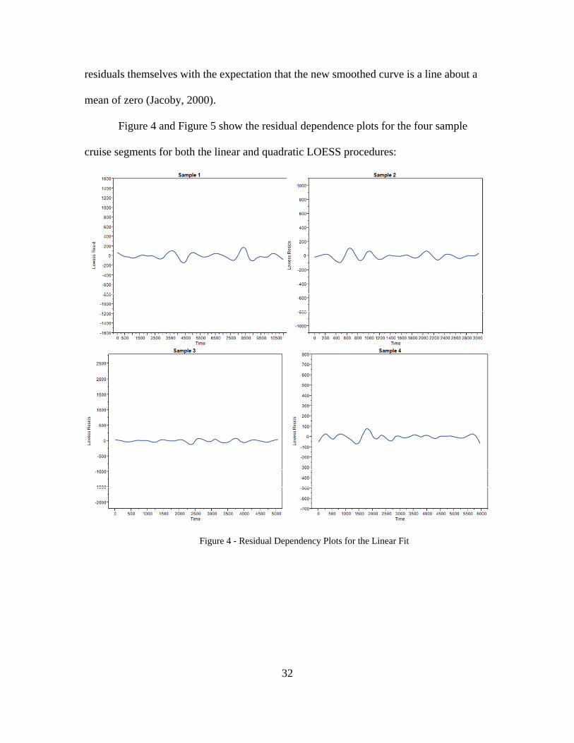
Cleveland (1993, p. 103) and Jacoby (2000) both advocate the use of “residual

dependence plots” as LOESS diagnostics. The idea is to plot the residuals from the

LOESS fit against the independent variable. The logic is similar to classical regression in

the sense that the LOESS smoother should capture the underlying trend between the

independent and dependent variable leaving nothing but white noise in the residuals.

With large datasets, it is appropriate to run the LOESS smoothing algorithm on the

32

residuals themselves with the expectation that the new smoothed curve is a line about a

mean of zero (Jacoby, 2000).

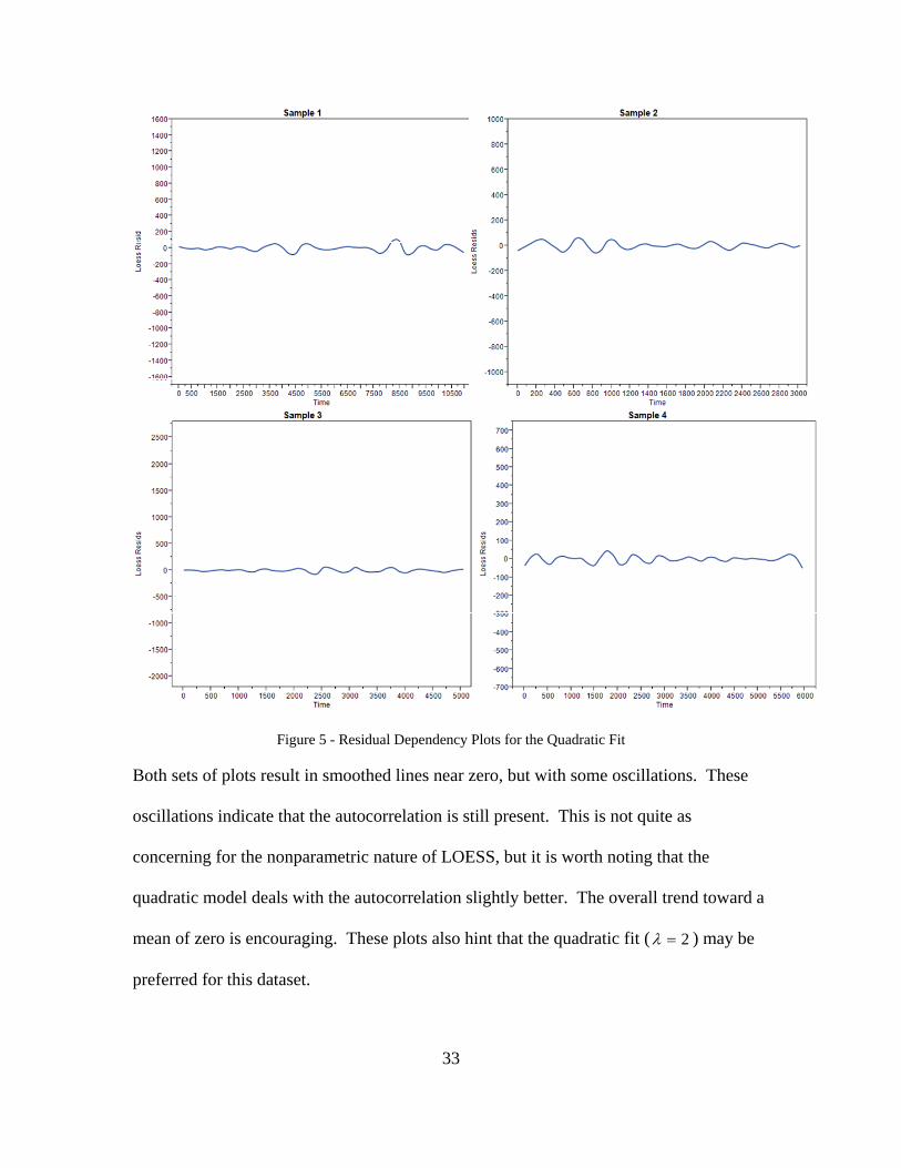
Figure 4 and Figure 5 show the residual dependence plots for the four sample

cruise segments for both the linear and quadratic LOESS procedures:

Figure 4 - Residual Dependency Plots for the Linear Fit

33

Figure 5 - Residual Dependency Plots for the Quadratic Fit

Both sets of plots result in smoothed lines near zero, but with some oscillations. These

oscillations indicate that the autocorrelation is still present. This is not quite as

concerning for the nonparametric nature of LOESS, but it is worth noting that the

quadratic model deals with the autocorrelation slightly better. The overall trend toward a

mean of zero is encouraging. These plots also hint that the quadratic fit ( 2 ) may be

preferred for this dataset.

34

A second LOESS diagnostic is the familiar Normal q-q plot (Cleveland, 1993, pp.

108-109) which provides justification for the weighted least squares fit utilized within

LOESS.

Figure 6 and Figure 7 below display the Normal q-q plots for the linear and

quadratic fits. They are nearly identical. The accompanying box plots show some

outliers, but the sample sizes are large enough that the data is not unduly influenced. For

smaller datasets with potential outliers, a robust version of LOESS is available

(Cleveland, 1993, pp. 110-116). The robust LOESS procedure involves iterative re-

weighting of the least squares fit based on the Median Absolute Deviation of the

residuals. The robust version is not considered for this study.

Figure 6 - Normal Quantile Plots for the Linear Fit

35

Figure 7 - Normal Quantile Plots for the Quadratic Fit

Before moving on to the results of the full analysis presented in Chapter IV, it is

worth noting that further LOESS diagnostics exist. These involve techniques aimed at

quantifying corollaries to some classic statistical techniques such as ANOVA tables, F-

values, 2R values and the like. This is accomplished through a variety of cross-

validation, bootstrapping techniques, and theory from Kernel densities. For LOESS,

classical statistical inference becomes somewhat dubious and difficult to interpret. In the

strictest sense, the LOESS smoother does not partition the sum of squares for error in a

way that allows for the classical ANOVA assumptions to hold (Jacoby, 2000). The

interested reader should refer to Jacoby (2000) and Simonoff (1996) for a discussion on

these diagnostics. Certain problems may gain insight from these calculations, but little

36

value is added for this study. The outcomes of the residual analysis presented above are

sufficient to move forward.

Comparison and Summary

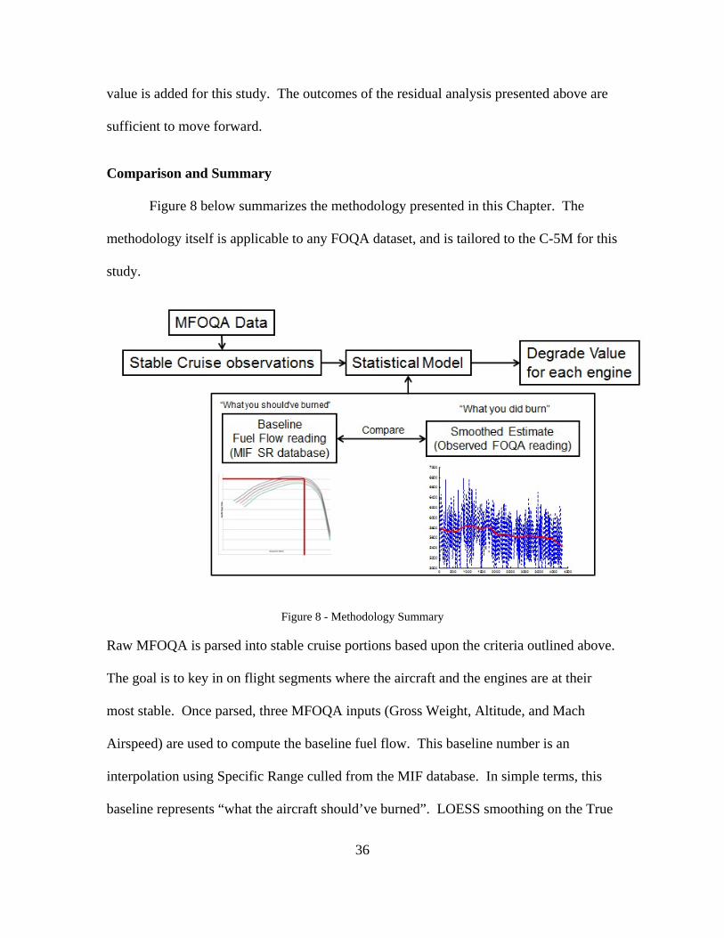
Figure 8 below summarizes the methodology presented in this Chapter. The

methodology itself is applicable to any FOQA dataset, and is tailored to the C-5M for this

study.

Figure 8 - Methodology Summary

Raw MFOQA is parsed into stable cruise portions based upon the criteria outlined above.

The goal is to key in on flight segments where the aircraft and the engines are at their

most stable. Once parsed, three MFOQA inputs (Gross Weight, Altitude, and Mach

Airspeed) are used to compute the baseline fuel flow. This baseline number is an

interpolation using Specific Range culled from the MIF database. In simple terms, this

baseline represents “what the aircraft should’ve burned”. LOESS smoothing on the True

37

Airspeed input reduces the noise in the baseline response. Next, the recorded fuel flows

are smoothed using the LOESS procedure to produce an estimate of actual fuel burn. The

final step is to integrate both of these curves and record the difference. This difference

divided by the baseline estimate is the degrade value. For this study, all of the

calculations are performed in MATLAB and are outlined in the pseudo-code in Appendix

A. A graphical example of the model output is presented in Figure 9 below:

38

Figure 9 - Smoothing Example

In this example, the top plot shows LOESS smoothing against the raw MFOQA fuel flow

responses for a single engine. The middle plot shows the four smoothed MFOQA

responses (one for each engine) against the smoothed baseline fuel burn. The bottom plot

39

is the same as the middle plot but shown on the same y scale as the top plot. This

demonstrates how the LOESS smoother reduces the noise in the data. The smoothing

technique is LOESS with 0.25 and 2 for the reasons discussed above. The area

between each smooth curve and the baseline curve represents the difference in fuel burn

in pounds. Expressing this difference as a percentage of the baseline produces the

degrade number. This degrade number is the overall goal of the study and is applicable

for mission planning as discussed in Chapter I. Results of the implementation of this

methodology on the full dataset are presented in Chapter IV.

40

IV. Analysis and Results

The first three chapters laid the groundwork for the fuel burn analysis specific to the C-

5M. This analysis is of interest to AMC for the reasons outlined in Chapter I and is the focus of

this chapter.

Quantifying the fuel degrade value

The methodology outlined Chapter III and summarized in Figure 8 was applied to 45

stable cruise observations. The model output is in the form of four degrade values (one value for

each engine). These numbers are then averaged providing the “tail-specific” fuel degrade for the

entire aircraft. This final number is an estimate of the fuel burn performance for the aircraft.

The tail-specific degrade value can then be applied to flight planning which results in more

accurate fueling procedures.

For this study, 45 stable cruise segments were obtained. Of the 45 stable cruise

segments, 40 observations come from a single aircraft. The remaining 5 observations are from a

different C-5M and work to validate the procedure. Two tables below were constructed from the

results of the 45 cruise segments. The first table provides summary statistics for the 40

observations from the case-study aircraft (Aircraft #1) and the second table summarizes the 5

observations from Aircraft #2. The tables were constructed using Excel’s Data Analysis Add-In

which provides concise summary statistics.

41

Table 3 - Summary statistics for Aircraft #1 (n=40) samples

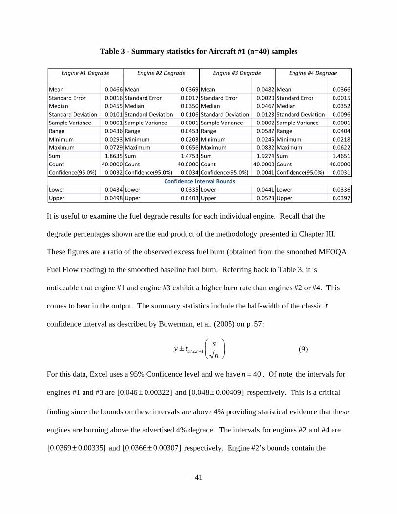
It is useful to examine the fuel degrade results for each individual engine. Recall that the

degrade percentages shown are the end product of the methodology presented in Chapter III.

These figures are a ratio of the observed excess fuel burn (obtained from the smoothed MFOQA

Fuel Flow reading) to the smoothed baseline fuel burn. Referring back to Table 3, it is

noticeable that engine #1 and engine #3 exhibit a higher burn rate than engines #2 or #4. This

comes to bear in the output. The summary statistics include the half-width of the classic t

confidence interval as described by Bowerman, et al. (2005) on p. 57:

/2, 1n

sy t

n

(9)

For this data, Excel uses a 95% Confidence level and we have 40n . Of note, the intervals for

engines #1 and #3 are [0.046 0.00322] and [0.048 0.00409] respectively. This is a critical

finding since the bounds on these intervals are above 4% providing statistical evidence that these

engines are burning above the advertised 4% degrade. The intervals for engines #2 and #4 are

[0.0369 0.00335] and [0.0366 0.00307] respectively. Engine #2’s bounds contain the

Mean 0.0466 Mean 0.0369 Mean 0.0482 Mean 0.0366

Standard Error 0.0016 Standard Error 0.0017 Standard Error 0.0020 Standard Error 0.0015

Median 0.0455 Median 0.0350 Median 0.0467 Median 0.0352

Standard Deviation 0.0101 Standard Deviation 0.0106 Standard Deviation 0.0128 Standard Deviation 0.0096

Sample Variance 0.0001 Sample Variance 0.0001 Sample Variance 0.0002 Sample Variance 0.0001

Range 0.0436 Range 0.0453 Range 0.0587 Range 0.0404

Minimum 0.0293 Minimum 0.0203 Minimum 0.0245 Minimum 0.0218

Maximum 0.0729 Maximum 0.0656 Maximum 0.0832 Maximum 0.0622

Sum 1.8635 Sum 1.4753 Sum 1.9274 Sum 1.4651

Count 40.0000 Count 40.0000 Count 40.0000 Count 40.0000

Confidence(95.0%) 0.0032 Confidence(95.0%) 0.0034 Confidence(95.0%) 0.0041 Confidence(95.0%) 0.0031

Lower 0.0434 Lower 0.0335 Lower 0.0441 Lower 0.0336

Upper 0.0498 Upper 0.0403 Upper 0.0523 Upper 0.0397

Engine #1 Degrade Engine #2 Degrade Engine #3 Degrade Engine #4 Degrade

Confidence Interval Bounds

42

advertised 4% value whereas Engine #4’s upper bound is very slightly below 4%. The overall

tail-specific degrade is the average of the 4 engine means is 0.04207 . The figure is slightly

above 4%, which indicates the case study aircraft is burning slightly more fuel than is accounted

for in the 4% flight planning figure. Critically, this provides evidence that the ramp fuel loads on

this particular aircraft are slightly too low and run the risk of causing costly diverts.

Similar analysis on Aircraft #2 data in Table 4 provides confidence intervals for all four

engines on a limited sample size for 5n .

Table 4 - Summary statistics for Aircraft #2 (n=5) samples

Notably, three out of four individual means are slightly below 4%; however, the limited sample

size precludes much further insight. Each of the individual engine confidence bounds contains

4% with the exception of Engine #2. Additional data would reveal whether or not this particular

aircraft is burning fuel at a different rate than the case study aircraft. A confidence interval

below 4% would hint at the idea the aircraft is being loaded with too much fuel and that savings

could be obtained by adjusting the degrade value. The fact that the results of the case study and

second C-5M data are similar is some evidence verifying the overall analysis.

Mean 0.0332 Mean 0.0292 Mean 0.0407 Mean 0.0329

Standard Error 0.0030 Standard Error 0.0031 Standard Error 0.0031 Standard Error 0.0032

Median 0.0337 Median 0.0298 Median 0.0405 Median 0.0328

Standard Deviation 0.0066 Standard Deviation 0.0068 Standard Deviation 0.0070 Standard Deviation 0.0072

Sample Variance 0.0000 Sample Variance 0.0000 Sample Variance 0.0000 Sample Variance 0.0001

Range 0.0165 Range 0.0168 Range 0.0183 Range 0.0166

Minimum 0.0240 Minimum 0.0197 Minimum 0.0311 Minimum 0.0234

Maximum 0.0405 Maximum 0.0364 Maximum 0.0494 Maximum 0.0399

Sum 0.1660 Sum 0.1460 Sum 0.2035 Sum 0.1645

Count 5.0000 Count 5.0000 Count 5.0000 Count 5.0000

Confidence(95.0%) 0.0082 Confidence(95.0%) 0.0085 Confidence(95.0%) 0.0087 Confidence(95.0%) 0.0089

Lower 0.0250 Lower 0.0207 Lower 0.0320 Lower 0.0240

Upper 0.0414 Upper 0.0377 Upper 0.0494 Upper 0.0418

Confidence Interval Bounds

Engine #1 Degrade Engine #2 Degrade Engine #3 Degrade Engine #4 Degrade

43

Computer Flight Plan Validation

Providing face validity is important to any data-based study. For AMC leadership to

consider MFOQA data analysis for fuel efficiency, a validation framework should be established.

A straightforward approach to validate the model presented in this study is through comparison

with AMC’s own flight planning output. AMC utilizes proprietary Computer Flight Planning

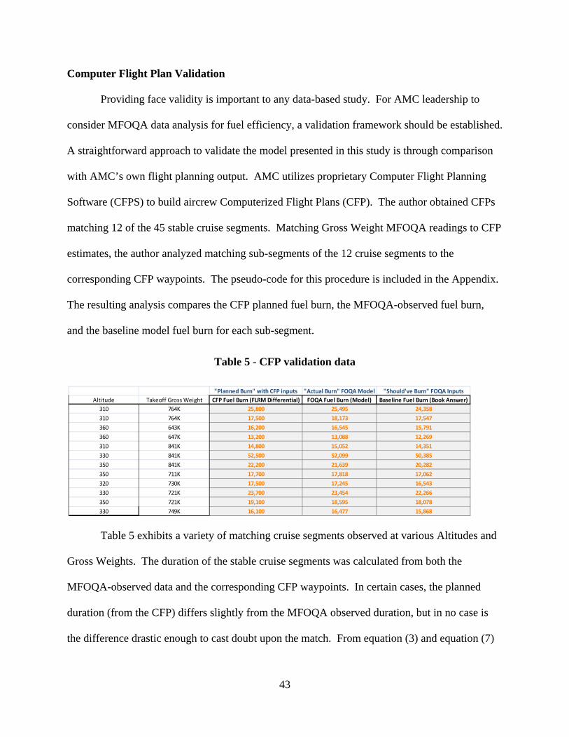
Software (CFPS) to build aircrew Computerized Flight Plans (CFP). The author obtained CFPs

matching 12 of the 45 stable cruise segments. Matching Gross Weight MFOQA readings to CFP

estimates, the author analyzed matching sub-segments of the 12 cruise segments to the

corresponding CFP waypoints. The pseudo-code for this procedure is included in the Appendix.

The resulting analysis compares the CFP planned fuel burn, the MFOQA-observed fuel burn,

and the baseline model fuel burn for each sub-segment.

Table 5 - CFP validation data

Table 5 exhibits a variety of matching cruise segments observed at various Altitudes and

Gross Weights. The duration of the stable cruise segments was calculated from both the

MFOQA-observed data and the corresponding CFP waypoints. In certain cases, the planned

duration (from the CFP) differs slightly from the MFOQA observed duration, but in no case is

the difference drastic enough to cast doubt upon the match. From equation (3) and equation (7)

"Planned Burn" with CFP inputs "Actual Burn" FOQA Model "Should've Burn" FOQA Inputs

Altitude Takeoff Gross Weight CFP Fuel Burn (FLRM Differential) FOQA Fuel Burn (Model) Baseline Fuel Burn (Book Answer)

310 764K 25,800 25,495 24,358

310 764K 17,500 18,173 17,547

360 643K 16,200 16,545 15,791

360 647K 13,200 13,088 12,269

310 841K 14,800 15,052 14,351

330 841K 52,500 52,099 50,385

350 841K 22,200 21,639 20,282

350 711K 17,700 17,818 17,062

320 730K 17,500 17,245 16,543

330 721K 23,700 23,454 22,266

350 721K 19,100 18,595 18,078

330 749K 16,100 16,477 15,868

44

described in Chapter III, the “baseline” fuel burns obtained from the electronic database will

change based on Altitude and Gross Weight and the interpolated values are listed in the

“Baseline Fuel Burn” column.

The differences in the columns in Table 5 yield the individual degrade values for each of

the 12 matching stable cruise segments. These values are the difference between the data and the

baseline expressed as a percentage of the baseline (the same as the output from the overall model

described in Chapter III). The means of these differences provides an estimate of the overall

degrade using CFP calculations and the model output. The 95% confidence intervals about these

means are [4.64 1.72] for the planned values and[4.61 0.76] for the model output. It is

remarkable that each of these values encompasses the advertised 4% degrade, but that the

planned values exhibit quite a bit more variability than the model. The overall result provides

validity to the implementation of the methodology described in Chapter III since this

methodology is completely independent of the computations involved with AMC’s CFP

program. A larger sample of matching cruise segments could provide further insight into how

well the model performs as compared to AMC’s flight planning software.

45

V. Conclusions and Recommendations

Using MFOQA to Quantify Fuel Degrade

The results presented in Chapter IV demonstrate the usefulness of MFOQA in

terms of quantifying a fuel degrade figure for an individual C-5M. Harnessing MFOQA

required quite a bit of data cleansing, but not to the point that implementation on a wide

scale is prohibitive. There are a few reasons for this. First off, there is only a very small

subset of the MFOQA database needed for fuel consumption analysis. The methodology

employed in this study really only pulls four quantities from the larger dataset: 1) Fuel

Flow (1 reading per engine), 2) Gross Weight, 3) Altitude, and 4) True Airspeed

(interchangeable with Mach speed). This relatively small subset of MFOQA was pulled

for this study using contracted algorithms and VBA code. The process can easily be

replicated.

The methodology summarized in Figure 8 is intended to provide a good estimate

of the actual performance of the engine in terms of fuel consumption. It utilizes various

techniques to reduce noisy autothrottle excursions while attempting to preserve the

underlying trend in fuel flow responses. As outlined in Chapter II and Chapter III, there

are many other mathematical and statistical techniques which could apply to quantifying

MFOQA fuel flow. The technique used to determine the fuel degrade value should be

validated. The precision and quantity of MFOQA data makes it a very reliable source for

any number of techniques.

The case study outlined in Chapter III and demonstrated in Chapter IV provides a

framework for determining a tail-specific fuel degrade quantity for an individual C-5M.

46

For the reasons discussed in Chapter I, a precise fuel degrade figure can lead to improved

mission planning and better overall fuel efficiency for an individual C-5M. The

individual fuel degrade figure coupled with aircraft-specific fuel planning can lead to

better overall fleet fuel efficiency.

Fleet Fuel Efficiency and Maintenance/Operations Implications

AMC is operating the C-5M under the assumption that the engines are operating

at a 4% degrade value. The 4% value accounts for deterioration and other differences

between the operating conditions and the flight test data provided in the original technical

order. This value translates into a “pad” factor added to the ramp fuel calculated to

perform a mission. Chapter IV results show the case study aircraft degrade at an average

of 4.2% meaning the case study aircraft is likely being under-fueled. As discussed in

Chapter I, razor thin fuel loading procedures could lead to costly diverts if a degrade

factor is undercut. Conversely, Aircraft #2 samples are trending toward a number less

than 4% meaning that this aircraft could be loading excess fuel and incurring unnecessary

cost. Chapter I discusses how over-fueling the aircraft wastes fuel and incurs added cost.

Whatever the case, there is evidence that a blanket value of 4% for the entire C-5M fleet

is most likely incorrect and wasting money and resources. Examining each C-5M

individually would lead to refined values for each aircraft and a possible overall increase

in fleet-wide fuel efficiency.

Although quantifying the fuel degrade number is useful for fuel planning, the

drastic differences in the performance of the individual engines provide evidence that the

engines themselves are consuming fuel at different rates. The overall goal of this study is

47

not anomaly detection per se, and analysis of MFOQA alone cannot account for the

variation in fuel burn. This analysis simply presents the results as they are, namely, that a

difference exists. In other words, this MFOQA fuel study cannot state “why” a certain

engine exhibits anomalous fuel consumption, but simply that it is occurring. Many of the

studies outlined in Chapter II harness FOQA for anomaly detection in a similar manner.

Within the context of AMC operations, identifying anomalous fuel consumption in an

engine is still very useful even if there is no upfront solution to the problem. Simply

identifying the problem is useful. Utilizing MFOQA provides maintenance personnel a

method of identifying “bad actors” within the fleet independent of the normal

maintenance and inspection procedures. Of course this also highlights the associated

challenges of implementing such analysis fleet-wide. For example, if an aircraft is sent

off to Depot maintenance and the engines are fine-tuned (or even swapped) then the

entire analysis must be re-run. Logically, the degrade number before and after a major

maintenance action would tend to differ.

Finally, aircraft operations should include consideration of differing fuel degrade

values. For instance, aircraft exhibiting consumption above 4% could be relegated to

missions of short duration and/or training missions. This would mitigate the impact of

the overconsumption. Aircraft performing at or below the 4% threshold should be

judiciously employed on long-haul missions to affect a lesser overall fuel burn. Despite

the inherent challenges with both the data and implementation of the analysis, there are

substantial fleet-wide benefits to quantifying the tail-specific fuel degrade.

48

Future Work

One of the drawbacks of this study was the limited scope of the case study.

Harnessing data from a single aircraft alongside only five additional samples from a

second aircraft severely limited the extent to which inferences could be drawn about the

C-5M in general. Clearly, the next step is to gather more MFOQA data on several

different aircraft. The methodology employed in this study could then be applied to

determine how these aircraft are consuming fuel. The confidence interval approach

shown in Chapter IV is still valid and the question of interest is whether or not the CIs on

the test aircraft’s engines contain the 4% value. Departures from the 4% value (either

above or below) would signal the need for a refined fuel “pad”. Aircraft operating below

4% should have their degrade factors lowered and ramp fuel loads reduced. Aircraft

operating above 4% should have their degrade factors raised and ramp fuel loads

increased. Degrade factors above 4% could also alert maintenance personnel to possible

malfunctions. After enough time that a large sample size is gathered, AMC may even

reconsider the “baseline” 4% value itself. If most aircraft are trending one direction or

the other (either above or below 4%), then there would be evidence that the population

fuel degrade value is something other than 4%.

In terms of the methodology itself, the use of the LOESS smoother upon MFOQA

fuel flow readings culled from stable cruise subsets is not the only procedure available.

The use of various regression algorithms such as those utilized by Srivastava (2012)

could apply. Control functions such as Kalman or Weiner filters may also be useful in

capturing the fuel flow readings while simultaneously reducing the autocorrelated noise.

The various studies from Simon and others described in Chapter II offer a springboard for

49

the use of such techniques upon MFOQA. Simulation techniques such as the Batched

Means method described by Law (2007) are effective at reducing autocorrelation and

could be effectively employed on the MFOQA fuel flow data. Any or all of these

avenues could be explored in future studies aimed at quantifying tail specific fuel degrade

values.

Recommendations for Action

Based on the outcomes of this study, it is recommended that AMC explore

methods of utilizing MFOQA to obtain tail-specific fuel degrade values for the C-5M.

Much of the groundwork is outlined in this study and the Lockheed (2014) study already

briefed to AMC. The data is available and the cost savings potential is real.

Summary

This thesis outlined the use of MFOQA data to improve C-5M fuel efficiency.

The first chapter explored the background of various issues surrounding the fueling and

operation of aircraft fleets and outlined the cost savings potential of the project. The

dataset itself is described and the applicable research outlined in Chapter II. Chapter III

provides an in-depth discussion of the thesis methodology and the techniques used to

translate MFOQA data into meaningful fuel degrade figures. The results of this study are

outlined in Chapter IV and demonstrate the usefulness of MFOQA in quantifying the fuel

consumption behavior of AMC’s C-5M aircraft. Although conducted as a case study, the

results have fleet-wide implications for both fuel efficiency and maintenance operations.

The analysis could be easily expanded to a greater number of aircraft which would yield

further insights on the fuel consumption behavior of the fleet.

50

Appendix A: Algorithms

Algorithm 1 Estimate Fuel Degrade using MFOQA

1: Obtain MFOQA readings at 1 sample/sec 2: Parse MFOQA dataset into stable cruise segments 3: while 27,000’ < Alt < 42,000’ and Alt±25’ do 4: Record stable cruise segment if > 3600 records (1 hr) 5: Trim first/last 5 min of cruise (300 records) to ensure level, stable flight 6: end while 7: Calculate baseline fuel burn 8: for all stable cruise segments do 9: Interpolate Specific Range values using MFOQA inputs

10: Convert each Specific Range value to an instantaneous Fuel Flow reading 11: Integrate Fuel Flow readings over stable cruise flight time to obtain

total baseline burn 12: end for 13: Calculate actual fuel burn 14: for all stable cruise segments do 15: Smooth MFOQA-observed Fuel Flow to reduce noise {this study uses

LOESS} 16: Integrate Fuel Flow readings over stable cruise flight time to obtain

total actual burn 17: end for 18: Calculate difference and percent degrade 19: for all stable cruise segments do 20: Subtract baseline estimate from actual estimate to obtain

"overconsumption" figure 21: Divide overconsumption figure by baseline estimate to obtain

"percent degrade" figure 22: end for 23: Aggregate output from each engine and each cruise segment to

estimate aircraft overall degrade

51

Algorithm 2 Compare CFP and MFOQA-observed Fuel Burn 1: Match stable cruise segments to CFP waypoints 2: for all stable cruise segments do 3: Match MFOQA Gross Weight to CFP Waypoint using ’FLRM’ 4: Record first/last CFP Waypoint corresponding to MFOQA Gross Weight 5: end for 6: for all matching cruise segments do 7: Match Lat/Long coordinates for each Waypoint in the span 8: - CFP Waypoint coords in DD MM S format 9: - MFOQA output in DD.nnnn format

10: - Conversion: MM S/60 ≈ nnnn 11: Calculate baseline fuel burn {Algorithm 1, steps 9-11} 12: Calculate acutal fuel burn {Algorithm 1, steps 14-15} 13: end for 14: Compare outputs 15: - Model output for baseline and MFOQA-observed 16: - Difference in ’FLRM’ for CFP

52

Appendix B: Quad Chart

53

Bibliography

Air Mobility Command. (2014). AMC fuel metrics. (Internal Study).AMC/A3F.

AMC Pamphlet 11-3. (2007). Birds fly free, AMC doesn't an aircrew guide for efficient fuel use.

Babikian, R., Lukachko, S. P., & Waitz, I. A. (2002). The historical fuel efficiency characteristics of regional aircraft from technological, operational, and cost perspectives. Journal of Air Transport Management, 8(6), 389-400.

Bowerman, B. L., O'Connell, R. T., & Koehler, A. B. (2005). Forecasting, time series, and regression: An applied approach South-Western Pub.

Chang, R. C. (2014). Examination of excessive fuel consumption for transport jet aircraft based on fuzzy-logic models of flight data. Fuzzy Sets and Systems, doi: http://dx.doi.org/10.1016/j.fss.2014.04.021

Chu, E., Gorinevsky, D., & Boyd, S. (2010). Detecting aircraft performance anomalies from cruise flight data. Paper presented at the AIAA Infotech Aerospace Conference, Atlanta, GA.

Chu, E., Gorinevsky, D., & Boyd, S. (2011). Scalable statistical monitoring of fleet data. Paper presented at the Proceedings of the 18th International Federation of Automatic Control World Congress Milan, Italy.

Cleveland, W. S. (1993). Visualizing data. New Jersey: Hobart Press.

Cleveland, W. S., & Loader, C. (1996). Smoothing by local regression: Principles and methods. In W. Härdle, & M. G. Schimek (Eds.), Statistical theory and computational aspects of smoothing (pp. 10-49) Physica Verlag Heidelberg.

Cleveland, W. S. (1979). Robust locally weighted regression and smoothing scatterplots. Journal of the American Statistical Association, 74(368), 829-836.

Cleveland, W. S., & Devlin, S. J. (1988). Locally weighted regression: An approach to regression analysis by local fitting. Journal of the American Statistical Association, 83(403), 596-610.

Collins, B. P. (1982). Estimation of aircraft fuel consumption. Journal of Aircraft, 19(11), 969-975.

54

Garbi, E. (2007). Effects of JetStream31 level cruise flight variations on fuel consumption. (Unpublished Masters). State University of New York at Buffalo, Buffalo, New York.

Gorinevsky, D., Matthews, B., & Martin, R. (2012). Aircraft anomaly detection using performance models trained on fleet data. Paper presented at the 2012 Conference on Intelligent Data Understanding (CIDU), Boulder, CO. 17-23.

Haas, D., Walker, J., & Kough, L. (2008). Using flight data to improve operational readiness in naval aviation. Paper presented at the American Helicopter Society 64th Annual Forum, Montreal, Canada. , 64(2) 1559.

Jacoby, W. G. (2000). Loess: A nonparametric, graphical tool for depicting relationships between variables. Electoral Studies, 19(4), 577-613.

Kalman, R. E. (1960). A new approach to linear filtering and prediction problems. Journal of Fluids Engineering, 82(1), 35-45.

Kobayashi, T., & Simon, D. L. (2003). Application of a bank of kalman filters for aircraft engine fault diagnostics. Paper presented at the ASME Turbo Expo 2003, Collocated with the 2003 International Joint Power Generation Conference, 461-470.

Kobayashi, T., & Simon, D. L. (2004). Evaluation of an enhanced bank of kalman filters for in-flight aircraft engine sensor fault diagnostics. Paper presented at the ASME Turbo Expo 2004: Power for Land, Sea, and Air, 635-645.

Kobayashi, T., & Simon, D. L. (2005). Hybrid neural-network genetic-algorithm technique for aircraft engine performance diagnostics. Journal of Propulsion and Power, 21(4), 751-758.

Kwan, I., Rutherford, D. & Zeinali, M. (2014). U.S. domestic airline fuel efficiency ranking 2011-2012. Retrieved from http://www.theicct.org/sites/default/files/publications/ICCT_airline-efficiency-ranking_2011-2012.pdf

Law, A. M. (2007). Simulation modeling and analysis McGraw Hill

Lee, J. J. (2010). Can we accelerate the improvement of energy efficiency in aircraft systems? Energy Conversion and Management, 51(1), 189-196.

Lee, J., Lukachko, S., & Waitz, I. (2004). Aircraft and energy use. In C. J. Cleveland, & R. U. Ayres (Eds.), Encyclopedia of energy V1 (). Amsterdam ; Boston: Elsevier Academic Press.

55

Li, G. (2010). Machine learning in fuel consumption prediction of aircraft. Paper presented at the 9th IEEE International Conference on Cognitive Informatics (ICCI'10), Beijing, China. 358-363.

Lishuai Li, Gariel, M., Hansman, R. J., & Palacios, R. (2011). Anomaly detection in onboard-recorded flight data using cluster analysis. Paper presented at the 2011 IEEE/AIAA 30th Digital Avionics Systems Conference (DASC), Seattle, WA. 4A4-1-4A4-11.

Lockheed Martin Aeronautics Company. (2012). Flight manual appendix 1: performance data USAF series C-5M and C-5M (SCM) airplanes. Robins AFB, GA: 730 ACSSS/EN.

Lockheed Martin Corporation. (2014). C-5M EDS specific range analysis. (No. LG13ER5254).

Lowe, S. E., Pfleiderer, E. E., & Chidester, T. R. (2012). Perceptions and efficacy of flight operational quality assurance (FOQA) programs among small-scale operators. ( No. DOT-FAA-AM-12/1). Oklahoma City, OK: Federal Aviation Administration.

Martinez, W. L., & Martinez, A. R. (2008). Computational statistics handbook with MATLAB, (chapman & Hall/Crc computer science & data analysis) (2nd ed.) Chapman & Hall/CRC.

Mehalic, C. M., & Ziemianski, J. A. (1980). Performance deterioration of commercial high-bypass ratio turbofan engines. ( No. 801118).SAE Technical Paper.

Mirtich, J. M. (2011). Cost index flying. (Unpublished Masters). Air Force Institute of Technology, Wright Patterson Air Force Base, Ohio. (AFIT/IMO/ENS/11-11)

Monnin, M., Voisin, A., Leger, J., & Iung, B. (2011). Fleet-wide health management architecture. Paper presented at the Annual Conference of the Prognostics and Health Management Society. Montreal, Quebec, Canada.

Montgomery, D. C., Peck, E. A., & Vining, G. G. (2012). Introduction to linear regression analysis John Wiley & Sons.

Reiman, A. D. (2014). Enterprise analysis of strategic airlift to obtain competitve advantage through fuel efficiency. (Unpublished Doctoral Dissertation). Air Force Institute of Technology, Wright Patterson Air Force Base, Ohio.

Reiman, A. D., Johnson, A. W., & Cunningham, W. A. (2011). Competitive advantage and fuel efficiency in aviation. Journal of Transportation Management, 22(2), 75.

56

Schilling, G. D. (1997). Modeling aircraft fuel consumption with a neural network. (Unpublished Masters). Virginia Polytechnic Institute and State University, Blacksburg, Virginia.

Simon, D. (2008). A comparison of filtering approaches for aircraft engine health estimation. Aerospace Science and Technology, 12(4), 276-284.

Simon, D., & Simon, D. L. (2010). Constrained kalman filtering via density function truncation for turbofan engine health estimation. International Journal of Systems Science, 41(2), 159-171.

Simon, D. L., & Garg, S. (2010). Optimal tuner selection for kalman filter-based aircraft engine performance estimation. Journal of Engineering for Gas Turbines and Power, 132(3), 031601.

Simon, D. (2008). A comparison of filtering approaches for aircraft engine health estimation. Aerospace Science and Technology, 12(4), 276-284.

Simonoff, J. S. (1996). Smoothing methods in statistics. New York: Springer.

Srivastava, A. N., Boyd, S., & Kumar, S. (2012). Reducing the environmental impact of aviation: A data mining approach to instantaneous estimation of fuel consumption. (Oral/Visual Presentation No. ARC-E-DAA-TN6001). Retrieved from NASA Technical Reports Server (NTRS)

Srivastava, A.,N. (2012). Greener aviation with virtual sensors: A case study. Data Mining and Knowledge Discovery, 24(2), 443-471.

Staszewski, W., Boller, C., & Tomlinson, G. R. (2004). Health monitoring of aerospace structures: Smart sensor technologies and signal processing. West Sussex, England: John Wiley & Sons.

Stolzer, A. J. (2002). Fuel consumption modeling of a transport category aircraft: a flight operations quality assurance (foqa) analysis (Unpublished Doctoral Dissertation). Indiana State University, Terre Haute, Indiana.

Stolzer, A. J. (2003). Fuel consumption modeling of a transport category aircraft: A flight operations quality assurance (FOQA) analysis. Journal of Air Transportation, 8(2), 3-18.

Stolzer, A. J., & Halford, C. (2007). Data mining methods applied to flight operations quality assurance data: A comparison to standard statistical methods. Journal of Air Transportation, 12(1), 6-24.

57

Torenbeek, E. (1997). Cruise performance and range prediction reconsidered. Progress in Aerospace Sciences, 33(5), 285-321.

United States Department of Energy. (2012). Air force achieves fuel efficiency through industry best practices. (No. DOE/GO-102012-3725).

Woodbury, T., & Srivastava, A. N. (2012). Analysis of virtual sensors for predicting aircraft fuel consumption. American Institute of Aeronautics and Astronautics

Woodbury, T., & Srivastava, A. N. (2012). Analysis of virtual sensors for predicting aircraft fuel consumption. Paper presented at Infotech@Aerospace 2012. Garden Grove, California. AIAA 2012-2449.

58

REPORT DOCUMENTATION PAGEForm Approved OMB No. 074-0188

The public reporting burden for this collection of information is estimated to average 1 hour per response, including the time for reviewing instructions, searching existing data sources, gathering and maintaining the data needed, and completing and reviewing the collection of information. Send comments regarding this burden estimate or any other aspect of the collection of information, including suggestions for reducing this burden to Department of Defense, Washington Headquarters Services, Directorate for Information Operations and Reports (0704-0188), 1215 Jefferson Davis Highway, Suite 1204, Arlington, VA 22202-4302. Respondents should be aware that notwithstanding any other provision of law, no person shall be subject to an penalty for failing to comply with a collection of information if it does not display a currently valid OMB control number. PLEASE DO NOT RETURN YOUR FORM TO THE ABOVE ADDRESS. 1. REPORT DATE (DD-MM-YYYY)

26-03-2015 2. REPORT TYPE

Master’s Thesis 3. DATES COVERED (From – To)

September 2013 – March 2015

TITLE AND SUBTITLE

C-5M Fuel Efficiency Through MFOQA Data Analysis

5a. CONTRACT NUMBER

5b. GRANT NUMBER

5c. PROGRAM ELEMENT NUMBER

6. AUTHOR(S)

Mariotti, Michael, P., Major, USAF

5d. PROJECT NUMBER

5e. TASK NUMBER

5f. WORK UNIT NUMBER

7. PERFORMING ORGANIZATION NAMES(S) AND ADDRESS(S) Air Force Institute of Technology

Graduate School of Engineering and Management (AFIT/EN) 2950 Hobson Way, Building 640 WPAFB OH 45433-8865

8. PERFORMING ORGANIZATION REPORT NUMBER


9. SPONSORING/MONITORING AGENCY NAME(S) AND ADDRESS(ES) Air Mobility Command Directorate of Analyses, Assessments, and Lessons Learned ATTN: Mr. Don Anderson 1 Soldier Way Scott AFB, IL 62225 618-220-7629

10. SPONSOR/MONITOR’S ACRONYM(S)

AMC/A9 11. SPONSOR/MONITOR’S REPORT NUMBER(S)

12. DISTRIBUTION/AVAILABILITY STATEMENT Distribution Statement A. Approved for Public Release; Distribution Unlimited.

13. SUPPLEMENTARY NOTES This work is declared a work of the U.S. Government and is not subject to copyright protection in the United States.

14. ABSTRACT This study investigates the usage of Military Flight Operations Quality Assurance (MFOQA) data as a means to obtain precise, aircraft-specific fuel loads. Currently, USAF C-5M aircraft include a 4% “degrade” value in their fueling practices. MFOQA data are analyzed in an attempt to refine this value. Case study data are analyzed from a single C-5M. A model is constructed using smoothing techniques which compare MFOQA actual observations to a baseline flight test model. The resulting figures are applicable to fuel planning and fuel efficiency concepts. Validation is presented through comparison with computerized flight planning software output. Results from the case study analysis are presented within the framework of fleet-wide implementation and maintenance practices.

15. SUBJECT TERMS Fuel Efficiency, Fuel Consumption, FOQA Data Analysis, Time Series Data, Military Transport Aircraft

16. SECURITY CLASSIFICATION OF:

17. LIMITATION OF ABSTRACT

UU

18. NUMBER OF PAGES

68

19a. NAME OF RESPONSIBLE PERSON Dr. Jeffery D. Weir, AFIT/ENS

a. REPORT

U

b. ABSTRACT

U

c. THIS PAGE

U

19b. TELEPHONE NUMBER (Include area code) (937) 255-3636, ext 4523 [email protected]

Standard Form 298 (Rev. 8-98) Prescribed by ANSI Std. Z39-18

Documents

AIR FORCE INSTITUTE OF TECHNOLOGY · Air Force Institute of Technology ... The MIF Project and Interpolating Specific Range ... fuel loaded. For example: 1,500 lbs of fuel is burned