DI

SC

US

SI

ON

P

AP

ER

S

ER

IE

S

Forschungsinstitut zur Zukunft der ArbeitInstitute for the Study of Labor

“Ain’t No Rest for the Wicked”:Population, Crime, and the 2013 Government Shutdown

IZA DP No. 8864

February 2015

Ricard GilMario Macis

“Ain’t No Rest for the Wicked”:

Population, Crime, and the 2013 Government Shutdown

Ricard Gil Johns Hopkins University

Mario Macis

Johns Hopkins University and IZA

Discussion Paper No. 8864 February 2015

IZA

P.O. Box 7240 53072 Bonn

Germany

Phone: +49-228-3894-0 Fax: +49-228-3894-180

E-mail: iza@iza.org

Any opinions expressed here are those of the author(s) and not those of IZA. Research published in this series may include views on policy, but the institute itself takes no institutional policy positions. The IZA research network is committed to the IZA Guiding Principles of Research Integrity. The Institute for the Study of Labor (IZA) in Bonn is a local and virtual international research center and a place of communication between science, politics and business. IZA is an independent nonprofit organization supported by Deutsche Post Foundation. The center is associated with the University of Bonn and offers a stimulating research environment through its international network, workshops and conferences, data service, project support, research visits and doctoral program. IZA engages in (i) original and internationally competitive research in all fields of labor economics, (ii) development of policy concepts, and (iii) dissemination of research results and concepts to the interested public. IZA Discussion Papers often represent preliminary work and are circulated to encourage discussion. Citation of such a paper should account for its provisional character. A revised version may be available directly from the author.

IZA Discussion Paper No. 8864 February 2015

ABSTRACT

“Ain’t No Rest for the Wicked”: Population, Crime, and the 2013 Government Shutdown*

The vast majority of the empirical literature on crime has focused on the effects of “supply-side” shocks such as the severity of laws and enforcement. In this paper we analyze the effects of a large and unexpected “demand-side” shock: the drop in daytime population in Washington, DC caused by the government shutdown of October 1-16, 2013. We derive implications from a simple theoretical model where criminals choose effort and allocate it across different criminal activities. We test these implications using the city of Baltimore as the comparison group, and employing difference-in-differences methods. Consistent with the model’s predictions (and inconsistent with alternative explanations), we find a 3% decline in crime in DC during the shutdown period, with the net effect resulting from a 9% decline during the day hours, and a 5% increase in crime during the evening and night hours, indicating reallocation of criminals’ effort induced by the shutdown. JEL Classification: K42, J22 Keywords: crime, population, labor supply Corresponding author: Mario Macis Johns Hopkins University Carey Business School 100 International Dr. Baltimore, MD 21202 USA E-mail: mmacis@jhu.edu

* This paper benefitted from discussions with Jens Prufer, Ben Vollaard, Miguel de Figueiredo, and Dan Klerman as well as comments from seminar and conference participants at ISNIE at Duke University. Bhaven Malde provided excellent research assistance. The usual disclaimer applies.

1. Introduction

There is a vast literature in economics and sociology on the determinants of crime, both because of academic interest and for the important policy implications of this topic. Although crime is the result of the interaction of many factors that characterized both the individuals involved and their environment, the literature has mainly focused on the “supply-side” determinants of crime such as the severity of laws and punishments, the number of police, or the effectiveness of policing strategies (Van Ours and Vollaard, 2014). See for example Levitt (2004) who revisits the literature around ten factors that traditionally explained the decrease in crime during the 1990s in the US. Meanwhile, the empirical literature on “demand-side” factors such as population density and demographics has been much more limited. Part of the reason why we observe this imbalance in the literature has to do with the first-order policy implications that one can derive from changing law enforcement and policing practices, but also because it is difficult to find events that provide exogenous variation on the demand side such as demographics without triggering a response on the supply side (both on the criminal and law enforcement side). It is precisely here where our paper contributes to the literature.

In this paper, we exploit an exogenous shock to the effective population of a large US city, Washington DC. Specifically, we use the government shutdown (the “shutdown” henceforth) that occurred between October 1st and October 16th of 2013. During this period, a large share of government workers in Washington DC was furloughed and exempted from having to show up at work. Anecdotal evidence of empty offices, streets, shops, restaurants in DC during the shutdown is corroborated by traffic data indicating that urban traffic in DC decreased 50 percent during the shutdown. Most tourist attractions (public museums, government buildings) were also closed, which caused a decline in the tourist population as well. At the same time, other determinants of crime were unchanged. In particular, law enforcement agencies including the DC metro police worked regularly during the shutdown.1 Also, although the shutdown was unexpected and of uncertain duration, it was known to be temporary in nature, so we can safely assume that the supply of criminal “bodies” did not change. The goal of this paper is to investigate the effect of this temporary, large and unexpected shift inward of “demand” on criminal activity in DC.

We employ a difference-in-difference strategy, using Baltimore, MD as the control group. The “treatment” is the shutdown period, with controls for city fixed effects and a full set of time fixed effects (year, month, week, day-of-the-week). In our model, identification requires that there are no contemporaneous city-level shocks that are concurrent with the Government shutdown and correlated with crime outcomes. To allow for potential uncommon trends pre-dating the shutdown period, and to corroborate the causal interpretation of our difference-in-differences

                                                            1 http://www.washingtonpost.com/local/dc-politics/mayor-gray-designates-all-of-district-government-essential-to-avoid-shutdown/2013/09/25/3df4047a-25f4-11e3-ad0d-b7c8d2a594b9_story.html  

results, we also include city-specific linear time trends (Angrist and Pischke 2014). We also estimate a triple difference model that uses variation across time of the day with varying propensities for being affected by the shutdown. Specifically, the shutdown had a larger impact on effective population in DC during day hours, and arguably little effect during the night hours.

We find that the shutdown was associated with a 3 percent reduction in daily crime in Washington DC. The net effect was the result of a 9 percent decline of crime during working hours (9AM-5PM), a 5.6 percent decline during the early morning hours (2AM-9AM) and a 5 percent increase in crime during the evening and night hours (5PM-2AM). We also found that the decline in crime was concentrated during workdays (4 percent reduction), while crime overall increased during weekends (1.9 percent increase). We thus find evidence of reallocation of criminal activities across times of the week and of the day consistent with reduced opportunities during days/times when the effective population of Washington DC declined due to the shutdown. The causal interpretation of our results is further corroborated by a placebo test where we redefined the shutdown to have taken place one year earlier (i.e., from October 1 through October 16 2012), finding no effects.

Our paper makes at least two novel contributions to the literature on the determinants of crime. First, we provide clean evidence from a large, unexpected (and thus plausibly exogenous) demand-side shock. As mentioned above, most of the existing literature focused on the supply-side causes of crime. This can be largely explained by the relatively higher frequency of supply-side changes which has provided scholars with a wealth of natural or quasi-natural experiments useful to isolate the effects of certain factors on criminal activity. Some prominent examples include the effect of police (Levitt 2002; McCrary 2002), law severity and enforcement (Katz, Levitt and Shustorovic 2003; Mocan and Gittings 2003), gun laws (Black and Nagin 1998; Duggan 2001), and factors affecting the supply of criminals (Donohue and Levitt 2001 and 2003; Gould, Weinberg and Mustard 1997; Ludwig 1998). Although research indicates that demand-side factors play an important role in driving criminal activity (Jacobs, 1961; Gleaser and Sacerdote, 1999; Gleaser, 2011), exogenous or quasi-exogenous changes in demand-side conditions occur much less frequently. Moreover, they typically take place over longer time horizons so that it becomes difficult to disentangle their effects from other concurrent causes. We are not the first to study the impact of demographics and population density on crime, but we are among the first to study this question through the lens of a natural experiment. As early as Watts (1931) to Harris (2006), the literature has found a statistical association between population density and crime while acknowledging that the location decisions of potential victims and criminals are endogenously determined (Glaeser and Sacerdote 1999). The closest paper to ours is Twinam (2014) who exploits exogenous variation in the mix of commercial and residential space across neighborhoods in Chicago to study how population density and zoning affect crime. He finds that although crime and population density are positively correlated, it does so less in neighborhoods with higher percentage of commercial area. Our paper thus adds to this literature

by exploiting a (rare) natural experiment with plausible exogenous variation on the “demand” side.

The second contribution of our paper is that we exploit the shutdown not just to measure its total effects on crime, but also to learn about criminals’ labor supply decisions. There has been an increasing literature on the dynamics of criminal activity (McCrary 2010) as well as temporal and geographical crime displacement (Jacob et al., 2007; Vollaard, 2014). The fact that the shutdown reduced the effective population of DC during certain parts of the day but not (or at least not to the same extent) at other times changed the criminals’ expected returns to effort across different parts of the day. Similarly, it is important to highlight that this change was known to be temporary and no changes in enforcement took place, thus medium and long-term considerations that may affect short-term behavior are negligible in our empirical setting. We are thus able to generate predictions from a simple static model where criminals make rational decisions on whether to exert effort in a number of different criminal activities and take these predictions to the data. Our results indicate that criminals change their behavior according to relative (and not just absolute) changes in the demand curve of crime between day and evening times. This finding is informative about labor supply decisions of criminals and important for design of future policies that aim to shape zoning regulations as well as police strategies oriented toward the containment of criminal activity during specific events that significantly change population level and density.

The remainder of the paper proceeds as follows. Section 2 describes the October 2013 Government Shutdown and documents its effects on the effective daytime population of Washington, DC. Section 3 presents a simple theoretical framework and derives some testable predictions for the effects of the shutdown on crime. Section 4 describes the data and our empirical strategy, and section 5 presents our results and discusses possible alternative explanations. Finally, section 6 offers a discussion of the implications of our findings and concludes.

2. The October 2013 US Government Shutdown

Following disagreement between the Democratic and Republican parties regarding the funding of the Affordable Care Act, and due to Republican control of the House since 2010, the United States federal government entered a temporary shutdown from October 1 through October 16, 2013 after Congress failed to enact legislation appropriating funds for fiscal year 2014. The federal government reopened on October 17, after President Obama signed an interim appropriations bill extending the “debt ceiling”.

During this period of time, the Federal Government shut down most routine operations. As a result, approximately 800,000 federal employees (those deemed “non essential”) were indefinitely furloughed, and another 1.3 million were required to report to work without known

payment dates. While some key government services were not interrupted (e.g., air traffic control), and some are self-funded (e.g., the US Postal Service) and thus continued normal operations, a number of federal agencies and programs were substantially affected by the shutdown, including the Department of Defense, the Treasury, the US Citizenship and Immigration Services, the National Park Service.2 In addition to the immediate consequences on these agencies’ employees and their families, and to the beneficiaries of many government programs, the shutdown also affected private business, including defense contractors and other firms that supply federal agencies with goods and services (e.g., healthcare providers).

Because a large share of government employees works and lives in the VA-MD-DC belt (approximately half of the 800,000 “non-essential” employees), the effect of the shutdown on the District of Columbia was expected to be larger than on other metropolitan areas with smaller shares of federal government employees. Although the local budget of the city of Washington DC must be approved by Congress, local government functions were not affected by the shutdown. In fact, the DC government used funds already approved by Congress to remain operational. Moreover, the Mayor of the District of Columbia declared all local government personnel as “essential to the protection of public safety, health, and property”, implying that they would continue reporting for work even in the event that reserve funds were exhausted. Of particular importance for our purposes in this paper, local DC police and enforcement agencies employees regularly went to work during the shutdown.3

3. Theoretical framework

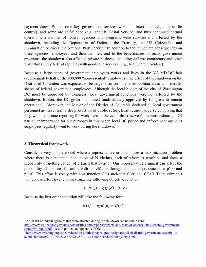
Consider a very simple model where a representative criminal faces a maximization problem where there is a potential population of N victims, each of whom is worth v, and faces a probability of getting caught of q (such that 0<q<1). Our representative criminal can affect the probability of a successful crime with his effort e through a function p(e) such that p’>0 and p’’<0. This effort is costly with cost function C(e) such that C’>0 and C’’>0. Then, criminals will choose effort level e to maximize the following objective function,

1

Because the first order condition will take the following form,

1 ′

                                                            2 A full list of federal agencies that were affected during the shutdown can be found here: http://www.whitehouse.gov/sites/default/files/omb/reports/impacts-and-costs-of-october-2013-federal-government-shutdown-report.pdf (see, in particular, Appendix Table 1). 3 http://www.washingtonpost.com/local/dc-politics/mayor-gray-designates-all-of-district-government-essential-to-avoid-shutdown/2013/09/25/3df4047a-25f4-11e3-ad0d-b7c8d2a594b9_story.html  

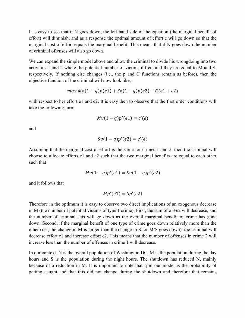
It is easy to see that if N goes down, the left-hand side of the equation (the marginal benefit of effort) will diminish, and as a response the optimal amount of effort e will go down so that the marginal cost of effort equals the marginal benefit. This means that if N goes down the number of criminal offenses will also go down.

We can expand the simple model above and allow the criminal to divide his wrongdoing into two activities 1 and 2 where the potential number of victims differs and they are equal to M and S, respectively. If nothing else changes (i.e., the p and C functions remain as before), then the objective function of the criminal will now look like,

1 1 1 2 1 2

with respect to her effort e1 and e2. It is easy then to observe that the first order conditions will take the following form

1 1 ′

and

1 2 ′

Assuming that the marginal cost of effort is the same for crimes 1 and 2, then the criminal will choose to allocate efforts e1 and e2 such that the two marginal benefits are equal to each other such that

1 1 1 2

and it follows that

1 ′ 2

Therefore in the optimum it is easy to observe two direct implications of an exogenous decrease in M (the number of potential victims of type 1 crime). First, the sum of e1+e2 will decrease, and the number of criminal acts will go down as the overall marginal benefit of crime has gone down. Second, if the marginal benefit of one type of crime goes down relatively more than the other (i.e., the change in M is larger than the change in S, or M/S goes down), the criminal will decrease effort e1 and increase effort e2. This means that the number of offenses in crime 2 will increase less than the number of offenses in crime 1 will decrease.

In our context, N is the overall population of Washington DC, M is the population during the day hours and S is the population during the night hours. The shutdown has reduced N, mainly because of a reduction in M. It is important to note that q in our model is the probability of getting caught and that this did not change during the shutdown and therefore that remains

constant, that is, the supply function of crime was unaffected.4 Thus, in the light of the model above, we have two empirically testable implications:

Implication 1: The shutdown caused an overall reduction in the number of criminal acts.

Implication 2: The shutdown caused a decline in criminal acts during the day hours and an increase in criminal acts during the night hours, with the former effect being larger in magnitude than the latter.

These two testable implications represent the basis of our empirical analyses. In the next section we describe the nature of our data, our empirical methodology and the institutional details behind our natural experiment.

4. Data and Empirical Strategy

4.1. Data

The data used in this study come from two main sources. The first data set provides information on monthly traffic at the state level and it comes from the Federal Highway Administration at the U.S. Department of Transportation.5 These data provides traffic volume in a monthly report based on hourly traffic count data reported by each state. These data are collected at approximately 4,000 continuous traffic counting locations nationwide and are used to estimate the percent change in traffic for the current month compared with the same month in the previous year. Estimates are re-adjusted annually to match the vehicle miles of travel from the Highway Performance Monitoring System and are continually updated with additional data. The data also breaks total number of miles driven by whether these are urban or rural miles driven. We use urban miles (there are no rural miles for Washington, DC), and our data include 1,581 month*state data points from August 2011 to February 2014. Table 1 provides summary statistics of these data that we will use in our empirical analysis to demonstrate that commuting traffic went down due to the government shutdown during October 2013.

The second type of data that we use in our empirical analysis consists of crime statistics that we obtained from the Washington DC Police Department and the Baltimore Police Department for the cities of Washington DC and Baltimore, respectively. The data span the period between 8/1/2012 and 2/28/2014.

These data detail all crime and specify exact location, exact time and day as well as type of crime. Table 2 shows summary statistics on daily criminal activity in the two cities, overall as well as by time of day, workdays/weekends, and by crime category.                                                             4 http://www.washingtonpost.com/local/dc‐politics/mayor‐gray‐designates‐all‐of‐district‐government‐essential‐to‐avoid‐shutdown/2013/09/25/3df4047a‐25f4‐11e3‐ad0d‐b7c8d2a594b9_story.html  5 http://www.fhwa.dot.gov/policyinformation/travel_monitoring/tvt.cfm

4.2 Empirical Strategy

We employ a difference-in-differences strategy using the city of Baltimore as a control group. Baltimore is often used as a comparison for Washington, DC because the two cities share some key demographics6 and are located in proximity of each other (40 miles apart) without being immediately adjacent. In our context, the physical distance between the two cities lessens the concern that the shutdown had a direct effect on Baltimore.7

In our analyses, we estimate the following econometric model:

Yit = α + βShutdownit + δDC*Shutdownit + γi + µy(i) + θm(i) + λw(i) + χ d(i) + τi t + uit (1)

In model (1), t denotes days (from 8/1/2012 through 2/28/2014), Yit is the number of crimes in city i (DC or Baltimore) on date t, Shutdown is an indicator equal to 1 for t between 10/1/2013 and 10/16/2013 (extremes included), and 0 otherwise. Our controls include city fixed effects (γi), year fixed effects (µy(i)), month fixed effects (θm(i)), week fixed effects (λw(i)), and day-of-the-week fixed effects (χ d(i)). To rule out that any results are due to differences in city trends pre-dating the shutdown, we also include city-specific time trends (τi ). This relaxes the “common trends” assumption allowing crime to follow non-parallel trajectories in the two cities (Angrist and Pischke 2014, Chapter 5). The coefficient on the DC*Shutdown interaction term, δ, is the difference-in-differences estimator, measuring the differential change in criminal activity during the shutdown period in DC compared to Baltimore. The standard errors are clustered on city-month (Bertrand, Duflo and Mullainathan 2004).

Given the very rich set of time dummies, and the city-specific trends included in the model, identification rests on an assumption of no contemporaneous city-level shocks that are concurrent with the Government shutdown and correlated with crime outcomes.

In addition, we exploit variation across days of the week and time of the day with varying propensities for being affected by the shutdown. Specifically, we estimate a version of model (1) separately for weekdays and weekend days, and for office hours (9AM-5PM), evening (5PM-2AM) and night hours (2AM-9AM). This is equivalent to estimating triple-difference regressions, based on the premise that the shutdown had a larger impact on effective population

                                                            6 Based on Census data, in 2013 Washington, DC had a total population of 646,449, with 49.5% African American, 10.1% Hispanic or Latino, and 35.8% White; in the same year, Baltimore had a population of 622,104, with about 63% African American, 4.6% Hispanic or Latino, and 28.3% White. 7 For example, Loftin, McDowall, Weirsema and Cottey (1991) examined the impact of changes in gun control policies in DC comparing downtown DC to its close-by suburbs within DC and finding a big impact of such laws. Nevertheless, Britt, Kleck and Bordua (1996) argued that even after adjusting for observables these were not comparable, and used the city of Baltimore as control group finding no impact of gun-control policies on crime. 

in DC during office hours, arguably a smaller effect on weekends compared to weekdays, and little effect during the night hours.8

5. Results

5.1 First-stage

A number of people commute into Washington, DC for work every day from nearby areas in Virginia and Maryland. According to recent estimates by the Census Bureau, the population of DC almost doubles during the day due to the inflow of commuters (79% increase; see US Census, 2010).9 Ideally, we would like to gather precise evidence about the number of people physically present in Washington DC on a daily basis before, during and after the shutdown, and show that the daytime DC population was substantially smaller during the shutdown, as suggested by anecdotal evidence and popular press coverage.10 Unfortunately, no data source exists that provides the actual number of commuters on a daily basis, or even the number of pedestrians walking around US cities. We are thus limited to using the amount of traffic at the state level by month (to the best of our knowledge and efforts, we do not know of and could not find traffic at the city level and/or day level). Fortunately, in the case of the District of Columbia the state and city limits are the same, and therefore we will not be adding any noise when estimating the impact of the government shutdown on urban traffic in Washington, DC.

Table 3 shows results of our first-stage when using urban traffic driven miles as the dependent variable. This table contains 5 different columns for which we always use a DC dummy, October 2013 dummy and the interaction of these two dummy variables. Column (1) does not include city fixed effects and therefore the DC dummy simply informs us that, not surprisingly, DC has much smaller levels of urban traffic than the 50 US states. The positive and significant coefficient on the October 2013 dummy indicates that, on average, traffic is more intense in October in all US states. The coefficient on the DC*October interaction, however, is negative and strongly statistically significant, indicating that urban traffic declined in DC during the shutdown compared to other US states. Column (2) introduces city fixed effects and shows no change in the interaction coefficient. Columns (3) and (4) add year and month*year fixed effects and show that the effect is still very robust. Finally, column (5) includes state*month and year fixed effects thus allowing for seasonality patterns to vary across all states as well as for differences in levels                                                             8 Substitution effects could also arise in the form of criminals traveling to other locations outside Washington DC to commit crimes. We are not exploring this possibility at this stage but we suspect the effect to be of second order. In fact, lower transportation costs and the reduced need to travel are thought to be among the reasons why criminals prefer to locate in large cities (Gleaser and Sacerdote 1999). 9 Note that despite Washington DC and Baltimore having roughly the same size (around 630,000 and 620,000 inhabitants respectively), the population of Baltimore City county increases its numbers by far less. McKenzie, Koerber, Fields, Benetsky, and Rapino (2013), Baltimore City County receives 100,000 workers on a daily basis and so given the population of Baltimore city this amounts to about 16%. 10http://lits-livingoncapitolhill-hell.blogspot.com/2013/10/government-shutdown-and-empty-streets.html 

across years. In this richer specification, our coefficient of interest drops from -126.6 (columns 1-4) to -58.1. Thus, our most conservative estimate indicates that the two-week long government shutdown was associated with about 58 million fewer urban miles driven in DC in the month of October 2013, corresponding to 25 percent of the average number of urban miles typically driven in DC monthly (206 million; see Table 1). By simple extrapolation, we can estimate that the government shutdown may have decreased traffic by close to 50% during the two weeks that it was in place.

5.2 Main Results

Our main results are reported in Table 4. The specification in column (1) includes city and time fixed effects (as described in section 4.2), whereas column (2) reports results from estimation of our econometric model that also includes city-specific time trends. The estimated effect of the shutdown is similar in both columns: we estimate a decline by 2.2 (p<0.05) in column (1) and a decline by 2.5 (p<0.1) criminal acts per day in DC during the shutdown, corresponding to 2.3%-2.6% of the mean. In column (3) we focus on assaults, burglaries and thefts, finding an estimated coefficient of -2.7 (p<0.05), corresponding to a 2.8% decline. We thus find corroboration for our Hypothesis 1 that the overall decline in the effective population of Washington DC during the shutdown caused a reduction in criminal activity.

As outlined above, the main way in which the shutdown reduced the effective population of Washington, DC was through reducing the number of people who commuted to DC to work (decline in M in the theoretical model of section 3). This implies that if the reduction in crime that we detect is indeed due to the shutdown, we should observe a larger decline during work hours. Column (2) of Table 5 shows results from our fully-specified regression (i.e., including city-specific time trends) but limited to crimes committed during office hours, i.e. between 9AM and 5PM; column (5) shows the same limited to assaults, burglaries and theft. The results indicate that the drop in crime associated with the shutdown was particularly large during the day hours: crime declined by about 4 units per day (p<0.01), corresponding to a 9% reduction, or more than ½ of one standard deviation.

5.3 Substitution Effects

With opportunities to commit crimes dropping dramatically during the day hours due to the reduced population, the marginal benefit to committing crimes experienced a relative increase at other times, namely during the night hours. The simple theoretical framework outlined in Section 3 implied that criminals would choose to reallocate their effort away from the day hours and toward the evening and night hours. Consistent with our hypothesis, we find that crime indeed

increased in Washington DC during the shutdown between 5PM and 2AM.11 As shown in columns (3) and (6) of Table 5, we estimate that crime went up by about 2 units (p<0.1) per day in the evening and night hours, corresponding to a 5.3% increase. As for the early morning hours (2AM – 9AM), we find a small, negative effect: -0.9 (p<0.1) in column (1) and -0.6 (p>0.15) in column (4). Thus, our Hypothesis 2 that crime declined more during the day than it increased during the night (because S from the theoretical model stayed the same or declined less than M) is also verified in the data.

Following the same logic, in Table 6 we look separately at workdays and weekends. We find that the decline in crime was concentrated during workdays. As reported in columns (1) and (3), we find that crime declined by about 4 units per day during workdays (p<0.05 in column (1) and p<0.01 in (2)). The results in columns (2) and (5), on the other hand, indicate that crime on average increased during weekends by around 2 units per day, although the estimates are not statistically significant (2.5, p>0.25 in column (2) and 1.8, p>0.4 in column (4)).

5.4 Placebo Test

The patterns we uncovered and described above, with crime declining during times when the shutdown had the largest effect on population size and staying roughly constant or increasing at other times, are consistent with our hypotheses and, in our view, not likely to be “accidental”. Nonetheless, we performed a placebo test where we redefine the “shutdown” to take place one year earlier, i.e. between October 1 and October 16 2012 and estimated the same regression as in model (1). As shown in column (4) of Table 4, the estimated coefficient on the interaction DC*Shutdown2012 is small in magnitude, 0.08 and is not statistically significant (p>0.9).

5.5 Alternative Explanations

In this section, we discuss potential alternative explanations for our results. First, an alternative model of criminal behavior is one where criminals have some “target” in mind. They may focus on a specific number of crimes per day or per week, or a specific value per day or per week. If this were true, criminal offenders would supply effort until they achieve their target regardless of their marginal benefit and their marginal cost per committed crime. However, our results allow us to rule out these “target” explanations. In fact, if criminals aimed to commit a given number of crimes per day/week, this would imply no change in the total number of crimes committed during the government shutdown. The results also rule out the hypothesis that criminals have an earnings target. The fact that the total number of crimes overall went down, with a decline in crimes during work hours and a (smaller) increase in the evening and night hours is consistent

                                                            11 We use 2 am cutoff because that is the time when bars and clubs close at night in both Washington DC and Baltimore.

with the standard model we proposed in section 3 but inconsistent with an earnings target model. In fact, under an earnings target model, the smaller increase in evening crimes would suggest that these crimes are more profitable than the morning ones. Then this would call into question why criminals do not concentrate their criminal activity from 5 pm to 2 am in the first place, since they would be able to achieve their goal faster and at a lower personal cost.

Another potential explanation is that the decrease in total crime came from crimes committed by casual offenders. These are not necessarily professional criminals and therefore our results might have little to say about the labor supply decisions of “career” criminals. This explanation would imply that our result is a compound of extensive (more or less criminals) and intensive (number of crimes committed per criminal) margins. Even though we cannot rule the fact that an adjustment occurs along both margins, the fact that we observe within-day temporal crime displacement from morning to evening crimes suggests that the reduction in the number of casual offenders is offset by the increase in the number of hours worked by “full-time” criminals. In a nutshell, although we cannot rule out this explanation, we are confident that this explanation is not driving our results.

Finally, another potential explanation is geographical crime displacement. Crime may have decreased in DC but increased in neighboring cities and suburbs. Wright and Decker (1997) through a number of interviews found that individuals rarely ever travel far to offend, and therefore we concentrate our efforts in obtaining daily crime data for Alexandria in Virginia and Montgomery County in Maryland. Data in these locations are not as readily available as they were in Washington DC and Baltimore, so we are forced to restrict our analysis to shorter time periods. Specifically, we were able to obtain crime data for Alexandria (VA) for September, October and November of 2012 and 2013, whereas Montgomery Country (MD) data were only available for September, October and November of 2013. Table 7 shows results of comparing the evolution of crime during the government shutdown in these locations relative to Baltimore. If displacement occurred we would observe that crime increased in these locations (while it decreased in DC). In column (1) of Table 7, we show that if anything crime went down in Alexandria. This is perhaps driven by the fact that Northern Virginia is also home to a lot of federal government agencies and potentially de facto population also went down. In column (2), we repeat the same exercise with crime data from Montgomery County in Maryland (immediately north of DC). Unfortunately, the data are limited to only three months in 2013, so we are left comparing those months with crime events in Baltimore during the same period of time for a total of only 182 daily observations. Although the sign of the estimated coefficient is positive, the standard error is large and thus we find no statistically significant change in crime.

We are only left to examine whether our finding is result of a mechanical countercyclical relationship between Baltimore and DC. Because the two cities are close to each other, one may argue that criminals in the area switch back and forth between these two conveniently located and connected cities of roughly the same size. To dissipate this type of concerns, we have repeated our analysis using Philadelphia, PA as control city. Despite the fact that Philadelphia is

substantially larger in population size and therefore average daily crime numbers, it is still located close enough that differences in weather and seasonality are not likely to play a role. Column (3) of Table 7 shows that results are qualitatively the same (same sign and same statistical significance), and even stronger in magnitude.

We want to end this section highlighting that our source of exogenous variation is on the population size and density, holding everything else constant, due to the shutdown of the US federal government in October 2013. The fact that no change in law or enforcement occurred during this time allows us to identify the shape of labor supply function of criminals and temporal displacement. A similar event is difficult to find in the literature because ours is a temporary change, with no impact on long-run enforcement or punishment. This attenuates concerns regarding the role of dynamics (McCrary 2010) and allows for a safer static interpretation of our findings. The fact that our treatment period rests in between control periods (prior to October 1st and after October 16th 2013) also helps us level changes in behavior during the shutdown against potential changes in behavior occurred after the shutdown.

A different interpretation of our results is that the victimization rate (probability of becoming a victim) goes up because density goes up. Although we do not know for sure how many government workers stopped commuting into DC during the shutdown, the fact that the victimization rate went up seems very likely to be the case and we do not oppose this interpretation consistent with Jacobs (1961) and Glaeser (2011). Our goal in this paper is to estimate the effect of an exogenous drop in daytime population on crime, and the criminals’ ability to substitute criminal activity between time of the day and days of the week. Our findings help to characterize other findings in the literature regarding time, geographical, and crime type displacement without having to pay much attention to dynamic considerations.

6. Discussion and Conclusions

We used the government shutdown of 2013 as a source of plausibly exogenous variation in effective population size and density in the city of Washington DC, and estimated its effect on criminal activity. Evidence from media reports corroborated by our own analysis of traffic data indicates that the effective population of Washington, DC was considerably reduced during the shutdown period. At the same time, other, supply-side determinants of crime were unchanged, including the criminal population, laws, and law enforcement presence.

We found that crime dropped by 3% on average during the shutdown. More precisely, crime dropped 9% during the day hours, when the effective population of Washington, DC declined the most due to the government shutdown. The effect is large, corresponding to about ½ of one standard deviation. This indicates that demand-side factors such as population are important determinants of criminal activity, confirming earlier results from Jacobs (1961) and Gleaser and Sacerdote (1999). Our evidence though differs from theirs in that our results show that a decrease

in population decreases the total number of crime, but it is inconclusive of whether it potentially increased the victimization rate. Because we observe an exogenous shock inward of the demand function for crime, our result is evidence that the labor supply curve of criminals is upward-sloping and not infinitely inelastic as some studies have suggested in the past (see Erlich 1996 for an early literature review).

We also found that criminals reacted to lower population density by increasing their labor supply (of crime) at times of the day and days that did not suffer an exogenous decrease in the value of their marginal effort, thereby attenuating the magnitude of the direct effect. Specifically, we estimate a 5% increase in criminal activity during the night. Combined with the direct effect described above, this is evidence that criminals reallocated their efforts away from the day hours, when the marginal return dropped, toward the night hours. Also, overall, crime declined during workdays whereas it increased during weekends (although the latter effect was not statistically significant at conventional levels).

Our findings have implications for public policy, specifically for law enforcement agencies. Criminal activity responded to the large and unexpected shock to the effective DC population caused by the shutdown in a way that is consistent with standard economic theory. Crime declined during the day, but criminals rationally reallocated their efforts so that crime increased during the night hours. A reallocation of police across shifts might have prevented crime from increasing so much during the evening hours. This is the most immediate policy implication of our findings. Given the exogenous nature of the natural experiment that we exploited, we are fairly confident that the effects we estimated are causal, so that the lessons (at least directionally) generalize to other contexts where a city’s effective population increases or drops substantially and temporarily due to an unexpected event (see Jacob et al (2007) for an example on severe weather conditions). Varying fines and punishments according to circumstances that increase opportunities to commit crime would also be possible strategies to neutralize the increased expected return to criminal activity. Similarly, our results have potential implications for zoning design and regulation (Twinam, 2014), as well as for policies encouraging potential victims to invest on precautionary behaviors as their availability may be an important determinant to final crime outcomes (Van Ours and Vollaard, 2014). Future research should then look for instances and events that provide plausible exogenous variation on the demand side of the market for crime (a la Becker 1968 or Erlich 1996) and further study which of these factors are more likely to lower crime and which type of crime is more sensitive to policy design.

References

Angrist, Joshua and Steve Pischke. 2014. “Mastering ‘Metrics: The Path from Cause to Effect”. Princeton University Press.

Becker, Gary. 1968. “Crime and Punishment: An Economic Approach,” Journal of Political Economy, Vol. 76, No. 2, pp. 169-217.

Black, Dan and Daniel Nagin. 1998. “Do ‘Right-to-Carry’ Laws Deter Violent Crime?” Journal of Legal Studies. 27:1, pp. 209–19.

Britt, Chester L., Gary Kleck, & David J. Bordua. 1996. "A Reassessment of the D.C. Gun Law: Some Cautionary Notes on the Use of Interrupted Time Series Designs for Policy Impact Assessment," 30 Law & Society Rev. 361.

Donohue, John and Steven Levitt. 2001. “Legalized Abortion and Crime.” Quarterly Journal of Economics. 116:2, pp. 379 –420. Donohue, John and Steven Levitt. 2004. “Further Evidence That Legalized Abortion Lowered Crime: A Reply to Joyce.” Journal of Human Resources, 34(1). Duggan, Mark. 2001. “More Guns, More Crime.” Journal of Political Economy. 109:5, pp. 1086–114.

Erlich, Isaac. 1996. “Crime, Punishment, and the Market for Offenses,” The Journal of Economic Perspectives, Vol. 10, No. 1 (Winter, 1996), pp. 43-67.

Glaeser, Edward. 2011. Triumph of the City: How our Greatest Invention Makes us Richer, Smarter, Greener, Healthier and Happier. Penguin Press.

Glaeser, Edward L., and Bruce Sacerdote. 1999. “Why is There More Crime in Cities?” Journal of Political Economy, Vol. 107, No. S6, pp. S225-S258.

Glaeser, Edward L., Bruce Sacerdote, and José A. Scheinkman. 1996. “Crime and Social Interactions,” The Quarterly Journal of Economics, Vol. 111, No. 2, pp. 507-548.

Gould, Eric, Bruce Weinberg and David Mustard. 2002. “Crime Rates and Local Labor Market Opportunities in the United States: 1979–1991.” The Review of Economics and Statistics, February 2002, 84(1): 45–61. Harris, Keith. 2006. “Property Crimes and Violence in United States: An Analysis of the influence of Population density,” International Journal of Criminal Justice Sciences, Vol. 1, Issue 2.

Jacobs, Jane, 1961. The death and life of great American cities. Random House.

Jacob, Brian, Lars Lefgren and Enrico Moretti, 2007. “The Dynamics of Criminal Behavior: Evidence from Weather Shocks,” Journal of Human Resources, vol. 42(3).

Katz, Lawrence, Steven Levitt and Ellen Shustorovich. 2003. “Prison Conditions, Capital Punishment, and Deterrence.” American Law and Economics Review. 5:2, pp. 318– 43. Levitt, Steven. 2002. “Using Electoral Cycles in Police Hiring to Estimate the Effect of Police on Crime: A Reply.” American Economic Review. September, 92, pp. 1244–250. Levitt, Steven. 2004. “Understanding Why Crime Fell in the 1990s: Four Factors That Explain the Decline and Six That Do Not,” The Journal of Economic Perspectives, Vol. 18, No. 1, pp. 163-190.

Loftin, Colin, David McDowall, Brian Wiersema, & TalbertJ. Cottey. 1991. "Effects of Restrictive Licensing of Handguns on Homicide and Suicide in the District of Columbia," 325 New England Journal of Medicine 1615.

Ludwig, Jens. 1998. “Concealed Gun Carrying Laws and Violent Crime: Evidence from State Panel Data.” International Review of Law and Economics. September, 18, pp. 239–54. McCrary, Justin. 2002. “Do Electoral Cycles in Police Hiring Really Help Us Estimate the Effect of Police on Crime? Comment.” American Economic Review. September, 92, pp. 1236–243. McCrary, Justin. 2010. “Dynamic Perspectives on Crime.” Chapter 4 in Handbook of the Economics of Crime, Edward Elgar, 2010. McKenzie, Brian, William Koerber, Alison Fields, Megan Benetsky, and Melanie Rapino. 2013. “Commuter-Adjusted Population Estimates: ACS 2006-10,” US Census Bureau Working Paper.

Mocan, Naci and R. Kaj Gittings. 2003. “Getting Off Death Row: Commuted Sentences and the Deterrent Effect of Capital Punishment.” Journal of Law and Economics. October, Forthcoming.

Twinam, Tate. 2015. “Danger Zone: The Casual Effects of High-Density And Mixed-Use Development on Neighborhood Crime,” Working Paper University of Pittsburgh.

US Census Bureau. 2010. “Commuter-Adjusted Population Estimates: ACS 2006-10”. Available at https://www.census.gov/hhes/commuting/data/daytimepop.html.

Van Ours, Jan C., and Ben Vollaard. 2014. “The Engine Immobilizer: A Non-Starter for Car Thieves.” Forthcoming at The Economic Journal.

Vollaard, Ben. 2014. “Temporal displacement of environmental crime. Evidence from marine oil pollution.” Working Paper Tilburg University.

Watts, Reginald. 1931. “The Influence of Population Density on Crime,” Journal of the American Statistical Association, Vol. 26, No. 173, pp. 11-20.

Wright, Richard T. and Scott H. Decker. 1997. “Armed Robbers in Action: Stickups and Street Culture.” Northeastern University Press.

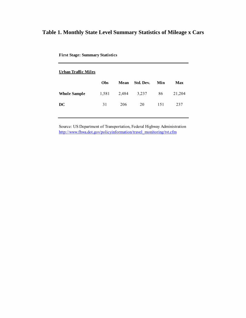
Table 1. Monthly State Level Summary Statistics of Mileage x Cars

First Stage: Summary Statistics

Urban Traffic Miles

Obs Mean Std. Dev. Min Max

Whole Sample 1,581 2,484 3,237 86 21,204

DC 31 206 20 151 237

Source: US Department of Transportation, Federal Highway Administrationhttp://www.fhwa.dot.gov/policyinformation/travel_monitoring/tvt.cfm

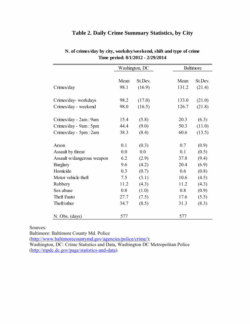
Table 2. Daily Crime Summary Statistics, by City

Sources: Baltimore: Baltimore County Md. Police (http://www.baltimorecountymd.gov/agencies/police/crime/); Washington, DC: Crime Statistics and Data, Washington DC Metropolitan Police (http://mpdc.dc.gov/page/statistics-and-data).

Mean St.Dev. Mean St.Dev.Crimes/day 98.1 (16.9) 131.2 (21.4)

Crimes/day- workdays 98.2 (17.0) 133.0 (21.0)Crimes/day - weekend 98.0 (16.5) 126.7 (21.8)

Crimes/day - 2am : 9am 15.4 (5.8) 20.3 (6.3)Crimes/day - 9am : 5pm 44.4 (9.0) 50.3 (11.0)Crimes/day - 5pm : 2am 38.3 (8.4) 60.6 (13.5)

Arson 0.1 (0.3) 0.7 (0.9)Assault by threat 0.0 0.0 0.1 (0.5)Assault w/dangerous weapon 6.2 (2.9) 37.8 (9.4)Burglary 9.6 (4.2) 20.4 (6.9)Homicide 0.3 (0.7) 0.6 (0.8)Motor vehicle theft 7.5 (3.1) 10.6 (4.5)Robbery 11.2 (4.3) 11.2 (4.3)Sex abuse 0.8 (1.0) 0.8 (0.9)Theft f/auto 27.7 (7.5) 17.6 (5.5)Theft/other 34.7 (8.5) 31.3 (8.3)

N. Obs. (days) 577 577

Washington, DC Baltimore

N. of crimes/day by city, workdsy/weekend, shift and type of crimeTime period: 8/1/2012 - 2/29/2014

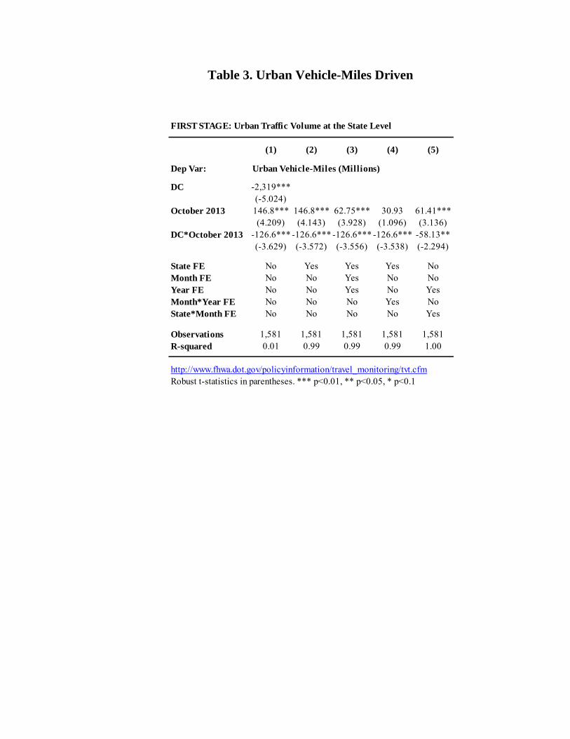
Table 3. Urban Vehicle-Miles Driven

FIRST STAGE: Urban Traffic Volume at the State Level

(1) (2) (3) (4) (5)

Dep Var: Urban Vehicle-Miles (Millions)

DC -2,319***(-5.024)

October 2013 146.8*** 146.8*** 62.75*** 30.93 61.41***(4.209) (4.143) (3.928) (1.096) (3.136)

DC*October 2013 -126.6*** -126.6*** -126.6*** -126.6*** -58.13**(-3.629) (-3.572) (-3.556) (-3.538) (-2.294)

State FE No Yes Yes Yes NoMonth FE No No Yes No NoYear FE No No Yes No YesMonth*Year FE No No No Yes NoState*Month FE No No No No Yes

Observations 1,581 1,581 1,581 1,581 1,581R-squared 0.01 0.99 0.99 0.99 1.00

http://www.fhwa.dot.gov/policyinformation/travel_monitoring/tvt.cfmRobust t-statistics in parentheses. *** p<0.01, ** p<0.05, * p<0.1

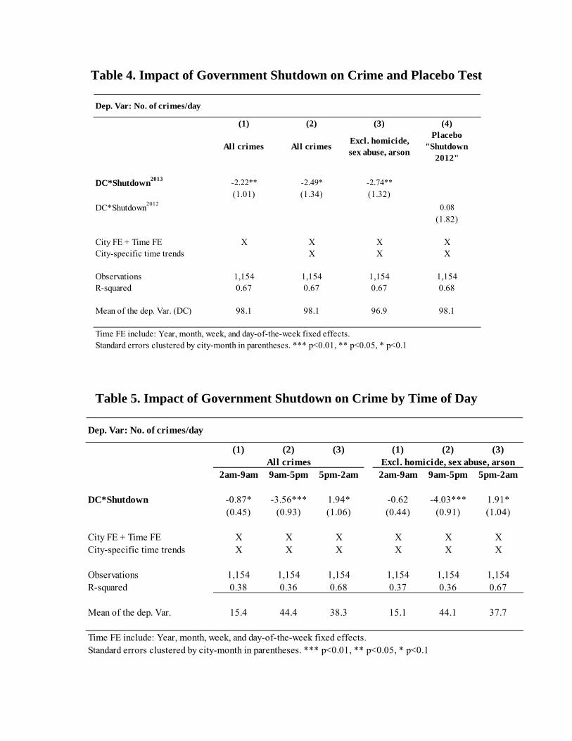
Table 4. Impact of Government Shutdown on Crime and Placebo Test

Table 5. Impact of Government Shutdown on Crime by Time of Day

(1) (2) (3) (4)

All crimes All crimesExcl. homicide, sex abuse, arson

Placebo"Shutdown

2012"

DC*Shutdown2013 -2.22** -2.49* -2.74**

(1.01) (1.34) (1.32)

DC*Shutdown2012 0.08

(1.82)

City FE + Time FE X X X XCity-specific time trends X X X

Observations 1,154 1,154 1,154 1,154R-squared 0.67 0.67 0.67 0.68

Mean of the dep. Var. (DC) 98.1 98.1 96.9 98.1

Dep. Var: No. of crimes/day

Time FE include: Year, month, week, and day-of-the-week fixed effects. Standard errors clustered by city-month in parentheses. *** p<0.01, ** p<0.05, * p<0.1

(1) (2) (3) (1) (2) (3)

2am-9am 9am-5pm 5pm-2am 2am-9am 9am-5pm 5pm-2am

DC*Shutdown -0.87* -3.56*** 1.94* -0.62 -4.03*** 1.91*(0.45) (0.93) (1.06) (0.44) (0.91) (1.04)

City FE + Time FE X X X X X XCity-specific time trends X X X X X X

Observations 1,154 1,154 1,154 1,154 1,154 1,154R-squared 0.38 0.36 0.68 0.37 0.36 0.67

Mean of the dep. Var. 15.4 44.4 38.3 15.1 44.1 37.7

Dep. Var: No. of crimes/day

Time FE include: Year, month, week, and day-of-the-week fixed effects. Standard errors clustered by city-month in parentheses. *** p<0.01, ** p<0.05, * p<0.1

Excl. homicide, sex abuse, arsonAll crimes

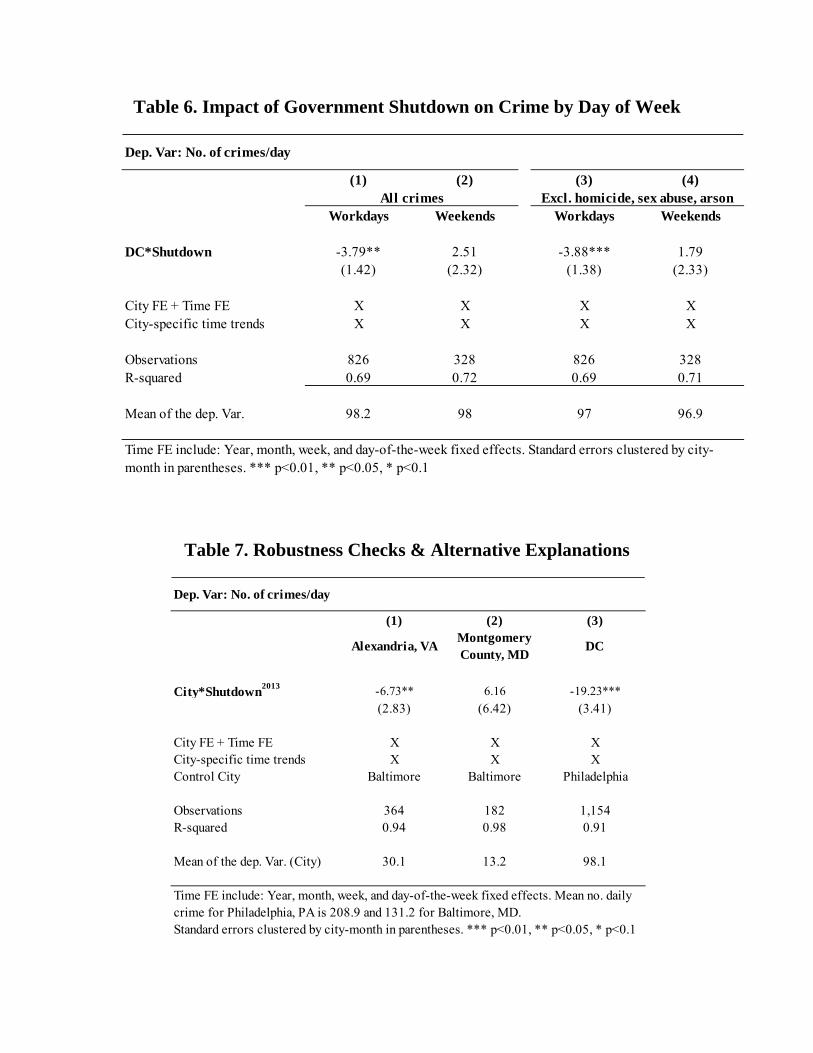
Table 6. Impact of Government Shutdown on Crime by Day of Week

Table 7. Robustness Checks & Alternative Explanations

(1) (2) (3) (4)

Workdays Weekends Workdays Weekends

DC*Shutdown -3.79** 2.51 -3.88*** 1.79(1.42) (2.32) (1.38) (2.33)

City FE + Time FE X X X XCity-specific time trends X X X X

Observations 826 328 826 328R-squared 0.69 0.72 0.69 0.71

Mean of the dep. Var. 98.2 98 97 96.9

Dep. Var: No. of crimes/day

Time FE include: Year, month, week, and day-of-the-week fixed effects. Standard errors clustered by city-month in parentheses. *** p<0.01, ** p<0.05, * p<0.1

All crimes Excl. homicide, sex abuse, arson

(1) (2) (3)

Alexandria, VAMontgomery County, MD

DC

City*Shutdown2013 -6.73** 6.16 -19.23***

(2.83) (6.42) (3.41)

City FE + Time FE X X XCity-specific time trends X X XControl City Baltimore Baltimore Philadelphia

Observations 364 182 1,154R-squared 0.94 0.98 0.91

Mean of the dep. Var. (City) 30.1 13.2 98.1

Dep. Var: No. of crimes/day

Time FE include: Year, month, week, and day-of-the-week fixed effects. Mean no. daily crime for Philadelphia, PA is 208.9 and 131.2 for Baltimore, MD.Standard errors clustered by city-month in parentheses. *** p<0.01, ** p<0.05, * p<0.1