ACTA ACUSTICA UNITED WITH ACUSTICA

Vol. 90 (2004) 781 – 787

Aim-mat: The Auditory Image Model in MATLAB

Stefan Bleeck, Tim Ives, Roy D. PattersonCentre for the Neural Basis of Hearing, Physiology Department, Downing Street, Cambridge CB2 3EG, UnitedKingdom

SummaryThis paper describes a version of the auditory image model (AIM) [1] implemented in MATLAB. It is referredto as “aim-mat” and it includes the basic modules that enable AIM to simulate the spectral analysis, neuralencoding and temporal integration performed by the auditory system. The dynamic representations produced bynon-static sounds can be viewed on a frame-by-frame basis or in movies with synchronized sound. The softwarehas a sophisticated graphical user interface designed to facilitate the auditory modelling. It is also possible toadd MATLAB code and complete modules to aim-mat. The software can be downloaded from http://www.mrc-cbu.cam.ac.uk/cnbh/aimmanual

PACS no. 43.66.Ba, 43.66.Hg, 43.72.Ar, 43.71.An

1. Introduction

The auditory image model (AIM) is a time-domain modelof the effective signal processing in the hearing systemwhich can be associated with specific stages of the as-cending auditory pathway. The ‘auditory image’ was firstdescribed by Patterson et al. [1]; it is meant to the simu-late the neural representation that underlies your first con-scious awareness of a sound. There is a computational im-plementation of AIM in ‘C’ code which is frequently usedby the auditory community to simulate the construction ofauditory images [2]. In this paper, we describe a MATLABversion of AIM referred to as aim-mat, which was devel-oped to make AIM more accessible to auditory modellersand to make it available on more computer platforms.

Aim-mat is a complete, stand-alone implementation ofAIM in which the processing modules, the resource filesand the graphical user interface are all written in MAT-LAB, so that the user has full control of the system at alllevels. The user can design, develop, program and debugnew auditory modules within the MATLAB environment,with the assistance of all the powerful tools provided inthe MATLAB environment. It is also possible to changethe displays and add new options to the graphical user in-terface.

AIM

This paper provides a brief introduction to AIM and theadvances introduced while developing aim-mat. The de-tails of AIM, a full manual for aim-mat and an extendedexample of how to use aim-mat are available on our web-page (http://www.mrc-cbu.cam.ac.uk/cnbh/aimmanual).

Received 10 April 2003, Revised 10 November 2003,accepted 16 December 2003.

The principle functions of AIM (and aim-mat) are todescribe and simulate:

1. pre-cochlear processing (PCP) of the sound up to theoval window,

2. the basilar membrane motion (BMM) produced in thecochlea,

3. the neural activity pattern (NAP) observed in the audi-tory nerve and cochlear nucleus,

4. the identification of the neural peak times (strobepoints) used to construct the auditory image(STROBES) and

5. the stabilized auditory image (SAI) that forms the basisof auditory perception. Table I shows the architectureof AIM and its relationship to the physiology and sig-nal processing of the auditory system.

New features in aim-mat

Aim-mat includes a number of new features that go beyondthe scope of previous implementations of AIM:

1. Aim-mat has a graphical user interface that allows oneto perform all operations without programming skillsor a deeper knowledge of MATLAB.

2. The auditory image is dynamic and aim-mat includesa facility for generating QuickTime movies of the SAIwith synchronised sound.

3. A number of new modules are available for each stage.For example, there are new modules for strobe genera-tion ‘sf2003’ and temporal integration ‘ti2003’, whichare described in this paper.

4. Aim-mat allows users to add new modules written inMATLAB. An extensive description of how this isdone can be found on the webpage.

All modules in aim-mat are controlled by a specifiedset of parameters that are saved in an accessible parameter

c�

S. Hirzel Verlag � EAA 781

ACTA ACUSTICA UNITED WITH ACUSTICA Bleeck et al.: Aim-mat: the auditory image model in MATLABVol. 90 (2004)

Table I. The relationship between the signal processing simulated in aim-mat (top row), the physiological structure associated with theprocessing (middle row) and the aim-mat module (bottom row) that performs the processing.

Process Band-pass filter Frequency analysis Sharpening Feature detection Temporal integration

physiological structure Pinna/ middle ear Cochlea Brainstem/Thalamus/Cortex

aim-mat module PCP BMM NAP STROBE SAI

file, and the user can control the operation of aim-mat andthe presentation of the graphics through this file. Not allparameters of all modules can be described in the scopeof this paper. All parameters are described in detail on thewebpage. Aim-mat can also be used with or without thegraphical user interface. The graphical user interface fa-cilitates control at the module level. However, aim-mat canalso be called as a script file to batch process sets of stimulior to investigate a range of parameter settings without hav-ing to operate the interface manually. It is also possible touse aim-mat as a pre- processor, restricting the operationto the simulation of, say, basilar membrane motion.

Input signals

All standard wave files can be used as an input for aim-mat. The package also includes tools for convenient stim-ulus generation. The sampling rate of the wave file deter-mines the sample rate of all calculations, and all samplingrates are supported.

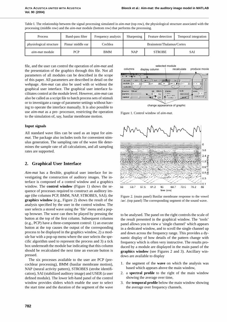
2. Graphical User Interface

Aim-mat has a flexible, graphical user interface for in-vestigating the construction of auditory images. The in-terface is composed of a control window and a graphicswindow. The control window (Figure 1) shows the se-quence of processes required to construct an auditory im-age (the columns PCP, BMM, NAP, STROBES, SAI); thegraphics window (e.g., Figure 2) shows the result of theanalysis specified by the user in the control window. Theuser selects a stored wave using the ‘file’ menu and a pop-up browser. The wave can then be played by pressing thebutton at the top of the first column. Subsequent columns(e.g., PCP) have a three-component control: 1) an executebutton at the top causes the output of the correspondingprocess to be displayed in the graphics window, 2) a mod-ule bar with a pop-up menu where the user selects the spe-cific algorithm used to represent the process and 3) a tickbox underneath the module bar indicating that this columnshould be recalculated the next time an execute button ispressed.

The six processes available to the user are PCP (pre-cochlear processing), BMM (basilar membrane motion),NAP (neural activity pattern), STROBES (strobe identifi-cation), SAI (stabilized auditory image) and USER (a userdefined module). The lower left-hand panel of the controlwindow provides sliders which enable the user to selectthe start time and the duration of the segment of the wave

columnsselected module

recalculatedisplay column

change appearance of graphic

produce movie

Figure 1. Control window of aim-mat.

Figure 2. (main panel) Basilar membrane response to the vowel/ae/. (top panel) The corresponding segment of the sound wave.

to be analysed. The panel on the right controls the scale ofthe result presented in the graphical window. The ‘tools’panel allows you to view a ‘single channel’ which appearsin a dedicated window, and to scroll the single channel upand down across the frequency range. This provides a dy-namic display of how details of the pattern change withfrequency which is often very instructive. The results pro-duced by a module are displayed in the main panel of thegraphics window (see Figures 2 and 3). Ancillary win-dows are available to display

1. the segment of the wave on which the analysis wasbased which appears above the main window,

2. a spectral profile to the right of the main windowshowing the average over time,

3. the temporal profile below the main window showingthe average over frequency channels.

782

Bleeck et al.: Aim-mat: the auditory image model in MATLAB ACTA ACUSTICA UNITED WITH ACUSTICA

Vol. 90 (2004)

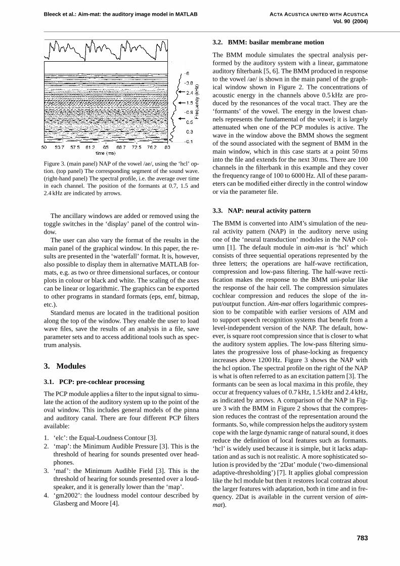
Figure 3. (main panel) NAP of the vowel /ae/, using the ‘hcl’ op-tion. (top panel) The corresponding segment of the sound wave.(right-hand panel) The spectral profile, i.e. the average over timein each channel. The position of the formants at 0.7, 1.5 and2.4 kHz are indicated by arrows.

The ancillary windows are added or removed using thetoggle switches in the ‘display’ panel of the control win-dow.

The user can also vary the format of the results in themain panel of the graphical window. In this paper, the re-sults are presented in the ‘waterfall’ format. It is, however,also possible to display them in alternative MATLAB for-mats, e.g. as two or three dimensional surfaces, or contourplots in colour or black and white. The scaling of the axescan be linear or logarithmic. The graphics can be exportedto other programs in standard formats (eps, emf, bitmap,etc.).

Standard menus are located in the traditional positionalong the top of the window. They enable the user to loadwave files, save the results of an analysis in a file, saveparameter sets and to access additional tools such as spec-trum analysis.

3. Modules

3.1. PCP: pre-cochlear processing

The PCP module applies a filter to the input signal to simu-late the action of the auditory system up to the point of theoval window. This includes general models of the pinnaand auditory canal. There are four different PCP filtersavailable:

1. ‘elc’: the Equal-Loudness Contour [3].2. ‘map’: the Minimum Audible Pressure [3]. This is the

threshold of hearing for sounds presented over head-phones.

3. ‘maf’: the Minimum Audible Field [3]. This is thethreshold of hearing for sounds presented over a loud-speaker, and it is generally lower than the ‘map’.

4. ‘gm2002’: the loudness model contour described byGlasberg and Moore [4].

3.2. BMM: basilar membrane motion

The BMM module simulates the spectral analysis per-formed by the auditory system with a linear, gammatoneauditory filterbank [5, 6]. The BMM produced in responseto the vowel /ae/ is shown in the main panel of the graph-ical window shown in Figure 2. The concentrations ofacoustic energy in the channels above 0.5 kHz are pro-duced by the resonances of the vocal tract. They are the‘formants’ of the vowel. The energy in the lowest chan-nels represents the fundamental of the vowel; it is largelyattenuated when one of the PCP modules is active. Thewave in the window above the BMM shows the segmentof the sound associated with the segment of BMM in themain window, which in this case starts at a point 50 msinto the file and extends for the next 30 ms. There are 100channels in the filterbank in this example and they coverthe frequency range of 100 to 6000 Hz. All of these param-eters can be modified either directly in the control windowor via the parameter file.

3.3. NAP: neural activity pattern

The BMM is converted into AIM’s simulation of the neu-ral activity pattern (NAP) in the auditory nerve usingone of the ‘neural transduction’ modules in the NAP col-umn [1]. The default module in aim-mat is ‘hcl’ whichconsists of three sequential operations represented by thethree letters; the operations are half-wave rectification,compression and low-pass filtering. The half-wave recti-fication makes the response to the BMM uni-polar likethe response of the hair cell. The compression simulatescochlear compression and reduces the slope of the in-put/output function. Aim-mat offers logarithmic compres-sion to be compatible with earlier versions of AIM andto support speech recognition systems that benefit from alevel-independent version of the NAP. The default, how-ever, is square root compression since that is closer to whatthe auditory system applies. The low-pass filtering simu-lates the progressive loss of phase-locking as frequencyincreases above 1200 Hz. Figure 3 shows the NAP withthe hcl option. The spectral profile on the right of the NAPis what is often referred to as an excitation pattern [3]. Theformants can be seen as local maxima in this profile, theyoccur at frequency values of 0.7 kHz, 1.5 kHz and 2.4 kHz,as indicated by arrows. A comparison of the NAP in Fig-ure 3 with the BMM in Figure 2 shows that the compres-sion reduces the contrast of the representation around theformants. So, while compression helps the auditory systemcope with the large dynamic range of natural sound, it doesreduce the definition of local features such as formants.‘hcl’ is widely used because it is simple, but it lacks adap-tation and as such is not realistic. A more sophisticated so-lution is provided by the ‘2Dat’ module (‘two-dimensionaladaptive-thresholding’) [7]. It applies global compressionlike the hcl module but then it restores local contrast aboutthe larger features with adaptation, both in time and in fre-quency. 2Dat is available in the current version of aim-mat).

783

ACTA ACUSTICA UNITED WITH ACUSTICA Bleeck et al.: Aim-mat: the auditory image model in MATLABVol. 90 (2004)

3.4. STROBES: strobe finding

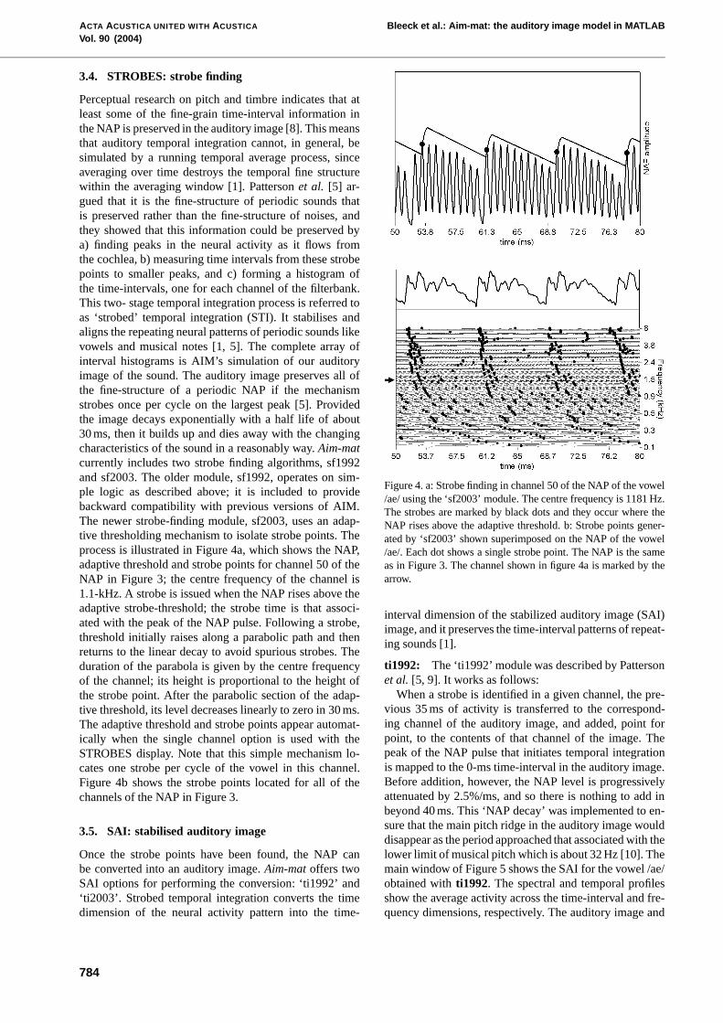
Perceptual research on pitch and timbre indicates that atleast some of the fine-grain time-interval information inthe NAP is preserved in the auditory image [8]. This meansthat auditory temporal integration cannot, in general, besimulated by a running temporal average process, sinceaveraging over time destroys the temporal fine structurewithin the averaging window [1]. Patterson et al. [5] ar-gued that it is the fine-structure of periodic sounds thatis preserved rather than the fine-structure of noises, andthey showed that this information could be preserved bya) finding peaks in the neural activity as it flows fromthe cochlea, b) measuring time intervals from these strobepoints to smaller peaks, and c) forming a histogram ofthe time-intervals, one for each channel of the filterbank.This two- stage temporal integration process is referred toas ‘strobed’ temporal integration (STI). It stabilises andaligns the repeating neural patterns of periodic sounds likevowels and musical notes [1, 5]. The complete array ofinterval histograms is AIM’s simulation of our auditoryimage of the sound. The auditory image preserves all ofthe fine-structure of a periodic NAP if the mechanismstrobes once per cycle on the largest peak [5]. Providedthe image decays exponentially with a half life of about30 ms, then it builds up and dies away with the changingcharacteristics of the sound in a reasonably way. Aim-matcurrently includes two strobe finding algorithms, sf1992and sf2003. The older module, sf1992, operates on sim-ple logic as described above; it is included to providebackward compatibility with previous versions of AIM.The newer strobe-finding module, sf2003, uses an adap-tive thresholding mechanism to isolate strobe points. Theprocess is illustrated in Figure 4a, which shows the NAP,adaptive threshold and strobe points for channel 50 of theNAP in Figure 3; the centre frequency of the channel is1.1-kHz. A strobe is issued when the NAP rises above theadaptive strobe-threshold; the strobe time is that associ-ated with the peak of the NAP pulse. Following a strobe,threshold initially raises along a parabolic path and thenreturns to the linear decay to avoid spurious strobes. Theduration of the parabola is given by the centre frequencyof the channel; its height is proportional to the height ofthe strobe point. After the parabolic section of the adap-tive threshold, its level decreases linearly to zero in 30 ms.The adaptive threshold and strobe points appear automat-ically when the single channel option is used with theSTROBES display. Note that this simple mechanism lo-cates one strobe per cycle of the vowel in this channel.Figure 4b shows the strobe points located for all of thechannels of the NAP in Figure 3.

3.5. SAI: stabilised auditory image

Once the strobe points have been found, the NAP canbe converted into an auditory image. Aim-mat offers twoSAI options for performing the conversion: ‘ti1992’ and‘ti2003’. Strobed temporal integration converts the timedimension of the neural activity pattern into the time-

Figure 4. a: Strobe finding in channel 50 of the NAP of the vowel/ae/ using the ‘sf2003’ module. The centre frequency is 1181 Hz.The strobes are marked by black dots and they occur where theNAP rises above the adaptive threshold. b: Strobe points gener-ated by ‘sf2003’ shown superimposed on the NAP of the vowel/ae/. Each dot shows a single strobe point. The NAP is the sameas in Figure 3. The channel shown in figure 4a is marked by thearrow.

interval dimension of the stabilized auditory image (SAI)image, and it preserves the time-interval patterns of repeat-ing sounds [1].

ti1992: The ‘ti1992’ module was described by Pattersonet al. [5, 9]. It works as follows:

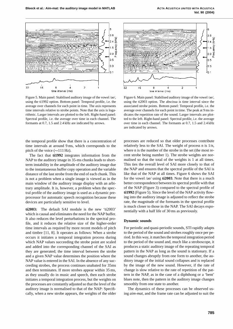
When a strobe is identified in a given channel, the pre-vious 35 ms of activity is transferred to the correspond-ing channel of the auditory image, and added, point forpoint, to the contents of that channel of the image. Thepeak of the NAP pulse that initiates temporal integrationis mapped to the 0-ms time-interval in the auditory image.Before addition, however, the NAP level is progressivelyattenuated by 2.5%/ms, and so there is nothing to add inbeyond 40 ms. This ‘NAP decay’ was implemented to en-sure that the main pitch ridge in the auditory image woulddisappear as the period approached that associated with thelower limit of musical pitch which is about 32 Hz [10]. Themain window of Figure 5 shows the SAI for the vowel /ae/obtained with ti1992. The spectral and temporal profilesshow the average activity across the time-interval and fre-quency dimensions, respectively. The auditory image and

784

Bleeck et al.: Aim-mat: the auditory image model in MATLAB ACTA ACUSTICA UNITED WITH ACUSTICA

Vol. 90 (2004)

Figure 5. Main panel: Stabilised auditory image of the vowel /ae/,using the ti1992 option. Bottom panel: Temporal profile, i.e. theaverage over channels for each point in time. The axis representstime intervals relative to strobe points. Note that the axis is loga-rithmic. Larger intervals are plotted to the left. Right-hand panel:Spectral profile, i.e. the average over time in each channel. Theformants at 0.7, 1.5 and 2.4 kHz are indicated by arrows.

the temporal profile show that there is a concentration oftime intervals at around 9 ms, which corresponds to thepitch of the voice ( � 111 Hz).

The fact that ti1992 integrates information from theNAP to the auditory image in 35-ms chunks leads to short-term instability in the amplitude of the auditory image dueto the instantaneous buffer copy operation and the variabledistance of the last strobe from the end of each chunk. Thisis not a problem when a single image is viewed as in themain window of the auditory image display with an arbi-trary amplitude. It is, however, a problem when the spec-tral profile of the auditory image is used as a dynamic pre-processor for automatic speech recognition because thesedevices are particularly sensitive to level.

ti2003: The default SAI module is the new ‘ti2003’which is causal and eliminates the need for the NAP buffer.It also reduces the level perturbations in the spectral pro-file, and it reduces the relative size of the higher-ordertime intervals as required by more recent models of pitchand timbre [11, 8]. It operates as follows: When a strobeoccurs it initiates a temporal integration process duringwhich NAP values succeeding the strobe point are scaledand added into the corresponding channel of the SAI asthey are generated; the time interval between the strobeand a given NAP value determines the position where theNAP value is entered in the SAI. In the absence of any suc-ceeding strobes, the process continues unabated for 35msand then terminates. If more strobes appear within 35 ms,as they usually do in music and speech, then each strobeinitiates a temporal integration process, but the weights onthe processes are constantly adjusted so that the level of theauditory image is normalised to that of the NAP: Specifi-cally, when a new strobe appears, the weights of the older

Figure 6. Main panel: Stabilised auditory image of the vowel /ae/,using the ti2003 option. The abscissa is time interval since theassociated strobe points. Bottom panel: Temporal profile, i.e. theaverage over channels for each point in time. The peak at 9 ms in-dicates the repetition rate of the sound. Larger intervals are plot-ted to the left. Right-hand panel: Spectral profile, i.e. the averageover time in each channel. The formants at 0.7, 1.5 and 2.4 kHzare indicated by arrows.

processes are reduced so that older processes contributerelatively less to the SAI. The weight of process n is 1/n,where n is the number of the strobe in the set (the most re-cent strobe being number 1). The strobe weights are nor-malised so that the total of the weights is 1 at all times.This ties the overall level of SAI more closely to that ofthe NAP and ensures that the spectral profile of the SAI islike that of the NAP at all times. Figure 6 shows the SAIfor the vowel /ae/ using ti2003. Note that there is a muchbetter correspondence between its spectral profile with thatof the NAP (Figure 3) compared to the spectral profile ofti1992 (Figure 5). Since the level of the NAP activity flow-ing into the auditory image is adjusted to reflect the stroberate, the magnitude of the formants in the spectral profileis much closer to those in the NAP. The SAI decays expo-nentially with a half life of 30 ms as previously.

Dynamic sounds

For periodic and quasi-periodic sounds, STI rapidly adaptsto the period of the sound and strobes roughly once per pe-riod. In this way, it matches the temporal integration periodto the period of the sound and, much like a stroboscope, itproduces a static auditory image of the repeating temporalpattern in the NAP as long as the sound is stationary. If asound changes abruptly from one form to another, the au-ditory image of the initial sound collapses and is replacedby the image of the new sound. However, if the rate ofchange is slow relative to the rate of repetition of the pat-tern in the NAP, as in the case of a diphthong or a ‘bent’blues note, then the pattern in the auditory image changessmoothly from one state to another.

The dynamics of these processes can be observed us-ing aim-mat, and the frame rate can be adjusted to suit the

785

ACTA ACUSTICA UNITED WITH ACUSTICA Bleeck et al.: Aim-mat: the auditory image model in MATLABVol. 90 (2004)

dynamics of the sound and the analysis. It is also possi-ble to generate a stand-alone QuickTime movie with syn-chronized sound for reviewing with standard media play-ers (see section 3.7). Examples of QuickTime movies ofstatic and dynamic sounds can be found on the web pages.

Time-interval scale (linear or logarithmic): aim-mat of-fers the option of plotting the SAI on either a linear time-interval scale as in previous versions of AIM, or on a log-arithmic time-interval scale. The latter was implementedfor compatibility with the musical scale. Vowels and mu-sical notes produce vertical structures in the SAI aroundtheir pitch period, and the peak in the time-interval profilespecifies the pitch. If the SAI is plotted on a logarithmicscale then the pitch peak in the time-interval profile movesequal distances along the pitch axis for equal musical in-tervals.

Autocorrelation: The time-interval calculations in AIMoften provoke comparison with autocorrelation, and in-deed, models of pitch perception based on AIM make sim-ilar predictions to those based on autocorrelation [12]. Ac-cordingly, the SAI column contains an autocorrelation op-tion to convert the NAP into an ‘autocorrelogram’ [13] forcomparison with the SAI. It is to be noted, however, thatthe autocorrelogram is symmetric locally about all verticalpitch ridges, and this limits it’s utility with regard to as-pects of perception other than pitch. For example, it cannotexplain the changes in perception that occur when soundsare reversed in time [14, 15]) whereas the SAI can.

3.6. USER: user modules

The user column is provided to facilitate auditory mod-elling based on auditory images, for example, pitch ex-traction [8] or vowel normalization [16]. The user can alsodefine new USER modules and add them to the menu. In-deed, they can add modules to any of the columns. Basi-cally, a new module can be added to aim-mat simply bycreating a new folder in the aim-mat ‘module’ folder andplacing interface files here. There is web-based documen-tation (http://www.mrc-cbu.cam.ac.uk/ cnbh/ aimmanual/index.html) with examples to explain the process of addinga new module

3.7. MOVIE: movies with synchronized sound

The auditory image is dynamic and aim-mat includes a fa-cility for generating QuickTime movies (MOVIE) of theSAI with synchronised sound. Aim-mat calculates snap-shots of the SAI at regular intervals in time and stores theimages in ‘frames’ which can then be assembled into aQuickTime movie with synchronous sound to illustrate thedynamic properties of sounds as they appear in the audi-tory image.

A movie of the SAI, can be generated by ticking the cal-culate box in the MOVIE column and clicking the MOVIEbutton. The movie is created from the bitmaps produced byaim- mat and so the movie is exactly what appears on thescreen. QuickTime movies are exceptionally portable and

the QuickTime player is readily available on the internet.4 Downloading aim-mat and documentation

Aim-mat is available free of charge for research pur-poses. It can be downloaded from http://www.mrc-cbu.cam.ac.uk/ cnbh/ aimmanual/ index.html. There is alsoweb based documentation at the same site with an ex-tended example of sound analysis to provide an introduc-tion to the time-domain processing of sounds.

System requirements: aim-mat runs on all operatingsystems supporting MATLAB 6.5 (Windows NT, 2000,XP; Linux, Solaris, Apple OS X). The graphical user in-terface will not run with older versions of MATLAB. Thesignal processing toolbox is necessary for the basilar mem-brane module.

Acknowledgement

This development of aim-mat was supported by theWellcome Trust and the UK Medical Research Council(G990369). We are grateful to three anonymous reviewersfor helpful comments on the initial manuscript.

References

[1] R. D. Patterson, M. H. Allerhand, C. Giguere: Time-domain modelling of peripheral auditory processing: amodular architecture and a software platform. J. Acoust.Soc. Am. 98 (1995) 1890–1894.

[2] R. Meddis, L. O’Mard: A unitary model of pitch per-ception. J. Acoustic. Soc. Am. 102 (1997) 1811–1820.http://www.essex.ac.uk/psychology/hearinglab/.

[3] B. R. Glasberg, B. C. J. Moore: Derivation of auditory filtershapes from notched noise data. Hear. Res. 47 (1990) 103–138.

[4] B. R. Glasberg, B. C. J. Moore: A model of loudness appli-cable to time-varying sounds. J. Audio Eng. Soc. 50 (2002)331–342.

[5] R. D. Patterson, K. Robinson, J. Holdsworth, D. McKe-own, C. Zhang, M. H. Allerhand: Complex sounds and au-ditory images. – In: Auditory physiology and perception. Y.Cazals, L. Demany, K. Horner (eds.). Pergamon, Oxford,1992, 429–446.

[6] R. D. Patterson, B. C. J. Moore: Auditory filter and exci-tation patterns as representations of frequency resolution. –In: Frequency selectivity in hearing. B. C. J. Moore (ed.).Academic, London, 1986, 123–177.

[7] R. D. Patterson, J. Holdsworth: A functional model ofneural activity patterns and auditory images. – In: Ad-vances in Speech, Hearing and Language Processing. W. A.Ainsworth (ed.). JAI, London, 1996, Vol. 3, Part B, 554–562.

[8] K. Krumbholz, R. D. Patterson, A. Nobbe, H. Fastl: Mi-crosecond temporal resolution in monaural hearing withoutspectral cues? J. Acoust. Soc. Am. 113 (2003) 2790–2800.

[9] R. D. Patterson: The sound of a sinusoid: Time-intervalmodels. J. Acoust. Soc. Am. 96 (1994) 1419–1428.

[10] D. Pressnitzer, R. D. Patterson, K. Krumbholz: The lowerlimit of melodic pitch. J. Acoust. Soc. Am. 109 (2001)2074–2084.

[11] C. Kaernbach, L. Demany: Psychophysical evidenceagainst the autocorrelation theory of auditory temporal pro-cessing. J. Acoust. Soc. Am. 104 (1998) 2298–2306.

786

Bleeck et al.: Aim-mat: the auditory image model in MATLAB ACTA ACUSTICA UNITED WITH ACUSTICA

Vol. 90 (2004)

[12] R. D. Patterson, W. A. Yost, S. Handel, J. A. Datta: The per-ceptual tone/noise ratio of merged iterated rippled noises. J.Acoust. Soc. Am. 107 (2000) 1578–1588.

[13] R. Meddis, M. J. Hewitt: Virtual pitch and phase sensitiv-ity of a computer model of the auditory periphery. I. Pitchidentification. J. Acoust. Soc. Am. 89 (1991) 2866–2882.

[14] M. A. Akeroyd, R. D. Patterson: A comparison of detectionand discrimination of temporally asymmetry in amplitudemodulation. J. Acoust. Soc. Am. 101 (1997) 430–439.

[15] R. D. Patterson, T. Irino: Modeling temporal asymmetry inthe auditory system. J. Acoust. Soc. Am. 104 (1998) 2967–2979.

[16] T. Irino, R. D. Patterson: Segregating information aboutthe size and shape of the vocal tract using a time-domainauditory model: The stabilised Wavelet-Mellin transform.Speech Communication 36 (2002) 181–203.

787