\

AIAA 2001-0636

Numerical Simulations of a MethanolPool Fire

Paul E. DesJardin, Thomas M. Smith, andChristopher J. RoySandia National LaboratoriesAlbuquerque, NM

Numerical Simulations of a Methanol Pool Fire

Paul E. DesJardin,§ Thomas M. Smith,† and Christopher J. Roy‡

Sandia National Laboratories

P. O. Box 5800

Albuquerque, NM 87185

AbstractSimulations of a turbulent methanol pool fire are con-

ducted using both Reynolds-Averaged Navier-Stokes(RANS) and Large Eddy Simulation (LES) modelingmethodologies. Two simple conserved scalar flamelet-based combustion models with assumed PDF are devel-oped and implemented. The first model assumes statisti-cal independence between mixture fraction and itsvariance and results in poor predictions of time-aver-aged temperature and velocity. The second combustionmodel makes use of the PDF transport equation for mix-ture fraction and does not employ the statistical inde-pendence assumption. Results using this model showgood agreement with experimental data for both the 2Dand 3D LES, indicating that the use of statistical inde-pendence between mixture fraction and its dissipation isnot valid for pool fire simulations. Lastly, “finger-like”flow structures near the base of the plume, generatedfrom stream-wise vorticity, are shown to be importantmixing mechanisms for accurate prediction of time-av-eraged temperature and velocity.

NomenclatureDm molecular diffusivity, m2/sDT turbulent diffusivity, m2/sk turbulent kinetic energy, m2/s2

I incomplete beta function

2

§ Senior Member of Technical Staff, Mail Stop 0836, E-mail: pedes-

ja@sandia.gov, Member AIAA† Senior Member of Technical Staff, Mail Stop 1111, E-mail: tm-

smith@sandia.gov, Member AIAA‡ Senior Member of Technical Staff, Mail Stop 0835, E-mail:

cjroy@sandia.gov, Member AIAA* Sandia is a multiprogram laboratory operated by Sandia Corpora-

tion, a Lockheed Martin Company, for the United States Depart-ment of Energy under Contract DE-AC04-94AL85000.

This paper is declared a work of the U. S. Government and isnot subject to copyright protection in the United States.

PZ probability density function (PDF) of ZPzχ joint PDF of Z and p pressure, N/m2

r radial coordinate, mT temperature, Kt time, su axial velocity component, m/sui velocity component in ith direction, m/sWs molecular weight of species s, kg/kmolx axial or stream-wise coordinate, mxi coordinate in ith direction, my, z transverse coordinates, mYs mass fraction of species sZ mixture fraction

mixture fraction composition variableβ1,2 parameters for the incomplete beta functionΓ gamma functionε dissipation rate of k, m2/s3

νs stoichiometric coefficient of species sdensity, kg/m3

mixture fraction variance (= )scalar dissipation rate, 1/sscalar dissipation rate fluctuation, 1/schemical production rate of species s, kg/s

SubscriptsF fuel propertyi, j indices for tensor notationO oxidizer propertys species sst stoichiometric surface valueSuperscripts– (overbar) Reynolds time-averaged or LES fil-

tered quantity~ (overtilde) Density weighted time or filtered

quantityDensity weighted time or filtered fluctuatingquantity

χ

ς ℑ,

ρσz

2 ~z″2

χχfω· s

″

AIAA 99-xxxx

IntroductionAn effort is currently underway to develop a compu-

tational tool to model the heat transfer from large-scalepool fires. This work is motivated by the need to insurethe safety of nuclear weapons systems immersed in hos-tile thermal environments. Such a pool fire scenariocould result from either an aviation fuel spill or an air-craft accident, therefore liquid hydrocarbon fuels are ofprimary interest.

A variety of different physical processes occur withinthe highly turbulent flame. The wide range of length andtime scales of these processes combined with the fluidturbulence make direct numerical simulation, where allrelevant physical processes are resolved on the grid,prohibitively expensive. The computational tool musttherefore rely on a number of physical sub-grid modelswhich introduce additional uncertainties into the calcu-lation.

The heating rate from a pool fire has contributionsfrom both convective and radiative heat transfer, withthe latter generally being the major contributor.1 The ra-diative heat transfer arises primarily due to the presenceof soot, which is strongly dependent on the location ofthe peak flame temperatures. The flame temperature, inturn, depends on both the chemistry and the transportproperties within the flame.

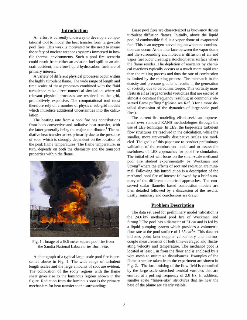
A photograph of a typical large-scale pool fire is pre-sented above in Fig. 1. The wide range of turbulentlength scales and the large amounts of soot are evident.The collocation of the sooty regions with the flamesheet gives rise to the luminous regions shown in thefigure. Radiation from the luminous soot is the primarymechanism for heat transfer to the surroundings.

Large pool fires are characterized as buoyancy driventurbulent diffusion flames. Initially, above the liquidpool of combustible fuel is a vapor dome of evaporatedfuel. This is an oxygen starved region where no combus-tion can occur. At the interface between the vapor domeand the surrounding air, molecular diffusion of air andvapor fuel occur creating a stoichiometric surface wherethe flame resides. The depletion of reactants by chemi-cal reactions typically occurs at a much more rapid ratethan the mixing process and thus the rate of combustionis limited by the mixing process. The mismatch in thedensity and pressure gradients results in the generationof vorticity due to baroclinic torque. This vorticity man-ifests itself as large toriodal vorticities that are ejected atalmost a constant frequency resulting in commonly ob-served flame puffing.2 (please see Ref. 3 for a more de-tailed discussion of the dynamics of large-scale poolfires).

The current fire modeling effort seeks an improve-ment over standard RANS methodologies through theuse of LES technique. In LES, the large-scale turbulentflow structures are resolved in the calculation, while thesmaller, more universally dissipative scales are mod-eled. The goals of this paper are to conduct preliminaryvalidation of the combustion model and to assess theusefulness of LES approaches for pool fire simulation.The initial effort will focus on the small-scale methanolpool fire studied experimentally by Weckman andStrong4 where the effects of soot and radiation are mini-mal. Following this introduction is a description of themethanol pool fire of interest followed by a brief sum-mary of the different numerical approaches. The con-served scalar flamelet based combustion models arethen detailed followed by a discussion of the results.Lastly, summary and conclusions are drawn.

Problem DescriptionThe data set used for preliminary model validation is

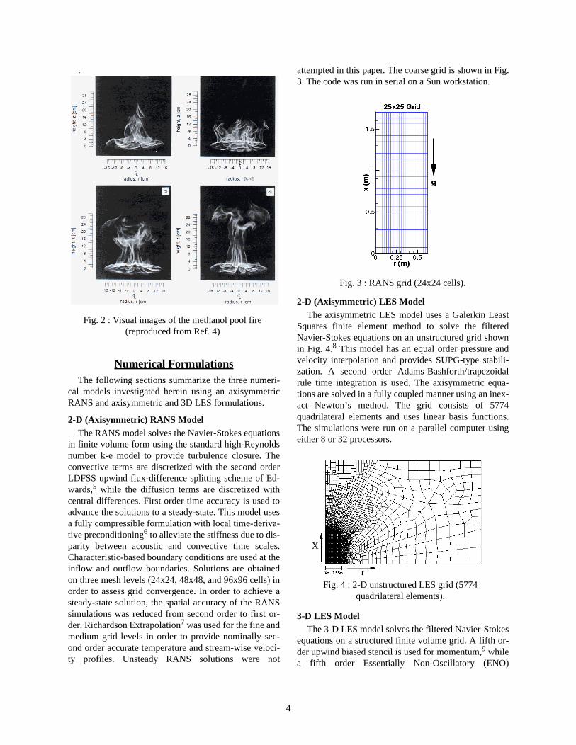
the 24.6 kW methanol pool fire of Weckman andStrong.4 The pool has a diameter of 31 cm and is fed bya liquid pumping system which provides a volumetricflow rate at the pool surface of 1.35 cm3/s. This data setincludes point laser doppler velocimetry and thermo-couple measurements of both time-averaged and fluctu-ating velocity and temperature. The methanol pool islocated at least 1 m from the floor and is enclosed by awire mesh to minimize disturbances. Examples of theflame structure taken from the experiment are shown inFig. 2. The local mixing of the flow field is controlledby the large scale stretched toroidal vorticies that areemitted at a puffing frequency of 2.8 Hz. In addition,smaller scale “finger-like” structures that lie near thebase of the plume are clearly visible.

Fig. 1 : Image of a 6x6 meter square pool fire from the Sandia National Laboratories Burn Site.

3

AIAA 99-xxxx

.

Numerical FormulationsThe following sections summarize the three numeri-

cal models investigated herein using an axisymmetricRANS and axisymmetric and 3D LES formulations.

2-D (Axisymmetric) RANS ModelThe RANS model solves the Navier-Stokes equations

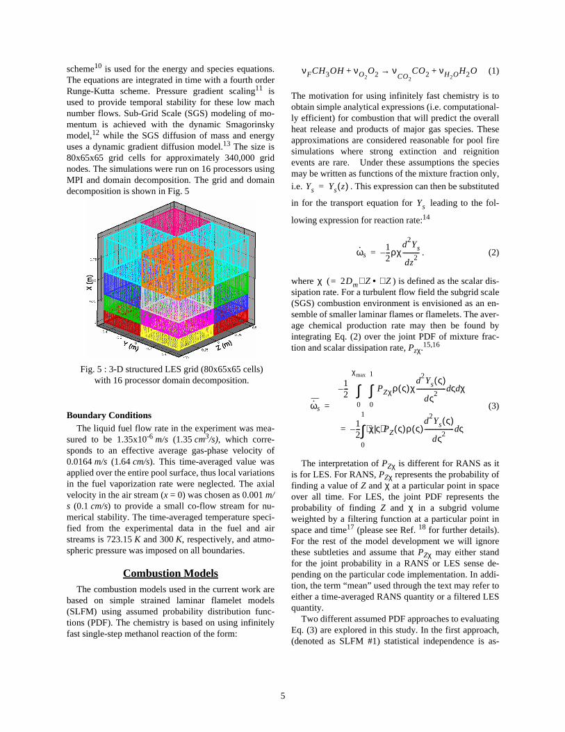
in finite volume form using the standard high-Reynoldsnumber k-e model to provide turbulence closure. Theconvective terms are discretized with the second orderLDFSS upwind flux-difference splitting scheme of Ed-wards,5 while the diffusion terms are discretized withcentral differences. First order time accuracy is used toadvance the solutions to a steady-state. This model usesa fully compressible formulation with local time-deriva-tive preconditioning6 to alleviate the stiffness due to dis-parity between acoustic and convective time scales.Characteristic-based boundary conditions are used at theinflow and outflow boundaries. Solutions are obtainedon three mesh levels (24x24, 48x48, and 96x96 cells) inorder to assess grid convergence. In order to achieve asteady-state solution, the spatial accuracy of the RANSsimulations was reduced from second order to first or-der. Richardson Extrapolation7 was used for the fine andmedium grid levels in order to provide nominally sec-ond order accurate temperature and stream-wise veloci-ty profiles. Unsteady RANS solutions were not

attempted in this paper. The coarse grid is shown in Fig.3. The code was run in serial on a Sun workstation.

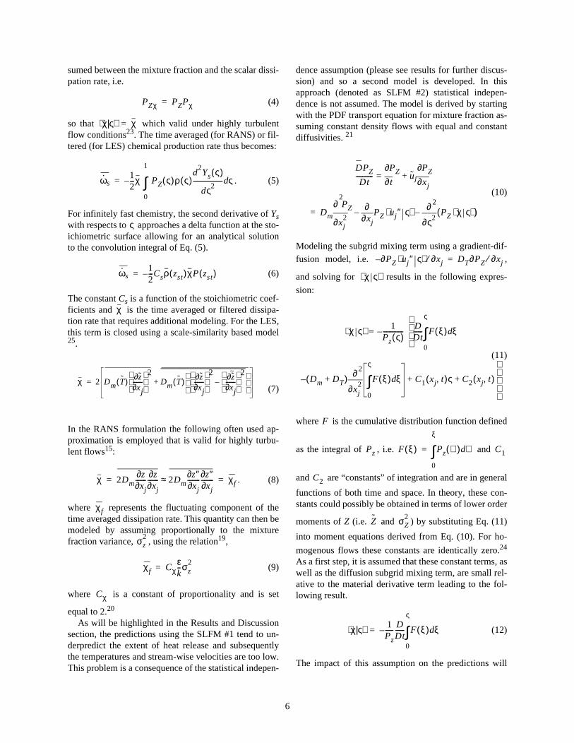
2-D (Axisymmetric) LES ModelThe axisymmetric LES model uses a Galerkin Least

Squares finite element method to solve the filteredNavier-Stokes equations on an unstructured grid shownin Fig. 4.8 This model has an equal order pressure andvelocity interpolation and provides SUPG-type stabili-zation. A second order Adams-Bashforth/trapezoidalrule time integration is used. The axisymmetric equa-tions are solved in a fully coupled manner using an inex-act Newton’s method. The grid consists of 5774quadrilateral elements and uses linear basis functions.The simulations were run on a parallel computer usingeither 8 or 32 processors.

3-D LES ModelThe 3-D LES model solves the filtered Navier-Stokes

equations on a structured finite volume grid. A fifth or-der upwind biased stencil is used for momentum,9 whilea fifth order Essentially Non-Oscillatory (ENO)

Fig. 2 : Visual images of the methanol pool fire (reproduced from Ref. 4)

Fig. 3 : RANS grid (24x24 cells).

Fig. 4 : 2-D unstructured LES grid (5774 quadrilateral elements).

X

r

4

AIAA 99-xxxx

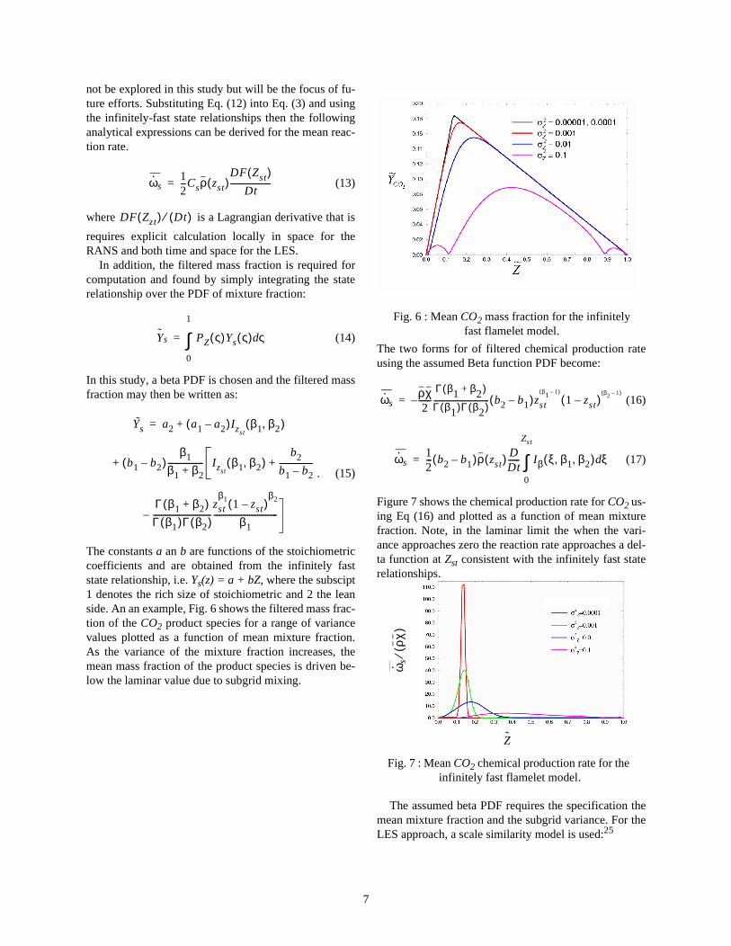
scheme10 is used for the energy and species equations.The equations are integrated in time with a fourth orderRunge-Kutta scheme. Pressure gradient scaling11 isused to provide temporal stability for these low machnumber flows. Sub-Grid Scale (SGS) modeling of mo-mentum is achieved with the dynamic Smagorinskymodel,12 while the SGS diffusion of mass and energyuses a dynamic gradient diffusion model.13 The size is80x65x65 grid cells for approximately 340,000 gridnodes. The simulations were run on 16 processors usingMPI and domain decomposition. The grid and domaindecomposition is shown in Fig. 5

Boundary ConditionsThe liquid fuel flow rate in the experiment was mea-

sured to be 1.35x10-6 m/s (1.35 cm3/s), which corre-sponds to an effective average gas-phase velocity of0.0164 m/s (1.64 cm/s). This time-averaged value wasapplied over the entire pool surface, thus local variationsin the fuel vaporization rate were neglected. The axialvelocity in the air stream (x = 0) was chosen as 0.001 m/s (0.1 cm/s) to provide a small co-flow stream for nu-merical stability. The time-averaged temperature speci-fied from the experimental data in the fuel and airstreams is 723.15 K and 300 K, respectively, and atmo-spheric pressure was imposed on all boundaries.

Combustion ModelsThe combustion models used in the current work are

based on simple strained laminar flamelet models(SLFM) using assumed probability distribution func-tions (PDF). The chemistry is based on using infinitelyfast single-step methanol reaction of the form:

(1)

The motivation for using infinitely fast chemistry is toobtain simple analytical expressions (i.e. computational-ly efficient) for combustion that will predict the overallheat release and products of major gas species. Theseapproximations are considered reasonable for pool firesimulations where strong extinction and reignitionevents are rare. Under these assumptions the speciesmay be written as functions of the mixture fraction only,i.e. . This expression can then be substituted

in for the transport equation for leading to the fol-

lowing expression for reaction rate:14

. (2)

where ( ) is defined as the scalar dis-sipation rate. For a turbulent flow field the subgrid scale(SGS) combustion environment is envisioned as an en-semble of smaller laminar flames or flamelets. The aver-age chemical production rate may then be found byintegrating Eq. (2) over the joint PDF of mixture frac-tion and scalar dissipation rate, Pzχ.15,16

(3)

The interpretation of PZχ is different for RANS as itis for LES. For RANS, PZχ represents the probability offinding a value of Z and χ at a particular point in spaceover all time. For LES, the joint PDF represents theprobability of finding Z and χ in a subgrid volumeweighted by a filtering function at a particular point inspace and time17 (please see Ref. 18 for further details).For the rest of the model development we will ignorethese subtleties and assume that PZχ may either standfor the joint probability in a RANS or LES sense de-pending on the particular code implementation. In addi-tion, the term “mean” used through the text may refer toeither a time-averaged RANS quantity or a filtered LESquantity.

Two different assumed PDF approaches to evaluatingEq. (3) are explored in this study. In the first approach,(denoted as SLFM #1) statistical independence is as-

Fig. 5 : 3-D structured LES grid (80x65x65 cells) with 16 processor domain decomposition.

νFCH3OH νO2O2 ν→

CO2CO2 νH2OH2O++

Ys Ys z( )=

Ys

ω· s12---ρχ

d2Ys

dz2

-----------–=

χ 2Dm Z∇ Z∇•=

ω· s

12---– PZχρ

0

1

∫0

χmax

∫ ς( )χd

2Ys ς( )

dς2------------------- ς χdd

12---– χ ς⟨ | ⟩ PZ ς( )ρ ς( )

d2Ys ς( )

dς2------------------- ςd

0

1

∫=

=

5

AIAA 99-xxxx

sumed between the mixture fraction and the scalar dissi-pation rate, i.e.

(4)

so that which valid under highly turbulentflow conditions23. The time averaged (for RANS) or fil-tered (for LES) chemical production rate thus becomes:

. (5)

For infinitely fast chemistry, the second derivative of Yswith respects to approaches a delta function at the sto-ichiometric surface allowing for an analytical solutionto the convolution integral of Eq. (5).

(6)

The constant Cs is a function of the stoichiometric coef-ficients and is the time averaged or filtered dissipa-tion rate that requires additional modeling. For the LES,this term is closed using a scale-similarity based model25.

(7)

In the RANS formulation the following often used ap-proximation is employed that is valid for highly turbu-lent flows15:

. (8)

where represents the fluctuating component of thetime averaged dissipation rate. This quantity can then bemodeled by assuming proportionally to the mixturefraction variance, , using the relation19,

(9)

where is a constant of proportionality and is set

equal to 2.20 As will be highlighted in the Results and Discussion

section, the predictions using the SLFM #1 tend to un-derpredict the extent of heat release and subsequentlythe temperatures and stream-wise velocities are too low.This problem is a consequence of the statistical indepen-

dence assumption (please see results for further discus-sion) and so a second model is developed. In thisapproach (denoted as SLFM #2) statistical indepen-dence is not assumed. The model is derived by startingwith the PDF transport equation for mixture fraction as-suming constant density flows with equal and constantdiffusivities. 21

(10)

Modeling the subgrid mixing term using a gradient-dif-fusion model, i.e. ,

and solving for results in the following expres-

sion:

(11)

where is the cumulative distribution function defined

as the integral of , i.e. and

and are “constants” of integration and are in general

functions of both time and space. In theory, these con-stants could possibly be obtained in terms of lower order

moments of Z (i.e. and ) by substituting Eq. (11)

into moment equations derived from Eq. (10). For ho-

mogenous flows these constants are identically zero.24

As a first step, it is assumed that these constant terms, aswell as the diffusion subgrid mixing term, are small rel-ative to the material derivative term leading to the fol-lowing result.

(12)

The impact of this assumption on the predictions will

PZχ PZPχ=

χ ς⟨ | ⟩ χ=

ω· s12---– χ

0

1

∫ PZ ς( )ρ ς( )d

2Ys ς( )

dς2------------------- ςd=

ς

ω· s12---Csρ zst( )χP zst( )–=

χ

χ 2 Dm T( ) z∂xj∂

------ 2

Dm T( ) z∂xj∂

------ 2 z∂

xj∂------

2

–

+~

=

_________________

χ 2Dmz∂xj∂-------

z∂xj∂------- 2Dm

z″∂xj∂--------

z″∂xj∂--------≈ χf= =

χf

σz2

χf Cχεk--σz

2=

Cχ

DPZ

Dt-----------

t∂∂PZ uj xj∂

∂PZ+=

Dmxj

2

2

∂

∂ PZ

xj∂∂

PZ uj″ ς⟨ ⟩ς2

2

∂

∂PZ χ ς⟨ ⟩( )––=

∂– PZ uj″ ς⟨ ⟩ ∂ xj⁄ DT∂PZ ∂xj⁄=

χ ς⟨ ⟩

χ ς⟨ ⟩ 1Pz ς( )-------------

DDt------ F ξ( ) ξd

0

ς

∫

–=

Dm DT+( )–xj

2

2

∂

∂F ξ( ) ξd

0

ς

∫ C1 xj t,( )ς C2 xj t,( )+ +

F

Pz F ξ( ) Pz ℑ( ) ℑd

0

ξ

∫= C1

C2

Z σZ2

χ ς⟨ | ⟩ 1Pz-----

DDt------ F ξ( ) ξd

0

ς

∫–=

6

AIAA 99-xxxx

not be explored in this study but will be the focus of fu-ture efforts. Substituting Eq. (12) into Eq. (3) and usingthe infinitely-fast state relationships then the followinganalytical expressions can be derived for the mean reac-tion rate.

(13)

where is a Lagrangian derivative that is

requires explicit calculation locally in space for theRANS and both time and space for the LES.

In addition, the filtered mass fraction is required forcomputation and found by simply integrating the staterelationship over the PDF of mixture fraction:

(14)

In this study, a beta PDF is chosen and the filtered massfraction may then be written as:

. (15)

The constants a an b are functions of the stoichiometriccoefficients and are obtained from the infinitely faststate relationship, i.e. Ys(z) = a + bZ, where the subscipt1 denotes the rich size of stoichiometric and 2 the leanside. An an example, Fig. 6 shows the filtered mass frac-tion of the CO2 product species for a range of variancevalues plotted as a function of mean mixture fraction.As the variance of the mixture fraction increases, themean mass fraction of the product species is driven be-low the laminar value due to subgrid mixing.

The two forms for of filtered chemical production rateusing the assumed Beta function PDF become:

(16)

(17)

Figure 7 shows the chemical production rate for CO2 us-ing Eq (16) and plotted as a function of mean mixturefraction. Note, in the laminar limit the when the vari-ance approaches zero the reaction rate approaches a del-ta function at Zst consistent with the infinitely fast staterelationships.

The assumed beta PDF requires the specification themean mixture fraction and the subgrid variance. For theLES approach, a scale similarity model is used:25

ω· s12---Csρ zst( )

DF Zst( )Dt

--------------------=

DF Zzt( ) Dt( )⁄

Ys

0

1

∫ PZ ς( )Ys ς( ) ςd=

Ys˜ a2 a1 a2–( )Izst

β1 β2,( )+=

b1 b2–( )+β1

β1 β2+------------------ Izst

β1 β2,( )b2

b1 b2–-----------------+

Γ β1 β2+( )Γ β1( )Γ β2( )-----------------------------–

zst

β1 1 zst–( )β2

β1--------------------------------

Fig. 6 : Mean CO2 mass fraction for the infinitely fast flamelet model.

2

2

2

2

ω· sρχ2

------Γ β1 β2+( )

Γ β1( )Γ β2( )------------------------------- b2 b1–( )zst

β1 1–( )

1 z– st( )β2 1–( )

–=

ω· s12--- b2 b1–( )ρ zst( ) D

Dt------ Iβ ξ β1 β2, ,( ) ξd

0

Zst

∫=

Fig. 7 : Mean CO2 chemical production rate for the infinitely fast flamelet model.

Z

ω· sρχ(

)⁄

7

AIAA 99-xxxx

(18)

For the RANS calculations, a transport equation issolved for the mixture fraction variance

(19)

where P is a production term and D represents diffusiondue to turbulent fluctuations.

Results and DiscussionThe mean reaction rate models based on Eqs. (16)

and (17) are run for both the axisymmetric and 3D LESwhile just the former is used in the RANS calculations.Predictions of time-averaged temperature and stream-wise velocity are compared to experimental data atheights of 0.02, 0.14 and 0.30 m above the pool surfaceto assess code (i.e 2D verses 3D and RANS verses.LES) and combustion model (i.e. SLFM #1 versesSLFM #2) performance. For the LES cases, time-aver-aged quantities are obtained by first allowing for initialtime dependent transients to wash out of the computa-tional domain and then statistics are collected over sev-eral (5-10) puff cycles for which the flow is consideredstatistical stationary.

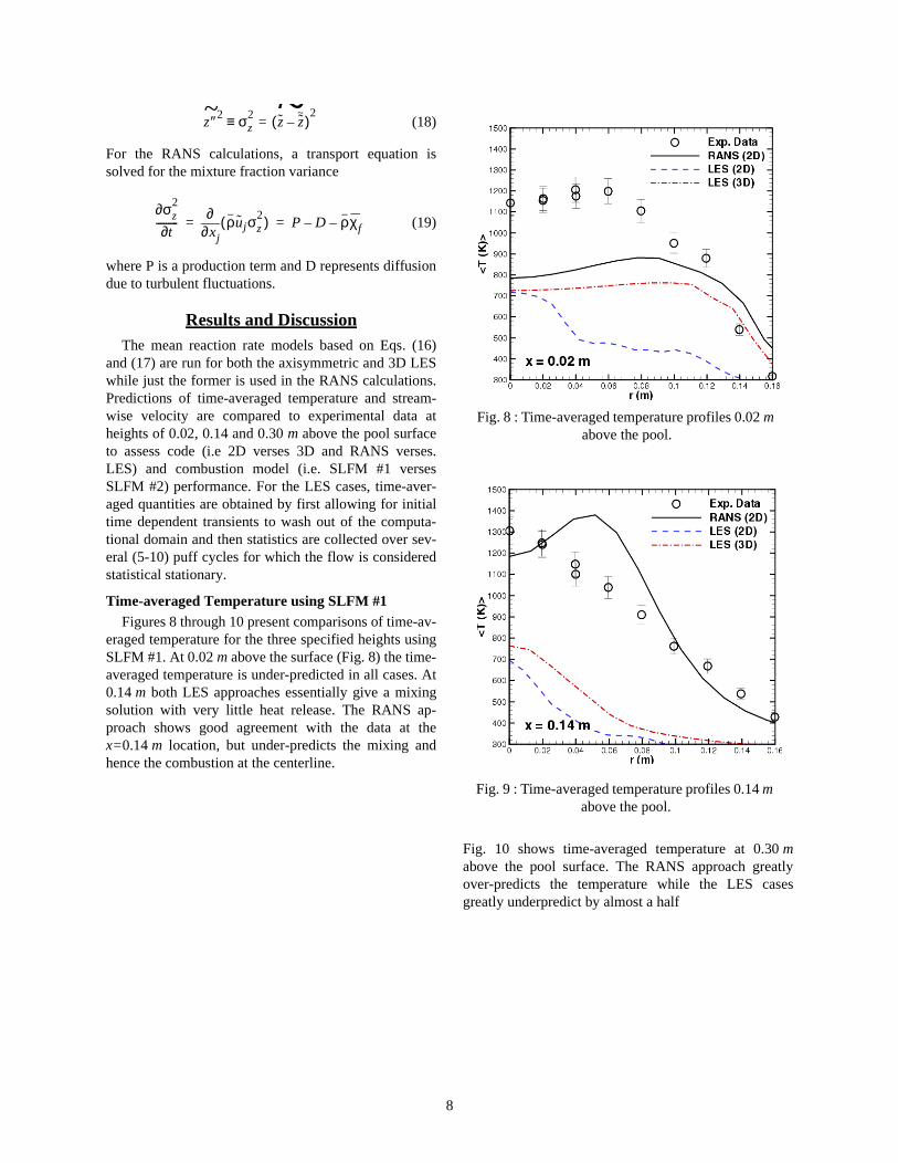
Time-averaged Temperature using SLFM #1Figures 8 through 10 present comparisons of time-av-

eraged temperature for the three specified heights usingSLFM #1. At 0.02 m above the surface (Fig. 8) the time-averaged temperature is under-predicted in all cases. At0.14 m both LES approaches essentially give a mixingsolution with very little heat release. The RANS ap-proach shows good agreement with the data at thex=0.14 m location, but under-predicts the mixing andhence the combustion at the centerline.

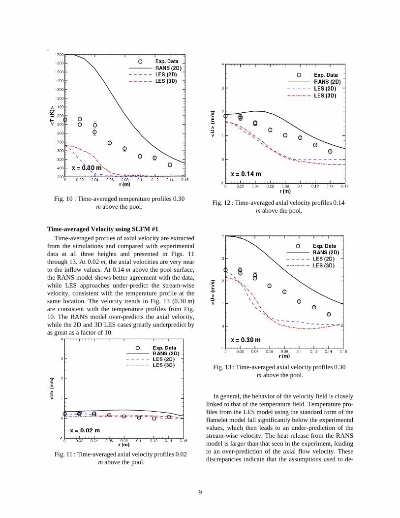
Fig. 10 shows time-averaged temperature at 0.30 mabove the pool surface. The RANS approach greatlyover-predicts the temperature while the LES casesgreatly underpredict by almost a half

~z″2 σz

2≡ z z–( )2~

= ~

σz2∂

t∂---------xj∂∂ ρujσz

2( ) P D– ρχf–= =

Fig. 8 : Time-averaged temperature profiles 0.02 m above the pool.

Fig. 9 : Time-averaged temperature profiles 0.14 m above the pool.

8

AIAA 99-xxxx

.

Time-averaged Velocity using SLFM #1Time-averaged profiles of axial velocity are extracted

from the simulations and compared with experimentaldata at all three heights and presented in Figs. 11through 13. At 0.02 m, the axial velocities are very nearto the inflow values. At 0.14 m above the pool surface,the RANS model shows better agreement with the data,while LES approaches under-predict the stream-wisevelocity, consistent with the temperature profile at thesame location. The velocity trends in Fig. 13 (0.30 m)are consistent with the temperature profiles from Fig.10. The RANS model over-predicts the axial velocity,while the 2D and 3D LES cases greatly underpredict byas great as a factor of 10.

In general, the behavior of the velocity field is closelylinked to that of the temperature field. Temperature pro-files from the LES model using the standard form of theflamelet model fall significantly below the experimentalvalues, which then leads to an under-prediction of thestream-wise velocity. The heat release from the RANSmodel is larger than that seen in the experiment, leadingto an over-prediction of the axial flow velocity. Thesediscrepancies indicate that the assumptions used to de-

Fig. 10 : Time-averaged temperature profiles 0.30 m above the pool.

Fig. 11 : Time-averaged axial velocity profiles 0.02 m above the pool.

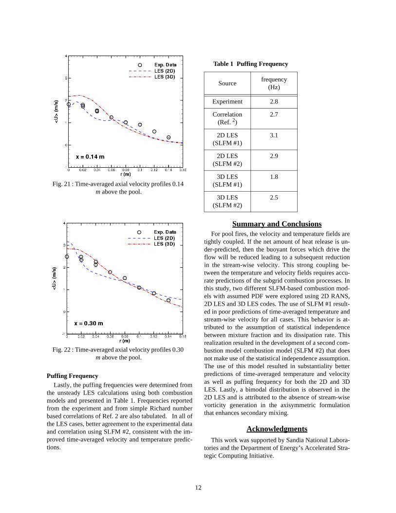
Fig. 12 : Time-averaged axial velocity profiles 0.14 m above the pool.

Fig. 13 : Time-averaged axial velocity profiles 0.30 m above the pool.

9

AIAA 99-xxxx

velop SLFM #1 are not well founded for this class offlows and an alternative model needs to be developed.

One of the main weaknesses in SLFM #1 is the as-sumption of statistical independence between Z and χ.This assumption is generally valid for highly turbulentflows but is breaks down in transitionally turbulentflows such as the very near field of a turbulent jet23 andso is also questionable for the transitionally turbulentpool fire flows in this study. In order to explore this as-sumption, a second combustion model is developedbased on using the PDF transport equation of mixturefraction and makes no assumption regarding the statisti-cal independence of Z and χ outlined previously in theCombustion Models section. Results using this newmodel are presented next for the 2D and 3D LES.

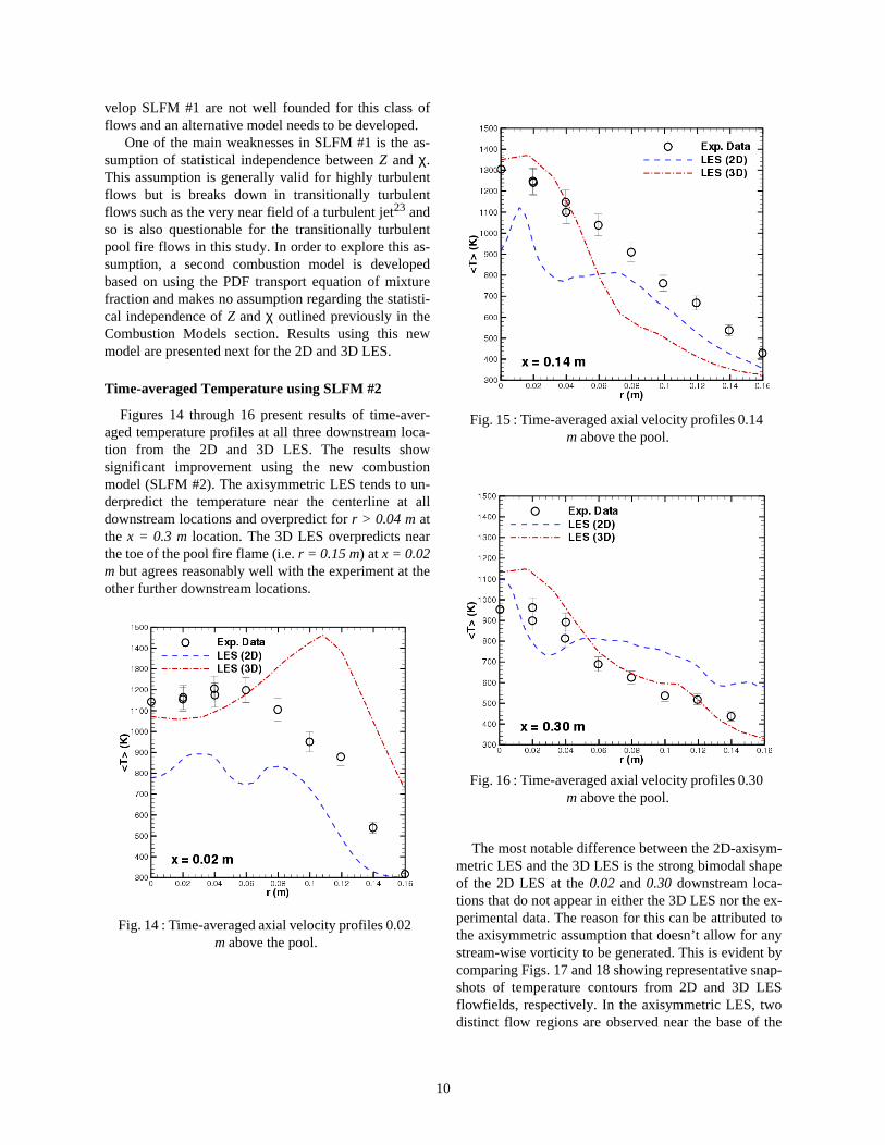
Time-averaged Temperature using SLFM #2

Figures 14 through 16 present results of time-aver-aged temperature profiles at all three downstream loca-tion from the 2D and 3D LES. The results showsignificant improvement using the new combustionmodel (SLFM #2). The axisymmetric LES tends to un-derpredict the temperature near the centerline at alldownstream locations and overpredict for r > 0.04 m atthe x = 0.3 m location. The 3D LES overpredicts nearthe toe of the pool fire flame (i.e. r = 0.15 m) at x = 0.02m but agrees reasonably well with the experiment at theother further downstream locations.

The most notable difference between the 2D-axisym-

metric LES and the 3D LES is the strong bimodal shapeof the 2D LES at the 0.02 and 0.30 downstream loca-tions that do not appear in either the 3D LES nor the ex-perimental data. The reason for this can be attributed tothe axisymmetric assumption that doesn’t allow for anystream-wise vorticity to be generated. This is evident bycomparing Figs. 17 and 18 showing representative snap-shots of temperature contours from 2D and 3D LESflowfields, respectively. In the axisymmetric LES, twodistinct flow regions are observed near the base of the

Fig. 14 : Time-averaged axial velocity profiles 0.02 m above the pool.

Fig. 15 : Time-averaged axial velocity profiles 0.14 m above the pool.

Fig. 16 : Time-averaged axial velocity profiles 0.30 m above the pool.

10

AIAA 99-xxxx

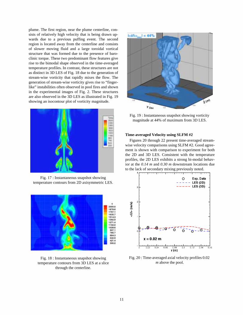
plume. The first region, near the plume centerline, con-sists of relatively high velocity that is being drawn up-wards due to a previous puffing event. The secondregion is located away from the centerline and consistsof slower moving fluid and a large toroidal vorticalstructure that was formed due to the presence of baro-clinic torque. These two predominant flow features giverise to the bimodal shape observed in the time-averagedtemperature profiles. In contrast, these structures are notas distinct in 3D LES of Fig. 18 due to the generation ofstream-wise vorticity that rapidly mixes the flow. Thegeneration of stream-wise vorticity gives rise to “finger-like” instabilities often observed in pool fires and shownin the experimental images of Fig. 2. These structuresare also observed in the 3D LES as illustrated in Fig. 19showing an isocontour plot of vorticity magnitude.

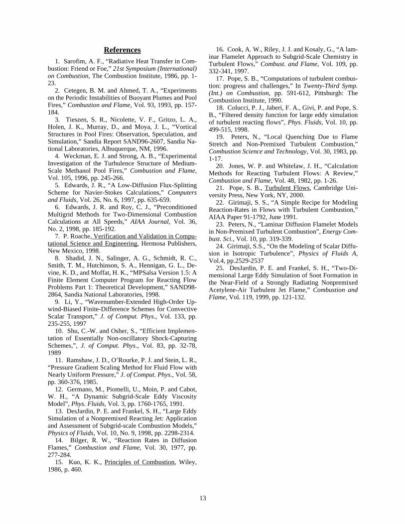
Time-averaged Velocity using SLFM #2Figures 20 through 22 present time-averaged stream-

wise velocity comparisons using SLFM #2. Good agree-ment is shown with comparison to experiment for boththe 2D and 3D LES. Consistent with the temperatureprofiles, the 2D LES exhibits a strong bi-modal behav-ior at the 0.14 m and 0.30 m downstream locations dueto the lack of secondary mixing previously noted.

Fig. 17 : Instantaneous snapshot showing temperature contours from 2D axisymmetric LES.

Fig. 18 : Instantaneous snapshot showing temperature contours from 3D LES at a slice

through the centerline.

Fig. 19 : Instantaneous snapshot showing vorticity magnitude at 44% of maximum from 3D LES.

Fig. 20 : Time-averaged axial velocity profiles 0.02 m above the pool.

11

AIAA 99-xxxx

Puffing FrequencyLastly, the puffing frequencies were determined from

the unsteady LES calculations using both combustionmodels and presented in Table 1. Frequencies reportedfrom the experiment and from simple Richard numberbased correlations of Ref. 2 are also tabulated. In all ofthe LES cases, better agreement to the experimental dataand correlation using SLFM #2, consistent with the im-proved time-averaged velocity and temperature predic-tions.

Summary and ConclusionsFor pool fires, the velocity and temperature fields are

tightly coupled. If the net amount of heat release is un-der-predicted, then the buoyant forces which drive theflow will be reduced leading to a subsequent reductionin the stream-wise velocity. This strong coupling be-tween the temperature and velocity fields requires accu-rate predictions of the subgrid combustion processes. Inthis study, two different SLFM-based combustion mod-els with assumed PDF were explored using 2D RANS,2D LES and 3D LES codes. The use of SLFM #1 result-ed in poor predictions of time-averaged temperature andstream-wise velocity for all cases. This behavior is at-tributed to the assumption of statistical independencebetween mixture fraction and its dissipation rate. Thisrealization resulted in the development of a second com-bustion model combustion model (SLFM #2) that doesnot make use of the statistical independence assumption.The use of this model resulted in substantiality betterpredictions of time-averaged temperature and velocityas well as puffing frequency for both the 2D and 3DLES. Lastly, a bimodal distribution is observed in the2D LES and is attributed to the absence of stream-wisevorticity generation in the axisymmetric formulationthat enhances secondary mixing.

AcknowledgmentsThis work was supported by Sandia National Labora-

tories and the Department of Energy’s Accelerated Stra-tegic Computing Initiative.

Fig. 21 : Time-averaged axial velocity profiles 0.14 m above the pool.

Fig. 22 : Time-averaged axial velocity profiles 0.30 m above the pool.

Table 1 Puffing Frequency

Sourcefrequency

(Hz)

Experiment 2.8

Correlation(Ref. 2)

2.7

2D LES (SLFM #1)

3.1

2D LES(SLFM #2)

2.9

3D LES(SLFM #1)

1.8

3D LES(SLFM #2)

2.5

12

AIAA 99-xxxx

References1. Sarofim, A. F., “Radiative Heat Transfer in Com-

bustion: Friend or Foe,” 21st Symposium (International)on Combustion, The Combustion Institute, 1986, pp. 1-23.

2. Cetegen, B. M. and Ahmed, T. A., “Experimentson the Periodic Instabilities of Buoyant Plumes and PoolFires,” Combustion and Flame, Vol. 93, 1993, pp. 157-184.

3. Tieszen, S. R., Nicolette, V. F., Gritzo, L. A.,Holen, J. K., Murray, D., and Moya, J. L., “VorticalStructures in Pool Fires: Observation, Speculation, andSimulation,” Sandia Report SAND96-2607, Sandia Na-tional Laboratories, Albuquerque, NM, 1996.

4. Weckman, E. J. and Strong, A. B., “ExperimentalInvestigation of the Turbulence Structure of Medium-Scale Methanol Pool Fires,” Combustion and Flame,Vol. 105, 1996, pp. 245-266.

5. Edwards, J. R., “A Low-Diffusion Flux-SplittingScheme for Navier-Stokes Calculations,” Computersand Fluids, Vol. 26, No. 6, 1997, pp. 635-659.

6. Edwards, J. R. and Roy, C. J., “PreconditionedMultigrid Methods for Two-Dimensional CombustionCalculations at All Speeds,” AIAA Journal, Vol. 36,No. 2, 1998, pp. 185-192.

7. P. Roache, Verification and Validation in Compu-tational Science and Engineering, Hermosa Publishers,New Mexico, 1998.

8. Shadid, J. N., Salinger, A. G., Schmidt, R. C.,Smith, T. M., Hutchinson, S. A., Hennigan, G. L., De-vine, K. D., and Moffat, H. K., “MPSalsa Version 1.5: AFinite Element Computer Program for Reacting FlowProblems Part 1: Theoretical Development,” SAND98-2864, Sandia National Laboratories, 1998.

9. Li, Y., “Wavenumber-Extended High-Order Up-wind-Biased Finite-Difference Schemes for ConvectiveScalar Transport,” J. of Comput. Phys., Vol. 133, pp.235-255, 1997

10. Shu, C.-W. and Osher, S., “Efficient Implemen-tation of Essentially Non-oscillatory Shock-CapturingSchemes,”, J. of Comput. Phys., Vol. 83, pp. 32-78,1989

11. Ramshaw, J. D., O’Rourke, P. J. and Stein, L. R.,“Pressure Gradient Scaling Method for Fluid Flow withNearly Uniform Pressure,” J. of Comput. Phys., Vol. 58,pp. 360-376, 1985.

12. Germano, M., Piomelli, U., Moin, P. and Cabot,W. H., “A Dynamic Subgrid-Scale Eddy ViscosityModel”, Phys. Fluids, Vol. 3, pp. 1760-1765, 1991.

13. DesJardin, P. E. and Frankel, S. H., “Large EddySimulation of a Nonpremixed Reacting Jet: Applicationand Assessment of Subgrid-scale Combustion Models,”Physics of Fluids, Vol. 10, No. 9, 1998, pp. 2298-2314.

14. Bilger, R. W., “Reaction Rates in DiffusionFlames,” Combustion and Flame, Vol. 30, 1977, pp.277-284.

15. Kuo, K. K., Principles of Combustion, Wiley,1986, p. 460.

16. Cook, A. W., Riley, J. J. and Kosaly, G., “A lam-inar Flamelet Approach to Subgrid-Scale Chemistry inTurbulent Flows,” Combust. and Flame, Vol. 109, pp.332-341, 1997.

17. Pope, S. B., “Computations of turbulent combus-tion: progress and challenges,” In Twenty-Third Symp.(Int.) on Combustion, pp. 591-612, Pittsburgh: TheCombustion Institute, 1990.

18. Colucci, P. J., Jaberi, F. A., Givi, P. and Pope, S.B., “Filtered density function for large eddy simulationof turbulent reacting flows”, Phys. Fluids, Vol. 10, pp.499-515, 1998.

19. Peters, N., “Local Quenching Due to FlameStretch and Non-Premixed Turbulent Combustion,”Combustion Science and Technology, Vol. 30, 1983, pp.1-17.

20. Jones, W. P. and Whitelaw, J. H., “CalculationMethods for Reacting Turbulent Flows: A Review,”Combustion and Flame, Vol. 48, 1982, pp. 1-26.

21. Pope, S. B., Turbulent Flows, Cambridge Uni-versity Press, New York, NY, 2000.

22. Girimaji, S. S., “A Simple Recipe for ModelingReaction-Rates in Flows with Turbulent Combustion,”AIAA Paper 91-1792, June 1991.

23. Peters, N., “Laminar Diffusion Flamelet Modelsin Non-Premixed Turbulent Combustion”, Energy Com-bust. Sci., Vol. 10, pp. 319-339.

24. Girimaji, S.S., “On the Modeling of Scalar Diffu-sion in Isotropic Turbulence”, Physics of Fluids A,Vol.4, pp.2529-2537

25. DesJardin, P. E. and Frankel, S. H., “Two-Di-mensional Large Eddy Simulation of Soot Formation inthe Near-Field of a Strongly Radiating NonpremixedAcetylene-Air Turbulent Jet Flame,” Combustion andFlame, Vol. 119, 1999, pp. 121-132.

13