Vol. 86 (1994) ACTA PHYSICA POLONICA A No. 5

Proceedings of the ISSSRNS ,94, Jaszowiec 1994

ANGULAR DISTRIBUTION OF PHOTOEMISSIONFROM SURFACES OF AMORPHOUS SOLIDS

A. JABŁOŃKSKIInstitute of Physical Chemistry, Polish Academy of Sciences

Kasprzaka 44/52, 01-224 Warszawa, Poland

As follows from the formalism of X-ray photoelectron spectroscopy,knowledge of the angular distribution of photoemission is crucial for cer-tain applications of quantitative X-ray photoelectron spectroscopy analysis.In the present work, the experimental data on the relative angular

distribution of photoemission from solid materials are reviewed and compared withtheoretical predictions. Noticeable discrepancies are usually observed. It hasbeen proved that major part of the observed discrepancies can be ascribed toełastic photoelectron scattering. The commonly used formahsm, where theelastic collisions are neglected, may be of insufficient reliability for certainsolids, or in certain experimental geometries. This formalism can be easilyextended to account for elastic photoelectroń collisions by introducing twocorrection factors, Qx and βeff. The second parameter, called the effectiveasymmetry parameter, describes the observed decrease in anisotropy of pho-toemission. Determinatioń of the correctioń factors requires a reliable theorydescribing elastic electron scattering in the solid. A need arises for accuratedifferential and total elastic electron scattering cross-sections pertinent tokinetic energies of considered photoelectrons or the Auger electrons. The in-creasingly important role of electron transport in surface analysis has stim-ulated an effort to construct a complete database containing the differentialand total atomic elastic scattering cross-sections.PACS numbers: 79.60.-i, 72.10.-d, 34.80.Bm

1. Introduction

Surfaces of polycrystalline and amorphous solids are frequently submitted tothe X-ray photoelectron spectroscopy (XPS) studies, in particular to the quantita-tive analysis of the surface layer. Examples of such solids are polymers, supportedcatalysts, biomaterials, high-Tc superconductors, etc. These applications of XPSrequire knowledge of possibly accurate relations between the recorded signal in-tensity and the concentration of a given element. According to the commonly usedformalism, the contribution to the signal, I, emitted in the layer of thickness dzat the depth z is given by the following expression:

dI = TDI0AΔΩN(dσX/dΩ) exp(—z/λ cos α)dz, (1)

(787)

788 A. Jabłoński

where T is the analyser transmission function, D is the detector efficiency, I 0 isthe flux of incident X-rays, A is the analysed area, ΔΩ is the solid acceptanceangle of the analyser, N is the atomic density, λ is the inelastic mean free path ofanalysed photoelectrons, and a is the detection angle with respect to the surface

normal. Parameter dσx/dΩ denotes the differential photoelectric cross-section.For unpolarized radiation and random orientation of atoms or molecules, thiscross-section is described by

where σx; is the total photoelectric cross-section, ψ is the angle between the di-rection of X-rays and the direction of analysis, and β is the socalled asymmetryparameter. Assuming that the analysed area increases with detection angle α ac-cording to A = A 0/ cos a, where A 0 is the area at normal direction of analysis, weobtain the foHowing expression on integration of Eq. (1):

Extensive derivation of the above formalism was published by Fadley et al. [l]. Asfollows from their considerations, Eqs. (l) and (2) involve the following assump-tions:

1. The X-ray refraction and reflection are neglected.2. The X-ray attenuation within the analysed volume is negligible.3. Elastic scattering of photoelectrons on atoms constituting the solid has

insignificant effect on the recorded photoelectron intensity.Fadley et al. [1] have already mentioned that the last assumption may not

always be valid. This problem was frequently addressed in more recent publica-tions [2-5]. These reports indicated that the neglecting of the elastic photoelectroncollisions in the formadism of XPS can affect the theoretically predicted charac-teristics e.g. intensity, thickness analysed, etc. The common formalism can leadto considerable errors in certain experimental geometries. In the present work,stress is put mainly on angular dependencies describing photoelectrons leavingthe solid. Knowledge of this distribution is of crucial importance in calculationsassociated with quantitative applications of XPS. As an example, the applicationsof angle-resolved XPS (ARXPS) are based on measurements of angular distribu-tion of photoelectrons. Experimental intensities are eventually transformed intocomposition profiles in near-surface regions. Obviously, the corresponding formal-ism should be possibly realistic to provide meaningfud results.

2. Theory

Example of the photoelectron trajectory in a solid is outlined in Fig. 1.Several photoelectron elastic collisions can occur affecting drasticaHy the originaldirection of emission. In effect, as indicated in Fig. 1, the photoelectron enteringthe analyser at an angle α can pass different distance in the solid as predictedby the common formalism. The probability of inelastic collision depends on thetotal distance travelled in the solid, and thus the monitored intensity can alsobe different than the intensity predicted from a formalism neglecting the elastic

Angular Distribution of Photoemission 789

photoelectron collisions. Thus, we can expect that the angular distribution of pho-toemission from isolated atoms or molecules constituting the solid is different thanthe angular distribution of photoemission from solid.

The Monte Carlo method was frequently used for simulation of the electrontransport in solids (Ref. [2] and references contained therein). The correspondingalgorithm creates a number of trajectories similar to trajectory shown in Fig. 1.The following assumptions are usually made:

1. Angular distribution of created photoelectrons follows Eq. (1).2. The trajectory is composed of linear steps, Λ, described by the exponential

distribution.3. The scattering event is defined by two angles, azimuthal, y, and polar, θ.

The azimuthal angles are distributed uniformly between 0 and 2π. The distributionof polar scattering angles is related to the elastic scattering cross-sections:

where dσ/dΩ is the differential elastic scattering cross-section, and σ t is the totalelastic scattering cross-section. A particular trajectory is followed until photoelec-tron leaves the solid or until the total trajectory length becomes excessively large(and the probability that the inelastic collisions do not occur becomes negligiblysmall). The contribution, .6,./; 1 , to the monitored current I is calculated accordingto the following rule:

790 A. Jabłoński

The photoelectron intensity is estimated from

where n. is the number of trajectories. The Monte Carlo calculations require knowl-edge of elastic scattering cross-sections, dσ/dΩ.. Extensive tables containing thesedata are available in the literature [6-11]. However, their application in MonteCarlo simulations is limited since the cross-sections are available for selected el-ements and energies. The cross-sections for particular element and energy, equalto the kinetic energy of photoelectrons, should be determined from an algorithmimplementing the so-caHed partial wave expansion method (PWEM). Numeroussuch algorithms were described in the literature [12-15]. As an example, a briefdescription of the relativistic PWEM algorithm is given below.

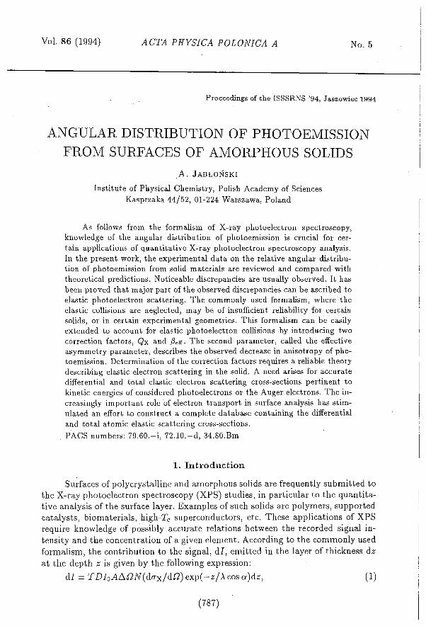
According to Lin et al. [13] and Bunyan and Schonfelder [14], the Diracequation describing the scattering event on a spherical potential V (r) can be trans-formed into the first order differential equation

where W is the total electron energy, k - = -l-1 for the "spin-up case" and k+ = 1for the "spin-down case". The system of units is such that energy is measured inunits of m.0c 2 and the distance in units of h/m0c. This equation describes thefunctions (.P. (r) which are related to the phase shifts

Angular Distribution of Photoemission 791

The algorithm implementing Eqs. (4) (6) for calculations of elastic scatteringcross-sections is rather involved. Thus, it is not practical to use the correspondingsoftware for fast reference, since calculations of cross-sections usually require a con-siderable computational effort. An effective solution to this problem is a creationof a computer controlled database providing the elastic scattering cross-sectionsfor all elements and for a wide energy range. Such database has been recently re-ported in the literature [16]. Examples of the relativistic and nonrelativistic elasticscattering cross-sections are shown in Fig. 2.

3. Anisotropy of photoemission

The theoretical studies of the angular distribution of photoemission fromamorphous solids were initiated in 1979 by Baschenko and Nefedov [17]. The theorydeveloped by these authors predicts a decay of anisotropy due to multiple elasticphotoelectron coHisions. This effect was studied in more detail in later reports[2-5, 18-20]. A marked decrease in the anisotropy was found in all reported cases.Figure 3 shows comparison of intensity of Au 4s photoelectrons calculated fromEq. (2) with results of the Monte Cardo calculations. These calculations are madefor different XPS configurations described by angles cap and ODX (Fig. 1). As one cansee, the decrease in anisotropy does not depend critically on the detection angle α.

As follows from Eq. (2), the anisotropy of photoemission from atoms andmolecules is defined by the value of the asymmetry parameter. This is iHustratedin Fig. 4. The isotropic photoemission, as shown in this plot, corresponds to thevalue of β equad to 0. Exten8ive theoretical data on the values of β calculated fordifferent subsheHs and different euergies of radiation are available in the literature

792 A. Jabłoński

Angular Distribution of Photoemission 793

[21-24]. These values vary in the range from -1 to 2. In considerable majorityof cases, these values are positive. In several reports, the theoretical values of pwere compared with the experimental values obtained for different gaseous species[25-27]. A reasonably good agreement was found.

Within the common XPS formalism, as shown in the previous section, theangular distribution of photoemission from solid surfaces is assumed to be identicalwith the photoemission from isolated atoms or molecules. Vulli [28] seems to be thefirst to show experimentally that the angular distribution of photoemission fromselected solids differs from the theory prediction. He has found that the measuredanisotropy of photoemission from s levels (i.e. of highest anisotropy) is somewhatless pronounced than the prediction for isolated atoms. However, the experimentalvalues of for other subshells were found to be larger than the theoretical values.Such effect is unexpected since the interactions of photoelectrons with the solidshould decrease the original anisotropy of emission. Thus, one can question thereliability of the above experiment. In 1984, the problem of angular distributionof photoemission from polycrystalline solid was addressed by Baschenko et al.[18]. These authors proposed a unique experimental arrangement which makespossible a relatively accurate measurements of the anisotropy of photoemission.The sample was a thin aluminium foil (about 5 ,am) irradiated on one side withX-rays. The foil of such thickness is transparent for X-rays and the photoemissioncan be observed on the other side of the foil. The described arrangement enablesunrestricted positioning of the movable analyser. Second modification, increasingthe reliability of results, consists in measurements of the ratio of peak intensitiesinstead of the intensity of a given peak. This way, the influence of the analysedarea on intensity is cancelled. Baschenko et al. [18] have found that the ratio ofthe Al 2s intensity to the Al 2p intensity is markedly different from zero in thedirection of X-rays. The asymmetry parameter for Al 2s photoelectrons is equalto 2 and, as foHows from Eq. (2), no photoelectron current should be observed insuch XPS configuration. The intensity observed experimentally was ascribed byBaschenko et al. [18] entirely to elastic photoelectron collisions. This hypothesiswas well supported by the Monte Carlo calculation using the published earlieralgorithm [17].

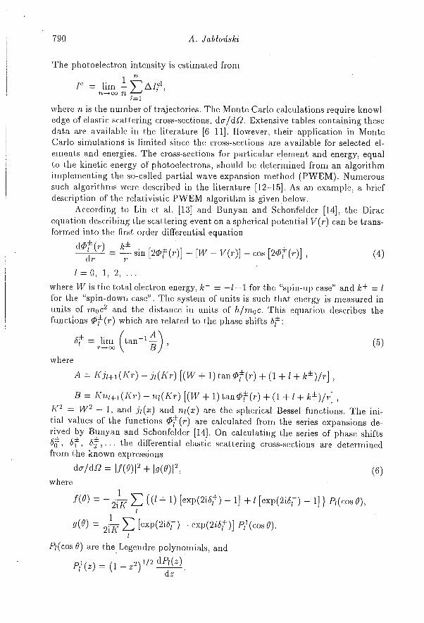
Similar experiments, with much larger number of data points, were repeatedby Zemek and Jabłoński [19] and Jabłoński and Zemek [20]. In these studies,it has been found that the decay in anisotropy observed experimentally is evenlarger than the anisotropy resulting from Monte Carlo calculations. This is shownin Fig. 5a and b. Except for the elastic photoelectron interactions, the observed de-cay in anisotropy may be also caused by other factors. The finite solid acceptanceangle of the analyser may distort the measured angular distribution of photoemis-sion leading to apparent "flattening" of anisotropy. Such effect has been provedtheoretically by Jabłoński et al. [29]. However, it has been found that the cor-responding decrease in anisotropy is not pronounced for the acceptance anglesusuaHy used in XPS. This problem has also been approached experimentaHy byJabłoński and Zemek [20]. Figure 5b shows the intensity ratios measured withintwo different acceptance angles: ±4.1° and ±1.4°. As one can see, no marked differ-ence can be observed. Angular distribution of photoemission can also be affected

794 A. Jabłoński

by the surface roughness. Probably, this effect is responsibde, to a large degree, forthe observed difference between experimental ratios and the ratios resulting fromthe Monte Carlo calculations.

Jabłoński and Zernek [20] proposed a modification of the described aboveexperimental geometry which makes possible the measurements of the angulardistribution of photoemission from any material. This geometry is outlined inFig. 6.The aluminium foil plays a role of a support. The 8tudied material isdeposited on one side of the foil. The thickness of the overlayer should be largerthan the escape depth of photoelectrons, i.e. 10 20 Å. This is easily controlledduring deposition by monitoring the photoelectron peaks from the support untilthey disappear. Overlayers of such thickness are also transparent for the excitingX-rays. Figure 7 shows the intensity ratios measured for gold overlayer. Similareffects as for aluminium are ob8erved. Experimental ratios deviate considerablyfrom the ratios resulting from the common formalism. The ratios obtained fromthe Monte Carlo calculations are relatively close to the experiment, although thedifference is still noticeable.

Angular Distribution of Photoemission . . . 795

4. Corrected formalism

To facilitate calculations associated with quantitative apphcations of XPS,simple expressions approximating the Monte Carlo results were proposed in the

796 A. Jabłoński

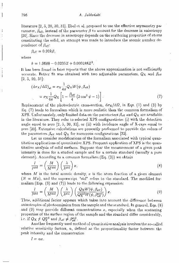
literature [2, 5, 20, 30, 31]. Ebel et al. proposed to use the effective asymmetry pa-rameter, βeff, instead of the parameter p to account for the decrease in anisotrop[30]. Since the decrease in anisotropy depends on the scattering properties of atomconstituting the solid, an attempt was made to introduce the atomic number d(pendence of β eff

where

It has been found in later reports that the above approximation is not sufficientlyaccurate. Better fit was obtained with two adjustable parameters, QDX and Par[2, 5, 20, 31]:

Replacement of the photoelectric cross-section, dσ DX/dΩ, in Eqs. (1) and (3) byEq. (7) leads to formalism which is more realistic than the common formalism ofXPS. Unfortunately, only limited data on the parameters βe ff and QDX are availablein the literature. They refer to selected XPS configurations: (i) with the detection angle equal to zero [2, 5, 30, 31], or (ii) with incidence angle of X-rays equal tozero [20]. Extensive calculations are presently performed to provide the values ofthe parameters βeff and QX for numerous configurations [32].

Let us consider modifications of the formalism associated with typical quan-titative applications of quantitative XPS. Frequent application of XPS is the quan-titative analysis of solid surfaces. Suppose that the measurement of a given peakintensity is done for a studied sample and for a certain standard (usually a pureelement). According to a common formalism (Eq. (3)) we obtain

Thus, additional factor appears which takes into account the difference betweenanisotropies of photoemission from the sample and the standard. In general, Eqs. (8and (9) may provide different concentrations x, especially when the scatteringproperties of the surface region of the sample and the standard differ considerably,

Another frequently used method of quantitative analysis involves the socalledrelative sensitivity factors, α, defined as the proportionality factor between thepeak intensity and the concentration

I = αx.

Angular Distribution of Photoemission 797

From Eq. (3) we get

where C = MΔΩI0 is a constant independent of the photoelectron line, S(E)is the spectrometer function. For a given spectrometer, the relative sensitivityfactors are determined experimentally or theoretically. The latter case is realized inprocedures proposed by Ebel et al. [33] and Hanke et al. [34]. Obviously, Eq. (7) ismore suitable to use in these procedures than Eq. (2) for calculating the differentialphotoelectric cross-section.

Frequent quantitative application of XPS is the estimation of the overlayerthickness [35, 36]. Jabłoński et al. [31] published extensive analysis of variationof the emission anisotropy in systems with overlayers. It has been found that thecorrection factors Neff and Q DX strongly depend on the overlayer thickness. Simpleexpressions describing this dependence were proposed. Thus, the above examplesshow that quantitative XPS requires the efficient methods providing the correctionparameters QDX and βeff for complex systems and for different XPS configurations.

5. Conclusions

The experimental data and the theoretical models of photoelectron trans-port in solids indicate that the initial anisotropy of photoemission is affected bythe elastic interactions within the surface region of a solid. In effect, the angu-lar distribution of photoemission from solid surface is different than the angulardistribution predicted for isolated atoms or molecules. This phenomenon may besignificant and should be accounted for in the formalism of quantitative XPS. Twocorrecting parameters, QDX and βeff, describe the actual anisotropy of photoemis-sion with sufficient accuracy. However, much work is still necessary to proposesimple and effective methods providing these parameters for routine quantitativeapplications of XPS.

References

[1] C.S. Fadley, R.J. Baird, W. Siekhaus, T. Novakov, S.Å. L. Bergström, J. ElectronSpectrosc. Relat. Phenom. 4, 93 (1974).

[2] A. Jabłoński, Surf. Interface Anal. 14, 659 (1989).

[3] W.S.M. Werner, l.S. Tilinin, Appl. Surf. Sci. 70/71, 29 (1993).

[4] I.S. Tilinin, W.S.M. Werner, Surf. Sci. 290, 119 (1993).

[5] A. Jabłoński, C.J. Powell, Surf. Interface Anal. 20, 771 (1993).

[6] M. Fink, A.C. Yates, At. Data Nucl. Data Tables 1, 385 (1970).

[7] M. Fink, J. Ingram, At. Data Nucl. Data Tables 4, 129 (1972).

[8] D. Gregory, M. Fink, At. Data Nuch. Data Tables 14, 39 (1974).

[9] M.E. Riley, C.J. McCallum, F. Biggs, At. Data Nucl. Data Tables 15, 443 (1975).

[10] L. Reimer, B. Lödding, Scanning 6, 128 (1984).

[11] Z. Czyzewski, D.O. MacCallum, A. Romig, D.C. Joy, J. Appl. Phys. 68, 3066 (1990).

798 A. Jabłoński

[12] F. Calogero, Variablc Phase Approach to Potential Scattering, Academic Press, NewYork 1967.

[13] S.-R. Lin N. Sherman, J.K. Percus, Nucl. Phys. 45, 492 (1963).[14] P.J. Bunyan, J.L. Schonfelder, Proc. Phys. Soc. 85, 455 (1965).[15] A. Jabłoński, Phys. Rev. B 43, 7546 (1991).[16] A. Jabłoński, S. Tougaard, Surf. Interface Anal., in press.[17] O.A. Baschenko, V.I. Nefedov, J. Electron Spectrosc. Relat. Phenom. 17, 405 (1979).[18] O.A. Baschenko, G.V. Machavariani, V.l. Nefedov, J. Electron Spectrosc. Rel