Agricultural Trade, Economic Growth and

Free Trade Agreements:

Studies of the Indonesian Case

ESTTY PURWADIANI HIDAYATIE

B. Sc (Statistics), Bogor Institute of Agriculture, Indonesia

M.Sc (Taxation Policy), University of Indonesia, Indonesia

Submitted in fulfillment of the requirements of the degree of

Doctor of Philosophy

Victoria Institute of Strategic Economic Studies (VISES)

Victoria University

Melbourne, Australia

July 2014

Abstract

For decades the importance of the agricultural sector in economic development has been

overshadowed by the industrialization, and indeed this was the case for much of the 20th

century. But the recent revival of the agricultural sector has confirmed its position as a

key to growth in many developing countries. One focus of this renewed attention has

been free trade agreements, with the hope that these would open markets in large or

growing markets in large or rapidly growing countries to the agricultural exports of

developing countries.

This thesis is concerned with the potential for agricultural exports, particularly that

facilitated through free trade agreements, to contribute to Indonesia’s growth.

Indonesia’s agricultural exports have risen strongly since 2004, and provide a rising

share of exports, so these issues are highly relevant to Indonesia.

The objective of this thesis is to examine the impact of agricultural exports on

Indonesian economic growth and the implication of the ASEAN-China Free Trade

Agreement (ACFTA) on agricultural exports of Indonesia. The study includes 35 of

Indonesia’s biggest exported agricultural commodities which covers more than 95 per

cent of total agricultural exports of Indonesia. The endogenous gravity model shows

that Indonesian agricultural exports to China have a positive and significant impact on

Indonesian economic growth. On the other hand, the autoregressive distributed lags

(ARDL) time series measurement reveals that the ACFTA programs have mixed

implication on Indonesian agricultural exports to China both in the short- and long-run.

However, tariff reduction under the Early Harvest Program (EHP) has not significantly

affected the export growth of agriculture in the short and long run. Furthermore, trade

facilitations under the ACFTA programs have also mixed influences on the

competitiveness of agricultural exports depend on the commodities.

It is concluded that the ACFTA role has not yet been reflected in the growth of

agricultural exports since there is no important agricultural commodities covered by

early programs of the ACFTA. Meanwhile the strong growth of agricultural exports

should be carefully addressed as an opportunity by Indonesian government to increase

its contribution to the economic growth.

i | P a g e

ii | P a g e

Acknowledgements

“Optimism is the faith that leads to achievement. Nothing can be done without hope and

confidence”

Helen Keller

Alhamdulillah, first and foremost, I thank Allah for His immense blessing for me to do

this PhD journey and complete my thesis. As Prophet Muhammad S.A.W said that “We

shouldseek knowledge, may it be as far away asChina”, this is my intention to broaden

my knowledge at Victoria University Australia.

My study period in completing my PhD degree was an amazing journey which enriched

my life. This journey has not only given me deeper and wider knowledge, but also

provided the best and most wonderful experience in my life.

This thesis has been seen as the light to my great debt to many people for their

contribution and support during my study. Sometimes, words are not enough to express

one’s deep gratitude to others.

Firstly, I extend a debt of gratitude and highest appreciation to my principal supervisor,

Professor Peter Sheehan, for his greatness and positive support in developing my thesis

and building my confidence in completing my thesis. Not only just his academic

knowledge, but also his clear guidance, patience and immense understanding throughout

my writing contributed greatly to this thesis. Furthermore, his invaluable experience and

unconditional supports along my study has given me confidence to completethis thesis.I

would also like to express sincere appreciation and thank to Professor Tran Van Hoa

(Jimmy) who has supervised me for my thesis, especially in econometric methods and

free trade theory. I am also very grateful and extend my sincere thanks to Jim Lang, for

his invaluable assistance in providing data and supervising me in understanding and

calculating the data.

iii | P a g e

I wholeheartedly thank Professor Bruce Rasmussen, Director of VISES, for

accommodating me in VISES and for all the administrative support and postgraduate

affairs. I also would like to thank to all staff at VISES for their friendship and

memories, especially Margarita Kumnick, and also Pete Symons for their assistance.

My sincere thanks to Tina Jeggo, faculty advisor at Victoria University for her

professional support during my study. I am also thankful to my student colleagues at

VISES and my Indonesian fellow student colleagues for their kindness, friendship, fond

memories and assistance; I feel I have a big family in Melbourne. I extend my thanks to

Margaret Jones, who has been very helpful in assisting me in the study and also living

in Melbourne.

Last but not least, I would like to dedicate this thesis to my family for their

unconditional love, patience, constant support, unceasing prayers, inspiration and

encouragement in supporting my study. Thank you to my mum who always gave me

positive support along this study period, my late father who always advised me to finish

my study and gave me confidence to do that. Thank you to my daughters, Namora and

Azzahra, who always were my sources of support in facing a difficult time during this

period. Also for my husband, Ahmad Husin Siregar, who patiently lived in Indonesia

while we lived in Australia. Without all of them, I would not have had the motivation to

complete my study. All of this is blessing from God who gave us the opportunity to

have this wonderful experience.

Finally, I would like also to extend my deepest gratitude to the Australian Government,

for financial support (Australian Awards Scholarship) to complete this study. And

special thanks to the Director General of Customs and Excise of Indonesia and all my

colleagues for their support and great help.

Estty Purwadiani Hidayatie

7 July 2014

iv | P a g e

Table of Contents

Abstract ............................................................................................................................ i Acknowledgements ........................................................................................................ iii Table of Contents ............................................................................................................ v

List of Tables .................................................................................................................. ix

List of Figures ................................................................................................................. x

List of Abbreviations and Acronyms .......................................................................... xii Executive Summary ..................................................................................................... xiv

Chapter 1 Introduction .............................................................................................. 1 1.1 Introduction ...................................................................................................................... 1 1.2 Research Background ....................................................................................................... 2 1.3 Research Problem ............................................................................................................. 4 1.4 Research Gap .................................................................................................................... 6 1.5 Research Questions and Objectives.................................................................................. 9 1.6 Research Methodology ................................................................................................... 11 1.7 Statement of Significance ............................................................................................... 12 1.8 Thesis Outline................................................................................................................. 14

Chapter 2 Agriculture, Economic Development and Trade Liberalization: A Critical Literature Review ........................................................................................... 17

2.1 Introduction .................................................................................................................... 17 2.2 Importance of Agriculture in Development ................................................................... 18

2.2.1 Multiplier Effect of Agricultural Growth ............................................................ 19 2.3 Agriculture and Poverty Reduction ................................................................................ 20 2.4 Declining Share of Agriculture in World Development ................................................. 22

2.4.1 Investment in Agricultural Sector ....................................................................... 24 2.4.2 The Revival of Agriculture.................................................................................. 26

2.5 Overview of Agricultural Trade and Economic Growth ................................................ 27 2.5.1 Government Trade Policy ................................................................................... 30

2.6 Agricultural Trade Liberalization ................................................................................... 31 2.6.1 Agriculture in World Trade Organization ........................................................... 31 2.6.2 Regional Free Trade Agreements ........................................................................ 33

2.7 Overview of the ASEAN-China Free Trade Agreement ................................................ 34 2.7.1 The Early Harvest Program ................................................................................. 37 2.7.2 Normal Track ...................................................................................................... 39 2.7.3 Sensitive Track .................................................................................................... 39 2.7.4 The Impact of the ACFTA for China and ASEAN Countries ............................. 41 2.7.5 The Impact of the EHP Implementation .............................................................. 42

2.8 Conclusion ...................................................................................................................... 43

Chapter 3 Indonesian Agriculture and Trade Policy: An Overview ................... 45 3.1 Introduction .................................................................................................................... 45 3.2 The Importance of Agriculture in the Indonesian Economy .......................................... 46

v | P a g e

3.3 Top Agricultural Commodities Production in Indonesia ............................................... 50 3.4 Export-Import Composition in Indonesian Agriculture ................................................. 53 3.5 Indonesian Agricultural Trade Policy ............................................................................ 59 3.6 Trade Liberalization and China trade Policy in Agriculture .......................................... 59 3.7 Conclusion ...................................................................................................................... 60

Chapter 4 Have Agricultural Exports Under the ASEAN-China Free Trade Agreement Increased Economic Growth in Indonesia? ........................................... 62

4.1 Introduction .................................................................................................................... 62 4.2 Literature Review ........................................................................................................... 63

4.2.1 Export-Led Growth Theory Approach ................................................................ 64 4.2.2 The Linkages of FDI and Growth ....................................................................... 67 4.2.3 Impacts of Global Financial Crisis on the Indonesian Economy and Trade ....... 71 4.2.4 Other Plausible Determinants of the Trade and Growth Model .......................... 72 4.2.5 Causality between Agriculture Exports and Economic Growth .......................... 73 4.2.6 Generalized Gravity Model ................................................................................. 76

4.3 Methodology .................................................................................................................. 78 4.3.1 Agricultural Export-Economic Growth Model Construction .............................. 78 4.3.2 Estimation of the Model ...................................................................................... 81 4.3.3 Model Robustness Test ....................................................................................... 82 4.3.3.1 Instrumental Variables Tests ........................................................................... 82 4.3.3.2 Model Reliability Test ..................................................................................... 83 4.3.4 Data ..................................................................................................................... 84

4.4 Empirical Results and Analysis ...................................................................................... 86 4.4.1 Model Robustness Result .................................................................................... 86 4.4.1.1 Significance of Instrumental Variables ........................................................... 87 4.4.1.2 Model Reliability ............................................................................................. 88 4.4.2 Estimation Results of the Growth-Agricultural Export Model ........................... 89 4.4.3 Implications of Indonesian Agricultural Exports and Economic Growth ........... 90 4.4.4 Implication of the ASEAN China Free Trade Agreement on Indonesian Economic Growth........................................................................................................... 92 4.4.5 The Role of Foreign Direct Investment in the Economic Growth of Indonesia .. 93 4.4.6 The Role of Other Factors on Indonesian Economic Growth ............................. 95 4.4.6.1 Crises ............................................................................................................... 95 4.4.6.2 Domestic GDP................................................................................................. 97 4.4.6.3 Indonesian Policy Reforms .............................................................................. 97

4.5 Conclusion ...................................................................................................................... 98

Chapter 5 The Implication of the ASEAN-China Free Trade Agreement on the Growth of Agricultural Exports from Indonesia to China ..................................... 100

5.1 Introduction .................................................................................................................. 100 5.2 Literature Review ......................................................................................................... 101

5.2.1 Impact of Free Trade Agreements on Agricultural Exports .............................. 101 5.2.2 Export Function ................................................................................................. 105 5.2.2.1 Relative Price Index ...................................................................................... 106 5.2.2.2 Trading Partner’s income ............................................................................. 107 5.2.2.3 Tariff Reduction ............................................................................................. 107 5.2.2.4 Exchange Rate Volatility ............................................................................... 109 5.2.2.5 Crises ............................................................................................................. 111 5.2.3 Timespan of the Free Trade Agreement Impacts .............................................. 111 5.2.4 Rationale for Autoregressive Distributed Lags Approach ................................ 113

vi | P a g e

5.3 Methodology for Agricultural Exports Model ............................................................. 115 5.3.1 Construction of Agricultural Exports Model ..................................................... 115 5.3.2 Estimation Approach for the Agricultural Export Model .................................. 117 5.3.3 Non-stationary Time Series ............................................................................... 121 5.3.4 Data ................................................................................................................... 122

5.4 Empirical Results and Analysis .................................................................................... 124 5.4.1 Unit Root Test Results ...................................................................................... 124 5.4.2 ARDL Bounds Test Results for the EHP and SL Models ................................. 126 5.4.3 Final EHP and SL Exports Models ................................................................... 128 5.4.3.1 EHP Model Validity ...................................................................................... 130 5.4.3.2 SL Model Validity .......................................................................................... 132 5.4.4 Long-run and Short-run Dynamics of the EHP Demand Functions .................. 133 5.4.4.1 ACFTA ........................................................................................................... 135 5.4.4.2 Tariff Reduction under the EHP .................................................................... 136 5.4.4.3 Relative Price Index ...................................................................................... 137 5.4.4.4 Exchange Rate Volatility ............................................................................... 138 5.4.4.5 Trade Partner’s Income (Real China’s GDP)............................................... 139 5.4.5 Long-run and Short-run Dynamics of the SL Demand Model Functions ......... 139 5.4.5.1 ACFTA ........................................................................................................... 141 5.4.5.2 Tariff Reduction under MFN Tariff Rates ..................................................... 142 5.4.5.3 Relative Price Index ...................................................................................... 143 5.4.5.4 Exchange Rate Volatility ............................................................................... 143 5.4.5.5 Trade Partner’s Income (Real China’s GDP)............................................... 144

5.5 Conclusion .................................................................................................................... 144

Chapter 6 Has the ASEAN-China Free Trade Agreement Increased Competitiveness of Agricultural Exports From Indonesia to China? ................... 147

6.1 Introduction .................................................................................................................. 147 6.2 Literature Review ......................................................................................................... 148

6.2.1 Concept of Agricultural Competitiveness ......................................................... 148 6.2.2 Competitiveness of Commodities under the ACFTA ....................................... 151 6.2.3 Gaps in Literature .............................................................................................. 156

6.3 Methodology ................................................................................................................ 157 6.3.1 Comparative Advantage from Trade Intensity View ........................................ 157 6.3.2 Dynamic Revealed Comparative Advantage..................................................... 160 6.3.3 Market Share Index ........................................................................................... 162 6.3.4 Data ................................................................................................................... 163

6.4 Empirical Results and Analysis .................................................................................... 164 6.4.1 Trade Intensity Index for the EHP Commodities .............................................. 164 6.4.2 Trade Intensity Index for SLCommodities ........................................................ 168 6.4.3 Dynamic Revealed Comparative Advantage for the EHP ................................ 169 6.4.4 Dynamic Revealed Comparative Advantage for the SL ................................... 173 6.4.5 Market Share Index of Indonesian Agricultural Exports to China .................... 174

6.5 Conclusion .................................................................................................................... 177

Chapter 7 Indonesian Agricultural Export Performance: A View from a Real Value Perspective ........................................................................................................ 180

7.1 Introduction .................................................................................................................. 180 7.2 Literature Review ......................................................................................................... 182

7.2.1 Importance of Real Value Calculation .............................................................. 182 7.2.2 Chain-linked Volume Measure ......................................................................... 183

vii | P a g e

7.3 Methodology ................................................................................................................ 184 7.3.1 Constructing a Volume Index ........................................................................... 184 7.3.2 Chain-linked Volume Formula .......................................................................... 185 7.3.3 Chain-linked Export Price Index ....................................................................... 187 7.3.4 The Classification of Agricultural Commodities .............................................. 188 7.3.5 Data ................................................................................................................... 192

7.4 Empirical Results and Analysis .................................................................................... 196 7.4.1 Major Markets for Indonesian Agricultural Exports ......................................... 197 7.4.2 Trends of Exports for Two Groups of Major Markets Countries ...................... 201 7.4.3 Indonesian Agricultural Export Worldwide Excluding Major Exports Destinations .................................................................................................................. 203 7.4.4 Performance of Indonesian Agricultural Exports Worldwide ........................... 205 7.4.5 The Behaviour of Exports for Agricultural Commodities Groups .................... 206 7.4.6 Composition of Biggest Indonesian Agricultural Exports Worldwide ............. 209 7.4.7 Commodities by Countries ................................................................................ 213 7.4.8 Review of the ACFTA and the Pattern of Indonesian Agricultural Exports to China 215 7.4.8.1 Indonesian Agricultural Exports to China .................................................... 217 7.4.8.2 Exports to China: Commodities Groups ....................................................... 218 7.4.8.3 Semi-processed Commodities Exports to China ........................................... 222

7.5 Conclusion .................................................................................................................... 223

Chapter 8 Conclusion and Policy Implication ..................................................... 225 8.1 Chapter Aims and Description ..................................................................................... 225 8.2 Research Summary ....................................................................................................... 226

8.2.1 Background of Agricultural Trade Development .............................................. 226 8.2.2 Empirical Studies Reviews ................................................................................ 227

8.3 Policy Implication ........................................................................................................ 232 8.4 Limitation of the Research and Recommendations for Future Research ..................... 234

References.................................................................................................................... 236

Appendix ..................................................................................................................... 275

viii | P a g e

List of Tables

Table 2.1 Agricultural Products included in the EHP ................................................................ 37 Table 2.2 Specific Agricultural Products covered by the EHP for Indonesia–China................. 38 Table 2.3 Tariff Reduction under the EHP ................................................................................ 39 Table 2.4 Sensitive List China-Indonesia .................................................................................. 40 Table 3.1 Indonesia’s Merchandise Trade Share in the World .................................................. 53 Table 3.2 Growth of GDP, Export and Import of Goods & Services and Merchandise ............. 54 Table 4.1 Estimation Results of Growth-Agricultural Export Model ......................................... 90 Table 5.1 Unit Root Test of Variables in Exports Models ........................................................ 125 Table 5.2 ARDL Co-integration Bounds Test.......................................................................... 127 Table 5.3 Validity Checks for the EHP Model ......................................................................... 130 Table 5.4 Validity Checks for the SL Model ........................................................................... 132 Table 5.5 Long-run and Short-run Results of the EHP model .................................................. 134 Table 5.6 Long-Run and Short-run Results of the SL model ................................................... 139 Table 6.1 Positioning Matrix of Export Competitiveness ......................................................... 160 Table 6.2 Trade Intensity Index for Indonesia's Agricultural Exports of EHP to China .......... 165 Table 6.3 Exports Share Growth from Indonesia to China ....................................................... 170 Table 6.4 DRCA for Sensitive Track Exports Share Growth from Indonesia to China ........... 173 Table 6.5 Market Share of Indonesia's Agricultural Exports in China (EHP Products) ......... 175 Table 7.1 Agriculture Commodities Groupings Based on AoA (Primary Bulk and Horticulture

Groups) .................................................................................................................... 189 Table 7.2 Agriculture Commodities Groupings Based on AoA (Semi-processed and Processed

Groups) .................................................................................................................... 190 Table 7.3 Groups of Agricultural Products .............................................................................. 193 Table 7.4 Annual Growth of Exports to Major Destination Countries .................................... 199 Table 7.5 Total Indonesian Agricultural Exports to Major Destination Countries (in $

million) .................................................................................................................... 200 Table 7.6 Indonesian Agricultural Exports to Two Market Groups .......................................... 202 Table 7.7 Indonesian Agricultural Exports Worldwide Excluding Major Destinations ........... 204 Table 7.8 Indonesian Agricultural Exports Worldwide ........................................................... 206 Table 7.9 Total Export of Indonesia Worldwide by Commodities ........................................... 208 Table 7.10 Growth of Value, Volume and Price of Ten Biggest Agricultural Products of

Indonesia ................................................................................................................. 211 Table 7.11 Biggest Exported Products in ACFTA Programs.................................................... 215 Table 7.12 Total Agricultural Exports of Indonesia to China .................................................. 217 Table 7.13 Agricultural Exports of Indonesia to China by Commodities ................................ 220

ix | P a g e

List of Figures

Figure 2.1 Value Added Percentage of GDP ............................................................................. 23 Figure 2.2 Food and Raw Agricultural Price Index ................................................................... 26 Figure 2.3 World Raw Agricultural Exports as Percentage of Merchandise Exports ................ 28 Figure 2.4 Growth of World Merchandise and Agricultural Exports ........................................ 28 Figure 3.1 GDP Share by Sector ................................................................................................. 46 Figure 3.2 Value Added Share of GDP ...................................................................................... 47 Figure 3.3 Agricultural Trade Share in Merchandise Trade of Indonesia ................................... 48 Figure 3.4 Growth of Indonesian Agricultural Trade .................................................................. 48 Figure 3.5 GDP by Agricultural Sub-sectors .............................................................................. 49 Figure 3.6 The Biggest Production of Indonesian Agricultural Commodities by Value (in

Thousands USD) Year 2000 and 2012 ...................................................................... 51 Figure 3.7 The Biggest Productions of Indonesian Agricultural Commodities by Quantity (in

Thousand Metric Tonnes) Year 2000 and 2012 ........................................................ 52 Figure 3.8 Indonesian Agricultural Export-Import Values ......................................................... 55 Figure 3.9 Agricultural Price Indexes ......................................................................................... 56 Figure 3.10 Export Destinations of Indonesian Agricultural Commodities ................................ 57 Figure 3.11 Import Origins of Agricultural Commodities to Indonesia ...................................... 58 Figure 3.12 Agricultural Export and Import from Indonesia to China ........................................ 58 Figure 4.1 Friedman-Kydland Criterion of Indonesian Economic Growth Model Performance 88 Figure 5.1 CUSUM of the EHP Model .................................................................................... 130 Figure 5.2 CUSUM of Squares of the EHP model.................................................................... 131 Figure 5.3 CUSUM of the SL Model ....................................................................................... 132 Figure 5.4 CUSUM of Squares of the SL ................................................................................ 133 Figure 6.1 Trade Intesity Index for the EHP Products for Period 2000-2012 .......................... 164 Figure 6.2 Trade Intensity Index for EHP Agricultural Commodities under HS 01-08 for Period

2000-2012 ............................................................................................................... 167 Figure 6.3 Trade Intensity Index for the Sensitive Track for Period 2000-2012 ..................... 169 Figure 6.4 Market Share Index for the EHP for Period 2000-2012 .......................................... 174 Figure 6.5 Market Share Index for the Sensitive Track for Period 2000-2012 ........................ 176 Figure 7.1 Indonesian Agricultural Exports to Major countries in Value, Volume and Price

Index for period 1993-2011 ..................................................................................... 196 Figure 7.2 Indonesian Agricultural Exports by Destinations ................................................. 198 Figure 7.3 Indonesian Agricultural Exports Price Index by Destinations ................................ 198 Figure 7.4 Agricultural Exports Worldwide excluding Major Destinations by Volume ......... 203 Figure 7.5 Indonesian Agricultural Exports Worldwide by Value, Volume and Price Index from

1992-2011 ............................................................................................................... 205 Figure 7.6 Indonesian Agricultural Exports 1992–93 and 2010–11 ......................................... 207

x | P a g e

Figure 7.7 Value and Volume of Ten Biggest Indonesian Agricultural Exports Products Worldwide ............................................................................................................... 210

Figure 7.8 Price Index of Indonesian Agricultural Exports Products Worldwide.................... 211 Figure 7.9 Agricultural Groups Exports Volume by Countries ............................................... 213 Figure 7.10 Indonesian Agricultural Exports to China ............................................................ 218 Figure 7.11 Exports to China by Volume of Commodities Groups ......................................... 219 Figure 7.12 Semi-processed Exports from Indonesia to China by Volume .............................. 222

xi | P a g e

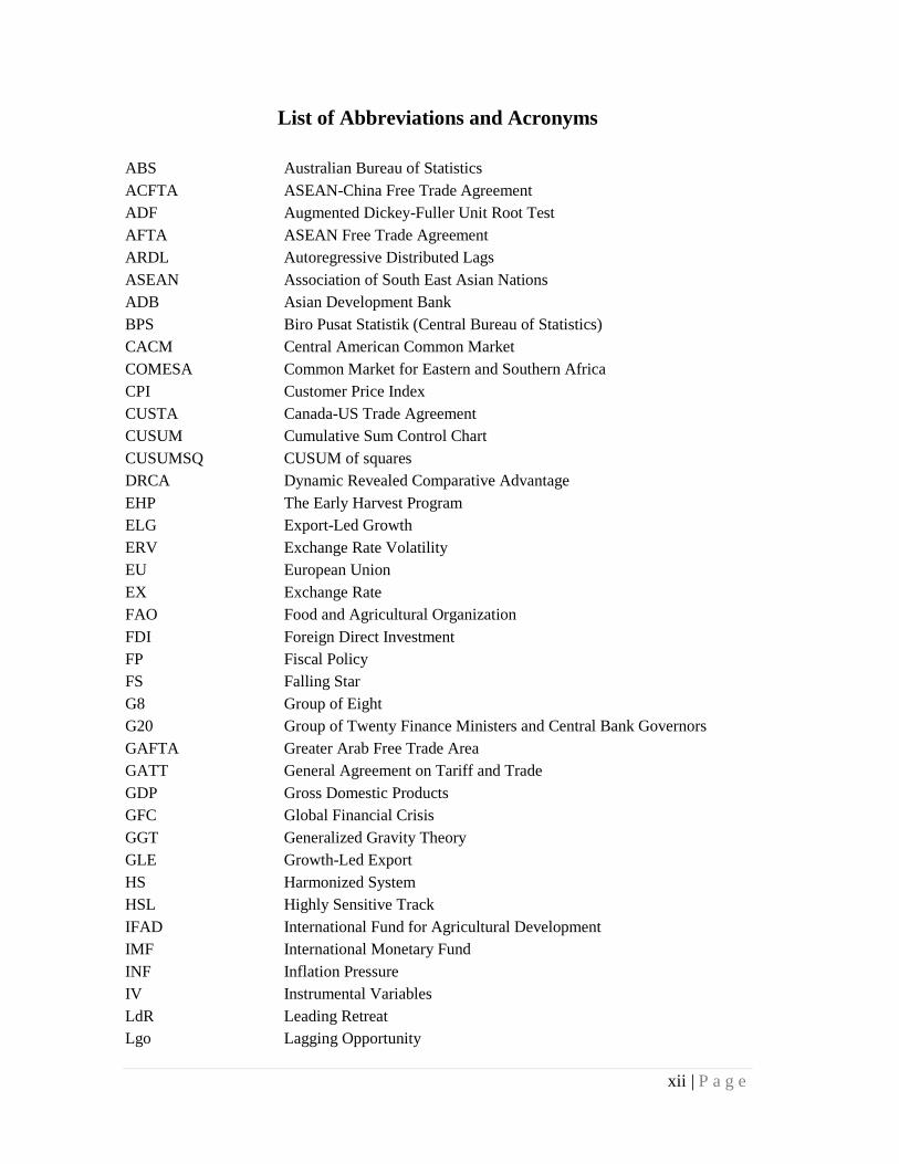
List of Abbreviations and Acronyms

ABS Australian Bureau of Statistics ACFTA ASEAN-China Free Trade Agreement ADF Augmented Dickey-Fuller Unit Root Test AFTA ASEAN Free Trade Agreement ARDL Autoregressive Distributed Lags ASEAN Association of South East Asian Nations ADB Asian Development Bank BPS Biro Pusat Statistik (Central Bureau of Statistics) CACM Central American Common Market COMESA Common Market for Eastern and Southern Africa CPI Customer Price Index CUSTA Canada-US Trade Agreement CUSUM Cumulative Sum Control Chart CUSUMSQ CUSUM of squares DRCA Dynamic Revealed Comparative Advantage EHP The Early Harvest Program ELG Export-Led Growth ERV Exchange Rate Volatility EU European Union EX Exchange Rate FAO Food and Agricultural Organization FDI Foreign Direct Investment FP Fiscal Policy FS Falling Star G8 Group of Eight G20 Group of Twenty Finance Ministers and Central Bank Governors GAFTA Greater Arab Free Trade Area GATT General Agreement on Tariff and Trade GDP Gross Domestic Products GFC Global Financial Crisis GGT Generalized Gravity Theory GLE Growth-Led Export HS Harmonized System HSL Highly Sensitive Track IFAD International Fund for Agricultural Development IMF International Monetary Fund INF Inflation Pressure IV Instrumental Variables LdR Leading Retreat Lgo Lagging Opportunity

xii | P a g e

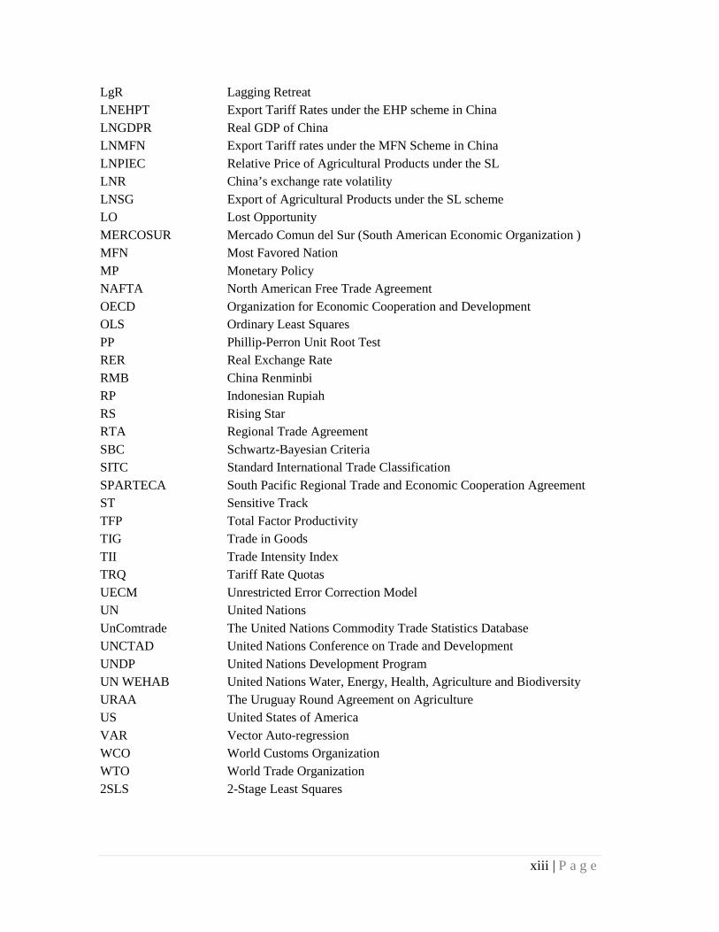
LgR Lagging Retreat LNEHPT Export Tariff Rates under the EHP scheme in China LNGDPR Real GDP of China LNMFN Export Tariff rates under the MFN Scheme in China LNPIEC Relative Price of Agricultural Products under the SL LNR China’s exchange rate volatility LNSG Export of Agricultural Products under the SL scheme LO Lost Opportunity MERCOSUR Mercado Comun del Sur (South American Economic Organization ) MFN Most Favored Nation MP Monetary Policy NAFTA North American Free Trade Agreement OECD Organization for Economic Cooperation and Development OLS Ordinary Least Squares PP Phillip-Perron Unit Root Test RER Real Exchange Rate RMB China Renminbi RP Indonesian Rupiah RS Rising Star RTA Regional Trade Agreement SBC Schwartz-Bayesian Criteria SITC Standard International Trade Classification SPARTECA South Pacific Regional Trade and Economic Cooperation Agreement ST Sensitive Track TFP Total Factor Productivity TIG Trade in Goods TII Trade Intensity Index TRQ Tariff Rate Quotas UECM Unrestricted Error Correction Model UN United Nations UnComtrade The United Nations Commodity Trade Statistics Database UNCTAD United Nations Conference on Trade and Development UNDP United Nations Development Program UN WEHAB United Nations Water, Energy, Health, Agriculture and Biodiversity URAA The Uruguay Round Agreement on Agriculture US United States of America VAR Vector Auto-regression WCO World Customs Organization WTO World Trade Organization 2SLS 2-Stage Least Squares

xiii | P a g e

Executive Summary

Agriculture is a sector that has multiple functions in the economy. However, its

importance in economic development has been dwarfed by industrialization, which was

seen as the main source for economic growth for much of the 20th century. Beside

developing countries hindered by their reliance on agriculture and falling relative prices

for their exports, the unwillingness of developed countries to open their market to

agriculture have resulted agriculture was neglected in in the literature and practice of

development. Nonetheless, renewed attention has been given to agriculture in recent

years as a key to growth in many countries, in the contexts of high process for many

commodities and the impact of rural development of the poor. One focus of this

renewed attention has been free trade agreements, with the hope that these would open

markets in large or rapidly growing countries to the agricultural exports of developing

countries.

This thesis focuses on the potential for agricultural exports to contribute to Indonesia’s

growth, and the implications of a free trade agreement on agricultural exports in terms

of export growth and competitiveness. Agriculture is an important sector in Indonesia as

it contributed around 15 per cent of Indonesia’s GDP in 2013, higher than in 2005 in

nominal terms, although declining slowly in real terms. In contrast with the share of

agriculture in merchandise exports worldwide, which has been declining, Indonesian

agricultural exports have risen strongly since 2004 and provide a rising share of

merchandise exports, so these issues are highly relevant to Indonesia.

Relevant literature and policy background concerning agricultural trade and growth and

the role of initiatives to create freer trade are reviewed in chapters one to three. Four

empirical analyses are reported in this thesis.

Chapter Four utilizes a generalized gravity model to study the impacts of Indonesian

agricultural exports to China and of ACFTA on Indonesia’s economic growth. Such a

model is successfully implemented, by standard econometric tests, on quarterly data for

the period 1996 to 2012. The analysis finds positive impacts of agricultural exports to

xiv | P a g e

China and the implementation of the ACFTA on Indonesia’s growth significant at the

10 per cent.

The second study (Chapter Five) uses autoregressive distributed lag (ARDL) models to

undertake a time series econometric study to explore the short-run and long-run effects

of the impact of two ACFTA programs on Indonesia’s agricultural exports to China.

These programs are tariff reductions under the Early Harvest Program (EHP) which was

completed in the period 2004 to 2006 and was a program to boost agricultural trade

between members. The second program is the Sensitive Track (SL) which started in

2012. This study has also measured other regulations under the ACFTA, such as the

Rule of Origin, on the agricultural exports. Co-integration tests are satisfied and there

are short-run and long-run effects to be analyzed. The estimation reveals different

results of the Early Harvest program and the Sensitive Track program results.

Based on the findings of this study, the impacts of the EHP scheme on Indonesian

agricultural export growth in China, to date, have been limited both in the short-run and

long-run. The results suggest that the tariff reduction facilitation under the EHP

program has no significant impact on the agricultural export growth both in the short-

run as well as the long-run. Meanwhile, the MFN tariff is applied to the SL products in

the period of study, 1996 to 2012, and this tariff implementation had a negative impact

on the agricultural export growth and significant at 5 per cent of the level in the short-

run with no significant impact shown in the long-run. This latter result is to be expected,

as tariff reductions do not begin until 2012 and the effect of the announcement only.

Furthermore, the implementation of the ACFTA had a positive and significant long-run

effect on Indonesia’s EHP exports to China, but that in the short-run the impact is

negative, but also significant at a 5 per cent level. But no impact of the ACFTA

implementation is apparent in either long-run or short-run model for agricultural export

growth of the SL products.

The impacts of the ACFTA programs on the competitiveness of agricultural products

are examined in chapter six. The analysis uses current price data and a range of standard

methods, including the Trade Intensity Index, Dynamic Revealed Comparative

Advantage (DRCA) and Market Share Index. The results show that the ACFTA

xv | P a g e

programs have influenced to only increase competitiveness on certain commodities,

mainly vegetable oils. There are only three commodities, related to vegetable oils and

fats, under the EHP program which have strong revealed competitiveness, and exports

of these products may have been assisted by the ACFTA. While for the rest

commodities covered by the EHP, Indonesia has a low comparative advantage. In

contrast, the competitiveness of agricultural products under the SL program has been

strongly increased, even though there was no tariff reduction facilitation. This program

includes the palm oil products. While their market share in China is already high, it is

expected to increase further with tariff reductions from 2012, if supply capacity is

available in Indonesia.

Finally, Chapter Seven turns to a more detailed analysis of Indonesia’s agricultural

exports, calculating for the first time price and volume measures for 35 commodities

which constitute the bulk of Indonesia’s agricultural exports and covers more than 95

per cent of the total of agricultural exports of Indonesia. Analysis of this data has shown

since 2001 both the price and volume of these exports have grown strongly, that they

are dominated by semi-processed products, mainly palm oils, and that the primary

growth markets are ASEAN, China and India. This analysis reveals a narrow basis for

Indonesia’s agricultural exports, with limited exports to other markets and in products

other than palm oils. This narrow base may be part of the reason for the variable results

of the modelling studies.

While the issues are complex and the empirical results are mixed, agricultural exports

facilitated by free trade agreements have the potential to contribute to Indonesia’s

growth. The findings show that Indonesia’s agricultural export base is very narrow in

terms of variety of commodities, and attention needs to be given to building a more

competitive base outside of palm oil, in part by initiatives on the supply side. For the

same reason the ACFTA has had limited impact on Indonesia’s exports to China,

because Indonesia has low competitiveness in most of the product areas covered. But

this will change as tariffs are reduced to commodities covered by the Sensitive Track, in

many of which Indonesia has stronger export potential.

xvi | P a g e

Chapter 1

Introduction

1.1 Introduction

Agriculture is an important sector that has multiple roles in the economy of any nation,

especially in developing countries (Timmer, CP 2002). These roles include ensuring food

security and poverty reduction in developing countries(Moon 2011), as well as building their

capacity to promote industrialisation and economic growth(Timmer, CP 1988; 2005b).Giventhis

importance of agriculture, agricultural reforms have been considered worldwide to improve this

sector and modernize its functions in the global economy (World Bank 2008). Joining free trade

agreements on multilateral, regional and bilateral level constitutes one of these efforts as they

allow countries to explore wider markets to export their agricultural products.

Nevertheless, the importance of agriculture has been outweighed by other sectors with

industrialisation and modernisation of the global economy. The deceleration of agricultural

growth is inevitable as the share of manufacturing and service sectors take precedence over

agriculture as the economy grows and matures (CSES 2011). This declining importance of

agriculture is evident in the falling rate of agricultural trade growth globally over time and

sidelining of agriculture in the economic priorities of governments worldwide. Despite recent

efforts at liberalization of agricultural trade, the relationship between agricultural export and

economic growth is not as straightforward and has been fiercely debated right from the middle of

the eighteenth century. Previous studies suggest that the effect of specialized in export of

primary product is detrimental to growth (Thirlwall 2006). This is concordant with the Prebisch-

Singer thesis which states that the price of primary products is on a long-run downward trend

relative to the price of manufactured goods due to the volatility of primary product prices, which

causes greater instability of revenue for exporters of these products (Prebisch 1950; Singer

1950).

As a country with abundant agricultural resources and almost 40 per cent of the population

working in the agricultural sector, agriculture is very important for Indonesia because of its

significant contribution to economic growth and its strategic role in achieving food security and

1 | P a g e

poverty reduction. Recently, Indonesia has joined many trade agreements, including multilateral,

regional and bilateral agreements, in order to strengthen its position in international trade.

Indonesia is a member of the ASEAN-China Free Trade Agreement (ACFTA) signed in 2002

between ASEAN countries and China. The implementation of this agreement is expected to

improve the trade and competitiveness of agricultural trade between ASEAN countries and

China (ASEAN 2004).

Given the existing consensus on the declining importance of agriculture in the economy, as well

as debates over the actual benefits from agricultural exports to economic growth, there is a need

to examine whether the efforts of an ACFTA treaty with China will yield the desired results for

Indonesia. Economic growth is the primary aim for a developing country like Indonesia that

mainly relies on its agricultural sector and has made attempts to improve agricultural trade

through trade liberalization.

The first chapter outlines an overview of the thesis. It begins with a brief outline of the research

background detailing the role of agricultural trade in the Indonesian economy and its effort

towards trade liberalization of agricultural commodities with the ACFTA signed with China.

This is followed by a statement of the research problem on debates over the relationship of

agricultural exports with economic growth, especially with the declining role of agriculture in the

world economy. A brief review of previous studies on the ACFTA is presented and the gap in the

literature in relation to the impact of the ACFTA on Indonesian agriculture is highlighted. The

general and specific objectives of this study are presented along with a brief description of the

research methodology to achieve those objectives. The importance and significance of the thesis

are highlighted, followed by the organization of this study at the end of the chapter.

1.2 Research Background

Agriculture has a strategic role in national economic development in a developing country like

Indonesia, especially in reducing poverty, providing employment, improving farmers’ welfare

and maintaining sustainable utilization of natural resources and the environment. The agricultural

sector plays a crucial role in the Indonesian economy, making a significant contribution to

economic growth, foreign exchange earnings, and food security (Timmer, CP 2005a). The annual

growth rate of agricultural output in Indonesia is around 3.5 per cent and the share of the

2 | P a g e

agriculture in the gross domestic product (GDP) is around 15 per cent throughout the period of

2000-2012. In the past, Indonesia traditionally performed an important facilitating function in

international trade as a trade link between ancient India and China because of the location of the

archipelago and its sea lanes. Recently, Indonesia has acquired memberships in many trade

agreements in an effort to strengthen its position in international trade (Bappenas 2009).

There has been a growing move towards opening the agricultural sector up to foreign trade that

has inspired agricultural trade liberalization (WTO 2012b). The shift towards trade liberalization

in agriculture was initiated by the Uruguay Round Agreement on Agriculture (URAA) followed

by the Doha Round. This agreement has commitments to reduce protection rates and trade

barriers on agricultural products, improving market access and establishing the disciplines and

rules on various aspects of global agricultural trade (WTO 2012e). One of the main goals of

these free trade agreements is to increase agricultural trade between members. With the objective

of expanding its presence in international trade, Indonesia has agreed to join trade agreements

bilaterally, regionally and multilaterally (Bappenas 2009). The multilateral agreements that

Indonesia has joined include the World Trade Organization (WTO), Asia Pacific Economic

Cooperation (APEC) and the Group of Twenty Finance Ministers and Central Bank Governors

(G20). In terms of the regional trade agreements, one of the trade agreements that Indonesia has

signed and implemented is the ASEAN China Free Trade Agreement (ACFTA). Because

ACFTA is a regional and relatively close-knit organization, its benefits are exclusive to member

countries. Mutual tariff reductions between member countries can make imports of products of

non-member countries lesscompetitive, with negative impacts on those countries’ total trade

volumes and economic welfare (Ahearne et al. 2006).

Agricultural commodities play an important role in the trade of ASEAN countries. Almost all the

ASEAN members are developing economies with a high share of the agricultural sector in the

economies. The ACFTA agreement has a special program focused on agricultural trade, namely

the Early Harvest Program (EHP). The implementation of this agreement is expected to improve

agricultural trade in growth and competitiveness between ASEAN and China. As China is a

developing country with a growing GDP and huge population, it has become a critical market

destination. The immense size and rapid growth of China’s markets and industries have fuelled

the need for a lot of raw materials and semi-finished materials. As the agriculturally rich nations

3 | P a g e

of ASEAN can benefit from supplying consumer commodities and raw materials to the growing

Chinese industries and markets, Indonesia expects that joining this agreement can broaden its

market to China for its agricultural products . This cooperation is expected to strengthen both

economies in the future (ASEAN 2004; Cordenillo 2005). The ACFTA agreement with China is

a major development in Indonesian trade, particularly for Indonesia’s agricultural sector with

significant implications for the national economy.

This thesis aims to explore whether improving agricultural exports through trade liberalization

with ACFTA will contribute to economic growth in Indonesia. Thus, the research aim of this

thesis is twofold, to examine the relationship between agricultural exports and economic growth,

and the impact of the free trade agreement on agricultural exports volume and competitiveness.

1.3 Research Problem

One of the core aims of the free trade agreement, establishment is tariff elimination. As part of

the Uruguay Round commitment, Indonesia has been reducing its border tariffs, opening its

market as well as reducing other domestic distortions, especially in the agricultural sector

(Feridhanusetyawan, Pangestu & Erwidodo 2002). The government of Indonesia has also been

implementing the agenda of the ACFTA to eliminate tariff barriers, especially import tariffs for

agricultural products. Indonesia’s involvement in these trade agreements poses a challenge for

the agricultural sector as it reduces government protection of domestic products and opens up the

market to foreign products. This poses a significant question about whether trade liberalization

can have a positive impact on the economy of the countries involved in free trade agreements. In

Southeast Asia, evidence shows that the benefit from trade liberalization in non-agricultural

goods has far outweighed the benefit of trade liberalization in agricultural goods (Hertel et al.

2000).

For developing countries, another obstacle in expanding agricultural exports comes from

capacity constraints that hinder the extension of primary products exports to developed countries

((Todaro 1977). Although the facts show that joining a free trade agreement does not

automatically increase agricultural exports, the passion to increase agricultural exports still

inspires developing countries, especially those with strong agricultural backgrounds in the Asian

region (Anderson, K & Martin 2005).

4 | P a g e

Agriculture is a sensitive and vulnerable sector,thus restructuring and adjustment to changing

market conditions takes a long time (Pupphavesa 2010). Furthermore, although most ASEAN

members are net exporters of agricultural products, they are reluctant to open up their domestic

market for agricultural trade (Pupphavesa 2010). In view of the distinctive and diverse role of

agriculture, Batie and Schweikhardt (2010) identify the issue of agricultural trade liberalization

as a ‘wicked problem’ in the sense that it is ‘highly resistant to resolution’ as the prolonged

WTO multilateral talks, and the view that agricultural trade liberalization is not convincing

argument to be followed up. The inclusion of agricultural trade in a free trade agreement does

not guarantee that agricultural trade will increase. The evidence from some free trade agreements

show the declining trend of agricultural shares in world trade, which is shown by the export of

agricultural goods that accounted for 6.3 per cent in 2005 compared to 8.2 per cent of world

exports in 1991 (Korinek & Melatos 2009). Widespread evidence shows the same results for

agricultural trade under the ASEAN Free Trade Area (AFTA), Common Market for Eastern and

Southern Africa (COMESA), European Union (EU) and North American Free Trade Agreement

(NAFTA), and only Mercado Comun del Sur/South American Economic Organization

(MERCOSUR) that has been shown to have increased agricultural exports (Korinek & Melatos

2009). Despite the great expectations about trade liberalization in agriculture, these obstacles to a

fair regime of liberalization for developing countries as well as weak evidence about the success

of free trade in agriculture, it is worth asking whether the free trade agreement with China under

the ACFTA can deliver the expected benefits for Indonesian agriculture.

There is also declining interest from the government and private sectors in the agricultural sector

with declining efforts to boost agriculture (Timmer, MP & de Vries 2009). The rate of growth in

agricultural trade is declining globally over time. In fact, the relationship between agricultural

exports and economic growth has been debated since the middle of the eighteenth century. In

their influential paper, Johnston and Mellor (1961) argued that imposing open trade policy for

agricultural sector will improve economic growth as well as the growth of agricultural export.

Many subsequent studies argue that agricultural export can play an important role in economic

growth and export-led growth from agriculture may represent optimal resource allocation for

those countries that have a comparative advantage in agricultural production. For example, the

research conducted by Dawson (2005); Levin and Raut (1997); Sanjuán‐López and Dawson

5 | P a g e

(2010); Tiffin and Irz (2006) show a positive link between agricultural exports and economic

growth.

In contrast, many prior studies argue that the effect of specialization in the export of primary

products is detrimental to growth. This is supported by the Prebisch-Singer thesis which states

that the price of primary products is on a downward trend relative to the price of manufactured

goods. It is also caused by the volatility of primary product prices as exporters of these products

experience greater instability of export revenue. Sachs and Warner (1997a), in their primary

analysis, claim a negative coefficient in growth regression when examining the link between

agricultural exports and economic growth in 83 countries over the period 1965 to 1990.

Similarly, Sala-i-Martin (1997) finds the share of primary products in total exports to be robustly

and negatively correlated with growth over many alternative regression specifications. Among

other studies, Esfahani (1991) shows that exports of primary commodities have no significant

impact on economic growth, while Faridi (2012) reveals a negative relationship between

agricultural exports and Pakistan’s economic growth. Even if there were gains to be made for

Indonesian agriculture from the ACFTA trade with China, it needs to be ascertained whether this

rise in agricultural exports leads to economic growth for the whole country.

1.4 Research Gap

Many studies have analysed the impacts of the ACFTA on the economic growth of the member

countries and have reached two general conclusions. Most studies have predicted that the

ACFTA will stimulate the economies of member countries by reducing trade barriers and

transaction costs, thereby promoting the development of bilateral trade. For example, Chirathivat

(2002), using a computable general equilibrium model, found that the establishment of the

ACFTA will increase the GDP growth of both China and ASEAN by 0.36 and 0.38 per cent,

representing $298.6 billion and $178.7 billion worth of gains respectively. Using the gravity

model, Devadason (2010) finds evidence to suggest that China’s trade has a positive relationship

with increasing intra-ASEAN exports. Likewise, there was also no indication to show that import

sourcing from China by ASEAN countries reduces intra-ASEAN export flows. China, as the

‘core’ country of the ACFTA can provide complementary in the export performance of ASEAN.

6 | P a g e

By implementing the Global Trade Analysis Project (GTAP) method to simulate the impact of

the ACFTA, Yue (2004) claims that exports between China and ASEAN countries would

increase both ways with a complimentary effect in bilateral trade between ASEAN and China,

bringing benefits for both parties. Sangsubhan (2010) argues that the implementation of the EHP

has brought positive impacts and increasing bilateral trade for Thailand, especially for

commodities under Harmonized System code (HS) 01 until HS 08. The trade between Thailand

and China was based on complementary benefit and not a competition between the two, where

Thai commodities like rice, rubber and tropical fruits were exchanged with cold climate fruits

from China. He also finds a positive impact of the ACFTA in Vietnam for the commodities that

are not competitive as the Vietnamese consumer can now get commodities, such as beef, dairy

products, fruit and vegetables, at lower prices. Using the gravity model, Yang and Chen (2008)

predict that the impact of the ACFTA will create a trade diversion effect which will be much

larger than trade creation. This condition may cause the impact of the ACFTA to reduce China’s

future prosperity.

In contrast, some studies argue that ASEAN countries will suffer from this bilateral agreement

because of the threat from China as China has a large market with lower labour costs and

production costs, as well as a reliable source of human capital. They argue that China’s cheaper

products will have negative impacts on the total welfare of ASEAN countries or at least on some

important sectors in ASEAN countries (Roland-Holst, Azis & Liu 2001; Tongzon 2005). Park

(2007) argues that ASEAN needs a transitional period in order to reap the benefits of the ACFTA

as ASEAN industries are less competitive than those of China. The un-readiness of ASEAN

countries in this liberalization will lead to losses in ASEAN industry. China’s relatively lower

cost of production compared to ASEAN has decreased competitiveness of ASEAN (Supriana

2013). Batra (2007) compares the impact of the ACFTA for China and other Asian countries,

such as India, and finds that tariff concessions on some commodities will have a negative impact

on India for marine products, such as fish, molluscs, and vegetables.

In contrast, Yunling (2010) finds that while the overall impact from the implementation of the

ACFTA is positive, the benefits are uneven for the member countries. The agreement will

increase export growth of Chinese products with comparative advantage, speed up the

development of these industries and thus promote the optimization of China’s agricultural export

structure. However, the impact of the implementation of the ACFTA is uneven across ASEAN

7 | P a g e

countries due to gaps in development level and differentiation in production cost. Okamoto

(2005) analises trading indicators and states that Singapore and Malaysia stand to obtain the

benefits of inter- and intra-industry specialization; while Thailand gains the advantage of intra-

industry specialization. Indonesia and the Philippines do not stand to gain much from this

agreement. In the Philippines, small farmers and producers could suffer from the impact of the

agreement because they lack access to a fallback mechanism, such as credit and insurance. The

EHP has not been effectively implemented in Laos due to the lack of preparation prior to the

signing of the agreement. Although the agreement has provided preferential tariff reductions, the

import prices for commodities from Laos are still high because of the high transportation cost.

Furthermore, the homogeneity in production and exports in the region also poses problems for

complementary trade. The main agricultural commodities exported from ASEAN countries,

including natural rubber, palm oil, coconut oil, spices and pineapples, are produced by almost all

ASEAN countries. The similarity of agricultural commodities produced across members is quite

pronounced. For example, Indonesia is a major exporter of natural rubber and palm oil while

Malaysia is also a major exporter in palm oil (WTO 2009). Hence, theoretically, only countries

with lowest cost production will gain from free trade. For example, Sudsawasd and Mongsawad

(2007) predict that the ACFTA will reduce the trade balance for Indonesia, Philippines,

Singapore and Thailand, but will increase GDP across five ASEAN members (Indonesia,

Malaysia, Philippines, Singapore and Thailand). Comparing the effect of the ACFTA on the

internal trade of China and ASEAN countries,Supriana (2013) claims the biggest positive

impacts of the ACFTA are received by Singapore, Malaysia, Thailand, consecutively in that

order, while the impact on Indonesia and the Philippines is negative.

The impact of the ACFTA on Indonesian trade has been perceived to be negative in previous

literature. Among the previous studies on the implementation of the ACFTA in Indonesia,

Supriana (2011) finds that the diversion and creation effects on Indonesia trade are not

significant. In contrast, Yue (2004) argues that the implementation of the ACFTA will increase

the exports of Indonesia, but will decrease the welfare of Indonesia by decreasing its GDP.

Employing the GTAP model, Ibrahim, Permata and Wibowo (2010) finds that even though the

net trade creation is around 2 per cent and exports are likely to increase by 2.1 per cent, the

ACFTA imposes negative impacts of 2.3 per cent on Indonesia’s overall tradebalance. In the

case of the mutual impact between Indonesia and China, Yunling (2010) mentions that China

8 | P a g e

stands to gain more benefits than Indonesia since the production level for most commodities in

China is much higher than that in Indonesia.

Since every member of the agreement expects to increase its trade, it becomes imperative to

examine the impact of the agreement on each specific country with more appropriate methods.

The literature shows the research on the impacts of ACFTA is mainly explored by simulation

methods such as GTAP or other general equilibrium methods to predict ex-ante impacts.

However, the ex-post impacts of the agreements for a specific sector from a simulation method

could be undetermined. By using more rigorous econometric methods, it is expected that the ex-

post impact of the agreement can be measured and the result will be robust and make a positive

contribution to the literature. In the literature related to agricultural exports and economic

growth, studies on the impact of agricultural exports on Indonesia’s economic growth are scarce.

Furthermore, the literature shows that, although the research on the ACFTA is abundant, studies

focusing on the impact of the ACFTA programs on related agricultural trade are rare. Thus, this

thesis is dedicated to providing a contribution to the literature by exploring the impact of

ACFTA programs focusing on agricultural trade between Indonesia and China.

1.5 Research Questions and Objectives

This research examines the impact of Indonesian agricultural exports to China under the ACFTA

on Indonesian economic growth. Given the importance of the agricultural sector for the

Indonesian economy, this study will also investigate the impact of free trade agreements on

agricultural exports. The specific free trade agreement focused on in this research is the ACFTA.

Analysis of various indicators of performance and characteristics of Indonesian exports is

specifically addressed in relation to ACFTA market coverage. The actual impact of the ACFTA

needs to be examined in order to measure whether the ACFTA has fulfilled the benefits expected

from its implementation.

This thesis explores the impacts of agricultural exports for economic growth and measures the

influence of implementation of free trade on agricultural exports. The aims of this thesis are thus

twofold—it attempts to explore the relationship of agricultural exports and economic growth

from the view of international trade in bilateral trade scheme and examines whether the trade

policy effort to open a wider market for agricultural trade makes a significant impact on

9 | P a g e

agricultural exports. With regard to this latter aim, the impact of the ACFTA on agricultural

exports can be measured from both the overall volume of exports and the competitiveness of

specific commodities exported from Indonesia to China. Therefore, this thesis will try to find

answers for the main questions on Indonesian agricultural exports to China under the ACFTA as

follows:

1. Is agricultural trade still important for Indonesia? To what extent does agricultural export

contribute to the economic growth of Indonesia?

2. Do efforts to improve agricultural trade, such as joining a free trade agreement, have a

significant impact on the growth of exports and competitiveness of the commodities?

3. How do policy reforms affect agricultural trade in Indonesia and what appropriate policy

reforms should be undertaken to improve agricultural trade?

Theoretically, the establishment of a free trade agreement aims to increase trade and

competitiveness of the trading commodities between members of the agreement, so this study

hypothesized that the ACFTA will increase the volume of agricultural trade and the

competitiveness of the agricultural commodities from Indonesia. It aims to portray the

development of Indonesian agricultural trade from a real value perspective, investigate the

influence of agricultural export on economic growth of Indonesia and to explore the impact of

implementation of free trade agreement, in this case ACFTA, on Indonesian agricultural trade

growth and competitiveness. This research will further focus on the impact of those programs on

agricultural trade growth and competitiveness.

From these research questions, the research objectives are as follows:

1. To empirically investigate the impact of agricultural exports under the ACFTA on

Indonesian economic growth;

2. To investigate the impact of the ACFTA programs on the growth of Indonesian

agricultural exports to China across the long-run and short-run dynamic of time series

study;

3. To examine the impact of the ACFTA programs on the competitiveness of agricultural

commodities exported from Indonesia and China;

10 | P a g e

4. To review the circumstance of Indonesian agricultural exports from the volume chain-

link perspective;

5. To analyse policies taken to promote economic growth and trade relations in the

agricultural sector in Indonesia, especially those related to the implementation of free

trade agreement.

1.6 Research Methodology

Each chapter of the empirical analysis is designed to address a particular research question and

objective of this study. As each of these empirical analyses applies its own methodology, they

are described within the chapters and the thesis does not have a separate methodology chapter.

Briefly, these methodologies can be described as follows:

1. The endogenous gravity theory is implemented in Chapter Four to analyze the impact of

Indonesian agricultural exports on Indonesian economic growth under the influence of

the ACFTA. The model developed in this analysis is an extension of existing methods

reviewing the relationship between trade and growth with inclusion of other relevant

variables of crisis, domestic GDP, investment and government reforms. Some other

determinants will be incorporated in the model as control and instrumental variables to

confirm the goodness of fit of the model. The two stage least square (2SLS) estimation

method will be implemented.

2. The Autoregressive Distributed lags (ARDL) modelling approach is employed on import

demand functions in Chapter Five to examine the impacts of the AFCTA programs,

namely the EHP and the Sensitive Track on the volume of Indonesian agricultural exports

to China.

3. The competitiveness measures provided by Trade Intensity Index (TII), Dynamic

Revealed Comparative Advantage (DRCA) and Market Share Index will be used in

Chapter Six to explore the impact of the ACFTA programs on the competitiveness of

specific commodities under the EHP and Sensitive Track.

4. The volume chain-link methodology is applied in Chapter Seven to determine the volume

(real value) and price index of Indonesian agricultural exports worldwide. This is applied

11 | P a g e

to 35 commodities as the biggest agriculture exported products of Indonesia that covered

more than 95 per cent of total agricultural exports.

This four-part methodology will clearly bring to the fore the full implications of the ACFTA on

agricultural exports in Indonesia. Since this research will focus on the trade relationship between

Indonesia and China, the benefit of the free trade agreement will be measured directly against the

changes of economic growth and trade growth experienced by Indonesia and also in China,

where relevant.

The data used in this thesis are obtained from the databases and resources from the following

sources:

• Datastream website

• Tradedata.net;

• World Bank;

• United Nations (UN);

• WTO;

• Food and Agriculture Organization (FAO);

• Asian Development Bank (ADB);

• ASEAN;

• Indonesian Bureau of Statistics (BPS);

• Bank of Indonesia.

Detailed information on the sources and formats of the data extracted will be mentioned with the

analysis in each chapter of the thesis.

1.7 Statement of Significance

According to the World Bank (2008), agriculture can be the leading sector for overall growth in

the agricultural-based countries by using a growth strategy anchored on agriculture development.

Although in Indonesia’s case, agriculture has not taken the lead in overall growth, its role in

economic growth is important. Indeed, the share of agriculture in Indonesia’s trade has been

12 | P a g e

increasing even when the share of agriculture in global trade has been declining. Although the

share of the agricultural exports of Indonesian GDP is relatively small compared to other sectors,

it is on a slow upward rise. Furthermore, agricultural exports have been increasing quite

significantly to become an important sector in Indonesia’s economy. This is mainly due to the

fact that the exports of palm oils have been rising, which have become the third largest

commodity contributing to foreign exchange earnings in the country. As the agricultural sector

has an important role in the Indonesian economy, the pattern of agricultural export performance

will help to determine the potential of agricultural products as well as appropriate agricultural

policy.

Agricultural exports have been the backbone of the Indonesian economy when the Asian

financial crisis hit Indonesia in 1997 (Basri, M.C. 2010). The fact that the agricultural sector

excelled during the financial crisis shows that the growth of the agricultural sector is more stable

than other sectors (Athukorala, P. et al. 2010). In Indonesia, the agricultural sector proved to be

important during the Asian crisis. While other sectors collapsed under the strain of the

crisis,Indonesia was able to survive the crisis because of strong agricultural exports (Soesastro &

Basri 2005). This denotes that the agricultural sector can be considered a robust sector in crisis

and its growth is unlikely to be disturbed by any shocks. As the agricultural sector has been an

important part of the country’s economy and a significant sector in trade, government trade

policy should protect and encourage the agricultural sector.

Many studies in the trade and development literature show that export has been a key role in the

growth of a country; however, these are more focused on total exports. There is comparatively

less attention on the empirical relationship between agricultural export and economic growth.

The contribution of agriculture exports to total exports is particularly beneficial, especially in

developing countries (Sanjuán‐López & Dawson 2010). As argued by Johnston and Mellor

(1961), expanding agricultural exports is one of the most promising means of increasing

incomes. In a global environment of lessening attention on the agricultural sector, it is important

to measure the impact of agricultural exports on economic growth, especially for a developing

country like Indonesia. The exploration of the importance of agricultural exports can hopefully

raise more attention to develop this sector for an agriculture-dependant country like Indonesia.

13 | P a g e

Considering the importance of agriculture in a country’s development, good policies and effort

from all stakeholders are required to enable the agriculture sector to achieve its optimum role in

promoting economic growth and poverty alleviation. The lopsided results from free trade

agreements in favour of developing countries make it imperative for developing countries to

prevent agriculture to be completely guided by market forces. Government actions are needed to

meet the multifunctional complexity of obstacles to the development of agricultural trade. Thus,

government intervention in trade and industrial policy for this sector is important and countries

need varying degrees of collective action to address widely divergent needs of agriculture. The

involvement of Indonesia in many free trade agreements, such as multilateral, regional and

bilateral agreements, should be able to force the expansion of agricultural exports yet protect its

domestic industry in this area by selectively permitting agricultural product imports. Those

determinants should be measured in order to evaluate their impact on the trade, so that in the

future most suitable policies can be created to avoid or to reduce negative effects. By enforcing

suitable trade policy, better conditions will be provided and the economy, along with the

agricultural sector will be improved.

1.8 Thesis Outline

ChapterOneprovides an introduction to the study, outlining the research context of the

agriculture sector in Indonesia and liberalization of agricultural trade under the ACFTA. The

chapter also outlined the effect of the ACFTA on the agricultural export and its subsequent

impact on economic growth. It highlighted the gap in the literature on the ACFTA and

agriculture sector. The chapter then highlighted the objectives of the research and methodology

to be used for each stage of analysis for measuring the impact of agriculture export on economic

growth and the implications of the ACFTA on trade volume and commodity competitiveness.

This was followed by a final note on the significance of the study in relation to the effect of

liberalization of agricultural trade, and contribution to policy makers to nurture any future

developments to boost the agriculture sector.

Chapter Two provides a comprehensive background for this thesis on free trade agreements in

the agricultural sector. This chapter is thus set aside for discussing the importance of the

14 | P a g e

agricultural sector, background on trade liberalization in the agricultural sector and an overview

of the ACFTA as the free trade agreement studied in this research.

Chapter Three presents the background of the thesis from Indonesian perspective. The

importance of agriculture for Indonesian economic growth, the strength of the agricultural

products of Indonesia worldwide and trade policy undertaken by Indonesia and China will be

discussed.

Chapter Four presents the empirical analyses of the impact of agricultural exports for economic

growth. This chapter will develop the theoretical framework of endogenous gravity theory which

will be used to investigate the impact of agricultural export under the influence of ACFTA and

global financial crisis on economic growth of Indonesia. Given the debate and even outright

rejection of the relationship between agricultural exports and economic growth by many

neoclassical economists, the contribution of agricultural export to Indonesian economic growth

remains dubious. The examination of this matter of empirical results with statistical and

quantitative analysis will be presented to explain the impact of agricultural export in Indonesia

on economic growth under the auspices of the ACFTA and global financial crisis.

Chapter Five analyses the implications of ACFTA on the volume of Indonesian agricultural

exports to China. The hypothesis is that implementing free trade agreements is positively

correlated with bilateral exports in agricultural commodities when accounting for other important

factors of trade volume. A theoretical framework combining import demand functions with

autoregressive distributive lags (ARDL) is used to examine this presumed positive correlation

between free trade agreements and trade in the short- and long-term.

Chapter Six focuses on the analyses of the implications of the ACFTA on the competitiveness of

agricultural commodities exported from Indonesia. The competitiveness of different agricultural

commodities listed as exports of Indonesia under the ACFTA auspices will be evaluated by

measuring their comparative advantage with Trade Intensity Index and Dynamic Revealed

Comparative Advantage (DRCA) methods. In addition, the Market Share Index will be used to

examine the market positioning of the commodities. This study will examine the impact of these

commodities after joining the ACFTA.

15 | P a g e

Chapter Seven is concerned with the calculation of the chain-linked volume (real value) and the

price of agricultural exports. As Indonesia is the biggest producer of many agricultural products,

it is important to discover the potential of agricultural products for export purposes. As the

presentation in nominal value will lead to biased results, a real value perspective will be better to

explain the Indonesian export performance. Unfortunately, agricultural export data provided in

real value is not yet available, so will need to be specially calculated for this research. Using the

real value will provide a clearer, more accurate picture of the exports, omitting bias caused by

inflation (which is one of the disadvantages when using the current value perspective). This

study will contribute to addressing the lack of an appropriate measure of agricultural export real

value by using a chain-linked volume measures.

Chapter Eight is the final chapter. After a brief review of the findings from the thesis, the chapter

reflects on the findings of this study, its implications for the agricultural industry under ACFTA.

It ends with remarks, noting some limitations of the present research and recommendations for

future research.

16 | P a g e

Chapter 2

Agriculture, Economic Development and Trade Liberalization: A Critical

Literature Review

2.1 Introduction

Agriculture sector plays an important role in economic growth and poverty reduction (World

Bank 2008). Nonetheless, in recent time, most developing countries experience lower

agricultural growth and a weakening role of agriculture in development. Rapid population

growth, declining farm size, falling soil fertility and missed opportunities for income

diversification and migration contributes to the decrease of agricultural contribution. In addition,

the policy of high taxes on agriculture policy, the policy bias towards urban regions, the lack of

government attention, underinvestment and low public spending in agricultural sector also

contribute to the low growth of the agricultural sector.

While economies grow, demand for non-agricultural products and services grow faster than for

agricultural products yet the share of agriculture in GDP and employment decline over time

(Timmer, CP 2002). Indeed, it is a broadly shared view among experts that agriculture has been

neglected in the past three decades, during which time investment in rural infrastructure has

fallen, reducing the capacity of rural economies to generate incomes and employment (Aksoy,

AM 2005b). The neglect of agriculture may be receding and giving way to the realization that

the full potential of agriculture in economic development and poverty reduction has not been

realized in many of the developing countries (World Bank 2008).

Fortunately, the resurgence of attention on the agricultural sector development has emerged in

recent time. One of the renewed interests is trade liberalization in the agricultural sector to

accelerate the agricultural trade (CSES 2011).

The purpose of this chapter is to provide a detailed explanation of the background of this

research. This background will explore the importance of the agricultural sector, overview of

trade in agriculture and trade liberalization in agriculture from the perspective of world trade.

Furthermore, discussion about ASEAN-China Free trade Agreement will be presented since this

agreement is the focus of this study.

17 | P a g e

2.2 Importance of Agriculture in Development

Agriculture contribution to development can be in many ways, including as an economic

activity, as a livelihood, and as a provider of environmental services (World Bank 2008). As an

economic activity, agriculture can be a source of growth for the national economy, a provider of

investment opportunities for the private sector, and a prime driver of agriculture-related

industries and the rural nonfarm economy. Meanwhile, agricultural production is important for

food security because it is a source of income for the majority of the rural poor (Godfray et al.

2010). Agriculture is also a source of livelihoods for an estimated 86 per cent of rural people

(Bezemer & Headey 2008). Furthermore, agricultural activities can be an important part in

contributing to climate change and environmental service issues (Howden et al. 2007).

This perspective about agriculture as a resource for other sectors has persisted in most

development models. There is an argument that this perspective is based on necessity for

industrial development and a matter of historical experience (Reynolds 1975). The industries and

services linked to agriculture in value chains often account for more than 30 per cent of GDP in

transforming and urbanized countries (World Bank 2008). Currently, there has been massive

transformation in agriculture in most developing countries (Hayami & Ruttan 1985), but the

speed of transformation has varied in different countries (World Bank 2008). For example, in

China, India and Indonesia, the share of agricultural employment was roughly same at about 74

per cent in 1961. In 2011, this share had declined to around 40 per cent in China, 35 per cent in

Indonesia but 50 per cent in India. This implies that, for various reasons, employment in industry

and services in China and Indonesia is growing faster than in India.

Agriculture is also an effective engine for growth for most agriculture-based countries. Two-

thirds of the world’s agricultural value added is created in developing countries, yet it generates

on average 29 per cent of the gross domestic product (GDP) and employs 65 per cent of the labor

force in agriculture-based countries (World Bank 2008). Agriculture is also important as it has

to meet global food demand that is predicted to double in 2050 due to population growth, along

with rising income and urbanization in developing countries (Godfray et al. 2010). In

agriculture-based countries, most of the production is generally used to feed the population as

food remains imperfectly tradable because of the high transaction cost and prevalence of staple

18 | P a g e

food that are lightly traded. Agricultural productivity, thus determines the price of food, which in

turn determines wage costs and competitiveness of the tradable sectors (Timmer, CP 2000).

2.2.1 Multiplier Effect of Agricultural Growth

Growth in both non-tradable and tradable sectors of agriculture also induces strong growth in

other sectors of the economy through multiplier effects. Economists, including Johnston and

Mellor (1961), Jorgenson (1961); Nicholls (1963); Schultz (1964) argue that the agricultural

sector must be viewed as part of the overall economy. They emphasize the importance of

interdependence between a country’s agriculture and its industrial and service sectors rather than

relegating agricultural sector to a mere resource reservoir for other sectors. Although the growth

of the agricultural sector is not as fast as other sectors, the multiplier effect of agricultural growth

has enhanced other sectors to grow even higher (Haggblade, Hammer & Hazell 1991). The

whole process of sectoral transformation creates forward and backward linkages between

agricultural and non-agricultural sectors (Ardeni & Freebairn 2002). The market links that

connect a dynamic agricultural sector to rapidly growing industry and service sector and new

technology transferred from this connection provide opportunities to grow agriculture and other

sectors together.

Many studies suggest that the agricultural multiplier effect is significantly greater than one. For

example, in rural Africa, typically characterized as closed, non-tradable economies, the

agriculture multiplier effect is often between two and three; while in more open economies, for

example, some Asian countries, the agricultural multiplier is around two in the early stages of

agricultural modernization when productivity gains are the fastest (Timmer, CP 2009). The

multiplier effect of the agricultural sectorto other sectors has been shown by Warr (2001), who

suggests that the agricultural sector contributes in stimulating growth in the secondary and the

tertiary sectors. For example, increased commercial agricultural activities may lead to the

expansion of small food processing industries, in turn increasing labour mobility from rural to

urban areas. The demand from a growing agricultural sector also feeds into higher growth in

non-agricultural sectors. As well as these examples, there is the growing demand for agriculture-

related machinery and manufacturing products. Similarly, Anderson, K (1987)shows in South

Asia, growth in rural incomes and employment is propelled by an expansion in agricultural

19 | P a g e

productivity that gives rise to increased demand for household products and agricultural inputs

by rural families that can be efficiently produced in rural areas. Rising agricultural incomes are

also spent on purchasing industrial products for households and services including education,

healthcare as well as financial and domestic services. Furthermore, Pack (2009) notes that in

China, Korea and Taiwan, a dramatic increase in agricultural productivity supported the growth

of the small and medium enterprise (SME) sector that sold its products to the farms. In addition,

the current awareness of climate change has further strengthened the indirect multiplier effect of

agriculture by increasing the demand for agro-fuels (World Bank 2008).

2.3 Agriculture and Poverty Reduction

Furthermore, agricultural growth is also noted for its contribution in poverty reduction. Mellor

(1976) argues since agriculture employs majority of the population in developing countries,

increasing agricultural output would boost the economy and hence reduce poverty. Many studies

have come to the conclusion that agricultural growth is highly beneficial for poverty reduction,

although the importance of agriculture diminishes as the economy grows and becomes more

diversified (Anderson, K, Cockburn & Martin 2011; Bezemer & Headey 2008; Dercon 2009;

Dollar, D & Kraay 2001). The importance of agriculture in poverty reduction is derived from the

fact that the occurrence of poverty is disproportionately high in the developing countries, which

still rely heavily on agriculture for income and employment; the poorest households, that have

few assets and low-skilled, rely more on agriculture and facing obstacles in connecting with the

non-agricultural economy for income and employment. As a result, poverty in developing

countries is primarily rural, as nearly 72 per cent of those in poverty live in rural areas (IFAD

2010).

The contribution of agricultural growth in providing a greater share in the employment of the

poor and the unskilled workforce, either directly or indirectly, gives it a crucial role in making

economic growth lift the poor out of poverty (Timmer, CP 2005a). The impact of agriculture on

poverty reduction depends on the interaction of several effects. First of all, the direct effect of

growth in the agriculture sector raises the income levels of those employed in this sector.

Second, the benefits from agriculture gains depends on the rate and participation of the poor in

agriculture as well as the type of agriculture or the ownership structure in a particular location.

20 | P a g e

Third, growth in agricultural incomes generally provides increased demand for both rural and

urban services, including construction, transport and personal services, in the surrounding areas.

Many empirical studies support the view that the growth in agriculture has been a leading source

of poverty reduction in most developing countries as it provides agricultural employment to the

poor and contributes to a greater supply of food that lower food prices that benefits both rural

and urban poor. For example, Chen, C and Duncan (2008) argue in China, agriculture is

recognized as leading source for poverty reduction. The impact of the primary sector on poverty

reduction was 3.5 times higher than the impact of either the secondary or the tertiary sectors.

Datt, Kozel and Ravallion (2003) claim that growth in agriculture and rural economy had been

highly beneficial to reducing rural poverty in India, while Virmani (2004) finds that higher

agricultural growth in India has an impact on poverty reduction in addition to its contribution to

overall GDP growth. Similarly, De Janvry (2010) argue that agricultural growth reduces poverty

in Vietnam.

In contrast, the impact of agricultural growth on poverty reduction varies across countries for

several reasons, including the type of agriculture, the relative size and growth rate of agriculture

in comparison with the non-agricultural sectors, the level of public and private investment in

agriculture and supportive government policies. Mellor, John W (1999) states the marked

slowing of poverty reduction in Asia and increasing poverty in Africa is the result of neglect of

agriculture by both governments and foreign aid institutions. De Janvry (2010) notes that the

positive impact of agricultural productivity growth on poverty reduction was noticeable in

developing countries of sub-Saharan Africa and other parts of Asia, but not in Latin America and

the Caribbean. Binswanger and Quizon (1986) find that agricultural growth effects of the Green

Revolution in India did not benefit the rural poor.

Furthermore, some studies argue that the role of agriculture in poverty reduction is considerably

less than those of other sectors. Suryahadi, Hadiwidjaja and Sumarto (2012) argue that the

growth of agricultural sector strongly reduced poverty in rural areas, the largest contributor to

poverty in Indonesia. However, their study shows that the growth of the service sector has played

a greater role in poverty reduction in both urban and rural areas. This is shown by the fact that

the growth elasticity of poverty for the service sector is higher than that for the agricultural sector

in the pre and post Asian financial crisis era (Suryahadi, Suryadarma & Sumarto 2009). Poverty

21 | P a g e

reduction in Latin America has also benefited the most from the service sector, while in East

Asia, the growth of the industrial sector has had the greatest effect on eliminating poverty (Hasan

& Quibria 2004).

2.4 Declining Share of Agriculture in World Development

One of the features of international trade in the second half of the twentieth century is the

remarkable change in its composition marked by an increase in the share of manufacturing

products and a sharp decline in the share of agricultural products. The structural transformation

of agriculture’s role in an economy is signed by the smaller share of agriculture in economic

output and labour force as income increased over time (Chenery & Syrquin 1975; Syrquin 1988).

The prevailing neoclassical view considers agriculture to be a declining sector, a resource which

provides food, labour and perhaps capital to the essential modernization efforts in industry (Little

1982). This view is supported by studies conducted by Clark (1940) and Kuznets (1966).

The neoclassical economists argue that no policy efforts for agriculture modernization were

needed because the sector declined naturally. Prebisch (1950) points out the declining terms of

trade for traditional products and Hirschman (1958) postulates the lack of direct stimulus in

agricultural sector to modern economies as reasons behind the decline of this sector. According

to Haggblade, Hazell and Dorosh (2007), the role of agriculture as a generator of overall growth

declines as an economy grows. This is marked by a sectoral transformation characterized by

falling shares of agriculture in both GDP and employment as the industry and services sectors

grow, even when the absolute size of agriculture sector in term of output continues to grow, as

shown in Figure 2.1.

22 | P a g e

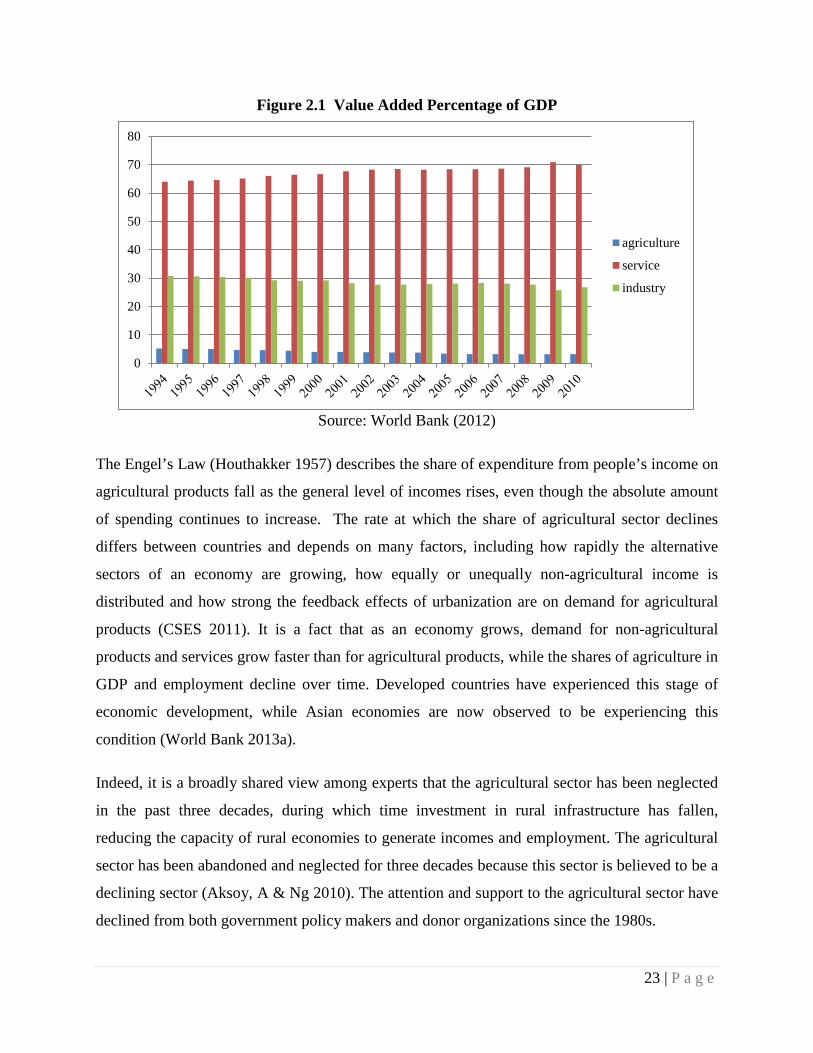
Figure 2.1 Value Added Percentage of GDP

Source: World Bank (2012)

The Engel’s Law (Houthakker 1957) describes the share of expenditure from people’s income on

agricultural products fall as the general level of incomes rises, even though the absolute amount

of spending continues to increase. The rate at which the share of agricultural sector declines

differs between countries and depends on many factors, including how rapidly the alternative

sectors of an economy are growing, how equally or unequally non-agricultural income is

distributed and how strong the feedback effects of urbanization are on demand for agricultural

products (CSES 2011). It is a fact that as an economy grows, demand for non-agricultural

products and services grow faster than for agricultural products, while the shares of agriculture in

GDP and employment decline over time. Developed countries have experienced this stage of

economic development, while Asian economies are now observed to be experiencing this

condition (World Bank 2013a).

Indeed, it is a broadly shared view among experts that the agricultural sector has been neglected

in the past three decades, during which time investment in rural infrastructure has fallen,

reducing the capacity of rural economies to generate incomes and employment. The agricultural

sector has been abandoned and neglected for three decades because this sector is believed to be a

declining sector (Aksoy, A & Ng 2010). The attention and support to the agricultural sector have

declined from both government policy makers and donor organizations since the 1980s.

0

10

20

30

40

50

60

70

80

agriculture

service

industry

23 | P a g e

The neglect of agriculture is likely to associate with a broader shift in economic strategy in many

countries which focused on reduction in budget deficits and resulted in a reduction in public

investment, especially in agriculture (CSES 2011). Others, including the World Bank, have

attributed the falling productivity in agriculture and poor performance of many agricultural

development projects to the decline in the global price of food and the rise of East Asia’s export-

led manufacturing growth. The United Nations Water, Energy, Health Agriculture and

Biodiversity (UN WEHAB) Working Group (2002) claims that donor organizations dropped

agriculture as priority for world development in the 1990s, when agriculture in the developed

countries was considered to be associated with overproduction, environmental pollution and

subsidies. This policy is followed by developing countries which also dropped agriculture as a

priority. Together, these factors made agriculture a low-priority sector and development

strategies were instead focused on export-oriented manufacturing and services as the key drivers

of national economic growth.

2.4.1 Investment in Agricultural Sector

The results of such abandonment have been observed as a fall in agricultural investment (Kumar

1992) and public sector support for agriculture has substantially declined (Bezemer & Headey

2008). Public investment in agriculture and public support for farmers has fallen around the

world, despite the demonstrated high rates of return and the reduction in poverty that come with

such investments. The growth of agricultural productivity has significantly slowed down since

the 1980s, coinciding with diminished investment in public agricultural research over the last

three decades. In line with global trends, the public investment in agricultural sector in

developing countries, such as India, Indonesia and China, also fell and this sector drifted into

relative policy neglect from the 1990s onward (CSES 2011). India’s agricultural growth has

decelerated during the same period and this continued up to the middle of the current decade

(Orden et al. 2007). Indonesia’s agricultural sector has also suffered from policy neglect after the

Asian Financial Crisis of 1997 to 1998 because of government’s urban bias policy (Suryahadi &

Hadiwidjaja 2011). In China, the urban biases in government’s development strategy and the

policy neglect of agriculture have contributed to the persistence of China’s rural poverty (De

Janvry & Sadoulet 2009). Institutional reforms have also suffered from policy neglect in China.

For example, private ownership of agricultural land is still subject to many constraints which

24 | P a g e

severely limit economic opportunities available to the rural population. Because private

investment has not flowed in to fill the gap, agriculture and the broader rural economy in most

countries have suffered from the withdrawal of public investment. Hence, the productivity

growth of agriculture is lower (Schreyer 2004).

The result of the policy neglect of agriculture for more than two decades means that this sector

now urgently needs new investment and complementary infrastructural and public goods (that is,

education, health, research and development, technology and other services) (World Bank 2008).

New and innovative technologies and processes are essential in the agricultural sector in field

technical methods, improving product quality and protecting the environment. Investment is

important in promoting capital formation, as well as replacing or compensating for capital

depreciation. To support the promotion of sustained and high-quality economic growth,

appropriate and well-designed investment scheme will be needed (World Bank 2005).

The World Bank (2012) believes that investment in science and technology will be even

important in the future, with rapidly changing markets, growing resource insecurity and greater

uncertainty. Since science is changing rapidly, it offers new opportunities and possibilities for

future agricultural growth. In the developing countries, nearly 94 per cent of agricultural research

and development comes from the public sector and did not increase as a share of agricultural

GDP (remaining at 0.52 per cent between 1981 and 2000 (World Bank 2008, p. 165). This public

sector domination in agricultural research and development is supply-driven, contrary to the

necessity of this sector being demand-driven to suit the needs of the farmers and consumers.

Investment in research and development has turned much of developing world agriculture into a

dynamic sector, with rapid technological innovation accelerating growth and reducing poverty

(World Bank 2008). Total factor productivity (TFP) of agriculture grew at 1 to 2 per cent a year

in Asia due to new technology (Rosegrant & Evenson 1995). This growth in TFP of agriculture

was responsible for half of the output growth in China and India, and 30 to 40 per cent in

Indonesia, reducing pressure on an increasing supply of scarce land. Although agriculture had a

declining share of GDP, it is not inherently a declining sector as proved by the rate of labor

productivity in the world’s agricultural sector that increase at an average 2.4 per cent annually

compared to 0.74 per cent in non-agricultural sector (Christiaensen, Demery & Kuhl 2011).

25 | P a g e

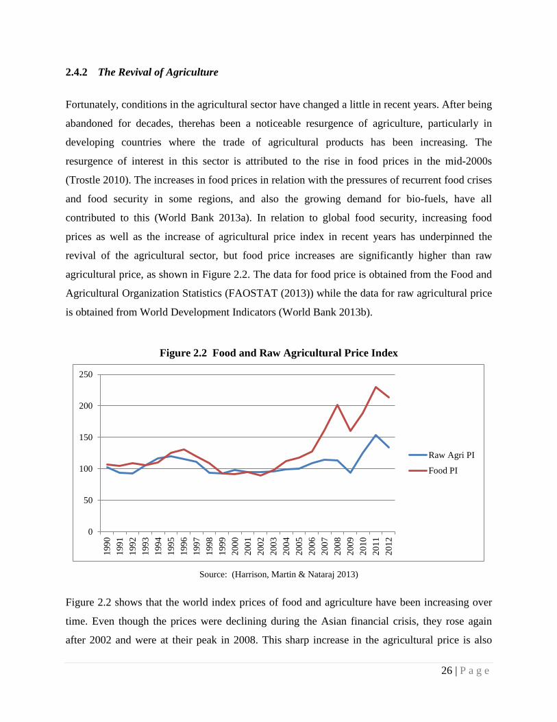
2.4.2 The Revival of Agriculture

Fortunately, conditions in the agricultural sector have changed a little in recent years. After being

abandoned for decades, therehas been a noticeable resurgence of agriculture, particularly in

developing countries where the trade of agricultural products has been increasing. The

resurgence of interest in this sector is attributed to the rise in food prices in the mid-2000s

(Trostle 2010). The increases in food prices in relation with the pressures of recurrent food crises

and food security in some regions, and also the growing demand for bio-fuels, have all

contributed to this (World Bank 2013a). In relation to global food security, increasing food

prices as well as the increase of agricultural price index in recent years has underpinned the

revival of the agricultural sector, but food price increases are significantly higher than raw

agricultural price, as shown in Figure 2.2. The data for food price is obtained from the Food and

Agricultural Organization Statistics (FAOSTAT (2013)) while the data for raw agricultural price

is obtained from World Development Indicators (World Bank 2013b).

Figure 2.2 Food and Raw Agricultural Price Index

Source: (Harrison, Martin & Nataraj 2013)

Figure 2.2 shows that the world index prices of food and agriculture have been increasing over

time. Even though the prices were declining during the Asian financial crisis, they rose again

after 2002 and were at their peak in 2008. This sharp increase in the agricultural price is also

0

50

100

150

200

250

1990

1991

1992

1993

1994

1995

1996

1997

1998

1999

2000

2001

2002

2003

2004

2005

2006

2007

2008

2009

2010

2011

2012

Raw Agri PI

Food PI

26 | P a g e

influenced by the real price of crude oil in mid-2008 which was, briefly, at nearly three times its

previous record. It seems that rising prices will continue for the foreseeable future with persistent

uncertainty on the supply side, including low stock levels, rising projected demand, especially

for biofuels and the inherently slow responsiveness of the global food system to supply and

demand shocks. The high food price in global markets may reverse their long-term downward

trend, creating rising uncertainties about global food security (Rosegrant and others, 2007, cited

in World Bank 2008). This has led to a great deal of uncertainty as to whether agriculture is

capable of meeting food demand that is projected to increase 70 per cent by 2050 from growth in

population and income in developing countries (Hanjra & Qureshi 2010; McCalla 1999). Thus,

good policies and sustained investment are required to manage the aggregate response of

agriculture to rising demand.

An important part of this resurgence of interest in agricultural development is also due to the

efforts to rejuvenate agriculture for economic development as well as poverty reduction from

worldwide organizations such as the International Fund for Agricultural Development (IFAD),

Food and Agricultural Organization of the United Nations (FAO), Organization for Economic

and Cultural Development (OECD), United Nations (UN), United Nations Development

Program (UNDP), and the World Bank (CSES 2011). Furthermore, a commitment to the

agriculture sector has also increased from the governments, development partners and private

sectors (World Bank 2013a). For example, the G8 and the G20 meetings in 2009 pledged funds

to support food security and agricultural growth in low-income countries.

2.5 Overview of Agricultural Trade and Economic Growth

The relationship between agricultural exports and economic growth has been debated since the

middle of eighteen century. The neoclassical economists’ view that the share of the agricultural

sector in economic development is declining in the globalization(Timmer, CP 2002)

accompanied with a decreased share of agricultural exports in any economy (Aksoy, A & Ng

2010). Indeed, Data from World Bank (2013b) shows that the percentage of agricultural export

in total merchandise exports is declining and the growth of agricultural exports is lagging behind

the growth of merchandise exports (Datastream 2012) as shown in Figures 2.3 and 2.4.

27 | P a g e

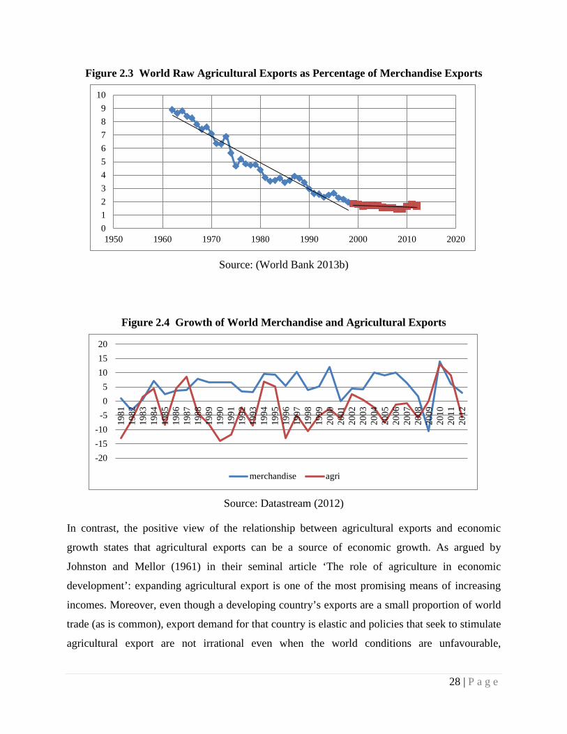
Figure 2.3 World Raw Agricultural Exports as Percentage of Merchandise Exports

Source: (World Bank 2013b)

Figure 2.4 Growth of World Merchandise and Agricultural Exports

Source: Datastream (2012)

In contrast, the positive view of the relationship between agricultural exports and economic

growth states that agricultural exports can be a source of economic growth. As argued by

Johnston and Mellor (1961) in their seminal article ‘The role of agriculture in economic

development’: expanding agricultural export is one of the most promising means of increasing

incomes. Moreover, even though a developing country’s exports are a small proportion of world

trade (as is common), export demand for that country is elastic and policies that seek to stimulate

agricultural export are not irrational even when the world conditions are unfavourable,

0123456789

10

1950 1960 1970 1980 1990 2000 2010 2020

-20-15-10

-505

101520

1981

1982

1983

1984

1985

1986

1987

1988

1989

1990

1991

1992

1993

1994

1995

1996

1997

1998

1999

2000

2001

2002

2003

2004

2005

2006

2007

2008

2009

2010

2011

2012

merchandise agri

28 | P a g e

particularly where few alternatives exist. Agricultural exports therefore can play an important

role in economic growth and export-led growth from agriculture may represent optimal resource

allocation for those countries that have a comparative advantage in agricultural production. This

positive view can be interpreted so that the agricultural sector should open to international trade

to earn foreign exchange.

Johnston and Mellor, Jorgenson (1961); Nicholls (1963); Schultz (1964) argue that the

agricultural economy must be viewed as part of overall economy and agricultural sector can

grow. They emphasize the importance of interdependence between a country’s agriculture and

the industrial and service sectors rather than assuming agricultural sector as a resource reservoir

for other sectors. The market linkages that connect a dynamic agricultural sector to a rapidly

growing industry and service sector and new technology transferred from these connections

provide an opportunity to grow agricultural and other sectors together.

Previous studies suggest that the effect of specialized in export of primary products is

detrimental to growth. This is supported by the Prebisch-Singer thesis (Prebisch 1950; Singer

1950) which states that the price of primary products is on a long run downward trend relative to

the price of manufactures. It is also caused by the volatility of primary product prices. Exporters

of these products experience greater instability of export revenue. Furthermore, there are some

evidences that support this postulation. Sachs and Warner (1997b) analyse the 1970 share of

primary exports in GDP to have significantly negative in a growth regression for 83 countries

over the period 1965 to 1990. Recent theories focus on the economic effects of natural resources

(Lane & Tornell 1996) or on the disincentive to invest in human capital because of higher returns

to unskilled labour (Asea & Lahiri 1999). Both of these arguments are open to Easterly et al.

(1993) objection that growth performance is much less persistent than these theories imply.

Other possibilities are the trends in the relative price of primary commodities over the recent

period have been significantly unfavourable than the long-term average; and the importance of

export price volatility.Sprout and Weaver (1992) argue that primary product exports do not affect

economic growth while Sala-i-Martin (1997) finds a negative relationship between the two

variables. These studies are supported by research conducted by Van den Berg and Lewer

(2007). Faridi (2012) implements Johansen’s co-integration test to measure the impact of

29 | P a g e

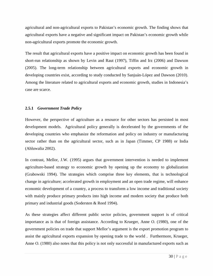
agricultural and non-agricultural exports to Pakistan’s economic growth. The finding shows that

agricultural exports have a negative and significant impact on Pakistan’s economic growth while

non-agricultural exports promote the economic growth.

The result that agricultural exports have a positive impact on economic growth has been found in

short-run relationship as shown by Levin and Raut (1997), Tiffin and Irz (2006) and Dawson

(2005). The long-term relationship between agricultural exports and economic growth in

developing countries exist, according to study conducted by Sanjuán‐López and Dawson (2010).

Among the literature related to agricultural exports and economic growth, studies in Indonesia’s

case are scarce.

2.5.1 Government Trade Policy

However, the perspective of agriculture as a resource for other sectors has persisted in most

development models. Agricultural policy generally is decelerated by the governments of the

developing countries who emphasize the reformation and policy on industry or manufacturing

sector rather than on the agricultural sector, such as in Japan (Timmer, CP 1988) or India

(Ahluwalia 2002).

In contrast, Mellor, J.W. (1995) argues that government intervention is needed to implement

agriculture-based strategy to economic growth by opening up the economy to globalization

(Grabowski 1994). The strategies which comprise three key elements, that is technological

change in agriculture; accelerated growth in employment and an open trade regime, will enhance

economic development of a country, a process to transform a low income and traditional society

with mainly produce primary products into high income and modern society that produce both

primary and industrial goods (Sodersten & Reed 1994).

As these strategies affect different public sector policies, government support is of critical

importance as is that of foreign assistance. According to Krueger, Anne O. (1980), one of the

government policies on trade that support Mellor’s argument is the export promotion program to

assist the agricultural exports expansion by opening trade to the world . Furthermore, Krueger,

Anne O. (1980) also notes that this policy is not only successful in manufactured exports such as

30 | P a g e

in Taiwan, South Korea and Brazil, but the policy has also succeeded in agricultural products

such as in Taiwan with banana exports, Peru with fishmeal exports, and Central America with

raw cotton.

2.6 Agricultural Trade Liberalization

In addition to the attention that has been given from worldwide organizations to the agricultural

sector (World Bank 2008), as well as trade policy attention of the governments to expand its

exports, governments realise the importance of widening agricultural export markets and linking

with world markets by joining regional free trade areas as well as implementing a trade

liberalization policy in the agricultural sector to improve their economic development.

In order to gain more market access for agricultural products to the world market, the World

Trade Organization (WTO) establishes an agreement in the agricultural sector. Agricultural

trade liberalization efforts started in 1986 when the international community puts the agricultural

sector under the General Agreement on Tariffs and Trade (GATT). Although one of the

objectives of the establishment of the free trade agreements is to support agricultural exports,

only a few are dedicated to the promotion of agricultural trade among members.

2.6.1 Agriculture in World Trade Organization

The Uruguay Round Agreement on Agriculture (URAA) is a milestone that began a series of

international trade negotiations on agriculture under GATT auspices which was established in

Uruguay for the period of 1986 to 1994. The agreement also commenced a new round of

multilateral trade negotiations at the end of the implementation period of the Uruguay Round

commitments for developed countries. The creation of the WTO strengthened the rules of GATT

and made it possible for developing countries to join trade talks (Beierle 2002). The Uruguay

Round has been the main driving force of agricultural sector liberalization for Asian countries

during the past decade. Even though in terms of actual trade liberalization this agreement seems

to be limited, its achievement was quite significant.

The URAA enforced trade reform in agriculture commodities to accomplish the reduction of

domestic subsidies, export subsidies and market barriers over six years for developed countries

31 | P a g e

and then 10 years for developing countries (Josling, TE 1994). The Uruguay Round Agreement

also introduced tariff rate quotas (TRQ) for a volume of import at a particular rate to create

additional market access where tariffs replaced non-tariff barriers. During the URAA, countries

agreed to convert all import barriers to their tariff equivalents in a process called ‘tariffication’

(Aksoy, M & Beghin 2005). Once the tariff equivalents were established, tariffs are supposed to

be restricted (Khor 2003). Removing the trade barriers to such trade presents a greater

opportunity for future gains. Although the establishment of the Uruguay Round of GATT

marked the starting point in agricultural trade liberalization, agricultural protection continues to

be the most critical issue in global trade negotiations. Free trade agreements are mostly based on,

but not limited to, elimination of tariff barriers between members. They have also expanded the

non-tariff barrier reduction and enhanced protection modes, such as regulatory mechanisms,

technical barriers to trade, sanitary and phytosanitary measures, as suggested by the Uruguay

Round Agreement on Agriculture.

Tariffs on agricultural commodities remain significantly higher than those on manufactured

goods almost all over the world, although trade in the agricultural sector comprised only 8.1 per

cent of world merchandise trade in 2005 (WTO 2007). Ingco (1995) finds that agricultural

protection was fifteen times higher than non-agricultural protection. In fact, many of the

agreements do not assist the agricultural sector in their scheme. For example, agricultural tariff

rates in the Canada-US Trade Agreement (CUSTA) and NAFTA were already low before

entering the agreement, but the non-tariff barrier increased significantly when the tariff rates

were reduced (Josling, T. 2011). Similarly,OECD (2004) reports that around 36 per cent and 63

per cent average tariffs are applied to agri-food products by OECD and non-OECD countries

respectively. Thus, the agreement has not resulted in tangible trade negotiations and resulted in

issues with legal adherence across different countries.

Aksoy, AM (2005a) observes that the lack of agricultural trade liberalization is associated with

actual levels of protection because:

1. post-URAA implementation, 70 per cent of the agricultural import tariff remains high;

2. The magnitude of international trade of agricultural commodities is higher in developed

countries that have their preferential trade agreement because the tariff barrier is absent

among the partner countries;

32 | P a g e

3. The increasing group of agricultural products, such as fruit and vegetables, has lower

protection compared to the declining group, such as coffee and grains, that are facing a

high protection level in developed countries;

4. The governments of these countries are unwilling to reduce existing levels of tariff and

domestic support for political reasons other than maximizing benefit (Conforti &

Salvatici 2004);

5. Developed countries have increased their domestic support for trade distorting subsidies

in the form of decoupled payments (Baffes & Meerman 1998).

While mainstream opinion perceives agricultural trade liberalization as a beneficial move for the

whole world, the protectionist attitude of developed countries towards their agricultural sector

has created obstacles in this direction (Ingco 1995). The implementation of the GATT-URAA

agreement did not seem to be as favourable for the developing countries as developed countries

acquired most of the benefits (Bouët et al. 2005). Agricultural subsidies implemented by the

developed countries to protect their domestic producers make free trade even more unworkable

(Moon 2011). In developed countries, the agriculture sector is perceived to hold

disproportionately large political power compared to its share in the GDP and the total labour

force. Disdier, Fontagné and Mimouni (2008) show that the imposing WTO rules has reduced

exports from developingcountries, but not affected the agricultural exports fromdeveloping

countries.

2.6.2 Regional Free Trade Agreements

As a response to the deficiencies in global trade agreements, many developing countries have

agreed on building their own free trade areas spanning the region where these countries can

achieve actual trade negotiations and streamline agreements to meet their mutual needs. The

growing importance of emerging economies in world agricultural trade is also manifested

through changing bilateral trade patterns. Agricultural exports from low-income countries have

been increasing rapidly, although they still account for a very small share of trade in agricultural

and processed products (Aksoy, M & Beghin 2005). This has also been a motivating factor

behind forming regional free trade areas. Regional free trade agreements have become the main

form of trade liberalization since the early 1990s (Calvo-Pardo, Freund & Ornelas 2009; Das

33 | P a g e

2004). Although a regional trade agreement does not follow the WTO principle that all countries

should apply the Most Favoured Nation (MFN) tariff to all WTO members, the exemption is

permitted by article XXIV of GATT.

In recent times, the regionalism of the free trade phenomenon has been proliferating throughout

all parts of the world. This can be seen in many regional organizations established both in

developed and developing countries. Chandra and ASEAN (2008) note that regionalism emerged

as a new way to respond to globalization and used it to prevent the negative impact of

globalization as well as minimize the state’s excessive domination.

The expansion of the free trade agreements as the major development in the world economy can

be traced back to the Treaty of Rome in 1958. Nowadays, the WTO has accepted around 489

notifications of the regional trade agreement (RTA) (WTO 2012c). In the current market

liberalization era, every country joining free trade arrangements under multilateral, regional or

bilateral commitments seeks to open its market for products, including agricultural commodities,

from other member countries.

2.7 Overview of the ASEAN-China Free Trade Agreement

ACFTA is one of the regional free trade area agreements that have a special program focused on

increasing agricultural trade among its members. This agreement was signed in 2002 by ASEAN

countries and China. The signing of the agreement on Trade in Goods (TIG) of the Framework

Agreement on Comprehensive Economic Cooperation between ASEAN and China at the

10thASEAN Summit in Vientiane, Laos in November 2004 was a milestone which carried out the

ASEAN-China free trade agreement for goods. This is set to be established by 2010 for ASEAN

6 (Brunei Darussalam, Indonesia, Malaysia, the Philippines, Singapore and Thailand) and China,

and by 2015 for the newer ASEAN member countries (Cambodia, Lao PDR, Myanmar and Viet

Nam). The ACFTA will be implemented gradually over ten years. ACFTA is the third largest

trade agreement in terms of its volume after the European Economic Area and the North

American Free Trade Area (Gooch 2010) and the biggest free trade agreement in the world in

terms of population size. In 2008, a combined nominal GDP of ASEAN members and the China

34 | P a g e

was approximately $6 trillion, while the total trade between the countries rose from $55 billion in

2003 to $193 billion in 2008 (Ananta 2009).

This agreement has a specific program focused on agricultural trade, namely the Early Harvest

program (EHP) along with other programs under the ACFTA, namely Normal track and

Sensitive (SL) and Highly Sensitive tracks (HSL). The Normal, SL and HSL schemes will be

implemented at different times after the completion of the EHP stage. These programs focused

on agricultural trade in the ACFTA make this free trade agreement unique in comparison to other

free trade agreements around the world where agricultural trade often forms a very small portion

of the agreement or is even excluded from trade liberalization due to state protectionism of the

agricultural sector. In developing countries, agriculture is a significant source of foreign

exchange rate earnings and is often the most substantial economic sector, providing large

employment opportunities (Pick & Vollrath 1994).

The ACFTA programs are to be implemented along with a set timeline. The EHP is the first

program of agricultural commodities with an acceleration scheme for agricultural trade between

ASEAN countries and China. The EHP is dedicated to reducing import tariff rates to 0 per cent

on certain agricultural products during 2004 to 2006. On the other hand, the ACFTA also has

other programs named the Normal Track and the Sensitive Track. The Sensitive Track prevents

the reduction of import tariff rates on certain agricultural commodities during 2012 to 2016.

These programs contain commodity lists that most members are reluctant to release to free

market forces with immediate effect. There are many reasons behind this, but the most common

is to protect their own industries, so similar goods imported from other countries facing trade

barriers from high import tariff rates are more costly than domestically produced goods. The SL

is scheduled to come into force for gradually reducing the tariff rates in 2012 for six ASEAN

countries and China while the HSL will start in 2016 (ASEAN 2004).

ACFTA aims to strengthen and enhance economic cooperation, increase trade flow, promote

open markets, enhance liberalization, facilitate trade and investment, and promote economic

relations to improve the welfare of the members. The agreement aims to achieve those goals by

eliminating both tariff and non-tariff barriers in all trade in goods and deepen economic linkages

between the parties. According to the ACFTA scheme(ASEAN 2004), ACFTA does not only

regulate tariff measures but also Rules of Origin, the Operational Certification Procedure (article

35 | P a g e

5 of the ACFTA), non-tariff measures, technical barriers to trade, sanitary and phytosanitary

measures, subsidies and countervailing measures, anti-dumping measures and intellectual

property rights (Article 7 of the ACFTA). The ASEAN-China free trade agreement encourages

ASEAN-China trade, indicating the growing economic interdependence between ASEAN and

China with the potential to expand their markets.

From the Chinese perspective, the intent behind implementing the ACFTA was mainly driven by

political reasons (Yuzhu & Tong 2010). The decision to implement ACFTA was taken to dispel

the growing concerns among ASEAN countries that China was an economic threat. The rapid

growth of China’s economy caused uneasiness with its neighbours. China was as a strong

competitor against ASEAN for exports to third markets as well as direct investment from foreign

countries. Joining this agreement seemed a favourable option to alleviate such concerns.

China’s ‘open door’ trade policy began with its acceptance into the WTO in 2001. This lowered

the import tariff of agricultural commodities and increased access to China’s market for foreign

agricultural products. In return, China’s agricultural products acquired broader access to

penetrate foreign markets (Martin 2001). However, lowering import tariffs does not necessarily

improve import growth. For example, lowering tariff rates on horticulture and meat products

might only affect a small part of the domestic market, such as those firms which only buy and

sell high quality products including meat for five star hotels that serve foreigners. Although the

tariff has fallen for these commodities, the reduction has not affected general traders and

producers. On the other hand, there are commodities called ‘national strategic products’ in which

China has no comparative advantages, but there is strong demand in their domestic market, such

as edible oil, rice, maize, sugar, cotton and wool. China has special permission under the WTO

terms to protect these commodities by imposing high rates for tariff rate quotas (TRQ) and place

a quota on these commodities (Chen, C & Duncan 2008).

According to China’s Ministry of Commerce (2012), China has risen to the position of largest

trading partner for ASEAN and ASEAN has become the third largest trading partner for China

since the implementation of the ACFTA. The trade between ASEAN and China has increased

significantly from $7.9 billion in 1991 to $292.7 billion in 2010 and, in the first half of 2011, the

bilateral trade was $171.1 billion; an increase of 25 per cent in year on year basis (Ministry of

Commerce of China 2012). With more than 500 million people and rich natural resources,

36 | P a g e

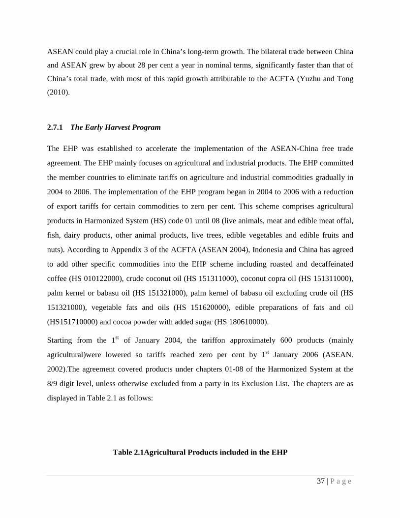
ASEAN could play a crucial role in China’s long-term growth. The bilateral trade between China

and ASEAN grew by about 28 per cent a year in nominal terms, significantly faster than that of

China’s total trade, with most of this rapid growth attributable to the ACFTA (Yuzhu and Tong

(2010).

2.7.1 The Early Harvest Program

The EHP was established to accelerate the implementation of the ASEAN-China free trade

agreement. The EHP mainly focuses on agricultural and industrial products. The EHP committed

the member countries to eliminate tariffs on agriculture and industrial commodities gradually in

2004 to 2006. The implementation of the EHP program began in 2004 to 2006 with a reduction

of export tariffs for certain commodities to zero per cent. This scheme comprises agricultural

products in Harmonized System (HS) code 01 until 08 (live animals, meat and edible meat offal,

fish, dairy products, other animal products, live trees, edible vegetables and edible fruits and

nuts). According to Appendix 3 of the ACFTA (ASEAN 2004), Indonesia and China has agreed

to add other specific commodities into the EHP scheme including roasted and decaffeinated

coffee (HS 010122000), crude coconut oil (HS 151311000), coconut copra oil (HS 151311000),

palm kernel or babasu oil (HS 151321000), palm kernel of babasu oil excluding crude oil (HS

151321000), vegetable fats and oils (HS 151620000), edible preparations of fats and oil

(HS151710000) and cocoa powder with added sugar (HS 180610000).

Starting from the 1st of January 2004, the tariffon approximately 600 products (mainly

agricultural)were lowered so tariffs reached zero per cent by 1st January 2006 (ASEAN.

2002).The agreement covered products under chapters 01-08 of the Harmonized System at the

8/9 digit level, unless otherwise excluded from a party in its Exclusion List. The chapters are as

displayed in Table 2.1 as follows:

Table 2.1Agricultural Products included in the EHP

37 | P a g e

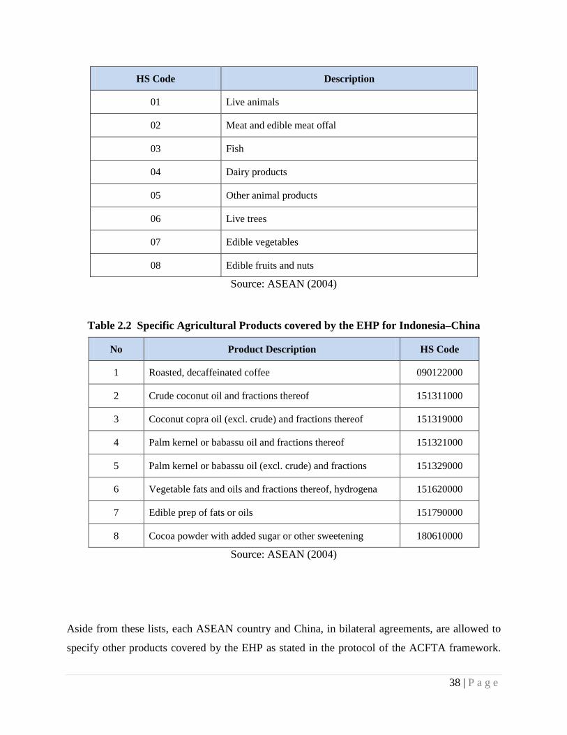
HS Code Description

01 Live animals

02 Meat and edible meat offal

03 Fish

04 Dairy products

05 Other animal products

06 Live trees

07 Edible vegetables

08 Edible fruits and nuts

Source: ASEAN (2004)

Table 2.2 Specific Agricultural Products covered by the EHP for Indonesia–China

No Product Description HS Code

1 Roasted, decaffeinated coffee 090122000

2 Crude coconut oil and fractions thereof 151311000

3 Coconut copra oil (excl. crude) and fractions thereof 151319000

4 Palm kernel or babassu oil and fractions thereof 151321000

5 Palm kernel or babassu oil (excl. crude) and fractions 151329000

6 Vegetable fats and oils and fractions thereof, hydrogena 151620000

7 Edible prep of fats or oils 151790000

8 Cocoa powder with added sugar or other sweetening 180610000

Source: ASEAN (2004)

Aside from these lists, each ASEAN country and China, in bilateral agreements, are allowed to

specify other products covered by the EHP as stated in the protocol of the ACFTA framework.

38 | P a g e

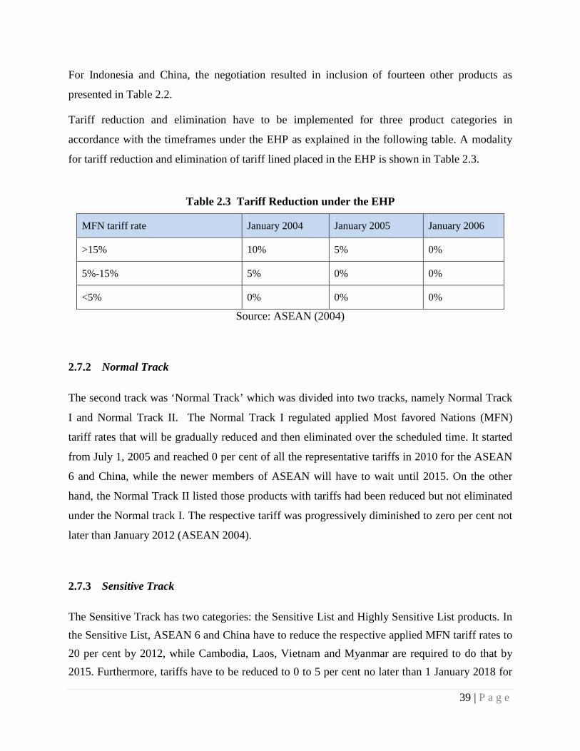
For Indonesia and China, the negotiation resulted in inclusion of fourteen other products as

presented in Table 2.2.

Tariff reduction and elimination have to be implemented for three product categories in

accordance with the timeframes under the EHP as explained in the following table. A modality

for tariff reduction and elimination of tariff lined placed in the EHP is shown in Table 2.3.

Table 2.3 Tariff Reduction under the EHP

MFN tariff rate January 2004 January 2005 January 2006

>15% 10% 5% 0%

5%-15% 5% 0% 0%

<5% 0% 0% 0%

Source: ASEAN (2004)

2.7.2 Normal Track

The second track was ‘Normal Track’ which was divided into two tracks, namely Normal Track

I and Normal Track II. The Normal Track I regulated applied Most favored Nations (MFN)

tariff rates that will be gradually reduced and then eliminated over the scheduled time. It started

from July 1, 2005 and reached 0 per cent of all the representative tariffs in 2010 for the ASEAN

6 and China, while the newer members of ASEAN will have to wait until 2015. On the other

hand, the Normal Track II listed those products with tariffs had been reduced but not eliminated

under the Normal track I. The respective tariff was progressively diminished to zero per cent not

later than January 2012 (ASEAN 2004).

2.7.3 Sensitive Track

The Sensitive Track has two categories: the Sensitive List and Highly Sensitive List products. In the Sensitive List, ASEAN 6 and China have to reduce the respective applied MFN tariff rates to 20 per cent by 2012, while Cambodia, Laos, Vietnam and Myanmar are required to do that by 2015. Furthermore, tariffs have to be reduced to 0 to 5 per cent no later than 1 January 2018 for

39 | P a g e

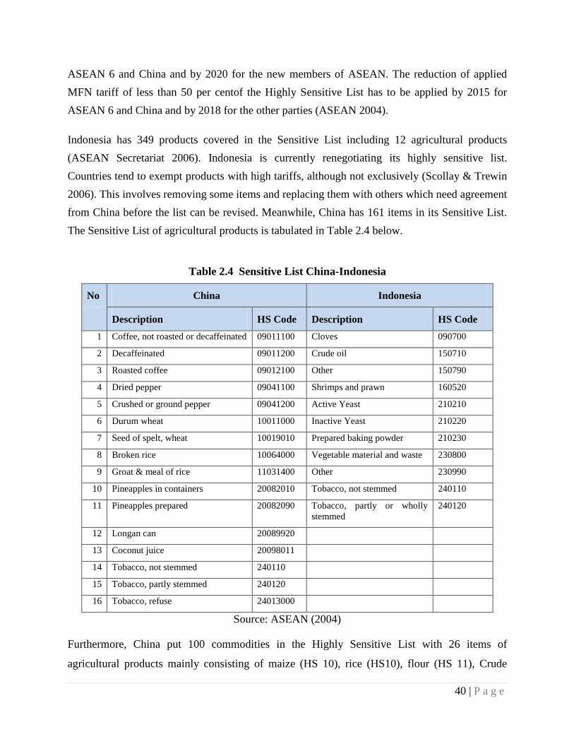
ASEAN 6 and China and by 2020 for the new members of ASEAN. The reduction of applied MFN tariff of less than 50 per centof the Highly Sensitive List has to be applied by 2015 for ASEAN 6 and China and by 2018 for the other parties (ASEAN 2004).

Indonesia has 349 products covered in the Sensitive List including 12 agricultural products (ASEAN Secretariat 2006). Indonesia is currently renegotiating its highly sensitive list. Countries tend to exempt products with high tariffs, although not exclusively (Scollay & Trewin 2006). This involves removing some items and replacing them with others which need agreement from China before the list can be revised. Meanwhile, China has 161 items in its Sensitive List. The Sensitive List of agricultural products is tabulated in Table 2.4 below.

Table 2.4 Sensitive List China-Indonesia

No China Indonesia

Description HS Code Description HS Code 1 Coffee, not roasted or decaffeinated 09011100 Cloves 090700

2 Decaffeinated 09011200 Crude oil 150710

3 Roasted coffee 09012100 Other 150790

4 Dried pepper 09041100 Shrimps and prawn 160520

5 Crushed or ground pepper 09041200 Active Yeast 210210

6 Durum wheat 10011000 Inactive Yeast 210220

7 Seed of spelt, wheat 10019010 Prepared baking powder 210230

8 Broken rice 10064000 Vegetable material and waste 230800

9 Groat & meal of rice 11031400 Other 230990

10 Pineapples in containers 20082010 Tobacco, not stemmed 240110

11 Pineapples prepared 20082090 Tobacco, partly or wholly stemmed

240120

12 Longan can 20089920

13 Coconut juice 20098011

14 Tobacco, not stemmed 240110

15 Tobacco, partly stemmed 240120

16 Tobacco, refuse 24013000

Source: ASEAN (2004)

Furthermore, China put 100 commodities in the Highly Sensitive List with 26 items of

agricultural products mainly consisting of maize (HS 10), rice (HS10), flour (HS 11), Crude

40 | P a g e

soya-bean oil (HS 150710, 150790), crude palm oil (HS 15111000), palm oil (excluding crude &

liquid fraction (HS 15119010), palm stearin (HS 15119020), other palm oil (HS 15119090),

crude oil (HS 151410), other (HS 151490), cane sugar (HS 170111), beet sugar (HS 170112),

other sugar (HS 170199), cigar (HS 24029000) and tobacco (HS 240310, 240391,240399).

Meanwhile, Indonesia has 50 items in the Highly Sensitive List including 13 agricultural

commodities mainly consisting of seed (HS 1005), rice (HS 1006), sugar (HS 1701), un-

denatured ethyl alcohol (HS 2207) and other (HS 2710.90).

2.7.4 The Impact of the ACFTA for China and ASEAN Countries

Because the ACFTA is a regional and relatively close-knit organization, its benefits are exclusive

to member countries. Mutual tariff reductions between member countries can make imports of

products of non-member countries less competitive, with negative impacts on those countries’

total trade volumes and economic welfare (Ahearne et al. 2006). Another study conducted by

(Batra 2007) compared the impact of the EHP for China and compared its impact for other Asian

countries, such as India. The study found that the EHP of the ACFTA that offers tariff

concessions on commodities of HS code 1-8 will have a negative impact on India. The

implementation of this agreement will reduce the trade on products such as fish, molluscs and

leguminous vegetables.

According to Yuzhu and Tong (2010), from the Chinese perspective, joining ACFTA is mainly

driven by political reasons. The decision to join is an attempt to dispel the growing concerns

among ASEAN countries of China as a threat. The rapid growth of China’s economy has caused

uneasiness for its neighbours. Economically, China has been raised as a strong competitor for

exports from ASEAN to third markets as well as for ASEAN’s foreign direct investment

attraction. Joining this agreement seemed a favourable option to alleviate such concerns.

The implementation of this trade agreement has increased the presence of China in the trade of

ASEAN countries.

Chakraborty and Kumar (2012) note the impact on the balance of trade for ASEAN countries are

uneven for period 1995 to 2010; some countries have growing deficit trade while some others

have the surplus. Positive trade balances are experienced by Brunei, Malaysia and the

41 | P a g e

Philippines; while the increasing deficit trade balance are faced by Indonesia, Cambodia,

Thailand, Vietnam and Singapore. Although Indonesia held a trade surplus before 2010, it had a

deficit in 2010. The inflow of China’s cheap products exports is dominant, yet are likely to

intensify following the full implementation of the ACFTA.

In terms of agricultural trade between China and ASEAN under the ACFTA agreement,

implements the gravity model and argues the free trade agreement and GDP are among factors

influencing bilateral trade in agriculture.

2.7.5 The Impact of the EHP Implementation

Yunling (2010) analyses the impact of the ACFTA and the EHP on the countries of ASEAN and

China. He argues that the effect of the ACFTA and the EHP are positive. However, the benefits

are uneven for every country due to competition. In his review, the implementation of the EHP

will promote the export growth of Chinese products with comparative advantage, speed up the

development of these industries and thus promote the optimization of China’s agricultural

export.

According to Yunling (2010), the impact of the EHP on ASEAN countries on trade between

ASEAN countries and China can be explained as follows:

1. China gains more benefits than Indonesia with the EHP as, for most commodities

included in EHP, the production level in China is much higher than that in Indonesia;

2. The effect of EHP seems to be negative despite the market potential provided by the

EHP. In the Philippines, small farmers and producers suffer from the impact of the

agreement because they lack access to fallback mechanisms such as credit and insurance;

3. The positive impact of the EHP is shown in Vietnam for commodities that are not

competitive. The consumer can now get commodities such as beef, dairy products, fruit

and vegetables with lower prices. Furthermore, in long-run, the net impact could be

positive if the local producers improve resource allocation efficiency. While in short-run,

the Vietnamese government should implement relevant policy measures to address the

short-term shock;

42 | P a g e

4. The EHP is an opportunity to develop the agricultural sector as a new source of economic

growth and poverty reduction in Cambodia by promoting agricultural exports. The

government should employ policies to increase agricultural production and marketing

system to assist small farmers to supply agricultural products in an efficient way to be

able to compete in local and international market. However, the traders in Cambodia are

not aware of this agreement and are thus unready to get the benefitsof the agreement.

5. The EHP has not been effectively implemented in Laos due to the lack of preparation

beforehand. Though the agreement has provided preferential tariff reduction, the import

prices for commodities from Laos are still high because of the high transportation cost.

Sangsubhan (2010) argues that the implementation of the EHP has brought positive impacts and

increasing bilateral trade for Thailand, especially for commodities under HS code 01-08. The

trade has increased more than 30 per cent during 2002 to2007 and balance of trade is relatively

stable despite the tough competition in the agricultural market. The trade is based on

complementary where rice, rubber and tropical fruits from Thailand are exchanged with cold

climate fruits from China.

2.8 Conclusion

This chapter provides an extensive background for this thesis comprising a literature review of

the importance of the agricultural sector in development and economic growth. The renewed

attention from the government and the private sector has reinvigorated the agricultural sector.

The revival of agriculture has been marked as agriculture is being included in trade free

agreements to increase agricultural trade.

ACFTA is one of the free trade agreements adopted by the Indonesian government that has a

special program enhancing agricultural trade between members. It is well known that Indonesia

has a foundation as an agricultural country with strong exported agricultural commodities. Hence

the impacts of the ACFTA to increase Indonesian agricultural exports should be explored.

However, previous studies as explained in the previous sections show the implementation of the

ACFTA has different impacts on every member of ASEAN. However the data used in these

studies cover exports of general commodities.

43 | P a g e

While the existing literature, mostly examines the impact of the ACFTA from many points of

view, it is hard to find literature that explores the agricultural exports under the specific programs

of ACFTA. In contrast, most of the members of ACFTA are producers of agricultural

commodities. Hence the agricultural export studies under ACFTA deserve to be examined.

Examining agricultural exports in relation to the ACFTA will give a different impression of the

ACFTA implementation. The next chapter will present a more detailed study about Indonesian

agricultural exports’ condition and agricultural trade liberalization undertaken by Indonesian

government.

44 | P a g e

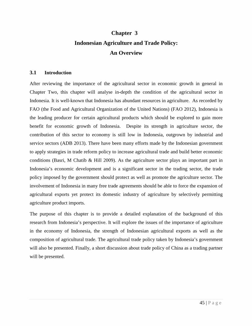
Chapter 3

Indonesian Agriculture and Trade Policy:

An Overview

3.1 Introduction

After reviewing the importance of the agricultural sector in economic growth in general in

Chapter Two, this chapter will analyse in-depth the condition of the agricultural sector in

Indonesia. It is well-known that Indonesia has abundant resources in agriculture. As recorded by

FAO (the Food and Agricultural Organization of the United Nations) (FAO 2012), Indonesia is

the leading producer for certain agricultural products which should be explored to gain more

benefit for economic growth of Indonesia. Despite its strength in agriculture sector, the

contribution of this sector to economy is still low in Indonesia, outgrown by industrial and

service sectors (ADB 2013). There have been many efforts made by the Indonesian government

to apply strategies in trade reform policy to increase agricultural trade and build better economic

conditions (Basri, M Chatib & Hill 2009). As the agriculture sector plays an important part in

Indonesia’s economic development and is a significant sector in the trading sector, the trade

policy imposed by the government should protect as well as promote the agriculture sector. The

involvement of Indonesia in many free trade agreements should be able to force the expansion of

agricultural exports yet protect its domestic industry of agriculture by selectively permitting

agriculture product imports.

The purpose of this chapter is to provide a detailed explanation of the background of this

research from Indonesia’s perspective. It will explore the issues of the importance of agriculture

in the economy of Indonesia, the strength of Indonesian agricultural exports as well as the

composition of agricultural trade. The agricultural trade policy taken by Indonesia’s government

will also be presented. Finally, a short discussion about trade policy of China as a trading partner

will be presented.

45 | P a g e

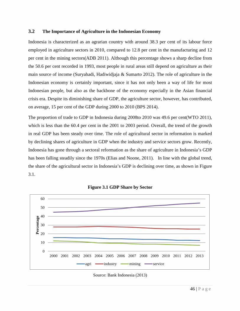
3.2 The Importance of Agriculture in the Indonesian Economy

Indonesia is characterized as an agrarian country with around 38.3 per cent of its labour force

employed in agriculture sectors in 2010, compared to 12.8 per cent in the manufacturing and 12

per cent in the mining sectors(ADB 2011). Although this percentage shows a sharp decline from

the 50.6 per cent recorded in 1993, most people in rural areas still depend on agriculture as their

main source of income (Suryahadi, Hadiwidjaja & Sumarto 2012). The role of agriculture in the

Indonesian economy is certainly important, since it has not only been a way of life for most

Indonesian people, but also as the backbone of the economy especially in the Asian financial

crisis era. Despite its diminishing share of GDP, the agriculture sector, however, has contributed,

on average, 15 per cent of the GDP during 2000 to 2010 (BPS 2014).

The proportion of trade to GDP in Indonesia during 2008to 2010 was 49.6 per cent(WTO 2011),

which is less than the 60.4 per cent in the 2001 to 2003 period. Overall, the trend of the growth

in real GDP has been steady over time. The role of agricultural sector in reformation is marked

by declining shares of agriculture in GDP when the industry and service sectors grow. Recently,

Indonesia has gone through a sectoral reformation as the share of agriculture in Indonesia’s GDP

has been falling steadily since the 1970s (Elias and Noone, 2011). In line with the global trend,

the share of the agricultural sector in Indonesia’s GDP is declining over time, as shown in Figure

3.1.

Figure 3.1 GDP Share by Sector

Source: Bank Indonesia (2013)

0

10

20

30

40

50

60

2000 2001 2002 2003 2004 2005 2006 2007 2008 2009 2010 2011 2012 2013

Perc

enta

ge

agri industry mining service

46 | P a g e

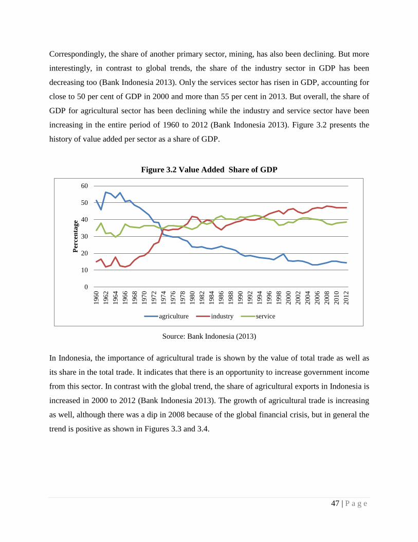
Correspondingly, the share of another primary sector, mining, has also been declining. But more

interestingly, in contrast to global trends, the share of the industry sector in GDP has been

decreasing too (Bank Indonesia 2013). Only the services sector has risen in GDP, accounting for

close to 50 per cent of GDP in 2000 and more than 55 per cent in 2013. But overall, the share of

GDP for agricultural sector has been declining while the industry and service sector have been

increasing in the entire period of 1960 to 2012 (Bank Indonesia 2013). Figure 3.2 presents the

history of value added per sector as a share of GDP.

Figure 3.2 Value Added Share of GDP

Source: Bank Indonesia (2013)

In Indonesia, the importance of agricultural trade is shown by the value of total trade as well as

its share in the total trade. It indicates that there is an opportunity to increase government income

from this sector. In contrast with the global trend, the share of agricultural exports in Indonesia is

increased in 2000 to 2012 (Bank Indonesia 2013). The growth of agricultural trade is increasing

as well, although there was a dip in 2008 because of the global financial crisis, but in general the

trend is positive as shown in Figures 3.3 and 3.4.

0

10

20

30

40

50

60

1960

1962

1964

1966

1968

1970

1972

1974

1976

1978

1980

1982

1984

1986

1988

1990

1992

1994

1996

1998

2000

2002

2004

2006

2008

2010

2012

Perc

enta

ge

agriculture industry service

47 | P a g e

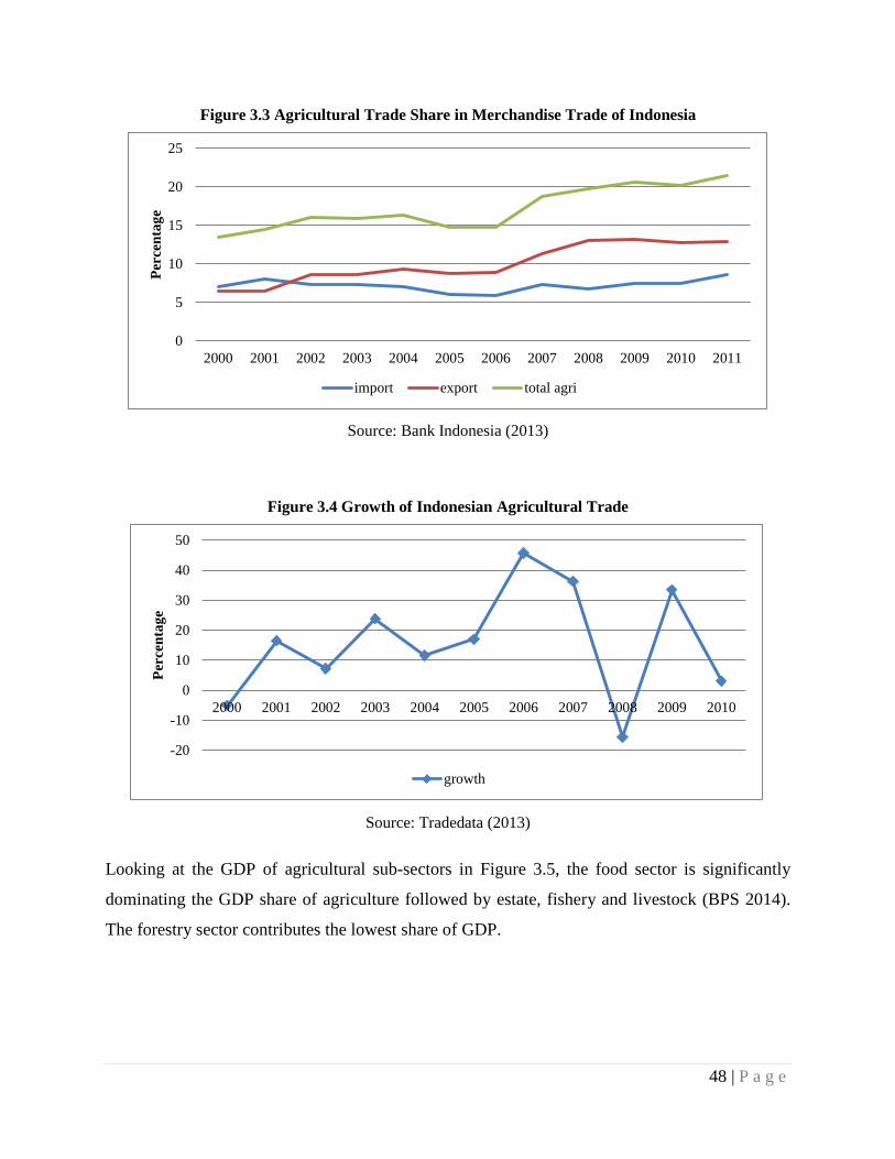
Figure 3.3 Agricultural Trade Share in Merchandise Trade of Indonesia

Source: Bank Indonesia (2013)

Figure 3.4 Growth of Indonesian Agricultural Trade

Source: Tradedata (2013)

Looking at the GDP of agricultural sub-sectors in Figure 3.5, the food sector is significantly

dominating the GDP share of agriculture followed by estate, fishery and livestock (BPS 2014).

The forestry sector contributes the lowest share of GDP.

0

5

10

15

20

25

2000 2001 2002 2003 2004 2005 2006 2007 2008 2009 2010 2011

Perc

enta

ge

import export total agri

-20

-10

0

10

20

30

40

50

2000 2001 2002 2003 2004 2005 2006 2007 2008 2009 2010

Perc

enta

ge

growth

48 | P a g e

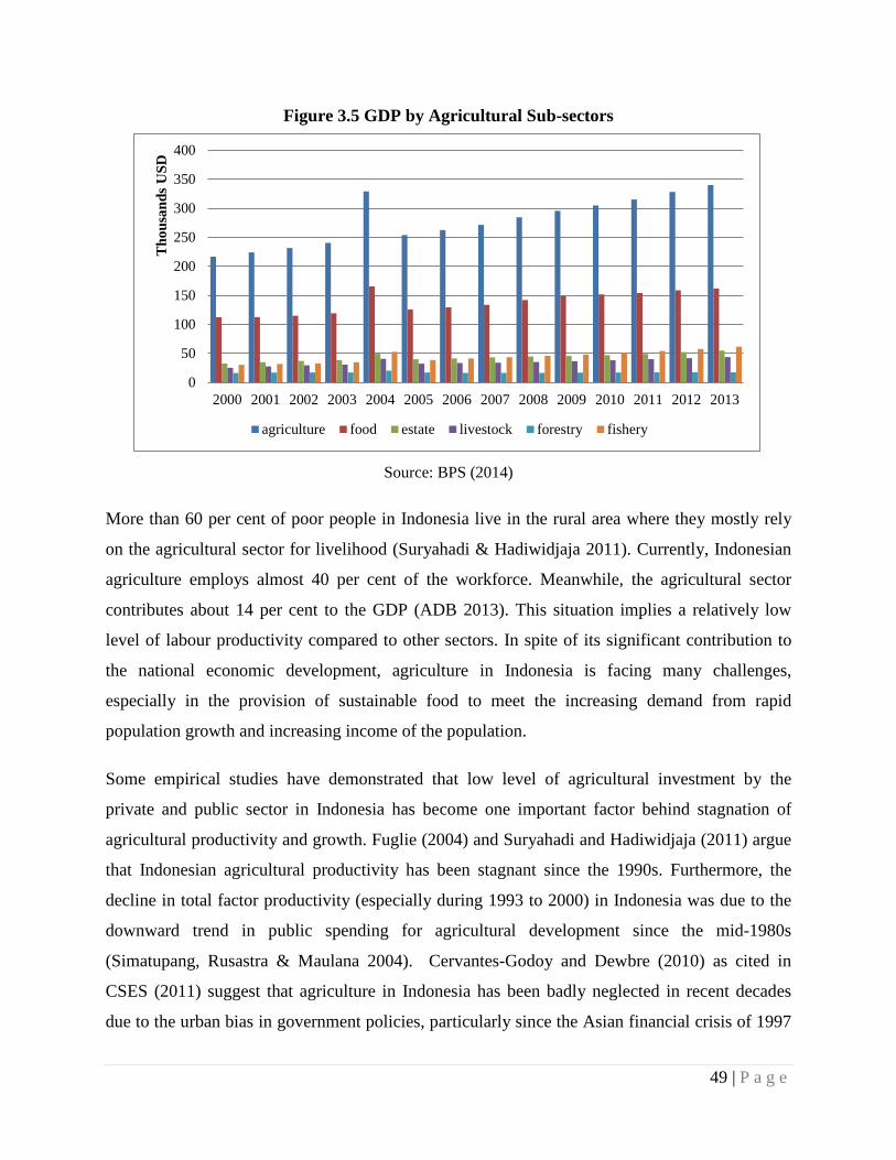
Figure 3.5 GDP by Agricultural Sub-sectors

Source: BPS (2014)

More than 60 per cent of poor people in Indonesia live in the rural area where they mostly rely

on the agricultural sector for livelihood (Suryahadi & Hadiwidjaja 2011). Currently, Indonesian

agriculture employs almost 40 per cent of the workforce. Meanwhile, the agricultural sector

contributes about 14 per cent to the GDP (ADB 2013). This situation implies a relatively low

level of labour productivity compared to other sectors. In spite of its significant contribution to

the national economic development, agriculture in Indonesia is facing many challenges,

especially in the provision of sustainable food to meet the increasing demand from rapid

population growth and increasing income of the population.

Some empirical studies have demonstrated that low level of agricultural investment by the

private and public sector in Indonesia has become one important factor behind stagnation of

agricultural productivity and growth. Fuglie (2004) and Suryahadi and Hadiwidjaja (2011) argue

that Indonesian agricultural productivity has been stagnant since the 1990s. Furthermore, the

decline in total factor productivity (especially during 1993 to 2000) in Indonesia was due to the

downward trend in public spending for agricultural development since the mid-1980s

(Simatupang, Rusastra & Maulana 2004). Cervantes-Godoy and Dewbre (2010) as cited in

CSES (2011) suggest that agriculture in Indonesia has been badly neglected in recent decades

due to the urban bias in government policies, particularly since the Asian financial crisis of 1997

0

50

100

150

200

250

300

350

400

2000 2001 2002 2003 2004 2005 2006 2007 2008 2009 2010 2011 2012 2013

Tho

usan

ds U

SD

agriculture food estate livestock forestry fishery

49 | P a g e

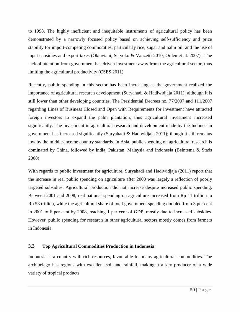
to 1998. The highly inefficient and inequitable instruments of agricultural policy has been

demonstrated by a narrowly focused policy based on achieving self-sufficiency and price

stability for import-competing commodities, particularly rice, sugar and palm oil, and the use of

input subsidies and export taxes (Oktaviani, Setyoko & Vanzetti 2010; Orden et al. 2007). The

lack of attention from government has driven investment away from the agricultural sector, thus

limiting the agricultural productivity (CSES 2011).

Recently, public spending in this sector has been increasing as the government realized the

importance of agricultural research development (Suryahadi & Hadiwidjaja 2011); although it is

still lower than other developing countries. The Presidential Decrees no. 77/2007 and 111/2007

regarding Lines of Business Closed and Open with Requirements for Investment have attracted

foreign investors to expand the palm plantation, thus agricultural investment increased

significantly. The investment in agricultural research and development made by the Indonesian

government has increased significantly (Suryahadi & Hadiwidjaja 2011); though it still remains

low by the middle-income country standards. In Asia, public spending on agricultural research is

dominated by China, followed by India, Pakistan, Malaysia and Indonesia (Beintema & Stads

2008)

With regards to public investment for agriculture, Suryahadi and Hadiwidjaja (2011) report that

the increase in real public spending on agriculture after 2000 was largely a reflection of poorly

targeted subsidies. Agricultural production did not increase despite increased public spending.

Between 2001 and 2008, real national spending on agriculture increased from Rp 11 trillion to

Rp 53 trillion, while the agricultural share of total government spending doubled from 3 per cent

in 2001 to 6 per cent by 2008, reaching 1 per cent of GDP, mostly due to increased subsidies.

However, public spending for research in other agricultural sectors mostly comes from farmers

in Indonesia.

3.3 Top Agricultural Commodities Production in Indonesia

Indonesia is a country with rich resources, favourable for many agricultural commodities. The

archipelago has regions with excellent soil and rainfall, making it a key producer of a wide

variety of tropical products.

50 | P a g e

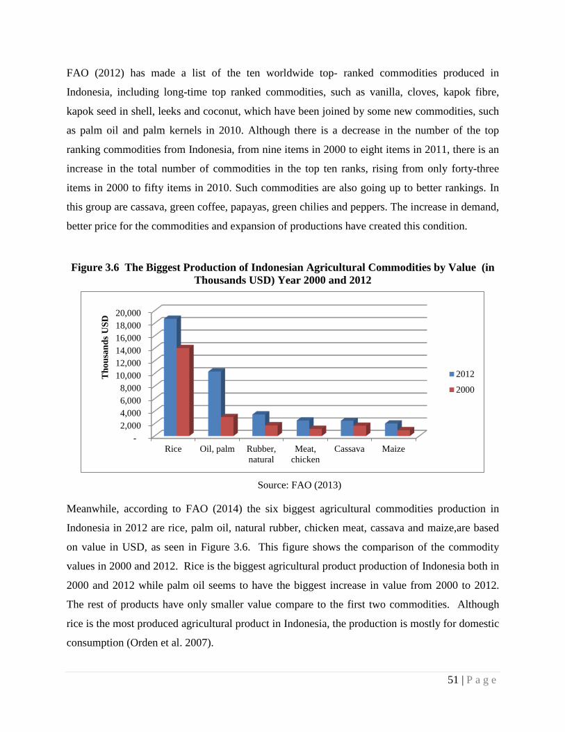
FAO (2012) has made a list of the ten worldwide top- ranked commodities produced in

Indonesia, including long-time top ranked commodities, such as vanilla, cloves, kapok fibre,

kapok seed in shell, leeks and coconut, which have been joined by some new commodities, such

as palm oil and palm kernels in 2010. Although there is a decrease in the number of the top

ranking commodities from Indonesia, from nine items in 2000 to eight items in 2011, there is an

increase in the total number of commodities in the top ten ranks, rising from only forty-three

items in 2000 to fifty items in 2010. Such commodities are also going up to better rankings. In

this group are cassava, green coffee, papayas, green chilies and peppers. The increase in demand,

better price for the commodities and expansion of productions have created this condition.

Figure 3.6 The Biggest Production of Indonesian Agricultural Commodities by Value (in Thousands USD) Year 2000 and 2012

Source: FAO (2013)

Meanwhile, according to FAO (2014) the six biggest agricultural commodities production in

Indonesia in 2012 are rice, palm oil, natural rubber, chicken meat, cassava and maize,are based

on value in USD, as seen in Figure 3.6. This figure shows the comparison of the commodity

values in 2000 and 2012. Rice is the biggest agricultural product production of Indonesia both in

2000 and 2012 while palm oil seems to have the biggest increase in value from 2000 to 2012.

The rest of products have only smaller value compare to the first two commodities. Although

rice is the most produced agricultural product in Indonesia, the production is mostly for domestic

consumption (Orden et al. 2007).

- 2,000 4,000 6,000 8,000

10,000 12,000 14,000 16,000 18,000 20,000

Rice Oil, palm Rubber,natural

Meat,chicken

Cassava Maize

Tho

usan

ds U

SD

2012

2000

51 | P a g e

In contrast, palm oil is the third largest agricultural product in Indonesia, but it is mostly

exported (Ministry of Industry 2011). The rapid growth of agricultural exports in Indonesia can

be attributed to the booming palm oil sector. The investment allocated in the agricultural sectors

has been increasing, especially in palm oil industry (Ministry of Industry 2011) leading to

increasing production. Higher production and higher demand of these products have led palm oil

products to become the third biggest exported commodity from Indonesia (BPS 2014). Thus,

palm oil is one of the most important commodities supporting Indonesian exports earning foreign

exchange (Pusdatin 2013).

Figure 3.7 The Biggest Productions of Indonesian Agricultural Commodities by Quantity (in Thousand Metric Tonnes) Year 2000 and 2012

Source: FAO (2013)

Figure 3.7 presents the biggest agricultural production of Indonesia in terms of quantity for year

2000 and 2012. Rice is the biggest production in both years, followed by sugar cane, cassava,

palm oil, maize and coconut. Palm oil has witnessed strong growth in quantity from 2000 to

2012 while sugarcane seems to have smallest growth in focused years. Although natural rubber

is high in value but it is small in production so that it is not in the list of six biggest commodities.

But some commodities that have higher value, that is natural rubber, chicken meat, however,

have very poor growth in production capacity. This could be a result of change in world demand

as well as production conditions, for example, the development of palm plantations are more

0

10000

20000

30000

40000

50000

60000

70000

Rice Sugar cane Cassava Oil, palm Maize Coconuts

Tho

usan

ds M

T

2012

2000

52 | P a g e

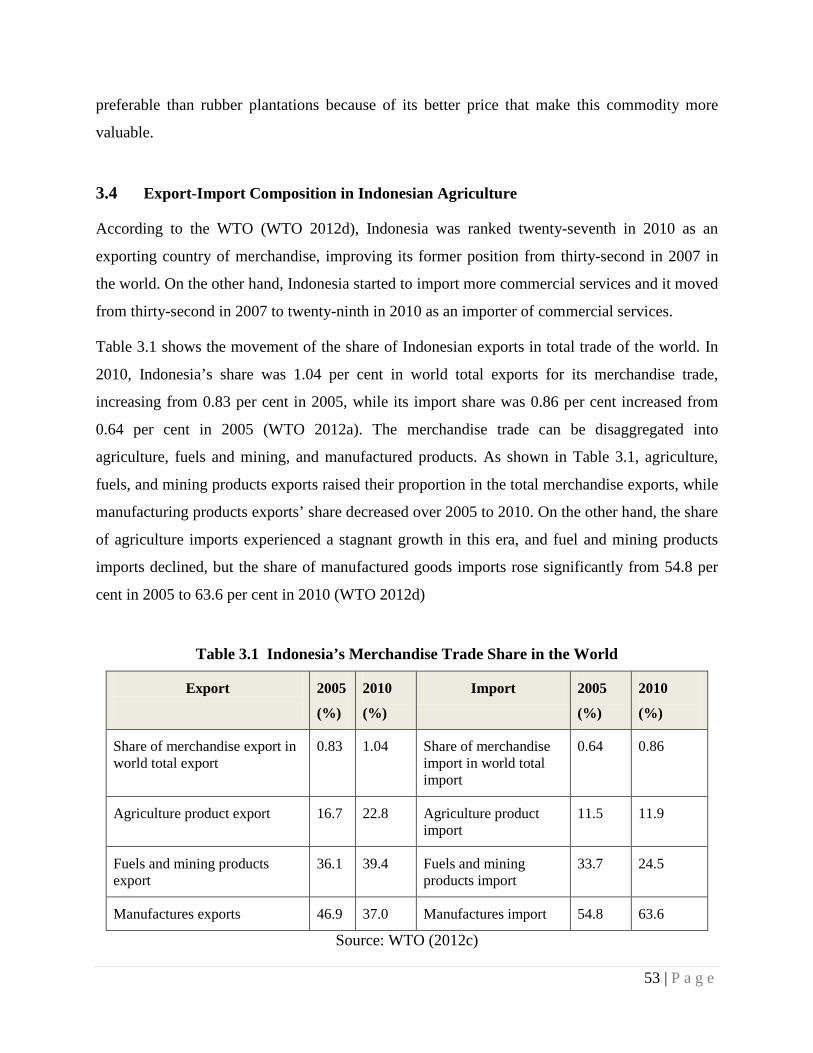
preferable than rubber plantations because of its better price that make this commodity more

valuable.

3.4 Export-Import Composition in Indonesian Agriculture

According to the WTO (WTO 2012d), Indonesia was ranked twenty-seventh in 2010 as an

exporting country of merchandise, improving its former position from thirty-second in 2007 in

the world. On the other hand, Indonesia started to import more commercial services and it moved

from thirty-second in 2007 to twenty-ninth in 2010 as an importer of commercial services.

Table 3.1 shows the movement of the share of Indonesian exports in total trade of the world. In

2010, Indonesia’s share was 1.04 per cent in world total exports for its merchandise trade,

increasing from 0.83 per cent in 2005, while its import share was 0.86 per cent increased from

0.64 per cent in 2005 (WTO 2012a). The merchandise trade can be disaggregated into

agriculture, fuels and mining, and manufactured products. As shown in Table 3.1, agriculture,

fuels, and mining products exports raised their proportion in the total merchandise exports, while

manufacturing products exports’ share decreased over 2005 to 2010. On the other hand, the share

of agriculture imports experienced a stagnant growth in this era, and fuel and mining products

imports declined, but the share of manufactured goods imports rose significantly from 54.8 per

cent in 2005 to 63.6 per cent in 2010 (WTO 2012d)

Table 3.1 Indonesia’s Merchandise Trade Share in the World

Export

2005

(%)

2010

(%)

Import 2005

(%)

2010

(%)

Share of merchandise export in world total export

0.83 1.04 Share of merchandise import in world total import

0.64 0.86

Agriculture product export 16.7 22.8 Agriculture product import

11.5 11.9

Fuels and mining products export

36.1 39.4 Fuels and mining products import

33.7 24.5

Manufactures exports 46.9 37.0 Manufactures import 54.8 63.6

Source: WTO (2012c)

53 | P a g e

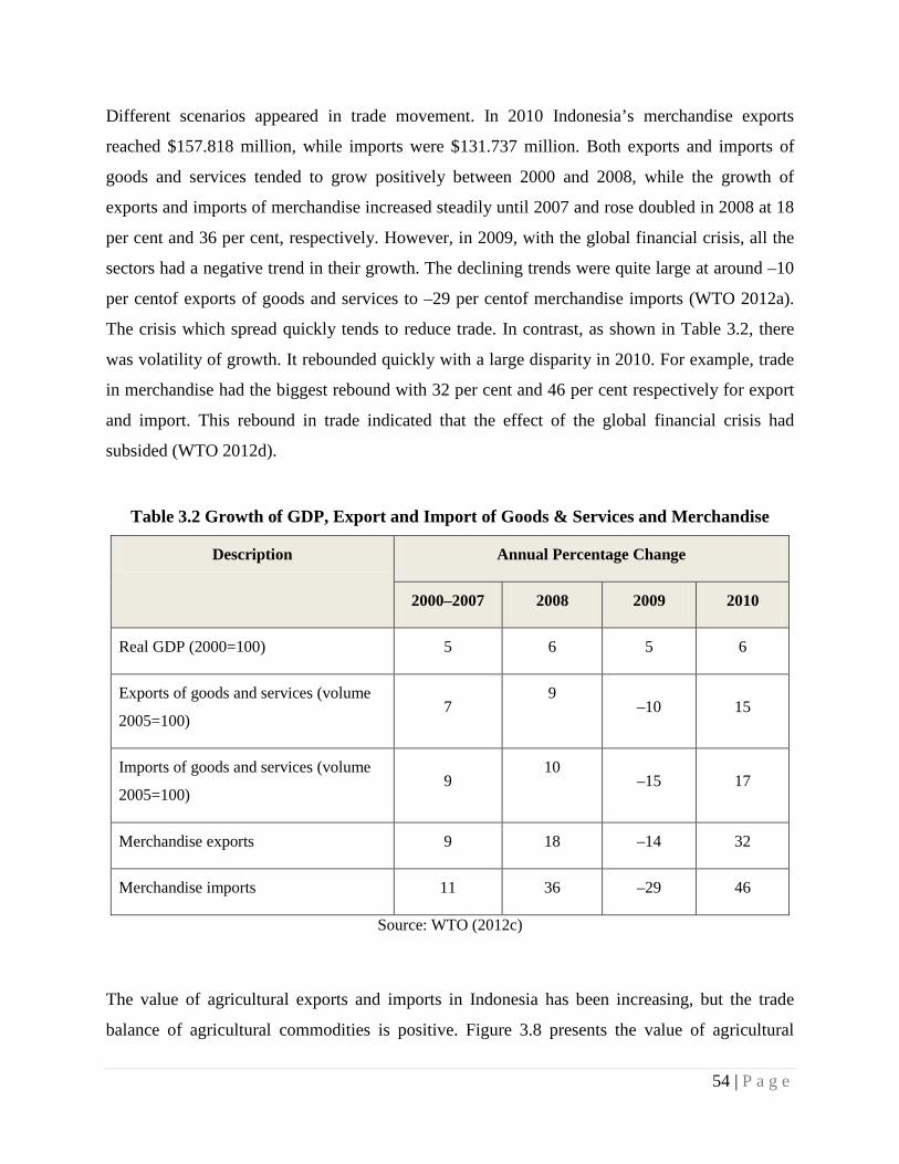
Different scenarios appeared in trade movement. In 2010 Indonesia’s merchandise exports

reached $157.818 million, while imports were $131.737 million. Both exports and imports of

goods and services tended to grow positively between 2000 and 2008, while the growth of

exports and imports of merchandise increased steadily until 2007 and rose doubled in 2008 at 18

per cent and 36 per cent, respectively. However, in 2009, with the global financial crisis, all the

sectors had a negative trend in their growth. The declining trends were quite large at around –10

per centof exports of goods and services to –29 per centof merchandise imports (WTO 2012a).

The crisis which spread quickly tends to reduce trade. In contrast, as shown in Table 3.2, there

was volatility of growth. It rebounded quickly with a large disparity in 2010. For example, trade

in merchandise had the biggest rebound with 32 per cent and 46 per cent respectively for export

and import. This rebound in trade indicated that the effect of the global financial crisis had

subsided (WTO 2012d).

Table 3.2 Growth of GDP, Export and Import of Goods & Services and Merchandise

Description Annual Percentage Change

2000–2007 2008 2009 2010

Real GDP (2000=100) 5 6 5 6

Exports of goods and services (volume

2005=100) 7

9 –10 15

Imports of goods and services (volume

2005=100) 9

10 –15 17

Merchandise exports 9 18 –14 32

Merchandise imports 11 36 –29 46

Source: WTO (2012c)

The value of agricultural exports and imports in Indonesia has been increasing, but the trade

balance of agricultural commodities is positive. Figure 3.8 presents the value of agricultural

54 | P a g e

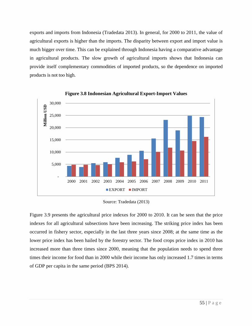
exports and imports from Indonesia (Tradedata 2013). In general, for 2000 to 2011, the value of

agricultural exports is higher than the imports. The disparity between export and import value is

much bigger over time. This can be explained through Indonesia having a comparative advantage

in agricultural products. The slow growth of agricultural imports shows that Indonesia can

provide itself complementary commodities of imported products, so the dependence on imported

products is not too high.

Figure 3.8 Indonesian Agricultural Export-Import Values

Source: Tradedata (2013)

Figure 3.9 presents the agricultural price indexes for 2000 to 2010. It can be seen that the price

indexes for all agricultural subsections have been increasing. The striking price index has been

occurred in fishery sector, especially in the last three years since 2008; at the same time as the

lower price index has been hailed by the forestry sector. The food crops price index in 2010 has

increased more than three times since 2000, meaning that the population needs to spend three

times their income for food than in 2000 while their income has only increased 1.7 times in terms

of GDP per capita in the same period (BPS 2014).

-

5,000

10,000

15,000

20,000

25,000

30,000

2000 2001 2002 2003 2004 2005 2006 2007 2008 2009 2010 2011

Mill

ion

USD

EXPORT IMPORT

55 | P a g e

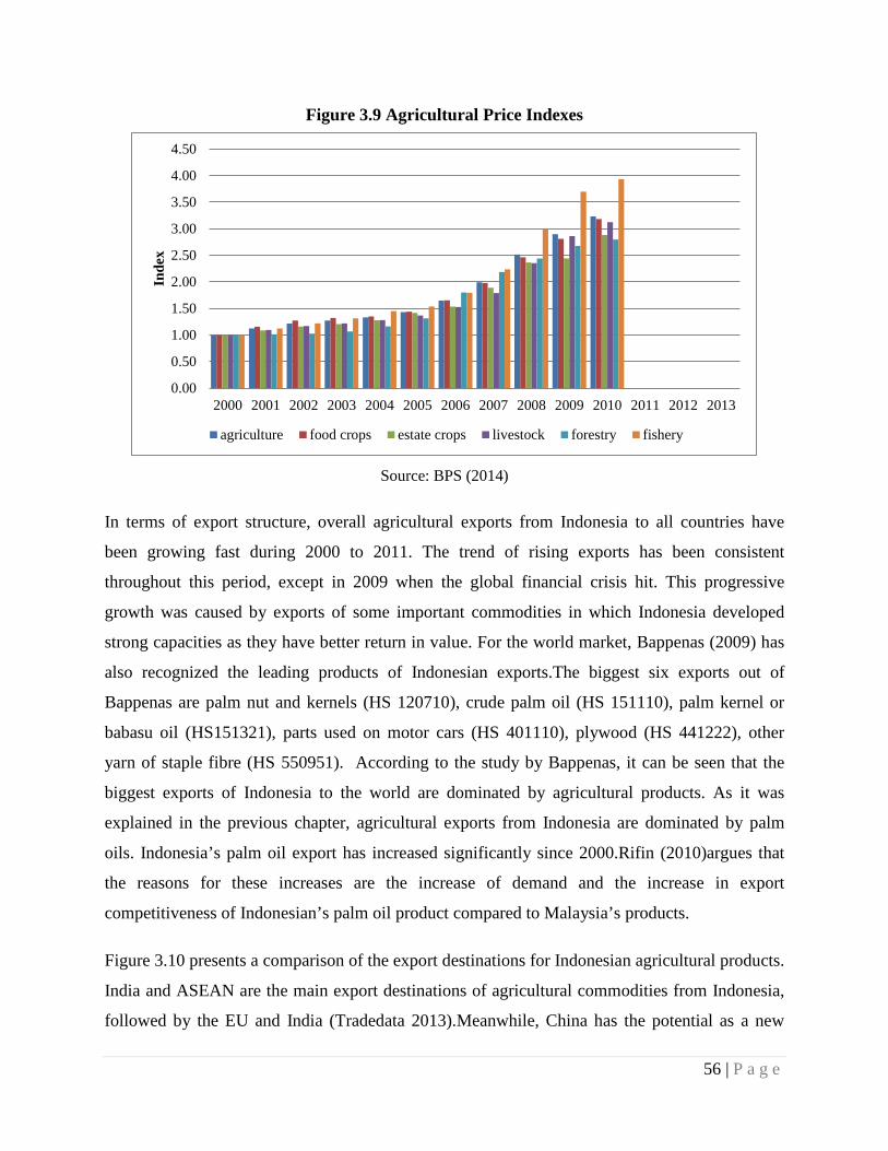
Figure 3.9 Agricultural Price Indexes

Source: BPS (2014)

In terms of export structure, overall agricultural exports from Indonesia to all countries have

been growing fast during 2000 to 2011. The trend of rising exports has been consistent

throughout this period, except in 2009 when the global financial crisis hit. This progressive

growth was caused by exports of some important commodities in which Indonesia developed

strong capacities as they have better return in value. For the world market, Bappenas (2009) has

also recognized the leading products of Indonesian exports.The biggest six exports out of

Bappenas are palm nut and kernels (HS 120710), crude palm oil (HS 151110), palm kernel or

babasu oil (HS151321), parts used on motor cars (HS 401110), plywood (HS 441222), other

yarn of staple fibre (HS 550951). According to the study by Bappenas, it can be seen that the

biggest exports of Indonesia to the world are dominated by agricultural products. As it was

explained in the previous chapter, agricultural exports from Indonesia are dominated by palm

oils. Indonesia’s palm oil export has increased significantly since 2000.Rifin (2010)argues that

the reasons for these increases are the increase of demand and the increase in export

competitiveness of Indonesian’s palm oil product compared to Malaysia’s products.

Figure 3.10 presents a comparison of the export destinations for Indonesian agricultural products.

India and ASEAN are the main export destinations of agricultural commodities from Indonesia,

followed by the EU and India (Tradedata 2013).Meanwhile, China has the potential as a new

0.00

0.50

1.00

1.50

2.00

2.50

3.00

3.50

4.00

4.50

2000 2001 2002 2003 2004 2005 2006 2007 2008 2009 2010 2011 2012 2013

Inde

x

agriculture food crops estate crops livestock forestry fishery

56 | P a g e

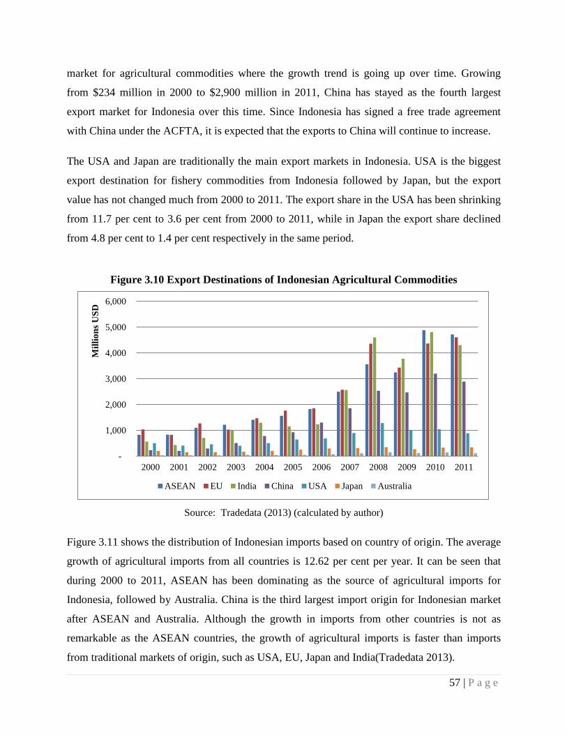
market for agricultural commodities where the growth trend is going up over time. Growing

from $234 million in 2000 to $2,900 million in 2011, China has stayed as the fourth largest

export market for Indonesia over this time. Since Indonesia has signed a free trade agreement

with China under the ACFTA, it is expected that the exports to China will continue to increase.

The USA and Japan are traditionally the main export markets in Indonesia. USA is the biggest

export destination for fishery commodities from Indonesia followed by Japan, but the export

value has not changed much from 2000 to 2011. The export share in the USA has been shrinking

from 11.7 per cent to 3.6 per cent from 2000 to 2011, while in Japan the export share declined

from 4.8 per cent to 1.4 per cent respectively in the same period.

Figure 3.10 Export Destinations of Indonesian Agricultural Commodities

Source: Tradedata (2013) (calculated by author)

Figure 3.11 shows the distribution of Indonesian imports based on country of origin. The average

growth of agricultural imports from all countries is 12.62 per cent per year. It can be seen that

during 2000 to 2011, ASEAN has been dominating as the source of agricultural imports for

Indonesia, followed by Australia. China is the third largest import origin for Indonesian market

after ASEAN and Australia. Although the growth in imports from other countries is not as

remarkable as the ASEAN countries, the growth of agricultural imports is faster than imports

from traditional markets of origin, such as USA, EU, Japan and India(Tradedata 2013).

-

1,000

2,000

3,000

4,000

5,000

6,000

2000 2001 2002 2003 2004 2005 2006 2007 2008 2009 2010 2011

Mill

ions

USD

ASEAN EU India China USA Japan Australia

57 | P a g e

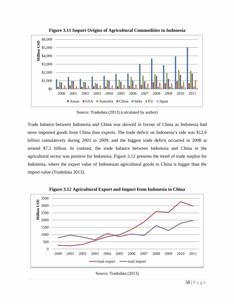
Figure 3.11 Import Origins of Agricultural Commodities to Indonesia

Source: Tradedata (2013) (calculated by author)

Trade balance between Indonesia and China was skewed in favour of China as Indonesia had

more imported goods from China than exports. The trade deficit on Indonesia’s side was $12.6

billion cumulatively during 2003 to 2009; and the biggest trade deficit occurred in 2008 at

around $7.2 billion. In contrast, the trade balance between Indonesia and China in the

agricultural sector was positive for Indonesia. Figure 3.12 presents the trend of trade surplus for

Indonesia, where the export value of Indonesian agricultural goods to China is bigger than the

import value (Tradedata 2013).

Figure 3.12 Agricultural Export and Import from Indonesia to China

Source: Tradedata (2013)

$0

$1,000

$2,000

$3,000

$4,000

$5,000

$6,000

2000 2001 2002 2003 2004 2005 2006 2007 2008 2009 2010 2011

Mill

ion

USD

Asean USA Australia China India EU Japan

0

500

1000

1500

2000

2500

3000

3500

2000 2001 2002 2003 2004 2005 2006 2007 2008 2009 2010 2011

Mill

ion

USD

total export total import

58 | P a g e

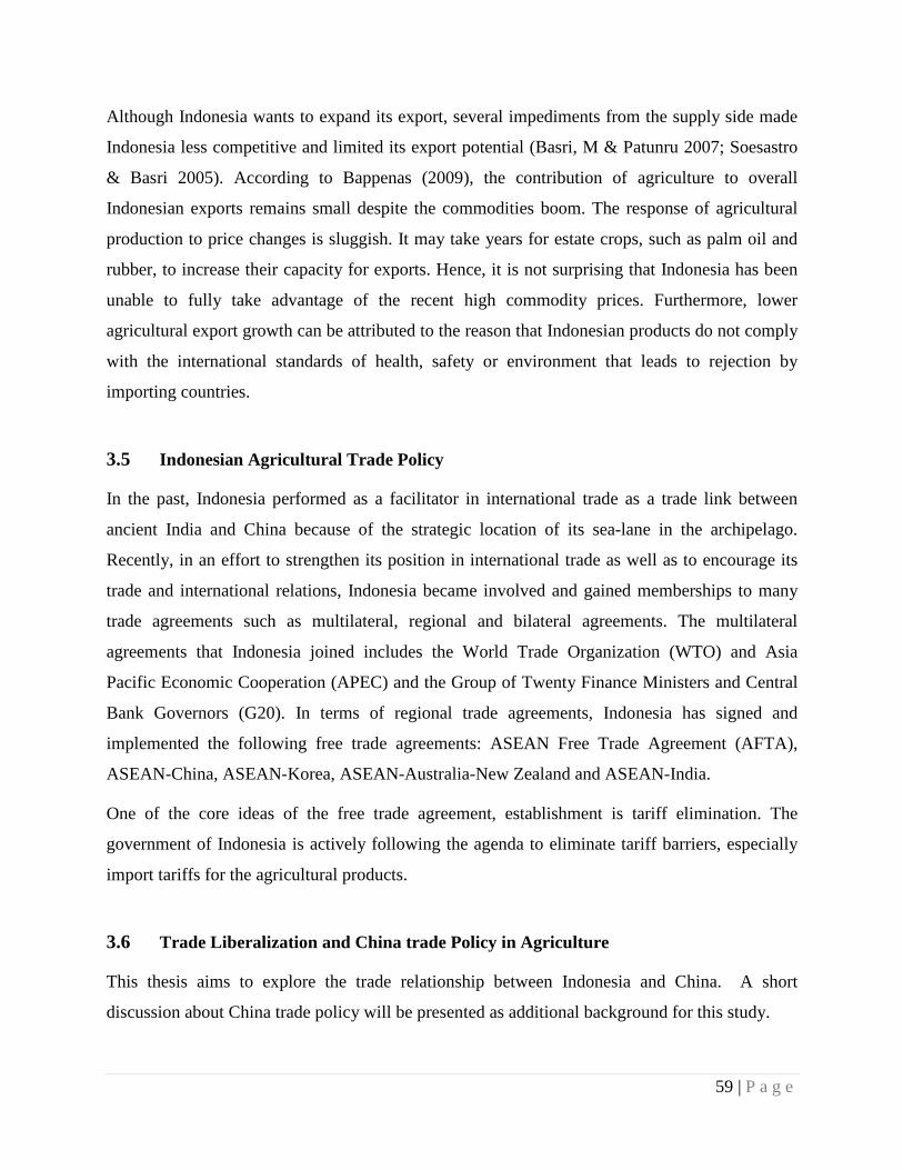
Although Indonesia wants to expand its export, several impediments from the supply side made

Indonesia less competitive and limited its export potential (Basri, M & Patunru 2007; Soesastro

& Basri 2005). According to Bappenas (2009), the contribution of agriculture to overall

Indonesian exports remains small despite the commodities boom. The response of agricultural

production to price changes is sluggish. It may take years for estate crops, such as palm oil and

rubber, to increase their capacity for exports. Hence, it is not surprising that Indonesia has been

unable to fully take advantage of the recent high commodity prices. Furthermore, lower

agricultural export growth can be attributed to the reason that Indonesian products do not comply

with the international standards of health, safety or environment that leads to rejection by

importing countries.

3.5 Indonesian Agricultural Trade Policy

In the past, Indonesia performed as a facilitator in international trade as a trade link between

ancient India and China because of the strategic location of its sea-lane in the archipelago.

Recently, in an effort to strengthen its position in international trade as well as to encourage its

trade and international relations, Indonesia became involved and gained memberships to many

trade agreements such as multilateral, regional and bilateral agreements. The multilateral

agreements that Indonesia joined includes the World Trade Organization (WTO) and Asia

Pacific Economic Cooperation (APEC) and the Group of Twenty Finance Ministers and Central

Bank Governors (G20). In terms of regional trade agreements, Indonesia has signed and

implemented the following free trade agreements: ASEAN Free Trade Agreement (AFTA),

ASEAN-China, ASEAN-Korea, ASEAN-Australia-New Zealand and ASEAN-India.

One of the core ideas of the free trade agreement, establishment is tariff elimination. The

government of Indonesia is actively following the agenda to eliminate tariff barriers, especially

import tariffs for the agricultural products.

3.6 Trade Liberalization and China trade Policy in Agriculture

This thesis aims to explore the trade relationship between Indonesia and China. A short

discussion about China trade policy will be presented as additional background for this study.

59 | P a g e

China’s ‘open door’ trade policy began when it gained WTO membership in 2001. The open

market access has lowered the import tariff of agricultural commodities and increased access to

China’s market for foreign agricultural products. In return, China’s agricultural products have

greater access in order to penetrate foreign markets (Martin 2001).

However, according to Chen, C and Duncan (2008), lowering the import tariffs does not

necessarily improve import growth. Indeed, China has a comparative advantage for some

agricultural products. For example, lowering tariff rates on horticulture and meat products might

impact on only a small part of the China’s domestic market, such as those who only buy and sell

high quality products, such as meat for five star hotels that serve foreigners. Although the tariff

has fallen for these commodities, since China export the commodities at below the market prices,

the reduction has not affected the traders and producers. For the commodities where China has

no comparative advantage, but have strong demand in domestic market, called ‘national strategic

products’ such as edible oil, rice, maize, sugar, cotton and wool, China has special treatments

that are allowed under the WTO agreement by imposing higher rates for in-quota tariff (TRQ)

and place a quota on these commodities. This trade policy has become the background of the

commodities selection involved in the ACFTA programs.

3.7 Conclusion

This chapter has provided an extensive background in this thesis comprising a literature review

of the importance of the agricultural sector, the agricultural strength of Indonesia, the terms of

trade of Indonesian agricultural product in agriculture and agricultural trade policy on

agricultural sector in Indonesia.

Indonesia has very good position in its agricultural trade. While agricultural shares in

merchandise export is declining worldwide, in Indonesia it is increasing. Furthermore, the trade

balance of agricultural commodities is positive means that exports are bigger than imports. It

denotes that agricultural exports have an important position yet potential to contribute more to

economic growth of Indonesia.

To explore and enhance the potential exports of agricultural products, the Indonesian

government is involved in many free trade agreements to enhance its trade, especially its

agricultural trade including the ACFTA. While the potential of agricultural products is very big,

60 | P a g e

the government expects adopting free trade will boost the trade in agriculture. However, the

results of the implementation of the free trade agreement in Indonesia have been rarely

measured. This chapter provided a detailed background of this thesis and is the foundation for

the next chapters.

61 | P a g e

Chapter 4

Have Agricultural Exports Under the ASEAN-China Free Trade Agreement

Increased Economic Growth in Indonesia?

4.1 Introduction

As identified in Chapter Three, the potential of agricultural exports of Indonesia is promising

with its increasing share in merchandise export as well as GDP. Joining the ACFTA is believed

can improve the trade which can further contribute more to economic growth.

According to Basri, M.C. (2010), Indonesia becomes one of the fastest growing countries in Asia

with economic growth of 6.1 per cent per year and agricultural exports from Indonesia have been

increasing significantly. As a consequence, it is important to measure whether agricultural

exports to China under the ACFTA can improve economic growth. This chapter is concerned

with accomplishing the objective ii stated in Chapter 1: ‘to investigate the impact of agricultural

exports under the ACFTA on Indonesian economic growth by using a rigorous methodology’.

The objective derives from the first research question guiding this thesis: ‘Is agricultural trade

still important for Indonesia? To what extent does agricultural export contribute to the economic

growth of Indonesia?

This chapter implements the generalized gravity model , estimated by the two stage least square

(2SLS) to map the impact of agricultural exports under the ACFTA with China on Indonesia’s

economic growth. The data used in the estimation are derived from the rates of change or growth

except for binary variables. Because of limited data availability, the period of study is from 1996

until 2012, with figures derived on a quarterly basis.

The chapter is divided into three parts. The first part presents a comprehensive literature review

of previous empirical studies that have yielded disparate results on the relationship between

economic growth and agricultural exports. This is followed by an outline of the generalized

gravity model that has been used effectively in previous research to map the effect of exports on

economic growth and its determinants. The second part of the chapter discusses the methodology

used for the estimation elaborating this with a description of the theoretical framework of

62 | P a g e

generalized gravity models constructed to model the impact of Indonesian agricultural exports on

economic growth along with the accompanying statistical tools and data used within the model.

The third and final part will present the results of the quantitative analysis, beginning with a

presentation of the statistical results of the model and followed by discussion of the impact of

Indonesian agricultural exports for economic growth as well as that of other determinants used in

the model.

4.2 Literature Review

Most economies depend on a diverse portfolio of unprocessed and processed primary-based

exports to generate foreign exchange. Indeed, exports-led growth theory postulating the positive

role of general exports in increasing economic growth proved by numerous studies in the

literature (Giles & Williams 2000). However, most of these studies account for total exports and

do not focus their attention on the study of agricultural exports and economic growth. Despite its

declining share of GDP, the lack of attention from governments and private sectors to the

agricultural sector is one of the reasons why the research on the impact of agricultural exports for

growth is very limited (World Bank 2008).

In their seminal article ‘The role of agriculture in economic development’, Johnston and Mellor

(1961) explain that expanding agricultural exports is one of the most promising means of

increasing incomes. Although recent empirical studies in this area are rare, many scholars agree

that agricultural export has a positive impact on economic growth in the short-run, for example,

Levin and Raut (1997) and Dawson (2005). Similarly, (Sanjuán‐López & Dawson 2010) find

that there is long-term relationship between agricultural exports and economic growth in

developing countries.

Export-led growth from agriculture may provide an optimal resource allocation for those

countries that have a comparative advantage in agricultural production. This positive view can be

interpreted that the agricultural sector should open to international trade to earn foreign

exchange.

On the other hand, there is a contradict view which suggests that the effect of specialized in

export of primary product is detrimental to growth. The strongest example of this view is found

63 | P a g e

in the Prebisch-Singer thesis (Prebisch 1950; Singer 1950) which states that the price of primary

products is on a long-term downward trend relative to the price of manufactured goods. This

downward slide is also caused by the volatility of primary product prices, consequently exporters

of these products experience greater instability of export revenue.

Furthermore, there are many empirical studies that show increasing evidence to support this

postulation across the world. In their analysis of the share of primary exports as a percentage of

GDP across the world, Sachs and Warner (1997a) find that primary exports recorded a

significantly negative coefficient in growth regression for eighty-three countries from 1965 to

1990. Similarly, Sala-i-Martin (1997) shows that the 1970 share of primary products in total

exports is robustly and negatively correlated with growth over many alternative regression

specifications. Sprout and Weaver (1992) argue that primary product exports do not affect

economic growth. Similarly, Esfahani, Sprout and Weaver (1992) examine the causality between

economic growth and export of small non-primary primary products in large developing

countries. They find small non-primary exports have a positive and significant impact on

economic growth while primary product exports do not affect economic growth.

Along with these global studies, research focused on specific countries has also found similar

results. In his study, Faridi (2012) implements Johansen’s co-integration test to measure the

impact of agricultural and non-agricultural exports to Pakistan’s economic growth. The finding

shows that agricultural exports have a negative and significant impact on Pakistan’s economic

growth while non-agricultural exports promote economic growth.

4.2.1 Export-Led Growth Theory Approach

The neoclassical theory of export-led growth has been used voluminously in the literature on the

relation between export and growth. This theory supports the idea that economic growth can be

achieved by exports(Adelman 1984). The theories based on that hypothesis can be described as

follows:

1. In accordance with the short-run Keynesian arguments, export growth leads to income

growth via the foreign trade multiplier effect (Stolper 1947).

64 | P a g e

2. Foreign exchange from exports can be used to finance imports manufactured and capital

goods and technology, which contribute to growth (Chenery & Strout 1966).

3. Competition leads to scale economies, technological advance and growth (Helpman &

Krugman 1985).

4. According to endogenous growth theory, the export sector creates positive externalities,

such as more efficient production methods, which lead to growth (Balassa, B 1978;

Grossman, G.M. & Helpman 1994).

5. The foreign trade multiplier analysis asserts that, given the spending function, an export

surplus will have an expansionary effect whose magnitude depends on the marginal

propensity to import. Transfer of scarce resources from low-productivity domestic industries

to higher-productivity export industries results in an increase in overall productivity,

accelerating output growth (McCombie & Thirlwall 1997). A higher level of exports might

contribute to economic growth as export revenues provide an important source of foreign

exchange, which is crucial when domestic saving are inadequate for making imports of

capital goods possible (Bairam & Dempster 1991)

6. Finally, export growth might also trigger economic growth through the expansion of the

efficient market size, bringing in substantial economies of scale that accelerate the rate of

capital formation and technical change (Reppas & Christopoulos 2005).

There are also further arguments supporting this hypothesis, such as those presented by Ben-

David and Loewy (1998); Hart (1983); Lal, D and Rajapatirana (1987). They argue that the

increased demand for export creates incentives for specialization in the export sector, scale

economies and reallocation of resources from the less efficient non-trade sector to the most

efficient trade sector; it ultimately increases productivity and output growth. In particular, it has

been argued that higher exports enhance access to advanced technologies, skill improvement,

learning by doing, management techniques and entrepreneurial activity (Ben-David & Loewy

1998).

Balassa, BA (1980) states that, in general, the production of export goods is concentrated in the

most efficient economic sectors, thus the export expansion helps channel investment in these

sectors, which in turn increases the overall productivity of the economy while Tyler

65 | P a g e

(1981)argues that a large export sector also allows a country to gain from economies of scales

and positive externalities that may lead to increased growth. This argument proposes that

domestic markets are too small for the optimal scale to be achieved, while increasing returns may

occur with access to foreign markets (Giles & Williams 2000). Furthermore, foreign competition

increases the pressure on industries exporting goods to keep costs relatively low and to promote

technological changes, which in turn improves productivity (Kavoussi 1984; Michaely 1977) and

may cause the workers’ skill level to rise in the export sector. Kavoussi (1984) also states the

growth of exports has a stimulating effect on total productivity of the economy as a whole

through its positive impact on higher rates of capital accumulation. Chenery and Strout (1966)

propose the ‘two-gap model’ which states that if the foreign exchange constraint is binding, the

growth of exports reduces the foreign exchange constraint, thereby facilitating imports of capital

goods and faster growth (Fajana 1979; Voivodas 1974; Williamson 1978). Feder (1983)

measures the contribution of exports to economic growth through resource allocation. By

dividing the economy into export and non-export sectors, and introducing exports into the

production of the non-export sectors, he finds exports have generated positive externalities for

the non-export sectors. Athukorala, Premachandra and Menon (1996) state export expansion

increases employment and real wages, leading to domestic spending which is becomes source of

output growth. Lal, D and Rajapatirana (1987) argue that an outward-oriented strategy of

development may provide greater opportunities and rewards for entrepreneurial activity, which is

the key to extended growth, as it is the entrepreneur who will seek out risk and opportunity.

While the above arguments support the hypothesis of export-led growth, some other researchers

provide only limited support to the export-led growth theory (Chen, EKY 1997; Chow, PCY

1987); and yet others yield mixed results (Kunst & Marin 1989; Nishimizu & Robinson 1984;

Oxley 1993; Tybout 1992).

Furthermore, some literature in this area focuses on Indonesia. Most of the studies use co-

integration test, error correction models and Granger-causality test to examine the relationship

between export and economic growth. Among those studies show that from a range of growth

factors, exporting has a strong influence on economic growth (Islam 1998; Jung & Marshall

1985; Piazolo 1996). Xu (1996) examines that the growth of export promotes the growth of the

economy of Indonesia. This evidence supports the idea that the export-led growth (ELG) theory

is applicable to Indonesia.

66 | P a g e

On the other hand, some studies on this relationship argue that the growth-led export (GLE)

theory is supported in Indonesia. For example,Ahmad, Jaleel and Harnhirun (1996) find that, for

Indonesia and other ASEAN countries, economic growth supports the growth of export; and

Rahman and Mustafa (1997) argue there are causality from economic growth to export growth

both in the short-run and the long- run.

The bi-directional causal relationship between economic growth and export growth in Indonesia

is shown by research conducted by Ekanayake (1999). By using annual data from 1960 to 1997

and employing the co-integration test and error correction models to examine the causal

relationship between exports and GDP for eight Asian developing countries, he showed that bi-

directional causality between those two variables exists in seven out of eight countries

considered. A study by Dodaro (1993) also shows the bi-directional causality between these two

variables in long-run equilibrium for Indonesia.

4.2.2 The Linkages of FDI and Growth

Often times, significant relationships between trade and growth may be due to improvement in

total productivity. Solow’s growth model attributes economic growth to capital accumulation,

labour force growth and technological change (Bhagwati, J. 1998). For developing countries,

capital accumulation can be generated by foreign direct investment (FDI) via the lower costs of

capital supplies. The impact of knowledge and technology spill-overs and diffusion can improve

the transformation of technology. Furthermore, FDI is considered as an important channel of

technology spill-overs from developed countries to developing countries through research and

development, including human capital development (Grossman, Gene M. & Helpman 1991).

The endogenous growth theory emphasizes trade as the principal channel through which

knowledge is transmitted internationally; from which the technological spill-overs could come

via imports as easily as exports (Grossman, Gene M. & Helpman 1991). Bhagwati, Jagdish

(1994) extends this theory through their ‘immiserizing growth theory’ that describes FDI flows

into a country with import substitution but restrictive trade policies can slow growth. Because

FDI has mostly moved into high capital intensity production, these countries lack comparative

advantage. On the other hand, the export promotion regime is superior to the import substitution

regime in reaping gains from FDI.

67 | P a g e

Foreign direct investment (FDI) has been a key aspect of increased globalisation in recent

decades. Growth in FDI has been higher than growth in international trade. Multinational firms

have come to account for about 10% of world output and 30% of world exports, and these firms

develop and control a large share of new technologies (Jungnickel 2002). The inflow of FDI

increased rapidly during the late 1980s and 1990s in almost every region of the world.

Given appropriate policies and a basic level of development, FDI can play a key role in the

process of creating a better economic environment. On the other hand, potential drawbacks do

exist, including a deterioration of the balance of payments as profits are repatriated, having

negative impacts on competition in national markets (Hansen & Rand 2006). The presence of

FDI in a certain industry, however, may exert an adverse effect on domestic firms in that

industry. By enjoying better technologies and lower production costs, firms with FDI may cut

into the market share of domestic firms without FDI. In a short-run imperfectly competitive

market structure, the productivity of domestic firms may be reduced when sales fall, so that fixed

costs are spread over fewer units. In the long run, however, the increased competition induced by

the increased presence of FDI in domestic industries may force inefficient domestic firms to exit

and surviving firms to improve their performance, leading to the potential improvement of social

welfare (Buckley, Peter J, Clegg & Wang 2002). At present the consensus seems to be that there

is a positive association between FDI inflows and economic growth, provided that receiving

countries have reached a minimum level of educational, technological and/or infrastructure

development. However, as in many other fields of development economics, there is not universal

agreement about the positive association between FDI inflows and economic growth (Hansen &

Rand 2006).

Numerous studies on the role of FDI in stimulating economic growth have been conducted.

Borensztein, De Gregorio and Lee (1998) argue FDI contributes to economic growth only when

a sufficient absorptive capability of the advanced technologies is available in the host

economy.De Mello Jr (1997) considers two main channels through which FDI may be growth

enhancing. First, FDI can encourage the adoption of new technology in the production process

through capital spillovers. Second, FDI may stimulate knowledge transfers, both in terms of

labour training and skill acquisition and by introducing alternative management practices and

better organisational arrangements. OECD (2002), in a survey, underpins that 11 out of 14

studies have found FDI to contribute positively to income growth and factor productivity. Both

68 | P a g e

de Mello and the OECD stress one key insight from all the studies reviewed: the way in which

FDI affects growth is likely to depend on the economic and technological conditions in the host

country. In particular, it appears that developing countries have to reach a certain level of

development, in education and/or infrastructure, before they are able to capture potential benefits

associated with FDI.

Meanwhile, in addition to the direct capital financing it supplies, FDI can be a source of valuable

technology and knowhow while fostering linkages with local firms which can help stimulate an

economy (Caves & ebrary 2007). Many policy makers and academics argue that FDI can have

important positive effects on a host country’s development (Markusen 1995). Based on these

arguments, industrialized and developing countries have offered incentives to encourage FDI in

their economies.

Foreign firms bring in new production processes or begin to produce new products. These

benefits to the country are likely to manifest themselves in relatively high productivity in foreign

firms. The effect of FDI from foreign firms to local firms could arise in spillovers. Spillovers

are generally measured as the impact of the presence of foreign multinational enterprises

(MNEs) on productivity in domestic firms. Positive spillovers could happen from the transfer of

technologies from foreign to domestic firms or from the expansion of markets for domestic

suppliers of intermediate goods. Negative spillovers could result from increased competition if

this forces domestic firms out of business or compels them to operate at a lower scale of

production. Evidences show that the productivity of local firms is enhanced because of FDI-

induced spillovers (Caves, 1974; Globerman, 1979, Liu et al., 2000) is balanced by other studies

finding negligible spillovers (Haddad and Harrison, 1993), or a negative correlation between FDI

and the performance of the host country economy (Singh, 1992).

However, the empirical evidence that FDI generates positive spill-overs for host countries is

ambiguous. Hanson (2009) finds that the evidence for positive spill-overs is weak, while Görg

and Greenaway (2004)argue the effects are mostly negative in this case. Lipsey (2004)has more

favourable views and argues there are positive impacts of FDI. Nevertheless, from the survey of

macro empirical research, Lipsey concludes that there is no consistent relation between the size

of FDI relative to GDP and growth.

69 | P a g e

The research on the linkages of FDI in primary sectors shows that the impacts of FDI are mostly

negative. Alfaro (2003), using cross-countries data for the period 1981 to 1999, claims that the

impact of FDI on the primary sector, however, tends to have a negative effect on growth, while

FDI in manufacturing has a positive impact and ambiguous in the service sector. UNCTAD

(2001) claims, ‘in the primary sector, the scope for linkages between foreign affiliates and local

suppliers is often limited’. Findlay (1978) and Wang, J-Y and Blomström (1992) argue that the

importance of FDI as a conduit for transferring technology relates to the inflow of foreign

investment to manufacturing or service sector rather than to the primary sector. Hirschman

(1988) notes the linkages between FDI and agriculture sector is weak.

Foreign direct Investment plays a key role in developing an economy. However, There are

differences of countries in their ability to attract and handle FDI, which depends on

characteristics such as: openness to FDI that is a necessary condition for attracting foreign

companies; business environment that is attractive to multinational firms; infrastructure; cost of

production; trade regimes; labour force skills and institutional quality. Hence, inflows of FDI

differ substantially among countries.

A crude measure of the role of inward FDI is the ratio of the inward stock of FDI to GDP

(Lipsey & Sjöholm 2011). Lipsey and Sjöholm (2011) shows that FDI flows to Indonesia have

been relatively modest, and lower than would be expected from the country’s size. Among the

ASEAN countries (Singapore, Thailand, Malaysia, Vietnam, Philippines), the inward FDI as

percentage of GDP to Indonesia is the smallest. For example Singapore has the inward FDI as

200.7 percent of the GDP, Vietnam has 57.1 per cent of the GDP, while Indonesia has only 13.5

per cent of the GDP in 2009.

UNCTAD (2010) confirms Indonesia’s under-performance in terms of FDI inflows relative to

predictions based on a set of country characteristics. This source ranks Indonesia 119th of 141

countries in terms of FDI inflows, but 85th in terms of an estimate of potential inflows based on

12 economic and policy variables. The history of FDI in Indonesia has thus been one of fairly

low participation of foreign firms compared with other countries in the region.

70 | P a g e

4.2.3 Impacts of Global Financial Crisis on the Indonesian Economy and Trade

The impact of the global financial crisis on Indonesian economic growth had occurred through

trade (Athukorala, P. et al. 2010). The downturn of export growth was reflected in the sluggish

growth of the Indonesian economy. However, Indonesia can still increase its economic growth.

Compared to other countries in Southeast Asia, the Indonesian economy, anchored essentially by

domestic demand, was quite strong with 6.1 per cent growth, which was one of the highest

growth countries in Asia, following India and China (Basri, M.C. 2010). Meanwhile, Thailand

experienced negative growth in –2.2 per cent, Cambodia at –2.0 per cent, Malaysia –1.7 per cent,

Singapore –1.3 per cent and Brunei –1.2 per cent. However, Myanmar, Vietnam and the

Philippines had positive growth at 4.4 per cent, 5.3 per cent and 0.9 per cent during the crisis.

It is assumed that Indonesia’s relatively good performance was due to the fact, Indonesia’s

economy is relatively insulated from the weakening global situation (Basri, M.C. 2010).

Indonesia’s total export share of the GDP amounted to 29 per cent. This figure was much smaller

compared to other countries such as Singapore (234 per cent), Taiwan (74 per cent), Korea (45

per cent).

Nevertheless, the weakness of global economic growth had an effect in terms of reducing

demand for Indonesian exports. In addition, the decline in global demand had already created a

weakness in demand for primary and additional exports and, as a result of this, the prices of

commodities and mining products also decreased (Basri, M.C. 2010).

Indonesian exports experienced a sharp decline, especially in the agriculture, oil and gas and

mineral sectors, during the crisis. There were two reasons behind this decline: first, to the fall in

commodity prices and second to the collapse of demand to the global slowdown. Papanek and

Basri (2010) indicate that there was an extremely sharp decline in exports, particularly in current

value. The total exports for the first half of 2009 compared to the same period in the previous

year declined around –31.8 per cent for current prices but only declined about –19.5 per cent for

constant prices. It is suggested that the decline in exports was mostly driven by price rather than

volume.

This sharp decline in exports was not only experienced by Indonesia but also China, Singapore,

Malaysia and Thailand. The magnitude of the contraction of exports to those countries, including

71 | P a g e

Indonesia, was similar (Basri, M.C. 2010). However, the impact of the global financial crisis on

the Indonesian economy was relatively limited compared to other countries in the region. Basri,

M Chatib and Hill (2011) argue that the structure of exports within the economy of Indonesia is

relatively small compared to countries such as Singapore, Thailand and Malaysia. In addition,

Indonesia was left behind in production networks (Ando & Kimura 2007). As a result, the

impact of the global financial on Indonesian economy was also limited. Several impediments

from the supply side are the reasons for Indonesia become less competitive and its growth of

exports relatively limited; although Indonesia wanted to expand its export share within the

economy (Basri, M & Patunru 2007; Soesastro & Basri 2005).

The research shows that the good performance of the Indonesian economic growth was mainly

sourced by strong domestic demand (Abimanyu 2007). The GDP data indicate that the growth

was dominated by non-tradable sectors such as electricity, gas and water, construction, trade,

hotels and restaurants, transportation and communication, financial, ownership and business

services as well as the services sector (Basri, M.C. 2010). In a situation where the crisis is still in

turmoil and undergoing problems, the big portion of the non-traded sector actually could provide

a cushion to lessen the impact of the ongoing global financial crisis.

In conclusion, the global financial crisis mostly affected the developed countries’ economic

growth. However Indonesia, as well as India and China, showed positive and strong economic

growth. Domestic demand supplied most of Indonesia’s economic growth while the exports

experienced a sharp decline, mainly in primary products such as agriculture, mineral, oil and gas.

4.2.4 Other Plausible Determinants of the Trade and Growth Model

Growth models aim to capture structural, dynamic features of economies (Novales, Fernandez &

Ruiz 2009). In constructing trade-growth modelling, Rodriguez et al. (2001) argue that inclusion

of other essential variables that determine economic growth in a model is important to avoid

omitted variable bias. The repeated finding of significant relationships between trade and growth

may be a reflection of this situation, thus some of the improvement in total factor productivity is

may be due to omitted variables and might be wrongly attributed to trade by the standard

statistical estimation methods.

72 | P a g e

To address omitted variable bias by involving all relevant variables in the regression. Levine and

Renelt (1992) have been using the sensitivity analysis of Leamer (1983); (1985a) to review more

than fifty determinant variables of growth from the literature that are statistically significant.

They do not find a robust independent relationship between any trade or international price-

distortion indicator and growth, but they do find a positive relationship between the share of

international trade and the share of investment.

Sala-i-Martin (1997) modifies the requirement of Levine and Renelt (1992) studies which asks

for 100 per cent of variables to be significant and of same sign in all regression, by reducing it to

95 per cent. He finds twenty-two robust variables that significantly correlated with growth.

Among these variables, there are four determinants of growth that related to international trade,

namely: years that the economy is open to trade, the foreign exchange black market premium,

primary exports and exchange rate distortion. The primary product exports have a negative

correlation with economic growth. This study was repeated by Doppelhofer, Miller and Sala-i-

Martin (2000). Dollar, D. (1992) integrates exchange rate variable to examine the impact of trade

on growth.

Rodrik, D. (2002) and Rodrik, Dani, Subramanian and Trebbi (2002) show that incorporated

institutional variables into the growth equation made trade variable insignificant. These

institutional variables included the rule of law, property rights and human rights. Rigobon and

Rodrik (2005) find that the openness variable has a negative impact on economic growth when

including institutional variables while Lee, Ricci and Rigobon (2004) claim the influence of

trade on growth is smaller than without institutional variables included.

4.2.5 Causality between Agriculture Exports and Economic Growth

The relationship between exports and economic growth has also been examined from the

simultaneity problem view. Simultaneity bias can be caused by the interrelationship between

dependent and independent variables in a regression equation. Furthermore, this condition may

create potential endogeneity bias (Wooldridge 2009). In the growth-trade model GDP, as a

function of net exports, is potentially endogenous to bilateral trade flow and vice versa, as

proposed by recent literature (Frankel, J & Romer 1996). Frankel, J and Romer (1999) note that

while international trade can influence a country income,national income can also be influenced

73 | P a g e

by the amount that the country’s population trade with each other. However, the findings of the

relationship between trade and growth with the causality test presented mixed results.

In regard to international trade and economic growth, Van den Berg and Lewer (2007)argue that

the relationship is bi-directional. It is highly likely that trade affects, and is affected by, the rate

of economic growth as estimated by Granger causality test. Similarly, Chow, PCY (1987) finds

significant causality between export and output growth for the small number of countries

included in his study. Bahmani-Oskooee, M. (1993) and Ahmad, J. and Harnhirun (1995)

employ the unit-root and co-integration tests to confirm the bi-directional Granger causality

between export growth and GDP for five ASEAN countries. However, the validity of causality

tests has been widely disputed. Leamer (1985b) argues that this test lacks a theoretical

foundation. Furthermore, this causality test uses regression to examine the relationship between

trade and growth in isolation. This limitation causes the regression to suffer from omitted

variable bias. Some other empirical studies using the same methods show little or no evidence of

causality between trade and growth as shown by Jung and Marshall (1985), Hsiao (1987),

Ahmad, Jaleel and Kwan (1991) and Dodaro (1993).

By implementing the vector auto-regression (VAR) method (Johansen, S 1988), Berg and

Schmidt (1994); Van den Berg (1996a, 1997) claim there is little evidence of causality from

trade to growth for Asian and Latin America countries. However, the results of the VAR test

come as the statistical significance level of overall Granger regression or VAR, not individual

regression (van Den Berg 1997).

By using cross-section data, Esfahani (1991) captures the causality possibility by implementing

simultaneous equations for modelling output growth, represented by GDP and trade relationship.

With the growth of export and growth of import variables as representative of trade, he builds the

first equation as a regression between economic growth and export growth and import growth

variables as representatives of trade. The second and third equations explain the relationship

between export growth and import growth respectively, with output growth as independent

variable which captures the reverse effects of growth in trade and investment. He confirms a

significant positive correlation between export and output growth. Yet his study also proves the

theory of export promotion policy that claims export as a determinant of economic development.

74 | P a g e

Similarly, Esfahani, Sprout and Weaver (1992) implement the simultaneous equations model

consisting of three equations for cross-section data from developing countries which is divided

into three samples: small non-primary product exporters, small primary product exporters and

large developing countries. They use export growth as representative of trade. From the first

equation, they find a significantly positive coefficient for growth of trade for small non-primary

product exporters and large developing countries. Significant relationships are also found in

other equations which proved that there is a simultaneous relationship between economic growth

and export growth. They also argue that primary product exports do not affect economic growth.

The trade growth models of Esfahani, Sprout and Weaver are further explored by Van den Berg

(1996a, 1996b) by comparing the single equation and simultaneous-equations estimates. He finds

that estimated coefficient for export growths in the simultaneous equations models for the first

equations are nearly all larger and more significant than when data is used in the first equation

alone. Thus he suggests that the positive coefficient in single equation models may not have been

amplified by simultaneity bias.

Frankel, J and Romer (1999) implement the instrumental variables (IV) method to examine the

gravity model of trade under liberalization and growth with an assumption of endogeneity

occurrence between trade and growth. By using geographic variables such as distance and

location to construct an instrumental variable to replace trade variables, the results show a

positive relationship. They also use data in terms of level rather than growth rates, arguing that

the level rates provide better statistical results.

From the explanation above, it is concluded that the previous studies in economic growth have

different findings, although the variables influencing the growth are similar. The inconsistent

results arise because of differences in methodologies, countries examined, variable definitions

and data sources. A gap in existing research is discernible throughout this review. It appears that

only a few studies in the area of free trade agreements have a specific focus on investigating the

impact of the agricultural trade under a free trade agreement on economic growth of a specific

country. Second, while most of the previous studies focus on the free trade agreements that have

been established a long time ago, only a few focuses on the ACFTA. Third, previous studies

75 | P a g e

generally implement the gravity theory without considering the causality problem that may occur

in this model.

4.2.6 Generalized Gravity Model

Tran Van Hoa (2002a) introduces a new approach of gravity modelling to examine the

relationship between trade and economic growth and their endogenous link from an economic

integration theory framework. This method is called the generalized gravity theory (GGT) model

which generalizes previous models of growth and trade and incorporates other relevant

determinants consistent with the recent literature on growth and trade. Similar to the study

conducted by Esfahani (1991), the economic variables in the GGT model are expressed as their

rates of change (being planar approximation to any functional form). This is the major feature as

well as advantage of this model as it assumes no a priori (for example linear or log linear)

functional form. Thus, this model can handle data on trade or budget deficit (having therefore

negative values) and real rates of interest when inflation exceeds the nominal rates. A relevant

study for this nonlinear approach has been conducted by Minier(2007).

By using the GGT model, Tran Van Hoa (2002b, 2004a, 2005b, 2006b, 2008, 2009, 2010, 2012)

has extensively examined the relationship between trade and economic growth between two

countries. Tran Van Hoa (2006c) examines the impact of trade between China and its trading

partners on China’s economic growth. Trade (represented by openness or the accumulation of

export and import) between China and its trading partners: ASEAN, Japan and the USA, was

found to have a positive and significant impact on China’s economic growth, while trade

between China and its partners in Australia and the EU had negative impacts on China’s

economic growth. In contrast, the trade has a positive impact on Australia’s economic growth

(Tran Van Hoa 2008). In another study, Tran Van Hoa (2004c) shows that trade (or openness)

between Korea and the USA has a significant negative impact on Korea’s economic growth, as

does trade between Korea and Europe, but the trading between Korea and Japan has a positive

impact on Korea’s growth. Tran Van Hoa (2008) also examines the impact of crises and trade

reforms in the models. He finds that the Asian crisis had no significant impact on growth in

Australia and China. Tran Van Hoa and Tang (2010) find that the Asian crisis and global

76 | P a g e

financial crisis had a significant negative impact on China’s and Korea’s growth, while trade

reform and WTO membership had positive effects on China’s growth (Tran Van Hoa 2004c).

Another significant advantage of this method is that it is historical-data-consistent as all required

elastics are estimated from the model and from available official data. The model uses

simultaneous-equation class with the incorporation of IVs that affect both trade and growth. This

enables the model to acquire asymptotically and statistically desirable and consistent properties

of the structural parameters when it is estimated by suitable methods such as 2SLS or other IV

methods for credible policy analysis (Frankel, J & Romer 1999). The model can also be extended

further into multiple equations depending on the objective of the research (Tran Van Hoa 1992).

To date, it is rare to find studies in modelling growth-trade in gravity theory that consider

causality of such multiple variables that can play a role in the relationship between exports and

growth. Of the main variables that have been consistently validated in previous research, trade is

assumed to be affected by exogenous factors of economic and non-economic activities such as

the demand from GDP partners, fiscal policy, monetary policy, inflation pressure (Romer 1993),

exchange rate (Rose, A, Lockwood & Quah 2000), industry policy (Otto, Voss & Willard 2003),

and population as a proxy for gravity theory (Frankel, J & Romer 1999), crisis, shocks and other

reforms (Johansen, L 1982; Tran Van Hoa 2002b, 2004b, 2007, 2009), and free trade agreements

(Coe, Helpman & Hoffmaister 2009).

This provides the rationale of this study to develop growth-trade model based on gravity theory

considering causality of these other determinants of trade and growth. In addition to the

endogenous variables trade and growth, it may incorporate other trade in services (such as

education, finance,tourism, labour) and investment (Foreign Direct Investment) and other reform

and non-economic events (Johansen, L 1982) that influence trade and growth. Crisis and shock

are also included, as they have been recognized in the economic modelling and policy studies as

obstacles of growth in the world economy (Johansen, L 1982).

77 | P a g e

4.3 Methodology

4.3.1 Agricultural Export-Economic Growth Model Construction

In this section, we describe the construction of the theoretical framework of generalized gravity

model to examine the relationship of agricultural exports to economic growth in Indonesia.

Choosing a suitable estimation method for econometric modelling is important. The conditions

for the estimation process should hold for consistency and efficient estimation.

This study uses an econometric approach to construct the equation models of empirical economic

analysis. The choice of variables incorporated in a model is determined by the economic theory

as well as data consideration (Wooldridge 2009). The empirical analysis might deal with testing

a certain aspect of economic theory or it might pertain to testing the effects of a government

policy. Wooldridge (2009) argues that empirical analysis sometimes uses formal economic

modelling but it is more common to use economic theory less formally or even to rely entirely on

intuition. Determinants of the model can be obtained by economic reasoning and underlying

economic theory.

The constructed model that will be used in this study has employs a partial equilibrium method

that is only focused in one area, the relationship between trade and economic growth. Partial

equilibrium, as opposed to general equilibrium, allows the study of the impact of a trade policy

on one sector of the economy. Koopmans (1965), as cited in Maddala and Lahiri (2009), argues

that in specifying an econometric model, it is better to start with a simplified model and

progressively construct more complicated models. Thus only the relevant variables with the

purpose of the study are picked and the rest of variables related to the economic growth will be

put in a basket called “disturbance”. This is the distinction between an economic model and an

econometric model (Maddala & Lahiri 2009).

This research uses the generalized gravity modelling approach to construct a simple, flexible

econometric model of economic growth of Indonesia in relation to agricultural exports to China

under the auspices of the ACFTA. The GGT trade–growth model consists of two implicit

functions for growth and trade that show the circular causal relationship between trade and

growth, where growth will be represented by GDP and trade will be represented by exports (T).

78 | P a g e

The trade variable in this research will be represented by the Indonesian agricultural exports to

China. The goal of this examination is to measure the impact of the T on economic growth,

which is represented by real GDP.

Thus, these equations can be written as:

𝐺𝐷𝑃 = 𝐺𝐷𝑃(𝑇) (1)

𝑇 = 𝑇(𝐺𝐷𝑃)(2)

However, this endogenous trade, in Equation (2), is also affected by economic activities, trade

related policies and structural change in Indonesia and its trading partners. Since this study is

focused on the economic growth model, those variables that influenced trade will become

instrumental variables in this equation. As explained in the previous section, crises, shocks, trade

reforms and other policy reforms relevant to Indonesia are assumed toaffect economic growth.

Indonesian economic growth is assumed to be affected by the crisis, shocks and other policy

reforms, so those variables are incorporated into the equation as suggested by L Johansen, L

(1982). The GGT model for Indonesian economic growth-agricultural export will be customized

with these other determinants that affect the relationship between those two main variables. From

the theory and previous empirical research, those instrumental variables consisting of GDP,

industry policy, and trade policy and crisis, will be chosen depending on data availability.

As implicit functions imply potentially complex non-linearity, the above model cannot be

directly estimated. For empirical implementation, Taylor series planar approximation is used to

change the above equations into mathematically equivalents as two stochastic equations with

neglecting the second and higher order terms (Baier & Bergstrand 2009). As the focus of this

study is to examine the impact of agricultural exports on growth, the equation (1) can be written

in planar approximations and in stochastic form simply in terms of the percentage rate of change

of all the included econometrically exogenous and endogenous variables, excepting binary

variables as follows:

𝑌% = 𝛼1 + 𝛼2𝑇% + 𝛼3𝑆𝐻 + 𝜀1 (3)

79 | P a g e

Where α’s are a structural and impact parameter; ε the error terms representing omitted variables

outside the model (Frankel, J & Romer 1999) or the disturbances with standard statistical

properties; and% denotes the percentage rate of change. It can be seen that equation (3) is linear.

As this model is based on trade–growth causality and economic integration theory (Frankel, J &

Romer 1996, 1999; Frankel, J, Romer & Cyrus 1996), the instantaneous causality between

growth and trade can be observed in this model and also in the sense of Granger (1981) or Engle

and Granger (1987) when the variables are either integrated of degree 0 or 1.

Adopting the trade-growth modelling of the generalized gravity theory, the Indonesian economic

growth-agricultural export model will be formed customized with the condition impacting the

relationship between those variables. As explained in the previous section, crises, shocks, trade

reforms and other policy reforms that occurred in Indonesia are assumed toaffect economic

growth and will be incorporated into the equation.

To elaborate further, in order to estimate the model, trade policy will be represented by the

implementation of a free trade agreement, in this case the ASEAN-China Free trade Agreement

(ACFTA); shock or crisis will be represented by the onset of the Asian financial crisis in 1997

and the global financial crisis in 2007; the investment variable will be represented by foreign

direct investment (FDI); and the macroeconomic and political conditions are represented by

Indonesian reforms that is, the start of reformation by the Indonesian government signalled by

the changes by government policy makers and starting of policy reforms in the late 1999 (Bird,

Hill & Cuthbertson 2008). Thus, the model of trade-growth of Indonesian agriculture will be

derived as:

𝑌% = 𝛼1 + 𝛼2𝑇% + 𝛼3𝐹𝐷𝐼% + 𝛼5𝐴𝐶 + 𝛼6𝐼𝑅 + 𝛼7𝐹𝑇𝐴 + 𝛼9𝐺𝐹𝐶 + 𝜀1 (4)

Where Y = Growth of the Indonesian economy that will be represented by real GDP

T = agricultural exports of Indonesia to China

FDI = inward foreign direct investment

AC = Asian crisis in late 1997

IR = Indonesian policy reforms in 1999

FTA = free trade agreement (ACFTA) in 2004

GFC = global financial crisis in 2008

80 | P a g e

𝛼𝑗 = representatives of the coefficient parameters of the variables in each equation

respectively

𝜀1 = the disturbances representing other unknown factors

The causal hypotheses of those models can be explained as follows: Indonesia’s growth is

assumed as being dependent on its endogenous variable, trade or export (T), and other exogenous

variables such as investment (FDI), trade policies and crisis, which are represented by the

occurrence of the Asian crisis, reformation, implementation of the ACFTA and the onset of the

global financial crisis. However, this endogenous trade is, in Equation (2), also affected by

economic activities, trade related policies and structural change in Indonesia and its trading

partners. Since this study is focused on the economic growth model, those variables that

influenced trade will become instrumental variables in this equation. Because of a lack of

sufficient sampling sizes for the data, Indonesia’s trading partner’s economic activities will be

represented by its GDP data (2002b, 2004b, 2005a, 2006a, 2006b, 2008).

The causality between Indonesia’s trade and its trading partner and the trade impact on

Indonesian agricultural growth are then based on the testing of the equation (4) by appropriate

statistical estimation and conventional testing procedures

The proposed model is expected to assist examination of the factors that influence the

relationship between economic growth and agricultural exports in Indonesia. This model is

expected to have an output to develop a sound estimation and policy implication to be

recommended to the Indonesian government and other countries with similar characteristics

4.3.2 Estimation of the Model

The agricultural export model in equation (3) can be regarded as a structural equation with

instrumental variables.As explained by many econometricians, this model proved to be better

estimated by an instrumental-variable estimation method(Bårdsen 2005; Wooldridge 2009).

This method also attempts to solve the omitted variables problem by replacing the unobservable

with a proxy variable called an instrumental variable (Wooldridge 2009).

81 | P a g e

Hence, an instrumental-variable estimator such as two-stage least squares (2SLS) will be used. It

is necessary to determine the instrumental variables for endogenous variable, T, to carry out the

estimation processes with the 2SLS.

As explained by Wooldridge (2009) and Studenmund (2010), endogenous variables,𝑥𝑡, are

regressed or assumed to have correlation with error or Cov(𝑥𝑡, 𝜀) ≠ 0. While exogenous

variables, 𝑧𝑡, are those that are determined outside of the model and are assumed to be not

correlated with the error of the equations model or Cov (𝑧𝑡, 𝜀) = 0, instrumental variables are

exogenous variables that strongly correlate with the endogenous variable. Eventhough the

distinction between endogenous and exogenous variables usually depends on how the researcher

defines the scope of the research project, they will likely need some testing to ensure that they

satisfy the hypotheses.The estimation procedures are undertaken by using the Stata statistical

software program.

4.3.3 Model Robustness Test

In order to obtain robust results, the model reliability should be conducted to confirm all

requirements of the empirical estimation have been addressed. According to Wooldridge (1998),

assumptions of independent error, conditionally homoscedasticity and no autocorrelation should

be held in order to obtain consistent results from regression. These will have to be tested with

appropriate methods. Furthermore, there are some other tests to be conducted to confirm the

robustness of the model.

4.3.3.1 Instrumental Variables Tests

The model estimation is constructed as the instrumental variable (IV) method, thus the

assumptions of the IV method should be met. According to Adkins and Hill (2008), IVs must be

outside the regression model, uncorrelated with the regression error and strongly correlated with

the endogenous variable. The IVs used in this equation are based on the theory and previous

empirical results. Those IVs are assumed to be exogenous to the model. However, to make sure

the result of the estimation is unbiased and consistent, it is necessary to test whether the IVs meet

the conditions.

82 | P a g e

The test is necessary as the macroeconomic environment of every country is different and the

influence of these variables will be different across different countries. Thus, relevant procedures

are needed to ensure that the variables included in the equation will provide a more precise and

consistent outcome of the estimation. The tests include:

i) Instrumental variable validity test.

It has been asserted that one endogenous variable must have at least one valid

instrumental variable or more (Baum, Christopher F, Schaffer & Stillman 2011). To test

this assumption, a significance test of instrumental variables will be performed on the

reduced form equation or the first stage equation from 2SLS estimation (Davidson &

MacKinnon 1993). The null hypothesis is that the coefficient of the IVs variables are

zero, and the alternative is that at least one of the coefficient is not zero.

ii) Under-identification test

The under-identification test is a Lagrange Multiplier (LM) test of whether the equation is

identified, that is. The excluded instruments are relevant and correlated with the

endogenous regressors. The null hypothesis is that the equation is under-identified. As the

estimation is under robust conditions, this test uses the Kleibergen-Paap statistics

(Kleibergen & Paap 2006).

iii) Weak-instrument-robust inference

When the excluded instruments are only weakly correlated with the endogenous

regressors, the estimators can perform poorly (Stock, J.H. & Yogo 2005). In addition to

being significant or strong IVs, the variables must also be valid in the sense they are

uncorrelated with the error term. The over-identifying restriction test for IVs to ensure

validity and arrive at weak-robust instrument inference can be conducted by the tests

developed by Anderson, TW and Rubin (1949) and Stock, James H and Wright (2000)

4.3.3.2 Model Reliability Test

The performance of the models can also be evaluated by the Friedman-Kydland Criterion data-

model consistency (Kydland 2006) where the discrepancy between the actual data and model

predictions has to be small. The criterion was encouraged by Milton Friedman (Brueton 1999) to

83 | P a g e

promote model and reality consistency as economists and policy-makers seemed to have

overlooked this in recent years.

4.3.4 Data

Although the model incorporates many variables that are assumed to influence trade and growth,

the actual model presented in this study will be customized depending on the availability of

relevant data. Due to the limitation of data provided, the relevant data to the model equation

includes economic growth in Indonesia represented by Indonesia’s GDP, trade in Indonesia

represented by agricultural exports from Indonesia to China, FDI,exchange rate volatility and

trading partner income represented by China’s GDP. All data are in real value and are obtained

from many sources for quarterly periods from 1996 to 2012. Crises are represented by the Asian

crisis in 1997 and global financial crisis in 2008, trade policy is represented by the

implementation of ACFTA in 2004and policy reforms after the overthrow of Soeharto’s regime

in 1999. These events are using dummy variables.

For the Indonesian agricultural commodities exports variables, data was retrieved from

Tradedata.net. The figures are in US dollars and volume in kilograms for all agricultural products

exported to China from every port in Indonesia on a monthly basis. The agricultural products

used in this study follow the Agreement of Agriculture (AoA) with the WTO, consisting of more

than 500,000 observations in six-digit Harmonized System (HS) code. In order to provide data

that is ready to be used in the modelling estimation, the current value exports should be

converted into real value to avoid bias caused by inflation. This conversion has been

accomplished with the chain-link volume method mentioned in the previous chapter. Afterwards,

the data is accumulated into one variable: total export of agricultural commodities. In terms of

time, the monthly data are converted into quarterly ones to be adjusted with availability of other

variables. The agricultural export data are then divided by the GDP of Indonesia.

Other macroeconomic data are obtained from the Datastream website. Datastream provides

comprehensive and detailed data compiled from all formal resources of the data, such as the

IMF, World Bank, OECD and national statistical bureaus. Quarterly data was found to be the

most appropriate format in terms of both the availability of the data and richness of information.

84 | P a g e

Data retrieved from this source relate to the GDP of Indonesia, the GDP of China, the exchange

rate and FDI. All the data is valued in US dollars.

This econometric model also uses dummy (binary) variables representing the occurrence of the

economic, financial and other major crises, policy shifts or reforms from 1996 to 2012. The

qualitative (dummy) variables that are used to represent crises are standard proxies. Other

alternative indicators, while possible, are numerous and often severely problematic for their

suitable selection and measurements. During the modelling stage, extensive experiments had also

been carried with other conventional determinant variables. They were however deleted based

on economic plausibility and statistical tests. The reported findings are from the preferred final

equations.

This study is focused on getting information about the impact of agricultural exports and the

implementation of ACFTA on Indonesian economic growth. In constructing the model, any

events occurring in Indonesia that could influences the economic growth of Indonesia have also

been incorporated. Specifically, they refer to the onset of the Asian crisis in 1997, the

reformation in the Indonesian government and policy reforms initiated in 1999 after the fall of

the Soeharto’s regime, the ACFTA that started in 2004, and the global financial crisis in 2007.

The Asian crisis influence the economy of Indonesia severely, thus this occurrence is included in

the model. The Indonesian policy reform is a milestone in Indonesian economic and policy

history for a new government that has opened up its economy to the world. The ACFTA is one

of trade policy taken by Indonesian government. Since this agreement including the ASEAN

members and China, it becomes an important decision has been made in international trade area.

The influence is expected to be positive for Indonesian trading. The global financial crisis is one

of the crises that affected Indonesia. This crisis is incorporated into the model to measure the

impact of this crisis on the Indonesian economic growth. These events are considered as one-off

events before and after the occurrence of the events. The value of the dummy variables is 0

before the occurrence of the events and 1 for the years onwards.

All non-binary variables are then converted to their percentage rate of change. The percentage

rate of the data is obtained by employing year-over-year change or annualised growth. The use of

this percentage measurement is the main feature of the generalized gravity model approach as it

85 | P a g e

avoids the problem of a priori known function and also of logarithmic transformations for

negative data (Tran Van Hoa 2010, 2012; 2013). Imposing this procedure will avoid the

seasonality effect which is common in time series data, especially agricultural data. Furthermore,

the use of this data type may also avoid the problem of non-stationary data that can lead to

spurious regression results (Wooldridge 2009).

4.4 Empirical Results and Analysis

4.4.1 Model Robustness Result

In order to obtain the best model for Indonesian agricultural exports, numerous experiments were

employed to test all the plausible models. All those models are compared to obtain the best

statistical efficiency for all parameters and in the sense of conformity with the hypothesis. As the

equations are constructed on the basis of hypothesized postulates and empirical evidence, it is

important to examine the validity of the variables in the model. As discussed earlier, the

evidence from the empirical research and the results of the model estimation can vary between

different countries. Furthermore, the estimation methods employed can lead to different results

even if the same model and data are being used in the process. Consequently, some scenarios of

the structural model specifications are then estimated, and the results are compared to gain the

most statistical efficiency.

Comparing the estimation results over two different periods spanning 1996 to 2012 and 2000 to

2012, shows that the former provides a better model with the most statistical efficiency for the

estimated parameters that are also in concordance with the hypothesis. After conducting

numerous model experiments, insignificant variables that do not change the model estimation

results are removed from the model to arrive at the most efficient model. The results for the best

model will be reported in this thesis.

Based on the availability of the data, the economic growth-agricultural export model of

Indonesia can be constructed as follows:

𝑌% = 𝛼1 + 𝛼2𝑇% + 𝛼3𝐹𝐷𝐼% + 𝛼5𝐴𝐶 + 𝛼6𝐼𝑅 + 𝛼7𝐹𝑇𝐴 + 𝛼9𝐺𝐹𝐶 + 𝜀1 (4)

86 | P a g e

The first attempt to estimate the equation leads to the fact that there are heteroskedasticity and

serious first or higher autocorrelation-induced or simple Markov’s scheme inefficiency

problems. To avoid the serial correlation problem, the lagged of the dependent variable will be

added as a control variable. Although this correction will reduce degrees of freedom through loss

of observations, it may help to omit the serial correlation problem (Pindyck & Rubinfeld 1991).

The heteroskedasticity test for 2SLS used the Pagan-Hall general test. The chi-sq value of the

Pagan-Hall test is 39.341, meaning that the null hypothesis of homoscedastic can be significantly

rejected. To address this problem, this equation will be estimated by using least squares along

with an estimator of its covariance that is consistent, regardless of whether errors are

heteroskedastic or not, which is called robust variance-covariance estimator. By using the Huber-

White sandwich estimator of the variance of the linear regression, the estimated standard error

will be valid (Baum, C.F., Schaffer & Stillman 2003).

Based on those results, the lag of the variable Y will be added into the model to address the

autocorrelation, thus, the modified equation will be:

𝑌% = 𝛼1 + 𝛼2𝑇% + 𝛼3𝐹𝐷𝐼% + 𝛼4𝐴𝐶 + 𝛼5𝐼𝑅 + 𝛼6𝐹𝑇𝐴 + 𝛼7𝐺𝐹𝐶 + 𝛼8𝑌 − 1 + 𝜀1 (5)

4.4.1.1 Significance of Instrumental Variables

Before executing the estimation of the model, the validity of the instrumental variables will be

examined. Based on the tests on instrumental variables, the combination of the instrumental

variables used on the model in this study met the requirements of instrumental variable validity.

The instrumental variables used in this model are Exchange Rate, GDP of China and Population

of China.

A significance test of instrumental variables is performed on the reduced form equation or the

first stage equation from 2SLS estimation (Davidson & MacKinnon 1993). The result shows the

F-statistics of the Cragg-Donald statistic (Cragg & Donald 1993) is 18.62 which is statistically

significant at 5 per cent.Based on the Kleibergen-Paap rk LM statistic and Wald statistic test for

the under-identification test, the instrumental variables are identified and correlated with the

endogenous variable since the test reject the null hypothesis of the equation is under-identified at

87 | P a g e

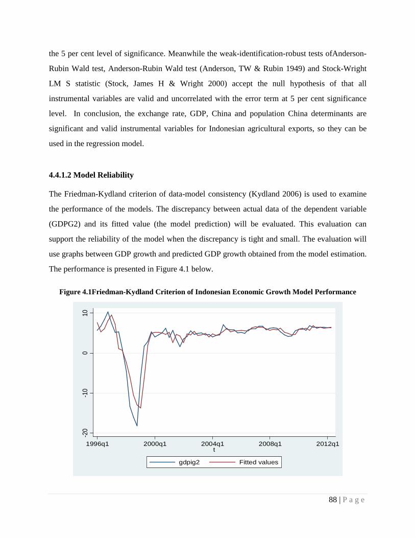
the 5 per cent level of significance. Meanwhile the weak-identification-robust tests ofAnderson-

Rubin Wald test, Anderson-Rubin Wald test (Anderson, TW & Rubin 1949) and Stock-Wright

LM S statistic (Stock, James H & Wright 2000) accept the null hypothesis of that all

instrumental variables are valid and uncorrelated with the error term at 5 per cent significance

level. In conclusion, the exchange rate, GDP, China and population China determinants are

significant and valid instrumental variables for Indonesian agricultural exports, so they can be

used in the regression model.

4.4.1.2 Model Reliability

The Friedman-Kydland criterion of data-model consistency (Kydland 2006) is used to examine

the performance of the models. The discrepancy between actual data of the dependent variable

(GDPG2) and its fitted value (the model prediction) will be evaluated. This evaluation can

support the reliability of the model when the discrepancy is tight and small. The evaluation will

use graphs between GDP growth and predicted GDP growth obtained from the model estimation.

The performance is presented in Figure 4.1 below.

Figure 4.1Friedman-Kydland Criterion of Indonesian Economic Growth Model Performance

-20

-10

010

1996q1 2000q1 2004q1 2008q1 2012q1t

gdpig2 Fitted values

88 | P a g e

From the movements or fluctuations of Indonesia’s actual economic growth plotted in Figure

4.1, it can be seen that the predicted value from the model imitates the actual data very well

throughout this period, showing peaks and turning points in actual growth and export. It can be

said that the discrepancy between actual trade and the predicted value is very small and tight. All

the variables incorporated in the model have structured a good equation to influence the

predicted dependent variable. The other important aspect of this performance property is the fact

that all economic variables have been expressed in terms of their rates of changes that are able to

omit the possibility of a unit root problem and hence avoid the spurious regression problem.

After testing the modelling reliability and predicting criteria described above, it can be affirmed

that the estimated economic growth model reveals acceptable statistically reliable results. Thus,

it can be confidently asserted that the reliability of the model in predicting the actual data of the

dependent variable (economic growth) is high.

4.4.2 Estimation Results of the Growth-Agricultural Export Model

Having performed the tests of the requirements for the robustness of the model, the estimation of

the model is conducted by employing the 2SLS method. Table 4.1 presents the statistical value

from the model estimations by 2SLS.

Table 4.1 shows that the estimation results from 2SLS. The F tests for the structure of the models

are significant under the 5 per cent significance level. The R2 value is 79.6 per cent, while the

RMSE value of 2SLS is at 2.388, implying that the model is good enough to explain the

economic growth of Indonesia. Almost all independent variables have significant impacts on

economic growth. It can be shown that that most of the variables fit the hypothesis and are in

concordance with previous empirical evidence.

The parameter of the Indonesian agricultural exports to China (EX), Indonesian policy

reformations (IDRF) and the implementation of the ACFTA have positive and significant

impacts on Indonesian economic growth at 10 per cent significance level. The economic growth

condition in the previous period (GDPI-1) has a positive impact on the present economic growth

at 5 per cent level. In contrast, the Asian crisis (AC) has a negative and significant impact while

the global financial crisis (GFC) seems to have a negative but an insignificant impact on

Indonesian economic growth. The inward foreign direct investment (FDI) provides a

89 | P a g e

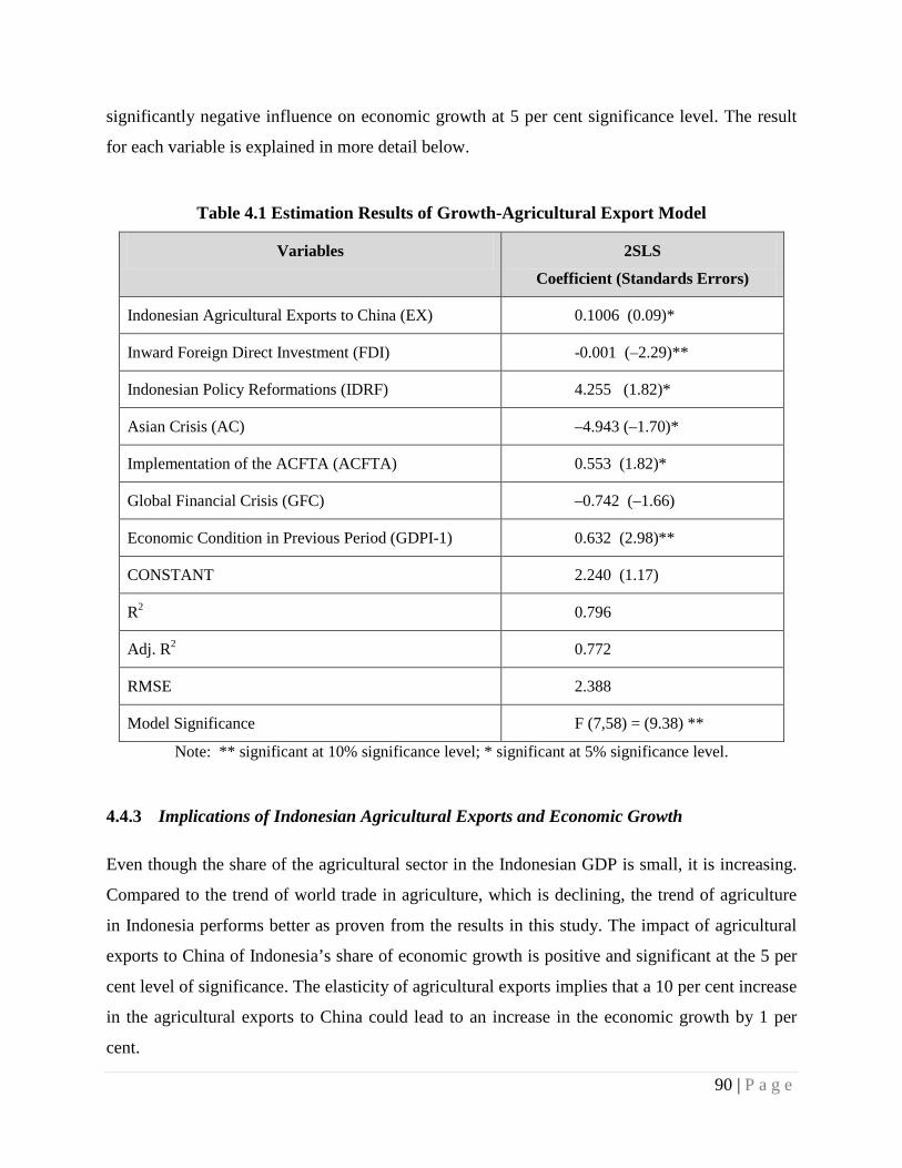
significantly negative influence on economic growth at 5 per cent significance level. The result

for each variable is explained in more detail below.

Table 4.1 Estimation Results of Growth-Agricultural Export Model

Variables 2SLS

Coefficient (Standards Errors)

Indonesian Agricultural Exports to China (EX) 0.1006 (0.09)*

Inward Foreign Direct Investment (FDI) -0.001 (–2.29)**

Indonesian Policy Reformations (IDRF) 4.255 (1.82)*

Asian Crisis (AC) –4.943 (–1.70)*

Implementation of the ACFTA (ACFTA) 0.553 (1.82)*

Global Financial Crisis (GFC) –0.742 (–1.66)

Economic Condition in Previous Period (GDPI-1) 0.632 (2.98)**

CONSTANT 2.240 (1.17)

R2 0.796

Adj. R2 0.772

RMSE 2.388

Model Significance F (7,58) = (9.38) **

Note: ** significant at 10% significance level; * significant at 5% significance level.

4.4.3 Implications of Indonesian Agricultural Exports and Economic Growth

Even though the share of the agricultural sector in the Indonesian GDP is small, it is increasing.

Compared to the trend of world trade in agriculture, which is declining, the trend of agriculture

in Indonesia performs better as proven from the results in this study. The impact of agricultural

exports to China of Indonesia’s share of economic growth is positive and significant at the 5 per

cent level of significance. The elasticity of agricultural exports implies that a 10 per cent increase

in the agricultural exports to China could lead to an increase in the economic growth by 1 per

cent.

90 | P a g e

The fact that agricultural exports have a positive impact on economic growth has proved that

agricultural exports have an important role in Indonesian economic growth as states by Johnston

and Mellor (1961). According to World Bank (2008), agriculture can be the lead sector for

overall growth in the agriculture-based countries by using a growth strategy that has to be

anchored on developing agriculture. Although in Indonesia’s case, agriculture is not the leader of

overall growth, but the role in economic growth is still important. In Indonesia, the agricultural

sector has been proven to be important in the Asian crisis era. The economy of Indonesia can

survive because of agricultural exports (Soesastro & Basri 2005), while other sectors have

collapsed because of the crisis. It denotes that the agricultural sector can be accounted as a robust

sector in the crisis and its growth is not disturbed by any shocks.

The increasing attention on the agricultural sector from governments and world organizations

also shows the commitment of the importance of the agricultural sector to the economy in

general(World Bank 2008). The fact that the agricultural sector is still very important for

developing countries should gain more attention for this sector.

North (1959)in his seminal paper reports that a successful agricultural export trade can and has

induced urbanisation, improvements in the factor markets, and a more effective allocation of

investment funds. His argument reflects the Indonesian agricultural exports. As agricultural

exports of Indonesia increase, the multiplier effect of this agricultural growth has generated

development in other sectors that lead to the improvement of the general economy.

The fact that Indonesia and China have committed to economically integrate with special

programs to boost agricultural trade has lifted the Indonesian agricultural export influence on

economic growth in recent times. Furthermore, the rapid growth of agricultural exports of

Indonesia can be accredited to the booming palm oil sector. The investment allocated in the

agricultural sectors has been increasing, especially in palm oil industry (Ministry of Industry

2011) that leads to increasing production. The higher production and higher demand of these

products have lead the palm oil products to be the third biggest exported commodities from

Indonesia (BPS 2014); hence its contribution to the Indonesian economy is considered very

important.

91 | P a g e

To compare this finding with others in the literature is difficult as studies investigating the

relationship between Indonesian agricultural trade and economic growth have been rarely carried

out. Despite its declining share of GDP, the lack of attention on the agricultural sector is one of

the reasons why research on the impact of agricultural exports for growth is very limited (World

Bank 2008). However, among studies that have been completed, Esfahani (1991) shows exports

of primary commodities have no significant impact on economic growth. Sala-i-Martin (1997)

and Doppelhofer, Miller and Sala-i-Martin (2000) find that primary commodities have a negative

impact on economic growth. Faridi (2012) reveals a negative relationship between agricultural

exports and Pakistan’s economic growth. Van den Berg and Lewer (2007) argue that the impact

of agricultural exports on economic growth is minimal due to the small size of agricultural trade

in exports compared to other sectors.

In contrast, this study presents different results from previous studies with a positive impact of

agricultural exports for economic growth. This can provide different view in the literature about

the revival of the agricultural sector in developing countries.

4.4.4 Implication of the ASEAN China Free Trade Agreement on Indonesian Economic

Growth

This study employs the extended endogenous gravity theory with the incorporation of the

dummy variable of the ACFTA to examine whether joining ACFTA will lead to Indonesian

economic growth. The decision of the Indonesian government to join the ASEAN-China Free

Trade Agreement appears to be a right choice as the results of this study show that the

implementation of the ACFTA has a positive and significant impact on Indonesian economic

growth. This is consistent with the theory that postulates the main objectives of the free trade

area establishments are to increase trade between members and to improve the welfare and

economic growth of the member countries.

Although China is not the biggest export market for Indonesia’s products, the trend of exports to

China is increasing. The elimination of tariff and non-tariff barriers in trade and other trade and

service facilities offered from the ACFTA have boosted the volume of trade. As ACFTA does

not only regulate the trade sector, but also the service and investment sector, it can be argued that

92 | P a g e

the service and investment sectors under the ACFTA have also contributed to improving

economic growth (Fukunaga & Ishido 2013; Xiao 2010). Hence this leads to a marked reduction

in income gaps that had existed between trading countries (Ben-David 1993; Ben-David &

Loewy 1998).

The finding of this study is consistent with numerous other studies that find a positive

relationship between trade liberalization and economic growth. North (1959) argues that

economic development of a country depends on its ability to become integrated into larger

markets of the world through exports. This study supports the hypothesis that integrate with

China by joining ACFTA has given Indonesia an opportunity to expand its market to the

potential offered by the large market of China. In the field of ACFTA studies, this study is

consistent the GTAP estimation study by Chirathivat (2002), and Sudsawasd and Mongsawad

(2007) who predicted that the ACFTA will increase the GDP of the ASEAN members and

China, but contradicts studies by Yue (2004), Holst and Weiss (2004) that predicted declining

GDP of Indonesia as a result of the ACFTA.

4.4.5 The Role of Foreign Direct Investment in the Economic Growth of Indonesia

This study uses FDI to measure the impact of inward capital investment flowing to Indonesia. As

this study focused on international trade, FDI is the most relevant form of capital inflow for

many countries, especially developing and emerging economies. Furthermore, increasing

globalisation also led to a growing interest in the activities of multinational companies which is

often represented by FDI data.

The result of this study shows that FDI has negative impacts on the economic growth of

Indonesia. The inward FDI of Indonesia is very low compared to neighbourhood countries. One

reason for the low inflow of FDI is that Indonesia has failed to integrate fully into international

production networks. The composition of FDI in Indonesia therefore differs from that in other

parts of East Asia, and foreign multinational firms seem often to choose other locations when

there are alternatives, especially in the manufacturing area. There are, however, other areas

where little progress has been made, leaving Indonesia a less attractive FDI destination than

other countries in the region. The continuing poor state of infrastructure is damaging to

93 | P a g e

Indonesia’s ability to attract FDI. The business environment is poorer than in many other East

Asian countries. Indonesian institutions and administrative capacity need to be improved further.

Despite some progress, corruption remains a larger problem in Indonesia than in most other

countries in East Asia. Poor institutions and corruption increase the costs of production.

FDI may be one way to improve infrastructure. Investments by foreign firms in infrastructure,

and also in utilities, finance, construction and other non-trade sectors, are affected by various

institutional factors such as competition and pricing policies. Complex regulations are often

required to attract investments in these sectors. Indonesia has a mixed history in dealing with

inward investment in infrastructure projects (Wells and Ahmed 2006). Lack of administrative

capacity, poor regulatory structures and corruption are some of the main causes of failing

investments in infrastructure.

A series of papers by Ando and Kimura, summarised in Ando, Arndt and Kimura (2006),

emphasises the importance of the growth of trade in machinery parts and components, and

contrasts that trend in Asian trade with its absence in Latin American trade. When countries are

arrayed in order of the importance of machinery and machinery parts and components in their

exports, seven East Asian countries are above the median, and only one, Indonesia, is below it.

Faster growth is an important goal of economic policy; it would seem to be in Indonesia’s

interest to increase inflows of FDI, given the benefits it brings in terms of productivity growth,

higher wages and strong employment growth. However, the Indonesian attitude towards FDI has

always been rather ambivalent.

Indonesia may reap benefits from FDI and attract more inward FDI if such parameters mentioned

by De Mello Jr (1997) have been conditioned. Firstly, a fundamental criterion for attracting FDI

is that the host country welcomes such investments. The business environment should be

supported by the government. Indonesia does not do well among East Asian countries in the

World Bank’s rankings for the quality of the business environment. The investment in Indonesia

is relatively low because of lack of administrative capacity, poor regulatory structures and

corruption (Hansen & Rand 2006). It is therefore more fruitful to consider how the business

climate in Indonesia can be made more conducive to FDI. Second, there needs to be

moreparticipation in the global production network of the foreign companies from developed

countries. Indonesia needs to attract the MNEs to locate their investment in Indonesia by

94 | P a g e

liberalisation of trade and border procedure and also by investment in infrastructure such as

improving the communication sector, the seaports and their supporting infrastructure. Moreover,

Indonesia needs to improve the numbers of their skilled people through education. The

education enrolment levels and attainment are poor in Indonesia (Barro & Lee 2013). Improved

education is important for attracting FDI, but it will also affect Indonesia’s absorptive capacity.

The better the level of education the more Indonesia will benefit from the presence of foreign

multinational enterprises (MNEs). Next, Indonesia needs to improve its technological capacity

to encourage MNEs to upgrade production to higher value added activities and to increase

spillovers by facilitating knowledge transfers from MNEs to local firms. The very low

investment in research and development in Indonesia is an indication of the poor state of

technological development and capability. Wells (2007) suggests some policies to improve the

investment regime for infrastructure projects: a closer look at international best practice; a ban on

equity arrangements under which importantly placed Indonesians to get a share of foreign

investments; and the granting of full responsibility to a single government agency to negotiate

and conclude agreements with foreign investors. The evidence from the studies surveyed leads to

conclude that Indonesia would benefit from higher FDI inflows.

4.4.6 The Role of Other Factors on Indonesian Economic Growth

The other variables in the equation consist of the onset of the Asian crisis in 1997, the

reformation in the Indonesian government and policy reforms after the end of Soeharto’s regime

and the occurrence of global financial crisis in 2007. This section discusses the impact of these

other variables of significant crises and policy reforms on economic growth of Indonesia based

on the estimated results.

4.4.6.1 Crises

It has been proven in the literature that sudden crises, shocks and major policy reform are the

source in the fluctuations in economic performance (Johansen, L 1982; Tran Van Hoa 2004b,

2006b, 2006c, 2008). Crises incorporated in this model are the Asian crisis and the global

financial crisis. Even though many more other crises have affected Indonesia,their impacts are

not significant enough for these to be included in the estimation.

95 | P a g e

The result shows that Indonesia’s economic growth suffered a negative and significant impact

from the Asian crisis. Indonesia was one of the Southeast Asian nations that experienced severe

conditions caused by the Asian crisis. The crisis that began around July 1997 had a very negative

impact on the Indonesian economy. The GDP of Indonesia fell during this crisis. This situation

was not only caused by the decline of trade, but an accumulation of many other factors. There

was a rapid increase in the price level during the Asian crisis driven by a sharp depreciation of

the rupiah, and declining investment that led Indonesia to experience annual net outflows of

foreign direct investment until 2001 (Elias and Noone, 2011). The accumulation of these various

conditions led to declining economic growth. Recently, the Indonesian economy has grown at

around 6.1 per cent, making Indonesia one of the fastest growing countries in Asia following

China and India. However, this is lower than the rate of economic growth of 7.2 per cent before

the Asian crisis (Basri, M.C. 2010).

The investment share of GDP prior to the crisis was over 30 per cent, however, the rapid outflow

of foreign capital contributed to a sharp contraction in investment during the Asian crisis.

Between 1997 and 1999, net FDI shifted from an inflow of 2.2 per cent of GDP to an outflow of

1.3 per cent, while the volume of investment fell by 45 per cent(Elias & Noone 2011). Indeed,

foreign investment only recently recorded strong growth. In 2010, net FDI inflows increased

fourfold to 1.9 per cent of GDP, with the increase broadly spread across industries. Nevertheless,

the increase has not been big enough to improve economic growth.

The global financial crisis severely impacted developed countries (Reinhart & Rogoff 2009).

However, based on the empirical findings of this study, the global financial crisis did not have a

significant impact on the Indonesian economy. This means that Indonesia’s growth performance

after the crisis was relatively good. The relatively good performance of Indonesia was due to the

fact that Indonesia’s economy was relatively insulated from the weakening global situation.

Basri, M.C. (2010)argues the structure of agricultural exports share within the economy of

Indonesia is relatively small compared to countries such as Singapore, Thailand and Malaysia. In

addition, Indonesia was left behind in production networks (Ando & Kimura 2007). As a result,

the impact of the global financial crisis on the Indonesian economy also became limited.

96 | P a g e

4.4.6.2 Domestic GDP

The impact of the lag 1 of the GDP Indonesia on recent GDP is highly positive and significant at

5 per cent significance level. In the growth-trade model, the GDP, as a function of net exports, is

potentially endogenous to bilateral trade flows, and vice versa, as proposed in the recent

literature (Frankel, J & Romer 1996). J Frankel, J and Romer (1999) note that while international

trade can influence a country income, national income can also be influenced by the amount that

the country’s residents trade with each other. Previous research shows that the good performance

of the Indonesian economic growth was mainly due to strong domestic demand. The GDP data

indicate that growth was dominated by non-tradable sectors, such as electricity, gas and water,

construction, trade, hotels and restaurants, transportation and communication, financial,

ownership and business services as well as services (Basri, M.C. 2010).

However, the findings of the relationship between trade and growth with causality test in this

study present mixed results. In a situation where the external situation is still in turmoil, the non-

tradable sector could cushion the economy from the negative impact of the ongoing global

financial crisis.

4.4.6.3 Indonesian Policy Reforms

Many policy reforms were undertaken during from 1996 to 2012 in Indonesia. After Soeharto’s

long period of rule, the election of a new President in 1999 initiated the reform era. Since late

1999, comprehensive reform programs have been commenced by the Indonesian government to

build up a strong investment climate in the financial and infrastructure sectors. The new

government launched many policy reform packages in government structure, politics, economics

and press freedom. This reform era coincides with the aftermath of the Asian crisis that put an

end to the continuation of economic growth. As suggested by the WTO (1998), Indonesia

encouraged more trade reformation to regain economic growth.

These reform efforts and stronger democratic credentials encouraged economic growth, as shown

by the results of this study. The result shows that the variable of government reforms had a

moderate effect on growth in the agricultural sector. This means that government reforms to the

97 | P a g e

economy, particularly the agricultural sector, had a role to play in its growth, Economic growth

has been increasing significantly in the wake of the reforms.

The policy reformation in investment led to resurgence in investment (Elias & Noone 2011).

Recognizing the importance of investment in the agricultural sector, the Indonesian government

increased its public spending to invest in this sector. The government issued Presidential Decree

no. 77/2007 and 111/2007 regarding Lines of Business Closed and Open with Requirements for

Investment that allow foreign investors to hold 95 per cent shares in a plantation company,

including palm plantation company. As a result, foreign investment in food crops and plantation

sector increased significantly from less than $200 million in 2003 to around $1200 million in

2007 (Bank of Indonesia 2009). During 2005 to 2011, an average of about 1.5 per cent of public

budget was allocated for agriculture, but this can be pegged higher at 2.5 per cent if the public

budget for irrigation was included (ADB 2011).

4.5 Conclusion

The main objective of the study in this chapter is to examine the impact of Indonesian

agricultural exports to China on Indonesian economic growth under the influence of the ACFTA,

taking into consideration the context of regional and global crises and domestic reforms. The

empirical result of the model estimation in Table 5.3 shows that the constant of the equation is

positive but not as significant as expected. Thus, it can be argued that the Indonesian economy

was growing under the influence of focused variables in the model but quite moderate. Among

other variables, reform in Indonesian government in early 1999, the implementation of ACFTA,

Indonesia’s domestic GDP had positive and significant impacts on Indonesian economic growth.

However, FDI and the Asian crisis exerted significant negative impacts of Indonesian economic

growth, but the negative impact of the global financial crisis was not as significant.

This means that the impact of Indonesian agricultural exports to China on Indonesian economic

growth is positive but not significant. Although exports are growing fast, the small share of

agricultural exports to China compared to other sectors may be the reason behind the lower

impact. Although agricultural trade has been accelerated by tariff reduction facilitation under the

ACFTA scheme, it has not been strong enough to dramatically increase the impact of agricultural

98 | P a g e

exports on growth. In contrast, the implementation of the ACFTA has a significant and positive

impact on economic growth. This indicates that economic integration has successfully influenced

economic growth.

Meanwhile, the Asian crisis in mid-1997 has negatively affected Indonesian economic growth to

a significant extent, whereas the global financial crisis in mid-2007 had no significant impact on

growth. The reformation in Indonesian government beginning in late 1999 significantly

improved economic growth because the policy reform packages successfully attracted

investments to improve the economy after the Asian crisis and long regime of President

Soeharto. On the other hand, FDI has a negative impact on economic growth, caused by the fact

that FDI resulted in more outflows than inflows in Indonesia.

This chapter presented an analysis of Indonesia’s economic growth in relation to its agricultural

exports to China. However, the agricultural export data used in this chapter are based on whole

agricultural exports to China. Hence, it is important to further explore the issue by dividing the

agricultural exports under the ACFTA to examine the more disaggregated influence of the

ACFTA on agricultural exports. The next two chapters will examine the impact of the ACFTA

on Indonesian agricultural exports to China in terms of their volume and competitiveness,

respectively.

99 | P a g e

Chapter 5

The Implication of the ASEAN-China Free Trade Agreement on the Growth

of Agricultural Exports from Indonesia to China

5.1 Introduction

China is the third biggest market for Indonesian agricultural exports (BPS, 2014) . The Indonesia

government hopes that acquiring greater access to China through the ACFTA will further

encourage agricultural exports.

The aim of this chapter is to analyse the impact of the ASEAN-China Free Trade Agreement

(ACFTA) programs for the growth in volume of agricultural commodities exported from

Indonesia to China. This chapter intends to address research objective III: ‘To investigate the

impact of the ACFTA programs on the growth of Indonesian agricultural exports to China across

the short- and long-term accounting for the effect of other control variables of partner GDP,

crises, exchange rate volatility’. The objective derives from research question II: “Do efforts to

improve agricultural trade, such as joining a free trade agreement, have a significant impact on

the growth of exports and competitiveness of the commodities?”.Hence, this chapter presents the

statistical and quantitative analysis conducted on Indonesian agricultural exports to China under

the ACFTA programs. The statistical analysis will test the hypotheses, whether the ACFTA

programs have positive impacts on Indonesian agricultural export growth in China.

Chapter four showed that the ACFTA increases Indonesian agricultural exports to China in

general. However, not all of these agricultural commodities are included in the ACFTA program.

Furthermore, the ACFTA has different schemes for certain agricultural products. So, this chapter

intends to explore the impacts of the ACFTA programs on relevant agricultural commodities

covered under them. In order to achieve this objective, two programs of the ACTA will be

investigated in this chapter: the Early Harvest Program (EHP) and the Sensitive Track (ST). For

the EHP scheme, the impacts of EHP’s export tariff reduction and other trade facilities for

related Indonesian agricultural export to China will be examined. For the ST scheme, the

sensitivity on Most Favoured Nation (MFN) tariff and other trade facilities for related

agricultural products will be measured as tariff reductions do not begin on this scheme until

100 | P a g e

2012. In addition, other variables that influence Indonesian agricultural exports to China will be

examined as control variables. It will also test the hypothesis that the occurrence of crisis,

especially the global financial crisis, will negatively affect the exports of agricultural

commodities of Indonesia. To examine these questions, the autoregressive distribution lag

(ARDL) model on export equations will be employed as it is considered more appropriate for the

purpose because ARDL can deal with stationary data occurring at different levels and dummy

variables used in the model. As the impacts of free trade agreement will vary over different time

spans, this study will use time series econometric analysis to examine the short-run and long-run

impact of the ACFTA.

5.2 Literature Review

5.2.1 Impact of Free Trade Agreements on Agricultural Exports

Gains from trade have been well analysed in the international trade theory. The traditional theory

from the comparative advantage of Ricardo emphasizes technological differences as the cause of

trade; the Heckscher-Ohlin-Samuelson model postulate differences in factor endowments, and

some alternative models are generated by varying assumptions about the number of goods and

factors (Krugman, PR 1987). Linder (1961) and Vernon (1966) point out endogenous

technological change while Spence (1976) and Dixit, AK and Stiglitz (1977) highlight the role of

increasing returns as a cause of international trade. Dixit, A and Norman (1980), Lancaster

(1980), and Krugman, P (1979) explain that not only underlying differences but also economies

of scale have led to arbitrary specialization by nations on products within monopolistically

competitive industries. Feenstra (2006) determines gains from trade in monopolistic competition

models can be arising from three sources: (i) price reductions due to increasing returns to scale;

(ii) increased product variety available to consumers; (iii) self-selection firms with only the most

efficient firms surviving after trade liberalization

Trade also brings winners and losers as stated in the Stolper-Samuelson Theorem (Samuelson

1962) that an increase in the relative price of a good will increase the real return to the factor

used intensively in that good. Jones (1965) called the formulation of this theorem the

“magnification effect”. Any change in the product prices has a magnified effect in the factor

101 | P a g e

prices. Whether the product price change is due to export opportunities for a country (the export

price goes up) or due to lowering import tariffs (so the import price goes down), the

magnification effect says that there will be both winners and losers due to this change. In the

Hecksher-Ohlin model, the abundant factor gains from trade (through the rise in the relative

export price, increasing the real return to that factor, used intensively in exports), while the

scarce factor loses from trade (through the fall in the relative import price, lowering the real

return to that factor).

To achieve Pareto gains from trade, that is a situation that everyone gains, the government has

ability to redistribute income from the winners to the losers. This mechanism is called lump sum

subsidies (Dixit, A & Norman 1986). This analysis can be extended to cover tariff reform by

multiple countries. This method is adopted by the World Trade Organization (WTO) to reduce

barriers to trade among its member countries. The fundamental principle of WTO is “Most

Favoured Nation” (MFN) that states all countries members should be treated equally. Thus

multilateral tariff reduction should be applied for all members.

On the other hand, there are regional agreements or preferential agreements where a group of

countries decide to completely eliminate all tariffs between them, without eliminating tariffs on

goods imported from the rest of the world. The forms of these agreements include Customs

Union and Free Trade Area. Because such agreements involve only partial elimination of tariffs,

they can lead to unexpected results. Viner, Jacob (1950) points out that the countries left out of

the union and even the countries inside the union, can become worse off.

To measure the impact of free trade agreements on agricultural trade, literature, mostly focuses

on trade creation and trade diversion as the consequences of the establishment of the free trade

agreements. Such research mostly uses gravity theory with aggregate data for the analysis, and

makes general conclusions for countries and general commodities included in the model. In

general, the findings present that the establishment of the free trade agreement increases

agricultural trade between members of the agreements and also expand trade with non-member

countries.

The positive effects of trade creation indicate the promotion of trade due to a shift of

consumption from high-cost domestic products with low-cost imported products from abroad

(Viner, J. 1983). Baldwin (2004) is of the opinion that trade liberalization, whether it originates

102 | P a g e

from regional or multilateral agreements, will also enhance more liberalization of trade with non-

members of the agreement. This reflects the spill-over efficiencies caused by free trade

agreements enabling members to increase export sales to non-partner exporters.

Conversely, the difference in tariffs applied to partners and non-partners will change the

direction of trading trend, and impose negative effects of trade diversion which refers to the

replacement of exported products that are low-cost from non-member countries with exported

products from partner countries that are high-cost. Therefore, trade diversion would reduce the

welfare effects due to the changes in supply orientation to a relatively more expensive source.

Panagariya and Krishna (2002) note that there is tendency to ignore possible welfare losses

derived from free trade agreements, especially with respect to non-member countries. They argue

that the concepts of trade creation and trade diversion are central to the policy debates about free

trade agreements and that the empirical analysis of these concepts by sector is important.

According to Viner, J. (1983), reducing tariff barriers through formation of the free trade

agreements will not necessarily improve welfare. The overall impacts can be positive, negative

or neutral depending on the size or the magnitude of trade creation and trade diversion as

indicators to measure the impact of free trade arrangements (Krueger, A.O. 1999; Viner, J.

1983).

An example of this theory is a research about ASEAN Free Trade Agreement (AFTA) conducted

by Korinek and Melatos (2009). Their study finds that fully implemented AFTA has encouraged

members to decrease their export of agricultural products to non-AFTA countries.

Lumber and McKoy (2008) argue that the establishment of free trade agreements increases intra-

bloc trade in agricultural and food products sectors. By using a gravity model and panel data of

the logarithm of the nominal value of the agricultural exports between two countries, their study

examines thirteen free trade agreements. They find that membership of a free trade agreement is

associated with increased intra- and extra-bloc trade in developing countries (for example,

NAFTA and EU) leading to trade creation in these sectors, but trade diversion also happens in

some free trade agreements in developing countries. Here, they find that the establishment of the

Common Market for Eastern and Southern Africa (COMESA) has diminished exports and export

of food, but increased agricultural trade with non-member countries in Africa region. This

finding is in agreement with Clarete and Roumasset (1990) and Shane et al. (2009) who argue

103 | P a g e

that there has been trade creation of agricultural trade as a result of Mercado Comun del

Sur/South American Economic Organization (MERCOSUR), Central American Common

Market (CACM), South Pacific Regional Trade and Economic Cooperation Agreement

(SPARTECA),Greater Arab Free Trade Area (GAFTA).

Koo, Kennedy and Skripnitchenko (2006) apply the gravity model toanalyse agricultural trade in

1999 and find evidence of trade creation among members of the free trade agreements on an

aggregate level. Their study also finds that trade between member and non-member countries has

also been enhanced, as bilateral trade was increased even when countries were not members of

the same free trade agreements. Furthermore, the results show that agricultural trade creation was

not significantly detected in individual free trade agreements such as the European Union (EU),

North American Free Trade Agreement (NAFTA) and Andean Pact, but statistically significant

in the ASEAN members. The increasing trade between ASEAN members and non-members

countries are also significant, whereas trade diversions exist in Andean Pact and NAFTA.

Other studies also support the increasing agricultural trade as a result of the establishment of the

Free Trade Agreements. For example, Zahniser and Coyle (2004) use time series data of

combined exporting-country GDP with preferential trade agreement membership and find

evidence of trade creation and trade diversion in NAFTA.

A recent study focused on trade creation and trade diversion on agricultural trade was conducted

by Vollrath and Hallahan (2010). Using gravity theory, they examine the impact of mutual

membership of free trade agreements for the exporters and importers compared to an asymmetric

membership of free trade agreements where the exporters and importers do not belong to the

same free trade agreements. The findings show that mutual membership typically increased

agricultural trade while asymmetric membership reduced agricultural trade. The finding also

focuses on the impact of WTO on agricultural trade. The result shows that the WTO has

enhanced trade between members and reduced trade with non-member countries.

It can be summarized from these explanations that the impact of free trade agreements is mostly

on agricultural trade examined from the trade creation and trade diversion view. The majority of

studies find that there is trade creation in agricultural trade when a free trade agreement is

imposed.

104 | P a g e

5.2.2 Export Function

Most of these empirical studies mentioned earlier evaluate the impacts of free trade agreements

on agricultural trade using two main methods: computer simulation studies of general

equilibrium effects and gravity theory (Burfisher, Robinson & Thierfelder 2001). The ex-ante

studies with computable general equilibrium (CGE) models use various simulation methods to

analyse a calibrated model economy for a particular base year. The literature on this method is

common. For example, the free trade agreements of Chile are estimated to benefit many sectors

of Chile by doing CGE simulations (Chumacero, Fuentes & Schmidt-Hebbel 2004). Paiva (2005)

confirms that the membership of the free trade agreements positively affect agricultural trade

among members where the impacts of the free trade agreements are broadly simulated by

implementing the CGE methods.

However, this method has been criticized for lacking detailed, up-to-date policy coverage and

product desegregation(Aksoy, AM 2005b). In response, researchers have used econometric

methods with historical time series and cross-sectional data to analyse the impact of the free

trade agreements on trade and welfare. The most commonly used of these methods is gravity

theory, but this model requires aggregate data for analysis, making it difficult to exploit

variations in the extent of trade liberalization across goods or industries. Also, the aggregate data

is sourced from the bilateral trade of both countries such that it becomes difficult to separate the

impact on a specific country in a two country model (Clausing 2001).

This study intends to examine the impact of ASEAN, China Free Trade Agreement (ACFTA) on

the agricultural exports from Indonesia to China. To undertake this examination, the export

demand function will be used as the volume of exports depends on the trading partner’s income

from the point of view of bilateral trade and relative price of the traded goods (Goldstein & Khan

1985; Hickman & Lau 1973; Houthakker & Magee 1969). Unlike the gravity model that takes

the model as an ad hoc representation, the current approach is developed on more grounded

economic theory of demand. The demand theory postulates that trading partner’s income has

positively influenced the exports while price has negative impact on exports (Senhadji &

Montenegro 1998). The demand function, both export and import, are widely used to examine

the trade in models examining two countries. For example, Bahmani-Oskooee, Mohsen (1998)

implement demand model to examine trade elasticity’s in less developed countries and find

105 | P a g e

devaluation can improve trade. A research conducted by Karemera and Koo (1994) analyses the

trade effects of removing tariff and non-tariff barriers between the USA and Canada by using

seemingly unrelated regression to estimate the import demand model. From their findings, they

conclude that the US exports of Canadian goods are more sensitive to domestic and bilateral

export prices than Canadian exports of the US goods. They also find that tariff and non-tariff

elimination would increase the bilateral trade volume across all commodities traded. Clausing

(2001) explores tariff variation at the detailed commodity level with US export data from 1989 to

1994 and finds that tariff liberalization has an impact on the growth of US exports but with little

evidence of trade creation.

The construction of agricultural export demand model for Indonesian agricultural exports to

China must also consider any other determinants that may affect the export of agricultural

products from Indonesia to China. These determinants are listed as follows.

5.2.2.1 Relative Price Index

One of determinant influenced export demand is relative price (Goldstein & Khan 1978). While

the demand theory assumed that demand responds negatively on the price, the empirical results

shows responses are mixed depend on countries (Goldstein & Khan 1985; Hickman & Lau 1973;

Houthakker & Magee 1969). The recent studies, for example, Wang, X and Reed (2013) argue

that fishery imports to the US are insensitive to price.

The significant impact of relative price of agricultural commodities can be related to the change

in food and agricultural products’ prices in the mid-2000s. Timmer, MP and de Vries (2009)

argue that market price of basic food commodities reflect the undervaluation of agriculture by

both the public and private sectors. The recent price rises in food and agricultural products have

influenced the movement of agricultural exports (WTO 2012e).

Goswami and Nag (2012) find that monetary shocks or over-expansionary monetary policy

results in overshooting of primary commodity price, while real shock in terms of rise in the

production of primary commodity mitigates the volatility of primary price. Thus, to address such

agricultural price volatility, policy towards improvement of agricultural sector should be

employed, such as increasing the production and greater access to the international market.

106 | P a g e

Furthermore, the implementation of fiscal policy and the autonomous rise in export can also

undershoot the volatility of the agricultural price.

From this discussion, it is apparent that there is a relationship between the relative price index

and agricultural trade. This means that relative price index is a significant factor in international

trade and must be included within the export volume estimation model. The relative price is

measured as the export price index deflated by an index of domestic prices.

5.2.2.2 Trading Partner’s income

As explained in the previous section, one determinant of export demand equation is trading

partner income. Hoque and Yusop (2010) note that the higher income elasticity of exports

indicates that higher income leads to higher consumption demand. This higher consumption

demand is mainly translated into higher exports rather than consumption of domestically

produced products because consumable domestic goods produced as a percentage of GDP were

gradually decreasing. They could not keep pace with higher consumption demand because

investments were diverted towards more lucrative export-oriented sectors. Baek and Koo (2011)

argue there is positive long-run impact of the United States’ GDP on Indonesian agricultural

exports. Because of a lack of sufficient sampling sizes for the data, Indonesia’s trading partner’s

income in this study will be represented by its GDP data (2002b, 2004b, 2005a, 2006a, 2006b,

2008). China’s real GDP will be used as a proxy for China’s income.

5.2.2.3 Tariff Reduction

The main characteristic of free trade establishment is export tariff reduction, so the impact of free

trade agreements can be examined from the relationship between export tariff and real value of

the export. When a country joins a regional trade agreement, it undertakes partial reforms of its

tariff where it reduces its tariff for trade with members of the agreement but maintains a high

tariff for other countries outside the union. Ju and Krishna (2000) develop the theorem of partial

tariff reform to analyse whether a country stands to gain or lose from tariff reduction under free

trade agreements.

107 | P a g e

The impact of tariff reduction has been reported to have a positive impact on increasing trade in

some studies. For example, a recent study conducted by the OECD examined a large number of

RTAs and focused on the reduction of tariff lines to zero as a result of RTAs to find that RTAs

have contributed to agricultural trade liberalization (OECD 2010). Similar findings showing the

responsiveness of export and demand of exports to the tariff reduction and the free trade

agreement preference are reported by Fukao, Okubo and Stern (2003), McDaniel and Agama

(2003) on the basis of export demand model for NAFTA.

Susanto, Rosson and Adcock (2007) examine the impacts of the US-Mexico trade agreement

under NAFTA. By using the import demand equation, the empirical findings suggest that US

agricultural imports from Mexico have been responsive to tariff rate reductions applied to

Mexican products. The results indicate the occurrence of trade creation rather than trade

diversion. A different study using general equilibrium simulation also finds that tariff reduction

in trade liberalization affected agricultural products and timber in bilateral trade between Canada

and the USA (Boyd, Doroodian & Abdul‐Latif 1993).

On the other hand, some other studies find that tariff reduction only delivers small benefits to

agricultural trade between Mexico and the US (Doroodian, Boyd & Piracha 1994). In their study

on exports from Bangladesh, Hoque and Yusop (2010) find that trade liberalization represented

by a non-tariff barrier has a low positive impact on aggregate export in the long-run while the

tariff reduction increases export substantially in the short-run but insignificant in the long-run.

As explained in the previous chapter, the ACFTA has three different programs. Due to the data

limitation, there only two groups of ACFTA that can be examined, namely the EHP and the SL

groups. Hence, the structural equations based on export demand theory for the both programs

should be established. The EHP started reducing its export tariff in January 2004 and a zero

percent export tariff was established since 2006. As a proxy for the tariff reduction of EHP

scheme, the MFN tariff will be multiplied by tariff reduction of EHP scheme. China will start

reducing its export tariff for the sensitive and highly sensitive lists commodities under the

ACFTA schemes after 2012 and 2016 respectively. Thus, the MFN tariff variable will represent

the tariff determinant of the SL group in the equation. For this research, export tariff for each

group will be added to the model. The purpose of this addition is to examine the influence of

tariff changes into agricultural exports.

108 | P a g e

5.2.2.4 Exchange Rate Volatility

The attention to the importance of exchange rate volatility has been increased since the

occurrence of a currency crash in Thailand and the Asian financial crisis (Poon, Choong &

Habibullah 2005). It is argued that the rapid increase in exchange rate volatility following the

collapse of Bretton-Woods system in 1971, has had significant adverse effects on international

trade, especially in emerging economies with underdeveloped capital markets and unstable

economic policies (Prasad et al. 2003).

The empirical results of exchange rate volatility in numerous studies have been mixed, and no

firm conclusion has been reached as to its definitive impact (Poon, Choong & Habibullah 2005).

It has been hypothesized that exchange rate risk can actually increase trade flows, as exporters

and exporters opt to increase the volume of trade to attain a certain income, making up for a

decrease in the per unit value of goods (Bahmani-Oskooee, Mohsen & Hegerty 2009). A

number of studies have also recognized the volatility of real exchange rate as additional variable

affecting export demand (Arize 1995; Moran 1989). However, Kristinek and Anderson (2002),

and Doroodian Sr, Jung and Boyd (1999) find that exchange rate volatility can influence the

volumee of agricultural trade. Choudhry (2005) argues that exchange rate volatility has enhanced

international trade flows from Canada, Japan and New Zealand to the United Kingdom. Baek

and Koo (2011) state the exchange rate has a positive and significant impact on agricultural

export from the USA to Canada and Indonesia. De Grauwe (1988) and Giavazzi and Giovannini

(1989) consider that exchange rate volatility induces producers to export more goods to avoid a

drastic decline in their revenue stream, thus, increasing trade. Doyle (2001) proposes that

exchange rate volatility enables multinationals to diversify exchange rate risk through

international intra-subsidiary changes in trade leading to more trade. Poon, Choong and

Habibullah (2005) argue that exchange rate volatility has positive, but insignificant impact on

exports in Indonesia.

On the other hand, some studies have dismissed the positive impact of exchange rate volatility.

According to McKenzie (1999), previous studies tend to favour that higher exchange rate

volatility is detrimental to exports. Some theoretical studies have supported the hypothesis that

an increase in exchange rate volatility might affect trade adversely; since risk-averse exporters

face greater risk and uncertainty with regard to profit earned, they reduce the supply of

109 | P a g e

tradegoods (Arize 1995; Chowdhury 1993; Cushman 1983; Ethier 1973). Comparing the

impact across the US economy, Cho, Sheldon and McCorriston (2002) report that exchange rate

volatility has a greater negative impact on agricultural trade compared to other sectors, a finding

that was affirmed in a later study by Kandilov (2008). In particular, Davis et al. (2014) report

that exchange rate volatility has a negative impact in the long-run but no impact in the short-run.

A number of empirical studies have found cases where a rise in exchange rate volatility may

have positive or negative implications on exports and imports, depending on the products and

countries (Asseery & Peel 1991; McKenzie 1998). Bahmani-Oskooee, Mohsen and Xu (2012),

for example, report varied impacts of positive, no impact and negative responses on trade for

industries between China and the USA, as well as with trade between Japan and China

(Bahmani-Oskooee, Mohsen, Hegerty & Xu 2012). Langley et al. (2000) find exchange rate

volatility had a positive impact on poultry exports from Thailand while Bonroy, Gervais and

Larue (2007) argue that exchange rate volatility has a positive relationship with pork exported to

the US, but a negative impact on pork exports to Japan.

In the ACFTA studies, Yusoff and Sabit (2014) explain that exchange rate volatility may

significantly affect exports from the ASEAN countries to China, while Chit, Rizov and

Willenbockel (2010) find that total elimination of exchange rate volatility would have increased

intra-regional trade of the ACFTAA by 5 per cent. Siregar and Rajan (2004) find that exchange

rate volatility has detrimental impacts on Indonesian exports and exports.

Maskus (1986) suggests that the responsiveness of bilateral trade to exchange rate volatility

could vary because of trade openness which can vary by sector, and other factors such as the use

of long-term contracts. This is particularly true for agricultural products where some

commodities are more protected than others and when biological and marketing lags require

producers to make output decisions before exchange rates are realized(Davis et al. 2014). M

Anderson, M and Garcia (1989) point out that many studies examined trade flows at more

aggregate levels, disregarding the fact that exchange rate impacts could differ by commodity.

As the exchange rate volatility has an influence on agricultural trade, this variable will be added

into the demand model. The volatility of the real exchange rate will be represented by the

logarithms of standard deviation of real exchange rate obtained by GRACH method.

110 | P a g e

5.2.2.5 Crises

Chavas (1983) argues that structural change may influence export demand. The structural

changes can be formed in trade policy or crises. Furthermore, as shown by much research,

occurrence of a shock or crisis may also affect the trend of exports (Tran Van Hoa 2008, 2009).

To examine the recent crises, the global financial crisis (GFC) and the Asian crisis will also be

incorporated as control variables.

5.2.3 Timespan of the Free Trade Agreement Impacts

Previous studies on the relationship between agricultural trade and trade liberalization have

mostly focused on trade creation and trade diversion under free trade agreements, but it is hard to

find studies examining the long-run and short-run impact of free trade agreement on agricultural

trade, especially for the ACFTA and Indonesian agricultural trade. Most studies of regional trade

agreements make an implicit assumption that trade flows immediately increase to a new level

with a free trade agreement (Sun & Reed 2010). They do not allow free trade agreement to

impact to vary over time. This assumption also rules out the possibilities that the trade effects of

the agreements may increase slowly over time (Magee 2008).

Using cross-sectional time series data, Krueger, A.O. (1999) finds that the establishment of

NAFTA had no impact on bilateral trade flows. A similar finding is reported by Gould (1998) in

a study using the gravity model to examine aggregate bilateral trade of NAFTA countries.

Burfisher, Robinson and Thierfelder (2001) argue that these findings discrediting the impact of

trade liberalization are caused by the fact that the time period of establishment of NAFTA was

not long enough to observe discernible impacts.

As has been explained before, the impact of trade liberalization is not immediate, but is more

apparent over the long-term, so it is important to distinguish the impacts of a free trade

agreement from the perspective of short-run and long-run dynamics. Hinojosa-Ojeda and

Robinson (1992) argue that the use of short-run, Keynesian macroeconomic trade multipliers in a

model seeking to analyse the long-term benefits of trade liberalization seems inappropriate.

Since the model involves only aggregating and macroeconomic trends, it cannot capture any of

the structural changes and gains from trade liberalization as predicted by neoclassical trade

111 | P a g e

theory. This argument is supported by the fact that free trade agreements often have a mechanism

of gradual reduction in tariffs over time rather than eliminating trade barriers immediately, so the

price support for increasing trade occurs over time (Frankel, JA, Stein & Wei 1997; Magee

2008).

To overcome this problem, phase-in effects have been applied in the trade model equation to

observe the implementation of free trade agreement clauses over time in studies by Baier and

Bergstrand (2007); Rose, AK (2004) and Grant, J.H. and Lambert, D.M. (2008). In order to

examine the varying impact of free trade agreement over time, Grant, J.H. and Lambert, D.M.

(2008) examine the lagged trade effects as an indicator of the transitional effects resulting from

phase-in periods of regional trade agreements and find significant statistical results for the lagged

time trade effects. Proposing a comparison of different time spans to examine the impact of the

free trade agreements over time, Vollrath (2012) began his study using a comparison of 21-year

period (1975 to 1994) and 31-year period (1975 to 2005) data. While the study found non-

significant impacts of free trade agreements on agricultural trade in the 21-year period for

CACM, ASEAN and NAFTA, different results were reported in the 31-year period, leading to

the conclusion that a longer timeframe of ongoing free trade agreement results in significantly

bigger magnitude of trade creation in those free trade agreements.

Furthermore, many other studies in the literature focus on the long-term impact and ignore

comparisons with short-term effects. These studies show that the impacts of free trade

agreements on trade are typically more pronounced during the first 10 to 15 years rather than

afterward (Baier & Bergstrand 2007; Grant, Jason H. & Lambert, Dayton M. 2008). Vollrath’s

(2012) extensive study analysed eleven RTAs that covered around 78 to 92 per cent of world

agricultural trade during the 1975 to 2005. This comprehensive study gives strong evidence for

the claim that the impacts of the free trade agreement are more discernible in the long-run.

Susanto, Rosson and Adcock (2007) argue that the first six years of NAFTA increased exports

by 5.31 per cent, which was higher than the last six years of NAFTA which only increased

exports by 2.62 per cent.

Considering that the impact of the free trade agreements can occur over a long period, recent free

trade agreement studies that find insignificant results may be flawed in that they only analyze

current data for a short-term. While there are a large number of studies researching the impact of

112 | P a g e

free trade agreements, only a few have focused on comparing the short-run and long-run impacts

of free trade agreements on agricultural trade. Bahmani-Oskooee, Mohsen and Ratha (2004)

argue that short-run results can differ significantly from long-run results, so it is crucial to

incorporate long-run dynamics in the model. Research on short-run and long-run impact of the

ACFTA will be especially useful as it has been recently established. Therefore, the estimation

model must incorporate tools to forecast the impact of the free trade agreements in long-term as

well as the short-term by enabling the integration of data over different time periods. The next

section describes the estimation technique using ARDL as an appropriate tool for this purpose.

5.2.4 Rationale for Autoregressive Distributed Lags Approach

In general, previous studies focused on the impact of free trade agreements use data in level or

logarithm type in a regression, but they ignore potential unit-root non-stationary features of the

variables in the model. Using non-stationary data in level without co-integration may lead to the

possibility of spurious regression, creating biased results (Granger & Newbold 1974). Some

studies examine the impacts of the free trade agreements considering the unit root problem of the

variables may estimate the impacts from the perspective of long-run and short-run dynamics.

More recent research considering the unit root and co-integration problem tends to use the

Johansen method (Johansen, L 1982; Johansen, S 1988) under the equally restrictive assumption

that all variables entering the model contain a unit root. The problem here is that in the presence

of a mixture of I (0) and I (1) regressors, statistical inference based on conventional likelihood

ratio statistics for co-integration is no longer valid (Harris 1995; Hassler 1996; Rahbek &

Mosconi 1999). Rahbek and Mosconi (1999) demonstrate that the presence of stationary

explanatory variables as extra regressors leads to nuisance parameters in the asymptotic

distribution of the trace statistic. However, both intuition and some previous evidence, suggest

that the standard demand equation is characterized by a mixture of I (0) and I (1) regressors. For

example, the income and relative price are expected and usually found to be integrated in order

one, while the volatility measure is level stationary (De Vita & Abbott 2004).

Engle and Granger (1987)suggest that a different way to address the problem arising from non-

stationary time series is to estimate a sufficiently complex dynamics specification that includes

lagged dependent and independent variables where the series are co-integrated (that is, the

113 | P a g e

ARDL model). The ARDL bounds test approach has several advantages over Johansen’s co-

integration method. First, the ARDL determines the co-integration, relation in small samples

more efficiently (Ghatak & Siddiki 2001; Tang 2003a), whereas co-integration methods of

Johansen, S (1988) and Engle and Granger (1987) require a large sample for validity. Pesaran

and Shin (1998) argue that the ARDL is more robust and performs better for small or finite

sample sizes than other co-integration techniques. Several previous studies, however, have

applied the ARDL approach to relatively small sample sizes. Gounder (1999); (2001) uses a

small sample size of around twenty-seven observations for a co-integration test using the ARDL

method to empirically test various growth hypotheses in Fiji. Similarly, Pattichis (1999), Mah

(2000), Tang and Nair (2002) and Tang (2003a) also applied the ARDL method with small

sample sizes to examine export demand functions.

Second, Johansen’s method requires the variables to be integrated with variables in the same

order for the co-integration test, while the ARDL approach can be applied irrespective of

whether the regressors are I (1) or I (0) or mutual co-integrated, in which the dependent variables

must be I (1). If the nature of the stationary of the data is not clear, then the use of the ARDL

Bounds test is more appropriate. A unit root test is not necessary if a conclusion can be made

from the ARDL bounds test for co-integration (Pesaran, Shin & Smith 2001).

Third, compared to the limited choices in Johansen’s method, a large number of choices can be

made with the ARDL method, in terms of the decisions regarding the number of endogenous and

exogenous variables, if any, for inclusion, as well as the treatment of deterministic elements

(Pahlavani, Wilson & Worthington 2005; Pesaran & Shin 1998). This means that dummy

variables can be included in the co-integration process in ARDL while this is not permitted in

Johansen’s method. Pesaran, Shin and Smith (2001) argue that the asymptotic theory developed

in the ARDL approach is not affected by the inclusion of such ‘one-zero’ dummy variables.

Moreover, the ARDL permits a diverse number of optimal lags in the order of vector auto-

regression (VAR) and the optimal number of lags to be used (Pahlavani, Wilson & Worthington

2005).

Pattichis (1999) applies the ARDL approach on export demand function to examine the long-run

price and income elasticity of export demand of disaggregated agricultural products in Cyprus

after the implementation of the Common Agricultural Policy. Marashdeh (2005), Pahlavani,

114 | P a g e

Wilson and Worthington (2005), Narayan and Smyth (2005) also use two dummy variables to

capture both the long-run and short-run impacts in their ARDL model of the budget deficit in

Lebanon, income growth in Iran, and trade liberalization and the economic growth in Fiji,

respectively. Bahmani-Oskooee, Mohsen and Hegerty (2009) use the ARDL method of the

export demand model to measure the impact of exchange rate volatility on commodities trade

between the USA and Mexico under the NAFTA agreement. Hoque and Yusop (2010) employ

the export demand equation estimated by the ARDL method to examine the impact of trade

liberalization on exports from Bangladesh. The finding shows that trade liberalization

represented by non-tariff barriers has a low positive impact on aggregate export in long-run

while the tariff reduction increases export substantially in short-run, but is insignificant in long-

run.

5.3 Methodology for Agricultural Exports Model

The research objective being addressed in this chapter is to investigate the impact of the ACFTA

and its programs for Indonesian agricultural export growth. Thus the hypothesis related to this

research objective is that implementing the ACFTA and its programs are positively correlated

with exports of agricultural commodities when accounting for other important factors of export

growth.

5.3.1 Construction of Agricultural Exports Model

This study will use the dynamic demand model to examine the impact of the ACFTA on

agricultural exports from Indonesia to China. The research objective in this chapter is to

investigate the impact of the ACFTA on Indonesian agricultural trade growth. Furthermore, it

intends to compare the impacts of the programs covered by the ACFTA implementation on

agricultural exports of Indonesia. Thus, the hypothesis related to this research objective is that

implementing free trade agreements is positively correlated with bilateral exports in agricultural

commodities when accounting for other factors of trade volume.

When testing this hypothesis, one must consider the argument developed by Baier and

Bergstrand (2007) that the effect of free trade agreements on trade flows is underestimated in

115 | P a g e

papers that do not account for other factors of trade volume. They argue that if a model does not

take into account the fact that free trade agreements may also be correlated with other factors that

affect trade flows, the estimate of the effect of free trade agreement on trade volume would be

incorrect. This study tests whether the presumed positive correlation between free trade

agreements and trade can also be found in the agricultural export sector when moderated by a

range of control variables.

The export equation for agricultural export is derived from demand theory that export demand

depends proportionally on income measured as the exporting country’s GDP and inversely

proportional to relative prices (Goldstein & Khan 1985; Tang 2003a). Following Gould (1998);

Karemera and Koo (1994), the export demand of agricultural goods will be represented by the

real exports value.

This will also explore the impacts of other determinants assumed to influence the exports as

control variables in the models. The control variables incorporated in the model includes GDP of

trading partners, relative export price index, exchange rate volatility, tariff reduction, free trade

agreement, and crises which is represented by Asian crisis and global financial crisis.

The hypothesis of the impact of other determinants in the model on the Indonesian agricultural

exports can be defined as follows. The export demand theory postulates that the GDP of trading

partner has a positive impact on exports, while the price increase would be expected to reduce

the volume of exports. The impact of real exchange rate volatilityon volume of export is

expected to be negative. Tariff reduction is expected to have a positive impact on the growth of

exports while the crises are expected to have negative impacts.

Following Bahmani-Oskooee, Mohsen and Hegerty (2009), the export model is constructed by

incorporating all variables explained previously and forms the equation as follows:

𝐿𝑁𝐸𝑖 = 𝛼1 + 𝛼2𝐿𝑁𝐺𝐷𝑃𝑅𝑖 + 𝛼3𝐿𝑁𝑃𝐼𝑖 + 𝛼4𝑙𝑛𝑅 + 𝛼5𝑇 + 𝛼6𝐹𝑇𝐴 + 𝛼7𝐴𝐶 + 𝛼8𝐺𝐹𝐶

+ 𝜀𝑖 , (1)

Where LNE denotes the dollar volume of agricultural exports from Indonesia to China,

LNGDPR denotes China’s GDP as a proxy of partner’s income, LNPI is relative export price

116 | P a g e

calculated as an agricultural export price index from Indonesia to China deflated by China’s

consumer price index, LNR is volatility of real exchange rate, T represents the tariff, FTA

represents dummy variable of ACFTA, AC and GFC are dummy variables represents Asian

crisis and global financial crisis, 𝜀𝑖 is the variance of the mode, and 𝛼𝑡 are constants.

This model is used to construct the Indonesian agricultural export model in general. In next

section, the model will represent more specific agricultural exports under the ACFTA programs.

Dummy variables will be used to represent the implementation of the ACFTA in 2004 and the

crises represented by the Asian crisis (AC) occurred in 1997 and global financial crisis (GFC) in

2008. These events are represented by dummy variables which are denoted as “zero” before their

occurrence and modified to “one” onwards. The use of dummy variables to capture the impact of

trade liberalization has been widely used in the literature. Santos‐Paulino and Thirlwall (2004)

use two dummy variables to capture short-run policy impacts. Ho and Wong (2008) employ two

dummy variables to measure long-run and short-run of policy impacts.

5.3.2 Estimation Approach for the Agricultural Export Model

The ADRL bound test approach, developed by Pesaran and Shin (1998), is a recent development

in the co-integration approach that has been widely accepted in the literature. This method is

used to test for the existence of a long-run relationship and to estimate the long-run and short-run

impact for an equation incorporating dummy variables, such as trade liberalization or other

structural changes. The method uses the unrestricted error correction model (UECM) for co-

integration estimated by least square. From the ADRL, a dynamic error correction model (ECM)

can be derived by following a simple linear transformation (Banerjee et al. 1993), where the

ECM integrates short-run dynamics with long-run equilibrium without losing long-run

information (Shrestha & Chowdhury 2005). Based on the formula developed by Pesaran and

Pesaran (1997), and Pesaran, Shin and Smith (2001), the augmented ARDL (𝑝, 𝑞1, 𝑞2, . . , 𝑞𝑘) the

model can be written as:

𝜙(𝐿,𝑝)𝑦𝑡 = 𝑐0 + �𝛽𝑖(𝐿, 𝑞𝑖)𝑥𝑖𝑡 + 𝛿′𝑤𝑡 + 𝑢𝑡 , 𝑡 = 1, . . ,𝑛𝑘

𝑖=1

(2)

117 | P a g e

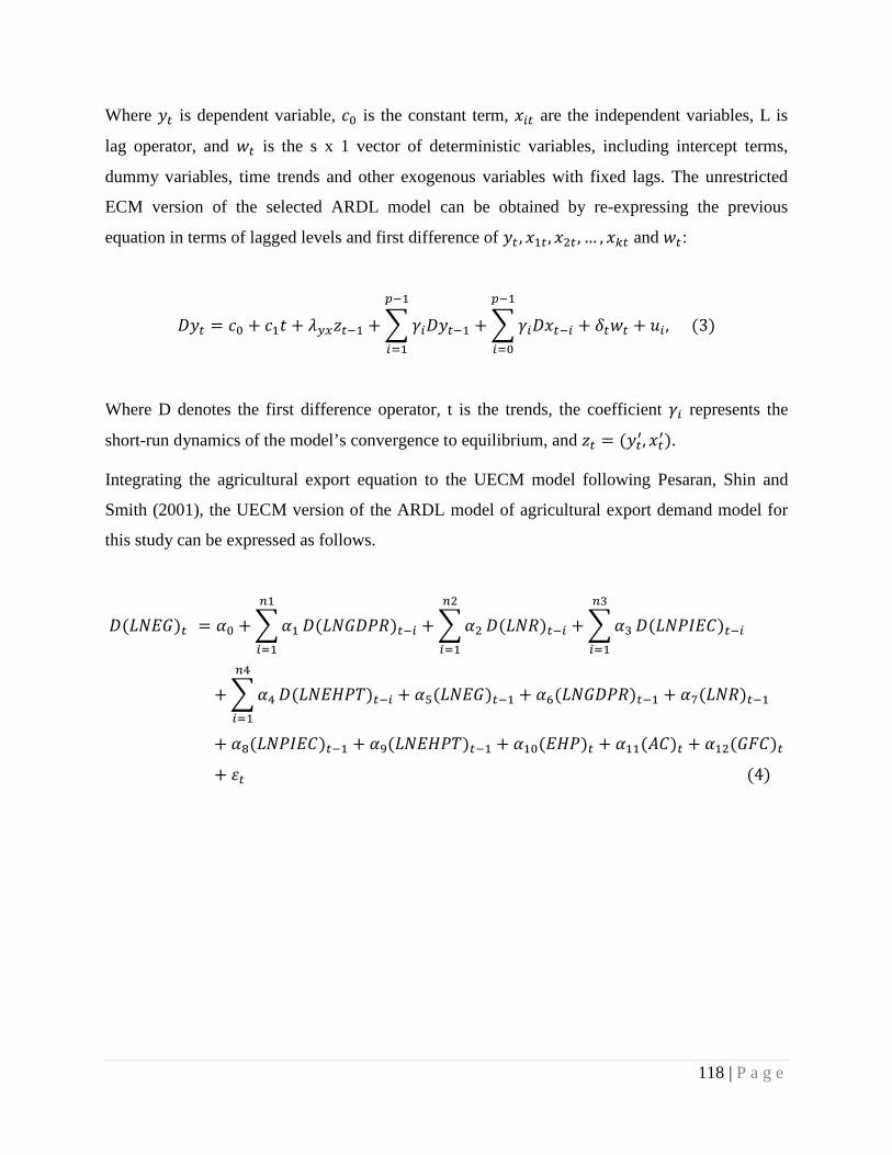
Where 𝑦𝑡 is dependent variable, 𝑐0 is the constant term, 𝑥𝑖𝑡 are the independent variables, L is

lag operator, and 𝑤𝑡 is the s x 1 vector of deterministic variables, including intercept terms,

dummy variables, time trends and other exogenous variables with fixed lags. The unrestricted

ECM version of the selected ARDL model can be obtained by re-expressing the previous

equation in terms of lagged levels and first difference of 𝑦𝑡 , 𝑥1𝑡, 𝑥2𝑡 , … , 𝑥𝑘𝑡 and 𝑤𝑡:

𝐷𝑦𝑡 = 𝑐0 + 𝑐1𝑡 + 𝜆𝑦𝑥𝑧𝑡−1 + �𝛾𝑖𝐷𝑦𝑡−1 + �𝛾𝑖𝐷𝑥𝑡−𝑖 + 𝛿𝑡𝑤𝑡 + 𝑢𝑖,𝑝−1

𝑖=0

𝑝−1

𝑖=1

(3)

Where D denotes the first difference operator, t is the trends, the coefficient 𝛾𝑖 represents the

short-run dynamics of the model’s convergence to equilibrium, and 𝑧𝑡 = (𝑦𝑡′, 𝑥𝑡′).

Integrating the agricultural export equation to the UECM model following Pesaran, Shin and

Smith (2001), the UECM version of the ARDL model of agricultural export demand model for

this study can be expressed as follows.

𝐷(𝐿𝑁𝐸𝐺)𝑡 = 𝛼0 + �𝛼1

𝑛1

𝑖=1

𝐷(𝐿𝑁𝐺𝐷𝑃𝑅)𝑡−𝑖 + �𝛼2

𝑛2

𝑖=1

𝐷(𝐿𝑁𝑅)𝑡−𝑖 + �𝛼3

𝑛3

𝑖=1

𝐷(𝐿𝑁𝑃𝐼𝐸𝐶)𝑡−𝑖

+ �𝛼4

𝑛4

𝑖=1

𝐷(𝐿𝑁𝐸𝐻𝑃𝑇)𝑡−𝑖 + 𝛼5(𝐿𝑁𝐸𝐺)𝑡−1 + 𝛼6(𝐿𝑁𝐺𝐷𝑃𝑅)𝑡−1 + 𝛼7(𝐿𝑁𝑅)𝑡−1

+ 𝛼8(𝐿𝑁𝑃𝐼𝐸𝐶)𝑡−1 + 𝛼9(𝐿𝑁𝐸𝐻𝑃𝑇)𝑡−1 + 𝛼10(𝐸𝐻𝑃)𝑡 + 𝛼11(𝐴𝐶)𝑡 + 𝛼12(𝐺𝐹𝐶)𝑡+ 𝜀𝑡 (4)

118 | P a g e

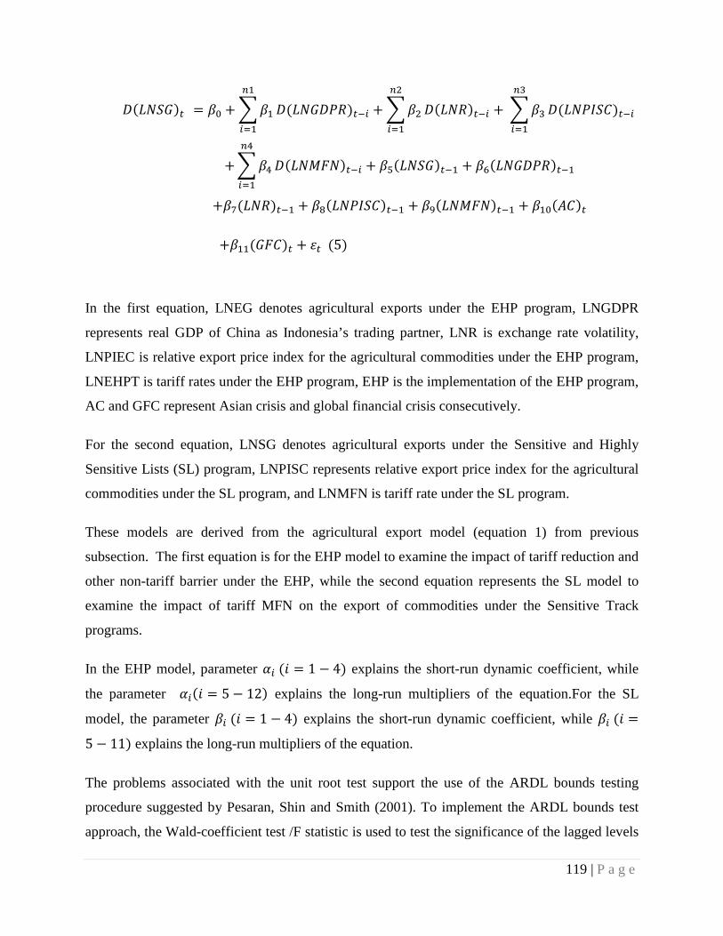
𝐷(𝐿𝑁𝑆𝐺)𝑡 = 𝛽0 + �𝛽1

𝑛1

𝑖=1

𝐷(𝐿𝑁𝐺𝐷𝑃𝑅)𝑡−𝑖 + �𝛽2

𝑛2

𝑖=1

𝐷(𝐿𝑁𝑅)𝑡−𝑖 + �𝛽3

𝑛3

𝑖=1

𝐷(𝐿𝑁𝑃𝐼𝑆𝐶)𝑡−𝑖

+�𝛽4

𝑛4

𝑖=1

𝐷(𝐿𝑁𝑀𝐹𝑁)𝑡−𝑖 + 𝛽5(𝐿𝑁𝑆𝐺)𝑡−1 + 𝛽6(𝐿𝑁𝐺𝐷𝑃𝑅)𝑡−1

+𝛽7(𝐿𝑁𝑅)𝑡−1 + 𝛽8(𝐿𝑁𝑃𝐼𝑆𝐶)𝑡−1 + 𝛽9(𝐿𝑁𝑀𝐹𝑁)𝑡−1 + 𝛽10(𝐴𝐶)𝑡

+𝛽11(𝐺𝐹𝐶)𝑡 + 𝜀𝑡 (5)

In the first equation, LNEG denotes agricultural exports under the EHP program, LNGDPR

represents real GDP of China as Indonesia’s trading partner, LNR is exchange rate volatility,

LNPIEC is relative export price index for the agricultural commodities under the EHP program,

LNEHPT is tariff rates under the EHP program, EHP is the implementation of the EHP program,

AC and GFC represent Asian crisis and global financial crisis consecutively.

For the second equation, LNSG denotes agricultural exports under the Sensitive and Highly

Sensitive Lists (SL) program, LNPISC represents relative export price index for the agricultural

commodities under the SL program, and LNMFN is tariff rate under the SL program.

These models are derived from the agricultural export model (equation 1) from previous

subsection. The first equation is for the EHP model to examine the impact of tariff reduction and

other non-tariff barrier under the EHP, while the second equation represents the SL model to

examine the impact of tariff MFN on the export of commodities under the Sensitive Track

programs.

In the EHP model, parameter 𝛼𝑖 (𝑖 = 1 − 4) explains the short-run dynamic coefficient, while

the parameter 𝛼𝑖(𝑖 = 5 − 12) explains the long-run multipliers of the equation.For the SL

model, the parameter 𝛽𝑖 (𝑖 = 1 − 4) explains the short-run dynamic coefficient, while 𝛽𝑖 (𝑖 =

5 − 11) explains the long-run multipliers of the equation.

The problems associated with the unit root test support the use of the ARDL bounds testing

procedure suggested by Pesaran, Shin and Smith (2001). To implement the ARDL bounds test

approach, the Wald-coefficient test /F statistic is used to test the significance of the lagged levels

119 | P a g e

of the variables in the conditional UECM. The lags of the model can be selected by employed

Schwartz-Bayesian Criteria (SBC), as suggested by Pesaran and Smith (1998), as it often has a

more parsimonious specification compared to other model specification criteria. Thus, the above

equations are estimated by the least square method to get a general ARDL model. Then, from the

general ARDL estimate, a parsimonious model can be obtained by following Hendry (1995)

general-to-specific modelling approach through a process of elimination of insignificant

variables and lags from the model.

There are three steps to execute the ARDL bounds test. The first step is to determine the

existence of the long-run co-integrating relationship among the variables in the equation. The

long-run level relationship between the variables is determined by the Wald-coefficient test or F

test. A joint significance test is performed in order to test the null hypothesis of no co-integration

by setting the coefficient of all the variables, the one lagged level variables equal to zero (Tang

2003a). The F statistics obtained from this test will then be compared to the bound critical values

for upper and lower bands of the I (1), I (0) variables tabulated at Pesaran, Shin and Smith (2001)

with the appropriate significance levels. If the estimated F statistic appears larger than the upper

bound of the critical value, then the null hypothesis of no co-integration is rejected, which

suggests that the variables included in the model are co-integrated. If the estimated F-statistic is

smaller than the lower bound of critical value, then the null hypothesis of no co-integration

cannot be rejected, which implies that the variables are not co-integrated. However, if the

computed F-statistic falls in between the upper and lower bounds, then the decision is

inconclusive regarding the null hypothesis of non co-integration. Here the order of integration of

the explanatory variables I (d) must be known for any conclusion. In this situation, if the

variables are I (0) then the variables are co-integrated on the basis of the lower bound;

conversely, if the variables are I (1) then the variables are not co-integrated on the basis of upper

bound (Shrestha & Chowdhury 2005; Tang 2003a).

If a long-run relationship is found in the first step, this means that the second step has to be

executed (Marashdeh 2005). The second step is to estimate the elasticity’s of the long-run

relationship and determine their values. The long-run elasticity’s are calculated from the

estimated respective coefficient of the one lagged level explanatory variable divided by the

coefficient of the one lagged level dependent variable and then multiplied with a negative sign

120 | P a g e

((Barsden et al. 1989) cited in Tang (2003a)). The long-run value for the dummy variable is used

directly from the estimated equation without dividing by the lag one level dependent variable

(Choong et al. 2005). If there is a long-run relationship between the variables, this indicates the

existence of an error correction representation.

The final third step is to estimate UECM model. The coefficient of the first differing variables in

the estimated UECM represent short-run elasticity’s(Tang 2003a). The UECM result indicates

the speed of adjustment back to long-run equilibrium after the short-run shock. When there is

more than one coefficient in a particular variable, they are added and their joint significance is

tested using the Wald-coefficient test. To ascertain the goodness of fit of the ARDL model,

relevant diagnostic tests and stability tests are conducted. The diagnostic tests examine the

normality, serial correlation, ARCH and heteroskedasticity associated with the model. The

structural stability test is conducted by employing the Cumulative Sum Control Chart (CUSUM)

and CUSUM of Squares tests.

5.3.3 Non-stationary Time Series

The use of econometric technique to analyse time series data is commonly based on the

assumption of data stationary (Gujarati 2006; Hill, Griffiths & Lim 2011; Wooldridge 2009). As

a general rule, non-stationary time series data will obtain a significant regression even when

there is none, leading to a problem called ‘spurious regression’ (Hill, Griffiths & Lim 2011). In

these cases, t-statistics obtained are not reliable because the least square estimator and least

square predictor do not have their usual properties (Gujarati 2011).

The problem caused by non-stationary variables can be avoided if the series is co-integrated

(Engle & Granger 1987). It denotes that even though two or more series are non-stationary they

nevertheless move closer together over time, so that the difference between them is stationary.

To test the order of integration of the variables used in this study, the Augmented Dickey Fuller

(ADF) (Dickey & Fuller 1979) and Phillips-Perron (PP) (Phillips & Perron 1988) unit root tests

will be conducted. The null hypothesis for this test is that the data has unit root or non-stationary

time series.

121 | P a g e

5.3.4 Data

Data required for establishing the export demand model in this study consists of observations on

agricultural export commodities from Indonesia to China in real value (chain-linked volume)

which is grouped based on the ACFTA programs, the relative export price, real exchange rate,

GDP of China, crisis and China’s import tariff rates for the commodities under the EHP and SL

schemes. As it studies, Indonesian agricultural exports under the ACFTA programs of the tariff

sensitivity of the EHP tariff reduction and the MFN tariff for the SL schemes, data for

commodities under the EHP and SL programs and the dummy variable of the implementation of

the EHP and crisis/shock will also be implemented. All data is derived on a quarterly basis

covering the period from the first quarter in 1996 until the second quarter in 2012, making up

sixty-six time series observations. The variables are measured as natural logarithms so that their

differences approximate growth rates, except for the dummy variables. The source of the data for

each variable varies, as explained below.

a. Real Value of China Agricultural Exports from Indonesia

For this study, the agricultural exports will be represented by the agricultural exports from

Indonesia to China. The real value of agricultural exports is obtained by converting the data from

nominal to real value by imposing the volume chain-linked methods. Due to limitations in

availability of agricultural export data, the ACFTA groups will be represented by the EHP and

the SL. The data for agricultural export commodities are retrieved from Tradedata.net (Tradedata

2013).

b. Gross Domestic Product of China

Real GDP of China represents the trading income partner as required in the demand model. The

data is in USD basis, and retrieved from the Datastream website (Datastream 2012)in quarterly

basis.

122 | P a g e

c. Relative Prices

Relative prices for the EHP and the SL commodities are obtained by calculating the export price

index of agricultural exports from Indonesia to China deflated by China’s consumer price index

(PI). The export price indices for EHP and SL groups are calculated by the volume chain-link

method. The data for the export price index is obtained from the Tradedata.net, while China’s

consumer price index is obtained from the Datastream website.

d. Real Exchange Rate Volatility (RER)

Exchange rate volatility is a measure that intends to capture the risk faced by the

exporters/exporters due to unpredictable fluctuations in the exchange rate. For this study, the real

bilateral exchange rate of China (RMB) against Indonesian currency (RP) is used. Data is

retrieved from Datastream website. The volatility of real exchange rate is measured by the

conditional variance of the first difference of the natural log of real exchange rate that is obtained

by employing the GARCH model proposed by (Bollerslev 1986). In this study, the conditional

variance of GARCH (1, 2) model is used.

Following Bollerslev (1986), the GARCH method is implemented to address relationships that

may exist among the different measures of variation and covariation. Such questions are

difficult to answer using conventional volatility models, but they are relatively easy to address

using this realized volatilities and correlations method.

e. China Import Tariff Rates

The China import tariff rates for EHP is measured by the average of weighted export tariff for

every agricultural commodity under the EHP, multiplied by the volume of exports for the related

commodities. The export tariff receives special treatment under the EHP from China. Data for

tariff rates is retrieved from Tariff Analysis Online from World Trade Organization website

(WTO 2014).

The import tariff rates for the Sensitive Track (SL) program is represented by the average of

weighted tariff for every agricultural commodity under the SL scheme multiplies by volume of

exports for the related commodities. Tariff rates under the SL scheme in China are represented

123 | P a g e

by MFN tariff lines as the SL program has no special tariff reduction from 2012 until 2016. The

tariff for these commodities follows the MFN rates during the time period when this study was

conducted. The data for the SL MFN tariff rates is retrieved from Tariff Analysis Online from

World Trade Organization website (WTO 2014).

5.4 Empirical Results and Analysis

The purpose of this section is to present the results of the empirical estimations on testing of the

hypothesis that the ACFTA implementation has a positive relation with agricultural exports from

Indonesia to China. The results are also separated for Indonesia’s agricultural exports with export

tariff reduction under the EHP and the SL commodities exports with the relative price and MFN

tariff. Previous studies of Frankel, JA, Stein and Wei (1997); Magee (2008); Sun and Reed

(2010), explore this issue in other contexts, find that the impact of the free trade agreements were

not immediate but significant in the long-term. The short-run and long-run effects of the ACFTA

have also been examined, especially because the ACFTA has not been in operation long enough

compared to other established free trade agreements. Although there are voluminous studies

focused on the impact of the ACFTA, it is hard to find studies focusing on agricultural trade,

especially in the time series analysis. Thus, this study is intended to address the limitation of past

literature in the time series analysis of the impact of the ACFTA on agricultural trade.

5.4.1 Unit Root Test Results

Although the bounds test is applicable irrespective of whether the variables are I (0) or I (1), the

implementation of unit root tests in the ARDL modelling procedure is still necessary to ensure

that none of the variables is I (2) or beyond because the computed F-statistics are not valid in the

presence of I (2) variables (Pesaran, Shin & Smith 2001). To this end, the Augmented Dickey

Fuller (ADF) and the Phillips-Perron tests have been employed in order to explore all the time

series data properties included in the equation, as suggested by Enders (1995). The tests are

performed on the variables at level and first difference, with optimal lag length for each test

determined automatically by the E-views 7 software. The null hypothesis for these tests is the

data series have unit root. A series is stationary if the null hypothesis is rejected in ADF or PP

tests. The unit root test results are presented in Table 5.1.

124 | P a g e

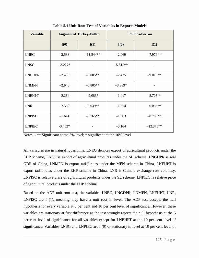
Table 5.1 Unit Root Test of Variables in Exports Models

Variable Augmented Dickey-Fuller Phillips-Perron

I(0) I(1) I(0) I(1)

LNEG –2.538 –11.544** –2.069 –7.979**

LNSG –3.227* - –5.615** -

LNGDPR –2.435 –9.005** –2.435 –9.010**

LNMFN –2.946 –6.805** –3.889* -

LNEHPT –2.284 –2.083* –1.417 –8.705**

LNR –2.589 –6.039** –1.814 –6.033**

LNPISC –1.614 –8.765** –1.503 –8.789**

LNPIEC -3.402* - –3.164 –12.370**

Notes: - ** Significant at the 5% level; * significant at the 10% level

All variables are in natural logarithms. LNEG denotes export of agricultural products under the

EHP scheme, LNSG is export of agricultural products under the SL scheme, LNGDPR is real

GDP of China, LNMFN is export tariff rates under the MFN scheme in China, LNEHPT is

export tariff rates under the EHP scheme in China, LNR is China’s exchange rate volatility,

LNPISC is relative price of agricultural products under the SL scheme, LNPIEC is relative price

of agricultural products under the EHP scheme.

Based on the ADF unit root test, the variables LNEG, LNGDPR, LNMFN, LNEHPT, LNR,

LNPISC are I (1), meaning they have a unit root in level. The ADF test accepts the null

hypothesis for every variable at 5 per cent and 10 per cent level of significance. However, these

variables are stationary at first difference as the test strongly rejects the null hypothesis at the 5

per cent level of significance for all variables except for LNEHPT at the 10 per cent level of

significance. Variables LNSG and LNPIEC are I (0) or stationary in level at 10 per cent level of

125 | P a g e

significance. For comparison, the PP unit root test reveals that the variables LNEG, LNGDPR,

LNEHPT, LNR, LNPISC and LNPIEC are I (1) or have a unit root in level as the PP test fails to

reject the existence of unit root at both 5 and 10 per cent level of significance. In addition,

variables LNSG and LNMFN are I (0) or stationary in level at 5 per cent level of significance.

Thus, it can be concluded that the natural logarithm data are mixed in I (0) and I (1). Obviously,

the mixture of both I(0) and I(1) variables provides a good rationale for using the ARDL bounds

test approach as suggested by Pesaran, Shin and Smith (2001)

5.4.2 ARDL Bounds Test Results for the EHP and SL Models

The model equation used in this study covered the implemented variables in a different order, I

(1) and I (0) and dummy variables are used as the sign for structural breaks and seasonal time

based on time series data. As explained in the literature review, Johansen’s co-integration

estimation does not allow dummy variables and requires all variables to be in the same order in

their system, so it is more appropriate to use the ARDL method.

To get parsimonious models, the maximum lag length in the ARDL model is selected by

employing the Schwartz-Bayesian Criteria (SBC). The maximum lag length of 2 is chosen and

implemented for in the SL model and maximum lag length 4 is chosen in the EHP model. Based

on these models, the long-run existence of the EHP and the SL export demand models are

examined. In this study, the null hypothesis of 𝛼𝑖 = 0, (i = coefficient for variables in

logarithm) for equation of the EHP model and 𝛽𝑖 = 0, (i = coefficient for variables in

logarithm) for the SL model will be tested by the Wald test. These are the coefficient of the one

lagged level variables included in the models including the dummy variables for the ACFTA.

This study has also employed Hendry’s General to Specific approach (1991) to arrive at a

parsimonious specification of the model. The initial optimal lag length based on the SBC is

implemented and eliminates the variables which are not significant, except for the level variables

and the intercept. The final models for the EHP and the SL are then re-examined for their long-

run significance. The co-integration relationships are present in both models proved by the fact

that the F statistics values that are higher than the Pesaran’s Table of bound critical values. The F

statistics of the Wald test on the level variables have stronger results as compared to the previous

models. This confirms the existence of the long - run relationship between the variables used in

126 | P a g e

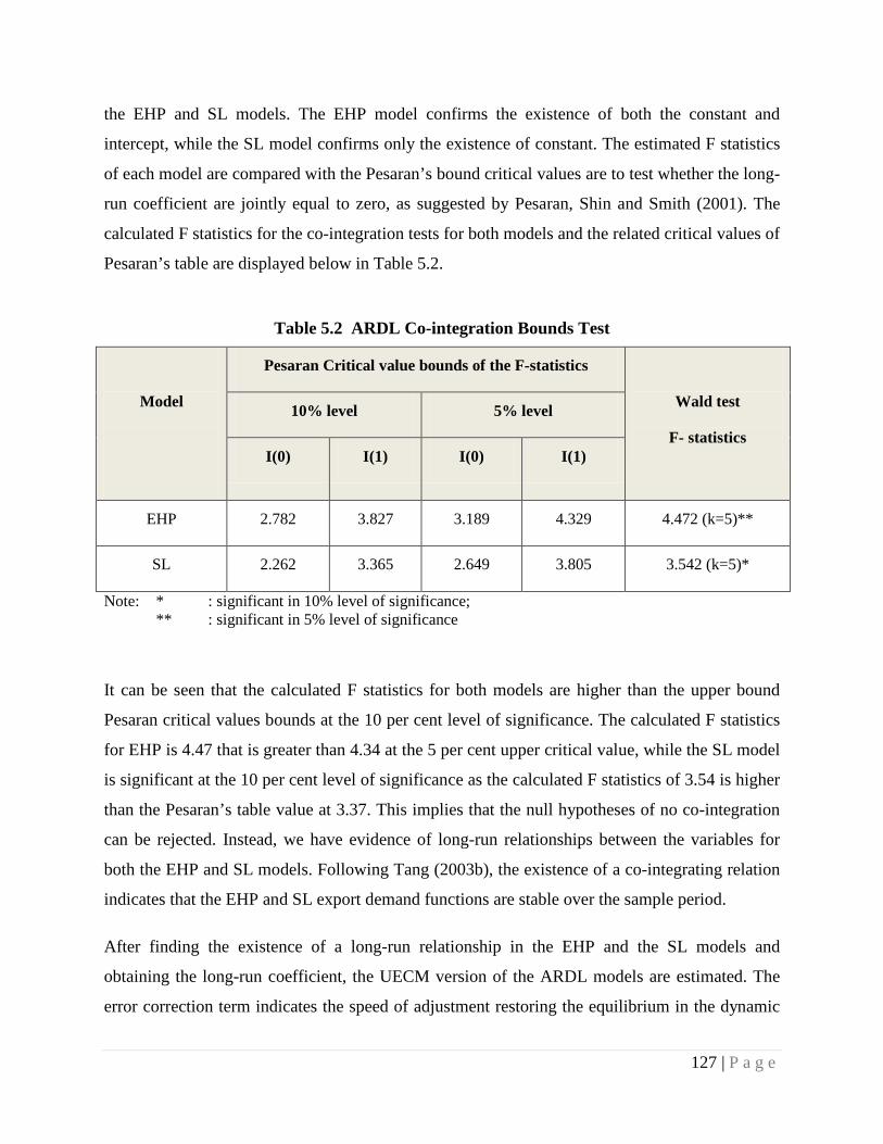
the EHP and SL models. The EHP model confirms the existence of both the constant and

intercept, while the SL model confirms only the existence of constant. The estimated F statistics

of each model are compared with the Pesaran’s bound critical values are to test whether the long-

run coefficient are jointly equal to zero, as suggested by Pesaran, Shin and Smith (2001). The

calculated F statistics for the co-integration tests for both models and the related critical values of

Pesaran’s table are displayed below in Table 5.2.

Table 5.2 ARDL Co-integration Bounds Test

Model

Pesaran Critical value bounds of the F-statistics

Wald test

F- statistics

10% level 5% level

I(0) I(1) I(0) I(1)

EHP 2.782 3.827 3.189 4.329 4.472 (k=5)**

SL 2.262 3.365 2.649 3.805 3.542 (k=5)*

Note: * : significant in 10% level of significance; ** : significant in 5% level of significance

It can be seen that the calculated F statistics for both models are higher than the upper bound

Pesaran critical values bounds at the 10 per cent level of significance. The calculated F statistics

for EHP is 4.47 that is greater than 4.34 at the 5 per cent upper critical value, while the SL model

is significant at the 10 per cent level of significance as the calculated F statistics of 3.54 is higher

than the Pesaran’s table value at 3.37. This implies that the null hypotheses of no co-integration

can be rejected. Instead, we have evidence of long-run relationships between the variables for

both the EHP and SL models. Following Tang (2003b), the existence of a co-integrating relation

indicates that the EHP and SL export demand functions are stable over the sample period.

After finding the existence of a long-run relationship in the EHP and the SL models and

obtaining the long-run coefficient, the UECM version of the ARDL models are estimated. The

error correction term indicates the speed of adjustment restoring the equilibrium in the dynamic

127 | P a g e

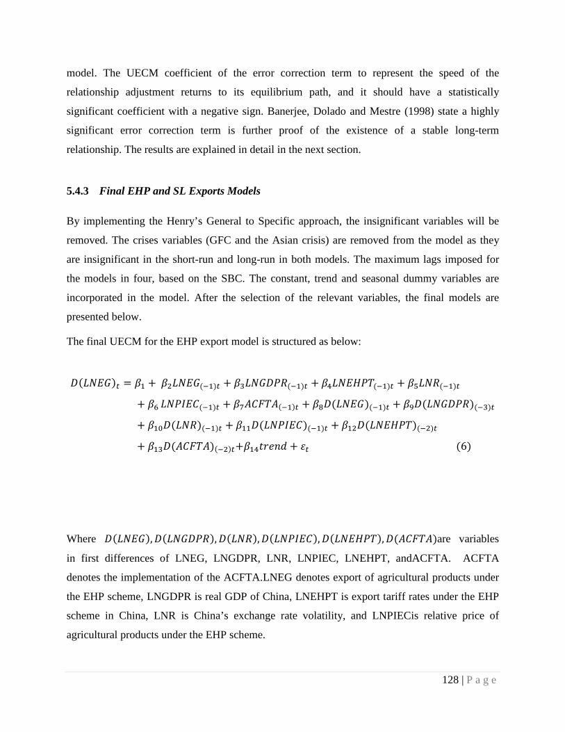
model. The UECM coefficient of the error correction term to represent the speed of the

relationship adjustment returns to its equilibrium path, and it should have a statistically

significant coefficient with a negative sign. Banerjee, Dolado and Mestre (1998) state a highly

significant error correction term is further proof of the existence of a stable long-term

relationship. The results are explained in detail in the next section.

5.4.3 Final EHP and SL Exports Models

By implementing the Henry’s General to Specific approach, the insignificant variables will be

removed. The crises variables (GFC and the Asian crisis) are removed from the model as they

are insignificant in the short-run and long-run in both models. The maximum lags imposed for

the models in four, based on the SBC. The constant, trend and seasonal dummy variables are

incorporated in the model. After the selection of the relevant variables, the final models are

presented below.

The final UECM for the EHP export model is structured as below:

𝐷(𝐿𝑁𝐸𝐺)𝑡 = 𝛽1 + 𝛽2𝐿𝑁𝐸𝐺(−1)𝑡 + 𝛽3𝐿𝑁𝐺𝐷𝑃𝑅(−1)𝑡 + 𝛽4𝐿𝑁𝐸𝐻𝑃𝑇(−1)𝑡 + 𝛽5𝐿𝑁𝑅(−1)𝑡

+ 𝛽6 𝐿𝑁𝑃𝐼𝐸𝐶(−1)𝑡 + 𝛽7𝐴𝐶𝐹𝑇𝐴(−1)𝑡 + 𝛽8𝐷(𝐿𝑁𝐸𝐺)(−1)𝑡 + 𝛽9𝐷(𝐿𝑁𝐺𝐷𝑃𝑅)(−3)𝑡

+ 𝛽10𝐷(𝐿𝑁𝑅)(−1)𝑡 + 𝛽11𝐷(𝐿𝑁𝑃𝐼𝐸𝐶)(−1)𝑡 + 𝛽12𝐷(𝐿𝑁𝐸𝐻𝑃𝑇)(−2)𝑡

+ 𝛽13𝐷(𝐴𝐶𝐹𝑇𝐴)(−2)𝑡+𝛽14𝑡𝑟𝑒𝑛𝑑 + 𝜀𝑡 (6)

Where 𝐷(𝐿𝑁𝐸𝐺),𝐷(𝐿𝑁𝐺𝐷𝑃𝑅),𝐷(𝐿𝑁𝑅),𝐷(𝐿𝑁𝑃𝐼𝐸𝐶),𝐷(𝐿𝑁𝐸𝐻𝑃𝑇),𝐷(𝐴𝐶𝐹𝑇𝐴)are variables

in first differences of LNEG, LNGDPR, LNR, LNPIEC, LNEHPT, andACFTA. ACFTA

denotes the implementation of the ACFTA.LNEG denotes export of agricultural products under

the EHP scheme, LNGDPR is real GDP of China, LNEHPT is export tariff rates under the EHP

scheme in China, LNR is China’s exchange rate volatility, and LNPIECis relative price of

agricultural products under the EHP scheme.

128 | P a g e

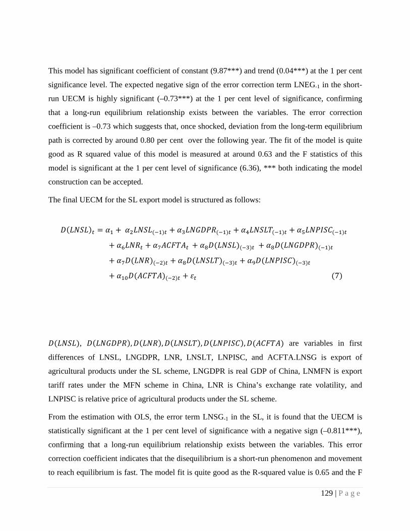
This model has significant coefficient of constant (9.87***) and trend (0.04***) at the 1 per cent

significance level. The expected negative sign of the error correction term LNEG-1 in the short-

run UECM is highly significant (–0.73***) at the 1 per cent level of significance, confirming

that a long-run equilibrium relationship exists between the variables. The error correction

coefficient is –0.73 which suggests that, once shocked, deviation from the long-term equilibrium

path is corrected by around 0.80 per cent over the following year. The fit of the model is quite

good as R squared value of this model is measured at around 0.63 and the F statistics of this

model is significant at the 1 per cent level of significance (6.36), *** both indicating the model

construction can be accepted.

The final UECM for the SL export model is structured as follows:

𝐷(𝐿𝑁𝑆𝐿)𝑡 = 𝛼1 + 𝛼2𝐿𝑁𝑆𝐿(−1)𝑡 + 𝛼3𝐿𝑁𝐺𝐷𝑃𝑅(−1)𝑡 + 𝛼4𝐿𝑁𝑆𝐿𝑇(−1)𝑡 + 𝛼5𝐿𝑁𝑃𝐼𝑆𝐶(−1)𝑡

+ 𝛼6𝐿𝑁𝑅𝑡 + 𝛼7𝐴𝐶𝐹𝑇𝐴𝑡 + 𝛼8𝐷(𝐿𝑁𝑆𝐿)(−3)𝑡 + 𝛼8𝐷(𝐿𝑁𝐺𝐷𝑃𝑅)(−1)𝑡

+ 𝛼7𝐷(𝐿𝑁𝑅)(−2)𝑡 + 𝛼8𝐷(𝐿𝑁𝑆𝐿𝑇)(−3)𝑡 + 𝛼9𝐷(𝐿𝑁𝑃𝐼𝑆𝐶)(−3)𝑡

+ 𝛼10𝐷(𝐴𝐶𝐹𝑇𝐴)(−2)𝑡 + 𝜀𝑡 (7)

𝐷(𝐿𝑁𝑆𝐿), 𝐷(𝐿𝑁𝐺𝐷𝑃𝑅),𝐷(𝐿𝑁𝑅),𝐷(𝐿𝑁𝑆𝐿𝑇),𝐷(𝐿𝑁𝑃𝐼𝑆𝐶),𝐷(𝐴𝐶𝐹𝑇𝐴) are variables in first

differences of LNSL, LNGDPR, LNR, LNSLT, LNPISC, and ACFTA.LNSG is export of

agricultural products under the SL scheme, LNGDPR is real GDP of China, LNMFN is export

tariff rates under the MFN scheme in China, LNR is China’s exchange rate volatility, and

LNPISC is relative price of agricultural products under the SL scheme.

From the estimation with OLS, the error term LNSG-1 in the SL, it is found that the UECM is

statistically significant at the 1 per cent level of significance with a negative sign (–0.811***),

confirming that a long-run equilibrium relationship exists between the variables. This error

correction coefficient indicates that the disequilibrium is a short-run phenomenon and movement

to reach equilibrium is fast. The model fit is quite good as the R-squared value is 0.65 and the F

129 | P a g e

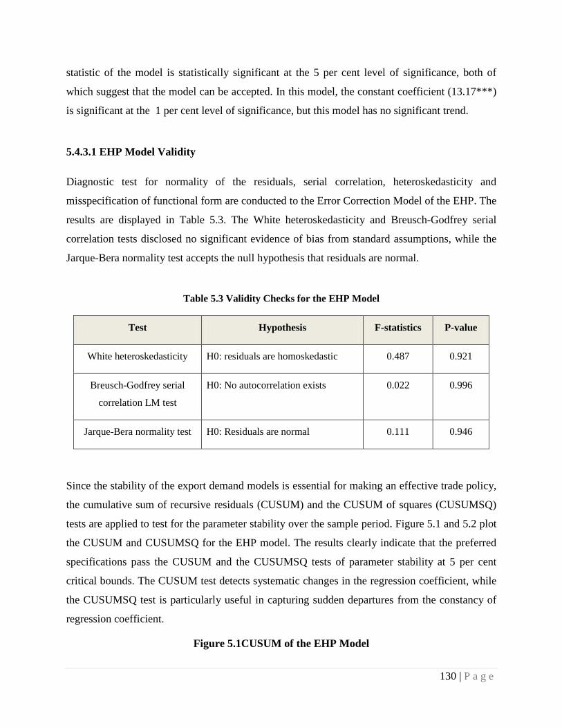
statistic of the model is statistically significant at the 5 per cent level of significance, both of

which suggest that the model can be accepted. In this model, the constant coefficient (13.17***)

is significant at the 1 per cent level of significance, but this model has no significant trend.

5.4.3.1 EHP Model Validity

Diagnostic test for normality of the residuals, serial correlation, heteroskedasticity and

misspecification of functional form are conducted to the Error Correction Model of the EHP. The

results are displayed in Table 5.3. The White heteroskedasticity and Breusch-Godfrey serial

correlation tests disclosed no significant evidence of bias from standard assumptions, while the

Jarque-Bera normality test accepts the null hypothesis that residuals are normal.

Table 5.3 Validity Checks for the EHP Model

Test Hypothesis F-statistics P-value

White heteroskedasticity H0: residuals are homoskedastic 0.487 0.921

Breusch-Godfrey serial

correlation LM test

H0: No autocorrelation exists 0.022 0.996

Jarque-Bera normality test H0: Residuals are normal 0.111 0.946

Since the stability of the export demand models is essential for making an effective trade policy,

the cumulative sum of recursive residuals (CUSUM) and the CUSUM of squares (CUSUMSQ)

tests are applied to test for the parameter stability over the sample period. Figure 5.1 and 5.2 plot

the CUSUM and CUSUMSQ for the EHP model. The results clearly indicate that the preferred

specifications pass the CUSUM and the CUSUMSQ tests of parameter stability at 5 per cent

critical bounds. The CUSUM test detects systematic changes in the regression coefficient, while

the CUSUMSQ test is particularly useful in capturing sudden departures from the constancy of

regression coefficient.

Figure 5.1CUSUM of the EHP Model

130 | P a g e

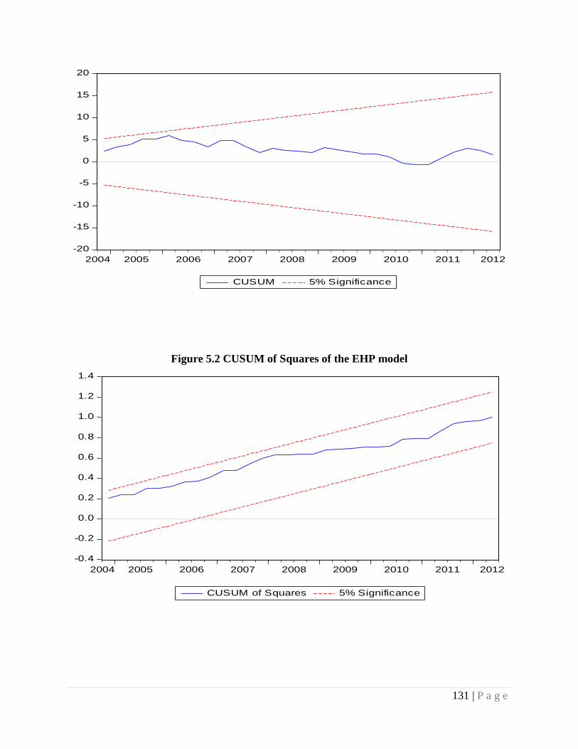
Figure 5.2 CUSUM of Squares of the EHP model

-20

-15

-10

-5

0

5

10

15

20

2004 2005 2006 2007 2008 2009 2010 2011 2012

CUSUM 5% Significance

-0.4

-0.2

0.0

0.2

0.4

0.6

0.8

1.0

1.2

1.4

2004 2005 2006 2007 2008 2009 2010 2011 2012

CUSUM of Squares 5% Significance

131 | P a g e

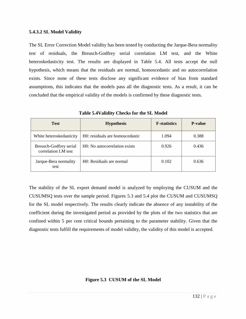
5.4.3.2 SL Model Validity

The SL Error Correction Model validity has been tested by conducting the Jarque-Bera normality

test of residuals, the Breusch-Godfrey serial correlation LM test, and the White

heteroskedasticity test. The results are displayed in Table 5.4. All tests accept the null

hypothesis, which means that the residuals are normal, homoscedastic and no autocorrelation

exists. Since none of these tests disclose any significant evidence of bias from standard

assumptions, this indicates that the models pass all the diagnostic tests. As a result, it can be

concluded that the empirical validity of the models is confirmed by these diagnostic tests.

Table 5.4Validity Checks for the SL Model

Test Hypothesis F-statistics P-value

White heteroskedasticity H0: residuals are homoscedastic 1.094 0.388

Breusch-Godfrey serial correlation LM test

H0: No autocorrelation exists 0.926 0.436

Jarque-Bera normality test

H0: Residuals are normal 0.102 0.636

The stability of the SL export demand model is analyzed by employing the CUSUM and the

CUSUMSQ tests over the sample period. Figures 5.3 and 5.4 plot the CUSUM and CUSUMSQ

for the SL model respectively. The results clearly indicate the absence of any instability of the

coefficient during the investigated period as provided by the plots of the two statistics that are

confined within 5 per cent critical bounds pertaining to the parameter stability. Given that the

diagnostic tests fulfill the requirements of model validity, the validity of this model is accepted.

Figure 5.3 CUSUM of the SL Model

132 | P a g e

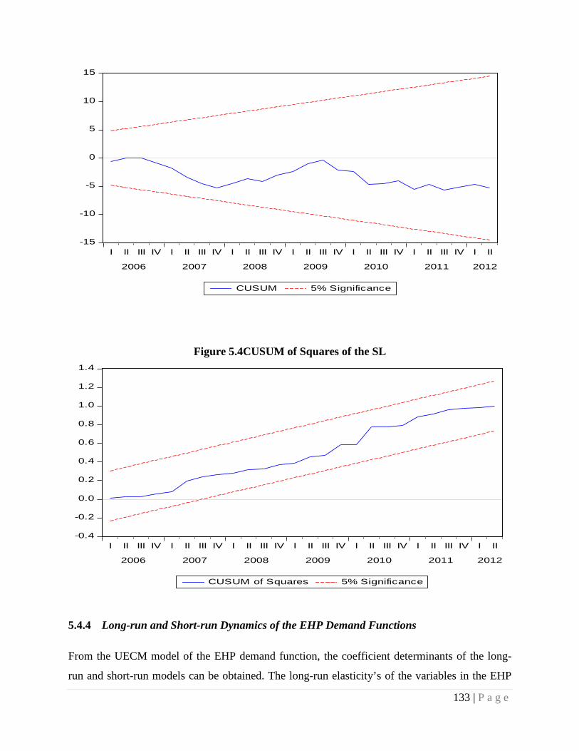
Figure 5.4CUSUM of Squares of the SL

5.4.4 Long-run and Short-run Dynamics of the EHP Demand Functions

From the UECM model of the EHP demand function, the coefficient determinants of the long-

run and short-run models can be obtained. The long-run elasticity’s of the variables in the EHP

-15

-10

-5

0

5

10

15

I II III IV I II III IV I II III IV I II III IV I II III IV I II III IV I II

2006 2007 2008 2009 2010 2011 2012

CUSUM 5% Significance

-0.4

-0.2

0.0

0.2

0.4

0.6

0.8

1.0

1.2

1.4

I II III IV I II III IV I II III IV I II III IV I II III IV I II III IV I II

2006 2007 2008 2009 2010 2011 2012

CUSUM of Squares 5% Significance

133 | P a g e

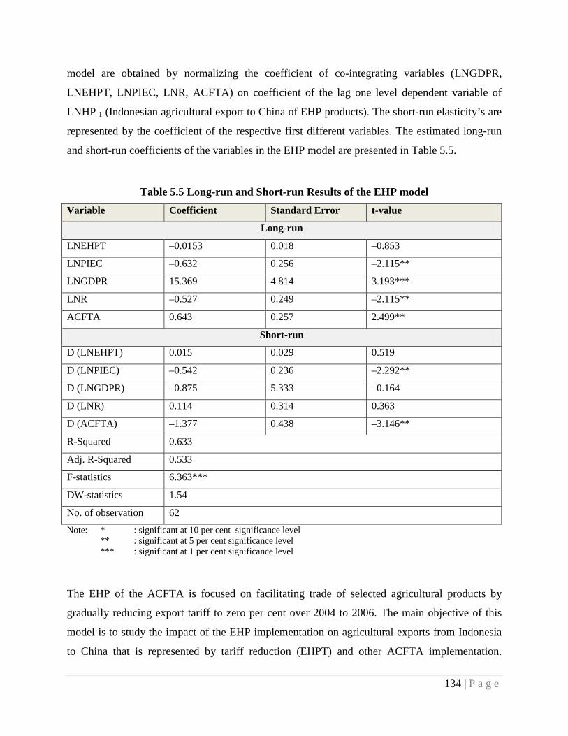
model are obtained by normalizing the coefficient of co-integrating variables (LNGDPR,

LNEHPT, LNPIEC, LNR, ACFTA) on coefficient of the lag one level dependent variable of

LNHP-1 (Indonesian agricultural export to China of EHP products). The short-run elasticity’s are

represented by the coefficient of the respective first different variables. The estimated long-run

and short-run coefficients of the variables in the EHP model are presented in Table 5.5.

Table 5.5 Long-run and Short-run Results of the EHP model Variable Coefficient Standard Error t-value

Long-run

LNEHPT –0.0153 0.018 –0.853

LNPIEC –0.632 0.256 –2.115**

LNGDPR 15.369 4.814 3.193***

LNR –0.527 0.249 –2.115**

ACFTA 0.643 0.257 2.499**

Short-run

D (LNEHPT) 0.015 0.029 0.519

D (LNPIEC) –0.542 0.236 –2.292**

D (LNGDPR) –0.875 5.333 –0.164

D (LNR) 0.114 0.314 0.363

D (ACFTA) –1.377 0.438 –3.146**

R-Squared 0.633

Adj. R-Squared 0.533

F-statistics 6.363***

DW-statistics 1.54

No. of observation 62 Note: * : significant at 10 per cent significance level ** : significant at 5 per cent significance level *** : significant at 1 per cent significance level

The EHP of the ACFTA is focused on facilitating trade of selected agricultural products by

gradually reducing export tariff to zero per cent over 2004 to 2006. The main objective of this

model is to study the impact of the EHP implementation on agricultural exports from Indonesia

to China that is represented by tariff reduction (EHPT) and other ACFTA implementation.

134 | P a g e

However, other variables predicted to influence the export are also included in the model as

control variables. The response of the independent variables in the model equation on

agricultural exports from Indonesia to China under the EHP program can be explained as

follows.

The long-run dynamics of Indonesian export of EHP agricultural products is also determined by

significant variables of LNPIEC (relative export price), LNGDPR (GDP of China), LNR

(exchange rate volatility) and ACFTA (implementation of ACFTA). On the other hand, the

LNEHPT variable (export tariff reduction of the EHP program) is not significant. From the long-

run perspective in Table 5.5, the coefficient of LNEHPT indicates that the response to the

implementation of the EHP with reduced export tariff from China does not have a significant

impact on increasing Indonesian exports to China of agricultural commodities under the EHP

program.

From the short-run perspective, Table 5.5 shows that the first difference of implementation of the

ACFTA (D(ACFTA)) has a significant impact on EHP agricultural export growth from

Indonesia as well as the change in relative price (D(LNPIEC)). However, the export tariff

reduction under the EHP scheme (D(LNEHPT), China’s income (D(LNGDPR)) and exchange

rate volatility (D(LNR)) have no significant impacts on EHP agricultural export from Indonesia

to China.More detailed explanations about the impacts of individual variables on the EHP

exports from Indonesia to China are given below.

5.4.4.1 ACFTA

The implementation of ACFTA was begun on the 1st of January 2005. The trade liberalization

dummy variable (ACFTA) represents the implementation of ACFTA rules other than tariff

reduction. The results show that the ACFTA has positive and significant impacts of Indonesian

agricultural export growth in China in the long-run according to the EHP model estimation.

From the finding in Table 5.5, the implementation of the ACFTA will increase Indonesian export

for the EHP agricultural commodities by around 0.64 per cent.

On the other hand, in the short-run, trade liberalization dummy (D (ACFTA)) shows significant

negative impact on Indonesian exports to China of EHP agricultural products. This determinant

has reduced the growth of export of agricultural commodities under the EHP from Indonesia to

135 | P a g e

China for –1.4 per cent. The implementation of other programs under the ACFTA, such as Rules

of Origin and the Operational Certification Procedure, provide the standards for commodities

exports to be fulfilled in the short-run, need to be adjusted by Indonesian exporters. This result is

consistent with the Disdier, Fontagné and Mimouni (2008) study which shows that the

implementation of these rules have a negative impact on agricultural exports from developing

countries.

5.4.4.2 Tariff Reduction under the EHP

Theoretically, free trade areas involve only partial eliminationof tariffs, and they can lead to

unexpected results. As explained by Viner (1950), the countries left out of the union and even the

countries inside the union can become worse off. Thus it is possible that a country could lose out

from joining the union.

The contribution of agriculture to overall Indonesian exports remains small, despite the

commodities boom. Agricultural production naturally responds sluggishly to changes in prices.

Thus it is not surprising that Indonesia has been unable to fully take advantage of the recent high

commodity prices. Moreover, the low agriculture export growthcould also be attributed to

rejections by importing countries, for the reason that Indonesian products do not comply with the

international or health, safety, and environment standard (Bappenas 2009).

The implementation of the EHP program aimed at reducing China’s export tariff to zero per cent

for the EHP commodities in the period of 2004-2006. The estimation of the model as displayed

in Table 5.5 shows that tariff reduction has the same impact both in the shortrun and the longrun.

There is no significant impact of the EHP implementation on Indonesian exports to China for the

EHP’s agricultural products. In fact, the reduction of China’s export tariff for the agricultural

commodities under the EHP program tends to decrease the Indonesian EHP agricultural exports

to China, which is shown by the positive sign of the coefficient of the D(LNEHPT) though not to

a significant extent. Furthermore, the volume of Indonesian agricultural exports tend to be

decreasing even though China’s export tariff is reduced to zero per cent for the commodities

under the EHP program. Although the percentageof change is not significant, 1 per cent of

China’s export tariff reduction tends to reduce Indonesian exportsof the EHP products by 0.01

per cent. This result contradicts the objective of the EHP program under the ACFTA to increase

136 | P a g e

agricultural trade between ASEAN countries and China in the longrun. This finding is consistent

with a study conducted by Vanzetti et al. (2011), who point out that Indonesia experiences a

trade reduction for certain agricultural commodities such as paddy rice, other cereal, oilseeds,

vegetable and fruits and other crops.

Tariff reduction on certain agricultural commodities under the EHP scheme produces a loss on

the Indonesian side. This condition can be further explained by looking into the details of the

trading agreement between Indonesia and China under the auspices of the ACFTA. First, the

types of commodities agreed for tariff reduction in the EHP program are not Indonesia’s superior

products and not widely produced for export in Indonesia. Instead, Indonesia has heavily

imported these commodities, especially for agricultural commodities under the HS code 01 to

08(BPS 2014). Second, according to Chen, C and Duncan (2008), China has comparative

advantage on some of these agricultural commodities, thus lowering the export tariff does not

necessarily increase import demand for these products from China’s side. For example, lowering

export tariff for horticulture and meat commodities will not change the domestic demand as

China has enough production of these commodities at a relatively low price. Third, in contrast to

the second reason, the commodities in which China has no comparative advantages, but has

strong demand in the domestic market are called ‘national strategic products’, such as edible oil,

rice, maize, sugar, cotton and wool. China’s government imposes special treatments that are

allowed under the WTO accession by imposing higher rates for in-quota tariff (TRQ) and place

quota on these commodities (Chen, C & Duncan 2008). These restrictive conditions from the

Chinese side could have contributed to the low demand for Indonesian exports despite the

incentive of reduced tariffs.

5.4.4.3 Relative Price Index

The relative price for EHP products (LNPIEC) is also significant in the long-run at 5 per cent

significance level. The sign of coefficient is negative, indicating that the reduction of price will

increase the demand of agricultural export for the EHP products. The coefficient of relative price

at around –0.69 is inelastic, which suggests that a 1 per cent decrease in relative prices will

137 | P a g e

increase the growth of the EHP agricultural export from Indonesia to China by 0.69 per cent.

This result was expected and is in accordance with the theory.

The change in the relative price index, (D(LNPIEC)), in the short-run also showed a similar

outcome as the long-run. The reduction of the relative price significantly increased the growth of

Indonesian agricultural exports under the EHP program at the 5 per cent significance level. The

negative coefficient of –0.542 denotes 1 per cent decrease in the relative price will enhance the

export growth by 0.54 per cent.

5.4.4.4 Exchange Rate Volatility

The volatility of exchange rates has a significant negative impact at the 5 per cent level of

significance on the growth of Indonesian exports to China of the EHP agricultural commodities

in the long-run. As expected, the coefficient is negative, which means that the higher volatility of

exchange rate will depress the growth of Indonesian EHP agricultural exports to China.

Lowering the exchange rate volatility of 1 per cent will increase Indonesian EHP agricultural

export to China by 0.53 per cent in the long-run. This result is consistent with Yusoff and Sabit

(2014) who find that a 1 per cent increase in exchange rate volatility will decrease exports from

the ASEAN members to China under the ACFTA by 0.21 per cent. In terms of global studies, De

Grauwe (1988), Cushman (1983), Ghosh et al. (1997) and Arize (1995) claim that exchange rate

volatility has a significant negative impact on international trade in general, while Cho, Sheldon

and McCorriston (2002) find a negative impact of exchange rate volatility on agricultural trade.

However, in the short-run, the exchange rate volatility does not have a significant influence on

the Indonesian agricultural export growth to China. This result is contrary to the extant evidence

that shows significant and negative impact on agricultural export demand growth. It is also

contrary to a previous study by Maskus (1986) which suggests that exchange rate volatility has a

negative impact on agricultural trade in the short-run.

These results can perhaps be justified by an explanation of the exchange rate policy taken by the

Chinese government. The Chinese government’s decision to change the exchange rate system

from a fixed to floating rate in the 1980s caused volatility in the RMB exchange rate. But the

Chinese government also pegged the exchange rate to the US dollar, which ensured that the

exchange rate was not too volatile (Huchet-Bourdon & Bahmani-Oskooee 2013). The relative

138 | P a g e

stability of the currency in the short term could have resulted in insignificant effect of exchange

rate, whereas greater volatility of the exchange rate in the long-term results in significant

negative impact on the growth of Indonesian agricultural exports to China.

5.4.4.5 Trade Partner’s Income (Real China’s GDP)

The variable of partner GDP, representing China’s income tends to support Indonesian exports to

China for the EHP group of agricultural commodities. The income elasticity is quite high —

15.37 and significant at the 5 per cent level of significance. China’s real GDP (LNGDPR) has a

positive and significant impact on the agricultural exports from Indonesia in the long-run,

indicating that a rise in real income of China leads to an increase in Indonesian agricultural

exports to China through the increased purchasing power of foreign consumers.

This finding is consistent with a study conducted by Yusoff and Sabit (2014) who argue the

China’s real GDP could significantly affect the bilateral exports of ASEAN countries to China.

However, in the short-run, the role of China’s GDP growth is not significant in improving

Indonesian agricultural export growth in China for EHP commodities. Even though economic

theory postulates that income of trading partner is a dominant factor for increasing trade, the

trading partner’s income does not seem to be a significant determinant for these agricultural

commodities,.

5.4.5 Long-run and Short-run Dynamics of the SL Demand Model Functions

Unlike the EHP program that facilitates trading between Indonesia and China by reducing export

tariff to zero per cent in the 2004 to 2006 period, the tariff of all commodity exports under the

Sensitive Track scheme in the ACFTA can only be reduced after 2012 and 2016. As there is no

export tariff reduction for the commodities under the Sensitive Track during the time period in

which this study is conducted, the proxy for tariff for the SL commoditiesused in this model is

the average of weighted related MFN tariff multiplied by the volume of exports. This means that

the construction of the SL demand model will use the MFN tariff for all related

commoditiesunder this scheme.

Table 5.6Long-Run and Short-run Results of the SL model

139 | P a g e

Variable Coefficient Standard Error t-value

Long-run

LNSLT –0.004 0.163 –0.023

LNPISC –0.2618 0.149 –1.758*

LNGDPR 11.249 4.503 2.498**

LNR –0.607 0.238 –2.550**

ACFTA –0.138 0.265 –0.519

Short-run

D (LNSLT) –0.320 0.105 –3.052**

D (LNPISC) –0.492 0.285 –1.725*

D (LNGDPR) –5.809 5.672 –1.024

D (LNR) –0.638 0.317 –2.013**

D (ACFTA) 0.385 0.419 0.920

R-Squared 0.651

Adj. R-Squared 0.547

F-statistics 6.268***

DW-statistics 2.163

No. of Observations 62 Note: * : significant at 10 per cent significance level ** : significant at 5 per cent significance level *** : significant at 1 per cent significance level

Table 5.6 displays the statistical measures of the SL Unconditional Error Correction Model of

ARDL approach. The long-run elasticity’s of the variables in the SL model are calculated. In

general, the long-run empirical results of the SL model show that relative price (LNPISC),

China’s GDP (LNGDPR), exchange rate volatility (LNR) is significant in influencing the growth

of Indonesian export to China for SL agricultural commodities at least at the 10 per cent level of

significance. This is broadly consistent with the theory. However, contrary to expectation, the

main variables of implementation of the ACFTA and export tariff variables do not have a

statistically significant influence in stimulating the growth of exports.

The short-run perspective presents a slightly different result from the long-run. While

implementation of the ACFTA (D(ACFTA)) is again found to have no significant impact on the

140 | P a g e

growth of exports, the variable of China’s GDP (D(LNGDPR)) is also found to be insignificant.

Meanwhile, export tariff ((D(LNSLT)) along with other variables of relative price (D(LNPISC)),

and exchange rate volatility (D(LNR)) have significant impacts on Indonesian agricultural export

to China for the SL commodities in the short-run.

5.4.5.1 ACFTA

The core variable in the demand model is the implementation of the ACFTA. Surprisingly, this

variable does not have a significant impact on the growth of SL agricultural exports from

Indonesia to China both in the long-run and short-run. In the long-run, the implementation of the

ACFTA tends to cause a decline in the exports, although not significantly. In the short-run, the

ACFTA is able to amplify the exports by 0.39 per cent, but this is not enough to significantly

raise the volume of exports. This result is inconsistent with a study by Vanzetti et al. (2011) who

find that the implementation of the ACFTA will increase trade in particular agricultural

commodities, such as vegetable oils and fats, by 0.8 per cent but decrease other processed

agricultural products by 0.1 per cent. Although the present study does not differentiate between

specific product categories, the discrepancies recorded by Vanzetti et al. are quite similar to

those in this study.

Palm oil products constitute one of the main commodities under this scheme as they have a very

high demand, but this commodity is also fraught with environmental sustainability issues. While

the ACFTA rules for all commodities must comply with the general WTO rules, there are

specific requirements for certain commodities that also need to be satisfied. For example, palm

oil products need to acquire a certification to meet the requirement of the Malaysia-based Round

Table on Sustainable Palm Oil (Pusdatin 2013). The adjustment period required by the exporters

to fulfill the requirement of the ACFTA can be responsible for this condition. Disdier, Fontagné

and Mimouni (2008) argue that this kind of additional requirement slows down exports from

developing countries.

141 | P a g e

5.4.5.2 Tariff Reduction under MFN Tariff Rates

As there is no export tariff reduction for the commodities under the Sensitive Track during the

time period in which this study is conducted, the proxy for tariff for the SL commoditiesused in

this model is the average of weighted related MFN tariff multiplied by the volume of exports. As

shown in Table 5.6, the response of Indonesian exports to China of the SL commodities for the

MFN tariff is not significant in the long-run. Even though the sign of the coefficient is negative,

implying that the reduction of the export tariff will increase the export, it is not able to raise the

export volume significantly. The reduction of 1 per cent MFN tariff will increase Indonesian

exports 0.004 per centof the SL agricultural products.

As many countries adopt protectionist strategies for their agricultural sector, export tariffs for

agricultural products are usually bigger than those for manufactured goods (Hoekman & Nicita

2011), causing the agricultural export tariff to remain high in the long-term(May 2011). The

Chinese government also uses the instrument of export tariffs to protect their strategic

agricultural products, including vegetable oils (Chen, C & Duncan 2008). But vegetable oils,

especially palm oils, are the main agricultural products exported from Indonesia included in the

SL program under the ACFTA. Hence, protectionist strategies by the Chinese government could

be the reason why the reduction of the MFN tariff has not had any substantial impact on

improving the export volume of these commodities.

A different result is obtained from the analysis of short-run dynamics of tariff reduction.

Indonesian exports to China of SL commodities seem to be very sensitive to the reduction of

MFN tariff in the short-run. Table 5.6 shows that the change of MFN export tariff is statistically

significant in influencing the exports at 5 per cent level of significance. Decreasing 1 per cent of

the MFN tariff will lift the exports by 0.32 per cent. Thus the volume of exports is more sensitive

to MFN tariff reduction in the short-run rather than the long-run.

Although the focus of this study is the impact of the ACFTA and tariff sensitivity, the model also

incorporates other variables that influence the exports of the SL commodities. The empirical

results for the other variables are explained in the following section.

142 | P a g e

5.4.5.3 Relative Price Index

The estimation results show that Indonesian exports to China of the SL agricultural products

have responded positively to the relative price index in the long-run and short-run. Reduction of

relative price index of the SL commodities has significantly influenced the growth of SL exports

at 10 per cent significance level; and the coefficient of the relative price is inelastic in both the

long-run and short-run. The negative elasticity of export demand growth in the long-run and

short-run, with respect to relative price, implies that the real appreciation of relative price

adversely affects the exports. While an increase of 1 per cent in relative price may reduce 0.004

per cent of the exports in the long-run, the escalation of 1 per cent of relative price will decrease

the exports by 0.49 per cent in the short-run. This also means that the impact of relative price in

the short-run is relatively bigger than in the long-run.

5.4.5.4 Exchange Rate Volatility

The results show that SL agricultural commodities exports from Indonesia to China have

responded negatively to the volatility of the exchange rate in the long-run and short-run. The

impact is statistically significant at 5 per cent significance level for both estimations. In the long-

run, the elasticity on exchange rate volatility is –0.61 per cent, which implies that increasing 1

per cent of exchange rate volatility will depress the exports by 0.61 per cent. This is consistent

with Cho, Sheldon and McCorriston (2002) who reveal that reduction in exchange rate volatility

can increase bilateral trade. On the other hand, increased volatility in the exchange rate of its

currency can make a country less competitive (Aghion & Howitt 2009) resulting in fewer

exports. Aghion and Howitt (2009) further report that volatility of exchange rate is more

pronounced in developing countries, making them less competitive. This finding, however,

contradicts Lal, AK and Lowinger (2002) who claim that there is no significant impact of any

change in the exchange rate on trade balance of Indonesia with the rest of the world.

Similarly, in the short-run, the elasticity of the experts on exchange rate volatility is negative at –

0.64, suggesting that upturn in volatility of 1 per cent will decrease the growth in SL agricultural

exports from Indonesia to China by 0.64 per cent. The finding of negative impacts of bilateral

exchange rate volatility on exports is consistent with many other previous studies, such as Yusoff

& Sabit, 2014, Bénassy-Quéré and Lahrèche-Révil (2003), Baak, Al-Mahmood and Vixathep

143 | P a g e

(2007) and Chit (2008). A study by Cushman (1983) indicates the exchange rate volatility has a

significant negative effect on trade, as does another study by Pick and Vollrath (1994). In

relation to Indonesia, Siregar and Rajan (2004) find the exchange rate volatility has detrimental

impacts on Indonesian exports of all commodities.

Ghosh et al. (1997) and Arize (1995) explain that increasing exchange rate volatility causes

negative effects on trade in the long-run, while Maskus (1986) mentionsthe volatility of

exchange rate has reduced US agricultural trade in the short-run.

5.4.5.5 Trade Partner’s Income (Real China’s GDP)

The finding also reveals that any increase in China’s income will increase the SL agricultural

exports from Indonesia to China. China’s income is found to be the most dominant variable in

the model in terms of its influence on the SL agricultural exports from Indonesia to China in the

long-run as it has the biggest coefficient compared to other variables. The result shows that a 1

per cent increase in China’s real GDP could increase the SL agricultural exports significantly by

11.04 per cent in the long-run. This is by far the highest value of positive impact recorded for

any variation on the SL exports.

In contrast, the finding does not show any significant influence of China’s GDP on Indonesian

exports of SL agricultural commodities in the short-run. The elasticity sign is negative, which

implies that China’s income affects Indonesian exports adversely, but the impact is not

significant. In numerical terms, a 1 per cent increase in China’s GDP has only reduced the

exports by 0.49 per cent. This number is far smaller compared with the positive and significant

impact of China’s income on the SL exports in the long-run.

5.5 Conclusion

This chapter presented the results of the study on the trade volume of Indonesian agricultural real

exports to China under the ACFTA programs for both the EHP and the SL products. To

undertake this examination, two ARDL models based on the export demand functions for EHP

and SL schemes have been built. Apart from the ACFTA variable, other variables assumed to

influence the growth of the agricultural exports have been incorporated into the models,

144 | P a g e

including export tariff, China’s income represented by China’s real GDP, relative price index,

exchange rate volatility and crises. The findings reveal that the co-integrations exist for both

EHP and SL models implying that there are long-run and short-run effects. The ARDL bound

test is applied to determine the variables that influence the growth of the exports for both

ACFTA programs.

The econometric test results show that the implementation of the ACFTA has a positive and

statistically significant impact in boosting the growth of the EHP agricultural exports from

Indonesia to China in the long-run. In contrast, the finding reveals a reverse result for the short-

run. Meanwhile, there is no evidence of a statistically significant impact of the ACFTA on the

SL agricultural commodities both in long-run and short-run conditions.

The implementation of tariff reduction under the EHP scheme has no significant success in

improving the growth of Indonesian exports to China for the EHP agricultural products both in

long-run and short-run dynamics. Furthermore, the growth of the SL commodities exports from

Indonesia to China shows no significant response to a reduction of the MFN tariff in the long-

run. However, in the short-run, the change in MFN tariff has a favorable significant impact on

the growth of SL exports.

The performance of the relative price index in the EHP and SL model is favorable. The variable

of the relative price index has played a critical role in driving up the growth of agricultural

exports from Indonesia to China under the ACFTA. This variable has significantly affected the

export growth for the EHP and SL agricultural commodities, both in the short-run and long-run.

This makes the relative price index a key determinant in the models that affects the growth of

exports. This suggests that increasing the relative price index will substantially reduce the growth

of the exports.

The variable of exchange rate volatility has a significantly negative influence on the growth of

EHP and SL exports in the long-run but presents a different behavior in the short-run. While the

exchange rate volatility has a negative and significant impact on the SL export growth in the

short-run, there is no significant evidence that this variable has an impact on the EHP export

growth in the short-run.

Among other variables that influence China’s export demand from Indonesia, the income of

China or the real GDP is found be one of the most powerful determinants of the growth of

145 | P a g e

exports for both the EHP and SL agricultural products. It has the biggest coefficient compared to

other determinants. The empirical results disclose that the China’s income (GDP) has a positive

and statistically significant impact on increasing the growth of export for the EHP and SL

commodities in the long-run, but there are no significant impacts on both in the short-run.

From the foregoing explanation of findings in this chapter, it is concluded that the growth of

Indonesian agricultural exports to China for the EHP and SL commodities depends on the

variables examined in both the models albeit to different degrees. As the EHP and SL consists of

a bunch of agricultural commodities, more detailed examination of every single commodity

under the EHP and the SL schemes will be employed in the next chapter. This will be done to

identify the kind of commodities that have actually experienced growth by measuring their

comparative advantages under these schemes.

146 | P a g e

Chapter 6

Has the ASEAN-China Free Trade Agreement Increased Competitiveness of

Agricultural Exports From Indonesia to China?

6.1 Introduction

The establishment of the ACFTA has an objective to increase trade between its members as well

as to improve the competitiveness of the commodities traded under such agreement (ASEAN

2004). These objectives are pursued by Indonesia by joining this agreement. As a country with

abundant agricultural resources to be exported, it is expected that this agreement can improve

market access to China’s market, increase trade flow as well as the competitiveness of

agricultural products.

With the proliferation of free trade agreements, it has become critical for countries to ensure that

their products are competitive enough to capture their share of trade in a global market. As a

result, it is necessary to grasp the concept of comparative advantage as a measurement to analyse

the trade pattern and competitiveness of the commodities in penetrating a new market. With

regard to this study, this analysis is concerned with precisely this matter of ascertaining the

competitiveness of Indonesian agricultural products in their efforts to penetrate China’s market

under the ACFTA.

In relation to the measurement of the influence of the ACFTA, Chapter Five presented the mixed

empirical results from the examination of the impacts of the ACFTA programs to increase the

growth of pertained agricultural commodity exports from Indonesia to China. The agricultural

products’ export growth has different responses on the trade facilitation under the ACFTA. Thus,

for comprehensive measurement, it is important to investigate the impacts of the ACFTAfrom a

point of view of their competitiveness.

As the exports in the previous chapter were treated as groups of commodities under the EHP and

Sensitive track, it is important to separate the groups into single commodities to identify the

commodities that have responded well to the agreements from the view of the competitiveness

and those that have failed to do so.

147 | P a g e

This chapter aims to convey the analysis of the impact of the ACFTA on relative

competitiveness of Indonesian agricultural products export to China. This is related with the

specific objective III): ‘to examine the impact of the ACFTA programs on the competitiveness of

agricultural commodities traded between Indonesia and China.’ The objective is derived from

research question II: ‘Do efforts to improve agricultural trade, such as joining a free trade

agreement, have a significant impact on the growth of exports and competitiveness of the

commodities?’.

6.2 Literature Review

6.2.1 Concept of Agricultural Competitiveness

Increasing global competition and growing openness of national economies generated the

importance of international competitiveness for enhancing trade and economic growth and

standards of living (Wahyuni & Kee 2008). This concept is often used to evaluate the

macroeconomic performance of a country (Rachman 2005). OECD glossary of the statistical

items defines competitiveness (in international trade) as a measure of a country’s advantage or

disadvantage in selling its products in international markets (OECD 2009). According to Porter

(1998), the meaning of competitiveness at the national level is national productivity, while

Hawkins (2006) describes competitiveness as the ability of a country to increase its share of the

domestic and export market. All this implies that the issue of competitiveness is the key factor in

the present trading system. Thus the government, has to, somehow, build competitiveness in

agriculture as well as other sectors or the country will lose its opportunity to capture the

maximum benefit resulting from trade liberalization.

Competitiveness is a relative measure (Esterhuizen 2006). The analysis of competitiveness

differs greatly and depend on what sectors of the economy is being examined, whether they are

individual, firm level, sector level and whole economy level (Drescher & Maurer 1999; Frohberg

& Hartmann 1997; Porter, M 1990). Thorne (2005) analyses the competitiveness of cereal

production in selected EU countries during 1996 to 2000 using strategic management theory.

Profitability was selected as a measure of competitive performance and cost of production, value

of output and partial productivity indicators were examined as possible sources of competitive

148 | P a g e

performance. Indicators based on absolute production and market share give little information on

the competitive position of a product, sector, or supply chain in an economy, so indicators that

compare one sector relative to others should be considered instead. Success in export markets,

measured by rising market share, is an indicator of an economy’s level of global integration

(Nabi & Luthria 2002). However, success in export markets needs to be interpreted carefully.

For instance, the loss of some market share in trade may not signify loss of overall

competitiveness, especially when there is a rising share of other products signalling an upward

movement in the value chain. A proper picture of competitiveness requires specifying the

relevant market shares, the cause of changes in shares and the changes that are desirable for

national welfare.

The competitiveness measures of agricultural products in this study will be examined by their

comparative advantage. Pappas et al. (1994) explain that comparative advantage is a central

concept in conventional neoclassical international trade theory. They define comparative

advantage as the ability of a country to produce a commodity at a relatively low price on the

basis of factor endowment and price prevailing in a pre-trade situation. This differential ability

arises from relative differences in resource endowments, preferences and tastes. Therefore,

comparative advantage is defined not only in terms of the assumptions of pure competition, but

also in term of pre-trade relative prices. Also, the range of technologies made available via

adaptive research and development investments to suit different relative factor scarcities

destabilizes comparative disadvantage (Alston, Beddow & Pardey 2009; Hayami & Ruttan

1985).

The classical theory of comparative advantage predicted that gains from exchange, maximizethe

welfare and free trade would lead to world economic prosperity. The notion of comparative

advantage as a determinant of international trade was popularized by Ricardo (1891). He evokes

factor endowments on physical and natural influences to describe how a country specializes in

production of those goods that it produces most efficiently, and resorts to the import of goods

otherwise. Thus, as long as the opportunity cost of one good differs across different regions, each

country has a different comparative advantage in the production of goods. Agriculture has

declined in the process of globalization as industrialization with other sectors, such as mining,

manufacturing or services, experience expanded export-led trade (Anderson, K 1987; Corden

1984). According to Eifert, Gelb and Ramachandran (2005), comparative advantage in the

149 | P a g e

agricultural sector can vary depending on many determinants: factor endowment, which can

change substantially as the economy grow at varying rates; difference in productivity and costs

which are determined by business environment, infrastructure and institution; difference in

technologies that can influence the supply side of the market; difference in preferred tastes that

may alter the demand side; and dynamic economies of scale in which newcomers may lose out to

existing players for market access.

In practice, researchers mostly use Ballasa’s Revealed Comparative Advantage to measure

comparative advantage. Following(Balassa, B 1965, 1978, 2008), a country’s relative export

performance in individual product categories reflects its ‘revealed’ comparative advantage

(RCA). Technically, the doctrine of RCA argues that if a country’s share in world exports of a

particular good is greater that its overall share in total world exports, then the country has an

RCA in exporting that good. In other words, if a country can produce a good at a lower relative

cost than other countries, then that country should devote more of its scarce resources to the

production of the goods for international trade. Through trade, that country can obtain other

goods at a lower price (opportunity cost) in exchange for the good in which it has a comparative

advantage.

The most famous and extensively cited literature in this area is a research conducted by Vollrath

(1988) who analyses international competitiveness in agriculture. He observes that the pattern of

agricultural competitive advantages of high-income countries showed an increasing trend, while

the competitiveness of low-income countries showed a declining trend and middle-income

countries experienced little change. Other researchers examine the comparative competitiveness

in the agricultural sector in specific regions or countries. Estherhuizen (2006) and Edwards and

Schoer (2001) applied this method on the competitiveness of export commodities in African

countries.

A great deal of research has also been done on the impact of establishment of free trade

agreements on the comparative advantage of certain industries or commodities. Abidin and Loke

(2008) examine the revealed comparative advantage of Malaysian exports in the manufacturing

sector and find that this is shifting manufacturing source-based to resource-based manufactured

exports. Banterle and Carraresi (2006) use several trade competitiveness indices, such as RCA,

the Vollrath Indices, Net Export Index and Grubel-Lloyd index, to assess the comparative

150 | P a g e

advantage of the prepared meat sector in EU countries. The result shows that the implementation

of the free trade agreement has different impacts for the member countries, where Italy, Spain,

Ireland, Austria, Germany and France have positive competitive performance while Denmark,

Belgium and the Netherlands have negative competitive performance. Thorne (2005) analyses

the competitiveness of cereal production in selected EU countries during 1996 to 2000 from the

point of view of strategic management theory. Profitability was selected as a measure of

competitive performance and cost of production, value of output and partial productivity

indicators were examined as possible sources of competitive performance.

6.2.2 Competitiveness of Commodities under the ACFTA

The literature on the competitiveness of exported commodities under the ACFTA, especially

agricultural products, is available although there are too few. They mainly concentrate on the

grouping of the commodities based on the Standard International Trade Classification (SITC) or

Harmonized System (HS) codes in general. These focus on the comparative advantage of a

country to the world. There are only a few that concentrate on the comparative advantage in

bilateral trade, especially for agricultural commodities. Based on the measurement technique, the

previous literature will be discussed in the following section.

a. Comparative Advantage: Trade Intensity Index Approach

Trade Intensity index can provide the measurement of the nature and importance of secular

changes in bilateral trade flows. The intensity of trade refers to a tendency from two countries to

trade more or less heavily with each other based on factors such as their global importance in

world exports and imports. The measure has been used since the 1960s in numerous analysis of

the direction and level of international trade, for example Kojima (1964), Drysdale and Garnaut

(1982), and Anderson, K (1983). Specifically, this index can highlight the relative importance

(seemingly minor) changes in trade between countries that have relatively small shares in global

trade. If the trade intensity index takes a value above unity, the countries have greater bilateral

trade than would be expected based on the partner’s share in world trade. When computed for a

single point in time, the measure is of limited utility because it does not incorporate the influence

of factors such as distance and languages on trade. However, analysis of changes in this index

151 | P a g e

over time can show whether two countries are experiencing an increased or decreased to trade

with each other (Yeats 1998).

The literature shows the findings on comparative advantage are vary. By using the trade

intensity index, Yeats (1998) shows that in Mercosur’s intra-trade, the most rapidly growing

products are generally goods in which members do not have a comparative advantage and have

not been able to export competitively to outside market. In his study in countries in Pacific rims,

Anderson, K (1983) finds that Japan has a strong and increasing comparative disadvantage in

food vis-à-vis manufacturing, while the resource-rich developed countries have maintained a

strong comparative advantage in food despite increases in their manufacturing comparative

advantage. Thailand, Philippines has retained their strong comparative advantage in food;

Malaysia has increased its comparative advantage in food; while Indonesia has reduced its

comparative advantage in food as petroleum exports has expanded. In agricultural commodities,

the Southeast Asian countries have comparative advantage prominently in timber, rubber and

sugar rather than food staples. Widyasanti (2010) used the export intensity index to examine the

comparative advantage of Indonesian commodities exports in ASEAN countries under the AFTA

circumstances. Her result shows that Indonesia has increasing export intensity index to the

ASEAN countries which means that AFTA has helped Indonesia to export more to other

ASEAN countries. It can be concluded that export intensity of Indonesia is continuously

increasing. Other ASEAN countries, such as Malaysia, Singapore and Thailand has also been

experiencing an increase of export intensity index under the AFTA auspices.

Several studies on the comparative advantage of commodities under the ACFTA program have

different results. Several methods are used in measuring the comparative advantage. In terms of

implementation of ACFTA, Widyasanti (2010) argues that exports intensity of Indonesia to

China is increasing for the commodities of ores, slag and ash (HS code 26), foodstuffs, footwear,

metals, mineral products, plastics and rubber, and skin/leather products after the implementation

of ACFTA. In addition, the share of mineral fuels, oils and product, and animal/vegetable fats

and oil are increasing from 26.1 per cent and 12.8 per cent in 2004 to 39.2 per cent and 18.2 per

cent in 2008. This structure of commodities is slightly changes compare to the commodities

exported to China before the implementation of ACFTA. Before ACFTA, wood and wood

articles were among the top ten export commodities to China.

152 | P a g e

Shohibul (2013) investigates the comparative advantage of trade between ASEAN countries and

China for primary and manufactured products under the ACFTA, to find that the comparative

advantage for food and animals (SITC 0), beverages and tobacco (SITC 2) is negative for all

countries. Inedible crude materials have a negative comparative advantage for China, Malaysia,

the Philippines and Singapore while it is positive for Indonesia and Thailand. It seems that trade

specialization advantage also existsin Indonesia, Malaysia and Singapore, while disadvantage

appeals for China, the Philippines and Thailand for the inedible crude materials. Indonesia and

Malaysia have a comparative advantageofproduct groups of mineral fuels, lubricants and related

materials (SITC 3) and, animal and vegetable oils, fats and waxes (SITC 4), while Singapore has

comparative advantage in SITC 3 and the Philippines in SITC 4. Indonesia also has comparative

advantage in chemical and related product groups (SITC 5) and manufactured goods classified

chiefly by material (SITC 6), however, Indonesia has a comparative disadvantage in machinery

and transport equipment (SITC 7) and miscellaneous manufactured articles (SITC 8).

Yunling (2010) argues that the implementation of the EHP will promote the growth of China’s

export products with comparative advantage. Bappenas (2009) compares the revealed

comparative advantage between Indonesia, Malaysia and China over the period 2000-2006 for

agriculture, mining and manufacture sectors. The number of Indonesian products with RCA>1

remained steady in the case of agriculture, but increased in the mining sector and decreased in

the manufacturing sector. For Malaysia, revealed comparative advantage is increasing in

manufacturing sector, especially for medium-technology products. In contrast, China has a very

high share of products with comparative advantage in almost all sectors far exceeding the

equivalent Figures for Indonesia and Malaysia. More than 45 per cent of its products have more

than one RCA, but most of them are in the low-technology group. This situation shows China as

main competitor in the region.

Tambunan (2010) analyses the relative competitiveness of agricultural commodities from the

ASEAN countries and China under ACFTA by calculating the RCA index. The findings reveal

that Thailand and China are more competitive than Indonesia in vegetables. In the Chinese

market, it is difficult for vegetables from Indonesia to compete with vegetables from a local

source and Thailand. For fruits, Indonesia may face no difficulties in competing with local fruits,

but has to face competition from the Philippines. Indonesia is the leading country for live

153 | P a g e

animals and its level of competitiveness is the same as China in this category, however, it seems

to be deteriorating. Indonesia has the strongest competitiveness in fish. This study covers only

the HS 01-08 covered in the EHP scheme. As the EHP has also covered the extended

commodities agreed bilaterally with Indonesia and China’s government, thus more expanded

study is needed to examine the impact of the EHP.

The measure of the RCA provides insight into the static competitiveness of commodities through

a comparison of the share of the commodity in domestic exports with that of the world as a

whole. The indicator is, however, less suitable for the analysis of changing competitiveness over

time. As a result, various attempts have been made to either create composite or ‘dynamic’ RCA

indicators (Valentine & Krasnik 2000) or to deconstruct changes in domestic share of world

trade (Tsikata 1999). The next section describes the idea behind the model of dynamic revealed

comparative advantage (DRCA).

b. Dynamic Revealed Comparative Advantage Approach

The dynamic comparative advantageportrays the comparative advantage from dynamic point of

view. Although some products may not constitute a large share of exports in a country, there are

several reasons to identify dynamic products in exports (Valentine & Krasnik 2000). First, if

above-average growth in these products continues for an extended period, these items may

eventually become an important source of a country’s export earnings. In addition, if the

dynamic products have specific production characteristics, this could also convey important

information on export opportunities in relation to other similar goods. Finally, there is an obvious

interest in identifying dynamic products to focus future multilateral or bilateral negotiation on

removal of trade barriers on such products in export markets.

The advantage of using the dynamic RCA as described by Widyasanti (2010)is to identify

dynamic products on the basis of their growth rate of RCA over a given period. In addition,

DRCA is more informative than static RCA in explaining the competitiveness of export

products.

Furthermore, DRCA has an additional function asmarket share indicator that measures market

share positioning (Estherhuizen 2006). This is able to provide information on product positioning

in the export destination countries, according to some criterias that cluster products in different

154 | P a g e

positions in the market. A country’s firms and industries are considered as ‘competitive’ in

products in which their market shares are on the rise. Therefore, DRCA is more useful than

traditional RCA, particularly if the study is going to identify the market position of the export

products. The combination of market attractiveness and business strength attributes to position

the product in question into one of these six categories: ‘Rising Star’ (RS), ‘Falling Star’ (FS),

‘Lagging Retreat’ (LgR), ‘Lost Opportunity’ (LO), ‘Leading Retreat’ (LdR) and ‘Lagging

Opportunity’ (LgO).

The DRCA is a modification of static RCA, and it is currently not as commonly used as static

RCA. Some researchers have used the DRCA, for example, Edwards and Schoer (2001),

examine the competitiveness of the commodities in South Africa, and Widyasanti (2010)

examine export competitiveness of Indonesia. In Indonesia’s case, Bappenas (2009) has

employed the DRCA to measure the competitiveness of Indonesian exports commodities in the

world market; and also identifies the position of the Indonesian export products dynamics in

world market for agricultural, mining and manufacturing sectors. Of the total 4,930 products

identified, 4.77 per cent are classified as ‘Rising Star’, 13.89 per cent as ‘Falling Star’, 21.42 per

cent as ‘Lost Opportunities’, and 59.92 per cent as ‘Retreat’ products. The agricultural

commodities that are categorized as ‘Rising Star’ are at 2.0 per cent, while 14.5, 13.8, and 69.6

per cents are grouped as ‘Falling Star’, ‘Lost Opportunities’ and ‘Retreat’ commodities.

Another study in Indonesia by Widyasanti (2010) implements this method to examine Indonesian

export commodities to China under the ACFTA. Widyasanti (2010) examines the DRCA of

Indonesian exports under the ACFTA for 2000 to 2006. She categorizes all of exports

commodities into 16 groups, including animal/vegetable oils, foodstuffs, and vegetable and

animal products. Widyasanti reveals that Indonesia has superior commodities for export in the

groups of minerals, plastics and rubber, and footwear which are categorized as ‘rising star’

products in the DRCA. On the other hand, animal/vegetable oils and foodstuff are categorized as

‘lagging opportunity’ products, live animals and animal products along with vegetable products

are in the group of ‘lagging retreat’.

c. Market Share Index Approach

155 | P a g e

The other competitiveness measure that has been largely used in the literature is the market share

index. Along with other global studies, studies on the ACFTA using this measure have been

conducted by Chakraborty and Kumar (2012) and Widyasanti (2010). Chakraborty and Kumar

(2012) analyse the market penetration of ASEAN members in China’s market and vice versa.

Their finding shows that the export shares of ASEAN countries in China’s trade basket are

relatively higher during 1995 to 2010, especially in Indonesia, Malaysia and Vietnam, while for

the other countries the export shares look stable. Furthermore, their result presents that the trade

balance of ASEAN countries in the China’s trade view tends to be positive for Brunei, Myanmar,

Singapore and Vietnam, and negative trade balance for the rest of ASEAN members.

Nonetheless, the shares of ASEAN countries’ trade in China market are very small, even after

the implementation of the ACFTA.

Widyasanti (2010) examines the market share of Indonesian commodities in China’s market and

finds that eight groups of commodities are increasing their market share. Among these groups,

only the animal/vegetable oil and foodstuff have increased market share while vegetables have a

stable market share and animal products have decreased market share. This study does not

mention the specific program of the ACFTA to which these commodities are related, thus it is

hard to say the exact impact of the ACFTA programs since the ACFTA have specific agricultural

commodities under its program.

6.2.3 Gaps in Literature

Studies focused to examine the competitiveness of the agricultural commodities under the

ACFTA have been explained in the previous section. However, there are several shortcomings

or gaps in these studies. First, these studies do not analyse the competitiveness of products under

the specific regulatory mechanisms of the EHP or the SL under the ACFTA programs that these

agricultural commodities are related to. Since all agricultural commodities are not covered in the

agreement, and every program under the ACFTA has specific agricultural commodities, it is

important to identify the impact of specific ACFTA programs on related agricultural

commodities. Second, while the EHP has generic commodities of HS code 01-08 under its

scheme, the EHP scheme has also expanded the commodities under its scheme depending on the

bilateral agreement between China and each ASEAN country. For the Indonesia-China

156 | P a g e

agreement, there is no study that examines the competitiveness of the extended agricultural

commodities. Third, the ACFTA has other programs outside the EHP program which are very

hard to find in studies in this area, especially in the agricultural export competitiveness. These

reasons motivate this research to fill up these literature gaps.

6.3 Methodology

Considering the various methods implemented in previous studies, a range of methods will be

employed in this study to analyse the competitiveness of agricultural export of Indonesia under

the ACFTA auspices. The methods of RCA and DRCA used to examine the agricultural export

competitiveness were briefly reviewed in the previous section in terms of their significance and

relevance, but this section explains the construction of estimation models with these methods.

6.3.1 Comparative Advantage from Trade Intensity View

Comparative advantage is an important concept central to economic theory. A better

understanding of how it pertains to the actual world is useful for identifying the consequences of

policy shifts and clarifying economic welfare. The aggregate comparative advantage can identify

the overall direction and thrust in which a country’s investment and trade should take in order to

exploit international differences in product and factor supply and demand. On the other side,

disaggregated measured of comparative advantage may be used to evaluate socially desirable

specialization patterns along narrow product lines (Vollrath,1991)

Balassa (1965) explores to determine patterns of comparative advantage. Balassa contends that

comparative advantage can be “revealed” through examination of real world country/commodity

trade patterns because actual exchange reflects relative costs as well as differences in non-price

factors.The concept of revealed comparative advantage relates to the relative trade performance

of individual countries in particular commodities (Balassa, B 1977, 1979, 1986). This is assumed

to reveal the comparative advantage of the trading countries on the assumption that the

commodity pattern of trade reflects the inter-country differences in relative costs as well as non-

price factors. The factors contribute to movements in revealed comparative

advantageoreconomic-structural change, improved world demand and trade specialization. The

revealed comparative advantage measures the competitiveness of a commodity by comparing a

157 | P a g e

country’s share of the world market for the commodity to its share of all traded goods. The

country is said to have a comparative advantage in that commodity if the RCA index exceeds 1,

this means that the commodity is more important for the country’s exports than for the exports of

the reference countries.

The primary role of the revealed comparative advantage is to quantify the commodity-specific

degree of comparative advantage, rank countries by the degree of comparative advantage and

provide a distinction between countries that enjoy a comparative advantage in some commodities

and those that do not(Buckley, P.J., Pass and Prescott (1988). Furthermore, revealed comparative

advantage can be employed to analyse shifts in comparative advantage, trade patterns and

structural adjustment in individual industries, countries and regions (Chow, P, Kellman &

Shachmurove 1994; Rana 1990; Yamazawa, Hirata & Yokota 1991).

Revealed Comparative Advantage (RCA) is comparative advantage indicator derived from real

world post-trade observations. The properties of various revealed comparative advantage indexes

intended to approximate actual comparative advantage have been analysed by many economist

including Hillman (1980), Bowen (1983), Ballance, Forstner and Murray (1985), Yeats (1985),

and Vollrath (1991).

One of the alternatives of the RCA is proposed by Kunimoto (1977). Heprovides a foundation

from which to evaluate trade intensity indexes. His formula is equivalent to the ratio of actual-

to-expected trade. In an attempt to provide an intuitive economic interpretation, Kunimoto

focuses on a specific index characterizing trade between two countries, i and j. This measure is

called the geographical intensity index. This index measures bilateral trade intensity relating one

country’s exports to another country’s imports. It is not a measure of global trade intensity or

revealed comparative advantage.

Kunimoto (1977, p.16) observes that impediments and inducements to international trade can be

conceptually divided into two categories: ’those which influence the levels of total exports and

imports of the countries in the world and those which influence their geographical distribution”.

Kunimoto hypothesizes a world in which there is no geographical specialization of international

trade. In such a hypothetical world, factors which affect the direction of world trade are absent.

He reasons that when countries’ trade are distributed according to their partners’ shares in

world trade, deviations of trade intensity index from unity identify the presence of factors which

158 | P a g e

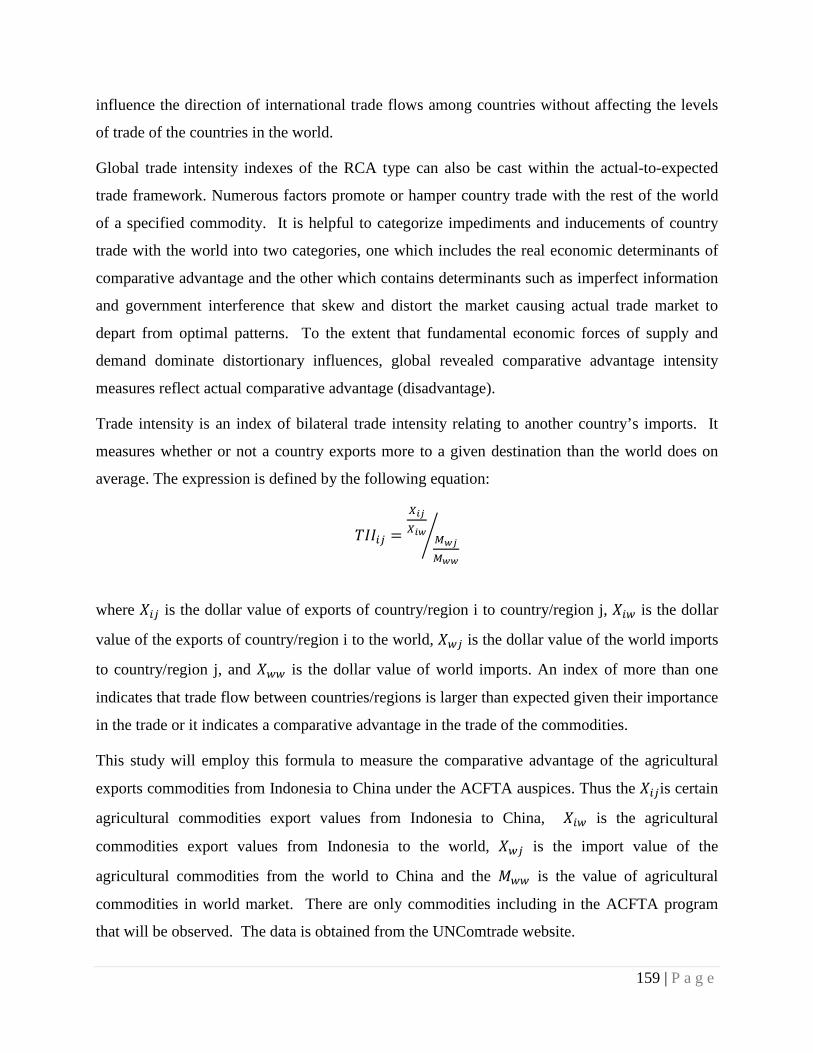
influence the direction of international trade flows among countries without affecting the levels

of trade of the countries in the world.

Global trade intensity indexes of the RCA type can also be cast within the actual-to-expected

trade framework. Numerous factors promote or hamper country trade with the rest of the world

of a specified commodity. It is helpful to categorize impediments and inducements of country

trade with the world into two categories, one which includes the real economic determinants of

comparative advantage and the other which contains determinants such as imperfect information

and government interference that skew and distort the market causing actual trade market to

depart from optimal patterns. To the extent that fundamental economic forces of supply and

demand dominate distortionary influences, global revealed comparative advantage intensity

measures reflect actual comparative advantage (disadvantage).

Trade intensity is an index of bilateral trade intensity relating to another country’s imports. It

measures whether or not a country exports more to a given destination than the world does on

average. The expression is defined by the following equation:

𝑇𝐼𝐼𝑖𝑗 =𝑋𝑖𝑗𝑋𝑖𝑤

𝑀𝑤𝑗

𝑀𝑤𝑤

�

where 𝑋𝑖𝑗 is the dollar value of exports of country/region i to country/region j, 𝑋𝑖𝑤 is the dollar

value of the exports of country/region i to the world, 𝑋𝑤𝑗 is the dollar value of the world imports

to country/region j, and 𝑋𝑤𝑤 is the dollar value of world imports. An index of more than one

indicates that trade flow between countries/regions is larger than expected given their importance

in the trade or it indicates a comparative advantage in the trade of the commodities.

This study will employ this formula to measure the comparative advantage of the agricultural

exports commodities from Indonesia to China under the ACFTA auspices. Thus the 𝑋𝑖𝑗is certain

agricultural commodities export values from Indonesia to China, 𝑋𝑖𝑤 is the agricultural

commodities export values from Indonesia to the world, 𝑋𝑤𝑗 is the import value of the

agricultural commodities from the world to China and the 𝑀𝑤𝑤 is the value of agricultural

commodities in world market. There are only commodities including in the ACFTA program

that will be observed. The data is obtained from the UNComtrade website.

159 | P a g e

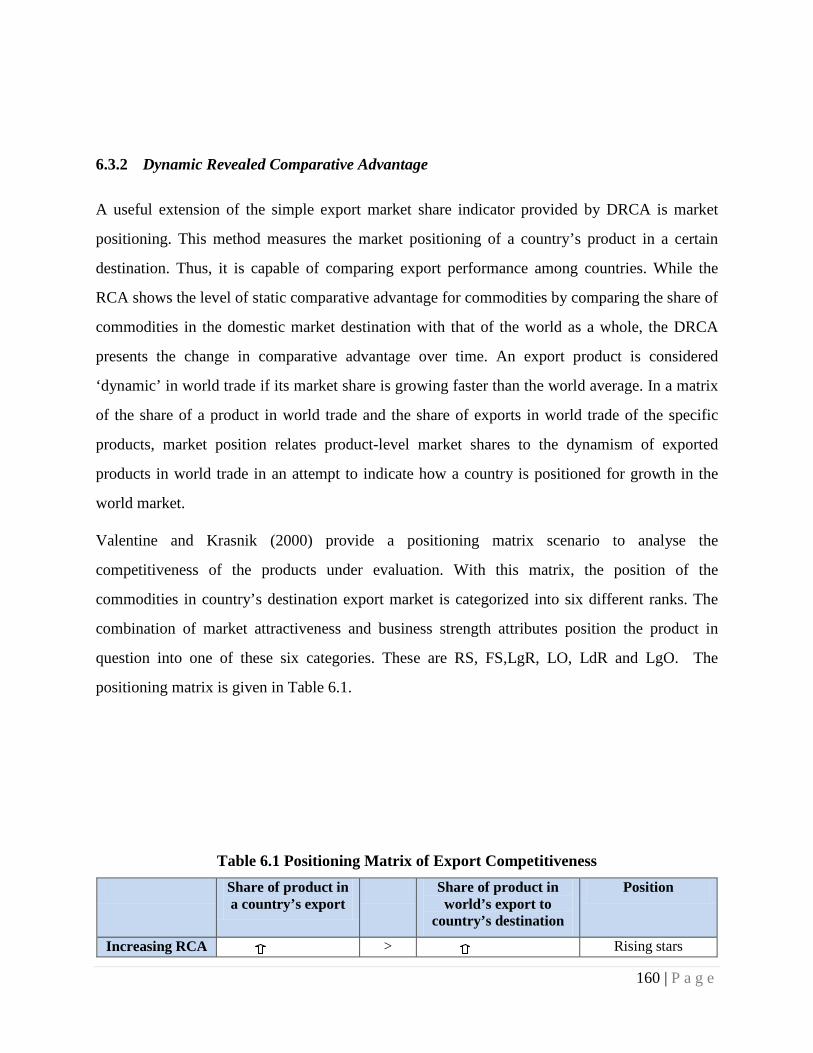
6.3.2 Dynamic Revealed Comparative Advantage

A useful extension of the simple export market share indicator provided by DRCA is market

positioning. This method measures the market positioning of a country’s product in a certain

destination. Thus, it is capable of comparing export performance among countries. While the

RCA shows the level of static comparative advantage for commodities by comparing the share of

commodities in the domestic market destination with that of the world as a whole, the DRCA

presents the change in comparative advantage over time. An export product is considered

‘dynamic’ in world trade if its market share is growing faster than the world average. In a matrix

of the share of a product in world trade and the share of exports in world trade of the specific

products, market position relates product-level market shares to the dynamism of exported

products in world trade in an attempt to indicate how a country is positioned for growth in the

world market.

Valentine and Krasnik (2000) provide a positioning matrix scenario to analyse the

competitiveness of the products under evaluation. With this matrix, the position of the

commodities in country’s destination export market is categorized into six different ranks. The

combination of market attractiveness and business strength attributes position the product in

question into one of these six categories. These are RS, FS,LgR, LO, LdR and LgO. The

positioning matrix is given in Table 6.1.

Table 6.1 Positioning Matrix of Export Competitiveness Share of product in

a country’s export Share of product in

world’s export to country’s destination

Position

Increasing RCA > Rising stars

160 | P a g e

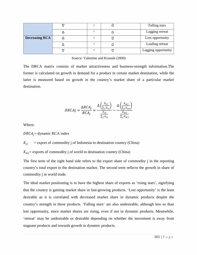
> Falling stars

> Lagging retreat

Decreasing RCA < Lost opportunity

< Leading retreat

< Lagging opportunity

Source: Valentine and Krasnik (2000)

The DRCA matrix consists of market attractiveness and business-strength information.The

former is calculated on growth in demand for a product in certain market destination, while the

latter is measured based on growth in the country’s market share of a particular market

destination.

𝐷𝑅𝐶𝐴𝑗 =∆𝑅𝐶𝐴𝑗𝑅𝐶𝐴𝑗

=∆ � 𝑋𝑖𝑗

∑ 𝑋𝑖𝑗𝑗�

𝑋𝑖𝑗∑ 𝑋𝑖𝑗𝑗

−∆ � 𝑋𝑤𝑗

∑ 𝑋𝑤𝑗𝑗�

𝑋𝑤𝑗∑ 𝑋𝑤𝑗𝑗

Where:

𝐷𝑅𝐶𝐴𝑗= dynamic RCA index

𝑋𝑖𝑗 = export of commodity j of Indonesia to destination country (China)

𝑋𝑤𝑗= exports of commodity j of world to destination country (China)

The first term of the right hand side refers to the export share of commodity j in the reporting

country’s total export to the destination market. The second term reflects the growth in share of

commodity j in world trade.

The ideal market positioning is to have the highest share of exports as ‘rising stars’, signifying

that the country is gaining market share in fast-growing products. ‘Lost opportunity’ is the least

desirable as it is correlated with decreased market share in dynamic products despite the

country’s strength in these products. ‘Falling stars’ are also undesirable, although less so than

lost opportunity, since market shares are rising, even if not in dynamic products. Meanwhile,

‘retreat’ may be undesirable or desirable depending on whether the movement is away from

stagnant products and towards growth in dynamic products.

161 | P a g e

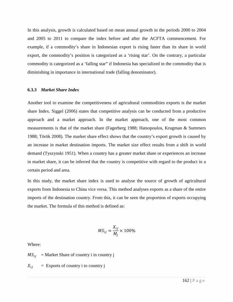
In this analysis, growth is calculated based on mean annual growth in the periods 2000 to 2004

and 2005 to 2011 to compare the index before and after the ACFTA commencement. For

example, if a commodity’s share in Indonesian export is rising faster than its share in world

export, the commodity’s position is categorized as a ‘rising star’. On the contrary, a particular

commodity is categorized as a ‘falling star” if Indonesia has specialized in the commodity that is

diminishing in importance in international trade (falling denominator).

6.3.3 Market Share Index

Another tool to examine the competitiveness of agricultural commodities exports is the market

share Index. Siggel (2006) states that competitive analysis can be conducted from a productive

approach and a market approach. In the market approach, one of the most common

measurements is that of the market share (Fagerberg 1988; Hatsopoulos, Krugman & Summers

1988; Török 2008). The market share effect shows that the country’s export growth is caused by

an increase in market destination imports. The market size effect results from a shift in world

demand (Tyszynski 1951). When a country has a greater market share or experiences an increase

in market share, it can be inferred that the country is competitive with regard to the product in a

certain period and area.

In this study, the market share index is used to analyse the source of growth of agricultural

exports from Indonesia to China vice versa. This method analyses exports as a share of the entire

imports of the destination country. From this, it can be seen the proportion of exports occupying

the market. The formula of this method is defined as:

𝑀𝑆𝑖𝑗 =𝑋𝑖𝑗𝑀𝑗

× 100%

Where:

𝑀𝑆𝑖𝑗 = Market Share of country i in country j

𝑋𝑖𝑗 = Exports of country i to country j

162 | P a g e

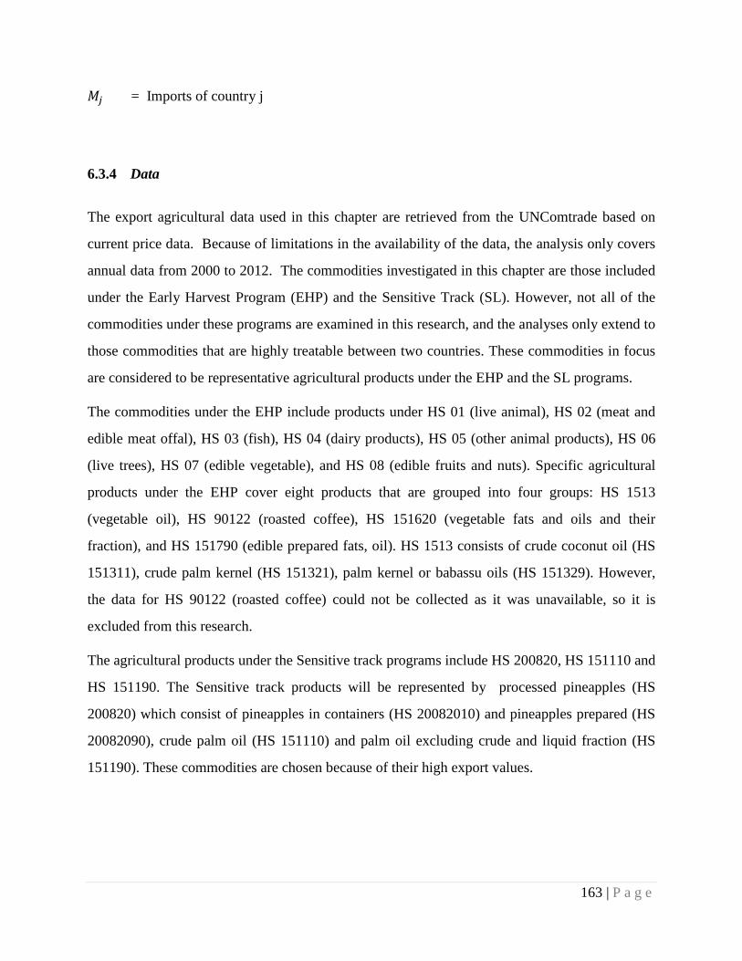
𝑀𝑗 = Imports of country j

6.3.4 Data

The export agricultural data used in this chapter are retrieved from the UNComtrade based on

current price data. Because of limitations in the availability of the data, the analysis only covers

annual data from 2000 to 2012. The commodities investigated in this chapter are those included

under the Early Harvest Program (EHP) and the Sensitive Track (SL). However, not all of the

commodities under these programs are examined in this research, and the analyses only extend to

those commodities that are highly treatable between two countries. These commodities in focus

are considered to be representative agricultural products under the EHP and the SL programs.

The commodities under the EHP include products under HS 01 (live animal), HS 02 (meat and

edible meat offal), HS 03 (fish), HS 04 (dairy products), HS 05 (other animal products), HS 06

(live trees), HS 07 (edible vegetable), and HS 08 (edible fruits and nuts). Specific agricultural

products under the EHP cover eight products that are grouped into four groups: HS 1513

(vegetable oil), HS 90122 (roasted coffee), HS 151620 (vegetable fats and oils and their

fraction), and HS 151790 (edible prepared fats, oil). HS 1513 consists of crude coconut oil (HS

151311), crude palm kernel (HS 151321), palm kernel or babassu oils (HS 151329). However,

the data for HS 90122 (roasted coffee) could not be collected as it was unavailable, so it is

excluded from this research.

The agricultural products under the Sensitive track programs include HS 200820, HS 151110 and

HS 151190. The Sensitive track products will be represented by processed pineapples (HS

200820) which consist of pineapples in containers (HS 20082010) and pineapples prepared (HS

20082090), crude palm oil (HS 151110) and palm oil excluding crude and liquid fraction (HS

151190). These commodities are chosen because of their high export values.

163 | P a g e

6.4 Empirical Results and Analysis

This section provides empirical results regarding the competitiveness of agricultural exports

from Indonesia to China under the auspices the ACFTA. This study examines the impact of the

competitiveness of Indonesian exports before and after joining ACFTA. It also investigates the

impact on agricultural exports, which have tariff reduction facilities and those that do not. This

study is different from previous studies as it is dedicated to exploring the impact of the programs

under the auspices of the ACFTA on certain agricultural products that are listed under the EHP

and SL programs. In this case, there will be a comparison of comparative advantage between

agricultural products under the EHP and the Sensitive track (SL). The first two parts present the

result and analysis of the RCA estimation for EHP and SL agricultural exports from Indonesia to

China respectively. The next two subsections discuss the result and analysis of the DRCA

estimation for EHP and SL agricultural exports from Indonesia to China. The final analysis will

discuss the results from the measurement of market share index for both EHP and SL groups

together.

6.4.1 Trade Intensity Index for the EHP Commodities

By exercising the trade intensity index (TII) on the exported agricultural products from Indonesia

to China, the comparative advantage of the commodities can be measured. Thus the impacts of

the EHP on agricultural competitiveness can be revealed. The TII is defined as the ration of a

particular commodity’s share in a country’s exports to that commodity’s share in country’s

trading partner share in the world. The more a ratio exceeds (is less than) unity, the stronger a

country’s apparent comparative advantage (disadvantage) in that commodity in partner’s

country. It means that the country has greater bilateral trade than would be expected based on

the partner’s share in the world. The trade intensity index measurement results for the

agricultural commodities included in the EHP scheme for 2000 to 2012 are shown in Figure 6.1.

Figure 6.1Trade Intesity Index for the EHP Products for Period 2000-2012

164 | P a g e

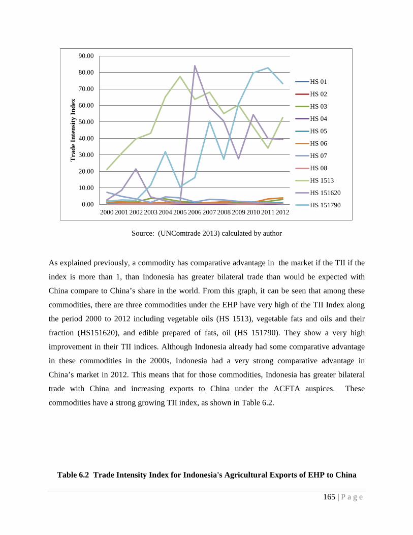
Source: (UNComtrade 2013) calculated by author

As explained previously, a commodity has comparative advantage in the market if the TII if the

index is more than 1, than Indonesia has greater bilateral trade than would be expected with

China compare to China’s share in the world. From this graph, it can be seen that among these

commodities, there are three commodities under the EHP have very high of the TII Index along

the period 2000 to 2012 including vegetable oils (HS 1513), vegetable fats and oils and their

fraction (HS151620), and edible prepared of fats, oil (HS 151790). They show a very high

improvement in their TII indices. Although Indonesia already had some comparative advantage

in these commodities in the 2000s, Indonesia had a very strong comparative advantage in

China’s market in 2012. This means that for those commodities, Indonesia has greater bilateral

trade with China and increasing exports to China under the ACFTA auspices. These

commodities have a strong growing TII index, as shown in Table 6.2.

Table 6.2 Trade Intensity Index for Indonesia's Agricultural Exports of EHP to China

0.00

10.00

20.00

30.00

40.00

50.00

60.00

70.00

80.00

90.00

2000 2001 2002 2003 2004 2005 2006 2007 2008 2009 2010 2011 2012

Tra

de In

tens

ity In

dex

HS 01

HS 02

HS 03

HS 04

HS 05

HS 06

HS 07

HS 08

HS 1513

HS 151620

HS 151790

165 | P a g e

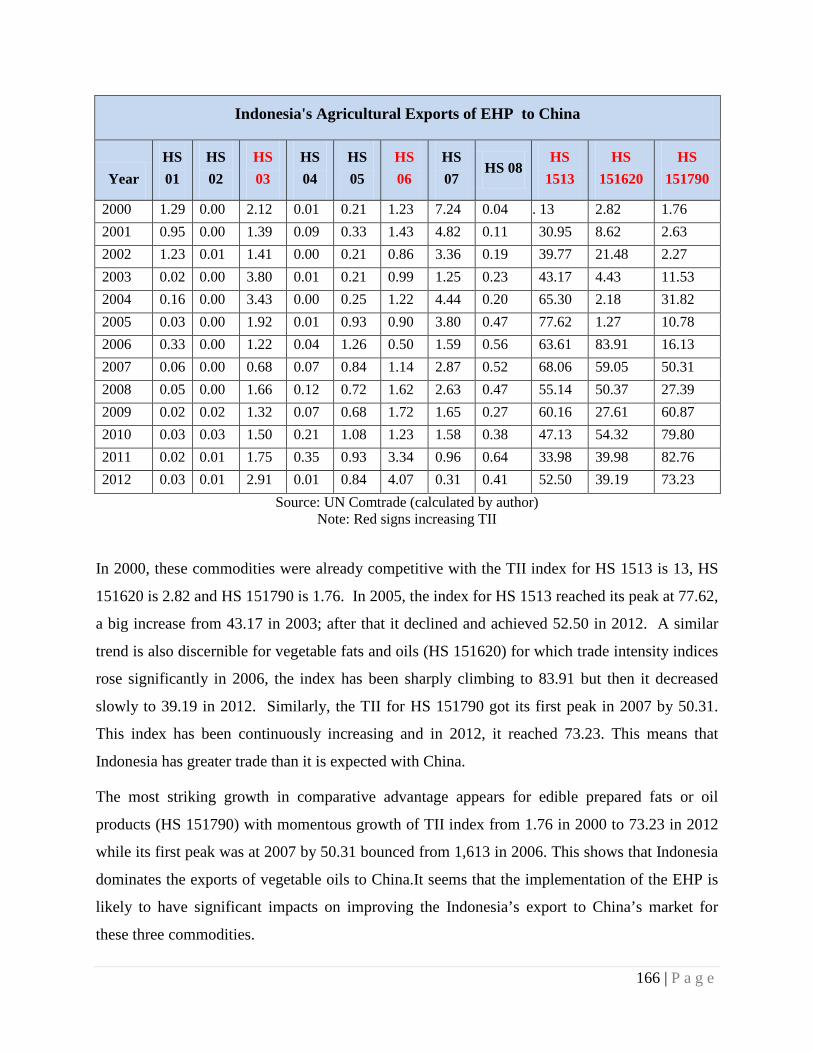
Indonesia's Agricultural Exports of EHP to China

Year HS 01

HS 02

HS 03

HS 04

HS 05

HS 06

HS 07

HS 08 HS

1513 HS

151620 HS

151790

2000 1.29 0.00 2.12 0.01 0.21 1.23 7.24 0.04 . 13 2.82 1.76 2001 0.95 0.00 1.39 0.09 0.33 1.43 4.82 0.11 30.95 8.62 2.63 2002 1.23 0.01 1.41 0.00 0.21 0.86 3.36 0.19 39.77 21.48 2.27 2003 0.02 0.00 3.80 0.01 0.21 0.99 1.25 0.23 43.17 4.43 11.53 2004 0.16 0.00 3.43 0.00 0.25 1.22 4.44 0.20 65.30 2.18 31.82 2005 0.03 0.00 1.92 0.01 0.93 0.90 3.80 0.47 77.62 1.27 10.78 2006 0.33 0.00 1.22 0.04 1.26 0.50 1.59 0.56 63.61 83.91 16.13 2007 0.06 0.00 0.68 0.07 0.84 1.14 2.87 0.52 68.06 59.05 50.31 2008 0.05 0.00 1.66 0.12 0.72 1.62 2.63 0.47 55.14 50.37 27.39 2009 0.02 0.02 1.32 0.07 0.68 1.72 1.65 0.27 60.16 27.61 60.87 2010 0.03 0.03 1.50 0.21 1.08 1.23 1.58 0.38 47.13 54.32 79.80 2011 0.02 0.01 1.75 0.35 0.93 3.34 0.96 0.64 33.98 39.98 82.76 2012 0.03 0.01 2.91 0.01 0.84 4.07 0.31 0.41 52.50 39.19 73.23

Source: UN Comtrade (calculated by author) Note: Red signs increasing TII

In 2000, these commodities were already competitive with the TII index for HS 1513 is 13, HS

151620 is 2.82 and HS 151790 is 1.76. In 2005, the index for HS 1513 reached its peak at 77.62,

a big increase from 43.17 in 2003; after that it declined and achieved 52.50 in 2012. A similar

trend is also discernible for vegetable fats and oils (HS 151620) for which trade intensity indices

rose significantly in 2006, the index has been sharply climbing to 83.91 but then it decreased

slowly to 39.19 in 2012. Similarly, the TII for HS 151790 got its first peak in 2007 by 50.31.

This index has been continuously increasing and in 2012, it reached 73.23. This means that

Indonesia has greater trade than it is expected with China.

The most striking growth in comparative advantage appears for edible prepared fats or oil

products (HS 151790) with momentous growth of TII index from 1.76 in 2000 to 73.23 in 2012

while its first peak was at 2007 by 50.31 bounced from 1,613 in 2006. This shows that Indonesia

dominates the exports of vegetable oils to China.It seems that the implementation of the EHP is

likely to have significant impacts on improving the Indonesia’s export to China’s market for

these three commodities.

166 | P a g e

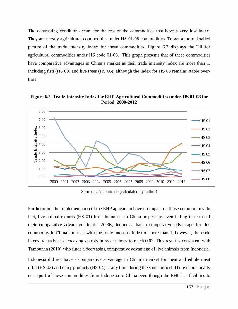
The contrasting condition occurs for the rest of the commodities that have a very low index.

They are mostly agricultural commodities under HS 01-08 commodities. To get a more detailed

picture of the trade intensity index for these commodities, Figure 6.2 displays the TII for

agricultural commodities under HS code 01-08. This graph presents that of these commodities

have comparative advantages in China’s market as their trade intensity index are more than 1,

including fish (HS 03) and live trees (HS 06), although the index for HS 03 remains stable over-

time.

Figure 6.2 Trade Intensity Index for EHP Agricultural Commodities under HS 01-08 for Period 2000-2012

Source: UNComtrade (calculated by author)

Furthermore, the implementation of the EHP appears to have no impact on those commodities. In

fact, live animal exports (HS 01) from Indonesia to China or perhaps even falling in terms of

their comparative advantage. In the 2000s, Indonesia had a comparative advantage for this

commodity in China’s market with the trade intensity index of more than 1, however, the trade

intensity has been decreasing sharply in recent times to reach 0.03. This result is consistent with

Tambunan (2010) who finds a decreasing comparative advantage of live animals from Indonesia.

Indonesia did not have a comparative advantage in China’s market for meat and edible meat

offal (HS 02) and dairy products (HS 04) at any time during the same period. There is practically

no export of these commodities from Indonesia to China even though the EHP has facilities to

0.00

1.00

2.00

3.00

4.00

5.00

6.00

7.00

8.00

2000 2001 2002 2003 2004 2005 2006 2007 2008 2009 2010 2011 2012

Tra

de In

tens

ity In

dex

HS 01

HS 02

HS 03

HS 04

HS 05

HS 06

HS 07

HS 08

167 | P a g e

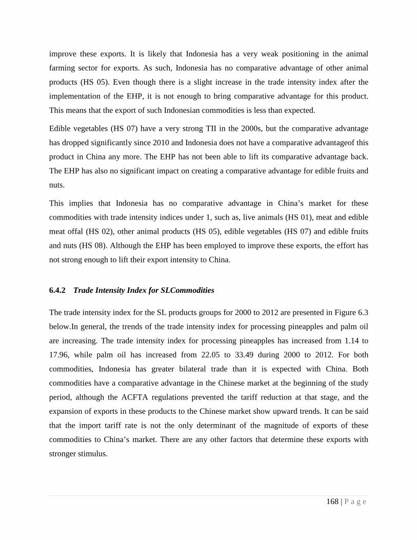
improve these exports. It is likely that Indonesia has a very weak positioning in the animal

farming sector for exports. As such, Indonesia has no comparative advantage of other animal

products (HS 05). Even though there is a slight increase in the trade intensity index after the

implementation of the EHP, it is not enough to bring comparative advantage for this product.

This means that the export of such Indonesian commodities is less than expected.

Edible vegetables (HS 07) have a very strong TII in the 2000s, but the comparative advantage

has dropped significantly since 2010 and Indonesia does not have a comparative advantageof this

product in China any more. The EHP has not been able to lift its comparative advantage back.

The EHP has also no significant impact on creating a comparative advantage for edible fruits and

nuts.

This implies that Indonesia has no comparative advantage in China’s market for these

commodities with trade intensity indices under 1, such as, live animals (HS 01), meat and edible

meat offal (HS 02), other animal products (HS 05), edible vegetables (HS 07) and edible fruits

and nuts (HS 08). Although the EHP has been employed to improve these exports, the effort has

not strong enough to lift their export intensity to China.

6.4.2 Trade Intensity Index for SLCommodities

The trade intensity index for the SL products groups for 2000 to 2012 are presented in Figure 6.3

below.In general, the trends of the trade intensity index for processing pineapples and palm oil

are increasing. The trade intensity index for processing pineapples has increased from 1.14 to

17.96, while palm oil has increased from 22.05 to 33.49 during 2000 to 2012. For both

commodities, Indonesia has greater bilateral trade than it is expected with China. Both

commodities have a comparative advantage in the Chinese market at the beginning of the study

period, although the ACFTA regulations prevented the tariff reduction at that stage, and the

expansion of exports in these products to the Chinese market show upward trends. It can be said

that the import tariff rate is not the only determinant of the magnitude of exports of these

commodities to China’s market. There are any other factors that determine these exports with

stronger stimulus.

168 | P a g e

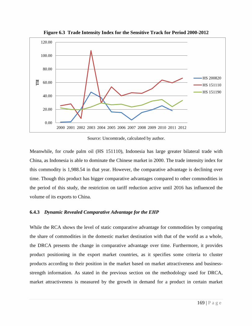
Figure 6.3 Trade Intensity Index for the Sensitive Track for Period 2000-2012

Source: Uncomtrade, calculated by author.

Meanwhile, for crude palm oil (HS 151110), Indonesia has large greater bilateral trade with

China, as Indonesia is able to dominate the Chinese market in 2000. The trade intensity index for

this commodity is 1,988.54 in that year. However, the comparative advantage is declining over

time. Though this product has bigger comparative advantages compared to other commodities in

the period of this study, the restriction on tariff reduction active until 2016 has influenced the

volume of its exports to China.

6.4.3 Dynamic Revealed Comparative Advantage for the EHP

While the RCA shows the level of static comparative advantage for commodities by comparing

the share of commodities in the domestic market destination with that of the world as a whole,

the DRCA presents the change in comparative advantage over time. Furthermore, it provides

product positioning in the export market countries, as it specifies some criteria to cluster

products according to their position in the market based on market attractiveness and business-

strength information. As stated in the previous section on the methodology used for DRCA,

market attractiveness is measured by the growth in demand for a product in certain market

0.00

20.00

40.00

60.00

80.00

100.00

120.00

2000 2001 2002 2003 2004 2005 2006 2007 2008 2009 2010 2011 2012

TII

HS 200820

HS 151110

HS 151190

169 | P a g e

destinations, while business-strength is assessed by the growth in the country’s market share of a

particular market destination.

The DRCAs are divided into two group periods: first is the group before the implementation of

the EHP for 2000 to 2003 and the second group is for the period of the implementation of the

EHP afterwards during 2004 to 2012. Both groups are then compared to examine whether the

implementation of the EHP brought positive impact on competitiveness of agricultural

commodities under this scheme.

Table 6.3 presents the D RCA of the commodities under the EHP scheme. Similar to the

previous section, there are eleven commodities chosen as representatives of the EHP products.

The table is divided between Indonesia’s share growth and China’s share growth. Indonesia’s

share growth means the growth of a commodity export’s share, compared to the whole exports

from Indonesia; the latter means the growth of a commodity export’s share in China compared to

the whole exports shipped to China. A commodity is classified as increasing its RCA if it is

grouped to ‘RS, ‘falling star’ and ‘lagging retreat’; and the remaining are declared as decreasing

RCA or declining its comparative advantage.

The first two columns of Table 6.3 reveal the results from 2000 to 2003, while the other columns

list those for 2004 to 2012. The position of each commodity depends on a comparison between

the growth share of exports in the origin country (Indonesia) and that in the market destination

(China). The positions indicate the commodities with increased competitiveness in China’s

market and those that fell behind.

Table 6.3Exports Share Growth from Indonesia to China

2000 to 2003 2004 to 2012

170 | P a g e

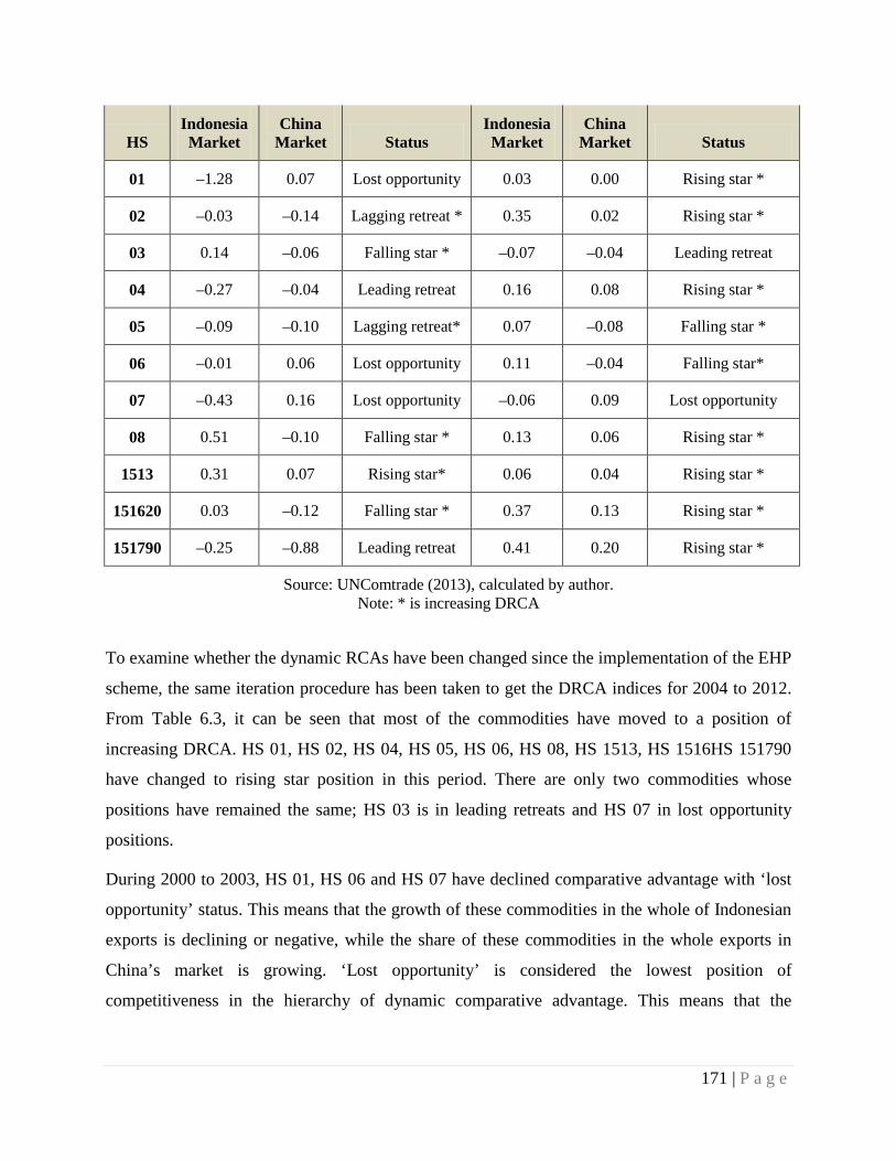
HS Indonesia Market

China Market Status

Indonesia Market

China Market Status

01 –1.28 0.07 Lost opportunity 0.03 0.00 Rising star *

02 –0.03 –0.14 Lagging retreat * 0.35 0.02 Rising star *

03 0.14 –0.06 Falling star * –0.07 –0.04 Leading retreat

04 –0.27 –0.04 Leading retreat 0.16 0.08 Rising star *

05 –0.09 –0.10 Lagging retreat* 0.07 –0.08 Falling star *

06 –0.01 0.06 Lost opportunity 0.11 –0.04 Falling star*

07 –0.43 0.16 Lost opportunity –0.06 0.09 Lost opportunity

08 0.51 –0.10 Falling star * 0.13 0.06 Rising star *

1513 0.31 0.07 Rising star* 0.06 0.04 Rising star *

151620 0.03 –0.12 Falling star * 0.37 0.13 Rising star *

151790 –0.25 –0.88 Leading retreat 0.41 0.20 Rising star *

Source: UNComtrade (2013), calculated by author. Note: * is increasing DRCA

To examine whether the dynamic RCAs have been changed since the implementation of the EHP

scheme, the same iteration procedure has been taken to get the DRCA indices for 2004 to 2012.

From Table 6.3, it can be seen that most of the commodities have moved to a position of

increasing DRCA. HS 01, HS 02, HS 04, HS 05, HS 06, HS 08, HS 1513, HS 1516HS 151790

have changed to rising star position in this period. There are only two commodities whose

positions have remained the same; HS 03 is in leading retreats and HS 07 in lost opportunity

positions.

During 2000 to 2003, HS 01, HS 06 and HS 07 have declined comparative advantage with ‘lost

opportunity’ status. This means that the growth of these commodities in the whole of Indonesian

exports is declining or negative, while the share of these commodities in the whole exports in

China’s market is growing. ‘Lost opportunity’ is considered the lowest position of

competitiveness in the hierarchy of dynamic comparative advantage. This means that the

171 | P a g e

commodities lost their opportunities to expand their exports in China’s market, yet they are not

able to keep pace with the growth of total exports in Indonesia.

In the same period, commodities under HS 02 and HS 05 take their position as ‘lagging retreat’.

Although this position is categorized as possessing an increasing RCA index, it is undesirable

because it indicates that the growth of exports of these commodities has been decreasing in both

the Indonesian and Chinese market. Nonetheless, the result shows that the declining share

growth in Indonesia’s export is not as low as the declining growth in China’s market.

Next, commodities under HS 03, HS 08 and HS 151690 in the DRCA show positions that fall

under ‘falling star’. But despite the negative connotation in its name, ‘falling star’ position is

grouped as an indicator of increasing comparative advantage. This position means that the

commodities have an increasing growth share in Indonesian exports as a whole, however, the

export share growth in the whole China’s export is declining. This is perhaps because it has

become difficult for these commodities to expand their market penetration in China due to

downturn in Chinese growth. To distribute the growing exports’ share in Indonesia, these

commodities need to be exported to other countries which have growing imports of these

products.

With regard to the next category, products under HS 04 and HS 151790 show that their dynamic

comparative advantage is in the ‘leading retreat’ position. This is an undesirable position because

it shows a declining RCA. It means that both Indonesia’s export share and China’s export share

growth are dropping, with these commodities’ share of Indonesia’s total exports growth

declining faster than the latter.

Finally, the position for dynamic RCA for HS 1513 is categorized as a ‘rising star’ during 2000

to 2003. This is a desirable position in the DRCA matrix as it means that HS 1513 has become a

favourite export commodity for this period.

In sum, from the growth of export share perspectives analysed here in the DRCA, it shows that

the EHP program has increased the export share of these commodities both in the export origin

country and market destination country. The most outstanding improvements have been

established for the commodities HS 01, HS 06, and HS 07 as they emerged from declining

growths under ‘lost opportunity’ to garner the position of ‘rising star’. This denotes that the

172 | P a g e

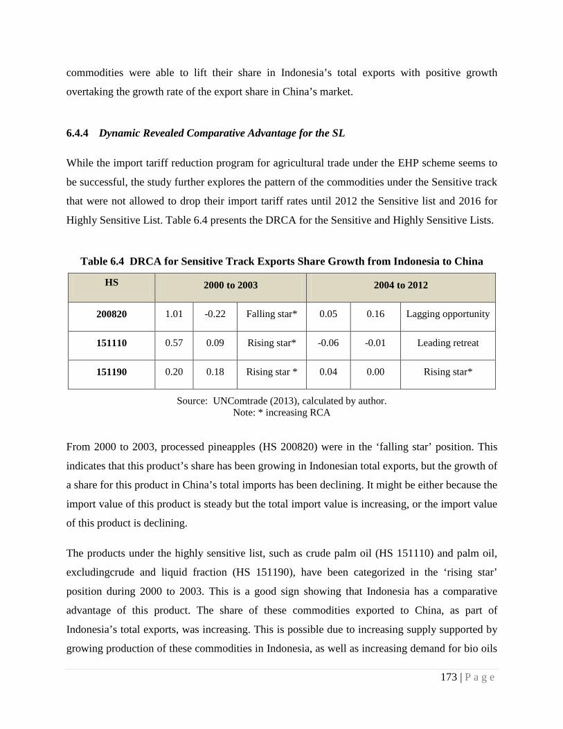
commodities were able to lift their share in Indonesia’s total exports with positive growth

overtaking the growth rate of the export share in China’s market.

6.4.4 Dynamic Revealed Comparative Advantage for the SL

While the import tariff reduction program for agricultural trade under the EHP scheme seems to

be successful, the study further explores the pattern of the commodities under the Sensitive track

that were not allowed to drop their import tariff rates until 2012 the Sensitive list and 2016 for

Highly Sensitive List. Table 6.4 presents the DRCA for the Sensitive and Highly Sensitive Lists.

Table 6.4 DRCA for Sensitive Track Exports Share Growth from Indonesia to China

HS 2000 to 2003 2004 to 2012

200820 1.01 -0.22 Falling star* 0.05 0.16 Lagging opportunity

151110 0.57 0.09 Rising star* -0.06 -0.01 Leading retreat

151190 0.20 0.18 Rising star * 0.04 0.00 Rising star*

Source: UNComtrade (2013), calculated by author. Note: * increasing RCA

From 2000 to 2003, processed pineapples (HS 200820) were in the ‘falling star’ position. This

indicates that this product’s share has been growing in Indonesian total exports, but the growth of

a share for this product in China’s total imports has been declining. It might be either because the

import value of this product is steady but the total import value is increasing, or the import value

of this product is declining.

The products under the highly sensitive list, such as crude palm oil (HS 151110) and palm oil,

excludingcrude and liquid fraction (HS 151190), have been categorized in the ‘rising star’

position during 2000 to 2003. This is a good sign showing that Indonesia has a comparative

advantage of this product. The share of these commodities exported to China, as part of

Indonesia’s total exports, was increasing. This is possible due to increasing supply supported by

growing production of these commodities in Indonesia, as well as increasing demand for bio oils

173 | P a g e

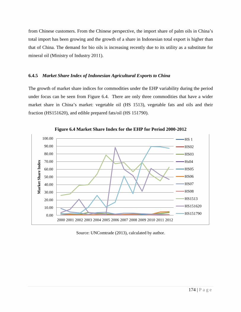
from Chinese customers. From the Chinese perspective, the import share of palm oils in China’s

total import has been growing and the growth of a share in Indonesian total export is higher than

that of China. The demand for bio oils is increasing recently due to its utility as a substitute for

mineral oil (Ministry of Industry 2011).

6.4.5 Market Share Index of Indonesian Agricultural Exports to China

The growth of market share indices for commodities under the EHP variability during the period

under focus can be seen from Figure 6.4. There are only three commodities that have a wider

market share in China’s market: vegetable oil (HS 1513), vegetable fats and oils and their

fraction (HS151620), and edible prepared fats/oil (HS 151790).

Figure 6.4 Market Share Index for the EHP for Period 2000-2012

Source: UNComtrade (2013), calculated by author.

0.00

10.00

20.00

30.00

40.00

50.00

60.00

70.00

80.00

90.00

100.00

2000 2001 2002 2003 2004 2005 2006 2007 2008 2009 2010 2011 2012

Mar

ket S

hare

Inde

x

HS 1

HS02

HS03

Hs04

HS05

HS06

HS07

HS08

HS1513

HS151620

HS151790

174 | P a g e

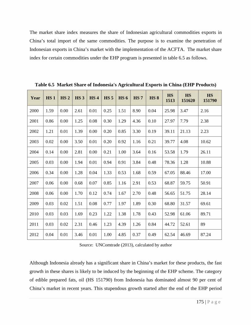
The market share index measures the share of Indonesian agricultural commodities exports in

China’s total import of the same commodities. The purpose is to examine the penetration of

Indonesian exports in China’s market with the implementation of the ACFTA. The market share

index for certain commodities under the EHP program is presented in table 6.5 as follows.

Table 6.5 Market Share of Indonesia's Agricultural Exports in China (EHP Products)

Year HS 1 HS 2 HS 3 HS 4 HS 5 HS 6 HS 7 HS 8 HS 1513

HS 151620

HS 151790

2000 1.59 0.00 2.61 0.01 0.25 1.51 8.90 0.04 25.98 3.47 2.16

2001 0.86 0.00 1.25 0.08 0.30 1.29 4.36 0.10 27.97 7.79 2.38

2002 1.21 0.01 1.39 0.00 0.20 0.85 3.30 0.19 39.11 21.13 2.23

2003 0.02 0.00 3.50 0.01 0.20 0.92 1.16 0.21 39.77 4.08 10.62

2004 0.14 0.00 2.81 0.00 0.21 1.00 3.64 0.16 53.58 1.79 26.11

2005 0.03 0.00 1.94 0.01 0.94 0.91 3.84 0.48 78.36 1.28 10.88

2006 0.34 0.00 1.28 0.04 1.33 0.53 1.68 0.59 67.05 88.46 17.00

2007 0.06 0.00 0.68 0.07 0.85 1.16 2.91 0.53 68.87 59.75 50.91

2008 0.06 0.00 1.70 0.12 0.74 1.67 2.70 0.48 56.65 51.75 28.14

2009 0.03 0.02 1.51 0.08 0.77 1.97 1.89 0.30 68.80 31.57 69.61

2010 0.03 0.03 1.69 0.23 1.22 1.38 1.78 0.43 52.98 61.06 89.71

2011 0.03 0.02 2.31 0.46 1.23 4.39 1.26 0.84 44.72 52.61 89

2012 0.04 0.01 3.46 0.01 1.00 4.85 0.37 0.49 62.54 46.69 87.24

Source: UNComtrade (2013), calculated by author

Although Indonesia already has a significant share in China’s market for these products, the fast

growth in these shares is likely to be induced by the beginning of the EHP scheme. The category

of edible prepared fats, oil (HS 151790) from Indonesia has dominated almost 90 per cent of

China’s market in recent years. This stupendous growth started after the end of the EHP period

175 | P a g e

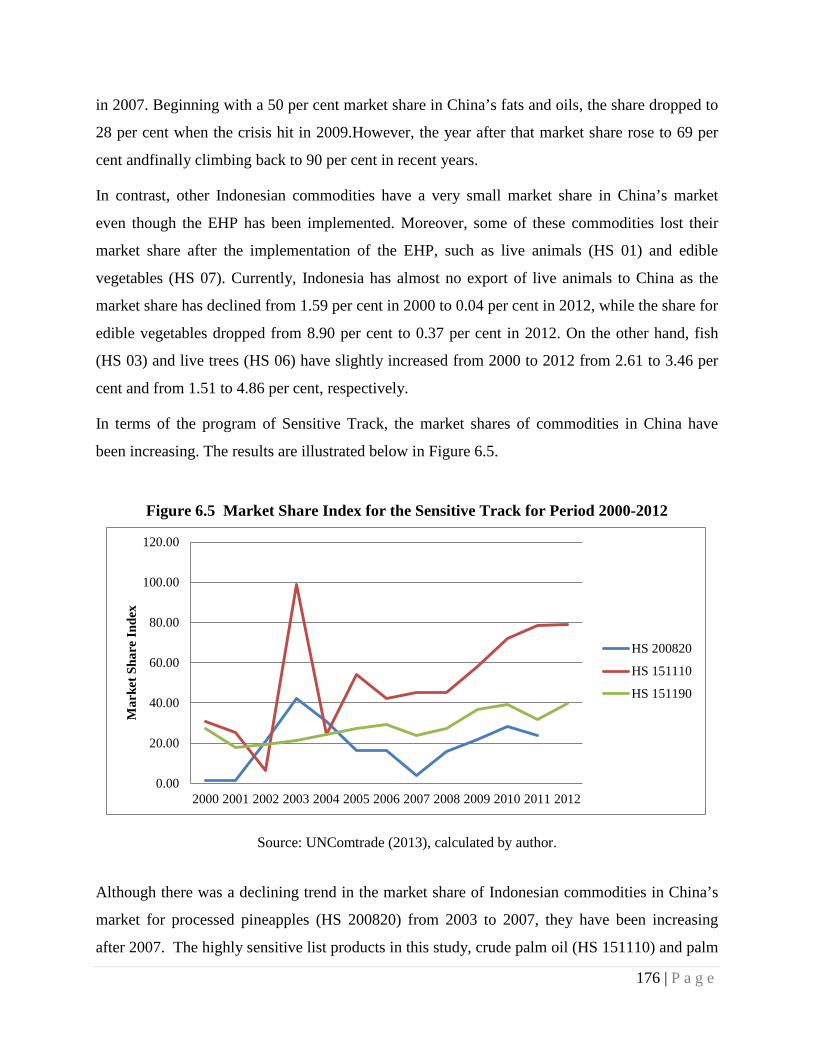
in 2007. Beginning with a 50 per cent market share in China’s fats and oils, the share dropped to

28 per cent when the crisis hit in 2009.However, the year after that market share rose to 69 per

cent andfinally climbing back to 90 per cent in recent years.

In contrast, other Indonesian commodities have a very small market share in China’s market

even though the EHP has been implemented. Moreover, some of these commodities lost their

market share after the implementation of the EHP, such as live animals (HS 01) and edible

vegetables (HS 07). Currently, Indonesia has almost no export of live animals to China as the

market share has declined from 1.59 per cent in 2000 to 0.04 per cent in 2012, while the share for

edible vegetables dropped from 8.90 per cent to 0.37 per cent in 2012. On the other hand, fish

(HS 03) and live trees (HS 06) have slightly increased from 2000 to 2012 from 2.61 to 3.46 per

cent and from 1.51 to 4.86 per cent, respectively.

In terms of the program of Sensitive Track, the market shares of commodities in China have

been increasing. The results are illustrated below in Figure 6.5.

Figure 6.5 Market Share Index for the Sensitive Track for Period 2000-2012

Source: UNComtrade (2013), calculated by author.

Although there was a declining trend in the market share of Indonesian commodities in China’s

market for processed pineapples (HS 200820) from 2003 to 2007, they have been increasing

after 2007. The highly sensitive list products in this study, crude palm oil (HS 151110) and palm

0.00

20.00

40.00

60.00

80.00

100.00

120.00

2000 2001 2002 2003 2004 2005 2006 2007 2008 2009 2010 2011 2012

Mar

ket S

hare

Inde

x

HS 200820

HS 151110

HS 151190

176 | P a g e

oil, excludingcrude and liquid fraction (HS 151190), tend to be acquiring more market share in

China’s market. In 2003, the crude palm oil products from Indonesia occupied almost 100 per

cent of China’s market. Although the share dropped in the following years, it has been on an

upward trend in recent years, and the share of export in China’s market has reached almost 80

per cent. This means that these commodities under the sensitive list have performed well despite

the fact that the ACFTA has impeded tariff reduction for these commodities.

6.5 Conclusion

The objective of the EHP is to reduce the tariff barrier for these commodities in the period from

2004 to 2006, so that at the end of 2006 the import tariff rates become zero per cent. Although

the reduced tariffs were expected to make Indonesian exports more favourable to China, the

competitiveness of agricultural products from Indonesia has experienced no change, especially

for commodities under the HS code 01-08. The commodities of code HS 01 to 08 constitute

animal and horticultural products, areas in which China has a strong comparative

advantage(Chen, C & Duncan 2008). So China is not as concerned that their domestic market

will be penetrated by foreign products in these categories as domestic producers will be able to

deal with the competition.

The trade intensity indexes for some Indonesian commodities exports are greater than unity,

especially for palm oil commodities. It means that Indonesia has greater bilateral trade with

China than would be expected based on China’s share in world trade. However, for some other

products such as commodities under HS code 01,02,04,05,and 08, the trade intensity indexes of

Indonesian exports are below the unity, which means that the export intensity to China is under

the expectation.

Meanwhile, China doesn’t have comparative advantagein some agricultural products such as

edible vegetable and animal oils, sugar, cotton and rice, but these have high demand in domestic

market. These commodities called ‘national strategic products’ are given high protection by the

Chinese government with high rates of TRQ, or placed in the Sensitive track of the ACFTA.

The implementation of the EHP scheme has only raised the competitiveness of products for

177 | P a g e

HS1513, HS 151620 and HS 151790, all of which are actually bio oil products and allied

commodities.

There are many other factors influencing the growth of bio oil exports from Indonesia to China.

The increase in the exports for bio oil groups is mostly caused by strong demand for bio oil, the

position of Indonesia as the biggest producer of palm oil and the spike in the bio oil prices.

According to the World Bank (2008), the spike in the bio oil prices in 2008 has mainly

influenced the trend of bio oil exports. This explains the growing exports for the bio oil from

Indonesia to China in this chapter. Indonesia is the biggest producer of palm oils in the world

(FAO 2012; WTO 2014), and the rise in exports of these products shown in the study come from

the volume and the price as explained in the Chapter Four.

In contrast, the competitiveness of the agricultural commodities under the Sensitive Track has

been increasing in the period from 2000 to 2012. This scheme includes processed pineapples (HS

200820), crude palm oil (HS 151110) and palm oil, excluding crude and liquid fraction (HS

151190). These commodities experienced increasing RCA index and market share index in the

period from 2000 to 2012. However, the DRCA index shows that the position of pineapples (HS

200820) and crude palm oil (HS 151110) is declining. The DRCA shows that the index for these

commodities fell from the increasing star before the implementation of the ACFTA to declining

star after the implementation of the ACFTA, but palm oil products, excluding crude and liquid

fraction (HS151190) continued as a ‘rising star’. This condition can be explained by the strong

demand for these commodities as Indonesia is the biggest producer of palm oil and alsoamajor

producer of pineapples. For these commodities, relative reduction of tariff doesn’t influence on

the competitiveness.

Through the implementation of the EHP has improved the competitiveness of certain

commodities that have received tariff reduction, others have experienced no growth. The

competitiveness of original agricultural commodities under HS code 01-08 showed no responses

to the preferential tariff reduction offered by the EHP program. There are some reasons behind

this condition,for example, China’s production of these commodities is bigger than Indonesia’s

and China has a strong comparative advantage for these commodities. China has also employed

trade policy to protect agricultural products in which they have not comparative advantage, but

have strong demand in their domestic market.

178 | P a g e

On the other hand, contrary to expectation, improved competitiveness is discernible even for

commodities under the Sensitive track which do not enjoy import tariff reduction. This means

that the competitiveness of commodities is more dependent on intrinsic strengths of Indonesia’s

production capacity as observed in the stupendous growth vegetable oil exports from Indonesia

to China. This also means that free trade agreement is likely to be less influential in this matter as

commodities under EHP that enjoy tariff reduction that have experienced little or no change,

whereas some, such as vegetable oils, under SL have grown even without tariff reduction.

179 | P a g e

Chapter 7

Indonesian Agricultural Export Performance: A View from a Real Value

Perspective

7.1 Introduction

In addition to the mixed results of studies in previous chapters on the growth and

competitiveness of Indonesian agricultural exports under the influence of the ASEAN-China

Free Trade Agreement, and the contribution of agricultural exports to China on Indonesian

economic growth, studies about the condition of the Indonesian agricultural exports will be

elaborated in this chapter. While the agricultural exports in the aforementioned chapters are in

‘bulk’ or ‘groups’ of commodities; this chapter will discuss the performance of agricultural

exports in detail from the view of commodities to understand the overall condition of Indonesian

agricultural exports in general. Imposing the real value of export is important as the use of

current prices can often give misleading and non-accurate estimations, especially in periods of

crisis with unstable prices and high inflation. The problem is the available on actual exports is

influenced by both price and volume changes, and such data free of these influences is not

available at the disaggregate level. Thus to address the lack of this appropriate data, the chain-

linked volume method will be applied to construct such data of chain-linked volume and price of

the exports. Using the chain-linked volume as real value (‘volume’) as a measure will provide a

clearer and more accurate picture of the exports, omitting bias caused by inflation or price

interference, which is one of the disadvantages when using the current value perspective.

The aim of this chapter is to accomplish the research objective stated in Chapter One: ‘to

overview the condition of Indonesian agricultural exports from the chain-linked volume

perspective’. Furthermore, it can support a more detailed interpretation of the results from the

preceding chapters.

This study will examine the biggest agricultural exported products which cover more than 95 per

cent of the total agricultural exports of Indonesia. These consist of thirty-five commodities. The

terms used to describe agricultural products in this chapter are based on the Agreement on

Agriculture (AoA) of World Trade Organization(WTO 2012e). Under this agreement, fish

products (HS 03) are not included as agricultural products. The study will focus on exports to all

180 | P a g e

countries and some major market destinations for Indonesian agricultural exports such as

ASEAN, India, China, the US and Japan.

Volume index numbers such as chain-linked volume or the Laspeyres index have been key

indicators for annual policy reviews (Boyle 1987). Furthermore, analysis of volume index

numbers of agricultural outputs and inputs has attracted attention of the agricultural economist

for decades (Boyle 1988). This method has been widely implemented into the national accounts

of developed countries over the past few years, and such data are available in these countries,

including the members of the European Union (Brueton 1999), Australia (ABS 1998), and a

number of OECD countries (Schreyer 2004). Unfortunately, there is no satisfactory disaggregate

level of either agricultural export real value or export price index for Indonesia. The Indonesian

Statistics Bureau (BPS) (BPS 2014) publishes quantity data in kilograms for individual export

item but does not publish an aggregate volume index. BPS has published wholesale price indices,

but only for a few agricultural products. This raises the need for an appropriate measurement of

agricultural export volume.

This study will attempt to address the lack of an appropriate measure of agricultural export real

value by using a chain-linked volume measures. This method is using unit values (export value

in dollars divided by the export quantity in kilograms) to construct a disaggregate measure of

monthly agricultural exports at constant prices. The agricultural commodities are at a very

detailed level at nine-digit level of HS code, where products are reasonably homogenous. If the

fixed prices hold, movements in export value can only be due to quantitative changes. This is

equivalent to measuring export volume by constructing a weighted average of export quantity

indices, with the weights being the value share of each item in total agricultural export. Once a

volume index has been constructed, an implicit export price index can be derived simply by

dividing the export value by export volume.

This chapter pursues this goal with the application of the chained-link volume method so that the

real value of export can be isolated from the interference of price. The first part of the chapter

will explain the methodology of chain-link volume and price index used for this purpose and the

second part will present the result of chain-link volume and the price index for Indonesian

agricultural exports.

181 | P a g e

7.2 Literature Review

7.2.1 Importance of Real Value Calculation

Imposing the real value of trade in calculating economic growth is important as the use of current

value can often give misleading and non-accurate estimations, especially in periods of crisis with

unstable prices and high inflation. An example of such a miscalculation from current value was

demonstrated during the Asian crisis when Indonesia experienced a slowdown in non-oil exports

(Rosner 2000). Despite the enormous depreciation, the non-oil export performance, measured in

dollars, did not accelerate during the first two years of the Asian crisis, even when non-oil

exports dropped sharply during the second year of the crisis. Rosner (2000) argues that main

reason for this was the fact that Indonesia suffered a massive deterioration in export prices

between 1997 and 1999. The export prices of major non-oil export products from Indonesia

experienced a sharp drop following the world market prices, which had fallen steadily since the

onset of the crisis. This contradicted the theory that the export quantity can be expected to rise

following a currency depreciation. James (2000) argues that if Indonesia’s non-oil export values

were deflated using an import price index for the United States, the non-oil exports in constant

price rose 1.58 per cent instead of falling when it was measured by current dollars. From this

example, it becomes evident that an analysis of the export performance must distinguish between

price movements and quantity movements.

The reason for having either chain volume or constant price estimates in the national accounts is

to provide a time series of expenditure and production aggregates which are free of the direct

effects of price change or inflation. All the current price aggregates of expenditure and

production appearing in the national accounts are estimates of the sums of the values of

individual transactions (ABS 2003). This should happen at the lowest level of aggregation

available for national account, because the price indices used at this level of aggregation have to

be considered like elementary price indices and they may or may not be constructed with the

same index number formula as the national accounts use for higher level aggregation (Schreyer

2004). Chapter XVI of the System of National Accounts (SNA 1993) on price and volume

measures describes the higher the level of aggregation at which national account index numbers

182 | P a g e

set in, the more the overall growth rate of GDP is shaped by the index number formulae that are

present in the elementary price indices used in the accounts (United Nations 2014a).

7.2.2 Chain-linked Volume Measure

Real value measures are commonly approached by constant price measures. However, in recent

years, this method using a five year rebasing is considered inefficient (Aspden, ADB & UN

ESCAP 2000). As the System of National Accounts 2008 (SNA 2008) (United Nations 2014b)

recommends rebasing every year and linking the resulting indices to form annually reweighted

chain volume measures, many countries moved on to the method of chain volume measures with

annual rebasing (annual chain-linking) to calculate their national account (United Nations 2012).

In general, annually linked and re-weighted chain volume measures are considered to more

accurately reflect volume changes over time (ABS 1998). It provides better indicators of

movement in real output and expenditure because they take account of changes to pricing

relativities that occur from one period to the next by compiling indices between consecutive

periods and annually updating the base period. This maximizes the number of commodities

common to both periods and enables more value comparisons to be made (ABS 2003). In

practice, the advantage of annual chain volume measures depends on the variability of the price

and volume relativities between the component series (ABS 1998). Thus, chain volume measures

are believed to provide better measures than constant price estimates.

This method uses unit values (export value in dollars divided by the export quantity in

kilograms) to construct an aggregate measure of monthly agricultural exports at constant prices.

If the fixed prices hold, movements in export value can only be due to quantitative changes. This

is equivalent to measuring export volume by constructing a weighted average of export quantity

indices, with the weights being the value share of each item in total agricultural export. Once a

volume index has been constructed, an implicit export price index can be derived simply by

dividing the export value by export volume. The next section describes the methodology used for

formulating the China volume measure on Indonesian exports in this thesis.

183 | P a g e

7.3 Methodology

7.3.1 Constructing a Volume Index

The Australian Bureau of Statistics (ABS 1998) describes the procedure of constructing a

volume index is given by the ratio of the two homogenous quantities in period 1 and 2 (quantity

relative). The value of the index in the period 1 is usually set as 100 and the next period index

will be the percentage increase or decrease in the volume of production. It can be formulated as

below:

𝑄𝐼𝑡 =𝑄𝑡𝑄𝑡−1

𝑥 100, 𝑡 𝑖𝑠 𝑡ℎ𝑒 𝑐𝑢𝑟𝑟𝑒𝑛𝑡 𝑝𝑒𝑟𝑖𝑜𝑑

For two or more commodities, it is necessary to introduce a weighting scheme. To construct a

volume index, one simple way would then be of value of the commodities at their prices in one

or other period and divide the total value of their combined production in the second period by

that in the first. The same prices must be used for both periods to ensure that the index only

reflects changes in quantities produced. The other way is to calculate the ratio of the quantities or

quantity relatives first for each commodity separately. One would expect a volume index to be

some kind of average of these quantity relatives. It can be shown that the index from previous

way are equivalent to weighted averages of the quantity relatives which use the total values of

each commodity in one or other period as weights (ABS 2003).

There are several ways of measuring the volume change depending on the choices of whether the

period of price is the first or the second. Index number theory offers a wide range of tools to this

end (Diewert 2005). One of those theories is the Laspeyres volume index method (Allen 1949)

that uses the first period of price in its calculation.

The Laspeyres volume index method measures the percentage change in the total value of

production holding prices constant at their year 1 levels. It is also equal to a weighted arithmetic

average of the quantity relatives for each of the commodities using the values produced in the

184 | P a g e

first year as weights (Brueton 1999). A period-to-period Laspeyres volume index formula for

rebased volume estimates is given by:

𝑄𝐼𝑡 = ∑𝑞𝑡𝑝𝑡−1∑𝑞𝑡−1𝑝𝑡−1

Where t is the current period under consideration, and t-1 is the period before the current period

and the base period for values in period n.

As the weights of a chain volume index change from period to period due to annual rebasing, a

time series of chain volume indices has no fixed base period in the sense in which a constant

price estimate or fixed-weight volume index does (Schreyer 2004). However, chain volume

measures must have a reference period, in which the index equals 100. It is also worth noting

that the chain volume measure in the reference period, expressed in dollar terms equals the

corresponding current price value.

7.3.2 Chain-linked Volume Formula

The basic idea of a chain-linking is to update the base year at a higher frequency and link the

short-term movements. In some countries, the updating is done on an annual basis. In that case,

period to period changes of volumes (the links in the chain) are calculated using the prices (and

hence weights) of the previous year. The Laspeyres chain-linked volume also estimates period-

to-period volume indices of an aggregate by expressing the value of the aggregate in each pair of

consecutive period in the prices of the earlier period, and then dividing the value of the later

period by the value of the earlier period. This is equivalent to weighing together the period-to-

period volume indices of the elementary components of the aggregate with the current price

values of the earlier period (United Nations 2014b)

The period-to-period indices from the previous chapter are compounded to form a long,

continuous chain volume time series that is called a Laspeyres chain volume index. This is

achieved using the following formula:

185 | P a g e

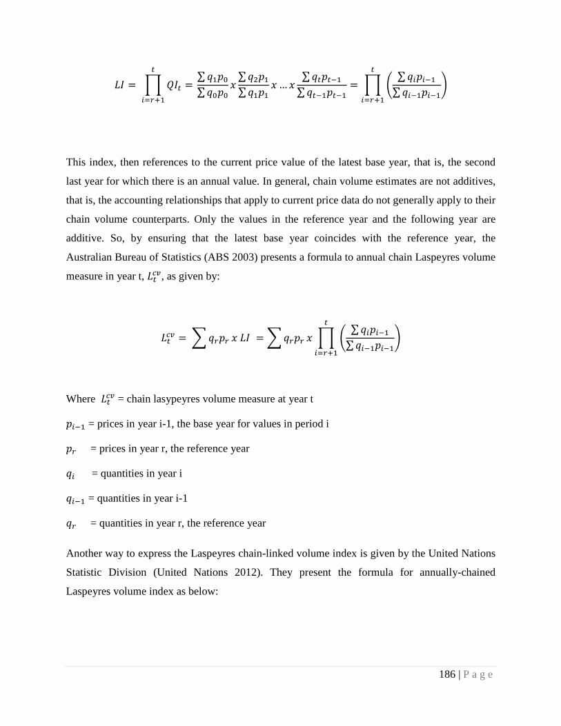
𝐿𝐼 = � 𝑄𝐼𝑡 = 𝑡

𝑖=𝑟+1

∑ 𝑞1𝑝0∑𝑞0𝑝0

𝑥∑𝑞2𝑝1∑𝑞1𝑝1

𝑥… 𝑥∑𝑞𝑡𝑝𝑡−1∑ 𝑞𝑡−1𝑝𝑡−1

= � �∑𝑞𝑖𝑝𝑖−1∑ 𝑞𝑖−1𝑝𝑖−1

�𝑡

𝑖=𝑟+1

This index, then references to the current price value of the latest base year, that is, the second

last year for which there is an annual value. In general, chain volume estimates are not additives,

that is, the accounting relationships that apply to current price data do not generally apply to their

chain volume counterparts. Only the values in the reference year and the following year are

additive. So, by ensuring that the latest base year coincides with the reference year, the

Australian Bureau of Statistics (ABS 2003) presents a formula to annual chain Laspeyres volume

measure in year t, 𝐿𝑡𝑐𝑣, as given by:

𝐿𝑡𝑐𝑣 = �𝑞𝑟𝑝𝑟 𝑥 𝐿𝐼 = �𝑞𝑟𝑝𝑟 𝑥 � �∑𝑞𝑖𝑝𝑖−1∑𝑞𝑖−1𝑝𝑖−1

�𝑡

𝑖=𝑟+1

Where 𝐿𝑡𝑐𝑣 = chain lasypeyres volume measure at year t

𝑝𝑖−1 = prices in year i-1, the base year for values in period i

𝑝𝑟 = prices in year r, the reference year

𝑞𝑖 = quantities in year i

𝑞𝑖−1 = quantities in year i-1

𝑞𝑟 = quantities in year r, the reference year

Another way to express the Laspeyres chain-linked volume index is given by the United Nations

Statistic Division (United Nations 2012). They present the formula for annually-chained

Laspeyres volume index as below:

186 | P a g e

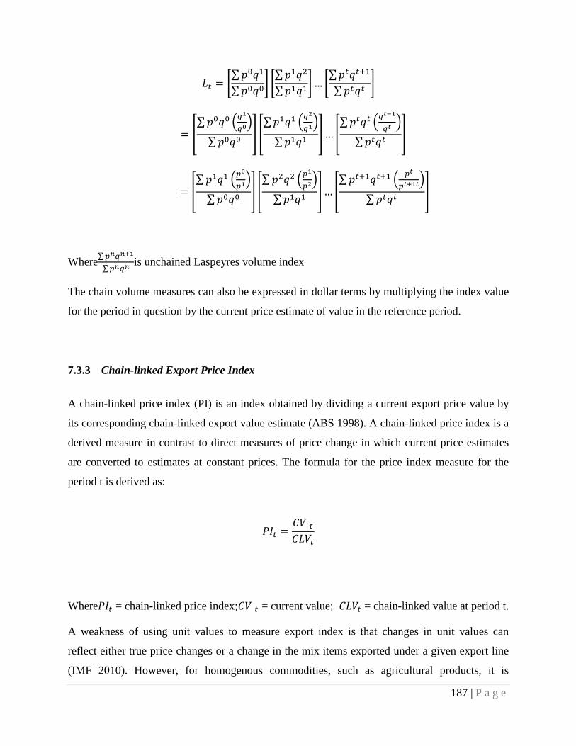
𝐿𝑡 = �∑𝑝0𝑞1

∑𝑝0𝑞0� �∑𝑝1𝑞2

∑𝑝1𝑞1�… �

∑𝑝𝑡𝑞𝑡+1

∑𝑝𝑡𝑞𝑡�

= �∑ 𝑝0𝑞0 �𝑞

1

𝑞0�

∑𝑝0𝑞0� �∑𝑝1𝑞1 �𝑞

2

𝑞1�

∑ 𝑝1𝑞1�… �

∑𝑝𝑡𝑞𝑡 �𝑞𝑡−1

𝑞𝑡�

∑𝑝𝑡𝑞𝑡�

= �∑𝑝1𝑞1 �𝑝

0

𝑝1�

∑ 𝑝0𝑞0� �∑ 𝑝2𝑞2 �𝑝

1

𝑝2�

∑ 𝑝1𝑞1�… �

∑𝑝𝑡+1𝑞𝑡+1 � 𝑝𝑡

𝑝𝑡+1𝑡�

∑𝑝𝑡𝑞𝑡�

Where∑𝑝𝑛𝑞𝑛+1

∑𝑝𝑛𝑞𝑛is unchained Laspeyres volume index

The chain volume measures can also be expressed in dollar terms by multiplying the index value

for the period in question by the current price estimate of value in the reference period.

7.3.3 Chain-linked Export Price Index

A chain-linked price index (PI) is an index obtained by dividing a current export price value by

its corresponding chain-linked export value estimate (ABS 1998). A chain-linked price index is a

derived measure in contrast to direct measures of price change in which current price estimates

are converted to estimates at constant prices. The formula for the price index measure for the

period t is derived as:

𝑃𝐼𝑡 =𝐶𝑉 𝑡𝐶𝐿𝑉𝑡

Where𝑃𝐼𝑡 = chain-linked price index;𝐶𝑉 𝑡 = current value; 𝐶𝐿𝑉𝑡 = chain-linked value at period t.

A weakness of using unit values to measure export index is that changes in unit values can

reflect either true price changes or a change in the mix items exported under a given export line

(IMF 2010). However, for homogenous commodities, such as agricultural products, it is

187 | P a g e

reasonable to assume that a given export line will track the same item over time, but for

heterogeneous products, such as manufactured goods, the aggregation will be bias. To avoid this

bias, it would be necessary to have direct price observations for individual export items and

identify export items with as much detail as possible. To minimize aggregation bias, the analysis

in this study will be conducted at the most detailed level possible with Indonesian agricultural

export data.

7.3.4 The Classification of Agricultural Commodities

Inthe next section, agricultural products will be determined according to the WTO Agreement on

Agriculture (AOA) (WTO 2012e) based on Harmonized System (HS) code. The HS provides a

nomenclature for classifying internationally traded goods. The definitions of HS commodity

groupings up to the 6-digit level are established by the World Customs Organization. This

agreement covers two-digit Harmonized System (HS) code 01 to code 24 excluding fish and fish

products and a number of manufactured agricultural products.

The HS provides a nomenclature for classifying internationally traded goods. The definitions of

HS commodity groupings up to the 6-digit level are established by the World Customs

Organization, excluding fish and fish products and a number of manufactured agricultural

products, as follows:

• HS chapters 1 to 24 include live animals, animal products, vegetable products, animal or

vegetable fats and oils, prepared edible fats, animal or vegetable waxes, [prepared

foodstuffs, beverages, spirits and vinegar, tobacco and manufactured tobacco substitutes;

less fish and fish products

• HS code 2905.43 (mannitol)

• HS code 2905.44 (sorbitol)

• HS heading 33.01 (essential oils)

• HS heading 35.01 to 35.05 (albuminoidal substances, modified starches, glues)

• HS code 3809.10 (finishing agents)

• HS code 3823.60 (sorbitol)

• HS headings 41.01 to 41.03 (hides and skins)

188 | P a g e

• HS heading 43.01 (raw fur skins)

• HS headings 50.01 to 50.03 (raw silk and silk waste)

• HS headings 51.01 to 51.03 (wool and animal hair)

• HS heading 52.01 to 52.03 (raw cotton, waste and cotton carded or combed)

• HS heading 53.01 (raw flax)

• HS heading 53.02 (raw hemp)

This research will segregate the agricultural commodities based on the HS classification into four

broad subsectors following Regmi et al. (2005).

i) Bulk commodities such as rice or coffee;

ii) Horticultural products such as fruits, cut flowers, tomatoes or spices;

iii) Semi-processed commodities such as vegetable oils or live animals;

iv) Processed products which consist of goods that require extensive processing prior to

consumption and are much closer to the consumer’s kitchen table such as processed fruit,

processed meat and beverages.

Those groupings are based primarily upon the relative dependence of production upon land

availability, geography and climatic conditions. The bulk and horticulture groups are more

reliant on these factors compared to semi-processed and processed categories which undergo

some transformation prior to their final use and, in principle, can be produced almost anywhere.

Furthermore, this agricultural grouping has also been used by the Organization for Economic Co-

operation and Development (OECD) and Food and Agriculture Organization of the United

Nation (FAO) to analyze agricultural sectors in their study (OECD & FAO 2007). Table 7.1 and

7.2 below present the list of the grouping system for these commodities.

Table 7.1 Agriculture Commodities Groupings Based on AoA (Primary Bulk and Horticulture Groups)

189 | P a g e

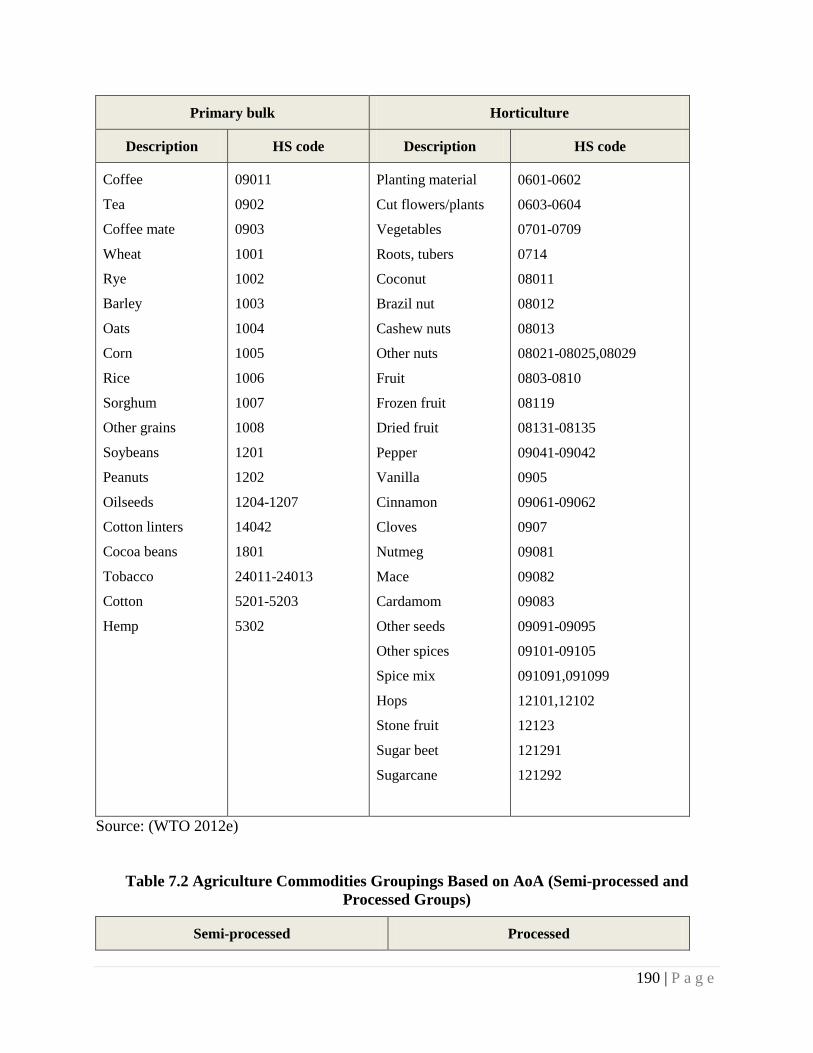
Primary bulk Horticulture

Description HS code Description HS code

Coffee

Tea

Coffee mate

Wheat

Rye

Barley

Oats

Corn

Rice

Sorghum

Other grains

Soybeans

Peanuts

Oilseeds

Cotton linters

Cocoa beans

Tobacco

Cotton

Hemp

09011

0902

0903

1001

1002

1003

1004

1005

1006

1007

1008

1201

1202

1204-1207

14042

1801

24011-24013

5201-5203

5302

Planting material

Cut flowers/plants

Vegetables

Roots, tubers

Coconut

Brazil nut

Cashew nuts

Other nuts

Fruit

Frozen fruit

Dried fruit

Pepper

Vanilla

Cinnamon

Cloves

Nutmeg

Mace

Cardamom

Other seeds

Other spices

Spice mix

Hops

Stone fruit

Sugar beet

Sugarcane

0601-0602

0603-0604

0701-0709

0714

08011

08012

08013

08021-08025,08029

0803-0810

08119

08131-08135

09041-09042

0905

09061-09062

0907

09081

09082

09083

09091-09095

09101-09105

091091,091099

12101,12102

12123

121291

121292

Source: (WTO 2012e)

Table 7.2 Agriculture Commodities Groupings Based on AoA (Semi-processed and Processed Groups)

Semi-processed Processed

190 | P a g e

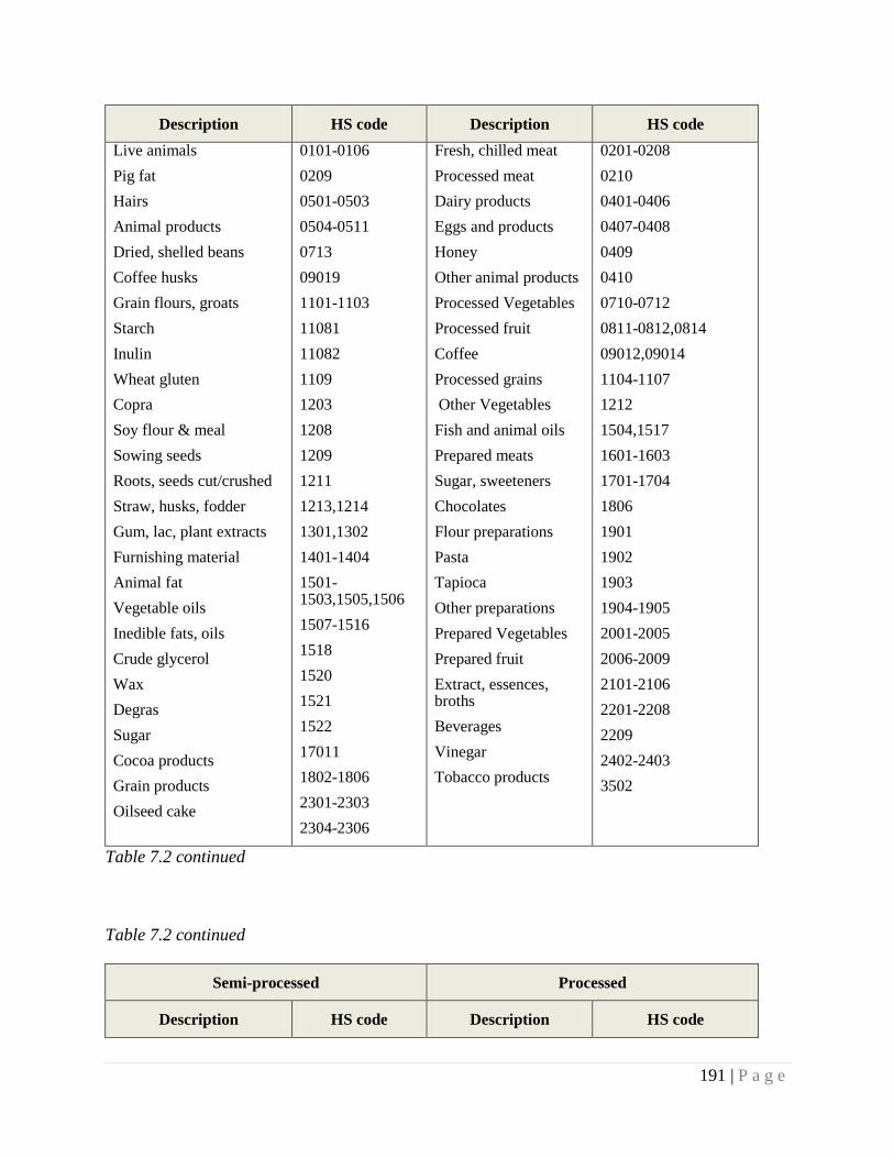
Description HS code Description HS code Live animals Pig fat Hairs Animal products Dried, shelled beans Coffee husks Grain flours, groats Starch Inulin Wheat gluten Copra Soy flour & meal Sowing seeds Roots, seeds cut/crushed Straw, husks, fodder Gum, lac, plant extracts Furnishing material Animal fat Vegetable oils Inedible fats, oils Crude glycerol Wax Degras Sugar Cocoa products Grain products Oilseed cake

0101-0106 0209 0501-0503 0504-0511 0713 09019 1101-1103 11081 11082 1109 1203 1208 1209 1211 1213,1214 1301,1302 1401-1404 1501-1503,1505,1506 1507-1516 1518 1520 1521 1522 17011 1802-1806 2301-2303 2304-2306

Fresh, chilled meat Processed meat Dairy products Eggs and products Honey Other animal products Processed Vegetables Processed fruit Coffee Processed grains Other Vegetables Fish and animal oils Prepared meats Sugar, sweeteners Chocolates Flour preparations Pasta Tapioca Other preparations Prepared Vegetables Prepared fruit Extract, essences, broths Beverages Vinegar Tobacco products

0201-0208 0210 0401-0406 0407-0408 0409 0410 0710-0712 0811-0812,0814 09012,09014 1104-1107 1212 1504,1517 1601-1603 1701-1704 1806 1901 1902 1903 1904-1905 2001-2005 2006-2009 2101-2106 2201-2208 2209 2402-2403 3502

Table 7.2 continued

Table 7.2 continued

Semi-processed Processed

Description HS code Description HS code

191 | P a g e

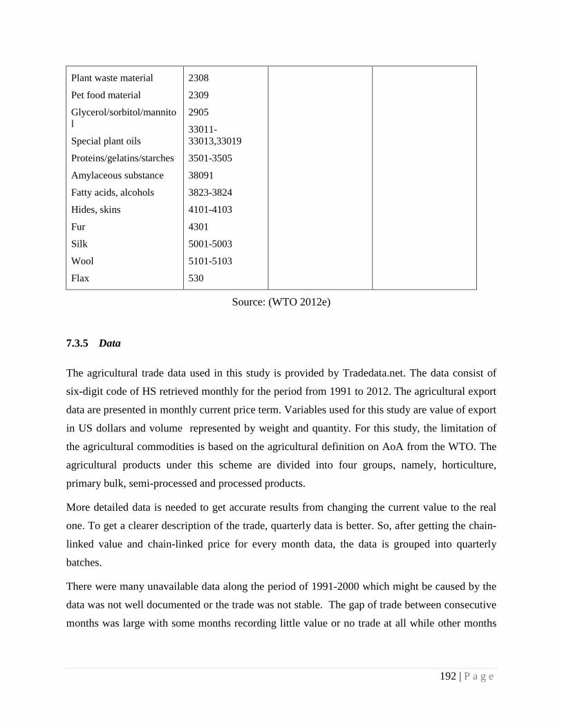
Plant waste material

Pet food material

Glycerol/sorbitol/mannitol

Special plant oils

Proteins/gelatins/starches

Amylaceous substance

Fatty acids, alcohols

Hides, skins

Fur

Silk

Wool

Flax

2308

2309

2905

33011-33013,33019

3501-3505

38091

3823-3824

4101-4103

4301

5001-5003

5101-5103

530

Source: (WTO 2012e)

7.3.5 Data

The agricultural trade data used in this study is provided by Tradedata.net. The data consist of

six-digit code of HS retrieved monthly for the period from 1991 to 2012. The agricultural export

data are presented in monthly current price term. Variables used for this study are value of export

in US dollars and volume represented by weight and quantity. For this study, the limitation of

the agricultural commodities is based on the agricultural definition on AoA from the WTO. The

agricultural products under this scheme are divided into four groups, namely, horticulture,

primary bulk, semi-processed and processed products.

More detailed data is needed to get accurate results from changing the current value to the real

one. To get a clearer description of the trade, quarterly data is better. So, after getting the chain-

linked value and chain-linked price for every month data, the data is grouped into quarterly

batches.

There were many unavailable data along the period of 1991-2000 which might be caused by the

data was not well documented or the trade was not stable. The gap of trade between consecutive

months was large with some months recording little value or no trade at all while other months

192 | P a g e

recorded a large value. However, after 2000, the export data was more stable in terms of the

amount of exports and the variety of commodities.

Raw monthly data for all agricultural products exported from every port in Indonesia is

collected. The data contains more than 500,000 individual export records, so these will be

aggregated for each commodity. To organize the data, the six-digit code HS data was first

grouped into agricultural data as a whole. This yielded data with 435 codes, showing the main

commodities that could be picked as the sample for this study. Twenty out of 435 commodities

covered more than 95 per cent of the total value of exports for the period 2000 to 2011.

Table 7.3 Groups of Agricultural Products

No Group Description HS 1 1 Pepper of the genus piper (excl. crushed or ground) 090411

2 1 Manioc (cassava) fresh, chilled, frozen or dried, whether or not sliced or in the form of pellets 071410

3 1 Coconuts (excl. desiccated) fresh or dried, whether or not shelled or peeled 080119

4 1 Desiccated coconuts, fresh or dried, whether or not shelled or peeled 080111

5 1 Nutmeg 090810

6 1 Nuts, fresh or dried, whether or not shelled or peeled (excl. coconuts, brazil nuts, cashew nuts, almonds, hazelnuts or filberts, walnuts, chestnuts, pistachios & macadamias)

080290

7 1 Cashew nuts, in shell, fresh or dried 080131 8 1 Cloves, whole fruit & stems 090700 9 2 Cocoa beans, whole or broken, raw or roasted 180100

Table 7.3 Continued

Table 7.3 Continued

No Group Description HS 10 2 Coffee (excl. roasted & decaffeinated) 090111 11 2 Black tea (fermented) & other partly fermented tea, whether or not 090240

193 | P a g e

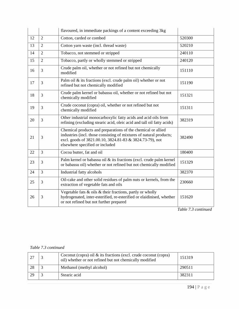
flavoured, in immediate packings of a content exceeding 3kg 12 2 Cotton, carded or combed 520300 13 2 Cotton yarn waste (incl. thread waste) 520210 14 2 Tobacco, not stemmed or stripped 240110 15 2 Tobacco, partly or wholly stemmed or stripped 240120

16 3 Crude palm oil, whether or not refined but not chemically modified 151110

17 3 Palm oil & its fractions (excl. crude palm oil) whether or not refined but not chemically modified 151190

18 3 Crude palm kernel or babassu oil, whether or not refined but not chemically modified 151321

19 3 Crude coconut (copra) oil, whether or not refined but not chemically modified 151311

20 3 Other industrial monocarboxylic fatty acids and acid oils from refining (excluding stearic acid, oleic acid and tall oil fatty acids) 382319

21 3 Chemical products and preparations of the chemical or allied industries (incl. those consisting of mixtures of natural products; excl. goods of 3821.00.10, 3824.81-83 & 3824.73-79), not elsewhere specified or included

382490

22 3 Cocoa butter, fat and oil 180400

23 3 Palm kernel or babassu oil & its fractions (excl. crude palm kernel or babassu oil) whether or not refined but not chemically modified 151329

24 3 Industrial fatty alcohols 382370

25 3 Oil-cake and other solid residues of palm nuts or kernels, from the extraction of vegetable fats and oils 230660

26 3 Vegetable fats & oils & their fractions, partly or wholly hydrogenated, inter-esterified, re-esterified or elaidinised, whether or not refined but not further prepared

151620

Table 7.3 continued Table 7.3 continued

27 3 Coconut (copra) oil & its fractions (excl. crude coconut (copra) oil) whether or not refined but not chemically modified 151319

28 3 Methanol (methyl alcohol) 290511 29 3 Stearic acid 382311

194 | P a g e

30 4 Edible mixtures or preparations of animal or vegetable fats or oils or of fractions of different fats or oils (excl. partly or wholly hydrogenated, inter-esterified, re-esterified or elaidinised fats or oils & margarine)

151790

31 4 Pineapples otherwise prepared or preserved, nes 200820

32 4 Seaweeds & other algae, of a kind used primarily for human consumption, fresh, chilled, frozen or dried, whether or not ground

121220

33 4 Unstuffed pasta, cooked or otherwise prepared 190230 34 4 Food preparations of flour and meal 210690 35 4 Cigarettes containing tobacco 240220

Source:Tradedata (2013), calculated by Author Note: 1 horticulture; 2 primary bulk; 3 semi-processed; 4 processed agricultural products

The rest only had a small share in the aggregate agricultural export and the data only had an

incomplete time series. Many of these products also included semi-processed products. Thus,

some other data are taken to fulfil the list of agricultural commodities as covered by the AoA of

the WTO. Those selected are in the top list of export values in each group of commodities. Due

to the availability of the data, 35 commodities are chosen as representative of the agricultural

products, namely, eight products of horticulture, seven products of primary bulk, fourteen

products of semi-processed group and six products of processed group. The chosen commodities

are listed in the Table 7.3.

Data from export trade with China, which is the focus of this study, is compared with those of

some other countries such as US, Japan, ASEAN and India, which are the other biggest export

destinations for Indonesian agricultural products. Furthermore, aggregate exports to the world

will also be examined to get a big picture of agricultural export patterns. This will be followed by

review of exports to the world excluding China to examine the impact of the export to China on

general agricultural exports.

Despite the availability of detailed raw data obtained from Tradedata.net, the data contain

significant errors, particularly in the quantity variable. For example, there is an inconsistent

quantity unit for the time series data. For more recent data, kilograms were uniformly used as the

measure of quantity; however, some of the older data either used tonne or kilograms. To respond

to this data error, a system of data cleaning is imposed. It is assumed that the export values for

195 | P a g e

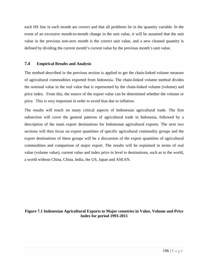
each HS line in each month are correct and that all problems lie in the quantity variable. In the

event of an excessive month-to-month change in the unit value, it will be assumed that the unit

value in the previous non-zero month is the correct unit value, and a new cleaned quantity is

defined by dividing the current month’s current value by the previous month’s unit value.

7.4 Empirical Results and Analysis

The method described in the previous section is applied to get the chain-linked volume measure

of agricultural commodities exported from Indonesia. The chain-linked volume method divides

the nominal value in the real value that is represented by the chain-linked volume (volume) and

price index. From this, the source of the export value can be determined whether the volume or

price. This is very important in order to avoid bias due to inflation.

The results will touch on many critical aspects of Indonesian agricultural trade. The first

subsection will cover the general patterns of agricultural trade in Indonesia, followed by a

description of the main export destinations for Indonesian agricultural exports. The next two

sections will then focus on export quantities of specific agricultural commodity groups and the

export destinations of these groups will be a discussion of the export quantities of agricultural

commodities and comparison of major export. The results will be explained in terms of real

value (volume value), current value and index price in level to destinations, such as to the world,

a world without China, China, India, the US, Japan and ASEAN.

Figure 7.1 Indonesian Agricultural Exports to Major countries in Value, Volume and Price Index for period 1993-2011

196 | P a g e

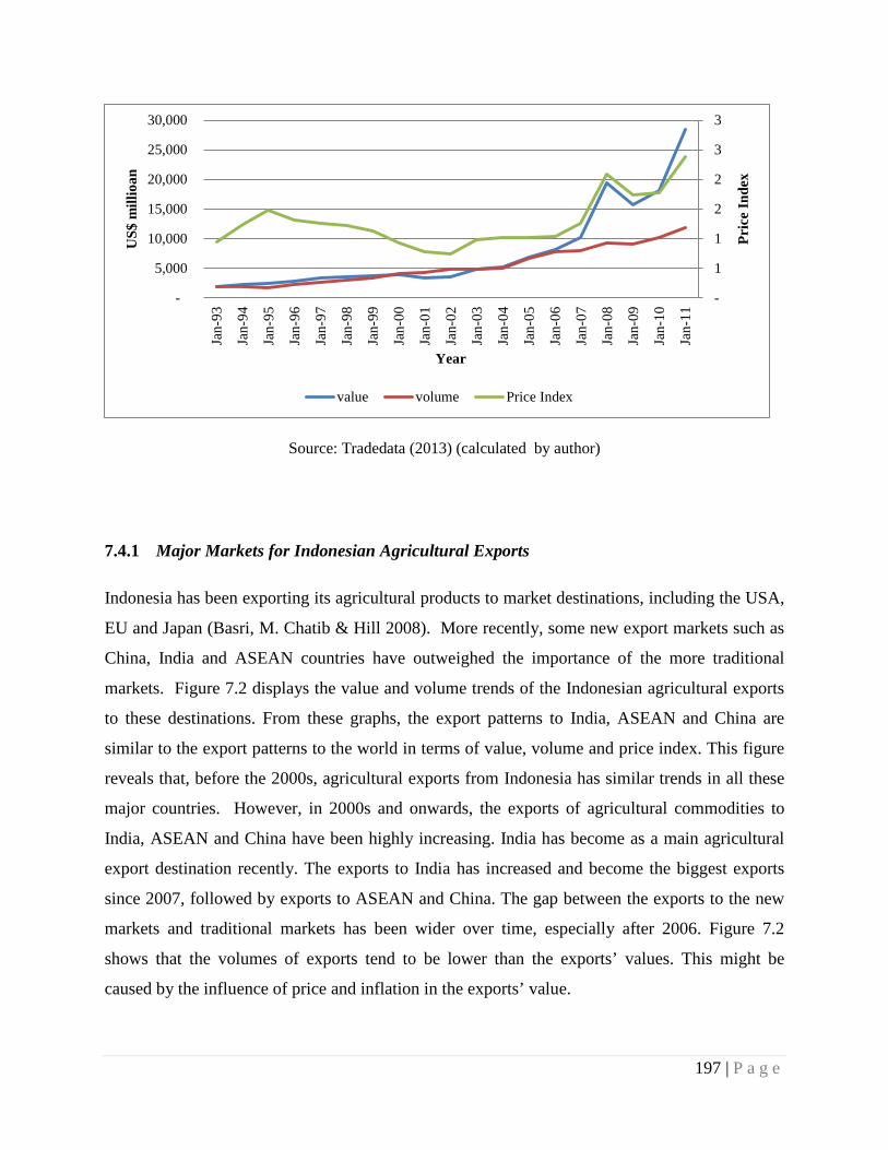
Source: Tradedata (2013) (calculated by author)

7.4.1 Major Markets for Indonesian Agricultural Exports

Indonesia has been exporting its agricultural products to market destinations, including the USA,

EU and Japan (Basri, M. Chatib & Hill 2008). More recently, some new export markets such as

China, India and ASEAN countries have outweighed the importance of the more traditional

markets. Figure 7.2 displays the value and volume trends of the Indonesian agricultural exports

to these destinations. From these graphs, the export patterns to India, ASEAN and China are

similar to the export patterns to the world in terms of value, volume and price index. This figure

reveals that, before the 2000s, agricultural exports from Indonesia has similar trends in all these

major countries. However, in 2000s and onwards, the exports of agricultural commodities to

India, ASEAN and China have been highly increasing. India has become as a main agricultural

export destination recently. The exports to India has increased and become the biggest exports

since 2007, followed by exports to ASEAN and China. The gap between the exports to the new

markets and traditional markets has been wider over time, especially after 2006. Figure 7.2

shows that the volumes of exports tend to be lower than the exports’ values. This might be

caused by the influence of price and inflation in the exports’ value.

-

1

1

2

2

3

3

-

5,000

10,000

15,000

20,000

25,000

30,000

Jan-

93

Jan-

94

Jan-

95

Jan-

96

Jan-

97

Jan-

98

Jan-

99

Jan-

00

Jan-

01

Jan-

02

Jan-

03

Jan-

04

Jan-

05

Jan-

06

Jan-

07

Jan-

08

Jan-

09

Jan-

10

Jan-

11

Pric

e In

dex

US$

mill

ioan

Year

value volume Price Index

197 | P a g e

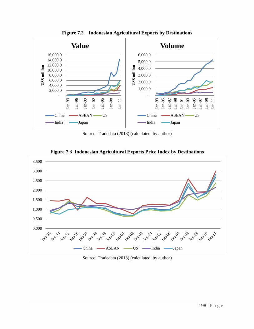
Figure 7.2 Indonesian Agricultural Exports by Destinations

Source: Tradedata (2013) (calculated by author)

Figure 7.3 Indonesian Agricultural Exports Price Index by Destinations

Source: Tradedata (2013) (calculated by author)

- 2,000.0 4,000.0 6,000.0 8,000.0

10,000.0 12,000.0 14,000.0 16,000.0

Jan-

93

Jan-

96

Jan-

99

Jan-

02

Jan-

05

Jan-

08

Jan-

11

US$

mill

ion

Value

China ASEAN US

India Japan

- 1,000.0 2,000.0 3,000.0 4,000.0 5,000.0 6,000.0

Jan-

93Ja

n-95

Jan-

97Ja

n-99

Jan-

01Ja

n-03

Jan-

05Ja

n-07

Jan-

09Ja

n-11

US$

mill

ion

Volume

China ASEAN US

India Japan

0.000

0.500

1.000

1.500

2.000

2.500

3.000

3.500

China ASEAN US India Japan

198 | P a g e

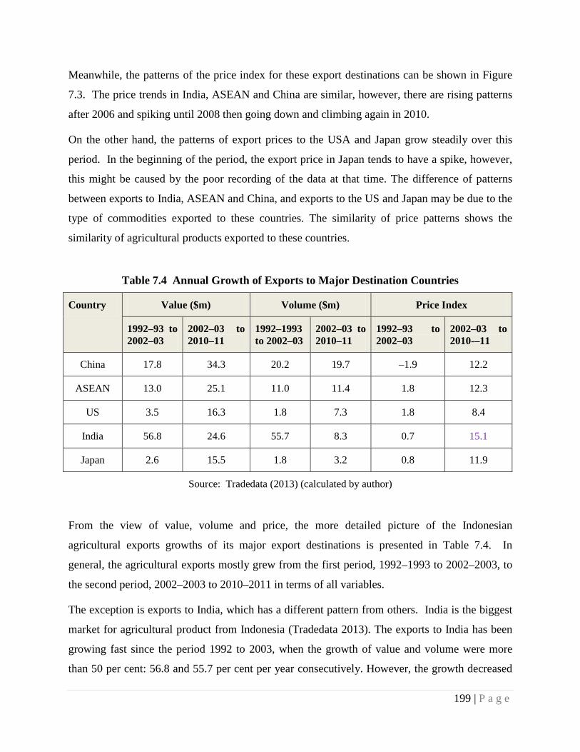
Meanwhile, the patterns of the price index for these export destinations can be shown in Figure

7.3. The price trends in India, ASEAN and China are similar, however, there are rising patterns

after 2006 and spiking until 2008 then going down and climbing again in 2010.

On the other hand, the patterns of export prices to the USA and Japan grow steadily over this

period. In the beginning of the period, the export price in Japan tends to have a spike, however,

this might be caused by the poor recording of the data at that time. The difference of patterns

between exports to India, ASEAN and China, and exports to the US and Japan may be due to the

type of commodities exported to these countries. The similarity of price patterns shows the

similarity of agricultural products exported to these countries.

Table 7.4 Annual Growth of Exports to Major Destination Countries

Country Value ($m) Volume ($m) Price Index

1992–93 to 2002–03

2002–03 to 2010–11

1992–1993 to 2002–03

2002–03 to 2010–11

1992–93 to 2002–03

2002–03 to 2010-–11

China 17.8 34.3 20.2 19.7 –1.9 12.2

ASEAN 13.0 25.1 11.0 11.4 1.8 12.3

US 3.5 16.3 1.8 7.3 1.8 8.4

India 56.8 24.6 55.7 8.3 0.7 15.1

Japan 2.6 15.5 1.8 3.2 0.8 11.9

Source: Tradedata (2013) (calculated by author)

From the view of value, volume and price, the more detailed picture of the Indonesian

agricultural exports growths of its major export destinations is presented in Table 7.4. In

general, the agricultural exports mostly grew from the first period, 1992–1993 to 2002–2003, to

the second period, 2002–2003 to 2010–2011 in terms of all variables.

The exception is exports to India, which has a different pattern from others. India is the biggest

market for agricultural product from Indonesia (Tradedata 2013). The exports to India has been

growing fast since the period 1992 to 2003, when the growth of value and volume were more

than 50 per cent: 56.8 and 55.7 per cent per year consecutively. However, the growth decreased

199 | P a g e

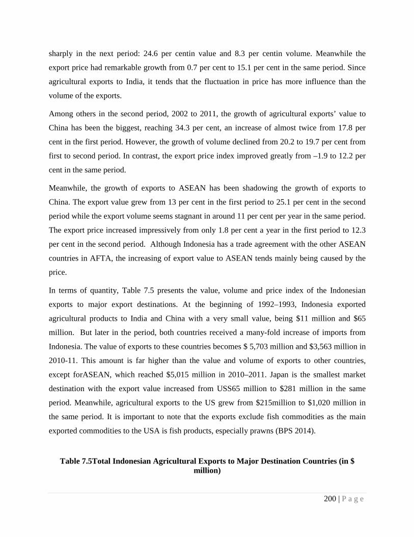
sharply in the next period: 24.6 per centin value and 8.3 per centin volume. Meanwhile the

export price had remarkable growth from 0.7 per cent to 15.1 per cent in the same period. Since

agricultural exports to India, it tends that the fluctuation in price has more influence than the

volume of the exports.

Among others in the second period, 2002 to 2011, the growth of agricultural exports’ value to

China has been the biggest, reaching 34.3 per cent, an increase of almost twice from 17.8 per

cent in the first period. However, the growth of volume declined from 20.2 to 19.7 per cent from

first to second period. In contrast, the export price index improved greatly from –1.9 to 12.2 per

cent in the same period.

Meanwhile, the growth of exports to ASEAN has been shadowing the growth of exports to

China. The export value grew from 13 per cent in the first period to 25.1 per cent in the second

period while the export volume seems stagnant in around 11 per cent per year in the same period.

The export price increased impressively from only 1.8 per cent a year in the first period to 12.3

per cent in the second period. Although Indonesia has a trade agreement with the other ASEAN

countries in AFTA, the increasing of export value to ASEAN tends mainly being caused by the

price.

In terms of quantity, Table 7.5 presents the value, volume and price index of the Indonesian

exports to major export destinations. At the beginning of 1992–1993, Indonesia exported

agricultural products to India and China with a very small value, being $11 million and $65

million. But later in the period, both countries received a many-fold increase of imports from

Indonesia. The value of exports to these countries becomes $ 5,703 million and $3,563 million in

2010-11. This amount is far higher than the value and volume of exports to other countries,

except forASEAN, which reached $5,015 million in 2010–2011. Japan is the smallest market

destination with the export value increased from USS65 million to $281 million in the same

period. Meanwhile, agricultural exports to the US grew from $215million to $1,020 million in

the same period. It is important to note that the exports exclude fish commodities as the main

exported commodities to the USA is fish products, especially prawns (BPS 2014).

Table 7.5Total Indonesian Agricultural Exports to Major Destination Countries (in $ million)

200 | P a g e

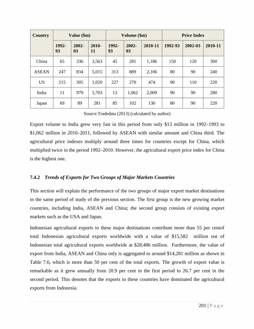
Country Value ($m) Volume ($m) Price Index

1992-93

2002-03

2010-11

1992-93

2002-03

2010-11 1992-93 2002-03 2010-11

China 65 336 3,563 45 281 1,186 150 120 300

ASEAN 247 834 5,015 313 889 2,106 80 90 240

US 215 305 1,020 227 270 474 90 110 220

India 11 979 5,703 13 1,062 2,009 90 90 280

Japan 69 89 281 85 102 130 80 90 220

Source:Tradedata (2013) (calculated by author)

Export volume to India grew very fast in this period from only $13 million in 1992–1993 to

$1,062 million in 2010–2011, followed by ASEAN with similar amount and China third. The

agricultural price indexes multiply around three times for countries except for China, which

multiplied twice in the period 1992–2010. However, the agricultural export price index for China

is the highest one.

7.4.2 Trends of Exports for Two Groups of Major Markets Countries

This section will explain the performance of the two groups of major export market destinations

in the same period of study of the previous section. The first group is the new growing market

countries, including India, ASEAN and China; the second group consists of existing export

markets such as the USA and Japan.

Indonesian agricultural exports to these major destinations contribute more than 55 per centof

total Indonesian agricultural exports worldwide with a value of $15,582 million out of

Indonesian total agricultural exports worldwide at $28,486 million. Furthermore, the value of

export from India, ASEAN and China only is aggregated to around $14,281 million as shown in

Table 7.6, which is more than 50 per cent of the total exports. The growth of export value is

remarkable as it grew annually from 20.9 per cent in the first period to 26.7 per cent in the

second period. This denotes that the exports to these countries have dominated the agricultural

exports from Indonesia.

201 | P a g e

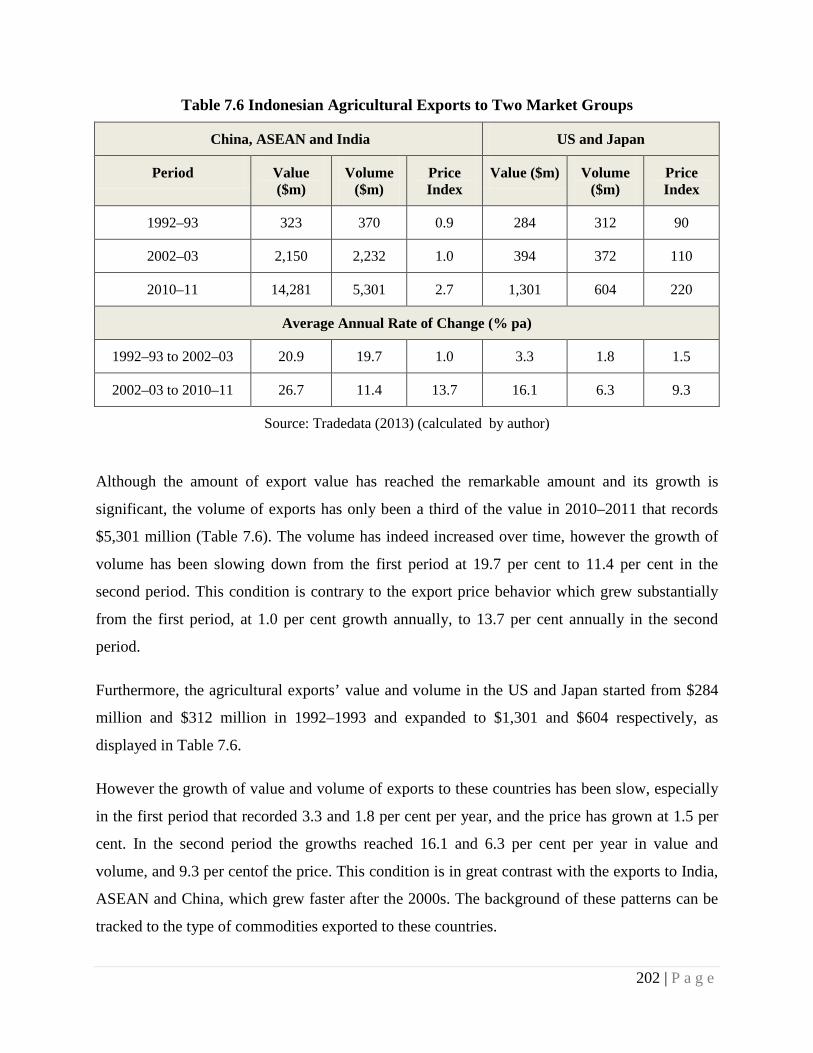
Table 7.6 Indonesian Agricultural Exports to Two Market Groups

China, ASEAN and India US and Japan

Period Value ($m)

Volume ($m)

Price Index

Value ($m) Volume ($m)

Price Index

1992–93 323 370 0.9 284 312 90

2002–03 2,150 2,232 1.0 394 372 110

2010–11 14,281 5,301 2.7 1,301 604 220

Average Annual Rate of Change (% pa)

1992–93 to 2002–03 20.9 19.7 1.0 3.3 1.8 1.5

2002–03 to 2010–11 26.7 11.4 13.7 16.1 6.3 9.3

Source: Tradedata (2013) (calculated by author)

Although the amount of export value has reached the remarkable amount and its growth is

significant, the volume of exports has only been a third of the value in 2010–2011 that records

$5,301 million (Table 7.6). The volume has indeed increased over time, however the growth of

volume has been slowing down from the first period at 19.7 per cent to 11.4 per cent in the

second period. This condition is contrary to the export price behavior which grew substantially

from the first period, at 1.0 per cent growth annually, to 13.7 per cent annually in the second

period.

Furthermore, the agricultural exports’ value and volume in the US and Japan started from $284

million and $312 million in 1992–1993 and expanded to $1,301 and $604 respectively, as

displayed in Table 7.6.

However the growth of value and volume of exports to these countries has been slow, especially

in the first period that recorded 3.3 and 1.8 per cent per year, and the price has grown at 1.5 per

cent. In the second period the growths reached 16.1 and 6.3 per cent per year in value and

volume, and 9.3 per centof the price. This condition is in great contrast with the exports to India,

ASEAN and China, which grew faster after the 2000s. The background of these patterns can be

tracked to the type of commodities exported to these countries.

202 | P a g e

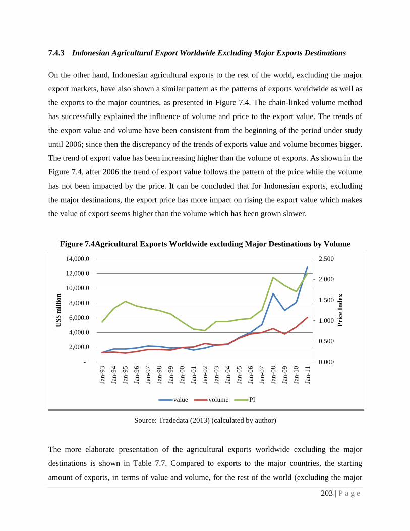
7.4.3 Indonesian Agricultural Export Worldwide Excluding Major Exports Destinations

On the other hand, Indonesian agricultural exports to the rest of the world, excluding the major

export markets, have also shown a similar pattern as the patterns of exports worldwide as well as

the exports to the major countries, as presented in Figure 7.4. The chain-linked volume method

has successfully explained the influence of volume and price to the export value. The trends of

the export value and volume have been consistent from the beginning of the period under study

until 2006; since then the discrepancy of the trends of exports value and volume becomes bigger.

The trend of export value has been increasing higher than the volume of exports. As shown in the

Figure 7.4, after 2006 the trend of export value follows the pattern of the price while the volume

has not been impacted by the price. It can be concluded that for Indonesian exports, excluding

the major destinations, the export price has more impact on rising the export value which makes

the value of export seems higher than the volume which has been grown slower.

Figure 7.4Agricultural Exports Worldwide excluding Major Destinations by Volume

Source: Tradedata (2013) (calculated by author)

The more elaborate presentation of the agricultural exports worldwide excluding the major

destinations is shown in Table 7.7. Compared to exports to the major countries, the starting

amount of exports, in terms of value and volume, for the rest of the world (excluding the major

0.000

0.500

1.000

1.500

2.000

2.500

-

2,000.0

4,000.0

6,000.0

8,000.0

10,000.0

12,000.0

14,000.0

Jan-

93

Jan-

94

Jan-

95

Jan-

96

Jan-

97

Jan-

98

Jan-

99

Jan-

00

Jan-

01

Jan-

02

Jan-

03

Jan-

04

Jan-

05

Jan-

06

Jan-

07

Jan-

08

Jan-

09

Jan-

10

Jan-

11

Pric

e In

dex

US$

mill

ion

value volume PI

203 | P a g e

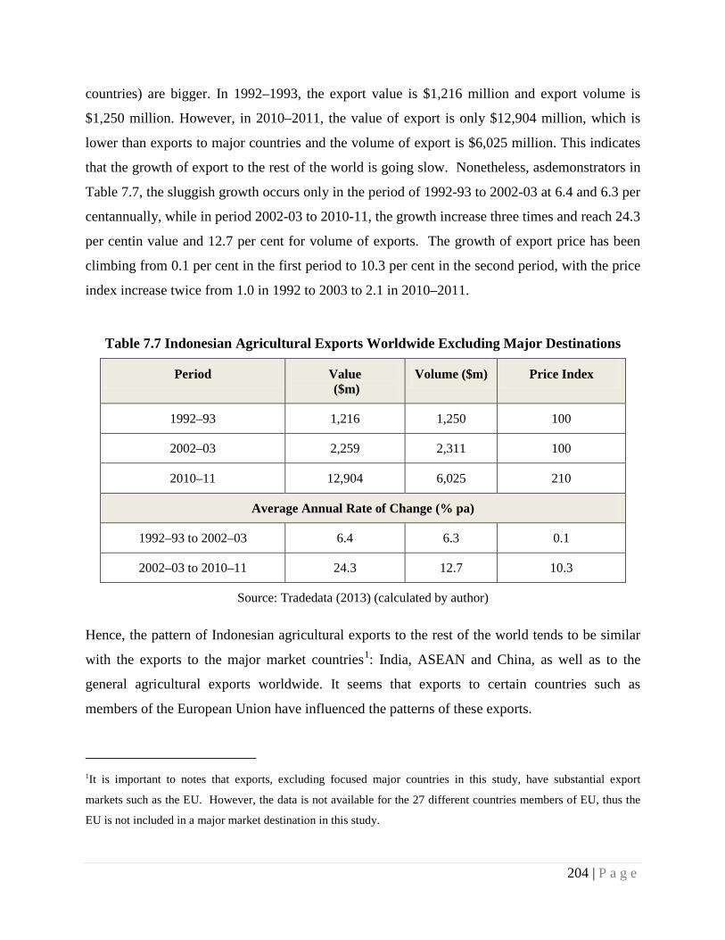
countries) are bigger. In 1992–1993, the export value is $1,216 million and export volume is

$1,250 million. However, in 2010–2011, the value of export is only $12,904 million, which is

lower than exports to major countries and the volume of export is $6,025 million. This indicates

that the growth of export to the rest of the world is going slow. Nonetheless, asdemonstrators in

Table 7.7, the sluggish growth occurs only in the period of 1992-93 to 2002-03 at 6.4 and 6.3 per

centannually, while in period 2002-03 to 2010-11, the growth increase three times and reach 24.3

per centin value and 12.7 per cent for volume of exports. The growth of export price has been

climbing from 0.1 per cent in the first period to 10.3 per cent in the second period, with the price

index increase twice from 1.0 in 1992 to 2003 to 2.1 in 2010–2011.

Table 7.7 Indonesian Agricultural Exports Worldwide Excluding Major Destinations

Period Value ($m)

Volume ($m) Price Index

1992–93 1,216 1,250 100

2002–03 2,259 2,311 100

2010–11 12,904 6,025 210

Average Annual Rate of Change (% pa)

1992–93 to 2002–03 6.4 6.3 0.1

2002–03 to 2010–11 24.3 12.7 10.3

Source: Tradedata (2013) (calculated by author)

Hence, the pattern of Indonesian agricultural exports to the rest of the world tends to be similar

with the exports to the major market countries1: India, ASEAN and China, as well as to the

general agricultural exports worldwide. It seems that exports to certain countries such as

members of the European Union have influenced the patterns of these exports.

1It is important to notes that exports, excluding focused major countries in this study, have substantial export

markets such as the EU. However, the data is not available for the 27 different countries members of EU, thus the

EU is not included in a major market destination in this study.

204 | P a g e

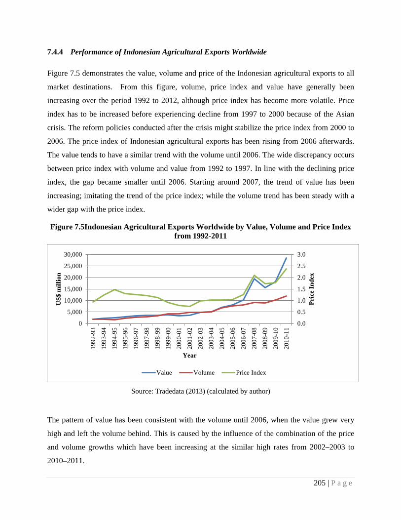
7.4.4 Performance of Indonesian Agricultural Exports Worldwide

Figure 7.5 demonstrates the value, volume and price of the Indonesian agricultural exports to all

market destinations. From this figure, volume, price index and value have generally been

increasing over the period 1992 to 2012, although price index has become more volatile. Price

index has to be increased before experiencing decline from 1997 to 2000 because of the Asian

crisis. The reform policies conducted after the crisis might stabilize the price index from 2000 to

2006. The price index of Indonesian agricultural exports has been rising from 2006 afterwards.

The value tends to have a similar trend with the volume until 2006. The wide discrepancy occurs

between price index with volume and value from 1992 to 1997. In line with the declining price

index, the gap became smaller until 2006. Starting around 2007, the trend of value has been

increasing; imitating the trend of the price index; while the volume trend has been steady with a

wider gap with the price index.

Figure 7.5Indonesian Agricultural Exports Worldwide by Value, Volume and Price Index from 1992-2011

Source: Tradedata (2013) (calculated by author)

The pattern of value has been consistent with the volume until 2006, when the value grew very

high and left the volume behind. This is caused by the influence of the combination of the price

and volume growths which have been increasing at the similar high rates from 2002–2003 to

2010–2011.

0.0

0.5

1.0

1.5

2.0

2.5

3.0

0

5,000

10,000

15,000

20,000

25,000

30,000

1992

-93

1993

-94

1994

-95

1995

-96

1996

-97

1997

-98

1998

-99

1999

-00

2000

-01

2001

-02

2002

-03

2003

-04

2004

-05

2005

-06

2006

-07

2007

-08

2008

-09

2009

-10

2010

-11

Pric

e In

dex

US$

mill

ion

Year

Value Volume Price Index

205 | P a g e

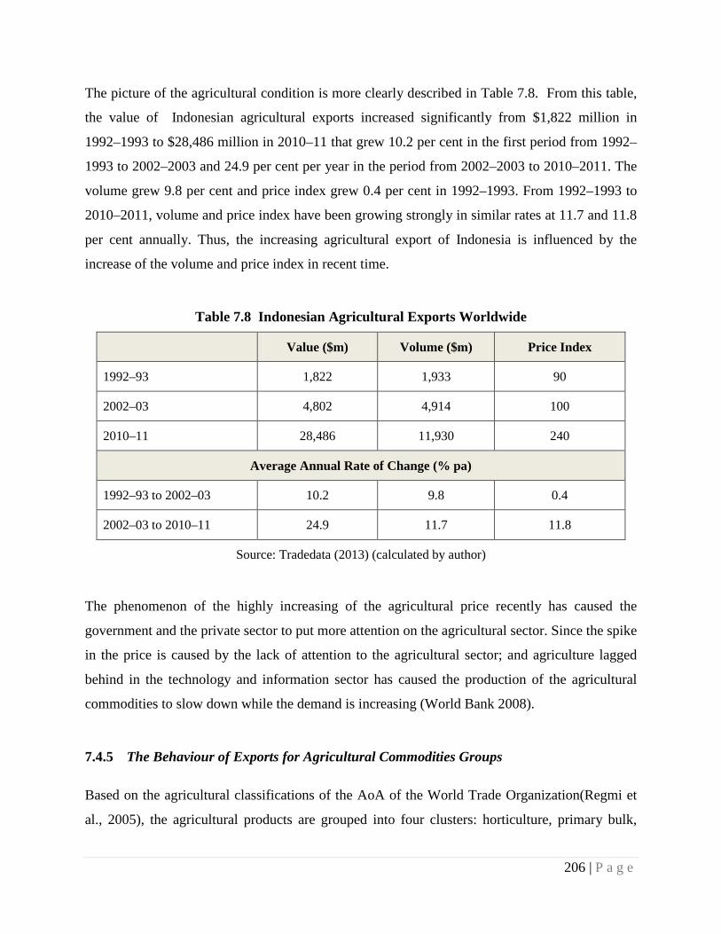
The picture of the agricultural condition is more clearly described in Table 7.8. From this table,

the value of Indonesian agricultural exports increased significantly from $1,822 million in

1992–1993 to $28,486 million in 2010–11 that grew 10.2 per cent in the first period from 1992–

1993 to 2002–2003 and 24.9 per cent per year in the period from 2002–2003 to 2010–2011. The

volume grew 9.8 per cent and price index grew 0.4 per cent in 1992–1993. From 1992–1993 to

2010–2011, volume and price index have been growing strongly in similar rates at 11.7 and 11.8

per cent annually. Thus, the increasing agricultural export of Indonesia is influenced by the

increase of the volume and price index in recent time.

Table 7.8 Indonesian Agricultural Exports Worldwide

Value ($m) Volume ($m) Price Index

1992–93 1,822 1,933 90

2002–03 4,802 4,914 100

2010–11 28,486 11,930 240

Average Annual Rate of Change (% pa)

1992–93 to 2002–03 10.2 9.8 0.4

2002–03 to 2010–11 24.9 11.7 11.8

Source: Tradedata (2013) (calculated by author)

The phenomenon of the highly increasing of the agricultural price recently has caused the

government and the private sector to put more attention on the agricultural sector. Since the spike

in the price is caused by the lack of attention to the agricultural sector; and agriculture lagged

behind in the technology and information sector has caused the production of the agricultural

commodities to slow down while the demand is increasing (World Bank 2008).

7.4.5 The Behaviour of Exports for Agricultural Commodities Groups

Based on the agricultural classifications of the AoA of the World Trade Organization(Regmi et

al., 2005), the agricultural products are grouped into four clusters: horticulture, primary bulk,

206 | P a g e

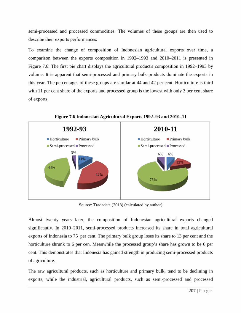
semi-processed and processed commodities. The volumes of these groups are then used to

describe their exports performances.

To examine the change of composition of Indonesian agricultural exports over time, a

comparison between the exports composition in 1992–1993 and 2010–2011 is presented in

Figure 7.6. The first pie chart displays the agricultural product's composition in 1992–1993 by

volume. It is apparent that semi-processed and primary bulk products dominate the exports in

this year. The percentages of these groups are similar at 44 and 42 per cent. Horticulture is third

with 11 per cent share of the exports and processed group is the lowest with only 3 per cent share

of exports.

Figure 7.6 Indonesian Agricultural Exports 1992–93 and 2010–11

Source: Tradedata (2013) (calculated by author)

Almost twenty years later, the composition of Indonesian agricultural exports changed

significantly. In 2010–2011, semi-processed products increased its share in total agricultural

exports of Indonesia to 75 per cent. The primary bulk group loses its share to 13 per cent and the

horticulture shrunk to 6 per cen. Meanwhile the processed group’s share has grown to be 6 per

cent. This demonstrates that Indonesia has gained strength in producing semi-processed products

of agriculture.

The raw agricultural products, such as horticulture and primary bulk, tend to be declining in

exports, while the industrial, agricultural products, such as semi-processed and processed

11%

42%

44%

3%

1992-93 Horticulture Primary bulk

Semi-processed Processed

6%

13%

75%

6%

2010-11 Horticulture Primary bulk

Semi-processed Processed

207 | P a g e

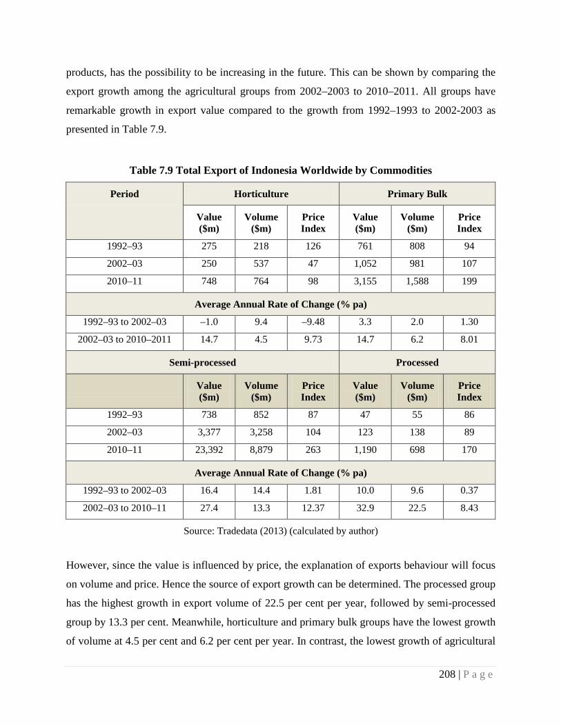
products, has the possibility to be increasing in the future. This can be shown by comparing the

export growth among the agricultural groups from 2002–2003 to 2010–2011. All groups have

remarkable growth in export value compared to the growth from 1992–1993 to 2002-2003 as

presented in Table 7.9.

Table 7.9 Total Export of Indonesia Worldwide by Commodities

Period Horticulture Primary Bulk

Value ($m)

Volume ($m)

Price Index

Value ($m)

Volume ($m)

Price Index

1992–93 275 218 126 761 808 94

2002–03 250 537 47 1,052 981 107

2010–11 748 764 98 3,155 1,588 199

Average Annual Rate of Change (% pa)

1992–93 to 2002–03 –1.0 9.4 –9.48 3.3 2.0 1.30

2002–03 to 2010–2011 14.7 4.5 9.73 14.7 6.2 8.01

Semi-processed Processed

Value ($m)

Volume ($m)

Price Index

Value ($m)

Volume ($m)

Price Index

1992–93 738 852 87 47 55 86

2002–03 3,377 3,258 104 123 138 89

2010–11 23,392 8,879 263 1,190 698 170

Average Annual Rate of Change (% pa)

1992–93 to 2002–03 16.4 14.4 1.81 10.0 9.6 0.37

2002–03 to 2010–11 27.4 13.3 12.37 32.9 22.5 8.43

Source: Tradedata (2013) (calculated by author)

However, since the value is influenced by price, the explanation of exports behaviour will focus

on volume and price. Hence the source of export growth can be determined. The processed group

has the highest growth in export volume of 22.5 per cent per year, followed by semi-processed

group by 13.3 per cent. Meanwhile, horticulture and primary bulk groups have the lowest growth

of volume at 4.5 per cent and 6.2 per cent per year. In contrast, the lowest growth of agricultural

208 | P a g e

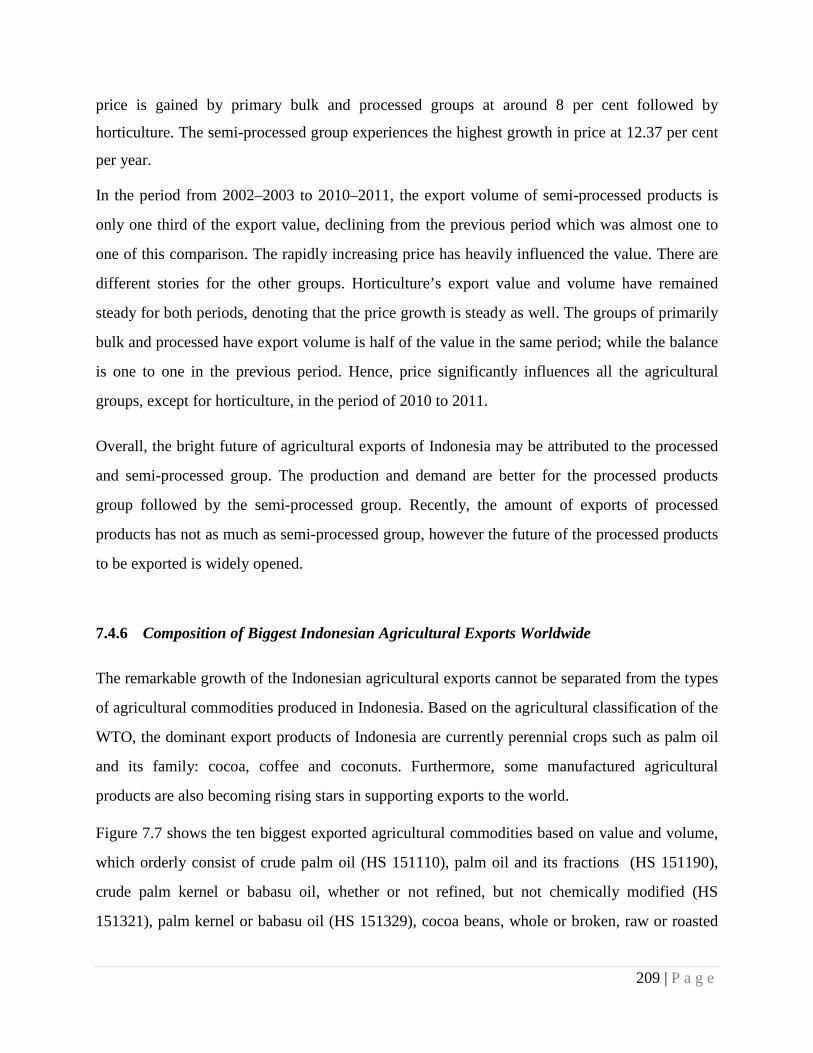
price is gained by primary bulk and processed groups at around 8 per cent followed by

horticulture. The semi-processed group experiences the highest growth in price at 12.37 per cent

per year.

In the period from 2002–2003 to 2010–2011, the export volume of semi-processed products is

only one third of the export value, declining from the previous period which was almost one to

one of this comparison. The rapidly increasing price has heavily influenced the value. There are

different stories for the other groups. Horticulture’s export value and volume have remained

steady for both periods, denoting that the price growth is steady as well. The groups of primarily

bulk and processed have export volume is half of the value in the same period; while the balance

is one to one in the previous period. Hence, price significantly influences all the agricultural

groups, except for horticulture, in the period of 2010 to 2011.

Overall, the bright future of agricultural exports of Indonesia may be attributed to the processed

and semi-processed group. The production and demand are better for the processed products

group followed by the semi-processed group. Recently, the amount of exports of processed

products has not as much as semi-processed group, however the future of the processed products

to be exported is widely opened.

7.4.6 Composition of Biggest Indonesian Agricultural Exports Worldwide

The remarkable growth of the Indonesian agricultural exports cannot be separated from the types

of agricultural commodities produced in Indonesia. Based on the agricultural classification of the

WTO, the dominant export products of Indonesia are currently perennial crops such as palm oil

and its family: cocoa, coffee and coconuts. Furthermore, some manufactured agricultural

products are also becoming rising stars in supporting exports to the world.

Figure 7.7 shows the ten biggest exported agricultural commodities based on value and volume,

which orderly consist of crude palm oil (HS 151110), palm oil and its fractions (HS 151190),

crude palm kernel or babasu oil, whether or not refined, but not chemically modified (HS

151321), palm kernel or babasu oil (HS 151329), cocoa beans, whole or broken, raw or roasted

209 | P a g e

(HS 180100), coffee, excluding roasted and decaffeinated (HS 090111), crude coconut (copra)

oil, whether or not refined but not chemically modified (HS 151311), cigarettes containing

tobacco (HS 240220), other industrial mono-carboxylic fatty acids and acid oil from refining (HS

382319) and edible mixtures or preparations of animal or vegetable fats or oils (HS 151790).

Figure 7.7 Value and Volume of Ten Biggest Indonesian Agricultural Exports Products Worldwide

Source: Tradedata (2013) (calculated by author)

Almost all of the biggest exported commodities are from the semi-processed group with only a

small number of representatives from the primary bulk group and processed group commodities.

There is no product from the horticultural group in the ten biggest exported products. With the

exception of coconut which is mostly produced for the domestic market, their production is

driven by external markets.

Palm oil products have dominated Indonesian agricultural exports. Crude palm oil (HS code

151110) and palm oil and its fractions (151190) have the biggest export value; far higher than

other commodities (see Figure 7.8). In terms of volume, three out of ten biggest agricultural

commodities have been standing out in exports after the 2000s onwards namely, crude palm oil

-

2,000

4,000

6,000

8,000

10,000

Jan-

93Ja

n-95

Jan-

97Ja

n-99

Jan-

01Ja

n-03

Jan-

05Ja

n-07

Jan-

09Ja

n-11

US$

mill

ion

Value

151110 151190 151321 180100

90111 151311 151329 240220

382319 151790

0.0500.0

1000.01500.02000.02500.03000.03500.0

Jan-

93

Jan-

95

Jan-

97

Jan-

99

Jan-

01

Jan-

03

Jan-

05

Jan-

07

Jan-

09

Jan-

11

US$

mill

ion

Volume

151110 151190 151321151329 180100 90111151311 382319 240220151790

210 | P a g e

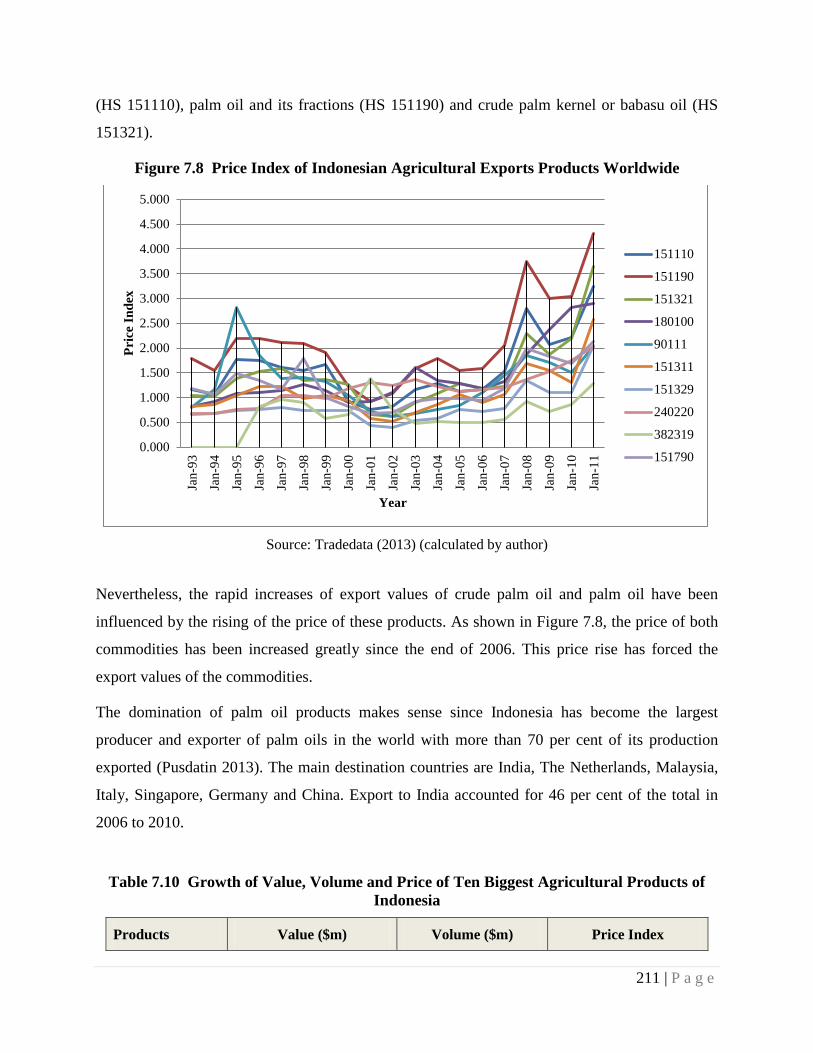
(HS 151110), palm oil and its fractions (HS 151190) and crude palm kernel or babasu oil (HS

151321).

Figure 7.8 Price Index of Indonesian Agricultural Exports Products Worldwide

Source: Tradedata (2013) (calculated by author)

Nevertheless, the rapid increases of export values of crude palm oil and palm oil have been

influenced by the rising of the price of these products. As shown in Figure 7.8, the price of both

commodities has been increased greatly since the end of 2006. This price rise has forced the

export values of the commodities.

The domination of palm oil products makes sense since Indonesia has become the largest

producer and exporter of palm oils in the world with more than 70 per cent of its production

exported (Pusdatin 2013). The main destination countries are India, The Netherlands, Malaysia,

Italy, Singapore, Germany and China. Export to India accounted for 46 per cent of the total in

2006 to 2010.

Table 7.10 Growth of Value, Volume and Price of Ten Biggest Agricultural Products of Indonesia

Products Value ($m) Volume ($m) Price Index

0.000

0.500

1.000

1.500

2.000

2.500

3.000

3.500

4.000

4.500

5.000Ja

n-93

Jan-

94

Jan-

95

Jan-

96

Jan-

97

Jan-

98

Jan-

99

Jan-

00

Jan-

01

Jan-

02

Jan-

03

Jan-

04

Jan-

05

Jan-

06

Jan-

07

Jan-

08

Jan-

09

Jan-

10

Jan-

11

Pric

e In

dex

Year

151110

151190

151321

180100

90111

151311

151329

240220

382319

151790

211 | P a g e

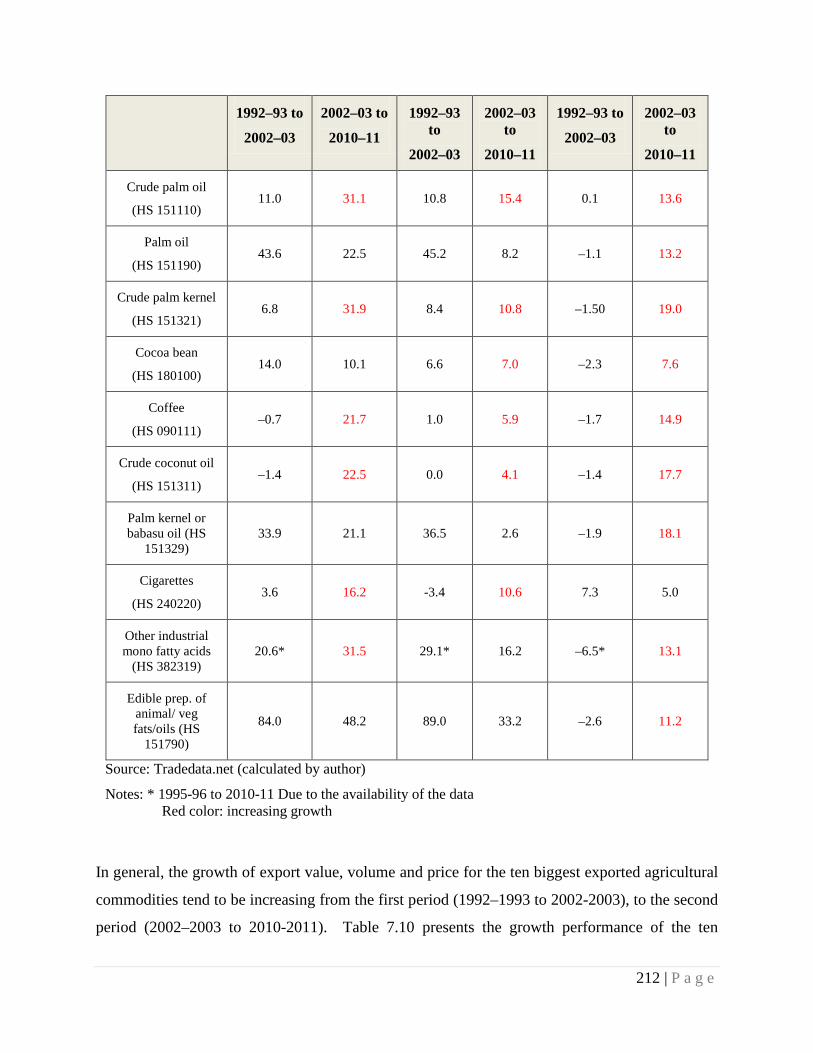
1992–93 to

2002–03

2002–03 to

2010–11

1992–93 to

2002–03

2002–03 to

2010–11

1992–93 to

2002–03

2002–03 to

2010–11

Crude palm oil

(HS 151110) 11.0 31.1 10.8 15.4 0.1 13.6

Palm oil

(HS 151190) 43.6 22.5 45.2 8.2 –1.1 13.2

Crude palm kernel

(HS 151321) 6.8 31.9 8.4 10.8 –1.50 19.0

Cocoa bean

(HS 180100) 14.0 10.1 6.6 7.0 –2.3 7.6

Coffee

(HS 090111) –0.7 21.7 1.0 5.9 –1.7 14.9

Crude coconut oil

(HS 151311) –1.4 22.5 0.0 4.1 –1.4 17.7

Palm kernel or babasu oil (HS

151329) 33.9 21.1 36.5 2.6 –1.9 18.1

Cigarettes

(HS 240220) 3.6 16.2 -3.4 10.6 7.3 5.0

Other industrial mono fatty acids

(HS 382319) 20.6* 31.5 29.1* 16.2 –6.5* 13.1

Edible prep. of animal/ veg fats/oils (HS

151790)

84.0 48.2 89.0 33.2 –2.6 11.2

Source: Tradedata.net (calculated by author)

Notes: * 1995-96 to 2010-11 Due to the availability of the data Red color: increasing growth

In general, the growth of export value, volume and price for the ten biggest exported agricultural

commodities tend to be increasing from the first period (1992–1993 to 2002-2003), to the second

period (2002–2003 to 2010-2011). Table 7.10 presents the growth performance of the ten

212 | P a g e

biggest commodities. Among these commodities that have strong volume growth inthe first

period, Palm oil (HS 151190), palm kernel or babasu oil (HS 151329), other industrial

monocarboxylic fatty acid ((HS 382319) and edible mixtures or preparations of animal or

vegetable fats or oils (HS 151790) have smaller growth rates of volume in the second period but

increasing price growth rates. This may indicate that the production of these commodities has not

addressedthe demand that caused the price to increase or the volume of exports are already high

in first period, thus the growth is slower, even though the amount is higher than the previous

period. Hence, the value of exports is mostly influenced by the increasing growth of its price.

Cocoa bean (HS 180100) has been declining in value, but increasing growth in volume and price.

This indicates that the production of cocoa has been expanding to meet the increasing demand.

Cigarettes containing tobacco (HS 240220) are the only product with declining growth of price

from first period to second period.

7.4.7 Commodities by Countries

Figure 7.9 shows the exports from Indonesian to five major export destinations for agricultural

groups for a period from 1992 to 2011. First, horticultural products are mainly exported to

ASEAN followed by India. The trend of horticultural exports to China is volatile and the volume

of export has been remained small. Japan and the USA are among the smallest market. Second,

different trends occur in the primary bulk group. The USA and ASEAN are the biggest export

markets for primary bulk products, followed by Japan. ASEAN has a positive trend that is

increasing while the United States has very low growth over the period after a significant

increase in 1995. China and India are the smallest export major destination for this group. Third,

India, ASEAN and China are superior export markets for semi-processed products with India as

the biggest market while the USA and Japan are inferior markets. Last, for processed products,

ASEAN is the biggest export market, followed by the USA and China. The export trends of

ASEAN and China are positive and increasing for this group. Meanwhile India and Japan are

smaller export markets for this product group and their export trends are flat.

Figure 7.9 Agricultural Groups Exports Volume by Countries

213 | P a g e

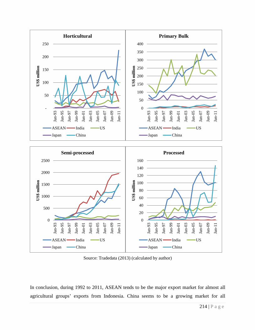
Source: Tradedata (2013) (calculated by author)

In conclusion, during 1992 to 2011, ASEAN tends to be the major export market for almost all

agricultural groups’ exports from Indonesia. China seems to be a growing market for all

-

50

100

150

200

250

Jan-

93

Jan-

95

Jan-

97

Jan-

99

Jan-

01

Jan-

03

Jan-

05

Jan-

07

Jan-

09

Jan-

11

US$

mill

ion

Horticultural

ASEAN India US

Japan China

0

50

100

150

200

250

300

350

400

Jan-

93

Jan-

95

Jan-

97

Jan-

99

Jan-

01

Jan-

03

Jan-

05

Jan-

07

Jan-

09

Jan-

11

US$

mill

ion

Primary Bulk

ASEAN India US

Japan China

0

500

1000

1500

2000

2500

Jan-

93

Jan-

95

Jan-

97

Jan-

99

Jan-

01

Jan-

03

Jan-

05

Jan-

07

Jan-

09

Jan-

11

US$

mill

ion

Semi-processed

ASEAN India US

Japan China

0

20

40

60

80

100

120

140

160

Jan-

93

Jan-

95

Jan-

97

Jan-

99

Jan-

01

Jan-

03

Jan-

05

Jan-

07

Jan-

09

Jan-

11

US$

mill

ion

Processed

ASEAN India US

Japan China

214 | P a g e

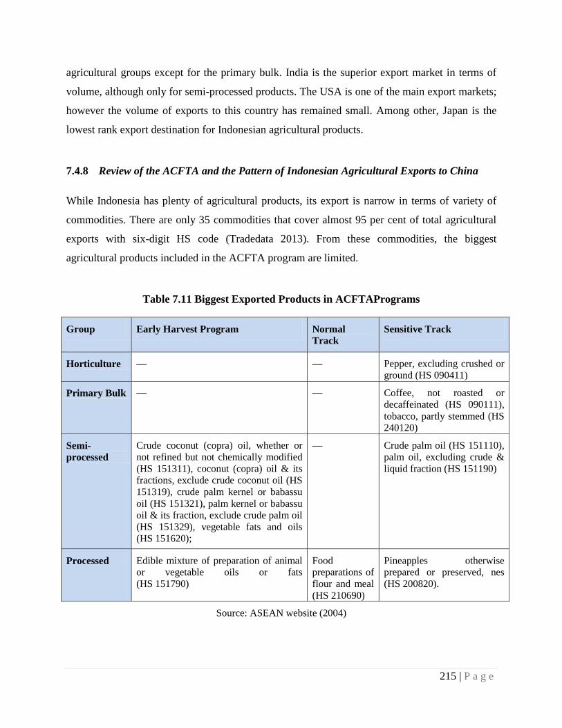
agricultural groups except for the primary bulk. India is the superior export market in terms of

volume, although only for semi-processed products. The USA is one of the main export markets;

however the volume of exports to this country has remained small. Among other, Japan is the

lowest rank export destination for Indonesian agricultural products.

7.4.8 Review of the ACFTA and the Pattern of Indonesian Agricultural Exports to China

While Indonesia has plenty of agricultural products, its export is narrow in terms of variety of

commodities. There are only 35 commodities that cover almost 95 per cent of total agricultural

exports with six-digit HS code (Tradedata 2013). From these commodities, the biggest

agricultural products included in the ACFTA program are limited.

Table 7.11 Biggest Exported Products in ACFTAPrograms

Group Early Harvest Program Normal Track

Sensitive Track

Horticulture — — Pepper, excluding crushed or ground (HS 090411)

Primary Bulk — — Coffee, not roasted or decaffeinated (HS 090111), tobacco, partly stemmed (HS 240120)

Semi-processed

Crude coconut (copra) oil, whether or not refined but not chemically modified (HS 151311), coconut (copra) oil & its fractions, exclude crude coconut oil (HS 151319), crude palm kernel or babassu oil (HS 151321), palm kernel or babassu oil & its fraction, exclude crude palm oil (HS 151329), vegetable fats and oils (HS 151620);

— Crude palm oil (HS 151110), palm oil, excluding crude & liquid fraction (HS 151190)

Processed Edible mixture of preparation of animal or vegetable oils or fats (HS 151790)

Food preparations of flour and meal (HS 210690)

Pineapples otherwise prepared or preserved, nes (HS 200820).

Source: ASEAN website (2004)

215 | P a g e

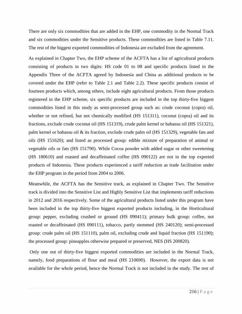
There are only six commodities that are added in the EHP, one commodity in the Normal Track

and six commodities under the Sensitive products. These commodities are listed in Table 7.11.

The rest of the biggest exported commodities of Indonesia are excluded from the agreement.

As explained in Chapter Two, the EHP scheme of the ACFTA has a list of agricultural products

consisting of products in two digits: HS code 01 to 08 and specific products listed in the

Appendix Three of the ACFTA agreed by Indonesia and China as additional products to be

covered under the EHP (refer to Table 2.1 and Table 2.2). These specific products consist of

fourteen products which, among others, include eight agricultural products. From those products

registered in the EHP scheme, six specific products are included in the top thirty-five biggest

commodities listed in this study as semi-processed group such as: crude coconut (copra) oil,

whether or not refined, but not chemically modified (HS 151311), coconut (copra) oil and its

fractions, exclude crude coconut oil (HS 151319), crude palm kernel or babassu oil (HS 151321),

palm kernel or babassu oil & its fraction, exclude crude palm oil (HS 151329), vegetable fats and

oils (HS 151620); and listed as processed group: edible mixture of preparation of animal or

vegetable oils or fats (HS 151790). While Cocoa powder with added sugar or other sweetening

(HS 180610) and roasted and decaffeinated coffee (HS 090122) are not in the top exported

products of Indonesia. These products experienced a tariff reduction as trade facilitation under

the EHP program in the period from 2004 to 2006.

Meanwhile, the ACFTA has the Sensitive track, as explained in Chapter Two. The Sensitive

track is divided into the Sensitive List and Highly Sensitive List that implements tariff reductions

in 2012 and 2016 respectively. Some of the agricultural products listed under this program have

been included in the top thirty-five biggest exported products including, in the Horticultural

group: pepper, excluding crushed or ground (HS 090411); primary bulk group: coffee, not

roasted or decaffeinated (HS 090111), tobacco, partly stemmed (HS 240120); semi-processed

group: crude palm oil (HS 151110), palm oil, excluding crude and liquid fraction (HS 151190);

the processed group: pineapples otherwise prepared or preserved, NES (HS 200820).

Only one out of thirty-five biggest exported commodities are included in the Normal Track,

namely, food preparations of flour and meal (HS 210690). However, the export data is not

available for the whole period, hence the Normal Track is not included in the study. The rest of

216 | P a g e

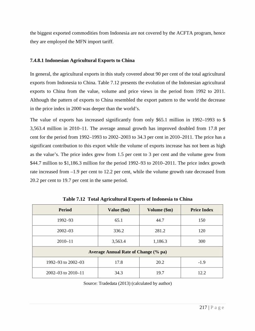
the biggest exported commodities from Indonesia are not covered by the ACFTA program, hence

they are employed the MFN import tariff.

7.4.8.1 Indonesian Agricultural Exports to China

In general, the agricultural exports in this study covered about 90 per cent of the total agricultural

exports from Indonesia to China. Table 7.12 presents the evolution of the Indonesian agricultural

exports to China from the value, volume and price views in the period from 1992 to 2011.

Although the pattern of exports to China resembled the export pattern to the world the decrease

in the price index in 2000 was deeper than the world’s.

The value of exports has increased significantly from only $65.1 million in 1992–1993 to $

3,563.4 million in 2010–11. The average annual growth has improved doubled from 17.8 per

cent for the period from 1992–1993 to 2002–2003 to 34.3 per cent in 2010–2011. The price has a

significant contribution to this export while the volume of exports increase has not been as high

as the value’s. The price index grew from 1.5 per cent to 3 per cent and the volume grew from

$44.7 million to $1,186.3 million for the period 1992–93 to 2010–2011. The price index growth

rate increased from –1.9 per cent to 12.2 per cent, while the volume growth rate decreased from

20.2 per cent to 19.7 per cent in the same period.

Table 7.12 Total Agricultural Exports of Indonesia to China

Period Value ($m) Volume ($m) Price Index

1992–93 65.1 44.7 150

2002–03 336.2 281.2 120

2010–11 3,563.4 1,186.3 300

Average Annual Rate of Change (% pa)

1992–93 to 2002–03 17.8 20.2 -1.9

2002–03 to 2010–11 34.3 19.7 12.2

Source: Tradedata (2013) (calculated by author)

217 | P a g e

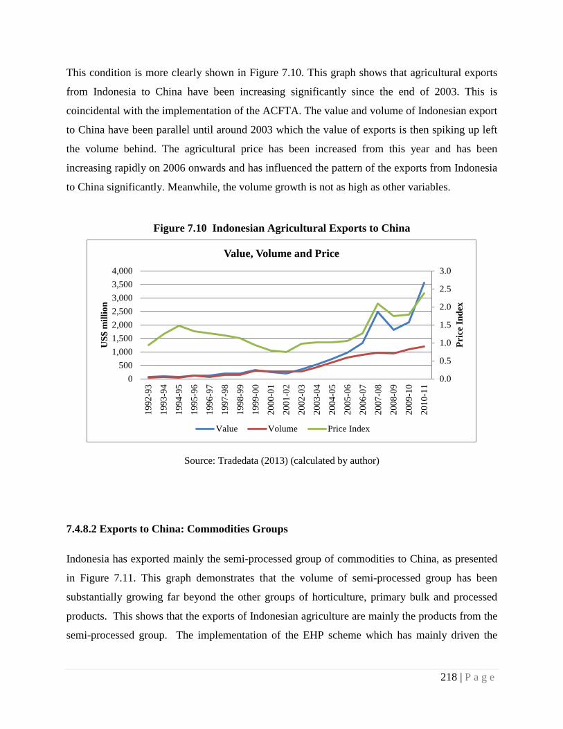
This condition is more clearly shown in Figure 7.10. This graph shows that agricultural exports

from Indonesia to China have been increasing significantly since the end of 2003. This is

coincidental with the implementation of the ACFTA. The value and volume of Indonesian export

to China have been parallel until around 2003 which the value of exports is then spiking up left

the volume behind. The agricultural price has been increased from this year and has been

increasing rapidly on 2006 onwards and has influenced the pattern of the exports from Indonesia

to China significantly. Meanwhile, the volume growth is not as high as other variables.

Figure 7.10 Indonesian Agricultural Exports to China

Source: Tradedata (2013) (calculated by author)

7.4.8.2 Exports to China: Commodities Groups

Indonesia has exported mainly the semi-processed group of commodities to China, as presented

in Figure 7.11. This graph demonstrates that the volume of semi-processed group has been

substantially growing far beyond the other groups of horticulture, primary bulk and processed

products. This shows that the exports of Indonesian agriculture are mainly the products from the

semi-processed group. The implementation of the EHP scheme which has mainly driven the

0.0

0.5

1.0

1.5

2.0

2.5

3.0

0500

1,0001,5002,0002,5003,0003,5004,000

1992

-93

1993

-94

1994

-95

1995

-96

1996

-97

1997

-98

1998

-99

1999

-00

2000

-01

2001

-02

2002

-03

2003

-04

2004

-05

2005

-06

2006

-07

2007

-08

2008

-09

2009

-10

2010

-11

Pric

e In

dex

US$

mill

ion

Value, Volume and Price

Value Volume Price Index

218 | P a g e

trade of the agricultural products under the HS code 01-08 seems to have no success in

improving Indonesian exports of these products.

However, there are five commodities of semi-processed groups under the EHP scheme. Since the

volume of semi-processed group has grown higher than other groups, there is possibility that the

semi-processed commodities under the EHP have also driven this growth. Thus a more detailed

examination of the semi-processed commodity needs to be undertaken.

Figure 7.11 Exports to China by Volume of Commodities Groups

Source: Tradedata (2013) (calculated by author)

A more detailed description of the agricultural groups’ exports phenomenon is displayed in

Table 7.13. This table presents the value, volume and price of the horticulture, primary bulk,

semi-processed and processed groups for three different periods: 1992 to 1993, 2002 to 2003 and

2010 to 2011. It also presents the growth of these variables for two periods: 1992–2003 to 2002-

03, and 2002–2003 to 2010–2011. The latter might also capture the influence of the ACFTA,

since this agreement was signed in 2002.

Table 7.13 shows that, in terms of exports value and volume, all groups have been growing in

from the period from 1992–1993 to 2010–2011. However, the smallest value and volume of

- 200.0 400.0 600.0 800.0

1,000.0 1,200.0 1,400.0 1,600.0 1,800.0

Jan-

93

Jan-

94

Jan-

95

Jan-

96

Jan-

97

Jan-

98

Jan-

99

Jan-

00

Jan-

01

Jan-

02

Jan-

03

Jan-

04

Jan-

05

Jan-

06

Jan-

07

Jan-

08

Jan-

09

Jan-

10

Jan-

11

Jan-

12

US$

mill

ion

horticulture primary semi-processed processed

219 | P a g e

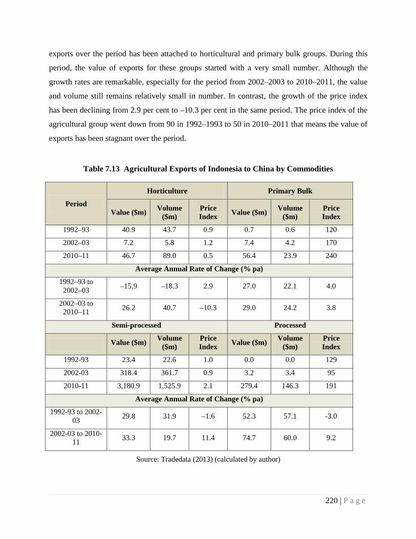
exports over the period has been attached to horticultural and primary bulk groups. During this

period, the value of exports for these groups started with a very small number. Although the

growth rates are remarkable, especially for the period from 2002–2003 to 2010–2011, the value

and volume still remains relatively small in number. In contrast, the growth of the price index

has been declining from 2.9 per cent to –10.3 per cent in the same period. The price index of the

agricultural group went down from 90 in 1992–1993 to 50 in 2010–2011 that means the value of

exports has been stagnant over the period.

Table 7.13 Agricultural Exports of Indonesia to China by Commodities

Period

Horticulture Primary Bulk

Value ($m) Volume ($m)

Price Index Value ($m) Volume

($m) Price Index

1992–93 40.9 43.7 0.9 0.7 0.6 120

2002–03 7.2 5.8 1.2 7.4 4.2 170

2010–11 46.7 89.0 0.5 56.4 23.9 240

Average Annual Rate of Change (% pa)

1992–93 to 2002–03 –15.9 –18.3 2.9 27.0 22.1 4.0

2002–03 to 2010–11 26.2 40.7 –10.3 29.0 24.2 3.8

Semi-processed Processed

Value ($m) Volume ($m)

Price Index Value ($m) Volume

($m) Price Index

1992-93 23.4 22.6 1.0 0.0 0.0 129

2002-03 318.4 361.7 0.9 3.2 3.4 95

2010-11 3,180.9 1,525.9 2.1 279.4 146.3 191

Average Annual Rate of Change (% pa)

1992-93 to 2002-03 29.8 31.9 –1.6 52.3 57.1 -3.0

2002-03 to 2010-11 33.3 19.7 11.4 74.7 60.0 9.2

Source: Tradedata (2013) (calculated by author)

220 | P a g e

The substantial growth of value, volume and price are experienced by the processed group

exports. The processed product group has been growing from a very low base. Although the

number is small, the growth of value and volume reached 52.3 per cent and 57.1 per cent in the

period 1992–1993 to 2002–2003 and jumped to 74.7 per cent and 60 per cent in the period from

2002–2003 to 2010–2011. Furthermore, the price index for this group has been growing

significantly, especially in the recent period, to about 9.2 per cent.

There were different conditions for semi-processed group exports. Their value and volume

significantly increased from $40.9 million and $43.7 million in 1992–93 to $3,563 million and

$1,525.9 million in 2010–2011. The growth of value was remarkable with 29.8 per cent in the

first period and 33.3 per cent for the latter period. However, the growth of volume has been

declining from 31.9 per cent to 19.7 per cent in the same period. In contrast, the growth of price

index has been expanded substantially by 11.4 per cent in the period of 2002–2003 to 2010–

2011. The pattern and number of the value, volume and price of this group looks similar to the

pattern of the general agricultural exports from Indonesia to China, as shown in Table 7.1. It

seems that general agricultural exports are heavily influenced by the exports from the semi-

processed group.

The increasing volume and price, especially in the period from 2002–2003 to 2010–2011, has

substantially influenced the value of exports. The exception is for the horticultural group which

has been declining in its price index, which then influenced the value of the exports, although the

volume had remarkable growth by more than 40 per cent in the recent period. This is important

to note that the commodities included in the Horticultural group are mostly the core commodities

under the EHP programs of the ACFTA which is intended to be improved. However the trade

facility of the EHP has not been able to increase the export significantly, as found in the previous

chapter. The explanation in this section supports the results from the previous chapters.

From this explanation, it is clear that the Indonesian agricultural exports to China have been

growing significantly for the most of groups of commodities. From the first period, 1992–1993

to 2002–2003, to the second period, 2002–2003 to 2010–2011, the volume of exports grew for

horticulture, primary bulk and processed groups but declining for the semi-processed group.

Although the semi processed group has the highest amount. For the same periods, the price

221 | P a g e

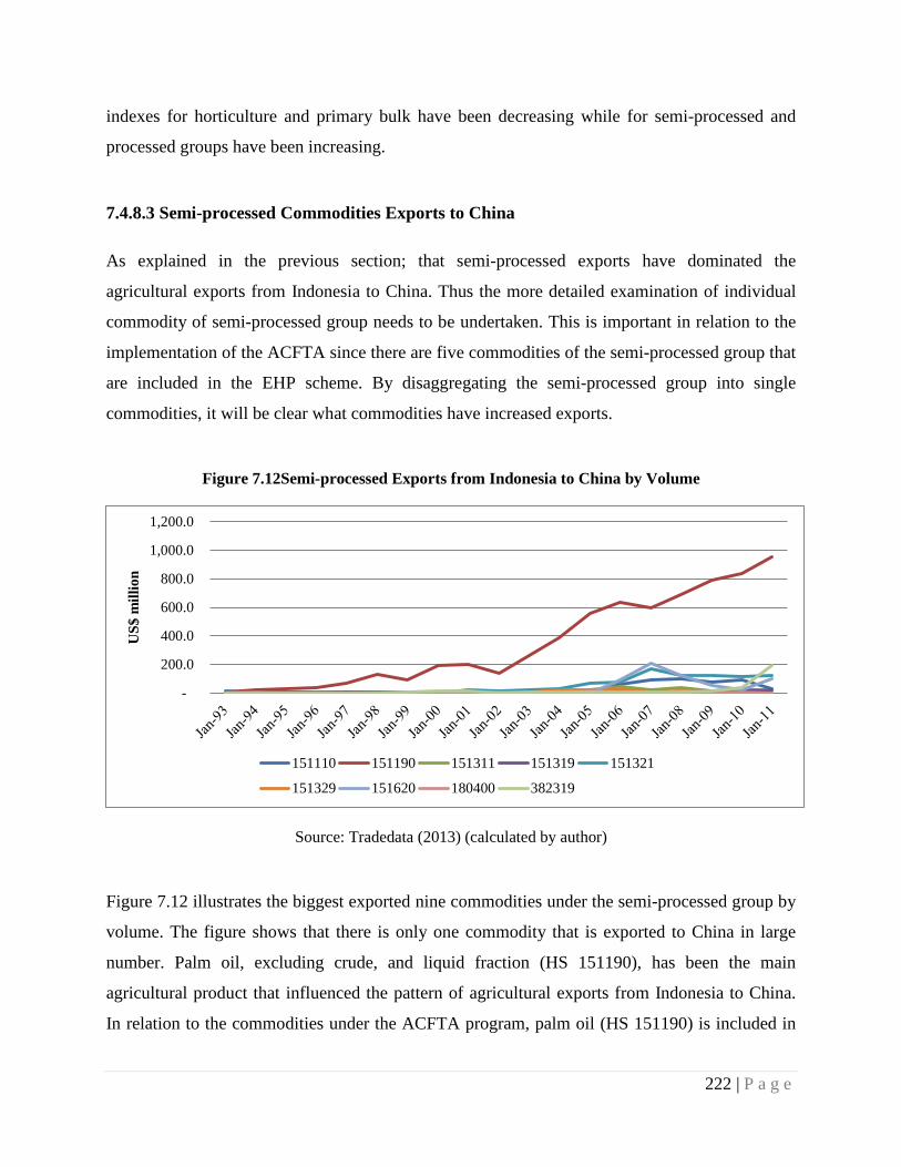
indexes for horticulture and primary bulk have been decreasing while for semi-processed and

processed groups have been increasing.

7.4.8.3 Semi-processed Commodities Exports to China

As explained in the previous section; that semi-processed exports have dominated the

agricultural exports from Indonesia to China. Thus the more detailed examination of individual

commodity of semi-processed group needs to be undertaken. This is important in relation to the

implementation of the ACFTA since there are five commodities of the semi-processed group that

are included in the EHP scheme. By disaggregating the semi-processed group into single

commodities, it will be clear what commodities have increased exports.

Figure 7.12Semi-processed Exports from Indonesia to China by Volume

Source: Tradedata (2013) (calculated by author)

Figure 7.12 illustrates the biggest exported nine commodities under the semi-processed group by

volume. The figure shows that there is only one commodity that is exported to China in large

number. Palm oil, excluding crude, and liquid fraction (HS 151190), has been the main

agricultural product that influenced the pattern of agricultural exports from Indonesia to China.

In relation to the commodities under the ACFTA program, palm oil (HS 151190) is included in

-

200.0

400.0

600.0

800.0

1,000.0

1,200.0

US$

mill

ion

151110 151190 151311 151319 151321

151329 151620 180400 382319

222 | P a g e

the Sensitive Track that has not yet been treated with trade facilitation in the period of study. On

the other hand, other commodities under the EHP scheme tend to have become stagnant. These

findings support the results of the impact of the ACFTA as explained in previous chapters.

7.5 Conclusion

This chapter provides an analytical description about the agricultural exports of Indonesia. From

the explanation in the previous sections, it can be concluded that, in general, Indonesian

agricultural exports have been increasing in the period from 1992 to 2011. The application of the

volume chain-link method to explore the real value of Indonesian exports has separated the

export value from the influence of price. Hence, it can be examined that mostly agricultural

export volume and price have been increasing.

Furthermore, it can also be concluded that more than 50 per cent of the Indonesian agricultural

exports are only exported to the three biggest countries: India, ASEAN and China. Indonesia

tends to lose its market share in the USA and Japan as the growth of exports to these countries

are sluggish and the amount of volume and value remained small and stagnant over the period.

In terms of the agricultural group exports, Indonesian exporthas been dominated by the semi-

processed group. Furthermore, the varieties of superior export commodities are limited to

vegetable oils, especially the groups of palm oils, which are included in the semi-processed

group. Indonesian exports are mainly supported by palm oils in terms of volume and value.

Hence, the increase of Indonesian agricultural exports has been heavily influenced by these

commodities, especially crude palm oil (HS 151110) and palm oil and its fraction (HS151190).

Although other agricultural groups have only small value and volume of exports to China, their

growth are very strong. As the export volumes start, on average, at a very low base, the export

volumes of these groups are still overshadowed by the semi-processed commodities. Considering

their high growth, there is a potential benefit to develop their exports to China that can be gained

by Indonesian government.

Nonetheless, the high growth in the exports seemed to have a little influence of the ACFTA. It

can be shown by the fact that the EHP, as part of the ACFTA program, that was created to boost

agricultural trade, does not cover the palm oil products of the crude palm oil (HS 151110) and

223 | P a g e

palm oil and its fraction (HS151190). The increasing exports mainly dominated by these, both

products that have no trade facilitation yet in the ACFTA. In contrast, the EHP has only included

products with very small contributions to exports. The narrow range of products for exports and

low coverage of the EHP on superior agricultural products of Indonesia supports the empirical

findings of ACFTA that was examined in previous chapters.

224 | P a g e

Chapter 8

Conclusion and Policy Implication

8.1 Chapter Aims and Description

This study has examined the potential for economic growth of agricultural exports from

Indonesia to China, especially those under ACFTA. Specifically, this study questions whether

agricultural exports still have an important impact on economic growth of Indonesia as well as

the impacts of the effort of joining the ACFTA on the agricultural exports. There are five

objectives for this research:

1. To empirically investigate the impacts of agricultural exports and the ACFTA programs on

Indonesian economic growth by using rigorous methodology;

2. To investigate the impact of the ACFTA programs for Indonesian agricultural export

growth;

3. To examine the competitiveness of agricultural export commodities under the ACFTA;

4. To overview the condition of Indonesian agricultural exports from the volume and price

perspective; and

5. To learn the policy implication of the implementation of the ACFTA. Mostly, the objectives

are examined in every different chapter due to different methodologies used to exercise

theirs.

This final chapter provides summary of the research and policy implications developed in this

thesis. The chapters in this thesis are divided into two parts: the first three chapters reviewed the

literature and policy background concerning agricultural position in development and growth and

trade liberalization in the agricultural sector. The other part consists of empirical studies

concerning the agricultural exports of Indonesia under the auspices of the ASEAN-China Free

Trade Agreement (ACFTA). Chapter Four examines the impact of Indonesian agricultural

exports to China on the economic growth of Indonesia. The impacts of the ACFTA programs on

related agricultural commodities exported from Indonesia to China are discussed in Chapter Five

for the growth of exports and Chapter Six for the competitiveness of the agricultural products.

225 | P a g e

Chapter Seven is dedicated to study in price and volume perspective on Indonesian agricultural

exports.

8.2 Research Summary

8.2.1 Background of Agricultural Trade Development

After being abandoned for decades because its importance in economics and development was

overshadowed by the importance of the industrialized sector, the agricultural sector has been

given renewed attention as a key to growth in many countries. The resurgence of the agricultural

sector sheds light on the importance of improving this sector to meet its many functions; from

providing food for the increasing population, poverty reduction, increasing economic growth and

addressing environmental sustainability and climate change issues.

Chapter Two provides an overview of the agricultural sector revival; that the importance of the

agricultural sector has been given attention in the position of development and in trade

liberalization. This chapter also discusses the ACFTA. This provides an explanation of the

background for this study and the rationale for this study. One of the ways to improve the

agricultural sector is trade liberalization. The initial effort for agricultural liberalization is the

establishment of the Uruguay Round Agreement on Agriculture (URAA); however, many

developing countries are unsatisfied with the progress of this agreement (Hathaway & Ingco

1995). As a result, they establish free trade agreements among themselves. The ACFTA is a free

trade agreement that has a special program focusing on agricultural trade, namely, the Early

Harvest Program (EHP) as well as other programs: the Normal Track and the Sensitive Track.

There is a huge literature studied on the ACFTA but only a limited number of them discuss the

agricultural trade in relation to the programs of the ACFTA. This study, therefore, attempts to

add to the literature in this area.

Chapter Three provides an overview of the Indonesian agricultural sector. Indonesia is a country

with a strong agricultural base with agricultural exports in the third position of their foreign

exchange earnings (Pusdatin 2013). Furthermore, the importance of agricultural trade is shown

226 | P a g e

by the increasing of the total value of trade and its growing share in merchandise trade of

Indonesia.

Based on export value, in 2011 Indonesia was the third biggest agricultural exporter in the world

after the United States and Malaysia (FAOSTAT 2013), improving from number eleven in 2004.

Although Indonesia is well-known as one of the biggest agricultural exported country in the

world, its export is quite narrow in terms of variety of commodities and export destinations. The

main agricultural commodity exported from Indonesia is palm oil with its value $17,261,248 in

2011, having increased from $3,441,776 in 2004. This commodity has primarily been exported

to new growing markets, including ASEAN countries, India and China. On the other hand,

exporting this commodity to traditional agricultural markets such as USA, EU, Japan has not

expanded.

To improve its exports, Indonesia has made many efforts, including joining many free trade

agreements. The ASEAN-China Free Trade Agreement (ACFTA) is one of the agreements

Indonesia has signed. It has been expected that this agreement will increase Indonesian exports,

especially the agricultural ones, to China. ACFTA has a special program to encourage

agricultural trade among members, named the Early Harvest program (EHP) that started in 2004.

Considering China is a prospectively big market with its huge population and a growing

economy, it is envisaged that Indonesia will gain benefit by increasing its exports to China in

spite of competition with other ASEAN countries that has similar exports.

The influence of the ACFTA can be shown by the movement of the trade between Indonesia and

China. The total trade balance between Indonesia and China is a deficitin Indonesia. This deficit

became bigger during 2000 to 2012 (UNComtrade 2013). In contrast, the trade balance for

agricultural commodities has been positive for Indonesia since 2005; yet the positive balance for

Indonesia has been getting wider until recently. This indicates that agricultural exports are an

important sector in Indonesia and there is an opportunity to increase economic growth from this

sector.

8.2.2 Empirical Studies Reviews

With respect to this endeavour to improve agricultural exports, it is foreseeable that this sector is

projected to contribute more to the economy of Indonesia. The first objective of this study was to

227 | P a g e

measure the influence of Indonesian agricultural exports to China and the implementation of the

ACFTA on Indonesian economic growth. This objective is examined in Chapter Four of this

thesis. In addition, this chapter also focuses on the effect of the global financial crisis on

Indonesian economic growth. The generalized gravity theory is employed to address this

objective. Considering the causality relationship between economic growth and exports, this

model employs the instrumental variables technique with two-stage least Squares (2SLS)

estimation to address this problem. The exercise of the requirements for instrumental variables

model found that there is no causality for the Indonesian economic growth-agricultural export

model. Furthermore, the model is estimated by employing the OLS estimation. The model

reliability is well as tested by employing the Friedman-Kydland criterion of data-model

consistency (Kydland 2006).

The export-led growth theory postulates that exports can be an engine for economic growth;

However, the findings show that Indonesian agricultural exports to China does not have any

influence on the economic growth of Indonesia at 10 per cent significance level. Although

agricultural exports to China have been increasing, their effect has not been strong enough to lift

the economy of Indonesia. The agricultural exports has small portion in the overall Indonesian

export compare to other sectors such as oil and mining and industries sectors. Even though the

agricultural exports have been increasing, the pace of growth is not as higher as the other sectors.

The agricultural exports’ share has been declining in the GDP while the other sectors have been

increasing. This finding is consistent with previous research that showagricultural exports have

no impact on economic growth(Doppelhofer, Miller & Sala-i-Martin 2000; Esfahani 1991; Sala-

i-Martin 1997) or negative impacts (Faridi 2012) of agricultural exports on economic growth.

In contrast, the implementation of the ACFTA has a positive and significant impact on

Indonesian economic growth at 5 per cent. This is consistent with the theory that free trade areas

are able to increase welfare of a country and voluminous literature supports this finding. The

trade integration with China has beneficial impacts for Indonesia as the export market has been

broadened. The implementation of trade facilities and tariff reduction gave Indonesian exports

more bargaining power in China’s market. This is demonstrated by increasing exports to China.

ACFTA implementation is not only for the agricultural sector, but for broader sectors such as

228 | P a g e

services and investment, hence the contribution of the ACFTA on the economic growth of

Indonesia may come from all of these sectors (Fukunaga & Ishido 2013; Xiao 2010).

The literature claims that crises, shocks and major policy reforms can be sources for fluctuations

in economic growth (Johansen, L 1982). However, the empirical result shows the occurrence of

the global financial crisis in 2007 had no significant impact on Indonesian economic growth at

10 per cent level. This finding is consistent with previous literature (Basri, M.C. 2010). It means

that the Indonesian economy is robust from the global financial crisis that mainly worsened the

economies in developed countries (Reinhart & Rogoff 2009).

Even though agricultural exports to China did not successfully improve the economic growth of

Indonesia, greatest increase and the movement from a deficit to a surplus trade balance after the

implementation of the ACFTA has made it worthwhile to examine whether the ACFTA has

contributed to this phenomenon or not. This, therefore, is the second objective of this study.

Chapter Five presented an examination of the ACFTA programs, especially the EHP and SL and

their relation to the related agricultural commodities exported from Indonesia to China. The

Autoregressive Distributed Lag (ARDL) approach has been implemented on import demand

models of EHP and SL. The findings show that co-integration exists for both models of EHP and

SL, thus the short-run and long-run impacts can be measured.

Tariff reductions as a trade facility of the EHP program ran from 2004 to 2006. Agricultural

commodities under this program were reduced to a zero percent tariff in 2006. However, based

on the empirical findings of this study, the tariff reduction as a signature project of the EHP had

no significant influence on the EHP agricultural products for both short-run and long-run. This

contradicts the theory that tariff reduction will improve trade. However, it can be shown that

agricultural commodities under the EHP program are not the key commodities from Indonesia.

Indonesia is not a strong producer of these commodities and the volume of exports is relatively

small. In contrary, China has a strong comparative advantageof these products, especially for

agricultural commodities under HS code 01-08 thus the tariff reduction has no implication in

increasing imports for these products.

Meanwhile, the MFN tariff rates are employed for the SL agricultural products. The implication

of MFN tariff reduction has been measured in the export growth of the SL agricultural

229 | P a g e

commodities as the exports of these products to China are growing fast. The empirical findings

show that the MFN tariff reduction has no significant effect on export growth for these products

in the long-run but has a negative and significant impact in short-run. This finding is to be

expected as the tariff reduction as trade facility under the ACFTA will be implemented in 2012

and 2016 for the Sensitive Track agricultural commodities.

Furthermore, the empirical results reveal that the implementation of the other regulation of the

ACFTA in the long - run has positive and significant impacts of the EHP agricultural products

but negative and significant impacts in short-run. This reflects the adjustment of the exporters in

Indonesia to follow new regulations under the ACFTA program which will bring positive

improvement in the long-term. The implementation of the ACFTA has no significant impacts on

the SL agricultural products for both short-run and long-run.

This can be explained that the main agricultural commodities exported from Indonesia, such as

palm oils and other vegetable oil products, are included in the list of China’s ‘national strategic

products’. This list consists of high demand products which China has no comparative advantage

in. China has a trade policy to employ strong protection for these products by implementing a

high import tariff or placing these commodities in the Sensitive Track of the ACFTA, thus the

tariff implemented for these commodities are very high which is unfavorable for Indonesian

exports to China. As agreed by both Indonesia and China, the Sensitive Track will get an import

tariff reduction starting in 2012 from the Sensitive List and 2016 for the Highly Sensitive List.

Hence, it is expected that the impacts of the ACFTA will be greater once the tariff has been

reduced for these commodities under the Sensitive Track.

The other reason for this is that most of the agricultural products listed in the EHP scheme are

not main products of Indonesia, especially for the products under HS code 01 until 08.

Furthermore, Indonesia tends to be importers of these products. Although Indonesia has many

exports in HS 03 (fish products) to other traditional export destinations, such as the USA, the

exports to China has been relatively small. Fortunately, due to further negotiation between

Indonesia and China, eight other commodities have been incorporated into the EHP scheme. In

this study, these eight commodities are grouped as three big commodities, based on HS codes.

These three groups, commodities reveal different responses for the tariff reduction under the

230 | P a g e

EHP scheme. This outcome can be shown in the examination of competitiveness for every single

commodity under this scheme.

Chapter Six was dedicated to the analysis of the impact of the ACFTA programs, the EHP and

Sensitive Tracks on the competitiveness of selected agricultural commodities. This chapter

explored more closely the competitiveness represented by the Trade Intensity Index (TII), the

Dynamic Revealed Comparative Advantage (DRCA), and Market Share Index for selected

agricultural products under the EHP and SL programs. The EHP scheme was represented by

agricultural commodities under HS code 01-08 and products related to vegetable oils and fats

(HS 1513, HS 151620, HS 151790); while the SL scheme will be represented by HS 200820

(processed pineapples), HS 151110 (crude palm oil) and HS 151190 (palm oil).

The results reveal that for the EHP products, there are only vegetable oils (HS 1513, HS 151620,

HS 151790) that are competitive in China’s market after the implementation of the ACFTA;

while for the most of the other products covered by the EHP, the agricultural products under HS

01-08, have very low level of competitiveness in terms of TII, DRCA and market share index.

The EHP has only done little to improve exports of the latter products.

Meanwhile, the Sensitive Track products have a very high level of competitiveness in China’s

market despite the fact there is no tariff reduction for them. Whereas their market share in China

has already high, it might be expected to increase further with tariff reductions from 2012, if

supply capacity is available in Indonesia.

While previous empirical studies use aggregate export data, a more detailed analysis ofexport

commodities was presented in Chapter Seven. The objective of this chapter was to calculate for

the first time chain-linked volume and price index measures for the thirty-five biggest

agricultural commodities that cover more than 90 per cent of the whole agricultural exports from

Indonesia. The benefit of these measures is free from the bias of price fluctuation so that the

examination of the agricultural export condition can be more objective.

By implementing chain-linked volume and chain-linked price index methods (ABS 1998), the

real value that is represented by the chain-linked volume and price index of the agricultural

exports was obtained. The findings reveal that the price and volume of Indonesian agricultural

exports have grown strongly since 2001. It also revealed that the price of the agricultural

231 | P a g e

products has been spiking since the end of 2006, outpacing the volume of exports. It indicates the

production of the agricultural products has not been as high as demand; therefore, the price has

been increasing rapidly. The high demand for agricultural products as sources for bio-fuels

production has forced the prices rise. The diversion of grain from food to bio-fuels or the land

conversion away from food when induced by distorting policies have meant food prices may

rise. Attention has been put on this condition by governments and also world organizations in

order to maintain food security globally.

The expanding agricultural exports are dominated by semi-processed products, mainly palm oils,

which are primarily going to the new growing agricultural export markets such as ASEAN,

China and India. The shares of exports to these countries have been magnified significantly

compared to the traditional agricultural export market such as the USA, Japan and the European

Union that tend to decline over time. This analysis reveals a narrow basis for Indonesia’s

agricultural exports, with limited exports to other markets in products other than palm oil

products. This narrow base may be part of the reason for variable results in the modelling

studies.

8.3 Policy Implication

While the issues are complex and the empirical results are mixed, agricultural exports facilitated

by free trade agreements have the potential to contribute to Indonesia’s growth. From the results

of the study, it is found that Indonesia in recent decades had strong growth in volume and price

and this opportunity should be focused on by the Indonesian Government to improve its

contribution to economy of Indonesia.

However, this good growth has not entirely reflected the role of the free trade agreement. In

comparison, between exports to India, China and ASEAN, the exports to India has the strongest

growth and biggest quantity despite not having a free trade agreement between Indonesia and

India in the period focused on. In the case of the ACFTA, there is no significant product that is

important for Indonesia covered by the early programs of the ACFTA such as the EHP and the

Normal track.

Since Indonesia’s agricultural export base is very narrow, and attention needs to be given to

building a more competitive base outside of palm oil, in part by initiatives on the supply side.

232 | P a g e

Indonesia needs to enhance the capacity of production for the agricultural products under the

EHP scheme as China seems to get more benefits from this agreement because the actual

production level in China is much higher than that in Indonesian.

Furthermore, the study shows that the other agricultural commodities have been fast growing

with very strong growth such as the processed group products. However, they started from a very

low amount. This should be paid attention to as it becomes a potential source of exports. There

should be greater diversity of products for exports, considering its potential growth, even if the

amount is low.

For the same reason ACFTA has had a limited impact on Indonesia’s exports to Chinaso far,

because Indonesia has low competitiveness in most of the product areas covered. But this will

change as tariffs are reduced to commodities covered by the Sensitive List, many of which

Indonesia has strong export potential.

To enhance the competitiveness of agricultural commodities, the government should ensure all

agricultural commodities are sustainable, as ruled by the trade partners and international

agreement, since the awareness of the environmental sustainability has been increasing in the

recent years. As such, the European countries and USA have raised concern in recent years that

palm oil plantations have destroyed Indonesian forests as well as created high greenhouse gas

emissions, which have negatively affected Indonesian exports of crude palm oil.

The competition for exports from other ASEAN countries that produce similar products should

also be considered, thus actions are needed to be taken by the Indonesian Government and

farmers to respond to this condition and to compete. Proper support from the government for the

farmers should also be provided in financial and technology sectors so that they can improve

their competence in productivity and quality of the commodities.

Summarizing the study, it is suggested when negotiating for future free trade agreement, the

Indonesian Government should consider the strong and superior products of Indonesia to be

included in the agreement, since they will provide a more significant contributionto the

economy. Also, a re-negotiation of the commodities included in the ACFTA might be considered

as this agreement seems to be negative for Indonesia.

233 | P a g e

8.4 Limitation of the Research and Recommendations for Future Research

The elaborate study on the impact of the ACFTA programs focused on specific sectors and

specific countries have been hard to find, hence this study contributes important evidence in the

literature. Although the findings from this study provide substantial findings about agricultural

exports from Indonesia to China under ACFTA, there are several limitations of this study that

provide opportunities to extend this study for further investigation in the future.

First, the availability of the data has limited the scope of this thesis. Throughout this thesis, the

examined periods were varied because of adjustments to the data availability of the variables

used in this study. The shortage of the data period has also given limited options to explore the

data for further analysis using different analysis technique to achieve reliable results.

The limitation of the data has also meant the type of data used in this study was varied. The use

of data on the same platform creates coherent and synchronized results, thus avoiding biased

results. The shortcoming of the data has also meant the study’s scope was limited.

Second, this study has only focused on the agricultural exports from Indonesia to China. This,

therefore, gives options to compare the impact of the ACFTA on other sectors and other member

countries. Hence, the scope of the impacts of the ACFTA can be broadened to enhance a more

holistic analysis in terms of trade, sectors and countries. The one way exports from Indonesia to

China have also caused difficulties when comparing the impact of the ACFTA on exports from

China to Indonesia. To analysis the reversible impacts of a free trade agreement, the scope can be

extended to exports and imports between Indonesia and China. Furthermore, the incorporation of

other ASEAN countries into the study can make the analysis more complete and find which

countries gain most benefit from this trade agreement.

Next, only the agriculture sector was focused on in this study, which caused difficulty when

comparing the impact of the agreement with other sectors, such as manufacture and service,

hence involving other sectors can enrich the analysis of the study. Thus, it can compare the

benefits and losses experienced by a country because of ACFTA. Furthermore, this study has

only focused on two programs under the ACFTA, so the impact of the ACFTA on the

commodities under the other programs remains unclear. To extend the study in order to get a

more complete analysis, the impact of all the programs under the ACFTA should be completed.

234 | P a g e

This study is limited to examining the Early Harvest Program (EHP) and Sensitive and Highly

Sensitive List (SL) program of the ACFTA. The ACFTA also has another program namely the

Normal Track program that is not included in this study due to the difficulties in obtaining the

data. There is also limitation on the long-run impact of the ACFTA as this program process is

still ongoing while this study is conducted. The finding impacts of the ACFTA from this thesis

are based on the process of the ACFTA program that has been done in the period of the study.

Thus there is the possibility of examining the impact of the ACFTA once the program has been

fully employed.

The scope of free trade agreements signed by a country should be considered. To capture the

impacts of free trade agreements on a country, it is better to compare all the impacts of free trade

agreements that a country is involved in. This, therefore, can compare the strength and weakness

of every trade agreement.

Third, the limitation of the methodology used in this study has restricted the breadth of study.

This thesis uses import demand equations for Chapter Four that impedes the opportunity to

explore the supply side of the agricultural commodities. Thus, further research can examine the

supply side to a more elaborate analysis.

Finally, it is difficult to obtain reliable research on agricultural trade under the ACFTA

programs. This, therefore, has limited ability to confirm and compare the robustness of the

results of this study with previous results in similar issues. The further research of this study will

enrich the literature in this sector.

235 | P a g e

References

Abidin, MZ & Loke, WH 2008, 'Revealed comparative advantage of Malaysian exports: The case for changing export composition', Asian Economic Papers, vol. 7, no. 3, pp. 130-47. Abimanyu, A 2007, 'Impact of agriculture trade and subsidy policy on the macroeconomy, distribution, and environment in Indonesia: a strategy for future industrial development', The Developing Economies, vol. 38, no. 4, pp. 547-71. ABS 1998, Introduction of chain volume measures in the Australian National Accounts: information paper, Australian Bureau of Statistics, Canberra. —— 2003, Demystifying volume measures, vol. 2013, Western Australian Statistical Indicators, Australian Bureau of Statistics. ADB 2011, Key indicators for Asia and the Pacific 2010, Asian Development Bank, <www.adb.org/statistics>. —— 2013, Key indicators for Asia and the Pacifics 2012, Asian Development Bank, <www.adb.org/statistics>. Adelman, I 1984, 'Beyond export-led growth', World development, vol. 12, no. 749-937. Adkins, LC & Hill, RC 2008, Using Stata for principles of econometrics, Wiley, Hoboken, NJ. Aghion, P & Howitt, P 2009, 'The economics of growth'. Ahearne, A, Fernald, J, Loungani, P & Schindler, J 2006, 'Flying geese or sitting ducks: China's impact on the trading fortunes of other Asian economies', FRB International Finance Discussion Paper, no. 887. Ahluwalia, MS 2002, 'Economic reforms in India since 1991: has gradualism worked?', The Journal of Economic Perspectives, vol. 16, no. 3, pp. 67-88. Ahmad, J & Harnhirun, S 1995, 'Unit roots and cointegration in estimating causality between exports and economic growth: empirical evidence from the ASEAN countries', Economics Letters, vol. 49, no. 3, pp. 329-34. Ahmad, J & Harnhirun, S 1996, 'Cointegration and causality between exports and economic growth: Evidence from the ASEAN countries', The Canadian Journal of Economics / Revue canadienne d'Economique, vol. 29, pp. S413-S6.

236 | P a g e

Ahmad, J & Kwan, AC 1991, 'Causality between exports and economic growth: empirical evidence from Africa', Economics Letters, vol. 37, no. 3, pp. 243-8. Aksoy, A & Ng, F 2010, 'The evolution of agricultural trade flows', World Bank Policy Research Working Paper Series, Vol. Aksoy, AM 2005a, 'The evolution of agricultural trade flows', in AM Aksoy & JC Beghin (eds), Global Agricultural Trade and Developing Countries, The World Bank, Washington DC, pp. 17-36. —— 2005b, 'Global agricultural trade policies', in MAAaJC Beghin (ed.), Global agricultural trade and developing countries, The World Bank, Washington DC, pp. 37-54. Aksoy, M & Beghin, J 2005, Global agricultural trade and developing countries, World Bank Publications. Alfaro, L 2003, 'Foreign direct investment and growth: Does the sector matter', Harvard Business School, pp. 1-31. Allen, RG 1949, 'The economic theory of index numbers', Economica, pp. 197-203. Alston, JM, Beddow, JM & Pardey, PG 2009, 'Agricultural research, productivity, and food prices in the long run', Science, vol. 325, no. 5945, pp. 1209-10. Ananta, A 2009, 'Indonesia and ASEAN Free Trade Agreement: Nationalist and Regional Integration Strategy', ASEAN Economic Bulletin, vol. 26, no. 2, pp. 232-5. Anderson, K 1983, 'Economic Growth, Comparative Advantage and Agricultural Trade of Pacific Rim Countries'', Review of Marketing and Agricultural Economics, vol. 51, no. 3, pp. 231-48. Anderson, K 1987, 'On why agriculture declines with economic growth', Agricultural economics, vol. 1, no. 3, pp. 195-207. Anderson, K, Cockburn, J & Martin, W 2011, 'Would freeing up world trade reduce poverty and inequality? The vexed role of agricultural distortions', The World Economy, vol. 34, no. 4, pp. 487-515. Anderson, K & Martin, W 2005, 'Agricultural trade reform and the Doha Development Agenda', The World Economy, vol. 28, no. 9, pp. 1301-27.

237 | P a g e

Anderson, M & Garcia, P 1989, 'Exchange rate uncertainty and the demand for US soybeans', American Journal of Agricultural Economics, vol. 71, no. 3, pp. 721-9. Anderson, TW & Rubin, H 1949, 'Estimation of the parameters of a single equation in a complete system of stochastic equations', The Annals of Mathematical Statistics, vol. 20, no. 1, pp. 46-63. Ando, M & Kimura, F 2007, Fragmentation in East Asia, viewed 20 March 2013, <www.haveman.org/EITI07/ando.pdf>. Ardeni, PG & Freebairn, J 2002, 'The macroeconomics of agriculture', Handbook of agricultural economics, vol. 2, pp. 1455-85. Arize, AC 1995, 'The effects of exchange-rate volatility on U. S. exports: An empirical investigation', Southern Economic Journal, vol. 62, no. 1, pp. 34-43. Asea, PK & Lahiri, A 1999, 'The precious bane', Journal of Economic Dynamics and Control, vol. 23, no. 5-6, pp. 823-49. ASEAN 2004, ASEAN-China free trade agreement, ASEAN, viewed 2 November 2013, <www.asean.org/archive/documents/acfta/>. ASEAN Secretariat 2006, Protocol to amend the agreement on trade in goods of the framework agreement on comprehensive economic co-operation between ASEAN and the People's Republic of China, viewed 10 July 2012. ASEAN. 2002, 'Services and economic growth in ASEAN economies', ASEAN Economic Bulletin, vol. 19, no. 2, p. 155. Aspden, C, ADB & UN ESCAP 2000, Introduction of chain volume and price measures-the Australian Approach, Joint ADB/ESCAP workshop on rebasing and linking of national account series, Bangkok. Asseery, A & Peel, DA 1991, 'The effects of exchange rate volatility on exports: some new estimates', Economics Letters, vol. 37, no. 2, pp. 173-7. Athukorala, P, Chongvilaivan, A, Green, DJ, Jongwanich, J, Tantisantiwong, N, Basri, MC, Rahardja, S, Kohpaiboon, A, Kulthanavit, P & Vijitnopparat, P 2010, 'The global financial crisis and Asian economies: Impacts and trade policy responses', ASEAN Economic Bulletini, vol. 27, no. 1, pp. 1–4.

238 | P a g e

Athukorala, P & Menon, J 1996, 'Foreign Investment and Industrialization in Malaysia: Exports, Employment and Spillovers*', Asian Economic Journal, vol. 10, no. 1, pp. 29-44. Baak, SJ, Al-Mahmood, M & Vixathep, S 2007, 'Exchange rate volatility and exports from East Asian countries to Japan and the USA', Applied Economics, vol. 39, no. 8, pp. 947-59. Baek, J & Koo, WW 2011, 'How sensitive is US agricultural trade to the bilateral exchange rate? Evidence from bulk, intermediate, and consumer‐oriented products', Agricultural economics, vol. 42, no. 3, pp. 387-403. Baffes, J & Meerman, J 1998, 'From Prices to Incomes: Agricultural Subsidization without Protection?', The World Bank Research Observer, vol. 13, no. 2, pp. 191-211. Bahmani-Oskooee, M 1993, 'Export growth and economic growth: An application of cointegration and error-correction modeling', The Journal of Developing Areas, vol. 27, no. 4, pp. 535-42. Bahmani-Oskooee, M 1998, 'Cointegration approach to estimate the long-run trade elasticities in LDCs', International Economic Journal, vol. 12, no. 3, pp. 89-96. Bahmani-Oskooee, M & Hegerty, SW 2009, 'The effects of exchange-rate volatility on commodity trade between the United States and Mexico', Southern Economic Journal, pp. 1019-44. Bahmani-Oskooee, M, Hegerty, SW & Xu, J 2012, 'Exchange-Rate volatility and industry trade Between Japan and China', Global Economy Journal, vol. 12, no. 3. Bahmani-Oskooee, M & Ratha, A 2004, 'The J-curve: a literature review', Applied Economics, vol. 36, no. 13, pp. 1377-98. Bahmani-Oskooee, M & Xu, J 2012, 'Impact of exchange rate volatility on commodity trade between US and China: is there a third country effect', Journal of Economics and Finance, vol. 36, no. 3, pp. 555-86. Baier, SL & Bergstrand, JH 2007, 'Do free trade agreements actually increase members' international trade?', Journal of International Economics, vol. 71, no. 1, pp. 72-95. —— 2009, 'Estimating the effects of free trade agreements on international trade flows using matching econometrics', Journal of International Economics, vol. 77, no. 1, pp. 63-76.

239 | P a g e

Bairam, EI & Dempster, GJ 1991, 'The Harrod foreign trade multiplier and economic growth in Asian countries', Applied Economics, vol. 23, no. 11, pp. 1719-24. Balassa, B 1965, 'Trade Liberation and Revealed Competitive Advantage', The Manchester School of Economic and Social Studies, vol. 7. —— 1977, '‘Revealed’comparative advantage revisited: An analysis of relative export shares of the industrial countries, 1953–1971', The Manchester School, vol. 45, no. 4, pp. 327-44. —— 1978, 'Exports and economic growth:: Further evidence', Journal of development economics, vol. 5, no. 2, pp. 181-9. —— 1979, 'The changing pattern of comparative advantage in manufactured goods', The Review of Economics and Statistics, vol. 61, no. 2, pp. 259-66. —— 1986, 'Comparative advantage in manufactured goods: a reappraisal', The Review of Economics and Statistics, pp. 315-9. —— 2008, 'Trade Liberalisation and “Revealed” Comparative Advantage1', The Manchester School, vol. 33, no. 2, pp. 99-123. Balassa, BA 1980, The process of industrial development and alternative development strategies, vol. 1, World Bank. Baldwin, RE 2004, Openness and growth: What’s the empirical relationship?, University of Chicago Press. Ballance, R, Forstner, H & Murray, T 1985, 'On measuring comparative advantage: A note on Bowen’s indices', Review of World Economics, vol. 121, no. 2, pp. 346-50. Banerjee, A, Dolado, J & Mestre, R 1998, 'Error‐correction mechanism tests for cointegration in a single‐equation framework', Journal of time series analysis, vol. 19, no. 3, pp. 267-83. Banerjee, A, Dolado, JJ, Galbraith, JW & Hendry, D 1993, 'Co-integration, error correction, and the econometric analysis of non-stationary data', OUP Catalogue. Bank Indonesia 2013, Indonesian financial statistics, Bank Indonesia, viewed 16 February 2014, <http://www.bi.go.id/en/statistik/seki/terkini/riil/Contents/Default.aspx>.

240 | P a g e

Bank of Indonesia 2009, Publication, Bank of Indonesia, viewed 2 December 2009 2009, <http://www.bi.go.id/web/en/Publikasi/Investor+Relation+Unit/Government+Press+Release/RDG_3_Juli_2009.htm>. Banterle, A & Carraresi, L 2006, 'International trade and competitiveness analysis in the European Union: the case of prepared meat sector', in presentation at the 98th EAAE Seminar “Marketing Dynamics within the Global Trading System: New Perspectives”, Chania, Crete, Greece, June 29th-July 2nd. Bappenas 2009, Trade and Investment in Indonesia: a Note on Competitiveness and Future Challenge, Ministry of State for National Development Planning/The National Development Planning Agency (BAPPENAS), Jakarta. Bårdsen, G 2005, The econometrics of macroeconomic modelling, Oxford Univ. Press, Oxford. Barro, RJ & Lee, JW 2013, 'A new data set of educational attainment in the world, 1950–2010', Journal of development economics, vol. 104, pp. 184-98. Barsden, H, Nilsen, V, Leknes, J & Hove, A 1989, 'Quantifying Saturation Distribution and Capillary Pressures Using Centrifuge and Computer Technology', in Second International Reservoir Characterization Technical Conference, Dallas, Texas, lune, pp. 25-8. Basri, M & Patunru, A 2007, 'How to keep trade policy open: the case of Indonesia', Institut of Strategic and International Studies (ISIS) Malaysia. Basri, MC 2010, 'The impact of global financial crisis on the Indonesian economy', in S-H Saw, Institute of Southeast Asian Studies. & Saw Centre for Quantitative Finance. (eds), Managing Economic Crisis in Southeast Asia, Institute of Southeast Asian Studies : Saw Centre for Quantitative Finance, Singapore, pp. xx, 340 p. Basri, MC & Hill, H 2008, 'Indonesia – Trade policy review 2007', World Economy, vol. 31, no. 11, pp. 1393-408. Basri, MC & Hill, H 2009, 'Indonesia–Trade policy', The World Economy: Global Trade Policy 2008, vol. 3, p. 11. —— 2011, 'Indonesian growth dynamics', Asian Economic Policy Review, vol. 6, no. 1, pp. 90-107. Batie, SS & Schweikhardt, DB 2010, 'Societal concerns as wicked problems: the case of trade liberalisation', in Policy Responses to Societal Concerns in Food and Agriculture Proceedings of an OECD Workshop p. 21.

241 | P a g e

Batra, A 2007, 'Asian Economic Integration: ASEAN+ 3+ 1 or ASEAN+ 1s?', ASEAN Economic Bulletin, pp. 181-204. Baum, CF, Schaffer, ME & Stillman, S 2003, 'Instrumental variables and GMM: Estimation and testing', Stata Journal, vol. 3, no. 1, pp. 1-31. Baum, CF, Schaffer, ME & Stillman, S 2011, 'IVREG29: Stata module for extended instrumental variables/2SLS and GMM estimation (v9)', Statistical Software Components. Beierle, TC 2002, 'From Uruguay to Doha: Agricultural trade negotiations at the World Trade Organization', Resources For the Future Discussion Paper, vol. 02-13. Beintema, NM & Stads, G-J 2008, Diversity in agricultural research resources in the Asia-Pacific region, International Food Policy Research Institute. Ben-David, D 1993, 'Equalizing exchange: Trade liberalization and income convergence', The Quarterly Journal of Economics, vol. 108, no. 3, pp. 653-79. Ben-David, D & Loewy, MB 1998, 'Free trade, growth, and convergence', Journal of Economic Growth, vol. 3, no. 2, pp. 143-70. Bénassy-Quéré, A & Lahrèche-Révil, A 2003, Trade linkages and exchange rates in Asia: the role of China, Citeseer. Berg, Hvd & Schmidt, JR 1994, 'Foreign trade and economic growth: time series evidence from Latin America', Journal of International Trade & Economic Development, vol. 3, no. 3, pp. 249-68. Bezemer, D & Headey, D 2008, 'Agriculture, development, and urban bias', World development, vol. 36, no. 8, pp. 1342-64. Bhagwati, J 1994, 'Free trade: old and new challenges', The Economic Journal, pp. 231-46. Bhagwati, J 1998, 'Trading preferentially: theory and policy', The Economic Journal, vol. 108, pp. 1128-48. Binswanger, HP & Quizon, JB 1986, 'What can agriculture do for the poorest rural groups', The balance between industry and agriculture in economic development.

242 | P a g e

Bird, K, Hill, H & Cuthbertson, S 2008, 'Making trade policy in a new democracy after a deep crisis: Indonesia', The World Economy, vol. 31, no. 7, pp. 947-68. Bollerslev, T 1986, 'Generalized autoregressive conditional heteroskedasticity', Journal of econometrics, vol. 31, no. 3, pp. 307-27. Bonroy, O, Gervais, JP & Larue, B 2007, 'Are exports a monotonic function of exchange rate volatility? Evidence from disaggregated pork exports', Canadian Journal of Economics/Revue canadienne d'économique, vol. 40, no. 1, pp. 127-54. Borensztein, E, De Gregorio, J & Lee, J-W 1998, 'How does foreign direct investment affect economic growth?', Journal of International Economics, vol. 45, no. 1, pp. 115-35. Bouët, A, Bureau, JC, Decreux, Y & Jean, S 2005, 'Multilateral agricultural trade liberalisation: The contrasting fortunes of developing countries in the Doha Round', The World Economy, vol. 28, no. 9, pp. 1329-54. Bowen, HP 1983, 'On the theoretical interpretation of indices of trade intensity and revealed comparative advantage', Weltwirtschaftliches Archiv, vol. 119, no. 3, pp. 464-72. Boyd, R, Doroodian, K & Abdul‐Latif, S 1993, 'The effects of tariff removals on the North American lumber trade', Canadian Journal of Agricultural Economics/Revue canadienne d'agroeconomie, vol. 41, no. 3, pp. 311-28. Boyle, G 1987, 'Agricultural volume index numbers and the choice of aggregation formula: an empirical investagation for the member states of the EC'. —— 1988, 'The economic theory of index numbers: empirical tests for volume indices of agricultural output', Irish Journal of Agricultural Economics and Rural Sociology, pp. 1-20. BPS 2014, Statistics Indonesia, Indonesia Bureau of Statistics, viewed 15 February 2014, <http://www.bps.go.id/eng/menutab.php?tabel=1&kat=3&id_subyek=54>. Brueton, A 1999, 'The development of chain-linked and harmonised estimates of GDP at constant prices', Economic Trends, vol. 552, pp. 39-45. Buckley, PJ, Clegg, J & Wang, C 2002, 'The impact of inward FDI on the performance of Chinese manufacturing firms', Journal of International Business Studies, pp. 637-55. Buckley, PJ, Pass, CL & Prescott, K 1988, 'Measures of international competitiveness: A critical survey∗†', Journal of marketing management, vol. 4, no. 2, pp. 175-200.

243 | P a g e

Burfisher, ME, Robinson, S & Thierfelder, K 2001, 'The impact of NAFTA on the United States', Journal of Economic Perspectives, pp. 125-44. Calvo-Pardo, H, Freund, C & Ornelas, E 2009, 'The ASEAN free trade agreement: impact on trade flows and external trade barriers', World Bank Policy Research Working Paper Series, Vol. Caves, RE & ebrary, I 2007, Multinational enterprise and economic analysis, Cambridge University Press, New York U6 - ctx_ver=Z39.88-2004&ctx_enc=info%3Aofi%2Fenc%3AUTF-8&rfr_id=info:sid/summon.serialssolutions.com&rft_val_fmt=info:ofi/fmt:kev:mtx:book&rft.genre=book&rft.title=Multinational+enterprise+and+economic+analysis&rft.au=Caves%2C+Richard+E&rft.series=Cambridge+surveys+of+economic+literature.&rft.date=2007-01-01&rft.pub=Cambridge+University+Press&rft.externalDocID=b29138863&paramdict=en-US U7 - eBook U8 - FETCH-vu_catalog_b291388631. Cervantes-Godoy, D & Dewbre, J 2010, Economic importance of agriculture for poverty reduction, OECD Publishing. Chakraborty, D & Kumar, A 2012, 'ASEAN and China: New Dimensions in Economic Engagement', China Report, vol. 48, no. 3, pp. 327-49. Chandra, AC & ASEAN. 2008, Indonesia and the ASEAN Free Trade Agreement : nationalists and regional integration strategy, Lexington Books/Rowman & Littlefield Pub., Lanham. Chavas, J-P 1983, 'Structural change in the demand for meat', American Journal of Agricultural Economics, vol. 65, no. 1, pp. 148-53. Chen, C & Duncan, R 2008, Agriculture and food security in China: What effect WTO accession and regional trade arrangements?, ANU E Press. Chen, EKY 1997, 'The total factor productivity debate: determinants of economic growth in East Asia', Asian‐Pacific Economic Literature, vol. 11, no. 1, pp. 18-38. Chenery, HB & Strout, A 1966, 'Foreign assistance and economic development', American Economic Review, pp. 679-732. Chenery, HB & Syrquin, M 1975, Patterns of development, 1950-1970, Oxford University Press, Oxford. Chirathivat, S 2002, 'ASEAN–China Free Trade Area: background, implications and future development', Journal of Asian Economics, vol. 13, no. 5, pp. 671-86.

244 | P a g e

Chit, MM 2008, 'Exchange rate volatility and exports: evidence from the ASEAN-China Free Trade Area', Journal of Chinese Economic and Business Studies, vol. 6, no. 3, pp. 261-77. Chit, MM, Rizov, M & Willenbockel, D 2010, 'Exchange rate volatility and exports: New empirical evidence from the emerging East Asian Economies', The World Economy, vol. 33, no. 2, pp. 239-63. Cho, G, Sheldon, IM & McCorriston, S 2002, 'Exchange rate uncertainty and agricultural trade', American Journal of Agricultural Economics, vol. 84, no. 4, pp. 931-42. Choong, CK, Yusop, Z, Law, SH & Sen, VLK 2005, 'Financial development and economic growth in Malaysia: The stock market perspective', Investment Management and Financial Innovations, vol. 4, pp. 105-15. Choudhry, T 2005, 'Exchange rate volatility and the United States exports: evidence from Canada and Japan', Journal of the Japanese and international economies, vol. 19, no. 1, pp. 51-71. Chow, P, Kellman, M & Shachmurove, Y 1994, 'East Asian NIC manufactured intra-industry trade 1965–1990', Journal of Asian Economics, vol. 5, no. 3, pp. 335-48. Chow, PCY 1987, 'Causality between export growth and industrial development: empirial evidence from the NICs', Journal of development economics, vol. 26, no. 1, pp. 55-63. Chowdhury, AR 1993, 'Does exchange rate volatility depress trade flows? Evidence from error-correction models', The Review of Economics and Statistics, pp. 700-6. Christiaensen, L, Demery, L & Kuhl, J 2011, 'The (evolving) role of agriculture in poverty reduction--An empirical perspective', Journal of development economics, vol. 96, no. 2, pp. 239-54. Chumacero, R, Fuentes, R & Schmidt-Hebbel, K 2004, 'Chile’s free trade agreements: How big is the deal?', Documento de trabajo, vol. 264. Clarete, RL & Roumasset, JA 1990, 'The relative welfare cost of industrial and agricultural policy distortions: a Philippine illustration', oxford economic Papers, vol. 42, no. 2, pp. 462-72. Clark, C 1940, The condition of economic progress, 3rd edn, Macmillan, London.

245 | P a g e

Clausing, KA 2001, 'Trade creation and trade diversion in the Canada–United States free trade agreement', Canadian Journal of Economics/Revue canadienne d'économique, vol. 34, no. 3, pp. 677-96. Coe, DT, Helpman, E & Hoffmaister, AW 2009, 'International R&D spillovers and institutions', vol. 53, no. 7, pp. 723-41. Conforti, P & Salvatici, L 2004, 'Agricultural trade liberalization in the Doha round. Alternative scenarios and strategic interactions between developed and developing countries', FAO Commodity and Trade Policy Research Working Papers, vol. 10. Corden, WM 1984, 'Booming sector and Dutch disease economics: survey and consolidation', oxford economic Papers, pp. 359-80. Cordenillo, RL 2005, The Economic Benefits to ASEAN of the ASEAN-China Free Trade Area (ACFTA), ASEAN Secretariat, viewed 24 March 2011, <http://www.aseansec.org/17310.htm>. Cragg, JG & Donald, SG 1993, 'Testing identifiability and specification in instrumental variable models', Econometric Theory, vol. 9, no. 02, pp. 222-40. CSES 2011, The role of agriculture in poverty reduction: Report to the Australian Centre for International Agricultural Research, Centre for Strategic Economic Studies, Victoria University, Melbourne. Cushman, DO 1983, 'The effects of real exchange rate risk on international trade', Journal of International Economics, vol. 15, no. 1-2, pp. 45-63. Das, DK 2004, Regionalism in global trade, Edward Elgar, Cheltenham, UK ; Northampton, MA. Datastream 2012, Datastream professional, Thomson Reuters, <https://www.thomsonone.com/DirectoryServices/2006-04-01/Web.Public/Login.aspx?brandname=datastream&version=3.7.9.18833&protocol=0>. Datt, G, Kozel, V & Ravallion, M 2003, 'A Model-based Assessment of India's Progress in Reducing Poverty in the 1990s', Economic and Political Weekly, pp. 355-61. Davidson, R & MacKinnon, JG 1993, 'Estimation and inference in econometrics', OUP Catalogue.

246 | P a g e

Davis, CG, Muhammad, A, Karemera, D & Harvey, D 2014, 'The Impact of Exchange Rate Volatility on World Broiler Trade', Agribusiness, vol. 30, no. 1, pp. 46-55. Dawson, P 2005, 'Agricultural exports and economic growth in less developed countries', Agricultural economics, vol. 33, no. 2, pp. 145-52. De Grauwe, P 1988, 'Exchange rate variability and the slowdown in growth of international trade', Staff Papers-International Monetary Fund, pp. 63-84. De Janvry, A 2010, 'Agriculture for development: new paradigm and options for success', Agricultural economics, vol. 41, no. s1, pp. 17-36. De Janvry, A & Sadoulet, E 2009, 'Agricultural growth and poverty reduction: Additional evidence', The World Bank Research Observer, p. lkp015. De Mello Jr, LR 1997, 'Foreign direct investment in developing countries and growth: A selective survey', The Journal of Development Studies, vol. 34, no. 1, pp. 1-34. De Vita, G & Abbott, A 2004, 'Real Exchange Rate Volatility and US Exports', Economic Issues, vol. 9, no. 1. Dercon, S 2009, 'Rural poverty: Old challenges in new contexts', World Bank Research Observer, vol. 24, no. 1, pp. 1-28. Devadason, ES 2010, 'ASEAN–China trade flows: moving forward with ACFTA', Journal of Contemporary China, vol. 19, no. 66, pp. 653-74. Dickey, DA & Fuller, WA 1979, 'Distribution of the estimators for autoregressive time series with a unit root', Journal of the American statistical Association, vol. 74, no. 366a, pp. 427-31. Diewert, WE 2005, 'Index number theory using differences rather than ratios', American Journal of Economics and Sociology, vol. 64, no. 1, pp. 311-60. Disdier, A-C, Fontagné, L & Mimouni, M 2008, 'The impact of regulations on agricultural trade: evidence from the SPS and TBT agreements', American Journal of Agricultural Economics, vol. 90, no. 2, pp. 336-50. Dixit, A & Norman, V 1980, Theory of international trade: A dual, general equilibrium approach, Cambridge University Press.

247 | P a g e

—— 1986, 'Gains from trade without lump-sum compensation', Journal of International Economics, vol. 21, no. 1, pp. 111-22. Dixit, AK & Stiglitz, JE 1977, 'Monopolistic competition and optimum product diversity', The American Economic Review, pp. 297-308. Dodaro, S 1993, 'Exports and growth: a reconsideration of causality', The Journal of Developing Areas, pp. 227-44. Dollar, D 1992, 'Outward-oriented developing economies really do grow more rapidly: evidence from 95 LDCs, 1976-1985', Economic Development and Cultural Change, vol. 40, no. 3, pp. 523-44. Dollar, D & Kraay, A 2001, Trade, growth and poverty. Doppelhofer, G, Miller, RI & Sala-i-Martin, X 2000, Determinants of long-term growth: A Bayesian averaging of classical estimates (BACE) approach, National Bureau of Economic Research. Doroodian, K, Boyd, RG & Piracha, M 1994, 'A CGE analysis of the impact of trade liberalization between the US and Mexico', Atlantic Economic Journal, vol. 22, no. 4, pp. 43-54. Doroodian Sr, K, Jung, C & Boyd, R 1999, 'The J-curve effect and US agricultural and industrial trade', Applied Economics, vol. 31, no. 6, pp. 687-95. Doyle, E 2001, 'Exchange rate volatility and Irish-UK trade, 1979-1992', Applied Economics, vol. 33, no. 2, pp. 249-65. Drescher, K & Maurer, O 1999, 'Competitiveness in the european dairy industries', Agribusiness, vol. 15, no. 2, pp. 163-77. Drysdale, P & Garnaut, R 1982, 'Trade intensities and the analysis of bilateral trade flows in a many-country world: a survey', Hitotsubashi Journal of Economics, vol. 22, no. 2, pp. 62-84. Easterly, W, Kremer, M, Pritchett, L & Summers, LH 1993, 'Good Policy or Good Luck?', Journal of Monetary Economics, vol. 32, no. 3, pp. 459-83. Edwards, L & Schoer, V 2001, 'The structure and competitiveness of South African trade', in pp. 10-2.

248 | P a g e

Eifert, B, Gelb, A & Ramachandran, V 2005, 'Business environment and comparative advantage in Africa: Evidence from the investment climate data', Center for Global Development Working Paper, no. 56. Ekanayake, E 1999, 'Exports and economic growth in Asian developing countries: Cointegration and error-correction models', Journal of Economic Development, vol. 24, no. 2, pp. 43-56. Elias, S & Noone, C 2011, The growth and develoment of the Indonesian economy, Reserve Bank of Australia, viewed 11 February 2014, <http://www.rba.gov.au/publications/bulletin/2011/dec/pdf/bu-1211-4.pdf>. Enders, W 1995, Applied econometric time series. Engle, RF & Granger, CWJ 1987, 'Co-integration and error correction: Representation, estimation, and testing', Econometrica, vol. 55, no. 2, pp. 251-76. Esfahani, HS 1991, 'Exports, imports, and economic growth in semi-industrialized countries', Journal of development economics, vol. 35, no. 1, pp. 93-116. Esterhuizen, D 2006, 'An evaluation of the competitiveness of the South African agribusiness sector', University of Pretoria Pretoria,, South Africa. Estherhuizen, D 2006, 'Measuring and Analyzing Competitiveness in the Agribusiness Sector: Methodological and Analytical Framework', University of Pretoria. Ethier, W 1973, 'International trade and the forward exchange market', The American Economic Review, pp. 494-503. Fagerberg, J 1988, 'International competitiveness', The Economic Journal, pp. 355-74. Fajana, O 1979, 'Trade and growth: The Nigerian experience', World development, vol. 7, no. 1, pp. 73-8. FAO 2012, Country Profiles Indonesia, Food and Agriculture Organization of the United Nations, viewed 8 March 2012, <http://www.fao.org/countries/55528/en/idn/>. —— 2014, FAOSTAT (Online). , Food and Agricultural Organization, United Nation, viewed 16 January 2014.

249 | P a g e

FAOSTAT 2013, FAOSTAT, Food and Agriculture Organization of the United Nations, viewed 03 March 2013, <http://faostat.fao.org/desktopdefault.aspx?pageid=342&lang=en&country=101>. Faridi, MZ 2012, 'Contribution of agricultural exports to economic growth in Pakistan', Pakistan Journal of Commerce & Social Sciences, vol. 6, no. 1. Feder, G 1983, 'On exports and economic growth', Journal of development economics, vol. 12, no. 1-2, pp. 59-73. Feenstra, RC 2006, 'New evidence on the gains from trade', Review of World Economics / Weltwirtschaftliches Archiv, vol. 142, no. 4, pp. 617-41. Feridhanusetyawan, T, Pangestu, M & Erwidodo 2002, 'Effects of AFTA and APEC trade policy reforms on Indonesian agriculture', in K Anderson, R Stringer, Erwidodo & T Feridhanusetyawan (eds), Indonesia in a reforming world economy: effects on agriculture, trade and environment University of Adelaide Press, Adelaide. Findlay, R 1978, 'Relative backwardness, direct foreign investment, and the transfer of technology: A simple dynamic model', The Quarterly Journal of Economics, vol. 92, no. 1, pp. 1-16. Frankel, J & Romer, D 1996, 'Trade and growth: An empirical investigation', NBER Working Paper 5476. —— 1999, 'Does trade cause growth?', The American Economic Review, vol. 89, no. 3, pp. 379-99. Frankel, J, Romer, D & Cyrus, T 1996, 'Trade and Growth in East Asian Countries: Cause and Effect?', University of California, Berkeley. Frankel, JA, Stein, E & Wei, S-J 1997, Regional trading blocs in the world economic system, Institute for International Economics, Washington, DC. Frohberg, K & Hartmann, M 1997, Comparing measures of competitiveness, Discussion paper//Institute of Agricultural Development in Central and Eastern Europe. Fuglie, KO 2004, 'Productivity growth in Indonesian agriculture, 1961–2000', Bulletin of Indonesian Economic Studies, vol. 40, no. 2, pp. 209-25.

250 | P a g e

Fukao, K, Okubo, T & Stern, RM 2003, 'An econometric analysis of trade diversion under NAFTA', The North American Journal of Economics and Finance, vol. 14, no. 1, pp. 3-24. Fukunaga, Y & Ishido, H 2013, Assessing the Progress of Services Liberalization in the ASEAN-China Free Trade Area (ACFTA). Ghatak, S & Siddiki, JU 2001, 'The use of the ARDL approach in estimating virtual exchange rates in India', Journal of Applied Statistics, vol. 28, no. 5, pp. 573-83. Ghosh, AR, Gulde, A-M, Ostry, JD & Wolf, HC 1997, Does the nominal exchange rate regime matter?, National Bureau of Economic Research. Giavazzi, F & Giovannini, A 1989, Limiting exchange rate flexibility: The European monetary system, Mit Press Cambridge, MA. Giles, JA & Williams, CL 2000, 'Export-led growth: a survey of the empirical literature and some non-causality results. Part 1', Journal of International Trade & Economic Development, vol. 9, no. 3, pp. 261-337. Godfray, HCJ, Beddington, JR, Crute, IR, Haddad, L, Lawrence, D, Muir, JF, Pretty, J, Robinson, S, Thomas, SM & Toulmin, C 2010, 'Food security: the challenge of feeding 9 billion people', Science, vol. 327, no. 5967, pp. 812-8. Goldstein, M & Khan, MS 1978, 'The supply and demand for exports: a simultaneous approach', The Review of Economics and Statistics, vol. 60, no. 2, pp. 275-86. —— 1985, 'Income and price effects in foreign trade', Handbook of international economics, vol. 2, pp. 1041-105. Gooch, L 2010, Asia Free-Trade Zone Raises Hopes, and Some Fears About China, viewed 16 June 2012, <http://www.nytimes.com/2010/01/01/business/global/01trade.html?_r=1>. Görg, H & Greenaway, D 2004, 'Much ado about nothing? Do domestic firms really benefit from foreign direct investment?', The World Bank Research Observer, vol. 19, no. 2, pp. 171-97. Goswami, B & Nag, RN 2012, 'Macroeconomics of Agricultural Trade Liberalization', Global Economic Review, vol. 41, no. 3, pp. 233-42. Gould, DM 1998, 'Has NAFTA changed North American trade?', Economic Review-Federal Reserve Bankof Dallas, pp. 12-23.

251 | P a g e

Gounder, R 1999, 'The political economy of development: empirical evidence from Fiji', Economic Analysis and Policy (EAP), vol. 29, no. 2, pp. 133-50. —— 2001, 'Aid-growth nexus: empirical evidence from Fiji', Applied Economics, vol. 33, no. 8, pp. 1009-19. Grabowski, R 1994, 'Import substitution, export promotion, and the state in economic development', The Journal of Developing Areas, pp. 535-54. Granger, CWJ 1981, 'Some properties of time series data and their use in econometric model specification', Journal of econometrics, vol. 16, no. 1, pp. 121-30. Granger, CWJ & Newbold, P 1974, 'Spurious regressions in econometrics', Journal of econometrics, vol. 2, no. 2, pp. 111-20. Grant, JH & Lambert, DM 2008, 'Do Regional Trade Agreements Increase Members' Agricultural Trade', American Journal of Agricultural Economics, vol. 90, no. 3, pp. 765-82. Grant, JH & Lambert, DM 2008, 'Do regional trade agreements increase members' agricultural trade?', American Journal of Agricultural Economics, vol. 90, no. 3, pp. 765-82. Grossman, GM & Helpman, E 1991, Innovation and growth in the global economy, MIT Press, Cambridge, Mass. Grossman, GM & Helpman, E 1994, 'Endogenous Innovation and the Theory of Growth', Journal of Economic Perspectives, pp. 23-44. Gujarati, DN 2006, Essentials of econometrics, 3rd edn, McGraw-Hill/Irwin, Boston, [MA]. —— 2011, Econometrics by example, Palgrave Macmillan, New York. Haggblade, S, Hammer, J & Hazell, P 1991, 'Modeling agricultural growth multipliers', American Journal of Agricultural Economics, vol. 73, no. 2, pp. 361-74. Haggblade, S, Hazell, PB & Dorosh, PA 2007, 'Sectoral growth linkages between agriculture and the rural nonfarm economy', Transforming the rural nonfarm economy: Opportunities and threats in the developing world, pp. 141-82. Hanjra, MA & Qureshi, ME 2010, 'Global water crisis and future food security in an era of climate change', Food Policy, vol. 35, no. 5, pp. 365-77.

252 | P a g e

Hansen, H & Rand, J 2006, 'On the causal links between FDI and growth in developing countries', The World Economy, vol. 29, no. 1, pp. 21-41. Hanson, GH 2009, 'Should countries promote foreign direct investment?'. Harris, RI 1995, Using cointegration analysis in econometric modelling, vol. 82, Prentice Hall London. Harrison, AE, Martin, LA & Nataraj, S 2013, 'Learning versus Stealing: How Important Are Market-Share Reallocations to India's Productivity Growth?', The World Bank Economic Review, vol. 27, no. 2, pp. 202-28. Hart, O 1983, 'The market mechanism as an incentive scheme', Bell Journal of Economics, vol. 14, pp. 831-5. Hasan, R & Quibria, MG 2004, 'Industry matters for poverty: A critique of agricultural fundamentalism', Kyklos, vol. 57, no. 2, pp. 253-64. Hassler, U 1996, 'Spurious regressions when stationary regressors are included', Economics Letters, vol. 50, no. 1, pp. 25-31. Hathaway, DE & Ingco, MD 1995, 'Agricultural liberalization and the Uruguay Round', World Bank Discussion Papers, pp. 1-24. Hatsopoulos, GN, Krugman, PR & Summers, LH 1988, 'US competitiveness: Beyond the trade deficit', Science, vol. 241, no. 4863, pp. 299-307. Hawkins, J 2006, 'The concept of competitiveness', Australian Treasury working paper, vol. 02. Hayami, Y & Ruttan, VW 1985, Agricultural development: an international perspective; revised and extended ed., Baltimore, Md/London: The Johns Hopkins Press. Helpman, E & Krugman, PR 1985, Market structure and foreign trade : increasing returns, imperfect competition, and the international economy, MIT Press, Cambridge, Mass. Hendry, DF 1995, Dynamics Econometrics, Oxford University Press. Hendry, DF & Ericsson, NR 1991, 'Modeling the demand for narrow money in the United Kingdom and the United States', European economic review, vol. 35, no. 4, pp. 833-81.

253 | P a g e

Hertel, T, Anderson, K, Francois, J, Martin, W & Australia, A 2000, 'Agriculture and non-agricultural liberalization in the millennium round'. Hickman, BG & Lau, LJ 1973, 'Elasticities of substitution and export demands in a world trade model', European economic review, vol. 4, no. 4, pp. 347-80. Hill, RC, Griffiths, WE & Lim, GC 2011, Principles of econometrics, Wiley, Hoboken, NJ. Hillman, AL 1980, 'Observations on the relation between “revealed comparative advantage” and comparative advantage as indicated by pre-trade relative prices', Review of World Economics, vol. 116, no. 2, pp. 315-21. Hinojosa-Ojeda, R & Robinson, S 1992, 'Labor issues in a North American free trade area', North American free trade: Assessing the impact, vol. 69, p. 74. Hirschman, AO 1958, The strategy of economic development, Westview Press. —— 1988, The strategy of economic development, Westview Press. Ho, LS & Wong, G 2008, 'Nexus between housing and the macro economy: the Hong Kong case', Pacific Economic Review, vol. 13, no. 2, pp. 223-39. Hoekman, B & Nicita, A 2011, 'Trade policy, trade costs, and developing country trade', World development, vol. 39, no. 12, pp. 2069-79. Holst, DR & Weiss, J 2004, 'ASEAN and China: export rivals or partners in regional growth?', The World Economy, vol. 27, no. 8, pp. 1255-74. Hoque, MM & Yusop, Z 2010, 'Impacts of trade liberalisation on aggregate import in Bangladesh: An ARDL Bounds test approach', Journal of Asian Economics, vol. 21, no. 1, pp. 37-52. Houthakker, HS 1957, 'An international comparison of household expenditure patterns, commemorating the centenary of Engel's law', Econometrica, Journal of the Econometric Society, pp. 532-51. Houthakker, HS & Magee, SP 1969, 'Income and price elasticities in world trade', The Review of Economics and Statistics, pp. 111-25.

254 | P a g e

Howden, SM, Soussana, J-F, Tubiello, FN, Chhetri, N, Dunlop, M & Meinke, H 2007, 'Adapting agriculture to climate change', Proceedings of the National Academy of Sciences, vol. 104, no. 50, pp. 19691-6. Hsiao, M-CW 1987, 'Tests of causality and exogeneity between exports and economic growth: the case of Asian NICs', Journal of Economic Development, vol. 12, no. 2, pp. 143-59. Huchet-Bourdon, M & Bahmani-Oskooee, M 2013, 'Exchange Rate Uncertainty and Trade Flows Between the United States and China', Chinese Economy, vol. 46, no. 2, pp. 29-53. Ibrahim, Permata, MI & Wibowo, WA 2010, 'The impact of ACFTA implementtaion on international trade of Indonesia ', Bulletin of Monetary, Economics and Banking, July 2010. IFAD 2010, Rural poverty report 2011: new realities, new challenges: new opportunities for tomorrow's generation, International Fund for agricultural Development, Rome. IMF 2010, Developing a revised manual for the export and import price indices, International Monetary Fund, viewed 04 June 2013, <http://www.imf.org/external/np/sta/tegeipi/ch2.pdf>. Ingco, MD 1995, Agricultural trade liberalization in the Uruguay Round: one step forward, one step back?, World Bank-free PDF. Islam, MN 1998, 'Export expansion and economic growth: testing for cointegration and causality', Applied Economics, vol. 30, no. 3, pp. 415-25. James, WE 2000, 'The impact of the asian crisis on foreign trade and economic performance: the case of Indonesia', Asian Economic Perspectives, vol. 11. Johansen, L 1982, 'Econometric Models and Economic Planning and Policy: Some Trends and Problems', in p. 91. Johansen, S 1988, 'Statistical analysis of cointegration vectors', Journal of Economic Dynamics and Control, vol. 12, no. 2-3, pp. 231-54. Johnston, B & Mellor, J 1961, 'The role of agriculture in economic development', The American Economic Review, vol. 51, no. 4, pp. 566-93. Jones, RW 1965, 'The structure of simple general equilibrium models', The Journal of Political Economy, pp. 557-72.

255 | P a g e

Jorgenson, DW 1961, 'The development of a dual economy', The Economic Journal, pp. 309-34. Josling, T 1994, 'The Uruguay Round Agreement on Agriculture: An Evolution', The International Agricultural Trade Research Consortium, vol. 94-9. Josling, T 2011, Economics of Agricultural Trade in PTAs, Preferential Trade Agreement Policies for Development: A Handbook, World Bank, Washington. Ju, J & Krishna, K 2000, 'Welfare and market access effects of piecemeal tariff reform', Journal of International Economics, vol. 51, no. 2, pp. 305-16. Jung, WS & Marshall, PJ 1985, 'Exports, growth and causality in developing countries', Journal of development economics, vol. 18, no. 1, pp. 1-12. Jungnickel, R 2002, Foreign-owned Firms: Are They Different?, Palgrave Macmillan Houndmills and New York, NY. Kandilov, IT 2008, 'The effects of exchange rate volatility on agricultural trade', American Journal of Agricultural Economics, vol. 90, no. 4, pp. 1028-43. Karemera, D & Koo, WW 1994, 'Trade Creation and Diversion Effects of the U.S.-Canadian Free Trade Agreement', Contemporary Economic Policy, vol. 12, no. 1, pp. 12-23. Kavoussi, RM 1984, 'Export expansion and economic growth:: Further empirical evidence', Journal of development economics, vol. 14, no. 1, pp. 241-50. Khor, M 2003, 'The WTO Agriculture Agreement: What Is at Stake', Southern and Eastern African Trade, Information and Negotiations Institute (SEATINI) Bulletin, vol. 6, no. 2, pp. 1-8. Kleibergen, F & Paap, R 2006, 'Generalized reduced rank tests using the singular value decomposition', Journal of econometrics, vol. 133, no. 1, pp. 97-126. Kojima, K 1964, 'The pattern of international trade among advanced countries', Hitotsubashi Journal of Economics, vol. 5, no. 1, pp. 16-36. Koo, WW, Kennedy, PL & Skripnitchenko, A 2006, 'Regional preferential trade agreements: Trade creation and diversion effects', Applied Economic Perspectives and Policy, vol. 28, no. 3, pp. 408-15.

256 | P a g e

Koopmans, T 1965, 'On the concept of optimal growth, The Econometric Approach to Development Planning', Econometric approach to development planning, 1st edn. North Holland, Amsterdam, pp. 225-87. Korinek, J & Melatos, M 2009, Trade impacts of selected regional trade agreements in agriculture, OECD Publishing. Kristinek, JJ & Anderson, DP 2002, Exchange rates and agriculture: a literature review, Agricultural and Food Policy Center, Department of Agricultural Economics, Texas Agricultural Experiment Station, Texas Cooperative Extension, Texas A & M University. Krueger, AO 1980, 'Trade Policy as an Input to Development', American Economic Review, vol. 70, no. 2, pp. 288-92. Krueger, AO 1999, Trade creation and trade diversion under NAFTA, National Bureau of Economic Research. Krugman, P 1979, 'A model of innovation, technology transfer, and the world distribution of income', The Journal of Political Economy, pp. 253-66. Krugman, PR 1987, 'Is free trade passé?', The Journal of Economic Perspectives, pp. 131-44. Kumar, AG 1992, 'Falling agricultural investment and its consequences', Economic and Political Weekly, pp. 2307-12. Kunst, RM & Marin, D 1989, 'On exports and productivity: a causal analysis', The Review of Economics and Statistics, pp. 699-703. Kuznets, S 1966, Modern economic growth: rate, structure, and spread, Yale University Press, New Haven, CT. Kydland, FE 2006, 'Quantitative Aggregate Economics', American Economic Review, vol. 96, no. 5, pp. 1373-83. Lal, AK & Lowinger, TC 2002, 'The J-curve: evidence from East Asia', Journal of Economic Integration, vol. 17, no. 2, pp. 397-415. Lal, D & Rajapatirana, S 1987, 'Foreign trade regime and economic growth in developing countries', World Bank Research Observer, vol. 2, no. 189-217.

257 | P a g e

Lancaster, K 1980, 'Intra-industry trade under perfect monopolistic competition', Journal of International Economics, vol. 10, no. 2, pp. 151-75. Lane, PR & Tornell, A 1996, 'Power, growth, and the voracity effect', Journal of Economic Growth, vol. 1, no. 2, pp. 213-41. Langley, SV, Giugale, M, Meyers, WH & Hallahan, C 2000, 'International financial volatility and agricultural commodity trade: a primer', American Journal of Agricultural Economics, pp. 695-700. Leamer, EE 1983, 'Let's take the con out of econometrics', The American Economic Review, vol. 73, no. 1, pp. 31-43. —— 1985a, 'Sensitivity analyses would help', The American Economic Review, vol. 75, no. 3, pp. 308-13. —— 1985b, 'Vector autoregressions for causal inference?', in Carnegie-Rochester Conference Series on Public Policy, vol. 22, pp. 255-304. Lee, HY, Ricci, LA & Rigobon, R 2004, 'Once again, is openness good for growth?', Journal of development economics, vol. 75, no. 2, pp. 451-72. Levin, A & Raut, LK 1997, 'Complementarities between Exports and Human Capital in Economic Growth: Evidence from the Semi‐industrialized Countries', Economic Development and Cultural Change, vol. 46, no. 1, pp. 155-74. Levine, R & Renelt, D 1992, 'A Sensitivity Analysis of Cross-Country Growth Regressions', American Economic Review, vol. 82, no. 4, pp. 942-63. Linder, SB 1961, An essay on trade and transformation, Almqvist & Wiksell Stockholm. Lipsey, RE 2004, 'Home-and host-country effects of foreign direct investment', in Challenges to globalization: analyzing the economics, University of Chicago Press, pp. 333-82. Lipsey, RE & Sjöholm, F 2011, 'Foreign direct investment and growth in East Asia: Lessons for Indonesia', Bulletin of Indonesian Economic Studies, vol. 47, no. 1, pp. 35-63. Little, IMD 1982, Economic development: theory, policy, and international relations, Basic Books New York. Maddala, GS & Lahiri, K 2009, Introduction to econometrics, Wiley, Hoboken, NJ.

258 | P a g e

Magee, CS 2008, 'New measures of trade creation and trade diversion', Journal of International Economics, vol. 75, no. 2, pp. 349-62. Mah, JS 2000, 'An empirical examination of the disaggregated import demand of Korea—the case of information technology products', Journal of Asian Economics, vol. 11, no. 2, pp. 237-44. Marashdeh, H 2005, 'Stock market integration in the MENA region: An application of the ARDL bounds testing approach', Faculty of Commerce-Economics Working Papers, p. 133. Markusen, JR 1995, 'The boundaries of multinational enterprises and the theory of international trade', The Journal of Economic Perspectives, vol. 9, no. 2, pp. 169-89. Martin, W 2001, 'Implications of reform and WTO accession for China’agricultural policies', Economics of Transition, vol. 9, no. 3, pp. 717-42. Maskus, KE 1986, 'Exchange rate risk and US trade: a sectoral analysis', Economic Review, vol. 71, no. 3, pp. 16-28. May, DE 2011, 'Agricultural trade liberalization under bilateralism: an international network perspective', Portuguese Economic Journal, vol. 10, no. 1, pp. 23-34. McCalla, RJ 1999, 'Global change, local pain: intermodal seaport terminals and their service areas', Journal of Transport Geography, vol. 7, no. 4, pp. 247-54. McCombie, JS & Thirlwall, AP 1997, 'The dynamic Harrod foreign trade multiplier and the demand-orientated approach to economic growth: an evaluation', International Review of Applied Economics, vol. 11, no. 1, pp. 5-26. McDaniel, CA & Agama, LA 2003, 'The NAFTA Preference and US‐Mexico Trade: Aggregate‐Level Analysis', The World Economy, vol. 26, no. 7, pp. 939-55. McKenzie, MD 1998, 'The impact of exchange rate volatility on Australian trade flows', Journal of International Financial Markets, Institutions and Money, vol. 8, no. 1, pp. 21-38. —— 1999, 'The impact of exchange rate volatility on international trade flows', Journal of Economic Surveys, vol. 13, no. 1, pp. 71-106. Mellor, JW 1995, Agriculture on the road to industrialization, Johns Hopkins University Press.

259 | P a g e

Mellor, JW 1999, 'Pro-poor Growth: The relation between growth in Agriculture and Poverty Reduction', Prepared for USAID/G/EGAD. http://agronor. org/Mellor1. htm. Michaely, M 1977, 'Exports and growth: an empirical investigation', Journal of development economics, vol. 4, no. 1, pp. 49-53. Minier, J 2007, 'Nonlinearities and Robustness in Growth Regressions', American Economic Review, vol. 97, no. 2, pp. 388-92. Ministry of Commerce of China 2012, ASEAN encourages trade expansion with China, Ministry of Commerce, People's Republic of China, viewed 02 August 2013, <http://english.mofcom.gov.cn/article/counselorsreport/asiareport/201211/20121108443340.shtml>. Ministry of Industry, RI 2011, Profile of Palm Cooking Oil Industry, Ministry of Industry Republic Indonesia, viewed 10 February 2014 2014, <Error! Hyperlink reference not valid.. Moon, W 2011, 'Is agriculture compatible with free trade?', Ecological Economics, vol. 71, pp. 13-24. Moran, C 1989, 'Imports under a foreign exchange constraint', The World Bank Economic Review, vol. 3, no. 2, pp. 279-95. Nabi, I & Luthria, M 2002, Building competitive firms: incentives and capabilities, World Bank Publications. Narayan, P & Smyth, R 2005, 'Trade Liberalization and Economic Growth in Fiji. An Empirical Assessment Using the ARDL Approach'. Nicholls, WH 1963, 'An" agricultural surplus" as a factor in economic development', The Journal of Political Economy, pp. 1-29. Nishimizu, M & Robinson, S 1984, 'Trade policies and productivity change in semi-industrialized countries', Journal of development economics, vol. 16, no. 1-2, pp. 177-206. North, DC 1959, 'Agriculture in regional economic growth', Journal of Farm Economics, vol. 41, no. 5, pp. 943-51. Novales, A, Fernandez, E & Ruiz, J 2009, Economic Growth, Theory and Numerical Solution Methods, Springer, Heidelberg.

260 | P a g e

OECD 2004, 'Regional trading arrangements and the multilateral trading system: agriculture,' COM/AGR/TD/WP(2004)9/FINAL. —— 2009, Economic Outlook Database Inventory, Organization For Economic Cooperation and Development, Paris. OECD & FAO 2007, OECD-FAO Agricultural Outlook 2007-2016, Organization for Economic Co-operation and Development-Food and Agriculture Organization of the United Nation. Okamoto, Y 2005, 'ASEAN, China, and India: Are they more Competitive or Complementary to each Other?', Department of Policy Studies, Doshisha University, Japan. Oktaviani, R, Setyoko, NR & Vanzetti, D 2010, 'Indonesian agricultural trade policy at the crossroads', in 2010 Conference (54th), February 10-12, 2010, Adelaide, Australia. Orden, D, Cheng, F, Nguyen, H, Grote, U, Thomas, M, Mullen, K & Sun, D 2007, Agricultural producer support estimates for developing countries: measurement issues and evidence from India, Indonesia, China, and Vietnam, International Food Policy Research Insitute. Otto, G, Voss, G & Willard, L 2003, 'A cross section study of the international transmission of business cycles', manuscript, University of New South Wales. Oxley, L 1993, 'Cointegration, causality and export-led growth in Portugal, 1865–1985', Economics Letters, vol. 43, no. 2, pp. 163-6. Pack, H 2009, 'Should South Asia emulate East Asian tigers?', in E. Ghani & S. Ahmed (eds), Accerelating growth and job creation in South ASIA, Oxford University Press for the World Bank, New Delhi, pp. 75-80. Pahlavani, M, Wilson, E & Worthington, AC 2005, 'Trade-GDP nexus in Iran: An application of the autoregressive distributed lag (ARDL) model', Faculty of Commerce-Papers, p. 144. Paiva, MC 2005, Assessing Protectionism and Subsidies in Agriculture: A Gravity Approach (EPub), International Monetary Fund. Panagariya, A & Krishna, P 2002, 'On necessarily welfare-enhancing free trade areas', Journal of International Economics, vol. 57, no. 2, pp. 353-67. Papanek, GF & Basri, MC 2010, 'The impact of the world recession on Indonesia and an appropriate policy response: Some lessons for Asia', Poverty and Sustainable Development in Asia, p. 13.

261 | P a g e

Pappas, N, Cheng, E, Sheehan, PJ, Victoria University of Technology. Centre for Strategic Economic, S, New & Old Industries in Australia, P 1994, The Rebirth of Australian industry: Australian trade in elaborately transformed manufactures, 1979-1993, Centre for Strategic Economic Studies, Victoria University of Technology, Melbourne, Vic. Pattichis, CA 1999, 'Price and income elasticities of disaggregated import demand: results from UECMs and an application', Applied Economics, vol. 31, no. 9, pp. 1061-71. Pesaran, MH & Pesaran, B 1997, Working with Microfit 4.0: interactive econometric analysis, Oxford University Press. Pesaran, MH & Shin, Y 1998, 'An autoregressive distributed-lag modelling approach to cointegration analysis', Econometric Society Monographs, vol. 31, pp. 371-413. Pesaran, MH, Shin, Y & Smith, RJ 2001, 'Bounds testing approaches to the analysis of level relationships', Journal of Applied Econometrics, vol. 16, no. 3, pp. 289-326. Pesaran, MH & Smith, RP 1998, 'Structural analysis of cointegrating VARs', Journal of Economic Surveys, vol. 12, no. 5, pp. 471-505. Phillips, PC & Perron, P 1988, 'Testing for a unit root in time series regression', Biometrika, vol. 75, no. 2, pp. 335-46. Piazolo, M 1996, 'Determinants of Indonesian Economic Growth, 1965-1992', Seoul Journal of Economics, vol. 9, no. 4, pp. 269-8. Pick, DH & Vollrath, TL 1994, 'Real exchange rate misalignment and agricultural export performance in developing countries', Economic Development and Cultural Change, pp. 555-71. Pindyck, RS & Rubinfeld, DL 1991, Econometric models and economic forecasts, McGraw-Hill, New York. Poon, W-C, Choong, C-K & Habibullah, MS 2005, 'Exchange Rate Volatility and Exports for Selected East Asian Countries', ASEAN Economic Bulletin, vol. 22, no. 2. Porter, M 1990, The competitive advantage of nations/Michael E. Porter, London: New York: Macmillan. Porter, ME 1998, The competitive advantage of nations : with a new introduction, New edn, Macmillan, Basingstoke, Hamps.

262 | P a g e

Prasad, E, Rogoff, K, Wei, S-J & Kose, MA 2003, Effects of financial globalization on developing countries: some empirical evidence, vol. 17, International Monetary Fund Washington, DC. Prebisch, R 1950, 'Economic development of Latin America and its principal problems'. Pupphavesa, W 2010, 'Economic and social effects of agricultural liberalization under China-ASEAN FTA with special focus on EHP: A case study from Thailand', in Z Yunling (ed.), Economic and social impact of liberalization, Paths International Ltd., Reading, UK. Pusdatin 2013, Summary information on crops, Palm Oil. , Pusdatin, Indonesian Ministry of Agriculture., viewed 20 March 2014, <http://pusdatin.setjen.pertanian.go.id/tinymcpuk/gambar/file/A1_Jan_Klp_Sawit.pdf>. Rachman, H 2005, 'Analyzing the Competitiveness of Indonesian Agricultural Commodities Under WTO Commitments', SSRN eLibrary. Rahbek, A & Mosconi, R 1999, 'Cointegration rank inference with stationary regressors in VAR models', The Econometrics Journal, vol. 2, no. 1, pp. 76-91. Rahman, M & Mustafa, M 1997, 'Dynamics of real exports and real economic growths in 13 selected Asian countries'', Journal of Economic Development, vol. 22, no. 2, pp. 81-95. Rana, PB 1990, 'Shifting comparative advantage among Asian and Pacific countries', The International Trade Journal, vol. 4, no. 3, pp. 243-58. Regmi, A, Gehlhar, M, Wainio, J, Vollrath, T, Johnston, P, Kathuria, N & Agriculture, USDo 2005, Market access for high-value foods, Agricultural Economic Report. Reinhart, CM & Rogoff, KS 2009, The aftermath of financial crises, National Bureau of Economic Research. Reppas, PA & Christopoulos, DK 2005, 'The export-output growth nexus: Evidence from African and Asian countries', Journal of Policy Modeling, vol. 27, no. 8, pp. 929-40. Reynolds, LG 1975, Agriculture in development theory, Yale Univerity Press, New Haven. Ricardo, D 1891, Principles of political economy and taxation, G. Bell and sons.

263 | P a g e

Rifin, A 2010, 'Export competitiveness of Indonesia’s palm oil product', Trends in Agricultural Economics, vol. 3, pp. 1-18. Rigobon, R & Rodrik, D 2005, 'Rule of law, democracy, openness, and income', Economics of Transition, vol. 13, no. 3, pp. 533-64. Rodriguez, F, Rodrik, D, Hseh, CT & Jones, CI 2001, 'Trade policy and economic growth: A skeptic's guide to the cross-national evidence', in M I T PRESS, CAMBRIDGE, vol. 15, pp. 261-. Rodrik, D 2002, 'Institutions, integration, and geography: in search of the deep determinants of economic growth', Modern Economic Growth: Analytical Country Studies. Rodrik, D, Subramanian, A & Trebbi, F 2002, Institutions rule: the primacy of institutions over geography and integration in economic development, National Bureau of Economic Research. Roland-Holst, D, Azis, I & Liu, LH 2001, 'An Overview of PRC's emergence and East Asian Trade Patterns to 2020', Research Paper vol. 44, no. Asian Development Bank Institute, Tokyo. Romer, D 1993, 'Openness and inflation: theory and evidence', The Quarterly Journal of Economics, vol. 108, no. 4, pp. 869-903. Rose, A, Lockwood, B & Quah, D 2000, 'One money, one market: the effect of common currencies on trade', Economic policy, pp. 9-45. Rose, AK 2004, 'Do We Really Know That the WTO Increases Trade?', American Economic Review, vol. 94, no. 1, pp. 98-114. Rosegrant, MW & Evenson, RE 1995, Total factor productivity and sources of long-term growth in Indian agriculture, International Food Policy Research Institute (IFPRI). Rosner, L 2000, 'Indonesia's Non-Oil Export Performance During the Economic Crisis: Distinguishing Price Trends from Quantity Trends', Bulletin of Indonesian Economic Studies, vol. 36, no. 2, pp. 61-95. Sachs, JD & Warner, AM 1997a, 'Fundamental sources of long-run growth', The American Economic Review, vol. 87, no. 2, pp. 184-8. —— 1997b, 'Sources of slow growth in African economies', Journal of African economies, vol. 6, no. 3, pp. 335-76.

264 | P a g e

Sala-i-Martin, XX 1997, 'I just ran two million regressions', The American Economic Review, pp. 178-83. Samuelson, PA 1962, 'The gains from international trade once again', The Economic Journal, vol. 72, no. 288, pp. 820-9. Sangsubhan, K 2010, '11. The rise of China and structural change in Thailand', The Rise of China and Structural Changes in Korea and Asia, p. 310. Sanjuán‐López, AI & Dawson, P 2010, 'Agricultural exports and economic growth in developing countries: a panel cointegration approach', Journal of Agricultural Economics, vol. 61, no. 3, pp. 565-83. Santos‐Paulino, A & Thirlwall, AP 2004, 'The impact of trade liberalisation on exports, imports and the balance of payments of developing countries', The Economic Journal, vol. 114, no. 493, pp. F50-F72. Schreyer, P 2004, 'Chain index number formulae in the national accounts', in document presentado al 8th OECD-NBS Workshop on National Accounts, vol. 6. Schultz, TW 1964, Transforming Traditional Agriculture, Yale University Press, New Haven, CT. Scollay, R & Trewin, R 2006, Australia and New Zealand BIlateral CEPs/FTAs with the ASEAN countries and their implications on the AANZFTA, Final Report, REPSF Project no. 05/003, June. Senhadji, A & Montenegro, C 1998, 'Time series analysis of export demand equations: a cross-country analysis'. Shane, M, Liefert, W, Morehart, M, Peters, M, Dillard, J, Torgerson, D & Edmondson, W 2009, 'The 2008/2009 World Economic Crisis: What It Means for US Agriculture', Economic Research Service. US Department of Agriculture, Washington, DC. Shohibul, A 2013, 'Revealed Comparative Advantage Measure: ASEAN-China Trade Flows', Journal of Economics and Sustainable Development, vol. 4, no. 7, pp. 136-45. Shrestha, MB & Chowdhury, K 2005, 'ARDL modelling approach to testing the financial liberalisation hypothesis'.

265 | P a g e

Siggel, E 2006, 'International competitiveness and comparative advantage: a survey and a proposal for measurement', Journal of Industry, Competition and Trade, vol. 6, no. 2, pp. 137-59. Simatupang, P, Rusastra, IW & Maulana, M 2004, 'How to solve supply bottleneck in agriculturral sector', in Thematic Workshop on Agriculture. Agriculture Policy for the Future. UNDP-UNSFIR, pp. 12-3. Singer, HW 1950, 'The distribution of gains bewteen investing and borrowing countries', American Economic Review, vol. 40, no. 2, pp. 473-85. Siregar, R & Rajan, RS 2004, 'Impact of exchange rate volatility on Indonesia's trade performance in the 1990s', Journal of the Japanese and international economies, vol. 18, no. 2, pp. 218-40. Sodersten, B & Reed, G 1994, International Economic, 3 edn, St. Martin's Press, New York. Soesastro, H & Basri, M 2005, 'The political economy of trade policy in Indonesia', Economics. Spence, M 1976, 'Product selection, fixed costs, and monopolistic competition', The Review of Economic Studies, pp. 217-35. Sprout, RV & Weaver, JH 1992, 'International distribution of income: 1960–1987', Kyklos, vol. 45, no. 2, pp. 237-58. Stock, JH & Wright, JH 2000, 'GMM with weak identification', Econometrica, vol. 68, no. 5, pp. 1055-96. Stock, JH & Yogo, M 2005, 'Testing for weak instruments in linear IV regression', in DWK Andrews & JH Stock (eds), Identification and Inference for econometric models: essays in honor of Thomas Rothenberg, ed, Cambridge University Press, Cambridge. Stolper, WF 1947, 'The Volume of Foreign Trade and the Level of Income', The Quarterly Journal of Economics, vol. 61, no. 2, pp. 285-310. Studenmund, AH 2010, Using econometrics: a practical guide, Pearson Education, Upper Saddle River, N.J. Sudsawasd, S & Mongsawad, P 2007, 'Go with the Gang, ASEAN!', ASEAN Economic Bulletin, pp. 339-56.

266 | P a g e

Sun, L & Reed, MR 2010, 'Impacts of Free Trade Agreements on Agricultural Trade Creation and Trade Diversion', American Journal of Agricultural Economics, vol. 92, no. 5, pp. 1351-63. Supriana, T 2011, 'Indonesia trade under China free trade area', Economic Journal of Emerging Markets, vol. 3, no. 2, pp. 153-64. —— 2013, 'Comparing the Effects of CAFTA on Internal Trade of China and ASEAN Countries', Technology and Investment, vol. 4, no. 03, p. 10. Suryahadi, A & Hadiwidjaja, G 2011, 'The role of agriculture in poverty reduction in Indonesia', in Centre for Strategic Economic Studies–Australian Centre for International Agricultural Research International Workshop on the Role of Agriculture in Poverty Reduction, Melbourne. Suryahadi, A, Hadiwidjaja, G & Sumarto, S 2012, 'Economic growth and poverty reduction in Indonesia before and after the asian financial crisis', Bulletin of Indonesian Economic Studies, vol. 48, no. 2, pp. 209-27. Suryahadi, A, Suryadarma, D & Sumarto, S 2009, 'The effects of location and sectoral components of economic growth on poverty: Evidence from Indonesia', Journal of development economics, vol. 89, no. 1, pp. 109-17. Susanto, D, Rosson, CP, III & Adcock, FJ 2007, 'Trade Creation and Trade Diversion in the North American Free Trade Agreement: The Case of the Agricultural Sector', Journal of Agricultural and Applied Economics, vol. 39, no. 1, pp. 121-34. Syrquin, M 1988, 'Patterns of structural change'. Tambunan, TTH 2010, 'Economic and social effects of agricultural liberalization under China-ASEAN FTA with special focus on EHP: A case study from Indonesia', in Z Yunling (ed.), China and Asean: Economic and Social Impact of Liberalization, Paths International Ltd, Reading, UK. Tang, TC 2003a, 'An empirical analysis of China's aggregate import demand function', China Economic Review, vol. 14, no. 2, pp. 142-63. —— 2003b, 'Japanese aggregate import demand function: reassessment from the ‘bounds’ testing approach', Japan and the World Economy, vol. 15, no. 4, pp. 419-36. Tang, TC & Nair, M 2002, 'A cointegration analysis of Malaysian import demand function: reassessment from the bounds test', Applied Economics Letters, vol. 9, no. 5, pp. 293-6.

267 | P a g e

Thirlwall, AP 2006, Growth and development, with special reference to developing economies, Palgrave Macmillan, Houndmills, Basingstoke, Hampshire. Thorne, FS 2005, 'Analysis of the Competitiveness of Cereal Production in Selected EU Countries', in 11th EAAE Congress, Copenhagen, Denmark, pp. 24-7. Tiffin, R & Irz, X 2006, 'Is agriculture the engine of growth?', Agricultural economics, vol. 35, no. 1, pp. 79-89. Timmer, CP 1988, 'The agricultural transformation', Handbook of development economics, vol. 1, no. Part II, pp. 276-331. Timmer, CP 2000, 'The macro dimensions of food security: economic growth, equitable distribution, and food price stability', Food Policy, vol. 25, no. 3, pp. 283-95. Timmer, CP 2002, 'Agriculture and economic development', in BL Gardner & GC Rausser (eds), Hanbook of agricultural economics, Amsterdam, North Holland, vol. 2A, pp. 1487-546. Timmer, CP 2005a, 'Agriculture and pro-poor growth: an Asian perspective', Asian J. Agric. Develop, vol. 5, no. 1. —— 2005b, 'Food security and economic growth: an Asian perspective', Asian‐Pacific Economic Literature, vol. 19, no. 1, pp. 1-17. —— 2009, A world without agriculture: The structural transformation in historical perspective, Aei Press. Timmer, MP & de Vries, GJ 2009, 'Structural change and growth accelerations in Asia and Latin America: a new sectoral data set', Cliometrica, vol. 3, no. 2, pp. 165-90. Todaro, M 1977, Economic Development in the Third World, Longman, London. Tongzon, J 2005, 'ASEAN-China free trade area: A bane or boon for ASEAN countries?', World Economy, vol. 28, no. 2, pp. 191-210. Török, Á 2008, 'Export competitiveness and the catch-up process of Hungary (1996-2001): a comparative analysis with some reflections on trade theory', Competitiveness Review: An International Business Journal incorporating Journal of Global Competitiveness, vol. 18, no. 1/2, pp. 131-53.

268 | P a g e

Tradedata 2013, Import and export information and analysis, Trade Data International Pty Ltd, viewed 06 June 2013, <http://www.tradedata.net/html/s01_home/home.asp?dsb=321>. Tran Van Hoa 1992, 'A multi‐equation model of energy consumption in Thailand', International Journal of Energy Research, vol. 16, no. 5, pp. 381-5. —— 2002a, 'Korea, China and Japan’s Trade with the World and Its Impact on New Asian Regionalism ASEAN+ 3', in pp. 21-2. —— 2002b, 'New Asian Regionalism: Evidence on ASEAN+ 3 Free Trade Agreement from Extended Gravity Theory and New Modelling Approach', Department of Economics, University of Wollongong, mimeo. —— 2004a, 'Australia-Thailand Free Trade Agreement: Implications for Bilateral Trade Policy and Closer Economic Relations', Thammasat Economic Journal, vol. 22, no. 1, pp. 113-37. —— 2004b, 'Impact of Economic Policy Reform and Global Shocks on Trade and Growth in East Asia: Econometric Evidence for China', Department of Economics, University of Wollongong. —— 2004c, 'Korea’s Trade, Growth of Trade and the World Economy in Post-crisis ASEAN+ 3 Free Trade Agreement: An Econometric and Policy Analysis', Journal of the Korean Economy, vol. 5, no. 2, pp. 73-108. —— 2005a, Advances in Household Economics, Consumer Behaviour and Economic Policy, Ashgate, Aldershot, Hants, England; Burlington, VT. —— 2005b, 'Modelling the Impact of China’s WTO Membership on Its Investment and Growth: A New Flexible Keynesian Approach', with Comment), in Heiduk GS and Wong, Karyiu (eds), WTO and World Trade, New York: Physica-Verlag, 2005. —— 2006a, 'East Asia-Australia Regionalism: Modelling Gains and Losses from an Australia-China Free Trade Agreement', paper presented to Asian Pacific Economic Forum V Chuncheon. —— 2006b, 'Effects of Economic Policy Change and Global Shocks on Korea's Trade and Growth', Journal of the KoreanEconomy, vol. 5, no. 2, pp. 73-108. —— 2006c, 'Impact of WTO Membership, Regional Economic Integration and Structural Change on China’s Trade and Growth', paper presented to WTO, China and the Asian Economies IV Conference, Beijing.

269 | P a g e

—— 2007, 'Foreign Aid and Development in Thailand: Causality and Political Economy', Thammasat Economic Journal (Thailand), vol. 25, no. 4, pp. 127-54. —— 2008, 'Australia-China Free Trade Agreement: Causal Empirics and Political Economy', Economic Papers, vol. 27, no. 1, pp. 19-29. —— 2009, 'The Global Economic Crisis and China’s Development and Trade: Evidence-based Policy Responses and Choices', paper presented to Shanghai Jiaotong University International Symposium Shanghai. —— 2010, 'Impact of the WTO Membership, Regional Economic Integration, and Structural Change on China's Trade and Growth', Review of Development Economics, vol. 14, no. 3, pp. 577-91. —— 2012, 'The Gains of Economic Integration: Substantive Evidence for an Australia-Korea Free Trade Agreement', Iranian Journal of Economic Studies, vol. 1, no. 1, pp. 91-110. Tran Van Hoa & Tang, Z 2010, 'The Global Financial Crisis, Economic Integration and China’s Exports: A Causal and Predictive Analysis', International Journal of Business and Development Studies, pp. 3-26. Trostle, R 2010, Global Agricultural Supply and Demand: Factors Contributing to the Recent Increase in Food Commodity Prices (rev, DIANE Publishing. Tsikata, YM 1999, Liberalization and trade performance in South Africa, World Bank, Southern Africa Department. Tybout, JR 1992, 'Linking trade and productivity: New research directions', The World Bank Economic Review, vol. 6, no. 2, pp. 189-211. Tyler, WG 1981, 'Growth and export expansion in developing countries:: Some empirical evidence', Journal of development economics, vol. 9, no. 1, pp. 121-30. Tyszynski, H 1951, 'World Trade in Manufactured Commodities, 1899‐19501', The Manchester School, vol. 19, no. 3, pp. 272-304. UNComtrade 2013, United nations commodity trade statistics Database, United Nations, viewed 12 March 2014, <http://comtrade.un.org/>. UNCTAD 2001, Trade and investment report, The United Nations, New York.

270 | P a g e

United Nations 2012, 'Volume measures and rebasing of National Accounts', paper presented to Training workshop on system of national accounts for ECO member countries, Tehran. —— 2014a, System of National Accounts (SNA 1993), United Nations, viewed 10 March 2014, <https://unstats.un.org/unsd/nationalaccount/sna1993.asp>. —— 2014b, System of National Accounts (SNA 2008), United Nations, viewed 10 February 2014, <http://unstats.un.org/unsd/nationalaccount/sna2008.asp>. United Nations WEHAB Working Group 2002, A framework for action on agriculture, United Nations, viewed 1 August 2011, <http://www.gdrc.org/sustdev/un-desd/wehab_agriculture.pdf>. Valentine, N & Krasnik, G 2000, 'SADC trade with the rest of the world: Winning export sectors and revealed comparative advantage ratios', South African Journal of Economics, vol. 68, no. 2, pp. 114-24. Van den Berg, H 1996a, 'Does simultaneity exaggerate empirical tests of the trade-growth relationship?', Applied Economics Letters, vol. 3, no. 4, pp. 225-31. —— 1996b, 'Trade as the engine of growth in Asia: what the econometric evidence reveals', Journal of Economic Integration, pp. 510-38. —— 1997, 'The relationship between international trade and economic growth in Mexico', The North American Journal of Economics and Finance, vol. 8, no. 1, pp. 1-21. Van den Berg, H & Lewer, JJ 2007, International trade and economic growth, M.E. Sharpe, Armonk, New York. Van Hoa, T & Limskul, K 2013, 'Economic impact of CO< sub> 2</sub> emissions on Thailand's growth and climate change mitigation policy: A modelling analysis', Economic Modelling, vol. 33, pp. 651-8. Vanzetti, D, Setyoko, NR, Ngoc Que, N & Trewin, R 2011, 'A comparison of Indonesian and Vietnamese approaches to agriculture in the ASEAN-China FTA', in. Vernon, R 1966, 'International investment and international trade in the product cycle', The Quarterly Journal of Economics, pp. 190-207. Viner, J 1950, 'The Process of Foreign Trade in the Post-War World', Readings in the Theory of International Trade.

271 | P a g e

Viner, J 1983, The customs union issue, Garland Pub. Virmani, A 2004, Accelerating Growth and Poverty Reduction: A Policy Framework for India's Development, Academic Foundation. Voivodas, CS 1974, 'The effect of foreign exchange instability on growth', The Review of Economics and Statistics, vol. 56, no. 3, pp. 410-2. Vollrath, TL 1988, Investigating the nature of world agricultural competitiveness, US Dept. of Agriculture, Economic Research Service. —— 1991, 'A theoretical evaluation of alternative trade intensity measures of revealed comparative advantage', Review of World Economics, vol. 127, no. 2, pp. 265-80. Wahyuni, S & Kee, N 2008, 'A Review of Indonesia's Competitiveness and its Investment Climate', Asia Competitiveness Institute Working Paper/Case Study Series. Wang, J-Y & Blomström, M 1992, 'Foreign investment and technology transfer: A simple model', European economic review, vol. 36, no. 1, pp. 137-55. Wang, X & Reed, M 2013, 'Estimation of Import Demand for Fishery Products in the US Using the Source-Differentiated AIDS Model', in 2013 Annual Meeting, August 4-6, 2013, Washington, DC. Warr, P 2001, 'Poverty reduction and sectoral growth: evidence from Southeast Asia', in WIDER Development Conference on Growth and Poverty, Helsinki. Widyasanti, AA 2010, 'Do regional trade areas improve export competitiveness? a case of Indonesia', Bulletin of Monetary Economics and Banking, vol. 13, no. 1. Williamson, RB 1978, 'The role of exports and foreign capital in Latin American economic growth', Southern Economic Journal, pp. 410-20. Wooldridge, JM 1998, Dynamic Econometrics, vol. 65, Blackwell Publisher Ltd Oxford. —— 2009, Introductory econometrics: a modern approach, South-Western Cengage Learning, Mason, Ohio. World Bank 2005, Agriculture Investment Sourcebook, World Bank Publications, Washington.

272 | P a g e

—— 2008, World Development Report 2008: Agriculture for Development, World Bank, Washington , D.C. —— 2012, World Development Indicators, World Bank, viewed 2 June 2012. —— 2013a, World bank group agriculture action plan:2013-2015, World Bank, viewed 18 February 2014, <http://documents.worldbank.org/curated/en/2013/01/17747135/implementing-agriculture-development-world-bank-group-agriculture-action-plan-2013-2015>. —— 2013b, World Development Indicators, World Bank, viewed 02 february 2014, <http://data.worldbank.org/data-catalog/world-development-indicators>. WTO 1998, Trade policy reviews: Indonesia, World Trade Organization, viewed 12 November 2013, <http://www.wto.org/english/tratop_e/tpr_e/tp94_e.htm>. —— 2007, Trade Policy Review: Indonesia, World Trade Organization,, viewed 28 June 2011, <http://www.wto.org/english/tratop_e/tpr_e/tp285_e.htm>. —— 2009, WTO International Trade Statistics 2009, World Trade Organization, viewed 23 November 2009, <http://www.wto.org/english/res_e/statis_e/its2009_e/section1_e/i20.xls>. —— 2011, What is the World Trade Organization?, World Trade Organization, viewed 17 June 2011, <http://www.wto.org/english/thewto_e/whatis_e/tif_e/fact1_e.htm>. —— 2012a, International trade statistics, World Trade Organization, viewed 26 July 2012, <http://www.wto.org/english/res_e/statis_e/its2011_e/its11_merch_trade_product_e.htm>. —— 2012b, Open trade can boost agricultural productivity, says new study, WTO, viewed 4 August 2012 2012, <https://www.wto.org/english/news_e/news12_e/igo_12jun12_e.htm>. —— 2012c, Regional trade agreements, World Trade Organization, viewed 27 March 2011, <http://www.wto.org/english/tratop_e/region_e/region_e.htm>. —— 2012d, Trade Profiles 2012, World Trade Organization, viewed 16 June 2013, <http://www.wto.org/english/res_e/booksp_e/anrep_e/trade_profiles11_e.pdf>. —— 2012e, Uruguay Round Agreement, Agreement on Agriculture, World Trade Organization, viewed 28 March 2012, <http://www.wto.org/english/docs_e/legal_e/14-ag_02_e.htm>. —— 2014, Tariff analysis online, World tariff analysis, viewed 14 January 2014, <https://tariffanalysis.wto.org/>.

273 | P a g e

Xiao, J 2010, '11. ASEAN–China FTA: a pragmatic approach to regulating services and investment', Competitiveness of the ASEAN Countries: Corporate and Regulatory Drivers, p. 237. Xu, Z 1996, 'On the causality between export growth and GDP growth: an empirical reinvestigation', Review of International Economics, vol. 4, no. 2, pp. 172-84. Yamazawa, I, Hirata, A & Yokota, K 1991, 'Evolving patterns of comparative advantage in the Pacific economies', The Pacific Economy: Growth and External Stability. Sydney: Allen and Unwin. Yang, J & Chen, C 2008, 'Agricultural trade between China and ASEAN', Agriculture and Food Security in China: What Effect Wto Accession and Regional Trade Agreements?, p. 346. Yeats, AJ 1985, 'On the appropriate interpretation of the revealed comparative advantage index: implications of a methodology based on industry sector analysis', Review of World Economics, vol. 121, no. 1, pp. 61-73. —— 1998, 'Does Mercosur's trade performance raise concerns about the effects of regional trade arrangements?', The World Bank Economic Review, vol. 12, no. 1, pp. 1-28. Yue, CS 2004, 'ASEAN-China free trade area', in pp. 12-3. Yunling, Z 2010, China and Asean: Economic and Social Impact of Liberalization, Paths International Ltd, Reading. Yusoff, MB & Sabit, AH 2014, 'The Effects of Exchange Rate Volatility on ASEAN-China Bilateral Exports'. Yuzhu, W & Tong, S 2010, 'China-ASEAN FTA Changes ASEAN's Perspective on China', East Asi-an Policy, EAI, National University of Singapore, pp. 47-54. Zahniser, S & Coyle, WT 2004, US-Mexico Corn Trade during the NAFTA era: New twists to an old story, US Department of Agriculture, Economic Research Service.

274 | P a g e

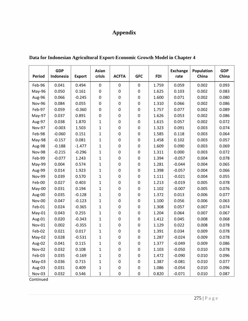
Appendix

Data for Indonesian Agricultural Export-Economic Growth Model in Chapter 4

Period GDP

Indonesia Export Asian crisis ACFTA GFC FDI

Exchange rate

Population China

GDP China

Feb-96 0.041 0.494 0 0 0 1.759 0.059 0.002 0.093 May-96 0.050 0.161 0 0 0 1.625 0.103 0.002 0.083 Aug-96 0.066 -0.245 0 0 0 1.600 0.071 0.002 0.080 Nov-96 0.084 0.055 0 0 0 1.310 0.066 0.002 0.086 Feb-97 0.059 -0.360 0 0 0 1.757 0.077 0.002 0.089 May-97 0.037 0.891 0 0 0 1.626 0.053 0.002 0.086 Aug-97 0.038 1.870 1 0 0 1.615 0.057 0.002 0.072 Nov-97 -0.003 1.503 1 0 0 1.323 0.091 0.003 0.074 Feb-98 -0.060 0.151 1 0 0 1.585 0.118 0.003 0.064 May-98 -0.157 0.081 1 0 0 1.458 0.102 0.003 0.057 Aug-98 -0.188 -1.477 1 0 0 1.609 0.090 0.003 0.069 Nov-98 -0.215 -0.296 1 0 0 1.311 0.000 0.003 0.072 Feb-99 -0.077 1.243 1 0 0 1.394 -0.057 0.004 0.078 May-99 0.004 0.574 1 0 0 1.281 -0.044 0.004 0.065 Aug-99 0.014 1.923 1 0 0 1.398 -0.057 0.004 0.066 Nov-99 0.039 0.570 1 0 0 1.111 -0.021 0.004 0.055 Feb-00 0.027 0.403 1 0 0 1.213 -0.019 0.005 0.078 May-00 0.031 0.194 1 0 0 1.102 -0.007 0.005 0.076 Aug-00 0.035 -0.128 1 0 0 1.372 0.013 0.006 0.077 Nov-00 0.047 -0.123 1 0 0 1.100 0.056 0.006 0.063 Feb-01 0.024 -0.365 1 0 0 1.308 0.057 0.007 0.074 May-01 0.043 0.255 1 0 0 1.204 0.064 0.007 0.067 Aug-01 0.020 -0.343 1 0 0 1.412 0.045 0.008 0.068 Nov-01 0.002 -0.355 1 0 0 1.129 0.022 0.008 0.078 Feb-02 0.021 0.017 1 0 0 1.391 0.034 0.009 0.078 May-02 0.028 -0.531 1 0 0 1.287 -0.024 0.009 0.078 Aug-02 0.041 0.115 1 0 0 1.377 -0.049 0.009 0.086 Nov-02 0.032 0.108 1 0 0 1.103 -0.050 0.010 0.078 Feb-03 0.035 -0.169 1 0 0 1.472 -0.090 0.010 0.096 May-03 0.036 0.715 1 0 0 1.387 -0.081 0.010 0.077 Aug-03 0.031 0.409 1 0 0 1.086 -0.054 0.010 0.096 Nov-03 0.032 0.546 1 0 0 0.820 -0.071 0.010 0.087

Continued

275 | P a g e

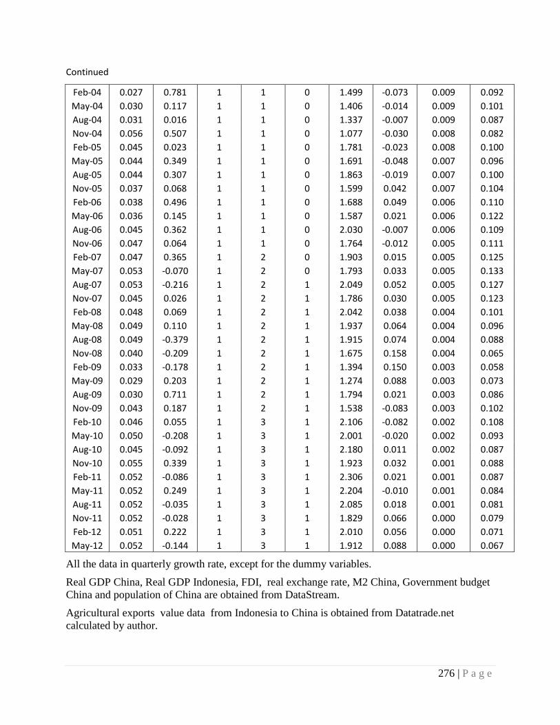
Continued

Feb-04 0.027 0.781 1 1 0 1.499 -0.073 0.009 0.092 May-04 0.030 0.117 1 1 0 1.406 -0.014 0.009 0.101 Aug-04 0.031 0.016 1 1 0 1.337 -0.007 0.009 0.087 Nov-04 0.056 0.507 1 1 0 1.077 -0.030 0.008 0.082 Feb-05 0.045 0.023 1 1 0 1.781 -0.023 0.008 0.100 May-05 0.044 0.349 1 1 0 1.691 -0.048 0.007 0.096 Aug-05 0.044 0.307 1 1 0 1.863 -0.019 0.007 0.100 Nov-05 0.037 0.068 1 1 0 1.599 0.042 0.007 0.104 Feb-06 0.038 0.496 1 1 0 1.688 0.049 0.006 0.110 May-06 0.036 0.145 1 1 0 1.587 0.021 0.006 0.122 Aug-06 0.045 0.362 1 1 0 2.030 -0.007 0.006 0.109 Nov-06 0.047 0.064 1 1 0 1.764 -0.012 0.005 0.111 Feb-07 0.047 0.365 1 2 0 1.903 0.015 0.005 0.125 May-07 0.053 -0.070 1 2 0 1.793 0.033 0.005 0.133 Aug-07 0.053 -0.216 1 2 1 2.049 0.052 0.005 0.127 Nov-07 0.045 0.026 1 2 1 1.786 0.030 0.005 0.123 Feb-08 0.048 0.069 1 2 1 2.042 0.038 0.004 0.101 May-08 0.049 0.110 1 2 1 1.937 0.064 0.004 0.096 Aug-08 0.049 -0.379 1 2 1 1.915 0.074 0.004 0.088 Nov-08 0.040 -0.209 1 2 1 1.675 0.158 0.004 0.065 Feb-09 0.033 -0.178 1 2 1 1.394 0.150 0.003 0.058 May-09 0.029 0.203 1 2 1 1.274 0.088 0.003 0.073 Aug-09 0.030 0.711 1 2 1 1.794 0.021 0.003 0.086 Nov-09 0.043 0.187 1 2 1 1.538 -0.083 0.003 0.102 Feb-10 0.046 0.055 1 3 1 2.106 -0.082 0.002 0.108 May-10 0.050 -0.208 1 3 1 2.001 -0.020 0.002 0.093 Aug-10 0.045 -0.092 1 3 1 2.180 0.011 0.002 0.087 Nov-10 0.055 0.339 1 3 1 1.923 0.032 0.001 0.088 Feb-11 0.052 -0.086 1 3 1 2.306 0.021 0.001 0.087 May-11 0.052 0.249 1 3 1 2.204 -0.010 0.001 0.084 Aug-11 0.052 -0.035 1 3 1 2.085 0.018 0.001 0.081 Nov-11 0.052 -0.028 1 3 1 1.829 0.066 0.000 0.079 Feb-12 0.051 0.222 1 3 1 2.010 0.056 0.000 0.071 May-12 0.052 -0.144 1 3 1 1.912 0.088 0.000 0.067

All the data in quarterly growth rate, except for the dummy variables. Real GDP China, Real GDP Indonesia, FDI, real exchange rate, M2 China, Government budget China and population of China are obtained from DataStream. Agricultural exports value data from Indonesia to China is obtained from Datatrade.net calculated by author.

276 | P a g e