Embed Size (px)
Citation preview

Agricultural Technology Assessment for Smallholder Farmsin Developing Countries: An Analysis using a Farm Simulation Model (FARMSIM)
Texas A&M University Integrated Decision Support System TeamUSAID Feed the Future Innovation Laboratory for Small-Scale Irrigation
James W. RichardsonCo-Director Agricultural and Food Policy Center,
Regents Professor Department of Agricultural EconomicsTexas A&M AgriLife Research Senior Faculty Fellow
Jean-Claude BizimanaAssociate Research Scientist
Texas A&M University, Department of Agricultural Economics
The authors wish to acknowledge the following agencies and individuals who were instrumental in providing data and expert advice for this report: the ILSSI-TAMU team specifically Abeyou Wale Worqlul and Yihun
Dile Taddele, Brian Herbst and David Ernstes of the Agricultural Food Policy Center/TAMU; the International Livestock Research Institute (ILRI); the International Food Policy Research Institute (IFPRI); the International
Water Management Institute (IWMI). Special thanks also to Azage Tegegne and Berhanu Gebremedhin of ILRI-LIVES (Livestock and Irrigation Value Chains for Ethiopian Smallholders) for data provision.
www.feedthefuture.gov

January 2017Research Report 17-1
Agricultural and Food Policy CenterDepartment of Agricultural Economics2124 TAMUCollege Station, TX 77843-2124Web site: www.afpc.tamu.edu

www.feedthefuture.gov i
Abstract The rural population in developing countries depends on agriculture. However, in many of these countries, agricultural productivity remains low with episodes of famines in drought-prone areas. One of the options to increase agricultural productivity is the adoption and use of improved agricultural technologies and management systems. Being a relatively high risk business due to factors related to production, marketing and finance, agriculture requires to devise risk mitigating strategies. Several models used to evaluate the adoption of agricultural technologies focus mainly on assessing the ex-post impact of technology without necessarily quantifying the profit and risk associated with the adoption of technologies. This paper introduces a farm simulation model (FARMSIM) that attempts to evaluate the potential economic and nutritional impacts of new agricultural technologies before they are adopted (ex-ante). FARMSIM is a Monte Carlo simulation model that simultaneously evaluates a baseline and an alternative farming technology. In this study, the model is used to analyze the impact of adoption of small scale irrigation technologies and fertilizers on the farm income and nutrition of smallholder farmers in Robit kebele, Amhara region of Ethiopia. The farming technologies under study comprise water lifting technologies (pulley and tank, rope and washer pump, gasoline/diesel motor and a solar pump) and use of fertilizers. The key output variables are the probability of positive annual net cash income and ending cash reserves, probability of positive net present value, and the probability of consumption exceeding average daily minimum requirements of an adult for calories, protein, fat, calcium, iron, and vitamin A. The application of recommended fertilizers on grain and vegetable crops, alongside the use of irrigation to grow vegetables and fodder using a motor pump had the highest net present value values compared to other scenarios. Similar results were observed for the net cash farm income and the ending cash reserves. As for the nutrition, the simulation results show an increase in quantities available to the farm family of all nutrition variables (calories, proteins, fat, calcium and iron) except for vitamin A under all alternative scenarios. Also, the daily minimum requirements per adult were met for calories, proteins and iron only but deficiencies were observed for fat, calcium and vitamin A. Key words: simulation, irrigation, technology, risk, nutrition

www.feedthefuture.gov ii

www.feedthefuture.gov
iii
Table of Contents
Abstract .......................................................................................................................................................................................................... i Table of Contents ...................................................................................................................................................................................... iii List of Tables and Figures ......................................................................................................................................................................... iv Introduction .................................................................................................................................................................................................. 1 Literature review ......................................................................................................................................................................................... 2 Technology adoption and agricultural development ....................................................................................................................... 2 Risk in agriculture & simulation analysis ............................................................................................................................................. 3 Methods ......................................................................................................................................................................................................... 4 FARMSIM model description ................................................................................................................................................................ 4 Base and alternative farming technology scenarios .................................................................................................................. 7 Livestock production technologies ............................................................................................................................................ 11 Nutritional and economic evaluation of irrigation and fertilizer technologies ...................................................................... 12 Water lifting technologies: description and assumptions ........................................................................................................... 15 Ranking of alternative scenarios ............................................................................................................................................................ 15 Source of data and study area ........................................................................................................................................................... 16 Micro and macro level assumptions .................................................................................................................................................. 17 Simulation results and discussion .......................................................................................................................................................... 19 NPV .......................................................................................................................................................................................................... 19 NCFI ......................................................................................................................................................................................................... 20 EC ............................................................................................................................................................................................................ 23 Nutrition results .................................................................................................................................................................................... 23 Calorie intake simulation results .................................................................................................................................................. 25 Protein intake simulation results .................................................................................................................................................. 27 Fat intake simulation results .......................................................................................................................................................... 27 Calcium intake simulation results ................................................................................................................................................ 30 Iron intake simulation results ........................................................................................................................................................ 30 Vitamin A intake simulation results ............................................................................................................................................. 33 Ranking of alternative farming technologies .................................................................................................................................. 33 Conclusions and policy recommendations .......................................................................................................................................... 36 References ................................................................................................................................................................................................. 37 Appendix A: FARMSIM Flowchart (excel worksheet organization) .............................................................................................. 40 Appendix B: FARMSIM model equations ............................................................................................................................................. 41

www.feedthefuture.gov
iv
Tables Table 1. Crop mix and land allocation (ha) scenarios for Robit kebele ....................................................................................... 8 Table 2. Current and recommended annual application rates of urea and DAP in Robit .................................................. 9 Table 3. Mean crop yields (Kg/ha) and input costs (Birr/ha) for the baseline and alternative scenarios in Robit ............ 10 Table 4. Input variables and livestock technology scenarios in Robit kebele ............................................................................ 12 Table 5. Water lifting technology (WLT) characteristics, Robit kebele ..................................................................................... 15 Table 6. Smallholder farm characteristics in Robit kebele ............................................................................................................. 18 Table 7. Summary results for nutritional and scenarios performance in Robit kebele ........................................................... 25 Figures Figure 1a. Yield distributions of teff for the baseline and alternative scenarios ....................................................................... 14 Figure 1b. Yield distributions of tomato for the baseline and alternative scenarios ............................................................... 14 Figure 2. Location of Robit kebele in Bahir Dar Zuria woreda, Amhara region ...................................................................... 17 Figure 3a. CDF of NPV for alternative irrigation technologies in Robit kebele ....................................................................... 21 Figure 3b. StopLight chart for per family NPV in Robit kebele .................................................................................................... 21 Figure 4a. CDF of NCFI for Robit kebele ......................................................................................................................................... 22 Figure 4b. StopLight chart for per-family NCFI in Robit kebele ................................................................................................. 22 Figure 5a. CDF of EC in Robit kebele ................................................................................................................................................ 24 Figure 5b. StopLight chart for per-family EC in Robit kebele ...................................................................................................... 24 Figure 6a. CDF of daily energy consumption per AE on a farm in Robit kebele ..................................................................... 26 Figure 6b. StopLight Chart for daily energy consumption per AE on a farm in Robit kebele ............................................... 26 Figure 7a. CDF of daily proteins consumption per AE on a farm in Robit kebele ................................................................. 28 Figure 7b. StopLight Chart for daily protein consumption per AE on a farm in Robit kebele ............................................. 28 Figure 8a. CDF of daily fat consumption per AE on a farm in Robit kebele ............................................................................. 29 Figure 8b. StopLight Chart for daily fat consumption per AE on a farm in Robit kebele ...................................................... 29 Figure 9a. CDF of daily calcium consumption per AE on a farm in Robit kebele .................................................................... 31 Figure 9b. StopLight Chart for daily calcium consumption per AE on a farm in Robit kebele ............................................. 31 Figure 10a. CDF of daily iron consumption per AE on a farm in Robit kebele ....................................................................... 32 Figure 10b. StopLight Chart for daily iron consumption per AE on a farm in Robit kebele ................................................ 32 Figure 11a. CDF of daily vitamin A consumption per AE on a farm in Robit kebele .............................................................. 34 Figure 11b. StopLight Chart for daily vitamin A intake per AE on a farm in Robit kebele ................................................... 34 Figure 12a. SERF ranking of alternative farming systems in Robit kebele .................................................................................. 35 Figure 12b. Risk premiums ranking of alternative farming systems in Robit kebele ................................................................ 35

www.feedthefuture.gov v

www.feedthefuture.gov 1
Introduction The rural poor in developing countries largely depends on agriculture and about 70 percent of extreme poverty around the world is found in rural areas (Norton, 2014). For most of the world’s poorest countries, especially those on the African continent, agriculture continues to be the main source of employment and contributes to a large portion of the GDP. However, in many of these countries, agricultural productivity remains low with episodes of famines in drought-prone areas (Qasim, 2012). To understand why people, remain poor and hungry it is important to know the factors affecting agricultural productivity which include but are not limited to technologies, resources and institutions that regulate the economy (Norton, 2014). One way of increasing agricultural productivity is the adoption and use of improved agricultural technologies and management systems. Adopting and using new agricultural technologies has never been an easy task because of many factors that are involved in the adoption process. Factors that influence the extent of adoption of technology can include: characteristics or attributes of technology; the adopters or clientele, the change agent (extension worker); and the socio-economic, biological, and physical environment in which the technology takes place (Cruz, 1987). Generally, farmers look at some or all of those factors and choose to adopt a technology based on their utility and profit maximization behaviors (Qasim, 2012; Barungi and Maonga, 2011). The assumption is that farmers engage in adoption of new technology only if the benefits or perceived utility of using the new technology outweighs the benefits of the current or old technology. There are a number of utility maximization theories that have been applied to farm production behavior but the difference between them and the theory of profit maximization is that utility maximization considers the dual character of a farm household as family and enterprise. Several models have been used to measure the adoption of technologies specifically the binary choice models, which do not necessarily quantify the profit and risk associated with production but rather assess the ex-post impact of technology adoption (Diagne et al., 2013; de Janvry et al., 2011). The key result from these models is the average effect of adoption on outcomes (yields, revenues, profit…) for those who have adopted technologies, also called the average treatment effect. However, because of the selection problem, the main challenge is to establish the proper counterfactual group against which to compare adopters especially in the early stage of adoption where we have large numbers of non-adopters (de Janvry et al., 2011). Another concern in impact assessment using this approach stems from the inability to detect statistically significant differences in poverty-related outcome measures and income when agricultural technologies generate only small increments in yields and income. Also, note the difficulty of capturing the spillover effect from adoption, which affects adopters and non-adopters. The main issue with the average treatment is its variation over time because the adopters change how they use the new technology with time as they learn more about it and a number of late adopters join the early adopters group. It is also a challenge to search for a counterfactual since a true counterfactual should not be “contaminated” by adopters. To overcome this issue, other types of approaches built around simulation models such as the computable general equilibrium models (CGE) have been used to measure the adoption of technology. While these are useful models (especially at the macro level), they neither estimate impacts nor capture the risk associated with agricultural production at the farm level. The method discussed above for evaluating the impact of technology has mainly focused on the ex-post evaluation. The approach this paper will focus on, however, evaluates the potential impacts of new agricultural technologies before adoption takes place (ex-ante evaluation). A farm level simulation model (FARMSIM) is used to carry out this task. In addition to assessing and quantifying the economic profit, the model evaluates the nutritional outcomes for a farm family of adopting new agricultural technologies based on the increased consumption and sale of production surplus to buy other foods not produced on the farms. All these output variables are projected for five years and presented in terms of probability distributions based on historical yield and price risk. It is recognized that the spillover effects from technology adoption are not captured by a farm level simulation model but can be properly handled by a sector model. Nonetheless, effects related to price elasticities to reflect the changes in revenues and costs from a potential increase in crop production are taken into account by the FARMSIM model. The goal of this paper is to project the probable economic and nutritional impacts of adopting agricultural technologies in developing countries using a case study from Ethiopia.
www.feedthefuture.gov 2
Ethiopia, as many other African countries, has an agriculture-dependent economy that includes crop and livestock production. Agriculture in Ethiopia contributes 45% to national GDP, employs more than 80% of the population and brings more than 90% of the foreign exchange earnings (Shitarek, 2012). However, the Ethiopian economy and specifically its agriculture development sector is vulnerable to external shocks such as climate shocks. Drought is the most prominent climate shock that affects not only food and livestock production but livelihoods in general. Historically Ethiopia has known several droughts but the worst and most memorable remains the one associated with the famine of 1983-1985. Recent severe droughts occurred in 2010-2011 and 2015, putting at risk several million people and causing the loss of several thousand animals (UN-OCHA, 2016). Given the loss of crops and livestock due to drought, one of the Ethiopian government priorities, as stipulated in its “Policy and Investment Framework (PIT)” is to increase irrigation for crop and livestock (USAID, 2011). However, substantial growth for crop and livestock production can only occur when irrigation is used alongside other agricultural inputs such as fertilizer and improved seed. Because of the limited availability and use of irrigation and improved seed and fertilizer, crop yields for smallholder farmers in Ethiopia are below the Sub-Saharan Africa averages. This paper is organized into three sections. First, a brief literature on technology adoption and risk in agriculture is offered, followed by a discussion of our method of analysis and empirical results. Lastly, summary conclusions and suggestions for future studies are provided. Literature review Technology adoption and agricultural development Productivity of small-scale farms in developing countries is known to be constrained by several policy and structural issues that have led to slow increases in crop yields and stagnation (Yengoh et al., 2009). The absence of technologies, limited access to or the use of inappropriate technologies have been in part blamed for the lack of increases in productivity and persistent food insecurity in developing countries. Most of the time it is assumed that with the right technology (seeds, irrigation, fertilizers, technique, tools), the agricultural production will be increased and food security will be restored in areas with physical and social limitations to production. However, this has not always been the case. National governments, international agencies and several development organizations have attempted to make agriculture more productive and profitable by introducing agricultural technologies but with modest results (Yengoh et al., 2009). Several factors have contributed to low or lack of adoption of new technologies in developing countries including the limited access to the technologies. Even where these technologies have been adopted at a low rate, the dissemination to a larger segment of the population has failed in some cases. For instance, conservation technologies have been introduced in places with steep slopes and where erosion was a major limiting factor to production, such as in the Ethiopian highlands (Gebrehaweria et al., 2013). Part of this technology package, the use of rainwater management (RWM) interventions, including soil and water conservation (SWC) techniques, is widely accepted as a key strategy to improve agricultural productivity by reducing water shortages, effects of droughts, and worsening soil conditions. However, in the rain-fed agro-ecological landscapes of Ethiopia, the low yield (on average about 35% of the potential) is usually not due to the lack of water but rather a result of the inefficient management of water, soils, and crops (Amede 2012). Given the modest impact and outcome of these conservation measures, it has since been emphasized that interventions should not only focus on the engineering and biophysical performance of conservation measures but also on the socioeconomic and livelihood benefits (Zemadim et al. 2011). Studies from the Ethiopian Highlands show that the adoption of RWM technologies is influenced by a variety of factors, including biophysical characteristics such as topography, slope, soil fertility, rainfall amount, and rainfall variability (Deressa et al. 2009). Experience also shows that even when technologies are appropriate for the biophysical setting, they are not always adopted because farmers consider a variety of factors when making a decision to adopt a particular intervention (McDonald and Brown 2000; Soule et al. 2000). In addition, studies have found that both farmers’ recognition of the problem (e.g., soil erosion and low agricultural productivity) and awareness of the potential solutions are necessary, but not sufficient conditions for the adoption and continued use of SWC technologies (Merrey and Gebreselassie 2011). Externally driven technical solutions are rarely sustained by farmers unless consideration is given to

www.feedthefuture.gov 3
socioeconomic, cultural and institutional as well as biophysical and technical factors (McDonald and Brown 2000; Merrey and Gebreselassie 2011). Improving agricultural productivity in the developing world in general and sub-Saharan Africa in particular has become a pressing issue. As Yengoh, Armah and Svensson (2009) stated, this pressure is “dictated by the population growth, uncertainty in global food markets, changing consumption patterns of food commodities, and the need to meet important milestones in food and nutrition in the region such as those of the millennium development goals (p.112).” Risk in agriculture & simulation analysis
a) Risk and coping strategies in agriculture:
Risk and uncertainty are part of many business decisions we do every day especially those involved in the agricultural sector. Hardaker et al. (2004, p.4) state that “Indeed, risk and uncertainty are inescapable in all walks of life. Because every decision has its consequences in the future, we can seldom be absolutely sure what those consequences will be.” The terms “risk” and “uncertainty” are defined differently. Risk is defined as an imperfect knowledge where the probabilities of the possible outcomes are known while uncertainty exists where these probabilities are not known (p.5). Agriculture is often characterized as a relatively high risk and uncertain enterprise in the economy due to a number of risky factors related to the agricultural business such as production, marketing and finance (Hardaker, et al., 2004; Qasim, 2012). Some of the risk and uncertainty components surrounding the production and marketing processes are related to unpredictable weather variation (drought, frost, flood, and wind storm), input quality, pest and disease attacks, price fluctuations, new technology failure, and changes in government policies. These factors are some of the main causes of farm production and income fluctuations both at the micro and macro-economic levels. Financial risk is more dependent on failure to meet liabilities with the cash generated through farm revenues due to a mismatch between cash inflows and outflows, the level of debt, and other sources of financial resources. The risk becomes more important when the household heavily depends on loans for farm investments. The combined effect of production, marketing, institutional and personal risk is called business risk (Hardaker et al., 2004). It is the cumulative effect of all the uncertainty surrounding the profitability of the firm. As for the financial risk, it results from the method of financing the firm. There is a need to explicitly take into account risk in agriculture because farmers cannot control all of the factors related to agricultural production and marketing. Along with knowing the risk factors, people have always devised ways and strategies to reduce the negative impacts of risk. Among other risk coping strategies are the diversification of production, price support (most of the time by government), off-farm income generation, and use of different tools (e.g. mobile phone) to acquire up-to-date information on weather and market prices (Qasim, 2012). Accounting for risk can be important in day-to-day farm management decisions where the accumulated effects of repeated choices (such as routine testing and treatment of dairy cows) may have important impacts on the overall business performance (Hardaker et al., 2004). Due to unpredictable weather and under harsh climatic and agro-ecological conditions, crop production failure can result in food insecurity and famines such as those that have happened to the highlands of Ethiopia over the last 40 years (Di Falco and Chavas, 2009). For instance, with recurring drought and a high risk of harvest failure, ex-ante farm production decisions based on crop and varietal choices are part of risk management strategies (p.599). Di Falco and Chavas argue that crop genetic diversity embedded in the crop seeds, especially those found in Ethiopia, can sustain productivity and help manage risk. In the same way, adopting water and land conservation along with the irrigation technologies can help cope with drought risk.
b) Use of Monte Carlo simulation in risk analysis:
There are basically two reasons why risk matters in agriculture: 1) most of people do not like risk (they are risk averse); and 2) reduction in payoff when assumptions do not hold (downside risk) (Hardaker et al., 2004). Most of people are risk averse when they face decisions and choices of risky wealth outcomes. Risk aversion refers to the willingness to forgo some expected return for a reduction in risk (p.7). While people may be less willing to take risky choices, those who take them become concerned about the downside risk which involves the payoff reduction when the assumed

www.feedthefuture.gov 4
conditions are not met. The level of the downside risk increases when a risky outcome (e.g. yield) depends on non-linear interactions of several random variables (prices, rainfall, temperature, pest attacks…). In agriculture, the weather (rainfall and temperature) fluctuation represents the most important source of risk for farm yield and production. Hardaker et al. (2004) caution about the use of a “normal” season to evaluate potential crop yields since the interaction of non-linear variables is most likely to produce a yield outcome different from that recorded in a normal year. To evaluate more accurately the downside risk, they recommend using the mean yield as a basis for risk analysis. However, the crop yield forecast and prediction become even more accurate (less risky) if the entire distribution of the rainfall is taken into account. Probability distributions rather than point estimates are used in risk and decision analysis to model uncertain events (uncertainties). There is a tendency to think about probability distributions of continuous uncertain quantities (yield for example) in terms of probability density functions (PDFs). A PDF is often (but not always) bell-shaped, with a central peak that indicates the most likely value or mode of the random variable and with low probability tails on either side of the peak. A PDF’s statistical property is that the area under the curve sums to one. However, the cumulative distribution functions (CDFs) are more convenient to use and read than the PDFs. Generally, in risk analysis, it is useful to compute the statistics that describe the main features of a distribution, which are the mean or average (measure of central tendency) and the dispersion from the mean (measure of variance or standard deviation). These are the first two moments of the distribution. The third and fourth moments are skewness and kurtosis which inform us respectively on the symmetry (or lack of symmetry) of the distribution and the presence of outliers (heavy or light tails). These four moments help describe the risk probability distribution of a random variable and are one of the approaches used to advise decision makers and business operators (including farmers) about risk. When decision makers and business operators are faced with risky choices, their goal is to pick alternative options with the highest expected utility and less risk (low variability). With the advance in computing technology and ease of access to personal computers, business analysts have relied for a long time on Microsoft® Excel to conduct economic feasibility analyses for prospective investments using Monte Carlo simulation models (Richardson et al., 2007). Also the availability of simulation add-ins for Excel have made the Monte Carlo simulation approaches a reliable tool for risk analysis (Hardaker et al., 2004; Richardson et al., 2007). In stochastic simulation, random or stochastic components are incorporated in simulation models to calculate the key output variables (KOVs), by repeatedly sampling from the probability distributions for multiple random variables to capture the uncertainty in the real system. Since many input variables are stochastically dependent, this requires estimating and simulating the joint distribution which in return provides the stochastic component for the simulation model used to generate the probability distributions of the key output variables (KOVs). In simulation modeling two methods of sampling random variables (Monte Carlo and Latin Hypercube) are available. The Latin Hypercube is more efficient in that it systematically samples all regions of the PDF which requires few iterations (trials) to simulation the risk for each random variable. For this reason, Monte Carlo simulation using the Latin Hypercube sampling procedure is used to generate random values from specified input distributions in FARMSIM. Each evaluation of the model by using randomly sampled realizations from the specified distribution is called an “iteration.” With enough iterations, the distribution of each KOV will converge to a stable distribution that will allow the analyst to evaluate the risk associated with the KOVs. Methods
FARMSIM model description
The farm simulation model “FARMSIM” is a Monte Carlo simulation model to, simultaneously evaluate a baseline and alternative technologies for a farm. The model is programmed in Microsoft ® Excel and utilizes the Simetar© add-in (Richardson et al., 2006) to estimate parameters for price and yield distributions, simulate random variables, estimate probability distributions for KOVs and rank technologies (see the flowchart in Appendix A). FARMSIM is a micro-computer, Excel/Simetar driven, enhanced version of FLIPSIM (Richardson and Nixon, 1985) which has been used extensively for policy analysis and technology assessment.

www.feedthefuture.gov 5
FARMSIM is programmed to recursively simulate a five-year planning horizon for a diversified crop and livestock farm and repeats the five-year planning horizon for 500 iterations1. A new sample of random values is drawn to simulate each iteration. After simulating 500 iterations, the resulting 500 values for each of the KOVs defines the empirical probability distributions for comparing the base and alternative farming system technologies. By comparing the probability distributions for the base and alternative technologies, decision makers can quantitatively analyze the probable consequences of introducing alternative farming systems. FARMSIM is programmed to simulate 1-15 crops as well as cattle, dairy, sheep, goats, chickens, and swine annually for five years. The farm family is modeled as the first claimant for crop and livestock production with deficit food production met through food purchases using net cash income from selling surplus crops and livestock production. Standard accounting procedures are used to calculate: receipts, expenses, net cash income, and annual cash flows. The KOVs for the model can include all endogenous variables in the model but most attention is focused on the following KOVs: annual net cash income (NCFI), annual ending cash reserves (EC), net present value (NPV), and annual family nutrient consumption of protein, calories, fat, calcium, iron, and vitamin A. Because FARMSIM is a stochastic model, probabilities can be assigned to exceeding target values for each of the KOV’s. For example, the results from comparing two technologies can be presented as: probability of economic success for the base technology is 60% and the probability for the alternative technology is 90%. Similarly, the probability of the farm family having a better diet (in terms of nutrients consumed) for the alternative technology relative to the base can be calculated and presented graphically. Stochastic annual output prices for crops and livestock are simulated using multivariate empirical probability distributions estimated from historical data. Stochastic annual crop yields are simulated from multivariate empirical probability distributions estimated using 32 years of crop yields generated by APEX (Agricultural Policy / Environmental eXtender) (Williams et al., 1998). APEX uses the most recent 32 years of local weather data, soil conditions, and an internationally validated crop growth modeling algorithm to simulate 32 yields for the baseline and alternative cropping/irrigation systems. APEX simulates plant growth from planting through harvest for all crops on the farm using the base technology (seed, fertilizer, soils, etc.) and the alternative technology (improved seed, fertilizer, soils, irrigation, etc.). Both technologies are simulated by APEX using the same historical weather data and plant growth parameters consistent with the assumed technologies so the only difference between the yield distributions is the technology package. The baseline and alternative technology scenarios are simulated by FARMSIM using the same equations so the only difference in the economic and family nutrition outcomes are due to the technology differences. The random crop yields are simulated using the same stochastic uniform standard deviates to ensure that the weather risk for a crop under the base and alternative technology scenarios are identical. The same stochastic prices for crops are used for both scenarios, unless the alternative scenarios call for a different marketing program which shifts the price distribution to a higher level. Since the base and alternative models use identical equations, the decision maker can be assured that the differences in the KOVs are due to the differences in the two farming systems and their assumed yield distributions. FARMSIM model has four major components: crop, livestock, nutritional, and financial. In the next section, each major component is described (see details of the FARMSIM model equations in Appendix B). Crop Model. The farm family can grow/consume 15 different crops/food stuffs. The crops in the model are dependent upon the local crops produced and consumed in the local area. The order of the crops is specified by the analyst so the model is applicable across countries and farming systems. Crop production equals the product of stochastic yield and hectares planted (Eq. 3). Family consumption is calculated as the maximum of average annual kilograms consumed or a fraction of total production. If surplus production exists it can be paid to employees and landowners, where applicable. After satisfying family food needs, employee compensation and rent requirements, the remaining crop production is sold. Cash receipts for crops equals quantity sold times the stochastic market price (Eq. 8). Market prices are simulated using either a GRKS probability distributions elicited through expert opinion in the absence of historical data or a multivariate
1 Extensive testing with the Latin Hypercube sampling procedure in Simetar has shown that a sample size of 500 iterations is more than adequate to estimate a probability distribution for KOVs in a business model with more than 100 random variables.

www.feedthefuture.gov 6
empirical (MVE) probability distribution where historical prices are available. As an input, the GRKS distribution (developed by Gray-Richardson-Klose and Schuman) uses three parameters (minimum, a mid-point, and a maximum) and then assigns a piecewise normal distribution such that 50% of the density is below the mid-point and 50% is above the mid-point. An additional benefit of the GRKS distribution is its capacity to assign 2.5% of the weight to values less than the minimum and 2.5% of the weight to values greater than the maximum allowing the possibility of outliers in both tails (Richardson, 2006; Palma et al., 2011). In the case of historical prices availability, parameters for a multivariate empirical probability distribution are estimated, allowing to take into account the correlation among prices. An MVE has three parameters or components to be estimated. First, a deterministic component that represents the projected value based on mean, trend regression, multiple regression or time series model for each random variable; second, a stochastic component representing the measure of the dispersion around the deterministic component; and third, a multivariate component representing the correlation matrix of rank m for the m random variables. Ignoring the correlation among random variables leads to a biased estimation of the KOVs. Cash costs of production for crops are calculated as the product of hectares planted and the sum of per hectare costs for seed, fertilizer, chemicals, weeding, irrigation, land preparation, harvesting, and other cash costs (Eq. 9). There are no econometric equations in the crop model because all simulated variables can be calculated as simple identities and standard accounting practices. Livestock Model. The livestock component of FARMSIM simulates annual production and herd dynamics for cattle, oxen, chickens, sheep, goats, and swine. Since the cattle sector is the most complex it is described here in detail (Eq. 13-27). The other livestock sectors are modeled similarly. The number of cows January 1 less cows consumed, cows die, and cows culled, plus raised replacements, and purchased cows equals the number of cows on December 31. Cows consumed and cows that die are calculated based on relevant fractions for consumption and death and the number of cows January 1. Cows culled and purchased are endogenous variables calculated annually to maintain the cow herd at the user’s pre-determined number of cows for each year. The number of calves born each year is the product of the number of mature cows January 1 and the stochastic annual calving rate. Half the calves are assumed to be heifers and half are bulls. The fraction of calves consumed by the family, die or are sold, decrease the number born to arrive at the number of yearling heifers and bulls on December 31. Different death rate, consumption, and sold fractions can be used for bull and heifer calves. The model can either sell bull calves or retain them to raise oxen on the farm. The number of 12-month-old heifers on December 31 equals the number of 12-24-month-old heifers January 1 of the subsequent year. The ending year number of 12-24-month-old heifers is calculated based on the fraction of two-year-old heifers that are consumed by the family, die or are sold during the year. The same process is used to dynamically simulate the 25-36 months old replacement heifers. It is assumed replacement heifers are bred to calve at 40-48 months when they enter the cow herd. The dynamics of the oxen herd is similar to the cowherd. The number of oxen on January 1 is reduced for the fractions consumed, die or are culled (sold). The number of oxen raised or purchased to maintain the desired herd size is added to the net January 1 herd size to calculate the inventory of oxen on December 31. Milk production is calculated by multiplying stochastic milk per cow times the number of lactating cows (Eq. 15). The number of lactating cows equals the number of cows that calved each year. Milk production per cow is a stochastic variable simulated using an expert opinion parameterized GRKS distribution that is augmented by fractional adjustments for forage production. Low (high) forage production reduces (increases) the stochastic milk per cow value in the current year. Low forage production not only affects milk production in the current year but also reduces the stochastic fertility rate. Thus, a drought causes decreased milk production for two years as fewer lactating cows are available in the second year. Milk consumption by the family is a fraction of total milk production. A fraction of the milk can be made into butter which can be consumed by the family or sold. Milk not consumed or made into butter is sold. Receipts for cattle are calculated using the stochastic prices for the respective age categories and the number of head sold plus receipts for

www.feedthefuture.gov 7
milk, butter, hides, and manure (Eq. 29). The receipts for hides come from multiplying a price for hides by the number of cattle and oxen that die or are consumed. Manure receipts are calculated as the product of manure prices and the sum of manure produced by the cows, calves, replacements, and oxen, if the manure is not used on the farm. Cash costs for the cattle herd are calculated by multiplying the annual cash costs for cows, calves, two year olds, three year olds, and oxen by the number of head on December 31 (Eq. 10). The annual cash costs are inflated each year by assumed rates of inflation. As indicated above, the livestock model has similar detail for simulating the herd dynamics, receipts, and costs for sheep, goats, and swine. For chickens the production, consumption, and sale of eggs is added to the flock dynamics which are similar to the other livestock species. Nutrition Model. The total kilograms of each raised crop consumed by the family plus the kilograms of purchased foodstuffs are multiplied by their respective nutrient scores to calculate total calories, protein, fat, calcium, iron and vitamin A from the food stocks (e.g. of proteins in Eq. 41). Similar calculations are made to simulate the nutrients derived from consuming cattle, oxen, milk, butter, chickens, eggs, mutton, lamb, nannies, kids, and pig meat. Total nutrients consumed by the family from all sources, including donated food, are summed across plant and animal food stocks and compared with minimum daily recommended amounts for adults. Financial Model. The financial model consists of three pro forma financial tables: income statement, cash flow, and balance sheet (Eq. 32-40). The income statement shows the source of annual receipts from crops, cattle, chickens, sheep, goats, and swine. Annual cash expenses from these same profit centers plus fixed costs and interest costs are summarized in the income statement. Annual net cash income equals total cash receipts minus total cash expenses. The cash flow statement calculates cash inflows, cash outflows, and ending cash reserves. Cash inflows equal the sum of beginning cash, net cash income, off farm income, and interest earned for cash reserves (Eq. 35-40). Cash outflows equal the sum of cash purchases of food, school expenses, family living expenses, income taxes, principal payments, and repayment of cash flow deficits in the previous year. Ending cash reserves on December 31 equals total cash inflows minus total cash outflows. The balance sheet summarizes assets and liabilities for the farm (Eq. 42-46). Annual assets equal the value of land, livestock, machinery, and positive cash reserves. Annual liabilities equal remaining debt for initial loans and new debts, and negative cash reserves. Net worth equals assets minus liabilities. Net present value for the farm family equals the present value of annual family withdrawals plus the value of crops and livestock consumed, plus the present value of ending net worth, minus the beginning net worth (Eq. 49). A 10% discount rate is used to calculate net present value. Base and alternative farming technology scenarios Data input into FARMSIM is entered in parallel. For each input variable, the user must provide information for the current (base) and alternative farming system (scenario) (see flowchart in Appendix A). The model is designed so the user can enter complete data sets for the base and 21 alternative scenarios. Due to the importance of irrigation in crop and livestock production and recurrent drought episodes observed in Ethiopia, small scale irrigation technologies will be discussed using a case study of a representative farm from the Robit village (kebele) in the Amhara region of Ethiopia. Small scale irrigation technologies enable smallholder farmers to have dry season crops that provide improved nutrition and generate income with less risk, provided that there is a sustainable source of water for the land area to be irrigated. The scenario analysis consists of the evaluation of water lifting technologies and fertilizer applications. Given that most of water used for irrigation in Amhara is groundwater from wells, four different water lifting technologies ranging from pulley and bucket, to rope and washer pump, to motor and solar pumps will be evaluated for their capacity and affordability (Appendix C).

www.feedthefuture.gov 8
Table 1. Crop mix and land allocation (ha) scenarios for Robit kebele
Scenarios Millet Teff Maize Chickpeas Potato Irrigateda Irrigated Irrigated Irrigated Cabbage Tomato Fodder Napier Total (ha)
Wet season Dry season Baseline 708.0 266.0 728.0 57.0 24.0 126.0 102.0 43.0 43.0 2,097.0 Alt.1 Pulley/tank 708.0 266.0 728.0 110.0 50.0 228.0 204.0 145.0 63.0 2,502.0 Alt. 2 Rope & Washer Pump 708.0 266.0 728.0 110.0 50.0 231.0 207.0 148.0 63.0 2,511.0 Alt. 3 Motor Pump 708.0 266.0 728.0 110.0 50.0 356.0 332.0 273.0 103.0 2,926.0 Alt. 4 Solar Pump 708.0 266.0 728.0 110.0 50.0 240.0 216.0 157.0 63.0 2,538.0
Note: a = total potential irrigable land in Robit is 787 ha (source: SWAT2 simulation results)
2 SWAT (Soil and Water Assessment Tool) model is described in paragraphs below.

www.feedthefuture.gov 9
Table 2. Current and recommended annual application rates of urea and DAP in Robit
Fertilizers (Kgs/ha)
Crops Urea (Kgs/ha) DAP (Kgs/ha)
Current Recommended Current Recommended
Teff 36 100 88 100
Maize 83 100 70 100
Millet 60 0 80 100
Tomato 56 200 0 200
Cabbage 8 100 0 40
Chickpeas 0 - 25.6 -
Potato 13.3 100 90.7 60
Fodder (oats & vetch) 0 100 0 100
Napier grass 0 100 0 100
Three major cereal crops consistent with the current cropping systems in Robit are considered. They comprise maize, teff and millet grown during the wet season. In addition to cereal crops, chickpeas, potato, cabbage, tomato, fodder and napier grass are considered in the model (table 1). Assuming no need for supplemental irrigation for the cereal crops, chickpeas and potato, the main difference in yield between the base and alternative scenarios in terms of technology input would mainly come from fertilizer application and use of improved seeds. Different sources of literature including a recent household survey carried out in Robit by the ILRI-LIVES project indicate that a relatively adequate amount of fertilizer (DAP and Urea), close to the recommended rates, is used in household farms in Robit for maize and millet (Minot and Sawyer, 2013; Rashid et al., 2013). Increased levels of fertilizers were used for teff in the alternative scenario. As for chickpeas and potato, additional fertilizers were applied in alternative scenarios for potato since chickpeas did not show any stress for phosphorus and has the capability of fixing nitrogen (tables 2 and 3). The survey information shows that most of the households used stored seeds from the previous harvest for the following planting season and that the use of chemicals was limited. It was also noted that the level of farm labor hiring for agricultural production was low since family members performed most of the agricultural tasks. It is worth mentioning that, the use of actual crops to feed animals is not common as most of the animal feed comes from crop residues.

www.feedthefuture.gov
10
Table 3. Mean crop yields (Kg/ha) and input costs (Birr/ha) for the baseline and alternative scenarios in Robit Baseline scenario Alternative scenario
Crops Mean yield Cost fert. Cost seed Cost irrig. Mean yield Cost fert. Cost seed Cost irrig.
Teff 838 1614 470 0 1995 4800 470 0
Maize 2127 4284 476 258 2773 4284 476 258
Millet 1640 3110 46 0 2257 3110 46 0
Tomato 14293 783 420 258 21714 642 420 10757
Cabbage 11376 110 880 258 18089 110 880 10757
Chickpeas 1274 358 122 258 1274 358 122 258
Potato 3770 0 0 736 7728 1504 2595 736
Fodder (oats & vetch) 1398 0 300 258 3285 3000 1200 10757
Napier grass 10936 926 234 258 10936 926 234 10757
The irrigated crops are grown during the dry season and consist mainly of tomato and cabbage in the vegetable category and fodder (vetch/oats) and napier grass in the animal feed category. Note however that a portion of fodder and napier grass production was simulated as a market commodity (cash crop) while the remainder was used to feed animals. While the required fertilizer rates for tomato were applied for the alternative scenario (Urea: 200 Kgs/ha and DAP: 50 Kgs/ha), household data from the ILRI-LIVES survey showed only limited application of the current fertilizer rates (baseline scenario) (table 2). Only Urea was applied by a few households at a rate of 150 Kgs/ha (average of all 10 households was 56 Kgs/ha) while no farmer applied DAP. In the case of cabbage, the baseline and alternative scenarios differed as to the quantities of applied irrigation water and subsequent water stress levels, which were at 50% for the baseline and 0% for the alternative scenarios. However, similar amounts of fertilizer rates were applied for both scenarios. For fodder and napier grass, additional amounts of fertilizer to the current levels were applied.
www.feedthefuture.gov
11
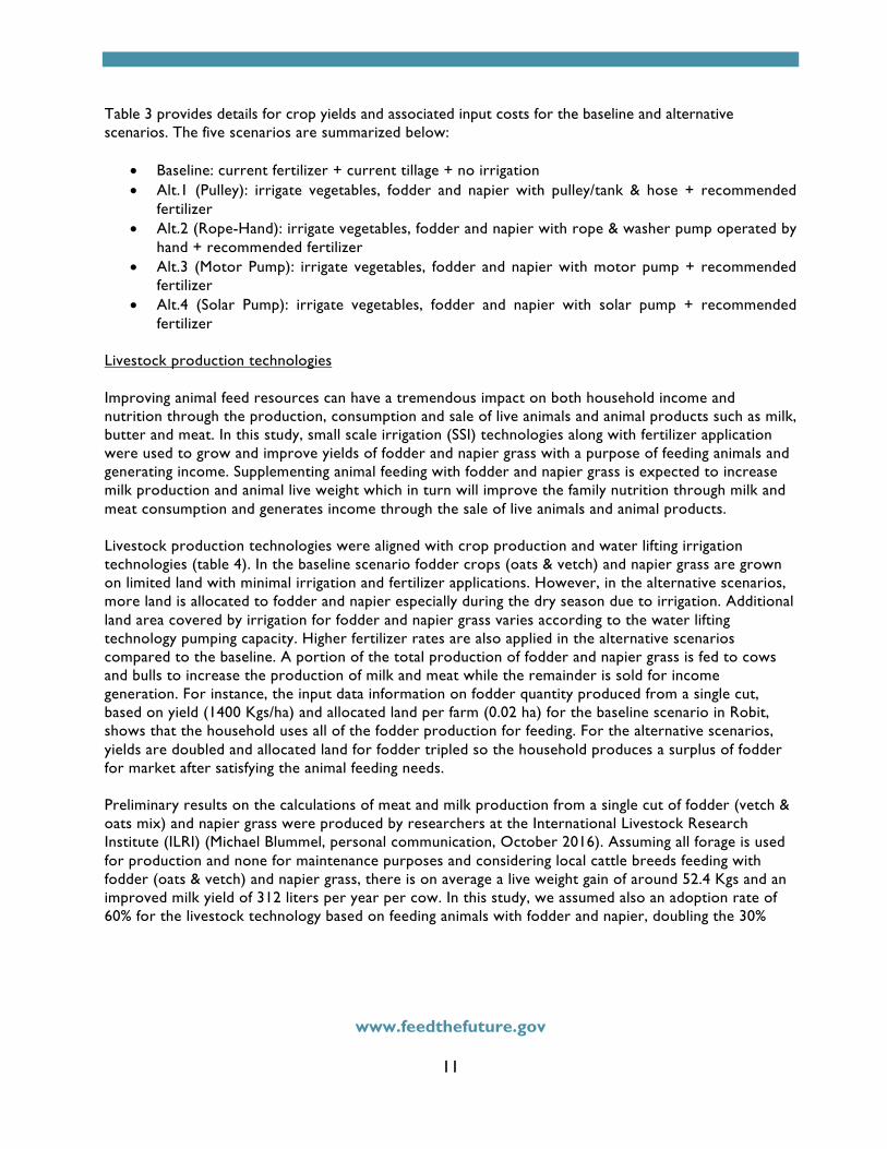
Table 3 provides details for crop yields and associated input costs for the baseline and alternative scenarios. The five scenarios are summarized below:
• Baseline: current fertilizer + current tillage + no irrigation • Alt.1 (Pulley): irrigate vegetables, fodder and napier with pulley/tank & hose + recommended
fertilizer • Alt.2 (Rope-Hand): irrigate vegetables, fodder and napier with rope & washer pump operated by
hand + recommended fertilizer • Alt.3 (Motor Pump): irrigate vegetables, fodder and napier with motor pump + recommended
fertilizer • Alt.4 (Solar Pump): irrigate vegetables, fodder and napier with solar pump + recommended
fertilizer Livestock production technologies Improving animal feed resources can have a tremendous impact on both household income and nutrition through the production, consumption and sale of live animals and animal products such as milk, butter and meat. In this study, small scale irrigation (SSI) technologies along with fertilizer application were used to grow and improve yields of fodder and napier grass with a purpose of feeding animals and generating income. Supplementing animal feeding with fodder and napier grass is expected to increase milk production and animal live weight which in turn will improve the family nutrition through milk and meat consumption and generates income through the sale of live animals and animal products. Livestock production technologies were aligned with crop production and water lifting irrigation technologies (table 4). In the baseline scenario fodder crops (oats & vetch) and napier grass are grown on limited land with minimal irrigation and fertilizer applications. However, in the alternative scenarios, more land is allocated to fodder and napier especially during the dry season due to irrigation. Additional land area covered by irrigation for fodder and napier grass varies according to the water lifting technology pumping capacity. Higher fertilizer rates are also applied in the alternative scenarios compared to the baseline. A portion of the total production of fodder and napier grass is fed to cows and bulls to increase the production of milk and meat while the remainder is sold for income generation. For instance, the input data information on fodder quantity produced from a single cut, based on yield (1400 Kgs/ha) and allocated land per farm (0.02 ha) for the baseline scenario in Robit, shows that the household uses all of the fodder production for feeding. For the alternative scenarios, yields are doubled and allocated land for fodder tripled so the household produces a surplus of fodder for market after satisfying the animal feeding needs. Preliminary results on the calculations of meat and milk production from a single cut of fodder (vetch & oats mix) and napier grass were produced by researchers at the International Livestock Research Institute (ILRI) (Michael Blummel, personal communication, October 2016). Assuming all forage is used for production and none for maintenance purposes and considering local cattle breeds feeding with fodder (oats & vetch) and napier grass, there is on average a live weight gain of around 52.4 Kgs and an improved milk yield of 312 liters per year per cow. In this study, we assumed also an adoption rate of 60% for the livestock technology based on feeding animals with fodder and napier, doubling the 30%

www.feedthefuture.gov
12
Table 4. Input variables and livestock technology scenarios in Robit kebele
Baseline scen. Alt. scen. 1 Alt. scen. 2 Alt. scen. 3 Alt. scen. 4 Cows Native 2640 2640 2640 2640 2640 Cross-breds 165 165 165 165 165
Milk per cow Liters/cow/year 185 312 312 312 312
Live Weight gain (Kgs) 0 52.4 52.4 52.4 52.4 Live weight /bull 184 236.4 236.4 236.4 236.4
Consumption Percent (%) Milk by family 28 38 38 38 38 Milk by employees 0 0 0 0 0 Made into butter 70 50 50 50 50 Butter sold 54 54 54 54 54
rate of adoption indicated by the LIVES household survey. The number of cattle is held constant for the 5 year planning horizon. Following are the baseline and alternative technology scenarios: Baseline: No irrigation + current animal feeding (no supplemental feed) Scenario 1: Irrigation of fodder & napier w/pulley + supplemental fodder feeding Scenario 2: Irrigation of fodder & napier w/rope & washer pump + supplemental fodder feeding Scenario 3: Irrigation of fodder & napier w/motor pump + supplemental fodder feeding Scenario 4: Irrigation of fodder & napier w/solar pump + supplemental fodder feeding Nutritional and economic evaluation of irrigation and fertilizer technologies The FARMSIM model carries out the nutritional and economic evaluation of farming technologies by comparing current farming systems (a base scenario-- with no or low agricultural technology input) with an improved farming system (alternative scenario-- with a high agricultural technology input) on one or both crops and livestock. In this study the model simulates the base scenario using household data under the current conditions of no or low irrigation practice (rain-fed system) simultaneously with an alternative scenario using improved irrigation practices to grow crops in the wet and dry season (double cropping). The base and alternative scenarios have the same data entries for the crops and livestock except for the changes made to variables related to irrigation and fertilizer in the alternative scenario that takes into account the improvement of the farming system and its impact on the yield distribution (figure 1). The affected model variables include the costs related to acquiring irrigation equipment, fertilizers, labor, maintenance and fuel consumption (table 3). Some of the cost information on improved practices and agricultural inputs are derived from previous studies, agencies and government reports (e.g. Rashid et al.,

www.feedthefuture.gov
13
2013; Ethiopian Central Statistics Agency (CSA); USAID-Feed The Future, 2011). An increase in cultivated area, costs and shift in yield distribution (increase) can be observed (tables 1 & 3; figures 1a & 1b). Prior to analyzing the economic and nutritional impacts of alternative farming technologies, a Soil and Water Assessment Tool (SWAT) model (Arnold et al., 1994) was used to assess the resulting soil and water characteristics at the watershed level. SWAT helped assess the availability of irrigation water in the watershed as well as the total potential irrigable land to ensure a sustainable supply of water for the alternative irrigation scenarios. Inside the watershed, at the field level, crop yields were simulated for 32 years by the APEX model at different levels of fertilizer and irrigation water quantities, using 32 years of actual weather data information. Note that both the baseline and alternative technologies were simulated by APEX using the same historical weather data and plant growth parameters consistent with the assumed technologies so the only difference between the yield distributions is the technology package. Figure 1 presents the PDFs for yields of teff and tomato for the baseline and alternative technologies. To evaluate the benefits and costs for alternative irrigation technologies (pulley vs. rope and washer, motor, and solar pumps) this analysis explicitly considers the costs of the different technologies and the associated amount of land that can be irrigated without water stress. The assessment is based on costs (operating and capital) and capacity of the water lifting technology (pumping rate) to irrigate available land for a given crop’s water needs. The following assumptions are considered for the analysis:
1) Number of active family members (adults) who will carry out the irrigation: 2 2) Number of hours per irrigation day: 1.5 3) Number of irrigation days per season, assuming the farmer irrigates every other day for three and
a half months (January-mid April): 65 4) Total number of hours of irrigation per season: 1.5*65 = 97.5 hours/season 5) Pumping rates (liter/min) for the different water lifting technologies are:
• Pulley/tank & hose: 15 liters/min • Rope and washer operated by hand: 15 liters/min • Motor pump: 170 liters/min • Solar pump: 16 liters/min
The pumping or discharge rates numbers were obtained from field data gathering during the period of March to June 2015 by IWMI on behalf of the ILSSI project. Based on SWAT model simulation results, it was determined that enough ground water was available to satisfy irrigation needs for all four alternative scenarios. The irrigator’s equation (see Martin, 2011) is used to estimate the total amount of water that can be delivered for each water lifting technology. Irrigator’s equation: Q*T = d*A
Q: flow or pumping rate (liters/min) T: time (min) for irrigation d: depth of irrigation water applied (mm)
A: area covered (m2 or ha)

www.feedthefuture.gov
14
Figure 1a. Yield distributions of teff for the baseline and alternative scenarios
Figure 1b. Yield distributions of tomato for the baseline and alternative scenarios
200 700 1,200 1,700 2,200 2,700
Yielddistributions(Kgs/ha)--Teff
Baseline Alt.scenario
10,000 14,000 18,000 22,000 26,000 30,000
Yielddistributions(Kgs/ha)--Tomato
Baseline Alt.scenario

www.feedthefuture.gov
15
Table 5. Water lifting technology (WLT) characteristics, Robit kebele
Types of WLT Operated
by Flow rate (l/min) Cost WLT
(Birr) Additional Irrigable Constraints
Land covered (ha) Pulley/tank & hose Hand 15 1310 411 labor
Rope & washer pump Hand 15 3700 411 breakdowns
Motor pump Fuel 170 8500 787 maintenance
Solar pump Solar 16 16000 438 capital costs
Note: we did not include the cost of digging wells in final estimation given that field data collected by IWMI in 2015 on behalf of ILSSI project shows that several households had a well. Water lifting technologies: description and assumptions Knowing the total amount of water (mm) required to irrigate a crop for the entire dry season and the total amount of water delivered by each water lifting technology per hectare (based on pumping rate and irrigation hours), we computed the fraction of water supply provided by each technology. Given the total irrigable land available for a crop (e.g. tomato) and its water requirements, we use the fraction of water supply by each technology to compute the fraction of available cropland that can be irrigated based on optimal water required to grow tomato for each water lifting technology. For instance, due to a high pumping rate, a motor pump would in most cases supply more than enough water to irrigate all available cropland. On the other hand, a rope and washer pump operated by hand, a pulley system or a solar pump, assuming the same number of irrigation hours, do not provide sufficient water to irrigate all of the available cropland. A different fraction of the total irrigable land is covered with each irrigation technology (table 5) which reduces the total quantity of tomatoes produced and consequently the farm revenue. Taking into account the initial investment and operating costs for motor and solar systems in the economic analysis, the use of a pulley/bucket or a rope and washer pump could be the preferred options for an average farmer to be able to supply enough water to crops during the dry season and make the investment in irrigation worthwhile. Based on water needs in the dry season for irrigated tomato and vetch, only the motor pump was able to provide the required water quantity to irrigate tomato and vetch (without any water stress) for the maximum irrigable land of 787 ha (table 5). The pulley irrigation system covered only 35% of the maximum land while the rope and washer pump and the solar pump irrigation systems covered about 70% of the maximum irrigable land. Ranking of alternative scenarios The nutrition and economic impacts of the baseline and alterative irrigation technologies can be evaluated and compared using mean values of the key output variables (KOVs) generated by the FARMSIM model

www.feedthefuture.gov
16
such as the NPV, ending cash reserves, net cash farm income, daily kilocalories, and grams of proteins per adult equivalent. However, comparing scenarios using mean values ignores the risk part of the results. While risk can be incorporated using other ranking options such as standard deviation, coefficient of variation, and probability distribution graphs (PDFs, CDFs), these ranking methods are not robust enough to always unambiguously rank scenarios without taking into account the risk preference of the decision maker. This is why utility based ranking methods are the most preferred approaches to compare alternative farming scenarios since they help the decision maker in selecting among the alternative farming systems (in this case: irrigation technologies) based on producer risk preferences. Four utility-based ranking functions are included in Simetar and can be used by the FARMSIM model to rank alternative farming scenarios. They comprise the Stochastic Dominance with Respect to a Function (SDRF), Certainty Equivalent (CE), Stochastic Efficiency with Respect to a Function (SERF) and Risk Premiums (RP). The SDRF and CE require the analyst to compute the decision makers (DM) risk aversion coefficient (RAC) as it is a parameter for the utility function. While some scholars such as Anderson and Dillon (1992) suggest setting a relative risk aversion coefficient (RRACs) table ranging from 0 to 4 (risk neutral to extremely risk averse), others such as Anderson and Hardaker (2003) propose to calculate the absolute risk aversion coefficient (ARAC) using the formula: ARAC=RRAC/wealth. The SDFR assumes two mutually exclusive distribution functions and a lower and upper RAC (LRAC and URAC) but often fails to pick a single alternative for the efficient set. For this reason, sometimes mixed ranking results can occur when the CDFs cross within the relevant range of URAC and LRAC. In this study, we will use SERF to rank the risky alternatives given its many advantages over the others. Hardaker, Richardson, Lien and Schuman (2004) merged the use of CE and Meyer’s range of risk aversion coefficients to create the stochastic efficiency with respect to a function (SERF) method for ranking risky alternatives. SERF assumes a utility function with a risk aversion range of U(r1(z), r2(z)) and evaluates the CEs over a range of risk aversion coefficients (RAC) between a LRAC (lower RAC) and an URAC (upper RAC). The range can go from an LRAC = 0 (risk neutral) to URAC = 1/wealth (normal risk aversion). In ranking the risky alternatives, the SERF approach compares the CE of all risky alternative scenarios for all RACs over the range and chooses the scenario with the highest CE at the decision maker’s RAC as the most preferred (identifying the efficient set) and summarizes the CE results in a chart. Any key output variable (NPV, NCFI, EC…) distribution can be selected to rank alternative farming systems (irrigation technologies). Source of data and study area The Robit analysis used both primary and secondary data to input farming information into the FARMSIM model. The primary data source consisted of a household and community survey3 conducted in 2014 by the ILRI-LIVES project (see Gebremedhin et al., 2015). The primary data were supplemented by secondary data that included expert opinion, research articles, and reports from government and non-government agencies. The information from the survey and other sources were summarized according to the FARMSIM model data input sheet which requires information on crops, livestock, assets, liabilities and fixed and variable costs for a representative farm. The input data for a representative farm in Robit was drawn from a sample of 24 households. Robit village (kebele) is located in Bahir Dar Zuria district (woreda), West Gojam zone in Amhara region of Ethiopia approximately 20 Kms from Bahir Dar town (fig. 2). The Robit village area has an average
3 For more information on the survey, see this link: https://lives-ethiopia.org/2014/06/06/baseline-surveys/

www.feedthefuture.gov
17
elevation of 1848 masl. According to the 2007 Ethiopia Census results a total of 8900 people are living in the kebele (Population Census Commission). A mixed crop/livestock production is the predominant farming system in the area where the main crops grown include maize, finger millet, teff, rice, and chickpeas. Crops are grown using both rain and irrigation water. Two major cropping seasons are identified in Ethiopia: Kiremt and Bega. Kiremt is the main rainy season (June-September) during which major field crops (mainly grains) are grown and harvested in Meher season. Irrigated crops such as tomatoes, grass peas, chickpeas, cabbage and onions are grown during the Bega season (dry from October to January). The main source of irrigation water is from shallow wells. Most of the households keep cattle, small ruminants, poultry and bees (apiculture). Cattle are basically raised to meet draught power requirements while milk, meat, manure, dung cake, breeding replacement stock are income sources, but are of secondary importance. The majority of the milk produced is retained for home consumption. However, some milk is processed into butter for sale and family consumption. Donkeys are as well kept, mainly for transportation purposes.
Figure 2. Location of Robit kebele in Bahir Dar Zuria woreda, Amhara region
www.feedthefuture.gov
18
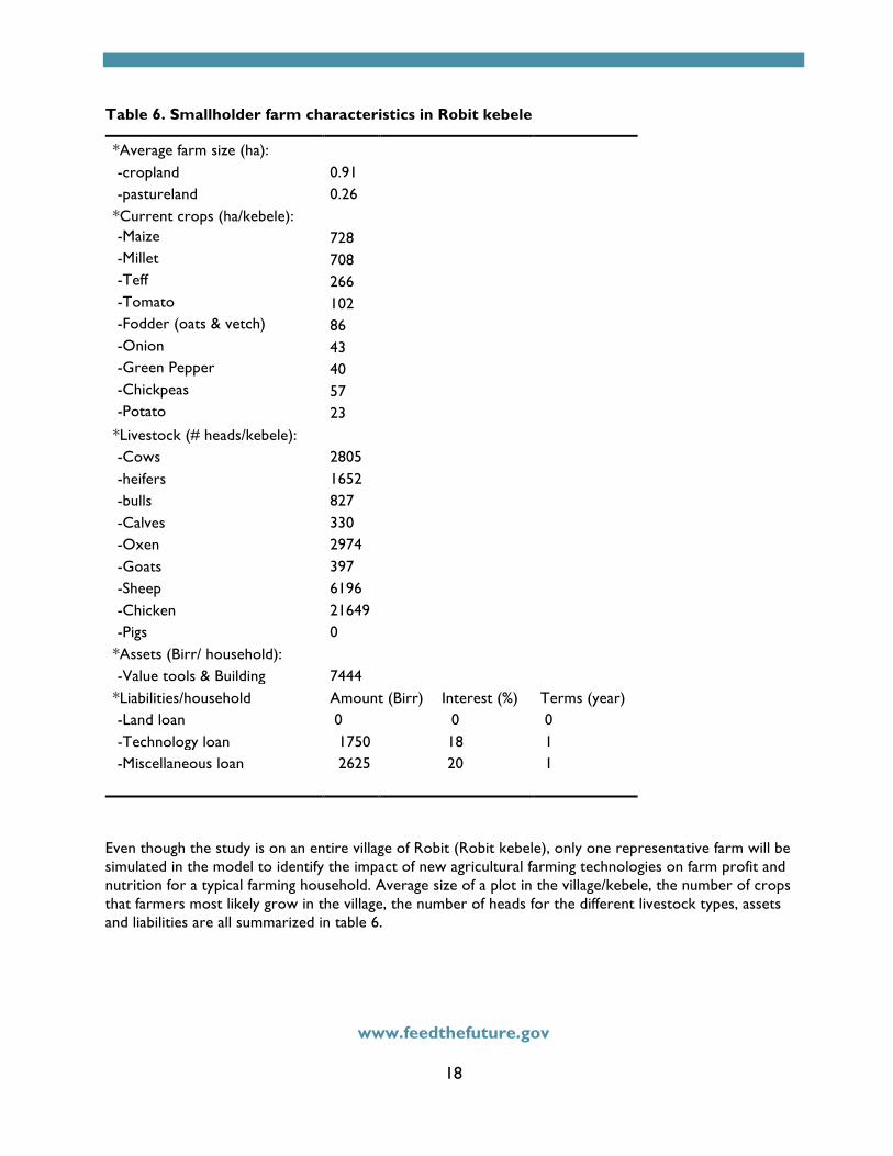
Table 6. Smallholder farm characteristics in Robit kebele
*Average farm size (ha): -cropland 0.91 -pastureland 0.26 *Current crops (ha/kebele): -Maize 728 -Millet 708 -Teff 266 -Tomato 102 -Fodder (oats & vetch) 86 -Onion 43 -Green Pepper 40 -Chickpeas 57 -Potato 23 *Livestock (# heads/kebele): -Cows 2805 -heifers 1652 -bulls 827 -Calves 330 -Oxen 2974 -Goats 397 -Sheep 6196 -Chicken 21649 -Pigs 0 *Assets (Birr/ household): -Value tools & Building 7444 *Liabilities/household Amount (Birr) Interest (%) Terms (year) -Land loan 0 0 0 -Technology loan 1750 18 1 -Miscellaneous loan 2625 20 1
Even though the study is on an entire village of Robit (Robit kebele), only one representative farm will be simulated in the model to identify the impact of new agricultural farming technologies on farm profit and nutrition for a typical farming household. Average size of a plot in the village/kebele, the number of crops that farmers most likely grow in the village, the number of heads for the different livestock types, assets and liabilities are all summarized in table 6.

www.feedthefuture.gov
19
Micro and macro level assumptions First, to show the full potential of adopting new technologies, we assumed that the alternative farming technologies (alternative scenarios) simulated in this study on crop production and use of water lifting technologies were adopted at 100 percent. The concern for farmers to acquire the irrigation tools such as pumps due to the high capital cost was partially addressed by making available, to farmers, loans to purchase the irrigation pumps through the Feed the Future Innovation Lab for Small Scale Irrigation (ILSSI)/International Water Management Institute (IWMI). As for livestock production technologies related to feeding animals with fodder and napier grass supplement, we assumed a 60% adoption rate, doubling the original adoption rate found from the household data survey which was 30 percent. Second, since the farmer’s profit mainly depends on the amount of crop and livestock (including livestock products) sold at the markets, accessibility to markets by the farmers is of paramount importance. The markets were assumed to be accessible and function competitively with no distortion where the supply and demand determine the market prices. Accessibility to markets and competitive market prices depend mainly on the existence of road and market infrastructure in the Bahir Dar Zuria district where survey results show that farmers reported on average 1.4 km (0.9 miles) distance to market. However, in the five-year economic forecast, market selling price in each of the five years was assumed to equal the average selling price of year 1 for each crop sold. Simulation results and discussion A baseline and four alternative scenarios were considered for this study to evaluate agricultural and livestock technologies in Robit Kebele of Amhara region in Ethiopia. The scenarios are defined as follows:
• Baseline: no irrigation + current fertilizers • Alt.1: irrigation of vegetables/fodder/napier grass with pulley and bucket + recommended
fertilizers • Alt.2: irrigation of vegetables/fodder/napier grass with rope-and-washer pump + recommended
fertilizers • Alt.3: irrigation of vegetables/fodder/napier grass with motor pump + recommended fertilizers • Alt.4: irrigation of vegetables/fodder/napier grass with solar pump + recommended • fertilizers
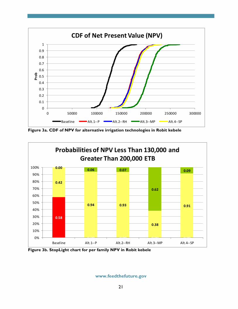
The results presented below in the stoplight chart and CDF graphs represent the year 5 simulation results from a 5-year forecasting period except for NCFI whose results are from year three. The farm-level simulation results for the five scenarios showed differences not only between the baseline and the alternative scenarios but also among the alternative scenarios in terms of financial variables (NCFI and EC) and nutrition. NPV NPV is an indicator that assesses the feasibility and profitability of an investment or project over a certain period of time. Overall, the NPV results, as illustrated by the CDF graph in figure 1a, indicate clearly that it is worth investing in irrigation and fertilizer application. The application of recommended fertilizers on grain and vegetable crops, together with the irrigation of vegetables and fodder crops using a pulley/tank,

www.feedthefuture.gov
20
rope-and-washer, motor, or solar pumps (Alts. 1, 2, 3, and 4, respectively) showed outstanding performance, in that their CDF values lie to the right of the baseline scenario for all 500 draws of the simulation model (fig. 3a). Notice that the motor pump scenario (Alt. 3) has the highest NPV value (at each risk level) compared to the pulley/tank, rope-and-washer and solar pump scenarios (Alts. 1, 2 and 4, respectively). All four of the alternative scenarios show higher NPV values than the baseline scenario. Legend Baseline: No irrigation; Alt.1--P: Pulley and Bucket; Alt.2--RH: Rope & Washer pump; Alt.3--MP: Motor pump Alt.4--SP: Solar pump The StopLight chart presents the probabilities of NPV being less than 130000 ETB (Ethiopian Birr) (red), greater than 200000 ETB (green), and between the two target values (yellow) for the five-year planning horizon (fig. 3b). The target values are: average NPV for the lowest-performing scenario (baseline scenario) for the lower bound; and the highest performing alternative scenario (Alt. 3) for the upper bound. In the baseline scenario, there is a 58% chance that NPV will be less than 130000 ETB, zero percent chance that NPV will exceed 200000 ETB, and 42% probability that NPV will fall between 130000 ETB and 200000 ETB. In the pulley/tank, rope-and-washer pump and solar pump scenarios (Alts. 1, 2 and 4, respectively) there is between 6% and 9% probability of generating NPV greater than 200000 ETB while there is about 93% chance to have an NPV that ranges between 130000 ETB and 200000 ETB. For the motor pump scenario (Alt. 3), there is a 62% probability that NPV will exceed the upper target of 200000 ETB, zero percent chance that NPV will be less than 130000 ETB and 38% that the NPV will fall between 130000 ETB and 200000 ETB. These results suggest that investment in motor-pump-based irrigation will increase the irrigated area, offset the costs, and pay large dividends by increasing income and wealth, more than any other water lifting technology. NCFI Annual NFCI measures the amount of profit generated by the farm for the baseline and alternative scenarios. The simulation results show that the motor pump scenario (Alt. 3) generated higher NCFI than the baseline and other alternative scenarios in that its CDF values lie completely to the right of the other scenarios (fig. 4a). The pulley/tank, rope-and-washer pump and solar pump scenarios (Alts. 1, 2 and 4, respectively) generated the next highest levels of NCFI. The StopLight chart for NCFI in year 3 of the 5-year planning horizon shows that, for a representative farm in the baseline scenario, there is a 53% probability that NCFI will be less than 20000 ETB and a 4% probability that NCFI will exceed 38000 ETB (fig. 4b). In contrast, in the motor pump scenario (Alt. 3), there is a 49% chance that annual NCFI will exceed 38000 ETB and an almost equal probability (48%) that NCFI will fall between 20000 and 38000 ETB. The second-best scenarios that generated higher profit are pulley/tank, rope-and-washer pump and solar pump scenarios (Alts. 1, 2 and 4, respectively), which recorded on average a 20% probability that NCFI will exceed 38000 ETB, and a 64% probability that annual NCFI will fall between 20000 and 38000 ETB. All of the alternative scenarios performed better and generated higher profits than the baseline scenario.
www.feedthefuture.gov
21
Figure 3a. CDF of NPV for alternative irrigation technologies in Robit kebele
Figure 3b. StopLight chart for per family NPV in Robit kebele
0
0.1
0.2
0.3
0.4
0.5
0.6
0.7
0.8
0.9
1
0 50000 100000 150000 200000 250000 300000
Prob
CDFofNetPresentValue(NPV)
Baseline Alt.1--P Alt.2--RH Alt.3--MP Alt.4--SP
0.58
0.00 0.00 0.00 0.00
0.42
0.94 0.93
0.38
0.91
0.00 0.06 0.07
0.62
0.09
0%
10%
20%
30%
40%
50%
60%
70%
80%
90%
100%
Baseline Alt.1--P Alt.2--RH Alt.3--MP Alt.4--SP
ProbabilitiesofNPVLessThan130,000andGreaterThan200,000ETB

www.feedthefuture.gov
22
Figure 4a. CDF of NCFI for Robit kebele
Figure 4b. StopLight chart for per-family NCFI in Robit kebele
00.10.20.30.40.50.60.70.80.91
0 10000 20000 30000 40000 50000 60000 70000 80000
Prob
CDFofNetCashFarmIncome(NCFI)inyear3
Baseline Alt.1--P Alt.2--RH Alt.3--MP Alt.4--SP
0.53
0.17 0.170.03
0.14
0.43
0.65 0.63
0.48
0.65
0.040.18 0.20
0.49
0.21
0%
10%
20%
30%
40%
50%
60%
70%
80%
90%
100%
Baseline Alt.1--P Alt.2--RH Alt.3--MP Alt.4--SP
ProbabilitiesofNCFILessThan20,000andGreaterThan38,000ETBinyear3

www.feedthefuture.gov
23
EC The EC simulation results highlight once again the dominant performance of the pulley/tank, motor, solar and rope-and-washer pump scenarios (Alts. 1, 3, 4 and 2). The pulley/tank, rope-and-washer and solar pumps scenarios (Alt. 1, 2, and 4) performed better than the baseline scenario but generated lower EC compared to the alternative scenario 3 which leads all the scenarios and involved the use of a motor pump (fig. 5a). The StopLight chart for EC shows that, in the baseline scenario, there is a 55% probability that EC in year 5 will be less than 102000 ETB and a 0% probability that EC will exceed 188000 ETB, respectively the averages of the baseline and alternative 3 scenario (motor pump) ending cash reserves (fig. 5b). Alternatively, in the motor pump scenario, there is a zero probability that EC will be less than 102000 ETB, and a 49% probability that EC will exceed 188000 ETB. The second-best choices are the pulley/tank, rope-and-washer and solar pump scenarios (Alts. 1, 2 and 4, respectively), which have between 4% and 5% chance of generating EC greater than 188000 ETB. Notice that all the alternative scenarios (Alts.1-4) generate higher EC than the baseline scenario. The above results show in general that the largest increase in net cash farm income and annual ending cash reserves is associated with the use of motor pump due to the increase in irrigated land area without water stress. Given that grain crops in Robit are mainly used for family consumption, the increases in farm revenue in each of the alternative scenarios are due largely to the sale of surplus tomato and cabbage rather than animal feed (fodder and napier grass). Two reasons may explain this situation. First, a portion of the animal feed production was used to feed livestock for meat and milk production, reducing thus the quantity allocated for sale at the market. Second, the increase in production of animal feed under the best performing alternative scenario (motor pump) did not result in an increase in net profit due to the high cost of production. Note however that the percentage of napier grass sold increased from 70% in baseline to 87% in alternative scenario three (motor pump) while fodder increased from 0% in baseline to 93.4% in alternative scenario three (Alt. 3-motot pump). Over the five years, the best performing scenario (Alt. 3), forecasted that sales of tomatoes and cabbage contributed 55% and 26% respectively to the total crops receipts, and 72% and 26%, respectively, to the net cash (profit). Nutrition results In general, adoption and proper use of agricultural technologies contribute to an increase in the quantity and variety of crops produced. The implications for family nutrition vary according to the types of crops grown and consumed. However, surplus crops can be sold and resulting revenues can be used to buy food items needed to complement nutrition requirements. In Robit kebele, the quantities of crops and livestock products consumed by families in both the baseline and alternative scenarios meet minimum daily requirements for calories, proteins, iron and vitamin A but were insufficient to meet minimum daily requirements for calcium and fat (see more detailed information on minimum requirements in FAO, 2001 and FAO, 2008). Moreover, the LIVES survey shows that individual households do not currently purchase large quantities of food or receive any food aid to supplement the food that they produce. Table 7 summarizes simulation results based on the last year of the 5-year planning horizon. Specifically, it lists the nutritional variables measured, the probability that the quantity of each nutrient consumed will exceed the minimum daily requirement, and whether the amounts consumed in the alternative scenarios show an improvement as compared to the baseline scenario.

www.feedthefuture.gov
24
Figure 5a. CDF of EC in Robit kebele
Figure 5b. StopLight chart for per-family EC in Robit kebele
0
0.10.20.30.40.50.60.70.80.9
1
0 50000 100000 150000 200000 250000 300000
Prob
CDFofEndingCashReserves(EC)
Baseline Alt.1--P Alt.2--RH Alt.3--MP Alt.4--SP
0.55
0.01 0.02 0.00 0.01
0.45
0.95 0.93
0.51
0.94
0.00 0.04 0.04
0.49
0.05
0%
10%
20%
30%
40%
50%
60%
70%
80%
90%
100%
Baseline Alt.1--P Alt.2--RH Alt.3--MP Alt.4--SP
ProbabilitiesofECLessThan102,000andGreaterThan188,000ETBinyear5

www.feedthefuture.gov
25
Table 7. Summary results for nutritional and scenarios performance in Robit kebele
Performance Nutrition variables Excess or deficit Probability: nutrient cons > Improvement from
min requirement baseline to alternative Calories Excess 1 Yes
Proteins Excess 1 Yes
Fat Deficit 0.18 Yes
Calcium Deficit 0 Yes
Iron Excess 1 Yes
Vitamin A Excess 1 Yes
Simulation results for each of the nutrition variables analyzed in this study are discussed in greater detail below. Calorie intake simulation results Grain or cereal crops represent the basic staple food and a source of calories (or energy) in many developing countries with agriculture-based economies, including Ethiopia (Gierend et al. 2014). In this study, the grain crops analyzed are teff, maize, and millet. Survey information shows that, on average, 68% of all grains produced by households in Robit kebele are consumed at home. The allocation of large land areas to the grain crops and the use of fertilizer contributed to an increase in grain production and mitigated any deficiency in energy and calories requirement per adult for both the baseline and alternative scenarios. In fact, for a typical household in Robit kebele, the simulation results indicate an average daily calories intake of 2700 and 3600 calories, respectively for the baseline and alternative scenarios which is significantly higher than the daily minimum requirement of 1750 calories per adult equivalent (AE) (fig. 6a). The StopLight chart for daily energy consumption per AE is presented in figure 6b. In the baseline scenario, there is a 29% chance that daily energy consumption per AE will be less than 2700 calories and a 71% chance that it will be between 2700 and 3600 calories. There is a 74% or greater probability of exceeding this target value of 3600 for the four alternative scenarios. Note that the high target value of 3600 calories represents the average daily calories intake per AE for the four alternative scenarios.

www.feedthefuture.gov
26
Figure 6a. CDF of daily energy consumption per AE on a farm in Robit kebele
Figure 6b. StopLight Chart for daily energy consumption per AE on a farm in Robit kebele
0
0.1
0.2
0.3
0.4
0.5
0.6
0.7
0.8
0.9
1
0 500 1000 1500 2000 2500 3000 3500 4000 4500
Prob
CDFofdailyenergyconsumption(cal)peradult
Baseline Alt.1--P Alt.2--RH Alt.3--MP Alt.4--SP MinKCal
0.29
0.00 0.00 0.00 0.00
0.71
0.26 0.260.18
0.25
0.00
0.74 0.740.82
0.75
0%
10%
20%
30%
40%
50%
60%
70%
80%
90%
100%
Baseline Alt.1--P Alt.2--RH Alt.3--MP Alt.4--SP
ProbabilitiesofdailyenergyconsumptionperadultLessThan2,700andGreaterThan3,600calories

www.feedthefuture.gov
27
Protein intake simulation results Animal products are often the main source of proteins at the household level. However, household surveys showed that the majority of the proteins consumed in Robit kebele were obtained from crops rather than animal products. This is a general pattern in many developing countries, and particularly in Ethiopia where the per capita consumption of livestock products, especially meat, is extremely low (Tafere and Worku 2012). The simulation results in figure 7a show that on average households in both the baseline and alternative scenarios meet and exceed the daily minimum requirement for proteins intake (67 and 93 grams/AE respectively compared to minimum requirement of 41 gr/AE). There is a significant improvement in protein intake for the alternative scenarios compared to the baseline scenario. The StopLight chart for protein consumption indicates that the four-alternative scenario performed significantly better than the baseline scenario in terms of protein intake (fig. 7b). The simulation results show that there is a zero probability that the daily protein intake per AE will be less than the minimum daily requirement of 41 grams for both the baseline and alternative scenarios. The chance that daily protein intake per AE will exceed 93 grams is zero in the baseline scenario but 55% for alternative 3 while the probability of having a daily protein intake less than 67 grams is 38% for the baseline scenario and zero for the alternative scenarios. Note that on average, the baseline and alternative scenarios protein intake (67 and 93 grams respectively) are significantly higher than the minimum required amount (41grams). Fat intake simulation results Fat along with carbohydrates are the main source of energy, providing the essential number of calories for the human body to function. Additionally, fat-soluble vitamins such as Vitamin A are easily absorbed by the body with a balanced dietary fat content (Global Hunger Index 2014). Simulation results for fat presented as a CDF graph in Robit kebele show a deficit in fat intake for both the baseline and alternative scenarios (fig. 8a). Although there is an improvement of fat intake between the baseline and the alternative scenarios, their respective averages, 28 and 37 grams, are still below the average of 39 grams daily minimum fat requirement for an adult. The StopLight chart for fat indicates a 35% probability that the fat intake per AE will be less than 28 grams and zero probability that it will be greater than 39 grams for the baseline scenario (fig. 8b). Alternatively, there is a zero probability that the fat intake per AE will be less than 28 grams and 30% chance on average it will be greater than 39 grams for alternative three. Note that there is respectively 65% and 77% probability that the daily fat intake for an AE ranges between 28 grams and 39 grams for the baseline and alternative scenarios.

www.feedthefuture.gov
28
Figure 7a. CDF of daily proteins consumption per AE on a farm in Robit kebele
Figure 7b. StopLight Chart for daily protein consumption per AE on a farm in Robit kebele
0
0.1
0.2
0.3
0.4
0.5
0.6
0.7
0.8
0.9
1
0 20 40 60 80 100 120
Prob
CDFofproteinintakeperadult(grams)
Baseline Alt.1--P Alt.2--RH Alt.3--MP Alt.4--SP MinGPro
0.38
0.00 0.00 0.00 0.00
0.62
0.72 0.72
0.45
0.69
0.00
0.28 0.28
0.55
0.31
0%
10%
20%
30%
40%
50%
60%
70%
80%
90%
100%
Baseline Alt.1--P Alt.2--RH Alt.3--MP Alt.4--SP
ProbabilitiesofproteinintakeLessThan67andGreaterThan93grams
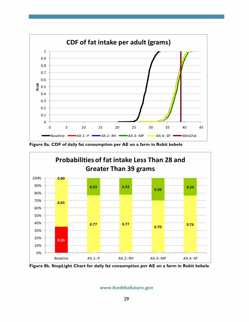
www.feedthefuture.gov
29
Figure 8a. CDF of daily fat consumption per AE on a farm in Robit kebele
Figure 8b. StopLight Chart for daily fat consumption per AE on a farm in Robit kebele
0
0.1
0.2
0.3
0.4
0.5
0.6
0.7
0.8
0.9
1
0 5 10 15 20 25 30 35 40 45
Prob
CDFoffatintakeperadult(grams)
Baseline Alt.1--P Alt.2--RH Alt.3--MP Alt.4--SP MinGFat
0.35
0.00 0.00 0.00 0.00
0.65
0.77 0.770.70 0.76
0.00
0.23 0.220.30 0.24
0%
10%
20%
30%
40%
50%
60%
70%
80%
90%
100%
Baseline Alt.1--P Alt.2--RH Alt.3--MP Alt.4--SP
ProbabilitiesoffatintakeLessThan28andGreaterThan39grams

www.feedthefuture.gov
30
Calcium intake simulation results The simulation results for calcium show large deficits in calcium intake in both the baseline and alternative scenarios (figs. 9a and 9b). The average calcium intake per AE is around 0.19 and 0.35 grams, respectively, for the baseline and four alternative scenarios, falling short of the daily minimum requirements of 1 gram per AE (fig. 9a). Note however the significant improvement of calcium intake from the baseline to the alternative scenarios. The StopLight chart in figure 9b shows that there is a 43% probability that the daily calcium intake per AE will be less than 0.19 grams and a zero probability that the intake will exceed 0.35 grams for the baseline. Alternatively, there is a zero probability that the calcium intake amount will be less than 0.19 grams and an average of 42% chance that the intake will exceed 0.35 grams for the alternative scenarios under the pulley/tank, rope and washer and solar pumps (second best performing scenarios). Under the motor pump alternative scenario, the calcium intake has an 88% chance of exceeding 0.35 grams which is almost one third of the minimum requirement for an adult equivalent (AE). Iron intake simulation results The consumption of micronutrients like iron, zinc, vitamin A, and iodine is important for human health and well-being (Global Hunger Index 2014), aiding in the absorption of other nutrients, and in child development. Iron deficiency, specifically, is a risk factor for maternal mortality and causes anemia in both mothers and children (Domenech 2015). Simulation results indicated that households in Robit kebele consume more than the required minimum levels of iron. The average iron intake per AE of all scenarios, estimated at 0.023 grams (or 23 mg), was more than two times greater than the daily minimum requirement of 0.009 grams (or 9 mg) per AE (fig. 10a). There was also a significant improvement between the baseline and the alternative scenarios in terms of iron intake, which averaged 0.19 and 0.27 grams respectively. The StopLight chart for iron intake indicates that the four alternative scenarios perform significantly better than the baseline scenario in terms of iron availability (fig. 10b). In the baseline scenario, there is a 34% probability that the daily iron intake per AE will be less than 0.019 grams and zero chance that the daily iron intake will be greater than 0.027 grams. Alternatively, there is on average a 75% chance that the daily iron intake per AE will exceed 0.027 grams and a zero chance that daily iron intake will be less than 0.019 grams for the four alternative scenarios. The target values (0.019 and 0.027 grams respectively) are the averages of the baseline and alternative scenarios.

www.feedthefuture.gov
31
Figure 9a. CDF of daily calcium consumption per AE on a farm in Robit kebele
Figure 9b. StopLight Chart for daily calcium consumption per AE on a farm in Robit kebele
0
0.1
0.2
0.3
0.4
0.5
0.6
0.7
0.8
0.9
1
0 0.2 0.4 0.6 0.8 1 1.2
Prob
CDFofcalciumintakeperadult(grams)
Baseline Alt.1--P Alt.2--RH Alt.3--MP Alt.4--SP MinGCal
0.43
0.00 0.00 0.00 0.00
0.57
0.60 0.58
0.12
0.56
0.00
0.40 0.42
0.88
0.44
0%
10%
20%
30%
40%
50%
60%
70%
80%
90%
100%
Baseline Alt.1--P Alt.2--RH Alt.3--MP Alt.4--SP
ProbabilitiesofcalciumintakeLessThan0.19andGreaterThan0.35grams

www.feedthefuture.gov
32
Figure 10a. CDF of daily iron consumption per AE on a farm in Robit kebele
Figure 10b. StopLight Chart for daily iron consumption per AE on a farm in Robit kebele
0
0.1
0.2
0.3
0.4
0.5
0.6
0.7
0.8
0.9
1
0 0.005 0.01 0.015 0.02 0.025 0.03 0.035
Prob
CDFofironintakeperadult(grams)
Baseline Alt.1--P Alt.2--RH Alt.3--MP Alt.4--SP MinGIron
0.34
0.00 0.00 0.00 0.00
0.66
0.32 0.330.17
0.31
0.00
0.68 0.670.83
0.69
0%
10%
20%
30%
40%
50%
60%
70%
80%
90%
100%
Baseline Alt.1--P Alt.2--RH Alt.3--MP Alt.4--SP
ProbabilitiesofironintakeLessThan0.019andGreaterThan0.027grams

www.feedthefuture.gov
33
Vitamin A intake simulation results Like iron, iodine, and zinc, vitamin A is an important micronutrient. Vitamin A is essential for healthy vision and plays a vital role in bone growth, reproduction and a healthy immune system. The simulation results for vitamin A intake indicate adequate to surplus vitamin A intake levels in both the baseline and alternative scenarios (figs. 11a & 11b). The average levels of vitamin A intake for the baseline (0.0026 grams) and the alternative scenarios (0.0064 grams) are 4 to 10 times higher than the daily minimum requirement for an adult equivalent (0.0006 grams) (fig. 11a). The StopLight chart in figure 11b shows, for the baseline scenario, that there is a 45% probability that the daily vitamin A intake per AE will be less than 0.0026 grams (baseline average), while there is a zero probability that the vitamin A intake will be greater than 0.0064 grams (alternative scenarios average). Likewise, for the alternative scenario under the motor pump, there is zero chance that the vitamin A intake will be less than the average baseline vitamin A intake for an adult while there is a 51% chance that vitamin A intake will exceed 0.0064 grams. The average of the three other alternative scenarios (pulley/tank, rope and washer pump and solar pump) shows a 32% chance that the vitamin A intake will exceed 0.0064 grams while there is a zero chance the vitamin A intake to be less than 0.0026 grams. Simulated levels of nutrition variables (calories, proteins, fat, calcium, iron and vitamin A) available to farm families increased substantially in the alternative scenarios because of production increases in the alternative scenarios due to farming technology (fertilizer and irrigation) and crop diversification. The increase in yields allowed farm families to produce sufficient food for consumption, which provided different nutrients needed for human consumption. Also, the representative farm grew seven different crops ranging from grains (maize, teff and millet), vegetables (tomatoes and cabbage), root crops (potatoes), pulse (chickpeas), and animal feed (fodder and napier). Although the animal feed crops are not directly used to feed humans but the feed is fed to livestock for milk, butter and meat production used in human consumption. For instance, milk is known to be a good source of calcium especially for growing children; the same as butter and meat, which are good sources of fat and proteins respectively. A grain crop such as maize with high content in carbohydrates is a good source not only for calories but also for fat and proteins. Teff calcium content is also outstanding, coming in second to animal products such as milk and cheese, and outperforming other crops consumed in the household. As for the vegetables, their consumption is a good source of vitamin A, a trace or micronutrient element needed for a healthy vision and immune system. The deficiencies in fat and calcium can be filled by the consumption of linseed, niger seed in addition to milk, eggs and cheese to increase the intake in calcium while the consumption of butter and livestock meat would increase fat intake. Note that the food purchased by the household, as shown in the household survey, ranged from potatoes, barley, wheat, mutton, beef and goat meat and contributed significantly to the family nutrition. Clearly, food supplements either through purchase or farming to increase the intake for fat and calcium will be needed to meet the nutritional requirements and the well-being of the families in Robit kebele. Ranking of alternative farming technologies Choosing among risky alternative can be difficult. Decision makers rank risky alternatives based on their utility for income and risk. Many ranking procedures do not take into account utility (e.g., mean, standard deviation, PDF, CDFs, and coefficient of variation) but the best approaches use utility to rank scenarios. We use SERF to identify the preferred risky scenario given its many advantages over the other ranking approaches.

www.feedthefuture.gov
34
Figure 11a. CDF of daily vitamin A consumption per AE on a farm in Robit kebele
Figure 11b. StopLight Chart for daily vitamin A intake per AE on a farm in Robit kebele
0
0.1
0.2
0.3
0.4
0.5
0.6
0.7
0.8
0.9
1
0 0.001 0.002 0.003 0.004 0.005 0.006 0.007 0.008 0.009
Prob
CDFofVitAintakeperadult(grams)
Baseline Alt.1--P Alt.2--RH Alt.3--MP Alt.4--SP MinGVitA
0.45
0.00 0.00 0.00 0.00
0.55
0.69 0.670.49
0.67
0.00
0.31 0.330.51
0.33
0%
10%
20%
30%
40%
50%
60%
70%
80%
90%
100%
Baseline Alt.1--P Alt.2--RH Alt.3--MP Alt.4--SP
ProbabilitiesofVitAintakeLessThan0.0026andGreaterThan0.0064grams

www.feedthefuture.gov
35
Figure 12a. SERF ranking of alternative farming systems in Robit kebele
Figure 12b. Risk premiums ranking of alternative farming systems in Robit kebele
Baseline
Alt.1--P
Alt.2--RH
Alt.3--MP
Alt.4--SP
10,000.00
15,000.00
20,000.00
25,000.00
30,000.00
35,000.00
40,000.00
CertaintyEquivalent
StochasticEfficiencywithRespecttoAFunction(SERF)UnderaNeg.ExponentialUtilityFunction
Baseline Alt.1--P Alt.2--RH Alt.3--MP Alt.4--SP
RiskNeutral
NormalRiskAversion
ModeratelyRisk Averse
ExtremelyRisk Averse
Baseline
Alt.1--P
Alt.2--RH
Alt.3--MP
Alt.4--SP
-
2,000.00
4,000.00
6,000.00
8,000.00
10,000.00
12,000.00
14,000.00
16,000.00
18,000.00
20,000.00
Neg.ExponentialUtilityWeightedRiskPremiumsRelativetoBaseline
Baseline Alt.1--P Alt.2--RH Alt.3--MP Alt.4--SP
RiskNeutral
NormalRiskAversion
ModeratelyRisk Averse
ExtremelyRisk Averse

www.feedthefuture.gov
36
In this study, the five scenarios (the baseline and four alternative scenarios) were ranked based on the year 3 simulation results for NCFI. Results in figure 12a show that the motor pump scenario (Alt. 3) is distinctively the most preferred scenario across all levels of risk aversion, ranging from 0 to 0.00025. Alternative 3 is the preferred scenario because the certainty equivalence values at every RAC level are greater than the other scenarios. The next most preferred scenarios are the pulley/tank and solar pump scenarios (Alts. 1 and 4) which are slightly ranked higher than the rope and washer pump (Alt. 2). In figure 12a the CEs for all scenarios functions decrease as we assume an increasingly risk averse decision maker. Notice that the rope and washer scenario crosses with the pulley/tank scenario and are not significantly far from each other, which implies some level of indifference of the decision maker in choosing between the two tools for irrigation. Three water lifting technologies scenarios (pulley, solar and rope and washer) are very close in ranking but performed distinctively better than the baseline scenario (no irrigation). The SERF option in Simetar produces as well a risk premium (RP) chart (fig. 12b). The chart shows the perceived premium that each risky scenario provides relative to the base scenario at different risk aversion levels. A positive RP over the range of RAC for an alternative scenario means that the alternative scenario is preferred over the baseline while a negative RP would mean the preference of the baseline scenario over the alternative scenario. Also, the difference in RP implies how much additional benefit in terms of NCFI a decision maker can receive by adopting a higher ranking alternative scenario compared to a baseline scenario. In this study, the motor pump scenario (Alt. 3) has the highest risk premium compared to other alternative scenarios and the baseline scenario. It is followed by the alternative scenario four (Alt. 4) that involves the use of a solar pump whose risk premium is slightly higher than that of a pulley/tank and rope and washer pump scenarios. Alternative 3 offers a moderately risk averse decision maker an RP of 16,000 ETB per year over the baseline scenario. Conclusions and policy recommendations The objective of this study was to evaluate the impacts of adopting agricultural technologies (increased fertilizers and irrigation) on household nutrition and farm profitability in Robit kebele, Bahir Dar Zuria woreda, Amhara region of Ethiopia. A baseline scenario with current fertilizer application rates and no or minimal irrigation was compared to four alternative scenarios where recommended fertilizers rates and irrigation were applied to crops. In the alternative scenarios, increased fertilizer rates were applied only to grow teff and potatoes since millet and maize showed adequate amounts of fertilizer as shown by the household surveys. Tomato, cabbage, fodder and napier grass received increased levels of fertilizers as well and were irrigated during the dry season using one of four alternative water-lifting technologies that include pulley/tank, rope and washer, motor and solar pumps. The preferred scenario, consisting of the use of recommended fertilizers in combination with motor-pump irrigation of tomato, cabbage, fodder, and napier grass, was alternative 3 (Alt. 3) which generated the highest income and profits for the farm. The next-best performing scenarios used pulley/tank, rope-and-washer or solar pump for irrigation in combination with recommended fertilizers (Alts. 1, 2 and 4, respectively). It is worth noting that the solar pump had the same outcome in terms of profit as the pulley/tank, rope and washer pump despite the relatively high investment costs of the solar pump. The baseline scenario was the least preferred of all five scenarios analyzed. The use of improved farming systems based on fertilizer and irrigation technologies had a positive impact on livestock production which increased the meat and milk output and improved the consumption of animal products at the household level. Nutrition levels improved significantly in the four alternative scenarios compared to the baseline scenario. This was a result of the improvements in crop yields due to the application of fertilizer and irrigation technologies. We would therefore propose expanding the types

www.feedthefuture.gov
37
of crops irrigated in the dry season to increase family nutrition and net cash income, but only if such crops can be irrigated without causing excessive soil erosion or reduction in environmental benefits. Further studies would focus on how the profits could increase if households shared a single pump for irrigation in the dry season, and on how diversifying the crops consumed (whether through the farming of additional crops or purchase) could impact nutrition. References
Amede, T. (2012). Rainwater management for Sustainable Agricultural Intensification in the Ethiopian Highlands. Presentation at 2012 World Water Week in Stockholm, Sweden.
Anderson, J.R. and J.L. Dillon J.L. (1992). Risk Analysis in Dryland Farming Systems. Farming Systems Management Series No. 2, FAO, Rome.
Anderson, J.R. and Hardaker, J.B. (2003). Risk aversion in economic decision-making: Pragmatic guides for consistent choice by natural resource managers’, in J. Wesseler, H.-P.Weikard and R. Weaver (eds), Risk and Uncertainty in Environmental Economics, Edward Elgar, Cheltenham, pp. 171–188.
Arnold, J., J. R. Williams, R. Srinivasan, K. W. King, and R. H. Griggs. (1994). SWAT-Soil and Water Assessment Tool. USDA, Agricultural Research Service, Grassland, Soil and Water Research Laboratory, Temple, Texas.
Barungi, M., & Maonga, B. B. (2011). Adoption of soil management technologies by smallholder farmers in central and southern malawi. Journal of Sustainable Development in Africa, 13(3), 28-38.
Cruz FA. (1987). Adoption and diffusion of agricultural extensions. In: An introduction to extension delivery systems by JB Valera, VA Martinez, and RF Plopino eds. 1987. Island Publishing House, Manila. P. 97-127.
De Janvry, A., Dustan, A., & Sadoulet, E. (2010). Recent advances in impact analysis methods for ex-post impact assessments of agricultural technology: Options for the CGIAR. SPIA report version 3.1. University of California at Berkeley.
Deressa, T. T., Hassan, R. M., Ringler, C., Alemu, T., & Yesuf, M. (2009). Determinants of farmers’ choice of adaptation methods to climate change in the nile basin of ethiopia. Global Environmental Change, 19(2), 248-255.
Diagne, A., Glover, S., Groom, B., and Phillips J. (2012). Africa’s Green Revolution? The determinants of the adoption of NERICAs in West Africa. SOAS Department of Economics Working Paper Series, No. 174, SOAS, University of London.
Di Falco, S., & Chavas, J. (2009). On crop biodiversity, risk exposure, and food security in the highlands of ethiopia. American Journal of Agricultural Economics, 91(3), 599-611.
Domènech, L. (2015). Is reliable water access the solution to undernutrition? A review of the potential of irrigation to solve nutrition and gender gaps in Africa south of the Sahara.
Food and Agriculture Organization of the United Nations (FAO). (2001). Human Vitamin and Mineral Requirements. Report of a Joint FAO/WHO Expert Consultation. Nutrition Division, Food and Agricultural Organization of the United Nations, Rome, Italy.
Food and Agriculture Organization of the United Nations (FAO). (2008). Fats and Fatty Acids in Human Nutrition. Report of an Expert Consultation. Food and Agricultural Organization of the United Nations, Rome, Italy.
Gebregziabher, G., Rebelo, L-M., Notenbaert, A., Ergano, K., & Abebe, Y. (2013). Determinants of Adoption of Rainwater Management Technologies among Farm Households in the Nile River Basin. IWMI Research Report 154. Available at:
http://www.iwmi.cgiar.org/Publications/IWMI_Research_Reports/PDF/pub154/rr154.pdf?galog=no Gebremedhin, B., Hoekstra, D., Tegegne, A., Shiferaw, K., & Bogale, A. (2015). Factors determining
household market participation in small ruminant production in the Highlands of Ethiopia.

www.feedthefuture.gov
38
Gierend, A., Tirfessa, A., Abdi, B. B., Seboka, B., & Nega, A. (2014). A combined ex-post/ex-ante impact analysis for improved sorghum varieties in Ethiopia, socioeconomics discussion paper series number 22.
Global Hunger Index. 2014. The Challenge of Hidden Hunger. Washington, DC: IFPRI. Available online at http://www.ifpri.org/publication/2014-global-hunger-index.
Hardaker, J. B., Richardson, J. W., Lien, G., & Schumann, K. D. (2004). Stochastic efficiency analysis with risk aversion bounds: A simplified approach. Australian Journal of Agricultural and Resource Economics, 48(2), 253-270.
Hardaker, J., Huirne, R., Anderson, J. R., & Lien, G. (2004). Coping with risk in agriculture. Oxfordshire, OX: CABI Publishing. McDonald, M., & Brown, K. (2000). Soil and water conservation projects and rural livelihoods: Options for
design and research to enhance adoption and adaptation. Land Degradation & Development, 11(4), 343-361.
Merrey, D. J., & Gebreselassie, T. (2011). Promoting improved rainwater and land management in the Blue Nile (Abay) basin of Ethiopia: Annexes.
Minot, N., & Sawyer, B. (2013). Agricultural production in Ethiopia: Results of the 2012 ATA baseline survey.
Norton, G. (2014). Hunger and Hope: Escaping Poverty and Achieving Food Security in Developing Countries. Long Grove, IL: Waveland Press, Inc.
Palma, M. A., Richardson, J. W., Roberson, B. E., Ribera, L. A., Outlaw, J., & Munster, C. (2011). Economic feasibility of a mobile fast pyrolysis system for sustainable bio-crude oil production. International Food and Agribusiness Management Review, 14(3)
Qasim, M. (2012). Determinants of farm income and agricultural risk management strategies: The case of rain-fed farm households in pakistan's Punjab. Kassel University press GmbH.
Rashid, S., Tefera, N., Minot, N., & Ayele, G. (2013). Fertilizer in Ethiopia: An assessment of policies, value chain, and profitability. IFPRI Discussion Paper 01304.
Richardson, J. W. (2006). Simulation for applied risk management. Unnumbered staff report, Department of Agricultural Economics, Agricultural and Food Policy Center, Texas A&M University, College Station, Texas.
Richardson, J. W., S. L. Klose, and Gray A. W. (2000). An applied procedure for estimating and simulating multivariate empirical (MVE) probability distributions in farm-level risk assessment and policy analysis. Journal of Agricultural and Applied Economics 32(2), 299-315.
Richardson, J. W., Herbst, B. K., Outlaw, J. L., & Gill, R. C. (2007). Including risk in economic feasibility analyses: The case of ethanol production in texas. Journal of Agribusiness, 25(2), 115.
Richardson, J. W., K. Schumann, and Feldman, P. (2006). Simetar: Simulation for Excel to analyze risk. Unnumbered staff report, Department of Agricultural Economics, Texas A&M University, College Station, Texas.
Richardson, J.W. & Nixon, C.J. (1985). FLIPSIM V: A General Firm Level Policy Simulation Model. B-1528. Department of Agricultural Economics, Texas A & M University, USA.
Shitarek, T. (2012). Ethiopia: Country Report, UK. Available at: https://www.gov.uk/government/uploads/system/uploads/attachment_data/file/197474/Econ-Res-Ethiopia-Country-Report.pdf (accessed in August 2013).
Soule, M. J., Tegene, A., & Wiebe, K. D. (2000). Land tenure and the adoption of conservation practices. American Journal of Agricultural Economics, 82(4), 993-1005.
Tafere, K., & Worku, I. (2012). Consumption patterns of livestock products in Ethiopia: Elasticity estimates
using HICES (2004/05) data. International Food Policy Research Institute (IFPRI) - Ethiopian Development Research Institute (EDRI), Addis Ababa, Ethiopia.

www.feedthefuture.gov
39
United Nations-Office for the Coordination of Humanitarian Affairs (UN-OCHA). 2016. Weekly Humanitarian Bulletin: Ethiopia. http://reliefweb.int/sites/reliefweb.int/files/resources/humanitarian_bulletin_4_january_2016.pdf. Accessed Jan. 2016.
United States Agency for International Development (USAID) (2011). Ethiopia Multi-Year Strategy. Available at: https://www.usaid.gov/sites/default/files/documents/1860/USAID%20FtF%20MYS%20Final%20Version.pdf. Accessed in October 2015.
Williams, J.R., J. G. Arnold, R. Srinivasan, and T. S. Ramanarayanan. 1998. APEX: A new tool for predicting the effects of climate and CO2 changes on erosion and water quality. In Modelling Soil Erosion by Water, ed. J. Boardman and D. Favis-Mortlock, 441-449. Heidelberg: Springer-Verlag.
Yengoh, G. T., Armah, F. A., & Svensson, M. G. (2009). Technology adoption in small-scale agriculture. Science, Technology and Innovation Studies, Vol. 5 (2), 111-131.
Zemadim, B., McCartney, M., Sharma, B., & Wale, A. (2011). Integrated rainwater management strategies in the blue nile basin of the ethiopian highlands. International Journal of Water Resources and Environmental Engineering, 3(10), 220-232.

www.feedthefuture.gov
40
APPENDICES Appendix A: FARMSIM Flowchart (excel worksheet organization)
Abbreviations and meaning of different worksheets in FARMSIM:
PRCBASE: price worksheet in baseline scenario
CropBASE: crop worksheet in baseline scenario
LVSKBASE: livestock worksheet in baseline scenario
NUTBASE: nutrition worksheet in baseline scenario
TABLEBASE: table worksheet in baseline scenario
Note: same meaning of the above worksheets applies to the alternative scenarios (CropALT…)
KOV: key output variable
SIMOUT: simulation output

www.feedthefuture.gov
41
Appendix B: FARMSIM model equations The equations in FARMSIM are summarized as follows: Stochastic annual yields are simulated as:
(1) !"#$%&' = !"#$%&' ∗ 1 + -./-0 12, 4 5 , 67182' !"#$%&'"9:#;<="#$%>?@A>B""<=#;AC, -./-0"9Cℎ#:E$C"F;A";C##:B"A"@;$?E<@C"><, 12"9Cℎ#:;CA"5>??A;@C"><;$%#F";C"><9?A>::#;<="#$%9?>A;$$@A>B9, 4 5 "9Cℎ#@E:E$;C"F#%"9CA"GEC"><0C>1?>ACℎ#12:;CA"5, ;<% 6�182"9;F#@C>A>?@>AA#$;C#%E<"?>A:9C;<%;A%%#F";C#9?>A@A>B="#$%9"<=#;AC.
All equations are repeated for both the base and alternative scenarios. In the case of crop yield each scenario has a different Sy matrix and !ieldNO vector to match the technology, but use the same CUSDy vector so both scenarios experience the same weather shocks. The model allows the farm to have up to 15 crops which can be made up of field crops and kitchen garden crops. Stochastic annual crop prices are simulated as:
(2) 0A"@#6&' = 0A"@#6&' ∗ 1 + -./-0 1P, 4 5 , 6718P' 0A"@#6&'"9:#;<BA"@#?>A@A>B""<=#;AC, -./-0"9Cℎ#:E$C"F;A";C##:B"A"@;$?E<@C"><, 1P"9Cℎ#:;CA"5>??A;@C"><;$%#F";C#9?A>::#;<BA"@#9?>A;$$@A>B9, 4 5 "9Cℎ#@E:E$;C"F#%"9CA"GEC"><0C>1?>ACℎ#1P:;CA"5, ;<% 6718P'"9;F#@C>A>?@>AA#$;C#%E<"?>A:9C;<%;A%%#F";C#9?>A@A>BBA"@#9"<=#;AC.
The mean price vectors can differ between the base and alternative technology scenarios if one scenario assumes a different marketing option or a different quality of the crop. The multivariate empirical methodology used by FARMSIM is described in detail in Richardson, Klose, and Gray (2000). Production of each crop i is simulated as: (3) 0A>%&' = Q@A#9&' ∗ !"#$%&' Acresit is the land area devoted to the crop and can be acres, hectares, or any other local name for land area. The model simulates the production identity using stochastic yield so production for each crop is stochastic given weather shocks to yields. The quantity of the crop which can be sold is the residual after subtracting out the quantity consumed by the family and livestock. Family consumption and livestock feed requirements are identities that are simulated as: (4) 4;:"$=6><9E:BC"><&' = R4& ∗ S>. Q%E$C/TE"F;$#<C QFi is the minimum quantity of crop i consumed per adult equivalent per year and No. Adult Equivalent is the number of adult equivalents in the farm family. (5) �"F#9C>@U4##%&' = (RW&X ∗ S>. Y#;%X')X QLij is the quantity of crop i fed to livestock type j each year and No. Headjt is the number of adult equivalent animals of type j where j is the type of livestock: cattle, swine, chickens, sheep, and goats. Quantity of each crop sold is simulated in two steps: (6) 0A>%[1&' = 0A>%&' − 4;:"$=6><9E:BC"><&' (7) 0A>%1>$%&' = -Q](0, (0A>%[1&' − W"F#9C>@U4##%&')) Cash receipts for crops are simulated as: (8) 6[&' = 0A>%1>$%&' ∗ 0A"@#6&' Variable costs for each crop i are simulated as:
(9) .6&' = X Q@A#9&' ∗ .&X' ∗ 1 + ^<?$[;C#X'

www.feedthefuture.gov
42
VCijt is total variable costs for each crop i in year t, Vij is the variable cash cost per acre (land unit) for input j applied to crop i, where j represents seed, fertilizer, herbicides, irrigation fuel, labor, marketing, etc., and Infl Ratejt is the annual inflation rate in the price per unit of inputj for year t. Variable costs for each livestock type are simulated as:
(10) .WX' = X S>. Y#;%X' ∗ .&X ∗ 1 + ^<?$[;C#X' VLjt is the variable cost for each type of livestock j, and Vij is the variable cash cost per adult animal of type j. Fixed cash costs for the farm are simulated by inflating the farm’s initial values and summing over the multiple categories of costs. (11) 46' = _ 46_'`a ∗ 1 + ^<?$[;C#_' + ^<C#A#9C0;=:#<C9?>AW;<%W>;< +^<C#A#9C0;=:#<C9?>A-;@ℎ"<#A=;<%W"F#9C>@UW>;<9 FCkt is fixed cost for k categories which include expenses for: land leasing, property taxes, insurance, interest for loans, etc. Total cash costs for the farm family are: (12) b6' = ( & .6&' + .WX' + 46') ∗ (1 + ^<C#A#9C[;C#)X The interest rate in equation (12) is the rate charged for the operating loan if one is in place. Livestock production is simulated similarly for cattle, swine, sheep, goats, and chickens with of course exceptions for milk production and the biological progression from infants to adults, i.e., calves to cows. Given that cattle is the most complicated livestock sector, its equations are presented in detail. The user must specify the number of cattle in four age groups (i.e., cows, 3 year-old heifers, 2 year-old heifers, and 1 year-old heifers). Calving fraction is a stochastic variable simulated using an empirical probability distribution. (13) 60' = 60' ∗ 1 + /-0(1, 4 5 , 718') 60' is the average calving fraction such as 0.50 meaning that on average half of the adult cows have a calf. Death rates for cattle are simulated for each age cohort and for bulls as a multivariate empirical distribution: (14) 8[c' = 8[c' ∗ 1 + -./-0 1, 4 5 , 6718' 8[c' is a vector of average death rates for cows, heifers 3, 2, and 1 years of age, calves, and bulls. Milk per cow is a stochastic variable simulated using an empirical probability distribution: (15) -/6' = -/6' ∗ 1 + /-0 1, 4 5 , 718 -/6' is average milk per cow.
Prices for cattle and milk as well as all livestock types are simulated as a multivariate empirical probability distribution for each technology scenario. (16) 0A"@#WX' = 0A"@#WX' ∗ 1 + -./-0 1, 4 5 , 6718' 0A"@#WX' is the average price vector for all livestock types by age cohort and product such as milk and eggs. Number of calves born is simulated as: (17) 6;$F#9' = 6>e9' ∗ 60' Number of calves that die during the year is simulated as: (18) 6;$F#98"#' = 6;$F#9' ∗ 8[@;$F#9' Number of heifer calves enter 1year heifer herd: (19) Y#"?#A91' = 6;$F#9' − 6;$F#98"#' ∗ 0.5 Number of 1 year-old heifers enter 2 years-old herd. (20) Y#"?#A92' = Y#"?#A91'`a ∗ 1 −8[Y#"?#A91' ∗ (1 − 8[Y#"?#A91') Number of 2 years-old heifers enter 3 years-old herd. (21) Y#"?#A93' = Y#"?#A92'`a ∗ 1 −8[Y#"?#A92' ∗ (1 − 8[Y#"?#A92')

www.feedthefuture.gov
43
Number of cows culled is simulated as: (22) 6>e96E$$#%' = 6>e9'`a ∗ 1 − 6>e6E$$4A;@C">< Number of adult cows that calve during the year is simulated as: (23) 6>e9' = 6>e9'`a + Y#"?#A93'`a − 6>e96E$$#%' ∗ 1 − 8[6>e9' Number of bulls die is simulated as: (24) iE$$98"#' = S>. iE$$9' ∗ 8[iE$$9' Number of bulls culled is simulated as: (25) iE$$96E$$#%' = S>. iE$$9' ∗ iE$$6E$$4A;@C">< Number of bulls to purchase is simulated as the difference between January 1 number of bulls and the number that die and are culled during the year: (26) iE$$9iE=' = S>. iE$$9' − iE$$98"#' − iE$$96E$$#%' No. Bullst is the number of herd sires at the start of the year. It is assumed that the number of bulls remains constant over the planning horizon so the number of bulls at year end is: (27) S>. iE$$9jklma,' = S>. iE$$9noca,' − iE$$98"#' − iE$$96E$$#%' + iE$$9iE=' Milk production is dependent on the number of cows that calved and milk per cow or: (28) -"$U' = 6>e9' ∗ -/6' ∗ 60' Cash receipts for cattle are calculated as: (29) 6[6;CC$#' = 06>e9' ∗ 6>e96E$$#%' + [0A"@#6;$F#9' ∗ (6;$F#9' − 6;$F#98"#') ∗ 0.5] + [0A"@#-"$U' ∗ -"$U' ∗ (1 − 4A;@C"><6><9E:#%')] + iE$$96E$$#%' ∗ 0A"@#iE$$9' Variable costs for cattle are calculated as: (30) .66;CC$#' = 6>e9' ∗ .66;CC$#'`a ∗ 1 + ^<?$[;C#' +(iE$$9iE=' ∗ 0A"@#6E$$#%iE$$9')
This equation is an expansion on the formula used for livestock and was presented earlier as equation 10. Similar detailed equations are in place for each livestock type. Total cash receipts for livestock on the farm are simulated by summing equations similar to equation 29 across all livestock types or: (31) W[' = 6[6;CC$#' + 6[1e"<#' + 6[1ℎ##B' + 6[r>;C9' + 6[6ℎ"@U#<9' Total cash receipts from the sale of crops and livestock are simulated as: (32) b[#@' = 6[&' + W& [' Total cash expenses for the farm family are the sum of variable costs for crops and livestock plus total fixed costs or: (33) b6>9C' = .6&' + 46'& + .66;CC$#' + .61e"<#' + .61ℎ##B' + .6r>;C9' +.66ℎ"@U#<9' Net cash farm income for the farm family is a KOV for comparing the base and alternative technology scenarios and is simulated as: (34) S64 '̂ = b[#@' − b6>9C' The cash flow for the family is a KOV for determining how an alternative technology scenario compares to the base scenario. Ending cash on December 31st is the objective for simulating the farm family’s cash flow. Cash inflows are simulated as: (35) 6;9ℎ^<?$>e' = i#s"<<"<s6;9ℎnoca,' + S64 '̂ + ^<C#A#9C/;A<#%'
Beginning Cash Jan 1 for t = 1 is given by the user; in subsequent years it is calculated as: (36) Beginning Casht = MAX (0, Ending Casht-1) for years t = 2, 3, 4, and 5 (37) Interest Earnedt = Beginning CashJan 1, t * Interest Ratet Cash outflows include principle payments, taxes, and expenses for food purchased and other family living expenses or:

www.feedthefuture.gov
44
(38) 6;9ℎtEC?$>e' = 0A"<@"B$#0;=:#<C9' + ^<@>:#b;5#9' + 1@ℎ>>$/5B#<9#9' +4>>%0EA@ℎ;9#%' + 4;:"$=W"F"<s/5B#<9#9' (39) 4>>%0EA@ℎ;9#%' = (0A"@#6&'& ∗ 8#?"@"C4>>%0EA@ℎ;9#%?>A6A>B&') + (0A"@#X WX' ∗ 8#?"@"C4>>%0EA@ℎ;9#%?>AW"F#9C>@Ub=B#X') If there is insufficient cash to cover all purchases of deficit food supplies, the model uses all available cash to purchase what food it can. Ending cash for the farm family is: (40) /<%"<s6;9ℎ' = 6;9ℎ^<?$>e' − 6;9ℎtEC?$>e' Nutrition calculations for the farm family extend FARMSIM beyond traditional farm budget and whole farm simulation models. The nutritional values for all crops and livestock products (meat, milk, and eggs) consumed by the family are simulated using FAO’s nutrient values for each crop and livestock product (UN-FAO, 2011), based on their average content of protein, calories, fat, iron, calcium and vitamin A. The formula to simulate protein intake for the farm family is: (41) 0A>C#"<' = [ 4;:"$=6><9E:BC"><&' + 0EA@ℎ;9#%6A>B&'& ∗ rA;:9>?0A>C#"</7<"C>?6A>B"] + [ (4;:"$=6><9E:BC"><X' + 0EA@ℎ;9#%X W"F#9C>@U0A>%E@CX') ∗ rA;:9>?0A>C#"</7<"C>?W"F#9C>@U0A>%E@CX] Equation 41 is repeated for each of the remaining nutrient categories of: calories, fat, iron, calcium and vitamin A. FARMSIM simulates the variables to construct a balance sheet for the farm family. Assets include cash on hand, land, machinery, and livestock. (42) Q99#C9' = -Q] 0, /<%"<s6;9ℎ' + W;<%.;$E#' + -;@ℎ"<#A=.;$E#' + W"F#9C>@U.;$E#' (43) W;<%.;$E#' = W;<%.;$E#'`a ∗ (1 + ^<?$[;C#') (44) -;@ℎ"<#A=.;$E#' = -;@ℎ"<#A=.;$E#'`a ∗ (1 + ^<?$[;C#') (45) W"F#9C>@U.;$E#' = (W0A"@#X' ∗ S>. Y#;%X')X (46) W";G"$"C"#9' = W;<%8#GC' + -;@ℎ"<#A=8#GC' + W"F#9C>@U8#GC' + -^S[0, (/<%"<s6;9ℎ' ∗ −1.0)] Debt and principal payments for the different assets are calculated in separate amortization tables to get annual interest and principal payments and remaining debt on December 31. Net worth is calculated as: (47) S#Cu>ACℎ' = Q99#C9' − W";G"$"C"#9' Present value of ending net worth is used as a KOV: (48) 0./Su = S#Cu>ACℎv ∗ [1/(1 + 8[)v] DR is the discount rate to convert future values to present year values. Net present value is simulated as: (49) S0. = −i#s"<<"<sS#Cu>ACℎ'wx + [ (4;:"$=W"F"<s/5B#<9#9'' + .;$E#4;A:0A>%E@C96><9E:#%') ∗ (1/ 1 + 8[)' − 0./Su (50) .;$E#4;A:0A>%E@C96><9E:#%' = (0A"@#6&' ∗ RE;<C"C=6A>B"6><9E:#%')& + 0A"@#WX' ∗ RE;<C"C=W"F#9C>@Ub=B#y6><9E:#%'X Probability of positive net cash farm income is calculated for each year t over the 500 iterations (s) as: (51) 0(S64 '̂) = 1"?S64 '̂z > 0, 0#$9# /500| Probability of a cash flow deficit is a counter variable summed over the 500 stochastic iterations and is calculated for each year. A separate probability is calculated for each year over the 500 iterations (s) as: (52) 0(648') = 1"?/<%"<s6;9ℎ'z < 0, 0#$9# /500z Probability of economic success is the probability that NPV is greater than zero. If NPV is positive then the farm family’s internal rate of return exceeds the discount rate (DR). The probability is the number of times NPV is positive over the 500 iterations (s) or: (53) 0(/1') = 1"?S0.z > 0, 0#$9# /500z

www.feedthefuture.gov
45
Probability that the farm family increased its real net worth is the number of times that PVENW exceeds beginning net worth over the 500 iterations (s) or: (54) 0 ^[Su = 1"?0./Suz > i#sS#Cu>ACℎ, 0#$9# /500z Probability that the farm family’s nutritional intake exceeds the FAO recommended daily requirements is calculated annually over the 500 iterations (s) for each of the six nutrient categories. The formula for each nutrient is the same as the equation for protein. (55) 0(0A>C#"<') = (1"?0A>C#"<'zz /365 > 8;"$=-"<":E:[#s, 0#$9#)/500

www.feedthefuture.gov
46
Appendix C: Water Lifting Technologies (WLT) Pulley/bucket system

www.feedthefuture.gov
47
Rope and washer pump operated by hand

www.feedthefuture.gov
48
Solar pump system
Motor pump system