AGRICULTURAL LIBERALIZATION IN MULTILATERAL AND …

AGRICULTURAL LIBERALIZATION IN MULTILATERAL AND REGIONAL TRADE NEGOTIATIONS1

PRELIMINARY DRAFT

By

Marcos Sawaya Jank EXPERT, SPECIAL INITIATIVE ON INTEGRATION AND TRADE, INT

Ian Fuchsloch

RESEARCH ASSISTANT, INT

Géraldine Kutas

RESEARCH ASSISTANT, INT

Washington, DC

September 23th 2002

1. Paper prepared for the International Seminar “Agricultural Liberalization and Integration: What to expect from the FTAA and the WTO?” hosted by the Special Initiative on Integration and Trade, Integration and Regional Programs Department, Inter-American Development Bank, Washington DC, 1-2 October 2002. The authors acknowledge the assistance of Rosa Rodrigues Finch at the first stage of the development of this paper, the insights of Paolo Giordano, and the comments given by Eugênio Diaz-Bonilla and Antoine Bouët. The views expressed herein are the authors and do not necessarily reflect those of the Inter-American Development Bank. Not for citation without the author’s permission.

2

INDEX

ABBREVIATIONS ........................................................................................................................4 INTRODUCTION ..........................................................................................................................6 1. The Political Economy of Agricultural Protection ............................................................7

1.1. Pressures Against Global Agricultural Trade Liberalization............................................7 1.2. Pressures in Favor of Global Agricultural Trade Liberalization.....................................11

2. Market Access for Agricultural Products in the Western Hemisphere and in the EU.15

2.1. Tariff Structure and Trade Profile in the Western Hemisphere.....................................16 2.1.1. Applied Methodology and Data Compilation ..........................................................16 2.1.2. Comparative Tariff Structure ..................................................................................17 2.1.3. Comparative Trade Profile .....................................................................................21

2.2. Measuring Tariff Protection for Sensitive Export Products ...........................................24 2.3. Comparing Tariff Protection in the Western Hemisphere .............................................26

2.3.1. Evaluating Tariff Protection in a Bilateral Agreement: the “Relative Tariff Ratio” Index (RTR)............................................................................................................29

2.3.2. Evaluating Tariff Protection in a Regional Integration Agreement: the “Regional Export Sensitive Tariff” Index (REST) ....................................................................31

3. Overview of Domestic and Export Agricultural Subsidies in the World ......................41

3.1. Evolution of domestic and export subsidies according to WTO notifications................43 3.2. Comparing WTO, OECD and Official Governments Data on Domestic Support..........45

3.2.1. Share of Domestic Support in the Value of Agricultural Output .............................46 3.2.2. Domestic Support Granted per Hectare and per Farmer .......................................47 3.2.3. Distribution of Domestic Support by Products........................................................51

4. Identification of Sensitive Agricultural Products ...........................................................57 5. Conclusions and Policy Recommendations ...................................................................62

3

Appendix A - Trade and Tariff Structure in the WH ...............................................................65 Appendix B - Export Weighted Tariffs for WH Countries......................................................67 Appendix C - The Regional Export Sensitive Tariff Index (REST)........................................73 Appendix D - Technical Notes .................................................................................................74 REFERENCES ...........................................................................................................................77

4

ABBREVIATIONS

AC Andean Community

ACP Africa, Caribbean and Pacific countries (71 members)

AMAD Agricultural Market Access Database

AMS Aggregate Measurement of Support

ASCM Agreement on Subsidies and Countervailing Measures

AVE Ad-Valorem Equivalent

CACM Central American Common Market

CAP Common Agricultural Policy

CARICOM Caribbean Community

FAO Food and Agriculture Organization of the United Nations

FAPRI Food and Agricultural Policy Research Institute

FTA Free Trade Agreement

FTAA Free Trade Area of the Americas

GATT General Agreement on Tariffs and Trade

GMO Genetically Modified Organisms

GSP Generalized System of Preferences

HDA Hemispheric Database of the Americas

HHI Hirschmann-Herfindahl Index

HS Harmonized System

IBAT International Bilateral Agricultural Trade Database

LAC Latin American and Caribbean Countries

MERCOSUR Common Market of the Southern Cone

MFN Most-Favored-Nation status

MPS Market Price Support

NAFTA North American Free Trade Agreement

NTB Non Tariff Barrier

NTC Non Trade Concerns

OECD Organization for Economic Co-operation and Development

5

PSE Producer Support Estimate of OECD

PTA Preferential Trade Agreement

REST Regional Export Sensitive Tariff Index

RIA Regional Integration Agreement

RTR Relative Tariff Ratio Index

SPS Agreement on Sanitary and Phytosanitary Measures

TBT Agreement on Technical Barriers to Trade

TRQ Tariff Rate Quota

URAA Uruguay Round Agreement on Agriculture

USDA United States Department of Agriculture

WH Western Hemisphere

WTO World Trade Organization

6

INTRODUCTION

For most Western Hemispheric countries agriculture is a sensitive, complex and heterogeneous sector, and its relevance and meaning vary from country to country. Agricultural trade in the Western Hemisphere (WH) totals US$ 200 billion and accounts for approximately 30% of the world’s agricultural trade and 9% of total trade in this region. Overall, it absorbs a considerable portion of the economically active population, and represents a high percentage of GDP and exports. For small economies such as most of the Caribbean countries, it means a strong dependence on preferential or duty-free access agreements like the Generalized System of Preferences (GSP) or the Lomé-Cotonou Agreements between the European Union (EU) and the African, Caribbean, and Pacific (ACP) countries. The elimination of subsidies is a sensitive issue for the “net food importers” countries, since they depend strongly on low-cost food imports and consequently resist the elimination of export incentives in the developed world such as agricultural export and credit subsidies and food aid mechanisms. For medium-sized economies such as Brazil and Argentina, agriculture is a competitive sector with strong potential to generate trade balance surpluses. These countries can be expected to demand further liberalization. For large economies like the EU, the United States (US) and Japan, agriculture is a politically sensitive sector due to the pressure that lobby groups exert on the lawmaking process. As a result, agriculture is a strategic issue for all American countries for both regional and multilateral trade negotiations.

This paper has been divided into four sections. The first section (the political economy of agricultural protection) stresses the diversity of pressures in favor of and against agricultural trade liberalization. The second section (market access for agricultural products in the Western Hemisphere and in the EU) employs various methods to measure the level of tariff protection in agricultural and non-agricultural products. This section introduces new indicators to evaluate tariff protection in bilateral and regional integration agreements. The third section (overview of domestic and export agricultural subsidies in the world) presents different sources of data and methodologies available to measure subsidies and compares their results according to different criteria. The fourth section (identification of sensitive agricultural products) displays a list of the most sensitive agricultural products in the WH based on various criteria: level of tariffs, use of tariff rate quotas, Sanitary and Phytosanitary measures (SPS) and Technical Barriers to Trade (TBT) notifications, subsidies and others. Finally, the last section (conclusions and policy recommendations) presents special recommendations for policymakers, based on the findings of this research paper.

7

1. The Political Economy of Agricultural Protection

Within international trade, agribusiness is the most disappointing sector and where the most obstacles have been encountered as regards the effects of market globalization and regional integration. Despite efforts to implement the first multilateral agreement in this area -- the Uruguay Round Agreement on Agriculture (URAA) -- and the signing of several preferential trade agreements benefiting mainly smaller and poorer countries, developed countries continue to display important tariff and non-tariff barriers in agricultural trade. They also offer heavy subsidies that often distort internal production and export patterns.

However, it is interesting to note that the resistance to the opening of agricultural markets has not prevented an impressive increase in foreign direct investments and mergers and acquisitions in agribusiness worldwide. Ironically, while American, European and Japanese farmers attempt to maintain subsidies, the largest agribusiness corporations from these same countries rapidly expand their operations abroad in the regions most affected by protectionism.

As a result of such a dichotomy, the issue of agricultural protectionism needs to be treated in a realistic and pragmatic way. The objective of this section is to differentiate between the economic, social and political forces that are struggling to maintain the protectionist status quo, and those attempting to change current conditions both at home and abroad.

1.1. Pressures Against Global Agricultural Trade Liberalization

The following eight factors lead to the rise (or at least the preservation) of agricultural protectionism in the developed world:

a) Intense Lobbying by Agricultural Interest Groups

This is the main factor explaining the persistence of high levels of agricultural protection in the world. Farmers and some agricultural related sectors (the machinery and agriculture equipment industry, the agricultural supplies industry, the transportation industry, the warehousing industry and the supporting banks) form powerful political lobbies in Europe, the US and Japan. Because this lobbying is concentrated and focused, the pressure exerted by this small group of

8

beneficiaries is politically more effective than the less focused and more disperse actions conducted by the main losers, namely consumers and taxpayers2.

b) The Argument for Food Security

War, hunger and xenophobia are the main reasons explaining why agriculture has been historically treated as an "exception" in multilateral liberalization. These motivations prompted Europe and Japan to develop policies that “protect” their consumers from the uncertainties of international market disruptions. Most of these arguments lost their importance after a long period of peace, and technological and logistical improvements that have spread agricultural surpluses worldwide. Although it has lost support in the developed world, the case for food security may remain strong in highly populated countries like India, China and Russia.

c) Quality Standards and Food Safety

At the end of the 1990's, Europe faced successive crises related to sanitary measures and food quality standards. The most important cases were the dioxin contamination in Belgium, the successive epidemics of "mad cow" and “foot and mouth” diseases, and the growing consumer aversion to genetically modified foods. Food safety and quality is occupying an increased space within the agricultural budgets of developed countries, and there are risks that some aspects of these issues could substitute traditional tariff-based protectionism.

d) Intrinsic Characteristics of Agriculture in Developed Countries

The aging of the rural population in developed countries, its low cost of opportunity and high cost of professional relocation are some of the factors explaining the producers and policymakers resistance to reduce agricultural subsidies in wealthy countries. The main argument, although it has not been proven, is that it is cheaper for governments to subsidize agriculture rather than pay the social cost of agricultural unemployment.

2. Many authors have analyzed the political economy of interest groups and the logic of collective action, especially those belonging to the so-called “Public Choice School of Economics.” We suggest the following texts: Gary Becker (1983), James Buchanan (1965), Russel Hardin (1994), Anne Krueger (1974), Terry Moe (1980), Mancur Olson (1971, 1984) and Todd Sandler (1995).

9

e) Agricultural Non-Trade Concerns (NTC)

In recent years, some countries have tried to promote a “fourth pillar” in the international agricultural negotiations, in addition to the three traditional ones – market access, export subsidies and domestic support. The most popular expression of Non-Trade Concerns (NTCs) is the evolving concept of the “multifunctionality” of agriculture (see OECD, 2001). According to this concept new subsidies may be justified on the basis that farmers perform a variety of roles that extrapolate commercial production of foods and fibers. From this point of view, the roles played by farmers, as opposed to other economic agents, produce positive externalities for societies that may justify the concession of differential treatments and subsidies. The occupation and management of national territory, the survival of small towns, the preservation of the rural landscape and eco-tourism, the maintenance of peasants’ culture and way of life, and, more importantly, the preservation of the environment are several examples of multifunctionality. Among these roles -- and many of them are difficult to define and measure -- environmental preservation is the central element of this new concept of “rurality”. A lot of attention has been paid to trade and environment in the World Trade Organization (WTO) Development Agenda in Doha as well as in the proposal for Mid-Term Review of the Common Agricultural Policy (CAP) Agenda 2000 presented recently by the European Commission3.

These five primary factors explain why agricultural protectionism proves to be so pervasive and long lasting in the developed world. Nevertheless, if only the industrialized countries tried to justify and implement agricultural protectionism, then developing countries might mobilize more leverage to address these five factors. However, the great majority of the developing world also supports the continuity of agricultural protectionism because of one or more of the following three reasons:

f) Intrinsic Characteristics of Agriculture in Developing Countries

For the majority of the developing world, agriculture is an important component of the GDP, employment and export agenda. In most of these countries competitive agricultural production is concentrated in a very small group of commodities, usually of tropical origin, and which face very little if any protectionism in the developed world. The majority of these countries see protectionism somewhat sympathetically for the following reasons: food security (as already mentioned), maintenance of subsistence agriculture, government support for exports, the fostering of rural development and land reform programs, and, most of all, due to a strong

3. Commission of the European Communities. Communication from the Commission to the Council and the European Parliament. Mid-Term Review of the Common Agricultural Policy. Brussels, COM (2002). July, 25 p.

10

concentration of voters in rural areas. In general, many poor countries tend to offer subsidies and protectionism to the agriculture sector with very limited success. Furthermore, they usually call for “special and differential treatment” in the multilateral trading system.

g) Food Dependence

Developed countries use to set prices above the supply and demand equilibrium, a practice that generates over-production by definition. Surpluses are released in the world markets through direct incentives to exports (eg, the EU export refunds), government credits (eg, the GSM 102 and 103 programs in the US) and food aid programs. This practice creates the possibility of acquiring cheap foods on the world market, and in turn generates a strong dependency on the part of the so-called “net food importers”4.

h) Trade Preferences

Preferential Trade Agreements are probably the most important factor explaining the international alliances among wealthy and poor countries in support for the agricultural “waiver” from free trade. The great majority of developing countries depend directly on the preferential access granted to the few commodities that are the bulk of their export schedule. Coffee, cocoa, sugar and bananas are good examples of products for which a completely free market could sweep away a large part of some developing countries world’s market share. Agreements like the GSP, ACP, AGOA, CBERA, ATPA5 and others are fundamental to the survival of many exports from the poorest countries of the world.

These are the eight factors, with emphasis on the first one in the case of the wealthiest countries and the last one in the case of the poorest countries, that can explain why agricultural protectionism in the world is so well entrenched.

4. In July 1999, the “net food importing developing countries” in the Western Hemisphere were Barbados, Cuba, Dominican Republic, Honduras, Jamaica, Peru, Saint Lucia, Trinidad and Tobago, and Venezuela. 5. Generalized System of Preferences (GSP), Africa Growth and Opportunity Act (AGOA), Andean Trade Preference Act (ATPA), Caribbean Basin Economic Recovery Act (CBERA) and the Lomé and Cotonou Agreements between the European Union and its former colonies from Africa, the Caribbean and Pacific regions (ACP).

11

1.2. Pressures in Favor of Global Agricultural Trade Liberalization

Six main factors help to explain the pressures on public policy-makers to reduce agricultural protection. A review of each one of these factors follows.

a) The Uruguay Round Agreement on Agriculture and the Cairns Group6

The General Agreement on Tariffs and Trade (GATT) Uruguay Round (1986-1994) brought the first multilateral agreement for agricultural trade, with rules and regulations in three basic areas: market access, domestic support and exports subsidies. A 9-year Peace Clause agreement was also signed7. In addition, in 1986 a group of 15 competitive commodity exporting countries met in the Australian city of Cairns, and formed a solid free-trade alliance which acted as a third force in the negotiations. Under Australia’s leadership, the Cairns Group remains active today, with 18 members. The 4th Ministerial Meeting of the WTO in Doha finally firmed up the track of agriculture negotiations, which should be concluded by January of 2005.

b) Agricultural Policy Inconsistencies in the Developed World

In developed countries, the group of farmers that truly benefit from subsidies and protection is continuously getting smaller while at the same time representing a larger portion of assets, including land and the value of production. The economic literature points to the fact that the current US and EU agricultural policy models - which have persisted since the 1930’s and 1950’s, respectively - do not make economic sense. Currently, only one-third of American farmers receive payments from the government, which in 2000 reached the equivalent of 50% of the agricultural net farm income. The bulk of subsidies essentially benefit the top 7% of producers, who are responsible for almost 70% of the value of the production and receive approximately half of the government payments (an average of US$ 61,000 per farmer in 1999). Roughly three-quarters of the farmers in the US are systematically losing money from agriculture and survive only from non-agricultural income (retirement, urban jobs, hobby farms, etc.). Similarly, the CAP consumes approximately half of the EU budget, while the high prices

6. The Cairns Group is a coalition of 18 agricultural exporting countries who account for one-third of the world’s agricultural exports: Argentina, Australia, Bolivia, Brazil, Canada, Chile, Colombia, Costa Rica, Fiji, Guatemala, Indonesia, Malaysia, New Zealand, Paraguay, Philippines, South Africa, Thailand and Uruguay. 7. Article 13 (“due restraint”) of the Agreement on Agriculture protects countries using subsidies that comply with the agreement from being challenged under other WTO agreements. Without this “peace clause”, countries would have greater freedom to take action against each other’s subsidies, based on the Subsidies and Countervailing Measures Agreement and related provisions. The peace clause is due to expire at the end of 2003 (WTO, 2002).

12

that support the CAP mainly benefit the largest farmers8. It is enough to say that less than 20% of European farmers benefit from the incentives to export, and that Europe has been slow to phase out.

Besides the problem of subsidies being concentrated in the hands of a small group of beneficiaries, other indicators reflect the inconsistencies of the agricultural policies in the developed countries, for instance: (i) in all those countries, agriculture has been losing relative importance as a percentage of GDP and employment, which means that its political leverage will be reduced over time; (ii) despite the concession of increasing incentives, two thirds of European and American farmers have abandoned agricultural activities since the end of the World War II, and the rural exodus continues; (iii) the rural population is getting progressively older since the descendents of small farmers do not want to continue to farm; and (iv) there is a transfer of subsidies via market support prices to the land price in Europe and US. Recent studies in the US show that 37% of the benefits of the commodities programs (market support prices and other payments per ton or hectare) go to the landlords. In other words, the policy ends up stimulating an undesirable rent-seeking behavior in the agricultural sector.

c) New Domestic Pressures

The inconsistencies mentioned above have convinced important sectors to favor a broader reform in trade and agricultural policies. On the one hand, organizations of industrial and end consumers and an increasing part of the American and European media are showing stronger support for agricultural policy reforms. On the other hand, in some countries there is increased pressure for a more “extensive” agricultural policy model, with less use of modern inputs (by stimulating organic production, for instance), and more respect for environmental preservation.9 In reality, there is a conflict of interest between political and budgetary forces. Politically, environmentalist interests (represented primarily by non-governmental organizations) tend to clash with the farmers’ trade interests, mainly with respect to agricultural traditional support systems. Consequently, there is growing competition between the allocation of resources for traditional price support policies and for conservation policies. This conflict has emerged with

8. An important factor that can be observed in the EU is the great disparity in family income that exists among farmers of different member countries. In 1989, a Dutch farmer’s family income was approximately four times higher than the European average. On the other extreme, Portuguese farmers had an income equivalent to one third of the overall European average, or only 9%of Dutch farmers. Furthermore, the net income per family for the so-called “large properties” is almost twenty-three times higher than the one for “small properties,” and six times higher than the overall average (Hill, 2000). 9. This new orientation, discussed previously, is reflected very clearly in the recent position paper of the German Ministry of Consumer Protection, Food and Agriculture, “EU Agricultural Policy for the Future” (2002).

13

some strength in the 2002 Farm Bill debates of the US Congress and will be very important at the next stage of reforms of the EU Common Agricultural Policy, scheduled for 2003.

d) Growing International Pressures

Along with the pressures that resulted from the new WTO multilateral trade round, where it seems that countries from the Cairns Group and others will have a stronger voice, the agricultural debate also tends to play a central role for many countries in regional forums. This is the case of the Free Trade Area of the Americas (FTAA), where Mercosur countries will certainly be demanding a balanced agreement that will have more effects on agricultural liberalization than in the North American Free Trade Agreement (NAFTA). At the same time, 10 countries from Eastern Europe, which are seeking accession into the European Union, will pressure the EU to expand their agricultural policy, entailing a significant change to the current model. Similarly, the EU will probably face a new assemblage of forces with the United Kingdom and Germany pushing for a broader CAP reform. These forces can be clearly seen in the latest proposal for Mid-Term Review of the CAP in July 2002. Internationally, several chairmen of multilateral organizations, as well as leaders of large private corporations and non-governmental organizations are all pressuring harder for change. The recent communiqué by the World Economic Forum shows increasing discontent with agricultural protectionism. It was signed by representatives of the WTO, OECD, World Bank and FAO, and by non-governmental organizations such as Consumers International and the Catholic Agency for Overseas Development, as well as by CEOs of corporations like Cargill, Unilever, Coca-Cola, General Mills, Kraft, Nestlé, Royal Ahold, A.T. Kearney and Sara Lee.

e) Internationalization of Large Agribusiness Corporations

There are strong movements towards the internationalization of agribusiness firms. Behind traditional commodities like soybean and chicken there are about half a dozen global players acting at the same time in the main producing regions of the world. In general, transnational corporations try to take advantage of cost gaps, tariffs and national incentives. Most of the time, these enterprises attempt to maintain their “market reserves” in their headquarter countries, and go abroad to produce and explore new markets. Such firms understand cost differences and competitiveness and know that they can operate in a much more efficient way with their production and export bases abroad to supply both local and third markets. While this internationalization grows in terms of investment and mergers and acquisitions, the interests of these firms converge more and more with the interests of countries interested in the elimination

14

of protections, especially because the long-term value of the assets of these enterprises abroad is at stake.

f) International Migration of Farmers

In a very preliminary way, a growing movement of commercial farmers can be observed worldwide, fueled by one or more of the following factors: (i) large differences in land prices and labor costs between countries with similar productive conditions; (ii) differences in the rigor of environmental laws, which makes the cost of production much higher in some regions (Netherlands and Denmark are good examples); and (iii) difficulty in expanding agriculture horizontally by exploring economies of scale, due to supply-control mechanisms (production quotas, set-aside, etc.).

As the current model of agricultural policy of the US and Europe is maintained, these differences become stronger. Therefore, Dutch farmers migrate to Eastern Europe, to the mid-western U.S., and to Australia. American farmers buy cheap land in the Brazilian Mid-west region. It is quite possible that farmers will globalize much faster than agriculture as a sector.

The following table 1.1 summarizes the main pressures for and against agricultural protectionist policies and subsidies in the modern world.

TABLE 1.1. SUMMARY OF PRESSURES FOR AND AGAINST AGRICULTURAL TRADE

LIBERALIZATION Against For

• Intense Lobbying by Agricultural Interest Groups

• The Argument for Food Security

• Quality Standards and Food Safety

• Intrinsic Characteristics of Agriculture

• Agricultural Non-Trade Concerns

• Food Dependence (Net Food Importers)

• Preferential Trade Agreements (PTAs)

• The Uruguay Round Agreement on Agriculture and the Cairns Group

• Agricultural Policy Inconsistencies in the Developed World

• New Domestic Pressures.

• Growing International Pressures.

• Internationalization of Agribusiness Corporations

• International Migration of Farmers.

15

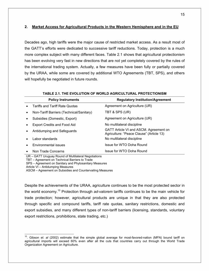
2. Market Access for Agricultural Products in the Western Hemisphere and in the EU

Decades ago, high tariffs were the major cause of restricted market access. As a result most of the GATT’s efforts were dedicated to successive tariff reductions. Today, protection is a much more complex subject with many different faces. Table 2.1 shows that agricultural protectionism has been evolving very fast in new directions that are not yet completely covered by the rules of the international trading system. Actually, a few measures have been fully or partially covered by the URAA, while some are covered by additional WTO Agreements (TBT, SPS), and others will hopefully be negotiated in future rounds.

TABLE 2.1. THE EVOLUTION OF WORLD AGRICULTURAL PROTECTIONISM

Policy Instruments Regulatory Institution/Agreement

• Tariffs and Tariff Rate Quotas Agreement on Agriculture (UR)

• Non-Tariff Barriers (Technical/Sanitary) TBT & SPS (UR)

• Subsidies (Domestic, Export) Agreement on Agriculture (UR)

• Export Credits and Food Aid No multilateral discipline

• Antidumping and Safeguards GATT Article VI and ASCM. Agreement on Agriculture: “Peace Clause” (Article 13)

• Labor standards No multilateral discipline

• Environmental issues Issue for WTO Doha Round

• Non Trade Concerns Issue for WTO Doha Round UR – GATT Uruguay Round of Multilateral Negotiations TBT – Agreement on Technical Barriers to Trade SPS – Agreement on Sanitary and Phytosanitary Measures Article VI – Antidumping Measures ASCM – Agreement on Subsidies and Countervailing Measures

Despite the achievements of the URAA, agriculture continues to be the most protected sector in the world economy.10 Protection through ad-valorem tariffs continues to be the main vehicle for trade protection; however, agricultural products are unique in that they are also protected through specific and compound tariffs, tariff rate quotas, sanitary restrictions, domestic and export subsidies, and many different types of non-tariff barriers (licensing, standards, voluntary export restrictions, prohibitions, state trading, etc.)

10. Gibson et. al (2002) estimate that the simple global average for most-favored-nation (MFN) bound tariff on agricultural imports will exceed 60% even after all the cuts that countries carry out through the World Trade Organization Agreement on Agriculture.

16

This section will examine some of those policy instruments affecting agricultural market access throughout the Western Hemisphere. It analyzes current agricultural trade in the region as well as tariff profiles and comparative levels of protectionism.

2.1. Tariff Structure and Trade Profile in the Western Hemisphere

2.1.1. Applied Methodology and Data Compilation

The objective of this section is to build a complete profile of protection levels by country and by main groups of products. The first step in developing tariff profiles is to convert specific and mixed tariffs11 into ad-valorem equivalents (AVE). According to the WTO, ad-valorem equivalents are usually calculated “either by comparing collected custom revenues to the value of imports or by comparing unit values of traded products with the applied non ad-valorem tariff”. The methodology followed in this study to obtain ad-valorem equivalents was to divide the product’s specific rate by its import price. In this case the price was calculated by dividing the value of imports by the quantity of imports. Where no trade data was available, the price of the closest related product was used. The data used comes from the 2001 Hemispheric Database of the Americas (HDA) and the Agricultural Market Access Database (AMAD).

This section uses data collected by the Inter-American Development Bank and compiled in the 2001 Hemispheric Database of the Americas for 30 of the 34 FTAA member countries (excluding Belize, Suriname, Guyana and Haiti, due to lack of trade-related data). The study uses primarily Most Favored Nation (MFN) applied rates, since these will be the tariffs used in the FTAA negotiations. However, to provide a realistic overview of the current level of trade protection the analysis was extended to include preferential and intra-bloc tariffs12.

In order to analyze and compare protection levels, several country databases were created for specific countries using data from the year 2000.13 The objective was to compile all trade-related data available for products by country in one database. The databases contain data in both 6- and 8-digit (or more) Harmonized System Code tariff lines,14 and include product descriptions, MFN ad-valorem tariffs, MFN specific and mixed tariffs, preferential rates, and ad-

11. Specific tariffs are tariffs that are set as a monetary amount per unit of import, i.e. a product can have a specific tariff, which charges $1.50 per kilogram. Countries may also combine ad-valorem and specific tariffs so that a product’s tariff may be the sum of the ad-valorem tariff plus the specific tariff, called mixed or compound tariffs. 12. For different methodologies to measure trade protection in agriculture see Bouët (2000) and Bouët, Fontagné, Mimouni & Kirchbach (2002). 13. For some countries where 2000 data was not available 1999 data was utilized. 14. “Tariff lines” refer to the category to which WTO members legally establish tariff applies.

17

valorem equivalents for such tariffs, imports value, quantity, imports price, exports value, export volume, indication of whether the tariff is a Tariff Rate Quota (TRQ)15, and tariff peaks (see appendix A). In addition, the data was further analyzed on an aggregate basis by being grouped into 32 “sensitive”16 groups of products based on the International Bilateral Agricultural Trade (IBAT) Database. Once all tariffs were expressed in terms of ad-valorem equivalents, we were able to calculate the number of tariff lines and TRQs, mean, median, tariff dispersion, maximum and minimum tariffs, and frequency distributions. J.C. Bureau from INRA-France provided data for the European Union.

Up to the 6-digit Harmonized System level (HS6), tariff schedules across countries use identical categories, which are established by the World Trade Organization, to aggregate different products. Beyond the 6-digit level, this correspondence does not exit, since aggregation may differ from country to country. Thus, in order to calculate the weighted average tariffs in sections 2.2 and 2.3, each country’s tariff lines and trade flow data were aggregated into 5113 category definitions to conform to the Harmonized System at the 6-digit level. Agricultural products were aggregated into 676 tariff lines while non-agricultural products were aggregated into 4437 tariff lines (a subgroup of 833 tariff lines was used for textile products).17 Furthermore, for these two sections, the over-quota tariff rate was used when TRQ tariffs were aggregated at the 6-digit level. Wainio and Gibson (2001) have stressed that TRQ’s do, in most cases, represent a binding constrain on additional trade. As such, over-quota rates give a more accurate account of the level of protection provided by the tariff schedule and should be used to reflect the overall restrictiveness of a country’s trade policy.

2.1.2. Comparative Tariff Structure

The most commonly used methods to measure tariff protection are the mean to depict the overall level of tariffs, and the standard deviation to measure tariff dispersion. Overall, the average tariff on agricultural products in the region is 16 percent, with Barbados, the Bahamas, 15. A TRQ is a two-tiered tariff under which a limited volume of goods (the quota amount) can be imported under the lower in-quota tariff, with any additional import quantity being subjected to a higher over-quota tariff. For more details, see IATRC (2000) and Skully (2001a). 16. “Sensitive products” are those accounting for a large percentage of a country’s total exports and that face relative high import barriers. 17. The definition of the WTO Harmonized system for Agricultural sector is covered by the following chapters: 1 to 24 less fish and fish products; 2905.43 (manitol); 2905.44 (sorbitol); 33.01 (essential oils); 35.01 to 35.05 (albuminoidal substances, modified starches, glues); 3809.10 (finishing agents); 3823.60 (sorbitol n.e.p); 41.01 to 41.03 (hides and skins); 43.01 (raw fur skins); 50.01 to 50.03 (raw silk and silk waste); 51.01 to 51.03 (wool and animal hair); 52.01 to 52.03 (raw cotton, waste and cotton carded or combed); 53.01 (raw flax); 53.02 (raw hemp). All other chapters were considered to be industrial (non-agricultural) sectors.

18

Mexico, Dominica, the Dominican Republic and Canada having the highest AVE, averaging over 20 percent. Nicaragua, Chile, Guatemala and Bolivia have the lowest average tariffs, below 10 percent (Figure 2.1 and Appendix A). However, aggregates such as the mean and dispersion do not tell the whole story. For example, comparing the mean and the median of a country’s tariff schedule may provide valuable insights into the agricultural trade policy of different countries.18

FIGURE 2.1. COMPARATIVE TARIFF STRUCTURE IN AGRICULTURE (HS8 2000)

Source: 2001 Hemispheric Database of the Americas. INT-IDB calculations.

Most countries of the WH have close mean and median tariffs. The median indicates the midpoint of the AVE tariff’s schedule distribution in an ascending order of value. Nevertheless, in countries like the US, Canada and Mexico, the median is far lower than the mean. This

18. The arithmetic mean is what is commonly called the average and is the sum of all the scores divided by the number of scores. Dispersion is measured through the standard deviation, which measures the degree to which a value varies from the distribution mean. The median is the midpoint of a tariff schedule’s distribution in ascending order of value: half the scores are above the median and half are below the median.

36.6

- 4 8 12 16 20 24 28 32 36

BarbadosBahamas

MexicoDominica

Dominican RepublicCanada

EUGrenada

St. Kitts and NevisAntigua and

JamaicaPeru

St. VincentTrinidad and

St. LuciaPanama

VenezuelaColombia

EcuadorCosta RicaArgentina

BrazilUruguay

ParaguayHonduras

United StatesEl Salvador

BoliviaGuatemala

ChileNicaragua

Average

MeanMedian

19

indicates the simultaneous presence of a large number of tariff lines far below the mean, and a few number of tariffs lines with very high rates (greater than 50%) commonly named “tariff peaks” or “megatariffs”. In other words, NAFTA countries are characterized by the application of very high tariffs on a very small group of politically sensitive products, while the rest of their tariffs are kept at low levels19 (see figure 2.2). The opposite is true for some Central American and Caribbean countries, where a large number of tariffs lines are set at high levels (greater than 15%), but a small group of very low and even zero tariffs exert downward pressure on the mean.

FIGURE 2.2. COMPARATIVE TARIFF STRUCTURE: FREQUENCY DISTRIBUTION AT HS8 (2000)

Source: 2001 Hemispheric Database of the Americas.

19. Olarreaga and Soloaga (1997) study several industry conditions that are correlated to high tariff protection, including high levels of industry concentration, low import penetration ratios, low share of sector production that is purchased by other sectors as intermediaries, high labor/capital ratio, and a small share of intra-industry trades.

0% 20% 40% 60% 80% 100%

Chile

Guatemala

Bolivia

El Salvador

Paraguay

Uruguay

Brazil

Argentina

Ecuador

Colombia

Venezuela

Peru

Dom Rep

Honduras

Nicaragua

CARICOM

Costa Rica

Panama

Mexico

US

Canada

0% 0%-15% 15%-30% 30%-50% >50%

20

In fact, NAFTA countries have disparate means and medians, with high dispersion of rates and the highest levels of maximum tariffs in the Western Hemisphere. Canada ranks first in the highest tariffs: 98 tariff lines are above 50%, with some products from the milling industry reaching equivalent rates of up to 530%. In the case of the US, four percent of its tariff lines (sixty-one lines) have rates above 50%, and up to 350% on some tobacco products. Nevertheless, the US large proportion of low rates (83% of its tariff lines have rates below 15%) offsets the impact of its megatariffs and ultimately results in a low overall average. In the case of Mexico, 5.1% of its tariff lines (54 tariff lines) are above 50%, and up to 260%, but Mexico also represents the third highest mean among all FTAA countries (23%). Canada is the country that has the largest percentage of zero tariffs (40.1%), however it is also the country with the highest amount of tariff rates above 50% (7.3%). Mercosur countries have only a small percentage of zero tariffs (8.4%), but do not have MFN ad-valorem tariffs that are above 30% (only one third of the tariffs lines are above 15%).

It is interesting to notice that all South American countries except Peru have means and medians that are very close. This shows that the process of liberalization after the 1980’s was accomplished without exclusions in the agricultural sector. Mercosur countries in particular have experienced a strong convergence in their agricultural tariffs. Their means are all approximately 12%; medians are exactly 13%; and their standard deviations are about 6%. Andean countries have means and medians placed between 10% and 17% and dispersions below 6.5%. Chile is a special case. Even though its ad-valorem tariffs appear to be one of the lowest, set at 9% for all products, agricultural imports are subject to price bands20 and other restrictions that significantly protect against imports. This is a clear example of how the existence of non-tariff barriers makes measurement of tariff protection a difficult task.

Another important measure of tariff protection is the type of tariff applied. Tariff barriers in agriculture are not only based on ad-valorem tariffs (high means and presence of peaks), but also on the extensive use of specific and mixed tariffs, and tariff-rate quotas21. NAFTA countries particularly stand out with their use of such tariffs. More than 43% of US tariffs are non ad- 20. Price bands regulate markets so prices remain within a specified range. In the case of Chile, for example, the price band for wheat is a pair of variable tariffs: one increase to defend a floor price and one decreases to defend the ceiling price. The band has two tariffs, an ad-valorem tariff that is always imposed, and a specific tariff that is determined by a tariff algorithm. When international prices are between the floor and the ceiling, the specific tariff is zero and only the ad-valorem tariff is imposed. When the international prices are below the floor or above the ceiling, the specific tariff is increased or lowered to keep the price within the set limits. The price band loses its capacity to offset international prices when the tariff increase reaches its bound level or when it is decreased to zero. See Skully (2001b). 21. Ad-valorem tariffs are calculated as a percentage of the value of the goods, which is normally the CIF (cost, insurance and freight). Specific tariffs are calculated as a percentage or a fixed amount per volume units (i.e., kilograms), and consequently result in higher protection levels the more competitive the exporting country is (lower import prices result in higher ad-valorem equivalents). Mixed or compound tariffs are a combination of ad-valorem plus specific rates.

21

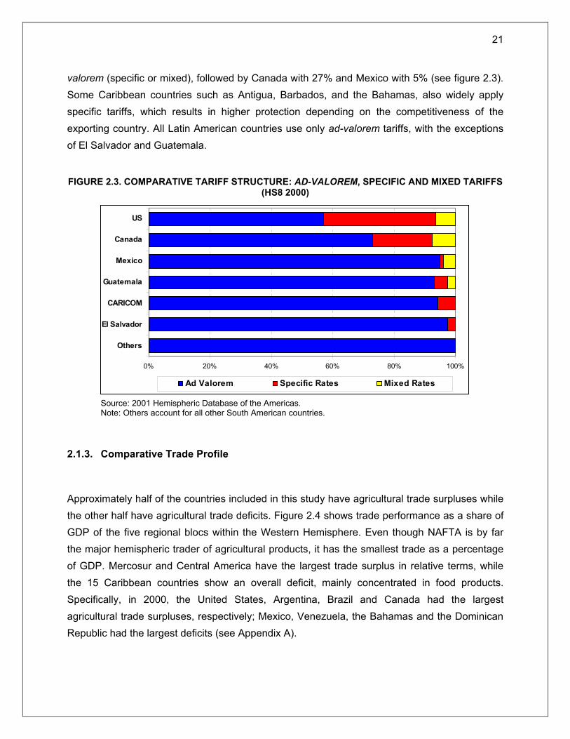
valorem (specific or mixed), followed by Canada with 27% and Mexico with 5% (see figure 2.3). Some Caribbean countries such as Antigua, Barbados, and the Bahamas, also widely apply specific tariffs, which results in higher protection depending on the competitiveness of the exporting country. All Latin American countries use only ad-valorem tariffs, with the exceptions of El Salvador and Guatemala.

FIGURE 2.3. COMPARATIVE TARIFF STRUCTURE: AD-VALOREM, SPECIFIC AND MIXED TARIFFS

(HS8 2000)

Source: 2001 Hemispheric Database of the Americas. Note: Others account for all other South American countries.

2.1.3. Comparative Trade Profile

Approximately half of the countries included in this study have agricultural trade surpluses while the other half have agricultural trade deficits. Figure 2.4 shows trade performance as a share of GDP of the five regional blocs within the Western Hemisphere. Even though NAFTA is by far the major hemispheric trader of agricultural products, it has the smallest trade as a percentage of GDP. Mercosur and Central America have the largest trade surplus in relative terms, while the 15 Caribbean countries show an overall deficit, mainly concentrated in food products. Specifically, in 2000, the United States, Argentina, Brazil and Canada had the largest agricultural trade surpluses, respectively; Mexico, Venezuela, the Bahamas and the Dominican Republic had the largest deficits (see Appendix A).

0% 20% 40% 60% 80% 100%

Others

El Salvador

CARICOM

Guatemala

Mexico

Canada

US

Ad Valorem Specific Rates Mixed Rates

22

FIGURE 2.4. TOTAL AGRICULTURAL TRADE IN THE WESTERN HEMISPHERE AS SHARE OF GDP (2000)

Note: Others are Chile, the Dominican Republic and Panama. Source: 2001 Hemispheric Database of the Americas.

The concentration of exports within some specific agricultural product groups is a clear phenomenon in Latin American and Caribbean countries. The Hirschmann-Herfindahl Index (HHI)22 can be used to measure the level of trade concentration in specific products. According to the HHI, exports are approximately seven times more concentrated than imports. Caribbean and Central American countries have the highest levels of export concentration in specific products (see figure 2.5). Examples are St. Kitts and Nevis, where raw sugar represents 75 percent of agricultural exports; St. Lucia, where bananas and beer represent 92 percent of exports; and Honduras, with coffee and bananas representing 74 percent of exports. Figure 2.6 clearly shows that 10 WH countries have more than 50% of their agricultural exports concentrated in only 3 products: coffee, bananas and sugar. The most diversified countries in terms of exports are the United States, Canada and Mexico.

22. The Hirschmann-Herfindahl Index (HHI) is equal to the sum of the squared shares of all products (tariff lines) exported, where i stands for a particular product and n is the total number of products. When a single export product or tariff line produces all the revenues, the HHI equals 100; when export revenues are evenly distributed over a large number of products, HHI approaches zero.

.100*

2

∑∑

=n

in

ii

i

X

XHHI

-6.0% -4.0% -2.0% 0.0% 2.0% 4.0% 6.0% 8.0% 10.0%

CACM

MERCOSUR

ANDEAN

NAFTA

CARICOM

Others

(% GDP)

Exports

Imports

Balance

23

FIGURE 2.5. AGRICULTURAL TRADE CONCENTRATION IN THE WH: THE HIRSCHMANN-HERFINDAHL INDEX

EXPORTS IMPORTS


FIGURE 2.6. AGRICULTURAL EXPORT CONCENTRATION FOR CARIBBEAN AND CENTRAL AMERICAN COUNTRIES (2000)

Source: 2001 Hemispheric Database of the Americas. INT-IDB calculations. Note: All – Average for all LAC countries.

39.3

36.934.534.4

29.827.1

23.3

22.019.5

17.2

17.216.8

14.713.6

13.110.8

8.1

8.07.67.4

6.86.3

5.9

5.43.8

3.0

2.619.6

0 10 20 30 40 50 60

HondurasEcuadorGrenada

DominicaEl SalvadorSt. Vincent

PanamaParaguay

NicaraguaBarbadosColombia

GuatemalaPeru

Costa RicaBolivia

JamaicaBrazil

UruguayArgentina

Dominican RepublicChile

Antigua and BarbudaTrinidad and Tobago

VenezuelaM exicoCanada

United StatesAverage

6.05.5

5.24.3

3.73.5

3.32.9

2.62.3

2.02.02.01.91.9

1.81.81.81.81.71.6

1.41.4

1.31.21.2

0.72.9

0 1 2 3 4 5 6 7 8 9

BrazilBo livia

DominicanColombia

ChileCosta Rica

VenezuelaSt. VincentHonduras

GuatemalaM exico

BahamasEl Salvador

NicaraguaUruguayPanama

DominicaGrenada

Trinidad andJamaicaSt. Lucia

St. Kitts and NevisAntigua and

ArgentinaUnited States

BarbadosCanada

Average

57.755.2

41.2

St. Kitts and NevisSt. Lucia

Bahamas

8.56.56.4

ParaguayEcuador

Peru

0% 10% 20% 30% 40% 50% 60% 70% 80% 90% 100%

All

Bahamas

Antigua and Barbuda

Grenada

Trinidad and Tobago

Dominican Republic

Barbados

Jamaica

Costa Rica

St Vincent

Nicaragua

Panama

Guatemala

El Salvador

Dominica

St Lucia

Honduras

St Kitts and Nevis

Coffee Bananas Sugar Grains and Soy Meats and Dairy Fruits, Vegetables Others

24

2.2. Measuring Tariff Protection for Sensitive Export Products

A country that mainly exports raw sugar and bananas is not interested in the overall level of tariffs imposed by another partner, but only on the tariffs imposed on its main exports. In fact, this country will be interested in the additional access it can gain for its primary traded products through multilateral and regional negotiations. Statistical aggregates such as those shown in the previous section 2.1 (e.g., means, medians and dispersions) do not measure the real importance and levels of tariff protection on very specific and sensitive products.

A better technique to access the real level of tariff protection would be to use weighted averages instead of simple means, since these take into account the proportional relevance of sensitive products rather than treating all products equally. The question that arises when calculating weighted averages is what values should be used to properly weight the tariffs that a country faces. Values such as production, consumption, import or export appear to be the natural candidates, but given that the purpose is to measure trade protection, only imports and exports should be considered. Using import values, however, produces a downward bias since the actual import of items with high tariffs will have little weight, as these high tariffs are likely to create “trade chilling” effects by restraining or even impeding trade. For example, even though the Brazilian sugar industry is very competitive, representing 57% of the WH total sugar export, it only accounts for approximately 10% of US total sugar imports. This is due to the quotas and high tariffs that the US applies to sugar imports. Thus, weighted average tariffs should depend on the importer tariffs and the composition of total exports. This approach emphasizes those tariffs in importing countries that are of greatest importance for exporting countries, and provides a dynamic view of the level of protection that each country imposes and faces in regards to its trading partners.

Figure 2.7 compares the values of US imposed MFN tariffs using the weighted average and simple mean method for each one of its WH partners. The figure shows that most countries face a weighted tariff in the US that is higher than the simple mean tariff (CARICOM corresponds to 10 countries of the Caribbean Community). This illustrates that these countries’ sensitive exports face high tariffs. Brazil faces the highest weighted average tariff for agricultural products (35.4%) mainly explained by the high tariffs on its tobacco, sugar and orange juice exports. Venezuela’s high value is mostly due to tobacco and dairy products.

25

FIGURE 2.7. US IMPOSED MFN AGRICULTURAL TARIFFS WEIGHTED BY EACH PARTNERS EXPORTS (HS6 MAX)


Appendix B provides a table with the average agricultural MFN tariffs weighted by total exports for all WH countries and the European Union. Using this methodology, on a bilateral basis the highest average duty would be faced by Ecuador (83.8%), Panama (76.1%) and Uruguay (75.3%) respectively if all their products were exported to the EU. In the case of Ecuador and Panama, the high tariff barriers applied to bananas can explain the elevated values to a great extent. Uruguay, on the other hand, faces high tariffs on its meat and diary products exports. If only the WH countries are considered, the highest tariffs are faced by the Dominican Republic (55.3%) and CARICOM (51.7%) both against Mexico, and Uruguay (51.1%) against Canada. For most Caribbean countries and the Dominican Republic, high duties on sugar are the main cause while for Uruguay, the main reason is still its dairy products. Overall, Mexico has the most protected market for agricultural products, followed by the European Union. Compared to all WH countries, Mexico’s average agricultural tariff is approximately 37%.

- 5 10 15 20 25 30 35 40

Ecuador

Honduras

Bolivia

Chile

Paraguay

Peru

Colombia

Panama

Costa Rica

El Salvador

Simple Mean

Mexico

Canada

Argentina

Guatemala

CARICOM

Nicaragua

Uruguay

Dom Rep

Venezuela

Brazil

26

2.3. Comparing Tariff Protection in the Western Hemisphere

So far, in the former sections, we have concentrated our analyses on the MFN tariff barriers faced by agricultural products. However, to provide a realistic picture of the effects of trade liberalization two other factors should be taken into consideration.

MFN versus Preferential Tariffs

The first factor is the existence of many preferential trade agreements and free trade areas in the Western Hemisphere. During the last decade more than 40 bilateral and regional agreements have been negotiated in the region. These agreements have significantly increased trade between partners by providing preferential or duty-free access to a great part of the trade in the hemisphere. When these preferential agreements are taken into consideration a different picture emerges. Figure 2.8 compares the US MFN and preferential imposed tariffs, weighted by exports, for agricultural products. In the case of Ecuador preferential access provides a 73% reduction in the tariff, decreasing it from the 6.3% to 1.7%. For Canada and Mexico, which are partners in the NAFTA, the tariff is reduced by approximately 40%.

FIGURE 2.8. US 2000 MFN VS PREFERENTIAL IMPOSED AGRICULTURAL TARIFFS (%)


0 5 10 15 20 25 30 35 40

Ecuador

Honduras

Bolivia

Chile

Paraguay

Peru

Colombia

Panama

Costa Rica

El Salvador

Mexico

Canada

Argentina

Guatemala

CARICOM

Nicaragua

Uruguay

EU

Dom Rep

Venezuela

Brazil

MFN

Preferential

.

27

It is interesting to observe that most of the so-called small economies, Caribbean and Central American countries, experience a significant decrease in the level of tariff protection. As it has been noticed in section 1.1, these countries depend on preferential access for the few commodities that make the bulk of their exports, such as coffee, cocoa, sugar and bananas (see figure 2.6). This provides a striking example of how a reduction in the tariffs faced by a few sensitive products can significantly impact the overall level of tariff barrier faced by a country. However, in the case of many South American countries, preferential access does not notably decrease the overall agricultural tariff barriers (since these agreements do not provide access to sensitive products). Therefore, using MFN rates to measure tariff protection creates, in some cases, an upward bias. Appendix B provides a table with the average agricultural preferential tariffs, weighted by total exports, for the WH countries and the European Union.

Tariffs on Agricultural versus Industrial Sectors

The second factor to be considered is that any negotiation that addresses the liberalization of trade barriers for agricultural goods will encompass trade offs. Many of the countries that face relative high tariff barriers for their agricultural exports impose, on the other hand, relative higher import tariff protection on non-agricultural products. It is thus expected that any decrease in the level of tariff protection in the agricultural sector will require further liberalization of non-agricultural sectors. Any investigation of the effects of trade liberalization would be incomplete if only one sector is taken into consideration. In the subsequent sections non-agricultural products were denominated as “industrial” products.

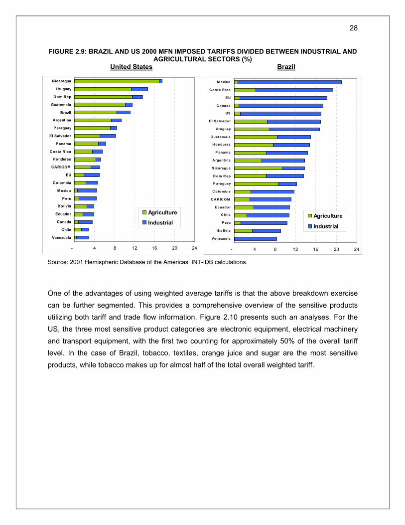
Figure 2.9 displays the breakdown of the MFN tariff protection imposed by Brazil and the US divided by sectors (agriculture and industry). The graph shows that in many cases a greater part of the overall tariff imposed by Brazil is due to industrial tariffs (especially in the case of the NAFTA countries). Almost 90% of the 17% overall weighted average tariff faced by the US in Brazil corresponds to tariffs imposed on its industrial exports. In the case of the US, the inverse is true for almost all WH countries. A greater part of the overall tariff is due to agricultural tariff barriers. Of the 11% overall tariff faced by Brazilian exports into the US, for example, more than 75% is imposed on its agricultural exports.

28

FIGURE 2.9: BRAZIL AND US 2000 MFN IMPOSED TARIFFS DIVIDED BETWEEN INDUSTRIAL AND AGRICULTURAL SECTORS (%)

United States Brazil


One of the advantages of using weighted average tariffs is that the above breakdown exercise can be further segmented. This provides a comprehensive overview of the sensitive products utilizing both tariff and trade flow information. Figure 2.10 presents such an analyses. For the US, the three most sensitive product categories are electronic equipment, electrical machinery and transport equipment, with the first two counting for approximately 50% of the overall tariff level. In the case of Brazil, tobacco, textiles, orange juice and sugar are the most sensitive products, while tobacco makes up for almost half of the total overall weighted tariff.

- 4 8 12 16 20 24

Venezuela

Chile

Canada

Ecuador

Bolivia

Peru

M exico

Colombia

EU

CARICOM

Honduras

Costa Rica

Panama

El Salvador

Paraguay

Argentina

Brazil

Guatemala

Dom Rep

Uruguay

Nicaragua

Agriculture

Industrial

- 4 8 12 16 20 2

Venezuela

B o liv ia

P eru

C hile

Ecuado r

C A R IC OM

C o lo mbia

P araguay

D o m R ep

N icaragua

A rgent ina

P anama

H o nduras

Guatemala

Uruguay

El Salvado r

US

C anada

EU

C o sta R ica

M exico

Agriculture

Industrial

4

29

FIGURE 2.10: BREAKDOWN OF OVERALL MFN IMPOSED TARIFFS BY SENSITIVE PRODUCTS (HS6 2000)

Brazil on the U.S. (17.0%) U.S. on Brazil (11.1%)


2.3.1. Evaluating Tariff Protection in a Bilateral Agreement: the “Relative Tariff Ratio” Index (RTR)

The previous section demonstrated that one of the challenges that exists in trade negotiations is the measurement and comparison of relative levels of tariff protection between trading partners. An index that measures the effects of trade liberalization in a bilateral negotiation is the Relative Tariff Ratio (RTR) Index, originally developed by Sandrey (2000), and further developed by Wainio & Gibson (2002) and Gehlhar and Wainio (2002). The index considers a two-country world, where each tariff line of country A is weighted by country’s B total exports for the same tariff line, and vice versa. The index is constructed as the ratio between a country’s faced tariffs in the numerator and its imposed tariffs in the denominator23. In general, a ratio close to one reflects the fact that both countries have similar tariff protection, and thus face/impose comparable barriers. However, this does not reflect the levels of tariffs, only their relative ratios. 23. The Relative Tariff Ratio Index is always calculated on a bilateral basis, or:

( )

( )∑

∑= n

i

Bi

Ai

n

i

Ai

Bi

AB

YX

YXRTR

.

.

Where: AB = Countries A e B; Xi = ad-valorem equivalent (AVE) tariff rate for product i

Yi = share of exports of product i in total exports.

Orange Juice9.8%

Tobacco49.4%

Textiles20.8%

Sugar5.8%

Meat3.2%

Industrial2.9%

Other - Agr8.2%

Electronic Equipment

29.5%

Electrical Machinery

20.6%

Transport Equipment

14.5%

Agriculture6.7%

Chemicals8.0%

Other - Ind16.8%

Textiles3.9%

30

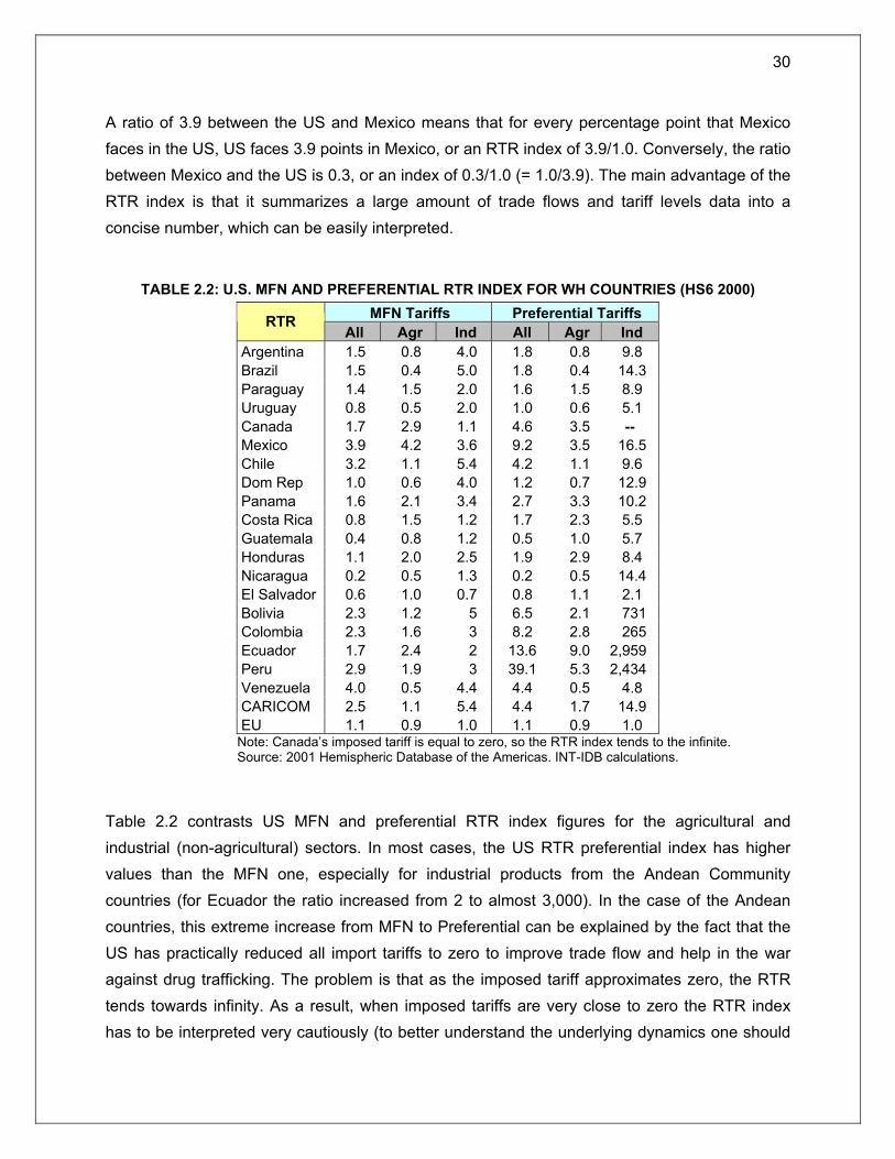
A ratio of 3.9 between the US and Mexico means that for every percentage point that Mexico faces in the US, US faces 3.9 points in Mexico, or an RTR index of 3.9/1.0. Conversely, the ratio between Mexico and the US is 0.3, or an index of 0.3/1.0 (= 1.0/3.9). The main advantage of the RTR index is that it summarizes a large amount of trade flows and tariff levels data into a concise number, which can be easily interpreted.

TABLE 2.2: U.S. MFN AND PREFERENTIAL RTR INDEX FOR WH COUNTRIES (HS6 2000) MFN Tariffs Preferential Tariffs RTR

All Agr Ind All Agr Ind Argentina 1.5 0.8 4.0 1.8 0.8 9.8 Brazil 1.5 0.4 5.0 1.8 0.4 14.3 Paraguay 1.4 1.5 2.0 1.6 1.5 8.9 Uruguay 0.8 0.5 2.0 1.0 0.6 5.1 Canada 1.7 2.9 1.1 4.6 3.5 -- Mexico 3.9 4.2 3.6 9.2 3.5 16.5 Chile 3.2 1.1 5.4 4.2 1.1 9.6 Dom Rep 1.0 0.6 4.0 1.2 0.7 12.9 Panama 1.6 2.1 3.4 2.7 3.3 10.2 Costa Rica 0.8 1.5 1.2 1.7 2.3 5.5 Guatemala 0.4 0.8 1.2 0.5 1.0 5.7 Honduras 1.1 2.0 2.5 1.9 2.9 8.4 Nicaragua 0.2 0.5 1.3 0.2 0.5 14.4 El Salvador 0.6 1.0 0.7 0.8 1.1 2.1 Bolivia 2.3 1.2 5 6.5 2.1 731 Colombia 2.3 1.6 3 8.2 2.8 265 Ecuador 1.7 2.4 2 13.6 9.0 2,959 Peru 2.9 1.9 3 39.1 5.3 2,434 Venezuela 4.0 0.5 4.4 4.4 0.5 4.8 CARICOM 2.5 1.1 5.4 4.4 1.7 14.9 EU 1.1 0.9 1.0 1.1 0.9 1.0 Note: Canada’s imposed tariff is equal to zero, so the RTR index tends to the infinite. Source: 2001 Hemispheric Database of the Americas. INT-IDB calculations.

Table 2.2 contrasts US MFN and preferential RTR index figures for the agricultural and industrial (non-agricultural) sectors. In most cases, the US RTR preferential index has higher values than the MFN one, especially for industrial products from the Andean Community countries (for Ecuador the ratio increased from 2 to almost 3,000). In the case of the Andean countries, this extreme increase from MFN to Preferential can be explained by the fact that the US has practically reduced all import tariffs to zero to improve trade flow and help in the war against drug trafficking. The problem is that as the imposed tariff approximates zero, the RTR tends towards infinity. As a result, when imposed tariffs are very close to zero the RTR index has to be interpreted very cautiously (to better understand the underlying dynamics one should

31

reflect on the imposed and faced tariffs values itself). Nevertheless, these high ratios indicate that the reduction of tariffs by the US under the preferential agreement has not been followed by a proportional decline in tariffs on the part of the Andean Community.

It is interesting to notice that this increase in the RTR index also occurs for Mexico and Canada, both partners in NAFTA. In the case of Canada, the overall index increased from 1.7 to 4.6, and for Mexico from 3.9 to 9.2. This implies that the US has provided relatively more access than it has gained from its partners in the NAFTA, when taking into consideration the RTR methodology. Furthermore, this liberalization has been primarily granted for industrial products.24 In the case of Mexico, the RTR industrial index increased from 3.6 to 16.5, however the RTR agricultural index was reduced from 4.2 to 3.5. In other words, while Mexico has reduced agricultural barriers, the US has provided more access to industrial imports, in relative terms.

The above illustration provides a powerful example of how useful the RTR index can be for measuring trade liberalization on a bilateral basis. The index can be used as a practical tool to appraise progress in a free trade agreement, and as a starting point to reveal potential sectors that negotiators should focus on. However, we should reflect upon the fact that the RTR index is limited in terms of accuracy. Sandrey (2000) warns that he would be hesitant to utilize the Index to analyze less and least developed economies, since income effects would make some of the assumptions unrealistic. However, he did point out that this does not invalidate the examination of exports from the developing world to the developed world. Overall, we believe that the potential data gains of using the RTR far outweigh its deficiencies.

2.3.2. Evaluating Tariff Protection in a Regional Integration Agreement: the “Regional Export Sensitive Tariff” Index (REST)

In keeping with the RTR concept, we propose an extension of a new RTR index at the regional level called the “Regional Export Sensitive Tariff” Index (REST). The REST index aggregates all tariffs faced and imposed by each country at the regional level into a single indicator, representing a ratio of the weighted value of those tariffs.

The index measures each country’s faced tariffs from its partners weighted by its total exports in the numerator, and each country’s imposed tariffs weighted by the total exports of all its partners in the denominator, calculated one by one, based on a potential Regional Integration

24. For Canada the RTR industrial index could not be calculated since tariffs faced and imposed are zero.

32

Agreement (RIA). Each combination of tariffs and share of export ratios for one country is weighted by the relative importance of total exports to the region in the case of faced tariffs, and total imports in the case of imposed tariffs25. Both the RTR and the REST indices can be used to gauge the concessions that each country makes relative to those it receives, in the event of the elimination of trade barriers. The advantage of the REST index is that it can go far beyond the bilateral level, and address the important issue of liberalization at a regional or multilateral level.

The REST index, like the RTR index, does have limitations, and is more of a pragmatic tool rather than an elegant academic measure. Two of these limitations do deserve special attention: the first limitation is that the REST index is based on tariffs and therefore does not take Non Tariff Barriers (NTB) into account, such as TBT and SPS barriers. Such barriers are extremely difficult to quantify and may one day become a major barrier to agricultural trade. SPS requirements, for instance, can impede trade to small economies due to the lack of financial and human resources to implement and administer the required procedures.

The second limitation is that the index fails to incorporate the effects of elasticity and trade substitution that may occur once barriers decrease. It assumes that all of a country’s sectoral exports will uniformly go to all its partners in the regional agreement. This is somewhat unrealistic, especially in the case of exports from bigger to smaller economies. However, the index is largely influenced by each country’s sensitive exports to its most important partners, giving marginal importance to other products and countries. Thus, the REST index contrasts countries’ competitive products with major trading partners’ barriers. It seems unrealistic to assume that 92% of a Caribbean country’s imports from the US will be industrial products (agriculture corresponded for only 8% of the US total exports in 2000). This seems even more

25. The scientific notation of the REST index is:

RESTA =

( ) ( ) ( )

( ) ( ) ( )∑∑∑

∑∑∑

===

===

∗

++∗

+∗

∗

++∗

+∗

n

i

Ni

AiA

T

AN

n

i

Ci

AiA

T

AC

n

i

Bi

AiA

T

AB

n

i

Ai

NiA

T

AN

n

i

Ai

CiA

T

AC

n

i

Ai

BiA

T

AB

yxMMyxM

MyxMM

yxXXyxX

XyxXX

111

111

...

...

Where: A, B, C,…, N = member countries of a Regional Integration Agreement x

i

A = maximum ad-valorem equivalent tariff rate at HS-96 level for tariff line i

yAi = share of exports of product i in total exports for each country

MB

A = country A’s total imports from country B

MT

A = country A’s total imports from all RIA countries

XB

A = country A’s total exports to country B

XT

A = country A’s total exports to all RIA countries

33

unlikely when we consider that these countries are net food importers and do have a relatively low level of income per capita. Nonetheless, since the Caribbean Community does represent less than 1% of US total exports in the WH, it has a small weight in the US REST index.

In sum, the advantages presented by a practical and concise figure that provides a measurement for sensitive products tariff barriers in a regional agreement, far outweigh any of the limitations mentioned. Therefore, the index could be used in negotiations to provide a valid and useful way to measure progress in the FTAA.

One final issue should be taken into account to avoid bias when using MFN data to compute the REST index: Preexisting regional Free Trade Area (FTA) agreements have to be considered when calculating the index by using preferential tariffs or assuming a zero tariff. This is the case since trade has already been liberalized under such agreements; undoubtedly increasing trade flows between its partners. In other words, existing FTA’s have already created trade and thus would induce bias in an index that is trying to gauge the level of distortion in trade flows produced by high tariff rates. Only trade data from non-Mercosur countries was used, for instance, to compute the Argentine MFN REST in the FTAA. As a result the Argentine MFN REST value measures the concessions that the country makes relative to those it receives while only taking into account the WH countries outside the Mercosur agreement. The same approach was used for the Andean Community, Central American Common Market (CACM) and NAFTA countries. It should be emphasized that such a concern does not exist when preferential tariffs are used to calculate the REST. In this case the existing trade flows do accurately reflect the applied preferential tariffs and thus no distortion has to be accounted for. When calculating the Preferential REST for the FTAA, each country was weighted against all other countries in the WH.

Table 2.3 summarizes the main strengths and weaknesses of the RTR and REST indexes.

34

TABLE 2.3: SUMMARY OF STRENGTHS AND WEAKNESSES OF THE RTR AND REST INDEXES

Strengths Weaknesses

• Pragmatic measure that can be easily interpreted.

• Summarizes a large amount of trade flows and tariff level data into a simple and concise number.

• Tariffs are weighted according to their importance with trading partners (index is mostly influenced by sensitive products and major trading partners).

• Excellent instrument for trade negotiators. Useful to set starting points and measure progress in FTA.

• Highlights potential sectors of possible negotiation difficulty.

• Ignores elasticity effects and substitutions possibilities that may occur once trade barriers decrease.

• Assumptions could be unrealistic for some least developed countries.

• Does not account for non-tariff measures and subsidies (SPS, TBT, anti-dumping, export restrictions, etc.).

• REST calculation has no sense when tariffs tend to zero.

Source: authors, based on Sandrey (2000), Wainio & Gibson (2001), and Gehlhar and Wainio (2002).

Appendix C provides a table with the aggregated regional tariffs that are weighted, faced and imposed for WH countries, and the respective REST index (both MFN and Preferential). As illustrated for the bilateral case of Brazil and the US, a breakdown of these aggregated tariffs by product could provide a comprehensive overview of a country’s sensitive export products on the regional level. Figure 2.11 displays the faced tariff for agricultural products while figure 2.12 displays imposed tariffs for industrial products. It can be observed that faced agricultural tariffs are twice as high on average as imposed industrial tariffs. Moreover, most countries experience a significant decrease in the regional agricultural tariff level when preferential agreements are taken into consideration. The same does not hold true when industrial imposed tariffs are analyzed. One possible interpretation is that trade for sensitive industrial products has already been liberalized, for the most part, while many sensitive agricultural products still depend on preferential treaties for market access.

When considering MFN figures, Brazil’s agricultural exports face the highest barriers in the Hemisphere. On the other hand, Brazil ranks second place in terms of imposed protection on industrial imports. Canada and the US are the countries that impose the lowest industrial tariffs for all partners: about 3% in the case of MFN tariffs and practically zero when preferential rates are considered. It is interesting to note that the US agricultural preferential faced tariff is actually higher than the MFN tariff. This is the case since the MFN calculations for “regional” tariffs do not take into consideration trade between existing FTA members (NAFTA members in this case). The preferential tariff ends up being higher because the US still faces some protection on

35

agricultural exports from other NAFTA members (section 2.3.1 pointed out that the US has provided relatively more access than it has gained from its NAFTA partners).

FIGURE 2.11: WH COUNTRIES FACED TARIFFS ON AGRICULTURAL PRODUCTS

(MFN AND PREFERENTIAL, HS-6, 2000)


FIGURE 2.12. WH COUNTRIES IMPOSED TARIFFS ON INDUSTRIAL PRODUCTS: (MFN AND PREFERENTIAL, HS-6, 2000)


0

5

10

15

20

25

30

35

Mex

ico

Braz

il

Dom

Rep

CAR

ICO

M

Peru

Arge

ntin

a

Uru

guay

Vene

zuel

a

Col

ombi

a

Para

guay

Boliv

ia

Pana

ma

Chi

le

Ecua

dor

Hon

dura

s

Gua

tem

ala

El S

alva

dor

Cos

ta R

ica

Can

ada

US

Nic

arag

ua

MFN

Preferential

0

5

10

15

20

25

30

35

Braz

il

Dom

Rep

Vene

zuel

a

Nic

arag

ua

Uru

guay

CAR

ICO

M

Gua

tem

ala

Arge

ntin

a

El S

alva

dor

Mex

ico

US

Chi

le

Can

ada

Pana

ma

Cos

ta R

ica

Col

ombi

a

Peru

Boliv

ia

Para

guay

Hon

dura

s

Ecua

dor

MFN

Preferential

36

Table 2.4 presents the results for the MFN and Preferential REST index for the whole economy, industrial sector and agriculture. To provide an easy visual interpretation, REST index figures from 0.8 to 1.2 represent similar tariff protections and are depicted in yellow. REST index numbers above 1.2 characterize higher faced than imposed weighted tariffs, therefore indicating a protectionist reality that could be reversed (depicted in green). When the index is below 0.8 it denotes lower faced than imposed tariffs, and therefore a country that would be a net liberalizer in that sector (symbolized in red).

TABLE 2.4. THE “REGIONAL EXPORT SENSITIVE TARIFFS” INDEX (REST) BY SECTORS FOR WH

COUNTRIES (MFN AND PREFERENTIAL, HS-6, 2000)

Note: CAR – Caribbean Community countries. Source: 2001 Hemispheric Database of the Americas. INT-IDB calculations.

In general, a REST ratio close to one can be interpreted as an overall evenness between a country’s tariff regime and that of its regional partners. Consequently, the objective of a regional FTA negotiation could be to progress towards REST values that are close to one for all partners. This does not necessarily mean that all tariffs should be close to zero. It rather implies that countries will have equivalent access for their most sensitive products exports at the

All Ind Agr All Ind AgrArgentina 0.9 0.4 1.2 0.7 0.3 1.1

Brazil 0.7 0.3 2.2 0.7 0.3 2.2

Paraguay 0.9 0.7 0.7 1.8 0.6 1.4

Uruguay 1.4 0.9 1.7 1.1 0.7 1.5

Canada 1.7 4.2 0.5 0.4 13.3 0.3

Mexico 0.7 0.9 0.4 0.2 0.2 0.3

US 1.4 3.6 0.7 3.2 11.7 2.5

Chile 0.9 0.8 1.7 1.0 0.8 1.9

Dom Rep 1.1 0.4 1.7 1.0 0.3 1.5

Panama 1.0 1.1 0.6 0.9 1.0 0.5

Costa Rica 1.6 1.4 0.8 1.2 1.2 0.6

Guatemala 2.8 1.8 1.3 2.7 1.7 1.4

Honduras 1.2 0.8 0.6 0.8 0.5 0.5

Nicaragua 5.5 3.6 1.9 4.0 2.5 1.5

El Salvador 2.4 2.1 1.3 1.3 0.9 1.1

Bolivia 0.8 0.7 1.1 0.8 0.7 1.1

Colombia 0.7 0.5 0.8 0.4 0.3 0.6

Ecuador 0.7 0.6 0.6 0.6 0.5 0.6

Peru 0.5 0.5 0.6 0.3 0.3 0.4

Venezuela 0.4 0.4 1.9 0.5 0.4 1.8

CARICOM 0.5 0.3 0.9 0.4 0.2 0.6

MFN PreferentialREST

37

regional level. Below we provide a detailed analysis of the REST index results for different sectors.

Agricultural Sector

Figure 2.13 and table 2.4 present the calculation of the REST Index for agricultural products using MFN and Preferential tariffs. The figure shows very clearly that NAFTA, Caribbean and most Andean countries impose higher weighted MFN tariffs than they face in the WH (REST below 1). The biggest face-off is Mexico and Canada, where high tariffs imposed on a very small group of key products are significant to potential FTAA partners. In other words, these countries are net liberalizers within the integration process in terms of agricultural tariff protection.

FIGURE 2.13. THE REST INDEX FOR AGRICULTURAL TRADE IN THE AMERICAS (HS6 2000)


On the other hand, most Mercosur members, Chile, and most Central American countries would have net gains in terms of agricultural market access . Brazil would rank first in this process above Uruguay, Chile and Argentina, as a result of the very high tariffs faced by Brazil’s sensitive products such as sugar, orange juice and tobacco, especially in the US. There are no major differences between the MFN and preferential REST figures for most countries other than

0.0

0.5

1.0

1.5

2.0

2.5

3.0

3.5

4.0

4.5

5.0

Braz

il

Nica

ragu

a

Vene

zuel

a

Chile

Urug

uay

Dom

Rep

Gua

tem

ala

El S

alva

dor

Arge

ntin

a

Boliv

ia

CARI

COM

Colo

mbi

a

Cost

a Ri

ca US

Para

guay

Peru

Hond

uras

Ecua

dor

Pana

ma

Cana

da

Mex

ico

MFNPreferential

38

the US and Paraguay. The US case has been previously clarified (the US has provided more access in agriculture trade to its NAFTA partners than it has received). Paraguay has a higher preferential REST index because it has virtually provided free access to its Mercosur partners while it still encounters some tariff barriers.

Industrial Sector

Figure 2.14 and table 2.4 provide an overview of the REST index for industrial products. The figure offers a very different view than the one provided by the agricultural REST. The US, Canada, and most Central American nations are the countries that have the highest industrial REST. These high ratios are mainly due to the fact that these countries apply very low tariffs on industrial imports. The very high preferential REST value for Canada and the US is a result of the near zero tariff that these countries impose on Mexico. These preferential ratios should be interpreted carefully, since they do not necessarily correspond to possible high trade offs (Canada faced tariff is approximately 0.44 while the imposed tariff is 0.03). For most Central American countries, the above one REST ratio is a consequence of their below average imposed tariffs, when these are compared to most South American countries and Mexico (they still imposed higher tariff barriers than the US and Canada).

FIGURE 2.14. THE REST INDEX FOR INDUSTRIAL TRADE IN THE AMERICAS (HS6 2000)


13.3 11.7

0.0

0.5

1.0

1.5

2.0

2.5

3.0

3.5

4.0

4.5

5.0

Cana

da

Nica

ragu

a US

El S

alva

dor

Gua

tem

ala

Cost

a Ri

ca

Pana

ma

Mex

ico

Urug

uay

Hond

uras

Chile

Boliv

ia

Para

guay

Ecua

dor

Colo

mbi

a

Peru

Arge

ntin

a

Dom

Rep

Vene

zuel

a

CARI

COM

Braz

ilMFNPreferential

39

Most Mercosur and Caribbean countries would become net liberalizers in the FTAA in industrial products, as they still enforce higher tariffs (especially when compared to the US and Canada). However, as is shown in figures 2.11 and 2.12, tariff barriers on industrial products are50% smaller on average than barriers on agricultural products. Even though there are still some segments in the industrial sector where further trade liberalization can be achieved, there is still much to be accomplished in the agricultural sector.

All (industry & Agriculture)

To complete our examination using the REST index we computed each country’s overall ratio, combining both industrial and agricultural tariff barriers (figure 2.15 and table 2.4). Through this analysis we can get a better understanding of all the trade-offs that would take place in an FTAA. Most Central American countries face higher tariffs than they impose, regardless of the tariff universe under consideration (MFN or preferential). These countries would have a strong interest in pushing the trade liberalization process forward. Actually, they would have net gains in overall market access from a simultaneous decrease on agricultural tariff barriers in North America and industrial tariffs in South America26. The countries in the best position are Nicaragua, Guatemala and El Salvador. Panama, The Dominican Republic and Chile are countries that have REST close to one. These countries sensitive products enjoy a relatively even access at the regional level.

The US is also a country that would benefit from a regional trade agreement, independent of the tariff universe considered. Its preferential REST ratio is the second highest since the country has provided more access than it has gained from several of its FTAA partners. Furthermore, even though the US does impose “megatariffs” on some agricultural products, agriculture represented only about 8% of total US exports in 2000. Canada has a REST above one for MFN tariffs and below one for preferential rates. This country would gain from a decrease in industrial tariff barriers in Latin America. On the other hand, the US still imposes relative higher agricultural tariff barriers towards its NAFTA partners and most South American countries. Mexico would become a net liberalizer, both in agriculture and industry, independent of the tariff scheme.

26. These results are very similar to those obtained by Diao et. al. (2002) in their CGE scenarios for the FTAA.

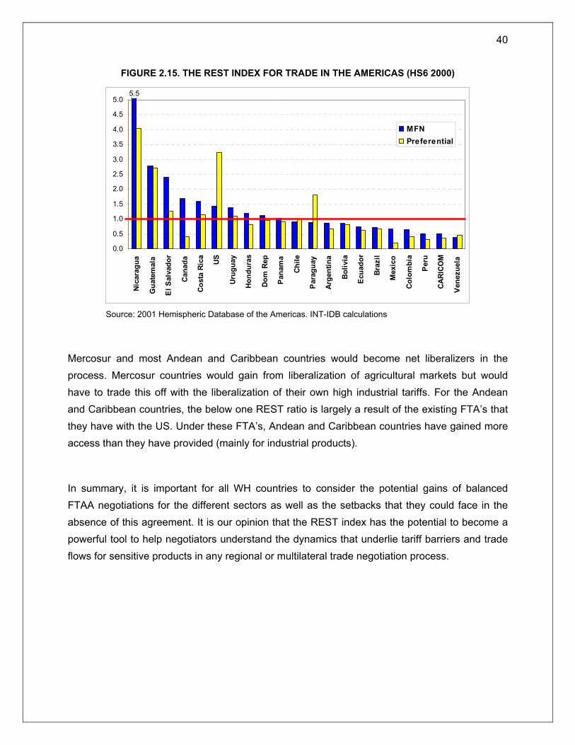
40

FIGURE 2.15. THE REST INDEX FOR TRADE IN THE AMERICAS (HS6 2000)

Source: 2001 Hemispheric Database of the Americas. INT-IDB calculations

Mercosur and most Andean and Caribbean countries would become net liberalizers in the process. Mercosur countries would gain from liberalization of agricultural markets but would have to trade this off with the liberalization of their own high industrial tariffs. For the Andean and Caribbean countries, the below one REST ratio is largely a result of the existing FTA’s that they have with the US. Under these FTA’s, Andean and Caribbean countries have gained more access than they have provided (mainly for industrial products).

In summary, it is important for all WH countries to consider the potential gains of balanced FTAA negotiations for the different sectors as well as the setbacks that they could face in the absence of this agreement. It is our opinion that the REST index has the potential to become a powerful tool to help negotiators understand the dynamics that underlie tariff barriers and trade flows for sensitive products in any regional or multilateral trade negotiation process.

5.5

0.0

0.5

1.0

1.5

2.0

2.5

3.0

3.5

4.0

4.5

5.0

Nica

ragu

a

Gua

tem

ala

El S

alva

dor

Cana

da

Cost

a Ri

ca US

Urug

uay

Hond

uras

Dom

Rep

Pana

ma

Chile

Para

guay

Arge

ntin

a

Boliv

ia

Ecua

dor

Braz

il

Mex

ico

Colo

mbi

a

Peru

CARI

COM

Vene

zuel

a

MFNPreferential

41

3. Overview of Domestic and Export Agricultural Subsidies in the World

One of the major breakthroughs of the URAA was the recognition of the direct link between agricultural subsidies and international trade. This was accompanied by the identification of the need to include agriculture in the world trading system, and under the same conditions as those applying to non-agricultural products. The agreement aimed at identifying and reducing the measures that have potential trade distorting effects on international trade27.

Export subsidies for industrial products have been prohibited during the eight multilateral rounds of the GATT. Nevertheless, in the case of agriculture, these subsidies were only subject to limited disciplines and reductions. In terms of domestic support, agricultural policies were classified in four boxes according to their potential to distort trade. Measures that have zero or minimal effects on production and trade were placed into the “green box,” and were exempted from any expenditure limits. In addition to measures covered by the green box, two other categories of domestic support were exempted from reduction commitments under the URAA: certain developmental policies in developing countries which fall into the “S&D box” and government payments under production-limiting programs which were placed into the “blue box”. All other measures of domestic support were considered as production and trade distorting, and are allocated into the “amber box”. Amber box subsidies are measured through an indicator named Total Aggregate Measurement of Support (AMS), which is subject to reduction commitments under the Agreement. In addition, the agreement required countries to notify all their export subsidies. This section provides an overview of the evolution of the use of domestic and exports subsidies in the world, in general, and in the EU and the US, in particular, during the implementation period of the Agreement.28 In order to present a coherent view of the ongoing trends and their potential influence on multilateral and regional negotiations, data was analyzed through a comparative approach29 using three different sources: WTO notifications on domestic support, OECD and governments published official data (see Box 3.1). Based on this approach, the evolution of domestic measures of support are discussed using different methodologies and various criteria and ratios, such as the amount of subsidies granted per hectare and per producer, for example. An analysis by product is also provided to help identify the most sensitive sectors.

27. For more details on trade distortions arising from domestic support policies, see Blandford (2001), Burfisher (2001), Josling (1998), OECD (1998) and Diakosavvas (2001). 28. The implementation period of the URAA was 1995-2000 for developed countries, and 1995-2004 for developing countries. 29. For other comparisons of agricultural support between countries, see Young et. al. (2002), Burfisher et. al. (2001), Diakosavvas (2001) and ABARE (2000).

42

BOX 3.1. Sources of Information and Methodologies to Measure Agricultural Subsidies

A. World Trade Organization: Notifications of members for domestic support WTO members classifies their domestic agricultural programs in four categories:

Green box: to qualify measures that should not be, or only minimally, trade distorting and they are exempted from reduction commitments. Programs must be financed by the government and must not provide price support to producers. Generally, they are not directed towards particular products, and include direct income supports for farmers that are decoupled from the current level of production or prices. Green box measures also include disaster assistance, government programs on research, and pest and disease control.

S&D box: A Special and Differential Treatment is granted to developing countries because government measures of assistance are seen as part of the development programs of these countries to encourage agricultural and rural development. These measures are exempted from domestic support reduction commitments that would otherwise be applicable to such measures.

Blue box: It covers direct payments under production-limiting programs (production quotas and land set-aside programs) that must be based on fixed area or yield or on 85% or less of the base level of production or head of livestock. Currently, very few WTO members are using the blue box.

Amber box: It includes any other domestic support measure that is production and/or trade distorting. Thirty WTO members have committed to reducing their AMS by 20% by the year 2000 – 13% by 2004, only for developing countries. Amber box subsidies affecting less than 5% of the value of production are exempt of commitments, due to a mechanism called “de minimis”. Members without commitments have to keep their AMS within the “de minimis level”, which is 5% for developed countries and 10% for developing countries. Nonexempt policies include market price support (MPS), and output and input subsidies. The AMS calculation of MPS is measured as the gap between the current government administered price and a fixed external reference price for each commodity, fixed at their nominal 1986-88 average. Trade policies are included only for commodities for which there is an administered price support program.

Export Subsidies: In the URAA, the following practices are subject to reduction commitments as export subsidies: (i) the provision by governments of direct subsidies, including payments-in-kind, contingent on export performance; (ii) the sale or disposal for export by governments of noncommercial stocks of agricultural products at a price lower than the comparable price charged for the like product to buyers in the domestic market; (iii) payments on the export of an agricultural product that are financed by virtue of governmental action; (iv) the provision of subsidies to reduce the costs of marketing exports of agricultural products; (v) internal transport and freight charges on export shipments, provided or mandated by governments, on terms more favorable than for domestic shipments; (vi) subsidies for agricultural products contingent on their incorporation into exported products. Under the URAA, new export subsidies are banned. 25 WTO members can subsidize exports, but they had to reduce the value of subsidized exports by 36% and the volume by 21% during the implementation period (1995-2000). Countries without commitments cannot subsidize exports at all. The commitments did not include export credit schemes and food aid disciplines.

43

BOX 3.1. (continued)

B. Organization for Economic Co-operation and Development: Producer Support Estimate (PSE) The Producer Support Estimate or PSE is the basic estimate of agricultural protection and support for agriculture calculated by the OECD since the mid-80’s. The PSE is an indicator of the annual monetary value of gross transfers from consumers and taxpayers to support agricultural producers, measured at farm gate level. It is the result of policy measures regardless of their nature, objectives or impacts on farm production or income, across all countries. Support is expressed as a percentage of gross farm receipts (%PSE), and shows the amount of support to farmers, irrespective of the sectoral structure of a given country. For this reason, the %PSE is the most widely used indicator for comparisons of support across countries, commodities, and time. The PSE has two components: MPS and budgetary outlays. The effects of trade policies are included in the measure of MPS, which is calculated as the gap between the domestic producer price and a current world reference price for each commodity. The main difference between the PSE and the AMS is that: 1) the PSE uses the price received by producers while the AMS uses the current government administered price; 2) the PSE utilizes the current international reference prices while the AMS utilizes the external reference price for 1986-1988.

Budgetary outlays (PSE without MPS) encompass payments based on output; payments based on area planted or number of animals; payments based on historical entitlements; payments based on input use; payments based on input constraints, and payments based on over-all farming income and miscellaneous payments. The indicator measures more than just the “subsidy element”.

C. Government Outlays Data on EU agricultural outlays comes from the European Agricultural Guidance and Guarantee Fund (EAGGF), and Financial Reports and the Agricultural Situation in the EU Reports. The years mentioned are financial years starting January 1 and ending December 31. Government expenditures for the US are based on the Commodity Credit Corporation (CCC) net outlays provided by the Farm Service Agency (FSA) of the United States Department of Agriculture. The years mentioned are fiscal years beginning on October 1 and ending on September 30. Fiscal years are designated by the calendar year in which they end.

3.1. Evolution of domestic and export subsidies according to WTO notifications

Figure 3.1 displays the evolution of domestic and export subsidy notifications in the world. The concentration of support in three major groups contrasts sharply with the low levels of subsidies in the rest of the world. Indeed, more than 95% of domestic support measures and export subsidies are concentrated in the US, EU and “like-minded” protectionist countries30.

In keeping with this tendency worldwide, figures for the EU and the like-minded group – countries that reported the highest level of AMS agricultural support at the beginning of the

30. In this section, the “like-minded” group of countries is defined as Japan, Korea, Czech Republic, Hungary, Iceland, Norway, Poland and Switzerland.

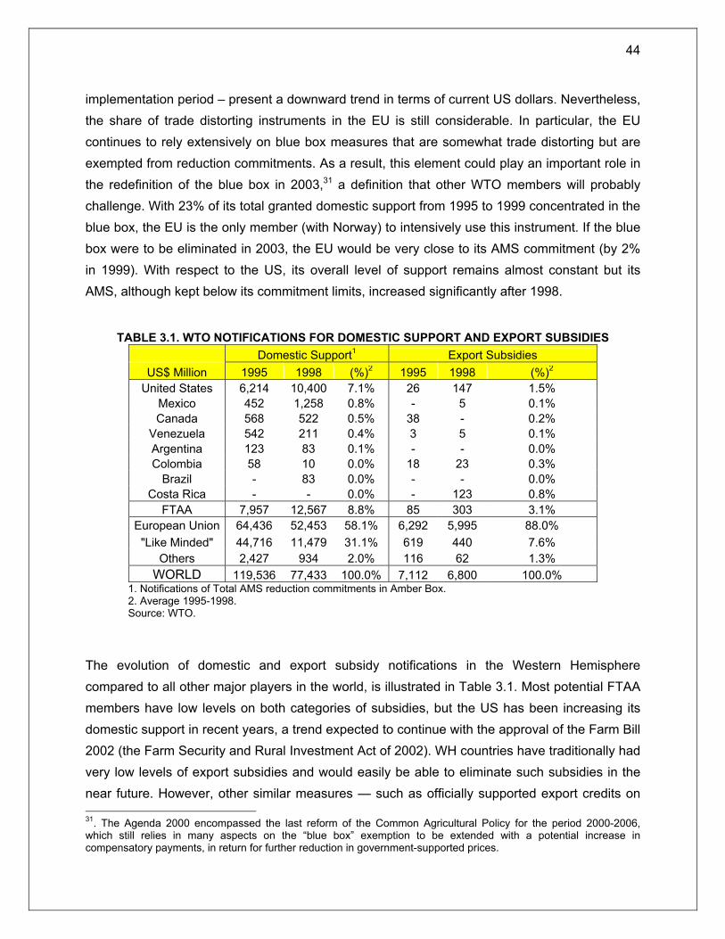
44

implementation period – present a downward trend in terms of current US dollars. Nevertheless, the share of trade distorting instruments in the EU is still considerable. In particular, the EU continues to rely extensively on blue box measures that are somewhat trade distorting but are exempted from reduction commitments. As a result, this element could play an important role in the redefinition of the blue box in 2003,31 a definition that other WTO members will probably challenge. With 23% of its total granted domestic support from 1995 to 1999 concentrated in the blue box, the EU is the only member (with Norway) to intensively use this instrument. If the blue box were to be eliminated in 2003, the EU would be very close to its AMS commitment (by 2% in 1999). With respect to the US, its overall level of support remains almost constant but its AMS, although kept below its commitment limits, increased significantly after 1998.

TABLE 3.1. WTO NOTIFICATIONS FOR DOMESTIC SUPPORT AND EXPORT SUBSIDIES

Domestic Support1 Export Subsidies US$ Million 1995 1998 (%)2 1995 1998 (%)2

United States 6,214 10,400 7.1% 26 147 1.5% Mexico 452 1,258 0.8% - 5 0.1% Canada 568 522 0.5% 38 - 0.2%

Venezuela 542 211 0.4% 3 5 0.1% Argentina 123 83 0.1% - - 0.0% Colombia 58 10 0.0% 18 23 0.3%

Brazil - 83 0.0% - - 0.0% Costa Rica - - 0.0% - 123 0.8%

FTAA 7,957 12,567 8.8% 85 303 3.1% European Union 64,436 52,453 58.1% 6,292 5,995 88.0%

"Like Minded" 44,716 11,479 31.1% 619 440 7.6% Others 2,427 934 2.0% 116 62 1.3%

WORLD 119,536 77,433 100.0% 7,112 6,800 100.0% 1. Notifications of Total AMS reduction commitments in Amber Box. 2. Average 1995-1998. Source: WTO.

The evolution of domestic and export subsidy notifications in the Western Hemisphere compared to all other major players in the world, is illustrated in Table 3.1. Most potential FTAA members have low levels on both categories of subsidies, but the US has been increasing its domestic support in recent years, a trend expected to continue with the approval of the Farm Bill 2002 (the Farm Security and Rural Investment Act of 2002). WH countries have traditionally had very low levels of export subsidies and would easily be able to eliminate such subsidies in the near future. However, other similar measures — such as officially supported export credits on 31. The Agenda 2000 encompassed the last reform of the Common Agricultural Policy for the period 2000-2006, which still relies in many aspects on the “blue box” exemption to be extended with a potential increase in compensatory payments, in return for further reduction in government-supported prices.

45

agriculture, the abuse of international food aid programs, the presence of state trading enterprises, and export restrictions — have been used in the region and could be relevant in multilateral and regional trade negotiations.

3.2. Comparing WTO, OECD and Official Governments Data on Domestic Support

The discipline on domestic support commitments proved to be the least binding for many countries as current total AMS has been kept below commitment levels. Although expenditures on agricultural policies with the greatest potential to affect production and trade have decreased since 1995, the actual impact of this reduction has been limited mainly because the agreed reductions only apply to the AMS and exclude blue and green-box measures as well as the amber box subsidies affecting less than 5% of the value of production (de minimis level).32 In fact, when measured by other methodologies, the evolution of the level of domestic support contrasts with the picture presented until now. Figures 3.2 and 3.3 compare the evolution of domestic subsidies in the EU and the US according to three different sources – WTO notifications in amber and blue box, OECD and government official data. Contrary to the downward trend shown by the AMS indicator, both Producer Support Estimate (PSE) and official government figures increased between 1995 and 2001, both in the EU and US. Two versions of the PSE indicator are presented. In the second one, the market price support (MPS) component has been removed to facilitate comparisons with government payments (see Box 3.1).

Figures 3.2 and 3.3 also indicate the level of domestic support vis-à-vis the amber box reduction commitments assumed by the two countries. In both cases the gap between commitments and current expenditures has been narrowing over this period. Furthermore, according to Hart and Babcock (2002), US subsidies would have exceeded the allowed WTO limits ($ 19.9 billion in

32. There are several reasons why the AMS is a poor indicator of production and trade distortions, among them the following: a) Total AMS production commitments are sector-wide, not product-specific (as is the PSE). This gives countries the opportunity to reduce support on some products leaving other products’ support unchanged or even higher. Countries’ notifications show that some of them have increased support to certain specific products. b) The market price support component of the AMS is based on the domestic administered support price and a fixed base-period world reference price (1986-1988). The domestic administered support price is a poor proxy for measuring the domestic market price because, in many important cases, it is not representative of actual internal supported prices, while the fixed external reference price of support does not represent the actual border price. This calls into question the measure of price support as defined by the URAA (the PSE uses current international reference prices). c) The exclusion of price support in cases where no administered price exists provides wide flexibility to governments in choosing policy instruments. d) The AMS only includes support provided through domestic measures and it does not capture distortions arising from trade measures that are excluded from the AMS provisions (e.g. tariffs and export subsidies). For more details, see Diakosavvas (2001) and Blandford (2001).

46

1999 and $19.1 billion in 2000)33, mainly because low world prices in the late 1990s did trigger high marketing loan and marketing loss assistance expenditures. This scenario would have occurred if the US could not have extensively used the “de minimis” provisions. Whether or not the US amber box expenditures continue exceeding commitments after the approval of the 2002 Farm Bill depends on factors that cannot easily be predicted.34 In any case, as a result of the additional $ 73.5 billion encompassed in the 2002 Farm Bill the overall level of domestic support will remain significant.

3.2.1. Share of Domestic Support in the Value of Agricultural Output

Under the URAA, the EU’s established commitments are more than three times higher than those of the US. The EU is still spending more than twice the amount of US subsidies. A similar trend can also be observed if we compare, in global terms, the share of domestic support in the value of the two countries’ production (Figures 3.4 and 3.535). However, if we consider the expenditures made by governments and the PSE indicator without MPS, we find that the gap between the EU and the US outlays has shrunk dramatically due to a surge in US payments during the last three years. In fact, in response to the deterioration of world prices Congress adopted four large emergency packages between 1998 and 2001, and dramatically increased the level of US farm support.

In July 2002 the US presented an ambitious package of reform to the WTO, The package had the following objectives: the reduction of trade barriers for agricultural products, greater equity in world agriculture, and expanding growth opportunities for international trade in agricultural products. Regarding domestic support, the US proposed to bring down trade distorting subsidies (amber and blue box measures) to substantially lower levels than those currently allowed by fixing the limit on expenditures at 5 percent of a country’s total value of agricultural production over a 5-year period. As can be seen in Figure 3.5, the proposal of the US is an attempt to return to its 1995-1997 levels of domestic support. Even though many have questioned the real US intentions regarding agricultural liberalization, after the 2002 Farm Bill was passed, the current proposition actually serves various US interests. First, the 5-percent

33. In order to see the real level of trade distorting domestic support, current AMS and “de minimis” levels are included in the amber box. 34. For more details on WTO commitment and its implication for the 2002 Farm Bill, see Becker (2002) and Hart & Babcock (2002), ABARE Current Issues (October 2001), Korves and Skorburg (2000). 35. In figures 3.4 and 3.5, PSE as a % of the agricultural is calculated as follows: PSE divided by total value of production at farm gates. It is not calculated as the OECD %PSE, which is obtained using the following formula: PSE/(Q.PP + PP) *100; where Q.PP is the value of production at producers prices and PP is PSE minus MPS.

47

rule would harmonize the level of support that is permitted among WTO members. Second, a strict commitment at the multilateral level would be a way to pin down US domestic policies and avoid future escalations in domestic support as occurred in the late 1990s. Finally, it would force the EU to significantly curb its use of subsidies and as a result deeply reform the Common Agricultural Policy.

The US proposal faces strong domestic and international resistance. Domestically, resistance comes from sectors that could lose with trade liberalization, such as dairy, sugar and orange juice. At an international level, the EU and the like-minded group both object, and argue that this proposition is much more demanding for the Europeans than for the US. Figure 3.4 shows the extent to which the EU would have to cut its domestic measures of support if the US proposal were adopted. Compared to the reduction the US should make, the difference is striking (a reduction of 72% for the EU versus 49% for the US, based on 2001 data).

3.2.2. Domestic Support Granted per Hectare and per Farmer

If we use other criteria, the imbalance in cost that the two countries would have to bear is not as clear. Figures 3.6 and 3.7 show the amount of domestic subsidies per hectare in the two countries. It is worth noting that the quantity of support per hectare increased between 1995 and 2001, while the surface of land used for agricultural purposes decreased. Although the difference in the level of domestic support per hectare granted on both sides of the Atlantic is impressive, we need to keep in mind that domestic subsidies in the US are highly concentrated within a small basket of products. In fact, the US heavily supports the grain and cotton sector while it does not subsidy the production of beef, poultry and pork meats. As a consequence, if pastures were removed from the land area used for agriculture purposes, the amount of domestic support per hectare in the US would be much higher. Furthermore, if we compare the level of domestic support granted per farmer in the EU and the US, as shown in Figures 3.8 and 3.9, we see that American producers are receiving more support than the Europeans – a situation that presents a different picture regarding the efforts that need to be made if the 5 percent rule were enforced. The main reason for these results is that there are three times less farmers in the US than in the EU, and therefore subsidies are highly concentrated, especially in the mid-western states.

FIGURE 3.1. WTO NOTIFICATIO

A. European Union

Note: Amber box includes “de minimis” level. Source: WTO notifications.

C. Like-Minded Countries


0102030405060708090

100110120130

1995 1996 1997

0102030405060708090

100110120130

1995 1996 1997

NS OF DOMESTIC SUPPORT AND EXPORT SUBSIDIES IN THE WORLD (US$ BILLIONS)

B. United States

1998-102030405060708090

100110120130

1995 1996 1997 1998

LEGEND Green box Blue box

Amber box S&D box

Export subsidies


D. Rest of the World

19980

102030405060708090

100110120130

1995 1996 1997 1998

Note: Amber box includes “de minimis” level. Amber box for 1998 is incomplete for most countries.

Source: WTO notifications.

FIGURE 3.2. EUROPEAN UNION: COMPARING DOMESTIC SUPPORT MEASURES (Euro)

Note: Amber box includes “de minimis”. Forecasts for 2000-01 Source: WTO, OECD, European Commission, FAPRI.

FIGURE 3.4. EUROPEAN UNION: DOMESTIC SUPPORT AS A % OF

THE AGRICULTURAL OUTPUT


FIGURE 3.3. UNITED STATES: COMPARING DOMESTIC SUPPORT MEASURES (US$)

0

20

40

60

80

100

120

95 96 97 98 99 00 01

Billi

ons

Amber box commitment PSEPSE without M PS Amber + blue box Gov Payments

0

10

20

30

40

50

60

95 96 97 98 99 2000 2001

Billi

ons

Amber box commitment PSEPSE without M PS Amber + blue box Gov Payments

Note: Amber box includes “de minimis”. Forecasts for 1999-01 Source: WTO, OECD, USDA-FSA, FAPRI.

FIGURE 3.5. UNITED STATES: DOMESTIC SUPPORT AS A % OF

THE AGRICULTURAL OUTPUT

05

101520253035404550

95 96 97 98 99 2000 2001US proposal PSEPse without M PS Amber + blue boxGovernment payments

`

05

101520253035404550

95 96 97 98 99 2000 2001US Proposal PSEPSE without M PS Amber + blue boxGovernment payments

Note: Amber box includes “de minimis”. Forecasts for 1999-01. Source: WTO, OECD, USDA-FSA, FAPRI.

FIGURE 3.6. EUROPEAN UNION: DOMESTIC SUPPORT PER HECTARE (Euros)

Note: Amber box includes “de minimis”. Forecasts for 2000-01 Source: WTO, OECD, European Commission, FAPRI, FAO.

FIGURE 3.8. EUROPEAN UNION: DOMESTIC SUPPORT PER

FARMER (Euros)


FIGURE 3.7. UNITED STATES: DOMESTIC SUPPORT PER HECTARE (US$)

0

100

200

300

400

500

600

700

800

95 96 97 98 99 2000 2001PSE PSE without M PSAmber + blue box Government payments

0

100

200

300

400

500

600

700

800


Note: Amber box includes “de minimis. Forecasts for 1999-01 Source: WTO, OECD, USDA-FSA, FAPRI.

FIGURE 3.9. UNITED STATES: DOMESTIC SUPPORT PER FARMER

(US$)

0

5,000

10,000

15,000

20,000

25,000

30,000

95 96 97 98 99 2000 2001

PSE PSE without M PS Amber + blue box Government payments

0

5,000

10,000

15,000

20,000

25,000

30,000


Note: Amber box includes “de minimis”. Forecasts for 1999-01. Source: WTO, OECD, USDA-FSA, FAPRI.

3.2.3. Distribution of Domestic Support by Products

Figures 3.10 to 3.12 present the distribution of domestic support by products in the EU, US and like-minded countries. Generally speaking, the graphs based on PSE without MPS data and government payments should be close since both methodologies shows the real government outlays intended for producers. Some payments, such as compensatory and loan deficiency payments are direct payments to producers, while others are indirect payments, such as export programs and promotion export measures. With respect to the graphs displaying amber and blue box data on one side and PSE data on the other side, differences in the obtained results can be attributed to the fact that the former excludes green box programs while the latter measures the overall level of domestic support. In addition, the two methodologies use different definitions to calculate MPS (for more details, see Box 3.1). As a matter of fact, the gap between PSE and amber plus blue box reflects the weaknesses of the AMS indicator that have enabled some countries to use any possible loopholes to actually maintain or increase their agricultural protection.

European Union

In the case of the EU, Figure 3.10 shows that data reported for government payments and PSE without MPS are consistent, while strong differences are displayed in amber plus blue box and PSE. The level of support for dairy and poultry and pork is larger in PSE than in amber plus blue box whereas the opposite occurs with cereals. These differences are due to the divergence in methodology when measuring support for prices. In addition, PSE not only measures government subsidies but also trade barriers, such as tariffs and tariff rate quotas that increase substantially domestic prices at the farm gate level compared to world prices. As a result, if cuts in amber plus blue box are made in dairy, the reduction on the overall level of support for this sector would be less than expected because a large share of the internal market prices for this sector is managed through border measures. Therefore, for products that benefit from border protection, a real reduction in the level of domestic support could only occur if market access for these goods is enhanced at the same time as subsidies are cut. This relation between trade policy and domestic support explains why reduction commitments are easier to reach for some products than others.36 The share of MPS in the overall support for agriculture is the part paid

36. For more details on the relationship between domestic support and trade policies, see De Gorter (1999).

52

by the consumers. In the EU, this component reached 60%37 by the year 2000, revealing that consumers, rather than governments, bear the largest cost of the agricultural protection.

United States

As Figure 3.11 shows, dissimilarities between government official outlays and PSE without MPS in the US are greater than in the EU. For instance, the absence of government payments for the meat sectors (beef, poultry and pork) contrasts with the data provided by the PSE without MPS indicator. The point is that in PSE, support for these sectors is concentrated in payments based on input use (interest concessions, fuel tax reductions and subsidies for grazing and irrigation) and to a lesser extent in payments based on overall farming income that are not necessarily product specific.38 Therefore these payments may be included in the category “non-product specific” of the government payments data. When comparing amber plus blue box and PSE, impressive differences arise not only with respect to products but also in the overall level of support. According to amber plus blue box projections, agricultural support did not reach US$ 20 billion in 2001 while the OECD reported a PSE amounting almost US$ 50 billion. PSE level for meats (beef and poultry and pork), dairy and cereals are significantly higher than the support reported in amber plus blue box probably due to the fact that these products benefit from border protections that are included in the PSE measure but are absent from the amber plus blue box calculations. In addition, the “de minimis and non-product specific” category deserves special attention. Since 1997 the US has been using this category intensively, and it is exempted from reduction commitments. According to Hart and Babcock (2002), as a result of the forecasted recuperation in world prices the US could increase even its spending even more with “de minimis”. In fact, higher international prices would raise production values, and as a consequence the “de minimis” exemption limits. Contrary to the EU, the US government largely finances the costs of supporting agriculture (68% of PSE was paid by the government in 2000).39 However, for certain commodities the costs borne by consumers are disproportionate. For instance, in 2000 consumers paid 85% and 80%, respectively, of the support granted to the dairy and sugar industry, two of the largest subsidized sectors in the US.

37. According to the OECD definition of market price support. 38. Payments based on input use include explicit and implicit payments affecting specific variable input costs; the cost of on-farm technical, sanitary and phytosanitary services; or affecting specific fixed input costs, including investment costs. Payments based on overall farming income do not depend on the production of specific commodities or on the use of specific fixed or variable inputs (OECD, 2001). 39. Calculated according to the OECD methodology: PSE minus market price support.

53

Like-Minded Countries40

As illustrated in Figure 3.12, the cost of supporting agriculture in like-minded countries is almost exclusively borne by consumers (88%).41 Dissimilarities between amber plus blue box level of support and PSE are even more impressive in like-minded countries, than in the EU or the US42. Furthermore, trends reversed in 1998 when Japan changed its program supporting the rice sector. Japan had traditionally supported this sector through the management of an administered price that maintains domestic prices at 5 or 6 times higher than world prices. In 1997, Japan’s AMS for rice amounted to $19 billion, of which $18 billion was MPS. In 1998, Japan notified the WTO that the government had stopped intervening in the price formation of rice, reducing its AMS in this sector to zero. However, according to the OECD, the internal prices for rice in Japan in 1998 were more than 5 times import parity. In fact, prices for rice were not affected by the change in government policy since the rice industry in Japan is heavily protected by border measures. This example illustrates one of the various weaknesses in the measurement of the price support element of the AMS that enables some countries to reduce their AMS substantially, even though their actual level of market distorting price support remains very high.

40. Like-minded countries are the Czech Republic Hungary, Iceland, Japan, Korea, Norway, Poland and Switzerland. 41. According to the OECD definition of market price support. 42. Government payments are not included due to the difficulty of obtaining official data from the eight countries included in the “like-minded” group in this paper.

FIGURE 3.10. EUROPEAN UNION: DISTRIBUTION OF DOMESTIC SUPPORT BY PRODUCT (Euros)

A. PSE without MPS B. Government payments

-

10

20

30

40

50

60

70

80

90

100

110

120

1995 1996 1997 1998 1999 2000

Bill

ions

OtherSugarOilseedsCerealsDairyPoultry Pork Beef

-

10

20

30

40

50

60

70

80

90

100

110

120

1995 1996 1997 1998 1999 2000 2001

Bill

ions

NPSOtherSugarOilseedsCerealsDairyPoultry Pork Beef

Source: OECD. Source: European Commission. C. Amber plus Blue boxes D. PSE

Source: WTO notifications. Source: OECD.

-

10

20

30

40

50

60

70

80

90

100

110

120

1995 1996 1997 1998 1999

Bill

ions

DeMin/NPSOtherSugarOilseedsCerealsDairyPoultry Pork Beef

-102030405060708090

100110120

1995 1996 1997 1998 1999 2000 2001

Bill

ions


FIGURE 3.11. UNITED STATES: DISTRIBUTION OF DOMESTIC SUPPORT BY PRODUCT (US$)

A. PSE without MPS B. Government payments

Source: OECD. Source: USDA –FSA.

C. Amber plus Blue boxes D. PSE

Source: WTO notifications, FAPRI. Forecasts for 1999-01. Source: OECD.

05

1015202530354045505560

1995 1996 1997 1998 1999 2000

Bill

ions


0

5

10

15

20

25

30

35

40

45

50

55

60

1995 1996 1997 1998 1999 2000 2001

Bill

ions

NPS

Other

Sugar

Oilseeds

Cereals

Dairy

0

5

10

15

20

25

30

35

40

45

50

55

60

1995 1996 1997 1998 1999 2000 2001

Bill

ions

DeMin/NPS

Other

Sugar

Oilseeds

Cereals

Dairy

05

1015

2025

3035

4045

5055

60

1995 1996 1997 1998 1999 2000 2001

Bill

ions

Other

Sugar

Oilseeds

Cereals

Dairy

Poultry Pork

Beef

FIGURE 3.12. LIKE-MINDED COUNTRIES43: DISTRIBUTION OF DOMESTIC SUPPORT BY PRODUCT (US$)

A. PSE without MPS

Source: OECD.

B. Amber plus Blue boxes

Source: WTO notifications.

C. PSE

Source: OECD.

43. Like-minded countries are the Czech Republic, Hungary, Iceland, Japan, Korea, Norway, Poland and Switzerland.

0

10

20

30

40

50

60

70

80

90

100

110

120

1995 1996 1997 1998 1999 2000

Bill

ions


0

10

20

30

40

50

60

70

80

90

100

110

120

1995 1996 1997 1998

Bill

ions

DeMin/NPSOtherSugarOilseedsCerealsDairyPoultry Pork Beef

0

10

20

30

40

50

60

70

80

90

100

110

120

1995 1996 1997 1998 1999 2000 2001

Bill

ions

Other

Sugar

Oilseeds

Cereals

Dairy

Poultry Pork

Beef

57

4. Identification of Sensitive Agricultural Products

In the previous sections 2 and 3, an attempt was made to provide a realistic view on the level of tariff protection and subsidies that exist in the WH for sensitive agricultural products. However, as it has been previously noted, a full picture of sensitive products can only emerge once the three different mechanisms that potentially distort trade are combined (tariff barriers, non tariff barriers, and subsidies). In this final section, an effort is made to aggregate MFN Equivalent Tariffs, Tariff Rate Quotas, TBT and SPS measures, Domestic Support, and Export Subsidies, into a single index of agricultural protection.

The first step was to group agricultural products into 32 sensitive categories. These categories were devised so as to present agricultural products groups in the WH that have significant trade flows, and/or face high dispersion on trade barriers.

The second step consisted in the creation of six different tables that provide a summary of the different potential trade distorting instruments by group of products and country. Tariff barriers measures are accounted for through MFN Tariffs and number of TRQs. To generate the tariff table, the simple average of the HS-8 digit MFN ad-valorem rates for each of the different group of products was calculated. As in the computations done in section 2, all specific and mixed tariffs were expressed in terms of an ad-valorem equivalent. The Tariff Rate Quota table is straightforward as it indicates the number, if any, of TRQ’s that exist for each one of the 32 groups of products.

NTB measures are accounted for through the SPS and TBT tables. These tables provide the number of measures per product that each country has notified the WTO of between 1995 and 2001. It is important to observe that these notifications only indicate a change in a regulation that one country informed the WTO of. Therefore, notifications indicate the number of additional notified NTB restrictions that exist in each group of products, but not the sanitary and technical barriers themselves. Furthermore, no discrimination has been made between notifications that could be totally justifiable and those that could be more trade restrictive than others. However, studies do indicate that the number of notifications provide a conservative indicator of SPS and TBT issues among countries.44

44. For an assessment of NTB measures on agricultural trade in the WH see Barros et.al. (2002) and Vega, H. (2002, forthcoming). The SPS table was constructed using the data made available by Barros et.al (2002), while the TBT table utilized data provided by Vega, H.

58

Tables were also constructed to measure domestic support and export subsidies, using official notifications by the WTO members. Both tables were built upon the previous analysis presented in section 3, and do provide the dollar denominated amount spent on subsidies for each group of products by country.45 One problem that arose during the construction of these tables was the fact that some subsidies could not be associated with one specific product and were therefore not taken into consideration when calculating the final protection index. Table 4.1 provides an overview of all the restrictions imposed by each WH country.

The next step was to combine the above mentioned six tables into a final table that provides the concluding index of agricultural protection for each group of products in the Western Hemisphere. One of the challenges faced when producing such an index was the fact that each restriction mechanism has different dimensions. To produce measures that can be combined the 32 product groups are ordered and divided into four groups, each containing eight product groups, for each one of the restriction mechanisms. For MFN tariff, for instance, the first group contains the eight product groups that face the highest tariff rates, and is therefore assigned an index of 4. The second group of eight products is assigned an index of 3, the third group an index of 2, and the fourth group, which contains the eight products with the smallest tariff rates, is assigned an index of 1. This procedure is repeated for all the six trade-restricting mechanisms. By assigning a weight to the different mechanisms and adding the values for each product group a final index is created. The weights used to calculate the index are as follows: 50% for traditional market access restricting mechanisms (30% for MFN Tariffs and 20% for number of TRQs); 25% for related issues in market access (20% for SPS and 5% for TBT notifications in the WTO); and 25% for subsidies (20% for domestic support and 5% for export subsidies notifications). The authors assigned these weights to give a higher magnitude to the measures related to market access. The maximum value of the index for one specific group of products is 4 and the minimum value is 1. In other words, an index close to 4 corresponds to a high level of trade restrictions while an index close to 1 represents a low level.

It should be noticed that this final index has no elegant theoretical background; it is much more of a qualitative measure than a quantitative one. The main purpose is to provide negotiators with an assessment of the most sensitive products for future agricultural negotiations.

45. Domestic Support values do encompass the WTO amber box and blue box AMS notifications.

59

Table 4.2 shows the index values by product for all WH countries. The table also provides a general overview of the different restrictions faced by each group of sensitive agricultural products. Dark blue represents high trade restrictions while white represents low trade restrictions. It should also be noted that several different weights were used when calculating the index. Nevertheless, no major change in the order of the sensitive products was observed when different weights were used in other simulations. The most protected product group, as per the protection index, is dairy. It faces high trade access restrictions through all the different mechanism. It is followed by meat (poultry and pork), sugar and food preparations, which face high trade restrictions through at least three of the six mechanisms.

60

TABLE 4.1. OVERVIEW OF AGRICULTURAL TRADE RESTRICTIONS BY COUNTRY IN THE WESTERN HEMISPHERE

Notes: a) Domestic Support includes “amber box”, “blue box” and “de minimis” WTO notifications. b) “Imposed Tariffs” correspond to the weighted average MFN ad-valorem equivalent tariff for each country as calculated in section 2.3.2. A combined tariff was calculated for the Caribbean Community countries.

Source: 2001 Hemispheric Database of the Americas, WTO notifications, AMAD, Barros et al. (2002), and Vega (2002). INT-IDB calculations.

Imposed Tariff (%)

TRQ (nb)

SPS (nb)

TBT (nb)

Domestic Support (US$ mn)

Export Subsidies (US$ mn)

Argentina 14.6 - 163 2 81 - Brazil 14.4 4 69 54 396 - Paraguay 14.1 - - - - - Uruguay 14.4 - 18 - 6 - Mexico 38.8 68 406 11 415 5 Canada 27.7 123 309 25 670 - United States 22.6 376 989 120 15,134 147 Bolivia 10.0 - - - - - Colombia 16.1 66 79 7 10 23 Ecuador 15.4 21 - - - - Peru 18.3 - 145 - - - Venezuela 16.0 59 - - 211 5 Costa Rica 17.0 73 56 4 1 123 Guatemala 15.7 31 31 - - - Honduras 15.1 - 15 - - - Nicaragua 13.0 17 - 3 - - El Salvador 12.5 37 84 67 - - Chile 9.0 - 137 2 - - Dominican Republic 18.1 - 1 - - - Panama 24.2 57 122 54 - - Antigua and Barbuda - - - - - Trinidad and Tobago - 1 - - - St. Lucia - - - - - St. Kitts and Nevis - - - - - Jamaica - 16 21 - - Grenada - - - - - Dominica - - - - - Barbados 4 1 - - Bahamas - - - St. Vincent - - -

FTAA 17.7 969 2,645 371 16,923 303 European Union n/a 256 n/a n/a 77,254 5,996

23.7

Country

37 - -

- -

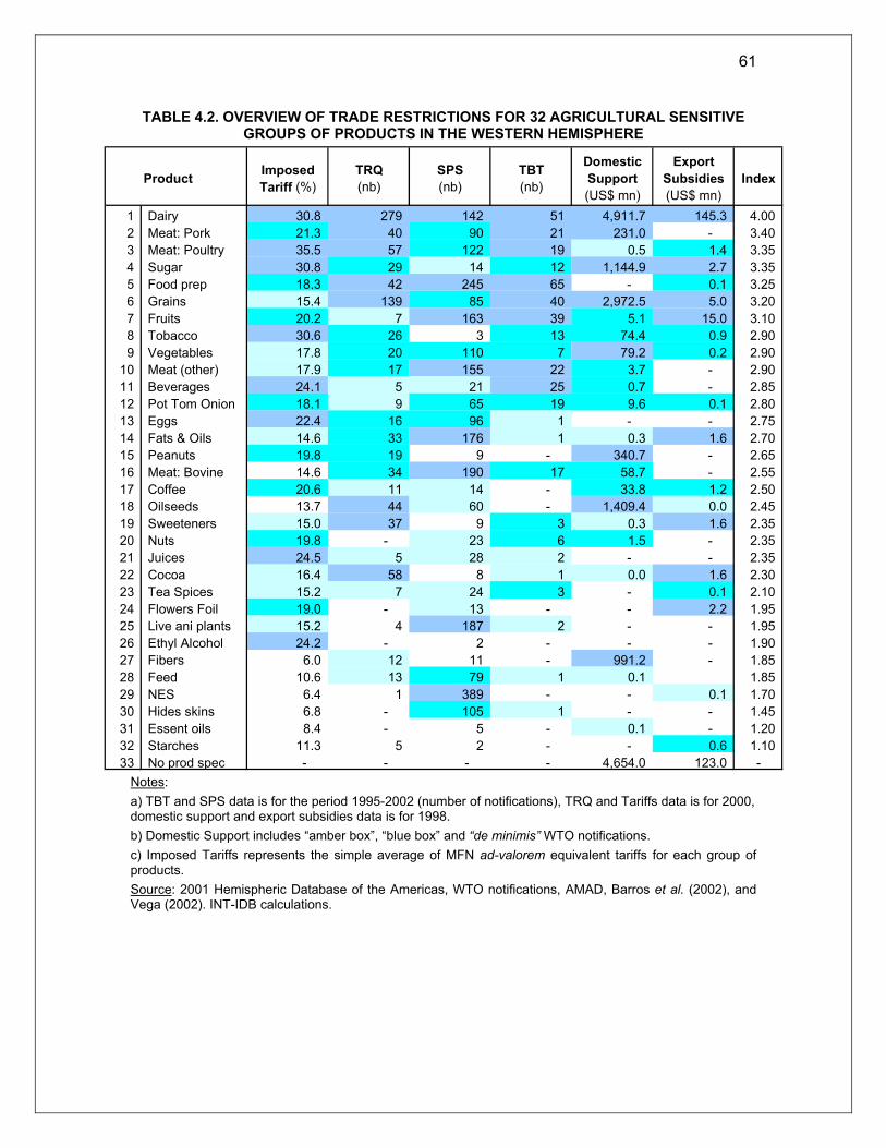
61

TABLE 4.2. OVERVIEW OF TRADE RESTRICTIONS FOR 32 AGRICULTURAL SENSITIVE GROUPS OF PRODUCTS IN THE WESTERN HEMISPHERE

Notes: a) TBT and SPS data is for the period 1995-2002 (number of notifications), TRQ and Tariffs data is for 2000, domestic support and export subsidies data is for 1998. b) Domestic Support includes “amber box”, “blue box” and “de minimis” WTO notifications. c) Imposed Tariffs represents the simple average of MFN ad-valorem equivalent tariffs for each group of products. Source: 2001 Hemispheric Database of the Americas, WTO notifications, AMAD, Barros et al. (2002), and Vega (2002). INT-IDB calculations.

Product Imposed Tariff (%)

TRQ (nb)

SPS (nb)

TBT (nb)

Domestic Support (US$ mn)

Export Subsidies (US$ mn)

Index

1 Dairy 30.8 279 142 51 4,911.7 145.3 4.00 2 Meat: Pork 21.3 40 90 21 231.0 - 3.40 3 Meat: Poultry 35.5 57 122 19 0.5 1.4 3.35 4 Sugar 30.8 29 14 12 1,144.9 2.7 3.35 5 Food prep 18.3 42 245 65 - 0.1 3.25 6 Grains 15.4 139 85 40 2,972.5 5.0 3.20 7 Fruits 20.2 7 163 39 5.1 15.0 3.10 8 Tobacco 30.6 26 3 13 74.4 0.9 2.90 9 Vegetables 17.8 20 110 7 79.2 0.2 2.90

10 Meat (other) 17.9 17 155 22 3.7 - 2.90 11 Beverages 24.1 5 21 25 0.7 - 2.85 12 Pot Tom Onion 18.1 9 65 19 9.6 0.1 2.80 13 Eggs 22.4 16 96 1 - - 2.75 14 Fats & Oils 14.6 33 176 1 0.3 1.6 2.70 15 Peanuts 19.8 19 9 - 340.7 - 2.65 16 Meat: Bovine 14.6 34 190 17 58.7 - 2.55 17 Coffee 20.6 11 14 - 33.8 1.2 2.50 18 Oilseeds 13.7 44 60 - 1,409.4 0.0 2.45 19 Sweeteners 15.0 37 9 3 0.3 1.6 2.35 20 Nuts 19.8 - 23 6 1.5 - 2.35 21 Juices 24.5 5 28 2 - - 2.35 22 Cocoa 16.4 58 8 1 0.0 1.6 2.30 23 Tea Spices 15.2 7 24 3 - 0.1 2.10 24 Flowers Foil 19.0 - 13 - - 2.2 1.95 25 Live ani plants 15.2 4 187 2 - - 1.95 26 Ethyl Alcohol 24.2 - 2 - - - 1.90 27 Fibers 6.0 12 11 - 991.2 - 1.85 28 Feed 10.6 13 79 1 0.1 1.85 29 NES 6.4 1 389 - - 0.1 1.70 30 Hides skins 6.8 - 105 1 - - 1.45 31 Essent oils 8.4 - 5 - 0.1 - 1.20 32 Starches 11.3 5 2 - - 0.6 1.10 33 No prod spec - - - - 4,654.0 123.0 -

62

5. Conclusions and Policy Recommendations

Considering the complexity and heterogeneousness of the agricultural sector in the Americas and its strategic importance both in regional and multilateral negotiations, these are our main conclusions and policy recommendations:

1. Simultaneous barriers to agricultural trade. Countries use several different trade distorting instruments in agriculture. Tariffs are the most commonly used, but other protection mechanisms such as TBT and SPS notifications, domestic support and export subsidies may also distort trade and are difficult to evaluate. Even tariffs barriers are difficult to measure since specific, mixed and TRQs are widely used by some WH countries. On one hand, the highest overall level of high agricultural tariffs has been observed on very small Caribbean islands. This represents a high tax on local poor consumers, as a large percentage of their per capita income is used to buy food products. On the other hand, developed countries are characterized by the application of very high tariffs to a very small group of politically sensitive products, while the rest of their tariffs are kept at very low levels. These sensitive products are further protected through specific and mixed tariffs, TRQs and other non-tariff barriers such as SPS and TBT.

2. Export concentration. In the majority of the Western Hemisphere countries, agricultural exports are highly concentrated in a small basket of specific products. Indeed for 10 countries coffee, bananas and sugar represent more than 50% of their agricultural exports. As a result, potential deadlocks in the negotiations will probably concern a very reduced group of products such as dairy, meats, sugar, tobacco, grains and fruits.

3. Key issues in regional and multilateral agricultural trade negotiations. Agriculture is an area that encompasses different systemic and non-systemic issues. Topics such as subsidies are systemic issues since any reduction of their use by one country will benefit all countries that this country trades with, and could have potential spillovers on world prices and market-shares. Subsidies are much better addressed through multilateral negotiations, such as the Doha Development Agenda of the WTO. On the other hand, market access issues, such as tariffs, TRQs and some non-tariff barriers, are non-systemic issues since they can be negotiated on a country-by-country basis without benefiting other trading partners. Market access is much better addressed in a bilateral or regional framework as negotiations between

63

a reduced number of countries allow for deeper trade liberalization, normally starting with applied tariffs. So if WH countries continue to invest political and human capital in the FTAA process, the launch of the WTO Development Agenda will be beneficial for hemispheric agricultural integration. The new round will allow for the separation of the two most sensitive issues - market access and subsidies - with market access being primarily discussed at a regional level and subsidies at the multilateral level. However, it is legitimate for competitive countries in agriculture to try to secure that other systemic issues (such as environment disciplines or intellectual property rights) would be addressed through multilateral negotiations. In this case, some FTAA issues could be Doha plus while others not.

4. RTR and REST as useful tools to balance tariff concessions. The best solution for trade liberalization in the WH would be to implement zero tariffs for all products without exceptions. The use of exception lists would certainly remove most of the “real” protected products from a RIA, and therefore undermine potential gains that could be achieved through such an agreement. However, if countries do insist on exceptions lists and/or a long tariff phase-out period, negotiators could use the RTR and REST indexes as a valid and useful tool to balance concessions and achieve progress in bilateral and regional agreements. Furthermore, they can also be used to detect potentially difficult sectors for future negotiations.

5. Market Access in the WH: main gains and trade-offs. The Central American countries, which face, on average, higher protection than they impose, would have the highest net gains in terms of overall market access, after a simultaneous lowering of agricultural tariff barriers in North America and industrial tariffs in South America. As regards the Mercosur countries, however, the agricultural sector liberalization will encompass trade-offs. While these countries would definitely gain from agricultural liberalization, they would also need to become net liberalizers of their industrial sector. The opposite is true for NAFTA countries. NAFTA countries will need to make trade-offs in terms of offering a broad agricultural access in order to secure access for industrial products.

6. Subsidies: URAA loopholes and the need to avoid exceptions. The URAA provides too many ways to avoid domestic and export subsidies reductions. The blue box, the presence of trade-distorting programs into the green box, the absence of disciplines on export credit guarantees and the abuse of food aid programs are examples of the current loopholes. In addition, some countries take advantage of the ”de minimis” exemption and non-product specific subsidies to increase their level of

64

domestic support without exceeding their WTO commitments. In our opinion, de minimis exemptions should be eliminated, and reductions commitments should be also established on a product-by-product basis. The S&D box is another exception that could be phased out if the majority of developing countries continue to be unable to use it. These countries are not applying trade-distorting subsidies, and there is no reason to keep or create boxes that will not really be used. If countries are really keen to eliminate all trade and production distorting subsidies, in the long run they should avoid any kind of exceptions.

7. Full decoupling of payments. Negotiators should target the full decoupling of the government payments to producers, as the best way to prevent distortion of production and trade. In other words, payments should be fully decoupled from the volume of production, planted area or animal unit.

8. Market access should be enhanced at the same time that subsidies are cut. Reductions in subsidies are very much related to market access enhancement and vice-versa. In fact, both subsidies through MPS and border measures (tariffs, TRQs, non-tariff barriers, etc.) contribute simultaneously to the fact that producer prices are set at higher levels when compared to world prices. The way MPS is calculated (depending on whether government administered prices are used or not) is particularly important because it has serious consequences in terms of which subsidies should be phased out for each product to really liberalize trade. For instance, Japan claimed to have eliminated amber box support for rice after it abolished the government-administered price for this product. However actual prices paid to producers remained unchanged for this sector, as they are still supported through border measures. This example illustrates that a real reduction in the level of domestic support could only happen if market access is enhanced at the same time that subsidies are cut. Comprehensive results could only be achieved if market access and subsidies are addressed at the same time. In the case that they are addressed in regional and multilateral parallel negotiations, policymakers should try to build a “global single undertaking” provision between these processes.

65

Appendix A Trade and Tariff Structure in the WH

Table 1. Agricultural Sector Trade and MFN Tariff Structure of the Western Hemisphere countries at HS 8 digit level (2000)

Note: 1. Non ad valorem = sum of all specific and mixed rates. Source: 2001 Hemispheric Database of the Americas and AMAD. IDB-INT calculations.

Ad Val Non Ad Val1 0% 0%-15% 15%-30% 30%-50% >50% Mean Median St Dev Max 1 Argentina 9,494,815 940 - 79 564 296 1 - 12.7 13.0 5.9 32.0 - 2 Brazil 8,050,652 940 - 79 565 296 - - 12.6 13.0 5.8 27.0 4 3 Paraguay 302,221 945 - 79 576 286 4 - 12.3 13.0 5.6 30.0 - 4 Uruguay 579,329 908 - 77 552 279 - - 12.4 13.0 5.6 23.0 - 5 Mexico (2,101,401) 1,016 53 30 496 427 62 54 23.3 15.0 37.8 260.0 68 6 Canada 4,142,472 979 362 538 656 46 3 98 22.4 3.0 63.1 538.0 123 7 United States 14,237,485 989 747 372 1,083 161 59 61 11.4 3.7 32.0 350.0 376 8 Bolivia 169,664 873 - 15 858 - - - 9.8 10.0 1.3 10.0 09 Colombia 1,441,657 881 - - 280 601 - - 14.5 15.0 5.5 20.0 66

10 Ecuador 1,117,100 865 - 20 268 577 - - 14.3 15.0 5.7 20.0 2111 Peru (258,173) 900 - - 530 314 56 - 17.1 12.0 6.5 30.0 012 Venezuela (1,309,192) 865 - - 278 591 - - 14.6 15.0 5.4 20.0 5913 Costa Rica 1,241,539 1,138 - 238 796 - 64 40 13.8 14.0 20.0 162.0 7314 Guatemala 919,306 811 60 208 215 388 - - 9.2 10.0 6.5 20.0 3115 Honduras 98,404 869 - - 425 426 13 5 11.5 15.0 8.4 55.0 016 Nicaragua 141,281 869 - 197 638 18 7 9 7.3 10.0 7.4 76.7 1717 El Salvador (90,269) 937 25 217 217 429 49 - 11.2 15.0 8.9 40.0 3718 Chile 1,567,390 747 - - 747 - - - 9.0 9.0 - 9.0 019 Dominican Republic (327,892) 778 - - 229 277 272 - 21.2 25.0 10.6 35.0 020 Panama (67,856) 1,334 - 67 455 723 48 41 15.0 15.0 20.8 300.0 5721 Antigua and Barbuda (73,457) 999 19 218 246 208 327 - 17.3 20.0 14.7 45.0 022 Trinidad and Tobago (49,375) 1,000 24 389 80 245 284 2 16.6 15.0 16.7 75.0 023 St. Lucia (43,929) 1,024 - 285 238 173 328 - 16.5 10.0 16.0 45.0 024 St. Kitts and Nevis (27,211) 998 22 257 257 120 364 - 17.5 10.0 16.3 40.0 025 Jamaica (133,611) 1,021 - 410 61 224 321 5 17.2 15.0 17.0 75.0 026 Grenada (19,639) 1,015 1 120 351 219 324 - 18.2 15.0 15.1 40.0 027 Dominica (8,666) 579 439 159 55 78 287 - 22.7 25.0 17.9 45.0 028 Barbados (94,877) 886 27 - 349 194 246 97 36.6 20.0 51.6 243.0 3729 Bahamas (615,499) 676 - 152 788 - - 3 25.4 30.0 17.6 260.0 030 St. Vincent (4,874) 1,007 13 117 392 228 270 - 17.0 10.0 15.0 40.0 0

38,277,394 926 60 144 442 261 113 14 16.0 14.1 15.4 98.9 969

31 EU-15 (4,625,098) 1,227 852 845 505 513 136 80 18.3 11.5 24.5 251.6 256

Main StatisticsTRQsCountry

Trade Balance ('000)

Nb of Tariff Lines Frequency Distribution of Tariff Rates

Sum or Average

66

Table 2. Industrial Sector Trade and MFN Tariff Structure of the Western Hemisphere countries at HS 8 digit level (2000)

Note: 1. Non ad valorem = sum of all specific and mixed rates. Source: 2001 Hemispheric Database of the Americas and AMAD. IDB-INT calculations.

Ad Val Non Ad Val1 0% 0%-15% 15%-30% 30%-50% >50% Mean Median St Dev Max 1 Argentina (8,591,613) 8,431 - 391 4,631 3,368 41 - 13.4 15.0 6.8 33.0 2 Brazil (13,958,529) 8,431 - 63 3,841 4,489 38 - 14.3 17.0 6.9 35.0 3 Paraguay (1,490,719) 8,450 - 397 5,216 2,837 - - 11.5 11.0 6.7 28.0 4 Uruguay (1,748,646) 7,945 - 338 4,627 2,980 - - 12.1 13.0 7.0 23.0 5 Mexico (1,672,518) 10,272 19 194 5,268 4,345 484 - 15.6 13.0 8.1 35.0 6 Canada 14,088,476 6,777 47 3,291 2,855 677 1 - 4.4 2.5 5.8 41.3 7 United States (478,163,301) 7,894 546 2,766 5,227 384 58 5 4.5 3.0 5.8 58.4 8 Bolivia (573,441) 5,815 - 390 5,425 - - - 9.1 10.0 2.7 10.0 9 Colombia 192,215 5,740 - 120 4,357 1,253 10 - 11.3 10.0 6.2 35.0

10 Ecuador 283,231 4,509 - 109 3,373 1,020 - 7 10.9 10.0 7.0 99.0 11 Peru (329,516) 5,694 - - 4,995 699 - - 13.0 12.0 2.6 20.0 12 Venezuela 17,373,749 5,742 - 38 4,435 1,257 12 - 11.6 10.0 6.0 35.0 13 Costa Rica (1,787,135) 5,119 - 2,671 2,443 - 5 - 4.8 - 5.7 49.0 14 Guatemala (3,104,732) 5,079 17 2,593 1,788 714 - 1 5.3 - 7.5 25.0 15 Honduras (1,961,542) 5,044 - - 3,926 1,111 7 - 6.9 1.0 7.5 35.0 16 Nicaragua (1,230,168) 5,018 - 2,636 2,382 - - - 3.4 - 3.9 15.0 17 El Salvador (2,374,375) 5,157 - 2,627 1,830 700 - - 6.7 - 8.4 30.0 18 Chile (456,412) 5,105 - - 5,105 - - - 9.0 9.0 - 9.0 19 Dominican Republic (4,826,041) 5,163 - - 2,838 1,935 390 - 17.3 15.0 10.1 35.0 20 Panama (2,538,561) 7,213 - 325 6,860 24 2 2 8.2 10.0 5.8 87.0 21 Antigua and Barbuda (230,467) 5,277 - 631 3,082 1,509 45 10 10.9 5.0 10.6 70.0 22 Trinidad and Tobago (626,901) 5,268 2 2,401 1,555 1,213 101 - 7.6 2.0 9.9 45.0 23 St. Lucia (228,631) 5,275 - 2,159 1,729 1,190 172 25 9.0 5.0 11.4 95.0 24 St. Kitts and Nevis (120,848) 5,279 - 1,186 2,490 1,477 116 10 10.9 5.0 11.6 70.0 25 Jamaica (1,307,825) 5,216 - 3,360 602 1,157 97 - 6.7 - 10.0 40.0 26 Grenada (123,467) 5,082 - 221 3,575 1,141 145 - 10.0 5.0 8.4 40.0 27 Dominica (70,919) 5,275 - 226 3,769 1,128 152 - 10.8 5.0 9.7 45.0 28 Barbados (715,563) 5,043 - - 3,701 1,161 142 39 11.0 5.0 11.7 145.0 29 Bahamas (3,306,719) 4,896 - 247 210 715 3,617 107 32.0 35.0 11.4 100.0 30 St. Vincent (131,971) 5,257 - 406 3,577 1,153 121 - 9.6 5.0 8.3 40.0

(499,732,889) 6,016 21 993 3,524 1,321 192 7 10.4 7.8 7.4 47.6

31 EU-15 (66,693,698) 10,659 41 2,314 8,176 210 - - 4.7 3.7 4.4 26.0

Sum or Average

Main StatisticsCountry

Trade Balance ('000)

Nb of Tariff Lines Frequency Distribution of Tariff Rates

67

Appendix B Export Weighted Tariffs for WH Countries

Table 1.a. Agricultural MFN Tariffs Weighted by Export at HS 6 digit level (2000)

Source: 2001 Hemispheric Database of the Americas and AMAD. IDB-INT calculations.

Caricom EUARG BRA PAR URU CAN MEX USA CHI DOM PAN CR GTM HND NIC SLV BOL COL ECU PER VEN Caricom EU

Argentina 14.5 11.6 16.0 14.2 15.8 14.1 15.4 17.1 15.1 13.9 15.0 13.8 14.9 15.7 12.0 14.7 13.7 14.0 16.4 18.9 17.8 Brazil 13.0 11.4 16.0 14.1 15.7 14.0 15.4 16.5 14.9 13.9 14.5 13.8 14.5 15.5 12.0 14.4 13.8 14.0 16.5 18.2 17.6 Paraguay 12.7 14.1 15.2 13.7 15.5 13.7 14.0 18.7 15.2 13.9 15.7 13.9 15.1 15.9 12.1 15.0 13.7 14.2 16.2 19.8 16.4 Uruguay 12.7 14.1 11.6 13.7 15.4 13.8 15.2 16.6 14.4 13.7 14.4 13.8 14.1 14.5 11.7 14.4 13.7 13.9 16.4 16.0 16.9 Canada 27.9 31.4 4.8 51.1 18.0 36.9 32.3 30.9 19.1 19.4 14.0 3.4 25.5 39.4 19.8 14.8 7.3 13.2 29.9 40.2 67.6 Mexico 45.6 49.8 25.2 38.7 35.1 50.8 32.0 55.3 32.6 28.2 37.9 25.3 37.9 44.3 21.8 38.5 30.1 26.5 30.3 51.7 44.5 United States 17.5 35.4 9.3 25.9 12.8 12.2 8.6 30.6 11.3 11.5 17.6 7.7 25.8 12.1 8.4 9.9 6.3 9.5 33.2 19.6 30.1 Chile 9.0 9.0 9.0 9.0 9.0 9.0 9.0 9.0 9.0 9.0 9.0 9.0 9.0 9.0 9.0 9.0 9.0 9.0 9.0 9.0 9.0 Dominican Republic 14.3 15.2 9.0 22.8 19.7 24.3 18.0 27.6 22.3 22.6 19.1 17.7 18.0 19.6 10.9 20.9 25.0 21.6 22.9 24.7 23.1 Panama 13.1 35.9 14.6 45.9 18.6 18.4 24.1 14.1 44.0 18.2 32.3 17.1 30.0 25.5 12.3 25.3 16.3 18.9 20.7 42.7 25.8 Costa Rica 10.2 19.3 5.1 24.8 13.7 15.4 17.2 14.6 21.6 17.9 18.3 14.9 21.6 17.5 8.6 17.0 14.1 14.5 14.2 22.2 21.5 Guatemala 10.6 12.9 4.9 40.4 12.9 39.4 14.8 17.0 19.5 15.8 14.9 14.7 15.3 16.2 7.7 15.0 15.5 14.1 30.6 26.7 18.0 Honduras 9.2 15.1 6.4 22.6 11.6 16.3 15.1 16.3 20.2 17.9 17.7 19.4 17.2 19.1 7.6 18.5 17.3 16.6 18.4 21.9 16.1 Nicaragua 8.7 17.8 4.5 16.8 7.2 10.4 13.5 9.4 18.6 12.2 10.4 15.0 10.2 13.6 6.4 12.7 10.3 10.4 9.9 18.3 10.7 El Salvador 8.3 12.6 4.9 20.3 12.4 16.9 12.4 14.6 19.5 16.8 15.0 17.4 15.1 17.1 7.2 16.4 14.7 14.4 15.1 22.3 17.3 Bolivia 10.0 10.0 10.0 10.0 10.0 10.0 10.0 10.0 10.0 9.7 10.0 10.0 10.0 10.0 10.0 10.0 10.0 10.0 10.0 10.0 10.0 Colombia 16.6 16.3 15.3 18.6 16.3 16.1 16.1 16.3 16.9 15.6 14.7 13.8 12.5 14.3 14.1 16.1 14.4 14.0 17.4 17.7 17.6 Ecuador 15.9 16.1 14.0 18.5 15.4 16.0 15.4 16.0 16.9 15.2 14.6 13.8 12.5 14.0 14.0 15.9 13.0 14.0 17.3 17.7 17.1 Peru 17.4 17.8 14.4 24.1 20.1 18.0 17.8 21.1 17.2 20.6 21.2 18.9 20.2 19.9 19.0 13.9 18.4 21.6 17.2 17.9 18.5 Venezuela 16.6 16.3 15.2 18.6 16.3 16.1 16.0 16.3 16.9 15.6 14.8 13.9 12.5 14.3 14.1 16.1 13.1 15.0 14.1 17.8 17.5 CARICOM 17.4 23.7 13.8 23.3 19.8 37.7 22.6 30.3 31.9 34.8 36.0 30.9 34.4 28.5 30.7 20.6 33.2 34.7 29.0 30.9 25.6 European Union 19.7 20.4 16.3 75.3 29.4 19.9 28.4 16.6 35.3 76.1 54.2 28.1 21.9 32.8 14.9 6.9 30.7 83.8 11.0 28.1 41.4Average 15.5 19.9 11.0 26.4 16.0 17.9 18.7 17.8 23.0 20.1 18.5 18.5 15.0 19.5 18.8 12.2 17.8 19.1 15.1 20.0 23.6 21.8

AndeanMercosur NAFTA CACMImposed/Faced Tariffs

68

Table 1.b. Agricultural Preferential Tariffs Weighted by Export at HS 6 digit level (2000)




AndeanMercosur NAFTA CACMImposed/Faced Tariffs

69

Table 2.a. Industrial MFN Tariffs Weighted by Export at HS 6 digit level (2000)




AndeanImposed/Faced Tariffs

Mercosur NAFTA CACM

70

Table 2.b. Industrial Preferential Tariffs Weighted by Export at HS 6 digit level (2000)





Mercosur NAFTA CACM

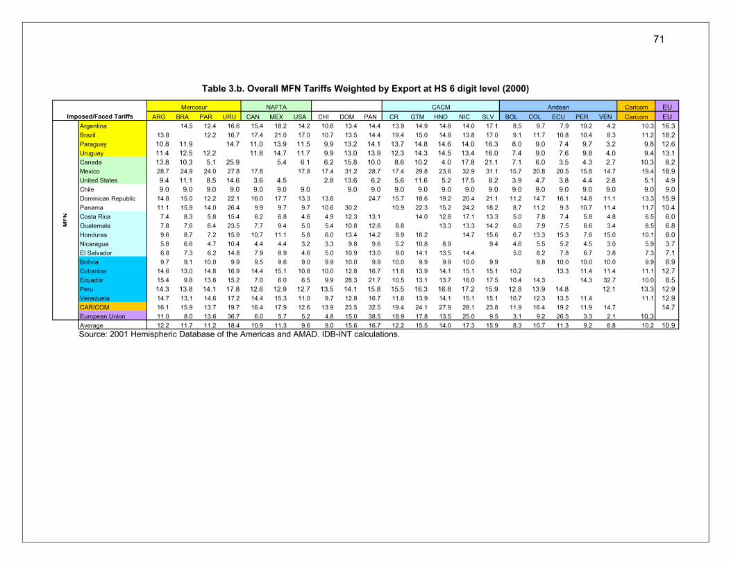
71

Table 3.b. Overall MFN Tariffs Weighted by Export at HS 6 digit level (2000)





Mercosur NAFTA CACM

72

Table 3.a. Overall Preferential Tariffs Weighted by Export at HS 6 digit level (2000)





Mercosur NAFTA CACM

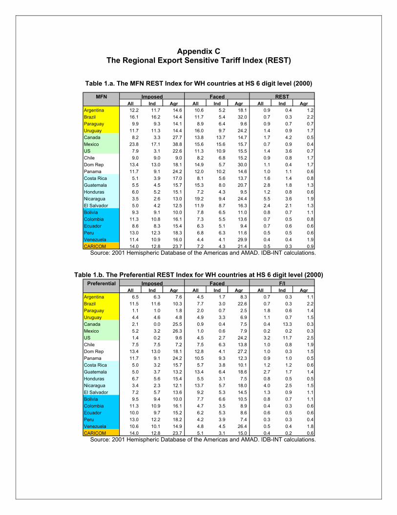
Appendix C The Regional Export Sensitive Tariff Index (REST)

Table 1.a. The MFN REST Index for WH countries at HS 6 digit level (2000)


Table 1.b. The Preferential REST Index for WH countries at HS 6 digit level (2000)


MFNAll Ind Agr All Ind Agr All Ind Agr

Argentina 12.2 11.7 14.6 10.6 5.2 18.1 0.9 0.4 1.2Brazil 16.1 16.2 14.4 11.7 5.4 32.0 0.7 0.3 2.2Paraguay 9.9 9.3 14.1 8.9 6.4 9.6 0.9 0.7 0.7Uruguay 11.7 11.3 14.4 16.0 9.7 24.2 1.4 0.9 1.7Canada 8.2 3.3 27.7 13.8 13.7 14.7 1.7 4.2 0.5Mexico 23.8 17.1 38.8 15.6 15.6 15.7 0.7 0.9 0.4US 7.9 3.1 22.6 11.3 10.9 15.5 1.4 3.6 0.7Chile 9.0 9.0 9.0 8.2 6.8 15.2 0.9 0.8 1.7Dom Rep 13.4 13.0 18.1 14.9 5.7 30.0 1.1 0.4 1.7Panama 11.7 9.1 24.2 12.0 10.2 14.6 1.0 1.1 0.6Costa Rica 5.1 3.9 17.0 8.1 5.6 13.7 1.6 1.4 0.8Guatemala 5.5 4.5 15.7 15.3 8.0 20.7 2.8 1.8 1.3Honduras 6.0 5.2 15.1 7.2 4.3 9.5 1.2 0.8 0.6Nicaragua 3.5 2.6 13.0 19.2 9.4 24.4 5.5 3.6 1.9El Salvador 5.0 4.2 12.5 11.9 8.7 16.3 2.4 2.1 1.3Bolivia 9.3 9.1 10.0 7.8 6.5 11.0 0.8 0.7 1.1Colombia 11.3 10.8 16.1 7.3 5.5 13.6 0.7 0.5 0.8Ecuador 8.6 8.3 15.4 6.3 5.1 9.4 0.7 0.6 0.6Peru 13.0 12.3 18.3 6.8 6.3 11.6 0.5 0.5 0.6Venezuela 11.4 10.9 16.0 4.4 4.1 29.9 0.4 0.4 1.9CARICOM 14.0 12.8 23.7 7.2 4.3 21.4 0.5 0.3 0.9

Imposed Faced REST

PreferentialAll Ind Agr All Ind Agr All Ind Agr

Argentina 6.5 6.3 7.6 4.5 1.7 8.3 0.7 0.3 1.1Brazil 11.5 11.6 10.3 7.7 3.0 22.6 0.7 0.3 2.2Paraguay 1.1 1.0 1.8 2.0 0.7 2.5 1.8 0.6 1.4Uruguay 4.4 4.6 4.8 4.9 3.3 6.9 1.1 0.7 1.5Canada 2.1 0.0 25.5 0.9 0.4 7.5 0.4 13.3 0.3Mexico 5.2 3.2 26.3 1.0 0.6 7.9 0.2 0.2 0.3US 1.4 0.2 9.6 4.5 2.7 24.2 3.2 11.7 2.5Chile 7.5 7.5 7.2 7.5 6.3 13.8 1.0 0.8 1.9Dom Rep 13.4 13.0 18.1 12.8 4.1 27.2 1.0 0.3 1.5Panama 11.7 9.1 24.2 10.5 9.3 12.3 0.9 1.0 0.5Costa Rica 5.0 3.2 15.7 5.7 3.8 10.1 1.2 1.2 0.6Guatemala 5.0 3.7 13.2 13.4 6.4 18.6 2.7 1.7 1.4Honduras 6.7 5.6 15.4 5.5 3.1 7.5 0.8 0.5 0.5Nicaragua 3.4 2.3 12.1 13.7 5.7 18.0 4.0 2.5 1.5El Salvador 7.2 5.7 13.6 9.2 5.3 14.5 1.3 0.9 1.1Bolivia 9.5 9.4 10.0 7.7 6.6 10.5 0.8 0.7 1.1Colombia 11.3 10.9 16.1 4.7 3.5 8.9 0.4 0.3 0.6Ecuador 10.0 9.7 15.2 6.2 5.3 8.6 0.6 0.5 0.6Peru 13.0 12.2 18.2 4.2 3.9 7.4 0.3 0.3 0.4Venezuela 10.6 10.1 14.9 4.8 4.5 26.4 0.5 0.4 1.8CARICOM 14.0 12.8 23.7 5.1 3.1 15.0 0.4 0.2 0.6

Imposed Faced F/I

74

Appendix D Technical Notes

General Methodology: the objective of the study was to compile all trade-related data available for agricultural products country by country, using the 2001 Hemispheric Database of the Americas. A database was created containing both 6- and 8-digit (or more) Harmonized System tariff lines for 30 of the 34 FTAA member countries (excluding Belize, Suriname, Guyana and Haiti, due to lack of trade-related data). It includes product descriptions, MFN ad valorem tariffs, MFN specific and mixed tariffs, preferential rates, and ad valorem equivalents for such tariffs, imports value and volume, imports price, exports value, export volume, and an indication of whether the tariff is a Tariff Rate Quota. In addition, the data was also analyzed in an aggregate basis by being grouped in 32 groups of products upon the International Bilateral Agricultural Trade (IBAT) Database. Once all tariffs were expressed in terms of ad valorem equivalents, we were able to calculate the number of tariff lines and TRQ, mean, median, tariff dispersion, maximum and minimum tariffs, and frequency distributions. Tariff conversions: the first step in developing tariff profiles was the conversion of all specific and mixed tariffs into ad valorem equivalents (AVE). Specific tariffs are tariffs that are set as a monetary amount per unit of import, i.e. a product can have a specific tariff, which charges $1.50 per kilogram. Countries may also combine ad valorem and specific tariffs so that a product’s tariff may be the sum of the ad valorem tariff plus the specific tariff, called mixed or compound tariffs. According to the WTO, AVE are usually calculated “either by comparing collected custom revenues to the value of imports or by comparing unit values of traded products with the applied non-ad valorem tariff”. The methodology followed in this study to obtain ad valorem equivalents was to divide the product’s specific rate by its import price. In this case the price was calculated by dividing the value of imports by the quantity of imports. Where no trade data was available, the price of the closest related product was used. Tariff Rate Quotas: as a result of the “tariffication” effort of the URAA, many products that used to be protected with import quotas are now protected through Tariff Rate Quotas (TRQs). In this case, lower “within access commitment” rates are set for specified quantities, and higher “over access commitment” rates are set for quantities that exceed the quota. The in-quota tariff would be the tariff rate up to the quota limit, and the over-quota tariff is the higher duty rate. Hirschmann-Herfindahl Index (HHI): The HHI is equal to the sum of the squared shares of all individual products exported, where i stands for a particular product and n is the total number of products. When a single export product (tariff line) produces all the revenues HHI equals 100; when export revenues are evenly distributed over a large number of products, HHI approaches zero.

.100*

2

∑∑

=n

in

ii

i

X

XHHI

75

“Relative Tariff Ratio” Index: the RTR index was originally developed by Sandrey (2000), and further developed by Wainio & Gibson (2002) and Gehlhar and Wainio (2002). It assumes, in first instance, that only the bilateral partners exist in the world, placing great emphasis on tariffs from an importing country that are of the greatest importance to the exporting partner. So, the index is always calculated in a bilateral basis, using country (A)’ total exports as weights in the calculation of a weighted average tariff of country (B), and vice-versa. For example, if the tariff line “boneless frozen meat of bovine animal” represents 23% of Uruguay’s exports, it will weight 23% on Uruguay’s “faced” tariffs from each FTAA country. The RTR is the ratio between country (A)’s faced tariffs in the numerator and imposed tariffs in the denominator, relative to country (B), or:

( )

( )∑

∑= n

i

Bi

Ai

n

i

Ai

Bi

AB

YX

YXRTR

.

.

where, A, B = Countries A e B Xi = ad valorem equivalent (AVE) tariff rate for product i; Yi = share of exports of product i in total exports;

In general, a ratio close to one reflects the fact that both countries have similar protection, and thus face/impose comparable tariff barriers. However, this does not reflect the absolute levels of tariffs, but their relative ratios. “Regional Export Sensitive Tariff” Index: the REST Index measures each country’s faced tariffs from its partners weighted by its total exports in the numerator and each country’s imposed tariffs weighted by the total exports of all its partners in the denominator, calculated one by one, considering a potential Regional Integration Agreement (RIA). Each combination of tariffs and share of export ratios for one country is weighted by the relative importance of total exports to the region in the case of faced tariffs and total imports in the case of imposed tariffs. Preexisting RTAs need to be considered using preferential tariffs or assuming zero tariffs in the case of a future free trade area.

76

The scientific notation of the REST index is:

RESTA =( ) ( ) ( )

( ) ( ) ( )∑∑∑

∑∑∑

===

===

∗

++∗

+∗

∗

++∗

+∗

n

i

Ni

AiA

T

AN

n

i

Ci

AiA

T

AC

n

i

Bi

AiA

T

AB

n

i

Ai

NiA

T

AN

n

i

Ai

CiA

T

AC

n

i

Ai

BiA

T

AB

yxMMyxM

MyxMM

yxXXyxX

XyxXX

111

111

...

...

Where: A, B, C,…, N = member countries of a Regional Integration Agreement xi

A = maximum ad-valorem equivalent tariff rate at HS-96 level for tariff line i

MB

A = country A’s total imports from country B

MT

A = country A’s total imports from all RIA countries

XB

A = country A’s total exports to country B

XT

A = country A’s total exports to all RIA countries

Green box: Measures of domestic support placed into the green box are not, or minimally, trade distorting. They are exempt from reduction commitments. S&D box: This box includes developmental programs in developing countries. They are exempt from reduction commitments. Blue box: It covers direct payments made under production-limiting programs. They are exempt from reduction commitments. Amber box: Trade and production distorting measures not included in the boxes mentioned previously fall into the amber box. The level of support is measured through an indicator called “Aggregate Measurement of Support” (AMS). AMS is subject to reduction commitments. However, amber box subsidies affecting less than 5% of the value of production (10% for developing countries) are exempt of commitments, due to a mechanism called ”de minimis” level. Export subsidies: Existing subsidies are subject to reduction commitments both in terms of volume and value of exports. New subsidies are banned. The commitments do not include export credit guarantees and food aid disciplines. Producer Support Estimate (PSE): PSE is the basic estimate of agricultural protection and support calculated by OECD since the mid 80’s. It is an indicator of the annual monetary value of gross transfers from consumers and taxpayers to support agricultural producers, measured at the farm gate level, arising from policy measures. PSE has two components: market price support (MPS) and budgetary outlays.

∑=

= n

i

iw

iwB

i

x

xy

1

xwi = country’s total exports of tariff line i to the world

77

REFERENCES ABARE. 2000. US and EU Agricultural Support: Who does it benefit? ABARE Current Issues

October 2, 2000.

ABARE. 2001. Rising US agricultural support, ABARE Current Issues, October 7, 2001.

Barros, G.S.C., H.L. Burnquist, S.H.G. Miranda and J.H. Cunha. 2002. SPS Issues of Agricultural Trade in the Western Hemisphere. CEPEA, Sao Paulo, Brazil.

Becker, G S. 2002. Farm Support Programs and World Trade Commitments. Washington, DC: Congressional Research Service.

Becker, G.S. 1983. Competition among Pressure Groups for Political Influence. The Quarterly Journal of Economics, 98, August, 371-400 p.

Blandford. D. 2001. Are Disciplines Required on Domestic Support? Journal of International Law and Trade Policy 2 (1). November.

Bouët, A. 2000. La Measure des Protections Commerciales Nationales. CEPII Working Paper, December 15, 2000.

Bouët, A.; L. Fontagné; M. Mimouni; F. Kirchbach. 2002. Market Access Map For GTAP: An Assessment of Bilateral Protection in Merchandise Trade. Paper prepared for the GTAP conference, Taipei, June.

Buchanan, J.M. 1965. An Economic Theory of Clubs. Economica, 32, p. 1-14, February.

Burfisher, M. (ed.). 2001 The Road Ahead: Agricultural Policy Reform in the WTO. USDA Summary Economic Report no, 797. Washington, DC: USDA-ERS.

Burfisher, M.E., and E.A. Jones. 1998. Regional Trade Agreements and the U.S. Agriculture. Washington, DC: Economic Research Service, Market and Trade Economic Division, U.S. Department of Agriculture.

De Gorter, Harry. 1999. Market Access, Export Subsidies and Domestic Support Measures: Issues and Suggestions for New Rules. Washington, DC: The World Bank’s integrated program of research and capacity building to enhance participation of developing countries in the WTO negotiations.

Deardorff, A., and R.M. Stern. 2001. Measurement of Non-tariff Barriers. Studies in International Economics. Ann Arbor: The University of Michigan Press.

Dell’Aquila, C.; R. Sarkel, K. Meilke. 1999. Regionalism and Trade in Agrifood Products, Mimeo, University of Guelph, Ontario.

Devlin, R., and A. Estevadeordal. 2001. What’s New in the New Regionalism in the Americas? In V. Bulmer-Thomas (ed.), Regional Integration in Latin America and the Caribbean: The Political Economy of Open Regionalism. London: ILAS.

78

Devlin, R., and R. Ffrench-Davis. 1999. Towards an Evaluation of Regional Integration in Latin America in the 1990s, The World Economy 22(2) March.

Diakosavvas, D. 2001. The Uruguay Round Agreement on Agriculture in Practice: How Open are OECD Markets? World Bank. Mimeo.

Diao, X.; E. Díaz-Bonilla; S. Robinson. 2002. Scenarios for Free Trade in the Americas. International Food Policy Research Institute (IFPRI). TMD Discussion Paper 90. February.

Economic Research Service USDA. 2002. Agricultural Outlook. June-July.

European Commission (2002). Mid-Term Review of the Common Agricultural Policy.

European Commission. Financial report – EAGGF Guarantee Section (1999-2001).

European Commission. The Agricultural Situation in the European Union – Report (1998-2000).

Frankel, J. 1997. Regional Trading Blocs in the World Trading System. Washington, DC: Institute for International Economics.

Gehlhar, M.; J. Wainio. 2002. A Reevaluation of Processed Food Tariffs facing Exporters: Implications for Liberalization. Paper prepared for 5th Annual Conference on Global Economic Analysis, June 5-7, Taipei, Taiwan.

Gibson, P.; J. Wainio; D. Whitley and M. Bohman. 2001. Profiles of Tariffs in Global Agricultural Markets. Economic Research Service (ERS-USDA). Agricultural Economic Report No. 796. 52 p. January.

Hardin, R. 1994. One for All: The Logic of Group Conflict. Princeton: Princeton University Press.

Hart, C. E. and B. A. Babcock. 2002 U.S. Farm Policy and the World Trade Organization: How Do They Match Up? Ames, Iowa: Center for Agricultural and Rural Development.

Hemispheric Database of the Americas. 2001. Version 1.0, November 1, 2001, designed by Rafael Cornejo.

Hill, B. 2000. Farm incomes, wealth and agricultural policy. Aldershot; Burlington, USA: Ashgate. 3rd edition.

Inter-American Development Bank (IDB). 2001. DATAINTAL Statistics. IDB, Washington, DC.

International Agricultural Trade Research Consortium (IATRC). 2000. Issues in Reforming Tariff-Rate Import Quotas in the Agreement on Agriculture in the WTO. Commissioned Paper 13. November.

International Monetary Fund. 2001. Direction of Trade Statistics. Washington, DC: IMF.

Jank, M. S., P. Giordano, and R. Devlin. 2002. Measuring Relative Tariff Protection for Sensitive Export Products in a Regional Integration Agreement. Integration, Trade and Hemispheric Issues Division, Inter-American Development Bank. (forthcoming)

79

Josling, T. 1998. Agricultural Trade Policy: Completing the Reform. Washington, DC: Institute for International Economics. Policy Analysis in International Economics, 53.

Korves R. and J. Skorburg. 2000. U.S Farm Program Spending and WTO Commitments. American Farm Bureau.

Krueger, A.O. 1974. The Political Economy of Rent-Seeking Society. American Economic Review 64 (June): 291-303.

Loyat, J. and Y. Petit. 1999. La Politique Agricole Commune. Paris: La documentation française.

Messerlin, P.A. 2001. Measuring the cost of protection in Europe – European Commercial Policy in the 2000s. Institute for International Economics.

Moe, T. 1980. The Organization of Interests: Incentives and the Internal Dynamics of Political Interest Groups. Midway Reprint. The University of Chicago Press. 282 p.

Olarreaga, M. and I. Soloaga. 1997. Endogenous Tariff Formation: The Case of Mercosur. World Bank Development Research Group.

Olson, M. 1971. The Logic of the Collective Action: Public Goods and the Theory of Groups. President and Fellows of Harvard College. 185 pp.

Olson, M. 1984. The political economy of interest groups. Manhattan Report on Economic Policy, vol. 4.

Organization for Economic Co-operation and Development (OECD). 1998. Agricultural Policy: The need for further reform. Paris: Discussion Paper.

Organization for Economic Co-operation and Development (OECD). 2002. Agricultural Policies in OECD Countries: Monitoring and Evaluation 2002. Paris: OECD, Agriculture and Food Division.

Organization for Economic Co-operation and Development (OECD). 2001. Agricultural Data bases.

Organization for Economic Co-operation and Development (OECD). 2001. Multifunctionality: Towards an Analytical Framework. France: OCDE Publications Service.

Sandler, T. 1995. Collective Action: Theory and Applications. The University of Michigan Press. 237 p.

Sandrey, R. 2000. The Relative Tariff Ratio Index. New Zealand Trade Consortium Working Paper, No.7.

Skully, D. 2001.(a) Economics of Tariff-Rate Quota Administration. Economic Research Service/USDA.

Skully, D. 2001.(b) Economics of Price Bands and Price Band Efficiency. SP/SAC-OMC/Di 17. March.

80

Tsigas, M., and M. Ingco. 2001. Market Access Liberalization for Food and Agricultural Products A General Equilibrium Assessment of Tariff-Rate Quotas. U.S. International Trade Commission.

United States Department of Agriculture (USDA). 1998. Free Trade in the Americas. Situation and Outlook Series. International Agriculture and Trade Reports. ERS. November.

United States Department of Agriculture (USDA). 2000. Farm and Land in Farms. National Agricultural Statistics Service. February.

Vega, H. 2002. Regionalism and Intra-Western Hemisphere Agricultural Trade: The Role of Technical Barriers to Trade. Master's thesis. Clemson University. (Forthcoming)

Wainio, J.; P. Gibson. 2001. U.S. Exports Face High Tariffs in some Key Markets, USDA/ERS. Washington, DC, Food Review Volume 4, Issue 3.

Wainio, J.; P. Gibson. 2002. Market Access: Tariff Reform within the Free Trade Area of the Americas (FTAA), Washington: USDA/ERS. (forthcoming)

Wollrath, T. 1998. RTAs and Agriculture Trade: A Retrospective Assessment. In M. Burfisher and E. Jones, Regional Trade Agreements and U.S. Agriculture. Washington, DC: Economic Research Service, Market and Trade Economic Division, U.S. Department of Agriculture.

World Trade Organization. 2001. Market Access: Unfinished Business. Economic Research and Analysis Division.

World Trade Organization. Members’ Notifications, Members’ Trade Policy Reviews and Background Papers by the Committee on Agriculture Secretariat.

Young, E.; M. Burfisher; F. Nelson, L. Mitchell. 2002. Domestic Support and the WTO: Comparison of Support among OECD countries. ERS-USDA.

Washington, September 23th 2002

Documents

AGRICULTURAL LIBERALIZATION IN MULTILATERAL AND …