PHYSICAL REVIEW E 91, 042107 (2015)

Aging scaled Brownian motion

Hadiseh Safdari,1,2 Aleksei V. Chechkin,3,2,4 Gholamreza R. Jafari,1 and Ralf Metzler2,5,*

1Department of Physics, Shahid Beheshti University, G.C., Evin, Tehran 19839, Iran2Institute of Physics & Astronomy, University of Potsdam, 14476 Potsdam-Golm, Germany

3Institute for Theoretical Physics, Kharkov Institute of Physics and Technology, Kharkov 61108, Ukraine4Max-Planck Institute for the Physics of Complex Systems, 01187 Dresden, Germany

5Department of Physics, Tampere University of Technology, FI-33101 Tampere, Finland(Received 20 January 2015; published 7 April 2015)

Scaled Brownian motion (SBM) is widely used to model anomalous diffusion of passive tracers in complex andbiological systems. It is a highly nonstationary process governed by the Langevin equation for Brownian motion,however, with a power-law time dependence of the noise strength. Here we study the aging properties of SBM forboth unconfined and confined motion. Specifically, we derive the ensemble and time averaged mean squared dis-placements and analyze their behavior in the regimes of weak, intermediate, and strong aging. A very rich behavioris revealed for confined aging SBM depending on different aging times and whether the process is sub- or superdif-fusive. We demonstrate that the information on the aging factorizes with respect to the lag time and exhibits a func-tional form that is identical to the aging behavior of scale-free continuous time random walk processes. While SBMexhibits a disparity between ensemble and time averaged observables and is thus weakly nonergodic, strong agingis shown to effect a convergence of the ensemble and time averaged mean squared displacement. Finally, we derivethe density of first passage times in the semi-infinite domain that features a crossover defined by the aging time.

DOI: 10.1103/PhysRevE.91.042107 PACS number(s): 05.40.−a

I. INTRODUCTION

Deviations from normal Brownian motion were reportedalready in the work of Richardson on the spreading of tracersin turbulent flows [1], and quantitative deviations from theBrownian law are discussed by Freundlich and Kruger [2].Today anomalous diffusion is typically defined in terms of thepower-law form

〈x2(t)〉 ∼ 2K∗αtα (1)

of the mean squared displacement (MSD) [3,4]. Depending onthe value of the anomalous diffusion exponent we distinguishthe regimes of subdiffusion (0 < α < 1) and superdiffusion(α > 1), including the special cases of Brownian motion (α =1) and ballistic transport (α = 2). The generalized diffusioncoefficient K∗

α in Eq. (1) has the physical dimension cm2/sα .Anomalous diffusion is observed in a wide range of

systems, including fields as diverse as charge carrier motionin amorphous and polymeric semiconductors [5,6], dispersionof chemicals in groundwater aquifers [7], particle dispersionin colloidal glasses [8], or the motion of tracers in weaklychaotic systems [9]. With the rise of experimental techniquessuch as fluorescence correlation spectroscopy or advancedsingle particle tracking methods, the discovery of anomalousdiffusion has gone through a sharp rise for the motion ofendogenous and artificial tracers in living biological cells[10–15]. Concurrent to this development an increasing amountof anomalous diffusion studies is reported in artificiallycrowded environments mimicking aspects of the superdensestate of the cellular fluid [16,17]. Within and along lipidmembranes anomalous diffusion was found from experimentand simulations [18].

*rmetzler@uni-potsdam.de

Brownian motion is intimately connected with the Gaussianprobability density function describing the spatial spreadingof a test particle as function of time. This Gaussian iseffected a forteriori by the central limit theorem, as Brownianmotion is well described on a stochastic level by the Wienerprocess. Anomalous diffusion loses this universal character,and instead different scenarios corresponding to the physicalsetting need to be considered. Among the most popular modelswe mention the Scher-Montroll continuous time randomwalk (CTRW), in which individual jumps are separated byindependent, random waiting times [5,19]. If the distributionof these waiting times is scale-free, subdiffusion emerges[20]. Fractional Brownian motion and the closely relatedfractional Langevin equation motion are stochastic processesfueled by Gaussian yet power-law correlated noise [21,22].Anomalous diffusion emerges when a conventional randomwalker is confined to move on a matrix with a fractal dimension[11,23,24]. Stochastic processes with multiplicative noise,corresponding to a space-dependent diffusion coefficient, alsoeffect anomalous diffusion [25,26]. A contemporary summaryof different anomalous diffusion processes exceeding the scopeof this introduction is provided in Ref. [27].

Here we deal with the remaining of these popularanomalous diffusion models, namely scaled Brownian motion(SBM). SBM is defined in terms of the stochastic equation

dx(t)

dt=

√2K (t)ξ (t), (2)

with nonstationary increments. The process is driven bywhite Gaussian noise of zero mean 〈ξ (t)〉 = 0 and withautocorrelation 〈ξ (t1)ξ (t2)〉 = δ(t1 − t2). The explicitly timedependent diffusion coefficient is taken as

K (t) = αK∗αtα−1. (3)

We allow α to range in the interval (0,2), such that the processdescribes both subdiffusion and subballistic superdiffusion.

1539-3755/2015/91(4)/042107(9) 042107-1 ©2015 American Physical Society

SAFDARI, CHECHKIN, JAFARI, AND METZLER PHYSICAL REVIEW E 91, 042107 (2015)

The idea of a power-law time dependent diffusion coefficientis essentially dating back to Batchelor (albeit he used α = 3)in his approach to Richardson turbulent diffusion [28]. SBM,especially in its subdiffusive form, is widely used to describeanomalous diffusion [29], albeit it is unsuitable as a physicalmodel for systems coupled to a thermal reservoir, due to theexplicit time dependence of the diffusion coefficient K (t).SBM was studied systematically in Refs. [26,30–32].

In stationary systems correlations measured between twotimes t1 and t2 are typically solely functions of the timedifference f (|t1 − t2|). In nonstationary systems this func-tional dependence is generally more involved, e.g., it canacquire the form f (t2/t1) [33]. In such a nonstationary settingthe origin of time can no longer be chosen arbitrarily. Thisraises the question of aging, that is, the explicit dependenceof physical observables on the time span ta between theoriginal preparation of the system and the start of therecording of data. Traditionally, aging is considered a keyproperty of glassy systems [34]. The aging time ta can beadjusted deliberately in certain experiments, such as for thetime of flight measurements of charge carriers in polymericsemiconductors in which the system is prepared by knockingout the charge carriers by a light flash [6]. Similarly, agingcould be checked directly in blinking quantum dot systems,in which the initiation time is given by the first exposure ofthe quantum dot to the laser light source. In other systems,for instance, the motion of tracers in living biological cells,the aging time is not always precisely defined. In such casesit is therefore important to have cognisance of the functionaleffects of aging as developed here.

In the following we will analyze in detail the agingproperties encoded in the SBM dynamics in both unconfinedand confined settings. For free aging SBM in Sec. II weshow that the result for the time averaged MSD factorizesinto a term containing all the information on the aging timeta and another capturing the physically relevant dependenceon the lag time �. This factorization is identical to that ofheterogeneous diffusion processes and scale-free, subdiffusiveCTRW processes. In Sec. III we explore the aging dynamics ofconfined SBM. For increasing aging time ta it is demonstratedthat the nonstationary features of SBM under confinement areprogressively washed out, a feature, which is important for theevaluation of measured time series. Section IV reports the firstpassage time density on a semi-infinite domain for aged SBMwhich includes a crossover between two scaling regimes as aresult of the additional time scale introduced by ta . Finally,Sec. V concludes this paper.

II. AGING EFFECT ON UNCONFINED SBM

The position autocorrelation function (covariance) for SBMin the conventional (ensemble) sense reads [30]

〈x(t1)x(t2)〉 = 2K∗α min(t1,t2)α. (4)

For an aged process, in which we measure the MSD startingfrom the aging time ta until time t , the result for the MSD thusbecomes

〈x2(t)〉a = 〈[x(ta + t) − x(ta)]2〉 = 2K∗α

[(t + ta)α − tαa

].

(5)

For a nonaged process with ta = 0 the standard scaling (1) ofthe MSD is recovered, as it should. In the aged process, theMSD (5) is reduced by the amount accumulated until time ta , atwhich the measurement starts. The limiting cases of expression(5) interestingly reveal the crossover behavior

〈x2(t)〉a ={

2αK∗αtα−1

a t, ta � t,

2K∗αtα, t � ta.

(6)

While for weak aging (ta � t) the aged MSD (5) becomesidentical to the nonaged form (1), for strong aging (ta � t) thescaling with the process time t is linear and thus, deceivingly,identical to that of normal Brownian diffusion. However, thepresence of the power tα−1

a is reminiscent of the anomaly α

of the process. We note that the behavior (5) and thus (6) isidentical to the result for the subdiffusive CTRW [35,36] aswell as aged heterogeneous diffusion processes with a power-law form of the position dependent diffusivity [37].

In single particle tracking experiments [38–41] one mea-sures the time series x(t) of the position of a labeled particle,which is then typically evaluated in terms of the time averagedMSD. For an aged process originally initiated at t = 0 andmeasured from ta for the duration (measurement time) t thistime averaged MSD is defined in the form [36]

δ2a(�) = 1

t − �

∫ t+ta−�

ta

[x(t ′ + �) − x(t ′)]2dt ′ (7)

as a function of the lag time � and the aging time ta . Averagingover an ensemble of N individual trajectories in the form

⟨δ2a(�)

⟩= 1

N

N∑i=1

δ2a,i(�), (8)

the structure function 〈[x(t ′ + �) − x(t ′)]2〉 in the integral ofexpression (7) can be evaluated in terms of the covariance (4).The exact result reads⟨

δ2a(�)

⟩= 2K∗

α

(α + 1)(t − �)

[(t + ta)α+1 − (ta + �)α+1

− (t + ta − �)α+1 + tα+1a

]. (9)

In the absence of aging, we recover the known result [26,31,32]⟨δ2(�)

⟩∼ 2K∗

α

�

t1−α. (10)

Its linear lag time dependence contrasts the power-law formof the ensemble averaged MSD (1) and thus demonstrates thatthis process is weakly nonergodic in the sense of the disparity[27,42,43] ⟨

δ2(�)⟩= 〈x2(�)〉. (11)

The equivalence and therefore ergodicity in the Boltzmannsense is only restored in the Brownian case α = 1. In thepresence of aging, expansion of expression (9) in the limitt,ta � � of short lag times yields⟨

δ2a(�)

⟩∼ �α(ta/t)

⟨δ2(�)

⟩, (12)

in which we defined the so-called aging depression as

�α(z) = (1 + z)α − zα. (13)

042107-2

AGING SCALED BROWNIAN MOTION PHYSICAL REVIEW E 91, 042107 (2015)

In this experimentally relevant limit all the information on theage of the process is thus contained in the aging depression�α , and the physically important dependence on the lag time �

factorizes, such that Eq. (12) contains the nonaged form (10).Result (12) is identical to the behavior of aged subdiffusiveCTRW [36] and heterogeneous diffusion processes [25]. Inthe limit ta � t of strong aging, the time averaged MSD (9)

10-3

10-2

10-1

100

101

102

103

100 101 102 103 104 105

<⎯δ⎯

a⎯2 ⎯(⎯Δ⎯⎯

) >

, <x2 (

t)>

a

t, Δ

α=0.5

individual TA MSDaveraged TA MSD

theoryMSD

10-3

10-2

10-1

100

101

102

103

100 101 102 103 104 105

<⎯δ⎯

a⎯2 ⎯(⎯Δ⎯⎯

) >

, <x2 (

t)>

a

t, Δ

α=0.5

individual TA MSDaveraged TA MSD

theoryMSD

10-4

10-3

10-2

10-1

100

101

102

103

100 101 102 103 104 105

<⎯δ⎯

a⎯2 ⎯(⎯Δ⎯⎯

) >

, <x2 (

t)>

a

t, Δ

α=0.5

Δ

individual TA MSDaveraged TA MSD

MSDtheory

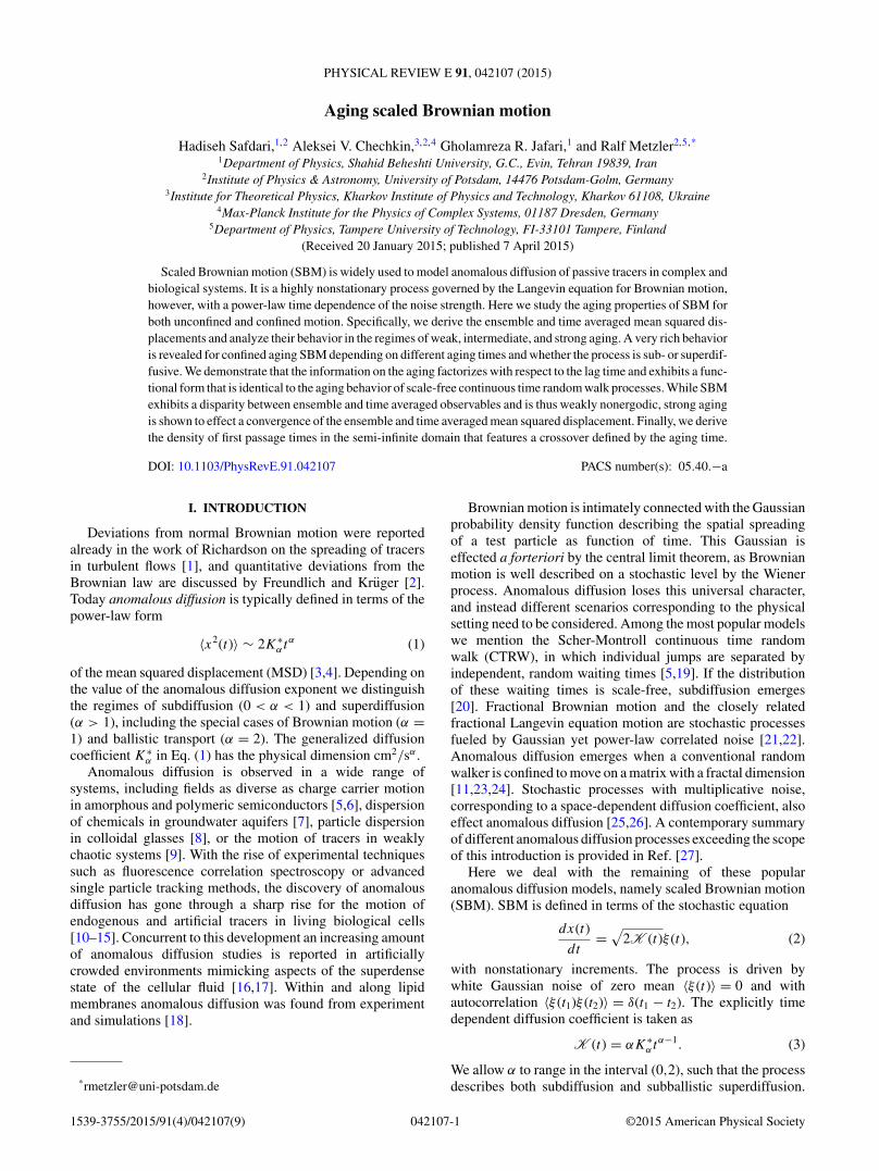
FIG. 1. (Color online) Ensemble and time averaged MSD forSBM with α = 1/2. Thin lines: Time averaged MSD for 20 individualtrajectories from simulations of the SBM Langevin equation (2) withtrajectory length t = 105. Circles: Averages over those 20 trajectories.Black thin line: Theory result (12). Thick green line: Ensembleaveraged MSD (5). Three different aging times were considered (topto bottom): (a) nonaged case ta = 0, (b) weak aging case ta = 103,and (c) strong aging case ta = 106. In all simulations K∗

α = 1/2 inthe following, unless otherwise indicated.

remarkably reduces to the form⟨δ2a(�)

⟩= 2αK∗

αtα−1a �. (14)

In this limit the time averaged MSD thus becomes equivalentto the aged ensemble averaged MSD, 〈δ2

a(�)〉 = 〈x2(�)〉a , asevidenced by comparison with result (5). In this limit, that is,ergodicity is apparently restored, as already observed for agedCTRW processes [36].

Figure 1 shows the behavior of the ensemble and timeaveraged MSD for unconfined SBM at different aging timesin the subdiffusive case with α = 1/2. The thin lines depictthe simulations results for the time averaged MSD for20 individual trajectories. The first observation is that theamplitude spread between these 20 time traces is fairly small.Note that the larger scatter for longer lag times � is due toworsening statistics when � approaches the trace length t .The circles in Fig. 1 correspond to the average over the 20different results for the time averaged MSD. The latter comparevery nicely with the theoretical expectation (12). Finally, thethick green line is the theoretical result (5) for the ensembleaveraged MSD. The detailed behavior in the three differentaging regimes is as follows:

(i) In the nonaged case (ta = 0, top panel of Fig. 1) thepower-law growth 〈x2(t)〉 tα of the MSD contrasts the linearform 〈δ2(�)〉 �, this disparity being at the heart of the weakergodicity breaking [26,31,32].

(ii) In the weak aging case (ta = 103, middle panel ofFig. 1) a major change is visible in the behavior of the MSD,namely, we see the crossover from the aging-dominated linearscaling 〈x2(t)〉 tα−1

a t to the anomalous scaling 〈x2(t)〉 tα ,encoded in Eqs. (6). The behavior of the time averaged MSDis largely unchanged in comparison to case (i).

(iii) In the strong aging case (ta = 106, bottom panel ofFig. 1) we see the apparent restoration of ergodicity: ensembleand time averaged MSDs coincide, as given by Eq. (14).

The convergence of the ensemble and time averaged MSDsin the strong aging case for the superdiffusive case with α =3/2 is nicely corroborated in Fig. 2.

103

104

105

106

107

108

100 101 102 103 104 105

<⎯δ

a⎯⎯ 2 ⎯(⎯Δ⎯

⎯) >

, <x2 (

t)>

a

t, Δ

α=1.5

Δ

individual TA MSDaveraged TA MSD

MSDtheory

FIG. 2. (Color online) Ensemble and time averaged MSD forSBM (2) with α = 3/2 in the strong aging case, ta = 106. Theobservation time is t = 105. The spread of the 20 single trajectory timeaverages is fairly small. As before, the ensemble and time averagedMSDs coincide, apparently restoring ergodicity.

042107-3

SAFDARI, CHECHKIN, JAFARI, AND METZLER PHYSICAL REVIEW E 91, 042107 (2015)

III. AGING EFFECT ON CONFINED SBM

In many cases an observed particle cannot be consideredfree during the observation. Examples contain particles mov-ing in confined space, for instance, within the confines ofliving biological cells [14,44]. Similarly, particles measuredin optical tweezer setups experience a confining Hookeanforce [12,17,45]. As a generic example for confined SBM weconsider the linear restoring force −kx(t) with force constantk. The corresponding stochastic equation for this confinedSBM reads [32]

dx(t)

dt= −kx(t) +

√2αK∗

αt (α−1)ξ (t), (15)

where, as before, ξ (t) represents white Gaussian noise ofzero mean. The covariance in this confined case yields in theform [32]

〈x(t1)x(t2)〉 = 2K∗αtα1 e−k(t1+t2)M(α,α + 1,2kt1), (16)

for t1 < t2 in terms of the confluent hypergeometric function ofthe first kind, also referred to as the Kummer function [32,46].Based on this result we now present the ensemble and timeaveraged MSDs.

A. Ensemble averaged MSD of confined SBM

The ensemble averaged MSD for aging SBM, 〈x2(t)〉a =〈[x(ta + t) − x(ta)]2〉 becomes

〈x2(t)〉a = 2M1(ta + t) + 2M1(ta) − 4e−ktM1(ta), (17)

where we used the abbreviation

M1(t) = K∗αtα exp(−2kt)M(α,α + 1,2kt). (18)

In the limit k → 0 of vanishing confinement, Eq. (5) forfree SBM is readily recovered from the property M(α,α +1,0) = 1.

We now discuss the result (17) in the three limits of thenonaged, weakly aged, and strongly aged processes. Theanalysis reveals a rich behavior depending on the values ofthe aging time ta and the anomalous diffusion exponent α. Forsub- and superdiffusion, respectively, the various crossoversare displayed in Figs. 3 and 4.

(i) In the absence of aging (ta = 0) we get back to the result

〈x2(t)〉 = 2M1(t) (19)

reported in Ref. [32]. For t � 1/k this reduces to the nonagedfree SBM result (1), while in the long time limit t � 1/k weuse the expansion

M(α,α + 1,z) ∼ αexp(z)

z(20)

of the Kummer function to obtain [32]

〈x2(t)〉 ∼ αK∗α

ktα−1. (21)

This result underlines the inherently nonstationary character ofSBM: for subdiffusion the MSD 〈x(t)2〉 progressively decays,while for superdiffusion it increases. This property reflects thetime dependence of the temperature encoded in the diffusivity(3) [32]. This nonaged behavior is shown in Figs. 3 and 4

10-6

10-5

10-4

10-3

10-2

10-1

100

101

10-2 100 102 104 106 108 1010

<x2 (t

)>

t

1/2

1

1

0

<x2(t)>4

FIG. 3. (Color online) Ensemble averaged MSD 〈x2(t)〉 for con-fined aging SBM in the subdiffusive case with α = 0.5 and Kα = 1at different aging times: (i) nonaged (ta = 0) denoted by the graylines; (ii) weakly aged (ta = 0.1) denoted by the blue lines; and(iii) strongly aged (ta = 106) denoted by the orange lines. In allcases, the full lines correspond to the force constant k = 0.1, whilethe dashed lines stand for k = 0.01. The green line at the bottom ofthe graph is a blowup [〈x2(t)〉4 of the case ta = 106 and k = 0.1] inwhich the crossover between the two plateaux is more visible.

as the gray lines for two different strengths k of the externalconfining potential. How does aging modify this behavior?

(ii) We first consider the case ta � 1/k. If in additiont � 1/k, this is but the above result (5) for free aging SBM.However, care needs to be taken when t � 1/k. From Eq. (17)we find that the first two terms (the third one is exponentially

10-4

10-2

100

102

104

106

108

10-2 100 102 104 106 108 1010

<x2 (t

)>

t

3/2

3/2

1

1/2

FIG. 4. (Color online) Ensemble averaged MSD 〈x2(t)〉 for con-fined aging SBM in the superdiffusive case with α = 1.5 and Kα = 1at different aging times: (i) nonaged (ta = 0) denoted by the graylines; (ii) weakly aged (ta = 0.1) denoted by the blue lines; and(iii) strongly aged (ta = 106) denoted by the orange lines. In allcases, the full lines correspond to the force constant k = 0.1, whilethe dashed lines stand for k = 0.01. In all cases the terminal scalingtα−1 is reached.

042107-4

AGING SCALED BROWNIAN MOTION PHYSICAL REVIEW E 91, 042107 (2015)

small in t and can be neglected) lead to the asymptotic behavior

〈x2(t)〉a ∼ αK∗α

ktα−1 + 2K∗

αtαa . (22)

This implies that for subdiffusion (0 < α < 1) the first termtends to zero and the leading behavior is the plateau

〈x2(t)〉a ∼ 2K∗αtαa . (23)

Even for very weak aging, the ensemble averaged MSD〈x2(t)〉a becomes ta dependent. When experimental data areevaluated and the exact equivalence ta = 0 is not guaranteed,the erroneous conclusion could be drawn that the process isstationary. Note, however, that result (23) is independent ofthe strength k of the confining potential and only dependson the diffusion coefficient K∗

α and the aging time ta , mirror-ing the fact that this term stems from the initial free motion dur-ing the aging period and thus indicates an out-of-equilibriumbehavior. Conversely, for superdiffusion (α > 1) the leadingorder term indeed shows the growth

〈x2(t)〉a ∼ αK∗α

ktα−1 (24)

of the ensemble averaged MSD. The weakly aged behavior isshown in Figs. 3 and 4 as the blue lines.

(iii) With the asymptotic expansion (20) of the Kummerfunction, we find that in the strong aging regime ta � 1/k theensemble averaged MSD becomes

〈x2(t)〉a ∼ αk−1K∗α

[(ta + t)α−1 + tα−1

a (1 − 2e−kt )]. (25)

At short times t � 1/k, this leads us back to the unconfinedresult 〈x2(t)〉a ∼ 2αK∗

αtα−1a t of Eq. (6). At long time t � 1/k,

however, we have to distinguish two different regimes. First,for ta � t � 1/k we obtain the plateau

〈x2(t)〉a ∼ 2αK∗α

ktα−1a , (26)

which differs from the above result (24) by the factor of2. Second, for t � ta � 1/k the leading order according toEq. (25) again differs between sub- and superdiffusive motion.For 0 < α < 1 the plateau

〈x2(t)〉a ∼ αK∗α

ktα−1a (27)

emerges. Note, however, that in comparison to Eq. (26) we nowhave half the amplitude. In the superdiffusive case α > 1 werecover result (24). This intricate behavior is shown in Figs. 3and 4 as the orange lines. In Fig. 3 we pronounce the crossoverbetween the two plateaux by plotting the fourth power of theensemble MSD as the green line.

B. Time averaged MSD of confined SBM

The time averaged MSD for confined SBM can be derivedby substituting the above covariance (16) into the integral (7).By help of the relation [47]∫ x

yαe−yM(α,1 + α,y)dy

= 1

1 + αx1+αe−xM(1 + α,2 + α,x), (28)

this procedure yields the general result⟨δ2a(�)

⟩= 2K∗

α

(t − �)(1 + α){M2(t + ta) − M2(ta + �)

+ M2(t + ta − �) − M2(ta)

− 2e−k� [M2(t + ta − �) − M2(ta)]}, (29)

where we used the abbreviation

M2(t) = t1+αe−2ktM(1 + α,2 + α,2kt). (30)

(i) In the limit k → 0 we recover the result (9) of unconfinedaging SBM, while the complete absence of aging restores theresult from Ref. [32].

In the presence of confinement, we distinguish the follow-ing regimes:

(ii) We now consider the case when the aging time is shortcompared to the relaxation time of the system, ta � 1/k.From the general expression (29) we then find the followingbehaviors: (a) when in addition the lag time is short (t �1/k � � � ta) we recover the nonaged result (10) with itslinear scaling in the lag time �. (b) When the lag time is long(t � � � 1/k � ta) we find the plateau⟨

δ2a(�)

⟩∼ 2K∗

α

ktα−1 (31)

known from the nonaged case [27]. (c) Finally, when thelag time approaches the length t of the time series, the timeaveraged MSD ⟨

δ2a(�)

⟩∼ αK∗

α

ktα−1 (32)

becomes equivalent to the ensemble averaged MSD, Eq. (24).In contrast to the ensemble averaged MSD, we thus find thatthe time averaged MSD is not affected by short aging times ascompared to the relaxation time scale ta � 1/k.

(iii) The second, more interesting case corresponds to longaging times compared to the relaxation time scale ta � 1/k.When also t � 1/k, the result is independent of the specificmagnitude of the lag time. From the general expression (29)by help of relation (20) we obtain⟨

δ2a(�)

⟩∼ K∗

α

k(t − �)

{(t + ta)α − (� + ta)α

+ (1 − 2e−k�)[(t + ta − �)α − tαa

]}. (33)

If we now consider the regime in which the lag time isshort, t,ta � 1/k � �, we obtain result (12) with the agingdepression (13) from unconfined aging SBM. In the oppositelimit t,ta � � � 1/k when the lag time is long compared tothe relaxation time, we find⟨

δ2a(�)

⟩∼ �α(ta/t)

⟨δ2(�)

⟩, (34)

where 〈δ2(�)〉 is equal to expression (31) and �α(z) is again theaging depression (13). In the strong aging limit t,ta � � �1/k, that is, the aged time averaged MSD is generally given by〈δ2

a(�)〉 ∼ �α(ta/t)〈δ2(�)〉 for any lag time. Similar to subd-iffusive CTRW processes [36], the occurrence of the factor �α

appears like a general feature for the aging dynamics of SBM.Figure 5 shows the behavior of the ensemble and time

averaged MSD for confined SBM at different degrees of

042107-5

SAFDARI, CHECHKIN, JAFARI, AND METZLER PHYSICAL REVIEW E 91, 042107 (2015)

10-2

10-1

100

101

102

100 101 102 103 104

<⎯δ

a⎯⎯ 2 ⎯(⎯Δ⎯

⎯) >

, <x2 (

t)>

a

t, Δ

~ tα

~ Δ

α=0.5

TA MSD k=0.1TA MSD k=0.01MSD k=0.1MSD k=0.01

10-2

10-1

100

101

100 101 102 103 104

<⎯δ

a⎯⎯ 2 ⎯(⎯Δ⎯

⎯) >

, <x2 (

t)>

a

t, Δ

~ tα

~ Δ

α=0.5

TA MSD k=0.1TA MSD k=0.01MSD k=0.1MSD k=0.01

10-3

10-2

10-1

100 101 102 103 104

<⎯δ

a⎯⎯ 2 ⎯(⎯Δ⎯

⎯) >

, <x2 (

t)>

a

t, Δ

α=0.5

~ t, Δ

TA MSD k=0.1TA MSD k=0.01MSD k=0.1MSD k=0.01

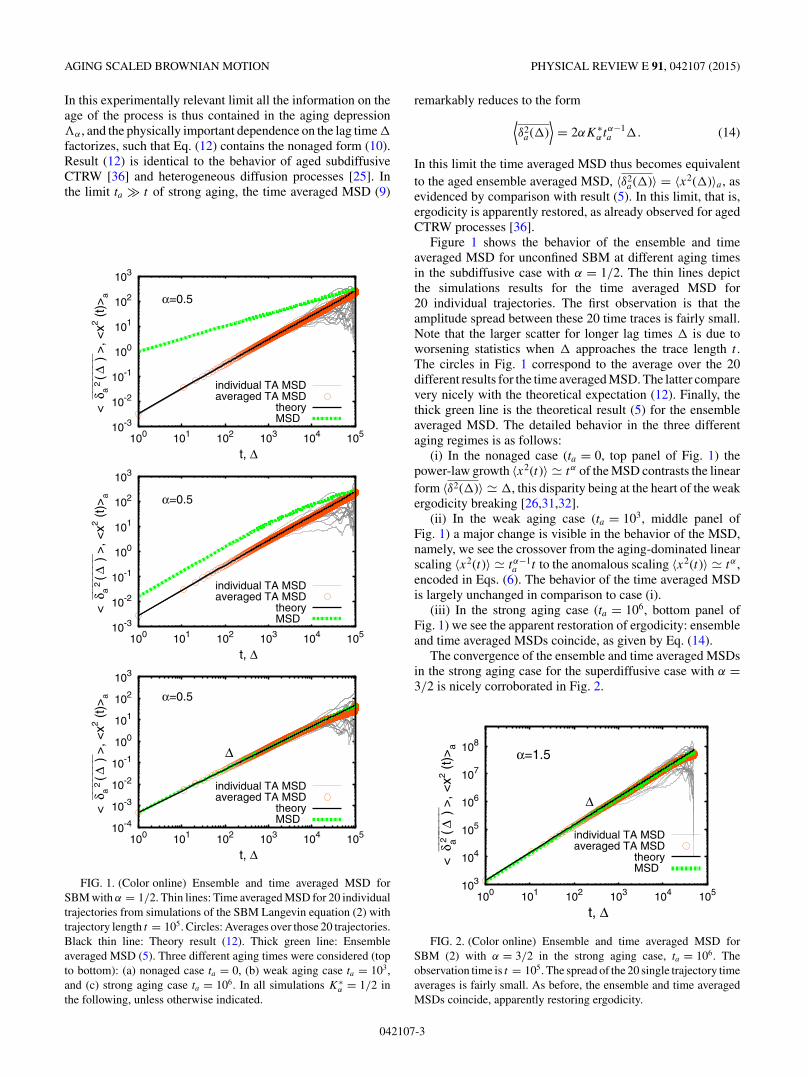
FIG. 5. (Color online) Ensemble and time averaged MSD forconfined SBM for α = 1/2. From top to bottom, the panels representthe nonaged (ta = 0) case, the case of weak aging (ta = 10−1), and thecase of strong aging (ta = 106), where the observation time is chosenas t = 5 × 104. The lines represent Eqs. (17) and (29). The forceconstants k are indicated in the panels. Note that the time averagedMSD indeed converges to the ensemble MSD in the limit � → t ,compare the discussion in Ref. [32] and the zoom-in provided inFig. 7.

aging. The graphs represent the full behavior according toEqs. (17) and (29). In the absence of aging, the initial lineargrowth 〈δ2

a(�)〉 � of the time averaged MSD crosses overto an apparent plateau, contrasting the functional behavior

1

10

100

100 101 102 103 104

<⎯δ

a⎯⎯ 2 ⎯(⎯Δ⎯

⎯) >

, <x2 (

t)>

a

t, Δ

×103

α=1.5

~ t, Δ

TA MSD, k=0.1TA MSD, k=0.01MSD, k=0.1MSD, k=0.01

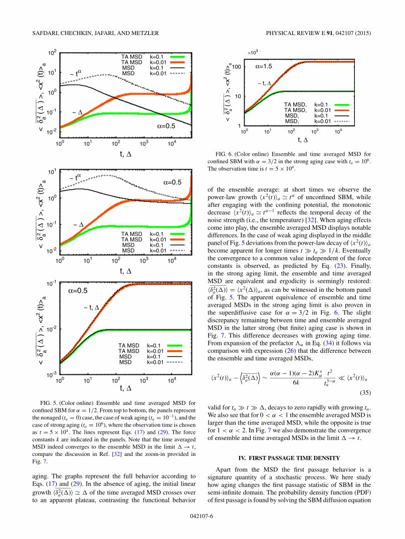
FIG. 6. (Color online) Ensemble and time averaged MSD forconfined SBM with α = 3/2 in the strong aging case with ta = 106.The observation time is t = 5 × 104.

of the ensemble average: at short times we observe thepower-law growth 〈x2(t)〉a tα of unconfined SBM, whileafter engaging with the confining potential, the monotonicdecrease 〈x2(t)〉a tα−1 reflects the temporal decay of thenoise strength (i.e., the temperature) [32]. When aging effectscome into play, the ensemble averaged MSD displays notabledifferences. In the case of weak aging displayed in the middlepanel of Fig. 5 deviations from the power-law decay of 〈x2(t)〉abecome apparent for longer times t � ta � 1/k. Eventuallythe convergence to a common value independent of the forceconstants is observed, as predicted by Eq. (23). Finally,in the strong aging limit, the ensemble and time averagedMSD are equivalent and ergodicity is seemingly restored:〈δ2

a(�)〉 = 〈x2(�)〉a , as can be witnessed in the bottom panelof Fig. 5. The apparent equivalence of ensemble and timeaveraged MSDs in the strong aging limit is also proven inthe superdiffusive case for α = 3/2 in Fig. 6. The slightdiscrepancy remaining between time and ensemble averagedMSD in the latter strong (but finite) aging case is shown inFig. 7. This difference decreases with growing aging time.From expansion of the prefactor �α in Eq. (34) it follows viacomparison with expression (26) that the difference betweenthe ensemble and time averaged MSDs,

〈x2(t)〉a −⟨δ2a(�)

⟩∼ α(α − 1)(α − 2)K∗

α

6k

t2

t3−αa

� 〈x2(t)〉a(35)

valid for ta � t � �, decays to zero rapidly with growing ta .We also see that for 0 < α < 1 the ensemble averaged MSD islarger than the time averaged MSD, while the opposite is truefor 1 < α < 2. In Fig. 7 we also demonstrate the convergenceof ensemble and time averaged MSDs in the limit � → t .

IV. FIRST PASSAGE TIME DENSITY

Apart from the MSD the first passage behavior is asignature quantity of a stochastic process. We here studyhow aging changes the first passage statistic of SBM in thesemi-infinite domain. The probability density function (PDF)of first passage is found by solving the SBM diffusion equation

042107-6

AGING SCALED BROWNIAN MOTION PHYSICAL REVIEW E 91, 042107 (2015)

4.90

4.95

5.00

102 103 104

<⎯δ⎯

a⎯⎯ 2 ⎯(⎯Δ⎯

⎯) >

, <x2

(t)>

a

t, Δ

×10-3

k=0.1α=0.5

EA MSDTA MSD

1.48

1.50

1.52

102 103 104

<⎯δ⎯

a⎯⎯ 2 ⎯(⎯Δ⎯

⎯) >

, <x2

(t)>

a

t, Δ

×104

k=0.1α=1.5

EA MSDTA MSD

4.90

4.95

5.00

103 104

<⎯δ⎯

a⎯⎯ 2 ⎯(⎯Δ⎯

⎯) >

, <x2

(t)>

a

t, Δ

×10-2

k=0.01α=0.5

EA MSDTA MSD

1.48

1.50

1.52

103 104

<⎯δ⎯

a⎯⎯ 2 ⎯(⎯Δ⎯

⎯) >

, <x2

(t)>

a

t, Δ

×105

k=0.01α=1.5

EA MSDTA MSD

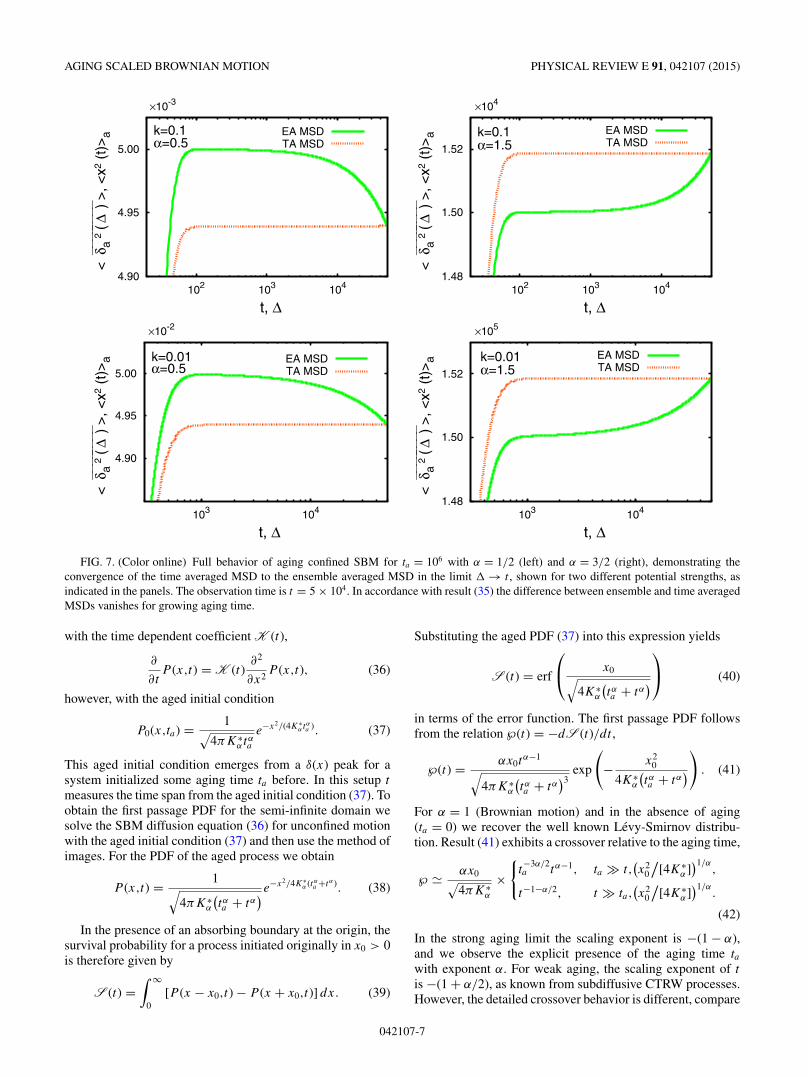
FIG. 7. (Color online) Full behavior of aging confined SBM for ta = 106 with α = 1/2 (left) and α = 3/2 (right), demonstrating theconvergence of the time averaged MSD to the ensemble averaged MSD in the limit � → t , shown for two different potential strengths, asindicated in the panels. The observation time is t = 5 × 104. In accordance with result (35) the difference between ensemble and time averagedMSDs vanishes for growing aging time.

with the time dependent coefficient K (t),

∂

∂tP (x,t) = K (t)

∂2

∂x2P (x,t), (36)

however, with the aged initial condition

P0(x,ta) = 1√4πK∗

αtαae−x2/(4K∗

α tαa ). (37)

This aged initial condition emerges from a δ(x) peak for asystem initialized some aging time ta before. In this setup t

measures the time span from the aged initial condition (37). Toobtain the first passage PDF for the semi-infinite domain wesolve the SBM diffusion equation (36) for unconfined motionwith the aged initial condition (37) and then use the method ofimages. For the PDF of the aged process we obtain

P (x,t) = 1√4πK∗

α

(tαa + tα

)e−x2/4K∗α (tαa +tα ). (38)

In the presence of an absorbing boundary at the origin, thesurvival probability for a process initiated originally in x0 > 0is therefore given by

S (t) =∫ ∞

0[P (x − x0,t) − P (x + x0,t)] dx. (39)

Substituting the aged PDF (37) into this expression yields

S (t) = erf

⎛⎝ x0√

4K∗α

(tαa + tα

)⎞⎠ (40)

in terms of the error function. The first passage PDF followsfrom the relation ℘(t) = −dS (t)/dt ,

℘(t) = αx0tα−1√

4πK∗α

(tαa + tα

)3exp

(− x2

0

4K∗α

(tαa + tα

))

. (41)

For α = 1 (Brownian motion) and in the absence of aging(ta = 0) we recover the well known Levy-Smirnov distribu-tion. Result (41) exhibits a crossover relative to the aging time,

℘ αx0√4πK∗

α

×{

t−3α/2a tα−1, ta � t,

(x2

0

/[4K∗

α])1/α

,

t−1−α/2, t � ta,(x2

0

/[4K∗

α])1/α

.

(42)

In the strong aging limit the scaling exponent is −(1 − α),and we observe the explicit presence of the aging time tawith exponent α. For weak aging, the scaling exponent of t

is −(1 + α/2), as known from subdiffusive CTRW processes.However, the detailed crossover behavior is different, compare

042107-7

SAFDARI, CHECHKIN, JAFARI, AND METZLER PHYSICAL REVIEW E 91, 042107 (2015)

10-20

10-18

10-16

10-14

10-12

10-10

10-8

10-6

10-4

10-2 100 102 104 106 108 1010 1012 1014

p(t)

t

-1/2

-5/4

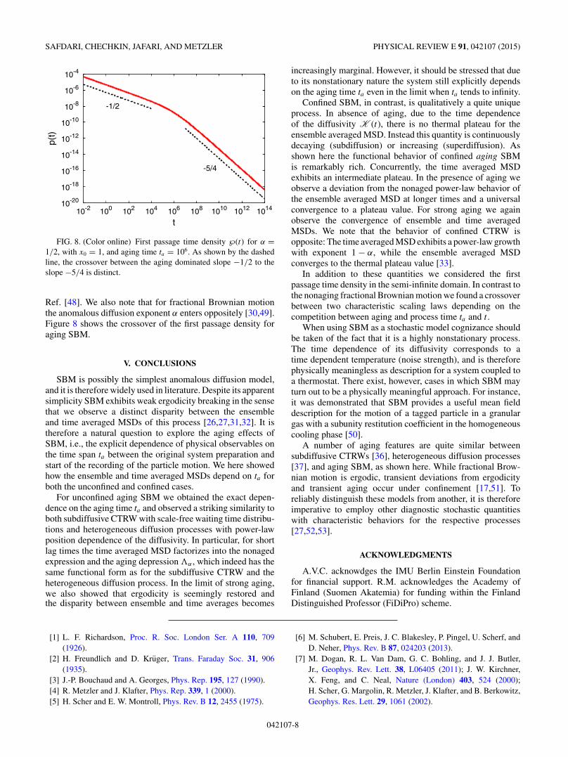
FIG. 8. (Color online) First passage time density ℘(t) for α =1/2, with x0 = 1, and aging time ta = 106. As shown by the dashedline, the crossover between the aging dominated slope −1/2 to theslope −5/4 is distinct.

Ref. [48]. We also note that for fractional Brownian motionthe anomalous diffusion exponent α enters oppositely [30,49].Figure 8 shows the crossover of the first passage density foraging SBM.

V. CONCLUSIONS

SBM is possibly the simplest anomalous diffusion model,and it is therefore widely used in literature. Despite its apparentsimplicity SBM exhibits weak ergodicity breaking in the sensethat we observe a distinct disparity between the ensembleand time averaged MSDs of this process [26,27,31,32]. It istherefore a natural question to explore the aging effects ofSBM, i.e., the explicit dependence of physical observables onthe time span ta between the original system preparation andstart of the recording of the particle motion. We here showedhow the ensemble and time averaged MSDs depend on ta forboth the unconfined and confined cases.

For unconfined aging SBM we obtained the exact depen-dence on the aging time ta and observed a striking similarity toboth subdiffusive CTRW with scale-free waiting time distribu-tions and heterogeneous diffusion processes with power-lawposition dependence of the diffusivity. In particular, for shortlag times the time averaged MSD factorizes into the nonagedexpression and the aging depression �α , which indeed has thesame functional form as for the subdiffusive CTRW and theheterogeneous diffusion process. In the limit of strong aging,we also showed that ergodicity is seemingly restored andthe disparity between ensemble and time averages becomes

increasingly marginal. However, it should be stressed that dueto its nonstationary nature the system still explicitly dependson the aging time ta even in the limit when ta tends to infinity.

Confined SBM, in contrast, is qualitatively a quite uniqueprocess. In absence of aging, due to the time dependenceof the diffusivity K (t), there is no thermal plateau for theensemble averaged MSD. Instead this quantity is continuouslydecaying (subdiffusion) or increasing (superdiffusion). Asshown here the functional behavior of confined aging SBMis remarkably rich. Concurrently, the time averaged MSDexhibits an intermediate plateau. In the presence of aging weobserve a deviation from the nonaged power-law behavior ofthe ensemble averaged MSD at longer times and a universalconvergence to a plateau value. For strong aging we againobserve the convergence of ensemble and time averagedMSDs. We note that the behavior of confined CTRW isopposite: The time averaged MSD exhibits a power-law growthwith exponent 1 − α, while the ensemble averaged MSDconverges to the thermal plateau value [33].

In addition to these quantities we considered the firstpassage time density in the semi-infinite domain. In contrast tothe nonaging fractional Brownian motion we found a crossoverbetween two characteristic scaling laws depending on thecompetition between aging and process time ta and t .

When using SBM as a stochastic model cognizance shouldbe taken of the fact that it is a highly nonstationary process.The time dependence of its diffusivity corresponds to atime dependent temperature (noise strength), and is thereforephysically meaningless as description for a system coupled toa thermostat. There exist, however, cases in which SBM mayturn out to be a physically meaningful approach. For instance,it was demonstrated that SBM provides a useful mean fielddescription for the motion of a tagged particle in a granulargas with a subunity restitution coefficient in the homogeneouscooling phase [50].

A number of aging features are quite similar betweensubdiffusive CTRWs [36], heterogeneous diffusion processes[37], and aging SBM, as shown here. While fractional Brow-nian motion is ergodic, transient deviations from ergodicityand transient aging occur under confinement [17,51]. Toreliably distinguish these models from another, it is thereforeimperative to employ other diagnostic stochastic quantitieswith characteristic behaviors for the respective processes[27,52,53].

ACKNOWLEDGMENTS

A.V.C. acknowdges the IMU Berlin Einstein Foundationfor financial support. R.M. acknowledges the Academy ofFinland (Suomen Akatemia) for funding within the FinlandDistinguished Professor (FiDiPro) scheme.

[1] L. F. Richardson, Proc. R. Soc. London Ser. A 110, 709(1926).

[2] H. Freundlich and D. Kruger, Trans. Faraday Soc. 31, 906(1935).

[3] J.-P. Bouchaud and A. Georges, Phys. Rep. 195, 127 (1990).[4] R. Metzler and J. Klafter, Phys. Rep. 339, 1 (2000).[5] H. Scher and E. W. Montroll, Phys. Rev. B 12, 2455 (1975).

[6] M. Schubert, E. Preis, J. C. Blakesley, P. Pingel, U. Scherf, andD. Neher, Phys. Rev. B 87, 024203 (2013).

[7] M. Dogan, R. L. Van Dam, G. C. Bohling, and J. J. Butler,Jr., Geophys. Rev. Lett. 38, L06405 (2011); J. W. Kirchner,X. Feng, and C. Neal, Nature (London) 403, 524 (2000);H. Scher, G. Margolin, R. Metzler, J. Klafter, and B. Berkowitz,Geophys. Res. Lett. 29, 1061 (2002).

042107-8

AGING SCALED BROWNIAN MOTION PHYSICAL REVIEW E 91, 042107 (2015)

[8] E. R. Weeks, J. C. Crocker, A. C. Levitt, A. Schofield, andD. A. Weitz, Science 287, 627 (2000); J. Mattsson, H. M. Wyss,A. Fernandez-Nieves, K. Miyazaki, Z. Hu, D. R. Reichman, andD. A. Weitz, Nature (London) 462, 83 (2009).

[9] T. H. Solomon, E. R. Weeks, and H. L. Swinney, Phys. Rev.Lett. 71, 3975 (1993); E. R. Weeks and H. L. Swinney, Phys.Rev. E 57, 4915 (1998).

[10] F. Hofling and T. Franosch, Rep. Progr. Phys. 76, 046602 (2013).[11] M. J. Saxton, Biophys. J. 103, 2411 (2012); ,72, 1744 (1997).[12] J.-H. Jeon, V. Tejedor, S. Burov, E. Barkai, C. Selhuber-Unkel,

K. Berg-Sørensen, L. Oddershede, and R. Metzler, Phys. Rev.Lett. 106, 048103 (2011).

[13] S. M. A. Tabei, S. Burov, H. Y. Kim, A. Kuznetsov, T. Huynh,J. Jureller, L. H. Philipson, A. R. Dinner, and N. F. Scherer,Proc. Natl. Acad. Sci. USA 110, 4911 (2013); D. Robert, T.-H. Nguyen, F. Gallet, and C. Wilhelm, PLoS ONE 5, e10046(2010).

[14] I. Golding and E. C. Cox, Phys. Rev. Lett. 96, 098102 (2006); S.C. Weber, A. J. Spakowitz, and J. A. Theriot, ibid. 104, 238102(2010).

[15] K. Burnecki, E. Kepten, J. Janczura, I. Bronshtein, Y. Garini, andA. Weron, Biophys. J. 103, 1839 (2012); I. Bronstein, Y. Israel,E. Kepten, S. Mai, Y. Shav-Tal, E. Barkai, and Y. Garini, Phys.Rev. Lett. 103, 018102 (2009).

[16] W. Pan, L. Filobelo, N. D. Q. Pham, O. Galkin, V. V. Uzunova,and P. G. Vekilov, Phys. Rev. Lett. 102, 058101 (2009);J. Szymanski and M. Weiss, ibid. 103, 038102 (2009); G. Guigas,C. Kalla, and M. Weiss, Biophys. J. 93, 316 (2007).

[17] J.-H. Jeon, N. Leijnse, L. B. Oddershede, and R. Metzler, NewJ. Phys. 15, 045011 (2013).

[18] E. Yamamoto, T. Akimoto, M. Yasui, and K. Yasuoka, Sci.Rep. 4, 4720 (2014); G. R. Kneller, K. Baczynski, andM. Pasienkewicz-Gierula, J. Chem. Phys. 135, 141105 (2011);J.-H. Jeon, H. Martinez-Seara Monne, M. Javanainen, andR. Metzler, Phys. Rev. Lett. 109, 188103 (2012).

[19] E. W. Montroll and G. H. Weiss, J. Math. Phys. 10, 753 (1969).[20] J. Klafter, A. Blumen, and M. F. Shlesinger, Phys. Rev. A 35,

3081 (1987).[21] B. B. Mandelbrot and J. W. van Ness, SIAM Rev. 10, 422 (1968);

A. N. Kolmogorov, Dokl. Acad. Sci. USSR 26, 115 (1940).[22] I. Goychuk, Phys. Rev. E 80, 046125 (2009); ,Adv. Chem. Phys.

150, 187 (2012); E. Lutz, Phys. Rev. E 64, 051106 (2001);G. Kneller, J. Chem. Phys. 141, 041105 (2014); P. Hanggi, Z.Phys. B 31, 407 (1978); P. Hanggi and F. Mojtabai, Phys. Rev. A26, 1168(R) (1982); S. C. Kou, Ann. Appl. Stat. 2, 501 (2008).

[23] S. Havlin and D. Ben-Avraham, Adv. Phys. 51, 187 (2002);Y. Meroz, I. M. Sokolov, and J. Klafter, Phys. Rev. E 81,010101(R) (2010); M. Spanner, F. Hofling, G. E. Schroder-Turk,K. Mecke, and T. Franosch, J. Phys. Condens. Matter 23, 234120(2011).

[24] A. Klemm, H.-P. Muller, and R. Kimmich, Phys. Rev. E 55,4413 (1997); A. Klemm, R. Metzler, and R. Kimmich, ibid. 65,021112 (2002).

[25] A. G. Cherstvy, A. V. Chechkin, and R. Metzler, New J. Phys.15, 083039 (2013); ,Soft Matter 10, 1591 (2014); A. G. Cherstvyand R. Metzler, Phys. Rev. E 90, 012134 (2014); ,Phys. Chem.Chem. Phys. 15, 20220 (2013); P. Massignan, C. Manzo, J. A.Torreno-Pina, M. F. Garcıa-Parajo, M. Lewenstein, and G. J.Lapeyre, Jr., Phys. Rev. Lett. 112, 150603 (2014).

[26] A. Fulinski, J. Chem. Phys. 138, 021101 (2013); ,Phys. Rev. E83, 061140 (2011).

[27] R. Metzler, J.-H. Jeon, A. G. Cherstvy, and E. Barkai, Phys.Chem. Chem. Phys. 16, 24128 (2014).

[28] G. K. Batchelor, Math. Proc. Cambridge Philos. Soc. 48, 345(1952).

[29] M. J. Saxton, Biophys. J. 81, 2226 (2001); T. J. Feder, I. Brust-Mascher, J. P. Slattery, B. Baird, and W. W. Webb, ibid. 70, 2767(1996); N. Periasmy and A. S. Verkman, ibid. 75, 557 (1998);M. Weiss, M. Elsner, F. Kartberg, and T. Nilsson, ibid. 87, 3518(2004); J. Wu and K. M. Berland, ibid. 95, 2049 (2008).

[30] S. C. Lim and S. V. Muniandy, Phys. Rev. E 66, 021114 (2002).[31] F. Thiel and I. M. Sokolov, Phys. Rev. E 89, 012115 (2014).[32] J.-H. Jeon, A. V. Chechkin, and R. Metzler, Phys. Chem. Chem.

Phys. 16, 15811 (2014).[33] S. Burov, R. Metzler, and E. Barkai, Proc. Natl. Acad. Sci. USA

107, 13228 (2010).[34] E.-J. Donth, The Glass Transition (Springer, Berlin, 2001);

W. Gotze, Complex Dynamics of Glass-Forming Liquids (Ox-ford University Press, Oxford, UK, 2009).

[35] E. Barkai, Phys. Rev. Lett. 90, 104101 (2003); E. Barkai andY. C. Cheng, J. Chem. Phys. 118, 6167 (2003).

[36] J. H. P. Schulz, E. Barkai, and R. Metzler, Phys. Rev. Lett. 110,020602 (2013); ,Phys. Rev. X 4, 011028 (2014).

[37] A. G. Cherstvy, A. V. Chechkin, and R. Metzler, J. Phys. A 47,485002 (2014).

[38] W. E. Moerner and M. Orrit, Science 283, 1670 (1999).[39] M. J. Saxton and K. Jacobsen, Annu. Rev. Biophys. Biomol.

Struct. 26, 373 (1997).[40] C. Brauchle, D. C. Lamb, and J. Michaelis, Single Particle

Tracking and Single Molecule Energy Transfer (Wiley-VCH,Weinheim, Germany, 2012).

[41] X. S. Xie, P. J. Choi, G.-W. Li, N. K. Lee, and G. Lia, Annu.Rev. Biophys. 37, 417 (2008).

[42] J.-P. Bouchaud, J. Phys. (Paris) I 2, 1705 (1992); C. Monthusand J.-P. Bouchaud, J. Phys. A 29, 3847 (1996).

[43] E. Barkai, Y. Garini, and R. Metzler, Phys. Today 65(8), 29(2012).

[44] Y. He, S. Burov, R. Metzler, and E. Barkai, Phys. Rev. Lett. 101,058101 (2008).

[45] M. A. Taylor, J. Janousek, V. Daria, J. Knittel, B. Hage, H.-A.Bachor, and W. P. Bowen, Nat. Phot. 7, 229 (2013).

[46] M. Abramowitz and I. A. Stegun, Handbook of MathematicalFunctions (Dover, New York, 1965).

[47] A. B. Prudnikov and Yu. A. Brychkov, Integrals and Series(Gordon and Breach, New York, 1986), Vol. 3.

[48] H. Krusemann, A. Godec, and R. Metzler, Phys. Rev. E 89,040101(R) (2014).

[49] J.-H. Jeon, A. V. Chechkin, and R. Metzler, Europhys. Lett. 94,20008 (2011).

[50] A. Bodrova, A. V. Chechkin, A. G. Cherstvy, and R. Metzler,arXiv:1501.04173.

[51] J. Kursawe, J. Schulz, and R. Metzler, Phys. Rev. E 88, 062124(2013); J.-H. Jeon and R. Metzler, ibid. 85, 021147 (2012).

[52] V. Tejedor, O. Benichou, R. Voituriez, R. Jungmann, F. Simmel,C. Selhuber-Unkel, L. Oddershede, and R. Metzler, Biophys. J.98, 1364 (2010).

[53] M. Magdziarz, A. Weron, K. Burnecki, and J. Klafter, Phys.Rev. Lett. 103, 180602 (2009).

042107-9