Aggregate Volatility Risk:

Explaining the Small Growth Anomaly

and the New Issues Puzzle†

Alexander Barinov∗

Terry College of BusinessUniversity of Georgia

E-mail: abarinov@terry.uga.eduhttp://abarinov.myweb.uga.edu/

This version: May 2012

Abstract

The paper shows that new issues earn low expected returns because they are a hedgeagainst increases in expected aggregate volatility. Consistent with that, the ICAPMwith the aggregate volatility risk factor can explain the new issues puzzle, as well asthe small growth anomaly and the cumulative issuance puzzle. The key mechanismis that, all else equal, growth options become less sensitive to the underlying assetvalue and more valuable as idiosyncratic volatility goes up. Idiosyncratic volatilityusually increases together with aggregate volatility, that is, in recessions.

JEL Classification: G12, G13, E44Keywords: idiosyncratic volatility, aggregate volatility risk, new issues, small growthanomaly, growth options

†I thank Mike Barclay, John Long, Harold Mulherin, Bill Schwert, Jerry Warner, and Wei Yang fortheir advice and inspiring discussions. I have also benefited from the comments of seminar participantsat University of Rochester, as well as the comments of the participants of the 2008 Northern FinancialAssociation Meetings, the All-Georgia Conference, and the 2008 Southern Financial Association Meetings.All remaining errors are mine.∗438 Brooks Hall, University of Georgia. Athens, GA 30602. Tel.: +1–706–542– 3650. Fax: +1–706–

542–9434. E-mail: abarinov@terry.uga.edu

1 Introduction

The underperformance of new equity issues (the new issues puzzle) has long been

puzzling for the corporate finance literature. The mispricing theories have argued that

the low returns of new issues arise because of the tendency of the manager to squander

part of the cash they raise in an issue (see, e.g., Jung, Kim, and Stulz, 1996), because the

managers of the issuing companies overinvest (see, e.g., Loughran and Ritter, 1997, and

Heaton, 2002), or because the managers are successful in selling to the investors overvalued

equity (see, e.g., Baker and Wurgler, 2002, and Graham and Harvey, 2001).

A rational theory of low expected returns to new issues would imply that new issues

have low risk and low cost of capital, a useful information for the capital budgeting deci-

sions. While a satisfactory rational explanation of the new issues puzzle remains elusive,

finding such an explanation would also imply that the managers of the issuing firms do

not engage in the value-destructive behavior blamed on them by the mispricing theories of

the new issues puzzle and that the managers do not take advantage of new investors. Both

conclusions would shed some light on the issues of corporate governance in new companies,

as well as the cost of issuing equity.

In this paper, I offer a firm-type explanation of the new issues puzzle. I argue that

new issues seem to underperform only because they are small growth firms, the type of

firms that has notoriously large negative alphas in the existing asset-pricing models (the

small growth anomaly). The empirical evidence in Brav et al. (2000) and in Sections 4.3

and 6.1 of this paper confirms that new issues are primarily small companies with high

market-to-book.

More importantly, I find that investors tolerate the low returns of new issues because

these firms tend to earn positive abnormal returns in response to surprise increases in

expected aggregate volatility. I treat the risk of losses in response to surprise increases in

expected aggregate volatility (henceforth, aggregate volatility risk) as a separate risk factor

in Merton’s (1973) Intertemporal CAPM (henceforth, ICAPM). I show that in the ICAPM

with the aggregate volatility risk factor, small growth firms and new issues load positively

on the factor that mimics innovations to aggregate volatility and therefore provide a hedge

against increases in aggregate volatility compared to firms with similar market betas. The

ICAPM alphas of new issues and small growth firms are insignificantly different from zero,

1

suggesting that the low returns of new issues are the evidence of their low cost of capital

rather than the value-destroying behavior of the management.

Changes in expected aggregate volatility provide information about future investment

opportunities and future consumption. Campbell (1993) and Chen (2002) present versions

of the ICAPM, in which aggregate volatility risk is priced. In Campbell (1993), an increase

in aggregate volatility implies that in the next period, risks will be higher and consumption

will be lower. Consumers, who wish to smoothen consumption, have to save and cut current

consumption if expected aggregate volatility unexpectedly goes up. Chen (2002) also notes

that, since aggregate volatility is persistent, higher current aggregate volatility means

higher aggregate volatility in the future. Therefore, consumers will build up precautionary

savings and cut current consumption in response to surprise increases in expected aggregate

volatility. Both Campbell (1993) and Chen (2002) show that stocks with the most negative

return correlation with surprise changes in expected aggregate volatility should earn a risk

premium. These stocks are risky because their value drops when consumption has to be

cut to increase savings.

In a recent paper, Ang et al. (2006) confirm the hypotheses of Campbell (1993) and

Chen (2002). Ang et al. use the CBOE VIX index, defined as the implied volatility of

S&P 100 options, to proxy for expected aggregate volatility. They show that firms with

more negative return sensitivity to the VIX index changes indeed have higher expected

returns than firms with less negative sensitivity to VIX changes.

My paper contributes to the aggregate volatility risk literature by identifying the firms

that are the least exposed to aggregate volatility risk. Small growth firms and new is-

sues usually have abundant growth options and high idiosyncratic volatility. I show that

the more growth options and idiosyncratic volatility a firm has, the less it is exposed to

aggregate volatility risk.

Holding everything else fixed, an increase in idiosyncratic volatility (that usually co-

incides with an increase in aggregate volatility, see Campbell et al., 2001, and Barinov,

2010, for the supporting evidence) leads to an increase in the value of growth stocks with

high idiosyncratic volatility for two reasons. First, the risk exposure of growth options

declines when idiosyncratic volatility increases, because option delta decreases in volatil-

ity. In recessions, when both idiosyncratic and aggregate volatility increase, the decreased

risk exposure of growth options leads to a smaller increase in expected returns and a

2

smaller drop in price1. Second, as Grullon et al. (2012) show, the value of growth options

increases significantly with idiosyncratic volatility, as the value of any option does. I con-

clude therefore that, controlling for market beta, growth stocks with high idiosyncratic

volatility covary positively with changes in aggregate volatility (i.e., beat the CAPM when

aggregate volatility increases), which makes them a hedge against aggregate volatility risk2.

My measure of innovations to expected aggregate volatility is the change in the VIX

index. The VIX index is the implied volatility of S&P 100 options, and therefore represents

the measure of price-implied expected aggregate volatility. Ang et al. (2006) show that

at the daily frequency, the autocorrelation of VIX is close to one, hence its change is a

suitable proxy for the innovation in expected aggregate volatility, and the innovation is

the main variable of interest in the ICAPM.

My aggregate volatility risk factor (hereafter, the FVIX factor) is the factor-mimicking

portfolio that tracks VIX changes. The FVIX factor is purged of firms that performed

an IPO or SEO in the past three years, as well as firms in the intersection of the top

market-to-book quintile with the two bottom size quintiles (small growth firms).

By construction, the FVIX portfolio earns mostly positive returns when expected ag-

gregate volatility increases. I expect FVIX to earn a negative risk premium, and find that

it does as the raw return to FVIX is -1.4% per month, and the Fama-French alpha is -37

bp per month. The negative risk premium of FVIX indicates that investors care about

aggregate volatility risk and are willing to pay a significant price for the hedge against it.

The negative risk premium of FVIX also implies that in the ICAPM with the market factor

and FVIX, positive FVIX betas indicate that the portfolio is a hedge against aggregate

volatility risk, and vice versa.

I start the empirical tests with showing that in the double sorts on market-to-book

and idiosyncratic volatility, FVIX betas indeed become significantly more positive as ei-

ther market-to-book or idiosyncratic volatility increase, and reach the maximum for the

portfolio with the highest market-to-book and the highest idiosyncratic volatility. I also

1 Note that the argument would not hold for systematic or total volatility. While the elasticity of

growth options declines with both idiosyncratic and systematic volatility, higher systematic volatility of

the underlying asset is equivalent to its higher beta. Hence, the overall effect of higher systematic/total

volatility of the underlying asset on the beta of growth options is ambiguous.2 The theory appendix at http://abarinov.myweb.uga.edu/Theory (June 2010).pdf contains the formal

derivation of the predictions in this paragraph.

3

find that more than two-thirds of the firms in the smallest growth portfolio are also in the

portfolio with the highest market-to-book and the highest idiosyncratic volatility.

In the main test of my theory, I find that the ICAPM with the FVIX factor produces

insignificant alphas of small growth firms and new issues, thus explaining the small growth

anomaly and the new issues puzzle. The ICAPM with FVIX also reveals significantly

positive loadings of small growth firms and new issues on the FVIX factor.

Consistent with my hypothesis that the new issues puzzle is driven by small growth

firms, I find that the new issues puzzle is indeed stronger for small firms and growth firms.

The FVIX factor explains this pattern by pointing out that small and growth new issues

are especially good hedges against aggregate volatility risk.

The FVIX factor is also able to explain the cumulative issuance puzzle of Daniel and

Titman (2006) by significantly reducing the alphas of the arbitrage portfolio long in routine

equity issuers and short in routine equity retirers. I also find that the cumulative issuance

puzzle is stronger for growth firms, because buying equity issuers and shorting equity

retirers leads to more positive FVIX betas in the growth subsample.

An important feature of my aggregate volatility risk story is that it is conditional

on the market risk. I do not argue that small growth firms and new issues gain when

aggregate volatility increases. Since the market return is strongly negatively correlated

with aggregate volatility: the monthly correlation between the market factor and the

change in VIX is -0.626, any stock with a positive beta will react negatively to increases

in expected aggregate volatility. New issues usually have market betas higher than one.

According to the CAPM, in recessions, when aggregate volatility increases, they are likely

to suffer larger-than-average losses. I assume that the negative effects of recessions, other

than the effect of volatility changes, on the value of new issues are adequately captured by

the market beta. What I focus on is the fact that new issues beat the CAPM prediction

when aggregate volatility increases. This is the reason why these firms have negative

CAPM alphas: their risk is smaller than what the CAPM says, because their losses in bad

times are smaller than what the CAPM predicts.

The paper proceeds as follows: Section 2 develops the empirical hypotheses and reviews

related literature. Section 3 describes the data, and Section 4 uses the FVIX factor to

explain the small growth anomaly. Section 5 presents the explanation of the new issues

puzzle and its relation to size and market-to-book. In Section 6, I examine the cumulative

4

issuance puzzle, its relation to the small growth anomaly and aggregate volatility risk, and

its dependence on size and market-to-book. Section 7 uses the changes in the VIX index

directly to show that high volatility growth firms, small growth firms, and equity issuers

indeed beat the CAPM when expected aggregate volatility increases, and also presents the

results of other robustness checks. Section 8 offers the conclusion.

2 Literature Review

The central theoretical idea of the paper is that higher idiosyncratic volatility of the

underlying asset makes the systematic risk of growth options smaller. My theory is related

to Veronesi (2000) and Johnson (2004). They show that parameter risk can negatively

affect expected returns by lowering the covariance of returns with the stochastic discount

factor. Johnson (2004) also uses the idea that the beta of equity is negatively related to

idiosyncratic volatility, since in the presence of risky debt, equity is a call option of the

firm’s assets. In my paper, I take a broader definition of idiosyncratic risk. I argue that

it can affect expected returns even if there is no parameter risk, but there is idiosyncratic

volatility. Contrary to Johnson (2004), I also focus on growth options instead of leverage.

The focus on growth options allows me to explain the small growth anomaly and the new

issues puzzle.

The most important contribution I make to the Johnson theory is using it to give

ground to the need for an additional factor. The Johnson model is set up in a one-factor

world, and the uncertainty in Johnson’s model impacts returns through the market beta.

That is, Johnson’s model predicts that uncertainty can be negatively related to expected

returns, but not to abnormal returns. This prediction contradicts what we see in the data,

where controlling for market risk does not help to alleviate the idiosyncratic volatility

discount of Ang et al. (2006) or the small growth anomaly.

In my theory, purely idiosyncratic risk at the level of the underlying asset changes

the systematic risk of growth options by changing their covariance with innovations to

aggregate volatility. That is, I propose moving into the two-factor world with the market

factor and the aggregate volatility risk factor, where the firm’s idiosyncratic volatility

changes the exposure to the aggregate volatility risk factor. The failure of the existing

model to control for this new risk factor is the reason for their inability to price correctly

5

the stocks with high idiosyncratic volatility, small growth stocks, etc.

My paper assumes that the firm value is the sum of the values of the assets in place

and the growth options, and looks at the risk of growth options in order to explain the

new issues puzzle. Carlson et al. (2006) take a similar approach to explaining the new

issues puzzle. However, the mechanism in their model is entirely different. They start

with the assumption that growth options are riskier than assets in place and argue that

new issues become less risky than their non-issuing peers because they execute their risky

growth options using the cash raised in the equity offering.

On the contrary, my approach can explain why growth options can be less risky than

assets in place, or at least less risky than assets in place with a similar market beta. I

show that new issues are less risky than their peers precisely because they have abundant

growth options. Since these growth options are usually written on volatile assets, the

growth options and the issuing firms as a whole are less risky than what the CAPM

suggests, because they beat the CAPM prediction when aggregate volatility increases.

Lyandres et al. (2008) use an approach similar to Carlson et al. (2006) in their empirical

paper that employs the investment factor to explain the new issues puzzle. They assume

that firms that invest heavily (in particular, new issues firms) do so because they are taking

advantage of the low-risk projects they have. Lyandres et al. find that the investment

factor (long in low investment firms, short in high investment firms) can explain 80% of

the new issues alphas.

In untabulated results, I find that the investment factor of Lyandres et al. is orthogonal

to my FVIX factor. The two factors are equally important in explaining the new issues

puzzle. However, the investment factor is not helpful in explaining the small growth

anomaly or the fact that the new issues puzzle is stronger for small firms and growth

firms. I also find that the explanatory power of the investment factor depends greatly

on one observation — January 2001, when small growth firms earned a huge 55% return,

IPOs gained 39%, and SEOs made 24%. Removing January 2001 from the sample does

not impact the FVIX factor, but reduces the explanatory power of the investment factor

from 80% of the new issues puzzle to 50%.

Lastly, my theory implies that the FVIX factor should explain the value effect and

the idiosyncratic volatility discount. In their paper, Ang et al. (2006) come to a differ-

ent conclusion about the link between the idiosyncratic volatility discount and aggregate

6

volatility risk. They show that making the sorts on idiosyncratic volatility conditional on

FVIX betas does not eliminate the idiosyncratic volatility discount, and conclude therefore

that aggregate volatility risk cannot explain the idiosyncratic volatility discount. In Bari-

nov (2010), I perform a more direct test by fitting the two-factor ICAPM with the market

factor and FVIX to the returns of the low-minus-high idiosyncratic volatility portfolio.

In the two-factor ICAPM, I find that the idiosyncratic volatility discount is completely

explained by aggregate volatility risk.

3 Data

The sample period used in the paper is from January 1986 to December 2006 and is

determined by the availability of the VIX index, my proxy for expected aggregate volatility.

To measure the innovations to expected aggregate volatility, I use daily changes in the old

version of the VIX index calculated by CBOE and available from WRDS. Using the old

version of VIX provides longer coverage. The VIX index measures the implied volatility

of the at-the-money options on the S&P100 index. For a detailed description of VIX, see

Whaley (2000) and Ang et al. (2006).

I form a factor-mimicking portfolio that tracks the daily changes in the VIX index. I

regress the daily changes in VIX on the daily excess returns to the base assets. The base

assets are five quintile portfolios sorted on the past return sensitivity to VIX changes, as

in Ang et al. (2006):

∆V IXt = γ0 + γ1 · (V IX1t −RFt) + γ2 · (V IX2t −RFt) +(1)

+ γ3 · (V IX3t −RFt) + γ4 · (V IX4t −RFt) + γ5 · (V IX5t −RFt),

where V IX1t, . . . , V IX5t are the VIX sensitivity quintiles described above, with V IX1t

being the quintile with the most negative sensitivity.

The fitted part of the regression above less the constant is my aggregate volatility risk

factor (FVIX factor):

FV IXt = γ̂1 · (V IX1t −RFt) + γ̂2 · (V IX2t −RFt) + γ̂3 · (V IX3t −RFt) +(2)

+ γ̂4 · (V IX4t −RFt) + γ̂5 · (V IX5t −RFt).

The return sensitivity to VIX changes I use to form the base assets is measured separately

for each firm-month by regressing stock excess returns on market excess returns and the

7

VIX index change using daily data (at least 15 non-missing returns are required):

(3) Rett −RFt = α + βMKT · (MKTt −RFt) + γ∆V IX · ∆V IXt.

To eliminate concerns that the explanatory power of FVIX may be mechanical, the

quintile portfolios and therefore FVIX are purged of firms that have performed an IPO or

SEO in the past three years, as well as of the firms from the intersection of the top market-

to-book quintile and the two bottom size quintiles (small growth firms). I cumulate FVIX

returns to the monthly level to get the monthly values of the FVIX factor. The results

in the paper are robust to changing the base assets to the six size and book-to-market

portfolios or to the ten industry portfolios (Fama and French (1997)), and to including the

new issues and small growth firms back into the construction of the FVIX factor.

I obtain the daily and monthly values of the three Fama-French factors and the risk-free

rate from Kenneth French’s Web site at http://mba.tuck.dartmouth.edu/pages/faculty

/ken.french/. The Web site also provides the returns to the smallest growth portfolio and

the second smallest growth portfolio, defined as the intersection of the top market-to-book

quintile with the bottom and the second-from-the bottom size quintiles, respectively.

In Section 4.1 I use five portfolio sorts to test the pricing power of the FVIX factor by

looking at the pricing errors it produces. The first three portfolio sets are the five-by-five

sorts on size and market-to-book (Fama and French (1993), data from Kenneth French’s

Web site), 48 industry portfolios (Fama and French (1997), data from Kenneth French’s

Web site), and the five-by-five sorts on size and price momentum (Fama and French (1996),

data from Kenneth French’s Web site).

The fourth portfolio set is the five-by-five sort on market-to-book and idiosyncratic

volatility. Market-to-book is from Compustat. It is defined as market value at the end of

the fiscal year (item #25 times item #199) over the book value of equity (item #60 plus

item #74). I measure idiosyncratic volatility as the standard deviation of the Fama-French

(1993) model residuals, which is fitted to daily data. I estimate the model separately for

each firm-month, and compute the residuals in the same month. I require at least 15 daily

returns to estimate the model and idiosyncratic volatility. The market-to-book portfolios

are rebalanced annually, the idiosyncratic volatility portfolios are rebalanced monthly.

The fifth portfolio set is the five-by-five sort on size and past return sensitivity to VIX

changes. Size is shares outstanding times price (both from CRSP) measured in December

8

of the past calendar year. The return sensitivity to VIX changes is measured as described

in the beginning of this section. The sorts on size are performed each year; the sorts on

the return sensitivity to VIX changes are performed each month.

In Section 5, I use the SDC Platinum database to extract the dates of new issues and

the identities of the issuing firms. I match new issues with the CRSP returns data by the

six-digit CUSIP, requiring at least one valid return observation in the three years after

the issue. My IPO and SEO portfolios are rebalanced monthly and include the IPOs and

SEOs performed from 2 to 37 months ago. The first month is excluded because of the

well-known IPO underpricing and the price support of the underwriters in the month after

the issue. The results are robust to keeping the first month in the sample. I include only

the IPOs and SEOs listed on NYSE/AMEX/NASDAQ after the issue (the exchcd listing

indicator from the CRSP events file is used). I keep utilities in my sample, as well as mixed

SEOs, but discard units issues (both IPOs and SEOs) and SEOs with no new shares issued.

Excluding utilities and mixed SEOs, or including units issues does not change my results.

My sample includes 5,969 IPOs and 6,974 SEOs performed between December 1982 and

October 2006 (new issues in 1983 enter the new issues portfolio in 1986 as two- to three-

year-old issues). When I look at the new issues puzzle in different size and market-to-book

portfolios, I measure size and market-to-book using the after-issue market capitalization

and total common equity values from SDC.

In Section 6, I follow the definition of the cumulative issuance variable in Daniel and

Titman (2006). Cumulative issuance is the growth of the market value unexplained by

returns to the pre-existing assets and is measured as the log market value growth minus

the log cumulative returns in the past five years. Market value is shares outstanding times

stock price (both from CRSP), stock returns are also from CRSP.

In all tests, I use monthly cum-dividend returns from CRSP and complement them by

the delisting returns from the CRSP events file. Following Shumway (1997) and Shumway

and Warther (1999), I set delisting returns to -30% for NYSE and AMEX firms (CRSP

exchcd codes equal to 1, 2, 11, or 22) and to -55% for NASDAQ firms (CRSP exchcd

codes equal to 3 or 33) if CRSP reports missing or zero delisting returns and delisting

is for performance reasons. My results are robust to setting missing delisting returns to

-100% or to using no correction for the delisting bias.

9

4 Aggregate Volatility Risk and the Small Growth

Anomaly

4.1 Is Aggregate Volatility Risk Priced?

The most fundamental necessary condition of the analysis in the paper is that the

aggregate volatility risk factor (the FVIX factor) I intend to use is priced. The FVIX

factor is the factor-mimicking portfolio that tracks daily changes in VIX, my measure

of innovations to expected aggregate volatility. As described in Section 3, FVIX is the

combination of the base assets, i.e. the five quintile portfolios sorted on past return

sensitivity to VIX changes. The base assets are purged of new issues and small growth

firms.

[Table 1 goes around here]

In Panel A of Table 1, I look at the descriptive statistics across the quintile portfolios

sorted on the past return sensitivity to changes in VIX. The return sensitivity to VIX

changes is measured separately in each firm-month by regressing excess return to the

stock on the excess return to the market and the change in VIX.

Since the quintile portfolios in Panel A serve as the base assets for the FVIX factor

(that is, FVIX is the linear combination of their returns), I am primarily interested in two

characteristics. First, I need to establish that sorting firms on return sensitivity to VIX

changes captures an important firm characteristic that is priced in the cross-section. To

that end, I look at the value-weighted raw returns to the VIX sensitivity portfolios, as well

as value-weighted CAPM and Fama-French alphas. I find that both the raw returns and

the alphas decline significantly and monotonically as the return sensitivity to changes in

VIX becomes more positive. The return/alpha differential between the quintile with the

most negative and the quintile with the most positive sensitivity is around 1% per month,

which confirms that investors indeed view the firms with the most positive sensitivity to

VIX changes as significantly less risky.

Second, I need to verify that the explanatory power of FVIX with respect to the small

growth anomaly and related anomalies is not mechanical, i.e., it does not arise because

of the fact that FVIX is long in small growth firms. While I have purged FVIX of small

growth firms and new issues, it would be valuable to establish that sorting on return

10

sensitivity to VIX changes does not imply a strong sorting on size, market-to-book, or

issuing activity.

Panel A of Table 1 presents reassuring evidence that, after purging the sample of

small growth firms and new issues, return sensitivity to VIX changes appears unrelated to

market-to-book and non-monotonically related to size and issuing activity. In particular,

the firms with both very negative and very positive return sensitivity to VIX changes have

similar size and cumulative issuance, but both are smaller and tend to issue more stock

(outside of IPOs and SEOs) than firms with intermediate levels of return sensitivity to

VIX changes.

The last row of Panel A reports the slopes from the factor-mimicking regression, which

are also the weights of the sensitivity quintile portfolios in the FVIX factor portfolio. If

the return sensitivity to VIX changes is a persistent characteristic, I expect that FVIX

will be shorting the firms with negative sensitivity and buying the firms with positive

sensitivity. Most of the evidence in Panel A is consistent with this prediction: the only

two VIX quintiles that are significantly shorted by FVIX are the most negative and the

second most negative sensitivity quintiles. Also, the only quintile FVIX takes the long

position in (though the coefficient is insignificant) is the most positive sensitivity quintile.

However, the coefficients do not increase monotonically with return sensitivity to changes

in VIX, as they should. A positive aspect of this is that after comparing the coefficients

in the factor-mimicking regression to the median size and median cumulative issuance of

the base assets, I conclude that FVIX is unlikely to be tilted towards or away from small

firms and routine issuers. This suggests that if FVIX is able to explain the small growth

anomaly and related anomalies, its explanatory power is likely to be genuine rather than

mechanical.

In order to be a valid asset-pricing factor, FVIX has to satisfy two basic conditions.

First, it should correlate significantly with the innovations to expected aggregate volatility

it tries to mimic. Second, it has to earn a significant risk premium. In the case of FVIX,

the risk premium has to be negative, as FVIX is a zero-investment portfolio that yields a

positive return when expected aggregate volatility increases, thus providing a very good

insurance against aggregate volatility risk.

In untabulated results, I look at the factor premium of FVIX and the correlations of

FVIX with change in VIX and the Fama-French risk factors. The raw return to FVIX

11

is −1.4% per month, t-statistic -3.77, the CAPM alpha of FVIX is -47 bp per month,

t-statistic -4.48, and the Fama-French alpha of FVIX is -37 bp per month, t-statistic

−4.36. The large negative risk premium of FVIX shows that investors care about aggregate

volatility risk and are willing to pay a significant price for the hedge against it. I also find

that the correlation between FVIX and the change in VIX is 0.612, t-statistic 12.2. FVIX

is also negatively correlated with the market factor, uncorrelated with SMB, and positively

correlated with HML.

In Panel B of Table 1, I use the Gibbons et al. (1989) (hereafter, GRS) test statistic

to compare the performance of the CAPM, the Fama-French model, and the ICAPM with

the FVIX factor. The GRS statistic tests whether the alphas of all portfolios in a portfolio

set are jointly equal to zero, and whether the FVIX betas of all portfolios are jointly equal

to zero. The GRS statistic gives greater weight to more precise alpha estimates, which

usually come from low volatility stocks. Because FVIX should explain the alphas of high

volatility firms, the GRS statistic estimates the usefulness of FVIX quite conservatively.

I test whether FVIX is priced and whether adding it improves the pricing errors for

five portfolio sets: five-by-five sorts on size and market-to-book (Fama and French (1993)),

48 industry portfolios (Fama and French (1997)), five-by-five sorts on market-to-book and

idiosyncratic volatility (see Section 3), five-by-five sorts on size and return sensitivity to

changes in VIX (Ang et al. (2006)), and five-by-five sorts on size and price momentum

(Fama and French (1996)). The portfolio formation is discussed in more detail in Section 3.

The tests in Panel B use equal-weighted returns to the portfolio sets. Using value-weighted

returns instead does not change the results.

Panel B brings me to two main conclusions. First, the FVIX betas are highly jointly

significant for all portfolio sets. Second, adding the FVIX factor to the CAPM materially

improves the GRS statistic for the alphas compared to both the CAPM and the Fama-

French model. Out of the five portfolio sets considered in Panel B, the only exception is

the five-by-five sorts on size and market-to-book, where the ICAPM underperforms the

CAPM and the Fama-French model in terms of the GRS statistic.

I conclude that FVIX is a valid aggregate volatility risk factor for three reasons. First,

it is strongly correlated with innovations to expected aggregate volatility. Second, it has

a large and significant risk premium. Third, it is priced for several portfolio sets and

significantly improves the pricing errors of the CAPM for a wide variety of portfolios.

12

4.2 Aggregate Volatility Risk, Idiosyncratic Volatility, and GrowthOptions

As discussed in Section 2, my theory for why aggregate volatility risk explains the

small growth anomaly runs as follows. I predict that exposure to aggregate volatility

risk declines with market-to-book and idiosyncratic volatility. Therefore, the firms with

high market-to-book and high idiosyncratic volatility are the best hedges against aggregate

volatility risk. Since size and idiosyncratic volatility are strongly negatively correlated, the

portfolio of firms with the highest market-to-book and the highest idiosyncratic volatility

(high volatility growth portfolio) overlaps significantly with the the portfolio of firms with

the highest market-to-book and the smallest size (the smallest growth portfolio). This

overlap ensures that the smallest growth portfolio is also a good hedge against aggregate

volatility risk.

In this subsection, I test the first necessary condition for this theory. Looking at

the five-by-five independent portfolio sorts on market-to-book and idiosyncratic volatility,

I test whether FVIX betas become more positive when either idiosyncratic volatility or

market-to-book increase and whether the high volatility growth portfolio is indeed the best

hedge against aggregate volatility risk. (Recall that aggregate volatility risk is the risk of

losses when aggregate volatility goes up, and therefore, a positive FVIX beta indicates

the hedging ability against aggregate volatility risk, since FVIX, by construction, tends to

yield positive returns when aggregate volatility increases).

[Table 2 goes around here]

In Table 2, I report βFV IX from the ICAPM with FVIX,

(4) Rett −RFt = α + βMKT · (MKTt −RFt) + βFV IX · FV IXt,

run at monthly frequency for each of the 25 idiosyncratic volatility/market-to-book port-

folios. A positive FVIX beta implies that the portfolio returns beat the CAPM prediction

when expected aggregate volatility increases. Hence, portfolios with positive FVIX betas

are hedges against aggregate volatility risk compared to other assets with similar market

betas.

Table 2 shows that growth firms have significantly higher FVIX betas than value firms,

and the spread in FVIX betas between growth and value increases with idiosyncratic

13

volatility (from -0.221, t-statistic -1.24, to 0.945, t-statistic 3.5). Similarly, high idiosyn-

cratic volatility firms also have positive FVIX betas that are significantly greater than the

FVIX betas of low volatility firms, and the spread in FVIX betas between high and low

volatility firms increases with market-to-book. This evidence is consistent with my theory

that growth options create a hedge against aggregate volatility risk only if the underlying

asset has high idiosyncratic volatility, and therefore, the firms with high market-to-book

and high idiosyncratic volatility are the best hedges against aggregate volatility risk.

Most importantly, the FVIX beta of the highest volatility growth portfolio is 1.487,

t-statistic 6.35, the largest number in the table. This evidence shows that the highest

volatility growth portfolio is a very good hedge against aggregate volatility increases — it

beats the CAPM by a wide margin when VIX increases. I conclude that, if the highest

volatility growth portfolio and the smallest growth portfolio overlap significantly, aggregate

volatility risk should explain the small growth anomaly.

4.3 Market-to-Book, Size, and Idiosyncratic Volatility

The previous subsection successfully tested for the existence of the link between id-

iosyncratic volatility, growth options, and aggregate volatility risk. I have established that

the exposure to aggregate volatility risk decreases in market-to-book and idiosyncratic

volatility. The next step that links the small growth anomaly and aggregate volatility risk

is to show that high idiosyncratic volatility growth firms are primarily small growth firms.

In Panel A of Table 3, I look at the median idiosyncratic volatility in the independent

double sorts on market-to-book and market cap. I find that in all market-to-book quintiles,

the median idiosyncratic volatility strongly and monotonically decreases with firm size, and

in all size quintiles, except for the largest firms, the median idiosyncratic volatility strongly

and monotonically increases with market-to-book. As a result, the firms in the smallest

growth portfolio have by far the largest idiosyncratic volatility at 3.374% per day, as

compared, for example, with the median idiosyncratic volatility of all firms in Compustat

(2.109%) or the median idiosyncratic volatility of the firms in the largest growth portfolio

(1.354%).

[Table 3 goes around here]

In Panel B of Table 3, I look at the percentage of the firms from the highest idiosyncratic

volatility portfolio that fall in each of the five size portfolios in the top market-to-book

14

quintile. I find that 68.9% of the firms from the highest idiosyncratic volatility growth

portfolio end up in the smallest growth portfolio, and an additional 15.7% fall into the

second-smallest growth portfolio.

In Panel C of Table 3, I take a similar look at where, in terms of the idiosyncratic

volatility quintiles, the firms from the smallest growth portfolio fall. I find that 71.5%

of firms from the smallest growth portfolio end up in the highest idiosyncratic volatility

growth portfolio.

The evidence in Table 3 brings me to the conclusion that everything that holds for

the highest volatility growth portfolio should also hold for the smallest growth portfolio,

because the vast majority of firms in one portfolio are also in the other. The smallest

growth portfolio should have the negative CAPM alpha, beat the CAPM when aggregate

volatility increases, and have large and positive FVIX beta. I also expect the FVIX factor

to explain the negative alpha of the smallest growth portfolio, just as the FVIX factor

explains the negative alpha of the highest idiosyncratic volatility growth portfolio (see

Barinov (2010)).

4.4 Can the FVIX Factor Price Small Growth Firms?

My explanation of the new issues puzzle is a firm-type story: I argue that new issues

seem to underperform because they are predominantly small growth firms, the type of

firms that is known to be mispriced by the existing asset-pricing models.

In explaining the small growth anomaly, I rely on my theory which predicts that high

volatility growth firms are a hedge against aggregate volatility risk, and on the empirical

fact that small firms usually have high idiosyncratic volatility. It leads me to the hypothesis

that the negative alphas of the smallest growth portfolios in the existing asset-pricing

models arise because small growth firms tend to beat the asset-pricing models’ predictions

when expected aggregate volatility increases. In other words, what is missing from the

existing asset-pricing models is the additional risk factor — the aggregate volatility risk

factor small growth firms hedge against.

In Table 4, I look at the top market-to-book quintile sorted into five size quintiles. The

small growth anomaly is measured by the alphas of the bottom two size quintiles within

the top market-to-book quintile (referred to as the smallest and the second-smallest growth

15

portfolios). I estimate and report the CAPM alpha from the regression

(5) Rett −RFt = α + βMKT · (MKTt −RFt),

the Fama-French alpha from the regression

(6) Rett −RFt = α + βMKT · (MKTt −RFt) + βSMB · SMBt + βHML ·HMLt,

and, in the bottom two rows of Table 4, the ICAPM alpha and the FVIX beta from the

regression

(7) Rett −RFt = α + βMKT · (MKTt −RFt) + βFV IX · FV IXt.

Table 4 shows that the smallest and the second-smallest growth portfolios earn large

and mostly significant CAPM alphas. The equal-weighted alphas of these portfolios are

-66 bp and -64 bp, respectively, t-statistics -1.58 and -2.73. I also observe the puzzling

negative size effect of -61 bp per month, t-statistic -1.38 in the extreme growth quintile.

The value-weighted CAPM alphas of the two smallest growth portfolios are -91 bp and

-52 bp per month, t-statistics -2.71 and -2.36, and the negative size effect for growth firms

is estimated at -91 bp per month, t-statistic -2.38.

The Fama-French model cannot explain the small growth anomaly and the negative

size effect for growth firms either. The alphas of the smallest growth portfolios drop by

25% to 50%, but remain significant. The estimate of the negative size effect barely changes

after I control for SMB and HML and becomes significant in equal-weighted returns.

[Table 4 goes around here]

When I estimate the ICAPM with the FVIX factor, which should be the cure for

the small growth anomaly, I see that the small growth anomaly is perfectly explained.

The equal-weighted and value-weighted alphas of the smallest growth portfolio are almost

exactly zero at 10 bp and -5 bp per month, t-statistics 0.19 and -0.11. The alphas and

t-statistics of the second-smallest portfolio also change sign and are only -8 bp and 8 bp per

month. The negative size effect in the growth portfolio becomes insignificantly positive at

-13 bp, t-statistic -0.24, and -5 bp, t-statistic -0.1, for equal-weighted and value-weighted

returns, respectively.

The aggregate volatility risk explanation of the small growth anomaly and the negative

size effect for growth firms is further supported by sizeable and significant FVIX betas of

16

the respective portfolios. For example, the value-weighted smallest growth portfolio has

the FVIX beta of 1.867, t-statistic 3.86, and the equal-weighted smallest growth port-

folio has the FVIX beta of 1.65, t-statistic 4.53. The positive FVIX betas signify that

these portfolios beat the CAPM when expected aggregate volatility increases. Therefore,

the positive FVIX betas indicate that small growth firms are a hedge against aggregate

volatility risk.

I also find (results not tabulated) that the lack of significance for some CAPM and

Fama-French alphas above is driven by only one data point — January 2001. In January

2001, the two smallest growth portfolios earn 56% and 36% equal-weighted returns, which

are 6 to 9 times larger than their average annual returns in my sample period and twice

larger than the second-largest returns in the sample. The January 2001 outlier is stronger

in equal-weighted returns. It is large enough to materially reduce the power of the tests

involving the smallest growth firms for the whole Compustat era. When I exclude this

outlier from the sample, the small growth anomaly becomes stronger. The CAPM alphas

of the smallest growth portfolios increase by about 25% and all of them become highly

significant. Yet, the FVIX factor has no trouble with reducing these increased alphas to

within 10 bp of zero.

5 Aggregate Volatility Risk and the New Issues Puz-

zle

5.1 Can the FVIX Factor Explain the New Issues Puzzle?

Brav et al. (2000) show that about one–half of IPOs and one–quarter of SEOs are the

firms from the smallest growth portfolio. The previous subsection shows that the FVIX

factor is successful in explaining the underperformance of this portfolio, increasing the

likelihood that the FVIX factor will explain the underperformance of IPOs and SEOs as

well.

In Table 5, I fit the CAPM (equation (5)), the Fama-French model (equation (6)), and

the ICAPM with FVIX (equation (7)) to the equal-weighted new issues portfolios. The

new issues portfolios consist of IPOs or SEOs performed from 2 to 37 months ago, and

are rebalanced monthly. The month after the issue is skipped because of the well-known

short-run IPO underpricing.

17

The CAPM and Fama-French alphas in Panel A show that the IPO underperformance

is strong in my sample period. The alphas are -58 bp and -40 bp per month, respectively,

and the t-statistics are -2.01 and -2.09. When I augment the CAPM with the FVIX factor,

the results change drastically: the alpha of IPOs changes sign and becomes positive at 8

bp per month, t-statistic is 0.25. Expectedly, the FVIX beta of IPOs is large, positive,

and significant (1.448 with t-statistic 8.21), indicating that IPOs tend to beat the CAPM

by a significant amount when expected aggregate volatility increases.

[Table 5 goes around here]

Panel B deals with the SEO portfolio and shows similar results. I start with the CAPM

and Fama-French alphas of -44 bp and -42 bp per month, t-statistics -2.25 and -3.17, which

are reduced by 80% to the ICAPM alpha of -7 bp, t-statistic -0.29. The FVIX beta of SEOs

is 0.803, t-statistic 5.75, demonstrating the significant ability of SEOs to beat the CAPM

when expected aggregate volatility increases and thus to be a hedge against aggregate

volatility risk.

Overall, the FVIX factor does a very good job reducing the alphas of the new issues

portfolios by almost 100% and producing economically large and statistically significant

positive FVIX betas. The positive FVIX betas show that new issues are hedges against

aggregate volatility increases, as predicted by my theory. The insignificant alphas of new

issues suggest that their low returns are the evidence of low risk and low cost of capital

rather than the value-destroying behavior of the managers (overinvestment, wasting the

raised cash) or their ability to issue overpriced equity.

I also find that the January 2001 problem is present for new issues (results not tabulated

to save space). In January 2001, the IPO portfolio makes 39%, and the SEO portfolio

makes 24%, 2.5 to 4 times their average annual returns. If I remove the January 2001

outlier from the sample, the new issues puzzle and its aggregate volatility risk explanation

both become stronger, with all CAPM and Fama-French alphas significant at the 1% level,

and the FVIX beta of IPOs having t-statistics in double digits.

Loughran and Ritter (2000) argue that weighting equally each firm rather than each

period produces a more powerful test of the new issues underperformance. They point to

the widely known IPO and SEO cycles and the stronger underperformance of new issues

after “hot markets” with high volume of issuance. If the cycles represent the waves of

18

sentiment and new issues are more overpriced when investors are more excited, weighting

each period equally is incorrect, because it puts relatively smaller weights on the issues

after “hot markets,” when the mispricing actually occurs.

This suggestion is debated by Schultz (2003), who proposes the pseudo market timing

story. Schultz hypothesizes that firms are more likely to issue equity when prices are

high. Then issues will cluster at peak prices and subsequently underperform in event-time,

even if the market is efficient and the managers have no market timing ability. Schultz

(2003) shows that calendar-time regressions, like the OLS I performed above, eliminate

the pseudo market timing bias, and the WLS regressions proposed in Loughran and Ritter

(2000) increase the bias.

As a robustness check, I follow Loughran and Ritter (2000) and re-estimate all my

models using weighted least squares with White (1980) standard errors (results not tab-

ulated for brevity). The weight is proportional to the number of issuing firms in each

period. I find that using the WLS with White standard errors slightly increases SEOs’

alphas and almost doubles IPOs’ alphas, making all alphas more significant. The mag-

nitude and significance of the FVIX betas do not change. Most importantly, controlling

for FVIX still reduces new issues’ alphas below any level of significance even in the WLS

regression. I conclude that using the weighting scheme proposed by Loughran and Ritter

(2000) does not influence the conclusion of this subsection that new issues have negative

alphas because they beat the CAPM when expected aggregate volatility increases.

5.2 The New Issues Puzzle in the Cross-Section

Several studies have noted that the new issues underperformance depends on size and

market-to-book. For example, Loughran and Ritter (1997) show that new issues by small

firms underperform more than issues by large firms, and Eckbo et al. (2000) show that

new issues by growth firms underperform more than issues by value firms. This evidence

is arguably inconsistent with the behavioral theories that attribute the new issues puzzle

to the failure of investors to recognize that the raised funds will be used inefficiently, since

the inefficient use of funds is more likely for large firms and value firms that do not have

enough profitable projects on hand.

This pattern is entirely consistent with my theory, which predicts that small growth

firms have low expected returns because they are good hedges against aggregate volatility

19

increases. It also predicts that IPOs and SEOs, which often are small growth firms, earn

negative abnormal returns in the existing asset-pricing models. If one takes it to the

extreme, it would suggest that small growth new issues should be driving the new issues

puzzle, and it should be absent for other issues.

In Table 6, I explore whether the new issues in my sample underperform more if the

issuers are small or growth, and whether this underperformance can be explained by the

FVIX factor, as my theory predicts. I look at single sorts, because the number of firms in

the new issues portfolios (which is very volatile and can drop as low as 160 IPOs) does not

allow drawing reliable conclusions from sensible double sorts. In sorting the firms by size

and growth, I first require the implied strategies to be tradable. Also, intersecting periods

of sorting into size portfolios and measuring returns would create mechanically larger

underperformance for smaller firms. They would possibly be ranked as small because they

lost value in the first months after the issue. To avoid this and make the portfolios tradable

I have to measure the book value and the market value in the month after the issue or

earlier.

Second, I prefer to use the after-issue book value and market value to lessen a possible

mechanical relation between the size of the issue and the underperformance. It is known

that small growth firms raise more funds relative to their value (see, e.g., Lyandres et al.,

2008). Under behavioral theories, more raised funds mean more funds for the managers

to squander and more bad news for the investors to underreact to.

This leads me to use the market value after the offer and the common equity after the

offer from the SDC database to sort my firms into size and market-to-book portfolios. I

first sort all NYSE (exchcd=1) firms into three size or market-to-book groups: top 30%,

middle 40%, and bottom 30%. Then I use the breakpoints to sort the firms in my new

issues sample into the same three size and market-to-book groups. The results are robust

to using CRSP breakpoints.

Size and market-to-book are strongly positively related in the cross-section. I predict

the underperformance to be stronger for growth firms and small firms. But small firms are

usually value firms, which can obscure the relation between size and the underperformance.

To avoid that, I make the size sorting conditional on market-to-book, that is, I determine

the size breakpoints separately for each market-to-book decile. The conditional sorting

does not qualitatively change my results, but makes them a bit cleaner.

20

[Table 6 goes around here]

In Table 6, I report the results of fitting the CAPM (equation (5)), the Fama-French

model (equation (6)), and the ICAPM with the FVIX factor (equation (7)) to new issues

portfolios in each size or market-to-book group. To save space, I only report the alphas

from all three models and the FVIX betas from the ICAPM. In Panel A (B) of Table 6, I

look at equal-weighted returns to the IPO (SEO) portfolio.

I first note that, consistent with my hypothesis and the existing evidence, small and

growth IPOs underperform greatly, whereas large and value IPOs do not underperform

at all. The IPOs from the large and value portfolios have insignificantly positive alphas,

compared to significant negative alphas of -64 bp and -84 bp per month of small IPOs and

growth IPOs, respectively. The difference between the alphas is -1.15% per month for the

market-to-book sorting and -0.91% per month for the size sorting, t-statistics -3.70 and

-2.37, respectively. Using the Fama-French model instead of the CAPM makes the alphas

of the small and growth IPOs and the difference in the alphas a bit smaller, but does not

change the tenor of my results.

The more negative alphas of small and growth IPOs seem to be inconsistent with the

view that the new issues puzzle arises because of overinvestment or the propensity of the

managers to waste the raised cash. Small and growth firms have more growth opportunities

than an average firm, and they should have less trouble finding a positive NPV project to

invest the raised cash than large firms and value firms. However, the more negative alphas

of small and growth IPOs are consistent with the idea that the managers are able to issue

overpriced equity, because small growth firms seem to be overpriced in general and exist

in a more opaque environment. If this is the case, the cost of issuing equity seems to be

less for small and growth firms, because they are more able to take advantage of the new

investors by issuing overpriced equity.

As predicted by my theory, adding the FVIX factor completely explains the under-

performance of the growth IPOs and small IPOs. The alpha of the growth IPOs changes

from -84 bp to 4 bp per month, and the alpha of the smallest IPOs changes from -64

bp to 7 bp per month. The IPO alphas in other size and market-to-book groups remain

insignificant. Adding the FVIX factor also explains the difference between the alphas of

growth and value (small and large) IPOs. The difference in the alphas of growth and value

IPOs declines from -115 bp per month, t-statistic -3.7, to -51 bp per month, t-statistic

21

-1.8. The difference between the alphas of small and large IPOs declines from -91 bp per

month, t-statistic -2.37, to -25 bp per month, t-statistic -0.67.

I conclude that the difference in the CAPM alphas of small and growth IPOs, on the

one hand, and large and value IPOs, on the other, reflects the difference in their risk and

their cost of capital rather than the ability of small and growth firms to issue overpriced

equity.

The aggregate volatility risk explanation of the small and growth IPOs’ underperfor-

mance and its difference from the performance of large and value IPOs is supported by the

FVIX betas. Small and growth IPOs have the FVIX betas of 1.544 and 1.924, both with

t-statistics around 8.0, compared to the FVIX betas of large and value IPOs of 0.16 and

0.6. The difference between the FVIX betas is economically large and highly significant for

both size and market-to-book sorts, which means that small and growth IPOs are indeed

much better hedges against aggregate volatility risk that large and value IPOs, just as my

hypothesis predicts.

In Panel B, I repeat the analysis for SEOs. Analogous to IPOs, I find that small

and growth SEOs have more negative CAPM alphas than large and value SEOs, but the

difference is smaller. For the market-to-book sorts, the alphas differ by 69 bp per month,

t-statistic 2.91, and for the size sorts they differ by 28 bp, t-statistic 1.14. I find that small

and growth SEOs have large and significantly positive FVIX betas and large and value

SEOs have FVIX betas very close to zero. The difference in the FVIX betas between value

and growth SEOs is 0.921, t-statistic 5.04, and the difference in the FVIX betas between

large and small SEOs is 0.872, t-statistic 2.96. After I add the FVIX factor, the alpha of

the growth SEOs is reduced from -66 bp, t-statistic -2.80, to -7.5 bp per month, t-statistic

-0.27 and the alpha of the small SEOs is reduced from -50 bp, t-statistic -2.04, to -6 bp

per month, t-statistic -0.19. The underperformance differential between value SEOs and

growth SEOs drops from 69 bp per month, t-statistic 2.91, to 25 bp, t-statistic 1.09, and

the differential between small SEOs and large SEOs changes its sign.

To sum up, the FVIX factor turns out to be very helpful in explaining the cross-section

of the new issues puzzle. The cross-sectional variation in FVIX betas of new issues across

size and market-to-book groups is significant and large enough to explain the large negative

CAPM alphas of small and growth new issues, and their difference from the zero CAPM

alphas of large and value new issues. The evidence suggests that small IPOs and growth

22

IPOs are a good hedge against aggregate volatility, and that makes their risk and their

cost of capital relatively low. I find no evidence that small growth firms are successful in

issuing overpriced equity or engage in value-destroying behavior after the issue.

6 The Cumulative Issuance Puzzle

6.1 The Definition and Descriptive Evidence

In a recent paper, Daniel and Titman (2006) establish the cumulative issuance puzzle,

defined as the negative return differential between the firms with the most positive and the

most negative net equity issuance. Daniel and Titman define cumulative issuance for a firm

as the part of the market capitalization growth unexplained by prior returns. In empirical

tests they measure this part as the difference between the log market capitalization growth

and the log cumulative returns in the past five years. According to Daniel and Titman,

the negative relation between cumulative issuance and future returns means that managers

make use of the windows of opportunity, created by investors’ underreaction to intangible

information. Managers issue overvalued stock that subsequently loses value, and retire

undervalued stock that subsequently performs well.

The cumulative issuance variable is a catch-all proxy for all types of issuance activity,

including stock grants, stock-for-stock mergers, dividends paid in kind, etc. It also includes

events like repurchases, which make cumulative issuance negative if they prevail. Clearly,

the cumulative issuance puzzle does not intersect with the IPO underperformance, because

a firm has to be public for at least five years to have the measure of the cumulative issuance.

The cumulative issuance puzzle can be correlated with SEO underperformance, but Daniel

and Titman show that in cross-sectional regressions, the SEO dummy does not subsume

the cumulative issuance effect on future returns.

In this section, I hypothesize and show that the cumulative issuance puzzle is explained

by the aggregate volatility risk exposure, similarly to the IPO and SEO underpricing.

Issuing firms are usually small and growth, and therefore they tend to beat the CAPM

when expected aggregate volatility increases, thereby providing a hedge against aggregate

volatility risk.

The missing link here is demonstrating that firms with high cumulative issuance are

predominantly small and growth. This is what is shown in Table 7. In Panel A, I sort the

23

firms on cumulative issuance into five quintiles and report the size and market-to-book

at the portfolio formation date. Size and cumulative issuance are measured annually in

December, and the market-to-book is from fiscal year t-1, if the fiscal year-end is in June

or earlier, and from fiscal year t-2, if the fiscal year-end is in July or earlier. Because all

measures are annual, I have only 21 observations between 1985 and 2005.

[Table 7 goes around here]

Panel A of Table 7 shows that high issuance firms are indeed much smaller and much

more growth-like than low issuance firms. Firms in the highest issuance quintile have

average capitalization of $1.057 bln and the average market-to-book of 5.425 versus the

$2.535 bln capitalization and the 2.5 market-to-book in the lowest issuance quintile. The

differences are highly statistically significant even for the small time-series sample.

Panel B reports the average cumulative issuance measure for 25 size/market-to-book

quintiles. In each market-to-book quintile, there are strong, significant, and mostly mono-

tone increases in cumulative issuance from large to small caps. Similarly, in each size

quintile, there are strongly significant and generally monotone increases in cumulative is-

suance from value to growth. Overall, the bottom left corner, where the small growth firms

are, sees cumulative issuance of half or even more of the firm value in the past five years.

The top right corner, where large value firms are, demonstrates close to no net issuance

at all.

I conclude that the evidence in Table 7 supports the hypothesis that firms with high

cumulative issuance are usually small growth. It makes me optimistic about the ability of

the FVIX factor to explain the cumulative issuance puzzle.

6.2 Explaining the Cumulative Issuance Puzzle

In Table 8, I show the alphas from the CAPM (equation (5)), the alphas from the Fama-

French model (equation (6)), and the alphas and the FVIX betas from the ICAPM with

the FVIX factor (equation (7)) for the cumulative issuance arbitrage portfolio that buys

the firms in the top 30% on cumulative issuance and shorts the firms in the bottom 30% on

cumulative issuance. The cumulative issuance sorts use NYSE (exchcd=1) breakpoints.

The left panel looks at equal-weighted returns, and the right panel deals with value-

weighted returns.

24

[Table 8 goes around here]

The left panel of Table 8 reports the large and significant cumulative issuance puzzle.

According to the CAPM, the cumulative issuance arbitrage portfolio earns a negative and

highly significant abnormal return of -64 bp per month, t-statistic -2.66. The Fama-French

alpha is smaller, but still significant at -39 bp per month, t-statistic -2.21. Adding the

FVIX factor to the CAPM brings the alpha of the high- minus-low portfolio to only -10

bp per month, t-statistic -0.35. The FVIX beta of the arbitrage portfolio is positive and

highly significant at 1.153, t-statistic 5.27, demonstrating that high issuance firms beat

the CAPM when expected aggregate volatility increases and are therefore a hedge against

aggregate volatility risk.

The right panel of Table 8 considers value-weighted returns. If FVIX is useful in

explaining the cumulative issuance puzzle because it resolves the small growth anomaly, I

expect it to be less useful in value-weighted returns, because they are dominated by mega-

caps. Value-weighting has a smaller impact for SEOs, which are almost never performed

by mega-caps, but the cumulative issuance measure is computed for the whole CRSP

population, including mega-caps.

The cumulative issuance puzzle in value-weighted returns has the same magnitude as

in equal-weighted returns. The CAPM alpha of the arbitrage portfolio that buys highest

issuance firms and sells lowest issuance firms is -58 bp per month, t-statistic -4.3, the

Fama-French alpha of the same portfolio is -44 bp, t-statistic -4.04. Adding the FVIX

factor to the CAPM reduces the alpha to -34 bp, t-statistic -2.36. The FVIX beta of the

arbitrage portfolio is 0.535, t-statistic 5.15, confirming that, controlling for the market

risk, routine equity issuers tend to beat routine equity retirers when expected aggregate

volatility increases, and therefore, routine equity issuers are less risky and have to earn

lower expected returns. I find limited evidence that firms can successfully time the market

by issuing equity when it is overpriced and retiring it when it is underpriced.

6.3 Cross-Section of the Cumulative Issuance Puzzle

Similar to the analysis in the previous section, Table 9 shows the cross-section of the

cumulative issuance puzzle and whether the FVIX factor can explain it. The hypothesis is

again that the cumulative issuance puzzle should be stronger for growth firms and small

25

caps, as my theory suggests than the cumulative issuance puzzle is driven primarily by

these firms.

Because of the strong relation between size and market-to-book, in Table 9 I make the

size sorts conditional on market-to-book. I first sort the firms into market-to-book deciles,

and then within each decile sort them on size into top 30%, middle 40%, and bottom 30%.

All sorts use NYSE (exchcd=1) breakpoints.

[Table 9 goes around here]

In the left part of Panel A, I look at equal-weighted returns in market-to-book sorts

and find that, consistent with my intuition, the cumulative issuance puzzle is limited to

the top 30% growth firms. The alpha of the cumulative issuance arbitrage portfolio is -106

bp per month, t-statistic -2.67, while for value firms the alpha is insignificantly positive at

12 bp, and for the neutral firms the alpha is -32 bp and insignificant. The difference in the

cumulative issuance puzzle between the growth and value subsamples is 1.19% per month,

t-statistic 4.3. The Fama-French model reduces the alphas across the board, but leaves

the puzzling ones significant: the cumulative issuance puzzle for growth firms is -60 bp,

t-statistic -2.11 after controlling for SMB and HML, and the difference in the cumulative

issuance puzzle between value and growth firms is -86 bp per month, t-statistic -3.68.

After controlling for the FVIX factor, the huge cumulative issuance puzzle for growth

firms decreases to a mere -5 bp per month, t-statistic -0.1, and the difference in the alphas

between value and growth decreases to -56 bp per month, t-statistic -1.51. The FVIX

betas of the cumulative issuance arbitrage portfolios vary from 0.845, t-statistic 5.92 for

value firms to 2.169, t-statistic 4.61 for growth firms. It supports my hypothesis that the

cumulative issuance puzzle arises because routine issuers are primarily small growth firms,

and small growth firms are a hedge against aggregate volatility risk.

In the right panel of Panel A, the dependence of the cumulative issuance puzzle on

market-to-book disappears in value-weighted returns. It appears that this happens be-

cause value-weighted returns are dominated by large firms, and the relation between the

cumulative issuance puzzle and market-to-book is driven by small growth firms. In the

CAPM, the difference in the cumulative issuance puzzle between value and growth firms is

-25 bp per month, t-statistic -0.73, and in the Fama-French model it is even smaller. The

ICAPM with FVIX is able to explain the cumulative issuance puzzle in all market-to-book

26

groups, with the biggest impact on the cumulative issuance puzzle in the growth sub-

sample, as predicted by my hypothesis. The FVIX betas of the low-minus-high issuance

portfolio increase from 0.164, t-statistic 0.94 in the value subsample, to 1.044, t-statistic

6.42 in the growth subsample. This is consistent with my theory and suggests that routine

issuers are good hedges against aggregate volatility risk only if they are growth firms.

In the size sorts, I fail to find any difference in the cumulative issuance puzzle between

small caps and large caps, but the point estimates are larger for the small stocks: in

value-weighted returns, the cumulative issuance puzzle is -80 bp per month for small firms

versus -59 bp per month for large firms. The FVIX betas of the high-minus-low issuance

portfolio are also flat across the size groups, with a slight decrease with size in value-

weighted returns, where the FVIX beta of the high-minus-low issuance portfolio changes

from 1.562 for in the small firm subsample to 0.726 in the large firm subsample (the

t-statistic for the difference is 1.99).

The overall conclusion is that the cross-section of the cumulative issuance puzzle is

driven by growth firms, but not by small firms. While the first finding is consistent

with the aggregate volatility risk story, the second one is not. The FVIX factor also

proves successful in explaining the cross-section of the cumulative issuance puzzle and in

explaining its most severe cases.

7 Robustness Checks

7.1 The Anomalies and the Exposure to VIX Changes

The previous sections argued that small growth firms and equity issuers earn negative

CAPM alphas, because the CAPM overestimates their negative reaction to increases in

expected aggregate volatility. The evidence is that in the ICAPM with the market factor

and the aggregate volatility risk factor (the FVIX factor), these firms have positive FVIX

betas. Because, by construction, the FVIX factor returns are strongly positively correlated

with changes in the VIX index, the positive FVIX betas imply that small growth firms

and equity issuers beat the CAPM when expected aggregate volatility increases, which

means that these firms can be a hedge against aggregate volatility risk, and thus they

have negative CAPM alphas.

In untabulated results (available upon request), I test the prediction that small growth

27

firms, new issues, and the cumulative issuance arbitrage portfolio react less negatively to

aggregate volatility increases by using the daily change in the VIX index directly. I choose

the daily frequency because at the daily horizon the autocorrelation of the VIX index is

much closer to one than at the monthly horizon, and its changes are therefore much closer

to innovations.

I look at the smallest growth portfolio, the second-smallest growth portfolio, the IPO

and SEO portfolios, and the cumulative issuance arbitrage portfolio. My hypothesis is

that all portfolios load positively on the VIX change and thereby represent a hedge against

aggregate volatility risk. The results show that indeed, all these portfolios load positively

on VIX changes and the loading is statistically significant for all five portfolios. The

magnitude of the loading suggests that when aggregate volatility increases, small growth

firms and equity issuers post losses that are about 50% smaller than the CAPM prediction.

I also look at the behavior of the anomalies in the cross-section. The IPO MB (IPO

Size) portfolio buys growth (small) IPOs and shorts value (large) IPOs. SEO MB, SEO

Size, and CumIss MB portfolios are constructed in the same fashion. Because my theory

and the previous analysis suggest that the new issues puzzle and the cumulative issues

puzzle are driven by small growth companies that issue stock, and this stock is a hedge

against aggregate volatility risk, I hypothesize that the portfolios above load positively on

the change in VIX.

The tests (untabulated) show that this is the case as three out of five the loadings on

the VIX change are significant at the 5% level, one loading is significant at the 10% level,

and the only insignificant loading is for the SEO Size portfolio (recall that in Table 6 the

alphas of small SEOs and large SEOs are not significantly different). The magnitude of

the loadings on VIX suggest that the anomalous portfolios beat the CAPM by 70% to

140% of the CAPM prediction.

7.2 Look-Ahead Bias?

When I construct the FVIX factor — the portfolio that mimics the daily changes in

VIX — I run one regression using all available observations. This is a common thing to do

since the classic paper by Breeden et al. (1989). The benefit of using the single regression is

that doing so significantly improves the precision of the estimates. The potential drawback

is that the results may suffer from the look-ahead bias. Indeed, in 1986 investors could

28

not run the factor-mimicking regression of the daily VIX changes on the excess returns

to the six size and book-to-market portfolios using the data from 1986 to 2006. The

common defense here is that in 1986, investors were very likely to be much more informed

about how to mimic changes in expected aggregate volatility than the econometrician.

Allegedly, investors had an idea about the values of current expected aggregate volatility

and its change long before the VIX index became available. Hence, by 1986 they likely

had years and even decades of experience mimicking the innovations to expected aggregate

volatility (unobservable to the econometrician before 1986). Assuming that the weights in

the FVIX portfolio are stable through time, it is possible that in 1986 investors already

knew the weights that the econometrician was able to figure out only by the end of 2006.

In this subsection, I revisit all results in the paper making the conservative assumption

that the information set of investors is the same as the information set of the econometri-

cian. I perform the factor-mimicking regression of the daily change in VIX on the excess

returns to the six size and book-to-market portfolios using only the past available infor-

mation. That is, if I need the weights of the six size and book-to-market portfolios in the

FVIX portfolio in January 1996, I perform the regression using the data from January

1986 to December 1995. I then multiply the returns to the six size and book-to-market

portfolios in January 1996 by the coefficients from this regression to get the FVIX return

in January 1996. Then in February 1996, I run a new regression using the data from

January 1986 to January 1996, etc. The resulting version of FVIX is a tradable portfolio

immune from the look-ahead bias. I call this portfolio FVIXT.

First, I compare FVIX and FVIXT using the sample from January 1991 to December

2006 (the results are untabulated and available on request). I set aside the first five years

(1986–1990) as the learning sample where the investors and the econometrician learn how

to mimic the changes in VIX using these first five years of data. I find that FVIX and

FVIXT are very similar to each other: the correlation between them is 0.968.

I also find that the factor premium of FVIXT is even larger than the factor premium

of FVIX: the average raw return (the CAPM alpha) of FVIX is -1.488% per month, t-

statistic -3.87 (-0.49% per month, t-statistic -3.67), versus the average raw return (the

CAPM alpha) of FVIXT of -1.884% per month, t-statistic -3.57 (-0.59% per month, t-

statistic -2.27).

Second, I look at all anomalous portfolios from the previous subsection and compute

29

their CAPM alphas, ICAPM alphas, and FVIX betas. If the results in the previous sections

are not influenced by the look-ahead bias, the ICAPM with FVIXT in 1991–2006 should

produce the same alphas as the ICAPM with FVIX in 1991–2006. The FVIXT betas

should be somewhat smaller than FVIX betas, because the factor premium of FVIXT is

larger than the factor premium of FVIX.

The results (untabulated) are consistent with the predictions above. In the 1991–2006

sample, all alphas in the ICAPM with the non-tradable FVIX are insignificant (whereas

the CAPM produces seven significant alphas out of ten). The ICAPM with the tradable

version of FVIX (ICAPMT) produces only one alpha that is significant at the 10% level.

The point estimates of the ICAPMT alphas are more negative than the point estimates

of the ICAPM alphas, but the difference is rarely substantial. For example, the ICAPM

alpha of the SEO portfolio is -15 bp per month, t-statistic -0.41, versus the ICAPMT

alpha of -39 bp per month, t-statistic -0.97. The reason why the ICAPMT alphas are

more negative is that the FVIXT betas are about twice smaller than the FVIX betas,

whereas the factor premiums of FVIX and FVIXT differ by less than a factor of two.

I conclude that the results in the paper are not likely to be contaminated by the

potential look-ahead bias in FVIX. I can achieve similar results using the fully tradable

version of FVIX that uses only the information available to the econometrician in each

moment of time. I prefer the full-sample version of FVIX because it is less noisy and

using it allows me to keep five more years of data (1986–1990) that I have to forego to the

learning sample if using the tradable version of FVIX.

8 Conclusion

My paper presents an explanation of the new issues puzzle and related puzzles such

as the small growth anomaly and the cumulative issuance puzzle. I suggest the use of a

new ICAPM factor — the aggregate volatility risk factor. I hypothesize that small growth

firms and equity issuers are a hedge against aggregate volatility risk.

I start with the argument that firms with abundant growth options and high idiosyn-

cratic volatility are a hedge against aggregate volatility risk. I then use the empirical

observation that the portfolio of firms with high market-to-book and high idiosyncratic

volatility and the portfolio of small growth firms significantly overlap to predict that small

30

growth firms are also a hedge against aggregate volatility risk. Similarly, I hypothesize

that the new issues puzzle and the cumulative issuance arise because issuers happen to be

mostly small growth firms, which are a hedge against aggregate volatility risk.

In the empirical tests, I introduce the aggregate volatility risk factor — the FVIX factor.

It is similar to the one used by Ang, Hodrick, Xing, and Zhang (2006). FVIX tracks daily

changes in the expected aggregate volatility proxied by the VIX factor using excess returns

to the quintile portfolios sorted on past return sensitivity to VIX changes. I show that

FVIX is strongly and positively correlated with innovations to expected aggregate volatility

(as proxied for by the changes in the VIX index), that FVIX earns a significant negative

risk premium, and that FVIX is priced for different portfolio sets. The negative risk

premium of FVIX arises because, by construction, it is correlated positively with changes

in VIX, and therefore provides the best possible hedge against aggregate volatility risk.

The negative risk premium of FVIX implies that negative FVIX betas indicate positive

exposure to aggregate volatility risk, and vice versa.

The ICAPM with FVIX explains the small growth anomaly and reduces the respective

alphas to almost zero. For both IPOs and SEOs, augmenting the CAPM with the FVIX

factor also reduces the new issues alphas to zero. The large and significantly positive

FVIX betas of small growth firms and the new issues portfolios confirm my hypothesis

that small growth firms and new issues earn low returns, because they beat the CAPM

when aggregate volatility increases.

In terms of corporate finance, my results suggest that the low returns of new issues are

the evidence that the new issues have low risk and low cost of capital. Controlling for the

low risk, there is no evidence that the low returns of new issues reveal the value-destroying

behavior of the managers (overinvestment, wasting the raised cash) or the ability of the

managers to issue overvalued equity.

I suggest that new issues seem mispriced because they are primarily small growth firms.

The implication is that new issues should have negative CAPM alphas only if they are

small growth firms, and should not have negative alphas otherwise. In the empirical tests,

consistent with my theory and existing empirical studies, I find that the IPO and SEO

underperformance is stronger for small firms and growth firms and absent for large and

value firms.

The new result is that this difference in underperformance can be explained by the

31

different exposure to FVIX. The ICAPM with the FVIX factor explains the abnormally

low returns to small and growth IPOs/SEOs, as well as the difference between them and

the returns to large and value IPOs/SEOs. The large and positive FVIX betas of small

and growth new issues suggest that they are good hedges against aggregate volatility risk,

as I predict.

The FVIX factor is also useful in explaining the return differential between the stocks

with the highest and lowest cumulative issuance. I show that high (low) issuance stocks are

primarily small growth (large value). In equal-weighted returns, FVIX is able to explain

almost 100% of the cumulative issuance puzzle. In value-weighted returns, which downplay

the role of small firms, the FVIX factor explains about 50% of the cumulative issuance

puzzle. The cumulative issuance puzzle is stronger for growth firms, but not for small

firms. The FVIX factor produces betas consistent with the cross-section of the cumulative

issuance puzzle and successfully explains where it is the strongest.

32

References

Ang, A., Hodrick, R., Xing, Y., Zhang, X., 2006. The Cross-Section of Volatility and

Expected Returns. Journal of Finance 61, 259–299.

Baker, M., Wurgler, J., 2002. Market Timing and Capital Structure. Journal of Finance

57, 1–32.

Barinov, A., 2010. Idiosyncratic Volatility, Growth Options, and the Cross-Section of

Returns. Working Paper, University of Georgia.

Brav, A., Geczy, C., Gompers, P., 2000. Is the Abnormal Return Following Equity Is-

suances Anomalous? Journal of Financial Economics 56, 209–249.

Breeden, D. T., Gibbons, M. R., and Litzenberger, R. H., 1989. Empirical Test of the

Consumption-Oriented CAPM. Journal of Finance 44, 231–262.

Campbell, J., 1993. Intertemporal Asset Pricing without Consumption Data. American

Economic Review 83, 487–512.

Campbell, J., Lettau, M., Malkiel, B., Xu, Y., 2001. Have Individual Stocks Become

More Volatile? An Empirical Exploration of Idiosyncratic Risk. Journal of Finance 56,

1–43.

Carlson, M., Fisher, A. J., Giammarino, R. 2006. Corporate Investment and Asset Price

Dynamics: Implications for SEO Event Studies and Long-Run Performance. Journal of

Finance 61, 1009–1034.

Chen, J., 2002. Intertemporal CAPM and the Cross-Section of Stock Returns. Unpub-

lished working paper. University of Southern California.

Daniel, K., Titman, S., 2006. Market Reactions to Tangible and Intangible Information.

Journal of Finance 61, 1605–1643.

Eckbo, B. E., Masulis, R., Norli, Ø, 2000. Seasoned Public Offerings: Resolution of the

New Issues Puzzle. Journal of Financial Economics 56, 251–291.

Fama, E. F., French, K. R., 1993. Common Risk Factors in the Returns on Stocks and

Bonds. Journal of Financial Economics 33, 3-56.

Fama, E. F., French, K. R., 1996. Multifactor Explanations of Asset Pricing Anomalies.

Journal of Finance 51, 55–84.

33

Fama, E. F., French, K. R., 1997. Industry Costs of Equity. Journal of Financial Eco-

nomics 43, 153-193.

Gibbons, M. R., Ross S. A., Shanken, J., 1989. A Test of the Efficiency of a Given

Portfolio. Econometrica 57, 1121–1152.

Graham, J. R., Harvey, C. R., 2001. The Theory and Practice of Corporate Finance:

Evidence from the Field. Journal of Financial Economics 60, 187–243.

Grullon, G., Lyandres E., Zhdanov A., 2012. Real Options, Volatility, and Stock Returns.

Journal of Finance, forthcoming

Heaton, J. B., 2002. Managerial Optimism and Corporate Finance, Financial Manage-

ment 31, 33–45.

Johnson, T., 2004. Forecast Dispersion and the Cross-Section of Expected Returns. Jour-

nal of Finance 59, 1957–1978.

Jung, K., Kim, Y.–C., Stulz, R., 1996. Managerial Discretion, Investment Opportunities,

and the Security Issue Decision. Journal of Financial Economics 42, 159–185.

Loughran, T., Ritter J., 1995. The New Issues Puzzle. Journal of Finance 50, 23–51.

Loughran, T., Ritter J., 1997. The Operating Performance of Firms Conducting Seasoned

Equity Offerings. Journal of Finance 52, 1823–1850.

Loughran, T., Ritter J., 2000. Uniformly Least Powerful Tests of Market Efficiency. Jour-

nal of Financial Economics 55, 361–389.

Lyandres, E., Sun, L., Zhang, L., 2008. The New Issues Puzzle: Testing the Investment-

Based Explanation. Review of Financial Studies 21, 2825–2855.

Merton, R., 1973. An Intertemporal Capital Asset Pricing Model. Econometrica 41, 867–

887.

Newey, W., West, K., 1987. A Simple Positive Semi-Definite Heteroskedasticity and Au-

tocorrelation Consistent Covariance Matrix. Econometrica 55, 703–708.

Schultz, P., 2003. Pseudo Market Timing and the Long-Run Underperformance of IPOs.

Journal of Finance 58, 483–517.

Shumway, T., 1997. The Delisting Bias in CRSP Data. Journal of Finance 52, 327–340.

34

Shumway, T., Warther, V. A., 1999. The Delisting Bias in CRSP’s NASDAQ Data and

Its Implications for the Size Effect. Journal of Finance 54, 2361–2379.

Veronesi, P., 2000. How Does Information Quality Affect Stock Returns? Journal of

Finance 55, 807–837.

Whaley, R. E., 2000. The Investor Fear Gauge. Journal of Portfolio Management 26,

12–17.

White, H. L., 1980. A Heteroscedasticity-Consistent Covariance Matrix Estimator and a

Direct Test for Heteroscedasticity. Econometrica 48, 817–838.

35

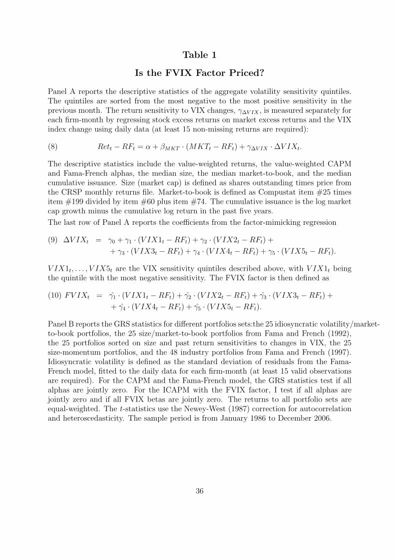
Table 1

Is the FVIX Factor Priced?

Panel A reports the descriptive statistics of the aggregate volatility sensitivity quintiles.The quintiles are sorted from the most negative to the most positive sensitivity in theprevious month. The return sensitivity to VIX changes, γ∆V IX , is measured separately foreach firm-month by regressing stock excess returns on market excess returns and the VIXindex change using daily data (at least 15 non-missing returns are required):

(8) Rett −RFt = α + βMKT · (MKTt −RFt) + γ∆V IX · ∆V IXt.

The descriptive statistics include the value-weighted returns, the value-weighted CAPMand Fama-French alphas, the median size, the median market-to-book, and the mediancumulative issuance. Size (market cap) is defined as shares outstanding times price fromthe CRSP monthly returns file. Market-to-book is defined as Compustat item #25 timesitem #199 divided by item #60 plus item #74. The cumulative issuance is the log marketcap growth minus the cumulative log return in the past five years.

The last row of Panel A reports the coefficients from the factor-mimicking regression

∆V IXt = γ0 + γ1 · (V IX1t −RFt) + γ2 · (V IX2t −RFt) +(9)

+ γ3 · (V IX3t −RFt) + γ4 · (V IX4t −RFt) + γ5 · (V IX5t −RFt).

V IX1t, . . . , V IX5t are the VIX sensitivity quintiles described above, with V IX1t beingthe quintile with the most negative sensitivity. The FVIX factor is then defined as

FV IXt = γ̂1 · (V IX1t −RFt) + γ̂2 · (V IX2t −RFt) + γ̂3 · (V IX3t −RFt) +(10)

+ γ̂4 · (V IX4t −RFt) + γ̂5 · (V IX5t −RFt).

Panel B reports the GRS statistics for different portfolios sets:the 25 idiosyncratic volatility/market-to-book portfolios, the 25 size/market-to-book portfolios from Fama and French (1992),the 25 portfolios sorted on size and past return sensitivities to changes in VIX, the 25size-momentum portfolios, and the 48 industry portfolios from Fama and French (1997).Idiosyncratic volatility is defined as the standard deviation of residuals from the Fama-French model, fitted to the daily data for each firm-month (at least 15 valid observationsare required). For the CAPM and the Fama-French model, the GRS statistics test if allalphas are jointly zero. For the ICAPM with the FVIX factor, I test if all alphas arejointly zero and if all FVIX betas are jointly zero. The returns to all portfolio sets areequal-weighted. The t-statistics use the Newey-West (1987) correction for autocorrelationand heteroscedasticity. The sample period is from January 1986 to December 2006.

36

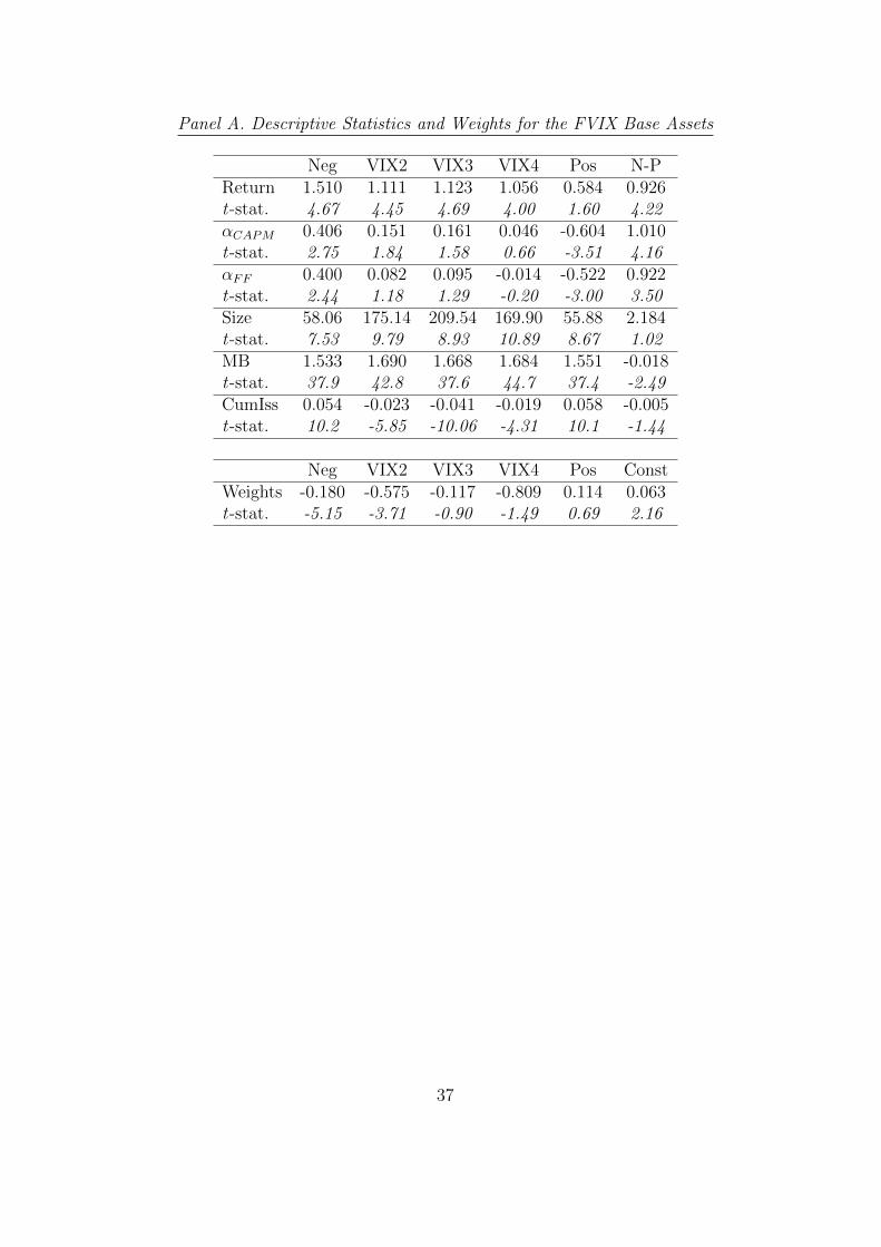
Panel A. Descriptive Statistics and Weights for the FVIX Base Assets

Neg VIX2 VIX3 VIX4 Pos N-PReturn 1.510 1.111 1.123 1.056 0.584 0.926t-stat. 4.67 4.45 4.69 4.00 1.60 4.22αCAPM 0.406 0.151 0.161 0.046 -0.604 1.010t-stat. 2.75 1.84 1.58 0.66 -3.51 4.16αFF 0.400 0.082 0.095 -0.014 -0.522 0.922t-stat. 2.44 1.18 1.29 -0.20 -3.00 3.50Size 58.06 175.14 209.54 169.90 55.88 2.184t-stat. 7.53 9.79 8.93 10.89 8.67 1.02MB 1.533 1.690 1.668 1.684 1.551 -0.018t-stat. 37.9 42.8 37.6 44.7 37.4 -2.49CumIss 0.054 -0.023 -0.041 -0.019 0.058 -0.005t-stat. 10.2 -5.85 -10.06 -4.31 10.1 -1.44

Neg VIX2 VIX3 VIX4 Pos ConstWeights -0.180 -0.575 -0.117 -0.809 0.114 0.063t-stat. -5.15 -3.71 -0.90 -1.49 0.69 2.16

37

Panel B. FVIX Factor Pricing for Different Portfolio Sets

25 IVol - M/B portfolios

αCAPM αFF αICAPM βFV IX

GRS 4.097 3.660 3.413 6.735p-value 0.000 0.000 0.000 0.000

25 Size - M/B portfolios

αCAPM αFF αICAPM βFV IX

GRS 6.788 6.126 6.963 9.806p-value 0.000 0.000 0.000 0.000

48 Industry portfolios

αCAPM αFF αICAPM βFV IX

GRS 1.806 1.866 1.808 3.924p-value 0.003 0.002 0.003 0.000

25 Size-VIX portfolios

αCAPM αFF αICAPM βFV IX

GRS 2.639 2.229 2.064 2.798p-value 0.000 0.001 0.003 0.000

25 Size-Momentum portfolios

αCAPM αFF αICAPM βFV IX

GRS 3.725 3.654 3.536 9.532p-value 0.000 0.000 0.000 0.000

38

Table 2

Market-to-Book, Idiosyncratic Volatility, and AggregateVolatility Risk

The table presents the FVIX betas of the 25 idiosyncratic volatility/market-to-book port-folios, sorted independently using NYSE (exchcd=1) breakpoints. Idiosyncratic volatilityis defined as the standard deviation of residuals from the Fama-French model, fitted to thedaily data for each firm-month (at least 15 valid observations are required). The idiosyn-cratic volatility (market-to-book) portfolios are rebalanced monthly (annually). Market-to-book is defined as Compustat item #25 times item #199 divided by item #60 plusitem #74. The FVIX betas are from the ICAPM with the FVIX factor:

(11) Rett −RFt = α + βMKT · (MKTt −RFt) + βFV IX · FV IXt.

The FVIX factor mimics the daily changes in the VIX index using the returns to thequintile portfolios sorted on past return sensitivity to VIX changes. The return sensitivityto VIX changes is measured separately for each firm-month by regressing stock excessreturns on market excess returns and the VIX index change using daily data (at least15 non-missing returns are required). The t-statistics reported use Newey-West (1987)correction for heteroscedasticity and autocorrelation. The sample period is from January1986 to December 2006.

Low IVol2 IVol3 IVol4 High L-HValue -0.524 -0.721 -0.463 -0.465 0.543 -1.067t-stat. -2.84 -2.82 -1.70 -1.89 3.27 -5.08MB2 -0.433 -0.675 -0.498 -0.220 0.724 -1.157t-stat. -2.43 -3.11 -1.93 -0.87 2.48 -2.80MB3 -0.155 -0.568 -0.470 0.002 0.545 -0.700t-stat. -0.79 -2.35 -2.57 0.01 2.96 -3.12MB4 -0.548 -0.872 -0.498 -0.020 1.201 -1.748t-stat. -3.92 -6.43 -2.27 -0.09 4.80 -7.77Growth -0.746 -0.480 -0.170 0.206 1.487 -2.233t-stat. -5.94 -3.87 -1.24 1.29 6.35 -7.89V-G 0.221 -0.241 -0.294 -0.671 -0.945 -1.166t-stat. 1.24 -0.84 -1.00 -2.58 -3.50 -4.32

39

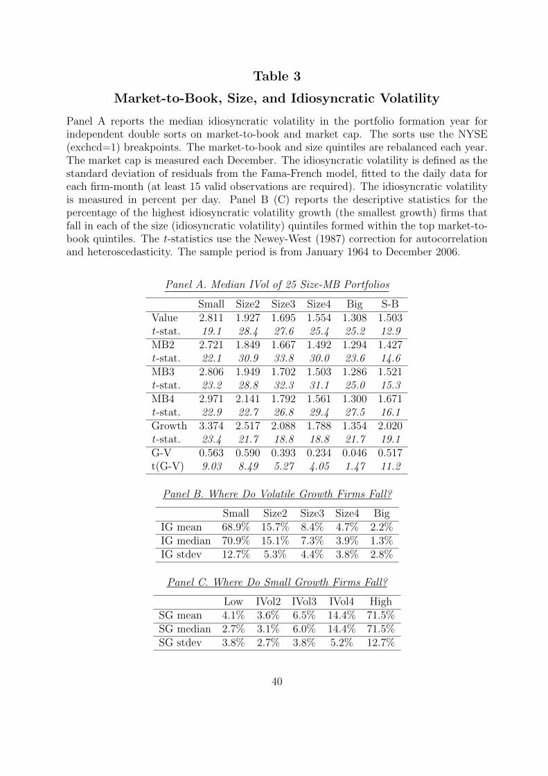
Table 3

Market-to-Book, Size, and Idiosyncratic Volatility

Panel A reports the median idiosyncratic volatility in the portfolio formation year forindependent double sorts on market-to-book and market cap. The sorts use the NYSE(exchcd=1) breakpoints. The market-to-book and size quintiles are rebalanced each year.The market cap is measured each December. The idiosyncratic volatility is defined as thestandard deviation of residuals from the Fama-French model, fitted to the daily data foreach firm-month (at least 15 valid observations are required). The idiosyncratic volatilityis measured in percent per day. Panel B (C) reports the descriptive statistics for thepercentage of the highest idiosyncratic volatility growth (the smallest growth) firms thatfall in each of the size (idiosyncratic volatility) quintiles formed within the top market-to-book quintiles. The t-statistics use the Newey-West (1987) correction for autocorrelationand heteroscedasticity. The sample period is from January 1964 to December 2006.

Panel A. Median IVol of 25 Size-MB Portfolios

Small Size2 Size3 Size4 Big S-BValue 2.811 1.927 1.695 1.554 1.308 1.503t-stat. 19.1 28.4 27.6 25.4 25.2 12.9MB2 2.721 1.849 1.667 1.492 1.294 1.427t-stat. 22.1 30.9 33.8 30.0 23.6 14.6MB3 2.806 1.949 1.702 1.503 1.286 1.521t-stat. 23.2 28.8 32.3 31.1 25.0 15.3MB4 2.971 2.141 1.792 1.561 1.300 1.671t-stat. 22.9 22.7 26.8 29.4 27.5 16.1Growth 3.374 2.517 2.088 1.788 1.354 2.020t-stat. 23.4 21.7 18.8 18.8 21.7 19.1G-V 0.563 0.590 0.393 0.234 0.046 0.517t(G-V) 9.03 8.49 5.27 4.05 1.47 11.2

Panel B. Where Do Volatile Growth Firms Fall?

Small Size2 Size3 Size4 BigIG mean 68.9% 15.7% 8.4% 4.7% 2.2%IG median 70.9% 15.1% 7.3% 3.9% 1.3%IG stdev 12.7% 5.3% 4.4% 3.8% 2.8%

Panel C. Where Do Small Growth Firms Fall?

Low IVol2 IVol3 IVol4 HighSG mean 4.1% 3.6% 6.5% 14.4% 71.5%SG median 2.7% 3.1% 6.0% 14.4% 71.5%SG stdev 3.8% 2.7% 3.8% 5.2% 12.7%

40

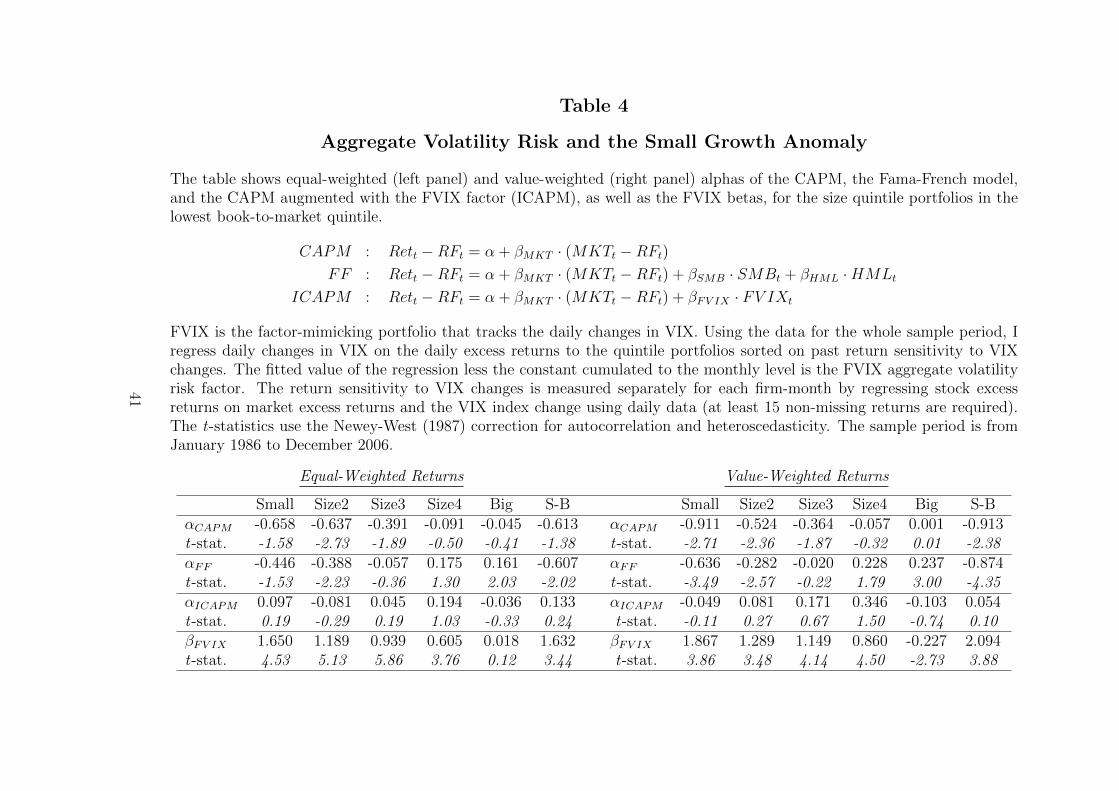
Table 4

Aggregate Volatility Risk and the Small Growth Anomaly

The table shows equal-weighted (left panel) and value-weighted (right panel) alphas of the CAPM, the Fama-French model,and the CAPM augmented with the FVIX factor (ICAPM), as well as the FVIX betas, for the size quintile portfolios in thelowest book-to-market quintile.

CAPM : Rett −RFt = α + βMKT · (MKTt −RFt)

FF : Rett −RFt = α + βMKT · (MKTt −RFt) + βSMB · SMBt + βHML ·HMLt

ICAPM : Rett −RFt = α + βMKT · (MKTt −RFt) + βFV IX · FV IXt

FVIX is the factor-mimicking portfolio that tracks the daily changes in VIX. Using the data for the whole sample period, Iregress daily changes in VIX on the daily excess returns to the quintile portfolios sorted on past return sensitivity to VIXchanges. The fitted value of the regression less the constant cumulated to the monthly level is the FVIX aggregate volatilityrisk factor. The return sensitivity to VIX changes is measured separately for each firm-month by regressing stock excessreturns on market excess returns and the VIX index change using daily data (at least 15 non-missing returns are required).The t-statistics use the Newey-West (1987) correction for autocorrelation and heteroscedasticity. The sample period is fromJanuary 1986 to December 2006.

Equal-Weighted Returns Value-Weighted Returns

Small Size2 Size3 Size4 Big S-B Small Size2 Size3 Size4 Big S-BαCAPM -0.658 -0.637 -0.391 -0.091 -0.045 -0.613 αCAPM -0.911 -0.524 -0.364 -0.057 0.001 -0.913t-stat. -1.58 -2.73 -1.89 -0.50 -0.41 -1.38 t-stat. -2.71 -2.36 -1.87 -0.32 0.01 -2.38αFF -0.446 -0.388 -0.057 0.175 0.161 -0.607 αFF -0.636 -0.282 -0.020 0.228 0.237 -0.874t-stat. -1.53 -2.23 -0.36 1.30 2.03 -2.02 t-stat. -3.49 -2.57 -0.22 1.79 3.00 -4.35αICAPM 0.097 -0.081 0.045 0.194 -0.036 0.133 αICAPM -0.049 0.081 0.171 0.346 -0.103 0.054t-stat. 0.19 -0.29 0.19 1.03 -0.33 0.24 t-stat. -0.11 0.27 0.67 1.50 -0.74 0.10βFV IX 1.650 1.189 0.939 0.605 0.018 1.632 βFV IX 1.867 1.289 1.149 0.860 -0.227 2.094t-stat. 4.53 5.13 5.86 3.76 0.12 3.44 t-stat. 3.86 3.48 4.14 4.50 -2.73 3.88

41

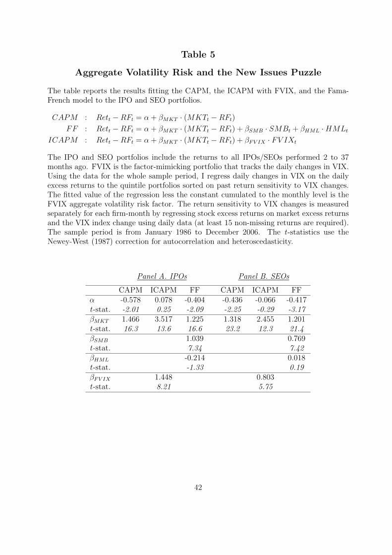
Table 5

Aggregate Volatility Risk and the New Issues Puzzle

The table reports the results fitting the CAPM, the ICAPM with FVIX, and the Fama-French model to the IPO and SEO portfolios.

CAPM : Rett −RFt = α + βMKT · (MKTt −RFt)

FF : Rett −RFt = α + βMKT · (MKTt −RFt) + βSMB · SMBt + βHML ·HMLt

ICAPM : Rett −RFt = α + βMKT · (MKTt −RFt) + βFV IX · FV IXt

The IPO and SEO portfolios include the returns to all IPOs/SEOs performed 2 to 37months ago. FVIX is the factor-mimicking portfolio that tracks the daily changes in VIX.Using the data for the whole sample period, I regress daily changes in VIX on the dailyexcess returns to the quintile portfolios sorted on past return sensitivity to VIX changes.The fitted value of the regression less the constant cumulated to the monthly level is theFVIX aggregate volatility risk factor. The return sensitivity to VIX changes is measuredseparately for each firm-month by regressing stock excess returns on market excess returnsand the VIX index change using daily data (at least 15 non-missing returns are required).The sample period is from January 1986 to December 2006. The t-statistics use theNewey-West (1987) correction for autocorrelation and heteroscedasticity.

Panel A. IPOs Panel B. SEOs

CAPM ICAPM FF CAPM ICAPM FFα -0.578 0.078 -0.404 -0.436 -0.066 -0.417t-stat. -2.01 0.25 -2.09 -2.25 -0.29 -3.17βMKT 1.466 3.517 1.225 1.318 2.455 1.201t-stat. 16.3 13.6 16.6 23.2 12.3 21.4βSMB 1.039 0.769t-stat. 7.34 7.42βHML -0.214 0.018t-stat. -1.33 0.19βFV IX 1.448 0.803t-stat. 8.21 5.75

42

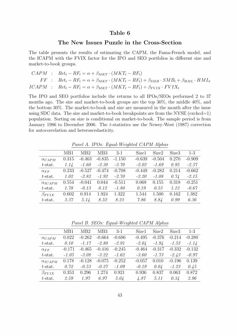
Table 6

The New Issues Puzzle in the Cross-Section

The table presents the results of estimating the CAPM, the Fama-French model, andthe ICAPM with the FVIX factor for the IPO and SEO portfolios in different size andmarket-to-book groups.

CAPM : Rett −RFt = α + βMKT · (MKTt −RFt)

FF : Rett −RFt = α + βMKT · (MKTt −RFt) + βSMB · SMBt + βHML ·HMLt

ICAPM : Rett −RFt = α + βMKT · (MKTt −RFt) + βFV IX · FV IXt

The IPO and SEO portfolios include the returns to all IPOs/SEOs performed 2 to 37months ago. The size and market-to-book groups are the top 30%, the middle 40%, andthe bottom 30%. The market-to-book and size are measured in the month after the issueusing SDC data. The size and market-to-book breakpoints are from the NYSE (exchcd=1)population. Sorting on size is conditional on market-to-book. The sample period is fromJanuary 1986 to December 2006. The t-statistics use the Newey-West (1987) correctionfor autocorrelation and heteroscedasticity.

Panel A. IPOs: Equal-Weighted CAPM Alphas

MB1 MB2 MB3 3-1 Size1 Size2 Size3 1-3αCAPM 0.315 -0.463 -0.835 -1.150 -0.639 -0.504 0.270 -0.909t-stat. 1.14 -1.60 -2.30 -3.70 -2.02 -1.69 0.95 -2.37αFF 0.233 -0.527 -0.474 -0.708 -0.449 -0.282 0.214 -0.662t-stat. 1.02 -2.82 -1.92 -2.70 -2.20 -1.08 0.74 -2.15αICAPM 0.554 -0.041 0.044 -0.511 0.068 0.155 0.318 -0.251t-stat. 1.78 -0.13 0.12 -1.80 0.19 0.53 1.12 -0.67βFV IX 0.602 0.914 1.924 1.322 1.544 1.500 0.162 1.382t-stat. 3.37 5.14 8.52 8.23 7.86 8.84 0.99 6.36

Panel B. SEOs: Equal-Weighted CAPM Alphas

MB1 MB2 MB3 3-1 Size1 Size2 Size3 1-3αCAPM 0.022 -0.262 -0.664 -0.686 -0.495 -0.376 -0.214 -0.280t-stat. 0.10 -1.17 -2.80 -2.91 -2.04 -1.94 -1.52 -1.14αFF -0.171 -0.465 -0.416 -0.245 -0.464 -0.317 -0.332 -0.132t-stat. -1.05 -3.08 -3.22 -1.62 -3.60 -1.73 -2.43 -0.97αICAPM 0.178 -0.128 -0.075 -0.252 -0.057 0.010 -0.196 0.139t-stat. 0.72 -0.53 -0.27 -1.09 -0.19 0.04 -1.23 0.45βFV IX 0.353 0.296 1.274 0.921 0.936 0.837 0.063 0.872t-stat. 2.59 1.97 6.97 5.04 4.87 5.11 0.34 2.96

43

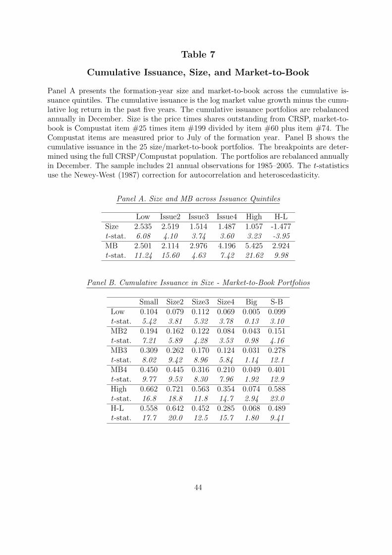
Table 7

Cumulative Issuance, Size, and Market-to-Book

Panel A presents the formation-year size and market-to-book across the cumulative is-suance quintiles. The cumulative issuance is the log market value growth minus the cumu-lative log return in the past five years. The cumulative issuance portfolios are rebalancedannually in December. Size is the price times shares outstanding from CRSP, market-to-book is Compustat item #25 times item #199 divided by item #60 plus item #74. TheCompustat items are measured prior to July of the formation year. Panel B shows thecumulative issuance in the 25 size/market-to-book portfolios. The breakpoints are deter-mined using the full CRSP/Compustat population. The portfolios are rebalanced annuallyin December. The sample includes 21 annual observations for 1985–2005. The t-statisticsuse the Newey-West (1987) correction for autocorrelation and heteroscedasticity.

Panel A. Size and MB across Issuance Quintiles

Low Issue2 Issue3 Issue4 High H-LSize 2.535 2.519 1.514 1.487 1.057 -1.477t-stat. 6.08 4.10 3.74 3.60 3.23 -3.95MB 2.501 2.114 2.976 4.196 5.425 2.924t-stat. 11.24 15.60 4.63 7.42 21.62 9.98

Panel B. Cumulative Issuance in Size - Market-to-Book Portfolios

Small Size2 Size3 Size4 Big S-BLow 0.104 0.079 0.112 0.069 0.005 0.099t-stat. 5.42 3.81 5.32 3.78 0.13 3.10MB2 0.194 0.162 0.122 0.084 0.043 0.151t-stat. 7.21 5.89 4.28 3.53 0.98 4.16MB3 0.309 0.262 0.170 0.124 0.031 0.278t-stat. 8.02 9.42 8.96 5.84 1.14 12.1MB4 0.450 0.445 0.316 0.210 0.049 0.401t-stat. 9.77 9.53 8.30 7.96 1.92 12.9High 0.662 0.721 0.563 0.354 0.074 0.588t-stat. 16.8 18.8 11.8 14.7 2.94 23.0H-L 0.558 0.642 0.452 0.285 0.068 0.489t-stat. 17.7 20.0 12.5 15.7 1.80 9.41

44

Table 8

Aggregate Volatility Risk and the Cumulative Issuance Puzzle

The table reports the results of fitting the CAPM, the Fama-French model, and the ICAPMwith FVIX to the cumulative issuance arbitrage portfolio.

CAPM : Rett −RFt = α + βMKT · (MKTt −RFt)

FF : Rett −RFt = α + βMKT · (MKTt −RFt) + βSMB · SMBt + βHML ·HMLt

ICAPM : Rett −RFt = α + βMKT · (MKTt −RFt) + βFV IX · FV IXt

FVIX is the factor-mimicking portfolio that tracks the daily changes in VIX. Using thedata for the whole sample period, I regress daily changes in VIX on the daily excess returnsto the quintile portfolios sorted on past return sensitivity to VIX changes. The fitted valueof the regression less the constant cumulated to the monthly level is the FVIX aggregatevolatility risk factor. The return sensitivity to VIX changes is measured separately for eachfirm-month by regressing stock excess returns on market excess returns and the VIX indexchange using daily data (at least 15 non-missing returns are required). The cumulativeissuance arbitrage portfolio buys the firms in the top 30% on cumulative issuance andshorts the firms in the bottom 30% on cumulative issuance. The cumulative issuance isthe log market value growth minus the cumulative log return in the past five years. Thesorts on cumulative issuance use NYSE (exchcd=1) breakpoints. The sample period is fromJanuary 1986 to December 2006. The t-statistics use the Newey-West (1987) correctionfor autocorrelation and heteroscedasticity.

Equal-Weighted Value-Weighted

CAPM ICAPM FF CAPM ICAPM FFα -0.638 -0.103 -0.388 -0.580 -0.339 -0.439t-stat. -2.66 -0.35 -2.21 -4.30 -2.36 -4.04βMKT 0.483 2.116 0.254 0.399 1.157 0.279t-stat. 6.26 7.06 4.16 8.01 7.93 7.10βSMB 0.622 0.291t-stat. 7.48 5.54βHML -0.365 -0.209t-stat. -3.28 -2.58βFV IX 1.153 0.535t-stat. 5.27 5.15

45

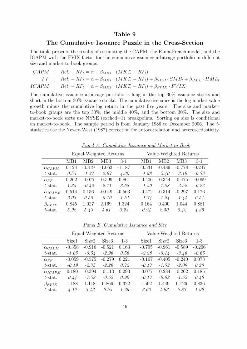
Table 9

The Cumulative Issuance Puzzle in the Cross-Section

The table presents the results of estimating the CAPM, the Fama-French model, and theICAPM with the FVIX factor for the cumulative issuance arbitrage portfolio in differentsize and market-to-book groups.

CAPM : Rett −RFt = α + βMKT · (MKTt −RFt)

FF : Rett −RFt = α + βMKT · (MKTt −RFt) + βSMB · SMBt + βHML ·HMLt

ICAPM : Rett −RFt = α + βMKT · (MKTt −RFt) + βFV IX · FV IXt

The cumulative issuance arbitrage portfolio is long in the top 30% issuance stocks andshort in the bottom 30% issuance stocks. The cumulative issuance is the log market valuegrowth minus the cumulative log return in the past five years. The size and market-to-book groups are the top 30%, the middle 40%, and the bottom 30%. The size andmarket-to-book sorts use NYSE (exchcd=1) breakpoints. Sorting on size is conditionalon market-to-book. The sample period is from January 1986 to December 2006. The t-statistics use the Newey-West (1987) correction for autocorrelation and heteroscedasticity.

Panel A. Cumulative Issuance and Market-to-Book

Equal-Weighted Returns Value-Weighted Returns

MB1 MB2 MB3 3-1 MB1 MB2 MB3 3-1αCAPM 0.124 -0.319 -1.063 -1.187 -0.531 -0.489 -0.778 -0.247t-stat. 0.55 -1.37 -2.67 -4.30 -1.98 -2.40 -3.19 -0.73αFF 0.262 -0.077 -0.599 -0.861 -0.406 -0.344 -0.475 -0.069t-stat. 1.35 -0.42 -2.11 -3.68 -1.50 -1.88 -2.52 -0.23αICAPM 0.514 0.156 -0.049 -0.563 -0.472 -0.314 -0.297 0.176t-stat. 2.03 0.55 -0.10 -1.51 -1.74 -1.24 -1.44 0.54βFV IX 0.845 1.027 2.169 1.324 0.164 0.400 1.044 0.881t-stat. 5.92 5.43 4.61 3.23 0.94 2.50 6.42 4.35

Panel B. Cumulative Issuance and Size

Equal-Weighted Returns Value-Weighted Returns

Size1 Size2 Size3 1-3 Size1 Size2 Size3 1-3αCAPM -0.358 -0.916 -0.521 0.163 -0.795 -0.961 -0.589 -0.206t-stat. -1.05 -3.54 -2.96 0.56 -2.28 -3.14 -3.46 -0.65αFF -0.059 -0.575 -0.279 0.221 -0.167 -0.405 -0.240 0.073t-stat. -0.19 -2.75 -2.26 0.72 -0.47 -1.53 -2.09 0.20αICAPM 0.180 -0.394 -0.113 0.293 -0.077 -0.284 -0.262 0.185t-stat. 0.44 -1.38 -0.62 0.90 -0.17 -0.82 -1.62 0.46βFV IX 1.188 1.118 0.866 0.322 1.562 1.449 0.726 0.836t-stat. 4.17 5.42 6.55 1.26 3.62 4.93 5.87 1.99

46