Embed Size (px)
Citation preview

1
Chapter 2
Aggregate Supply – Aggregate Demand and the Phillips Curve
EPP, 2011 Yann Algan
2
1. INTRODUCION
Questions
Impact of supply and demand shocks on the economy ?
Expectations, credibility and Public Policies
Relation between inflation, unemployment and fluctuations ?

3
Need a more general framework than the IS-LM model
Nominal rigidities • Prices on the product market are less rigid than wages • Need to integrate price adjustment and inflation
Natures of shocks • Fluctuations are not uniquely driven by demand shocks and shortage of demand • Role of supply shocks : ex stagflation
Synthesis • AS/AD framework: wage rigidities but price flexibility • Inflation and output fluctuations: Phillips curve

4
US case
Unemployment (%)
Inflation (% per year)
0 1 2 3 4 5 6 7 8 9 10 2
4
6
8
10
1968 1966
1961 1962 1963
1967 1965
1964
Illustration Phillips curve

5 Unemployment (%)
Inflation (% per year)
0 1 2 3 4 5 6 7 8 9 10 2
4
6
8
10
1973 1971 1969 1970 1968
1966
1961 1962 1963
1967 1965
1964
1972
6
2. Aggregate Supply
Framework for understanding the determinants of aggregate supply
Interplay between labor market and product market
Positive relationship between aggregate supply and prices
7
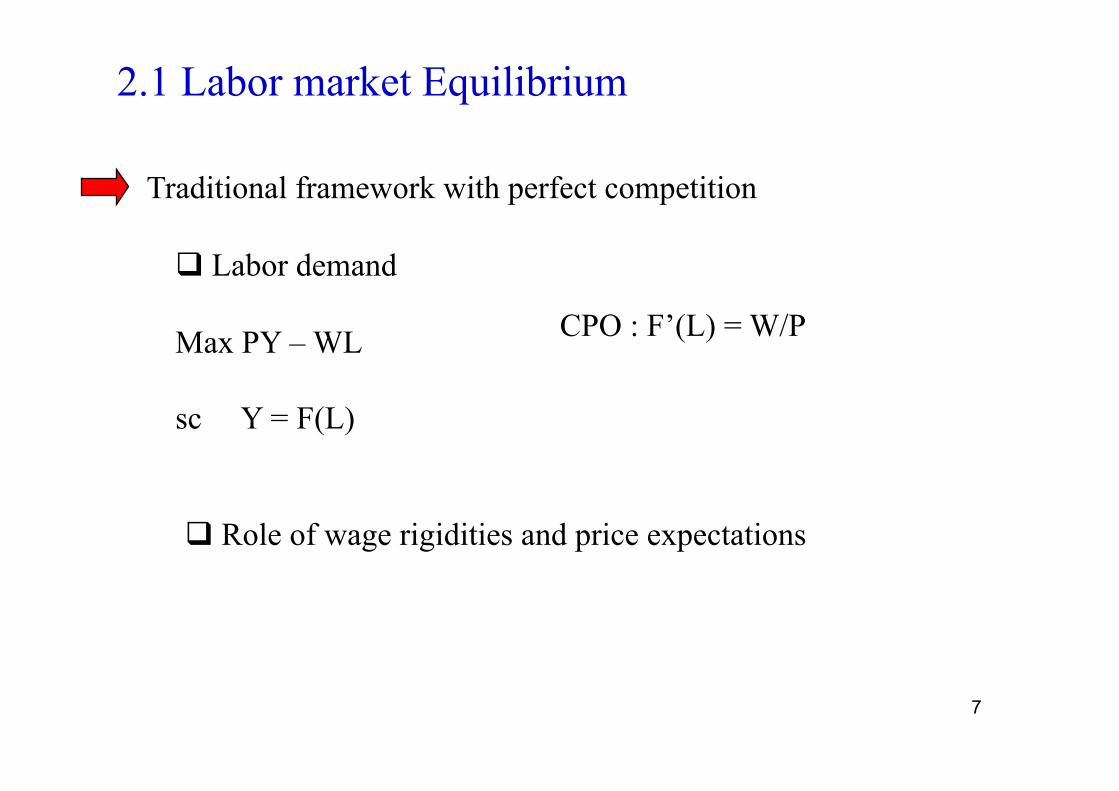
2.1 Labor market Equilibrium
Traditional framework with perfect competition
Labor demand
Max PY – WL
sc Y = F(L)
CPO : F’(L) = W/P
Role of wage rigidities and price expectations
8
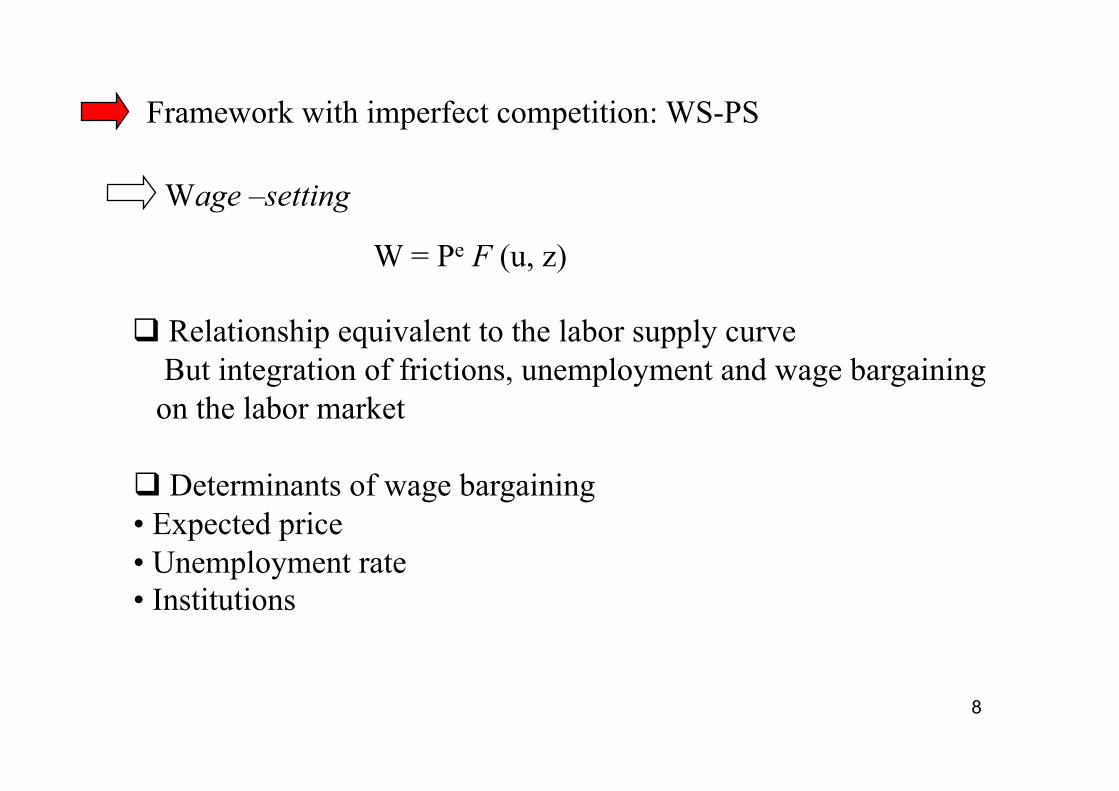
Wage –setting
Framework with imperfect competition: WS-PS
Determinants of wage bargaining • Expected price • Unemployment rate • Institutions
W = Pe F (u, z)
Relationship equivalent to the labor supply curve But integration of frictions, unemployment and wage bargaining on the labor market

9
Price-setting curve
P = (1 + µ) W
Relation PS equivalent to the labor demand … But integration of imperfect competition on the product market
10
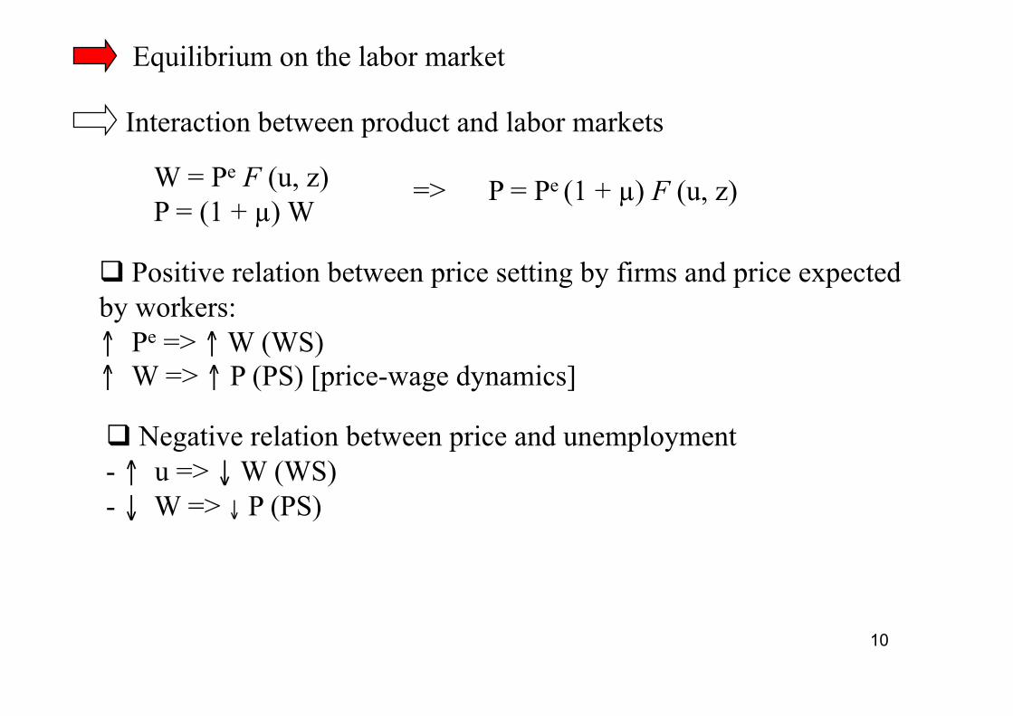
Equilibrium on the labor market
Interaction between product and labor markets
W = Pe F (u, z) P = (1 + µ) W
=> P = Pe (1 + µ) F (u, z)
Positive relation between price setting by firms and price expected by workers: ↑ Pe => ↑ W (WS) ↑ W => ↑ P (PS) [price-wage dynamics]
Negative relation between price and unemployment - ↑ u => ↓ W (WS) - ↓ W => ↓ P (PS)
11
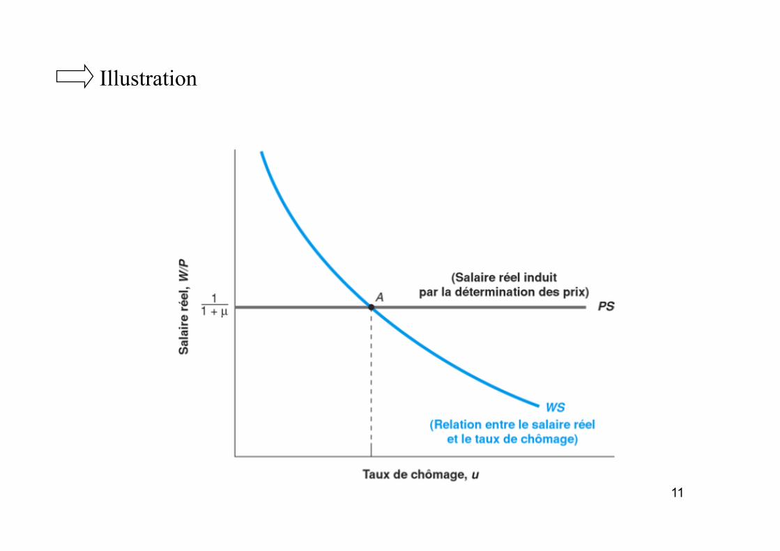
Illustration
12
2.2 Aggregate Supply Positive relation between supply of goods and the price level
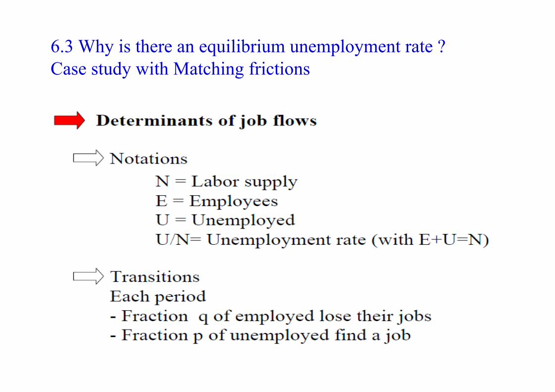
Unemployment rate: u = U/ L where L=N+U=Employed + Unemployed= Active population
Production: Y=N
u = 1 – N/L = 1 – Y/ L
Production, employment and unemployment

13
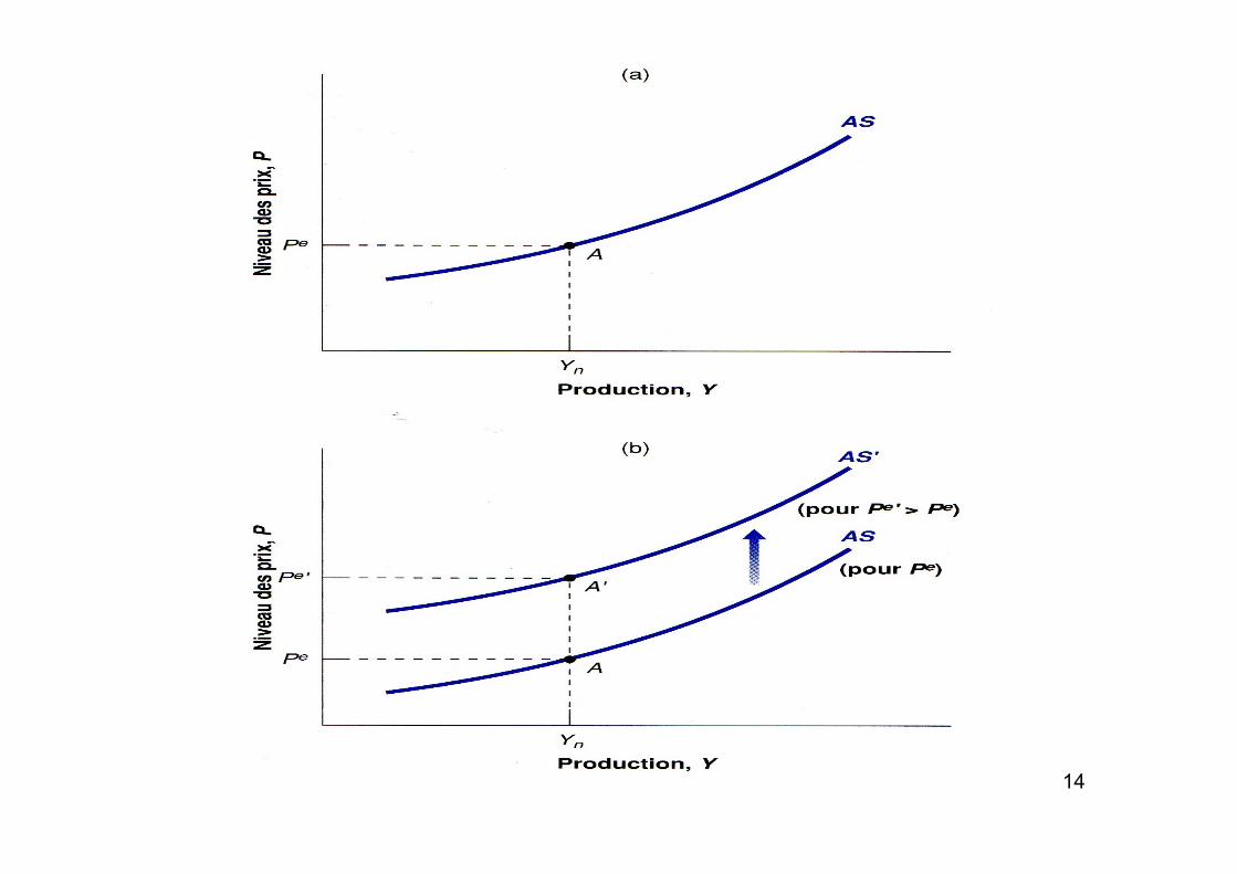
Aggregate supply
P = Pe (1 + µ) F (1-Y/L, z)
Positive relation between Y and P
• ↑ Y => ↑ N (cf. production function Y = N) • ↑ N => ↓ u • ↓ u => ↑ W (WS) • ↑ W => ↑ P (PS)
Implication : AS curve, for a given Pe, increases with P
14
15
Equilibrium production
Production Yn associated with equilibrium (un)employment
Natural output, or potential output
In the medium run: Adjustement of prices expectations and wages - ↑ Pe = P => ↑ W to leave the level of W/P unchanged
- N and Y will remain unchanged in the medium rate following a variation in P
Production independent of prices

16
Equilibrium unemployement when P= Pe
Equalization
Structural unemployment rate: Real rigidities and frictions (mark-up, institutions…)
W = Pe F (u, z) P = (1 + µ) W
and P = Pe (WS) (PS)
In the short run, potential fluctuations of unemployment around the equilibrium unemployment. In the medium run: equilibrium unemployment independent of prices

17
Definition
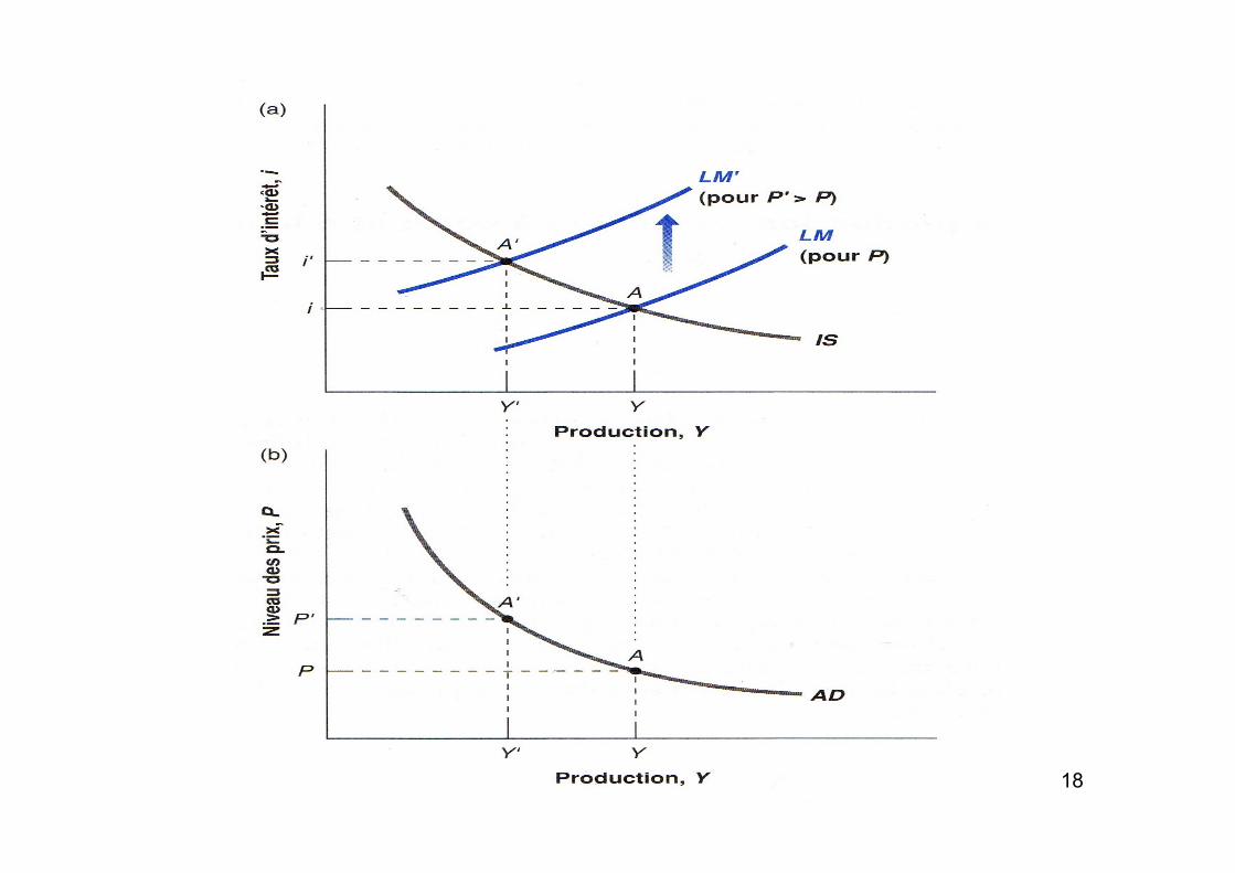
3. Aggregate Demand
Demand on the product market consistent with money market equilibrium. Derived from the IS-LM side.
Integration of price effect on demand: decreasing relation between demand and prices
↑ P => ↓ M/ P => LM curve shifts upward ↑ i and ↓ de Y
Aggregate demand determinants
Y = Y(M/P, G, T) (+ , + , - )
LM IS
18
19
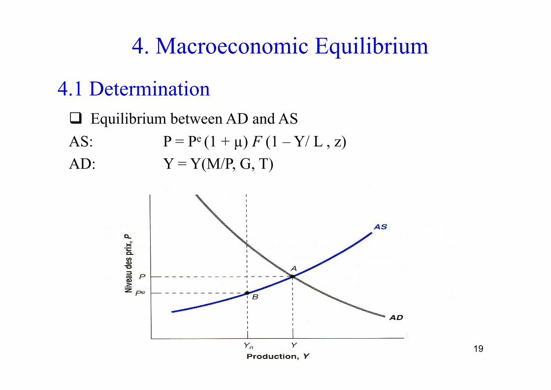
4. Macroeconomic Equilibrium
4.1 Determination Equilibrium between AD and AS AS: P = Pe (1 + µ) F (1 – Y/ L , z) AD: Y = Y(M/P, G, T)
20
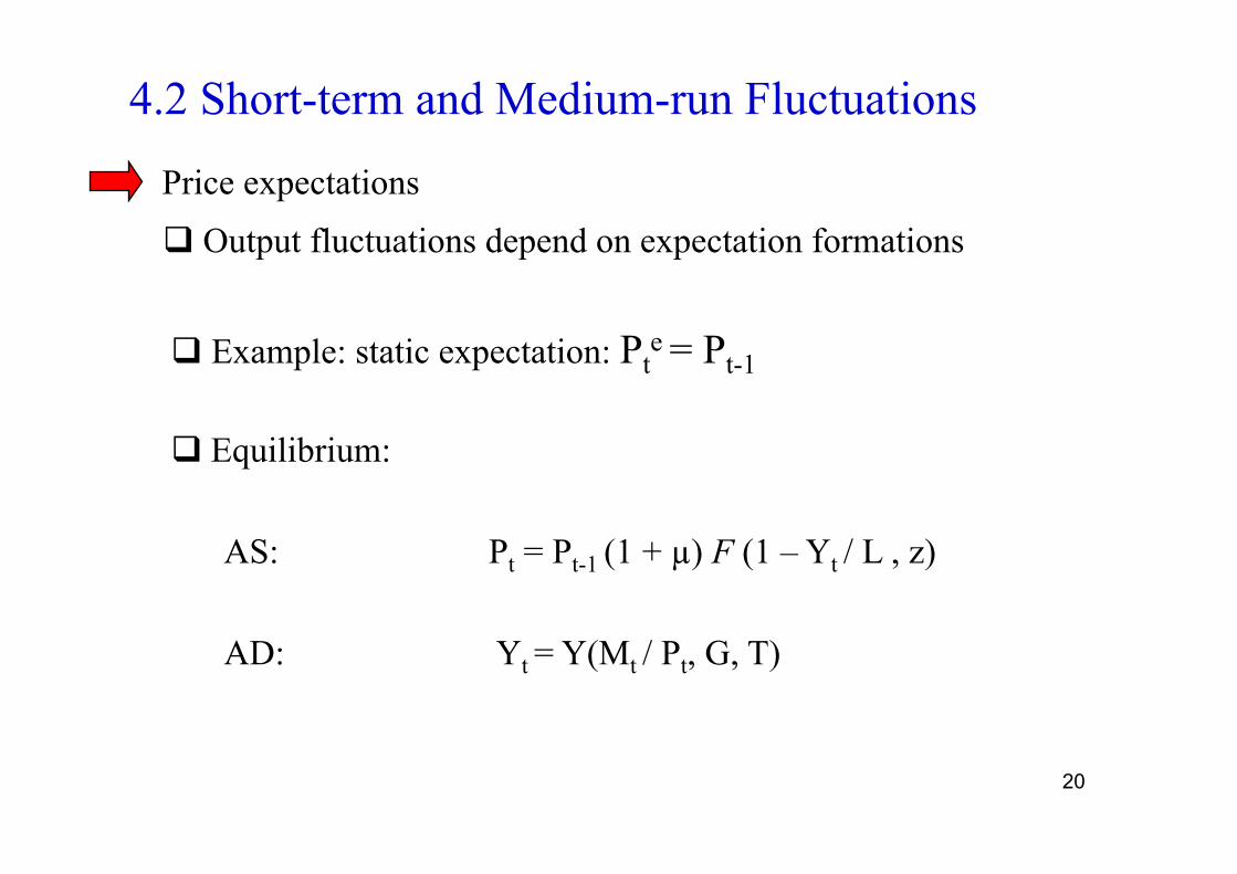
4.2 Short-term and Medium-run Fluctuations
Equilibrium:
AS: Pt = Pt-1 (1 + µ) F (1 – Yt / L , z)
AD: Yt = Y(Mt / Pt, G, T)
Price expectations
Output fluctuations depend on expectation formations
Example: static expectation: Pte = Pt-1
21
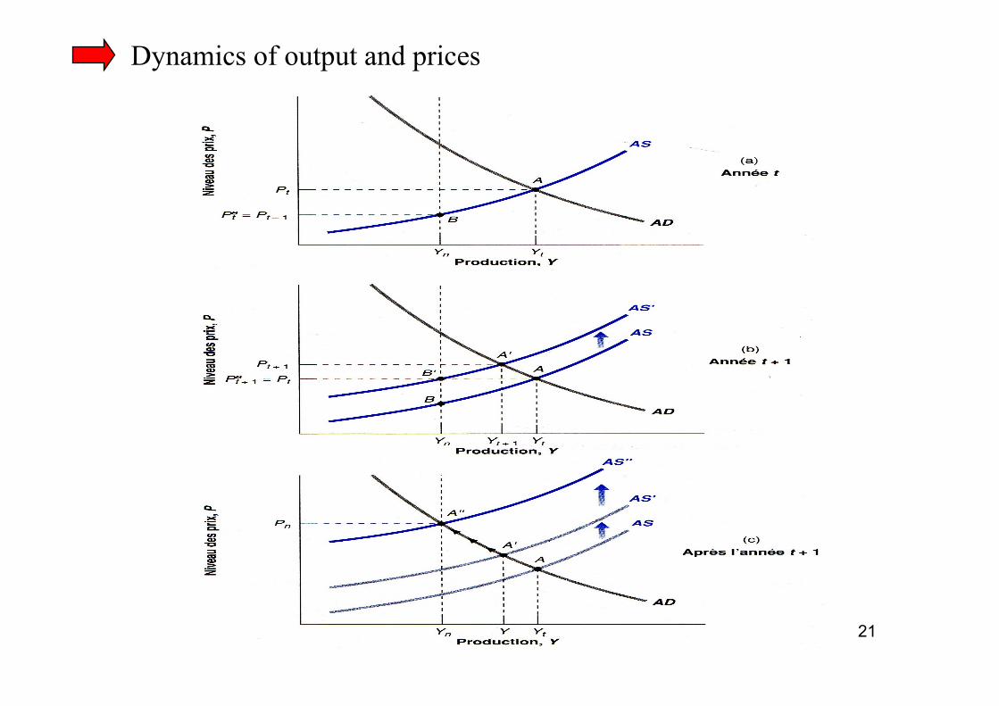
Dynamics of output and prices
22
In the short run, output can be higher or lower than potential output
But in the mid-term, output converges to its equilibrium level following adjustments of expectations and prices
Speed of the adjustment process depends on price and wage flexibility and on expectation formations
23
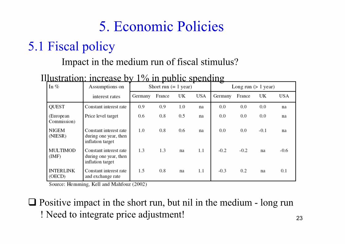
5. Economic Policies 5.1 Fiscal policy
Impact in the medium run of fiscal stimulus?
Positive impact in the short run, but nil in the medium - long run ! Need to integrate price adjustment!
Illustration: increase by 1% in public spending
24
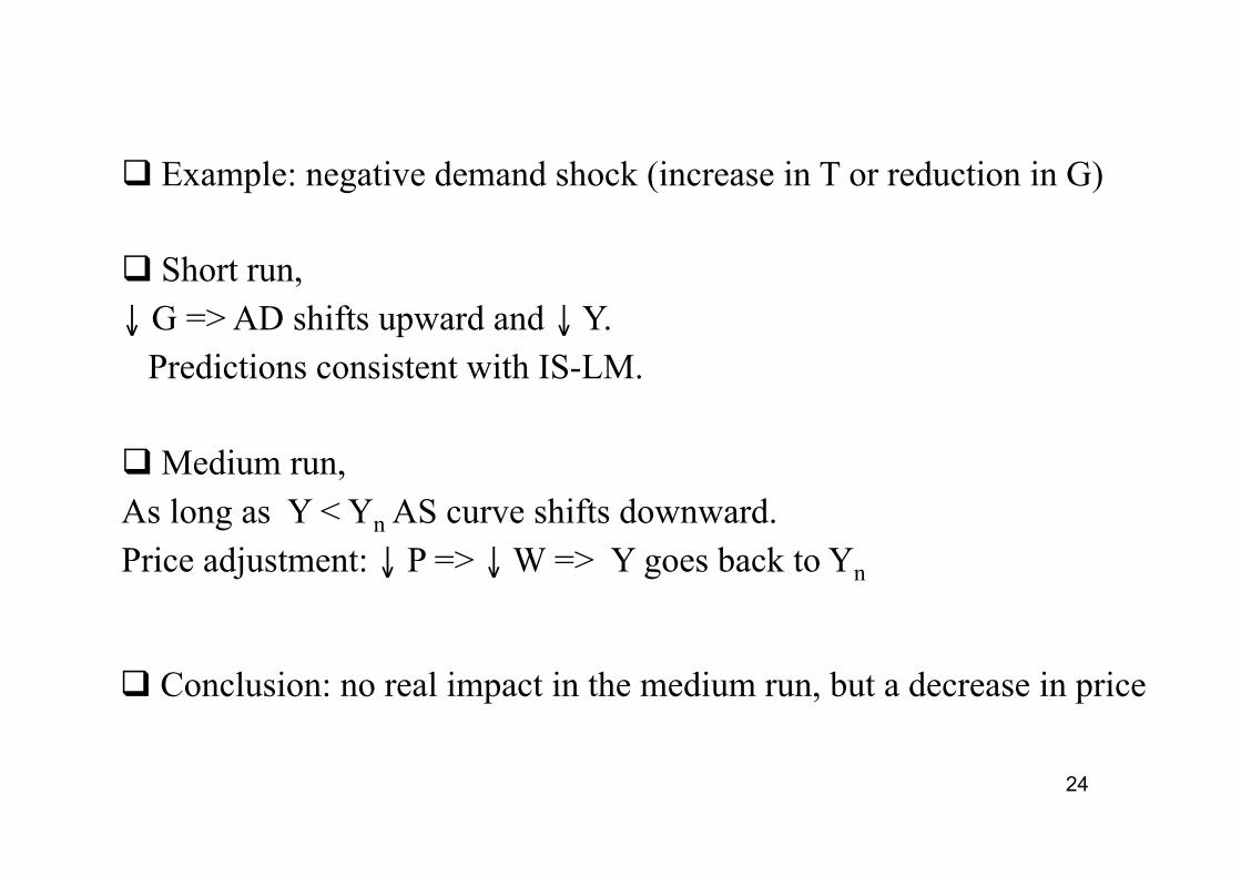
Example: negative demand shock (increase in T or reduction in G)
Short run, ↓ G => AD shifts upward and ↓ Y. Predictions consistent with IS-LM.
Medium run, As long as Y < Yn AS curve shifts downward. Price adjustment: ↓ P => ↓ W => Y goes back to Yn
Conclusion: no real impact in the medium run, but a decrease in price
25

26
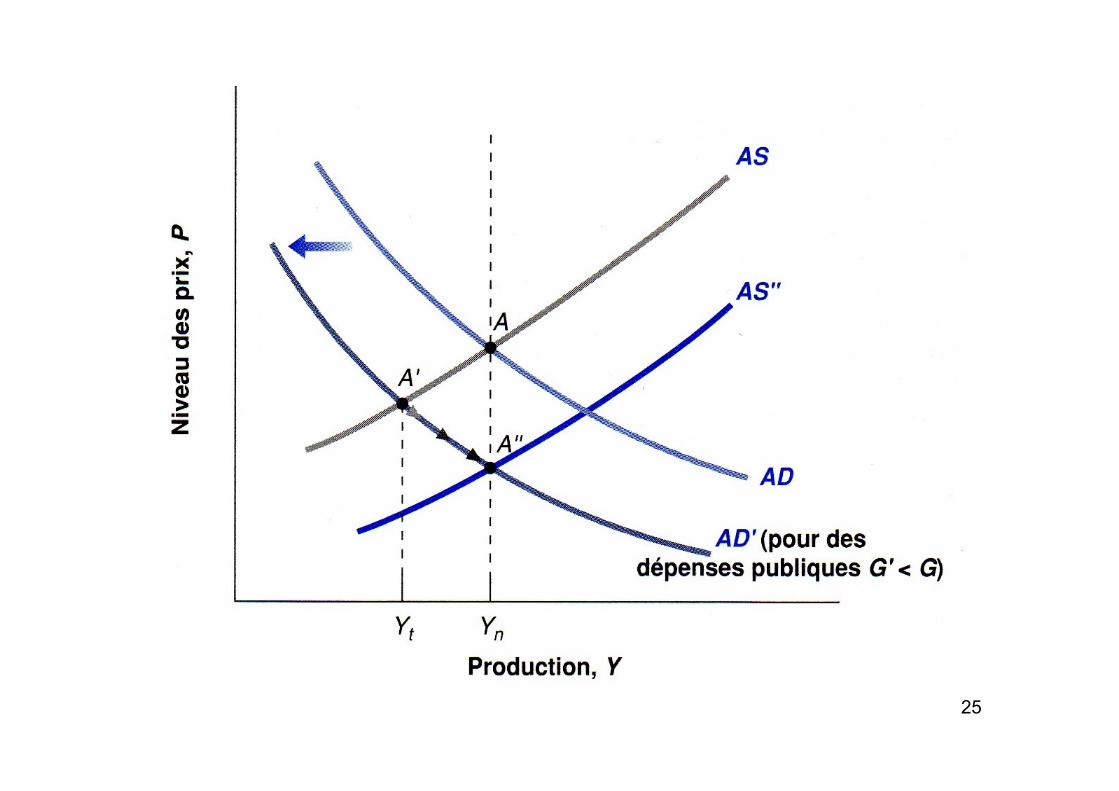
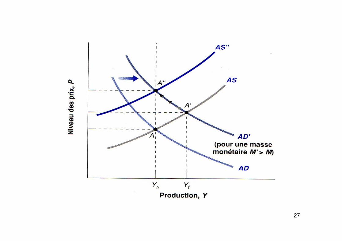
5.2 Monetary Policy
Assume production is at its equilibrium Y = Yn,,
Expansionary monetary policy: short-run impact ↑ M => ↑ AD => ↑ Y > Yn
Price adjustment in the medium run => ↑ P => ↑ W => AS shifts upward=> Y goes back to Yn
Conclusion: monetary policy is neutral in the medium run, price adjust in proportion to the increase in M
Estimates in the US • Peak in output after three quarters: + 1,8% of GDP, but vanishes after • 4 years latter, P increases by 1,5 % but Y has increased by 0,3% only
27
28
29
6. Phillips Curve
Questions
• Relations between inflation, unemployment an output
• Is there a trade-off between inflation and unemployment ?
• Credibility of monetary policy and Independance of Central Bank
30
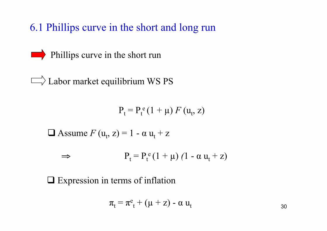
6.1 Phillips curve in the short and long run
Phillips curve in the short run
Pt = Pte (1 + µ) F (ut, z)
Labor market equilibrium WS PS
Assume F (ut, z) = 1 - α ut + z
⇒ Pt = Pte (1 + µ) (1 - α ut + z)
πt = πet + (µ + z) - α ut
Expression in terms of inflation
31
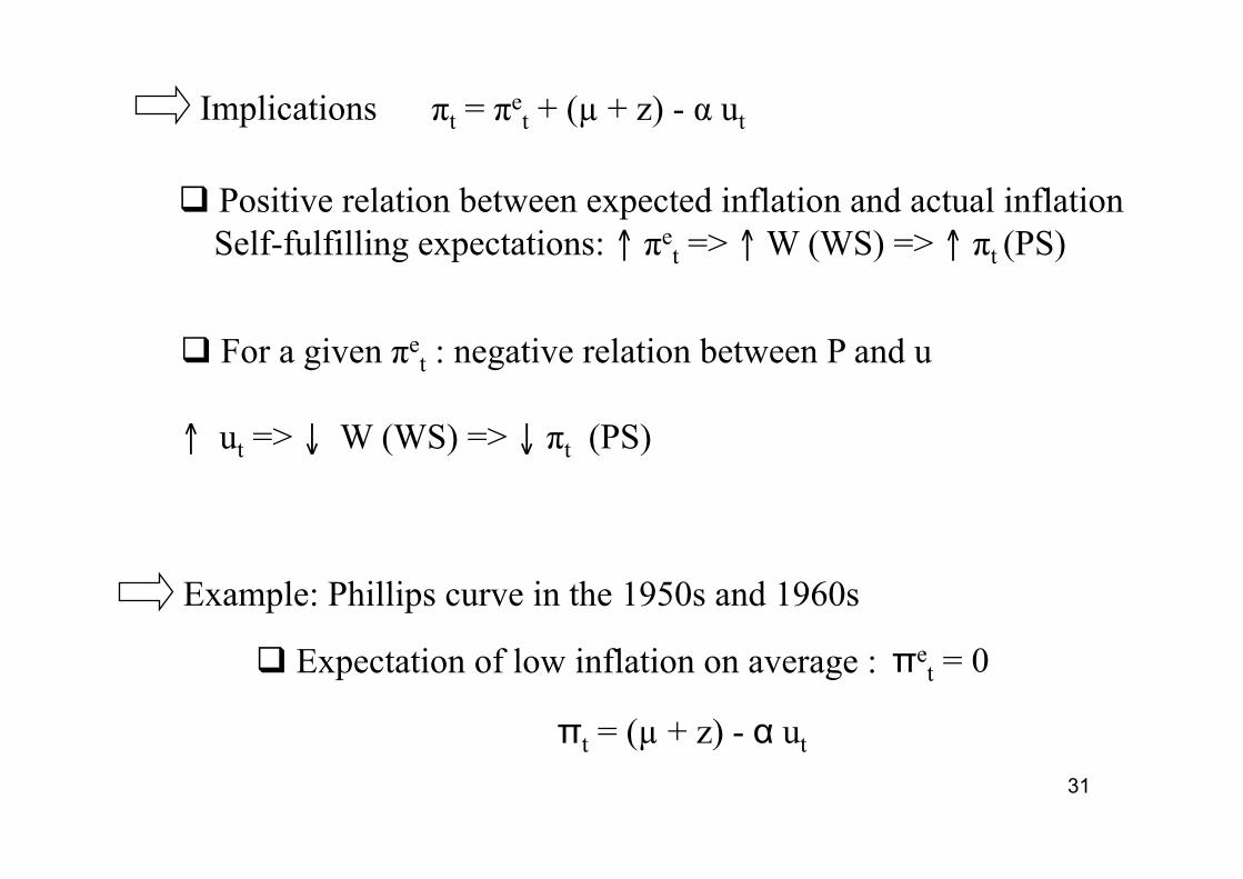
Implications
Positive relation between expected inflation and actual inflation Self-fulfilling expectations: ↑ πe
t => ↑ W (WS) => ↑ πt (PS)
πt = πet + (µ + z) - α ut
For a given πet : negative relation between P and u
↑ ut => ↓ W (WS) => ↓ πt (PS)
Example: Phillips curve in the 1950s and 1960s
Expectation of low inflation on average :

32
Trade off between inflation policy and unemployment
Phillips curve
0
(b) Phillips curve
Inflation
u 0
(a) AD-AS curves
P
AD
AD’
B
4
6
(Y= 8,000)
A
7
2
(Y= 7,500)
A
7,500
102
(u= 7%)
B
8,000
106
(u=4%)
AS in the SR
Y
33
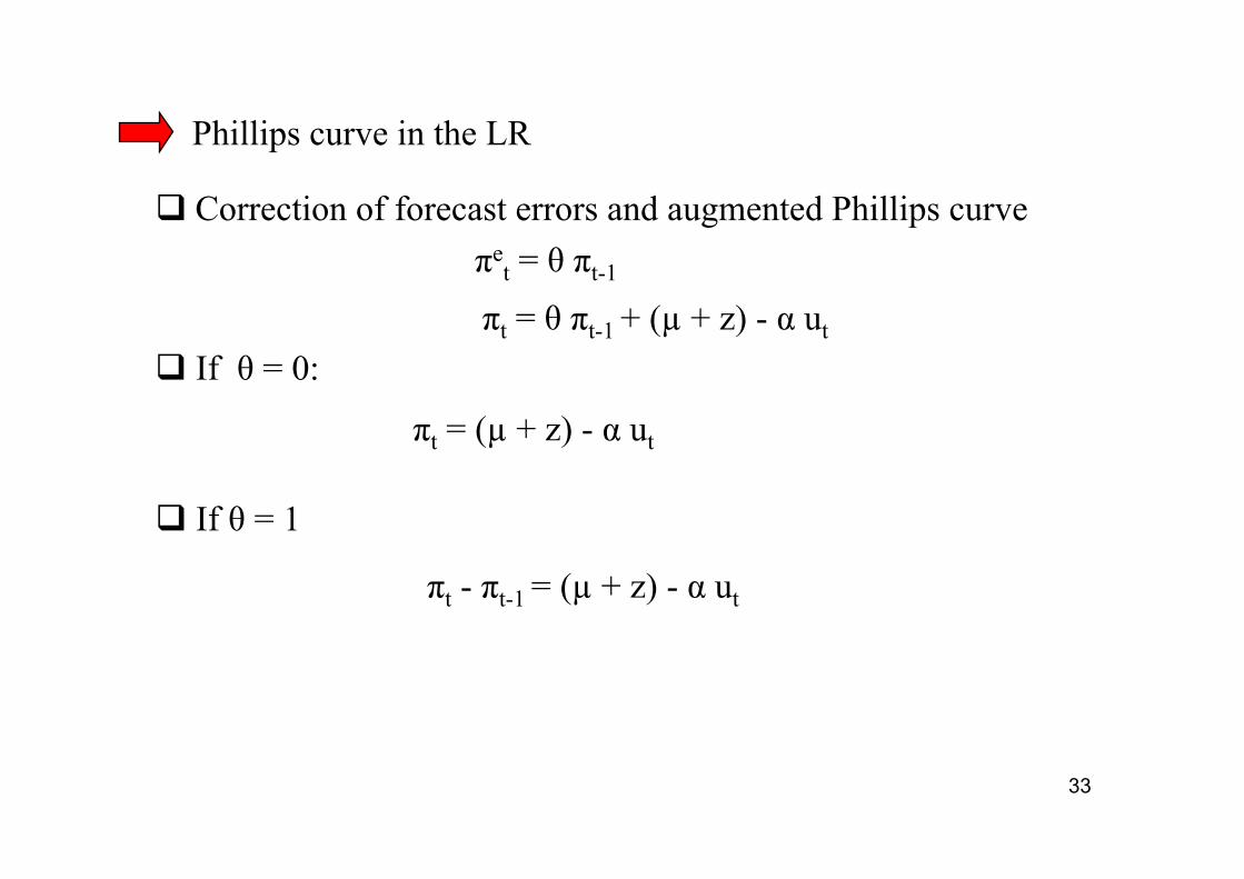
Phillips curve in the LR
Correction of forecast errors and augmented Phillips curve πe
t = θ πt-1
If θ = 1
πt = θ πt-1 + (µ + z) - α ut
If θ = 0:
πt = (µ + z) - α ut
πt - πt-1 = (µ + z) - α ut
34
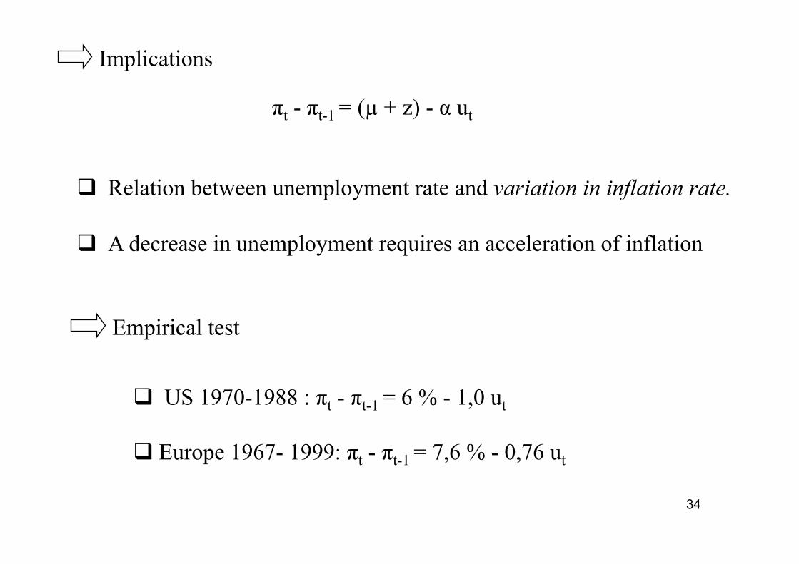
Relation between unemployment rate and variation in inflation rate.
A decrease in unemployment requires an acceleration of inflation
Implications
πt - πt-1 = (µ + z) - α ut
Empirical test
US 1970-1988 : πt - πt-1 = 6 % - 1,0 ut
Europe 1967- 1999: πt - πt-1 = 7,6 % - 0,76 ut

35
36
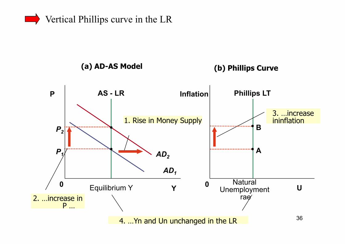
Vertical Phillips curve in the LR
Natural Unemployment
rae
Phillips LT
0
(b) Phillips Curve
Inflation
A
Equilibrium Y 0
P1
AD1
AS - LR
(a) AD-AS Model
P
4. …Yn and Un unchanged in the LR
P2
2. …increase in P …
Y U
1. Rise in Money Supply
AD2
B
3. …increase ininflation
37
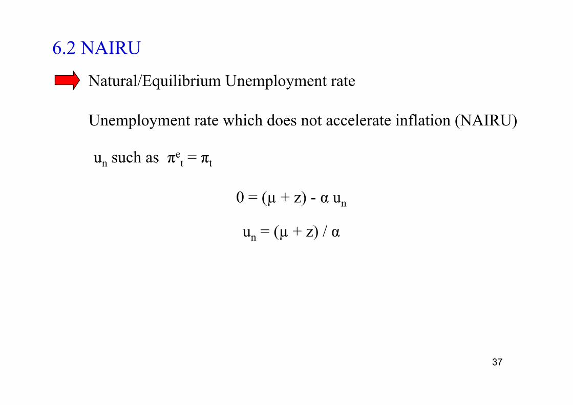
6.2 NAIRU
Natural/Equilibrium Unemployment rate
Unemployment rate which does not accelerate inflation (NAIRU)
un such as πet = πt
0 = (µ + z) - α un
un = (µ + z) / α

38
Augmented Phillips curve
NAIRU
⇒ Variation in inflation depends on unemployment gap
⇒ un NAIRU (Non-accelerating inflation rate Unemployment)
Phillips curve with natural unemployment rate
α un = µ + z =>
39
40
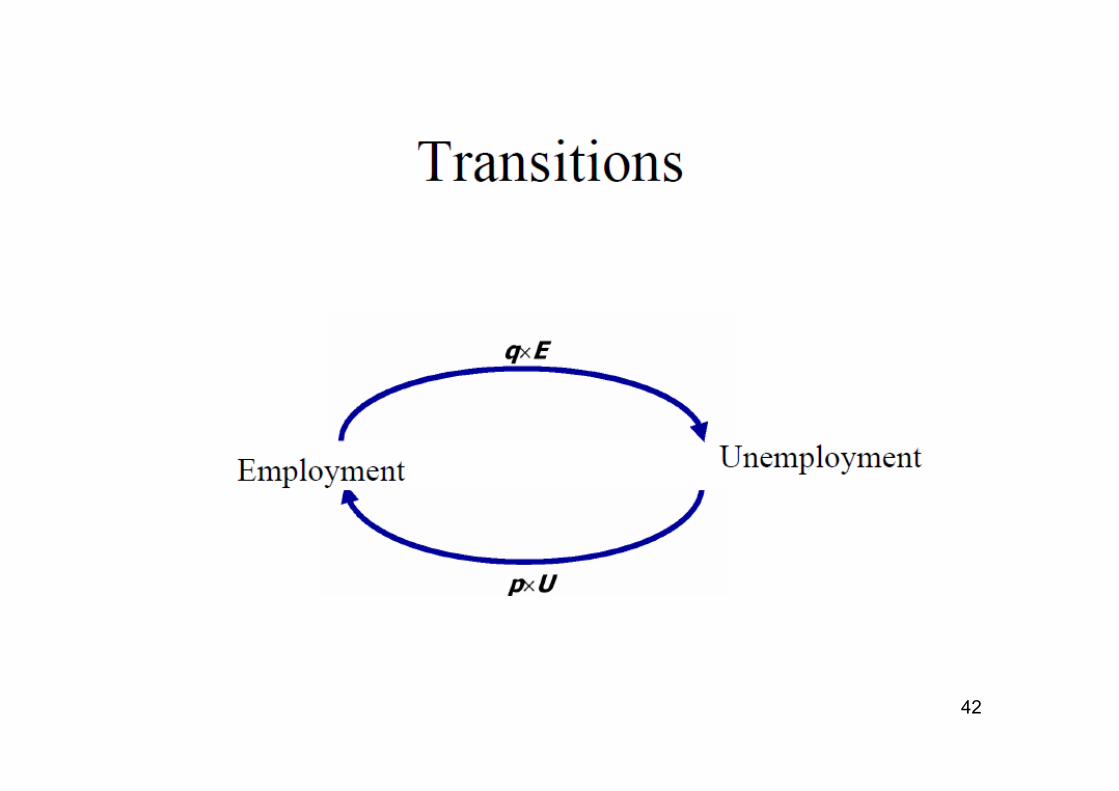
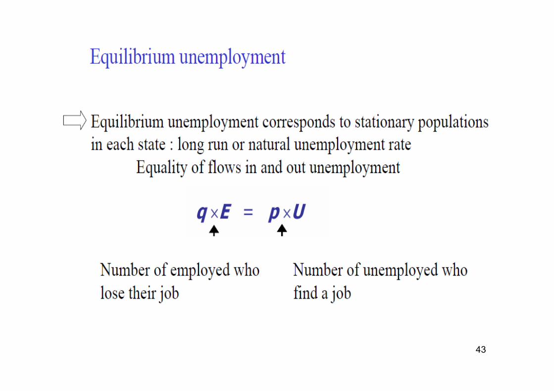
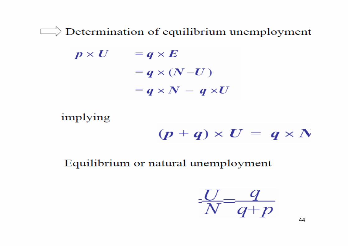
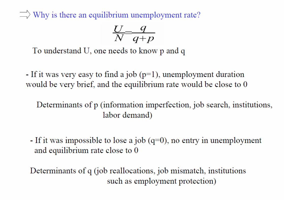
6.3 Why is there an equilibrium unemployment rate ? Case study with Matching frictions

41
42
43
44
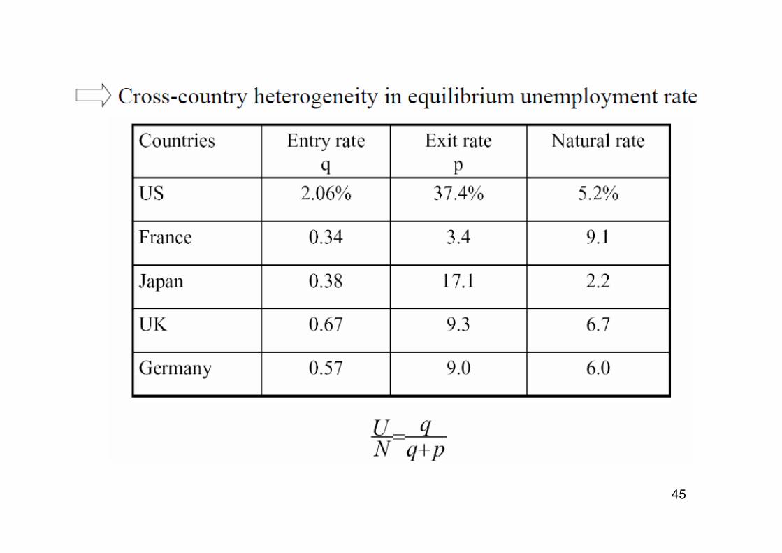
45
46
47
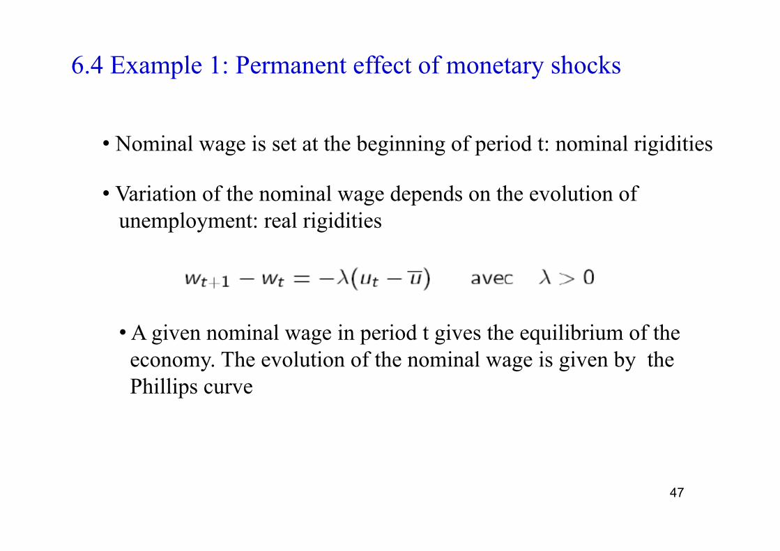
6.4 Example 1: Permanent effect of monetary shocks
• Nominal wage is set at the beginning of period t: nominal rigidities
• Variation of the nominal wage depends on the evolution of unemployment: real rigidities
• A given nominal wage in period t gives the equilibrium of the economy. The evolution of the nominal wage is given by the Phillips curve

48
• Aggregate demand
• Aggregate supply
- Production
- Flexible prices Labor demand is given by the maximization of the profit
Equilibrium on the good market
49
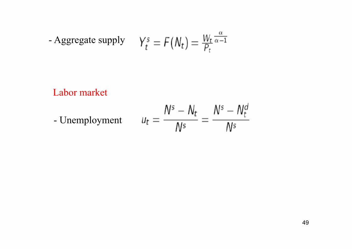
- Aggregate supply
- Unemployment
Labor market

50
Macroeconomic equilibrium
Log linear representation
Find the equilibrium for a given period and determine the law of motion of the equilibrium

51
• Equilibrium price: equality between AD and AS
• Equilibrium output: Substitute equilibrium price in AD or AS
• Law of motion of output

52
• Law of motion of unemployment
- Using the definition of output
- From the equilibrium price equation and the definition of inflation

53
• Equilibrium unemployment
Stationary solution such that
Equilibrium unemployment given by
• Implications:
- Monetary policy can have a long run impact on unemployment
- Impact depends on the adjustment of wages (impact nil if immediate adjustment of wages to unemployment)
54
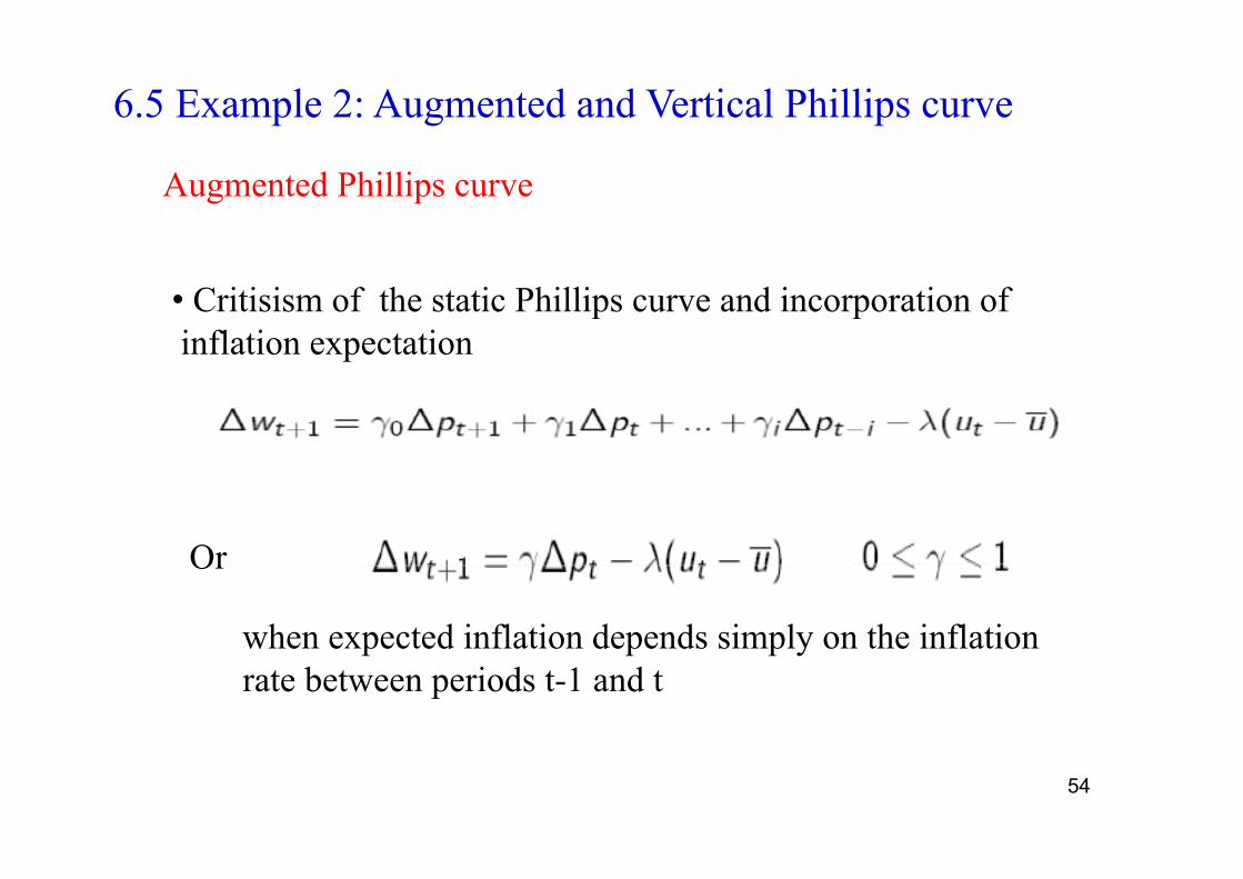
6.5 Example 2: Augmented and Vertical Phillips curve
Augmented Phillips curve
• Critisism of the static Phillips curve and incorporation of inflation expectation
Or
when expected inflation depends simply on the inflation rate between periods t-1 and t
55
• Nominal rigidities: wage growth depends on past inflation and not on the current one
• : measure of the indexation of wages on prices in the long run
56
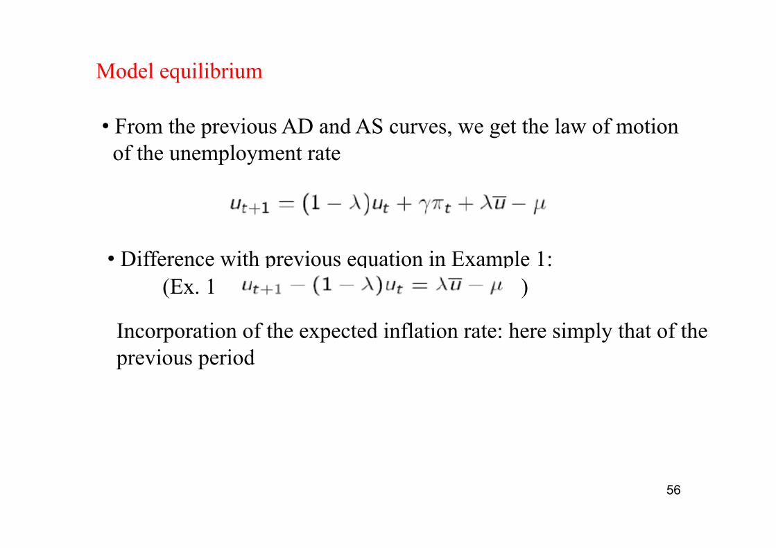
Model equilibrium
• From the previous AD and AS curves, we get the law of motion of the unemployment rate
• Difference with previous equation in Example 1: (Ex. 1 )
Incorporation of the expected inflation rate: here simply that of the previous period

57
• From the previous structure of the model in Ex. 1, and taking into account the new equation for wage formation:
Law of motion of the inflation rate
58
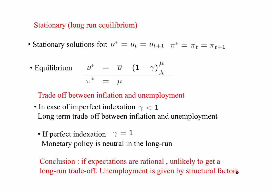
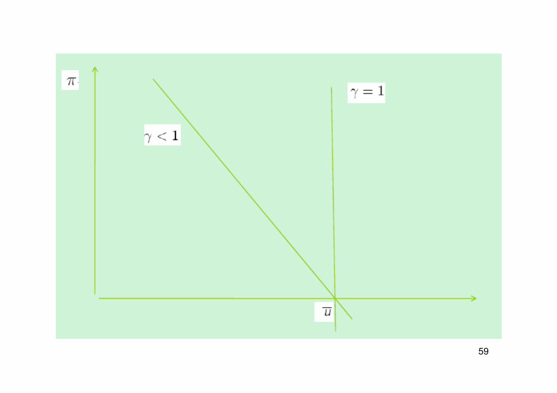
Stationary (long run equilibrium)
• Stationary solutions for: :
• Equilibrium
• In case of imperfect indexation Long term trade-off between inflation and unemployment
• If perfect indexation Monetary policy is neutral in the long-run
Trade off between inflation and unemployment
Conclusion : if expectations are rational , unlikely to get a long-run trade-off. Unemployment is given by structural factors
59
60
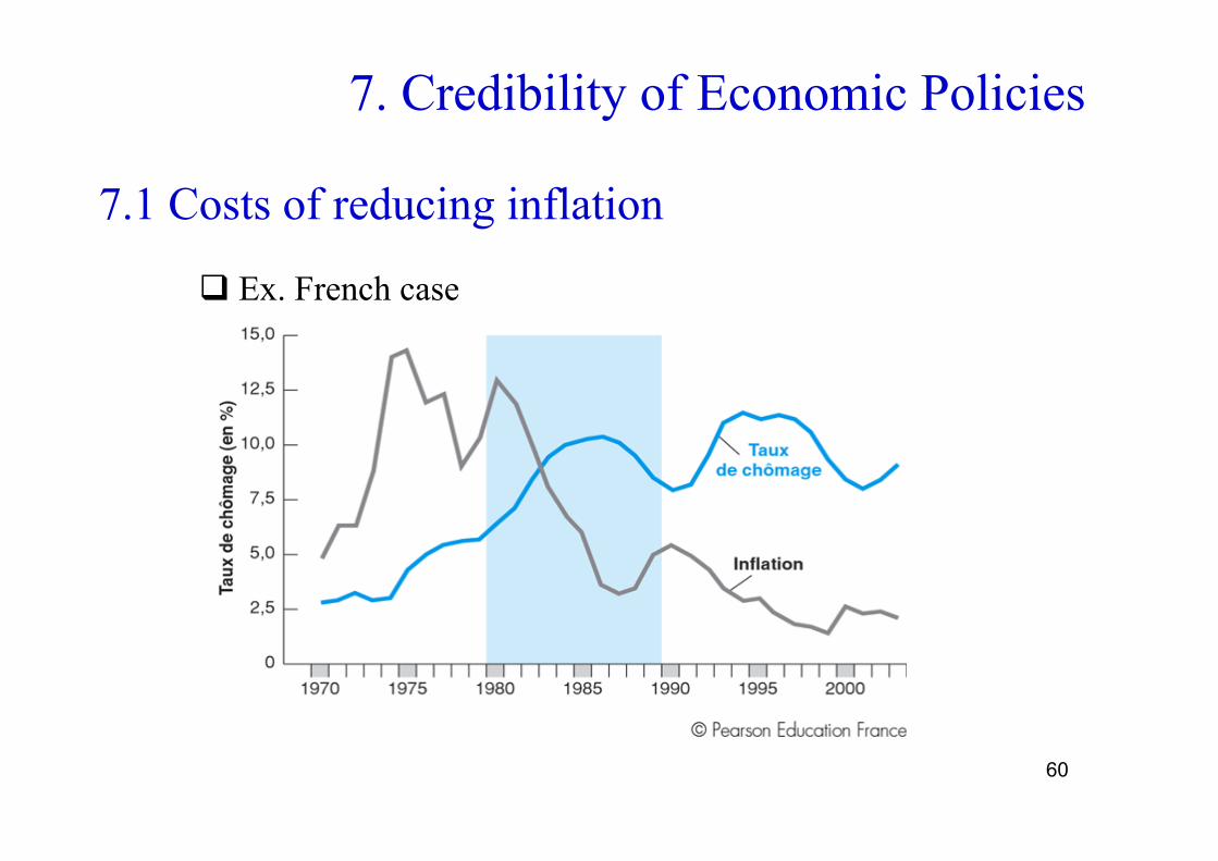
7. Credibility of Economic Policies
7.1 Costs of reducing inflation
Ex. French case
61
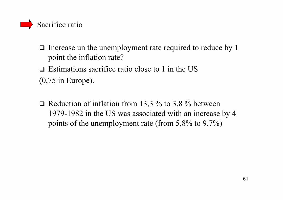
Increase un the unemployment rate required to reduce by 1 point the inflation rate?
Estimations sacrifice ratio close to 1 in the US (0,75 in Europe).
Reduction of inflation from 13,3 % to 3,8 % between 1979-1982 in the US was associated with an increase by 4 points of the unemployment rate (from 5,8% to 9,7%)
Sacrifice ratio
62
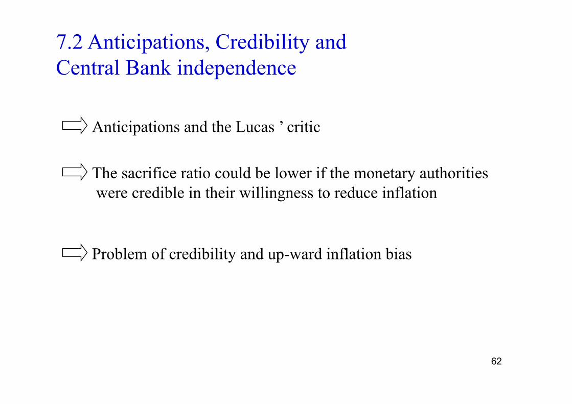
Anticipations and the Lucas ’ critic
7.2 Anticipations, Credibility and Central Bank independence
The sacrifice ratio could be lower if the monetary authorities were credible in their willingness to reduce inflation
Problem of credibility and up-ward inflation bias

63
Barro-Gordon solution: independence of Central Bank

64
Evolution index of Central Bank Independence
CONCLUSION: Financial crisis and Monetary Policy, Should we rethink the optimal monetary policy (see text Blanchard et al. (2010))