© Wiley 2007

Aggregate Planning

Operations Management by

R. Dan Reid & Nada R. Sanders 3rd Edition © Wiley 2007

PowerPoint Presentation by R.B. Clough – UNH

M. E. Henrie - UAA

© Wiley 2007

Learning Objectives

Identify different aggregate planning strategies and options for

changing demand and/or capacity in aggregate plans

Develop aggregate plans, calculate associated costs, and

evaluate the plan in terms of operations, marketing, finance,

and human resources

© Wiley 2007

The Role of Aggregate Planning

Integral to part of the business planning process

Supports the strategic plan

Also known as the production plan

Identifies resources required for operations for the next 6 -18 months

Details the aggregate production rate and size of work force required

© Wiley 2007

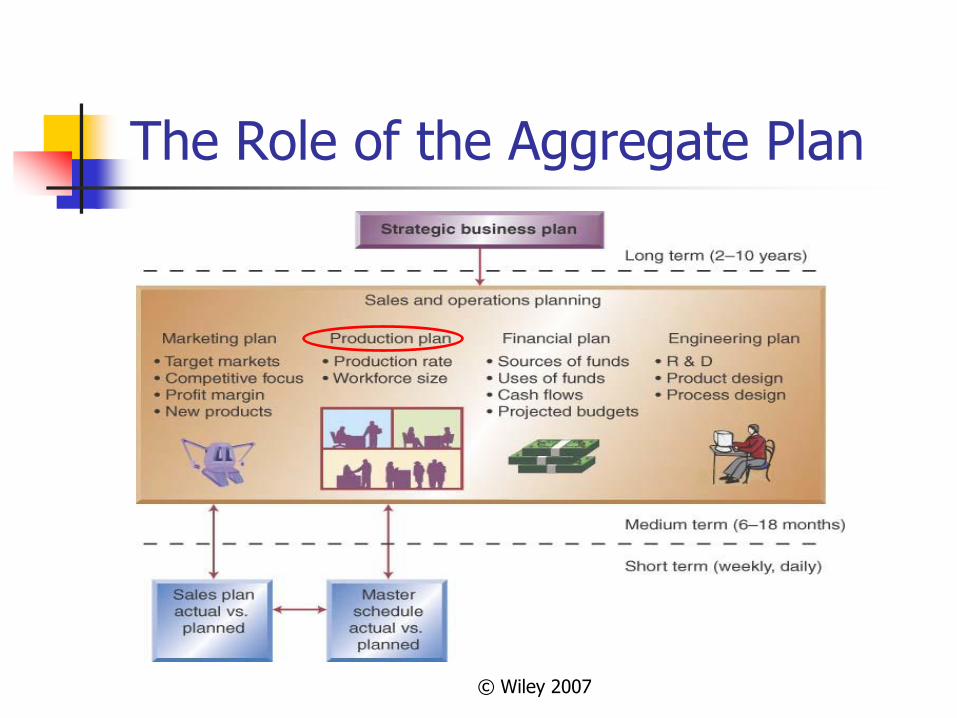
The Role of the Aggregate Plan

© Wiley 2007

Types of Aggregate Plans

1- Level Aggregate Plans

2- Chase Aggregate Plans

3- Hybrid Aggregate Plans

© Wiley 2007

Types of Aggregate Plans

1- Level Aggregate Plans

Maintains a constant workforce

Sets capacity to accommodate average demand

Often used for make-to-stock products like appliances

Disadvantage- builds inventory and/or uses back orders

© Wiley 2007

Level Plan Example

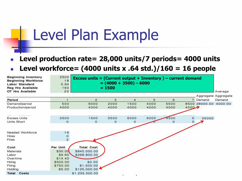
Level production rate= 28,000 units/7 periods= 4000 units

Level workforce= (4000 units x .64 std.)/160 = 16 people

Excess units = (Current output + Inventory ) – current demand = (4000 + 3500) – 6000 = 1500

© Wiley 2007

Types of Aggregate Plans

2- Chase Aggregate Plans

Produces exactly what is needed each period

Sets labor/equipment capacity to satisfy period demands

Disadvantage- constantly changing short term capacity

© Wiley 2007

Chase Plan Example

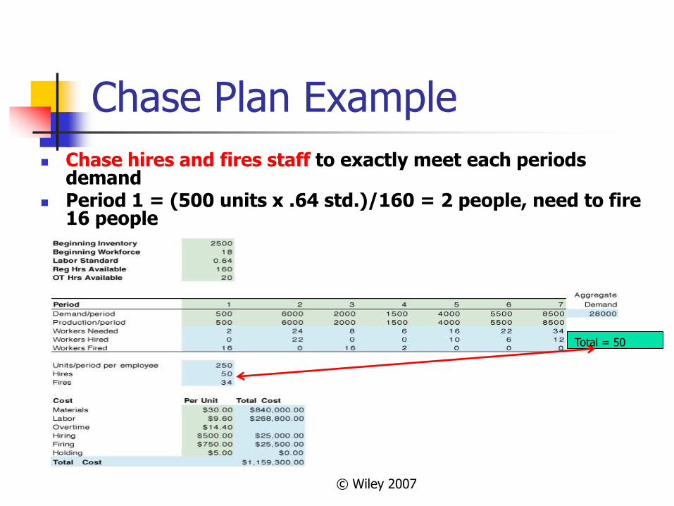
Chase hires and fires staff to exactly meet each periods demand

Period 1 = (500 units x .64 std.)/160 = 2 people, need to fire 16 people

Total = 50

© Wiley 2007

Types of Aggregate Plans (Cont.)

3- Hybrid Aggregate Plans

Uses a combination of options

Options should be limited to facilitate execution

May use a level workforce with overtime & temps

May allow inventory buildup and some backordering

May use short term sourcing

© Wiley 2007

Aggregate Planning Options

Demand based options

Reactive: uses finished goods inventories and

backorders for fluctuations

Proactive: shifts the demand patterns to minimize fluctuations e.g. early bird dinner prices at a restaurant

Capacity based options

Changes output capacity to meet demand

Uses overtime, under time, subcontracting, hiring, firing, and part-timers – cost and operational implications

© Wiley 2007

Evaluating the Current Situation

Important to evaluate current situation in terms of; Point of Departure

Current % of normal capacity Options are different depending on present situation

Magnitude of change Larger changes need more dramatic measures

Duration of change Is the length of time a brief seasonal change? Is a permanent change in capacity needed?

© Wiley 2007

Developing the Aggregate Plan

Step 1- Choose strategy: level, chase, or Hybrid

Step 2- Determine the aggregate production rate

Step 3- Calculate the size of the workforce

Step 4- Test the plan as follows: Calculate Inventory, expected hiring/firing, overtime needs

Calculate total cost of plan

Step 5- Evaluate performance: cost, service, human resources, and operations

© Wiley 2007

Plan for Companies with Tangible

Products – Plans A, B, C, D

Plan A: Level aggregate plan using inventories and back orders

Plan B: Level plan using inventories but no back orders

Plan C: Chase aggregate plan using hiring and firing

Plan D: Hybrid plan using initial workforce and overtime as needed

© Wiley 2007

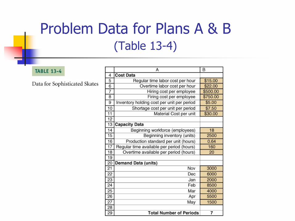
Problem Data for Plans A & B

(Table 13-4)

© Wiley 2007

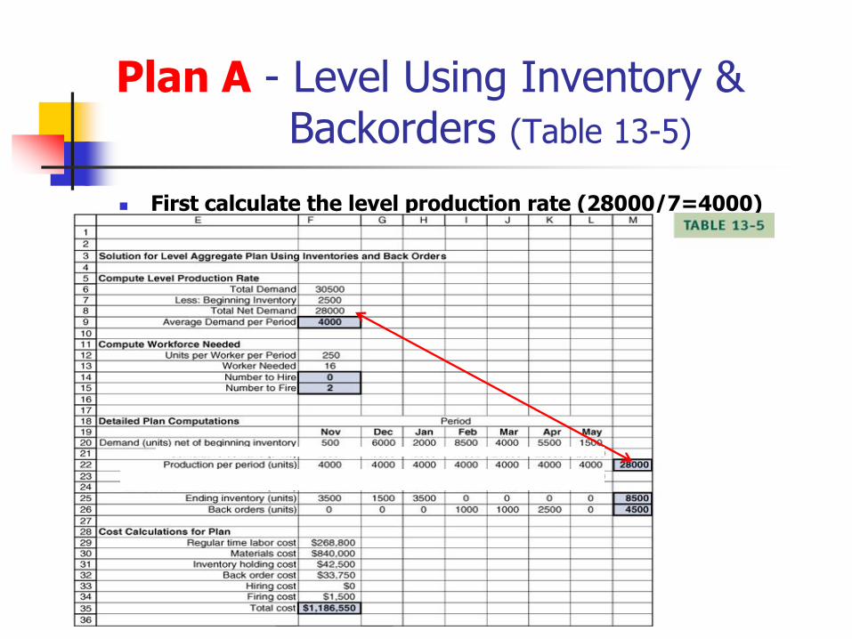
Plan A - Level Using Inventory & Backorders (Table 13-5)

First calculate the level production rate (28000/7=4000)

© Wiley 2007

Plan A Evaluation

Fill rate is 83.9%

Fill rate is likely to low

Inventory levels seem to be okay

Human resources fires two employees

© Wiley 2007

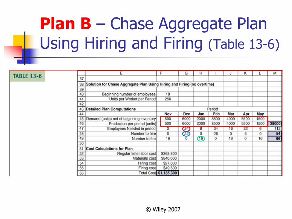
Plan B – Chase Aggregate Plan Using Hiring and Firing (Table 13-6)

© Wiley 2007

Plan B Evaluation

Plan B costs slightly less than the level plan.

Hiring demands ranges from two in November to thirty-four in February

Utilization is highest, 70.6%, in December and even lower in the other months

Space and equipment are underutilized in every other month of the plan

© Wiley 2007

Aggregate Plans for Service Companies with Non-Tangible Products- Plans E, F, G

Options remain the same – level, chase, and hybrid plans Overtime and under time can be used

Staff can be hired and fired

Inventory cannot be used to level the service plan

All demand must be satisfied or lose business to a competing service provider

© Wiley 2007

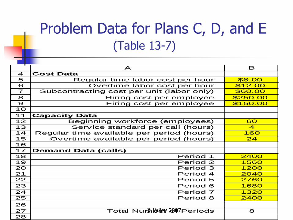
Problem Data for Plans C, D, and E (Table 13-7)

4

5

6

7

8

9

10

11

12

13

14

15

16

17

18

19

20

21

22

23

24

25

26

27

28

A B

Cost Data

Regular time labor cost per hour $8.00

Overtime labor cost per hour $12.00

Subcontracting cost per unit (labor only) $60.00

Hiring cost per employee $250.00

Firing cost per employee $150.00

Capacity Data

Beginning workforce (employees) 60

Service standard per call (hours) 4

Regular time available per period (hours) 160

Overtime available per period (hours) 24

Demand Data (calls)

Period 1 2400

Period 2 1560

Period 3 1200

Period 4 2040

Period 5 2760

Period 6 1680

Period 7 1320

Period 8 2400

Total Number of Periods 8

© Wiley 2007

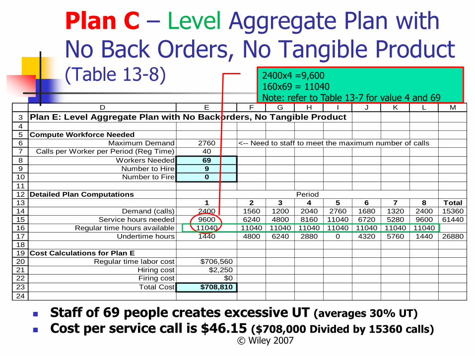
Plan C – Level Aggregate Plan with No Back Orders, No Tangible Product (Table 13-8)

3

4

5

6

7

8

9

10

11

12

13

14

15

16

17

18

19

20

21

22

23

24

D E F G H I J K L M

Plan E: Level Aggregate Plan with No Backorders, No Tangible Product

Compute Workforce Needed

Maximum Demand 2760 <-- Need to staff to meet the maximum number of calls

Calls per Worker per Period (Reg Time) 40

Workers Needed 69

Number to Hire 9

Number to Fire 0

Detailed Plan Computations

1 2 3 4 5 6 7 8 Total

Demand (calls) 2400 1560 1200 2040 2760 1680 1320 2400 15360

Service hours needed 9600 6240 4800 8160 11040 6720 5280 9600 61440

Regular time hours available 11040 11040 11040 11040 11040 11040 11040 11040

Undertime hours 1440 4800 6240 2880 0 4320 5760 1440 26880

Cost Calculations for Plan E

Regular time labor cost $706,560

Hiring cost $2,250

Firing cost $0

Total Cost $708,810

Period

Staff of 69 people creates excessive UT (averages 30% UT)

Cost per service call is $46.15 ($708,000 Divided by 15360 calls)

2400x4 =9,600 160x69 = 11040 Note: refer to Table 13-7 for value 4 and 69

© Wiley 2007

Plan D – Hybrid Aggregate Plan Using Initial Workforce and OT as Needed (Table 13-9)

26

27

28

29

30

31

32

33

34

35

36

37

38

39

D E F G H I J K L M

Plan F: Hybrid Aggregate Plan Using Initial Workforce and Overtime as Needed

Detailed Plan Computations

1 2 3 4 5 6 7 8 Total

Demand (calls) 2400 1560 1200 2040 2760 1680 1320 2400 15360

Service hours needed 9600 6240 4800 8160 11040 6720 5280 9600 61440

Regular time hours of capacity 9600 9600 9600 9600 9600 9600 9600 9600 76800

Overtime hours needed 0 0 0 0 1440 0 0 0 1440

Undertime hours 0 3360 4800 1440 0 2880 4320 0 16800

Cost Calculations for Plan F

Regular time labor cost $614,400

Overtime labor cost $17,280

Total Cost $631,680

Period

Costs reduced by $77K and under time to an average of 20% Cost per service call reduced to $41.13 (-$5.02)

© Wiley 2007

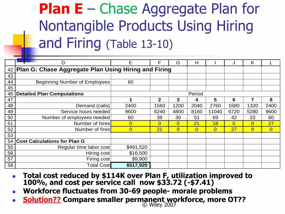
Plan E – Chase Aggregate Plan for Nontangible Products Using Hiring and Firing (Table 13-10)

Total cost reduced by $114K over Plan F, utilization improved to 100%, and cost per service call now $33.72 (-$7.41)

Workforce fluctuates from 30-69 people- morale problems Solution?? Compare smaller permanent workforce, more OT??

42

43

44

45

46

47

48

49

50

51

52

53

54

55

56

57

58

D E F G H I J K L

Plan G: Chase Aggregate Plan Using Hiring and Firing

Beginning Number of Employees 60

Detailed Plan Computations

1 2 3 4 5 6 7 8

Demand (calls) 2400 1560 1200 2040 2760 1680 1320 2400

Service hours needed 9600 6240 4800 8160 11040 6720 5280 9600

Number of employees needed 60 39 30 51 69 42 33 60

Number of hires 0 0 0 21 18 0 0 27

Number of fires 0 21 9 0 0 27 9 0

Cost Calculations for Plan G

Regular time labor cost $491,520

Hiring cost $16,500

Firing cost $9,900

Total Cost $517,920

Period

…OK des ka?...