Aggregate Demand I: Building the IS–LM ModelI).pdf · In Chapter 10, we derived the aggregate demand curve from the quan-tity theory of money, and we showed that monetary policy

311

Aggregate Demand I: Building the IS–LM Model

I shall argue that the postulates of the classical theory are applicable to a spe-

cial case only and not to the general case. . . . Moreover, the characteristics of

the special case assumed by the classical theory happen not to be those of the

economic society in which we actually live, with the result that its teaching is

misleading and disastrous if we attempt to apply it to the facts of experience.

—John Maynard Keynes, The General Theory

Of all the economic fluctuations in world history, the one that stands out as particularly large, painful, and intellectually significant is the Great Depression of the 1930s. During this time, the United States

and many other countries experienced massive unemployment and greatly reduced incomes. In the worst year, 1933, one-fourth of the U.S. labor force was unemployed, and real GDP was 30 percent below its 1929 level.

This devastating episode caused many economists to question the validity of classical economic theory—the theory we examined in Chapters 3 through 7. Classical theory seemed incapable of explaining the Depression. According to that theory, national income depends on factor supplies and the available technology, neither of which changed substantially from 1929 to 1933. After the onset of the Depression, many economists believed that a new model was needed to explain such a large and sudden economic downturn and to sug-gest government policies that might reduce the economic hardship so many people faced.

In 1936 the British economist John Maynard Keynes revolutionized econom-ics with his book The General Theory of Employment, Interest, and Money. Keynes proposed a new way to analyze the economy, which he presented as an alterna-tive to classical theory. His vision of how the economy works quickly became a center of controversy. Yet, as economists debated The General Theory, a new understanding of economic fluctuations gradually developed.

Keynes proposed that low aggregate demand is responsible for the low income and high unemployment that characterize economic downturns. He criticized

11C H A P T E R

312 | P A R T I V Business Cycle Theory: The Economy in the Short Run

classical theory for assuming that aggregate supply alone—capital, labor, and technology—determines national income. Economists today reconcile these two views with the model of aggregate demand and aggregate supply introduced in Chapter 10. In the long run, prices are flexible, and aggregate supply determines income. But in the short run, prices are sticky, so changes in aggregate demand influence income.

Keynes’s ideas about short-run fluctuations have been prominent since he proposed them in the 1930s, but they have commanded renewed attention in recent years. In the aftermath of the financial crisis of 2008–2009, the United States and Europe descended into a deep recession, followed by a weak recovery. As unemployment lingered at high levels, policymakers around the world debated how best to increase aggregate demand. Many of the issues that gripped economists during the Great Depression were once again at the center of the economic policy debate.

In this chapter and the next, we continue our study of economic fluctuations by looking more closely at aggregate demand. Our goal is to identify the variables that shift the aggregate demand curve, causing fluctuations in national income. We also examine more fully the tools policymakers can use to influence aggregate demand. In Chapter 10, we derived the aggregate demand curve from the quan-tity theory of money, and we showed that monetary policy can shift the aggregate demand curve. In this chapter, we see that the government can influence aggre-gate demand with both monetary and fiscal policy.

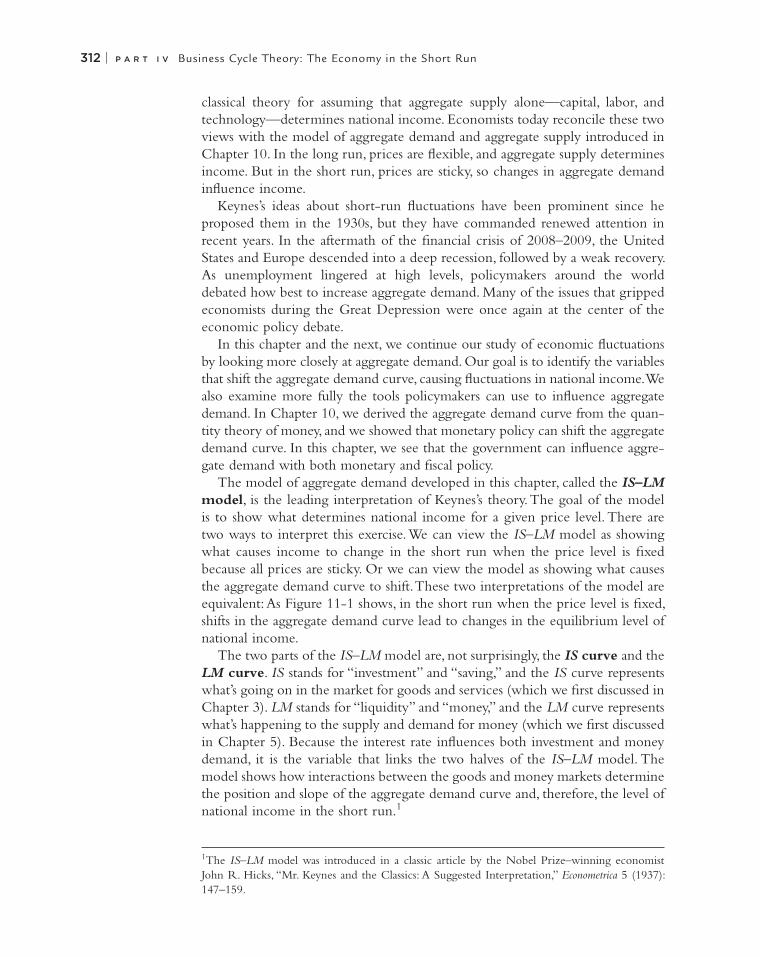
The model of aggregate demand developed in this chapter, called the IS–LM model, is the leading interpretation of Keynes’s theory. The goal of the model is to show what determines national income for a given price level. There are two ways to interpret this exercise. We can view the IS–LM model as showing what causes income to change in the short run when the price level is fixed because all prices are sticky. Or we can view the model as showing what causes the aggregate demand curve to shift. These two interpretations of the model are equivalent: As Figure 11-1 shows, in the short run when the price level is fixed, shifts in the aggregate demand curve lead to changes in the equilibrium level of national income.

The two parts of the IS–LM model are, not surprisingly, the IS curve and the LM curve. IS stands for “investment” and “saving,” and the IS curve represents what’s going on in the market for goods and services (which we first discussed in Chapter 3). LM stands for “liquidity” and “money,” and the LM curve represents what’s happening to the supply and demand for money (which we first discussed in Chapter 5). Because the interest rate influences both investment and money demand, it is the variable that links the two halves of the IS–LM model. The model shows how interactions between the goods and money markets determine the position and slope of the aggregate demand curve and, therefore, the level of national income in the short run.1

1The IS–LM model was introduced in a classic article by the Nobel Prize–winning economist John R. Hicks, “Mr. Keynes and the Classics: A Suggested Interpretation,” Econometrica 5 (1937): 147–159.

C H A P T E R 1 1 Aggregate Demand I: Building the IS–LM Model | 313

11-1 The Goods Market and the IS Curve

The IS curve plots the relationship between the interest rate and the level of income that arises in the market for goods and services. To develop this relation-ship, we start with a basic model called the Keynesian cross. This model is the simplest interpretation of Keynes’s theory of how national income is determined and is a building block for the more complex and realistic IS–LM model.

The Keynesian Cross

In The General Theory, Keynes proposed that an economy’s total income is, in the short run, determined largely by the spending plans of households, busi-nesses, and government. The more people want to spend, the more goods and services firms can sell. The more firms can sell, the more output they will choose to produce and the more workers they will choose to hire. Keynes believed that the problem during recessions and depressions is inadequate spending. The Keynesian cross is an attempt to model this insight.

Planned Expenditure We begin our derivation of the Keynesian cross by drawing a distinction between actual and planned expenditure. Actual expenditure is the amount households, firms, and the government spend on goods and ser-vices, and as we first saw in Chapter 2, it equals the economy’s gross domestic product (GDP). Planned expenditure is the amount households, firms, and the government would like to spend on goods and services.

Why would actual expenditure ever differ from planned expenditure? The answer is that firms might engage in unplanned inventory investment because their sales do not meet their expectations. When firms sell less of their product

Shifts in Aggregate Demand For a given price level, national income fluctuates because of shifts in the aggregate demand curve. The IS–LM model takes the price level as given and shows what causes income to change. The model therefore shows what causes aggregate demand to shift.

Price level, P

Income, output, YY1 Y2 Y3

AD1 AD2 AD3

Fixedpricelevel(SRAS)

FIGURE 11-1


than they planned, their stock of inventories automatically rises; conversely, when firms sell more than planned, their stock of inventories falls. Because these unplanned changes in inventory are counted as investment spending by firms, actual expenditure can be either above or below planned expenditure.

Now consider the determinants of planned expenditure. Assuming that the economy is closed, so that net exports are zero, we write planned expenditure PE as the sum of consumption C, planned investment I, and government purchases G:

PE 5 C 1 I 1 G.

To this equation, we add the consumption function:

C 5 C(Y 2 T ).

This equation states that consumption depends on disposable income (Y 2 T ), which is total income Y minus taxes T. To keep things simple, for now we take planned investment as exogenously fixed:

I 5 I–.

Finally, as in Chapter 3, we assume that fiscal policy—the levels of government purchases and taxes—is fixed:

G 5 G–.

T 5 T–

.

Combining these five equations, we obtain

PE 5 C(Y 2 T–) 1 I– 1 G–.

This equation shows that planned expenditure is a function of income Y, the level of planned investment I

–, and the fiscal policy variables G– and T–.

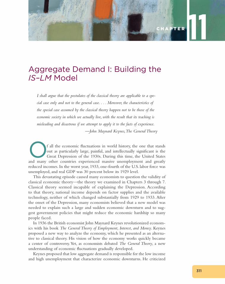
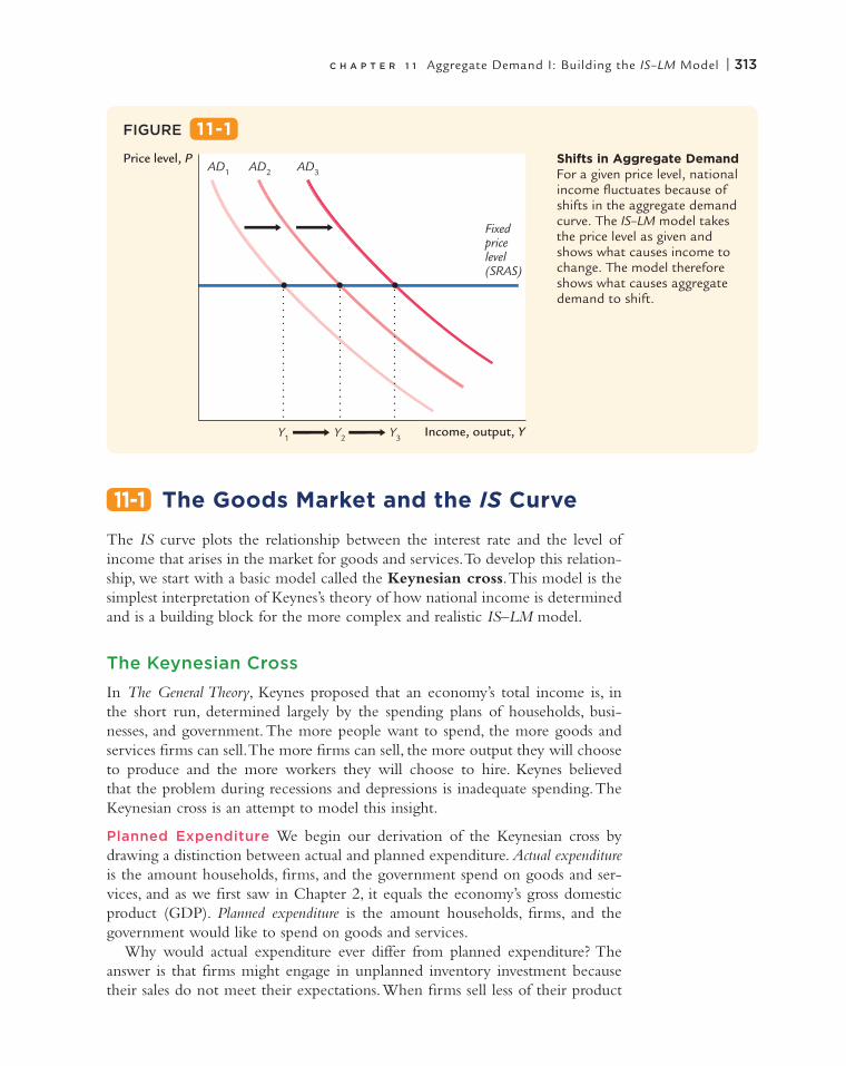
Figure 11-2 graphs planned expenditure as a function of the level of income. This line slopes upward because higher income leads to higher consumption and

Planned Expenditure as a Function of Income Planned expendi-ture PE depends on income because higher income leads to higher consumption, which is part of planned expenditure. The slope of the planned-expenditure function is the marginal pro-pensity to consume, MPC.

FIGURE 11-2

Plannedexpenditure, PE

Income, output, Y

$1

MPC

Planned expenditure, PE � C(Y � T) � I � G


thus higher planned expenditure. The slope of this line is the marginal propen-sity to consume, MPC: it shows how much planned expenditure increases when income rises by $1. This planned-expenditure function is the first piece of the Keynesian cross.

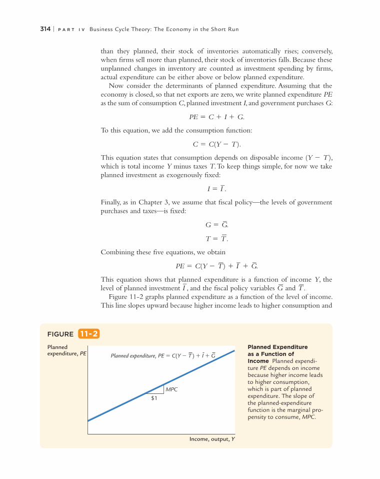
The Economy in Equilibrium The next piece of the Keynesian cross is the assumption that the economy is in equilibrium when actual expenditure equals planned expenditure. This assumption is based on the idea that when people’s plans have been realized, they have no reason to change what they are doing. Recalling that Y as GDP equals not only total income but also total actual expenditure on goods and services, we can write this equilibrium condition as

Actual Expenditure 5 Planned Expenditure

Y 5 PE.

The 45-degree line in Figure 11-3 plots the points where this condition holds. With the addition of the planned-expenditure function, this diagram becomes the Keynesian cross. The equilibrium of this economy is at point A, where the planned-expenditure function crosses the 45-degree line.

How does the economy get to equilibrium? In this model, inventories play an important role in the adjustment process. Whenever an economy is not in equilibrium, firms experience unplanned changes in inventories, and this induces them to change production levels. Changes in production in turn influence total income and expenditure, moving the economy toward equilibrium.

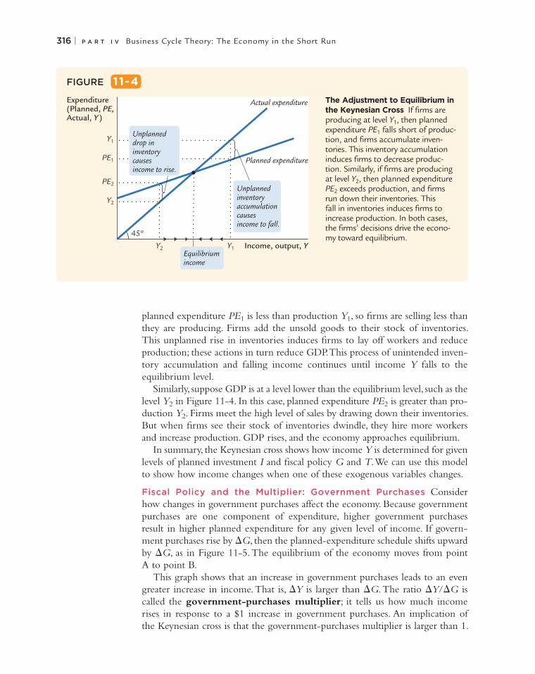
For example, suppose the economy finds itself with GDP at a level greater than the equilibrium level, such as the level Y1 in Figure 11-4. In this case,

The Keynesian Cross The equilibrium in the Keynesian cross is the point at which income (actual expenditure) equals planned expenditure (point A).

FIGURE 11-3

Expenditure(Planned, PEActual, Y

Income, output, Y

Actual expenditure,Y � PE

Planned expenditure, PE � C � I � GA

45º

Equilibriumincome

)


planned expenditure PE1 is less than production Y1, so firms are selling less than they are producing. Firms add the unsold goods to their stock of inventories. This unplanned rise in inventories induces firms to lay off workers and reduce production; these actions in turn reduce GDP. This process of unintended inven-tory accumulation and falling income continues until income Y falls to the equilibrium level.

Similarly, suppose GDP is at a level lower than the equilibrium level, such as the level Y2 in Figure 11-4. In this case, planned expenditure PE2 is greater than pro-duction Y2. Firms meet the high level of sales by drawing down their inventories. But when firms see their stock of inventories dwindle, they hire more workers and increase production. GDP rises, and the economy approaches equilibrium.

In summary, the Keynesian cross shows how income Y is determined for given levels of planned investment I and fiscal policy G and T. We can use this model to show how income changes when one of these exogenous variables changes.

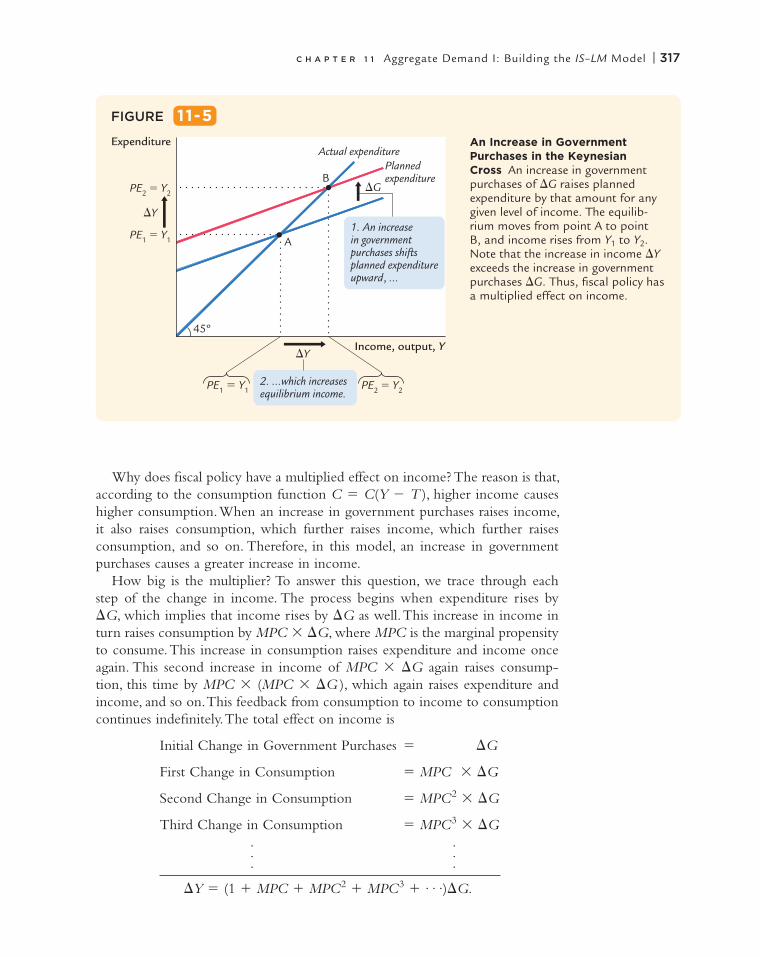
Fiscal Policy and the Multiplier: Government Purchases Consider how changes in government purchases affect the economy. Because government purchases are one component of expenditure, higher government purchases result in higher planned expenditure for any given level of income. If govern-ment purchases rise by DG, then the planned-expenditure schedule shifts upward by DG, as in Figure 11-5. The equilibrium of the economy moves from point A to point B.

This graph shows that an increase in government purchases leads to an even greater increase in income. That is, DY is larger than DG. The ratio DY/DG is called the government-purchases multiplier; it tells us how much income rises in response to a $1 increase in government purchases. An implication of the Keynesian cross is that the government-purchases multiplier is larger than 1.

The Adjustment to Equilibrium in the Keynesian Cross If firms are producing at level Y1, then planned expenditure PE1 falls short of produc-tion, and firms accumulate inven-tories. This inventory accumulation induces firms to decrease produc-tion. Similarly, if firms are producing at level Y2, then planned expenditure PE2 exceeds production, and firms run down their inventories. This fall in inventories induces firms to increase production. In both cases, the firms’ decisions drive the econo-my toward equilibrium.

FIGURE 11-4

Expenditure(Planned, PE,Actual, Y

Income, output, Y

Y1

PE1

PE2

Y2

Y2 Y1

Actual expenditure

Planned expenditure

Equilibriumincome

Unplanned drop in inventorycauses income to rise.

Unplanned inventoryaccumulationcauses income to fall.

45º

)


Why does fiscal policy have a multiplied effect on income? The reason is that, according to the consumption function C 5 C(Y 2 T ), higher income causes higher consumption. When an increase in government purchases raises income, it also raises consumption, which further raises income, which further raises consumption, and so on. Therefore, in this model, an increase in government purchases causes a greater increase in income.

How big is the multiplier? To answer this question, we trace through each step of the change in income. The process begins when expenditure rises by DG, which implies that income rises by DG as well. This increase in income in turn raises consumption by MPC 3 DG, where MPC is the marginal propensity to consume. This increase in consumption raises expenditure and income once again. This second increase in income of MPC 3 DG again raises consump-tion, this time by MPC 3 (MPC 3 DG ), which again raises expenditure and income, and so on. This feedback from consumption to income to consumption continues indefinitely. The total effect on income is

Initial Change in Government Purchases 5 DG

First Change in Consumption 5 MPC 3 DG

Second Change in Consumption 5 MPC2 3 DG

Third Change in Consumption 5 MPC3 3 DG . . . . . .

DY 5 (1 1 MPC 1 MPC2 1 MPC3 1 . . .)DG.

An Increase in Government Purchases in the Keynesian Cross An increase in government purchases of DG raises planned expenditure by that amount for any given level of income. The equilib-rium moves from point A to point B, and income rises from Y1 to Y2. Note that the increase in income DY exceeds the increase in government purchases DG. Thus, fiscal policy has a multiplied effect on income.

FIGURE 11-5

Expenditure

Income, output, Y

2. ...which increasesequilibrium income.

�G

�Y

�Y

Actual expenditurePlanned expenditure

PE2 � Y2

PE1 � Y1 PE2 � Y2

PE1 � Y1

B

A

45º

1. An increasein governmentpurchases shiftsplanned expenditureupward, ...


The government-purchases multiplier is

DY/DG 5 1 1 MPC 1 MPC2 1 MPC3 1 . . . .

This expression for the multiplier is an example of an infinite geometric series. A result from algebra allows us to write the multiplier as2

DY/DG 5 1/(1 2 MPC ).

For example, if the marginal propensity to consume is 0.6, the multiplier is

DY/DG 5 1 1 0.6 1 0.62 1 0.63 1 . . .

5 1/(1 2 0.6)

5 2.5.

In this case, a $1.00 increase in government purchases raises equilibrium income by $2.50.3

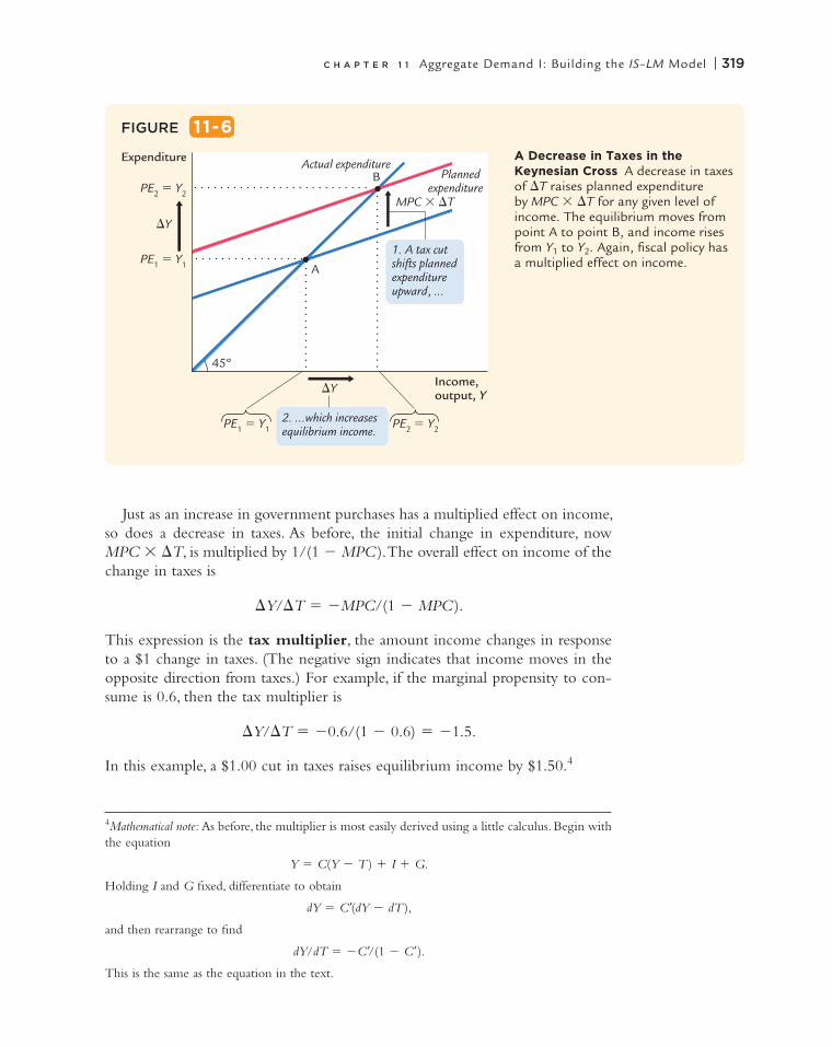
Fiscal Policy and the Multiplier: Taxes Now consider how changes in taxes affect equilibrium income. A decrease in taxes of DT immediately raises disposable income Y 2 T by DT and, therefore, increases consumption by MPC 3 DT. For any given level of income Y, planned expenditure is now higher. As Figure 11-6 shows, the planned-expenditure schedule shifts upward by MPC 3 DT. The equilibrium of the economy moves from point A to point B.

2Mathematical note: We prove this algebraic result as follows. For |x| , 1, let

z 5 1 1 x 1 x2 1 . . . .

Multiply both sides of this equation by x:

xz 5 x 1 x2 1 x3 1 . . . .

Subtract the second equation from the first:

z 2 xz 5 1.

Rearrange this last equation to obtain

z(1 2 x ) 5 1,

which implies

z 5 1/(1 2 x ).

This completes the proof.3Mathematical note: The government-purchases multiplier is most easily derived using a little calculus. Begin with the equation

Y 5 C(Y 2 T ) 1 I 1 G.

Holding T and I fixed, differentiate to obtain

dY 5 CdY 1 dG,

and then rearrange to find

dY/dG 5 1/(1 2 C).

This is the same as the equation in the text.


FIGURE 11-6

Expenditure

Income, output, Y

2. ...which increasesequilibrium income.

�Y

�Y

PE2 � Y2

PE1 � Y1 PE2 � Y2

PE1 � Y1

MPC � �T

B

A

45º

1. A tax cutshifts plannedexpenditureupward, ...

Actual expenditurePlanned

expenditure

A Decrease in Taxes in the Keynesian Cross A decrease in taxes of DT raises planned expenditure by MPC 3 DT for any given level of income. The equilibrium moves from point A to point B, and income rises from Y1 to Y2. Again, fiscal policy has a multiplied effect on income.

Just as an increase in government purchases has a multiplied effect on income, so does a decrease in taxes. As before, the initial change in expenditure, now MPC 3 DT, is multiplied by 1/(1 2 MPC ). The overall effect on income of the change in taxes is

DY/DT 5 2MPC/(1 2 MPC ).

This expression is the tax multiplier, the amount income changes in response to a $1 change in taxes. (The negative sign indicates that income moves in the opposite direction from taxes.) For example, if the marginal propensity to con-sume is 0.6, then the tax multiplier is

DY/DT 5 20.6/(1 2 0.6) 5 21.5.

In this example, a $1.00 cut in taxes raises equilibrium income by $1.50.4

4Mathematical note: As before, the multiplier is most easily derived using a little calculus. Begin with the equation

Y 5 C(Y 2 T ) 1 I 1 G.

Holding I and G fixed, differentiate to obtain

dY 5 C(dY 2 dT ),

and then rearrange to find

dY/dT 5 2C/(1 2 C).

This is the same as the equation in the text.


Cutting Taxes to Stimulate the Economy: The Kennedy and Bush Tax Cuts

When John F. Kennedy became president of the United States in 1961, he brought to Washington some of the brightest young economists of the day to work on his Council of Economic Advisers. These economists, who had been schooled in the economics of Keynes, brought Keynesian ideas to discussions of economic policy at the highest level.

One of the council’s first proposals was to expand national income by reducing taxes. This eventually led to a substantial cut in personal and corporate income taxes in 1964. The tax cut was intended to stimulate expenditure on consump-tion and investment and thus lead to higher levels of income and employment. When a reporter asked Kennedy why he advocated a tax cut, Kennedy replied, “To stimulate the economy. Don’t you remember your Economics 101?”

As Kennedy’s economic advisers predicted, the passage of the tax cut was fol-lowed by an economic boom. Growth in real GDP was 5.8 percent in 1964 and 6.5 percent in 1965. The unemployment rate fell from 5.6 percent in 1963 to 5.2 percent in 1964 and then to 4.5 percent in 1965.

Economists continue to debate the source of this rapid growth in the early 1960s. A group called supply-siders argue that the economic boom resulted from the incentive effects of the cut in income tax rates. According to supply-siders, when workers are allowed to keep a higher fraction of their earnings, they supply substantially more labor and expand the aggregate supply of goods and services. Keynesians, however, emphasize the impact of tax cuts on aggregate demand. Most likely, there is some truth to both views: Tax cuts stimulate aggregate supply by improving workers’ incentives and expand aggregate demand by raising households’ disposable income.

When George W. Bush was elected president in 2000, a major element of his platform was a cut in income taxes. Bush and his advisers used both supply-side and Keynesian rhetoric to make the case for their policy. (Full disclosure: The author of this textbook was one of Bush’s economic advisers from 2003 to 2005.) During the campaign, when the economy was doing fine, they argued that lower marginal tax rates would improve work incentives. But when the economy started to slow, and unemployment started to rise, the argument shifted to emphasize that the tax cut would stimulate spending and help the economy recover from the recession.

Congress passed major tax cuts in 2001 and 2003. After the second tax cut, the weak recovery from the 2001 recession turned into a more robust one. Growth in real GDP was 3.8 percent in 2004. The unemployment rate fell from its peak of 6.3 percent in June 2003 to 4.9 percent in December 2005.

When President Bush signed the 2003 tax bill, he explained the measure using the logic of aggregate demand: “When people have more money, they can spend it on goods and services. And in our society, when they demand an additional good or a service, somebody will produce the good or a service. And when somebody produces that good or a service, it means somebody is more likely to be able to find a job.” The explanation could have come from an exam in Economics 101. n

CASE STUDY


Increasing Government Purchases to Stimulate the Economy: The Obama Stimulus

When President Barack Obama took office in January 2009, the economy was suffering from a significant recession. (The causes of this recession are discussed in a Case Study in the next chapter and in more detail in Chapter 20.) Even before he was inaugurated, the president and his advisers proposed a sizable stim-ulus package to increase aggregate demand. As proposed, the package would cost the federal government about $800 billion, or about 5 percent of annual GDP. The package included some tax cuts and higher transfer payments, but much of it was made up of increases in government purchases of goods and services.

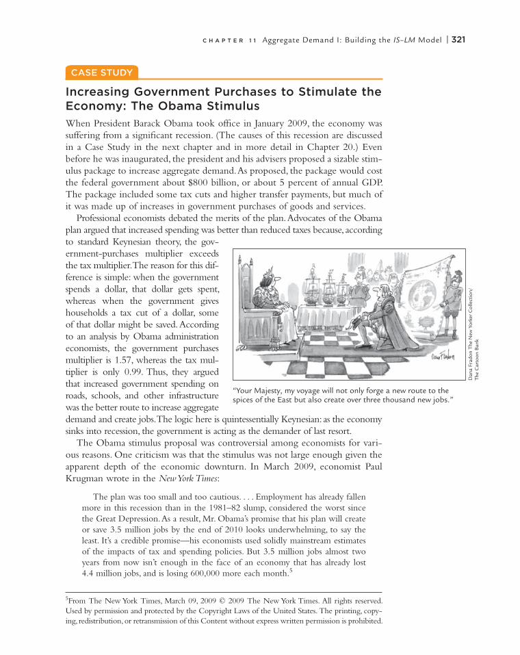
Professional economists debated the merits of the plan. Advocates of the Obama plan argued that increased spending was better than reduced taxes because, according to standard Keynesian theory, the gov-ernment-purchases multiplier exceeds the tax multiplier. The reason for this dif-ference is simple: when the government spends a dollar, that dollar gets spent, whereas when the government gives households a tax cut of a dollar, some of that dollar might be saved. According to an analysis by Obama administration economists, the government purchases multiplier is 1.57, whereas the tax mul-tiplier is only 0.99. Thus, they argued that increased government spending on roads, schools, and other infrastructure was the better route to increase aggregate demand and create jobs. The logic here is quintessentially Keynesian: as the economy sinks into recession, the government is acting as the demander of last resort.

The Obama stimulus proposal was controversial among economists for vari-ous reasons. One criticism was that the stimulus was not large enough given the apparent depth of the economic downturn. In March 2009, economist Paul Krugman wrote in the New York Times:

The plan was too small and too cautious. . . . Employment has already fallen more in this recession than in the 1981–82 slump, considered the worst since the Great Depression. As a result, Mr. Obama’s promise that his plan will create or save 3.5 million jobs by the end of 2010 looks underwhelming, to say the least. It’s a credible promise—his economists used solidly mainstream estimates of the impacts of tax and spending policies. But 3.5 million jobs almost two years from now isn’t enough in the face of an economy that has already lost 4.4 million jobs, and is losing 600,000 more each month.5

CASE STUDY

Dan

a Fr

adon

The

New

Yor

ker

Col

lect

ion/

Th

e C

arto

on B

ank

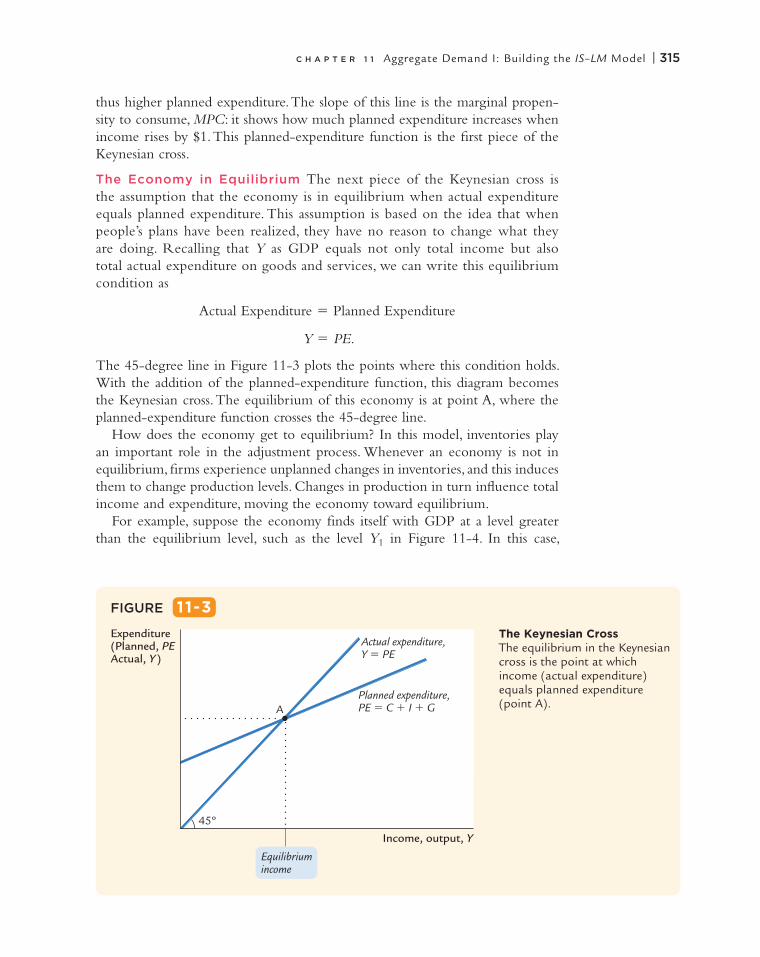
“Your Majesty, my voyage will not only forge a new route to the spices of the East but also create over three thousand new jobs.”

5From The New York Times, March 09, 2009 © 2009 The New York Times. All rights reserved. Used by permission and protected by the Copyright Laws of the United States. The printing, copy-ing, redistribution, or retransmission of this Content without express written permission is prohibited.


Still other economists argued that despite the predictions of conventional Keynesian models, spending-based fiscal stimulus is not as effective as tax-based initiatives. A study of fiscal policy since 1970 in countries that are members of the Organization for Economic Cooperation and Development (OECD) examined which kinds of fiscal stimulus have historically been most successful at promoting growth in economic activity. It found that successful fiscal stimulus relies almost entirely on cuts in business and income taxes, whereas failed fiscal stimulus relies primarily on increases in government spending.6

In addition, some economists thought that using infrastructure spending to promote employment might conflict with the goal of obtaining the infrastruc-ture that was most needed. Here is how economist Gary Becker explained the concern on his blog:

Putting new infrastructure spending in depressed areas like Detroit might have a big stimulating effect since infrastructure building projects in these areas can utilize some of the considerable unemployed resources there. However, many of these areas are also declining because they have been producing goods and services that are not in great demand, and will not be in demand in the future. Therefore, the overall value added by improving their roads and other infra-structure is likely to be a lot less than if the new infrastructure were located in growing areas that might have relatively little unemployment, but do have great demand for more roads, schools, and other types of long-term infrastructure.

In the end, Congress went ahead with President Obama’s proposed stimulus plans with relatively minor modifications. The president signed the $787 billion bill on February 17, 2009. Did it work? The economy recovered from the recession, but more slowly than the Obama administration economists ini-tially forecast. Whether the slow recovery reflects the failure of stimulus policy or a sicker economy than the economists first appreciated is a question of continuing debate. n

Using Regional Data to Estimate Multipliers

As the preceding two case studies show, policymakers often change taxes and government spending to influence the economy. The short-run effects of these policy moves can be understood using Keynesian theory, such as the Keynesian cross and the IS–LM model. But do these policies work as well in practice as they do in theory?

Unfortunately, that question is hard to answer. When policymakers change fiscal policy, they usually do so for good reason. Because many other things are happening at the same time, there is no easy way to separate the effects of the

CASE STUDY

6Alberto Alesina and Silvia Ardagna, “Large Changes in Fiscal Policy: Taxes Versus Spending,” Tax Policy and the Economy 24 (2010): 35–68. Another study reporting a tax multiplier that exceeds the spending multiplier is Robert J. Barro and Charles J. Redlick, “Macroeconomic Effects from Government Purchases and Taxes,” Quarterly Journal of Economics, 126 (2011): 51–102.


fiscal policy from the effects of the other events. For example, President Obama proposed his 2009 stimulus plan because the economy was suffering in the after-math of a financial crisis. We can observe what happened to the economy after the stimulus was passed, but disentangling the effects of the stimulus from the lingering effects of the financial crisis is a formidable task.

Increasingly, economists have tried to estimate multipliers for fiscal policy using regional data from states or provinces within a country. The use of regional data has two advantages. First, it increases the number of observations: the United States, for instance, has only one national economy but 50 state economies. Second, and more important, it is possible to find variation in regional govern-ment spending that is plausibly unrelated to other events affecting the regional economy. By examining such random variation in government spending, a researcher can more easily identify its macroeconomic effects without being led astray by other, confounding variables.

In one such study, Emi Nakamura and Jón Steinsson looked at the impact of defense spending on state economies. They began with the fact that states vary considerably in the size of their defense industries. For example, military con-tractors are more important in California than in Illinois: when the U.S. federal government increases defense spending by 1% of U.S. GDP, defense spending in California rises on average by about 3% of California GDP, while defense spending in Illinois rises by only about 0.5% of Illinois GDP. By examining what happens to the California economy relative to the Illinois economy when the United States embarks on a military buildup, we can estimate the effects of government spending. Using data from all 50 states, Nakamura and Steinsson reported a government-purchases multiplier of 1.5. That is, when the govern-ment increases defense spending in a state by $1.00, it increases that state’s GDP by $1.50.

In another study, Antonio Acconcia, Giancarlo Corsetti, and Saverio Simonelli used data from provinces within Italy to study the multiplier. Here the varia-tion in government spending comes not from military buildups but from an Italian law cracking down on organized crime. According to the law, whenever the police uncover incriminating evidence that the Mafia has infiltrated a city council, the council is dismissed and replaced by external commissioners. These commissioners typically implement an immediate, unanticipated, and temporary cut in public investment projects. The study reported that this cut in government spending has a significant impact on the province’s GDP. Once again, the mul-tiplier is estimated to be about 1.5. Hence, these studies confirm the prediction of Keynesian theory that changes in government purchases can have a sizeable effect on an economy’s output of goods and services.

It is unclear, however, how to use these estimates from regional economies to draw inferences about national economies. One problem is that the regional government spending these researchers studied was not financed with regional taxes. Defense spending in California is largely paid for by federal taxes levied on the other 49 states, and the public investment projects in an Italian province are largely paid for at the national level. By contrast, when a nation increases its government spending, it has to increase taxes, either in the present or the future,


The Interest Rate, Investment, and the IS Curve

The Keynesian cross is only a stepping-stone on our path to the IS–LM model, which explains the economy’s aggregate demand curve. The Keynesian cross is useful because it shows how the spending plans of households, firms, and the government determine the economy’s income. Yet it makes the simplifying assumption that the level of planned investment I is fixed. As we discussed in Chapter 3, an important macroeconomic relationship is that planned investment depends on the interest rate r.

To add this relationship between the interest rate and investment to our model, we write the level of planned investment as

I 5 I(r ).

This investment function is graphed in panel (a) of Figure 11-7. Because the interest rate is the cost of borrowing to finance investment projects, an increase in the interest rate reduces planned investment. As a result, the investment func-tion slopes downward.

to pay for it. These higher taxes could depress economic activity, leading to a smaller multiplier. A second problem is that these regional changes in govern-ment spending do not influence monetary policy, because central banks focus on national rather than regional conditions. By contrast, a national change in gov-ernment spending could well induce a change in monetary policy. In its attempt to stabilize the economy, the central bank may offset some of the effects of fiscal policy, making the multiplier smaller.

Although both of these problems suggest that national multipliers are likely smaller than regional multipliers, a third problem works in the opposite direction. In a small regional economy, such as a state, many of the goods and services people buy are imported from neighboring states, whereas imports are a smaller share of a large national economy. When imports play a larger role, the marginal propensity to consume on domestic goods (those made within the state) is smaller. As the Keynesian cross describes, a smaller marginal propensity to con-sume on domestic goods leads to smaller second- and third-round effects and, thereby, a smaller multiplier. For this reason, national multipliers could be larger than regional multipliers.

The bottom line from studies of regional economies is that the demand from government purchases can exert a strong influence on economic activity. But the size of that effect as measured by the multiplier at the national level remains open to debate.7 n

7Emi Nakamura and Jón Steinsson, “Fiscal Stimulus in a Monetary Union: Evidence from US Regions” American Economic Review 104 (March 2014): 753–792. Antonio Acconcia, Giancarlo Corsetti, and Saverio Simonelli, “Mafia and Public Spending: Evidence on the Fiscal Multiplier from a Quasi-experiment,” American Economic Review 104 (July 2014): 2185–2209. Similar results are reported in Daniel Shoag, “Using State Pension Shocks to Estimate Fiscal Multipliers since the Great Recession,” American Economic Review 103 (May 2013): 121–24.


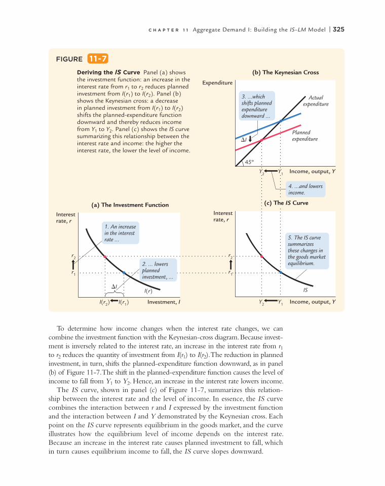
To determine how income changes when the interest rate changes, we can combine the investment function with the Keynesian-cross diagram. Because invest-ment is inversely related to the interest rate, an increase in the interest rate from r1 to r2 reduces the quantity of investment from I(r1) to I(r2). The reduction in planned investment, in turn, shifts the planned-expenditure function downward, as in panel (b) of Figure 11-7. The shift in the planned-expenditure function causes the level of income to fall from Y1 to Y2. Hence, an increase in the interest rate lowers income.

The IS curve, shown in panel (c) of Figure 11-7, summarizes this relation-ship between the interest rate and the level of income. In essence, the IS curve combines the interaction between r and I expressed by the investment function and the interaction between I and Y demonstrated by the Keynesian cross. Each point on the IS curve represents equilibrium in the goods market, and the curve illustrates how the equilibrium level of income depends on the interest rate. Because an increase in the interest rate causes planned investment to fall, which in turn causes equilibrium income to fall, the IS curve slopes downward.

FIGURE 11-7

Expenditure

Interestrate, r

Interestrate, r

Income, output, Y

Investment, I Income, output, Y

IS

Y1Y2

r2

r1

�I

I(r1)

I(r)

I(r2)

Actualexpenditure

Planned expenditure�I

45º

r2

r1

(a) The Investment Function

(b) The Keynesian Cross

(c) The IS Curve

Y1Y2

3. ...whichshifts plannedexpendituredownward ...

5. The IS curvesummarizesthese changes inthe goods marketequilibrium.

4. ...and lowersincome.

2. ... lowersplannedinvestment, ...

1. An increasein the interestrate ...

Deriving the IS Curve Panel (a) shows the investment function: an increase in the interest rate from r1 to r2 reduces planned investment from I(r1) to I(r2). Panel (b) shows the Keynesian cross: a decrease in planned investment from I(r1) to I(r2) shifts the planned-expenditure function downward and thereby reduces income from Y1 to Y2. Panel (c) shows the IS curve summarizing this relationship between the interest rate and income: the higher the interest rate, the lower the level of income.


How Fiscal Policy Shifts the IS Curve

The IS curve shows us, for any given interest rate, the level of income that brings the goods market into equilibrium. As we learned from the Keynesian cross, the equilibrium level of income also depends on government spending G and taxes T. The IS curve is drawn for a given fiscal policy; that is, when we construct the IS curve, we hold G and T fixed. When fiscal policy changes, the IS curve shifts.

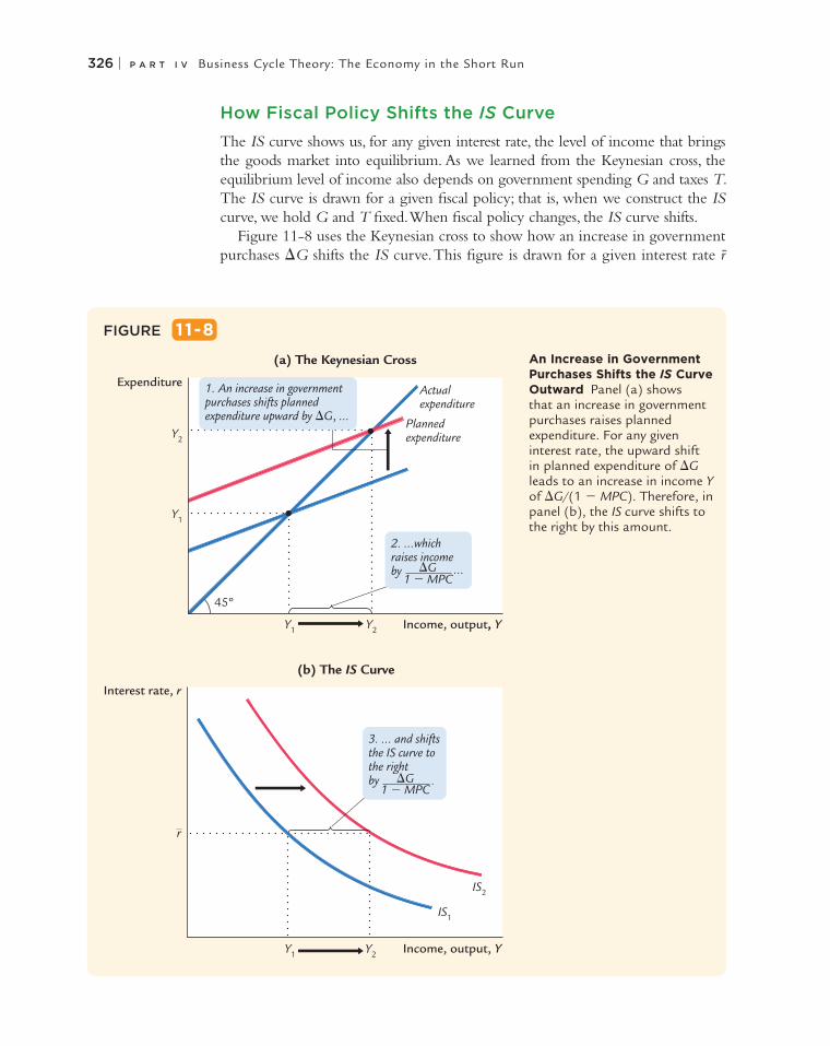
Figure 11-8 uses the Keynesian cross to show how an increase in government purchases DG shifts the IS curve. This figure is drawn for a given interest rate r̄

FIGURE 11-8

Income, output, Y

Income, output, Y

Actualexpenditure

Y2

Y1 Y2

Y1

45º

Plannedexpenditure

r

Y1 Y2

IS1

IS2

Expenditure

Interest rate, r

3. ... and shiftsthe IS curve tothe rightby �G

1 � MPC.

(a) The Keynesian Cross

(b) The IS Curve

2. ...whichraises incomeby �G

1 � MPC

1. An increase in governmentpurchases shifts plannedexpenditure upward by �G, ...

...

An Increase in Government Purchases Shifts the IS Curve Outward Panel (a) shows that an increase in government purchases raises planned expenditure. For any given interest rate, the upward shift in planned expenditure of DG leads to an increase in income Y of DG/(1 2 MPC). Therefore, in panel (b), the IS curve shifts to the right by this amount.


and thus for a given level of planned investment. The Keynesian cross in panel (a) shows that this change in fiscal policy raises planned expenditure and thereby increases equilibrium income from Y1 to Y2. Therefore, in panel (b), the increase in government purchases shifts the IS curve outward.

We can use the Keynesian cross to see how other changes in fiscal policy shift the IS curve. Because a decrease in taxes also expands expenditure and income, it, too, shifts the IS curve outward. A decrease in government purchases or an increase in taxes reduces income; therefore, such a change in fiscal policy shifts the IS curve inward.

In summary, the IS curve shows the combinations of the interest rate and the level of income that are consistent with equilibrium in the market for goods and services. The IS curve is drawn for a given fiscal policy. Changes in fiscal policy that raise the demand for goods and services shift the IS curve to the right. Changes in fiscal policy that reduce the demand for goods and services shift the IS curve to the left.

11-2 The Money Market and the LM Curve

The LM curve plots the relationship between the interest rate and the level of income that arises in the market for money balances. To understand this relation-ship, we begin by looking at a theory of the interest rate called the theory of liquidity preference.

The Theory of Liquidity Preference

In his classic work The General Theory, Keynes offered his view of how the inter-est rate is determined in the short run. His explanation is called the theory of liquidity preference because it posits that the interest rate adjusts to balance the supply and demand for the economy’s most liquid asset—money. Just as the Keynesian cross is a building block for the IS curve, the theory of liquidity pref-erence is a building block for the LM curve.

To develop this theory, we begin with the supply of real money balances. If M stands for the supply of money and P stands for the price level, then M/P is the supply of real money balances. The theory of liquidity preference assumes there is a fixed supply of real money balances. That is,

(M/P)s 5 M–/P–

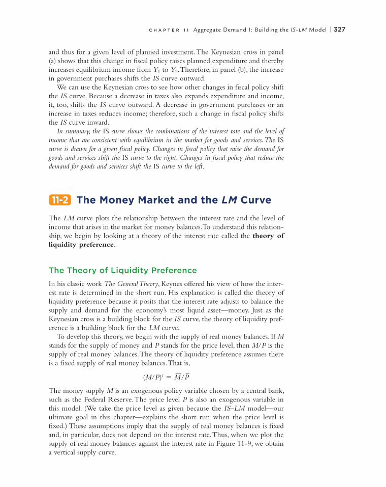
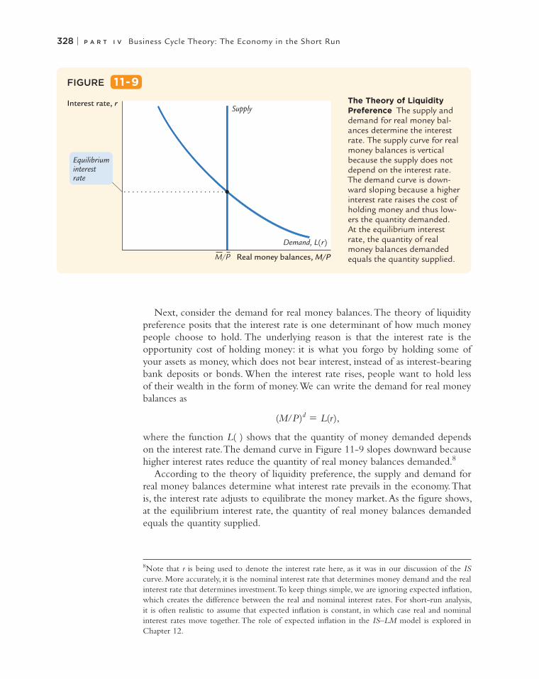
The money supply M is an exogenous policy variable chosen by a central bank, such as the Federal Reserve. The price level P is also an exogenous variable in this model. (We take the price level as given because the IS–LM model—our ultimate goal in this chapter—explains the short run when the price level is fixed.) These assumptions imply that the supply of real money balances is fixed and, in particular, does not depend on the interest rate. Thus, when we plot the supply of real money balances against the interest rate in Figure 11-9, we obtain a vertical supply curve.


Next, consider the demand for real money balances. The theory of liquidity preference posits that the interest rate is one determinant of how much money people choose to hold. The underlying reason is that the interest rate is the opportunity cost of holding money: it is what you forgo by holding some of your assets as money, which does not bear interest, instead of as interest-bearing bank deposits or bonds. When the interest rate rises, people want to hold less of their wealth in the form of money. We can write the demand for real money balances as

(M/P )d 5 L(r ),

where the function L( ) shows that the quantity of money demanded depends on the interest rate. The demand curve in Figure 11-9 slopes downward because higher interest rates reduce the quantity of real money balances demanded.8

According to the theory of liquidity preference, the supply and demand for real money balances determine what interest rate prevails in the economy. That is, the interest rate adjusts to equilibrate the money market. As the figure shows, at the equilibrium interest rate, the quantity of real money balances demanded equals the quantity supplied.

FIGURE 11-9

The Theory of Liquidity Preference The supply and demand for real money bal-ances determine the interest rate. The supply curve for real money balances is vertical because the supply does not depend on the interest rate. The demand curve is down-ward sloping because a higher interest rate raises the cost of holding money and thus low-ers the quantity demanded. At the equilibrium interest rate, the quantity of real money balances demanded equals the quantity supplied.

Interest rate, r

Real money balances, M/P

Demand, L(r)

Supply

M/P

Equilibriuminterestrate

8Note that r is being used to denote the interest rate here, as it was in our discussion of the IS curve. More accurately, it is the nominal interest rate that determines money demand and the real interest rate that determines investment. To keep things simple, we are ignoring expected inflation, which creates the difference between the real and nominal interest rates. For short-run analysis, it is often realistic to assume that expected inflation is constant, in which case real and nominal interest rates move together. The role of expected inflation in the IS–LM model is explored in Chapter 12.


How does the interest rate get to this equilibrium of money supply and money demand? The adjustment occurs because whenever the money mar-ket is not in equilibrium, people try to adjust their portfolios of assets and, in the process, alter the interest rate. For instance, if the interest rate is above the equilibrium level, the quantity of real money balances supplied exceeds the quantity demanded. Individuals holding the excess supply of money try to convert some of their non-interest-bearing money into interest-bearing bank deposits or bonds. Banks and bond issuers, which prefer to pay lower interest rates, respond to this excess supply of money by lowering the inter-est rates they offer. Conversely, if the interest rate is below the equilibrium level, so that the quantity of money demanded exceeds the quantity supplied, individuals try to obtain money by selling bonds or making bank withdrawals. To attract now-scarcer funds, banks and bond issuers respond by increasing the interest rates they offer. Eventually, the interest rate reaches the equilib-rium level, at which people are content with their portfolios of monetary and nonmonetary assets.

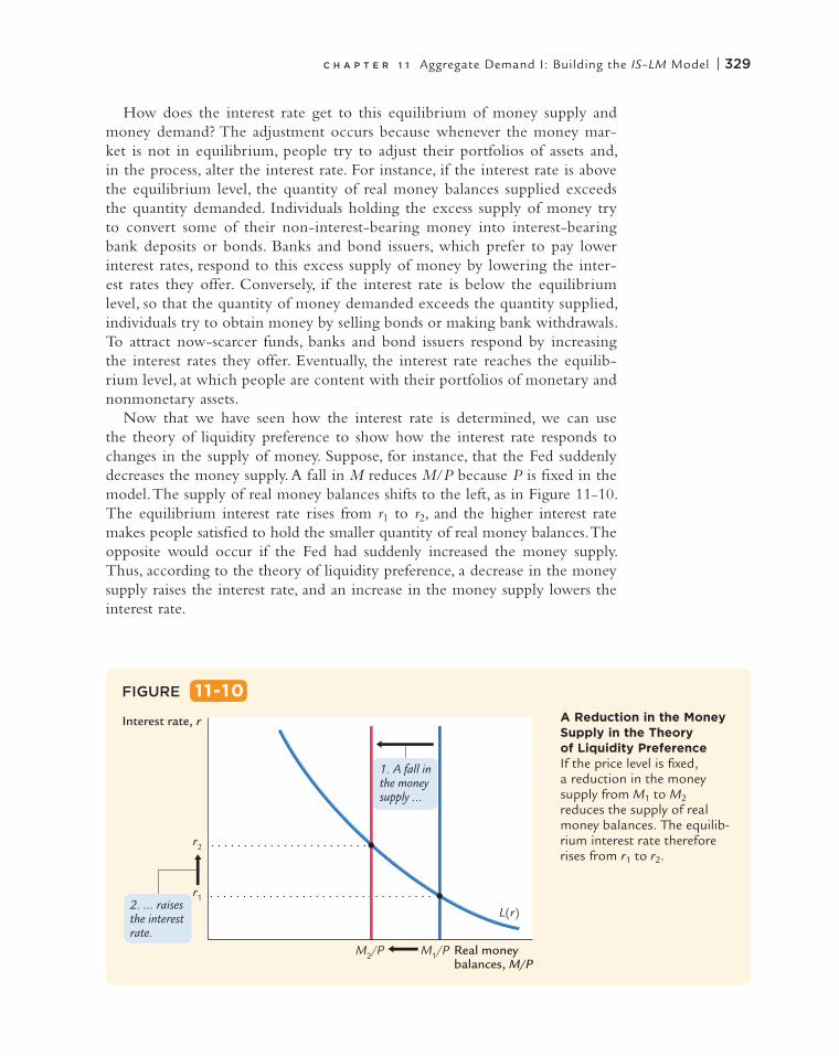
Now that we have seen how the interest rate is determined, we can use the theory of liquidity preference to show how the interest rate responds to changes in the supply of money. Suppose, for instance, that the Fed suddenly decreases the money supply. A fall in M reduces M/P because P is fixed in the model. The supply of real money balances shifts to the left, as in Figure 11-10. The equilibrium interest rate rises from r1 to r2, and the higher interest rate makes people satisfied to hold the smaller quantity of real money balances. The opposite would occur if the Fed had suddenly increased the money supply. Thus, according to the theory of liquidity preference, a decrease in the money supply raises the interest rate, and an increase in the money supply lowers the interest rate.

FIGURE 11-10

Interest rate, r


L(r)

M2/P

r1

r2

M1/P

2. ... raisesthe interestrate.

1. A fall inthe moneysupply ...

A Reduction in the Money Supply in the Theory of Liquidity Preference If the price level is fixed, a reduction in the money supply from M1 to M2 reduces the supply of real money balances. The equilib-rium interest rate therefore rises from r1 to r2.


Income, Money Demand, and the LM Curve

Having developed the theory of liquidity preference as an explanation for how the interest rate is determined, we can now use the theory to derive the LM curve. We begin by considering the following question: How does a change in

Does a Monetary Tightening Raise or Lower Interest Rates?

How does a tightening of monetary policy influence nominal interest rates? According to the theories we have been developing, the answer depends on the time horizon. Our analysis of the Fisher effect in Chapter 5 suggests that, in the long run when prices are flexible, a reduction in money growth would lower inflation, and this in turn would lead to lower nominal interest rates. Yet the theory of liquidity preference predicts that, in the short run when prices are sticky, anti-inflationary monetary policy would lead to falling real money balances and higher interest rates.

Both conclusions are consistent with experience. A good illustration occurred during the early 1980s, when the U.S. economy saw the largest and quickest reduction in inflation in recent history.

Here’s the background: By the late 1970s, inflation in the U.S. economy had reached the double-digit range and was a major national problem. In 1979 consumer prices were rising at a rate of 11.3 percent per year. In October of that year, only two months after becoming the chairman of the Federal Reserve, Paul Volcker decided that it was time to change course. He announced that monetary policy would aim to reduce the rate of inflation. This announcement began a period of tight money that, by 1983, brought the inflation rate down to 3.2 percent.

Let’s look at what happened to nominal interest rates. If we look at the period immediately after the October 1979 announcement of tighter monetary policy, we see a fall in real money balances and a rise in the interest rate—just as the theory of liquidity preference predicts. Nominal interest rates on three-month Treasury bills rose from 10.3 percent just before the October 1979 announce-ment to 11.4 percent in 1980 and 14.0 percent in 1981. Yet these high interest rates were only temporary. As Volcker’s change in monetary policy lowered infla-tion and expectations of inflation, nominal interest rates gradually fell, reaching 6.0 percent in 1986.

This episode illustrates a general lesson: to understand the link between monetary policy and nominal interest rates, we need to keep in mind both the theory of liquidity preference and the Fisher effect. A monetary tightening leads to higher nominal interest rates in the short run and lower nominal interest rates in the long run. n

CASE STUDY


the economy’s level of income Y affect the market for real money balances? The answer (which should be familiar from Chapter 5) is that the level of income affects the demand for money. When income is high, expenditure is high, so people engage in more transactions that require the use of money. Thus, greater income implies greater money demand. We can express these ideas by writing the money demand function as

(M/P )d 5 L(r, Y ).

The quantity of real money balances demanded is negatively related to the interest rate and positively related to income.

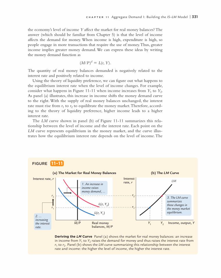
Using the theory of liquidity preference, we can figure out what happens to the equilibrium interest rate when the level of income changes. For example, consider what happens in Figure 11-11 when income increases from Y1 to Y2. As panel (a) illustrates, this increase in income shifts the money demand curve to the right. With the supply of real money balances unchanged, the interest rate must rise from r1 to r2 to equilibrate the money market. Therefore, accord-ing to the theory of liquidity preference, higher income leads to a higher interest rate.

The LM curve shown in panel (b) of Figure 11-11 summarizes this rela-tionship between the level of income and the interest rate. Each point on the LM curve represents equilibrium in the money market, and the curve illus-trates how the equilibrium interest rate depends on the level of income. The

FIGURE 11-11

Interest rate, r Interest rate, r


Income, output, Y

r2

M/P

L(r, Y1)

L(r, Y2)r1

Y1 Y2

LM

2. ... increasingthe interestrate.

r2

r1

1. An increase inincome raisesmoney demand, ...

3. The LM curvesummarizesthese changes in the money marketequilibrium.

(a) The Market for Real Money Balances (b) The LM Curve

Deriving the LM Curve Panel (a) shows the market for real money balances: an increase in income from Y1 to Y2 raises the demand for money and thus raises the interest rate from r1 to r2. Panel (b) shows the LM curve summarizing this relationship between the interest rate and income: the higher the level of income, the higher the interest rate.


higher the level of income, the higher the demand for real money balances, and the higher the equilibrium interest rate. For this reason, the LM curve slopes upward.

How Monetary Policy Shifts the LM Curve

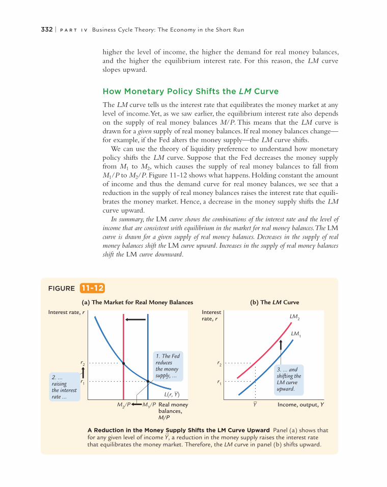
The LM curve tells us the interest rate that equilibrates the money market at any level of income. Yet, as we saw earlier, the equilibrium interest rate also depends on the supply of real money balances M/P. This means that the LM curve is drawn for a given supply of real money balances. If real money balances change—for example, if the Fed alters the money supply—the LM curve shifts.

We can use the theory of liquidity preference to understand how monetary policy shifts the LM curve. Suppose that the Fed decreases the money supply from M1 to M2, which causes the supply of real money balances to fall from M1/P to M2/P. Figure 11-12 shows what happens. Holding constant the amount of income and thus the demand curve for real money balances, we see that a reduction in the supply of real money balances raises the interest rate that equili-brates the money market. Hence, a decrease in the money supply shifts the LM curve upward.

In summary, the LM curve shows the combinations of the interest rate and the level of income that are consistent with equilibrium in the market for real money balances. The LM curve is drawn for a given supply of real money balances. Decreases in the supply of real money balances shift the LM curve upward. Increases in the supply of real money balances shift the LM curve downward.

FIGURE 11-12

A Reduction in the Money Supply Shifts the LM Curve Upward Panel (a) shows that for any given level of income Y

–, a reduction in the money supply raises the interest rate

that equilibrates the money market. Therefore, the LM curve in panel (b) shifts upward.

Interest rate, r Interest rate, r


Income, output, YM2/P M1/P

L(r, Y)

r2

r1

Y

LM1

LM2

r2

r1

3. ... andshifting theLM curveupward.

(a) The Market for Real Money Balances (b) The LM Curve

1. The Fedreducesthe moneysupply, ...2. ...

raisingthe interestrate ...


11-3 Conclusion: The Short-Run Equilibrium

We now have all the pieces of the IS–LM model. The two equations of this model are

Y 5 C(Y 2 T ) 1 I(r) 1 G IS,

M/P 5 L(r, Y ) LM.

The model takes fiscal policy G and T, monetary policy M, and the price level P as exogenous. Given these exogenous variables, the IS curve provides the combi-nations of r and Y that satisfy the equation representing the goods market, and the LM curve provides the combinations of r and Y that satisfy the equation repre-senting the money market. These two curves are shown together in Figure 11-13.

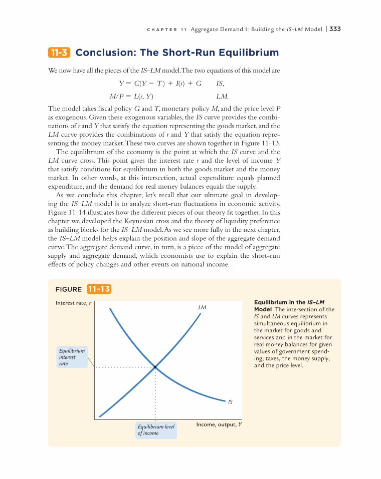
The equilibrium of the economy is the point at which the IS curve and the LM curve cross. This point gives the interest rate r and the level of income Y that satisfy conditions for equilibrium in both the goods market and the money market. In other words, at this intersection, actual expenditure equals planned expenditure, and the demand for real money balances equals the supply.

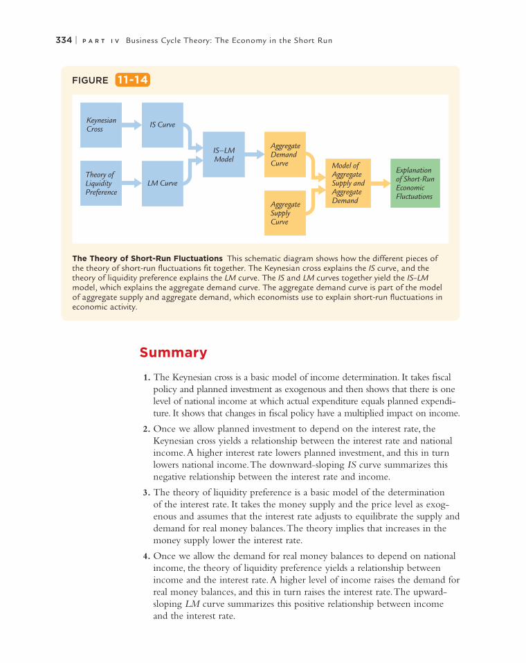
As we conclude this chapter, let’s recall that our ultimate goal in develop-ing the IS–LM model is to analyze short-run fluctuations in economic activity. Figure 11-14 illustrates how the different pieces of our theory fit together. In this chapter we developed the Keynesian cross and the theory of liquidity preference as building blocks for the IS–LM model. As we see more fully in the next chapter, the IS–LM model helps explain the position and slope of the aggregate demand curve. The aggregate demand curve, in turn, is a piece of the model of aggregate supply and aggregate demand, which economists use to explain the short-run effects of policy changes and other events on national income.

FIGURE 11-13

Equilibrium in the IS–LM Model The intersection of the IS and LM curves represents simultaneous equilibrium in the market for goods and services and in the market for real money balances for given values of government spend-ing, taxes, the money supply, and the price level.

Interest rate, r

Income, output, Y

Equilibriuminterestrate

LM

IS

Equilibrium levelof income


Summary

1. The Keynesian cross is a basic model of income determination. It takes fiscal policy and planned investment as exogenous and then shows that there is one level of national income at which actual expenditure equals planned expendi-ture. It shows that changes in fiscal policy have a multiplied impact on income.

2. Once we allow planned investment to depend on the interest rate, the Keynesian cross yields a relationship between the interest rate and national income. A higher interest rate lowers planned investment, and this in turn lowers national income. The downward-sloping IS curve summarizes this negative relationship between the interest rate and income.

3. The theory of liquidity preference is a basic model of the determination of the interest rate. It takes the money supply and the price level as exog-enous and assumes that the interest rate adjusts to equilibrate the supply and demand for real money balances. The theory implies that increases in the money supply lower the interest rate.

4. Once we allow the demand for real money balances to depend on national income, the theory of liquidity preference yields a relationship between income and the interest rate. A higher level of income raises the demand for real money balances, and this in turn raises the interest rate. The upward-sloping LM curve summarizes this positive relationship between income and the interest rate.

FIGURE 11-14

KeynesianCross

Theory ofLiquidityPreference

Model ofAggregateSupply andAggregateDemand

IS–LMModel

LM Curve

IS Curve

Explanationof Short-RunEconomicFluctuations

AggregateDemandCurve

AggregateSupplyCurve

The Theory of Short-Run Fluctuations This schematic diagram shows how the different pieces of the theory of short-run fluctuations fit together. The Keynesian cross explains the IS curve, and the theory of liquidity preference explains the LM curve. The IS and LM curves together yield the IS–LM model, which explains the aggregate demand curve. The aggregate demand curve is part of the model of aggregate supply and aggregate demand, which economists use to explain short-run fluctuations in economic activity.


5. The IS–LM model combines the elements of the Keynesian cross and the elements of the theory of liquidity preference. The IS curve shows the points that satisfy equilibrium in the goods market, and the LM curve shows the points that satisfy equilibrium in the money market. The inter-section of the IS and LM curves shows the interest rate and income that satisfy equilibrium in both markets for a given price level.

K E Y C O N C E P T S

IS–LM model

IS curve

LM curve

Keynesian cross

Government-purchases multiplier

Tax multiplier

Theory of liquidity preference

Q U E S T I O N S F O R R E V I E W

1. Use the Keynesian cross to explain why fiscal policy has a multiplied effect on national income.

2. Use the theory of liquidity preference to explain why an increase in the money supply lowers the

interest rate. What does this explanation assume about the price level?

3. Why does the IS curve slope downward?

4. Why does the LM curve slope upward?

1. Use the Keynesian cross model to predict the impact on equilibrium GDP of the following. In each case, state the direction of the change and give a formula for the size of the impact.

a. An increase in government purchases

b. An increase in taxes

c. Equal-sized increases in both government purchases and taxes

2. • In the Keynesian cross model, assume that the consumption function is given by

C 5 120 1 0.8 (Y 2 T ).

Planned investment is 200; government purchases and taxes are both 400.

a. Graph planned expenditure as a function of income.

b. What is the equilibrium level of income?

c. If government purchases increase to 420, what is the new equilibrium income? What is the multiplier for government purchases?

P R O B L E M S A N D A P P L I C A T I O N S

d. What level of government purchases is needed to achieve an income of 2,400? (Taxes remain at 400.)

e. What level of taxes is needed to achieve an income of 2,400? (Government purchases remain at 400.)

3. Although our development of the Keynesian cross in this chapter assumes that taxes are a fixed amount, most countries levy some taxes that rise automatically with national income. (Examples in the United States include the income tax and the payroll tax.) Let’s represent the tax system by writing tax revenue as

T 5 –T 1 tY,

where T and t are parameters of the tax code. The parameter t is the marginal tax rate: if income rises by $1, taxes rise by t 3 $1.

a. How does this tax system change the way consumption responds to changes in GDP?


b. In the Keynesian cross, how does this tax sys-tem alter the government-purchases multiplier?

c. In the IS–LM model, how does this tax sys-tem alter the slope of the IS curve?

4. Consider the impact of an increase in thriftiness in the Keynesian cross model. Suppose the con-sumption function is

C 5 –C 1 c(Y 2 T ),

where C is a parameter called autonomous con-sumption that represents exogenous influences on consumption and c is the marginal propensity to consume.

a. What happens to equilibrium income when the society becomes more thrifty, as repre-sented by a decline in –C ?

b. What happens to equilibrium saving?

c. Why do you suppose this result is called the paradox of thrift?

d. Does this paradox arise in the classical model of Chapter 3? Why or why not?

5. • Suppose that the money demand function is

(M/P )d 5 800 2 50r,

where r is the interest rate in percent. The money supply M is 2,000 and the price level P is fixed at 5.

a. Graph the supply and demand for real money balances.

b. What is the equilibrium interest rate?

c. What happens to the equilibrium interest rate if the supply of money is reduced from 2,000 to 1,500?

d. If the central bank wants the interest rate to be 4 percent, what money supply should it set?

6. • The following equations describe an economy.

Y 5 C 1 I 1 G.

C 5 50 1 0.75 (Y 2 T ).

I 5 150 2 10 r.

(M/P )d 5 Y 2 50r.

G 5 250.

T 5 200.

M 5 3,000.

P 5 4.

a. Identify each of the variables and briefly explain their meaning.

b. From the above list, use the relevant set of equations to derive the IS curve. Graph the IS curve on an appropriately labeled graph.

c. From the above list, use the relevant set of equations to derive the LM curve. Graph the LM curve on the same graph you used in part (b).

d. What are the equilibrium level of income and the equilibrium interest rate?

For any problem marked with , there is a Work It Out online tutorial available for a similar problem. To access these interactive, step-by-step tutorials and other resources, visit LaunchPad for Macroeconomics 9e at www.macmillanhighered.com/launchpad/mankiw9e

Documents

Aggregate Demand I: Building the IS–LM ModelI).pdf · In Chapter 10, we derived the aggregate demand curve from the quan-tity theory of money, and we showed that monetary policy