arX

iv:1

201.

4497

v2 [

mat

h-ph

] 2

0 N

ov 2

012

A geometrical introduction to screw theory

E. Minguzzi∗

Abstract

This work introduces screw theory, a venerable but yet little known theory

aimed at describing rigid body dynamics. This formulation of mechanics unifies

in the concept of screw the translational and rotational degrees of freedom of

the body. It captures a remarkable mathematical analogy between mechanical

momenta and linear velocities, and between forces and angular velocities. For

instance, it clarifies that angular velocities should be treated as applied vectors

and that, under the composition of motions, they sum with the same rules of

applied forces. This work provides a short and rigorous introduction to screw

theory intended to an undergraduate and general readership.

Keywords: rigid body, screw theory, rotation axis, central axis, twist, wrench.MSC: 70E55, 70E60, 70E99.

Contents

1 Introduction 2

1.1 Comments on previous treatments . . . . . . . . . . . . . . . . . . . . 4

2 Abstract screw theory 6

2.1 The commutator . . . . . . . . . . . . . . . . . . . . . . . . . . . . . . 112.2 The dual space and the reference frame reduction to R

6 . . . . . . . . 12

3 The kinematical screw and the composition of rigid motions 14

4 Dynamical examples of screws 15

4.1 The cardinal equations of mechanics . . . . . . . . . . . . . . . . . . . 164.1.1 The cardinal equation in a rigidly moving non-inertial frame . 17

4.2 The inertia map . . . . . . . . . . . . . . . . . . . . . . . . . . . . . . 184.3 Screw scalar product examples: Kinetic energy, power and reciprocal

screws . . . . . . . . . . . . . . . . . . . . . . . . . . . . . . . . . . . . 19

5 Lie algebra interpretation and Chasles’ theorem 21

5.1 Invariant bilinear forms and screw scalar product . . . . . . . . . . . . 22

∗Dipartimento di Matematica Applicata “G. Sansone”, Universita degli Studi di Firenze, Via S.

Marta 3, I-50139 Firenze, Italy. E-mail: ettore.minguzzi@unifi.it

1

6 Conclusions 23

1 Introduction

The second law of Newtonian mechanics states that if F is the force acting on a pointparticle of mass m and a is its acceleration, then ma = F . In a sense, the physicalmeaning of this expression lies in its tacit assumptions, namely that forces are vectors,that is, elements of a vector space, and as such they sum. This experimental factembodied in the second law is what prevent us from considering the previous identityas a mere definition of force.

Coming to the study of the rigid body, one can deduce the first cardinal equationof mechanics MC = F , where C is the affine point of the center of mass, M is thetotal mass and F ext =

∑

i Fexti is the resultant of the external applied forces. This

equation does not fix the dynamical evolution of the body, indeed one need to addthe second cardinal equation of mechanics L(O) = M(O), where L(O) and M(O),are respectively, the total angular momentum and the total mechanical momentumwith respect to an arbitrary fixed point O. Naively adding the applied forces mightresult in an incorrect calculation of M(O). As it is well known, one must take intoaccount the line of action of each force F ext

i in order to determine the central axis,namely the locus of allowed application points of the resultant.

These considerations show that applied forces do not really form a vector space.This unfortunate circumstance can be amended considering, in place of the force,the field of mechanical momenta that it determines (the so called dynamical screw).These type of fields are constrained by the law which establishes the change of themechanical momenta under change of pole

M(P )−M(Q) = F × (P −Q).

An analogy between momenta and velocities, and between force resultant and angularvelocity is apparent considering the so called fundamental formula of the rigid body,namely a constraint which characterizes the velocity vector field of the rigid body

v(P )− v(Q) = ω × (P −Q).

The correspondence can be pushed forward for instance by noting that the conceptof instantaneous axis of rotation is analogous to that of central axis. Screw theoryexplores these analogies in a systematic way and relates them to the Lie group ofrigid motions on the Euclidean space.

Perhaps, one of the most interesting consequences of screw theory is that it allowsus to fully understand that angular velocities should be treated as vectors applied tothe instantaneous axis of rotation, rather than as free vectors. This fact is not at alobvious. Let us recall that the angular velocity is defined through Poisson theorem,which states that, given a frame K ′ moving with respect to an absolute frame K, anynormalized vector e′ which is fixed with respect to K ′ satisfies

de′

dt= ω × e′,

2

in the original frame K, where ω is unique. The uniqueness allows us to unambigu-ously define ω as the angular velocity of K ′ with respect to K. As the vectors e′ arefree, their application point is not fixed and so, according to this traditional definition,ω is not given an application point.

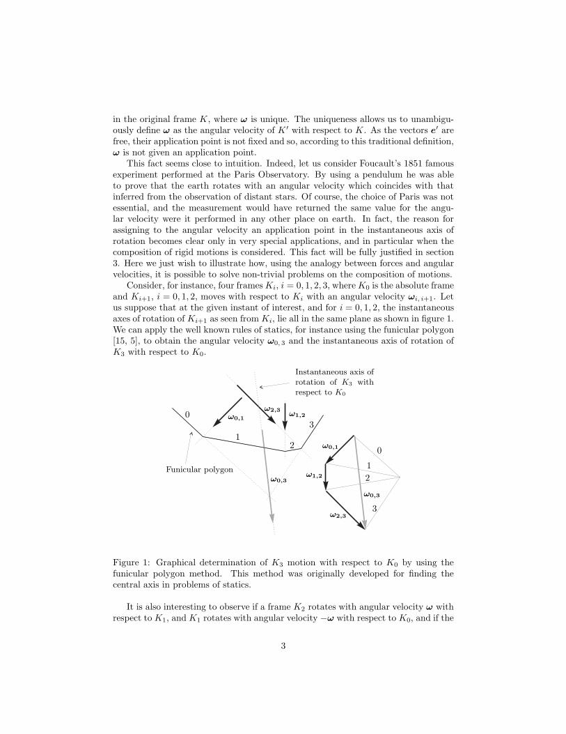
This fact seems close to intuition. Indeed, let us consider Foucault’s 1851 famousexperiment performed at the Paris Observatory. By using a pendulum he was ableto prove that the earth rotates with an angular velocity which coincides with thatinferred from the observation of distant stars. Of course, the choice of Paris was notessential, and the measurement would have returned the same value for the angu-lar velocity were it performed in any other place on earth. In fact, the reason forassigning to the angular velocity an application point in the instantaneous axis ofrotation becomes clear only in very special applications, and in particular when thecomposition of rigid motions is considered. This fact will be fully justified in section3. Here we just wish to illustrate how, using the analogy between forces and angularvelocities, it is possible to solve non-trivial problems on the composition of motions.

Consider, for instance, four framesKi, i = 0, 1, 2, 3, whereK0 is the absolute frameand Ki+1, i = 0, 1, 2, moves with respect to Ki with an angular velocity ωi, i+1. Letus suppose that at the given instant of interest, and for i = 0, 1, 2, the instantaneousaxes of rotation of Ki+1 as seen from Ki, lie all in the same plane as shown in figure 1.We can apply the well known rules of statics, for instance using the funicular polygon[15, 5], to obtain the angular velocity ω0, 3 and the instantaneous axis of rotation ofK3 with respect to K0.

0

0

1

1

2

2

3

3

ω0,1

ω0,1

ω1,2

ω1,2

ω2,3

ω2,3

ω0,3

ω0,3

Instantaneous axis of

rotation of K3 with

respect to K0

Funicular polygon

Figure 1: Graphical determination of K3 motion with respect to K0 by using thefunicular polygon method. This method was originally developed for finding thecentral axis in problems of statics.

It is also interesting to observe if a frame K2 rotates with angular velocity ω withrespect to K1, and K1 rotates with angular velocity −ω with respect to K0, and if the

3

two instantaneous axes of rotation are parallel and separated by an arm of length d,then, at the given instant, K2 translates with velocity ωd in a direction perpendicularto the plane determined by the two axes. As a consequence, any act of translationcan be reduced to a composition of acts of pure rotation.

This result is analogous to the usual observation that two opposite forces F and−F with arm d generate a constant mechanical momenta of magnitude dF and di-rection perpendicular to the plane determined by the two forces. As a consequence,any applied momenta can be seen as the effect of a couple of forces.

Of course, screw theory has other interesting consequences and advantages. Weinvite the reader to discover and explore them in the following sections.

The key ideas leading to screw theory included in this article have been taughtat a second year undergraduate course of “Rational Mechanics” at the Faculty ofEngineer of Florence University (saved for the last technical section). We shaped thistext so as to be used by our students for self study and by any other scholars whomight want to introduce screw theory in an undergraduate course. Indeed, we believethat it is time to introduce this beautiful approach to mechanics already at the levelof undergraduate University programs.

1.1 Comments on previous treatments

Screw theory is venerable (for an account of the early history see [3]). It originatedfrom the works of Euler, Mozzi and Chasles, who discovered that any rigid motioncan be obtained as a rotation followed by a translation in the direction of the rota-tion’s axis (this is the celebrated Chasles’s theorem which was actually first obtainedby Giulio Mozzi [2]), and by Poinsot, Chasles and Mobius, who noted the analogybetween forces and angular velocities for the first time [3].

It was developed and reviewed by Sir R. Ball in his 1870 treatise [1], and furtherdeveloped, especially in connection with its algebraic formulation, by Clifford, Ko-tel’nikov, Zeylinger, Study and others. Unfortunately, by the end of the nineteenthcentury it was essentially forgotten to be then fully rediscovered only in the second halfof the twentieth century. It remains largely unknown and keeps being rediscoveredby various authors interested in rigid body mechanics (including this author).

Unfortunately, screw theory is usually explained following descriptive definitionsrather than short axiomatic lines of reasoning. As a result, the available introductionsare somewhat unsatisfactory to the modern mathematical and physical minded reader.Perhaps for this reason, some authors among the few that are aware of the existenceof screw theory claim that it is too complicated to deserve to be taught. For instance,the last edition of Goldstein’s textbook [7] includes a footnote which, after introducingthe full version of Chasles’ theorem (Sect. 5), which might be regarded as the startingpoint of screw theory, comments

[. . .] there seems to be little present use for this version of Chasles’ theorem,nor for the elaborate mathematics of screw motions elaborated at the endof the nineteenth century.

Were it written in the fifties of the last century this claim could have been shared,but further on screw theory has become a main tool for robotics [9] where it is ordi-

4

narily used. Furthermore, while elaborate the mathematics of screw theory simplifiesthe development of mechanics. Admittedly, however, some people could be dissat-isfied with available treatments and so its main advantages can be underestimated.We offer here a shorter introduction which, hopefully, could convince these readers oftaking a route into screw theory.

Let us comment on some definitions of screw that can be found in the literature,so as to justify our choices.

A first approach, that this author does not find appealing, introduces the screw bymeans of the concept ofmotor. This formalism depends on the point of reduction, andone finds the added difficulty of proving the independence of the various deductionsfrom the chosen reduction point. It hides the geometrical content of the screw andmakes proofs lengthier. Nevertheless, it must be said that the motor approach couldbe convenient for reducing screw calculations to a matter of algebra (the so calledscrew calculus [3]).

In a similar vein, some references, including Selig’s [14], introduce the screw froma matrix formulation that tacitly assumes that a choice of reference frame has beenmade (thus losing the invariance at sight of the definition).

Still concerning the screw definition, some literature follows the practical andtraditional approach which introduces the screw from its properties (screw axis, pitch,etc.) [1, 8, 6], like in old fashioned linear algebra where one would have defined avector from its direction, verse and module, instead of defining it as an element of avector space (to complicate matters, some authors define the screw up to a positiveconstant, in other words they work with a projective space rather that a vectorspace). This approach could be more intuitive but might also give a false confidenceof understanding, and it is less suited for a formal development of the theory. It isclear that the vector space approach in linear algebra, while less intuitive at first,proves to be much more powerful than any descriptive approach. Of course, one hasto complement it with the descriptive point of view in order to help the intuition.In my opinion the same type of strategy should be followed in screw theory, with amaybe more formal introduction, giving a solid basis, aided by examples to help theintuition. Since descriptive intuitive approaches are not lacking in the literature, thiswork aims at giving a short introduction of more abstract and geometrical type.

It should be said that at places there is an excess of formality in the availablepresentations of screw theory. I refer to the tendency of giving separated definitionsof screws, one for the kinematical twist describing the velocity field of the rigid body,and the other for the wrench describing the forces acting on the body. This type ofapproach, requiring definitions for screws and their dual elements (sometimes calledco-screws), lengthens the presentation and forces the introduction and use of the dualspace of a vector space, a choice which is not so popular especially for undergraduateteaching.

Who adopts this point of view argues that it should also be adopted for forces inmechanics, which should be treated as 1-forms instead as vectors. This suggestion,inspired by the concept of conjugate momenta of Lagrangian and Hamiltonian theory,sounds more modern, but would be geometrically well founded only if one coulddevelop mechanics without any mention to the scalar product. The scalar productallows us to identify a vector space with its dual and hence to work only with the

5

former. If what really matters is the pairing between a vector space and its dual then,as this makes sense even without scalar product, we could dispense of it. It is easy torealize that in order to develop mechanics we need a vector space (and/or its dual) aswell as a scalar product and an orientation (although most physical combinations ofinterest might be rewritten so as a to get rid of it, e.g. the kinetic energy is T = 1

2p[v]).Analogously, in screw theory, it could seem more appealing to look at kinematical

twists as screws and to dynamical wrenches as co-screws, but geometrically this choicedoes not seem compelling, and in fact it is questionable, given the price to be paid interms of length and loss of unity of the presentation. Therefore, we are going to usejust one mathematical entity - the screw - emphasizing the role of the screw scalarproduct in identifying screws and dual elements.

In this work I took care at introducing screw theory in a way as far as coordi-nate independent as possible, but avoiding the traditional descriptive route. In thisapproach the relation with the Lie algebra of rigid maps becomes particularly trans-parent. Finally, most approaches postpone the definition of screw after the examplesof systems of applied forces from which the idea of screw can been derived. I thinkthat it is better to introduce the screw first and then to look at the applications.

In this way, through some key choices, I have obtained a hopefully clear andstraightforward introduction to screw theory, which is at the same time mathemat-ically rigorous. My hope is that after reading these notes, the reader will share theauthor’s opinion that screw theory is indeed “the right” way of teaching rigid bodymechanics as the tight relation with the Lie group of rigid maps suggests.

2 Abstract screw theory

In this section we define the screw and prove some fundamental properties. Specificapplications will appear in the next sections.

Let us denote with E the affine Euclidean space modeled on the three dimensionalvector space V . The space V is endowed with a positive definite scalar product· : V ×V → R, and is given an orientation. This structure is represented with a triple(V, ·, o) where o denotes the orientation. Note that thanks to this structure a vectorproduct × : V × V → V can be naturally defined on V . Points of E are denotedwith capital letters e.g. P,Q, . . . while points in V are denoted as a, b, . . . We shallrepeatedly use the fact that the mixed product a · (b × c) changes sign under oddpermutations of its terms and remains the same under even permutations. A vectorfield is a map f : E → V .

An applied vector is an element of E × V , namely a pair (Q,v) where Q is theapplication point of (Q,v). A sliding vector is an equivalence class of applied vectors,where two applied vectors (Q,v) and (Q′,v′) are equivalent if v = v′ and for someλ ∈ R, Q′ −Q = λv, namely they have the same line of action. We shall preferablyuse the concept of applied vector even in those cases in which it could be equivalentlyreplaced by that of sliding vector. The reason is that the concept of sliding vectoris superfluous because it is more convenient to regard applied and sliding vectors asspecial types of screws.

Occasionally, we shall use the concept of reference frame which is defined by a

6

choice of origin O ∈ E, and of positive oriented orthonormal base {e1, e2, e3} for(V, ·, o). Once a reference frame has been fixed, any point P ∈ E is univocallydetermined by its coordinates xi, i = 1, 2, 3, defined through the equation P = O +∑

i xiei.

Remark 2.1. In order to lighten the formalism we shall consider different physical vec-tor quantities, such as position, velocity, linear momenta, force, mechanical momenta,as elements of the same vector space V . A more rigorous treatment would introducea different vector space for each one of these concepts. The reader might imagine tohave fixed the dimension units. It is understood that, say, a linear momenta cannotbe summed to a force even though in our treatment they appear to belong to thesame vector space.

Definition 2.2. A screw is a vector field s : E → V which admits some s ∈ V insuch a way that for any two points P,Q ∈ E

s(P )− s(Q) = s× (P −Q). (1)

For any screw s the vector s is unique, indeed if s and s ′ satisfy the aboveequation, then subtracting the corresponding equations (s ′ − s) × (P − Q) = 0 andfrom the arbitrariness of P , s ′ = s. The vector s is called the resultant of the screw.If the resultant of the screw vanishes then s(P ) does not depend on P and the screwis said to be constant. Equation (1) is the constitutive equation of the screw.

Definition 2.3. If s is a screw the quantity s(P ) · s does not depend on the pointand in called the scalar invariant of the screw. The vector invariant of the screw isthe quantity (independent of P ) and defined by

∫ = s(P ), if s = 0,

∫ =s(P ) · s

s · ss, if s 6= 0.

Thus if s 6= 0 the vector invariant of the screw is the projection of s(P ) on thedirection given by the resultant, and it is actually independent of P .

Proposition 2.4. The screws form a vector space S and the map which sends s tos is linear.

Proof. If s1 and s2 are two screws

s1(P )− s1(Q) = s1 × (P −Q),

s2(P )− s2(Q) = s2 × (P −Q).

Multiplying by α the first equation and adding the latter multiplied by β we get

(αs1 + βs2)(P )− (αs1 + βs2)(Q) = (αs1 + βs2)× (P −Q), (2)

which implies that the screws form a vector space and that the resultant of the screwαs1 + βs2 is αs1 + βs2, that is, the map s→ s is linear.

7

Given two screws s1 and s2 let us consider the quantity

〈s1, s2〉(P ) := s1 · s2(P ) + s2 · s1(P ).

Proposition 2.5. For any two points P,Q ∈ E, 〈s1, s2〉(P ) = 〈s1, s2〉(Q).

Proof. By definition s1(P )−s1(Q) = s1× (P −Q) and s2(P )−s2(Q) = s2× (P −Q),thus

s1 · s2(P )+s2 · s1(P ) = s1 · (s2(Q) + s2 × (P −Q)) + s2 · (s1(Q) + s1 × (P −Q))

= s1 · s2(Q) + s2 · s1(Q) + {s1 · [s2 × (P −Q)] + s2 · [s1 × (P −Q)]}

= s1 · s2(Q) + s2 · s1(Q).

According to the previous result we can simply write 〈s1, s2〉 in place of 〈s1, s2〉(P ).

Definition 2.6. The screw scalar product is the symmetric bilinear map 〈·, ·〉 : S ×S → R which sends (s1, s2) to 〈s1, s2〉.

Note that the scalar invariant of a screw is one-half the screw scalar product of thescrew by itself. Since this scalar invariant can be negative, the screw scalar producton S is not positive definite. Nevertheless, we shall see that it is non-degenerate (Sect.2.2).

The cartesian product V × V endowed with the usual sum and product by scalargives the direct sum V ⊕ V . Typically, there will be three ways to construct screwsout of (applied) vectors. The easy proofs to the next two propositions are left to thereader.

Proposition 2.7. The map α : V → S given by v → s(P ) := v sends a (free)vector to a constant screw. The map β : E × V → S given by (Q,w) → s(P ) :=w × (P −Q) sends an applied vector to a screw. The map γ : E × V × V → S givenby ((Q,w),v) → s(P ) := v + w × (P − Q) sends a pair given by an applied vectorand a free vector to a screw.

The screws in the image of α will be called constant or free screws. The screwsin the image of β will be called applied screws. Clearly, by the constitutive equationof the screw, the map γ is surjective. In particular, every screw is the sum of a freescrew and an applied screw.

Proposition 2.8. Let γO = γ(O, ·, ·) : V ⊕ V → S, then this linear map is bijective.

Its inverse γ−1O : S → V ⊕ V is called motor reduction at O. Once we agree on

the reduction point O, any pair (s, s(O)) as in the previous proposition is called amotor at O. Sometimes we shall write sO for s(O), thus the motor at O reads (s, sO).Often, for reasons that will be soon clear, we will prefer to represent the ordered pairin a column form of two elements of V .

We can write the found bijective correspondence between S and V 2 as follows

s ∈ Sorigin O←−−−−→

(

s

sO

)

∈ V ⊕ V.

8

In this representation the screw scalar product is given by 〈s1, s2〉 = s1 · sO2 + s2 · s

O1 ,

thus is is mediated by the matrix

(

0 II 0

)

where I : V → V is the identity map.

Let us now recall that any point O ∈ E can be used as origin, namely it allowsus to establish a bijective correspondence between E and V given by P → P −O. Ifwe additionally introduce a positive oriented orthonormal base then we further have

the linear isomorphism Vbase←−→ R

3, thus, as a result, given a full reference frame thescrew gets represented by an element of R6 in which the first three components arethose of s while the last three components are those of sO.

Definition 2.9. Given a screw s ∈ S, the screw axis of s is the set of points for whichthe screw field has minimum module.

Proposition 2.10. The screw axis coincides with the set E if s = 0 and with a lineof direction s if s 6= 0. In both cases, if Q is any point in the screw axis then

s(P ) = ∫ + s× (P −Q). (3)

As a consequence, the screw axis is the set of points for which the screw field coincideswith ∫ . For any point Q on the axis the motor reduction at Q is s⊕ ∫ .

Let us observe that the former term in the right-hand side of Eq. (3) is proportionalto s and independent of the point, while the latter term is orthogonal to to s anddependent on the point.

Proof. Let us suppose s 6= 0, the other case being trivial. Let A be any point, thenit is easy to check that the axis which passes through Q in direction s where

Q = A+s× s(A)

s · s, (4)

is made of points R for which s(R) = ∫ . Using the constitutive equation of screwswe find that Eq. (3) holds. If P is another point for which s(P ) = ∫ then that sameequation gives s × (P − Q) = 0, which implies that P stays in the axis. Thus thefound axis is the locus of points P for which s(P ) = ∫ . Equation (3) and the factthat ∫ ∝ s imply that this axis is made of points for which the screw field is minimal.The other claims follow easily.

Remark 2.11. Usually the vector invariant and the screw axis are defined only fors 6= 0. However, we observe that it is convenient to extend the definition as donehere in such a way that Eq. (3) holds for any screw. The case s = 0 is admittedlyspecial and can be called degenerate.

Remark 2.12. The composition of applied vectors is nothing but the addition ofthe corresponding screws in the vector space S. The resultant screw can then berepresented with its motor in the screw axis which is given by the resultant s alignedwith the axis and the invariant vector ∫ having the same direction (Fig. 2). Inthis sense the composition of applied vectors does not give an applied vector. Theoperation of composition is closed only if the full space of screws is considered.

9

→

|∫ ||s|

∫ ∫

1

2|s|e2

ss

s/2

Screw axis

Figure 2: Reduction of a screw to the simplest system of applied screws (case s 6= 0).

Remark 2.13. Two systems of applied vectors are said to be equivalent if they deter-mine the same screw. One often looks for the simplest way of representing a screwby applied vectors. This is accomplished as follows. The screw is the sum of the freescrew given by ∫ and the applied screw determined by the resultant s applied onthe screw axis. The free screw is generated by two opposite applied vectors s2, −s2,placed in a plane perpendicular to ∫ and such that their magnitude times their armgives ∫ . This reduces any screw to the sum of at most three applied screw (two ifs = 0). If s 6= 0 the number can be reduced to two regarding s as the sum 1

2s+ 12s,

and absorbing one term of type 12s through a redefinition of s2, and analogously for

the other (see Fig. 2). The arm can be chosen in such a way that the resultants ofthe two applied screws are perpendicular. In summary any screw is generated by twoapplied screws whose resultants are either opposite with screw axes belonging to thesame plane (if s = 0), or equal in magnitude and perpendicular (if s 6= 0).

Definition 2.14. The pitch p ∈ R of a screw s, with s 6= 0, is that constant suchthat ∫ = p

2πs. If s = 0 and ∫ 6= 0, we set by definition p = +∞.

Clearly, for a non-trivial screw, the pitch vanishes if and only if the screw is anapplied screw, and the pitch equals +∞ if and only if the screw is a free screw. Thescrews with a given pitch do not form a vector subspace.

Remark 2.15. Using the pitch the screw can be rewritten

s(P ) = a[p

2πe+ e× (P −Q)],

where s = ae, with e normalized vector and a ≥ 0. The quantity a is called amplitudeof the screw. It must be said that for Sir R. S. Ball [1] the screw is s/a. However, itis not particularly convenient to regard s/a as a fundamental object since these typeof normalized screws do not form a vector space. Sir R. S. Ball would refer to ourscrews as screw motions. We prefer to use our shorter terminology (shared by [14])

10

because, for a dynamical screw d, which we shall later introduce, no actual motionneeds to take place. Note also that the normalization of the pitch is chosen in such away that, integrating the screw vector field by a parameter 2π, i.e. by making a fullrotation, one gets a diffeomorphism which is a translation by p along the screw axis.In other words, with the chosen normalization, the pitch gives the translation of thescrew for any full rotation.

2.1 The commutator

Every screw is a vector field, thus we can form the Lie bracket [s1, s2] of two screws[10]. In this section we check that this commutator is itself a screw and calculate itsresultant.

Proposition 2.16. The Lie bracket s = [s1, s2] is a screw with resultant s = −s1×s2and satisfies

s(P ) = s2 × s1(P )− s1 × s2(P ). (5)

.

Remark 2.17. Some authors define the commutator of two screws as minus the Liebracket.

Proof. Let s1 and s2 be two screws

s1(P )− s1(Q) = s1 × (P −Q), (6)

s2(P )− s2(Q) = s2 × (P −Q). (7)

Let us fix a cartesian coordinate system {xi}, then the Lie bracket reads

si = sj1∂jsi2 − sj2∂js

i1.

Note that sj1∂jsi2(P ) = limǫ→0

1ǫ[si2(P+ǫs1(P ))−si2(P )] which, using Eq. (7) becomes

sj1∂jsi2(P ) = [s2 × s1(P )]i. Inverting the roles of s1 and s2 we calculate the second

term, thus we obtain the interesting expression

s(P ) = s2 × s1(P )− s1 × s2(P ).

Let us check that it is a screw, indeed

s(P )− s(Q) = s2 × s1(P )− s1 × s2(P )− s2 × s1(Q) + s1 × s2(Q)

= s2 × [s1(P )− s1(Q)]− s1 × [s2(P )− s2(Q)]

= s2 × [s1 × (P −Q)]− s1 × [s2 × (P −Q)]

= [s2 · (P −Q))]s1 − [s1 · (P −Q))]s2 = (−s1 × s2)× (P −Q),

which proves also that the resultant is as claimed.

The relation between the commutator and the scalar product is clarified by thefollowing result

11

Proposition 2.18. Let s1, s2, s3, be three screws, then

〈s1, [s3, s2]〉+ 〈[s3, s1], s2〉 = 0. (8)

Furthermore, the quantity 〈s1, [s3, s2]〉 reads

〈s1, [s3, s2]〉 = s3(P ) · (s1 × s2) + s2(P ) · (s3 × s1) + s1(P ) · (s2 × s3),

is independent of P , and does not change under cyclic permutations of its terms.

Proof. We use Eq. (5)

〈s1, [s3, s2]〉 = s1 · [s2 × s3(P )− s3 × s2(P )] + s1(P ) · (−s3 × s2)

= s3(P ) · (s1 × s2) + s2(P ) · (s3 × s1) + s1(P ) · (s2 × s3).

This expression changes sign under exchange of s1 and s2, thus we obtain the desiredconclusion.

2.2 The dual space and the reference frame reduction to R6

Given a screw s ∈ S it is possible to construct the linear map 〈s, ·〉 : S → R which isan element of the dual space S∗.

Proposition 2.19. The linear map 〈s, ·〉 sends every screw to zero (namely, it is thenull map), if and only if s = 0.

Proof. If s is such that s 6= 0, then the scalar product with the free screw s′(P ) := s,shows that 0 = 〈s, s′〉 = s2, a contradiction.

If s is a constant screw with vector invariant ∫ , then the screw scalar product withthe applied screw s′(P ) := ∫ × (P −Q), where Q is some point, gives 0 = 〈s, s′〉 = ∫ 2,hence ∫ = 0 and thus s is the null screw.

We have shown that the linear map s → 〈s, ·〉 is injective. We wish to showthat s → 〈s, ·〉 is surjective, namely any element of the dual vector space S∗, can beregarded as the scalar product with some screw. We could deduce this fact using theinjectivity and the equal finite dimensionality of S and S∗, but we shall proceed ina more detailed way which will allow us to introduce a useful basis for the space ofscrews and its dual.

Let us choose Q ∈ E, and let {e1, e2, e3} be a positive oriented orthonormal basefor (V, ·, o), where o denotes the orientation. Namely, assume that we have madea choice of reference frame. The six screws, fi = ((Q, ei),0), mi = ((Q,0), ei),i = 1, 2, 3 generate the whole space S. Indeed, if s is a screw and ((Q, s), s(Q)) is itsmotor at Q, s = a1e1+a2e2+a3e3, s(Q) = b1e1+ b2e2+ b3e3 , then ((Q, s), s(Q)) =∑3

i=1[aifi + bimi]. As a consequence, every reference frame establishes a bijectionbetween the screw space S and R

6 as follows

s ∈ Sreference frame←−−−−−−−−−−−→

(

ab

)

∈ R6

12

where a, b ∈ R3 (vectors in R

3 are denoted with a bar, while the boldface notation isreserved for vectors in V ).

The screw scalar product between s, s′ ∈ S in this representation takes the form

〈s, s′〉 = a · b′ + b · a′, (9)

thus the screw scalar product quadratic form is given by the 6× 6 matrix(

0 II 0

)

, (10)

where I is the identity 3× 3 matrix.Let us now consider the six linear functionals 〈mi, ·〉, 〈fi, ·〉, i = 1, 2, 3. From the

definition of scalar product evaluated at Q it is immediate that

〈mi, ·〉(fj) = 〈mi, fj〉 = δij ,

〈fi, ·〉(mj) = 〈fi,mj〉 = δij ,

〈mi, ·〉(mj) = 〈mi,mj〉 = 0,

〈fi, ·〉(fj) = 〈fi, fj〉 = 0.

that is {〈mi, ·〉, 〈fi, ·〉; i = 1, 2, 3} is the dual base to {fi,mi; i = 1, 2, 3}.Every element z ∈ S∗ is uniquely determined by the values ci, di, i = 1, 2, 3, that

it takes on the six base screws fi,mi, i = 1, 2, 3. By the above formulas, the linearcombination

3∑

i=1

[ci〈mi, ·〉+ di〈fi, ·〉] = 〈

3∑

i=1

[cimi + difi], ·〉

takes the same values on the screw base and thus coincides with z. We can thereforeestablish a bijection of the dual space S∗ with R

6 as follows

z ∈ S∗ reference frame←−−−−−−−−−−−→

(

cd

)

∈ R6

where c, d ∈ R3 (it is convenient to distinguish this copy of R6 with that isomorphic

with S introduced above).As a consequence

Proposition 2.20. The linear map s→ 〈s, ·〉, from S to S∗ is bijective.

Thanks to this result any screw can be regarded either as an element of S or,acting with the screw scalar product, as an element of S∗. It must be stressed that

if s ∈ S is represented by

(

ab

)

then 〈s, ·〉 ∈ S∗ is represented by

(

ba

)

, that is, the

map from S to S∗ which sends s to 〈s, ·〉 is given in this representation by the matrix(

0 II 0

)

. The pairing between the elements of S∗ and those of S is the usual one on

R6. Nevertheless, it is useful to keep in mind that we are actually in presence of two

copies of R6 (as we consider two isomorphisms), the former isomorphic with S andthe latter isomorphic with S∗.

13

Remark 2.21. All this reduction to R6 depends on the reference frame. As mentioned

in the introduction most references of screw theory introduce the screw starting fromits reduction or using a descriptive approach (the screw has an axis, a pitch, etc.). Aswe argued in the introduction, it is pedagogically and logically preferable to definethe screw without making reference to any reference frame.

For future reference we calculate, using Prop. 2.16, the commutator between thescrew base elements

[mi,mj ] = 0,

[fi,mj ] = −[mj, fi] = −∑

k

ǫijkmk,

[fi, fj] = −∑

k

ǫijkfk.

The reader will recognize the Lie algebra commutation relations of the group SE(3)of rigid maps. We shall return to this non accidental fact later on.

Given a screw s we consider the map ads : S → S which acts as s′ → adss′ :=

[s, s′]. Clearly, adss′ = −ads′s and if x, y, z are screws, the Jacobi identity for the Lie

bracket of vector fields [x, [y, z]] + [z, [x, y]] + [y, [z, x]] = 0, becomes

adadxy = adxady − adyadx. (11)

Let an origin O be given and let us use the isomorphism with V ⊕ V . Let s be

represented by

(

s

sO

)

. If we introduce a full reference frame it is possible to check with

a little algebra that, according to the above commutations, the map ads is representedby the matrix

adsorigin O←−−−−→

(

−s× 0−sO× −s×

)

(12)

where for every v ∈ V , v× : V → V is an endomorphism of V induced by the vectorproduct. Of course, if we had kept the reference frame R

6 isomorphism, then, as it is

customary, with v× we would mean the 3× 3 matrix

(

0 −v3 v2

v3 0 −v1

−v2 v1 0

)

.

3 The kinematical screw and the composition of

rigid motions

A rigid motion is a continuous map ϕ : [0, 1]×E → E, which preserves the distancesbetween points, i.e. for every P,Q ∈ E, t ∈ [0, 1], we have |ϕ(t, P )−ϕ(t, Q)| = |P−Q|,and such that ϕ(0, ·) : E → E is the identity map. A rigid map is the result of a rigidmotion, that is a map of type ϕ(1, ·) : E → E. It can be shown that every rigid mapis an affine map which preserves the scalar product and is orientation preserving [11,App. 6]. The rigid maps form a group usually denoted SE(3).

14

In kinematics the velocity field of bodies performing a rigid motion satisfies thefundamental formula of the rigid body

v(P )− v(Q) = ω × (P −Q). (13)

This formula is usually deduced from Poisson formula for the time derivative of anormalized vector: de′

dt = ω × e′.Equation (13) defines a screw which is called twist in the literature. Let us denote

this screw with k, then k(P ) = v(P ) and k = ω, where ω is the angular velocity ofthe rigid body. The instantaneous axis of rotation is by definition the screw axis ofk.

Let us recall that if a point moves with respect to a frame K ′ which is in motionwith respect to a frame K, then the velocity of the point with respect to K is obtainedby summing the drag velocity of the point, as if it were rigidly connected with frameK ′, with the velocity relative to K ′. If two kinematical screws are given and summedthen the result gives a velocity field which represents (by interpreting one of thescrew field as the velocity field of the points at rest in K ′ with respect to K) thecomposition of two rigid motions. The nice fact is that the result is independent ofwhich screw is regarded as describing the motion of K ′. In other words the result hasan interpretation in which the role of the screws can be interchanged.

More generally, one may have a certain number of frames K(i), i = 0, 1, . . . , n,of which we know the screw ki+1 which describes the rigid motion of K(i+1) withrespect to K(i). The motion of K(n) with respect to K(0) is then described by thescrew

∑n

i=1 ki. In particular, since the map which sends a screw to its resultant islinear, the angular velocity of K(n) with respect to K(0) is the sum of the angularvelocities:

∑n

i=1 ωi. As illustrated in the introduction, the screw approach tells ussomething more. Indeed, one can establish the direction of the instantaneous axis ofrotation of K(n) with respect to K(0) by using the same methods used to determinethe central axis in a problem of applied forces. Indeed, we shall see in a moment thatthere is a parallelism between forces and angular velocities as they are both resultantsof some screw.

4 Dynamical examples of screws

In dynamics the most important screw is that given by the moment field, and is calledwrench. Let us recall that the momentum M(Q) of a set of applied forces (Pi,Fi)with respect to a point Q is given by

M(Q) =∑

i

(Pi −Q)× Fi. (14)

If we consider P in place of Q we get

M(P ) =∑

i

(Pi−P )×Fi =∑

i

(Pi−Q+Q−P )×Fi = M(Q)+F × (P −Q), (15)

where F =∑

i Fi is the force resultant. This equation shows that we are in presenceof a screw d such that d(P ) = M(P ), d = F . The central axis of a system of forcesis nothing but the screw axis.

15

Another example of screw is given by the angular momentum field. The angularmomentum L(Q) of a system of point particles located at Ri with momentum pi withrespect to a point Q is given by

L(Q) =∑

i

(Ri −Q)× pi. (16)

If we consider B in place of Q we get

L(B) =∑

i

(Ri −B)× pi =∑

i

(Ri −Q+Q− B)× pi = L(Q) + P × (B −Q),

where P =∑

i pi is the total linear momentum. This equation shows that we are inpresence of a screw l such that l(Q) = L(Q), l = P .

4.1 The cardinal equations of mechanics

Let us consider the constitutive equation of the screw of angular momentum

L(B)−L(Q) = P × (B −Q).

The vector L(B) changes in time as the distribution of velocity and mass changes.Actually, we can consider here another source of time change if we allow the point Bto change in time. Let us first consider the case in which the angular momentum isconsidered with respect to a fixed point.

By differentiating the previous equation with respect to time we get equation (15).In other words the dynamic screw d is the time derivative of the dynamic screw l

∂l

∂t= d. (17)

We use here a partial derivative to remind us that the poles are fixed.This equation replaces the first and second cardinal equation of mechanics. Indeed,

as the map l → l is linear it follows

∂l

∂t= d, (18)

which is the first cardinal equation dP /dt = F in disguise. (Alternatively, writelt(P ) = lt(Q) + lt × (P −Q) and differentiate). Here the partial derivative coincideswith the total derivative because the resultant is a free vector, it does not depend onthe point. The second cardinal equation with respect to a point O

∂L(O)

∂t= M(O),

is obtained by evaluating Eq. (17) at the point O.

16

4.1.1 The cardinal equation in a rigidly moving non-inertial frame

In Eq. (17) we have differentiated with respect to time assuming that the point withrespect to which we evaluate the angular momentum does not change in time. In otherwords we have adopted a Eulerian point of view. Suppose now that on space we havea vector field v(P ) which describes the motion of a continuum (not necessarily a rigidbody). In this case we have to distinguish the Eulerian derivative with respect to time,which we have denoted ∂/∂t, from the Lagrangian or total derivative with respect totime d/dt. According to the latter, the second cardinal equation of mechanics reads

dL(O)

dt= −v(O) × P +M(O), (19)

where O(t) is the moving pole. Let us differentiate

L(B)−L(Q) = P × (B −Q),

with respect to time using the Lagrangian description, that is, assuming that B and Qmove respectively with velocities v(B), v(Q), and considering the angular momentawith respect to the moving points. We obtain

dL(B)

dt−

dL(Q)

dt= F × (B −Q) + P × (v(B)− v(Q)). (20)

Using the second cardinal equation (19) we find that this is the constitutive equationof the momentum screw. Nevertheless, the total derivative of the angular momentumis not a screw.

The relation between the partial and total derivative is as follows

dL(B)

dt=

∂L(B)

∂t+∇

v(B)L,

where

∇v(B)L = lim

ǫ→0

1

ǫ[L(B + v(B)ǫ)−L(B)] = lim

ǫ→0

1

ǫ[P × v(B)ǫ] = P × v(B),

thusdL(B)

dt=

∂L(B)

∂t+ P × v(B). (21)

However, suppose that the velocity field is itself a screw,

v(P )− v(R) = ω × (P −R),

so that the continuum moves rigidly, then from Eq. (20), using the previous resultsfor commutators

[dL(B)

dt−ω ×L(B)]− [

dL(Q)

dt− ω ×L(Q)]

= F × (B −Q) + [P × v(B) − ω ×L(B)]− [P × v(Q)− ω ×L(Q)]

= F × (B −Q) + [k, l](B)− [k, l](Q) = F × (B −Q) + (−ω × P )× (B −Q)

= [F − ω × P ]× (B −Q).

17

The time derivative ddt )R with respect to the moving frame reads by Poisson formula,

ddt)R = d

dt − ω×, thus the previous result can be summarized as follows

Theorem 4.1. Let us denote with d/dt the total derivative with respect to points thatmove rigidly according to a kinematical screw k of vector field v(Q), and with d

dt )Rthe time derivative relative to the corresponding rigidly moving frame. The quantity

d

dtL(Q) )R =

dL(Q)

dt− ω ×L(Q),

defines a screw with resultant ddtP )R = F − ω × P . This screw coincides with the

screwM(Q) + [k, l](Q),

thusdl

dt)R =

∂l

∂t+ [k, l].

Proof. We have only to prove the last statement, which follows easily from Eq. (21)and the definition of commutator.

It must be remarked that in the previous result the angular momentum L iscalculated as in the original inertial frame, and not using the point particle velocitiesas given in the moving frame of twist k. Nevertheless, the previous result is quiteinteresting as it gives a dynamical application of the commutator.

4.2 The inertia map

Given a rigid body the kinematical screw k fixes the velocity of every point of the rigidbody and hence determines the angular momentum screw l. The map k → l is linearand is an extension of the momentum of inertia map which includes the translationalinertia provided by the mass.

Let us recall that given some continuum and fixed a point Q, the momentum ofinertia map I : V → V , η → IQ(η), is the linear map defined by the expression

IQ(η) =∑

i

mi(Ri −Q)× [η × (Ri −Q)]

where we have discretized the continuum into point masses mi located, respectively,at positions Ri. Let C be the center of mass, namely the point defined by

∑

imi(Ri−Q) = M(C −Q) where M =

∑

imi. It is easy to prove the Huygens-Steiner formula

IQ(η) = IC(η) +M(C −Q)× [η × (C −Q)].

Let us consider a rigid motion described by a kinematical screw. From Eq. (16)

L(Q) =∑

i

mi(Ri −Q)× v(Ri), (22)

where v(R) is the kinematical screw. It is clear that this map sends a screw into whathas been proved to be another screw, and that this map depends on the location of

18

the masses. Let us differentiate with respect to time the equation∑

imi(Ri −Q) =M(C −Q) and use v(Ri) = v(O) + ω × (Ri −O) to get

C =1

M

∑

i

mivi =1

M

∑

i

mi[v(O) + ω × (Ri −O)] = v(O) + ω × (C −O) = v(C).

From this equation we also obtain P = Mv(C). We have by writing v(Ri) = v(C) +ω × (Ri − C)

L(Q) =∑

i

mi(Ri −Q)× v(Ri)

= (C −Q)× (Mv(C)) +∑

i

mi(Ri − C)× [ω × (Ri − C)]

= (Mv(C))× (Q − C) + IC(ω).

This equation shows how the kinematical screw determines the dynamical screw l.Plugging Q = C we find L(C) = IC(ω), and we reobtain, as we already know,l = P = Mv(C).

According to Eq. (4) the screw axis of the angular momentum screw passesthrough the point

Q = C +v(C)× IC(ω)

Mv(C)2

with direction v(C) while the instantaneous axis of rotation passes through the point

O = C +ω × v(C)

ω2

and has direction ω.

4.3 Screw scalar product examples: Kinetic energy, power and

reciprocal screws

Let us consider a rigid body and let us decompose it into point particles of mass mi

located at Ri with mass velocity vi and momentum pi = mivi.Let Q be any point

T =∑

i

1

2miv

2i =

1

2

∑

i

pi(v(Q) + ω × (Ri −Q)) =1

2P · v(Q) +

1

2

∑

i

pi · (ω × (Ri −Q))

=1

2P · v(Q) +

1

2

∑

i

ω · ((Ri −Q)× pi) =1

2[v(Q) · P + ω ·L(Q) ] =

1

2〈k, l〉.

Thus the kinetic energy is one half the screw scalar product between the kinetic screwand the angular momentum screw.

Let us now suppose that on each point particle of mass mi located at Ri acts aforce Fi possibly null. The power of the applied forces is the sum of the powers of

19

the single forces. Denoting with L the work done by the forces

dL

dt=∑

i

Fi · vi =∑

i

Fi · [v(O) + ω × (Ri −O)]

= F · v(O) +∑

i

Fi · [ω × (Ri −O)] = F · v(O) +∑

i

ω · [(Ri −O)× Fi]

= F · v(O) + ω ·M(O) = 〈k, d〉,

that is, the total power is the screw scalar product between the kinematical screwand the dynamical screw. Since the scalar product is independent of O, let us chooseO = C

dL

dt= F · P /M + ω ·

dIC(ω)

dt+ ω · (v(C) × P ) =

d

dt

(

P 2

2M

)

+ ω ·dIC(ω)

dt

=d

dt

(

P 2

2M+

1

2ω · IC(ω)

)

+1

2ω ·

dICdt

(ω) =dT

dt+

1

2ω ·

dICdt

(ω),

where we used Konig’s decomposition theorem. From the kinetic energy theorem weknow that the variation of kinetic energy equals the work done by the forces on therigid body, thus we expect that the last term vanishes. This is indeed so thanks tothe following lemma.

Lemma 4.2. For a rigid body ω · dICdt (ω) = 0.

Proof. Let us fix a base for the vector space V so that IC becomes represented bya time dependent matrix OT (t)DO(t) where D is the diagonal (time independent)matrix of the principal moments of inertia and O(t) is a time dependent matrix givingthe rotation of the principal directions of inertia with respect to a chosen fixed baseof V . Differentiating with respect to time we obtain dIC

dt = −AIC + ICA where

A = OT dOdt is an antisymmetric matrix. However, ω belongs to the kernel of this

matrix from which the desired result follows.

Remark 4.3. The screw is particularly useful when modeling workless constraintsbetween rigid bodies (think for example of a robotic arm and at its constituent rigidparts). Indeed, suppose that the body is made of N rigid parts and let us focuson part i. The constraints will reduce the possible motions of part i for a givenposition of the other parts. In particular, the possible kinematical status of part ifor any given relative configuration of all parts will be described by a screw subspaceW ⊂ S of all the possible twists of part i. Let k ∈W and let d be the wrench actingon rigid body i as a result of the interaction with the neighboring bodies. Since,by assumption, the constraints are workless we must have 〈d, k〉 = 0. We concludethat the vector subspace Z ⊂ S made of the screws which are screw-orthogonal tothe allowed movements (i.e. screw-orthogonal to W ), is made by all the possiblewrenches acting on body i so as to make no work. Two screws with vanishing screwscalar product (i.e. screw-orthogonal) are said to be reciprocal and the subspace Z issaid to be reciprocal to subspace W .

20

5 Lie algebra interpretation and Chasles’ theorem

Let g : E → E be a rigid map, namely the result of a rigid motion as it has beendefined in section 3. We shall omit the proof that g is an affine map such thatg(P + a) = g(P ) + l(a) where l : V → V is a linear map which preserves the scalarproduct and the orientation. The rigid maps form a group denoted SE(3) (whichsometimes we shall simply denote G). In the coordinates induced by a reference

frame P ′ = g(P ) has coordinates xi′ which are related to those of P by

xi′ =∑

j

Oijx

j + bi,

where O is a special orthogonal 3×3 matrix. This expression clarifies that SE(3) is aLie group. The three Euler angles determining O and the three translation coefficients{bi}, can provide a coordinate system on the 6-dimensional group manifold. We stressthat we regard SE(3) as an abstract Lie group, and we do not make any privilegedchoice of coordinates on it (we do not want to make considerations that depend onthe choice of reference coordinates). The Lie algebra se(3) (which sometimes we shallsimply denote G ) of SE(3) is the family of left invariant vector fields on SE(3). TheLie commutator of two Lie algebra elements is still an element of the Lie algebra. Thisstructure can be identified with the tangent space TGe, e being the identity elementon G, endowed with the Lie bracket [, ] : TGe × TGe → TGe.

Let G × E → E be the above (left) group action on E so that g2(g1(P )) =(g2g1)(P ). Each point P ∈ E induces an orbit map uP : G → E given by uP (g) =g(P ), thus uP∗ : TGg → TEg(P ). We are interested on uP∗ at g = e, so thatg(P ) = P . If v ∈ TGe then s(P ) := uP∗(v), gives, for every P ∈ E, a vector field onE which is the image of the Lie algebra element v. Such vector fields on E are calledfundamental vector fields.

Let us consider the exponential g(t) = exp(tv) which is obtained by the integrationof the vector field v from e. The orbit g(t)(P ) passing through P is obtained from theintegration of the vector field s starting from P . In other words, the 1-parameter groupof rigid maps g(t) coincides with the 1-parameter group of diffeomorphisms (whichare rigid maps) generated by the vector field s. Conversely, every such 1-parametergroup of rigid maps determines a Lie algebra element. Since every screw element,once integrated, gives a non-trivial 1-parameter group of rigid maps, every screw is thefundamental vector field of some Lie algebra element. That is, the map uP∗|e : G → Sis surjective. But G and S are two vector spaces of the same dimensionality, thusthis map is also injective. In summary, the screws are the representation on E of theelements of se(3).

It is particularly convenient to study the Lie algebra of SE(3) through their rep-resentative vector fields on E, indeed many features, such as the existence of a screwaxis for each Lie algebra element, become very clear.

We can now use several results from the study of Lie groups and their actions onmanifolds [10, 4]. A central result is that the bijective map v → s is linear and sendsthe Lie bracket to the commutator of vector fields on E. In some cases the exponentialmap from the Lie algebra to the Lie group is surjective (which is not always true as

21

the example of SL(2,R) shows [4, 13]). This is the case of the group SE(3) (see [12,Prop. 2.9]) thus, since every element of the Lie algebra se(3) corresponds to a screw s,and the exponential map corresponds to the rigid map obtained from the integrationof the screw vector field by a parameter 1, the surjectivity of the exponential mapimplies that every rigid map can be accomplished as the result of the integrationalong a screw, or, which is the same, by a suitable rotation along an axis combinedwith the translation along the same axis. This is the celebrated Chasles’ theorem[14]) reformulated and reobtained in the Lie algebra language.

5.1 Invariant bilinear forms and screw scalar product

Let us recall that if x, y ∈ G , then the expression adxy := [x, y] defines a linear mapadx : G → G called adjoint endomorphism. The trace of the composition of two suchendomorphisms defines a symmetric bilinear form

K(x, y) = trace(adxady),

called Killing form on G . The Killing form is a special invariant bilinear form Q onG , namely it is bilinear and satisfies (use Eq. (11))

Q(adzx, y) +Q(x, adzy) = 0.

Proposition 2.18 shows that the scalar product of screws provides an invariant sym-metric bilinear form on the Lie algebra. We wish to establish if there is any connectionwith the Killing form.

As done in section 2.2 let us introduce an origin O and use the isomorphism of S

with V ⊕ V . If x, y ∈ S are represented by

(

x

xO

)

and

(

y

yO

)

, then the screw scalar

product is〈x, y〉 = x · yO + xO · y.

According to the result of section 2.2 we have

K(x, y) = trace

((

−x× 0−xO× −x×

)(

−y× 0−yO× −y×

))

= trace

(

x× (y× 0xO × (y ×+x× (yO× x× (y×

)

= trace

(

−(x · y)I + y(x· 0xO × (y ×+x× (yO× −(x · y)I + y(x·

)

= −4x · y.

We conclude that the Killing form is an invariant bilinear form which is distinctfrom the screw scalar product. It coincides with the Killing form of the Lie groupof rotations alone and thus, it does not involve the translational information insidethe O-terms. Therefore, the screw scalar product provides a new interesting invariantbilinear form, which is sometimes referred to as the Klein form of se(3).

From Eq. (12) we find that adzx is represented by

adzxorigin O←−−−−→

(

x× z

xO × z + x× zO

)

22

from which, using the symmetry properties of the mixed product, we can check againthat the screw scalar product is invariant

〈adzx, y〉+ 〈x, adzy〉 =[(x× z) · yO + (xO × z) · yO + (x× zO) · y]

+ [(y × z) · xO + (yO × z) · x+ (y × zO) · x] = 0.

6 Conclusions

Screw theory, although venerable, has found some difficulties in affirming itself in thecurricula of the physicist and the mechanical engineer. This has changed in the lastdecades, when screw theory has finally found application in robotics, where its abilityto deal with the composition of rigid motions has proved to be much superior withrespect to treatments based on Euler coordinates.

We have given here a short introduction to screw theory which can provide agood starting point to a full self study of the subject. We started from a coordinateindependent definition of screw and we went to introduce the concepts of screw axis,screw scalar product and screw commutator. We introduced the dual space andshowed that any frame induces an isomorphism on R

6 which might be used to performcalculations. We then went to consider kinematical and dynamical examples of screws,reformulating the cardinal equations of mechanics in this language.

Particularly important was the application of the screw scalar product in theexpressions for the kinetic energy and power, in fact the virtual work (power) iscrucial in the formulation of Lagrangian mechanics. In this connection, we mentionedthe importance of reciprocal screws. Finally, we showed that the space of screws isnothing but the Lie algebra se(3), and that the screw scalar product is the Klein form.

Philosophically speaking, screw theory clarifies that the most natural basic dynam-ical action is not the force, but rather the force aligned with a mechanical momenta(Remark 2.12). In teaching we might illustrate the former action with a pushing fingerand the latter action with a kind of pushing hand. Analogously, the basic kinematicalaction is not given by the act of pure rotation (or translation) but by that of rotationaligned with translation. Again, for illustration purposes this type of motion can berepresented with that of a (real) screw.

Clearly, in our introduction we had to omit some arguments. For instance, wedid not present neither the cylindroid nor the calculus of screws. Nevertheless, thearguments that we touched were covered in full generality, emphasizing the geometri-cal foundations of screw theory and its connection with the Lie group of rigid maps.We hope that this work will promote screw theory providing an easily accessiblepresentation to its key ideas.

Acknowledgments

I thank D. Zlatanov and and M. Zoppi for suggesting some of the cited references.This work has been partially supported by GNFM of INDAM.

23

References

[1] Ball, R. S.: The Theory of Screws: A study in the dynamics of a rigid body.Dublin: Hodges, Foster & Co. (1876)

[2] Ceccarelli, M.: Screw axis defined by Giulio Mozzi in 1763 and early studies onhelicoidal motion. Mechanism and Machine Theory 35, 761–770 (2000)

[3] Dimentberg, F. M.: The screw calculus and its applications in mechanics. U.S.Department of Commerce, NTIS, AD-680 993 (1968)

[4] Duistermaat, J. J. and Kolk, J. A. C.: Lie groups. Berlin: Springer (2000)

[5] Fasano, A., De Rienzo, V., and Messina, A.: Corso di Meccanica Razionale. Bari:Laterza (1978)

[6] Featherstone, R.: Rigid Body Dynamics Algorithms. New York: Springer (2008)

[7] Goldstein, H., Poole, C. P., and Safko, J. L.: Classical mechanics (3rd edition).Reading, Massachusetts: Addison-Wesley Publishing Company (2001)

[8] Hunt, K. H.: Kinematic geometry of mechanisms. Oxford University Press (1990)

[9] Jazar, R. N.: Theory of applied robotics. New York: Springer (2010)

[10] Kobayashi, S. and Nomizu, K.: Foundations of Differential Geometry, vol. I ofInterscience tracts in pure and applied mathematics. New York: IntersciencePublishers (1963)

[11] Mac Lane, S. and Birkhoff, G.: Algebra. Providence, Rhode Island: AMS ChelseaPublishing (1999)

[12] Murray, R. M., Li, Z., and Sastri, S. S.: A mathematical introduction to roboticmanipulation. Boca Raton, Florida: CRC Press (1994)

[13] Sattinger, D. H. and Weaver, O. L.: Lie Groups and Algebras with Applicationsto Physics, Geometry, and Mechanics. New York: Springer-Verlag (1986)

[14] Selig, J. M.: Geometric fundamentals of robotics. New York: Springer (2005)

[15] Timoshenko, S. P. and Young, D. H.: Theory of structures. New York: McGraw-Hill (1965)

24