Embed Size (px)
Citation preview

Chapter 19
AGENT-BASED MODELS AND HUMAN SUBJECTEXPERIMENTS
JOHN DUFFY *
Department of Economics, University of Pittsburgh, Pittsburgh, PA 15260, USAe-mail: [email protected]; url: http://www.pitt.edu/~jduffy/
Contents
Abstract 950Keywords 9501. Introduction 9512. Zero-intelligence agents 955
2.1. The double auction environment 9552.2. Gode and Sunder’s zero-intelligence traders 9572.3. Reaction and response 9612.4. Other applications of the ZI methodology 9642.5. ZI agents in general equilibrium 9662.6. Summary 971
3. Reinforcement and belief-based models of agent behavior 9723.1. Reinforcement learning 9723.2. Belief-based learning 9793.3. Comparisons of reinforcement and belief-based learning 9843.4. Summary 985
4. Evolutionary algorithms as models of agent behavior 9864.1. Replicator dynamics 9874.2. Genetic algorithms 9894.3. Comparisons between genetic algorithm and reinforcement learning 9984.4. Classifier systems 9994.5. Genetic programming 10014.6. Summary 1003
5. Conclusions and directions for the future 1003References 1005
* I thank Jasmina Arifovic, Thomas Brenner, Sean Crockett, Cars Hommes, Thomas Riechmann, ShyamSunder, Leigh Tesfatsion and Utku Ünver for helpful comments on earlier drafts.
Handbook of Computational Economics, Volume 2. Edited by Leigh Tesfatsion and Kenneth L. Judd© 2006 Elsevier B.V. All rights reservedDOI: 10.1016/S1574-0021(05)02019-8

950 J. Duffy
Abstract
This chapter examines the relationship between agent-based modeling and economicdecision-making experiments with human subjects. Both approaches exploit controlled“laboratory” conditions as a means of isolating the sources of aggregate phenomena.Research findings from laboratory studies of human subject behavior have inspiredstudies using artificial agents in “computational laboratories” and vice versa. In certaincases, both methods have been used to examine the same phenomenon. The focus ofthis chapter is on the empirical validity of agent-based modeling approaches in terms ofexplaining data from human subject experiments. We also point out synergies betweenthe two methodologies that have been exploited as well as promising new possibilities.
Keywords
agent-based modeling, human subject experiments
JEL classification: B4, C6, C9

Ch. 19: Agent-Based Models and Human Subject Experiments 951
1. Introduction
The advent of fast and cheap computing power has led to the parallel development oftwo new technologies for doing economic research—the computational and the exper-imental laboratory. Agent-based modeling using computational laboratories grew outof frustration with the highly centralized, top-down, deductive approach that continuesto characterize much of mainstream, neoclassical economic-theorizing.1 This standardapproach favors models where agents do not vary much in their type, beliefs or endow-ments, and where great effort is devoted to deriving closed-form, analytic solutionsand associated comparative static exercises. By contrast, agent-based computationaleconomic (ACE) researchers consider decentralized, dynamic environments with pop-ulations of evolving, heterogeneous, boundedly rational agents who interact with oneanother, typically locally. These models do not usually give rise to closed-form solu-tions and so results are obtained using simulations. ACE researchers are interested inthe aggregate outcomes or norms of behavior that emerge and are sustained over timeas the artificial agents make decisions and react to the consequences of those decisions.
Controlled laboratory experimentation with human subjects has a longer history thanagent-based modeling as the experimental methodology does not require the use of lab-oratories with networked computers; indeed the experimental methodology predates thedevelopment of the personal computer.2 However, computerization offers several ad-vantages over the “paper-and-pencil” methodology for conducting experiments. Theseinclude lower costs, as fewer experimenters are needed, greater accuracy of data collec-tion and greater control of the information and data revealed to subjects. Perhaps mostimportantly, computerization allows for more replications of an experimental treatmentthan are possible with paper-and-pencil, and with more replications, experimenters canmore accurately assess whether players’ behavior changes with experience. For all ofthese reasons, many human subject experiments are now computerized.
With advances in computing power, the possibility of combining the agent-basedcomputational methodology with the human subject experimental methodology hasbeen explored by a number of researchers, and this combination of methodologiesserves as the subject of this survey chapter. Most of the studies combining the two ap-proaches have used the agent-based methodology to understand results obtained fromlaboratory studies with human subjects; with a few notable exceptions, researchers havenot sought to understand findings from agent-based simulations with follow-up ex-periments involving human subjects. The reasons for this pattern are straightforward.The economic environments explored by experimenters tend to be simpler than thoseexplored by ACE researchers as there are limits to the number of different agent char-acteristics that one can hope to “induce” in an experimental laboratory and time andbudget constraints limit the number of periods or replications of a treatment that can be
1 See, e.g., Axelrod and Tesfatsion (2006) or Batten (2000) for introductions to the ACE methodology.2 See, Davis and Holt (1993) and Roth (1995) for histories of the experimental methodology.

952 J. Duffy
considered in a human subject experiment; for instance, one has to worry about humansubjects becoming bored! As human subject experiments impose more constraints onwhat a researcher can do than do agent-based modeling simulations, it seems quite nat-ural that agent-based models would be employed to understand laboratory findings andnot the other way around.
There is, however, a second explanation for why the ACE methodology has been usedto understand experimental findings with human subjects. Once a human subject exper-imental design has been computerized, it is a relatively simple matter to replace someor all of the human subjects with “robot” agents. Indeed, one could make the case thatsome of the earliest ACE researchers were researchers conducting experiments with hu-man subjects. For instance, Roth and Murnighan (1978) had individual human subjectsplay repeated prisoner’s dilemma games of various expected durations against artificial“programmed opponents” in order to more clearly assess the effect of variations in theexpected duration of the game on the human subjects’ behavior. Similarly, Coursey et al.(1984) and Brown-Kruse (1991) tested contestable market theories with human subjectsin the role of sellers and robots in the role of buyers. The robots were programmed tofully reveal their market valuations and were introduced after human subject buyerswere found to be playing strategically, in violation of the theory being tested. Gode andSunder (1993) were the first researchers to “go all the way” and completely replacethe human subject buyers and sellers in the experimental laboratory double auction en-vironment with artificial agents, whom they dubbed “zero-intelligence” agents. Theirapproach, discussed in greater detail below, serves as the starting point for our sur-vey. Subsequently, many researchers have devised a variety of agent-based models inan effort to explain, understand and sometimes to predict behavior in human subjectexperiments.3
Of course, the great majority of ACE researchers, following the lead of Schelling(1978), Axelrod (1984), or Epstein and Axtell (1996), do not feel constrained in anyway by the results of human subject experiments or other behavioral research in theirACE modeling exercises. These researchers endow their artificial agents with certainpreferences and what they perceive to be simple, adaptive learning rules. As these ar-tificial agents interact with one another and their environment, adaptation takes placeat the individual level, or at the population level via relative fitness considerations, orboth. The details of how agents adapt are less important than the aggregate outcomesthat emerge from repeated interactions among these artificial agents.
ACE researchers contend that these emergent outcomes cannot be deduced withoutresorting to simulation exercises, and that is the reason to abandon standard neoclas-sical approaches.4 But it is not always clear when ACE approaches are preferred overstandard, deductive economic theorizing. As Lucas (1986, p. 218) observed,
3 See Mirowski (2002) for an engaging history of the emergence of economics as a “cyborg science,” and, inparticular, the role played by experimentalists. See also Miller (2002) for a history of experimental analysesof financial markets.4 Batten (2000) offers some advice as to when ACE models are appropriate and when old-fashioned analytic
methods are preferred.

Ch. 19: Agent-Based Models and Human Subject Experiments 953
“It would be useful, though, if we could say something in a general way about thecharacteristics of social science prediction problems where models emphasizingadaptive aspects of behavior are likely to be successful versus those where thenon-adaptive or equilibrium models of economic theory are more promising.”
Lucas went on to suggest that experiments with human subjects might serve to re-solve such questions, and gave several examples. Of course, economic experiments arenot without problems of their own. ACE researchers (e.g., Gode and Sunder, 1993;Chan et al., 1999) have argued that agent-based modeling permits greater control overthe preferences and information-processing capabilities of agents than is possible inlaboratory experiments, where human subjects often vary in their learning abilities orpreferences (e.g. in their attitudes towards risk), despite careful efforts to control someof these differences by experimenters. Further, one can question the external validity ofthe behavior of the human subjects, who are often inexperienced with the task under ex-amination and who may earn payments that do not accurately approximate “real-world”incentives.5
In addition to questioning when the ACE methodology is appropriate, one can alsoquestion the external validity of ACE modeling assumptions and simulation findings.Many ACE researchers, following the lead of Epstein and Axtell (1996) adopt the“generative approach” to understanding empirical phenomena. This involves pointingto some empirical phenomenon, for example, skewed wealth distributions, and asking:“can you grow it?” In other words, can you specify a multi-agent complex adaptivesystem that generates the empirical phenomenon.
While the ability to generate a particular empirical phenomenon via an ACE simula-tion exercise does represent a certain kind of understanding of the empirical phenom-enon, ACE researchers could do more to increase our confidence in this understanding.Indeed, the empirical phenomena under study are often the result of some casual em-piricism on the part of the ACE researcher. More precise and careful empirical support,using field data or other observations could be brought to bear in support of a particularphenomenon, but this is not (yet) the standard practice. Further, the processes by whichagents in ACE models form expectations, choose actions or otherwise adapt to a chang-ing environment is not typically based on any specific micro evidence; the empiricalcomparisons that most interest ACE researchers are between the simulated aggregateoutcomes and the empirical phenomenon of interest. The shortcomings of such an ap-proach have not gone unnoticed. Simon (1982) for example, writes:
Armchair speculation about expectations, rational or other, is not a satisfactorysubstitute for factual knowledge as to how human beings go about anticipatingthe future, what factors they take into account, and how these factors, rather thanothers, come within the range of their attention.
5 However, as Smith (1982, p. 930) observes, “... there can be no doubt that control and measurement canbe and are much more precise in the laboratory than in the field experiment or in a body of Department ofCommerce data.”

954 J. Duffy
As I argue in this chapter, data from human subject experiments provide a ready-madesource of empirical regularities that can be used to calibrate or test ACE models of in-dividual decision-making and belief or expectation formation. Explaining the aggregatefindings of a human subject experiment might also serve as the goal of an agent-basedmodelling exercise.
The main behavioral principle that ACE researchers use in modeling individual ar-tificial agent behavior is, what Axelrod (1997) has termed, the “keep-it-simple-stupid”(KISS) principle. The rationale behind this folksy maxim is that the phenomena thatemerge from simulation exercises should be the result of multi-agent interactions andadaptation, and not because of complex assumptions about individual behavior and/orthe presence of “too many” free parameters. Of course, there are many different waysto adhere to the KISS principle. Choosing simple, parsimonious adaptive learning rulesthat also compare favorably with the behavior of human subjects in controlled labora-tory settings would seem to be a highly reasonable selection criterion.
Experimental economists and ACE researchers are natural allies, as both are inter-ested in dynamic, decentralized inductive reasoning processes and both appreciate theimportance of heterogeneity in agent types. Further, the economic environments de-signed for human subject experiments provide an important testbed for agent-basedmodelers. The results of human subject experiments are useful for evaluating the ex-ternal validity of agent-based models at the two different levels mentioned above. Atthe aggregate level, researchers can and have asked whether agent-based models giverise to the same aggregate findings that are obtained in human subject experiments. Forinstance, do artificial adaptive agents achieve the same outcome or convention that hu-man subjects achieve? Is this outcome an equilibrium outcome in some fully rational,optimizing framework or something different? At the individual level, ACE researcherscan and have considered the external validity of the adaptive rules they assign to theirartificial agents by comparing the behavior of individual human subjects in laboratoryenvironments with the behavior of individual artificial agents placed in the same en-vironments. Achieving some kind of external validity, at either the aggregate or theindividual level, should enable agent-based modelers to feel more confident in theirsimulation findings. They may then choose to abandon, with even greater justification,the constraints associated with the experimental methodology or those of standard, de-ductive economic theorizing.
This chapter surveys and critiques three main areas in which agent-based models havebeen used to study findings from human subject experiments. In the next section, we ex-plore what has been termed the “zero-intelligent” agent approach, which consists of aset of agent-based models with very low rationality constraints. In the following section,we explore a set of agent-based models that employ somewhat more sophisticated indi-vidual behaviors, ranging from simple stimulus-response learning to more complicatedbelief-based learning approaches. Finally, in the last section, we explore agent-basedmodels where individual learning is even more complicated, as in a classifier system, oris controlled by population-wide selection criteria as in genetic algorithms. In all cases,

Ch. 19: Agent-Based Models and Human Subject Experiments 955
we compare the findings of human subject experiments with those of agent-based sim-ulations.
2. Zero-intelligence agents
The zero-intelligence agent trading model was developed to explain findings from lab-oratory double auction experiments with human subjects. We therefore begin with adiscussion of the double auction environment and laboratory findings.
2.1. The double auction environment
The double auction is one of the most celebrated market institutions, and is widely usedin all kinds of markets including stock exchanges and business-to-business e-commerce.The convergence and efficiency properties of the double auction institution have beenthe subject of intense interest among experimental economists, beginning with the workof Smith (1962), who built on the early work of Chamberlin (1948). Altering Chamber-lin’s design so that information on bids and asks was centralized as in a stock market,Smith (1962) was able to demonstrate that experimental markets operating under doubleauction rules yielded prices and trading volumes consistent with competitive equilib-rium predictions, despite limited knowledge on the part of participants of the reservevalues of other participants.
The double auction markets studied by Smith and subsequently by other experimen-talists and ACE researchers can be described using a simple, one-good environment,though multi-good environments are also studied. The single good can be bought andsold over a fixed sequence of trading periods, each of finite length. The N participantsare often divided up between buyers or sellers (in some environments agents can playeither role). Buyer i has valuation for unit j = 1, 2, . . . of the good, vij , where thevaluations satisfy the principle of diminishing marginal utility in that vij � vik for allj < k. Similarly, seller i has a cost of selling unit j = 1, 2, . . . of the good, cij , whichsatisfies the principle of increasing marginal cost, cij � cik for all j < k. Sorting theindividual valuations from highest to lowest gives us a step-level market demand curve,and sorting the individual costs from lowest to highest gives us a step-level market sup-ply curve. The intersection of these two curves, if there is one, reveals the competitiveequilibrium price and quantity. The left panel of Figure 1 taken from Smith (1962), pro-vides an illustration. In this figure, the valuations of the 11 buyers (for a single unit) havebeen sorted from highest to lowest, and the costs to the 11 sellers (of a single unit) havebeen sorted from lowest to highest. The equilibrium price is $2.00 and the equilibriumquantity is 6 units bought and sold.
In the experimental double auction markets, subjects are informed as to whether theywill be buyers or sellers and they remain in this role for the duration of the session.Buyers are endowed with private values for a certain number of units and sellers areendowed with private costs for a certain number of units. No subject is informed of the

956J.D
uffy
Figure 1. Values and costs induced in an experimental double auction design (left panel) and the path of prices achieved by human subjects (right panel). Source:Smith (1962, Chart 1).

Ch. 19: Agent-Based Models and Human Subject Experiments 957
valuations or costs of other participants. Buyers are instructed that their payoff frombuying their j th unit is equal to vij − pj , where pj is the price the buyer agrees to payfor the j th unit. Similarly, sellers are instructed that their payoff from selling their j th
unit at price pj is equal to pj − cij . The double auction market rules vary somewhatacross studies, but mainly consist of the following simple rules. During a trading period,buyers may post any bid order and sellers may post any ask order at any time. Further,buyers may accept any ask or sellers may accept any bid at any time. If a buyer andseller agree on a price, that unit is exchanged and is no longer available for (re)sale forthe duration of the period. The buyer-seller pair earns the profit each realized on theirtransaction.
In many double auction experiments, the order book is cleared following each trans-action, so that buyers and sellers have to resubmit bids and asks. It is also standardpractice to assume a closed order book, meaning that subjects can only observe thebest bid and ask price at any moment in time. To surplant the current best bid (ask) abuyer (seller) has to submit a bid (ask) that is higher (lower) than the best bid (ask); thisis known as the standard bid/ask improvement rule. At all times, the current best bid-ask spread is known to all market participants. The entire history of market transactionprices is also public knowledge.
The striking result from applying these double auction rules in laboratory markets isthe rapid convergence to the competitive equilibrium price and quantity. The right panelof Figure 1, shows the path of prices over five trading periods in session 1 of the Smith(1962) study. The first transacted price in period 1 is for $1.70, the second for $1.80,etc. Notice that the number of transacted prices in period 1 is 5, which is one short of thecompetitive equilibrium prediction, and these prices all lie below the competitive equi-librium price of $2.00. As subjects gain experience over trading periods 2–5, however,the deviations of traded prices and quantities from the competitive equilibrium valuessteadily decrease. This main finding has been replicated in many subsequent experi-ments, and continues to hold even with small numbers of buyers and sellers (e.g., 3–5of each).
2.2. Gode and Sunder’s zero-intelligence traders
Gode and Sunder (1993) were interested in assessing the source of this rapid con-vergence to competitive equilibrium in laboratory double auction markets. They hy-pothesized that the double auction rules alone might be responsible for the laboratoryfindings and so they chose to compare the behavior of human subject traders with thatof programmed robot traders following simple rules. As these robot players chose bidsand asks randomly, over some range, Gode and Sunder chose to label them “zero-intelligence” (or ZI) machine traders. This choice of terminology has stimulated muchdebate, despite Gode and Sunder’s disclaimer that “ZI traders are not intended as de-scriptive models of individual behavior.”
Gode and Sunder’s 12 ZI traders were divided up equally into buyers and sellers. Inthe most basic environment, the buyer’s bids and the seller’s asks were random draws

958 J. Duffy
from a uniform distribution, U [0, B], where the upper bound B, was chosen so as toexceed the highest valuation among all buyers. In particular, Gode and Sunder choseB = 200. Buyers’ bids and sellers’ asks were made without concern for whether thebids or asks were profitable. Gode and Sunder referred to these unconstrained traders asZI-U traders. In the other, more restrictive environment they considered, buyer i’s bidfor unit j was a random draw from the uniform distribution, U [0, vij ] and seller i’s askfor unit j was random draw from the uniform distribution U [cij , B]. As the traders inthis environment were constrained from making unprofitable trades, they were referredto as ZI-C traders.
A trading period consisted of 30 seconds for the ZI traders and 4 minutes for a paral-lel human subject experiment. Within the 30 second period, the standard double auctionrules applied: the best available bid is the one that is currently the highest of all bidssubmitted since the last transaction, while the best available ask is the one that is cur-rently the lowest of all asks submitted since the last transaction. A transaction occursif either a new bid is made that equals or exceeds the current-best ask, in which casethe transaction occurs at the current-best ask price, or a new ask is made that equals orfalls below the current-best bid, in which case the transaction occurs at the current-bestbid price. Once a transaction occurs, all unaccepted bids/asks are cleared from the orderbook and, provided that the period has not ended, the process of bid/ask submission be-gins anew. Traders were further restricted to buying/selling their j th unit before buyingor selling their j + 1th unit. This sequencing restriction is not a double auction trad-ing restriction, and it appears to be quite important to Gode and Sunder’s results.6 Ofcourse, if every agent has a single inframarginal unit to buy or sell (those units to the leftof the intersection of demand and supply) and one or more extramarginal units (units tothe right of the intersection point), as is often the case in double auction experiments,then there is no sequencing issue.
The results from a simulation run of the ZI-U and ZI-C artificial trading environ-ment and from a human subject experiment with 13 subjects (1 extra buyer) are shownin the three panels of Figure 2. The left panels show the induced demand and supplystep-functions and the competitive equilibrium prediction (price = 80, quantity = 24)while the right panels show the path of transaction prices across the 6 trading periods.Gode and Sunder’s striking finding is that the transaction price path with the budget con-strained ZI-C traders bears some resemblance to the path of prices in the human subjectexperiment. In particular, prices remain close to the competitive equilibrium price, andwithin a trading period, the price volatility declines so that prices become even closerto the competitive equilibrium prediction. This finding stands in contrast to the ZI-Uenvironment, where transaction prices are extremely volatile and there is no evidence ofconvergence to the competitive equilibrium. As the ZI-C or ZI-U agents have no mem-ory regarding past prices, the difference in the simulation findings are entirely due tothe difference in trading rules, namely the constraint imposed on ZI-C traders ruling
6 See, e.g., the discussion of Brewer et al. (2002) below.

Ch. 19: Agent-Based Models and Human Subject Experiments 959
Figure 2. Competitive equilibrium prediction (left) and path of transaction prices (right). Source: Gode andSunder (1993, figure 1).
out unprofitable trades. The dampened volatility in prices over the course of a tradingperiod arises from the fact that units with the highest valuations or lowest costs tend tobe traded earlier in the period, as the range over which ZI-C agents may submit bids orasks for these units is larger than for other units. After these units are traded, the bidand ask ranges of ZI-C agents with units left to trade become increasingly narrow, andconsequently, the volatility of transaction prices becomes more damped.
Gode and Sunder also examine the “allocative efficiency” of their simulated and hu-man subject markets, which is defined as the sum of total profit earned over all trading

960 J. Duffy
periods divided by the maximum possible profit, which is simply the sum of consumerand producer surplus (e.g., the shaded area in the left panel of Figure 1). They find thatwith the ZI-U traders, market efficiency averages 78.3 percent, while with ZI-C tradersit averages 98.7 percent; the latter figure is slightly higher than the average efficiencyachieved by human subjects, 97.6 percent! Gode and Sunder summarized their findingsas follows:
“Our point is that imposing market discipline on random unintelligent behavior issufficient to raise the efficiency from the baseline level [that attained using ZI-Uagents] to almost 100 percent in a double auction. The effect of human motivationsand cognitive abilities has a second-order magnitude at best.”
One explanation for the high efficiency with the ZI-C agents is provided in Godeand Sunder (1997b). They consider the consequences for allocative efficiency of addingor subtracting various market rules and arrive at some very intuitive conclusions. First,they claim that voluntary exchange by agents who are sophisticated enough to avoidlosses is necessary to eliminate one source of inefficiency, namely unprofitable trades.By voluntary exchange, they mean that agents are free to accept or reject offers. Thesecond part of this observation, that agents are sophisticated enough to avoid losses, isthe hallmark of the ZI-C agent model, but its empirical validity is not really addressed.We know from experimental auction markets, for example, where private values or costsare induced and subjects have perfect information about these values or costs, that sub-jects sometimes bid in excess of their private valuations (Kagel et al., 1987). Gode andSunder (1997a) are careful to note that they “are not trying to accurately model humanbehavior,” (p. 604) but the subtext of their research is that the no unprofitable trades as-sumption does not presume great sophistication; the traders are “zero-intelligence” butconstrained. Perhaps the more restrictive assumption is that agents have perfect infor-mation about their valuations and costs and perfect recall about units they have alreadybought or sold. Absent such certainty, it might be harder to reconcile the assumptionof no unprofitable trades with the observation that individuals and firms are sometimesforced to declare bankruptcy.
Other sources of inefficiency are that ZI-C traders fail to achieve any trades, and thatextramarginal traders—traders whose valuations and costs lie to the right of the inter-section of demand and supply—displace inframarginal traders whose valuations lie tothe left of the intersection of demand and supply and who have the potential to realizegains from trade. Gode and Sunder (1997a, 1997b) define an expected efficiency metricbased on a simplified model of induced demand and supply and show that inefficienciesarising from failure to trade can be reduced by having multiple rounds of trading. Ineffi-ciencies arising from the displacement of inframarginal traders by extramarginal traderscan depend on the “shape” of the extramarginal demand and supply, e.g., whether it issteep or not and on the market rules, e.g., whether bids and asks are ranked and a sin-gle market clearing price is determined (as in a call market) or whether decentralizedtrading is allowed (as in the standard, double auction).

Ch. 19: Agent-Based Models and Human Subject Experiments 961
Gode and Sunder (2004) further consider the consequences of nonbinding price ceil-ings on transaction prices and allocative efficiency in double auctions with ZI-C traders(the analysis of price floors follows a symmetric logic). A nonbinding price ceiling is anupper bound on admissible bid and ask prices that lies above the competitive equilibriumprice. If a submitted bid or ask exceeds the price ceiling it is either rejected or reset atthe ceiling bound. Since the bound lies above the competitive equilibrium price, theoret-ically it should not matter. However, in experimental double-auction markets conductedby Isaac and Plott (1981) and Smith and Williams (1981), non-binding price ceilingswork to depress transaction prices below the competitive equilibrium level relative tothe case where such ceilings are absent. Gode and Sunder (2004) report a similar findingwhen ZI-C agents are placed in double auction environments with non-binding priceceilings similar to the environments examined in the experimental studies. Gode andSunder explain their finding by noting that a price ceiling reduces the upper-bound onthe bid ask range, and with ZI-C agents, this reduction immediately implies a reductionin the mean transaction price relative to the case without the price ceiling. Further theyshow that with ZI-C agents, a price ceiling reduces allocative efficiency as well (whichis consistent with the experimental evidence) by making it more likely that extramar-ginal buyers are not outbid by inframarginal buyers, and by excluding extramarginalsellers with costs above the ceiling from playing any role.
Summing up, what Gode and Sunder (1993, 1997a, 1997b, 2004) have shown is thatsimple trading rules in combination with certain market institutions can generate dataon transaction prices and allocative efficiency that approach or exceed those achievedby human actors operating in the same experimental environment. This research findingserves as an important behavioral foundation for the “KISS” principle that is widelyadopted in agent-based modeling. However, agent-based modelers are not always ascareful as Gode and Sunder to provide external validity (experimental or other evidence)for the simple rules they assign to their artificial agents.
2.3. Reaction and response
Not surprisingly, the Gode and Sunder (1993) paper provoked a reaction, especially byexperimenters, who viewed the results as suggesting that market institutions were pre-eminent and that human rationality/cognition was unimportant. Of course, the variousdifferent market institutions are all of human construction, and are continually evolving,so the concern about the source of market efficiency (institutional or human behavior)seems misplaced.7 Nonetheless, there is some experimental literature addressing whathuman subjects can do that Gode and Sunder-type ZI agents cannot.
Van Boening and Wilcox (1996) consider double auction environments where buyersall have the same market valuation for units of the good, and sellers do not have fixed
7 Analogously, there was great outcry in May 1997 when Gary Kasparov, widely considered to be the great-est player in the history of chess, first lost a chess match to a machine nicknamed “Big Blue,” even thoughBig Blue’s hardware and algorithms were developed over many years by (human) researchers at IBM.

962 J. Duffy
or marginal costs for various units, but instead have large “avoidable costs”—costs theyincur only if they decide to actively engage in exchange. In such environments, sellerdecisions to enter the market can be fraught with peril since they cannot anticipate theentry decisions of other sellers and consequently, supply, and a seller’s average costs(avoidable cost divided by number of units sold) can be highly variable. Van Boeningand Wilcox report that the efficiency of human subject traders in the more complex DA-avoidable costs environment is much lower than in the standard DA environment withpure marginal costs, but the efficiency of ZI traders in the DA-avoidable cost market issignificantly worse than the human subject traders operating in the same environment.
Brewer et al. (2002) consider a different but similarly challenging variant of the dou-ble auction environment, where demand and supply conditions do not change within atrading period as exchanges between buyers and sellers remove units from trade, butwhere instead, market conditions remain invariant over each (and all) trading periods.This is accomplished by continually refreshing the units that all buyers (sellers) areable to buy (sell) following any trades, and Brewer et al. refer to this market environ-ment as one with continuously refreshed supply and demand (CRSD).8 Recall that thedampened volatility of prices over a trading period in the ZI-C simulations was owingto the greater likelihood that inframarginal units with the lowest marginal cost/highestreservation value would trade earlier than other inframarginal units where the differencebetween marginal cost and valuation was lower. In the continually refreshed design ofBrewer et al. the forces working to dampen price adjustment over the course of a tradingperiod are removed. Hence prices generated by ZI-C traders in the CRSD environmentare quite random and exhibit no tendency toward convergence to any competitive equi-librium notion (Brewer et al. consider several). On the other hand, the human subjecttraders in the CRSD environment have no difficulty converging to the “velocity-based”competitive equilibrium, and are also able to adjust to occasional perturbations to thisequilibrium.
Sadrieh (1998) studies the behavior of both human subjects and ZI agents in an“alternating” double-auction market, a discrete-time version of the continuous double-auction market that retains the double auction trading rules. The alternating DA is moreconducive to a game-theoretic analysis but differs in some respects from the standardcontinuous DA in that only one side of the market (buyers or sellers) is active at once,the bids or asks submitted are sealed (made simultaneously), and there is complete in-formation about values, costs and ex post offers of all players. The determination of theopening market side (buyers or sellers) is randomly determined, and then alternates overthe course of a trading period. Sadrieh’s game-theoretic prediction is that convergenceto the competitive equilibrium price would be from above (below) when sellers (buyers)opened the market. By contrast, ZI simulations suggested that convergence to the mar-ket price would be from above (below) when the surplus accruing to buyers (sellers) in
8 A motivating example is housing or labor markets without entry or exit of participants. A worker attractedby a firm to fill a job vacancy, leaves another vacancy at his old firm, so that labor demand is effectivelyconstant.

Ch. 19: Agent-Based Models and Human Subject Experiments 963
Figure 3. Demand (D) and supply (S) curves for four economies. Source: Cliff and Bruten (1997b).
the competitive equilibrium was relatively larger than that accruing to sellers (buyers).Sadrieh’s experimental findings, however, were at odds with both of these predictions;the most typical path for prices in an experimental session involves convergence to thecompetitive equilibrium from below, regardless of which side opens the market or therelative size of the surpluses. On the other hand, ZI simulations accurately predicted theextent of another of Sadrieh’s findings, “the proposer’s curse.” The curse is that thosesubmitting bids or asks tend to do so at levels that yield them lower profits relative tothe competitive equilibrium price; the additional gains go to the players accepting thosebids or asks. Sadrieh reports that the frequency of proposer’s curse among inexperiencedsubjects was comparable to that found in ZI simulations, though experienced subjectslearned to avoid the curse.
Experimentalists are not the only ones to challenge Gode and Sunder’s findings. AIresearchers Cliff and Bruten (1997a, 1997b) have examined the sensitivity of Gode andSunder’s findings to the elasticity of supply and demand. In particular they examine DAswith four different types of induced demand and supply curves as shown in Figure 3.Of these four economies, simulations using ZI-C agents converge to the competitiveequilibrium price, P0 and quantity, Q0 only in economies of type A, the same type thatGode and Sunder consider, and not in economies of type B, C or D. The intuitive rea-son for this finding (which Cliff and Bruten formalize) is that the probability densityfunction (pdf) for transaction prices (a random variable with ZI agents) is symmetricabout the competitive equilibrium price, P0, only in the case of economy A; in theother economies, the transaction price pdf has P0 as an upper or lower bound. Since

964 J. Duffy
the expected value of a random variable, such as the transaction price, is the “center ofgravity” of the pdf, it follows that price convergence with ZI-C agents only occurs ineconomies of type A. Cliff and Bruten’s simulations bear out this conclusion. It remainsto be seen how human subject traders would fare in economies such as B, C and D.However, as a purely theoretical exercise, Cliff and Bruten suggest that an alternativealgorithm, which they call “zero-intelligence plus” (ZIP), achieves convergence to com-petitive equilibrium in economies such as B, C, and D more reliably than does Gode andSunder’s ZI approach. By contrast with ZI agents, ZIP agents aim for a particular profitmargin on each unit bought or sold, and this profit margin dictates the bid or ask theysubmit. Each agent’s profit margin is adjusted in real time depending on several factorsmost of which concern properties of the most recent bids, asks and transactions made.Hence ZIP involves some memory though it is limited to the most recent data available.Comparisons of ZIP simulations with some of Smith’s aggregate experimental findingsare encouraging, though a more detailed analysis of the ZIP mechanism’s profit marginadjustment dynamic with experimental data has yet to be performed.
As these critiques make clear, it is relatively easy to construct environments wherehuman subjects outperform ZI agents or environments where ZI agents fail to convergeto competitive equilibrium. However the broader point of Gode and Sunder’s pioneeringwork is not that human cognitive skills are unimportant. Rather it is that, in certainmarket environments, aggregate allocation, price and efficiency outcomes can approachthe predictions of models premised on high levels of individual rationality even whenindividual traders are only minimally rational. Understanding precisely the conditionsunder which such a mapping can be assured clearly requires parallel experiments withboth human and artificial subjects.
2.4. Other applications of the ZI methodology
In addition to Cliff and Bruten, several other researchers have begun the process ofaugmenting the basic ZI methodology in an effort to explain economic phenomena invarious environments. The process of carefully building up an agent-based frameworkfrom a simple foundation, namely budget-constrained randomness, seems quite sensi-ble, and indeed, is well under way.
Bosch-Doménech and Sunder (2001) expand the Gode and Sunder (1993) doubleauction environment to the case of m interlinked markets populated by dedicated buyersin market 1, by dedicated sellers in market m, and consisting exclusively of arbitragetraders operating in markets i = 1, 2, . . . , m. In the baseline model, arbitrageurs areprevented from holding any inventory between transactions. They operate in adjacentmarkets, simultaneously buying units in market i + 1 and selling them in market i. Asmarket m is the only one with a positive net supply of the asset, trading necessarilybegins there. Absent the possibility of inventories, a transaction in market m instanta-neously ripples through the entire economy (the other m − 1 markets) so that the goodtraded quickly ends up in the hands of one of the dedicated buyers in market 1. Oneinterpretation of this set-up is that of a supply-chain, consisting of producers in mar-
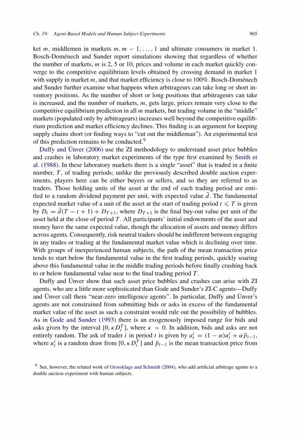
Ch. 19: Agent-Based Models and Human Subject Experiments 965
ket m, middlemen in markets m,m − 1, . . . , 1 and ultimate consumers in market 1.Bosch-Doménech and Sunder report simulations showing that regardless of whetherthe number of markets, m is 2, 5 or 10, prices and volume in each market quickly con-verge to the competitive equilibrium levels obtained by crossing demand in market 1with supply in market m, and that market efficiency is close to 100%. Bosch-Doménechand Sunder further examine what happens when arbitrageurs can take long or short in-ventory positions. As the number of short or long positions that arbitrageurs can takeis increased, and the number of markets, m, gets large, prices remain very close to thecompetitive equilibrium prediction in all m markets, but trading volume in the “middle”markets (populated only by arbitrageurs) increases well beyond the competitive equilib-rium prediction and market efficiency declines. This finding is an argument for keepingsupply chains short (or finding ways to “cut out the middleman”). An experimental testof this prediction remains to be conducted.9
Duffy and Ünver (2006) use the ZI methodology to understand asset price bubblesand crashes in laboratory market experiments of the type first examined by Smith etal. (1988). In these laboratory markets there is a single “asset” that is traded in a finitenumber, T , of trading periods; unlike the previously described double auction exper-iments, players here can be either buyers or sellers, and so they are referred to astraders. Those holding units of the asset at the end of each trading period are enti-tled to a random dividend payment per unit, with expected value d. The fundamentalexpected market value of a unit of the asset at the start of trading period t � T is givenby Dt = d(T − t + 1) + DT +1, where DT +1 is the final buy-out value per unit of theasset held at the close of period T . All participants’ initial endowments of the asset andmoney have the same expected value, though the allocation of assets and money differsacross agents. Consequently, risk neutral traders should be indifferent between engagingin any trades or trading at the fundamental market value which is declining over time.With groups of inexperienced human subjects, the path of the mean transaction pricetends to start below the fundamental value in the first trading periods, quickly soaringabove this fundamental value in the middle trading periods before finally crashing backto or below fundamental value near to the final trading period T .
Duffy and Ünver show that such asset price bubbles and crashes can arise with ZIagents, who are a little more sophisticated than Gode and Sunder’s ZI-C agents—Duffyand Ünver call them “near-zero intelligence agents”. In particular, Duffy and Ünver’sagents are not constrained from submitting bids or asks in excess of the fundamentalmarket value of the asset as such a constraint would rule out the possibility of bubbles.As in Gode and Sunder (1993) there is an exogenously imposed range for bids andasks given by the interval [0, κDT
t ], where κ > 0. In addition, bids and asks are notentirely random. The ask of trader i in period t is given by ai
t = (1 − α)uit + αpt−1,
where uit is a random draw from [0, κDT
t ] and pt−1 is the mean transaction price from
9 See, however, the related work of Grossklags and Schmidt (2004), who add artificial arbitrage agents to adouble auction experiment with human subjects.
966 J. Duffy
the previous trading period; the weight given to the latter, α, if positive, introduces asimple herding effect, and further implies that ask prices must rise over the first fewperiods. A similar herding rule is used to determine bids. The random component tobids and asks serves to insure that some transactions take place. As in Gode and Sunder(1993) budget constraints are enforced; traders cannot sell units they do not own, norcan traders submit bids in excess of their available cash balances. Finally, to accountfor the finite horizon, which was known to the human subjects, Duffy and Ünver endowtheir artificial agents with some weak foresight; specifically, the probability that a tradersubmits a bid (as opposed to an ask) is initially 0.5, and decreases over time, so, overtime, there are more asks than bids being submitted reflecting the declining fundamentalvalue of the asset. Standard double auction trading rules are in effect. Duffy and Ünveruse a simulated method of moments procedure to calibrate the parameter choices oftheir model, e.g. κ , α, so as to minimize the mean squared deviations between the priceand volume path of their simulated economies and the human subject markets of Smithet al. (1988). They are able to find calibrations that yield asset price bubbles and crashescomparable to those observed in the laboratory experiments and are able to match other,more subtle features of the data as well.
2.5. ZI agents in general equilibrium
The original Gode and Sunder (1993) study follows the Smith (1962) partial equilibriumlaboratory design, where market demand and supply are exogenously given. In more re-cent work, zero-intelligence traders have been placed in general equilibrium settings,with the aim of exploring whether they might achieve competitive equilibrium in suchenvironments. Gode et al. (2000) placed zero-intelligence traders, who could both buyand sell, in a two-good, pure exchange economy (an Edgeworth box). Traders are di-vided up into two types i = 1, 2, that differ only in terms of the parameters of theirCobb–Douglas utility function defined over the two goods and their initial endowmentsof these two goods. The trading rules for ZI agents in the general equilibrium environ-ment are similar to rules found in the partial equilibrium environment. In particular, inthe general equilibrium environment, ZI agents’s bids and asks are limited to utility im-proving allocations. Specifically, each agent of type i begins by calculating the slope ofits indifference map at its current endowment point. The slope is calculated in terms ofradians, r , where 0 � r � π
2 ; this gives the number of units of good y the trader is will-ing to give up per unit of good x. Next, the agent picks two random numbers, b ∈ [0, r]and a ∈ [r, π/2], with the first representing its bid price for units of good y in terms ofgood x, and the second representing its ask price for units of good y in terms of good x.Finally, the unit of a transaction for simulation purposes involves a discrete step sizein the quantity of both goods; otherwise, with an infinitesimal quantity exchanged eachperiod, convergence could take a long time. A consequence of this discrete step sizeassumption is that an adjustment has to be made to the bid and ask ranges to account forthe curvature of the indifference map. Given these trading restrictions, and the doubleauction rules, market transactions will be limited to lie in the set of Pareto improving re-
Ch. 19: Agent-Based Models and Human Subject Experiments 967
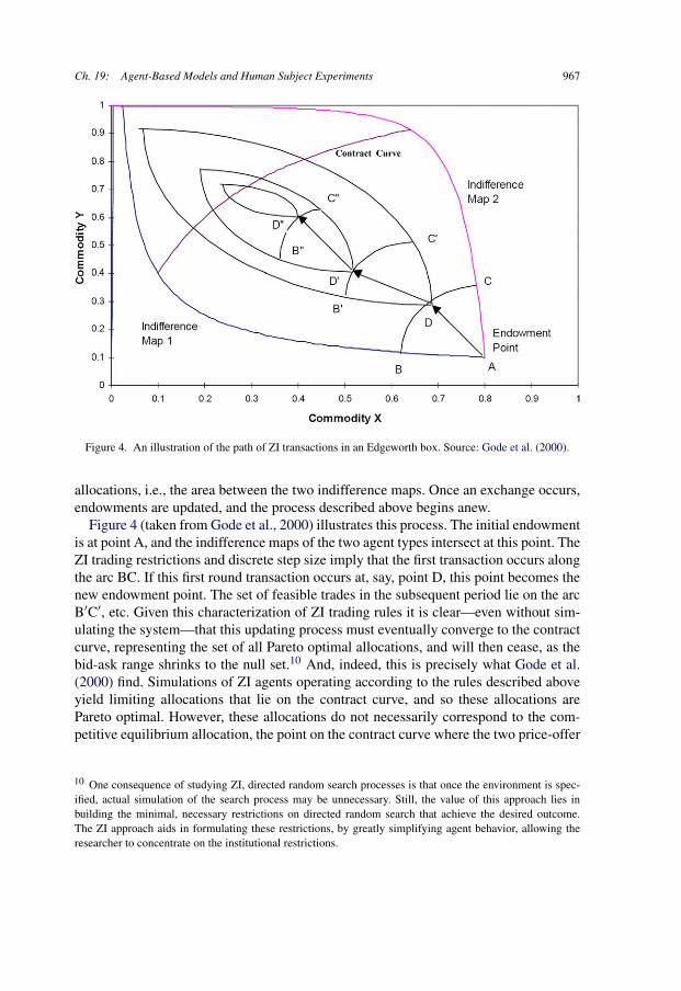
Figure 4. An illustration of the path of ZI transactions in an Edgeworth box. Source: Gode et al. (2000).
allocations, i.e., the area between the two indifference maps. Once an exchange occurs,endowments are updated, and the process described above begins anew.
Figure 4 (taken from Gode et al., 2000) illustrates this process. The initial endowmentis at point A, and the indifference maps of the two agent types intersect at this point. TheZI trading restrictions and discrete step size imply that the first transaction occurs alongthe arc BC. If this first round transaction occurs at, say, point D, this point becomes thenew endowment point. The set of feasible trades in the subsequent period lie on the arcB′C′, etc. Given this characterization of ZI trading rules it is clear—even without sim-ulating the system—that this updating process must eventually converge to the contractcurve, representing the set of all Pareto optimal allocations, and will then cease, as thebid-ask range shrinks to the null set.10 And, indeed, this is precisely what Gode et al.(2000) find. Simulations of ZI agents operating according to the rules described aboveyield limiting allocations that lie on the contract curve, and so these allocations arePareto optimal. However, these allocations do not necessarily correspond to the com-petitive equilibrium allocation, the point on the contract curve where the two price-offer
10 One consequence of studying ZI, directed random search processes is that once the environment is spec-ified, actual simulation of the search process may be unnecessary. Still, the value of this approach lies inbuilding the minimal, necessary restrictions on directed random search that achieve the desired outcome.The ZI approach aids in formulating these restrictions, by greatly simplifying agent behavior, allowing theresearcher to concentrate on the institutional restrictions.

968 J. Duffy
curves of the two agent types intersect. So, by contrast with the findings in the partialequilibrium framework, ZI-trading rules turn out to be insufficient to guarantee conver-gence to competitive equilibrium in the two-good general equilibrium environment.
The nonconvergence of the ZI algorithm to competitive equilibrium is further ad-dressed by Crockett, Spear and Sunder (CSS) (Crockett et al., 2004) who provide ananswer to the question of “how much additional ‘intelligence’ is required” for ZI agentsto find a competitive equilibrium in a general equilibrium setting with M agents and� commodities. In their environment, ZI agents do not submit bids or asks. Rather aproposed allocation of the � goods across the M agents is repeatedly made, correspond-ing to a random draw from an epsilon-cube centered at the current endowment point.Agent i compares the utility he gets from the proposed allocation with the utility he re-ceives from the current endowment. If the utility from the proposed allocation is higher,agent i is willing to accept the proposal. If all M agents accept the proposal, the pro-posed allocation becomes the new endowment point. The random proposal generationprocess (directed search) then begins anew and continues until no further utility im-provements are achieved. At this point the economy has reached a near-Pareto optimum(an allocation that lies approximately in the Pareto set), though not necessarily a com-petitive equilibrium; this outcome is analogous to the final outcome of the Gode et al.(2000) algorithm. Crockett, Spear and Sunder further assume that once agents havereached this approximate Pareto optimum (PO), they are able to calculate the common,normalized utility gradient at the PO allocation. The ZI agents are then able to deter-mine whether this gradient passes through their initial endowment point (the conditionfor a competitive equilibrium) or not. If it does not, then, in the PO allocation, someagents are subsidizing other agents. Note that these assumptions endow the ZI agentswith some calculation and recall abilities that are not provided (or necessary) in Godeand Sunder’s partial equilibrium environment.
Consider for example, the two agent, two-good case. In this case, the normalizedutility gradient corresponds to a price line through the tangency point of the two indif-ference curves (preferences must be convex), representing the relative price of good 2in units of good 1 at the PO allocation. Suppose that at the end of trading period t , agenti’s approximate PO allocation is xt
i ∈ R2+. Agent i’s gain at this PO allocation can bewritten as:
λti = pt
(xti − ωi
),
where pt is the price line at the end of period t and ωi ∈ R2+ is agent i’s initial endow-ment. Agent i is said to be subsidizing the other agent(s) if λi < 0. That is, at pt � 0,agent i cannot afford to purchase his initial endowment. Crockett et al.’s innovation isto imagine that if agent i was a ‘subsidizer’ in trading period t , then in trading periodt + 1 he agrees to trade for only those allocations, xt+1 that increase his utility and thatsatisfy:
0 � pt(xt+1i − ωi
)� λt
i + νi,
Ch. 19: Agent-Based Models and Human Subject Experiments 969
where νi is a small, positive bound. With this additional constraint in place, the POallocation achieved at the end of period t + 1, xt+1, is associated with a larger gainfor the subsidizing agent i, i.e. λt+1
i > λti , so he subsidizes less in period t + 1 than
in period t . When all i agents’ gains satisfy a certain tolerance condition, convergenceto a competitive equilibrium is declared. Crockett et al. show that while cycling is apossibility, it can only be a transitory phenomenon. Indeed, they provide a rigorousproof that their algorithm converges to the competitive equilibrium with probability 1.
This subsidization constraint puts to work the Second Welfare theorem—that everyPareto optimum is a competitive equilibrium for some reallocation of initial endow-ments. Here, of course, the initial endowment is not being reallocated. Instead, agentsare learning over time to demand more (i.e. refuse trades that violate the subsidizationconstraint) if they have been subsidizing other agents in previous periods. The realloca-tion takes place in the amounts that agents agree to exchange with one another.
The appeal of Crockett et al.’s “ε-intelligent” learning algorithm is that it imple-ments competitive equilibrium using only decentralized knowledge on the part of agenti, who only needs to know his own utility function and be able to calculate the nor-malized utility gradient at the PO allocation attained at the end of the previous period(or more simply, to observe immediate past prices). Using this information, he deter-mines whether or not he was a subsidizer, and if so, he must abide by the subsidizationconstraint in the following period. The algorithm is simple enough so that one mightexpect that simulations of it would serve as a kind of lower bound on the speed withwhich agents actually learn competitive equilibrium in multi-good, multi-agent generalequilibrium environments, analogous to Gode and Sunder’s (1993) claim for ZI agentsoperating in the double auction.
Indeed, Crockett (2004) has conducted an experiment with paid human subjectsaimed precisely at testing this hypothesis. Crocket’s experiment brings the ZI researchagenda full circle; his experiment with human subjects is designed to provide externalvalidity for a ZI, agent-based algorithm whereas the original Gode and Sunder (1993)ZI model was developed to better comprehend the ability of human subjects to achievecompetitive equilibrium in Smith’s double auction model. Crockett’s study explores sev-eral different experimental treatments that vary in the number of subjects per economyand in the parameters of the CES utility function defined over the two goods. For eachsubject, a preference function was induced, and subjects were trained in their inducedutility function, i.e., how to assess whether a proposed allocation was utility improving.Further, at the end of each trading period, Crocket calculated for subjects the end-of-period-t marginal rate of substitution, pt , as well as the value of the end-of-period-tallocation, ptxi , but did not tell subjects what to do with that information, which re-mained on subjects’ screens for the duration of the following period, t + 1. Subjectscould plot the end-of-period-t price line on their screens to determine whether or notit passed through their beginning-of-period-t endowment point. Thus, subjects had allthe information necessary to behave in accordance with the CSS algorithm, that is, theyknew what comprised a utility improving trade and they had the information necessaryto construct and abide by the subsidization constraint.

970J.D
uffy
Figure 5. Median, end-of-period CSS-ZI allocations over periods 1–10 (left panel) versus median, end-of-period human subject allocations in periods 1 and 10(right panel) in an Edgeworth box.

Ch. 19: Agent-Based Models and Human Subject Experiments 971
The left panel of Figure 5 presents the median end-of-period allocation of CSS–ZIagents for a particular 2-player CES parameterization, over trading periods 1–10, de-picted in an Edgeworth box (the competitive equilibrium is labeled CE). The rightpanel of Figure 5 presents comparable median end-of-period allocations from one ofCrockett’s human subject sessions conducted in the same environment. Support for thehypothesis that the CSS-ZI algorithm accurately characterizes the behavior of paid hu-man subjects appears to be mixed. On the one hand, nearly all of the human subjectsare able to recognize and adopt utility improving trades, so that end of period alloca-tions typically lie on or very close to the contract curve. And, once the contract curve isachieved, in subsequent periods, the human subjects appear to be moving in the direc-tion of the competitive equilibrium allocation, as evidenced by the change in the medianallocation at the end of period 10 relative to the median at the end of period 1 in the rightpanel of Figure 5. On the other hand, simulations of the CSS–ZI algorithm (left panelof Figure 5) suggest that convergence to the competitive equilibrium should have beenachieved by period 6.
The reason for the slow convergence is that most, though not all subjects in Crockett’sexperiments are not abiding by the subsidization constraint; most are content to simplyaccept utility improving trades, while a few behave as CSS-ZI agents. The median al-location masks these differences, though the presence of some “CSS-ZI-type” agentsmoves the median allocation towards the competitive equilibrium. Hence, there is somesupport for the CSS-ZI algorithm, though convergence to competitive equilibrium bythe human subjects is far slower than predicted by the algorithm.
2.6. Summary
The ZI approach is a useful benchmark, agent-based model for assessing the marginalcontribution of institutional features and of human cognition in experimental settings.Building up agent-based models starting from zero memory and random action choicesseems quite sensible and is in accord with Axelrod’s KISS principle. Using ZI as abaseline, the researcher can ask: what is the minimal additional structure or restrictionson agent behavior that are necessary to achieve a certain goal such as near convergenceto a competitive equilibrium, or a better fit to human subject data.
Thus far, the ZI methodology has been largely restricted to understanding the processby which agents converge to competitive equilibrium in either the partial equilibriumdouble auction setting or in simple general equilibrium pure exchange economies. ZImodels have achieved some success in characterizing the behavior of human subjectsin these same environments. More complicated economic environments, e.g. produc-tion economies or labor search models would seem to be natural candidates for furtherapplications of the ZI approach.
The ZI approach is perhaps best suited to competitive environments, where individu-als are atomistic and, as a consequence, institutional features together with constraintson unprofitable trades will largely dictate the behavior that emerges. In environmentswhere agents have some strategic power, so that beliefs about the behavior of others

972 J. Duffy
become important, the ZI approach is less likely to be a useful modeling strategy. Insuch environments—typically game-theoretic—somewhat more sophisticated learningalgorithms may be called for. We turn our attention to such learning models in the nextsection.
3. Reinforcement and belief-based models of agent behavior
Whether agents learn or adapt depends on the importance of the problem or choice thatagents face. Assuming the problem commands agents’ attention, e.g., because payoffdifferences are sufficiently salient, the manner in which agents learn is largely a func-tion of the information they posses and of their cognitive abilities. If agents have littleinformation about their environment and/or they are relatively unsophisticated, then wemight expect simple, backward-looking adaptive processes to perform well as charac-terizations of learning behavior over time. On the other hand, if the environment isinformationally rich and/or agents are cognitively sophisticated, we might expect moresophisticated, even forward-looking learning behavior to be the norm.
This distinction leads to two broad sets of learning processes that have appeared inthe agent-based literature, which we refer to here as reinforcement and belief learningfollowing Selten (1991). Both learning processes are distinct from the fully rational,deductive reasoning processes that economists assign to the agents who populate theirmodels. The important difference is that both reinforcement and belief learning ap-proaches are decentralized, inductive, real-time, on-line learning algorithms that areunique to each agent’s history of play. In this sense, they comprise agent-based modelsof learning. Our purpose here is to discuss the use of these algorithms in the context ofthe experimental literature, with the particular aim of evaluating the empirical plausibil-ity of these learning processes.
3.1. Reinforcement learning
The hallmark of “reinforcement,” “stimulus–response” or “rote” learning is Thorndike’s(1911) ‘law of effect’: that actions or strategies that have yielded relatively higher(lower) payoffs in the past are more (less) likely to be played in the future. Rein-forcement learning involves an inductive discovery of these payoffs; actions that arenot chosen initially, are, in the absence of sufficient experimentation, less likely to beplayed over time, and may in fact, never be played (recognized). Finally, reinforcementlearning does not require any information about the play of other participants or even therecognition that the reinforcement learner may be participating in a market or playing agame with others in which strategic considerations might be important. Thus, reinforce-ment learning involves a very minimal level of rationality that is only somewhat greaterthan that possessed by ZI agents.
Reinforcement learning has a long history associated with behaviorist psychologists(such as B.F. Skinner), whose views dominated psychology from 1920 through the

Ch. 19: Agent-Based Models and Human Subject Experiments 973
1960s, until cognitive approaches gained ascendancy. Models of reinforcement learn-ing first appeared in the mathematical psychology literature, e.g. Bush and Mosteller(1955) and Suppes and Atkinson (1960). Reinforcement learning was not imported intoeconomics however, until very recently, perhaps owing to economists’ long-held scep-ticism toward psychological methods or of limited-rationality heuristics.11
Brian Arthur (1991, 1993) was among the first economists to suggest modeling agentbehavior using reinforcement-type learning algorithms and to calibrate the parametersof such learning models using data from human subject experiments. In his 1991 paper,Arthur asks whether it is possible to design a learning algorithm that mimics humanbehavior in a simple N -armed bandit problem. Toward this aim, Arthur used data froman individual-choice, psychology experiment—a 2-armed bandit problem—conductedby Laval Robillard four decades earlier in 1952–3 and reported in Bush and Mosteller(1955) to calibrate his model.12
In Arthur’s model, an agent assigns initial “strength” si0 to each of the i = 1, 2, . . . , N
possible actions. The probability of choosing action i in period t is then pit = si
t /Ct ,where Ct = ∑
i sit . Given that action i is chosen in period t , its strength is then updated:
si′t = si
t + φit , where φi
t � 0 is the payoff that action i earned in period t . Finally, all ofthe strengths, including the updated si′
t are renormalized so as to achieve a prespecifiedconstant value for the sum of strengths in period t : Ct = Ctν , where C and ν representthe two learning parameters. When ν = 0 (as in Arthur’s calibration) the speed oflearning is constant and equal to 1/C.
Arthur ‘calibrated’ his learning model to the experimental data by minimizing thesum of squared errors between simulations of the learning model (for different (C, ν)
combinations) and the human subject data over all experimental treatments, whichamounted to variations in the payoffs to the two arms of the bandit. He showed thatregardless of the treatment, the calibrated model tracked the experimental data ratherwell. In subsequent work, (e.g. the Santa Fe Artificial Stock Market (Arthur et al., 1997)discussed in LeBaron’s (LeBaron, 2006) chapter), Arthur and associates appear to havegiven up on the idea of calibrating individual learning rules to experimental data in fa-vor of model calibrations that yield aggregate data that are similar to relevant field data.Of course, for experimental economists, the relevant data remain those generated inthe laboratory, and so much of the subsequent development of reinforcement and othertypes of inductive, individual learning routines in economic settings has been with theaim of exploring experimental data.
Roth and Erev (1995) and Erev and Roth (1998) go beyond Arthur’s study of theindividual-choice, N -armed bandit problem and examine how well reinforcement learn-ing algorithms track experimental data across various different multi-player games that
11 An even earlier effort, due to Cross (1983), is discussed in Brenner’s (Brenner, 2006) chapter.12 Regarding the paucity at the time of available experimental data, Arthur (1991, pp. 355–356) wrote:“I would prefer to calibrate on more recent experiments but these have gone out of fashion among psy-chologists, and no recent more definitive results appear to be available.” Of course, economists have recentlytaken to conducting many such experiments.

974 J. Duffy
have been studied by experimental economists. The reinforcement model that Roth andErev (1995) develop is similar to Arthur’s, but there are some differences and importantmodifications that have mainly served to improve the fit of the model to experimentaldata. The general Roth–Erev model can be described as follows.
Suppose there are N actions/pure strategies. In round t , player i has a propensityqij (t) to play the j th pure strategy (propensities are equivalent to strengths in Arthur’smodel). Initial (round 1) propensities (among players in the same role) are equal,qij (1) = qik(1) for all available strategies j , k, and
∑j qij (1) = Si(1), where Si(1)
is an initial strength parameter, equal to a constant that is the same for all players,Si(1) = S(1); the higher (lower) is S(1) the slower (faster) is learning.
The probability that agent i plays strategy j in period t is made according to the linearchoice rule:
pij (t) = qij (t)∑nj=1 qij (t)
.
Some researchers prefer to work with the exponential choice rule:
pij (t) = exp[λqij (t)]∑nj=1 exp[λqij (t)] ,
where λ is an additional parameter that measures the sensitivity of probabilities to rein-forcements. For now, however, we follow Roth and Erev (1995) and focus on the linearchoice rule.
Suppose that, in round t , player i plays strategy k and receives a payoff of x. LetR(x) = x −xmin, where xmin is the smallest possible payoff. Then i updates his propen-sity to play action j according to the rule:
qij (t + 1) = (1 − φ)qij (t) + Ek
(j, R(x)
),
Ek
(j, R(x)
) ={
(1 − ε)R(x) if j = k,(ε/(N − 1)
)R(x) otherwise.
This is a three-parameter learning model, where the parameters are (1) the initialstrength parameter, S(1), (2) a forgetting parameter φ that gradually reduces the roleof past experience, and (3) an experimentation parameter ε that allows for some exper-imentation.13 Notice that if φ = ε = 0 we have a version of Arthur’s model, where themain difference is that the sum of the propensities is not being renormalized in everyperiod to equal a fixed constant. This difference is important, as it implies that as thepropensities grow, so too will the denominator in the linear choice rule and the impactof payoffs for the choice of strategies will become attenuated. Thus, one possibility is
13 In certain contexts, the range of strategies over which experimentation is allowed is restricted to thosestrategies that are local to strategy k; in this case, the parameter ε can be regarded also as a ‘generalization’parameter, as players generalize from their recent experience to similar strategies.

Ch. 19: Agent-Based Models and Human Subject Experiments 975
that certain strategies that earn relatively high payoffs initially get played more often,and over time, there is lock-in to these strategies; alternatively, the “learning curve” isinitially steep and then flattens out, properties that are consistent with the experimentalpsychology literature (Blackburn’s (1936) “Power Law of Practice”).
The ability of reinforcement learning models to track or predict data from human sub-ject experiments has been the subject of a large and growing literature. Roth and Erev(1995) compare the performance of various versions of their reinforcement learningmodel with experimental data from three different sequential games: a market game, abest-shot/weakest link game and the ultimatum bargaining game; in all of these games,the unique subgame perfect equilibrium calls for one player to capture all or nearly allof the gains, though the experimental evidence is much more varied, with evidence ofconvergence to the perfect equilibrium in the case of the market and best-shot gamesbut not in the case of the ultimatum game. Roth and Erev’s simulations with their re-inforcement learning algorithm yield this same divergent result. Erev and Roth (1998)use simulations of two versions of their reinforcement model (a one parameter versionwhere φ = ε = 0) and the three parameter version to predict play in several repeatednormal form games where the unique Nash equilibrium is in mixed strategies. They re-port that the one and three-parameter models are better at predicting experimental dataas compared with the Nash equilibrium point predictions, and that the three-parametermodel even outperforms a version of fictitious play (discussed in the next section).
Figure 6 provides an illustration of the performance of the three models relative tohuman subject data from a simple matching pennies experiment conducted by Ochs(1995). This game is of the form
Player 2A2 B2
Player 1 A1 x, 0 0, 1B1 0, 1 1, 0
where x is a payoff parameter that takes on different values in three treatments (x = 1,4 or 9). The unique mixed strategy equilibrium calls for player 1 to play A1 with prob-ability .5, and player 2 to play A2 with probability 1/(1 + x); these Nash equilibriumpoint predictions are illustrated in the figure, which shows results for the three differentversions of the game (according to the value of x). The data shown in Figure 6 are theaggregate frequencies with which the two players play actions A over repeated plays ofthe game. The first column gives the experimental data, columns 2–3 give the results ofthe 1 and 3 parameter reinforcement learning models, while column 4 gives the resultfrom a fictitious play-like learning model. The relatively better fit of the three-parametermodel is determined on the basis of the deviation of the path of the experimental datafrom the path of the simulated data. Erev and Roth suggest that the success of reinforce-ment learning in predicting experimental data over Nash equilibrium point predictionsis owing to the inductive, real-time nature of these algorithms as opposed to the de-ductive approach of game theory, with its assumptions of full rationality and commonknowledge.

976 J. Duffy
Figure 6. Experimental data from Ochs (1995) and the predictions of the Roth–Erev and fictitious play learn-ing models. Source: Erev and Roth (1998).
Other variants of reinforcement learning have been proposed with the aim of bet-ter explaining experimental data. Sarin and Vahid (1999, 2001), for instance, proposea simple deterministic reinforcement-type model where agents have “subjective assess-ments,” qj (t), for each of the j = 1, 2, . . . , N possible strategies. As in Roth and Erev’smodel, an agent’s subjective assessment of strategy j gets updated only when strategyj is played: qj (t + 1) = (1 − φ)qj (t) + φπj (t), where πj (t) is the payoff to strategy j
at time t , and φ is the forgetting factor and sole parameter of their model. The maindifference between Sarin and Vahid’s model and Roth and Erev’s is that the strategyan agent chooses at time t in Sarin and Vahid’s model is the strategy with the maxi-mum subjective assessment through period t − 1. Thus, in Sarin and Vahid’s model,agents are acting more like optimizers than in the probabilistic choice framework of

Ch. 19: Agent-Based Models and Human Subject Experiments 977
Roth and Erev. Sarin and Vahid show that their one parameter model often performswell and sometimes better than Roth and Erev’s 1 or 3-parameter, probabilistic choicereinforcement learning models in the same games that Erev and Roth (1998) explore.
Duffy and Feltovich (1999) modify Roth and Erev’s (Roth and Erev, 1995) modelto capture the possibility that agents learn not only from their own experience, but alsofrom the experience of other agents. Specifically, they imagine an environment whereagent i plays a strategy r and learns his payoff in period t , πi
r (t) but also observes thestrategy s played by another player j (of the same type as i) in period t and the payoffthat player earned from playing strategy s, π
js (t). Player i updates his propensity to
play strategy r in the same manner as Roth and Erev, (with φ = ε = 0) but also updateshis propensity to play strategy s: qi
s(t + 1) = qis(t) + βπ
js (t), where β � 0 is the
weight given to observed payoffs, or “second-hand” experience. Duffy and Feltovichset β = .50 and simulate behavior in two of the games studied in Roth and Erev (1995),the best-shot game and the ultimatum game. They then test their simulation predictionsby conducting an experiment with human subjects; their reinforcement-based modelof the effect of observation of others provides a very good prediction of the role thatobservation of others’ actions and payoffs plays in the experiment.
Another modification of reinforcement learning is to suppose that agents have cer-tain “aspiration levels” in payoff terms that they are trying to achieve. This idea has along history in economics dating back to Simon’s (Simon, 1955) notion of satisficing.Aspiration learning has recently been resuscitated in game theory, e.g. by Karandikaret al. (1998) and Börgers and Sarin (2000) among others. Bendor et al. (2001) providean overview and additional references. The reinforcement learning models discussedabove can be viewed as ones where a player’s period aspiration level is constant andless than or equal to the minimum payoff a player earns from playing any action inthe given strategy set, so that the aspiration level plays no role in learning behavior.More generally, one might imagine that an agent’s aspiration level evolves along withthe agent’s probabilistic choice of strategies (or propensities), and this aspiration levellies above the minimum possible payoff. Thus, in aspiration-based reinforcement learn-ing models, the state space is enlarged to include a player’s aspiration level in period t ,ai(t). Suppose player i chooses strategy j in period t yielding a payoff of πi
j (t). If
πij (t) � ai(t), then player i’s propensity to play strategy j in subsequent periods is
assumed to be (weakly) higher than before; precisely how this is modeled varies some-what in the literature, but the end result is the same: i’s probability of playing strategy j
satisfies pij (t +1) � pi
j (t). On the other hand, if πij (t) < ai(t), then pi
j (t +1) < pij (t).
Finally, aspirations evolve according to:
ait = λai
t + (1 − λ)πij (t),
where λ ∈ (0, 1). This adjustment rule captures the idea that aspirations vary with anagent’s history of play. The initial aspiration level a0 as with the initial probabilitiesfor choosing actions, are assumed to be exogenously given. Karandikar et al. (1998)also add a small noise term to the aspiration updating equation representing trembles.
978 J. Duffy
They show, for a class of 2 × 2 games that includes the prisoner’s dilemma, that if thesetrembles are small, and aspiration updating is slow (λ is close to 1) that in the long-run,both players are cooperating most of the time.
There is some experimental evidence in support of aspiration learning. Bereby-Meyerand Erev (1998) studied behavior in a binary choice game where the probabilities ofachieving a ‘success’ were exogenously fixed at 0.7 for choice 1 and 0.3 for choice 2.In one treatment, subject payoffs were set at 2 for a success and −2 for a failure, whilein another treatment, the payoffs were 4 for a success and 0 for a failure, amountingto an addition of 2 to the payoffs in the first case. They found that learning of theoptimal choice of strategies (choice 1) was significantly reduced when the payoffs were(4, 0) relative to the case where the payoffs were (2,−2). Erev et al. (1999) explainthis result by presenting an adjustable reference point reinforcement learning model. Inplace of the assumption that R(x) = x − xmin in the Roth–Erev model, they proposethat R(x, t) = x(t) − ρ(t), and let the reference point, ρ(t) be a weighted average ofthe past reference point and current payoffs, where the weights depend on the differencebetween the payoff and the reference point; if payoffs are highly variable relative to thereference point, learning is slower than if payoffs are less variable; this is simply anotherversion of aspiration learning. They report that this model tracks the difference in theexperimental findings rather well.
Huck et al. (2002) find evidence of aspiration learning in a laboratory oligopolyexperiment. They test the theoretical proposition that bilateral mergers in oligopolymarkets with n > 2 firms, homogeneous goods and constant returns to scale are un-profitable; the profit share of the merged firm, 1/n − 1 is less than the total share ofthe two firms prior to the merger 2/n (1/n each). In the experiment, n > 2 subjectsmake quantity decisions in a Cournot game and midway through a session, two of thesubjects combine decision-making as a merged firm. The authors report that, contraryto theory, the subjects in the role of the merged firm produce significantly more outputthan the other unmerged firms and come close to sustaining total profit levels they wouldhave achieved as unmerged firms. The authors argue that pre-merger aspiration-levelscause merged firms to increase output with the aim of maintaining total profits and theother firms acquiesce by reducing their output. They connect this finding with Cyertand March’s (1956) observation that oligopoly firms are guided by “an acceptable-levelprofit norm” that is a function of market history.
Varieties of reinforcement learning algorithms have become a mainstay of agent-based modeling, perhaps because they accord with Axelrod’s KISS principle. Otherattractive features are the low level of history-dependent rationality, and relatively fewparameters. Examples of the use of reinforcement learning in agent-based models arecommonplace. Epstein and Axtell (1996) use several variants of reinforcement learningin their Sugarscape model. Nicolaisen et al. (2001) use Roth–Erev-type reinforcementlearning to model buyer and seller price–quantity decisions in a computational model ofthe wholesale electricity market. Pemantle and Skyrms (2003) use reinforcement learn-ing to study how groups of players play games in endogenously formed social networks.Franke (2003) uses reinforcement learning to study Arthur’s (Arthur, 1994) El Farol Bar
Ch. 19: Agent-Based Models and Human Subject Experiments 979
problem; Kutschinski et al. (2003) use a reinforcement learning model to study buyersearch and seller price setting behavior in a competitive market with induced demandand supply schedules. Bendor et al. (2003) use a reinforcement learning model withendogenous aspirations to model voter turn-out. Finally, Erev and Barron (2003) applyreinforcement learning to cognitive strategies, e.g., loss avoidance, hill-climbing, ratherthan to the direct strategies available to agents in simple, repeated decision problems.
There is also a parallel and much more voluminous literature on reinforcement learn-ing in the machine learning literature. See, e.g., Kaelbling et al. (1996) and Sutton andBarto (1998) for surveys. A popular reinforcement learning model in this literature isQ-learning (Watkins, 1989), which is closely related to Bellman’s approach to dynamicprogramming, but differs from the latter in being much less informationally demanding,e.g. the agent need not know the period payoff or state transition functions. (See, e.g.,Mitchell, 1997 for a good introduction the topic.) Q-learning algorithms involve on-lineestimation of an evaluation function, denoted Q(s, a), representing the maximum ex-pected discounted sum of future payoffs the agent earns from taking action a in state s.Starting from some random initialization of values, estimation of the Q function oc-curs in real-time using the history of states and payoffs earned by the agent from actionchoices in those states. To determine the action chosen, a probabilistic choice rule isused: actions with higher Q-values for the given state s and the current approximationof the Q-function, are more likely to be chosen than actions with lower Q-values. Thus,the main difference between Q-learning and the reinforcement-learning models stud-ied by economists is that Q-learners are learning an evaluation function mapping fromstates to actions, analogous to the policy function of dynamic programming. An advan-tage of Q-learning over reinforcement learning algorithms studied by economists is thatconvergence results for Q-learning can be proved under certain assumptions, e.g. forsimple Markov-decision processes. Surprisingly, the predictions of Q-learning modelshave yet to be compared with data from controlled laboratory experiments with humansubjects—a good topic for future research.
3.2. Belief-based learning
The primary difference between belief-based learning algorithms and reinforcementlearning algorithms is that in belief-learning models, players recognize they are play-ing a game or participating in a market with other players, and form beliefs about thelikely play of these other players. Their choice of strategy is then a best response totheir beliefs. By contrast, reinforcement learners do not form beliefs about other play-ers and need not even realize that they are playing a game or participating in a marketwith others. Belief-based learning models range from naive, Cournot-type learning toslightly more sophisticated “fictitious play,” to fully rational, Bayesian learning. Herewe discuss the first two types of belief learning models.
Fictitious play was proposed by Brown (1951) as a model of how players form beliefsand best respond to them in two-person zero sum games. Fictitious play was originallyproposed as a means of determining the value of a game; indeed, Robinson (1951) shows

980 J. Duffy
that fictitious play converges to equilibrium in 2 × 2 zero sum games, though Shapleyshows via a counterexample that this result does not hold in more general games. Sub-sequently, fictitious play has come to serve as a model of boundedly rational learning:players form beliefs about their opponents based on the historical frequency of theiropponent’s actions choices and play myopic best responses to these beliefs; the bestresponses are myopic because agents do not anticipate that their opponent is behavingsimilarly toward them.
Cheung and Friedman (1997) propose a one-parameter class of learning rules thatyields Cournot and fictitious play learning as special cases and thus serves to com-pactly illustrate the main difference between the two approaches. They suppose thereare i = 1, 2, . . . , N players, each of whom chooses an action ai from the set of possibleactions, A, in each period. Player i’s payoff function is π(ai, s
−i ), where s−i is a statevector representing the distribution of action choices chosen by all of i’s opponents. Itis assumed that each player i discounts past states using a constant discount factor, γi ,and possesses some initial prior, s−i (1). Player i’s belief about the state that will prevailin periods t = 1, 2, . . . is given by:
s−i (t + 1) = s−i (t) + ∑t−1k=1 γ k
i s−i (t − k)
1 + ∑t−1k=1 γ k
i
.
Cournot (naive) belief learning results from setting γi = 0 for all i; in this case,players hold the naive belief that s−i (t + 1) = s−i (t). Fictitious play belief learningresults from setting γi = 1 for all i; in this case, players’ beliefs about the current stateare simply the average of all past observed states. Weighted average, adaptive belieflearning results from setting 0 < γi < 1.14 Given beliefs, a player’s decision is tochoose ai ∈ A so as to maximize his expected payoff (i.e., maxai∈A π(ai, s
−i )).Consider by way of illustration, the class of 2 player, binary choice games that have
been widely studied in the experimental literature. Let the 2 × 2 payoff matrix be givenby M = (mij ), and let us assign a ‘1’ to the choice of action 1 and a ‘0’ to the choiceof action 2. With a single opponent per period, s−i (t) ∈ {0, 1} and s−i (t) ∈ [0, 1]represents player i’s belief about the likelihood that his opponent will play action 1 inperiod t .15 Player i evaluates the expected payoff differential from choosing action 1over action 2:
ri1 = R(s−i (t)
) = (1,−1)M(s−i (t), 1 − s−i (t)
)′.
A deterministic best response in the binary choice game is to choose action 1 ifR(s−i (t)) > 0 and to choose action 2 if R(s−i (t)) < 0. Some kind of tie-breakingrule is needed for the special case where R(s−i (t)) = 0. As Fudenberg and Levine
14 Other, less plausible possibilities include γ > 1, so that the past is given more weight than the present andγi < 0, which implies cycling.15 More generally, if player i faces up to n � N − 1 opponents in a binary action game, then s−i (t) =n−1 ∑n
j=1 I (aj ), where I (j) = 1 if aj = 1 and I (aj ) = 0 otherwise.

Ch. 19: Agent-Based Models and Human Subject Experiments 981
(1998) note, fictitious play (γ = 1) is a form of Bayesian learning in the special casewhere a player’s prior beliefs over the distribution of opponent strategies is Dirichlet.
As was the case under reinforcement learning, researchers examining the predictionsof Cournot or fictitious play belief learning have added some kind of noise to the de-terministic best response. Boylan and El-Gamal (1993) propose that agents play thedeterministic best response with probability 1 − ε, and any of the available actionsa ∈ A with probability ε/A.
Fudenberg and Levine (1998) propose a stochastic approximation to deterministicfictitious play—smooth fictitious play—which can be implemented, as in Cheung andFriedman (1997), through the use of the logistic function:
pij (t) = 1
1 + e−xi (t), where xi(t) = αi + βirij (t),
where αi is an individual specific fixed effect indicating individual i’s bias for actionj (αi = 0 reveals an unbiased choice) and βi representing the sensitivity of choices toexpected payoff differentials.
These stochastic versions of fictitious play have several advantages over deterministicfictitious play. First, they do not imply that behavior switches dramatically with smallchanges in the data agents use to form beliefs. Second, insisting that strategies remainprobabilistic has certain advantages, e.g., when agents have achieved near convergenceto a mixed strategy equilibrium and need to keep their opponent guessing even thoughthe differences in utility from the various actions may be quite small. (See Fudenbergand Levine, 1998 for a further discussion.)
Boylan and El-Gamal (1993) use a Bayesian approach to assess the likelihood thatbehavior in 9 different matrix game experiments (conducted by other researchers) isconsistent with either the noisy-Cournot or the noisy-fictitious play hypothesis. Theyfind that for some games, the Cournot belief hypothesis is favored while for other gamesthe fictitious play hypothesis is favored. Their over all assessment of the relative validityof the two learning hypotheses is that fictitious play describes the experimental databetter than Cournot learning.
Cheung and Friedman (1997) estimate their three parameter model (α, β, γ ) on datafrom several different bimatrix games. Median estimates of α, β and γ are all signifi-cantly positive; the finding that γ > 0 rules out the Cournot belief hypothesis. Furtherthey report they can reject the hypothesis that γ = 1 (fictitious play). Indeed, their esti-mates of γ always lie between 0 and 1 indicating that subjects’ belief updating processis neither Cournot or fictitious play, but is instead approximated best by some adaptiveintermediate case.
In addition to asking which belief-based learning model best predicts experimentaldata, one can also explore the empirical validity of the belief formation process as-sociated with these belief-based models. This can be simply accomplished by askingsubjects to state, prior to play of the game, their beliefs about their opponent’s play andcomparing these stated beliefs with those predicted by belief-based learning models.Nyarko and Schotter (2002) have carried out such an exercise in a simple 2 × 2 ma-trix game where the unique Nash equilibrium prediction is in mixed strategies. The two

982 J. Duffy
Figure 7. Stated versus fictitious play beliefs of a typical subject in Nyarko and Schotter’s experiment. Source:Nyarko and Schotter (2002, fig. 2).
strategies were labeled Green and Red, and the equilibrium calls on both players to playGreen (Red) with probability .4 (.6). Nyarko and Schotter asked subjects to state theprobability with which they thought their opponent would play Green prior to the playof each round. Subjects’ compensation was determined in part by the accuracy of theirstated beliefs and in part by the payoffs they received from playing the game.
Figure 7 plots stated beliefs against those predicted by fictitious play for a “typicalsubject” in Nyarko and Schotter’s experiment. As is apparent, the variance in subjectbeliefs is much greater than predicted by fictitious play, and the differences do not de-crease with experience. A similar difference is found in a comparison of the subjects’beliefs with Cournot beliefs. Nyarko and Schotter further conclude that best responsesto subjects’ stated beliefs provide a better account of the path of actions chosen by sub-jects than does reinforcement or a hybrid belief-reinforcement model discussed below.

Ch. 19: Agent-Based Models and Human Subject Experiments 983
This evidence suggests both that subjects are following some kind of belief-learningprocess and that a good model of that belief formation process has yet to be developed.
Belief-based learning models also make strong predictions regarding equilibriumselection in environments with multiple, Pareto rankable equilibria. Essentially, belief-based models predict that if the initial conditions lie in the domain of attraction of aparticular equilibria under the belief learning dynamic, then, with experience, agentswill learn over time to coordinate on that equilibrium, regardless of its efficiency. Thishypothesis has been experimentally tested by Van Huyck et al. (1997) and Battalio etal. (2001) in the context of simple coordination games where the domain of attractionof the two symmetric pure strategy equilibria is defined by the best response separatrix.Van Huyck et al. (1997) show that both Cournot and fictitious play learning dynamicspredict different equilibrium outcomes depending on initial conditions in a median ef-fort game (involving strategic complementarities), and their experimental findings areremarkably accurate on this score. If the initial condition (median effort) lies in the do-main of attraction of the unique, payoff-dominant equilibrium, subjects subsequentlycoordinate on that equilibrium, otherwise they coordinate on the other symmetric Nashequilibrium. As Van Huyck et al. point out, this behavior is very different from deduc-tive equilibrium selection principles, which might involve, for instance, calculation ofall equilibria and selection of the payoff dominant one.
The use of belief-based learning models by economists is not limited to normal formgames. Varieties of belief-based learning models have also been used to study bid andask behavior in the double auction.16 Gjerstad and Dickhaut (1998) provide a partic-ularly elegant characterization of the DA and propose heuristic rules by which buyersand sellers assess and update the probability that their bids or asks will be accepted,given market history. Using these beliefs together with private information on valua-tions and costs, individual buyers or sellers propose bids or asks that maximize their(myopic) expected surplus. The main parameter in their model is the length of memorythat players use in calculating probabilities. Using a stricter convergence criterion thanGode and Sunder adopt, Gjerstad and Dickhaut show via simulations that their heuristicbelief-learning model can more reliably achieve convergence to competitive equilibriumthan Gode and Sunder’s ZI-C model, and the belief-learning model provides a better fitto the aggregate human subject data as well. Indeed, in their chapter in this handbook,Mackie-Mason and Wellman (2006) argue that this heuristic belief-learning model rep-resents the best agent-based model of the DA. Still, the fit of this belief-learning modelto individual human subject behavior remains to be examined.
Belief-based learning models are less common in the agent-based literature than arereinforcement learning models, perhaps for the simple reason that belief-based modelsrequire that agents possess more memory (e.g. the histories of their opponents). Still,some versions of belief-based learning can be found see, e.g. Kandori et al. (1993),Young (1993, 1998); naive Cournot best response behavior is also found see, e.g. Ellison(1993) or Morris (2000).
16 Early efforts include Friedman (1991) and Easley and Ledyard (1993).

984 J. Duffy
3.3. Comparisons of reinforcement and belief-based learning
A large literature is devoted to testing whether simple reinforcement or more compli-cated belief-based learning algorithms better characterize experimental data from a widevariety of different games. In addition to the papers of Roth and Erev and Cheung andFriedman mentioned above, other papers comparing versions of these two approachesto learning include Mookherjee and Sopher (1994, 1997), Camerer and Ho (1999),Feltovich (2000), Salmon (2001), Blume et al. (2002), Stahl (1999) and Haruvy andStahl (2004) among others. In making these comparisons, researchers have adoptedsome kind of goodness-of-fit metric or made use of an econometric estimator to assessthe fit of various candidate learning models to experimental data.
The findings from this literature are varied, but several conclusions appear to havewide support. First, the evidence is very strong that either reinforcement or belief-basedlearning models are better predictors of human subject behavior than are the static Nashequilibrium point predictions. This is strong evidence in favor of the bottom-up, in-ductive reasoning approaches used by ACE researchers as opposed to the top-down,forward-looking, deductive reasoning of fully rational players that gives rise to thoseequilibrium point predictions. Second, in the simple games that experimentalists havestudied, reinforcement and belief-based learning models do not yield predictions thatare all that distinct from one another and so identifying which rule performs well acrossa variety of different games leads to murky outcomes that appear sensitive to variousparticulars of the datasets or games examined (Feltovich, 2000; Salmon, 2001). Giventhe lack of a clear bias in favor of reinforcement or belief-based approaches over a widevariety of games, a natural approach is to adopt a hybrid model that allows for bothreinforcement and belief-based learning as special cases, as well as mixtures of both.The hybrid modelling approach is taken e.g., by Camerer and Ho (1999), and discussedin Brenner’s (Brenner, 2006) chapter. While this approach has had some success inexplaining data from human subject experiments (see Camerer, 2003 for an extensiveand detailed assessment), the additional complexity of such models, e.g., more parame-ters to calibrate, may make this approach less appealing to ACE researchers.17 Third,there is some evidence that if subjects’ information is restricted to their own historiesof play, that reinforcement learning models perform slightly better than belief-basedlearning models that use data on opponent’s histories that was unavailable to subjects.Analogously, in environments where data on opponent’s histories was made available,players appear to condition their expectations, in part, on those histories, in line withthe predictions of belief-based models (Blume et al., 2002). These findings are not sosurprising, and, indeed, simply confirm that players use histories to form expectations.Finally, there is some evidence that the complexity of the game, the manner in whichplayers are matched and the length of play are all important factors in the accuracy oflearning models in predicting the play of human subjects.
17 See, however, a simpler, one-parameter version of their model given in Ho et al. (2002).
Ch. 19: Agent-Based Models and Human Subject Experiments 985
On the latter point, much of the observed differences in the two approaches to mod-eling learning may be tied up with the relatively small periods of time over whichindividual human subject experiments are conducted. While experimentalists often givetheir subjects repeated experience with a game or decision, concerns about subject bore-dom or the salience of participation payments severely restrict the length of the timeseries that can be generated in the laboratory for any individual subject. By contrast,ACE researchers do not feel bound by such considerations, and think nothing of sim-ulating their models out for very long periods of time. Asymptotically, the behavior ofreinforcement and belief-based models may not be all that different. Hopkins (2002)shows that both reinforcement learning and stochastic fictitious play can be viewedas noisy versions of replicator dynamics (discussed later in Section 4.1), and that theasymptotic predictions of these two models may be the same; roughly speaking if anequilibrium is locally stable under stochastic fictitious play, then the same holds trueunder reinforcement learning. Duffy and Hopkins (2005) conduct experiments with alonger than typical number of repetitions under various information conditions in aneffort to test this prediction and find that it has some, qualified support. An implicationof these findings for ACE researchers is that the kind of learning rule that agents areendowed with may not be of such great importance if the research interest lies in thelong-run behavior of the agent-based system.
3.4. Summary
Unlike ZI agent models, reinforcement and belief-based learning models presume thatagents have some memory. These models of inductive reasoning have been primarilystudied in the context of simple two player games. Reinforcement learners conditiontheir actions on their own histories of play and abide by the principle that actions thathave yielded relatively high (low) payoffs in the past are more (less) likely to be playedin subsequent periods. Belief-based learning models assume that players have historydependent beliefs over the actions their opponents are likely to play, and they chooseactions that are myopic best responses to these beliefs. While there is no guarantee thateither type of learning model converges to an equilibrium, these models have neverthe-less proven useful in tracking the behavior of human subjects in controlled laboratorysettings.
Reinforcement learning models have been widely used in the agent-based literature,perhaps for the simple reason that they require only information on an individual’s ownhistory (payoffs and actions). In complex, multi-agent settings, this parsimony of infor-mation may be an important consideration in the modeling of agent learning. On theother hand, in settings with just a few agents, and especially in settings where agentsinteract with one another repeatedly, a belief-based learning approach may be more ap-propriate. Indeed, the available experimental evidence suggests that agents do conditiontheir actions on both their own history of play and, when available, on information aboutthe play of their opponents. However, the manner in which they do this does not appear

986 J. Duffy
to be strictly consistent with either reinforcement or belief-based learning models. As-ymptotically, there may be little difference between the two approaches.
4. Evolutionary algorithms as models of agent behavior
In addition to directed random (ZI-agent) searches and individual learning approaches,agent-based researchers have used a variety of different evolutionary algorithms tocharacterize the behavior of populations of heterogenous, interacting, boundedly ratio-nal agents facing various economic decisions. Examples include replicator dynamics,genetic algorithms, classifier systems and genetic programming. These evolutionaryalgorithms differ from the learning processes considered so far in several respects.First, evolutionary algorithms were designed to mimic naturally occurring, biologicalprocesses. Not surprisingly, these algorithms can be difficult for social scientists to in-terpret and for experimentalists to test in the laboratory. Second, these methods arepopulation-based, which is to say that the fitness of a particular individual or strategy(the distinction becomes blurred in this literature) is based on its performance relativeto a certain population of individuals (or strategies). Thus, these algorithms presumethat fitness values across individuals/strategies are readily and immediately availablefor comparison purposes; in this regard, they can be viewed as the most complex classof algorithms (or least decentralized) in the set of approaches considered in this chapter.Third, as with ZI or reinforcement learning, evolutionary algorithms are not belief-based; players are not aware that they are playing a game against other players anddo not act strategically in any way. Fourth, some evolutionary algorithms, e.g., geneticalgorithms and genetic programming, are employed in environments where strategiesor equilibrium policy functions cannot be characterized analytically. This (alternative)use of evolutionary algorithms is owing to the performance of these algorithms as func-tion optimizers in complex landscapes; indeed, genetic algorithms were developed forprecisely this purpose. Finally, evolutionary algorithms may or may not be well-suitedto modeling economic decision-making. Evolution is often a slow process and so algo-rithms that mimic this process tend to work best on an unchanging landscape. However,economic systems are often modeled as state dependent, and may also be subject totemporary shocks or more permanent structural shifts. In such environments, the perfor-mance of evolutionary algorithms may be degraded relative to the less volatile (natural)landscapes for which they were developed.
Despite these potential problems and shortcomings, evolutionary algorithms arewidely used by agent-based modelers. By contrast with the other agent-based ap-proaches we have discussed, evolutionary algorithms have not been developed oradapted to explain data from economic decision-making experiments. For the most part,the opposite has occurred; agent-based researchers have sought to validate the predic-tions of evolutionary algorithms by conducting experiments with human subjects placedin the same environments. In certain cases, the experimental environment has been mod-ified to better approximate the evolutionary environment! These comparisons have met

Ch. 19: Agent-Based Models and Human Subject Experiments 987
with some success, but as I will argue, some difficulties of interpretation remain, forexample, the question of the appropriate time-frame for comparisons. It may simply bethat evolutionary algorithms cannot be adequately tested using human subject experi-ments.
4.1. Replicator dynamics
Replicator dynamics comprise the simplest class of evolutionary algorithms that econo-mists have used to model the behavior of populations of players. See Hofbauer andSigmund (1988, 1998) for a complete treatment. These models presume that the set ofstrategies (or phenotypes) does not evolve, and that reproduction is asexual. The as-sumption of a small strategy space is most likely to be satisfied in simple games, andso it is not surprising that replicator dynamics have mainly been employed by gametheorists.
To understand how replicator dynamics work, consider a game with N strategies, andlet s(t) ≡ (si(t))i=1,2,...,N be a vector representing the proportions of the N strategiesin the population at time t ;
∑i si(t) = 1 for all t . The N × N payoff matrix M = (mij )
here represents the payoff earned by each strategy in the population when matchedagainst every other strategy, including itself. For illustration purposes, we focus herein the simplest case where M is symmetric, known as the one-population model. Thefitness of strategy i at time t is given by Mis(t), where Mi denotes the row of the payoffmatrix corresponding to strategy i. The idea of assessing how a strategy fares against theentire population of strategies is what Maynard Smith termed “playing the field.” Thedeterministic replicator dynamic posits that strategy i’s representation in the populationbe updated as follows:
si(t + 1) = si(t)Mis(t)
s′(t)Ms(t),
where the denominator can be interpreted as the average fitness level in the entire pop-ulation of strategies, including strategy i. The idea of the replicator dynamic is thatstrategies with above average fitness see their proportion in the population increasewhile those with below average fitness see their proportion in the population decrease.Further, if s is a Nash equilibrium of the symmetric game M , then it is also a fixed pointof the replicator dynamic. In the deterministic version of the replicator dynamic, theproportion of certain strategies can go to zero, i.e., extinction is possible. A stochasticversion of replicator dynamics due to Foster and Young (1990) eliminates extinction,and can have quite different limiting dynamics than the deterministic version.
Friedman (1996) and Cheung and Friedman (1998) have examined the predictionsof replicator dynamics using data from human subject experiments. Friedman stud-ies the predictions of the replicator dynamic for equilibrium stability, and Cheung andFriedman compare replicator dynamic predictions with that of the individual, belief-based, stochastic fictitious play learning algorithm. Most of the games they study aretwo player, binary choice games with a unique Nash equilibrium in either mixed or

988 J. Duffy
pure strategies. In such games, the state, s(t)′ = (s1(t)), (1 − s1(t)), and the replicatordynamic for strategy s1 is written as:
�s1(t + 1)
s1(t)= β
[M1s(t) − s(t)′Ms(t)]s(t)′Ms(t)
,
where β > 0 represents an adjustment parameter, and �s1(t + 1) = s1(t + 1) − s1(t).Cheung and Friedman omit the denominator on the right hand side, s(t)′Ms(t), whichserves as a normalization device ensuring that proportions sum up to one; in the binarychoice case this device is unnecessary, and furthermore, Cheung and Friedman reportthat the unnormalized version fits the data better.
In their experimental design, these authors make some accommodation for the “play-ing the field” nature of the replicator dynamic; in their “mean matching” treatment,each player is matched against all other players, receiving the average payoff from hischoice of action against that of all others. The other matching treatment is the standard,random pairwise matching protocol. While game theory would treat these two environ-ments very differently, with the first corresponding to an n-player repeated game andthe second to a two-player, one-shot game, the only difference under the replicator dy-namic lies in the greater variance in payoffs that players receive in the random pairwisematching protocol. Friedman and Cheung and Friedman are careful to address issuesconcerning group size, the length of play of a single game, and of the information thatplayers receive, all of which are important to approximating the environment for whichthe replicator dynamic was devised.
Cheung and Friedman (1998) use experimental data from the two binary choicegames they study to estimate the linear equation:
�s1(t + 1)/s1(t) = α + β[M1s(t) − s(t)′Ms(t)
] + γ dt + ε,
where dt = I (t)[M1s(t) − s(t)′Ms(t)], I (t) = 1 if the mean matching treatmentwas used, and ε is an error term. They report that α is typically significantly differ-ent from zero, implying a persistent bias from the pure replicator dynamic, and thatβ is significantly positive as is γ . The latter finding suggests that the mean matchingprotocol aids in the speed of adjustment relative to random pairings. In a head-to-headcomparison of the explanatory power of the replicator dynamic versus an individual, be-lief learning model—the three parameter weighted fictitious play model of Cheung andFriedman (1997) described in Section 3.2—Cheung and Friedman report that over thetwo games they study, the belief learning model outperforms the replicator dynamic,where performance is measured by either the root mean squared errors or the meanabsolute deviations computed from the three parameter belief-learning or replicator dy-namic model.
This finding suggests that there is some value to thinking of human players as playingbest responses to beliefs about their opponents’ actions rather than thinking of themas playing a game against nature. On the other hand, it is less clear that Cheung andFriedman have successfully implemented the evolutionary game environment germaneto the use of replicator dynamics or that such an environment could be implemented

Ch. 19: Agent-Based Models and Human Subject Experiments 989
in the laboratory, where budget and time constraints limit the number of subjects andreplications of a treatment that are possible. Further work reconciling the replicatordynamic with human learning processes is needed.
4.2. Genetic algorithms
Genetic algorithms (GAs) have been widely used by economists to model learning bypopulations of heterogenous, adaptive agents especially following Sargent’s (Sargent,1993) encouraging assessment and the subsequent use of GAs by his student, JasminaArifovic. These algorithms differ from replicator dynamics in that they allow for thedevelopment of new strategies or decisions that may not have been included in theinitial population. As such, they are efficient sampling methods most appropriate tolarge decision or strategy spaces.
Indeed, genetic algorithms, originally developed by Holland (1975), are stochastic,directed search algorithms based on principles of population biology.18 These algo-rithms have been demonstrated to perform well in large or “rugged” search spaces whereclassical methods, e.g., grid search or gradient descent, are either inefficient or suscepti-ble to getting stuck at local optima. While there is wide variation in the specific details ofgenetic algorithms, there are some general principles and procedures that are regardedas relatively standard. First, the researcher must specify the objective function of thegenetic algorithm search, the parameter values that will be used to maximize (or mini-mize) that objective, and the range of admissible parameter values allowed in the searchfor an optimum. Second, vectors of parameters, representing candidate solutions areencoded as strings of finite length L. The strings are intended to mimic chromosomes,with the individual elements of a string representing genes; hence the name genetic al-gorithm. In the earliest implementation of genetic algorithms (e.g., Goldberg, 1989),parameters were encoded using the binary {0, 1} alphabet, and much of the theory ofgenetic algorithms as function optimizers is developed for binary encodings. However,more recently, researchers have made use of real-valued, character, or tree encodingsin place of traditional binary encodings. Researchers typically work with a populationof strings of some fixed size, N . Third, the performance of each string in the popula-tion is evaluated using the objective criterion—this is the string’s fitness. Fourth, a newgeneration of N strings is determined using operations that mimic natural selection andnaturally occurring biological processes.
The first step in a genetic algorithm, known as selection, is to randomly select N
strings from the existing population in such a way that the fitness of the N randomly se-lected strings is on average higher than the average fitness of the population from whichthey were chosen. This selection operation can be accomplished in many ways, includ-ing the biased roulette wheel selection mechanism originally proposed by Holland, in
18 For a complete treatment of genetic algorithms see, e.g., Goldberg (1989) or Michalewicz (1996). Dawid(1999a) provides a thorough discussion of genetic algorithms as applied to economic problems. See alsoSargent (1993) and Judd (1998).

990 J. Duffy
g = 0initialize population of N strings, P(0)while tolerance criterion remains unmet or g < G
evaluate fitness of strings in P(g)
select N strings for P(g + 1) based on relative fitnessapply crossover to selected stringsapply mutation to recombined stringsevaluate tolerance criteriong = g + 1end while
Figure 8. Pseudo-code for a genetic algorithm.
which the likelihood of selecting a string is proportional to its relative population-widefitness or other methods e.g. binary tournaments or rank order lists. The selection oper-ation is intended to mimic Darwinian survival-of-the-fittest. Once a new set of N stringshas been selected, these strings undergo two main biological operations that mimic ge-netic inheritance. The first, crossover, typically involves randomly pairing strings and,with some probability, pc, randomly cutting the two strings at one or more points andswapping elements. Once crossover is applied to all strings, a second operator, mutationis applied, which involves randomly changing each element in a string with a (small)probability pm, to some other value; in the case of binary strings, a ‘0’ is flipped to a‘1’ and vice versa. After these operations are complete, the new generation of N stringsis evaluated in fitness terms and the process of choosing a new generation begins again.The genetic algorithm is terminated after a set number of generations, G, or after sometolerance criterion based on the objective function has been satisfied. Some pseudo-codefor a genetic algorithm is given in Figure 8.
The main theoretical result for genetic algorithms is known as the schema theorem(Holland, 1975). The idea of a schema can be understood by the addition of a don’t carecharacter, *, to the binary alphabet that is typically used to encode strings. A schemais a template characterizing a set of chromosomes. For example, the schema of length5, (*101*) characterizes the set of chromosomes {(11011), (11010), (01011), (11010)}.The order of a schema is the number of fixed positions; e.g., the order of the schema inour example is 3. The schema theorem (proved, e.g. in Goldberg, 1989) states that low-order, above-average (below-average) schema appear exponentially more often (lessoften) in subsequent generations of a genetic algorithm. This theorem follows directlyfrom the operation of fitness-proportional selection. These low-order schema are some-times referred to as “building blocks.” Crossover plays the role of introducing newschemata and mutation also contributes to variability while at the same time preventingpremature convergence to local optima.
How are the genetic operators to be interpreted when applied to economic systems?Several authors, e.g., Arifovic (1996), Bullard and Duffy (1998), Dawid (1999a), Riech-mann (1999, 2001a, 2001b), have offered interpretations. One can think of the individual

Ch. 19: Agent-Based Models and Human Subject Experiments 991
strings as representing the strategies/decisions of individual agents, so that the GA ismade up of many interacting agents. Alternatively, one can imagine there is a singleagent with the individual strings of the GA representing different decisions/strategiesthat agent might adopt. The selection operation is perhaps the easiest to defend; thisoperator just insures that agents or decisions that have worked well in the past are morelikely to be chosen in the future while decisions that have fared poorly are more likelyto be discarded. This probabilistic choice of decisions based on relative payoff or fitnesssuccess is similar to stochastic reinforcement learning or stochastic replicator dynamics.The turnover of population need not be interpreted so literally as one of birth and death;instead it can be interpreted as a turnover of decisions or ideas among players who arelong-lived. The crossover/recombination operator is easiest to interpret if the popula-tion of strings is viewed as representing individual agents. In that case, crossover can bethought of as communication between pairs of agents, who exchange bits and piece ofideas, though the population as a whole retains core principles (low-order schema) thathave yielded high payoffs in the past. Finally, the mutation operator can be viewed asrepresenting trembles or experimentation.
A further issue concerns the choice of GA parameters: the number of strings, N , thestring length, the mutation and crossover parameters, pc, pm, etc. Here, the practice hasbeen to adopt parameterizations that computer scientists have found to perform well ontest suites of difficult static optimization problems. These optimization problems are notones that are so applicable to the dynamic settings studied by economists, and so furtherresearch into this issue would be of some value.
What about the external validity of simulations using genetic algorithms? Arifovic(1994) was the first to directly compare simulations of a genetic algorithm with thebehavior of human subjects in a controlled laboratory experiment.19 The economic en-vironment studied was a textbook version of Ezekiel’s (Ezekiel, 1938) “Cobweb” modelof demand and supply for a single good. In this model, market demand in period t is adecreasing, linear function of current period price, pt , while market supply in period t
is an increasing, linear function of the market price that suppliers expected in periodt − 1 would prevail in period t , Et−1pt ; the latter assumption captures the notion thatit takes time (one-period) to produce the good, and makes the model dynamic. Arifovicfollowed experimental researchers, Carlson (1968) and Wellford (1989), who adoptedEzekiel’s assumption of naive and homogeneous expectations, i.e. Et−1pt = pt−1 as abenchmark assumption for expectation formation; in that case, the equilibrium is stable(unstable) if the ratio of the slope of the supply curve to the slope of the demand curve,in absolute value, is less than (greater than) unity. Bray and Savin (1986) have shown ina stochastic version of the linear cobweb model that adaptive learners, running regres-sions of prices on past prices, can learn the equilibrium price level in the stable case but
19 Similarly, Axelrod (1987) sought to determine whether the human-submitted ‘tit-for-tat’ strategy that wonhis (Axelrod, 1984) prisoner’s dilemma tournament would emerge in a simulation exercise that used a geneticalgorithm to evolve strategies (it did).

992 J. Duffy
not in the unstable case.20 By contrast, a main finding of the experimental studies wasthat groups of subjects generally converged to a neighborhood of the unique equilibriumregardless of whether that equilibrium was stable or unstable under the naive expecta-tions assumption. However, the variance of quantities or prices was much greater andmore persistent in the unstable case as compared with the stable case.
Arifovic represented firms (suppliers) in two ways. In the single-population repre-sentation, each firm was represented as one of N = 30 strings in a single population.In the multiple population representation, each of the m firms is represented by a dif-ferent population of 30 strings. In both cases, each string in a population represents adecision as to how much a firm might produce in the current period, qi(t) ∈ [0, q],absent knowledge of the market price that will prevail. This decision was encoded as astring, of length 30, using a binary alphabet; initial ‘bit’ values were randomly deter-mined. The fitness criterion used was the firm’s current period profit; to evaluate fitness,strings had to be decoded to real quantities. In addition to using the standard genetic al-gorithm operations of selection, crossover and mutation on the binary strings, Arifovicadopted a fourth operator, which amounted to an augmented, elitist selection criterionwhich Arifovic called “election.” Following crossover and mutation, which yields twonew strings from two parent strings, the fitness of the new, offspring strings is evaluatedand compared with the fitness of the parent strings; of this group of four strings, the twostrings with the highest fitness values are allowed to enter the next generation of candi-date solutions. This election operator simply allows the genetic algorithm to converge,asymptotically to a solution; without it, mutations would lead to persistent heterogene-ity in the string population in the neighborhood of a solution. In the case of the singlepopulation representation, Arifovic reported the average value of q(t) in the populationof 30 strings; in the case of the multiple population simulation, Arifovic imagined thateach firm randomly chose one of its strings to determine its quantity decision in each pe-riod; she then reported the average of these m quantity decisions. In certain simulations,the model parameters were chosen to be the same as in one of Wellford’s treatments,including the number of periods, 30, and the number of firms, m = 5.
Figure 9 shows results for the unstable parameter case; the left panel shows theaverage quantity produced (with a 1-standard deviation band) for the human subject ex-periments and the right panel shows the same for a simulation of the multiple-populationversion of the genetic algorithm over the same number of periods. Both the human sub-jects and the genetic algorithm converges to a neighborhood of the equilibrium quantityof 14 though convergence takes longer and is more volatile in this ‘unstable case’ thanin the stable case (not shown). However, the average quantity in the GA simulation ap-pears to get very close to the equilibrium prediction beginning after period 10 while thesame cannot be said of the experimental data. However, consistent with the experimen-tal evidence, Arifovic is able to reject the null of no difference between the volatility
20 Hommes (1994) studies the more general case where demand is linear and supply is nonlinear. He providesconditions under which adaptive learning dynamics converge to limit cycles or chaos in the unstable case.Sonnemans et al. (2004) provide experimental evidence in support of Hommes’ predictions.

Ch.19:
Agent-B
asedM
odelsand
Hum
anSubjectE
xperiments
993
Figure 9. Average quantity in the Cobweb model, unstable case (plus/minus one st. dev.). Left panel: human subject data, right panel: multiple-population GAsimulation. Source: Arifovic (1994).

994 J. Duffy
of prices in the stable and unstable cases using the simulation data. These findings pro-vide some support for the reasonableness of genetic algorithms as models of adaptiveprocesses.
Several papers explore GA learning in general equilibrium, overlapping generationmodels of money, and compare the results with experimental findings. Arifovic (1996)studies exchange rate volatility in a two-country, two-currency, two-period overlap-ping generations model due to Kareken and Wallace (1981). Details of this model arediscussed in LeBaron’s (LeBaron, 2006) chapter. Arifovic’s main conclusion is that,counter to the theoretical prediction derived under the rational expectations assumption,under genetic algorithm learning, the exchange rate displays persistent volatility, whichis due to the persistence of mutation and the election operator.
By contrast, Arifovic (1995) shows that in a single country model, an equilibriumwith valued fiat currency and low inflation is asymptotically stable under GA learningwith persistent mutation and the election operator in place. The selection by the GA ofthe stationary, low inflation equilibrium, rather than another high inflation, stationaryequilibrium is consistent with the laboratory findings of Marimon and Sunder (1993).Other, homogeneous and non-evolutionary learning algorithms, such as recursive leastsquares learning, fail to converge to the same low inflation equilibrium (see, e.g., Marcetand Sargent, 1989).
In Arifovic’s work, the strings of the GA encode decisions that agents make, e.g.,how much to consume in the first period. The GA then works to find the optimal de-cision, given feasibility and budget constraints. In Marimon and Sunder’s (Marimonand Sunder, 1993, 1994) overlapping generation experiments, subjects were not askedto make consumption/savings decisions as pilot studies suggested that subjects had adifficult time solving that kind of intertemporal optimization problem. Instead, Mari-mon and Sunder asked subjects to provide forecasts of the price level they expectedwould prevail in the next period. Given a subject’s forecast, the computer programsolved that subject’s optimal consumption/savings allocation and determined marketclearing prices. Bullard and Duffy (1999) adopted this same learning-how-to-forecastdesign in a GA-learning simulation of the environment studied by Arifovic (1995). Theyimagine that agents have some belief about how prices in period t + 1 will be related toprices in period t , and the strings of the GA encode this belief. Given the price forecast,the program optimally determines each agent’s consumption/savings decision, alongwith market clearing prices. Bullard and Duffy (1999) show that this learning-how-to-forecast implementation of GA learning results in findings that are consistent with theexperimental evidence of Marimon and Sunder (1994) and also with Arifovic (1995)’slearning-how-to-optimize implementation of GA learning.
Several papers use GAs to understand findings from auction experiments. A difficultywith auctions is that participants frequently fail to win an item or agree to a transaction,so that the fitness of strategies may need to be assessed over a longer period of time thanis typical in other applications of GAs.
Andreoni and Miller (1995) use genetic algorithms as a way of studying how closepopulations of adaptive agents might come to learn equilibrium bid functions in a vari-

Ch. 19: Agent-Based Models and Human Subject Experiments 995
ety of auction formats: first and second price affiliated-values auctions, first and secondprice private-values auctions, and common value auctions. The design of their sim-ulation experiments is aligned with that of laboratory experiments with paid humansubjects in several dimensions, e.g., the number of bidders in a group and the informa-tion available to these bidders. However, their 20 simulation runs of 1000 generationsper auction format is more difficult to compare with the 20–30 auctions that human sub-jects participate in the typical experiment. In Andreoni and Miller’s implementation, thegenetic algorithm is employed to search over two parameters of a general linear biddingfunction of the form
b(xi) = βi1xi + βi2ε,
where xi is agent (string) i’s valuation and ε is some distribution parameter that variesaccording to the knowledge that agents are assumed to have, e.g., whether valuationsare private-independent, private-affiliated or common. This functional form nests (to anapproximation) all the equilibrium bid functions that are predicted to obtain in the var-ious auction formats. The binary strings of the GA encode the two parameters, β1 andβ2. For the standard GA implementation, Andreoni and Miller report that the GA sim-ulations come closest to learning the equilibrium bid functions in the affiliated privatevalue, first or second price auction formats and have more difficulty achieving the equi-librium bid functions in the independent-private and common value formats. Consistentwith evidence from human subject experiments, e.g. Cox et al. (1982), Kagel and Levin(1986), they find violations of revenue equivalence between first- and second-price auc-tion formats, and they find that smaller groups of 4 rather than 8 bidders are less proneto the winner’s curse in common value auctions.
Dawid (1999b) examines genetic algorithm learning in a sealed bid, double auctionmarket. The N buyers’ each have some value, v, from consuming a unit of the singlegood while the N sellers’ have some cost, c, of producing a unit of the good, and 1 >
v > c > 0. The strings of the GA encode the buyers’ bids and the sellers’ asks. In eachperiod, buyer and sellers are randomly paired. If a buyer’s bid, pb, exceeds a sellers’ask, pa , a transaction occurs at price p = (pa +pb)/2; otherwise no transaction occurs.Profits are determined in the usual way, v − p for buyers and p − c for sellers, andthe fitness of buyer/seller rules and application of genetic operators is assessed everym periods. Dawid shows analytically that the only locally stable equilibria under GAdynamics are those where all buyers (sellers) submit the same bid (ask) in the interval[v, c]. In 50 simulation runs where v = 1 and c = 0, he reports that the most commonoutcome is a single price equilibrium in a small neighborhood of .5. Interestingly, thisfinding is quite similar to that observed in an experiment conducted by Valley et al.(2002), where values of v and c are drawn randomly from [0, 1] and after learningthese values, pairs of players were allowed to communicate with one another prior tosubmitting bids/asks. The most common outcome, in cases where gains from trade arepossible (v > c), was for both buyer and seller to name the same price. While thisexperimental finding may not be so surprising, the fact that the GA simulation delivers

996 J. Duffy
this same finding, without any explicit communication between populations of buyersand sellers, is quite interesting.
Finally, there are several papers comparing GA simulations with experimental find-ings in labor markets. Pingle and Tesfatsion (2001) examine the impact of varying levelsof non-employment benefits on worker–employer matches and on-the-job cooperationusing data from both human subject experiments and computational experiments thatmake use of genetic algorithms. The environment studied is a repeated two-stage gamewhere in the first stage workers decide whether (and for which employer) to work orremain unemployed while employers decide whether to accept these offers or keepa position vacant. At the end of this first stage, unemployed workers and employerswith vacancies receive a fixed non-employment benefit while matched workers andemployers proceed to the second stage, which involves play of a prisoner’s dilemmagame, with strategies labeled ‘shirk’ and ‘don’t shirk.’ The single treatment variable wasthe size of the non-employment benefit. The human subject experiments revealed thatincreases in the non-employment benefit both decreased the frequency with which re-lationships formed, and the frequency of mutual cooperation between worker-employerpairs, though this effect was not monotonic. Further, long-term relationships betweenthe same worker and employer were rare. The computational labor market had fourtimes as many workers and employers as the human subject experiment and was simu-lated for a much longer period of time: 1000 generations. Each generation consisted ofsuccessive trade cycles followed by an evolutionary step that updated strategies; the ge-netic algorithm operates in the latter stage. A trade cycle consisted of both a matchingprocess, which utilizes a reinforcement learning algorithm to determine the expectedutility of potential partners, followed by a work-site interaction among matched play-ers. The work-site interaction was governed by a finite state automaton, and the geneticalgorithm was used to search for potentially better work-site rules in the evolution step.Among the findings from simulations of this model are that, consistent with the hu-man subject experiments, the frequency of employment relationships decreases withincreases in the non-employment benefit. On the other hand, by contrast with the humansubject findings, in the computational experiment, nearly all employers and workers endup in long-term fixed relationships, and either mutual cooperation or mutual defectionbecomes the norm, depending on initial conditions. The authors suggest that these dif-ferences may be owing to differences in the design of the two experiments, in particularthe different number of employers and workers in the computational versus the humansubject experiments appears to have played an important role in the outcomes, thoughthe different time-frames of analysis may also be a contributing factor.
Ünver (2001a) and Haruvy et al. (2002) use genetic algorithms to model the two-sided, worker-firm matching process in markets for medical intern and federal law clerksand compare these results with human subject experiments. These entry-level labor mar-kets as well as others, have been susceptible to a phenomenon known as unraveling, inwhich the date at which firms and workers agree to contracts becomes increasinglyearlier in time relative to the actual start-date of employment leading to possible inef-ficiencies in matches due to unavailability of relevant information. Some markets have

Ch. 19: Agent-Based Models and Human Subject Experiments 997
sought to address this problem by having centralized clearinghouses that match work-ers with firms. Ünver studies three centralized matching mechanisms used in Britishmedical-intern markets. Of these three, two are still in use, though only one of thesetwo is stable in the Gale and Shapley (1962) sense. Ünver uses a GA to encode andmodel the evolution of worker-firm strategies under these three mechanisms. Amongother findings, he shows that the theoretically unstable, “linear programming” matchingprotocol may not be susceptible to unraveling under the GA adaptation, which is con-sistent with the continued use of this mechanism in the field. He is able to corroborateother findings of two-sided matching experiments conducted by Kagel and Roth (2000)and Ünver (2001b) that explore the unraveling in the British medical intern markets.
Haruvy et al. (2002) conduct a parallel experiment with human subjects and withartificial agents modeled using a genetic algorithm with the aim of studying two-sidedmatching in the market for federal law clerks. Applicants initially decide whether tosubmit applications to judges of varying qualities, and judges may in turn accept of-fers. The grades of applicants, affecting the payoff from a match, are only fully revealedlater, during a centralized matching process. Matches not made by the end of the firsttwo periods (years) are, in certain treatments, subject to a centralized match in period 3using a stable matching protocol. In the ‘idealized-centralized’ treatment, applicants arenot required to submit offers prior to the centralized match in order to participate in it,while in the coerced-centralized treatment they are required to submit offers prior to thematch. In both cases, offers accepted prior to the centralized match date are binding,consistent with practice in this market, though in the idealized treatment, binding offerscan be avoided by waiting for the centralized match. In the human subject experiments,the authors report that many more subjects in the role of applicants and judges waitfor the centralized match under the ‘idealized-centralized’ treatment than do so underthe coerced-centralized treatment, and given the additional information that can be ob-tained by waiting, welfare is higher in the former treatment than in the latter. In geneticalgorithm simulations, where the strategies of applicants and judges co-evolve, a similarfinding obtains. Haruvy et al. are careful to compare their findings for human subjectexperiments over the same time-scale used in the genetic algorithm simulations. Theythen carry out the genetic algorithm simulation exercise much further in time, and findthat this difference becomes even more pronounced over time. This seems a reasonablemerger of the two technologies they use to understand these matching markets. As theyobserve (p. 3), “the computations will give us some assurance that our experimentalresults are not artifacts of slow learning in the laboratory, while experiments will as-sure us that the behavior produced by the genetic algorithms is in fact similar to humanbehavior.”
The findings from all of these studies provide some support for the reasonablenessof genetic algorithms as models of adaptive learning by populations of heterogenousagents. Genetic algorithms appear best suited for large, complex search spaces where itis more efficient to sample from the set of possible actions/strategies than to enumerateall possibilities and consider their relative fitness at every decision step. At the sametime, most of the studies treat the genetic algorithm as a kind of black box generator of

998 J. Duffy
new-and-improved decisions or strategies, without much regard to the interpretation ofgenetic operators, or how they compare with actual human decision-making processes.Toward this goal, it would be of interest to consider the marginal contribution of each ofthe genetic operators in explaining data from human subjects, an exercise akin to addingadditional structure to ZI-algorithms or moving from reinforcement to hypothetical re-inforcement (belief) learning models.
4.3. Comparisons between genetic algorithm and reinforcement learning
Two papers have compared the performance of genetic algorithm learning and reinforce-ment learning in terms of explaining data from human subject experiments. Haruvy andÜnver (2003) study matching behavior in procurement-type markets where the match-ing decision is consequential to both the seller and the buyer. They are interested in thequestion of whether buyers and sellers achieve a stable outcome, á la Gale and Shap-ley (1962) and if so, whether the stable matching is optimal for the party who initiatesa proposed match (buyers or sellers). As the strategy space in the repeated game theyconsider is highly complex, and there are multiple stable outcomes, deductive reason-ing is not very useful and so they turn to inductive reasoning processes, in particular,reinforcement learning and genetic algorithm learning, to predict what will happen inthe experiments they conduct with human subjects. Both the reinforcement and geneticalgorithm learning simulations predict that in seller- (buyer-) proposing markets, sellers(buyers) are most likely to achieve the seller- (buyer-) optimal stable outcome, and thisprediction is consistent with the experimental findings. Aside from the observation thatthe two learning models yield the same prediction however, Haruvy and Ünver do notgo into a deeper comparison of the performance of the two learning models.
By contrast, Arifovic and Ledyard (2004) look for a clear winner between reinforce-ment and genetic algorithm learning in the context of a repeated public good gamethat makes use of a Groves–Ledyard allocation mechanism. As the authors point out,this environment differs from those typically studied by learning researchers in that thestrategy space is continuous. They compare the predictions of an “individual evolu-tionary learning” model (a GA-without-crossover for each individual’s strategies) withRoth–Erev-style reinforcement learning and Camerer and Ho’s (Camerer and Ho, 1999)hybrid reinforcement-belief learning algorithm in terms of the fit of simulations of thesemodels to the experimental data. To facilitate a comparison, some discretization ofthe action space is necessary. They report that for two different ways of discretizingthe strategy space, reinforcement learning fares substantially worse than the other twolearning approaches in that it takes much longer to converge to the Nash equilibriumthan does the human subjects. However, the version of reinforcement learning they useis not as general as Roth and Erev allow. For instance, there is no forgetting factor noris there any spillover in the probability choice updating to nearby strategies. Given thelarge strategy space considered, it is not so surprising that the genetic algorithm appearsto perform best for the reasons noted above. However, before concluding in favor ofone approach over others, it would be useful to compare the predictions of evolutionary

Ch. 19: Agent-Based Models and Human Subject Experiments 999
and reinforcement-type learning models on a broad range of games including those withboth continuous and discrete strategy sets.
4.4. Classifier systems
Classifier systems, first proposed by Holland (1986), are inductive, rule-based learn-ing systems that combine reinforcement-type learning over a set of simple logical rulescalled classifiers, with occasional use of a genetic algorithm search for new classifiers.As with genetic algorithms, there are many variants, but a typical classifier system con-sists of four parts: 1) a set of if–then decision rules or classifiers, 2) an accountingsystem for assessing the strength of classifiers and for apportioning credit, 3) an auctionsystem for determining which classifiers are invoked and 4) a genetic algorithm for theintroduction of new classifiers. Classifier systems are perhaps best viewed as models ofindividual learning, akin to expert systems, while genetic algorithms, as typically mod-eled are often interpreted as models of population or social learning. As Vriend (2000)points out, simulations with classifier systems used to model social learning (mimicry)at the population level can yield outcomes that differ substantially from simulations withclassifier systems used to model learning at the level of individual agents, especially inenvironments where strategic considerations come into play.21
The first use of a classifier system (or a genetic algorithm) in an economic applicationwas due to Marimon et al. (1990), who used a classifier system to model behavior inKiyotaki and Wright’s (Kiyotaki and Wright, 1989) model of money as a medium ofexchange. That model has equal numbers of three types of agents who produce eithergood 1, 2 or 3, but who desire to consume another good, e.g. type 1 produces good 2,type 2 produces good 3, and type 3 produces good 1. Each agent may store a single unitof a good at a time, and the goods have different storage costs, with good 1 being theleast costly to store and good 3 being the most costly to store. Agents receive utilityfrom consumption of the good they desire in an amount that exceeds the highest stor-age cost. In each period, agents are randomly paired and decide whether to engage intrade with their match. Trades must be mutually agreed upon by both parties, in whichcase inventories of the two goods are swapped; otherwise, inventories of goods do notchange. Agents earn utility only when they trade for the good they desire; in that casethey immediately produce a new unit of their production good. In every period they in-cur storage costs based on the type of good they hold in inventory. The optimal tradingstrategy for a type 2 or 3 player is a fundamental, cost-reducing pure strategy in whichthey agree (refuse) to trade the good they hold in storage for less (more) costly-to-storegoods in route to getting the good they desire to consume. On the other hand, dependingon parameter values, type 1 players may find it optimal to adopt the fundamental strat-egy, or a speculative strategy in which they trade their production good 2 for the morecostly to store good 3 with the rational expectation that speculating in the more costlyto store good 3 will reduce the time it takes to acquire the good they desire, good 1.
21 For a further discussion of this issue see, e.g., Riechmann (2002) and Arifovic and Maschek (2004).

1000 J. Duffy
In Marimon et al.’s implementation, there are two classifier systems for every agent, aset of trade and consumption classifiers represented by strings. The trade classifier takesas input the good an agent has in storage and the good that his match has in storage, andprovides, as output, a decision (or message) of whether to trade or not. The consumptionclassifier takes as input the good a player has in storage and provides as output, a deci-sion (message) of whether or not to consume that good. Each classifier has a strength orfitness measure associated with it. In each period, the collection of classifiers that satisfythe current state for an agent, consisting of the good the agent holds in storage and thegood in storage of the matched player, bid a fraction of their current strengths in an auc-tion that determines which classifier the agent adopts; the highest bidding classifier ofeach type is chosen, its bid is deducted from its strength and its decision is implemented.The bid of the winning exchange classifier in the current period is paid to (added to thestrength of) the previous period’s winning consumption classifier, which determinedthe current good the agent holds in storage, while the bid of the winning consumptionclassifier is paid to the current period winning exchange classifier, which determine thegood the agent holds in storage. This payment system is what Holland termed a ‘bucketbrigade’ wherein classifiers that are not necessarily active in the current period, butwhich were critical for activating classifiers that were active can still earn some shareof credit and see their strengths improve. The current winning consumption classifierearns the ‘external’ payoff associated with its decision, which depends on whether thegood in storage is the desired good or not. Finally a genetic algorithm is called on, withsome decreasing frequency, to generate new classifiers, with the population of parentstrings being selected from the population of classifiers according to relative strengths.The set of strings resulting from the genetic operators are assigned the strengths of theparent strings.
In simulations of this system, Marimon et al. report many interesting findings, butthe main finding is that speculative trading strategies (e.g. by type 1 players) are notobserved in environments where, in equilibrium, they would comprise a unique bestresponse. Marimon et al. comment on this finding by observing that the behavior ofthe artificial agents, modeled using classifier systems, can be very myopic in the begin-ning, while it may take time for some optimal strategies, such as speculation, to achievestrengths that will sustain these strategies. They conclude that “the present algorithmseems defective in that it has too little experimentation to support the speculative equi-librium even in the long simulations we have run.” 22
Inspired by Marimon et al.’s simulation findings, Duffy and Ochs (1999, 2002) soughtto test the Kiyotaki–Wright model in a laboratory experiment. They made an effort toprovide subjects with all the information relevant to making optimal decisions in thetheoretical environment. Duffy and Ochs sought to induce a stationary infinite horizon,
22 Subsequent applications of classifier systems in economic applications, include Basçi (1999), Beltramettiet al. (1997) and Vriend (2000). LeBaron’s (LeBaron, 2006) chapter discusses the Santa Fe artificial stockmarket (Arthur et al., 1997) which makes use of a classifier system to model traders’ decisions. See Lettauand Uhlig (1999) for a comparison between classifier/rule learning and dynamic programming.

Ch. 19: Agent-Based Models and Human Subject Experiments 1001
as the theory presumes, by having an indefinite end to a sequence of pairwise trad-ing rounds. Such concerns with implementation of infinite horizons do not typicallyconcern agent-based modelers, as the artificial agents in their models are not typicallyforward-looking, alleviating concerns about backward induction due to end-game ef-fects. Finally, among the parameterizations they chose was one that was also used byMarimon et al. (1990). Though Duffy and Ochs had only 8 or 10 agents of each ofthe three types, while Marimon et al. had 50, the findings from the human subject ex-periments were quite similar to those obtained in the artificial agent simulations usingclassifier systems. In particular, Duffy and Ochs also find that subjects failed to adoptspeculative trading strategies in environments where such strategies comprise an equi-librium best response.23
Duffy (2001) considers two alterations of the Kiyotaki–Wright model that mightserve to promote the adoption of speculative strategies. In one version, agents whoseoptimal equilibrium strategy calls for speculation are given more encounters with sit-uations where playing the speculative strategy results in higher expected utility. In theother, two of the three agent types are constrained to playing the strategies that are op-timal for them in equilibrium. Duffy adopts a reinforcement learning model which issimilar to the exchange classifier of Marimon et al. (1990), automates the consumptionclassifier and gets rid of the genetic algorithm. A similar model was found to providea good fit to the experimental data of Duffy and Ochs (1999). Duffy uses this rein-forcement model to simulate what will happen in the two alternative environments, andreports that both alternatives speed up the learning of speculative strategies. However,the adoption of speculative strategies is greater in the second alternative, where twothirds of the agent types are constrained to playing optimal strategies. He then conductsan experiment with human subjects designed to test these same alternatives. In the hu-man subject experiment, the model parameters, the number of agents, and other featuresof the environment are kept as similar as possible to that of the simulated environmentsto facilitate comparisons. The human subject findings are largely consistent with theartificial agent findings. Duffy stresses that agent-based modeling exercises of this typecan be a useful tool for experimental design, and at the same time, the results of humansubject experiments might be useful in thinking about how to model the decisions ofartificial agents.
4.5. Genetic programming
Another variant of genetic algorithm learning, known as genetic programming, was de-veloped by Koza (1992). In genetic programming, the same genetic operators of theGA are used to search over a population self-executing computer programs represented
23 Brown (1996) conducted an experimental test of the Kiyotaki–Wright that was more narrowly focused onthe speculative equilibrium prediction and came to the same conclusion: most subjects failed to adopt thespeculative trading strategy.

1002 J. Duffy
as decision trees (variable-length strings) in an effort to obtain an optimal functionalrelationship or program. This type of genetic search is well-suited to finding functionalsolutions to problems that do not readily yield closed-form solutions. Genetic program-ming has been mainly used by economists to study financial market phenomena, e.g., touncover technical trading rules or to discover pricing formulas for financial derivatives.Chen (2002) provides a good survey.
However, the external validity of genetic programming has been assessed through afew comparisons with the results of human subject experiments. Perhaps the best knownwork is that of Chen and Yeh (1996), who revisit the unstable cobweb model studied byArifovic (1994) and examined experimentally by Wellford (1989). Chen and Yeh notethat it is more general to view agents as learning a functional relationship for prices,e.g. Et−1pt = f (pt−1, pt−2, . . .) than for them to be learning about what quantity toproduce as in Arifovic’s (Arifovic, 1994) implementation, as the former approach al-lows for the possibility that the equilibrium is not a fixed point, e.g., it could be a limitcycle. Chen and Yeh apply a genetic programming algorithm to search over a class ofprice forecast functions. Essentially the algorithm allows for a wide range of linear andnonlinear functions mapping from observations on as many as 10 past prices to deliver aforecast for period t . These forecast functions determine quantities which subsequentlydetermine actual market prices via the equilibrium market clearing condition. Fitness ofindividual forecast functions is then assessed, and genetic operations are applied to ad-vance the search for better price forecast functions in a manner analogous to the geneticalgorithm search. Chen and Yeh report that for the same unstable parameterization of themodel considered by Arifovic and Wellford, (as well as for some even more egregiouscases) their genetic programming algorithm has no difficulty yielding price predictionsthat were very close to the equilibrium price level without the need for an election oper-ator to contain the effects of the mutation operator. The price forecasting functions areinitially quite complex and difficult to interpret. However, as convergence to the equi-librium obtains, the price forecasting functions become quite simple, as prices cease tovary so much.24
In a quite different application, Duffy and Engle-Warnick (2002) use genetic pro-gramming to infer the strategies that human subjects play in a simple bargaining game,given only the actions and histories of the players. This approach, which Koza (1992)termed “symbolic regression”, involves evaluation of a population of computer pro-grams in terms of their relative success in mapping from inputs, e.g., players’ histories,to output, e.g., player’s action choices. An advantage of this approach is that the userdoes not have to specify the functional form of the strategy model in advance, aside fromspecifying a set of model primitives; both the form and the coefficients of the computer
24 Chen et al. (2002) use a genetic programming algorithm to reach a similar conclusion in a median effortcoordination game studied experimentally by Van Huyck et al. (1994). Chen et al. show that a steady stateeffort level that is theoretically unstable under a myopic, homogeneous best-response learning dynamic turnsout to be stable under the genetic-programming-based learning system in accordance with Van Huyck et al.’s(Van Huyck et al., 1994) finding from human subject experiments.

Ch. 19: Agent-Based Models and Human Subject Experiments 1003
programs are estimated simultaneously. Using this algorithm, Duffy and Engle-Warnickreport that simple threshold strategies characterize the behavior of most of the humansubject participants.
4.6. Summary
Evolutionary algorithms, by contrast with ZI and individual learning algorithms, arederived from principles of population biology. While the principle of survival and prop-agation based on relative fitness is similar to reinforcement learning, fitness assessmentsin evolutionary algorithms are not made on the basis of an individual agent or strategy’sown history, but instead are based on population-wide measures. The biological mod-els from which evolutionary algorithms derive lead to some difficulties of interpretationfor social scientists. While some efforts have been made to interpret the operators ofevolutionary algorithms, the more common approach has been to treat these algorithmsas a kind of black box model of social learning and focus on the similarity betweenaggregate outcomes in simulations and in human subject experiments.
Two main approaches in evolutionary models have been identified. With the replicatordynamic, the set of strategies or actions must be fully specified at the outset. Such anapproach is reasonable in environments where the set of actions or strategies is small.In environments where the search space is larger, a genetic algorithm approach may bepreferred. GAs are effective, population-based search algorithms that optimize on thetradeoff between finding new strategies, and exploiting strategies that have worked wellin the past.
Comparisons between simulations using evolutionary algorithms and human subjectexperiments suggest that there is some support for the use of evolutionary algorithmsas models of population learning. However, the time-frame and the number of agentsused in simulation of evolution algorithms is often quite different from that adopted inhuman subject experiments.
5. Conclusions and directions for the future
Two parallel computer-based technologies, the experimental and the computational lab-oratory, have begun to have a major impact on economic research. While top-down,deductive theorizing with fully rational agents remains the standard in economics, thefindings of experimentalists and ACE researchers using bottom-up, boundedly rational,inductive models of behavior are attracting increasing attention in the profession, asthese models often provide a better fit to experimental (as well as to field) data, andoperate without the centralized coordinating devices found in standard theory.
There are difficulties with the external validity of both approaches. Agent-based mod-els have many degrees of freedom, while experimental methods are unable to perfectlyinduce or control subject behavior, etc. Still, the fact that findings from agent-basedmodels and human subject experiments are often in agreement helps to allay concerns

1004 J. Duffy
with either approach individually. Can an argument be made for one approach over theother? Analogous to Judd’s (Judd, 1997) answer to the question of whether computa-tional economics and economic theory are substitutes or complements, we have seenthat agent-based models and humans subject experiments are sometimes nearly perfectsubstitutes (e.g., zero intelligent agents in certain versions of the double auction market)but are more often complements (e.g., the degree of sophistication in individual learningmodels can be calibrated based on experimental data).
There are several directions for future research. First, further comparisons of differentagent-based models using a variety of experimental data sets are needed. “Horse-races”such as those between reinforcement learning and belief-learning and between belief-learning and replicator dynamics are important for choosing among agent-based mod-eling approaches. Second, further parallel experiments with human and artificial agentssituated in the same environment are needed to better understand the external validityof agent-based models as well as to appropriately calibrate those models. These parallelexperiments will necessarily involve more constraints on agent-based modeling exer-cises than on human subject designs owing to the stricter time and budget constraints oflaboratory research. However, if agent-based models can accurately track the behaviorof human subjects over the short-time frame of a human subject experiment, that find-ing would give the ACE researcher some license to carry out simulations of the modelover a much longer time-frame, as might be necessary to achieve convergence to anequilibrium. Third, new agent-based models might be developed based on laboratoryevidence.
There are at least two possibilities for attacking the latter goal. First, researcherscould seek to determine how players go about analyzing the experimental environmentsin which they are placed. For example, the kind of information subjects consider, theircognitive skills and other characteristics that Costa-Gomes et al. (2001) have termedthe players’ strategic sophistication. Costa-Gomes et al.’s use of the Mouselab softwarewhich enables the researcher to capture and study the information that players considerin playing normal form games, as well as Camerer et al.’s (Camerer et al., 1993) use ofthe Mouselab software to study behavior in extensive form games, is very useful in iden-tifying heterogeneity of player types, and testing cognitive concepts such as backwardinduction.
A second possibility for designing agent-based models more fully grounded in labo-ratory evidence is to make greater use of an experimental design known as the strategymethod, first proposed by Selten (1967). The strategy method requires subjects to simul-taneously specify, prior to the start of a game, the strategies they will play in that game,i.e. their action choice at every information set. Subjects’ choices are then made for thembased on the strategies they submit.25 Unlike observing how players make decisions asa game unfolds in real-time and attempting to infer subjects’ strategies from their action
25 The counterpart of the strategy method in the agent-based literature is to hold a tournament á laAxelrod (1984), in which researchers submit computer code (strategies) characterizing the behavior oftheir gladiatorial-agent models. The tournament organizers then use some matching protocol or test suite

Ch. 19: Agent-Based Models and Human Subject Experiments 1005
choices, the strategy method provides researchers with all the information necessary toprogram artificial agent strategies.26 In more complex environments, it may be neces-sary to give subjects experience with the game prior to having them submit strategies.For instance, Selten et al. (1997) have subjects play a Cournot duopoly game repeatedlyand then ask them to program their strategies. The programmed strategies were thenplayed against one another and the programmers were allowed to alter their strategiesbased on their performance. The adoption of such an approach might well lead to thedevelopment of new adaptive models with a greater claim to the term ‘agent-based.’
References
Andreoni, J., Miller, J.H. (1995). “Auctions with artificial adaptive agents”. Games and Economic Behav-ior 58, 211–221.
Arifovic, J. (1994). “Genetic algorithm learning and the cobweb model”. Journal of Economic Dynamics andControl 18, 3–28.
Arifovic, J. (1995). “Genetic algorithms and inflationary economies”. Journal of Monetary Economics 36,219–243.
Arifovic, J. (1996). “The behavior of the exchange rate in the genetic algorithm and experimental economies”.Journal of Political Economy 104, 510–541.
Arifovic, J., Ledyard, J. (2004). “Scaling up learning models in public good games”. Journal of Public Eco-nomic Theory 6, 203–238.
Arifovic, J., Maschek, M.K. (2004). “Social vs. individual learning—What makes a difference?”, workingpaper, Simon Fraser University.
Arthur, W.B. (1991). “Designing economic agents that act like human agents: A behavioral approach tobounded rationality”. American Economic Review Papers and Proceedings 81, 353–359.
Arthur, W.B. (1993). “On designing economic agents that behave like human agents”. Journal of EvolutionaryEconomics 3, 1–22.
Arthur, W.B. (1994). “Inductive reasoning and bounded rationality”. American Economic Review Papers andProceedings 84, 406–411.
Arthur, W.B., Holland, J.H., LeBaron, B., Palmer, R., Taylor, P. (1997). “Asset pricing under endogenous ex-pectations in an artificial stock market”. In: Arthur, W.B., Durlauf, S.N., Lane, D.A. (Eds.), The Economyas an Evolving Complex System II, Proceedings Volume XXVII, Santa Fe Institute Studies in the Scienceof Complexity. Addison-Wesley, Reading, MA, pp. 15–44.
Axelrod, R. (1984). The Evolution of Cooperation. Basic Books, New York.
of problems/data to determine a winning strategy/program. (See, e.g. the Trading Agent Competition,http://www.sics.se/tac/ or The Turing Tournament, http://turing.ssel.caltech.edu/). However, tournaments, es-pecially the winner-take-all variety, may alter incentives so that the strategies/programs submitted do notreflect decisions agents would make in non-tournament environments, e.g. in random-pairwise interactions.For instance, winner-take-all tournaments might give rise to a higher variance in payoffs than simple randompair-wise interactions. If there is free entry/exit into a tournament (as is typically the case), then one mightexpect tournament participants to have a higher tolerance for risk than would agents interacting in randompair-wise encounters, so that tournament findings could be misleading for agent-based modelers. Further, tour-naments are expensive to run, and are infrequently conducted more than once. By contrast, eliciting strategiesfrom human subjects in non-tournament environments is relatively cheap and can be done repeatedly.26 Some researchers believe that the strategy method changes the way players play a game. The experimentalevidence on this question is mixed. See, e.g. Brandts and Charness (2000) and Brosig et al. (2003).

1006 J. Duffy
Axelrod, R. (1987). “The evolution of strategies in the iterated prisoner’s dilemma”. In: Davis, L. (Ed.),Genetic Algorithms and Simulated Annealing. Morgan Kaufmann, Los Alamos, CA, pp. 32–41.
Axelrod, R. (1997). The Complexity of Cooperation: Agent-Based Models of Competition and Collaboration.Princeton University Press, Princeton, NJ.
Axelrod, R., Tesfatsion, L. (2006). “A guide for newcomers to agent-based modeling in the social sciences”,this handbook.
Basçi, E. (1999). “Learning by imitation”. Journal of Economic Dynamics and Control 23, 1569–1585.Battalio, R., Samuelson, L., Van Huyck, J. (2001). “Optimization incentives and coordination failure in labo-
ratory stag hunt games”. Econometrica 69, 749–764.Batten, D.F. (2000). Discovering Artificial Economics: How Agents Learn and Economies Evolve. Westview
Press, Boulder, CO.Beltrametti, L., et al. (1997). “A learning-to-forecast experiment on the foreign exchange market with a clas-
sifier system”. Journal of Economic Dynamics and Control 21, 1543–1575.Bendor, J., Mookherjee, D., Ray, D. (2001). “Aspiration-based reinforcement learning in repeated interaction
games: An overview”. International Game Theory Review 3, 159–174.Bendor, J., Diermeir, D., Ting, M. (2003). “A behavioral model of turnout”. American Political Science
Review 97, 261–280.Bereby-Meyer, Y., Erev, I. (1998). “On learning to become a successful loser: A comparison of alternative
abstractions of learning in the loss domain”. Journal of Mathematical Psychology 42, 266–286.Blume, A., DeJong, D.V., Neumann, G.R., Savin, N.E. (2002). “Learning and communication in sender–
receiver games: An econometric investigation”. Journal of Applied Econometrics 17, 225–247.Börgers, T., Sarin, R. (2000). “Naive reinforcement learning with endogenous aspirations”. International Eco-
nomic Review 41, 921–950.Bosch-Doménech, A., Sunder, S. (2001). “Tracking the invisible hand: Convergence of double auctions to
competitive equilibrium”. Computational Economics 16, 257–284.Boylan, R.T., El-Gamal, M.A. (1993). “Fictitious play: A statistical study of multiple economic experiments”.
Games and Economic Behavior 5, 205–222.Bray, M.M., Savin, N.E. (1986). “Rational expectations equilibria, learning, and model specification”. Econo-
metrica 54, 1129–1160.Brandts, J., Charness, G. (2000). “Hot vs. cold: Sequential responses and preference stability in experimental
games”. Experimental Economics 2, 227–238.Brenner, T. (2006). “Agent learning representation: Advice on modelling economic learning”, this handbook.Brewer, P.J., Huang, M., Nelson, B., Plott, C.R. (2002). “On the behavioral foundations of the law of supply
and demand: Human convergence and robot randomness”. Experimental Economics 5, 179–208.Brosig, J., Weimann, J., Yang, C.-L. (2003). “The hot versus cold effect in a simple bargaining experiment”.
Experimental Economics 6, 75–90.Brown, G.W. (1951). “Iterative solution of games by fictitious play”. In: Koopmans, T. (Ed.), Activity Analy-
sis of Production and Allocation. Wiley, New York, pp. 374–376.Brown, P. (1996). “Experimental evidence on money as a medium of exchange”. Journal of Economic Dy-
namics and Control 20, 583–600.Brown-Kruse, J.L. (1991). “Contestability in the presence of an alternative market: An experimental exami-
nation”. Rand Journal of Economics 22, 136–147.Bullard, J., Duffy, J. (1998). “A model of learning and emulation with artificial adaptive agents”. Journal of
Economic Dynamics and Control 22, 179–207.Bullard, J., Duffy, J. (1999). “Using genetic algorithms to model the evolution of heterogeneous beliefs”.
Computational Economics 13, 41–60.Bush, R.R., Mosteller, F. (1955). Stochastic Models for Learning. John Wiley & Sons, New York.Camerer, C. (2003). Behavioral Game Theory: Experiments in Strategic Interaction. Princeton University
Press, Princeton.Camerer, C., Ho, T.-H. (1999). “Experience-weighted attraction learning in normal form games”. Economet-
rica 67, 827–874.

Ch. 19: Agent-Based Models and Human Subject Experiments 1007
Camerer, C., Johnson, E., Rymon, T., Sen, S. (1993). “Cognition and framing in sequential bargaining forgains and losses”. In: Binmore, K., et al. (Eds.), Frontiers of Game Theory. MIT Press, Cambridge, MA,pp. 27–47.
Carlson, J. (1968). “An invariably stable cobweb model”. Review of Economic Studies 35, 360–362.Chamberlin, E.H. (1948). “An experimental imperfect market”. Journal of Political Economy 56, 95–108.Chan, N.T., LeBaron, B., Lo, A.W., Poggio, T. (1999). “Agent-based models of financial markets: A compar-
ison with experimental markets”, working paper.Chen, S.H. (2002). Genetic Algorithms and Genetic Programming in Computational Finance. Kluwer, Dor-
drecht.Chen, S.H., Yeh, C.H. (1996). “Genetic programming learning and the cobweb model”. In: Angeline, P.J.,
Kinnear, K.E. Jr. (Eds.), Advances in Genetic Programming 2. MIT Press, Cambridge, MA, pp. 443–466.Chen, S.H., Duffy, J., Yeh, C.H. (2002). “Equilibrium selection via adaptation: Using genetic programming to
model learning in a coordination game”. The Electronic Journal of Evolutionary Modelling and EconomicDynamicshttp://e-jemed.org~article~1002 .
Cheung, Y.-W., Friedman, D. (1997). “Learning in evolutionary games: some laboratory results”. Games andEconomic Behavior 19, 46–76.
Cheung, Y.-W., Friedman, D. (1998). “A comparison of learning and replicator dynamics using experimentaldata”. Journal of Economic Behavior and Organization 35, 263–280.
Cliff, D., Bruten, J. (1997a). “Minimal-intelligence agents for bargaining behaviors in market-based environ-ments”, Technical report HP-97-91, Hewlett–Packard Research Labs, Bristol, England.
Cliff, D., Bruten, J. (1997b). “More than zero intelligence needed for continuous double-auction trading”,Hewlett Packard Laboratories Paper HPL-97-157, Bristol, England.
Coursey, D., Issac, R.M., Luke, M., Smith, V.L. (1984). “Market contestability in the presence of sunk (entry)costs”. Rand Journal of Economics 15, 69–84.
Costa-Gomes, M., Crawford, V., Broseta, B. (2001). “Cognition and behavior in normal-form games: Anexperimental study”. Econometrica 69, 1193–1235.
Cox, J.C., Roberson, B., Smith, V.L. (1982). “Theory and behavior of single object auctions”. In: Smith, V.L.(Ed.), Research in Experimental Economics. JAI Press, Greenwich, CT.
Crockett, S. (2004). “Learning competitive equilibrium in experimental exchange economies”, working paper,Carnegie-Mellon University.
Crockett, S., Spear, S., Sunder, S. (2004). “A simple decentralized institution for learning competitive equi-librium”, working paper, Carnegie-Mellon and Yale Universities.
Cross, J.G. (1983). A Theory of Adaptive Economic Behavior. Cambridge University Press, Cambridge, UK.Cyert, R.M., March, J.G. (1956). “Organizational factors in the theory of oligopoly”. Quarterly Journal of
Economics 70, 44–64.Davis, D.D., Holt, C.A. (1993). Experimental Economics. Princeton University Press, Princeton.Dawid, H. (1999a). Adaptive Learning by Genetic Algorithms: Analytical Results and Applications to Eco-
nomic Models, 2nd revised and enlarged edition. Springer-Verlag, Berlin.Dawid, H. (1999b). “On the convergence of genetic learning in a double auction market”. Journal of Economic
Dynamics and Control 23, 1545–1569.Duffy, J. (2001). “Learning to speculate: Experiments with artificial and real agents”. Journal of Economic
Dynamics and Control 25, 295–319.Duffy, J., Feltovich, N. (1999). “Does observation of others affect learning in strategic environments? an
experimental study”. International Journal of Game Theory 28, 131–152.Duffy, J., Ochs, J. (1999). “Emergence of money as a medium of exchange: An experimental study”. Ameri-
can Economic Review 89, 847–877.Duffy, J., Engle-Warnick, J. (2002). “Using symbolic regression to infer strategies from experimental data”.
In: Chen, S.H. (Ed.), Evolutionary Computation in Economics and Finance. Physica-Verlag, New York,pp. 61–82.
Duffy, J., Ochs, J. (2002). “Intrinsically worthless objects as media of exchange: Experimental evidence”.International Economic Review 43, 637–673.

1008 J. Duffy
Duffy, J., Hopkins, E. (2005). “Learning, information and sorting in market entry games: Theory and evi-dence”. Games and Economic Behavior 51, 31–62.
Duffy, J., Ünver, M.U. (2006). “Asset price bubbles and crashes with near zero-intelligence traders”. Eco-nomic Theory 27, 537–563.
Ellison, G. (1993). “Learning, local interaction and coordination”. Econometrica 61, 1047–1071.Easley, D., Ledyard, J.O. (1993). “Theories of price formation and exchange in double oral auctions”. In:
Friedman, D., Rust, J. (Eds.), The Double Auction Market: Institutions Theories, and Evidence, Santa FeInstitute Studies in the Sciences of Complexity, vol. 14. Addison–Wesley, Reading, MA, pp. 63–97.
Epstein, J.M., Axtell, R. (1996). Growing Artificial Societies: Social Science from the Bottom Up. MIT Press,Cambridge, MA.
Erev, I., Roth, A.E. (1998). “Predicting how people play games: Reinforcement learning in experimentalgames with unique, mixed strategy equilibria”. American Economic Review 88, 848–881.
Erev, I., Barron, G. (2003). “On adaptation, maximization and reinforcement learning among cognitive strate-gies”, working paper, Technion and Harvard Universities.
Erev, I., Bereby-Meyer, Y., Roth, A.E. (1999). “The effect of adding a constant to all payoffs: Experimentalinvestigation and implications for reinforcement learning models”. Journal of Economic Behavior andOrganization 39, 111–128.
Ezekiel, M. (1938). “The cobweb theorem”. Quarterly Journal of Economics 52, 255–280.Feltovich, N. (2000). “Reinforcement-based vs. belief-based learning models in experimental asymmetric
information games”. Econometrica 68, 605–641.Franke, R. (2003). “Reinforcement learning in the El Farol model”. Journal of Economic Behavior and Orga-
nization 51, 367–388.Friedman (1991). “A simple testable model of double auction markets”. Journal of Economic Behavior and
Organization 15, 47–70.Friedman (1996). “Equilibrium in evolutionary games: some experimental results”. Economic Journal 106,
1–25.Foster, D., Young, H.P. (1990). “Stochastic evolutionary game dynamics”. Theoretical Population Biology 38,
219–232.Fudenberg, D., Levine, D.K. (1998). The Theory of Learning in Games. MIT Press, Cambridge, MA.Gale, D., Shapley, L.S. (1962). “College admissions and the stability of marriage”. American Mathematical
Monthly 69, 9–15.Gjerstad, S., Dickhaut, J. (1998). “Price formation in double auctions”. Games and Economic Behavior 22,
1–29.Gode, D.K., Sunder, S. (1993). “Allocative efficiency of markets with zero-intelligence traders: Market as a
partial substitute for individual rationality”. Journal of Political Economy 101, 119–137.Gode, D.K., Sunder, S. (1997a). “What makes markets allocationally efficient?”. Quarterly Journal of Eco-
nomics 112, 603–630.Gode, D.K., Sunder, S. (1997b). “Lower bounds for efficiency of surplus extraction in double auctions”. In:
Friedman, D., Rust, J. (Eds.), The Double Auction Market: Institutions Theories, and Evidence, Santa FeInstitute Studies in the Sciences of Complexity, vol. 14. Addison–Wesley, Reading, MA, pp. 199–220.
Gode, D.K., Sunder, S. (2004). “Double auction dynamics: structural effects of non-binding price controls”.Journal of Economic Dynamics and Control 28, 1707–1731.
Gode, D.K., Spear, S.E., Sunder, S. (2000). “Convergence of double auctions to competitive equilibrium inan Edgeworth box”, working paper.
Goldberg, D.E. (1989). Genetic Algorithms in Search, Optimization, and Machine Learning. Addison–Wesley, Reading, MA.
Grossklags, J., Schmidt, C. (2004). “Artificial software agents on thin double auction markets—A humantrader experiment”, working paper, University of California, Berkeley.
Haruvy, E., Ünver, M.U. (2002). “Equilibrium selection in repeated B2B matching markets”, working paper,University of Texas, Dallas and Koç University.
Haruvy, E., Roth, A.E., Ünver, M.U. (2002). “The dynamics of law clerk matching: An experimental andcomputational investigation of proposals for reform of the market”, working paper.

Ch. 19: Agent-Based Models and Human Subject Experiments 1009
Haruvy, E., Stahl, D.O. (2004). “Deductive versus inductive equilibrium selection: Experimental results”.Journal of Economic Behavior and Organization 53, 319–331.
Ho, T.-H., Camerer, C., Chong, J.-K. (2002). “Economic value of EWA lite: A functional theory of learningin games”, working paper.
Hofbauer, J., Sigmund, K. (1988). The Theory of Evolution and Dynamical Systems: Mathematical Aspectsof Selection. Cambridge University Press, Cambridge, UK.
Hofbauer, J., Sigmund, K. (1998). Evolutionary Games and Population Dynamics. Cambridge UniversityPress, Cambridge, UK.
Holland, J.H. (1975). Adaptation in Natural and Artificial Systems. University of Michigan Press, Ann Arbor,MI.
Holland, J.H. (1986). “Escaping brittleness: The possibilities of general purpose learning algorithms ap-plied to parallel rule-based systems”. In: Michalski, R.S., Carbonell, J.G., Mitchell, T.M. (Eds.), MachineLearning: An Artificial Intelligence Approach. Morgan Kaufmann, Los Altos, CA.
Hommes, C.H. (1994). “Dynamics of the cobweb model with adaptive expectations and nonlinear supply anddemand”. Journal of Economic Behavior and Organization 24, 315–335.
Hopkins, E. (2002). “Two competing models of how agents learn in games”. Econometrica 70, 2141–2166.Huck, S., Konrad, K.A., Müller, W., Normann, H.-T. (2002). “Mergers and the perception of market power”,
working paper, University College London.Isaac, R.M., Plott, C.R. (1981). “Price controls and the behavior of auction markets: An experimental evalua-
tion”. American Economic Review 71, 448–459.Judd, K.L. (1997). “Computational economics and economic theory: Substitutes or complements?”. Journal
of Economic Dynamics and Control 21, 907–942.Judd, K.L. (1998). Numerical Methods in Economics. MIT Press, Cambridge, MA.Kaelbling, L.P., Littman, M.L., Moore, A.W. (1996). “Reinforcement learning: A survey”. Journal of Artificial
Intelligence Research 4, 237–285.Kagel, J.H., Levin, D. (1986). “The winner’s curse and public information in common value auctions”. Amer-
ican Economic Review 76, 894–920.Kagel, J.H., Roth, A.E. (2000). “The dynamics of reorganization in matching markets: A laboratory experi-
ment motivated by a natural experiment”. Quarterly Journal of Economics 115, 201–235.Kagel, J.H., Harstad, R.M., Levin, D. (1987). “Information impact and allocation rules in auctions with affil-
iated private values: A laboratory study”. Econometrica 55, 1275–1304.Kandori, M., Mailath, G.J., Rob, R. (1993). “Learning, mutation, and long run equilibria in games”. Econo-
metrica 61, 29–56.Karandikar, R., Mookherjee, D., Ray, D., Vega-Redondo, F. (1998). “Evolving aspirations and cooperation”.
Journal of Economic Theory 80, 292–331.Kareken, J.H., Wallace, N. (1981). “On the indeterminacy of equilibrium exchange rates”. Quarterly Journal
of Economics 96, 207–222.Kiyotaki, N., Wright, R. (1989). “On money as a medium of exchange”. Journal of Political Economy 97,
927–954.Koza, J.R. (1992). Genetic Programming. MIT Press, Cambridge, MA.Kutschinski, E., Uthmann, T., Polani, D. (2003). “Learning competitive pricing strategies by multi-agent
reinforcement learning”. Journal of Economic Dynamics and Control 27, 2207–2218.LeBaron, B. (2006). “Agent-based computational finance”, this handbook.Lettau, M., Uhlig, H. (1999). “Rules of thumb versus dynamic programming”. American Economic Re-
view 89, 148–174.Lucas, R.E. (1986). “Adaptive behavior and economic theory”. Journal of Business 59, S401–S426.Mackie-Mason, J., Wellman, M. (2006). “Automated markets and trading agents”, this handbook.Marcet, A., Sargent, T.J. (1989). “Least-squares learning and the dynamics of hyperflation”. In: Barnett, et al.
(Eds.), Economic Complexity: Chaos, Sunspots, Bubbles, and Nonlinearity. Cambridge University Press,New York, pp. 119–137.
Marimon, R., Sunder, S. (1993). “Indeterminacy of equilibria in a hyperinflationary world: Experimentalevidence”. Econometrica 61, 1073–1107.

1010 J. Duffy
Marimon, R., Sunder, S. (1994). “Expectations and learning under alternative monetary regimes: An experi-mental approach”. Economic Theory 4, 131–162.
Marimon, R., McGrattan, E., Sargent, T.J. (1990). “Money as a medium of exchange in an economy withartificially intelligent agents”. Journal of Economic Dynamics and Control 14, 329–373.
Michalewicz, Z. (1996). Genetic Algorithms + Data Structures = Evolution Programs, 3rd edition. Springer-Verlag, Berlin.
Miller, R.M. (2002). Paving Wall Street: Experimental Economics and the Quest for the Perfect Market. JohnWiley, New York.
Mirowski, P. (2002). Machine Dreams: Economics Becomes a Cyborg Science. Cambridge University Press,Cambridge, UK.
Mitchell, T.M. (1997). Machine Learning. McGraw Hill, New York.Morris, S. (2000). “Contagion”. Review of Economic Studies 67, 57–78.Mookherjee, D., Sopher, B. (1997). “Learning and decision costs in experimental constant sum games”.
Games and Economic Behavior 19, 97–132.Mookherjee, D., Sopher, B. (1994). “Learning behavior in an experimental matching pennies game”. Games
and Economic Behavior 7, 62–91.Nicolaisen, J., Petrov, V., Tesfatsion, L. (2001). “Market power and efficiency in a computational electricity
market with discriminatory double auction pricing”. IEEE Transactions on Evolutionary Computation 5,504–523.
Nyarko, Y., Schotter, A. (2002). “An experimental study of belief learning using elicited beliefs”. Economet-rica 70, 971–1005.
Ochs, J. (1995). “Games with unique, mixed strategy equilibria: An experimental study”. Games and Eco-nomic Behavior 10, 202–217.
Pemantle, R., Skyrms, B. (2003). “Network formation by reinforcement learning: The long and medium run”,working paper, UC Irivne.
Pingle, M., Tesfatsion, L. (2001). “Non-employment payoffs and the evolution of worker-employer coopera-tion: Experiments with real and computational agents”, Economic Report 55, Iowa State University.
Riechmann, T. (1999). “Learning and behavioral stability—An economic interpretation of genetic algo-rithms”. Journal of Evolutionary Economics 9, 225–242.
Riechmann, T. (2001a). Learning in Economics: Analysis and Application of Genetic Algorithms. Springer-Verlag, Berlin.
Riechmann, T. (2001b). “Genetic algorithm learning and evolutionary games”. Journal of Economic Dynam-ics and Control 25, 1019–1037.
Riechmann, T. (2002). “Cournot or Walras? Agent based learning, Rationality and long run results inoligopoly games”, discussion paper, University of Hannover.
Robinson, J. (1951). “An iterative method of solving a game”. The Annals of Mathematics 54, 296–301.Roth, A.E. (1995). “Introduction to experimental economics”. In: Kagel, J., Roth, A.E. (Eds.), Handbook of
Experimental Economics. Princeton University Press, Princeton, NJ.Roth, A.E., Murnighan, J.K. (1978). “Equilibrium behavior and repeated play of the prisoner’s dilemma”.
Journal of Mathematical Psychology 17, 189–198.Roth, A.E., Erev, I. (1995). “Learning in extensive-form games: Experimental data and simple dynamic mod-
els in the intermediate term”. Games and Economic Behavior 8, 164–212.Sadrieh, A. (1998). The Alternating Double Auction Market: A Game Theoretic and Experimental Investiga-
tion. Lecture Notes in Economics and Mathematical Systems, vol. 466. Springer, Berlin.Salmon, T.C. (2001). “An evaluation of econometric models of adaptive learning”. Econometrica 69, 1597–
1628.Sargent, T.J. (1993). Bounded Rationality in Macroeconomics. Oxford University Press, Oxford.Sarin, R., Vahid, F. (1999). “Payoff assessments without probabilities: A simple dynamic model of choice”.
Games and Economic Behavior 28, 294–309.Sarin, R., Vahid, F. (2001). “Predicting how people play games: A simple dynamic model of choice”. Games
and Economic Behavior 34, 104–122.

Ch. 19: Agent-Based Models and Human Subject Experiments 1011
Schelling, T.C. (1978). Micromotives and Macrobehavior. W.W. Norton, New York.Selten, R. (1967). “Die strategiemethdoe zur erforschung des eingeschränkt rationalen verhaltens im rahmen
eines oligopolexperiments”. In: Sauermann, H. (Ed.), Beiträge zur Experimentellen Wirtschaftsforschung.J.C.B. Mohr, Tübingen, pp. 136–168.
Selten, R. (1991). “Evolution, learning and economic behavior”. Games and Economic Behavior 3, 3–24.Selten, R., Mitzkewitz, M., Uhlich, G.R. (1997). “Duopoly strategies programmed by experienced players”.
Econometrica 65, 517–555.Simon, H.A. (1955). “A behavioral model of rational choice”. Quarterly Journal of Economics 69, 99–118.Simon, H.A. (1982). Models of Bounded Rationality. MIT Press, Cambridge, MA.Smith, V.L. (1962). “An experimental study of competitive market behavior”. Journal of Political Econ-
omy 70, 111–137.Smith, V.L. (1982). “Microeconomic systems as an experimental science”. American Economic Review 72,
923–955.Smith, V.L., Williams, A.W. (1981). “On nonbinding price controls in a competitive market”. American Eco-
nomic Review 71, 467–474.Smith, V.L., Suchanek, G.L., Williams, A.W. (1988). “Bubbles, crashes, and endogenous expectations in
experimental spot asset markets”. Econometrica 56, 1119–1151.Sonnemans, J., Hommes, C., Tuinstra, J., v.d. Velden, H. (2004). “The instability of a heterogeneous cobweb
economy: A strategy experiment on expectation formation”. Journal of Economic Behavior and Organi-zation 54, 453–481.
Stahl, D. (1999). “A horse race among action-reinforcement learning models”, working paper, University ofTexas-Austin.
Suppes, P., Atkinson, R. (1960). Markov Learning Models for Multiperson Interactions. Stanford UniversityPress, Stanford.
Sutton, R.S., Barto, A.G. (1998). Reinforcement Learning: An Introduction. MIT Press, Cambridge, MA.Thorndike, E.L. (1911). Animal Intelligence. Hafner Publishing, New York.Ünver, M.U. (2001a). “Backward unraveling over time: The evolution of strategic behavior in the entry level
British medical labor markets”. Journal of Economic Dynamics and Control 25, 1039–1080.Ünver, M.U. (2001b). “On the survival of some unstable two-sided matching mechanisms: An experimental
and computational investigation of the stability hypothesis”, working paper, Koç University.Valley, K., Thompson, L., Gibbons, R., Bazerman, M.H. (2002). “How communication improves efficiency
in bargaining games”. Games and Economic Behavior 38, 127–155.Van Boening, M.V., Wilcox, N.T. (1996). “Avoidable cost: Ride a double auction roller coaster”. American
Economic Review 86, 461–477.Van Huyck, J.B., Cook, J.P., Battalio, R.C. (1994). “Selection dynamics, asymptotic stability, and adaptive
behavior”. Journal of Political Economy 102, 975–1005.Van Huyck, J.B., Cook, J.P., Battalio, R.C. (1997). “Adaptive behavior and coordination failure”. Journal of
Economic Behavior and Organization 32, 483–503.Vriend, N.J. (2000). “An illustration of the essential difference between individual and social learning, and its
consequences for computational analyses”. Journal of Economic Dynamics and Control 24, 1–19.Watkins, C. (1989). Learning From Delayed Rewards (PhD Dissertation), King’s College Cambridge, Eng-
land.Wellford, C.P. (1989). “A laboratory analysis of price dynamics and expectations in the cobweb model”,
Discussion Paper 89-15, Department of Economics, University of Arizona.Young, P.H. (1993). “The evolution of conventions”. Econometrica 61, 57–84.Young, P.H. (1998). Individual Strategy and Social Structure: An Evolutionary Theory of Institutions. Prince-
ton University Press, Princeton.