This version is available at https://doi.org/10.14279/depositonce-7802

Copyright applies. A non-exclusive, non-transferable and limited right to use is granted. This document is intended solely for personal, non-commercial use.

Terms of Use

Michael Balmer, Kay Axhausen, Kai Nagel, Agent-Based Demand-Modeling Framework for Large-Scale Microsimulations, Transportation Research Record: Journal of the Transportation Research Board (Vol 1985) pp. 125-134. Copyright © [2006] (Sage). DOI: [10.3141/1985-14].

Michael Balmer, Kay Axhausen, Kai Nagel

Agent-Based Demand-Modeling Framework for Large-Scale Microsimulations

Accepted manuscript (Postprint)Journal article |

and so on. Since not all this activity can be done at the same loca-tion, they have to travel, thus producing traffic. To plan an efficientday, each person makes many decisions:

• Which route should I take to get to work? (route choice decision)• Which mode should I use to go to the lake? (mode choice

decision)• Should I drink another beer before going home? (activity dura-

tion choice decision)• Should I go shopping near my home or at the mall? (location

choice decision)• When should I play tennis today? (activity starting time choice

decision)• Should I go to visit a friend? (activity type choice decision)• Who should I take along? (group composition decision)• Should I go swimming before or after work? (activity sequence

decision)

There are more decisions to make; some of them are made hours(days, months) in advance, whereas others are made spontaneouslyas a reaction to specific circumstances. Many decisions induceother decisions. For example, if one is late for work, one must worklonger, leaving no time to go shopping that day; therefore, one willneed time tomorrow to do the shopping. This example shows theimportance of describing schedules for each individual in a simu-lation model because it is the schedule and the decisions made bythe person who adheres to this schedule that produce traffic.

To simulate a typical day in an urban area, microsimulation toolsrequire information about the schedule of each individual and someknowledge about people’s decision-making processes. The chal-lenge is to create this individual demand out of general input data.In practice, there is a large variety of input data. These data can dif-fer in quality, spatial resolution, purpose, and so on. The challengefor a flexible demand-modeling framework is to combine this vari-ety to produce individual schedules. In addition, the data have todefine precise interfaces to provide portability to other models andprograms, and they should be suitable for large-scale scenarios thatinclude many millions of individuals. Since the model should beadaptable to the given input data, the framework needs to be easilyextensible with new packages, algorithms, and models.

Such a modeling framework is presented for large-scale scenar-ios. After a summary about related research and a description of theprogram structure, the framework is used to model daily demand fortwo different scenarios. One is a medium-resolution scenario thattakes place in the canton of Zurich and consists of about 1.3 millionindividuals. The second large-scale scenario is defined for Berlinand Brandenburg for about 7 million inhabitants. The two scenariosdiffer in the amount of available information, spatial resolution, andsize, as well as in the demand-modeling process itself.

Microsimulation is becoming increasingly important in traffic demandmodeling. The major advantage over traditional four-step models is theability to simulate each traveler individually. Decision-making processescan be included for each individual. Traffic demand is the result of thedifferent decisions made by individuals; these decisions lead to plans thatthe individuals then try to optimize. Therefore, such microsimulationmodels need appropriate initial demand patterns for all given individu-als. The challenge is to create individual demand patterns out of generalinput data. In practice, there is a large variety of input data, which candiffer in quality, spatial resolution, purpose, and other characteristics.The challenge for a flexible demand-modeling framework is to combinethe various data types to produce individual demand patterns. In addi-tion, the modeling framework has to define precise interfaces to provideportability to other models, programs, and frameworks, and it should besuitable for large-scale applications that use many millions of individu-als. Because the model has to be adaptable to the given input data, theframework needs to be easily extensible with new algorithms and mod-els. The presented demand-modeling framework for large-scale scenar-ios fulfils all these requirements. By modeling the demand for twodifferent scenarios (Zurich, Switzerland, and the German states of Berlinand Brandenburg), the framework shows its flexibility in aspects ofdiverse input data, interfaces to third-party products, spatial resolution,and last but not least, the modeling process itself.

Microsimulation is becoming increasingly important in traffic sim-ulation, traffic analysis, and traffic forecasting (1; 2, pp. 171–184; 3).Some advantages over conventional models are

• Computational savings in the calculation and storage of largemultidimensional probability arrays;

• Larger range of output options, from overall statistics toinformation about each synthetic traveler in the simulation; and

• Explicit modeling of the decision-making processes ofindividuals.

The last point is important since it is not the vehicle that producestraffic, it is the person who drives the vehicle. People do not just pro-duce traffic; instead, each of them tries to manage his or her day(week, life) in a profitable way. They go to work to earn money, theygo hiking for health and pleasure, they visit relatives for pleasure orbecause they feel obliged to do so, they shop to cook dinner at home,

M. Balmer and K. W. Axhausen, Institute for Transport Planning and Systems (IVT), ETH Zurich, Switzerland. K. Nagel, Transport Systems Planning and TransportTelematics (VSP), Technischen Universität Berlin, Berlin, Germany.

Agent-Based Demand-Modeling Frameworkfor Large-Scale Microsimulations

Michael Balmer, Kay W. Axhausen, and Kai Nagel

1

A short overview is then given about further use of the generateddaily demand. For that, an iterative, large-scale microsimulationmodel is used (4).

RELATED RESEARCH

The work presented here falls into the area of activity-based demandgeneration (ABDG) and encompasses a fair number of existingABDG packages (1; 2, pp. 171–184; 3; 5–7). Internally, those pack-ages are structurally comparable with what is described here, and interms of methods, they are considerably more sophisticated. Yet theiroutput is typically expressed in terms of (time-dependent) origin–destination (O-D) matrices to be fed into dynamic traffic assignment(DTA) models (8–10).

An important exception is TRANSIMS (11), which generates indi-vidual activity plans as input to the DTA. TRANSIMS was difficult toobtain outside the United States for a few years, and thus MATSIM(4) was spawned as an alternative. In the meantime, TRANSIMShas become open source (http://tmip.fhwa.dot.gov/transims), butMATSIM now goes beyond TRANSIMS in the following aspects:

• TRANSIMS uses “flat” file formats between modules, whereasMATSIM uses more powerful hierarchical XML formats (12).

• With the XML format, it is always possible to do all informationexchanges between modules with the same file format and the samedocument type definition (DTD), varying only the detail level of theincluded information (12). This development means that arbitrarycombinations of partial ABDG modules can be used.

• MATSIM keeps track of multiple plans per agent (12) generi-cally; for TRANSIMS, this function would require considerablechanges in the implementation.

• The MATSIM traffic flow simulation (although simplifiedwhen compared with TRANSIMS) runs considerably faster, thusallowing meaningful runs in days instead of weeks (13).

• In contrast to TRANSIMS, the MATSIM DTA process keepstrack of activity chain consistency along the time axis; travelershave to spend a minimum amount of time at an activity beforethey can proceed.

The approach described here is similar to TRANSIMS in beingfully traveler-oriented (agent-oriented) on all levels, and it is similarto the MATSIM standards in terms of structuring and formattinginformation. In contrast to TRANSIMS, the approach described hereis flexible and universal in terms of the data input requirements andthis aspect is tested with data available in Switzerland and Germany.

Other approaches are the agent-based land use models, for exam-ple, UrbanSim (14), ILUTE (15), or the models by Hunt et al. (16).These models face difficulties similar to the experiences describedhere, particularly the need to assemble a consistent agent-basedview of the world from diverse data sources (17).

In the long run, it would be useful to have a plug-and-play approachbetween these different models, that is, modules could be interchangedbetween different modeling systems and coupled in various ways.

FRAMEWORK

The demand-modeling process for each individual is highly depen-dent on the available input data. The more precise the data, the fewermethods or algorithms are needed to synthesize parts of the demandof an individual. For example, if complete information were availableabout what people do, it would be a simple conversion to describe itin an appropriate data format. But in practice, all the information isnot accessible because of data privacy, imprecise or aggregated data,costs of the required surveys, and limitations of census data.

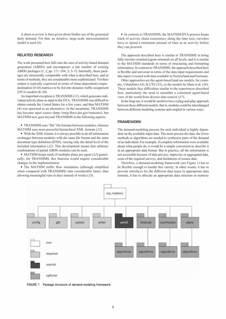
Therefore, a demand-modeling framework (see Figure 1) has tobe flexible enough to handle this variety. In other words, it has toprovide interfaces for the different data types in appropriate dataformats, it has to allocate an appropriate data structure in memory

FIGURE 1 Package structure of demand-modeling framework.

2

require spatial information (e.g., generating departure times ofactivities).

Land Use and Commuters Packages

The land use and commuters packages are optional packages thatstore information for the demand-modeling process. Dependent onthe input data, these packages are used, for example, to find locationsof work activities or to create sets of leisure facilities. The frameworkallows the addition of other optional packages in the same manner asthe land use and commuters packages for new data sources.

Plans Package

The plans package is, in principle, the core of the demand-modelingframework. The data structure is based on the MATSIM scheduleDTD (in MATSIM called a “plans DTD”), which can also beaccessed via the MATSIM website (4), and it is used as a workingfile, utilizing the extreme flexibility of the MATSIM schedule file.In the minimum version, the file holds only the identity numbers(IDs) of all simulated persons. However, it is possible to add alarge amount of information about each person to the file, such asage, sex, car ownership, home and work location (at different worldresolutions), and more.

In addition, each person can access one or many different indi-vidual schedules, describing when a person wants to start an activ-ity, where it will be performed, which route and mode to take to gofrom one location to the next, and so forth.

The internal data structure of the plans package provides exactlythe same flexibility as the XML file format. Therefore, it is possibleto sequentially add additional schedule details to an incompleteMATSIM plans file.

Demand Algorithms

Algorithms can be added to each package to verify, manipulate, add,or delete data items according to the purpose of the algorithm. Sincedifferent algorithms have to be used or implemented for each newscenario, it is critical that algorithms be clearly separated from thedata structure. They also should be easily exchangeable. The orderin which algorithms are called should be flexible as well.

The algorithms are collected into a subpackage of the data struc-ture that they manipulate. Therefore, an algorithm at org.matsimJ.commuters.algorithms manipulates data in the commuters datastructure (see examples later in this discussion).

External Models

At any point during the demand-modeling process, the frameworkallows the storage of all data into well-defined XML data files. Bydefinition, these files respect the format as described in the under-lying DTDs. Therefore, a clean interface to third-party programsand models is available even when those models are not part of thedemand-modeling framework described here.

For the two case studies described in the following sections, theexternal secondary location choice module (20) in its adapted ver-sion as described by Balmer et al. (21, pp. 5–36) was used, whichchooses locations for secondary activities in such a way that each

such that each data point can be accessed in a feasible amount of time, and it needs to ensure the uniqueness of data points while creating, manipulating, and deleting them.

General Framework Structure

The framework consists of required modules, optional modules, and a special world package (see Figure 1). The necessary packages pro-vide general XML parsing and XML writing interfaces, global con-stants, and a global and unique data structure for accessing input parameters. Optional packages are based on a specified input writ-ten in XML format (4). The base functionality of each optional package is to read the defined XML data, store them in an appropri-ate data structure, and write them again in the XML data format in an enriched, reduced, or unchanged form.

Framework Packages

Parser, Writer, and Gbl Packages

The parser package provides a general base class for parsing XML data via the SAX parser (18). The writer package provides the base for writing XML files. The purpose of the gbl package is to hold global constants and globally accessible functions.

Config Package

In the entire framework, just one configuration data structure exists, which holds all required input parameters for a specific demand-modeling process. Typical parameters are locations of input data, different file formats, special function parameters, and so on. The information stored in this package can be accessed from every part of the framework (global singleton design pattern) (19).

World Package

The world package has a special functionality: it describes the region for which the demand is being modeled. Therefore, it must guaran-tee that only one world exists during the demand-modeling process. This package holds all the information about cells, blocks, zones, municipalities, and so on, which are modeled as primitive shapes. If the other optional packages refer to such shapes, they have to point to them in world. With this function, the uniqueness of each shape object is guaranteed. Furthermore, it is also a control mechanism to verify that other input data are consistent with the given scenario.

Another important functionality of the world package has to be mentioned. During the demand-modeling process, the resolution of the world can differ. For example, land use information might be based on a raster of 100- by 100-m cells, whereas a commuter matrix is based on traffic analysis zones. Therefore, it is necessary to dis-aggregate one data set into another world resolution. The world package will hold this mapping for an arbitrary number of resolu-tions of the same region. With it, on-the-fly disaggregation is pro-vided. The mapping between two resolution layers can either be generated by the framework according to a specified mapping rule or given as predefined input data.

Although this package plays a central role in the framework, it is not required because certain demand-modeling steps do not

3

Mapping between those two levels was also available. The map-ping rule is nonambiguous. Each raster cell belongs to no or onemunicipality, whereas each municipality holds at least one rastercell. Further, the municipalities hold only those cells that includeurban areas; that is, the “lake cells” are not part of the mapping.

Information about population distribution in the municipalitieswas generated by Frick (23). It holds about 1.3 million inhabitantswith the following data:

• Home location (R),• Population group (children, workers, nonworkers, seniors),• Mobility (car, season ticket ownership, bike, walking),• Age, and• Sex.

The Swiss Federal Office for Statistics (BFS) (24) provides landuse data that contain information about capacities of different activ-ity types like work, shopping, education, and so on. That informationis based on raster level (R).

The Pendlermatrix 2000 (commuter matrix) (25) contains infor-mation about work and school commuters at the municipal level (M).

The microcensus (26) is a periodic travel behavior survey of theSwiss population. It has been run every 5 years since 1974. The micro-census is carried out by the Federal Office for Spatial Development(ARE) in cooperation with the BFS and contains detailed informationabout the mobility behavior of 30,000 persons from all over Switzer-land (27, pp. 61–79). About 1,670 different activity chains can befound in Microcensus 2000. Most of them appear rarely, so only the100 most frequently occurring activity chains were used, which stillcovers more than 90% of all chains. By reducing the number of activ-ity types to home, work, education, shop, and leisure, some activitytypes like service were recoded to work. The result was 21 differentactivity chains (21, pp. 5–36) and their distribution.

Steps in Demand-Modeling Process

The demand-modeling process is split into six sequential steps (seeFigure 2 for an overview). Each process step (except the first) usesone specific data resource to add details to each individual schedule:

1. Conversion. This process step converts the input population fileinto the XML person description file. None of the person tags holds aplan yet. But additional attributes like age, sex, and so on are included.It also defines in which land use raster element (R) this person lives.

2. Mapping. Each raster element of the land use data belongs tojust one municipality. By using this kind of mapping, each agent canbe assigned to the municipality of his or her home location.

3. Distribution. Given the distribution of the activity chainsdescribed earlier, one of the chains was assigned to each personaccording to the given distribution. The fact that children do not goto work was also taken into account, and therefore persons of youngage are not allowed to hold an activity chain including a work activ-ity. Independent random sampling from aggregate distributions cancause a lack of consistency with the given distribution. To avoid thisproblem, it was necessary to parse the population twice to obtainaggregate information (see Computational Issues).

4. Distribution. The Pendlermatrix 2000 (25) contains informa-tion about work and school commuters at the municipality level(M). With the assumption about primary activities (21, pp. 5–36),it was possible to add locations for the primary activities of workand education. Unfortunately, similar data for the primary activi-

agent improves its daily activity chain. In each given activity chain,there are clearly specified primary activities, and others are definedas secondary activities (21, pp. 5–36). The module uses the sameDTD, allowing simple information interchange.

Computational Issues

One important issue for demand modeling is the amount of inputinformation needed. Because of the variety of possible demand-modeling algorithms and input sources, it is necessary to have fastaccess to those data. One simple and rapid solution is to load allinformation into memory and provide a hierarchical data structure(tree structure) to access any item from any other location in O[2 *log(n)], where n is the depth of the data tree.

The hierarchical data structure is already provided by the input data(XML format), but the available space in the memory might not be suf-ficient. Although the description of the world, the land use data, com-muter matrices, and others typically holds a relatively small amountof data, the amount of information for individuals goes far beyond thesize of typical memory capacity (on average, around 1 to 2 GB).

To handle this problem, the demand-modeling framework uses theidea of sequential individual demand generation (streaming of indi-viduals). In other words, the framework reads one individual at atime, runs the defined algorithms for it, writes the results to file, andfrees the memory. In this way, the number of individuals in a givenscenario is unlimited. This idea will still work if, instead of singlepersons, demand at the household level for a small number of per-sons is modeled. But the limit of this approach will be reached if it isalso desired to add the concept of social networks (22). In that case,demand modeling of one individual can, in principle, depend on allother individuals in the scenario, and therefore the whole populationmust be stored in memory.

Nevertheless, the plans package still allows one to store all indi-viduals in memory if the amount of data is not too large or if one hasaccess to machines with a sufficient amount of memory. The user ofthe framework can switch between streaming and no streaming bysetting a defined parameter flag.

DEMAND MODELING FOR CANTON OF ZURICH, SWITZERLAND

With the framework described in the previous section, the stepstaken to model daily demand for the canton of Zurich, Switzerland,are presented. The following subsections describe briefly whichinput data were used and which algorithms were employed tomodel the daily demand.

It should be noted that the algorithms used are not very sophis-ticated. They demonstrate the use of the framework rather thandelivering state-of-the-art demand-modeling processes.

Data Resources

The world package describes the region (canton of Zurich,Switzerland) at two different resolutions:

• Municipality level M: 170 municipalities and 12 additionaldistricts inside the city of Zurich and

• Raster of 100- by 100-m cell resolution (raster level denotedR); in total, 167,881 cells are given.

4

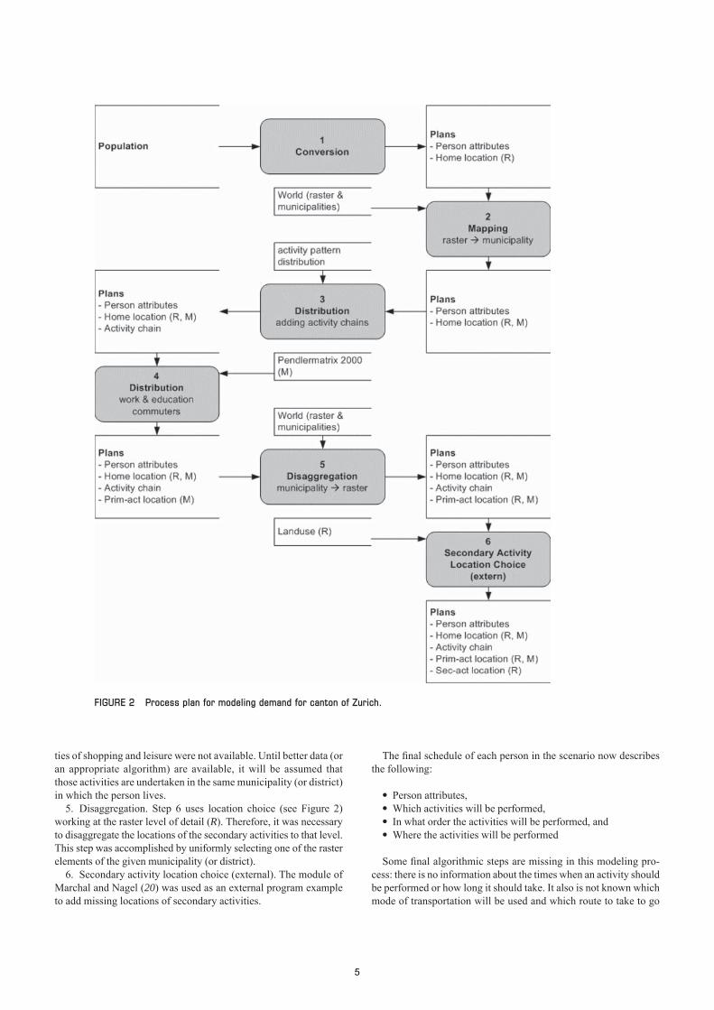
ties of shopping and leisure were not available. Until better data (oran appropriate algorithm) are available, it will be assumed thatthose activities are undertaken in the same municipality (or district)in which the person lives.

5. Disaggregation. Step 6 uses location choice (see Figure 2)working at the raster level of detail (R). Therefore, it was necessaryto disaggregate the locations of the secondary activities to that level.This step was accomplished by uniformly selecting one of the rasterelements of the given municipality (or district).

6. Secondary activity location choice (external). The module ofMarchal and Nagel (20) was used as an external program exampleto add missing locations of secondary activities.

The final schedule of each person in the scenario now describesthe following:

• Person attributes,• Which activities will be performed,• In what order the activities will be performed, and• Where the activities will be performed

Some final algorithmic steps are missing in this modeling pro-cess: there is no information about the times when an activity shouldbe performed or how long it should take. It also is not known whichmode of transportation will be used and which route to take to go

FIGURE 2 Process plan for modeling demand for canton of Zurich.

5

Demand-Modeling Process Steps

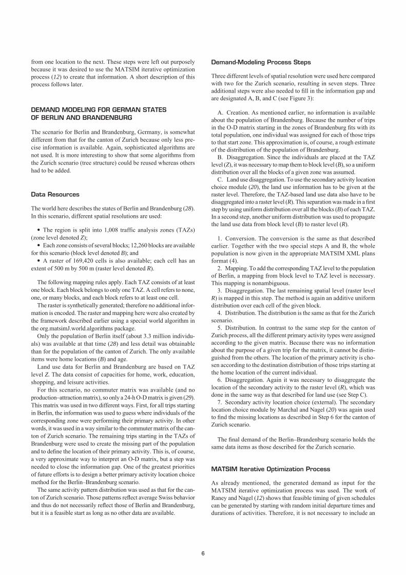
Three different levels of spatial resolution were used here comparedwith two for the Zurich scenario, resulting in seven steps. Threeadditional steps were also needed to fill in the information gap andare designated A, B, and C (see Figure 3):

A. Creation. As mentioned earlier, no information is availableabout the population of Brandenburg. Because the number of tripsin the O-D matrix starting in the zones of Brandenburg fits with itstotal population, one individual was assigned for each of those tripsto that start zone. This approximation is, of course, a rough estimateof the distribution of the population of Brandenburg.

B. Disaggregation. Since the individuals are placed at the TAZlevel (Z), it was necessary to map them to block level (B), so a uniformdistribution over all the blocks of a given zone was assumed.

C. Land use disaggregation. To use the secondary activity locationchoice module (20), the land use information has to be given at theraster level. Therefore, the TAZ-based land use data also have to bedisaggregated into a raster level (R). This separation was made in a firststep by using uniform distribution over all the blocks (B) of each TAZ.In a second step, another uniform distribution was used to propagatethe land use data from block level (B) to raster level (R).

1. Conversion. The conversion is the same as that describedearlier. Together with the two special steps A and B, the wholepopulation is now given in the appropriate MATSIM XML plansformat (4).

2. Mapping. To add the corresponding TAZ level to the populationof Berlin, a mapping from block level to TAZ level is necessary.This mapping is nonambiguous.

3. Disaggregation. The last remaining spatial level (raster levelR) is mapped in this step. The method is again an additive uniformdistribution over each cell of the given block.

4. Distribution. The distribution is the same as that for the Zurichscenario.

5. Distribution. In contrast to the same step for the canton ofZurich process, all the different primary activity types were assignedaccording to the given matrix. Because there was no informationabout the purpose of a given trip for the matrix, it cannot be distin-guished from the others. The location of the primary activity is cho-sen according to the destination distribution of those trips starting atthe home location of the current individual.

6. Disaggregation. Again it was necessary to disaggregate thelocation of the secondary activity to the raster level (R), which wasdone in the same way as that described for land use (see Step C).

7. Secondary activity location choice (external). The secondarylocation choice module by Marchal and Nagel (20) was again usedto find the missing locations as described in Step 6 for the canton ofZurich scenario.

The final demand of the Berlin–Brandenburg scenario holds thesame data items as those described for the Zurich scenario.

MATSIM Iterative Optimization Process

As already mentioned, the generated demand as input for theMATSIM iterative optimization process was used. The work ofRaney and Nagel (12) shows that feasible timing of given schedulescan be generated by starting with random initial departure times anddurations of activities. Therefore, it is not necessary to include an

from one location to the next. These steps were left out purposelybecause it was desired to use the MATSIM iterative optimizationprocess (12) to create that information. A short description of thisprocess follows later.

DEMAND MODELING FOR GERMAN STATES OF BERLIN AND BRANDENBURG

The scenario for Berlin and Brandenburg, Germany, is somewhatdifferent from that for the canton of Zurich because only less pre-cise information is available. Again, sophisticated algorithms arenot used. It is more interesting to show that some algorithms fromthe Zurich scenario (tree structure) could be reused whereas othershad to be added.

Data Resources

The world here describes the states of Berlin and Brandenburg (28).In this scenario, different spatial resolutions are used:

• The region is split into 1,008 traffic analysis zones (TAZs)(zone level denoted Z);

• Each zone consists of several blocks; 12,260 blocks are availablefor this scenario (block level denoted B); and

• A raster of 169,420 cells is also available; each cell has anextent of 500 m by 500 m (raster level denoted R).

The following mapping rules apply. Each TAZ consists of at leastone block. Each block belongs to only one TAZ. A cell refers to none,one, or many blocks, and each block refers to at least one cell.

The raster is synthetically generated; therefore no additional infor-mation is encoded. The raster and mapping here were also created bythe framework described earlier using a special world algorithm inthe org.matsimJ.world.algorithms package.

Only the population of Berlin itself (about 3.3 million individu-als) was available at that time (28) and less detail was obtainablethan for the population of the canton of Zurich. The only availableitems were home locations (B) and age.

Land use data for Berlin and Brandenburg are based on TAZlevel Z. The data consist of capacities for home, work, education,shopping, and leisure activities.

For this scenario, no commuter matrix was available (and no production–attraction matrix), so only a 24-h O-D matrix is given (29).This matrix was used in two different ways. First, for all trips startingin Berlin, the information was used to guess where individuals of thecorresponding zone were performing their primary activity. In otherwords, it was used in a way similar to the commuter matrix of the can-ton of Zurich scenario. The remaining trips starting in the TAZs ofBrandenburg were used to create the missing part of the populationand to define the location of their primary activity. This is, of course,a very approximate way to interpret an O-D matrix, but a step wasneeded to close the information gap. One of the greatest prioritiesof future efforts is to design a better primary activity location choicemethod for the Berlin–Brandenburg scenario.

The same activity pattern distribution was used as that for the can-ton of Zurich scenario. Those patterns reflect average Swiss behaviorand thus do not necessarily reflect those of Berlin and Brandenburg,but it is a feasible start as long as no other data are available.

6

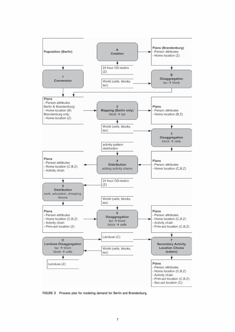
FIGURE 3 Process plan for modeling demand for Berlin and Brandenburg.

7

essary resources grow considerably more slowly than the samplesize. Such results will be reported on in the future.

The planomat MATSIM module mentioned earlier provides anattractive amount of functionality. Since it also supplies, besides thealready-used time choice, a location choice and a mode choice mod-ule, it is interesting to actually use these functionalities. To do that,the module requires additional information.

As a first step, it is necessary to provide an alternative to the indi-vidual transport mode in MATSIM. Therefore, the demand-modelingframework will be extended so that it delivers information abouttravel times from one zone (block, district, TAZ, or municipality) toanother. With it, the planomat module decides which mode will beused for each person in the population.

As a second step, another package will be added to the frameworkcontaining data about activity spaces, catchment areas, and com-muter sheds (32). With those data, the primary activity location choice(commuter package) and secondary activity location choice (exter-nal module) can be replaced by adding a set of possible locationsfor all available activity types to each person in the population. Thisset will then be used by the planomat module to find iteratively, inthe MATSIM framework, an appropriate location for the givenactivities of each individual.

As already mentioned, it is a relatively simple task to extend thedemand-modeling framework via the idea of intrahousehold inter-action. Externally, the main change would be to group householdmembers into corresponding XML brackets in the plans file. Allmodules would function as before at the person level, and householdinteractions could be introduced module by module.

SUMMARY

An agent-based demand-modeling framework for large-scale micro-simulations is presented. With the framework for the Zurich and theBerlin–Brandenburg scenarios, it is shown that the framework

• Is flexible enough to handle a variety of input data (Zurich datadiffer from Berlin–Brandenburg data);

• Is flexible enough to extend or replace algorithms (differentalgorithms for Berlin–Brandenburg commuter data than for Zurichcommuters);

• Provides disaggregation to different spatial resolutions (twolevels of resolution for the Zurich scenario and three levels for theBerlin–Brandenburg scenario);

• Provides a robust interface to third-party models, programs,and frameworks (the external modules: secondary activity locationchoice and MATSIM dynamic traffic assignment);

• Is suitable for an unlimited number of individuals (about7 million people for the Berlin–Brandenburg scenario); and

• Is easy to extend, to replace algorithms with more enhancedones, to add new algorithms for existing packages, and to add newpackages to handle new input data.

Nevertheless, it is only a framework. The algorithms presented formodeling are very simple. Resources are needed to enhance thosealgorithms and to validate the resulting demand against behavioralissues.

This work also shows the importance of interaction between thetransportation community and computer scientists. To satisfy data

appropriate algorithm in the demand-modeling framework sinceMATSIM can be used as a final external module for that purpose.

In contrast to the work by Raney and Nagel (12), an enhanced timeallocation module called planomat was used (30). With the conceptof genetic algorithms, this module can be used for time schedulingas well as for location or mode choice. Since activity chain choiceand location choice are already done by the demand-modeling frame-work and the traffic flow simulation of MATSIM (13) handles theindividual transport mode, the functionality of the planomat moduleis reduced to time choice.

MATSIM optimizes (daily) schedules and not single trips. There-fore, the consistency at the individual level is guaranteed (an agentmust leave a location before he arrives here). This is, in fact, oneof the most important issues in describing demand on the basis ofindividuals instead of losing important information by using O-Dmatrices.

Time Scheduling Results

With the same MATSIM setup as that described by Balmer et al.(21, pp. 5–36), a 1% sample of the canton of Zurich scenario popu-lation was run. By artificially reducing each link’s capacities withinthe given network (13) by a factor of 50, congestion patterns simi-lar to those obtained by using all persons were produced. Becauseof the small sample size, the simulations displayed considerabletraffic pattern fluctuations from one iteration to the next; using thosesimulations to identify bottlenecks would be difficult. Nevertheless,as will be explained in the following, the aggregated time structureof the results is quite plausible.

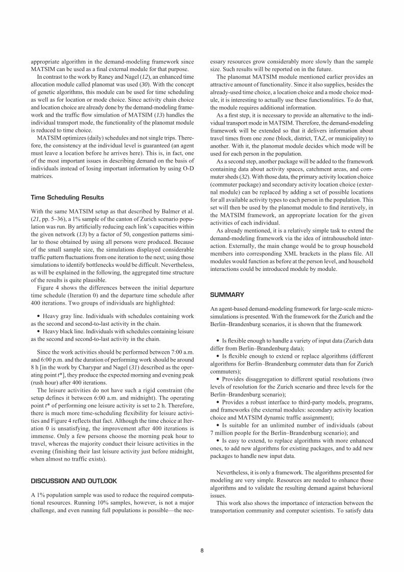
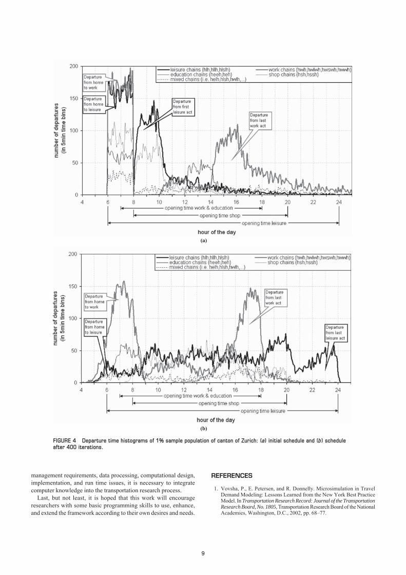
Figure 4 shows the differences between the initial departuretime schedule (Iteration 0) and the departure time schedule after400 iterations. Two groups of individuals are highlighted:

• Heavy gray line. Individuals with schedules containing workas the second and second-to-last activity in the chain.

• Heavy black line. Individuals with schedules containing leisureas the second and second-to-last activity in the chain.

Since the work activities should be performed between 7:00 a.m.and 6:00 p.m. and the duration of performing work should be around8 h [in the work by Charypar and Nagel (31) described as the oper-ating point t*], they produce the expected morning and evening peak(rush hour) after 400 iterations.

The leisure activities do not have such a rigid constraint (thesetup defines it between 6:00 a.m. and midnight). The operatingpoint t* of performing one leisure activity is set to 2 h. Therefore,there is much more time-scheduling flexibility for leisure activi-ties and Figure 4 reflects that fact. Although the time choice at Iter-ation 0 is unsatisfying, the improvement after 400 iterations isimmense. Only a few persons choose the morning peak hour totravel, whereas the majority conduct their leisure activities in theevening (finishing their last leisure activity just before midnight,when almost no traffic exists).

DISCUSSION AND OUTLOOK

A 1% population sample was used to reduce the required computa-tional resources. Running 10% samples, however, is not a majorchallenge, and even running full populations is possible—the nec-

8

management requirements, data processing, computational design,implementation, and run time issues, it is necessary to integratecomputer knowledge into the transportation research process.

Last, but not least, it is hoped that this work will encourageresearchers with some basic programming skills to use, enhance,and extend the framework according to their own desires and needs.

REFERENCES

1. Vovsha, P., E. Petersen, and R. Donnelly. Microsimulation in TravelDemand Modeling: Lessons Learned from the New York Best PracticeModel. In Transportation Research Record: Journal of the TransportationResearch Board, No. 1805, Transportation Research Board of the NationalAcademies, Washington, D.C., 2002, pp. 68–77.

(a)

(b)

FIGURE 4 Departure time histograms of 1% sample population of canton of Zurich: (a) initial schedule and (b) scheduleafter 400 iterations.

9

2. Bowman, J. L., M. Bradley, Y. Shiftan, T. K. Lawton, and M. Ben-Akiva.Demonstration of an Activity-Based Model for Portland. In World Trans-port Research: Selected Proceedings of the 8th World Conference onTransport Research 1998, Vol. 3, Elsevier, Oxford, United Kingdom,1999.

3. Bhat, C. R., J. Y. Guo, S. Srinivasan, and A. Sivakumar. ComprehensiveEconometric Microsimulator for Daily Activity-Travel Patterns. InTransportation Research Record: Journal of the TransportationResearch Board, No. 1894, Transportation Research Board of the NationalAcademies, Washington, D.C., 2004, pp. 57–66.

4. MATSIM, Multi Agent Traffic SIMulation. www.matsim.org. AccessedOct. 2005.

5. VISEM. Planung Transport und Verkehr (PTV), Karlsruhe, Germany.www.ptv.de/cgi-bin/traffic/traf_visem.pl. Accessed Oct. 2005.

6. Pendyala, R. M. Phased Implementation of a Multimodal Activity-BasedTravel Demand Modeling System in Florida. Final Report. ResearchCenter, Florida Department of Transportation, Tallahassee, 2004.www.dot.state.fl.us/research-center/Completed_Proj/Summary_PTO/FDOT_BA496.pdf. Accessed Oct. 2005.

7. Arentze, T., F. Hofman, H. van Mourik, and H. Timmermans. ALBA-TROSS: Multiagent, Rule-Based Model of Activity Pattern Decisions. InTransportation Research Record: Journal of the Transportation ResearchBoard, No. 1706, TRB, National Research Council, Washington, D.C.,2000, pp. 136–144.

8. DynaMIT. Massachusetts Institute of Technology, Cambridge. mit.edu/its/dynamit.html. Accessed Oct. 2005.

9. DYNASMART. University of Maryland, College Park. www.dynasmart.umd.edu. Accessed Oct. 2005.

10. Friedrich, M., I. Hofsäss, K. Nökel, and P. Vortisch. A Dynamic Traf-fic Assignment Method for Planning and Telematic Applications.Proc., Seminar K, European Transport Conference, Cambridge, UnitedKingdom, 2000.

11. TRANSIMS, TRansportation ANalysis and SIMulation System. LosAlamos National Laboratory, Los Alamos, N. Mex. transims.tsasa.lanl.gov. Accessed Oct. 2005.

12. Raney, B., and K. Nagel. An Improved Framework for Large-ScaleMulti-Agent Simulations of Travel Behavior. In Towards Better Per-forming European Transportation Systems (P. Rietveld, B. Jourquin,and K. Westin, eds.), 2005 (in press). www.vsp.tu-berlin.de/publications.Accessed Oct. 2005.

13. Cetin, N., and K. Nagel. A Large-Scale Agent-Based Traffic Micro-Simulation Based on Queue Model. Presented at the Swiss TransportResearch Conference, Monte Verita, Ascona, Switzerland, 2005.

14. Waddell, P., A. Borning, M. Noth, N. Freier, M. Becke, and G. Ulfarsson.Microsimulation of Urban Development and Location Choices: Designand Implementation of UrbanSim. Networks and Spatial Economics,Vol. 3, No. 1, 2003, pp. 43–67.

15. Salvini, P. A., and E. J. Miller. ILUTE: An Operational Prototype of aComprehensive Microsimulation Model of Urban Systems. Networksand Spatial Economics, Vol. 5, No. 2, 2005, pp. 217–234.

16. Hunt, J. D., R. Johnston, J. E. Abraham, C. J. Rodier, G. R. Garry,S. H. Putman, and T. de la Barra. Comparisons from Sacramento ModelTest Bed. In Transportation Research Record: Journal of the Trans-portation Research Board, No. 1780, TRB, National Research Council,Washington, D.C., 2001, pp. 53–63.

17. Abraham, J. E., T. Weidner, J. Gliebe, C. Willison, and J. D. Hunt.Three Methods for Synthesizing Base-Year Built Form for IntegratedLand Use–Transport Models. In Transportation Research Record:Journal of the Transportation Research Board, No. 1902, Transporta-

tion Research Board of the National Academies, Washington, D.C.,2005, pp. 114–123.

18. SAX, Simple API for XML. www.saxproject.org. Accessed Oct. 2005.19. Gamma, E., R. Helm, R. Johnson, and J. Vlissides. Design Patterns:

Elements of Reusable Object-Oriented Software. Addison-WesleyProfessional Computing Series, Boston, Mass., 1995.

20. Marchal, F., and K. Nagel. Modeling Location Choice of SecondaryActivities with a Social Network of Cooperative Agents. In Transporta-tion Research Record: Journal of the Transportation Research Board,No. 1935, Transportation Research Board of the National Academies,Washington, D.C., 2005, pp. 141–146.

21. Balmer, M., M. Rieser, A. Vogel, K. W. Axhausen, and K. Nagel. Gen-erating Day Plans Using Hourly Origin-Destination Matrices. In Jahrbuch2004/05 Schweizerische Verkehrswirtschaft (T. Bieger, C. Laesser, andR. Maggi, eds.), SVWG, St. Gallen, Switzerland, 2005.

22. Axhausen, K. W. Activity Spaces, Biographies, Social Networks andTheir Welfare Gains and Externalities: Some Hypotheses and EmpiricalResults. Presented at PROCESSUS Colloquium, Toronto, Ontario,Canada, 2005. www.civ.utoronto.ca/sect/traeng/ilute/processus2005/PaperSession/Paper18_Axhausen_ActivitySpacesBiographies_CD_.pdf.Accessed Oct. 2005.

23. Frick, M. A. Generating Synthetic Populations Using IPF and MonteCarlo Techniques: Some New Results. Presented at 4th Swiss TransportResearch Conference, Monte Verita, Ascona, Switz., 2004. www.ivt.ethz.ch/vpl/publications/reports. Accessed Oct. 2005.

24. BFS, Swiss Federal Statistical Office. www.bfs.admin.ch/bfs/portal/en/index.html. Accessed Oct. 2005.

25. Vrtic, M., and K. W. Axhausen. Experiment mit einem dynamischenUmlegungsverfahren. Strassenverkehrstechnik, Vol. 47, No. 3, 2003,pp. 121–126.

26. Mobilität in der Schweiz, Ergebnisse des Mikrozensus 2000 zumVerkehrsverhalten. ARE, Bundesamt für Raumentwicklung und Bunde-samt für Statistik, Bern und Neuchâtel, Switzerland, 2001. www.are.admin.ch/are/de. Accessed Oct. 2005.

27. Axhausen, K. W., and M. Frick. Nutzungen, Strukturen, Verkehr. InStadtverkehrsplanung: Grundlagen, Methoden, Ziele (G. Steierwald,H.-D. Künne, and W. Vogt, eds.), Springer, Heidelberg, Germany.

28. RBS, Raumbezugssystem Berlin. Bevoelkerungsverteilung, Teil-Verkehrszellen und Block Geometrie/Hierarchie. Statistisches LandesamtBerlin, 2000. www.statistik-berlin.de. Accessed Oct. 2005.

29. Datengrundlagen Stadtentwicklungsplan Verkehr. SfSB, Senatsverwal-tung für Stadtentwicklung Berlin, 1998. www.stadtentwicklung.berlin.de.Accessed Oct. 2005.

30. Meister, K., and M. Balmer. An Improved Replanning Module for Agent-Based Micro-Simulations of Travel Behavior. Working Paper. Institute forTransport Planning and Systems (IVT), ETH Zurich, Switzerland, 2005.www.ivt.ethz.ch/vpl/publications/reports. Accessed Oct. 2005.

31. Charypar, D., and K. Nagel. Generating Complete All-Day ActivityPlans with Genetic Algorithms. Transportation, Vol. 32, No. 4, 2005,pp. 369–397.

32. Axhausen, K. W., M. Botte, and S. Schönfelder. Systematic Measure-ment of Catchment Areas. CTPP 2000 Status Report. U.S. Departmentof Transportation, 2004. www.fhwa.dot.gov/ctpp/sr0804.pdf. AccessedOct. 2005.

The Traveler Behavior and Values Committee sponsored publication of this paper.

10