Embed Size (px)
Citation preview

Masterarbeit am Institut für Informatik der Freien Universität Berlin,
Arbeitsgruppe Künstliche Intelligenz
Agent-based Blackboard Architecture for aHigher-Order Theorem Prover
Betreuer: PD. Dr. Christoph Benzmüller
Berlin, den 17. Oktober 2014

Abstract
The automated theorem prover Leo was one of the first systems ableto prove theorems in higher-order logic. Since the first version of Leomany other systems emerged and outperformed Leo and its successorLeo-II. The Leo-III project’s aim is to develop a new prover reclaimingthe lead in the area of higher-order theorem proving.
Current competitive theorem provers sequentially manipulate sets offormulas in a global loop to obtain a proof. Nowadays in almost everyarea in computer science, concurrent and parallel approaches are increas-ingly used. Although some research towards parallel theorem proving hasbeen done and even some systems were implemented, most modern the-orem provers do not use any form of parallelism.
In this thesis we present an architecture for Leo-III that use paral-lelism in its very core. To this end an agent-based blackboard architectureis employed. Agents denote independent programs which can act on theirown. In comparison to classical theorem prover architectures, the globalloop is broken down to a set of tasks that can be computed in paral-lel. The results produced by all agents will be stored in a blackboard, aglobally shared datastructure, thus visible to all other agents.
For a proof of concept example agents are given demonstrating anagent-based approach can be used to implemented a higher-order theoremprover.

Eidesstattliche Erklärung
Ich versichere hiermit an Eides statt, dass diese Arbeit von niemand an-derem als meiner Person verfasst worden ist. Alle verwendeten Hilfsmittelwie Berichte, Bücher, Internetseiten oder ähnliches sind im Literaturverzeich-nis angegeben, Zitate aus fremden Arbeiten sind als solche kenntlich gemacht.Die Arbeit wurde bisher in gleicher oder ähnlicher Form keiner anderen Prü-fungskommission vorgelegt und auch nicht veröffentlicht.
Berlin, den(Unterschrift)

Contents
1 Introduction 1
2 Theorem Proving 22.1 Higher Order Logic . . . . . . . . . . . . . . . . . . . . . . . . . 32.2 Automated Theorem Proving . . . . . . . . . . . . . . . . . . . 72.3 Parallelization of Theorem Proving . . . . . . . . . . . . . . . . 10
3 Blackboard 153.1 Blackboard Systems . . . . . . . . . . . . . . . . . . . . . . . . 153.2 Blackboard Synchronization . . . . . . . . . . . . . . . . . . . . 173.3 Chosen Synchronization Mechanism . . . . . . . . . . . . . . . 22
4 Agents 224.1 Multiagent Systems . . . . . . . . . . . . . . . . . . . . . . . . . 234.2 Leo-III Agent . . . . . . . . . . . . . . . . . . . . . . . . . . . . 274.3 Leo-III MAS Architecture . . . . . . . . . . . . . . . . . . . . . 314.4 Execution of Agents . . . . . . . . . . . . . . . . . . . . . . . . 35
5 Games & Auctions 385.1 Game Theory . . . . . . . . . . . . . . . . . . . . . . . . . . . . 385.2 Combinatorical Auctions . . . . . . . . . . . . . . . . . . . . . . 425.3 Auction Scheduler . . . . . . . . . . . . . . . . . . . . . . . . . 475.4 Optimality . . . . . . . . . . . . . . . . . . . . . . . . . . . . . . 50
6 Agent Implementations 516.1 Loop Agent . . . . . . . . . . . . . . . . . . . . . . . . . . . . . 526.2 Rule-Agent . . . . . . . . . . . . . . . . . . . . . . . . . . . . . 536.3 Meta Prover . . . . . . . . . . . . . . . . . . . . . . . . . . . . . 556.4 Utility Agents . . . . . . . . . . . . . . . . . . . . . . . . . . . . 56
7 Blackboard Datastructures 587.1 Context Splitting . . . . . . . . . . . . . . . . . . . . . . . . . . 587.2 Message Queues . . . . . . . . . . . . . . . . . . . . . . . . . . . 62
8 Related Work 63
9 Further Work 63
10 Conclusion 65
11 Bibliography 67

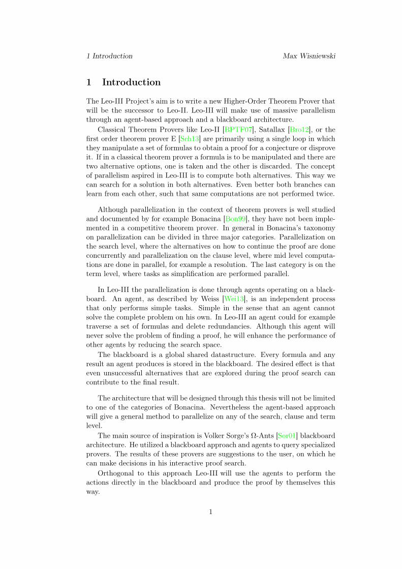
1 Introduction Max Wisniewski
1 Introduction
The Leo-III Project’s aim is to write a new Higher-Order Theorem Prover thatwill be the successor to Leo-II. Leo-III will make use of massive parallelismthrough an agent-based approach and a blackboard architecture.
Classical Theorem Provers like Leo-II [BPTF07], Satallax [Bro12], or thefirst order theorem prover E [Sch13] are primarily using a single loop in whichthey manipulate a set of formulas to obtain a proof for a conjecture or disproveit. If in a classical theorem prover a formula is to be manipulated and there aretwo alternative options, one is taken and the other is discarded. The conceptof parallelism aspired in Leo-III is to compute both alternatives. This way wecan search for a solution in both alternatives. Even better both branches canlearn from each other, such that same computations are not performed twice.
Although parallelization in the context of theorem provers is well studiedand documented by for example Bonacina [Bon99], they have not been imple-mented in a competitive theorem prover. In general in Bonacina’s taxonomyon parallelization can be divided in three major categories. Parallelization onthe search level, where the alternatives on how to continue the proof are doneconcurrently and parallelization on the clause level, where mid level computa-tions are done in parallel, for example a resolution. The last category is on theterm level, where tasks as simplification are performed parallel.
In Leo-III the parallelization is done through agents operating on a black-board. An agent, as described by Weiss [Wei13], is an independent processthat only performs simple tasks. Simple in the sense that an agent cannotsolve the complete problem on his own. In Leo-III an agent could for exampletraverse a set of formulas and delete redundancies. Although this agent willnever solve the problem of finding a proof, he will enhance the performance ofother agents by reducing the search space.
The blackboard is a global shared datastructure. Every formula and anyresult an agent produces is stored in the blackboard. The desired effect is thateven unsuccessful alternatives that are explored during the proof search cancontribute to the final result.
The architecture that will be designed through this thesis will not be limitedto one of the categories of Bonacina. Nevertheless the agent-based approachwill give a general method to parallelize on any of the search, clause and termlevel.
The main source of inspiration is Volker Sorge’s Ω-Ants [Sor01] blackboardarchitecture. He utilized a blackboard approach and agents to query specializedprovers. The results of these provers are suggestions to the user, on which hecan make decisions in his interactive proof search.
Orthogonal to this approach Leo-III will use the agents to perform theactions directly in the blackboard and produce the proof by themselves thisway.
1
2 Theorem Proving Max Wisniewski
The goal of this thesis is to show that an agent-based approach can be usedto implement a competitive automated theorem prover.
The outline of the thesis is the following. In section 2 the concepts oftheorem proving and automation are presented. In section 3 the blackboardis introduced and some synchronization techniques, investigated through thecourse of this thesis, are presented and concluded by the decision for the syn-chronization of Leo-III ’s blackboard. In section 4 agents and multiagent sys-tems are introduced and the (multi-)agent architecture for Leo-III is explained.Section 5 deals with the scheduler for the agents and introduces game theoryas the foundations for the scheduling algorithm. In section 6 and 7 exampleagents and datastructures for Leo-III are presented and evaluated.
2 Theorem Proving
The art of proving a statement based on a set of assumptions is a millenniaold tradition in the western world. In ancient Greek philosophers as Plato,Socrates and especially Aristoteles in his Organon introduced an uniform wayof deriving new information from given ones. Thus the first logic was born.
These early attempts of logic struggled with problems due to interpretationon either the facts in their proofs and on the other hand the derivation style.The human language was a big problem in this case, because the interpretationof words can change in different context. A fact formulated in human language,even if logical consistent derived, can be wrong if interpreted in another way.Without a formalization in which way to read certain facts, this poses a greatproblem as can be seen in table 2.1.
A Nothing is better than moneyB A sandwich is better than nothingC A sandwich is better than money from A, B
Table 2.1: Simple example of two different interpretations of the term nothing.
Without question we would syntactically agree on the derivation of C, buteven if most people would agree on A and B, they would most certainly notagree on C. The problem here is the interpretation of nothing. In A nothingcan be seen as a quantification of the whole sentence – for all objects that exist,money is better than each of it. In B a reference to the ranking itself is made,in this case some kind of measure. Nothing has the measure 0 where a setcontaining the sandwich has a measure strictly greater. In this sentence thereis no quantification, but nothing is the description of the empty set.
Not only is A a implicit quantified sentence and B a propositional, but weeven cannot be sure the comparison better means the same relation.
Nonetheless the first formalization of the proof emphasizes the derivation iscorrect. In a sense this derivation is still correct, if we take nothing, sandwich
2

2.1 Higher Order Logic Max Wisniewski
and money as simple objects. But then we would have not modeled what ourintended interpretation was.
The formalization of logic is a rather recent development and goes back toFrege in his Begriffsschrift [Fre79] in 1879. He developed a style to write downa proof mathematically, without uncertainty. The logic addressed in his articlewas classical predicate logic.
In figure 2.1 the induction principle is shown. It states in both cases thesame. If P holds for some 0 and we can derive from P (x) that it holds for thesuccessor s(x), then we can conclude it holds for all natural numbers. We canalready see a resemblance in both calculi. Most natural deduction calculi arewritten down as a tree, exactly as Frege introduced his calculus. The differenceis just in the set of rules that can be applied and a the notation of the trees.
P n P(n)
P(s(x))
P(x)
P(0)
x
P (0)
P (x)
...P (s(x))
∀n . P (n)
Figure 2.1: Induction principle in Frege’s proof style compared to naturaldeduction.
With the beginning of the formalization of proofs there was suddenly thepossibility to analyze proof systems formally with their own methods. Today,especially in philosophy, there exists a variety of different proof systems andlogics.
In the remainder of this section we firstly introduce the logic Leo-III issituated in. After this we will look at the automation of the proofs and in theend the key aspect to Leo-III, the parallelization, is illuminated.
2.1 Higher Order Logic
One of the key features of natural language is the abstraction from specificthings to talk about. For humans it is natural to formulate sentences in thestyle of every student in the course sits in the lecture hall or every (somethingwith predicate abstraction.
In the first example we see an abstraction over students, i.e. quantificationover each student and in the second an abstraction over all predicates. Earlywork on this subject is again done in Frege’s Begriffsschrift [Fre79]. He doesnot explicitly mention the fact that he allows quantification over predicates,but as he encodes the induction principle (see figure 2.1), we can assume thatthis is the case.
Bertrand Russel [Rus08] first pointed out that quantification, as introducedby Frege, is inconsistent, by introducing his famous Russel Paradox.
3
2.1 Higher Order Logic Max Wisniewski
He has proven that in Frege’s logic it is possible to formulate the followingset – the set of all sets, that do not contain itself. It is not provable if this setcontains itself or the contradiction.
To get rid of this paradox Russel introduced his ramified theory of types.But as Goedel has shown in his first incompleteness theorem [Gö31] therecannot exist a consistent, complete proof calculi when quantifying unrestrictedover predicates. The classical higher order logic or simple type theory usednowadays refers to the work of Alonso Church [And14] with henkin models toensure the existence of such a proof calculi.
2.1.1 Church’s simple theory of types
The input language of Leo-III is similar to the language used in Church’s simpletype theory. This section shortly introduces his logic. For most parts, we cansee classical higher order logic as a typed λ-calculus with special symbols forthe connectives to define the logic.
Definition 2.1. (type)We call o and ι base types, and α → β a function type from a type α to atype β.
The set of all types is denoted by T . y
The type o will be the Boolean type, whereas ι is the type of individuals,the simplest objects in the logic. Based on these the typed terms of the simplytyped λ-calculus are introduced.
Definition 2.2. (typed term)A term t in the simply typed λ-calculus annotated with a type α, meaning tαis the term t with type α. The Baccus Nauer form for well-typed terms is asfollows.
tα ::= cα, Xα
| t1β→α t2β
| (λXβ . t1γ)β→γ , with α = β → γ
Where cα is a constant symbol of type α from a set of symbols C, Xα is avariable of type α from a set of variable symbols σ, t1β→αt
2β is an application
and (λXβ . t1γ) is a function. As in the untyped λ-calculus we can introduce
the set of free terms. A variable Xα is free in t, if it is contained in t and noabstraction (λX.t′) exists where this X is contained in t′. A variable is boundotherwise.
Observe that it is not possible to pass a wrong typed argument to a func-tion, as there cannot be a well-formed application with wrong type. y
Higher-order logic is a term describing a quantification over higher orderedvariables. We will look at this concept later in this chapter. The next definitionintroduces the order for the term.
4
2.1 Higher Order Logic Max Wisniewski
Definition 2.3. (Type / Term order)The order function ord is defined inductively through
ord(o) = ord(ι) = 0ord(α→ β) = maxord(α) + 1, ord(β).
The order of a term tα is defined by ord(tα) = ord(α).
This definition is enough to introduce higher-order logic. The logical con-nectives and operators can be introduced as constant symbols with a fixedinterpretation that has to be available in the semantics later on. To evaluatethese terms a applicative structure [BBK04] can be used to carry the infor-mation to constant and variable symbols. For simplicity reasons the approachhere is to define the set of symbols and their semantics explicitly on top of thetyped λ-calculus, inspired by Andrews [And14].
Definition 2.4. (higher order-logic syntax)The classical higher-order logic (HOL) is a typed λ calculus with the connec-tives ∀(α→o)→o, ¬o→o, ∧o→o→o. y
The other logical connectives can be defined the usual way. Observe thatthe quantifier ∀ does not introduce a binding mechanism. Whereas usually aquantification is written by ∀X.PX, it is written as ∀(λX.PX) in HOL. Thisway quantifiers do not have to be part of the syntax definition, but can bedefined as constant symbols with a fixed meaning.
A term to is called a sentence if all variables are bound.Using this we can express the difference between higher-order and first-
order logic. First order quantifiers allow only quantification over predicates Pwith ord(P ) = 1, where the 1 is the relevant term. This logic is called first-order logic (FOL). In higher-order logic quantification is allowed over any kindof predicate P , in particular ord(P ) > 1.
2.1.2 Semantics
The semantic of HOL can be introduced in various ways. Since this thesis doesnot tackle the logical side, we will restrict ourselves to a simple introductionto standard and henkin semantics.
We start by introducing the models for the evaluation of the formulas.
Definition 2.5. (Frame & Interpretation)Let Dαα∈T be a collection of sets, where a Dα is a set of elements of typeα called domain. The domain Do = T, F contains two elements denotingtruth and falsehood. The domain Dι 6= ∅ can be chosen arbitrarily and Dα→βis a set of functions from Dα to Dβ .Dαα∈T is called a frame.
An interpretation 〈Dαα∈T , I〉 is a frame paired with a function I, thatmaps each constant symbol cα to an element in Dα. The function I has to betotal, such that each constant symbol has a element assigned. y
5
2.1 Higher Order Logic Max Wisniewski
The interpretation of the HOL connectives ∧o→o→o,¬o→o∏α
(α→o)→o is theusually assumed, s.t. I(∧) returns true, if and only if both arguments are true,and I(¬) returns the other element in Do. Lastly I(
∏α) returns true for agiven function pα→o, if the predicate is T for all elements in Dα. We need theinterpretation to contain at least these functions.
Definition 2.6. (Valuation)Let 〈Dαα∈T , I〉 and σ a variable mapping that assigns a variable Xα anelement of the domain Dα. The substitution σ[a/Xα] denotes the assignmentthat maps all variables to the same element, except Xα, that maps now to a.
The valuation V maps a term tα with a variable mapping σ to an elementof the domain Dα with
V(Xα, σ) = σ(Xα) , for Xα variableV(cα, σ) = I(cα) , for cα constantV((sα→βrα), σ) = (V(sα→β, σ)V(rα, σ))V((λXα . sβ), σ) = fα→β ∈ Dα→β , s.t. each z ∈ Dα is mapped to V(sβ, σ[z/Xα])
y
An interpretation 〈Dαα→β, I〉 is a henkin or standard model if a valuationV exists. If it is a henkin/standard model, then the valuation is unique.
The above definitions exactly define henkin model and hence for the valu-ation henkin semantic. The difference between standard and henkin models,is that a domain in a henkin model the domain Dα→β ⊆ DDα
β is a subset ofall functions. In a standard model the domain Dα→β = DDα
β is always full.Lastly we can define validity for a model.
Definition 2.7. (Validity)A term to called formula is valid in a henkin/standard model H if and only iffor all variable assignments σ V(to, σ) = T , for V the unique valuation for H.
We write H |= to.
A formula to is valid in henkin(standard) semantic, if for all henkin(standard)models H H |= to, then we write |= to. y
To show the model validity of a formula, human cannot go the way of thevaluation function, since the domains Dα can be infinite. Hence the notion ofa proof system is necessary to show validity.
2.1.3 Proofs
The task of a proof calculus is to generate from a set of valid formulas newvalid formulas. To form a proof calculus an initial set of valid and rules abouthow to generate new valid formulas have to be given.
The next definition introduces the notion of a proof in one of the simplestproof calculi first formulated by Hilbert [vH02].
6
2.2 Automated Theorem Proving Max Wisniewski
Definition 2.8. (Hilbert Proof System)Let Γ be a set of formulas called axioms and R a set of inference rules.
1. A sequence φ0, φ1, . . . , φn is a proof sequence if for all i
• φi ∈ Γ
• φi follows from a rule in R by some φj1 , . . . , φjk ,whereby j1, . . . , jk ≤ i.
2. A proof sequence φ0, . . . , φn is a proof for the hypotheses Ψ if φn = Ψ.
We write Γ `R Ψ.
The proof calculus was introduced to proof formulas without the modalvalidity. The next definition introduces two properties for a proof calculusthat makes a connection to the model validity.
Definition 2.9. (Soundness & Completeness)Let (R,Γ) be a proof calculus. The proof calculus is called
1. sound if for all Φo terms of type o holds
Γ `R Φo ⇒|= Φo.
2. correct if for all Φo terms of type o holds
|= Φo ⇒ Γ `R Φo
The result of Goedel’s incompleteness result [Gö31] has shown that forstandard models there is no sound and complete proof calculus. Therefor wealready introduced henkin models for which sound and complete calculi exist.On the other hand this result is due to the fact that HOL with henkin modelsis exactly as expressive as first-order logic.
2.2 Automated Theorem Proving
From the development of the first to modern computers, the computationpower as well es the applications had a great boost. Their first role as mathe-matical computation engine was soon applied in many non mathematical fields.Whereas computer were on the rise through the century in many application, inmathematics their application stagnated except for some discipline that reliedon heavy computation.
Using computers in the proof search, which is a key aspect of mathematics,has been and in some parts is still a proscribed topic.
The first automated theorem prover, getting known and used for its sta-bility, was Otter [McC90] which was released 1989. Otter is a first-order logictheorem prover using resolution and paramodulation. Since Otter has beenstable a long time, many fields started applying theorem proving. Some of the
7
2.2 Automated Theorem Proving Max Wisniewski
more popular applications are the seL4 kernel [KEH+09], where a completekernel written in C was proven correctly. The DVD codec’s correctness proofin Coq [YB04] could be automatically translated to executable ML code thatwas firstly done by Ralph Loader by using the Curry-Howard isomorphismto generate executable code. A last application is in philosophy and formallogics, where recently Gödels ontological argument could be verified [BP14].Although not widely used in mathematics, there are examples of proofs thatwere only found through theorem provers. Firstly there was the four color the-orem proven in Coq and most recently the Kepler conjecture, that was provenwith help of Isabelle/HOL [NPW02].
In computer aided proving there are two major styles to distinguish. Onetries to find a proof directly by themselves, completely liberating the personfrom the work process. The result is either a proof object, which can be veri-fied by another program or the human himself, or simpler the answer yes/no.These kind of provers are called automated theorem prover (ATP). The otherapproach is a more interactive variant. The computer just supports the humanin the proof search by showing him possible applications of rules, applying therules and verifying every step. The verification support ensures, that no slipis in the proof. These provers are called interactive theorem prover (ITP).
2.2.1 Automated Proof Calculi
We have already seen the syntax and semantics of higher-order logics that wewant to use and have seen a derivation system that can formulate a proof. Butfor a computer these simple derivation systems as presented in definition 2.8are poorly efficient, since a computer would not know which axioms to takeand initiate. In the worst case the proof will never be found.
For this reason more suitable proof calculi have been implemented. Someexamples are
Tableaux: Tableaux style proofs split conjunctive clauses in the formula setand branches them into a tree structure. A proof is found if every branchis closed, namely false could be derived.
Resolution: Resolution proofs work by translating the formula set step-wiseinto conjunctive clause normal form (CNF). By combining to CNF clauses,if they contain a formula φ and its negated formula ¬φ, a new clause canbe generated, with all formulas of both combined clauses without the φ.
The proof can be closed if the empty clause could be derived.
Both tableaux and resolution are well described by Fitting [Fit90].
DP: The proof style of Davis and Putnam [DP60] works by instantiating theliterals of a CNF with values true or false.
Through an intelligent backtracking in the case that the empty clausecould be derived in one instantiation, the proof can either find a validinstantiation, or show, that now instantiation can be found.
8
2.2 Automated Theorem Proving Max Wisniewski
This proof style is a satisfiability proof style that can return a model inthe case that the initial formula set is not valid.
All the above proof calculi have been proven sound and complete.
Modern Theorem Provers Since Otter many new provers came up withenhancements in different fields. On the one hand, there are Spass, E, andProver9, which is the direct successor to Otter, in the field of first order logic,on the other hand there are Leo-II and Satallax.
Today’s performance is mainly due to the yearly competitions in whichthe provers can compete in different categories. They differ in more advancedcalculi, better selection and filtering for the rules to apply or partial rewritingof formulas to a more suitable form to produce each year faster provers.
2.2.2 The TPTP World
In the early days every new prover came up with its own interface, its owninput language and its own proof output. This has proven to be a challengingtask for people trying to use these theorem provers since often multiple proverswere needed for a single problem due to their individual strengths.
The need for some kind of standard was immanent, since both users anddevelopers do not have to be burdened with syntax for each new prover, butconcentrate on the real problem they want to solve. In the pure quantified theo-rem proving context the most established framework is the Thousand Problemsfor Theorem Provers (TPTP) [Sut09] developed and maintained by Goeff Sut-cliffe. The TPTP is on the one hand a library for test problems for theoremprovers and on the other hand TPTP defines many categories of input lan-guages, such as cnf for input in clause normal form, fof for untyped first orderproblems and – important for Leo-III – thf the typed higher order form.
As it already happened in logics by Frege it is necessary to standardizethe languages of theorem provers. If there is a standard theorem proving canpropagate to many possible application areas, e.g. philosophy, mathematicsand computer linguists. The problem library allows a transparent testing oftheorem provers. This way a developer of a new prover does not have tothink of possible problems and on the other hand he cannot cheat in theirevaluation of the prover. Each prover has some problems on which he runsfaster than others. A standardized testing framework prohibits a new proverto profile himself by only running on suitable test for him, but allows a nonbiased evaluation of the qualities the prover owns.
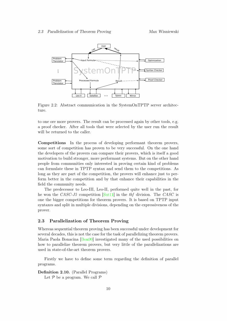
Since many ATPs began to use TPTP as their input language and usedthe problem library, a web interface called SystemOnTPTP allows to run manyprovers remotely on servers in Miami. SystemOnTPTP workflow is describedin figure 2.2. A problem in one of the supported syntaxes is send to the server.On the server there are sever tools for syntax checking and optimize formulationof the input syntax. For provers that do not support TPTP’s syntax as theirinput format translation tools are available. The processed input is then send
9
2.3 Parallelization of Theorem Proving Max Wisniewski
ProblemTranslator
ProblemTranslator
...
Leo-II SpassSatallax Nitrox...
Optimization
Syntax Checker
Proof Checker
SystemOnTPTP
Input Formula
Processed Formula Result
User
callresult
Figure 2.2: Abstract communication in the SystemOnTPTP server architec-ture.
to one ore more provers. The result can be processed again by other tools, e.g.a proof checker. After all tools that were selected by the user run the resultwill be returned to the caller.
Competitions In the process of developing performant theorem provers,some sort of competition has proven to be very successful. On the one handthe developers of the provers can compare their provers, which is itself a goodmotivation to build stronger, more performant systems. But on the other handpeople from communities only interested in proving certain kind of problemscan formulate these in TPTP syntax and send them to the competitions. Aslong as they are part of the competition, the provers will enhance just to per-form better in the competition and by that enhance their capabilities in thefield the community needs.
The predecessor to Leo-III, Leo-II, performed quite well in the past, forhe won the CASC-J5 competition [Sut11] in the thf division. The CASC isone the bigger competitions for theorem provers. It is based on TPTP inputsyntaxes and split in multiple divisions, depending on the expressiveness of theprover.
2.3 Parallelization of Theorem Proving
Whereas sequential theorem proving has been successful under development forseveral decades, this is not the case for the task of parallelizing theorem provers.Maria Paola Bonacina [Bon99] investigated many of the used possibilities onhow to parallelize theorem provers, but very little of the parallelizations areused in state-of-the-art theorem provers.
Firstly we have to define some term regarding the definition of parallelprograms.
Definition 2.10. (Parallel Programs)Let P be a program. We call P
10
2.3 Parallelization of Theorem Proving Max Wisniewski
multisearch
distributedsearch
heterogeneousinferencesystem
homogeneousinferencesystem
parallel-inference
OR-parallelism
AND-parallelism
parallelrewriting
parallelunification
parallelmatching
parallelism atthe search level
parallelism atthe clause level
parallelism atthe term level
parallelism in deduction
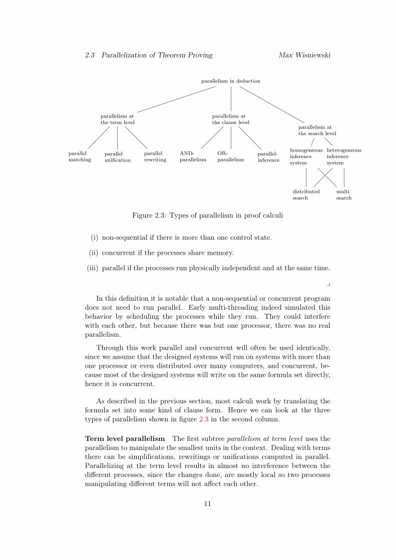
Figure 2.3: Types of parallelism in proof calculi
(i) non-sequential if there is more than one control state.
(ii) concurrent if the processes share memory.
(iii) parallel if the processes run physically independent and at the same time.
y
In this definition it is notable that a non-sequential or concurrent programdoes not need to run parallel. Early multi-threading indeed simulated thisbehavior by scheduling the processes while they run. They could interferewith each other, but because there was but one processor, there was no realparallelism.
Through this work parallel and concurrent will often be used identically,since we assume that the designed systems will run on systems with more thanone processor or even distributed over many computers, and concurrent, be-cause most of the designed systems will write on the same formula set directly,hence it is concurrent.
As described in the previous section, most calculi work by translating theformula set into some kind of clause form. Hence we can look at the threetypes of parallelism shown in figure 2.3 in the second column.
Term level parallelism The first subtree parallelism at term level uses theparallelism to manipulate the smallest units in the context. Dealing with termsthere can be simplifications, rewritings or unifications computed in parallel.Parallelizing at the term level results in almost no interference between thedifferent processes, since the changes done, are mostly local so two processesmanipulating different terms will not affect each other.
11
2.3 Parallelization of Theorem Proving Max Wisniewski
α-rule β-ruleA ∧B A, B -¬(A ∧B) - ¬A, ¬BA ∨B - A, B¬(A ∨B) ¬A, ¬B -A ⊃ B - ¬A, B¬(A ⊃ B) A, ¬B -
...
Table 2.2: α - β - nature of connectives
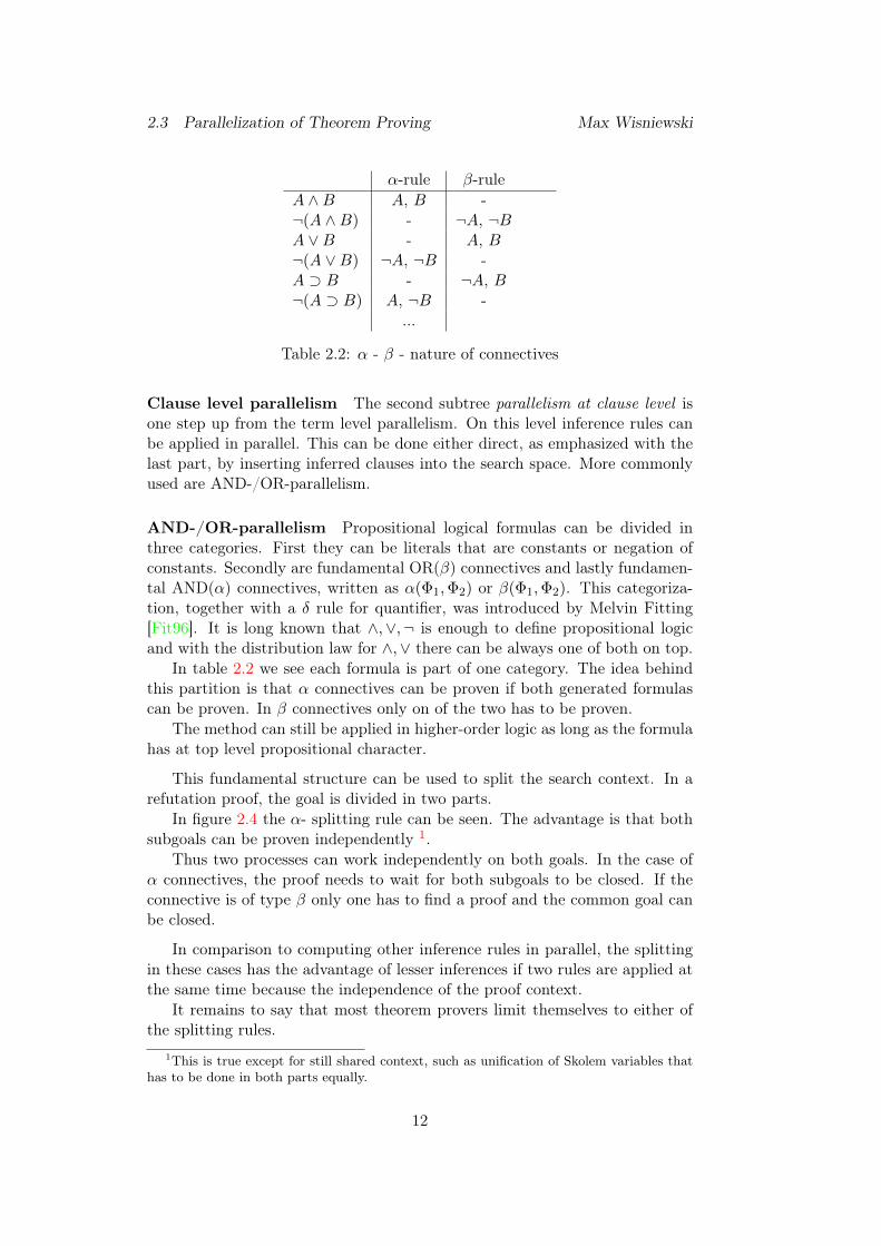
Clause level parallelism The second subtree parallelism at clause level isone step up from the term level parallelism. On this level inference rules canbe applied in parallel. This can be done either direct, as emphasized with thelast part, by inserting inferred clauses into the search space. More commonlyused are AND-/OR-parallelism.
AND-/OR-parallelism Propositional logical formulas can be divided inthree categories. First they can be literals that are constants or negation ofconstants. Secondly are fundamental OR(β) connectives and lastly fundamen-tal AND(α) connectives, written as α(Φ1,Φ2) or β(Φ1,Φ2). This categoriza-tion, together with a δ rule for quantifier, was introduced by Melvin Fitting[Fit96]. It is long known that ∧,∨,¬ is enough to define propositional logicand with the distribution law for ∧,∨ there can be always one of both on top.
In table 2.2 we see each formula is part of one category. The idea behindthis partition is that α connectives can be proven if both generated formulascan be proven. In β connectives only on of the two has to be proven.
The method can still be applied in higher-order logic as long as the formulahas at top level propositional character.
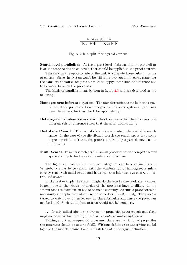
This fundamental structure can be used to split the search context. In arefutation proof, the goal is divided in two parts.
In figure 2.4 the α- splitting rule can be seen. The advantage is that bothsubgoals can be proven independently 1.
Thus two processes can work independently on both goals. In the case ofα connectives, the proof needs to wait for both subgoals to be closed. If theconnective is of type β only one has to find a proof and the common goal canbe closed.
In comparison to computing other inference rules in parallel, the splittingin these cases has the advantage of lesser inferences if two rules are applied atthe same time because the independence of the proof context.
It remains to say that most theorem provers limit themselves to either ofthe splitting rules.
1This is true except for still shared context, such as unification of Skolem variables thathas to be done in both parts equally.
12
2.3 Parallelization of Theorem Proving Max Wisniewski
Φ, α(ϕ1, ϕ2) ` Ψ
Φ, ϕ1 ` Ψ Φ, ϕ2 ` Ψ
Figure 2.4: α-split of the proof context
Search level parallelism At the highest level of abstraction the parallelismis at the stage to decide on a rule, that should be applied to the proof context.
This task on the opposite site of the task to compute these rules on termsor clauses. Since the system won’t benefit from two equal processes, searchingthe same set of clauses for possible rules to apply, some kind of difference hasto be made between the processes.
The kinds of parallelism can be seen in figure 2.3 and are described in thefollowing.
Homogeneous inference system. The first distinction is made in the capa-bilities of the processes. In a homogeneous inference system all processeshave the same rules they check for applicability.
Heterogeneous inference system. The other case is that the processes havedifferent sets of inference rules, that check for applicability.
Distributed Search. The second distinction is made in the available searchspace. In the case of the distributed search the search space is to somedegree divided, such that the processes have only a partial view on theformula set.
Multi Search. In multi search parallelism all processes see the complete searchspace and try to find applicable inference rules here.
The figure emphasizes that the two categories can be combined freely.Whereby one has to be careful with the combination of homogeneous infer-ence systems with multi search and heterogeneous inference systems with dis-tributed search.
In the first example the system might do the exact same work many times.Hence at least the search strategies of the processes have to differ. In thesecond case the distribution has to be made carefully. Assume a proof containsnecessarily an application of rule R1 on some formulas Φ1, . . .Φn. The processtasked to watch over R1 never sees all these formulas and hence the proof cannot be found. Such an implementation would not be complete.
As already talked about the two major properties proof calculi and theirimplementations should always have are soundness and completeness.
Talking about non-sequential programs, there are two kinds of propertiesthe programs should be able to fulfill. Without defining the underlying modallogic or the models behind them, we will look at a colloquial definition.
13
2.3 Parallelization of Theorem Proving Max Wisniewski
Definition 2.11. (Safety & Liveness Properties)Let P be a property andM a program.
1. A safety property save(P ) is valid in the programM if never during theexecution ofM stating in a valid start state the formula P is true.
2. A liveness property live(P ) is valid in the programM if the formula Pis evaluated infinitely often to true during every possible computation ofM starting in a valid start state.
In designing parallel theorem provers both these kinds of properties areclosely connected.
Soundness / Safety. To proof soundness of a parallel theorem prover, almostalways some kind of safety property has to be proven.
One imagine a theorem prover where the underlying calculus is correct,but in the parallel execution an error happens. Two processes attemptto write at the same time and in the result they add a formula to thecontext that should not be derivable, for example false.
Another example dealt with is in the parallelized version of Otter calledROO [LMS92a]. An invariant from Otter that in the set of processedformulas every pair of formulas was mutually normalized is establishedhad to be maintained This was some work, that must not be dealt within Otter, because there only one formula, was processed at a time. InROO, many formulas could be processed in parallel, such that it mightoccur, that at the same time processed formulas, where not mutuallynormalized. The invariant of Otter became a safety property in ROO,that had to be maintained.
Most of the time the safety properties are invariants made on the mem-bers of the datastructures.
Completeness / Liveness. The completeness of most calculi relies heavilyon the fact that every inference rule can be applied infinitely many times.
If for example the α rule mentioned above could no longer be applied,but there are still and connectives in the context that have to be split,the proof might not be found.
Hence the completeness of the calculus relies on the fact, that each pro-cess can execute infinitely often.
The agent-based blackboard architecture presented in this thesis is notlimited to one of the kinds of parallelization. The architecture is only a toolthat can be used to implement agents on all of these levels of parallelism.
14
3 Blackboard Max Wisniewski
3 Blackboard
One of the key aspects for Leo-III is the massive use of parallelism. Thereforthe aim is to write all datastructures ready for concurrent access and modifi-cation. Aside from the concurrent access the general idea in Leo-III is infor-mation sharing.
The approach in Leo-III is to share the information by making almost everydata used for the computation by the agents public. An architecture for theserequirements is the Blackboard Architecture.
All agents write their intermediate results onto the blackboard, where theother agents can see partial results. Hence a computation has probably neverto be done twice in different contexts, if it has already been done, and even afailed proof attempt can leave conclusions in the context of the proof search,such that the next attempt can learn from previous failures.
In this section we will firstly describe what a blackboard is and as a secondstep look at some synchronization mechanisms possible for the datastructuresin it.
3.1 Blackboard Systems
The Blackboard Architecture was introduced and mostly used in artificial intel-ligence as a knowledge representation architecture. The first program that usedthis architecture was the Hearsay-II speech-understanding system by Ermanet al. [EL80].
The way blackboard systems work is often described [Wei13] by the follow-ing metaphor.
Imagine a group of human specialists seated next to a largeblackboard. The specialists are working cooperatively to solve aproblem, using the blackboard as the workplace for developing thesolution.
Problem solving begins when the problem and initial data arewritten onto the blackboard. The specialists watch the blackboard,looking for an opportunity to apply their expertise to the devel-oping solution. When a specialist finds sufficient information tomake a contribution, he records the contribution on the blackboard,hopefully enabling other specialists to apply their expertise. Thisprocess of adding contributions to the blackboard continues untilthe problem has been solved.
This metaphor emphasizes the key aspects a blackboard system offers.
Modular Solutions Each specialist looks only at the blackboard and de-cides to write on it if he sees something interesting for him. Hence we can addand remove specialists as we like without dealing with interactions betweenthe specialists.
15
3.1 Blackboard Systems Max Wisniewski
Therefor we are also independent of the specialized knowledge of one ofthem, as long as there is a combination of other specialists that subsumes thebehavior of that one.
As the word “specialist” suggests one of them is never enough to find asolution. The solution will always be a combination of work done by thespecialists.
Multiple Solutions In a complex problem and with many specialists therecan be multiple ways to find a solution, depending on the interaction of thespecialists. In fact a blackboard system can explore many approaches simul-taneously. In this case the fastest solution wins.
Of course a communication between the different solution approaches canhappen, because every data is stored visible at the blackboard.
Free Canvas & Readability The blackboard architecture itself does notdetermine the kind of data stored in it. As the material blackboard it is justa canvas where everyone can write everything.
But of course for the interaction of the specialist one has a priory define acommon language, i.e. datastructures and access methods if a specific black-board is implemented.
As in real life there can be many specialists write something on the black-board, but if no one understands the other one, they will never find a solutionas long as no one can find it by himself.
Information Retrieval The data stored on the blackboard can grow verylarge. A specialist that wants to provide additional data has to look in thiswhole set of data for the small set he needs to conclude additional data.
Hence a blackboard always has access methods to efficiently search formany aspects of the data. Often the data is stored many times, each timesorted after a different property of the information.
This way an expert must not perform his own search, but ask the black-board to give him the most interesting data.
Event-based The specialists work in a trigger mechanism. They look at theblackboard until something is written with which they can work. This eventthen triggers the expert to update the blackboard.
Therefor a blackboard architecture can be seen as purely reactive, onlydepending on the change on the blackboard.
Control Mechanism Although the experts work independently of eachother, they cannot roam freely on the blackboard.
One image the case that two specialists want to modify the same formulaat the same time. In the physical world there is only room for one, but in thecomputer both might interfere with each other.
16
3.2 Blackboard Synchronization Max Wisniewski
For this case some mechanism has to be designed to assign the control toone of the specialists to write.
All these aspects are typical for a blackboard and conclude in three facets,that have to be implemented.
A – The data storage together with its interface, such that we have the com-mon language every specialist has to use while writing on the blackboardand a storage that allows multiple access, such that many experts mightwork separately as long as there are no conflicts.
B – The specialists itself have to be implemented.
C – The control mechanism has to be designed which determines who canwrite onto the blackboard.
For the rest of the section we will stick to point A. Point B will be dealtwith in section 4 and the control mechanism in section 5.
3.2 Blackboard Synchronization
The blackboard as described before is a big canvas accessible for many spe-cialists at once. All these specialists share the blackboard as their single placeto store data. The problem arises how to handle multiple write actions to theblackboard at ones.
If two specialists work on disjoint objects this should be no problem. But asstated in section 3.1 the blackboard consists of multiple search datastructuresand the concurrent access to a datastructure always needs to be taken care ofespecially. Another problem has to be addressed when both write the samedata.
The specialists on the other hand do not know of the datastructures storedin the blackboard, hence they are not the ones that can avoid clashes.
In this section some possibilities for the datastructure synchronization arepresented and advantages and disadvantages are compared.
3.2.1 Monitor (Blackboard Layer)
A monitor is a high abstraction for the concurrency problem. A monitor sup-plies a simple lock in which only one process at a time can execute code. Thesynchronization can be written with a high abstraction of the interleaving ofthe processes. The points at which the processes can interleave is defined bythe user through the operations wait and signal.
A monitor would hold a simple solution to the problem and it would beeasy to write an access that allows multiple access to the data structure atonce, as long they are reading or accessing different areas in the blackboard.
17
3.2 Blackboard Synchronization Max Wisniewski
Since Java 1.5 a fair implementation of monitor is supported in the form ofCondition variables and a ReentrantLock that mainly orients on C monitors.This monitor mechanism would support strong fairness (in fact it supportsfirst-come-first-serve) instead of no guarantee at all, but lacks the syntacticsugar of the Java’s monitors.
This approach would use unsynchronized data structures within the black-board and synchronize in the blackboard.
Pro:
• The solution is easy to implement. For the blackboard it would bea simple readers writers solution.• The datastructures itself do not have to be synchronized. Adding
new datastructures to the blackboard is no different then in thesequential case.• It is easy to verify safety and liveness properties, i.e. correctness
of the algorithm, for we can use the guaranteed liveness and safetyproperties of the monitor.• Monitors are supported in the standard Java library, hence are al-
ready included within Scala. No external program has to be usedand there are fewer error sources.• Computation time to verify which process enters the critical section
would be small.• Java Conditions are fair and therefor provide the possibility to prove
completeness of the system.
Con:
• The blackboard will be locked extensively, i.e. a write to a datastructure locks it for any other read or write, but in reality it couldbe possible for other read operations to access other parts of the datastructure with no conflict or even write is possible without conflict.A top level approach would therefor loose valuable computationtime with suspended processes.• Most processes will rewrite a huge part of the formula set the whole
time we will get a high amount of write locks which will result ina nearly sequential behavior. The benefit of the concurrent ap-proach would degenerate to a random execution order approach.This is also a nice approach, because we can use machine learningapproaches trying to find the optimal order, but with a less strictlocking we can still do this and compute in parallel nonetheless.
3.2.2 Monitor (Datastructure Layer)
In comparison to the blackboard layer not all datastructures have to be lockedcompletely. In the top level approach we have one lock for every datastructure,
18
3.2 Blackboard Synchronization Max Wisniewski
hence can not update more than one at the same time. A first step optimizationwould be to move the monitor inside the datastructure. This would allow alldatastructures to be manipulated concurrently. If an update to the blackboardalways happens in the same order we can then see this update as a pipeline asused in processors.
But the implementation of the synchronization may now differ from datas-tructure to datastructure and even be more efficient.
Example – Branch locking As an example we will look on a simple solutionto synchronize a tree structure for editing and querying.
Suppose we have a binary search tree T . Each node n ∈ T has a readand write variable rn, wn assigned in the monitor. If a query is executed on Tthen it happens as in the sequential case. The difference is that the executingprocess will enter the monitor for each node and check if no process attempts towrite the node, meaning wn is false. If this is the case he increases rn and thenexecutes the sequential code in the node. Since every query process works thisway many of these can execute in parallel. If they exit the node, they decreasern.
Editing works in the same manner. Except the process sets wn to true andwaits until no process is reading the node, meaning wn = 0. Then he makesthe changes to the node and releases the lock, advancing his work to the nextnode. If an action has to take multiple locks at once, he does so by taking themall at once inside the monitor. This way there cannot be circular dependenciesthat will lead to deadlocks.
This simple locking already allows multiple reading and also writing, aslong as the writing happens on independent nodes of T .
The data structure can handle access more freely, but on the other handthe blackboard has another problem with this kind of locking. Faster searchingfor various properties of the formula set uses not one search datastructure butmany. If each data structure locks for itself a modify for the same set of datacan leave an inconsistent state of the whole blackboard.
Problem – Inconsistency Let P1, P2 be two processes that want to modifysome data x at the same time. The data x is stored in T1, T2 for two differentproperties.
If P1 and P2 now race for the update of x to either y or z they may outpaceeach other.
In a specific scenario P1 might be first, updating x to y in T1. The slowerone P2 updates x to z, such that z is in T1 the new value. The next time P2
gets faster and passes P1, leading to a situation where y was inserted last inT1.
We end up in a situation where in T1 z is saved and in T2 it is y. The setof data is inconsistent, since either one or both should be in T1 and T2.
19
3.2 Blackboard Synchronization Max Wisniewski
Pro:
• Local solutions have a higher throughput than top level locking.• Multiple read or write operations can accesses at the blackboard at
the same time.• It is still easy to prove completeness due to fairness properties of
the monitor.
Con:
• Extra synchronization for modification of the same element is nec-essary.• Standard datastructures have to be reimplemented with locking for
most implementations do only top level locking.• Soundness is an issue, since a race condition as mentioned above
could violate invariants.
3.2.3 Software Transactional Memory
Software Transactional Memory (STM) is a mechanism analogous to trans-actions on databases. A sequence of read, write and modification of sharedvariables can be put inside a transaction. In the semantics we can view atransaction as a sequence of code that can not be interrupted, i.e. we canview all our code inside transactions as single threaded. This is a great fea-ture because correctness proofs will be not much harder than for sequentialprograms.
For a transactional system there can various implementations. They reachfrom code reordering (in the case of Scala and Java byte code reordering),locking (for example the infamous two-phase-locking) to lock-free algorithms.
The implementation reflected in more detail in this work is CCSTM [BCO10]which implements lock-free algorithms for STM. In the case of a lock-free al-gorithm one process may fail if the set of read variables has been manipulatedbefore the commit.
As in section 3.2.2 this approach has a higher throughput than toplevellocking, because two processes with disjoint write and read sets can operatewithout conflict.
A major downside is that a failing process may fail infinite times, such thatwe are not guaranteed that an agent will finally perform an action. This waywe can not satisfy completeness. At last because we are only interested intransactions on the blackboard it is of no interest that I/O access can not berolled back.
One key feature of CCSTM is its guaranteed strong isolation by the typesystem of Scala. Hence no extra computation time is needed but isolation ischecked at compile time. For this each variable used has to be wrapped in aRef class and we have to rewrite any data structure we want to use.
20
3.2 Blackboard Synchronization Max Wisniewski
Pro:
• Higher throughput than top level locking.
• Hardly any extra coordination for synchronization.
• Easy proofs for soundness.
Cons:
• No guaranteed completeness.
• Processes may starve in failing.
3.2.4 Lock-free Datastructures
Lock-free data structures can be viewed as transactional memory. The Lock-free data structures meant here are CTries implemented by Aleksander Prokopec,Nathan Bronson, et al. [PBBO12]. The datastructure handles multiple accessby generating snapshots of a trie’s branch for each accessing process. The re-sults are stored as a DAG (directed acyclic graph) at the node the processessplit. The information of the trie can always be reconstructed using the DAG.For the trie not to grow to big, the DAG Snapshots are consolidated from timeto time.
This approach has much in common with the internal blocking datastruc-tures. Where the blocking datastructures lose time in the blocking state, thelock-free data structures lose time in the growing size, recapitulation in thefollowing steps and the consolidation. In neither the lock-free case nor theblocking case there occurs a problem if two processes work in different areasof the trie.
But as the internal blocking datastructure this one also poses problems inthe multiple search instances of the formula set and needs extra handling.
Pro:
• CTries are already implemented and part of Scala standard library.
• CTries have a high throughput and are at least on par with theother possibilities.
• Since the implementation is already proven to be correct we can useit to proof soudness and completeness.
Cons:
• Needs extra locking for modification of the same element.
• Parallel writings create versions of the nodes that have to be mergedat some time, consuming ressources on this end.
21
3.3 Chosen Synchronization Mechanism Max Wisniewski
3.3 Chosen Synchronization Mechanism
The decision for the synchronization is based on some the following propertieswe want from the blackboard.
Extendability: Through the development and the enhancement later on, itis necessary to add or change datastructures in the blackboard.
Independent access: If different areas are accessed, two specialists shouldbe able to compute in parallel if they do not conflict each other.
Consistency: With many datastructures the blackboard should be able tokeep all data stored consistendly.
The second point prohibits us to put all datastructures behind a globallock or inside a monitor. The search could not be performed concurrently butonly sequentially. This would be a big downside, because search is by far thegreatest factor for the runtime in ATPs. If this would be the bottleneck of thesystem, we would get virtually no improvement compared to a sequential ATP.
The first desired property forces us to step back from a global synchroniza-tion solution for the datastructures. If Leo-III would use a global synchroniza-tion, not necessarily one big lock, the complete mechanism has to be changedeach time a datastructure is added.
Since we cannot use a global synchronization, the burden of synchronizationis shifted to the programmers of the datastructures. Looking at the last section,this is not that bad, since for a specific datastructure a faster synchronizationcan be found, compared to a general approach.
Using local synchronization leaves us with the problem of consistency ofthe datastructures. As we explored, the consistency can be violated if twospecialists try to modify the same data at the same time.
The means of consistency will be burdened on the communication betweenthe specialists that are the agents in Leo-III. Thus we will explore this problemin more detail in the next section.
As already mentioned, this thesis will mostly cover the agents for Leo-III.We see that for the blackboard virtually nothing is done or implemented, buta great amount of decisions concerning the blackboard have been done.
Since these decision have a huge impact on the agent system of Leo-III,they are covered at all and first.
4 Agents
The agent-based approach goes back to Thomas Schelling [Sch71] who firstthought of the agent-based approach. From the time Schelling simulated theagents on paper and with coins agent-based systems have come a long way
22
4.1 Multiagent Systems Max Wisniewski
Agent
Sensor
Decision Unit
Effector
Perception
Strategy
Environment
Observation
Action
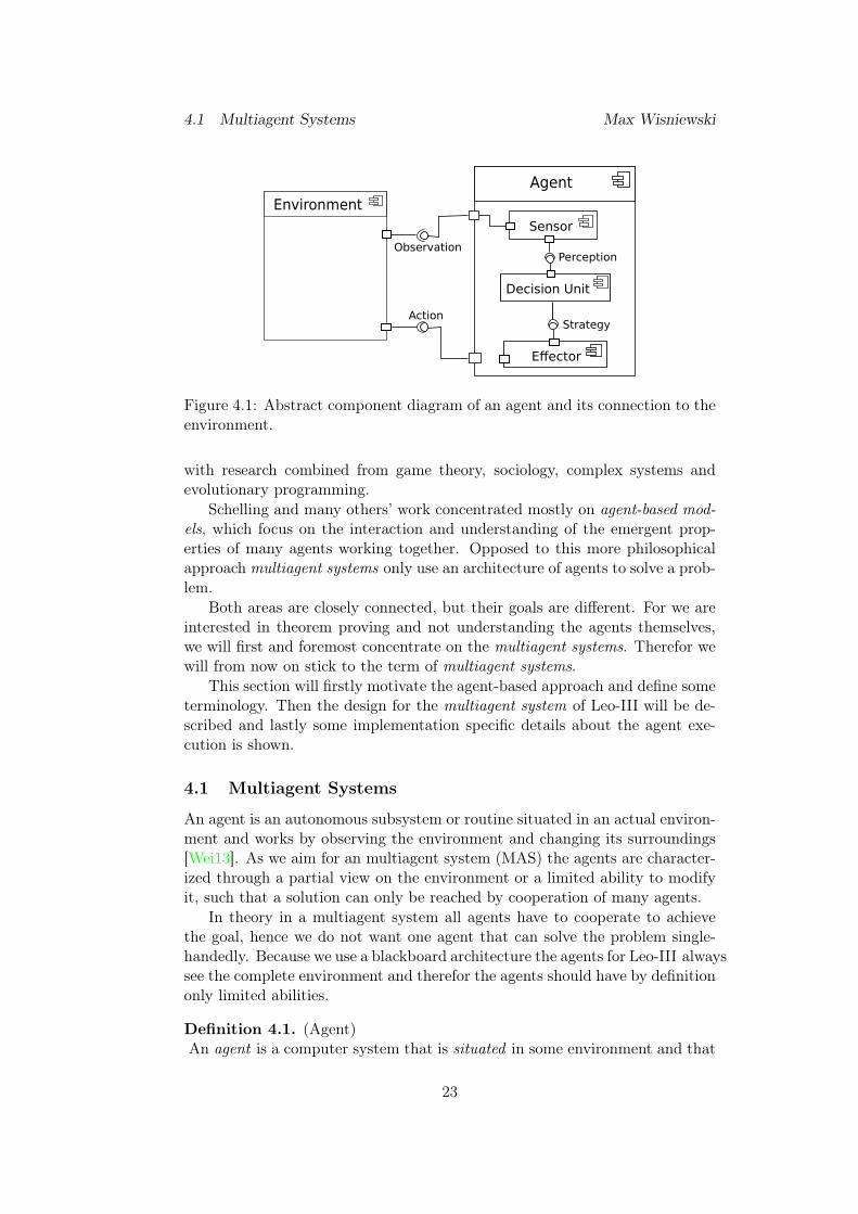
Figure 4.1: Abstract component diagram of an agent and its connection to theenvironment.
with research combined from game theory, sociology, complex systems andevolutionary programming.
Schelling and many others’ work concentrated mostly on agent-based mod-els, which focus on the interaction and understanding of the emergent prop-erties of many agents working together. Opposed to this more philosophicalapproach multiagent systems only use an architecture of agents to solve a prob-lem.
Both areas are closely connected, but their goals are different. For we areinterested in theorem proving and not understanding the agents themselves,we will first and foremost concentrate on the multiagent systems. Therefor wewill from now on stick to the term of multiagent systems.
This section will firstly motivate the agent-based approach and define someterminology. Then the design for the multiagent system of Leo-III will be de-scribed and lastly some implementation specific details about the agent exe-cution is shown.
4.1 Multiagent Systems
An agent is an autonomous subsystem or routine situated in an actual environ-ment and works by observing the environment and changing its surroundings[Wei13]. As we aim for an multiagent system (MAS) the agents are character-ized through a partial view on the environment or a limited ability to modifyit, such that a solution can only be reached by cooperation of many agents.
In theory in a multiagent system all agents have to cooperate to achievethe goal, hence we do not want one agent that can solve the problem single-handedly. Because we use a blackboard architecture the agents for Leo-III alwayssee the complete environment and therefor the agents should have by definitiononly limited abilities.
Definition 4.1. (Agent)An agent is a computer system that is situated in some environment and that
23
4.1 Multiagent Systems Max Wisniewski
is capable of autonomous action in this environment in order to achieve itsdelegated objectives. y
We note that an agent consists of at least three components (see figure 4.1)
(1) A sensor, allowing the agent to perceive its surroundings.
(2) A decision unit, allowing the agent to decide on the strategy based on itsperception of the environment.
(3) An effector, allowing the agent to manipulate the environment based onthe strategy chosen.
This concept of a agent is fairly vague and can be seen as the commonancestor of all agent types. Before looking at the global architecture consistingof many agents, one has to look at the different agent-architectures that arebased on the way the agent deals with the environment and the way the agentitself makes decisions.
We can roughly distinguish between three different kinds of agent-architectures[Woo02].
Reactive Agents make decisions only trigger basedly. They act on theirperception alone, do not save knowledge about the world and have nodecision procedure. In their behavior they work as human reflexes. Ifa human perceives a pain in a limb, he will instinctively move the limbto the center of the body. There is no thinking about the action. Theperception triggers the action spontaneously.
Adaptive Agents gain knowledge about the world through their perceptionand save it. This way an adaptive agent is able to make decisions basedon their current perception and their gained knowledge.
The knowledge is saved in suitable datastructures and can be changeddepending on the perception.
For example a human can glean information on the current weather. Hecan remember the weather of the last days, he knows the current seasonand on the perception of the sky he can make a prediction on the weathertoday and e.g. take an umbrella with him.
Cognitive Agents are on the other end of the spectrum. They do not act ontheir perception, but first interpret their perception into their own savedmodel of the world.
Based on the model a cognitive agent has of the world he than startsto take action. Many autonomous robotic systems used this approach,where they first build up a map of the surroundings and then start toplan a route to take, based purely on the virtual map.
A human uses such a behavior, just as the robot, if he walks throughhis house in the dark. He cannot see, but in his mind he can remember
24
4.1 Multiagent Systems Max Wisniewski
where everything should be. He acts purely on his internal map of thehouse. Of course this approach has difficulties if the model of the worldis wrong. In the case of the human for example if someone has moved achair. The internal map has the chair not in it, such that he will mostlikely trip over it.
There are different and finer classification, for example by Russel andNorvig [RN03]. Since the inside of our agents are not known and made upby the developers of the specific agents we stick to this simple classification.In this case Leo-III agents can be reactive, adaptive or something in between.
Because the functions of one agent are mostly limited, many agents areneeded for a system, that can actively solve tasks. This leads to the definitionof a multiagent system.
Definition 4.2. (Multiagent system)A multiagent system is a system of multiple agents in which no single agentcan solve the global objective by himself. y
The definition for MAS is fairly vague. The only information we can obtainfrom the definition is that a MAS is not a system in which we plug in someindividual systems and let them compete.
There are many possible architecture to employ a MAS and one of themis the blackboard architecture described above. But the MAS is not limited tothis architecture.
Belief-Desire-Intention Architecture The most famous architecture inMAS is the belief-desire-intention (BDI) architecture [DLG+04, Woo02]. InBDIs the agents declare a goal they want to achieve. Based on their believes oftheir perception they will act in an intended way. The architecture is slightlydifferent from the blackboard architecture since all agents have their own beliefdatabase that will be manipulated. Except from the beliefs the desired actionsbuild a database on their own to generate an action. Lastly the generatedaction is filtered and checked if they met the intention.
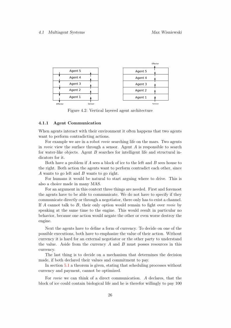
Layered Agent Architectures As the name conveys the agent are arrangedin layers visualized in figure 4.2. In layer architectures [Woo02] the agents donecessarily rely on the sensors, but the agents are chained. One output of anagent is the input for another agent.
Agents in this context work similar to a filter in a pipes-and-filter archi-tecture as visualized on the right side. In the left side only the first agent issituated in the real world. The agent pipe the information first upwards andthen the result is written back down to the first agent which can communicatewith effectors.
25
4.1 Multiagent Systems Max Wisniewski
Agent 1
Agent 2
Agent 3
Agent 4
Agent 5
Agent 1
Agent 1
Agent 1
SensorEffector
Agent 1
Agent 2
Agent 3
Agent 4
Agent 5
Agent 1
Agent 1
Agent 1
Sensor
Effector
Figure 4.2: Vertical layered agent architecture
4.1.1 Agent Communication
When agents interact with their environment it often happens that two agentswant to perform contradicting actions.
For example we are in a robot rovie searching life on the mars. Two agentsin rovie view the surface through a sensor. Agent A is responsible to searchfor water-like objects. Agent B searches for intelligent life and structural in-dicators for it.
Both have a problem if A sees a block of ice to the left and B sees house tothe right. Both action the agents want to perform contradict each other, sinceA wants to go left and B wants to go right.
For humans it would be natural to start arguing where to drive. This isalso a choice made in many MAS.
For an argument in this context three things are needed. First and foremostthe agents have to be able to communicate. We do not have to specify if theycommunicate directly or through a negotiator, there only has to exist a channel.If A cannot talk to B, their only option would remain to fight over rovie byspeaking at the same time to the engine. This would result in particular nobehavior, because one action would negate the other or even worse destroy theengine.
Next the agents have to define a form of currency. To decide on one of thepossible executions, both have to emphasize the value of their action. Withoutcurrency it is hard for an external negotiator or the other party to understandthe value. Aside from the currency A and B must posses resources in thiscurrency.
The last thing is to decide on a mechanism that determines the decisionmade, if both declared their values and commitment to pay.
In section 5.1 a theorem is given, stating that scheduling processes withoutcurrency and payment, cannot be optimized.
For rovie we can think of a direct communication. A declares, that theblock of ice could contain biological life and he is therefor willingly to pay 100
26
4.2 Leo-III Agent Max Wisniewski
units. B declares that the house looks like a rock and is therefor only willingto pay 50 units. They both decide that A can drive rovie to the ice block bypaying 50 units.
The communication and decision finding has been heavily explored throughgame theory. Since the communication of the agents decides on the access toshared objects, in rovie’s case the actuators of the tires and the engine, thiscommunication will act as the scheduler for the blackboard. In the remainderof this section, the internal structure of the agents for Leo-III will be discussed.The communication and game theoretic background will be tackled in section5.
4.2 Leo-III Agent
Before describing the design for the MAS of Leo-III it remains to describe thegeneral concept of an agent for Leo-III. In section 4.1 we introduced three typesof agent-architectures.
Since Leo-III is designed to be an extendable platform through the agents,we cannot determine every structure the agents might take, but there is ageneral concept. The blackboard approach introduced in section 3 is designedto share each and every information. Agents should therefor have no internaldatastructures to keep track of knowledge.
If this approach is used, we can see the agents as reactive agents, becausethey make decision purely on their perception of the world, in this case theblackboard. On the other hand the agent can keep track of their knowledge bysaving it in the blackboard. Hence their behavior resembles that of an adaptiveagent.
Since both these architectures are represented the desired Leo-III agent hasan architecture in between these two. This keeps us with the task to define inwhich way his perception, decision and action unit should work.
Through this work, three major approaches were tested of which the lastone was taken for Leo-III.
4.2.1 Simple Processes
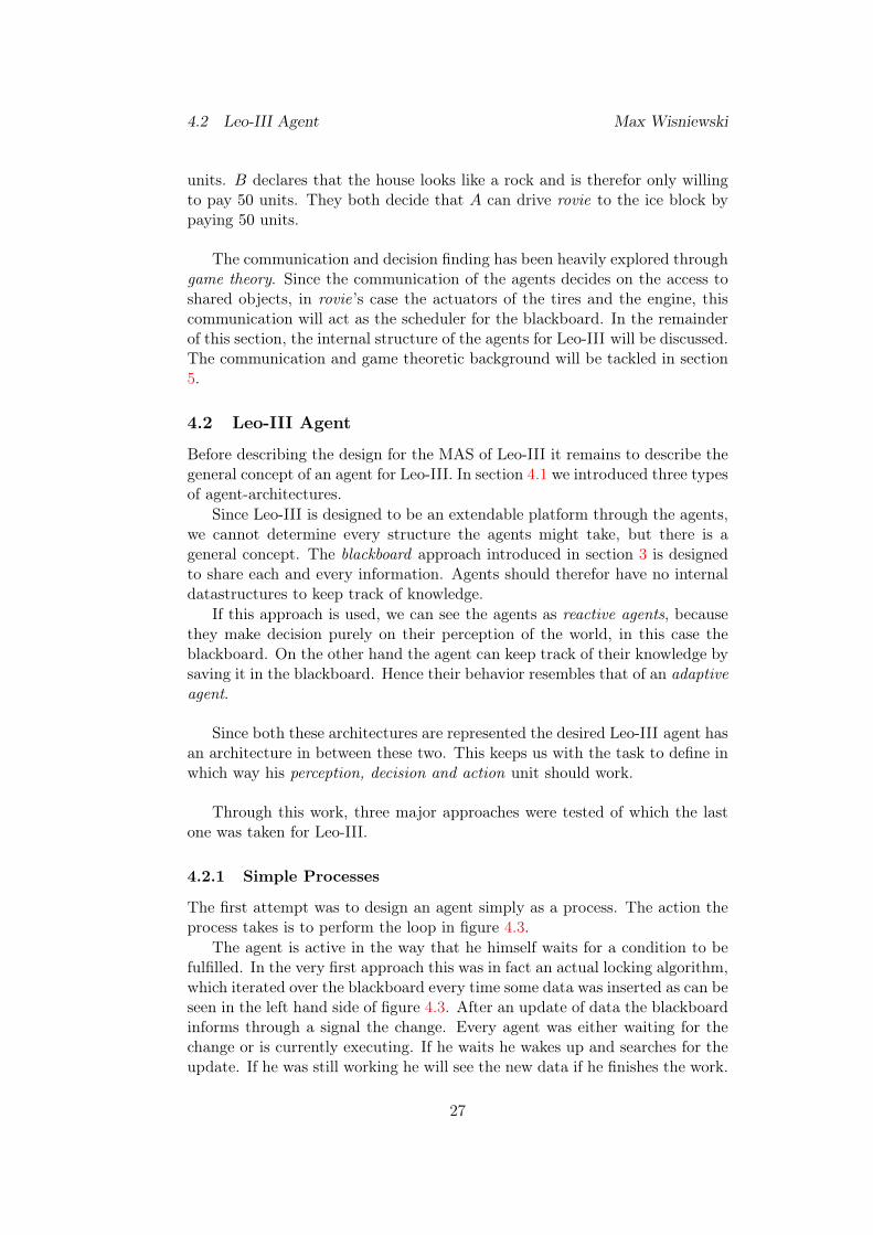
The first attempt was to design an agent simply as a process. The action theprocess takes is to perform the loop in figure 4.3.
The agent is active in the way that he himself waits for a condition to befulfilled. In the very first approach this was in fact an actual locking algorithm,which iterated over the blackboard every time some data was inserted as can beseen in the left hand side of figure 4.3. After an update of data the blackboardinforms through a signal the change. Every agent was either waiting for thechange or is currently executing. If he waits he wakes up and searches for theupdate. If he was still working he will see the new data if he finishes the work.
27
4.2 Leo-III Agent Max Wisniewski
Agent1 Blackboard Agent2
update(data)
signal signal
performableDataperformableData
nothingsome(data)
update(data)
Agent1 Blackboard Agent2
update(data)
filter(data) filter(data)
lookup(data)
some(data)
update(data)
Figure 4.3: Workflow for an agent designed as a simple process
In our example only Agent1 can perform, but Agent2 cannot. Then both makea lookup in the blackboard, whether there is something to operate on. OnlyAgent1 finds something and updates the result of its computation in the end.
This approach was quite slow, since the agent did not keep track of thechanges that where made, such that he iterated over every data for each change.A solution that survived into the final version, is to define a filter for an agent.Each agent can thereby be informed more explicitly, what has changed andwith this as a hint perform a faster lookup in the blackboard as can be seen inthe right hand side of figure 4.3. Here Agent2 can already see on the updateddata that he has nothing to and stops. Agent1 still performs his lookup, butthis time he has more information, namely that only something compatiblewith the updated data should lead to a new result.
This approach is the most direct one. It requires virtually no architecturein this case MAS and was a good design for first tests. The biggest problemarising, using this kind of agents, is the lack of synchronization support. Insection 3.2 some of the blackboard possibilities are explored and the decisionwas to make the datastructures themselves save for multiple access and not forconsistency, as described in that section.
4.2.2 Software Transactional Memory
As described in section 3.3 the datastructures in the blackboard are synchro-nized each one for themselves. This burdens the task of conflict resolution tothe MAS and the agent implementation. On the other hand Leo-III shouldprovide a general architecture to extend the prover. Hence we cannot burdenthe implementation with the synchronization.
A Leo-III agent should be of the kind that he can act as if no other agentexist in the world, i.e. the agent is isolated. His action should be atomic inthe sense that either all his changes are written to the blackboard or none. Iftwo processes update formulas at the same time the resulting state has to beconsistent as we already explored in 3.2. Lastly if a process is done writing its
28
4.2 Leo-III Agent Max Wisniewski
AgentBlackboard STM
filter(data)
lookup(data)
some(data)
execute(transaction)
write(changes)
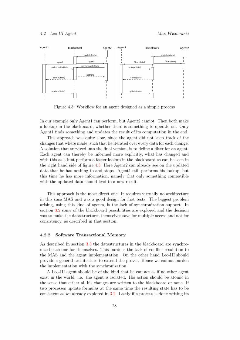
Figure 4.4: Workflow for an agent designed with software transactional mem-ory.
action to the blackboard the change cannot be undone so the action has to bedurable.
All these properties for the actions of an agent are the same as for a trans-action in database management systems. This is evident since the blackboarditself is a specialized database.
Since we need all the features of a transactional system, the first attemptevaluated in this context was a system of software transactional memory.
As can be seen in figure 4.4 the overall workflow is still the same as on theright of figure 4.3, but the execution and write back into the blackboard are nowcapsuled into a transaction and executed through the software transactionalsystem.
This approach was not taken due to two reasons. Firstly to write an agentwith transactions has proven itself to be difficult, since the syntax is a burden tothe programmer. The desired agent for Leo-III should make it only necessaryto write the behavior of the agent. The programmer should not bother withsynchronization mechanisms or possible other agents in the systems.
The second reason is that the transactional memory allows to execute theactions in parallel, but we have no control which actions should be takenpreferably. Then again conflicting transactions should maybe never executedif in the new context the action could no longer be applied.
One thing we learned from this design was that a transactional design solvesmostly all problems we burdened on us by using a local synchronization in theblackboard. On the other hand we see that the use of transactions gives us theopportunity to separate the agents generation of an action from its execution.
In the last approach we will hence concentrate on two things. How to hidethe transactional behavior, a way to gain more control over the transaction
29
4.2 Leo-III Agent Max Wisniewski
AgentBlackboard Executor
filter(data)
lookup(data)
some(data)
addTasks(tasks)
getTasks()
List(tasks)
writeChanges()
Figure 4.5: Workflow for the transaction agent.
execution and, lastly an approach to implement an agent without an staticbound process.
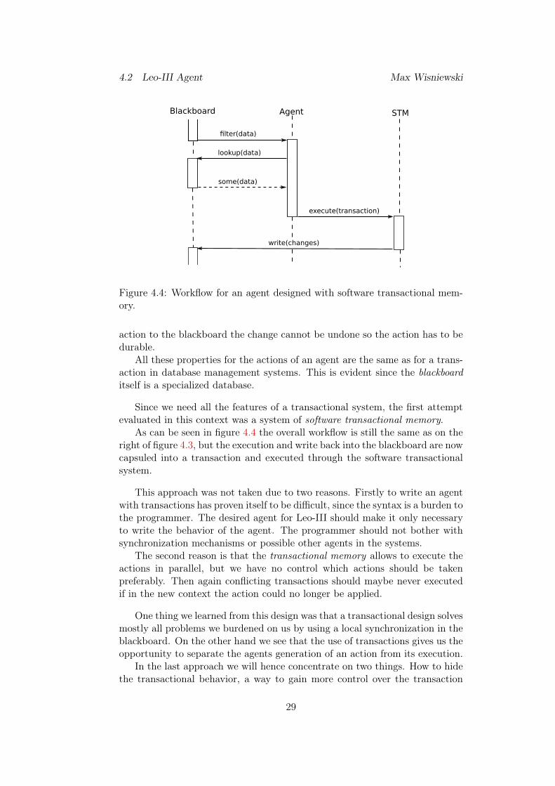
4.2.3 Transactions
The last explored approach uses an own transaction system for the agents. Theworkflow is designed as seen in figure 4.5. Agent1 does not create a softwaretransaction, but an object called task that capsules a deferred action. A taskis send to a scheduler which is in fact the same as the software transactionalmemory, with the difference that the scheduler can be customized specific toLeo-III.
The designed concept of the execution was explored by Guessoum andBriot [GB99] as active agents. The concept behind this idea is to model theexecution of an agent as an active object [Agh86]. Active Objects are a wayto work asynchronously with concurrency. In this context a function does notreturn the value as a result, but as a promise that sometime in the future theresult will be there. The object, often called future, has a blocking method toget the result, but the caller does not have to call this method immediately.
In the background a task containing the implementation of the functionand a reference to the future is inserted in a queue. If the task is consideredfor execution by a scheduler, the task is executed and the result is inserted intothe future, where henceforth the result can be accessed non-blockingly.
This is the general concept behind this last idea, but with a major differ-ence. In the context of active agents / active objects a task is inserted into aqueue, where this task has an execution method. Leo-III calls the run method
30
4.3 Leo-III MAS Architecture Max Wisniewski
on the agent, with the task as an input. This way an agent has more controlover their tasks and can, if really necessary, handle internal datastructures.
Implementing a multiagent system with this agent architecture requiresthree things.
1. A transactional behavior that allows only tasks to execute that do notconflict each other.
2. An execution engine, that performs the execution of the task.
3. A scheduler, that decides on the next tasks to be executed.
All three are major parts of the mulitagent architecture as they decide onthe interaction of the agents with their environment.
4.3 Leo-III MAS Architecture
In this section the general concept and design of the MAS for Leo-III is pre-sented. Since we already decided on a blackboard based architecture that wasintroduced in section 3 we will concentrate in more detail on the specifics ofthe chosen implementation in this section.
In the context of Leo-III an agent is situated in the blackboard as the onlyenvironment. Compared to the two other possible architectures presented,there is virtually no structure between the agents. The attention of an agentis directed at the blackboard.
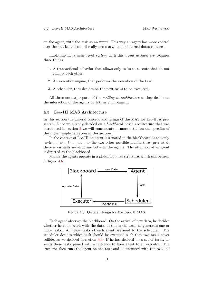
Mainly the agents operate in a global loop like structure, which can be seenin figure 4.6
Agent
SchedulerExecutor
Blackboard new Data
Task
(Agent,Task)
update Data
Figure 4.6: General design for the Leo-III MAS
Each agent observes the blackboard. On the arrival of new data, he decideswhether he could work with the data. If this is the case, he generates one ormore tasks. All these tasks of each agent are send to the scheduler. Thescheduler decides which task should be executed such that two tasks nevercollide, as we decided in section 3.3. If he has decided on a set of tasks, hesends these tasks paired with a reference to their agent to an executor. Theexecutor then runs the agent on the task and is entrusted with the task, so
31
4.3 Leo-III MAS Architecture Max Wisniewski
that the result is written back to the blackboard. This new data closes thecircle, since a next iteration of task generation is initiated.
The workflow matches the abstract agent design in figure 4.1. The sensorunit is here directly coupled with the blackboard. This one knows, which datahave been added and therefor the sensor unit can be omitted. The newly addeddata can be directly perceived by the agent. The decision unit is represented bythe task generation, whereby the strategy is called task in the Leo-III context.The effector is the result of the agent. The action is performed in the executorby writing the data to the blackboard.
With the blackboard structure already given in section 3, we have to dealwith the remaining questions. These are task generation of the agents, schedul-ing of the task, execution of the task and lastly writing of the result back tothe blackboard.
Task Generation The chosen agent architecture offers a filter method forupdated formulas to generate new tasks. The multiagent architecturenow has to use this function. Since agents react purely passive, there hasto be some part in the architecture to call this method.
In figure 4.4 the blackboard called the filter method after the formulaswere updated. The architecture pattern used here is the observer pattern.
In the observer pattern an object can register itself to a certain type ofevents. The pattern is often used in interactive programs, e.g. graphicalapplications. In there an event could be a click on a button. In thisprogram a variety of objects have to be updated, not all explicitly knownto the button. In the graphical application we could imagine a buttonthat switches between two modes of operation. First of all, the interfacehas to be switched to the new mode. Then the new mode might requirea reset of a number of datastructures.
The click now notifies all registered objects, in this case the interfaceand the datastructures, about its activation. The button does not know,what changes have to be applied, but each of the objects does and thebutton has references to these objects.
The pattern is easy to update actively by runtime. For example if anundoing tool is added, the tool needs to know of the mode change tomake an undo step available. For the button nothing changes, exceptanother observer registers and will be called if the activation happens.
In the case of Leo-III all agents are observers on the blackboard, inter-ested in a data update. Thus the architecture is allowed to add agentswithout changing the implementation of the blackboard. The observerpattern even allows to remove or add agents during the execution of theprogram. This way specialized provers can be added if the analyzedcontext emphasizes that they could be beneficial.
32
4.3 Leo-III MAS Architecture Max Wisniewski
The one thing that requires more thought than in the button example,is the notification of the observers. The button had the advantage of asingular indivisible action that happened. As soon as the click occurred,the graphical interface and all other datastructures could be informed.
In the context of the blackboard the agents are interested in an update ofdata. Since the update of data always happens inside of a transaction, thenotification cannot be send each time data is updated in the blackboard.This is due to the atomicity of the transactions, since a transaction willupdate sequentially in the blackboard. If the notification happens aftereach update, the filter would be applied to an unobservable state, ac-cording to atomicity, since one formula of the transaction is updated butanother is not.
Hence the notification has to be done coupled with the writing to theblackboard. This problem will be tackled below in the writing to theblackboard.
Lastly the tasks which were generated after a notification has been donehave to be saved. The agreement in the beginning was that all data issaved in the blackboard. In this case the tasks are saved in the agentsand the blackboard has a method to access the tasks through the agents.The explanation will be given in section 5.3.
Scheduler This is the second time the scheduler is mentioned. The first timein section 3 the scheduler was an abstract routine that selects whichspecialist may write to the blackboard. After deciding on an (multi)agentarchitecture, there are more requirements for the scheduler.
The chosen agent architecture demands that the scheduler should bea transactional system. Hence he has to take care that no two tasksexecutions may collide with each other. The property of collision be-tween tasks, if their read and write sets intersect, was first formulated byBernstein [Ber66]. For transactional systems there are many well knownpossibilities to avoid collision, such as two-phase locking, time-stampordering or serialization graph checking[BHG86].
The scheduler will implement a form of strict two-phase locking. SinceLeo-III uses a scheduler which makes it easier to implement the two-phase locking, because one central instance, the scheduler, acquires alllocks and releases all locks at once.
In comparison to the above mentioned methods to implement transactiona scheduler performs slower, since the scheduler itself is not parallelized.Two-phase locking itself requires serial behavior only if two processes at-tempt to work at the same time, but their tasks are colliding. Otherwiseboth will run completely independent, hence there is no communicationoverhead.
33
4.3 Leo-III MAS Architecture Max Wisniewski
In section 3 we already observed that in Leo-III coordination of agents isnecessary. The scheduler is thus not only the place where the transactionsystem is implemented, but also the part of the system that decides whichtasks are to prioritize.
The prioritization is an important part in Leo-III. Depending on thefreedom of the implemented agents, a vast space of possibilities couldbe explored. Returning to the mars rover from section 4.1.1, a badprioritization might lead to a behavior where the agents A and B driverovie to the water and to the stone structure, but never remain longenough at one side for the real research. The rover would be working thewhole time, but accomplish nothing.
Execution To this point, the agent can generate transactions, called tasks,submit them to the scheduler and have them selected. The next stepis the execution of the tasks. Since the next section 4.4 is dedicated tothis topic and the point is self explaining, we will not further explain thefunctionality here.
Since the blackboard and agents are purely passive, the execution unitis designed as an active process. The execution unit is itself designed asan agent that observes the blackboard for changes in the scheduling. Ifnew tasks are available and the execution agent has capacity left, he willcall the scheduling method in the blackboard and execute the tasks.
The general design of the execution agent resembles the simple processarchitecture we first analyzed for the Leo-III agents. Since this agentfollows only this simple pattern and is stimulated only if tasks are created,there is no need for a more complex structure. Also he cannot be part ofthe structure as the other agents, since there would be no active executionagent to run his tasks.
Writing After the task was created, chosen and executed, the result still hasto be written back into the blackboard.
As all other processes in Leo-III, the processes to write the results to theblackboard are designed as an agent. The data he is interested in arethe results created by the other agents. The task he creates applies theupdates in the result to the blackboard.
In comparison to the normal agents in Leo-III, his observing behavioris not fed by the blackboard. The execution agent inserts the resultsdirectly as write back tasks into his internal queue. Since he should bethe only one interested in these result, this makes the communicationeasy.
The design as tasks allows the writing to the blackboard again to bemade in parallel. Also depending on the implementation of the executionagent, there are no more resources needed for the writing. All executionresources remain with the execution agent.
34
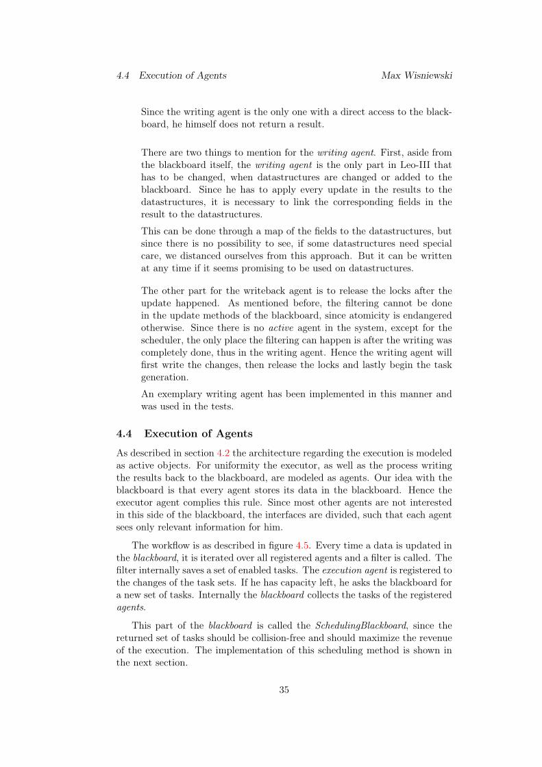
4.4 Execution of Agents Max Wisniewski
Since the writing agent is the only one with a direct access to the black-board, he himself does not return a result.
There are two things to mention for the writing agent. First, aside fromthe blackboard itself, the writing agent is the only part in Leo-III thathas to be changed, when datastructures are changed or added to theblackboard. Since he has to apply every update in the results to thedatastructures, it is necessary to link the corresponding fields in theresult to the datastructures.
This can be done through a map of the fields to the datastructures, butsince there is no possibility to see, if some datastructures need specialcare, we distanced ourselves from this approach. But it can be writtenat any time if it seems promising to be used on datastructures.
The other part for the writeback agent is to release the locks after theupdate happened. As mentioned before, the filtering cannot be donein the update methods of the blackboard, since atomicity is endangeredotherwise. Since there is no active agent in the system, except for thescheduler, the only place the filtering can happen is after the writing wascompletely done, thus in the writing agent. Hence the writing agent willfirst write the changes, then release the locks and lastly begin the taskgeneration.
An exemplary writing agent has been implemented in this manner andwas used in the tests.
4.4 Execution of Agents
As described in section 4.2 the architecture regarding the execution is modeledas active objects. For uniformity the executor, as well as the process writingthe results back to the blackboard, are modeled as agents. Our idea with theblackboard is that every agent stores its data in the blackboard. Hence theexecutor agent complies this rule. Since most other agents are not interestedin this side of the blackboard, the interfaces are divided, such that each agentsees only relevant information for him.
The workflow is as described in figure 4.5. Every time a data is updated inthe blackboard, it is iterated over all registered agents and a filter is called. Thefilter internally saves a set of enabled tasks. The execution agent is registered tothe changes of the task sets. If he has capacity left, he asks the blackboard fora new set of tasks. Internally the blackboard collects the tasks of the registeredagents.
This part of the blackboard is called the SchedulingBlackboard, since thereturned set of tasks should be collision-free and should maximize the revenueof the execution. The implementation of this scheduling method is shown inthe next section.
35
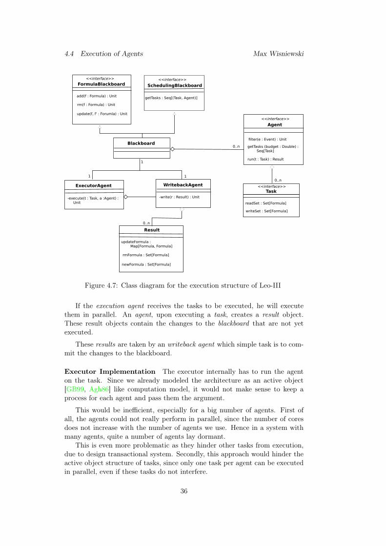
4.4 Execution of Agents Max Wisniewski
FormulaBlackboard
add(f : Formula) : Unit
rm(f : Formula) : Unit
update(f, f' : Forumla) : Unit
<<interface>>
SchedulingBlackboard<<interface>>
getTasks : Seq[(Task, Agent)]
Blackboard
ExecutorAgent
-execute(t : Task, a :Agent) : Unit
WritebackAgent
-write(r : Result) : Unit
Result
newFormula : Set[Formula]
rmFormula : Set[Formula]
updateFormula : Map[Formula, Formula]
Agent
filter(e : Event) : Unit
getTasks (budget : Double) : Seq[Task]
run(t : Task) : Result
<<interface>>
Task
writeSet : Set[Formula]
readSet : Set[Formula]
<<interface>>
0..n
1
0..n
0..n
1 1
Figure 4.7: Class diagram for the execution structure of Leo-III
If the execution agent receives the tasks to be executed, he will executethem in parallel. An agent, upon executing a task, creates a result object.These result objects contain the changes to the blackboard that are not yetexecuted.
These results are taken by an writeback agent which simple task is to com-mit the changes to the blackboard.
Executor Implementation The executor internally has to run the agenton the task. Since we already modeled the architecture as an active object[GB99, Agh86] like computation model, it would not make sense to keep aprocess for each agent and pass them the argument.
This would be inefficient, especially for a big number of agents. First ofall, the agents could not really perform in parallel, since the number of coresdoes not increase with the number of agents we use. Hence in a system withmany agents, quite a number of agents lay dormant.
This is even more problematic as they hinder other tasks from execution,due to design transactional system. Secondly, this approach would hinder theactive object structure of tasks, since only one task per agent can be executedin parallel, even if these tasks do not interfere.
36
4.4 Execution of Agents Max Wisniewski
Luckily in Java there is already a structure of processes implemented thatare not limited to one task. The object is an ExecutorService that allows theuser to define a priori a number of threads which should run in parallel.
After initialization a Runnable can be generated, encapsulating the execu-tion of the Task. The Runnable can be given to the ExecutorService, whichwill assign a thread for execution as soon as there is one available.
The advantage of this implementation is that we can limit the number ofthreads, hence to not overburden the system that runs Leo-III.
Properties of the Implementation This chosen design and implementa-tion have proven to be very independent of the agent implementation until now.
It is a desirable feature to implement the execution of tasks, rather thanthat of agents. This way an agent can run in parallel to itself and work thatcan be done independently, will automatically be parallelized.
If agents were designed as processes, for a parallelization of the agents work,the agent has to be inserted multiple times into the system.
This would contribute nothing new to the system, but another object re-sponsible for handling the tasks.
The use of an executor service is beneficial to the resource consumption,since we can limit the number of threads running without limiting the numberof agents.
By implementing the transactional system on top of the agents, a developerof a new agent does not have to concern with side effects or collisions with otheragents. He only specifies when the agent is interested to operate, the action ofhis operation and the returned result.
The interest and the action are always part of an agent implementation.The result objects are the only extra task burdened on the developer. Forthis he is guaranteed that his execution is always written consistently to theblackboard.
If the blackboard is enriched with more datastructures through the devel-opment of Leo-III the single changes made to the execution system are thewriteback agent and the Result interface 2.
If new kinds of data are written, they must be tracked in the result. Thewriteback agent must apply all changes to the blackboard, but old agents donot have to concern themselves with the new data and act as if nothing haschanged.
After describing the execution and design of the agents and describing thegeneral design of the blackboard, the only thing remaining for the execution isscheduling the tasks.
2The blackboard interface changes as well, but as long as only additions are made, theagent and execution structure is not concerned.
37
5 Games & Auctions Max Wisniewski
5 Games & Auctions
In section 4 the general design for the agents to interact with the blackboardand each other was discussed.
The design of the scheduler was to execute only not interfering tasks, butthe method to choose these tasks is still open. In the proving context wecannot simply implement a method that has a good response time or a highthroughput, as seen in standard scheduling algorithms. We neither can proofhard guarantees as in real-time systems.
The agent approach heavily depends on the right choice at the right time.Each evaluated task has a certain value for the agents in any given context.We assume the agents to be social, i.e. they do not cheat the system. Thescheduler should now work in order to always to optimize the welfare of thewhole system.
The mechanism that chooses tasks has to satisfy certain conditions. Firstlyonly non interfering tasks should be chosen. Next, each tasks is rated througha profit function, how much does an agent gain if the tasks are executed.The mechanism should then choose a set of tasks that maximizes the totalprofit. Lastly, because this is the method the scheduler uses to assign tasksfor execution, the mechanism should satisfy certain liveness properties. Oneof the central ones is that each agent may eventually run a task on a set offormulas.
In this section we will take a look at the general game theoretic foundationsfor such a mechanism and then give a fast approximating algorithm for theproblem.
5.1 Game Theory
This section is mainly based on Nisan et al. [NRTV07].Game theory deals with the interaction of players with each other in the
presence of individual goals each player wants to achieve.The applications were firstly seen in economics, politics and in law. Later
computer science applied game theory as well as biology in their domains.In this section some foundations are explained which are needed for the
algorithm the scheduler uses and will be explained at the end of the section.
Games
Definition 5.1. (Game)Let p1, ..., pn = P be a set players and SP a set of individual strategies foreach player.
A vector s = (si ∈ SP)i∈P is called (pure) strategy and (s | sk) for sk ∈ SPis the strategy s except the player k plays the individual strategy sk.
A function g : Sp1 × . . . × Spn → Rn that assigns a strategy the payofffor each player is called a game. And gpi is the projection to the payoff of theplayer pi. y
38
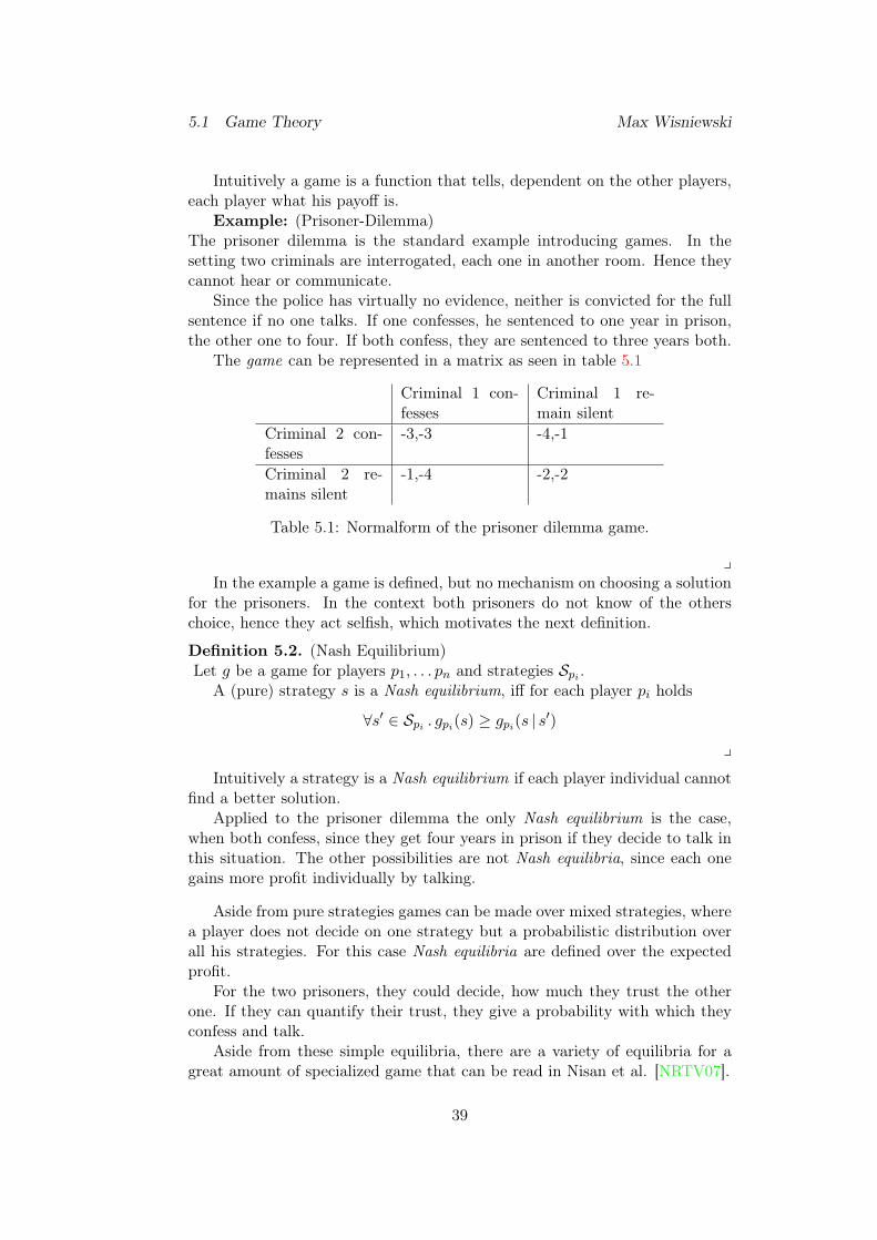
5.1 Game Theory Max Wisniewski
Intuitively a game is a function that tells, dependent on the other players,each player what his payoff is.
Example: (Prisoner-Dilemma)The prisoner dilemma is the standard example introducing games. In thesetting two criminals are interrogated, each one in another room. Hence theycannot hear or communicate.
Since the police has virtually no evidence, neither is convicted for the fullsentence if no one talks. If one confesses, he sentenced to one year in prison,the other one to four. If both confess, they are sentenced to three years both.
The game can be represented in a matrix as seen in table 5.1
Criminal 1 con-fesses
Criminal 1 re-main silent
Criminal 2 con-fesses
-3,-3 -4,-1
Criminal 2 re-mains silent
-1,-4 -2,-2
Table 5.1: Normalform of the prisoner dilemma game.
yIn the example a game is defined, but no mechanism on choosing a solution
for the prisoners. In the context both prisoners do not know of the otherschoice, hence they act selfish, which motivates the next definition.
Definition 5.2. (Nash Equilibrium)Let g be a game for players p1, . . . pn and strategies Spi .
A (pure) strategy s is a Nash equilibrium, iff for each player pi holds
∀s′ ∈ Spi . gpi(s) ≥ gpi(s | s′)
y
Intuitively a strategy is a Nash equilibrium if each player individual cannotfind a better solution.
Applied to the prisoner dilemma the only Nash equilibrium is the case,when both confess, since they get four years in prison if they decide to talk inthis situation. The other possibilities are not Nash equilibria, since each onegains more profit individually by talking.
Aside from pure strategies games can be made over mixed strategies, wherea player does not decide on one strategy but a probabilistic distribution overall his strategies. For this case Nash equilibria are defined over the expectedprofit.
For the two prisoners, they could decide, how much they trust the otherone. If they can quantify their trust, they give a probability with which theyconfess and talk.
Aside from these simple equilibria, there are a variety of equilibria for agreat amount of specialized game that can be read in Nisan et al. [NRTV07].
39
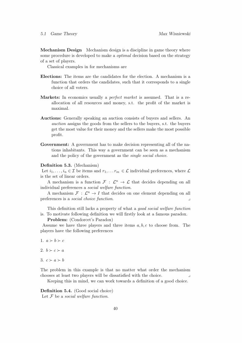
5.1 Game Theory Max Wisniewski
Mechanism Design Mechanism design is a discipline in game theory wheresome procedure is developed to make a optimal decision based on the strategyof a set of players.
Classical examples in for mechanisms are
Elections: The items are the candidates for the election. A mechanism is afunction that orders the candidates, such that it corresponds to a singlechoice of all voters.
Markets: In economics usually a perfect market is assumed. That is a re-allocation of all resources and money, s.t. the profit of the market ismaximal.
Auctions: Generally speaking an auction consists of buyers and sellers. Anauction assigns the goods from the sellers to the buyers, s.t. the buyersget the most value for their money and the sellers make the most possibleprofit.
Government: A government has to make decision representing all of the na-tions inhabitants. This way a government can be seen as a mechanismand the policy of the government as the single social choice.
Definition 5.3. (Mechanism)Let i1, . . . , in ∈ I be items and r1, . . . rm ∈ L individual preferences, where Lis the set of linear orders.
A mechanism is a function F : Ln → L that decides depending on allindividual preferences a social welfare function.
A mechanism F : Ln → I that decides on one element depending on allpreferences is a social choice function. y
This definition still lacks a property of what a good social welfare functionis. To motivate following definition we will firstly look at a famous paradox.
Problem: (Condorcet’s Paradox)Assume we have three players and three items a, b, c to choose from. Theplayers have the following preferences
1. a b c
2. b c a
3. c a b
The problem in this example is that no matter what order the mechanismchooses at least two players will be dissatisfied with the choice. y
Keeping this in mind, we can work towards a definition of a good choice.
Definition 5.4. (Good social choice)Let F be a social welfare function.
40
5.1 Game Theory Max Wisniewski
1. F satisfies unanimity if for all ≺∈ L,F (≺, . . . ,≺) =≺.
Intuitively this means that if all agree on an order the mechanism willchoose this order.
2. A player pi is a dictator if for all ≺p1 , . . . ≺pm∈ L F (≺p1 , . . . ,≺pm) =≺pi .
Intuitively a dictator says what to do, independent of the choice of pref-erences.
3. F is independent of irrelevant alternatives if the preference between twoitems a, b ∈ I is only dependent on the players.
Formally this property means, if for all ≺1, . . . ,≺m,≺′1, . . . ,≺′m∈ L with≺= F (≺1, . . . ,≺m) and ≺′= F (≺′1, . . . ,≺′m), then a ≺i b ⇔ a ≺′i b forall i implies asuccb⇔ a ≺′ b.
Intuitively this means that the ordering of a and b in the social welfaredoes not depend on a third element c.
y
The next is the famous impossibility result by Arrow [Arr51], which can bestated as follows.
Theorem 5.5. (Arrow’s Theorem) Every social welfare function over a set ofmore than two candidates that satisfies unanimity and independence of irrele-vant alternatives is a dictatorship.
A simple proof was given by Ning Neil Yu [Yu12].Arrow’s theorem is famous in economics. Colloquially speaking it states
that in a system without money, no mechanism for fair solutions can be found.
If money is involved there is an escape from dictatorship. Each playerassigns a value to the items, thereby ordering them. The mechanism can nowmake a decision by charging the players a few, if their choice was taken.
In this setting each player wants to maximize his value. The mechanismsalmost always optimize a global revenue function that ensures to some extendthat all players are pleased.
Auctions One type of social welfare function that can be optimized withmoney is an auction. We are interested in these specific games, because thescheduler will be based on them.
Definition 5.6. (Auction)Let P = p1, . . . , pn be bidders (players) and I = i1, . . . , im Items. Eachplayer has a value function vpi : I → R+ and an budget bp1 , . . . , bpn .
An auction (auction mechanism) is a mapping of items to bidders
σ : I → P
41
5.2 Combinatorical Auctions Max Wisniewski
and a prizing functionρ : I → R+
such that no one buys more than he can afford
∀1 ≤ p ≤ n :∑
i∈σ−1(p)
ρ(i) ≤ bp
and the total valuen∑p=1
∑i∈σ−1(p)
vp(i)
is maximized. y
This is the basic definition of a market with no dividable resources andno sellers. The intuition behind this simple market is that the auctioneer isselfless and wants to maximize the social revenue.
We will go with this definition, rather than a auctioneer that is interestedin his own profit or with many sellers, because this fits the market we willdefine the scheduler on.
One last alteration is that in reality the value function v for the players isnot known to the auctioneer. Hence the bidders can start to manipulate theauctioneer by telling false values.
Definition 5.7. (Incentive Compatible)An auction mechanism is called incentive compatible if the bidders refer tellingthe truth over a lie.
Note that only allowing the bidders to send the bids according to their own,makes an auction a game. Otherwise there would be no room for strategies.
5.2 Combinatorical Auctions
After we looked at simple auctions and mechanisms this section is dedicatedto the problem we want to solve for the scheduling problem.
The problem is already applied to the setting of tasks, whereas the standardcombinatorical auction speaks about sets and intersections.
Preliminaries To talk about the solutions, firstly we have to fix some nota-tion.
Definition 5.8. (Tasks)Let F be a set of items.
A task t over F is a three tupel (R,W, V ), where R ⊆ F is the read set ofthe task, W ⊆ F is the write set of the task and V ∈ R+ is its value.
We define tr = R, tw = W and tb = V as shorthands for the elements ofthe tupel. y
42
5.2 Combinatorical Auctions Max Wisniewski
With this we can start define what an “intersection” for tasks means.
Definition 5.9. (Collision)Let t1, t2 be two tasks.
We call t1 and t2 colliding if and only if
tw1 ∩ tw2 = ∅ ∧ tr1 ∩ tw2 = ∅ ∧ tw1 ∩ tr2 = ∅.
We call t1 and t2 non-colliding if and only if both are not colliding.We introduce the the two predicates col(t1, t2) and ncol(t1, t2) for both
these properties. y
Definition 5.10. (Collision-free)Let t1, . . . , tn be a set of tasks and T ⊆ [n] be an index sets.
The subset of tasks defined by T are called collision-free, if and only if
∀i∈T ∀j∈T \incol(ti, tj).
For abbreviation colfreet1,...,tnT or we can omit the tasks if they are clearin the context.
y
Combinatorical Auction A combinatorical auction takes place in a setting,where every player wants to obtain a subset of items to achieve a goal. E.g.a mechanic would like to buy a broken car, but only in combination with anengine and new wheels. In this context the mechanic has no benefit in buyingonly one of the items, because neither works on its own. He would only pay aprice if he can get the car, the engine and the wheels together.
In the auction there are many of these players and each one wants a differentsubset of items. The auctioneer on the other hand wants to maximize hisincome. That is the total amount of money he gets from each player.
The task for the mechanism for this auction is to assign the items distinctlyto all players, such that the income for the auctioneer is maximized, but noitem is given to two different persons.
This is the case in the standard combinatorical auction setting. But forour scheduler we have items that can be shared through many players if theydo not wish to modify the item. If they want to change the items they haveto state that they want it for their own.
Hence we exchange the property that the subsets do not intersect, i.e. noitem is given to two different players, with the property of collision-freeness.
Definition 5.11. (Combinatorical Auction)Let t1, . . . , tn be a set of tasks over a set of items R.
A combinatorical auction is a mechanism for the following optimizationproblem.
43
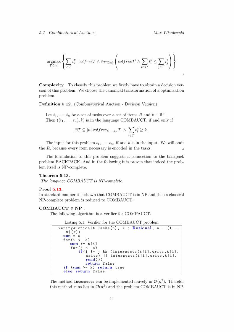
5.2 Combinatorical Auctions Max Wisniewski
argmaxT ⊆[n]
∑i∈T
tpi
∣∣∣∣∣∣ colfreeT ∧ ∀T ′⊆[n]colfreeT ′ ∧∑
i∈T ′tpi ≤
∑j∈T
tpj
y
Complexity To classify this problem we firstly have to obtain a decision ver-sion of this problem. We choose the canonical transformation of a optimizationproblem.
Definition 5.12. (Combinatorical Auction - Decision Version)
Let t1, . . . , tn be a set of tasks over a set of items R and k ∈ R+.Then ((t1, . . . , tn), k) is in the language COMBAUCT, if and only if
∃T ⊆ [n].colfreet1,...,tnT ∧∑i∈T
tpi ≥ k.
The input for this problem t1, . . . , tn, R and k is in the input. We will omitthe R, because every item necessary is encoded in the tasks. y
The formulation to this problem suggests a connection to the backpackproblem BACKPACK. And in the following it is proven that indeed the prob-lem itself is NP-complete.
Theorem 5.13.The language COMBAUCT is NP-complete.
Proof 5.13.In standard manner it is shown that COMBAUCT is in NP and then a classicalNP-complete problem is reduced to COMBAUCT.
COMBAUCT ∈ NP :The following algorithm is a verifier for COMPAUCT.
Listing 5.1: Verifier for the COMBAUCT problemverifyAuction(t Tasks[n], k : Rational , a : 1...
n[r])sum = 0for(i <- a)
sum += t[i]for(j <- a)
i f (i != j && (intersects(t[i].write ,t[i].write) || intersects(t[i].write ,t[i].read)))return false
i f (sum >= k) return truee l se return false
The method intersects can be implemented naively in O(n2). Thereforthis method runs lies in O(n3) and the problem COMBAUCT is in NP.
44
5.2 Combinatorical Auctions Max Wisniewski
SETPACK ≺p COMBAUCT :For the polynomial reduction we want to show that there exists a functionf that runs in polynomial time such that
x ∈ SETPACK⇔ f(x) ∈ COMBAUCT.
Set Packing is one of Karp’s 21 NP-complete problems and has the fol-lowing formulation.
Definition 5.14. (Set Packing)Let U be a universe and S ⊂ S ⊂ U a set of subsets of the universe.A packing of S is a subset C ⊂ S, s.t. all elements of C are pairwisedisjoint.A maximum set packing is a packing C, s.t. there exist no packing C′with |C| < |C′|. y
For the NP formulation of the problem a number k is given and it ischecked whether there is a packing C with |C| ≥ k.The function f now takes every s ∈ S and makes a task ts of it withtws = s, trs = ∅ and tps = 1. The number k of sets we want to take isdirectly taken for the value the auctioneer wants to get. The functionperforms a simple rewriting of the input is linear.
x ∈ SETPACK⇒ f(x) ∈ COMBAUCT :Let C be the packing with |C| ≥ k. Then the translated set T =ts | s ∈ C is collision-free.The total value ∑
s∈Ttps
Def. f= |C| · 1 ≥ k
is greater than k and therefore f(C) is a solution to COMBAUCT.f(x) ∈ COMBAUCT⇒ x ∈ SETPACK :
Let T = ts, | s ∈ C be a solution for COMBAUCT and C theoriginal set of subsets the tasks in T were derived from.From f(x) ∈ COMBAUCT we know that the value of the set isgreater than k, hence we can derive
k ≤∑s∈T
tpsDef. f
=∑s∈T
1 = |T | = |C|.
Therefor C is a solution for SETPACK.
This result poses a problem on the approach to use these kind of auctions
to implement our scheduler. On the one hand we want a globally good choiceof tasks to be executed, i.e. the ones with the highest price, but on the otherhand we do not have the time to compute the best choice.
On the edge between being efficient and finding a good solution one stan-dard approach is to approximate the solution.
45
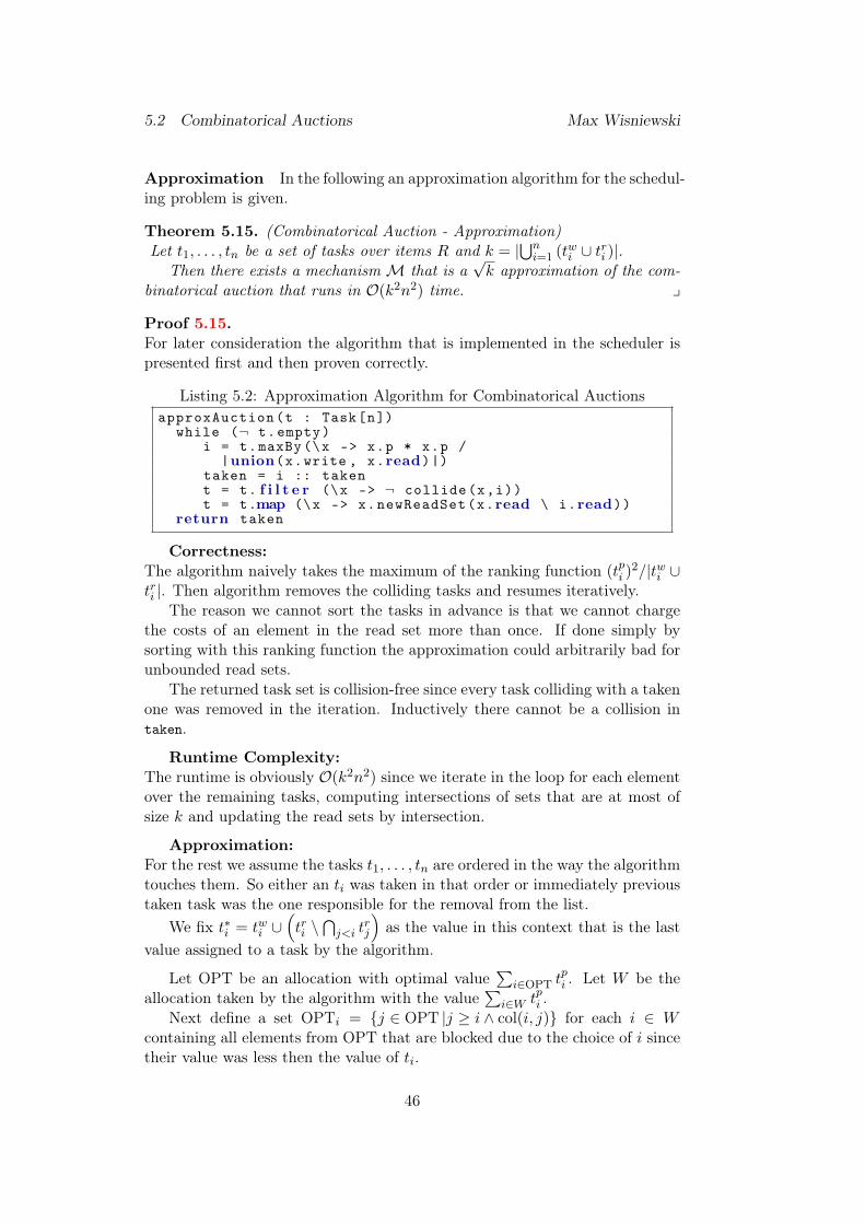
5.2 Combinatorical Auctions Max Wisniewski
Approximation In the following an approximation algorithm for the schedul-ing problem is given.
Theorem 5.15. (Combinatorical Auction - Approximation)Let t1, . . . , tn be a set of tasks over items R and k = |
⋃ni=1 (twi ∪ tri )|.
Then there exists a mechanismM that is a√k approximation of the com-
binatorical auction that runs in O(k2n2) time. y
Proof 5.15.For later consideration the algorithm that is implemented in the scheduler ispresented first and then proven correctly.
Listing 5.2: Approximation Algorithm for Combinatorical AuctionsapproxAuction(t : Task[n])
while (¬ t.empty)i = t.maxBy (\x -> x.p * x.p /
|union(x.write , x.read)|)taken = i :: takent = t. f i l t e r (\x -> ¬ collide(x,i))t = t.map (\x -> x.newReadSet(x.read \ i.read))
return taken
Correctness:The algorithm naively takes the maximum of the ranking function (tpi )
2/|twi ∪tri |. Then algorithm removes the colliding tasks and resumes iteratively.
The reason we cannot sort the tasks in advance is that we cannot chargethe costs of an element in the read set more than once. If done simply bysorting with this ranking function the approximation could arbitrarily bad forunbounded read sets.
The returned task set is collision-free since every task colliding with a takenone was removed in the iteration. Inductively there cannot be a collision intaken.
Runtime Complexity:The runtime is obviously O(k2n2) since we iterate in the loop for each elementover the remaining tasks, computing intersections of sets that are at most ofsize k and updating the read sets by intersection.
Approximation:For the rest we assume the tasks t1, . . . , tn are ordered in the way the algorithmtouches them. So either an ti was taken in that order or immediately previoustaken task was the one responsible for the removal from the list.
We fix t∗i = twi ∪(tri \
⋂j<i t
rj
)as the value in this context that is the last
value assigned to a task by the algorithm.
Let OPT be an allocation with optimal value∑
i∈OPT tpi . Let W be the
allocation taken by the algorithm with the value∑
i∈W tpi .Next define a set OPTi = j ∈ OPT |j ≥ i ∧ col(i, j) for each i ∈ W
containing all elements from OPT that are blocked due to the choice of i sincetheir value was less then the value of ti.
46
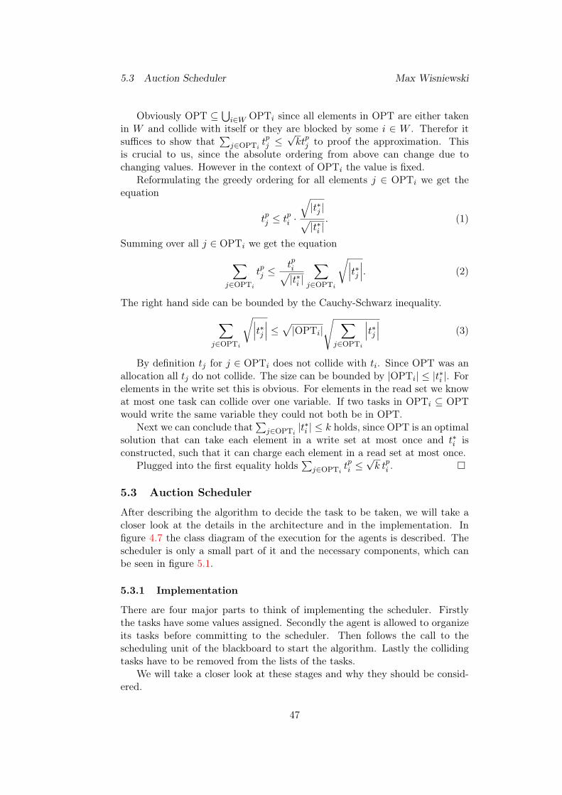
5.3 Auction Scheduler Max Wisniewski
Obviously OPT ⊆⋃i∈W OPTi since all elements in OPT are either taken
in W and collide with itself or they are blocked by some i ∈ W . Therefor itsuffices to show that
∑j∈OPTi t
pj ≤
√ktpj to proof the approximation. This
is crucial to us, since the absolute ordering from above can change due tochanging values. However in the context of OPTi the value is fixed.
Reformulating the greedy ordering for all elements j ∈ OPTi we get theequation
tpj ≤ tpi ·
√|t∗j |√|t∗i |
. (1)
Summing over all j ∈ OPTi we get the equation∑j∈OPTi
tpj ≤tpi√|t∗i |
∑j∈OPTi
√∣∣∣t∗j ∣∣∣. (2)
The right hand side can be bounded by the Cauchy-Schwarz inequality.∑j∈OPTi
√∣∣∣t∗j ∣∣∣ ≤√|OPTi|√ ∑j∈OPTi
∣∣∣t∗j ∣∣∣ (3)
By definition tj for j ∈ OPTi does not collide with ti. Since OPT was anallocation all tj do not collide. The size can be bounded by |OPTi| ≤ |t∗i |. Forelements in the write set this is obvious. For elements in the read set we knowat most one task can collide over one variable. If two tasks in OPTi ⊆ OPTwould write the same variable they could not both be in OPT.
Next we can conclude that∑
j∈OPTi |t∗i | ≤ k holds, since OPT is an optimal
solution that can take each element in a write set at most once and t∗i isconstructed, such that it can charge each element in a read set at most once.
Plugged into the first equality holds∑
j∈OPTi tpi ≤√k tpi .
5.3 Auction Scheduler
After describing the algorithm to decide the task to be taken, we will take acloser look at the details in the architecture and in the implementation. Infigure 4.7 the class diagram of the execution for the agents is described. Thescheduler is only a small part of it and the necessary components, which canbe seen in figure 5.1.
5.3.1 Implementation
There are four major parts to think of implementing the scheduler. Firstlythe tasks have some values assigned. Secondly the agent is allowed to organizeits tasks before committing to the scheduler. Then follows the call to thescheduling unit of the blackboard to start the algorithm. Lastly the collidingtasks have to be removed from the lists of the tasks.
We will take a closer look at these stages and why they should be consid-ered.
47
5.3 Auction Scheduler Max Wisniewski
ExecutorAgent
- execute(t : Task, a :Agent) : Unit
0..n
1
0..n1
Blackboard
getTasks : Seq[(Task, Agent)]
Task
writeSet : Set[Formula]
readSet : Set[Formula]
<<interface>>
bid (budget : Double) : Double
Agent
filter(e : Event) : Unit
getTasks (budget : Double) : Seq[Task]
run(t : Task) : Result
<<interface>>
removeColliding(ts : Set[Task]) : Unit
Figure 5.1: Excerpt of the execution class diagram important for the scheduler.
Task bidding In the scheduling algorithm each task must have a value orbid assigned. Therefor it should be no surprise, that tasks have a method,that returns exactly the bid the agent makes. In contrast to the scenario ofthe auction in the last section, the agents have to pay a fee if their tasksis executed. Since no real currency exists inside the system, the schedulerintroduces a virtual currency. Each round of the bidding, the scheduler givesan allowance to the agents.
With this money each scheduler can now try to bid for the execution of itstasks.
The money remains in the blackboard. If the money is not manipulatableby the agents they cannot cheat. Another reason for the money to remain inthe blackboard is that the blackboard needs to reconstruct the value of thetask. Hence he needs access to the assets of the agents at each time.
An upside in the value dependency on the assets of the agents is that anatural form of aging is implemented into the scheduler. If the agent doesassign a bid proportional to his wealth, then the task will increase in valueuntil it is executed.
Hence we can ensure that each agent can execute tasks infinitely often ifthey assign bids corresponding to their wealth.
The ranking itself is not determined by this construct. The ranking can besomething that is solely done inside the task, leaving external reasons aside ordone through the agent, that can determine the value based on his perceptionof the blackboard.
What we will look at later is the possibility to determine the value of atask, by coefficients that are stored in the blackboard. This way an externalagent can analyze the current workload and goal and change the values of the
48
5.3 Auction Scheduler Max Wisniewski
tasks correspondingly. It is even possible to use on-the-fly machine learningalgorithms to optimize the values.
Considering the difficult assignment of a good value function to the tasks„the optimization through a defined set of coefficients seems more beneficial.Even if the parameters are learned in the beginning from the outside.
Preselection In the structure implemented is the possibility for the agentsto first select their tasks.
The main motivation for this decision is, that the scheduling algorithm issuper-linear on a set of tasks, such that more rounds of auction are faster thanone big round. The preselection allows the agent to make a choice on the taskshe wants to have executed, before the scheduler comes into play.
This can be beneficial, because he has more information about his owntasks than the scheduler.
A possible problem arising from the shift of the selection to the agents thatthe completeness can be threatened. In the last paragraph it was described,that the allowance mechanism implements an aging mechanism that shouldensure completeness in the resulting system.
To ensure this property, we are now heavily dependent that an agent mayeventually send each task to the scheduler.
This is a burden made on the developer of an agent. In section 6 someabstract agents are introduced that already tackle this problem. A developerdoes not want to concern himself with this problem, can choose from a set ofstandard behaviors.
Scheduling Blackboard The scheduling datastructure used by the execu-tion agent to select tasks to be executed is a composition of the schedulingalgorithm and the set of agents.
getTasks : Seq[Task]toAuction <- []for (a <- agents)
wealth[a] += ALLOWANCEtoAcution += a.getTasks(wealth[a])
toAcution <- curExec. f i l t e r (_.colliding)toExec <- approxAuction(toAuction)for (a <- agents)
a.removeColliding(toExec)curExec += curExecreturn toExec
Listing 5.3: Scheduling algorithm as used by the blackboard
In listing 5.3 a simple version of the blackboard scheduling algorithm, basedon the approximation scheduling algorithm, is presented. The implementedalgorithm works on pairs to combine the tasks with the agents, such that theycan be executed later.
49
5.4 Optimality Max Wisniewski
We can observe that an agent is granted his allowance in the beginning ofeach round. With their current wealth each agent can select a set of tasks hewants to have executed.
With these gained tasks the approximation can be done. In the last step,the agents are informed which tasks where taken.
Of course the scheduler is a composition of the scheduling blackboard andthe execution agent that calls the scheduling method and prepares the agentsfor execution.
Task removal The removal of tasks has two goals. First of all the cleaningof the lists itself.
Imagine the following scenario. One task is selected for execution andanother conflicting task is still in the queue. If the executed task writes aformula the remaining task depends on the execution of the later task will leadto an inconsistent state.
Another possibility might be that a task with some data d1 within the readset takes a long time to execute. Meanwhile the undeleted task with d1 in thewrite set is allowed to execute and updates this data to some d2. Dependingon the invariants for the execution of the first task, we are now in another kindof inconsistent state.
For this reason it is beneficial for the task to mark data only as read, if itdemands no changes during his execution.
The second reason for the task removal is the game nature of the auction.If the agent has no feedback of his strategies in the game, he cannot adapt. Bygiving him the executing tasks he can change his strategy depending on theresult.
A possible adaption is to send less tasks with higher value to the scheduler,if he has not executed for a long time.
5.4 Optimality
For the scheduling method there remain two things to mention.The auction algorithm has the proven properties, such that it is indeed an
approximation for the auction problem. On the other hand, this schedulingalgorithm is not optimal or an approximation. As described, the algorithmworks in rounds. Every time the execution agent has capacity, he demandsnew tasks. This means on the other hand that the auction itself is a localoptimal solution to the problem.
It is indeed not a global optimal solution, since we have no information onthe execution time. If a task is selected, that blocks many variables and takesa long computation time, other tasks might be denied the execution.
This will happen independently of the bid of these tasks if they appear ata later time.
50
6 Agent Implementations Max Wisniewski
This problem describes another rule the execution agent has to implement.Since the overlapping of rounds might schedule tasks t1, t2 infinitely often suchthat t3 never is executed.
Imagine that t1 has x on the write set and t2 has y on it. If t3 has both,it might occur that t1 and t2 are scheduled overlapping infinitely often, i.e. t1starts before it ends t2 begins and so on, than t3 can never be executed.
Hence the execution agent has either to wait for all tasks to finish fromtime to time, to assure that completeness can be proven for Leo-III.
5.4.1 Testing & Optimization
The next chapter will describe some agents that are already implemented inLeo-III.
These served to prove that the concept of the scheduler can work. Theabstract agents, used in all example agent implementations, implement a queuebehavior or a priority queue behavior for their tasks.
Since the tested agents obeyed the rule to send only a constant number oftasks to the scheduler, the workload for the algorithm was never bigger than20 tasks, mostly having singleton sets for read and write sets.
Hence the scheduling took very little time and was mostly done while atleast 3 other agents were still executing. For a real test we would need moreagent implementations, a proof calculus and real problems, such that the sys-tem can be compared to other agent-based systems and other theorem provers.
What the testing and debugging of the system showed, is that many work,could be avoided if stronger requirements are placed on the agents.
At the moment the scheduler trusts the agents little such that he has tocheck if the tasks are not colliding with the current execution tasks. He hasalso to check that no agent wants to spend more money than he has.
Work like this is done currently twice, since the agents do already checkthese conditions. To leave the workload to the executing agent has the advan-tage that he can perform faster on his own data, that is more specialized.
It remains to decide whether the burden is in the system on the cost ofruntime or the developer of an agent has to maintain more invariants.
6 Agent Implementations
In this section some implementations for specific agents are described to demon-strate the concept of the architecture and show that the agent-based approachcan indeed work in many ways.
We will study three major applications of agent-based theorem proving andsome minor utility agents usable in many of the applications.
51
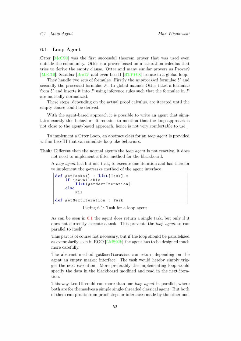
6.1 Loop Agent Max Wisniewski
6.1 Loop Agent
Otter [McC90] was the first successful theorem prover that was used evenoutside the community. Otter is a prover based on a saturation calculus thattries to derive the empty clause. Otter and many similar provers as Prover9[McC10], Satallax [Bro12] and even Leo-II [BTPF08] iterate in a global loop.
They handle two sets of formulae. Firstly the unprocessed formulae U andsecondly the processed formulae P . In global manner Otter takes a formulaefrom U and inserts it into P using inference rules such that the formulae in Pare mutually normalized.
These steps, depending on the actual proof calculus, are iterated until theempty clause could be derived.
With the agent-based approach it is possible to write an agent that simu-lates exactly this behavior. It remains to mention that the loop approach isnot close to the agent-based approach, hence is not very comfortable to use.
To implement a Otter Loop, an abstract class for an loop agent is providedwithin Leo-III that can simulate loop like behaviors.
Task: Different then the normal agents the loop agent is not reactive, it doesnot need to implement a filter method for the blackboard.
A loop agent has but one task, to execute one iteration and has thereforto implement the getTasks method of the agent interface.
def getTasks () : List [Task] =i f isAvailable
List (getNextIteration)e l se
Nil
def getNextIteration : Task
Listing 6.1: Task for a loop agent
As can be seen in 6.1 the agent does return a single task, but only if itdoes not currently execute a task. This prevents the loop agent to runparallel to itself.
This part is of course not necessary, but if the loop should be parallelizedas exemplarily seen in ROO [LMS92b] the agent has to be designed muchmore carefully.
The abstract method getNextIteration can return depending on theagent an empty marker interface. The task would hereby simply trig-ger the next execution. More preferably the implementing loop wouldspecify the data in the blackboard modified and read in the next itera-tion.
This way Leo-III could run more than one loop agent in parallel, whereboth are for themselves a simple single-threaded classical agent. But bothof them can profits from proof steps or inferences made by the other one.
52
6.2 Rule-Agent Max Wisniewski
Run: The loop is break open through the task design. The agent has toremember either internally or through the tasks what to execute next.Therefor a loop agent resembles a state machine from the outside.
The run method of the agent is the body of the loop that will be imple-mented with one exception. The change will not be written immediatelyinto the blackboard, but stored internally. The internally stored changescan influence the loop agent, but have no site effects to the outside.
Result: The result consists of all internally stored changes as they will bewritten back in one step to not destroy atomicity of the transactionalagent.
6.2 Rule-Agent
The rule agent tries another approach then the classical loop by implementinginference rules directly and letting them compete with each other.
This agent is inspired by Volker Sorges approach in Ω-Ants [Sor01]. In Ω-Ants the agent where firstly used to present enabled inference rules to the userin an interactive proof. This agent adepts the idea which was also presentedby Volker Sorge, to fully automize the evaluation and application of inferencerules.
An important part of the implementation is the biding and selection ofactive inferences that gets rid of the human interaction.
The rule agent is a parallelization on the clause level as presented in ??
Task: Each time a new formula is added to the blackboard the rule agent hasto check if its premise is satisfied for some formulae in the blackboard.
Thus it is necessary for the rule agent to implement extra datastructuresto check for possible partners in the inference step. If this is not the casethe running time of the filter is a polynom with the degree of the inferencepartners for the newly added formula in the size of the blackboard.
Each tupel of inference partners can be added as a new task. Dependingif it is a generating inference or writing inference the formula can beadded to the read or write sets of the task.
Run: After the task is selected to be executed the inference rule can be exe-cuted.
To check whether the premise of the interference rule is active, often thesolution is at least partially computed during the search. Therefor it is agood alternative to write the partial solution into the task such that therun method does not have to recompute this result.
Result: Depending if the inference is generating or writing the agent willgenerate a Result object that has the inferred formulae as new formulaeor updated formulae.
53
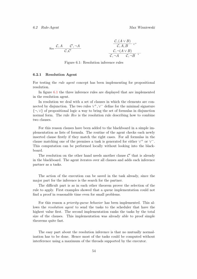
6.2 Rule-Agent Max Wisniewski
C, A C′,¬ARes
C, C′
C, (A ∨B)∨+C, A,B
C,¬(A ∨B)∨−C,¬A C,¬B
Figure 6.1: Resolution inference rules
6.2.1 Resolution Agent
For testing the rule agent concept has been implementing for propositionalresolution.
In figure 6.1 the three inference rules are displayed that are implementedin the resolution agent.
In resolution we deal with a set of clauses in which the elements are con-nected by disjunction. The two rules ∨+,∨− define for the minimal signature¬,∨ of propositional logic a way to bring the set of formulas in disjunctionnormal form. The rule Res is the resolution rule describing how to combinetwo clauses.
For this reason clauses have been added to the blackboard in a simple im-plementation as lists of formula. The routine of the agent checks each newlyinserted clause firstly if they match the right cases. For all formulas in theclause matching one of the premises a task is generated for either ∨+ or ∨−.This computation can be performed locally without looking into the black-board.
The resolution on the other hand needs another clause C′ that is alreadyin the blackboard. The agent iterates over all clauses and adds each inferencepartner as a tasks.
The action of the execution can be saved in the task already, since themajor part for the inference is the search for the partner.
The difficult part is as in each other theorem prover the selection of therule to apply. First examples showed that a queue implementation could notfind a proof in reasonable time even for small problems.
For this reason a priority-queue behavior has been implemented. This al-lows the resolution agent to send the tasks to the scheduler that have thehighest value first. The second implementation ranks the tasks by the totalsize of the clauses. This implementation was already able to proof simpletheorems quite fast.
The easy part about the resolution inference is that no mutually normal-ization has to be done. Hence most of the tasks could be computed withoutinterference using a maximum of the threads supported by the executor.
54
6.3 Meta Prover Max Wisniewski
6.3 Meta Prover
Another fundamental approach uses the parallelism in the simplest ways. Justlike Isabelle’s sledgehammer tool [Pau10] Leo-III can be used to run multipletheorem provers at once, waiting for the earliest or best result.
In this concept an agent is a proxy for another theorem prover. The par-allelization here is on the search level. Depending on the set of formulas com-mited to the prover and if different provers are taken at once this can be eachof the parallelizations in this category.
Task: The agent takes the whole set of formulae or a selection of everythingthat should be send to the theorem prover and everything written into atask.
A possible addition to this behavior is a filtering, if the external proveris suitable for this kind of problem, by analyzing the set of formulae.
In the meta prover there could be some propositional, some first orderand a few higher order solver be implemented as agents. For a proposi-tional problem many first and higher order provers perform worse thanthe purely propositional ones. Hence we only want to run agents withpropositional provers. The other way around it does not make sense touse propositional or first order provers for a higher order logic formulae,because they will most likely not solve the problem.
Run: Before the external prover can be run, all formula have to be translatedinto a format the prover can understand. As in Isabelle it is possible tooptimize the translation according to the prover such that he can performbest on the task.
The translation is then send to the external prover via a native call toa script or the executable. The agent waits for the answer that is thetermination of the external prover.
As soon as the result is delivered the agent has to interpret it.
In the simplest case the result, theorem or non-theorem, can be addedto the context, but it is also possible to interpret the generated proofobject.
In an additional step or an additional agent the generated proofs can besimplified, checked or combined with the proofs found by other theoremprovers.
Result: Depending on the answer of the prover, the result can be inserted intothe blackboard and the proof after both are translated into a internalrepresentation.
6.3.1 TPTP Agent
The first simple solution to implement the meta prover is to call the Systme-OnTPTP introduced in section 2.2.2.
55
6.4 Utility Agents Max Wisniewski
For the call a script supported on the TPTP homepage can be used. Theagent has to transform a context of the formulae to the thf input format. Thenthe script can be called through a native call.
Depending on the context higher-order theorem provers as Leo-II or Satal-lax, first-order theorem provers as Vampire or E or even propositional proversas MiniSAT can be called.
The result given by the call has to be reinterpreted. If the result is a simpleSZS status then in the positive case the context can be closed, i.e. a proof wasfound.
In the negative case there could still be something done if a proof objectis returned. The data can be interpreted and extra information can insertedinto the blackboard. This would also be the case of counter model finder suchas Nitrox are used.
One major problem if run in parallel to an other mode, such as the inferenceor the loop agents, is to decide when to launch the TPTP agents. If Leo-III isrun solely as a meta prover the tptp agents can be run immediately.
6.4 Utility Agents
Different to the conceptual agents for the proof calculus as described before,the agent-based approach can use many subroutines usable in all of the abovementioned design concepts.
A variety of search problems that can be parallelized, can be externallyimplemented as agents to the main proof calculus to decrease the effectivesearch time compared to sequential implementation.
6.4.1 Normalization Agents
Most provers need to bring formulae into some kind of normalform. Not onlythat these kind of task are highly parallelizable, because they are mutuallyindependent, but the resulting calculus can even begin to work on alreadynormalized formulae beside the remaining normalization.
In their structure they resemble the ∨+,∨− inference rules of the resolutionagent. Since they work on formulae and not clauses they can be considered asparallelism at the term level.
Task: A newly added formula is checked if it is in the expected normalform.If this is not the case a task containing the unnormalized formula.
Normally the check for simple normalforms is a local matter so thatthe rest of the blackboard remains untouched. However, caching theresult about the normalform of a formula proved itself to be practical.Otherwise the test for the normal form can be performed numerous timesthrough the process until the execution of the agent.
Run: The transformation into the normal form is performed.
56
6.4 Utility Agents Max Wisniewski
Result: The new formula is marked for an update, since normalization is anupdating rule.
For testing purposes an abstract normalization agent has been implemented.The agent accepts a normalization matching a suitable interface. For the testa simplification, negation normalform, skolemization and prenex normalformhave been implemented.
6.4.2 Context Splitting Agent
One of the more fundamental approaches to parallelize the proof search isAND-OR-Parallelism [Bon99]. As mentioned in section 2.3 AND-OR-Parallelismreplaces the current goal of the proof, by a suitable subset of new goals, allconnected through conjunction or disjunction. This produces two new set offormulae, for each goal one set that can be processed in parallel.
Depending on the kind of split one or all of the sub goals have to beproven. Hence a context splitting agent is responsible to decide, when to spliton a formula. After this he is responsible to check the subgoals for completionand close the initial goal.
For the context splitting there has to be support in the blackboard. Andother agents have to be aware that they can only perform on formulae in thesame context. In section 7 two possibilities for the context splitting on the sideof the blackboard are presented.
Task: Each time a formula is added the context splitting agent has to decidewhether he wants to split at this formula. If he decides that a split canbe done on this formula he creates a task for it.
Aside from the splitting he has to observe the context if at some pointthe empty clause is inserted. He is the only one to now when the parentcontext is closed and thus he has to look for this event.
Run: If the task was a split on a formula he performs the split and remembersfor each new goal a new context and its connection.
If a context is closed the task was generated when all subcontexts areclosed too. The context splitting agent can then start to close the parentcontext.
Result: In the split case the result introduces new contexts to the blackboard.How this can be done will be explained in section 7.
The closing case will mark the parent context as closed which may triggerthe next task for the context splitting agent. In the end such a closeoperation will bubble to the initial context where hence a proof wasfound.
57
7 Blackboard Datastructures Max Wisniewski
The structure of the context splitting reminds of a tableaux calculus proof.The difference is that sometimes not all branches have to be closed to mark anode as closed. Since the context splitting should not be a complete tableauxcalculus the splitting has to be strongly limited or have a low value for thescheduling.
6.4.3 Learning Agent
A state of the art theorem prover has about fifty parameters where each changessome behavior in the proof search. The amount and interaction between theseparameters is not feasible for a human. Therefor machine learning techniquesare used to determine the best combination for a problem.
This work is done outside the prover by running the prover numerous timeson the same problems changing parameters and comparing the results.
In the agent approach the learning and updating of the already learnedcould be performed on the fly. One major point were this can be used is indeciding the bids for the scheduler. This is also a task not feasible for humanand can change through the state of the proof search.
7 Blackboard Datastructures
In this section we will look at possible datastructures. Through this thesis Iconcentrated myself on the general design of the blackboard and the agents,such that only general ideas for datastructures exists.
Since most datastructures will be explicitly designed for the proof calculus,there was no way to start implementing before a proof calculus was chosen.
There are some datastructures already thought of to be implemented, butwe will look only at two datastructures. The first one is needed if the con-text splitting agent is implemented. The other one is necessary to turn theLeo-III agents into real agents and not only expert systems.
7.1 Context Splitting
In the last section the context splitting agent was introduced as a method toimplement AND-/OR- parallelism in Leo-III.
The problem arising from this approach is to implement the splitting of theformula set, such that manipulation and search is efficient and the size doesnot grow to large in comparison to the not splitted context.
The datastructure must support insertion, deletion and update to formulaein a context. Furthermore it must be possible to pose the same search queriesas for the non splitted case.
There are two approaches that are possible depending on the datastructureused without splitting.
58
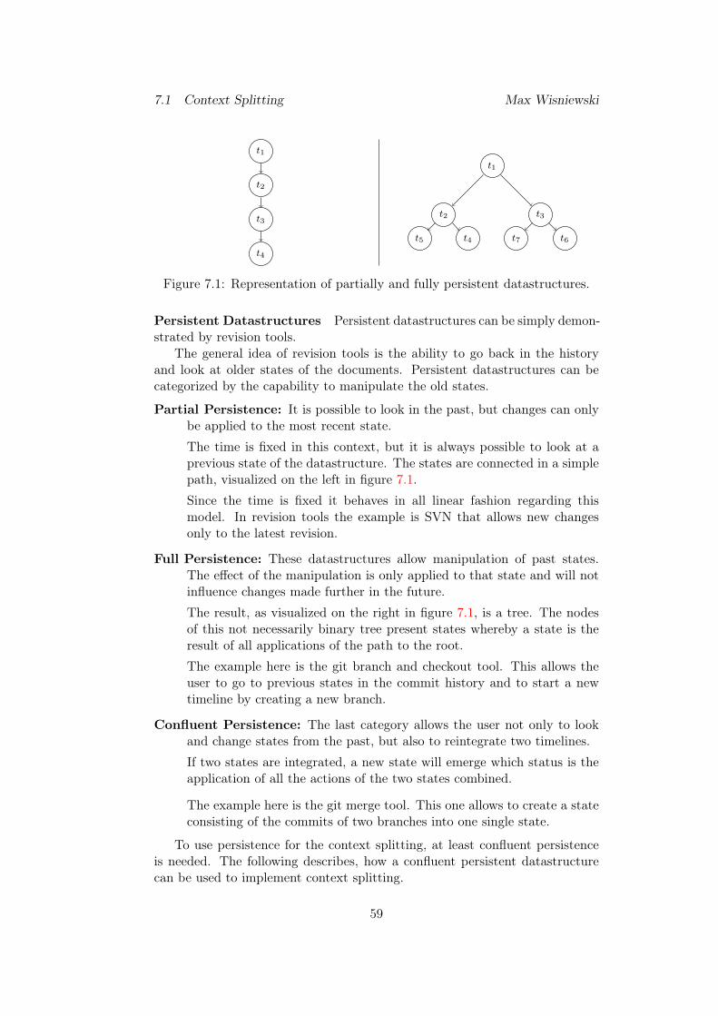
7.1 Context Splitting Max Wisniewski
t1
t2
t3
t4
t1
t2 t3
t4t5 t6t7
Figure 7.1: Representation of partially and fully persistent datastructures.
Persistent Datastructures Persistent datastructures can be simply demon-strated by revision tools.
The general idea of revision tools is the ability to go back in the historyand look at older states of the documents. Persistent datastructures can becategorized by the capability to manipulate the old states.
Partial Persistence: It is possible to look in the past, but changes can onlybe applied to the most recent state.
The time is fixed in this context, but it is always possible to look at aprevious state of the datastructure. The states are connected in a simplepath, visualized on the left in figure 7.1.
Since the time is fixed it behaves in all linear fashion regarding thismodel. In revision tools the example is SVN that allows new changesonly to the latest revision.
Full Persistence: These datastructures allow manipulation of past states.The effect of the manipulation is only applied to that state and will notinfluence changes made further in the future.
The result, as visualized on the right in figure 7.1, is a tree. The nodesof this not necessarily binary tree present states whereby a state is theresult of all applications of the path to the root.
The example here is the git branch and checkout tool. This allows theuser to go to previous states in the commit history and to start a newtimeline by creating a new branch.
Confluent Persistence: The last category allows the user not only to lookand change states from the past, but also to reintegrate two timelines.
If two states are integrated, a new state will emerge which status is theapplication of all the actions of the two states combined.
The example here is the git merge tool. This one allows to create a stateconsisting of the commits of two branches into one single state.
To use persistence for the context splitting, at least confluent persistenceis needed. The following describes, how a confluent persistent datastructurecan be used to implement context splitting.
59
7.1 Context Splitting Max Wisniewski
Preliminaries: Let P be the confluent persistent datastructure and v be amapping of the contexts to states in the datastructure.
Invariant: For each context c, the state v(c) in P contains exactly all formulaspresent in the context c.
Insert: Inserting an element f into the context c can be done by going tov(c) and insert the element f into the datastructure in this state. Theformula f now exists in one state, but not in any context below c. Henceeach context c′ has to be merged with the new state.
Lastly the mapping v has to be updated for each of the new states.
Delete/Update: The same as insertion, except delete/update is invoked onv(c).
Search: Querying the datastructure in a context c is possible by querying thedatastructure in state v(c).
Driscoll and Tarjan [DSST86] have shown a transformation to make anydatastructure persistent. The conditions based on the datastructures are thatthey are pointer based. This means that the datastructure consists of nodeswith finite space and pointers to other nodes. To apply the transformationto a persistent datastructure, the in-degree of these datastructures has to befinite, too.
In the case of confluent persistence some kind of merging mechanism hasto be supported.
If all these requirements are satisfied, the transformation creates a datas-tructure that has amortized the same space and runtime complexity as theinitial datastructure, but for a constant multiplier.
The confluent persistence could be omitted. A full persistent datastructureis enough if no data is inserted or deleted after it is build up for the first time.This static datastructure can be used for querying only, but there exist anothertransformation [SB79] for dynamization of datastructures. The downside isthat the amortized runtime gets worse once again.
The conditions here are rather strong and even if they can be met, there re-mains the problem that the manipulation method for the context datastructurehas to merge all subcontext states.
In the manipulation step we see that confluence is needed. If there wouldbe no way to merge, the changed formula f would never be conveyed to thesubstates. The only other option would be to recompute all subchanges againfor the new context with the changed f .
The upside of this approach is, that the query time is the same as if nosplitting was used.
60
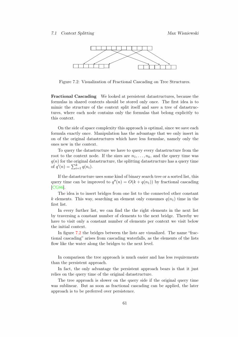
7.1 Context Splitting Max Wisniewski
Figure 7.2: Visualization of Fractional Cascading on Tree Structures.
Fractional Cascading We looked at persistent datastructures, because theformulas in shared contexts should be stored only once. The first idea is tomimic the structure of the context split itself and save a tree of datastruc-tures, where each node contains only the formulas that belong explicitly tothis context.
On the side of space complexity this approach is optimal, since we save eachformula exactly once. Manipulation has the advantage that we only insert inon of the original datastructures which have less formulae, namely only theones new in the context.
To query the datastructure we have to query every datastructure from theroot to the context node. If the sizes are n1, . . . , nk, and the query time wasq(n) for the original datastructure, the splitting datastructure has a query timeof q′(n) =
∑ki=1 q(ni).
If the datastructure uses some kind of binary search tree or a sorted list, thisquery time can be improved to q′′(n) = O(k + q(n1)) by fractional cascading[CG86].
The idea is to insert bridges from one list to the connected other constantk elements. This way, searching an element only consumes q(n1) time in thefirst list.
In every further list, we can find the the right elements in the next listby traversing a constant number of elements to the next bridge. Thereby wehave to visit only a constant number of elements per context we visit belowthe initial context.
In figure 7.2 the bridges between the lists are visualized. The name “frac-tional cascading” arises from cascading waterfalls, as the elements of the listsflow like the water along the bridges to the next level.
In comparison the tree approach is much easier and has less requirementsthan the persistent approach.
In fact, the only advantage the persistent approach bears is that it justrelies on the query time of the original datastructure.
The tree approach is slower on the query side if the original query timewas sublinear. But as soon as fractional cascading can be applied, the laterapproach is to be preferred over persistence.
61
7.2 Message Queues Max Wisniewski
7.2 Message Queues
One of the features of agents compared to expert systems is the ability tocommunicate and cooperate with other agents.
To this point the architecture used the agents only as experts. The reasonour agents still fulfill the definition of an agent is the blackboard architecture.
Regarding communication, people often imagine direct, synchronous com-munication. Thereby messages are directly conveyed to the receiver. As longknown in computer science a synchronous communication is hard to simulate.Both sender and receiver have to be present at the same time and signal thereceiving to the other party.
Even at this level the communication just simulates synchronicity, becausethe message is stored internally. The other end waits for the signal send, whenthe recipient read the message.
Hence an asynchronous communication is much more preferable. In theblackboard context, this is easy to implement, since a message becomes a newtype of data written on the blackboard. If the agent is interested in this kindof message, he will read it and generate a new task.
The design chosen to implement messages in Leo-III orients itself on themailbox system of Erlang [Arm10]. Each agent has a queue of messages as-signed. Other agents can send messages to the agents by inserting them intothe queue. If the receiving agent is ready to work on the message, he can takethem from the queue and work on them.
The motivation to design the run method inside the agents and not in thetask was, to be able to design agents just as Erlang processes. The communi-cation and acting of the agents looks exactly the same.
Compared to single formulas, the messages can be optimized for the agents.First of all, only a single agent has to be informed when a message is send tohim. This approach does not have to be fixed, as another agent might beinterested in the information flow.
We can visualize the communication over the blackboard by writing thenames of the agents on the blackboard. Each time an agent wants to send amessage, he writes the message under his name. Now the receiving agent canlook at the message and react to it.
In this context it might occur, that another agent can work with this infor-mation, too. For example, the message says to work on a specific subset of theformula. Then another agent could adapt and try not to touch these formulas.
Depending on the existence of such processes, the signaling must be adapted.
62
8 Related Work Max Wisniewski
8 Related Work
Even though agent systems are under development since the 1970s, there areno prominent automated theorem provers using agents as their architecture.
In artificial intelligence it is more common to use agent-based architecture.An example with a real application is dMARS [DLG+04]. The dMARS archi-tecture was used by the NASA in space shuttles to observe the reaction controlsystem and to monitor telecommunication network systems in real time.
On the side of theorem provers there are even nowadays hardly parallelizedversions. One of the most used provers that uses some kind of parallelization isIsabelle/HOL’s sledgehammer [Pau10]. Sledgehammer translates the currentproblem into suitable import formats of external theorem provers, sends themthe input and presents the user all results. This philosophy is exactly thesame as the intended use of Leo-III as a meta prover through the describedmetaprover agents.
Higher-order theorem provers such as Leo-II and Satallax use first-orderand propositional provers as subprogams. They reduce the problems into asuitable form and send these problems to the subprovers. Recently Yves Müllerresearched a way to parallelize the subprovers for Leo-II [M13].
Combining the context splitting agent and the meta prover agents statesan easy way to simulate this idea.
As already mentioned in section 4.2 the work of Volker Sorge [Sor01] hasinfluenced this work in many ways. In comparison to Ω-Ants Leo-III uses theagents to manipulate the formulas directly and not to make suggestions to theuser. This way Leo-III’s architecture can be seen as a step to make Ω-Antsfrom an interactive theorem prover into a automated theorem prover.
9 Further Work
This work concentrated on the architecture of Leo-III. The further work wewill look into will be related to the designed architecture.
Blackboard Datastructures This work mainly concentrated on the overallagent architecture and although everything is trimmed to use the blackboardas its main source of information, the blackboard itself does not contain manyaccess methods.
As soon as the first calculi agents are written, there is the possibility todecide on suitable search datastructures and extra information to store in theblackboard.
One already discussed datastructure in section 7 is the α-β-splitting sup-port datastructures, singular.
Other possibilities are search structures for resolution partners of clauses,unification partners and structures for already instantiated variables.
63
9 Further Work Max Wisniewski
Auction Learning As already mentioned in section 6.4.3 the design of thescheduler leaves room for machine learning techniques to optimize the schedul-ing behavior.
This can be achieved at runtime in form of an agent, allowing the rankingfunctions to change according to the current problem and goal.
Another possibility which is used in many theorem provers, is to make astatic analysis for a large problem set and perform machine learning exter-nally. This puts less burden on the runtime, but is not as flexible as the agentapproach.
Auction Games Auctions are introduced in game theory (see section 5.1).The agents, as introduced in this work, do not play a game. Instead, they onlysend their value of a task statically to the scheduler.
One possible enhancement is to allow agents to be more responsive, i.e.give them information about who won for which price, s.t. they can adjusttheir bidding.
In this context it would necessitate a different game mechanism than thefirst-price-auction mechanism chosen at the moment. But a good alternative,the second-price-vickrey-auction, costs just as much runtime and prohibits lyingagents.
Price of Anarchy As stated in section 5.11 the scheduling algorithm makeslocal optimal decisions and we analyzed the approximation factor to be
√k
where k is the number of all used data by the tasks.First of all the bound is not tight and could be further analyzed. Secondly
the local optimal decision can be compared the the global optimal decision.This competitive ratio is known as the price of anarchy. In many problemsthis ratio can be bound such that the approximation factor can be used todetermine a maximal global value loss factor.
In some applications with certain restrictions on the value functions theequilibrium computed by the mechanism is indeed global optimal.
Hence further work can on the one hand compute the price of anarchy andon the other hand search for restrictions to the bidding functions such thatthere is no price to pay.
Abstract Agent Interfaces The interface for an agent is quite complexdue to the methods needed in the scheduling process. For easier use a varietyof abstract behaviors can be implemented and used by programmers.
For a start there are already a StdAgent and a PriorityAgent implemented.The first one inserts all new tasks in a simple queue, whereas the second oneplaces each one in a priority queue.
Both have the advantage, that only the filter, task, execution and the resulthave to be implemented. These are characteristic for an agent as they define
64
10 Conclusion Max Wisniewski
them. The programmer has therefor not to deal with other implementationissues.
Agent scripting engine Another possibility for easier programming withagents is to define a script language for agents. This would allow agents to bewritten without writing in Scala or changing the system.
For compatibility this scripting language can orient itself on the tpi lan-guage of the TPTP syntax.
Agents & Testing As soon as some agents are written, especially for theproof calculus it is possible to test the performance of the system compared toother theorem provers.
What is interesting, aside from the overall performance, is the time used forscheduling, synchronization overhead and speed up due to parallel computing.
10 Conclusion
Through the course of this thesis an agent-based blackboard architecture hasbeen designed and implemented.
The designed agents perform adaptive on the blackboard. The implemen-tation divides the agents from the execution itself such that agents do notconsume capacity if they do not work as would simple processes do. Ratherthan that, the action of an agent can be assigned to a process that executesthis action.
An upside of this design is that agents can run in parallel to themselvesarbitrarily often, without registering the agent more than once.
The design of an action of the agents is done as a transaction. This wayan developer of a new agent has only to specify the requirements on which theaction can be executed, the action itself and lastly a result.
The complete synchronization is then completely done by the system, hencenot bothering the developer.
The first tested agents performed quite well. The synchronization workedgood, since no conflicts occurred. The self parallelization also performed quitewell.
The first test to be implemented was the normalization agents. Althoughthey could not conflict each other by design, we could already see that theyparallelized quite well. The next agent to be implemented for testing was theresolution agent.
It was of no surprise, that an unreflected application of the resolution stepsperformed quite badly, since many irrelevant clauses were generated. But al-ready a simple order on the clauses, namely the size of the resulting clause, gavea first simple propositional theorem prover that could find a proof relativelyfast.
65
10 Conclusion Max Wisniewski
In this context it remains to mention that the architecture itself does notguarantee correctness of the implemented algorithms. The agent architecturepresented is only a tool like a monitor or a semaphore helping the implementerto develop concurrent and parallel programs. But as the other tools the ar-chitecture does not guarantee a correct program. Hence the agents have to bedesigned carefully and not all agents will be able to perform at the same time.
The goal of this thesis was to proof that an agent-based approach for anautomated theorem prover is possible. Since the first tests with a resolutioncalculus did already run and found some proofs, we can say in this sense thatthe agent-based approach good work.
To test the performance of an agent-based system, it is necessarily to firstwrite a could proof calculus. Then we could start testing the architecture forcompetitiveness.
But as already shown, the Leo-III architecture allows to implemented clas-sical sequential loop based provers as state-machine programs.
Hence in the further development we can balance the amount of paralleliza-tion from either a complete parallelization on inference level, as we stated withthe resolution agent, to a nearly sequential proof calculus. In the sequentialcalculus, there is still the advantage, that easy to parallelize subtasks can bedecoupled and run while the global loop still performs.
An example, that is already used in competitive higher-order theoremprovers, is to make parallel calls to first order theorem provers, just as itis already done in Leo-II.
Conclusively we can say, that the agent-based approach looks promisingfor the further development of Leo-II, as the first test emphasizes, that theparallelization does indeed work. Future tests will show, how much of a speedup Leo-III can get through a concurrent implementation compared to othersystems.
66
11 Bibliography Max Wisniewski
11 Bibliography
References
[Agh86] Gul Agha. Actors: A Model of Concurrent Computation in Dis-tributed Systems. MIT Press, Cambridge, MA, USA, 1986.
[And14] Peter Andrews. Church’s type theory. In Edward N. Zalta, editor,The Stanford Encyclopedia of Philosophy. Spring 2014 edition, 2014.
[Arm10] Joe Armstrong. Erlang. Commun. ACM, 53(9):68–75, September2010.
[Arr51] K.J. Arrow. Social choice and individual values. 1951.
[BBK04] Christoph Benzmüller, Chad Brown, and Michael Kohlhase.Higher-order semantics and extensionality. Journal of SymbolicLogic, 69(4):1027–1088, 2004.
[BCO10] Nathan G. Bronson, Hassan Chafi, and Kunle Olukotun. Ccstm: Alibrary-based stm for scala. In In The First Annual Scala Workshopat Scala Days, 2010.
[Ber66] A.J. Bernstein. Analysis of programs for parallel processing. Elec-tronic Computers, IEEE Transactions on, EC-15(5):757–763, Oct1966.
[BHG86] Philip A Bernstein, Vassos Hadzilacos, and Nathan Goodman. Con-currency Control and Recovery in Database Systems. Addison-Wesley Longman Publishing Co., Inc., Boston, MA, USA, 1986.
[Bon99] Maria Paola Bonacina. A taxonomy of parallel strategies for deduc-tion. Annals of Mathematics and Artificial Intelligence, 29:223–257,1999.
[BP14] Christoph Benzmüller and Bruno Woltzenlogel Paleo. AutomatingGödel’s ontological proof of god’s existence with higher-order auto-mated theorem provers. In Torsten Schaub, Gerhard Friedrich, andBarry O’Sullivan, editors, ECAI 2014, volume 263 of Frontiers inArtificial Intelligence and Applications, pages 163 – 168. IOS Press,2014.
[BPTF07] Christoph Benzmüller, Larry Paulson, Frank Theiss, and ArnaudFietzke. The LEO-II project. In Proceedings of the FourteenthWorkshop on Automated Reasoning, Bridging the Gap between The-ory and Practice. Imperial College, London, England, 2007.
[Bro12] Chad E. Brown. Satallax: An automatic higher-order prover. InAutomated Reasoning - 6th International Joint Conference, IJCAR
67
References Max Wisniewski
2012, Manchester, UK, June 26-29, 2012. Proceedings, pages 111–117, 2012.
[BTPF08] Christoph Benzmüller, Frank Theiss, Larry Paulson, and ArnaudFietzke. LEO-II - a cooperative automatic theorem prover forhigher-order logic. In Alessandro Armando, Peter Baumgartner,and Gilles Dowek, editors, Automated Reasoning, 4th InternationalJoint Conference, IJCAR 2008, Sydney, Australia, August 12-15,2008, Proceedings, volume 5195 of LNCS, pages 162–170. Springer,2008.
[CG86] Bernard Chazelle and Leonidas J. Guibas. Fractional cascading: I.a data structuring technique. Algorithmica, 1:133–162, 1986.
[DLG+04] Mark D’Inverno, Michael Luck, Michael Georgeff, David Kinny, andMichael Wooldridge. The dmars architecture: A specification of thedistributed multi-agent reasoning system. Autonomous Agents andMulti-Agent Systems, 9(1-2):5–53, 2004.
[DP60] Martin Davis and Hilary Putnam. A computing procedure for quan-tification theory. J. ACM, 7(3):201–215, July 1960.
[DSST86] J R Driscoll, N Sarnak, D D Sleator, and R E Tarjan. Makingdata structures persistent. In Proceedings of the Eighteenth AnnualACM Symposium on Theory of Computing, STOC ’86, pages 109–121, New York, NY, USA, 1986. ACM.
[EL80] Lee D. Erman and Victor R. Lesser. The hearsay-ii speech un-derstanding system: Integrating knowledge to resolve uncertainty.Computing Surveys, 12:213–253, 1980.
[Fit90] Melvin Fitting. First-order logic and automated theorem proving.Springer-Verlag New York, Inc., New York, NY, USA, 1990.
[Fit96] Melvin Fitting. First-order Logic and Automated Theorem Proving(2Nd Ed.). Springer-Verlag New York, Inc., Secaucus, NJ, USA,1996.
[Fre79] Gottlob Frege. Begriffsschrift, 1879.
[GB99] Zahia Guessoum and Jean-Pierre Briot. From active objects toautonomous agents. IEEE Concurrency, 7(3):68–76, 1999.
[Gö31] Kurt Gödel. Über formal unentscheidbare sätze der principia math-ematica und verwandter systeme i. Monatshefte für Mathematikund Physik, 38(1):173–198, 1931.
[KEH+09] Gerwin Klein, Kevin Elphinstone, Gernot Heiser, June Andronick,David Cock, Philip Derrin, Dhammika Elkaduwe, Kai Engelhardt,Rafal Kolanski, Michael Norrish, Thomas Sewell, Harvey Tuch, and
68
References Max Wisniewski
Simon Winwood. sel4: Formal verification of an os kernel. InProceedings of the ACM SIGOPS 22Nd Symposium on OperatingSystems Principles, SOSP ’09, pages 207–220, New York, NY, USA,2009. ACM.
[LMS92a] Ewing L. Lusk, William McCune, and John K. Slaney. ROO: A par-allel theorem prover. In Automated Deduction - CADE-11, 11th In-ternational Conference on Automated Deduction, Saratoga Springs,NY, USA, June 15-18, 1992, Proceedings, pages 731–734, 1992.
[LMS92b] Ewing L. Lusk, William McCune, and John K. Slaney. Roo: Aparallel theorem prover. In Deepak Kapur, editor, CADE, volume607 of Lecture Notes in Computer Science, pages 731–734. Springer,1992.
[M13] Yves Müller. Subprover parallelism in the automated theoremprover leo-ii, 2013.
[McC90] William McCune. OTTER 2.0. In 10th International Conferenceon Automated Deduction, Kaiserslautern, FRG, July 24-27, 1990,Proceedings, pages 663–664, 1990.
[McC10] W. McCune. Prover9 and mace4.http://www.cs.unm.edu/~mccune/prover9/, 2005–2010.
[NPW02] Tobias Nipkow, Lawrence C. Paulson, and Markus Wenzel. Is-abelle/HOL — A Proof Assistant for Higher-Order Logic, volume2283 of LNCS. Springer, 2002.
[NRTV07] Noam Nisan, Tim Roughgarden, Eva Tardos, and Vijay V. Vazi-rani. Algorithmic Game Theory. Cambridge University Press, NewYork, NY, USA, 2007.
[Pau10] Lawrence C. Paulson. Three years of experience with sledgeham-mer, a practical link between automatic and interactive theoremprovers. In Proceedings of the 2nd Workshop on Practical Aspectsof Automated Reasoning, PAAR-2010, Edinburgh, Scotland, UK,July 14, 2010, pages 1–10, 2010.
[PBBO12] Aleksandar Prokopec, Nathan Grasso Bronson, Phil Bagwell, andMartin Odersky. Concurrent tries with efficient non-blocking snap-shots. SIGPLAN Not., 47(8):151–160, February 2012.
[RN03] Stuart J. Russell and Peter Norvig. Artificial Intelligence: A Mod-ern Approach. Pearson Education, 2 edition, 2003.
[Rus08] Bertrand Russell. Mathematical logic as based on the theory oftypes. American Journal of Mathematics, 30(3):222–262, 1908.
69
References Max Wisniewski
[SB79] James B. Saxe and Jon Louis Bentley. Transforming static datastructures to dynamic structures (abridged version). In FOCS,pages 148–168. IEEE Computer Society, 1979.
[Sch71] T. C. Schelling. Dynamic models of segregation. J. Math. Sociol.,1(2):143–186, 1971.
[Sch13] Stephan Schulz. System Description: E 1.8. In Ken McMillan,Aart Middeldorp, and Andrei Voronkov, editors, Proc. of the 19thLPAR, Stellenbosch, volume 8312 of LNCS. Springer, 2013.
[Sor01] Volker Sorge. Omega-ants: A blackboard architecture for the in-tegration of reasoning techniques into proof planning. PhD thesis,Universität des Saarlandes, Postfach 151141, 66041 Saarbrücken,2001.
[Sut09] G. Sutcliffe. The TPTP Problem Library and Associated Infras-tructure: The FOF and CNF Parts, v3.5.0. Journal of AutomatedReasoning, 43(4):337–362, 2009.
[Sut11] G. Sutcliffe. The 5th IJCAR Automated Theorem Proving SystemCompetition - CASC-J5. AI Communications, 24(1):75–89, 2011.
[vH02] Jean van Heijenoort. From Frege to Gödel : A Source Book inMathematical Logic, 1879-1931 (Source Books in the History of theSciences). Harvard University Press, January 2002.
[Wei13] Gerhard et al. Weiss. Multiagent Systems. MIT Press, 2013.
[Woo02] Michael Wooldridge. Intelligent agents: The key concepts. In inProceedings of the 9th ECCAI-ACAI/EASSS 2001, AEMAS 2001,HoloMAS 2001 on Multi-Agent-Systems and Applications IISelectedRevised Papers, ser. LNAI, pages 3–43. Springer-Verlag, 2002.
[YB04] P. Castéran Y. Beriot. Interactive Theorem Proving and ProgramDevelopment – Coq’Art: The Calculus of Inductive Constructions.Springer-Verlag, 2004.
[Yu12] NingNeil Yu. A one-shot proof of arrow’s impossibility theorem.Economic Theory, 50(2):523–525, 2012.
70
Indexα-splitting, 13λ-calculus
Term, 4Type, 4
Agent, 23Agent Architecture, 27, 28, 30AND-/OR-parallelism, 12Arrow’s Theorem, 41Auction, 41
Blackboard Architecture, 15
Collisioncolliding, 43collision-free, 43
Combinatorical Auction, 44Approximation, 46Decision, 44Optimization, 43
Completeness, 14Condorcet’s Paradox, 40
Equilibrium,Nash Equilibrium, 39
Frame, 5
Game, 38
Higher-Order Logic, 5
Incentive Compatible, 42Interpretation, 5
Loop Agent, 52
Mechanism, 40Meta Prover, 55Multiagent System, 25
Proof, 7
Rule Agent, 53
Set Packing, 45Social Choice, 40
Sound, Complete, 7Soundness, 14
TaskAuction, 42
Term Order, 5
Validity, 6Valuation, 6
71