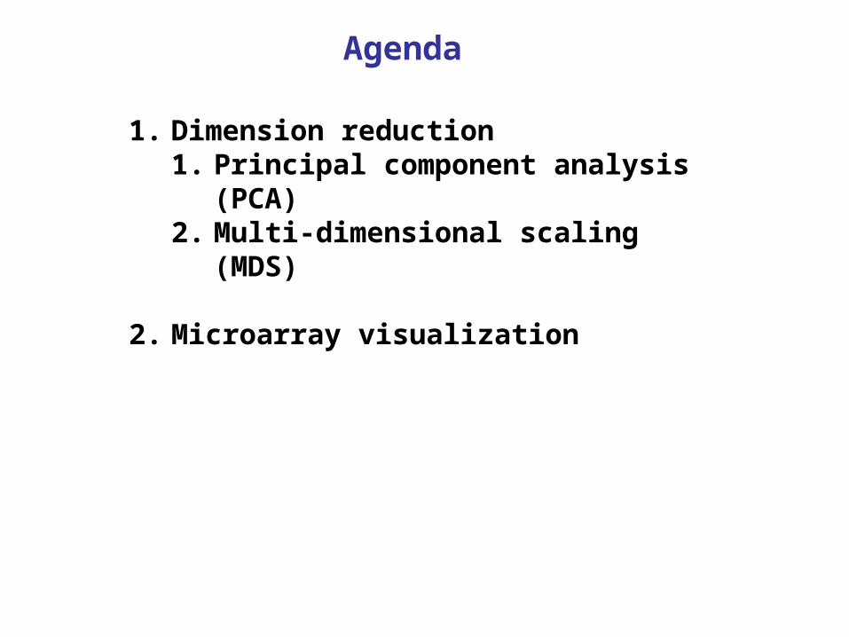
Agenda

1. Dimension reduction1. Principal component analysis (PCA)2. Multi-dimensional scaling (MDS)

2. Microarray visualization

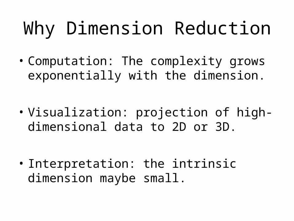
Why Dimension Reduction

• Computation: The complexity grows exponentially with the dimension.

• Visualization: projection of high-dimensional data to 2D or 3D.

• Interpretation: the intrinsic dimension maybe small.

1. Principal component analysis (PCA)

2. Multi-dimensional Scaling (MDS)

1. Dimension reduction

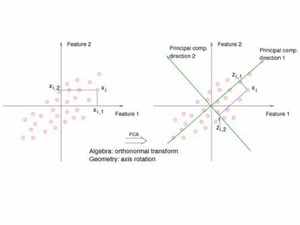
Philosophy of PCA• A PCA is concerned with explaining the

variance-covariance sturcture of a set of variables through a few linear combinations.

• We typically have a data matrix of n observations on p correlated variables x1,x2,…xp

• PCA looks for a transformation of the xi into p new variables yi that are uncorrelated.

• Want to present x1,x2,…xp with a few yi’s without lossing much information.

PCA

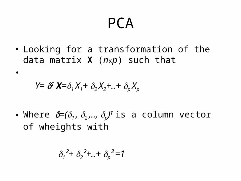
• Looking for a transformation of the data matrix X (nxp) such that

•

Y= T X=1 X1+ 2 X2+..+ p Xp

• Where =(1 , 2 ,.., p)T is a column vector of wheights with

1²+ 2²+..+ p² =1

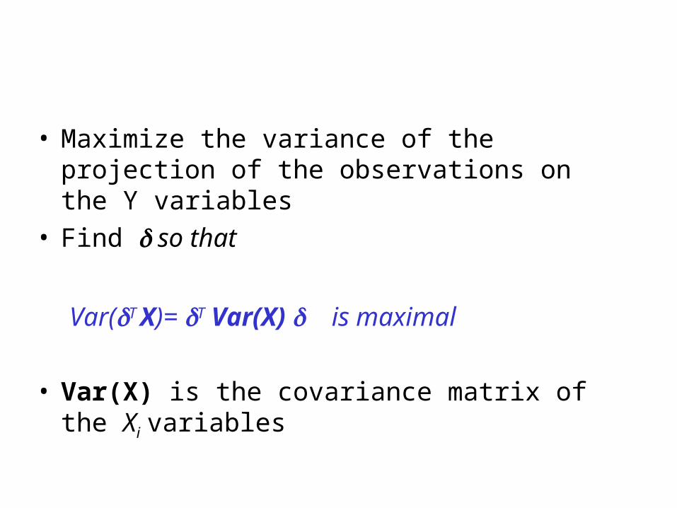
• Maximize the variance of the projection of the observations on the Y variables

• Find so that

Var(T X)= T Var(X) is maximal

• Var(X) is the covariance matrix of the Xi variables

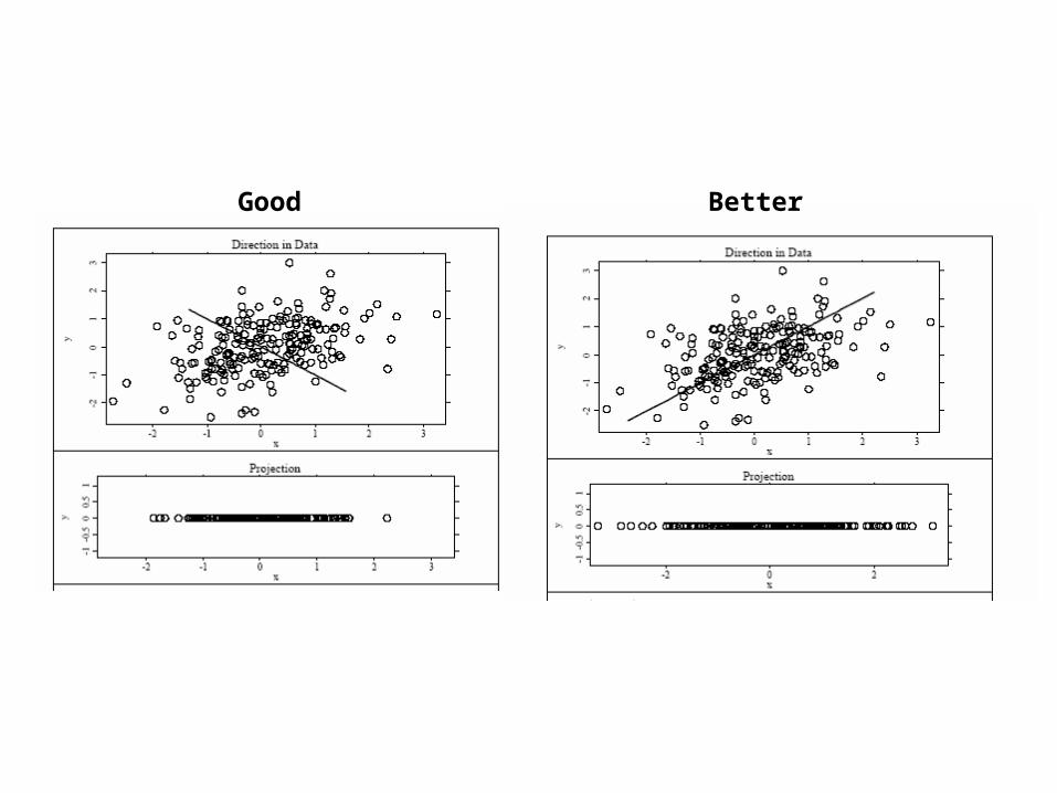
Good Better

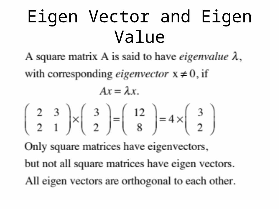
Eigen Vector and Eigen Value

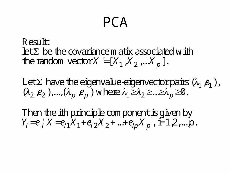
PCA

1 2

1 1

2 2 1 2

be the covariance matix associated with the random vector ' [ , ].

Let have

Result: let

,...

),( , ),...,(

the eigenvalue-eigenvector pairs , ) where ... 0.

Then the ith pr

(

i

,

p

p p p

X

e

X

e

X X

e

1 1 2 2

nciple component is given by ' ... , i=1,2,...,p.i i i i ip pY e X e X e X e X

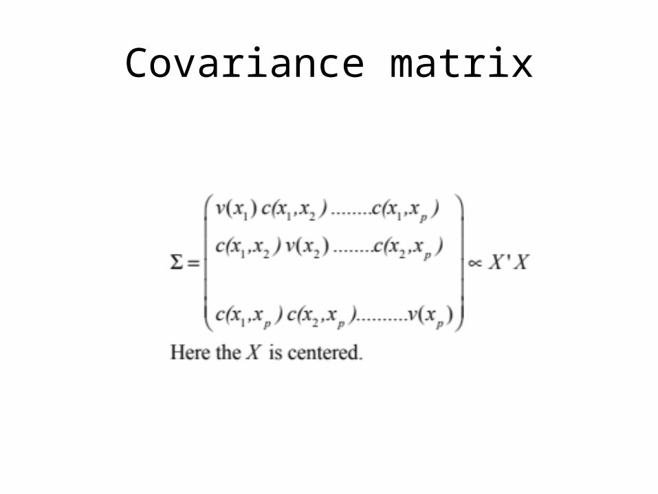
Covariance matrix

And so.. We find that• The direction of is given by the eigenvector

1 correponding to the largest eigenvalue of matrix Σ

• The second vector that is orthogonal (uncorrelated) to the first is the one that has the second highest variance which comes to be the eignevector corresponding to the second eigenvalue

• And so on …

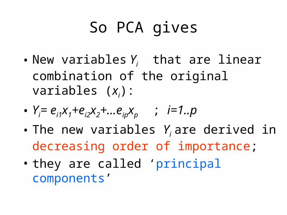
So PCA gives

• New variables Yi that are linear combination of the original variables (xi):

• Yi= ei1x1+ei2x2+…eipxp ; i=1..p

• The new variables Yi are derived in decreasing order of importance;

• they are called ‘principal components’

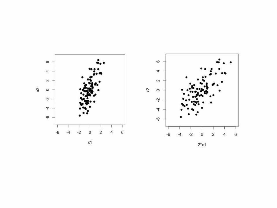
Scale before PCA

• PCA is sensitive to scale

• PCA should be applied on data that have approximately the same scale in each variable

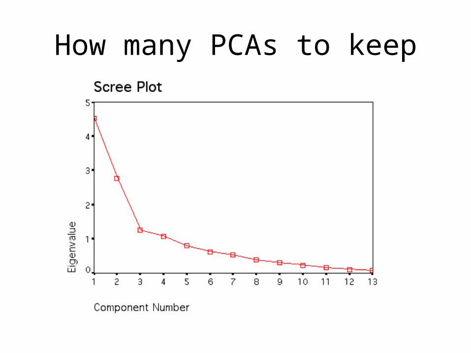
How many PCAs to keep

SVD (singular value decomposition)

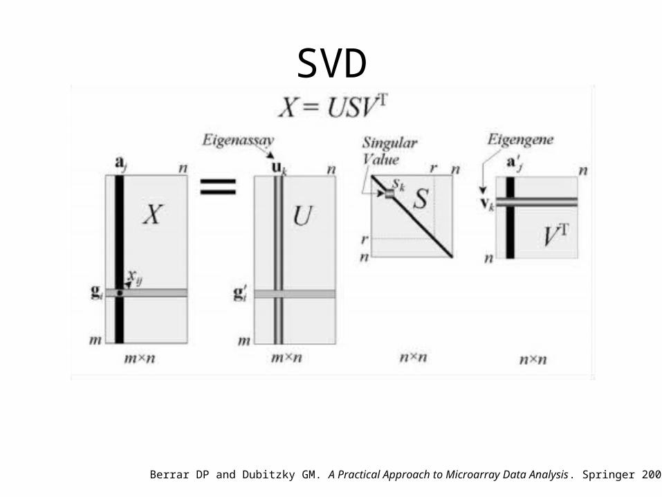
SVD

Berrar DP and Dubitzky GM. A Practical Approach to Microarray Data Analysis. Springer 2003.

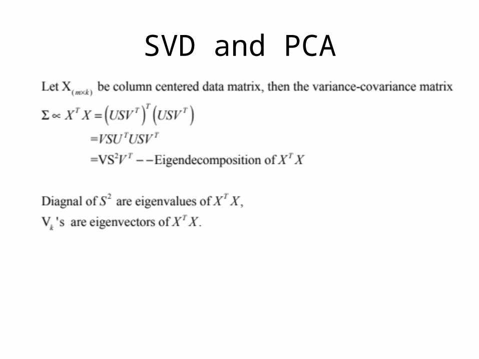
SVD and PCA

PCA application: genomic study

• Population stratification: allele frequency differences between cases and controls due to systematic ancestry differences—can cause spurious associations in disease studies.

• PCA could be used to infer underlying population structure.

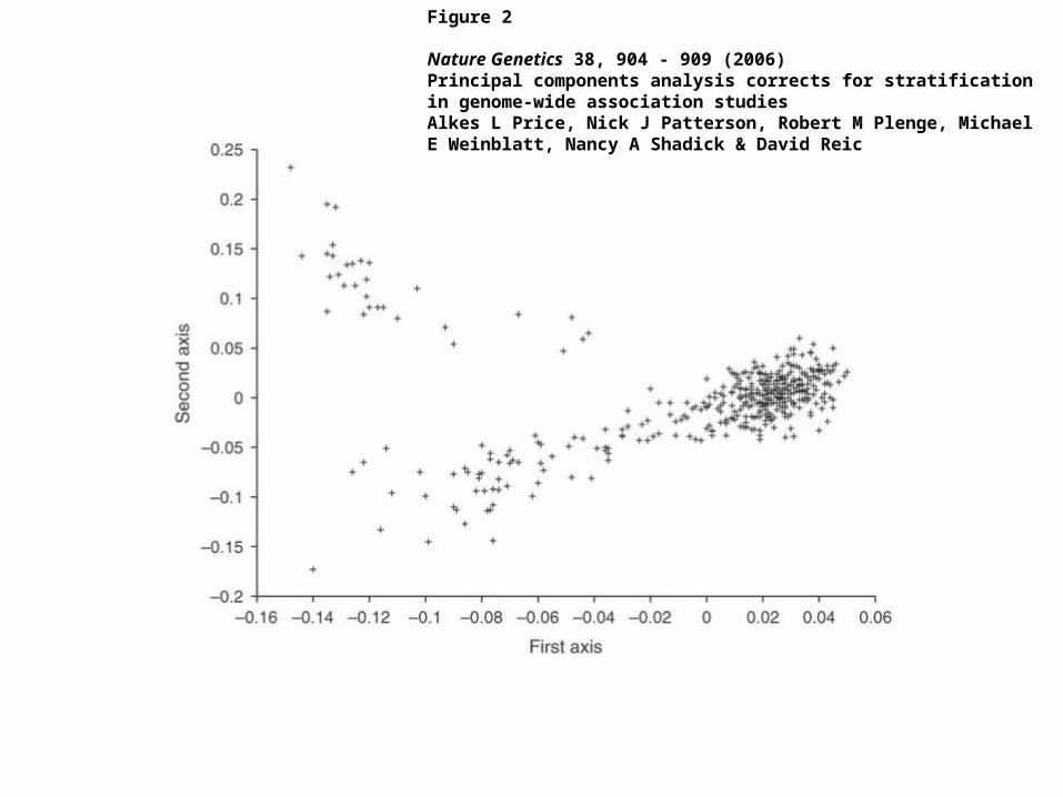
Figure 2

Nature Genetics 38, 904 - 909 (2006) Principal components analysis corrects for stratification in genome-wide association studiesAlkes L Price, Nick J Patterson, Robert M Plenge, Michael E Weinblatt, Nancy A Shadick & David Reic

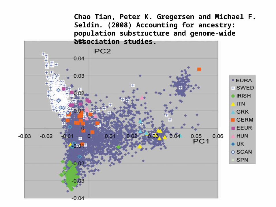
Chao Tian, Peter K. Gregersen and Michael F. Seldin. (2008) Accounting for ancestry: population substructure and genome-wide association studies.

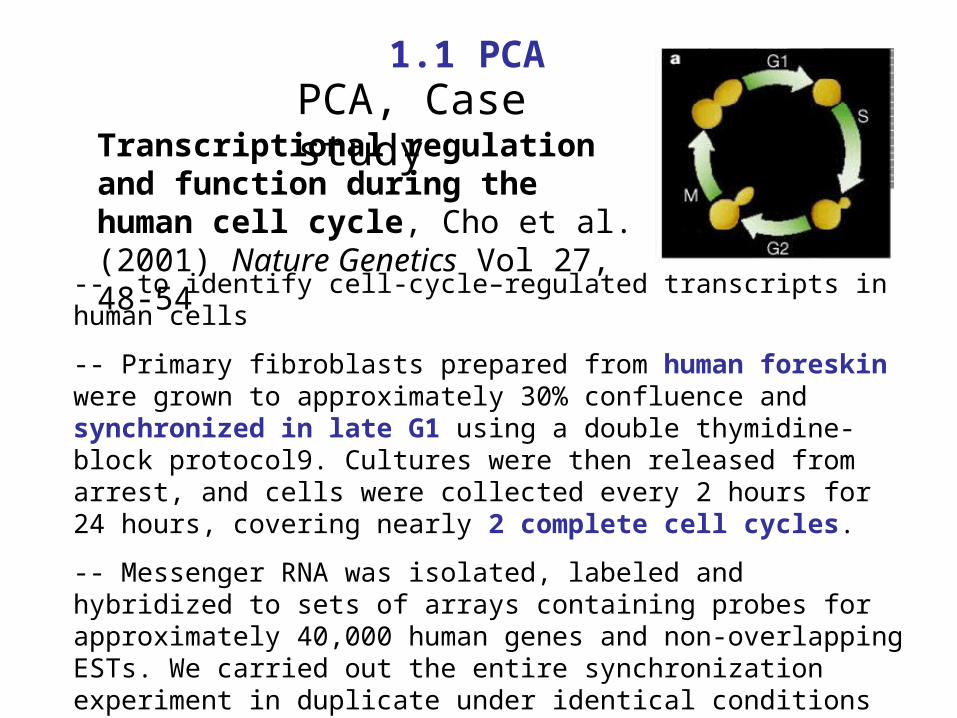
Transcriptional regulation and function during the human cell cycle, Cho et al. (2001) Nature Genetics Vol 27, 48-54

PCA, Case study

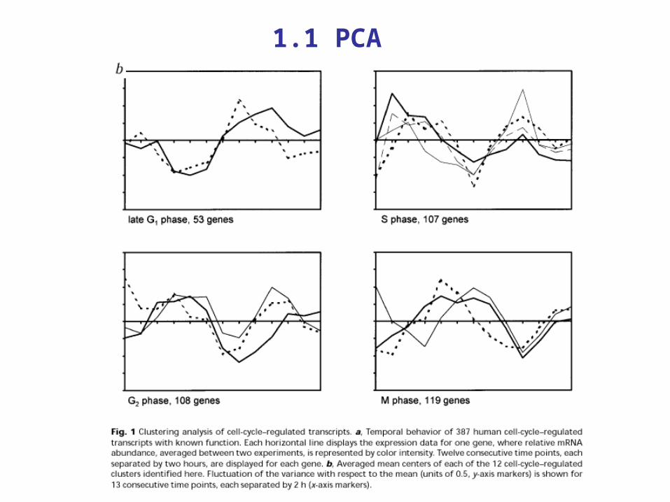
-- to identify cell-cycle–regulated transcripts in human cells

-- Primary fibroblasts prepared from human foreskin were grown to approximately 30% confluence and synchronized in late G1 using a double thymidine-block protocol9. Cultures were then released from arrest, and cells were collected every 2 hours for 24 hours, covering nearly 2 complete cell cycles.

-- Messenger RNA was isolated, labeled and hybridized to sets of arrays containing probes for approximately 40,000 human genes and non-overlapping ESTs. We carried out the entire synchronization experiment in duplicate under identical conditions for 6,800 genes on Affy array. The two data sets were averaged and analyzed using both supervised and unsupervised clustering of expression patterns.

1.1 PCA

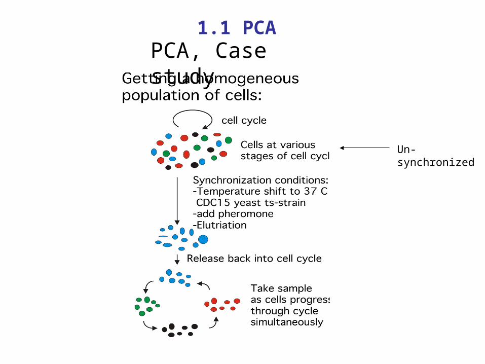
Un-synchronized

PCA, Case study1.1 PCA

1.1 PCA

cycle.pca$scores[, 1]

cycl

e.p

ca$

sco

res[

, 2

]

-2 0 2 4

-20

24

1

11

1

11

111

1

1

1

11

11

11

111

1

1

1

1

1

1

11

1

11

11

1

11 1

11

1

1

1

1

1

1

11

1

1

1

1

1

2

2

2

2

2

2

2

2

22

2

2

2

2

2

2

2

2

2

2

2

2

22

2

22

2

2

2

22

2

2

2

2

2

2

2 2

2

22

2

2

2

22

2

2

2

2

2

22

2

2

2

2

2

2

2

2

22

2

2

2

2

2

2

2 2

2

2

2

2

2 2

2

2

2

22

2

2

2

2

2

2

2

22

2

2

2

22

2

2

2

2

2

2

2

2

2

2

2

2

2

2

3

3

3

3

3

3

33

3

33

3 3

3

3

3 3

3

33

3

3

3

3

3

3

3

3

3

3

3

3

33

3

3

3

33

3

3

3

3 3

3

3

3

3

3

33

3

3

3

3

3

3

3

3

3

3

3

3

3

3

3

3

3

3

3

3

3

3

3

3

3

3

3

3

3

3

3

3

3

33

3

3

3

3

3

33

3

3

3

3

3

3

3

3

3

3

3

3

3

3

3

3

3

3

3

3 3

3

33

3

3

33

3

3

3

3

3

3

3 3

3

3

3

3

33

3

3

3

3

3

3

4

4

44

4

4

444

4

4

4

44

4

4

4

4 4

4

4

4

4

44

4

4

4

4

4

4

4

4

44

44

4

4

4

4

4 44

44

4

4

44

4

4

44

4

4

4

4

4

4

4

4

4

4

4

4

44

4

4

4

4

44

44

4

4

4 4

4

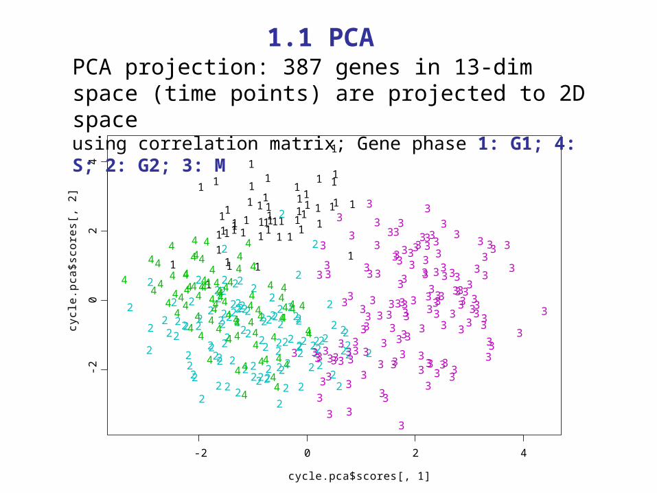
PCA projection: 387 genes in 13-dim space (time points) are projected to 2D spaceusing correlation matrix; Gene phase 1: G1; 4: S; 2: G2; 3: M

1.1 PCA

0.0

0.5

1.0

1.5

2.0

2.5

3.0

Comp. 1Comp. 2Comp. 3Comp. 4Comp. 5Comp. 6Comp. 7Comp. 8Comp. 9Comp. 10

Var

ianc

es

0.225

0.411

0.53

0.621

0.691 0.757

0.8080.853

0.891 0.925

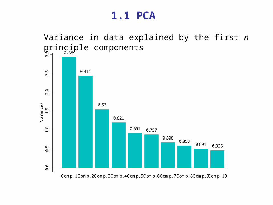
Variance in data explained by the first n principle components

1.1 PCA

Index

cycl

e.p

ca$

loa

din

gs[

, i]

2 4 6 8 10 12

-0.6

0.0

0.4

0.8

Index

cycl

e.p

ca$

loa

din

gs[

, i]

2 4 6 8 10 12

-0.6

0.0

0.4

0.8

Index

cycl

e.p

ca$

loa

din

gs[

, i]

2 4 6 8 10 12

-0.6

0.0

0.4

0.8

Index

cycl

e.p

ca$

loa

din

gs[

, i]

2 4 6 8 10 12

-0.6

0.0

0.4

0.8

Index

cycl

e.p

ca$

loa

din

gs[

, i]

2 4 6 8 10 12

-0.6

0.0

0.4

0.8

Index

cycl

e.p

ca$

loa

din

gs[

, i]

2 4 6 8 10 12

-0.6

0.0

0.4

0.8

Index

cycl

e.p

ca$

loa

din

gs[

, i]

2 4 6 8 10 12

-0.6

0.0

0.4

0.8

Index

cycl

e.p

ca$

loa

din

gs[

, i]

2 4 6 8 10 12

-0.6

0.0

0.4

0.8

Index

cycl

e.p

ca$

loa

din

gs[

, i]

2 4 6 8 10 12

-0.6

0.0

0.4

0.8

Index

cycl

e.p

ca$

loa

din

gs[

, i]

2 4 6 8 10 12

-0.6

0.0

0.4

0.8

Index

cycl

e.p

ca$

loa

din

gs[

, i]

2 4 6 8 10 12

-0.6

0.0

0.4

0.8

Index

cycl

e.p

ca$

loa

din

gs[

, i]

2 4 6 8 10 12

-0.6

0.0

0.4

0.8

Index

cycl

e.p

ca$

loa

din

gs[

, i]

2 4 6 8 10 12

-0.6

0.0

0.4

0.8

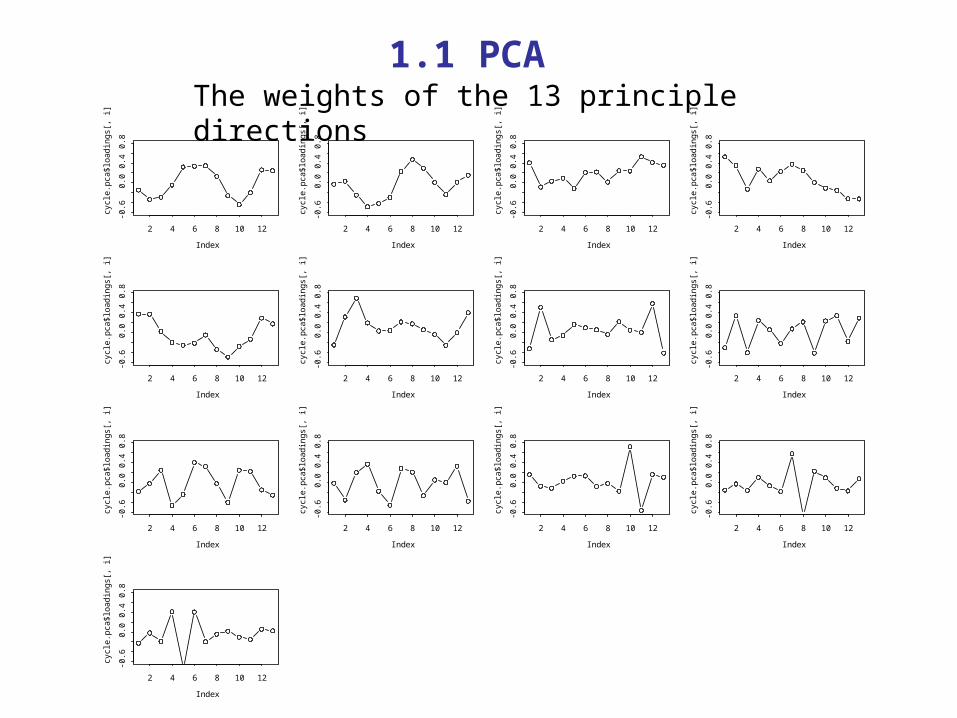
The weights of the 13 principle directions 1.1 PCA

cycle.pca2$scores[, 1]

cycl

e.p

ca2

$sc

ore

s[,

2]

-10 0 10 20

-15

-10

-50

51

01

5

1

2

3

45

6

7

8

9

10

11

1213

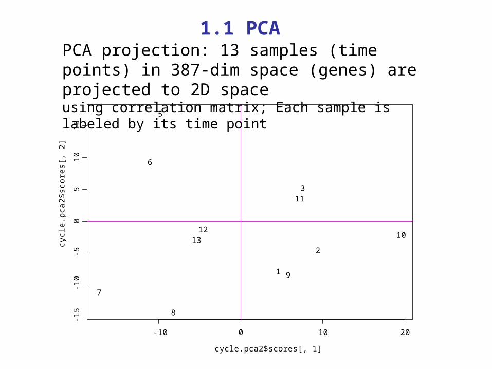
PCA projection: 13 samples (time points) in 387-dim space (genes) are projected to 2D spaceusing correlation matrix; Each sample is labeled by its time point

1.1 PCA

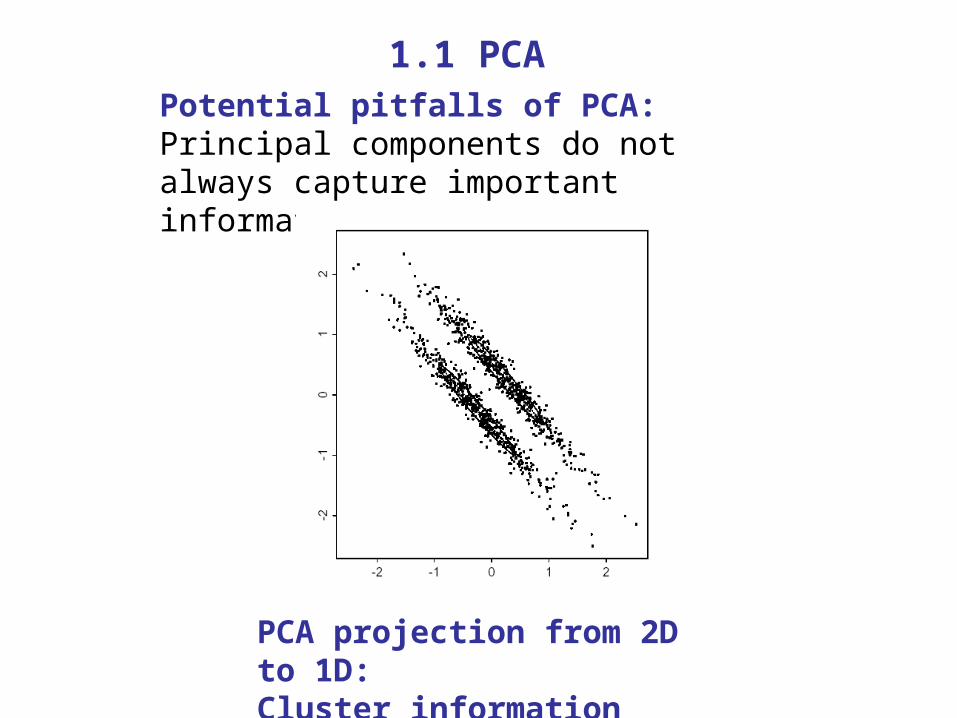
Potential pitfalls of PCA:Principal components do not always capture important information needed.

1.1 PCA

PCA projection from 2D to 1D: Cluster information will be lost.

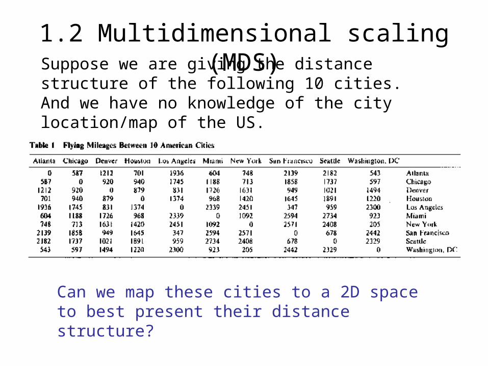
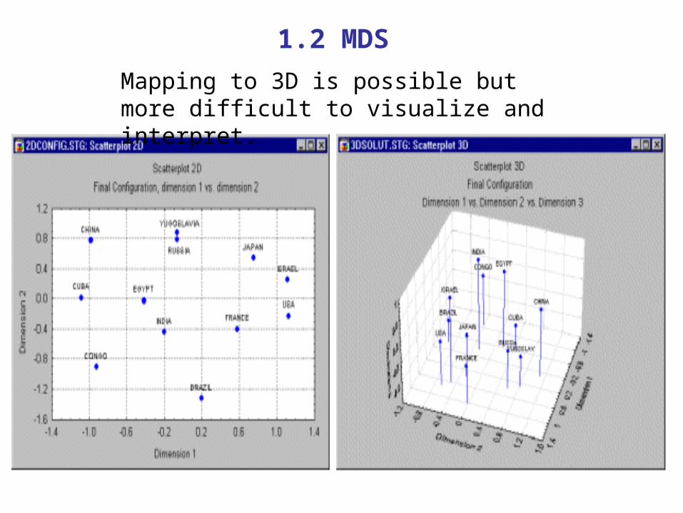
Suppose we are giving the distance structure of the following 10 cities. And we have no knowledge of the city location/map of the US.

Can we map these cities to a 2D space to best present their distance structure?

1.2 Multidimensional scaling (MDS)

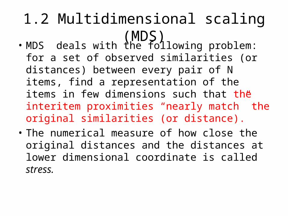
1.2 Multidimensional scaling (MDS)• MDS deals with the following problem: for a

set of observed similarities (or distances) between every pair of N items, find a representation of the items in few dimensions such that the interitem proximities “nearly match” the original similarities (or distance).

• The numerical measure of how close the original distances and the distances at lower dimensional coordinate is called stress.

1.2 MDS

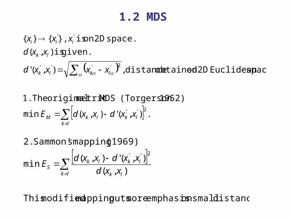
.),('),(min

1952) (Torgerson MDS metric original The 1.

spaceEuclidean 2Don obtained distance ,),('

given. is ),(

space. 2Don is },{}{

2''

2''''

''

lklklkM

lklk

lk

iii

xxdxxd E

xxxxd

xxd

xxx

distances. smallon emphasis more puts mapping modified This

),(

),('),(min

(1969) mapping sSammon' 2.2''

lk lk

lklkS xxd

xxdxxd E

1.2 MDS

1.2 MDS

Mapping to 3D is possible but more difficult to visualize and interpret.

1.2 MDS

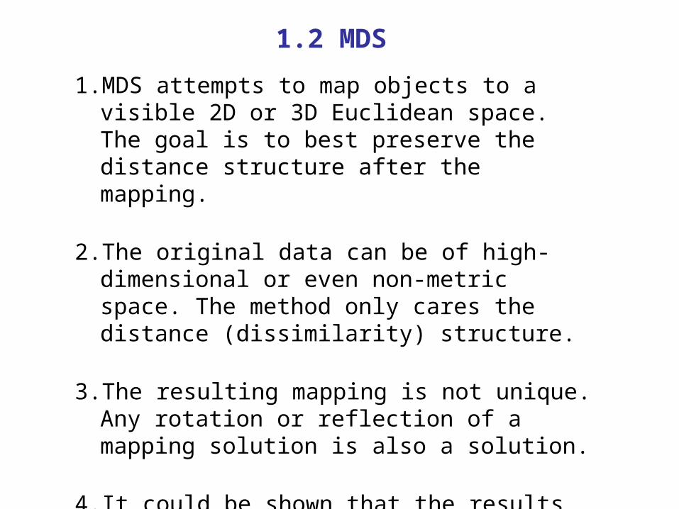
1. MDS attempts to map objects to a visible 2D or 3D Euclidean space. The goal is to best preserve the distance structure after the mapping.

2. The original data can be of high-dimensional or even non-metric space. The method only cares the distance (dissimilarity) structure.

3. The resulting mapping is not unique. Any rotation or reflection of a mapping solution is also a solution.

4. It could be shown that the results of PCA are exactly those of classical MDS if the distances calculated from the data matrix are Euclidean.

PCA MDS

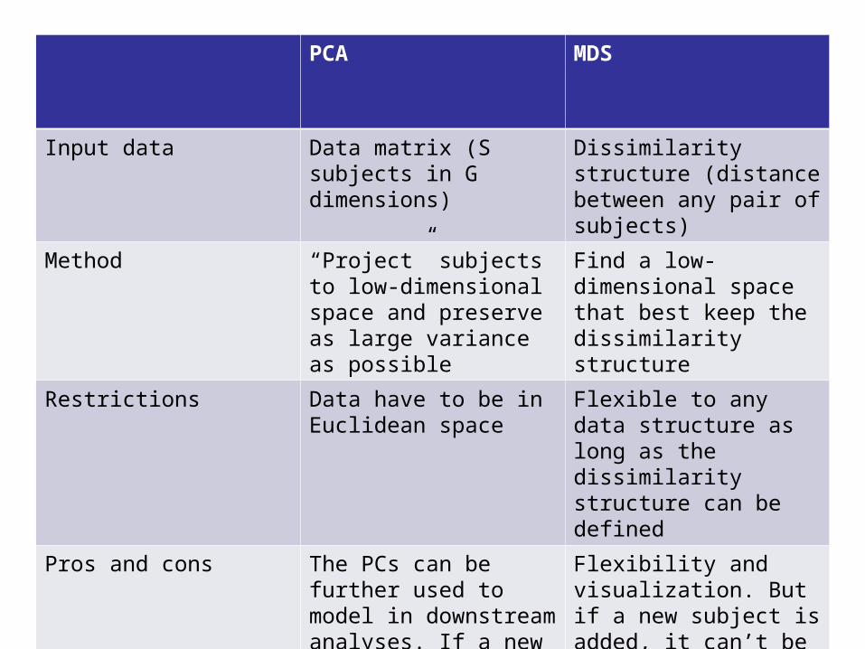
Input data Data matrix (S subjects in G dimensions)

Dissimilarity structure (distance between any pair of subjects)

Method “Project” subjects to low-dimensional space and preserve as large variance as possible

Find a low-dimensional space that best keep the dissimilarity structure

Restrictions Data have to be in Euclidean space

Flexible to any data structure as long as the dissimilarity structure can be defined

Pros and cons The PCs can be further used to model in downstream analyses. If a new subject is added, it can be similarly projected.

Flexibility and visualization. But if a new subject is added, it can’t be shown in an existing MDS solution.

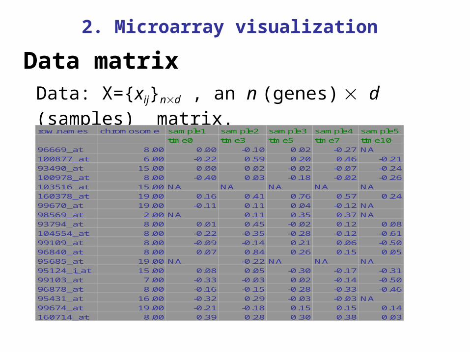
Data matrixData: X={xij}nd , an n (genes) d (samples) matrix.

row.names chromosome sample1 sample2 sample3 sample4 sample5

time0 time3 time5 time7 time10

96669_at 8.00 0.00 -0.10 0.02 -0.27 NA

100877_at 6.00 -0.22 0.59 0.20 0.46 -0.21

93490_at 15.00 0.00 0.02 -0.02 -0.07 -0.24

100978_at 8.00 -0.40 0.03 -0.18 -0.02 -0.26

103516_at 15.00 NA NA NA NA NA

160378_at 19.00 0.16 0.41 0.76 0.57 0.24

99670_at 19.00 -0.11 0.11 0.04 -0.12 NA

98569_at 2.00 NA 0.11 0.35 0.37 NA

93794_at 8.00 0.01 0.45 -0.02 0.12 0.08

104554_at 8.00 -0.22 -0.35 -0.28 -0.12 -0.61

99109_at 8.00 -0.09 -0.14 0.21 0.06 -0.50

96840_at 8.00 0.07 0.84 0.26 0.15 0.05

95685_at 19.00 NA -0.22 NA NA NA

95124_i_at 15.00 0.08 0.05 -0.30 -0.17 -0.31

99103_at 7.00 -0.33 -0.03 0.02 -0.14 -0.50

96878_at 8.00 -0.16 -0.15 -0.28 -0.33 -0.46

95431_at 16.00 -0.32 0.29 -0.03 -0.03 NA

99674_at 19.00 -0.21 -0.18 0.15 0.15 0.14

160714_at 8.00 0.39 0.28 0.30 0.38 0.03

2. Microarray visualization

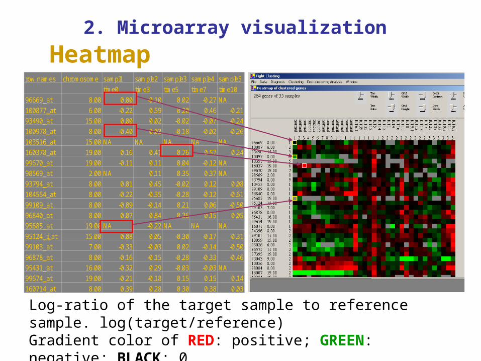
Heatmaprow.names chromosome sampl1 sample2 sample3 sample4 sample5

time0 time3 time5 time7 time10

96669_at 8.00 0.00 -0.10 0.02 -0.27 NA

100877_at 6.00 -0.22 0.59 0.20 0.46 -0.21

93490_at 15.00 0.00 0.02 -0.02 -0.07 -0.24

100978_at 8.00 -0.40 0.03 -0.18 -0.02 -0.26

103516_at 15.00 NA NA NA NA NA

160378_at 19.00 0.16 0.41 0.76 0.57 0.24

99670_at 19.00 -0.11 0.11 0.04 -0.12 NA

98569_at 2.00 NA 0.11 0.35 0.37 NA

93794_at 8.00 0.01 0.45 -0.02 0.12 0.08

104554_at 8.00 -0.22 -0.35 -0.28 -0.12 -0.61

99109_at 8.00 -0.09 -0.14 0.21 0.06 -0.50

96840_at 8.00 0.07 0.84 0.26 0.15 0.05

95685_at 19.00 NA -0.22 NA NA NA

95124_i_at 15.00 0.08 0.05 -0.30 -0.17 -0.31

99103_at 7.00 -0.33 -0.03 0.02 -0.14 -0.50

96878_at 8.00 -0.16 -0.15 -0.28 -0.33 -0.46

95431_at 16.00 -0.32 0.29 -0.03 -0.03 NA

99674_at 19.00 -0.21 -0.18 0.15 0.15 0.14

160714_at 8.00 0.39 0.28 0.30 0.38 0.03

2. Microarray visualization

Log-ratio of the target sample to reference sample. log(target/reference)Gradient color of RED: positive; GREEN: negative; BLACK: 0.LIGHT GREY: missing value.

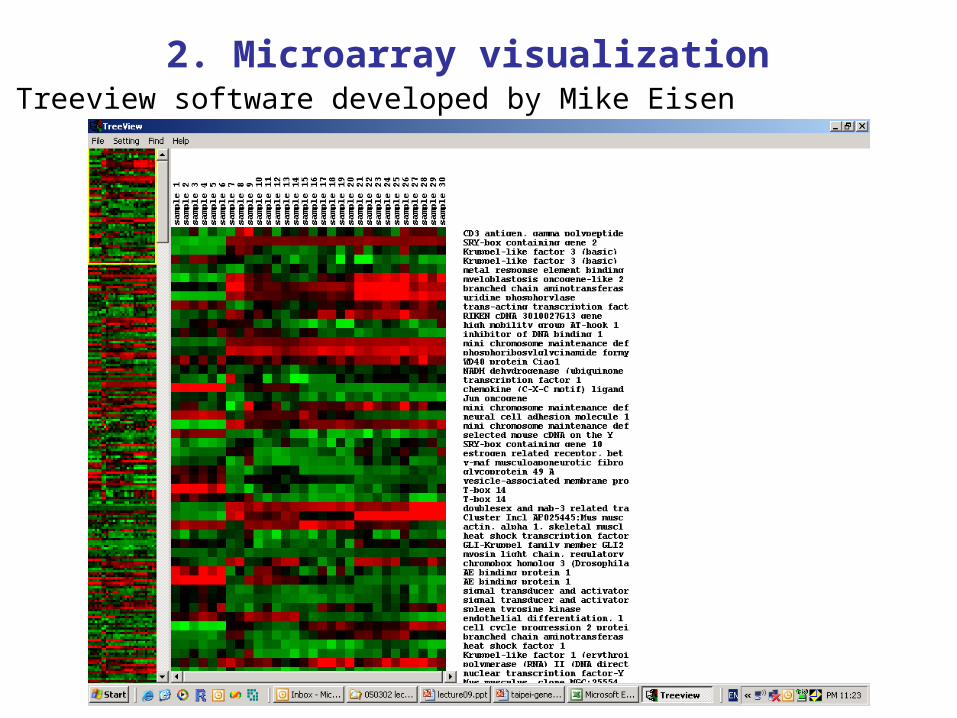
2. Microarray visualizationTreeview software developed by Mike Eisen

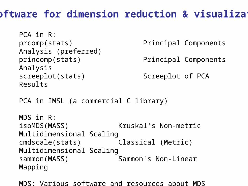
3. Software for dimension reduction & visualization

PCA in R:prcomp(stats) Principal Components Analysis (preferred)princomp(stats) Principal Components Analysisscreeplot(stats) Screeplot of PCA Results

PCA in IMSL (a commercial C library)

MDS in R:isoMDS(MASS) Kruskal's Non-metric Multidimensional Scalingcmdscale(stats) Classical (Metric) Multidimensional Scalingsammon(MASS) Sammon's Non-Linear Mapping

MDS: Various software and resources about MDShttp://www.granular.com/MDS/

Heatmap visualization:Treeview http://rana.lbl.gov/EisenSoftware.htm