PkANN: Non-Linear Matter Power Spectrum Interpolation throughArtificial Neural Networks

by

Shankar Agarwal, Ph.D

Submitted to the Department of Physics and Astronomy and the Facultyof the Graduate School of the University of Kansas in partial fulfillment of

the requirements for the degree of Doctor of Philosophy

Committee:

Dr. Hume Feldman, Chairper-son

Dr. Mikhail V. Medvedev

Dr. Danny Marfatia

Dr. Jack Shi

Dr. David Lerner

Date defended: 30 November 2012

The Dissertation Committee for Shankar Agarwal, Ph.D certifies that thisis the approved version of the following dissertation:

PkANN: Non-Linear Matter Power Spectrum Interpolation throughArtificial Neural Networks

Committee:

Dr. Hume Feldman, Chairper-son

Dr. Mikhail V. Medvedev

Dr. Danny Marfatia

Dr. Jack Shi

Dr. David Lerner

Date approved: 30 November 2012

ii

Abstract

We investigate the interpolation of power spectra of matter fluctuations using ar-

tificial neural networks (ANNs). We present a new approach to confront small-scale

non-linearities in the matter power spectrum. This ever-present and pernicious uncer-

tainty is often the Achilles’ heel in cosmological studies and must be reduced if we are

to see the advent of precision cosmology in the late-time Universe. We detail how an

accurate interpolation of the matter power spectrum is achievable with only a sparsely

sampled grid of cosmological parameters. We show that an optimally trained ANN,

when presented with a set of cosmological parameters (Ωmh2,Ωbh

2, ns, w0, σ8,∑mν and

z), can provide a worst-case error ≤ 1 per cent (for redshift z ≤ 2) fit to the non-linear

matter power spectrum deduced through large-scale N-body simulations, for modes up

to k ≤ 0.9hMpc−1. Our power spectrum interpolator, which we label ‘PkANN’, is

designed to simulate a range of cosmological models including massive neutrinos and

dark energy equation of state w0 6= −1. PkANN is accurate in the quasi-non-linear

regime (0.1hMpc−1 ≤ k ≤ 0.9hMpc−1) over the entire parameter space and marks

a significant improvement over some of the current power spectrum calculators. The

response of the power spectrum to variations in the cosmological parameters is explored

using PkANN. Using a compilation of existing peculiar velocity surveys, we investi-

gate the cosmic Mach number statistic and show that PkANN not only successfully

accounts for the non-linear motions on small scales, but also, unlike N-body simula-

tions which are computationally expensive and/or infeasible, it can be an extremely

quick and reliable tool in interpreting cosmological observations and testing theories of

structure-formation.

iii

Acknowledgements

I would like to express my sincere gratitude to my advisor Dr. Hume A. Feldman for the

continuous support of my Ph.D study and research. PkANN code was made possible

in collaboration with Dr. Ofer Lahav, Dr. Filipe B. Abdalla and Dr. Shaun A. Thomas

at the University College London, UK. I thank Dr. Salman Habib and Dr. Katrin

Heitmann at the Argonne National Laboratory, University of Chicago, USA, for their

insightful comments and suggestions on the PkANN code.

This work was supported by the National Science Foundation through TeraGrid re-

sources provided by the National Center for Supercomputing Applications (NCSA) and

by a grant from the Research Corporation. Computations described in this work were

performed using the enzo code developed by the Laboratory for Computational Astro-

physics at the University of California, San Diego (http://lca.ucsd.edu). I thank the

users of yt (python-based package for analyzing cosmological datasets) and enzo for

useful discussions and guidance towards running and analyzing simulations. I am grate-

ful to Dr. Roman Scoccimarro at the New York University, USA, and the LasDamas

(Large Suite of Dark Matter Simulations) collaboration for providing the LasDamas

simulations suite.

iv

Contents

1 Introduction 1

2 Numerical Simulations 5

2.1 Prelude . . . . . . . . . . . . . . . . . . . . . . . . . . . . . . . . . . . . 5

2.2 Probing Structure Formation through Neutrinos . . . . . . . . . . . . . 5

2.3 Implementing Neutrinos in N-body Simulations . . . . . . . . . . . . . . 7

2.4 Semi-Analytic Approach to Treat Neutrinos in N-body Simulations . . . 9

2.5 N-body Simulations: Optimizing Boxsize and Number of Particles . . . 10

2.6 Impact of Massive Neutrinos on Structural Growth . . . . . . . . . . . . 15

2.7 Resolving Neutrino Mass Hierarchy from Numerical Simulations . . . . 21

2.8 Comparison: Semi-Analytic versus Full Numerical Treatment . . . . . . 26

2.9 Matter Power Spectrum Error Estimates . . . . . . . . . . . . . . . . . . 28

2.10 Summary . . . . . . . . . . . . . . . . . . . . . . . . . . . . . . . . . . . 29

3 Developing PkANN – A Non-Linear Matter Power Spectrum Inter-

polator 30

3.1 Prelude . . . . . . . . . . . . . . . . . . . . . . . . . . . . . . . . . . . . 30

3.2 Machine-Learning . . . . . . . . . . . . . . . . . . . . . . . . . . . . . . . 30

3.3 Artificial Neural Networks . . . . . . . . . . . . . . . . . . . . . . . . . . 32

3.4 Latin Hypercube Parameter Sampling . . . . . . . . . . . . . . . . . . . 41

3.4.1 Setting up an improved Latin hypercube for cosmological param-

eters . . . . . . . . . . . . . . . . . . . . . . . . . . . . . . . . . . 43

3.5 Summary . . . . . . . . . . . . . . . . . . . . . . . . . . . . . . . . . . . 47

4 Interpolating Matter Power Spectrum using PkANN 48

4.1 Prelude . . . . . . . . . . . . . . . . . . . . . . . . . . . . . . . . . . . . 48

4.2 Comparing PkANN’s Performance against Numerical Simulations . . . . 48

4.3 Exploring Cosmological Parameter Space with PkANN . . . . . . . . . 56

v

4.4 Summary . . . . . . . . . . . . . . . . . . . . . . . . . . . . . . . . . . . 57

5 Estimating the Cosmic Mach Number using PkANN 63

5.1 Prelude . . . . . . . . . . . . . . . . . . . . . . . . . . . . . . . . . . . . 63

5.2 The Cosmic Mach Number . . . . . . . . . . . . . . . . . . . . . . . . . 65

5.3 N-body Simulations . . . . . . . . . . . . . . . . . . . . . . . . . . . . . 67

5.4 Peculiar Velocity Catalogues . . . . . . . . . . . . . . . . . . . . . . . . . 69

5.4.1 Real Catalogues . . . . . . . . . . . . . . . . . . . . . . . . . . . 69

5.4.2 Mock Catalogues . . . . . . . . . . . . . . . . . . . . . . . . . . . 70

5.5 The Maximum Likelihood Estimate Method . . . . . . . . . . . . . . . . 70

5.6 Cosmic Mach Number Statistics . . . . . . . . . . . . . . . . . . . . . . 74

5.7 Mach statistics for DEEP mocks . . . . . . . . . . . . . . . . . . . . . . 74

5.8 Mach statistics for Gaussian mocks . . . . . . . . . . . . . . . . . . . . . 75

5.9 Mach statistics for other mocks . . . . . . . . . . . . . . . . . . . . . . . 77

5.10 Moving Beyond N-Body Simulations: Mach Predictions Using PkANN . 82

5.11 Mach Number Estimates From Real Catalogues . . . . . . . . . . . . . . 83

5.12 Summary . . . . . . . . . . . . . . . . . . . . . . . . . . . . . . . . . . . 85

6 Conclusions 87

7 Appendix 89

7.1 PkANN Cost Function . . . . . . . . . . . . . . . . . . . . . . . . . . . . 89

7.2 Quasi-Newton Method . . . . . . . . . . . . . . . . . . . . . . . . . . . . 91

7.3 PkANN Cost Function Gradient . . . . . . . . . . . . . . . . . . . . . . 93

7.3.1 Gradient w.r.t. First Layer Weights . . . . . . . . . . . . . . . . . 94

7.3.2 Gradient w.r.t. Second Layer Weights . . . . . . . . . . . . . . . 96

7.4 BFGS Approximation for Inverse-Hessian Matrix . . . . . . . . . . . . . 97

7.5 Regularization Parameter ξ . . . . . . . . . . . . . . . . . . . . . . . . . 98

7.6 Exact Calculation of Hubble Parameter h . . . . . . . . . . . . . . . . . 100

vi

8 References 102

vii

List of Tables

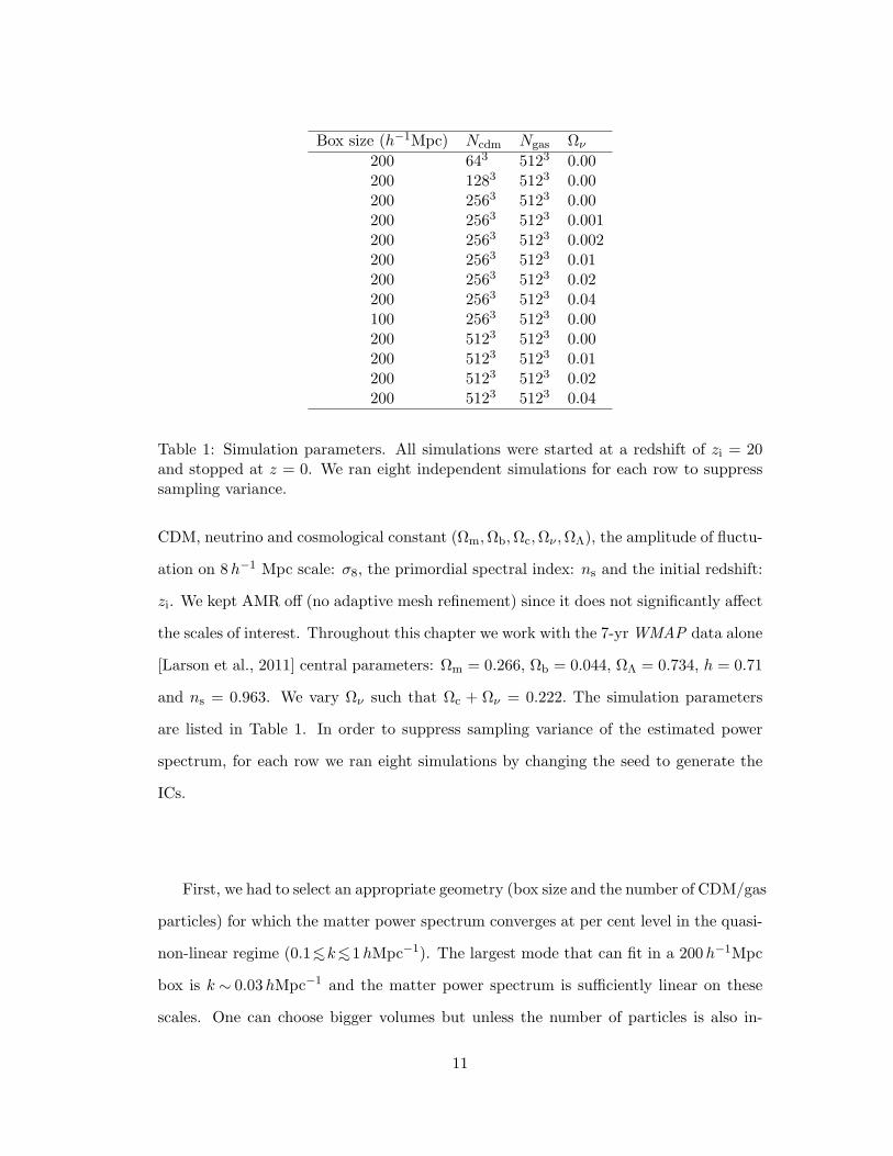
1 Simulation parameters. All simulations were started at a redshift of zi =

20 and stopped at z = 0. We ran eight independent simulations for each

row to suppress sampling variance. . . . . . . . . . . . . . . . . . . . . . 11

2 The six cosmological parameters and their ranges, used in generating the ANN

training and validation sets. This six-dimensional parameter space is sampled

using the improved Latin hypercube technique (see text for details). The last

column shows the corresponding 7-yr WMAP+BAO+H0 constraints at 68 per

cent CL. . . . . . . . . . . . . . . . . . . . . . . . . . . . . . . . . . . . . 44

3 The six cosmological parameters and their ranges, used in generating the ANN

testing set. This six-dimensional parameter space is sampled using the improved

Latin hypercube technique (see the text for details). The parameter ranges are

chosen so as to avoid the boundaries of the parameter space. See Table 2 for

the parameter boundaries. Note that the lower bound on neutrino mass is still

set at zero, since neutrinos are physically bound (∑mν & 0). The last column

shows the 7-yr WMAP+BAO+H0 constraints at 68 per cent CL. . . . . . . . 52

4 The cosmological parameters and the design specifications of the LD-

Carmen simulations. . . . . . . . . . . . . . . . . . . . . . . . . . . . . . 68

5 The rms values of the bulk flow (2nd column), velocity dispersion (3rd

column) and cosmic Mach number (4th column) together with their 1σ

CL intervals for Gaussian windows with width R (1st column). These

values are calculated for the LD cosmology (for the LD parameters, see

Table 4). . . . . . . . . . . . . . . . . . . . . . . . . . . . . . . . . . . . . 78

viii

6 Peculiar velocity statistics for various surveys (1st column). For each

survey, 4100 mocks were extracted from the LD cosmology (for the LD

parameters, see Table 4). The characteristic depth R (2nd column) of

the mock catalogues is estimated from the effective width of their win-

dow functions shown in Fig. 5.6. For reference, the error-weighted depth∑wnrn/

∑wn where wn = 1/(σ2

n+σ2∗), is mentioned in the 3rd column.

The rms values of the bulk flow (4th column), velocity dispersion (5th

column) and cosmic Mach number (6th column) are mentioned together

with their 1σ CL intervals. . . . . . . . . . . . . . . . . . . . . . . . . . . 80

7 Similar to Table 6, but for the real data. The quoted errors are calculated

using the radial distance uncertainties. . . . . . . . . . . . . . . . . . . . 85

ix

List of Figures

2.1 Matter power spectrum at z = 0 for undersampled ICs at zi = 20 with

Ncdm =643−solid (red), 1283−long dash-dotted (green), 2563−dashed (blue)

and 5123 − long-dashed (cyan). The vertical lines are the kNy wavenum-

bers for 643, 1283, 2563 and 5123 CDM particles. Also plotted (dash-

dotted line) is the linear theoretical power spectrum. For k > kNy, par-

ticle shot noise dominates the true power spectrum. . . . . . . . . . . . 13

2.2 Same as Fig. 2.1 expressed as fractional suppression of the matter power

spectrum at z=0 when 643−solid (red), 1283− long dash-dotted (green)

and 2563−dashed (blue) CDM particles are used to sample the ICs w.r.t

the case where 5123−long-dashed (cyan) CDM particles are used. Ων = 0

for all four cases.The error bars correspond to eight simulations with

different seeds for the ICs. . . . . . . . . . . . . . . . . . . . . . . . . . 14

2.3 Matter power spectrum at z = 0 from 100h−1Mpc − solid (green) and

200h−1Mpc − dashed (blue) box simulations. The linear theory spec-

trum (dash-dotted line) is also shown. The vertical dashed line is the

maximum wavenumber up to which the power spectrum from 200h−1Mpc

box simulations can be trusted at per cent level. . . . . . . . . . . . . . 16

2.4 Same as Fig. 2.3 expressed as fractional suppression of the matter power

spectrum at z=0 as a function of the box size. Spectrum from 100h−1Mpc − solid (green)

and 200h−1Mpc − dashed (blue) box agree at per cent level for k <∼

1hMpc−1. . . . . . . . . . . . . . . . . . . . . . . . . . . . . . . . . . . 17

x

2.5 Slices of baryon density distribution. All slices are 200h−1Mpc wide and

show the baryonic mass averaged over the volume of a grid cell. Each

grid cell is ∼ 391h−1kpc. The top panel shows a simulation without

neutrinos. The middle and the bottom panels are taken from simulations

with Ων = 0.02 (Σmν = 0.95 eV) and Ων = 0.04 (Σmν = 1.9 eV). The

baryon density fields in the middle and the bottom panels are less evolved

relative to the no-neutrino (top panel) case. The simulations were run

with Ncdm =2563, Ngas =5123. The density projections were made using

yt: an analysis and visualization tool [Turk, 2008]. . . . . . . . . . . . 19

2.6 Matter power spectrum at z = 0 from simulations and linear theory

(dash-dotted lines) as a function of neutrino mass. The four neutrino

models are: Ων = 0 (Σmν = 0 eV) – solid (red), Ων = 0.01 (Σmν =

0.475 eV) – long dash-dotted (green), Ων =0.02 (Σmν = 0.95 eV) – dashed

(blue) and Ων = 0.04 (Σmν = 1.9 eV) – long-dashed (cyan). The vertical

dashed line is the maximum wavenumber up to which the power spectra

from 200h−1Mpc box simulations are valid at 1 per cent level. . . . . . 20

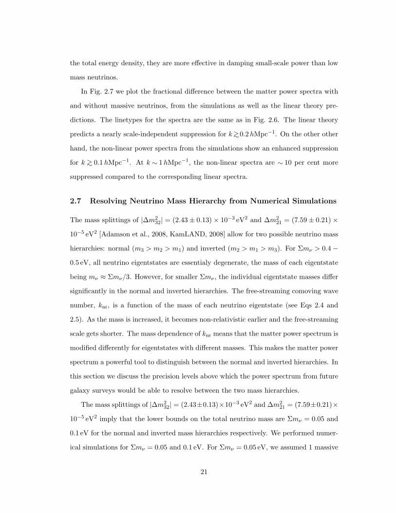
2.7 Fractional difference between the matter power spectra with and without

massive neutrinos at z = 0, from the simulations and the linear theory

predictions (dash-dotted lines). The four neutrino models are: Ων =

0 (Σmν = 0 eV) – solid (red), Ων = 0.01 (Σmν = 0.475 eV) – long dash-

dotted (green), Ων = 0.02 (Σmν = 0.95 eV) – dashed (blue) and Ων =

0.04 (Σmν = 1.9 eV) – long-dashed (cyan). The error bars correspond to

eight simulations with different seeds for the ICs. . . . . . . . . . . . . 22

2.8 Same as Fig. 2.7, but for neutrino models with much lower neutrino

mass: Ων = 0.001 (Σmν = 0.05 eV) – long dash-dotted (green) and Ων =

0.002 (Σmν = 0.1 eV) – dashed (blue). . . . . . . . . . . . . . . . . . . . 23

xi

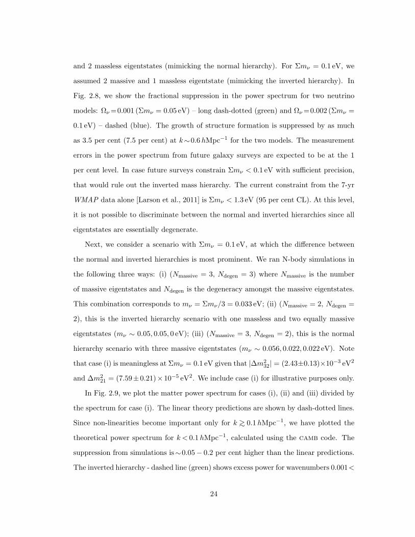
2.9 Matter power spectrum for normal – long dash-dotted line (blue) and

inverted – dashed line (green) hierarchies divided by the matter power

spectrum for mν = Σmν/3 – solid line (red). The linear theory predic-

tions are shown by dash-dotted lines. The neutrino model considered

here is Σmν = 0 eV. The individual masses for the three eigentstates

are (mν ∼ 0.05, 0.05 and 0 eV) for the inverted hierarchy and (mν ∼

0.056, 0.022 and 0.022 eV) for the normal hierarchy. The inverted hierar-

chy shows more damping of small-scale power than the normal hierarchy.

. . . . . . . . . . . . . . . . . . . . . . . . . . . . . . . . . . . . . . . . . 25

2.10 Fractional difference between the matter power spectra with and without

massive neutrinos at z = 0, from numerical simulations and linear theory

predictions (dash-dotted lines). The four neutrino models are: Ων =

0.001 (Σmν = 0.05 eV) – dotted (green), Ων = 0.002 (Σmν = 0.1 eV)

– dashed (blue), Ων = 0.01 (Σmν = 0.475 eV) – long-dashed (cyan) and

Ων =0.02 (Σmν = 0.95 eV) – long dash-dotted (magenta). The maximum

relative suppression of ∆P/P ∼−10fν is shown as short horizontal dotted

lines. The horizontal (red) dotted line for Σmν = 0.95 eV is at ∆P/P ∼

−8.6fν . . . . . . . . . . . . . . . . . . . . . . . . . . . . . . . . . . . . . 27

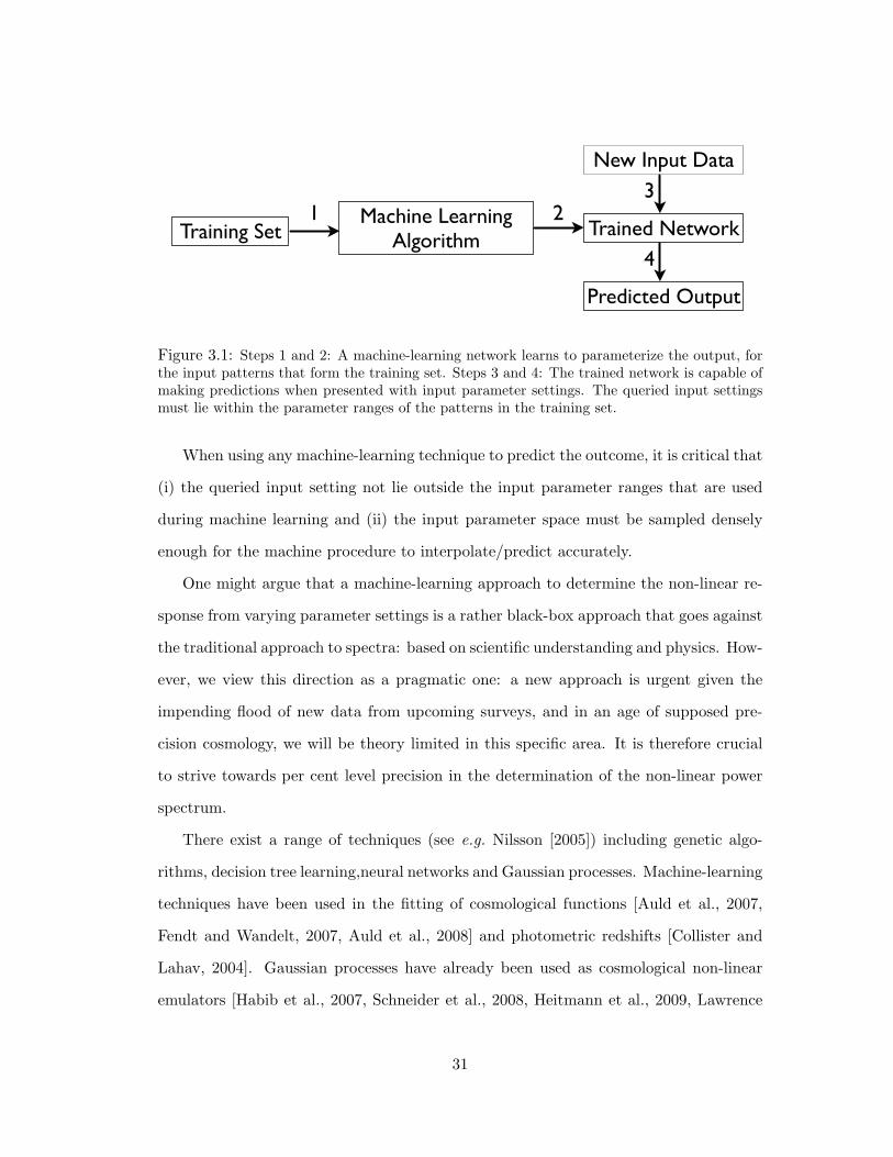
3.1 Steps 1 and 2: A machine-learning network learns to parameterize the output,

for the input patterns that form the training set. Steps 3 and 4: The trained

network is capable of making predictions when presented with input parameter

settings. The queried input settings must lie within the parameter ranges of the

patterns in the training set. . . . . . . . . . . . . . . . . . . . . . . . . . . 31

3.2 A typical ANN architecture (left-hand panel) with node activation formulae for

the hidden and output layers (right-hand panels). . . . . . . . . . . . . . . . 34

xii

3.3 Top: matter power spectrum evaluated at redshift z = 0 (upper set) and z = 1

(lower set). At each redshift, the spectrum is calculated using (i) linear theory

(dash-dotted), (ii) N-body (dotted), (iii) halofit (dashed) and (iv) cosmic

emulator (solid, see Lawrence et al. [2010]). The cosmological parameters are:

I ≡ (0.13, 0.0224, 0.986,−1.23, 0.72, 0) with h = 0.8. Our N-body power spectra

agree with the cosmic emulator at per cent level for k ≤ 0.8hMpc−1. Middle:

The ratio of the N-body spectrum to cosmic emulator’s prediction at z = 0.

The error bars correspond to the scatter in the N-body results. The horizontal

dotted lines denote ±2,±1 and 0 per cent error. Bottom: The same as the

middle panel, at z = 1. . . . . . . . . . . . . . . . . . . . . . . . . . . . . 38

3.4 Linear theory, halofit and N-body spectra from Fig. 3.3, top panel are re-

plotted – with the only difference that on scales k ≤ 0.085hMpc−1 the N-body

spectrum is approximated by the one-Loop standard PT. The stitched spectrum

is then sampled at 50 k-values between 0.006hMpc−1 ≤ k ≤ 1hMpc−1 and used

as Pnl(k, z) for ANN training. . . . . . . . . . . . . . . . . . . . . . . . . . 39

3.5 Left: An example of a Latin hypercube distribution. Every interval dx and

dy is sampled; however each row and column are sampled only once. Right: an

improved Latin hypercube where the distribution is more evenly spread through

the space. Each subspace is equally sampled and there are no voids or clusters

as in the left-hand panel (bottom left and right corners, respectively). . . . . 42

3.6 Upper triangle: ANN training set with 130 viable cosmologies, in a six-dimensional

parameter space. Lower triangle: ANN validation set with 32 viable cosmolo-

gies, in a six-dimensional parameter space. See Table 2 for the parameter priors

used to generate the training and validation sets. . . . . . . . . . . . . . . . 45

3.7 Upper triangle: extending the ANN training set (upper triangle in Fig. 3.6) with

70 cosmologies with∑mν = 0. Lower triangle: extending the ANN validation

set (lower triangle in Fig. 3.6) with 18 cosmologies with∑mν = 0. . . . . . . 46

xiii

4.1 Percentage error at redshift z = 0 (left-hand panel), z = 1 (middle panel)

and z = 2 (right-hand panel) between the predicted non-linear power spectrum

(using PkANN) and the true underlying spectrum (using N-body simulations)

for 200 training set cosmologies shown in the upper triangles of Figs. 3.6 and 3.7.

The shaded region contains the middle 99.73% (3σ) of the residuals. The rows

(from top to bottom) correspond to Nhidden = 14− 98 in increments of 14. The

mean error over all 200 cosmologies is shown by a solid line – an indicator of

any bias in the ANN training scheme. . . . . . . . . . . . . . . . . . . . . . 49

4.2 The residual error χ2C(w) (see Eq. 3.8) evaluated as a function of the number

of nodes in the hidden layer, Nhidden. The error is a monotonically decreasing

function for the training set (dashed line) while for the validation set (solid line),

it starts increasing beyond Nhidden = 70 indicating that the generalizing ability

of the neural network is best with Nhidden = 70. The error bars correspond to

the spread in χ2C(w) for the 16 ANN committee members. . . . . . . . . . . 51

4.3 Similar to Fig. 4.1, using 50 validation set cosmologies. The validation set is

shown in the lower triangles of Figs 3.6 and 3.7. . . . . . . . . . . . . . . . 53

4.4 Upper triangle: ANN testing set with 180 cosmologies with∑mν > 0. Lower

triangle: extending the ANN testing set with 150 cosmologies with∑mν = 0.

See Table 3 for the parameter priors used to generate the testing set. . . . . . 54

4.5 Similar to Fig. 4.1, using 330 testing set cosmologies shown in Fig. 4.4. . . . . 55

xiv

4.6 Variations in the power spectrum at redshift z = 0 (top row), z = 1 (middle row),

z = 2 (bottom row). Parameter Ωmh2 is varied between its minimum and max-

imum value (Table 3, columns 2 and 3) while Ωbh2, ns, w0, σ8 are fixed at their

central values.∑mν = 0 to facilitate comparison with the cosmic emulator.

The left-hand panels show natural logarithm of the ratio of the power spectra

with different Ωmh2 to the base power spectrum. The base power spectrum

corresponds to Ωmh2 = 0.135,Ωbh

2 = 0.0225, ns = 0.95, w0 = −1, σ8 = 0.775,

with∑mν = 0. The absolute power spectra are shown in the right-hand pan-

els. Within each panel, the power spectra (from top to bottom) correspond to

increasing values of Ωmh2. PkANN predictions (dotted) are within 0.2% of the

cosmic emulator spectra (solid lines). At z = 2, only PkANN predictions

are shown. . . . . . . . . . . . . . . . . . . . . . . . . . . . . . . . . . . . 58

4.7 Similar to Fig. 4.6, but for a range of Ωbh2 values. Within each panel, the power

spectra from bottom to top correspond to increasing Ωbh2 values. . . . . . . 59

4.8 Similar to Fig. 4.6, but for a range of ns values. Within each panel, the power

spectra from top to bottom correspond to increasing ns values. . . . . . . . . 60

4.9 Similar to Fig. 4.6, but for a range of w0 values. Within each panel, the power

spectra from top to bottom correspond to increasing w0 values. . . . . . . . 61

4.10 Similar to Fig. 4.6, but for a range of σ8 values. Within each panel, the power

spectra from bottom to top correspond to increasing σ8 values. . . . . . . . . 62

5.1 Top row: DEEP catalogue (left) and its radial distribution (right). Bottom row:

DEEP mock catalogue (left) and its radial distribution (right). . . . . . . . . 69

xv

5.2 The window functions W 2ii of the bulk flow components calculated using MLE

weights for the DEEP catalogue (left-hand panel). The x, y, z components are

dot-dashed, short-dashed and long-dashed lines, respectively. The solid lines are

the ideal window functions IW 2ij for scales R = 10 − 40h−1Mpc (in 5h−1Mpc

increments), the window functions being narrower for larger scales. The window

functions for a subset of 4100 DEEP mocks are shown in the right-hand panel

(solid lines). The characteristic depth of the DEEP catalogue and its mocks is

∼ R = 35h−1Mpc (dashed line, right-hand panel). . . . . . . . . . . . . . . 74

5.3 Histograms showing the normalized probability distribution for the 4100 DEEP

mocks: bulk flow u (left-hand panel), dispersion σ (middle panel) and the cos-

mic Mach number M (right-hand panel). We also superimpose the best-fitting

Maxwellian (for bulk and Mach) and Gaussian (for dispersion) distributions

with the same widths as the corresponding histograms. The rms values and the

1σ CL intervals are mentioned within each panel. These results correspond to

the LD cosmology. . . . . . . . . . . . . . . . . . . . . . . . . . . . . . . . 75

5.4 The rms values of the bulk flow (left-hand panel), dispersion (middle panel)

and the cosmic Mach number (right-hand panel) are plotted as a function of

scale R. In each panel, the dashed line corresponds to measurements from the

Gaussian mocks. The shaded region is the 1σ CL interval for the Gaussian

mocks. The solid circle at R = 35h−1Mpc is for the DEEP mocks. The error

bar is the statistical variance calculated from the 4100 DEEP mocks. Linear

theory predictions are shown by solid line. These results correspond to the LD

cosmology. . . . . . . . . . . . . . . . . . . . . . . . . . . . . . . . . . . . 76

xvi

5.5 The same as Fig. 5.3, but for Gaussian window with R = 15h−1Mpc (dot-

ted), R = 35h−1Mpc (solid), R = 55h−1Mpc (short-dashed), R = 75h−1Mpc

(long-dashed), R = 95h−1Mpc (dot-dashed). For clarity, instead of the his-

tograms, only the best-fitting Maxellian/Gaussian distributions with the same

widths as the corresponding histograms are shown. The rms values and the 1σ

CL intervals for R = 35h−1Mpc are mentioned within each panel, and are in

good agreement with the corresponding values for the DEEP mocks (shown in

Fig. 5.3). Table 5 summarizes the results for Gaussian widths R = 10 − 100

h−1Mpc. . . . . . . . . . . . . . . . . . . . . . . . . . . . . . . . . . . . . 76

5.6 Similar to Fig. 5.2, for the SBF, ENEAR, SFI++g, SNIa, SFI++f, DEEP and

SC catalogues (top to bottom row, respectively). . . . . . . . . . . . . . . . 79

5.7 Similar to Fig. 5.4, including results for the SBF (open triangle), ENEAR (solid

triangle), SFI++g (open square), SNIa (solid square), SFI++f (open circle),

DEEP (solid circle) and SC (cross) mocks. The DEEP compilation includes the

SC, SNIa, SMAC, EFAR and Willick surveys. . . . . . . . . . . . . . . . . . 81

5.8 Similar to Fig. 5.7, but instead of showing linear theory predictions, we plot

predictions based on the non-linear matter power spectrum for the LD cosmology

estimated using PkANN. . . . . . . . . . . . . . . . . . . . . . . . . . . . 82

5.9 Similar to Fig. 5.8, but instead of showing the Mach numbers for the mocks, we

plot the Mach numbers for the real surveys. The error bars are calculated using

the radial distance uncertainties. . . . . . . . . . . . . . . . . . . . . . . . 84

xvii

1 Introduction

The growth of structure is a direct consequence of the primordial gravitational instabil-

ity present in our Universe. Observations of galaxy clustering is a powerful tool to test

structure-formation theories and complements the cosmic variance limited cosmic mi-

crowave background. This complementarity explains the large number of galaxy surveys

in various stages of planning and construction that promise to refine or even alter our

understanding of the cosmos, e.g. DES [The Dark Energy Survey Collaboration, 2005],

the Large Synoptic Survey Telescope (LSST) [Ivezic et al., 2008], and the Baryon Os-

cillation Spectroscopic Survey (BOSS) [Eisenstein et al., 2011]. These surveys promise

to achieve high-precision measurements of matter power spectrum (Fourier transform

of the matter density field) amplitudes and offer a possibility to improve constraints

on cosmological parameters including dark energy and neutrino masses. However, with

this promise comes a great technical and systematic difficulty.

Arguably the most ubiquitous problem in both galaxy clustering and weak lensing

surveys is that as structures collapse they evolve from being linear, for which one can

solve analytically, to non-linear, for which one cannot. Using N-body simulations [Heit-

mann et al., 2010, Agarwal and Feldman, 2011] and analytical studies inspired from

perturbation theory (PT) [Scoccimarro et al., 1999, Saito et al., 2008], the non-linear

effects have been shown to be significant compared to the precision levels of future

surveys. A consequence of this is the uncertainty in calculating the theoretical matter

power spectrum over small scales and at low redshifts. There is frequently a choice to

either exclude – and therefore waste – the wealth of available and expensively obtained

data, or to use an inaccurate procedure, which may bias and invalidate any measurement

determined with anticipated precision.

At present there are several approaches to deal with this fruitful yet frustrating

regime. One is to use sophisticated N-body simulations commonly produced with codes

such as enzo [O’Shea et al., 2010] and gadget [Springel, 2005]. The most popular

1

non-linear prescription halofit [Smith et al., 2003] is a semi-analytical fit and has

been fantastically successful. However, with larger and ever-improving state of the art

of N-body simulations, the non-linearities on smaller scales have been shown to be at

levels higher than the ones that were used in calibrating halofit. On small scales

(λ <∼ 60h−1Mpc, i.e. wavenumbers k ≡ 2π/λ >∼ 0.1hMpc−1, where 1 Mpc ≈ 3.26

million light-years and h is the present-day normalized Hubble parameter in units of

100 km s−1 Mpc−1), the matter power spectra estimated by halofit do not match the

high precision N-body results well enough. If we are to perform precision cosmology

it is imperative to go far beyond the levels of precision offered by current analytical

approximations. An obstacle to further progress in obtaining accurate fits to underlying

spectra is the vast computational demand from detailed N-body simulations and a high

dimensionality in the cosmological parameter space.

There have been attempts (see Bird et al. [2012]) to calibrate halofit using N-body

simulations to estimate suppression of matter power spectrum for cosmological models

with massive neutrinos. However, semi-analytical fits like halofit will themselves be-

come obsolete with near-future surveys that promise to reach per cent level of precision.

Moreover, implementing neutrinos as particles in numerical simulations is a topic of

ongoing research, with results (see Brandbyge and Hannestad [2009a], Viel et al. [2010])

contradictory at a level (factor of ∼ 5 or higher) that can not be justified as due to

(non)-inclusion of baryonic physics.

An alternative procedure to tackle small-scale non-linearities is to use higher order

PT (e.g. Saito et al. [2008], Nishimichi et al. [2009], Saito et al. [2009a]) to push further

into the quasi-linear domain. Using high-resolution N-body simulations as reference,

Carlson et al. [2009] have shown that although PT improves upon a linear description

of the power spectrum on large scales (k ∼ 0.04hMpc−1), it expectedly fails on smaller

scales (k >∼ 0.08hMpc−1). The range of scales where PT is reliable at per cent level is

both redshift and cosmological model dependent. For cosmologies close to the 3-yr and

5-yr Wilkinson Microwave Anisotropy Probe (WMAP ; Spergel et al. [2007], Komatsu

2

et al. [2009]) best-fit parameters, Taruya et al. [2009] have shown that at redshift z = 0,

the one-Loop standard perturbation sequence to the non-linear matter power spectrum

is expected to converge with the N-body simulation results to within 1 per cent - only

for scales k <∼ 0.09hMpc−1. With the measurements from surveys expected to be at 1

per cent level precision, these upcoming data sets create new challenges in analyses and

need alternative ways to efficiently estimate cosmological parameters.

halofit is accurate at the 5−10 per cent level at best (see Heitmann et al. [2010]).

A far more accurate matter power spectrum calculator is the cosmic emulator (see

Heitmann et al. [2009], Lawrence et al. [2010]); although accurate at sub-per cent level,

it makes predictions that are valid only for redshifts z ≤ 1 and does not include cosmo-

logical models with massive neutrinos. In order to (i) extend the interpolation validity

range to z ≤ 2, (ii) incorporate massive neutrino cosmologies, and (iii) improve the

accuracy levels, we work on a new technique to fit results from cosmological N-body

simulations using an ANN procedure with an improved Latin hypercube sampling of the

cosmological parameter space. Using a suite of N-body simulations spanning cosmolo-

gies close to the 7-yr WMAP [Komatsu et al., 2011] central parameters, we show that

the ANN formalism enables a remarkable fit with a manageable number of simulations.

The organization of chapters is as follows.

a Chapter 2: Numerical Simulations: The numerical methods employed in some

recent cosmological studies of neutrinos are discussed. We introduce an alter-

native approach to incorporate neutrinos in N-body simulations. The conver-

gence tests for the matter power spectrum calculated from N-body simulations

are presented. The impact of massive neutrinos on the power spectrum of mat-

ter fluctuations is shown. The precision levels at which future galaxy surveys

would need to measure the matter power spectrum in order to distinguish

between the normal and inverted neutrino mass hierarchies is explored.

b Chapter 3: Developing PkANN – A Non-Linear Matter Power Spectrum

Interpolator: The concept of machine learning is discussed. PkANN – an

3

artificial neural network framework, is developed to interpolate the power

spectrum of matter fluctuations as a function of cosmological parameters.

An improved Latin hypercube sampling of the underlying parameter space,

which keeps the simulation number manageable and fitting accuracy high, is

detailed.

c Chapter 4: Interpolating Matter Power Spectrum using PkANN: The mat-

ter power spectra estimated using PkANN are compared with the spectra

computed directly from numerical simulations. The PkANN spectra are also

compared to those estimated using a popular power spectrum calculator, the

cosmic emulator. The sensitivity of the power spectrum to variations in

the cosmological parameters is explored.

d Chapter 5: Estimating the Cosmic Mach Number using PkANN: The cos-

mic Mach number, a measure of the growth of cosmological structure, is

reviewed. The statistical distribution of the Mach number is studied using

numerical simulations of a WMAP -type cosmology, and compared with the

Mach predictions based on PkANN spectra. Mach numbers are estimated

for various galaxy peculiar velocity surveys using the maximum likelihood

estimate (MLE) method.

4

2 Numerical Simulations

2.1 Prelude

In this chapter, we discuss the impact of massive neutrinos on the growth of large-

scale structure in the Universe. We describe the methods employed to include massive

neutrinos in numerical simulations in some recent studies. We present an alternate

implementation of neutrinos in N-body simulations. The simulation volume and mass

resolution tests are presented, with the intention of calculating the matter power spec-

trum at per cent level accuracy. We show the impact of massive neutrinos on the matter

distribution through the matter power spectrum. The precision level at which future

surveys would need to measure the matter power spectrum in order to distinguish be-

tween the normal and inverted neutrino mass hierarchies is discussed. We compare our

results with the neutrino simulations performed by other groups.

2.2 Probing Structure Formation through Neutrinos

In the standard model of particle physics there are three types (flavors) of neutrinos:

electron neutrino (νe), muon neutrino (νµ) and tau neutrino (ντ ). Neutrino oscillation

experiments [KamLAND, 2008, SNO, 2004] in the past decade indicate that at least

two neutrino eigentstates have non-zero masses. The direct implication of massive

neutrinos is a non-zero hot dark matter (HDM) contribution to the total energy density

of the Universe. Being sensitive to the mass squared differences between the neutrino

eigentstates, the oscillation experiments only provide a lower bound on the total neutrino

mass. Mass splittings of |∆m232| = (2.43± 0.13)× 10−3 eV2 and ∆m2

21 = (7.59± 0.21)×

10−5 eV2 [Adamson et al., 2008, KamLAND, 2008] imply a lower limit for the sum of

the neutrino masses to be 0.05 and 0.1 eV for the normal and inverted mass hierarchies

[Otten and Weinheimer, 2008], respectively.

During the radiation era, matter perturbations on the sub-horizon scales grow log-

arithmically. The earlier a mode enters the horizon, the more it is suppressed due to

5

the decaying gravitational potentials. On the other hand, the super-horizon modes do

not decay until they enter the horizon. As a result, the matter power spectrum turns

over at a scale that corresponds to the one that entered the horizon at radiation–matter

equality. Neutrinos with mass on the sub-eV scale behave as a hot component of the

dark matter. Neutrinos stream out of high-density regions into low-density regions,

thereby damping out small-scale density perturbations. Massive neutrinos, therefore,

suppress the logarithmic growth of sub-horizon modes. Extremely low mass neutrinos

become non-relativistic after the radiation era is over and the free-streaming damping

of matter perturbations affects even those scales that were always outside the horizon

during the radiation era.

The redshift-dependent free-streaming comoving wave number, kfs, is given by

kfs(z) =

√32

H(z)(1 + z)vth

, (2.1)

where H(z) and vth are the Hubble parameter and the neutrino thermal velocity, respec-

tively. For relativistic neutrinos, the free-streaming comoving wave number shrinks in

proportion to the comoving Hubble wave number (Eq. 2.1). After a neutrino eigentstate

becomes non-relativistic, its thermal velocity decays as

vth ≈ 3Tνmν

= 3(

411

)1/3 T 0γ (1 + z)mν

≈ 151(1 + z)(

1 eVmν

)km/s, (2.2)

where mν is the mass of a neutrino eigentstate in eV and the present-day photon tem-

perature, T 0γ , is 2.725 K [Komatsu et al., 2010].

Thus the free-streaming comoving wave number for non-relativistic neutrinos is given

by

kfs ≈ 0.81

√ΩΛ + Ωm(1 + z)3

(1 + z)2

( mν

1 eV

)hMpc−1. (2.3)

For a massive eigentstate, the redshift of non-relativistic transition (mν ≈ 3Tν) is given

6

by

1 + znr ≈ 1987( mν

1 eV

). (2.4)

After a neutrino eigentstate becomes non-relativistic, kfs begins to grow as kfs ∝ (1 +

z)−1/2. Thus, kfs passes through a minimum, knr, which can be shown to be (from

Eq. 2.3)

knr ≈ 0.018( mν

1 eV

)1/2(Ωmh

2)1/2 Mpc−1. (2.5)

For modes with k > kfs, the neutrino density perturbations are erased. This weakens

the gravitational potential wells and the growth of cold dark matter (CDM) perturba-

tions is suppressed. Perturbations are free to grow again once their comoving wave

numbers fall below kfs. Modes with k < knr are never affected by free-streaming and

neutrino perturbations evolve like CDM perturbations. Baryon density perturbations,

on the other hand, being pressure supported, can grow in amplitude only after photon

decoupling. At the time of photon decoupling, baryons fall into the neutrino-damped

dark matter potential wells. Thus, accurate measurements of the amplitude of clustering

of matter in the Universe can provide strong upper bounds on the mass of neutrinos.

2.3 Implementing Neutrinos in N-body Simulations

Numerical studies of the effect of neutrinos on the matter distribution have been per-

formed independently by [Brandbyge et al., 2008, Brandbyge and Hannestad, 2009b,

2010] and Viel et al. [2010]. Both groups choose similar cosmological parameters:

(Ωm = 0.3,Ωb = 0.05,Ωc + Ων = 0.25,ΩΛ = 0.7, h = 0.7, ns = 1), a 512h−1Mpc

box and an initial redshift for simulations, zi = 49. Brandbyge et al. [2008] and Brand-

byge and Hannestad [2009b, 2010] use a weighted sum of the CDM+baryon transfer

functions (since they do not have baryons in their simulations) to generate the ini-

tial conditions (ICs) for the CDM component using Zel’dovich Approximation (ZA;

Zel’dovich [1970])+second-order Lagrangian perturbation theory (2LPT; Scoccimarro

[1998]). The Viel et al. [2010] simulations include baryons and use ZA to generate ICs.

7

Both groups include neutrinos in their N-body simulations either as N-body particles,

as a linear grid or use a hybrid method where neutrinos are treated as grid or particles

depending on their thermal motion. In the grid-based implementation, the neutrino grid

is evolved linearly and does not include the non-linear corrections. The particle-based

implementation accounts for the non-linearities by including the coupling between the

gravitational potential and neutrinos.

Brandbyge and Hannestad [2009b] (their fig. 1, middle panel) show that the error

from neglecting non-linear neutrino perturbations at z = 0 is at most 1.25 per cent

level at k∼ 0.25hMpc−1 for Σmν = 0.6 eV. Also, the error between the grid and par-

ticle representations is shown to become smaller on small scales. Specifically, the two

representations converge for k >∼ 0.2hMpc−1. This is attributed to the fact that the

neutrino white noise (due to the finite number of neutrino N-body particles) contribu-

tion to the matter power spectrum dominates only on ever smaller scales as the CDM

perturbations grow at low redshifts. Viel et al. [2010] (their fig. 2, right panel) show

that the non-linear correction at z = 0 may be as high as 6 per cent at k∼1hMpc−1 for

Σmν = 0.6 eV and the agreement between the grid and particle representations begins

to improve only at k>∼ 1hMpc−1. The discrepancies between the results from the two

groups worsens significantly when the above comparison is done at z = 1. These large

discrepancies can not be explained solely due to the absence/presence of baryons or

whether ZA or ZA+2LPT is used to generate the ICs since (i) the baryons closely trace

the CDM distribution on scales k <∼ 1hMpc−1 and (ii) ZA or ZA+2LPT do not affect

the final results significantly when the simulations start at a high redshift (zi = 49).

The extent and the scale-dependence of non-linear neutrino corrections are topics of

ongoing research.

8

2.4 Semi-Analytic Approach to Treat Neutrinos in N-body Simula-

tions

Neutrinos in the mass range 0.05 < Σmν < 1 eV have present-day free-streaming

scales 0.04 < kfs < 0.3hMpc−1 (150 > λfs > 20h−1Mpc) and thermal velocities

3000 > vth > 450 km/s respectively. Such large thermal velocities would prevent neutri-

nos from clustering with CDM and baryons, thereby keeping the neutrino perturbations

in the linear regime. As such, in our numerical simulations, we safely assume that the

non-linear neutrino perturbations can be ignored and include the linear neutrino per-

turbations in the ICs only.

To generate the ICs for CDM particles and baryons, we use the publicly available

codes camb [Lewis et al., 2000] and enzo1 [O’Shea et al., 2004, Norman et al., 2007] – an

adaptive mesh refinement (AMR), grid-based hybrid code (hydro + N-Body) designed to

simulate cosmological structure formation. We use the camb code to calculate the linear

transfer functions for a given CDM+baryon+neutrino+Λ model. The linear density

fluctuation field for CDM particles and baryons is then calculated from their transfer

functions using enzo. The initial positions and velocities for CDM particles and baryon

velocities are calculated using the ZA. We do not include neutrinos in our simulations as

N-body particles or as a linear grid. Neutrinos enter our simulations only as neutrino-

weighted CDM and baryon transfer functions from camb.

The linear matter power spectrum Plin can be calculated as the weighted average of

the neutrino (P νlin) and the combined CDM plus baryon(P cblin) linear spectra:

Plin(k) =(

(f c + fb)√P cb

lin(k) + fν√P νlin(k)

)2

, (2.6)

where the weights are f i = Ωi/Ωm and Ωm = Ωb + Ωc + Ων . The CDM plus baryon1http://lca.ucsd.edu/projects/enzo

9

power spectrum is

P cblin(k) = (f c + fb)−2

(f c√P c

lin(k) + fb√P b

lin(k))2

, (2.7)

where P clin and P b

lin are the linear CDM and baryon power spectra respectively. Through-

out this work, the subscripts ‘lin’ and ‘nl’ will indicate quantities in the linear and

non-linear regimes, respectively. On smaller scales the matter perturbations have gone

non-linear. So, the non-linear matter power spectrum Pnl becomes

Pnl(k) =(

(f c + fb)√P cb

nl (k) + fν√P νlin(k)

)2

, (2.8)

where,

P cbnl (k) = (f c + fb)−2

(f c√P c

nl(k) + fb√P b

nl(k))2

. (2.9)

In Eq. 2.8, we calculate P cbnl at redshift z = 0 from N-body simulations and combine

it with P νlin at z = 0 as solved by the camb code to construct Pnl. We do not account for

the non-linear neutrino corrections in Eq. 2.8. Saito et al. [2009b] studied the non-linear

neutrino perturbations using the higher-order perturbation theory (PT) to show that

for low neutrino fractions (fν <∼ 0.05), the amplitude of the non-linear matter power

spectrum increases by<∼0.01 per cent at k∼0.2hMpc−1 at z = 3 and by<∼0.15 per cent

at k∼ 0.1hMpc−1 at z = 0. Since at z = 0, PT is expected to reproduce the N-body

simulation results within 1 per cent – only up to k<∼0.1−0.15hMpc−1 (see Taruya et al.

[2009]), the non-linear neutrino corrections at z = 0 may be somewhat larger on scales

we probe in our simulations (0.1 ≤ k ≤ 1hMpc−1) – the estimate of which requires

multiple particle (CDM+baryon+neutrino) simulations.

2.5 N-body Simulations: Optimizing Boxsize and Number of Particles

We performed N-body simulations with the enzo code. The code allows us to choose

the geometry (box size, number of particles), the normalized densities of matter, baryon,

10

Box size (h−1Mpc) Ncdm Ngas Ων

200 643 5123 0.00200 1283 5123 0.00200 2563 5123 0.00200 2563 5123 0.001200 2563 5123 0.002200 2563 5123 0.01200 2563 5123 0.02200 2563 5123 0.04100 2563 5123 0.00200 5123 5123 0.00200 5123 5123 0.01200 5123 5123 0.02200 5123 5123 0.04

Table 1: Simulation parameters. All simulations were started at a redshift of zi = 20and stopped at z = 0. We ran eight independent simulations for each row to suppresssampling variance.

CDM, neutrino and cosmological constant (Ωm,Ωb,Ωc,Ων ,ΩΛ), the amplitude of fluctu-

ation on 8h−1 Mpc scale: σ8, the primordial spectral index: ns and the initial redshift:

zi. We kept AMR off (no adaptive mesh refinement) since it does not significantly affect

the scales of interest. Throughout this chapter we work with the 7-yr WMAP data alone

[Larson et al., 2011] central parameters: Ωm = 0.266, Ωb = 0.044, ΩΛ = 0.734, h = 0.71

and ns = 0.963. We vary Ων such that Ωc + Ων = 0.222. The simulation parameters

are listed in Table 1. In order to suppress sampling variance of the estimated power

spectrum, for each row we ran eight simulations by changing the seed to generate the

ICs.

First, we had to select an appropriate geometry (box size and the number of CDM/gas

particles) for which the matter power spectrum converges at per cent level in the quasi-

non-linear regime (0.1<∼k<∼1hMpc−1). The largest mode that can fit in a 200h−1Mpc

box is k ∼ 0.03hMpc−1 and the matter power spectrum is sufficiently linear on these

scales. One can choose bigger volumes but unless the number of particles is also in-

11

creased accordingly, it leads to a poor mass resolution. Also, N-body simulations suffer

from a discreteness problem that arises due to the finite number of macroparticles used

to sample the matter distribution in the universe. Thus, given any theoretical cosmo-

logical model, the ICs are always undersampled.

The smallest scale for which the power spectrum can be resolved accurately is related

to the Nyquist wavenumber, kNy, given by:

kNy =π(Npart)1/3

LBox. (2.10)

Given a combination of the number of particles and the box size, the power spectrum

is dominated by shot noise for k >∼ kNy. For Ncdm = 643 particles in a 200h−1Mpc

box, kNy is 1.01hMpc−1, while the modes we aim to probe through simulations are

0.1<∼k<∼1hMpc−1. Thus Ncdm =643 particles in a 200h−1Mpc box seems a reasonable

combination to start with.

The number of gas particles fixes the root grid that determines the force resolution

for the simulation. enzo uses a particle mesh technique to calculate the gravitational

potential on the root grid [O’Shea et al., 2005]. Forces are first computed on the

mesh by finite-differencing the gravitational potential and then interpolated to the dark

matter particle positions to update the particle’s position and velocity information. This

methodology requires that the root grid be at least twice as fine as the mean interparticle

separation to obtain accurate forces down to the scale of the mean interparticle spacing.

A coarse root grid renders the forces on the scale of the mean interparticle spacing,

inaccurate.

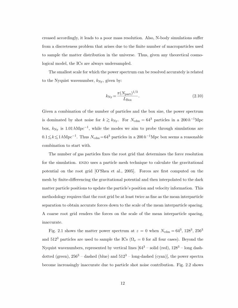
Fig. 2.1 shows the matter power spectrum at z = 0 when Ncdm = 643, 1283, 2563

and 5123 particles are used to sample the ICs (Ων = 0 for all four cases). Beyond the

Nyquist wavenumbers, represented by vertical lines [643 – solid (red), 1283 – long dash-

dotted (green), 2563 – dashed (blue) and 5123 – long-dashed (cyan)], the power spectra

become increasingly inaccurate due to particle shot noise contribution. Fig. 2.2 shows

12

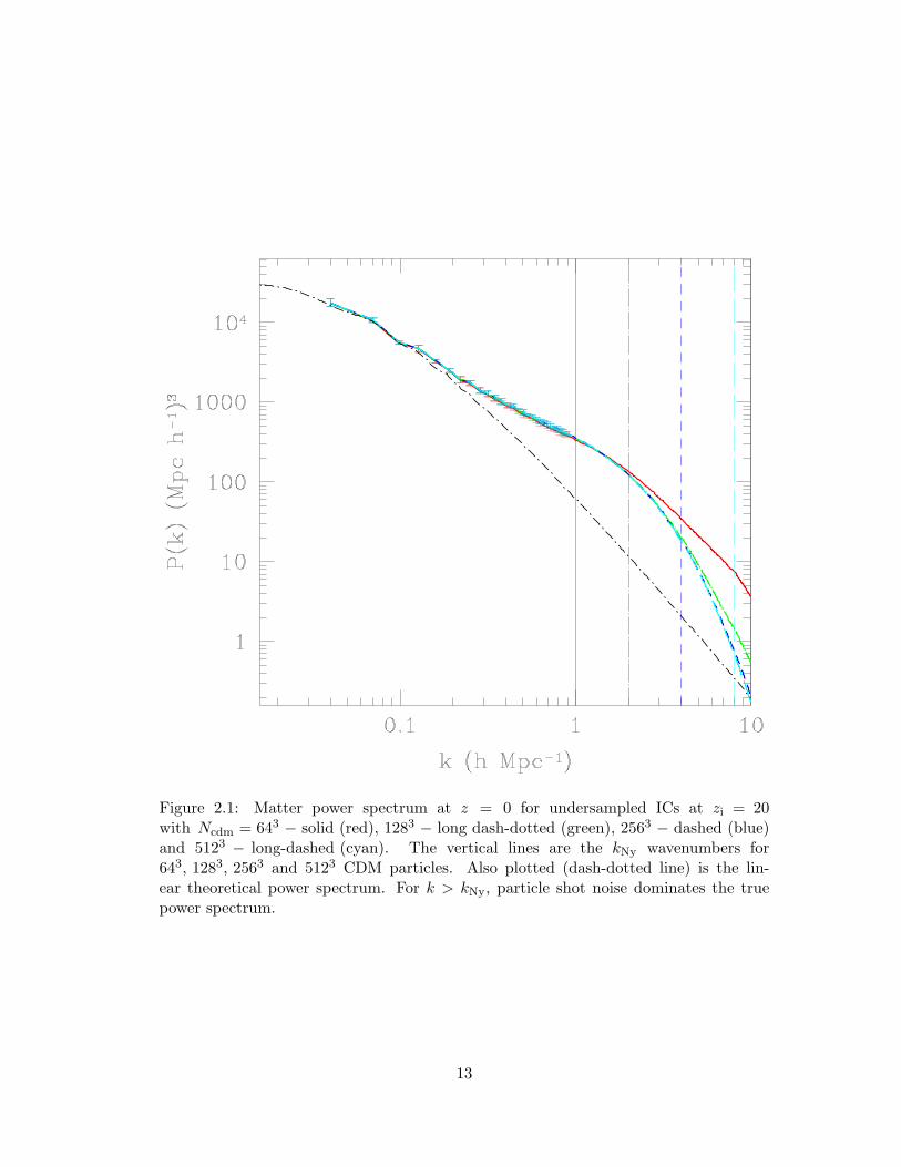
Figure 2.1: Matter power spectrum at z = 0 for undersampled ICs at zi = 20with Ncdm = 643 − solid (red), 1283 − long dash-dotted (green), 2563 − dashed (blue)and 5123 − long-dashed (cyan). The vertical lines are the kNy wavenumbers for643, 1283, 2563 and 5123 CDM particles. Also plotted (dash-dotted line) is the lin-ear theoretical power spectrum. For k > kNy, particle shot noise dominates the truepower spectrum.

13

Figure 2.2: Same as Fig. 2.1 expressed as fractional suppression of the matter powerspectrum at z= 0 when 643 − solid (red), 1283 − long dash-dotted (green) and 2563 −dashed (blue) CDM particles are used to sample the ICs w.r.t the case where 5123 −long-dashed (cyan) CDM particles are used. Ων = 0 for all four cases.The error barscorrespond to eight simulations with different seeds for the ICs.

14

the fractional suppression of the matter power spectrum at z = 0. For k <∼ 1hMpc−1,

the error due to undersampling the ICs is <∼5 per cent for the 643 run, <∼0.5 per cent for

the 1283 run and negligibly small for the 2563 run. To keep the undersampling error at

k= 1hMpc−1 below 0.5 per cent, we narrowed down to a combination of Ncdm = 2563,

Ngas = 5123 in a 200h−1Mpc box to investigate the effect of massive neutrinos on the

matter power spectrum in the regime 0.1 ≤ k ≤ 1hMpc−1. Finally, we checked the

smallest scales that are accurately resolved by the 200h−1Mpc box. Towards this, we

ran eight simulations in a 100h−1Mpc box with Ncdm =2563, Ngas =5123. In Fig. 2.3, we

plot the power spectrum from 100 and 200h−1Mpc boxes. The matter power spectrum

from 100h−1Mpc box simulations begins to show excess power for k>∼1hMpc−1. The

non-linear evolution of perturbations on scales k>∼1hMpc−1 is missed in the 200h−1Mpc

box simulations. The spectrum from 200h−1Mpc box simulations shows convergence at

per cent level for k<∼1hMpc−1 (Fig. 2.4).

2.6 Impact of Massive Neutrinos on Structural Growth

The contribution of massive neutrinos to the present-day critical energy density is given

by:

Ων =Σmν

94.22h2, (2.11)

where Σmν is the sum of the masses of all neutrino eigentstates. In this section we

consider four neutrino models: Ων = 0, 0.01, 0.02 and 0.04 corresponding to Σmν =

0, 0.475, 0.95 and 1.9 eV, respectively. We assume three degenerate neutrino eigentstates,

so that mν = Σmν/3.

In Fig. 2.5 we show slices of the baryon density field at z = 0 extracted from

200h−1Mpc box with Ncdm = 2563, Ngas = 5123. The top panel is from a simulation

without neutrinos, the middle and the bottom panels correspond to simulations with

Ων = 0.02 and 0.04 respectively. All slices are 200h−1Mpc wide. The slices show the

15

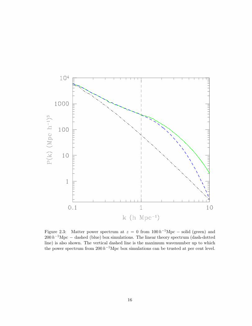
Figure 2.3: Matter power spectrum at z = 0 from 100h−1Mpc − solid (green) and200h−1Mpc − dashed (blue) box simulations. The linear theory spectrum (dash-dottedline) is also shown. The vertical dashed line is the maximum wavenumber up to whichthe power spectrum from 200h−1Mpc box simulations can be trusted at per cent level.

16

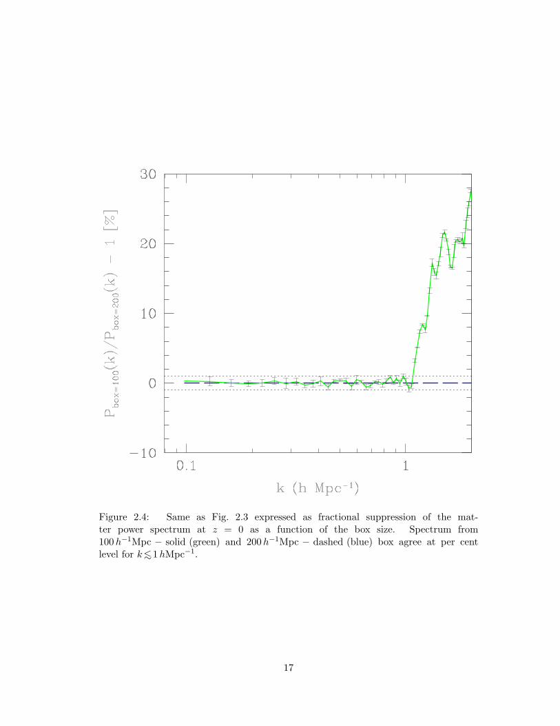
Figure 2.4: Same as Fig. 2.3 expressed as fractional suppression of the mat-ter power spectrum at z = 0 as a function of the box size. Spectrum from100h−1Mpc − solid (green) and 200h−1Mpc − dashed (blue) box agree at per centlevel for k<∼1hMpc−1.

17

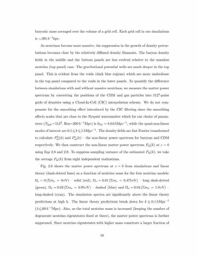
baryonic mass averaged over the volume of a grid cell. Each grid cell in our simulations

is ∼391h−1kpc.

As neutrinos become more massive, the suppression in the growth of density pertur-

bations becomes clear by the relatively diffused density filaments. The baryon density

fields in the middle and the bottom panels are less evolved relative to the massless

neutrino (top panel) case. The gravitational potential wells are much deeper in the top

panel. This is evident from the voids (dark blue regions) which are more underdense

in the top panel compared to the voids in the lower panels. To quantify the difference

between simulations with and without massive neutrinos, we measure the matter power

spectrum by converting the positions of the CDM and gas particles into 5123-point

grids of densities using a Cloud-In-Cell (CIC) interpolation scheme. We do not com-

pensate for the smoothing effect introduced by the CIC filtering since the smoothing

affects scales that are close to the Nyquist wavenumber which for our choice of param-

eters (Ngas =5123, Box=200h−1Mpc) is kNy = 8.04hMpc−1, while the quasi-non-linear

modes of interest are 0.1<∼k<∼1hMpc−1. The density fields are fast Fourier transformed

to calculate P bnl(k) and P c

nl(k) – the non-linear power spectrum for baryons and CDM

respectively. We then construct the non-linear matter power spectrum Pnl(k) at z = 0

using Eqs 2.8 and 2.9. To suppress sampling variance of the estimated Pnl(k), we take

the average Pnl(k) from eight independent realizations.

Fig. 2.6 shows the matter power spectrum at z = 0 from simulations and linear

theory (dash-dotted lines) as a function of neutrino mass for the four neutrino models:

Ων = 0 (Σmν = 0 eV) – solid (red), Ων = 0.01 (Σmν = 0.475 eV) – long dash-dotted

(green), Ων = 0.02 (Σmν = 0.95 eV) – dashed (blue) and Ων = 0.04 (Σmν = 1.9 eV) –

long-dashed (cyan). The simulation spectra are significantly above the linear theory

predictions at high k. The linear theory predictions break down for k >∼ 0.1hMpc−1

(λ<∼60h−1Mpc). Also, as the total neutrino mass is increased (keeping the number of

degenerate neutrino eigentstates fixed at three), the matter power spectrum is further

suppressed. Since neutrino eigentstates with higher mass constitute a larger fraction of

18

Figure 2.5: Slices of baryon density distribution. All slices are 200h−1Mpc wide andshow the baryonic mass averaged over the volume of a grid cell. Each grid cell is∼ 391h−1kpc. The top panel shows a simulation without neutrinos. The middle andthe bottom panels are taken from simulations with Ων = 0.02 (Σmν = 0.95 eV) andΩν = 0.04 (Σmν = 1.9 eV). The baryon density fields in the middle and the bottompanels are less evolved relative to the no-neutrino (top panel) case. The simulationswere run with Ncdm = 2563, Ngas = 5123. The density projections were made using yt:an analysis and visualization tool [Turk, 2008].

19

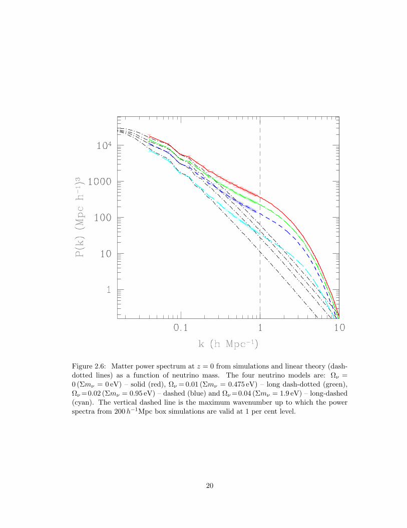
Figure 2.6: Matter power spectrum at z = 0 from simulations and linear theory (dash-dotted lines) as a function of neutrino mass. The four neutrino models are: Ων =0 (Σmν = 0 eV) – solid (red), Ων = 0.01 (Σmν = 0.475 eV) – long dash-dotted (green),Ων =0.02 (Σmν = 0.95 eV) – dashed (blue) and Ων =0.04 (Σmν = 1.9 eV) – long-dashed(cyan). The vertical dashed line is the maximum wavenumber up to which the powerspectra from 200h−1Mpc box simulations are valid at 1 per cent level.

20

the total energy density, they are more effective in damping small-scale power than low

mass neutrinos.

In Fig. 2.7 we plot the fractional difference between the matter power spectra with

and without massive neutrinos, from the simulations as well as the linear theory pre-

dictions. The linetypes for the spectra are the same as in Fig. 2.6. The linear theory

predicts a nearly scale-independent suppression for k>∼0.2hMpc−1. On the other other

hand, the non-linear power spectra from the simulations show an enhanced suppression

for k >∼ 0.1hMpc−1. At k ∼ 1hMpc−1, the non-linear spectra are ∼ 10 per cent more

suppressed compared to the corresponding linear spectra.

2.7 Resolving Neutrino Mass Hierarchy from Numerical Simulations

The mass splittings of |∆m232| = (2.43± 0.13)× 10−3 eV2 and ∆m2

21 = (7.59± 0.21)×

10−5 eV2 [Adamson et al., 2008, KamLAND, 2008] allow for two possible neutrino mass

hierarchies: normal (m3 > m2 > m1) and inverted (m2 > m1 > m3). For Σmν > 0.4−

0.5 eV, all neutrino eigentstates are essentialy degenerate, the mass of each eigentstate

being mν ≈ Σmν/3. However, for smaller Σmν , the individual eigentstate masses differ

significantly in the normal and inverted hierarchies. The free-streaming comoving wave

number, knr, is a function of the mass of each neutrino eigentstate (see Eqs 2.4 and

2.5). As the mass is increased, it becomes non-relativistic earlier and the free-streaming

scale gets shorter. The mass dependence of knr means that the matter power spectrum is

modified differently for eigentstates with different masses. This makes the matter power

spectrum a powerful tool to distinguish between the normal and inverted hierarchies. In

this section we discuss the precision levels above which the power spectrum from future

galaxy surveys would be able to resolve between the two mass hierarchies.

The mass splittings of |∆m232| = (2.43±0.13)×10−3 eV2 and ∆m2

21 = (7.59±0.21)×

10−5 eV2 imply that the lower bounds on the total neutrino mass are Σmν = 0.05 and

0.1 eV for the normal and inverted mass hierarchies respectively. We performed numer-

ical simulations for Σmν = 0.05 and 0.1 eV. For Σmν = 0.05 eV, we assumed 1 massive

21

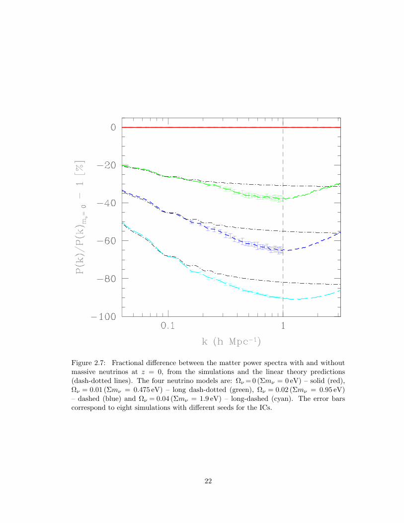
Figure 2.7: Fractional difference between the matter power spectra with and withoutmassive neutrinos at z = 0, from the simulations and the linear theory predictions(dash-dotted lines). The four neutrino models are: Ων = 0 (Σmν = 0 eV) – solid (red),Ων = 0.01 (Σmν = 0.475 eV) – long dash-dotted (green), Ων = 0.02 (Σmν = 0.95 eV)– dashed (blue) and Ων = 0.04 (Σmν = 1.9 eV) – long-dashed (cyan). The error barscorrespond to eight simulations with different seeds for the ICs.

22

Figure 2.8: Same as Fig. 2.7, but for neutrino models with much lower neutrino mass:Ων =0.001 (Σmν = 0.05 eV) – long dash-dotted (green) and Ων =0.002 (Σmν = 0.1 eV)– dashed (blue).

23

and 2 massless eigentstates (mimicking the normal hierarchy). For Σmν = 0.1 eV, we

assumed 2 massive and 1 massless eigentstate (mimicking the inverted hierarchy). In

Fig. 2.8, we show the fractional suppression in the power spectrum for two neutrino

models: Ων =0.001 (Σmν = 0.05 eV) – long dash-dotted (green) and Ων =0.002 (Σmν =

0.1 eV) – dashed (blue). The growth of structure formation is suppressed by as much

as 3.5 per cent (7.5 per cent) at k∼0.6hMpc−1 for the two models. The measurement

errors in the power spectrum from future galaxy surveys are expected to be at the 1

per cent level. In case future surveys constrain Σmν < 0.1 eV with sufficient precision,

that would rule out the inverted mass hierarchy. The current constraint from the 7-yr

WMAP data alone [Larson et al., 2011] is Σmν < 1.3 eV (95 per cent CL). At this level,

it is not possible to discriminate between the normal and inverted hierarchies since all

eigentstates are essentially degenerate.

Next, we consider a scenario with Σmν = 0.1 eV, at which the difference between

the normal and inverted hierarchies is most prominent. We ran N-body simulations in

the following three ways: (i) (Nmassive = 3, Ndegen = 3) where Nmassive is the number

of massive eigentstates and Ndegen is the degeneracy amongst the massive eigentstates.

This combination corresponds to mν = Σmν/3 = 0.033 eV; (ii) (Nmassive = 2, Ndegen =

2), this is the inverted hierarchy scenario with one massless and two equally massive

eigentstates (mν ∼ 0.05, 0.05, 0 eV); (iii) (Nmassive = 3, Ndegen = 2), this is the normal

hierarchy scenario with three massive eigentstates (mν ∼ 0.056, 0.022, 0.022 eV). Note

that case (i) is meaningless at Σmν = 0.1 eV given that |∆m232| = (2.43±0.13)×10−3 eV2

and ∆m221 = (7.59±0.21)×10−5 eV2. We include case (i) for illustrative purposes only.

In Fig. 2.9, we plot the matter power spectrum for cases (i), (ii) and (iii) divided by

the spectrum for case (i). The linear theory predictions are shown by dash-dotted lines.

Since non-linearities become important only for k >∼ 0.1hMpc−1, we have plotted the

theoretical power spectrum for k < 0.1hMpc−1, calculated using the camb code. The

suppression from simulations is∼0.05− 0.2 per cent higher than the linear predictions.

The inverted hierarchy - dashed line (green) shows excess power for wavenumbers 0.001<

24

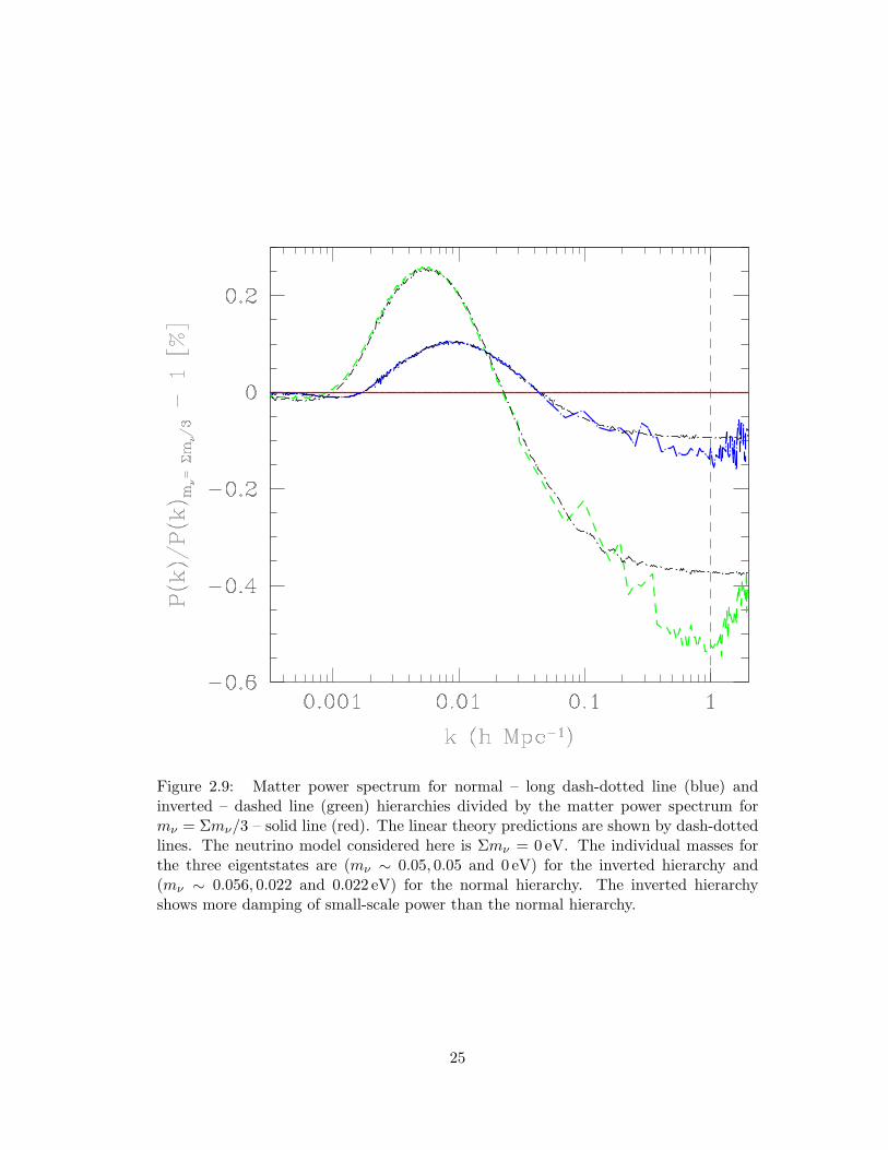
Figure 2.9: Matter power spectrum for normal – long dash-dotted line (blue) andinverted – dashed line (green) hierarchies divided by the matter power spectrum formν = Σmν/3 – solid line (red). The linear theory predictions are shown by dash-dottedlines. The neutrino model considered here is Σmν = 0 eV. The individual masses forthe three eigentstates are (mν ∼ 0.05, 0.05 and 0 eV) for the inverted hierarchy and(mν ∼ 0.056, 0.022 and 0.022 eV) for the normal hierarchy. The inverted hierarchyshows more damping of small-scale power than the normal hierarchy.

25

k<0.02hMpc−1 and an enhanced suppression of ∼0.5 per cent at k∼1hMpc−1 relative

to case (i). This can be explained by the fact that in case (ii) Σmν = 0.1 eV is shared

equally between two eigentstates, while in case (i) Σmν = 0.1 eV is shared equally

between three eigentstates. Each eigentstate is more massive in case (ii), thereby making

the free-streaming length shorter compared to that in case (i). Higher mass neutrinos are

better at wiping out small-scale perturbations and their shorter free-streaming length

implies that the spatial extent of damping is limited.

Another factor contributing to the appearance of Fig. 2.9 is a shift in the radiation–

matter equality redshift. Higher mass neutrinos become non-relativistic at higher red-

shifts and start contributing to Ωm before low mass neutrinos do. This shifts the

radiation–matter equality epoch to a higher redshift and reduces the scale corresponding

to the one that entered the horizon at radiation–matter equality. The modes entering

the horizon after radiation–matter equality grow linearly (as opposed to logarithmically

during the radiation era) which contributes to the excess power [compare dashed (green)

and solid (red) lines in Fig. 2.9] for wavenumbers 0.001<k< 0.02hMpc−1. The same

reasoning can be applied to the normal hierarchy – long dash-dotted line (blue). At

Σmν = 0.1 eV, precision better than 0.5 per cent would be needed in measuring the

matter power spectrum to discriminate between the normal and inverted hierarchies.

For Σmν > 0.2 eV all eigentstates become degenerate, this would make it extremely

difficult for a future survey to resolve the two hierarchies.

2.8 Comparison: Semi-Analytic versus Full Numerical Treatment

In this section we compare the estimated overall suppression of the matter power spec-

trum due to massive neutrinos from our N-body simulations with the results obtained

by Brandbyge et al. [2008] and Viel et al. [2010]. In linear theory, the suppression

of the matter power spectrum amplitude is approximately given by ∆P/P ∼ −8fν

[Hu et al., 1998]. Numerical simulations, however, show that the neutrino suppres-

sion is enhanced in the non-linear regime (k >∼ 0.1hMpc−1). In Fig. 2.10 we plot

26

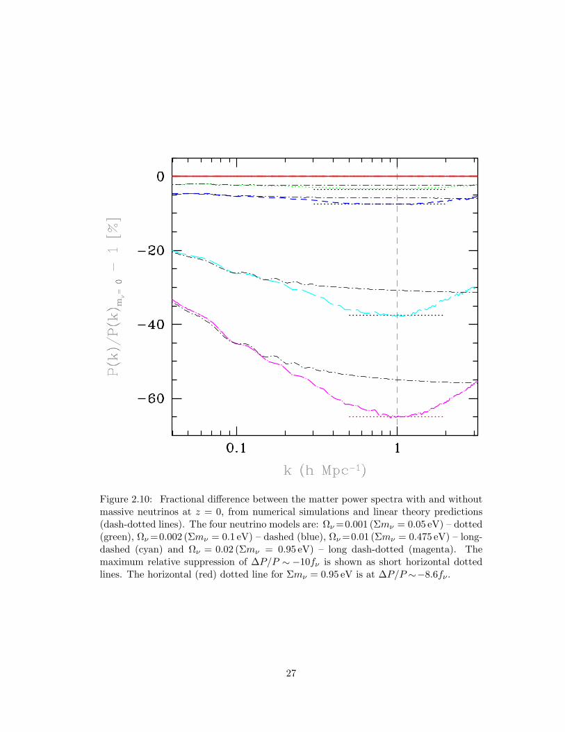
Figure 2.10: Fractional difference between the matter power spectra with and withoutmassive neutrinos at z = 0, from numerical simulations and linear theory predictions(dash-dotted lines). The four neutrino models are: Ων =0.001 (Σmν = 0.05 eV) – dotted(green), Ων =0.002 (Σmν = 0.1 eV) – dashed (blue), Ων =0.01 (Σmν = 0.475 eV) – long-dashed (cyan) and Ων = 0.02 (Σmν = 0.95 eV) – long dash-dotted (magenta). Themaximum relative suppression of ∆P/P ∼−10fν is shown as short horizontal dottedlines. The horizontal (red) dotted line for Σmν = 0.95 eV is at ∆P/P ∼−8.6fν .

27

the fractional difference between the matter power spectra with and without massive

neutrinos at z = 0, from numerical simulations as well as linear theory predictions

(dash-dotted lines) for four neutrino models: Ων = 0.001 (Σmν = 0.05 eV) – dotted

(green), Ων = 0.002 (Σmν = 0.1 eV) – dashed (blue), Ων = 0.01 (Σmν = 0.475 eV)

– long-dashed (cyan) and Ων = 0.02 (Σmν = 0.95 eV) – long dash-dotted (magenta).

We found a maximum non-linear suppression of ∆P/P ∼ −10fν for neutrino masses

Σmν = 0.05, 0.1, 0.475 eV. Although we ran our simulations with a slightly differ-

ent set of cosmological parameters, Brandbyge et al. [2008] measured ∆P/P ∼−9.8fν

for Σmν ≤ 0.6 eV while Viel et al. [2010] reported ∆P/P ∼ −9.5fν at z = 0. For

Σmν = 0.95 eV, we get ∆P/P ∼−8.6fν while Viel et al. [2010] reported ∆P/P ∼−8fν

for Σmν = 1.2 eV. The scale at which the suppression turns over, knr, moves from

knr ∼ 0.6 − 0.7hMpc−1 for Σmν = 0.05 eV to knr ∼ 1hMpc−1 for Σmν = 0.95 eV.

The turnover may be related to the non-linear collapse of structures as discussed in

Brandbyge et al. [2008] who reported knr∼1hMpc−1.

2.9 Matter Power Spectrum Error Estimates

In our N-body simulations, we have implemented neutrinos in the ICs only. Neutrino-

weighted CDM and baryon transfer functions from camb were used to generate the ICs

for CDM particles and baryons. To construct Pnl(k) at z = 0, we used Eq. 2.8. We

calculated P cbnl from N-body simulations and combined it with P νlin at z = 0 as solved

by the camb code. This methodology introduces errors in the estimated matter power

spectrum for two reasons: (i) the linear neutrino perturbations were taken into account

only at the initial (zi = 20) and the final (z = 0) redshifts. There is no feedback from

the neutrinos on to the CDM component in our N-body simulations. (ii) the non-linear

evolution of neutrino perturbations was not accounted for in our N-body simulations.

While the extent of non-linear neutrino corrections to the matter power spectrum is still

being studied, we use Brandbyge et al. [2008] and Brandbyge and Hannestad [2009b] to

estimate the errors in our N-body spectra. Brandbyge and Hannestad [2009b] describe

28

the linear neutrino density on a grid and evolve this density forward in time using linear

theory. The neutrino contribution is added to the CDM component when calculating

the gravitational forces. Thus, the linear neutrino component is accounted for recur-

sively over the redshift range over which the matter power spectrum is to be evolved.

Brandbyge et al. [2008] (their fig. 7, left panel) show that the matter power spectrum

is underesolved by∼ 3 per cent for Σmν ≤ 0.6 eV on scales k ≥ 0.2hMpc−1 when the

neutrino grid is neglected. Accordingly, our matter power spectrum estimates are ex-

pected to be underesolved by roughly<∼4, 1 and 0.1 per cent for Σmν = 0.95, 0.475 and

0.1 eV, respectively, for k>∼ 0.2hMpc−1 at z = 0. Fig. 1 in Brandbyge and Hannestad

[2009b] shows that the power is further suppressed by∼5 per cent for Σmν ≤ 1.2 eV at

k ≈ 0.2− 0.3hMpc−1 when the neutrino non-linearities are neglected. Overall, we esti-

mate our N-body spectrum errors to be<∼5, 1.5 and 0.1 per cent for Σmν = 0.95, 0.475

and 0.1 eV, respectively, for k>∼0.2hMpc−1 at z = 0.

2.10 Summary

In this chapter we simulated the matter power spectrum at z = 0 in order to study

how massive neutrinos impact structure formation. The most important factors in

obtaining an accurate power spectrum are (i) the Nyquist wavenumber, which depends

on the simulation box size and the number of particles and (ii) the force resolution,

which depends on the size of the root grid. Above the Nyquist wavenumber, the power

spectrum is dominated by shot noise. For modes up to k <∼ 1hMpc−1, we found that

Ncdm = 2563 in a 200h−1Mpc box is enough to keep the sampling errors at per cent

level. We used a root grid of Ngas =5123, which is twice as fine as Ncdm, to accurately

calculate the gravitational forces down to the scale of the mean interparticle spacing.

We showed that neutrinos with mass ∼ 0.5 eV or less, can be treated with linear theory

since the errors due to neglecting non-linear neutrino perturbations are at sub-per cent

level.

29

3 Developing PkANN – A Non-Linear Matter Power Spectrum Inter-

polator

3.1 Prelude

Achieving high-precision measurements of galaxy power spectrum from numerical sim-

ulations is computationally expensive and time consuming. Exploring the cosmological

parameter space through a brute force application of simulations can be not only chal-

lenging, but in some cases impossible given the computing resources available. In this

chapter we will develop the formalism for estimating the non-linear matter power spec-

trum using Artificial Neural Networks (ANN). As we discuss in the next chapter, the

ANN technique is extremely fast and, more importantly, accurate way to determine the

fully non-linear power spectrum.

3.2 Machine-Learning

Machine-learning is associated with a series of algorithms that allow a computational

unit to evolve in its behavior, given access to empirical data. The major benefit of

machine learning is the potential to automatically learn complex patterns. As a subset

of artificial intelligence, machine learning has been used in a variety of applications

ranging from brain-machine interfaces [Jenatton et al., 2011, Pedregosa et al., 2012] to

the analyses of stock market [Ghosh, 2011, Hurwitz and Marwala, 2012].

Fig. 3.1 shows a skeleton of a machine-learning network. Using a suitable training

set (input parameters for which data is available), the machine-learning algorithm is

trained to learn a parameterization. With this parameterization the network is capable

of reproducing (as closely as possible) the output, when queried with input parameter

settings that are part of the training set. The trained network can now be presented

with new settings of the input parameters (for which one does not have any prior data)

and by using the same parameterization learnt during the training process, the network

makes predictions.

30

Training SetMachine Learning

Algorithm Trained Network

New Input Data

Predicted Output

1 23

4

Tuesday, November 6, 2012

Figure 3.1: Steps 1 and 2: A machine-learning network learns to parameterize the output, forthe input patterns that form the training set. Steps 3 and 4: The trained network is capable ofmaking predictions when presented with input parameter settings. The queried input settingsmust lie within the parameter ranges of the patterns in the training set.

When using any machine-learning technique to predict the outcome, it is critical that

(i) the queried input setting not lie outside the input parameter ranges that are used

during machine learning and (ii) the input parameter space must be sampled densely

enough for the machine procedure to interpolate/predict accurately.

One might argue that a machine-learning approach to determine the non-linear re-

sponse from varying parameter settings is a rather black-box approach that goes against

the traditional approach to spectra: based on scientific understanding and physics. How-

ever, we view this direction as a pragmatic one: a new approach is urgent given the

impending flood of new data from upcoming surveys, and in an age of supposed pre-

cision cosmology, we will be theory limited in this specific area. It is therefore crucial

to strive towards per cent level precision in the determination of the non-linear power

spectrum.

There exist a range of techniques (see e.g. Nilsson [2005]) including genetic algo-

rithms, decision tree learning,neural networks and Gaussian processes. Machine-learning

techniques have been used in the fitting of cosmological functions [Auld et al., 2007,

Fendt and Wandelt, 2007, Auld et al., 2008] and photometric redshifts [Collister and

Lahav, 2004]. Gaussian processes have already been used as cosmological non-linear

emulators [Habib et al., 2007, Schneider et al., 2008, Heitmann et al., 2009, Lawrence

31

et al., 2010, Schneider et al., 2011]. Gaussian process modeling (see MacKay [1997],

Rasmussen and Williams [2006] for a basic introduction to Gaussian processes) is a

non-linear interpolation scheme that, after optimal learning, is capable of making pre-

dictions when queried at a suitable input setting.

There are several advantages and disadvantages when using neural networks and

Gaussian processes to interpolate data. From a practical point of view, a neural net-

work compresses data into a small number of weight parameters, so a large number of

simulations could be fitted into a small number of files whereas a Gaussian process has

to carry a large matrix which can be of the order of the number of points used for train-

ing the Gaussian process. [Heitmann et al., 2009] dealt with large matrices by using

principal component analysis (PCA) to reduce their sizes to ones easily manipulated.

Again from a practical point of view, usually Gaussian processes can do better than

neural networks in the case of a small number of training points given that a neural

network could be flexible enough to be misused and misfit the data. From a theoretical

point of view, the two methods should fare equally especially as there are certain kernels

used in Gaussian processes which are equivalent to the interpolation and fit one would

have with neural networks. Overall, given the implementation, we believe that the two

methods should produce equivalent results especially if the ANN procedure is trained

using a larger number of simulations. In this work we focus on the neural network

technique.

3.3 Artificial Neural Networks

An ANN is simply an interconnection of neurons or nodes analogous to the neural

structure of the brain. This can take a more specific form whereby the nodes are

arranged in a series of layers with each node in a layer connected, with a weight, to

all other nodes in adjacent layers. This is often referred to as a multi-layer perceptron

(MLP). In this case one can impart values onto the nodes of the first layer (called the

input layer), have a series of hidden layers and finally receive information from the last

32

layer (called the output layer). The configuration of nodes is often called the network’s

architecture and is specified from input to output as Nin : N1 : N2 : ... : Nn : Nout.

That is, a network with an architecture 4 : 9 : 5 : 7 has 4 inputs, two hidden layers

with 9 and 5 nodes respectively, and finally 7 outputs. An extra node (called the bias

node) is added to the input layer as well as to each of the hidden layers. The bias nodes

are added in order to compensate for the difference between the mean of the output

vector of the network and the mean of the output vector of training set patterns (for

details, refer Bishop [1995]). Each bias node connects to all the nodes in the next layer.

Note that the counts Nin, N1, N2, ..., Nn do not include the bias nodes. The output layer

has no bias node. The total number of connections (also called the weights) NW for a

generic architecture Nin : N1 : N2 : ... : Nn : Nout can be calculated using the formula

NW = Nin ·N1 +n∑l=2

Nl−1 ·Nl +Nn ·Nout +n∑l=1

Nl +Nout, (3.1)

where the summation index l is over the hidden layers only. For a network with a single

hidden layer, the second term on the right-hand side is absent. As an example, the

architecture 7 : 49 : 50 has a total of 7 × 49 + 0 + 49 × 50 + 49 + 50 = 2892 weights,

which we call the weight vector w.

In Fig. 3.2, we show a typical ANN architecture (left-hand panel) and the formulae

to calculate the node activations (right-hand panels). In the network configuration

depicted, there are Nin input parameters/features (x1, ..., xi), a single hidden layer with

N1 nodes (z1, ..., zj), and Nout output parameters/features (y1, ..., yk). The bias nodes

in the input and hidden layers are x0 and z0, respectively.

Each node in the lth hidden layer is a neuron with an activation, zj ≡ g(aj), taking

as its argument

aj =∑i=0

wjizi, (3.2)

where the sum is over all nodes i (including the bias node) of the previous layer sending

connections to the jth node (barring the bias node) of the current layer. Note that for

33

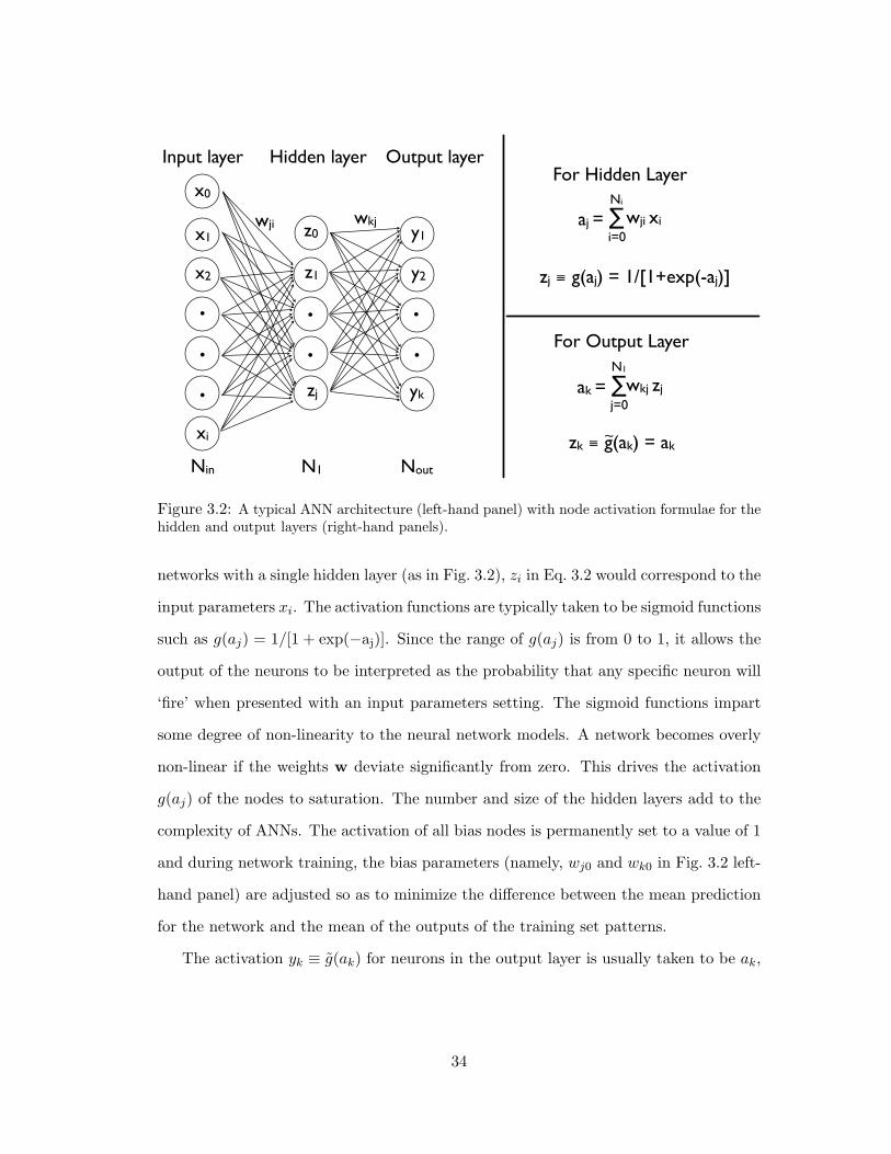
Input layer Hidden layer Output layer

Nin Nout N1

aj = Ni

wji xii=0x1

x2

xi

z1

zj

wji wkjy1

yk

.

y2

x0

z0

ak = N1

wkj zjj=0

zj g(aj) = 1/[1+exp(-aj)]

zk g(ak) = ak

For Hidden Layer

For Output Layer

....

.

.

Thursday, November 22, 2012

Figure 3.2: A typical ANN architecture (left-hand panel) with node activation formulae for thehidden and output layers (right-hand panels).

networks with a single hidden layer (as in Fig. 3.2), zi in Eq. 3.2 would correspond to the

input parameters xi. The activation functions are typically taken to be sigmoid functions

such as g(aj) = 1/[1 + exp(−aj)]. Since the range of g(aj) is from 0 to 1, it allows the

output of the neurons to be interpreted as the probability that any specific neuron will

‘fire’ when presented with an input parameters setting. The sigmoid functions impart

some degree of non-linearity to the neural network models. A network becomes overly

non-linear if the weights w deviate significantly from zero. This drives the activation

g(aj) of the nodes to saturation. The number and size of the hidden layers add to the

complexity of ANNs. The activation of all bias nodes is permanently set to a value of 1

and during network training, the bias parameters (namely, wj0 and wk0 in Fig. 3.2 left-

hand panel) are adjusted so as to minimize the difference between the mean prediction

for the network and the mean of the outputs of the training set patterns.

The activation yk ≡ g(ak) for neurons in the output layer is usually taken to be ak,

34

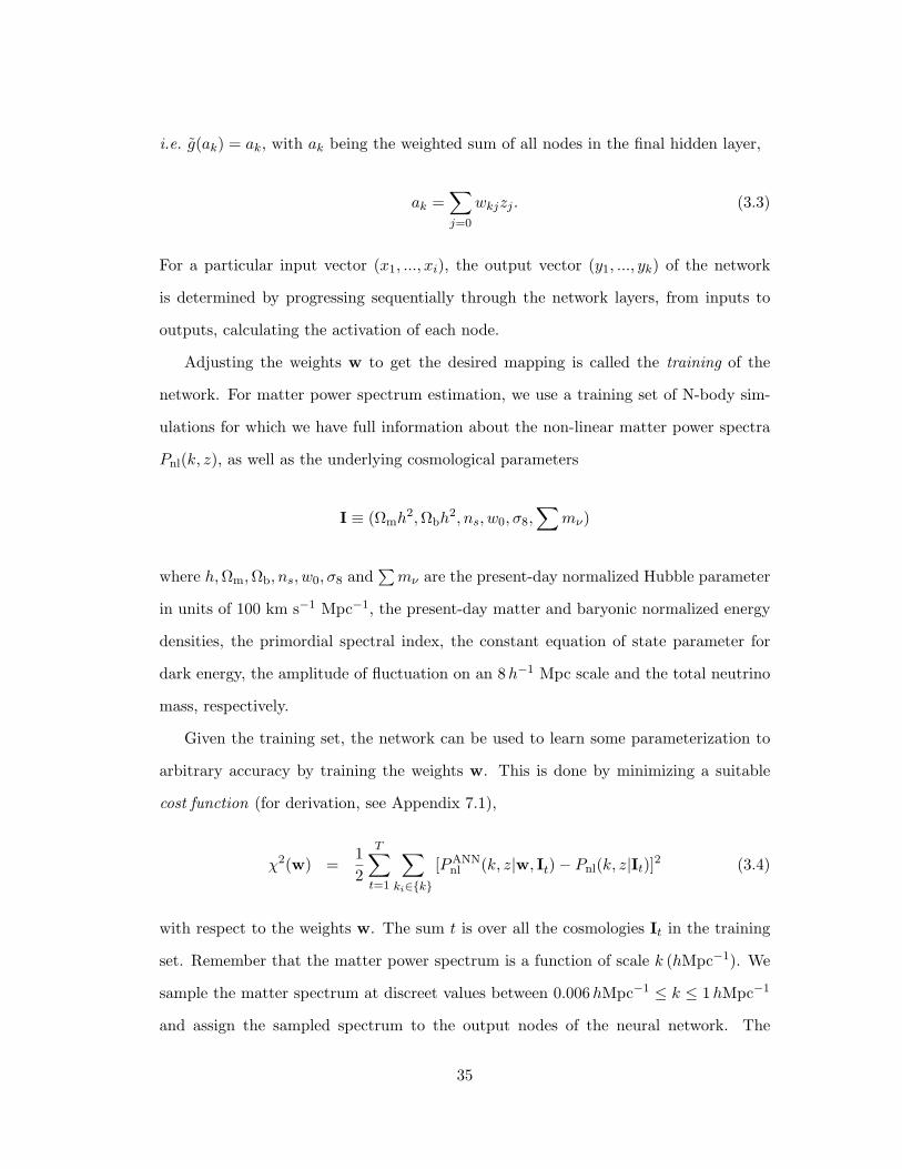
i.e. g(ak) = ak, with ak being the weighted sum of all nodes in the final hidden layer,

ak =∑j=0

wkjzj . (3.3)

For a particular input vector (x1, ..., xi), the output vector (y1, ..., yk) of the network

is determined by progressing sequentially through the network layers, from inputs to

outputs, calculating the activation of each node.

Adjusting the weights w to get the desired mapping is called the training of the

network. For matter power spectrum estimation, we use a training set of N-body sim-

ulations for which we have full information about the non-linear matter power spectra

Pnl(k, z), as well as the underlying cosmological parameters

I ≡ (Ωmh2,Ωbh

2, ns, w0, σ8,∑

mν)

where h,Ωm,Ωb, ns, w0, σ8 and∑mν are the present-day normalized Hubble parameter

in units of 100 km s−1 Mpc−1, the present-day matter and baryonic normalized energy

densities, the primordial spectral index, the constant equation of state parameter for

dark energy, the amplitude of fluctuation on an 8h−1 Mpc scale and the total neutrino

mass, respectively.

Given the training set, the network can be used to learn some parameterization to

arbitrary accuracy by training the weights w. This is done by minimizing a suitable

cost function (for derivation, see Appendix 7.1),

χ2(w) =12

T∑t=1

∑ki∈k

[PANNnl (k, z|w, It)− Pnl(k, z|It)]2 (3.4)

with respect to the weights w. The sum t is over all the cosmologies It in the training

set. Remember that the matter power spectrum is a function of scale k (hMpc−1). We

sample the matter spectrum at discreet values between 0.006hMpc−1 ≤ k ≤ 1hMpc−1

and assign the sampled spectrum to the output nodes of the neural network. The

35

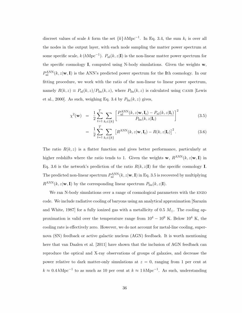
discreet values of scale k form the set khMpc−1. In Eq. 3.4, the sum ki is over all

the nodes in the output layer, with each node sampling the matter power spectrum at

some specific scale, k (hMpc−1). Pnl(k, z|I) is the non-linear matter power spectrum for

the specific cosmology I, computed using N-body simulations. Given the weights w,

PANNnl (k, z|w, I) is the ANN’s predicted power spectrum for the Ith cosmology. In our

fitting procedure, we work with the ratio of the non-linear to linear power spectrum,

namely R(k, z) ≡ Pnl(k, z)/Plin(k, z), where Plin(k, z) is calculated using camb [Lewis

et al., 2000]. As such, weighing Eq. 3.4 by Plin(k, z) gives,

χ2(w) =12

T∑t=1

∑ki∈k

[PANN

nl (k, z|w, It)− Pnl(k, z|It)Plin(k, z|It)

]2

(3.5)

=12

T∑t=1

∑ki∈k

[RANN(k, z|w, It)−R(k, z|It)

]2. (3.6)

The ratio R(k, z) is a flatter function and gives better performance, particularly at

higher redshifts where the ratio tends to 1. Given the weights w, RANN(k, z|w, I) in

Eq. 3.6 is the network’s prediction of the ratio R(k, z|I) for the specific cosmology I.

The predicted non-linear spectrum PANNnl (k, z|w, I) in Eq. 3.5 is recovered by multiplying

RANN(k, z|w, I) by the corresponding linear spectrum Plin(k, z|I).

We ran N-body simulations over a range of cosmological parameters with the enzo

code. We include radiative cooling of baryons using an analytical approximation [Sarazin

and White, 1987] for a fully ionized gas with a metallicity of 0.5 M. The cooling ap-

proximation is valid over the temperature range from 104 − 109 K. Below 104 K, the

cooling rate is effectively zero. However, we do not account for metal-line cooling, super-

nova (SN) feedback or active galactic nucleus (AGN) feedback. It is worth mentioning

here that van Daalen et al. [2011] have shown that the inclusion of AGN feedback can

reproduce the optical and X-ray observations of groups of galaxies, and decrease the

power relative to dark matter-only simulations at z = 0, ranging from 1 per cent at

k ≈ 0.4hMpc−1 to as much as 10 per cent at k ≈ 1hMpc−1. As such, understanding

36

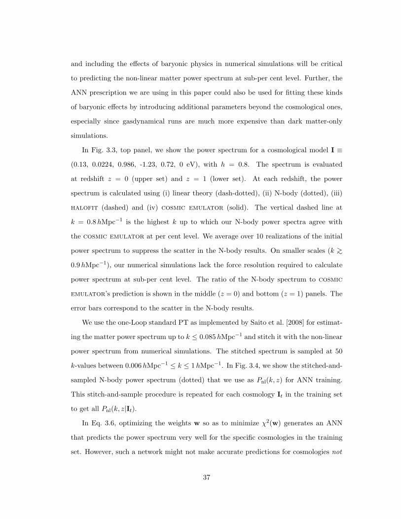
and including the effects of baryonic physics in numerical simulations will be critical

to predicting the non-linear matter power spectrum at sub-per cent level. Further, the

ANN prescription we are using in this paper could also be used for fitting these kinds

of baryonic effects by introducing additional parameters beyond the cosmological ones,

especially since gasdynamical runs are much more expensive than dark matter-only

simulations.

In Fig. 3.3, top panel, we show the power spectrum for a cosmological model I ≡

(0.13, 0.0224, 0.986, -1.23, 0.72, 0 eV), with h = 0.8. The spectrum is evaluated

at redshift z = 0 (upper set) and z = 1 (lower set). At each redshift, the power

spectrum is calculated using (i) linear theory (dash-dotted), (ii) N-body (dotted), (iii)

halofit (dashed) and (iv) cosmic emulator (solid). The vertical dashed line at

k = 0.8hMpc−1 is the highest k up to which our N-body power spectra agree with

the cosmic emulator at per cent level. We average over 10 realizations of the initial

power spectrum to suppress the scatter in the N-body results. On smaller scales (k >∼

0.9hMpc−1), our numerical simulations lack the force resolution required to calculate

power spectrum at sub-per cent level. The ratio of the N-body spectrum to cosmic

emulator’s prediction is shown in the middle (z = 0) and bottom (z = 1) panels. The

error bars correspond to the scatter in the N-body results.

We use the one-Loop standard PT as implemented by Saito et al. [2008] for estimat-

ing the matter power spectrum up to k ≤ 0.085hMpc−1 and stitch it with the non-linear

power spectrum from numerical simulations. The stitched spectrum is sampled at 50

k-values between 0.006hMpc−1 ≤ k ≤ 1hMpc−1. In Fig. 3.4, we show the stitched-and-

sampled N-body power spectrum (dotted) that we use as Pnl(k, z) for ANN training.

This stitch-and-sample procedure is repeated for each cosmology It in the training set

to get all Pnl(k, z|It).

In Eq. 3.6, optimizing the weights w so as to minimize χ2(w) generates an ANN

that predicts the power spectrum very well for the specific cosmologies in the training

set. However, such a network might not make accurate predictions for cosmologies not

37

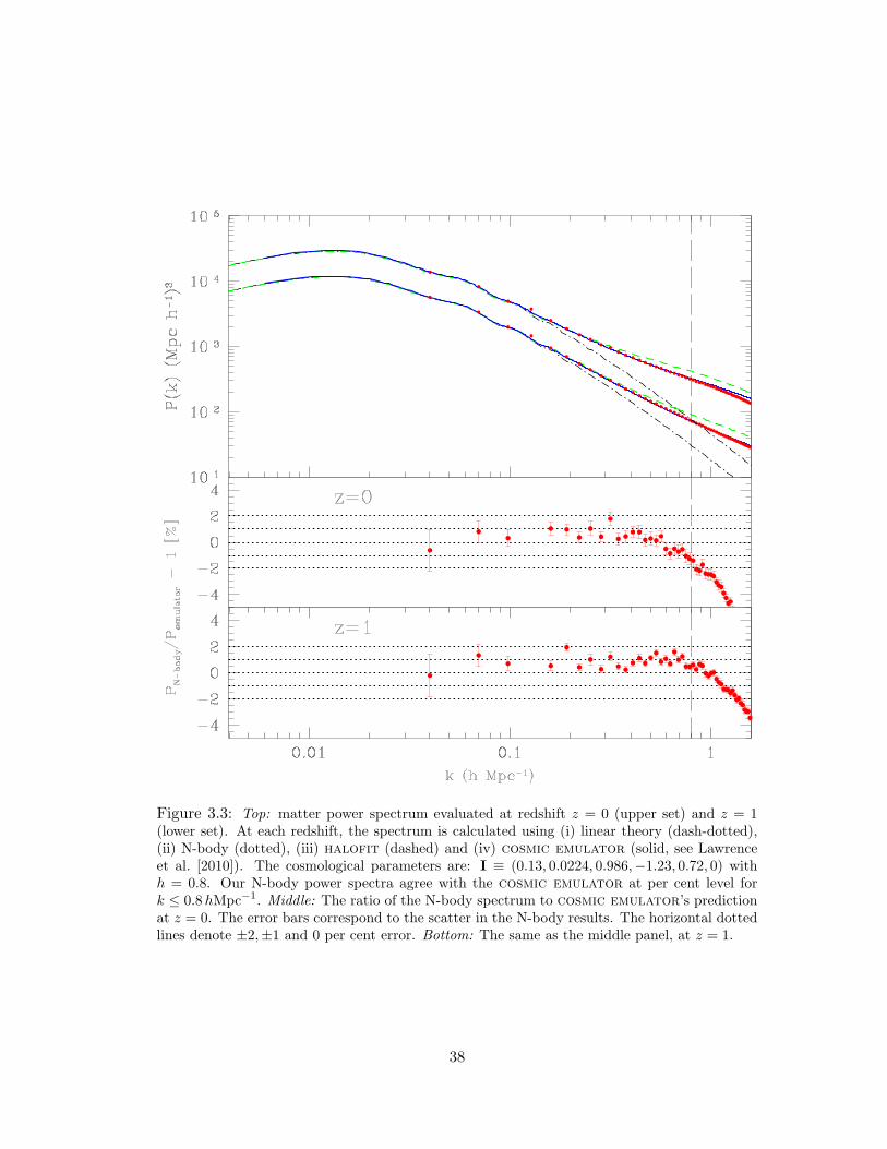
Figure 3.3: Top: matter power spectrum evaluated at redshift z = 0 (upper set) and z = 1(lower set). At each redshift, the spectrum is calculated using (i) linear theory (dash-dotted),(ii) N-body (dotted), (iii) halofit (dashed) and (iv) cosmic emulator (solid, see Lawrenceet al. [2010]). The cosmological parameters are: I ≡ (0.13, 0.0224, 0.986,−1.23, 0.72, 0) withh = 0.8. Our N-body power spectra agree with the cosmic emulator at per cent level fork ≤ 0.8hMpc−1. Middle: The ratio of the N-body spectrum to cosmic emulator’s predictionat z = 0. The error bars correspond to the scatter in the N-body results. The horizontal dottedlines denote ±2,±1 and 0 per cent error. Bottom: The same as the middle panel, at z = 1.

38

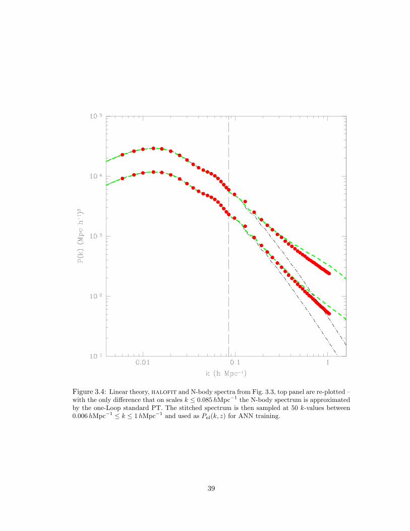
Figure 3.4: Linear theory, halofit and N-body spectra from Fig. 3.3, top panel are re-plotted –with the only difference that on scales k ≤ 0.085hMpc−1 the N-body spectrum is approximatedby the one-Loop standard PT. The stitched spectrum is then sampled at 50 k-values between0.006hMpc−1 ≤ k ≤ 1hMpc−1 and used as Pnl(k, z) for ANN training.

39

included in the training set. This usually indicates (i) an overly simple network archi-

tecture (very few hidden layer nodes), (ii) very sparsely or poorly sampled parameter

space and/or (iii) a highly complex non-linear mapping that actually over-fits to the

noise on the training dataset. In order to generate smoother network mappings that

generalize better when presented with new cosmologies that are not part of the training

set, a penalty term χ2Q(w) is added to the cost function χ2(w),

χ2Q(w) =

ξ

2||w||2, (3.7)

where ||w||2 is the quadratic sum of all the weights. The regularization parameter ξ

controls the degree of regularization (smoothing) of a network’s predictions. Thus, the

overall cost function which is presented to the ANN for minimization with respect to

the weights w is,

χ2C(w) =

12

T∑t=1

∑ki∈k

[RANN(k, z|w, It)−R(k, z|It)

]2+ξ

2||w||2. (3.8)

To minimize χ2C(w) with respect to the weights w, we use an iterative quasi-Newton

algorithm (Appendix 7.2) that involves evaluating the first-order derivative (gradient)

of the cost function. See Appendix 7.3 for the derivation of the gradient. The quasi-

Newton algorithm also involves information about the inverse of the Hessian (second-

order derivative) matrix which we approximate using the Broyden–Fletcher–Goldfarb–

Shanno (BFGS) method (see Appendix 7.4. For details, see Bishop [1995]).

The penalty term χ2Q(w), usually a quadratic sum of the weights, prevents them

from becoming too large during the training process by penalizing in proportion to the

sum. After having initialized ξ, its value is re-estimated during the training process

iteratively. For the update formula, see Appendix 7.5. For its derivation, see Bishop

[1995].

Starting with randomly assigned weights w, their values are re-estimated iteratively,

40

making sure that each iteration proceeds in a direction that lowers the cost function

χ2C(w). In order to avoid over-fitting to the training set, after each iteration to the

weights, Eq. 3.8 is also calculated for what is known in neural network parlance as a

validation set. The validation set for our application of neural networks, is a small set

of simulations with known I ≡ (Ωmh2,Ωbh

2, ns, w0, σ8,∑mν) and Pnl(k, z). The final

weights wf are chosen such as to give the best fit (minimum χ2C(w)) to the validation

set. The network training is considered finished once χ2C(w) is minimized with respect

to the validation set. The trained network can now be used to predict Pnl(k, z) for

new cosmologies. In practice, a number of networks are trained that start with an

alternative random configuration of weights. The trained networks are collectively called

a committee of networks and subsequently give rise to better performance. The final

output is usually given by averaging over the outputs of the committee members.

It has been shown (see Hornik [1991], Ito [1991], Bishop [1995]) that networks with

a single hidden layer are capable of making arbitrarily accurate approximation to a

function and its derivatives. As such, for PkANN’s architecture, we restrict our analysis

to single-hidden layer with sigmoidal activations and output nodes with linear (g(ak) =

ak) activations.

As can be seen in Fig. 3.3, the halofit predictions are in error by as much as 50 per

cent on small scales. Our intention is to use this neural network technique to iterpolate

the non-linear matter power spectrum as a function of cosmological parameters by

training on N-body simulations. This natural fitting procedure removes both the effort

and unnecessary potential bias that results from invoking ultimately imperfect sets of

fitting equations such as the halofit.

3.4 Latin Hypercube Parameter Sampling

In order to fit a set of parameters optimally one strives to sample them as finely and

as evenly as possible. However, a regularly spaced grid with N sampling intervals

along one dimension and d parameters scales as Nd. For a six-dimensional parameter

41

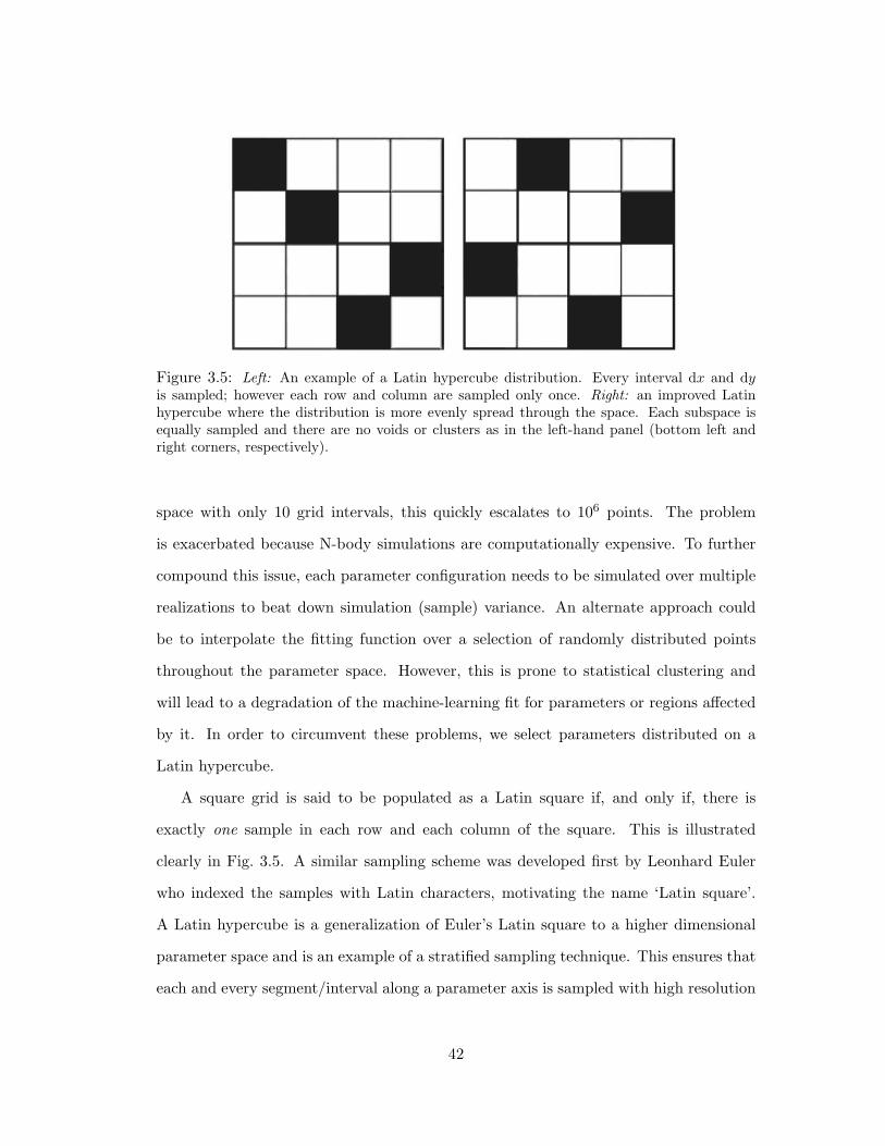
Figure 3.5: Left: An example of a Latin hypercube distribution. Every interval dx and dyis sampled; however each row and column are sampled only once. Right: an improved Latinhypercube where the distribution is more evenly spread through the space. Each subspace isequally sampled and there are no voids or clusters as in the left-hand panel (bottom left andright corners, respectively).

space with only 10 grid intervals, this quickly escalates to 106 points. The problem

is exacerbated because N-body simulations are computationally expensive. To further

compound this issue, each parameter configuration needs to be simulated over multiple

realizations to beat down simulation (sample) variance. An alternate approach could

be to interpolate the fitting function over a selection of randomly distributed points

throughout the parameter space. However, this is prone to statistical clustering and

will lead to a degradation of the machine-learning fit for parameters or regions affected

by it. In order to circumvent these problems, we select parameters distributed on a

Latin hypercube.

A square grid is said to be populated as a Latin square if, and only if, there is

exactly one sample in each row and each column of the square. This is illustrated

clearly in Fig. 3.5. A similar sampling scheme was developed first by Leonhard Euler

who indexed the samples with Latin characters, motivating the name ‘Latin square’.

A Latin hypercube is a generalization of Euler’s Latin square to a higher dimensional

parameter space and is an example of a stratified sampling technique. This ensures that

each and every segment/interval along a parameter axis is sampled with high resolution

42

without a vast number of points. That is, one can sample a d-dimensional space with

n simulations and have all parameters evaluated along every dx = (b− a)/n increment,

where b and a are the upper and lower limits of the parameter, respectively. Therefore, it

is independent of d. However, a random implementation of a Latin hypercube algorithm

can still lead to statistically under-sampled regions. An example of this can be seen in

Fig. 3.5. Each panel shows a random implementation of Latin hypercube algorithm.

In both panels, the square is partitioned into four subspaces. The left-hand panel has

voids (and clusters) in two of its subspaces. The right-hand panel has each subspace

equally sampled (while still obeying the Latin hypercube definition) and represents an

improved Latin hypercube sampling. In this case the sample space is partitioned into

equally probable subspaces and the variance in the pairwise separation of the sampled

points is minimized.

Since the introduction of the Latin hypercube sampling technique [McKay et al.,

1979], the procedure has become common in computer science, uncertainty analysis

and engineering emulation (where simulation of complex machinery is overwhelmingly

time consuming). Similarly, variations of the Latin hypercube sampling technique have

been implemented in cosmological analyses before, e.g., [Habib et al., 2007, Heitmann

et al., 2009, Schneider et al., 2011] and references therein. In this paper, we use the

improved Latin hypercube technique to set up the cosmological models to be used for

ANN training.

3.4.1 Setting up an improved Latin hypercube for cosmological parameters

We varied six cosmological parameters I ≡ (Ωmh2,Ωbh

2, ns, w0, σ8,∑mν) between the

limits specified in Table 2. The limits on this six-dimensional parameter space are

chosen so as to include the 7-yr WMAP+BAO+H0 [Komatsu et al., 2011] constraints

(see Table 2).

Throughout this paper, we only consider spatially flat models with the present-day

CMB temperature Tγ0 = 2.725K. We also assume that all massive neutrino species are

43

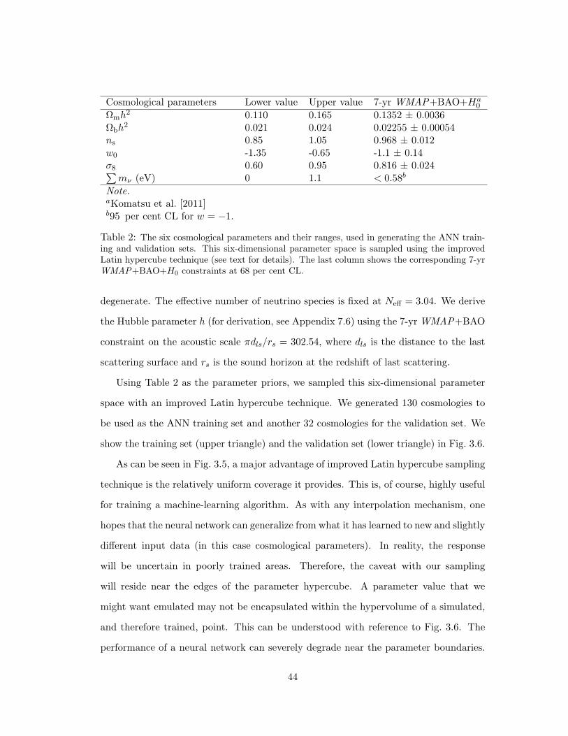
Cosmological parameters Lower value Upper value 7-yr WMAP+BAO+Ha0

Ωmh2 0.110 0.165 0.1352 ± 0.0036

Ωbh2 0.021 0.024 0.02255 ± 0.00054

ns 0.85 1.05 0.968 ± 0.012w0 -1.35 -0.65 -1.1 ± 0.14σ8 0.60 0.95 0.816 ± 0.024∑mν (eV) 0 1.1 < 0.58b

Note.aKomatsu et al. [2011]b95 per cent CL for w = −1.

Table 2: The six cosmological parameters and their ranges, used in generating the ANN train-ing and validation sets. This six-dimensional parameter space is sampled using the improvedLatin hypercube technique (see text for details). The last column shows the corresponding 7-yrWMAP+BAO+H0 constraints at 68 per cent CL.

degenerate. The effective number of neutrino species is fixed at Neff = 3.04. We derive

the Hubble parameter h (for derivation, see Appendix 7.6) using the 7-yr WMAP+BAO

constraint on the acoustic scale πdls/rs = 302.54, where dls is the distance to the last

scattering surface and rs is the sound horizon at the redshift of last scattering.

Using Table 2 as the parameter priors, we sampled this six-dimensional parameter

space with an improved Latin hypercube technique. We generated 130 cosmologies to

be used as the ANN training set and another 32 cosmologies for the validation set. We

show the training set (upper triangle) and the validation set (lower triangle) in Fig. 3.6.

As can be seen in Fig. 3.5, a major advantage of improved Latin hypercube sampling

technique is the relatively uniform coverage it provides. This is, of course, highly useful

for training a machine-learning algorithm. As with any interpolation mechanism, one

hopes that the neural network can generalize from what it has learned to new and slightly

different input data (in this case cosmological parameters). In reality, the response

will be uncertain in poorly trained areas. Therefore, the caveat with our sampling

will reside near the edges of the parameter hypercube. A parameter value that we

might want emulated may not be encapsulated within the hypervolume of a simulated,

and therefore trained, point. This can be understood with reference to Fig. 3.6. The

performance of a neural network can severely degrade near the parameter boundaries.

44

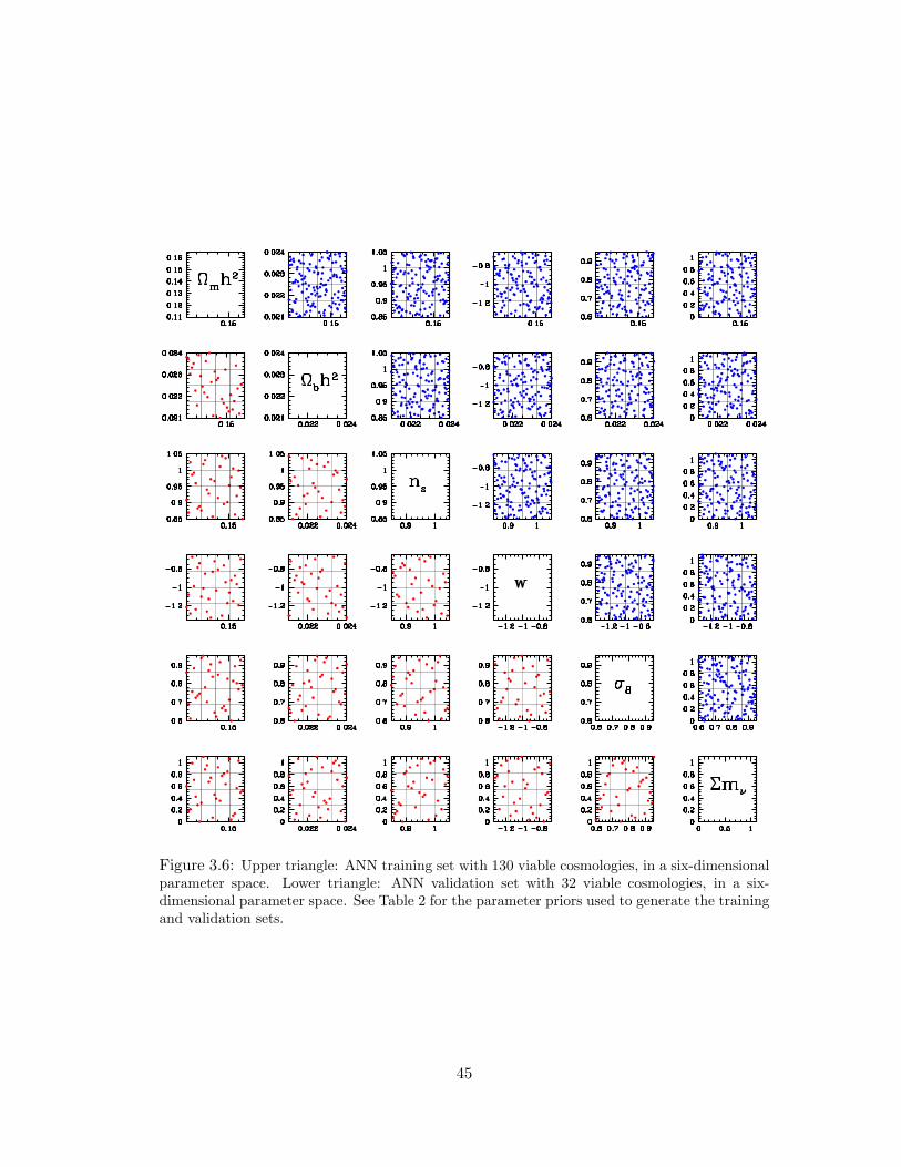
Figure 3.6: Upper triangle: ANN training set with 130 viable cosmologies, in a six-dimensionalparameter space. Lower triangle: ANN validation set with 32 viable cosmologies, in a six-dimensional parameter space. See Table 2 for the parameter priors used to generate the trainingand validation sets.

45

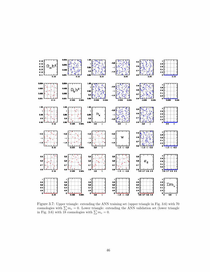
Figure 3.7: Upper triangle: extending the ANN training set (upper triangle in Fig. 3.6) with 70cosmologies with

∑mν = 0. Lower triangle: extending the ANN validation set (lower triangle

in Fig. 3.6) with 18 cosmologies with∑mν = 0.

46

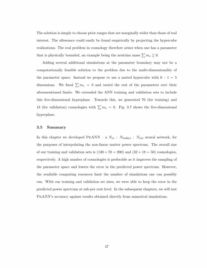
The solution is simply to choose prior ranges that are marginally wider than those of real

interest. The allowance could easily be found empirically by projecting the hypercube

realizations. The real problem in cosmology therefore arises when one has a parameter

that is physically bounded, an example being the neutrino mass∑mν & 0.

Adding several additional simulations at the parameter boundary may not be a

computationally feasible solution to the problem due to the multi-dimensionality of

the parameter space. Instead we propose to use a nested hypercube with 6 − 1 = 5

dimensions. We fixed∑mν = 0 and varied the rest of the parameters over their

aforementioned limits. We extended the ANN training and validation sets to include

this five-dimensional hyperplane. Towards this, we generated 70 (for training) and

18 (for validation) cosmologies with∑mν = 0. Fig. 3.7 shows the five-dimensional

hyperplane.

3.5 Summary

In this chapter we developed PkANN – a Nin : Nhidden : Nout neural network, for

the purposes of interpolating the non-linear matter power spectrum. The overall size

of our training and validation sets is (130 + 70 = 200) and (32 + 18 = 50) cosmologies,

respectively. A high number of cosmologies is preferable as it improves the sampling of

the parameter space and lowers the error in the predicted power spectrum. However,

the available computing resources limit the number of simulations one can possibly

run. With our training and validation set sizes, we were able to keep the error in the

predicted power spectrum at sub-per cent level. In the subsequent chapters, we will test

PkANN’s accuracy against results obtained directly from numerical simulations.

47

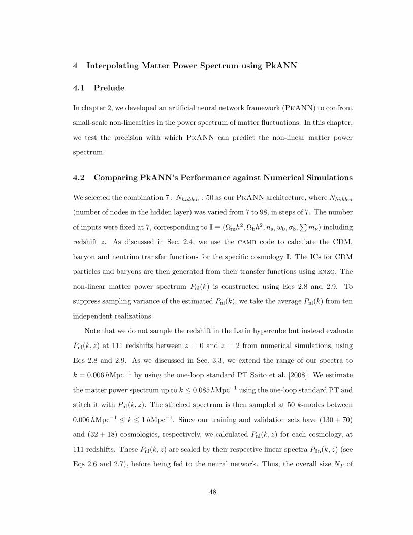
4 Interpolating Matter Power Spectrum using PkANN

4.1 Prelude

In chapter 2, we developed an artificial neural network framework (PkANN) to confront

small-scale non-linearities in the power spectrum of matter fluctuations. In this chapter,

we test the precision with which PkANN can predict the non-linear matter power

spectrum.

4.2 Comparing PkANN’s Performance against Numerical Simulations

We selected the combination 7 : Nhidden : 50 as our PkANN architecture, where Nhidden

(number of nodes in the hidden layer) was varied from 7 to 98, in steps of 7. The number

of inputs were fixed at 7, corresponding to I ≡ (Ωmh2,Ωbh

2, ns, w0, σ8,∑mν) including

redshift z. As discussed in Sec. 2.4, we use the camb code to calculate the CDM,

baryon and neutrino transfer functions for the specific cosmology I. The ICs for CDM

particles and baryons are then generated from their transfer functions using enzo. The

non-linear matter power spectrum Pnl(k) is constructed using Eqs 2.8 and 2.9. To

suppress sampling variance of the estimated Pnl(k), we take the average Pnl(k) from ten

independent realizations.

Note that we do not sample the redshift in the Latin hypercube but instead evaluate

Pnl(k, z) at 111 redshifts between z = 0 and z = 2 from numerical simulations, using

Eqs 2.8 and 2.9. As we discussed in Sec. 3.3, we extend the range of our spectra to

k = 0.006hMpc−1 by using the one-loop standard PT Saito et al. [2008]. We estimate

the matter power spectrum up to k ≤ 0.085hMpc−1 using the one-loop standard PT and

stitch it with Pnl(k, z). The stitched spectrum is then sampled at 50 k-modes between

0.006hMpc−1 ≤ k ≤ 1hMpc−1. Since our training and validation sets have (130 + 70)

and (32 + 18) cosmologies, respectively, we calculated Pnl(k, z) for each cosmology, at

111 redshifts. These Pnl(k, z) are scaled by their respective linear spectra Plin(k, z) (see

Eqs 2.6 and 2.7), before being fed to the neural network. Thus, the overall size NT of

48

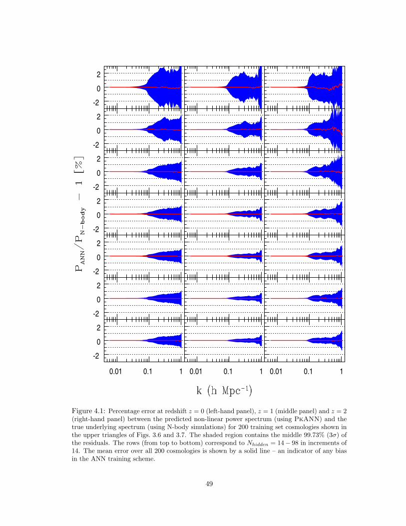
-202

-202

-202

-202

-202

-202

0.01 0.1 1

-202

0.01 0.1 1 0.01 0.1 1

Figure 4.1: Percentage error at redshift z = 0 (left-hand panel), z = 1 (middle panel) and z = 2(right-hand panel) between the predicted non-linear power spectrum (using PkANN) and thetrue underlying spectrum (using N-body simulations) for 200 training set cosmologies shown inthe upper triangles of Figs. 3.6 and 3.7. The shaded region contains the middle 99.73% (3σ) ofthe residuals. The rows (from top to bottom) correspond to Nhidden = 14− 98 in increments of14. The mean error over all 200 cosmologies is shown by a solid line – an indicator of any biasin the ANN training scheme.

49

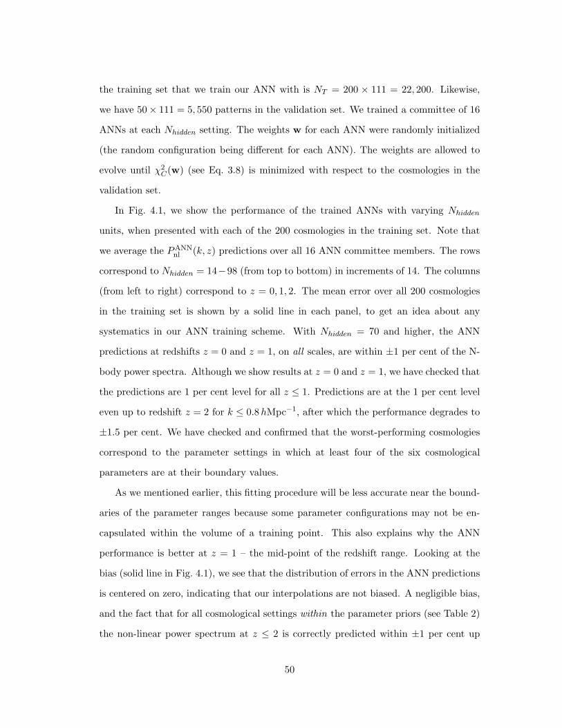
the training set that we train our ANN with is NT = 200 × 111 = 22, 200. Likewise,

we have 50× 111 = 5, 550 patterns in the validation set. We trained a committee of 16

ANNs at each Nhidden setting. The weights w for each ANN were randomly initialized

(the random configuration being different for each ANN). The weights are allowed to

evolve until χ2C(w) (see Eq. 3.8) is minimized with respect to the cosmologies in the

validation set.

In Fig. 4.1, we show the performance of the trained ANNs with varying Nhidden

units, when presented with each of the 200 cosmologies in the training set. Note that

we average the PANNnl (k, z) predictions over all 16 ANN committee members. The rows

correspond to Nhidden = 14−98 (from top to bottom) in increments of 14. The columns

(from left to right) correspond to z = 0, 1, 2. The mean error over all 200 cosmologies

in the training set is shown by a solid line in each panel, to get an idea about any

systematics in our ANN training scheme. With Nhidden = 70 and higher, the ANN

predictions at redshifts z = 0 and z = 1, on all scales, are within ±1 per cent of the N-

body power spectra. Although we show results at z = 0 and z = 1, we have checked that

the predictions are 1 per cent level for all z ≤ 1. Predictions are at the 1 per cent level

even up to redshift z = 2 for k ≤ 0.8hMpc−1, after which the performance degrades to

±1.5 per cent. We have checked and confirmed that the worst-performing cosmologies

correspond to the parameter settings in which at least four of the six cosmological

parameters are at their boundary values.

As we mentioned earlier, this fitting procedure will be less accurate near the bound-

aries of the parameter ranges because some parameter configurations may not be en-

capsulated within the volume of a training point. This also explains why the ANN

performance is better at z = 1 – the mid-point of the redshift range. Looking at the

bias (solid line in Fig. 4.1), we see that the distribution of errors in the ANN predictions

is centered on zero, indicating that our interpolations are not biased. A negligible bias,

and the fact that for all cosmological settings within the parameter priors (see Table 2)

the non-linear power spectrum at z ≤ 2 is correctly predicted within ±1 per cent up

50

Figure 4.2: The residual error χ2C(w) (see Eq. 3.8) evaluated as a function of the number

of nodes in the hidden layer, Nhidden. The error is a monotonically decreasing function forthe training set (dashed line) while for the validation set (solid line), it starts increasing beyondNhidden = 70 indicating that the generalizing ability of the neural network is best with Nhidden =70. The error bars correspond to the spread in χ2

C(w) for the 16 ANN committee members.

to k ≤ 0.8hMpc−1, demonstrates the stability of our ANN strategy. This marks a

remarkable improvement over the currently popular interpolation scheme – the cosmic

emulator, which has a significant number (∼50 per cent) of cosmological models with

errors at ∼0.5−1 per cent level. We note, however, that the cosmic emulator, based

on Gaussian processes, is able to achieve sub-per cent accuracy with only 37 distinct

cosmologies while in the ANN scheme we use a suite of around 200 cosmologies. Com-

paring Fig. 10 from Lawrence et al. [2010] with our Fig. 4.1, we see that the ANN

implementation performs better on all scales and redshifts.

Increasing the number of nodes in the hidden layer increases the flexibility of a neural

network. An increasingly complex network can make extremely accurate predictions on

the training set. This is evident from Fig. 4.1, where the prediction over the training

set becomes progressively better (from top to bottom) with increasing Nhidden units.

However, such complex networks can adversely affect their generalizing ability when

51

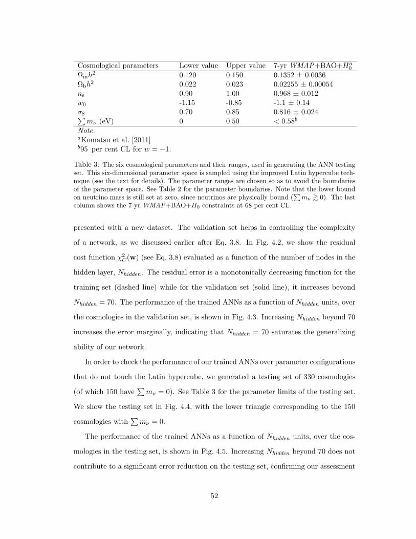
Cosmological parameters Lower value Upper value 7-yr WMAP+BAO+Ha0

Ωmh2 0.120 0.150 0.1352 ± 0.0036

Ωbh2 0.022 0.023 0.02255 ± 0.00054

ns 0.90 1.00 0.968 ± 0.012w0 -1.15 -0.85 -1.1 ± 0.14σ8 0.70 0.85 0.816 ± 0.024∑mν (eV) 0 0.50 < 0.58b

Note.aKomatsu et al. [2011]b95 per cent CL for w = −1.

Table 3: The six cosmological parameters and their ranges, used in generating the ANN testingset. This six-dimensional parameter space is sampled using the improved Latin hypercube tech-nique (see the text for details). The parameter ranges are chosen so as to avoid the boundariesof the parameter space. See Table 2 for the parameter boundaries. Note that the lower boundon neutrino mass is still set at zero, since neutrinos are physically bound (

∑mν & 0). The last

column shows the 7-yr WMAP+BAO+H0 constraints at 68 per cent CL.

presented with a new dataset. The validation set helps in controlling the complexity

of a network, as we discussed earlier after Eq. 3.8. In Fig. 4.2, we show the residual

cost function χ2C(w) (see Eq. 3.8) evaluated as a function of the number of nodes in the

hidden layer, Nhidden. The residual error is a monotonically decreasing function for the

training set (dashed line) while for the validation set (solid line), it increases beyond

Nhidden = 70. The performance of the trained ANNs as a function of Nhidden units, over

the cosmologies in the validation set, is shown in Fig. 4.3. Increasing Nhidden beyond 70

increases the error marginally, indicating that Nhidden = 70 saturates the generalizing

ability of our network.

In order to check the performance of our trained ANNs over parameter configurations

that do not touch the Latin hypercube, we generated a testing set of 330 cosmologies

(of which 150 have∑mν = 0). See Table 3 for the parameter limits of the testing set.

We show the testing set in Fig. 4.4, with the lower triangle corresponding to the 150

cosmologies with∑mν = 0.

The performance of the trained ANNs as a function of Nhidden units, over the cos-

mologies in the testing set, is shown in Fig. 4.5. Increasing Nhidden beyond 70 does not

contribute to a significant error reduction on the testing set, confirming our assessment

52

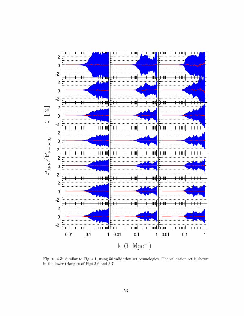
-202

-202

-202

-202

-202

-202

0.01 0.1 1

-202

0.01 0.1 1 0.01 0.1 1

Figure 4.3: Similar to Fig. 4.1, using 50 validation set cosmologies. The validation set is shownin the lower triangles of Figs 3.6 and 3.7.

53

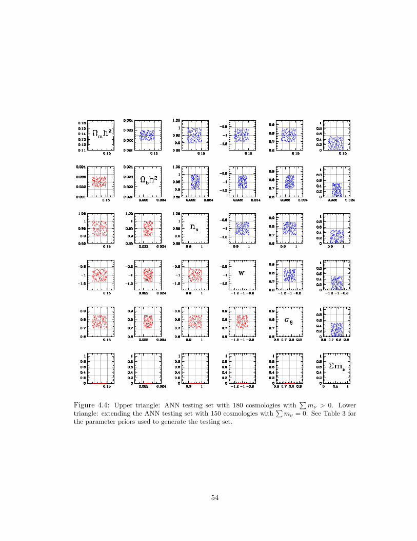
Figure 4.4: Upper triangle: ANN testing set with 180 cosmologies with∑mν > 0. Lower

triangle: extending the ANN testing set with 150 cosmologies with∑mν = 0. See Table 3 for

the parameter priors used to generate the testing set.

54

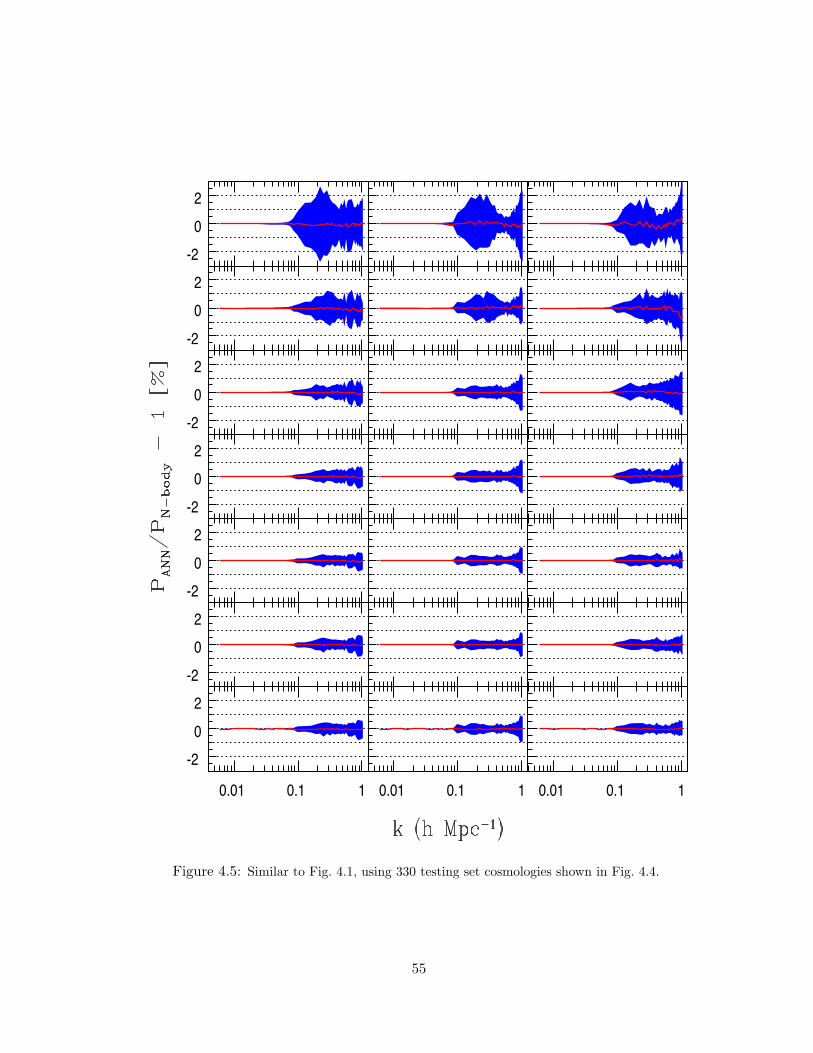
-202

-202

-202

-202

-202

-202

0.01 0.1 1

-202

0.01 0.1 1 0.01 0.1 1

Figure 4.5: Similar to Fig. 4.1, using 330 testing set cosmologies shown in Fig. 4.4.

55

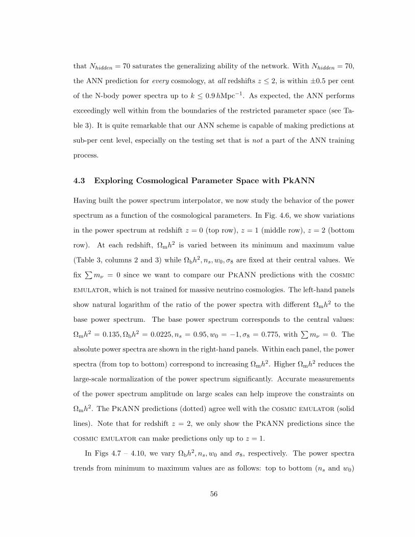
that Nhidden = 70 saturates the generalizing ability of the network. With Nhidden = 70,

the ANN prediction for every cosmology, at all redshifts z ≤ 2, is within ±0.5 per cent

of the N-body power spectra up to k ≤ 0.9hMpc−1. As expected, the ANN performs

exceedingly well within from the boundaries of the restricted parameter space (see Ta-

ble 3). It is quite remarkable that our ANN scheme is capable of making predictions at

sub-per cent level, especially on the testing set that is not a part of the ANN training

process.

4.3 Exploring Cosmological Parameter Space with PkANN

Having built the power spectrum interpolator, we now study the behavior of the power

spectrum as a function of the cosmological parameters. In Fig. 4.6, we show variations

in the power spectrum at redshift z = 0 (top row), z = 1 (middle row), z = 2 (bottom

row). At each redshift, Ωmh2 is varied between its minimum and maximum value

(Table 3, columns 2 and 3) while Ωbh2, ns, w0, σ8 are fixed at their central values. We

fix∑mν = 0 since we want to compare our PkANN predictions with the cosmic

emulator, which is not trained for massive neutrino cosmologies. The left-hand panels

show natural logarithm of the ratio of the power spectra with different Ωmh2 to the

base power spectrum. The base power spectrum corresponds to the central values:

Ωmh2 = 0.135,Ωbh

2 = 0.0225, ns = 0.95, w0 = −1, σ8 = 0.775, with∑mν = 0. The

absolute power spectra are shown in the right-hand panels. Within each panel, the power

spectra (from top to bottom) correspond to increasing Ωmh2. Higher Ωmh

2 reduces the

large-scale normalization of the power spectrum significantly. Accurate measurements

of the power spectrum amplitude on large scales can help improve the constraints on

Ωmh2. The PkANN predictions (dotted) agree well with the cosmic emulator (solid

lines). Note that for redshift z = 2, we only show the PkANN predictions since the

cosmic emulator can make predictions only up to z = 1.

In Figs 4.7 – 4.10, we vary Ωbh2, ns, w0 and σ8, respectively. The power spectra

trends from minimum to maximum values are as follows: top to bottom (ns and w0)

56

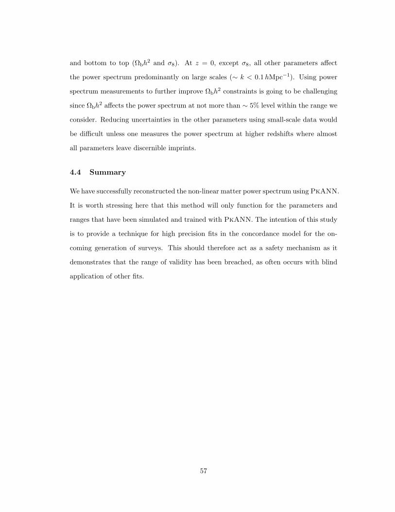
and bottom to top (Ωbh2 and σ8). At z = 0, except σ8, all other parameters affect

the power spectrum predominantly on large scales (∼ k < 0.1hMpc−1). Using power

spectrum measurements to further improve Ωbh2 constraints is going to be challenging

since Ωbh2 affects the power spectrum at not more than ∼ 5% level within the range we

consider. Reducing uncertainties in the other parameters using small-scale data would

be difficult unless one measures the power spectrum at higher redshifts where almost

all parameters leave discernible imprints.

4.4 Summary

We have successfully reconstructed the non-linear matter power spectrum using PkANN.

It is worth stressing here that this method will only function for the parameters and

ranges that have been simulated and trained with PkANN. The intention of this study

is to provide a technique for high precision fits in the concordance model for the on-

coming generation of surveys. This should therefore act as a safety mechanism as it

demonstrates that the range of validity has been breached, as often occurs with blind

application of other fits.

57

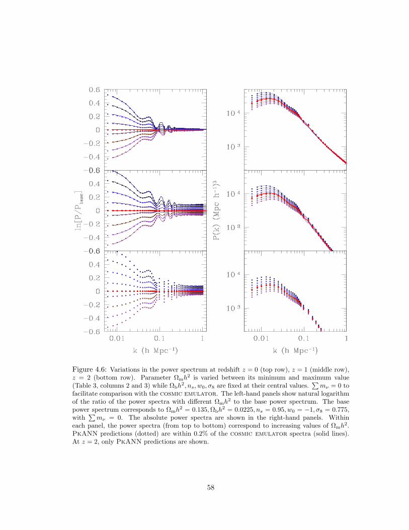
Figure 4.6: Variations in the power spectrum at redshift z = 0 (top row), z = 1 (middle row),z = 2 (bottom row). Parameter Ωmh

2 is varied between its minimum and maximum value(Table 3, columns 2 and 3) while Ωbh

2, ns, w0, σ8 are fixed at their central values.∑mν = 0 to

facilitate comparison with the cosmic emulator. The left-hand panels show natural logarithmof the ratio of the power spectra with different Ωmh

2 to the base power spectrum. The basepower spectrum corresponds to Ωmh

2 = 0.135,Ωbh2 = 0.0225, ns = 0.95, w0 = −1, σ8 = 0.775,

with∑mν = 0. The absolute power spectra are shown in the right-hand panels. Within

each panel, the power spectra (from top to bottom) correspond to increasing values of Ωmh2.

PkANN predictions (dotted) are within 0.2% of the cosmic emulator spectra (solid lines).At z = 2, only PkANN predictions are shown.

58

Figure 4.7: Similar to Fig. 4.6, but for a range of Ωbh2 values. Within each panel, the power

spectra from bottom to top correspond to increasing Ωbh2 values.

59

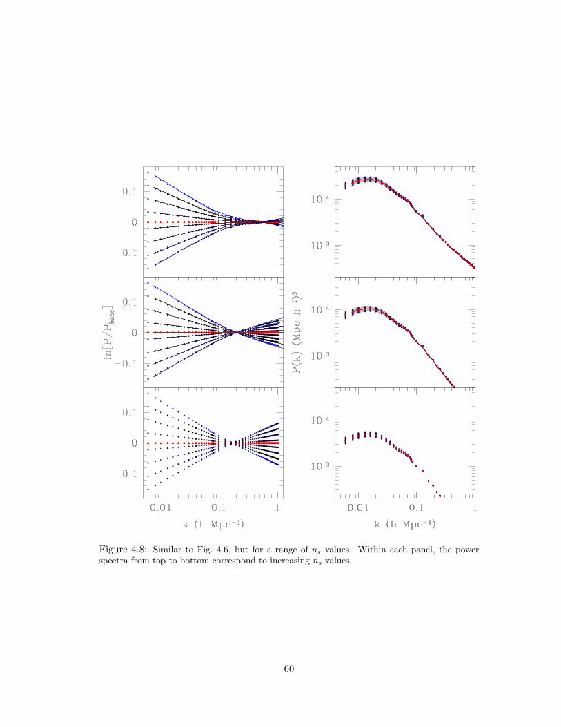
Figure 4.8: Similar to Fig. 4.6, but for a range of ns values. Within each panel, the powerspectra from top to bottom correspond to increasing ns values.

60

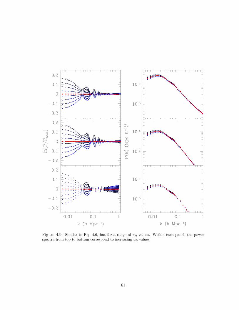
Figure 4.9: Similar to Fig. 4.6, but for a range of w0 values. Within each panel, the powerspectra from top to bottom correspond to increasing w0 values.

61

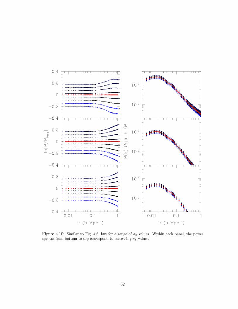
Figure 4.10: Similar to Fig. 4.6, but for a range of σ8 values. Within each panel, the powerspectra from bottom to top correspond to increasing σ8 values.

62

5 Estimating the Cosmic Mach Number using PkANN

5.1 Prelude

Peculiar velocities are a sensitive probe of the underlying large-scale matter density fluc-

tuations in our Universe. In particular, large, all-sky surveys of the peculiar velocities of

galaxies or clusters of galaxies can provide important constraints on cosmological param-

eters. However, studies of peculiar velocities suffer from several drawbacks, including (i)

the presence of small-scale, non-linear flows, such as infall into clusters, can potentially

bias analyses which typically rely on linear theory, (ii) sparse, non-uniform sampling of

the peculiar velocity field can lead to aliasing of small-scale power on to large scales and

bias due to heavier sampling of dense regions, (iii) large measurement uncertainties of

individual peculiar velocity measurements, particularly for distant galaxies or clusters,

make it necessary to work with large surveys in order to extract meaningful constraints.

Ostriker and Suto [1990] introduced a dimensionless statistic of the cosmological

structure - the cosmic Mach number, as a way to measure the warmth/coldness of the

velocity field on some scale R. Specifically, one measures the bulk flow u(x0;R) of a

region of size R centered at x0, as well as the velocity dispersion σ(x0;R) of the ob-

jects within this region. The ratio of the bulk flow to the velocity dispersion, namely

(|u(x0;R)|2/σ2(x0;R))1/2 ≡M(x0;R), is the cosmic Mach number. The ensemble aver-

age over x0 gives the statistic M(R). Since both |u(x0;R)|2 and σ2(x0;R) scale equally

by the amplitude of the matter density perturbation, the statistic M is independent (at

least in linear approximation) of the normalization of the matter power spectrum.

In linear theory, given the cosmological parameters, M can be readily calculated and

compared with its measured value from the peculiar velocity field catalogues. However,

comparing theoretical predictions with observations is not straightforward: (i) one has

to correct for the small-scale non-linearities in observations as well as take into account

the fact that observations represent only a discreet sample of the continuous velocity

field. This can be remedied by smoothing the velocity field on a suitable scale rs

63

(∼ 5h−1Mpc, since on larger scales the matter density field is expected to be linear),

before estimating the quantities u(x0;R) and σ(x0;R). However, any residual non-

linearity in the observed field can still bias the M estimates; (ii) Non-uniform, noisy

and sparse sampling of the peculiar velocity field can lead to aliasing of small-scale

power onto larger scales. When making comparisons with theory, one has to carefully

take into account the selection function and the noise of the real dataset.

Over the last couple of decades, the statistic M has been investigated: Ostriker and

Suto [1990] used linear theory and Gaussian selection function to show that standard

Cold Dark Matter (sCDM) model is inconsistent (predicts M almost twice the observed

value) with observations at ∼ 95% CL; Suto et al. [1992], using Tophat and Gaussian

selection functions, studied the distribution of M using N-body simulations to rule out

the sCDM scenario at 99% CL; Strauss et al. [1993] took into account the selection

function of real surveys and extracted mocks from numerical simulations over a range

of cosmologies including sCDM and tilted CDM (scalar spectral index, ns 6= 1) among

others, to reject the sCDM model at 94% CL; Ma et al. [2012] explored the potential of

using M in distinguishing cosmological models, including modified gravity and massive

neutrino cosmologies.

In this chapter, (i) we estimate the cosmic Mach number for various galaxy peculiar

velocity datasets; (ii) we investigate how likely it is to get these Mach values in a ΛCDM

universe. To achieve this, we study the statistical distribution of the expected Mach

number by extracting mocks of the real catalogues from numerical simulations of a

ΛCDM universe. We show that a ΛCDM universe with 7-yr WMAP type cosmology

is consistent with the Mach observations at 2σ CL; (iii) we further show that our M

estimates for the mocks are not biased by the selection function of the mocks. Towards

this, we extract dense and nearly-isotropic distributions with a Gaussian profile f(r) ∝

e−r2/2R2

withR = 10−100h−1Mpc. We show that the Mach numbers estimated from the

mocks are very similar to the values based on Gaussian profiles (of similar depth R as the

mocks); (iv) we use the non-linear matter power spectrum interpolation scheme PkANN

64

to check if we can avoid N-body simulations completely and predict M(R) by only

using PkANN’s prediction for the non-linear power spectrum. This is crucial because

high-resolution hydrodynamic N-body simulations are computationally expensive and

extremely time consuming. Exploring the parameter space with numerical simulations

with reasonable computing resources and time might not be possible. A full use of a

statistic like M can only be realized with a prescription for the non-linear matter power

spectrum.

It is worth mentioning here the reason for our choice of a Gaussian profile f(r) over,

for example, a Tophat filter in our analysis. A Tophat filter gets significant contribution

from smaller (than Tophat size R) scales, which are contaminated by non-linearities

at low redshifts. Bulk flow calculated using a Tophat filter can be compared with

expectations from linear theory only if the observed velocity field is reasonably dense

and uniform, so that the small-scale systematics average out. However, observations

typically are sparse and non-uniform with large uncertainties. This leads to aliasing

of small-scale power on to large scales, making comparison with theory difficult. A

Gaussian filter, on the other hand, gets very little contribution from small scales, thereby

making comparison with linear theory meaningful.

5.2 The Cosmic Mach Number

Given a peculiar velocity field v(x), one can calculate the bulk flow, which represent the

net streaming motion of a region in some direction relative to the background Hubble

expansion. The bulk flow u(x0;R) of a region of size R centered at x0 can be defined

as

u(x0;R) =∫dx v(x)F (|x− x0|, R), (5.1)

where F (|x− x0|, R) is the filter used to average the velocity field v(x) on a char-

acteristic scale R. Although Tophats and Gaussian filters are the preferred choices,

65

F (|x− x0|, R) can be designed to mimic the selection function of the real datasets.

This is useful when dealing with datasets whose selection function depends strongly on

the position in the sky. In Fourier space, Eq. 5.1 can be written as

u(x0;R) =∫dk v(k)W (k, R)e−ik·x0 , (5.2)

where v(k) and W (k, R) are the Fourier transforms of the peculiar velocity field v(x)

and the filter F (|x− x0|, R), respectively.

In linear theory of structure formation, at low redshifts, the velocities are related to

the matter overdensities via

v(k) = ifH0δ(k)kk2, (5.3)

where δ(k) is the Fourier transform of the overdensity field δ(x). The linear growth rate

factor f can be approximated as f = Ω0.6m . Thus, the velocity power spectrum Pv(k) is

proportional to the matter power spectrum P (k) at low redshifts,

Pv(k) = (H0f)2P (k)k2

. (5.4)

Using Eq. 5.2 and Eq. 5.4, the mean-squared bulk value of u(x0;R) can be shown to be

σ2v(R) ≡ < u2(x0;R) > =

H20 Ω1.2

m

2π2

∫dk P (k)W 2(kR), (5.5)

where the average is taken over all spatial positions x0.

The squared velocity dispersion within a region of size R centered at x0 can be

similarly defined as

σ2(x0;R) =∫dx |v(x)|2F (|x− x0|, R)− |u(x0;R)|2. (5.6)

66

In Fourier space, the ensamble average of Eq. 5.6 over x0 becomes

σ2(R) ≡ < σ2(x0;R) > =H2

0 Ω1.2m

2π2

∫dk P (k)

(1−W 2(kR)

). (5.7)

Using Eq. 5.5 and Eq. 5.7, the cosmic Mach number can now be defined as

M(R) ≡ < M2(x0;R) >1/2 =(σ2v(R)σ2(R)

)1/2

. (5.8)

As discussed in literature [Ostriker and Suto, 1990, Suto et al., 1992, Strauss et al.,

1993], the cosmic Mach number is essentially a measure of the shape of the matter power

spectrum: The rms bulk flow σv(R) gets most of its contribution from scales larger than

R, while the velocity dispersion σ(R) is a measure of the strength of velocities on scales

smaller than R and gets most contribution from small scales. Furthermore, the statistic

M is expected to be independent of the matter power spectrum normalization – at least

on large scales, where the perturbations are still well described by linear theory and

affect both σ2v(R) and σ2(R) equally. M can be a powerful tool to test not only the

ΛCDM scenario, but also a wide range of cosmologies including models with massive

neutrinos. Massive neutrinos suppress the matter power spectrum in a scale dependent

way, thereby altering the velocity dispersion much more prominently than the bulk flow.

Mach number M provides an easy to interpret technique to distinguish between various

cosmological models.

5.3 N-body Simulations

In order to study the statistical distribution of M , we extract mock surveys from the

41 numerical realizations of a ΛCDM universe. The N-body simulation we use in our

analysis is Large Suite of Dark Matter Simulations (LasDamas, hereafter LD) (McBride

et al. [2009]; McBride et al. [2011] in prep2). The LD simulation parameters are: Ωm =

0.25, Ωb = 0.04, ΩΛ = 0.75, h = 0.7, σ8 = 0.8, ns = 1.0 and LBox = 1h−1Gpc for the2http://lss.phy.vanderbilt.edu/lasdamas

67

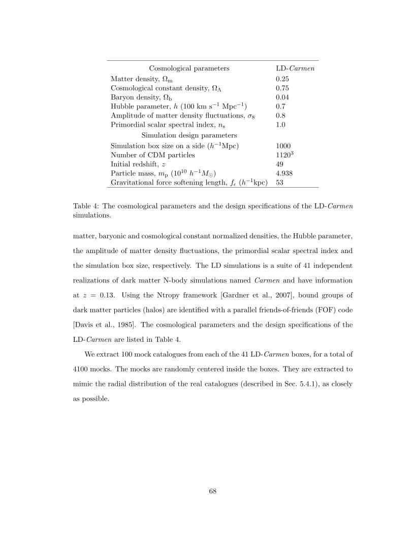
Cosmological parameters LD-CarmenMatter density, Ωm 0.25Cosmological constant density, ΩΛ 0.75Baryon density, Ωb 0.04Hubble parameter, h (100 km s−1 Mpc−1) 0.7Amplitude of matter density fluctuations, σ8 0.8Primordial scalar spectral index, ns 1.0

Simulation design parametersSimulation box size on a side (h−1Mpc) 1000Number of CDM particles 11203

Initial redshift, z 49Particle mass, mp (1010 h−1M) 4.938Gravitational force softening length, fε (h−1kpc) 53

Table 4: The cosmological parameters and the design specifications of the LD-Carmensimulations.

matter, baryonic and cosmological constant normalized densities, the Hubble parameter,

the amplitude of matter density fluctuations, the primordial scalar spectral index and

the simulation box size, respectively. The LD simulations is a suite of 41 independent

realizations of dark matter N-body simulations named Carmen and have information

at z = 0.13. Using the Ntropy framework [Gardner et al., 2007], bound groups of

dark matter particles (halos) are identified with a parallel friends-of-friends (FOF) code

[Davis et al., 1985]. The cosmological parameters and the design specifications of the

LD-Carmen are listed in Table 4.

We extract 100 mock catalogues from each of the 41 LD-Carmen boxes, for a total of

4100 mocks. The mocks are randomly centered inside the boxes. They are extracted to

mimic the radial distribution of the real catalogues (described in Sec. 5.4.1), as closely

as possible.

68

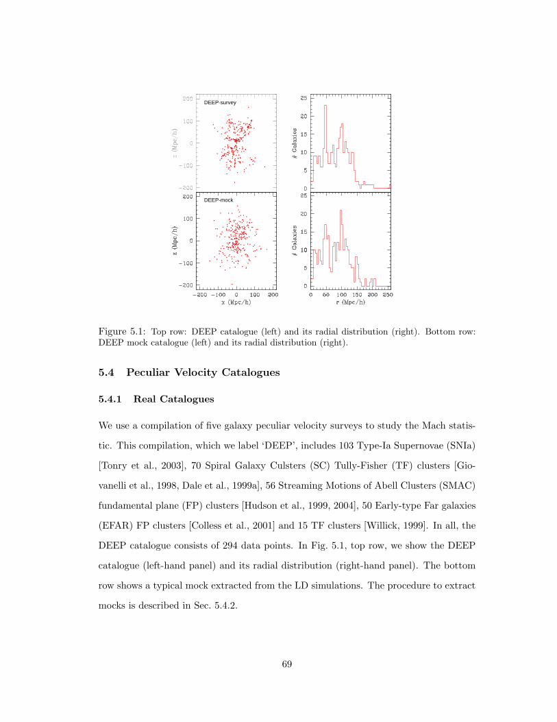
DEEP-survey

DEEP-mock

Figure 5.1: Top row: DEEP catalogue (left) and its radial distribution (right). Bottom row:DEEP mock catalogue (left) and its radial distribution (right).

5.4 Peculiar Velocity Catalogues

5.4.1 Real Catalogues

We use a compilation of five galaxy peculiar velocity surveys to study the Mach statis-

tic. This compilation, which we label ‘DEEP’, includes 103 Type-Ia Supernovae (SNIa)

[Tonry et al., 2003], 70 Spiral Galaxy Culsters (SC) Tully-Fisher (TF) clusters [Gio-

vanelli et al., 1998, Dale et al., 1999a], 56 Streaming Motions of Abell Clusters (SMAC)

fundamental plane (FP) clusters [Hudson et al., 1999, 2004], 50 Early-type Far galaxies

(EFAR) FP clusters [Colless et al., 2001] and 15 TF clusters [Willick, 1999]. In all, the

DEEP catalogue consists of 294 data points. In Fig. 5.1, top row, we show the DEEP

catalogue (left-hand panel) and its radial distribution (right-hand panel). The bottom

row shows a typical mock extracted from the LD simulations. The procedure to extract

mocks is described in Sec. 5.4.2.

69

5.4.2 Mock Catalogues

Inside the N-body simulation box, we first select a point at random. Next, we extract a

mock realization of the real catalogue by imposing the constraint that the mock should

have a similar radial distribution to the real catalogue. The right-hand panels in Fig. 5.1

show the radial distribution of galaxies in the DEEP catalogue (top) and its mock

(bottom). We do not constrain the mocks to have the same angular distribution as the

real catalogue for two reasons: (i) the LD simulation boxes are not dense enough to give

us mocks that are exact replicas of the real catalogue, (ii) the objects in a real survey are

typically weighted depending only on their velocity errors. Consequently, even though

the real catalogue and its mocks have similar radial profiles, their angular distribution

differ considerably, with the mocks having a relatively featureless angular distribution.

To make the mocks more realistic, we impose a 10o latitude zone-of-avoidance cut.

Using the angular position rx, ry, rz, the true radial distance ds from the mock

center and the peculiar velocity vector v, we calculate the true line-of-sight peculiar

velocity vs and the redshift cz = ds + vs for each mock galaxy, all in km s−1. We then

perturb the true radial distance ds of the mock galaxy with a velocity error drawn from

a Gaussian distribution of width equal to the corresponding real galaxy’s velocity error,

e. Thus, dp = ds + δd, where dp is the perturbed radial distance of the mock galaxy

(in km s−1) and δd is the velocity error drawn from a Gaussian of width e. The mock

galaxy’s measured line-of-sight peculiar velocity vp is then assigned to be vp = cz − dp,

where cz is the redshift we found above. This procedure ensures that the weights we

assign to the mock galaxies are similar to the weights of the real galaxies.

5.5 The Maximum Likelihood Estimate Method

One of the most common weighting scheme used in analysis of the bulk flow is the maxi-

mum likelihood estimate (hereafter MLE) method, obtained from a maximum likelihood

analysis introduced by Kaiser [1988]. The motion of galaxies is modeled as being due

to a streaming flow with Gaussian distributed measurement uncertainties. Given a pe-

70

culiar velocity survey, the MLE estimate of its bulk flow is obtained from the likelihood

function

L[ui|Sn, σn, σ∗] =∏n

1√σ2n + σ2

∗exp

(−1

2(Sn − rn,iui)2

σ2n + σ2

∗

), (5.9)

where rn is the unit position vector of the nth galaxy, σn is the measurement uncertainty

of the nth galaxy and σ∗ is the 1-D velocity dispersion accounting for smaller-scale

motions. The three components of the bulk flow ui can be written as weighted sum of

the measured radial peculiar velocities of a survey

ui =∑n

wi,nSn, (5.10)

where Sn is the radial peculiar velocity of the nth galaxy of a survey, and wi,n is

the weight assigned to this velocity in the calculation of ui. Throughout this paper,

subscripts i, j and k run over the 3 components of the bulk flow, while subscripts m

and n run over the galaxies. Maximizing the likelihood given by Eq. 5.9, gives the three

components of the bulk flow ui with the MLE weights

wi,n =3∑j=1

A−1ij

rn,jσ2n + σ2

∗, (5.11)

where

Aij =∑n

rn,irn,jσ2n + σ2

∗. (5.12)

The 1-D velocity dispersion σ∗ is 1/√

3 of the 3-D velocity dispersion (see Eq. 5.7)

which we aim to ultimately measure. Since the weights wi,n (and ui) are themselves a

function of σ∗, we converge on to the MLE estimate for σ∗ iteratively. See Strauss et al.

[1993] for a discussion on how to estimate the best-fit ui and σ∗ iteratively.

The effective depth of a survey can be roughly estimated by a weighted sum∑wnrn/

∑wn

of the radial distances rn of the survey objects, where wn = 1/(σ2n+σ2

∗). This weighting

scheme has been used by Ma, Ostriker, and Zhao [2012] in their analyses of peculiar

71

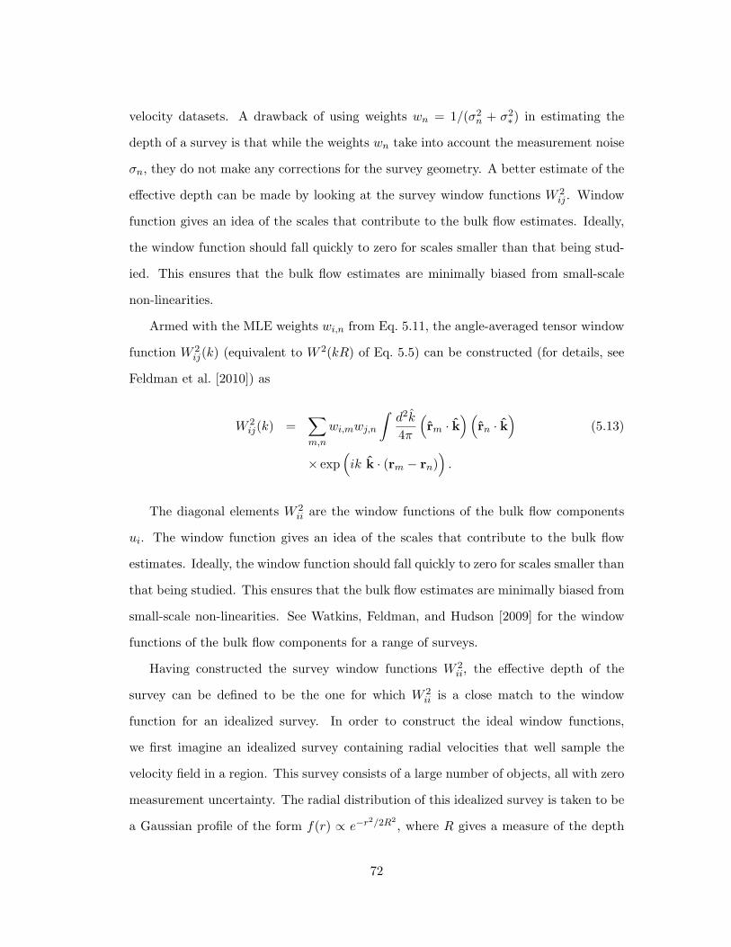
velocity datasets. A drawback of using weights wn = 1/(σ2n + σ2

∗) in estimating the

depth of a survey is that while the weights wn take into account the measurement noise

σn, they do not make any corrections for the survey geometry. A better estimate of the

effective depth can be made by looking at the survey window functions W 2ij . Window

function gives an idea of the scales that contribute to the bulk flow estimates. Ideally,

the window function should fall quickly to zero for scales smaller than that being stud-

ied. This ensures that the bulk flow estimates are minimally biased from small-scale

non-linearities.

Armed with the MLE weights wi,n from Eq. 5.11, the angle-averaged tensor window

function W 2ij(k) (equivalent to W 2(kR) of Eq. 5.5) can be constructed (for details, see

Feldman et al. [2010]) as

W 2ij(k) =

∑m,n

wi,mwj,n

∫d2k

4π

(rm · k

)(rn · k

)(5.13)

× exp(ik k · (rm − rn)

).

The diagonal elements W 2ii are the window functions of the bulk flow components

ui. The window function gives an idea of the scales that contribute to the bulk flow

estimates. Ideally, the window function should fall quickly to zero for scales smaller than

that being studied. This ensures that the bulk flow estimates are minimally biased from

small-scale non-linearities. See Watkins, Feldman, and Hudson [2009] for the window

functions of the bulk flow components for a range of surveys.

Having constructed the survey window functions W 2ii, the effective depth of the

survey can be defined to be the one for which W 2ii is a close match to the window

function for an idealized survey. In order to construct the ideal window functions,

we first imagine an idealized survey containing radial velocities that well sample the

velocity field in a region. This survey consists of a large number of objects, all with zero

measurement uncertainty. The radial distribution of this idealized survey is taken to be

a Gaussian profile of the form f(r) ∝ e−r2/2R2

, where R gives a measure of the depth

72

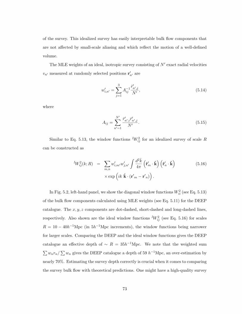
of the survey. This idealized survey has easily interpretable bulk flow components that

are not affected by small-scale aliasing and which reflect the motion of a well-defined

volume.

The MLE weights of an ideal, isotropic survey consisting of N ′ exact radial velocities

vn′ measured at randomly selected positions r′n′ are

w′i,n′ =3∑j=1

A−1ij

r′n′,jN ′

, (5.14)

where

Aij =N ′∑n′=1

r′n′,ir′n′,j

N ′. (5.15)

Similar to Eq. 5.13, the window functions IW 2ij for an idealized survey of scale R

can be constructed as

IW 2ij(k;R) =

∑m,n

w′i,m′w′j,n′

∫d2k

4π

(r′m · k

)(r′n · k

)(5.16)

× exp(ik k · (r′m − r′n)

).

In Fig. 5.2, left-hand panel, we show the diagonal window functionsW 2ii (see Eq. 5.13)

of the bulk flow components calculated using MLE weights (see Eq. 5.11) for the DEEP

catalogue. The x, y, z components are dot-dashed, short-dashed and long-dashed lines,

respectively. Also shown are the ideal window functions IW 2ij (see Eq. 5.16) for scales

R = 10 − 40h−1Mpc (in 5h−1Mpc increments), the window functions being narrower

for larger scales. Comparing the DEEP and the ideal window functions gives the DEEP

catalogue an effective depth of ∼ R = 35h−1Mpc. We note that the weighted sum∑wnrn/

∑wn gives the DEEP catalogue a depth of 59 h−1Mpc, an over-estimation by

nearly 70%. Estimating the survey depth correctly is crucial when it comes to comparing

the survey bulk flow with theoretical predictions. One might have a high-quality survey

73

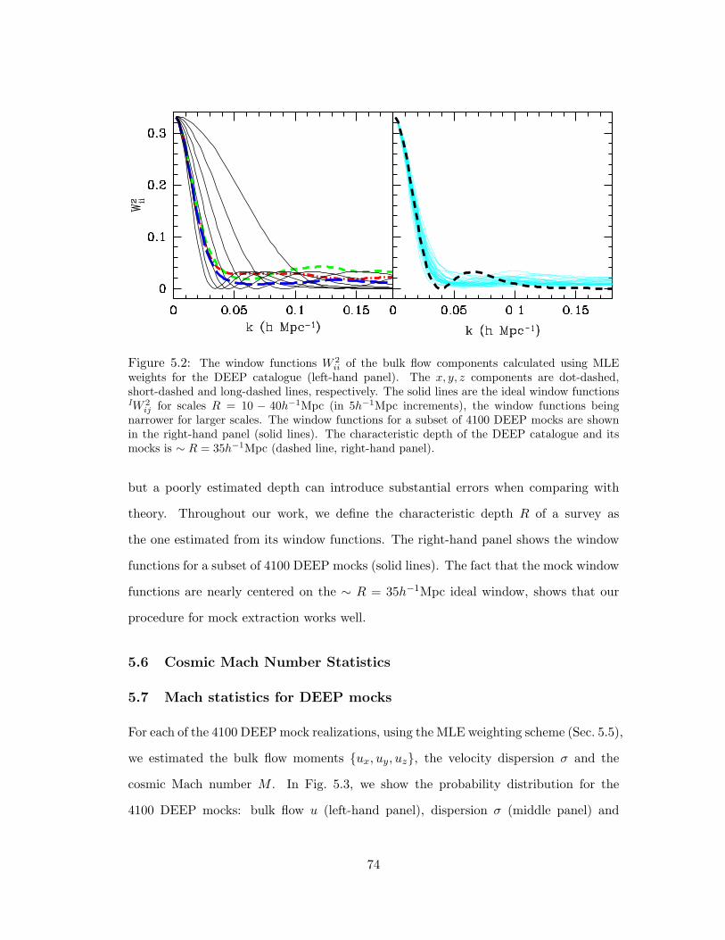
Figure 5.2: The window functions W 2ii of the bulk flow components calculated using MLE

weights for the DEEP catalogue (left-hand panel). The x, y, z components are dot-dashed,short-dashed and long-dashed lines, respectively. The solid lines are the ideal window functionsIW 2

ij for scales R = 10 − 40h−1Mpc (in 5h−1Mpc increments), the window functions beingnarrower for larger scales. The window functions for a subset of 4100 DEEP mocks are shownin the right-hand panel (solid lines). The characteristic depth of the DEEP catalogue and itsmocks is ∼ R = 35h−1Mpc (dashed line, right-hand panel).

but a poorly estimated depth can introduce substantial errors when comparing with

theory. Throughout our work, we define the characteristic depth R of a survey as

the one estimated from its window functions. The right-hand panel shows the window

functions for a subset of 4100 DEEP mocks (solid lines). The fact that the mock window

functions are nearly centered on the ∼ R = 35h−1Mpc ideal window, shows that our

procedure for mock extraction works well.

5.6 Cosmic Mach Number Statistics

5.7 Mach statistics for DEEP mocks

For each of the 4100 DEEP mock realizations, using the MLE weighting scheme (Sec. 5.5),

we estimated the bulk flow moments ux, uy, uz, the velocity dispersion σ and the

cosmic Mach number M . In Fig. 5.3, we show the probability distribution for the

4100 DEEP mocks: bulk flow u (left-hand panel), dispersion σ (middle panel) and

74

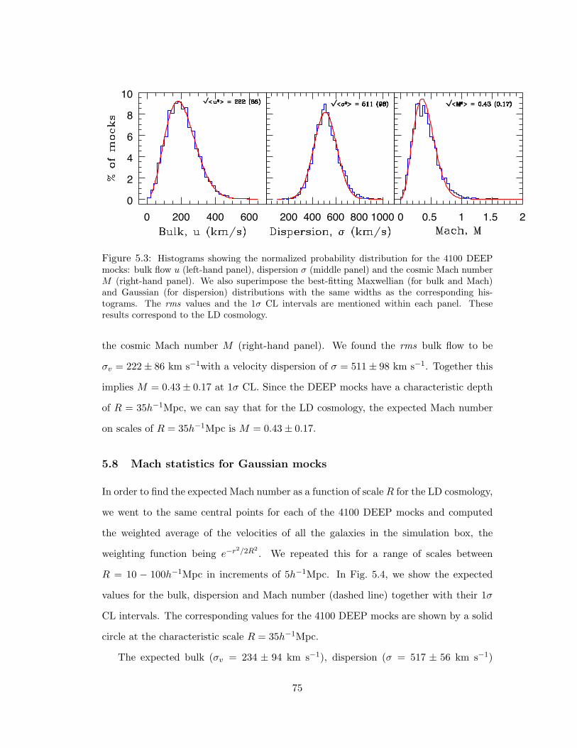
0 200 400 6000

2

4

6

8

10

200 400 600 800 1000 0 0.5 1 1.5 2

Figure 5.3: Histograms showing the normalized probability distribution for the 4100 DEEPmocks: bulk flow u (left-hand panel), dispersion σ (middle panel) and the cosmic Mach numberM (right-hand panel). We also superimpose the best-fitting Maxwellian (for bulk and Mach)and Gaussian (for dispersion) distributions with the same widths as the corresponding his-tograms. The rms values and the 1σ CL intervals are mentioned within each panel. Theseresults correspond to the LD cosmology.

the cosmic Mach number M (right-hand panel). We found the rms bulk flow to be

σv = 222± 86 km s−1with a velocity dispersion of σ = 511± 98 km s−1. Together this

implies M = 0.43± 0.17 at 1σ CL. Since the DEEP mocks have a characteristic depth

of R = 35h−1Mpc, we can say that for the LD cosmology, the expected Mach number

on scales of R = 35h−1Mpc is M = 0.43± 0.17.

5.8 Mach statistics for Gaussian mocks

In order to find the expected Mach number as a function of scale R for the LD cosmology,

we went to the same central points for each of the 4100 DEEP mocks and computed

the weighted average of the velocities of all the galaxies in the simulation box, the

weighting function being e−r2/2R2

. We repeated this for a range of scales between

R = 10 − 100h−1Mpc in increments of 5h−1Mpc. In Fig. 5.4, we show the expected

values for the bulk, dispersion and Mach number (dashed line) together with their 1σ

CL intervals. The corresponding values for the 4100 DEEP mocks are shown by a solid

circle at the characteristic scale R = 35h−1Mpc.

The expected bulk (σv = 234 ± 94 km s−1), dispersion (σ = 517 ± 56 km s−1)

75

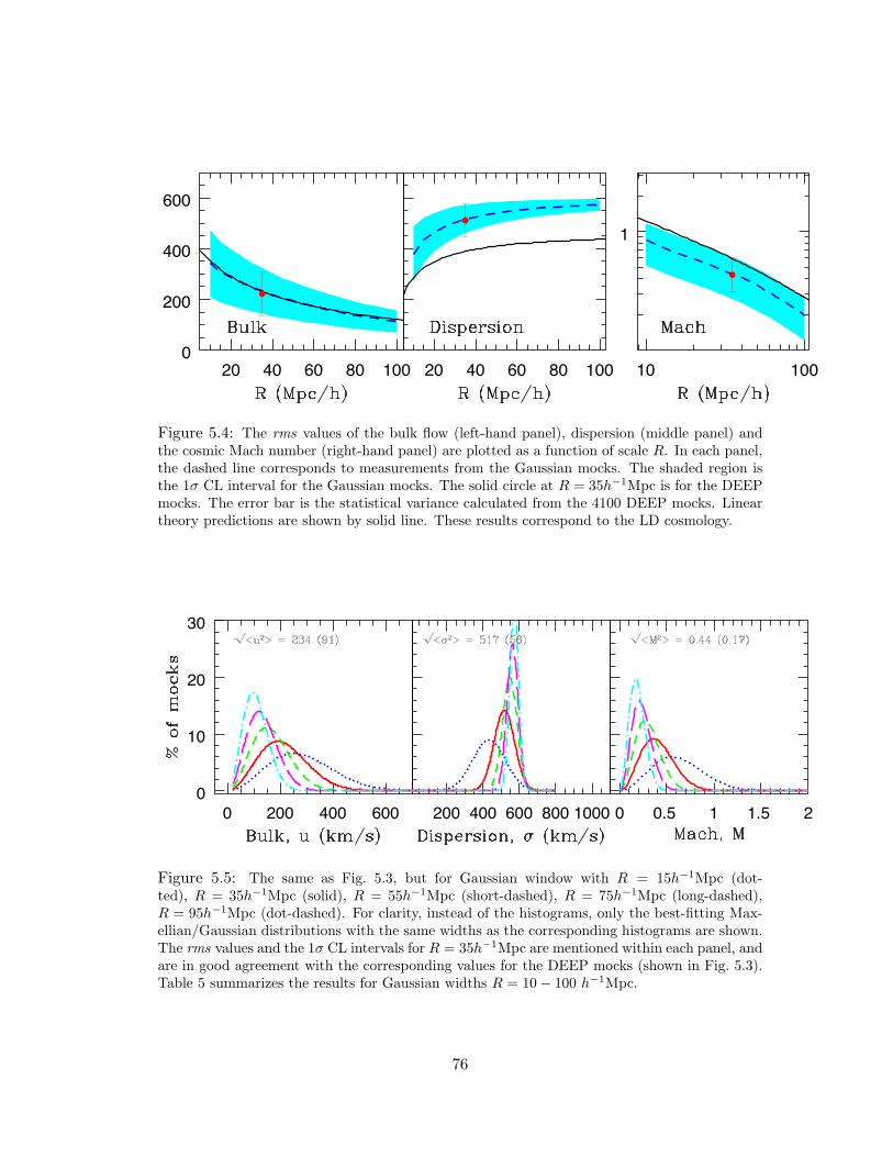
20 40 60 80 1000

200

400

600

20 40 60 80 100 10 100

1

Figure 5.4: The rms values of the bulk flow (left-hand panel), dispersion (middle panel) andthe cosmic Mach number (right-hand panel) are plotted as a function of scale R. In each panel,the dashed line corresponds to measurements from the Gaussian mocks. The shaded region isthe 1σ CL interval for the Gaussian mocks. The solid circle at R = 35h−1Mpc is for the DEEPmocks. The error bar is the statistical variance calculated from the 4100 DEEP mocks. Lineartheory predictions are shown by solid line. These results correspond to the LD cosmology.

0 200 400 6000

10

20

30

200 400 600 800 1000 0 0.5 1 1.5 2

Figure 5.5: The same as Fig. 5.3, but for Gaussian window with R = 15h−1Mpc (dot-ted), R = 35h−1Mpc (solid), R = 55h−1Mpc (short-dashed), R = 75h−1Mpc (long-dashed),R = 95h−1Mpc (dot-dashed). For clarity, instead of the histograms, only the best-fitting Max-ellian/Gaussian distributions with the same widths as the corresponding histograms are shown.The rms values and the 1σ CL intervals for R = 35h−1Mpc are mentioned within each panel, andare in good agreement with the corresponding values for the DEEP mocks (shown in Fig. 5.3).Table 5 summarizes the results for Gaussian widths R = 10− 100 h−1Mpc.

76

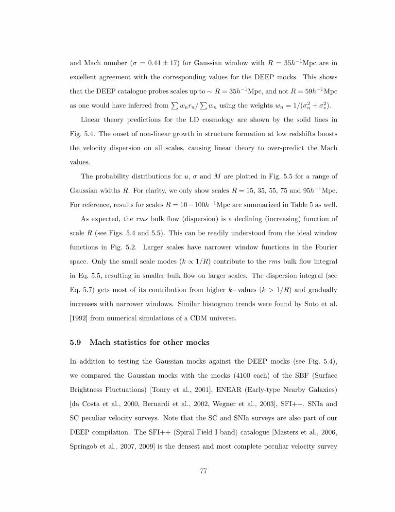
and Mach number (σ = 0.44 ± 17) for Gaussian window with R = 35h−1Mpc are in

excellent agreement with the corresponding values for the DEEP mocks. This shows

that the DEEP catalogue probes scales up to ∼ R = 35h−1Mpc, and not R = 59h−1Mpc

as one would have inferred from∑wnrn/

∑wn using the weights wn = 1/(σ2

n + σ2∗).

Linear theory predictions for the LD cosmology are shown by the solid lines in

Fig. 5.4. The onset of non-linear growth in structure formation at low redshifts boosts

the velocity dispersion on all scales, causing linear theory to over-predict the Mach

values.

The probability distributions for u, σ and M are plotted in Fig. 5.5 for a range of

Gaussian widths R. For clarity, we only show scales R = 15, 35, 55, 75 and 95h−1Mpc.

For reference, results for scales R = 10−100h−1Mpc are summarized in Table 5 as well.

As expected, the rms bulk flow (dispersion) is a declining (increasing) function of

scale R (see Figs. 5.4 and 5.5). This can be readily understood from the ideal window

functions in Fig. 5.2. Larger scales have narrower window functions in the Fourier

space. Only the small scale modes (k ∝ 1/R) contribute to the rms bulk flow integral

in Eq. 5.5, resulting in smaller bulk flow on larger scales. The dispersion integral (see

Eq. 5.7) gets most of its contribution from higher k−values (k > 1/R) and gradually

increases with narrower windows. Similar histogram trends were found by Suto et al.

[1992] from numerical simulations of a CDM universe.

5.9 Mach statistics for other mocks

In addition to testing the Gaussian mocks against the DEEP mocks (see Fig. 5.4),

we compared the Gaussian mocks with the mocks (4100 each) of the SBF (Surface

Brightness Fluctuations) [Tonry et al., 2001], ENEAR (Early-type Nearby Galaxies)

[da Costa et al., 2000, Bernardi et al., 2002, Wegner et al., 2003], SFI++, SNIa and

SC peculiar velocity surveys. Note that the SC and SNIa surveys are also part of our

DEEP compilation. The SFI++ (Spiral Field I-band) catalogue [Masters et al., 2006,

Springob et al., 2007, 2009] is the densest and most complete peculiar velocity survey

77

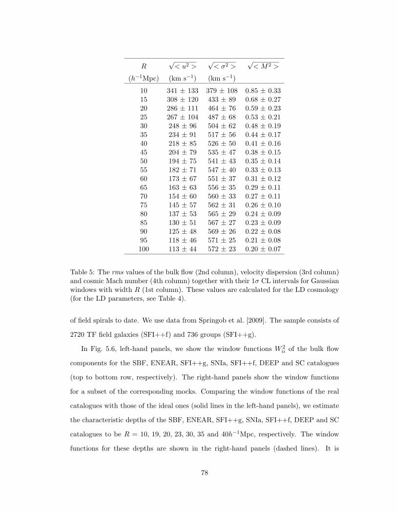
R√< u2 >

√< σ2 >

√< M2 >

(h−1Mpc) (km s−1) (km s−1)

10 341 ± 133 379 ± 108 0.85 ± 0.3315 308 ± 120 433 ± 89 0.68 ± 0.2720 286 ± 111 464 ± 76 0.59 ± 0.2325 267 ± 104 487 ± 68 0.53 ± 0.2130 248 ± 96 504 ± 62 0.48 ± 0.1935 234 ± 91 517 ± 56 0.44 ± 0.1740 218 ± 85 526 ± 50 0.41 ± 0.1645 204 ± 79 535 ± 47 0.38 ± 0.1550 194 ± 75 541 ± 43 0.35 ± 0.1455 182 ± 71 547 ± 40 0.33 ± 0.1360 173 ± 67 551 ± 37 0.31 ± 0.1265 163 ± 63 556 ± 35 0.29 ± 0.1170 154 ± 60 560 ± 33 0.27 ± 0.1175 145 ± 57 562 ± 31 0.26 ± 0.1080 137 ± 53 565 ± 29 0.24 ± 0.0985 130 ± 51 567 ± 27 0.23 ± 0.0990 125 ± 48 569 ± 26 0.22 ± 0.0895 118 ± 46 571 ± 25 0.21 ± 0.08100 113 ± 44 572 ± 23 0.20 ± 0.07

Table 5: The rms values of the bulk flow (2nd column), velocity dispersion (3rd column)and cosmic Mach number (4th column) together with their 1σ CL intervals for Gaussianwindows with width R (1st column). These values are calculated for the LD cosmology(for the LD parameters, see Table 4).

of field spirals to date. We use data from Springob et al. [2009]. The sample consists of

2720 TF field galaxies (SFI++f) and 736 groups (SFI++g).

In Fig. 5.6, left-hand panels, we show the window functions W 2ii of the bulk flow

components for the SBF, ENEAR, SFI++g, SNIa, SFI++f, DEEP and SC catalogues

(top to bottom row, respectively). The right-hand panels show the window functions

for a subset of the corresponding mocks. Comparing the window functions of the real

catalogues with those of the ideal ones (solid lines in the left-hand panels), we estimate

the characteristic depths of the SBF, ENEAR, SFI++g, SNIa, SFI++f, DEEP and SC

catalogues to be R = 10, 19, 20, 23, 30, 35 and 40h−1Mpc, respectively. The window

functions for these depths are shown in the right-hand panels (dashed lines). It is

78

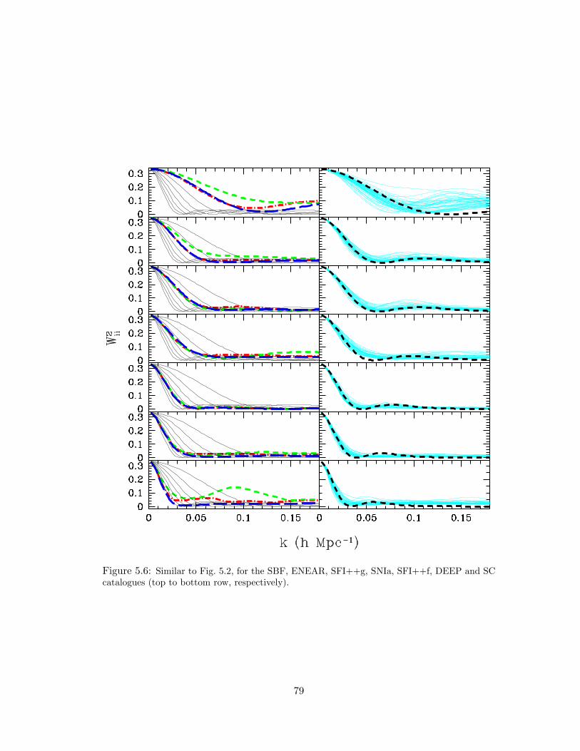
Figure 5.6: Similar to Fig. 5.2, for the SBF, ENEAR, SFI++g, SNIa, SFI++f, DEEP and SCcatalogues (top to bottom row, respectively).

79

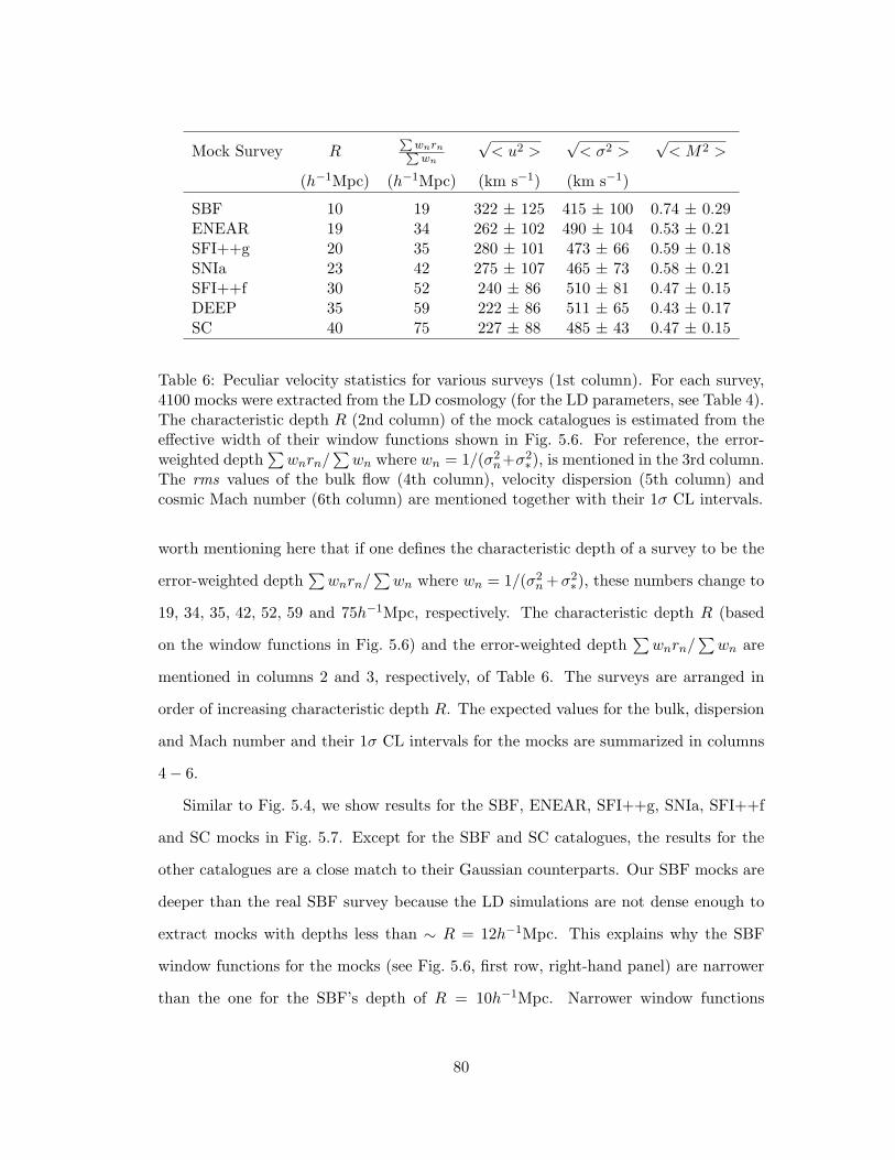
Mock Survey RPwnrnPwn

√< u2 >

√< σ2 >

√< M2 >

(h−1Mpc) (h−1Mpc) (km s−1) (km s−1)

SBF 10 19 322 ± 125 415 ± 100 0.74 ± 0.29ENEAR 19 34 262 ± 102 490 ± 104 0.53 ± 0.21SFI++g 20 35 280 ± 101 473 ± 66 0.59 ± 0.18SNIa 23 42 275 ± 107 465 ± 73 0.58 ± 0.21SFI++f 30 52 240 ± 86 510 ± 81 0.47 ± 0.15DEEP 35 59 222 ± 86 511 ± 65 0.43 ± 0.17SC 40 75 227 ± 88 485 ± 43 0.47 ± 0.15

Table 6: Peculiar velocity statistics for various surveys (1st column). For each survey,4100 mocks were extracted from the LD cosmology (for the LD parameters, see Table 4).The characteristic depth R (2nd column) of the mock catalogues is estimated from theeffective width of their window functions shown in Fig. 5.6. For reference, the error-weighted depth

∑wnrn/

∑wn where wn = 1/(σ2

n+σ2∗), is mentioned in the 3rd column.

The rms values of the bulk flow (4th column), velocity dispersion (5th column) andcosmic Mach number (6th column) are mentioned together with their 1σ CL intervals.

worth mentioning here that if one defines the characteristic depth of a survey to be the

error-weighted depth∑wnrn/

∑wn where wn = 1/(σ2

n +σ2∗), these numbers change to

19, 34, 35, 42, 52, 59 and 75h−1Mpc, respectively. The characteristic depth R (based

on the window functions in Fig. 5.6) and the error-weighted depth∑wnrn/

∑wn are

mentioned in columns 2 and 3, respectively, of Table 6. The surveys are arranged in

order of increasing characteristic depth R. The expected values for the bulk, dispersion

and Mach number and their 1σ CL intervals for the mocks are summarized in columns

4− 6.

Similar to Fig. 5.4, we show results for the SBF, ENEAR, SFI++g, SNIa, SFI++f

and SC mocks in Fig. 5.7. Except for the SBF and SC catalogues, the results for the

other catalogues are a close match to their Gaussian counterparts. Our SBF mocks are

deeper than the real SBF survey because the LD simulations are not dense enough to

extract mocks with depths less than ∼ R = 12h−1Mpc. This explains why the SBF

window functions for the mocks (see Fig. 5.6, first row, right-hand panel) are narrower

than the one for the SBF’s depth of R = 10h−1Mpc. Narrower window functions

80

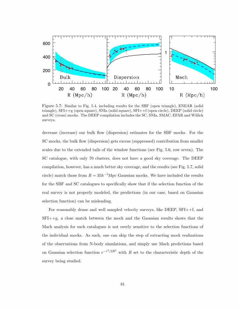
20 40 60 80 1000

200

400

600

20 40 60 80 100 10 100

1

Figure 5.7: Similar to Fig. 5.4, including results for the SBF (open triangle), ENEAR (solidtriangle), SFI++g (open square), SNIa (solid square), SFI++f (open circle), DEEP (solid circle)and SC (cross) mocks. The DEEP compilation includes the SC, SNIa, SMAC, EFAR and Willicksurveys.

decrease (increase) our bulk flow (dispersion) estimates for the SBF mocks. For the

SC mocks, the bulk flow (dispersion) gets excess (suppressed) contribution from smaller

scales due to the extended tails of the window functions (see Fig. 5.6, row seven). The

SC catalogue, with only 70 clusters, does not have a good sky coverage. The DEEP

compilation, however, has a much better sky coverage, and the results (see Fig. 5.7, solid

circle) match those from R = 35h−1Mpc Gaussian mocks. We have included the results

for the SBF and SC catalogues to specifically show that if the selection function of the

real survey is not properly modeled, the predictions (in our case, based on Gaussian

selection function) can be misleading.

For reasonably dense and well sampled velocity surveys, like DEEP, SFI++f, and

SFI++g, a close match between the mock and the Gaussian results shows that the

Mach analysis for such catalogues is not overly sensitive to the selection functions of

the individual mocks. As such, one can skip the step of extracting mock realizations

of the observations from N-body simulations, and simply use Mach predictions based

on Gaussian selection function e−r2/2R2

with R set to the characteristic depth of the

survey being studied.

81

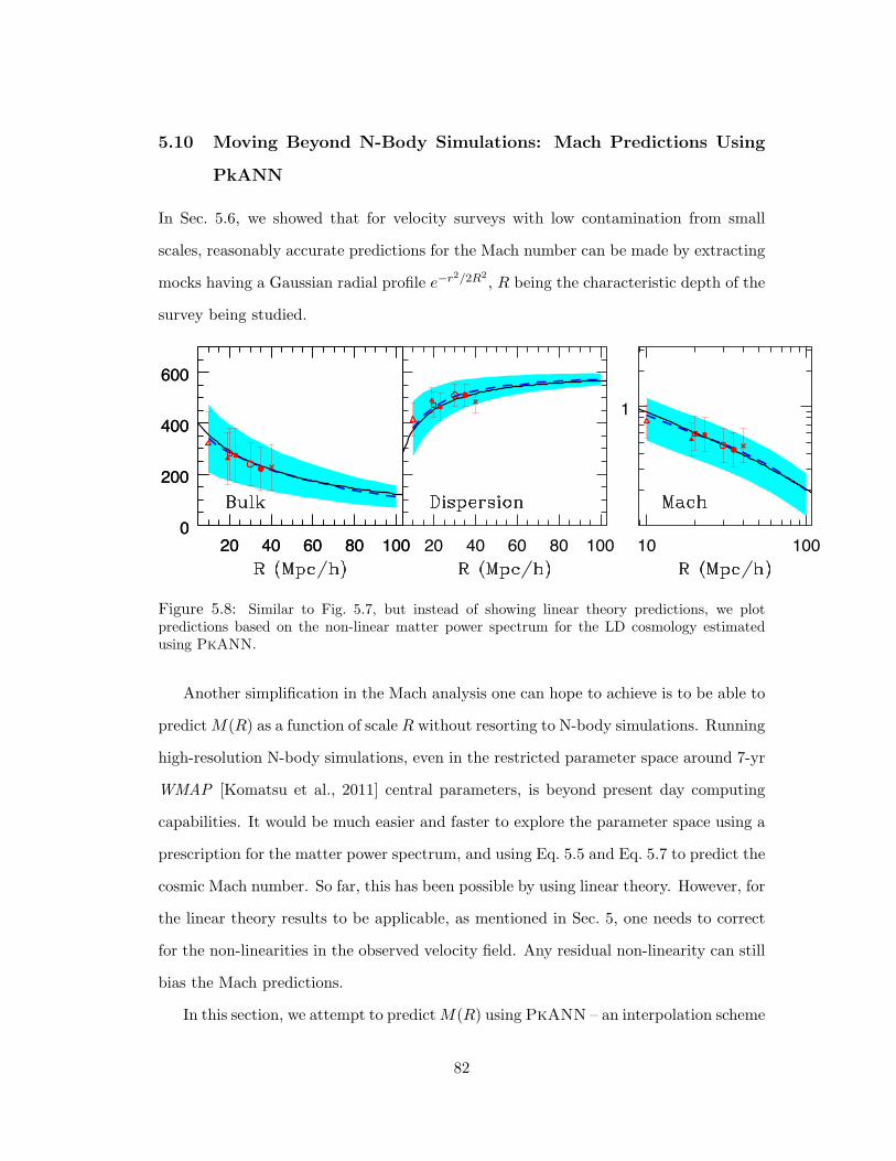
5.10 Moving Beyond N-Body Simulations: Mach Predictions Using

PkANN

In Sec. 5.6, we showed that for velocity surveys with low contamination from small

scales, reasonably accurate predictions for the Mach number can be made by extracting

mocks having a Gaussian radial profile e−r2/2R2

, R being the characteristic depth of the

survey being studied.

20 40 60 80 1000

200

400

600

20 40 60 80 1000

200

400

600

20 40 60 80 100 10 100

1

Figure 5.8: Similar to Fig. 5.7, but instead of showing linear theory predictions, we plotpredictions based on the non-linear matter power spectrum for the LD cosmology estimatedusing PkANN.

Another simplification in the Mach analysis one can hope to achieve is to be able to

predict M(R) as a function of scale R without resorting to N-body simulations. Running

high-resolution N-body simulations, even in the restricted parameter space around 7-yr

WMAP [Komatsu et al., 2011] central parameters, is beyond present day computing

capabilities. It would be much easier and faster to explore the parameter space using a

prescription for the matter power spectrum, and using Eq. 5.5 and Eq. 5.7 to predict the

cosmic Mach number. So far, this has been possible by using linear theory. However, for

the linear theory results to be applicable, as mentioned in Sec. 5, one needs to correct

for the non-linearities in the observed velocity field. Any residual non-linearity can still

bias the Mach predictions.

In this section, we attempt to predictM(R) using PkANN – an interpolation scheme

82

to predict the non-linear matter power spectrum up to k <∼ 0.9hMpc−1 between redshifts

z = 0− 2. Although PkANN accuracy worsens (starts under-predicting the non-linear

spectrum for k >∼ 0.9hMpc−1), we do not attempt to correct this by smoothing the

velocity field over the relevant spatial scale.

In Fig. 5.8, we replace linear theory predictions shown in Fig. 5.7, with the ones

calculated using PkANN for the LD cosmology. PkANN does an excellent job on all

scales, showing it can substitute numerical simulations for the purpose of calculating

the Mach number given a set of cosmological parameters. Although, we have shown

PkANN’s performance for only the LD cosmology, it is expected to perform satisfac-

torily for cosmologies around 7-yr WMAP central parameters for which PkANN has

been specifically trained.

5.11 Mach Number Estimates From Real Catalogues

Ma et al. [2012] measured Mach number for four peculiar velocity surveys (SBF, EN-

EAR, SNIa and SFI++f ) and found that the ΛCDM model with 7-yr WMAP param-

eters is mildly consistent with the Mach number estimates for these four surveys at

3σ CL. However, as the authors mention in their work, their estimates are based on

using linear approximation for the power spectrum. Given the fact that at low redshifts

structure formation has gone non-linear on small scales, it is necessary to consider non-

linearities when making theoretical predictions. Comparing Figs. 5.7 and 5.8 (middle

panels), one can see that dispersion is significantly boosted by non-linearities, lowering

the Mach predictions (third panels) by 1σ level.

Further, they work with Tophat window functions in their analysis. A Tophat filter

assumes a volume-limited survey with a sharp edge in real space. However, the number

density of objects sampled in a real survey typically fall at large distances. Real surveys

thus have a narrower depth than what a Tophat would suggest. The sharp edge of a

Tophat creates extended tails in k-space. Since it is the small scale modes that are

most contaminated by non-linearities at low redshifts, a Tophat filter leads to aliasing

83

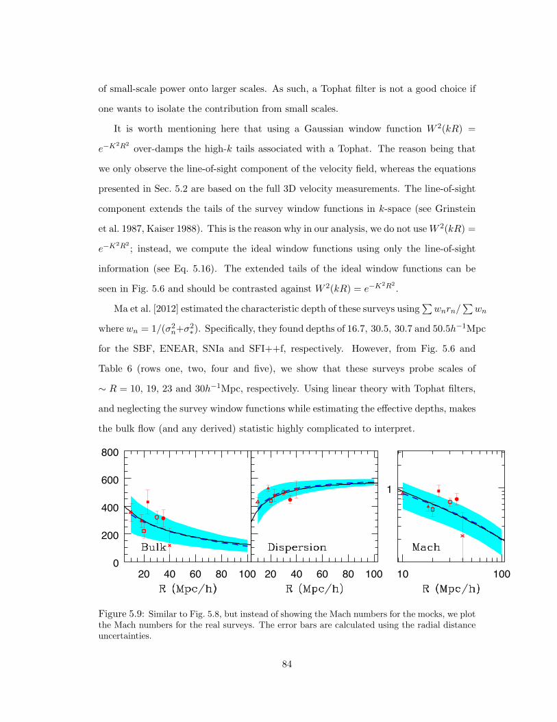
of small-scale power onto larger scales. As such, a Tophat filter is not a good choice if

one wants to isolate the contribution from small scales.

It is worth mentioning here that using a Gaussian window function W 2(kR) =

e−K2R2

over-damps the high-k tails associated with a Tophat. The reason being that

we only observe the line-of-sight component of the velocity field, whereas the equations

presented in Sec. 5.2 are based on the full 3D velocity measurements. The line-of-sight

component extends the tails of the survey window functions in k-space (see Grinstein

et al. 1987, Kaiser 1988). This is the reason why in our analysis, we do not useW 2(kR) =

e−K2R2

; instead, we compute the ideal window functions using only the line-of-sight

information (see Eq. 5.16). The extended tails of the ideal window functions can be

seen in Fig. 5.6 and should be contrasted against W 2(kR) = e−K2R2

.

Ma et al. [2012] estimated the characteristic depth of these surveys using∑wnrn/

∑wn

where wn = 1/(σ2n+σ2

∗). Specifically, they found depths of 16.7, 30.5, 30.7 and 50.5h−1Mpc

for the SBF, ENEAR, SNIa and SFI++f, respectively. However, from Fig. 5.6 and

Table 6 (rows one, two, four and five), we show that these surveys probe scales of

∼ R = 10, 19, 23 and 30h−1Mpc, respectively. Using linear theory with Tophat filters,

and neglecting the survey window functions while estimating the effective depths, makes

the bulk flow (and any derived) statistic highly complicated to interpret.

20 40 60 80 1000

200

400

600

800

20 40 60 80 100 10 100

1

Figure 5.9: Similar to Fig. 5.8, but instead of showing the Mach numbers for the mocks, we plotthe Mach numbers for the real surveys. The error bars are calculated using the radial distanceuncertainties.

84

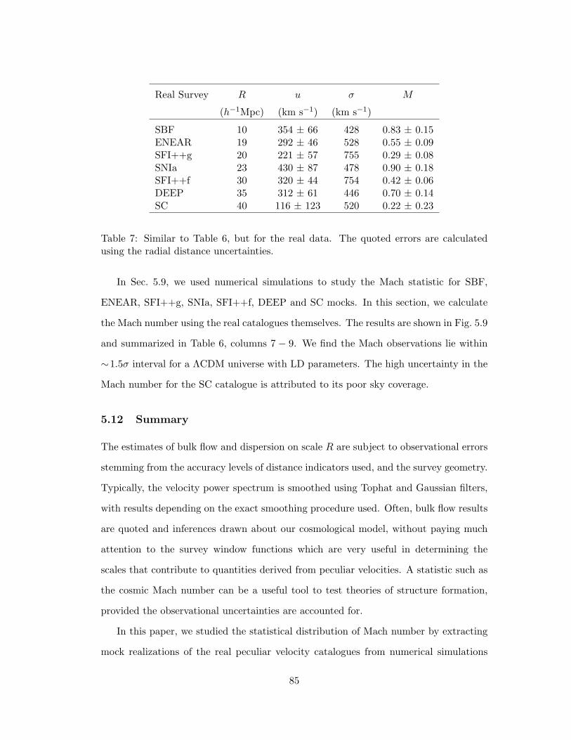
Real Survey R u σ M

(h−1Mpc) (km s−1) (km s−1)

SBF 10 354 ± 66 428 0.83 ± 0.15ENEAR 19 292 ± 46 528 0.55 ± 0.09SFI++g 20 221 ± 57 755 0.29 ± 0.08SNIa 23 430 ± 87 478 0.90 ± 0.18SFI++f 30 320 ± 44 754 0.42 ± 0.06DEEP 35 312 ± 61 446 0.70 ± 0.14SC 40 116 ± 123 520 0.22 ± 0.23

Table 7: Similar to Table 6, but for the real data. The quoted errors are calculatedusing the radial distance uncertainties.

In Sec. 5.9, we used numerical simulations to study the Mach statistic for SBF,

ENEAR, SFI++g, SNIa, SFI++f, DEEP and SC mocks. In this section, we calculate

the Mach number using the real catalogues themselves. The results are shown in Fig. 5.9

and summarized in Table 6, columns 7 − 9. We find the Mach observations lie within

∼1.5σ interval for a ΛCDM universe with LD parameters. The high uncertainty in the

Mach number for the SC catalogue is attributed to its poor sky coverage.

5.12 Summary

The estimates of bulk flow and dispersion on scale R are subject to observational errors

stemming from the accuracy levels of distance indicators used, and the survey geometry.

Typically, the velocity power spectrum is smoothed using Tophat and Gaussian filters,

with results depending on the exact smoothing procedure used. Often, bulk flow results

are quoted and inferences drawn about our cosmological model, without paying much

attention to the survey window functions which are very useful in determining the

scales that contribute to quantities derived from peculiar velocities. A statistic such as

the cosmic Mach number can be a useful tool to test theories of structure formation,

provided the observational uncertainties are accounted for.

In this paper, we studied the statistical distribution of Mach number by extracting

mock realizations of the real peculiar velocity catalogues from numerical simulations

85

of a ΛCDM universe with 7-yr WMAP type cosmology. We showed that the Mach

number estimates from the real catalogues agree with the expectations for a ΛCDM

universe at ∼ 1.5σ level. We checked if our Mach expectations derived from mock

surveys were biased by the selection function effects: we extracted realizations with a

Gaussian profile f(r) ∝ e−r2/2R2

and found no significant change to our Mach values

for the mock surveys.

We presented an alternative method to study the cosmic Mach number – by us-

ing a prescription for the non-linear matter power spectrum, instead of running time-

consuming and computationally-intensive numerical simulations. Non-linear power spec-

trum interpolators like PkANN offer tremendous leverage over numerical simulations,

by being able to explore the parameter space quickly. The role of such interpolating

schemes in the study of quantities derived from peculiar velocities needs further inves-

tigation.

86

6 Conclusions

The advent of the era of precision cosmology poses a serious challenge to theoretical

physics. The upcoming generation of surveys has the potential to breach per cent level

of accuracy. Such high-precision data will improve our constraints on cosmological

parameters including dark energy, curvature and neutrino masses. Efficiently dealing

with this impending flood of precise data on ever smaller scales and lower redshifts

requires that we move on from linear theory as well as any imperfect sets of non-

linear approximations. Although numerical simulations are capable of achieving the

levels of precision required by the near-future surveys, the high dimensionality of the

cosmological parameter space renders their brute force usage impractical.

We have introduced a unique approach to coping with non-linearities in the matter

power spectra in cosmology. By employing a multi-layer perceptron neural network

together with an improved Latin hypercube parameter sampling technique, we have

demonstrated that the non-linear spectrum can be reconstructed from a full set of Λ

cold dark matter parameters to better than 1 per cent over the parameter space spanning

3σ confidence level around the 7-yr WMAP central values. Parameters that are likely

to reside by some hard physical prior, such as the neutrino mass, can be successfully

brought under the realm of ANNs by sprinkling extra simulations in the corresponding

(e.g.∑mν = 0) hyper-plane. PkANN is the first power spectrum calculator capable

of predicting the non-linear matter power spectrum at sub-per cent level up to redshift

z = 2 for a range of cosmological models, including massive neutrinos.

As a potential use of PkANN, we studied the cosmic Mach number statistic and

found excellent agreement with results obtained directly from the LasDamas numerical

simulations. While high-resolution numerical simulations can take millions of hours of

computing, the PkANN code estimates the non-linear matter power spectrum in less

than a second. However, one must be careful to use the PkANN code only for the

parameters and ranges that have been simulated and trained with PkANN.

87

Looking forward, our ANN procedure can be readily employed for a variety of cos-

mological tasks such as fitting halo mass functions obtained through high resolution

N-body simulations. Moreover, mixed datasets such as the matter power spectra and

the halo mass functions can be combined and presented to a neural network as the

training set. An ANN trained with such a heterogeneous dataset would be capable of

cosmological parameter estimation when presented with the combined observations of

the matter power spectrum and the measured halo mass function. The implementation

of our technique avoids complex calculations and, through the execution of only the

neural network weights, is extremely fast. We intend to release an automated PkANN

function for the scientific community. Beyond this we hope that with our method a

collaborative effort could reduce non-linear error to only uncertainty in the N-body

simulation’s baryon interactions.

88

7 Appendix

7.1 PkANN Cost Function

For training the PkANN neural network to predict the matter power spectrum, we con-

sider a training set consisting of cosmological models for which we have full information

about the non-linear matter power spectra Pnl (computed from N-body simulations) as

a function of scale k and redshift z, as well as the underlying cosmological parameters:

I ≡ (Ωmh2,Ωbh

2, ns, w0, σ8,∑mν). The joint likelihood of getting the set of matter

power spectra Pnl(z; It) for all cosmologies It in the training set is

L [Pnl(z; It)] =T∏t=1

p[Pnl(z; It)]

=T∏t=1

p[Pnl(z|It)] p[It], (7.1)

where p[Pnl(z|It)] is to be interpreted as the conditional probability of getting spectrum

Pnl(z) given cosmology It, while p[It] is the unconditional probability that the cosmo-

logical parameters I take a particular setting of It. The sum t is over all the cosmologies

It in the training set. We can take the product of the individual probabilities since each

model It is drawn independently from the cosmological parameter space.

The weights w of the PkANN network are chosen (iteratively during network train-

ing) so as to minimize the negative logarithm of the likelihood L (which is equivalent

to maximizing L),

χ2 = − ln L =T∑t=1

ln p[Pnl(z|It)] +T∑t=1

ln p[It]. (7.2)

If the power spectrum is sampled at different values of scale k (the k-modes being

89

represented by the set khMpc−1), we can write p[Pnl(z|It)] as

p[Pnl(z|It)] =∏

ki∈k

p[Pnl(k, z|It)], (7.3)

where the product ki is over all the scales that form the set khMpc−1, and we have

assumed that Pnl(k, z|It) have independent distributions.

To suppress sampling uncertainties in the power spectrum Pnl(k, z|It), the numerical

simulation code is run multiple times with different seeds while keeping the underlying

cosmological model It fixed. Assuming Pnl(k, z|It) has Gaussian distribution about the

true power spectrum PTrnl (k, z|It) with variance σ2, we can write the probability that a

numerical run would give Pnl(k, z|It) as

p[Pnl(k, z|It)] =1

(2πσ2)1/2e−[PTr

nl (k,z|It)−Pnl(k,z|It)]22σ2 . (7.4)

N-body codes give larger variance σ2 on scales comparable to the simulation volume

since the density field on these scales can only be sampled fewer times. However, to

simplify the PkANN training algorithm, in Eq. 7.4 we have assumed that the variance

σ2 is independent of the scale k and model It.

Since the aim of developing PkANN is to model the true spectrum PTrnl (k, z|It) by

making an optimal choice for the network weights w, we replace PTrnl (k, z|It) in Eq. 7.4

by the ANN prediction PANNnl (k, z|w, It) to get

p[Pnl(k, z|It)] =1

(2πσ2)1/2e−[PANN

nl (k,z|w,It)−Pnl(k,z|It)]22σ2 . (7.5)

Inserting Eq. 7.5 into Eq. 7.3, we get

p[Pnl(z|It)] =1

(2πσ2)Nout/2e−

Pki∈k[P

ANNnl (k,z|w,It)−Pnl(k,z|It)]2

2σ2 , (7.6)

where Nout is the number of k-modes in the set k. Remember that, by construction,

90

Nout is also the number of nodes in the output layer of the PkANN network. Using

Eq. 7.6, we can now write Eq. 7.2 as

χ2(w) =1

2σ2

T∑t=1

∑ki∈k

[PANN

nl (k, z|w, It)− Pnl(k, z|It)]2

− T ln

[1

(2πσ2)Nout/2

]+

T∑t=1

ln p[It]. (7.7)

We can drop the terms that do not depend on the weights w, since these terms

merely scale χ2(w) without altering its location in the weight-space. Thus, the cost

function for the purposes error minimization can be written as

χ2(w) =12

T∑t=1

∑ki∈k

[PANN

nl (k, z|w, It)− Pnl(k, z|It)]2. (7.8)

7.2 Quasi-Newton Method

Quasi-Newton method, used for finding stationary points (local maxima and minima)

of a function, assumes that the function can be approximated by a quadratic in the

region around a stationary point. Taylor expanding the PkANN cost function χ2C(w)

(see Eq. 3.8) around some point w0 in the weight space and retaining terms up to

second-order, we get

χ2C(w) = χ2

C(w0) + (w −w0)Tgw0 +12

(w −w0)THw0(w −w0), (7.9)

where the superscript T stands for the transpose and gw0 is defined to be the gradient

of χ2C evaluated at w0,

gw0 ≡ 5χ2C

∣∣w0. (7.10)

91

Hw0 is a symmetric NW ×NW Hessian matrix (evaluated at w0) with elements

Hij

∣∣w0≡

∂2χ2C

∂wi∂wj

∣∣∣∣w0

, (7.11)

where NW (see Eq. 3.1) is the total number of nodes in the network. Note that in

Eq. 7.11, instead of referencing the weights by the relevant nodes they connect to, for

the sake of clarity we refer to the weights with a single subscript running from 1−NW .

Taking the gradient of Eq. 7.9 gives the local approximation for the gradient itself,

gw = gw0 + Hw0(w −w0). (7.12)

To find the stationary point around w0, one sets gw in Eq. 7.12 to zero, thereby

giving the Newton step,

w = w0 −H−1w0

gw0 . (7.13)

Since the cost function χ2C(w) is not an exact quadratic function, the Newton step

of Eq. 7.13 does not point to the local minimum around w0. As such, we apply Eq. 7.13

iteratively, and if the Hessian matrix is positive definite (i.e. all of its eigenvalues are

positive), then each successive Newton step moves closer to the local minimum. If the

initial choice of the weights w happens to be around a local maximum of χ2C(w), then

the Hessian matrix is not positive definite and the cost function may increase with each

Newton step.

One can apply some modifications to the Newton method that guarantee convergence

towards a local minimum, irrespective of the initial choice of the weights. Instead of

taking a step in the Newton direction (−H−1g), one proceeds in a quasi-Newton direction

(−Gg),

w = w0 − λw0Gw0gw0 , (7.14)

92

where matrix G represents an approximation to the inverse of the Hessian H−1, and λ

is the size of the step taken along the quasi-Newton direction −Gg. The step size λ is

allowed to vary with each iteration to the weights. Its value is determined by proceeding

in the direction −Gg until the minimum of the cost function is found along −Gg. Thus,

in Eq. 7.14, λw0 is such that the gradient of χ2C at w (namely, gw) vanishes along the

direction −Gw0gw0 ,

(−Gw0gw0)T gw = 0. (7.15)

The quasi-Newton algorithm involves taking a a series of steps τ of Eq. 7.14, which

can be written as

wτ+1 = wτ − λwτGwτgwτ , (7.16)

with the step size λwτ for the τth step being such that

(−Gwτgwτ )T gwτ+1 = 0. (7.17)

At each step of the algorithm, G is constructed to be positive definite, ensuring that

the direction −Gg proceeds towards a local minimum of the cost function. To construct

G, we use the Broyden–Fletcher–Goldfarb–Shanno (BFGS) method (see Appendix 7.4).

7.3 PkANN Cost Function Gradient

The overall cost function which is presented to the ANN for minimization with respect

to the weights w is given by (see Eq. 3.8),

χ2C(w) =

12

T∑t=1

∑ki∈k

[RANN(k, z|w, It)−R(k, z|It)

]2+ξ

2||w||2. (7.18)

We now derive the expression for the derivative with respect to the weights w.

93

PKANN’s network architecture is Nin : N1 : Nout with two layers of adaptive weights.

The first layer of weights wji connect the input layer nodes (x0, x1, ..., xi) to the hidden

nodes (z1, ..., zj). Note that the hidden bias node activation z0 is permanently fixed at

1 and therefore, does not receive any connections from the input layer. The activation

of each hidden node is zj ≡ g(aj), taking as its argument

aj =Nin∑i=0

wjixi, (7.19)

where the sum is over all input nodes i (including the input bias) sending connections

to the jth hidden node (barring the hidden bias node).

PkANN’s hidden nodes have sigmoidal activations g(aj) = 1/[1 + exp(−aj)]. The

second layer of weights wkj connect the hidden nodes (z0, z1, ..., zj) to the network

outputs (y1, ..., yk). The output nodes have linear activations yk = ak, with ak being

the weighted sum of all hidden nodes,

ak =N1∑j=0

wkjzj . (7.20)

PkANN has two layers of adaptive weights and we will consider the cost function

derivatives separately for the two layers.

7.3.1 Gradient w.r.t. First Layer Weights

Taking the gradient of Eq. 7.18 with respect to a first layer weight wji, we get

∂[χ2C(w)

]∂wji

=∑t,k

[RANN(k, z|w, It)−R(k, z|It)

] ∂RANN

∂wji+ ξwji. (7.21)

Since RANN(k, z|w, It) = a(k, z|w, It) (see Eq. 7.20) for the output nodes, we get

∂[χ2C(w)

]∂wji

=∑t,k

[RANN(k, z|w, It)−R(k, z|It)

] ∂atk∂wji

+ ξwji, (7.22)

94

where we have introduced the shorthand notation atk ≡ a(k, z|w, It). Using Eq. 7.20 for

ak together with sigmoidal activation for zj , we get

∂atk∂wji

=N1∑j′=0

wkj′∂ztj′

∂wji

=N1∑j′=0

wkj′∂g(atj′)

∂atj′

∂atj′

∂wji. (7.23)

For sigmoidal activation functions, it is straightforward to show that

∂g(atj)∂atj

= g(atj)(1− g(atj)

). (7.24)

Inserting Eq. 7.24 into Eq. 7.23, we get

∂atk∂wji

=N1∑j′=0

wkj′gtj′(1− gtj′

) ∂atj′∂wji

. (7.25)

Differentiating Eq. 7.19 with respect to the weights wji, we get

∂atj′

∂wji=

Nin∑i′=0

xti′∂wj′i′

∂wji

=Nin∑i′=0

xti′δii′δjj′ = xtiδjj′ . (7.26)

Inserting Eq. 7.26 into Eq. 7.25, we get

∂atk∂wji

=N1∑j′=0

wkj′gtj′(1− gtj′

)xtiδjj′

= wkjgtj

(1− gtj

)xti. (7.27)

From Eqs. 7.22 and 7.27, we get our final equation for the derivative of the PkANN

95

cost function with respect to the first layer of adaptive weights wji to be

∂[χ2C(w)

]∂wji

=∑t,k

[RANN(k, z|w, It)−R(k, z|It)

]wkjg

tj

(1− gtj

)xti + ξwji. (7.28)

7.3.2 Gradient w.r.t. Second Layer Weights

Taking the gradient of Eq. 7.18 with respect to a second layer weight wkj , we get

∂[χ2C(w)

]∂wkj

=∑t,k′

[RANN(k′, z|w, It)−R(k′, z|It)

] ∂RANN

∂wkj+ ξwkj . (7.29)

Since RANN(k′, z|w, It) = a(k′, z|w, It) (see Eq. 7.20) for the output nodes, we get

∂[χ2C(w)

]∂wkj

=∑t,k′

[RANN(k′, z|w, It)−R(k′, z|It)

] ∂atk′∂wkj

+ ξwkj , (7.30)

where as before, we use the shorthand notation atk′ ≡ a(k′, z|w, It). From Eq. 7.20, we

get

∂atk′

∂wkj=

N1∑j′=0

∂wk′j′

∂wkjztj′

=N1∑j′=0

δkk′δjj′ztj′ = δkk′z

tj (7.31)

Inserting Eq. 7.31 into Eq. 7.30, we get our final equation for the derivative of the

PkANN cost function with respect to the second layer of adaptive weights wkj to be

∂[χ2C(w)

]∂wkj

=∑t,k′

[RANN(k′, z|w, It)−R(k′, z|It)

]δkk′z

tj + ξwkj

=∑t

[RANN(k, z|w, It)−R(k, z|It)

]ztj + ξwkj (7.32)

For any choice of weights w, the network output vector RANN(k, z|w, It) is deter-

mined for each cosmology It in the training set, by progressing sequentially through the

96

network layers, from inputs to outputs, calculating the activation of each node. Having

calculated the activations and network outputs for all cosmologies, it is straightforward

to compute the derivatives in Eqs. 7.28 and 7.32.

7.4 BFGS Approximation for Inverse-Hessian Matrix

In order to minimize the PkANN cost function χ2C(w) (see Eq. 3.8) with respect to the

weights w, the weights are first randomly initialized to w0 and then updated iteratively

using Eq. 7.16.

Updating the weights involves estimating G – an approximation to the inverse Hes-

sian matrix H−1. The inverse Hessian H−1 evaluated at w0 is approximated by a

NW × NW identity matrix (i.e. Gw0 = I). Following our discussion in Appendix 7.2,

the weight vector is updated to w1 as

w1 = w0 − λw0gw0 (7.33)

by stepping a distance λw0 in the quasi-Newton direction −gw0. Note that the gradient

gw0 is computed using Eqs. 7.28 and 7.32. The step size λw0 is such that the gradient

of χ2C at w1 (namely, gw1) vanishes along the direction −gw0

,

− gTw0gw1 = 0. (7.34)

To make any further updates in the weight space, one needs to evaluate H−1w1

. The

inverse Hessian, being a NW×NW matrix, can be computationally expensive to calculate

exactly for networks with NW >∼ 1000 connections. We employ the BFGS method to

approximate H−1w1

by Gw1 . In general, for the (τ + 1) step, the approximation Gwτ+1 is

Gwτ+1 = Gwτ +1S1

[(1 +

S2

S1

)aaT − abTGwτ −GwτbaT

], (7.35)

where we use the following definitions for the vectors (a and b) and the scalars (S1 and

97

S2),

a = wτ+1 −wτ

b = gwτ+1 − gwτ

S1 = aTb

S2 = bTGb (7.36)

At each step, the BFGS method makes increasingly more accurate approximations

for G. Moreover, since G is positive definite (by construction), the χ2C(w) minimization

algorithm is guaranteed to converge to a local minimum.

7.5 Regularization Parameter ξ

In situations where the training data is noisy, controlling the complexity of a network

is crucial to avoid overfitting and underfitting issues. An overly complex network may

fit the noise in the training data. On the other hand, a very simple network may not

be able to capture the signal in a dataset, leading to underfitting. Both overfitting

and underfitting lead to models with low predictive performance. One of the methods

employed to regularize the complexity of a neural network is to train the network by

minimizing a cost function that includes a penalty term χ2Q(w) (e.g. see Eq. 3.7).

Small (large) values of the regularization parameter ξ lead to complex (simple)

networks. Since the optimum value for ξ is not known a priori, its value is initialized

randomly, and updated iteratively by the cost minimization algorithm.

Here, we only present the updating rule for ξ. For its derivation, refer Bishop [1995].

The PkANN cost function (Eq. 3.8) can be written as

χ2C(w) = β

12

T∑t=1

∑ki∈k

[RANN(k, z|w, It)−R(k, z|It)

]2+

α

2β||w||2

, (7.37)

where α and β are the regularization parameters with ξ ≡ α/β and β = 1. For the

98

purposes of cost minimization, the overall scale factor β is irrelevant and the degree of

regularization depends only on the ratio ξ ≡ α/β. For networks where the number of

training patterns NT far exceeds the number of weights NW , Bishop [1995] derives the

following updating rules for α and β,

ατ+1 =NW

||wτ ||2(7.38)

βτ+1 =NT

χ2(wτ ), (7.39)

where χ2(w) (see Eq. 3.6) is the sum of squares of residuals for the training data. Thus,

we update ξ as

ξτ+1 =NW

NT

χ2(wτ )||wτ ||2

. (7.40)

From Eq. 7.40, we see that for sufficiently complex networks (NW >> 1) with lots of

training data (NT >> NW ), the parameter ξ << 1. It shows that underfitting and

overfitting issues can be avoided by simply choosing network architectures that satisfy

conditions: (i) NW >> 1 and (ii) NT >> NW . However, both these conditions can put

tremendous load on the computing resources. In situations where the computing time

is at a premium, a penalty term is used to achieve a balance between computing load

and desired prediction accuracy of the neural network.

99

7.6 Exact Calculation of Hubble Parameter h

(i) For a given Ωbh2 and Ωmh

2, compute the redshift of the last scattering surface, zls,

using the fit proposed by Hu and Sugiyama [1996]:

zls = 1048[1 +

0.00124(Ωbh2)0.738

] [1 + b1(Ωmh

2)b2]

(7.41)

b1 =0.0783

(Ωbh2)0.238

[1 + 39.5(Ωbh

2)0.763]−1 (7.42)

b2 =0.560

1 + 21.1(Ωbh2)1.81(7.43)

(ii) For a given Ωbh2, Ωmh

2 and∑mν , choose a value for h and compute its evo-

lution, h(a). Here we follow section 3.3 from Komatsu et al. [2011], which accounts for

the effect of massive neutrinos on h(a):

h(a) = h

√Ωb + Ωc

a3+

Ωγ

a4

[1 +

Ων

Ωγ

]+

ΩΛ

a3(1+w0)(7.44)

Ων

Ωγ= Neff

78

(411

)4/3

F (y) (7.45)

F (y) =1207π4

∫ ∞0

x2√x2 + y2

ex + 1dx, (7.46)

where

y ≡ mνa

Tν0

Tν0 =

(411

)1/3

Tγ0

Ωγ =2.4706× 10−5

h2

(Tγ

0

2.725

)4

.

Tν0 is the present-day neutrino temperature and Ωγ is the present-day normalized

photon energy density. Given∑mν , the function F (y) calculates the contribution of

neutrinos to the radiation energy density at scale factor a.

(iii) Using h(a) from step (ii), compute the comoving sound horizon rs(z) at the last

100

scattering redshift zls:

rs(zls) =c√3

∫ 1/(1+zls)

a=0

da

a2h(a)√

1 + (3Ωb/4Ωγ)a. (7.47)

(iv) Using rs(zls) from step (iii), together with the 7-yr WMAP+BAO constraint

on the acoustic scale πdls/rs = 302.54, compute the comoving distance to the last

scattering surface, dls:

dls =302.54π

rs(zls). (7.48)

(v) Using h(a) from step (ii), compute the comoving distance to the surface of last

scattering χ(zls):

χ(zls) = c

∫ a=1

1/(1+zls)

da

a2h(a). (7.49)

(vi) Compare results from steps (iv) and (v). Minimize the difference |dls − χ(zls)|

by varying h in step (ii) and re-estimating steps (ii)-(v).

101

8 References

References

Matthew Turk. Analysis and visualization of multi-scale astrophysical simulations using

python and numpy. In Gael Varoquaux, Travis Vaught, and Jarrod Millman, editors,

Proceedings of the 7th Python in Science Conference, pages 46 – 50, Pasadena, CA

USA, 2008.

E. Lawrence, K. Heitmann, M. White, D. Higdon, C. Wagner, S. Habib, and

B. Williams. The coyote universe. iii. simulation suite and precision emulator

for the nonlinear matter power spectrum. ApJ, 713:1322–1331, April 2010. doi:

10.1088/0004-637X/713/2/1322.

The Dark Energy Survey Collaboration. The dark energy survey. arXiv:astro-

ph/0510346, October 2005.

Z. Ivezic, J. A. Tyson, E. Acosta, R. Allsman, S. F. Anderson, J. Andrew, R. Angel,

T. Axelrod, J. D. Barr, A. C. Becker, J. Becla, C. Beldica, R. D. Blandford, J. S.

Bloom, K. Borne, W. N. Brandt, M. E. Brown, J. S. Bullock, D. L. Burke, S. Chan-

drasekharan, S. Chesley, C. F. Claver, A. Connolly, K. H. Cook, A. Cooray, K. R.

Covey, C. Cribbs, R. Cutri, G. Daues, F. Delgado, H. Ferguson, E. Gawiser, J. C.

Geary, P. Gee, M. Geha, R. R. Gibson, D. K. Gilmore, W. J. Gressler, C. Hogan,

M. E. Huffer, S. H. Jacoby, B. Jain, J. G. Jernigan, R. L. Jones, M. Juric, S. M.

Kahn, J. S. Kalirai, J. P. Kantor, R. Kessler, D. Kirkby, L. Knox, V. L. Krabben-

dam, S. Krughoff, S. Kulkarni, R. Lambert, D. Levine, M. Liang, K. Lim, R. H.

Lupton, P. Marshall, S. Marshall, M. May, M. Miller, D. J. Mills, D. G. Monet, D. R.

Neill, M. Nordby, P. O’Connor, J. Oliver, S. S. Olivier, K. Olsen, R. E. Owen, J. R.

Peterson, C. E. Petry, F. Pierfederici, S. Pietrowicz, R. Pike, P. A. Pinto, R. Plante,

V. Radeka, A. Rasmussen, S. T. Ridgway, W. Rosing, A. Saha, T. L. Schalk, R. H.

Schindler, D. P. Schneider, G. Schumacher, J. Sebag, L. G. Seppala, I. Shipsey, N. Sil-

102

vestri, J. A. Smith, R. C. Smith, M. A. Strauss, C. W. Stubbs, D. Sweeney, A. Szalay,

J. J. Thaler, D. Vanden Berk, L. Walkowicz, M. Warner, B. Willman, D. Wittman,

S. C. Wolff, W. M. Wood-Vasey, P. Yoachim, H. Zhan, and for the LSST Collabora-

tion. LSST: from Science Drivers to Reference Design and Anticipated Data Products.

arXiv:0805.2366v2, May 2008.

D. J. Eisenstein, D. H. Weinberg, E. Agol, H. Aihara, C. Allende Prieto, S. F. Anderson,

J. A. Arns, E. Aubourg, S. Bailey, E. Balbinot, and et al. SDSS-III: Massive Spec-

troscopic Surveys of the Distant Universe, the Milky Way, and Extra-Solar Planetary

Systems. AJ, 142:72, sep 2011. doi: 10.1088/0004-6256/142/3/72.

K. Heitmann, M. White, C. Wagner, S. Habib, and D. Higdon. The coyote universe. i.

precision determination of the nonlinear matter power spectrum. ApJ, 715:104–121,

May 2010. doi: 10.1088/0004-637X/715/1/104.

S. Agarwal and H. A. Feldman. The effect of massive neutrinos on the matter power

spectrum. MNRAS, 410:1647–1654, January 2011.

R. Scoccimarro, M. Zaldarriaga, and L. Hui. Power Spectrum Correlations Induced by

Nonlinear Clustering. ApJ, 527:1–15, December 1999. doi: 10.1086/308059.

S. Saito, M. Takada, and A. Taruya. Impact of massive neutrinos on the nonlinear

matter power spectrum. Physical Review Letters, 100(19):191301, May 2008. doi:

10.1103/PhysRevLett.100.191301.

B. W. O’Shea, G. Bryan, J. Bordner, M. L. Norman, T. Abel, R. Harkness, and A. Krit-

suk. Enzo: AMR Cosmology Application. Astrophysics Source Code Library, page

10072, October 2010.

V. Springel. The cosmological simulation code GADGET-2. MNRAS, 364:1105–1134,

December 2005. doi: 10.1111/j.1365-2966.2005.09655.x.

103

R. E. Smith, J. A. Peacock, A. Jenkins, S. D. M. White, C. S. Frenk, F. R. Pearce, P. A.

Thomas, G. Efstathiou, and H. M. P. Couchman. Stable clustering, the halo model

and non-linear cosmological power spectra. MNRAS, 341:1311–1332, June 2003. doi:

10.1046/j.1365-8711.2003.06503.x.

S. Bird, M. Viel, and M. G. Haehnelt. Massive neutrinos and the non-linear matter power

spectrum. MNRAS, page 2175, January 2012. doi: 10.1111/j.1365-2966.2011.20222.x.

J. Brandbyge and S. Hannestad. Grid based linear neutrino perturbations in cosmologi-

cal n-body simulations. JCAP, 5:2, May 2009a. doi: 10.1088/1475-7516/2009/05/002.

M. Viel, M. G. Haehnelt, and V. Springel. The effect of neutrinos on the matter

distribution as probed by the intergalactic medium. Journal of Cosmology and Astro-

Particle Physics, 6:15–+, June 2010. doi: 10.1088/1475-7516/2010/06/015.

T. Nishimichi, A. Shirata, A. Taruya, K. Yahata, S. Saito, Y. Suto, R. Takahashi,

N. Yoshida, T. Matsubara, N. Sugiyama, I. Kayo, Y. Jing, and K. Yoshikawa. Mod-

eling Nonlinear Evolution of Baryon Acoustic Oscillations: Convergence Regime of

N-body Simulations and Analytic Models. PASJ, 61:321–, February 2009.

S. Saito, M. Takada, and A. Taruya. Nonlinear power spectrum in the presence of mas-

sive neutrinos: Perturbation theory approach, galaxy bias, and parameter forecasts.

PRD, 80(8):083528, October 2009a. doi: 10.1103/PhysRevD.80.083528.

J. Carlson, M. White, and N. Padmanabhan. Critical look at cosmological perturbation

theory techniques. PRD, 80(4):043531, August 2009. doi: 10.1103/PhysRevD.80.

043531.

D. N. Spergel, R. Bean, O. Dore, M. R. Nolta, C. L. Bennett, J. Dunkley, G. Hin-

shaw, N. Jarosik, E. Komatsu, L. Page, H. V. Peiris, L. Verde, M. Halpern, R. S.

Hill, A. Kogut, M. Limon, S. S. Meyer, N. Odegard, G. S. Tucker, J. L. Weiland,

E. Wollack, and E. L. Wright. Three-Year Wilkinson Microwave Anisotropy Probe

104

(WMAP) Observations: Implications for Cosmology. ApJS, 170:377–408, June 2007.

doi: 10.1086/513700.

E. Komatsu, J. Dunkley, M. R. Nolta, C. L. Bennett, B. Gold, G. Hinshaw, N. Jarosik,

D. Larson, M. Limon, L. Page, D. N. Spergel, M. Halpern, R. S. Hill, A. Kogut,

S. S. Meyer, G. S. Tucker, J. L. Weiland, E. Wollack, and E. L. Wright. Five-Year

Wilkinson Microwave Anisotropy Probe Observations: Cosmological Interpretation.

ApJS, 180:330–376, February 2009. doi: 10.1088/0067-0049/180/2/330.

A. Taruya, T. Nishimichi, S. Saito, and T. Hiramatsu. Nonlinear evolution of baryon

acoustic oscillations from improved perturbation theory in real and redshift spaces.

PRD, 80(12):123503–+, December 2009.

K. Heitmann, D. Higdon, M. White, S. Habib, B. J. Williams, E. Lawrence, and

C. Wagner. The coyote universe. ii. cosmological models and precision emulation

of the nonlinear matter power spectrum. ApJ, 705:156–174, November 2009. doi:

10.1088/0004-637X/705/1/156.

E. Komatsu, K. M. Smith, J. Dunkley, C. L. Bennett, B. Gold, G. Hinshaw, N. Jarosik,

D. Larson, M. R. Nolta, L. Page, D. N. Spergel, M. Halpern, R. S. Hill, A. Kogut,

M. Limon, S. S. Meyer, N. Odegard, G. S. Tucker, J. L. Weiland, E. Wollack, and

E. L. Wright. Seven-year wilkinson microwave anisotropy probe (wmap) observations:

Cosmological interpretation. ApJS, 192:18, February 2011.

KamLAND. Precision measurement of neutrino oscillation parameters with kamland.

Physical Review Letters, 100:221803, 2008. URL doi:10.1103/PhysRevLett.100.

221803.

SNO. Measurement of the total active 8b solar neutrino flux at the sudbury neutrino

observatory with enhanced neutral current sensitivity. Physical Review Letters, 92:

181301, 2004. URL doi:10.1103/PhysRevLett.92.181301.

105

P. Adamson, C. Andreopoulos, K. E. Arms, R. Armstrong, D. J. Auty, D. S. Ayres,

B. Baller, P. D. Barnes, G. Barr, W. L. Barrett, B. R. Becker, A. Belias, R. H. Bern-

stein, D. Bhattacharya, M. Bishai, A. Blake, G. J. Bock, J. Boehm, D. J. Boehnlein,

D. Bogert, C. Bower, E. Buckley-Geer, S. Cavanaugh, J. D. Chapman, D. Cherdack,

S. Childress, and B. C. Choudhary. Measurement of neutrino oscillations with the

minos detectors in the numi beam. Phys. Rev. Lett., 101(13):131802, Sep 2008. doi:

10.1103/PhysRevLett.101.131802.

E. W. Otten and C. Weinheimer. Neutrino mass limit from tritium beta decay. Re-

ports on Progress in Physics, 71:086201, 2008. URL http://www.citebase.org/

abstract?id=oai:arXiv.org:0909.2104.

E. Komatsu, K. M. Smith, J. Dunkley, C. L. Bennett, B. Gold, G. Hinshaw, N. Jarosik,

D. Larson, M. R. Nolta, L. Page, D. N. Spergel, M. Halpern, R. S. Hill, A. Kogut,

M. Limon, S. S. Meyer, N. Odegard, G. S. Tucker, J. L. Weiland, E. Wollack, and E. L.

Wright. Seven-Year Wilkinson Microwave Anisotropy Probe (WMAP) Observations:

Cosmological Interpretation. ArXiv e-prints, January 2010.

J. Brandbyge, S. Hannestad, T. Haugbølle, and B. Thomsen. The effect of thermal neu-

trino motion on the non-linear cosmological matter power spectrum. Journal of Cos-

mology and Astro-Particle Physics, 8:20–+, August 2008. doi: 10.1088/1475-7516/

2008/08/020.

J. Brandbyge and S. Hannestad. Grid based linear neutrino perturbations in cosmolog-

ical N-body simulations. Journal of Cosmology and Astro-Particle Physics, 5:2–+,

May 2009b. doi: 10.1088/1475-7516/2009/05/002.

J. Brandbyge and S. Hannestad. Resolving cosmic neutrino structure: a hybrid neutrino

N-body scheme. Journal of Cosmology and Astro-Particle Physics, 1:21–+, January

2010. doi: 10.1088/1475-7516/2010/01/021.

106

Y. B. Zel’dovich. Gravitational instability: An approximate theory for large density

perturbations. A&A, 5:84–89, March 1970.

R. Scoccimarro. Transients from initial conditions: a perturbative analysis. MNRAS,

299:1097–1118, October 1998. doi: 10.1046/j.1365-8711.1998.01845.x.

A. Lewis, A. Challinor, and A. Lasenby. Efficient computation of cosmic microwave

background anisotropies in closed friedmann-robertson-walker models. ApJ, 538:473–

476, August 2000. doi: 10.1086/309179.

B. W. O’Shea, G. Bryan, J. Bordner, M. L. Norman, T. Abel, R. Harkness, and A. Krit-

suk. Introducing Enzo, an AMR Cosmology Application. ArXiv Astrophysics e-prints,

March 2004.

M. L. Norman, G. L. Bryan, R. Harkness, J. Bordner, D. Reynolds, B. O’Shea, and

R. Wagner. Simulating Cosmological Evolution with Enzo. arXiv:0705.1556, May

2007.

S. Saito, M. Takada, and A. Taruya. Nonlinear power spectrum in the presence of mas-

sive neutrinos: Perturbation theory approach, galaxy bias, and parameter forecasts.

PRD, 80(8):083528–+, October 2009b. doi: 10.1103/PhysRevD.80.083528.

D. Larson, J. Dunkley, G. Hinshaw, E. Komatsu, M. R. Nolta, C. L. Bennett, B. Gold,

M. Halpern, R. S. Hill, N. Jarosik, A. Kogut, M. Limon, S. S. Meyer, N. Odegard,

L. Page, K. M. Smith, D. N. Spergel, G. S. Tucker, J. L. Weiland, E. Wollack, and E. L.

Wright. Seven-year Wilkinson Microwave Anisotropy Probe (WMAP) Observations:

Power Spectra and WMAP-derived Parameters. ApJS, 192:16, February 2011. doi:

10.1088/0067-0049/192/2/16.

B. W. O’Shea, K. Nagamine, V. Springel, L. Hernquist, and M. L. Norman. Comparing

AMR and SPH Cosmological Simulations. I. Dark Matter and Adiabatic Simulations.

ApJS, 160:1–27, September 2005. doi: 10.1086/432645.

107

W. Hu, D. J. Eisenstein, and M. Tegmark. Weighing Neutrinos with Galaxy Surveys.

Physical Review Letters, 80:5255–5258, June 1998. doi: 10.1103/PhysRevLett.80.

5255.

R. Jenatton, A. Gramfort, V. Michel, G. Obozinski, E. Eger, F. Bach, and

B. Thirion. Multi-scale Mining of fMRI data with Hierarchical Structured Sparsity.

arXiv:1105.0363, May 2011.

F. Pedregosa, A. Gramfort, G. Varoquaux, B. Thirion, C. Pallier, and E. Cauvet. Im-

proved brain pattern recovery through ranking approaches. arXiv:1207.3520, July

2012.

A. Ghosh. Comparative study of Financial Time Series Prediction by Artificial Neural

Network with Gradient Descent Learning. arXiv:1111.4930, November 2011.

E. Hurwitz and T. Marwala. Common Mistakes when Applying Computational Intel-

ligence and Machine Learning to Stock Market modelling. arXiv:1208.4429, August

2012.

Nils J. Nilsson. Machine learn., 56, 387, 2005.

T. Auld, M. Bridges, M. P. Hobson, and S. F. Gull. Fast cosmological parameter

estimation using neural networks. MNRAS, 376:L11–L15, March 2007. doi: 10.1111/

j.1745-3933.2006.00276.x.

W. A. Fendt and B. D. Wandelt. Computing high accuracy power spectra with pico.

ApJ, 654:2, December 2007.

T. Auld, M. Bridges, and M. P. Hobson. Cosmonet: fast cosmological parameter esti-

mation in non-flat models using neural networks. MNRAS, 387:1575–1582, July 2008.

doi: 10.1111/j.1365-2966.2008.13279.x.

A. A. Collister and O. Lahav. Annz: Estimating photometric redshifts using artificial

neural networks. PASP, 116:345–351, April 2004.

108

S. Habib, K. Heitmann, D. Higdon, C. Nakhleh, and B. Williams. Cosmic calibration:

Constraints from the matter power spectrum and the cosmic microwave background.

PRD, 76(8):083503–+, October 2007. doi: 10.1103/PhysRevD.76.083503.

M. D. Schneider, L. Knox, S. Habib, K. Heitmann, D. Higdon, and C. Nakhleh. Simu-

lations and cosmological inference: A statistical model for power spectra means and

covariances. PRD, 78(6):063529–+, September 2008. doi: 10.1103/PhysRevD.78.

063529.

M. D. Schneider, O. Holm, and L. Knox. Intelligent design: On the emulation of

cosmological simulations. ApJ, 728:137–+, February 2011. doi: 10.1088/0004-637X/

728/2/137.

David J. C. MacKay. Gaussian processes – a replacement for supervised neural net-

works? Lecture notes for a tutorial at NIPS 1997, 1997.

Carl E. Rasmussen and Christopher Williams. Gaussian Processes for Machine Learn-

ing. MIT Press, Cambridge, MA, 2006. URL http://www.gaussianprocess.org/

gpml/.

Christopher M. Bishop. Neural Networks for Pattern Recognition. Oxford Univ. Press,

New York, 1995.

C. L. Sarazin and R. E. White, III. Steady state cooling flow models for normal elliptical

galaxies. ApJ, 320:32–48, September 1987. doi: 10.1086/165522.

M. P. van Daalen, J. Schaye, C. M. Booth, and C. Dalla Vecchia. The effects of galaxy

formation on the matter power spectrum: a challenge for precision cosmology. MN-

RAS, 415:3649–3665, August 2011. doi: 10.1111/j.1365-2966.2011.18981.x.

Kurt Hornik. Approximation capabilities of multilayer feedforward networks. Neural

Networks, 4(2):251 – 257, 1991. ISSN 0893-6080. doi: 10.1016/0893-6080(91)90009-T.

URL http://www.sciencedirect.com/science/article/pii/089360809190009T.

109

Yoshifusa Ito. Representation of functions by superpositions of a step or sigmoid function

and their applications to neural network theory. Neural Networks, 4(3):385 – 394,

1991. ISSN 0893-6080. doi: 10.1016/0893-6080(91)90075-G. URL http://www.

sciencedirect.com/science/article/pii/089360809190075G.

M. D. McKay, R. J. Beckman, and W. J. Conover. A comparison of three methods for

selecting values of input variables in the analysis of output from a computer code.

Technometrics, 21:239–245, May 1979. doi: doi:10.2307/1268522.

J. P. Ostriker and Y. Suto. The Mach number of the cosmic flow - A critical test for

current theories. ApJ, 348:378–382, January 1990. doi: 10.1086/168247.

Y. Suto, R. Cen, and J. P. Ostriker. Statistics of the cosmic Mach number from numerical

simulations of a cold dark matter universe. ApJ, 395:1–20, August 1992. doi: 10.

1086/171626.

M. A. Strauss, R. Cen, and J. P. Ostriker. The cosmic Mach number - Direct comparisons

of observations and models. ApJ, 408:389–402, May 1993. doi: 10.1086/172596.

Y.-Z. Ma, J. P. Ostriker, and G.-B. Zhao. Cosmic Mach Number: a sensitive probe for

the growth of structure. JCAP, 6:026, June 2012. doi: 10.1088/1475-7516/2012/06/

026.

C. McBride, A. Berlind, R. Scoccimarro, R. Wechsler, M. Busha, J. Gardner, and F. van

den Bosch. LasDamas Mock Galaxy Catalogs for SDSS. In BAAS, volume 41, page

425.06, January 2009.

J. P. Gardner, A. Connolly, and C. McBride. A Framework for Analyzing Massive

Astrophysical Datasets on a Distributed Grid. In R. A. Shaw, F. Hill, and D. J.

Bell, editors, Astronomical Data Analysis Software and Systems XVI, volume 376 of

Astronomical Society of the Pacific Conference Series, page 69, October 2007.

110

M. Davis, G. Efstathiou, C. S. Frenk, and S. D. M. White. The evolution of large-scale

structure in a universe dominated by cold dark matter. ApJ, 292:371–394, May 1985.

doi: 10.1086/163168.

J. L. Tonry, B. P. Schmidt, B. Barris, P. Candia, P. Challis, A. Clocchiatti, A. L. Coil,

A. V. Filippenko, P. Garnavich, C. Hogan, S. T. Holland, S. Jha, R. P. Kirshner,

K. Krisciunas, B. Leibundgut, W. Li, T. Matheson, M. M. Phillips, A. G. Riess,

R. Schommer, R. C. Smith, J. Sollerman, J. Spyromilio, C. W. Stubbs, and N. B.

Suntzeff. Cosmological Results from High-z Supernovae. ApJ, 594:1–24, September

2003.

R. Giovanelli, M. P. Haynes, J. J. Salzer, G. Wegner, L. N. da Costa, and W. Freudling.

The Motions of Clusters of Galaxies and the Dipoles of the Peculiar Velocity Field.

AJ, 116:2632–2643, December 1998. doi: 10.1086/300652.

D. A. Dale, R. Giovanelli, M. P. Haynes, L. E. Campusano, and E. Hardy. Seeking the

Local Convergence Depth. V. Tully-Fisher Peculiar Velocities for 52 Abell Clusters.

AJ, 118:1489–1505, October 1999a.

M. J. Hudson, R. J. Smith, J. R. Lucey, D. J. Schlegel, and R. L. Davies. A Large-scale

Bulk Flow of Galaxy Clusters. ApJL, 512:L79–L82, February 1999.

M. J. Hudson, R. J. Smith, J. R. Lucey, and E. Branchini. Streaming motions of galaxy

clusters within 12 000 km s−1 – V. The peculiar velocity field. MNRAS, 352:61–75,

July 2004.

M. Colless, R. P. Saglia, D. Burstein, R. L. Davies, R. K. McMahan, and G. Wegner.

The peculiar motions of early-type galaxies in two distant regions - VII. Peculiar

velocities and bulk motions. MNRAS, 321:277–305, February 2001.

J. A. Willick. The Las Campanas Observatory/Palomar 10,000 Kilometer per Second

Cluster Survey. II. Constraints on Large-Scale Streaming. ApJ, 522:647–660, Septem-

ber 1999.

111

N. Kaiser. Theoretical implications of deviations from Hubble flow. MNRAS, 231:

149–167, March 1988.

H. A. Feldman, R. Watkins, and M. J. Hudson. Cosmic flows on 100 h−1 Mpc scales:

standardized minimum variance bulk flow, shear and octupole moments. MNRAS,

407:2328–2338, October 2010. doi: 10.1111/j.1365-2966.2010.17052.x.

R. Watkins, H. A. Feldman, and M. J. Hudson. Consistently large cosmic flows on

scales of 100h−1Mpc: a challenge for the standard ΛCDM cosmology. MNRAS, 392:

743–756, January 2009. doi: 10.1111/j.1365-2966.2008.14089.x.

J. L. Tonry, A. Dressler, J. P. Blakeslee, E. A. Ajhar, A. B. Fletcher, G. A. Luppino,

M. R. Metzger, and C. B. Moore. The SBF Survey of Galaxy Distances. IV. SBF

Magnitudes, Colors, and Distances. ApJ, 546:681–693, January 2001. doi: 10.1086/

318301.

L. N. da Costa, M. Bernardi, M. V. Alonso, G. Wegner, C. N. A. Willmer, P. S.

Pellegrini, C. Rite, and M. A. G. Maia. Redshift-Distance Survey of Early-Type

Galaxies. I. Sample Selection, Properties, and Completeness. AJ, 120:95–109, July

2000.

M. Bernardi, M. V. Alonso, L. N. da Costa, C. N. A. Willmer, G. Wegner, P. S.

Pellegrini, C. Rite, and M. A. G. Maia. Redshift-Distance Survey of Early-Type

Galaxies. I. The ENEARc Cluster Sample. AJ, 123:2990–3017, June 2002.

G. Wegner, M. Bernardi, C. N. A. Willmer, L. N. da Costa, M. V. Alonso, P. S.

Pellegrini, M. A. G. Maia, O. L. Chaves, and C. Rite. Redshift-Distance Survey

of Early-Type Galaxies: Spectroscopic Data. AJ, 126:2268–2280, November 2003.

doi: 10.1086/378959.

K. L. Masters, C. M. Springob, M. P. Haynes, and R. Giovanelli. SFI++ I: A New I-

Band Tully-Fisher Template, the Cluster Peculiar Velocity Dispersion, and H0. ApJ,

653:861–880, December 2006. doi: 10.1086/508924.

112

C. M. Springob, K. L. Masters, M. P. Haynes, R. Giovanelli, and C. Marinoni. SFI++.

II. A New I-Band Tully-Fisher Catalog, Derivation of Peculiar Velocities, and Data

Set Properties. ApJS, 172:599–614, October 2007. doi: 10.1086/519527.

C. M. Springob, K. L. Masters, M. P. Haynes, R. Giovanelli, and C. Marinoni. Erratum:

”SFI++ II: A New I-Band Tully-Fisher Catalog, Derivation of Peculiar Velocities and

Data Set Properties” (2007, ApJS, 172, 599). ApJS, 182:474–475, May 2009. doi:

10.1088/0067-0049/182/1/474.

B. Grinstein, H. D. Politzer, S.-J. Rey, and M. B. Wise. Interpretation of large-scale

deviations from the Hubble flow. ApJ, 314:431–438, March 1987. doi: 10.1086/165076.

W. Hu and N. Sugiyama. Small-scale cosmological perturbations: an analytic approach.

ApJ, 471:542, November 1996.

113