After the Panic: Are Financial Crises Demand or Supply

After the Panic:Are Financial Crises Demand or Supply Shocks?

Evidence from International Trade?

Felipe Benguria† Alan M. Taylor ‡

June 2017

PRELIMINARY: COMMENTS WELCOME

Abstract

Are financial crises a negative shock to demand or a negative shock to supply? Thisis a huge and fundamental question for both macroeconomics researchers and thoseinvolved in real-time policymaking, and in both cases the question has become muchmore urgent in the aftermath of the recent financial crisis. Arguments for monetaryand fiscal stimulus responses usually interpret such events as demand-side shortfalls.Conversely, arguments for tax cuts and structural reform often proceed from supply-sidefrictions. Resolving the question requires models capable of admitting both mechanisms,and empirical tests that can tell them apart. We develop a simple small open economymodel, where a country is subject to deleveraging shocks that impose binding creditconstraints on households and/or firms. These financial crisis events leave distinctstatistical signatures in the empirical time series record, and they divide sharply betweeneach type of shock. Household deleveraging shocks are mainly demand shocks, contractimports, leave exports largely unchanged, and depreciate the real exchange rate. Firmdeleveraging shocks are mainly supply shocks, contract exports, leave imports largelyunchanged, and appreciate the real exchange rate. To test these predictions, we compilea crossed dataset of 200+ years of trade data and dates of 100+ financial crises in a largesample of countries. Empirical analysis gives a clearer picture of how financial distressaffects trade and relative prices: after a financial crisis event we find that importscontract, exports hold steady or even rise, and the real exchange rate depreciates.History shows that, on average, financial crises are very clearly a negative shock todemand.

?This work was kindly supported by a research grant from The Bankard Fund for Political Economy at theUniversity of Virginia. All errors are our own.

†University of Kentucky ([email protected]).‡Department of Economics and Graduate School of Management, University of California, Davis; NBER;

and CEPR ([email protected]).

mailto:[email protected]

mailto:[email protected]

1. Introduction

What is the link between financial crises and trade collapses, and what can macroeconomists

learn from it? In the paper we look to the past, and explore evidence from up to 200 years of

international trade and price data to answer this question. Our historical long-run approach

is unique, differs from existing studies, and could open up new avenues of research.

In particular, we want to ask a very general question: are financial crises, on average,

associated with a negative shock to demand or a negative shock to supply? This is an

important question to answer, because it can help guide better policy responses to future

financial crises. And arguably, had we known more back in 2008, it might have made for a

clearer answer as to what was to blame for the Great Recession, and, thus, helped in the

search for the most effective policy response. In real time, that clarity was sadly lacking:

many economists and policymakers sided with a demand shock explanations, but a sizable

number also argued the problem was on the supply side. Yet few, on either side, seemed

able to adduce reasons based on what the historical record had to say about similar events

in the past. But with two viewpoints in strong contradiction, having some evidence-based

arguments to hand might have been useful to cut through the intellectual and political fogs

in the depths of the crisis.

Our focus on trade takes off from an emerging literature since 2008. A wave of studies

since the crisis attests to the interest in the study of macroeconomic crises, and their

repercussions for exports and imports in an open economy. Some have focused on direct

financial effects on certain sectors or firms (Chor and Manova (2012); Amiti and Weinstein

1

(2011); Iacovone and Zavacka (2009); Abiad et al. (2014)).1 Another suggestion is that

international trade in inputs is subject to greater fixed costs of shipments; fixed costs induce

periodic ordering, but wait-and-see might postpone trades when a supply shock hits the

input importer (Alessandria et al. (2010)). Part of the trade collapse could be a composition

effect, since international trade is dominated so much by durable goods and intermediate

inputs, and these are much more cyclical than GDP itself (Levchenko et al. (2010); Eaton

et al. (2011); Behrens et al. (2013)), yet even here much of the mystery remains unexplained,

and these and other explanations may or may not be shown to be mutually exclusive in

the end. Finally, increases in uncertainty, often associated with financial crisis events, may

trigger a disproportionate decline in imports relative to domestic nontraded activity due to

the interplay between the fixed costs of trade and the option value of waiting to place an

order for shipment (Novy and Taylor (2014)).2

Gaps in our knowledge exposed by the recent crisis should encourage a return to

economic history to evaluate the broader questions using a larger universe of data, and

a larger sample of financial crises. In this way, we can accumulate better evidence about

how crises affect the macroeconomy. This is the rationale for expanding the time frame of

the analysis. Financial crises are relatively rare events. To say anything meaningful from

a statistical standpoint, we must expand our data across countries, and back in time, as

recent research has shown (Reinhart and Rogoff (2009, 2011); and Schularick and Taylor

1Using data from 1970-2009 Abiad et al. (2014) find that financial crises in importers, much more than inexporters, depress bilateral trade. We build on this work by treating financial crises as exogenous, expandingthe sample time horizon fivefold to include many more crisis episodes (particularly the 2008-2009 financialcrisis and the Great Depression), examining the consequences of crises on the bilateral real exchange rate,and rationalizing these findings with a model of household and firm deleveraging shocks.

2These and other explanations are gathered in Baldwin (2009). Further empirical work on crises and tradeincludes Freund (2009) who examines the response of trade to global downturns; and Bems et al. (2011) whostudy the role of vertical linkages in amplifying the trade collapse.

2

(2012)).

The first part of our paper introduces some stylized facts and then turns to theory.

We develop a simple small open economy model, where the home country is subject to

deleveraging shocks that impose binding credit constraints on households and/or firms,

following Eggertsson and Krugman (2012). In simulations, we regard financial crisis events

as deleveraging shocks, and ask what kind of statistical signature such events would leave

in the empirical time series record.

The answers are very clear, and divide sharply between each type of shock. Household

deleveraging shocks, setting aside second order equilibrium effects, are pure demand

shocks; these will tend to contract imports, leave exports largely unchanged, and depreciate

the real exchange rate. Firm deleveraging shocks, setting aside second order equilibrium

effects, are pure supply shocks; these will tend to contract exports, leave imports largely

unchanged, and appreciate the real exchange rate. Though the model is a stripped down

and purely real model of one country, we argue that the central insights will prevail in

more general frameworks, such as with sticky prices or with a two-country setup.

These clear contrasts in the model predictions help us take the theory to the data. What

does history show? When we look at the long-run trade and price data, and match them

with established crisis timings, do we find that financial crises exhibit the symptoms of

demand shocks or supply shocks? The answer will turn out to be strikingly unambiguous.

It is in the second part of our paper that we present the empirical evidence. Our analysis

centers on a substantial effort to assemble a new large data historical set. In particular

we propose to extend and then match two types of datasets, historical bilateral data on

trade flows, and country specific data on macroeconomic aggregates and financial crisis

3

dates. With that done, we can look over a universe of roughly 100 financial crises, and

use empirical methods to get a clearer picture of how financial distress affects trade. Very

clearly, after a financial crisis event we see, on impact, that imports contract, exports hold

steady or even rise, and the real exchange rate depreciates. All effects are statistically

significant, and especially so in the bilateral data where the contemporaneous sample size

exceeds 180,000 pair-year observations for trade flows and 100,000 for real exchange rates.

The effects persist out to a five year horizon.

Clearly, over the long sweep of history, the dominant effects of a financial crisis event

have corresponded to the theoretical predictions of a demand shock, not a supply shock, as

judged by the evidence left in the time series data for trade flows and real exchange rates.

2. Data: Trade and Financial Crises.

The dataset used in this paper includes 70 developed and developing countries and we

focus on the period 1816–2014. We combine bilateral trade flows between all country pairs

with data on financial crises, GDP, and bilateral real exchange rates. We have also included

in the dataset information on bilateral trade barriers as used in typical gravity models of

trade. Our dataset is assembled gathering several data sources which we describe below.

2.1. Financial Crisis Dates

We rely on data on the dates of financial crises compiled by Reinhart and Rogoff (2011).

While this source dates various types of economic crises, our focus is on banking (i.e.,

financial) crises. During the period 1816–2014, the median country faces 3 crisis episodes.

At the extremes, the country at the 10th percentile faces a single financial crisis episode,

4

while the country at the 90th percentile faces 8 crises over these two centuries. In the

full sample of countries, we observe 245 such episodes. Reinhart and Rogoff (2011) mark

financial crisis dates using dummy variables at an annual frequency. We identify the first

year of a crisis as the relevant shock event. Reinhart and Rogoff (2011) define as banking

crises episodes where bank runs lead to the public sector assuming control of financial

institutions, and/or episodes of large-scale financial assistance from the govermnment to

financial institutions.

2.2. Bilateral Trade Flows and Frictions

Bilateral trade data were obtained mainly from the CEPII TRADHIST database for the

pre-WW2 period and entirely from the IMF’s Direction of Trade Statistics for the post-WW2

period.3 Trade figures are reported in nominal U.S. dollars, which we deflate using the

U.S. GDP deflator. While we record positive trade flows for more than 90 percent of

exporter-importer pair cells in recent years, the share of non-zero falls to 50 percent of cells

when we go back to 1960, and to about 20 percent of cells in the 1930s.

We also assemble a secondary dataset on country-level aggregate exports, imports,

GDP and crises over the same period and sample of countries to provide more aggregate

evidence on the trajectory of trade following crises.

2.3. GDP and Real Exchange Rates

Our historical GDP series are assembled from various sources. Whenever possible we

obtain real GDP series from Glick and Taylor (2010) and from Maddison (1995, 2001). In

3For details on the construction of see CEPII TRADHIST database see Fouquin et al. (2016).

5

recent years, we use the World Bank’s World Development Indicators database. To fill in gaps

in the early years in our sample we also use Barro and Ursua (2008) and Mitchell (1992,

1993, 1995).

We also construct measures of bilateral real exchange rates. We obtain nominal exchange

rates from the IMF’s International Financial Statistics for the post-1950 period and from Global

Financial Data for the pre-WW2 period. We obtain series on price levels from Jorda and

Taylor (2011) for most of our sample, and from the IMF’s World Economic Outlook for very

recent years.

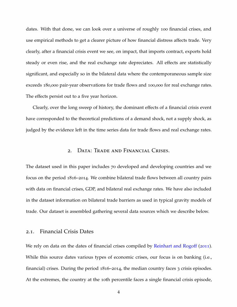
2.4. World Trade and Major Crises

To motivate our analysis, we note that what was witnessed after the global financial crisis

in 2008 was nothing new, especially not the so-called Great Trade Collapse, meaning the fall

in trade volumes relative to GDP. Figure 1 shows the trajectory of world exports/GDP after

the major global financial crises between 1827 and the present. We aggregate total exports

and GDP over this period for a constant set of countries. This limits our world-trade figure

to 10 countries with continuously available trade and GDP data over the 1827–2014 period.

We exclude years of world wars in which trade or GDP data are missing for many countries.

From this graph, the trade collapse following the recent 2008–2009 financial crisis is

unsurprising. Our figure also shows, with vertical dashed lines, the starting dates of the

Panic of 1873 episode, the 1930s Great Depression episode, the 1980s LDC Sovereign-

Financial Crises episode, and the 2008 Great Recession episode. Similar declines in world

trade can be seen to have occurred after each of these episodes. Two years following the

start of the Great Recession in 2008, world exports to GDP in our data had fallen by 0.93

6

Figure 1: World Trade and Major Crises.

This figure is constructed aggregating exports and GDP for a constant sample of the following 10 countries:Australia, Chile, Denmark, Spain, France, United Kingdom, Netherlands, Portugal, Sweden, and the UnitedStates. Vertical dashed lines indicate the starting year of four major world financial crises: the Panic of 1873

episode, the 1930s Great Depression episode, the 1980s LDC Sovereign-Financial Crises episode, and the 2008

Great Recession episode.

.06

.08

.1.1

2.1

4.1

6E

xpor

ts to

GD

P

1820 1850 1880 1910 1940 1970 2000Year

percentage points. This is a similar decline to that in the early 1980s, when the trade to

GDP fell ratio fell by 0.86 percentage points. The impact of the Great Depression, however,

was almost twice as large, with a 1.45 percentage point fall in world trade to GDP.

However, the recovery of trade after the recent “trade collapse” was faster — compared

to output — than that seen in previous episodes. Five years following the start of the Great

Recession the exports-to-GDP ratio was 0.1 percentage points higher than in the year prior

to the start of the crisis, while in the 1980s debt crisis and the Panic of 1873 it was still one

percentage point lower. The Great Depression stands out in this regard. Due perhaps to

7

rising protectionist measures adopted by the U.S. and other countries during this period

(and other rising frictions, such as the collapse of the gold standard) exports-to-GDP were

still more than 3 percentage points lower than in the year prior to the start of the crisis.

This figure nicely motivates our study by revealing an enduring link between crisis

events and trade outcomes. What is obscured in this figure, however, is the uneven impact

of financial crises on imports and exports, and the correlation between those shocks and

the location of the underlying financial crisis events. The remainder of this paper focuses

on those issues with a combination of parsimonious theory and granular empirics.

3. A Crisis-Deleveraging Model: Demand, Supply, and Trade Shocks

We study a small open economy and introduce borrowing limits into both the firm and

household side of the economy. This is guided by our desire to understand whether the

macroeconomic effects of financial crises can be best understood as demand or supply

shocks. In the case of households, this apparatus exactly mirrors the approach of Eggertsson

and Krugman (2012).4 We add the same apparatus to the firm side of the model to make

our modeling of the two shocks conceptually as simple and symmetric as possible.

Formally, we will describe an economy populated by patient and impatient households.

These households derive utility from the consumption of an import good and a non-traded

good. Firms in the economy produce a non-traded good sold locally and an export good

sold abroad. They produce using labor and must borrow from the world to finance a share

of their production cost in advance. Both impatient households and firms face exogenous,

4In related work Benigno and Romei (2014) study how debt deleveraging in one country spreads to therest of theworld economy.

8

binding borrowing limits, and we study the impact on the economy of sudden declines in

the amount that households or firms can borrow.

3.1. Households

We assume that households maximize lifetime utility

U = E0

∞

∑t=0

(βi)t ·(

log(CiMt) + log(Ci

Nt)−Ni1+φ

t1 + φ

),

subject to a budget constraint discussed below, with i ε{B, S} indexing borrowers and savers

and time preference parameters such that βs > βb. We denote by CiM and Ci

N a household’s

consumption of the import good and the non-traded good, respectively. The household

budget constraint supposes that they receive income as a wage for labor supplied to local

firms in the non-traded and export sectors. In addition, patient households (only) own and

receive firm profits.5 The economy faces an exogenous world price of the import good, PM,

and an endogenously determined price of the non-traded good, PN. Households borrow

from, or lend to, the rest of the world at an exogenous real interest rate r, subject to limits.

We assume that the impatient households’ budget constraint is given by

PMt · CbMt + PN t · Cb

N t − Dbt = wt · Nb

t − (1 + rt−1) · Dbt−1 ,

and the binding borrowing constraint we impose on the impatient households is

(1 + rt) · Dbt ≤ D .

5This assumption is for analytical simplicity. It follows Martinez and Philippon (2014), who show that itmay be consequential quantitatively, but not qualitatively.

9

Similarly, we assume that the patient households’ budget constraint is given by

PMt · CsMt + PN t · Cs

N t − Dst = wt · Ns

t +πXt

χ+

πN t

χ− (1 + rt−1) · Ds

t−1 ,

where χ and 1− χ denote the fraction of patient and impatient households in the economy.

Aggregate consumption of each good is the sum of consumption across households:

CMt = χ · CsMt + (1− χ) · Cb

Mt ,

CNt = χ · CsNt + (1− χ) · Cb

Nt .

Finally, aggregate hours supplied are given by:

Nt = χ · Nst + (1− χ) · Nb

t .

3.2. Production

We assume that in both the export and the non-traded sectors there is a continuum of

firms of measure one that produce output using only labor. Firms in the export sector sell

their goods to the rest of the world at the exogenous world price PX, while firms in the

non-traded sector sell their good domestically at a price PN determined in equilibrium.

In both sectors, firms must borrow a fraction λ of their cost to finance production. Firms

borrow from the rest of the world at an exogenous real interest rate r, subject to limits.

10

We assume that the firms’ budget constraint is given by

πt + δt = δt−1 · (1 + rt−1) + πt ,

where δt is the amount borrowed in period t, π denotes profits paid to households, and π

denotes profits excluding the financing cost (revenue minus production cost). We impose a

binding limit δ on the amount firms can borrow.

Firms’ production function is

qt = lt ,

and their cost is Ct(qt, wt) = wt · qt. The borrowing limit restricts the amount firms can

produce. Firms borrow each period λ · Ct = δ, which implies firms produce qt = δ/λ · wt.

3.3. Equilibrium

In equilibrium the non-traded good’s market clears, determining its price PN, where the

condition for demand equals supply is given by

χ · csN t + (1− χ) · cb

N t = qN t .

Finally, we assume wages evolve according to the following Phillips curve:

wt = wt−1 · (1 + κ · (Nt−1 − Nss)) .

This assumption follows Martinez and Philippon (2014). We denote by Nss the steady state

11

level of aggregate hours. The parameter κ regulates the speed of adjustment of wages,

which is proportional to the deviation of aggregate hours from steady state. Wages are

sticky, but in the limit κ → ∞ the economy converges to one with flexible wages. The

reason we adopt this formulation is that slow adjustment in wages prevents changes in

firm borrowing limits from being absorbed immediately into wages, which would impacts

on quantities, including trade, running counter to the empirical evidence, as we see below.

3.4. Calibration

A first set of parameters is chosen directly based on the literature. Following Eggertsson

and Krugman (2012) and Martin and Philippon (2014) we assume half the households are

constrained (χ = 0.5). We assign a value 0.02 to the real interest rate, and set the discount

factor of patient households such that βs = 1/(1 + r). Based on Martinez and Philippon

(2014) we set the slope of the Phillips curve κ = 0.1 and the inverse elasticity of labor supply

φ is set to 1 as in Monacelli (2009).

The remaining parameters are the price of the export good (PX), the price of the import

good (PM), the borrowing limit for impatient households (D), the borrowing limit for firms

(δ), and the fraction of firms’ cost that must be financed before production takes place

(λ). These parameters are set to target the following conditions. First, we target the trade

balance equal to zero. Second, we target the ratio of exports (or imports) to GDP equal to

the post-1990 sample mean (31%). Third, we target the terms of trade equal to one, such

that the price of the import good is equal to the price of the export good. Fourth, we target

the debt to income ratio of impatient households equal to one, and assumption which

follows Eggertsson and Krugman (2012). Finally, we target the ratio of debt to revenue for

12

firms to equal 0.1.

3.5. Simulations

The goal of the model is to permit us to simulate the responses of the economy to delever-

aging shocks to households and firms.

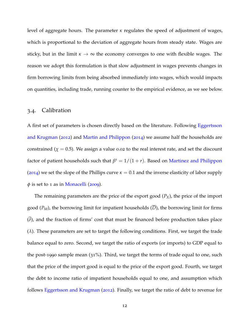
Demand shock We interpret a decline in the borrowing limit for impatient households as

a demand shock. All else equal,such households are forced to spend less on consumption,

given their reduced ability to borrow. On impact, they reduce their consumption as they

borrow a now lower amount but still repay a higher amount borrowed in the previous

period. This reduces demand for both the import and the non-traded good, leading to lower

aggregate demand. In response, the price of the non-traded good falls. Lower demand for

the import good leads to lower imports, while exports do not vary as they depend only on

the borrowing limit to firms. We simulate the response to two types of shocks to impatient

households’ borrowing limit.

Figure 2 graphs the adjustment of exports, imports, the trade balance, and the price and

consumption of the non-traded good in response to each of these shocks. The first shock,

shown in panel A, is an unanticipated permanent decline in the borrowing limit. Given

the fall in GDP, the ratio of exports to GDP rises while imports to GDP fall, as imports fall

further than GDP. The trade balance rises in response to the decline in imports. The price

of the non-traded good falls.

The second shock, in panel B of figure 2, is an unanticipated gradual decline and

subsequent recovery in the borrowing limit, representing a more realistic multi-year finan-

13

cial crisis. This generates initially similar paths for exports, imports and the price of the

non-traded good. All these series, however, recover and “overshoot” beyond the initial level

as the borrowing limit returns to the original. The reason is that as the borrowing limit

falls, constrained households are paying higher level of past debt than they can borrow,

which reduces their consumption. As the borrowing limit increases, the opposite happens,

leading to an increase in their consumption.

Supply shock In turn, we interpret a decline in the borrowing limit for firms as a supply

shock. All else equal, every firm is forced to produce less output from less input, given their

reduced ability to borrow.

The immediate impact is to reduce the production of both the export good and the

non-traded good, as firms in both sectors face a tighter borrowing constraint. Exports fall

directly due to the shock. Further, the price of the non-traded good rises due to a decline

in supply. The shock also lowers wages and firm profits in both sectors. This leads to

lower income to both patient and impatient households. Patient households are able to

smooth the impact of the shock over time, with a minor decline in demand, but impatient

households cannot borrow and translate their lower income fully into lower consumption.

Figure 3 illustrates the adjustment in response to this shock. As before, we simulate the

economy’s adjustment to both an unanticipated permanent decline in the firms’ borrowing

limit (in panel A) and an unanticipated gradual decline and subsequent recovery in the

borrowing limit (in panel B). As with the shock to households, the gradual firm deleveraging

shock in panel B generates a slight “overshooting” in all outcomes.

14

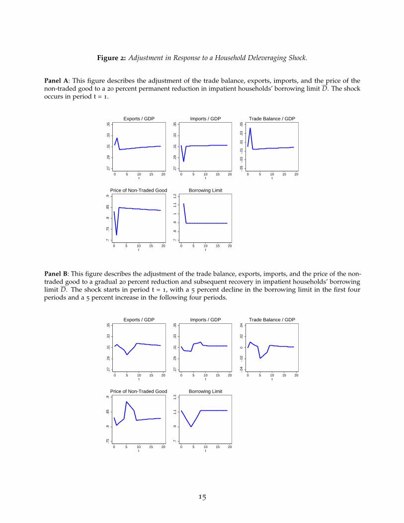
Figure 2: Adjustment in Response to a Household Deleveraging Shock.

Panel A: This figure describes the adjustment of the trade balance, exports, imports, and the price of thenon-traded good to a 20 percent permanent reduction in impatient households’ borrowing limit D. The shockoccurs in period t = 1.

.27

.29

.31

.33

.35

0 5 10 15 20t

Exports / GDP

.27

.29

.31

.33

.35

0 5 10 15 20t

Imports / GDP

-.05

-.03

-.01

.01

.03

.05

0 5 10 15 20t

Trade Balance / GDP

.7.7

5.8

.85

.9

0 5 10 15 20t

Price of Non-Traded Good

.7.8

.91

1.1

1.2

0 5 10 15 20t

Borrowing Limit

Panel B: This figure describes the adjustment of the trade balance, exports, imports, and the price of the non-traded good to a gradual 20 percent reduction and subsequent recovery in impatient households’ borrowinglimit D. The shock starts in period t = 1, with a 5 percent decline in the borrowing limit in the first fourperiods and a 5 percent increase in the following four periods.

.27

.29

.31

.33

.35

0 5 10 15 20t

Exports / GDP

.27

.29

.31

.33

.35

0 5 10 15 20t

Imports / GDP

-.04

-.02

0.0

2.0

4

0 5 10 15 20t

Trade Balance / GDP

.75

.8.8

5.9

0 5 10 15 20t


.7.9

1.1

1.3

0 5 10 15 20t

Borrowing Limit

15

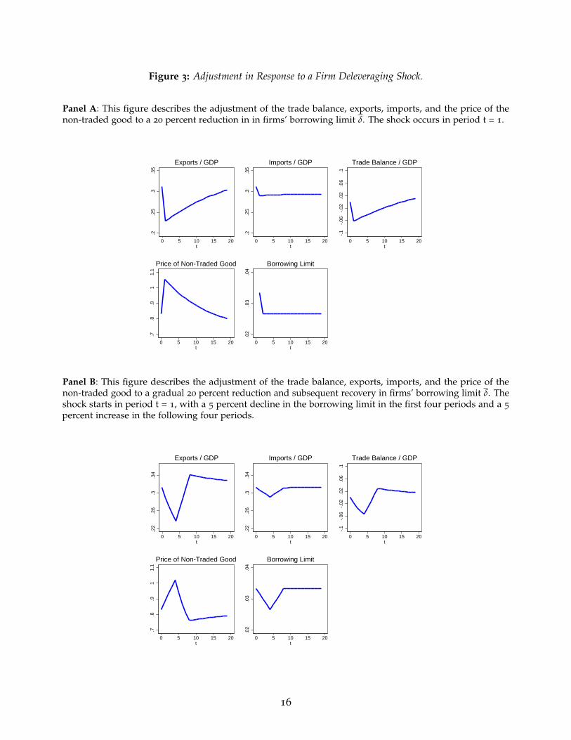
Figure 3: Adjustment in Response to a Firm Deleveraging Shock.

Panel A: This figure describes the adjustment of the trade balance, exports, imports, and the price of thenon-traded good to a 20 percent reduction in in firms’ borrowing limit δ. The shock occurs in period t = 1.

.2.2

5.3

.35

0 5 10 15 20t

Exports / GDP

.2.2

5.3

.35

0 5 10 15 20t

Imports / GDP

-.1

-.06

-.02

.02

.06

.1

0 5 10 15 20t

Trade Balance / GDP

.7.8

.91

1.1

0 5 10 15 20t


.02

.03

.04

0 5 10 15 20t

Borrowing Limit

Panel B: This figure describes the adjustment of the trade balance, exports, imports, and the price of thenon-traded good to a gradual 20 percent reduction and subsequent recovery in firms’ borrowing limit δ. Theshock starts in period t = 1, with a 5 percent decline in the borrowing limit in the first four periods and a 5

percent increase in the following four periods.

.22

.26

.3.3

4

0 5 10 15 20t

Exports / GDP

.22

.26

.3.3

4

0 5 10 15 20t

Imports / GDP

-.1

-.06

-.02

.02

.06

.1

0 5 10 15 20t

Trade Balance / GDP

.7.8

.91

1.1

0 5 10 15 20t


.02

.03

.04

0 5 10 15 20t

Borrowing Limit

16

4. Response of Total Trade Flows to Financial Crises

Our first empirical exercise examines the evolution of countries’ aggregate exports and

imports following financial crises in our historical 1816–2014 panel. We count 172 such crisis

episodes, a third of which occur in the developed countries in our sample. Reinhart and

Rogoff (2009) and others have documented the deep impact of crisis episodes on various

outcomes such as output, unemployment, and government debt, and the pace of recovery.

With the same historical perspective, we will focus on international trade.

We graph the growth rates of real exports, imports and GDP in the years immediately

before and following banking crises. We compute unweighted means across all episodes

for the 70 countries in our sample. We identify the beginning of a crisis in year t and graph

the growth rates of these outcomes in a pre-crisis period, in period t, and in the following

three years. The series are normalized to zero in the pre-crisis baseline period. In each

set of results, we graph real exports (in blue) and GDP (in red) on the left panel and real

imports and GDP on the right. Figure 4(a) illustrates the results for the full set of countries.

Studies of the “trade collapse” during the recent Great Recession document and are

motivated by the very large fall in trade in comparison to output. The first message that

emerges from these figures is that historically this has been the normal behavior of trade

following crises. Both exports and imports fall well beyond GDP. The second message—key

to our main argument in this paper—is that the decline in imports is substantially larger

than the fall in exports. In 4(a), which includes the entire 1816-2014 period and is based

on 172 crisis episodes, the growth rate in real imports one year after a crisis starts (period

t + 1 in the figure) is 11 percentage points lower than in the pre-crisis period, while the

17

t + 1 growth rate in exports is only 4 percentage points lower than in the pre-crisis period.

A third finding from these figures is that the recovery is fairly fast. Growth rates of both

exports and imports are back to normal in the second year after the start of a crisis.

If we exclude the Great Recession, as shown in Figure 4(b), the results are very similar,

with a slightly smaller drop in imports. In the post-WW2 sample shown in 4(c) the fall in

imports is even larger than in the full sample with an average growth rate 14 percentage

points lower than in the pre-crisis period. On the other hand, the fall in export growth rates

in this period is somewhat softer than in the full sample. In the pre-WW2 sample where

our data is less dense, we see drops in imports of similar magnitude compared to the full

sample, but recoveries with much higher growth rates. In the case of exports, the decline is

larger than in the post-WW2 years, and again differently than in this period, growth rates

are above pre-crisis averages after the initial plunge.

We also examine the response of exports and imports in developed and developing

countries separately, as shown in Figures 5 and 6 respectively. We count 14 countries in our

sample as developed and the remaining 56 as developing. While largely our main messages

remain valid for both samples, there are some differences. In the developed-country sample,

during the post-WW2 period, differences in the decline in exports and imports following a

crisis—while still there— are not as marked as in the developing country sample. Second, a

feature of the developing country sample is the magnitude of the impact on imports, which,

in the full sample is almost 50 percent larger. Finally, the results for the pre-WW2 period

in developing countries (in 6(d)) are the only ones for which we don’t observe the larger

post-crisis drop in imports than in exports, although the precision of our estimates for this

limited subsample is considerably lower.

18

Figure 4: Impulse Response: Full Sample.

The red dashed line represents the growth rate of GDP and the blue solid line, the growth rate of exports(left) or imports (right). Shaded regions indicate 90% confidence intervals.

(a) Entire Period

-.2

-.15

-.1

-.05

0.0

5.1

.15

D lo

g

pre-crisis t t+1 t+2 t+3time

Growth Real GDP

Growth Real Exports

Based on 172 crisis episodes

-.2

-.15

-.1

-.05

0.0

5.1

.15

D lo

g


Growth Real GDP

Growth Real Imports


(b) Excluding Great Recession

-.2

-.15

-.1

-.05

0.0

5.1

.15

D lo

g


Growth Real GDP

Growth Real Exports


-.2

-.15

-.1

-.05

0.0

5.1

.15

D lo

g


Growth Real GDP

Growth Real Imports


(c) Post-WW2

-.2

-.15

-.1

-.05

0.0

5.1

.15

D lo

g


Growth Real GDP

Growth Real Exports


-.2

-.15

-.1

-.05

0.0

5.1

.15

D lo

g


Growth Real GDP

Growth Real Imports


(d) Pre-WW2

-.2

-.15

-.1

-.05

0.0

5.1

.15

D lo

g


Growth Real GDP

Growth Real Exports


-.2

-.15

-.1

-.05

0.0

5.1

.15

D lo

g


Growth Real GDP

Growth Real Imports


19

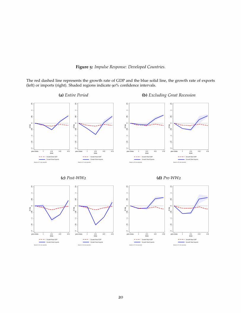
Figure 5: Impulse Response: Developed Countries.


(a) Entire Period

-.2

-.15

-.1

-.05

0.0

5.1

.15

D lo

g


Growth Real GDP

Growth Real Exports


-.2

-.15

-.1

-.05

0.0

5.1

.15

D lo

g


Growth Real GDP

Growth Real Imports



-.2

-.15

-.1

-.05

0.0

5.1

.15

D lo

g


Growth Real GDP

Growth Real Exports


-.2

-.15

-.1

-.05

0.0

5.1

.15

D lo

g


Growth Real GDP

Growth Real Imports


(c) Post-WW2

-.2

-.15

-.1

-.05

0.0

5.1

.15

D lo

g


Growth Real GDP

Growth Real Exports


-.2

-.15

-.1

-.05

0.0

5.1

.15

D lo

g


Growth Real GDP

Growth Real Imports


(d) Pre-WW2

-.2

-.15

-.1

-.05

0.0

5.1

.15

D lo

g


Growth Real GDP

Growth Real Exports


-.2

-.15

-.1

-.05

0.0

5.1

.15

D lo

g


Growth Real GDP

Growth Real Imports


20

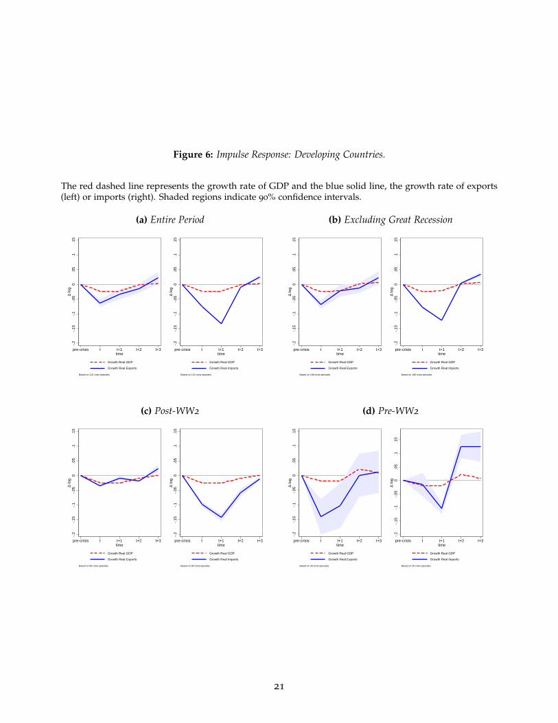
Figure 6: Impulse Response: Developing Countries.


(a) Entire Period

-.2

-.15

-.1

-.05

0.0

5.1

.15

D lo

g


Growth Real GDP

Growth Real Exports


-.2

-.15

-.1

-.05

0.0

5.1

.15

D lo

g


Growth Real GDP

Growth Real Imports



-.2

-.15

-.1

-.05

0.0

5.1

.15

D lo

g


Growth Real GDP

Growth Real Exports


-.2

-.15

-.1

-.05

0.0

5.1

.15

D lo

g


Growth Real GDP

Growth Real Imports


(c) Post-WW2

-.2

-.15

-.1

-.05

0.0

5.1

.15

D lo

g


Growth Real GDP

Growth Real Exports


-.2

-.15

-.1

-.05

0.0

5.1

.15

D lo

g


Growth Real GDP

Growth Real Imports


(d) Pre-WW2

-.2

-.15

-.1

-.05

0.0

5.1

.15

D lo

g


Growth Real GDP

Growth Real Exports


-.2

-.15

-.1

-.05

0.0

5.1

.15

D lo

g


Growth Real GDP

Growth Real Imports


21

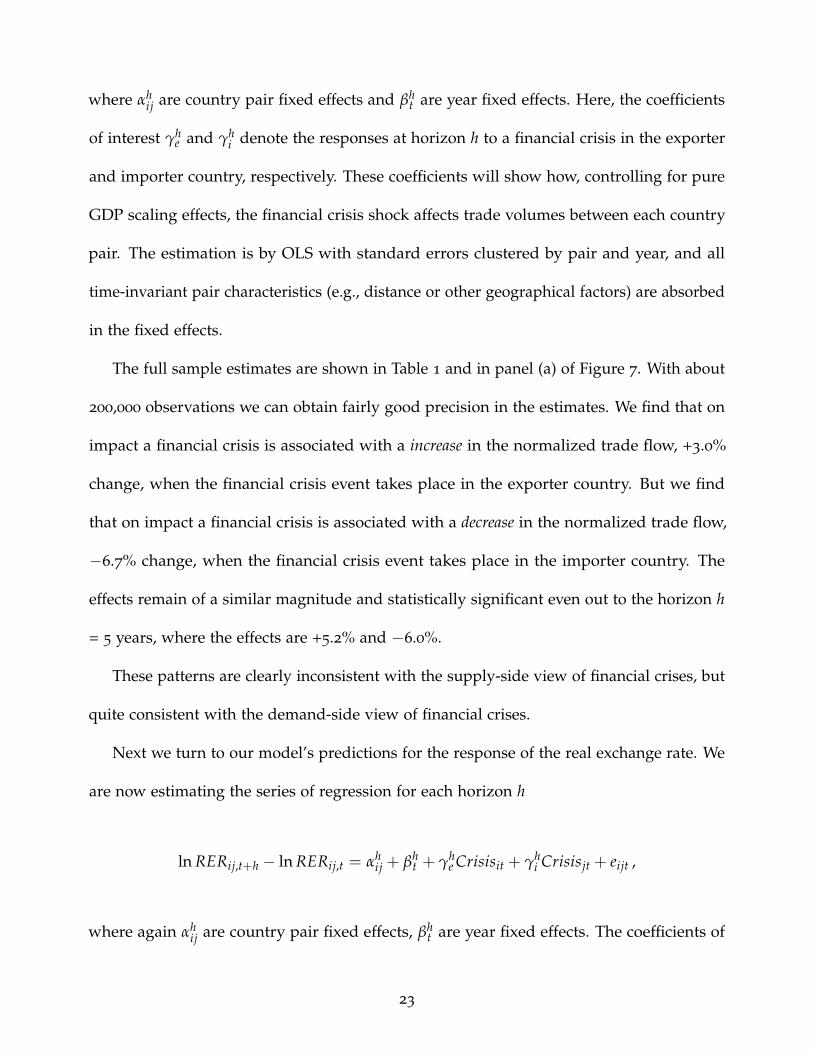
5. Response of Bilateral Trade Flows to Financial Crises

In this section we take our empirical work to the most granular level possible. We now

consider all country pairs, in all years, and look at the post-crisis response of exports,

imports, and the real exchange rate for every given pair-year observation. Not only will

this greatly expand the number of observations, it will also allow us to more exactly control

for the incidence of financial crises potentially affecting one or both trading partners in

any given observation. As a starting point, we treat crises as exogenous events. Later we

will address reverse causality, that is, the concern that financial crisis episodes might be a

“nonrandom treatment” which is endogenous to macroeconomic conditions.

Formally, let ln Tijt be the trade export flow from exporter country i to importer country

j in year t, measured in real constant dollars. In the same units we also measure GDP

levels in the two countries, denoted Yit and Yjt. As is standard gravity models of trade, and

imposing a benchmark unit trade elasticity (homotheticity) with respect to country GDP

size, we examine the size-normalized trade flow given by ln(Tijt/[YitYjt]). We are interested

in the dynamic response of this object, in the aftermath of a financial crisis event in either

country i or country j, or both. Thus, we denote by Crisisit the dummy variable which

indicates the start of a financial crisis event in country i. We then trace out the response

of the normalized trade flow from time t to time t + h across all episodes, using the local

projection method of Jorda (2005) and estimating the series of regression for each horizon h

ln(Tij,t+h/[Yi,t+hYj,t+h])− ln(Tijt/[YitYjt]) = αhij + βh

t + γhe Crisisit + γh

i Crisisjt + eijt ,

22

where αhij are country pair fixed effects and βh

t are year fixed effects. Here, the coefficients

of interest γhe and γh

i denote the responses at horizon h to a financial crisis in the exporter

and importer country, respectively. These coefficients will show how, controlling for pure

GDP scaling effects, the financial crisis shock affects trade volumes between each country

pair. The estimation is by OLS with standard errors clustered by pair and year, and all

time-invariant pair characteristics (e.g., distance or other geographical factors) are absorbed

in the fixed effects.

The full sample estimates are shown in Table 1 and in panel (a) of Figure 7. With about

200,000 observations we can obtain fairly good precision in the estimates. We find that on

impact a financial crisis is associated with a increase in the normalized trade flow, +3.0%

change, when the financial crisis event takes place in the exporter country. But we find

that on impact a financial crisis is associated with a decrease in the normalized trade flow,

−6.7% change, when the financial crisis event takes place in the importer country. The

effects remain of a similar magnitude and statistically significant even out to the horizon h

= 5 years, where the effects are +5.2% and −6.0%.

These patterns are clearly inconsistent with the supply-side view of financial crises, but

quite consistent with the demand-side view of financial crises.

Next we turn to our model’s predictions for the response of the real exchange rate. We

are now estimating the series of regression for each horizon h

ln RERij,t+h − ln RERij,t = αhij + βh

t + γhe Crisisit + γh

i Crisisjt + eijt ,

where again αhij are country pair fixed effects, βh

t are year fixed effects. The coefficients of

23

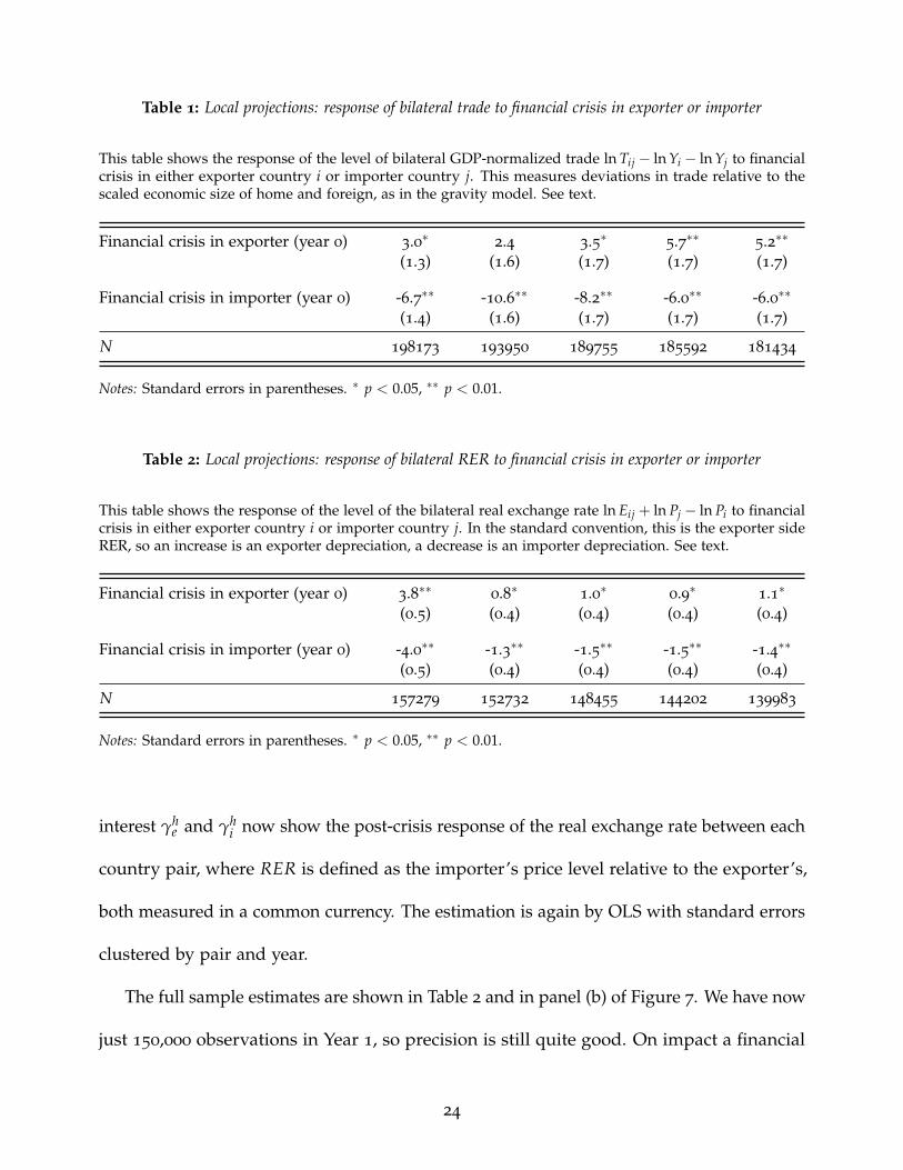
Table 1: Local projections: response of bilateral trade to financial crisis in exporter or importer

This table shows the response of the level of bilateral GDP-normalized trade ln Tij − ln Yi − ln Yj to financialcrisis in either exporter country i or importer country j. This measures deviations in trade relative to thescaled economic size of home and foreign, as in the gravity model. See text.

Financial crisis in exporter (year 0) 3.0∗ 2.4 3.5∗ 5.7∗∗ 5.2∗∗

(1.3) (1.6) (1.7) (1.7) (1.7)

Financial crisis in importer (year 0) -6.7∗∗ -10.6∗∗ -8.2∗∗ -6.0∗∗ -6.0∗∗

(1.4) (1.6) (1.7) (1.7) (1.7)

N 198173 193950 189755 185592 181434

Notes: Standard errors in parentheses. ∗ p < 0.05, ∗∗ p < 0.01.

Table 2: Local projections: response of bilateral RER to financial crisis in exporter or importer

This table shows the response of the level of the bilateral real exchange rate ln Eij + ln Pj − ln Pi to financialcrisis in either exporter country i or importer country j. In the standard convention, this is the exporter sideRER, so an increase is an exporter depreciation, a decrease is an importer depreciation. See text.

Financial crisis in exporter (year 0) 3.8∗∗ 0.8∗ 1.0∗ 0.9∗ 1.1∗

(0.5) (0.4) (0.4) (0.4) (0.4)


(0.5) (0.4) (0.4) (0.4) (0.4)

N 157279 152732 148455 144202 139983


interest γhe and γh

i now show the post-crisis response of the real exchange rate between each

country pair, where RER is defined as the importer’s price level relative to the exporter’s,

both measured in a common currency. The estimation is again by OLS with standard errors

clustered by pair and year.

The full sample estimates are shown in Table 2 and in panel (b) of Figure 7. We have now

just 150,000 observations in Year 1, so precision is still quite good. On impact a financial

24

Figure 7: Local projections: response of bilateral trade and RER to financial crisis in exporter or importer

This figure shows the response of the level of bilateral GDP-normalized trade ln Tij − ln Yi − ln Yj and thelevel of the bilateral real exchange rate ln Eij + ln Pj − ln Pi to financial crisis in either exporter country i orimporter country j. See text.

-15

-10

-50

510

Perc

ent

0 1 2 3 4 5Year

Country i (exporter) financial crisis at time 0Country j (importer) financial crisis at time 0

(a) Bilateral trade (exports from i sold as imports to j)

-50

5Pe

rcen

t

0 1 2 3 4 5Year

Country i (exporter) financial crisis at time 0Country j (importer) financial crisis at time 0

(b) Bilateral RER (exporter i CPI / importer j CPI)

Notes: Shaded regions indicate 90% confidence intervals.

crisis is associated with an appreciation in the real exchange rate, +3.8% change, when the

financial crisis event takes place in the exporter country. But we find that on impact a

financial crisis is associated with a depreciation in the real exchange rate, −4.0% change,

when the financial crisis event takes place in the importer country. Even at horizon h = 5

years, the effects are +1.1% and −1.4% and statistically significant.

Again, the patterns are clearly inconsistent with the supply-side view, but quite consis-

tent with the demand-side view of financial crises.

25

6. Crisis Endogeneity and Inverse Probability Weighting

We address the concern that financial crisis episodes might be endogenous to macroeco-

nomic conditions using the method of inverse probability weighting. This procedure assigns

more influence in our bilateral trade and RER regressions to observations that are relatively

unpredictable by prior macroeconomic conditions. This method has been discussed in a

time series context by Angrist et al. (2017) and applied to the study of financial crises (Jorda

et al. (2011) ; Jorda et al. (2016)) and to the study of fiscal policy (Jorda and Taylor (2016)).

To start, we construct a first-stage estimator of the probability that country c has a

financial crisis at time t. As a predictor of crises, we use credit growth over the five-year

period leading to each crisis (between years t− 6 and t− 1). This choice follows Schularick

and Taylor (2012) who show that credit growth is a powerful predictor of financial crises.6

We fit logit models for the probability of experiencing a financial crisis including either

country or country and year fixed effects.

A successful predictor of our binary outcome (to experience or not a financial crisis)

will maximize the rate of true positives and minimize the rate of false positives. An “ROC”

curve reflects the trade-off between these two goals. The “area under the ROC curve”

statistic summarizes the predictor’s quality in this regard.7 This statistic ranges from 0.5

(for a predictor not different than a random guess) to 1 (for a perfect predictor), and is

independent of the cutoff value used to predict an outcome.

We report the first-stage results in table 3. Column 1 corresponds to the benchmark case

6Credit is measured as domestic credit to GDP and obtained from the World Bank’s World DevelopmentIndicators. Credit data is only available for our wide sample of developed and developing countries for thepost-WWII period.

7See Jorda and Taylor (2011) for a detailed explanation of these concepts.

26

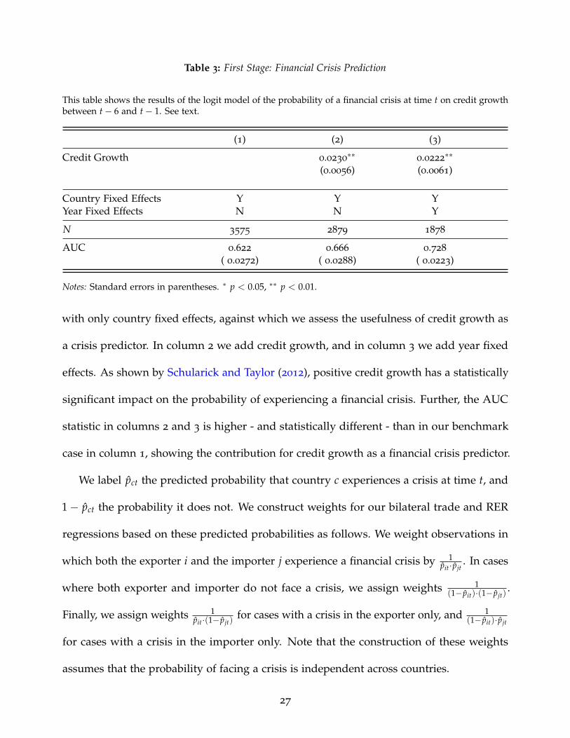
Table 3: First Stage: Financial Crisis Prediction

This table shows the results of the logit model of the probability of a financial crisis at time t on credit growthbetween t− 6 and t− 1. See text.

(1) (2) (3)

Credit Growth 0.0230∗∗

0.0222∗∗

(0.0056) (0.0061)

Country Fixed Effects Y Y YYear Fixed Effects N N Y

N 3575 2879 1878

AUC 0.622 0.666 0.728

( 0.0272) ( 0.0288) ( 0.0223)


with only country fixed effects, against which we assess the usefulness of credit growth as

a crisis predictor. In column 2 we add credit growth, and in column 3 we add year fixed

effects. As shown by Schularick and Taylor (2012), positive credit growth has a statistically

significant impact on the probability of experiencing a financial crisis. Further, the AUC

statistic in columns 2 and 3 is higher - and statistically different - than in our benchmark

case in column 1, showing the contribution for credit growth as a financial crisis predictor.

We label pct the predicted probability that country c experiences a crisis at time t, and

1− pct the probability it does not. We construct weights for our bilateral trade and RER

regressions based on these predicted probabilities as follows. We weight observations in

which both the exporter i and the importer j experience a financial crisis by 1pit· pjt

. In cases

where both exporter and importer do not face a crisis, we assign weights 1(1− pit)·(1− pjt)

.

Finally, we assign weights 1pit·(1− pjt)

for cases with a crisis in the exporter only, and 1(1− pit)· pjt

for cases with a crisis in the importer only. Note that the construction of these weights

assumes that the probability of facing a crisis is independent across countries.

27

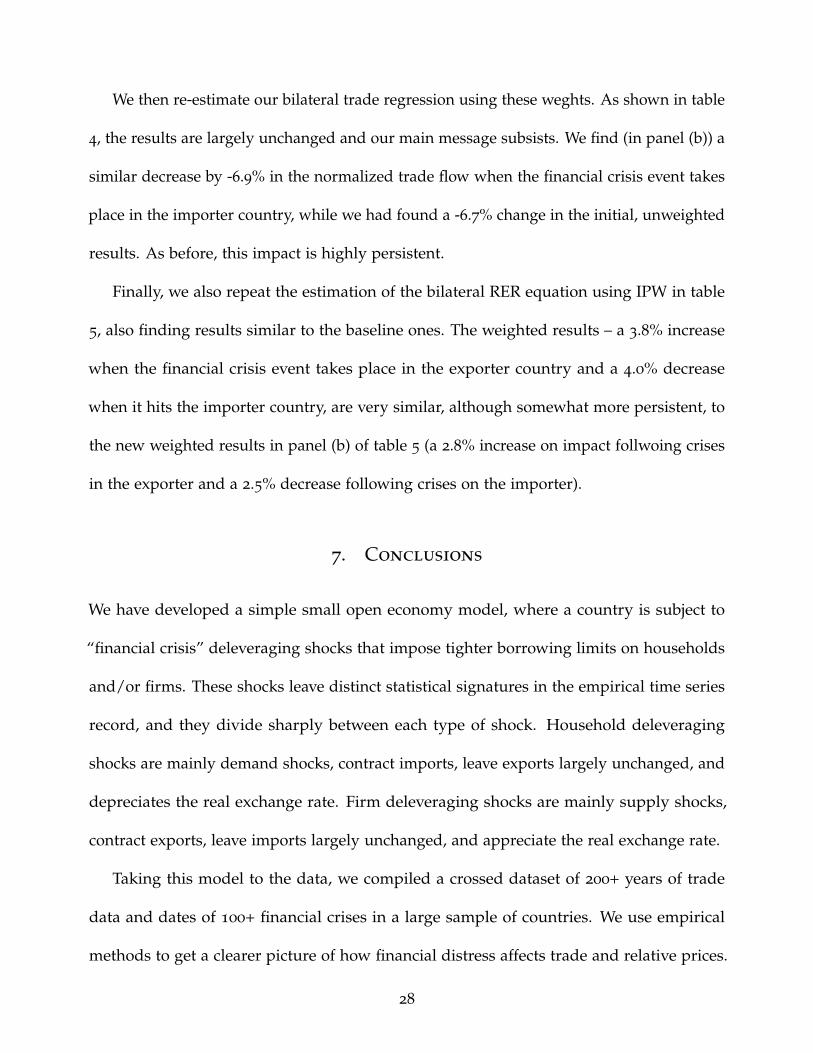
We then re-estimate our bilateral trade regression using these weghts. As shown in table

4, the results are largely unchanged and our main message subsists. We find (in panel (b)) a

similar decrease by -6.9% in the normalized trade flow when the financial crisis event takes

place in the importer country, while we had found a -6.7% change in the initial, unweighted

results. As before, this impact is highly persistent.

Finally, we also repeat the estimation of the bilateral RER equation using IPW in table

5, also finding results similar to the baseline ones. The weighted results – a 3.8% increase

when the financial crisis event takes place in the exporter country and a 4.0% decrease

when it hits the importer country, are very similar, although somewhat more persistent, to

the new weighted results in panel (b) of table 5 (a 2.8% increase on impact follwoing crises

in the exporter and a 2.5% decrease following crises on the importer).

7. Conclusions

We have developed a simple small open economy model, where a country is subject to

“financial crisis” deleveraging shocks that impose tighter borrowing limits on households

and/or firms. These shocks leave distinct statistical signatures in the empirical time series

record, and they divide sharply between each type of shock. Household deleveraging

shocks are mainly demand shocks, contract imports, leave exports largely unchanged, and

depreciates the real exchange rate. Firm deleveraging shocks are mainly supply shocks,

contract exports, leave imports largely unchanged, and appreciate the real exchange rate.

Taking this model to the data, we compiled a crossed dataset of 200+ years of trade

data and dates of 100+ financial crises in a large sample of countries. We use empirical

methods to get a clearer picture of how financial distress affects trade and relative prices.

28

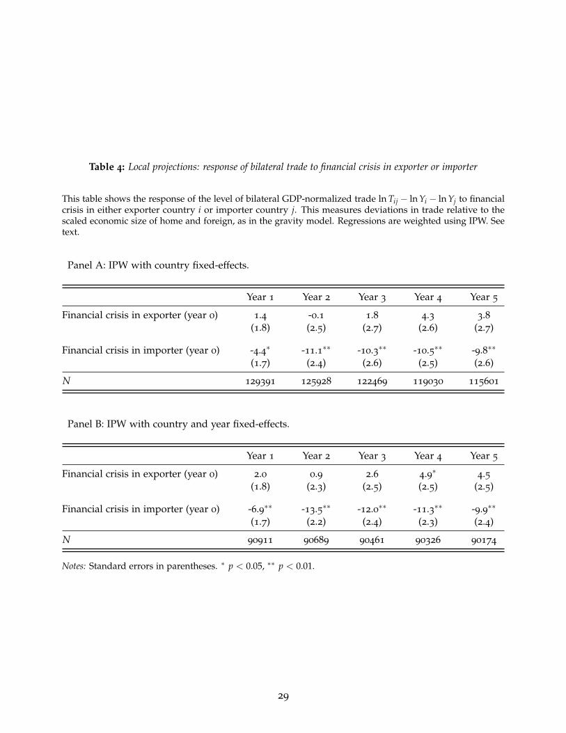
Table 4: Local projections: response of bilateral trade to financial crisis in exporter or importer

This table shows the response of the level of bilateral GDP-normalized trade ln Tij − ln Yi − ln Yj to financialcrisis in either exporter country i or importer country j. This measures deviations in trade relative to thescaled economic size of home and foreign, as in the gravity model. Regressions are weighted using IPW. Seetext.

Panel A: IPW with country fixed-effects.

Year 1 Year 2 Year 3 Year 4 Year 5

Financial crisis in exporter (year 0) 1.4 -0.1 1.8 4.3 3.8(1.8) (2.5) (2.7) (2.6) (2.7)

Financial crisis in importer (year 0) -4.4∗ -11.1∗∗ -10.3∗∗ -10.5∗∗ -9.8∗∗

(1.7) (2.4) (2.6) (2.5) (2.6)

N 129391 125928 122469 119030 115601

Panel B: IPW with country and year fixed-effects.


Financial crisis in exporter (year 0) 2.0 0.9 2.6 4.9∗ 4.5(1.8) (2.3) (2.5) (2.5) (2.5)


(1.7) (2.2) (2.4) (2.3) (2.4)

N 90911 90689 90461 90326 90174


29

Table 5: Local projections: response of bilateral RER to financial crisis in exporter or importer

This table shows the response of the level of the bilateral real exchange rate ln Eij + ln Pj − ln Pi to financialcrisis in either exporter country i or importer country j. In the standard convention, this is the exporter sideRER, so an increase is an exporter depreciation, a decrease is an importer depreciation. Regressions areweighted using IPW. See text.

Panel A: IPW with country fixed-effects.


Financial crisis in exporter (year 0) 3.7∗∗ 0.2 -0.9 1.1 1.0(0.9) (0.6) (0.6) (0.8) (0.8)

Financial crisis in importer (year 0) -2.9∗∗ 0.7 0.5 -0.2 -0.7(0.9) (0.6) (0.6) (0.8) (0.9)

N 112661 108947 105373 101760 98167

Panel B: IPW with country and year fixed-effects.


Financial crisis in exporter (year 0) 2.8∗∗ 0.6 -0.5 1.3∗ 0.7(0.7) (0.5) (0.6) (0.7) (0.7)

Financial crisis in importer (year 0) -2.5∗∗ 0.3 0.3 -0.7 -0.4(0.7) (0.5) (0.6) (0.7) (0.7)

N 81100 79879 78559 77248 75906


30

Very clearly, after a financial crisis event we see, on impact, that imports contract, exports

hold steady or even rise, and the real exchange rate depreciate, with effects persisting for

five years.

Based on both price and quantity evidence from the very long run, a robust interpretation

emerges. History shows that on average financial crises are not, for the most part, a supply

shock. Rather, they are very clearly a negative shock to demand.

31

8. References

Abiad, Abdul, Mishra, Prachi, and Topalova, Petia. 2014. How Does Trade Evolve in theAftermath of Financial Crisesandquest. IMF Economic Review, 62(2), 213–247.

Alessandria, George, Kaboski, Joseph P, Midrigan, Virgiliu, et al. 2010. The Great TradeCollapse of 2008–09: An Inventory Adjustmentandquest. IMF Economic Review, 58(2),254–294.

Amiti, Mary, and Weinstein, David E. 2011. Exports and Financial Shocks. The QuarterlyJournal of Economics, 126(4), 1841–1877.

Angrist, Joshua D, Jorda, Oscar, and Kuersteiner, Guido M. 2017. Semiparametric estimatesof monetary policy effects: string theory revisited. Journal of Business and EconomicStatistics, 1–17.

Baldwin, Richard E. 2009. The great trade collapse: Causes, Consequences and Prospects. Cepr.

Barro, Robert J, and Ursua, Jose F. 2008. Macroeconomic crises since 1870.

Behrens, Kristian, Corcos, Gregory, and Mion, Giordano. 2013. Trade crisis? What tradecrisis? Review of economics and statistics, 95(2), 702–709.

Bems, Rudolfs, Johnson, Robert C, and Yi, Kei-Mu. 2011. Vertical linkages and the collapseof global trade. The American Economic Review, 101(3), 308–317.

Benigno, Pierpaolo, and Romei, Federica. 2014. Debt deleveraging and the exchange rate.Journal of International Economics, 93(1), 1–16.

Chor, Davin, and Manova, Kalina. 2012. Off the cliff and back? Credit conditions andinternational trade during the global financial crisis. Journal of international economics,87(1), 117–133.

Eaton, Jonathan, Kortum, Samuel, Neiman, Brent, and Romalis, John. 2011. Trade and theglobal recession.

Eggertsson, Gauti B, and Krugman, Paul. 2012. Debt, deleveraging, and the liquidity trap:A Fisher-Minsky-Koo approach. The Quarterly Journal of Economics, 127(3), 1469–1513.

Fouquin, Michel, Hugot, Jules, et al. 2016. Two Centuries of Bilateral Trade and GravityData: 1827-2014.

Freund, Caroline L. 2009. The trade response to global downturns: historical evidence.World Bank Policy Research Working Paper Series, Vol.

Glick, Reuven, and Taylor, Alan M. 2010. Collateral damage: Trade disruption and theeconomic impact of war. The Review of Economics and Statistics, 92(1), 102–127.

32

Iacovone, Leonardo, and Zavacka, Veronika. 2009. 13. Banking crises and exports: Lessonsfrom the past for the recent trade collapse. The Great Trade Collapse: Causes, Consequencesand Prospects, 107.

Jorda, Oscar. 2005. Estimation and inference of impulse responses by local projections.American economic review, 161–182.

Jorda, Oscar, and Taylor, Alan M. 2011. Performance evaluation of zero net-investmentstrategies.

Jorda, Oscar, and Taylor, Alan M. 2016. The time for austerity: estimating the averagetreatment effect of fiscal policy. The Economic Journal, 126(590), 219–255.

Jorda, Oscar, Schularick, Moritz, and Taylor, Alan M. 2011. Financial crises, credit booms,and external imbalances: 140 years of lessons. IMF Economic Review, 59(2), 340–378.

Jorda, Oscar, Schularick, Moritz, and Taylor, Alan M. 2016. Sovereigns versus banks: credit,crises, and consequences. Journal of the European Economic Association, 14(1), 45–79.

Levchenko, Andrei A, Lewis, Logan T, and Tesar, Linda L. 2010. The collapse of internationaltrade during the 2008–09 crisis: in search of the smoking gun. IMF Economic review, 58(2),214–253.

Maddison, Angus. 1995. Monitoring the world economy, 1820-1992.

Maddison, Angus. 2001. The World Economy: A Millenial Perspective, Development Centre ofthe Organization for Economic Cooperation and Development.

Martin, Philippe, and Philippon, Thomas. 2014. Inspecting the mechanism: leverage andthe Great Recession in the Eurozone.

Martinez, Joseba, and Philippon, Thomas. 2014. Does a currency union need a capitalmarket union.

Mitchell, B. 1992. International Historical Statistics Europe (1750-1988).

Mitchell, B. 1993. International history statistics: the Americas (1750-1988).

Mitchell, B. 1995. International historical statistics Africa Asia and Oceania (1750-1988).

Monacelli, Tommaso. 2009. New Keynesian models, durable goods, and collateral con-straints. Journal of Monetary Economics, 56(2), 242–254.

Novy, Dennis, and Taylor, Alan M. 2014. Trade and uncertainty.

Reinhart, Carmen M, and Rogoff, Kenneth S. 2009. The aftermath of financial crises.

Reinhart, Carmen M, and Rogoff, Kenneth S. 2011. From financial crash to debt crisis. TheAmerican Economic Review, 101(5), 1676–1706.

Schularick, Moritz, and Taylor, Alan M. 2012. Credit booms gone bust: monetary policy,leverage cycles, and financial crises, 1870–2008. The American Economic Review, 102(2),1029–1061.

33

Appendices

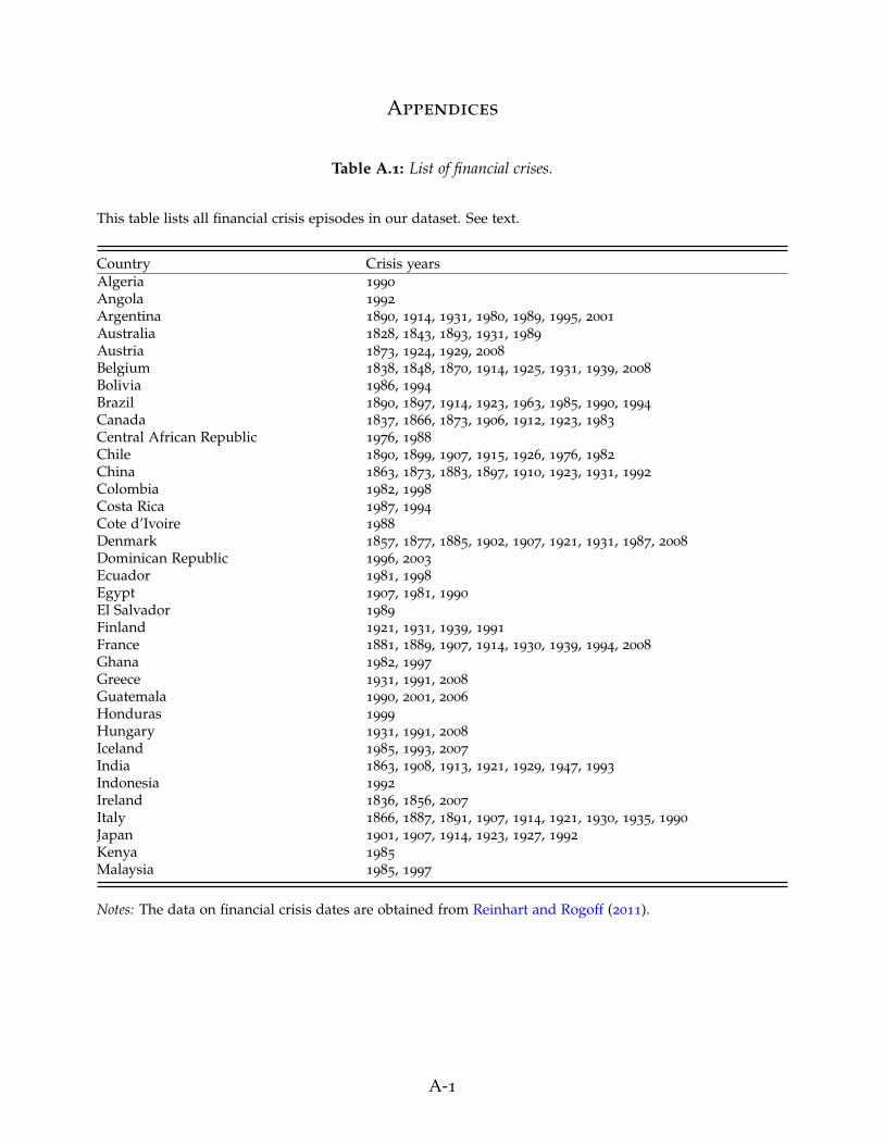
Table A.1: List of financial crises.

This table lists all financial crisis episodes in our dataset. See text.

Country Crisis yearsAlgeria 1990

Angola 1992

Argentina 1890, 1914, 1931, 1980, 1989, 1995, 2001

Australia 1828, 1843, 1893, 1931, 1989

Austria 1873, 1924, 1929, 2008

Belgium 1838, 1848, 1870, 1914, 1925, 1931, 1939, 2008

Bolivia 1986, 1994

Brazil 1890, 1897, 1914, 1923, 1963, 1985, 1990, 1994

Canada 1837, 1866, 1873, 1906, 1912, 1923, 1983

Central African Republic 1976, 1988

Chile 1890, 1899, 1907, 1915, 1926, 1976, 1982

China 1863, 1873, 1883, 1897, 1910, 1923, 1931, 1992

Colombia 1982, 1998

Costa Rica 1987, 1994

Cote d’Ivoire 1988

Denmark 1857, 1877, 1885, 1902, 1907, 1921, 1931, 1987, 2008

Dominican Republic 1996, 2003

Ecuador 1981, 1998

Egypt 1907, 1981, 1990

El Salvador 1989

Finland 1921, 1931, 1939, 1991

France 1881, 1889, 1907, 1914, 1930, 1939, 1994, 2008

Ghana 1982, 1997

Greece 1931, 1991, 2008

Guatemala 1990, 2001, 2006

Honduras 1999

Hungary 1931, 1991, 2008

Iceland 1985, 1993, 2007

India 1863, 1908, 1913, 1921, 1929, 1947, 1993

Indonesia 1992

Ireland 1836, 1856, 2007

Italy 1866, 1887, 1891, 1907, 1914, 1921, 1930, 1935, 1990

Japan 1901, 1907, 1914, 1923, 1927, 1992

Kenya 1985

Malaysia 1985, 1997

Notes: The data on financial crisis dates are obtained from Reinhart and Rogoff (2011).

A-1

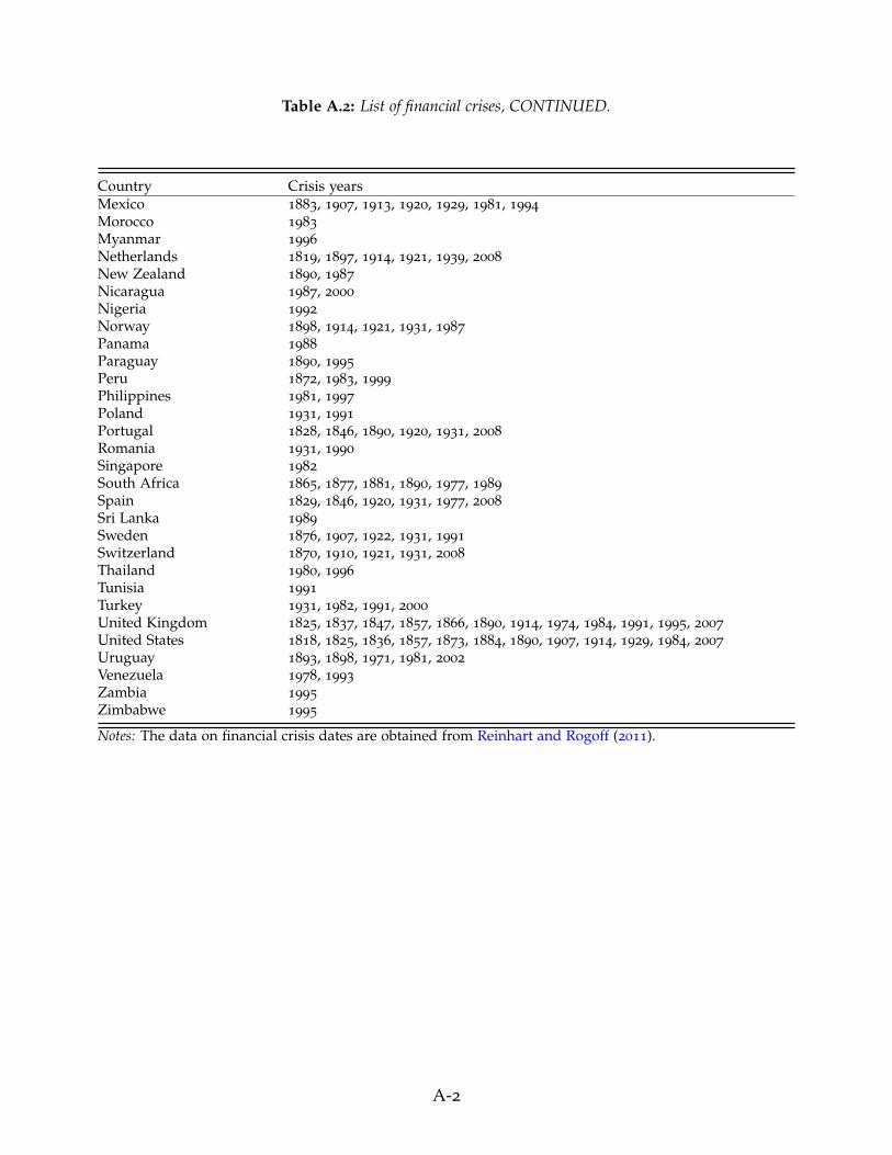
Table A.2: List of financial crises, CONTINUED.

Country Crisis yearsMexico 1883, 1907, 1913, 1920, 1929, 1981, 1994

Morocco 1983

Myanmar 1996

Netherlands 1819, 1897, 1914, 1921, 1939, 2008

New Zealand 1890, 1987

Nicaragua 1987, 2000

Nigeria 1992

Norway 1898, 1914, 1921, 1931, 1987

Panama 1988

Paraguay 1890, 1995

Peru 1872, 1983, 1999

Philippines 1981, 1997

Poland 1931, 1991

Portugal 1828, 1846, 1890, 1920, 1931, 2008

Romania 1931, 1990

Singapore 1982

South Africa 1865, 1877, 1881, 1890, 1977, 1989

Spain 1829, 1846, 1920, 1931, 1977, 2008

Sri Lanka 1989

Sweden 1876, 1907, 1922, 1931, 1991

Switzerland 1870, 1910, 1921, 1931, 2008

Thailand 1980, 1996

Tunisia 1991

Turkey 1931, 1982, 1991, 2000

United Kingdom 1825, 1837, 1847, 1857, 1866, 1890, 1914, 1974, 1984, 1991, 1995, 2007

United States 1818, 1825, 1836, 1857, 1873, 1884, 1890, 1907, 1914, 1929, 1984, 2007

Uruguay 1893, 1898, 1971, 1981, 2002

Venezuela 1978, 1993

Zambia 1995

Zimbabwe 1995


A-2

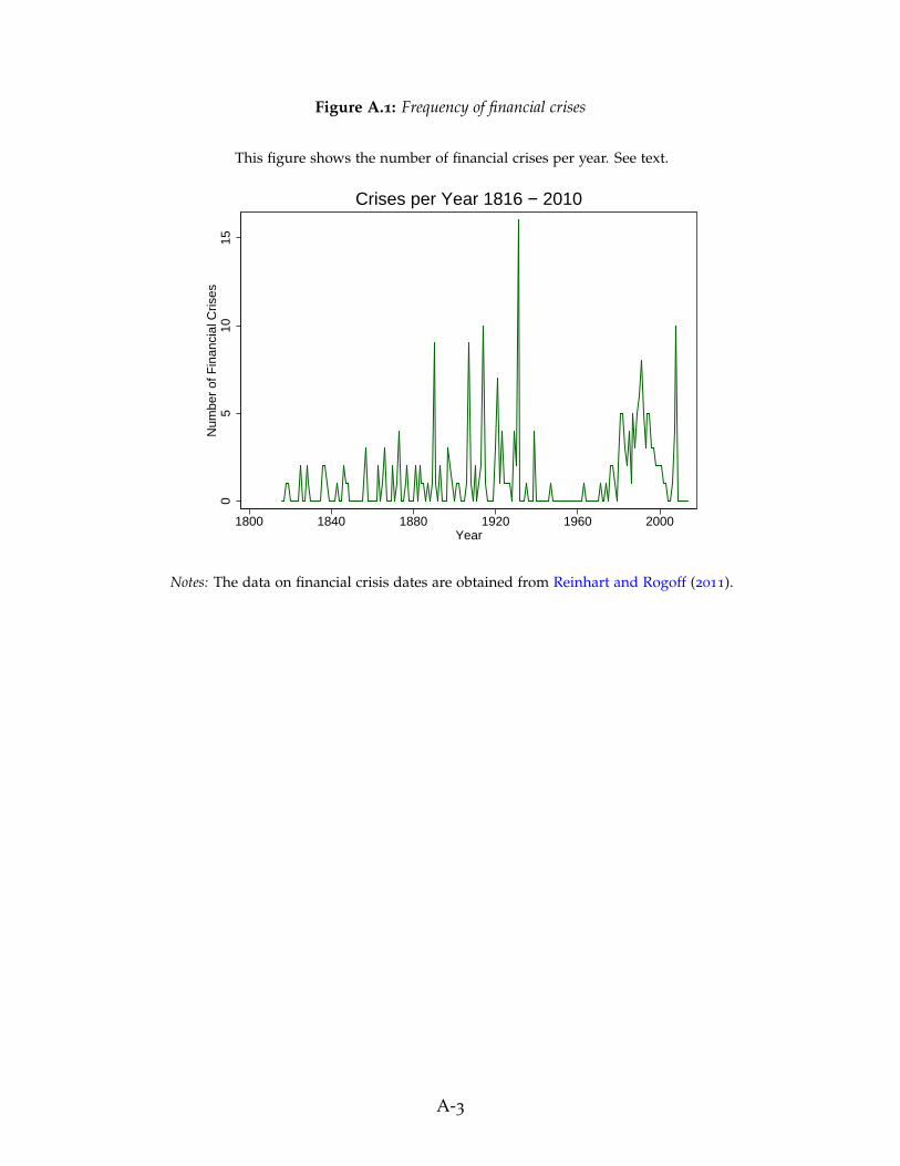
Figure A.1: Frequency of financial crises

This figure shows the number of financial crises per year. See text.

05

1015

Num

ber

of F

inan

cial

Cris

es

1800 1840 1880 1920 1960 2000Year

Crises per Year 1816 − 2010


A-3

Documents

After the Panic: Are Financial Crises Demand or Supply