Embed Size (px)
Citation preview
AFRL-RZ-WP-TR-2009-2206
PROPULSION AND POWER RAPID RESPONSE RESEARCH AND DEVELOPMENT (R&D) SUPPORT Delivery Order 0011: Advanced Propulsion Fuels Research and Development‒Subtask: Framework and Guidance for Estimating Greenhouse Gas Footprints of Aviation Fuels David T. Allen, Charles Allport, Kristopher Atkins, Joyce S. Cooper, Robert M. Dilmore, Laura C. Draucker, Kenneth E. Eickmann, Jeffrey C. Gillen, Warren Gillette, W. Michael Griffin, William E. Harrison III, James I. Hileman, John R. Ingham, Fred A. Kimler III, Aaron Levy, Cynthia F. Murphy, Michael J. O’Donnell, David Pamplin, Greg Schivley, Timothy J. Skone, Shannon M. Strank, Russell W. Stratton, Philip H. Taylor, Valerie M. Thomas, Michael Q. Wang, and Thomas Zidow The Aviation Fuel Life Cycle Assessment Working Group
APRIL 2009 Interim Report
Approved for public release; distribution unlimited.
See additional restrictions described on inside pages
STINFO COPY
AIR FORCE RESEARCH LABORATORY PROPULSION DIRECTORATE
WRIGHT-PATTERSON AIR FORCE BASE, OH 45433-7251 AIR FORCE MATERIEL COMMAND
UNITED STATES AIR FORCE
NOTICE AND SIGNATURE PAGE
Using Government drawings, specifications, or other data included in this document for any purpose other than Government procurement does not in any way obligate the U.S. Government. The fact that the Government formulated or supplied the drawings, specifications, or other data does not license the holder or any other person or corporation; or convey any rights or permission to manufacture, use, or sell any patented invention that may relate to them. This report was cleared for public release by the USAF 88th Air Base Wing (88 ABW) Public Affairs Office (PAO) and is available to the general public, including foreign nationals. Copies may be obtained from the Defense Technical Information Center (DTIC) (http://www.dtic.mil). AFRL-RZ-WP-TR-2009-2206 HAS BEEN REVIEWED AND IS APPROVED FOR PUBLICATION IN ACCORDANCE WITH ASSIGNED DISTRIBUTION STATEMENT. *//Signature// //Signature// WILLIAM E. HARRISON III, AFRL/RZ DOUGLAS L. BOWERS, SES, AFRL/RZ Technical Advisor, Fuels & Energy Director Propulsion Directorate Propulsion Directorate This report is published in the interest of scientific and technical information exchange and its publication does not constitute the Government’s approval or disapproval of its ideas or findings. *Disseminated copies will show “//Signature//” stamped or typed above the signature blocks.
i
REPORT DOCUMENTATION PAGE Form Approved
OMB No. 0704-0188
The public reporting burden for this collection of information is estimated to average 1 hour per response, including the time for reviewing instructions, searching existing data sources, gathering and maintaining the data needed, and completing and reviewing the collection of information. Send comments regarding this burden estimate or any other aspect of this collection of information, including suggestions for reducing this burden, to Department of Defense, Washington Headquarters Services, Directorate for Information Operations and Reports (0704-0188), 1215 Jefferson Davis Highway, Suite 1204, Arlington, VA 22202-4302. Respondents should be aware that notwithstanding any other provision of law, no person shall be subject to any penalty for failing to comply with a collection of information if it does not display a currently valid OMB control number. PLEASE DO NOT RETURN YOUR FORM TO THE ABOVE ADDRESS.
1. REPORT DATE (DD-MM-YY) 2. REPORT TYPE 3. DATES COVERED (From - To)
April 2009 Interim 08 February 2009 – 30 April 2009 4. TITLE AND SUBTITLE
PROPULSION AND POWER RAPID RESPONSE RESEARCH AND DEVELOPMENT (R&D) SUPPORT Delivery Order 0011: Advanced Propulsion Fuels Research and Development‒Subtask: Framework and Guidance for Estimating Greenhouse Gas Footprints of Aviation Fuels
5a. CONTRACT NUMBER
FA8650-08-D-2806-0011 5b. GRANT NUMBER
5c. PROGRAM ELEMENT NUMBER
63216F
6. AUTHOR(S)
David T. Allen, Charles Allport, Kristopher Atkins, Joyce S. Cooper, Robert M. Dilmore, Laura C. Draucker, Kenneth E. Eickmann, Jeffrey C. Gillen, Warren Gillette, W. Michael Griffin, William E. Harrison III, James I. Hileman, John R. Ingham, Fred A. Kimler III, Aaron Levy, Cynthia F. Murphy, Michael J. O’Donnell, David Pamplin, Greg Schivley, Timothy J. Skone, Shannon M. Strank, Russell W. Stratton, Philip H. Taylor, Valerie M. Thomas, Michael Q. Wang, and Thomas Zidow
5d. PROJECT NUMBER
2480 5e. TASK NUMBER
07 5f. WORK UNIT NUMBER
248007P8 7. PERFORMING ORGANIZATION NAME(S) AND ADDRESS(ES)
By: For:
8. PERFORMING ORGANIZATION REPORT NUMBER
The Aviation Fuel Life Cycle Assessment Universal Technology Corporation Working Group 1270 N. Fairfield Road
Dayton, OH 45432-2600
9. SPONSORING/MONITORING AGENCY NAME(S) AND ADDRESS(ES) 10. SPONSORING/MONITORING AGENCY ACRONYM(S)
Air Force Research Laboratory Propulsion Directorate Wright-Patterson Air Force Base, OH 45433-7251 Air Force Materiel Command United States Air Force
AFRL/RZ 11. SPONSORING/MONITORING AGENCY REPORT NUMBER(S)
AFRL-RZ-WP-TR-2009-2206
12. DISTRIBUTION/AVAILABILITY STATEMENT
Approved for public release; distribution unlimited.
13. SUPPLEMENTARY NOTES
PAO Case Number: 88ABW-2009-4320, Clearance Date: 09 October 2009. Report contains color.
14. ABSTRACT
The purpose of this report is to provide a framework and guidance for estimating the life cycle greenhouse gas emissions for transportation fuels, specifically aviation fuels. The focus on aviation fuels was driven by the patterns of fuel use by the federal government. Policies such as those outlined in Section 526 of EISA 2007 cause federal agencies to institute enforceable guidelines for procuring low carbon alternative fuels. Federal consumption of fuels is dominated by the Department of Defense and the Air Force consumes more fuel than any of the other military services or federal agencies (Defense Science Board 2008). Thus, aviation applications may become early adopters of low carbon transportation fuels.
The U.S. Air Force convened a working group of individuals from government agencies, universities and companies actively engaged in assessing greenhouse gas emissions from transportation fuels, and requested that this group develop guidance on procedures for estimating greenhouse gas emissions in aviation applications, using currently available data and tools.
15. SUBJECT TERMS
aviation fuel, carbon footprint, greenhouse gas footprint, aviation footprint, jet fuel footprint, life cycle greenhouse gas emissions, section 526 EISA 2007
16. SECURITY CLASSIFICATION OF: 17. LIMITATION OF ABSTRACT:
SAR
18. NUMBER OF PAGES
134
19a. NAME OF RESPONSIBLE PERSON (Monitor)
a. REPORT Unclassified
b. ABSTRACT Unclassified
c. THIS PAGE Unclassified
William E. Harrison III 19b. TELEPHONE NUMBER (Include Area Code)
N/A
Standard Form 298 (Rev. 8-98) Prescribed by ANSI Std. Z39-18
iii
TABLE OF CONTENTS
Section Page
LIST OF FIGURES ...................................................................................................................... vi
LIST OF TABLES ...................................................................................................................... viii
1.0 EXECUTIVE SUMMARY .................................................................................................. 1
2.0 INTRODUCTION ................................................................................................................ 4
2.1 Background ........................................................................................................................... 4
2.2 Life Cycle Assessments ........................................................................................................ 4
2.3 Characterizing Uncertainties in Life Cycle Assessment of Transportation Fuels ................ 6
2.4 Models in Environment Regulatory Decision-Making ......................................................... 7
2.5 Framework and Guidance for Estimating Life Cycle Greenhouse Gas Emissions for
Aviation Fuels in the Context of Section 526 of EISA 2007 ......................................................... 8
3.0 GUIDING PRINCIPLES AND FUNCTIONAL UNITS ................................................... 10
3.1 Setting the Stage ................................................................................................................. 10
3.2 Types of LCAs .................................................................................................................... 11
3.2.1 Average vs. Marginal LCA .............................................................................................. 11
3.2.2 Attributional vs. Consequential LCAs ............................................................................. 11
3.2.3 Levels of Resolution ........................................................................................................ 12
3.3 Goals and Scope Definition ................................................................................................ 12
3.3.1 Programmatic Goals for Alternative Jet Fuels ................................................................. 12
3.3.2 Conventional Petroleum-Based Fuels: A Baseline for Comparison ............................... 13
3.3.3 LCA Study Goal and Scope Definition ........................................................................... 14
3.4 The Primary Fuel Process Chain......................................................................................... 16
3.4.1 Defining Life-Cycle Stages .............................................................................................. 16
3.4.2 Life-Cycle Boundaries ..................................................................................................... 16
3.4.3 Example Primary Production Chains ............................................................................... 17
3.5 Examining the Life Cycle Stages ........................................................................................ 21
3.5.1 Primary Production Chain Inventory Modeling .............................................................. 21
3.5.2 System Boundary ............................................................................................................. 22
3.5.3 Disaggregation, System Expansion, and Allocation ........................................................ 22
3.5.4 Inventory Data ................................................................................................................. 23
3.6 Scope Definition Parameters ............................................................................................... 24
iv
3.7 Combustion Emissions (Tank-to-Wake)............................................................................. 24
3.8 Functional Unit and Reference Flows................................................................................. 29
4.0 SYSTEM BOUNDARY DEFINITION AND ANALYSIS ............................................... 31
4.1 Background ......................................................................................................................... 31
4.2 System Boundary Determination Approaches .................................................................... 31
4.3 Quantitative Process-Based Approaches to Boundary Definition Using Cutoff Criteria ... 31
4.3.1 The ISO ............................................................................................................................ 31
4.3.2 Critique of Cutoff Criteria Approaches to Boundary Definition ..................................... 33
4.4 Input-Output (IO) Based Approaches to Boundary Definition........................................... 33
4.5 System Boundary Guidance ................................................................................................ 34
4.6 Recommended Method Details ........................................................................................... 35
4.7 Characterization of the Primary Process Chain .................................................................. 36
4.7.1 Identification of the Initial System Boundaries/First Order Processes ............................ 37
4.8 Characterization of Second Order/Secondary Processes .................................................... 39
4.9 Identification of Surrogate Higher Order Process Information .......................................... 41
4.10 Surrogate Data Example ..................................................................................................... 42
4.11 Modeling GHG Emissions For Indirect Land Use Change ................................................ 43
4.11.1 Background ...................................................................................................................... 43
4.11.2 LUC Illustrative Example ................................................................................................ 44
4.11.3 Matching Methodological Assumptions For System Boundary Definition .................... 52
4.11.4 Recommended Steps For Modeling GHG Emissions For Indirect Land Use Change .... 53
4.11.5 References ........................................................................................................................ 54
4.12 Unit Process Exclusions ...................................................................................................... 55
5.0 APPROPRIATE MANAGEMENT OF CO-PRODUCTS ................................................. 56
5.1 Background ......................................................................................................................... 56
5.2 Methods for Allocating Inputs and Outputs Among Co-Products...................................... 56
5.2.1 Allocation by Mass, Energy, or Economic Value of Co-Products .................................. 56
5.2.2 Disaggregation ................................................................................................................. 57
5.2.3 Expansion of System Boundaries .................................................................................... 57
5.3 Discussion of Approaches................................................................................................... 58
5.3.1 Discussion of Allocation by Measures Such as Mass, Energy or Value ......................... 58
5.4 Discussion of Disaggregation ............................................................................................. 60
5.5 Discussion of Displacement ................................................................................................ 62
v
5.5.1 Completeness of the Displacement .................................................................................. 62
5.5.2 Identification of Substitute Production Processes............................................................ 64
5.5.3 Displacement Uniqueness ................................................................................................ 64
5.5.4 System Boundary Consistency ........................................................................................ 64
5.5.5 Time Dependence ............................................................................................................ 64
5.5.6 Consistency With Other GHG Protocols ......................................................................... 64
5.6 Guidance for Attribution and Allocation ............................................................................ 65
6.0 DOCUMENTING DATA QUALITY AND UNCERTAINTY ......................................... 70
6.1 Background ......................................................................................................................... 70
6.2 Data Quality ........................................................................................................................ 70
6.3 Data Sources, Types, and Aggregation ............................................................................... 71
6.4 Dealing With Confidential Data ......................................................................................... 72
6.5 Assessing and Documenting LCA Quality ......................................................................... 72
6.6 Assessing Data Quality ....................................................................................................... 74
6.7 Model Uncertainty .............................................................................................................. 79
6.8 Scenario Uncertainty ........................................................................................................... 81
6.9 Documenting LCA Study Quality and Known Data Limitations ....................................... 83
6.10 Data Limitations.................................................................................................................. 83
6.11 Data Quality Assessment .................................................................................................... 84
6.12 Minimum Guidelines for Reporting Comparative LCA Results ........................................ 85
7.0 CONCLUSIONS................................................................................................................. 88
APPENDIX A
List of Attendees .......................................................................................................................... 90
APPENDIX B
IPCC Global Warming Potentials ................................................................................................ 91
BIBLIOGRAPHY ........................................................................................................................ 94
LIST OF ACRONYMS ............................................................................................................. 100
GLOSSARY .............................................................................................................................. 103

vi
LIST OF FIGURES
Figure Page
1. Greenhouse Gas Emissions (expressed as Global Warming Potential in Units of Equivalent
CO2 Emissions) for 13 Different Assessments of the Well to Tank Emissions for Diesel Fuel
Production (Skone and Gerdes 2008) ............................................................................................ 6
2. Three Objectives That Need to be Balanced With Alternative Fuels ..................................... 10
3. Simplified Schematic of a Life Cycle Primary Production Chain for a Petroleum-Based
Aviation Fuels .............................................................................................................................. 18
4. Simplified Schematic of Life Cycles Stages for the Primary
Production Chain of a Conventional Bio-Oil to Jet Fuel ............................................................. 18
5. Simplified Schematic of Life Cycle Stages for the Primary Production
Chain of a CBTL-Based Jet Fuel Production Chain .................................................................... 19
6. Simplified Schematic f Life Cycle Stages for the Primary Production
Chain of an Algae-Derived Bio-Oil to Jet Fuel ........................................................................... 20
7. Simplified Schematic of Life Cycle Stages for the Primary Production Chain of a Jet Fuel
Created From a Blend of Petroleum-Derived Jet Fuel Stock and a Bio-Derived Jet Fuel Stock 21
8. System Boundary Decision Flow ........................................................................................... 36
9. Simplified Process Schematic Defining First and Second Order Process Flows ................... 40
10. Second Order Process Flows in Algae Production ............................................................... 41
11. Market Interactions and the Scope of the Example Biojet LCA .......................................... 46
12. Example Indirect LUC GHG Emissions (Per Indirect Ha Converted From
Forest to the new crop mix) .......................................................................................................... 48
13. Example Project Life Cycle GHG Emissions: Per mmBTU (30.4 Liters)
Produced Per Year ....................................................................................................................... 50
14. Cumulative Net Jet GHG Emissions With Variation in the Life Cycle Biojet Production
GHG Emissions: Per mmBTU (30.4 Liters) Produced Per Year From 2010-2040.................... 51
15. Processes With More Than One Product Require Decisions About How the Inputs and
Outputs of the Process are to be Allocated to Each Product ........................................................ 56
16. Disaggregation Into Sub-Processes May Reveal Additional Insight Into Co-Product
Allocations ................................................................................................................................... 57
17. An Alternate Process That Produces Product 2 That is the Same as, or Can be
Used as a Substitute for, the Co-Product 2 .................................................................................. 58
18. Tracking the Flow of Products Through Specific Unit Operations at the Refinery Allows
Some Disaggregation of the Inputs and Outputs Among Products and Eliminates Some of the
Need for Allocation (Derived From (Skone and Gerdes 2008)).................................................. 61
19. Illustration of the Process for Developing an Allocation Approach for a Product System .. 66
20. Process for Assessing and Documenting Uncertainty in LCA ............................................. 73

vii
21. Process for Assessing and Documenting Data Uncertainty .................................................. 74
22. Process for Assessing and Documenting Model Uncertainty ............................................... 80
23. Process for Assessing and Documenting Scenario Uncertainty ........................................... 82
viii
LIST OF TABLES
Table Page
1. Certification and Use Goals for the Commercial Aviation Sector
(as Represented by CAAFI and the US Air Force)...................................................................... 13
2. Definition of Life Cycle Goal for Alternative Aviation Production/Consumption Chains .... 15
3. Example of an Alternative Aviation Fuel Life Cycle Greenhouse Gas Study Design ........... 24
4. Compositional Properties and Emissions Indices (EI) for CO2, H2O, and SOx ...................... 25
5. Uncertainties, Gaps, and Issues for the Use of GWP to Examine Emissions From
Aviation That Impact Global Climate Change. (Wuebbles, Yang and Herman 2008) ............... 28
6. Commercial and Military Jet Fuel Standards for the United States,
United Kingdom and Canada ....................................................................................................... 29
7. Global Warming Potential of Greenhouse Gases (IPCC, 2007) ............................................. 30
8. Life Cycle Stage Descriptions ................................................................................................ 38
9. CTL Process Primary Inputs and Outputs .............................................................................. 39
10. Indirect Land Use Assumptions Used in the Example (For Illustrative Purposes Only) ..... 45
11. GHG Emissions Associated With Indirect Land Conversion for the Biojet LCA
Example (Per Indirect Ha Converted, See Table 12 for the Data and Equations Used) .............. 47
12. Estimation of GHG Emissions for Indirect Land Conversion
(Per Indirect Ha Converted) ......................................................................................................... 48
13. Allocation of Emissions Between Soy Oil and Soybean Meal (Wong 2008) ...................... 59
14. Allocation Based on Mass, Energy and Value for a Refinery
(Wang, Lee and Molberg 2004) ................................................................................................... 59
15. Allocation of Energy Use Based on Plant- and Process-Level Analyses of a Petroleum
Refinery (Wang, Lee and Molberg 2004) .................................................................................... 62
16. Allocation of GHG Emissions Between Soy Oil and Soybean Meal
(Wong, 2008, Table 56) ............................................................................................................... 63
17. Example Alternative Aviation Fuel Life Cycle Greenhouse Gas Study Design .................. 70
18. Example Data Quality Matrix (Adapted From (Weidema and Wesnaes 1996)) .................. 76
19. Data Quality Assessment of Study Methodology and Results
(Adapted From (ISO 2006b))....................................................................................................... 84
20. Example of Completed Data Quality Assessment of Study Methodology and Results ...... 85

1
1.0 EXECUTIVE SUMMARY
A number of governmental agencies and non-governmental organizations have developed or are
developing requirements for defining and regulating the emissions of greenhouse gases (GHG)
resulting from the production, transport, and consumption of transportation fuels. This
Framework and Guidance Document was developed specifically in response to the Energy
Independence and Security Act (EISA) of 2007, enacted into law on December 19, 2007. EISA
7 placed a unique greenhouse gas emission requirement on all Federal agencies; specifically,
Section 526 provides that:
No Federal agency shall enter into a contract for procurement of an alternative or synthetic fuel,
including a fuel produced from nonconventional petroleum sources, for any mobility-related use,
other than for research or testing, unless the contract specifies that the lifecycle greenhouse gas
emissions associated with the production and combustion of the fuel supplied under the contract
must, on an ongoing basis, be less than or equal to such emissions from the equivalent
conventional fuel produced from conventional petroleum sources.
In order for Federal agencies procurement of mobility-related fuels to be in compliance with Sec.
526 of EISA, producers of alternative and synthetic fuels must be able to demonstrate the fuel’s
GHG emissions is less than or equal to fuel produced from conventional petroleum sources. The
first step is to establish GHG emissions baselines for conventional fuels produced from
conventional petroleum sources. Once these baselines are established, producers of alternative
and synthetic fuels can then determine if the fuel is Sec. 526 compliant.
To determine whether alternative and synthetic fuels are Sec. 526 compliant, the producer must
assess all GHG emissions; from production field to vehicle fuel tank and from fuel tank to
vehicle exhaust. This scope of emission assessment is commonly referred to as a “well-to-
wheels”, or in the case of aviation, a “well-to-wake” analysis. To ensure a standardized process
for determining Sec. 526 compliance, Life Cycle Assessments (LCA) for both a baseline
petroleum fuel and alternative fuels must be developed.
This Framework and Guidance Document was developed to define the LCA methodologies and
data required for generating the emissions information on specific fuels at specific locations from
defined feedstocks. The life cycle emissions analysis provides the quantitative information for
the Defense Energy Support Center (DESC), or other agencies responsible for procurement, to
assess compliance with Federal statute.
The U.S. Air Force is the largest user of aviation fuel in the Department of Defense and the lead
agency for testing and certifying alternative fuels. In 4 Sep 2008, the AF convened a working
group of individuals from diverse government agencies, universities, and corporations who are
actively engaged in assessing greenhouse gas emissions from transportation fuels. Under the Air
Force’s leadership, this group developed this guidance on procedures for estimating greenhouse
gas emissions in aviation applications. The working group met four times in the Fall of 2008 and
the Spring of 2009 to define issues, review practices, and make recommendations. This report
documents the findings and recommendations of the group.
Finding: Although there have been extensive analyses of the greenhouse gas emissions
associated with petroleum based fuels and alternative fuels, there are still substantial
uncertainties associated with these estimates. Even for well established fuel systems with
extensive data availability, differences in excess of 10% are common in estimates of life cycle
2
greenhouse gas emissions based on assumptions used in the analyses. Some uncertainties and
modeling differences are much larger. In regulatory contexts, model uncertainties such as these
are generally characterized by comparing model predictions to measurements. While the
greenhouse gas emissions associated with the individual components of a life cycle are directly
measurable, such as the emissions from a vehicle hauling fuel from refinery to market, many of
the elements in the life cycle emissions of a fuel system are not directly measurable. Therefore,
the collective emissions are not directly measurable. This makes evaluating greenhouse gas
emissions a model-dependent exercise.
Recommendation: In developing greenhouse gas emission estimates, in addition to
specifying the magnitude of the emissions, data and modeling details must be specified. The specifications should include methods used to determine what should be included in the
analysis and what could be omitted (system boundaries), how processes producing multiple
products (e.g., food and fuel) could be computationally handled, and how inventory data quality
and uncertainty should be assessed.
Finding: Complying with EISA will require the comparison of life cycle greenhouse gas
emissions associated with proposed synthetic and alternative fuels to an aviation fuel life
cycle baseline; however, there is not currently an official aviation fuel baseline for
comparison. Providers of both conventional and alternative fuels are using different data and
methods to determine life cycle greenhouse gas emissions, leading to confusion by reviewers of
the information. A baseline determined by using a standardized set of LCA methodology is
required. Such a baseline is critical to the development of system boundaries for the
development of comparative assessments of synthetic and alternative fuels under EISA
consideration.
Recommendation: To facilitate comparative analyses of emissions required by EISA, a
baseline for greenhouse gas emissions from aviation fuels derived from conventional
petroleum sources must be developed. This baseline should describe the methodologies and
the data used. It should be transparent in its data sources and should present uncertainty
estimates. The baseline should also recognize that, as the sources of oil and the characteristics of
oil production and refining change, greenhouse gas emissions are likely to change over time even
for conventional petroleum fuels.,.
Finding: The evaluation of greenhouse gas emissions from alternative and synthetic fuels is
likely to involve processes and modeling needs that are not included in the evaluation of
fuels from petroleum based sources. These might include processes such as irrigation,
fertilization, separation of materials such as algae oils from water, and conversion of land from
one type of use to another, changing the carbon stored in the land.
Recommendation: Guidance for modeling anticipated processes for alternative fuels
should be provided. Methodological guidance is needed in as many of these alternative fuel
operations as can be anticipated, providing a framework for agencies responsible for
procurement to assess compliance under EISA.
Recommendation: Once published use the framework document as a basis for a few case
studies to help establish best practices for LCA analysis of jet fuels.
This report provides methodological guidance for the development of greenhouse gas emission
estimation from aviation fuels and is based on the collective consensus of a working group with
3
extensive experience in aviation fuels and LCAs. The methodological guidance is directed
toward the analysts who will perform and interpret the LCAs of fuel systems. The
methodological guidance addresses issues of system boundaries, allocation and data quality and
the need for comprehensive analyses, transparency of methodologies and data, and well-
characterized uncertainties. The work group anticipates this methodological guidance will
evolve over time and the modeling of life cycle greenhouse gas emissions from transportation
fuels will have its own life cycle. This report is intended as a first step toward a well
documented and evolving approach to applying life cycle greenhouse gas emission models in a
regulatory or contractual context.
4
2.0 INTRODUCTION
2.1 Background
Although there have been extensive analyses of the greenhouse gas emissions associated with
petroleum based fuels and alternative fuels, there are still substantial uncertainties associated
with some of the estimates of the greenhouse gas impacts of these fuel systems. Nevertheless, a
variety of governmental agencies and non-governmental organizations are developing
approaches for estimating or regulating the emissions of greenhouse gases associated with the
production and use of transportation fuels. Specifically Congress included Section 526 in the
EISA of 20071 that states:
No Federal agency shall enter into a contract for procurement of an alternative or synthetic fuel,
including a fuel produced from nonconventional petroleum sources, for any mobility-related use,
other than for research or testing, unless the contract specifies that the lifecycle greenhouse gas
emissions associated with the production and combustion of the fuel supplied under the contract
must, on an ongoing basis, be less than or equal to such emissions from the equivalent
conventional fuel produced from conventional petroleum sources.
In addition, a number of states are considering greenhouse gas emission regulations. For
example, the California Global Warming Solutions Act of 20062 has resulted in draft regulations
that establish a limit for life cycle greenhouse gas emissions of transportation fuels.
Both the California low carbon fuel standard and Section 526 of EISA require a life-cycle
evaluation of the greenhouse gas emissions of transportation fuels, and this is becoming a
common approach to considering greenhouse gas emissions. Employing a life cycle approach in
estimating greenhouse gas emissions from the production and use of transportation fuels means
assessing all emissions from field to the vehicle tank and from tank to vehicle exhaust. This
scope of emissions assessment is frequently referred to as a “well-to-wheels”, or in the case of
aviation, a “well-to-wake” analysis.
With the significant interest in both the Department of Defense (DOD) and the civil aviation
community to purchase only alternative fuels that are in compliance with emerging greenhouse
gas emission requirements, a consistent framework for conducting a LCA of greenhouse gas
emissions must be developed to assure that candidate fuels are adequately evaluated for
environmental compliance.
2.2 Life Cycle Assessments
There is some variability in LCA terminology, but the most widely accepted terminology has
been codified by the International Standards Organization (ISO 14000 series of standards3) and
international groups convened by the Society for Environmental Toxicology and Chemistry
(SETAC) (see, for example, (Consoli, et al. 1993); (Allen, Consoli, et al. 1997)). Therefore, the
terminologies employed by these organizations and governmental agencies, such as the
California Air Resources Board, the U.S. Environmental Protection Agency, and the European
Environment Agency, are employed in this report. Definitions of life cycle terminology are
1 HR 6, available at: http://frwebgate.access.gpo.gov/cgi-bin/getdoc.cgi?dbname=110_cong_bills&docid=f:h6enr.txt.pdf 2 AB 32, available at: http://www.leginfo.ca.gov/pub/05-06/bill/asm/ab_0001-0050/ab_32_bill_20060927_chaptered.pdf 3 Available at: http://www.iso.org/iso/iso_14000_essentials
5
provided in the Glossary, so detailed explanations of commonly used terms will not be provided
in the text of the report.
As applied to the estimation of greenhouse gas emissions from transportation fuels, the steps in a
LCA are as follows ((Allen and Shonnard 2001), (ISO 2006a), (ISO 2006b)):
Step 1: Determine the goal and scope of the assessment. Goal and scope definition articulates
the intended application and scope of the LCA by defining what the system will produce and
what processes and impacts will be studied. Multiple choices are made at this stage, which have
the potential to significantly impact the results of the assessment. For example and depending on
the study goal, an LCA can be scoped to quantify climate change impacts based on the heat
released by a fuel (e.g. kg CO2e/mmBTU or g CO2e/MJ) or the distance traveled by a vehicle
using the fuel (e.g., kg CO2e/vehicle mile traveled). Further, an LCA can be based on
greenhouse gas data representing the operation of a specific fuel refinery, or data representing
the average operations of all refineries in a state, region, or nation. Also, the contribution to
climate change might be estimated to include not only industrial and combustion related
greenhouse gas emissions but also the implications of changes in land use at local, regional,
national or global scales.
Step 2: Develop an inventory of the greenhouse gas emissions throughout the life cycle
system. In an LCA, inventory analysis prepares an account of inputs and outputs to the fuel
production system based on the technologies applied. For example, inputs to the production
system might include crude oil, iron ore, and water while outputs might include emissions of
greenhouse gases. Again, multiple choices are made by the life cycle practitioner at this stage,
which have the potential to significantly impact the results of the analysis. Among the sets of
choices in inventory analysis are selecting time periods and spatial scales for data gathering,
strategies for filling data gaps, and computational considerations for managing the variety of
products produced by the processes within the system. An example of how the time period for
data collection may influence the results of an inventory analysis is provided by considering the
petroleum-based fuel greenhouse gas emission baseline as of 2005, pursuant to Title II, Subtitle
A, Sec. 201 of EISA. In 2005, disruptions due to Hurricanes Katrina and Rita had substantial
impacts on refining operations. Other years without these disruptions may have different
greenhouse gas emission characteristics, suggesting that the choice of the year of data collection
may be significant. Petroleum refining also provides an example of the impact of choices for
managing the variety of products produced by the processes in the system. A simple example is
the allocation selection methodology associated with analyzing the greenhouse gas emissions
associated with a refinery unit operation such as the crude oil distillation unit. Specifically,
petroleum entering a refinery is separated into lighter (e.g. gasoline) and heavier (e.g., lubrication
oils, heavy (bunker) fuels) components in a distillation unit that consumes energy and
consequently has greenhouse gas emissions. If the unit produces a pound of gasoline for every
pound of bunker fuel, should the energy use and emissions from the unit be assigned equally to
the two products? Should the assignment be based on the relative economic value or the relative
heating values of the products? The choice can influence the results of the analysis, as
demonstrated in case studies cited in Section 5.0.
Step 3: Assess the climate change impacts of the life cycle inventory. For greenhouse gas
emissions, assessment of global warming potentials (GWPs) is usually performed using factors
6
developed by the Intergovernmental Panel on Climate Change (IPCC 2007)4; however, choices
that influence results are still made in analyses at this stage. For example, it is recognized that
the altitude at which emissions occur can influence climate change impacts. Depending on the
assumptions made regarding GWPs of emissions at altitude, aviation fuels that have different
emissions at altitude may have very different greenhouse gas emission profiles. This issue is
described in more depth in Section 3.0.
Further, many LCAs consider only high volume emissions (e.g., emissions of CO2, CH4, and
N2O), omitting consideration of other greenhouse gas emissions and the influence of land use
changes. As the scientific understanding of climate change is still developing, typical and
simplifying assumptions can influence the results of the LCAs. Specifically, land use changes
(e.g., those associated with crop-based fuels) can result in changes in the ability of soils to store
carbon, changing carbon balances, resulting in changes to the climate system. The time scales
over which these changes occur are not well understood, so evaluating GWPs such as the 100-
year time horizon global warming potential requires assumptions that may influence results.
Step 4: Interpretation of the LCA results. Interpretation explains the LCA results, including
the investigations of data quality, parameter sensitivity, and data and model uncertainty within
the context of the goal of the study. Important issues for interpretation are presented and
discussed in Section 6.0.
2.3 Characterizing Uncertainties in Life Cycle Assessment of Transportation Fuels
Assumptions, methodological choices, strategies for filling data gaps, and other factors
throughout the life cycle substantially influence the results of life cycle greenhouse gas
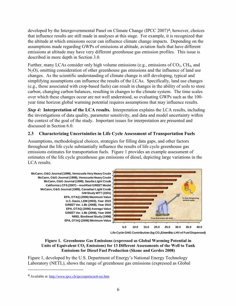
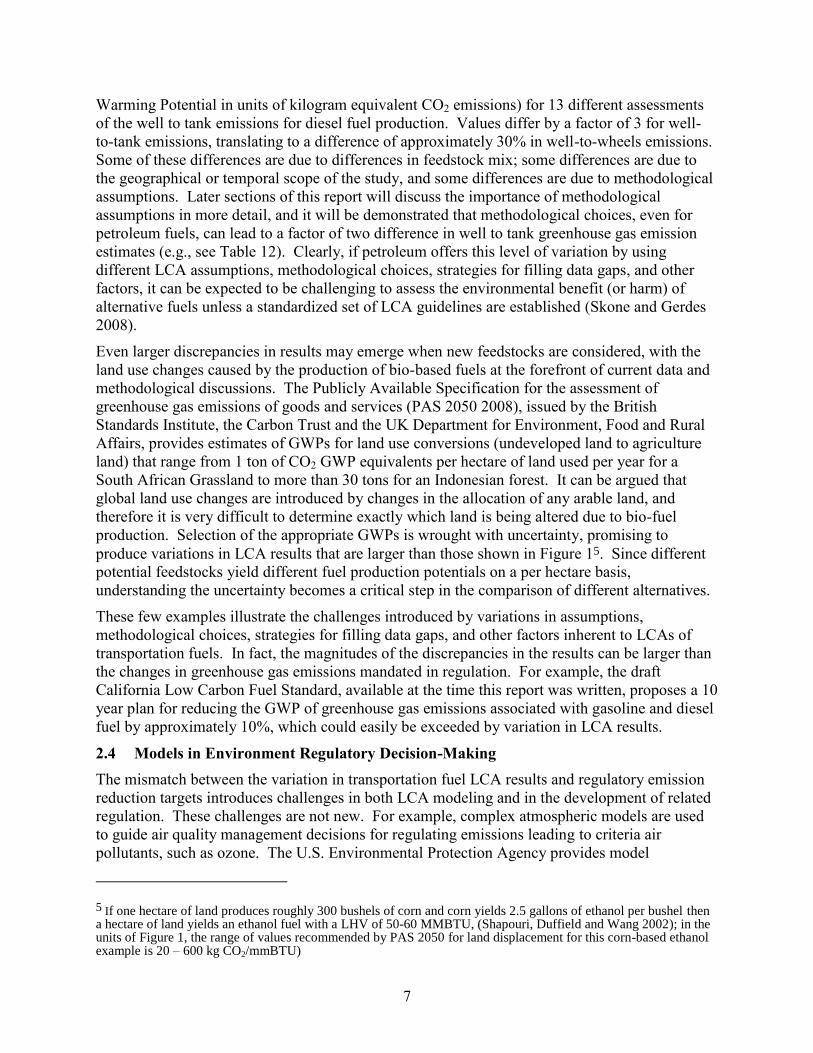
emissions estimates for transportation fuels. Figure 1 provides an example assessment of
estimates of the life cycle greenhouse gas emissions of diesel, depicting large variations in the
LCA results.
Figure 1. Greenhouse Gas Emissions (expressed as Global Warming Potential in
Units of Equivalent CO2 Emissions) for 13 Different Assessments of the Well to Tank
Emissions for Diesel Fuel Production (Skone and Gerdes 2008)
Figure 1, developed by the U.S. Department of Energy’s National Energy Technology
Laboratory (NETL), shows the range of greenhouse gas emissions (expressed as Global
4 Available at: http://www.ipcc.ch/ipccreports/ar4-syr.htm
McCann, O&G Journal (1999), Venezuela Very Heavy Crude
McCann, O&G Journal (1999), Venezuela Heavy Crude
McCann, O&G Journal (1999), Saudia Light Crude
California LCFS (2007) –modified GREET Model
McCann, O&G Journal (1999), Canadian Light Crude
GM Study WTT (2201)
EPA, OTAQ (2006) Maximum Value
U.C. Davis, LEM (2003), Year 2015
GREET Ver. 1.8b (2008), Year 2010
EPA, OTAQ (2006) Average Value
GREET Ver. 1.8b (2008), Year 2005
NREL Biodiesel Study (1998)
EPA, OTAQ (2006) Minimum Value
Life Cycle GHG Contribution (kg CO2E/mmBtu LHV of Fuel Dispensed)
40.035.030.025.020.015.010.05.0
. . . To Fuel Dispensing(vehicle tank).
From Extraction (oil well) . . .
7
Warming Potential in units of kilogram equivalent CO2 emissions) for 13 different assessments
of the well to tank emissions for diesel fuel production. Values differ by a factor of 3 for well-
to-tank emissions, translating to a difference of approximately 30% in well-to-wheels emissions.
Some of these differences are due to differences in feedstock mix; some differences are due to
the geographical or temporal scope of the study, and some differences are due to methodological
assumptions. Later sections of this report will discuss the importance of methodological
assumptions in more detail, and it will be demonstrated that methodological choices, even for
petroleum fuels, can lead to a factor of two difference in well to tank greenhouse gas emission
estimates (e.g., see Table 12). Clearly, if petroleum offers this level of variation by using
different LCA assumptions, methodological choices, strategies for filling data gaps, and other
factors, it can be expected to be challenging to assess the environmental benefit (or harm) of
alternative fuels unless a standardized set of LCA guidelines are established (Skone and Gerdes
2008).
Even larger discrepancies in results may emerge when new feedstocks are considered, with the
land use changes caused by the production of bio-based fuels at the forefront of current data and
methodological discussions. The Publicly Available Specification for the assessment of
greenhouse gas emissions of goods and services (PAS 2050 2008), issued by the British
Standards Institute, the Carbon Trust and the UK Department for Environment, Food and Rural
Affairs, provides estimates of GWPs for land use conversions (undeveloped land to agriculture
land) that range from 1 ton of CO2 GWP equivalents per hectare of land used per year for a
South African Grassland to more than 30 tons for an Indonesian forest. It can be argued that
global land use changes are introduced by changes in the allocation of any arable land, and
therefore it is very difficult to determine exactly which land is being altered due to bio-fuel
production. Selection of the appropriate GWPs is wrought with uncertainty, promising to
produce variations in LCA results that are larger than those shown in Figure 15. Since different
potential feedstocks yield different fuel production potentials on a per hectare basis,
understanding the uncertainty becomes a critical step in the comparison of different alternatives.
These few examples illustrate the challenges introduced by variations in assumptions,
methodological choices, strategies for filling data gaps, and other factors inherent to LCAs of
transportation fuels. In fact, the magnitudes of the discrepancies in the results can be larger than
the changes in greenhouse gas emissions mandated in regulation. For example, the draft
California Low Carbon Fuel Standard, available at the time this report was written, proposes a 10
year plan for reducing the GWP of greenhouse gas emissions associated with gasoline and diesel
fuel by approximately 10%, which could easily be exceeded by variation in LCA results.
2.4 Models in Environment Regulatory Decision-Making
The mismatch between the variation in transportation fuel LCA results and regulatory emission
reduction targets introduces challenges in both LCA modeling and in the development of related
regulation. These challenges are not new. For example, complex atmospheric models are used
to guide air quality management decisions for regulating emissions leading to criteria air
pollutants, such as ozone. The U.S. Environmental Protection Agency provides model
5 If one hectare of land produces roughly 300 bushels of corn and corn yields 2.5 gallons of ethanol per bushel then a hectare of land yields an ethanol fuel with a LHV of 50-60 MMBTU, (Shapouri, Duffield and Wang 2002); in the units of Figure 1, the range of values recommended by PAS 2050 for land displacement for this corn-based ethanol example is 20 – 600 kg CO2/mmBTU)
8
evaluation guidance that suggests criteria for model performance in predicting ozone
concentrations. Specifically, model performance in predicting ozone concentrations is frequently
in the range of 15% for normalized biases and 25% for normalized gross errors (EPA 2007). Yet
these models are used to guide multi-billion dollar decisions that may influence ozone
concentrations by just a few percent (e.g., reducing ozone concentrations from an 8-hour average
concentration of 90 to 85 parts per billion) (National Research Council 2004).
Guidance in how to use models in these types of complex regulatory contexts was recently
developed by the National Research Council at the request of the EPA’s Council for Regulatory
Environmental Modeling (National Research Council 2007). The NRC recommended model
development, documentation, and evaluation processes that can improve the use of complex
models in regulatory contexts. Specifically, the NRC report made recommendations related to:
Peer review of models
Communication of model uncertainty
The effective integration of models and measurements
Retrospective analyses of models
Assessment of the balance between the level of detail incorporated into models and the
ability to evaluate the performance of these model features (model parsimony)
Overall model management.
These recommendations provide a framework for guiding the evolution of life cycle models for
estimating greenhouse gas emissions and will be used in framing the recommendations made in
this report.
2.5 Framework and Guidance for Estimating Life Cycle Greenhouse Gas Emissions for
Aviation Fuels in the Context of Section 526 of EISA 2007
The purpose of this report is to provide a framework and guidance for estimating the life cycle
greenhouse gas emissions for transportation fuels, specifically aviation fuels. The focus on
aviation fuels was driven by the patterns of fuel use by the federal government. Policies such as
those outlined in Section 526 of EISA 2007 cause federal agencies to institute enforceable
guidelines for procuring low carbon alternative fuels. Federal consumption of fuels is dominated
by the Department of Defense and the Air Force consumes more fuel than any of the other
military services or federal agencies (Defense Science Board 2008). Thus, aviation applications
may become early adopters of low carbon transportation fuels.
The U.S. Air Force convened a working group of individuals from government agencies,
universities and companies actively engaged in assessing greenhouse gas emissions from
transportation fuels, and requested that this group develop guidance on procedures for estimating
greenhouse gas emissions in aviation applications, using currently available data and tools. The
group also provided recommendations for model development and evaluation activities. A
listing of the participants in this working group is provided at Appendix A: List of Attendees.

9
The working group met four times in the fall of 2008 and the spring of 2009 to define issues,
review practices, and make recommendations. This report documents the findings and
recommendations of the group.
The report is organized into major sections addressing:
Guiding principles and functional units
System boundary definitions and analyses
Accounting for co-products
Documenting data quality and uncertainty
Life cycle model management
In each of these sections, the major questions and issues are defined, the work group’s findings
are described, and recommendations for future activities are made. The overall goal of the work
group’s activities and this report is to improve transparency and the quality of information
available to decision-makers as complex life cycle models of greenhouse gas emissions begin to
be used in regulatory and contractual contexts.
10
3.0 GUIDING PRINCIPLES AND FUNCTIONAL UNITS
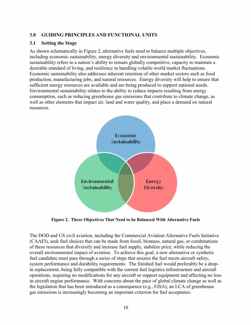
3.1 Setting the Stage
As shown schematically in Figure 2, alternative fuels need to balance multiple objectives,
including economic sustainability, energy diversity and environmental sustainability. Economic
sustainability refers to a nation’s ability to remain globally competitive, capacity to maintain a
desirable standard of living, and resilience in handling volatile world market fluctuations.
Economic sustainability also addresses inherent retention of other market sectors such as food
production, manufacturing jobs, and natural resources. Energy diversity will help to ensure that
sufficient energy resources are available and are being produced to support national needs.
Environmental sustainability relates to the ability to reduce impacts resulting from energy
consumption, such as reducing greenhouse gas emissions that contribute to climate change, as
well as other elements that impact air, land and water quality, and place a demand on natural
resources.
Figure 2. Three Objectives That Need to be Balanced With Alternative Fuels
The DOD and US civil aviation, including the Commercial Aviation Alternative Fuels Initiative
(CAAFI), seek fuel choices that can be made from fossil, biomass, natural gas, or combinations
of these resources that diversify and increase fuel supply, stabilize price, while reducing the
overall environmental impact of aviation. To achieve this goal, a new alternative or synthetic
fuel candidate must pass through a series of steps that assures the fuel meets aircraft safety,
system performance and durability requirements. The finished fuel would preferably be a drop-
in replacement, being fully compatible with the current fuel logistics infrastructure and aircraft
operations, requiring no modifications for any aircraft or support equipment and affecting no loss
in aircraft engine performance. With concerns about the pace of global climate change as well as
the legislation that has been introduced as a consequence (e.g., EISA), an LCA of greenhouse
gas emissions is increasingly becoming an important criterion for fuel acceptance.

11
3.2 Types of LCAs
LCA methodologies to evaluate life cycle energy and material flows associated with a product
system or activity are commonly categorized based on the type of data used to characterize a
system (average vs. marginal), approach used to address material and energy flows (attributional
vs. consequential), and by resolution of analysis (screening, standard, or comprehensive). The
following section provides a brief description of each of these LCA categories as they are used in
this guidance document.
3.2.1 Average vs. Marginal LCA
An average LCA considers the energy and material flows that have occurred over an extended
period of time and under conditions such that the inventory may be considered generally
representative of, or “average”, for a particular unit operation or industrial sector. A marginal
LCA considers the “nth” product produced or process run and is representative of a very short
period of time and/or very specific conditions. Any LCA model can be used to conduct either
average or marginal LCAs, as it depends upon the data collected and used rather than the
analysis itself. For example, if an alternative jet fuel were to be introduced such that it displaced
some portion of conventional, petroleum-derived jet fuel, the alternative could be compared with
the conventional fuel using an average LCA. In this case, data representing the average practice
for this particular type of alternative jet fuel industry along with the average practices of the
petroleum jet fuel industry would be gathered and used in the evaluation.
By contrast a marginal LCA assumes that the alternative jet fuel industry will, at the time of the
analysis, contribute a small fraction of the total jet fuel used. The introduction of the alternative
jet fuel will displace a subset of the conventional jet fuel industry. That is, the alternative jet fuel
will displace conventional jet fuels at an economic margin. The data to be used in a marginal
LCA should be gathered to represent the marginal production of the conventional jet fuel.
While marginal analysis, in theory, may better represent what could happen in the marketplace
when the alternative jet fuel is introduced, it is difficult to identify which facilities producing
conventional jet fuel operate at the margin and would be displaced by the new fuel.
Characterization of marginal processes, including identification of appropriate parameters and
data, is also likely to be a challenge.
3.2.2 Attributional vs. Consequential LCAs
LCA models may also differ in the approach used to address material and energy flows in cases
where more than one output of value is produced. LCA models that assume an isolated system
are termed attributional LCAs. In this instance, all flows and their associated environmental
burdens are attributed by one of several available methods to each of the individual products.
All of the attributed environmental burdens from all life cycle pathway stages for a product are
aggregated as the total environmental burden of producing a target product and any co-products
that are accounted for within the system. These attribution or allocation methods are described
in more detail in Section 5.0.
In contrast, consequential LCAs assume an open product system and take a systems response
approach in assessing impacts throughout the system as a result in a change in output of the
functional unit under study. The most commonly used form of a consequential LCA (CLCA)
relies on systems level economic models. These models track economic, material, and energy
across economic sectors. Weidema (2003) and Ekvall and Weidema (2004) describe the CLCA
12
methodology including consequential process identification and the use of marginal process data
and supply and demand price elasticities to quantify the impacts of industrial processes outside
the life cycle of interest but within the CLCA system boundaries.
This guidance document focuses primarily on average attributional LCAs for conventional and
alternative aviation fuels.
3.2.3 Levels of Resolution
The LCA can be thought of as falling into three levels, listed in order of decreasing level of study
completeness, data quality requirements, level of effort requirement, and confidence in analysis
results6:
Level I: Comprehensive
Level II: Standard
Level III: Screening
A Level III, or Screening, LCA is appropriate when performing a preliminary assessment of a
technology alternative or informing research funding decision making. A Level II, or Standard,
LCA examines all major unit operations, but with a lower degree of inventory completeness and
data quality requirements than for a Level I LCA. A Level I, or Comprehensive, LCA, with its
higher degree of accountability, is most appropriate for meeting the requirements of Section 526
of EISA 2007. Data, allocation, and system boundary definition requirements meeting the
standard of a Level I LCA are discussed in this document.
3.3 Goals and Scope Definition
3.3.1 Programmatic Goals for Alternative Jet Fuels
The Air Force and the civil aviation sector have developed and published processes to assess the
technical compliance of candidate jet fuels. The Air Force has documented the process in
Military Handbook 510 (2008) and the commercial sector has documented their process in
ASTM procedures (e.g., D4054). Both the Air Force and the civilian aviation sector have goals
of approving and using alternative jet fuels, some of which are summarized in Table 1. To
ensure full compatibility with existing systems in the near term, certification efforts have focused
on alternative fuel blends with petroleum. For example, both the Air Force and the civilian
aviation sector have focused on 50/50 blends of petroleum fuels with either Fischer-Tropsch
(F-T) or Hydroprocessed Renewable Jet (HRJ) fuels. Since Section 526 of EISA 2007 mandates
that any alternative fuel have a life cycle greenhouse gas profile less than or equal to an
equivalent conventional petroleum-based fuel, the process of evaluating candidate fuels must
also include some quantification of their life-cycle GHG emissions.
6 Section 6.6, entitled Assessing Data Quality, provides a thorough discussion of three levels of LCA analysis, Comprehensive, Standard, and Screening. These levels reflect varied levels of data quality and are meant to answer the needs of varied life-cycle analysis.

13
Table 1. Certification and Use Goals for the Commercial Aviation Sector
(as Represented by CAAFI and the US Air Force)
Year CAAFI Certification Goals USAF Certification and Use Goals
2009 50% Fischer-Tropsch Syngas-based blends
including biomass to liquid (BTL)
2010 -50% Hydroprocessed Renewable Jet (HRJ)
fuel from non-food sources, including algae
2011 - Complete testing and certification on all
aircraft and support systems for use of 50/50
alternative fuel blends
2013 -100% Hydroprocessed Renewable Jet (HRJ)
fuel
2016 - Competitively acquire 50% of the domestic
aviation fuel requirement using certified
alternative aviation fuel blends (50/50).
- Procure 800 Million gallons of alternative
renewable fuels
Several fuels are currently being considered for certification, such as Fischer-Tropsch, syngas-
based fuels and HRJ fuels. HRJ fuels are produced from triglycerides which are broken into
single chains and subsequently hydrotreated in order to eliminate oxygenated compounds. Both
are termed Synthetic Paraffinic Kerosene (SPK) fuels. SPK fuels, as the name implies, are
synthetic, (i.e., created from a source other than petroleum) kerosene fuels comprised of
paraffinic hydrocarbons. In other words, they have similar composition and properties to
conventional jet fuel, but with one major exception -- they do not contain aromatic hydrocarbon
compounds. Other fuels, such as fatty acid methyl esters (biodiesel) and alcohols (ethanol and
butanol), are not being proposed for aviation certification for a multitude of reasons, including
safety, compatibility, and energy density. For these reasons, the guidelines presented in this
document are focused on alternative jet fuels that have an SPK composition. It is, however,
conceivable that, in the future, other fuel compositions will be considered for certification as jet
fuel, and the guiding principles spelled out in this report should be broadly applicable to analysis
of the life cycles of those novel jet fuel compositions and those of other transportation fuels.
3.3.2 Conventional Petroleum-Based Fuels: A Baseline for Comparison
Fuel baselines needed to judge whether or not a candidate alternative fuel has life-cycle GHG
emissions that are “less than or equal to such emissions from the equivalent conventional fuel
produced from conventional petroleum sources.” Section 526 of EISA, from which this quote
was taken, does not define this comparative baseline fuel; however, Title II, Subtitle A, Sec. 201
of EISA 2007, which amends the Clean Air Act, defines the term “baseline life cycle greenhouse
gas emissions” to be the average life cycle greenhouse gas emissions of gasoline and diesel sold
or distributed as a transportation fuel in 2005. Although this Title II definition does not directly
apply to Section 526, it will be assumed to be the relevant baseline for the purposes of this
document.
A recent report by NETL (Skone and Gerdes 2008) provides one of the most rigorous
examinations of the life cycle greenhouse gas emissions profiles from U.S. domestically sold and
distributed conventional petroleum sources for the year 2005. This study reports the U.S.
average life cycle GHG emissions of conventional gasoline, conventional diesel fuel with less
than 500 parts per million of sulfur, and kerosene-based jet fuel. The reported central estimate of
14
well-to-wake emissions for kerosene-based jet fuel was 88.1 g CO2e/MJ (92.9 kg of CO2
equivalents per million BTUs of Lower Heating Value, LHV, fuel consumed). CO2 equivalent is
determined by summing the weighted contributions from carbon dioxide, methane, and nitrous
oxide, using the 2007 IPCC 100-year global warming potential CO2 equivalent factors. The
NETL study included both CO2 and non-CO2 emissions from the combustion of kerosene-type
jet fuel. If non-CO2 combustion emissions were excluded from the NETL estimate, as will be
recommended later in this section, then the central estimate of well-to-wake emissions for
kerosene-based jet fuel is 87.5 g CO2e / MJ. This study, although based on some data that are
not available for public review7 and requiring additional data and boundary validation, provides
perhaps the best basis for the development of baseline conventional fuel LCAs for EISA
3.3.3 LCA Study Goal and Scope Definition
The required level of detail appropriate for an LCA changes as a function of the question that the
analysis is being developed to address. For example, to be compliant with Section 526 of EISA
2007, it is necessary to determine whether the fuel supplied produces life-cycle GHG emissions
less than or equal to those produced from a baseline conventional fuel. Such an analysis would
examine existing facilities (or those planned for the immediate future) and use high quality data
with a minimum of assumptions as it will be used for compliance purposes. Another question
that may be asked is whether or not it is to society’s benefit to promote the development of a
specific fuel industry. Such an analysis would examine a hypothetical future industry, such as
large-scale algae production, that could replace a considerable quantity of all commercially
consumed conventional jet fuel (e.g., 1.6 million barrels per day or more in the US alone,
(Energy Information Administration 2007)). This analysis would more than likely have to rely
on simulations rather than actual operational data and may also require a considerable amount of
forecasting of technology performance. Both of these increase the uncertainty in the overall
analysis.
This document is meant to provide guidelines for assessing the life-cycle emissions for fuel
production at a typical, individual facility in the near term. This choice relates well to the needs
of the DESC and other agencies responsible for procurement, but it also serves fuel
manufacturers who would like to assess and certify the life-cycle GHG emissions of their
specific fuel production pathway.
ISO 14044: 2006(E) (2006b) requires the goal and scope of a study to be clearly defined and
consistent with the level of detail and intended use of the study results. The following questions
provide guidance in defining the appropriate level of LCA to be conducted:
What is the purpose of the study? The purpose of the LCAs required under Section
526 of EISA 2007 is narrowly focused toward the direct comparison of life cycle
greenhouse gas emissions generated from alternative jet fuels produced at a specific
facility through a specific production chain, as related to the purchase of synthetic and
alternative fuels by the US government, with average greenhouse gas emissions from
conventional, petroleum based sources.
7 Data used in this study are contained within the GaBi LCA software system which limits public publication of unit process data. Data can be reviewed with purchase of the software, see http://www.gabi-software.com/
15
Who is the intended audience? The DESC purchases aviation fuel for the DOD and is
expected to be the primary procurement agency that will oversee fuel vendor compliance
with Section 526 of EISA 2007. It is also anticipated that prospective fuel producers,
civilian fuel purchasers, and environmental interests may use this document as guidance
in comparing or conducting their own LCAs as well.
What is the intended level of detail? To meet the requirement of EISA 2007
(demonstrating that lifecycle greenhouse gas emissions associated with the alternative
aviation fuel supplied to Federal agencies are, on an ongoing basis, less than or equal to
those of conventional petroleum-derived jet fuel), it will be necessary for the fuel
manufacturers and LCA practitioners to develop a comprehensive (Level I), high-quality
LCA that is determined to sufficiently account for full lifecycle greenhouse gas emissions
from all phases of alternative aviation fuel production, transport, and use.
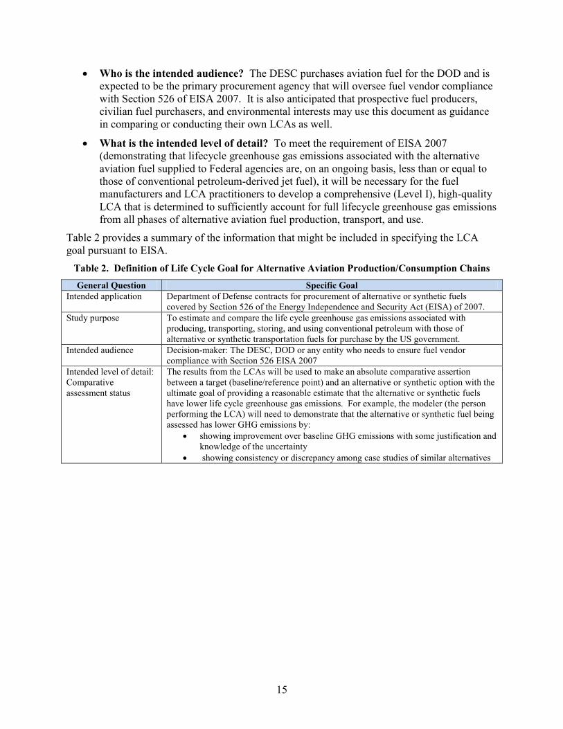
Table 2 provides a summary of the information that might be included in specifying the LCA
goal pursuant to EISA.
Table 2. Definition of Life Cycle Goal for Alternative Aviation Production/Consumption Chains
General Question Specific Goal
Intended application Department of Defense contracts for procurement of alternative or synthetic fuels
covered by Section 526 of the Energy Independence and Security Act (EISA) of 2007.
Study purpose To estimate and compare the life cycle greenhouse gas emissions associated with
producing, transporting, storing, and using conventional petroleum with those of
alternative or synthetic transportation fuels for purchase by the US government.
Intended audience Decision-maker: The DESC, DOD or any entity who needs to ensure fuel vendor
compliance with Section 526 EISA 2007
Intended level of detail:
Comparative
assessment status
The results from the LCAs will be used to make an absolute comparative assertion
between a target (baseline/reference point) and an alternative or synthetic option with the
ultimate goal of providing a reasonable estimate that the alternative or synthetic fuels
have lower life cycle greenhouse gas emissions. For example, the modeler (the person
performing the LCA) will need to demonstrate that the alternative or synthetic fuel being
assessed has lower GHG emissions by:
showing improvement over baseline GHG emissions with some justification and
knowledge of the uncertainty
showing consistency or discrepancy among case studies of similar alternatives
16
3.4 The Primary Fuel Process Chain
3.4.1 Defining Life-Cycle Stages
Assessments performed in accordance with these guidelines are to consider the full fuel life cycle
from cradle-to-grave, i.e. from raw material production or extraction through the combustion of
the refined fuel by the aircraft. A first step toward developing a robust and defensible LCA of a
candidate synthetic or alternative aviation fuel is to explicitly define the primary production
chain for which an LCA is to be developed. In the interest of standardization, and in keeping
with specifications of ISO 14040 (2006a), the following six general life cycle stages are the
preferred format for organizing inventory data and reporting of inventory/assessment results and
representing the primary fuel production chain:
Life Cycle Stage #1: Raw Material Acquisition
Life Cycle Stage #2: Raw Material Transport
Life Cycle Stage #3: Liquid Fuels Production
Life Cycle Stage #4: Product Transport and Refueling
Life Cycle Stage #5: Use/Aircraft Operation
Life Cycle Stage #6: End of Life
3.4.2 Life-Cycle Boundaries
While details of system boundaries and level of detail necessary for developing life cycle
inventories will be provided in subsequent sections, a brief description of the key activities and
boundaries for each life-cycle stage of petroleum-based fuel production chain is provided as an
example.
Life Cycle Stage #1: Raw Material Acquisition
o Including land-use changes, the extraction of raw feedstocks from the earth and
any partial processing of the raw materials that may occur (e.g., oil seed
harvesting and processing, upgrading to meet quality requirements for crude
pipeline transport).
Life Cycle Stage #2: Raw Material Transport
o Starting at the end of extraction/pre-processing of the raw materials and ends at
the entrance to the refinery facility.
o Refinery feedstocks may be transported from both domestic and foreign sources
to U.S. refineries.
Life Cycle Stage #3: Liquid Fuels Production
o Starting with the receipt of refinery inputs at the entrance of the refinery facility
and ends at the point of aviation fuel input to the product transport system.
o Emissions associated with acquisition and production of indirect fuel inputs (e.g.,
purchased power and steam, purchased fuels such as natural gas and coal, and
fuels produced and subsequently used in the refinery) are included in this stage.
17
o Emissions associated with on-site and off-site hydrogen production are accounted
for in this stage, including emissions associated with raw material acquisition for
hydrogen plant feedstock and fuel.
Life Cycle Stage #4: Product Transport and Refueling
o Starting at the gate of the petroleum refinery with aviation fuel already loaded
into the product transport system and ends with dispensing the fuel into the
aircraft.
o Including the operation of the bulk fuel storage depot, transport of jet fuel from
storage tanks to the aircraft, and aircraft refueling.
Life Cycle Stage #5: Use/Aircraft Operation
o Starting starts at the aircraft fuel tank and ending with the combustion of the
liquid fuel.
Life Cycle Stage #6: End of Life
o It should not be necessary to include end of life, such as recycling or disposal, in
the scope of jet fuel LCAs, since the final product is consumed in Life Cycle
Stage #5. As such, Stage #6 is not discussed further in this document.
3.4.3 Example Primary Production Chains
Simplified process schematics provide a straightforward and visually intuitive means of
representing the primary production chains through the five most significant life cycle stages.
The following figures provide several commonly cited synthetic and alternative aviation fuel
production chains and give examples of sub-processes within the life cycle stage framework.
The five significant schematic processes reflect: (1) Petroleum, (2) Biomass, (3) Coal and
Biomass to Liquid (CBTL), (4) HRJ Fuel, and (5) Hybrid Petroleum/Biomass fuel stages.
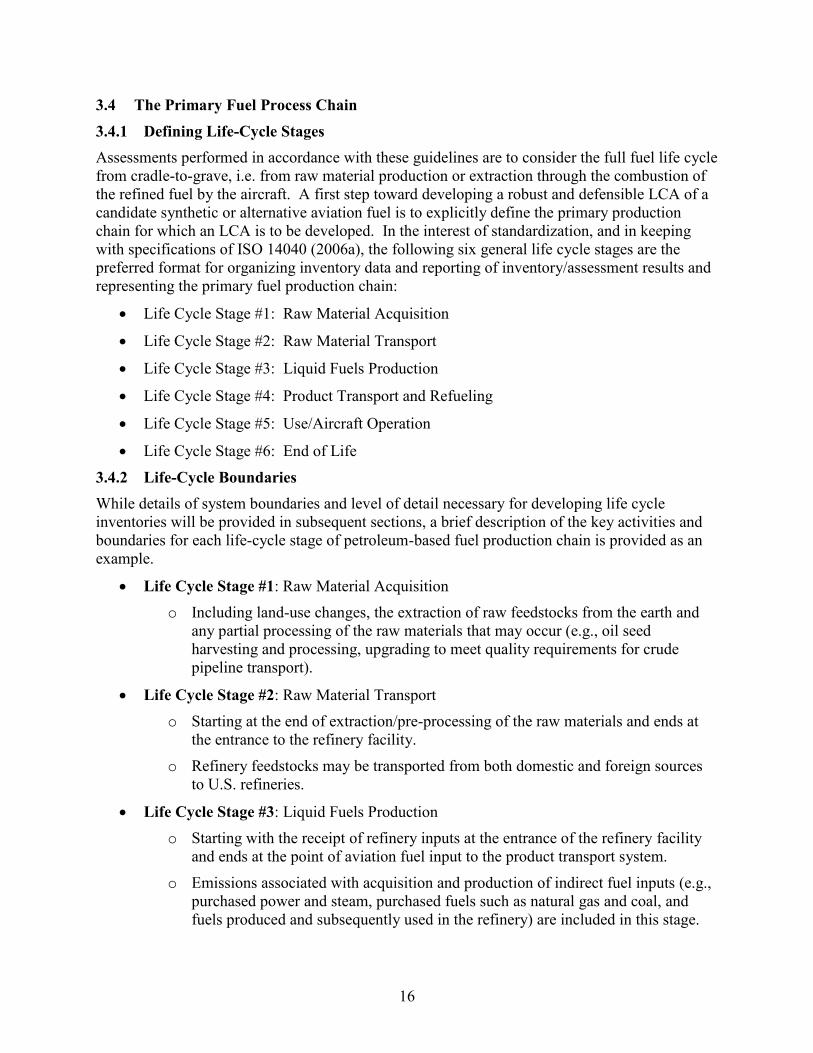
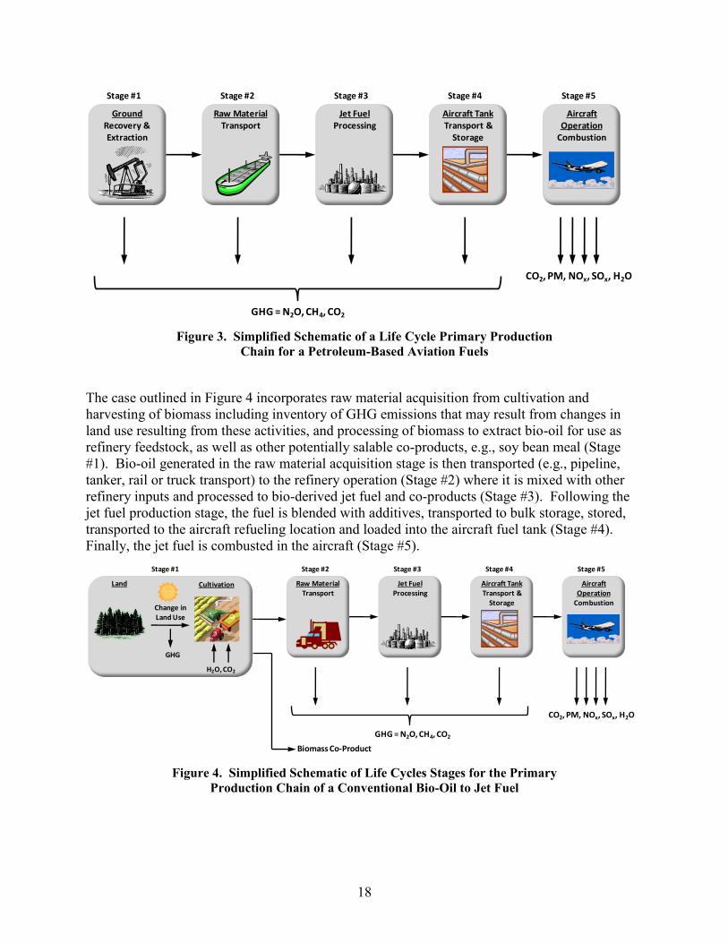
The case outlined in Figure 3 includes extraction of conventional and unconventional crude oil
from domestic and foreign sources (Stage #1), pipeline, tanker, rail and truck transport of crude
oil to refineries, domestic and foreign, serving in whole or part the domestic jet fuel market
(Stage #2), refinement of crude oil to produce the primary products of gasoline, diesel fuel, and
jet fuel (Stage #3), transport of jet fuel for U.S. consumption (Stage #4), and combustion of jet
fuel (Stage #5).
18
Figure 3. Simplified Schematic of a Life Cycle Primary Production
Chain for a Petroleum-Based Aviation Fuels
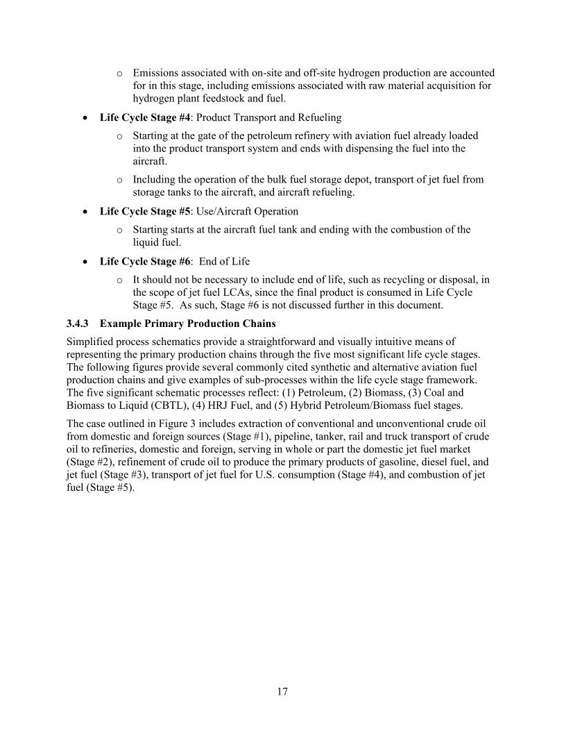
The case outlined in Figure 4 incorporates raw material acquisition from cultivation and
harvesting of biomass including inventory of GHG emissions that may result from changes in
land use resulting from these activities, and processing of biomass to extract bio-oil for use as
refinery feedstock, as well as other potentially salable co-products, e.g., soy bean meal (Stage
#1). Bio-oil generated in the raw material acquisition stage is then transported (e.g., pipeline,
tanker, rail or truck transport) to the refinery operation (Stage #2) where it is mixed with other
refinery inputs and processed to bio-derived jet fuel and co-products (Stage #3). Following the
jet fuel production stage, the fuel is blended with additives, transported to bulk storage, stored,
transported to the aircraft refueling location and loaded into the aircraft fuel tank (Stage #4).
Finally, the jet fuel is combusted in the aircraft (Stage #5).
Figure 4. Simplified Schematic of Life Cycles Stages for the Primary
Production Chain of a Conventional Bio-Oil to Jet Fuel
GroundRecovery & Extraction
Stage #1
Raw MaterialTransport
Stage #2
Jet FuelProcessing
Stage #3
Aircraft TankTransport &
Storage
Stage #4
Aircraft Operation
Combustion
Stage #5
GHG = N2O, CH4, CO2
CO2, PM, NOx, SOx, H2O
Land
Stage #1
Raw MaterialTransport
Stage #2
Jet FuelProcessing
Stage #3
Aircraft TankTransport &
Storage
Stage #4
Aircraft Operation
Combustion
Stage #5
GHG = N2O, CH4, CO2
CO2, PM, NOx, SOx, H2O
Cultivation
Change in Land Use
GHG
H2O, CO2
Biomass Co-Product
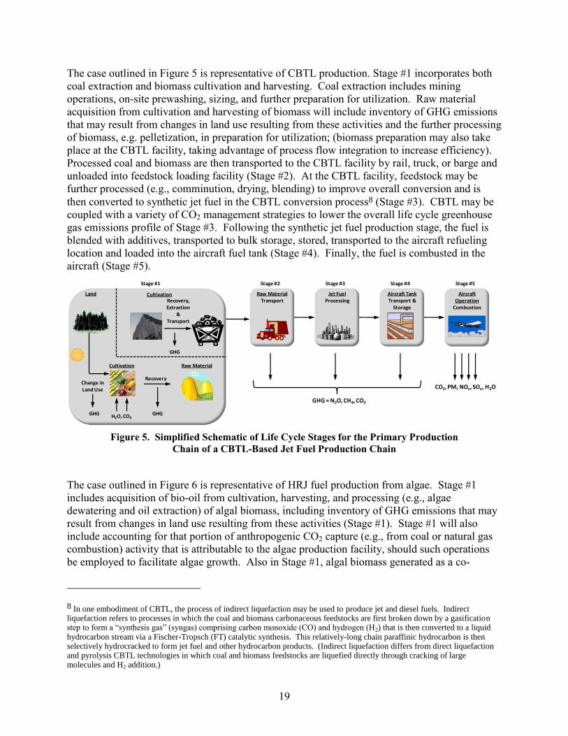
19
The case outlined in Figure 5 is representative of CBTL production. Stage #1 incorporates both
coal extraction and biomass cultivation and harvesting. Coal extraction includes mining
operations, on-site prewashing, sizing, and further preparation for utilization. Raw material
acquisition from cultivation and harvesting of biomass will include inventory of GHG emissions
that may result from changes in land use resulting from these activities and the further processing
of biomass, e.g. pelletization, in preparation for utilization; (biomass preparation may also take
place at the CBTL facility, taking advantage of process flow integration to increase efficiency).
Processed coal and biomass are then transported to the CBTL facility by rail, truck, or barge and
unloaded into feedstock loading facility (Stage #2). At the CBTL facility, feedstock may be
further processed (e.g., comminution, drying, blending) to improve overall conversion and is
then converted to synthetic jet fuel in the CBTL conversion process8 (Stage #3). CBTL may be
coupled with a variety of CO2 management strategies to lower the overall life cycle greenhouse
gas emissions profile of Stage #3. Following the synthetic jet fuel production stage, the fuel is
blended with additives, transported to bulk storage, stored, transported to the aircraft refueling
location and loaded into the aircraft fuel tank (Stage #4). Finally, the fuel is combusted in the
aircraft (Stage #5).
Figure 5. Simplified Schematic of Life Cycle Stages for the Primary Production
Chain of a CBTL-Based Jet Fuel Production Chain
The case outlined in Figure 6 is representative of HRJ fuel production from algae. Stage #1
includes acquisition of bio-oil from cultivation, harvesting, and processing (e.g., algae
dewatering and oil extraction) of algal biomass, including inventory of GHG emissions that may
result from changes in land use resulting from these activities (Stage #1). Stage #1 will also
include accounting for that portion of anthropogenic CO2 capture (e.g., from coal or natural gas
combustion) activity that is attributable to the algae production facility, should such operations
be employed to facilitate algae growth. Also in Stage #1, algal biomass generated as a co-
8 In one embodiment of CBTL, the process of indirect liquefaction may be used to produce jet and diesel fuels. Indirect liquefaction refers to processes in which the coal and biomass carbonaceous feedstocks are first broken down by a gasification step to form a “synthesis gas” (syngas) comprising carbon monoxide (CO) and hydrogen (H2) that is then converted to a liquid hydrocarbon stream via a Fischer-Tropsch (FT) catalytic synthesis. This relatively-long chain paraffinic hydrocarbon is then selectively hydrocracked to form jet fuel and other hydrocarbon products. (Indirect liquefaction differs from direct liquefaction and pyrolysis CBTL technologies in which coal and biomass feedstocks are liquefied directly through cracking of large molecules and H2 addition.)
Land
Stage #1
Raw MaterialTransport
Stage #2
Jet FuelProcessing
Stage #3
Aircraft TankTransport &
Storage
Stage #4
Aircraft Operation
Combustion
Stage #5
GHG = N2O, CH4, CO2
CO2, PM, NOx, SOx, H2O
Cultivation
Change in Land Use
GHG H2O, CO2
Cultivation
Recovery
GHG
Recovery, Extraction
& Transport
GHG
Raw Material
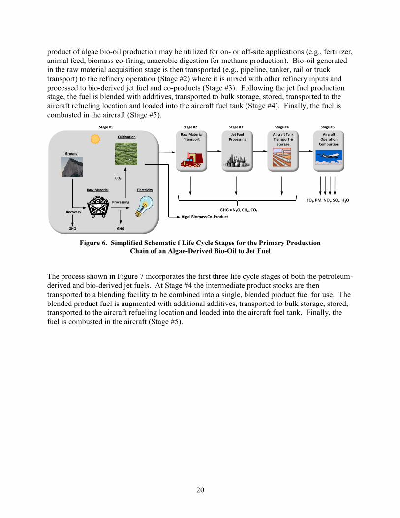
20
product of algae bio-oil production may be utilized for on- or off-site applications (e.g., fertilizer,
animal feed, biomass co-firing, anaerobic digestion for methane production). Bio-oil generated
in the raw material acquisition stage is then transported (e.g., pipeline, tanker, rail or truck
transport) to the refinery operation (Stage #2) where it is mixed with other refinery inputs and
processed to bio-derived jet fuel and co-products (Stage #3). Following the jet fuel production
stage, the fuel is blended with additives, transported to bulk storage, stored, transported to the
aircraft refueling location and loaded into the aircraft fuel tank (Stage #4). Finally, the fuel is
combusted in the aircraft (Stage #5).
Figure 6. Simplified Schematic f Life Cycle Stages for the Primary Production
Chain of an Algae-Derived Bio-Oil to Jet Fuel
The process shown in Figure 7 incorporates the first three life cycle stages of both the petroleum-
derived and bio-derived jet fuels. At Stage #4 the intermediate product stocks are then
transported to a blending facility to be combined into a single, blended product fuel for use. The
blended product fuel is augmented with additional additives, transported to bulk storage, stored,
transported to the aircraft refueling location and loaded into the aircraft fuel tank. Finally, the
fuel is combusted in the aircraft (Stage #5).
Stage #1
Raw MaterialTransport
Stage #2
Jet FuelProcessing
Stage #3
Aircraft TankTransport &
Storage
Stage #4
Aircraft Operation
Combustion
Stage #5
GHG = N2O, CH4, CO2
CO2, PM, NOx, SOx, H2O
Cultivation
GHG
Recovery
GHG
Raw Material
Processing
Ground
Electricity
CO2
Algal Biomass Co-Product
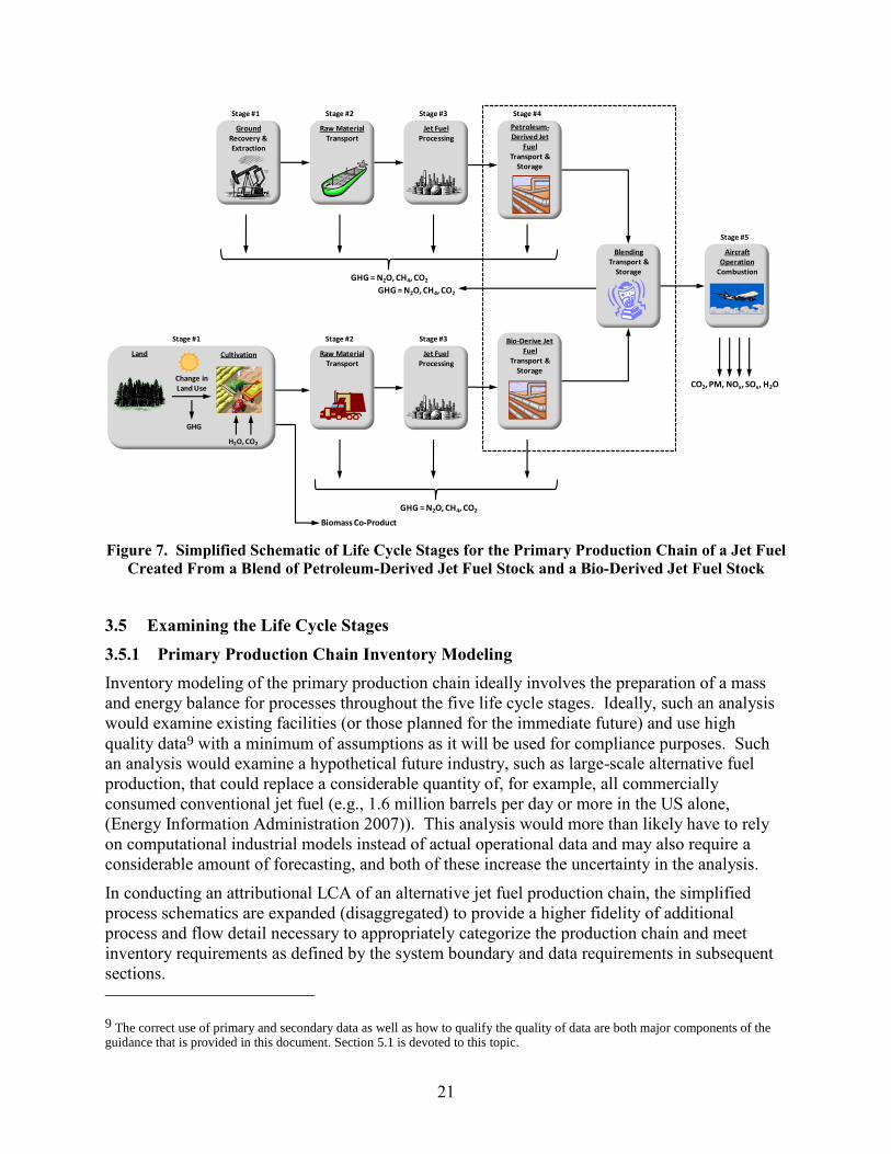
21
Figure 7. Simplified Schematic of Life Cycle Stages for the Primary Production Chain of a Jet Fuel
Created From a Blend of Petroleum-Derived Jet Fuel Stock and a Bio-Derived Jet Fuel Stock
3.5 Examining the Life Cycle Stages
3.5.1 Primary Production Chain Inventory Modeling
Inventory modeling of the primary production chain ideally involves the preparation of a mass
and energy balance for processes throughout the five life cycle stages. Ideally, such an analysis
would examine existing facilities (or those planned for the immediate future) and use high
quality data9 with a minimum of assumptions as it will be used for compliance purposes. Such
an analysis would examine a hypothetical future industry, such as large-scale alternative fuel
production, that could replace a considerable quantity of, for example, all commercially
consumed conventional jet fuel (e.g., 1.6 million barrels per day or more in the US alone,
(Energy Information Administration 2007)). This analysis would more than likely have to rely
on computational industrial models instead of actual operational data and may also require a
considerable amount of forecasting, and both of these increase the uncertainty in the analysis.
In conducting an attributional LCA of an alternative jet fuel production chain, the simplified
process schematics are expanded (disaggregated) to provide a higher fidelity of additional
process and flow detail necessary to appropriately categorize the production chain and meet
inventory requirements as defined by the system boundary and data requirements in subsequent
sections.
9 The correct use of primary and secondary data as well as how to qualify the quality of data are both major components of the guidance that is provided in this document. Section 5.1 is devoted to this topic.
Land
Stage #1
Raw MaterialTransport
Stage #2
Jet FuelProcessing
Stage #3 Bio-Derive Jet Fuel
Transport & Storage
GHG = N2O, CH4, CO2
Cultivation
Change in Land Use
GHG
H2O, CO2
Biomass Co-Product
GroundRecovery & Extraction
Stage #1
Raw MaterialTransport
Stage #2
Jet FuelProcessing
Stage #3
Petroleum-Derived Jet
FuelTransport &
Storage
Stage #4
Aircraft Operation
Combustion
Stage #5
GHG = N2O, CH4, CO2
CO2, PM, NOx, SOx, H2O
BlendingTransport &
Storage
GHG = N2O, CH4, CO2
22
3.5.2 System Boundary
A comprehensive LCA requires full accounting of all process-associated flows and activities, not
only those within the processes of the primary production chains, but also activities and
material/energy flows supporting necessary input to the primary production chain. For example,
the operation of an oil well consumes fuels, electricity and processing chemicals and requires
construction materials (e.g., steel tubulars and cement that make up the wellbore casing system),
transport of drill rig and construction materials to the reservoir, well drilling and completion,
intermittent well workovers during production, well plugging and abandonment, and well
construction material end-of-life management (e.g., recycling of steel casing elements). The life
cycles of all of these materials and activities are also included within the life cycle system
boundaries. Furthermore, a very small fraction of the construction and materials associated with
building of the plant where those construction materials, etc. were manufactured (e.g., the steel
plant where the well casing was manufactured) could also be included in a complete LCA.
Categorical exclusions from the system boundary would include low frequency, non-predictable
catastrophic events, such as large spills, and human activities (e.g. workers’ lunch breaks and
commuting activities).
Definition of a life cycle assessment system boundary serves to constrain the life cycle
assessment according to a set of clearly-defined geographic, temporal, and level of resolution
thresholds that are consistent with the intended purpose of conducting the life cycle assessment.
Greenhouse gas global warming impacts may be constrained to consider only those constituents
that are recognized by the IPCC as having significant and well definable global warming
potential, with global warming potential assessed using 2007 IPCC 100 year GWP factors. Land
use GHG emissions may include both soil emissions from directly-impacted land as well as
emissions arising from indirect land use, with land use emissions considered over a fixed time
period following initial land perturbation (emissions effectively amortized over that time period).
An appropriate system boundary will include the inventory of all relevant activities necessary to
appropriately account for significant life cycle emissions. A succinct methodology has been
developed to provide guidance in definition of appropriate system boundaries for analyzing an
alternative aviation fuel pathway, and is presented in Section 4.0.
3.5.3 Disaggregation, System Expansion, and Allocation
In LCA, a co-product is defined as “any two or more products coming from the same unit
process or product system” (ISO 2006a). Inevitably, some unit process co-products are used
neither within the primary fuel production system nor within the additional processes within the
life cycle. For example, in the production of petroleum jet fuel, gasoline, diesel, industrial
chemicals, and other products are co-produced. ISO 14044 (2006b) states that inputs and outputs
shall be allocated to the different co-products using methods in the following order:
1. Process disaggregation: dividing the unit process into two or more sub-processes and
collecting the input and output data related to these sub-processes.
2. System expansion: expanding the product system to include the additional functions
related to the co-products.
3. Allocation by physical relationships: inputs and outputs are partitioned between its
different co-products in a way that reflects the underlying physical relationships (e.g.,
mass, volume, energy content) between them

23
4. Allocation by other relationships: when physical relationship alone cannot be
established, inputs and outputs are partitioned between its different co-products in a way
that reflects other relationships (e.g., economic relationships) between them.
Many fuel production processes produce co- products along with the primary product. Such
multi-output processes complicate the development of a life cycle inventory because the inputs
and outputs of the processes need to be divided, or allocated, between all the products. In some
instances, a more detailed process model may be all that is required in order to disaggregate
material and energy flows associated with specific products. If co-products substitute for other
products in the economy, these substitutions can be integrated into the analysis through system
boundary expansion. In other cases, the processes are co-mingled to the extent than more
sophisticated methods of appropriately partitioning environmental burdens are required. Most
desirable is to partition inputs and outputs between multiple products on the basis of an
underlying physical relationship between them, such as mass or energy content. Challenges may
be inherent in this approach, however, when the functions of the co-products are quite different,
as is the case where products derived from biomass may consist of both fuels for their energy
content and feed for nutrient value. In such cases, the most uniform common metric may be
their final economic value. The choice of allocation approach can have a significant effect on
the overall results. Clarity in the choice of allocation method and the implications of this choice
are needed in order to provide a meaningful basis for comparison among fuels as well as other
life cycle systems. Guidance on allocation is provided in Section 5.0.
3.5.4 Inventory Data
To meet the EISA 2007 requirement fuel producers must develop comprehensive, high-quality
data for LCA. GHG life cycle inventories should completely represent all process life cycle
stages and phases of operation, including consideration of all inherent system variability, and to
account for emissions associated with all activities and material transformations back to
elemental flows (i.e., flows drawn from the environment). In practice, the expectation is that a
life cycle inventory will be developed using data of sufficient quality, representativeness
(technology, temporal, geographic), and completeness as to be consistent with the stated goal and
scope of the study: comparative analysis with baseline life cycle GHG emissions of comparable
petroleum-based jet fuel. It is expected that data used to populate the life cycle inventory will be
assembled from a variety of sources; while a substantial portion of these data are expected to be
fuel producer-generated data providing detailed categorization of the range of fuel production
technology performance, it will also be necessary to use data for raw material or energy inputs
acquired from a number of secondary sources (e.g., data from publicly available reports of
process or industry-level performance or aggregated cradle-to-gate profile data).
Variability in the sources and quality of data that may be considered for use in an LCA is almost
inevitable. Some methodologies that could be used in selection of appropriate data, specific
guidance on data quality requirements, and methodologies for reporting of results and
incorporation of sensitivity/uncertainty analyses are provided in Section 6.0.
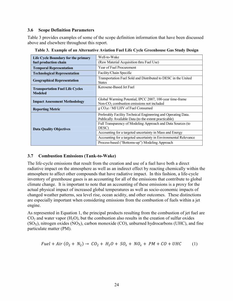
24
3.6 Scope Definition Parameters
Table 3 provides examples of some of the scope definition information that have been discussed
above and elsewhere throughout this report.
Table 3. Example of an Alternative Aviation Fuel Life Cycle Greenhouse Gas Study Design
Life Cycle Boundary for the primary
fuel production chain
Well-to-Wake
(Raw Material Acquisition thru Fuel Use)
Temporal Representation Year of Fuel Procurement
Technological Representation Facility/Chain Specific
Geographical Representation Transportation Fuel Sold and Distributed to DESC in the United
States
Transportation Fuel Life Cycles
Modeled
Kerosene-Based Jet Fuel
Impact Assessment Methodology Global Warming Potential, IPCC 2007, 100-year time-frame
Non-CO2 combustion emissions not included
Reporting Metric g CO2e / MJ LHV of Fuel Consumed
Data Quality Objectives
Preferably Facility Technical Engineering and Operating Data.
Publically Available Data (to the extent practicable)
Full Transparency of Modeling Approach and Data Sources (to
DESC)
Accounting for a targeted uncertainty in Mass and Energy
Accounting for a targeted uncertainty in Environmental Relevance
Process-based (“Bottoms-up”) Modeling Approach
3.7 Combustion Emissions (Tank-to-Wake)
The life-cycle emissions that result from the creation and use of a fuel have both a direct
radiative impact on the atmosphere as well as an indirect effect by reacting chemically within the
atmosphere to affect other compounds that have radiative impact. In this fashion, a life-cycle
inventory of greenhouse gases is an accounting for all of the emissions that contribute to global
climate change. It is important to note that an accounting of these emissions is a proxy for the
actual physical impact of increased global temperatures as well as socio-economic impacts of
changed weather patterns, sea level rise, ocean acidity, and other outcomes. These distinctions
are especially important when considering emissions from the combustion of fuels within a jet
engine.
As represented in Equation 1, the principal products resulting from the combustion of jet fuel are
CO2 and water vapor (H2O), but the combustion also results in the creation of sulfur oxides
(SOX), nitrogen oxides (NOX), carbon monoxide (CO), unburned hydrocarbons (UHC), and fine
particulate matter (PM).
𝐹𝑢𝑒𝑙 + 𝐴𝑖𝑟 𝑂2 + 𝑁2 → 𝐶𝑂2 + 𝐻2𝑂 + 𝑆𝑂𝑥 + 𝑁𝑂𝑥 + 𝑃𝑀 + 𝐶𝑂 + 𝑈𝐻𝐶 (1)

25
The mass of emissions per mass of fuel consumed, a quantity known as an emissions index or
emissions factor, have been compiled for all of the quantities listed in Equation 1 for commercial
and military jet engines. It is important to note that the emissions indices of PM, CO, UHC, and
NOx vary with engine operation (e.g., idle, takeoff, and cruise operations), and there are
recommended practices for estimating the time and fuel use in each operating mode. The
interested reader is directed to Kim, et al. (2007) to learn more about the System for assessing
Aviation’s Global Emissions (SAGE) tool which is used to create annual emissions inventories
for the US FAA.
The life-cycle analyst may be tempted to include estimates of methane and nitrous oxide
emissions as they are discussed in the IPCC guidelines and are included in the well-to-tank
portion of the LCA; however, as noted by the IPCC, these emissions have considerable
uncertainty in whether or not these emissions are even being produced by modern gas turbine
engines (quote from Page 3.56 of (IPCC 2007)).
Methane (CH4) may be emitted by gas turbines during idle and by older technology engines, but
recent data suggest that little or no CH4 is emitted by modern engines. Emissions depend on the
number and type of aircraft operations; the types and efficiency of the aircraft engines; the fuel
used; the length of flight; the power setting; the time spent at each stage of flight; and, to a lesser
degree, the altitude at which exhaust gases are emitted.
IPCC also notes that modern gas turbine engines produce little to no N2O emissions as well
(IPCC 1999).
Alternative fuels may change the emissions produced by aircraft. For example, because the
chemical composition of alternative fuels such as SPKs, produced either via the F-T process or
hydroprocessing of renewable oil sources, differ from that of conventional jet fuel, there will be
changes in the combustion products, as compared to petroleum-derived fuels. Our collective
knowledge of these changes varies with our fundamental understanding of how these pollutants
are created. The emissions of CO2, H2O, and SOX can be estimated for any fuel composition,
including SPK, based on complete combustion. These emissions indices are summarized along
with the carbon mass fraction of the fuel and the fuel sulfur content in Table 4 (Hileman and
Donohoo, 2009).
Table 4. Compositional Properties and Emissions Indices (EI) for CO2, H2O, and SOx
Fuel Carbon
Mass Fraction
Fuel Sulfur
Content (ppm)
Energy
Content
(MJ/kg)
CO2 EI
(g/kg)
H2O EI
(g/kg)
SOX EI
(g/kg)
JP-8 0.862 600 43.2 3,159 1,231 1.20
SPK 0.847 ~0 44.1 3,105 1,363 ~0
The emissions of NOx may change with the use of SPK fuels relative to JP-8. NOx results from
the oxidation of atmospheric nitrogen during combustion, and for gas turbine engines NOx
formation is largely a function of combustion temperature. Estimation of other byproducts, such
as PM, CO, and UHC (which are the result of incomplete fuel combustion) are less understood,
even for conventional jet fuel; however, initial tests indicate that there is a decrease in PM
emissions with the use of SPK fuels in gas turbine engines, ((Corporan, DeWitt and Klingshirn,
et al. 2007a), (Whitefield 2008)). Recent tests conducted in February 2009 at NASA's Dryden
Flight Research Center under the name of the Alternative Aviation Fuels EXperiment (AAFEX)
should shed more light on how these emissions change with SPK combustion.
26
Because it has a long life time in the atmosphere, the impact of a unit of CO2 that is emitted by
an aircraft in the upper atmosphere is, on average over the lifetime of the species in the
atmosphere, essentially the same as if had been emitted by a car; however, for other emissions
from jet fuel combustion in the upper atmosphere, both atmospheric lifetime and average
radiative properties are important in determining their global warming potentials. As noted by
Hileman, et al. (2009), most of these emissions have an impact on global climate.
Aircraft emissions that impact global climate change include the direct effects from CO2 and
water (H2O) emissions, the indirect forcing from changes in the distributions and concentrations
of ozone and methane as a consequence of NOX emissions, the direct effects (and indirect effects
on clouds) from aerosols and aerosol precursors, and the effects associated with condensation
trails (contrails) and high-altitude (cirrus) clouds. Each of these emissions and effects has a
varied residence time within the atmosphere; CO2 has a life time of 50 to 200 years, methane of 8
to 10 years, ozone on the order of months, water vapor and NOX on the order of weeks, and
contrails and cirrus clouds on the order of hours. Taken together, these individual effects act to
further increase the warming effect of aviation relative to that associated with CO2 alone,
although the relative amount of this additional warming is still the subject of scientific study
((IPCC 1999), (Sausen, et al. 2005), and (Wuebbles, Gupta and Ko 2007)).
The non-CO2 combustion emissions from aviation are known to have comparable influence on
global climate change as the combustion CO2 emissions ((IPCC 1999), (Sausen, et al. 2005),
(Wuebbles, Gupta and Ko 2007), (Marais, et al. 2008)). SOX emissions during cruise tend to cool
the climate while NOX emissions are generally predicted to warm the climate in terms of globally-
averaged surface temperature. Depending on where it is emitted within the upper atmosphere,
water vapor can be an important GHG (especially when emitted in the stratosphere, where
approximately 20 to 40 percent of aircraft emissions are deposited ((IPCC 1999); (Hoinka,
Reinhardt and Metz 1993); (Baughcum 1996); (Schumann 1997); (Gettelman and Baughcum
1999)). In contrast, water-vapor emissions at the ground and in the troposphere have a minor
impact as a GHG because of the naturally large abundance of water in the hydrological cycle
(IPCC 1999). If a fuel results in significant increases in water-vapor emissions when used in
aviation, it might be advantageous from a global climate change perspective to use that fuel in
ground transportation.
As part of the Aviation Climate Change Research Initiative (ACCRI), several white papers were
compiled to summarize the state of the science of aviation’s impact on global climate change10.
The interested reader is highly encouraged to review these documents. One of the white papers,
by Wuebbles et al. (2008), summarizes the state of climate metrics for aviation. Wuebbles et al.
(2008) note that “all of the well-accepted metrics of radiative forcing and GWPs … have major
limitations that affect their interpretation when used to address many of the policy questions of
interest to climate”. The following excerpt from the conclusions of Wuebbles et al. (2008)
further elucidates the problems with current climate metrics.
For example, the equivalent RF [Radiative Forcing] concept can be useful to address questions
related to changes in climate for the atmospheric agents that have been emitted over a specific
period of time. However, equivalent radiative forcing is not an emissions-based metric.
Emissions-based metrics are likely the primary choice for addressing most questions of interest
for technological or policy considerations and/or trade-offs.
10 As of February 13, 2008, the ACCRI white papers could be downloaded from http://www.faa.gov/about/office_org/headquarters_offices/aep/aviation_climate/
27
GWPs [Global Warming Potentials] (and AGWPs [Absolute Global Warming Potentials]) are
well established but may be difficult to apply to aviation emissions. We recommend that the
existing concept be modified to include efficacies, and tests done to see if all effects can be
conceptually included. While there have been many criticisms about this, no one has really
attempted to see if the concept could be readily modified to include contrails and other cloud
effects, e.g., by basing these effects in a more general sense on the emissions associated with fuel
burn. Despite its limitations, the GWP concept is so well engrained in current international
climate policy considerations that it might actually impede the progress of negotiations to
promote use of an alternative metric. As a result, decision-makers are faced with weighing
scientific precision relative to practical applicability (Fuglestvedt, et al. 2000).
The answer may lie in using similar metrics that address some of the scientific concerns raised by
GWPs. Specifically, the GTP [Global Temperature Profile] and the LTR [Linearized
Temperature Response] approaches have some major advantages, but neither has been
adequately tested. GTPs assume either pulse or sustained emissions while LTR generally uses a
pulse of one year of emissions. Both may also be applicable to emissions scenarios.
Additional research needs to be done to identify appropriate metrics for evaluating emissions
from aviation and from other transportation and energy sectors. The application of existing
metrics to aviation emissions needs to be evaluated individually and relative to each other. Some
metrics such as the LTR approaches need further development to be scientifically robust. New
metrics should also be considered.
The preferred method for comparison of CO2 and non-CO2 life cycle greenhouse gas emissions
(N2O and CH4) recommended in these guidelines is GWP reported on a CO2 equivalents basis;
however, as noted by Wuebbles et al. (2008) and summarized in Table 5, GWP may not be
appropriate for examining aviation’s non-CO2 combustion emissions.

28
Table 5. Uncertainties, Gaps, and Issues for the Use of GWP to Examine Emissions From Aviation
That Impact Global Climate Change. (Wuebbles, Yang and Herman 2008)
Metric Uncertainties Gaps Improvement issues
GWPs -- Global
Warming Potentials
Although commonly
used in climate studies
and policy
considerations, it is not
known how well this
metric could be applied
to aviation.
Difficult to know what
an appropriate time
horizon should be,
although the 100-year
horizon has become the
standard.
Not clear if GWPs could
be applied to regional
analyses.
Not clear what time
integration of radiative
forcing means.
Characterization of the
impact of a gas is not
robust with respect to
the climate impact.
Difficult to account for
contrail formation and
other non-emission
related effects using
GWPs.
Not applicable in
traditional configuration
(fixed integration period
integration) for fixed
target policy analyses.
Applicability for
aviation needs to be
evaluated.
Applicability for
comparing aviation with
other transportation /
energy sectors needs to
be tested.
Testing needed using
efficacies.
Given the uncertainty in estimating jet engine combustion emissions from alternative fuels, the
state of the science of aviation climate change, and the lack of metrics to examine the non-CO2
combustion emissions from aviation, it is recommended that only emissions of CO2 be
included in the combustion stage of the LCA at this time, and that the emissions of CO2
from bio-derived fuels be tracked separately from the CO2 emissions from fossil-based
fuels. This will allow for a net contribution to atmospheric carbon dioxide to be estimated, while
still allowing for data collection would serve multiple purposes. In addition, non-combustion
CO2 emissions should be tracked, to the extent that is practical, for future examination using an
appropriate metric.
This approach, of collecting and documenting data that may be required as approaches to the
estimation of life cycle greenhouse gas emissions of aviation fuels evolve, will be repeated in
other parts of these guidelines, and can be viewed as a guiding principle. For example, recent
research has shown that land use change may include both soil emissions from directly-impacted
land as well as emissions arising from indirect land use, with land use emissions considered over
a 30 year period following initial land perturbation (emissions effectively amortized over that 30
year period). As described later in this report, the guidelines recommended in this report suggest
collecting data on land use impacts, in anticipation of the emergence of widely accepted methods
for defining indirect land use impacts.
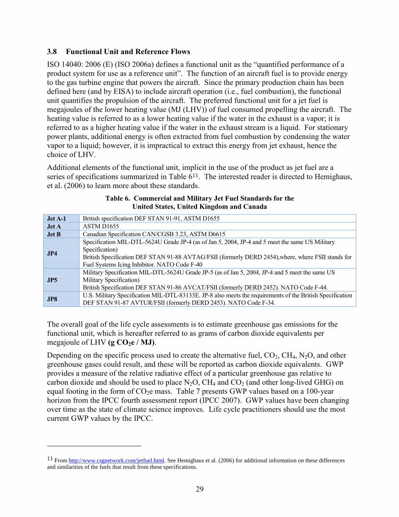
29
3.8 Functional Unit and Reference Flows
ISO 14040: 2006 (E) (ISO 2006a) defines a functional unit as the “quantified performance of a
product system for use as a reference unit”. The function of an aircraft fuel is to provide energy
to the gas turbine engine that powers the aircraft. Since the primary production chain has been
defined here (and by EISA) to include aircraft operation (i.e., fuel combustion), the functional
unit quantifies the propulsion of the aircraft. The preferred functional unit for a jet fuel is
megajoules of the lower heating value (MJ (LHV)) of fuel consumed propelling the aircraft. The
heating value is referred to as a lower heating value if the water in the exhaust is a vapor; it is
referred to as a higher heating value if the water in the exhaust stream is a liquid. For stationary
power plants, additional energy is often extracted from fuel combustion by condensing the water
vapor to a liquid; however, it is impractical to extract this energy from jet exhaust, hence the
choice of LHV.
Additional elements of the functional unit, implicit in the use of the product as jet fuel are a
series of specifications summarized in Table 611. The interested reader is directed to Hemighaus,
et al. (2006) to learn more about these standards.
Table 6. Commercial and Military Jet Fuel Standards for the
United States, United Kingdom and Canada
Jet A-1 British specification DEF STAN 91-91, ASTM D1655
Jet A ASTM D1655
Jet B Canadian Specification CAN/CGSB 3.23, ASTM D6615
JP4
Specification MIL-DTL-5624U Grade JP-4 (as of Jan 5, 2004, JP-4 and 5 meet the same US Military
Specification)
British Specification DEF STAN 91-88 AVTAG/FSII (formerly DERD 2454),where, where FSII stands for
Fuel Systems Icing Inhibitor. NATO Code F-40
JP5
Military Specification MIL-DTL-5624U Grade JP-5 (as of Jan 5, 2004, JP-4 and 5 meet the same US
Military Specification)
British Specification DEF STAN 91-86 AVCAT/FSII (formerly DERD 2452). NATO Code F-44.
JP8 U.S. Military Specification MIL-DTL-83133E. JP-8 also meets the requirements of the British Specification
DEF STAN 91-87 AVTUR/FSII (formerly DERD 2453). NATO Code F-34.
The overall goal of the life cycle assessments is to estimate greenhouse gas emissions for the
functional unit, which is hereafter referred to as grams of carbon dioxide equivalents per
megajoule of LHV (g CO2e / MJ).
Depending on the specific process used to create the alternative fuel, CO2, CH4, N2O, and other
greenhouse gases could result, and these will be reported as carbon dioxide equivalents. GWP
provides a measure of the relative radiative effect of a particular greenhouse gas relative to
carbon dioxide and should be used to place N2O, CH4 and CO2 (and other long-lived GHG) on
equal footing in the form of CO2e mass. Table 7 presents GWP values based on a 100-year
horizon from the IPCC fourth assessment report (IPCC 2007). GWP values have been changing
over time as the state of climate science improves. Life cycle practitioners should use the most
current GWP values by the IPCC.
11 From http://www.csgnetwork.com/jetfuel.html. See Hemighaus et al. (2006) for additional information on these differences and similarities of the fuels that result from these specifications.
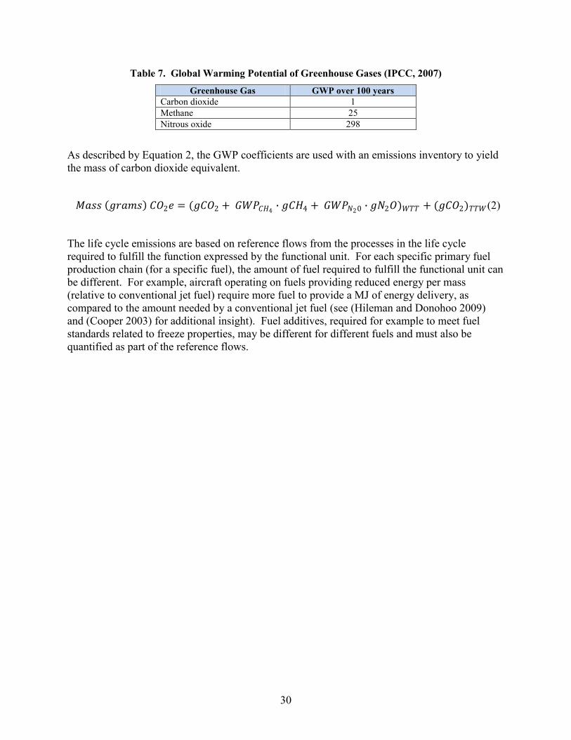
30
Table 7. Global Warming Potential of Greenhouse Gases (IPCC, 2007)
Greenhouse Gas GWP over 100 years
Carbon dioxide 1
Methane 25
Nitrous oxide 298
As described by Equation 2, the GWP coefficients are used with an emissions inventory to yield
the mass of carbon dioxide equivalent.
𝑀𝑎𝑠𝑠 𝑔𝑟𝑎𝑚𝑠 𝐶𝑂2𝑒 = (𝑔𝐶𝑂2 + 𝐺𝑊𝑃𝐶𝐻4∙ 𝑔𝐶𝐻4 + 𝐺𝑊𝑃𝑁20 ∙ 𝑔𝑁2𝑂)𝑊𝑇𝑇 + (𝑔𝐶𝑂2)𝑇𝑇𝑊(2)
The life cycle emissions are based on reference flows from the processes in the life cycle
required to fulfill the function expressed by the functional unit. For each specific primary fuel
production chain (for a specific fuel), the amount of fuel required to fulfill the functional unit can
be different. For example, aircraft operating on fuels providing reduced energy per mass
(relative to conventional jet fuel) require more fuel to provide a MJ of energy delivery, as
compared to the amount needed by a conventional jet fuel (see (Hileman and Donohoo 2009)
and (Cooper 2003) for additional insight). Fuel additives, required for example to meet fuel
standards related to freeze properties, may be different for different fuels and must also be
quantified as part of the reference flows.
31
4.0 SYSTEM BOUNDARY DEFINITION AND ANALYSIS
4.1 Background
System boundaries are defined by specifying the unit processes that are to be included in the
study and the level of detail to which each unit process is to be resolved. The selection of the
system boundary, according to the ISO standards, shall be consistent with the goal of the study,
which was defined in Section 3.0. Several methods have been used to determine life cycle
system boundaries, all with their individual strengths and weaknesses. This section outlines a
preferred method for a comparative aircraft fuel LCAs which is based on methods described in
LCA literature. Note that it is assumed herein and as required by the EISA, an LCA to be used
for making comparative assertions in the public domain will require quantification of life cycle
impacts of a baseline or reference system as well as the alternative of interest.
4.2 System Boundary Determination Approaches
The definition of the goal, functional unit, and primary fuel production chain provide a starting
place for system boundary determination. Reap, et al. (2008) provides some system boundary
method descriptions and a level of critique. In general these authors warn that when appropriate
boundaries are not selected, there is a danger that LCA results may either: (1) not reflect reality
well and lead to incorrect interpretations and comparisons ((Graedel 1998); (Lee, O’Callaghan
and Allen 1995)), or (2) provide the perception to the decision maker that there is a high degree
of uncertainty that effectively lowers confidence in decisions based on the results.
Specifically, Reap, et al. (2008) identify four categories of approaches to boundary selection:
Qualitative or semi-quantitative approaches
Quantitative approaches guided by data availability
Quantitative process-based approaches using cutoff criteria
Input–output (IO) based approaches
Omitting consideration of the first two methods due to criticisms related to subjectivity,
irreproducibility, and lack of scientific bases (Raynolds, Fraser and Checkel 2000), a focus on
the latter two methods follows.
4.3 Quantitative Process-Based Approaches to Boundary Definition Using Cutoff
Criteria
4.3.1 The ISO
Although noting that the ideal system includes all unit processes needed to ensure that only
elemental flows (or inputs and outputs to nature) cross the boundary of the system, the ISO
14044:2006(E) suggests a method for boundary definition based on cutoff criteria that can be
described with the following four steps (alluded to in section 4.2.3.3.2 of the ISO 14044:2006
(E) standard; (2006b)):
1. Make an initial identification of processes within the system boundaries using available
data.
32
2. Given the initial process set, list material and energy flows between processes within the
system boundary. This effort may be undertaken with data collected from specific sites
or from published sources.
3. Apply cutoff criteria to add and remove processes within the system boundary. The
standard suggests several cutoff criteria that may be used by LCA practitioners to decide
which inputs are to be included in the assessment, and that these criteria can be based on
mass, energy, or environmental significance:
a. Cutoff criteria based on mass: requires the inclusion of unit processes for the
production of all inputs and the management of all outputs that cumulatively
contribute more than a defined percentage (e.g., ≥1%) of the mass input of the
product system being modeled.
b. Cutoff criteria based on energy: requires the inclusion of unit processes for the
production of all inputs and the management of all outputs that cumulatively
contribute more than a defined percentage (e.g., ≥1%) of the product’s energy
inputs.
c. Cutoff criteria based on environmental significance: requires the inclusion of all
unit processes for the production of all inputs and the management of all outputs
that cumulatively contribute more than a defined percentage (e.g., ≥1%) of impact
of the selected environmental relevant metric.
4. Refine the system boundary. Identify and document material and energy flows that are
omitted during the course of the study.
Referring to the fourth step which reflects the iterative nature of LCA, the standard states that
decisions regarding omitted data shall be based on a sensitivity analysis to determine their
significance to the overall LCA, thereby verifying the initial analysis outlined in ISO 14044:2006
(E), section 4.2.3.3 (2006b). The ISO standard calls for documentation of the results of this
iterative system boundary setting process and any sensitivity analysis performed. The sensitivity
analysis demonstrates the significance of included or excluded unit processes on the overall
results of the study. This procedure serves to limit the subsequent data handling to those inputs
and output data that are determined to impact the goal of the LCA.
Implementation of cutoff criteria is investigated by Raynolds, et al. (2000). These authors define
the Relative Mass-Energy-Economic (RMEE) method for system boundary selection, essentially
assuming the modeler will move outward from the primary production chain which provides the
functional unit. As the modeler moves outward, decisions are made as to whether or not each
unit process providing a product or service is to be included in the system boundary using a
“relative ratio” to determine inclusion. The ratio is intended to act as a proxy for the potential
life cycle impact of the product or service on the overall system. Specifically, one ratio (ZRMEE)
is established for all mass, energy, and economic criteria as a percent of the total mass, energy,
and economic value of the system functional unit, for example:
33
given ZRMEE = 1%,
if
𝑚𝑎𝑠𝑠 𝑜𝑓 𝑡𝑒 𝑢𝑛𝑖𝑡 𝑝𝑟𝑜𝑐𝑒𝑠𝑠 𝑖𝑛𝑝𝑢𝑡 𝑜𝑟 𝑜𝑢𝑡𝑝𝑢𝑡 𝑏𝑒𝑖𝑛𝑔 𝑡𝑒𝑠𝑡𝑒𝑑 (𝑘𝑔)
𝑚𝑎𝑠𝑠 𝑜𝑓 𝑡𝑒 𝑓𝑢𝑛𝑐𝑡𝑖𝑜𝑛𝑎𝑙 𝑢𝑛𝑖𝑡 (𝑘𝑔)≥ 1% or
𝑒𝑛𝑒𝑟𝑔𝑦 𝑜𝑓 𝑡𝑒 𝑢𝑛𝑖𝑡 𝑝𝑟𝑜𝑐𝑒𝑠𝑠 𝑖𝑛𝑝𝑢𝑡 𝑜𝑟 𝑜𝑢𝑡𝑝𝑢𝑡 𝑏𝑒𝑖𝑛𝑔 𝑡𝑒𝑠𝑡𝑒𝑑 (𝑀𝐽 )
𝑒𝑛𝑒𝑟𝑔𝑦 𝑜𝑓 𝑡𝑒 𝑓𝑢𝑛𝑐𝑡𝑖𝑜𝑛𝑎𝑙 𝑢𝑛𝑖𝑡 (𝑀𝐽 )≥ 1% or
𝑒𝑐𝑜𝑛𝑜𝑚𝑖𝑐 𝑣𝑎𝑙𝑢𝑒 𝑜𝑓 𝑡𝑒 𝑢𝑛𝑖𝑡 𝑝𝑟𝑜𝑐𝑒𝑠𝑠 𝑖𝑛𝑝𝑢𝑡 𝑜𝑟 𝑜𝑢𝑡𝑝𝑢𝑡 𝑏𝑒𝑖𝑛𝑔 𝑡𝑒𝑠𝑡𝑒𝑑 (𝑈𝑆$)
𝑒𝑐𝑜𝑛𝑜𝑚𝑖𝑐 𝑣𝑎𝑙𝑢𝑒 𝑜𝑓 𝑡𝑒 𝑓𝑢𝑛𝑐𝑡𝑖𝑜𝑛𝑎𝑙 𝑢𝑛𝑖𝑡 (𝑈𝑆$)≥ 1%
then, the life cycle processes for the production of the unit process input or output being
tested is included in the system.
Thus, starting with the unit process producing the product of interest, if the ratio of the mass,
energy, and economic value of a process input or service to the total mass, energy, and economic
value of the system functional unit is greater than ZRMEE, then a unit process producing that
product or service is included in the system. This process is repeated for all products and
services needed by the unit process producing the product of interest, as well as those
subsequently added to the system boundary, until all relative ratios are less than ZRMEE.
4.3.2 Critique of Cutoff Criteria Approaches to Boundary Definition
Reap, et al. (2008) suggest that process-based approaches which use cutoff criteria such as the
RMEE method essentially introduce truncation error that can be substantial. In other words,
there is no guarantee that a small mass or energy contribution lost through use of cutoff criteria
will always result in negligible mass, energy, economic value, or environmental impact across
the product life cycle. For example and within the context of carbon footprinting, although an
energy input associated with a land use change may fall below a cutoff criteria threshold, the
greenhouse gas emissions of this land use change, as described in Section 2.0, can be substantial.
Further, the ISO standard states that if a study is intended for comparative assertions and is to be
released to the public, a sensitivity analysis shall include mass, energy and environmental
significance criteria relative to the system boundary. Such a system-boundary-level sensitivity
analysis is intended to re-test the importance of a cutoff unit process flow to the cumulative
system impact (e.g., to ensure that a cutoff flow deemed a small percentage of a unit process
flow is not significant at the system-level). Such a system-level sensitivity analysis requires the
total flows for the life cycle to be known (Reap, et al. 2008). If a practitioner has gathered all the
data needed to establish the true final totals, why would some of the data be cut off? For this
reason the guidelines proposed in this report eliminate the need to define a cutoff criteria.
4.4 Input-Output (IO) Based Approaches to Boundary Definition
The Economic Input-Output analysis-based LCA (EIOLCA) method uses economic input-output
data derived from inter-industry transaction matrices for the US and publicly available
environmental data to arrive at comprehensive, industry-wide environmental impacts ((Lave, et
al. 1995); (Hendrickson, Horvath, et al. 1998); (Hendrickson, Lave and Matthews 2005)). For
the US, the implementation of input-output (IO) modeling, including GHG emissions, is found in
the EIOLCA model (available at www.eiolca.net). EIOLCA employs the 2002 U.S. Department
of Commerce 426-sector industry-by-industry input-output matrix (Stewart, Stone and
Streitwieser 2007), and publicly available environmental data, mostly from the U.S. Department
34
of Energy and Environmental Protection Agency ((EPA 1995); (EPA 2002)). The power of this
model is in its ability to determine system level environmental impacts with the goal of reducing
cutoff error. The system includes the activities of all upstream suppliers (i.e., the product, the
service suppliers of the product, the suppliers of the suppliers, and beyond) and thus upstream
supplier environmental impact (e.g., GHG emissions) linked to the flow of interest by economic
exchanges, measured in US dollars. While some of these suppliers are included in a typical
process-based LCA, others remain elusive as they are too far up the supply chain from primary
activities or are omitted based on cut off criteria.
The EIOLCA model has a number of weaknesses, however, that limits its utility for detailed
analyses of a comparative nature where resolution between specific technologies is required.
EIOLCA cannot resolve impacts on a product level (as in differences between types of organic
chemicals or non-ferrous metals) but rather looks at sector impacts. In other words, the EIOLCA
data have a high degree of product and service aggregation. For instance, the production of
different organic fuel additives would map to the “Other Organic Chemicals” sector, yielding the
impacts of the average manufacturer in the sector and not reflecting the difference in production
technologies between different organic fuel additives. Also, the EIOLCA model reflects
transactions occurring in the US economy, it treats imports (e.g. imported crude oil) as if they
were produced in the US with US technologies and logistics. Further, the EIOLCA model
cannot strictly account for use, disposal or recycling of the products.
To offset some of these limitations, a hybrid LCA modeling methodology has been developed
(Suh, et al. 2004) that combines process modeling of the primary system with EIOLCA data for
products and services needed by each primary system unit process. Hybrid LCA comes in two
general forms: a combination of physical flows and monetary flows and a combination of sector
and process data. Examples of these general forms include the tiered hybrid analysis, input-
output hybrid analysis, and an integrated hybrid analysis. The latter two methods require the
disaggregation of salient US sectors (for instance the electricity sector) or the addition of the
detailed input-output model of the process under consideration to alleviate the need for product
allocation during the analysis, respectively. The tiered hybrid approach, the method
suggested for possible use in this guidance, involves developing a detailed process model for
first order and some lower order processes that have a recognized critical impact and using
the EIOLCA model to quantify the other inputs.
It is important to note that the EIOLCA methods do not explicitly select boundaries. The
EIOLCA tool implicitly sets the boundaries at the level of materials extracted from the earth,
referred to as elementary flows (note that these are not flows of chemical elements, but flows of
materials extracted from the earth in the chemical form in which they are extracted). As pointed
out by Suh and co-authors (2004) even though the ISO standard has a goal of defining a
boundary where all inputs and output are elementary flows, this is a difficult goal for those
conducting process-based analyses. The EIOLCA approaches this goal, at least to the level of
the US economy.
4.5 System Boundary Guidance
Based on the above description of both quantitative process-based approaches using cutoff
criteria and IO boundary definition approaches, a blended method leveraging the useful attributes
of each method is presented here. The system boundary determination guidance in this report
seeks to:
35
Eliminate the use of subjective cutoff criteria
Create reasonable data collection burdens in support of current fuel policies, including a
quantification of the on-going unit process operation within the primary production
pathway chain
Extend the boundaries as close to elementary flows at the system boundary as possible
(identified by the ISO standard as the ideal)
Target data collection efforts towards what is needed for understanding and estimating
significant impact contributors
It is important to remember the goal of the study: to provide a comparative assertion. It is
assumed that the modeler will prepare or have access to a baseline system from which unit
process and life cycle GHG emissions can be compared.
4.6 Recommended Method Details
The following decision tree outlines an iterative process for defining the system boundary. Each
of these steps will be described below.
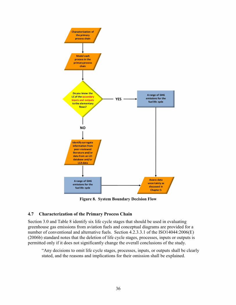
36
Figure 8. System Boundary Decision Flow
4.7 Characterization of the Primary Process Chain
Section 3.0 and Table 8 identify six life cycle stages that should be used in evaluating
greenhouse gas emissions from aviation fuels and conceptual diagrams are provided for a
number of conventional and alternative fuels. Section 4.2.3.3.1 of the ISO14044:2006(E)
(2006b) standard notes that the deletion of life cycle stages, processes, inputs or outputs is
permitted only if it does not significantly change the overall conclusions of the study.
“Any decisions to omit life cycle stages, processes, inputs, or outputs shall be clearly
stated, and the reasons and implications for their omission shall be explained.
Characterization of the primary
process chain
Model each process in the
primary process chain
Do you know the LC of the secondary inputs and outputs to the elementary
flows?
NO
YES
Identify surrogate information from
peer-reviewed literature and/or data from an LCI database and/or
LCA data
A range of GHG emissions for the
fuel life cycle
Assess data uncertainty as
discussed in Chapter 5
A range of GHG emissions for the
fuel life cycle
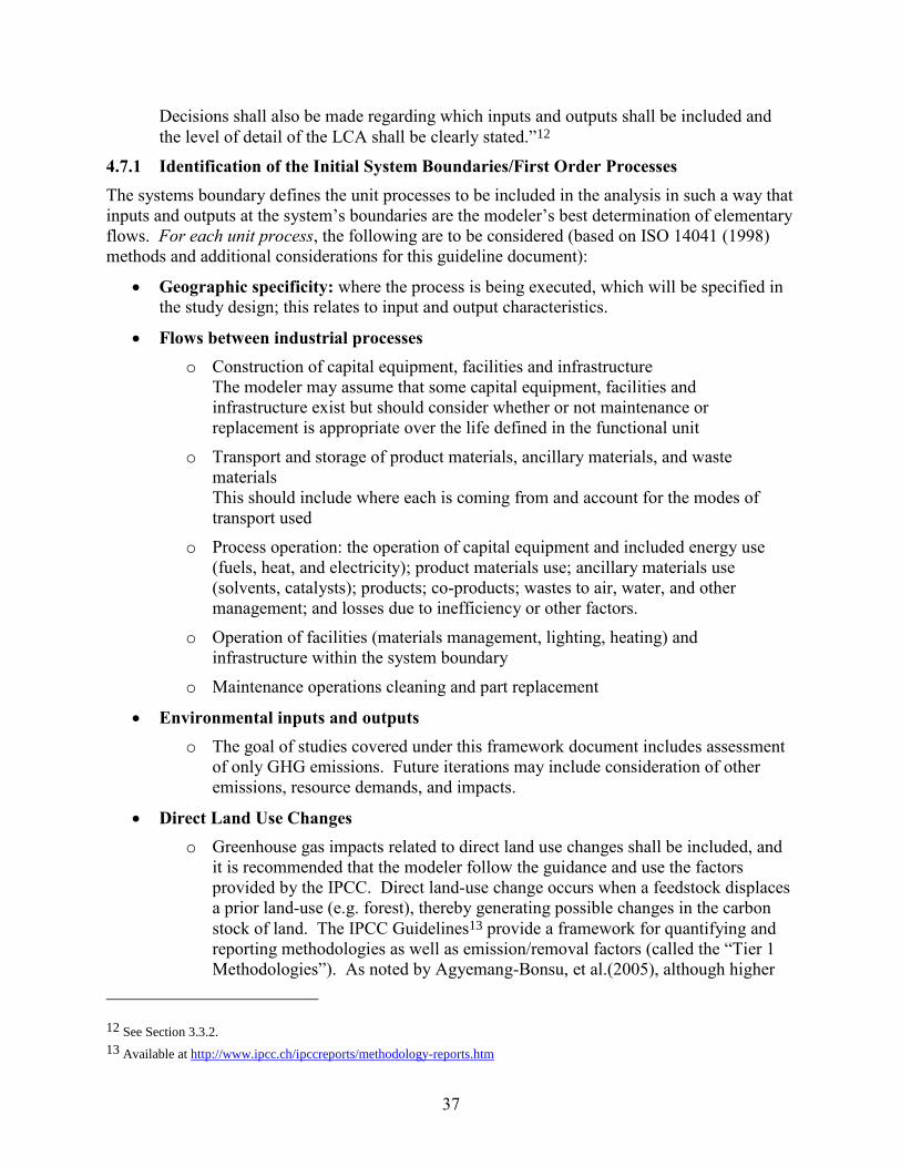
37
Decisions shall also be made regarding which inputs and outputs shall be included and
the level of detail of the LCA shall be clearly stated.”12
4.7.1 Identification of the Initial System Boundaries/First Order Processes
The systems boundary defines the unit processes to be included in the analysis in such a way that
inputs and outputs at the system’s boundaries are the modeler’s best determination of elementary
flows. For each unit process, the following are to be considered (based on ISO 14041 (1998)
methods and additional considerations for this guideline document):
Geographic specificity: where the process is being executed, which will be specified in
the study design; this relates to input and output characteristics.
Flows between industrial processes
o Construction of capital equipment, facilities and infrastructure
The modeler may assume that some capital equipment, facilities and
infrastructure exist but should consider whether or not maintenance or
replacement is appropriate over the life defined in the functional unit
o Transport and storage of product materials, ancillary materials, and waste
materials
This should include where each is coming from and account for the modes of
transport used
o Process operation: the operation of capital equipment and included energy use
(fuels, heat, and electricity); product materials use; ancillary materials use
(solvents, catalysts); products; co-products; wastes to air, water, and other
management; and losses due to inefficiency or other factors.
o Operation of facilities (materials management, lighting, heating) and
infrastructure within the system boundary
o Maintenance operations cleaning and part replacement
Environmental inputs and outputs
o The goal of studies covered under this framework document includes assessment
of only GHG emissions. Future iterations may include consideration of other
emissions, resource demands, and impacts.
Direct Land Use Changes
o Greenhouse gas impacts related to direct land use changes shall be included, and
it is recommended that the modeler follow the guidance and use the factors
provided by the IPCC. Direct land-use change occurs when a feedstock displaces
a prior land-use (e.g. forest), thereby generating possible changes in the carbon
stock of land. The IPCC Guidelines13 provide a framework for quantifying and
reporting methodologies as well as emission/removal factors (called the “Tier 1
Methodologies”). As noted by Agyemang-Bonsu, et al.(2005), although higher
12 See Section 3.3.2.
13 Available at http://www.ipcc.ch/ipccreports/methodology-reports.htm

38
tier IPCC methodologies are based on more sophisticated methods for estimating
emissions/removals and on the use of national or regional parameters that
accommodate the specific national circumstances, these methods are not always
described in detail in the IPCC Guidelines. Herein, as suggested by Agyemang-
Bonsu, et al. (2005), the use of transparent and well documented methods
consistent with those in the IPCC Guidelines is encouraged14.
Indirect Land Use Changes
o Indirect land-use change occurs when the displacement of previous activity or
land use induces land use changes on other lands. Indirect land use change
(discussed below) should be considered once regulatory guidance of its
calculation and impact is issued.
Keeping in mind the above unit process considerations, the identification of initial system
boundaries involves specifying the first order processes (the primary process chain) in each of
the life cycle stages, which will depend directly on the goal and scope of a given study. Several
simplified process schematics defining first order or primary processes are available in Section
3.0. Table 8 defines the life cycle stages that are used throughout this guidance.
Table 8. Life Cycle Stage Descriptions
Stage Name Stage
Abbreviation
Stage Description
1 Raw Material Acquisition RMA Boundary includes extraction of raw feedstocks from the earth
and any partial processing of the raw materials that may occur
(e.g., oil seed harvesting and processing, upgrading to meet
quality requirements for crude pipeline transport)
2 Raw Material Transport RMT Boundary begins at the end of extraction/pre-processing of the
raw materials and ends at the entrance to the refinery facility.
Refinery feedstocks may be transported from both domestic and
foreign sources to US refineries
3 Liquid Fuels Production
(Manufacturing or
Conversion)
LFP Boundary starts with the receipt of refinery inputs at the entrance
of the refinery facility and ends at the point of aviation fuel input
to the product transport system.
Emissions associated with acquisition and production of indirect
fuel inputs (e.g., purchased power and steam, purchased fuels
such as natural gas and coal, and fuels produced and subsequently
used in the refinery) are included in this stage.
Emissions associated with on-site and off-site hydrogen
production (for hydrogen used in liquid fuels production) are
included in this stage, including emissions associated with raw
material acquisition for hydrogen plant feedstock and fuel.
14 Available at http://www.ipcc.ch/pdf/special-reports/srccs/srccs_chapter9.pdf

39
Table 8. Life Cycle Stage Descriptions (Cont’d)
Stage Name Stage
Abbreviation
Stage Description
4 Product Transport and
Refueling
PT Boundary starts at the gate of the petroleum refinery with aviation
fuel already loaded into the product transport system and ends
with the dispensing of the fuel into the aircraft.
Boundary includes the operation of the bulk fuel storage depot,
transport of jet fuel from storage tanks to the aircraft, and aircraft
refueling.
5 Use/Aircraft Operation Use Boundary starts at the aircraft fuel tank and ends with the
combustion of the liquid fuel.
6 End-of-Life EOL Boundary starts when the value of the product to the end user has
expired. This stage is excluded for the first order process when
the primary reference flow is a fuel that will be combusted during
Stage 5, the use stage.
An example of each life cycle stage is presented in simplified form for a hypothetical coal-to-
liquid (CTL) aviation fuels process. Table 9 outlines the processes as well as the inputs and
outputs for each stage. In the interest of simplicity of presentation, only select among the “flows
between industrial processes,” and the “environmental inputs and outputs” listed in Section 4.7.1
have been included in Table 9.
Table 9. CTL Process Primary Inputs and Outputs
LC Stage Process Inputs Outputs
RMA Coal Mining Electricity, Diesel, Mining and Coal Preparation
Equipment
Coal, GHG
RMT Coal Transport by Rail Coal, Diesel, Railcars and Railway Equipment Coal, GHG
LFP Fischer-Tropsch Facility for Coal to
Liquid Fuel
Coal, Fuel Oil, Electricity, Chemicals [catalysts,
solvents], Facility Equipment
Fuel, GHG
PT Transport of Liquid Fuel by Pipeline Fuel, Pipeline Equipment Fuel, GHG
Use Combustion of Liquid Fuel Fuel, Chemicals (Jet Fuel Additives) Fuel, GHG
EOL Not applicable at the first order process level for this example
4.8 Characterization of Second Order/Secondary Processes
First order process flows have their own life cycles which are provided by secondary or second
order life cycle processes (using the terminology within this guideline document). Figure 9
provides an example of a simplified process schematic to define first order versus second order
process distinctions.
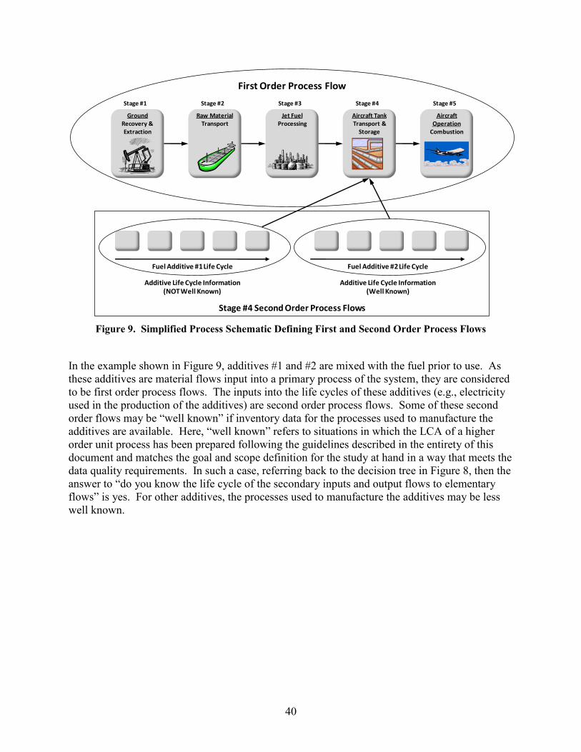
40
Figure 9. Simplified Process Schematic Defining First and Second Order Process Flows
In the example shown in Figure 9, additives #1 and #2 are mixed with the fuel prior to use. As
these additives are material flows input into a primary process of the system, they are considered
to be first order process flows. The inputs into the life cycles of these additives (e.g., electricity
used in the production of the additives) are second order process flows. Some of these second
order flows may be “well known” if inventory data for the processes used to manufacture the
additives are available. Here, “well known” refers to situations in which the LCA of a higher
order unit process has been prepared following the guidelines described in the entirety of this
document and matches the goal and scope definition for the study at hand in a way that meets the
data quality requirements. In such a case, referring back to the decision tree in Figure 8, then the
answer to “do you know the life cycle of the secondary inputs and output flows to elementary
flows” is yes. For other additives, the processes used to manufacture the additives may be less
well known.
GroundRecovery & Extraction
Stage #1
Raw MaterialTransport
Stage #2
Jet FuelProcessing
Stage #3
Aircraft TankTransport &
Storage
Stage #4
Aircraft Operation
Combustion
Stage #5
Fuel Additive #1 Life Cycle
Additive Life Cycle Information(NOT Well Known)
Fuel Additive #2 Life Cycle
Additive Life Cycle Information(Well Known)
Stage #4 Second Order Process Flows
First Order Process Flow

41
Figure 10. Second Order Process Flows in Algae Production
Another example of second order process flows is given in Figure 10, in which the primary
process flows of electricity, fertilizer and water are used in algae production. In this case the
second order process flows would be the inputs to electricity production, fertilizer and water.
Life cycle data for the electricity and fertilizer second order flows are likely to be well known.
In this case, referring back to the decision tree in Figure 8, the answer to “do you know the life
cycle of the secondary inputs and outputs to the elementary flows” is yes, and thus
characterization of this secondary flow is straight-forward. In contrast in this example, the inputs
required to provide water for algae production depend on local sources and water quality
requirements for the algae production and may not be well known. At this juncture, the modeler
must search for the data needed to characterize the life cycle of the production of water. A
methodology recommended for use in identifying surrogate higher-order process data is provided
below.
4.9 Identification of Surrogate Higher Order Process Information
This guideline document recommends two sources of surrogate data for use beyond the primary
process chain when life cycle data are not readily available. Both approaches should be used,
documented, and verified during the LCA critical or peer review, resulting in a range of potential
values for life cycle GHG emissions.
Data source 1: peer reviewed documentation of the life cycle of surrogate processes in archival literature, in a project report, or in a LCI database. Although striving to
achieve the closest match to the system at hand, these data may not match geographic,
temporal, technological, or other specific characteristics of the higher order process of
interest. Examples of LCI databases include, but are not limited to, national database
Stage #1
Raw MaterialTransport
Stage #2
Jet FuelProcessing
Stage #3
Aircraft TankTransport &
Storage
Stage #4
Aircraft Operation
Combustion
Stage #5
Algae Growth & Oil
Harvesting
System Boundary Issues for Jet Fuel Production: Bio-Fuel Baseline
Water Life Cycle (Geographically Specific)
Electricity Life Cycle (Well Defined)
Fertilizer Life Cycle (Well Defined)
Amounts User Defined
Amounts User Defined
Amounts User Defined

42
projects (such as the National Renewable Energy Laboratory’s US LCI database or the
database at the University of Washington15) or those maintained by private organizations
such as within the GaBi (see http://www.gabi-software.com/) or SimaPro (see
http://www.pre.nl/simapro/) LCA software tools. Note also that although such studies or
data sets can provide the modeler with an inventory of life cycle data for many
compounds and processes, often times these data are based on proprietary information
subject to data aggregation to protect the original data source. These data are considered
herein to be not transparent enough for a comprehensive LCA to be used as the sole
source of life cycle GHG emissions without further investigation.
Data source 2: EIOLCA data for the life cycle of the sector in which the higher
order flow is produced. Specifically, the modeler can apply the EIOLCA model,
including the sector-based sensitivity analysis described by Hendrickson, Lave, and
Matthews (2005)16, or use the high end of the range for the relative standard error for the
sectors of 10% to 20%, to determine the range of life cycle GHG emissions for the flow.
The resulting range of GHG values provided by the EIOLCA sensitivity analysis
presumably contains within it the US value for the higher order flow of interest, thus
providing the best currently available conservative estimate of a process-based LCA
extended to elementary flows.
Given these two data sources, if multiple studies or data sets describe viable surrogates, all
identified surrogate data sets should be included in the continuing steps in the boundary
definition assessment. Since the EIOLCA model covers the entire economic sector and can
provide a range of values, there should not be a case in which applying these data will not result
in a range of possible values for any given flow. Thus, if the modeler is not able to define
surrogate life cycle GHG emissions using these methods the higher order process should be
modeled as if it were a primary process (i.e., following the steps outlined in the section above).
Finally, it is the responsibility of the modeler and peer review team to ensure all such data have
been peer reviewed.
Once the range of surrogate life cycle GHG emissions are determined, the modeler can decide to
accept the range, proceed with the characterization of the remaining higher order processes, and
move forward to sensitivity analysis as defined in Section 6.0. Alternatively the modeler could
determine that this range of values is not sufficiently representative, will unduly impact the study
results, and collect more detail on the higher order process.
At this point in the boundary definition process the modeler either has a value for the life cycle
GHG emissions of the fuel (because they answered yes to “do you know the life cycle of the
secondary inputs and output flows to elementary flows”) or a range based on the two surrogate
LC data methods described above. The system boundary will be defined, and the modeler will
proceed to sensitivity and uncertainty analysis as described in Section 6.0.
4.10 Surrogate Data Example
Alternative aviation fuels may have less sulfur and other heteroatoms than conventional
petroleum-derived jet fuels and therefore require the addition of additives for lubricity (sulfur
15 Available at: http://faculty.washington.edu/cooperjs/Research/database%20projects.htm
16 See Appendix 4 of the reference for method.
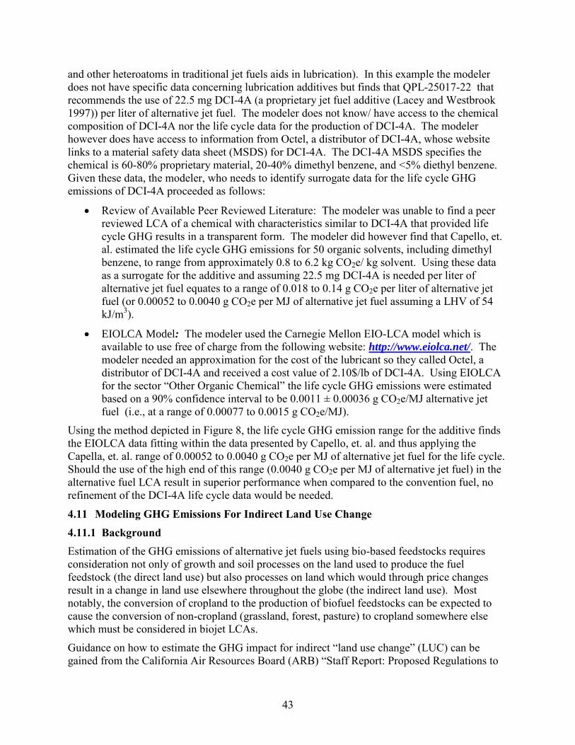
43
and other heteroatoms in traditional jet fuels aids in lubrication). In this example the modeler
does not have specific data concerning lubrication additives but finds that QPL-25017-22 that
recommends the use of 22.5 mg DCI-4A (a proprietary jet fuel additive (Lacey and Westbrook
1997)) per liter of alternative jet fuel. The modeler does not know/ have access to the chemical
composition of DCI-4A nor the life cycle data for the production of DCI-4A. The modeler
however does have access to information from Octel, a distributor of DCI-4A, whose website
links to a material safety data sheet (MSDS) for DCI-4A. The DCI-4A MSDS specifies the
chemical is 60-80% proprietary material, 20-40% dimethyl benzene, and <5% diethyl benzene.
Given these data, the modeler, who needs to identify surrogate data for the life cycle GHG
emissions of DCI-4A proceeded as follows:
Review of Available Peer Reviewed Literature: The modeler was unable to find a peer
reviewed LCA of a chemical with characteristics similar to DCI-4A that provided life
cycle GHG results in a transparent form. The modeler did however find that Capello, et.
al. estimated the life cycle GHG emissions for 50 organic solvents, including dimethyl
benzene, to range from approximately 0.8 to 6.2 kg CO2e/ kg solvent. Using these data
as a surrogate for the additive and assuming 22.5 mg DCI-4A is needed per liter of
alternative jet fuel equates to a range of 0.018 to 0.14 g CO2e per liter of alternative jet
fuel (or 0.00052 to 0.0040 g CO2e per MJ of alternative jet fuel assuming a LHV of 54
kJ/m3).
EIOLCA Model: The modeler used the Carnegie Mellon EIO-LCA model which is
available to use free of charge from the following website: http://www.eiolca.net/. The
modeler needed an approximation for the cost of the lubricant so they called Octel, a
distributor of DCI-4A and received a cost value of 2.10$/lb of DCI-4A. Using EIOLCA
for the sector “Other Organic Chemical” the life cycle GHG emissions were estimated
based on a 90% confidence interval to be 0.0011 ± 0.00036 g CO2e/MJ alternative jet
fuel (i.e., at a range of 0.00077 to 0.0015 g CO2e/MJ).
Using the method depicted in Figure 8, the life cycle GHG emission range for the additive finds
the EIOLCA data fitting within the data presented by Capello, et. al. and thus applying the
Capella, et. al. range of 0.00052 to 0.0040 g CO2e per MJ of alternative jet fuel for the life cycle.
Should the use of the high end of this range (0.0040 g CO2e per MJ of alternative jet fuel) in the
alternative fuel LCA result in superior performance when compared to the convention fuel, no
refinement of the DCI-4A life cycle data would be needed.
4.11 Modeling GHG Emissions For Indirect Land Use Change
4.11.1 Background
Estimation of the GHG emissions of alternative jet fuels using bio-based feedstocks requires
consideration not only of growth and soil processes on the land used to produce the fuel
feedstock (the direct land use) but also processes on land which would through price changes
result in a change in land use elsewhere throughout the globe (the indirect land use). Most
notably, the conversion of cropland to the production of biofuel feedstocks can be expected to
cause the conversion of non-cropland (grassland, forest, pasture) to cropland somewhere else
which must be considered in biojet LCAs.
Guidance on how to estimate the GHG impact for indirect “land use change” (LUC) can be
gained from the California Air Resources Board (ARB) “Staff Report: Proposed Regulations to

44
Implement the Low Carbon Fuel Standard” [1] and the US EPA’s “Draft Regulatory Impact
Analysis: Changes to Renewable Fuel Standard Program” [2]. They suggest a framework based
on five key questions:
How much land is converted?
Where does land use change occur?
What types of land are converted?
What are the GHG emissions from that land conversion?
How do we account for the variable timing of land use change GHG releases?
Guidance on how to respond to these questions is provided within the USEPA document [2], and
is the subject of on-going research and policy discussions. As follows, an example of the
estimation of indirect LUC GHG emissions within a hypothetical biojet LCA is presented, with
attention paid to uncertain decisions and the limitations of assumptions throughout.
4.11.2 LUC Illustrative Example
Suppose the intent is to produce biojet as a replacement to conventional jet fuel and that the
feedstock of interest is to be grown on land that was previously used for production of crop A.
The increase in the demand for crop A causes a shortage in the first growing season. In
subsequent growing seasons, the supply of crop A and the supply of substitute crops (e.g., crops
B, C, and D) increase to meet the new demand, such that prices eventually equilibrate and finally
decrease over time - supply outstripping demand. The final increase in supply means that new
lands are brought into the production of crops A – D (the “new crop mix”) at varying levels of
production efficiency (i.e., in the new crop mix, it is possible that crop A will be produced more
or less efficiently than the original production of crop A). These phenomena combine to form a
“market-mediated response,” which is discussed conceptually by Hertel, et. al. (2009) [3] with
related sources of uncertainty described by the EPA in detail [2] and in a public EPA fact sheet
[4]. The land used to produce the “new crop mix” for the final increase in supply is the indirect
LUC.
For this example, the assumptions used for purposes of illustration in the estimation of the GHG
emissions from the indirect LUC are presented in Table 10. Limitations for each assumption are
noted, which in all cases deal with the ability of the modeler to be confident in the relevance and
comprehensiveness of land use types, management regimes, and the associated data. Ongoing
indirect land use change research (e.g., as part of EPA’s Renewable Fuel Standard rulemaking)
will provide further insight and guidance on how to appropriately determine the
assumptions/values described in Table 10.

45
Table 10. Indirect Land Use Assumptions Used in the Example (For Illustrative Purposes Only)
Indirect land use assumptions for the example Assumption notes and limitations
How much land is
converted?
500 liters of biojet are produced per ha of direct
land (which at 5.23 mmBTU/bbl (LHV) equates to
30.4 liters/mmBTU) or
0.061 direct ha producing crop A/ mmBTU of
biojet produced per year
0.011 indirect ha producing the new crop mix/
mmBTU of biojet produced per year
The land area indirectly converted must consider a
range of factors that affect global agricultural
commodity markets, and the modeler must be
confident their choice is relevant and
comprehensively describes subsequent indirect land
uses.
Where does land
use change occur? In a temperate, dry region
Indirect LUC impacts can occur in many different
regions. Regional variations in GHG emissions
data are wide, and the modeler must be confident
their choice is relevant and comprehensively
describes subsequent indirect land uses.
What types of land
are converted?
The previous use of the indirect land before
conversion: A coniferous, unmanaged, continental
forest with above-ground biomass at 50-150
tonnes/ ha and low activity soils is cleared with fire
The use of the indirect lands after conversion: Cropping system containing perennial species
(long-term cultivation, full tillage)
A wide range of forest, grassland, and pastureland
types could be affected by indirect LUC; thus,
assuming that all land conversion results in
deforestation provides an extreme example for
illustrative purposes only. The modeler must be
confident their choice is relevant and
comprehensively describes previous land uses.
A wide range of crop and cultivation/ tillage
practices are possible, and the modeler must be
confident their choice is relevant and
comprehensively describes subsequent land uses.
What are the GHG
emissions from that
land conversion?
Use IPCC default data and methods to calculate:
Change in the life cycle emissions from
crop production,
Change in biomass carbon stocks,
Non-CO2 emissions from land clearing,
Lost forest sequestration, and
Change in soil carbon stocks
GHG emissions estimation must match region and
types of lands converted and the conversion
methods, and the modeler must be confident their
choice is relevant and comprehensively describes
subsequent indirect land uses.
Default IPCC data should be considered a general
approximation (or Tier I approach) due to coarse
resolution. Precision can be added with higher
resolution data sets from the scientific literature.
How do we account
for the variable
timing of land use
change GHG
releases?
Physical life cycle GHG emissions, including
emissions resulting from indirect land use change,
are displayed from 2010 to 2040 (over 30 years)
GHG emissions from biofuel-induced land use
changes can vary considerably over time. The
modeler should show how emissions vary over
time. If the modeler aggregates emissions over
time, the modeler must be confident their choice of
time horizon and accounting methods are relevant
and appropriate.
Based on the information presented in Table 10, Figure 11 depicts the market interactions given
the dissemination of the biojet production system and the resulting scope of the example biojet
LCA. As shown, the current system, based on the production of 1mmBTU of conventional jet
and the production of crop A on 0.061 ha of land, is replaced by a system producing 1mmBTU of
biojet and the new crop mix on 0.011 ha of land. On the crop side, the production of the “new
crop mix” is assumed to meet the final increase in supply resulting from the increase in demand
for crop A.
On the fuel side, it is assumed that the biojet is added to the jet fuel market resulting in changes,
or “rebound effects,” in fuel markets. In a manner similar to the market changes considered for
indirect LUC, rebound effects account for market changes that might result from new production
of biojet. Several rebound effects could result. For example, an increase in jet fuel supply when
46
could result in a subsequent drop in the price of jet fuel and an increase in its use, such that
prices eventually equilibrate and finally increase over time – demand outstripping supply. A
second rebound effect would involve a decrease in the production of jet fuel from crude oil
which would have oil refineries blend the portion of the crude oil that would have been used for
the production of jet fuel into “other crude oil refinery products” (gasoline, diesel, chemical
precursors, etc.) and resulting in an increase in the supply and a decrease in the price of the
“other crude oil refinery products.” A third rebound effect would also involve a decrease in the
production of jet fuel from crude oil but would have the oil refineries use the jet fuel (or some
version of the portion of the crude used as jet fuel feed) as a fuel to support refining processes.
Other rebound effects are possible, and a mix of rebound effects is likely.
Figure 11. Market Interactions and the Scope of the Example Biojet LCA
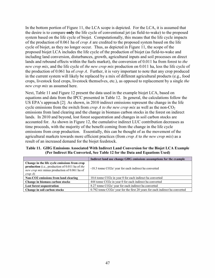
47
In the bottom portion of Figure 11, the LCA scope is depicted. For the LCA, it is assumed that
the desire is to compare only the life cycle of conventional jet (as field-to-wake) to the proposed
system based on the life cycle of biojet. Computationally, this means that the life cycle impacts
of the production of 0.061 ha of crop A are credited to the proposed system based on the life
cycle of biojet, as they no longer occur. Thus, as depicted in Figure 11, the scope of the
proposed biojet LCA includes the life cycle of the production of biojet (as field-to-wake and
including land conversion, disturbances, growth, agricultural inputs and soil processes on direct
lands and rebound effects within the fuels market), the conversion of 0.011 ha from forest to the
new crop mix, and the life cycle of the new crop mix production on 0.011 ha, less the life cycle of
the production of 0.061 ha of crop A. Further, it is very important to note that any crop produced
in the current system will likely be replaced by a mix of different agricultural products (e.g., food
crops, livestock feed crops, livestock themselves, etc.), as opposed to replacement by a single the
new crop mix as assumed here.
Next, Table 11 and Figure 12 present the data used in the example biojet LCA, based on
equations and data from the IPCC presented in Table 12. In general, the calculations follow the
US EPA’s approach [2]. As shown, in 2010 indirect emissions represent the change in the life
cycle emissions from the switch from crop A to the new crop mix as well as the non-CO2
emissions from land clearing and the change in biomass carbon stocks in the forest on indirect
lands. In 2010 and beyond, lost forest sequestration and changes in soil carbon stocks are
accounted for. As shown in Figure 12, the cumulative indirect LUC contribution decreases as
time proceeds, with the majority of the benefit coming from the change in the life cycle
emissions from crop production. Essentially, this can be thought of as the movement of the
agricultural markets towards more efficient practices (from crop A to the new crop mix) as a
result of an increased demand for the biojet feedstock.
Table 11. GHG Emissions Associated With Indirect Land Conversion for the Biojet LCA Example
(Per Indirect Ha Converted, See Table 12 for the Data and Equations Used)
Indirect land use change GHG emissions assumptions for the example
Change in the life cycle emissions from crop
production (i.e., production of 0.011 ha of the
new crop mix minus production of 0.061 ha of
crop A)
-18.3 tonne CO2e/ year for each indirect ha converted
Non-CO2 emissions from land clearing 10.6 tonne CO2e in year 0 for each indirect ha converted
Change in biomass carbon stocks 444 tonne CO2e in year 0 for each indirect ha converted
Lost forest sequestration 8.27 tonne CO2e/ year for each indirect ha converted
Change in soil carbon stocks 0.792 tonne CO2e/ year for the first 20 years for each indirect ha converted

48
Figure 12. Example Indirect LUC GHG Emissions
(Per Indirect Ha Converted From Forest to the new crop mix)
Table 12. Estimation of GHG Emissions for Indirect Land
Conversion (Per Indirect Ha Converted)
Indirect land use assumptions for the example
Change in
the life cycle
emissions
from crop
production
Change in the life cycle emissions from crop production = -18.3 tonne CO2e/ yr for each indirect ha
converted
Estimated as:
Change in the life cycle emissions from crop production = LCIC*IA -(LCDC*DA)
IA assuming
LCIC= the life cycle GHG emissions for the new crop mix produced on indirect lands during biojet
production is 4.6 tonnes CO2 e/ha/yr
IA = the ha of indirect land used for the new crop mix production is 0.011 ha/ mmBTU biojet
LCDC= the life cycle GHG emissions for crop A produced on direct lands prior to biojet production is 4.0
tonnes CO2 e/ha/yr
DA = the ha of direct land used for biojet production is 0.061 ha/ mmBTU biojet
Non-CO2
emissions
from land
clearing
Non-CO2 emissions from land clearing= 10.6 tonne CO2e in yr 0 for each indirect ha converted
Assuming the forest is cleared by fire, non-CO2 GHG emissions were estimated using Equation 2.27 of the
IPCC AFOLU [6] assuming:
The fuel (dead organic matter plus live biomass) biomass consumption is 50.4 tonnes dry matter/ ha (for non-Eucalyptis forests temperate forests from Table 2.4 of the IPCC [6])
The emission factors for CH4 and N2O are 7.1 and 0.11 g/kg dry matter combusted respectively (from
the IPCC [7] Table 3A.1.16, on page 3.185); and
The GWPs of CH4 and N2O are 25 and 298 tonne CO2e/ tonne emitted respectively (as suggested in
the IPCC AR4)
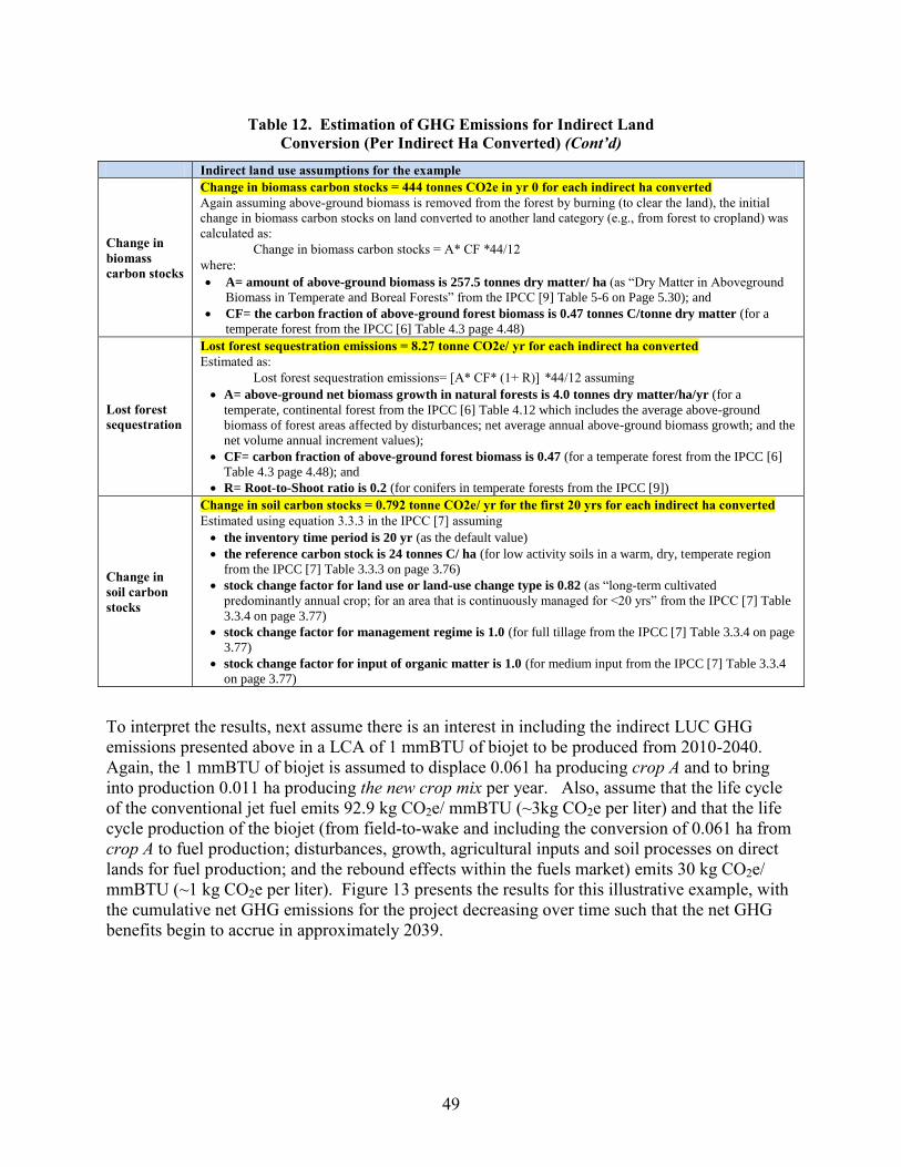
49
Table 12. Estimation of GHG Emissions for Indirect Land
Conversion (Per Indirect Ha Converted) (Cont’d)
Indirect land use assumptions for the example
Change in
biomass
carbon stocks
Change in biomass carbon stocks = 444 tonnes CO2e in yr 0 for each indirect ha converted
Again assuming above-ground biomass is removed from the forest by burning (to clear the land), the initial
change in biomass carbon stocks on land converted to another land category (e.g., from forest to cropland) was
calculated as:
Change in biomass carbon stocks = A* CF *44/12
where:
A= amount of above-ground biomass is 257.5 tonnes dry matter/ ha (as “Dry Matter in Aboveground
Biomass in Temperate and Boreal Forests” from the IPCC [9] Table 5-6 on Page 5.30); and
CF= the carbon fraction of above-ground forest biomass is 0.47 tonnes C/tonne dry matter (for a
temperate forest from the IPCC [6] Table 4.3 page 4.48)
Lost forest
sequestration
Lost forest sequestration emissions = 8.27 tonne CO2e/ yr for each indirect ha converted
Estimated as:
Lost forest sequestration emissions= [A* CF* (1+ R)] *44/12 assuming
A= above-ground net biomass growth in natural forests is 4.0 tonnes dry matter/ha/yr (for a
temperate, continental forest from the IPCC [6] Table 4.12 which includes the average above-ground
biomass of forest areas affected by disturbances; net average annual above-ground biomass growth; and the
net volume annual increment values);
CF= carbon fraction of above-ground forest biomass is 0.47 (for a temperate forest from the IPCC [6]
Table 4.3 page 4.48); and
R= Root-to-Shoot ratio is 0.2 (for conifers in temperate forests from the IPCC [9])
Change in
soil carbon
stocks
Change in soil carbon stocks = 0.792 tonne CO2e/ yr for the first 20 yrs for each indirect ha converted
Estimated using equation 3.3.3 in the IPCC [7] assuming
the inventory time period is 20 yr (as the default value)
the reference carbon stock is 24 tonnes C/ ha (for low activity soils in a warm, dry, temperate region
from the IPCC [7] Table 3.3.3 on page 3.76)
stock change factor for land use or land-use change type is 0.82 (as “long-term cultivated
predominantly annual crop; for an area that is continuously managed for <20 yrs” from the IPCC [7] Table
3.3.4 on page 3.77)
stock change factor for management regime is 1.0 (for full tillage from the IPCC [7] Table 3.3.4 on page
3.77)
stock change factor for input of organic matter is 1.0 (for medium input from the IPCC [7] Table 3.3.4
on page 3.77)
To interpret the results, next assume there is an interest in including the indirect LUC GHG
emissions presented above in a LCA of 1 mmBTU of biojet to be produced from 2010-2040.
Again, the 1 mmBTU of biojet is assumed to displace 0.061 ha producing crop A and to bring
into production 0.011 ha producing the new crop mix per year. Also, assume that the life cycle
of the conventional jet fuel emits 92.9 kg CO2e/ mmBTU (~3kg CO2e per liter) and that the life
cycle production of the biojet (from field-to-wake and including the conversion of 0.061 ha from
crop A to fuel production; disturbances, growth, agricultural inputs and soil processes on direct
lands for fuel production; and the rebound effects within the fuels market) emits 30 kg CO2e/
mmBTU (~1 kg CO2e per liter). Figure 13 presents the results for this illustrative example, with
the cumulative net GHG emissions for the project decreasing over time such that the net GHG
benefits begin to accrue in approximately 2039.
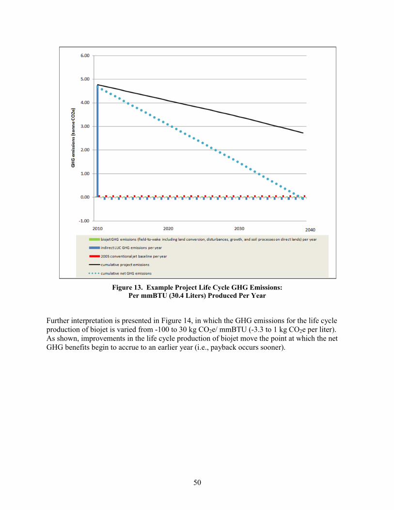
50
Figure 13. Example Project Life Cycle GHG Emissions:
Per mmBTU (30.4 Liters) Produced Per Year
Further interpretation is presented in Figure 14, in which the GHG emissions for the life cycle
production of biojet is varied from -100 to 30 kg CO2e/ mmBTU (-3.3 to 1 kg CO2e per liter).
As shown, improvements in the life cycle production of biojet move the point at which the net
GHG benefits begin to accrue to an earlier year (i.e., payback occurs sooner).

51
Figure 14. Cumulative Net Jet GHG Emissions With Variation in the Life Cycle Biojet Production
GHG Emissions: Per mmBTU (30.4 Liters) Produced Per Year From 2010-2040
Due to these types of trends, the USEPA [2] calculates a net present value (NPV) of emissions to
provide a common metric for direct comparison of life cycle emissions from alternative and
conventional fuels. Guidance on the estimation of NPV for biofuel GHG emissions is provided
by O'Hare, et al. [5] who offer a methodology for discounting physical quantities using a damage
function based on the contribution of GHG emissions to radiative forcing over time. To estimate
the NPV, the modeler must be confident that their damage function, discount factor, and
assumed time frame are relevant and comprehensively describe direct and indirect GHG
emissions. For example, whereas the California ARB [1] uses a time horizon of 30 years and a
0% discount rate, the USEPA [2] presents results with time horizons of 30 and 100 years and
discount factors of 0% and 2% in the estimation of NPV for GHG emissions. Neither describe
the damage function used.

52
The intended purpose of the example described above is to provide guidance on the system
boundaries and information needs for consideration of indirect LUC within a biojet LCA. The
related policy, science, and assessment methodology are in a state of flux, with the USEPA and
researchers throughout the globe working towards consensus. Given this, the example presented
here uses GHG emissions data for a single condition, with the goal of demonstrating the use of
data accessible directly from the IPCC guidance documents [6,7]. Specifically, in contrast to the
US EPA’s methodology [2]:
In the example presented here, a single land area and a single type of land conversion
are assumed (specifically, the conversion of 0.011 ha / mmBTU of LUC in a temperate,
dry region from a coniferous, unmanaged, continental forest with low activity soils’ to a
set of long-term cultivated, full tillage perennial cropping systems for the new crop mix),
In the USEPA GHG assessment [2], the Farm and Agricultural Policy Research
Institute (FAPRI) and the Forestry and Agriculture Sector Optimization Model (FOSOM)
agricultural models are used to estimate domestic and international crop expansion
respectively for a wide variety of agricultural products, with the type of land conversion
then matched to the ecological zone and management practices in specific countries or
regions, based on recent land use change patterns observed in satellite imagery.
As the USEPA continues to prepare guidelines and data for a wide range of biofeedstocks, the
modeler’s role in formulating answers to the 5 key questions, and in the development of data to
represent the wide range of land types and crops ultimately affected, will be reduced.
4.11.3 Matching Methodological Assumptions For System Boundary Definition
As noted in Section 3.2.2, this guidance document focuses primarily on average attributional
LCAs for conventional and alternative aviation fuels representing “an isolated system.” As
defined above, indirect LUC is a consequence of alternative fuels production and is thus outside
such an attributional LCA’s isolated system. Consequential LCA, also mentioned in Section
3.2.2, includes assessment of not only the consequences of LUC but also the consequences other
economic aspects of the alternative fuel’s life cycle.
In a consequential LCA, “consequential processes” are added within the system as resources
enter or leave economic markets, thusly change the supply and demand characteristics of the
markets, and, like LUC, cause the potential for a change in resource use and waste and
associated environmental impact. A consequential LCA assumes market interaction either as a
result of process multi-functionality, as a result of the use or production of open loop recyclables
(as a special case of multi-functionality), or when production of a resource is constrained (i.e., a
resource for which there is competition in the market, caused by market forces, natural
limitations on the availability of the resource, or due to an intervention such as a government
regulation) (Ekvall and Weidema [8]). Such processes are included in a consequential LCA
using system expansion as described in Section 3.5.3 with the ultimate computational goal of
only the product that leaves the system boundaries is the product of interest. For example, in an
algae-to-jet consequential LCA, the desire is that only jet fuel is produced. This means for
example that the use of recycled wastewater for algal growth may result in the replacement of
land applied wastewater with irrigation and fertilizers; the use of methanol for algae oil
transesterifcation may result in the replacement of the use of methanol as a chemical precursor;
and the co-production of diesel and gasoline with jet by hydrocracking may displace the use of
other fuels in mobile and stationary energy generation. Further, in an ideal consequential LCA
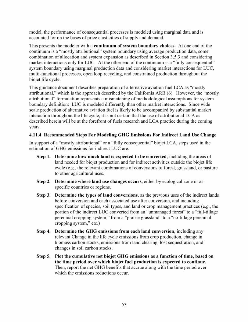
53
model, the performance of consequential processes is modeled using marginal data and is
accounted for on the bases of price elasticities of supply and demand.
This presents the modeler with a continuum of system boundary choices. At one end of the
continuum is a “mostly attributional” system boundary using average production data, some
combination of allocation and system expansion as described in Section 3.5.3 and considering
market interactions only for LUC. At the other end of the continuum is a “fully consequential”
system boundary using marginal production data and considering market interactions for LUC,
multi-functional processes, open loop recycling, and constrained production throughout the
biojet life cycle.
This guidance document describes preparation of alternative aviation fuel LCA as “mostly
attributional,” which is the approach described by the California ARB (6). However, the “mostly
attributional” formulation represents a mismatching of methodological assumptions for system
boundary definition: LUC is modeled differently than other market interactions. Since wide
scale production of alternative aviation fuel is likely to be accompanied by substantial market
interaction throughout the life cycle, it is not certain that the use of attributional LCA as
described herein will be at the forefront of fuels research and LCA practice during the coming
years.
4.11.4 Recommended Steps For Modeling GHG Emissions For Indirect Land Use Change
In support of a “mostly attributional” or a “fully consequential” biojet LCA, steps used in the
estimation of GHG emissions for indirect LUC are:
Step 1. Determine how much land is expected to be converted, including the areas of
land needed for biojet production and for indirect activities outside the biojet life
cycle (e.g., the relevant combinations of conversions of forest, grassland, or pasture
to other agricultural uses.
Step 2. Determine where land use changes occurs, either by ecological zone or as
specific countries or regions.
Step 3. Determine the types of land conversions, as the previous uses of the indirect lands
before conversion and each associated use after conversion, and including
specification of species, soil types, and land or crop management practices (e.g., the
portion of the indirect LUC converted from an “unmanaged forest” to a “full-tillage
perennial cropping system,” from a “prairie grassland” to a “no-tillage perennial
cropping system,” etc.)
Step 4. Determine the GHG emissions from each land conversion, including any
relevant Change in the life cycle emissions from crop production, change in
biomass carbon stocks, emissions from land clearing, lost sequestration, and
changes in soil carbon stocks.
Step 5. Plot the cumulative net biojet GHG emissions as a function of time, based on
the time period over which biojet fuel production is expected to continue.
Then, report the net GHG benefits that accrue along with the time period over
which the emissions reductions occur.

54
Step 6. Quantify the uncertainty in indirect land use change estimates. Present
uncertainty estimates for each Step 1-4, and cumulatively. See the uncertainty
protocol in Chapter 5 for further guidance.
In the absence of reliable information and data for domestic and international crop expansion or
for any of the items listed above, the modeler should prepare a worst case scenario, assuming for
example an acre- for-acre crop expansion (i.e., 1 ha indirect LUC/ ha direct LUC), based on a
worst case set of GHG emissions from the land conversion based on the IPCC data [6,7], and
using the data quality and uncertainty protocol described in Chapter 5. Again, as the USEPA and
researchers throughout the globe continue to prepare guidelines and data for a wide range of
biofeedstocks, the modeler’s role in modeling the GHG emissions from indirect LUC will be
reduced.
4.11.5 References
1. CARB (2009), Califonia Air Resources Board, Proposed Regulation to Implement the
Low Carbon Fuel Standard, Volumes 1 and 2, March 5, 2009, available at
http://www.arb.ca.gov/fuels/lcfs/030409lcfs_isor_vol1.pdf, and
http://www.arb.ca.gov/fuels/lcfs/030409lcfs_isor_vol2.pdf
2. USEPA (2009) Draft Regulatory Impact Analysis: Changes to Renewable Fuel Standard
Program, available at http://www.epa.gov/OMS/renewablefuels/420d09001.pdf
3. Hertel et al. (2009) Hertel, T.W., Golub, A.A., Jones, A.D., O’Hare, M., Plevin, R.J.,
Kammen, D.M., (2009) Global Land Use and Greenhouse Gas Emissions Impacts of U.S.
Maize Ethanol: The Role of Market-Meditate Responses, GTAP Working Paper No. 55,
http://ideas.repec.org/s/gta/workpp.html
4. USEPA (2009) Technical Highlights: EPA Lifecycle Analysis of Greenhouse Gas
Emissions from Renewable Fuels, Office of Transportation and Air Quality, EPA-420-F-
09-024, http://www.epa.gov/OMS/renewablefuels/420f09024.pdf
5. O'Hare,M., R .J. Plevin, J. I. Martin, A.D. Jones, A. Kendall, E. Hopson (2009) Proper
accounting for time increases crop-based biofuels' greenhouse gas deficit versus
petroleum, Environmental Research Letters, 4 (2) 1-7
6. IPCC (2006) 2006 IPCC Guidelines for National Greenhouse Gas Inventories. 2006.
Agriculture, Forestry and Other Land Uses. Volume 4, available at http://www.ipcc-
nggip.iges.or.jp/public/2006gl/vol4.html
7. IPCC (2003) Good Practice Guidance for Land Use, Land-Use Change and Forestry,
available at http://www.ipcc-nggip.iges.or.jp/public/gpglulucf/gpglulucf_contents.html
8. Ekvall, T., B.P.Weidema (2004) “System Boundaries and Input Data in Consequential
Life Cycle Inventory Analysis” International Journal of Life Cycle Assessment, 9 (3)
161-171
9. IPCC (1996) Revised 1996 IPCC Guidelines for National Greenhouse Gas Inventories:
Reference Manual, available at http://www.ipcc-nggip.iges.or.jp/public/gl/invs1.html
55
4.12 Unit Process Exclusions
For the purpose of completing an LCA that meets the goals outlined in this guideline document,
the inclusion of the following data is not expected:
Although activities such as commuting to and from work and producing food for
consumption during working hours may be omitted, activities that humans perform while
on the job, such as driving a tractor or using facilities such as lighting while at work
(which will impact the overall auxiliary power needs of the facility) should be included
within the system.
Low-frequency, high-magnitude, non-predictable environmental events (e.g., non-
routine/fugitive/accidental releases) are not included in the system because such
circumstances are difficult to associate with a particular product; however, more frequent
or predictable events, such as material loss during transport, are included in the system
boundary. Also, low frequency, high magnitude events that occur on a predictable basis
are included in the system boundary.
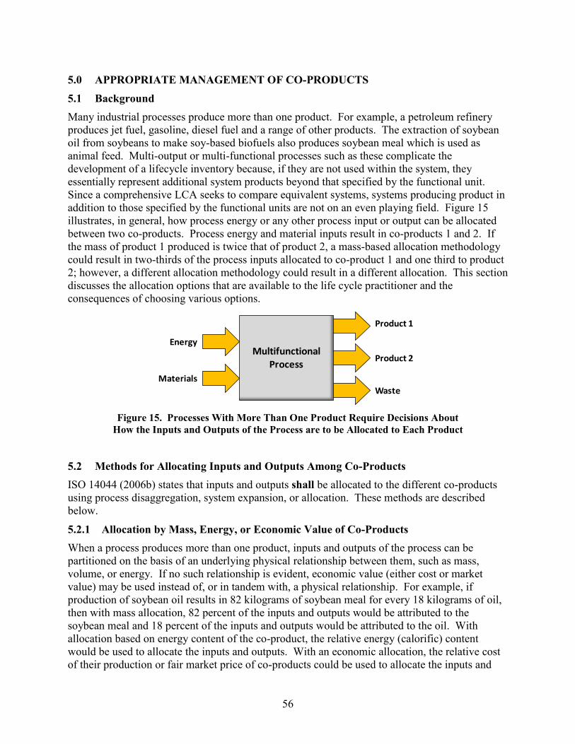
56
5.0 APPROPRIATE MANAGEMENT OF CO-PRODUCTS
5.1 Background
Many industrial processes produce more than one product. For example, a petroleum refinery
produces jet fuel, gasoline, diesel fuel and a range of other products. The extraction of soybean
oil from soybeans to make soy-based biofuels also produces soybean meal which is used as
animal feed. Multi-output or multi-functional processes such as these complicate the
development of a lifecycle inventory because, if they are not used within the system, they
essentially represent additional system products beyond that specified by the functional unit.
Since a comprehensive LCA seeks to compare equivalent systems, systems producing product in
addition to those specified by the functional units are not on an even playing field. Figure 15
illustrates, in general, how process energy or any other process input or output can be allocated
between two co-products. Process energy and material inputs result in co-products 1 and 2. If
the mass of product 1 produced is twice that of product 2, a mass-based allocation methodology
could result in two-thirds of the process inputs allocated to co-product 1 and one third to product
2; however, a different allocation methodology could result in a different allocation. This section
discusses the allocation options that are available to the life cycle practitioner and the
consequences of choosing various options.
Figure 15. Processes With More Than One Product Require Decisions About
How the Inputs and Outputs of the Process are to be Allocated to Each Product
5.2 Methods for Allocating Inputs and Outputs Among Co-Products
ISO 14044 (2006b) states that inputs and outputs shall be allocated to the different co-products
using process disaggregation, system expansion, or allocation. These methods are described
below.
5.2.1 Allocation by Mass, Energy, or Economic Value of Co-Products
When a process produces more than one product, inputs and outputs of the process can be
partitioned on the basis of an underlying physical relationship between them, such as mass,
volume, or energy. If no such relationship is evident, economic value (either cost or market
value) may be used instead of, or in tandem with, a physical relationship. For example, if
production of soybean oil results in 82 kilograms of soybean meal for every 18 kilograms of oil,
then with mass allocation, 82 percent of the inputs and outputs would be attributed to the
soybean meal and 18 percent of the inputs and outputs would be attributed to the oil. With
allocation based on energy content of the co-product, the relative energy (calorific) content
would be used to allocate the inputs and outputs. With an economic allocation, the relative cost
of their production or fair market price of co-products could be used to allocate the inputs and
Energy
Materials
Product 1
Product 2
Waste
Multifunctional Process
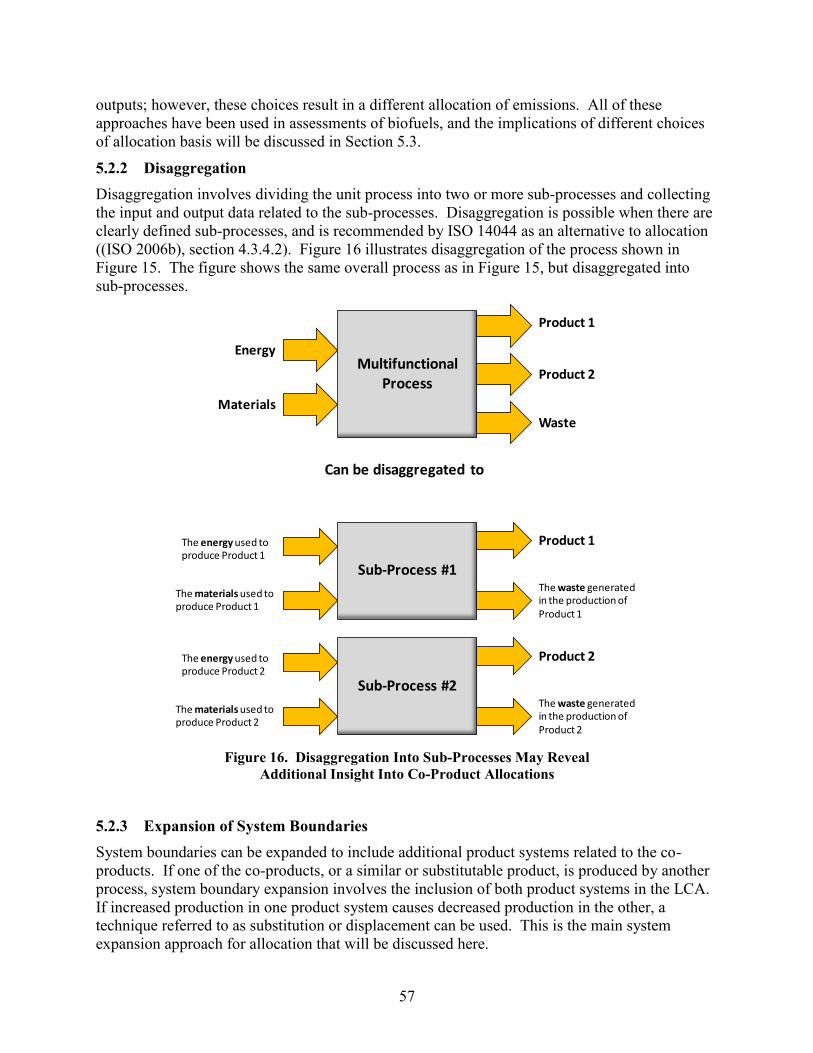
57
outputs; however, these choices result in a different allocation of emissions. All of these
approaches have been used in assessments of biofuels, and the implications of different choices
of allocation basis will be discussed in Section 5.3.
5.2.2 Disaggregation
Disaggregation involves dividing the unit process into two or more sub-processes and collecting
the input and output data related to the sub-processes. Disaggregation is possible when there are
clearly defined sub-processes, and is recommended by ISO 14044 as an alternative to allocation
((ISO 2006b), section 4.3.4.2). Figure 16 illustrates disaggregation of the process shown in
Figure 15. The figure shows the same overall process as in Figure 15, but disaggregated into
sub-processes.
Figure 16. Disaggregation Into Sub-Processes May Reveal
Additional Insight Into Co-Product Allocations
5.2.3 Expansion of System Boundaries
System boundaries can be expanded to include additional product systems related to the co-
products. If one of the co-products, or a similar or substitutable product, is produced by another
process, system boundary expansion involves the inclusion of both product systems in the LCA.
If increased production in one product system causes decreased production in the other, a
technique referred to as substitution or displacement can be used. This is the main system
expansion approach for allocation that will be discussed here.
Energy
Materials
Product 1
Product 2
Waste
Multifunctional Process
Can be disaggregated to
The energy used to produce Product 1
The materials used to produce Product 1
Sub-Process #1
Product 1
The waste generated in the production of Product 1
The energy used to produce Product 2
The materials used to produce Product 2
Sub-Process #2
Product 2
The waste generated in the production of Product 2

58
In a displacement calculation, the mass and energy that would have been used and the emissions
that would have been generated during production of the displaced product are counted as credits
for the co-product. These credits are subtracted from the total mass and energy used and
emissions associated with the product (e.g. an aviation fuel) under evaluation (Huo, et al. 2008).
For example, if glycerin is produced as a by-product of bio-diesel production, that glycerin may
displace glycerin that is made from an alternate process. The emissions that would have been
generated in the alternate process, that are now being displaced by glycerin as a co-product from
bio-diesel manufacturing, are counted as emission credits. Figure 17 illustrates an example of a
displacement calculation.
Figure 17. An Alternate Process That Produces Product 2 That is the
Same as, or Can be Used as a Substitute for, the Co-Product 2
5.3 Discussion of Approaches
5.3.1 Discussion of Allocation by Measures Such as Mass, Energy or Value
The advantage of allocation by measures such as co-product mass, energy or economic value is
that the calculation is based just on the physical properties of the process streams and data from
the production facility, and the allocation parameter can generally be quantified easily. In
contrast, economic allocation metrics are dependent on markets which fluctuate on time scales
that are different than the time scales for the design of production facilities.
The co-products of soy-derived fuels have been allocated in a number of different ways in
different studies. Hill, et al. (2006) allocated the processing energy between soybean oil and
soybean meal on the basis of mass. In contrast, Shapouri, et al. (2006) allocated by energy
(calorific) value for co-products used as food or agricultural feed. Pradhan, et al. (2008)
reviewed studies of soy biodiesel and found that allocation was responsible for most of the
difference between studies.
Energy
Materials
Product 1
Product 2
Waste
Multifunctional Process
Less or Minus
The life cycles of energy used to produce Product 2
The life cycles of materials used to produce Product 2
Alternative method to
produce Product #2
Product 2
The life cycles of waste management for wastes produced with Product 2
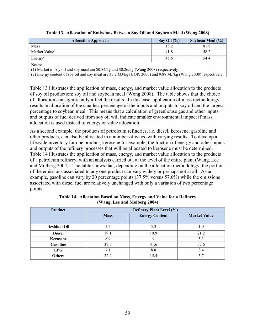
59
Table 13. Allocation of Emissions Between Soy Oil and Soybean Meal (Wong 2008)
Allocation Approach Soy Oil (%) Soybean Meal (%)
Mass 18.2 81.8
Market Value1 41.8 58.2
Energy2 45.6 54.4
Notes:
(1) Market of soy oil and soy meal are $0.84/kg and $0.26/kg (Wang 2008) respectively
(2) Energy content of soy oil and soy meal are 37.2 MJ/kg (UOP, 2005) and 9.88 MJ/kg (Wang 2008) respectively
Table 13 illustrates the application of mass, energy, and market value allocation to the products
of soy oil production: soy oil and soybean meal (Wong 2008). The table shows that the choice
of allocation can significantly affect the results. In this case, application of mass methodology
results in allocation of the smallest percentage of the inputs and outputs to soy oil and the largest
percentage to soybean meal. This means that a calculation of greenhouse gas and other inputs
and outputs of fuel derived from soy oil will indicate smaller environmental impact if mass
allocation is used instead of energy or value allocation.
As a second example, the products of petroleum refineries, i.e. diesel, kerosene, gasoline and
other products, can also be allocated in a number of ways, with varying results. To develop a
lifecycle inventory for one product, kerosene for example, the fraction of energy and other inputs
and outputs of the refinery processes that will be allocated to kerosene must be determined.
Table 14 illustrates the application of mass, energy, and market value allocation to the products
of a petroleum refinery, with an analysis carried out at the level of the entire plant (Wang, Lee
and Molberg 2004). The table shows that, depending on the allocation methodology, the portion
of the emissions associated to any one product can vary widely or perhaps not at all. As an
example, gasoline can vary by 20 percentage points (37.5% versus 57.6%) while the emissions
associated with diesel fuel are relatively unchanged with only a variation of two percentage
points.
Table 14. Allocation Based on Mass, Energy and Value for a Refinery
(Wang, Lee and Molberg 2004)
Product Refinery Plant Level (%)
Mass Energy Content Market Value
Residual Oil 5.2 5.3 1.9
Diesel 19.1 19.9 21.2
Kerosene 8.9 9 5.3
Gasoline 37.5 41.6 57.6
LPG 7.1 8.8 8.4
Others 22.2 15.4 5.7
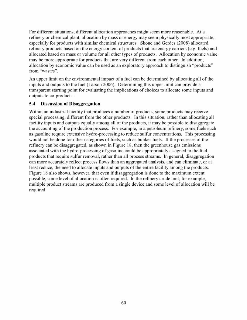
60
For different situations, different allocation approaches might seem more reasonable. At a
refinery or chemical plant, allocation by mass or energy may seem physically most appropriate,
especially for products with similar chemical structures. Skone and Gerdes (2008) allocated
refinery products based on the energy content of products that are energy carriers (e.g. fuels) and
allocated based on mass or volume for all other types of products. Allocation by economic value
may be more appropriate for products that are very different from each other. In addition,
allocation by economic value can be used as an exploratory approach to distinguish “products”
from “wastes”.
An upper limit on the environmental impact of a fuel can be determined by allocating all of the
inputs and outputs to the fuel (Larson 2006). Determining this upper limit can provide a
transparent starting point for evaluating the implications of choices to allocate some inputs and
outputs to co-products.
5.4 Discussion of Disaggregation
Within an industrial facility that produces a number of products, some products may receive
special processing, different from the other products. In this situation, rather than allocating all
facility inputs and outputs equally among all of the products, it may be possible to disaggregate
the accounting of the production process. For example, in a petroleum refinery, some fuels such
as gasoline require extensive hydro-processing to reduce sulfur concentrations. This processing
would not be done for other categories of fuels, such as bunker fuels. If the processes of the
refinery can be disaggregated, as shown in Figure 18, then the greenhouse gas emissions
associated with the hydro-processing of gasoline could be appropriately assigned to the fuel
products that require sulfur removal, rather than all process streams. In general, disaggregation
can more accurately reflect process flows than an aggregated analysis, and can eliminate, or at
least reduce, the need to allocate inputs and outputs of the entire facility among the products.
Figure 18 also shows, however, that even if disaggregation is done to the maximum extent
possible, some level of allocation is often required. In the refinery crude unit, for example,
multiple product streams are produced from a single device and some level of allocation will be
required
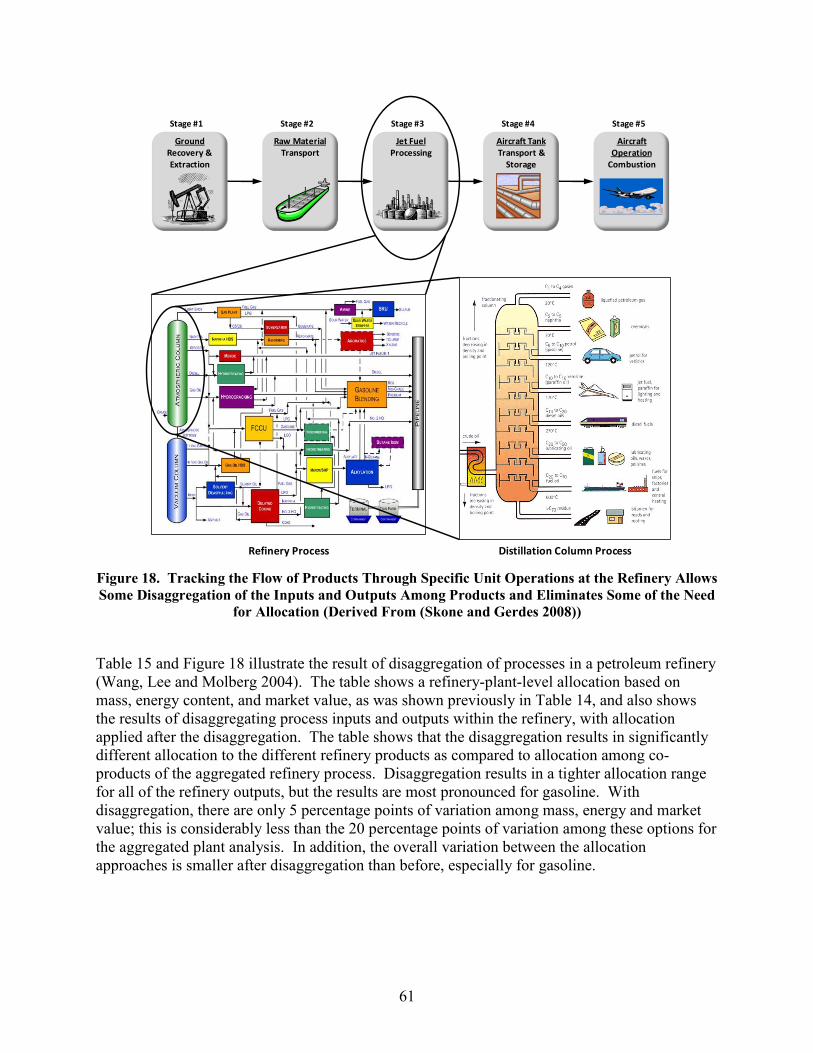
61
Figure 18. Tracking the Flow of Products Through Specific Unit Operations at the Refinery Allows
Some Disaggregation of the Inputs and Outputs Among Products and Eliminates Some of the Need
for Allocation (Derived From (Skone and Gerdes 2008))
Table 15 and Figure 18 illustrate the result of disaggregation of processes in a petroleum refinery
(Wang, Lee and Molberg 2004). The table shows a refinery-plant-level allocation based on
mass, energy content, and market value, as was shown previously in Table 14, and also shows
the results of disaggregating process inputs and outputs within the refinery, with allocation
applied after the disaggregation. The table shows that the disaggregation results in significantly
different allocation to the different refinery products as compared to allocation among co-
products of the aggregated refinery process. Disaggregation results in a tighter allocation range
for all of the refinery outputs, but the results are most pronounced for gasoline. With
disaggregation, there are only 5 percentage points of variation among mass, energy and market
value; this is considerably less than the 20 percentage points of variation among these options for
the aggregated plant analysis. In addition, the overall variation between the allocation
approaches is smaller after disaggregation than before, especially for gasoline.
GroundRecovery & Extraction
Stage #1
Raw MaterialTransport
Stage #2
Jet FuelProcessing
Stage #3
Aircraft TankTransport &
Storage
Stage #4
Aircraft Operation
Combustion
Stage #5
Refinery Process Distillation Column Process
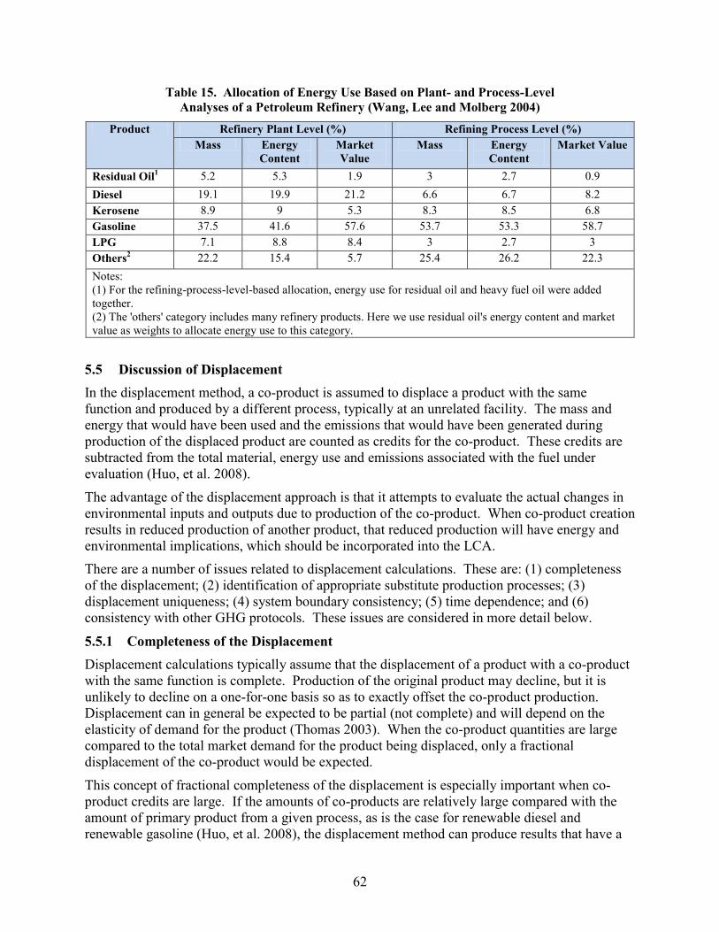
62
Table 15. Allocation of Energy Use Based on Plant- and Process-Level
Analyses of a Petroleum Refinery (Wang, Lee and Molberg 2004)
Product Refinery Plant Level (%) Refining Process Level (%)
Mass Energy
Content
Market
Value
Mass Energy
Content
Market Value
Residual Oil1 5.2 5.3 1.9 3 2.7 0.9
Diesel 19.1 19.9 21.2 6.6 6.7 8.2
Kerosene 8.9 9 5.3 8.3 8.5 6.8
Gasoline 37.5 41.6 57.6 53.7 53.3 58.7
LPG 7.1 8.8 8.4 3 2.7 3
Others2 22.2 15.4 5.7 25.4 26.2 22.3
Notes:
(1) For the refining-process-level-based allocation, energy use for residual oil and heavy fuel oil were added
together.
(2) The 'others' category includes many refinery products. Here we use residual oil's energy content and market
value as weights to allocate energy use to this category.
5.5 Discussion of Displacement
In the displacement method, a co-product is assumed to displace a product with the same
function and produced by a different process, typically at an unrelated facility. The mass and
energy that would have been used and the emissions that would have been generated during
production of the displaced product are counted as credits for the co-product. These credits are
subtracted from the total material, energy use and emissions associated with the fuel under
evaluation (Huo, et al. 2008).
The advantage of the displacement approach is that it attempts to evaluate the actual changes in
environmental inputs and outputs due to production of the co-product. When co-product creation
results in reduced production of another product, that reduced production will have energy and
environmental implications, which should be incorporated into the LCA.
There are a number of issues related to displacement calculations. These are: (1) completeness
of the displacement; (2) identification of appropriate substitute production processes; (3)
displacement uniqueness; (4) system boundary consistency; (5) time dependence; and (6)
consistency with other GHG protocols. These issues are considered in more detail below.
5.5.1 Completeness of the Displacement
Displacement calculations typically assume that the displacement of a product with a co-product
with the same function is complete. Production of the original product may decline, but it is
unlikely to decline on a one-for-one basis so as to exactly offset the co-product production.
Displacement can in general be expected to be partial (not complete) and will depend on the
elasticity of demand for the product (Thomas 2003). When the co-product quantities are large
compared to the total market demand for the product being displaced, only a fractional
displacement of the co-product would be expected.
This concept of fractional completeness of the displacement is especially important when co-
product credits are large. If the amounts of co-products are relatively large compared with the
amount of primary product from a given process, as is the case for renewable diesel and
renewable gasoline (Huo, et al. 2008), the displacement method can produce results that have a
63
large impact on the LCA of the fuel. It is mathematically possible for displacement calculations
to result in negative energy and environmental impacts for the fuel chain, if the co-products are
calculated as having less environmental impact than the product that they are displacing (Table
16).
Table 16 shows six different approaches to allocation between soy oil and soybean meal. The
first three rows show allocation by mass, market value, and energy, as was previously shown in
Table 13. The rest of the table shows displacement calculations in which soybean meal is
assumed to displace barley, corn, or soybeans. Because production of barley and corn, in this
illustration, have greater GHG emissions than production of the corresponding amount of
soybean meal, the displacement of these products by soybean meal is calculated to be greater
than all the inputs and outputs of the soy oil/soybean meal production process. The result is that
in some cases, production of soy oil is calculated to have a negative allocation, meaning that the
soy oil is calculated to have a net environmental benefit.
Table 16. Allocation of GHG Emissions Between Soy Oil and
Soybean Meal (Wong, 2008, Table 56)
Allocation Approach Soy Oil (%) Soybean Meal (%)
Mass 18.2 81.8
Market Value1 45.6 54.4
Energy2 41.8 58.2
Displacement of barley
(1kg soymeal = 4kg barley)3
LUC included from soybeans
and barley
-5 105
LUC included from soy but
not barley
71 29
no LUC -217 317
Displacement of corn
(1kg soymeal = 5.3kg corn)3
LUC included from soybeans
and barley
-233 333
LUC included from soy but
not barley
64 36
no LUC -301 401
Displacement of soybean
(1kg soymeal = 1.2kg soybean)3
LUC included from soybeans
and barley
4.3 95.7
LUC included from soy but
not barley
95 5
no LUC 45.3 54.7
Notes:
(1) Market of soy oil and soy meal are $0.84/kg and $0.26/kg (GREET, 2007) respectively
(2) Energy content of soy oil and soy meal are 37.2 MJ/kg (UOP, 2005) and 9.88 MJ/kg (Wang, 2008) respectively
(3) Equivalency between soymeal and displaced product was done on protein equivalency
(4) Lifecycle GHG emissions from soybean faming and soy oil extraction are 60.3gCO2e/MJ of fuel produced
(5) LUC refers to land use change
For a fuel system, the use of co-products to substitute for other products can be tracked over
time, although robust data are likely to be available only after major industrial development of
the fuel system. Moreover, substitution effects will be intertwined with economic changes in the
demand for the co-products and its substitutes that may be independent of the fuel production
system. Quantification of the extent of substitution/displacement is likely to be uncertain; this
uncertainty should be acknowledged in the analysis.
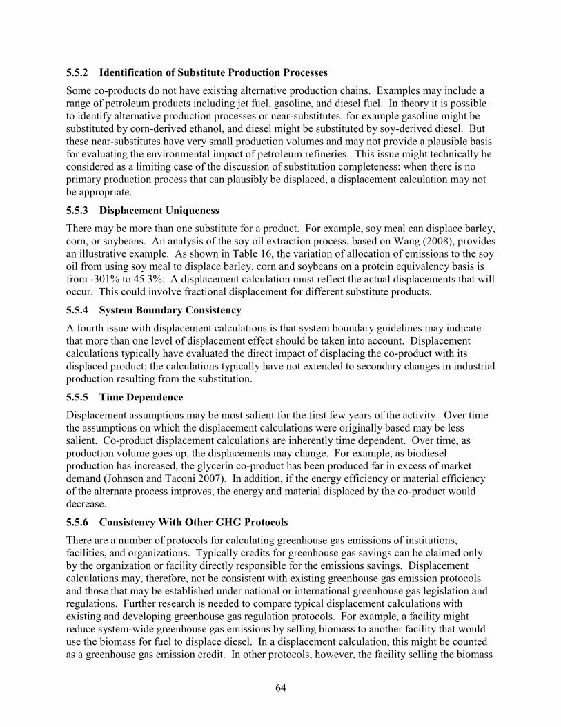
64
5.5.2 Identification of Substitute Production Processes
Some co-products do not have existing alternative production chains. Examples may include a
range of petroleum products including jet fuel, gasoline, and diesel fuel. In theory it is possible
to identify alternative production processes or near-substitutes: for example gasoline might be
substituted by corn-derived ethanol, and diesel might be substituted by soy-derived diesel. But
these near-substitutes have very small production volumes and may not provide a plausible basis
for evaluating the environmental impact of petroleum refineries. This issue might technically be
considered as a limiting case of the discussion of substitution completeness: when there is no
primary production process that can plausibly be displaced, a displacement calculation may not
be appropriate.
5.5.3 Displacement Uniqueness
There may be more than one substitute for a product. For example, soy meal can displace barley,
corn, or soybeans. An analysis of the soy oil extraction process, based on Wang (2008), provides
an illustrative example. As shown in Table 16, the variation of allocation of emissions to the soy
oil from using soy meal to displace barley, corn and soybeans on a protein equivalency basis is
from -301% to 45.3%. A displacement calculation must reflect the actual displacements that will
occur. This could involve fractional displacement for different substitute products.
5.5.4 System Boundary Consistency
A fourth issue with displacement calculations is that system boundary guidelines may indicate
that more than one level of displacement effect should be taken into account. Displacement
calculations typically have evaluated the direct impact of displacing the co-product with its
displaced product; the calculations typically have not extended to secondary changes in industrial
production resulting from the substitution.
5.5.5 Time Dependence
Displacement assumptions may be most salient for the first few years of the activity. Over time
the assumptions on which the displacement calculations were originally based may be less
salient. Co-product displacement calculations are inherently time dependent. Over time, as
production volume goes up, the displacements may change. For example, as biodiesel
production has increased, the glycerin co-product has been produced far in excess of market
demand (Johnson and Taconi 2007). In addition, if the energy efficiency or material efficiency
of the alternate process improves, the energy and material displaced by the co-product would
decrease.
5.5.6 Consistency With Other GHG Protocols
There are a number of protocols for calculating greenhouse gas emissions of institutions,
facilities, and organizations. Typically credits for greenhouse gas savings can be claimed only
by the organization or facility directly responsible for the emissions savings. Displacement
calculations may, therefore, not be consistent with existing greenhouse gas emission protocols
and those that may be established under national or international greenhouse gas legislation and
regulations. Further research is needed to compare typical displacement calculations with
existing and developing greenhouse gas regulation protocols. For example, a facility might
reduce system-wide greenhouse gas emissions by selling biomass to another facility that would
use the biomass for fuel to displace diesel. In a displacement calculation, this might be counted
as a greenhouse gas emission credit. In other protocols, however, the facility selling the biomass

65
may not be able to count that biomass as a greenhouse gas credit, because the reductions would
be counted in the greenhouse gas emission inventory of the facility that uses the biomass as a
fuel ((The Climate Registry 2008), (Rich 2008)).
5.6 Guidance for Attribution and Allocation
Figure 19 below provides a decision tree summarizing the recommended methodology for
selection of an appropriate allocation approach for a product system. The decision process is
discussed in further detail below.
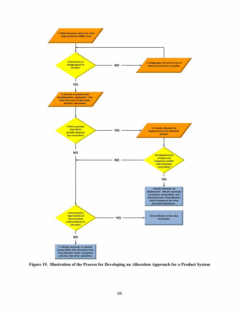
66
Figure 19. Illustration of the Process for Developing an Allocation Approach for a Product System
Consider allocation by displacement. Allocate cautiously
to maintain comparability with alternative fuels. Keep allocation
choice transparent and show alternative calculations..
1. Define the points where the multi-output processes (MOP) occur.
2. Disaggregate the process into as many sub-processes as possible.
Is the process as disaggregated as
possible?
5. Allocate cautiously to maintain comparability with alternative fuels. Keep allocation choice transparent and show alternative calculations.
Is there a product that will be
partially displaced by a co-product?
Is the economic value fraction of any co-product
small compared to the mass?
Can displacements of inputs and
outputs be verified with acceptable
uncertainty?
3. Describe co-products and develop baseline applications that
show the results of alternative allocation approaches.
4. Consider allocation by displacement of the substitute
product.
NO
YES
YES
Do not allocate to low value co-products.YES
NO
NO
NO
YES

67
1. Identify the points where multi-output processes occur: The first step in allocating among
co-products is to identify the points at which more than one product is produced.
2. Disaggregation: The second step is to determine if the process flows can be disaggregated
to more clearly identify how inputs and outputs should be allocated to each co-product.
If there is sufficient information about the sub-process inputs and outputs, the process
should be disaggregated.
3. Describe co-products and develop baseline alternative allocation calculations: The third
step is to develop a baseline allocation that can be used as a point of reference for
developing a more refined analysis. The mass fraction, potential use and substitutes,
energy content (for energy carriers), and economic value should be identified and
described. Clearly showing what allocations might be used, and how this would affect
the results, will provide a basis for comparing results with other studies and indicating
how allocation choices affect the outcome.
4. Displacement: The fourth step is to determine if any of the co-products can be
characterized as displacing another product. This involves:
a) Determining what product or products is displaced, and the quantitative
relationship between the co-product and the displaced product;
b) Determining how much of the co-product would be used for the same purpose as
the displaced product; and
c) Determining the extent to which production of the displaced product will decrease
per unit increase in supply of the co-product.
Substitution calculations should include an estimate of the completeness of the
displacement (fraction of displacement f), and should indicate the uncertainty in the
completeness estimate. The fraction of the co-product that does not displace the alternate
product (1-f) should not be subtracted from the inventory. These determinations should
be clearly documented and verified if possible, and the uncertainty should be
characterized. Displacement calculations may introduce considerable uncertainty into the
calculation and may not be feasible for all products and co-products. Ekvall and
Finnveden (2001) have argued that, due to the difficulties of developing an accurate
displacement calculation, allocation procedures based on mass, energy, or other physical
relationships may in many cases be the preferred approach. If the displacement cannot be
adequately validated, displacement should not be used.
5. Allocate cautiously, if justified, by property such as mass, energy or economic value: The
general recommendations for allocation as presented in ISO 14044 are as follows (ISO
2006b):
The inputs and outputs shall be allocated to the different products according to
clearly stated procedures that shall be documented and explained together with
the allocation procedure.
The sum of the allocated inputs and outputs of a unit process shall be equal to the
inputs and outputs of the unit process before allocation.

68
Whenever several alternative allocation procedures seem applicable, a sensitivity
analysis shall be conducted to illustrate the consequences of the departure from
the selected approach.
In addition, we offer the following guidance for allocation calculations:
For processes that produce mostly or entirely fuels, the standard practice is to use energy content
as the basis for allocation. This is particularly relevant for products of petrochemical refineries,
to the extent that disaggregation cannot resolve co-product allocation issues. As is shown in
Table 15, allocation by mass and energy give approximately the same result for products of
petroleum refineries.
Allocation by mass has the advantage of being easy to apply to a wide range of co-products;
however, mass allocation inherently ascribes most of the environmental impact to the heaviest
products. In the case of soy-derived fuels, mass allocation is the choice that shifts most of the
impact away from the fuel. In cases such as this, mass allocation should be used with caution.
Moreover, mass allocation has the potential to be applied to materials that might otherwise be
classified as wastes. Process inputs and outputs should never be allocated to wastes, that is, to
products that are not used in the economy; however, innovation can provide new uses for what
were formerly considered wastes, and the development of productive uses for wastes can have
environmental benefits (Allen and Behmanesh 1994). Accordingly, allocation of inputs and
outputs to co-products that might formerly have been considered wastes is potentially acceptable,
but should be carried out with caution.
Allocation by economic value has the advantage of attributing most of the environmental impact
to the most valuable products. A disadvantage of using economic value to allocate inputs and
outputs is that prices fluctuate over time. At times of low fuel prices, a value-based allocation
would result in the environmental impacts being shifted to co-products; at times of high fuel
prices, a value-based allocation would allocate inputs and outputs more to the fuel. Price
volatility could be addressed by taking a time average of prices over several years.
LCIs are typically developed to compare one product with another. Regardless of the method
used, allocation inherently divides the inputs and outputs of processes that are in fact physically
linked. Methods to separate, attribute, or allocate one product from another involve
approximations and in some cases adoption of conventions for calculations. In interpreting the
results of these calculations, it is important to acknowledge the limitations of these
approximations. All forms of co-product allocation introduce significant limitations to the
interpretation of the results.
Clearly, when comparing products made with a similar process, the allocation needs to be done
the same way for both processes in order to compare them. When comparing two products made
with different processes, even more care is needed in comparing the products. For petroleum,
the choice of allocation method does not greatly affect the overall greenhouse gas emission
calculation, because most of the emissions are directly related to combustion of the fuel itself,
rather than due to the process energy used in the refinery; however, for a biofuel, the allocation
method can dominate the calculation, because most of the emissions are associated with growing
and processing the fuel.
In comparing multiple alternative fuels, it may be helpful to evaluate all of the fuels with the
same allocation method; however, for some fuels it may be relatively straightforward to use a

69
displacement calculation, whereas for other fuels a displacement calculation may not be feasible
because data are not available about the co-product substitution. This could result in one fuel
appearing to have a much different environmental footprint than another, due entirely to the way
the calculation was done, rather than due to the underlying environmental impact. Because of
this potential for different calculations to be used for different fuels, developing several
allocation calculations would provide a basis for comparing fuels.
70
6.0 DOCUMENTING DATA QUALITY AND UNCERTAINTY
6.1 Background
Inventory data is the fundamental element that determines the quality of an LCA. The ability to
compare alternative aviation fuels to evaluate their relative difference in life cycle greenhouse
gas emissions is dependent on how the data selected to model each process throughout the life
cycle match the defined goal and scope of the study.
As stated in Section 2.0, the purpose of this guidance document is to provide a framework for
developing comparative LCAs that can be used to inform decisions on alternative aviation fuels.
A high level of data quality is required to meet this purpose.
The guidance in this section introduces a framework for assessing the quality of the data used to
model processes, for evaluating the completeness and representativeness of the life cycle, and for
documenting whether the study meets the intended goal and scope
6.2 Data Quality
“Good data”, “bad data”, “high quality data”, “low quality data”…these are common terms used
out of context to describe data that are used to model unit operations in a life cycle. The reality
is that there are no absolutely “good” or “bad” data. The appropriate issue is “Is the data quality
sufficient to meet the goal and scope of the study?” This question provides insight into the real
objective of assessing data quality: to ensure that data used in development of an LCA accurately
reflects the purpose of the study, the temporal, technological, and geographical representation,
and the study data quality objectives. Table 17, a reproduction of Table 3 in Section 3.0,
provides an example of study design parameters and includes data quality objectives
Table 17. Example Alternative Aviation Fuel Life Cycle Greenhouse Gas Study Design
Life Cycle Boundary Well-to-Wake
(Raw Material Acquisition thru Fuel Use)
Temporal Representation Year of Fuel Procurement
Technological Representation Facility/Chain Specific
Geographical Representation Transportation Fuel Sold or Distributed to DESC in the United
States
Transportation Fuel Life Cycles
Modeled Kerosene-Based Jet Fuel
Impact Assessment Methodology Global Warming Potential, IPCC 2007, 100-year time-frame
Non-CO2 combustion emissions not included
Reporting Metric g CO2e/MJ LHV of Fuel Consumed
Data Quality Objectives
Preferably Facility Technical Engineering and Operating Data
Publically Available Data (to the extent practicable)
Full Transparency of Modeling Approach and Data Sources (to
DESC)
Accounting for a targeted uncertainty in Mass and Energy
Accounting for a targeted uncertainty in Environmental Relevance
Process-based (“Bottoms-up”) Modeling Approach
71
6.3 Data Sources, Types, and Aggregation
Various types of inventory data can be used to characterize unit processes within the system
boundary of the life cycle. The following are examples of sources of data that could be used in a
typical LCA (adapted from (SAIC 2006)):
Meter readings from equipment
Equipment operating logs/journals
Industry data reports, databases, or consultants
Laboratory test results
Government documents, reports, databases, and clearinghouses
Other publicly available databases or clearinghouses
Journals, papers, books, and patents
Reference books
Trade associations
Related/previous life cycle inventory studies
Equipment and process specifications
Best engineering judgment
The type of data selected to model each unit process should be examined, and documented, to
ensure the data meets the goal and scope of the study. For the purposes of this guidance
document, data of the highest quality should be used in accordance with the recommendations
for a Level I: Comprehensive LCA. Examples of data types include (starting with the highest
priority) (adapted from (SAIC 2006)):
Measured continuously, over a time period adequate to represent continuous operation
Sampled intermittently, using a representative sample size
Modeled, using a well documented, peer reviewed computational method
Equipment vendor data or patents
Data representing a similar site or similar technology (i.e., surrogate data)
The level of aggregation of data should also be documented, for example, whether data are
representative of one process or several sub-processes. When measured data are not used, data
should be collected from a variety of sources. Whenever possible, it is best to get well-
characterized process data. Note also that processes often become more efficient or change over
time, so it is important to seek the most current data available. Inventory data can be facility-
specific or more general and still remain current.
Several levels of data aggregation are often used in inventories (starting with the most
disaggregated) (SAIC 2006):
Individual process- and facility-specific data from a particular operation within a given
facility that are not combined in any way
72
Composite data from the same operation or activity combined across locations
Aggregated data combining more than one process operation
Industry-average data derived from a representative sample of locations and believed to
provide a statistically accurate description of the typical operation across technologies
Generic data, while it may not be known how well the data set represents the system
flow, these data sets are qualitatively descriptive of a process or technology
6.4 Dealing With Confidential Data
The protection of confidential business information should be weighed against the need for a full
and detailed analysis or disclosure of information. Information disclosed in a public forum may
require aggregation with other data (i.e., aggregation of unit processes) to protect a business’s
intellectual property (corresponding to competitive advantage in the marketplace); however,
detailed information may require disclosure in a non-public forum with the primary decision
maker (e.g., purchasing agent) to verify the results presented in the final study report. This type
of information should be made available under a form of confidentiality agreement determined
acceptable by both parties. Life cycle data purchased from a data provider may have licensing
restrictions that also prevent the direct public release of the raw data; however, the data can
typically be reported in a public study when aggregated with other data or combined to calculate
the global warming potential of the operation. It is important in all cases to ensure data use
restrictions are not compromised.
6.5 Assessing and Documenting LCA Quality
Uncertainty can take many forms, including a lack of knowledge about the true value of a
quantity; the true form of a model; or the appropriateness of a modeling or methodological
decision (Reap, et al. 2008). The guidance provided in this report recognizes that it is not
necessary to quantify all uncertainty in data, modeling and scenarios, for the purpose of
comparing life cycle greenhouse gas emissions to a baseline value. Instead, it should be shown
that the uncertainty does not affect the final results. The following factors should be considered
when assessing and documenting data and uncertainty in life cycle analyses:
The quality of data used to model each unit process as described in ISO 4.2.3.6.2
The uncertainty in modeling choices
The uncertainty in scenario choices (e.g., future systems)
The sensitivity of key processes or data elements that contribute significantly to the well-
to-wake results and total life cycle results
The overall quality of the life cycle study and known data limitations
Figure 20 outlines the process to effectively assess and document the data used to model the life
cycle when conducting a Level I “Comprehensive LCA”.
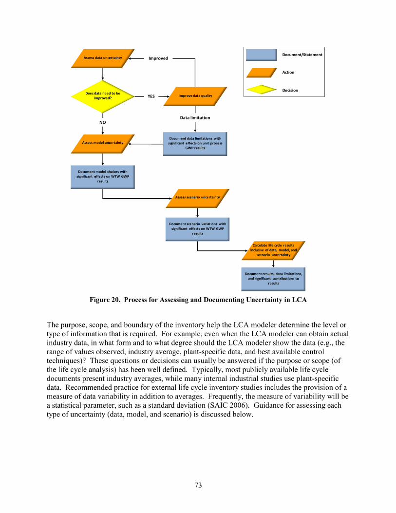
73
Figure 20. Process for Assessing and Documenting Uncertainty in LCA
The purpose, scope, and boundary of the inventory help the LCA modeler determine the level or
type of information that is required. For example, even when the LCA modeler can obtain actual
industry data, in what form and to what degree should the LCA modeler show the data (e.g., the
range of values observed, industry average, plant-specific data, and best available control
techniques)? These questions or decisions can usually be answered if the purpose or scope (of
the life cycle analysis) has been well defined. Typically, most publicly available life cycle
documents present industry averages, while many internal industrial studies use plant-specific
data. Recommended practice for external life cycle inventory studies includes the provision of a
measure of data variability in addition to averages. Frequently, the measure of variability will be
a statistical parameter, such as a standard deviation (SAIC 2006). Guidance for assessing each
type of uncertainty (data, model, and scenario) is discussed below.
Assess data uncertainty
Does data need to be improved?
Document data limitations with significant effects on unit process
GWP results
YES
NO
Improve data quality
Assess model uncertainty
Improved
Data limitation
Document model choices with significant effects on WTW GWP
results
Assess scenario uncertainty
Document scenario variations with significant effects on WTW GWP
results
Calculate life cycle results inclusive of data, model, and
scenario uncertainty
Document results, data limitations, and significant contributions to
results
Document/Statement
Action
Decision
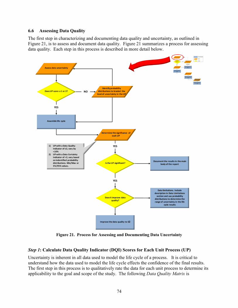
74
6.6 Assessing Data Quality
The first step in characterizing and documenting data quality and uncertainty, as outlined in
Figure 21, is to assess and document data quality. Figure 21 summarizes a process for assessing
data quality. Each step in this process is described in more detail below.
Figure 21. Process for Assessing and Documenting Data Uncertainty
Step 1: Calculate Data Quality Indicator (DQI) Scores for Each Unit Process (UP)
Uncertainty is inherent in all data used to model the life cycle of a process. It is critical to
understand how the data used to model the life cycle effects the confidence of the final results.
The first step in this process is to qualitatively rate the data for each unit process to determine its
applicability to the goal and scope of the study. The following Data Quality Matrix is
Assess data uncertainty
Does UP score a 1 or 2? NO
YES
Identify probability distributions to bracket the
level of uncertainty in the UP
Assemble life cycle
Improve the data quality to ≤2
Document the results in the main body of the report
Determine the significance of each UP
Is the UP significant?
YES
YES
Does it improve data quality?
Data limitations. Include description in Data Limitations
section and use probability distributions to determine the range of uncertainty in the life
cycle results
1) UP with a Data Quality Indicator of ≤2, vary by <10%
2) UP with a Data Certainty Indicator of >2, vary based on indentified probability distributions. Min/Max or 5%/95% values.
75
recommended to characterize the quality of data used in each unit process. The resulting
characterization is referred to as a Data Quality Indicator.
Table 18 outlines a pedigree matrix for a qualitative indication of LCI data quality for each unit
process used to characterize the life cycle of interest. This matrix was developed by Weidema
and Wesnaes (1996) and has been modified to reflect criteria specific to this guidance document.
The approach developed by Weidema and Wesnaes has been used in multiple studies and
variations on the matrix have been used in several uncertainty approaches Sonnemann,
Schuhmacher and Castells 2003), including the European LCI database “ecoinvent”
(Frischknecht, et al. 2005). The text in this table is meant to serve only as a guide from which to
assign indicator scores. In many cases, especially when two or more factors affect an indicator,
professional judgments will need to be considered when assigning scores. For some indicators,
determination of the score has rigid qualifications, and for others determination is more subject
to professional judgment. It is the modeler’s discretion which scores to assign in these cases,
although rationales used should be documented when they are subjective (or include an element
of subjectivity). Definitions of terms used in the data quality matrix and clarifications follow the
table.
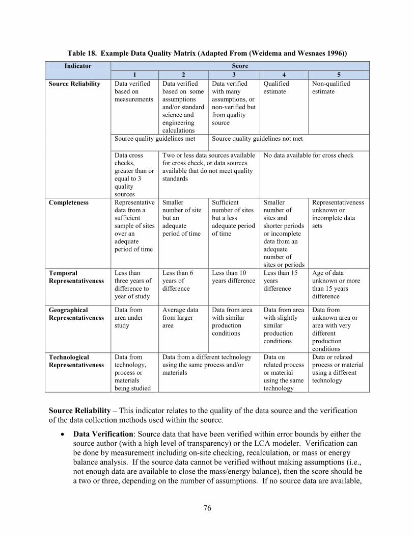
76
Table 18. Example Data Quality Matrix (Adapted From (Weidema and Wesnaes 1996))
Indicator Score
1 2 3 4 5
Source Reliability Data verified
based on
measurements
Data verified
based on some
assumptions
and/or standard
science and
engineering
calculations
Data verified
with many
assumptions, or
non-verified but
from quality
source
Qualified
estimate
Non-qualified
estimate
Source quality guidelines met Source quality guidelines not met
Data cross
checks,
greater than or
equal to 3
quality
sources
Two or less data sources available
for cross check, or data sources
available that do not meet quality
standards
No data available for cross check
Completeness Representative
data from a
sufficient
sample of sites
over an
adequate
period of time
Smaller
number of site
but an
adequate
period of time
Sufficient
number of sites
but a less
adequate period
of time
Smaller
number of
sites and
shorter periods
or incomplete
data from an
adequate
number of
sites or periods
Representativeness
unknown or
incomplete data
sets
Temporal
Representativeness
Less than
three years of
difference to
year of study
Less than 6
years of
difference
Less than 10
years difference
Less than 15
years
difference
Age of data
unknown or more
than 15 years
difference
Geographical
Representativeness
Data from
area under
study
Average data
from larger
area
Data from area
with similar
production
conditions
Data from area
with slightly
similar
production
conditions
Data from
unknown area or
area with very
different
production
conditions
Technological
Representativeness
Data from
technology,
process or
materials
being studied
Data from a different technology
using the same process and/or
materials
Data on
related process
or material
using the same
technology
Data or related
process or material
using a different
technology
Source Reliability – This indicator relates to the quality of the data source and the verification
of the data collection methods used within the source.
Data Verification: Source data that have been verified within error bounds by either the
source author (with a high level of transparency) or the LCA modeler. Verification can
be done by measurement including on-site checking, recalculation, or mass or energy
balance analysis. If the source data cannot be verified without making assumptions (i.e.,
not enough data are available to close the mass/energy balance), then the score should be
a two or three, depending on the number of assumptions. If no source data are available,
77
a qualified estimate from an expert in the field should receive a score of four, and an
estimate from a non-expert should receive a score of five.
Source Quality Guidelines: The highest quality source should meet the following
criteria.
o Be from a peer reviewed journal or a government sponsored study. If the source
is an LCA, it must meet ISO requirements.
o The source is publicly available either for free or at cost, or directly representative
of the process of interest.
o The source is written/published by an unbiased party.
o The source is an unbiased survey of experts or process locations.
When the source used for data is a reputable model that does not specifically meet the
above criteria, it is the discretion of the modeler to determine the rank of the source. An
example for justification would be if the data have been used in published reports that
met the data quality standards.
Data Cross Check: The number of sources that verify the same data point or series,
within reason. As a general benchmark, a high standard is greater than or equal to three
data cross checks with quality approved sources.
Completeness – This indicator quantifies the statistical robustness of the source data. This
ranking is based on how many data points were taken, how representative the sample is to the
studied process, and whether the data were taken for an acceptable time period to even out
normal process fluctuations. The following examples are given to help clarify this indicator.
Pollutant output data were collected from all available power plants within a region from
11 pm to 12 am. This would be sufficient sampling but for inadequate periods of time, so
it would receive a ranking of three.
Natural gas use data at one power plant for a year. This data would be assigned a rank
of two, because the sample size is not representative but the time period is.
Efficiency of a new bio-refinery system using two types of biomass, and the source
reports error within five percent. The ranking of these data would range from two to
four, subject to the judgment of the modeler both on acceptable error and because it is a
new technology (multiple sampling sites would not be available). However, it is
important to note that using these data for a biomass type not tested would affect the
technological appropriateness ranking, defined below.
Specific numbers for amount of data or sample size are not given; these should be determined
using the modeler’s best professional judgment based on the type of data (new or existing
technologies) and the reported error.
Temporal Representativeness – This indicator represents how well the time period in which the
data were collected corresponds with the year of the study. If the study is set to evaluate the use
of a technology from 2000 to 2040, data from 1970 would not be very accurate. It is important
when assigning this ranking to take notice of any discrepancies between the year the source was
published and the data were collected.
78
Geographical Representativeness – This indicator represents the appropriateness between the
region of study and the source data region. This indicator becomes important when comparing
data from different countries. For example, technological advances might reasonably be
expected to develop differently in different countries, so efficiency and energy use might be very
different. This is also important when looking at best management practices for carbon
mitigation.
Technological Representativeness – This indicator embodies all other differences that may be
present between the study goals and the data source. From the above example, using data for a
type of biomass that is not being studied in the LCA should result in a lower technological
representativeness ranking.
Step 2: Uncertainty Distributions for Unit Processes with Low Quality Data
Unit processes with data quality indicator scores of one or two for all five data quality indicator
categories outlined in the data quality indicator matrix (e.g., 1, 2, 1, 2, 2) is considered high
quality because the data meets the goal and scope of the study. Uncertainty estimates using
probability distributions for data would generally not be necessary to meet the objectives of the
study, however, if uncertainty information is known for one or more of the unit processes (i.e.,
provided with the data or derived from sampling data) the probability distributions should be
included in the documentation to further improve the interpretation of the study results.
All unit processes that scored a three, four, or five in any of the five data quality categories
should be further evaluated to properly assess the uncertainty introduced by data that failed to
meet the goal and scope of the study. Uncertainty should be expressed in terms of a probability
distribution (e.g., uniform, triangular, normal, lognormal, or other appropriate distribution). This
information will be used in Step 4 below when determining the significance of each unit process.
Below are brief descriptions of some common distribution types, and when each might be used.
Many other sources, such as Morgan and Henrion (1990) and IPCC (2006), address this subject
in more detail.
A uniform distribution is one of the simplest ways to represent uncertainty about a model
input. All values between an upper and lower bound are equally likely; this could be from
expert judgment or physical limitations.
The triangular distribution represents knowledge of upper and lower bounds, as well as a
most likely value somewhere between the two. This can also be used to represent expert
judgment.
The normal distribution is commonly used to represent the additive effect of various data
points with unknown levels of uncertainty that are believed to be acting in a random
manner. The normal distribution represents a symmetric continuous distribution that is
unbounded on both ends (i.e., from infinity to infinity).
The lognormal distribution is often used to represent the value of a process where the
percent change in the value is random or independent of other parameters. For example,
the oil industry uses lognormal distributions to represent oil reserve potential. The
lognormal distribution is also different from the normal distribution such that the values
are always positive; they range from zero to infinity.
79
Step 3: Assemble the Unit Processes to Model the Life Cycle
The next step is to assemble each of the unit processes into the five life cycle stages (see Section
3.0) and link them to generate the functional unit of the study.
Step 4: Determine the Significance of Each Unit Process
At this point, an analysis of the model response to each unit process is performed to assess the
significance of each unit process. The inputs for each high quality unit process (DQI 1 or 2)
should be individually varied by ±10 percent, and the inputs of low quality unit processes (DQI
3-5) should be varied to the minimum and maximum values or 95 percent confidence interval of
the uncertainty range. If the change in the final result from a single unit process is greater than a
threshold value, for example 0.1 g CO2e/MJ, then the processes should be flagged for possible
additional data quality refinement. This approach determines which unit processes could
potentially contribute a significant amount of uncertainty to the final result of the study. The
value of 0.1 g CO2e/MJ is approximately 0.1 percent of the anticipated baseline of conventional
aviation fuel (Skone and Gerdes 2008). In general, the threshold value should be selected to
represent a contribution of 0.1 percent to the comparative baseline or 0.1 percent of the life cycle
under study if not intended for comparative assessment. In both cases, the selected threshold
value must be clearly stated to support the data quality assessment.
While this is similar to a sensitivity analysis, it would be more accurate to say that the model
response to uncertainty is being tested in each unit process, with an assumed uncertainty of ±10
percent in cases where high quality data is used. Sources for more information on conducting a
sensitivity analysis include Morgan and Henrion (1990) and the EPA Models Guidance Draft
(Council for Regulatory Environmental Modeling 2003).
Step 5: Improve Data Quality of Significant Processes with Low Quality Data
If a unit process is based on low quality data and contributes an uncertainty of greater than 0.1 g
CO2e/MJ, an attempt should be made to find additional data and reduce the uncertainty range. In
cases where energy or mass limitations were used to determine the uncertainty bounds, this could
be additional sources that allow for a tighter bracketing of the uncertainty.
Step 6: Document Data Quality
In cases where uncertainty due to poor data quality cannot be reduced (or reduced enough to
lower the model response below the threshold) a discussion regarding the impact of the
uncertainty on the study outcome should be included with final presentation of results. When
high quality data inputs are determined to have a minor impact to the final results (i.e., below the
0.1 gCO2e/MJ threshold), the data sources should be documented within the report.
6.7 Model Uncertainty
Once the quality of data used to develop the life cycle has been assessed and improved to meet
the goal and scope of the study (to the extent possible) the next step is to assess and document
the effects of model uncertainty on the life cycle results. This is the second phase mapped in
Figure 20. Model uncertainty is classified within this guidance document as any modeling
choice that could not be adequately supported by data (i.e., professional judgment was required
to determine the modeling choice). Examples include:
More than one allocation method could be applied to products and co-products.
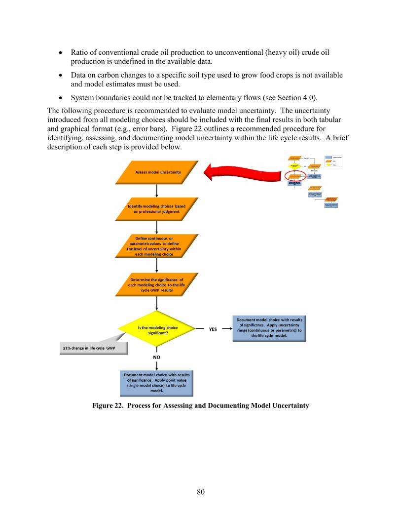
80
Ratio of conventional crude oil production to unconventional (heavy oil) crude oil
production is undefined in the available data.
Data on carbon changes to a specific soil type used to grow food crops is not available
and model estimates must be used.
System boundaries could not be tracked to elementary flows (see Section 4.0).
The following procedure is recommended to evaluate model uncertainty. The uncertainty
introduced from all modeling choices should be included with the final results in both tabular
and graphical format (e.g., error bars). Figure 22 outlines a recommended procedure for
identifying, assessing, and documenting model uncertainty within the life cycle results. A brief
description of each step is provided below.
Figure 22. Process for Assessing and Documenting Model Uncertainty
Document model choice with results of significance. Apply uncertainty
range (continuous or parametric) to the life cycle model.
Is the modeling choice significant?
Assess model uncertainty
Identify modeling choices based on professional judgment
Define continuous or parametric values to define
the level of uncertainty within each modeling choice
Determine the significance of each modeling choice to the life
cycle GWP results
YES
Document model choice with results of significance. Apply point value (single model choice) to life cycle
model.
NO
≤1% change in life cycle GWP
81
Step 1: Identify Modeling Choices Based on Professional Judgment
Throughout the process of assembling the life cycle, choices were required by the LCA modeler
on how to represent the life cycle. Most of these choices were supported by data or other
information to guide the selection. In some cases, professional judgment may have been
required to overcome inadequate detail in available data or more than one selection choice could
have been selected (e.g., method of allocation). All modeling choices that required professional
judgment to be used in selecting the appropriate choice should be identified and then evaluated
in the following step.
Step 2: Determine Uncertainty Distributions or Parametric Values for Modeling Choices
Modeling choices can be either represented as a probability distribution or a set of parametric
choices (distinct model values). The selection of different allocation methods is an example of
distinct parametric choices. An example of a modeling choice that would use a probability
distribution is where the ratio between two quantities is unknown (for example, the types of
specific sub-bituminous coals fed to a gasification unit), but there are reasonable boundaries
(e.g., technical limits) with or without a most likely (i.e., probable) value. The uncertainty of all
modeling choices should be evaluated to determine the significance to the total life cycle GWP
results.
Step 3: Determine the Significance of Each Modeling Choice
The effect of model uncertainty should be measured against the well-to-wake (WTW)17 life
cycle GWP using a form of sensitivity analysis (sometimes referred to as “scenario analysis”).
Point values (mean, average or most probable) contained within the current model should be
used to assess the effect of model uncertainty. The effects of data uncertainty and model
uncertainty, as well as scenario uncertainty, should be included in the final life cycle study
results interpretation and reporting section.
Results of the modified sensitivity analysis can be graphed and ranked to display the modeling
choices and identify the choices with a significant effect (greater than 1% change in the life cycle
GWP results).
Step 4: Document Modeling Choices and Known Data Limitations
Any modeling choice that causes a change of 1% or greater to the total life cycle GWP results
should be discussed as a data limitation with the final results.
Modeling choices that are determined to affect the final results by less than 1% should be briefly
discussed in the report but are not required to be noted as a data limitation that impacts the
comparability of the results.
6.8 Scenario Uncertainty
When forecasting operations that will occur in the future there is a level of uncertainty associated
with the source of electricity, the methods of biomass collection, and potential regulatory
17 The point of comparison for determining sensitivity is on the full life cycle basis (well-to-wake), unlike the data uncertainty section that requires the evaluation be conducted at the well-to-tank perspective. The full life cycle basis (well-to-wake) equates to the functional unit of the study and therefore is the primary comparison point for decision-making purposes. This value has yet to be determined when evaluating data quality when using the systematic process outlined within this guidance document. Therefore, the only relative point of reference to ensure adequate data quality is the unit process.
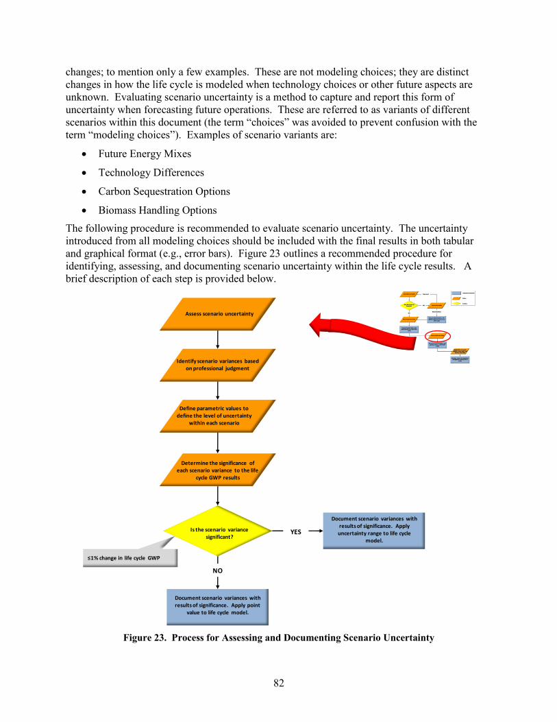
82
changes; to mention only a few examples. These are not modeling choices; they are distinct
changes in how the life cycle is modeled when technology choices or other future aspects are
unknown. Evaluating scenario uncertainty is a method to capture and report this form of
uncertainty when forecasting future operations. These are referred to as variants of different
scenarios within this document (the term “choices” was avoided to prevent confusion with the
term “modeling choices”). Examples of scenario variants are:
Future Energy Mixes
Technology Differences
Carbon Sequestration Options
Biomass Handling Options
The following procedure is recommended to evaluate scenario uncertainty. The uncertainty
introduced from all modeling choices should be included with the final results in both tabular
and graphical format (e.g., error bars). Figure 23 outlines a recommended procedure for
identifying, assessing, and documenting scenario uncertainty within the life cycle results. A
brief description of each step is provided below.
Figure 23. Process for Assessing and Documenting Scenario Uncertainty
Document scenario variances with results of significance. Apply
uncertainty range to life cycle model.
Is the scenario variance significant?
Assess scenario uncertainty
Identify scenario variances based on professional judgment
Define parametric values to define the level of uncertainty
within each scenario
Determine the significance of each scenario variance to the life
cycle GWP results
YES
Document scenario variances with results of significance. Apply point
value to life cycle model.
NO
≤1% change in life cycle GWP
83
Step 1: Identify Scenario Variants Based on Professional Judgment
All scenario variations that are employed to capture the probable range of variations in modeling
future operations should be identified and assessed to convey the potential effect on the final life
cycle GWP results.
Step 2: Determine Uncertainty Distributions or Parametric Values for Scenario Variants
Scenario variations are commonly represented as a set of parametric choices (distinct model
values). For example the electricity profile in year 2030 is modeled with or without a carbon
constrained profile. Variations of the change in energy efficiency of biomass harvesting or
energy production would also be examples of scenario uncertainty. The uncertainty of all
scenario variants should be evaluated to determine the significance to the total life cycle GWP
results.
Step 3: Determine the Significance of Each Scenario Variant
The effect of scenario uncertainty should be measured against the WTW life cycle GWP using a
form of sensitivity analysis (sometimes referred to as “scenario analysis”). Point values (mean,
average or most probable) contained within the current model should be used to assess the effect
of scenario uncertainty. The effects of data uncertainty, model uncertainty, and scenario
uncertainty, should be combined in the final life cycle study results, interpretation and reporting
section.
Results of the modified sensitivity analysis can be graphed and ranked to display the scenario
variances with the greatest to least effect and identify the variants with a significant effect
(greater than 1% change in the life cycle GWP results).
Step 4: Document Scenario Variants and Known Data Limitations
Any scenario variance that causes a change of 1% or greater to the total life cycle GWP results
should be discussed as a data limitation with the final results.
Scenario variances that are determined to affect the final results by less than 1% should be
documented, but are not data limitations that impact the comparability of the results.
6.9 Documenting LCA Study Quality and Known Data Limitations
Once the three primary forms of uncertainty have been identified and assessed (data, model, and
scenario), the three uncertainty distributions need to be combined into a single model and
evaluated using a form of Monte Carlo analysis to determine the cumulative uncertainty in the
final GWP results.
Results should be presented for each life cycle stage, well-to-tank basis, and the total well-to-
wake life cycle GWP results. All results should be presented in both a tabular and graphical
format in the LCA report. Results of the sensitivity analyses conducted throughout the overall
LCA should be reported on the significant unit process and/or data elements with the discussion
of final results.
6.10 Data Limitations
It is imperative to report all known data limitations identified throughout the study to ensure
decision-makers are fully informed when interpreting the final study results. A separate section
entitled “Data Limitations” should be included with the final results to highlight each form of
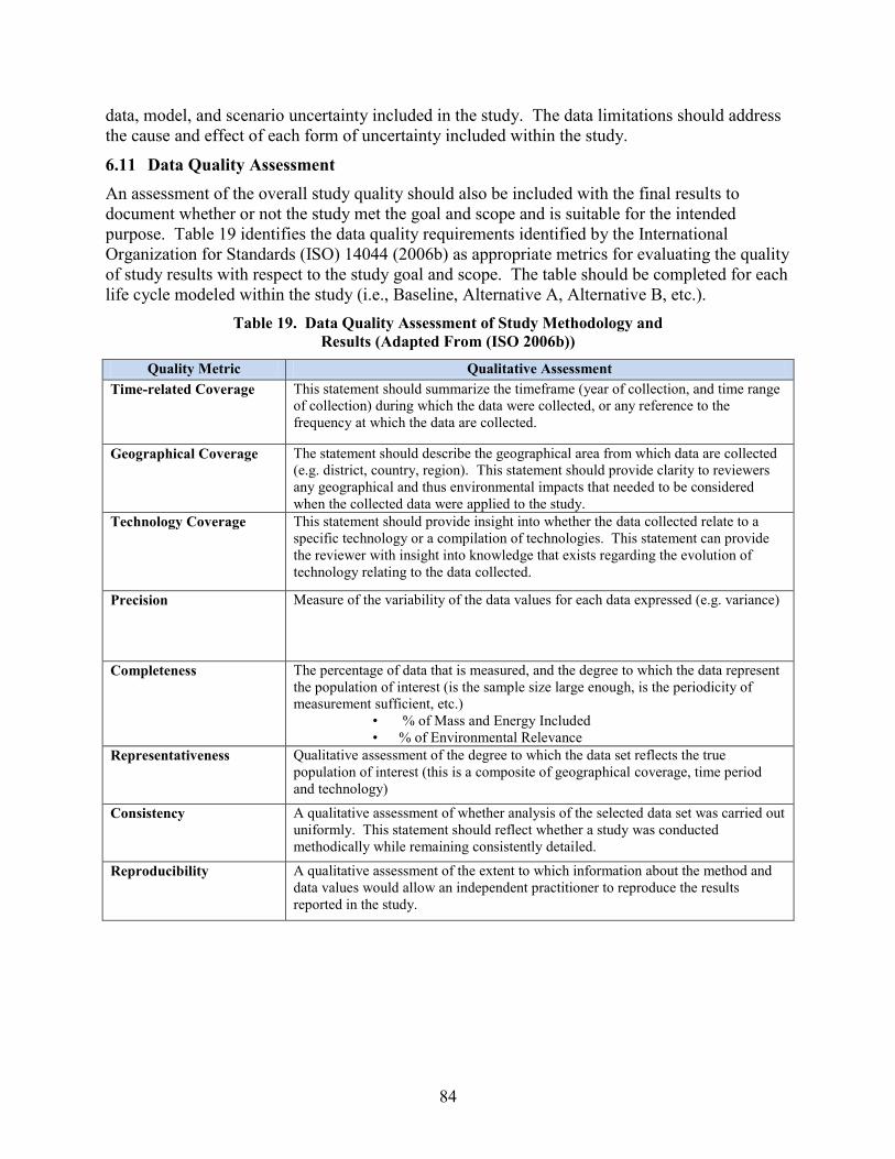
84
data, model, and scenario uncertainty included in the study. The data limitations should address
the cause and effect of each form of uncertainty included within the study.
6.11 Data Quality Assessment
An assessment of the overall study quality should also be included with the final results to
document whether or not the study met the goal and scope and is suitable for the intended
purpose. Table 19 identifies the data quality requirements identified by the International
Organization for Standards (ISO) 14044 (2006b) as appropriate metrics for evaluating the quality
of study results with respect to the study goal and scope. The table should be completed for each
life cycle modeled within the study (i.e., Baseline, Alternative A, Alternative B, etc.).
Table 19. Data Quality Assessment of Study Methodology and
Results (Adapted From (ISO 2006b))
Quality Metric Qualitative Assessment
Time-related Coverage This statement should summarize the timeframe (year of collection, and time range
of collection) during which the data were collected, or any reference to the
frequency at which the data are collected.
Geographical Coverage The statement should describe the geographical area from which data are collected
(e.g. district, country, region). This statement should provide clarity to reviewers
any geographical and thus environmental impacts that needed to be considered
when the collected data were applied to the study.
Technology Coverage This statement should provide insight into whether the data collected relate to a
specific technology or a compilation of technologies. This statement can provide
the reviewer with insight into knowledge that exists regarding the evolution of
technology relating to the data collected.
Precision Measure of the variability of the data values for each data expressed (e.g. variance)
Completeness The percentage of data that is measured, and the degree to which the data represent
the population of interest (is the sample size large enough, is the periodicity of
measurement sufficient, etc.)
• % of Mass and Energy Included
• % of Environmental Relevance
Representativeness Qualitative assessment of the degree to which the data set reflects the true
population of interest (this is a composite of geographical coverage, time period
and technology)
Consistency A qualitative assessment of whether analysis of the selected data set was carried out
uniformly. This statement should reflect whether a study was conducted
methodically while remaining consistently detailed.
Reproducibility A qualitative assessment of the extent to which information about the method and
data values would allow an independent practitioner to reproduce the results
reported in the study.
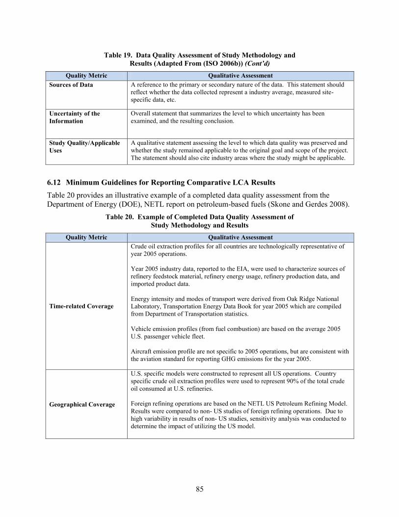
85
Table 19. Data Quality Assessment of Study Methodology and
Results (Adapted From (ISO 2006b)) (Cont’d)
Quality Metric Qualitative Assessment
Sources of Data A reference to the primary or secondary nature of the data. This statement should
reflect whether the data collected represent a industry average, measured site-
specific data, etc.
Uncertainty of the
Information
Overall statement that summarizes the level to which uncertainty has been
examined, and the resulting conclusion.
Study Quality/Applicable
Uses
A qualitative statement assessing the level to which data quality was preserved and
whether the study remained applicable to the original goal and scope of the project.
The statement should also cite industry areas where the study might be applicable.
6.12 Minimum Guidelines for Reporting Comparative LCA Results
Table 20 provides an illustrative example of a completed data quality assessment from the
Department of Energy (DOE), NETL report on petroleum-based fuels (Skone and Gerdes 2008).
Table 20. Example of Completed Data Quality Assessment of
Study Methodology and Results
Quality Metric Qualitative Assessment
Time-related Coverage
Crude oil extraction profiles for all countries are technologically representative of
year 2005 operations.
Year 2005 industry data, reported to the EIA, were used to characterize sources of
refinery feedstock material, refinery energy usage, refinery production data, and
imported product data.
Energy intensity and modes of transport were derived from Oak Ridge National
Laboratory, Transportation Energy Data Book for year 2005 which are compiled
from Department of Transportation statistics.
Vehicle emission profiles (from fuel combustion) are based on the average 2005
U.S. passenger vehicle fleet.
Aircraft emission profile are not specific to 2005 operations, but are consistent with
the aviation standard for reporting GHG emissions for the year 2005.
Geographical Coverage
U.S. specific models were constructed to represent all US operations. Country
specific crude oil extraction profiles were used to represent 90% of the total crude
oil consumed at U.S. refineries.
Foreign refining operations are based on the NETL US Petroleum Refining Model.
Results were compared to non- US studies of foreign refining operations. Due to
high variability in results of non- US studies, sensitivity analysis was conducted to
determine the impact of utilizing the US model.
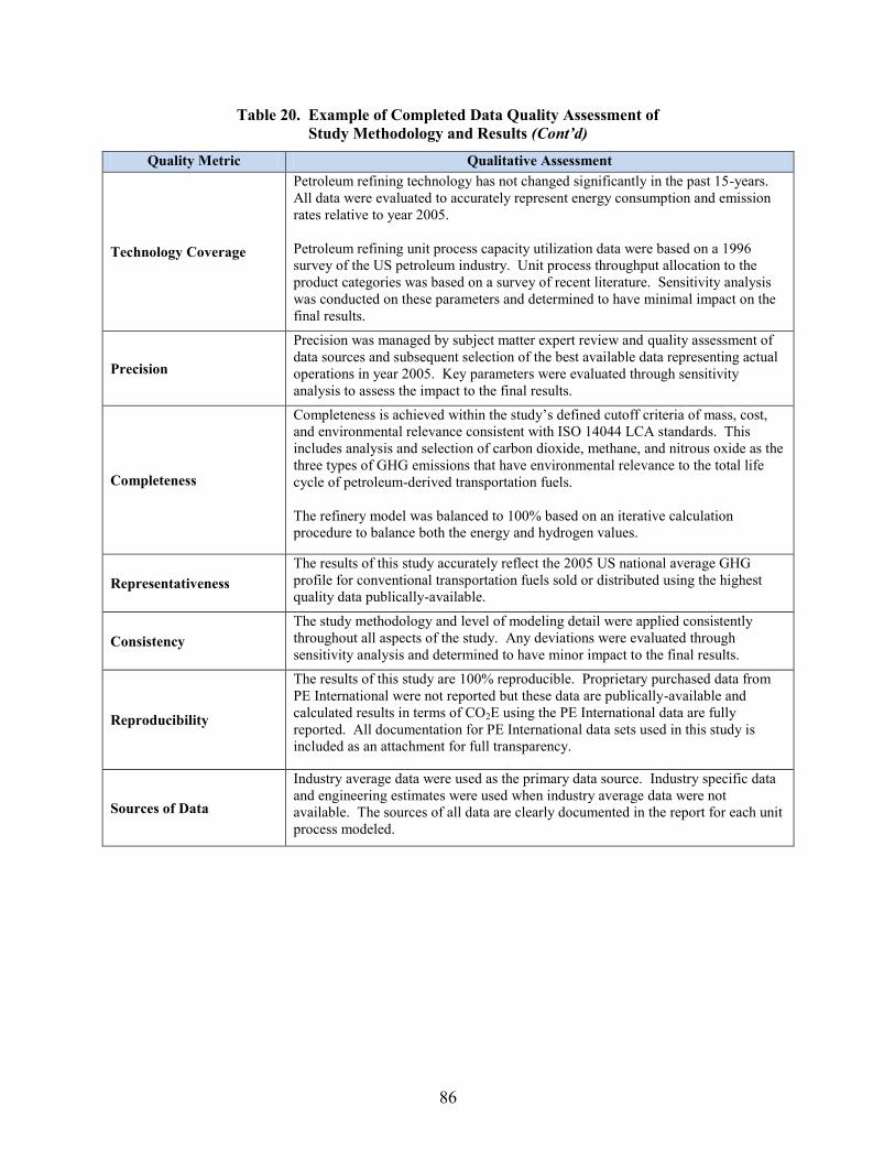
86
Table 20. Example of Completed Data Quality Assessment of
Study Methodology and Results (Cont’d)
Quality Metric Qualitative Assessment
Technology Coverage
Petroleum refining technology has not changed significantly in the past 15-years.
All data were evaluated to accurately represent energy consumption and emission
rates relative to year 2005.
Petroleum refining unit process capacity utilization data were based on a 1996
survey of the US petroleum industry. Unit process throughput allocation to the
product categories was based on a survey of recent literature. Sensitivity analysis
was conducted on these parameters and determined to have minimal impact on the
final results.
Precision
Precision was managed by subject matter expert review and quality assessment of
data sources and subsequent selection of the best available data representing actual
operations in year 2005. Key parameters were evaluated through sensitivity
analysis to assess the impact to the final results.
Completeness
Completeness is achieved within the study’s defined cutoff criteria of mass, cost,
and environmental relevance consistent with ISO 14044 LCA standards. This
includes analysis and selection of carbon dioxide, methane, and nitrous oxide as the
three types of GHG emissions that have environmental relevance to the total life
cycle of petroleum-derived transportation fuels.
The refinery model was balanced to 100% based on an iterative calculation
procedure to balance both the energy and hydrogen values.
Representativeness
The results of this study accurately reflect the 2005 US national average GHG
profile for conventional transportation fuels sold or distributed using the highest
quality data publically-available.
Consistency
The study methodology and level of modeling detail were applied consistently
throughout all aspects of the study. Any deviations were evaluated through
sensitivity analysis and determined to have minor impact to the final results.
Reproducibility
The results of this study are 100% reproducible. Proprietary purchased data from
PE International were not reported but these data are publically-available and
calculated results in terms of CO2E using the PE International data are fully
reported. All documentation for PE International data sets used in this study is
included as an attachment for full transparency.
Sources of Data
Industry average data were used as the primary data source. Industry specific data
and engineering estimates were used when industry average data were not
available. The sources of all data are clearly documented in the report for each unit
process modeled.
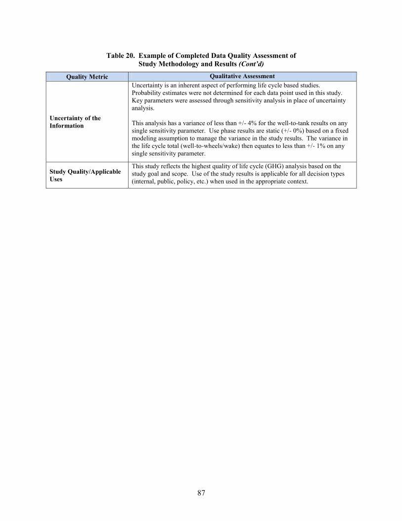
87
Table 20. Example of Completed Data Quality Assessment of
Study Methodology and Results (Cont’d)
Quality Metric Qualitative Assessment
Uncertainty of the
Information
Uncertainty is an inherent aspect of performing life cycle based studies.
Probability estimates were not determined for each data point used in this study.
Key parameters were assessed through sensitivity analysis in place of uncertainty
analysis.
This analysis has a variance of less than +/- 4% for the well-to-tank results on any
single sensitivity parameter. Use phase results are static (+/- 0%) based on a fixed
modeling assumption to manage the variance in the study results. The variance in
the life cycle total (well-to-wheels/wake) then equates to less than +/- 1% on any
single sensitivity parameter.
Study Quality/Applicable
Uses
This study reflects the highest quality of life cycle (GHG) analysis based on the
study goal and scope. Use of the study results is applicable for all decision types
(internal, public, policy, etc.) when used in the appropriate context.

88
7.0 CONCLUSIONS
As described in this guidance document, the methodologies and data for estimating life cycle
greenhouse gas emissions for aviation fuels are beginning to be used in regulatory and
procurement decision-making. As with other complex models used in environmental decisions,
a rigorous and transparent model development, documentation, and evaluation processes can
improve the regulatory process. This report represents a first step in that direction. As noted in
Section 2.0, for complex models used in environmental regulatory decision-making, the National
Research Council (2004) made a number of recommendations regarding the use of models in
environmental decision-making. The NRC recommendations, and the role of this guidance
document in responding to those recommendations, are summarized below:
NRC recommendation: Provide model documentation throughout the development and
use of the model. The working group that produced this guidance document anticipates
that this report can serve as a starting point for the documentation of modeling procedures
for the life cycle greenhouse gas emissions associated with aviation fuels, as these
procedures evolve.
NRC recommendation: Peer review models. The NRC report recommends that models
and modeling applications be reviewed. For life cycle studies done for the purpose of
initial EISA Section 526 compliance assessments for aviation fuels, reviews may be
independent peer reviews of life cycle studies done for fuels being considered for
procurement, or reviews done by the procuring entity. In either case, the working group
anticipates that, for the purposes of initial EISA Section 526 compliance assessments for
aviation fuels, this report can serve as guidance for peer reviewers of alternative fuel
assessments.
NRC recommendation: Communicate model uncertainty. This document provides
guidance on methods for characterizing, quantifying and reporting uncertainty in the life
cycle greenhouse gas emissions of aviation fuels.
NRC recommendation: Integrate models and measurements. This document also
describes methods for combining various types of data and model estimates and describes
methods for reporting these procedures
NRC recommendation: Perform retrospective analyses of models. Use of life cycle
greenhouse gas emission estimates in federal aviation fuel procurement is just beginning.
This document, which was developed with the sponsorship of the Air Force, represents a
starting point for model documentation. By continuing to providing on-going updates to
this document, as data and procedures evolve, the Air Force and other groups with
interests in life cycle greenhouse emissions of aviation fuels, can lay the ground-work for
retrospective analyses
NRC recommendation: Assess the balance between the level of detail incorporated into
models and the ability to evaluate the performance of these model features (model
parsimony). The system boundary guidance developed in this document describes
methods for identifying processes that contribute significantly to model estimates, and
describes methods for documenting which processes can be assumed to be negligible.

89
NRC recommendation: Establish procedures for overall model management. By
sponsoring the development of this document, the Air Force has initiated a process of
active model management; the working group recommends that this process continue.
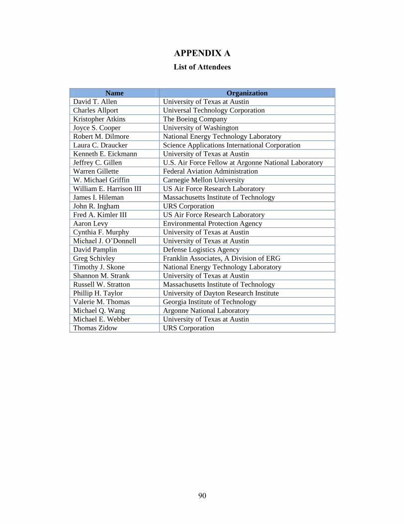
90
APPENDIX A
List of Attendees
Name Organization
David T. Allen University of Texas at Austin
Charles Allport Universal Technology Corporation
Kristopher Atkins The Boeing Company
Joyce S. Cooper University of Washington
Robert M. Dilmore National Energy Technology Laboratory
Laura C. Draucker Science Applications International Corporation
Kenneth E. Eickmann University of Texas at Austin
Jeffrey C. Gillen U.S. Air Force Fellow at Argonne National Laboratory
Warren Gillette Federal Aviation Administration
W. Michael Griffin Carnegie Mellon University
William E. Harrison III US Air Force Research Laboratory
James I. Hileman Massachusetts Institute of Technology
John R. Ingham URS Corporation
Fred A. Kimler III US Air Force Research Laboratory
Aaron Levy Environmental Protection Agency
Cynthia F. Murphy University of Texas at Austin
Michael J. O’Donnell University of Texas at Austin
David Pamplin Defense Logistics Agency
Greg Schivley Franklin Associates, A Division of ERG
Timothy J. Skone National Energy Technology Laboratory
Shannon M. Strank University of Texas at Austin
Russell W. Stratton Massachusetts Institute of Technology
Phillip H. Taylor University of Dayton Research Institute
Valerie M. Thomas Georgia Institute of Technology
Michael Q. Wang Argonne National Laboratory
Michael E. Webber University of Texas at Austin
Thomas Zidow URS Corporation
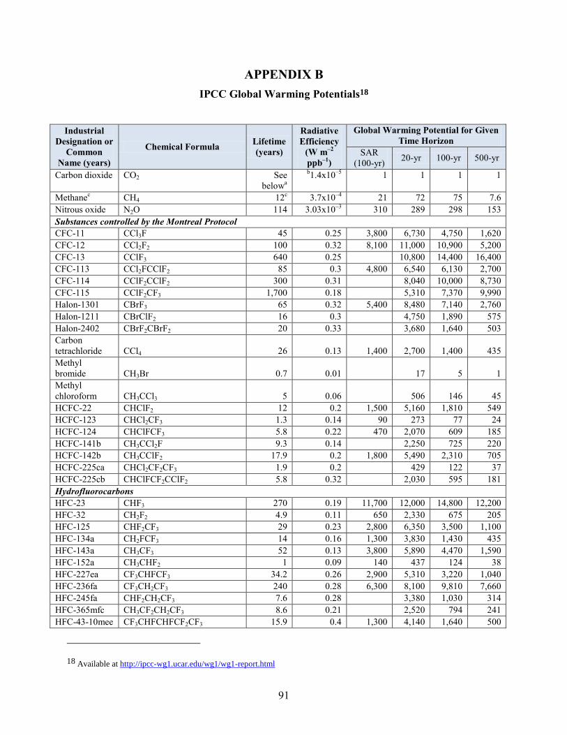
91
APPENDIX B
IPCC Global Warming Potentials18
Industrial
Designation or
Common
Name (years)
Chemical Formula Lifetime
(years)
Radiative
Efficiency
(W m–2
ppb–1
)
Global Warming Potential for Given
Time Horizon
SAR
(100-yr) 20-yr 100-yr 500-yr
Carbon dioxide CO2 See
belowa
b1.4x10
–5 1 1 1 1
Methanec CH4 12
c 3.7x10
–4 21 72 75 7.6
Nitrous oxide N2O 114 3.03x10⁻³
310 289 298 153
Substances controlled by the Montreal Protocol
CFC-11 CCl3F 45 0.25 3,800 6,730 4,750 1,620
CFC-12 CCl2F2 100 0.32 8,100 11,000 10,900 5,200
CFC-13 CClF3 640 0.25 10,800 14,400 16,400
CFC-113 CCl2FCClF2 85 0.3 4,800 6,540 6,130 2,700
CFC-114 CClF2CClF2 300 0.31 8,040 10,000 8,730
CFC-115 CClF2CF3 1,700 0.18 5,310 7,370 9,990
Halon-1301 CBrF3 65 0.32 5,400 8,480 7,140 2,760
Halon-1211 CBrClF2 16 0.3 4,750 1,890 575
Halon-2402 CBrF2CBrF2 20 0.33 3,680 1,640 503
Carbon
tetrachloride CCl4 26 0.13 1,400 2,700 1,400 435
Methyl
bromide CH3Br 0.7 0.01 17 5 1
Methyl
chloroform CH3CCl3 5 0.06 506 146 45
HCFC-22 CHClF2 12 0.2 1,500 5,160 1,810 549
HCFC-123 CHCl2CF3 1.3 0.14 90 273 77 24
HCFC-124 CHClFCF3 5.8 0.22 470 2,070 609 185
HCFC-141b CH3CCl2F 9.3 0.14 2,250 725 220
HCFC-142b CH3CClF2 17.9 0.2 1,800 5,490 2,310 705
HCFC-225ca CHCl2CF2CF3 1.9 0.2 429 122 37
HCFC-225cb CHClFCF2CClF2 5.8 0.32 2,030 595 181
Hydrofluorocarbons
HFC-23 CHF3 270 0.19 11,700 12,000 14,800 12,200
HFC-32 CH2F2 4.9 0.11 650 2,330 675 205
HFC-125 CHF2CF3 29 0.23 2,800 6,350 3,500 1,100
HFC-134a CH2FCF3 14 0.16 1,300 3,830 1,430 435
HFC-143a CH3CF3 52 0.13 3,800 5,890 4,470 1,590
HFC-152a CH3CHF2 1 0.09 140 437 124 38
HFC-227ea CF3CHFCF3 34.2 0.26 2,900 5,310 3,220 1,040
HFC-236fa CF3CH2CF3 240 0.28 6,300 8,100 9,810 7,660
HFC-245fa CHF2CH2CF3 7.6 0.28 3,380 1,030 314
HFC-365mfc CH3CF2CH2CF3 8.6 0.21 2,520 794 241
HFC-43-10mee CF3CHFCHFCF2CF3 15.9 0.4 1,300 4,140 1,640 500
18 Available at http://ipcc-wg1.ucar.edu/wg1/wg1-report.html

92
Industrial
Designation or
Common
Name (years)
Chemical Formula Lifetime
(years)
Radiative
Efficiency
(W m–2
ppb–1
)
Global Warming Potential for Given
Time Horizon
SAR
(100-yr) 20-yr 100-yr 500-yr
Perfluorinated compounds
Sulphur
hexafluoride SF6 3,200 1 23,900 16,300 22,800 32,600
Nitrogen
trifluoride NF3 740 0 12,300 17,200 20,700
PFC-14 CF4 50,000 0.1 6,500 5,210 7,390 11,200
PFC-116 C2F6 10,000 0.26 9,200 8,630 12,200 18,200
PFC-218 C3F8 2,600 0 7,000 6,310 8,830 12,500
PFC-318 c-C4F8 3,200 0 8,700 7,310 10,300 14,700
PFC-3-1-10 C4F10 2,600 0.33 7,000 6,330 8,860 12,500
PFC-4-1-12 C5F12 4,100 0.41 6,510 9,160 13,300
PFC-5-1-14 C6F14 3,200 0.49 7,400 6,600 9,300 13,300
PFC-9-1-18 C10F18 >1,000d 0.56 >5,500 >7,500 >9,500
trifluoromethyl
sulphur
pentafluoride SF5CF3 800 1 13,200 17,700 21,200
Fluorinated ethers
HFE-125 CHF2OCF3 136 0 13,800 14,900 8,490
HFE-134 CHF2OCHF2 26 0 12,200 6,320 1,960
HFE-143a CH3OCF3 4 0.27 2,630 756 230
HCFE-235da2 CHF2OCHClCF3 3 0.38 1,230 350 106
HFE-245cb2 CH3OCF2CHF2 5 0.32 2,440 708 215
HFE-245fa2 CHF2OCH2CF3 5 0.31 2,280 659 200
HFE-254cb2 CH3OCF2CHF2 2.6 0 1,260 359 109
HFE-347mcc3 CH3OCF2CF2CF3 5.2 0.34 1,980 575 175
HFE-347pcf2 CHF2CF2OCH2CF3 7.1 0.25 1,900 580 175
HFE-356pcc3 CH3OCF2CF2CHF2 0.33 0.93 386 110 33
HFE-449sl
(HFE-7100) C4F9OCH3 3.8 0.31 1,040 297 90
HFE-569sf2
(HFE-7200) C4F9OC2H5 0.77 0.3 207 59 18
HFE-43-
10pccc124 (H-
Galden 1040x) CHF2OCF2OC2F4OCHF2 6.3 1.37 6,320 1,870 569
HFE-236ca12
(HG-10) CHF2OCF2OCHF2 12.1 0.66 8,000 2,800 860
HFE-338pcc13 CHF2OCF2CF2OCHF2 6.2 0.87 5,100 1,500 460
Perfluoropolyethers
PFPMIE CF3OCF(CF3)CF2OCF2OCF3 800 0.65 7,620 10,300 12,400
Hydrocarbons and other compounds – Direct Effects
Dimethylether CH3OCH3 0 0 1 1 <<1
Methylene
chloride CH2Cl2 0 0 31 9 3
Methyl
chloride CH3Cl 1 0 45 13 4
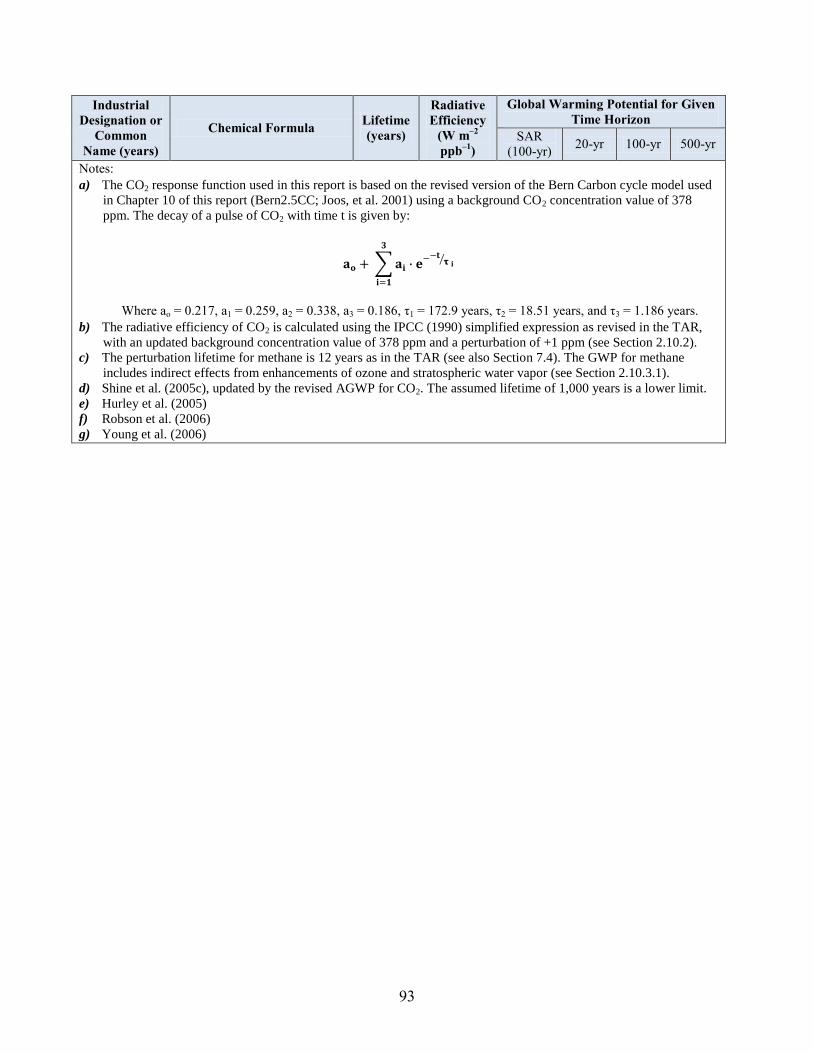
93
Industrial
Designation or
Common
Name (years)
Chemical Formula Lifetime
(years)
Radiative
Efficiency
(W m–2
ppb–1
)
Global Warming Potential for Given
Time Horizon
SAR
(100-yr) 20-yr 100-yr 500-yr
Notes:
a) The CO2 response function used in this report is based on the revised version of the Bern Carbon cycle model used
in Chapter 10 of this report (Bern2.5CC; Joos, et al. 2001) using a background CO2 concentration value of 378
ppm. The decay of a pulse of CO2 with time t is given by:
𝐚𝐨 + 𝐚𝐢 ∙ 𝐞−−𝐭
𝛕 𝐢
𝟑
𝐢=𝟏
Where ao = 0.217, a1 = 0.259, a2 = 0.338, a3 = 0.186, τ1 = 172.9 years, τ2 = 18.51 years, and τ3 = 1.186 years.
b) The radiative efficiency of CO2 is calculated using the IPCC (1990) simplified expression as revised in the TAR,
with an updated background concentration value of 378 ppm and a perturbation of +1 ppm (see Section 2.10.2).
c) The perturbation lifetime for methane is 12 years as in the TAR (see also Section 7.4). The GWP for methane
includes indirect effects from enhancements of ozone and stratospheric water vapor (see Section 2.10.3.1).
d) Shine et al. (2005c), updated by the revised AGWP for CO2. The assumed lifetime of 1,000 years is a lower limit.
e) Hurley et al. (2005)
f) Robson et al. (2006)
g) Young et al. (2006)

94
BIBLIOGRAPHY
1) Agyemang-Bonsu, William Kojo, A.M. Al-Ibrahim, Carlos Lopez, Gregg Marland,
Huang Shenchu, and Oleg Tailakov. "Chapter 9: Implications of carbon dioxide capture
and storage for greenhouse gas inventories and accounting." In Carbon Dioxide Capture
and Storage, by IPCC, 363-379. Cambridge: Cambridge University Press, 2005.
2) Allen, D., and N. Behmanesh. "Wastes as Raw Materials." In The Greening of Industrial
Ecosystems, edited by B. R. Allenby and D. J. Richards. Washington, DC: National
Academy Press, 1994.
3) Allen, David T., and D. R. Shonnard. Green Engineering: Environmentally Conscious
Design of Chemical Processes. Englewood Cliffs: Prentice Hall, 2001.
4) Allen, David T., F. J. Consoli, G. A. Davis, J. A. Fava, and J. L. Warren. Public Policy
Applications of Life Cycle Assessment. Pensacola: SETAC Press, 1997.
5) Baughcum, Steven L. Aircraft Emissions Deposited in the Stratosphere and Within the
Arctic Polar Vortex. Langley Research Center, Hampton: National Aeronautics and
Space Administration, 1996.
6) British Standards Institute; The Carbon Trust; UK Department for Environment, Food
and Rural Affairs. Publicly Available Specification for the Assessment of greenhouse gas
emissions of goods and services. London: British Standards Institute, 2008.
7) CARB. The California Low-Emission Vehicle Regulations. Sacramento: California Air
Resources Board, 2007.
8) Consoli, F., et al. Guidlines for Life Cycle Assessment: A Code of Practice. Pensacola:
SETAC Press, 1993.
9) Cooper, Joyce S. Life Cycle Assessment of Producing Electricity from California Forest
Wildfire Fuels Treatments. Public Interest Energy Research Program, Sacramento:
California Energy Commission, 2008.
10) Cooper, Joyce S. "Specifying Functional Units and Reference Flows for Comparable
Alternatives." International Journal of Life Cycle Assessment 8 (2003): 337-349.
11) Corporan, Edwin, et al. "Emissions Characteristics of a Turbine Engine and Research
Combustor Burning a Fischer-Tropsch Jet Fuel." Energy & Fuels 21, no. 2007a (2007b):
2615-2626.
12) Corporan, Edwin, Matthew J. DeWitt, Christopher D. Klingshirn, and Richard C.
Striebich. "DOD Assured Fuels Initiative: B-52 Aircraft Emissions Burning a Fischer-
Tropsch/JP-8 Fuel Blend." IASH 2007: 10th International Conference on Stability,
Handling and Use of Liquid Fuels. Tuscon: International Association for Stability,
Handling and Use of Liquid Fuels, October 2007a.
13) Council for Regulatory Environmental Modeling. Draft Guidance on the Development,
Evaluation, and Application of Regulatory Environmental Models. Office of Science
Policy, Washington, DC: Office of Research and Development, 2003.

95
14) Curzons, Alan D., Concepcion Jimenez-Gonzalez, Ailsa, L. Duncan, David J. C.
Constable, and Virginia L. Cunningham. "Fast Life Cycle Assessment of Synthetic
Chemistry (FLASCTM) Tool." International Journal of Life Cycle Assessment 12, no. 4
(2007): 272-280.
15) Defense Science Board. Final Report of the Defense Science Board Task Force on DOD
Energy Strategy. Washington, DC: Office of the Under Secretary of Defense For
Acquisition, Technology, and Logistics, 2008.
16) Ekvall, T., and G. Finnvedeen. "Allocation in ISO 14041 - a critical review." Journal of
Cleaner Production 9, no. 3 (2001): 197-208.
17) Energy Information Administration. Petroleum Navigator. 2007.
http://tonto.eia.doe.gov/dnav/pet/pet_cons_psup_dc_nus_mbblpd_a.htm (accessed April
17, 2009).
18) EPA. Greenhouse Gas Emissions from the U.S. Transportation Sector: 1990-2003.
Office of Transportation and Air Quality (OTAQ), Washington, DC: US Environmental
Protection Agency, 2006.
19) EPA. Guidance on the Use of Models and Other Anaylses for Demonstrating Attainment
of Air Quality Goals for Ozone. Washington, DC: US Environmental Protection Agency,
2007.
20) EPA. National Biennial RCRA Hazardous Waste Report 1993. Solid Waste and
Emergency Response, Washington, DC: U.S. Environmental Protection Agency, 1995.
21) EPA. Toxics Release Inventory. Office of Pollution Prevention and Toxics, Washington,
DC: U.S. Environmental Protection Agency, 2002.
22) Frischknecht, Rolf, et al. "The ecoinvent Database: Overview and Methodological
Framework." International Journal of LCA 10, no. 1 (2005): 3-9.
23) Fuglestvedt, J. S., T. K. Berntsen, O. Godal, and T. Skodvin. "Climate implications of
GWP-based reductions in greenhouse gas emissions." Geophysical Research Letters 27
(2000): 409-412.
24) Gettelman, Andrew, and Steven L. Baughcum. "Direct deposition of subsonic aircraft
emissions into the stratosphere." Journal of Geophysical Research 104, no. D7 (1999):
8317–8328.
25) GM. Volume 3: Well-to-Tank Energy Use and Greenhouse Gas Emissions of
Transportation Fuels - North American Analysis. Detroit: General Motors Corporation,
2001.
26) Graedel, T. E. Streamlined Life-Cycle Assessment. Upper Saddle River: Prentice Hall,
1998.
27) Hemighaus, Greg, et al. Aviation Fuels Technical Review. Houston: Chevron
Corporation, 2006.
28) Hendrickson, C. T., A. Horvath, S. Joshi, and L. B. Lave. "Economic Input-Output
Model for Environmental Life Cycle Assessment." Environmental Science and
Technology, April 1998: 184A-191A.
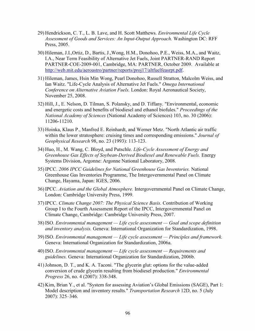
96
29) Hendrickson, C. T., L. B. Lave, and H. Scott Matthews. Environmental Life Cycle
Assessment of Goods and Services: An Input-Output Approach. Washington DC: RFF
Press, 2005.
30) Hileman, J.I.,Ortiz, D., Bartis, J.,Wong, H.M., Donohoo, P.E., Weiss, M.A., and Waitz,
I.A., Near Term Feasibility of Alternative Jet Fuels, Joint PARTNER-RAND Report
PARTNER-COE-2009-001, Cambridge, MA: PARTNER, October 2009. Available at
http://web.mit.edu/aeroastro/partner/reports/proj17/altfuelfeasrpt.pdf.
31) Hileman, James, Hsin Min Wong, Pearl Donohoo, Russell Stratton, Malcolm Weiss, and
Ian Waitz. "Life-Cycle Analysis of Alternative Jet Fuels." Omega International
Conference on Alternative Aviation Fuels. London: Royal Aeronautical Society,
November 25, 2008.
32) Hill, J., E. Nelson, D. Tilman, S. Polansky, and D. Tiffany. "Environmental, economic
and energetic costs and benefits of biodiesel and ethanol biofules." Proceedings of the
National Academy of Sciences (National Academy of Sciences) 103, no. 30 (2006):
11206-11210.
33) Hoinka, Klaus P., Manfred E. Reinhardt, and Werner Metz. "North Atlantic air traffic
within the lower stratosphere: cruising times and corresponding emissions." Journal of
Geophysical Research 98, no. 23 (1993): 113-123.
34) Huo, H., M. Wang, C. Bloyd, and Putschle. Life-Cycle Assessment of Energy and
Greenhouse Gas Effects of Soybean-Derived Biodiesel and Renewable Fuels. Energy
Systems Division, Argonne: Argonne National Laboratory, 2008.
35) IPCC. 2006 IPCC Guidelines for National Greenhouse Gas Inventories. National
Greenhouse Gas Inventories Programme, The Intergovernmental Panel on Climate
Change, Hayama, Japan: IGES, 2006.
36) IPCC. Aviation and the Global Atmosphere. Intergovernmental Panel on Climate Change,
London: Cambridge University Press, 1999.
37) IPCC. Climate Change 2007: The Physical Science Basis. Contribution of Working
Group I to the Fourth Assessment Report of the IPCC, Intergovernmental Panel on
Climate Change, Cambridge: Cambridge University Press, 2007.
38) ISO. Environmental management — Life cycle assessment — Goal and scope definition
and inventory analysis. Geneva: International Organization for Standardization, 1998.
39) ISO. Environmental management — Life cycle assessment — Principles and framework.
Geneva: International Organization for Standardization, 2006a.
40) ISO. Environmental management — Life cycle assessment — Requirements and
guidelines. Geneva: International Organization for Standardization, 2006b.
41) Johnson, D. T., and K. A. Taconi. "The glycerin glut: options for the value-added
conversion of crude glycerin resulting from biodiesel production." Environmental
Progress 26, no. 4 (2007): 338-348.
42) Kim, Brian Y., et al. "System for assessing Aviation’s Global Emissions (SAGE), Part 1:
Model description and inventory results." Transportation Research 12D, no. 5 (July
2007): 325–346.
97
43) Lacey, P. I., and S. R. Westbrook. Fuel Lubricity Additive Evaluation. Mobility
Technology Center, U. S. Army, Ft. Belvoir: Defense Technical Information Center,
1997.
44) Larson, E. "A review of life-cycle analysis studies on liquid biofuel systems for teh
transport sector." Energy for Sustainable Development X, no. 2 (2006): 109-126.
45) Lave, Lester B., Elisa Cobas-Flores, Chris T. Hendrickson, and Francis C. McMichael.
"Using Input-Output Analysis to Estimate Economy-wide Discharges." Environmental
Science & Technology (The American Chemical Society) 29, no. 9 (1995): 420A-426A.
46) Lazarenko, V. P., G. B. Skovorodin, I. V. Rozhkov, Z. A. Sablina, and E. S.
Churshaukov. "Influence of Corrosion Inhibitors on Jet Fuel Lubricity." Chemistry and
Technology of Fuels and Oils 5 (1975): 19-21.
47) Lee, Jacquetta J., P. O’Callaghan, and D. Allen. "Critical review of life cycle analysis and
assessment techniques and their application to commercial activities." Resources,
Conservation and Recycling 13 (1995): 37-56.
48) Marais, K., S. P. Lukachko, M. Jun, A. Mahashabde, and I. A. Waitz. "Assessing the
Impact of Aviation on Climate." Meteorologische Zeitschrift 17, no. 2 (April 2008): 157-
172.
49) Maurice, B., R. Frischknecht, V. Coelho-Schwirtz, and K. Hungerbuhler. "Uncertainty
analysis in life cycle inventory. Application to the production of electricity with French
coal power plants." Journal of Cleaner Production 8 (2000): 95-108.
50) McCann, T., and P. Magee. "Crude Oil Greenhouse Gas Life Cycle Analysis Helps
Assign Values for CO2 Emissions Trading." Oil and Gas Journal 97, no. 8 (February
1999): 38-43.
51) Morgan, M. G., and M. Henrion. Uncertainty: A Guide to Dealing with Uncertainty in
Quantitative Risk and Policy Analysis. Cambridge: Cambridge University Press, 1990.
52) National Research Council. Air Quality Management in the United States. Washington,
DC: National Academy Press, 2004.
53) National Research Council. Models in Environmental Regulatory Decision Making.
Washington, DC: National Academy Press, 2007.
54) Pascual, P., N. Stiber, and E. Sunderland. Draft Guidance on the Development,
Evaluation, and Application of Regulatory Environmental Models. Council on
Regulatory Environmental Models, Washinton, DC: U.S. Environmental Protection
Agency, 2003.
55) Pradhan, A., D. S. Shrestha, J. V. Gerpen, and J. Duffield. "The energy balance of
soybean oil biodiesel production: a review of past studies." Transactions of the ASABE
51, no. 1 (2008): 185-194.
56) Raynolds, Marlo, Roydon Fraser, and David Checkel. "The Relative Mass-Energy-
Economic (RMEE) Method for System Boundary Selection." International Journal of
Life Cycle Assessment 5, no. 1 (2000): 37-46.
98
57) Reap, J., F. Roman, S. Duncan, and B. Bras. "A survey of unresolved problems in life
cycle assessment Part 1: goal and scope and inventory analysis." International Journal of
Life Cycle Assessment 13 (2008): 290-300.
58) Rich, D. Designing a U.S. Greenhouse Gas Emissions Registry. Washington, DC: World
Resources Institute, 2008.
59) SAIC. Life Cycle Assessment: Princilpes and Practice. National Risk Management
Research Laboratory, Office of Research and Development, Cincinnati: U.S.
Environmental Protection Agency, 2006.
60) Sausen, R., et al. "Aviation radiative forcing in 2000: An update on IPCC (1999)."
Meteorologische Zeitschrift 14 (2005): 555–561.
61) Schumann, U. "The impact of nitrogen oxides emissions from the aircraft upon the
atmosphere at flight altitudes-results from the AERONOx Project." Atmospheric
Environment 31 (1997): 1723-1733.
62) Shapouri, H., Michael Wang, and James Duffield. "Net energy balance and fuel-cycle
analysis." In Renewables-Based Technology, edited by J. Van Langenhove, H. Dewulf,
73-86. Chichester, UK: John Wiley and Sons, 2006.
63) Shapouri, Hosein, James A. Duffield, and Michael Wang. The Energy Balance of Corn
Ethanol: An Update. Washington, DC: US Department of Agriculture, 2002.
64) Sheehan, John, Vince Camobreco, James Duffield, Michael Graboski, and Housein
Shapouri. Life Cycle Inventory of Biodiesel and Petroleum Diesel for Use in an Urban
Bus: Final Report. Office of Fuels Development, National Renewable Energy
Laboratory, Golden: US Department of Energy, 1998.
65) Skone, Timothy J., and Kristin Gerdes. "Development of Baseline Data and Analysis of
Life Cycle Greenhouse Gas Emissions of Petroleum-Based Fuels." US Department of
Energy, National Energy Technology Laboratory, Office of Systems, Analysis and
Planning. November 26, 2008. http://www.netl.doe.gov/energy-
analyses/pubs/NETL%20LCA%20Petroleum-Based%20Fuels%20Nov%202008.pdf
(accessed December 8, 2008).
66) Sonnemann, Guido W., Marta Schuhmacher, and Francesco Castells. "Uncertainty
assessment by a Monte Carlo simulation in a life cycle inventory of electricity produced
by a waste incinerator." Journal of Cleaner Production 11 (2003): 279-292.
67) Stewart, R. L., B. S. Stone, and M. L. Streitwieser. U.S. Benchmark Input-Output
Accounts, 2002. Washington, DC: U.S. Bureau of Economic Analysis, 2007.
68) Suh, S., et al. "System boundary selection in life-cycle inventories using hybrid
approaches." Environmental Science and Technology 38 (2004): 658-664.
69) The Climate Registry. General Reporting Protocol, version 1.1. Los Angeles: The
Climate Registry, 2008.
70) Thomas, V. M. "Demand and dematerialization impacts of second-hand markets: Reuse
or more use?" Journal of Industrial Ecology 7, no. 2 (2003): 65-78.

99
71) U.S. Air Force. Aerospace Fuels Certification. Philadelphia: Document Automation and
Production Service, 2008.
72) Vigon, B. W., D. A. Tolle, B. W. Cornaby, and H. C. Latham. Life Cycle Assessment:
Inventory Guidelines and Principles. Washington, DC: U.S. Environmental rotection
Agency, 1993.
73) Wang, Michael. Greenhouse Gases, Regulated Emissions, and Energy Use in
Transportation (GREET) Model, Version 1.8b. Argonne National Laboratory, Ann
Arbor: Department of Energy, 2008.
74) Wang, Michael, H. Lee, and J. Molberg. "Allocation of energy use in petroleum
refineries to petroleum products: Implications for life-cycle energy use and emission
inventory of petroleum transportation fuels." International Journal of Life Cycle Analysis
9, no. 1 (2004): 34-44.
75) Weidema, B. P., and M. S. Wesnaes. "Data Quality Management for Life Cycle
Inventories - an example using Data Quality Indicators." Journal of Cleaner Production
4, no. 3-1 (1996): 167-174.
76) Whitefield, P. "Inter Comparisons of PM and HAP Emissions from a CFM56 Engine
Burning Bio, FT and Conventional Fuels." Omega International Conference on
Alternative Aviation Fuels. London: Royal Aeronautical Society, November 25, 2008.
77) Wong, H.M. Life-cycle Assessment of Greenhouse Gas Emissions from Alternative Jet
Fuels. Technology and Policy Program, Engineering Systems Division, Boston:
Massachusetts Institute of Technology, 2008.
78) Wuebbles, Don, Mohan Gupta, and Malcolm Ko. "Evaluating the Impacts of Aviation on
Climate Change." EOS, Transactions (American Geophysical Union) 88, no. 14 (April
2007): 157–168.
79) Wuebbles, Donald J., Huiguang Yang, and Redina Herman. Climate Metrics and
Aviation: Analysis of Current Understanding and Uncertainties. Washington, DC:
Federal Aviation Administration, 2008.
80) Zhang, Yi, Bhavik R. Bakshi, and E. Sahle Demessie. "Life Cycle Assessment of an
Ionic Liquid versus Molecular Solvents and Their Applications." Environmental Science
and Technology 42, no. 5 (2008): 1724-1730.
100
LIST OF ACRONYMS, ABBREVIATIONS, AND SYMBOLS
AAFEX Alternative Aviation Fuels EXperiment
ACCRI Aviation Climate Change Research Initiative
AGWP Absolute Global Temperature Potentials
ARB Air Resources Board
ASTM American Society of Testing Materials
BTU British Thermal Unit
CAAFI Commercial Aviation Alternative Fuels Initiative
CARB California Air Resources Board
CBTL Coal/Biomass to Liquids
CLCA Consequential Life Cycle Assessment
CO Carbon Monoxide
CO2 Carbon Dioxide
CO2e/MJ Carbon Dioxide Equivalent per Mega-Joule
CTL Coal-To-Liquid
DESC Defense Energy Supply Center
DOD Department of Defense
DOE Department of Energy
EIOLCA Economic Input-Output Life Cycle Assessment
EISA Energy Independence and Security Act
EOL End-of-Life
EPA Environmental Protection Agency
FAPRI Farm and Agricultural Policy Research Institute
FOSOM Forestry and Agriculture Sector Optimization Model
F-T Fischer-Tropsch
GHG Greenhouse Gases
GTP Global Temperature Potentials
GWP Global Warming Potentials
HRJ Hydrotreated Renewable Jet
H2O Water
IATA International Air Transport Association
101
IO Input - Output
IPCC Intergovernmental Panel on Climate Change
ISO International Standards Organization
LC Life Cycle
LCA Life Cycle Assessment
LCI Life Cycle Inventory
LHV Lower Heating Value
LTR Linearized Temperature Response
LUC Land Use Change
M/C Manufacturing or Conversion
MJ Mega-Joule
mmBTU Million BTU
MSDS Material Safety Data Sheet
NETL National Energy Technology Laboratory
NOx Nitrogen Oxides
NPV Net Present Value
NRC National Research Council
PAS Publicly Available Specification
PM Particulate Matter
ppm Parts Per Million
PT Product Transport
RCRA Resource Conservation Recovery Act
RF Radiative Forcing
RMA Raw Material Acquisition
RMEE Relative Mass, Energy and Economics
RMT Raw Material Transport and Storage
SAGE System for assessing Aviation’s Global Emissions
SAIC Science Applications International Corporation
SETAC Society for Environmental Toxicology and Chemistry
SOx Sulfur Oxides
SPK Synthetic Paraffinic Kerosene
TRI Toxics Release Inventory
TTW Tank-to-Wake

102
UHC Unburned Hydrocarbons
UP Uncertainty Principle or Unit Process
USAF United States Air Force
WTT Well-to-Tank
WTW Well-to-Wake

103
GLOSSARY
Term
Reference19
Definition
Abiotic resource F Object that can be extracted from the environment to
serve as an input for the product system and is
distinguished from a biotic resource by its nonliving
nature.
Accidental emission A An unintended environmental release.
Allocation C Partitioning the input or output flows of a process
between the product system under study and one or more
other product systems.
Alternative fuels E Collectively refers to natural gas (CNG, LNG,
biomethane), LPG, electricity, hydrogen, an ethanol
blend, a biomass-based-diesel blend, B100, and E100.
Ancillary input F Material input that is used by the unit process producing
the product, but is not used directly as a part of the
product.
Anticipated life cycle
greenhouse gas
emissions
B Initial estimate of greenhouse gas (see 3.26 for a
definition of greenhouse gases) emissions for a product
(see 3.37 for a definition of product) that is calculated
using secondary data (see 3.43 for a definition of
secondary data) or a combination of primary (see 3.36 for
a definition of primary activity data) and secondary data,
for all processes used in the life cycle of the product.
Areas for protection F Broad social values with respect to the environmental
policy (e.g. human health, ecological health, biodiversity,
intergenerational material welfare, aesthetic values).
Attributional LCA A An LCA that accounts for flows/impacts of pollutants,
resources, and exchanges among processes within a
chosen temporal window.
B100 E Biodiesel meeting ASTM D6751-07be1 (Standard
Specification for Biodiesel Fuel Blend Stock (B100) for
Middle Distillate Fuels).
19 This provides the source of the definition as is provided at the end of the Glossary.
104
Term
Reference19
Definition
Background data A The background data include energy and materials that
are delivered to the foreground system as aggregated data
sets in which individual plants and operations are not
identified.
Biodiesel E A diesel fuel substitute produced from nonpetroleum
renewable resources that meet the registration
requirements for fuels and fuel additives established by
the Environmental Protection Agency under section 211
of the Clean Air Act. It includes biodiesel meeting the
following:
(1) Registered as a motor vehicle fuel or fuel additive
under 40 CFR part 79;
(2) A mono-alkyl ester;
(3) Meets ASTM D-6751-07, entitled "Standard
Specification for Biodiesel Fuel Blendstock (B100) for
Middle Distillate Fuels";
(4) Intended for use in engines that are designed to run
on conventional diesel fuel;
(5) Derived from nonpetroleum renewable resources (as
defined in paragraph (m) of this section).
Biogenic C Derived from biomass, but not fossilized or from fossil
sources.
Biomass B Material of biological origin, excluding material
embedded in geological formations or transformed to
fossil [Adapted from CEN/TR 14980:2004, 4.3].
Biomass-based diesel E A biodiesel (mono-alkyl ester) or a renewable biodiesel
that complies with ASTM D975. This includes a
renewable fuel derived from co-processing biomass with
a petroleum feedstock.
Biomethane E Pipeline-quality gas derived from biomass as defined by
the California Energy Commission (CEC), which
includes any organic material not derived from fossil
fuels, including agricultural crops, agricultural and
forestry wastes and residues, and construction wood
wastes, among others.
105
Term
Reference19
Definition
Biotic resource F Object that can be extracted from the environment to
serve as an input for the product system, and that is
distinguished from an abiotic resource by its living
nature.
Blendstock E The blending component(s) that produce a finished fuel
used in a motor vehicle. Each blendstock corresponds to
a fuel chain in the ARB CA GREET. A blendstock that
is used directly in a vehicle is considered a finished fuel.
Boundary C Set of criteria specifying which unit processes are part of
a product system (life cycle).
Brines (oilfield) A Wastewater produced along with crude oil and natural
gas from oilfield operations.
Business-to-business B Provision of inputs, including products, to another party
that is not the end user.
Business-to-
consumer
B Provision of inputs, including products, to the end user.
By-Products A An incidental product deriving from a manufacturing
process or chemical reaction, and not the primary product
or service being produced. A by-product can be useful
and marketable, or it can have negative ecological
consequences.
Capital goods B Goods, such as machinery, equipment and buildings,
used in the life cycle of products.
Carbon dioxide
equivalent (CO2e)
B Unit for comparing the radiative forcing of a GHG to
carbon dioxide [BS ISO 14064-1:2006, 2.19].
-Note 1: The carbon dioxide equivalent value is
calculated by multiplying the mass of a given GHG by its
global warming potential (see 3.25 for a definition of
global warming potential).
-Note 2: Greenhouse gases, other than CO2, are converted
to their carbon dioxide equivalent value on the basis of
their per unit radiative forcing using 100-year global
warming potentials defined by the Intergovernmental
Panel on Climate Change (IPCC).

106
Term
Reference19
Definition
Carbon footprint C The level of greenhouse gas emissions produced by a
particular activity or entity.
Carbon intensity E The amount of greenhouse gas emissions, measured on a
life cycle basis, per unit of energy of fuel delivered. In
this regulation, the units used are grams of carbon
dioxide equivalent per megajoule (gCO2e/MJ).
Carbon sequestration B Removal of carbon from the atmosphere.
Carbon storage B Retaining carbon of biogenic or atmospheric origin in a
form other than as an atmospheric gas.
Characterization A Characterization is the second step of an impact
assessment and characterizes the magnitude of the
potential impacts of each inventory flow to its
corresponding environmental impact.
Characterization
factor (exposure
factor, effect factor,
exposure-effect actor,
equivalence factor)
F A factor which expresses the contribution of a unit
environmental intervention (such as the atmospheric
emission of 1 kg CFC-11) to the chosen impact
categories (such as global warming and ozone depletion).
Classification A Classification is the first step of an impact assessment
and is the process of assigning inventory outputs into
specific environmental impact categories.
Combined heat and
power (CHP)
B Simultaneous generation in one process of useable
thermal, electrical and/or mechanical energy.
Comparative
assertion
F Environmental claim regarding the superiority or
equivalence of one product versus a competing product
which performs the same function.
Competent person B Person with training, experience or knowledge and other
qualities, and with access to the required tools, equipment
and information, sufficient to enable them to carry out a
defined task.
Completeness check F Process of verifying that information from the different
phases (inventory analysis, life cycle impact assessment)
is sufficient for interpretation to reach conclusions.
107
Term
Reference19
Definition
Composite Data A Data from multiple facilities performing the same
operation that have been combined or averaged in some
manner.
Conclusions and
recommendations
F Conclusions summarize the identification and evaluation
of significant environmental issues. Recommendations
are those features that arise directly from conclusions,
given the goal of the study.
Consequential LCA A An LCA that attempts to account for flows/impacts that
are caused beyond the immediate system in response to a
change to the system.
Consistency check F Process of verifying that the interpretation is done in
accordance with the goal and scope definition, before
conclusions are reached.
Consumable B Ancillary input that is necessary for a process to occur
but that does not form a tangible part of the product or
co-products arising from the process.
-Note 1: Consumables include lubricating oil, tools and
other rapidly wearing inputs to a process. Consumables
differ from capital goods in that they have an expected
life of one year or less, or a need to replenish on a one
year or less basis.
-Note 2: Fuel and energy inputs to the life cycle of a
product are not considered consumables.
Consumer B User of goods or services.
Conventional crude
oil
E A crude oil produced by a primary, secondary, or tertiary
oil recovery process.
Co-products C Any of two or more products from the same unit process
or product system [BS EN ISO 14044:2006, 3.10].
108
Term
Reference19
Definition
Credits/deficits E The mass of CO2e, measured in metric tons, calculated
from the difference between allowed emissions, set by
either the gasoline or diesel standard, and the actual
emissions generated by the use of a regulated fuel. A
credit is generated when the actual emissions is less than
the allowed emissions. A deficit is generated when the
actual emissions is greater than the allowed emissions. In
the LCFS, the total credit, calculated from the sum of
credits generated under the gasoline and diesel groups, is
used for the determination of compliance.
Data category F Classificatory division of the input and output flows from
a unit process or product system.
Data quality B Characteristics of data that relate to their ability to satisfy
stated requirements [BS EN ISO14044:2006, 3.19].
Dedicated fuel
vehicle
E A vehicle that uses a single external source of fuel for its
operation. The fuel can be a pure fuel such as gasoline or
a blended fuel such as E85 or B20. A dedicated fuel
vehicle has one fueling port onboard the vehicle.
Examples include BEV, E85 FFV, diesel running on B5
or B20, and grid independent hybrids such as a Prius.
Downstream
emissions
C GHG emissions associated with processes that occur in
the life cycle of a product subsequent to the processes
owned or operated by the organization in question.
E100 E Also known as "Denatured Fuel Ethanol," a nominally
anhydrous ethyl alcohol meeting ASTM D4806-08
(Standard Specification for Denatured Fuel Ethanol for
Blending with Gasolines for Use as Automotive Spark-
Ignition Engine Fuel).
Economic value B Market value of a product, co-product or waste (see 3.50
for a definition of waste) at the point of production.
Effect F A specific change in human health, in eco-system or the
global resource situation as a consequence of a specific
impact.
109
Term
Reference19
Definition
Elementary flow F (1) Material or energy entering the system being studied,
which has been drawn from the environment without
previous human transformation
(2) Material or energy leaving the system being studied,
which is discarded into the environment without
subsequent human transformation.
Emission factor B Amount of greenhouse gases emitted, expressed as
carbon dioxide equivalent and relative to a unit of
activity. Note: For example, kgCO2e per unit input.
Emission factor data would be obtained from secondary
data sources.
Emissions B Release to air and discharges to water and land that result
in GHGs entering the atmosphere.
Energy flow F Input flow to or output flow from a unit process or
product system measured in units of energy.
Environment F Entire surroundings and conditions in which individuals,
populations and organizations operate and interrelate.
The surroundings include air, water, land, natural
resources, flora, fauna and humans and extend from
within an organization's location to the global system.
Environmental
Aspects
A Elements of a business' products, actions, or activities
that may interact with the environment.
Environmental index F Resulting score representing the perceived harmfulness to
the environment, obtained by quantitative weighting as a
result of the valuation element.
Environmental
intervention
(environmental flow,
environmental
burden, stressor,
elementary flow)
F Exchange between the atmosphere (the "economy") and
the environment including resource use, emissions to air,
water, or soil.
110
Term
Reference19
Definition
Environmental issue F Inputs and outputs (results from the LCI) and-if
additionally conducted environmental indicators (results
from the LCIA), which are defined in general terms as
being important in the goal and scope definition.
Environmental
Loadings
A Releases of pollutants to the environment, such as
atmospheric and waterborne emissions and solid wastes.
Environmentally
extended input-output
(EEIO)
B Analysis method of estimating the GHG emissions (and
other environmental impacts) arising from sectors within
an economy through the analysis of economic flows.
Note: Alternative terms, such as economic input-output
LCA (EIO-LCA), input output based LCA (IOLCA) and
hybrid LCA (HLCA) refer to different approaches to
implementing EEIO analysis.
Equivalency factor A An indicator of the potential of each chemical to impact
the given environmental impact category in comparison
to the reference chemical used.
Equivalent usage
ratio
A A basis for comparing two or more products that fulfill
the same function. For example, comparing two
containers based on a set volume of beverage to be
delivered to the customer.
Evaluation F It is the second step within the life cycle interpretation
including completeness check, sensitivity check,
consistency check, as well as other checks.
Facility-specific data A Data from a particular operation within a given facility
that are not combined in any way.
Feedstock energy F Gross combustion heat of raw material inputs, which are
not used as an energy source, to a product system.
Final product F Product which requires no additional transformation prior
to its use.
Finished fuel E A fuel that is used directly in a vehicle for transportation
purposes without requiring additional chemical or
physical processing.

111
Term
Reference19
Definition
Foreground data A Data from the foreground system that is the system of
primary concern to the analyst.
Fossil B Derived from fossil fuel or another fossil source,
including peat [Adapted from IPCC 2006 Guidelines for
National Greenhouse Gas Inventories, Glossary, see
Clause 2]
Fuel P&D A Activities involved in the processing and delivery of fuel
used to run a process; also called Precombustion Energy.
Fugitive releases F Uncontrolled emission to air, water or land.
Functional unit F Quantified performance of a product system for use as a
reference unit in a LCA study.
GHG emissions B Release of GHGs to the atmosphere.
Global warming
potential (GWP)
B Factor describing the radiative forcing impact of one
mass-based unit of a given greenhouse gas relative to an
equivalent unit of carbon dioxide over a given period of
time [BS ISO 14064-1:2006, 2.18]. Note: Carbon
dioxide is assigned a GWP of 1, while the GWP of other
gases is expressed relative to the GWP of carbon dioxide
from fossil carbon sources. Annex A contains global
warming potentials for a 100-year time period produced
by the Intergovernmental Panel on Climate Change.
Carbon dioxide arising from biogenic sources of carbon
is assigned a GWP of zero in specific circumstances
specified in this PAS.
Goal and scope
definition
F Activity that initiates an LCA, defining its purpose,
boundaries, limitations, main lines and procedures (see
above).
Green technology A A technology that offers a more environmentally benign
approach compared to an existing technology.

112
Term
Reference19
Definition
Greenhouse gases
(GHGs)
C Gaseous constituents of the atmosphere, both natural and
anthropogenic, that absorb and emit radiation at specific
wavelengths within the spectrum of infrared radiation
emitted by the Earth's surface, the atmosphere, and
clouds. Note: GHGs include carbon dioxide (CO2),
methane (CH4), nitrous oxide (N2O), hydrofluoro-
carbons (HFCs), perfluorocarbons (PFCs) and sulfur
hexafluoride (SF6).
HDV E Heavy Duty Vehicle. A vehicle that is rated at 14,001 or
more pounds gross vehicle weight rating (GVWR).
Home fueling E An appliance that is located on or within a residential
property with access limited to a single household.
Impact F The consequences for health, for the well-being of flora
and fauna or for the future availability of natural
resources, attributable to the input and output streams of
a system.
Impact assessment A The assessment of the environmental consequences of
energy and natural resource consumption and waste
releases associated with an actual or proposed action.
Impact categories A Classifications of human health and environmental
effects caused by a product throughout its life cycle.
Impact indicators A Impact indicators measure the potential for an impact to
occur rather than directly quantifying the actual impact.
Impact score F Contribution of a product system to one impact category.
Impact score profile
(environmental
profile)
F List of impact scores for all impact categories.
113
Term
Reference19
Definition
Impact vs. effect F Most of the environmental problems treated in present
characterization methods are quantified at the level of
environmental impacts (e.g., ozone formation, H+
deposition, ozone depletion, rise of radiate forcing).
Environmental effects are the chosen endpoints within
these impact chains (e.g., reduced human health, reduced
growth of crop, dying of plants, reduced biodiversity
etc.). This means that all steps in the cause-effect chain
are impacts while effects are the chosen endpoints.
Indicator F A simplification and distillation of complex information
intended as a summary description of conditions or trends
to assist decisions.
Industrial system A A collection of operations that together perform some
defined function.
Input B Product, material or energy flow that enters a unit process
[BS EN ISO 14040:2006, 3.21]
Interested party F Individual or group concerned with or affected by the
environmental performance of a product system, or by
the results of the LCA.
Intermediate product F Input or output from a unit process which requires further
transformation.
International
Reference Life Cycle
Data System (ILCD)
B Series of technical guidance documents with quality,
method, nomenclature, documentation and review
requirements for quality ensured life cycle data and
studies, coordinated for Europe by the European
Commission's Joint Research Centre [2]
Interpretation A The evaluation of the results of the inventory analysis
and impact assessment to reduce environmental releases
and resource use with a clear understanding of the
uncertainty and the assumptions used to generate the
results.
Inventory analysis A The identification and quantification of energy, resource
usage, and environmental emissions for a particular
product, process, or activity.
114
Term
Reference19
Definition
Inventory table F List of environmental entities added to and taken from
the environment (environmental interventions) through
economic actions which are directly caused by processes
within a product system. It is the main result of the
inventory analysis.
LDV E Light Duty Vehicle. A vehicle that is rated at 8500
pounds or less GVWR.
Life cycle B Consecutive and interlinked stages of a product system,
from raw material acquisition or generation of natural
resources to end of life, inclusive of any recycling or
recovery activity [Adapted from BS EN ISO 14040:2006,
3.1]
Life cycle assessment
(LCA)
B Compilation and evaluation of inputs, outputs and
potential environmental impacts of a product system
throughout its life cycle [BS EN ISO 14040:2006, 3.2]
Life cycle GHG
emissions
B Sum of greenhouse gas emissions resulting from all
stages of the life cycle of a product and within the
specified system boundaries of the product. Note: This
includes all emissions that are released as part of the
processes within the boundary of the life cycle of the
product, including obtaining, creating, modifying,
transporting, storing, operating, using and end of life
disposal of the product.
Life cycle
Greenhouse Gas
Emissions
E The aggregate quantity of greenhouse gas emissions
(including direct emissions and significant indirect
emissions such as significant emissions from land use
changes), as determined by the Administrator, related to
the full fuel lifecycle, including all stages of fuel and
feedstock production and distribution, from feedstock
generation or extraction through the distribution and
delivery and use of the finished fuel to the ultimate
consumer, where the mass values for all greenhouse
gases are adjusted to account for their relative global
warming potential. (From Section 211(o)(1) of the Clean
Air Act)
115
Term
Reference19
Definition
LMV E Light/Medium Vehicles. A vehicle category that
includes both light-duty (LDV) and medium duty
vehicles (MDV).
Mass balance C Quantification of total materials flowing into and out of a
process.
Material contribution B Contribution from any one source of GHG emissions of
more than 1% of the anticipated life cycle GHG
emissions associated with a product. Note: A materiality
threshold of 1% has been established to ensure that very
minor sources of life cycle GHG emissions do not require
the same treatment as more significant sources.
Material P&D A Activities involved in the processing and delivery of
materials to a process.
MDV E Medium Duty Vehicle. A vehicle that is rated between
8501 and 14,000 pounds GVWR.
Multi-fuel vehicle E A vehicle that uses two or more distinct fuels for its
operation. A multi-fuel vehicle (also called a vehicle
operating in blended-mode) includes a bi-fuel vehicle and
can have two or more fueling ports onboard the vehicle.
A fueling port can be an electrical plug or a receptacle for
liquid or gaseous fuel. As an example, a plug-in hybrid
hydrogen ICEV uses both electricity and hydrogen as the
fuel source and can be "refueled" using two separately
distinct fueling ports.
Non-conventional
crude oil
E A crude oil produced from oil sands, tarsands, oil shale,
or processes such as gas-to-liquid (GTL) and coal-to
liquid (CTL).
Normalization A Normalization is a technique for changing impact
indicator values with differing units into a common,
unitless format by dividing the value(s) by a selected
reference quantity. This process increases the
comparability of data among various impact categories.
116
Term
Reference19
Definition
Offsetting B Mechanism for claiming a reduction in GHG emissions
associated with a process or product through the removal
of, or preventing the release of, GHG emissions in a
process unrelated to the life cycle of the product being
assessed. Note: An example is the purchase of Certified
Emission Reductions generated by Clean Development
Mechanism projects under the Kyoto Protocol [3].
Output B Product, material or energy that leaves a unit process
[Adapted from BS EN ISO 14044:2006, 3.25]. Note:
Materials may include raw materials, intermediate
products, co-products, products and emissions.
Precombustion
energy
A The extraction, transportation, and processing of fuels
used for power generation, including adjusting for
inefficiencies in power generation and transmission
losses.
Primary activity data B Quantitative measurement of activity from a product's
life cycle that, when multiplied by an emission factor,
determines the GHG emissions arising from a process.
-Note 1: Examples of primary activity data include the
amount of energy used, material produced, service
provided or area of land affected.
-Note 2: Primary activity data sources are typically
preferable to secondary data sources as the data will
reflect the specific nature/efficiency of the process, and
the GHG emissions associated with the process.
-Note 3: Primary activity data does not include emission
factors.
Private access E A fueling pump with access restricted to privately
distributed electronic cards ("cardlock") or is located in a
secure area not accessible to the public.

117
Term
Reference19
Definition
Product B Any good or service. Note: Services have tangible and
intangible elements. The provision of a service can
involve, for example, the following:
(a) an activity performed on a consumer-supplied
tangible product (e.g. automobile to be repaired);
(b) an activity performed on a consumer-supplied
intangible product (e.g. the income statement needed to
prepare a tax return);
(c) the delivery of an intangible product (e.g. the
delivery of information in the context of knowledge
transmission);
(d) the creation of ambience for the consumer (e.g. in
hotels and restaurants);
(e) software consists of information and is generally
intangible and can be in the form of approaches,
transactions or procedures. [Adapted from BS ISO
14040:2006, 3.9]
Product category B Group of products that can fulfill equivalent functions
[BS ISO 14025:2006, 3.12]
Product category
rules (PCRs)
B Set of specific rules, requirements and guidelines for
developing Type III environmental declarations for one
or more product categories [BS ISO 14025:2006, 3.5]
Product life cycle A The life cycle of a product system begins with the
acquisition of raw materials and includes bulk material
processing, engineered materials production, manufacture
and assembly, use, retirement, and disposal of residuals
produced in each stage.
Product system B Collection of unit processes with elementary and product
flows, performing one or more defined functions, that
models the life cycle of a product [BS EN ISO
14040:2006, 3.28]
118
Term
Reference19
Definition
Product(s) C Any good(s) or service(s). Note: Services have tangible
and intangible elements. Provision of a service can
involve, for example, the following: an activity
performed on a consumer-supplied tangible product (e.g.
automobile to be repaired); an activity performed on a
consumer-supplied intangible product (e.g. the income
statement needed to prepare a tax return); the delivery of
an intangible product (e.g. the delivery of information in
the context of knowledge transmission); the creation of
ambience for the consumer (e.g. in hotels and
restaurants); software consists of information and is
generally intangible and can be in the form of
approaches, transactions or procedures.
Public access E A fueling pump that is accessible to the public.
Pure denatured
ethanol
E Also known as "denatured fuel ethanol," (E100) means
nominally anhydrous ethyl alcohol meeting ASTM
D4806-08 (Standard Specification for Denatured Fuel
Ethanol for Blending with Gasoline for Use as
Automotive Spark-Ignition Engine Fuel).
Racing vehicle E A competition vehicle not used on city streets.
Raw material B Primary or secondary material that is used to produce a
product. Note Secondary material includes recycled
material. [BS EN ISO 14040:2006, 3.15]
Raw material C Primary or secondary material used to produce a product.
Recycling, closed
loop
F Recovery of material on the same factory that produced
the material. This kind of recovery requires a "take back"
arrangement.
Regulated fuel E Fuel, for use in a motor vehicle, which is subject to this
regulation.
Regulated party E A refiner, importer, producer, or provider of a
transportation fuel in California subject to this regulation.

119
Term
Reference19
Definition
Renewable biomass E (1) Planted crops and crop residue harvested from
agricultural land cleared or cultivated at any time prior to
the enactment of this sentence that is either actively
managed or fallow, and non-forested;
(2) Planted trees and tree residue from actively managed
tree plantations on nonfederal land cleared at any time
prior to enactment of this sentence, including land
belonging to an Indian tribe or an Indian individual, that
is held in trust by the United States or subject to a
restriction against alienation imposed by the United
States;
(3) Animal waste material and animal byproducts;
(4) Slash and pre-commercial thinnings that are from
non-federal forestlands, including forestlands belonging
to an Indian tribe or an Indian individual, that are held in
trust by the United States or subject to a restriction
against alienation imposed by the United States, but not
forests or forestlands that are ecological communities
with a global or State ranking of critically imperiled,
imperiled, or rare pursuant to a State Natural Heritage
Program, old growth forest, or late successional forest;
(5) Biomass obtained from the immediate vicinity of
buildings and other areas regularly occupied by people,
or of public infrastructure, at risk from wildfire;
(vi) Algae;
(6) Separated yard waste or food waste, including
recycled cooking and trap grease.
[Commentary. This definition comes from section 201 of
Energy Independence and Security Act of 2007. ARB
staff is seeking comments on the appropriateness and
necessity of including this definition and how it might be
used in the LCFS.]
Renewable diesel E A motor vehicle fuel or fuel additive which is all the
following:
(1) Registered as a motor vehicle fuel or fuel additive
under 40 CFR Part 79;
(2) Not a mono-alkyl ester;
(3) Intended for use in engines that are designed to run
on conventional diesel fuel;
(4) Derived from nonpetroleum renewable resources.
120
Term
Reference19
Definition
Renewable energy B Energy from non-fossil energy sources: wind, solar,
geothermal, wave, tidal, hydropower, biomass, landfill
gas, sewage treatment plant gas and biogases [Adapted
from Directive 2001/77/EC, Article 2 [4]]
Routine emissions A Those releases that normally occur from a process, as
opposed to accidental releases that proceed from
abnormal process conditions.
Secondary data B Data obtained from sources other than direct
measurement of the processes included in the life cycle
of the product. Note: Secondary data are used when
primary activity data are not available or it is impractical
to obtain primary activity data.
Sensitivity analysis A A systematic evaluation process for describing the effect
of variations of inputs to a system on the output.
Specific data A Data that are characteristic of a particular subsystem, or
process.
Stressors A A set of conditions that may lead to an environmental
impact. For example, an increase in greenhouse gases
may lead to global warming.
System boundary B Set of criteria specifying which unit processes are part of
a product system [BS EN ISO 14040:2006, 3.32]
System flow diagram A A depiction of the inputs and outputs of a system and
how they are connected.
Transparency F Open, comprehensive and understandable presentation of
information.

121
Term
Reference19
Definition
Transportation fuel E Any fuel used or intended for use as a motor vehicle fuel,
other than racing fuel. In addition, "transportation fuel"
includes diesel fuel used or intended for use in non-
vehicular sources other than the following:
(1) Locomotives, other than diesel electric intrastate
locomotives as defined in title 17, California Code of
Regulations, section 93117; and
(2) Marine vessels, other than harbor craft as defined in
title 17, California Code of Regulations, section 93117.
Uncertainty analysis F A systematic procedure to ascertain and quantify the
uncertainty introduced in the results of a LCI due to the
cumulative effects of input uncertainty and data
variability. It uses either ranges or probability
distributions to determine uncertainty in the results.
Unit-process F Smallest portion of a product system for which data are
collected when performing an LCA.
Upstream emissions B GHG emissions associated with processes that occur in
the life cycle of a product prior to the processes owned,
operated or controlled by the organization implementing
this PAS.
Use phase B That part of the life cycle of a product that occurs
between the transfer of the product to the consumer and
the end of life of the product. Note: For services, the use
phase includes the provision of the service.
Use profile B Criteria against which the GHG emissions arising from
the use phase are determined.
Useful energy B Energy that meets a demand by displacing another source
of energy. Note: For example, where heat production
from a CHP unit is utilized to meet a demand for heat
that was previously met by another form of energy, or
meets a new demand for heat that would have required
additional energy input, then the heat from the CHP is
providing useful energy. Had the heat from the CHP not
met a demand, but instead been dissipated (e.g. vented to
the atmosphere), the heat would not be considered useful
energy (in which case no emissions from the CHP would
be assigned to the heat production).
122
Term
Reference19
Definition
Valuation factor F Factor in the evaluation element transforming the impact
score profile in an environmental index.
Valuation/weighting F Last element within impact assessment following the
characterization/normalization element, in which the
results of the characterization/normalization, in particular
the (normalized) impact scores, are weighted against each
other in a quantitative and/or qualitative way in order to
be able to make the impact information more decision-
friendly. This is an element which necessarily involves
qualitative or quantitative valuations which are not only
based on natural sciences. For instance, political and/or
ethical values can be used in this element. The valuation
can result in an environmental index.
Waste F Any output from the product system which is disposed
of.
Weighting A The act of assigning subjective, value-based weighting
factors to the different impact categories based on their
perceived importance or relevance.