Embed Size (px)
Citation preview

AFRL-HE-WP-TR-2002-0012
UNITED STATES AIR FORCE RESEARCH LABORATORY
Measurements of Sonic Booms Due to ACM Training in the Elgin MOA Subsection of the Nellis Range
Complex
Kenneth D. Frampton Michael J. Lucas
Kenneth J. Plotkin
WYLE RESEARCH WYLE LABORATORIES
2001 Jefferson Davis Highway Arlington VA 22202
Kevin Elmer
DOUGLAS AIRCRAFT COMPANY 3855 Lakewood Blvd
Long Beach CA 90846-0001
April 1993
Interim Report for the Period January 1987 to April 1993
20020318 104
Approved for public release; distribution is unlimited.
Human Effectiveness Directorate Crew System Interface Division 2610 Seventh Street Wright-Patterson AFB OH 45433-7901

NOTICES
When US Government drawings, specifications, or other data are used for any purpose other than a definitely related Government procurement operation, the Government thereby incurs no responsibility nor any obligation whatsoever, and the fact that the Government may have formulated, furnished, or in any way supplied the said drawings, specifications, or other data, is not to be regarded by implication or otherwise, as in any manner licensing the holder or any other person or corporation, or conveying any rights or permission to manufacture, use, or sell any patented invention that may in any way be related thereto.
Please do not request copies of this report from the Air Force Research Laboratory. Additional copies may be purchased from:
National Technical Information Service 5285 Port Royal Road Springfield, Virginia 22161
Federal Government agencies and their contractors registered with the Defense Technical Information Center should direct requests for copies of this report to:
Defense Technical Information Center 8725 John J. Kingman Road, Suite 0944 Ft. Belvoir, Virginia 22060-6218
DISCLAIMER This Technical Report is published as received and has not been edited by the Air Force Research Laboratory, Human Effectiveness Directorate.
TECHNICAL REVIEW AND APPROVAL
AFRL-HE-WP-TR-2002-0012
This report has been reviewed by the Office of Public Affairs (PA) and is releasable to the National Technical Information Service (NTIS). At NTIS, it will be available to the general public.
This technical report has been reviewed and is approved for publication.
FOR THE COMMANDER
MARIS <M. VIKMÄNIS Chief, Crew System Interface Division Air Force Research Laboratory

REPORT DOCUMENTATION PAGE Form Approved OMB No. 0704-0188
Public reporting burden for this collection of information is estimated to average 1 hour per response, including the time for reviewing instructions, searching existing data sources, gathering and maintaining the data needed, and completing and reviewing the collection of information. Send comments regarding this burden estimate or any other aspect of this collection of information, including suggestions for reducing this burden, to Washington Headquarters Services, Directorate for Information Operations and Reports, 1215 Jefferson Davis Highway, Suite 1204, Arlington, VA 22202-4302, and to the Office of Management and Budget, Paperwork Reduction Project (0704-0188), Washington, DC 20503.
1. AGENCY USE ONLY (Leave blank) 2. REPORT DATE
April 1993 '
3. REPORT TYPE AND DATES COVERED
Interim - January 1987 to April 1993 4. TITLE AND SUBTITLE
Measurements of Sonic Booms Due to ACM Training in the Elgin MOA Subsection of the Nellis Range Complex 6. AUTHOR(S)
Kenneth D. Frampton, Michael J. Lucas, Kenneth J. Plotkin (Wyle) Kevin Elmer (Douglas Aircraft Company)
5. FUNDING NUMBERS
C - NAS1-19060 PE - 62202F PR - 7757 TA - 7757C1 WU - 7757C101
7. PERFORMING ORGANIZATION NAME(S) AND ADDRESS(ES)
Wyle Research Wyle Laboratories Douglas Aircraft Company 2001 Jefferson Davis Highway 3855 Lakewood Blvd Arlington VA 22202 Long Beach CA 90846-0001
8. PERFORMING ORGANIZATION REPORT »UMBER
WR-93-5
9. SPONSORING/MONITORING AGENCY NAME(S) AND ADDRESS(ES)
Air Force Research Laboratory, Human Effectiveness Directorate Crew System Interface Division Aural Displays and Bioacoustics Branch Air Force Materiel Command Wright-Patterson AFB OH 45433-7901
10. SPONSORING/MONITORING AGENCY REPORT NUMBER
AFRL-HE-WP-TR-2002-0012
11. SUPPLEMENTARY NOTES
12a. DISTRIBUTION AVAILABILITY STATEMENT
Approved for public release; distribution is unlimited.
12b. DISTRIBUTION CODE
13. ABSTRACT (Maximum 200 words!
The Elgin MOA is a subsection of the Nellis Range Complex located in southern Nevada. This airspace is regularly used for air combat maneuver (ACM) training which involves occasional supersonic flight. A sonic boom measurement program was conducted during the period from 25 March through 30 September 1992. The primary purpose of the measurement program was to obtain data suitable for the assessment of the sonic boom noise environment within the Elgin MOA. A secondary purpose of the program was to further refine current sonic boom noise environment prediction models.
The sonic boom monitoring program described in this report was similar to the WSMR project in that monitors were distributed throughout the Elgin MOA over a six-month period. However, as in the R-2301E monitoring program, all of the monitors were BEARs. Data were also collected from all Air Combat Maneuver Instumentation (ACMI) equipped flights in the Elgin MOA over the measurement period.
This report contains a description of the Elgin MOA and the corresponding ACM operations in Section 2. The test plan including monitoring locations, operations data, and ACMI data are described in Section 3. Execution of the measurement program is described in Section 4, and the analysis of the collected data is described in Section 5. Finally, an updated model of theLcdn contours associated with sonic booms resulting from ACM operations is presented in Section 6. 14. SUBJECT TERMS
Sonic Booms, Air Combat Maneuvering, Aircraft
15. NUMBER OF PAGES
115 16. PRICE CODE
17. SECURITY CLASSIFICATION OF REPORT
UNCLASSIFIED
18. SECURITY CLASSIFICATION OF THIS PAGE
UNCLASSIFIED
19. SECURITY CLASSIFICATION OF ABSTRACT
UNCLASSIFIED
20. LIMITATION OF ABSTRACT
UL Standard Form 298 (Rev. 2-89) (EG) Prescribed by ANSI Std. 239.18 Designed using Perform Pro, WHSIDI0R, Oct 94

This page intentionally left blank.
n

TABLE OF CONTENTS Page
1.0 INTRODUCTION 1
2.0 ACM TRAINING AND THE ELGIN MOA 3
2.1 ACM Training 3
2.2 The Elgin MOA 5
2.3 ACM Operations and Scheduling 7
2.3.1 Operations 7
2.3.2 Scheduling 7
3.0 TEST PLAN 13
3.1 Sonic Boom Monitoring Equipment 13
3.1.1 Characteristics of Sonic Booms 13
3.1.2 Sonic Boom Metrics 15
3.1.3 BEAR Monitor System 17
3.2 Monitoring Locations 20
3.2.1 ACMI Data Analysis 20
3.2.2 Ideal Site Selection by D-Optimality 22
3.3 Operations Data and ACMI Analysis 25
3.3.1 Operations Data 25
3.3.2 ACMI Data Analysis 25
4.0 MONITORING PROGRAM EXECUTION 29
4.1 Momtor Deployment and Operation . ... . . . . . 29
4.1.1 Installation 29
4.1.2 Operation 31
4.1.3 Monitor Removal 32
4.2 Processing of Sonic Boom Data 32
4.3 Collection of Operations Data 36
4.4 Processing of Operations Data 37
4.5 Collection and Processing Atmospheric Profiles 37
nx

TABLE OF CONTENTS (Continued) Page
5.0 ANALYSIS 40
5.1 Operations 40
5.2 The Measured Sonic Boom Environment 40
5.3 ACMI Analysis 52
5.3.1 ACMI Statistics 52
5.3.2 Boom-Map3 Analysis 59
6.0 MODELING L^ IN ACM AIRSPACES 62
6.1 Historical Lcdn Modeling Techniques 62
6.2 Modeling Lcdn in the Elgin MOA 62
6.3 Refinement of the ACM Airspace Sonic Boom Lcdn Model .... 64
6.3.1 Lcdn Ellipse Scaling Factor 64
6.3.2 Ellipse Axis Orientation 65
6.3.3 The Standard Deviations of the Lcdn Model 67
6.3.4 ACM Sonic Boom Lcdn Model Summary 68
7.0 CONCLUSIONS 70
REFERENCES Rl
APPENDIX A: Overpressure Distributions, Recorded Sonic Booms .... Al
LIST OF FIGURES Fig. No.
1 The Nellis Range Complex 6
2 The Elgin MOA 8
3 Flight Tracks for a Typical ACM Training Mission 9
4 ACMI Data Sheet 11
5 Sonic Boom Waveform Generation 14
6 Types of Boom Signatures in a Focal Region 16
7 Boom Event Analyzer Recorder (BEAR) 18
IV

Fig. No.
LIST OF FIGURES (Continued)
8 Supersonic Flight Tracks From 30 ACMI Mission Tapes 21
9 Boom Hits From 30 ACMI Mission Tapes 23
10 Gaussian Distribution of Boom Hits for 30 ACMI Mission Tapes .... 24
11 Elgin MOA Monitor Site Locations 27
12 BEAR Installation 30
13 Example BEAR Record 33
14 Example BEAR Record 34
15 Overpressure Cumulative Probability Distribution 45
16 Overpressure Cumulative Probability Distribution 46
17 Peak Level Cumulative Probability Distribution 47
18 C-Weighted Sound Exposure Level Cumulative Probability Distribution . . 48
19 A-Weighted Sound Exposure Level Cumulative Probability Distribution . . 49
20 Perceived Loudness Cumulative Probability Distribution 50
21 Elgin MOA Lcdn Contours Based on Measured Data 51
22 Mach Number Distribution for 14 F-18 Supersonic Sorties 53
23 Mach Number Distribution for 140 F-16 Supersonic Sorties 54
24 Mach Number Distribution for 219 F-15 Supersonic Sorties 55
25 Altitude Distribution for 14 F-18 Supersonic Sorties 56
26 Altitude Distribution for 140 F-16 Supersonic Sorties ....... 57
27 Altitude Distribution for 219 F-15 Supersonic Sorties 58
28 Elgin MOA Lan Contours as Predicted by Boom-Map3 60
29 Elgin MOA Scaled Lcdn Contours Without Anomalous Low-Altitude Carpet Boom 61
30 Elliptical Lcdn Contours Based on Measured Data 63
31 Available Airspace Ellipse for the Elgin MOA 69

Table No.
LIST OF TABLES
Page
1 Nellis Range Group Schedule Excerpt 10
2 Elgin MOA Monitor Site Locations Relative to ACMI Center 26
3 Example BEARLOUD Output File 35
4 Excerpt From Mission/Boom Data Base 38
5 Operations in the Elgin MOA 39
6 ACM Activity in Elgin MOA, 1 April 1992 Through 30 September 1992 . 41
7 Elgin Range Individual Site Statistics 43
8 Booms Greater Than 5 psf 44
9 Supersonic Operations for ACMI Sorties 52
vi

1.0 INTRODUCTION
The Elgin MOA is a subsection of the Nellis Range Complex located in
southern Nevada. This airspace is regularly used for air combat maneuver (ACM)
training which involves occasional supersonic flight. A sonic boom measurement
program was conducted during the period from 25 March through 30 Septem-
ber 1992. The primary purpose of the measurement program was to obtain data
suitable for the assessment of the sonic boom noise environment within the
Elgin MOA. A secondary purpose of the program was to further refine current
sonic boom noise environment prediction models.
Two similar sonic boom monitoring programs have been executed in the
past. The first sonic boom monitoring program took place at the White Sands
Missile Range in 1988.2 That program employed 17 Sonic Boom Monitoring 1
systems (SBM-1),2 which record sonic boom overpressure and C-weighted Sound
Exposure Level (CSEL),3 and 21 Boom Event Analyzer Recorders (BEARs)4 which
record complete sonic boom signatures. These monitors were placed throughout
the Lava/Mesa airspace and operated for a period of six months. During the
monitoring period, tracking data from an Air Combat Maneuver Instrumentation
(ACMI) system5 were collected and analyzed. Results from that monitoring pro-
gram led to the development of an elliptical model for the LCdn contours associated
with ACM activity and the resulting sonic booms.
A second sonic boom monitoring program took place in R-2301E, a section
of the Barry Goldwater Range in southern Arizona from 28 January through
26 April 1991.6 That program attempted to exploit the elliptical nature of Lcdn
contours by arranging a minimum complement of 12 BEARs in a cross pattern
corresponding to the expected major and minor axes of the ellipse. Results from
that monitoring program did produced contours which were generally elliptical
along the major axis but increased linearly along the minor axis. These non-
conclusive results were attributed to the limited number of available monitors and
the relatively short measurement period. Analysis of the ACMI data obtained for
the measurement period did produce Lcdn contours which were elliptical in shape.
The sonic boom monitoring program described in this report was similar to
the WSMR project in that monitors were distributed throughout the Elgin MOA
over a six-month period. However, as in the R-2301E monitoring program, all of
the monitors were BEARs. Data were also collected from all Air Combat Maneuver
Instrumentation (ACMI) equipped flights in the Elgin MOA over the measure-
ment period.
This report contains a description of the Elgin MOA and the corresponding
ACM operations in Section 2. The test plan including monitoring locations,
operations data, and ACMI data are described in Section 3. Execution of the
measurement program is described in Section 4, and the analysis of the collected
data is described in Section 5. Finally, an updated model for the Lcdn contours
associated with sonic booms resulting from ACM operations is presented in
Section 6.

2.0 ACM TRAINING AND THE ELGIN MOA
2.1 ACM Training
ACM training is an activity designed to provide fighter pilots with
proficiency in air-to-air combat against other fighters. There is a variety of
mission types involved, depending on the level and type of training. Basic Fighter
Maneuver (BFM) missions consist of pilots learning the types of maneuvers
involved in ACM. A BFM mission will generally consist of a flight of two to four
aircraft, working together. Air Combat Training (ACT) missions consist of realistic
exercises where two flights of aircraft (two to four aircraft in each) take aggressor/
defender roles. Engagements include simulated weapon release and scoring kills.
Dissimilar Air Combat Training (DACT) involves the aggressor/defender roles
being taken by different aircraft types and/or different tactics. The ultimate goal
is for pilots to become proficient at flying against the aircraft and tactics employed
by their opponents, and to train under realistic circumstances. ACT and DACT
missions are typically two versus two to four versus four. Major exercises can
include more fighter aircraft, and also support aircraft such as Airborne Warning
And Control System (AWACS). There are also a number of other basic categories
of ACM in addition to BFM, ACT, and DACT, but these three exemplify the genre.
A typical ACM mission consists of entering the airspace, conducting several
engagements, then leaving the airspace. Upon entering the airspace, pilots first
perform g-familiarization maneuvers as a warmup. The aggressors and defenders
then proceed to setup points about 30 to 50 miles apart. This is the distance at
which combat aircraft generally begin to use their internal electronic systems to
detect and track opponents. The setup points themselves tend to be based on
prominent visual references which are regularly used in a given airspace. Once at
the setup points, the two flights will head toward an engagement. Depending on
the nature of the mission, the nature of this start can vary. For BFM, it can be by
mutual agreement. For ACT or DACT, the aggressor flight might begin and the
defenders initiate an intercept when they detect the aggressors. For many
scenarios, a forward controller (perhaps an AWACS or a ground controller simu-
lating AWACS) may provide attack or intercept vectors. Once the aircraft leave the
setup points, they may proceed directly or circuitously toward an engagement
point. Depending on tactics, they may remain together or divide into smaller

groups. The actual engagement point(s) evolve, depending on the tactics employed by each side.
When aircraft are 10 to 20 miles apart, each pilot will have formed his plan.
Since maneuver capability is a major element to survival, each aircraft will
generally accelerate to an airspeed representing the best maneuver capability of
that aircraft. This typically corresponds to some indicated airspeed, so that the
true airspeed will vary with altitude. If an aircraft is at a high enough altitude, it
will be supersonic. Acceleration to a desired airspeed is often referred to as "energy addition".
When aircraft are close to each other, the engagement itself (dogfight or
"furball") begins. This generally takes place in a region between the setup points.
It is characterized by tight maneuvers as each pilot tries to maneuver an opponent
into his weapon envelope. Speeds are nearly always subsonic, with the maneuver
capability of the aircraft a major [but not sole) consideration. Speeds can become
supersonic if momentary tactics require it. This generally occurs in a dive as one
aircraft chases another or builds up speed preparatory to a maneuver. Given the
nature of air combat, one cannot predict what will happen or where it will happen
during a given engagement.
The furball phase will end with one side or the other declared to be the
winner, or with a disengagement by one or more of the aircraft. A disengagement
can consist of leaving the furball at high (often supersonic) speed when at a
tactical disadvantage. In actual combat, this would often be followed by
maneuvering to a better position, then reengaging. In training situations, the
engagement is usually ended, aircraft return to the setup points, and another
engagement is begun. An engagement can also be terminated if a potential safety
hazard arises or if airspace boundaries are about to be exceeded.
The training value of ACM is greatly enhanced by the use of an Air Combat
Maneuver Instrumentation (ACMI) system.5 This system consists of a set of
ground tracking stations and a transponder pod attached to each aircraft. Each
pod contains its own internal navigation system and pitot tube. Every 100 to
200 milliseconds each pod is interrogated by a ground station. It telemeters the
aircraft coordinates, velocity, g-load. angular rates, air speed. Mach number, etc.
These data are recorded and are used to generate a real-time video display in a

small theater, where training officers and other pilots can observe the mission as
it takes place. A Range Training Officer (RTO) monitors the mission and can
select various views of the mission on the display. The RTO serves as referee in
scoring kills, monitors safety or airspace constraints, and can act as a simulated
advance controller. After a mission, the recording may be played back so that
pilots can analyze their performance. The primary recording medium for ACMI is
analog magnetic tape. A digital version of each mission is also prepared.
The value of an ACMI system for the current project is that it provides
tracking data of actual missions. These data, while designed for video simulation
(as opposed to flight test tracking) purposes, are precise enough for calculation of
sonic booms from supersonic segments of ACM missions. They also provide a
quantitative record of how the airspace is utilized on a given mission. These data
are available on standard nine-track digital tape.
2.2 The Elgin MOA
The Elgin MOA is a subsection of the Nellis Range Complex located just
north of Las Vegas, Nevada. Figure 1 depicts the Nellis Range Complex with the
Elgin MOA shaded. Figure 2 shows the Elgin MOA boundaries (including the
Elgin North and Elgin South subdivisions) along with the partial boundaries of the
Caliente MOA located to the north. The symbols to the north and south of the
Elgin MOA indicate the towns of Caliente and Moapa, respectively. The cross in
the center of the Elgin MOA indicates the ACMI coordinate center.
The primary users of the Elgin MOA are F-15s and F-16s from Nellis AFB.
Many different mission scenarios are practiced in the Elgin MOA. The most
common mission types include basic fighter maneuvers (BFM), air combat tactics
(ACT), surface-to-air tactics (SAT), and air combat maneuvers (ACM). Other
mission types include dissimilar air combat tactics (DACT), tactical intercept (TI),
weapons delivery (WPN), and electronic combat tactics (ECT).
The terrain under the Elgin MOA consists of mountains, particularly in the
northern part of the MOA, and high desert valleys. Most of the land is the
property of the U.S. government and falls under the jurisdiction of the Bureau of
Land Management (BLM). Much of the land is used for cattle grazing by local
ranchers. There are very few inhabitants under the Elgin MOA. Some are located

a E o O <u too c
to
(U
3 too

in the town of Elgin in the northern part of the MOA. The town of Caliente
(indicated in Figure 2) is located just north of the Elgin MOA boundary and
experiences some sonic boom from operations which spill over into the Cali-
ente MOA. The town of Moapa is located just to the south of the Elgin MOA
boundary, as indicated in Figure 2. There are also some isolated ranches located
along the Union Pacific Railroad service road which runs north to south through
the middle of the MOA
2.3 ACM Operations and Scheduling
2.3.1 Operations
Most ACM activity in this airspace involves two-versus-two or four-versus-
four. The setup points are a group of water tanks at Leith Station in the north-
central region of the MOA and the "farms", a group of irrigated fields in the south
central part of the MOA. Figure 3 shows flight tracks from a typical mission.
Dashed lines represent subsonic flight, and solid lines represent supersonic flight
segments. Note the flight tracks over the southern setup point, and the
somewhat random track pattern roughly centered within the airspace.
ACM operations are always above 5,000 feet above ground level (AGL). ACM
operations in the Elgin MOA occasionally venture out of the range boundaries into
the Caliente MOA to the north. Operations rarely exceed the boundaries to the
east, west, or south with the exception of range entry and exit.
2.3.2 Scheduling
All activity in the Elgin MOA is scheduled through the Nellis AFB Range
Group. The data base provided by the Range Group contained "as-flown"
information organized chronologically. Included in the data base is the date, time
block reserved for each mission, unit to which the scheduled missions belonged,
range subdivision being used, mission type, number and type of aircraft, mission
call sign, and other information. An excerpt from the data base is shown in
Table 1.
Schedules of ACMI missions are maintained by the ACMI operator. Figure 4
shows a typical ACMI schedule sheet. A mission number, constructed from the

Q
Figure 2. The Elgin MOA.

0
G
Figure 3. Flight Tracks for a Typical ACM Training Mission.

Table 1
Nellis Range Group Schedule Excerpt
0092040107000745FWS 2TTA57ELGTI FX02F15 RAHBO 01 0270CHAFF/F 0092040107000745FWS 2TTA57ELG X02F15 CONAN 01 0272 0092040107000745VFA- 151 2TTA57ELG X02F18 VCSL 11
0092040107000745VFA- 25 2TTA57ELG X04F18 VCSL 01
0092040107450845422 2TTA57ELG06 FX02F15E BAT 01 4340NOHE
0092040108450930422 2TTA57ELGACT FX04F16 VIPER 01 CHAFF/F
0092040108450930422 2TTA57ELG X08F-15 VCSL
0092040109301030AT 2TTA57ELGSAC FX02F16 HIG 01 4301CHAFF/F
0092040109301030AT 2TTA57ELG X02F16 IVAN 01 4311
0092040110301200FWS 2TTA57ELG X02F16 COBRA 01 0254HK82 (I 0092040110301200FWS 2TTA57ELG X02F16 UOLF 01 0260
0092040110301200FWS 2TTA57ELG X02F16 SHARK 01
0092040110301200FWS 2TTA57ELGSAT- 3FX02F16 SHAKE 01 CHAFF/F 0092040110301200FWS 2TTA57ELG X02F16 SHAKE 11 0092040110301200FWS 2TTA57ELG X02F16 SPIE 01
0092040112151315FWS 2TTA57ELGTI FX02F15 RAHBO 01 0270CHAFF/F 0092040112151315FWS 2TTA57ELG X02F15 COHAN 01 0272
0092040112151315VFA- 151 2TTA57ELG X02F18 VCSL 11
0092040112151315VFA- 25 2TTA57ELG X04F18 VCSL 01
0092040113151400422 7TWA53ELG05 FX02F15C RIHGO 01 4330NONE
0092040113161400AT 2TTA57ELGSAC FX02F16 HIG 01 4301CHAFF/F
0092040113161400AT 2TTA57ELG X02F16 IVAN 01 4311
0092040114001500422 2TTA57ELG06 FX02F15E BAT 01 4340NONE
10

ACM I MISSION DATA
FLIGHT NUMBER DATE JF. Ja/ 92.
RANGE TIME
RTO MODE PK 9o
AUTO REBIRTH /ö SEC.
s%T*H^<r STOP TIME
A/C SQDN A/C TYPE/ POO LOC.
A/C CONF.
POD S/N
POD ID
TAIL NO. CALL SIGN PILOT NAME
WEAPONS TYPE/#/TYPE/#
PERF. CODE
c 1 fhs. HS/AO 4vtx dryl P«.*»h* Ol Q c
2 .'; ''/o* *7-f »*£§ i?,^, Art as 0 c ' A "^o HI 6 öt*/ Cr\r>* y-y C2. %
C ' H 1 > VäO *ST2 *\< C.C1 >'»<'.*'» Ö 1 %
5
6
7
8
9
10
11
;. FREQUENCIES 259.1 357.1 26S.2 243.0
RTO REMARKS
DOS OPERATOR USE ONLY
ACTION YES NO yes NO y** NO ya HO PODS LOADED - Au PRIMARY AIRCRAFT vX DATA CALLED IN ON TIME \^ ACMI FREQUENCIES USED v" RTO PRESENT \S MISSION DEBRIEFED u^
AUTO MBlilTH IU11I TOR ALL A/C: l-*0 SCC. 0 - HO *.». A/C CONFIGURATION A = BORESIGHT AIM 7 & 9 F = A-10 AIM 9 CONTROL B = B.S. 7. OFF B.S. 9 I = F/A-18 INTERNAL AIS C = OFF B.S. 7, B.S. 9 M = MSIP F-15 D = OFF B.S. 7 4 9 N = S-2 LOGIC F-16
E = SERIAL DATA F-lS
MODE 6 0 6A = 6B = 6C = 6D =
.FORMA
PTIONS 1 SHOT ANYWHERE KILL 1 SHOT BEHIND 3/9 LINE KILL 2 SHOTS ANYWHERE KILL 2 SHOTS BEHIND 3/9 LINE KILL NCE CODES
0 = GOOD TRACKING 3 = AIR DATA PROBLEMS 1 = POOR TRACKING - NON EFFECTIVE " = GOOD TRACKING WITH SIM PROBLEMS 2 = INTERMITTENT TRACKING 5 = NO RESPONSE
•AFH Form 0-161. NOV 88 Pr evlo us ed ltlon i3 0 baoLet .e
Figure 4. ACMI Data Sheet. 11

Julian date and an index representing half-hour time blocks, is assigned to each
mission, and appears in the upper left corner. This allows identification of the
scheduled time of any mission. The aircraft involved and the pod on/off times are
also noted on the ACMI sheet.
Correlation between ACMI schedules and range schedules for ACMI
missions was found to be very good. Using these two resources, the pertinent
activity in the Elgin MOA was well established for the period of this study.
12

3.0 TEST PLAN
The monitoring project consisted of collecting two ty^es of data: sonic
boom data as measured on the ground under the Elgin MOA and information on
ACM operations flown during the monitoring period. Collection of the sonic boom
data required installation and servicing of many monitoring devices distributed
throughout the area. The monitors are discussed in Section 3.1, while the loca-
tions of these monitors are discussed in Section 3.2. ACM operations information
was gathered from two sources including ACMI data and scheduling information
from the Range Group. Each of these topics are covered in Section 3.3.
3.1 Sonic Boom Monitoring Equipment
3.1.1 Characteristics of Sonic Booms
Figure 5 is a sketch of a sonic boom generated by an aircraft in supersonic
level flight. Near the aircraft, there is a complex shock wave pattern associated
with aerodynamic loads. Far away from the aircraft, this pattern distorts and
coalesces into the "N-wave" shape shown. There is an initial shock wave, followed
by a linear expansion, then a tail shock almost equal in strength to the bow shock.
This type of signature occurs for fighter aircraft at 5,000 feet AGL and above. For
fighter aircraft between 5,000 feet and 40,000 feet AGL, the shock strength (peak
overpressure) is in the range 1 to 10 pounds per square foot (psf) (lower at higher
altitudes) and the duration between shocks is in the range 100 to 200 milli-
seconds (longer at higher altitudes). The shock waves themselves are not instan-
taneous jumps, but are ramps with rise times in the range of 1 to 10 milliseconds.
The sonic boom sketched in Figure 5 occurs directly under the flight path.
To the side of the flight track, the boom is generally similar but with lower
amplitude. Due to refraction by wind and temperature gradients in the
atmosphere, there is a lateral cutoff distance beyond which there is no boom. It is
common to refer to the area impacted by boom, between the cutoff distances and
extending for the length of the flight track, as a some boom "carpet", and the
associated N-wave as a "carpet boom". Measurements of carpet booms generally
agree with the ideal N-wave sketched in Figure 5, but atmospheric turbulence can
cause significant fine-scale distortion. Instrumentation must be capable of
recording N-waves when they depart from nominal.
13

NEAR FIELD: F-FUNCTION
STEEPENING, SHOCK FORMATION
FAR FIELD: N-VAVE
Figure 5. Sonic Boom Waveform Generation.
14

Aircraft engaged in ACM rarely sustain supersonic speeds for more than a
few tens of seconds, and even more rarely do this in steady level flight.
ACM supersonic events tend to include acceleration, deceleration, and turns.
Maneuvers can enhance the boom by focusing (nominally during acceleration or
toward the inside of turns) or defocusing (deceleration, outside of turns).
Acceleration to supersonic speeds generally causes a focus. When focusing occurs,
there is a narrow focal zone where the boom is an enhanced focus boom with a
distorted "U-wave" shape. The shock peaks are typically enhanced by a factor of
two to three.7 Downtrack of the focus boom, there is a transition to carpet boom.
In this transition, there is a carpet-like N-wave and a decaying U-wave. Some-
times, the N-wave in this region is referred to as being "pre-focus" and the U-wave
as "post-focus". Uptrack of the focus boom, there is a decaying "evanescent" wave
which has a rounded shape. Figure 6 shows these three types of focal zone sonic
boom. There can be substantial variations in detail in particular cases, there can
be overlap of different types, and there can be turbulent distortion. Even in
non-ideal cases, however, an understanding of the basic sonic boom waveforms
(i.e., those shown in Figures 5 and 6) may be used to identify sonic boom records.
3.1.2 Sonic Boom Metrics
It is desirable to have a description of a given sonic boom which is simpler
than presenting the complete pressure-time signature. An N-wave sonic boom is
described completely by the peak overpressure and the duration. The over-
pressure is the dominant parameter affecting environmental impact, so that most
sonic boom data are reported in terms of overpressures. The peak overpressure
Ppk, in psf, can be converted into a decibel level, re 20 |xPa, by the relation:
Lpk = 127.6 + 201og10PPk/ 1 psf (1)
The peak level can be measured by standard impulse sound level meters and
readily converted to Ppk. This quantity is directly applicable to existing studies of
N-wave sonic boom impact, but does not relate directly to studies involving other
impulsive noise.
It has been found8 that the environmental impact of a variety of impulsive
sounds, including sonic boom, correlates well with the C-weighted sound expo-
sure level (CSEL). CSEL is obtained by filtering the waveform via a standard
15

a. Maximum Focus U-Wave.
b. Transitional N-U Combination.
c. Evanescent Wave.
Figure 6. Types of Boom Signatures in a Focal Region.
16

C-weighting filter,9 which attenuates energy below 25 Hz and above 10,000 Hz (the
nominal audio frequency range), then computing the total energy and presenting
this as a sound level. For N-wave sonic booms, Lpk - CSEL = 26 dB to within
±2 dB.10 For U-wave focal zone booms, Lpk- CSEL is larger, while for rounded
booms (lateral cutoff, evanescent focal zone) it is smaller. CSEL can be computed
from a complete waveform, and can also be directly measured by an integrating
sound level meter. With individual booms characterized by CSEL, the cumulative
impact of sonic booms over long periods is characterized by the C-weighted
day-night equivalent level (Lcdn). Lcdn is obtained by summing the energy associ-
ated with CSEL for each event in a given period of some number of days, dividing
by the length of the period, and presenting this average energy rate as a sound
level. Events occurring at night (2200-0700) are penalized by adding 10 dB to
the CSEL. Interpretive criteria for land-use compatibility is based on the relation-
ship to annoyance presented in Reference 8.
3.1.3 BEAR Monitor System
The BEAR (Boom Event Analyzer Recorder) was developed by the Air Force
for automatic recording of sonic boom signatures.4 It is a digital microprocessor-
controlled recording system. This system has a frequency response of 0.5 Hz to
2500 Hz, and records complete sonic boom waveforms. It incorporates pattern
recognition algorithms so that it will record only those events which have the
characteristics of a sonic boom.
There are two models of BEAR. The original design, referred to as "old"
BEAR, stores data in removable RAM modules. The "new" BEAR design uses fixed
data storage, and data are accessed via an RS-232 communication port.
Figure 7 is a sketch of an old BEAR system. The microphone (PCB 106B50)
employed with the BEAR unit is mounted inside a hemispherical, foam inner wind-
screen, with its diaphragm one-half diameter above and facing a steel baseplate on
the ground. A conical outer windscreen, constructed of wire mesh and covered
with nylon fabric, is placed over this. Sound detected by the BEAR is digitized at
a rate of 8,000 samples per second and enters a recirculating buffer memory with
two-second duration. When the signal exceeds a programmed threshold
(generally set to 105 dB. 0.075 psf), the system examines the waveform to assess if
17

BOOM EVENT ANALYZER RECORDER (BEAR)
RAM MO
STEEL BASE PIATE
Figure 7. Boom Event Analyzer Recorder (BEAR).
18

it is a candidate sonic boom. Parameters examined include the rise time of the
initial signal, time to reach the maximum, and the duration of the first positive
phase of the signal. If the event satisfies the programmed criteria, the event
(from the signal start until it falls below a lower "off threshold) is recorded in
non-volatile random access memory (RAM). Record length varies, corresponding
to the actual duration of the boom plus some time before and after it. The system
has 512 kB of RAM, capable of storing a total of about 40 seconds of data. This is
adequate for over 100 sonic booms of 200 msec duration each.
The old BEAR data RAM is contained in removable modules. When the
BEAR is serviced in the field, the modules are removed and replaced with fresh
ones. Data from the RAMs are transferred to a personal computer, where they are
stored on disk and may then be analyzed. This transfer takes place in two steps.
First, the RAMs are inserted into a Data Retrieval Unit (DRU), which is connected
to a computer via an RS-232 link. Data transfer is controlled by the program
COMM. This results in a master file which is an image of the RAM contents.
Second, the master file is operated on by program PROCESS. This program
divides the master file into individual records. Each record is written as a
separate file. The name of each file is constructed from the site number, the date,
and the time to the nearest minute. The recorded waveforms are plotted for
examination. The discrimination criteria in the BEAR are somewhat liberal so
that, while excluding most non-boom events, there will be some records which
are not booms. These are easily identified and rejected by visually examining
them and comparing them with the types of waveforms discussed in Section 3.1.1.
Functionality of the new BEAR is similar, except that BEAR RAM is fixed
and stored data are collected by transfer, via an RS-232 connection, to a com-
puter. This is accomplished in the field with a portable computer and program
PCBEAR. Data are transferred directly as processed individual files. The serial
port also allows data download via modem, should a telephone link be available at
the measurement site.
Each BEAR was located in an environmentally sealed box and equipped with
a solar panel. The box was secured to the ground with a screw-in anchor. The
solar panels served to recharge the battery. Further details of BEAR installation
are discussed later in Section 4.1.1.
19

3.2 Monitoring Locations
A total of 41 BEARs were available for this measurement program. Thirty
five of these BEARs were fielded in and around the Elgin MOA while one BEAR was
placed in each of the towns Rachel, Hico, and Caliente. Since some of the ACM
operations in the Elgin MOA spilled over into the Caliente MOA, the data collected
with the BEAR located in Caliente were considered in this study. The towns of
Rachel and Hico were too far removed from these operations to be considered.
The booms recorded in these towns were associated with missions in other
sections of the Nellis Range Complex.
A significant amount of boom activity was noted, after three months of
monitoring were completed, along the eastern edge of the airspace. One of the
monitors located near the center of the Elgin MOA was moved at this time in
order to better cover this region. This brought the total number of measurement
sites covering the 2,400-square-mile Elgin MOA to 37.
The process of selecting specific site locations for the available sonic boom
monitors was similar to that used for the WSMR sonic boom study.1 Prior to the
field measurement program, data from 30 ACMI missions flown in the Elgin MOA
were analyzed. This information was used to estimate the distribution of boom
impact throughout the Elgin MOA, from which a D-optimal grid11 was designed.
The available ACMI data and its analysis are described in Section 3.2.1. The use of
D-optimality and the design of an ideal monitor placement grid are discussed in
Section 3.2.2 along with the adaptation for practical considerations.
3.2.1 ACMI Data Analysis
Prior to the start of the field measurements, ACMI tapes from 30 training
missions in the Elgin MOA were obtained. These 30 missions included 116
sorties, of which 80 involved supersonic flight. The information on the tapes was
read onto a PC and converted into ACMI library files. Software was prepared
which would read an ACMI library and compute the number of booms, using ray-
tracing algorithms equivalent to those in Boom-Map3.12
Figure 8 shows the supersonic tracks from this library. These tracks are
plotted as they would have been by Boom-Map3. Notice that the general grouping
20

G
Figure 8. Supersonic Flight Tracks From 30 ACMI Mission Tapes.
21

of these tracks illustrate the elliptical airspace utilization which is expected from ACM activity.1-13
Figure 9 shows computed numbers of booms. This set of contours was
developed by dividing the area into a matrix grid of square-mile cells and counting
how many boom events impinged each cell. A boom event was considered to be
the ground footprint associated with a single excursion above Mach one. For each
such supersonic excursion, the envelope of the footprint was computed and a
boom "hit" count was incremented for each cell within the footprint. Definition of
a boom footprint did not include impingement of post-focus U-waves, since those
would occur at locations covered by primary focus or carpet boom from the same
event. No consideration was given to boom amplitude. Contours were generated
from the final count matrix via a commercial contouring software package. The
contours shown are actual counts for the 116 sorties, and have not been
normalized. Dividing by 116 would, however, yield booms per sortie.
Figure 9 represents contours fitted directly to the numerical boom count
results. Since calculating the ideal site locations with D-optimality requires a
functional representation of the measurement distribution the data was fitted, in a
least-square-error sense, to a two-dimensional Gaussian distribution. This func-
tion is represented in Figure 10. The standard deviations of the distribution along
the major and minor axes are 14.3 and 10.7 miles, respectively, and the entire
ellipse is rotated clockwise by 25 degrees relative to true north.
The elliptical nature of the sonic boom impingement obtained from this
analysis is consistent with results form the original Oceana model13 and subse-
quent sonic boom modeling programs.1-6 It is very convenient that the distribution
of sonic booms in such a complex environment as ACM is accurately described by a
Gaussian distribution. The well-understood parameters of this distribution make
modeling the sonic boom environment relatively easy.
3.2.2 Ideal Site Selection by D-Qptimalitv
To determine the ideal locations for the sonic boom monitors, the
previously discussed Gaussian boom hit distribution was used with D-optimality
calculations. This calculation selects the statistically best points to place the
22

G
G
Figure 9. Boom Hits From 30 ACMI Mission Tapes.
23

G
G
Figure 10. Gaussian Distribution of Boom Hits for 30 ACMI Mission Tapes.
24

boom monitors in order to characterize the expected Gaussian distribution.
A detailed description of D-optimality as applied to this task can be found in
References 1 and 11.
Once the optimum set of monitor locations was obtained, they had to be
adjusted for practical considerations. The primary constraint on monitor
locations was the need to be able to access them by road. The set of ideal monitor
locations were located on USGS maps of the area. These locations were then
adjusted to be close to available roads. This process dictated the locations of 35 of
the 37 boom monitoring sites. Of the two remaining sites, site 37 was located in
the town of Caliente, NV, just north of the Elgin MOA boundary. Site 36 came as a
result of relocating site 28 halfway through the monitoring program. It was noted
that the area just east of the Elgin MOA boundary was receiving some sonic boom
activity and was lacking good monitor coverage. For this reason, site 28, which
was among a group of relatively closely spaced monitors near the center of the
MOA was relocated to a convenient access location east of the boundary.
The specific locations of each of the monitors relative to the ACMI
coordinate center (37° 6' 30" W, 114° 26* 42" N) are listed in Table 2 and shown
relative to the Elgin MOA boundaries in Figure 11.
3.3 Operations Data and ACMI Analysis
3.3.1 Operations Data
Arrangements were made with the Nellis Range Group to obtain as-flown
schedule information for the entire Nellis Range Complex, including the
Elgin MOA, for the period of the measurement program. ACMI data and schedule
sheets were supplied by Loral Aerospace, Inc., who are responsible for ACMI data
maintenance at Nellis AFB.
3.3.2 ACMI Data Analysis
The Air Force developed a series of computer programs which access ACMI
tracking data for sonic boom analysis, falling under the general name of
Boom-Map. The original software,1415 hosted on a CDC 170 computer at AFESC,
Tyndall AFB, consisted of three programs. The first, EXTRACT, reads ACMI tapes
25

Table 2
Elgin MOA Monitor Site Locations Relative to ACMI Center, 37° 06.5"N, 114° 26.7"W
Site X (mile) Y (mile) Site X (mile) Y (mile)
1 -23.3 -22.4 20 -18.5 -1.4
2 -15.6 +23.2 21 -14.3 +2.9
3 -6.8 +25.3 22 -6.0 +3.9
4 +4.1 +25.3 23 +4.2 +2.7
5 + 14.4 +24.2 24 +6.6 -3.7
6 -9.0 +17.5 25 -2.2 -0.2
7 -4.3 + 15.8 26 -6.6 -4.0
8 +9.7 + 19.6 27 -11.1 -10.9
9 -21.8 + 13.5 28 -11.4 -14.2
10 -11.5 + 11.1 29 -11.3 -20.5
11 +3.6 + 10.7 30 -29.3 -15.9
12 + 15.9 +10.0 31 -28.5 -21.3
13 -28.7 + 11.9 32 -18.1 -23.6
14 -21.4 +9.3 33 -13.8 -26.4
15 -10.9 +7.9 34 -7.7 -15.2
16 -3.9 +7.8 35 -2.0 -22.5
17 + 12.0 +4.7 36 20.5 5.5
18 -29.9 -9.1 37 -4.0 35.5
19 -21.8 -4.6
26

13
18
30
31
G
Figure 11. Elgin MOA Monitor Site Locations.
27

and generates a library of tracking data for the supersonic segments of ACMI
missions. The second program, MOAOPS, generates statistical reports of these
data. The third program, Boom-Map itself, reads the supersonic library and
calculates the resultant sonic boom footprints. The boom footprints are combined
to give Lcdn contours for all operations in a given library. More recently, the
EXTRACT program has been ported to a PC and software was developed for use on
a PC which performed the same task as MOAOPS.
The Boom-Map program was further developed under the WSMR and
Luke AFB sonic boom monitoring programs. Most notable was the development of
Boom-Map3. Boom-Map3 is a totally new computer program written for the MS
DOS/PC environment. It performs the same analysis as Boom-Map2 but employs a
much faster ray tracing algorithm. Boom-Map3 is additionally capable of accom-
modating arbitrary atmospheric profiles. It has been found6 that it is necessary to
use the correct local atmospheric model.
Development of Boom-Map3 continued through this project. All ACMI data
obtained for the monitoring period was analyzed to predict Lcdn contours for the
measurement period. Atmospheric profile data were obtained for each day of
the measurement period from radiosonde balloon launches performed daily at
Mercury, NV, on the southern edge of the Nellis Range Complex. The availability
of "real-time" atmospheric data greatly improved the accuracy of the Boom-
Map3 predictions.
28
4.0 MONITORING PROGRAM EXECUTION
Field operations were based in Las Vegas, Nevada. Geo-Marine, Inc., pro-
vided a field crew chief and Wyle Laboratories provided three additional field crew
members. Two 4-wheel-drive vehicles were leased for use by the field crew.
Additional Wyle Laboratories personnel participated in the installation.
4.1 Monitor Deployment and Operation
4.1.1 Installation
All sites were installed during the period 19 March through 2 April 1991
with the exception of site 37 in Caliente, NV, installed on 9 April. Site 36 was
installed on 9 July and was actually the relocation of site 28.
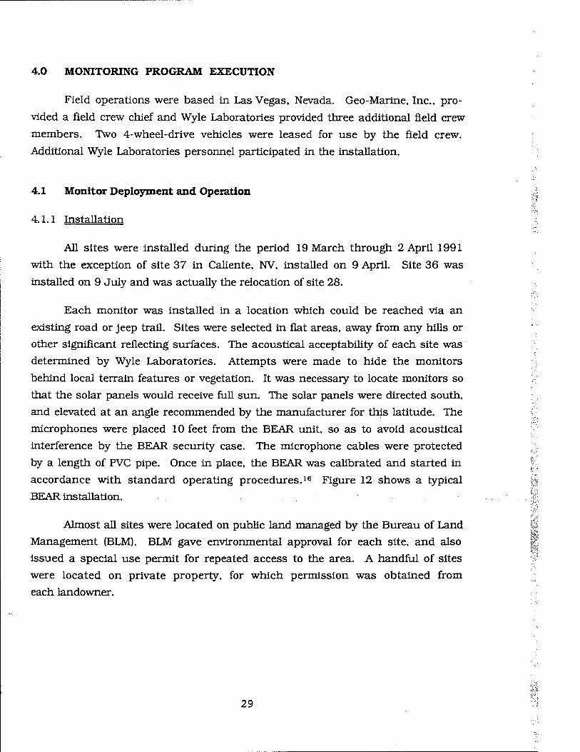
Each monitor was installed in a location which could be reached via an
existing road or jeep trail. Sites were selected in flat areas, away from any hills or
other significant reflecting surfaces. The acoustical acceptability of each site was
determined by Wyle Laboratories. Attempts were made to hide the monitors
behind local terrain features or vegetation. It was necessary to locate monitors so
that the solar panels would receive full sun. The solar panels were directed south,
and elevated at an angle recommended by the manufacturer for this latitude. The
microphones were placed 10 feet from the BEAR unit, so as to avoid acoustical
interference by the BEAR security case. The microphone cables were protected
by a length of PVC pipe. Once in place, the BEAR was calibrated and started in
accordance with standard operating procedures.16 Figure 12 shows a typical
BEAR installation.
Almost all sites were located on public land managed by the Bureau of Land
Management (BLM). BLM gave environmental approval for each site, and also
issued a special use permit for repeated access to the area. A handful of sites
were located on private property, for which permission was obtained from
each landowner.
29

c o
iS p—(
CO -t-J co C
t—t
w PQ
CN
CU
tic
30

4.1.2 Operation
Servicing followed the procedures as employed at WSMR using the BEAR
procedures in Reference 16 with some routine modification for the new BEARs.
Each BEAR was visited at least once per week. Each service visit consisted of the
following steps:
• Inspect the monitor for physical condition and signs of animal or human
tampering. No significant animal damage occurred, although one site
was moved when it was discovered that its location was occasionally
used as a river.
• Note the number of records indicated on the front panel, check BEAR
system time relative to a reference timepiece, and measure the battery
voltage.
• Remove the RAMs on old BEAR units. New BEAR units were connected
to a laptop computer via serial cable through which data files were
downloaded and system parameters were reset.
• Correct any problems noted in the inspection. Sufficient spare parts
(microphones, cables, batteries, and a spare BEAR) were carried so that
virtually any problem could be corrected.
• For old BEARs, install new RAMs, reset the clock and operating
parameters. Calibrate both old and new BEARs using a B&K Type 4220
pistonphone.
• Start the BEAR and secure the site.
During operation of these monitors, most problems were similar in nature
to those encountered at WSMR and R-2301E. Those were either RAM filling with
extraneous non-boom events and occasional instrument malfunctions. Malfunc-
tions were rarer than at WSMR and R-2301E, due to additional reliability
development of BEARs by the Air Force, based on field experience to date.
The overall up-time, averaged across all sites, was about 83 percent. This
was comparable to the 87 percent up-time achieved at WSMR.
31

4.1.3 Monitor Removal
The final day of monitoring was 30 September 1992. During the scheduled
service visits over the next few days, all BEARs were removed.
4.2 Processing of Sonic Boom Data
Following each day's servicing, old BEAR RAM modules were downloaded at
the Las Vegas field office. Retaining backup copies in Las Vegas, data were
shipped to Douglas Aircraft Company for preliminary screening and printing of the
boom records. Data were organized and correlated with monitor operating times
from the field logs. Obvious bad BEAR records were removed from the data at this
time and the remaining data was shipped to Wyle's Arlington office. This data
consisted of the BEAR event files on floppy disk, printed representations of each
of the data files, and copies of the field data logs. Data logs were reviewed to
establish time periods when each monitor was actively collecting data.
All recorded pressure signatures were examined. Some of the data files
were edited in order to remove spurious "spikes" in the data due to radio
frequency interference. Consecutive files which had been split by quirks in BEAR
logic were spliced together. All of the BEAR data files which were clearly not
sonic boom events were discarded.
Figures 13 and 14 are examples of two BEAR recordings of sonic booms.
Each plot shows the pressure signature, i.e.. pressure (psf) as a function of time.
Annotation on the plot shows the site number, the time and date, the file name,
and other supporting information. The sonic boom shown in Figure 13 is a good
example of an N-wave. Figure 14 is an example of an N-wave followed by a U-wave
as would be expected in a post-focus region. Both signatures exhibit atmospheric
turbulence distortion.
The pressure signatures as shown in Figures 13 and 14 directly provide the
peak pressure and duration, as well as the type of boom (N-wave, U-wave, etc.). As
discussed in Section 3.1.2, environmental analysis requires other metrics, in
particular the peak level and the C-weighted sound exposure level (CSEL). The
analysis software17 includes the computer program BBALL. This program com-
putes noise metrics for groups of BEAR signature files, and generates a tabulated
32

File w200823R.715 08:23:39.23 July 15 1992 Pmax= .81 Pmin = -.56 7050 points SIte 20 S/N 4016
50 100 150. 200. 250.
Time, milliseconds
300. 350.
Figure 13. Example BEAR Record.
33

File w231809R.827 18:09:15.00 August 27 1992 Pmax= 1.61 Pmin = -1.11 16124 points Site 23 S/N 1004
600.
Time, mi
800. 1000.
[ iseconds
Figure 14. Example BEAR Record.
34

Table 3
Example BEARLOUD Output File
BEAR LOUDNESS METRICS
FILE NAME POINTS Pmax Pmin Lpk ESEL ASEL CSEL PLDB WARNING CODE
(PSF) (PSF) (dB) (dB) (dB) (dB) (d8)
B031225A.100 4161 .252 -.201 115.6 103.3 74.7 88.7 85.6
B031101B.430 1594 .214 -.127 114.2 100.2 70.9 86.4 82.4
B031239A.430 11650 .638 -.399 123.7 111.7 80.0 100.7 94.2 B
B031339A.501 4458 .272 -.153 116.3 103.4 74.5 89.0 84.5
B030654A.505 15944 1.045 -1.577 128.0 119.6 84.2 101.0 97.4 E
B030655A.505 3056 .829 -.587 126.0 110.4 78.8 101.6 94.2
B030719A.508 6701 .755 -.859 125.2 113.8 82.4 100.7 96.6 E
B030730A.508 5266 1.500 -1.086 131.1 115.2 89.8 107.9 104.7
B031509A.813 12841 .277 -.361 116.5 107.5 79.7 93.7 90.8 B E
B030725A.821 15856 1.561 -1.332 131.5 119.9 85.9 108.1 102.1
B030736A.821 15951 1.442 -2.004 130.8 121.8 93.6 110.6 108.1 B E
B030820A.904 7968 .359 -.206 118.7 105.2 77.4 89.8 87.9
B031324A.909 6618 .242 -.203 115.3 103.8 76.8 89.0 87.0
B031317A.910 16077 1.587 -1.599 131.6 122.5 88.2 108.2 103.6 E
B032025A.F26 15811 1.325 -1.086 130.0 117.9 84.2 104.9 100.2
B031857A.F27 15752 .275
WARNING
-.259
MESSAGE
116.4
CODES
105.7 81.2 92.1 91.9
A : °Ppk8>=10 CHECK FOR SPIKE
B : Lpk - CSEL <= 23 : NO N-UAVE 7
C : Lpk - CSEL >= 29 : U WAVE ?
D : NPTS > 16384 : SPECT TRUNCATED
E : °PHIN° > PMAX !
35

summary. An example of a BBALL output file is shown in Table 3. The first column
lists the names of the files processed. The next column lists the number of data
points in the data file. This is followed by two columns containing the maximum
and minimum pressure in pounds per square foot, a column of the LpCak, four
columns containing the unweighted SEL, ASEL, CSEL, and PLDB, in dB. The last
column contains various warning codes which flag data files for possible problems.
These problems include spikes in the data file (due to RF noise), files which may
not contain sonic boom data (Lpk - CSEL < 23 dB), files which contain only a
U-wave (Lpk - CSEL > 29 dB) (the accompanying N-wave may be in a separate data
file), and files which exhibit a greater negative peak pressure than positive peak
pressure (lPmln I > Pmax ).
A BEARLOUD file was prepared for each site. Lcdn at each site (the primary
environmental metric) could then be calculated by combination of CSELs, as
described in Section 3.1.2. Analyses of both single-event metrics (peak pressure
or CSEL) and the cumulative metric (Lcdn) are presented in Section 5.
4.3 Collection of Operations Data
While sonic boom data were being recorded in the airspace, all available
related operations data were collected from Nellis AFB. The following operations
data items were obtained:
1. Range Group schedule data, as discussed in Section 3.3.1. were
collected at the end of the measurement program.
2. ACMI schedules, as discussed in Section 2.3.2, were shipped
periodically with ACMI tapes.
3. ACMI data tapes. The digital tapes for each mission are normally
returned to the available supply after a mission has been analyzed. They
were instead placed in a container which could hold ten tapes. When
the container was filled, it was sent to Wyle's Arlington, VA office.
Upon reaching Wyle, the ACMI tapes were immediately processed by
EXTRACT, then returned. A supply of 100 blank tapes was provided. This
36
ensured that Loral Aerospace's normal supply of tapes would not be depleted by
those in transit. A total of 508 tapes were received which contained 320
training events.
4.4 Processing of Operations Data
The primary objective of collecting operations data was to develop a time-
line of activity in the Elgin MOA, then correlate each measured sonic boom with a
specific training event. This would identify those booms associated with ACM
training. The numbers of associated sorties, mission types, etc., would also be
known, allowing statistical projection of current results to other airspaces.
The foundation for a time-line of activity were the Range Group schedule
and the ACMI summaries. All the missions in the Elgin MOA were entered in
chronological order into a computerized data base. Only known ACM (Air Combat
Maneuver) missions scheduled for the Elgin MOA were considered in creating
this time-line.
Table 4 is an excerpt from this data base. Scheduled missions were cross-
checked against the ACMI summaries to complete the information for each
mission. Whenever inconsistencies were encountered, the ACMI as-flown sum-
maries were assumed to be correct. For missions with ACMI data, the pod "on"
and "off' times were noted. Any occurrences of sonic booms were also noted.
The total operations occurring during the monitoring period are sum-
marized in Table 5. ACMI data were obtained for 20 percent of ACM sorties.
4.5 Collection and Processing Atmospheric Profiles
It has been found in past studies6 that boom prediction by Boom-Map3 is
very sensitive to the atmospheric profile used. For this reason, data was collected
from the National Oceanic and Atmospheric Administration (NOAA) on atmo-
spheric profiles. NOAA launches radiosonde balloons twice daily at 3 p.m. and
3 a.m. which collected temperature, pressure, wind, and other information from
their Mercury, NV site. This site is located on the southern edge of the Nellis
Range Complex.
37

Table 4
Excerpt From Mission/Boom Data Base
Date Mission # AC Call Schedule | ACM I Time | Measured Booms
Type AC Type Name Start Stop| Pod Start Stop | Site Time Peak SEL EVENT #
03309H Tl 02 F15 RAHBO 01 0730 I 0815 I
10 808 .165 84.0 015
033092 02 F15 CONAN 01 0730 0815 26 833 1.050 103.7 016
033092 02 F18 VCSL 01 0730 0815 10 837 .270 86.5 017
033092 04 F18 VCSL 01 0730 0815 23 837 .905 101.8 017
033092 04 F16 HIG 01 0815 0900 X 0808 0902 24 838 .915 99.4 017
033092 06 02 F15C RINGO 01 0815 0900 X 0808 0902 16 849 .643 99.1 018
033092 02 F16 VENOM 01 1115 1200
033092 06 04 F16 VIPER 01 1115 1200
033092 1NCT 01 F16 TBIRD 07 1200 1230
033092 00 REST 1220 2359 27 1237 .959 124.1 019
033092 00 REST 1220 2359
033092 02 F16 MIG 01 1230 1315
033092 02 F15 RINGO 01 1230 1315
033092 02 F15 BURNER 1230 1315
033092 02 F16 IVAN 1230 1315
033092 02 F15C COWBOY 1230 1315
033092 02 F15 RINGO02 1230 1315
033092 02 F15 CONAN 01 1315 1400
033092 TI 02 F15 RAM80 01 1315 1400
033092 02 F18 VCSL 01 1315 1400
033092 04 F18 VCSL 01 1315 1400
033092 00 TBIRD 08 1445 1615
033092 02 F15 RAMBO 01 1615 1700
033092 02 F18 VCSL 1615 1700
033092 SAT 24 F117 VCSL 11 1730 2300
38

Table 5
Operations in the Elgin MOA
Aircraft ACM ACMI Type Sorties Sorties
F-lll 33 0
F-18 509 66
F-16 3,101 447
F-15 2,333 690 F-14 18 0
F-5 2 2
F-4 2 0
Other 227 0
TOTAL 6,225 1,213
Data from these balloon launches was obtain from NOAA for each day of the
monitoring period. This provided actual atmospheric data from which atmo-
spheric profiles could be constructed for use with Boom-Map3.
39
5.0 ANALYSIS
Data analysis consisted of three main tasks. These included a summary of
total ACM operations which are presented in Section 5.1. statistical summaries of
booms measured at each site, and empirical Lcdn contours which are discussed in
Section 5.2. The data analysis also included an analysis of ACMI data which
consisted of Boom-Map3 Lcdn predictions. This topic is discussed in Section 5.3.
5.1 Operations
During the monitoring period, schedule data documenting Air Force
operations in the Elgin MOA were collected. Table 6 summarizes the ACM activity
obtained from this data base. Included are distributions by aircraft mix. In
Table 5, a sortie is a single aircraft and a mission is a flight of aircraft operating
together under one call sign. A training event consists of one or more missions
operating in an airspace at the same time. The predominant aircraft utilizing the
Elgin MOA for ACM operations were F-15s and F-16s. There were a total of 6,225
ACM sorties, grouped in 1,080 training events during the six-month monitoring
period. Of the 1,080 ACM training events, ACMI data were obtained for 320.
5.2 The Measured Sonic Boom Environment
A total of 1,337 sonic booms were recorded by the BEAR monitors. Since a
single boom event may be recorded by more than one monitor, multiple boom
recordings which were part of one boom event were grouped together. These
booms were grouped such that the time between recorded booms was consistent
with sound propagation speed, aircraft speed, and site spacing. Recorded booms
which were not consistent with these parameters were counted as separate
events. Counting booms in this manner yielded a total of 609 individual
boom events.
Of the 609 boom events, 584 correlated with scheduled ACM activity. The
source of the remaining booms is apparently from mission types which are not
classified as ACM or, perhaps, unscheduled ACM missions. The 584 ACM boom
40
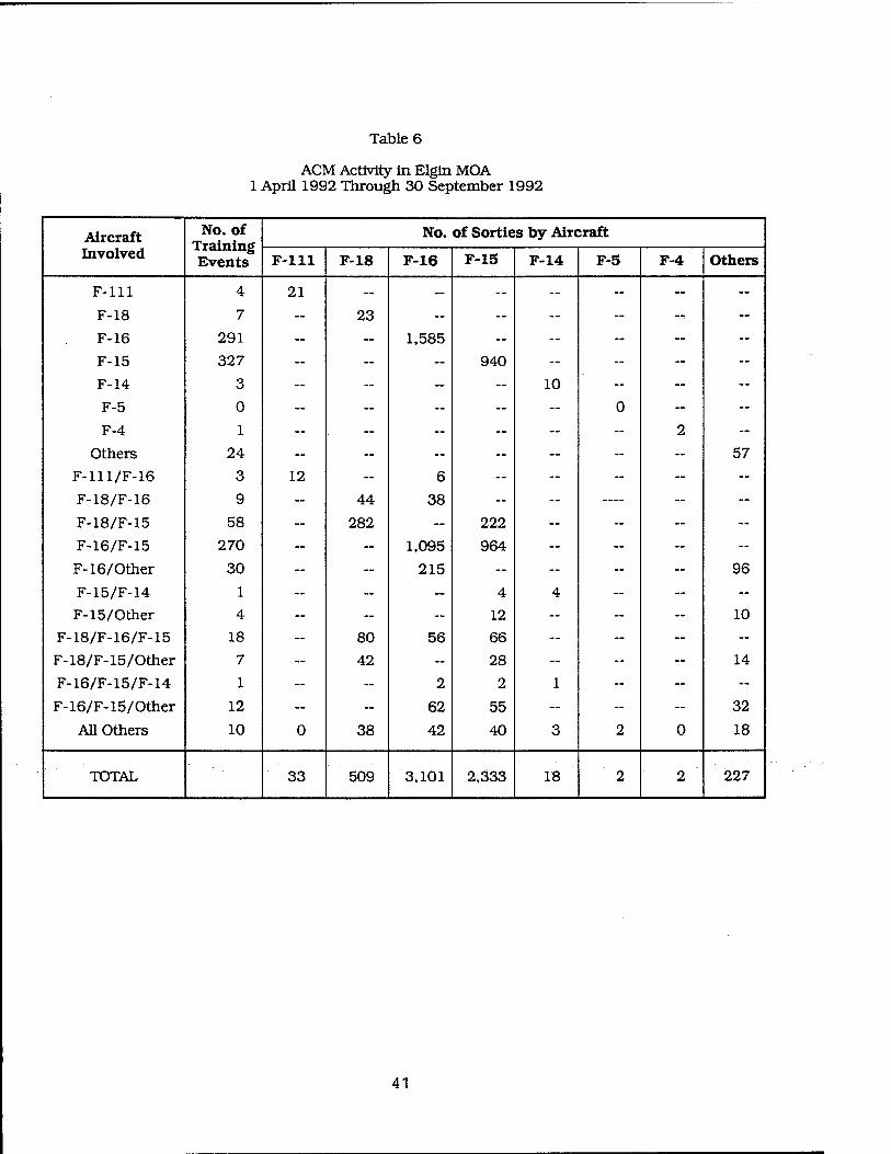
Table 6
ACM Activity In Elgin MOA 1 April 1992 Through 30 September 1992
Aircraft Involved
No. of Training Events
No. of Sorties by Aircraft
F-lll F-18 F-16 F-15 F-14 F-5 F-4 Others
F-lll 4 21 ~ — — ~ -- ~ ~
F-18 7 -- 23 — — ~ ~ --. ~
F-16 291 ~ — 1.585 — — ~ - —
F-15 327 ~ — — 940 ~ - ~ —
F-14 3 - ~ — ~ 10 - — —
F-5 0 - ~ ~ — ~ 0 — —
F-4 1 ~ ~ — ~ ~ -- 2 -
Others 24 ~ ~ ~ — — ~ — 57
F-lll/F-16 3 12 — 6 ~ -- ~ — ~
F-18/F-16 9 ~ 44 38 ~ — — — ~
F-18/F-15 58 - 282 ~ 222 — ~ - ~
F-16/F-15 270 ~ ~ 1,095 964 -- — ~ -
F-16/Other 30 ~ ~ 215 ~ — — ~ 96
F-15/F-14 1 - ~ — 4 4 ~ - —
F-15/Other 4 - - - 12 — ~ ~ 10
F-18/F-16/F-15 18 - 80 56 66 ~ ~ ~ —
F-18/F-15/Other 7 ~ 42 ~ 28 ~ ~ - 14
F-16/F-15/F-14 1 - ~ 2 2 1 ~ ~ —
F-16/F-l5/Other 12 ~ ~ 62 55 — - — 32
All Others 10 0 38 42 40 3 2 0 18
TOTAL 33 509 3.101 2,333 18 2 2 227
41

events represented 0.09 boom per sortie, which is close to the 0.11 boom per
sortie obtained at WSMR Of the 584 ACM boom events, 210 were associated with
ACMI missions.
Table 7 lists summary site-by-site recorded boom statistics including the
following: site number, the number of monitor operating days, the total booms
recorded, the number of acoustical day and night booms, the maximum and
average boom overpressure, the number of booms greater than 5 psf overpressure,
the maximum and energy average of the peak level, the maximum and energy
average of the CSEL, and the total Lcdn. Site locations can be seen in Figure 11
and are listed in Table 2. Recall that site 37 is located in the town of Caliente, NV.
As noted previously, a total of 1,337 booms were recorded, of which 62
occurred during acoustical night (between 2200 and 0700). A total of 18 booms
were recorded which had peak overpressures greater than 5 psf. These booms
are summarized in Table 8. The overall average boom overpressure was 0.93 psf.
This is slightly larger than the 0.69 psf and 0.67 psf average boom overpressure
measured at R-2301E6 and WSMR,1 respectively.
The cumulative distribution of all recorded booms, i.e., the percentage of
booms which exceeded various overpressures, is shown in Figures 15 and 16.
Peak overpressure is shown on a linear scale in Figure 15 and a logarithmic scale
in Figure 16. The central portion of Figure 16 is a straight line, which corre-
sponds to (on this log probability plot) a log normal distribution, which is
commonly found for sonic booms. Similar plots for individual sites are provided in
Appendix A.
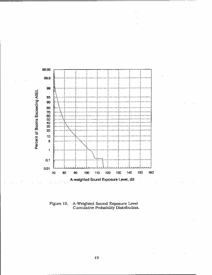
Figures 17 through 20 show Lpk, C-weighted SEL, ASEL, and Perceived
Loudness (PLdB) distributions for all measured booms. ASEL and PLdB are shown
because of recent interest in these metrics for assessing human response to
sonic booms.18
Contours of Lcdn as measured at each site are shown in Figure 21. Notice
how the empirical contours form a generally elliptical shape. This coincides well
with the previously developed concept of elliptical contours for the description of
Lcdn under ACM airspace.1-6-13
42
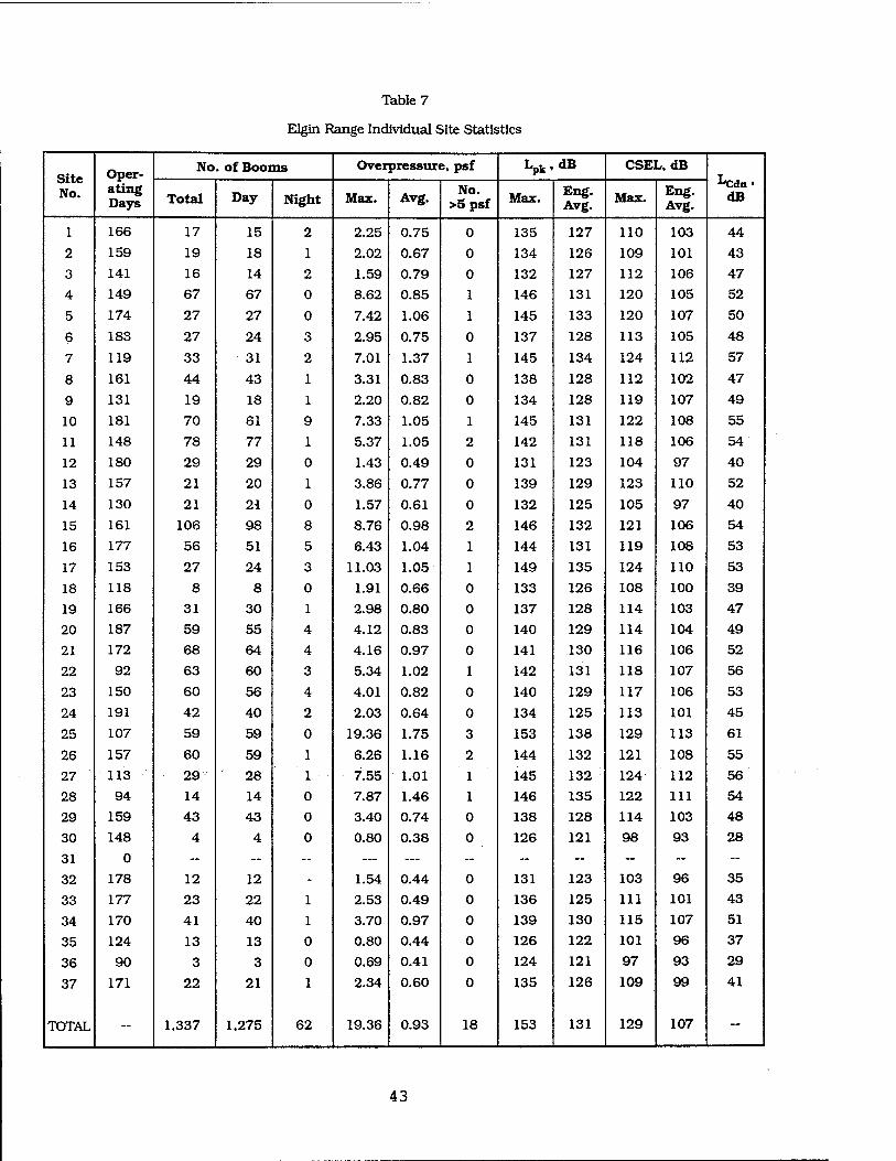
Table 7
Elgin Range Individual Site Statistics
Site No.
Oper- ating Days
No . of Booms Overpressure, psf Lpk« dB CSEL, dB LCdn« dB Total Day Night Max. Avg,
No. >S psf Max.
Eng. Avg.
Max. Eng. Avg.
1 166 17 15 2 2.25 0.75 0 135 127 110 103 44
2 159 19 18 1 2.02 0.67 0 134 126 109 101 43
3 141 16 14 2 1.59 0.79 0 132 127 112 106 47
4 149 67 67 0 8.62 0.85 1 146 131 120 105 52
5 174 27 27 0 7.42 1.06 1 145 133 120 107 50
6 183 27 24 3 2.95 0.75 0 137 128 113 105 48
7 119 33 31 2 7.01 1.37 1 145 134 124 112 57
8 161 44 43 1 3.31 0.83 0 138 128 112 102 47
9 131 19 18 1 2.20 0.82 0 134 128 119 107 49
10 181 70 61 9 7.33 1.05 1 145 131 122 108 55
11 148 78 77 1 5.37 1.05 2 142 131 118 106 54
12 180 29 29 0 1.43 0.49 0 131 123 104 97 40
13 157 21 20 1 3.86 0.77 0 139 129 123 110 52
14 130 21 21 0 1.57 0.61 0 132 125 105 97 40
15 161 106 98 8 8.76 0.98 2 146 132 121 106 54
16 177 56 51 5 6.43 1.04 1 144 131 119 108 53
17 153 27 24 3 11.03 1.05 1 149 135 124 110 53
18 118 8 8 0 1.91 0.66 0 133 126 108 100 39
19 166 31 30 1 2.98 0.80 0 137 128 114 103 47
20 187 59 55 4 4.12 0.83 0 140 129 114 104 49
21 172 68 64 4 4.16 0.97 0 141 130 116 106 52
22 92 63 60 3 5.34 1.02 1 142 131 118 107 56
23 150 60 56 4 4.01 0.82 0 140 129 117 106 53
24 191 42 40 2 2.03 0.64 0 134 125 113 101 45
25 107 59 59 0 19.36 1.75 3 153 138 129 113 61
26 157 60 59 1 6.26 1.16 2 144 132 121 108 55
27 113 29 28 1 7.55 1.01 1 145 132 124 112 56
28 94 14 14 0 7.87 1.46 1 146 135 122 111 54
29 159 43 43 0 3.40 0.74 0 138 128 114 103 48
30
31
32
148
0
178
4 4 0 0.80 0.38 0 126 121 98 93 28
12 12 _ 1.54 0.44 0 131 123 103 96 35
33 177 23 22 1 2.53 0.49 0 136 125 111 101 43
34 170 41 40 1 3.70 0.97 0 139 130 115 107 51
35 124 13 13 0 0.80 0.44 0 126 122 101 96 37
36 90 3 3 0 0.69 0.41 0 124 121 97 93 29
37 171 22 21 1 2.34 0.60 0 135 126 109 99 41
TOTAL - 1,337 1,275 62 19.36 0.93 18 153 131 129 107 -
43

Table 8
Booms Greater Than 5 psf
Site No. Date Time
Maximum Overpressure,
psf dB CSEL,
dB
28 7 Apr 92 1055 7.87 145.5 121.8
25 8 Apr 92 1347 19.37 153.3 129.2
26 8 Apr 92 0815 5.71 142.7 120.6
26 8 Apr 92 1110 6.26 143.5 119.5
25 29 Apr 92 1244 8.30 146.0 119.6
25 29 Apr 92 1244 6.00 143.2 116.4
16 1 May 92 1338 6.43 143.8 119.2
22 14 May 92 0912 5.34 142.1 114.6
10 20 May 92 1424 7.33 144.9 118.3
15 20 May 92 1424 7.91 145.6 115.3
27 26 May 92 1807 7.55 145.2 120.4
4 23 Jun 92 1316 8.62 146.3 120.2
5 25 Jun 92 1346 7.42 145.0 120.0
17 25 Jun 92 1741 11.03 148.5 123.8
11 25 Aug 92 1321 5.37 142.2 118.4
7 10 Sep 92 1315 7.02 144.5 119.0
15 18 Sep 92 1740 8.76 146.4 121.4
11 24 Sep 92 1311 5.19 141.9 115.7
44

03 L.
«n en 03
03 > o ca a. O) c T3 03 03 O
ä CO
E o o m
c 03 u 03 a.
99.99
99.9
99
95 90
80 70 | 60 50 40 30 20
10 5
1 I
0.1 =
0.01
■ _ i i t i i -J j i i
i i i i i i i i i i
0 2 4 6 8 10 12 14 16 18 20
Peak Overpressure, psf
Figure 15. Overpressure Cumulative Probability Distribution.
45

99.99
(1) 99.9 l_ D cn en <D 99 D. u. Q) > o 95
.* 90 CO
0_ 80 O) 70
60 <D 50 Ü 40
d3 30 cn 20 E o 10 Ü m 5 *^ o
•♦-• c 1 (D U u. <U D_ 0.1
0.01
r- *- - f- -»■-:■<• «■ -' - ■»■ \ ' ! : -i C- ».( i 4 ;.. *, ..r c J .; : I (- C + I <■ I ..
r- f j.....»—j-f-j-ij-j ; ,V..j...;..;..;..;.;,; ; j....;...;..;..;..;.;.; j ;....;...;..;..;..;
~ i j f"|-f i H ! f ! ?■•!'•!•!■ f-St * ;....;...;..;..;..;.;.; ; ;....♦...»..,..;..;
™ * {....*...}..«..i-.j.j.j f. ;....4...;..,*..;..;.;; .v.■-•■;• ••.-*—j-i-.i-t-i.; i ;....*...;..;..;..;
0.01 0.1 1 10
Peak Overpressure, psf
100
Figure 16. Overpressure Cumulative Probability Distribution.
46

99.99
99.9
0) > 99 <u _l
m 95 <D a. 90 O) .c 80
70 0) Ü 60 ffi 50 (0 40 E 30 o o 20 ffl t^- 10 o *-* 5 c <D C) i_ <D 1 a.
0.1
0.01 I i i I i i i i i
70 80 90 100 110 120 130 140 150 160
Peak Level, dB
Figure 17. Peak Level Cumulative Probability Distribution.
47

99.99
99.9
_J 99 uu CO o 95 O) c 90 T> CD 80 0) Ü 70 X at 60 <n 50 E 40 o o 30 m 20 H—
O ■*-* 10 c CD C) 5 u. CD Q.
1 r-
0.1
0.01 : i i i i i \ i . i
70 80 90 100 110 120 130 140 150 160
C-weighted Sound Exposure Level, dB
Figure 18. C-Weighted Sound Exposure Level Cumulative Probability Distribution.
48
99.99
99.9
99
CO < 95
90 TJ <D R0 QU O 70 iä 60 en 50 b 40 o o 30 m ?0 o 4-* m c Ü 5 v— <D a.
1 j
0.1
0.01
~ j...\-. i | i | i-
70 80 90 100 110 120 130 140 150 160
A-weighted Sound Exposure Level, dB
Figure 19. A-Weighted Sound Exposure Level Cumulative Probability Distribution.
49

0} OT a> c
■o a o _i ■o 03 > CD O L. <u a. D) C T3 03 03 CJ
■s CO
E o o
CD
c 03 Ü h- 03 Q.
99.99
99.9 h
99
95 90
80 70 60 50 40 30 20
10 5
0.1 r
0.01
~ * i I Nr r ! f i t*
70 80 90 100 110 120 130 140 150 160
Perceived Loudness, dB
Figure 20. Perceived Loudness Cumulative Probability Distribution.
50

Figure 21. Elgin MOA Lcdn Contours Based on Measured Data.
51
5.3 ACMI Analysis
ACMI tapes were processed for 320 training events containing 1,203
sorties. This represented 20 percent of ACM sorties flown. Two types of analysis
were performed on ACMI data including statistical summaries of altitudes and
Mach numbers for supersonic flight time and sonic boom predictions with
Boom-Map3.
5.3.1 ACMI Statistics
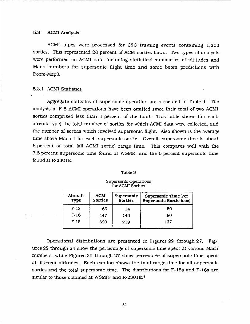
Aggregate statistics of supersonic operation are presented in Table 9. The
analysis of F-5 ACMI operations have been omitted since their total of two ACMI
sorties comprised less than 1 percent of the total. This table shows (for each
aircraft type) the total number of sorties for which ACMI data were collected, and
the number of sorties which involved supersonic flight. Also shown is the average
time above Mach 1 for each supersonic sortie. Overall, supersonic time is about
6 percent of total (all ACMI sortie) range time. This compares well with the
7.5 percent supersonic time found at WSMR, and the 5 percent supersonic time
foundatR-2301E.
Table 9
Supersonic Operations for ACMI Sorties
Aircraft Type
ACM Sorties
Supersonic Sorties
Supersonic Time Per Supersonic Sortie (sec)
F-18 66 14 59 F-16 447 140 80 F-15 690 219 137
Operational distributions are presented in Figures 22 through 27. Fig-
ures 22 through 24 show the percentage of supersonic time spent at various Mach
numbers, while Figures 25 through 27 show percentage of supersonic time spent
at different altitudes. Each caption shows the total range time for all supersonic
sorties and the total supersonic time. The distributions for F-15s and F-16s are
similar to those obtained at WSMR1 and R-2301E.6
52

22
20
cM 8 o 16
14
12
10
8
6
4
2
1 r -i r
c <u o i_ 0)
Q_
u 'c o GO v_ 0) Q.
CO
0
i i i i
0.9 1.1 1.3 1.5 1.7 1.9 Mach Number
2.1 2.3 2.5
Figure 22. Mach Number Distribution for 14 F-18 Supersonic Sorties. Total Supersonic Time = 38 minutes. Total Time on Range = 1,320 minutes.
53

22
20
g>18 -i—' c 1 6 o o 14
Q_
CD" 12 E P 10 h o c 8 o
*5 6
Q. ^ 4
00
2
0.9 1 .1
-i | 1 1 r -i 1 r i 1 r
-i 1 i_ -I 1 1 L J 1-3 1-5 1.7 1.9 2.1 2.3 2.5
Moch Number
Figure 23. Mach Number Distribution for 140 F-16 Supersonic Sorties. Total Supersonic Time = 579 minutes. Total Range Time = 13,342 minutes.
54

22
20 CD
o c 1 6 o u 14
Q_
oJ 12 E P10 o
-i r
c o en a>
8
6
4
2
0 0.9 1.1 1.3 1.5 1.7 1.9
Mach Number 2.1 2.3 2.5
Figure 24. Mach Number Distribution for 219 F-15 Supersonic Sorties. Total Supersonic Time = 1,196 minutes. Total Time on Range = 15,726 minutes.
55

20
18
g^16
g14
£12
E 10 t— 0 8 c 0 IT) h i_ <U CL 3 4
(71
2
-1 r
0 0
1 r -) 1 r "1 r
5 20 25 30 35 40 45 Altitude, KFeet
Figure 25. Altitude Distribution for 14 F-18 Supersonic Sorties. Total Supersonic Time = 38 minutes.
Total Time on Range = 1.320 minutes.
56

20
18 CD
-i—>
c CD 1 4
^ 1 O Q_ 1 2 CD £10
.y 8 c o c en 6
1 r
CD Q_
(/I 4
2
0 0
-, | , | , 1 r "I r
' 1 0 15 20 25 30 35 40 45 Altitude, KFeet
Figure 26. Altitude Distribution for 140 F-16 Supersonic Sorties. Total Supersonic Time = 579 minutes.
Total Time on Range = 13,342 minutes.
57

20 i 1 1 : r i 1 r i 1 1 r
18 CD
c
£l2 CD
E 10
u 8 c o U) h L_ CD CL 4
CO
2 -
0 0 10 15 20 25 30 35 40 45
Altitude, KFeet
Figure 27. Altitude Distribution for 219 F-15 Supersonic Sorties. Total Supersonic Time = 1,196 minutes. Total Time on Range = 15,726 minutes.
58

5.3.2 Boom-Map3 Analysis
As described in Section 3.3.2, Boom-Map3 is a model which computes the
sonic boom resulting from each supersonic event, using ACMI tracking data and
full ray-tracing sonic boom theory. This model is a research tool used for
understanding detailed mechanisms involved in ACM sonic booms. Versions are
available which compute single-event psf contours for individual missions or
sorties, and which compute Lcdn contours for a library of ACMI data.
Figure 28 shows calculated Lcdn contours for all ACMI missions using the
average atmospheric profile for the entire measurement period. These levels have
been scaled to account for all ACM sorties flown. The 55 dB contour which starts
at the ACMI origin and streaks out over the northern Elgin MOA boundary was
caused by a single sortie. This single supersonic track was flown at about
6,000 feet AGL and at a Mach number between 1.07 and 1.12. Because of the low
altitude, the sonic boom footprint was narrow and fell between several monitors
but was not detected on any.
Figure 29 shows the Lcdn contours without this single sortie. Notice how,
without this anomalous sortie, there is excellent agreement between the pre-
dicted Lcdn contours and the measured contours shown in Figure 21.
This boom, while not being included in the Boom-Map3 contours, was a
real event, comparable to the 20 psf boom measured at Site 25 on 8 April. There
is a question as to the meaning of including such rare events in Lcdn contours.
Lcdn is an average level, quantifying the cumulative impact of a number of booms
over an extended period. We. feel that it is appropriate to omit statistically rare
anomalous booms from this average. It is important, however, to recognize their
existence (as we have done in Table 8 for measured booms) and account for the
impact of these occasional worst-case events.
As mentioned previously, Boom-Map3 predictions are sensitive to the
atmospheric profile. In this project, actual atmospheric profiles, obtained from
NOAA, provided an accurate atmospheric model from which to predict sonic
booms. Previous sonic boom studies have suffered from a lack of appropriate
atmospheric data. The accuracy with which Boom-Map3 was able to predict the
Lcdn contours for the measurement period is largely attributed to the availability of
this local atmospheric information.
59

Figure 28. Elgin MOA Lcdn Contours as Predicted by Boom-Map3. Levels have been scaled to reflect time and operations.
60

Figure 29. Elgin MOA Scaled Lcdn Contours Without Anomalous Low-Altitude Carpet Boom.
61

6.0 MODELING Lcdn IN ACM AIRSPACES
6.1 Historical L^ Modeling Techniques
Each of the previous sonic boom studies1-613 has attempted to further
develop practical modeling of Lcdn in ACM airspaces. One of the goals of this
project was to enhance and/or modify the currently accepted model as developed
in the WSMR study.1 This model defines the L^ level as follows:
.. f(x.f+ in2} Lean = Lo + lOlogioN + lOlogio e2[[Cx' l0y'J (2)
where N is the number of sorties per month, L0 is an amplitude constant, and
cx and ay are the standard deviations along the minor and major axes. This
equation essentially defines the distribution of the average sound energy as
Gaussian, which, when transformed by the base 10 logarithm, defines elliptical
average sound level contours.
The parameters of this equation, namely L0, ox , and ay, were determined,
from a least-squares curve fit to the data measured at WSMR,1 to be 25 dB,
11.1 miles, and 18.9 miles, respectively. This form of the model fit the data
collected at WSMR much better than the previously developed Oceana model.13
Since that time the model developed from the WSMR project has been used to
estimate sonic boom noise levels in other ACM airspaces.
The measurement program performed at R-2301E was targeted at
exploiting the elliptical nature of the Lcdn contours. Those data supported the
value of L0, but were too sparse and irregular to apply to ax and oy.
6.2 Modeling L^ in the Elgin MOA
This sonic boom monitoring program offers good supportive evidence for
the elliptical model of Lcdn contours. Simple examination of both the measured
and predicted LCdn contours supports the validity of the model. Performing a
least-squares fit to Equation (2), the measurement data yields 25 dB, 7.9 miles,
and 10.8 miles for L0, ax . and ay , respectively. Contours of this least-squares fit
ellipse are shown in Figure 30. These contours agree very well with both the
measured and predicted data.
62

Figure 30. Elliptical Lcdn Contours Based on Measured Data.
63

6.3 Refinement of the ACM Airspace Sonic Boom L^ Model
The results from this sonic boom monitoring program have provided an
information source with which to refine the model for Lcdn within ACM airspaces.
It has already been demonstrated that the elliptical Lcdn contour, first postulated
for the Oceana model13 and further refined in the WSMR study,1 is the most
appropriate model. Results from the study conducted in R-2301E,6 although not
as convincing as this study, are also supportive of this model.
Each parameter of the Lcdn model will be discussed in the following
sections. First is the ellipse center amplitude scaling parameter, L0, which is
discussed in Section 6.3.1. This is followed by a discussion of contour ellipse
orientation in Section 6.3.2. Finally, the standard deviations are covered in Sec-
tion 6.3.3. The complete, refined Lcdn model is then summarized in Section 6.3.4.
6.3.1 Lrj„ Ellipse Scaling Factor
The first parameter in the Lcdn model is the overall scaling factor, L0. This
parameter, along with the operations term 10 log10(N), establishes scaling of Lcdn
at the center of the ellipse to the appropriate level. The sum of these two terms
will be the maximum Lcdn for the ACM arena in question.
Intuitively, the Lcdn at the center of the ellipse will be a function of many
parameters. The most obvious of these is the number of operations conducted in
the airspace. If the number of operations is doubled, one would expect that the
number of booms to hit the ground would double. For this reason, the term
governing the Lcdn as a function of the number of operations was treated separately
from the other parameters influencing the ellipse. This separate treatment of the
number of operations is expressed as 10 log10 (N) in the model, where N is the
number of monthly sorties.
Other factors which would influence the Lcdn at the center of the ellipse are
the number of booms produced by a sortie, the amplitude of these booms, and the
size of the boom footprint. Each of these parameters are themselves functions of
the altitude at which the aircraft are operating, the Mach number of the aircraft
during supersonic fligh, and the types of maneuvers the aircraft are involved in
during supersonic flight.
64

At first it may seem plausible to construct some "average" values for these
parameters which would permit the theoretical calculation of a viable scaling
factor (L0). However, due to the complex and variable nature of ACM operations,
calculating averages is somewhat dubious. It has been demonstrated that the
variability among ACM operations is quite large, resulting difficult to predict sonic
boom footprints. Unpredictability is an inherent aspect of ACM operations.
Predictable pilots do not last long in air-to-air combat. Also, many obvious
parameters (e.g., dive angle, Mach number) have a decidedly non-linear effect on
boom footprints, so that average values can be misleading.
However, the scaling factor (L0) can be, and has been, determined
empirically. At WSMR, the first full-scale sonic boom monitoring project, the
scaling factor, based on a least-squares fit of the measured data to the elliptical
model, was found to be 25 dB.* The same value for the scaling factor was obtained
from the R-2301E project and again for this project in the Elgin MOA. The
similarity between these three projects is not coincidental. Comparison of the
distributions of altitude and Mach number between the three projects shows them
to be very similar. This' implies that the nature of ACM operations is very much
the same at each of the three locations. It is reasonable to expect that this is true
of all ACM airspaces utilized by the U.S. Air Force.
This evidence suggests that a value of 25 dB for the L0 parameter is
appropriate.
6.3.2 Ellipse Axis Orientation
The orientation of the ellipse, as defined in the model, is such that the
major ellipse axis is coincident with the y-ordinate and the minor axis is
coincident with the x-ordinate. However, it is important to position the origin of
the x,y axis system and correctly. The location and orientation of the axis is a
function of the set-up points utilized by the ACM participants.
L0 by itself represents the long-term average Lcdn for an average of one sortie per month
65
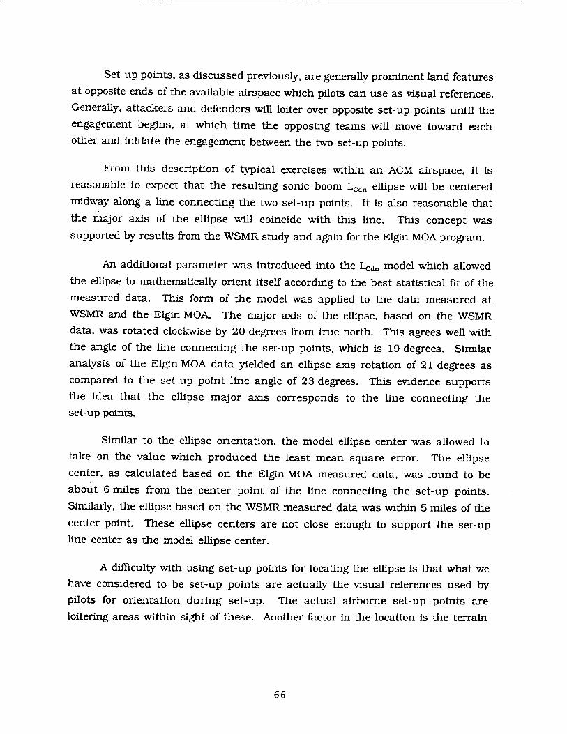
Set-up points, as discussed previously, are generally prominent land features
at opposite ends of the available airspace which pilots can use as visual references.
Generally, attackers and defenders will loiter over opposite set-up points until the
engagement begins, at which time the opposing teams will move toward each
other and initiate the engagement between the two set-up points.
From this description of typical exercises within an ACM airspace, it is
reasonable to expect that the resulting sonic boom Lcdn ellipse will be centered
midway along a line connecting the two set-up points. It is also reasonable that
the major axis of the ellipse will coincide with this line. This concept was
supported by results from the WSMR study and again for the Elgin MOA program.
An additional parameter was introduced into the Lcdn model which allowed
the ellipse to mathematically orient itself according to the best statistical fit of the
measured data. This form of the model was applied to the data measured at
WSMR and the Elgin MOA. The major axis of the ellipse, based on the WSMR
data, was rotated clockwise by 20 degrees from true north. This agrees well with
the angle of the line connecting the set-up points, which is 19 degrees. Similar
analysis of the Elgin MOA data yielded an ellipse axis rotation of 21 degrees as
compared to the set-up point line angle of 23 degrees. This evidence supports
the idea that the ellipse major axis corresponds to the line connecting the set-up points.
Similar to the ellipse orientation, the model ellipse center was allowed to
take on the value which produced the least mean square error. The ellipse
center, as calculated based on the Elgin MOA measured data, was found to be
about 6 miles from the center point of the line connecting the set-up points.
Similarly, the ellipse based on the WSMR measured data was within 5 miles of the
center point. These ellipse centers are not close enough to support the set-up
line center as the model ellipse center.
A difficulty with using set-up points for locating the ellipse is that what we
have considered to be set-up points are actually the visual references used by
pilots for orientation during set-up. The actual airborne set-up points are
loitering areas within sight of these. Another factor in the location is the terrain
66

under the main engagement area. There is a preference for this to be over a
valley, for the sake of more vertical space. This can lead to asymmetry with
regard to set-up points.
Overall, while set-up points are a good reference for ellipse orientation,
they may not provide precise enough information for ellipse location. Examination
of ACMI data at additional airspaces may be required to establish a useful relation.
Another potential guide for ellipse location is the airspace boundary, which places
real constraints on maneuver area.
6.3.3 The Standard Deviations of the Ln^ Model
The final parameters for the elliptical sonic boom noise environment model
are the standard deviations (ox, oy). These parameters describe how the level
decreases away from the ellipse center. It is logical to assume that the values of
these standard deviations would be a function of the dimensions of the airspace
available for the ACM operations. The larger the airspace is the more spread out
the operations will be, which would lead to larger standard deviations.
At WSMR the standard deviations were found to be 11.1 miles and
18.9 miles along the minor and major axes, respectively. At R-2301E the major
axis standard deviation was found to be 11.1 miles. Data along the minor axis did
not permit the calculation of a meaningful standard deviation. For the Elgin MCA,
the standard deviations were found to be 7.9 miles and 10.8 miles along the minor
and major axes, respectively. Direct comparison of these values yields no
discernible pattern.
However, considering the previously mentioned concept that the standard
deviations are a function of the available airspace, a distinct pattern does emerge.
Notice in Figure 8 that most of the supersonic tracks fall within an imaginary
ellipse which fills the Elgin MOA. Operations avoid the remote comers of the
airspace. This tendency was also observed at WSMR and R-2301E. These
relatively "tight" corners of the airspace are avoided by the pilots since their
maneuvering room is limited and they run the risk of exceeding the air-
space boundaries.
67

If the Lcdn model standard deviations for each of the three studied airspaces
are compared to the dimensions of the available airspace, a predictable pattern is
obtained. At WSMR, the ratio of both standard deviations to the respective
dimensions of the available airspace is 0.29. For R-2301E, a similar dimension
comparison (in the major axis direction only) yields a ratio of 0.25. For the
Elgin MOA the ratios are 0.25 and 0.26 along the major and minor axes,
respectively. This is fairly good reproduction of the ratio from one study
to another.
This method requires defining the available airspace in order to obtain the
standard deviations. Given the variable and irregular shapes defining airspace
boundaries, the concept of available airspace can be vague. A tentative definition of
available airspace is to inscribe an ellipse within the boundaries, oriented with the
set-up points. An example of the inscribed ellipse for the Elgin MOA is shown in
Figure 31. The standard deviations will be 27 percent (the average ratio from
WSMR, R-2301E, and Elgin MOA) of the width and height of this eUipse. Note
that this ellipse is centered somewhat north of the center of the airspace, forced
there because of the narrowing of the southern portion. This location is con-
sistent with the data, so that an inscribed ellipse may also provide a definition of
the location.
6.3.4 ACM Sonic Boom Lr^„ Model Summary
To summarize, the refined model for the Lcdn associated with sonic booms
under an ACM operations is as follows:
(3) Lcdn = L0 + 10 1og]0(N) + 10 1og10 exp -£(4*4
where L», = 25 dB
N = number of monthly operations.
xy = coordinates corresponding to the ellipse major/minor axis, y-axis
is coincident with a line connecting the set-up areas. Coordinate
origin is located midway between the set-up points.
ax, ay = 0.27 times the corresponding available airspace dimension.
68
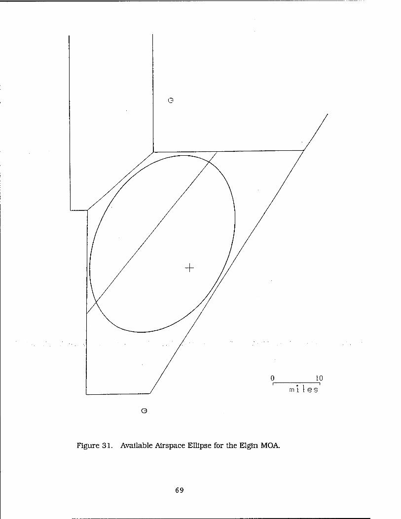
o
Figure 31. Available Airspace Ellipse for the Elgin MOA.
69

7.0 CONCLUSIONS
A measurement program has been conducted of the sonic boom
environment in the Elgin MOA subsection of the Nellis Range Complex. Thirty-six
sonic boom monitors were optimally arranged throughout the area for a period of six months.
The sonic boom environment measured in the Elgin MOA is consistent with
those measured at WSMR1 and R-2301E.6 In addition, combined results of the
three sonic boom monitoring programs has resulted in an improved model for the
Lcdn contours associated with ACM operations. This model is as follows:
(4) LCdn = L0 + 10 1og10(N) + lOlogJexp -Ü^^- \ [ z\ox a/
where: L0 = 25 dB
N = number of monthly operations.
x. y = coordinates corresponding to the ellipse major/minor axis. The
y-axis is coincident with a line connecting the set-up areas.
Coordinate origin is located midway between the set-up points.
cx, ay = 0.27 times the corresponding available airspace dimension.
Another benefit of this program was the demonstrated accuracy of the sonic
boom prediction computer program Boom-Map3. Through the utilization of ACMI
tracking data and accurate atmospheric profiles. Boom-Map3 was capable of
accurately predicting the sonic boom noise environment.
70

REFERENCES
1. Plotkin, K.J., Desai, V.R., Moulton, C.L., Lucas, M.J., and Brown, R, "Meas- urements of Sonic Booms Due to ACM Training at White Sands Missile Range", Wyle Research Report WR 89-18, September 1989. Also, "Sonic Boom Environment Under an ACM Training Arena", J. Aircraft, November- December 1992.
2. "Instrumentation for the Measurement of Sonic Booms", Wyle Research Report WR 85-31, March 1986.
3. "Assessment of Community Response to High-Energy Impulsive Sounds", National Research Council, Committee on Hearing, Bioacoustics, and Bio- mechanics, 1981.
4. Lee, R, Mazurek, D., and Palmer, B., "Boom Event Analyzer Recorder (BEAR) Operators Manual", AAMRL/BBE, WPAFB, OH. September 1987.
5. St. Clair, M., and Rostamizadeh, A, "Data Reduction User Guide for Mission Standard Data Reduction Programs", Cubic Corporation, San Diego, CA, December 1981.
6. Plotkin, K.J., Frampton, K.D., Lucas, M.J., and Desai, V.R. "Measurements of Sonic Booms Due to ACM Training in R-2301E of the Barry Goldwater Air Force Range". Wyle Research Report WR 92-4, March 1992.
7. Plotkin, K.J., "Sonic Boom Focal Zones From Tactical Air Maneuvers", J. Aircraft, 30 (1). January-February 1993
8. "Assessment of Community Response to High-Energy Impulsive Sounds", National Research Council, Committee on Hearing, Bioacoustics, and Bio- mechanics, 1981.
9. Appendix C, ANSI S1.4 (1983), American National Standard for Sound Level Meters.
10. Galloway, W.J., "Studies to Improve Environmental Assessments of Sonic Booms Produced During Air Combat Maneuvering", AFAMRL-TR-93-078, October 1983.
11. Lucas, M.J., "Selecting Optimum Sonic Boom Monitoring Sites in a Special- Use Airspace", to be presented at Noise-Con 93, Williamsburg, VA.
12. Desai, V.R., and Plotkin, K.J., "Boom-Map3 Computer Program for Sonic Boom Analysis", Wyle Research Report WR 92-5, April 1992.
13. Galloway, W.J., "Development of C-Weighted Day-Night Average Sound Level Contours for F-15 Air Combat Maneuvering Areas", BBN Report 4430, August 1980.
14. Wilby, E., Horonjeff, R, and Bishop, D., "User's Guide to MOAOPS and Boom-Map Computer Programs for Sonic Boom Research", HSD-TR- 87-004, May 1987.
R1 71

REFERENCES (Continued)
15. Bishop, D.E.. Haber, J.M.. and Wilby, E.G., "BOOMAP2 Computer Program for Sonic Boom Research: Technical Report", BBN Report 6487, Novem- ber 1987.
17. Desai, V.R., Lucas, M.J., and Moulton, C.L., "Software Developed to Support Sonic Boom Measurements at White Sands Missile Range", Wyle Research Technical Note TN 89-15, December 1989.
16. Brown, R, and Moulton, C, "Data Accumulation and Field Servicing Pro- cedures for the White Sands Missile Range Sonic Boom Study", Wyle Research Technical Note TN 89-15, December 1989.
18. Leatherwood, J.D., and Sullivan, B.M., "Subjective Loudness Response to Simulated Sonic Booms", High-Speed Research: Sonic Boom, NASA Con- ference Publication 3172, February 1992.
R2 72

APPENDIX A
Overpressure Distribution, Recorded Sonic Booms
Al 73
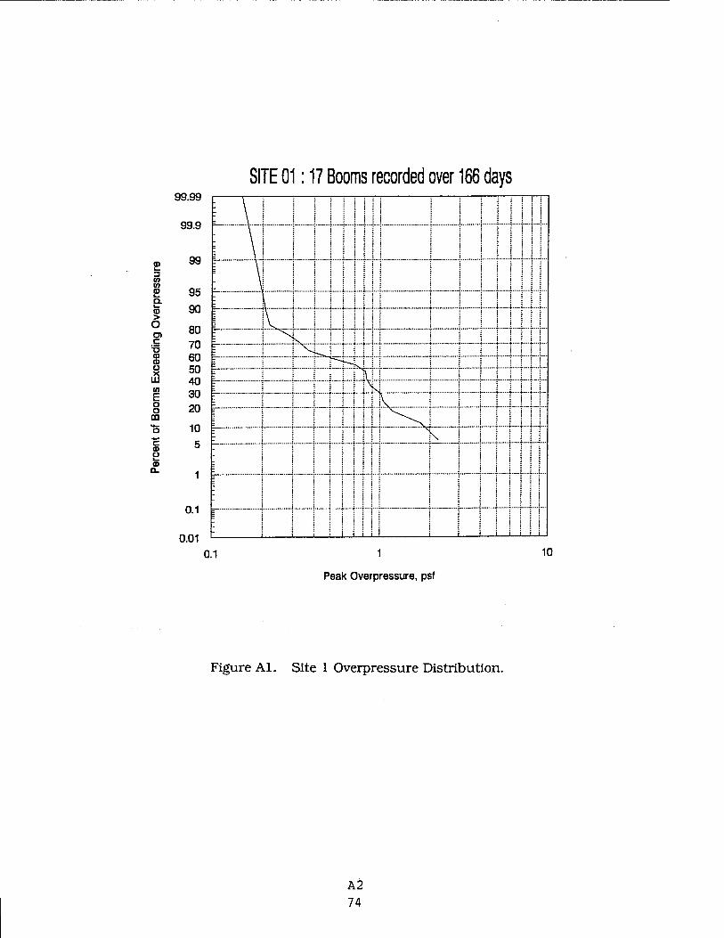
SITE 01:17 Booms recorded over 166 days 99.99
99.9
0) 99 ^ 3 CO CO m 95 a. CD 90 > O 80 c 70 CD CD 60 Ü 50
40 CO
E 30 o o 20 m o 10 .(_. c CD 5 C) ^ CD EL 1
0.1
0.01
0.1 1
Peak Overpressure, psf
10
Figure Al. Site 1 Overpressure Distribution.
A2 74

99.99
99.9
99 3 10 tn ?. 9b a.
90 > O D) 80 C
T3 70 a> ffi 60 u 50
IJS 40 10 E 30 o o 20 m o 10 c 5 U i- a) Q. 1
0.1
0.01 0.1
SITE 02:19 Booms recorded over 159 days
; \
= I j
i
: \ i
: \ I i
: : i \
i : I : : i
: : \^_^ = !
TT
TT
i
: I
E j
i i i i i i i i i J,,
1
Peak Overpressure, psf
10
Figure A2. Site 2 Overpressure Distribution.
A3 75

99.99
99.9 :-
3 (0
8 95 Q.
90 > O 80 C 70
OS 60 Ü 50
u3 40 to E 30 o o 20 m **— o 10 c 5 « k. (D
EL 1 i-
0.1 =
0.01
SITE 03:16 Booms recorded over 141 days
~ -f V j ; -1 i....i...+™j..-j i i ; i +....*...£
— -j j-v j -j ■♦—j- —•—t—*— ♦ i i ♦ ♦...-<....*.
— 1 ; j 4 +....4...+..-(.., j JT^ + j j + +■—«•••-«-■
— 4 j 1 4 4--—J---4—!--•; 1 4 j j 4 4.....f...4..
0.1 1 10
Peak Overpressure, psf
Figure A3. Site 3 Overpressure Distribution.
A4 76

SITE 04:67 Booms recorded over 149 days
3 10 CO a
CO > O c
T3 (D CD U
.2 CO
E o o m
c 8 L. CD Q.
99.99
99.9
95
90
80 70 60 50 40 30 20
10 5
1
0.1
0.01
- Ill I | | II: I j || III • • I III I I II
I ! ; L U i i j ' i i ' 11 i 1—i—i i i I i
0.01 0.1 1
Peak Overpressure, psf
10
Figure A4. Site 4 Overpressure Distribution.
A5 77

99.99
99.9
CD 99 k_ 3 m CO CD 95 Q. O 90 > o 80 c T3 70 a> a> 60 o 50 iS 40 CO
E 30 o a 20 m •*- o 10 •*-• c CD 5 Ü k. CD Q.
0.1
0.01 0.1
SITE 05:27 Booms recorded over 174 days
— 4^"-— i ; 4 *....*....+...j...i * i i + «.....(.... t
— ► i^X^j i i....i...i...;...j i | ; | «.....,'.. .4
1
Peak Overpressure, psf
10
Figure A5. Site 5 Overpressure Distribution.
A6 78

99.99
99.9
3 10 (0 (D 95 Q. O 90 > O O) 80 c 'S 70 03 (D 60 Ü
l3 50 40
09 E 30 o o 20 m "5 10 c 5 K <D 0-
0.1
0.01
SITE 06:27 Booms recorded over 183 days
99 V
: \ i ••!!!! I i i ! I j
i- -i i j f i.-.j—♦-■-^^v- + j i ♦ +—<
— 4 j j -t—*«...£...+ .rÄfc^j™-4- i j + +-—1—•*■
I I \ : ! : : I : j : I !
0.1 1
Peak Overpressure, psf
10
Figure A6. Site 6 Overpressure Distribution.
A7 79

en 01 CD
> O O) c
TJ CD (0 o ä CO
E o o m
8 CD
OL
SITE 07:33 booms recorded over 119 days 99.99
99.9
99
95
90
80
70 60 50 40 30
20
10
5
1 h
0.1
0.01
7— 4 j j ► +....+...+... j...j .77T7?r»^^™.i i j 1 4-....j....{..
~ 4 » t 4 4 ■--•4— 4---i---i 4 j -^V 4 .j..-.*....*..
: ! j j i i j I i i ■ I I | I |
0.1 1 10
Peak Overpressure, psf
Figure A7. Site 7 Overpressure Distribution.
A8 80

99.99
99.9
ID 99 ^ 3 10 OT ID 95 Q. ID 90 > o 80 c
T5 70 (D m 60
50 40
10 E 30 o o 20 m o 10 c 5 « h_ ID a.
0.1
0.01
SITE 08:44 booms recorded over 161 days
z ....._......S^. | «4—*—+».+ + ; i * *....*....*.«.
—- -V .TTj^*-™.; 4 +....+.-♦ ♦ -. j j + +....«....*...
^— -f i j •► ♦-...♦...♦.^j»*|-_ i j ~ +—+....<*....+...
0.1 1 10
Peak Overpressure, psf
Figure A8. Site 8 Overpressure Distribution.
A9 81

SITE 09:19 booms recorded over 131 days
3 10
CD > o O) c
TJ CD CD U
ä 0) E o o m
c CO o k_ CD a.
99.99
99.9
99 f~
95
90
80 70 60 50 40 30 20
10
5
1 £
0.01
: : i ::!::! : j ■ j ! i :
0.1 1
Peak Overpressure, psf
10
Figure A9. Site 9 Overpressure Distribution.
A10
82

99.99
99.9
CD 99 V- 3 10 CO CD 9b a CD 90 > O 80 c
'■5 70
CD CD 60 U SO
UJ 40 to E 30 0 0 20 m *- 0 10 c 5 « u. CD a. 1
0.1
0.01
SITE 10:70 booms recorded over 181 days
'•'•'••'' iii!
0.1 10
Peak Overpressure, psf
Figure A10. Site 10 Overpressure Distribution.
A11
83

SITE 11:78 booms recorded over 148 days 99.99
99.9
m 99 k. 3 to in <D 95 Q. k. ID 90 > O O) 80 c 70
60 u 50
u3 40 to E 30 o o 20 m o 10 c 5 « L. 03 Q. 1
0.1
0.01
: t | I | | || | || | | | | M
f ] | j j-j-yyj'j j |" j i i i |
0.1 1
Peak Overpressure, psf
10
Figure All. Site 11 Overpressure Distribution.
A12 84
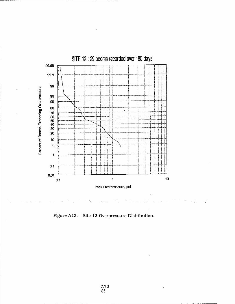
SITE 12:29 booms recorded over 180 days
3 HI V) <D
(D > o c
TJ (D CD U
|S CO E o o m
c CD U v- 00 Q.
99.99
99.9 f-
99 |
95 90
80 70 60 50 40 30 20
10
5
1
0.1
0.01 0.1
L .\....i I ! 1—*....*...* —* i 1—* *—♦--•■
£_ ; .\...j i ; ♦....♦..-♦ * ♦ i j j ♦....«...-.
jz=)==i[=5==)i|=[j:
I : : t • : : : I > • : I ■ t i
1
Peak Overpressure, psf
10
Figure A12. Site 12 Overpressure Distribution.
A13 85

SITE 13:21 booms recorded over 157 days 99.99
99.9
ID 99 k. 3 ID
8 95 a. (0 90 > Ü 80
T3 70
(D ID 6U U 50 IÜ 40 B)
E 30 o o 20 m o 10 c 5 « l_ 0
CL 1
0.1
0.01 : I I | ! i! 11! ! ! | ! I j! H I ! I INI!
0.01 0.1 1
Peak Overpressure, psf
10
Figure A13. Site 13 Overpressure Distribution.
A14 86

SITE 14:21 booms recorded over 130 days
3 CO 10 ID
ID > O at c
'-a m <D
i CO
E o o m
c CD
e CD Q.
99.99
99.9 F-
99
95
90
80 70 60 50 40 30 20
10 5
1
0.1
0.01 0.1
L + Js^™...! ] ]....♦— j { * {-•—♦•••|-
- i i i ; i i i i I i 1 1 i—i—i—i—1_
1
Peak Overpressure, psf
10
Figure A14. Site 14 Overpressure Distribution.
A15 87

SITE 15:106 booms recorded over 161 days 99.99
99.9
ID 99 u ^J m w> a> 95 n. CD 90 > o 80 c 70 ID CD 60 U 50 ixi 40 in E 30 a o 20 m •*— o 10 c 5 « u. a> a. 1
0.1
0.01
! \ I I i M i Hi I ! I I ! ! !
\ : : •!•'■:! : : : : : : :
E_ i..\. j j ■* +....*...*...:...; i i ! + i....i...i
E ' \v ' '• \ :'■•': \ • : : : ! :
E_ i j.:V....; i ;....;...;...j...i ; j j i ;....;•.••;.
i_ i ; 'i i »....;...^v^-i ..; ; ; ♦ ■».—j—f
z— 4 i \ 4 |....|...|...J...J .7^^™-; i * ^....f...^.
'. : ! i ; i i i i i ! I ! I : I i
0.1 1
Peak Overpressure, psf
10
Figure Al5. Site 15 Overpressure Distribution.
A16 88

99.99
99.9 *-■
99
to 10 (0 9b Q. (D 9Ü > o O)
80 c 'S 70
60 u 50
IÜ 40 (0 E 30 o o 20
CD
o 10 c b Ü ^ (D a. 1
0.1
0.01 0.1
SITE 16:56 boons recorded over 177 days
: : : i i i i : : i i i i
1
Peak Overpressure, psf
10
Figure A16. Site 16 Overpressure Distribution.
A17 89

SITE 17:27 booms recorded over 153 days 99.99
99.9
CD 99 *— 3 (0 CO CD 9b a. ID 90 > * o 80 c 70 a) 0) 60 u 50
l±j 40 CO
E 30 o o 20 m o 10
CD 5 U t— CD a. 1 '-
0.01 0.1 1 10
Peak Overpressure, psf
100
Figure A17. Site 17 Overpressure Distribution.
A18 90

SITE 18:8 booms recorded over 118 days 99.99
99.9 -•
99 3 0) B» CD 9b Q. w ID 90 > o 80 c 'S 70
CD ID 6U U 50 ä 40 to E 30 o o 20 m o 10 c 5 « u. CD Q. 1
0.1
0.01
L 1 1 j | |....;.X~j | i +—|—}—•—I
'_ i j ] I j. | | —}-4 |
'. i I i i i i i j .._i j i i i
0.1 10
Peak Overpressure, psf
Figure A18. Site 18 Overpressure Distribution.
Al 9 91

3 at tn
01 c <D (D U
i2 w E o o m
c a> Ü b.
a.
99.99
99.9
99
95
90
80 70 60 50 40 30 20
10 5
1 '-
0.1
0.01
SITE 19:31 booms recorded over 166 days
':
| : : j Mill i III
j
j
i ""■ T "= = x
|
\ r i V : i i j i ! i 1 | | 1 LI ...j... : ]"" l^sl : • i J j
- • - \ - • '• : : ~ —-;--- - I : :
E
:
- Ill
: : : ■ i | j j ■ ■ : : II!
i i i
: : ! ! i
i i i 'r i 1 i i i i i j L
0.1 1
Peak Overpressure, psf
10
Figure A19. Site 19 Overpressure Distribution.
A20 92

SITE 20:63 booms recorded over 187 days 99.99
99.9
to 99 k. 3 in 10 a> 9b a. a 90 > O 80 c
T3 70 (D <D 6Ü U 50
111 40
E 30 a o 20 m "o 10 c b u h_ (D a. 1
0.1
0.01 0.1
L - I.A. I-- ^.....|.._*...i { | { i—|-*~
: ■ ■ ! i i i i
1
Peak Overpressure, psf
10
Figure A20. Site 20 Overpressure Distribution.
A21 93

SITE 21:68 booms recorded over 172 days 99.99
99.9
ID 99 k- 3 in CO m 95 a.
90 > O 80 c T5 70 (D ID 60 u 50 i2 40
30 o o 20 m "o 10 c 5 « L_ <D Q. 1
0.1
0.01 '. \ • • i : ! : i I ! ill!::
0.1 1
Peak Overpressure, psf
10
Figure A21. Site 21 Overpressure Distribution.
A22 94

SITE 22:65 booms recorded over 92 days 99.99
99.9
m 99 ^ 3 OT to (D 95 Q. CD 90 > o 80 Ol c
T3 70 CD CD 60 U 50 iä 40
CO E 30 o o 20 m o 10 c 5 « CD Q. 1
0.1
0.01
: i>^..—i 4 +-••■*—j * " * —••*■""?•
'. I ! ! • : j ll I 1 I I
0.1 10
Peak Overpressure, psf
Figure A22. Site 22 Overpressure Distribution.
A23 95

SITE 23:60 booms recorded over 150 days 99.99
3 w 0) a> i. a. i— m > O O) c
T3 a> o u iS 10 E o a m
c 8 <D a.
Peak Overpressure, psf
Figure A23. Site 23 Overpressure Distribution.
A24 96

SITE 24:42 booms recorded over 191 days
o Z3 (0 10 CD
O > O OJ c (D m
& m E o o m
(D Q.
99.99
99.9
99
95
90
80 70 60 50 40 30 20
10
5
1
0.1
0.01 : • ; : til
0.1 1
Peak Overpressure, psf
10
Figure A24. Site 24 Overpressure Distribution.
A25 97

SITE 25:59 booms recorded over 107 days 99.99
99.9
CD 99 L. 73 10 10 0 95 Q. 1— 09 90 > O 80 c 70 CD CO 60 U 50 lä 40 CO
E 30 o o 20 m »4— o 10 4-i c CD 5 U L- CD a. 1
0.1
0.01
\ I : : i : : : f i : j j : j : : j j : | • i ; I ! ! : \ t j ::;::: : : ! J ! j • : : : : ■>:::: t
]\ j !■::::: : : I • I ! : : I I ! ;:;:;:
; : \ ;::::: : : : : i i : i : : : : i : : : : : :_ ; v....i....i....;..4..i..i.-i * » » »—t-t—*•■*•* ! '. ■»—•*—•;—•■•*■■<
I i IVI i! I III I M M In! i I i I Uli i_ ; i i\-w.;..-i-i -i-i f i » f—«—i •■»•■>•* j * ,....;...;...!..<..;.
L_ i i ;....;.••;••»..;..;..; .^v.; ; j }••••—* •*■*■<; i i I —f—i—•■•;••;■
L_ i t +....;....;.-4--!••!•♦ ♦■ j t.....j...f ..j.. ■»•■»• t ; j 4"--t-"-»"!"i";-
t : :::::: : : : : : : :"s^i • • :::::!:
". • I I i i I ! ! i ! ! ! I I I ! ! i • I ! i ! i ! I
0.1 1 10
Peak Overpressure, psf
100
Figure A25. Site 25 Overpressure Distribution.
A26 98

(D
. SITE 26:60 booms recorded over 157 days 99.99
99.9
01 (0 IS 9b D.
90 > O 80 c
'-a 70 m o 60 u 50
u3 40 CO
E 30 o o 20 m 'S 10 c (0 b u L. (D Q. 1
0.1
0.01 0.1 1
Peak Overpressure, psf
10
Figure A26. Site 26 Overpressure Distribution.
A27 99

SITE 27:29 booms recorded over 113 days 99.99
99.9
ID 99 k. 3 en in CD 95 Q. CD 90 > O 0) 80 c
T3 70 CD CD 60 U 50
u) 40 CO
E 30 o o 20 m o 10 c CO 5 Ü l_ CD Q. 1
0.1
0.01 0.1 1
Peak Overpressure, psf
10
Figure A27. Site 27 Overpressure Distribution.
A28 100

SITE 28:14 booms recorded over 94 days 99.99
99.9
99 i 3 CO CO CD 95 a CD 90 > O O) 80 c
T3 70 CD CD 60 Ü 50 ä 40 CO
E 30 o o 20 m o 10 c CD b O L. CD a. 1
0.1
0.01
I : : I ! : • • j J i ; i II i ! : • I J : : ! : i
0.1 1
Peak Overpressure, psf
10
Figure A28. Site 28 Overpressure Distribution.
A29 101

SITE 29:43 booms recorded over 159 days
3 CO
o > O o> c
T> CD ID U
|2 CO
E o o m
c CD U i— CD 0.
99.99
99.9
99
95
90
80 70 60 50 40 30 20
10
5
1 i-
0.01
: \ | | | | | I |! I | ||i
" ; I I I I l ! I ! ; j j : ■ I
0.1 1
Peak Overpressure, psf
10
Figure A29. Site 29 Overpressure Distribution.
A30 102
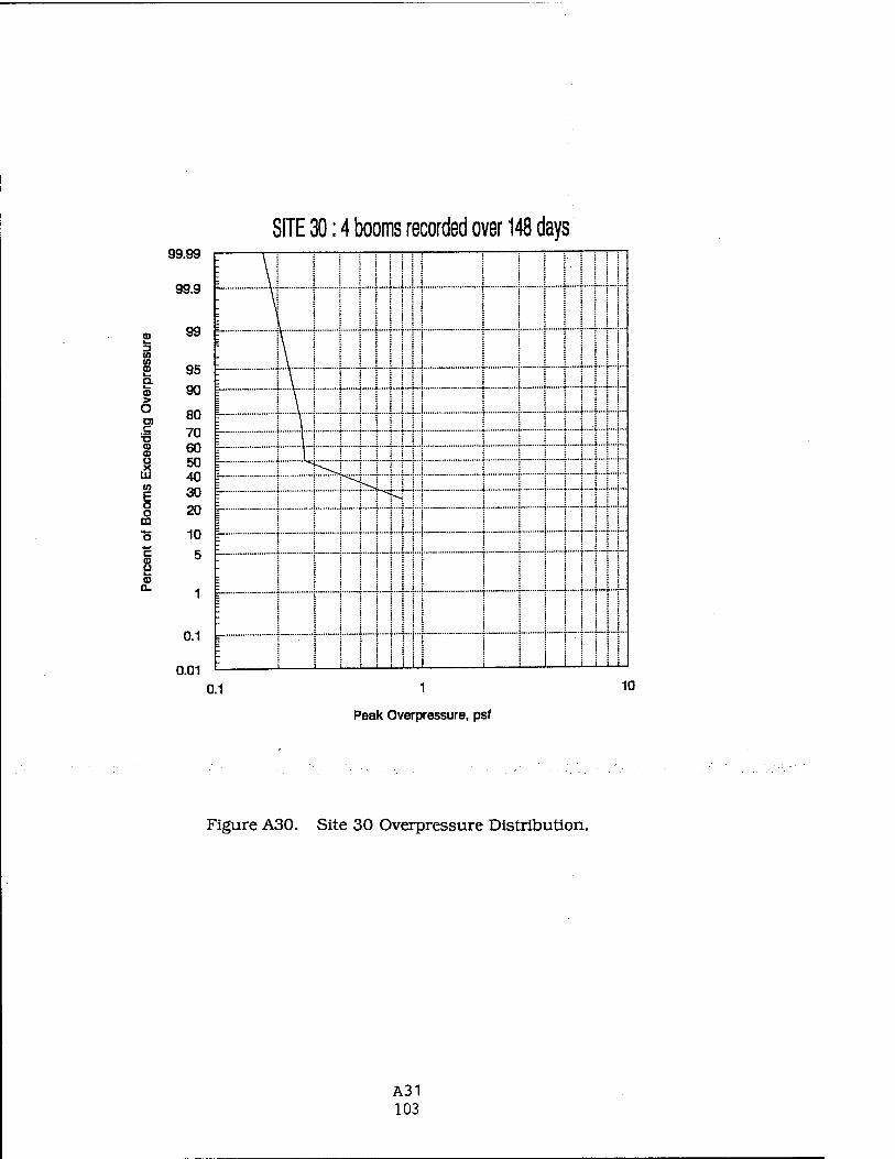
99.99
99.9
m 99 k. D 0)
ig 95 Q. <D 90 > o en 80 c
T5 70 CD CD 60 U 50
IJS 40 (0 E 30 o a 20 m 'S 10 c 5 « k. 0)
QL A
0.1 r
0.01
c 3ITE 30:4 booms recorded over 148 days ti
tii
r i
mil
l i
i
i i
i i i i j : i | 1 j t !
.
- : \ i i : : i
= : \ : : : : i
" • I • : z
- '• i^-J :::::: i : ::::!: = ! j s^tj ! Ml ! i • 1 l ] ] j Z~ : • i j JT^j | | j • :■::::
ItllllMH
E j j j ! i ! { ! ! 1 III
= | ! 1 ! ! ! ! 1 i ! ! 1 !
: : ! : i : i j ! : j ] • j j • • : i ■■•••!: : ! ::::::
1 1 ! 1 i i i i i j j | i i ! M i ! • :!!::!! ! j : ; ■ ■ i • : : : : ! i j i j : ■ i : : : j : i i i i i i I I 1 i i 11-1111
0.1 1
Peak Overpressure, psf
10
Figure A30. Site 30 Overpressure Distribution.
A31 103

SITE 32:12 booms recorded over 178 days 99.99
99.9
IT) 99 k. 3 m to 0) 95 Q.
a> 90 > O 80 c
'■n 70 a> a> 60 o 50
u3 40 to E 30 o o 20 m O 10 c 5 « 1— (D a. 1
0.1
0.01
- i | i I | I ! j I I | ! | | I
0.1 1
Peak Overpressure, psf
10
Figure A31. Site 32 Overpressure Distribution.
A32 104

SITE 33:23 booms recorded over 177 days
in
s CD > o oi c
'-Ü CO CD U
l2 to E □ o m
c 8 CD
QL
99.99
99.9 H
99
95 90
80 70 60 50 40 30 20
10
5
1 £
0.1
0.01
it I I II II
- ! ! ! i ! ! i i ! i ! I : i ; i ; i i i I ! ! i
0.1 1
Peak Overpressure, psf
10
Figure A32. Site 33 Overpressure Distribution.
A33 105

SITE 34:41 booms recorded over 170 days
CO 10 CD
CD > o O) c
T3 CD CO U
i2 to E o o m
c CD O L. CD a.
99.99
99.9
99
95 90
80 70 60 50 40 30 20
10
5
1
0.1 k
0.01 0.1
~ i j j j ♦....;...;...;...p^r-^—^.. ; ; ; ; +....«.—
1 10
Peak Overpressure, psf
Figure A33. Site 34 Overpressure Distribution.
A34 106

<D a.
SITE 35:13 booms recorded over 124 days 99.99
99.9 -
99
CD 95 CL <D 90 6 O)
80 c
T3 70 IS ID 60 U 50 ft 40 HI
E 30 o o 20 m o 10 c 5 8
1 r
0.1
0.01 0.1 1
Peak Overpressure, psf
10
Figure A34. Site 35 Overpressure Distribution.
A35 107

SITE 36:3 booms recorded over 90 days
CO to CD w a. i— CD > O O) e CD CD U
ä CO
E o o m
CD u u CD 0-
99.99
99.9
99 p-
95
90
80 70 60 50 40 30 20
10
5
1
0.1 k-
0.01 0.1
! i i Mill! ! ! I i i \_ j i i i_ ]..[.].]..] i i i 1....1
z 4 \ j } 4—-4-—|—-i—t -f j j ♦ t t
: I I \ I M i I I ! ! i I I i
1
Peak Overpressure, psf
10
Figure A35. Site 36 Overpressure Distribution.
A36 108

SITE 92:22 booms recorded over 171 days
<D k. 3 10 01 (D
ID > o O) c
T5 m m u ä to E o o m »*- o
§
a.
99.99
99.9 h
99
95
90
80 70 60 50 40 30 20
10 5
0.1
0.01
7 ; j T j—•j""j—-j j j j - •• *j" r* ; j
: I I I ! ! i ! j i l I I I I ! I =_ .U j i «4 i....i.-i...| * ;• J f +—t—1*"|
E_ \ i j 4«_|^i!s£»*j-»j ♦ | j +•—+*"<""?""!
Z ! : : : : : J | i j : i : 1 : : I : : i : : : : : j I • • • i : i
0.1 1
Peak Overpressure, psf
10
Figure A36. Site 92 Overpressure Distribution.
A37 109