Embed Size (px)
Citation preview

AFIT/GAE/ENY/96D-8
EXPERIMENTAL INVESTIGATIONOF TRANSVERSE SUPERSONIC
GASEOUS INJECTION ENHANCEMENTINTO SUPERSONIC FLOW
THESIS
Mark P. Wilson, Captain, USAF
AFIT/GAE/ENY/96D-8
Approved for public release; distribution unlimited
19961203 024

DISCLAIMER NOTICEo oa.
THIS DOCUMENT IS BEST
QUALITY AVAILABLE. THE
COPY FURNISHED TO DTIC
CONTAINED A SIGNIFICANT
NUMBER OF PAGES WHICH DO
NOT REPRODUCE LEGIBLY.

Disclaimer Statement
The views expressed in this thesis are those of the author and do not reflect the official policy or position ofthe Department of Defense or the U.S. Government.
AFIT/GAE/ENY/96D-8
EXPERIMENTAL INVESTIGATIONOF TRANSVERSE SUPERSONIC
GASEOUS INJECTION ENHANCEMENTINTO SUPERSONIC FLOW
THESIS
Presented to the Faculty of the School of Engineering of the Air Force
Institute of Technology
Air University
In partial Fulfillment of the Requirements for the Degree of Master of
Science in Aeronautical Engineering
Mark P. Wilson, B.S.A.E.
Captain, USAF
December 1996
Approved for public release; distribution unlimited

Acknowledgments
This work would not have been possible without the expert foresight and guidance of my thesis
advisor, Dr. Rodney D. W. Bowersox. He provided ample expertise when needed, but also the freedom I
required to conduct and arrive at my own conclusions during the course of this investigation.
The assistance of Dr. Sivram Gogeni and Dr. Diana Glawe in the setup and fine tune adjustment
of the laser imaging system provided by WLIPOPT was also indispensable. The science and art of laser
flow visualization is non-trivial, yet the help of these two experts made realization of the images seem
simple.
Considerable use of the expertise of the members of the newsgroup comp.sys.hp48 aided in the
data reduction of this work. In particular the unparalleled programming knowledge of Mika Heiskanen,
the file manipulation knowledge of John H. Meyers, and the excellent support of the other regular members
enabled me to complete in hours what I would not have otherwise been able to do.
I would also like to thank the efforts of the reading committee. They suffered through the weighty
drafts and the final copy; with their sage advice the readability of this document was substantially
increased.
I dedicate this work to my family. My wife Michele bore the brunt of everything else that was not
the thesis, and never failed to remind me when to work and when not to. My children, who saw more of
the back of my head than the front, will hopefully benefit from the application of this research. Perhaps
someday, they will recognize the term Mach Five as more than Speed Racer's car.
Mark Philipp Wilson
ii

Table of Contents
Page
Acknowledgments ................................ ii
List of Figures ................................................................ vi
List of Tables................................................................xi
List of Symbols ............................................................... xii
Abstract ................................................................... xiii
I. Introduction ................................................................ 1.1
1.1 Motivation ............................................................. 1.11.2 Background ............................................................ 1.21.3 Object and Scope of Present Study ............................................ 1.21.4 PME Configuration and Rationale ............................................. 1.31.5 Limitations of Present Study ................................................. 1.61.6 Organization of Present Study ............................................... 1.7
11. Background ............................................................... 2.1
2.1 Flow Fundamentals ....................................................... 2.12.2 Transverse Injection ...................................................... 2.32.3 Ramp and Aeroramp Injection ............................................... 2.42.4 Vortex Mixing .......................................................... 2.62.5 Magnus Effect .......................................................... 2.82.6 Computational Investigations ................................................ 2.82.7 Applications To Current Investigations ........................................ 2.10
111. Facilities and Instrumentation .................................................. 3.1
3.1 AFIT Mach Three Wind Tunnel .............................................. 3.13.2 Transverse Injector Model ................................................... 3.2
3.2.1 Tunnel coordinate System and Dimensions ................................... 3.23.2.2 Injector Model Modifications ............................................ 3.33.2.3 Injection Parameters .................................................. 3.4
3.3 PME Ramps ............................................................ 3.43.4 Measurement Locations .................................................... 3.63.5 Mean Flow Probes ....................................................... 3.6
3.5.1 Pressure Probes ...................................................... 3.73.5.2 Probe Traverse System ................................................ 3.7
3.6 Flow Visualization ........................................................ 3.73.6.1 Shadowgraph Photography Setup ......................................... 3.73.6.2 Rayleigh-Mie Scattering Laser System ...................................... 3.8
3.7 Data Acquisition System and Computational Resources .............................. 3.9
Page
IV. Data Reduction and Processing ................................................. 4.1
iii

4.1 M ean Pressure M easurem ents ................................................ 4.14.1.1 Determination of Flow Mach Number ...................................... 4.14.1.2 Determination of Plume Static and Total Pressure ............................. 4.2
4.2 Total Pressure Loss ........................................................ 4.24.3 Plume Area and Penetration Determination ....................................... 4.3
4.3.1 Freestream M ach Number Definition ...................................... 4.44.3.1.1 Freestream Mach Number Definition I: Graphical Method ................. 4.54.3.1.2 Freestream Mach Number Definition II: Box Method .................... 4.74.3.1.3 Freestream Mach Number Definition II: Modified Box Method ............. 4.8
4.3.2 Plum e Area Determ ination .............................................. 4.94.3.3 Plume Penetration Determination ........................................ 4.10
4.4 Flow Visualization Techniques ............................................... 4.104.4.1 Parallel Flow Orientation .............................................. 4.10
4.4.1.1 Parallel Flow Orientation Analysis, Plume Trajectory Determination ......... 4.124.4.1.2 Parallel Flow Orientation Analysis, Rate Of Centerline Decay .............. 4.14
V. PME Ramp Flow Field Results And Analysis ........................................ 5.1
5.1 Sim ple Transverse Injector .................................................. 5.25.1.1 Simple Transverse Injector Flow Visualization ............................... 5.2
5.1.1.1 Simple Transverse Injector Shadowgraph ............................. 5.25.1.1.2 Simple Transverse Injector Parallel Oriented Images ..................... 5.45.1.1.3 Simple Transverse Injector Cross Flow Images ......................... 5.6
5.1.2 Simple Transverse Injector Mach Contour Plots ............................... 5.85.1.3 Simple Transverse Injector Total Pressure Loss .............................. 5.105.1.4 Simple Transverse Injector Digital Image Quantitative Analysis .................. 5.10
5.2 Injector Ramp Group #1: Symmetric Ramps ..................................... 5.145.2.1 Symmetric Ramp Flow Visualization ..................................... 5.14
5.2.1.1 Symmetric Ramp Shadowgraph Photography ......................... 5.145.2.1.2 Symmetric Ramp Parallel Oriented Images ........................... 5.175.2.1.3 Symmetric Ramp Cross Flow Oriented Images ........................ 5.22
5.2.2 Symmetric Ramp Mach Contour Plots ..................................... 5.255.2.3 Symmetric Ramp Total Pressure Loss ..................................... 5.335.2.4 Symmetric Ramp Digital Image Quantitative Analysis ......................... 5.34
5.3 Injector Ramp Group #2: Extended Ramps ..................................... 5.405.3.1 Extended Ramp Flow Visualization ...................................... 5.40
5.3.1.1 Extended Ramp Shadowgraph Photography ........................... 5.405.3.1.2 Extended Ramp Parallel Oriented Images ............................ 5.445.3.1.3 Extended Ramp Cross Flow Oriented Images .......................... 5.49
5.3.2 Extended Ramp Mach Contour Plots ...................................... 5.525.3.3 Extended Ramp Total Pressure Loss ...................................... 5.605.3.4 Extended Ramp Digital Image Quantitative Analysis .......................... 5.60
5.4 Injector Ramp Group #3: Asymmetric Ramps ................................... 5.655.4.1 Asymmetric Ramp Flow Visualization .................................... 5.65
5.4.1.1 Asymmetric Ramp Shadowgraph Photography ........................ 5.655.4.1.2 Asymmetric Ramp Parallel Oriented Images .......................... 5.675.4.1.3 Asymmetric Ramp Cross Flow Oriented Images ....................... 5.72
5.4.2 Asymmetric Ramp Mach Contour Plots .................................... 5.74Page
5.4.3 Asymmetric Ramp Total Pressure Loss .................................... 5.795.4.4 Asymmetric Ramp Digital Image Quantitative Analysis ........................ 5.80
5.5 Sum m ary of Results ...................................................... 5.845.5.1 Total Pressure Loss Evaluations ......................................... 5.84
iv

5.5.2 Mean Flow Data Based Evaluations ...................................... 5.84
5.5.3 Digital Image Data Based Evaluations ..................................... 5.87
VI. Conclusions and Recommendations .............................................. 6.1
6.1 Conclusions ........................................................... 6.16.2 Recommendations ....................................................... 6.1
Appendix A: Total Pressure Contour Plots ........................................... A. 1
Appendix B: Instantaneous Cross Flow Oriented Images ................................. B. 1
Appendix C: Uncertainty Analysis ................................................. C. 1
Bibliography................................................................. R. 1
Vita ...................................................................... V.1I

List of Figures
Figure Page
1.1. Symmetric Ramp Models SR 1, SR 2 and SR 3 ..................................... 1.4
1.2. Extended Ramp Models ER 1, ER 2 and ER 3 ...................................... 1.4
1.3. Asymmetric Ramp Models AR 1 And AR 2 ....................................... 1.4
2.1. Time-Averaged Example Injection Shadowgraph .................................... 2.2
2.2. Typical Low W edge Angle Swept Ramp .......................................... 2.5
3.1. Tunnel Coordinate System .................................................... 3.2
3.2. Side V iew of Test Section ..................................................... 3.3
3.3. Sym m etric PM E Ram ps ...................................................... 3.5
3.4. Extended PM E Ram ps ....................................................... 3.5
3.5. Asymm etric PM E Ramps ..................................................... 3.6
3.6. Rayleigh-Mie Scattering Laser and CCD System .................................... 3.8
4.1. Simple Transverse Injector Mach Contour Plot With Plume Search Region ................. 4.4
4.2. Graphical Method Local Freestream Search Region .................................. 4.6
4.3. Box Method Local Freestream Search Region ...................................... 4.7
4.4. Instantaneous Digital image, M odel 1 ........................................... 4.11
4.5. Averaged Digital Im age, M odel 1 .............................................. 4.11
4.6. Plume Image M easurement Stations ............................................ 4.12
4.7. Seed Condensation On Ramp Injector Model ...................................... 4.13
5.1. Simple Transverse Injector Composite Shadowgraph ................................. 5.2
5.2. Simple Transverse Injector, Instantaneous Parallel Oriented Laser Image ................... 5.4
5.3. Simple Transverse Injector, Time-Averaged Parallel Oriented Laser Image ................. 5.5
5.4. Simple Transverse Injector, Instantaneous Cross Flow Image ........................... 5.6
5.5. Simple Transverse Injector, Time-Averaged Image Cross Flow Oriented Image .............. 5.7
Page
vi

5.6. Simple Transverse Injection Mach Contour Plot ..................................... 5.8
5.7. Simple Transverse Injection Area Contour Plot ...................................... 5.9
5.8. Simple Transverse Injector Plume Centerline Trajectory .............................. 5.11
5.9. Simple Transverse Injector Plume Centerline Average Intensity Decay ................... 5.12
5.10. Double Diamond Ramp SR 1 Composite Shadowgraph .............................. 5.14
5.11. Double Cone Ramp SR 2 Composite Shadowgraph ................................. 5.15
5.12. Double Ramp SR 3 Composite Shadowgraph ..................................... 5.16
5.13. Double Diamond Ramp SR 1, Instantaneous Parallel Oriented Laser Image ............... 5.17
5.14. Double Diamond Ramp SR 1, Time-Averaged Parallel Oriented Laser Image .............. 5.18
5.15. Double Cone Ramp SR 2, Instantaneous Parallel Oriented Laser Image .................. 5.19
5.16. Double Cone Ramp SR 2, Time-Averaged Parallel Oriented Laser Image ................. 5.20
5.17. Double Ramp SR 3, Instantaneous Parallel Oriented Laser Image ....................... 5.20
5.18. Double Ramp SR 3, Time-Averaged Parallel Oriented Laser Image ..................... 5.21
5.19. Double Diamond Ramp SR 1, Time-Averaged Cross Flow Oriented Laser Image ........... 5.22
5.20. Double Cone Ramp SR 2, Time-Averaged Cross Flow Oriented Laser Image .............. 5.23
5.21. Double Ramp SR 3, Time-Averaged Cross Flow Oriented Laser Image .................. 5.24
5.22. Double Diamond Ramp SR 1 Mach Contour Plot .................................. 5.25
5.23. Double Diamond Ramp SR 1 Area Contour Plot ................................... 5.26
5.24. Double Cone Ramp SR 2 Mach Contour Plot ..................................... 5.28
5.25. Double Cone Ramp SR 2 Area Contour Plot ...................................... 5.29
5.26. Double Ramp SR 3 Mach Contour Plot ......................................... 5.31
5.27. Double Ramp SR 3 Area Contour Plot .......................................... 5.32
5.28. Double Diamond Ramp SR 1 Plume Centerline Trajectory ........................... 5.34
5.29. Double Diamond Ramp SR 1 Plume Centerline Average Intensity Decay ................. 5.35
vii

Page
5.30. Double Cone Ramp SR 2 Plume Centerline Trajectory .............................. 5.36
5.31. Double Cone Ramp SR 2 Plume Centerline Average Intensity Decay .................... 5.37
5.32. Double Ramp SR 3 Plume Centerline Trajectory ................................... 5.38
5.33. Double Ramp SR 3 Plume Centerline Average Intensity Decay ........................ 5.39
5.34. Extended Diamond Ramp ER 1 Composite Shadowgraph ............................ 5.40
5.35. Truncated Extended Ramp ER 2 Composite Shadowgraph ........................... 5.42
5.36. Tapered Extended Ramp ER 3 Composite Shadowgraph ............................. 5.43
5.37. Extended Diamond Ramp ER 1, Instantaneous Parallel Oriented Laser Image .............. 5.44
5.38. Extended Diamond Ramp ER 1, Time-Averaged Parallel Oriented Laser Image ............ 5.44
5.39. Truncated Extended Ramp ER 2, Instantaneous Parallel Oriented Laser Image ............. 5.45
5.40. Truncated Extended Ramp ER 2, Time-Averaged Parallel Oriented Laser Image ........... 5.46
5.41. Tapered Extended Ramp ER 3, Instantaneous Parallel Oriented Laser Image .............. 5.47
5.42. Tapered Extended Ramp ER 3, Time-Averaged Parallel Oriented Laser Image ............. 5.48
5.43. Extended Diamond Ramp ER 1, Time-Averaged Cross Flow Oriented Laser Image ......... 5.49
5.44. Truncated Extended Ramp ER 2, Time-Averaged Cross Flow Oriented Laser Image ........ 5.50
5.45. Tapered Extended Ramp ER 3, Time-Averaged Cross Flow Oriented Laser Image .......... 5.51
5.46. Extended Diamond Ramp ER 1 Mach Contour Plot ................................ 5.52
5.47. Truncated Extended Cone Ramp ER 2 Mach Contour Plot ............................ 5.54
5.48. Truncated Extended Cone Ramp ER 2 Area Contour Plot ............................ 5.55
5.49. Tapered Extended Ramp ER 3 Mach Contour Plot ................................. 5.57
5.50. Tapered Extended Ramp ER 3 Area Contour Plot .................................. 5.58
5.51. Truncated Extended Ramp ER 2 Plume Centerline Trajectory ......................... 5.61
5.52. Truncated Extended Ramp ER 2 Plume Centerline Average Intensity Decay .............. 5.62
5.53. Tapered Extended Ramp ER 3 Plume Centerline Trajectory ........................... 5.63
Viii

Page
5.54. Tapered Extended Ramp ER 3 Plume Centerline Average Intensity Decay ................ 5.64
5.55. Wide Ramp AR 2 Composite Shadowgraph ...................................... 5.65
5.56. Narrow Ramp AR 3 Composite Shadowgraph .................................... 5.66
5.57. Wide Ramp AR 2, Instantaneous Parallel Oriented Laser Image ........................ 5.67
5.58. Wide Ramp AR 2, Time-Averaged Parallel Oriented Laser Image ...................... 5.68
5.59. Narrow Ramp AR 3, Instantaneous Parallel Oriented Laser Image ...................... 5.70
5.60. Narrow Ramp AR 3, Time-Averaged Parallel Oriented Laser Image .................... 5.70
5.61. Wide Ramp AR 2, Time-Averaged Cross Flow Oriented Laser Image ................... 5.72
5.62. Narrow Ramp AR 3, Time-Averaged Cross Flow Oriented Laser Image .................. 5.73
5.63. W ide Ramp AR 2 Mach Contour Plot .......................................... 5.74
5.64. W ide Ramp AR 2 Area Contour Plot ........................................... 5.76
5.65. Narrow Ramp AR 3 Mach Contour Plot ......................................... 5.77
5.66. Narrow Ramp AR 3 Area Contour Plot ......................................... 5.78
5.67. Wide Ramp AR 2 Plume Centerline Trajectory .................................... 5.80
5.68. Wide Ramp AR 2 Plume Centerline Average Intensity Decay ......................... 5.81
5.69. Narrow Ramp AR 3 Plume Centerline Trajectory .................................. 5.82
5.70. Narrow Ramp AR 3 Plume Centerline Average Intensity Decay ........................ 5.83
5.71. Normalized Average Plume Area vs. H- ......................................... 5.85
5.72. Normalized Average Plume Centroid vs. H1 ...................................... 5.85
5.73. Normalized Average Plume Centerline Trajectory vs. Hl ............................. 5.87
5.74. Normalized Average Plume Intensity Decay Rate vs. I .............................. 5.88
A .1. Sim ple Transverse Injection .................................................. A .1
A.2. Double Diamond Ramp SR 1 ................................................. A. 1
A .3. Double Cone Ramp SR 2 .................................................... A .1
ix

Page
A.4. Double Ramp SR 3 ........................................................ A.lI
A.5. Truncated Extended Ramp ER 2 .............................................. A.2
A.6. Tapered Extended Ramp ER 3 ................................................ A.2
A.7. Wide Ramp AR 1 ......................................................... A.2
A.8. Narrow Ramp AR 2........................................................ A.2
A.9. Test Section, No Injection or PME Ramp........................................ A.2
B-l. Simple Transverse Injecfion ................................ ................. B.lI
B.2. Double Diamond Ramp SR 1 ................................................. B.l1
B.3. Double Cone Ramp SR 2 ................................................... B. 1
B-4. Double Ramp SR 3........................................................ B.lI
B.5. Extended Diamond Ramp ER 1 ............................................... B.2
B.6. Truncated Extended Ramp ER 2 .............................................. B.2
B.7. Tapered Extended Ramp ER 3 ................................................ B.2
B.8. Wide Ramp AR 1 ......................................................... B.2
B.9. Narrow Ramp AR 2........................................................ B.2

List of Tables
Table Page
3.1. Wind Tunnel and Injector Nozzle Exit Dimensions ................................... 3.2
3.2. Freestream Flow Conditions ................................................... 3.3
3.3. Injector Jet Flow Conditions ................................................... 3.4
5.1. Simple Transverse Injector Area and Centroid Results ............................... 5.10
5.2. Double Diamond Ramp Area and Centroid Results .................................. 5.27
5.3. Double Cone Ramp Area and Centroid Results ..................................... 5.29
5.4. Double Ramp Area and Centroid Results ......................................... 5.33
5.5. Symmetric Ramp Group Total Pressure Loss ...................................... 5.33
5.6. Truncated Extended Ramp Area and Centroid Results ................................ 5.56
5.7. Tapered Extended Ramp Area and Centroid Results ................................. 5.59
5.8. Extended Ramp Group Total Pressure Loss ....................................... 5.60
5.9. W ide Ramp Area and Centroid Results .......................................... 5.76
5.10. Narrow Ramp Area and Centroid Results ........................................ 5.79
5.11. Asymmetric Ramp Group Total Pressure Loss .................................... 5.79
5.12. Injector Total Pressure Loss Ratio, II ........................................... 5.84
C. 1. Uncertainties in Calculations ................................................. C.2
xi

List of Symbols
A - Area, cm 2
a - Speed of sound, m/sd - Injector nozzle exit minor diameter, mmM - Mach numberP,p - Pressure, Pa
q - Dynamic pressure ratio, (pu 2 )j/(pu 2 ).
q - Turbulent transport variableT - Temperature, Ku,V - Velocity, rn/sx - Streamwise tunnel coordinatey - Vertical tunnel coordinatez - Horizontal tunnel coordinate
Greek
6 - Boundary layer thickness, cmS - Uncertaintyy - Ratio of specific heats?I - Mass Flux Ratio, (pu)j/(pu).H7 - Total pressure ratiop - Density, kg/m3
co - Turbulent transport variableX - Species concentration, mole/m
Subscripts
0 - Upstream property1 - Local property2 - Pitot probe propertyc - Cone-staticeb - Effective backt - Total property
xii

AFIT/GAE/ENY/96D-8
Abstract
In pursuit of more efficient and effective fuel-air mixing for a SCRAMJET combustor, this study
was conducted to investigate relative near field enhancements of penetration and mixing of a discrete low-
angled (250) injected air jet into a supersonic (M=2.9) cross flow. The enhancements were achieved by
injecting the transverse air jet parallel to the compression face of eight different ramp geometries. The jet-
ramp interactions created collinear shock structures, baroclinic torque vorticity enhancement, ramp spillage
enhanced vorticity, magnus effect penetration enhancement, and increased total pressure loss.
Shadowgraph photography was used to identify the shock structures and interactions in the flow field.
Measurements of mean flow properties were used to establish the jet plume size, jet plume penetration and
to quantify the total pressure loss created by the ramps. Rayleigh-Mie scattering images were used for both
qualitative flow field assessments and quantitative analysis of the plume trajectory and mixing rate.
Results indicate that up to a 20% increase in penetration height and plume expansion can be achieved by
injection over a ramp compared to simple transverse injection. This increase in penetration and mixing
incurs up to a 15% loss in total pressure. The most critical geometric aspects that affect the flow are the
ramp compression face shape and frontal aspect, and the location and strength of ramp generated
expansion.
Xiii

I. Introduction
1.1 Motivation
A plateau has been reached in the realm of air-breathing propulsion. Despite the explosive growth
and technological progression seen during the last century'2, the state of the art has been stalled for the last
thirty years. The cause of this tailing off of the "higher and faster" progression is that current air-breathing
propulsion systems have been pushed to the material and chemical limits they can withstand. This limit in
speed is in the sub-hypersonic regime, or below Mach 6. Currently the fastest known air-breathing manned
aircraft is the SR-7 1, capable of speeds in excess of Mach 3. The ramjet powered D-21 unmanned
reconnaissance drone, which was launched from the SR-71, was capable of speeds in excess of Mach 5.
Both of these designs are products of the late 1950s, and were the cutting edge of material and
aerodynamic science for their time. As a result of the National Aerospace Plane program and other related
projects, a renaissance of hypersonic research is now underway. The end of the hiatus in high speed
research has again hit the same material and aerodynamic limits of the 1950's; in order to again reach
"higher and faster" a different method of propulsion must be employed than the current turbojet or ramjet
approach. This method will most likely involve combustion in flows at supersonic speeds as well as ram or
body compression, or a SCRAMjet engine.
Issues preventing the realization of hypersonic air-breathing propulsion are as real now as the
control and structure issues faced in the late 1940s, during the breaking of the sound barrier. The option of
slowing the hypersonic freestream flow to subsonic speeds for combustion as in a turbojet or ramjet is not
physically feasible. A simple example demonstrates this; at 30 km altitude and a relatively low hypersonic
flight speed of Mach 8, the stagnation temperature will easily exceed 3100 K. The extremely high
stagnation temperature for ambient air at the proposed flight conditions will incinerate all metals and most
other materials suitable for airframe structures. Additionally, the fuel combustion products would
dissociate at these high temperatures, thus offsetting most of the heat released during combustion. If the
flow could be slowed by the vehicle's bow shock and inlet shocks to Mach 2 through the combustor, the
still high but more manageable static temperature would be approximately 1900' K. The problem now
becomes how to manage efficient and effective mixing and burning of fuel for the extremely short
residence time the working fluid will have in the combustor.
1.1

1.2 Background
Several schemes have been employed during the last thirty years to enhance the penetration and
mixing of an injected plume into supersonic freestream conditions. Initial studies were conducted to
examine the effect and governing conditions for normally injected underexpanded jets. These earlier
works provided fundamental analysis of the structures associated with transverse injection and laid the
groundwork for the initial computational approaches. Vorticity generated by the pressure differential
across the front to rear face of the emerging jet was identified as a major near-field mixing factor.5 '6 While
work has continued in transverse injection, 7'8 '9 later studies sought to produce greater vorticity while
retaining the jet momentum in the direction of thrust through low angle injection from the rear face of
injector ramps. 2,10,11,13,14 These ramp configurations were intended to generate vorticity from the spillage
of high pressure air off and around the leading compression surface. A further refinement recently tested
was the aero-ramp concept of Fuller et al. This concept employed multiple injection ports arranged in the
planform of a physical ramp to create vorticity with lower shock losses than the physical ramp would
cause)0 Other investigations have explored the effects of a shock wave passing through a vortex plume
and how the pressure differential of the shock across the plume cross section produces the baroclinic torque
6mechanism which has been shown to enhance vorticity.
1.3 Object and Scope of Present Study
The primary objective of this study is to increase the near-field penetration and mixing of a fuel
plume into a SCRAMjet combustor. This is accomplished by examination of the relative near-field
enhancement of penetration and mixing of a Mach 1.87 underexpanded supersonic air jet transversely
injected at 25' into a nominally Mach 2.9 air freestream. The enhancement is achieved by placing a
penetration and mixing enhancement (PME) ramp immediately downstream of the injection port; eight
dissimilar geometries of PME ramps were investigated. This injection scheme was devised to capitalize on
the better near-field mixing of transverse injection and the superior far-field mixing of ramp generated
vorticity, Several additional benefits can be realized from this injection arrangement. Pressure losses of
the PME ramp should be minimal since the compression face is parallel to the angle of injection. Any
resulting shocks from the PME ramp should be relatively weak. Near field mixing could be increased
without adversely affecting penetration by exploiting the baroclinic torque from the weak PME ramp
1.2

shock. The solid boundary of the PME ramp compression face should also delay the turning of the plume.
This would enhance penetration, as well as increase the vertical height the freestream would be able to add
vorticity to the plume. Additionally, the solid boundaries and the plume vortex pair should couple to
increase penetration via the magnus effect. In high enthalpy flows, this injection scheme could also
provide effective film cooling for injection ramps which otherwise might not survive the ambient
conditions. 5
The relative measure of penetration and mixing enhancement was attained by normalizing the
results of the eight individual PME ramp models with the results of injection over a flat wall, or simple
transverse injection. Measurements of mean flow properties were used to establish the extent of
penetration and to indirectly determine the extent of mixing produced by the PME ramp models. Digital
processing Rayleigh-Mie scattering images of the flow were used to directly measure the jet plume size and
to establish a means of determining the rate of plume centerline concentration decay with downstream
position based upon injectant seed concentrations.
1.4 PME Configurations and Rationale
The eight PME ramp models, Figures 1.1 to 1.3, can be grouped into three distinct groups with
similar geometric features. The ramp models are shown in top view, with the flow direction from bottom
to top. See section 3.3 for complete dimensionality. The models were oriented with the leading 25'
inclined face directly behind the rear lip of the injector nozzle exit port.
Figure 1.1: Symmetric Ramp Models SR 1, SR 2 and SR 3
1.3

Figure 1.2: Extended Ramp Models ER 1, ER 2 and ER 3
Figure 1.3: Asymmetric Ramp Models AR 1 And AR 2
The first group is the Symmetric Ramp (SR) injectors, which are symmetric about the y-z plane of
the tunnel coordinate system. Models SR 1, SR 2 and SR 3 belong to this group. Each model in this group
has a rising compression surface the plume is expected to interact and lift off from, and a trailing expansion
surface to accelerate the flow behind the ramp. The models have varying degrees of three-dimensional
relieving effects on the model induced shock wave. 0 For example, at one end of the spectrum is the model
SR 3 compression surface which is a flat plate to induce a two-dimensional shock. At the other extreme
the model SR 2 compression surface is a half cone extending from the tunnel ceiling, which in the near
vicinity of the expanding plume should have a greater three-dimensional relieving effect on the model
induced shock wave. Model SR 1 is a compromise between the two, having a three-dimensional but
faceted compression surface.
The second group is the Extended Ramp models. Models ER 1, ER 2 and ER 3 belong to this
group. These models have an extension that is parallel to the test section ceiling behind the rising
compression surface. The purpose of the extension is twofold. It provides an additional surface for the
magnus effect to lift the plume further into the freestream. Additionally, the extension decreases the
1.4

strength of the expansion around the top of the model to the rear face. There are four reasons to minimize
the flow expansion. First, the expansion accelerates the plume which in turn reduces the residence time the
fuel plume and freestream air have to mix and combust. Second, the extension provides a physical barrier
that prevents the plume from turning back toward the tunnel ceiling. Third, minimizing the expansion
reduces the pressure loss through the recompression shock. Fourth, strong expansions can stabilize the
flow (i. e., decrease the magnitude of turbulent fluctuations) which would reduce the mixing. The
extensions used were intended to test two additional mechanisms to enhance penetration and mixing.
Model ER 3 is a tapered wedge that when extended to the end of the model meets at a point. The
anticipated effect is that the flow traveling along the sides of the ramp will experience a smooth transition
upon rejoining the freestream to minimize pressure losses. Strong shock waves are not expected, since the
model is about the height of the boundary layer. Model ER 2 is slightly less tapered than model ER 3 but
of the same length. This terminates the extension as a truncated triangle when viewed from above. This
truncated geometry is expected to provide a recirculation region that would be suitable for either flame
holding or additional jet injection. Model ER 1 is an exaggerated extended surface used to determine what
effect if any longer extensions would have on the plume. Model ER 1 was included mainly for qualitative
analysis, as the scaling is not representative of the other models.
The third group consists of models AR 1 and AR 2. These PME ramp models are simple
asymmetric tapered wedges. The only difference between the two models is the taper ratio. Model AR 1
tapers from 4 d to 2 d at the top of the compression surface. Model AR 2 tapers from 4 d to 1 d at the top
of the compression surface. The primary mixing mechanism associated with these types of ramps is
vorticity generated by spillage from the high pressure compression surface to the lower pressure side and
rear faces.1 ° The degree of sweep in a ramp has been shown to affect mixing and combustion efficiency,
with unswept ramps generally performing poorer than the swept ramps. 16 The freestream pressure-induced
vorticity will be limited by the presence of the plume, which will deflect the freestream away from the
compression surface. However, the plume itself will become the high pressure mechanism to induce
additional vorticity and freestream entrainment for mixing.
1.5 Limitations of Present Study
1.5

Limitations of this study include availability of facilities, the use of similar, uncombusted gas
injectant and freestream, number of downstream locations sampled and available data. A time constraint
imposed on the use of shared experimental resources, as well as the number of PME ramp models
investigated, limited the mean flow measurements to one axial station downstream of the injection site.
The facilities used at the time of this study were incapable of either combustion or measuring the species
concentration of a binary gas. This study is limited to pressure data and image data, and provides no direct
measure of mixing enhancement features such as relative strengths of the vorticity the ramp models may
produce. The limitation in downstream test locations is overcome in two manners. First, the laser plane
imaging captures the plume development and interactions with the PME ramp models up to the mean flow
measurement location. Second, the fuel plume under the proposed flight conditions of a hypersonic
vehicle will most likely combust in the near-field due to the extreme high temperatures to be expected in
the flow.17 Once combustion occurs the mechanisms governing the plume size, shape and concentrations
become drastically different from the mechanisms studied here. The similar gas injection limitation was
partially overcome by normalizing the results; a comparable order enhancement of hydrogen fuel injection
may be expected for injection over a similar geometry as investigated here. The limitations on the data
collected affect the understanding of the detail mechanisms acting in the flow. However, this study is
primarily an observation of macroscopic effects. A comparison of a diverse set of PME ramp model
performance trends can establish what geometric features appear to enhance overall mixing. After such
large scale observations, detailed investigations for further research and optimization will be merited.
1.6 Organization of Present Study
The remainder of this investigation is organized into five additional chapters. The second chapter
provides a detailed review of previous research into supersonic injection schemes. Topics reviewed are
presented in the following order. Basic mechanisms of transverse injection normal and to an angle with the
main flow are explained. Other schemes, including ramp injection and aeroramp injections, are presented.
The role of vorticity as a means of mixing an injectant plume and freestrearn are explored. An analysis of
the current state of computational fluid dynamics and supersonic injection problems is given. The results
of earlier works that are expected to be exploited in this investigation are analyzed. The third chapter
describes the experimental setup used. The mean flow pressure probe and the laser imaging systems are
1.6

depicted. The fourth chapter explains the data reduction and analysis techniques employed to derive the
results. This chapter includes the analytical methods used to determine the plume properties of area and
penetration from both the pressure probe and laser imaging data. Chapter Five presents the results of this
investigation. Analysis of the data and comparisons to previous research are given. A summary of the
results concludes this chapter. Finally, the sixth chapter details conclusions as to the effectiveness of and
penalties incurred by injection over a ramp in enhancing mixing and penetration into supersonic cross flow.
Recommendations for future research are submitted.
1.7

II. Background
A considerable wealth of both experimental and computational research has been conducted in the
study of transverse supersonic injection and supersonic injection behind a ramp. This chapter is a review
of the fundamental concepts and results from past investigations, and development of how they are applied
to the current investigation. The topics covered are flow and injection fundamentals, transverse injection,
ramp and aeroramp investigations, vorticity generation, the magnus effect and computational efforts. The
chapter concludes by relating the earlier works as a foundation for the desired results of this experiment.
2.1 Flow Fundamentals
In an effort to provide a basis of comparison between studies under diverse conditions, several
injection parameters and flow variables have been established. The injection parameters include injector-
to-freestream ratios such as the velocity ratio, mass flux ratio and expansion ratio." An additional injector-
to-freestream ratio to consider is the dynamic pressure ratio q, also known as the momentum flux ratio.
Where ramps are involved, a standard set of geometric parameters arise such as the ramp dimension to
injector port diameter ratios, the ramp wedge angle and the degree of sweep of the ramp vertical sides. The
primary flow variables of concern for this type of study are the injector diameter based Reynolds number,
the boundary layer depth to injector diameter ratio - , and the flow total properties.
With the exception of expansion ratio, these injection parameters and flow properties are
relatively straightforward. The expansion ratio is the ratio of the jet exit pressure and effective back
4pressure peb as put forth by Schetz and Billig. Effective back pressure is a means of estimating the
pressure to which a jet will expand from the similarities between cross flow injection and injection into a
quiescent medium.' Effective back pressure was originally treated as a simple proportionality to either the
pressure behind a the plume bow shock or the pressure in the separated zone ahead of the injection port
45 4depending on the - value, and was limited to normal injections. This concept has evolved to mored
advanced models, including one for injection at an angle. The newer model for peb treats it as an average
of the approach flow static pressure and the Newtonian impact theory for pressure on inclined bodies.1 9
2.1
The inclination angles used in this approach are based upon the injection geometry and injection Mach
disk, described below.
Injection of an underexpanded sonic or supersonic jet into a supersonic freestream produces
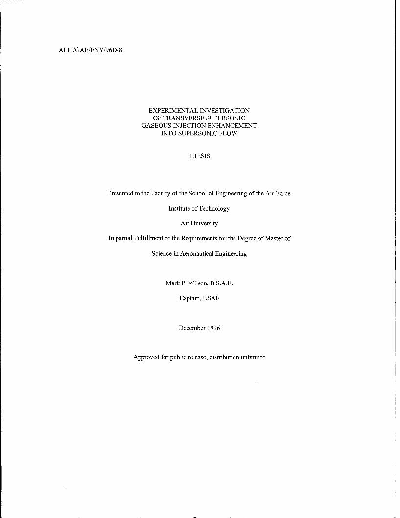
several flow structures. The first of these is a bow shock produced as the freestream impacts the injection
streamtube; in this respect the injectant acts as a solid cylindrical body. For injector geometries where -5
d
is on the order of one or more, a separation bubble can form slightly upstream of the injector port.4 5 The
separation bubble results in a lambda shock formation through the boundary layer.20 After entering the
freestream, the jet experiences a rapid Prandtl-Meyer expansion (usually assumed to be an isentropic
process) surrounded by a barrel shock.9 A normal shock (i.e., normal to the jet path) known as the Mach
disk terminates the barrel shock, and recompresses the flow to peb. Before the Mach disk, the injectant
and freestream are typically treated as separate entities; afterwards vorticity and other turbulent
mechanisms induce large scale mixing. Figure 2.1 depicts a time-averaged shadowgraph of an injection at
250 with the generic injection related structures identified.
Barrel Shock PlumeRecompressionl
: Shock
Figure 2.1: Time-Averaged Example Injection Shadowgraph
2.2

With the basic framework of underexpanded jet injection structures and terminology put forth,
discussion of the various injection schemes can ensue. The mechanics and structures of each type of
injection is discussed and related to the basic theory of injection described above. The relative strengths
and weaknesses of each method are also presented.
2.2 Transverse Injection
Transverse injection of an underexpanded jet into supersonic flow has been well documented over
the last thirty years. Transverse injection is arguably the simplest injection configuration, requiring only an
injection port (sonic or supersonic) at the desired injection angle, usually normal to the plane of the
injection wall and parallel with the direction of flow. In either normal or angled injection, the entry of the
injectant jet into the mainstream flow can be regarded as a two stage process.4 The jet first enters the main
flow and remains relatively intact as it expands to the height of the Mach disk. Beyond the Mach disk, the
flow turns and accelerates with the main flow. In the second stage, the jet acts as a coaxial vortex mixing
structure.
In the near field, the injection parameter q has been shown to strongly impact mixing and affect
penetration. For mixing, the initial rate of mixing is proportional to -. " This can be interpreted fromq
continuity and momentum principles. As the dynamic pressure of the injectant is increased, it would
initially enter the freestream either faster (pj constant) or denser ( V constant). In the first case, the
injectant jet itself would reduce the residence time it has to mix with the local freestream. In the second,
the jet would present a more solid obstacle to the flow, requiring greater time and hence distance to
disperse. In the far field, q has been shown to have little impact on mixing rates. A benefit from
increasing q for low injection angles is a decrease in total pressure loss from the added streamwise
component of jet momentum. 3 Penetration is enhanced with increasing q in that the Mach disk is pushed
further out into the freestream; however, the plume then turns more sharply with the main flow. 4 This
-4effect was seen to diminish with increasing q.
2.3
The effect of the injection angle on near field injectant jet penetration and mixing has received
surprisingly little attention to date. However, the available far field results are insightful. In the far field,
mixing rates are related by the injectant decay of maximum concentration proportionality
X .. GC (2.1)
where the exponent n can be used for mixing comparisons. 5 On a Log-Log plot of maximum
concentration decay with downstream location n is the slope of the maximum concentration decay line. As
the angle of injection is increased, holding all other flow variables and injection parameters constant, far
field mixing rates increase. 8 In conjunction with the far field mixing increase, there is an increased bow
shock strength and total pressure loss. 8 A parametric mixing/total pressure loss trade-off study would be
required to determine the optimum injection angle, which would most likely be Mach number dependent
(due to decreased residence time with increased Mach number). Further, low angle injection has been
shown to create a measurable increase in the overall combustion thrust potential6,21 which intuitively would
not be as great with normal or higher angle injection.
2.3 Ramp and Aeroramp Injection
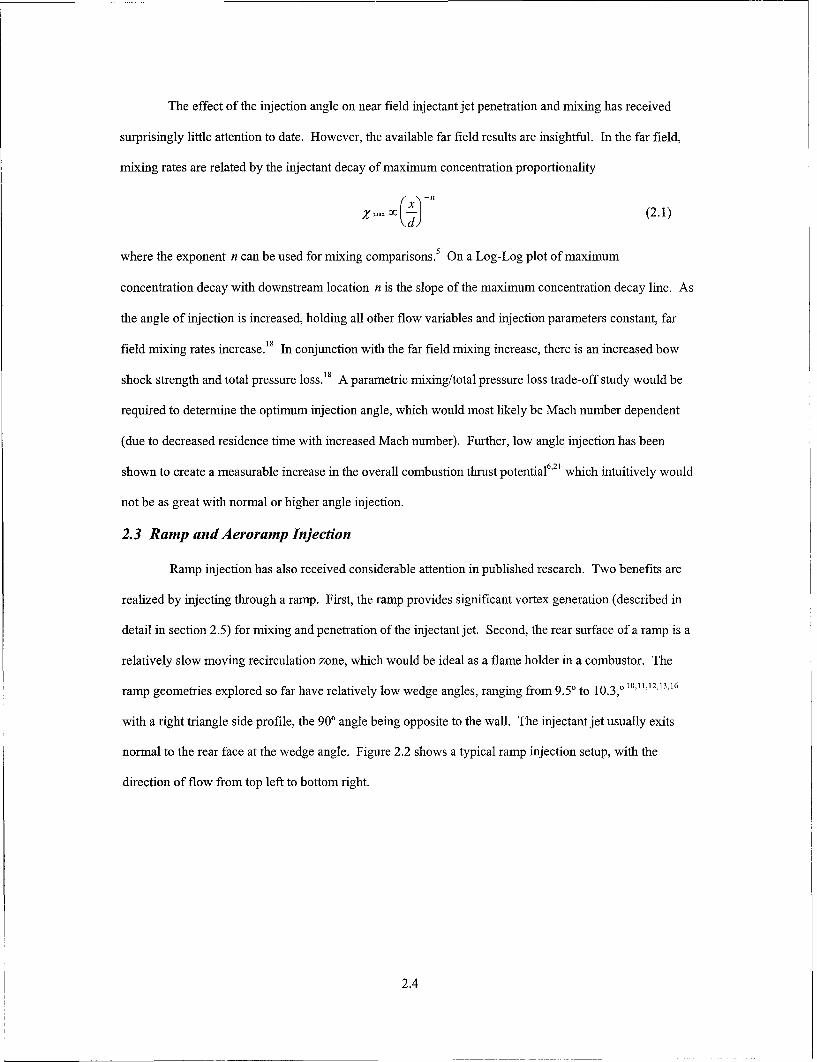
Ramp injection has also received considerable attention in published research. Two benefits are
realized by injecting through a ramp. First, the ramp provides significant vortex generation (described in
detail in section 2.5) for mixing and penetration of the injectant jet. Second, the rear surface of a ramp is a
relatively slow moving recirculation zone, which would be ideal as a flame holder in a combustor. The
ramp geometries explored so far have relatively low wedge angles, ranging from 9.50 to 10.3,0 10,11,12,13,16
with a right triangle side profile, the 90' angle being opposite to the wall. The injectant jet usually exits
normal to the rear face at the wedge angle. Figure 2.2 shows a typical ramp injection setup, with the
direction of flow from top left to bottom right.
2.4

Figure 2.2: Typical Low Wedge Angle Swept Ramp
Once injected, the jet does not behave exactly as a transverse jet would. Though the generic
underexpanded jet structures described in section 2.2 are present, there are additional ramp base effects,
including multiple three-dimensional shocks and expansions, which impact the flow structure. Analytical
results indicate dramatic decreases in circulation (based upon Stokes Law) from the base of the ramp and
up to half a ramp length downstream due to ramp base effects and jet interactions.10 This region of the
flow is highly three-dimensional and turbulent; not all of the interactions and flow mechanics have been
completely mapped or explained. Beyond the ramp base the plume becomes basically indistinguishable
from a similar parameter low angle transverse injection (with the exception of the strength of the vortex
rotation pair).
The aeroramp concept was put forth recently by Fuller et al.13 The aeroramp is actually three
rows and columns of staged and angled transverse injection ports in the planform of a swept ramp. The
idea employed was that with proper multiaxis angling of the injector rows, a buildup of injectant would
form in the profile of a ramp.13 This concept has been demonstrated before, where the second jet in a
tandem transverse arrangement was able to penetrate further into the freestream due to the partial shielding
provided by the first transverse injectant plume.5 By simulation of a solid ramp with gaseous injectant the
total pressure losses in the flow field were noticeably reduced and increased at a slower rate with
downstream location than the similar solid ramp. 3 Though penetration and mixing were reduced
2.5

with the aeroramp, a substantial gain in both measurands was obtained by doubling q from 1.0 to 2.08.
Full details of the injector geometries and similarity parameters can be found in reference 13.
2.4 Vortex Mixing
Regardless of the injection scheme employed, vorticity is the driving mixing mechanism in the
near field.5 In transverse injection, streamwise vorticity is generated by two primary mechanisms. The
first is the external pressure differential created across the front and rear faces of the emerging jet. The
main flow must split around the injectant jet, creating high pressure regions on the front and partially on
the side faces of the jet. The resulting low pressure on the rear or leeward side of the jet becomes an
entrainment region for the local freestream. The flow bisection and downstream entrainment results in a
counter-rotating vortex pair inside the largely circular injectant jet. A second source of vorticity is created
as the plume is bent coaxially with the freestream. The bend accelerates the outer portion of the plume,
decreasing the internal pressure. The inside region of the plume which is not as greatly accelerated is then
22drawn into the plume center, similar to the flow in a curved duct.
For ramp injection, the primary vortex generation comes from the ramp not the injectant plume.
Flow pressurization occurs in the shock layer between the ramp induced bow shock and the ramp
compression face. This high pressure fluid then spills around the ramp causing a stream wise vorticity. 10
The vorticity causes large-scale convective mixing that forms a counter rotating vortex pair.6 This
mechanism is analogous to the vortex lift generated by a delta wing, except vortices are generated on both
sides of the ramp. The relative strength of the vorticity generated is dependent on freestream Mach
number, all other parameters and properties being equal. For a constant injector mass flux ratio, Hartfield
et al. demonstrated indirectly through mole fraction contour plots that the vorticity created in a Mach 2.9
freestream "is much stronger than that generated at Mach 2"." Additional vorticity is imparted by the
pressurized flow expanding over the rear face of the ramp and wrapping around the low pressure region
encircling the underexpanded jet plume.12 A final ramp induced vortex mechanism is baroclinic torque
created by passing a shock through a jet, described by Waitz et al.6 The shock is created by the
recompression of the main flow. After expanding over the top to the rear face of a ramp, the flow must
turn away from the wall behind the ramp, creating a shock. Waitz et al. reasoned the pressure gradient
imposed by the shock across the density gradient of the freestream-injectant interface generates vorticity
2.6

along the interfacial density gradient.6 This vorticity again forms a counter rotating pair, oriented
additively with the other vortex generation systems.
The effect of side wall sweep on the ability of the ramp to generate vorticity has been established
in previous works. Riggins and Vitt found that swept ramp similar to the one shown in Figure 2.2
produced a 30% increase in pressure over a straight sided wedge ramp of equal flow blockage. 0 The
relatively stronger bow shock of the more three-dimensional swept ramp resulted in stronger spillage
induced vorticity from three-dimensional relieving effects than the flatter, more two-dimensional unswept
ramp.1 0 In combusting flows, Northam and Capriotti found the swept ramp design increased combustion
efficiency and had less total temperature sensitivity than the unswept ramp."
Once the counter-rotating vortex pair is generated, it becomes the dominant mixing mechanism in
the near field. A cross section view of the developed plume remains circular, with "kidney bean 20
structures forming around the vortex cores. The orientation of the vorticity is such that to an observer
looking downstream at a bottom-injected jet cross section, the right side vortex would have a clockwise
motion. The vorticity can be fairly intense; McCann and Bowersox measured 15,000 1/s rotation rate for
250 transverse injection into Mach 2.9 flow. 22 The strength of vorticity has been shown experimentally by
Fuller et al. to decrease with increases in q, resulting in reduced mixing." At some point in the
downstream flow, mixing becomes dominated by small scale turbulence as the vortex strength is
dissipated. Hollo et al. found this length to be about ten d for tandem normal injectors in Mach two flow;
this distance would increase for lower injection angles and faster freestreams.5 Once the small scale
turbulence has taken over mixing, equation (2.1) and the exponent n of section 2.3 can be used to compare
mixing rates as the slope of the aforementioned Log-Log plots. However, the intercept of the maximum
concentration decay line is decided in the near field by the effects of vorticity and the injector geometry.
Therefore enhanced vortex mixing will be reflected throughout the flow field.
2.7

2.5 Magnus Effect
Vorticity also has an effect on penetration as well as mixing. For low angle ramp injections, the
6,11vortex pair provides a lift-off from the near wall due to a "magnus effect". , Consider a cross section
view of a counter rotating vortex pair; the left side vortex rotating clockwise and the right side vortex
rotating counterclockwise. The region directly above the vortex pair interface is an influx region due to the
low pressure of the convergent vortical velocity components. Conversely, the region directly below the
vortex pair interface is the outflux of the vortex pair. The resultant pressure differential along the vortex
pair interface longitudinal axis results in the convection of the vortex pair towards the convergent spin side.
The previously described baroclinic torque can adversely affect penetration through reversing the magnus
effect. The vorticity imparted on a plume by a shock is oriented such that plume will migrate in the
direction of the shock; a sufficiently strong shock reflection off of the opposing wall in a combustor could
potentially negate or reverse the original vorticity. This action would either stop the outward magnus
effect induced migration or create a movement back towards the near wall.'
2.6 Computational Investigations
The current state of computational fluid dynamics, or CFD, and numeric flow modeling applied to
injection has advanced in pace with the explosive growth of computer power seen in the last decades.
There are practical limits which CFD has proven unable to overcome. The first and most critical lacking of
CFD is experimental results with which to validate CFD code. Numerous studies overcome this issue by
co-opting existing experimental results and replicate them. 12,13,23,24,21 Code validation however is
substantially separated from producing accurate results for complicated mixing schemes independently.
Cost is another barrier to using CFD. For code employing the advanced full, thin layer or parabolized
Navier-Stoke equations such as the SPARK code, 12 cost is on the order of $10,000 per run.2 5 The
computational complexity associated with flow fields involving underexpanded injection, viscous
boundary layers, solid objects in the flow and highly three-dimensional supersonic shock and expansion
structures could be understated as non-trivial.
In spite of the limitations of CFD, progress has been achieved in several notable injection related
test cases. An investigation into reacting parallel wall hydrogen injection was made by Brescianini and
23Morgan. This computational effort was notable in that it included the previously ignored chemical
2.8

reactions and turbulent mixing in the solution of two-dimensional, steady parabolic Navier-Stokes
equations for high enthalpy flows. Prior to this effort, the flow reactions and turbulent mixing was
neglected because the computational power required for a solution was not available.23 For this particular
CFD-experimental comparison, the CFD code showed some agreement with the experimental data.
However, considerable scatter and coarseness in the experimental data, which was generated in a pulsed
facility, made exact determination of the source of data disparities impossible. 21
Several investigations have been performed for two dimensional slot injection, which greatly
reduces the difficulty in the numerical methods from three dimensional transverse injection. Gerlinger et
al. conducted CFD analysis of a two-dimensional sonic slot injection into a supersonic freestream.24 The
intent of their investigation was to increase the robustness of near wall turbulence models by applying
corrections to the standard q-ao turbulence model. Comparison with similar experimental results revealed
that two corrections, a limit to the turbulent length scale and a compressibility correction to the q-co
turbulence model yielded the closest agreement. 24 A similar low Reynolds number effect comparison that
compared favorably with experimental results was accomplished by Grasso and Magi. 9 They simulated
transverse gas slot injection using Favre-averaged Navier-Stokes equation in an effort to accurately model
the low Reynolds number effects encountered in the boundary layer, such as the separation bubble in front
of a transverse jet slot.9 Ramakrishnan and Singh conducted a simulation of normal slot N2 injection into a
Mach 3.8 air freestream using the SPARK code which showed reasonable agreement with experimental
data except in the upstream separation bubble region due to three-dimensional effects.'
Donohue et al. conducted a limited comparison of CFD and experimental results for 100 wedge
angle swept ramp injection into Mach two flow. The CFD approach employed the full three-dimensional
Navier-Stokes SPARK code in comparison to experimental planar laser-induced iodine fluorescence
(PLIIF) data. Results indicated the CFD analysis was generally within 5% of the experimental results,
except for specific regions (the ramp base or the Mach disk region for example) where the agreement
lessened. 2 The CFD code also underestimated the vortex strength due to insufficient grid resolution
artificially enhancing viscous effects. 12 A later work by Donohue and McDaniel expanded the flow scope
of the PLIIF measurement technique to cover the entire flow field.14 Again, agreement on the order of 5%
was found in the majority of the experimental-CFD comparisons, with exceptions as noted above. 14
2.9

2. 7 Applications To Current Investigations
This investigation combines elements of the previous injection systems in an as yet untried
configuration. In this scheme, the injectant plume enters the freestream just upstream of a ramp designed
to enhance penetration and mixing. The symmetric PME ramps were intended to test several effects. The
first is the potential penetration enhancement from vortical lift-off of the compression face, or the magnus
effect. The counter rotating vortices have been shown to create a lifting effect away from the injection
wall. PME ramps SR 1, SR 2 and SR 3 (Figure 1.1) each present a progressively broader surface for this
magnus effect lift-off to occur. Second, for each of the symmetric ramps, baroclinic torque generated by
the ramp compression face has the potential to enhance fuel mixing. Each PME ramp in this group will
generate a significantly different shaped conical shock, which should be reflected in the effect on vorticity.
Ramp SR 2 has the most continuous and three-dimensional cross section, which should result in a stronger
three-dimensional relieving effect. SR 3 has a broad, flat and straight sided wedge profile, which should
create a very focused and strong bow shock. SR 1 has a faceted compression face to provide a step
between the SR 2 and SR 3 ends of the dimensionality spectrum. Third, a uniform expansion over the
model tops should occur. The expansion should have a detrimental effect on the vorticity cohesion,
resulting in earlier vortex break down and greater mixing. Similar to the baroclinic torque effect, each
model in the symmetric ramp group should produce a different focusing effect on the expansion. SR 1 has
the narrowest profile at the peak of the ramp, which presents the smallest area for a strong expansion to
occur. Ramps SR 2 and SR 3 have successively larger and broader cross sections for a strong expansion to
occur. It is recognized that the second and third effects are contradictory. The measurement techniques
available to this investigation are realistically capable of capturing vorticity enhancements and limited
expansion effects only from flow visualization. If dispersion of the vortex is observed, then the third
mechanism occurred. If not, then either the baroclinic torque enhancement exceeded the expansion
dispersion, or the expansion dispersion did not occur as expected.
The second PME group, extended ramps, is similar to the previously explored injection ramps
described in section 2.4 with the exception of a horizontal extension instead of the right triangle profile
normally used (Figure 1.2 vs. Figure 2.2). These extensions are also the primary difference between this
ramp group and the asymmetric ramp group, which allows a direct comparison of the effects, if any, they
2.10

yield. The extended ramps are expected to take advantage of several complementary effects. The first is
an increase of near field vorticity. The injectant plume and freestream will both pressurize the upper
surfaces of PME ramps ER 2 and ER 3, and induce spillage generated vorticity as well as baroclinic torque.
This vorticity is expected entrain the freestream surrounding the ramps to enhance mixing, as well as
provide a lift-off from the flat compression face of the wedge. Secondly, the ramps extension prevent an
immediate expansion from disrupting the coalescing vortex pair. For both ER 2 and ER 3 the expansion
over the top side to the rear face or edge should be minimal. Third, the extensions are a solid barrier to
prevent any migration back towards the injection wall. Any impingement of the plume on the extensions
should generate the magnus lift-off effect from the plume vortices. The fourth effect to examine is that of a
trailing edge expansion on PME ramp ER 2 versus a trailing edge shock on ramp ER 3. Ramp ER 3 tapers
to a sharp edge, whereas ER 2 tapers from 2 d to 1/2 d. Assuming supersonic flow around both ramp
trailing edges, ER 2 should produce an expansion followed by a recompression shock, and ER 3 should
produce only a recompression shock. These flow structures will be primarily oriented to spread outward
horizontally, instead of the plume-intersecting vertical expansions produced by the symmetric ramp group.
The only differences between the ramps ER 2 and ER 3 are the taper ratio and trailing edge configuration,
therefore analysis of the available data can be tied directly to the geometry. PME ramp ER 1 was intended
mainly for qualitative analysis. As such, and as a link between the symmetric ramps and extended ramps,
it should prove insightful.
The final ramp group is the asymmetric ramps AR 1 and AR 2, Figure 1.3. These ramps were
intended to provide a basis of comparison with the extended ramp group. Similar to the extended ramp
group, spillage and baroclinic torque generated vorticity is expected to enhance the transverse injection
vorticity. Both asymmetric PME ramps have a flat surface from which the vortex pair can generate a
magnus effect and lift off. However, both AR 1 and AR 2 have vertical rear faces which should create a
strong vertical expansions over the ramp peaks. The lower sweep angle of AR 1 should reduce the ramp
generated vorticity from AR 2. Similarly, the larger expansion surface of AR 1 will create a stronger and
more cohesive expansion. The combination of these two effects will weaken the vorticity generated by AR
1 when compared to AR 2, which should be reflected in the experimental results and flow visualization.
Both asymmetric PME ramps will demonstrate the effect an expansion has on the vortex pair when
2.11
compared to the extended PME ramp results. Additionally, the recirculation zone just downstream of the
ramp may prove useful as a flameholder for combustion.
For all of the above PME ramps, another prime consideration is total pressure loss. For each case
the freestream and injection conditions are identical, therefore a direct macroscopic level comparison of
total pressure loss is possible. Additionally, the total pressure losses incurred just by the transverse
injection are available to normalize the PME ramp results. To minimize the total pressure loss, all PME
ramp leading edges are parallel to the injection initial trajectory. Since the PME ramps are partially
masked by the injectant plume, the total pressure loss increase from the blank transverse injection case
should be reduced considerably. In other words, flow deflection caused by the ramps is approximately that
of the injection, hence the strength of additional shock structures should be relatively small.
2.12

III. Facilities and Instrumentation
This chapter describes the facilities and instrumentation used to conduct this investigation.
Descriptions of the hardware setup include the AFIT Mach three wind tunnel, the transverse injector and
the eight PME ramps. A summary of the mean flow probes and the laser imaging system follow. The
chapter concludes by detailing the data acquisition system and software.
3.1 AFIT Mach Three Wind Tunnel
All tests for this investigation were conducted in the AFIT Mach Three wind tunnel. The AFIT
Mach three wind tunnel is a blow-down design, employing a pressure-vacuum system. The pressurized air
was supplied at 0.69 MPa by two Atlas Copco GAU 807 compressors at a 0.5 kg/s flow rate. The air was
dried by two Pioneer R500A Refrigerant Air Dryers en route to the pressure side of the tunnel. Final
drying and filtering is provided by a cyclone separator and multiple layers of Filtrite® filter paper.
The vacuum system consisted of 16 vacuum tanks of approximately 16 m3 volume each. The
evacuation was accomplished by three Stokes Micro Vac pumps, rated at 7.5 hp at 230 V. The vacuum
tanks were evacuated to 8.0 mm Hg prior to each run. This level of vacuum provided approximately 25
seconds of acceptable tunnel run time
The tunnel consists of a plenum chamber upstream of a converging-diverging nozzle to create
supersonic flow. The nominal Mach number of the nozzle is 2.8, ± 1.8%.27 Flow straightening screens are
placed between the tunnel air supply and the plenum chamber. An Endevco 0-690 kPag pressure
transducer is mounted to the plenum chamber as the test total pressure measure. The total pressure
fluctuations during tunnel test runs were no more than ± 1.6%. An Omega Engineering type K
thermocouple provides plenum total temperature. The standard operating total temperature of the tunnel
was 294 K during test runs. The total temperature fluctuations during tunnel test runs were no more than -
0.4%.
3.1
3.2 Transverse Injector Model
26The simple transverse injector model is described in full detail by McCann, who originally used
the injector setup to conduct a detailed turbulence study of low angle injection. Since a primary objective
of this study is to measure enhancements to penetration and mixing of transverse injection, minimal
modifications were made to the transverse injector.
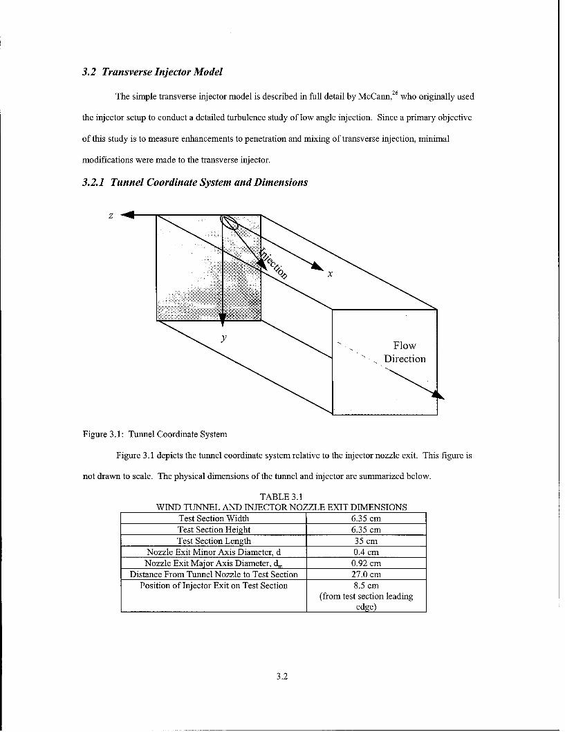
3.2.1 Tunnel Coordinate System and Dimensions
Z
Y " .Flow
- Direction
Figure 3.1: Tunnel Coordinate System
Figure 3.1 depicts the tunnel coordinate system relative to the injector nozzle exit. This figure is
not drawn to scale. The physical dimensions of the tunnel and injector are summarized below.
TABLE 3.1WIND TUNNEL AND INJECTOR NOZZLE EXIT DIMENSIONS
Test Section Width 6.35 cmTest Section Height 6.35 cmTest Section Length 35 cm
Nozzle Exit Minor Axis Diameter, d 0.4 cmNozzle Exit Major Axis Diameter, d 0.92 cm
Distance From Tunnel Nozzle to Test Section 27.0 cmPosition of Injector Exit on Test Section 8.5 cm
(from test section leadingedge)
3.2

Table 3.2 summarizes the standard freestream conditions for a test run.
TABLE 3.2FREESTREAM FLOW CONDITIONS
Mach 2.9P, 217874 (Pa)
TO 294 (K)P 8028 (Pa)T 114 (K)y 1.4Uo 608 (m/s)
3.2.2 Injector Model Modifications
The primary physical modifications made to the injector model test section were the removal of a
1 cm deep 2.55 x 7.1 section of the tunnel ceiling directly behind (flow wise) and centered on the rear lip
of the injector exit nozzle. The removed section enabled flush mounting of either the PME ramp models,
or a blank section for simple transverse injection. A second modification was to bevel the settling
chamber exit to smooth the flow transition into the injector nozzle. Figure 3.2, not to scale, shows the side
view of the tunnel (negative z axis into page) with an example PME ramp in place.
Pressurized Air
+Pressure Transducer
SettlingChamber
PMERamp )250
Direction Of Flow x :Conventional Pressure Probe:x/d-20 Measurement Station
Figure 3.2: Side View of Test Section
3.3

The settling chamber consists of a 1.9 cm spherical bottom and a cylindrical top of the same
diameter. The injector outlet from the spherical bottom shows the bevel described above. The throat
diameter of the injector outlet is 0.3241 cm, expanding to 0.4 cm across the exit minor axis. The upper
cylindrical portion of the settling chamber was tapped to accept an Endevco 0-690 kPag pressure
transducer and a high pressure air line from the wind tunnel air supply. This arrangement ensures the total
temperature of both the freestream and injectant are identical. For mean flow measurements, the settling
chamber pressure was held constant at 30 psig.
3.2.3 Injection Parameters
Table 3.3 summarizes the relevant injector jet conditions. The variation in the following
parameters is no more than 1.8%.
TABLE 3.3INJECTOR JET FLOW CONDITIONS
Mach 1.87Poq 304541 (Pa)TOM 294 (K)Pi 47595 (Pa)Ti 173 (K)Y! 1.4
Ui 493 (m/s)
X 3.52q 2.85
3.3 PME Ramps
The dimensions of the PME ramps based upon the injector exit minor diameter d are shown in the
following three-view drawings. Each ramp was machined to the front edge of an aluminum block that was
fitted flush with the tunnel ceiling to reduce step shocks. The design philosophy of each ramp is detailed in
section 2.7.
3.4

250 4d 250
Side
Top 25' 25 ° Top Side Top SideTp2020 Tp250 250
Front 9.46 d or 2 1 Front 9.46 d or 21 Front 9.46 d or 21
SR I SR 2 SR 3
Figure 3.3: Symmetric PME Ramps
Ild
4 d 4 d I
Top 250 Side Top 25' Side
47 d Z / 4.7 d
9.46d 9.46d
Front
ER 2 ER 3
250
Top Side25o 25'
4.7 d
23.65 d
Front
ER I
Figure 3.4: Extended PME Ramps
3.5

4 d Side 4d Side
Top 250 Top 250/" 4.7 d __ 4.7 d "
/47 d 47d
Front or Front or
AR 1
AR 2
Figure 3.5: Asymmetric PME Ramps
3.4 Measurement Locations
The measurement location for the mean flow data occurred at x/d = 20. The z direction horizontal
width of the tunnel consisted of 29 stations, each 0.1643 cm apart for a coverage of 4.60 cm. In the tunnel
coordinate system, this is a range from -5.6 to +5.6 z/d. This doubles the spatial resolution across a similar
16range used by McCann for mean flow measurements. Vertically, the span covered was 5.08 cm, which
translates toy/d from 0.4 to 11.5.
The cross flow oriented Rayleigh-Mie scattering laser sheet location is identical to the mean flow
measurement plane. The laser sheet was sized to cover 5.08 cm of the tunnel cross section, and centered in
the y-z plane. The parallel oriented laser sheet was arranged along the tunnel centerline, parallel to the x-y
plane, and sized to cover 5.08 cm measured from the front lip of the injector nozzle exit. The useful
coverage provided by the parallel oriented sheet ended approximately 2 d upstream of the mean flow
measurement plane.
3.5 Mean Flow Probes
Mean flow data was acquired through a system consisting of pressure probes, transducers and a
traversing mount.
3.6

3.5.1 Pressure Probes
Two types of pressure probes were used to collect the mean flow data. A Pitot probe constructed
of 1.6 mm outer diameter stainless steel was fitted to a series of larger diameter tubes for structural support.
The pressure sensed by the probe was fed by Tygon tubing to an Endevco 0-103 kPag transducer. The
cone-static probe consisted of four evenly spaced circumferential 0.34 mm diameter taps that fed into a
common chamber. This design is insensitive to misalignment errors up to 60 off centerline of the flow.
The cone-static probe pressure was also fed into an Endevco 0-103 kPag transducer through Tygon tubing.
For both probe types, the output of the pressure transducer was filtered by Endevco model 4225 signal
conditioners. A specific signal conditioner was assigned and calibrated for each transducer used.
3.5.2 Probe Traverse System
The mean flow probes were swept through the vertically oriented y/d range for each of the 29 z
axis stations across the tunnel cross section. The traverse system used an Arrick Robotics MD-2 dual
stepper motor driver and a Size 23 Stepper Motor.26 The position of the traverse was recorded as a voltage
by a TransTek Model 0217 linear voltage displacement transducer. For the range of motion the stepper
motor traversed the probe through, the voltage-position relation was linear.
3.6 Flow Visualization
Two types of flow visualization were accomplished during this study. The first was shadowgraph
photography. The second was digital imagery through Rayleigh-Mie scattering.
3.6.1 Shadowgraph Photography Setup
Shadowgraph images were taken for each injector configuration. Due to the limited coverage
provided by the optical glass wind tunnel side walls, two images were needed to from a composite image to
capture the flowfield around the injection and ramps. The light source used was a Cordin Model 5401 arc
light with a 600 ns spark, and aligned by hand. The light was collimated by a 100 cm focal length mirror
and passed through the test section. Polaroid Type 57 film was used for the images.
3.7

3.6.2 Rayleigh-Mie Scattering Laser System
Bottom Table Top Table
Aperature
GreenPrism Beam @ M irror
532 unm .
Red
Beam @ Nd:YAGCylindrical 607 nm Laser ILens
Lens Nd:Yag
Laser II GreenBeam @
532 nm
Lens
Mirror PrsPrism
F ITest Section
Mirror Reflecting Up E- 1 oorL. GlassFloo 1- -- -Through Tunnel Glass Floor - --- Flow Direction
Glass Sidewall "
Power Macintosh
Kodak-l DCS 460c
Figure 3.6: Rayleigh-Mie Scattering Laser and CCD System
The laser system depicted in Figure 3.6 was used to generate the digital images used in this
investigation. The laser sheet was aligned through the cylindrical lens system on the lower table for either
parallel or cross flow orientation. The view of the test section is a top view, looking down onto the glass
3.8
tunnel floor through which the laser passed. The CCD camera was mounted to a stable test support, and
aligned either perpendicular or 260 off the tunnel centerline for the parallel and cross flow images,
respectively.
The lasers used were two Surelite Nd:YAG lasers powered by two Continuum Model SLI-10
power supplies. The beams produced by each laser had wavelengths of 532 (green) and 1064 nm. The
higher wavelength was filtered out with a series of beam splitters. The right side laser beam depicted in
Figure 3.6 was passed through a Raman Cell to convert the 532 nm beam to 607 nm (red). The pulse
duration of each laser was 10 ns, and the beam was pulsed 10 times per second (i.e., ten Hz).
The camera used was a Kodak Model 460C CCD camera, with a Nikon N90 lens. The exposure
times used varied depending upon the type of image required. For instantaneous images, the exposure time
was 1/8 seconds, with an f-stop setting of 5.6. Therefor, one 10 ns pulse was captured for each
instantaneous image. The time-averaged images were exposed for four seconds at an f-stop of 16. The
time averaging of the exposure captured 40 10 ns pulses.
3.7 Data Acquisition System and Computational Resources
Data acquisition was accomplished through the National MIO- 1 6E PC based data acquisition
board connected to an ACER Pentium computer. DANTEC Streamware® software was used to acquire the
raw voltage readings collected by the MIO-16E board from the pressure probes. This board has a relative
voltage response scale of 10 V. The sample rate used for data acquisition on all channels was 400 Hz.
Once acquired, the data was converted to comma separated text files for processing by the data reduction
routines.
The ACER Pentium PC provided data acquisition, traverse control and partial data reduction
functions. Data reduction was also accomplished on a HP-48. AFIT Sun Sparc 2 and 10 workstations
were used to generate all contour plots through TECPLOT. All other charts and plots were generated using
Microsoft EXCEL. AFIT library scanners were used to convert the shadowgraph images to digital format.
A Power PC 6100 was used to acquire and process the digital Rayleigh-Mie scattering images, which were
converted from the raw Kodak digital format by Adobe Photoshop.
3.9

IV. Data Reduction and Processing
This chapter details the data reduction routines applied to the raw pressure probe data collected
with the cone-static probe, the pitot probe, and the flow stagnation probe. The methods used to develop
measures of the total pressure loss, plume penetration and plume area are detailed. The process of
generating a mean flow image of the plume region and deriving quantitative relations from the images is
also explained.
4.1 Mean Pressure Measurements
For both flow pressure probes the raw data were converted from gauge pressures to absolute
pressures and reduced to mean pressure measurements. This was accomplished using a BASIC data
reduction routine. The routine first scaled the probe voltages to psi by the appropriate factor depending on
probe type. Second, the gauge psi values were converted to inHg and added to the atmospheric pressure in
the wind tunnel room. Third, the converted pressures were averaged by groups of 41 points into a single
point. The BASIC routine also determined the position of the probes by averaging the same range of
traverse position voltages into a single point. At the 400 Hz sample rate, 41 samples comprised 0.1025
seconds of traverse movement. This span of movement covers 0.0323 cm for each mean datum and
provides a spatial resolution of 142 mean datum over the 4.572 cm of traverse travel.
4.1.1 Determination of Flow Mach Number
The Mach number at each mean point was determined through the ratio of the cone-static and
pitot pressure data (Pc/Pt2). The cone-static and pitot pressure data were collected on separate wind tunnel
runs, and on separate days. The probe pressure ratios were normalized to each other with the recorded total
pressure of the flow for the data run.
P, P, Pt2(4.1)
Pt2 PtO Pto
4.1

The Mach number relation to the pressure ratio PJ/Pt2 was determined through a least squares fit
developed by Bowersox29 for a 100 cone-static probe.
123- = -0.052976 + 4.6840x - 18.6786x 2+ 50.7006x 3 _ 54.1577x 4 (4.2)M
Where x = PJPt2 and 0.0805 _ x _ 0.358. Equation (4.2) is acceptable over the range of Mach
numbers from 1.5 to 4.4, and has a standard deviation of 0.06%.
4.1.2 Determination of Plume Static and Total Pressure
The static pressure of the flow within the plume was determined by application of the Rayleigh
Pitot tube formula.3 °
y±1 (4.3)
Pt2 (7+1M )7@1
2
The total pressure in the injection plume, Ptl, differs from the tunnel freestream total pressure, Pto.
P, was determined from the Mach number relation of total pressure ratios. By multiplying equation (4.3)
by the isentropic pressure relation 28
Pt (1+ - 1 Mi )7 (4.4)
Pi 2
of equation (4.4) to eliminate P1, the ratio of Ptl to P 2 was determined.3 °
ry _ll(1 ly-1f M2(r-1)
(1'\-1) 1± - l__i 27_ M,_2 2P-7+1 y MI1 (4.5)
2)
4.2 Total Pressure Loss
Each injector ramp model produces a disturbance to the flow, and hence, a shock wave. The
shock waves in turn reduce the flow total pressure. In addition turbulent mixing, which may be enhanced
by the injector ramp, also causes total pressure loss. Since a primary objective of this research is to
enhance injection penetration and mixing while minimizing the total pressure loss, a means to quantify the
4.2

injector ramp induced total pressure loss was required. A method was developed to determine the total
pressure loss.
The method applied was to sum the total pressure ratio Pt/Ptl across the test section of the simple
transverse injection case and compare the results of similar integration for each injector ramp model. To
normalize the results, the ratio of P,0/Pt, of the simple transverse injection was divided by Pt0/Pt for the
injector ramp model. Therefore, the simple transverse injection has a loss parameter of unity, and the
negative impact on total pressure of the injector ramp models would lower their respective loss parameters
below one.
- (PtO / Ptl)o Ramp
(PtO / Ptl)PMR Ramp
4.3 Plume Area and Penetration Determination
A definition of the plume was made to determine the possible enhancement by the various ramp
injector models of plume penetration into the freestream. The plume is defined as the area within the search
region where the Mach number was at 95% of the freestream value in the search region. This criteria is
intended to capture plume and vortex structures, not necessarily the distribution of injectant or
concentration information. The plume search region was initially constrained by y/d of 0.8 to 4, and z/d of
± 2.4. A complication arose in establishing where the injectant plume ended and the boundary layer began
due to using air for both the freestream and the injectant. There was apparent entrainment of the boundary
layer by the plume's counter rotating vortices, as evinced in the thinner boundary layer in the area under the
plume. Since the plume and boundary layer components are indistinguishable in these plots, flow
visualization imagery was used to establish a cutoff between the plume and tunnel ceiling boundary layer.
The demarcation between the plume and tunnel ceiling boundary layer was made at the point of greatest
necking of the plume contours. The bottom, left and right side boundaries of the search region were
selected to include the plume as well as freestream regions within the ramp injector model shock cone,
without including the shock cone. Figure 4.1 shows the Mach contour plot of the simple transverse injector
with the plume search region defined.
4.3

Mach #
32.95
2 j 2.9Plume 2.85Search 2.8Region 2.75
2.7R2.7
2.652.62.552.5
y/d 62.452.42.352.32.252.22.152.10
10 2.052
-4 -2 0 2 4z/d
Figure 4.1: Simple Transverse Injector Mach Contour Plot With Plume Search Region
4.3.1 Freestream Mach Number Definition
The region between the plume, the tunnel ceiling boundary layer, and the shock wave created by
the ramp injector model and flow recompression around the plume is defined as the plume region local
freestream. Two methods were used to establish the local freestream Mach number based upon
quantitative assessments of Mach contour plots. These methods required first establishment of a rejection
Mach number which was used to separate the data points associated with the plume, tunnel ceiling
boundary layer and the recompression shock cone from the local freestream. The average of the local
freestream Mach values were then used in the plume search region to determine the plume area as a
percentage of the local freestream Mach number. The Mach contours were created with TECPLOT 3 at a
contour separation of 0.05 Mach. A third method was developed to avoid use of the contours as a criteria.
Each method has advantages and disadvantages depending upon the flow geometry around the plume.
4.4

4.3.1.1 Freestream Mach Number Definition I: Graphical Method
The first method defined the local freestream of the entire search region around the plume. At the
0.05 Mach contour resolution, the majority of plume contours were distinguishable from the freestream
region due to the orderly, concentric, and proximate nature of the plume contours. The Mach number
gradient, M / d(a) / d] where ot is the tunnel coordinate direction, of the plot contours was used to
establish the rejection Mach number of the freestream region. The search for a local freestream Mach
contour that met this criteria had to be constrained to the upper half of the plume to avoid selecting an
entrained boundary layer contour. The upper half of the plume was defined as the region above the y/d
value where a tangent line to four or more concentric plume contours was vertical. In cases where there
was asymmetry about the y/d axis in the plume, the average y/d value of both sides of the plume was used.
The first contour, starting from the center of the plume, that was below a gradient of 0.25 was determined
to be the freestream region. The Mach number of the contour defined as the freestream region was used in
a SYSRPL data reduction routine to filter the entire plume search region data points by rejecting any points
with a Mach number lower than the freestream contour. The average Mach number in the freestream was
then determined as the average of the remaining data points. Figure 4.2 details the graphical method local
freestream search region and the Mach number contour selected as the local freestream.
4.5
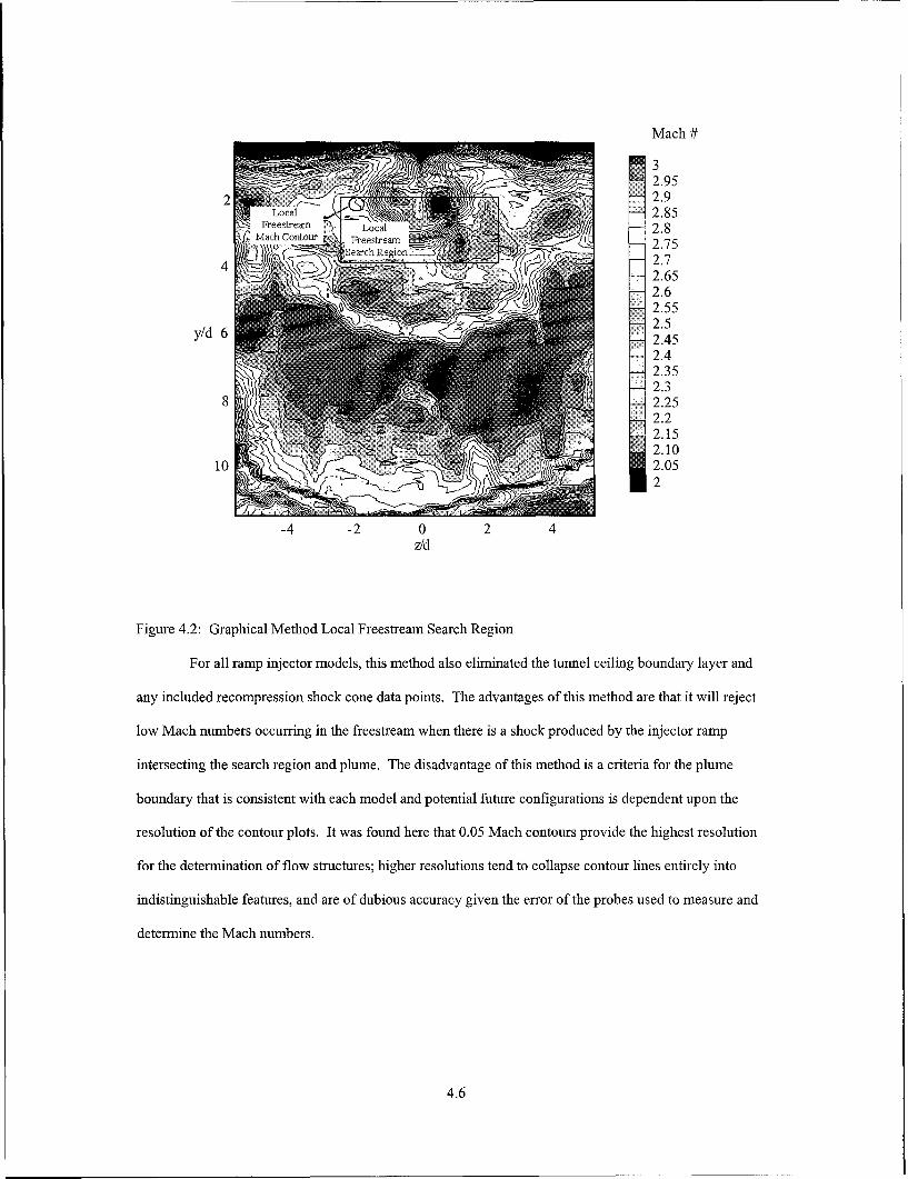
Mach #
32.95
2 ~ <2.9J, Cal2.85
2 Freestrearn Local 2.8Mach Contour Freestream __ 27
2.75erch Regicn2.72.652.62.552.52.45y/d 6 2.42.42.352.3
8 2.252.22.152.10
10 2.052
-4 -2 0 2 4z/d
Figure 4.2: Graphical Method Local Freestream Search Region
For all ramp injector models, this method also eliminated the tunnel ceiling boundary layer and
any included recompression shock cone data points. The advantages of this method are that it will reject
low Mach numbers occurring in the freestream when there is a shock produced by the injector ramp
intersecting the search region and plume. The disadvantage of this method is a criteria for the plume
boundary that is consistent with each model and potential future configurations is dependent upon the
resolution of the contour plots. It was found here that 0.05 Mach contours provide the highest resolution
for the determination of flow structures; higher resolutions tend to collapse contour lines entirely into
indistinguishable features, and are of dubious accuracy given the error of the probes used to measure and
determine the Mach numbers.
4.6

4.3.1.2 Freestream Mach Number Definition IH Box Method
The second method used to establish the freestream Mach number in the plume region applied a
similar filtering method, using a modified version of the first method SYSRPL data reduction routine. The
boundary of the plume search region along y/d of 4, and z/d of ± 2.4 was used to provide the data points.
Instead of using the plume Mach contours to determine a rejection Mach number as in section 4.3.1.1, the
tunnel ceiling boundary layer inside the recompression shock cone was used. The boundary layer Mach
contours were distinguishable from the local freestream as relatively parallel and compacted in comparison.
Mach #
-32.95Boundary Layer SeletedM 2.9Mach Contour S BondI Lyer
earch Rgions Mach Contour 2.8572.8
2.754-------t 2.7
2.652.62.552.5y/d 6 2.52.452.42.352.32.252.22.152.10
10 2.05~2
-4 -2 0 2 4z/d
Figure 4.3: Box Method Local Freestream Search Region
The edge of the tunnel ceiling boundary layer was defined outward from the tunnel ceiling as the
lowest Mach contour with a Mach number to injector diameter gradient less than 0.25 at any location from
the next interior boundary layer contour. The boundary layer contours were tested along the z/d of
4.7

- 2.8 to - 2.0 and 2.0 to 2.8 on each side of the vertical boundaries of the plume search region for this
condition. Figure 4.3 shows the boundary layer-local freestream search regions.
The ± 0.4 range around the vertical search region boundaries confined the boundary layer
contours to those least affected by the injector ramp shock cone impingement or the plume entrainment
region. Again, this rejection criteria proved suitable for elimination of the ramp injector model-
recompression shock cone, which for all models had lower Mach numbers than the tunnel ceiling boundary
layer. The advantages and disadvantages of this method are the same as the graphical method with one
additional disadvantage. This method tends to be the most subjective of the methods used, as the
intersection of the tunnel ceiling boundary layer and the recompression shock cone can occur in the
horizontal search regions (z/d of - 2.8 to - 2.0 and 2.0 to 2.8). In such cases, the intersection area usually
has a lower than 0.25 gradient. However, because of the spreading effect of cone-static probes on shock
waves, these regions are not considered representative of the local tunnel ceiling boundary layer.
Subjectivity becomes a factor when the experimenter must decide to use or not use a rejection Mach
contour based upon proximity to a shock-boundary layer interaction. In this investigation this was not a
problem because there were boundary layer contours that met the gradient criteria inside the plume search
region vertical boundaries.
4.3.1.3 Freestream Mach Number Definition II: Modified Box Method
A second use of the box method, with slightly different criteria, was also tested. In the second
method, no contours were dropped from the average Mach number calculation based upon a rejection
Mach number. The top of the vertical boundaries were selected at both y/d of 1.2 and 1.6. For most
models, y/d of 1.2 was well outside the apparent boundary layer; those cases in which it was not is noted.
The bottoms of the vertical boundaries and the sides of the top boundaries were also cropped to avoid
including the recompression shock cone. The average Mach number was then the average of all points
along the lines, with no filtering. The results of this method correlated well with those of the graphical and
box method. The advantage of this method is an independence from determining a graphical based criteria
to separate the plume. The major disadvantage, as seen with models ER 2 and ER 3, is that it will not
reject the low Mach numbers of a shock wave passing through the plume. This lowers the computed value
of the overall freestream speed, and reduces the plume area in turn.
4.8

4.3.2 Plume Area Determination
With the freestream Mach number established, the plume region was distinguished from the
freestream using a SYSRPL filtering routine. To avoid counting the tunnel ceiling boundary layer as the
plume area, the upper limit of each ramp injector model plume search region was lowered to the top of the
plume. The effect of reducing the upper limit confines the search to the circular portion of the plume,
which is consistent with previous researches "2 and the flow visualization accomplished in this
investigation (see Figure 4.8). The routine counted all points in the plume region that had a Mach number
of 95% or less of the freestream Mach number. The criteria of 95% of the freestream Mach was selected
after comparison with the 99% and 90% criteria. The 99% criteria was rejected after review of the contour
plots. Because of the varying freestream Mach number around the plume, the 99% criteria captured large
areas of the freestream. The 90% criteria was rejected as being too low a resolution; at the 90% Mach
contour the plume areas show little separation. Thus the contours below 90% are useful for confining the
plume core, while the contours above 90% contain the plume outer layers. Since the outer layers of the
13 26plume have been identified as important mixing regions by Fuller" and McCann, inclusion of this area is
important. The 95% criteria provides ample separation from the freestream, but also includes the
outermost mixing layers. To avoid capturing the ramp injector model shock cone, the search area of the
plume region was further constrained to exclude any shock cone Mach number contours that were less than
the freestream Mach number. Each datum represents a rectangular area of 0.1588 cm in the z direction,
and 0.0323 cm in they direction, for an area of 0.005161 cm 2.
4.9
4.3.3 Plume Penetration Determination
A measure of plume penetration into the freestream was put forth by McCann and Bowersox.22
This method of measurement was based on the distance from the tunnel ceiling to the plume center. An
approach put forth by Fuller13 used a threshold 0.5% mass fraction of helium injectant to define the
outermost plume boundary, and hence the furthest penetration into the freestream. Since this technique is
not available for this investigation, the definition of McCann and Bowersox was used. The centroid of the
plume area was found based upon the integral relation
J (y / d)dA- (4.7)
which was computed by a SYSRPL routine.
4.4 Flow Visualization Techniques
Flow visualization was accomplished through two methods. The first method is shadowgraph
photography, which for this study is used for qualitative analysis. The second method employed a two
inch wide Nd:YAG laser sheet and gaseous particle seeding through the injector nozzle. The laser sheet
was oriented both parallel and perpendicular to the test section y-x plane for each model. Both orientations
provide detail about the penetration and mixing of the flow.
4.4.1 Parallel Flow Orientation
The parallel oriented laser sheet was adjusted to cover two inches of the test section starting at the
forward edge of the injector port, and centered along the test section longitudinal axis. Two types of digital
images were attained in this orientation for each injector ramp model. The first image type was an
instantaneous image, which was taken with a digital camera with an f-stop setting of 5.6 an and exposure
time of 1/8 seconds. The laser was pulsed at ten Hz during the exposure, effectively freezing the flow in
the image. Figure 4.4 is an example of an instantaneous image.
4.10

Figure 4.4: Instantaneous Digital image, Model 1
These images capture the extremely unsteady nature of the vorticity in the axial direction. The
second image type is a time-averaged image acquired at an f-stop setting of 16 and an exposure time of
four seconds (i.e., 40 laser pulses). This combination has the effect of averaging the image, Figure 4.5,
which allows meaningful quantitative analysis.
Figure 4.5: Averaged Digital Image, Model 1
Two types of analysis were applied to the parallel oriented average images. The centerline
trajectory of the plume was determined. Also, a measure of the rate at which the image intensity decays in
the axial direction was made.
4.11

4.4.1.1 Parallel Flow Orientation Analysis, Plume Trajectory Determination
The method to establish the plume trajectory was based upon the grayscale intensity of each pixel
in the digital image. The images were first converted from color bitmaps to 256 shade grayscale bitmaps.
This process assigns ASCII characters 0 to 255 to each pixel depending upon intensity, where ASCII
character number zero corresponds to black, and ASCII character number 255 corresponds to white. A
SYSRPL routine was used to interrogate the numeric value of the ASCII character representing a pixel.
The column and row position of the pixels above a threshold value of ASCII character number 75 were
recorded for twenty axial stations, covering from the center of the injector exit to 17 diameters
downstream, near the end of the laser sheet, as shown in Figure 4.6.
Figure 4.6: Plume Image Measurement Stations
Before the images could be processed two steps were taken to ensure reliable results. Despite
coating the tunnel ceiling and the injector ramp models with flat black paint to reduce reflections, a
noticeable glare can be seen in the photographs. To avoid detecting the glare as part of the seeded plume,
all solid injector ramp model and test section boundaries were filled with black. Additionally, in several of
the images large globules of seed can be seen, Figure 4.7.
4.12
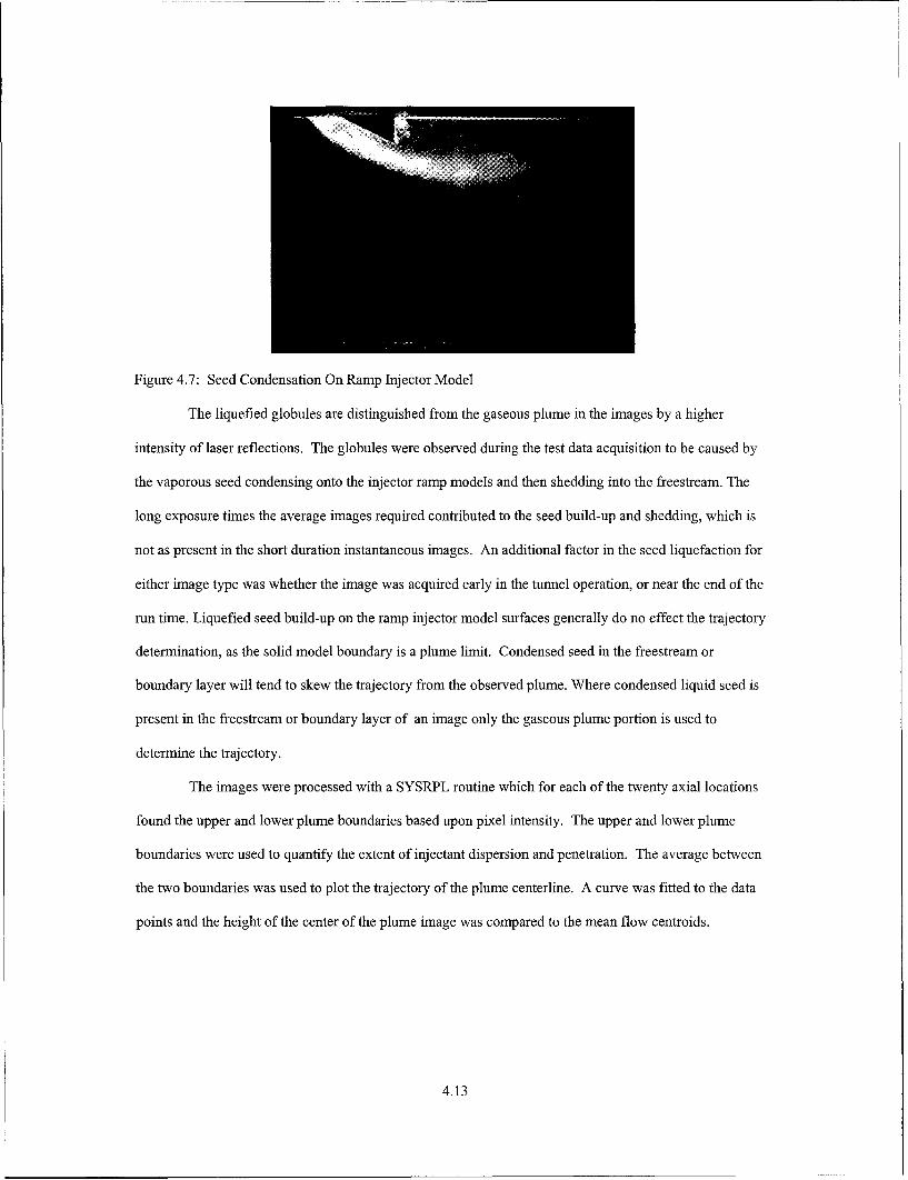
Figure 4.7: Seed Condensation On Ramp Injector Model
The liquefied globules are distinguished from the gaseous plume in the images by a higher
intensity of laser reflections. The globules were observed during the test data acquisition to be caused by
the vaporous seed condensing onto the injector ramp models and then shedding into the freestream. The
long exposure times the average images required contributed to the seed build-up and shedding, which is
not as present in the short duration instantaneous images. An additional factor in the seed liquefaction for
either image type was whether the image was acquired early in the tunnel operation, or near the end of the
run time. Liquefied seed build-up on the ramp injector model surfaces generally do no effect the trajectory
determination, as the solid model boundary is a plume limit. Condensed seed in the freestream or
boundary layer will tend to skew the trajectory from the observed plume. Where condensed liquid seed is
present in the freestream or boundary layer of an image only the gaseous plume portion is used to
determine the trajectory.
The images were processed with a SYSRPL routine which for each of the twenty axial locations
found the upper and lower plume boundaries based upon pixel intensity. The upper and lower plume
boundaries were used to quantify the extent of injectant dispersion and penetration. The average between
the two boundaries was used to plot the trajectory of the plume centerline. A curve was fitted to the data
points and the height of the center of the plume image was compared to the mean flow centroids.
4.13

4.4.1.2 Parallel Flow Orientation Analysis, Rate Of Centerline Decay
Due to the limitations of this investigation, exact rates of concentration decay with downstream
position are not possible. However, approximate and relative measures are possible. The laser illuminated
sheet of seed particles can provide a measure of how quickly the concentrated center of the plume is
dispersed by the injection generated vorticity. As the plume enters the freestream, it is largely a
homogenous entity, 19 which can be seen in Figures 4.4 and 4.5. As the plume turns roughly parallel to the
freestream the injection generated vorticity becomes the dominant mixing mechanism. 4'13 This mixing
action spreads the injectant to the periphery of the plume which in turn reduces the concentration of the
injectant at the centerline. The intensity of the plume digital image is seen to decay along the centerline as
a result of this action, which is consistent with previous investigations.6"1
There are several caveats associated with this analysis. The plume seed is not ideal and cannot
totally map the injectant locations. The laser sheet loses intensity along the fringes, which could contribute
to a decay in the image. The quantity of seed injected in each test run varied slightly, which affects the
level of intensity reflected. To compensate for this issue, the intensity of each image is scaled according to
the intensity at the injector nozzle exit. This procedure will level the effect of variations in the quantity of
injected seed. Additionally, though not ideal, the seed should map each injector ramp flowfield in a similar
manner. A relative comparison was therefore possible. The loss of intensity in the laser sheet does not
appear to have affected any of the images as the reflected intensity decays well upstream of the end of the
laser sheet, Figure 4.7.
The process of determining the rate of centerline decay follows from the procedure for finding the
plume trajectory. For the twenty axial stations outlined in Figure 4.6, the average of the plume pixel
intensities was determined by a SYSRPL routine. The average intensity for each location was scaled by
the average intensity of the injector nozzle exit plume pixels. An average intensity was then plotted against
downstream axial location. The effect of liquefied seed artificially raising the average intensity value is
recognized. To eliminate the effects of liquefied seed, an upper threshold was used to filter out points too
intense to be gaseous plume.
4.14

V. PME Ramp Flow Field Results And Analysis
This chapter describes the flow field for each of the nine injector configurations (simple transverse
injection and the eight ramp cases). The three basic qualitative and quantitative techniques, shadowgraph
photography, mean flow pressure data and laser imaging are employed collectively for each model. This
is necessary because together the available data provides a consistent and complete analysis of the injection
flow field that the individual techniques alone can not. The PME ramp models with similar geometries are
grouped and compared independently to simple transverse injection. Chapter five is organized into four
subsections, one for the simple transverse injection analysis and the three PME ramp groups. The case of
injection over a simple transverse tunnel ceiling is presented first to illustrate the salient flow features and
to provide a basis of comparison. The first PME ramp group is those models which are symmetrical about
the y-z plane of the tunnel coordinate system, which includes models SR 1, SR 2 and SR 3. The second
PME ramp group is the models with extended surfaces beyond the initial ramp, or models ER 1, ER 2, and
ER 3. The final PME ramp group is the asymmetric swept ramps, models AR 1 and AR 2 which have
geometries that have been the subject of extensive experimental and numerical investigations in the
past.10,11,12,13,16
For all configurations studied, the following order of analysis is used. First, shadowgraph flow
visualization images are used for qualitative analysis. The basic flow shock structures along the centerline
x-y plane are examined. Second, the laser sheet images are qualitatively analyzed in both parallel and cross
flow orientations. Third, the mean flow field pressure data results are presented, from which Mach number
contour plots were computed. Fourth, the four methods of determining the plume region local freestream
Mach number as defined in section 4.3.1 and attendant injection plume area at the measurement station are
tabulated, and contour plots comparing the results are presented. Fifth, the centroid based plume
penetration values are analyzed. Sixth, the total pressure loss parameter for each injector ramp model is
presented. Seventh, quantitative analysis of the digital images plume boundaries and centerline mean
plume trajectory of the averaged digital images are plotted. The rate of decay of the
5.1

plume centerline digital image intensity is plotted and correlated with the cross flow image data and the
pressure probe results.
5.1 Simple Transverse Injector
Injection over a flat or simple transverse model provides a relative basis of comparison for the
objects of this investigation: plume expansion, plume penetration and total pressure loss. The following
sections provide a fundamental analysis of flow structures and observations common to all injector models.
Basic injection induced flow structures are examined through flow visualization and quantitative
techniques, and compared to previous researchers. Results for four quantitative methods of determining
plume area and penetration are summarized in Table 5.1. Pressure losses in the form of the total pressure
loss parameters H is presented for use in normalizing the total pressure losses of the PME ramps.
5.1.1 Simple Transverse Injector Flow Visualization
This section includes all of the flow visualization accomplished for the simple transverse injector.
The shadowgraph is used to determine basic flow shock structures. The parallel oriented laser sheet
instantaneous and time averaged images are used to provide details of the plume structures observed. The
cross flow oriented laser sheet instantaneous and time averaged images depict the plume shape and show
the plume vortex mechanisms in action.
5.1.1.1 Simple Transverse Injector Shadowgraph
N.Window
Injection Port Frame
StrongBow Shock
WeakRecompressionShock
x/d= 20MeasurementPlane
Figure 5.1: Simple Transverse Injector Composite Shadowgraph
5.2

Figure 5.1 shows a composite of two shadowgraphs for the simple transverse injector model.
Boundary layer structures are visible in Figure 5.1 along the lower and upper surfaces up to the point of
injection. After injection, the upper boundary layer is disturbed and does not appear as clearly as before.
Just above the upper boundary layer and slightly behind the injection point is a strong bow shock created as
the plume enters the freestream. For injection of an underexpanded jet into a supersonic freestream, the
plume acts as a blunt body which results in the strong shock.4 The plume main shock starts at an angle of
approximately 33' then bends to approximately 250 by the middle of the test section. A weaker secondary
shock can be seen above the main bow shock as a faint roughly parallel line towards the right side of the
picture (the divergence is about 50). The origin of this shock is not visible in this image but it can be seen
to exit the image at about the middle of the upper right window clamp. This shock is a recompression
shock created as the main flow rejoins around the plume. This shock is limited by two mechanisms. First,
there is only a relatively small height between the bottom of the plume and the tunnel ceiling boundary
layer where recompression can occur. This height is created by the plume as it enters the freestream and
rises to the height of the Mach disk, before turning in the direction of the main flow. Second, above and in
the plume there is either no main flow expansion or the plume expansion prevents the main flow from
recompressing. The secondary shock appears to form on the bottom side of the plume, though it most
likely forms on the top side of the plume and passes through it.
The small black triangle at the top and center of the image is the side wall of the optical glass
window. Due to the alignment of the images inclusion of part of the tunnel window side wall was
necessary. A very weak shock is faintly visible crossing from left to right and top to bottom of the image
at 200. This weak shock is due to a small misalignment upstream of the test section. The vertical streaks
throughout the image are due to the film used and are not part of the flow structure. The two bright patches
near the bottom boundary layer are due to light reflection. The rectangular blocks along the glass
periphery are window clamps. The measurement plane for the pressure probes is indicated in Figure 5.1.
The plume structures are visible in this shadowgraph, though not clearly due to obscuring effects
of the boundary layer and the plume vorticity. Further analysis of the plume structure is made in the
5.3

following section with the parallel oriented laser sheet image. A much more illuminating analysis can be
developed from the side laser sheet images.
5.1.1.2 Simple Transverse Injector Parallel Oriented Images
Figure 5.2: Simple Transverse Injector, Instantaneous Parallel Oriented Laser Image
Figures 5.2 and 5.3 show the plume seeded and illuminated as described in section 4.4.1. The
barrel shock, outlined in Figure 5.2, created by the underexpanded plume isentropically expanding then
compressing is visible, as well as the general area and orientation of the Mach disk that terminates the
barrel shock. The barrel shock region provides the majority of the vorticity generation for the plume. As
the plume protrudes out of the boundary layer, the high velocity freestream wraps around both side of
higher pressure plume and imparts a rotation.4 The rotation manifests itself as counter-rotating vortex pair,
6which has been identified as the major mixing mechanism for this type of injection. In measurements
under similar circumstances (i.e., in the same tunnel using the same injector but at a different injection
22pressure ratio) McCann and Bowersox measured a maximum axial vorticity of approximately 15,000/s at
the downstream x/d of 40 location.
5.4

Figure 5.3: Simple Transverse Injector, Time-Averaged Parallel Oriented Laser Image
Beyond the barrel shock the plume turns sharply towards the downstream direction which in turn
aligns the vortices roughly axially. In Figure 5.2 this is annotated as the "vortex development and plume
foldover region." Directly above the barrel shock, the plume is seen to roll back up towards the tunnel
ceiling. This foldover of the plume obscures the bottom right of the barrel shock. After the bend in the
plume, no vorticity is imparted and the plume becomes a streamwise vortex mixing structure that decays
and dissipates from viscous effects. The highly unsteady vortex structures visible in Figure 5.2 are due to
the short exposure time used which effectively froze the helical structure of the plume. A rapid decrease in
the plume intensity towards the right side of the image is apparent in Figure 5.3. This intensity drop-off is
consistent with centerline planar injectant mole fractions measurements, which show a marked
concentration drop in the 15-20 d region for a Mach two freestream.5 Noted on Figure 5.3 are the
boundary layer edges as determined from the shadowgraph image, Figure 5.1. Finally, the extremely
bright spots at the rear lip of the injector port in both images are the result of seed particles being drawn
upstream by the two recirculation cells shown in the surface flow visualization of Bowersox. °
5.5
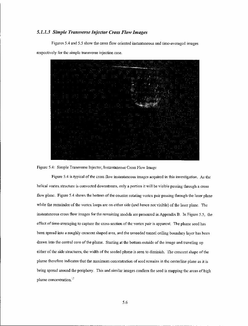
5.1.1.3 Simple Transverse Injector Cross Flow Images
Figures 5.4 and 5.5 show the cross flow oriented instantaneous and time-averaged images
respectively for the simple transverse injection case.
Figure 5.4: Simple Transverse Injector, Instantaneous Cross Flow Image
Figure 5.4 is typical of the cross flow instantaneous images acquired in this investigation. As the
helical vortex structure is convected downstream, only a portion it will be visible passing through a cross
flow plane. Figure 5.4 shows the bottom of the counter rotating vortex pair passing through the laser plane
while the remainder of the vortex loops are on either side (and hence not visible) of the laser plane. The
instantaneous cross flow images for the remaining models are presented in Appendix B. In Figure 5.5, the
effect of time-averaging to capture the cross-section of the vortex pair is apparent. The plume seed has
been spread into a roughly crescent shaped area, and the unseeded tunnel ceiling boundary layer has been
drawn into the central core of the plume. Starting at the bottom outside of the image and traveling up
either of the side structures, the width of the seeded plume is seen to diminish. The crescent shape of the
plume therefore indicates that the maximum concentration of seed remains in the centerline plane as it is
being spread around the periphery. This and similar images confirm the seed is mapping the areas of high
plume concentration. 3
5.6
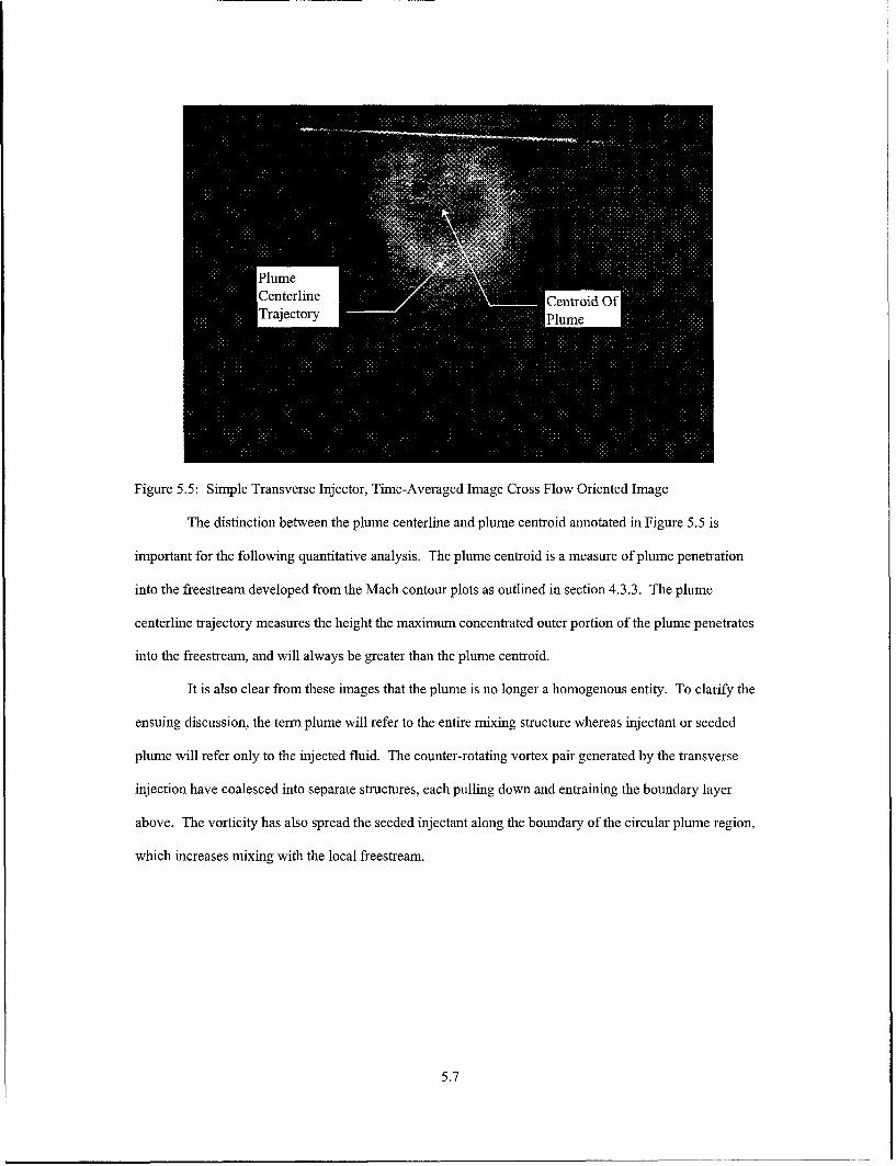
PlumeCenterline Centroid OfTrajectory Plume
Figure 5.5: Simple Transverse Injector, Time-Averaged Image Cross Flow Oriented Image
The distinction between the plume centerline and plume centroid annotated in Figure 5.5 is
important for the following quantitative analysis. The plume centroid is a measure of plume penetration
into the freestream developed from the Mach contour plots as outlined in section 4.3.3. The plume
centerline trajectory measures the height the maximum concentrated outer portion of the plume penetrates
into the freestream, and will always be greater than the plume centroid.
It is also clear from these images that the plume is no longer a homogenous entity. To clarify the
ensuing discussion, the term plume will refer to the entire mixing structure whereas injectant or seeded
plume will refer only to the injected fluid. The counter-rotating vortex pair generated by the transverse
injection have coalesced into separate structures, each pulling down and entraining the boundary layer
above. The vorticity has also spread the seeded injectant along the boundary of the circular plume region,
which increases mixing with the local freestream.
5.7

5.1.2 Simple Transverse Injector Mach Contour Plots
Mach #-- :ii 3.2
.. 3.111
2 3.021Turnel L < ...... 2.932Ceiling 2.842
B.L. 2.7532.663
117 2.574LJPlume Vortex- ((--) ".82"7
Cores2.484Cres -2.395
2.305y/d 6_- , ,_-_ :2. 12.216
: .. W eak 2.126
Recompression 1.4~1.9478 1.858~1.768
~ -~ 1.679J ~~ 1.589
10 r-Bow Shock --- i >\\Q 1.5
-4 -2 0 2 4z/d
Figure 5.6: Simple Transverse Injection Mach Contour Plot
The x/d = 20 Mach contour plot for the simple transverse injection case is shown in Figure 5.6.
This contour plot is scaled to cover a broader range of Mach numbers than the plot used in data processing,
section 4.3. The plot is oriented so that an observer would be upstream of the measurement plane and
looking in the direction of the flow (i.e. the flow direction is into the page). Basic plume and flow
structures are observable in the contour plots. The plume is readily discernible at the center and top of the
plot. With the exception of the boundary layer entrainment at the top of the plot (y/d < 1.6, z/d = + 0.8)
the plume has the roughly circular shape expected from the cross flow imagery, Figure 5.6. Inside the
plume, the twin cores of the counter-rotating vortex pair is visible. The lower Mach number of the vortex
cores is caused by the entrainment of the tunnel ceiling boundary layer, which is slower than the injected
portion of the plume. Outside the plume, the secondary conical recompression shock is visible
5.8

encircling the plume as an arcing structure that peaks at abouty/d = 6. For this particular injection scheme,
the recompression shock is weak enough to disappear from the contour plot if the scaling is not selected to
highlight it.26 The large arcing structure seen starting at y/d of 10 is the edge of the conical shock created
by the injection plume. The structure seen spreading from y/d of approximately 7 to 11 at z/d of +5.6 is the
plume conical shock interacting with the tunnel side wall boundary layer. The tunnel ceiling boundary
layer is seen ranging from approximately y/d = 1.6 at the outside edges to y/d = 1 in the plume area,
depending upon the level of entrainment the boundary layer is subjected to by the plume.
The results of the plume area based upon the local freestream Mach contours as described in
section 4.3.1 are shown in Figure 5.7. The lines aty/d = 1 and y/d = 4 are the respective top boundary and
bottom boundaries for the plume area and centroid location search. The four contours collapse into
essentially one contour for most of the area, with minor disagreement near the tunnel ceiling boundary
layer. Table 5.1 summarizes the area and centroid location results based upon method.
2 Mach #
2.7249
y/d 2.7110
3 -2.6992.6988
-2 -1 0 1 2z/d
Figure 5.7: Simple Transverse Injection Area Contour Plot
5.9

TABLE 5.1SIMPLE TRANSVERSE AREA AND CENTROID RESULTS
Area Method 95% Freestream Mach Area (cm) Centroid (y/d)
Graphical 2.72 1.058 2.04
Box 2.71 1.006 2.06
Modified Box, y/d=1.2 2.69 0.980 2.07
Modified Box, y/d=1.6 2.69 0.980 2.07
Average 2.70 1.006 2.06
The results for the areas and the centroids are within 7.5% and 1.2% of each other, respectively.
This particular case shows excellent agreement between the box and modified box methods, which is
consistent with the relatively benign local flow field around the plume. As will be seen for the PME
ramps, the presence of the ramp can significantly increase the complexity and number of flow structures at
the y/d = 20 measurement location.
5.1.3 Simple Transverse Injector Total Pressure Loss
The total pressure loss incurred by each of the following PME ramps is based upon the average
upstream to local total pressure ratio as detailed in section 4.2. The value of the total pressure ratio for the
simple transverse injection is used to normalize the results for relative comparisons. As such the average
upstream-to-local total pressure ratio for the simple transverse injection case is 1.24. The value of ri for
the simple transverse case is defined as one. The total pressure contour plots for simple transverse
injection and each PME ramp are presented in Appendix A.
5.1.4 Simple Transverse Injector Digital Image Quantitative Analysis
Two types of quantitative analysis were performed on the digital images. The first was the plume
boundary and centerline trajectories, as described in section 4.4.1.1. Figure 5.8 is a plot the plume
trajectories of the simple transverse injector.
5.10

6
5
4 -
y/d 3
2
00 2 4 6 8 10 12 14
x/d
Figure 5.8: Simple Transverse Injector Plume Centerline Trajectory
Recall from section 4.4.1.1 that these traces represent the outer edge, inner edge and the plume
centerline. The plume centerline is the average y/d value of the image pixels at the measurement location
that met the plume intensity criteria. The outer and inner traces map the extremes of the data at the
measurement location, and as such may reflect a single outlying point. This effect is illustrated at x/d of
seven, where the plume inner boundary shows a sudden drop to y/d of one. At the eighth and ninth
measurement locations, singular seed particles in the boundary layer were counted as part of the plume
inner boundary. The plume centerline trajectory does not reflect this drop as the centerline locations at
stations eight and nine are a fifty point average, which one outlying point does not significantly alter.
Additionally, the first three measurement locations are at the injection port, so the inner boundary lies
directly on the tunnel ceiling. Note the data represents only 16 of the 20 axial measurement locations;
beyond the 16th location the plume image fades and becomes indiscernible from the background.
The centerline trajectory measures the deepest near-field penetration of the most concentrated
portion of the plume. In other words, by x/d > 10 the trajectory represents the center of the thick bottom
5.11

portion of the injectant crescent, not the centroid of the plume. For the simple transverse injector, this
penetration is to y/d = 3.32 at an x/d of 9.78. The slope of a best fit line passed through the first eight data
points, which is one ramp length downstream of the injector exit, is 0.23. The one ramp length
corresponds to the x/d length of the PME ramp compression faces. The trajectory of the plume centerline
is relatively flat after x/d of 10. Also beyond x/d of 10, the plume outer and inner boundaries converge
rapidly on the plume centerline trajectory. This tapering of the plume with downstream location is caused
by the freestream-vortex interaction stripping away the outermost centerline concentration of injectant to
the outer side portions of the crescent shaped seeded plume. At this point and further downstream the
plume continues to expand and migrate further out into the freestream, as seen in a similar study by
McCann and Bowersox.22
The second quantitative analysis performed on the digital images is the centerline rate of intensity
decay. This provides the most direct measure of mixing between the various PME ramps since, as seen in
Figures 5.5 and 5.6, the vortex driven mixing strips away the central core of injectant to the plume
periphery. Figure 5.9 show the rate of centerline intensity decay with axial position for the simple
transverse injector.
1.4
1.2
1
0.8
,5 0.6
0.4
0.2
00 2 4 6 8 10 12 14 16
x/d
Figure 5.9: Simple Transverse Injector Plume Centerline Average Intensity Decay
The data shows a nearly linear decay of image intensity. A linear regression of this data provides
a slope of -0.0372, with a 0.96 correlation. This analysis should not be confused with the far-field decay of
5.12

maximum concentration parameter which is frequently used when concentration data is available. The far-
field decay of maximum concentration is usually fitted by a power law curve fit, and measure the decay of
maximum concentration across the entire plume. This method only considers the centerline plume
intensity decay as a measure of how quickly the injectant seed is spread around the plume periphery, with
no consideration of overall concentration.
5.13
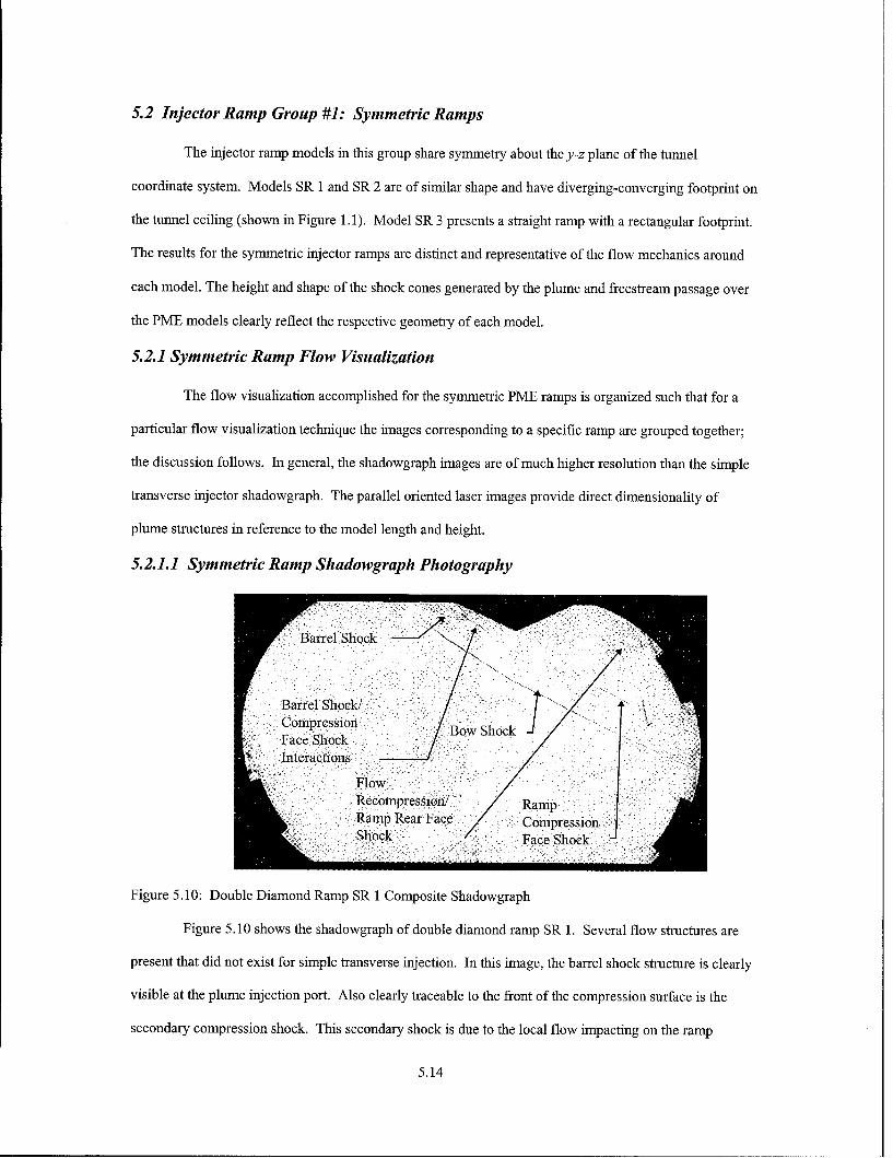
5.2 Injector Ramp Group #1: Symmetric Ramps
The injector ramp models in this group share symmetry about the y-z plane of the tunnel
coordinate system. Models SR 1 and SR 2 are of similar shape and have diverging-converging footprint on
the tunnel ceiling (shown in Figure 1.1). Model SR 3 presents a straight ramp with a rectangular footprint.
The results for the symmetric injector ramps are distinct and representative of the flow mechanics around
each model. The height and shape of the shock cones generated by the plume and freestream passage over
the PME models clearly reflect the respective geometry of each model.
5.2.1 Symmetric Ramp Flow Visualization
The flow visualization accomplished for the symmetric PME ramps is organized such that for a
particular flow visualization technique the images corresponding to a specific ramp are grouped together;
the discussion follows. In general, the shadowgraph images are of much higher resolution than the simple
transverse injector shadowgraph. The parallel oriented laser images provide direct dimensionality of
plume structures in reference to the model length and height.
5.2.1.1 Symmetric Ramp Shadowgraph Photography
Barrel Shock
Barrel Shock!Comrpression Bow ShockFace ShockInteractions
FlowRecompression ,/ RampRamp Rear Face ComipressionShock .Face Shock
Figure 5.10: Double Diamond Ramp SR 1 Composite Shadowgraph
Figure 5.10 shows the shadowgraph of double diamond ramp SR 1. Several flow structures are
present that did not exist for simple transverse injection. In this image, the barrel shock structure is clearly
visible at the plume injection port. Also clearly traceable to the front of the compression surface is the
secondary compression shock. This secondary shock is due to the local flow impacting on the ramp
5.14
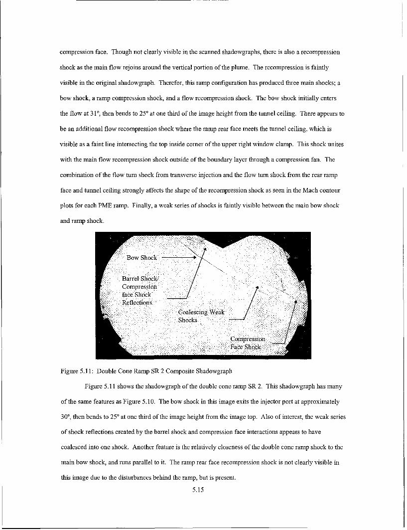
compression face. Though not clearly visible in the scanned shadowgraphs, there is also a recompression
shock as the main flow rejoins around the vertical portion of the plume. The recompression is faintly
visible in the original shadowgraph. Therefor, this ramp configuration has produced three main shocks; a
bow shock, a ramp compression shock, and a flow recompression shock. The bow shock initially enters
the flow at 310, then bends to 250 at one third of the image height from the tunnel ceiling. There appears to
be an additional flow recompression shock where the ramp rear face meets the tunnel ceiling, which is
visible as a faint line intersecting the top inside comer of the upper right window clamp. This shock unites
with the main flow recompression shock outside of the boundary layer through a compression fan. The
combination of the flow turn shock from transverse injection and the flow turn shock from the rear ramp
face and tunnel ceiling strongly affects the shape of the recompression shock as seen in the Mach contour
plots for each PME ramp. Finally, a weak series of shocks is faintly visible between the main bow shock
and ramp shock.
Bow Shock
Barrel Shock!Compression >4
face ShockReflections
Coalescing WeakShocks
CompressionFace Sh~ock
Figure 5.11: Double Cone Ramp SR 2 Composite Shadowgraph
Figure 5.11 shows the shadowgraph of the double cone ramp SR 2. This shadowgraph has many
of the same features as Figure 5.10. The bow shock in this image exits the injector port at approximately
300, then bends to 250 at one third of the image height from the image top. Also of interest, the weak series
of shock reflections created by the barrel shock and compression face interactions appears to have
coalesced into one shock. Another feature is the relatively closeness of the double cone ramp shock to the
main bow shock, and runs parallel to it. The ramp rear face recompression shock is not clearly visible in
this image due to the disturbances behind the ramp, but is present.
5.15

For both Figures 5.10 and 5.11, the three dimensional relieving effect is obvious. In two
dimensional flow, two objects inclined at the same angle (here the plume and the ramp compression face)
should produce different shock angles. In particular, the two-dimensional shock should be at a larger angle
than the three-dimensional due to the local flow behind the two-dimensional shock being slower than the
global freestream. For both the double diamond ramp and the double cone ramp, the ramp compression
shock is nearly parallel to the bow shock of the plume. Thus the three dimensional relieving effect was
achieved, which allows the compression face shock to lie at a lower angle than it would in a two
dimensional situation. The closer position of the secondary shock for the double cone ramp confirms a
slightly higher degree of three dimensional relieving than seen for the double diamond ramp.
Plume Bow Shock '
Barrel Shock And RampCompression Face ShockInteraction
FlowRecompression
Shock
Figure 5.12: Double Ramp SR 3 Composite Shadowgraph
Figure 5.12 is the shadowgraph of the double ramp, SR 3. Here the plume bow shock and ramp
compression shock coalesce into basically one structure by the vertical midpoint of the test section. The
bow shock of the plume enters the flow at approximately 33', then turns to 250, similar to the simple
transverse injection bow shock, Figure 5.1. The angle of the double ramp compression shock is
approximately 35'. This indicates the desired two-dimensional effect was achieved with this ramp. The
5.16

ramp rear face recompression shock is more clearly visible in this image than the previous two as a dark
line coalescing from a boundary layer Mach wave fan and passing slightly above the inner top corner of the
upper right window clamp.
5.2.1.2 Symmetric Ramp Parallel Oriented Images
As previously noted, the instantaneous images are best for capturing the unsteady nature of the
plume vortex structures. The time-averaged images are useful for describing the flow structures, but also
can provide insight into the PME ramp-plume interactions. These images are scaled to 125% of actual
size.
Figure 5.13: Double Diamond Ramp SR 1, Instantaneous Parallel Oriented Laser Image
Figures 5.13 and 5.14 are the instantaneous and time-averaged parallel oriented laser sheet images
for the double diamond ramp. In Figure 5.13 the plume exit barrel shock structure is visible, as well as a
lift-off from the magnus effect between the counter-rotating vortex cores and the ramp compression face.
These features are visible in the time-averaged image, Figure 5.14, though the lift-off effect is partially
obscured by accumulated surface flow of the injectant seed. Immediately below the barrel shock, the
plume foldover region and axial vortex development are visible. Beyond the foldover region, the plume
can be seen to form into a regular helical vortex pattern.
5.17

Figure 5.14: Double Diamond Ramp SR 1, Time-Averaged Parallel Oriented Laser Image
A significant difference between the two images is the width of the injectant plume. In Figure
5.13, the instantaneous image, the barrel shock appears to dwarf the plume vortex region in width. In
Figure 5.14, the time-averaged image, the width of the plume is approximately the same as the barrel
shock. These effects are a result of the exposure time used for each type of image, where the unsteady
flow structures are effectively frozen in the instantaneous image, and smeared in the time-averaged image.
In comparison to the instantaneous and time-averaged parallel oriented images in section 5.1.1.2,
the primary difference of the double diamond ramp images is the level of seed injected with the plume.
The overall shape and tapering trend of the time averaged simple transverse injection and the double
diamond ramp images are similar, with the exception of the slightly greater penetration achieved by the
double diamond ramp plume.
Visible in Figure 5.14 is the general trajectory trend of the double diamond ramp plume. In
particular, the plume can be seen to have a relatively flat trajectory downstream of the ramp rear face. The
flat tail trajectory of the double diamond ramp is similar to the tail trajectory of simple transverse injection.
The double diamond ramp plume also tapers evenly from the upper and lower boundaries due to the vortex
stripping of the plume centerline injectant to the plume periphery.
5.18

Figures 5.15 and 5.16 show the instantaneous and time-averaged parallel oriented laser images for
the double cone ramp, SR 2. In Figure 5.15, the plume was lightly seeded relative to the other images.
The effect of the light seed concentration is a highlight of the flow structures edges. In particular, the flow
injection barrel shock is clearly outlined, as well as the surface flow accumulation around the barrel shock.
Figure 5.15: Double Cone Ramp SR 2, Instantaneous Parallel Oriented Laser Image
An additional feature visible in Figure 5.16 is surface flow particles exiting the double cone vertex
and spreading behind the ramp towards the tunnel ceiling. The bright spot on the ramp rear surface
immediately behind the ramp vertex indicates a small recirculation zone is present. In a combustor
application, this location could potentially be used for a flameholder.
The plume trajectory visible in Figure 5.16 shows a slight trend back towards the tunnel ceiling.
Overall, the plume trajectory from the injector exit to the right side edge of the laser sheet follows a
parabolic path. The intensity decay observable towards the rear of the plume indicates the vortices are
effectively dispersing the centerline seed particles to the plume periphery.
5.19

Figure 5.16: Double Cone Ramp SR 2, Time-Averaged Parallel Oriented Laser Image
Figure 5.17: Double Ramp SR 3, Instantaneous Parallel Oriented Laser Image
Figures 5.17 and 5.18 show the instantaneous and time-averaged parallel oriented laser images for
the double ramp, SR 3. Visible in Figure 5.17 is a clear separation between the plume and the double ramp
compression face. This indicates the broad, flat compression face enabled a magnus effect lift-off from the
5.20

ramp to enhance local penetration. In Figure 5.18, the magnus effect separation is partially obscured by
accumulated surface flow seed particles, but still visible in the bright central core of the plume.
A feature of interest captured in Figure 5.17 is the wider spacing of the vortex helical structure
when compared to Figure 5.2 for simple transverse injection. For the same time scale in Figure 5.17 and
5.2, the increase in spacing for the double ramp is a direct decrease in vorticity and rotational velocity. The
only vortex enhancing feature in the geometry of the double ramp is baroclinic torque from the ramp
compression face. The decrease in vorticity from simple transverse injection for the double ramp is
directly related to the strong two-dimensional expansion associated with the ramp vertex.
Figure 5.18: Double Ramp SR 3, Time-Averaged Parallel Oriented Laser Image
Figure 5.18 shows the overall plume trajectory trend. The double ramp plume closely follows the
simple transverse injection plume, Figure 5.3. The centerline tail of the plume for the double ramp tapers
evenly from the upper and lower plume boundaries, and has a relatively flat profile after the ramp vertex.
Also visible in Figure 5.18 are large seed particles shed off of the ramp vertex and rear face, as a result of
surface flow over the ramp faces accumulation.
5.2.1.3 Symmetric Ramp Cross Flow Oriented Images
5.21

Figure 5.19: Double Diamond Ramp SR 1, Time-Averaged Cross Flow Oriented Laser Image
Figure 5.19 shows the double diamond ramp SR 1 time-averaged cross flow oriented laser image.
This image clearly depicts the crescent shaped injected seed plume similar to Figure 5.5 for the simple
transverse injection. The action of the plume vorticity on the plume centerline concentration of seed
particles has resulted in a fairly even distribution of the image intensity, indicating even mixing throughout
the crescent structure.
Figure 5.20 shows the double cone ramp SR 2 time-averaged cross flow oriented laser image. The
crescent profile observed in Figure 5.5 for simple transverse injection is visible, though two differences are
apparent for the double cone ramp image. The first is the approximately 150 rotation of the plume in the
counterclockwise direction. There is no defect or asymmetry in the double cone injector ramp to have
induced this rotation, which was observed during two separate test runs.
5.22

Figure 5.20: Double Cone Ramp SR 2, Time-Averaged Cross Flow Oriented Laser Image
The second difference between the double cone ramp cross flow image and the simple
transverse injection is the degree of particles concentration in the plume center. The double ramp plume
center is relatively clouded with seed particles compared to simple transverse injection, while the bottom of
the crescent is noticeably thicker than the crescent bottom of simple transverse injection. The clouding of
the plume center is most likely due to the surface flow particles that have spread off the double cone
vertex, seen in Figure 5.16.
Figure 5.21 shows the double ramp SR 3 time-averaged cross flow oriented laser image. Similar
to the double cone, the crescent profile observed in Figure 5.5 for simple transverse injection is still visible.
However, the differences for the double ramp from the simple transverse injection are increased. The
double ramp cross flow image has a greater degree of particle concentration in the plume center than the
simple transverse injection. The bottom of the crescent is also noticeably thicker than the crescent bottom
of simple transverse injection. Thickening of the crescent bottom is a result of the ramp expansion
reduction of vorticity, which lessens the amount of tunnel ceiling boundary layer drawn into the plume
core. Without the vortical action drawing the boundary layer into the plume core and distributing the
injected seed around the plume boundary, the injected seed remains concentrated in the plume center.
5.23

Figure 5.21: Double Ramp SR 3, Time-Averaged Cross Flow Oriented Laser Image
Also visible in this image is a greater separation from the tunnel ceiling for the double ramp
plume than the simple transverse injection cross flow image, Figure 5.5. The separation of the plume
bottom and the laser reflection from the tunnel ceiling for the double ramp is approximately twice the
separation of the simple transverse injection.
5.24

5.2.2 Symmetric Ramp Mach Contour Plots
Mach #
3.27 A 3.1112 jD-- 4 3.0212--A2.932
Plme 2,842
2,753"fCrescent, .5
2.6634- 2.574
~2,484Main Flow 2.395
y/d 6 Ramp Recompression 2.305./ 6 Rm Shock 2.216
Compression 2.126FaceShock !2.037
0 t ¢ 1.9478 - _ - 1.858
1.768e)- -1.679
10 -, Plume Bow c1 .510 C} .. l" - "-,Shock1.
-4 -2 0 2 4z/d
Figure 5.22: Double Diamond Ramp SR 1 Mach Contour Plot
The Mach contour plot for the double diamond ramp SR 1 is shown in Figure 5.22. The structures
observed in this plot correlate exactly with the observations made in the flow visualization. Aside from the
usual shock and flow structures observed in figure 5.6 for simple transverse injection, there are several
unique features of this plot. First, the main flow recompression shock is clearer than observed for the bank
injection. The recompression shock has taken on a distinctively triangular appearance as opposed to the
more rounded profile of the simple transverse injector. Through the turn combination described in section
5.2.1.1, the main flow recompression shock is strengthened from that seen for the simple transverse
injector and the shape of the PME ramp is reflected. The main flow recompression shock also does not
penetrate as far into the freestream aty/d of 5.4 as the simple
5.25

transverse flow recompression shock, at y/d of six. All of these effects described on the flow
recompression shock are a result of the ramp geometry, which creates a three dimensional relieving effect
as the flow turns away from the ramp rear faces and the tunnel ceiling. Second, the plume core has the
previously observed crescent shape, which is nearly identical to the seeded portion of the plume in Figure
5.19. However, the vortex cores are not as obvious as those in the simple transverse injection. The vortex
structures appear to have been weakened by the expansion created as the plume passes from the rising front
face to the declining rear face. Third, there is an additional shock that is barely distinguishable from the
plume bow shock at the image bottom. This is the ramp compression shock, which is almost coincidental
with the injection plume bow shock. The lack of resolution between the two shocks is due to the spreading
effect the 100 cone-static probe has when passing through shock waves. The ramp compression face shock
is relatively weak due to the masking effect of the plume bow shock, which meets one of the objectives for
this model.
2 Mach #
2.7095y/d 2.7040
3 2.68112.6781
4
-2 -1 0 1 2z/d
Figure 5.23: Double Diamond Ramp SR 1 Area Contour Plot
Figure 5.23 depicts the Mach contours representing the plume area as determined by the four
methods outlined in section 4.3. The top and bottom lines represent the modified search boundaries to
avoid counting shock and boundary layer structures as part of the plume. In general, the freestream local
5.26

Mach numbers and the Mach contours for the plume area are lower than the simple transverse injection,
Figure 5.7. The area contours show relatively close agreement with the exception of the positive z/d side
of the plot. The plume areas and centroids determined by the four methods is summarized in Table 5.2
TABLE 5.2DOUBLE DIAMOND RAMP AREA AND CENTROID RESULTS
Area Method 95% Freestream Mach Area (cm2) Centroid (y/d)
Graphical 2.70 1.09 2.20
Box 2.71 1.10 2.19
Modified Box, y/d=1.2 2.68 1.01 2.17
Modified Box, y/d=1.6 2.68 0.99 2.16
Average 2.69 1.05 2.18
The results for the double diamond ramp plume area vary by 9% from highest to lowest. The
agreement in the double diamond ramp area results is 2.5% worse than the plume area agreement for
simple transverse injection. Comparing Figures 5.22 and 5.23, the four area determination methods appear
to have used too high a Mach number in determining the plume boundary, which results in capturing part
of the tunnel ceiling boundary layer and the local freestream as part of the double diamond ramp plume.
The double diamond ramp plume centroid results are in better agreement, varying less than 2% from
highest to lowest. In comparison to Table 5.1, the average double diamond ramp plume area is 9% larger
than the simple transverse injection plume area. Also, the average double diamond ramp plume centroid is
6% further into the freestream than the simple transverse injection plume centroid. Depending upon the
method used, the double diamond ramp plume area may be artificially enlarged by inclusion of non-plume
structures. The double diamond ramp plume centroid results are consistent enough to show greater
independence from the method used than the plume area.
Figure 5.24 shows the Mach contour plot for the double cone ramp SR 2. The flow patterns
observed in the double cone ramp Mach contour plot are similar to those observed for the simple transverse
injection, Figure 5.6. There are several interesting exceptions. The first is the plume vortex core, which
differs by having one large elliptical core as opposed to separate vortex cores observed for
5.27

simple transverse injection. This may be the result of vortex degeneration due to the strong expansion the
plume passes through from the ramp front to rear faces.
Mach #3.2~3.111
3.0212.932
_\_5 2.842
2.7532.663
4 Q 2.574Plume Single 2.484
Flow jElliptical 2.395
Recompression Vortex Core 2.305~2.216
2.1262.037,Ramp Plume Bow Shock 1.947
8 Compression 1.858cSh ock 1.76% :::: - , - .. .> . ... ,-1.679
-- -. _ 1.589
-4 -2 0 2 4z/d
Figure 5.24: Double Cone Ramp SR 2 Mach Contour Plot
A second feature that distinguishes the double cone ramp Mach contour plot from that of simple
transverse injection is the ramp face compression shock. This shock was observed lying nearly parallel to
the plume bow shock in the double cone ramp shadowgraph, Figure 5.11, indicative of the three-
dimensional relieving effect achieved with the conical compression face. Third, the double cone ramp flow
recompression shock is more coherent but penetrates less than the simple transverse injection flow
recompression shock. The double cone ramp flow recompression shock reaches its maximum height aty/d
of 5.2, compared to six for simple transverse injection.
Figure 5.25 shows the plume area Mach contours of each area determination method for the
double cone ramp. The modified search boundaries to exclude the tunnel ceiling boundary layer and
5.28

shock structures are indicated. The double cone ramp area contours show close agreement, similar to
simple transverse injection. Table 5.3 summarizes the double cone ramp plume area and centroid results
by method.
2 Mach#
2.6446y/d 2.6422
3 -2.62782.6161
4I ,.,,I r I I
-2 -1 0 1 2z/d
Figure 5.25: Double Cone Ramp SR 2 Area Contour Plot
TABLE 5.3DOUBLE CONE RAMP AREA AND CENTROID RESULTS
Area Method 95% Freestream Mach Area (cm 2i) Centroid (y/d)
Graphical 2.64 0.99 2.09
Box 2.64 0.98 2.10
Modified Box, y/d= 1.2 2.61 0.90 2.11
Modified Box, y/d=1.6 2.63 0.94 2.10
Average 2.63 0.95 2.10
The results for the double cone ramp plume areas and centroids vary by 6% and less than 1%
respectively from highest to lowest. Both modified box methods result in lower area Mach number
contours due to inclusion of some tunnel boundary layer regions in the local freestream calculation (recall
the modified box methods do not use a rejection criteria). The centroids are in excellent agreement, which
indicates the double cone ramp plume contours are highly concentric. The different Mach contours
5.29

selected by the four area determination methods therefore are simply different depths of the same plume
structure, analogous to peeling an onion.
A comparison to Table 5.1 reveals the double cone ramp plume average area is 5% smaller than
the simple transverse injection plume average area. The average double cone ramp plume centroid is 2%
further into the freestream than the simple transverse injection plume average centroid. The lower area and
approximately same centroid penetration between the double cone ramp and simple transverse injection
indicates that whatever magnus effect lift-off from the ramp surface occurs is negated by the plume
expansion around the front to rear faces of the double cone ramp. The double cone ramp design was also
not intended to enhance vorticity, so the negative effect of expansion on the vortex structures results in
vortex core breakdown.
Figure 5.26 shows the Mach contour plot for the double ramp SR 3. The vortex core of the
double ramp differs substantially from the simple transverse injection vortices. The vortex core region is
nearly circular, and appears more as a streamtube into the page than a twin vortex core system. The strong
two-dimensional expansion from front to rear of the double ramp has resulted in significant vortex
structure breakdown. A similar indication of the vortex breakdown was observed in section 5.2.1.3, Figure
5.17.
The flow recompression for the double ramp shock reflects the frontal profile of the double ramp.
The double ramp flow recompression shock has a relatively flat midsection, and steeper sloped sides. This
pattern, the flow shock reflecting the frontal profile of the PME ramp, is observable in all of the PME ramp
Mach contour plots.
5.30

Mach #~3.2
3.111
3.0212.932
-"Boundary Layer 2.8422.753
2.574
2.4842 Single Circular 2.395y / 6 Recompression2.0y/d 6 Vortex Core 2.305
t2.216
2.037
8 Combined Plume , (4F 1.947Bow Shock And 1.8Ramp Compression - 1.768
1.6791o -1.589
-4 -2 0 2 4z/d
Figure 5.26: Double Ramp SR 3 Mach Contour Plot
The two-dimensional aspect of the double ramp is observed in the combined bow shock
and ramp compression face shock. The masking effect achieved by the plume bow shock for the double
ramp compression face is substantially greater than the effect achieved for the previous two symmetric
ramps. At the mean flow measurement location of x/d = 20, the two shocks have become collinear. The
strength of the combined bow plume and compression face shocks, indicated by the Mach contour levels, is
stronger than the simple transverse injection, Figure 5.6.
Annotated in Figure 5.26 is a unique structure identified as the boundary layer surge. This flow
structure appears to be ramp generated vorticity from the double ramp. Since the double ramp at 4 d is
relatively wide compared to the developing plume, a magnus effect lift-off was expected from the broad
compression face. The double ramp compression face also acts as a ramp spillage vortex generation device
with the main flow passing around the plume and along the ramp side. Due to the width of the
5.31

double ramp, the vortices generated by ramp spillage are separated far enough apart to prevent a magnus
effect lift-off from developing. Ramp spillage vorticity essentially forms in the tunnel ceiling boundary
layer, where the separation of the vortex cores prevents migration away from the wall. The boundary layer
surge created by the ramp spillage vorticity does not appear to enhance mixing.
2 Machb#2.6391
y/d 2.6121
3 2.61162.6029
-2 -1 0 1 2z/d
Figure 5.27: Double Ramp SR 3 Area Contour Plot
Figure 5.27 shows the results of the area determinations for the double ramp. These contours are
on average 0.9 Mach lower than the contours for simple transverse injection, Figure 5.7. Three of the
methods are in excellent agreement. The fourth, the box method, selected a higher Mach contour for area
based upon the tunnel ceiling boundary layer rejection Mach criteria detailed in section 4.3.1.2. Despite
the difference in the plume boundary Mach contour, the four methods all capture the same basic plume
shape. Table 5.4 summarizes the area and centroid results by method for the double ramp.
5.32

TABLE 5.4DOUBLE RAMP AREA AND CENTROID RESULTS
Area Method 95% Freestream Mach Area (cm 2) Centroid (y/d)
Graphical 2.60 0.68 2.61
Box 2.64 0.77 2.65
Modified Box, y/d=1.2 2.61 0.71 2.63
Modified Box, y/d=1.6 2.61 0.69 2.62
Average 2.62 0.72 2.63
The variation between methods from highest to lowest is 12% for the areas and 1.5% for the
centroids. The disparity in the area computations is a result of the higher plume boundary Mach number of
the box method. The centroid results are in good agreement, indicating again that the area results have
found different concentric layers of the same flow structure.
The average plume area for the double ramp is 30% lower than the simple transverse injection
average area. The average centroid height for the double ramp is 28% greater than the average centroid of
the simple transverse injection. These results are not necessarily contradictory. The plume area defined
from the Mach contours measures the size of the plume vortex structures, not concentration or injectant
dispersion. Compared to simple transverse injection, the double ramp area results indicate the vorticity of
the plume has been diminished substantially. However, penetration was clearly enhanced by a magnus
effect lift-off from the ramp face.
5.2.3 Symmetric Ramp Total Pressure Loss
TABLE 5.5SYMMETRIC RAMP GROUP TOTAL PRESSURE LOSS
PME Ramp Average Total 1H
Pressure Ratio
Double Diamond Ramp, SR 1 1.29 0.95
Double Cone Ramp, SR 2 1.36 0.91
Double Ramp, SR 3 1.49 0.83
Table 5.9 describes the total pressure losses for the extended ramp group based upon the average
total pressure loss ratio. The results reflect the frontal profiles of the respective ramps. The double
5.33

diamond ramp, SR 1, has the lowest frontal area presented to the flow, resulting in less obstruction and
relatively weaker shocks than the progressively larger aspect double cone ramp and double ramp.
5.2.4 Symmetric Ramp Digital Image Quantitative Analysis
Figures 5.28 to 5.33 are plots of the plume centerline trajectories and centerline intensity decay for
symmetric ramps SR 1, SR 2 and SR 3. These plots are oriented as horizontal mirror images of the original
plume images, where y/d of zero is the tunnel ceiling.
6
5-
4
y/d 3 --
I~ . . . 1111 '1 .. II ' ' . . . .... .. .... ..
2
0
0 2 4 6 8 10 12 14 16
x/d
Figure 5.28: Double Diamond Ramp SR 1 Plume Centerline Trajectory
Figure 5.28 is the centerline trajectory plot of the double diamond ramp, SR 1. The lower trace
represents the inner plume boundary on the tunnel ceiling side and the higher trace is the plume outer
boundary penetration into the freestream. At x/d of 4.07 a large spike is visible, resulting from a single
seed particle approximately 10 d into the freestream. This single seed particle has a negligible effect on the
centerline trajectory, which is an average of all points at the measurement plane above the threshold
intensity level described in section 4.4.1.1.
The slope of the first eight centerline data points tracks the trajectory of the plume in contact with
or directly below the compression ramp face, and provides a measure of the lift-off effect achieved
5.34

from the compression face. For the double diamond ramp, the slope of the first eight data points is 0.34.
This slope is a 48% increase over the first eight point slope for simple transverse injection. The maximum
y/d penetration of the plume centerline is 3.53 at x/d of 12.2, compared to y/d of 3.32 at x/d of 9.78 for the
simple transverse injection centerline maximum penetration. An enhancement in penetration was achieved
with the faceted face
1.4
1.2
1
.u 0.8
0.6
0.4
0.2
0 2 4 6 8 10 12 14 16 18
x/d
Figure 5.29: Double Diamond Ramp SR 1 Plume Centerline Average Intensity Decay
Figure 5.29 is the centerline average intensity decay plot of the double diamond ramp, SR 1. This
plot is similar in profile to the simple transverse injection centerline average intensity decay plot. The
overall slope of the double ramp intensity decay plot is -0.043, which is an 11% increase to the simple
transverse injection decay rate, -0.037. The higher decay rate indicates the injectant spreading to the
plume periphery is enhanced by the presence of the ramp.
Figure 5.30 is the centerline trajectory plot of the double cone ramp, SR 2. The variations of the
plume inner boundary represented by the plot bottom trace are due to the surface flow seed particles shed
by the ramp. The slope of the first eight data points of the double cone ramp centerline trace is 0.38, a 65%
increase over the simple transverse injection initial slope. The maximum centerline y/d penetration for the
double cone ramp occurs at x/d of 4.9, with ay/d value of 3.34. This maximum penetration height is
essentially the same as the simple transverse injection. However, for the double ramp the maximum
5.35
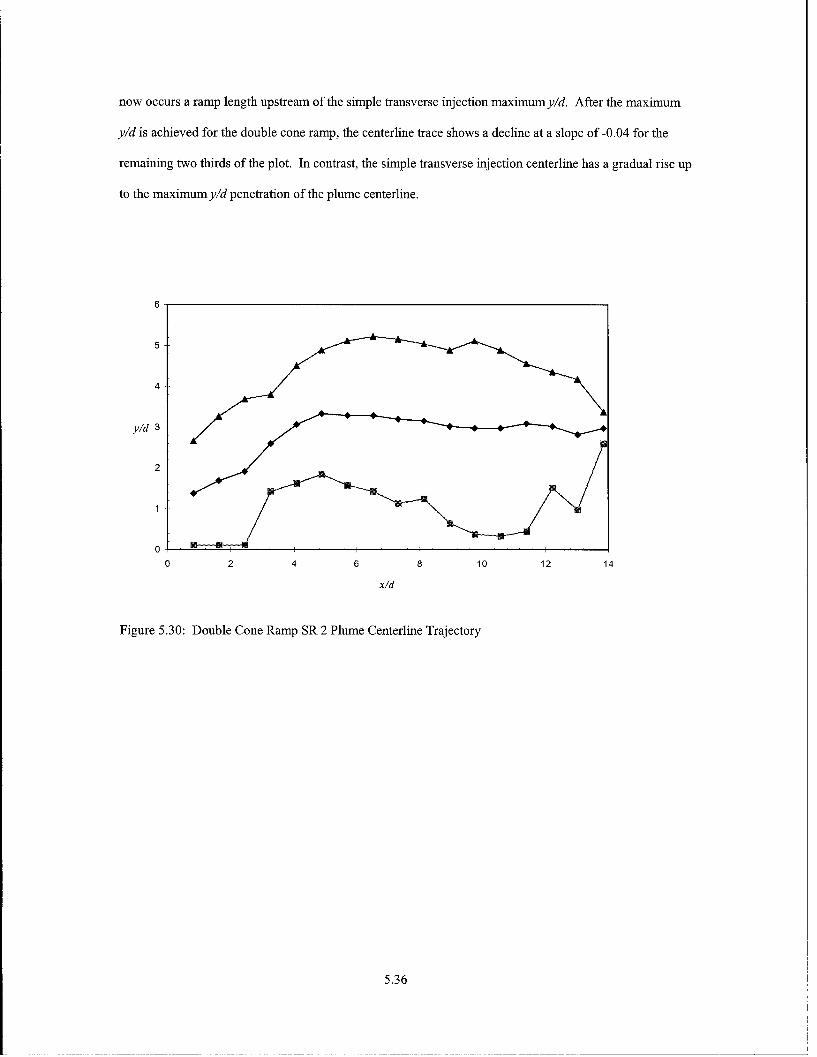
now occurs a ramp length upstream of the simple transverse injection maximum y/d. After the maximum
y/d is achieved for the double cone ramp, the centerline trace shows a decline at a slope of -0.04 for the
remaining two thirds of the plot. In contrast, the simple transverse injection centerline has a gradual rise up
to the maximum y/d penetration of the plume centerline.
6
5
4 -
y/d 3
2
00 2 4 6 8 10 12 14
x/d
Figure 5.30: Double Cone Ramp SR 2 Plume Centerline Trajectory
5.36
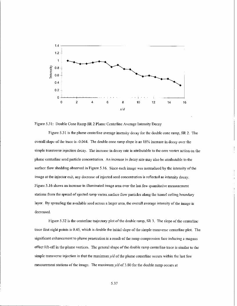
1.4
1.2
1
.t 0.8
0.6
0.4
0.2
0 I
0 2 4 6 8 10 12 14 16
x/d
Figure 5.31: Double Cone Ramp SR 2 Plume Centerline Average Intensity Decay
Figure 5.31 is the plume centerline average intensity decay for the double cone ramp, SR 2. The
overall slope of the trace is -0.044. The double cone ramp slope is an 18% increase in decay over the
simple transverse injection decay. The increase in decay rate is attributable to the core vortex action on the
plume centerline seed particle concentration. An increase in decay rate may also be attributable to the
surface flow shedding observed in Figure 5.16. Since each image was normalized by the intensity of the
image at the injector exit, any decrease of injected seed concentration is reflected as intensity decay.
Figure 5.16 shows an increase in illuminated image area over the last few quantitative measurement
stations from the spread of ejected ramp vertex surface flow particles along the tunnel ceiling boundary
layer. By spreading the available seed across a larger area, the overall average intensity of the image is
decreased.
Figure 5.32 is the centerline trajectory plot of the double ramp, SR 3. The slope of the centerline
trace first eight points is 0.45, which is double the initial slope of the simple transverse centerline plot. The
significant enhancement to plume penetration is a result of the ramp compression face inducing a magnus
effect lift-off in the plume vortices. The general shape of the double ramp centerline trace is similar to the
simple transverse injection in that the maximum y/d of the plume centerline occurs within the last few
measurement stations of the image. The maximum y/d of 3.80 for the double ramp occurs at
5.37

x/d of 13, compared to y/d of 3.32 at x/d 9.78 for simple transverse injection. The inner and outer plume
boundary traces show a similar convergence on the plume centerline trace as the simple transverse
injection, however, the plume inner and outer boundaries are slightly larger for the double ramp.
6
5
y/d 3
2
0
0 2 4 6 8 10 12 14 16
x/d
Figure 5.32: Double Ramp SR 3 Plume Centerline Trajectory
Figure 5.33 is the plume centerline average intensity decay for the double ramp, SR 3. The
overall slope of the trace is -0.05 1. The double ramp slope is an 37% increase in decay over the simple
transverse injection decay. Part of the increase in decay rate is attributable to the core vortex action on the
plume centerline seed particle concentration. However, the vortex core structures as measured in the area
contour plot for the double ramp, Figure 5.27, are significantly smaller than simple transverse injection.
Figure 5.18, the time-averaged parallel oriented laser image for the double ramp, shows considerable seed
spread between the plume inner boundary and the tunnel ceiling. Though not intense enough to affect the
plume centerline trajectory, the quantity of seed in the boundary layer does reduce the overall image
intensity.
5.38

1.4
1.2
1-
0.8
0.6
0.4
0.2
0 . II0 2 4 6 8 10 12 14 16
x/d
Figure 5.33: Double Ramp SR 3 Plume Centerline Average Intensity Decay
5.39

5.3 Injector Ramp Group #2: Extended Ramps
This PME ramp group was designed to test a modification to the simple ramp geometry by adding
a tapering extension beyond the compression face, Figure 1.2. Models ER 2 and ER 3 differ in ramp
sweep angle which results in a truncated trailing edge for ER 2 and a sharp trailing edge for ER 3. Model
ER 1 and the double diamond ramp SR 1 share the same compression face geometry. Instead of a
symmetric rear face like ramp SR 1, the extended diamond ramp ER 1 has an extension that crosses beyond
the mean flow measurement plane. As should be expected for such similar geometries, the results for
truncated ramp ER 2 and tapered ramp ER 3 share many features. PME ramp ER 1 provides interesting
qualitative results.
5.3.1 Extended Ramp Flow Visualization
The flow visualization results are presented as in section 5.2.1. For each PME ramp, the images
are organized by type, starting with shadowgraph photography. The salient features of the shadowgraphs
are highlighted and annotated. The parallel oriented and cross flow oriented laser planar images are next
examined.
5.3.1.1 Extended Ramp Shadowgraph Photography
.Barrel 'Shock
Intersection Shok
Shock,
Plume BowShock Ramp
Cdmpression
Face Shock
Figure 5.34: Extended Diamond Ramp ER 1 Composite Shadowgraph
In Figure 5.34, the plume bow shock is seen to start at approximately 330 and then turns to
approximately 250 as it descends through the top third of the image. The angles and locations of bends in
5.40

the bow shock are nearly identical to the simple transverse case, Figure 5.1. Since the flow is fully
supersonic in this region, there is no mechanism for the shape of the ramp behind the plume to be
broadcasted upstream and affect the bow shock shape. It is conceivable that the bow shocks would differ
further downstream as the ramp unique structure (shocks and expansions) interacted with the bow shock.
The limited height of the test section prevents these effects from being observed. This image also shows
several shock structures that are not seen in the simple transverse injection case, Figure 5.1. A shock can
be seen emerging from the base of the compression face. There is also a shock reflection where the barrel
shock and ramp compression face shock intersect. This shock is observable as a thin, weak line that
appears to intersect the bottom of the ramp compression face. These shock structures will provide
baroclinic torque to the plume and enhance the vorticity. A third shock annotated in Figure 5.34 as the
weak shock is unique to the extended diamond shadowgraph. The exact origin of the shock is not
observable because the ramp extension intersects the shock. The weak shock does not appear to be part of
the barrel shock-compression face reflection. A possible source for the weak shock is a recompression of
the plume. If the magnus lift-off effect is not substantial, components of the plume in the foldover region
(identified in the simple transverse instantaneous parallel oriented image, Figure 5.2) that curve back up
towards the tunnel ceiling would impinge upon the ramp extension creating the weak shock. The presence
of this shock therefor indicates the diamond ramp compression face does not enhance penetration
significantly from the simple transverse case. Another significant feature of this image is the apparent lack
of a downstream plume recompression shock. The missing recompression shock is logical since the large
extension prevents any area for the flow to coherently recompress around the plume, again confirming the
lack of a lift-off effect from this ramp configuration.
5.41

Barrel Shock
Plume BowTunnel ShockCeiling BReflection BarrelI
Shock!CompressionFace Reflection Compression
Face Shock.
Figure 5.35: Truncated Extended Ramp ER 2 Composite Shadowgraph
Figure 5.35 is the shadowgraph for the truncated extended ramp, ER 2. The bow shock angles
observed in this image are 330 at the origin, and 250 after the bend which results in an identical profile to
the one observed for the simple transverse injection, Figure 5.1. The ramp compression face shock and
barrel shock-compression face shock reflection are at slightly higher angles than the bow shock, which is
due to the two-dimensional effect of the flat compression face. These shocks eventually run into the bow
shock by the right edge of the image. Favorable baroclinic torque of some degree will be generated by the
plume passage through these combined shock structures. Also of interest in this image is the lack of a flow
recompression shock from the main flow passing over the rear edge of the ramp and turning towards the
tunnel ceiling. In this image the shock is not visible due to the separation region behind the ramp, which
disturbs the flow and obscures most flow structures. The lack of discernible flow features in the image
after the end of the ramp indicate the design achieved one of its objectives. The truncated trailing edge was
intended to provide a recirculation region as well as create an expansion before the flow passing around the
sides of extended ramp is shocked upon rejoining. The absence of a visible shock from the side flows
rejoining immediately downstream of the ramp rear face in the local region of the expansion confirms this
effect. In effect the expansion delays or weakens the shock created as the side flows rejoin. Since this
shock is nearly parallel to the plume, the alignment of the shock pressure gradient and the plume-air
interface density gradient may not be conducive to producing baroclinic torque. The tunnel ceiling
reflection was due to a minor misalignment in the shadowgraph light source.
5.42
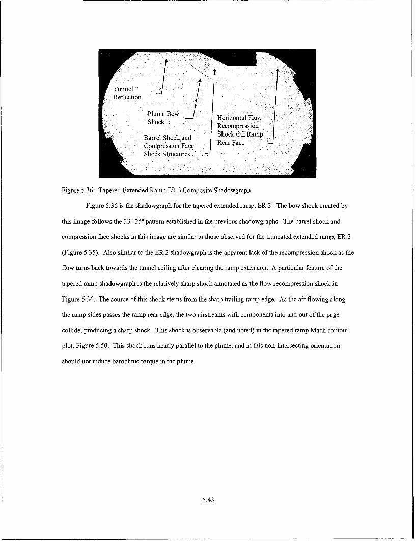
TunnelReflection
Plume Bow Horizontal FlowShock RecompressionShoc ShIok Off Ram
Barrel Shock andCompression Face RearFace
Shock Structures
Figure 5.36: Tapered Extended Ramp ER 3 Composite Shadowgraph
Figure 5.36 is the shadowgraph for the tapered extended ramp, ER 3. The bow shock created by
this image follows the 330-25' pattern established in the previous shadowgraphs. The barrel shock and
compression face shocks in this image are similar to those observed for the truncated extended ramp, ER 2
(Figure 5.35). Also similar to the ER 2 shadowgraph is the apparent lack of the recompression shock as the
flow turns back towards the tunnel ceiling after clearing the ramp extension. A particular feature of the
tapered ramp shadowgraph is the relatively sharp shock annotated as the flow recompression shock in
Figure 5.36. The source of this shock stems from the sharp trailing ramp edge. As the air flowing along
the ramp sides passes the ramp rear edge, the two airstreams with components into and out of the page
collide, producing a sharp shock. This shock is observable (and noted) in the tapered ramp Mach contour
plot, Figure 5.50. This shock runs nearly parallel to the plume, and in this non-intersecting orientation
should not induce baroclinic torque in the plume.
5.43

5.3.1.2 Extended Ramp Parallel Oriented Images
...: .. ...
Figure 5.37: Extended Diamond Ramp ER 1, Instantaneous Parallel Oriented Laser Image
Figure 5.38: Extended Diamond Ramp ER 1, Time-Averaged Parallel Oriented Laser Image
Shown in Figures 5.37 and 5.38 are the instantaneous and time-averaged parallel oriented laser
sheet images for the extended diamond ramp, ER 1. In both images, the full length of the ramp extension
is illuminated. What is immediately unusual about both if these images is the amount of plume visible
5.44

below the edge of the ramp extension. For all parallel oriented images, the laser sheet was oriented along
the model centerline. With such an orientation, only seed in the centerline plane should be illuminated.
However, there is considerable scatter off the sharp bottom edge of the diamond ramp extension.
Reflections off the sloped sides of the extension also give both images a three-dimensional aspect. This
indicates the laser sheet was either slightly off center or slightly wider than the vertex edge of the ramp
extension. The structure identified as the curved plume boundary is unique to ramp ER 1. The curved
plume boundary is most likely the outside of the plume after the plume foldover below the Mach disk.
This structure does not appear to be injectant seed surface flow on the model, as it was observed to occur
during all phases of the plume seeding (i.e., the curved boundary was observable before seed surface flow
could develop). The tail of the plume is seen to spread almost to the tunnel ceiling, which for this
geometry means that seed particles up to 2 d off the tunnel ceiling centerline are illuminated. The intensity
of the plume tail drops to background levels well before the illumination along the ramp bottom edge
decays, indicating the majority of the seed material has been moved out of the centerline plane by vortex
action.
Figure 5.39: Truncated Ramp Extended ER 2, Instantaneous Parallel Oriented Laser Image
5.45

Figure 5.40: Truncated Extended Ramp ER 2, Time-Averaged Parallel Oriented Laser Image
The instantaneous and time-averaged parallel oriented images for the truncated extended ramp ER
2 are shown in Figure 5.39 and 5.40 respectively. The instantaneous image captures a substantial magnus
effect lift-off away from the compression face of the ramp, which is blurred due to the exposure time and
surface flows in the time-averaged image, Figure 5.40. In Figure 5.40, the effect of the lift-off is visible in
the annotated core region of the plume. For either case, the magnus effect creates a local enhancement in
penetration. The presence of seed particles between the plume core and the truncated ramp compression
face results from surface flow on the ramp face, which accumulated during the length of the exposure. The
surface flows provide a small indication of the plume vorticity where visible on the ramp vertical sides.
Another exposure length related feature of the time-averaged image is the linear exiting of seed particles
from the bottom rear of the ramp. The truncated rear face of this particular ramp provides a recirculation
zone in which seed particles gather and shed. The seed particles are shed along a streamline that is
approximately 180. This streamline is located in the center of the vortex pair, which draw the ramp rear
face collected seed particles out into the freestream. In the region the exiting seed particles intersect the
main plume, the image intensity decreases as the bottom centerline plume injectant is distributed around
the plume periphery by vortex mixing action.
5.46

In comparison to the simple transverse injection case, Figures 5.2 and 5.3, both images of the
truncated extended ramp ER 2 show a significant bend of the plume centerline back towards the tunnel
ceiling. In Figure 5.39, a line is fitted to the plume to indicate the bend in the plume and flow back
towards the tunnel ceiling after clearing the end of the ramp. This bending indicates that the overall plume
trajectory may be bending back towards the tunnel ceiling after passing through the vertically oriented
expansion fan formed along the bottom rear face of the extension.
To summarize the complicated aspects of the trailing edge flow, three distinct and separate effects
are visible in the time-averaged truncated extended ramp image, Figure 5.40. First, the collected seed
particles on the ramp rear face are drawn into the freestream by the counter-rotating vortex pair, at an angle
of 180. Second, the outer bottom edge seed concentration of the plume is drawn out of the centerline plane
by the vortex mixing action, resulting in a lower image intensity. Finally, the entire plume structure
appears to bend back to the tunnel ceiling after passing through the expansion off the extension's bottom
rear. Through the duct flow analogy presented in section 2.4, this bending should increase vorticity.
Figure 5.41: Tapered Extended Ramp ER 3, Instantaneous Parallel Oriented Laser Image
5.47

Figure 5.42: Tapered Extended Ramp ER 3, Time-Averaged Parallel Oriented Laser Image
Figures 5.41 and 5.42 show the instantaneous and time-averaged parallel oriented images for the
tapered ramp. Features similar to the truncated extended ramp flow images include an early magnus effect
lift-off from the ramp compression face, which results in a greater penetration than seen in the simple
transverse case. Also, surface flow is visible on the compression ramp face, as well as injectant collecting
along the rear edge of the ramp. The plume centerline trajectory is indicated in Figure 5.41, with a bend
observable as the plume passes by the ramp rear edge. There are differences between the images that are
of interest. The injectant exit angle (created by the center of the vortex pair drawing accumulated seed
particles, shown in Figure 5.42) is 110. The bend in the plume trajectory in this image appears less than the
bend observed in the truncated extended ramp. The flow passing under the rear edge of the ramp can only
expand over a thin edge instead of a broader truncated edge, which will result in a weaker expansion and
less plume turning back towards the tunnel ceiling. The lesser bend incurred by the weaker expansion of
the tapered extended ramp results in weaker duct flow induced vorticity, and hence a slighter injectant exit
angle off of the ramp rear edge
5.48
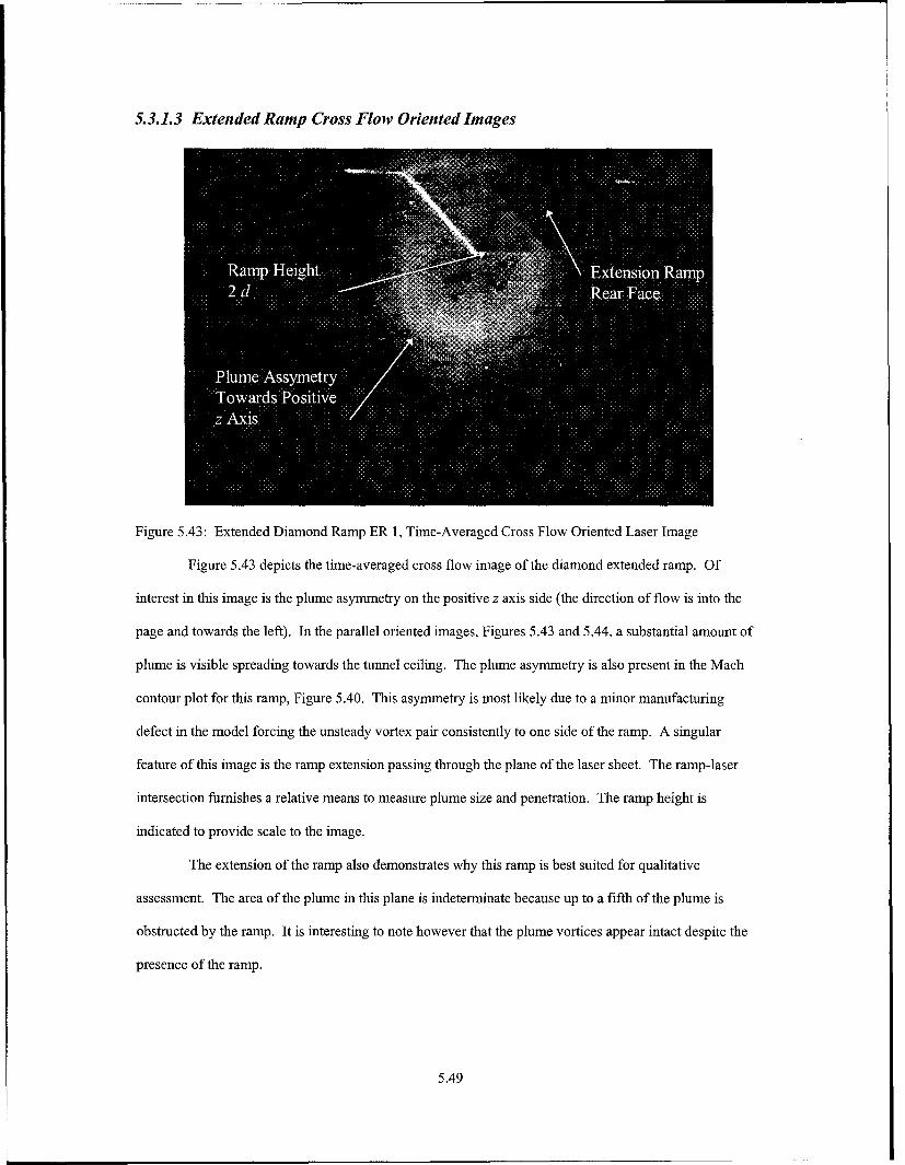
5.3.1.3 Extended Ramp Cross Flow Oriented Images
Figure 5.43: Extended Diamond Ramp ER 1, Time-Averaged Cross Flow Oriented Laser Image
Figure 5.43 depicts the time-averaged cross flow image of the diamond extended ramp. Of
interest in this image is the plume asymmetry on the positive z axis side (the direction of flow is into the
page and towards the left). In the parallel oriented images, Figures 5.43 and 5.44, a substantial amount of
plume is visible spreading towards the tunnel ceiling. The plume asymmetry is also present in the Mach
contour plot for this ramp, Figure 5.40. This asymmetry is most likely due to a minor manufacturing
defect in the model forcing the unsteady vortex pair consistently to one side of the ramp. A singular
feature of this image is the ramp extension passing through the plane of the laser sheet. The ramp-laser
intersection furnishes a relative means to measure plume size and penetration. The ramp height is
indicated to provide scale to the image.
The extension of the ramp also demonstrates why this ramp is best suited for qualitative
assessment. The area of the plume in this plane is indeterminate because up to a fifth of the plume is
obstructed by the ramp. It is interesting to note however that the plume vortices appear intact despite the
presence of the ramp.
5.49

Figure 5.44: Truncated Extended Ramp ER 2, Time-Averaged Cross Flow Oriented Laser Image
Shown in Figure 5.44 is the cross flow oriented image for the truncated extended ramp, ER 2.
The plume cross section has the general crescent shape observed for the simple transverse injection case in
Figure 5.5. However, two differences are observable from the simple transverse injection case. First, there
is a possible second set of counter rotating vortex cores generated from the flow spillage on the ramp and
extension. Instead of the uniform, evenly tapering crescent shape seen along the inside periphery of the
simple transverse injection case, this plume cross section has two opposing structures that appear to be
slightly drawn into the center of the plume. This would result from two vortices stacked on top of each
other with the same spin direction. Directly below the arrow pointing to the possible ramp generated core
is the most visible of these structures.
A second difference in the truncated extended ramp image from the simple transverse cross flow
image is the relatively bright region in the plume center bottom. This bright region reflects a relatively
high injectant concentration and is a result of the stream of particles exiting the ramp rear surface being
convected to the bottom of the plume by the counter rotating vortices. Figure 5.40 shows the particle
stream exiting the ramp rear face at approximately 180, which would intersect the outer bottom of the
plume by the x/d of 20 station where these images were acquired. Once the particles enter the bottom
5.50

center portion of the crescent, they would remain there until dispersed by the vortices to the plume
periphery.
Figure 5.45: Tapered Extended Ramp ER 3, Time-Averaged Cross Flow Oriented Laser Image
Figure 5.45 shows the cross flow oriented image for the tapered extended ramp, ER 3. This image
is basically identical to the simple transverse case with the exception of a slight concentration rise in the
bottom center of the crescent shape. The slight increase in concentration is due to the surface flow seed
particles collecting at and shedding off the tapered ramp rear edge. From Figure 5.36 the angle of the
particle shedding is 110, which would intersect the plume crescent boundary by the measurement plane of
this image. The relative intensity of the high concentration region (in comparison to the rest of the plume
intensity) is lower in the tapered ramp image than the truncated ramp image high concentration region,
Figure 5.44. The reason for this is the thin trailing edge of the tapered ramp provides a much more limited
area for the seed particles to collect and shed than the broader rear face of the truncated ramp.
5.51

5.3.2 Extended Ramp Mach Contour Plots
Mach #~3.2
3.1112z --- 3.021
2.932, 2.842
2.7534. - 2.663
.2.574V 2.484
\6Plume Vortex 2.395y/d 6 2.305
2.216'A ,2.126
8: 1.9471.858
Plume Bow - . 1.768{ Shock 1.59!' LV' 1.58
-4 -2 0 2 4z/d
Figure 5.46: Extended Diamond Ramp ER 1 Mach Contour Plot
Figure 5.46 is the Mach contour plot generated for the diamond extended ramp, ER 1. Several
interesting effects of the ramp extension are readily observable. First, the plume asymmetry noted in the
cross flow image, Figure 5.43, of this ramp is confirmed. The entire plume has migrated upwards to the
tunnel ceiling along the positive z axis side of the ramp. The twin vortex cores are still visible, though
highly distorted as compared to the usual circular shapes seen in the other PME ramp and the simple
transverse Mach contour plots. Second, a broad, flat shock is discernible, but incohesive. This is in sharp
contrast to the regular and continuous (albeit relatively weak) flow recompression shock observed for
simple transverse injection, Figure 5.6. This shock appears to be the weak shock identified in Figure 5.34,
which would intersect the pressure probe measurement plane at the height the Mach contour shock
intersects the tunnel centerline.
5.52

Another feature, or lack thereof, of interest is the ramp extension boundary layer. To capture the
flow field around the extension, the pressure probes were initially placed within one half of a probe
diameter from the extended ramp surface. Therefore, the probe measurements were 1/32 inches from the
ramp surface, which was still not close enough to capture the developing boundary layer on the ramp
extension. This provides an interesting contrast to the tunnel boundary layer, which is approximately 1/4
inches outside the region affected by the ramp.
In general, the flow field for the extended diamond ramp can best be described as disturbed. The
shock and vortex structures are incoherent and distorted. The enhancement in penetration from the simple
transverse injection case is solely due to the left side vortex being constrained physically by the ramp
vertex. Asymmetry has been introduced to the flow field, resulting in a consistent migration of the plume.
Magnus effects are not observed; to the contrary the plume-ramp extension interaction resulted in the
plume moving back towards the tunnel ceiling. These effects, as well as the inability to capture the entire
flow field near the ramp extension preclude the use of numerical analysis to estimate the plume size.
Shown in Figure 5.47 is the Mach contour plot of the truncated extended ramp, ER 2. This
contour plot contains numerous differences from the simple transverse injection Mach contour plot, Figure
5.6. First, the bow shock appears similar, but as seen from the truncated extended ramp shadowgraph,
Figure 5.35, these two shocks become collinear. This is due to the two-dimensional effect of the flat
compression face increasing the compression face shock angle enough to coincide with the bow shock by
y/d of 10, and is a feature common to all PME ramps with a flat compression face. The combined shock
structure is not significantly stronger than the singular bow shock of the simple transverse case, therefore
total pressure losses from the ramp compression face should be minimal.
5.53

Mach #
Rectangular 3.2/Vortex Core 3.111
2 )\III Separation 3.021/ ; Q/:--; ...... 2.932
2.8422.753
)U7 iI) 2.663
2.5742.484
Elongated 2.395
y/d 6 Vortex Core 2.305L Horizontal Flo ] 2.21Recopresio Vrtical Flow 2.126
ecompression Recompression 2.037'Soc 7: -$Shc 1.947
8 - -S ho ck 1 .8 5 8
1.768
., ,-. Combined Bow and 1.67910 Compression Face 1.589==, , -- ._,sShock 1.
-4 -2 0 2 4z/d
Figure 5.47: Truncated Extended Ramp ER 2 Mach Contour Plot
Second, the plume vortex cores are elongated vertically from the relatively circular vortex cores of
the simple transverse case. The vortex core elongations indicate the injection generated vortices and the
ramp spillage generated cores have combined into essentially one core, which meets one intended goal of
this particular ramp configuration.
Third, there is a distinctly rectangular separation between the plume cores that reflects the
geometry of the bottom rear edge of the truncated ramp extension. This region gives the impression that
the sharp turn around the ramp bottom rear edge in effect drove the injection generated vortices to either
side of the ramp and into the ramp spillage generated vortex structures. The splitting effect of the truncated
ramp extension was not anticipated as part of the ramp geometric concept.
Fourth, there are two layers of shocks around the plume, one below and one passing through the
plume center. The shock labeled as the vertical recompression shock is a feature common to the PME
ramp contour plots and the simple transverse injection. This shock is created by the airstream turning
5.54

around the ramp in the vertical plane of the flow and impinging on the tunnel ceiling behind the ramp. The
truncated extended ramp vertical recompression shock seen in Figure 5.47 is unique from the shocks
created by the PME ramps in the other two groups because it does not wrap completely around the model
to terminate on the tunnel ceiling. Instead, it reflects the geometry only of the front and top surfaces of the
truncated extended ramp model.
The second shock layer not previously observed is the horizontal flow recompression shock. The
origin of the horizontal recompression shock is the flow passing on either side of the ramp recombining
supersonically beyond the truncated ramp expansion region. This shock runs nearly parallel to the plume,
which would impart little baroclinic torque to enhance vorticity. The horizontal recompression shock also
indicates asymmetry in the flow, as it is not as fully developed on the positive z axis side. In summary,
three features distinguish the truncated extended ramp Mach contours from the other PME ramp Mach
contours: vortex elongation, vortex separation, and a horizontal shock intersecting the plume.
1
2.7298
y/d - 2.7196
2.69222.6903
-2 -1 0 1 2z/d
Figure 5.48: Truncated Extended Ramp ER 2 Area Contour Plot
Figure 5.48 shows the Mach contours produced through the four plume area determination
methods. The upper and lower boundaries indicate the modified region used to exclude boundary layer or
5.55

shock structures from the plume area. For this particular case, the plume area includes a section of the
horizontal recompression shock, which artificially inflates the area computation. Again, the Mach contours
collapse into a single line for the majority of the search region, with relatively minor discrepancies in the
bottom outer edge and boundary layer. Table 5.6 summarizes the area and centroid location results for the
truncated extended ramp.
TABLE 5.6TRUNCATED EXTENDED RAMP AREA AND CENTROID RESULTS
Area Method 95% Freestream Mach Area (cm) Centroid (y/d)
Graphical 2.73 1.17 2.24
Box 2.72 1.15 2.24
Modified Box, y/d=1.2 2.69 1.07 2.22
Modified Box, y/d=1.6 2.69 1.07 2.22
Average 2.71 1.11 2.23
The four methods agree approximately as well in computing the plume area and centroid as with
the simple transverse case. For the truncated extended ramp, the areas vary by 9%, a 1.5% increase in the
value spread from the simple transverse computations. The modified box method results are lower than the
other two methods because this method does not have a Mach number rejection criteria. In computing the
local freestream Mach number, the modified box methods include the relatively low Mach number of the
vertical compression shock. The graphical method and box method reject the vertical compression shock,
based upon the Mach gradient criteria. The centroid results show a 1% range, similar to the 1.2% variation
for simple transverse injection. Comparing the capture areas used by each method, the graphical method
and box method count a portion of the horizontal recompression shock as plume area, which also raises the
centroid value. The modified box method in both cases returns identical results, and does not include any
of the horizontal recompression shock. Therefore, for the truncated extended ramp the results from the
modified box methods give the most accurate assessment of the plume geometry. The y/d value of the
average centroid for the truncated extended ramp is 7.6% further into the freestream than the average
simple transverse injection centroid.
5.56
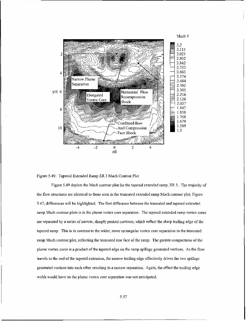
Mach #
3.2
3.1112 3.021
2.932
2.8422.753
4 2.663, - --- 2.574dN"allow Plume 1 2.484S'eparation 40352 9
2.395y/d 6 Horizontal Flow 2.216
-2.16i orte Core Shock~2.037
1.9471.8581.768
-Combined Bow 1.679--.-And Compression/ 1.589- - -r --------.. - f-'- Face Shock J 1.5
-4 -2 0 2 4z/d
Figure 5.49: Tapered Extended Ramp ER 3 Mach Contour Plot
Figure 5.49 depicts the Mach contour plot for the tapered extended ramp, ER 3. The majority of
the flow structures are identical to those seen in the truncated extended ramp Mach contour plot, Figure
5.47; differences will be highlighted. The first difference between the truncated and tapered extended
ramp Mach contour plots is in the plume vortex core separation. The tapered extended ramp vortex cores
are separated by a series of narrow, sharply peaked contours, which reflect the sharp trailing edge of the
tapered ramp. This is in contrast to the wider, more rectangular vortex core separation in the truncated
ramp Mach contour plot, reflecting the truncated rear face of the ramp. The greater compactness of the
plume vortex cores is a product of the tapered edge on the ramp spillage generated vortices. As the flow
travels to the end of the tapered extension, the narrow trailing edge effectively drives the two spillage
generated vortices into each other resulting in a narrow separation. Again, the effect the trailing edge
width would have on the plume vortex core separation was not anticipated.
5.57
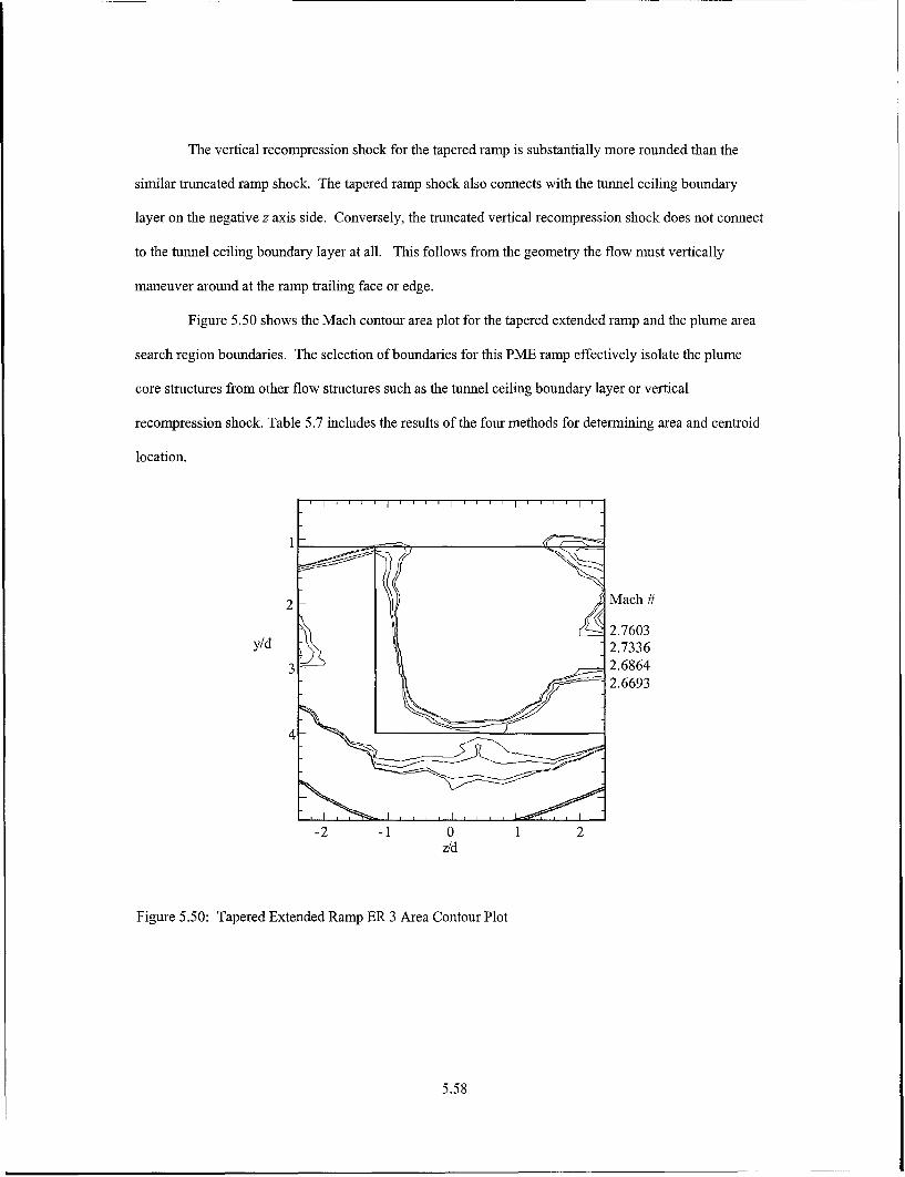
The vertical recompression shock for the tapered ramp is substantially more rounded than the
similar truncated ramp shock. The tapered ramp shock also connects with the tunnel ceiling boundary
layer on the negative z axis side. Conversely, the truncated vertical recompression shock does not connect
to the tunnel ceiling boundary layer at all. This follows from the geometry the flow must vertically
maneuver around at the ramp trailing face or edge.
Figure 5.50 shows the Mach contour area plot for the tapered extended ramp and the plume area
search region boundaries. The selection of boundaries for this PME ramp effectively isolate the plume
core structures from other flow structures such as the tunnel ceiling boundary layer or vertical
recompression shock. Table 5.7 includes the results of the four methods for determining area and centroid
location.
2 Mach
2.7603y/d 2.7336
3 2.68642.6693
4-
-2 -1 0 1 2z/d
Figure 5.50: Tapered Extended Ramp ER 3 Area Contour Plot
5.58

TABLE 5.7TAPERED EXTENDED RAMP AREA AND CENTROID RESULTS
Area Method 95% Freestream Mach Area (cm2 ) Centroid (y/d)
Graphical 2.76 1.32 2.37
Box 2.73 1.25 2.35
Modified Box, y/d=1.2 2.68 1.17 2.35
Modified Box, y/d=1.6 2.67 1.10 2.35
Average 2.71 1.21 2.35
Agreement between the four methods of determining area is not as close as for simple transverse
injection. For the tapered extended ramp, the areas have a 17% difference between top and bottom values.
Several factors contribute to this spread. First, in the Mach contour plot, Figure 5.49, the tunnel ceiling
boundary layer on the negative z axis side is thicker than the boundary layers on either side of the simple
transverse injection Mach contour. The lower Mach number flow associated with the boundary layer
would be included in the average freestream Mach number computation of both modified box methods,
which do not reject any data points. Additionally, the relatively lower Mach number flow in the vertical
recompression shock would also be used in the average. The graphical method and box method would
reject the low Mach number regions based upon the Mach gradient criteria. The agreement in the centroid
locations is excellent, since reducing the local freestream Mach number from highest to lowest strips away
essentially concentric layers from the plume area plot. The centroid computed for the extended tapered
ramp was 12% further into the freestream than the simple transverse case
As suggested, the expansion off of the truncated rear face of PME ramp ER 2 has a mildly
detrimental effect on penetration and plume area when compared to PME ramp ER 3. Though in both
cases the ramp extension appears to increase vorticity through ramp spillage, the rear face expansion of the
truncated ramp noticeably decreases penetration immediately downstream of the ramp. The angle of the
expansion off the ramp rear face is 900 which, barring separation affects, created an expansion fan and
pulled the plume back towards the tunnel ceiling. The expansion is focused in a region of the plume
5.59
where some bending back towards the tunnel ceiling would naturally occur for simple transverse injection.
The combined expansion-natural bending effect propels the plume back up towards the tunnel ceiling.
5.3.3 Extended Ramp Total Pressure Loss
Table 5.9 describes the total pressure losses for the extended ramp group based upon the average
total pressure loss ratio. The extended diamond ramp provides an interesting result, having the second
lowest total pressure loss of all the PME ramp models. This is a result of there being no downstream
recompression shocks by the x/d of 20 measurement location since the ramp extension passes through the
measurement plane. It is reasonable to assume that the total pressure losses incurred by the extended
diamond ramp would increase noticeably if the measurement plane was behind the rear face of the ramp.
Also of interest is the effect of the truncated vs. tapered trailing edge for ramps ER 2 and ER 3.
The slight frontal aspect increase of the less tapered truncated ramp is more than off set by the effect of the
tapered trailing edge in total pressure loss effect. This result indicates that even a slight truncation is
preferable to a sharp, flow recompression shock enhancing trailing edge when total pressure loss is to be
minimized. An additional factor in the higher total pressure loss of the tapered ramp is the slightly more
coherent ramp compression face shock, which appears more coherent than the truncated ramp compression
face shock.
TABLE 5.8EXTENDED RAMP GROUP TOTAL PRESSURE LOSS
PME Ramp Average Total H
Pressure Ratio
Extended Diamond Ramp, ER 1 1.33 0.93
Truncated Extended Ramp, ER 2 1.35 0.92
Tapered Extended Ramp, ER 3 1.44 0.86
5.3.4 Extended Ramp Digital Image Quantitative Analysis
Figures 5.51 to 5.54 are plots of the plume centerline trajectories and centerline intensity decay for
extended ramps ER 2 and ER 3. These plots are oriented as horizontal mirror images of the original plume
images, where y/d of zero is the tunnel ceiling.
5.60

6
5
4-
y/d 3
2
0 2 4 6 8 10 12 14 16 18
x/d
Figure 5.51: Truncated Extended Ramp ER 2 Plume Centerline Trajectory
Figure 5.51 is the centerline trajectory plot of the truncated extended ramp, ER 2. The middle line is the
average centerline of the plume from Figure 5.40. The inner trace outlines the ramp to x/d of 10, then
tapers up slightly as the plume is dispersed. Initially the plume centerline shows no lift-off from the ramp
compression face. This is because the first three points on the inner trace map the injection port outlet,
which artificially lowers the plume centerline trajectory. Additionally, surface flows on the compression
face and ramp extension keep the inner trace on these surfaces, instead of capturing the magnus effect lift-
off observed in the truncated ramp instantaneous parallel oriented image, Figure 5.39. From x/d of six to
11, the plume centerline is seen to separate and lift away from the ramp extension. The slope of the first
eight centerline points is 0.45, nearly double the 0.23 slope for simple transverse injection, which indicates
a substantial magnus effect lift-off was achieved. The maximum centerline penetration in this region is to
y/d of 3.76 at x/d of 10.60. The spike in the outer trace at x/d of 10.60 is due to a single seed particle, and
does not significantly alter the average of points at the x/d of 10.60 measurement location. This location is
after the trailing edge for the ramp extension, therefore the centerline trajectory is no longer affected by
surface flow on the ramp top. The lift-off was anticipated from the magnus effect acting on the extension.
5.61

The centerline and plume outer trace indicate a sharp turn back towards the tunnel ceiling at x/d of 14,
which is a result of the plume being turned by the expansion off the truncated ramp rear face. The slope of
the best fit line through the last four points in the plume centerline trace is -0.24. These observations match
the centroid results for the truncated extended ramp, which indicated the truncated ramp achieves less
penetration than the simple transverse case.
1.4
1.2
0.8
0.6
0.4
0.2
0 .0 2 4 6 8 10 12 14 16 18
x/d
Figure 5.52: Truncated Extended Ramp ER 2 Plume Centerline Average Intensity Decay
Figure 5.52 is the truncated extended ramp ER 2 centerline intensity decay plot. The general
trend in the image shows a rapid decay in image intensity after x/d of 10. This decay rate is nearly triple the
overall plot decay rate observed from Figure 5.9 for simple transverse injection, -0.037. The overall decay
rate of the entire truncated extended ramp plot is -0.039, which is essentially identical to the overall decay
rate of the simple transverse case. The slope of a best fit line passing through the data points greater than
x/d 9 is -0.093. The high decay rate over the last 11 data points indicates the truncation of the ramp
extension has a considerable impact on the rate at which the plume core is removed from the centerline
plane to the plume periphery. The shift in the trace at x/d of 13 corresponds to the location where the more
intense stream of seed particles shed from the ramp rear face intersect with the main plume, and raises the
overall intensity. Scatter seen in the x/d zero to seven range is a result of the bright surface flow regions
raising the average intensity in the measurement plane.
5.62

6-
5 -
4
y/d 3
2 -
00 2 4 6 8 10 12 14 16
x/d
Figure 5.53: Tapered Extended Ramp ER 3 Plume Centerline Trajectory
Figure 5.53 is the plot of the plume centerline and boundaries for the tapered extended ramp, ER
3. The trends observed in this plot match those of Figure 5.51, with a few notable exceptions. The plume
inner trace shows a slight lift-off from the magnus effect at x/d of three and four. The initial trajectory of
the first eight centerline points is 0.46, which is double the first eight point slope of 0.23 for simple
transverse injection. The inner trace also captures the effect of the stream of seed particles from the ramp
extension trailing edge. A single particle trapped in the tunnel ceiling boundary layer at x/d of 14 resulted
in the spike at that location. The single particle is reflected in the plume inner boundary, but does not
significantly alter the average of the other 35 points at x/d of 13.85 used to determine the average plume
centerline trajectory.
The plume centerline or middle trace rises nearly linearly to x/d of 8.9 and y/d of 3.75, which is
the maximum penetration achieved in the truncated ramp plot, Figure 5.51. The remaining points along
5.63

the plume centerline follow a relatively flat profile, with a slight downward slope in the last four points.
This pattern was observed in Figure 5.41 as a slight downturn in the plume. The best fit slope of the last
four points is -0.14. This trend of a slight down turn in the plume centerline (which again reflects the
middle of the crescent downstream of x/d of 10) does not appear to significantly reduce the tapered ramp
plume penetration, as the average centroid location for the tapered extended ramp exceeds the simple
transverse average centroid values by about 12%.
1.4
1.2
., 0.8
0.6
0.4
0.2
0 'C 'C '
0 2 4 6 8 10 12 14 16
x/d
Figure 5.54: Tapered Extended Ramp ER 3 Plume Centerline Average Intensity Decay
Figure 5.54 shows the extended tapered ramp ER 3 decay of centerline intensity. The profile of
the intensity decay rate is nearly identical to the plot observed in Figure 5.9 for the simple transverse case.
However, the slope of the best fit line is -0.05, which is a 34% increase over the simple transverse injection
decay rate. The greater intensity decay rate indicates the rate at which the ramp enhanced vortex pair strips
away the plume centerline injectant seed to the plume periphery. The addition of the relatively weaker
particle stream from the ramp rear edge (in comparison to the stronger stream observed in Figure 5.40)
does not significantly alter the average plume intensity.
5.64

5.4 Injector Ramp Group #3: Asymmetric Ramps
This PME ramp group is intended to combine the two primary vorticity generation mechanism
studied to date. The first is the vorticity inherent in transverse injection. The second is the vortex
generation created by ramp spillover. These ramps are identical with the exception of the taper ratio. The
wide ramp AR 1 tapers from 4 d to 2 d at the top of the compression surface. The narrow ramp AR 2
tapers from 4 d to 1 d at the top of the compression surface. Increasing the ramp sweep angle has been
demonstrated to increase vorticity generation (described in detail in section 2.3). Both ramps in this group
have a noticeable effect on the flow structures.
5.4.1 Asymmetric Ramp Flow Visualization
The flow visualization results are presented in the format of previous sections. For each PME
ramp, the images are organized by type, starting with shadowgraph photography. The salient features of
the shadowgraphs are highlighted and annotated. Analysis of the parallel oriented and cross flow oriented
laser planar images follows.
5.4.1.1 Asymmetric Ramp Shadowgraph Photography
Plume BowShock
Barrel ShockAnd Ramp Flow HorizontalCompression RecompressionFace Structures Shock
Flow VerticalRecompressionShock
Figure 5.55: Wide Ramp AR 1 Composite Shadowgraph
Figure 5.55 is the wide ramp AR 1 shadowgraph image. The flow structures before the ramp
trailing face are similar to the structures observed in previous shadowgraphs. The plume bow shock
follows the established 330-250 angle patterns. The ramp compression face presents a two-dimensional
aspect to the flow, resulting in a greater compression shock angle than the bow shock. The compression
5.65

face shock passes directly through the barrel shock, which should enhance the developing vorticity with
baroclinic torque. The bow shock and compression face shock appear to combine by the vertical middle of
the image. Features unique to swept ramp geometries are the horizontal and vertical recompression shocks.
Similar to the truncated extended ramp ER 2 and tapered extended ramp ER 3, the flow off the rear face
experiences two compressions. The vertical shock is created by the flow passing under the ramp tuming
towards the tunnel ceiling. This ramp has a relatively wide top rear surface, which should result in a strong
vertical shock structure. The horizontal shock results from the side flows recombining at the taper angle of
the ramp. Since this ramp is relatively wide at the rear surface, the strength of the recombination shock
should be attendantly weak. The vertical recompression shock exits the image further into the freestream
than previously observed in the PME ramp shadowgraphs. This is because the wide ramp is half the total
length of the other PME models, which moves the origin of the shock forward approximately three cm.
The movement forward impacts the second baroclinic torque effect, since the shock intersects the plume at
a further upstream point. This translates into a region of the plume where vorticity should be stronger than
the further downstream location because viscous effects will not have worked as long to dissipate the
plume.
Horizontal FlowRecompressionShock
Vertical Flow'RecompressionShock
Figure 5.56: Narrow Ramp AR 2 Composite Shadowgraph
Figure 5.56 is the narrow ramp AR 2 shadowgraph. The majority of features, including the plume
bow shock angles, barrel shock and compression face structures are identical to those observed for
5.66

the wide ramp, Figure 5.55. Also similar to the wide ramp, the relative shortness of the narrow ramp will
move the vertical flow recompression shock forward relative to the other groups of PME ramps, with a
resulting change in the baroclinic torque. However, ramp AR 2 is narrower than ramp AR 1 in respect to
the top rear faces. The narrow trailing edge should effectively reverse the magnitudes of the vertical and
horizontal shocks. With less surface for the flow to turn vertically back towards the tunnel ceiling, the
vertical shock for the narrow ramp should be lessened compared to the wide ramp. Conversely, with a
greater sweep angle, the side flow components should be greater than the narrow ramp, resulting in a
stronger collision and horizontal shock.
5.4.1.2 Asymmetric Ramp Parallel Oriented Images
Figure 5.57: Wide Ramp AR 1, Instantaneous Parallel Oriented Laser Image
5.67

Figure 5.58: Wide Ramp AR 1, Time-Averaged Parallel Oriented Laser Image
Figures 5.57 and 5.58 show the instantaneous and time-averaged parallel oriented laser images for
the wide ramp, AR 1. For Figure 5.57, the injection was seeded relatively lightly compared to the other
PME instantaneous parallel oriented images. Heavier seeding or time-averaging tends to push the plume
dispersion point farther downstream, where it is almost coincidental with the laser sheet intensity decline.
The light seeding clearly highlights the rapid decrease in plume intensity well before an intensity decrease
is observed for the laser sheet from its reflection off the tunnel ceiling. Lighter seeding also helps define
the plume barrel shock edges, since fewer particles are present to obscure the barrel shock center.
Figure 5.58, the time-averaged parallel oriented image for the wide ramp, has several features not
captured in the instantaneous image. First, the plume shows an immediate magnus effect lift-off from the
ramp compression face, which is traceable almost to the front edge of the compression face. Second, some
surface flow is visible on the ramp compression face. Third, the surface flow is seen to accumulate in a
recirculation region that is almost 1/2 d at the widest, and cover the entire vertical height of the ramp rear
face. The recirculation region was anticipated for this design, and could prove usefuil as a flameholder in a
supersonic combustor. Unlike the similar extended ramp images, Figures 5.40 and 5.42, there is no
5.68

clear, coherent stream of particles exiting the rear face recirculation zone. There is an indication of a
particle exit path, but this may also be a temporary structure due to the ramp base effects.
The bend observed in the plume centerplane path for the wide ramp occurs at approximately two
ramp lengths from the injector exit. This is the area that the centerplane plume bend occurs for all previous
ramps (excluding the extended diamond ramp, ER 1). Unlike the truncated extended ramp, ER 2, the
expansion over the rear edge of the wide ramp does not increase the bend in the plume. The explanation
for these effects is geometric scaling. The truncated extended ramp induces a strong expansion in a region
where the plume would naturally turn slightly back towards the tunnel ceiling (as evinced by the weak flow
recompression shock observed for simple transverse injection in section 5.1), in effect enhancing the
natural turn. The wide ramp, AR 1, ends just after the plume foldover region. At the end of the wide
ramp, the plume vortices are still aligning with the main flow direction. The strong expansion off the wide
ramp rear face also coincides with the generation or enhancement of plume vorticity from ramp spillage.
Therefore, the expansion interacts with the plume while a substantial amount of the injected momentum is
directed out into the freestream and the developing vorticity is being enhanced. The combination of these
effects result in a steeper centerline penetration trajectory than observed for the simple transverse injection
case.
5.69
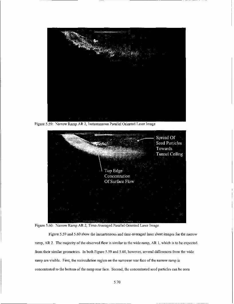
Figure 5.59: Narrow Ramp AR 2, Instantaneous Parallel Oriented Laser Image
Figure 5.60: Narrow Ramp AR 2, Time-Averaged Parallel Oriented Laser Image
Figure 5.59 and 5.60 show the instantaneous and time-averaged laser sheet images for the narrow
ramp, AR 2. The majority of the observed flow is similar to the wide ramp, AR 1, which is to be expected
from their similar geometries. In both Figure 5.59 and 5.60, however, several differences from the wide
ramp are visible. First, the recirculation region on the narrower rear face of the narrow ramp is
concentrated to the bottom of the ramp rear face. Second, the concentrated seed particles can be seen
5.70

coherently exiting the ramp rear face almost parallel to the tunnel ceiling. The coherent ramp rear face exit
stream begins to disintegrate by one half a ramp length from the ramp rear face, and rapidly disperses in
the region between the tunnel ceiling and the visible plume core. Third, the surface flow from the ramp
compression face that feeds the seed particle accumulation on the rear face is visible on the side of the
ramp bottom. For the straight sided PME ramps, the surface flows are normally observed as thin, high
intensity lines on the ramp compression surface which clearly delineate the solid ramp boundary. For the
narrow ramp, the flow has swept some of the surface flow material into the vortex spillage off the ramp
compression face. Clear observation of this wrapping effect is somewhat fortuitous; the effect was noted
where visible for the other straight sided PME ramps, but the vortex wrapping was not as distinctly defined
as the narrow ramp. This is due to the extra width of the other straight sided PME ramps diffusing the laser
sheet intensity out of the centerline plane.
Similar to the simple transverse injection case, the narrow ramp plume centerline trajectory
undergoes a slight bend approximately two ramp lengths downstream from the injection. The final visible
trajectory of the plume centerline is essentially horizontal, which also matches the trajectories seen for the
simple transverse case. The overall degree of the downstream bending is less than the bending at the same
location for the wide ramp. This reflects the weaker effect of the narrow ramp rear edge expansion than
the expansion over the wide ramp rear edge.
5.4.1.3 Asymmetric Ramp Cross Flow Oriented Images
Figure 5.61 is the time-averaged cross flow oriented laser image for the wide ramp, AR 1. The
vortex core in this image is relatively clear in comparison the cross flow image of the simple transverse
case, Figure 5.5. The seed particles observed in the core region are large and distinct from the core
background. Around the inside periphery of the crescent shaped seed structure, a further collection of
relatively large seed particles is visible. The large seed particles are the result of shedding surface flow
from the wide ramp rear face. This indicates a different mechanism for surface flow shedding than the
method explained in section 5.3.1.2 for the extended ramps ER 2 and ER 3. In this case, instead of the
5.71

shed seed particles traveling linearly in between the plume vortex cores, the shed seed appears to be
immediately entrained along the inner region of the vortex cores. Since the inside of the vortex cores
rotate slower than the outer vortex periphery, mixing will occur at a slower rate, allowing the large seed
particles to remain intact.
Figure 5.61: Wide Ramp AR 1, Time-Averaged Cross Flow Oriented Laser Image
The seeded plume crescent differs from the simple transverse injection by remaining at the same
relative intensity from the bottom to the tops of the crescent. This indicates the ramp spillover enhanced
vortices have distributed the seed more evenly throughout the entire crescent, instead of a high
concentration remaining in the bottom of the crescent. Overall, the crescent structure is coherent, with
little spreading to the bottom, sides, or interior. This indicates the wide ramp can provide even mixing
concentration, which would allow for more even combustion of fuel than simple transverse injection if
used in a combustor.
5.72

Figure 5.62: Narrow Ramp AR 2, Time-Averaged Cross Flow Oriented Laser Image
Figure 5.62 is the time-averaged cross flow oriented laser image for the narrow ramp, AR 2. The
narrow ramp cross flow image has a steady intensity throughout the crescent, which depicts a more even
seed spreading through the crescent than the simple transverse injection case. The more even spreading of
the narrow ramp crescent intensity is a consequence of the enhanced vorticity generated by ramp spillover
effects. In the center of the vortex core region, a vertically oriented strip of low intensity seed particles is
visible. The seed strip provides a demarcation between the two counter rotating vortex cores. This feature
is not visible in the simple transverse injection, which has a more even spread of seed particles across the
plume core region. The centers of the vortex core are distinguishable for the narrow ramp image as two
darker circular regions on either side of the demarcation strip.
5.73

5.4.2 Asymmetric Ramp Mach Contour Plots
Mach #
_111 . ....... 3 .2c+ , / \\ > tw~~3.111
2 - ' , 3.021Zig-Zag Plume 2.932)Y°
ABoudre ('e& "' 2.8424 _-Asymmetric 216634 :-Vortex 2.663ij, ? . Structures 2.574
2.4842.395
y/d 6 Semicircular 2.216r 2.216Shock 2.126
Combined Ramp 2.0378 1.947Compression 1.858Face And Bow 1.768
10%' Shock .. 7 1.67910 ....... . j/. S__yZL1.589
S- 71.5
-4 -2 0 2 4z/d
Figure 5.63: Wide Ramp AR 1 Mach Contour Plot
Figure 5.63 depicts the Mach contour plot for the wide ramp, AR 1. The effect of the wide ramp
on the flow field and plume is evident when compared to the simple transverse injection, Figure 5.6. The
flow recompression shock created as the injected plume turns slightly back towards the tunnel ceiling is
substantially more pronounced for the wide ramp than for simple transverse injection. This stronger shock
is created from the flow passage through the ramp compression face-rear face expansion fan. The
expansion accelerates the flow and intensifies the resulting shock as the flow turns away from the tunnel
ceiling. Aty/d of 5.6, the peak height into the freestream of the wide ramp flow recompression shock is
slightly less than the simple transverse injection, which peaks aty/d of six.
The wide ramp plume bow shock does not appear to be substantially stronger than the simple
transverse shock, though the wide ramp bow shock is coincidental with the ramp compression face shock.
An objective of masking the ramp partially with the plume bow shock appears to be achieved. The wide
5.74

ramp Mach contour does not reflect any additional shock structures beyond the three observed, though an
additional weak shock was observed in the wide ramp shadowgraph, Figure 5.46. This was interpreted as a
shock produced as the two ramp side flows rejoin and turn with the tunnel flow, similar to the effects
observed in section 5.3 for extended ramps ER 2 and ER 3. It is possible that the weak shock observed in
the wide ramp shadowgraph was too weak to produce an effect in the Mach contours.
An interesting feature of the wide ramp Mach contour plot is the unusual asymmetry in the plume
shape. In the simple transverse and PME ramp Mach contour plots where the twin vortex cores are distinct
(i. e., for ramps ER 2, ER 3, AR 1 and AR 2), a trend for a larger core in the positive z/d side vortex is
present. The asymmetry appears to be the result of a slight injector misalignment, as noted by McCann" .
However, the plume for the wide ramp appears on the whole to have rotated clockwise, relative to the
Mach contour plot. The zigzag plume boundaries identified in Figure 5.63 appear to reflect the bottom
edge of the wide ramp rear, rotated clockwise. A similar effect to the vortex core separation was noted for
the truncated extended ramp, ER 2. There are no discernible defects in the manufacturing of the wide
ramp, or any other physical cause in the shape of the wide ramp to suggest a cause for the apparent
rotation.
Figure 5.64 presents the Mach contours generated by the four area determination methods. In
general, the Mach contours (and hence the local freestream) are lower than the area contours for simple
transverse injection, Figure 5.7. The contours essentially collapse into a single line for the majority of the
plume; indicating the plume vortex structure Mach contours are tightly packed. The plume areas and
centroids by method are summarized in Table 5.9.
5.75

2 C,- Mach #
2.7116y/d 2.7088
3 2.68212.6813
-2 -1 0 1 2z/d
Figure 5.64: Wide Ramp AR 1 Area Contour Plot
TABLE 5.9WIDE RAMP AREA AND CENTROID RESULTS
Area Method 95% Freestream Mach Area (cm2) Centroid (y/d)
Graphical 2.71 1.09 2.33
Box 2.71 1.10 2.33
Modified Box, y/d=1.2 2.68 1.04 2.32
Modified Box, y/d=1.6 2.68 1.04 2.32
Average 2.69 1.07 2.33
The results for the wide ramp plume area vary 5% from largest to smallest. The variations in plume
centroid locations are in essence insignificant. The excellent agreement for centroid location indicates the
plume center was found, and that the area determination methods are in agreement as to the fundamental
shape of the plume. The average area results for the wide ramp show an increase of 6% over the simple
transverse injection average area result, Table 5.1. Area expansion is most likely due to the additional
vorticity generated by the ramp spillover. The average centroid for the wide ramp is a 13% increase in
penetration over the simple transverse injection. The increase in penetration can be tied directly to the
5.76
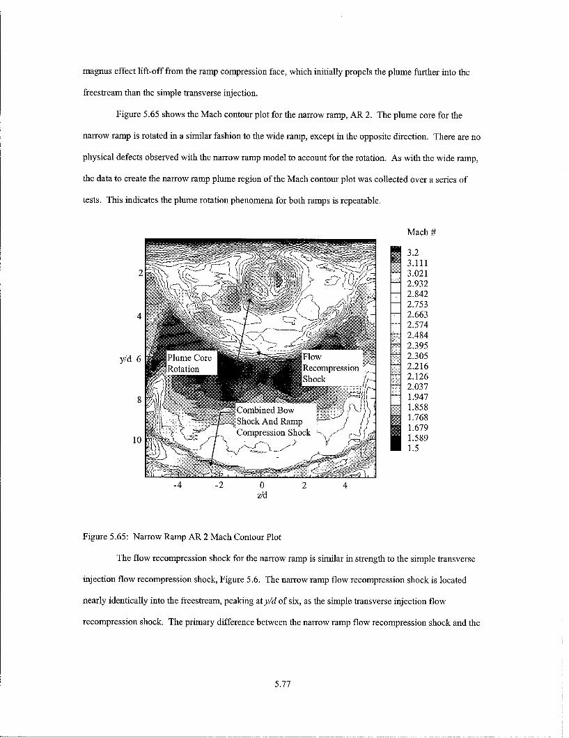
magnus effect lift-off from the ramp compression face, which initially propels the plume further into the
freestream than the simple transverse injection.
Figure 5.65 shows the Mach contour plot for the narrow ramp, AR 2. The plume core for the
narrow ramp is rotated in a similar fashion to the wide ramp, except in the opposite direction. There are no
physical defects observed with the narrow ramp model to account for the rotation. As with the wide ramp,
the data to create the narrow ramp plume region of the Mach contour plot was collected over a series of
tests. This indicates the plume rotation phenomena for both ramps is repeatable.
Mach #
3.23.111
2 > \ ,,zz( 3.0212.9322.842?\:: 2.753
4 2.663-- f7y ; 2.574
2.484
2.395
y/d 6 Plume Core Flow 2.305
Rotation Recompression 2.216Shock 2.126~2.037
8 1.947Combined Bow 1.858
Shock And Ramp 1.768
Compression Shock '1.6791.5
-4 -2 0 2 4z/d
Figure 5.65: Narrow Ramp AR 2 Mach Contour Plot
The flow recompression shock for the narrow ramp is similar in strength to the simple transverse
injection flow recompression shock, Figure 5.6. The narrow ramp flow recompression shock is located
nearly identically into the freestream, peaking at y/d of six, as the simple transverse injection flow
recompression shock. The primary difference between the narrow ramp flow recompression shock and the
5.77

simple transverse injection flow recompression shock is the coherence of the narrow ramp flow
recompression shock.
The bow shock for the narrow ramp has combined with the ramp face compression shock, which
appears as a single shock in the Mach contour plot. This again indicates the goal of reducing the ramp
shock by placing the ramp compression face behind the plume has been achieved. Similar to the wide
ramp Mach contour plot, the weak horizontal shock identified in Figure 5.47 is not manifested in the
narrow ramp Mach contour plot.
2 Mach #
2.7472y/d 2.7413
2.73782.7198
-2 -1 0 1 2z/d
Figure 5.66: Narrow Ramp AR 2 Area Contour Plot
Figure 5.66 shows the area Mach contour plot generated for the narrow ramp, AR 2 from the four
area determination methods. As can be seen in Figure 5.66, three of the four methods are in practically
exact agreement. The dissenting Mach contour is from the modified box method using y/d of 1.2 as the
bottom of the local freestream search region. This y/d is well into the tunnel ceiling boundary layer, which
results in an overall lower local freestream Mach number and plume area. Table 5.10 summarizes the
results of the area and centroid computed for each method.
5.78

TABLE 5.10NARROW RAMP AREA AND CENTROID RESULTS
Area Method 95% Freestream Mach Area (cm') Centroid (y/d)
Graphical 2.74 1.21 2.43
Box 2.75 1.21 2.43
Modified Box, y/d=1.2 2.72 1.16 2.45
Modified Box, y/d=1.6 2.74 1.21 2.43
Average 2.73 1.20 2.44
The presence of the ramp on the plume is readily apparent in comparison to the area and centroid for the
simple transverse injection. The average local freestream Mach number for the narrow ramp is not
significantly faster than the simple transverse injection local freestream Mach number. The average area
for the narrow ramp plume however is 19% larger than the simple transverse injection average area. The
average centroid for the narrow ramp plume is also 19% larger than the simple transverse injection average
centroid.
5.4.3 Asymmetric Ramp Total Pressure Loss
Table 5.9 describes the total pressure losses for the asymmetric ramp group based upon the
average total pressure loss ratio.
TABLE 5.11ASYMMETRIC RAMP GROUP TOTAL PRESSURE LOSS
PME Ramp Average Total I
Pressure Ratio
Wide Ramp, AR 1 1.40 0.88
Narrow Ramp, AR 2 1.40 0.88
As seen in Table 5.11, the total pressure losses incurred by placing either of the two asymmetric ramps into
the post plume flow field is 12%. The first difference between the two ramps for the value of average total
pressure ratio is to three decimal points, which is not considered significant.
5.4.4 Asymmetric Ramp Digital Image Quantitative Analysis
5.79

Figures 5.67 to 5.70 are plots of the plume centerline trajectories and centerline intensity decay for
extended ramps AR 1 and AR 2. These plots are oriented as horizontal mirror images of the original plume
images, where y/d of zero is the tunnel ceiling.
6
5
4 -
y/d 3
2-
0 2 4 6 8 10 12 14 16
x/d
Figure 5.67: Wide Ramp AR 1 Plume Centerline Trajectory
Figure 5.67 is the plot of plume centerline trajectory for the wide ramp, AR 1. The wide ramp
plume centerline trajectory depicted by the center trace shows a steep linear rise along the compression
face of the ramp. The slope of the first eight centerline points is 0.51, which is over double the slope of
0.23 for first eight points of the simple transverse injection centerline, Figure 5.8. The centerline trajectory
for the wide ramp peaks at x/d of 6.5 and y/d of 3.60, compared to a maximum height of 3.32 for simple
transverse injection, a 9% increase. After the peak, and through the region of the post ramp expansion fan,
the plume centerline is relatively flat, following a similar profile to the simple transverse injection plume
centerline trajectory. The primary enhancement in penetration for the wide ramp is
5.80

clearly achieved from a magnus effect lift-off of the plume from the ramp compression face. After the
rapid rise, the wide ramp plume undergoes a decay in centerline position associated with the vortices
stripping the injectant away from the plume centerline to the plume periphery. The expansion fan
associated with the ramp rear face also appears to create a slight downward trend in the plume centerline
trajectory.
1.4
1.2
u 0.8
0.6
0.4
0.2
0 .
0 2 4 6 8 10 12 14 16
x/d
Figure 5.68: Wide Ramp AR 1 Plume Centerline Average Intensity Decay
Figure 5.68 is the plot of centerline intensity decay for the wide ramp, AR 1. The slope of the
decay line is -0.047, a 26% increase in decay from simple transverse injection. The increased decay rate is
a direct result of the ramp spillage enhanced vorticity spreading the concentrated plume centerline core
seed to the outer plume periphery. The slight dip in the trace at x/d of 12.2 is the result of a streak in the
tunnel window through which the image was acquired, and not indicative of any unusual flow behavior.
Figure 5.69 is the narrow ramp AR 2 plume centerline trajectory plot. The narrow ramp plume
centerline trajectory shows a linear rise along the compression face of the ramp. The slope of the first eight
centerline points is 0.40, which is almost double the slope of 0.23 for first eight points of the simple
transverse injection centerline, Figure 5.8. Unlike the previously examined wide ramp, the linear rise at the
0.40 slope in the centerline plume trajectory continues to x/d of 9.8 before significantly tapering off.
5.81

The maximum centerline height achieved is y/d of 3.69 at x/d of 10.6, an 11% increase over simple
transverse injection maximum centerline y/d. After the maximum height is achieved, the plume centerline
has a slight decrease in the slope of the remaining points, similar to the simple transverse injection.
6
5-
4-
y/d 3
2-
0 2 4 6 8 10 12 14 16
x/d
Figure 5.69: Narrow Ramp AR 2 Plume Centerline Trajectory
Figure 5.70 is the plume centerline average intensity decay plot. The overall slope of the plot is -
0.042, which is a 13% increase in decay over simple transverse injection. Similar to the wide ramp plume
centerline average intensity decay plot, the higher decay rate for the narrow ramp over simple transverse
injection can be attributed to the ramp induced vorticity enhancement. The narrow ramp plume centerline
intensity decay plot does reflect the geometry of the ramp, i. e., there is a spike or discontinuity to indicate
the ramp location or shape. The discontinuity occurs at x/d of 4.07, which is the location of the high
concentration of surface flow seed particles accumulating on the ramp vertical surfaces from the vortex
wrapping effect, Figure 5.51.
5.82

1.4
1.2
. 0.8
0.6
0.4
0.2
00 2 4 6 8 10 12 14 16
x/d
Figure 5.70: Narrow Ramp AR 2 Plume Centerline Average Intensity Decay
5.83
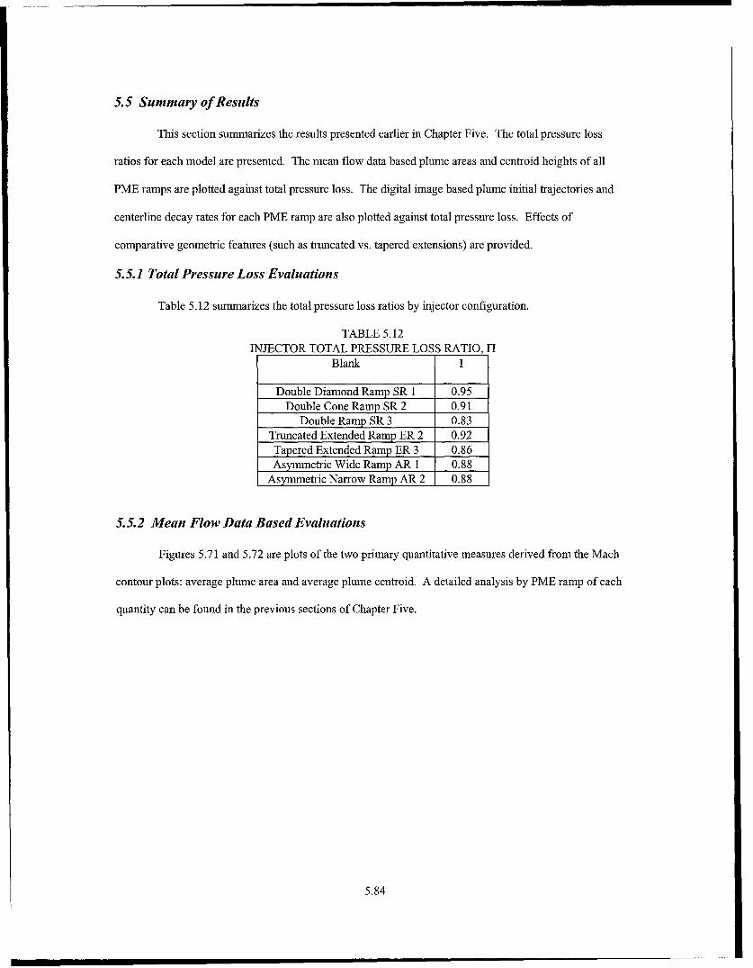
5.5 Summary of Results
This section summarizes the results presented earlier in Chapter Five. The total pressure loss
ratios for each model are presented. The mean flow data based plume areas and centroid heights of all
PME ramps are plotted against total pressure loss. The digital image based plume initial trajectories and
centerline decay rates for each PME ramp are also plotted against total pressure loss. Effects of
comparative geometric features (such as truncated vs. tapered extensions) are provided.
5.5.1 Total Pressure Loss Evaluations
Table 5.12 summarizes the total pressure loss ratios by injector configuration.
TABLE 5.12INJECTOR TOTAL PRESSURE LOSS RATIO, II
Blank 1
Double Diamond Ramp SR 1 0.95Double Cone Ramp SR 2 0.91
Double Ramp SR 3 0.83Truncated Extended Ramp ER 2 0.92Tapered Extended Ramp ER 3 0.86Asymmetric Wide Ramp AR 1 0.88
Asymmetric Narrow Ramp AR 2 0.88
5.5.2 Mean Flow Data Based Evaluations
Figures 5.71 and 5.72 are plots of the two primary quantitative measures derived from the Mach
contour plots: average plume area and average plume centroid. A detailed analysis by PME ramp of each
quantity can be found in the previous sections of Chapter Five.
5.84

1.4
1.3
1.2 - * No rp
ESR1
1.1 +ASR2
XSR3.N 1
A sER2
o 0.9 - ER3+AR1
0.8 .AR2
0.7 X
0.6 i
0.75 0.8 0.85 0.9 0.95 1
H
Figure 5.71: Normalized Average Plume Area vs. Hl
1.3X
1.2
* No Rarp• +1.1 ,SR1
A SR 2
1 XSR3
L) )K ER20.9ER3
E 0.8 +AR1Z 0.7.AR2
0.7
0.60.75 0.8 0.85 0.9 0.95 1
1H
Figure 5.72: Normalized Average Plume Centroid vs. 1
In Figure 5.71, the average plume areas as measured by Mach contours are plotted against Hl. In
this figure as well as the three following, all results are normalized with the simple transverse injection
results. With the exception of the double ramp SR 3, there is a declining trend in 17 as the area is
5.85

increased. This is logical, since large plume mixing structures will result in regions of relatively high
pressure loss. However, two ramps perform worse in measured average plume area than the simple
transverse injection, the double cone ramp SR 2 and the double ramp SR 3. Both of these ramps generate
an expansion that has a detrimental effect on vortex strength. In contrast, the wide ramp AR 1, narrow
ramp AR 2 and truncated extended ramp ER 2 also produce a vortex reducing expansion, but this is offset
by strong vortex enhancement from ramp or extension spillage. Moving across the chart horizontally, the
results for ramps SR 3, SR 2, SR 1, AR 1, ER 2, AR 2 and ER 3 can be seen in order of increasing plume
area. This order of the ramps is also the order for decreasing expansion strength, with ramp SR 3 having
the most focused expansion in the cross sectional plane of the plume. Ramp ER 3, which should not have
any appreciable expansion across the plume, has the highest average plume area. In comparison, Ramp ER
2 has an expansion across the ramp rear face which results in an 8% area reduction from ramp ER 3.
Therefore, an expansion has been demonstrated to adversely affect vortex structures. The 8% increase in
plume structure area of ER 3 over ER 2 was incurred at a 6% total pressure loss penalty due to the sharp
convergence of the tapered extended model.
In Figure 5.72, the normalized average centroids of the plumes are plotted against II. An
interesting result is the double ramp, SR 3, has a significantly greater penetration than all other
configurations. This appears to be a product of the two-dimensional frontal aspect of the double ramp,
which effectively blocks the flow from turning back towards the tunnel ceiling. Aside from the unique
results for the double ramp SR 3, a general trend observed for Figure 5.71 is repeated. Those ramps with
weaker expansion generating geometries penetrate further than similar geometries that produce strong
expansions. An example can be seen between ramp ER 2 and ER 3, AR 1 and AR 2, and SR 1 and SR 2.
Ramps ER 2, AR 1 and SR 1 produce greater expansions than the similar geometries of ramps ER 3, AR 2
and SR 2. Another interesting feature to note is the extended ramp group does not improve penetration
over the asymmetric ramp group. This result indicates that the main enhancement to penetration occurs on
the ramp compression face, and that the extension does not enhance penetration. Further evidence to
support this conclusion comes from the Mach contour plots for the extended ramps, Figures 5.47 and
5.86

5.49. In both cases, the trailing profile of the extension (i. e., the truncated or tapered rear of the ramp) is
clearly reflected in the plume. Figure 5.47, the Mach contour plot for the truncated extended ramp ER 2,
has a wide, nearly rectangular separation between the vertically elongated vortex cores. This separation, as
well as the vortex degrading rear edge expansion of the truncated ramp, could have impeded the convective
interaction between the counter rotating vortex pair and lead to lesser penetration than the tapered
configuration, ER 3. Figure 5.49, the Mach contour plot for the tapered extended ramp has closely packed
elongated vortex cores with tapered contour separation. The closely packed vortex pair was able to interact
and convect into the freestream to a similar depth of the asymmetric ramps.
5.5.3 Digital Image Data Based Evaluations
Figures 5.73 and 5.74 are plots of the two primary quantitative measures derived from the parallel
oriented time-averaged laser images: the plume initial trajectory and centerline decay rate. A detailed
analysis by PME ramp of each quantity can be found in the previous sections of Chapter Five.
2.5
>, +
S2 X X- * SRI1
~SR21.5xSR3
)K ER 2
0ER3N "-AR
0.5 -AR20z
0 I I
0.75 0.8 0.85 0.9 0.95 1
n
Figure 5.73: Normalized Average Plume Centerline Trajectory vs. IH
5.87

1.4x
1.3 ~+041.2 , No Rarrp
1.2 AMSR1
1.1 ASR 2
1 x SR3
1- )ER2
0.9 0ER3N
;+AR10.8 ,AR 2
0.7
0.6 i0.75 0.8 0.85 0.9 0.95 1
H1
Figure 5.74: Normalized Average Plume Intensity Decay Rate vs. II
Figure 5.73 is a plot of the normalized plume centerline initial trajectory, or the slope of the first
eight data points correlating to the length of the ramp compression surface, vs. 1H. In all PME ramp cases,
an appreciable gain in initial plume trajectory is achieved over the simple transverse injection. Another
general trend is that the broader the ramp face, the better the initial penetration. The double diamond ramp
SR 1 and double cone ramp SR 2 both present the narrowest frontal profile to the oncoming plume, which
results in less surface for plume interaction to occur. In the region where the plume is observed to lift-off
of the ramp compression faces, vorticity is still developing from the freestream impacting the plume
stream tube. Whether enough vorticity is created to generate a magnus effect lift-off, or the plume simply
impinges on and reflects from the ramp compression face is indeterminate. Support for a magnus effect
lift-off comes from the widest profile ramp, the double ramp SR 3. Flow passing around the injectant
plume is obstructed by the broad compression face of the double ramp, which may reduce the amount of
spin imparted by shear on the plume. If less spin is initially imparted on the plume, less of a magnus effect
would be initially observed. Overall, the symmetric ramp group shows a nearly linear trend between initial
plume centerline trajectory and H. As the symmetric ramp compression faces are progressively enlarged,
the initial trajectory as well as total pressure loss increase. Another feature of
5.88

interest in Figure 5.73 is the difference between the wide ramp AR 1 and the narrow ramp AR 2. Here the
trend of a broader face increasing the initial trajectory is followed, but there is no attendant total pressure
loss.
Figure 5.74 is a plot of the normalized average digital image intensity decay vs H. This plot
shows a negative trend of increasing pressure loss with increasing intensity decay rate. One exception is
ramp ER 2, the truncated extended ramp, which has a low decay rate relative to the other PME ramps. This
lower centerline decay rate is most likely a result of the vortex cores for the truncated ramp being split
apart by the ramp trailing edge, which weakens the vortex pair centerline interactions and mixing effect.
Overall, this plot shows considerable scatter, which may be due to an inappropriate choice of scaling
factor. The image intensity can also be impacted by factors such as the quantity of seed injected, PME
ramp surfaces flows extracting seed from the measured portion of the plume image or seed particles
collecting on the tunnel glass sides, obscuring and diffusing the image.
5.89

VI. Conclusions and Recommendations
This chapter outlines the primary conclusions drawn from the analysis of Chapter Five. The
optimum geometric configurations based upon a set of design criteria are presented. Recommendations for
further study are submitted.
6.1 Conclusions
As previously stated, the primary objectives of this investigation were to enhance the penetration
and mixing of an injected gaseous jet into a supersonic freestream without adversely impacting total
pressure losses. The measures developed in conducting this investigation have a clear trend: increases to
any of the mixing and penetration parameters over simple transverse injection will result in a relative total
pressure loss.
In general the summary plots (Figures 5.71 through 5.74) show fair agreement with expected
trends. The results for comparable geometries, such as simple asymmetric ramps and extended ramps are
coherent enough to draw reasonable conclusions about the nature of the flow and plume dynamics.
Overall, there is considerable scatter amongst the PME ramp results (the highest least squares regression
correlation for any of the plots was below 0.30). This is to be expected, though, considering the spectrum
of geometric features tested and the range of expected results. However, for specific geometric features
and effects, such as expansion creating geometries, the results correlate well between the similar models.
In conclusion, the best gains in penetration and mixing enhancement as defined throughout this
study with the relative least total pressure detriment are achieved by the swept sided ramps with the
greatest side sweep. The two ramps that have this geometry are PME ramps ER 3 and AR 2. The tapered
extended ramp ER 3 and narrow ramp AR 2 have the best increases in the penetration and mixing
parameters considered. Both ramps incur a total pressure loss in the 10 to 15% range, but both produce 15
to 20% gains in plume structure area and centroid penetration. The effect of the ramp extension appears to
be negligible; most likely because the ramp extensions are either too low or too narrow for the plume to
interact with. The frontal aspect of the ramp is crucial for its effect on the plume as seen with the double
ramp SR 3, but also for the impact on total pressure loss. Finally, the total pressure loss incurred by the
PME ramp rear surface can be substantial, as observed in the 6% greater total pressure loss from the
truncated extended ramp ER 2 to the tapered extended ramp ER 3.
6.1

6.2 Recommendations
Results have been established which clearly indicate the potential of transverse injection over a
ramp. The next step in conducting this experiment is to further explore the geometric features shown to
enhance penetration, i. e., swept ramps with high degrees of sweep. Another consideration is to further
examine the PME ramps that occupy both ends of the performance spectrum simultaneously, such as the
double ramp, SR 3. Along a similar vein, the relative gains in penetration and mixing must be weighed
against the total pressure loss purely from a combustion standpoint to establish whether any of these
configurations are usable or produce an unacceptable detriment to thrust production.
The methods used in this investigation provide a complete picture of the flow structures. The
mean flow data presents an excellent means of capturing the relative size and strength of the injection flow
field. The laser imagery captured in this investigation also provides flow visualization from which to
interpret the mean flow data. There are three routes, however, to enhance future exploration.
First, hot wire or hot film anemometer has been used to directly measure the strength of
vorticity2° ' 22 2 6 and turbulent properties, both essential for any successful mixing scheme. Though the
results observed correlate well with the various techniques employed in this experiment, direct
measurement of vortex strength is required to ensure the flow has been properly characterized. For
example, the single vortex core observed in the Mach contour plots for the double cone ramp SR 2 and
double ramp SR 3, Figures 5.24 and 5.26, may still have vestiges of the twin vortices that mean flow
probes can not resolve. Hot wire anemometry presents a means to directly measure cause and effect
relations on vorticity.
Second, plume concentration data is required to measure the near field mixing enhancements
directly. Correlations exist between mixing and the flow structures observed in the Mach contour plots and
flow visualization. However, some of the flow structures have contradictory effects, such as shocks
inducing baroclinic torque to enhance vorticity and expansions weakening vorticity. In order to determine
the absolute effects of the flow structures, as opposed to the relative effects observed here, concentration
data can provide the final assessment of mixing enhancement. The difficulty with such measurements now
is that AFIT resources currently do not include concentration measurement equipment, though this is not
an insurmountable problem. A relatively simple modification to the injector gas supply would enable
6.2

helium injection for binary gas mixtures. The majority of the hardware for concentration measurements is
easily fabricated or obtained. Future efforts in injection should be aimed toward developing concentration
measuring capabilities.
Third, the data collected has unused potential. Specifically, the planar laser images were acquired
using a particle imaging velocimeter (PIV) setup. Since both red and green laser sheet information are in
each of the parallel oriented images, the image data could be resolved into local velocity vector fields.
Once a mean flow velocity in the plume is established the rotation rate of the plume vortices would be a
function of the frequency between vortex helix peaks, similar to measuring frequency from a sine wave
output. PIV measurements would allow direct non-intrusive velocity and vorticity measurements in a
plane at any downstream location. An examination of the relative differences by downstream location
could determine the full development of ramp geometry flow effects.
A final recommendation for future research is to continue using the techniques employed in this
investigation. A fairly broad assortment of geometries have been tested and preliminary evaluations of
geometric features that enhance and hurt penetration and mixing made. Future research can be focused on
broadening the basic understanding of such complex flow fields. Once a suitable base of knowledge exists,
refinement of the designs can lead to an optimum configuration.
6.3

Appendix A: Total Pressure Contour Plots
These figures are the total pressure ratio contour plots generated during the course of the investigation. As
should be expected, the contour profiles closely match those of the Mach contour plots in Chapter Five. The final
contour plot in this series is that of the wind tunnel cross section with neither injection nor PME ramps in the flow.
10 ....... . .
... -i. " <
Ks K < -'
8 - P 1 NZ .,., .Pi.1,50-
1 9 1.31,29 129'
1;.18 6 1208yld 1.07 y/d 1 2 -1
0 t ' l' ' 096 094$ ,Qo. B.06 0.80
4. 075 4 0750 640.64
('4/ / 054
02 41.42 . 32 2 44/ .0.31
0000
-4 -2 0 2 4 A -2 0 2
zfd z/d
Figure A. 1: Simple Transverse Injection Figure A.3: Double Cone Ramp SR 2
10 . '
1 501.39 1 39~f~
8-I. ' P.u/" ",o".8. .......... / ( "i/Pin
, 1 29 j\1 29
8 N: < "" ?", 11 1
y/d 1.07 y/d I D7096 a 096
086 0 6
4075 4075
0.64 0640.54 /""054
0.4,3 1 04,
2 0.32 2 0320.21 0 21
0,11I Oil
000 0.00
4 -2 0 2 4 -4 -2 0 2 4
z/d z/d
Figure A.2: Double Diamond Ramp SR 1 Figure A.4: Double Ramp SR 3
A.1

. . . . . ..... .. .,0, - / ,' .
10 10
8 1/Plo 8 Pl/t
129 t4 / S 12:
6 118 6..,0', 1 118y/d 17 yld 107". 6 0 9~~~~086 , 0' 060.86
0.75 4 G 75
064 0,64
0443
0.322 0 2 1
-4 -2 0 2 4
z/dz/d z/d Figure A. 8: Narrow Ramp AR 2Figure A. 5: Truncated Extended Ramp ER 2
. .., = 1 0 : ...10
0'\ ii. ........ . <.' 1 lo .> ,: 1.39.:8 PH / 1015
>6.5 3 ' \ .2
1.29 61y 6 ..\/4 "9\/' '"0. 118 ! : ' 0': o96o.9 :: ::0. 6y/d
0,,,70 0,6
4_ 0.75
4 0.75o 0 . '' ;.: ::-Z=:
=. -~i : 0
= : .64
064 .70.54 0 64 ;; = :: -- :;:: : : 0.430.I054 ,, o o.. -.. --' i 032
0.3 2 .21
021 ~. . /0"0------~0.00
o.11 D
0o -4 -2 0 2 4
-4 -2 0 2 4 z/d
z/d Figure A.9: Test Section, No Injection or PME RampFigure A.6: Tapered Extended Ramp ER 3
10
( .- 1.1.2
87)-. '
00', -0 % !17 ,.oiiii> .. , ' o 0; -: i!," 1.00
y/d 6 ...... -" [.- / 118
4,SS 0.75/0864 '.\0 ' ,;"I oz
0, 0/0 -..* 1 03'o , /o 0.00
-4 -2 0 2 4z/d
Figure A.7: Wide Ramp AR 1
A.2

Appendix B: Instantaneous Cross Flow Oriented Images
These figures are the cross flow oriented instantaneosu images. In general, the level of detail and
resolution of these images suffers from the off-centerline angle these images were acquired at. The time averaged
images did not suffer this resolution problem, being blurred anyway.
Fi ureB.1: Sim le Transverse Inection Fi ureB.4: DoubleRam SR 3
Figure B.2: Double Diamond Ramp SR 1 Figure B.5: Extended Diamond Ramp ER 1
Figure B.3: Double Cone Ramp SR 2 Figure B6 Truncated Extended Ramp ER 2
B.1

Figure B.7: Tapered Extended Ramp ER 3
Fi ure B.7: Wide Ra AR 1
Figure B.9: Narrow Ramp AR 2
B.2

Appendix C: Uncertainty Analysis
Several types of uncertainty are present in this investigation. This appendix details the sources of
uncertainty, estimates the potential effect of uncertainty present in the investigation on the experimental
results.
C.1 Position Uncertainty
The measurements conducted in this experiment were made in two dimensions. In the horizontal
direction, the mean flow data was collected across 4.60 cm of the z axis divided into 29 stations separated
by 0.16423 cm. A steel ruler was mounted to the mean flow probe holder, which was used to position the
mean flow probes at the correct z axis location relative to a fixed mark on the tunnel floor. The ruler was
graduated into 0.07938 cm divisions. A maximum misalignment of 1/2 of the axial station seperation
distance would be possible based upon the ruler graduation. This translates into a maximum z axis position
uncertainty of± 0.2 d.
For each z axis station, a probe sweep of 5.08 cm of the tunnel cross section was made by the
traverse system. The vertical position of the probe was tracked by the LVDT system described in section
3.5.2. The position indicated by the LVDT voltage had a recorded variance of + 0.13%. This error is two
orders of magnitude lower than the horizontal position error, and is considered insignificant.
Position uncertainty of the digital images is considered insignificant as well. The resolution of the
images resulted in a pixel grid of 28.6 pixels per cm. Converting to d scaling this results in 11.4 pixels per
d. The maximum error in position from a one pixel misalignment therefor is ± 0.8 d. However, all images
were processed with exactly the same station spacing, so the relative uncertainty between images is zero.
C. 1

C.4 Data Uncertainty
The mean flow data acquired has two associated uncertainties, related to gain uncertainty and gain
stability across the measurement range. The gain uncertainty was 0.5% and the stability uncertainty was
0.2%. Including digital conversion effects, Huffman27 found the overall pressure uncertainty was 0.54%.
McCann 26 found the Mach number error for similar measurements to be 0.2, or 7%.
C.4 Calculated Uncertainty
Table C. 1 summarizes the uncertainties of the various assumed or acquired properties
TABLE C. 1UNCERTAINTIES IN CALCULATIONS
Property Uncertainty Equations FiguresMach 7% 4.5 5.6, 5.7, 5.22-5.27, 5.46-5.50,Number 5.63-5.66, 6.1, 6.2Pressure 0.54% 4.1, 4.6 6.1-6.4, A.l-A.9z Position 0.2d 5.6, 5.7, 5.22-5.27, 5.46-5.50,
5.63-5.66, 6.1, 6.2, A.1-A.9y Position 0.13% 4.7 5.6, 5.7, 5.22-5.27, 5.46-5.50,
5.63-5.66, 6.1, 6.2Pixel 0.8 d 5.8, 5.9, 528-5.33, 5.51-5.54,Position 5.67-5.70, 6.3, 6.4
C.2

Bibliography
1. Anderson, John D. Jr., Hypersonic and High Temperature Gas Dynamics, McGraw-Hill, Inc., NewYork, 1989.
2. Heiser, W. H., and D. T. Pratt, Hypersonic Airbreathing Propulsion, American Institute of Aeronauticsand Astronautics, Washington, DC, 1994.
3. Billig, F. S., R. C. Orth, and M. Lasky, "A Unified Analysis of Gaseous Jet Penetration", AIAA Journal,Vol. 9, No. 6, June 1971, 1048-1057.
4. Schetz J. A. and F. S. Billig, "Penetration of Gaseous Jets Injected into a Supersonic Stream", Journal ofSpacecraft and Rockets, Vol. 3, No. 11, November 1966, 1658-1665.
5. Hollo, S. D., J. C. McDaniel and R. J. Harfield, "Quantitative Investigation of Compressible Mixing:Staged Transverse Injection into Mach 2 Flow", AIAA Journal, Vol. 32, No. 3, March 1994, 528-534.
6. Waitz, Ian A., F. E. Marble and E.E. Zukoski, "Investigation of a Contoured Wall Injector forHypervelocity Mixing Augmentation", AIAA Journal, Vol. 31, No. 6, June 1993, 1014-1021.
7. Schetz, J. A., R. H. Thomas, and F. S. Billig, Mixing of Transverse Jets and Wall Jets in SupersonicFlow, Springer-Verlag, Berlin, 1991.
8. Ramakrishnan, R. and D. J. Singh, "Modeling Scramjet Combustor Flowfields with a Grid AdaptationScheme", AIAA Journal, Vol. 32, No. 5, May 1994, pp. 930-935.
9. Grasso, F., and V. Magi, "Simulation of Transverse Gas Injection in Turbulent Supersonic Air Flows",AIAA Journal, Vol. 33, No. 1, January 1995, pp. 56-62.
10. Riggins, D. W., and P. H. Vitt, "Vortex Generation and mixing in Three-dimensional SupersonicCombustors", Journal of Propulsion and Power, Vol. 11, No.3, May-June 1995, pp. 4 19 -4 2 5 .
11. Hartfield, R. J. Jr., S. D. Hollo, J. C. McDaniel, "Experimental Investigation of a Supersonic SweptRamp Injector Using Laser-Induced Iodine Flourescence", Journal of Propulsion and Power, Vol. 10, No.1, Jan- Feb 1994, 129-135.
12. Donohue, J. M., J. C. McDaniel Jr., and Hossein Haj-Hariri, "Experimental and Numerical Study ofSwept Ramp Injection into a Supersonic Flowfield", AIAA Journal, Vol. 32, No. 9, September 1994, pp.1860-1867.
13. Fuller, R. P., P.-K. Wu, A.S. Nejad, and J. A. Schetz, "Fuel-Vortex Interaction for Enhanced Mixing inSupersonic Flow", AIAA 96-2661, 1996,.
14. Donohue, J. M. and J. C. McDaniel Jr., "Complete Three-Dimensional Multiparameter Mapping of aSupersonic Ramp Fuel Injector Flowfield", AIAA Journal, Vol. 34, No. 3, March 1996, pp. 455-462.
15. Cary, A. M., Jr. and J. N. Hefier, "Film Cooling Effectiveneness in Hypersonic Turbulent Flow",AIAA Journal, Vol. 8, No. 11, November 1970, 2090-2091.
16. Northam, G. B., I. Greenberg, C. S. Byington and D. P. Capriotti, "Evaluation of ParallelConfigurations for Mach 2 Combustion", Journal of Propulsion and Power, Vol. 8, No. 2, March-April1992, 491-498.
R.1
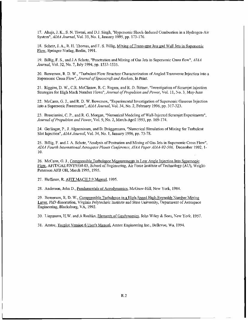
17. Ahuja, J. K., S. N. Tiwari, and D.J. Singh, "Hypersonic Shock-Induced Combustion in a Hydrogen-AirSystem", AIAA Journal, Vol. 33, No. 1, January 1995, pp. 173-176.
18. Schetz, J. A., R. H. Thomas, and F. S. Billig, Mixing of Transverse Jets and Wall Jets in SupersonicFlow, Springer-Verlag, Berlin, 1991.
19. Billig, F. S., and J.A Schetz, "Penetration and Mixing of Gas Jets in Supersonic Cross flow", AIAAJournal, Vol. 32, No. 7, July 1994, pp. 1533-1535.
20. Bowersox, R. D. W., "Turbulent Flow Structure Characterization of Angled Transverse Injection into aSupersonic Cross Flow", Journal of Spacecraft and Rockets, In Print.
21. Riggins, D. W., C.R. McClinton, R. C. Rogers, and R. D. Bittner, "Investigation of Scramjet InjectionStrategies for High Mach Number Flows", Journal of Propulsion and Power, Vol. 11, No. 3, May-June
22. McCann, G. J., and R. D. W. Bowersox, "Experimental Investigation of Supersonic Gaseous Injectioninto a Supersonic Freestream", AIAA Journal, Vol. 34, No. 2, February 1996, pp. 317-323.
23. Brescianini, C. P., and R. G. Morgan, "Numerical Modeling of Wall-Injected Scrarmjet Experiments",Journal of Propulsion and Power, Vol. 9, No. 2, March-April 1993, pp. 169-174.
24. Gerlinger, P., J. Algermissen, and D. Briiggemann, "Numerical Simulation of Mixing for TurbulentSlot Injection", AIAA Journal, Vol. 34, No. 1, January 1996, pp. 73-78.
25. Billig, F. and J. A. Schetz, "Analysis of Pentration and Mixing of Gas Jets in Supersonic Cross Flow",AIAA Fourth International Aerospace Planes Conference, AIAA Paper AIAA-92-506, December 1992, 1-10.
26. McCann, G. J., Compressible Turbulence Measurements in Low Angle Injection Into SupersonicFlow, AFIT/GAE/ENY95M-03, School of Engineering, Air Force Institute of Technology (AU), Wright-Patterson AFB OH, March 1995, 1995.
27. Huffman, R. AFIT MACH 2.9 Manual, 1995.
28. Anderson, John D., Fundamentals of Aerodynamics, McGraw-Hill, New York, 1984.
29. Bowersox, R. D. W., Compressible Turbulence in a High-Speed High-ReYnolds Number MixingLayer, PhD dissertation, Virginia Polytechnic Institute and State University, Department of AerospaceEngineering, Blacksburg, VA, 1992.
30. Liepmann, H.W. and A Roshko, Elements of Gasdynamics, John Wiley & Sons, New York, 1957.
31. Amtec, Tecplot Version 6 User's Manual, Amtec Engineering Inc., Bellevue, Wa, 1994.
R.2

CaptMarkP.Wilson -'----
IOG Hepauad from Monmouth Academy in the spring of 1986, and *=oflein the Aeronsatical
Engineering program of Embry-Piddle Aeronautical University under a four year RO'rC scholarship. He
was commissioned and graduated Cum Laud. with a Bachelor of Science degrec in Aeronautical
Engineering in April of 1990.
Capt Wilson's firs: assignment wan to the United States Air Force Academy, Colorado Springs
Colorado, as a Manpower Officer. He entered the engineering career field in April of 1993 by accepting an
opcrahlona test and evaluation reliability and maiainability assignment with the B-2 Spirit Combined
Task Force, Edwards Air Force Base, California In May of 1995 Capt Wilson entere die School of
Engineering, Air Force Institute of Technology.
V.1