Embed Size (px)
Citation preview

AHNA Methodology – Population and Household Projections 1
AFFORDABLE HOUSING NEEDS ASSESSMENT
Population and Household Projection Methodology
Prepared by the Shimberg Center for Affordable HousingRinker School of Building Construction
College of Design, Construction and PlanningUniversity of Florida
September, 2006
AHNA Methodology – Population and Household Projections 2
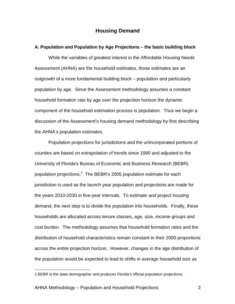
Housing Demand
A. Population and Population by Age Projections – the basic building block
While the variables of greatest interest in the Affordable Housing Needs
Assessment (AHNA) are the household estimates, those estimates are an
outgrowth of a more fundamental building block – population and particularly
population by age. Since the Assessment methodology assumes a constant
household formation rate by age over the projection horizon the dynamic
component of the household estimation process is population. Thus we begin a
discussion of the Assessment’s housing demand methodology by first describing
the AHNA’s population estimates.
Population projections for jurisdictions and the unincorporated portions of
counties are based on extrapolation of trends since 1990 and adjusted to the
University of Florida's Bureau of Economic and Business Research (BEBR)
population projections.1 The BEBR's 2005 population estimate for each
jurisdiction is used as the launch year population and projections are made for
the years 2010-2030 in five-year intervals. To estimate and project housing
demand, the next step is to divide the population into households. Finally, these
households are allocated across tenure classes, age, size, income groups and
cost burden. The methodology assumes that household formation rates and the
distribution of household characteristics remain constant in their 2000 proportions
across the entire projection horizon. However, changes in the age distribution of
the population would be expected to lead to shifts in average household size as
1 BEBR is the state demographer and produces Florida’s official population projections.
AHNA Methodology – Population and Household Projections 3
different age groups have different propensities to form households. Therefore,
the number of households is estimated using age-specific headship rates to
reflect the projected changing age structure.
1. Population Projections
Following the University of Florida's Bureau of Economic and Business
Research (BEBR) approach to small area population forecasts, six methods were
used to project the population of jurisdictions in the county, including the
unincorporated portion of the county. The highest and lowest of the results of these
six methods is dropped, and the remaining four are averaged. Finally, the results
are adjusted to sum to the mid-range county projection, which is obtained from the
BEBR. The population projections form the basis for the projection of population by
age and ultimately the projection of households by age of householder.
Assumptions
The methodology uses the most currently available year, in this case
2005, as the benchmark or launch year and develops projections for the years
2010-2030 in five-year increments. The Bureau of Economic and Business
Research (BEBR) provides the launch year population for each jurisdiction and
county as well as the 2010-2030 county projections based on that launch year.
Population for the base years (1990 and 2000) comes from the U.S. Census.
County population projections prepared by BEBR control the population
projections for each jurisdiction within a county. The methodology uses the
BEBR’s middle (medium) range population projections.
AHNA Methodology – Population and Household Projections 4
Population projections are based on previous trends in a jurisdiction, and
as such are not able to account for a particular community having limited land
availability. Other local conditions not reflected in the estimates would be
aggressive annexation policy (the BEBR estimates of population herein do
include annexations as of the date of the estimate), recent commencement of
large development projects, or dramatic and recent changes in local institutional
facilities with large populations such as prisons.
Description of Population Projections
The most important base data for preparing estimates and projections of
housing demand is population data. Population is the basis of estimates and
projections of households, and the difference between households and housing
inventory, when adjusted for the need for vacancies to allow a smoothly
functioning housing market, is equal to the basic construction need for housing
units.
Population estimates and projections for small areas such as cities, as
compared to the nation or a state, are difficult because of the influence of in- and
out- migration of population, annexation, land availability, zoning, infrastructure
availability, and other factors that have a large impact at the local level. In
addition, in a smaller city the impact of growth is magnified under certain
projection techniques. To overcome this problem, four techniques are used to
project population. In addition, in the application of two of these techniques two
different time periods are used resulting in six estimates. The highest and lowest
AHNA Methodology – Population and Household Projections 5
estimates are dropped to eliminate extreme numbers, and the remaining four are
averaged.
The four approaches to population projection consist of two ratio
techniques, relating one area to a larger area, and two mathematical
extrapolation techniques that project population based on historical trends. We
use the following terminology to describe each technique in the methodology:
1. Base year - the year of the earliest observed population used to make a projection;
2. Launch year - the year of the latest observed population used to make a projection;
3. Target year - the year for which population is projected;4. Base period - the interval between the base year and the launch year;5. Projection horizon - the interval between the launch year and the target
year;6. Medium, high and low projections - the BEBR county projections based
on a variety of projection techniques; the high and low projections are derived from the Bureau’s analysis of projection forecast errors for approximately 3,000 counties in the U.S.; the high and low projections are two-thirds confidence intervals around the medium projection.
Data requirements include jurisdiction and total county population for base
and launch years (1990, 2000 and 2005) using census data or BEBR estimates.
For target years (2010, 2015, etc.) BEBR medium range county projections are
used.
The four basic projection techniques used in the methodology include the
linear, exponential, share and shift methods. The linear and exponential
techniques use the mathematical extrapolation approach; they take the
jurisdiction’s population from the base period and extrapolate it into the future.
The shift and share methods use the ratio approach; they express the data as
ratios or shares of the larger, parent population, for which a projection already

AHNA Methodology – Population and Household Projections 6
exists. Therefore, these techniques require a county or parent population
projection. The linear and share techniques use both 5 and 15-year base
periods, resulting in a total of six projections. The base periods change over time
as the launch year moves forward in time; the current base periods reflect the
1990 and 2000 base years and the 2005 launch year. A more detailed account
of each technique is provided below.
There is one final twist to the projection methodology. It is only the
resident population of the jurisdiction that we want to project, so institutional
populations such as prison inmates, military personnel or college students are
removed from total county and jurisdiction populations prior to the calculations.
(At a different point in the methodology the household-forming portion of this
institutional population will be added back to the resident population to create a
total household-forming population. However, only off-base military and off-
campus college populations are considered household forming in this
methodology.) Sources for institutional population are the Florida Departments
of Corrections and Children and Families, U.S. Department of Defense, and the
State Universities, as compiled by the Bureau of Economic and Business
Research and the Shimberg Center.
Population Projection Formulas
The four projection techniques are patterned after the University of Florida
Bureau of Economic and Business Research's (BEBR) county population
projections. The trends established during a particular base period (e.g. 1990-
2005) are measured and continued through a growth period or projection horizon
AHNA Methodology – Population and Household Projections 7
(e.g. 2010-2015) to establish the population projection. Though the techniques are
simple, more sophisticated projection methodologies do not necessarily produce
more accurate results.
Attributes of each of the four techniques are as follows:
Technique Attributes
Mathematical ExtrapolationLinear Bottom-up ApproachExponential Extrapolation of Small-Area
Population
RatioShift Top-down ApproachShare Ratio of Parent Population
Projection
Formulas for each of the techniques are as follows:
Linear (Amount of Change)Linear projection = (((launch year pop - base year pop)/(launch year-base
year)* (target year - launch year)) + launch year pop
Two linear projections are developed by using two different base years. The population change between each base year and the launch year is divided by the difference in the two periods to compute an average annual population increase (or decrease). This annual increase is multiplied by the number of years in the projection horizon to generate the total population growth for the area. This growth is added to the area's launch year population to establish its population.
Exponential (Percent of Change)Exponential = launch year pop *EXP(LN(percent pop change))
where: LN(percent pop change)=LN(launch year pop/base year pop) *((target year -launch year)/(launch year-base year))
The template breaks this equation into two parts: a) computation of an average growth rate (using natural logarithms), and b) extrapolation of this rate to produce projected population. The former calculates the average rate of change in population between the oldest base year and the launch year. This rate is applied to the launch year population to project the population in the target year. The technique divides the area’s launch year population by that for the base year
AHNA Methodology – Population and Household Projections 8
to compute the percent change. This is multiplied by the projection period adjustment: (target year - launch year)/(launch year-base year).
ShareShare = ((area’s launch year pop - area’s base year pop)/(county launch pop -
county base year pop)*(county target year pop - county launch year pop)) + area’s launch year pop
Two share projections are developed by using two different base years. This method computes the area’s share of the county's population growth between launch year and the two base years, and then allocates to it an equal share of the county's projected population growth over the projection period.
ShiftShift = county’s target year pop * ((launch year area pop/launch year county pop) +
((target year - launch year)/launch year-base year) * ((area’s launch year pop /county’s launch year pop) - (area’s base year pop/county’s base year pop)))
The shift method combines elements of the linear and share methods, making a linear extrapolation of the change in each area’s share of the county population between the oldest base year (1990) and launch year.
AverageAverage = (linear proj.1 + linear proj.2 + exponential projection + share proj.1 +
share proj.2 + shift proj. - highest proj. - lowest proj.)/4
The accuracy of the four previously discussed techniques will vary according to the time period of the projection and the size of the area. No single technique is the most accurate, and certain techniques may yield rather explosive projections. To avoid producing the largest possible error we sum the six projections minus the lowest and highest of the six and take the average of the remaining four.
Adjusted AverageAdjusted Average = area projection * (county projection / sum of area average
projections)
The shift and share methods use apportionment techniques which generate county totals consistent with the overall county projection. However, the linear and exponential techniques ignore the county population projection, relying instead on extrapolation of the historic area trends. Since the Average includes the results of all four techniques, it is unlikely that it will produce county totals identical to the BEBR’s county projection. The Adjusted Average computes the ratio of the projected county population to total area averages and then applies the ratio to each area average projection. The sum of the adjusted projections equals the county projection.
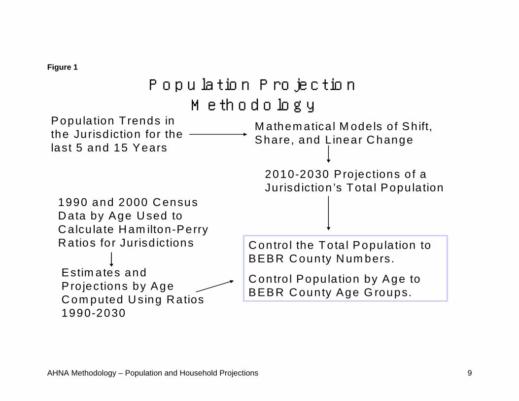
AHNA Methodology – Population and Household Projections 9
Figure 1
Po p u lat io n P ro jec t io n Meth o d o lo g y
2010-2030 Pro jections o f a Jurisd iction ’s Tota l Popu lation
Popu la tion T rends in the Jurisd iction for the last 5 and 15 Years
M athem atica l M ode ls o f Sh ift, Share, and L inear C hange
1990 and 2000 C ensus D ata by Age U sed to C alcu la te H am ilton-Perry R atios fo r Jurisd ictions
Estim ates and P ro jections by Age C om puted U sing R atios 1990-2030
C ontro l the Tota l Popu la tion to BEBR C ounty N um bers.
C ontro l Popu lation by Age to BEBR C ounty Age G roups.
AHNA Methodology – Population and Household Projections 10
2. Population by Age - Background
The age distribution of the population serves as the basis for projecting
the number of households and other aspects of housing demand. This is a
fundamental assumption and the estimates and projections of population by age
are a crucial component of the Assessment methodology. Several avenues are
closed off to a method that must project an age distribution at the jurisdiction (or
other small area) level. Cohort-component and econometric techniques require
detail generally lacking at this geographic level. Small area techniques
appropriate to total population projection are not so for age projections. Similarly,
extrapolating trends in age groups may not be appropriate for rapidly growing
areas like Florida. The Assessment’s methodology produces sub-county
estimates and projections with age detail, using data sources and techniques that
are readily available, reliable, and relatively inexpensive.
Since the United States conducts its population census every ten years,
there is a substantial need for current information in the years between
censuses. Population estimation techniques have been created to fill this need.
Methods fall into three broad categories: 1) extrapolation of past trends, 2)
allocation of current trends from other geographic areas, and 3) use of
symptomatic data about the particular geographic area of interest.
Extrapolation methods utilize data previously collected about an area to
calculate a trend over time and then carry that trend forward to the present.
Estimates can be created easily using extrapolation methods since the
calculations are often simple and census data is commonly available.
AHNA Methodology – Population and Household Projections 11
Extrapolation techniques do not work well in places that are increasing or
decreasing in population at an unpredictable rate. Also, extrapolation techniques
are not applicable for geographic areas whose boundaries are defined by the
user (such as a 2 mile radius around a bank) rather than by a typical political and
analysis geography for which data are regularly collected (such as cities or
counties).
Allocation methods produce population estimates by applying trends in
one area to a second area. For example, if a reliable estimate exists for a state
in 2005, then a 2005 estimate could be produced for a county by applying the
state’s average annual growth rate since 2000 to the 2000 population of the
county. Ratios are often used to allocate population change from larger areas to
smaller areas. For example, the absolute increase in population that occurred in
the state since the last census can be divided among the constituent counties
based on their share of the state’s population at some prior point. Similar to
extrapolation, allocation methods are fairly easy to calculate, but allocation is
limited in that it requires data for two places, not just one. Also, allocation of
trends is only reliable if there is continuity over time in the relationship between
the two places. If the underlying ratios change over time, but there is no data
available to detect that change, then an estimate produced by an allocation
method will be unreliable.
Collection of symptomatic data about the place of interest is going to
produce the most reliable estimates of population, but this approach has the
highest costs. Data sources for small areas vary greatly in terms of availability,
AHNA Methodology – Population and Household Projections 12
cost, and precision. Some researchers use data on vital statistics (births and
deaths), housing units, water usage, special surveys, and property appraiser
parcels. Any consistent series that reflects the underlying demographic change
occurring in the area is useful in calculating a trend and updating the results from
the last census.
Once an estimate is created for the total population, detail can be
generated for different segments of the population and the current trends can be
projected into the future. Since projections are based on historical data and
trends in an area, projection methods fall into the extrapolation classification. For
national estimates and projections, numerous data sources are available that
generate quality results. Data availability and reliability are roughly proportionate
to the size of place under investigation. There are far fewer options for
calculating estimates and projections for counties than for the nation as a whole–
and even fewer are available for sub-county areas. In general, the arduousness
of a calculation and its potential error are increased by adding levels of detail
(total population vs. age, sex, and income detail), decreasing the size of the
place (nation vs. county vs. census tract), and increasing the time since the last
base point (estimate for 5 years since the last census vs. 20 year projection vs.
50 year projection). Estimating and projecting a population’s composition is
especially problematic for small geographic areas. That objective crosses all
three areas of difficulty–detail, size, and horizon.
No single method has been the authoritative choice for detailed sub-
county population estimates and projections. Cohort-component techniques
AHNA Methodology – Population and Household Projections 13
(which fall into the extrapolation classification) have been the primary method
used for national and state-level projections of the population by age. Cohort-
component applies historical fertility, mortality, and migration patterns to a base
population to produce a detailed depiction of the population at some subsequent
point. Since fertility, mortality, and migration do not happen on a daily basis to all
age segments of the population, accurate measurement of those demographic
events in smaller populations is nearly impossible. Cohort-component has been
used successfully for counties, but rarely for sub-county areas due to its data
requirements. In the next section we examine the usefulness of a variation of the
cohort-component method employed in the Assessment.
3. Hamilton-Perry Ratios
There are no population by age estimates or projections available at the
local level to the extent needed for this model. In fact there are no population
projections for all Florida jurisdictions, so development of these numbers was a
critical first step in the methodology. The population age projection used in the
housing needs assessment is a technique in which survival rates (births and
deaths) are combined with net migration rates into a single ratio for each age
group. This survival/net migration ratio is then used to project the age group into
the future. This methodology is, in turn, a simplified application of the cohort-
component method of projection in which births, deaths, and migration (the
components of population change) are projected separately for each age-sex group
in the population (Hamilton and Perry, 1962; Smith and Shahidullah, 1995).
AHNA Methodology – Population and Household Projections 14
The choice of this approach for use in the Assessment is notable, in part,
because of what can’t reasonably be done at a small geographic level that meets
the objectives of low cost and accessibility. The conventional cohort-component
approach requires individual detail for births, deaths, and migration not available
at the jurisdiction level; for econometric modeling the jurisdiction is generally too
small a unit of measure; typical small area population projection techniques like
shift and share are not appropriate for age projections; and extrapolating trends
in age groups is not appropriate for rapidly growing areas with volatile migration
patterns.
To calculate population by age, a net migration/survival ratio is determined
for each age group. Two points in time are needed to construct the survival/net
migration ratio – in our case the jurisdiction’s population by age group for 1990
and 2000. The sources for this data are the respective census counts. The third
set of data needed for this methodology is the jurisdiction’s population for each of
the projection years.
Since we are interested in projecting our resident population we subtract
out the institutional population to give us an adjusted population. It is the
adjusted population that we will project and, where necessary, add back the
institutional population to give a final total population by age group. The data for
institutional population by age group comes from the Florida Departments of
Corrections and Children and Families, the U.S. Department of Defense, and the
State Universities as compiled by the Bureau of Economic and Business
Research (BEBR) and the Shimberg Center (The institutional population for two
AHNA Methodology – Population and Household Projections 15
counties, Alachua and Leon, are special cases, please see the appendix for a
description of how those two counties are handled).
The Hamilton-Perry ratio is the change in the population of a particular set
of birth years between two dates (an age cohort). The ratio is designed to
capture the change in the size of an age cohort over a ten-year period. For
example, the population aged 10-14 in 2000 is divided by the population ten
years earlier, that is, the population aged 0-4 in 1990. The ratio is then applied to
the population aged 0-4 in 2000 to project the population aged 10-14 in 2010 and
to the population aged 0-4 in 2010 to project population aged 10-14 in 2020. The
population in a cohort changes as a result of both the survival of the population in
the cohort at the beginning of the ten-year period and the in- or out-migration of
population in the particular set of birth years. In most age groups, migration is
the dominant factor affecting changes in the population of an age group. Further,
many parts of Florida have experienced large net in-migration.
Calculation of the migration/survival ratio reflects the past impact of
migration on various age groups and uses that trend as a basis to project the
population by age group, with the total adjusted to the previously calculated
jurisdiction total. Finally, the projections are “tweaked” slightly by making an
adjustment to the projections of the population age 0-9 and 75+. To accomplish
this slight adjustment, the Bureau of Economic and Business Research’s
estimates and projections of age group totals for each county are employed.
AHNA Methodology – Population and Household Projections 16
Adjustment To The 0 - 9 and 75+ Age Ranges
Two age groups require a modification to the general calculation,
children aged 0-9 and persons aged 75 and older. To create the ratio for
population aged 75+, divide that population in 2000 (75+) by the sum of populations
age 65 to 75+ in 1990.
The population less than ten years old is projected by calculating the ratio of
children age 0-9 to the population age 15-44 in 2000 (0-9/15-44) and applying that
ratio to the population age 15-44 ten years later. We still have to divide the
population age 0-9 into the two population groups age 0-4 and 5-9. To do that we
make an assumption that the share of children age 0-4 to those age 0-9 in the
jurisdiction is the same as that of the county as a whole.
4. Finalize the population by age projections
The preceding calculations have given us a preliminary projection for the
year 2010. But the total jurisdiction population projected using this methodology
may be inconsistent with that of the population projection methodology in Part 1.
So, to complete the projection for 2010, the population of each age group is
adjusted to reflect the total jurisdiction population calculated previously. The
controlled age projection for 2010 computes the ratio of the projected jurisdiction
population (control total) to the sum of age group populations (the jurisdiction’s
total uncontrolled population) and applies that ratio to each age group population.
Age group projections for 2020 and 2030 are calculated in the same
fashion. The survival/net migration ratio is applied to the age group population in
the year 2010 (using the final or controlled age projection figure, rather than the
AHNA Methodology – Population and Household Projections 17
uncontrolled figure) to produce a 2020 projection and that step is repeated again
for the 2030 projection using 2020 as a base. The preliminary (or uncontrolled)
age group projection is then adjusted using the ratio of the projected population
(from the preceding methodology -- Part 1) to the sum of age group populations
(total controlled population) to produce a final (or controlled) projection. We
derive the projections for the launch year (2005), and the mid-decade points,
2015, etc., by using the compound growth rate between decades. The function
is:
Pop of year 2000+n = pop2000 * e ^ (n/10 * ln(pop2000/pop2010))(n = 2 or n = 5)
Pop of year 2015 = pop2010 * e ^ (5/10 * ln(pop2010/pop2020))
Pop of year 2025 = pop2020 * e ^ (5/10 * ln(pop2020/pop2030))
The Hamilton-Perry ratios seem less able to capture the volatility in young
adult and elderly populations. In counties like Charlotte, for example, the
accelerated in-migration of elderly in the 1980’s and 1990’s and the
corresponding shift in the age structure fell outside the rates captured by the H-P
ratios. The use of the BEBR county age projections provides a way to recapture
that important shift. So, the last step in the population by age projection
methodology is to control the sum of jurisdictions by age group to the BEBR
county age group projection. This is an iterative mathematical procedure that
produces a best fit between the jurisdiction’s total population and the county age
group total.
AHNA Methodology – Population and Household Projections 18
B. Householder by Age and Tenure
1. A fundamental assumption: headship rates
Households are the basic unit of demand for housing. They are the way in
which the population divides itself to occupy housing units. One member of a
household is considered the representative of that household and is referred to
as the householder. The percentage of the population in a given age group that
are householders is the headship rate in that age group, or the propensity of
persons in that age group to be household heads. Therefore, headship rates
allow the conversion of the population of an age group into households. Different
age groups have different propensities for forming households, so that as the age
structure of the population shifts, the number of households that a given
population would yield would also change.
The way in which the population divides itself into households is related to
a number of economic and social factors including income, housing prices,
governmental assistance, marriage and divorce rates, and the mobility of the
population. While household sizes declined significantly in the 1970s and
continued to decline more slowly in the 1980s, the rate of decline slowed
significantly during the 1990s. Further, factors that lead to changes in household
size do not exhibit a clear and convincing pointer to the direction of future
change. The fundamental assumption in the construction of household estimates
in the Assessment is that household formation rates and the distribution of
household characteristics remained constant in their 2000 proportions across the
projection horizon. Estimates and projections of households are therefore based
AHNA Methodology – Population and Household Projections 19
on age-specific householder (headship) rates. These headship rates are applied
to the age-specific population projections calculated in the previous section.
The projection of householder by age, tenure, and size (headship) builds on the
age group projections developed in Part 2. Three data sets are needed --
householder by tenure and age (at a minimum), population by age from the 2000
Census for each jurisdiction and the age group projections previously calculated.
A headship rate is calculated from the 2000 census data by dividing the number
of householders in each tenure/age group by the total population of that age
group. The projection of householder by age/tenure is then calculated by
applying that ratio (headship rate) to the age group projections of population for
each projection period. The numbers of households in each age group are
summed to the projected number of households.
However, to meet the twin objectives of housing plan- and housing
program-friendly formats in conjunction with more accurate household
projections, the AHNA model requires complex cross-tabulations.
2. Household Projection Methodology
In order to produce a complex cross-tabulation of household characteristics
such as – Tenure X Age X Size X Income X Cost Burden projections (for a
projection horizon of 2010-2030) – the data requirements of the methodology
are:
1. Population by age estimates/projections (2000-2030);
2. 2000 Household Count by Tenure X Age X Size X Income X Cost Burden
AHNA Methodology – Population and Household Projections 20
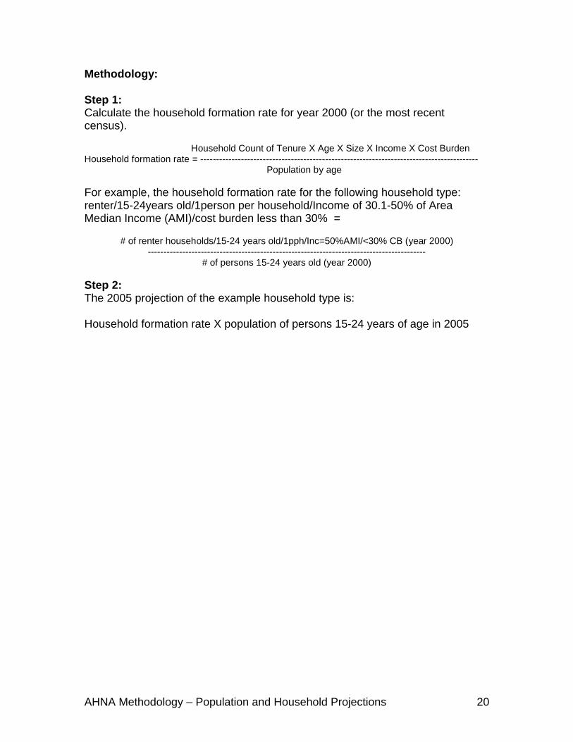
Methodology:
Step 1:Calculate the household formation rate for year 2000 (or the most recent census).
Household Count of Tenure X Age X Size X Income X Cost BurdenHousehold formation rate = ----------------------------------------------------------------------------------------- Population by age
For example, the household formation rate for the following household type: renter/15-24years old/1person per household/Income of 30.1-50% of Area Median Income (AMI)/cost burden less than 30% =
# of renter households/15-24 years old/1pph/Inc=50%AMI/<30% CB (year 2000)-----------------------------------------------------------------------------------------
# of persons 15-24 years old (year 2000)
Step 2: The 2005 projection of the example household type is:
Household formation rate X population of persons 15-24 years of age in 2005
AHNA Methodology – Population and Household Projections 21
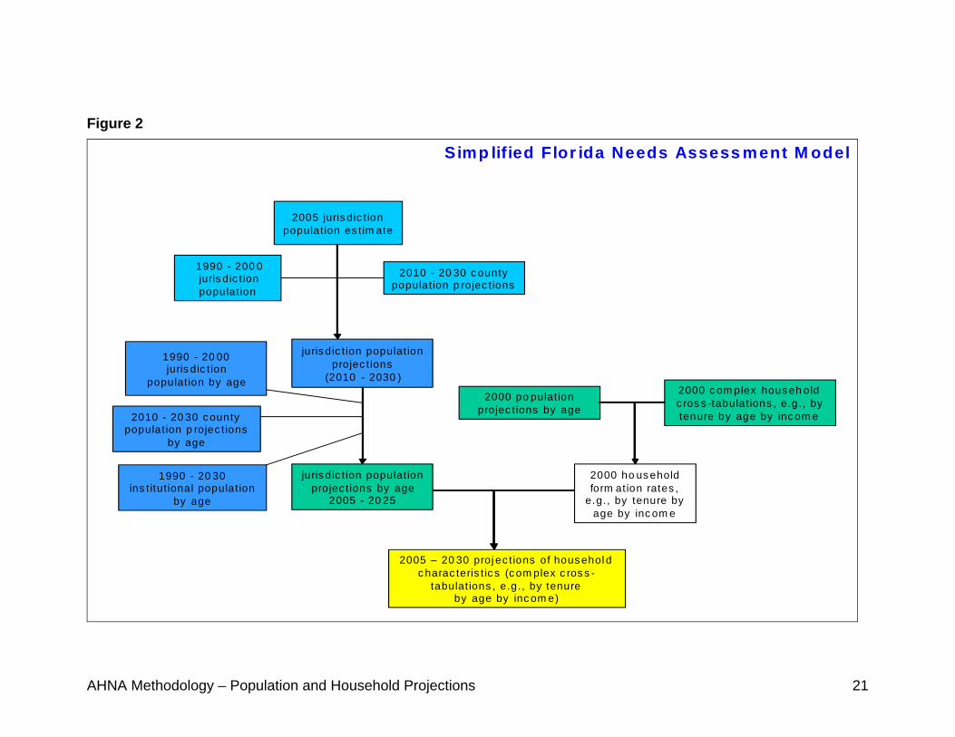
Figure 2
Simp lified Flor ida Needs Assess ment M odel
juris dic t ion populat ion projec t ions by age
2005 - 20 25
2000 ho us ehold form ation rates ,
e.g., by tenure by age by inc om e
2005 – 20 30 proj ec t ions of hous ehol d c harac teris t ic s (c om plex c ros s -
tabulat ions , e.g., by tenure by age by inc om e)
2000 po pulat ion projec t ions by age
2000 c om plex hous eh old c ros s -tabulat ions , e.g., by tenure by age by inc om e
1990 - 200 0juris dic t ion populat ion
2005 juris dic t ion populat ion es tim ate
juris dic t ion populat ion projec t ions
(2010 - 2030 )
2010 - 20 30 c ountypopulat ion p rojec t ions
1990 - 20 00 juris dic t ion
populat ion by age
2010 - 20 30 c ounty populat ion p rojec t ions
by age
1990 - 20 30 ins t itut ional populat ion
by age
AHNA Methodology – Population and Household Projections 22
APPENDIX
A discussion of the FSU/FAMU and UF enrollment figures
The FSU/FAMU and UF enrollment figures for three universities – Florida State University and Florida A&M University in Leon County and University of Florida in Alachua County – their distribution by age and their distribution by on-and off-campus population, have a significant influence on the household projections contained in the Needs Assessment (AHNA) for Leon and Alachua counties. This is an explanation of how that was accomplished. Planning officials in these two counties should pay close attention to the assumptions and the resulting population and household estimates and projections.
Institutional populations such as major university enrollments, inmate populations, and the armed forces are subtracted from total population estimates before the AHNA projections of “permanent” population are made. Projections of the institutional populations are made separately and these populations are added back to the permanent population projections to produce a final population total. Household estimates and projections are made from the “permanent” population figures, i.e., the permanent population is the household-forming population and does not generally include the institutional population. In certain counties the institutional population or some part of it is considered a household-forming population. In Alachua and Leon Counties a portion of the university headcount, the off-campus portion, is added back to the permanent population (by age) and the total is used to project households.
The FSU/FAMU and UF headcounts include all students and, if the information is available, the spouses and children of students residing in on-campus family housing. The actual and projected headcounts, the distribution of headcount by age, and on-campus occupancy were obtained from various sources at the three universities. In certain cases projections had to be extrapolated by assuming an average annual increase derived from the last year of projected headcount that the Shimberg Center could obtain from university sources.
To distribute the university headcounts geographically we attributed all the on-campus student population plus a varying percentage of the off-campus to Tallahassee or Gainesville; the remainder was attributed to the unincorporated area. The percentage of off-campus UF headcount attributed to Gainesville was: 40%-1989/90, 45%-thereafter. The off-campus distribution for Leon County was derived from data obtained from the Tallahassee-Leon County Planning Department.