Embed Size (px)
Citation preview
Affective Forecasting Time Course 1
Running Head: AFFECTIVE FORECASTING TIME COURSE
Mispredicting Distress Following Romantic Breakup:
Revealing the Time Course of the Affective Forecasting Error
Paul W. Eastwick and Eli J. Finkel
Northwestern University
Tamar Krishnamurti and George Loewenstein
Carnegie Mellon University
Word count: 5,110
June 29th, 2007
In Press, Journal of Experimental Social Psychology
Affective Forecasting Time Course 2
Abstract
People evidence significant inaccuracies when predicting their response to many emotional life
events. One unanswered question is whether such affective forecasting errors are due to
participants’ poor estimation of their initial emotional reactions (an initial intensity bias), poor
estimation of the rate at which these emotional reactions diminish over time (a decay bias), or
both. The present research used intensive longitudinal procedures to explore this question in the
wake of an upsetting life event: the dissolution of a romantic relationship. Results revealed that the
affective forecasting error is entirely accounted for by an initial intensity bias, with no contribution
by a decay bias. In addition, several moderators of the affective forecasting error emerged:
Participants who were more in love with their partners, who thought it was unlikely they would
soon enter a new relationship, and who played less of a role in initiating the breakup made
especially inaccurate forecasts.
KEYWORDS: affective forecasting, breakup, romantic relationships, love, longitudinal
(149 words)
Affective Forecasting Time Course 3
Mispredicting Distress Following Romantic Breakup:
Revealing the Time Course of the Affective Forecasting Error
“If you should ever leave me, though life would still go on, believe me;
The world could show nothing to me, so what good would living do me?”
– God Only Knows, The Beach Boys
The termination of a romantic relationship is among life’s most distressing and disruptive
events. Indeed, the negative health consequences of divorce are well documented (e.g., Kiecolt-
Glaser et al., 1987), and even nonmarital romantic breakup is powerful enough to generate
considerable sadness and anger (Sbarra, 2006) and to unveil people’s deepest insecurities (Davis,
Shaver, & Vernon, 2003). Furthermore, this distress is not necessarily alleviated if one actively
chooses to end a relationship: “Breakers” tend to experience guilt and even physical symptoms
such as headaches and sleeping irregularities (Akert, 1998, as cited in Aronson, Wilson, & Akert,
2005).
Regardless of who initiates a breakup, it is likely that people are typically well aware that
relationship dissolution is an unpleasant experience. After all, people strive to maintain their social
relationships even in the face of strong external barriers (Baumeister & Leary, 1995), presumably
because the alternative life without a particular close other seems dark and miserable. But how
accurately can people predict the magnitude of this post-breakup distress? A burgeoning literature
on affective forecasting reveals that individuals demonstrate remarkably poor insight when asked
to predict the magnitude of their distress following emotional events (Gilbert, Pinel, Wilson,
Blumberg, & Wheatley, 1998; for reviews, see Wilson & Gilbert, 2003, 2005). From
disappointing election results (Gilbert et al., 1998) to lost football games (Wilson, Wheatley,
Meyers, Gilbert, & Axsom, 2000) to unpleasant medical procedures (Riis et al., 2005), individuals
tend to predict that such events will cause greater levels of distress and negative affect than is
Affective Forecasting Time Course 4
actually the case. (Although the present report examines the affective forecasting error regarding a
negative event, participants also tend to overestimate their emotional responses to positive events;
e.g., Wilson et al., 2000.)
Since the initial demonstration of the affective forecasting error (Gilbert et al., 1998), over
two dozen additional articles have empirically explored the characteristics of and processes
underlying this pervasive bias. These experiments have uncovered a number of independent
reasons why people commit affective forecasting errors. To take one example, participants’
forecasts seem not to account for their own psychological immune systems: that is, their ability to
effortlessly make sense of and subsequently reduce the emotional impact of unexpected negative
events (Gilbert, Lieberman, Morewedge, & Wilson, 2004; Gilbert et al., 1998). Another source of
bias is called focalism, which refers to participants’ tendency to focus only on the emotional event
in question when making their forecasts, frequently ignoring other life events that could raise or
lower their distress in the wake of the event (Wilson et al., 2000). In other cases, errors are due to
an empathy gap (Loewenstein, 1996; 2005) whereby participants insufficiently correct their
forecasts to counteract the biases introduced by their current emotional states (Gilbert, Gill, &
Wilson, 2002). The affective forecasting error is consistent and persistent; one or several possible
mechanisms may conspire to produce it (see Wilson & Gilbert, 2003, for a comprehensive list).
One central yet unresolved issue in this literature concerns the precise time course of the
forecasting error. Wilson and Gilbert (2003) noted that all extant data were consistent with either
or both of two possibilities: an initial intensity bias, which refers to erroneous predictions about
the initial emotional impact of an event, or a decay bias, which refers to erroneous predictions
about the rate that an emotional reaction diminishes over time.1 That is, participants could be
making incorrect affective forecasts because (a) they believe that emotional reactions are initially
more acute than is actually the case and/or (b) they believe that emotional reactions decay at a
Affective Forecasting Time Course 5
slower rate than is actually the case. The currently preferred term impact bias, defined as an error
“whereby people overestimate the impact of future events on their emotional reactions” (Wilson &
Gilbert, 2003, p. 353), subsumes both the initial intensity and decay biases.
Research can reveal greater insight into the nature of the affective forecasting error by
teasing apart the relative contributions of the initial intensity bias and the decay bias. Perhaps
forecasting errors are optimally characterized as an overestimation of the immediate distress
people feel after an emotional event, or perhaps they are due to people’s underestimation of the
speed at which emotional reactions diminish over time. Why is it that virtually no research has
compared the initial intensity and decay biases? A plausible answer is that such a study would
entail significant methodological complexity. It would ideally use a within-subjects design,
requiring participants to provide both a forecast (before an event) and an actual rating (after an
event) of their emotions. This design is more rigorous than a between-subjects design (where some
participants are “forecasters” and others are “experiencers”), but it is more difficult to execute
because it requires that participants be recruited for the study before the occurrence of the
emotional event. Furthermore, such a study would require that participants (a) forecast their future
affective experiences at multiple (at least 2, but preferably 3 or more) time points following the
emotional event and (b) report their actual emotions at those time points that correspond to the
forecasts. To date, only one published study has used such a design (Kermer, Driver-Linn, Wilson,
& Gilbert, 2006, Study 2). In advance of placing a bet, participants in this study forecasted their
happiness immediately and 10 minutes after winning or losing it; they then won or lost the bet and
provided their actual happiness ratings immediately and 10 minutes later. The researchers found
that participants who lost the bet committed an affective forecasting error, and the magnitude of
this error did not differ significantly between the first and second assessments (D. Kermer,
personal communication, November 26, 2006). That is, participants’ emotional reactions were
Affective Forecasting Time Course 6
immediately less intense than they had predicted (i.e., an initial intensity bias), and though their
forecasts and actual emotions moved toward baseline over the ensuing 10 minutes, the slopes of
these two lines did not differ significantly (i.e., no decay bias).
Though entirely appropriate for the research goals of Kermer and colleagues (2006), 10
minutes is a very short amount of time to test for the existence of the decay bias. It is plausible that
time course differences between forecasted and actual emotions might only emerge given a
sufficient time lapse since the emotional event. We constructed the present study to test for both
the initial intensity bias and the decay bias over approximately three months and in response to a
consequential real-life event: the breakup of a romantic relationship.
The Current Research
When people are asked to recall depressing or adverse events in their life, the vast majority
of their answers reference some form of relationship distress, with the dissolution of a romantic
relationship emerging as one of the most common answers (e.g., Harter, 1999; Veroff, Douvan, &
Kulka, 1981). For this reason, we chose to explore the time course of the affective forecasting
error using romantic breakup as the target emotional event. In general, it is tricky to design a
longitudinal study that captures a distressing yet unscheduled major life event. But romantic
breakups happen to nearly everyone at one point or another, making it plausible that we could
conduct an affective forecasting study using the more rigorous within-subjects design. Previous
successful within-subjects designs have used lost football games (Wilson et al., 2000),
disappointing elections, or negative feedback in an experimental setting (Gilbert et al., 1998;
Wilson, Meyers, & Gilbert, 2003); these events, though clearly unpleasant, probably do not have
the same potential for lasting distress as a romantic breakup. In fact, Gilbert and colleagues used a
romantic breakup scenario in their very first demonstration of the affective forecasting error
(Gilbert et al., 1998, Study 1), though they used a between-subjects design (comparing one group
Affective Forecasting Time Course 7
of forecasters to a separate group of experiencers), presumably due to the aforementioned
methodological complexities.
In the present study, we overcame these methodological hurdles using a 9-month
longitudinal study of dating behavior. All of the participants were college freshmen involved in a
romantic relationship at study entry, and 38% of them broke up with that partner during the 6
months that followed. For these participants who experienced a breakup, we compared their
forecasted distress (reported 2 weeks prior to the report of the breakup) with their actual distress at
4 different time points covering the initial weeks and months following the breakup. With these
multiple assessments in hand, we could probe the existence of both the initial intensity bias and
the decay bias. In addition, we explored three potential moderators of the affective forecasting
bias: participants’ reports of how much they were in love with their romantic partner, their
likelihood judgments of whether they would soon begin a new relationship, and their reports of
who initiated the breakup. We hypothesized that participants who were especially in love with
their partner, who could not envision themselves beginning a new relationship, or who played less
of a role in initiating the breakup would be especially likely to overestimate their post-breakup
distress. These moderators seemed sensible from the perspectives of both interdependence theory
(i.e., affective forecasting errors are pronounced when the outcomes of a relationship are good and
the loss of the relationship would be costly; Thibaut & Kelley, 1959) and attachment theory (i.e.,
forecasting errors are pronounced when one is bonded to and disinclined to separate from one’s
romantic partner; Mikulincer & Shaver, 2007).
Method
Participants
Sixty-nine Northwestern University freshmen participated in a 9-month paid longitudinal
study. Eligibility criteria required that each participant be a first-year undergraduate at
Affective Forecasting Time Course 8
Northwestern University, a native English speaker, involved in a dating relationship of at least two
months in duration, between 17 and 19 years old, and the only member of a given couple to
participate in the study.
All data in this report pertain to the 26 participants (10 female) whose romantic
relationship at study entry ended during the first 6 months (14 waves) of the study. Most
participants were 18 years old (two were 17 and five were 19); they had been dating their partner
for an average of 14.0 months (SD=10.6 months) at study entry. The questionnaire completion rate
was excellent: Of the 208 Distress reports required for the present analyses (26 participants × 8
reports per participant), only 1 report was missing.
Procedure
This study was part of a larger investigation of dating processes and contained two
components that are relevant to the present report. Participants completed an Intake Questionnaire
at home sent via campus mail and an Online Questionnaire every other week for 38 weeks (for a
total of 20 online sessions). The first 14 Online Questionnaires took approximately 10-15 minutes
to complete; the remaining 6 (abbreviated) Online Questionnaires took only 1-2 minutes to
complete. Participants could earn up to $100 by completing the first 14 Online Questionnaires; for
each of the 6 remaining (shorter) questionnaires completed, participants received one entry into a
$100 raffle.
Materials
As part of the Intake Questionnaire, participants provided demographic information and
reported the length of their current relationship. As part of the biweekly Online Questionnaires,
they reported whether or not they were still involved in a romantic relationship with the partner
they had been dating at the start of the study. If participants reported that they were no longer
romantically involved with their partner, they completed a 2-item measure of Actual Distress. This
Affective Forecasting Time Course 9
construct was an average of the items “In general, I am pretty happy these days” (reverse scored;
see Gilbert et al., 1998) and “I am extremely upset that my relationship with [name] ended”
(α=.62). (Unless otherwise noted, all items were assessed on 1 [strongly disagree] to 7 [strongly
agree] scales.) Participants subsequently completed this measure on all remaining Online
Questionnaires. In addition, on each of the first 14 (longer) Online Questionnaires, participants
completed four versions of a 2-item measure of Predicted Distress if they were still involved with
their partner from study entry. Both items began with the following stem: “If your relationship
were to end in sometime within the next two weeks, to what degree will you agree with this
statement in two [four, eight, twelve] weeks:” and then continued with, “In general, I am pretty
happy these days” (reverse scored) and “I am extremely upset my relationship ended” (α=.80).
We also explored several potential moderators of the affective forecasting error. If
participants reported on the Online Questionnaire that they were still involved with their partner
from study entry, they completed a 1-item measure assessing how much they were In Love (“I am
‘in love’ with my partner”) and a 1-item measure assessing New Relationship Likelihood (“It is
likely that I will start a new romantic relationship over the next two weeks”). Finally, the first time
that participants reported on the Online Questionnaire that they were no longer dating their
partner, they indicated who was the Breakup Initiator (“me”, “mutual”, or “partner”).
Analysis strategy. The Predicted Distress ratings analyzed in the present report were those
reported on the Online Questionnaire 2 weeks before participants reported that their relationship
ended. In other words, the dataset included participants’ Predicted Distress ratings that
corresponded to the breakup session 2 weeks later (Time 0), as well as to the Online Questionnaire
sessions that were 2, 6, and 10 weeks following the breakup session (Time 2, 6, and 10,
respectively). The Actual Distress ratings included in the dataset are those actually reported by the
participants on the Online Questionnaire at the breakup session (Time 0) as well as at the sessions
Affective Forecasting Time Course 10
2, 6, and 10 weeks following the breakup session. The In Love and New Relationship Likelihood
ratings analyzed in the present report were also those reported on the Online Questionnaire 2
weeks before participants reported that their relationship ended.
We employed growth curve procedures (e.g., Singer & Willett, 2003) to analyze these data.
Growth curve analysis can reveal in a single regression equation whether a predictor has an effect
on the initial level and/or the slope of a dependent variable’s trajectory over time. In this case, the
initial intensity vs. decay bias distinction maps on perfectly to the distinction between an initial
status and slope effect (see Results section). Each participant provided 8 rows of data: four Actual
Distress reports and four Predicted Distress reports. These reports correspond to Time 0 (the
breakup session), 2, 6, or 10; one unit of time corresponds to 1 week in real time. Distress reports
at each time point (Level 1) were nested within the dummy variable Distress Type (Level 2),
which was coded 0 for Actual and 1 for Predicted, and Distress Type was nested within participant
(Level 3). These nested observations violate the Ordinary Least Squares regression assumption of
independence. Growth curve models account for this nonindependence by simultaneously
examining variance associated with each level of nesting, thereby providing unbiased hypothesis
tests.
Results
Affective Forecasting Error
Did participants commit an affective forecasting error when asked to predict how
distressed they would be if their romantic relationship ended? This error could possibly take either
(or both) of two forms: an initial intensity bias or a decay bias. These possibilities could be
revealed by the following regression analysis:
Distress = γ0 + γ1DistressType + γ2Time + γ3(DistressType × Time) + error. (1)
Affective Forecasting Time Course 11
Distress was left on the original 1-7 metric, DistressType was dummy coded (0=Actual;
1=Predicted), and Time was coded as 0, 2, 6, or 10. The coefficient γ0 indicates the initial status
(Time 0) of Actual Distress. The coefficient γ1 indicates whether participants’ predicted distress
reports differed from their actual reports at Time 0; a positive value for this parameter would
indicate an affective forecasting initial intensity bias (statistically referred to as an initial status or
intercept effect; see Singer & Willett, 2003). The coefficient γ2 indicates whether participants’
Actual Distress reports changed over time. Finally, the coefficient γ3 indicates whether or not this
change over time differed as a function of whether the reports were predicted versus actual; a
positive value for this parameter would indicate an affective forecasting decay bias (statistically
referred to as a slope or rate of change effect). Both the initial status (γ0) and slope (γ2) of Distress
were permitted to vary randomly across participants (Level 3) and across Distress Type (Level 2).
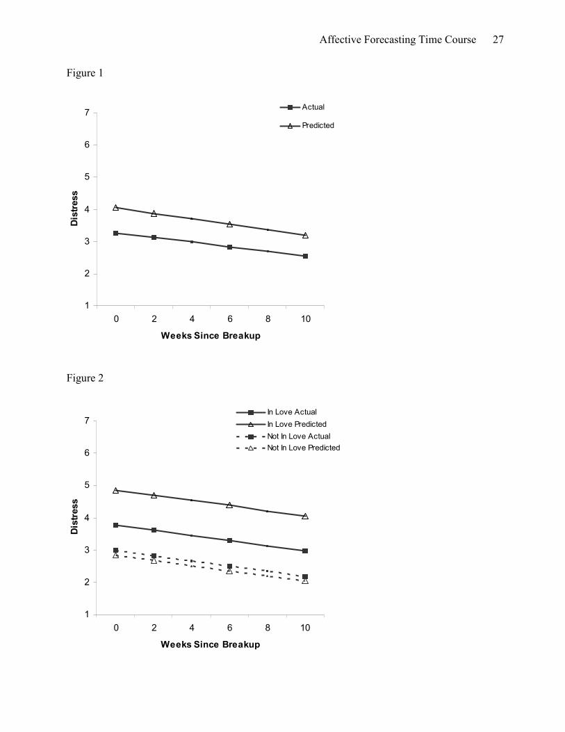
Results of this regression are displayed graphically in Figure 1. As hypothesized, the
coefficient γ1 was significant and positive, γ1=.79, t(24)=4.30, p<.001, indicating that participants’
Predicted Distress ratings were higher than their Actual Distress ratings at Time 0 (i.e., an initial
intensity bias). The coefficient γ2 was significant and negative, γ2=-.07, t(6)=-3.12, p=.021,
indicating that participants’ Actual Distress ratings decreased over time. Interestingly,
participants’ Predicted Distress ratings decreased at a rate that did not differ significantly from
their Actual Distress ratings, γ3=-.02, t(24)=-0.55, p=.591. In other words, the data revealed no
evidence of a decay bias. Furthermore, even 10 weeks after the break-up (i.e., the last Actual
Distress assessment), participants’ Predicted Distress ratings still overestimated their Actual
Distress (simple effect γ1 at week 10=.64, t(24)=2.85, p=.009). Thus, the Equation 1 regression
revealed evidence of an initial intensity bias (γ1) but no evidence of a decay bias (γ3): Participants’
Affective Forecasting Time Course 12
Predicted Distress was significantly greater than their Actual Distress at wave 0, and both Distress
types decreased over time at roughly the same rate.
Moderators of the Affective Forecasting Effect
Perhaps the affective forecasting error was more pronounced for some individuals than for
others. First, we hypothesized that individuals would overestimate their distress following a
breakup to the extent that they reported being in love with their partner at the session immediately
preceding the breakup. To examine this possibility, we conducted a second regression analysis:
Distress = γ0 + γ1DistressType + γ2Time + γ3InLove + γ4(DistressType × InLove) + error. (2)
Again, distress was left on the original 1-7 metric, DistressType was dummy coded (0=Actual;
1=Predicted), and Time was coded as 0, 2, 6, or 10.2 InLove was a Level 3 variable and was
standardized (M=0, SD=1). Coefficients γ0, γ1, and γ2 have the same conceptual meaning as in
Equation 1. Coefficient γ3 indicates whether or not participants who were more in love with their
partner experienced more Actual Distress at Time 0, and coefficient γ4 tests whether the
discrepancy between Predicted Distress and Actual Distress ratings was more pronounced for
participants who were in love. For example, a positive value for γ4 would indicate that participants
who were more in love evidenced a greater initial intensity bias.
As in Equation 1, the coefficient γ1 in Equation 2 was significant and positive, γ1=.47,
t(35)=3.20, p=.003, and the coefficient γ2 was significant and negative, γ2=-.08, t(35)=-6.08,
p<.001. Coefficient γ3 was marginally significant and positive, γ3=.40, t(35)=1.90, p=.066,
indicating that participants were (marginally) more likely to experience distress after breakup to
the extent that they had reported being in love with their partner just prior to the breakup. For the
critical parameter γ4, In Love indeed proved to be a significant moderator of the initial intensity
Affective Forecasting Time Course 13
bias, γ4=.62, t(35)=3.78, p<.001. Figure 2 presents predicted trajectories for participants whose In
Love reports were 1 standard deviation above (“in love”) and below (“not in love”) the mean. The
simple effect of Distress Type for “in love” participants was both substantial and significant:
γ1=1.08, t(34)=5.55, p<.001. That is, participants who were in love with their partners greatly
overestimated the amount of distress they would feel immediately after the breakup. On the other
hand, the simple effect of Distress Type for “not in love” participants was both small and
nonsignificant, γ1=-.15, t(34)=-0.63, p=.533. In other words, those participants who were not in
love with their romantic partners closely preceding the breakup were quite accurate when asked to
forecast their distress. Taken together, the results from Equation 2 suggest that participants made
severe affective forecasting errors (specifically the initial intensity bias) to the extent that they
were in love with their romantic partner just prior to the breakup, but they tended not to make such
errors when they were not especially in love.
In a second moderational analysis, we hypothesized that participants would be more likely
to overestimate their distress if they reported at the session before the breakup that it was unlikely
that they would enter into a new relationship during the next two weeks. To examine this
possibility, we substituted InLove in Equation 2 with the variable New Relationship Likelihood,
which was standardized. Again, the coefficient γ1 was significant and positive, γ1=.70, t(35)=5.14,
p<.001, and the coefficient γ2 was significant and negative, γ2=-.08, t(35)=-5.54, p<.001.
Coefficient γ3 was nonsignificant in this case, γ3=-.13, t(35)=-0.06, p=.554, indicating that
participants were not significantly more or less likely to experience distress after breakup to the
extent that they thought they were likely to begin a new relationship. However, γ4 was significant,
indicating that New Relationship Likelihood moderated the initial intensity bias, γ4=-.76, t(35)=-
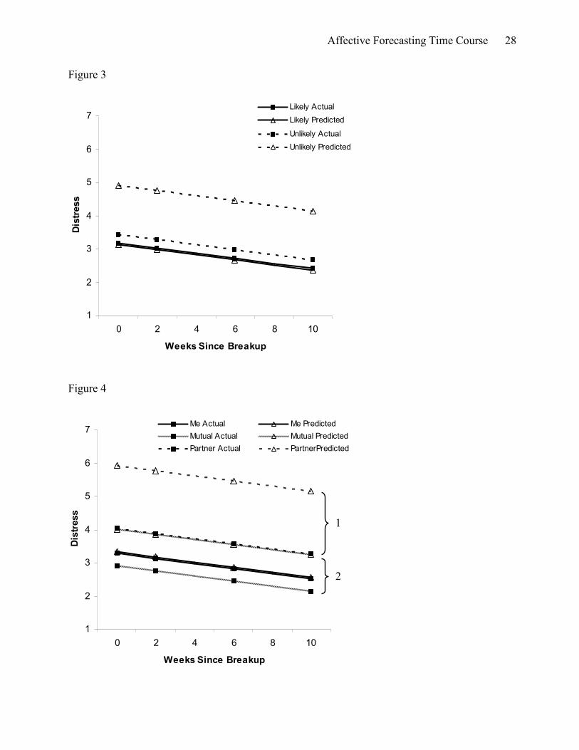
5.52, p<.001. Figure 3 presents predicted trajectories for participants whose New Relationship
Likelihood reports were 1 standard deviation above (“likely”) and below (“unlikely”) the mean.
Affective Forecasting Time Course 14
The simple effect of Distress Type for participants 1 SD above the New Relationship Likelihood
mean was nonsignificant: γ1=-.05, t(33)=-0.28, p=.783, indicating that participants forecasted their
distress reasonably accurately if they thought they were likely to begin a new relationship in the
next two weeks. On the other hand, the simple effect of Distress Type for participants 1 SD below
the mean on New Relationship Likelihood was large and significant, γ1=1.46, t(35)=7.61, p<.001.
In other words, participants made especially severe affective forecasting errors if, shortly before
the breakup, they thought it was unlikely they would start a new relationship during that period.
In a third moderational analysis, we hypothesized that participants’ affective forecasting
errors would be worse to the extent that they played less of a role in initiating the breakup. We
substituted InLove in Equation 2 with the variable Breakup Initiator, which we treated as a
categorical variable (me, mutual, or partner). Both Actual and Predicted Distress trajectories for
participants who answered “me” (N=14), “mutual” (N=7), and “partner” (N=5) are displayed in
Figure 4. The overall F test for the main effect of Breakup Initiator (γ3) was nonsignificant,
F(2,35)=1.71, p=.196, suggesting that participants were no more or less likely to experience
distress after breakup depending on who broke it off.3 As predicted, however, the interaction of
DistressType × Breakup Initiator (γ4) was significant, F(2,35)=14.44, p<.001. The simple effect of
Distress Type (γ1) was significant for participants who reported that their partner initiated the
breakup, γ1=1.89, t(35)=6.14, p<.001 (see Figure 4 bracket 1), and for participants who reported
that the breakup was mutual, γ1=1.10, t(35)=4.31, p<.001 (see Figure 4 bracket 2). However, this
simple effect was nonsignificant for participants who reported that they alone had initiated the
breakup, γ1=.05, t(35)=0.27, p=.792. This analysis suggests that participants made reasonably
accurate forecasts if they themselves ultimately were the ones who broke off the relationship, but
participants tended to make affective forecasting errors if they were (at least in part) the recipient
of the breakup.
Affective Forecasting Time Course 15
Finally, we simultaneously added the New Relationship Likelihood and Breakup Initiator
main effects and the DistressType × New Relationship Likelihood and DistressType × Breakup
Initiator interactions to Equation 2. In this rigorous analysis, the DistressType × InLove
interaction, γ=.35, t(35)=2.03, p=.050, and the DistressType × New Relationship Likelihood
interaction, γ=-.62, t(35)=-4.43, p<.001, remained significant. However, the DistressType ×
Breakup Initiator interaction did not achieve significance, F(2,35)=2.14, p=.133. This analysis
suggests that the In Love and New Relationship Likelihood moderational effects are at least
partially independent.
Correlational Accuracy?
Although the results reported thus far have demonstrated that many participants evidence
significant inaccuracies when making affective forecasts, there is another way of examining
accuracy in the present study. Whereas the previous results have examined the size of the mean
difference between participants’ Actual and Predicted Distress ratings, the within-subjects design
of this study also permits the calculation of the correlation between participants’ Actual and
Predicted Distress. A significant correlation would indicate that participants who predicted higher
distress ratings for themselves (compared to other participants) actually did experience greater
distress (compared to other participants).
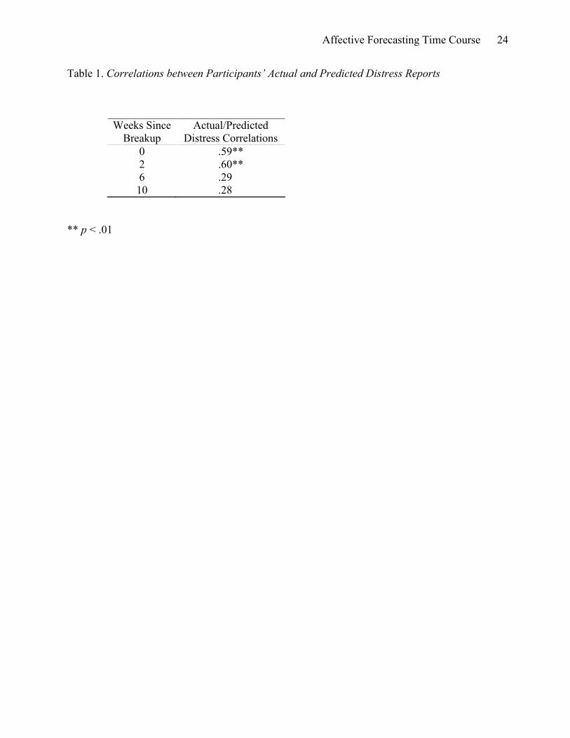
Table 1 presents the correlations between participants’ Actual and Predicted Distress
separately for the four assessment waves. In fact, participants’ Predicted Distress reports exhibited
substantial accuracy using this correlational metric, especially for the distress reports
corresponding to waves 0 and 2. It seems that the mean difference inaccuracies evidenced by
participants’ affective forecasting errors can coexist alongside substantial correlational accuracy.
Discussion
Affective Forecasting Time Course 16
This report explored participants’ predicted and actual distress in response to the breakup
of a romantic relationship. On average, participants’ predicted distress ratings, provided 2 weeks
prior to the report of the breakup, overestimated their actual distress during the 3-month period
following the breakup. Participants’ actual distress decreased over time, but their predicted distress
decreased at roughly the same rate; these findings are consistent with an affective forecasting
initial intensity bias but not with a decay bias. That is, even as participants were first reporting (at
Time 0) that they had broken up with their romantic partner, they were not as distressed as they
had predicted two weeks earlier. But participants did not make the additional error of predicting
that their rate of recovery from the breakup would be slower than it actually was. In fact,
participants both forecasted that they would and actually did experience decreasing distress as
time elapsed after the breakup, but because they had initially overestimated their distress,
participants’ predicted distress ratings remained substantially higher than their actual distress even
several months after the breakup.
A second set of analyses revealed that not all participants committed affective forecasting
errors. The initial intensity bias was more pronounced for individuals who (a) were more
(compared to less) in love with their partners, (b) felt it was less (compared to more) likely that
they would soon begin a new relationship, and (c) played less (compared to more) of a role in
initiating the breakup. These moderational effects were consistent with the typical form of the
impact bias (in which mild predictions tend to be more accurate) and with several known affective
forecasting mechanisms. Perhaps these accurate individuals were already preparing for the
impending breakup and imagining the positive features of their new single life (focalism), or
perhaps their reduced passion for their partner meant that their predicted and actual reports were
made in a similarly cool, rational state (empathy gap). Additional research will be required to
determine precisely which mechanisms are responsible for these effects. For now, these
Affective Forecasting Time Course 17
moderators join the ranks of a small handful of other naturally occurring individual differences,
such as culture of origin (Lam, Buehler, McFarland, Ross, & Cheung, 2005) and temporal focus
(Buehler & McFarland, 2001), that predict who is more or less susceptible to committing affective
forecasting errors.
These findings are the first to address directly the time course of the affective forecasting
error and to explore simultaneously the relative contributions of the initial intensity bias and the
decay bias (see Wilson & Gilbert, 2003). The results illustrate why a within-subjects design with
multiple time points is optimal for teasing apart these two possible biases: If we had only assessed
actual and predicted distress, say, 10 weeks after the initial report of the breakup, the results would
have appeared consistent with a decay bias. In other words, the difference between predicted and
actual distress at this single point in time might have indicated participants’ ignorance of the speed
at which their emotional reactions decay. Using a longitudinal model with multiple time points
(Singer & Willett, 2003), the present study revealed that all of the “action” in the affective
forecasting error had occurred by the very first assessment.
A romantic breakup is in many ways an ideal event for testing hypotheses about affective
forecasting (which perhaps explains why it was the very first event explored by Gilbert, Wilson,
and colleagues; Gilbert et al., 1998). It does, however, represent only a single type of emotionally
distressing event; it is certainly plausible that the initial intensity and decay biases play out
differently depending on the event in question. Furthermore, for romantic breakups in particular,
participants may be more likely to self-present by downplaying their actual distress to avoid
appearing rejected and vulnerable. Future work across multiple affective domains will be helpful
in determining to what extent the initial intensity bias but not the decay bias characterizes
forecasting errors.
Affective Forecasting Time Course 18
The present study contributes to our understanding of how people recover from a blow that
beforehand seems unbearably crushing. The affective forecasting literature has demonstrated that
recovery takes less time than people originally anticipate, and the present data suggest that these
unexpected gains are realized remarkably soon after the distressing event. Whether the
discrepancies between people’s predicted and actual distress are caused by their psychological
immune systems, their inability to foresee positive life events on the horizon, or their inaccurate
affective theories, a romantic breakup is apparently not as upsetting as the average individual
believes it will be. Does God only know what post-breakup maladies await individuals whose
relationships terminate? Perhaps, but it is probable that living will continue to do them plenty of
good.
Affective Forecasting Time Course 19
References
Akert, R. M. (1998). Terminating romantic relationships: The role of personal responsibility and
gender. Unpublished Manuscript, Wellesley College.
Aronson, E., Wilson, T. D., & Akert, R. M. (2005). Social psychology (5th ed.). Upper Saddle
River, NJ: Prentice Hall.
Baumeister, R. F., & Leary, M. R. (1995). The need to belong: Desire for interpersonal
attachments as a fundamental human motivation. Psychological Bulletin, 117, 497-529.
Buehler, R., & McFarland, C. (2001). Intensity bias in affective forecasting: The role of temporal
focus. Personality and Social Psychology Bulletin, 27, 1480-1493.
Davis, D., Shaver, P. R., & Vernon, M. L. (2003). Physical, emotional, and behavioral reactions to
breaking up: The roles of gender, age, emotional involvement, and attachment style.
Personality and Social Psychology Bulletin, 29, 871-884.
Gilbert, D. T., Gill, M. J., & Wilson, T. D. (2002). The future is now: Temporal correction in
affective forecasting. Organizational Behavior and Human Decision Processes, 88, 430-
444.
Gilbert, D. T., Lieberman, M. D., Morewedge, C. K., & Wilson, T. D. (2004). The peculiar
longevity of things not so bad. Psychological Science, 15, 14-19.
Gilbert, D. T., Pinel, E. C., Wilson, T. D., Blumberg, S. J., & Wheatley, T. P. (1998). Immune
neglect: A source of durability bias in affective forecasting. Journal of Personality and
Social Psychology, 75, 617-638.
Harter, S. (1999). The construction of self: A developmental perspective. New York: Guilford
Press.
Kermer, D. A., Driver-Linn, E., Wilson, T. D., & Gilbert, D. T. (2006). Loss aversion is an
affective forecasting error. Psychological Science, 17, 649-653.
Affective Forecasting Time Course 20
Kiecolt-Glaser, J. K., Fisher, L. D., Ogrocki, P., Stout, J. C., Speicher, C. E., & Glaser, R. (1987).
Marital quality, marital disruption, and immune function. Psychosomatic Medicine, 49, 13-
34.
Lam, K. C. H., Buehler, R., McFarland, C., Ross, M., & Cheung, I. (2005). Cultural differences in
affective forecasting: The role of focalism. Personality and Social Psychology Bulletin, 31,
1296-1309.
Loewenstein, G. (1996). Out of control: Visceral influences on behavior. Organizational Behavior
& Human Decision Processes, 65, 272-292.
Loewenstein, G. (2005). Hot-cold empathy gaps and medical decision making. Health
Psychology, 24, S49-S56.
Mikulincer, M., & Shaver, P. R. (2007). Attachment in adulthood: Structure, dynamics, and
change. New York: Guilford Press.
Riis, J., Loewenstein, G., Baron, J., Jepson, C., Fagerlin, A., & Ubel, P. A. (2005). Ignorance of
hedonic adaptation to hemodialysis: A study using ecological momentary assessment.
Journal of Experimental Psychology: General, 134, 3-9.
Sbarra, D. A. (2006). Predicting the onset of emotional recovery following nonmarital relationship
dissolution: Survival analyses of sadness and anger. Personality and Social Psychology
Bulletin, 32, 298-312.
Singer, J. D., & Willett, J. B. (2003). Applied longitudinal data analysis. New York: Oxford
University Press.
Thibaut, J. W., & Kelley, H. H. (1959). The social psychology of groups. New York: Wiley.
Veroff, J., Douvan, E., & Kulka, R. A. (1981). The inner American: A self-portrait from 1957 to
1976. New York: Basic Books.
Affective Forecasting Time Course 21
Wilson, T. D., & Gilbert, D. T. (2003). Affective forecasting. In M. P. Zanna (Ed.), Advances in
experimental social psychology (pp. 345-411). New York: Elsevier.
Wilson, T. D., & Gilbert, D. T. (2005). Affective forecasting: Knowing what to want. Current
Directions in Psychological Science, 14, 131-134.
Wilson, T. D., Meyers, J., & Gilbert, D. T. (2003). "How happy was I, anyway?" A retrospective
impact bias. Social Cognition, 21, 421-446.
Wilson, T. D., Wheatley, T., Meyers, J. M., Gilbert, D. T., & Axsom, D. (2000). Focalism: A
source of durability bias in affective forecasting. Journal of Personality and Social
Psychology, 78, 821-836.
Affective Forecasting Time Course 22
Author Note
Paul W. Eastwick and Eli J. Finkel, Department of Psychology, Northwestern University. Tamar
Krishnamurti and George Loewenstein, Department of Social and Decisions Sciences, Carnegie
Mellon University. This research was supported by a National Science Foundation Graduate
Research Fellowship awarded to PWE. Correspondence concerning this article should be
addressed to Paul Eastwick or Eli Finkel, Northwestern University, 2029 Sheridan Road, Swift
Hall Rm. 102, Evanston, IL, 60208-2710. E-mail may be sent to [email protected] or
Affective Forecasting Time Course 23
Footnotes
1The terms initial intensity bias and decay bias differ slightly from those used by Wilson and
Gilbert (2003). We adopt this modified terminology to provide precise language relevant to both
the theoretical and statistical analyses in this report.
2The DistressType × Time parameter was not included in this analysis because it was
nonsignificant in Equation 1 (and is again nonsignificant if added to Equation 2, γ=-.02, t[23]=-
.79, p=.437). Indeed, Time did not show significant random variability in Equation 1 at either
Level 2 (σ=.003, z=1.08, p=.139) or Level 3 (σ=.000). Therefore, for this analysis, only the initial
status (γ0) was permitted to vary randomly across participants (Level 3) and across Distress Type
(Level 2). Finally, the 3-way interaction DistressType × Time × InLove, which would have
indicated that InLove moderates the (nonexistent) decay bias, was not significant, γ =-.01, t(23)=-
.45, p=.658, and was therefore excluded from Equation 2.
3The Breakup Initiator simple effect of mutual vs. partner predicting actual distress was marginally
significant, γ0=-1.11, t(35)=-1.84, p=.075; participants were somewhat less likely to experience
distress for mutual compared partner-initiated breakups.
Affective Forecasting Time Course 24
Table 1. Correlations between Participants’ Actual and Predicted Distress Reports
Weeks Since Breakup
Actual/Predicted Distress Correlations
0 .59** 2 .60** 6 .29 10 .28
** p < .01
Affective Forecasting Time Course 25
Figure Captions
Figure 1. Actual (squares) and Predicted (triangles) Distress trajectories (see Equation 1)
following the breakup of a romantic relationship. Predicted Distress ratings were provided two
weeks prior to the report of the breakup (which was reported at Time 0).
Figure 2. Actual (squares) and Predicted (triangles) Distress trajectories (see Equation 2)
following the breakup of a romantic relationship. Trajectories are presented separately for
participants who were “In Love” (1 SD above the mean; solid lines) and “Not in Love” (1 SD
below the mean; dotted lines) with their partners. Predicted Distress and In Love ratings were
provided two weeks prior to the report of the breakup (which was reported at Time 0).
Figure 3. Actual (squares) and Predicted (triangles) Distress trajectories following the breakup of a
romantic relationship. Trajectories are presented separately for participants who believed they
were “Likely” (1 SD above the mean; solid lines) and “Unlikely” (1 SD below the mean; dotted
lines) to begin a new relationship during the two-week period that preceded the breakup. Predicted
Distress and New Relationship Likelihood ratings were provided two weeks prior to the report of
the breakup (which was reported at Time 0).
Figure 4. Actual (squares) and Predicted (triangles) Distress trajectories following the breakup of a
romantic relationship. Trajectories are presented separately for participants who reported that the
actual initiator of the breakup was the self (“me”, solid lines), both the self and the partner
(“mutual”, grey lines), or solely the partner (“partner”, dotted lines). Significant forecasting errors
were committed by participants reporting “partner” (bracket 1) and “mutual” (bracket 2) but not
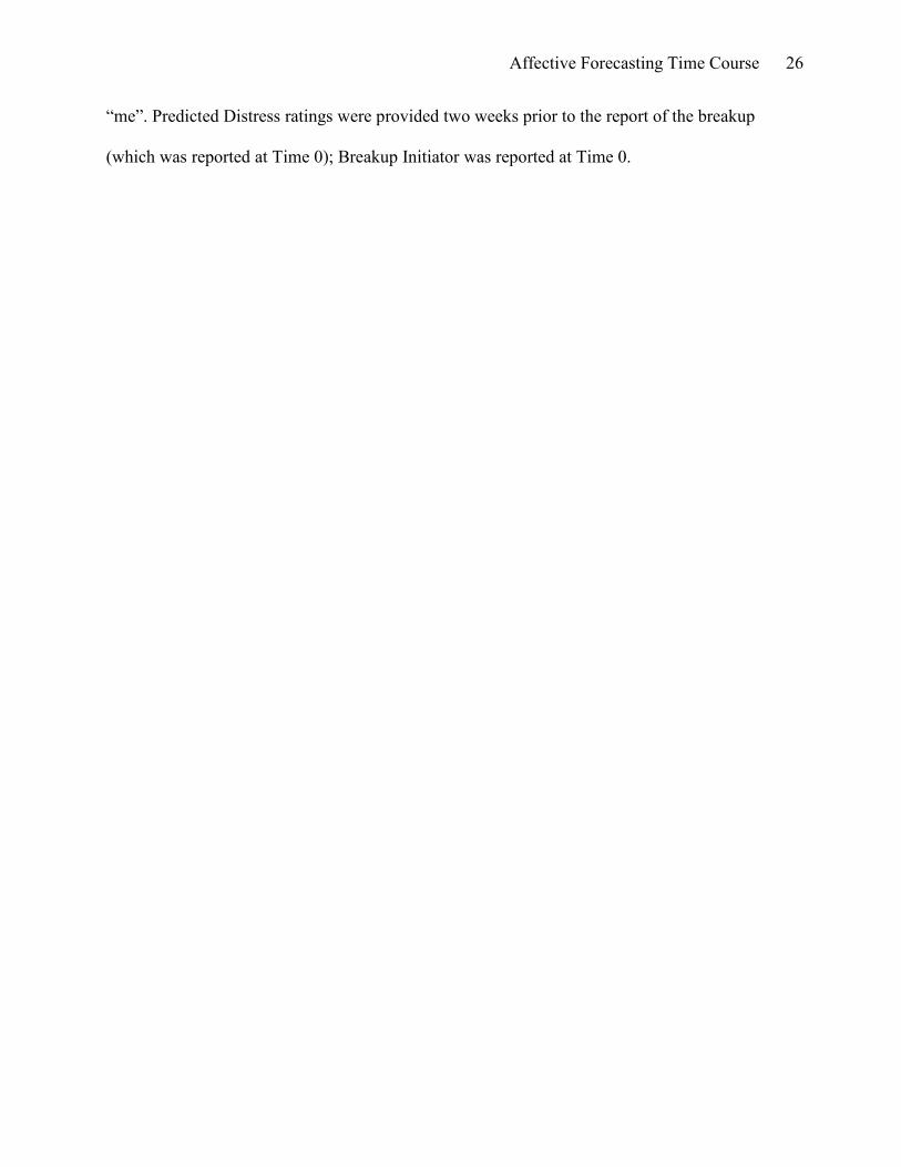
Affective Forecasting Time Course 26
“me”. Predicted Distress ratings were provided two weeks prior to the report of the breakup
(which was reported at Time 0); Breakup Initiator was reported at Time 0.
Affective Forecasting Time Course 27
Figure 1
Figure 2
1
2
3
4
5
6
7
0 2 4 6 8 10
Weeks Since Breakup
Distress
Actual
Predicted
1
2
3
4
5
6
7
0 2 4 6 8 10
Weeks Since Breakup
Distress
In Love Actual
In Love Predicted
Not In Love Actual
Not In Love Predicted
Affective Forecasting Time Course 28
Figure 3 Figure 4
1
2
3
4
5
6
7
0 2 4 6 8 10
Weeks Since Breakup
Distress
Likely Actual
Likely Predicted
Unlikely Actual
Unlikely Predicted
1
2
3
4
5
6
7
0 2 4 6 8 10
Weeks Since Breakup
Distress
Me Actual Me Predicted
Mutual Actual Mutual Predicted
Partner Actual PartnerPredicted
1
2