INCAS BULLETIN, Volume 4, Issue 4/ 2012, pp. 41 – 56 ISSN 2066 – 8201

Aeroservoelastic flutter and frequency response interactions

on the CL-704 aircraft

Ruxandra BOTEZ*,1

, Adrian HILIUTA1, Nicholas STATHOPOULOS

2,

Sylvain THÉRIEN2, Alexandre RATHÉ

2, Martin DICKINSON

2

*Corresponding author

*,1

ETS, 1100 Notre Dame West, Montreal, Que., Canada, H3C-1K3

Ruxandra.Botez@etsmtl.ca 2Bombardier Aerospace, 400 Cote Vertu Ouest, Dorval, Que., Canada

Abstract: Two methods for the aerodynamic forces conversions from frequency into Laplace domain

were conceived and validated: Least Squares LS and Minimum State MS, on the Bombardier CL-604

aircraft. A new feature was added in these two methods consisting in the writing of the error

calculated by LS and MS classical methods under an analytical form similar to the LS and MS form of

approximated aerodynamic forces; this error was once again minimized. Then, new methods using

this new feature were called: Corrected Least Squares CLS and Corrected Minimum State CMS

methods (as error was once again corrected). All these four methods were programmed in Matlab to

approximate the unsteady aerodynamic forces from frequency domain to Laplace domain.

Key Words: aerodynamic forces, Laplace domain, classical methods, flutter algorithm, frequency

domain, Matlab codes, aeroservoelasticity studies

1. INTRODUCTION

Aerodynamic forces in frequency domain were firstly calculated in Nastran by use of the

Doublet Lattice Method DLM at one Mach number M = 0.88 on a CL-604 Bombardier

Aerospace aircraft. These forces were secondly converted with the above four (two classical

and two new corrected) mentioned methods of aerodynamic forces conversions from

frequency into Laplace domain by use of Matlab codes developed at ETS and delivered to

Bombardier Aerospace team.

First set of flutter frequencies and speeds were calculated by integration of aerodynamic

forces initially calculated in Nastran in frequency domain into the flutter algorithm. Second

set of flutter speeds and frequencies were calculated by integration of aerodynamic forces

calculated by the four different methods of aerodynamic forces conversions from frequency

into Laplace domain into the flutter algorithm.

Matlab codes were developed at ÉTS to calculate and compare the second set of flutter

speeds and frequencies in the Laplace domain with the first set of initially obtained flutter

speeds and frequencies in the frequency domain. The first set of flutter results expressed in

terms of flutter speeds and frequencies was compared with the second set of flutter results

obtained with aerodynamic forces obtained by four methods, and following this comparison,

and in agreement with Bombardier Aerospace team, the LS method with a number of four

lag terms was chosen as the best method for aerodynamic forces conversion from frequency

into Laplace domain (from execution time and precision point of view) for the CL-604

Bombardier Aerospace aircraft. In addition, a new routine for eigenvalues and eigenvectors

studies (necessary for flutter frequencies and speeds calculations) developed at ÉTS gave a

very good and a much better flutter analysis results visualization than the previous program

DOI: 10.13111/2066-8201.2012.4.4.4

R. BOTEZ, A. HILIUTA, N. STATHOPOULOS, S. THÉRIEN, A. RATHÉ, M. DICKINSON 42

INCAS BULLETIN, Volume 4, Issue 4/ 2012

used at Bombardier, which is a fact extremely important in flutter analysis of future aircraft

at Bombardier Aerospace. Following the comparison between the results obtained with these

two methods, the best method was chosen from these two methods in common agreement

with Bombardier Aerospace team. The aircraft frequency response was computed in both

open loop and closed loop cases for aeroservoelasticity studies. The Matlab codes for these

cases were developed at ÉTS separately of Bombardier Aerospace and a comparison

between obtained results in both cases was done. Same types of results were obtained with

both Matlab codes developed separately by both teams. Theory and results obtained during

this period of time are here presented.

2. BIBLIOGRAPHICAL RESEARCH

The aeroservoelastic codes (with respect to Nastran code which is only an aeroelastic code)

implemented the unsteady aerodynamic forces conversion from frequency Q(k,M) to Laplace domain

Q(s). All the aeroservoelastic codes used mainly the following two methods for the unsteady

aerodynamic forces conversion which are:

1. Least Squares LS method is used in the aeroservoelastic computer programs: ADAM [1], ISAC

at Nasa Langley Research Center [2, 3] and STARS at NASA Dryden Flight Research Center (Dr

Gupta [4, 5] and Mr Marty Brenner [6, 7]).

2. Minimum State MS method is used in the aeroservoelastic computer programs: ASTROS and

ZAERO (Dr Moti Karpel [8, 9, 10 , 11, 12, 13] is the main author for the MS method and works in

collaboration with NASA Langley Research Center [11] and Zona Technology [14,15,16]). MS

method is used also in France at Airbus and Onera (Zimmermann [17] et Porion [18]),

and in addition:

3. A 3rd

approximation method is used at Boeing Company in St-Louis (Mr Dale Pitt [19] is the

main author for this method) which is still not very popular with respect to the LS and MS methods

[20, 21, 22].

These methods were computed in the aeroservoelastic codes as well as in Matlab at NASA

DFRC on the F-18 SRA at ETS, LARCASE [23]. Following a comparison between results obtained

with the LS, CLS, MS and CMS methods that are described in our previous works [24]- [35], the LS

method is used due mainly to its time of execution.

3. INTEGRATION OF THE AERODYNAMIC APPROXIMATION INTO

AEROELASTIC EQUATIONS OF MOTION

(SELECTION OF THE BEST METHOD)

Two approaches for the LS method integration in the flutter equations were studied and they

are described in the following section:

3.1 First formulation of the Least Squares LS method applied in the flutter

equations of motion (by use of a small A matrix)

The aeroelastic aircraft equations of motion under the aerodynamic forces influences are:

0Q(k)ηKηηCηM dyn q (1)

where M is the mass matrix, C is the damping matrix, K is the stiffness matrix, Q is the

aerodynamic forces matrix, qdyn is the dynamic pressure and is the generalized coordinates

vector. The matrix Q(k) is computed in NASTRAN by the Doublet Lattice Method DLM

method in the subsonic regime. The aerodynamic forces matrix is computed for a range of

reduced frequencies k at one Mach number M which depends on the aircraft true airspeed V

and is written under the following form:

43 Aeroservoelastic flutter and frequency response interactions on the CL-704 a ircraft

INCAS BULLETIN, Volume 4, Issue 4/ 2012

kjkk IR QQQ (2)

where QR is the real part of Q and QI is the imaginary part of Q. Equation (2) is introduced

in equation (1), so that the following system of equations is obtained:

0)(Q)(Q2

kqKkq

kV

cCM RdynIdyn

(3)

where no excitation force applies. From equation (3), the second derivative of generalized

coordinates is obtained:

0)()(2

11

kQqKMkQq

kV

cCM RdynIdyn

(4)

Equation (4) is rearranged under the following matrix form:

(5)

Matrix equation (5) may be written as follows:

xAx (6)

where

x and

0

)(2

)(2

11

I

kQqkV

cKMkQq

kV

cCM

A IdynIdyn

3.2 Second application of the Least Squares LS method in the flutter equations of

motion (by use of a big A matrix)

The aerodynamic forces matrix expressed by Pade approximations is introduced into eq. (1)

and we obtain:

0ηsAsAAKηηCηM4

1

2

2

210dyn

ii

i

b

Vs

sAq

(7)

where ks j is modified Laplace domain. The state variable Xi is next defined:

i

i

b

Vs

sX

(8)

Equations (7) can be written under the following form:

0XAqXAqXAq

-XAq-ηA-KηACηAM

46dyn35dyn24dyn

13dyn0dyn1

2

2

q

V

bq

V

bq dyndyn

(9)

Equations (9) may be written as follows:

0

)()(2

11

I

kQqKMkQqkV

cCM RdynIdyn

R. BOTEZ, A. HILIUTA, N. STATHOPOULOS, S. THÉRIEN, A. RATHÉ, M. DICKINSON 44

INCAS BULLETIN, Volume 4, Issue 4/ 2012

0XAq-XAq-XAq-XAq-K~

C~

M~

46dyn35dyn24dyn23dyn (10)

where

2

2dynV

bAq-MM

~

,

V

bAq-CC

~1dyn

and 0dynAq-KK~

Therefore, we obtain the following matrix system of equations:

4

3

2

1

4

3

2

1

6

1

5

1

4

1

3

111

4

3

2

1

0000

0000

0000

0000

~~~~~~00000

X

X

X

X

Ib

VI

Ib

VI

Ib

VI

Ib

VI

AMqAMqAMqAMqCMKM

I

X

X

X

X

dyndyndyndyn

(11)

which may be again written under the following form:

xAx (12)

where

4

3

2

1

X

X

X

X

η

η

x

and

Ib

VI

Ib

VI

Ib

VI

Ib

VI

AMqAMqAMqAMqCMKM

I

dyndyndyndyn

4

3

2

1

6

1

5

1

4

1

3

111

0000

0000

0000

0000

~~~~~~00000

A

(13)

This formulation has been chosen to be the best one to approximate aerodynamic forces

in the Laplace domain. In the next section, a comparison of results obtained at ETS versus

results obtained at Bombardier Aerospace is realized for the numerical flutter results

(damping and frequencies versus flutter speeds).

4. COMPARISON OF THE SET OF NUMERICAL FLUTTER RESULTS

4.1 Comparison of the first set of numerical flutter results (damping and

frequencies versus flutter speeds)

At ETS and Bombardier Aerospace, separate codes were developed, and compared. Results

were obtained following the Least Squares LS application (by use of a big matrix A) using

the same input data. The comparison of the first set of results gave almost the same flutter

results at ETS and at Bombardier Aerospace. Following same input data are used in the

computer codes (at ÉTS and Bombardier Aerospace) and were provided to ETS by

Bombardier Aerospace for validation purposes. These input data are the following:

45 Aeroservoelastic flutter and frequency response interactions on the CL-704 a ircraft

INCAS BULLETIN, Volume 4, Issue 4/ 2012

Mass, damping and stiffness matrices M, C, K for 110 modes

Among these 110 modes, there are 6 rigid modes, 50 elastic anti-symmetric modes, 44

elastic symmetric modes and 10 control modes.

Reduced frequencies k

k = [0.001 0.1 0.3 0.5 0.7 0.9 1.1 1.4]

Equivalent airspeed EAS is:

EAS = [0.01,0.1,0.4,1,2,3.5,5.5,8,11,15,21,29,40:10:1000] knots

Mach number Mach = 0.88;

Modes = [2,4,6,8,9,10,12,13,16,17,20,21,22,24,27,28,31,33,35,39];

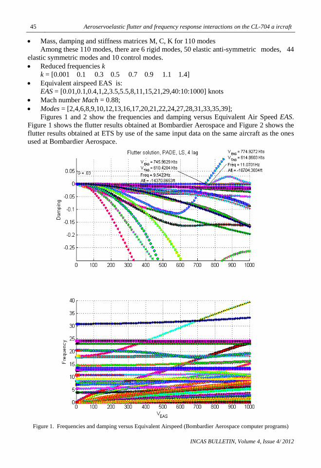
Figures 1 and 2 show the frequencies and damping versus Equivalent Air Speed EAS.

Figure 1 shows the flutter results obtained at Bombardier Aerospace and Figure 2 shows the

flutter results obtained at ETS by use of the same input data on the same aircraft as the ones

used at Bombardier Aerospace.

Figure 1. Frequencies and damping versus Equivalent Airspeed (Bombardier Aerospace computer programs)

R. BOTEZ, A. HILIUTA, N. STATHOPOULOS, S. THÉRIEN, A. RATHÉ, M. DICKINSON 46

INCAS BULLETIN, Volume 4, Issue 4/ 2012

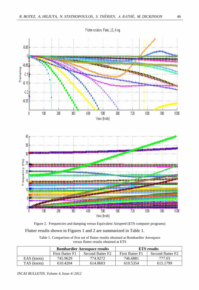
Figure 2. Frequencies and damping versus Equivalent Airspeed (ETS computer programs)

Flutter results shown in Figures 1 and 2 are summarized in Table 1.

Table 1. Comparison of first set of flutter results obtained at Bombardier Aerospace

versus flutter results obtained at ETS

Bombardier Aerospace results ETS results

First flutter F1 Second flutter F2 First flutter F1 Second flutter F2

EAS (knots) 745.9629 774.9272 746.6881 777.03

TAS (knots) 610.4204 614.8603 610.5354 615.1799

47 Aeroservoelastic flutter and frequency response interactions on the CL-704 a ircraft

INCAS BULLETIN, Volume 4, Issue 4/ 2012

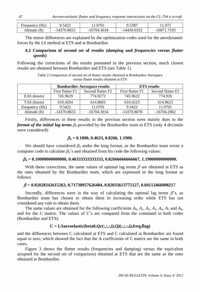
Frequency (Hz) 9.5422 11.0701 9.5387 11.072

Altitude (ft) -14370.8653 -16704.3034 -14430.0352 -16871.7193

The minor differences are explained by the optimization codes used for the aerodynamic

forces by the LS method at ETS and at Bombardier.

4.2 Comparison of second set of results (damping and frequencies versus flutter

speeds)

Following the corrections of the results presented in the previous section, much closest

results are obtained between Bombardier and ETS (see Table 1).

Table 2 Comparison of second set of flutter results obtained at Bombardier Aerospace

versus flutter results obtained at ETS

Bombardier Aerospace results ETS results

First flutter F1 Second flutter F2 First flutter F1 Second flutter F2

EAS (knots) 745.9629 774.9272 745.9622 774.926

TAS (knots) 610.4204 614.8603 610.4223 614.8623

Frequency (Hz) 9.5422 11.0701 9.5422 11.0701

Altitude (ft) -14370.8653 -16704.3034 -14370.8078 -16704.2062

Firstly, differences in these results in the previous section were mainly dues to the

format of the initial lag terms 0 provided by the Bombardier team to ETS (only 4 decimals

were considered):

0 = 0.1000, 0.4633, 0.8266, 1.1900.

We should have considered 0 under the long format, as the Bombardier team wrote a

computer code to calculate 0’s and obtained from his code the following values:

0 = 0.10000000000000, 0.46333333333333, 0.82666666666667, 1.19000000000000.

With these corrections, the same values of optimal lag terms are obtained at ETS as

the ones obtained by the Bombardier team, which are expressed in the long format as

follows:

= 0.02028342615263, 0.71738957626484, 0.82035613775127, 0.84113466008217.

Secondly, differences were in the way of calculating the optimal lag terms ’s, as

Bombardier team has chosen to obtain them in increasing order while ETS has not

considered any rule to obtain them.

The same values are obtained for the following coefficients A0, A1, A2, A3, A4, A5 and A6,

and for the C matrix. The values of C’s are compared from the command in both codes

(Bombardier and ETS):

C = LSaeroelastic(beta0,Qr(:,:,:,i),Qi(:,:,:,i),freq,flag)

and the differences between C calculated at ETS and C calculated at Bombardier are found

equal to zero, which showed the fact that the A coefficients of C matrix are the same in both

cases.

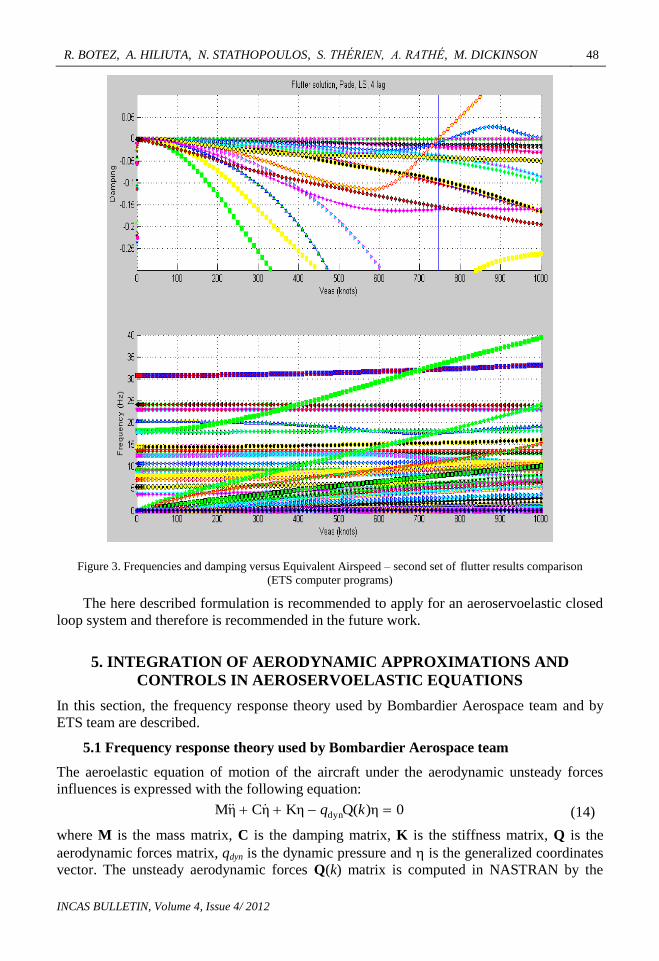
Figure 3 shows the flutter results (frequencies and damping) versus the equivalent

airspeed for the second set of comparison) obtained at ETS that are the same as the ones

obtained at Bombardier.

R. BOTEZ, A. HILIUTA, N. STATHOPOULOS, S. THÉRIEN, A. RATHÉ, M. DICKINSON 48

INCAS BULLETIN, Volume 4, Issue 4/ 2012

Figure 3. Frequencies and damping versus Equivalent Airspeed – second set of flutter results comparison

(ETS computer programs)

The here described formulation is recommended to apply for an aeroservoelastic closed

loop system and therefore is recommended in the future work.

5. INTEGRATION OF AERODYNAMIC APPROXIMATIONS AND

CONTROLS IN AEROSERVOELASTIC EQUATIONS

In this section, the frequency response theory used by Bombardier Aerospace team and by

ETS team are described.

5.1 Frequency response theory used by Bombardier Aerospace team

The aeroelastic equation of motion of the aircraft under the aerodynamic unsteady forces

influences is expressed with the following equation:

0)ηQ(KηηCηM dyn kq (14)

where M is the mass matrix, C is the damping matrix, K is the stiffness matrix, Q is the

aerodynamic forces matrix, qdyn is the dynamic pressure and is the generalized coordinates

vector. The unsteady aerodynamic forces Q(k) matrix is computed in NASTRAN by the

49 Aeroservoelastic flutter and frequency response interactions on the CL-704 a ircraft

INCAS BULLETIN, Volume 4, Issue 4/ 2012

Doublet Lattice Method DLM method for one Mach number and a range of reduced

frequencies k and is a complex aerodynamic matrix – so that is written as follows:

jR Ik k k Q Q Q (15)

where QR is the real part of Q and QI is the imaginary part of Q. Aerodynamic forces Q(k)

are approximated with the LS method with 4 lag terms 1, 2, 3 and 4 by use of Padé

polynomials as follows :

6

4

5

3

4

2

3

1

22

10j

j

j

j

j

j

j

j)j(AjA)(Q A

k

kA

k

kA

k

kA

k

kAkkk

(16)

where A0, A1, A2, A3, A4, A5 and A6 are Padé polynomials coefficients of dimensions equal to

the Q(k) matrix dimensions and are calculated from the Least Squares LS algorithm, and

where 1,2,3 and4 are the four lag terms calculated by the fmincon Matlab function

optimization algorithm. Unsteady forces matrix given by equation (16) is replaced in

equation (14) and following equation is obtained:

0ηsAsAAKηηCηM4

1

22

210dyn

ii

i

b

Vs

sAq (17)

where jk is replaced by

ks j = j b / V (18)

which is called the modified Laplace domain variable and where i = 1,2,3,4.

Generalized coordinates are written under the oscillatory form as = ejt

then the

first and second derivatives of generalized coordinates are written as:

ηjjη j te and η- )-(η 22 tej . (19)

We next calculate, from equations (18) and (19):

ηηjηj

η V

b

V

b

V

bs

(20)

and

222

2

22 ηηj

ηV

b

V

bs

(21)

The state variable Xi is next defined :

X ηi

i

s

Vs

b

where i = 1,2,3,4 (22)

From where, by inverse Laplace transform, we obtain following equation:

ii ηX iib

VX (23)

Equations (20), (21) and (23) where i = 1,2,3,4 for the four lag terms are replaced in

equations (17) which are further written under the following concise form:

dyn 3 1 dyn 4 2 dyn 5 3 dyn 6 4Mη Cη + Kη - q A X - q A X - q A X - q A X 0 (24)

where

R. BOTEZ, A. HILIUTA, N. STATHOPOULOS, S. THÉRIEN, A. RATHÉ, M. DICKINSON 50

INCAS BULLETIN, Volume 4, Issue 4/ 2012

2

2dynV

bAq-MM

~

,

V

bAq-CC

~1dyn and 0dynAq-KK

~ (25)

Equations (23) and (24) are used to obtain the following matrix system of equations

(after pre-multiplying both sides of equation (24) by M -1:

I-000I0

0I-00I0

00I-0I0

000I-I0

AM~

AM~

AM~

AM~

C~

M-K~

M

0000I0

X

X

X

X

η

η

4

3

2

1

61

51

41

3111

4

3

2

1

b

Vb

Vb

Vb

V

qqqq dyndyndyndyn

(26)

which is written under the following concise form:

xAx (27)

where

4

3

2

1

X

X

X

X

η

η

x

and

I-000I0

0I-00I0

00I-0I0

000I-I0

AM~

AM~

AM~

AM~

C~

M~

-K~

M~

0000I0

A

4

3

2

1

61

51

41

311-1

b

Vb

Vb

Vb

V

qqqq dyndyndyndyn

(28)

Separation of the rigid r and elastic modes e (which is written as a common vector 1)

from control modes c is applied in equation (24) and following equation is obtained:

c2c2c2

4635241311111

ηK~

ηC~

ηM~

-

XAXAXAXAηK~

ηC~

ηM~

dyndyndyndyn qqqq

(29)

where 1η

r

e

is the common vector for rigid and elastic modes, and c is the control

modes vector, rr re

1

er ee

M MM

M M

, rr re

1

er ee

C CC

C C

and rr re

1

er ee

K KK

K K

are the structural

mass, damping and stiffness matrices for rigid and elastic modes interactions, and

rc

2

ec

MM =

M

, rc

2

ec

CC =

C

and rc

2

ec

KK =

K

are the structural mass, damping and stiffness

matrices for control modes. Matrices 1 1 1M , C and K are square matrices with (r + e) lines

and (r + e) columns, and matrices 2 2 2M , C and K are square matrices with (r + e) lines and c

columns.

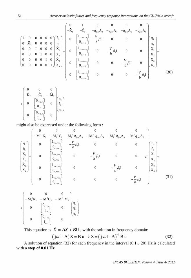
51 Aeroservoelastic flutter and frequency response interactions on the CL-704 a ircraft

INCAS BULLETIN, Volume 4, Issue 4/ 2012

1 1 3 4 5 6

,1

1

,11

,11

,2

3

4

0 I 0 0 0 0

K C A A A A

IηI 0 0 0 0 0 0 I 0 0 0

0η0 M 0 0 0 0

IX0 0 I 0 0 00 0 I 0 0

0X0 0 0 I 0 0

X0 0 0 0 I 0

X0 0 0 0 0 I

dyn dyn dyn dyn

r e r e

c r e

r e r e

c r e

q q q q

V

b

V

b

1

1

1

2

3,

14,

,

1

,

2 2 2

,

,

,

,

η

η

X

X

XI0 0 0 I 0

X0

I0 0 0 0 I

0

0 0 0

- K - C - M

00 0

0

00 0

I

r e r e

c r e

r e r e

c r e

r e c

c c

r e c

c c

V

b

V

b

c

c

c

η

η

η

(30)

might also be expressed under the following form :

-1 -1 -1 -1 -1 -1

1 1 1 1 1 3 1 4 1 5 1 6

,1

1

,1

,11

,2

3 ,

4 ,

0 I 0 0 0 0

M K M C M A M A M A M A

Iη 0 I 0 0 0

0η

IX0 0 I 0 0

0X

X I0

X 0

dyn dyn dyn dyn

r e r e

c r e

r e r e

c r e

r e r e

c r e

q q q q

V

b

V

b

1

1

1

2

3

14

,

1

,

-1 -1 -1

1 2 1 2 1 2

,

,

,

,

η

η

X

X

X0 0 I 0

X

I0 0 0 0 I

0

0 0 0

M K M C M M

00 0

0

00 0

I

r e r e

c r e

r e c

c c

r e c

c c

V

b

V

b

c

c

c

η

η

η

(31)

This equation is BUAXX , with the solution in frequency domain:

1

j I - A X B u X j I - A B u

(32)

A solution of equation (32) for each frequency in the interval (0.1…20) Hz is calculated

with a step of 0.01 Hz.

R. BOTEZ, A. HILIUTA, N. STATHOPOULOS, S. THÉRIEN, A. RATHÉ, M. DICKINSON 52

INCAS BULLETIN, Volume 4, Issue 4/ 2012

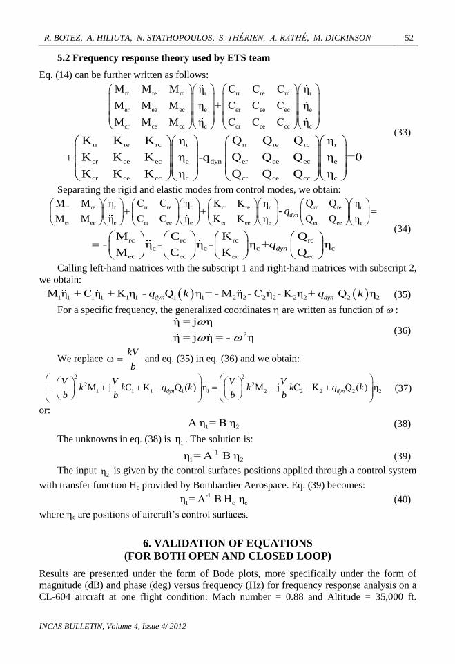
5.2 Frequency response theory used by ETS team

Eq. (14) can be further written as follows:

rr re rc r rr re rc r

er ee ec e er ee ec e

cr ce cc c cr ce cc c

M M M η C C C η

M M M η + C C C η

M M M η C C C η

rr re rc r rr re rc r

er ee ec e dyn er ee ec e

cr ce cc c cr ce cc c

K K K η Q Q Q η

K K K η -q Q Q Q η =0

K K K η Q Q Q η

(33)

Separating the rigid and elastic modes from control modes, we obtain:

rr re r rr re r rr re r rr re r

er ee e er ee e er ee e er ee e

M M η C C η K K η Q Q η-

M M η C C η K K η Q Q ηdynq

rc rc rc rc

c c c c

ec ec ec ec

M C K Q- η - η - η + η

M C K Qdynq

(34)

Calling left-hand matrices with the subscript 1 and right-hand matrices with subscript 2,

we obtain:

1 1 1 1 1 1 1 1 2 2 2 2 2 2 2 2M η + C η + K η - Q η = - M η - C η - K η + Q ηdyn dynq k q k (35)

For a specific frequency, the generalized coordinates are written as function of :

2

η = j η

η = j η = - η

(36)

We replace b

kV and eq. (35) in eq. (36) and we obtain:

2 2

2 2

1 1 1 1 1 2 2 2 2 2M j C K Q ( ) η M j C K Q ( ) ηdyn dyn

V V V Vk k q k k k q k

b b b b

(37)

or:

1 2A η = B η (38)

The unknowns in eq. (38) is 1η . The solution is:

-1

1 2η = A B η (39)

The input 2η is given by the control surfaces positions applied through a control system

with transfer function Hc provided by Bombardier Aerospace. Eq. (39) becomes: -1

1 c cη = A B H η (40)

where c are positions of aircraft’s control surfaces.

6. VALIDATION OF EQUATIONS

(FOR BOTH OPEN AND CLOSED LOOP)

Results are presented under the form of Bode plots, more specifically under the form of

magnitude (dB) and phase (deg) versus frequency (Hz) for frequency response analysis on a

CL-604 aircraft at one flight condition: Mach number = 0.88 and Altitude = 35,000 ft.

53 Aeroservoelastic flutter and frequency response interactions on the CL-704 a ircraft

INCAS BULLETIN, Volume 4, Issue 4/ 2012

Aerodynamic forces were approximated with the Padé approximations by use of the Least

Squares LS method.

TF1

TF2

Elastic

Aircraft

TF3

Roll rate

Roll rate

Left

aileron

Right

aileron

Roll rate

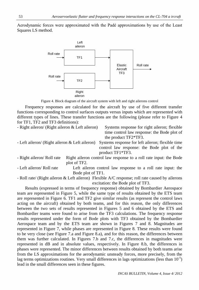
Figure 4. Block diagram of the aircraft system with left and right ailerons control

Frequency responses are calculated for the aircraft by use of five different transfer

functions corresponding to control surfaces outputs versus inputs which are represented with

different types of lines. These transfer functions are the following (please refer to Figure 4

for TF1, TF2 and TF3 definitions):

- Right aileron/ (Right aileron & Left aileron) Systems response for right aileron; flexible

time control law response: the Bode plot of

the product TF2*TF3.

- Left aileron/ (Right aileron & Left aileron) Systems response for left aileron; flexible time

control law response: the Bode plot of the

product TF1*TF3.

- Right aileron/ Roll rate Right aileron control law response to a roll rate input: the Bode

plot of TF2.

- Left aileron/ Roll rate Left aileron control law response to a roll rate input: the

Bode plot of TF1.

- Roll rate/ (Right aileron & Left aileron) Flexible A/C response; roll rate caused by ailerons

excitation: the Bode plot of TF3.

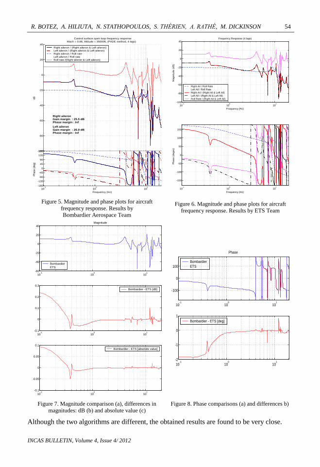
Results (expressed in terms of frequency response) obtained by Bombardier Aerospace

team are represented in Figure 5, while the same type of results obtained by the ETS team

are represented in Figure 6. TF1 and TF2 give similar results (as represent the control laws

acting on the aircraft) obtained by both teams, and for this reason, the only differences

between the two sets of results represented in Figures 5 and 6 obtained by the ETS and

Bombardier teams were found to arise from the TF3 calculations. The frequency response

results represented under the form of Bode plots with TF3 obtained by the Bombardier

Aerospace team and by the ETS team are shown in Figures 7 and 8. Magnitudes are

represented in Figure 7, while phases are represented in Figure 8. These results were found

to be very close (see Figure 7.a and Figure 8.a), and for this reason, the differences between

them was further calculated. In Figures 7.b and 7.c, the differences in magnitudes were

represented in dB and in absolute values, respectively. In Figure 8.b, the differences in

phases were represented. The minor differences between results obtained by both teams arise

from the LS approximations for the aerodynamic unsteady forces, more precisely, from the

lag terms optimizations routines. Very small differences in lags optimizations (less than 10-5

)

lead in the small differences seen in these figures.

R. BOTEZ, A. HILIUTA, N. STATHOPOULOS, S. THÉRIEN, A. RATHÉ, M. DICKINSON 54

INCAS BULLETIN, Volume 4, Issue 4/ 2012

-100

-80

-60

-40

-20

0

20

40

dB

Control surface open loop frequency response

Mach = 0.88, Altitude = 35000ft, (PADE method, 4 lags)

Right aileronGain margin : 25.5 dBPhase margin : Inf

Left aileronGain margin : 26.9 dBPhase margin : Inf

10-1

100

101

-180

-135

-90

-45

0

45

90

135

180

Ph

ase

(d

eg

)

Frequency (Hz)

Right aileron / (Right aileron & Left aileron)

Left aileron / (Right aileron & Left aileron)

Right aileron / Roll rate

Left aileron / Roll rate

Roll rate /(Right aileron & Left aileron)

10-1

100

101

-100

-80

-60

-40

-20

0

20

40

Frequency (Hz)

Ma

gn

itu

de

(d

B)

Frequency Response (4 lags)

Right Ail / Roll Rate

Left Ail / Roll Rate

Right AIl / (Right Ail & Left Ail)

Left AIl / (Right Ail & Left Ail)

Roll Rate / (Right Ail & Left Ail)

10-1

100

101

-150

-100

-50

0

50

100

150

Frequency (Hz)

Ph

ase

(d

eg

re)

Figure 5. Magnitude and phase plots for aircraft

frequency response. Results by

Bombardier Aerospace Team

Figure 6. Magnitude and phase plots for aircraft

frequency response. Results by ETS Team

10-1

100

101

-60

-40

-20

0

20

40Magnitude

Bombardier

ETS

10-1

100

101

-0.1

0

0.1

0.2

0.3

Bombardier - ETS [dB]

10-1

100

101

-0.1

-0.05

0

0.05

0.1

Bombardier - ETS [absolute value]

10-1

100

101

-100

0

100

Phase

Bombardier

ETS

10-1

100

101

-2

-1

0

1

Bombardier - ETS [deg]

Figure 7. Magnitude comparison (a), differences in

magnitudes: dB (b) and absolute value (c)

Figure 8. Phase comparisons (a) and differences b)

Although the two algorithms are different, the obtained results are found to be very close.

55 Aeroservoelastic flutter and frequency response interactions on the CL-704 a ircraft

INCAS BULLETIN, Volume 4, Issue 4/ 2012

7. DISCUSSION ON THE ADVANTAGES AND LIMITATIONS OF THIS WORK

For the CL-604 aircraft here studied, we have chosen among four methods LS, MS, CLS and

CMS as the best method – the method Least Squares with 4 lag terms for the aerodynamic

forces conversions from frequency into Laplace domain.

This choice was mainly based mainly on the comparison of flutter analysis results obtained

by use of this method with respect to the flutter analysis results initially obtained with the pk

flutter standard method. This method has been chosen as is faster and easier to integrate with

the flutter equations of motion for aeroservoelastic interactions studies. Two approaches

were studied and one of these approaches (use of A big matrix) was selected as being much

better than the other (use of A small matrix).

In future works, the LS method should be chosen for aeroservoelasticity studies, but we

might need a different number of lag terms (than 4) depending on the aircraft type. Each time

the finite elements aircraft model will be different, number of optimal lags might be

different. On the other hand, our computer programs are written in such a way that the

number of optimal lags will take very little time to choose for each aircraft time.

The frequency response was analyzed in this work only by use of ailerons inputs. As future

work, we will need to calculate and analyze the frequency response by use also of the other

control surfaces inputs such as elevators and rudder. Control laws were simple in the work

here performed. In future work, we will need to analyze full control laws and non-linearities

– so that computer programs will become heavier.

REFERENCES

[1] T. Noll, M. Blair, and J. Cerra, ADAM, An aeroservoelastic analysis method for analog or digital systems,

Journal of Aircraft, Vol. 23(11), 1986.

[2] W. M. Jr. Adams, S. T. Hoadley, ISAC: A tool for aeroservoelastic modeling and analysis, Collection of

Technical Papers - AIAA/ASME Structures, Structural Dynamics and Materials Conference, Vol. 2, pp.

1010-1018, 1993.

[3] C. Buttrill, B. Bacon, J. Heeg, J. Houck, D. Wood, Simulation and model reduction for the active flexible

wing program, Journal of Aircraft, Vol 32(1), Jan-Feb, pp. 23-31, 1995.

[4] K. K. Gupta, Development and application of an integrated multidisciplinary analysis capability, International

Journal for Numerical Methods in Engineering, v 40, n 3, Feb 15, 1997, pp. 533-550.

[5] Cole H. Stephens, Andrew S. Jr. Arena, Kajal K. Gupta, Application of the transpiration method for

aeroservoelastic prediction using CFD, Collection of Technical Papers - AIAA/ASME/ASCE/AHS/ASC

Structures, Structural Dynamics & Materials Conference, v 4, AIAA-98-2071, 1998, pp. 3092-3099.

[6] M. Brenner, R. Lind, Wavelet-processed flight data for robust aeroservoelastic stability margins, Journal of

Guidance, Control, and Dynamics, Vol. 21, n 6, Nov-Dec, pp. 823-829, 1998.

[7] M. Brenner, Nonstationary dynamics data analysis with wavelet-SVD filtering, Collection of Technical

Papers - AIAA/ASME/ASCE/AHS/ASC Structures, Structural Dynamics and Materials Conference, Vol.4,

pp. 2973-2987, 2001.

[8] M. Karpel, Time-domain aeroservoelastic modeling using weighted unsteady aerodynamic forces, Journal of

Guidance, Control, and Dynamics, Vol 13(1), Jan-Feb, pp. 30-37, 1990.

[9] M. Karpel, Reduced size first-order subsonic and supersonic aeroelastic modeling, Collection of Technical

Papers - AIAA/ASME/ASCE/AHS Structures, Structural Dynamics & Materials Conference, n pt 3, pp.

1405-1417, 1990.

[10] M. Karpel, Sensitivity derivatives of flutter characteristics and stability margins for aeroservoelastic design,

Journal of Aircraft, Vol 27(4), pp. 368-375, 1990.

[11] S. T. Hoadley, M. Karpel, Application of aeroservoelastic modeling using minimum-state unsteady

aerodynamic approximations, Journal of Guidance, Control, and Dynamics, Vol 14(6), Nov-Dec, pp.

1267-1276, 1991.

[12] I. Herszberg, M. Karpel, Flutter sensitivity analysis using residualization for actively controlled flight

vehicles, Structural Optimization, v 12, n 4, Dec, pp. 229-236, 1996.

R. BOTEZ, A. HILIUTA, N. STATHOPOULOS, S. THÉRIEN, A. RATHÉ, M. DICKINSON 56

INCAS BULLETIN, Volume 4, Issue 4/ 2012

[13] M. Karpel (Technion-Israel Inst of Technology), Reduced-order models for integrated aeroservoelastic

optimization, Journal of Aircraft, Vol. 36(1), Jan-Feb, 1999, pp. 146-155.

[14] P. C. Chen, D. Sarhaddi, D. D. Liu, Transonic-aerodynamic-influence-coefficient approach for aeroelastic

and MDO applications, Journal of Aircraft, Vol. 37(1), Jan, 2000, pp. 85-94.

[15] C. Nam, P. C. Chen, D. D. Liu, J. Urnes, R. Yurkorvich, Adaptive reconfigurable control based on reduced

order system identification for flutter and aeroservoelastic instability suppression, Collection of Technical

Papers - AIAA/ASME/ASCE/AHS/ASC Structures, Structural Dynamics and Materials Conference, v 4,

2001, p 2531-2543.

[16] P. C. Chen, E. Sulaeman, Nonlinear response of aeroservoelastic systems using discrete state-space

approach, AIAA Journal, v 41, n 9, September, 2003, p 1658-1666.

[17] H. Zimmermann, Aeroservoelasticity, Computer Methods in Applied Mechanics and Engineering,

Vol 90(1-3), p. 719-735, 1991.

[18] F. Porion, Multi-Mach rational approximation to generalized aerodynamic forces Journal of Aircraft, Vol

33(6), Nov-Dec, p 1199-1201, 1996.

[19] D. M. Pitt, FAMUSS: A new aeroservoelastic modeling tool, AIAA-92-2395-CP, 1992.

[20] B. M. Fritchman, R. A. Hammond, New method for modeling large flexible structures, Simulation, Vol

61(1), July, p 53-58, 1993.

[21] B. A. Winther, P. J. Goggin, J. R. Dykman, Reduced order dynamic aeroelastic model development and

integration with nonlinear simulation, Collection of Technical Papers - AIAA/ASME/ASCE/AHS/ASC

Structures, Structural Dynamics & Materials Conference, v 2, AIAA-98-1897, 1998, p 1694-1704.

[22] F. Engelsen, E. Livne, A design-oriented mode acceleration method for Lyapunov's equation based random

gust stresses in aeroservoelastic optimization, Collection of Technical Papers –

AIAA/ASME/ASCE/AHS/ASC Structures, Structural Dynamics and Materials Conference, v 4, 2002, p

2206-2226.

[23] D. E. Biskri, R. M. Botez, Method for aerodynamic unsteady forces time calculations on an F/A-18 aircraft,

The Aeronautical Journal, Vol. 112 (1127), pp. 1-6, 2007.

[24] D. E. Biskri, R. M. Botez, S. Thérien, A. Rathé, N. Stathopoulos, M. Dickinson, Aeroservoelasticity analysis

method based on an error analytical form, Journal of Vibration and Control, Vol. 14(8), pp. 1217-1230,

2007.

[25] R. M. Botez, A. Dinu, I. Cotoi, Method based on Chebyshev polynomials for aerservoelastic Interactions on

an F/A-18 aircraft, AIAA Journal of Aircraft, Vol. 44(1), pp. 330-333, 2007.

[26] R. M. Botez, D. E. Biskri, Unsteady aerodynamic forces mixed method for aeroservoelasticity studies on an

F/A-18 aircraft, AIAA Journal of Aircraft, Vol. 44(4), pp. 1378-1383, 2007.

[27] R. M. Botez, A. Dinu, I. Cotoi, N. Stathopoulos, S. Terrien, A. Rathé, M. Dickinson, Improved method for

creating time-domain unsteady aerodynamic models, The Journal of Aerospace Engineering, Vol. 20(3),

pp. 204-206, 2007.

[28] D. E. Biskri, R. M. Botez, Aerodynamic forces based on an error analytical formulation for

aeroservoelasticity studies on an F/A-18 aircraft, Journal of Aerospace Engineering, Vol. 220 (G), pp.

421-428, 2006.

[29] D. E. Biskri, R. M. Botez, N. Stathopoulos, S. Thérien, A. Rathé, M. Dickinson, New mixed method for

unsteady aerodynamic force approximations for aeroservoelasticity studies, AIAA Journal of Aircraft,

Vol. 43(5), pp. 1538-1542, 2006.

[30] A. Dinu, R. M. Botez, I. Cotoi, Chebyshev polynomials for unsteady aerodynamic calculations in

aeroservoelasticity, AIAA Journal of Aircraft, Vol. 43(1), pp. 165-171, 2006.

[31] A. Dinu, R. M. Botez, I. Cotoi, Aerodynamic forces approximations by Chebyshev method for

aeroservoelasticity studies, Canadian Aeronautical Society Journal CASJ, Vol. 51(4), pp. 167-175, 2005.

[32] R. M. Botez, D. E. Biskri, A. Doin, I. Cotoi, P. Parvu, Closed loop aeroservoelastic analysis method, AIAA

Journal of Aircraft, Vol. 41(4), pp. 962-964, 2004.

[33] R. M. Botez, A. Doin, D. Biskri, I. Cotoi, D. Hamza, P. Parvu, Method for flutter aeroservoelastic open loop

analysis, Canadian Aeronautical Society Journal CASJ, Vol. 49(4), pp. 179-190, 2003.

[34] I. Cotoi, R. M. Botez, Method of unsteady aerodynamic forces approximation for aeroseroelastic

interactions, AIAA Journal of Guidance, Control, and Dynamics Scope, Vol. 25(5), pp. 985-987, 2002.

[35] R. M. Botez, P. Bigras, Methods for the aerodynamic approximation in the Laplace domain for the

aeroservoelastic studies, Libertas Matematica, Vol. XIX, pp. 171-181, 1999.