The Cryosphere, 15, 1719–1730, 2021https://doi.org/10.5194/tc-15-1719-2021© Author(s) 2021. This work is distributed underthe Creative Commons Attribution 4.0 License.

Aerogeophysical characterization of Titan Dome, East Antarctica,and potential as an ice core targetLucas H. Beem1, Duncan A. Young2, Jamin S. Greenbaum2, Donald D. Blankenship2, Marie G. P. Cavitte3,Jingxue Guo4, and Sun Bo4

1Department of Earth Sciences, Montana State University, Bozeman, MT 59717, USA2Institute for Geophysics, University of Texas at Austin, Austin, TX 78758, USA3Université catholique de Louvain, Earth and Life Institute, Georges Lemaítre Centre for Earth and Climate Research,Place Louis Pasteur, 1348 Louvain-la-Neuve, Belgium4Polar Research Institute of China, Shanghai 200136, China

Correspondence: Lucas H. Beem (lucas.beem@montana.edu)

Received: 21 July 2020 – Discussion started: 31 July 2020Revised: 20 January 2021 – Accepted: 8 February 2021 – Published: 8 April 2021

Abstract. Based on sparse data, Titan Dome has been iden-tified as having a higher probability of containing ice thatwould capture the middle Pleistocene transition (1.25 to0.7 Ma). New aerogeophysical observations (radar and laseraltimetry) collected over Titan Dome, located about 200 kmfrom the South Pole within the East Antarctic Ice Sheet, wereused to characterize the region (e.g., geometry, internal struc-ture, bed reflectivity, and flow history) and assess its suitabil-ity as a paleoclimate ice core site. The radar coupled with anavailable ice core chronology enabled the tracing of dated in-ternal reflecting horizons throughout the region, which alsoserved as constraints on basal ice age modeling. The resultsof the survey revealed new basal topographic detail and bet-ter constrain the ice topographical location of Titan Dome,which differs between community datasets. Titan Dome isnot expected to be relevant to the study of the middle Pleis-tocene transition due to a combination of past fast flow dy-namics, the basal ice likely being too young, and the temporalresolution likely being too coarse if 1 Ma ice were to exist.

1 Introduction

The ice domes and ridges of Antarctica hold the best strati-graphically ordered records of past ice sheet and climate evo-lution. There is an ongoing international effort (e.g., Fischeret al., 2013; Passalacqua et al., 2018) to find suitable ice coredrilling sites that will have an interpretable climate record

that spans the middle Pleistocene transition, dated to between1.25 and 0.7 Ma (Clark et al., 2006). During this period, ma-rine oxygen isotope records indicate a transition in major icevolume and climate cycles from a predominately ∼ 41 000-year obliquity-driven periodicity to a∼ 100 000-year period-icity. The trapped atmospheric gases and isotopic chemistryof ice cores are proxy records of atmospheric and ice sheetconfiguration that are key to understanding this transition andclimate dynamics more generally.

Identifying coring locations to study the middle Pleis-tocene transition has primarily been the result of modelingefforts that find regions that have ice dynamic and thermo-dynamic stability suitable to allow for both 1.5 Ma of icesurvival and the existence of a well-preserved ice stratig-raphy. One such effort used a one-dimensional thermody-namic model to find where the bed is sufficiently cold toprevent present-day basal melting (Van Liefferinge and Pat-tyn, 2013). With their model results and the additional cri-teria of present-day slow flow of less than 2 m yr−1 and icethickness greater than 2000 m, they identified regions withincreased likelihood for the recovery of an ice core datingto the middle Pleistocene transition (Fig. 1). Follow-on work(Van Liefferinge et al., 2018), used updated methodology andincluded additional processes, such as parametrization thatallows for accumulation rate variability, to refine the bound-aries of promising regions. For the regions near Titan Dome(Fig. 1), the boundaries are consistent.

Published by Copernicus Publications on behalf of the European Geosciences Union.

1720 L. H. Beem et al.: Characterization of Titan Dome

Not all relevant processes and conditions have been ex-plicitly considered in site determination efforts. Additionalconsiderations that might impact the existence or qualityof the desired ice core include past ice flow reorganiza-tion and/or ice divide migration (Beem et al., 2017; Win-ter et al., 2018), subglacial groundwater flow (Gooch et al.,2016), ice surface wind erosion, heterogenous geothermalflux (e.g., Jordan et al., 2018), and minimum age resolu-tion of ∼ 10 kyr m−1 of ice (Fischer et al., 2013). Withoutgeophysical observations, and in some cases direct access,the presence or significance of these processes cannot be de-termined. Aerial and ground geophysical surveys have oc-curred for some high-probability coring targets, including atDome C of East Antarctica (Young et al., 2017). Planningfor drilling at Dome C is proceeding based on the charac-terization of the region (Young et al., 2017), the existenceof a proximal ∼ 800 000-year-old EPICA ice core (Augustinet al., 2004), and promising ice age modeling (Parrenin et al.,2017). However, finding additional targets remains of inter-est to enable multiple correlatable cores and the examinationof spatial heterogeneity in climate processes.

Titan Dome, located approximately 200 km along the170◦W meridian from the South Pole, is a region that waspreviously identified as a contender for the existence of1.5-million-year-old ice (Van Liefferinge and Pattyn, 2013;Van Liefferinge et al., 2018). In 2016 and 2017, a partnershipbetween the University of Texas Institute for Geophysics andthe Polar Research Institute of China surveyed the South Polecorridor (SPC) grid to evaluate the location as an ice coretarget. The existence of the South Pole Ice Core chronology(Casey et al., 2014; Winski et al., 2019), plus previously col-lected aerial–geophysical surveys in the region (Carter et al.,2007), helps propagate the age of internal reflecting horizons(IRHs) throughout the region. The work presented here ispart of an expanded mapping of IRH across the Antarctic IceSheet (e.g., Winter et al., 2019; Ashmore et al., 2020).

In this paper, we describe new basal topography and sur-face elevation, determine that the basal ice age is likelyyounger than would be needed to capture the middle Pleis-tocene transition, and describe areas on the flanks of TitanDome that may have previously experienced faster flow thanat present.

2 Data

2.1 New data

The SPC survey was conducted by an aerogeophysical suiteinstalled on the Polar Research Institute of China BT-67airframe (Cui et al., 2018, 2020) that includes a coherent60 MHz center frequency radar ice sounder (Peters et al.,2005), a laser altimeter, a cesium magnetometer, a three-axisstabilized gravimeter, and a downward-looking camera. Thelaser altimeter was a Riegl LD90-3800-HiP and collected

data at 4 Hz, with an expected accuracy of 15 cm. Two sur-vey flights were conducted, in February of 2016 and 2017(Fig. 1), over the area of Titan Dome. A grid of roughly150 km by 150 km with 25 km grid spacing was surveyed.One survey line was flown within 500 m of the South PoleIce Core to enable the propagation of the core’s chronology(Winski et al., 2019) throughout the region.

2.2 Existing data

One older radar survey of the region is used in this analysis.The Pensacola–Pole Transect (PPT) was collected in 1998–1999. These data were collected with a radar system that wasa direct ancestor of the system used for the SPC survey. ThePPT survey used a 60 MHz center frequency with a 250 nspulse width radar mounted on a Twin Otter airframe (Carteret al., 2007).

3 Methods

3.1 Radar processing

The radar data were processed to a 1D focused state (Peterset al., 2007), without range migration. Focusing is applied todifferentiate between nadir and off-nadir reflections and im-prove the resolution of the resulting radargram by increasingthe discrimination of internal structures and the basal bound-ary of the ice sheet.

The calculated basal reflection coefficient has been cor-rected for geometric spreading loss and for assumed ice at-tenuation, which is primarily a function of ice temperature(MacGregor et al., 2007; Matsuoka et al., 2012). Geometricspreading loss follows the standard theoretical relation us-ing the infinite mirror approximation (e.g., Lindzey et al.,2020). This study uses an attenuation value of 10 dB km−1

everywhere and reported as two-way travel through a givenice thickness. Although attenuation is expected to be vari-able due to spatial heterogeneity in ice temperature and/or icechemistry, an attempt to constrain the variability is not madedue to the numerous additional processes for which a controlwould be needed (e.g., subglacial water distribution, geother-mal flux heterogeneity, ice chemistry, basal roughness). Therelative consistency of low-magnitude basal reflection andthe lack of inferred basal water, as will be described later(Sect. 4.2), support the assumptions used in determining themagnitude of the dielectric loss.

To determine the attenuation value, multiple regressions(Fig. 2) with a combination of thickness distribution (> 800and > 1200 m) and reflection values in each thickness bin(all, five highest, five lowest) resulted in a range of possiblevalues (6–15 dB km−1). Using the highest and lowest valuesin a bin attempts to isolate the effects of dialectic loss withinthe ice column by assuming the end-member basal reflectioncoefficient is consistent throughout the survey. A south po-lar ice column has an approximate average temperature of

The Cryosphere, 15, 1719–1730, 2021 https://doi.org/10.5194/tc-15-1719-2021

L. H. Beem et al.: Characterization of Titan Dome 1721

Figure 1. South Pole and Titan Dome region. For both panels, flight lines from the South Pole corridor (SPC) survey and previously publishedobservations of Pensacola–Pole Transect (PPT; Carter et al., 2007) and PolarGAP (Jordan et al., 2018) surveys are also plotted. The orangeshading shows candidate regions of increased paleoclimate ice core potential plotted as basal temperature (Van Liefferinge and Pattyn, 2013).Each color bar applies to both panels. The two coring candidate regions discussed in this paper are labeled A and B. The location of TitanDome summit, as determined from the SPC survey, is the white triangle. The background shading and contours are from the Bamber et al.(2009) surface elevation DEM. The coordinate system used is polar stereographic (EPSG:3031).

−35 ◦C (Beem et al., 2017), and the theoretical values ofattenuation for such ice are within 7–15 dB km−1, depend-ing on ice chemistry (MacGregor et al., 2007). These valuesare also in agreement with the results of an ice-sheet-wideestimate of englacial attenuation (Matsuoka et al., 2012).Consistent with theory and observations, 10 dB km−1 is usedhere.

3.2 Laser altimetry processing

Laser altimetry was corrected for biases in the attitude of thesensor through minimization of the transect intersection dif-ferences (Young et al., 2015) with data from the 2016 survey.As the laser and inertial navigation system was not removedfrom the aircraft between field seasons, recalibration of thesecond season was not required.

3.3 Surface, bed, and internal reflecting horizontracing

The manual tracing of the surface and bed within the radarobservations was consistent with the methodology describedin Blankenship et al. (2001). The human tracers applied afirst return criteria to identify the bed. This has the effect ofidentifying the minimum possible ice thickness and smooth-ing basal topography, especially in regions with steep andvariable relief. Using the traced interfaces along with aircraftposition, the surface elevation, bed elevation, and ice thick-ness are determined. Radar wave speed in ice is assumed tobe 1.67× 108 m s−1.

Internal reflecting horizons were manually traced us-ing Landmark DecisionSpace semi-autonomous picking thatuses the maximum value of the reflector. The South Pole IceCore chronology (Winski et al., 2019) was projected ontothe radargram that flew most proximal to the core location(∼ 500 m), by correlating the ice depth of both the ice coreand radar observations. Where IRH are completely continu-ous the age record was propagated. Internal reflecting hori-zons may have discontinuities in visibility due to dip steep-ness, being obscured by radar clutter, the effects or radar pro-cessing, or ceasing to generate a suitably strong reflection forother reasons (Siegert, 1999; Harrison, 1973; Holschuh et al.,2014). Nine dated IRHs were traced to their maximum pos-sible extent from the South Pole Ice Core: 0 ka (taken as thesurface), 4.7, 10.7, 16.8, 29.1, 37.6, 51.4, 72.5, and 93.9 ka.

The surface, bed, and ice thickness were compared towidely used community datasets (Fretwell et al., 2013; Bam-ber et al., 2009; Helm et al., 2014) by interpolating the grid-ded data to each geophysical observation location using a bi-variate spline approximation.

3.4 Basal ice age model

The age of the basal ice (a) can be modeled with the con-straints provided by radar observations and dated IRH. Two1D models are compared to estimate the age of the basal ice.One model uses the simplest Nye assumptions, which are asteady-state ice thickness (H ) and a constant strain rate withdepth (Cuffey and Paterson, 2010, Eq. 15.8),

https://doi.org/10.5194/tc-15-1719-2021 The Cryosphere, 15, 1719–1730, 2021

1722 L. H. Beem et al.: Characterization of Titan Dome

Figure 2. Attenuation determination. The color field represents thenumber of observations in each 1.5 dB geometrically corrected echostrength by a 27 m thickness bin. The solid lines are regressionsusing observations with ice thickness greater than 800 m and thedotted lines greater than 1200 m. The orange lines use all observa-tions in each thickness bin. The blue lines use the five highest echostrengths in each thickness bin, and the green line uses the five low-est. The legend reports the regression slope.

a =H

bln

(1

1− z/H

). (1)

For this model, the one unknown parameter is surface ac-cumulation rate in ice equivalent thickness (b). Basal ice isarbitrarily defined as a depth (z) 30 m above the bed, and icethickness (H ) is defined by radar observations. The modelis run for each vertical radar observation independently bysolving for the accumulation rate that minimizes the rootmean squared error between the model depth for each IRHage and the traced depth of the IRH. The resulting accu-mulation field enables an estimate of the spatial patternsof average accumulation rate. Comparing the spatial distri-bution of accumulation from the model to independent ob-servations/modeling of accumulation (Arthern et al., 2006;Wessem et al., 2014; Studinger et al., 2020) serves as partialmodel verification.

The second age model uses the Dansgaard–Johnson set ofassumptions concerning vertical strain rates (Cuffey and Pa-terson, 2010, Eqs. 15.14 and 15.15),

a = a′+2H −h

b+

(h

z− 1

), (2)

a′ =2H −h

2bln

(2H −h

h

). (3)

A characteristic height (h) above the bed marks the transitionfrom constant vertical strain above to linearly varying to zerobelow. A range of transitional heights (h) were tested, 20 %to 50 % of ice thickness above the bed. In this model, z isheight above bed. The Dansgaard–Johnson model is solvedindependently for each vertical radar observation by solv-ing for the accumulation (b) that minimizes the root meansquared misfit between the model depth for each IRH ageand the traced depth of the IRH. This model is highly sen-sitive to accumulation rate, which determines the magnitudeof vertical strain, but less sensitive to the chosen transitionalheight. Additionally, the model is sensitive to the definitionof basal ice, given the high degree of non-linearity this modelproduces near the bed. To improve on the arbitrarily defined30 m above the bed, a minimum desired temporal resolutionof ice, 10 kyr m−1 (Fischer et al., 2013), is used to determinethe basal ice age. The basal age output of the model is theage at the depth where this temporal resolution threshold isexceeded.

3.5 Submergence

Investigating the submergence rate, the speed that a datedIRH takes to reach its current position, can be informativeof the flow history in the region. The submergence rate iscalculated with published methodology (Beem et al., 2017)and assuming m= 1,

w =−b( z

H

)m

. (4)

The model assumes the form of the vertical strain rate pro-file and determines the magnitude of vertical strain necessaryto submerge an IRH of a given age to its observed depth.Submergence rates (w) are calculated for each dated IRH-bounded interval within the ice column. In the above equa-tion, b is ice equivalent surface accumulation, H is ice thick-ness, and z is height above the bed. There is a correction stepthat removes the influence of the strain from each youngerinterval (Beem et al., 2017). Patterns in submergence thatexceed expected spatial gradients in accumulation are inter-preted to represent heterogenous basal melt or ice flow. Theresults create a temporal history that can be interpreted aschanges to processes that effect submergence rates (e.g., ac-cumulation, basal melt, and/or horizontal strain).

The Cryosphere, 15, 1719–1730, 2021 https://doi.org/10.5194/tc-15-1719-2021

L. H. Beem et al.: Characterization of Titan Dome 1723

4 Results

4.1 Bed topography, surface elevation, and icethickness

The bed elevation determined by radar reflection reveals amountainous subglacial terrain that was previously unknown.The bed is rugged, with > 1 km of relief along the surveylines and bed slopes of up to 45◦ (Figs. 3 and 7). The 20 kmline spacing does not resolve the extent of these features, andthe effectiveness of mass conservation methods of bed inter-polation is limited by low ice velocities (Morlighem et al.,2020), restricting the use of only 1D modeling approaches.The new observations suggest that the main ice dome is lo-cated on a basal topographic high instead of a depression.The ice thickness in this region is therefore commensuratelythinner than previously estimated (Fretwell et al., 2013).

There are two independent surface elevation digital ele-vation models (DEMs) of the Titan Dome region (Bamberet al., 2009; Helm et al., 2014) which other gridded DEMproducts (e.g., Bedmap2, REMA, BedMachine) use to fill intheir data gaps south of 86◦ S (Fretwell et al., 2013; Howatet al., 2019; Morlighem et al., 2020). Generally, there is goodagreement between the available DEM products and the newlaser altimetry observations of surface elevation (Figs. 3 and4). The Bamber et al. (2009) DEM is 20± 62 m (average± 2standard deviations) higher than the SPC radar observations,and the Helm et al. (2014) DEM is 23± 73 m higher. The Ti-tan Dome summit location differs by at least 34 km betweenthe Bamber et al. (2009) and Helm et al. (2014) DEMs. Thesurface altimetry collected here is sparse and cannot explic-itly constrain the location of the Titan Dome, but the domelocation in the Bamber et al. (2009) DEM was used in surveyplanning and corresponds to the location of highest eleva-tion observed in this survey. The dome elevation observedby the survey’s laser altimetry is 3154 m, within 10 m eleva-tion of Bamber et al. (2009) data, and occurs at 88.1716◦ S,170.4765◦W, the same position as the Bamber et al. (2009)defined summit.

The bed elevation and ice thickness of the SPC surveycompared to the Bedmap2 dataset show significant variance.Bedmap2 is 30± 550 m (average± 2 standard deviations)thicker than the SPC radar observations. A total of 50 % ofthe radar observations within candidate A (Fig. 1) have thin-ner ice than Bedmap2 when interpolated from the grid. Giventhe gridded nature, 69 % of the Bedmap2 pixels within can-didate A that were surveyed have thicker ice than the radarobservations. The region of the SPC survey only had sparseobservations previously available, and differences betweenthe available gridded datasets and the new observations areexpected.

4.2 Basal reflectivity

The bed beneath Titan Dome and the surrounding regionshow generally low reflectivity and heterogenous character.Localized regions of higher values (>−30 dB) are observedin the subglacial drainages that flow towards the Filchner–Ronne Ice Shelf (generally grid north or northwest). Highervalues are also seen beneath a region of thin ice (Fig. 5 near0 km easting and −50 km northing).

The low values of basal reflectivity suggest that the basalice beneath the Titan Dome region is frozen to the bed, andthere is limited basal melt and water movement. This con-clusion is consistent with previous basal temperature mod-eling efforts (e.g., Beem et al., 2017; Van Liefferinge et al.,2018; Van Liefferinge and Pattyn, 2013; Price et al., 2002)that conclude the bed in the region is 10 ◦C or more belowthe pressure melting temperature. It is unlikely that bodies ofwater were detected by radar, but the local reflectivity max-imums suggest a higher likelihood of a smoother bed and/orsmall amounts of basal water in these regions, potentially inthe form of saturated sediments or interfacial water. The highreflectivity seen beneath shallow ice may be the result of theattenuation correction that is too large for the cold ice ex-pected there.

4.3 Basal ice age

Two models were used to estimate the age of the basal ice,each constrained by radar observations and dated IRH. TheNye age model calculates basal ages as old as 360 ka, butmuch of the region is younger. The modeled accumulationfield used to minimize the misfit between dated IRH andmodeled ages has a mean accumulation (in ice equivalent)of 4.4 cm yr−1. The spatial distribution of accumulation haslower magnitudes near the dome summit (3 to 5 cm yr−1) andhigher rates at lower elevations (up to 9 cm yr−1). This pat-tern and magnitude is generally consistent with spaceborneand reanalysis estimates of accumulation patterns of the re-gion (Arthern et al., 2006; Wessem et al., 2014). The highestvalues of accumulation are seen in a region of a broad flat icesurface topographic trough. This matches a recent accumu-lation study (Studinger et al., 2020) that finds 3 to 5 cm yr−1

accumulation on the summit and implies higher values of ac-cumulation, up to 20 cm yr−1, in the ice surface trough. Thisage model result is not expected to be predictive of modernaccumulation rates, and there are deviations from availableobservations; however, the general patterns are plausibly re-alistic and lend credence to the model performance despiteits simplicity.

The Dansgaard–Johnson age model calculates older agesthan the Nye model due to assumptions that lead to smaller-magnitude vertical strain rates near the bed. Isolated regionsexceeding 1 Ma of age are predicted to exist in the mostfavorable parameter sets; however, ages between 600 and800 ka are more typical. The higher the transitional height

https://doi.org/10.5194/tc-15-1719-2021 The Cryosphere, 15, 1719–1730, 2021

1724 L. H. Beem et al.: Characterization of Titan Dome

Figure 3. Geophysically observed ice geometry. Panel (a) is laser surface elevation with background 100 m elevation contours from theBamber et al. (2009) DEM. (b) Radar-derived bed elevation. (c) Radar-derived ice thickness. (d) Surface elevation difference between theSPC survey and the Bamber et al. (2009) DEM. (e) Bed elevation difference between the SPC survey and Bedmap2 (Fretwell et al., 2013).(f) Ice thickness difference between the SPC survey and Bedmap2 (Fretwell et al., 2013). The dome summit is marked with a black trianglein each panel. The coordinate system used is polar stereographic (EPSG:3031).

Figure 4. Difference between aerial observations and community DEMs. (a) Laser surface elevation difference for both Bamber et al. (2009)and Helm et al. (2014), (b) radar bed elevation observation difference from Fretwell et al. (2013), and (c) radar ice thickness observationfrom Fretwell et al. (2013).

in the Dansgaard–Johnson model, the older the maximumbasal age due to a greater proportion of the ice thicknesswith smaller vertical strain rates. With a transitional height(h) at 20 % of ice thickness the maximum age was ∼ 0.9 Ma,and when the height is at 50 % of ice thickness the maxi-mum age increased to greater than 1.4 Ma. In every model

case the probability of suitably old ice to capture the middlePleistocene transition is low.

The height above the bed of basal ice used by theDansgaard–Johnson model ranges from 5 to 120 m, due todefining it with a temporal threshold of the model output.When the transitional height (h) is 20 % of ice thickness themean basal ice is 61 m above the bed, and when h is 50 %

The Cryosphere, 15, 1719–1730, 2021 https://doi.org/10.5194/tc-15-1719-2021

L. H. Beem et al.: Characterization of Titan Dome 1725

Figure 5. Observed relative basal reflectivity. Reflectivity is cor-rected for geometric spreading and englacial dielectric attenuation.Locations of reflectivity that exceed−30 dB are plotted in blue. Thecandidate A ice core target region is in orange (Van Liefferinge andPattyn, 2013). The dome summit location is plotted as a black tri-angle. The 500 Pa contour intervals are hydraulic potential usingBedmap2 (Fretwell et al., 2013) and zero effective pressure. Thehighest contour surrounding the dome summit is 29 kPa. The coor-dinate system used is polar stereographic (EPSG:3031).

the mean basal ice is 79 m above the bed. Spatial variabil-ity in accumulation patterns and magnitudes were consistentwith the Nye model results, with less accumulation on thedome (∼ 2 cm yr−1) and higher amounts on the flanks (up to10 cm yr−1).

At an ice divide, the Dansgaard–Johnson model may bestbe applied with a transitional height that equals ice thickness,resulting in a vertical strain rate that varies linearly from thesurface to the bed (Cuffey and Paterson, 2010, p. 619). In thisscenario, the basal ages become considerably older, at mul-tiple millions of years. Although such a strain rate profile isonly relevant for a small portion of the survey, it creates ahypothetical that if the dome position was highly stable, thelocal conditions would create a suitable site for the extractionof an ice core that captures the middle Pleistocene transition.However, dome stability over these timescales is generallynot expected, particularly for Titan Dome given its proxim-ity to dynamic ice drainages (trans-Antarctic mountain outletglaciers and Filchner–Ronne ice streams) and evidence thatsuggest the region has experienced more rapid flow in thepast (Sect. 4.4 below; Beem et al., 2017; Lilien et al., 2018;Bingham et al., 2007; Winter et al., 2018).

Figure 6. Age model results. The top shows the results of the Nyemodel and the bottom row the results of the Dansgaard–Johnsonmodel. The RMSE fit is the difference between the model and thedated IRH. Accumulation is reported in ice equivalent units. In pan-els (d), (e), and (f), “h” is the characteristic height used in theDansgaard–Johnson model. Each panel is plotted over the candi-date A ice core target region in orange (Van Liefferinge and Pattyn,2013) and 100 m surface elevation contours (Bamber et al., 2009).The dome is surrounded by the 3100 m contour. The coordinate sys-tem used is polar stereographic (EPSG:3031).

4.4 Internal reflecting horizon depth and submergence

Nine dated IRHs were traced to their maximum extent. Theyounger IRHs were traceable throughout the entire surveyregion, but older IRHs suffered from discontinuities that pre-vented tracing. The 72.5 ka IRH was traced throughout a ma-jority of the survey, but it was not possible to trace the 93.9 kaIRH beyond a few tens of kilometers from the ice core loca-tion.

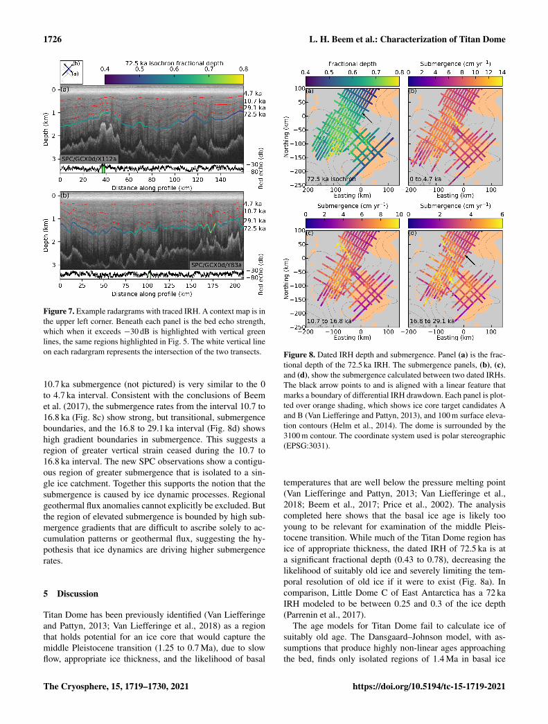
The fractional depth of the 72.5 ka IRH ranges from 0.43to 0.78 with a mean of 0.60 (Figs. 7 and 8). The surveyeddome flanks show the deepest fractional depth for any givenIRH. Shallower IRH depths exist nearer the present-day icedivide between Titan Dome and South Pole.

Present-day flow over candidate A is less than 2 m yr−1;however, submergence calculations put bounds on the tim-ing of faster ice flow in the past. For the interval starting atthe present, 0 to 4.7 ka, the submergence gradients (Fig. 8b)are similar to both the magnitude and pattern of present-day accumulation (Arthern et al., 2006; Wessem et al., 2014;Studinger et al., 2020), suggesting that this interval has beendominated by accumulation-driven vertical strain. The 4.7 to

https://doi.org/10.5194/tc-15-1719-2021 The Cryosphere, 15, 1719–1730, 2021

1726 L. H. Beem et al.: Characterization of Titan Dome

Figure 7. Example radargrams with traced IRH. A context map is inthe upper left corner. Beneath each panel is the bed echo strength,which when it exceeds −30 dB is highlighted with vertical greenlines, the same regions highlighted in Fig. 5. The white vertical lineon each radargram represents the intersection of the two transects.

10.7 ka submergence (not pictured) is very similar to the 0to 4.7 ka interval. Consistent with the conclusions of Beemet al. (2017), the submergence rates from the interval 10.7 to16.8 ka (Fig. 8c) show strong, but transitional, submergenceboundaries, and the 16.8 to 29.1 ka interval (Fig. 8d) showshigh gradient boundaries in submergence. This suggests aregion of greater vertical strain ceased during the 10.7 to16.8 ka interval. The new SPC observations show a contigu-ous region of greater submergence that is isolated to a sin-gle ice catchment. Together this supports the notion that thesubmergence is caused by ice dynamic processes. Regionalgeothermal flux anomalies cannot explicitly be excluded. Butthe region of elevated submergence is bounded by high sub-mergence gradients that are difficult to ascribe solely to ac-cumulation patterns or geothermal flux, suggesting the hy-pothesis that ice dynamics are driving higher submergencerates.

5 Discussion

Titan Dome has been previously identified (Van Liefferingeand Pattyn, 2013; Van Liefferinge et al., 2018) as a regionthat holds potential for an ice core that would capture themiddle Pleistocene transition (1.25 to 0.7 Ma), due to slowflow, appropriate ice thickness, and the likelihood of basal

Figure 8. Dated IRH depth and submergence. Panel (a) is the frac-tional depth of the 72.5 ka IRH. The submergence panels, (b), (c),and (d), show the submergence calculated between two dated IRHs.The black arrow points to and is aligned with a linear feature thatmarks a boundary of differential IRH drawdown. Each panel is plot-ted over orange shading, which shows ice core target candidates Aand B (Van Liefferinge and Pattyn, 2013), and 100 m surface eleva-tion contours (Helm et al., 2014). The dome is surrounded by the3100 m contour. The coordinate system used is polar stereographic(EPSG:3031).

temperatures that are well below the pressure melting point(Van Liefferinge and Pattyn, 2013; Van Liefferinge et al.,2018; Beem et al., 2017; Price et al., 2002). The analysiscompleted here shows that the basal ice age is likely tooyoung to be relevant for examination of the middle Pleis-tocene transition. While much of the Titan Dome region hasice of appropriate thickness, the dated IRH of 72.5 ka is ata significant fractional depth (0.43 to 0.78), decreasing thelikelihood of suitably old ice and severely limiting the tem-poral resolution of old ice if it were to exist (Fig. 8a). Incomparison, Little Dome C of East Antarctica has a 72 kaIRH modeled to be between 0.25 and 0.3 of the ice depth(Parrenin et al., 2017).

The age models for Titan Dome fail to calculate ice ofsuitably old age. The Dansgaard–Johnson model, with as-sumptions that produce highly non-linear ages approachingthe bed, finds only isolated regions of 1.4 Ma in basal ice

The Cryosphere, 15, 1719–1730, 2021 https://doi.org/10.5194/tc-15-1719-2021

L. H. Beem et al.: Characterization of Titan Dome 1727

age. Although it is encouraging that the oldest modeled agesare on the dome and flanking ice divides, a typically suitablelocation for drilling an ice core (Van Liefferinge and Pattyn,2013; Fischer et al., 2013; Van Liefferinge et al., 2018; Pas-salacqua et al., 2018), the specific locations with the oldestages in this study have been previously excluded from con-sideration due to exceeding the modern ice flow threshold of2 m yr−1 (Van Liefferinge and Pattyn, 2013).

The new observations have the effect of reducing the areaof suitable regions identified by ice sheet modeling (Van Li-efferinge and Pattyn, 2013). The effect of the observed thin-ner ice, compared to Bedmap2 used to identify candidate A,is twofold and would have competing effects. Thinner icewould tend to increase the area of the region suitable for re-covering middle Pleistocene age ice, because fewer locationswould exceed their geothermal heat flux threshold for melt-ing. Thinner ice would, however, increase calculated balancevelocities excluding more area due to excessive horizontaladvection. The candidate A boundary is more ice flow lim-ited than temperature limited, and the net effect of thinnerice would likely be a reduction in the extent of the promisingregion. For instance, the area between candidates A and B isexcluded from Van Liefferinge and Pattyn (2013) because itexceeds their balance velocity threshold of > 2 m yr−1; alsosee Bingham et al. (2007).

The flanks of Titan Dome show evidence of increased iceflow in the past, ceasing between 10.7 and 16.8 ka. Thisflow history could result in the loss of basal ice throughbasal melting and complications in stratigraphic layeringdue to elevated strain rates. Recent publications have indi-cated past ice flow on the flanks of Titan Dome is consistentwith ice stream transitional flow (Beem et al., 2017; Lilienet al., 2018), which is that between slow ice-deformation-dominated flow in the interior ice sheet and basal-slip-dominated ice streaming. Given this dynamic history thedome may be prone to divide migration (Winter et al.,2018). Internal reflecting horizon drawdown is consistentwith one or more of the following: regional melt from ele-vated geothermal flux, extensional strain from ice flow, andfrictional heating from past ice dynamics. The drawdownpattern includes a linear boundary (see arrow in Fig. 8a) andis completely within a single ice catchment, which supportsan ice dynamically induced drawdown. The linear boundaryhas previously been interpreted as a relic shear margin (Beemet al., 2017). The IRH drawdown (expressed both as elevatedsubmergence and greater IRH depth) seen in the new SPC ob-servations is consistent and contiguous with the pattern fromthe older PPT observations. The evident ice streaming pro-cesses makes this region more complicated for paleoclimateage model construction and the survivability of ice greaterthan 1 Ma.

Candidate B (Fig. 1), a region of modeled cold based ice,along the ∼ 45◦ E meridian from South Pole, does not showenhanced flow history expressed through submergence rates(Beem et al., 2017). Using the same dated IRH, but traced

wholly within the older PPT data (Carter et al., 2007), thethickness of ice below the 93.9 ka IRH is generally less than1200 m and in some cases considerably less. The fractionaldepth for the 93.9 ka IRH is 0.60 to 0.70, for the region withradar observations. If any ice were greater than 1 Ma, it isunlikely to have suitable temporal resolution.

The role or existence of elevated geothermal heat flux inthe study region is difficult to determine, but there is lim-ited evidence to support its existence. Previous work has sug-gested a region proximal to Titan Dome has elevated geother-mal flux (Jordan et al., 2018), but the basal characterizationof Titan Dome neither confirms nor refutes the existence ofelevated geothermal flux outside of the SPC survey area. Thenew survey presented here is of a different subglacial catch-ment than that identified to host elevated geothermal flux byJordan et al. (2018), and heterogeneity in geothermal flux isexpected over length scales of hundreds of kilometers. Thebasal reflectivity of Titan Dome does show a few localizedareas with a higher likelihood for the existence of water. Itis possible that localized geothermal flux could be causingthe increased basal reflectivity, which may be in addition toor an alternative hypothesis to remnant heat from past basalsliding (Beem et al., 2017). These hypotheses could be testedthrough direct access of the bed to characterize the geologyand measure geothermal flux.

6 Conclusions

Titan Dome is unlikely to be a suitable site for the extractionof an ice core that captures the middle Pleistocene transition.The depth of dated IRH, the age models, and implications forfaster flow that ceased during the last glacial maximum areeach discouraging to the possibility of suitably old ice. Agemodels all indicate basal ice age between 300 and 800 ka inthe most promising locations. Older modeled ages do occurin some regions when using end-member model parameters.In all instances, the age is younger than the 1.5 Ma ice neededto study the complete middle Pleistocene transition. If 1 Maor older ice were to exist, IRH ages that are dated and propa-gated from the South Pole Ice Core (Casey et al., 2014; Win-ski et al., 2019) would be too deep to have a suitable tempo-ral resolution. Further complication to any extracted ice corefrom Titan Dome is the evidence for faster flow in the past,which would distort chronology and source regions for anygiven layer within the core.

The new observations also describe previously unknownbasal topography that can be used to further improve com-munity datasets in this region; they have already been addedto the BedMachine product (Morlighem et al., 2020). The lo-cation of the Titan Dome summit is observed to be consistentwith the Bamber et al. (2009) ice surface DEM and locatedat 88.1716◦ S, 170.4765◦W.

https://doi.org/10.5194/tc-15-1719-2021 The Cryosphere, 15, 1719–1730, 2021

1728 L. H. Beem et al.: Characterization of Titan Dome

Data availability. The L2 data are made available through theUSAP data center: https://doi.org/10.15784/601437 (Beem et al.,2021).

Author contributions. This project was made possible by fundingacquired by DDB, DAY, JG, and SB and project administration byDAY, DDB, JG, and SB. Conceptualization of the project was com-pleted by LHB, DAY, MPGC, and JSG with investigation by JSG.Formal analysis and visualization was completed by LHB. Method-ology was developed by LHB and MGCP. LHB wrote the originaldraft, and all authors contributed to review and editing. Data cura-tion was completed by DAY and LHB.

Competing interests. The authors declare they have no conflict ofinterest.

Special issue statement. This article is part of the special issue“Oldest Ice: finding and interpreting climate proxies in ice olderthan 700 000 years (TC/CP/ESSD inter-journal SI)”. It is not asso-ciated with a conference.

Acknowledgements. The authors would like to thank the Polar Re-search Institute of China for their support and making their aerialgeophysical platform available for this research. The authors alsothank Ken Borek Ltd. pilots and engineers for their involvement andsupport in data collection. The authors thank Mercy Grace Browderand Roccio Castillo for their efforts in radar interpretation and thesupport of the Jackson School for Geoscience GEOFORCE pro-gram. We thank Massimo Frezzotti and Neil Ross for their thought-ful and helpful reviews. This is UTIG contribution no. 3773.

Financial support. This research has been supported by the Na-tional Science Foundation, Office of Polar Programs (grant no.1443690), the G. Unger Vetlesen Foundation, the National Natu-ral Science Foundation of China (grant no. 41876227), and the Na-tional Key Research and Development Program of China (grant no.2018YFB1307504).

Review statement. This paper was edited by Joel Savarino and re-viewed by Massimo Frezzotti and Neil Ross.

References

Arthern, R. J., Winebrenner, D. P., and Vaughan, D. G.: Antarc-tic snow accumulation mapped using polarization of 4.3 cmwavelength microwave emission, J. Geophys. Res.-Atmos., 111,D06107, https://doi.org/10.1029/2004JD005667, 2006.

Ashmore, D. W., Bingham, R. G., Ross, N., Siegert, M. J., Jordan,T. A., and Mair, D. W.: Englacial architecture and age-depth con-straints across the West Antarctic Ice Sheet, Geophys. Res. Lett.,

47, e2019GL086663, https://doi.org/10.1029/2019GL086663,2020.

Augustin, L., Barbante, C., Barnes, P. R. F., Marc Barnola, J.,Bigler,M., Castellano, E., Cattani, O., Chappellaz, J., Dahl-Jensen,D., Delmonte, B., Dreyfus, G., Durand, G., Falourd, S.,Fischer,H., Flückiger, J., Hansson, M. E., Huybrechts, P.,Jugie, G.,Johnsen, S. J., Jouzel, J., Kaufmann, P., Kipfstuhl, J.,Lambert,F., Lipenkov, V. Y., Littot, G. C., Longinelli, A., Lor-rain,R., Maggi, V., Masson-Delmotte, V., Miller, H., Mul-vaney,R., Oerlemans, J., Oerter, H., Orombelli, G., Parrenin, F.,Peel,D. A., Petit, J.-R., Raynaud, D., Ritz, C., Ruth, U., Schwan-der, J., Siegenthaler, U., Souchez, R., Stauffer, B., Peder Stef-fensen, J., Stenni, B., Stocker, T. F., Tabacco, I. E., Udisti,R.,van de Wal, R. S. W., van den Broeke, M., Weiss, J., Wil-helms, F., Winther, J.-G., Wolff, E. W., and Zucchelli, M.: Eightglacial cycles from an Antarctic ice core, Nature, 429, 623–628,https://doi.org/10.1038/nature02599, 2004.

Bamber, J. L., Gomez-Dans, J. L., and Griggs, J. A.: A new 1 kmdigital elevation model of the Antarctic derived from combinedsatellite radar and laser data – Part 1: Data and methods, TheCryosphere, 3, 101–111, https://doi.org/10.5194/tc-3-101-2009,2009.

Beem, L. H., Cavitte, M. G. P., Blankenship, D. D., Carter, S. P.,Young, D. A., Moldoon, G., Jackson, C. S., and Siegert, M. J.:Ice-flow reorganization within the East Antarctic Ice Sheet deep60 interior, in: Exploration of Subsurface Antarctica: UncoveringPast Changes and Modern Processes, edited by: Siegert, M. J.,Jamieson, S. R., and White, D. A., Geological Society, London,461, 35–47, https://doi.org/10.1144/SP461.14, 2017.

Beem, L. H., Young, D. A., Greenbaum, J., Ng, G., Blankenship,D. D., Cavitte, M. G. P., Jingxue, G., and Bo, S.: Titan Dome,East Antarctica, Aerogephysical Survey, U.S. Antarctic Program(USAP) Data Center, https://doi.org/10.15784/601437, 2021.

Bingham, R. G., Siegert, M. J., Young, D. A., and Blankenship,D. D.: Organized flow from the South Pole to the Filchner-Ronneice shelf: An assessment of balance velocities in interior EastAntarctica using radio echo sounding data, J. Geophys. Res.-Earth, 112, F03S26, https://doi.org/10.1029/2006JF000556,2007.

Blankenship, D., Morse, D., Finn, C., Bell, R., Peters, M., Kempf,S., Hodge, S., Studinger, M., Behrendt, J. C., and Brozena,J.: Geologic controls on the initiation of rapid basal mo-tion for West Antarctic ice streams: A geophysical perspec-tive including new airborne radar sounding and laser altime-try results, in: The West Antarctic Ice Sheet: Behavior andEnvironment, edited by: Alley, R. B. and Bindschadler, R.A., American Geophysical Union, Washington, D.C., 105–121,https://doi.org/10.1029/AR077p0105, 2001.

Carter, S. P., Blankenship, D. D., Peters, M. E., Young, D. A.,Holt, J. W., and Morse, D. L.: Radar-based subglacial lake clas-sification in Antarctica, Geochem. Geophy. Geosy., 8, Q03016,https://doi.org/10.1029/2006GC001408, 2007.

Casey, K. A., Fudge, T. J., Neumann, T., Steig, E. J., Cavitte, M.,and Blankenship, D. D.: The 1500 m South Pole ice core: recov-ering a 40 ka environmental record, Ann. Glaciol., 55, 137–146,https://doi.org/10.3189/2014AoG68A016, 2014.

Clark, P. U., Archer, D., Pollard, D., Blum, J. D., Rial,J. A., Brovkin, V., Mix, A. C., Pisias, N. G., and Roy,M.: The middle Pleistocene transition: characteristics, mech-

The Cryosphere, 15, 1719–1730, 2021 https://doi.org/10.5194/tc-15-1719-2021

L. H. Beem et al.: Characterization of Titan Dome 1729

anisms, and implications for long-term changes in at-mospheric pCO2, Quaternary Sci. Rev., 25, 3150–3184,https://doi.org/10.1016/j.quascirev.2006.07.008, 2006.

Cuffey, K. M. and Paterson, W. S. B.: The Physics of Glaciers, 4thEdn., Butterworth-Heinemann, Burlington, MA, p. 693, 2010.

Cui, X., Greenbaum, J. S., Beem, L. H., Guo, J., Ng, G., Li, L.,Blankenship, D., and Sun, B.: The First Fixed-wing Aircraft forChinese Antarctic Expeditions: Airframe, modifications, Scien-tific Instrumentation and Applications, J. Environ. Eng. Geoph.,23, 1–13, https://doi.org/10.2113/JEEG23.1.1, 2018.

Cui, X., Greenbaum, J. S., Lang, S., Zhao, X., Li, L., Guo, J., andSun, B.: The Scientific Operations of Snow Eagle 601 in Antarc-tica in the Past Five Austral Seasons, Remote Sens.-Basel, 12,2994, https://doi.org/10.3390/rs12182994, 2020.

Fischer, H., Severinghaus, J., Brook, E., Wolff, E., Albert, M., Ale-many, O., Arthern, R., Bentley, C., Blankenship, D., Chappellaz,J., Creyts, T., Dahl-Jensen, D., Dinn, M., Frezzotti, M., Fujita,S., Gallee, H., Hindmarsh, R., Hudspeth, D., Jugie, G., Kawa-mura, K., Lipenkov, V., Miller, H., Mulvaney, R., Parrenin, F.,Pattyn, F., Ritz, C., Schwander, J., Steinhage, D., van Ommen,T., and Wilhelms, F.: Where to find 1.5 million year old icefor the IPICS “Oldest-Ice” ice core, Clim. Past, 9, 2489–2505,https://doi.org/10.5194/cp-9-2489-2013, 2013.

Fretwell, P., Pritchard, H. D., Vaughan, D. G., Bamber, J. L., Bar-rand, N. E., Bell, R., Bianchi, C., Bingham, R. G., Blanken-ship, D. D., Casassa, G., Catania, G., Callens, D., Conway, H.,Cook, A. J., Corr, H. F. J., Damaske, D., Damm, V., Ferracci-oli, F., Forsberg, R., Fujita, S., Gim, Y., Gogineni, P., Griggs,J. A., Hindmarsh, R. C. A., Holmlund, P., Holt, J. W., Jacobel,R. W., Jenkins, A., Jokat, W., Jordan, T., King, E. C., Kohler,J., Krabill, W., Riger-Kusk, M., Langley, K. A., Leitchenkov,G., Leuschen, C., Luyendyk, B. P., Matsuoka, K., Mouginot,J., Nitsche, F. O., Nogi, Y., Nost, O. A., Popov, S. V., Rignot,E., Rippin, D. M., Rivera, A., Roberts, J., Ross, N., Siegert,M. J., Smith, A. M., Steinhage, D., Studinger, M., Sun, B.,Tinto, B. K., Welch, B. C., Wilson, D., Young, D. A., Xiangbin,C., and Zirizzotti, A.: Bedmap2: improved ice bed, surface andthickness datasets for Antarctica, The Cryosphere, 7, 375–393,https://doi.org/10.5194/tc-7-375-2013, 2013.

Gooch, B. T., Young, D. A., and Blankenship, D. D.: Po-tential groundwater and heterogeneous heat source contri-butions to ice sheet dynamics in critical submarine basinsof East Antarctica, Geochem. Geophy. Geosy., 17, 395–409,https://doi.org/10.1002/2015GC006117, 2016.

Harrison, C. H.: Radio echo sounding of hori-zontal layers in ice, J. Glaciol., 12, 383–397,https://doi.org/10.3189/S0022143000031804, 1973.

Helm, V., Humbert, A., and Miller, H.: Elevation and elevationchange of Greenland and Antarctica derived from CryoSat-2, The Cryosphere, 8, 1539–1559, https://doi.org/10.5194/tc-8-1539-2014, 2014.

Holschuh, N., Christianson, K., and Anandakrishnan, S.:Power loss in dipping internal reflectors, imaged us-ing ice-penetrating radar, Ann. Glaciol., 55, 49–56,https://doi.org/10.3189/2014AoG67A005, 2014.

Howat, I. M., Porter, C., Smith, B. E., Noh, M.-J., and Morin, P.:The Reference Elevation Model of Antarctica, The Cryosphere,13, 665–674, https://doi.org/10.5194/tc-13-665-2019, 2019.

Jordan, T., Martin, C., Ferraccioli, F., Matsuoka, K., Corr, H.,Forsberg, R., Olesen, A., and Siegert, M.: Anomalously highgeothermal flux near the South Pole, Sci. Rep.-UK, 8, 16785,https://doi.org/10.1038/s41598-018-35182-0, 2018.

Lilien, D. A., Fudge, T., Koutnik, M. R., Conway, H., Os-terberg, E. C., Ferris, D. G., Waddington, E. D., andStevens, C. M.: Holocene Ice-Flow Speedup in the Vicin-ity of the South Pole, Geophys. Res. Lett., 45, 6557–6565,https://doi.org/10.1029/2018GL078253, 2018.

Lindzey, L. E., Beem, L. H., Young, D. A., Quartini, E., Blanken-ship, D. D., Lee, C.-K., Lee, W. S., Lee, J. I., and Lee, J.: Aero-geophysical characterization of an active subglacial lake systemin the David Glacier catchment, Antarctica, The Cryosphere, 14,2217–2233, https://doi.org/10.5194/tc-14-2217-2020, 2020.

MacGregor, J. A., Winebrenner, D. P., Conway, H. B., Matsuoka,K., Mayewski, P. A., and Clow, G. D.: Modeling englacial radarattenuation at Siple Dome, West Antarctica, using ice chem-istry and temperature data, J. Geophys. Res.-Earth, 112, F03008,https://doi.org/10.1029/2006JF000717, 2007.

Matsuoka, K., MacGregor, J. A., and Pattyn, F.: Predicting radarattenuation within the Antarctic ice sheet, Earth Planet. Sc. Lett.,359, 173–183, https://doi.org/10.1016/j.epsl.2012.10.018, 2012.

Morlighem, M., Rignot, E., Binder, T., Blankenship, D., Drews, R.,Eagles, G., Eisen, O., Ferraccioli, F., Forsberg, R., Fretwell, P.,Goel, V., Greenbaum, J. S., Gudmundsson, H., Guo, J., Helm,V., Hofstede, C., Howat, I., Humbert, A., Jokat, W., Karls-son, N. B., Lee, W. S., Matsuoka, K., Millan, R., Mouginot,J., Paden, J., Pattyn, F., Roberts, J., Rosier, S., Ruppel, A.,Seroussi, H., Smith, E. C., Steinhage, D., Sun, B., Broeke, M.R. V. D., Ommen, T. D. V., Wessem, M. V., and Young, D. A.:Deep glacial troughs and stabilizing ridges unveiled beneath themargins of the Antarctic ice sheet, Nat. Geosci., 13, 132–137,https://doi.org/10.1038/s41561-019-0510-8, 2020.

Parrenin, F., Cavitte, M. G. P., Blankenship, D. D., Chappellaz,J., Fischer, H., Gagliardini, O., Masson-Delmotte, V., Passalac-qua, O., Ritz, C., Roberts, J., Siegert, M. J., and Young, D. A.:Is there 1.5-million-year-old ice near Dome C, Antarctica?, TheCryosphere, 11, 2427–2437, https://doi.org/10.5194/tc-11-2427-2017, 2017.

Passalacqua, O., Cavitte, M., Gagliardini, O., Gillet-Chaulet, F.,Parrenin, F., Ritz, C., and Young, D.: Brief communication: Can-didate sites of 1.5 Myr old ice 37 km southwest of the DomeC summit, East Antarctica, The Cryosphere, 12, 2167–2174,https://doi.org/10.5194/tc-12-2167-2018, 2018.

Peters, M. E., Blankenship, D. D., and Morse, D. L.: Analysis tech-niques for coherent airborne radar sounding: Application to WestAntarctic ice streams, J. Geophys. Res.-Sol. Ea., 110, B06303,https://doi.org/10.1029/2004JB003222, 2005.

Peters, M. E., Blankenship, D. D., Carter, S. P., Kempf, S. D.,Young, D. A., and Holt, J. W.: Along-track focusing of airborneradar sounding data from West Antarctica for improving basalreflection analysis and layer detection, IEEE T. Geosci. Remote,45, 2725–2736, https://doi.org/10.1109/TGRS.2007.897416,2007.

Price, P. B., Nagornov, O. V., Bay, R., Chirkin, D., He, Y., Mioci-novic, P., Richards, A., Woschnagg, K., Koci, B., and Zagorod-nov, V.: Temperature profile for glacial ice at the South Pole: Im-plications for life in a nearby subglacial lake, P. Natl. Acad. Sci.

https://doi.org/10.5194/tc-15-1719-2021 The Cryosphere, 15, 1719–1730, 2021

1730 L. H. Beem et al.: Characterization of Titan Dome

USA, 99, 7844–7847, https://doi.org/10.1073/pnas.082238999,2002.

Siegert, M. J.: On the origin, nature and uses of Antarctic ice-sheet radio-echo layering, Prog. Phys. Geog., 23, 159–179,https://doi.org/10.1177/030913339902300201, 1999.

Studinger, M., Medley, B. C., Brunt, K. M., Casey, K. A., Kurtz, N.T., Manizade, S. S., Neumann, T. A., and Overly, T. B.: Tempo-ral and spatial variability in surface roughness and accumulationrate around 88◦ S from repeat airborne geophysical surveys, TheCryosphere, 14, 3287–3308, https://doi.org/10.5194/tc-14-3287-2020, 2020.

Van Liefferinge, B. and Pattyn, F.: Using ice-flow models toevaluate potential sites of million year-old ice in Antarctica,Clim. Past, 9, 2335–2345, https://doi.org/10.5194/cp-9-2335-2013, 2013.

Van Liefferinge, B., Pattyn, F., Cavitte, M. G. P., Karlsson, N. B.,Young, D. A., Sutter, J., and Eisen, O.: Promising Oldest Icesites in East Antarctica based on thermodynamical modelling,The Cryosphere, 12, 2773–2787, https://doi.org/10.5194/tc-12-2773-2018, 2018.

Wessem, J. M. V., Reijmer, C. H., Morlighem, M., Mouginot, J.,Rignot, E., Medley, B., Joughin, I., Wouters, B., DePoorter,M. A., Bamber, J. L., Lenaerts, J. T. M., van de Berg, W. J.,van den Broeke, M. R., and van Meijgaard, E.: Improved rep-resentation of East Antarctic surface mass balance in a re-gional atmospheric climate model, J. Glaciol., 60, 761–770,https://doi.org/10.3189/2014JoG14J051, 2014.

Winski, D. A., Fudge, T. J., Ferris, D. G., Osterberg, E. C., Fe-gyveresi, J. M., Cole-Dai, J., Thundercloud, Z., Cox, T. S.,Kreutz, K. J., Ortman, N., Buizert, C., Epifanio, J., Brook, E. J.,Beaudette, R., Severinghaus, J., Sowers, T., Steig, E. J., Kahle,E. C., Jones, T. R., Morris, V., Aydin, M., Nicewonger, M. R.,Casey, K. A., Alley, R. B., Waddington, E. D., Iverson, N. A.,Dunbar, N. W., Bay, R. C., Souney, J. M., Sigl, M., and Mc-Connell, J. R.: The SP19 chronology for the South Pole Ice Core– Part 1: volcanic matching and annual layer counting, Clim.Past, 15, 1793–1808, https://doi.org/10.5194/cp-15-1793-2019,2019.

Winter, A., Steinhage, D., Creyts, T. T., Kleiner, T., and Eisen, O.:Age stratigraphy in the East Antarctic Ice Sheet inferred fromradio-echo sounding horizons, Earth Syst. Sci. Data, 11, 1069–1081, https://doi.org/10.5194/essd-11-1069-2019, 2019.

Winter, K., Ross, N., Ferraccioli, F., Jordan, T. A., Corr, H. F., Fors-berg, R., Matsuoka, K., Olesen, A. V., and Casal, T. G.: Topo-graphic steering of enhanced ice flow at the bottleneck betweenEast and West Antarctica, Geophys. Res. Lett., 45, 4899–4907,https://doi.org/10.1029/2018GL077504, 2018.

Young, D. A., Lindzey, L. E., Blankenship, D. D., Greenbaum, J.S., de Gorord, A. G., Kempf, S. D., Roberts, J. L., Warner, R. C.,Van Ommen, T., Siegert, M. J., and Le Meur, E.: Land-ice ele-vation changes from photon-counting swath altimetry: first ap-plications over the Antarctic ice sheet, J. Glaciol., 61, 17–28,https://doi.org/10.3189/2015JoG14J048, 2015.

Young, D. A., Roberts, J. L., Ritz, C., Frezzotti, M., Quartini, E.,Cavitte, M. G. P., Tozer, C. R., Steinhage, D., Urbini, S., Corr, H.F. J., van Ommen, T., and Blankenship, D. D.: High-resolutionboundary conditions of an old ice target near Dome C, Antarc-tica, The Cryosphere, 11, 1897–1911, https://doi.org/10.5194/tc-11-1897-2017, 2017.

The Cryosphere, 15, 1719–1730, 2021 https://doi.org/10.5194/tc-15-1719-2021