Embed Size (px)
Citation preview
Aeroelastic Uncertainty Quantification Studies Using the S4TWind Tunnel Model
Melike Nikbay∗
National Institute of Aerospace, Hampton, Virginia, 23666, USA
Istanbul Technical University, Maslak, Istanbul, 34469, Turkey
andJennifer Heeg †
NASA Langley Research Center, Hampton, Virginia, 23681, USA
This paper originates from the joint efforts of an aeroelastic study team in the Applied Vehicle Technol-ogy Panel from NATO Science and Technology Organization, with the Task Group number AVT-191, titled“Application of Sensitivity Analysis and Uncertainty Quantification to Military Vehicle Design.” We presentaeroelastic uncertainty quantification studies using the SemiSpan Supersonic Transport wind tunnel model atthe NASA Langley Research Center. The aeroelastic study team decided treat both structural and aerodynamicinput parameters as uncertain and represent them as samples drawn from statistical distributions, propagat-ing them through aeroelastic analysis frameworks. Uncertainty quantification processes require many functionevaluations to asses the impact of variations in numerous parameters on the vehicle characteristics, rapidly in-creasing the computational time requirement relative to that required to assess a system deterministically. Theincreased computational time is particularly prohibitive if high-fidelity analyses are employed. As a remedy,the Istanbul Technical University team employed an Euler solver in an aeroelastic analysis framework, andimplemented reduced order modeling with Polynomial Chaos Expansion and Proper Orthogonal Decomposi-tion to perform the uncertainty propagation. The NASA team chose to reduce the prohibitive computationaltime by employing linear solution processes. The NASA team also focused on determining input sample distri-butions.
Nomenclature
LHS Latin Hypercube SamplingMCS Monte Carlo SamplingPCE Polynomial Chaos ExpansionPOD Proper Orthogonal DecompositionROM Reduced order model
I. Introduction
A eroelasticity, as a multidisciplinary research field, investigates the behavior of an elastic structure in the airstreamand the interactions between inertial, aerodynamic, and structural forces. With the use of advanced technologies
in aircraft design and analysis, the need for predicting such aerostructural interactions by using high-fidelity compu-tational models has increased. Most analysis procedures involving high-fidelity modeling consider the system andsolution as deterministic. However, as computational models have advanced, parametric sensitivities have becomemore intrinsic and more hidden. Recent work has demonstrated solution sensitivity to small changes in geometry,freestream conditions and computational parameter specifications. This sensitivity leads to considering these simu-lations from an uncertainty standpoint. As another motivation in experiments, input parameters are only controlledto within some precision level and the input and output parameters are only known to within measurement errors.Comparisons between computations and experiments should consider these uncertainties.
∗Currently, Senior Research Engineer at National Institute of Aerospace, located at NASA Langley Research Center, Aeronautical SystemsAnalysis Branch & Associate Professor, Faculty of Aeronautics and Astronautics, AIAA Associate Fellow
†Senior Research Engineer, Aeroelasticity Branch, AIAA Associate Fellow
1 of 18
American Institute of Aeronautics and Astronautics
https://ntrs.nasa.gov/search.jsp?R=20170001232 2018-07-11T16:18:31+00:00Z
In the current paper, we endeavor to recast our aeroelastic simulation inputs and outputs to treat the analyses asstochastic processes. Two different approaches and philosophical viewpoints are utilized to quantify the effects ofuncertainties in aeroelastic systems. The methods, modeling and results are produced from research efforts of teamsfrom NASA and Istanbul Technical University (ITU). The NASA work utilizes linear aerodynamic modeling, while theITU work utilizes higher fidelity aerodynamic modeling and a reduced order model (ROM) approach for propagatingthe uncertain parameters.
A flexible vehicle configuration, the NASA Semispan Supersonic Transport (S4T) wind tunnel model, was chosenas the basis for uncertainty studies and propagation. The current work utilizes information, analytical models and datareported by the (S4T) project team in 2012 at a special session at the 53rd AIAA/ASME/ASCE/AHS/ASC Structures,Structural Dynamics and Materials Conference. A program overview paper was authored by Silva36 that documentsthe wind tunnel model, four wind tunnel tests conducted between 2007 and 2010, and references laboratory tests andanalyses. The products from those efforts are utilized as the starting point for the current uncertainty analyses; theseaspects will be further identified in the body of this paper.
The current paper focuses on defining statistical distributions of input parameters, propagating them through thetwo analysis processes, and examining the statistical distributions of output parameters. The analysis approaches willbe described first, followed by a description of the development of an example input parameter distribution to representuncertainty associated with a structural parameter. Example results from each of the analysis methods will then bepresented, followed by discussion and concluding remarks.
II. Analysis Approaches
A. Uncertainty Propagation Using Linear Analyses
The methods, modeling and results generated by the NASA team were produced from linear aerodynamic and struc-tural computations. The models used as the baseline cases came from the project team that designed, tested andanalyzed the configuration. The major steps taken in performing the uncertainty propagations were:
• Define input variation
• Generate random input samples
• Generate input file for each input sample
• Perform simulation for each input sample
• Extract output parameters from each simulation
• Perform statistical analyses of the evaluation parameters
Three types of simulations were performed in the NASA analyses: static aeroelastic analyses, normal modes anal-yses and flutter solutions. Each of the analyses were performed using standard analysis options in MSC NASTRAN.18
Input and output parameter screening was performed using static aeroelastic analysis. Normal modes analyses wereperformed to show the sensitivity of modal frequencies to the structural variations. Flutter analyses were performed toshow the sensitivity to modal parameters in addition to sensitivity to the more fundamental input parameters.
B. Reduced Order Modeling Using Euler Simulations
The ITU team performed static aeroelastic and flutter analyses of the S4T wing by using the Polynomial Chaos Expan-sion (PCE)22–25 and Proper Orthogonal Decomposition (POD)27, 29–31, 33, 34 based Reduced Order Models,26, 32 whichwere generated by using an Euler flow based aeroelastic solver in ZEUS19 software. The aeroelastic solver of ZEUSemploys mode shapes obtained from the NASTRAN modal solver. The ROM results were compared to the initial com-putational results of the high-fidelity models. These ROMs could predict the responses in a small input data range, andin this case both the PCE and POD methods gave satisfactory results while their accuracies were thoroughly discussedin the present work. Secondly, both the PCE and POD methods were used to construct a ROM, which was accuratewhen large variations of input parameters were considered. The flutter behavior of the S4T wing could accurately bepredicted over the entire flight regime for Mach numbers ranging from 0.60 to 1.20 by the PCE and POD based ROMs.This will be demonstrated in this paper through detailed comparisons of the flutter results of the ROMs to the initialhigh-fidelity computational analyses.
Uncertainty distributions of structural and aerodynamic input parameters were then propagated using the ROMs.Output parameters from the reduced order static aeroelastic and flutter analyses were examined to assess the influences
2 of 18
American Institute of Aeronautics and Astronautics
of the input parameters that were varied. The input sampling was performed using Monte Carlo Simulation (MCS) andLatin Hypercube Sampling (LHS) techniques, which are frequently used to propagate uncertainties in a probabilisticframework. The input parameters that were treated as uncertain in these analyses were angle of attack, Young’smodulus and dynamic pressure. The influence of the first two were assessed for both the static aeroelastic and flutteranalyses. The dynamic pressure uncertainty was only evaluated for the static aeroelastic cases. The output parametersthat were examined were flutter frequency, flutter speed, flutter dynamic pressure, lift coefficient (CL), drag coefficient(CD), pitching moment coefficient (Cm), and wing tip twist angle.
1. Polynomial Chaos Expansion (PCE) Methodology
Nonintrusive PCE defines a ROM basis in terms of orthogonal polynomials. In the present study, Hermite polynomialsare used as the orthogonal polynomials since the input parameters are assumed to vary with respect to Gaussiandistribution. The definition of the first few Hermite polynomials are given below in terms of the standard variable, ξ :
Ho(ξ ) = 1 (1)
H1(ξ ) = ξ (2)
H2(ξ ) = ξ2 −1 (3)
H3(ξ ) = ξ3 −3ξ (4)
H4(ξ ) = ξ4 −6ξ
2 +3 (5)
H5(ξ ) = ξ5 −10ξ
3 +15ξ (6)
H6(ξ ) = ξ6 −15ξ
4 +45ξ2 −15 (7)
The chaos coefficients can be calculated by using the following relation for a general physical system:
u1
u2
.
.
un
=
H10 H11 H12. . H1p
H20 H21 H22. . H2p
. . . . .
. . . . .
Hn0 Hn1 Hn2. . Hnp
a1
a2
.
.
ap+1
(8)
where ui (i = 1 to n) is an output response that is known from the analyses and a j ( j = 1 to p+ 1) shows chaoscoefficients to be determined. The order of the approximation is denoted by p and n shows the dimension. In thismatrix system, the parameters Hi j indicate the multiplication of Hi and H j functions defined in Eq. (4) to (10).However, in the two-dimensional case, H j is the function of the first standard random variable, ξ , while Hi is thefunction of the second standard random variable, η . Since three input parameters are defined in the present work,Hi jk = Hi(ξ ) ·H j(η) ·Hk(γ) (where γ is also a standard random variable) multiplications should be computed. TheROM can be constructed by using the chaos coefficients. In order to calculate the chaos coefficients, linear regressioncan be applied. Considering the standard normal variables ξ , η and γ , a general linear regression model, U , can bedefined in closed form as below:
U = Ha+ ε (9)
where ε denotes the error between real values and approximate values. The regression coefficients, a, can be computedby using Eq. (10):
a = (HT H)−1HTU (10)
After determining the regression coefficients, the ROM to represent the reference initial design can be constructed forthe two input variable case by using the relation below:
U j(ξ∗,η∗) = a1H j0(ξ
∗,η∗)+a2H j1(ξ∗,η∗)+ ...+ap+1H jp(ξ
∗,η∗) (11)
where ξ ∗ and η∗ are the values of the standard random variables for the case that needs to be computed.
3 of 18
American Institute of Aeronautics and Astronautics
2. Proper Orthogonal Decomposition (POD) Approach
The Proper Orthogonal Decomposition (POD) method is used to generate a ROM. The system is defined as a linearcombination of independent orthogonal basis functions. The orthogonal functions, called the “POD basis functions,”are formulated such that the effect of the first mode is the highest and the second mode is less effective and so on. Aphysical model with n outputs can be expressed as a linear combination given as below:
[y](n×1) =k
∑j=1
a j[Φ j](n×1) (12)
where y is an output response vector for a snapshot of the input variables, a j are POD coefficients, Φ j are POD basisvectors and k is the order of ROM (k < n). In this study, the “method of snapshots”35 is used for creating ROMs.A snapshot matrix T , is an n×m matrix (m is number of snapshots) and can be constructed by using the outputparameters of the system:
[T ](n×m) =
y(1)1 y(2)1 . y(m)
1. . . .
. . . .
y(1)n . . y(m)n
(n×m)
Any physical system given with a snapshot matrix can be represented by a surrogate response function which super-poses the basic modes of the model. The correlation matrix is defined in terms of the snapshot matrix and the numberof POD basis vectors:
[C](n×n) =1n[T ](n×m) • [T ]T(m×n) (13)
The POD basis vectors and coefficients are defined through the eigenvalues and eigenvectors of the correlation ma-trix [C]Φ = ΛΦ. Singular Value Decomposition (SVD) facilitates the construction of the POD based ROMs. In thismethod, the factorization of a real matrix, T is given below:
[T ]n×m = [U ](n×n)[Σ](n×m)[V ]T (m×m) (14)
where U , the columns of which consist of the eigenvectors of [T ] [T ]T , is the left singular vector of T and theseeigenvectors are POD basis vectors. V , the columns of which consist of the eigenvectors of [T ]T [T ], is the right singularvector of T . [Σ] is a diagonal matrix representing the square roots of POD eigenvalues, λi. The POD coefficients arecalculated by projecting the snapshots on the POD basis.
a j = [Tj]T(1×n) • [Φ j](n×1) (15)
The number of POD basis vectors is equal to the number of snapshots m (and also POD coefficients), however, thenumber of retained POD basis vectors (POD modes) k is determined by considering the captured energy from theoriginal model. The total captured energy is defined as:
Etotal =k
∑i=1
λi (16)
where λ is the vector of normalized eigenvalues of the correlation matrix, C, and k is the required number of PODmodes to reach the specified captured energy level. In the present work, the captured energy level is taken as 99.9 %in all applications.
4 of 18
American Institute of Aeronautics and Astronautics
III. Development of Statistical Distributions of Input Parameters
Development of statistical distributions to represent input parameter variations were performed by the NASAteam. The information required to formulate the distributions of structural parameters is discussed in this section.The model hardware, testing and finite element model (FEM) tuning process were the key elements in developing theinput parameter distributions. The variations for other input variables that are utilized in the current work—angle ofattack, dynamic pressure, Mach number and modal frequencies—are not discussed in detail here; the processes andassumptions for developing these additional input parameter variations are detailed in the NATO-STO-AVT-191 TaskGroup Report.17
A. Hardware Characterization Testing
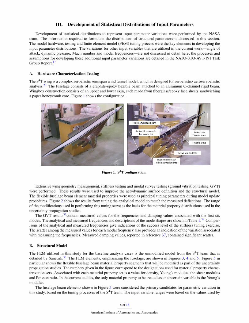
The S4T wing is a complex aeroelastic semispan wind tunnel model, which is designed for aeroelastic/ aeroservoelasticanalysis.20 The fuselage consists of a graphite-epoxy flexible beam attached to an aluminum C-channel rigid beam.Wingbox construction consists of an upper and lower skin, each made from fiberglass/epoxy face sheets sandwichinga paper honeycomb core. Figure 1 shows the configuration.
Figure 1. S4T configuration.
Extensive wing geometry measurement, stiffness testing and modal survey testing (ground vibration testing, GVT)were performed. These results were used to improve the aerodynamic surface definition and the structural model.The flexible fuselage beam element material properties were used as principal tuning parameters during model updateprocedures. Figure 2 shows the results from tuning the analytical model to match the measured deflections. The rangeof the modifications used in performing this tuning serve as the basis for the material property distributions used in theuncertainty propagation studies.
The GVT results37contain measured values for the frequencies and damping values associated with the first sixmodes. The analytical and measured frequencies and descriptions of the mode shapes are shown in Table 1.38 Compar-isons of the analytical and measured frequencies give indications of the success level of the stiffness tuning exercise.The scatter among the measured values for each modal frequency also provides an indication of the variation associatedwith measuring the frequencies. Measured damping values, reported in reference 37, contained significant scatter.
B. Structural Model
The FEM utilized in this study for the baseline analysis cases is the unmodified model from the S4T team that isdetailed by Sanetrik.38 The FEM elements, emphasizing the fuselage, are shown in Figures 3, 4 and 5. Figure 5 inparticular shows the flexible fuselage beam material property segments that will be modified as part of the uncertaintypropagation studies. The numbers given in the figure correspond to the designations used for material property charac-terization sets. Associated with each material property set is a value for density, Young’s modulus, the shear modulusand Poisson ratio. In the current studies, the only material property to be treated as an uncertain variable is the Young’smodulus.
The fuselage beam elements shown in Figure 5 were considered the primary candidates for parametric variation inthis study, based on the tuning processes of the S4T team. The input variable ranges were based on the values used by
5 of 18
American Institute of Aeronautics and Astronautics
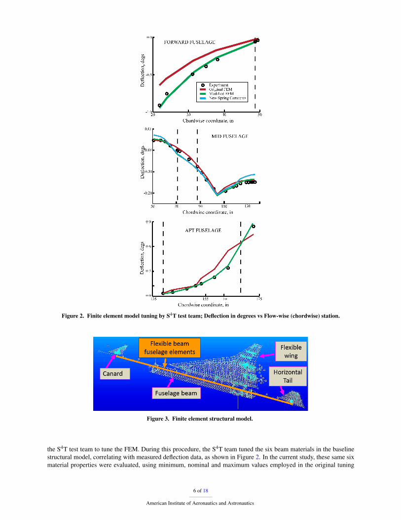
Figure 2. Finite element model tuning by S4T test team; Deflection in degrees vs Flow-wise (chordwise) station.
Figure 3. Finite element structural model.
the S4T test team to tune the FEM. During this procedure, the S4T team tuned the six beam materials in the baselinestructural model, correlating with measured deflection data, as shown in Figure 2. In the current study, these same sixmaterial properties were evaluated, using minimum, nominal and maximum values employed in the original tuning
6 of 18
American Institute of Aeronautics and Astronautics
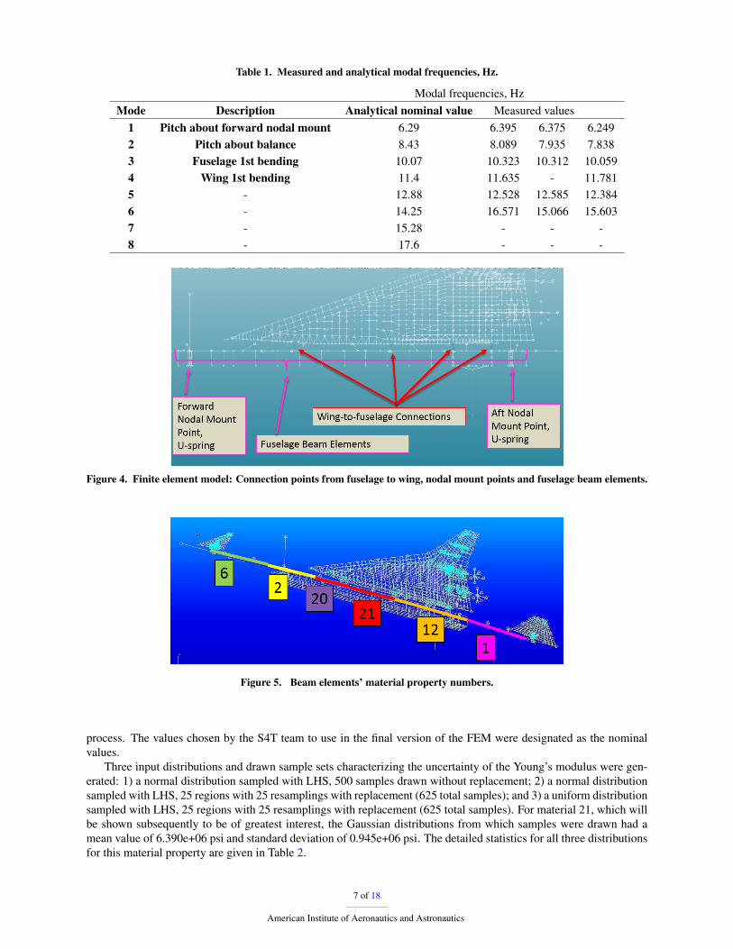
Table 1. Measured and analytical modal frequencies, Hz.
Modal frequencies, HzMode Description Analytical nominal value Measured values
1 Pitch about forward nodal mount 6.29 6.395 6.375 6.2492 Pitch about balance 8.43 8.089 7.935 7.8383 Fuselage 1st bending 10.07 10.323 10.312 10.0594 Wing 1st bending 11.4 11.635 - 11.7815 - 12.88 12.528 12.585 12.3846 - 14.25 16.571 15.066 15.6037 - 15.28 - - -8 - 17.6 - - -
Figure 4. Finite element model: Connection points from fuselage to wing, nodal mount points and fuselage beam elements.
Figure 5. Beam elements’ material property numbers.
process. The values chosen by the S4T team to use in the final version of the FEM were designated as the nominalvalues.
Three input distributions and drawn sample sets characterizing the uncertainty of the Young’s modulus were gen-erated: 1) a normal distribution sampled with LHS, 500 samples drawn without replacement; 2) a normal distributionsampled with LHS, 25 regions with 25 resamplings with replacement (625 total samples); and 3) a uniform distributionsampled with LHS, 25 regions with 25 resamplings with replacement (625 total samples). For material 21, which willbe shown subsequently to be of greatest interest, the Gaussian distributions from which samples were drawn had amean value of 6.390e+06 psi and standard deviation of 0.945e+06 psi. The detailed statistics for all three distributionsfor this material property are given in Table 2.
7 of 18
American Institute of Aeronautics and Astronautics
IV. Linear Analyses
A small subset of the linear analysis results generated in this study are discussed and presented in the current paper.Additional results and comparisons with different uncertainty quantification approaches are detailed in reference 17.In the current section, an example of parameter screening using static aeroelastic analysis is presented, along with anexample case of propagating a distribution of an input parameter through a normal modes analysis. Finally, exampleresults are shown for propagating both uniform and normal distributions of an input parameter through the flutteranalysis process.
A. Static Aeroelastic Analyses for Parameter Screening
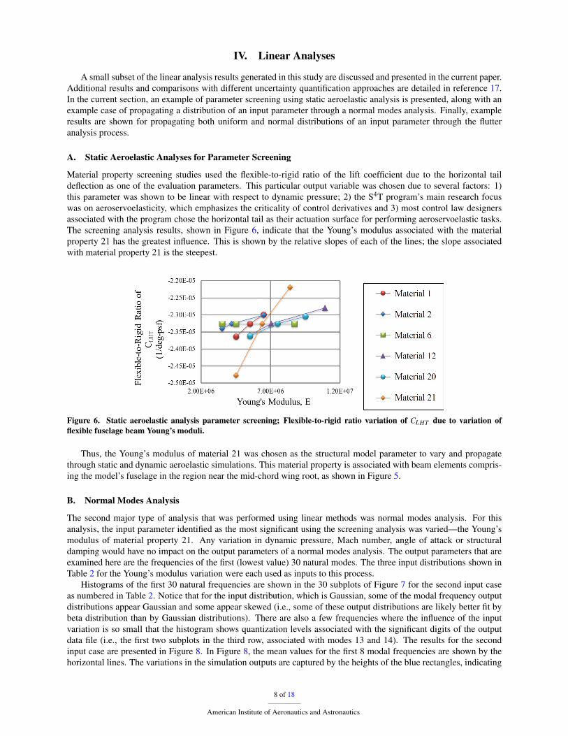
Material property screening studies used the flexible-to-rigid ratio of the lift coefficient due to the horizontal taildeflection as one of the evaluation parameters. This particular output variable was chosen due to several factors: 1)this parameter was shown to be linear with respect to dynamic pressure; 2) the S4T program’s main research focuswas on aeroservoelasticity, which emphasizes the criticality of control derivatives and 3) most control law designersassociated with the program chose the horizontal tail as their actuation surface for performing aeroservoelastic tasks.The screening analysis results, shown in Figure 6, indicate that the Young’s modulus associated with the materialproperty 21 has the greatest influence. This is shown by the relative slopes of each of the lines; the slope associatedwith material property 21 is the steepest.
Figure 6. Static aeroelastic analysis parameter screening; Flexible-to-rigid ratio variation of CLHT due to variation offlexible fuselage beam Young’s moduli.
Thus, the Young’s modulus of material 21 was chosen as the structural model parameter to vary and propagatethrough static and dynamic aeroelastic simulations. This material property is associated with beam elements compris-ing the model’s fuselage in the region near the mid-chord wing root, as shown in Figure 5.
B. Normal Modes Analysis
The second major type of analysis that was performed using linear methods was normal modes analysis. For thisanalysis, the input parameter identified as the most significant using the screening analysis was varied—the Young’smodulus of material property 21. Any variation in dynamic pressure, Mach number, angle of attack or structuraldamping would have no impact on the output parameters of a normal modes analysis. The output parameters that areexamined here are the frequencies of the first (lowest value) 30 natural modes. The three input distributions shown inTable 2 for the Young’s modulus variation were each used as inputs to this process.
Histograms of the first 30 natural frequencies are shown in the 30 subplots of Figure 7 for the second input caseas numbered in Table 2. Notice that for the input distribution, which is Gaussian, some of the modal frequency outputdistributions appear Gaussian and some appear skewed (i.e., some of these output distributions are likely better fit bybeta distribution than by Gaussian distributions). There are also a few frequencies where the influence of the inputvariation is so small that the histogram shows quantization levels associated with the significant digits of the outputdata file (i.e., the first two subplots in the third row, associated with modes 13 and 14). The results for the secondinput case are presented in Figure 8. In Figure 8, the mean values for the first 8 modal frequencies are shown by thehorizontal lines. The variations in the simulation outputs are captured by the heights of the blue rectangles, indicating
8 of 18
American Institute of Aeronautics and Astronautics
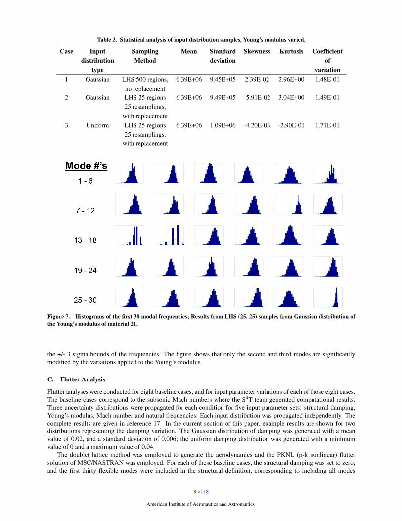
Table 2. Statistical analysis of input distribution samples, Young’s modulus varied.
Case Input Sampling Mean Standard Skewness Kurtosis Coefficientdistribution Method deviation of
type variation1 Gaussian LHS 500 regions, 6.39E+06 9.45E+05 2.39E-02 2.96E+00 1.48E-01
no replacement2 Gaussian LHS 25 regions 6.39E+06 9.49E+05 -5.91E-02 3.04E+00 1.49E-01
25 resamplings,with replacement
3 Uniform LHS 25 regions 6.39E+06 1.09E+06 -4.20E-03 -2.90E-01 1.71E-0125 resamplings,
with replacement
Figure 7. Histograms of the first 30 modal frequencies; Results from LHS (25, 25) samples from Gaussian distribution ofthe Young’s modulus of material 21.
the +/- 3 sigma bounds of the frequencies. The figure shows that only the second and third modes are significantlymodified by the variations applied to the Young’s modulus.
C. Flutter Analysis
Flutter analyses were conducted for eight baseline cases, and for input parameter variations of each of those eight cases.The baseline cases correspond to the subsonic Mach numbers where the S4T team generated computational results.Three uncertainty distributions were propagated for each condition for five input parameter sets: structural damping,Young’s modulus, Mach number and natural frequencies. Each input distribution was propagated independently. Thecomplete results are given in reference 17. In the current section of this paper, example results are shown for twodistributions representing the damping variation. The Gaussian distribution of damping was generated with a meanvalue of 0.02, and a standard deviation of 0.006; the uniform damping distribution was generated with a minimumvalue of 0 and a maximum value of 0.04.
The doublet lattice method was employed to generate the aerodynamics and the PKNL (p-k nonlinear) fluttersolution of MSC/NASTRAN was employed. For each of these baseline cases, the structural damping was set to zero,and the first thirty flexible modes were included in the structural definition, corresponding to including all modes
9 of 18
American Institute of Aeronautics and Astronautics
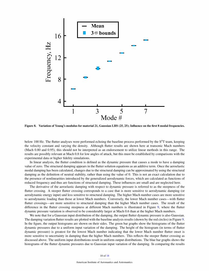
Figure 8. Variation of Young’s modulus for material 21, Gaussian LHS (25, 25); Influence on the first 8 modal frequencies.
below 100 Hz. The flutter analyses were performed echoing the baseline process performed by the S4T team, keepingthe velocity constant and varying the density. Although flutter results are shown here at transonic Mach numbers(Mach 0.80 and 0.95), this should not be interpreted as an endorsement to utilize linear methods in this range. Theresults are possibly relevant at Mach 0.8 for low angles of attack, but this must be established by comparisons with theexperimental data or higher fidelity simulations.
In linear analysis, the flutter condition is defined as the dynamic pressure that causes a mode to have a dampingvalue of zero. The structural damping appears in the flutter solution equations as an additive term. Once the aeroelasticmodal damping has been calculated, changes due to the structural damping can be approximated by using the structuraldamping as the definition of neutral stability, rather than using the value of 0. This is not an exact calculation due tothe presence of nonlinearities introduced by the generalized aerodynamic forces, which are calculated as functions ofreduced frequency and thus are functions of structural damping. These influences are small and are neglected here.
The derivative of the aeroelastic damping with respect to dynamic pressure is referred to as the steepness of theflutter crossing. A steeper flutter crossing corresponds to a case that is more sensitive to aerodynamic damping (oraerodynamic energy input) and less sensitive to structural damping. The higher Mach number cases are more sensitiveto aerodynamic loading than those at lower Mach numbers. Conversely, the lower Mach number cases—with flatterflutter crossings—are more sensitive to structural damping than the higher Mach number cases. The result of thedifference in the flutter crossing steepness at different Mach numbers is illustrated in Figure 9, where the flutterdynamic pressure variation is observed to be considerably larger at Mach 0.6 than at the higher Mach numbers.
We note that for a Gaussian input distribution of the damping, the output flutter dynamic pressure is also Gaussian.The damping variation flutter results are plotted with the baseline analysis results (shown by the red circles) in Figure 9.In the figure, the output histograms are shown on their sides. The green bar graphs show the histograms of the flutterdynamic pressures due to a uniform input variation of the damping. The height of the histogram (in terms of flutterdynamic pressure) is greatest for the lowest Mach number indicating that the lower Mach number flutter onset ismore sensitive to uncertainty in damping than the higher Mach numbers. This reflects the steeper flutter crossing asdiscussed above. The uniform input distributions result in uniform output distributions. The blue bar graphs shows thehistograms of the flutter dynamic pressures due to Gaussian input variation of the damping. In comparing the results
10 of 18
American Institute of Aeronautics and Astronautics
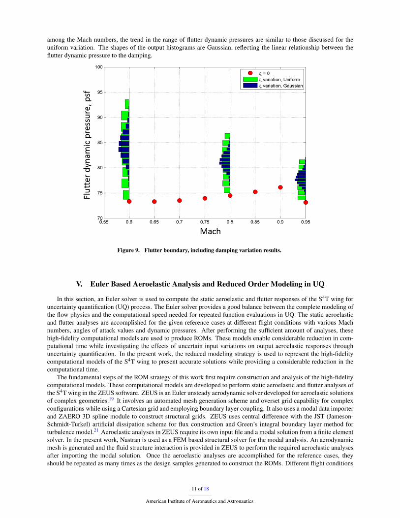
among the Mach numbers, the trend in the range of flutter dynamic pressures are similar to those discussed for theuniform variation. The shapes of the output histograms are Gaussian, reflecting the linear relationship between theflutter dynamic pressure to the damping.
Figure 9. Flutter boundary, including damping variation results.
V. Euler Based Aeroelastic Analysis and Reduced Order Modeling in UQ
In this section, an Euler solver is used to compute the static aeroelastic and flutter responses of the S4T wing foruncertainty quantification (UQ) process. The Euler solver provides a good balance between the complete modeling ofthe flow physics and the computational speed needed for repeated function evaluations in UQ. The static aeroelasticand flutter analyses are accomplished for the given reference cases at different flight conditions with various Machnumbers, angles of attack values and dynamic pressures. After performing the sufficient amount of analyses, thesehigh-fidelity computational models are used to produce ROMs. These models enable considerable reduction in com-putational time while investigating the effects of uncertain input variations on output aeroelastic responses throughuncertainty quantification. In the present work, the reduced modeling strategy is used to represent the high-fidelitycomputational models of the S4T wing to present accurate solutions while providing a considerable reduction in thecomputational time.
The fundamental steps of the ROM strategy of this work first require construction and analysis of the high-fidelitycomputational models. These computational models are developed to perform static aeroelastic and flutter analyses ofthe S4T wing in the ZEUS software. ZEUS is an Euler unsteady aerodynamic solver developed for aeroelastic solutionsof complex geometries.19 It involves an automated mesh generation scheme and overset grid capability for complexconfigurations while using a Cartesian grid and employing boundary layer coupling. It also uses a modal data importerand ZAERO 3D spline module to construct structural grids. ZEUS uses central difference with the JST (Jameson-Schmidt-Turkel) artificial dissipation scheme for flux construction and Green’s integral boundary layer method forturbulence model.21 Aeroelastic analyses in ZEUS require its own input file and a modal solution from a finite elementsolver. In the present work, Nastran is used as a FEM based structural solver for the modal analysis. An aerodynamicmesh is generated and the fluid structure interaction is provided in ZEUS to perform the required aeroelastic analysesafter importing the modal solution. Once the aeroelastic analyses are accomplished for the reference cases, theyshould be repeated as many times as the design samples generated to construct the ROMs. Different flight conditions
11 of 18
American Institute of Aeronautics and Astronautics
with various Mach numbers, dynamic pressures, and angle of attack values, for a total of 3 reference cases for flutteranalyses and 9 reference cases for static aeroelastic analyses are considered. After generating an adequate numberof sampling for each reference case, the model reduction is performed by using the nonintrusive Polynomial ChaosExpansion (PCE) and Proper Orthogonal Decomposition (POD) methods. Both the PCE and POD methods aim toameliorate the computational efficiency.
Firstly, the static aeroelastic and flutter analyses of the S4T wing were performed for the reference cases by usingthe PCE and POD based ROMs. Then, the ROM results were compared to the initial computational results of thehigh-fidelity models. These ROMs could predict the responses in a small input data range, and in this case both thePCE and POD methods give satisfactory results while their accuracies will be thoroughly discussed in the presentwork.
Secondly, both the PCE and POD methods were used to construct a ROM, which is accurate when large variationsof input parameters are considered. The flutter behavior of the S4T wing could accurately be predicted over the entireflight regime for Mach numbers ranging from 0.60 to 1.20 by the PCE and POD based ROMs. This case will alsobe evaluated in more detail by comparing the flutter results of the ROMs to the initial high-fidelity computationalanalyses.
Finally, structural and aerodynamic uncertainties, which influence static aeroelastic and flutter computational so-lutions, were propagated using ROMs. The uncertainty quantification was performed by using MCS and LHS tech-niques, which are frequently used to propagate uncertainties in a probabilistic system. The effects of uncertain inputvariables on the flutter and static aeroelastic responses were investigated. For the static aeroelastic simulations, the un-certain input variables examined were angle of attack, elasticity modulus and dynamic pressure. The static aeroelasticoutput variables were aerodynamic lift, drag, moment coefficients and wing tip twist angle. For the flutter simulations,the angle of attack and elasticity modulus were the uncertain input variables. The flutter output variables examinedwere flutter frequency, flutter speed and flutter dynamic pressure.
A. Static Aeroelastic and Flutter Uncertainty Quantification
In the aeroelastic UQ analysis, we used the distributions for the angle of attack and dynamic pressure as given bythe AVT-191 task group. Each structural modal solution was used in the aeroelastic analysis and the final resultswere classified according to the given clusters divided for angle of attack and dynamic pressure values. In our study,instead of giving a distribution to the modal frequencies, elasticity modulus of Material 21 was distributed by using10 samples with a 5% uncertainty around the mean value of 6.39MPa. However, the uncertainty distributions for theangle of attack and dynamic pressure were the same as provided by the AVT-191 Task Group. These distributions weredivided into different clusters and each cluster was defined with a mean value and a standard deviation (see Table 3)with a normal distribution assumption.
Table 3. Clusters for aeroelastic UQ analysis.
Cluster Angle of attack (degs) Dynamic pressure (psf)Number Designation Mean Standard deviation Mean Standard deviation
1 20 psf Cluster 1 0.204571 0.016328 21.40429 0.1822542 20 psf Cluster 2 0.826455 0.097638 20.17791 0.1718113 35 psf Cluster 0.327333 0.06912 35.55383 0.3978824 60 psf Cluster 1 -0.19118 0.065167 60.97871 0.5192235 60 psf Cluster 2 0.193625 0.043197 60.3455 0.513832
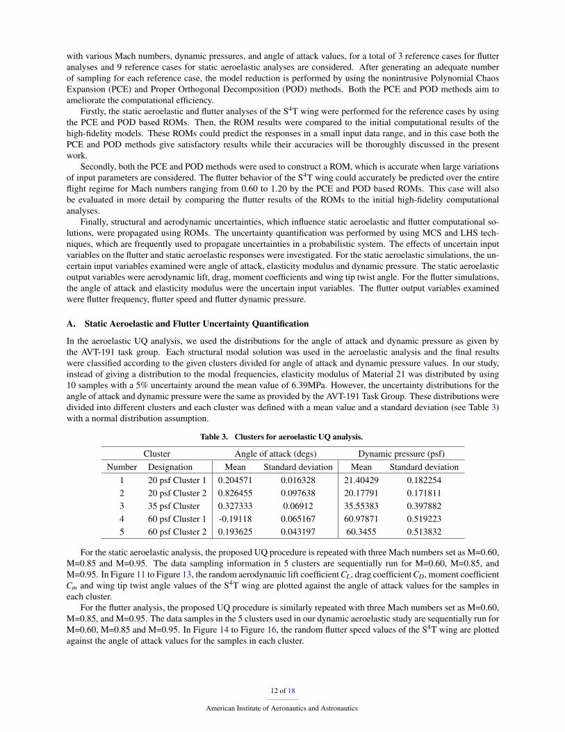
For the static aeroelastic analysis, the proposed UQ procedure is repeated with three Mach numbers set as M=0.60,M=0.85 and M=0.95. The data sampling information in 5 clusters are sequentially run for M=0.60, M=0.85, andM=0.95. In Figure 11 to Figure 13, the random aerodynamic lift coefficient CL, drag coefficient CD, moment coefficientCm and wing tip twist angle values of the S4T wing are plotted against the angle of attack values for the samples ineach cluster.
For the flutter analysis, the proposed UQ procedure is similarly repeated with three Mach numbers set as M=0.60,M=0.85, and M=0.95. The data samples in the 5 clusters used in our dynamic aeroelastic study are sequentially run forM=0.60, M=0.85 and M=0.95. In Figure 14 to Figure 16, the random flutter speed values of the S4T wing are plottedagainst the angle of attack values for the samples in each cluster.
12 of 18
American Institute of Aeronautics and Astronautics
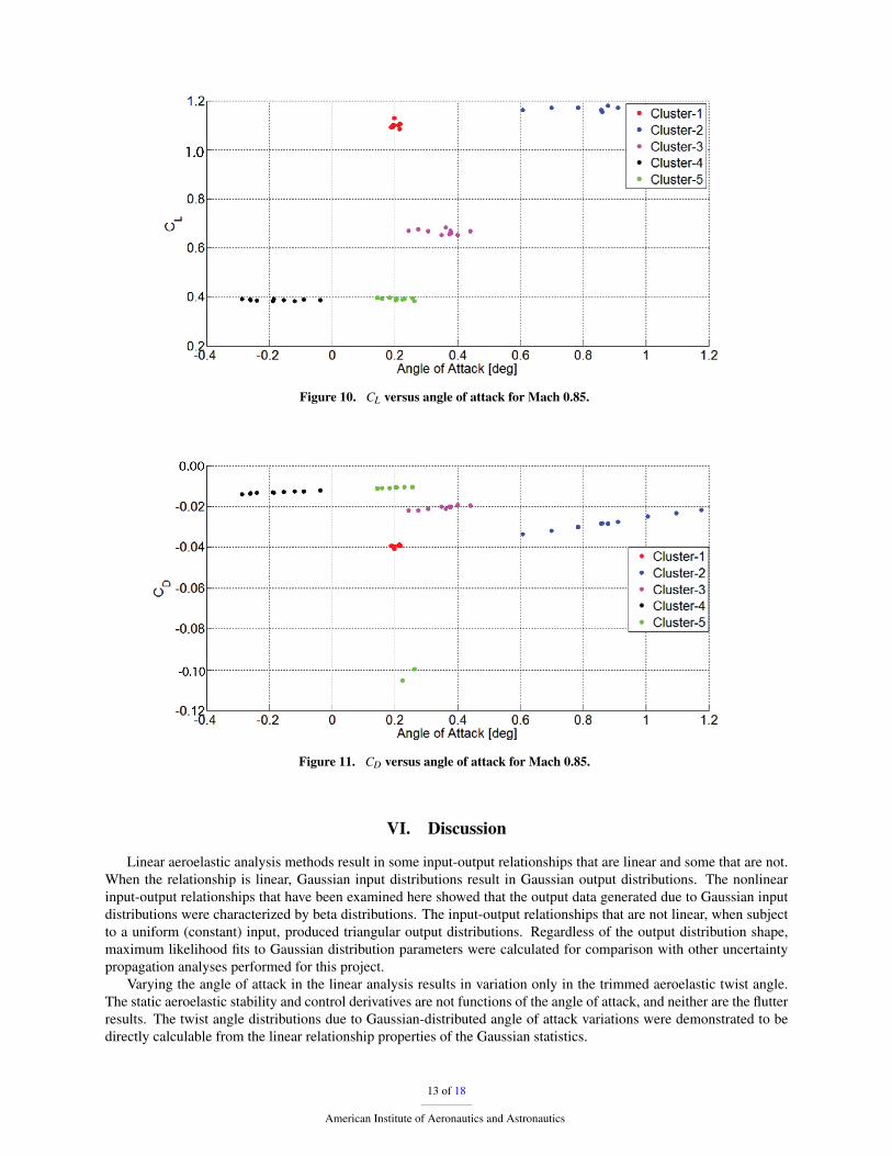
Figure 10. CL versus angle of attack for Mach 0.85.
Figure 11. CD versus angle of attack for Mach 0.85.
VI. Discussion
Linear aeroelastic analysis methods result in some input-output relationships that are linear and some that are not.When the relationship is linear, Gaussian input distributions result in Gaussian output distributions. The nonlinearinput-output relationships that have been examined here showed that the output data generated due to Gaussian inputdistributions were characterized by beta distributions. The input-output relationships that are not linear, when subjectto a uniform (constant) input, produced triangular output distributions. Regardless of the output distribution shape,maximum likelihood fits to Gaussian distribution parameters were calculated for comparison with other uncertaintypropagation analyses performed for this project.
Varying the angle of attack in the linear analysis results in variation only in the trimmed aeroelastic twist angle.The static aeroelastic stability and control derivatives are not functions of the angle of attack, and neither are the flutterresults. The twist angle distributions due to Gaussian-distributed angle of attack variations were demonstrated to bedirectly calculable from the linear relationship properties of the Gaussian statistics.
13 of 18
American Institute of Aeronautics and Astronautics
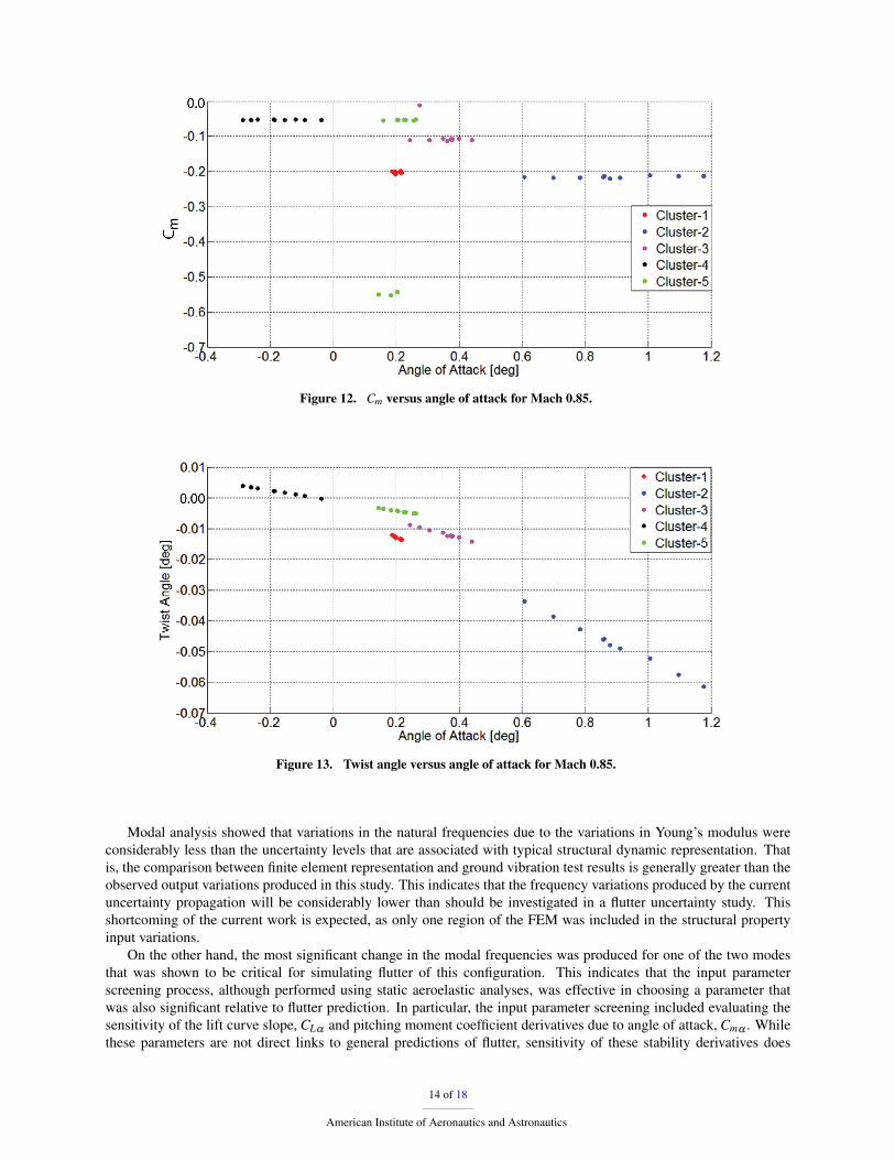
Figure 12. Cm versus angle of attack for Mach 0.85.
Figure 13. Twist angle versus angle of attack for Mach 0.85.
Modal analysis showed that variations in the natural frequencies due to the variations in Young’s modulus wereconsiderably less than the uncertainty levels that are associated with typical structural dynamic representation. Thatis, the comparison between finite element representation and ground vibration test results is generally greater than theobserved output variations produced in this study. This indicates that the frequency variations produced by the currentuncertainty propagation will be considerably lower than should be investigated in a flutter uncertainty study. Thisshortcoming of the current work is expected, as only one region of the FEM was included in the structural propertyinput variations.
On the other hand, the most significant change in the modal frequencies was produced for one of the two modesthat was shown to be critical for simulating flutter of this configuration. This indicates that the input parameterscreening process, although performed using static aeroelastic analyses, was effective in choosing a parameter thatwas also significant relative to flutter prediction. In particular, the input parameter screening included evaluating thesensitivity of the lift curve slope, CLα and pitching moment coefficient derivatives due to angle of attack, Cmα . Whilethese parameters are not direct links to general predictions of flutter, sensitivity of these stability derivatives does
14 of 18
American Institute of Aeronautics and Astronautics
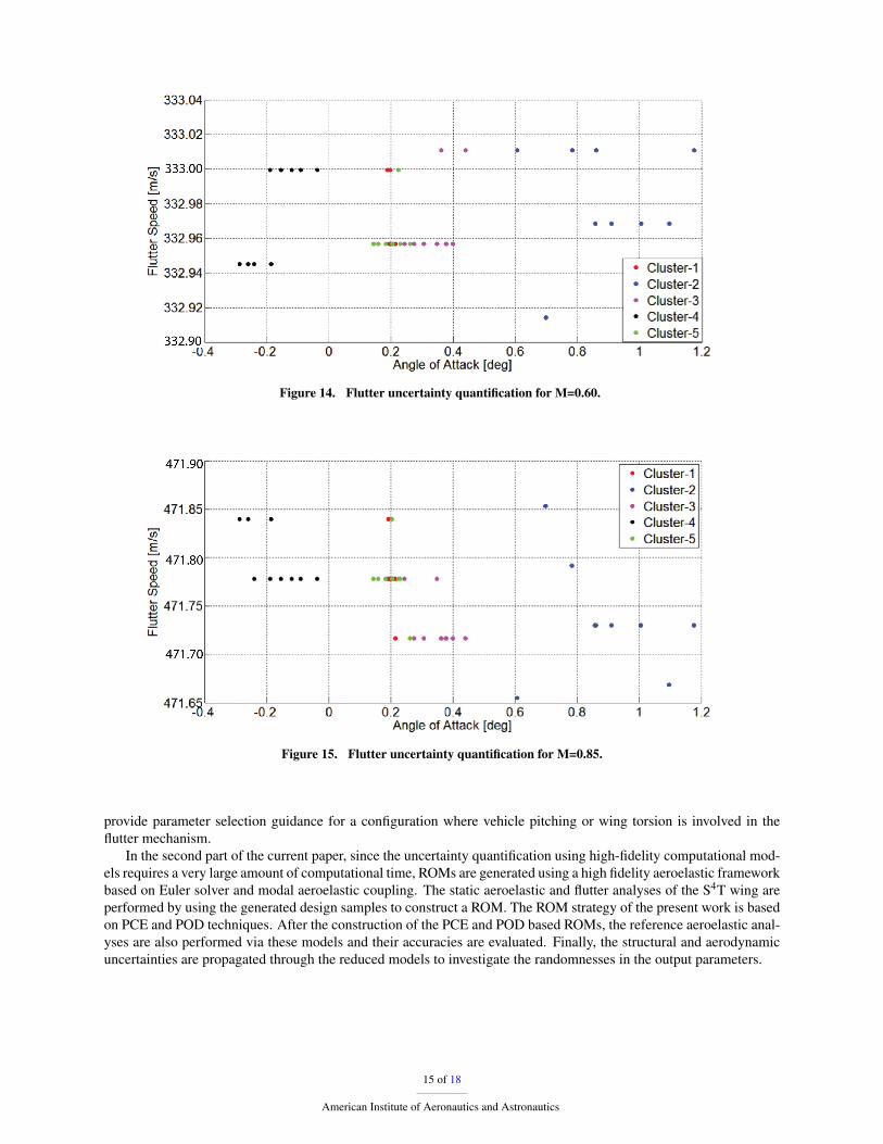
Figure 14. Flutter uncertainty quantification for M=0.60.
Figure 15. Flutter uncertainty quantification for M=0.85.
provide parameter selection guidance for a configuration where vehicle pitching or wing torsion is involved in theflutter mechanism.
In the second part of the current paper, since the uncertainty quantification using high-fidelity computational mod-els requires a very large amount of computational time, ROMs are generated using a high fidelity aeroelastic frameworkbased on Euler solver and modal aeroelastic coupling. The static aeroelastic and flutter analyses of the S4T wing areperformed by using the generated design samples to construct a ROM. The ROM strategy of the present work is basedon PCE and POD techniques. After the construction of the PCE and POD based ROMs, the reference aeroelastic anal-yses are also performed via these models and their accuracies are evaluated. Finally, the structural and aerodynamicuncertainties are propagated through the reduced models to investigate the randomnesses in the output parameters.
15 of 18
American Institute of Aeronautics and Astronautics
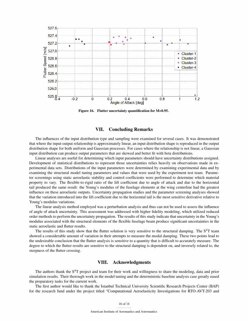
Figure 16. Flutter uncertainty quantification for M=0.95.
VII. Concluding Remarks
The influences of the input distribution type and sampling were examined for several cases. It was demonstratedthat where the input-output relationship is approximately linear, an input distribution shape is reproduced in the outputdistribution shape for both uniform and Gaussian processes. For cases where the relationship is not linear, a Gaussianinput distribution can produce output parameters that are skewed and better fit with beta distributions.
Linear analyses are useful for determining which input parameters should have uncertainty distributions assigned.Development of statistical distributions to represent those uncertainties relies heavily on observations made in ex-perimental data sets. Distributions of the input parameters were determined by examining experimental data and byexamining the structural model tuning parameters and values that were used by the experiment test team. Parame-ter screenings using static aeroelastic stability and control coefficients were performed to determine which materialproperty to vary. The flexible-to-rigid ratio of the lift coefficient due to angle of attack and due to the horizontaltail produced the same result: the Young’s modulus of the fuselage elements at the wing centerline had the greatestinfluence on these aeroelastic outputs. Uncertainty propagation studies and the parameter screening analyses showedthat the variation introduced into the lift coefficient due to the horizontal tail is the most sensitive derivative relative toYoung’s modulus variations.
The linear analysis method employed was a perturbation analysis and thus can not be used to assess the influenceof angle of attack uncertainty. This assessment was addressed with higher fidelity modeling, which utilized reducedorder methods to perform the uncertainty propagation. The results of this study indicate that uncertainty in the Young’smodulus associated with the structural elements of the flexible fuselage beam produce significant uncertainties in thestatic aeroelastic and flutter results.
The results of this study show that the flutter solution is very sensitive to the structural damping. The S4T teamshowed a considerable amount of variation in their attempts to measure the modal damping. These two points lead tothe undesirable conclusion that the flutter analysis is sensitive to a quantity that is difficult to accurately measure. Thedegree to which the flutter results are sensitive to the structural damping is dependent on, and inversely related to, thesteepness of the flutter crossing.
VIII. Acknowledgments
The authors thank the S4T project and team for their work and willingness to share the modeling, data and priorsimulation results. Their thorough work in the model tuning and the deterministic baseline analysis case greatly easedthe preparatory tasks for the current work.
The first author would like to thank the Istanbul Technical University Scientific Research Projects Center (BAP)for the research fund under the project titled “Computational Aeroelasticity Investigations for RTO-AVT-203 and
16 of 18
American Institute of Aeronautics and Astronautics

Aeroelastic Prediction Workshop”.
References1Guruswamy, G. P., “Computational-Fluid-Dynamics- and Computational-Structural-Dynamics-Based Time-Accurate Aeroelasticity of He-
licopter Rotor Blades,” Journal of Aircraft, Vol. 47, No. 3, pp. 858-863, 2010.2http://overflow.larc.nasa.gov3Lee-Rausch, E. M. and Batina, J. T., “Wing Flutter Computations Using an Aerodynamic Model Based on the Navier-Stokes Equations,”
Journal of Aircraft, Vol. 33, No. 6, pp. 1139-1147, 1996.4Lee-Rausch, E. M. and Batina, J. T., “Wing Flutter Boundary Prediction Using Unsteady Euler Method,” Journal of Aircraft, Vol. 2, No. 32,
pp. 416-422, 1995.5Giunta, A., “A Novel Sensitivity Analysis Method for High-Fidelity Multidisciplinary Optimization of Aero-Structural Systems,” AIAA,
38th Aerospace Science Meeting and Exhibit, Paper 2000-0683, Reno, NV, Jan. 20006Maute, K., Nikbay, M., and Farhat, C., “Coupled Analytical Sensitivity Analysis for Aeroelastic Optimization,” AIAA, 8th AIAA/USAF/
NASA/ISSMO Symposium on Multidisciplinary Analysis and Optimization, Paper 2000-4825, Long Beach, CA, Sept. 2000.7Maute, K., Nikbay, M., and Farhat, C., “Coupled Analytical Sensitivity Analysis and Optimization of Three-Dimensional Nonlinear Aero-
elastic Systems,” AIAA Journal, Vol. 39, No. 11, 2001, pp. 2051-2061. doi:10.2514/2.12278Maute, K., Nikbay, M., and Farhat, C., “Sensitivity Analysis and Design Optimization of Three-Dimensional Nonlinear Aeroelastic Systems
by the Adjoint Method,” International Journal for Numerical Methods in Engineering, Vol. 56, No. 6, Feb. 2003, pp. 911-933. doi:10.1002/nme.5999Nikbay, M., “Coupled Sensitivity Analysis by Discrete-Analytical Direct and Adjoint Methods with Applications to Aeroelastic Optimization
and Sonic Boom Minimization,” Ph.D. Thesis, Univ. of Colorado at Boulder, Boulder, CO, 2002.10Moller, H., and Lund, E., “Shape Sensitivity Analysis of Strongly Coupled FluidStructure Interaction Problems,” AIAA, 8th
AIAA/USAF/NASA/ISSMO Symposium on Multidisciplinary Analysis and Optimization, Paper 2000-4825, Long Beach, CA, Sept. 2000.11Hou, G.-W., and Satyanarayana, A., “Analytical Sensitivity Analysis of a Statical Aeroelastic Wing,” AIAA, 8th AIAA/USAF/NASA/ISSMO
Symposium on Multidisciplinary Analysis and Optimization,Paper 2000-4825, Long Beach, CA, Sept. 2000.12Gumbert, C., Hou, G.-W., and Newman, P., “Simultaneous Aerodynamic Analysis and Design Optimization (SAADO) for a 3-D Flexible
Wing,” AIAA, 43rd AIAA/ASME/ASCE/AHS/ASC Structures, Structural Dynamics, and Materials Conference, Paper 2002-1483, Denver, CO,April 2002.
13Martins, J., Alonso, J., and Reuther, J., “High-Fidelity Aero-Structural Design Optimization of a Supersonic Business Jet,” AIAA, 43rdAIAA/ ASME/ASCE/AHS/ASC Structures, Structural Dynamics, and Materials Conference, Paper 2002-1483, Denver, CO, April 2002.
14Barcelos, M., and Maute, K., “Aeroelastic Design Optimization for Laminar and Turbulent Flows,” Computer Methods in Applied Mechanicsand Engineering, Vol. 197, Nos. 19-20, 2008, pp. 1813-1832. doi:10.1016/j.cma.2007.03.009
15Nikbay, M.,Oncu, L., and Aysan, A.“Multidisciplinary Code Coupling for Analysis and Optimization of Aeroelastic Systems”, AIAA Journalof Aircraft Vol. 46, No. 6, November-December 2009, DOI: 10.2514/1.41491
16Zhang, Z., Yang, S., Chen, P. C., “Linearized Euler Solver for Rapid Frequency-Domain Aeroelastic Analysis,” Journal of Aircraft, Vol. 49,No. 3, pp. 922-932, 2012.
17NATO-STO AVT-191 Task Group Report, “Application of Sensitivity Analysis and Uncertainty Quantification to Military Vehicle Design”18http://www.mscsoftware.com/product/msc-nastran19http://www.zonatech.com/ZEUS.htm20Perry, B., Silva, W. A., Florance, J. R., Wieseman, C. D., Pototzky, A. S., Sanetrik, M. D. et al., “Plans and Status of Wind-Tunnel Testing
Employing an Aeroservoelastic Semispan Model,” 48th AIAA/ASME/ASCE/AHS/ASC Structures, Structural Dynamics, and Materials Conference,AIAA 2007-1770, Honolulu, HI, USA, 2007.
21Chen, P. C, Zhang, Z., Sengupta, A., and Liu, D., “Overset Euler/Boundary Layer Solver with Panel Based Aerodynamic Modeling forAeroelastic Applications,” Journal of Aircraft, Vol. 46, No. 6, pp. 2054-2068, 2009
22Wiener, N., ”The homogenous chaos,” American Journal of Mathematics, Vol. 60, pp: 897-936, 1938.23Eldred, M. S., ”Recent Advances in Non-Intrusive Polynomial Chaos and Stochastic Collocation Methods for Uncertainty Analysis and De-
signs,” 50th AIAA/ASME/ASCE/AHS/ASC Structures, Structural Dynamics, and Materials Conference, AIAA 2009-2274, Palm Springs, California,USA, 2009.
24Eldred, M. S. and Burkardt, J., ”Comparision of Non-Intusive Polynomial Chaos and Stochastic Collocation Methods for UncertaintyQuantification,” 47th AIAA Aerospace Sciences Meeting and Exhibit, AIAA 2009-0976, Orlando, FL, USA, 2009.
25Witteveen, J. A. S. and Bijl, H., ”Using Polynomial Chaos for Uncertainty Quantification in Problems with Nonlinearities,” 47thAIAA/ASME/ASCE/AHS/ASC Structures, Structural Dynamics, and Materials Conference, AIAA 2006-2066, Newport, Rhode Island, USA, 2006.
26Beran, P. and Silva, W., ”Reduced Order Modeling: New Approaches to Computational Physics,” 39th AIAA Aerospace Sciences Meetingand Exhibit, AIAA 2001-0853, Reno, NV, USA, 2001.
27Hoetelling, H., ”Simplified calculation of principal component analysis,” Psychometrica, 1: 27-35, 1935.28Bui-Thanh, T. and Willcox, K., ”Model Reduction for Large Scale CFD Applications Using the Balanced Proper Orthogonal Decomposi-
tion,” 17th AIAA Computational Fluid Dynamics Conference, AIAA 2005-4617, Toronto, Canada, 2005.29LeGresley, P. A. and Alonso, J., ”Investigation of Non-Linear Projection for POD Based Reduced Order Models for Aerodynamics,” 39th
AIAA Sciences Meeting and Exhibit, AIAA 2001-0926, Reno, NV, USA, 2001.30Hall, K. C., Thomas, J. P. and Dowell, E. H., ”Investigation of Non-Linear Proper Orthogonal Decomposition Technique for Transonic
Unsteady Aerodynamic Flows,” AIAA Journal, Vol. 38, No. 10, pp: 1853-1862, 2000.31Thomas, J. P., Dowell, E. H. and Hall, K. C., ”Three-Dimensional Transonic Aeroelasticity Using Proper Orthogonal Decomposition-Based
Reduced-Order Models,” Journal of Aircraft, Vol. 40, No. 3, pp: 544-551, 2003.32Allen, M., Weickum, G. and Maute, K., ”Application of Reduced Order Models for the Stochastic Design Optimization of Dynamic Sys-
tems,” 10th AIAA/ISSMO Multidisciplinary Analysis and Optimization Conference, AIAA 2004-4614, Albany, NY, USA, 2004.
17 of 18
American Institute of Aeronautics and Astronautics

33Chatterjee, A., ”An Introduction to the Proper Orthogonal Decomposition,” Current Science-Bangalore, Vol. 78, No. 7, pp: 808-817, 2000.34Pinnau, R., ”Model Reduction via Proper Orthogonal Decomposition,” Model Order Reduction: Theory, Research Aspects and Applications,
Springer, 2008.35Sirovich, L., ”Turbulence and the dynamics of coherent structures. IIII,” Quart. Appl. Math., Vol. 45, No. 3, pp: 561-590, 1987.36Silva, W. A., et al. “An overview of the Semi-Span Super-Sonic Transport (S4T) wind-tunnel model program” 53rd
AIAA/ASME/ASCE/AHS/ASC Structures, Structural Dynamics and Materials Conference. Honolulu, 2012.37Florance, J. R. “Lessons in the design and characterization testing of the Semi-Span Super-Sonic Transport (S4T) wind-tunnel model” 53rd
AIAA/ASME/ASCE/AHS/ASC Structures, Structural Dynamics and Materials Conference. Honolulu, 2012.38Sanetrik, M. S. “Computational aeroelastic analysis of the Semi-Span Super-Sonic Transport (S4T) wind-tunnel model”. 53rd
AIAA/ASME/ASCE/AHS/ASC Structures, Structural Dynamics and Materials Conference, Honolulu, 2012
18 of 18
American Institute of Aeronautics and Astronautics